Embed Size (px)
Citation preview

ERC/HSV-TR92-06 CT'
0Co
(C
N N
U TP
'-V
0
LD
-CT
U
C -4
,J4 . D
- o c . j— ' rC
'C LJ • - Z 0. L
I_ a) v i-V) G) .
J< .)u-N- b
ow 0 -' 0 3. C
cw a).—
I CD — C —
tf WCv' <CO4JC C . U.. c u. 0
L) -4 '-' U
Development of a CFD Code for
Casting Simulation
September 1992 Interim Report
/1/V
1
P-65'
Prepared for: George C. Marshall Space Flight Center
National Aeronautics and Space Administration
Contract NAS8-39241
Prepared by: ERC, Incorporated
Huntsville Operation 555 Sparkman Drive, Suite 1622
Huntsville, AL 35816 (205) 430-3080 • Fax (205) 430-3081
NASA Report Documentation Page So.-ice
1. Report No. 2. Government Accession No. 3. Recipient's Catalog No.
4. Title and Subtitle 5. Report Date
Development of a CFD Code for Casting SimulationSeptember 16, 1992
6. Performing Organization Code
ERCI
7. Author(s) B. Performing Organization Report No.
Jesse E. Murph ERC/HSV-TR92-06
10. Work Unit No.
9. Performing Organization Name and Address ERC, Inc.
11. Contractor Grant No. 555 Sparkman Drive Suite 1622 NAS8-39241 Huntsville, AL 35816
13. Type of Report and Period Covered 12. Sponsoring Agency Name and Address
NASA/MSFC Interim
Marshall Space Flight Center, AL 35812 14. Sponsoring Agency Code
NASA
15. Supplementary Notes
iS. Abstract The task of developing a computational fluid dynamics (CFD) code to accurately'
model the mold filling phase of a casting operation was accomplished in a systematic manner. First the state-of-the-art was determined through a literature search, a code searchand participation with casting industry personnel involved in consortium start-ups. From this material and inputs from industry personnel, an evaluation of the currently available codes was made. It was determined that a few of the codes already contained sophisticated CFD algorithms and further validation of one of these codes could preclude the development of a new CFD code for this purpose. With industry concurrence, ProCAST (developed by UES, Inc.) was chosen for further evaluation. Two benchmark cases were used to evaluate the code's performance using a Silicon Graphics Personal Iris system. The results of these limited evaluations (because of machine an time contraints) are presented along with discussions of possible improvements and recommendations for further evaluation.
17. Key Words (Suggested by Author(s)) 18. Distribution Statement CFD CN22D CC01/Sheehan Computer Simulation AT01 ED35/Andrews Investment Casting DCAS/AFPRO/NAVPRO SA71/Ellis
EH23/Bhat SP72/Self UES/ COTR/P. McConr'aughey NASA/STIC M. Sam
19. Security Classil. (of this report) 20. Security Classif. (of this page) 21. No. of pages 22. Price
Unclassified Unclassified
nd s
PJM rvniv, Ibb OCT 8

OMofMt Ci11
Table of Contents COLOR tLLi;
Page
Listof Tables.................................................................................................................
Listof Figures...............................................................................................................
1.0 Introduction ........................................................................................................ i
2.0 Technology Search............................................................................................3
2.1 Literature Search ....................................................................................4
2.2 Code Search............................................................................................5
2.3 Consortium Activities ..............................................................................7
3.0. Evaluation of Codes.........................................................................................12
4.0. Benchmarking of Pr0CAST Code ....................................................................14
4.1 Backward-Facing Step...........................................................................16
4 .2 Duct Flow..............................................................................................21
4.3 Mold Filling Demonstration ...................................................................24
5.0 Conclusions.....................................................................................................25
6.0 Recommendations...........................................................................................26
Bibliography................................................................................................................49

List of Tables
I Page
I
Table I. Survey of Casting Simulation Codes..........................................................27
TableII. Attendees List.............................................................................................30
Table Ill. Predicted Detachment and Re-Attachment Locations From I Backward Facing Step Solutions ................................................................. 31

List of Figures
Page Figure 1. Backward-Facing Step 2-D Flowfield Geometry...................................... 32 Figure 2. Experimental Results from Reference 149.............................................. 33 Figure 3. Predicted Results from Reference 149.................................................... 33 Figure 4. Finite Element Meshes for Backward-Facing Step.................................. 34 Figure 5. Inlet Average Velocities for Backward-Facing Step................................. 35 Figure 6. Velocity Vectors for the Medium Mesh, Re = 100 Case .......................... 36 Figure 7. Velocity Contours for the Fine Mesh, Re = 1,200 Case .......................... 37 Figure 8. Predicted Results versus Reference 149 Experimental Results .............38 Figure 9. Predicted Results versus Reference 149 Predicted Results................... 38 Figure 10. Duct Flow Finite Element Mesh from PATRAN........................................ 39 Figure 11. Comparison of Current Mesh and Reference 150 Mesh ......................... 40 Figure 12. Inlet Velocity for Duct Flow...................................................................... 41 Figure 13. Velocity Magnitude Contours for Duct Flow............................................. 42 Figure 14. Radial (y-direction) Velocity Contours for Duct Flow............................... 43 Figure 15. Radial Streamwise Velocity Profiles for Duct Flow.................................. 44 Figure 16. Velocity Profiles Across the Span (z-direction) for Duct Flow ................. 45 Figure 17. Mold Filling Flowfield Demonstration....................................................... 46 Figure 18. Proposed New Mesh for Duct Flow ......................................................... 48
1.0 Introduction
Because of high rejection rates for large structural castings (e.g. the Space Shuttle Main Engine Alternate Turbopump Design Program), a reliable casting simulation computer code is very desirable. This code would reduce both the development time and life cycle costs by allowing accurate modeling of the entire casting process. While this code could be used for other types of castings, the most significant reductions of time and cost would probably be realized in complex investment castings, where any reduction in the number of development castings would be of significant benefit.
The casting process is conveniently divided into three distinct phases:
1) mold filling, where the melt is poured or forced into the mold cavity,
2) solidification, where the melt undergoes a phase change to the solid state, and
3) cool down, where the solidified part continues to cool to ambient conditions.
While these phases may appear to be separate and distinct, temporal overlaps do exist between phases (e.g. local solidification occurring during mold filling) and some phenomenological events are affected by others (e.g. residual stresses depend on solidification and cooling rates). Therefore, a reliable code must accurately model all three phases and the interactions between each. While many codes have been developed (to various stages of complexity) to model the solidification and cool down phases, only a few codes have been developed to model mold filling.
The current task involves developing a computational fluid dynamics (CFD) code to accurately model the mold filling phase. This task is being accomplished using a systematic approach, which includes a technology search, an evaluation of existing codes and a code development effort. The technology search includes a literature search, a code search and participation with casting industry personnel and officials involved in casting consortium start-ups. The literature search, while not exhaustive, is comprehensive and includes both technical and informative material covering all phases of casting processes and modeling. While much of the literature described available casting simulation codes, additional literature and material was obtained from the code developers and code users as a part of the code search. From this material and inputs from industry personnel, an evaluation of these codes was made to determine their suitability for continued development into a reliable, accurate and comprehensive casting simulation code. As a result of this evaluation, a decision was made that development of a new CFD code was not cost effective or necessary. The approach selected, and supported by the casting industry, was to support further development of existing codes. Also with industry concurrence, ProCAST (developed and marketed by UES) was selected for further development by means of providing an independent evaluation of the code's casting simulation capabilities. The first step of

this process was to evaluate the mold filling analysis capabilities. This should be extended in subsequent efforts to include evaluations of the solidification and cool down analysis capabilities.
The ProCAST code was used to model two different steady-state fluid flow cases which have previously been used to benchmark other CFD codes. The first case was air flowing through a channel with a backward-facing step. The second case was water flowing through a square duct turning a 900 bend. The results of the ProCAST analysis of each case are compared to both test data and previous analytical results. While some of the results agree well with test data and predictions, other results do not. Most of the discrepancies are easily attributable to limitations in the models chosen. While much more complex models could be used, requiring much more set-up time, CPU time, computer storage requirements and post-processing time, the models are probably already more complex than would normally be used for most casting simulation analyses. Moreover, the intent of the evaluation process is not to rigorously exercise the code using supercomputer capabilities, but to determine the code's capabilities on smaller computer systems (such as the SGI Personal Iris system used here) using reasonably sized models normally used in casting simulations, where the flowfield is only a portion of the overall simulation. Furthermore, most casting companies that will be using this code do not have access to a supercomputer, and even if they did, it may not be cost effective.
As a demonstration of the code's mold filling (free surface tracking) capabilities, a simple, two-dimensional model was configured to qualitatively test the code's ability to predict several fluid flow phenomena.
• Recommendations are included to identify future efforts to be accomplished before the ProCAST code can be used as a reliable casting simulation code to support casting and quality issues.

2.0 Technology Search While the technology search includes primarily the literature search, the code
search and the consortium activities, other meetings and discussions with casting industry personnel contributed to the overall information gathering process. The literature search, code search and consortium activities are discussed in the following subsections. A brief description of a few of the other meetings and discussions is
included here. A casting simulation meeting was attended at MSFC. Personnel from Howmet
Corporation and
Pratt & Whitney made presentations to MSFC and ERCI attendees.
• Mr. Jan Lane, Technical Manager, Howmet, Hampton, VA, gave an informative briefing on the investment casting process, identifying many of the problems encountered and how they relate to lack of understanding the mold filling and solidification processes. Ninety (90) percent of today's investment casting problems are related to hot spots in the mold (shell) created during mold filling. Fluid flow simulation of this process could identify and alleviate many of the problems.
.Dr. John. S. Tu, Staff Engineer, Howmet, Whitehall, Ml, presented examples of solidification simulation recently performed using TOPAZ. He discussed many of the problems encountered during solidification and the need for better modeling/simulation capabilities.
• Mr. Rick Montero, Pratt & Whitney, presented a Structural Casting Process ModelingTechnology Development Program, identifying a very comprehensive effort to improve the ability to model castings.
Contact was made via telephone with Tom Glascow, Chief, Processing Science and Technology Branch, NASA/Lewis Research Center (LeRC). Discussions revealed that they are/have:
• formed a multi-disciplinary Computational Materials Laboratory analysis/performance of solidification processes, CVD, etc.
I. evaluated several codes - FIDAP, FLUENT, NEKTON.....
funding FIDAP improvements through an SBIR funding creare.x to improve phase change chemistry in FLUENT I Subsequent to this discussion, MSFC personnel (Dr. Paul K. McConnaughey/ED32 and
Dr. Biliyar BhatJEH23) visited LeRC to ensure that the current effort is synergistic with I their efforts and is not redundant or represent excessive overlap of technical assignments.
Most of the literature and code search efforts were accomplished near the I beginning of the effort with only limited updates afterward. Therefore, these efforts are not as current or complete as they could be. Any extended effort should include an
Iupdate as soon as possible.
1 3

2.1 Literature Search
The literature search was a multi-purpose effort to identify what has been and is being done in the area of casting simulation, especially investment castings. Of the three casting phases (mold filling, solidification and cooldown), emphasis is placed on the first two, especially where the melt is still liquidus and fluid flow simulation is applicable. Additionally, references are located which have general interest to the fluid flow (mold filling) simulation process and the solidification process, even for some time after the melt has solidified.
In the process of acquiring references both directly and indirectly related to the simulation process, much general information on casting processes and casting technology was also found. The references obtained are divided into three categories in the attached Bibliography:
• Mold Filling (53 references, No. I through 53)
U. Solidification (31 references, No. 54 through 84)
• General Casting Technology (64 references, No. 85 through 148)
IWhile many references are of a technical nature, many are semi-technical and
some are non-technical, which were included in the search since the intent was to learn as much as possible about casting processes, terminology, materials, innovations, I industry perceptions, etc. that could prove useful during the code development process. Most of these references were used as a tool for establishing the current state-of-the-art of casting simulation; therefore, a large portion of a synopsis of the references I would read like a tutorial of casting processes and problems, and is not included here.
4

2.2 Code Search
The intent of the code search was to identify all available CFD codes with mold filling capabilities, as well as the best solidification codes available. The mold filling I codes will be evaluated to determine the need for a new code or further development of one of the existing codes. Knowledge of the solidification codes will provide a basis for future development in this area, especially if it were determined that a new CFD mold I filling code needed to be developed, which would need to interface with one of the solidification codes.
IThe search for casting codes was aided by the literature search, the consortium
activities and other communications. The casting codes identified are very briefly described in Table I. While many of the codes are solidification only, with no mold I filling capabilities, they are included here for previously described interests. Emphasis is placed on the mold filling codes, which span a broad range of complexity, from very simple (and, consequently, of very limited use) to very complex. The details of the I more complex codes (user techniques, mathematics, physics, etc.) are usually proprietary, with only limited marketing information available. However, general descriptions of the codes' methodologies are not proprietary and much additional I
information has been gained through telephone conversations, marketing and other literature and personal visits, as described below. The following is a brief synopsis of
I
information obtained on the mold filling codes:
1. Pr0CAST, developed and marketed by UES, Inc. (reference 3), is touted by many people in the casting industry as the only finite element code that
Isimulates mold filling. Actually, there are other FE codes, such as NEKTON, but Pr0CAST is the only one to have been developed specifically for mold filling, and solves the full, unsteady Navier Stokes equations, and includes a k-c
Iturbulence model. Dr. Mark Samonds, who directs the ProCAST development group at LIES, visited I
MSFC on December 5, 1991 and discussed the technical details of the code. While most of the details of the code are presented in reference 2 (previously provided by Dr. Samonds), the presentation and discussions/questions were
I very informative. Also discussed were other codes (He says Magmasoft is his biggest competition) and pre-processors (Pr0CAST uses PreCAST which interfaces with PATRAN, IDEAS or ANVIL). Dr. Samonds also provided a list of
Icurrent users of the latest version of Pr0CAST, containing the mold filling simulation capability. I have contacted a few of these but they have so far used I
the fluid dynamics version of Pr0CAST on very limited applications. Several plan to use the code more extensively and a follow-up survey should be conducted at a later date. I 2. Magmasoft, developed and marketed by Magma (in Germany), is a finite difference code for which little is known. Since this code is said to be the
5

strongest competition for Pr0CAST, more information about the code and its users should be obtained.
3. Simulor, developed and marketed by Aluminium Pechiney of Voreppe, France, is a finite difference mold filling code which solves the full, unsteady Navier Stokes equations. References 4, 5 and 39 provide some limited information about the code along with some examples of applications of both mold filling and solidification. The code contains a few numerical options (numerical simplifications/approximations) such as "free surface smoothing" and the "false transient approach" to decrease execution times. No American user's of the code have yet been located.
4. RaPiDcast, developed by Metalworking Technology, Inc. (MTI), under a U. S. Navy contract is to be marketed by a third party. The code is finite difference, based on SOLA-VOF, and is an extension/variation of the Ph.D. dissertation work that Dr. C. Wang performed at the University of Pittsburgh under the direction of Prof. Robert Stoehr. The solution technique is time-accurate explicit, although an implicit version is currently being written. The R, P and 0 in RaPiDcast represent an acronym for "Rational Process Design," which is the philosophy of MTI, a non-profit subsidiary of the University of Pittsburgh. MTI continues to improve both the CFD and the solidification segments of the code. (Information obtained from Mike Tims and Dr. Anand Paul of MTI). See Reference 38.
5. FLOW3D, marketed by Flow Science, Inc., is (according to the users I have talked to) a very versatile finite difference code which gives good numerical results, but is not user friendly and requires long execution times. A copy of a marketing brochure was obtained from Dr. John Tu of Howmet. See References 8 and 9.
I 6. FLOCAST - Developed at the University of Pittsburgh under the direction of Prof. Robert Stoehr, uses the finite difference SOLA-VOF method, as does RaPiDcast. Not much is known about FLOCAST at this time. Additional
Iinformation is needed.
7. NEKTON - Developed by Nektonics, Inc., marketed by creare.x, uses the FE I spectral element method. The marketing brochure (reference 40) indicates that the code will handle Boussinesq natural convection, creeping flows, and other phenomena, varying boundary conditions and special applications. Casting I simulation is only one of the many applications advertised. Therefore, it could suffer from too much generality (as FLOW3D), resulting in less user friendliness and long run times.
I
6

2.3 Consortium Activities
Discussion with industry personnel identified a number of consortium activities, some well established and some in the initial (startup) phase. It was decided that participation in these activities would be of benefit in establishing industry direction in casting simulation efforts. Of primary interest were the Sandia FASTCAST and the NIST/NCAT consortiums, for which large portions of the consortiums activities are directed toward modeling/simulation efforts. These activities are described below.
Sandia FASTCAST Consortium
The Sandia National Laboratories Investment Casting Workshop, held November 5 - 6, 1991, was filled with informative presentations, discussions and tours. The purpose of the workshop was to inform the casting industry of the work that Sandia has been doing, their future plans and their idea of organizing a consortium to compliment and transfer this technology. The workshop was well organized, well planned and well attended (I estimate approximately 50 industry attendees and approximately 30 Sandia participants). Other than two presentations on investment casting perspectives by industry officials, the remainder of the workshop was conducted by Sandia personnel, with Mr. Frank Zanner as the organizer and moderator. All the Sandia presentations highlighted the organized effort to develop the FASTCAST Process which includes the following technology areas:
• Rapid prototyping
• Solid modeling
• Rules for casting
• Systems integration
• Numerical simulation
[While our primary interest is in the area of numerical simulation, we must also be familiar with and interface with the other disciplines.]
Rapid prototyping involves techniques for quickly manufacturing an investment pattern without the need for a mold. Several methods and equipment are available for this process, the most promising being:
I. • Stereolithography, which is a three-dimensional process which solidifies liquid photo-curable polymer into a programmed shape.
I. Selective Laser Sintering, where a thin layer of wax/refractory powder is
laser-sintered into a programmed shape.
. Fused Deposition Modeling, where a thermoplastic material is extruded onto the model in thin layers which are then bonded by thermal heating.
7

All three processes can access CAD data files. Other methods are also being considered by Sandia for further study.
Solid modeling of the part (to be cast) on a CAD system is necessary to enable automated mesh/grid generation for numerical simulation and for rapid prototyping. Most users of these systems are not satisfied with their current capabilities and ease of use (user friendliness).
The "rules for casting" is a part of the Casting Toolkit, which also includes experimental data, design rules and design history. Sandia has run a series of casting experiments to determine the fluidity of the melt when filling thin wall sections. While the results of these experiments are to date incomplete, they should eventually lead to useful design/casting rules for the Casting Toolbox. The consortium would identify and fund more technology efforts such as this.
The system integration technology "simply" ties all the various modeling, design,
I analysis, Casting Toolkit, rapid prototyping, etc. together in an orderly process. This is not a simple task.
IThe numerical simulation is the technology of most interest since this includes
the thermal, structural, and most especially, the fluid flow modeling of the mold filling process. Sandia is now in the process of developing a system of codes and
I
methodology to accomplish complete modeling of the mold filling, solidification and cooldown of the part and the mold.
IThe currently proposed fluid flow code is NACHOS II unless a better code is
found. No details of the code's methodology or capabilities were given in the presentation. However, it was stated that the least amount of time was spent on this
Iportion (fluid flow) part of the analyses. The fluid flow modeling is to be started this year. It was also stated that they had never previously considered free surfaces. Therefore, the NACHOS Il code must not have this capability. It was also stated that
Ithey are looking at ProCAST and possibly other codes.
The proposed investment casting consortium would be organized similarly to the I Specialty Materials Processing Consortium (SMPC) consortium, where Sandia directs the technical program and participates in the technical activities. What research efforts
I are to be funded and where they are to be performed is decided by the consortium. The results of the research efforts are available only to members of the consortium. The cost for each member will be $50,000/year with DOE providing matching amounts.
I Several general comments from the attendees are synopsized as follows:
I. It seems like a worthwhile effort, well worth the investment.
Modeling efforts to date are fragmented, have fallen short of expectations and need to be coordinated.
1 8

. Solid modeling capabilities need enhancement. • Rapid prototyping, when functional, can significantly reduce costs. • Industry needs to work together cooperatively to be competitive with
Europe and the Pacific Rim. • A great need exists for user support after the code is developed and in
production. • The analysis process must be robust, must work every time, with little to
no problems.
It would seem reasonable, if the consortium is formed, to coordinate any MSFC CFD code development with the FASTCAST Process being developed at Sandia for a number of reasons:
• Sandia has had little to no effort in the fluid flow modeling task.
• The only Sandia code mentioned for consideration is NACHOS II, which is an old research code (not a production code) which will require significant modification, especially since it will not model free surfaces.
• The other code mentioned for consideration (Pr0CAST) is being evaluated/developed currently, but there is the question of proprietary rights and how the code could be used if chosen for FASTCAST.
- • MSFC apparently has much more CFD expertise than Sandia.
I. Developing a CFD code as a part of FASTCAST would possibly provide
for instant acceptance of the code by the members of the consortium. Outside the consortium?... Maybe the consortium will sell or lease I rights? A large negative might be in being forced to adapt Sandia interfaces for
Ithe code's input and output.
However, as a follow-up to the Sandia consortium meeting of November 5 - 6, I 1991, a call was made to see what progress was being made. They had not yet re-contacted the participants to establish a firm interest for the consortium. Apparently the effort continues mostly as an in-house activity at this time. I NIST Consortium
UAnother consortium is being organized by the National Institute for Standards
and Technology (NIST) and the National Center for Advanced Technologies (NCAT). A meeting was held January 16, 1992 at the Aerospace Industries Association (AlA) to determine if there is sufficient interest to form the Casting of Aerospace Alloys Consortium to improve the modeling process and perhaps develop a data base for selected alloys. Dr. Thomas Tom, Director, Advanced Technology, Howmet, sent me a
9

copy of his invitation including an invitation list. The list of 19 people included academia, engine builders, casting houses, a NIST representative, and a NSF representative. Note the obvious absence of NASA, government laboratories and military organizations. However, according to the agenda, DARPA will be represented. An invitation to the meeting was acquired through a call to NCAT. The actual attendance list is reproduced in Table II.
The purpose of the consortium is to execute joint research efforts to develop process modeling tools and improve existing casting processes. NIST is to administer the consortium with Dr. Thomas (Tom) Yolken acting as Consortium Manager and Dr. William (Bill) Boettinger as Principal Scientist. Membership fees of $10 - 15,000 will be used for administration of the consortium. At present, funding for industrial efforts will be provided solely by participants. DOD and other fundings will be sought. University fundings have also not been identified, but NSF and industry will try to help. It has been proposed that this consortium coordinate efforts with the DARPA consortium, however, the DARPA consortium membership is much more limited, and the exact mechanism of cooperation is not yet understood.
All the participants of the meeting were enthusiastic about the prospects of the consortium. Some of the industry representatives are already suggesting related joint efforts with competitors to pursue DOD and other funds. A group of volunteers were assigned the duty of contacting other industry representatives and establishing further interest and a consolidated consortium plan (better definition of research efforts). The results will be reviewed by the meeting participants and then sent out to all AlA member companies . Even if only a small percentage sign up, this could become a relatively large consortium.
A short time after the meeting, Dr. Thomas Yolken sent me a draft of the
Iproposal for the consortium. After reviewing it, I called him with several comments and questions. We discussed some mechanisms by which NASA (particularly MSFC) can become a participating member of the consortium. Looking beyond the current I evaluation/benchmarking of the ProCAST code, MSFC efforts of the Metallurgy Research Branch/EH23 in the areas of metallurgical thermophysical properties I research and evaluation (and possibly others) can be used as "in-kind" research toward participation in the consortium. This and other topics in the consortium proposal have been discussed with Dr. Biliyar BhatIEH23, who has shown interest in I participating in the consortium and attended the second planning meeting April 28, 1992 in Gaithersburg, Maryland. Sign-up of members and initiation of the consortium research programs were planned for July 1, 1992, which has now slipped.
Other Consortiums:
IConversely, the DARPA Consortium to Develop Software for Solidification
Modeling (called the Precision Investment Castings Consortium) currently will have only seven (7) members. These seven were chosen from an original group of 121, I
1 10

which were reduced to 50, then to seven. The seven include HOWMET, Pratt & Whitney, PCC, UES, Allison, GE, and TiLine. Six million dollars will be funded by DARPA over a two year period. The members will provide matching funds. This consortium is also considered as an experiment in procurement and is expected to receive high level Congressional review. The consortium will be looking at generic technologies for casting: electronic data transfer, automatic mesh generation, automatic shell generation, material properties, etc. The goal is to develop technologies to achieve model preparation within 8 hours - currently it takes I - 4 weeks.
11

3.0. Evaluation of Codes
During the literature search, code search, consortium activities and discussions with industry personnel, much specific and general information was acquired concerning the available casting simulation codes. Based upon this information, which is certainly not exhaustive, the codes were evaluated for suitability of further development based on the following general criteria:
1. Does it contain a rigorous CFD mold filling model?
2. Does it contain a good solidification model?
3. Does it contain a good cooldown model?
4. Is the simulation relatively fast and accurate?
5. Is it relatively user friendly and inexpensive to use?
6. Is it supported by the developers?
7. Is it continually being improved?
While most of the codes in Table I either do not contain mold filling capabilities or are
Inot generally used in the casting industry (for reasons described earlier), only a few codes reasonable satisfy all the above criteria:
I 0 ProCAST
RaPiDcast I .Simulor
- Any one of these four would be a good candidate for further development. However,
I P0CAST was chosen as the best candidate for the following reasons. While both RaPiDcast and Pr0CAST are essentially equivalently ranked on criteria 2 though 7, ProCAST has the advantage in terms of a rigorous CFD mold filling model primarily
I because the solution algorithms are formulated using finite element methods rather than finite volume (finite difference). Finite element formulations are generally more accurate than finite difference methods and represent the preferable approach for
Iaccurate simulations of complex investment castings.
Magmasoft is reportedly the strongest competition to ProCAST, and it also uses
I a finite difference formulation. But since very little information has been located in the open literature, probably due in part to its development and marketing by a German firm (Magma), the code was not selected for further development in the current effort.
I12

The Simulor code, developed and marketed by a French firm (Aluminium
IPechiney), uses a finite difference approach, but does include some useful options to reduce execution times (at the expense of accuracy). Simulor suffers from the same lack of exposure in the open literature, and was also eliminated from further I development in the current effort.
Since the evaluation of codes was not strictly objective (i.e., reduced to a numerical comparison), it should again be stated that the selection of ProCAST as the best candidate for further development was not simply derived by the above comparisons or earlier stated comparisons, but was additionally influenced by communications with industry personnel.
IAt this point, a decision must be made as to whether the ProCAST code will be
further developed or a new code will be developed. The development of a new code, including documentation, benchmarking, etc. would be very costly and then there are I the questions of user support and continued development. Whereas the ProCAST code represents a very good basis with well chosen mathematical models, on-going development and continuous user support. A duplication of any of this development I effort seems unwarranted and self serving. Therefore, a decision was made to help develop the ProCAST code via benchmarking the code's capabilities.
13
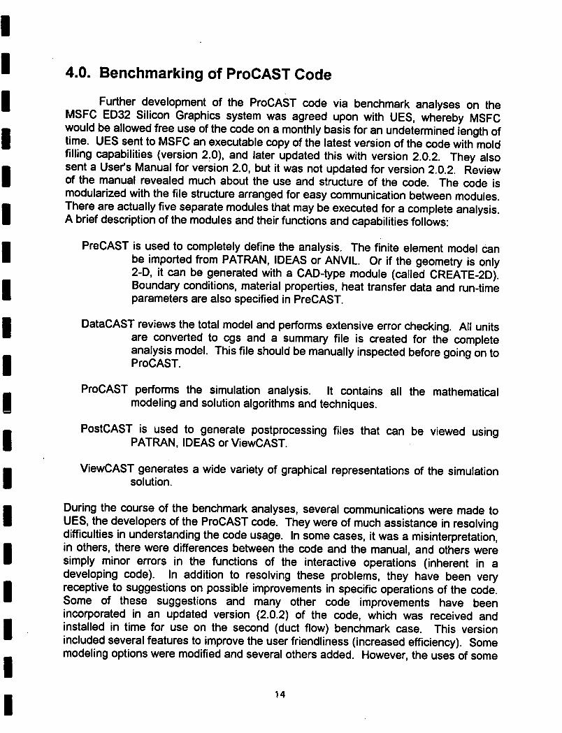
4.0. Benchmarking of ProCAST Code
Further development of the ProCAST code via benchmark analyses on the MSFC ED32 Silicon Graphics system was agreed upon with UES, whereby MSFC would be allowed free use of the code on a monthly basis for an undetermined length of time. UES sent to MSFC an executable copy of the latest version of the code with mold filling capabilities (version 2.0), and later updated this with version 2.0.2. They also sent a User's Manual for version 2.0, but it was not updated for version 2.0.2. Review of the manual revealed much about the use and structure of the code. The code is modularized with the file structure arranged for easy communication between modules. There are actually five separate modules that may be executed for a complete analysis. A brief description of the modules and their functions and capabilities follows:
PreCAST is used to completely define the analysis. The finite element model can be imported from PATRAN, IDEAS or ANVIL. Or if the geometry is only 2-D, it can be generated with a CAD-type module (called CREATE-2D). Boundary conditions, material properties, heat transfer data and run-time parameters are also specified in PreCAST.
DataCAST reviews the total model and performs extensive error checking. All units are converted to cgs and a summary file is created for the complete analysis model. This file should be manually inspected before going on to ProCAST.
ProCAST performs the simulation analysis. It contains all the mathematical modeling and solution algorithms and techniques.
P0stCAST is used to generate postprocessing files that can be viewed using PATRAN, IDEAS or V1ewCAST.
ViewCAST generates a wide variety of graphical representations of the simulation solution.
During the course of the benchmark analyses, several communications were made to LIES, the developers of the ProCAST code. They were of much assistance in resolving difficulties in understanding the code usage. In some cases, it was a misinterpretation, in others, there were differences between the code and the manual, and others were simply minor errors in the functions of the interactive operations (inherent in a developing code). In addition to resolving these problems, they have been very receptive to suggestions on possible improvements in specific operations of the code. Some of these suggestions and many other code improvements have been incorporated in an updated version (2.0.2) of the code, which was received and installed in time for use on the second (duct flow) benchmark case. This version included several features to improve the user friendliness (increased efficiency). Some modeling options were modified and several others added. However, the uses of some
14

of these were unclear since an updated user's manual was not available. Also, minor problems and questions about the code continue to be directed to UES personnel in an effort to better understand the code's functions and to help them improve subsequent versions of the code.
I Two benchmark cases and a mold filling demonstration were accomplished in the current effort. The two benchmark cases are simulations of experimental
I configurations where much test data is available for direct comparisons with predicted results. While the two cases do not involve, actual mold filling transients, they both represent steady state conditions which can exist behind the free surface during mold filling. And the use of liquid metal as the fluid media is not necessary since the code has the flexibility to model any common fluid, liquid or gas.
IThe backward-facing step case (Section 4.1) involves air flowing through a duct
with a sudden increase in flow area. The flow inherently separates from the wall at the discontinuous (step) surface and re-attaches to the wall further downstream. I Additionally, a series of adverse pressure gradients are formed downstream of the re-attachment, on the opposite wall and possibly within the primary separation region. These gradients, if strong enough, produôe additional separation (recirculation) I
regions. The ProCAST code's ability to predict the existence and locations of these regions was tested in this case. The results are compared to both test data and
U predictions from Reference 149.
The duct flow case (Section 4.2) involves water flowing through a square duct turning a 900 bend. Higher pressures are generated on the outside of the turn than on
! the inside, creating a crossflow pressure gradient. This affects a secondary flow with radial and spanwise components which significantly affect the streamwise velocity profiles. The ability of the Pr0CAST code to predict the complete three-dimensional velocity profile was tested, and the results are compared with both test data and predicted results from Reference 150.
The mold filling demonstration (Section 4.3) was performed simply for qualitative evaluation of the code's ability to track a free surface undergoing extreme distortions. No test data or prior predictions are available for comparisons.
15

4.1 Backward-Facing Step
IThe two-dimensional backward-facing step geometrical characteristics are
depicted in Figure 1. Fully-developed laminar flow enters from the left side and I encounters an instantaneous (step) increase in flow area. The flow detaches at the corner and reattaches to the lower wall at location X1. Two other experimentally determined separation (recirculation) regions can occur as located by X2 & X3 and X4 I & X5. Figure 2 (extracted from Reference 149) depicts the locations of these regions for air at various Reynolds numbers in terms of multiples of the step height, S. The predictions performed in Reference 149 (Figure 3) indicate an additional separation I
region, located by X6 and X7, within the primary separation region (upstream of X1) for Re> 1000.
The model for this case was chosen to be two dimensional along the centerline of the apparatus, ignoring spanwise variations and effects. Although the experimental apparatus was (necessarily) three dimensional, the composite data of Reference 149 shows that 3-D effects are minimal below Re = 400. A 2-D model was chosen primarily for two reasons: 1) Simplicity, since this was the first modeling attempt with the code, and 2) To use the code's mesh generation capability, which utilizes only 2-D triangular elements.
Three different fluid mesh sizes (Figure 4) were used to model the step flow. The coarse grid has only five freestream nodes across the height of the downstream channel, whereas, the medium mesh has eleven and the fine mesh has twenty. The meshes in Figure 4 depict only a small portion of the entire model, whereas the step height, S, is 0.49 cm. and the model extends upstream for 20 cm and downstream for 20 cm. Comparing the total number of elements and nodes shows the vast differences in sizes of the three models.
No. of elements No. of nodes Coarse mesh
2,733
1,836 Medium mesh
9,575
5,261 Fine mesh
26,997
14,291
The Dirichlet boundary conditions applied to these models include:
No slip at the walls, uv=0, standard conditions for a viscous solution. 2. Inlet velocity: horizontal component only, vertical component is zero. The
average magnitude of the inlet velocity varies with desired Reynolds number as described below.
3. Exit pressure: one atmosphere applied across the exit plane.
16

Reynolds numbers for each case were determined using a technique compatible with that of Reference 149:
Re = pVD/j.t, where, for air at I atm and 20 °C, p = 0.001 204 gm/cm3
= 1.824 E-5 N sec/m2
The characteristic dimension D is computed as the hydraulic diameter of the inlet channel and is equal to twice its height, D = 2h. The velocity, V, used in Reference 149 was defined as two-thirds of the measured maximum inlet velocity, which corresponds in the fully-developed laminar case to the average inlet velocity. The actual value of the input inlet velocity used in each model is dependent on the mesh configuration since a linear interpolation of the Dirichlet velocity boundary condition is used between the wall and the adjacent node. For a uniform velocity applied to all freestream nodes across the inlet plane, this results in different average velocities as depicted in Figure 5. When a uniform velocity was used across the inlet freestream nodes, the following table defines the velocities (in cm/sec) required for each Reynolds number used in the parametric analyses.
Required Velocity Velocity Velocity Re Average Velocity (Coarse Mesh) (Medium Mesh) (Fine Mesh) 100 14.67 22.0 18.3 16.5
1000 146.7 220.0 - - 1200 174.8 - 220.0 196.7 2000 293.4 440.0 - - 2400 349.6 - 440.0 - 5000 733.5 1100.0 - - 6000 880.0 - 1100.0 -
While the above input velocity profiles do not accurately represent developed flow, they are simpler to input and represent an insignificant source of error for the current models. The length-to-height ratio (lid) of the entrance duct is 38.5 (20 cm/.52 cm), more than sufficient for the velocity, profile to fully develop before reaching the step. In fact, some of the medium and fine mesh models were re-run with a better representation of fully developed laminar input velocity profiles. This resulted in no discernible differences in the flow field solutions at and downstream of the step.
Converged solutions for all cases were obtained through a series of analyses utilizing the code's restart capabilities. Since these analyses required steady state
17

U
solutions to a relatively complex flow field filled with flow detachments and reattachments (regions of separated flow), the solution parameters were changed I before each restart to ensure that a progressively more accurate solution was obtained. This is different from a normal casting simulation, which is transient, with the dominant concern being the location of the liquid metal free surface. The prediction of the flow field behind the free surface is also important for prediction of mold heating and metal cooling and solidification. So, while the current analyses represent a solution technique somewhat different from a normal casting, it is important that the results be reasonably accurate. And these more accurate solutions require additional iterations and CPU time, beyond what would be used for a typical mold filling simulation. The I iteration and time requirements are given below for comparison purposes only, and even so, are not directly comparable because of the lack of an objective numerical criteria for convergence of steady state solutions. As is always the case, the finer
I. meshes require more setup time, data storage requirements, CPU time, and data
reduction time; and they are more difficult to achieve convergence. Convergence was subjectively determined from observations of on-screen graphics, usually sequential x-I velocity contours at every twentieth iteration. When the changes became very small or, in some cases, exhibited small oscillations about a stationary norm, the case was re-run with an additional 100 to 200 iterations to ensure that no additional change in
Ithe solution occurred.
Coarse Mesh Medium Mesh Fine Mesh
I Re (iter/CPU-hr) (iter/CPU-hr) (iter/CPU-hr) 100 400/0.3 1600/5.9 3100/43.9
1000 600/0.4 - - I 1200 - 600/3.5 2100/35.5
2000 1000/0.6 - -
2400 - 800/3.3 - I 5000 400/0.3 - -
6000 - 400/1.8 -
Post-processing of the solutions was initiated with the examination of the entire I mesh network to ensure that the elements and nodes were located properly and that boundary and initial conditions were applied correctly. Also, the initial determination of detachment and reattachment points was made by examining the velocity components I of the fluid nodes immediately adjacent to the walls. It became immediately obvious that the location of flow reversal (in the longitudinal, x-direction) was not the proper location of the separation/reattachment since the slope of the zero-velocity line was I very shallow and the mesh definition was not very good, particularly for the coarse mesh. Interpolation methods would be needed to accurately project the zero-velocity line to the wall. These methods are already available in ViewCAST (the post-processor I in Pr0CAST), where velocity vector and velocity contour plots can be used to better examine the entire flow field.
1 18

An example of a velocity vector plot is shown in Figure 6, which represents a portion of the backward-facing step flow field solution for the medium mesh with a Reynolds number of 100. This type of plot portrays a global picture of the flow field. While some features are readily discernible, such as the primary separation aft of the step and changes in velocity vectors indicated by changes in direction/size/color of arrows, quantitative results are not readily obtained directly from the figure. The recirculation of gases in the primary separation zone is apparent, but locating the exact boundary of the primary zone would be difficult. For this type of information, a velocity contour plot would be much more meaningful.
Figure 7 is a representative velocity contour plot of the x-component of velocity for the fine mesh with Reynolds number of 1,200. The typical color spectrum has been modified to provide a better contrast between color (x-velocity magnitude) changes. Note that the zero velocity value occurs at the interface between blue and yellow. This interface (or zero-velocity line) is rather well-behaved and essentially linear down to the last set of freestream nodes adjacent to the wall. The contour plotting interpolation routine breaks down at this point and cannot correctly project the line onto the wall. This is a result of a change in sign of the x-component of velocity (flow reversal) between two freestream nodes adjacent to the no-slip wall nodes. The contour code cannot project the zero-velocity line beyond this location.
The projection of the zero-velocity line to the wall is the same technique used in I the experimental data of Reference 149 to locate attachment and detachment locations. However, the non-intrusive laser-Doppler anemometer used in Reference 149 allowed measurements very close to the wall so that the projection inaccuracies were I
minimized. Measurements within 0.1 mm of the wall were routinely made, providing accurate locations of the long, shallow separated flow regions.
Table Ill shows the separation regions that have been reduced from the current analyses. All of the primary separation regions (terminated at X1/S) have been predicted. Note that only the re-attachment of the primary separation region (Xj/S) is identifiable with the coarse mesh solution. Sufficient mesh density is not available adjacent to the walls (nodes approximately 0.20 cm from the walls) to detect the shallow separation zones that are present above a Reynolds number of 400. The medium mesh, with about four times as many elements, has a better definition at the walls (nodes approximately 0.09 cm from the walls), and is able to compute some separation regions and provide strong indications of others. Data from the fine mesh solutions with its higher density mesh (nodes approximately 0.055 cm from the walls) better defines all separation regions for the two Reynolds numbers (100 and 1200). Some of the top wall regions, defined by X4/S and X5/S, have been located and projected to the wall. Some of the top wall data indicate sharp drops in the x-component of velocity but no flow reversal. This indicates the presence of an adverse pressure gradient and the possibility of a separation region that is shallower than can be computed by the mesh size. A better definition (denser mesh) at the walls is normally provided with fewer nodes by packing the nodes near the walls, but this
19
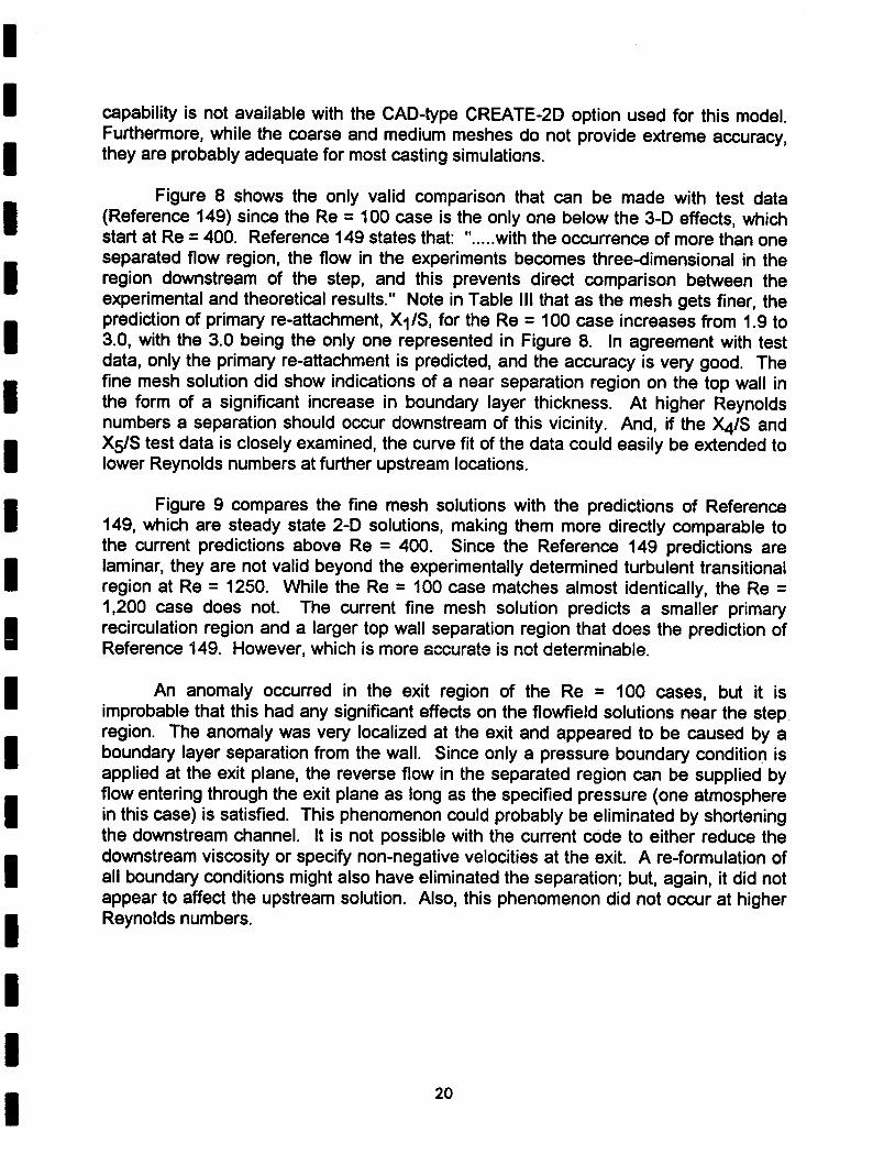
capability is not available with the CAD-type CREATE-213 option used for this model. Furthermore, while the coarse and medium meshes do not provide extreme accuracy, they are probably adequate for most casting simulations.
Figure 8 shows the only valid comparison that can be made with test data (Reference 149) since the Re = 100 case is the only one below the 3-0 effects, which start at Re = 400. Reference 149 states that: ".....with the occurrence of more than one separated flow region, the flow in the experiments becomes three-dimensional in the region downstream of the step, and this prevents direct comparison between the experimental and theoretical results." Note in Table Ill that as the mesh gets finer, the prediction of primary re-attachment, X1 IS, for the Re = 100 case increases from 1.9 to 3.0, with the 3.0 being the only one represented in Figure 8. In agreement with test data, only the primary re-attachment is predicted, and the accuracy is very good. The fine mesh solution did show indications of a near separation region on the top wall in the form of a significant increase in boundary layer thickness. At higher Reynolds numbers a separation should occur downstream of this vicinity. And, if the X4/S and X5/Stest data is closely examined, the curve fit of the data could easily be extended to lower Reynolds numbers at further upstream locations.
IFigure 9 compares the fine mesh solutions with the predictions of Reference
149, which are steady state 2-13 solutions, making them more directly comparable to the current predictions above Re = 400. Since the Reference 149 predictions are I laminar, they are not valid beyond the experimentally determined turbulent transitional region at Re = 1250. While the Re = 100 case matches almost identically, the Re = 1,200 case does not. The current fine mesh solution predicts a smaller primary I recirculation region and a larger top wall separation region that does the prediction of Reference 149. However, which is more accurate is not determinable.
An anomaly occurred in the exit region of the Re = 100 cases, but it is improbable that this had any significant effects on the flowfield solutions near the step region. The anomaly was very localized at the exit and appeared to be caused by a boundary layer separation from the wall. Since only a pressure boundary condition is applied at the exit plane, the reverse flow in the separated region can be supplied by flow entering through the exit plane as long as the specified pressure (one atmosphere in this case) is satisfied. This phenomenon could probably be eliminated by shortening the downstream channel. It is not possible with the current code to either reduce the downstream viscosity or specify non-negative velocities at the exit. A re-formulation of all boundary conditions might also have eliminated the separation; but, again, it did not appear to affect the upstream solution. Also, this phenomenon did not occur at higher Reynolds numbers.

4.2 Duct Flow
IThis benchmark case consists of water flowing through a constant area duct of square cross section (40 mm x 40 mm) turning a 900 bend with a 2.3 radius ratio and a Reynolds number* of 790, corresponding to a Dean numbert of 368. The 3-D finite element mesh shown in Figure 10 was generated using PATRAN. The mesh is 7x7x67, consisting of 7x7 equal spaced nodes at each of 67 cross sections, resulting in 2,376 I brick elements with 3,283 nodes. This represents a much coarser mesh than the 21x21x51 mesh used in Reference 150, as depicted in Figure 11. The solutions in the reference were obtained using a CRAY XMP, which obviously has much more I computing power than the SGI Personal Iris workstation used in this effort. Also, no packing of the mesh was done at the walls as was done in the reference.
IBoundary conditions consisted of a pressure of one atmosphere across the exit
plane, no slip (u=v=w=0) at the walls and an inlet velocity profile derived from test data. Figure 12a depicts the test data velocity contours and the smoothed contours I (normalized to 1.98 cm/sec) established in Reference 150, with a 7x7 grid superimposed. Since it was not possible to achieve a reasonable representation of the boundary layer because of the very coarse mesh with no nodes near the walls, a I simplistic approach was taken for the velocity profile. The velocity for each freestream inlet nodal location was taken directly from the mesh overlay. The actual input velocity map (in cm/sec) is shown in Figure 12b, where, for the inlet plane only, the velocities are interpolated linearly between all nodes.
The computational steady state solution to this case was obtained with 1000 iterations requiring 20.0 hours of CPU time on the SGI system. The interpolation of the results was accomplished through a series of velocity contour maps (generated using ViewCAST) at various planes within the flowfield. Figure 13 shows two color velocity contour maps depicting velocity magnitudes around the bend and at a downstream cross-section. The contour map around the bend (water flow from right to left) depicts the velocity profiles along the symmetry plane (the center of the duct in the spanwise direction, z). While the contrasting color spectrum makes it more difficult to peruse the
* Reynolds number is defined as: Re a pvd/
where p is water density vis average inlet velocity (1.98 cm/sec) d is hydraulic diameter (40 mm) j,t is water absolute viscosity
t Dean number is defined as: DeReJd / (ç + r0)]
where Re is Reynolds number d is hydraulic diameter (40 mm) r is inside radius of bend (72 mm) r0 is outside radius of bend (112 mm)
21

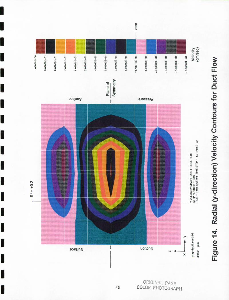
global environment, it is very advantageous when determining velocity profiles at a given location, especially since velocity profiles are not directly obtainable from ViewCAST. The inset contour in Figure 13 is a cross-section as indicated from a location 0.25d downstream of the end of the bend, where d is the hydraulic diameter, 40 mm. Note that both sides (mirror images) of the symmetry plane are shown here.
When a fluid is turned by a duct, the induced centrifugal forces and the frictional effects at the walls combine to create a secondary flow in and downstream of the bend. The centrifugal forces decelerate the flow on the outside (pressure) surface, resulting in increased pressure and a crossflow pressure gradient toward the inner (suction) surface. The frictional effects (creating the boundary layer) provide a path for the pressure gradient to produce a secondary flow consisting of two counter-rotating vortices. Figure 14 shows this at the +0.25d plane in the form of y-velocity contours. The flow along the side walls is produced by the cross-flow pressure gradient in the boundary layer, while the flow in the central region is in the opposite direction.
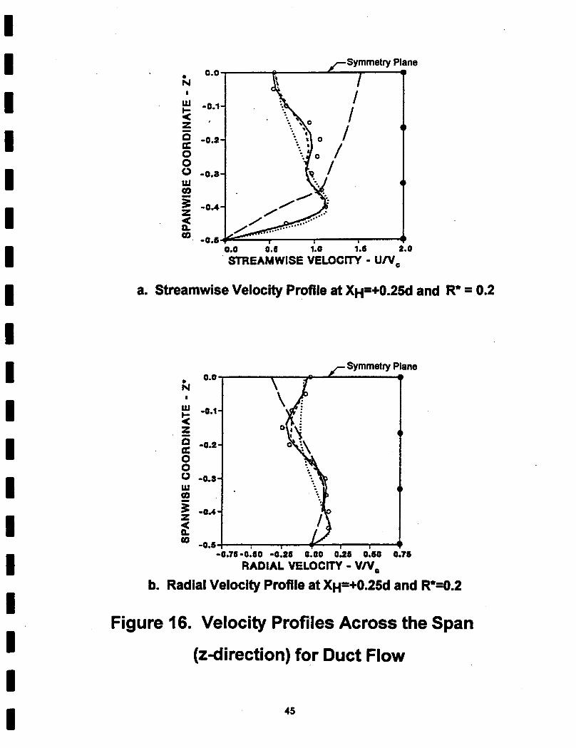
The velocity profiles deduced from the color velocity contour plots are compared in Figures 15 and 16 to test data and predicted results from Reference 150. The plots for each location contain five sets of data: the test data is represented by symbols, the predictions from Reference 150 are represented by a dotted line for the 21x21 mesh, a short dashed line for the 31x31 mesh and a solid line for the 41x41 mesh, and the current predictions are represented by a long dashed line. Figure 15 represents streamwise velocity profiles radially along the plane of symmetry at four different locations around and downstream of the bend as indicated, where 0=0 represents the start of the bend. While the three predictions of Reference 150 match test data fairly well, with the coarsest mesh beginning to deviate from the other two, the current prediction does not match well. The same trend is true for the profiles of Figure 16, where spanwise (z-direction) profiles of streamwise and radial velocity components are depicted at the normalized radius R*=0 . 2, which corresponds to 12 mm from the inside (suction) surface.
Two factors, both relating to the coarse mesh, are believed to be responsible for the inaccuracies. First the inlet velocity profile (Figure 12b) does not accurately represent the boundary layer. Note that a linear interpolation from the wall to the first freestream node (6.67 mm from the wall) provides velocities well below test data values for the entire 6.67 mm, thus effectively providing a much thicker boundary layer. Secondly, since there are no nodes within the boundary layer, which with this geometry represents more than half the cross-sectional area, the strong secondary flow that originates here cannot be predicted accurately. Further, this lack of definition denies an accurate prediction of an adverse streamwise pressure gradient along the suction surface and a faborable gradient along the pressure surface, which significantly affect the development of the streamwise velocities. Moreover, the basic problem is the oversized boundary layer produces too much core flow so that the effects of the secondary flow and streamwise pressure gradients are subdued. The thicker than desired boundary layers are easily seen in all profiles of Figures 15 (wall at R*=0.5)
22

and 16 (wall at z*=0.5). The nodal locations for the 7x7 mesh are superimposed on the right side of each of the figures for reference. It is obvious that additional nodes in the boundary layer are needed if a better accuracy is to be achieved. This is normally accomplished by using a finer mesh and packing the nodes near the wall, as done in Reference 150 (Figure 11 a).
An anomaly very similar to that described in Section 4.1 again occurred in the exit duct. The exit duct is very long with an l/d of 50, and flow separation occurred at an l/d of approximately 30. Reverse flow in the separated region resulted in reverse flow through a portion of the exit plane, just as was the case for the backward-facing step. Also, just as before, it should not cause any inaccuracies of the flow solution in the vicinity of the bend since it occurred so far downstream. Shortening the exit duct should eliminate this phenomenon.
23

4.3 Mold Filling Demonstration
A simple 2-D mold filling model was formulated to qualitatively evaluate the ProCAST codes ability to track the liquid metal free surface during the mold filling transient. This model involves no heat transfer (i.e., all surfaces are adiabatic) but does demonstrate many fluid flow phenomenon. A finite element mesh of 5,103 triangular elements and 3,016 nodes with molten iron flowing in at a rate of 20 cm/sec used 300 time steps to predict the 6-second filling transient, requiring approximately one hour of CPU time. Eight sequenced snapshots showing the iron filling the mold cavity (mold not shown) are depicted in Figure 17. The color contours represent velocity magnitudes, independent of direction. Several intuitive observations can be made:
• In Figure 17a, the horizontal arm is being filled by horizontal convection driven by potential energy (differences in free surface heights).
• In Figure 17b, the horizontal arm and column are filled and the flow down the ramp is again the result of gravity, converting potential energy into kinetic energy. Note that because of the fluid viscosity, the highest velocities are achieved on the liquid surface.
• The momentum of the fluid in Figure 17c causes it to follow the circular surface of the mold creating a crest which, afterward, does free fall back to the higher velocity surface. Note also that velocities exceeding 100 cm/sec are achieved at the surface of the fluid near the bottom of the ramp.
• After the wave falls in Figure 17d, a side-to-side sloshing motion is established and persists throughout the filling transient. Depending on the position and motion of the sloshing fluid, the high velocity fluid flowing down the ramp either penetrates the sloshing fluid (Figure 17f), flows along the top of the sloshing fluid (Figure 17g), or is in a transition between these two conditions (Figures 17e and 17h). Examination of the entire recorded solution (every 10 steps) much better reveals the transition between these events.
While no experimental data are available for verification and no quantitative assessment has been accomplished, the motion of the fluid appears as expected.
24

5.0 Conclusions
I Several casting simulation codes contain mold filling capabilities, but only a few contain the fluid dynamics sophistication desired. Of these codes, ProCAST was I chosen as the best candidate for further development via benchmark analyses. The decision was made that this approach would be better than developing an entirely new code since an enormous effort has already been expended on ProCAST and the I modeling approach would be very similar. Furthermore, the level of continued development and user support provided by UES, Inc. (developer and marketer of the ProCAST code) cannot easily be matched - and should not be. Therefore, the most cost effective approach was to help the casting industry evaluate the ProCAST code.
The results of the two benchmark cases show that the code can accurately I predict certain steady state 2-0 and 3-D laminar flow fields if the finite element mesh size is small enough. When the mesh size is increased, the accuracy of the flow details is reduced, but the global aspects of the flowfield solutions are still retained. I Knowing how the solution will be affected by a larger grid size is an important feature when typical casting simulations are performed with a minimal number of fluid elements. I
25

6.0 Recommendations
In order to more thoroughly benchmark the ProCAST code so that it can be used as an analysis tool to support casting and quality issues, it is desirable to extend the current one year effort for one additional year. During this extension, several tasks would be accomplished as follows:
I. Continued development of the ProCAST code via additional benchmark cases to
include:
I- an improved model of the duct flow case with better boundary layer
definition. Figure 18 depicts the model currently being considered. Using the code's symmetry capability and shortening the inlet and exit duct I lengths allows a much higher cross-section nodal density (effectively 13x13/packed at the walls vs. 7x7/uniform) while increasing the total number of nodes by only 69 percent. I - a 2-0 pressure wave/reflection case to examine the time accuracy of the code
I- a turbulent case since turbulence is the source of many defects,
particularly inclusions of oxides sheared from the mold surfaces - a 2-D Howmet mold filling case to model liquid metal free surface I movement and the creation of hot spots on the surface and subsurface of
the mold
I- a 3-D solidification model of an SSME part to evaluate all aspects of the
code, including macro and micro modeling capabilities Update the literature and code reviews, placing more emphasis on solidification I modeling
IWhen the fluid flow benchmarks are completed and the solidification modeling
begins, the management of the effort should transition from ED32 (CFD expertise) to EH23 (Metallurgical expertise). During the course of the current effort, EH23 has I participated and provided support, and this will again be welcome during the proposed extended effort. Likewise, continued support from E032 will be needed after the transition to EH23. I
26

V
C
U) * C
a)
— C 0
U) t U) 4) .0
C
CL
— 0. 4) C C.)C 151
U) a) —a 0
L
cc
a.,
)>1 —a
0.
z
a)
.0 15
•0cc >
— 15 15 —. 0
cu
C C 2.. C >. a) =
0.0.
E5
8o
• x
U) a)
0 0 0
E Cl)
C)
U)
0 0 >1
>
U)
co
I-
G)
Cl co
C1 CD
ci
U) CD
,.(0CD U)
• •
10 1 c'1
0 C.)
I-cl co
C.)=
Cl) S ••
.• S 0 .
IC
—
S
I
o. .E 4) .0
.- .
u15•c
i a.
0 15
tm
< C U)
01 .= U)
0 . C 15
LL:. • . . . .
co 4, 0 C 15 4)
0 C
.0 U) -
0 — 0
U)
ZU) CM .4)
=
U)
U.LU >
cc
o LLc Cs .J 0) C
4,> CS •
X • .0
C .2=
LM
CL M E a,
Q-0E > 5 E
<=
15
o< CS
>oU) _i 0
C.)
4,
0I-Cl)
o
C.)
CO)
00 U-
00
0
0_J _j
27

Ll 4-0 C a) 'S
• 1
0
C) .t
CL
= — = C
U
a) .0
C .2 > - (5
to I- =
C >1 4-
- co 0.0. E
• x
SI
5CC 0.
-c
0 U (I) w
0 C.)
C 0
CD
E C/)
C
U) CD
C-)
0
> w
CD
I—
cei
• to LO coo V co
Cl) U) C\1
I-+ >1
qw
Cl)
(.)U
co
U It)
0) 0.
0
•co
I.- OWC6 Ir
.• - • 0 • CO a.
=CO) Cl) ZCl)
CC0 U) 0
ts —co
CC) C)U,
'5 .0 CC
3< =U) .2
— — 'S
C? = o .
Cl)2W V I).0
=
— CO) CC
o a E
.2o V
C.).ci co
• a. VU)00)
U)0.-
'5 • C)
.? 0 0
0. (5 Z
4- Cl)Cc LL. IL
.0CD 0
U) Cc
.3..
C)
iz C) Z — •— 0
•6CL
mom
• .0 — = •0 0 = W q V L. Xu- u.. o
o u.a. •'-
cc
C cc cc cm cc
0 .2
co° -
>'5 cc 0Cl)-W
0 0 CM V 0 cc z.o
I-• CO)
I— o co o E <2
cc (Ow O.0 2
za. a.
28

0)
.0 cc
C cc
.2 > — ca U) — Fo C C
C >
0.0.
E5
80
•X
w
0 C.)
U)
0 C-)
0
E U)
cn
U)
C-) 1I0 >
I-
* C) to U) It)
0) CO
N CO
C),.o
co 4t) U)
I-It)
• 0 • • • o 0 It) C.) co
cc
.v .
• •.
=
C U) . C!) 0 0 0. a) - 0 0.
G) U)• CE -— cc cc cm ca U)
cn
.< .
>IU)UC ca.2 2
(I) cc 0)C>VU). Ca)a)
09.
00 C' zoa)ODE '. ucuc0.
Q) U)a) U)
.2>- Ia
•! .
ccCa
o U)a) = a)
OLL
LL a) 0.
Cc 0
E Co 0. c o .
CD 0 a)
U) CO CD
• C 0
•- E0 —
CC
dri
•caE LL u,X X XXX
C
C CM
E > —C 0 —
CL fVG4 : 8 . 2 a)0
E
C
<a-
a) a- >0cc _I a)
C>
I— CD
a) • I—
o'a 0 I-
Cl) < N
o
CL
2 75
—IU)
•
Ui
E o CO) CO COU)I-
a) C
0
a) .0 cc
> Cl) U)
.0
C1 U)
C.)
0 CO)
a) U
C
a) • •.
0—
2C5 = 0.
•(4')
cc
a)
U) a)
0 z
29

Table II. Attendees List Casting of Aerospace Alloys Consortium Planning Meeting
January 16, 1992 Aerospace Industries Association, Washington, DC
1. Prof. John T. Berry, Univ. of Alabama, Dept. of Metallurgical & Materials Eng. 2. Mr. Michael Blaney, NIST 3. Dr. William Boettinger, NIST, Metallurgy Division 4. Dr. C. Robert Crowe, DARPA, Naval Research Laboratory 5. Dr. Ared Cezairliyan, NIST, Thermophysics Division 6. Prof. Jonathan A. Dantzig, University of Illinois, Dept. of Mech. & Ind. Eng. 7. Ms. Sara Dillich, Staff Engineer, U. S. Bureau of Mines 8. Mr. Robert Ehrenstrom, Allison Gas Turbine Division, General Motors Corp. 9. Mr. Donald J. Frasier, Allison Gas Turbine Division, General Motors Corp. 10. Mr. J. A. Friedericy, Dir., Research & Tech., Allied-Signal Aerospace Co. 11. Dr. Harold L. Gegel, Dir., Process Science Div., UES, Inc. 12. Dr. Larry Graham, Technical Director, PCC Airfoils, Inc. 13. Mr. Richard Hartke, AlA, Inc. 14. Dr. Sulekh C. Jam, GE Aircraft Engines 15. Dr. Bruce M. Kramer, Prog. Dir., Mat. Proc. & Mfg., NatI. Science Foundation 16. Dr. Bruce A. MacDonald, National Science Foundation, Div. Mat'l Research 17. Dr. Francois R. Mollard, Mgr., Casting Dept., Metalworking Technology, Inc. 18. Mr. Enrique E. Montero, United Technologies, Pratt & Whitney 19. Mr. Jesse Murph, ERC, Inc. 20. Dr. Bruce T. Murray, Applied & Computational Mathematics Div., NIST 21. Mr. Donald R. Parille, United Technologies, Pratt & Whitney 22. Dr. Anand J. Paul, Dir., Engineering Analysis, Metalworking Technology, Inc. 23. Dr. Thomas Piwonka, Dir., Metal Casting Tech. Center, The University of Alabama 24. Dr. Emanuel Sachs, Massachusetts Institute of Technology 25. Dr. Kim A. Stelson, Dept. of Mechanical Engineering, University of Minnesota 26. Mr. Dennis C. Stewart, United Technologies, Pratt & Whitney 27. Prof. Julian Szekely, Dept. of Mat'I Science & Eng., Mass. Institute of Tech. 28. Dr. Thomas Tom, Dir., Adv. Technology, Howmet Corporation 29. Prof. Kuo-King Wang, Sibley Prof. Mech. & Aerospace Eng., Cornell Univ. 30. Dr. H. Thomas Yolken, Chief, Office of Intelligent Processing & Materials, National
Institute of Standards & Technology
30

Table Ill. Predicted Detachment and Re-Attachment Locations From Backward Facing Step Solutions
Coarse Mesh
Re X1IS X2/S X3/S X4/S X5/S X6/S X7IS
100 1.9 X X x X X X 1,000 5.0 X X X X X X 2,000 5.4 X X X X X X 5,000 7.1 X X X X X X
Medium Mesh
Re X1IS X215 X3/S X4/S X5/S X6/S X7IS
100 2.6 X X X X X X 1,200 6.3 X X (3.5) (10.0) X X 2,400 7.3 X X 6.3 10.1 [0] [2.7] 6,000 6.1 X X 6.1 11.6 X X
Fine Mesh
Re X1/S X2IS X3/S X4/S X5/S Xe/S X7IS
100 3.0 X X (3.8) (4.7) X X
1,200 4.9 X X 3.1 11.5 X X
X No event detected. () No separation, but significant increase in boundary layer thickness. [1 Indications are present, but flow not well established.
31

f__ h *
* vout
Figure 1. Backward-Facing Step 2-D Flowfield Geometry
32

12
10
X3
0
XS
XI
&
£
54
£
o
5A
0 • - ReXIU -
Figure 2. Experimental Results from Reference 149
X S
2
x S
II
I ' I •óoo .1200 1
40 • 600 800 Re 0 200
Figure 3. Predicted Results from Reference 149
33

• Figure 4. Finite Element Meshes for Backward-Facing Step
34

Coarse Mesh
V= Vi.
Medium Mesh
V=Vffi
Fine Mesh
I I Figure 5. Inlet Average Velocities for Backward-Facing Step
35

— o Ec
o
LLJ
- -
— c Uw
+ E I g.. cc
N E
C) Cl)
0 0 0
U
a,
-c Cl) a,
E
a,
a, -C
0
C.) a, >
C.) 0 a, >
a,
0)
U-
ORIGiNAL FAG:
36
COLOR PHOTOGRAPH

117 C C C + -
66 66 w
C
tI
0
Q) N
C) Cl) Cu
C) 0 0
II C)
(I) C)
C) C
U-C)
-C
0 C 0
Lim
C-)
0 0 C) >
N
-o,
L U L L .- E
! I ! ! ! ! ! !
C-U-
U-
>'
-
>
H LI.
37 COLc

50 Current Predictions
X3
2 0X3
£
£
a x1
S
a x S xI
0 .1
/-x4
S
3-D Effects
0 1 2 3D.vI(r 4 5 6 7
Figure 8. Predicted Results vs. Ref. 149 Experimental Results
0 Current Predictions
14
12
10
6
4
21 Turbulent
0 200 400 600 800 1000 Re 1200
Figure 9. Predicted Results vs. Ref. 149 Predicted Results
38

I mm - uw0
P= I atm
Figure 10. Duct Flow Finite Element Mesh from PATRAN
39

AV ..e ...lI-A
a. 21x21 Mesh from Reference 150
at waII=b.b(mm
b. 7x7 Mesh of Current Analysis
Figure 11. Comparison of Current Mesh and Reference 150 Mesh
all

1INIllllllf
0 0
C,)
0 h..
'I) U, 0 h..
C-
Symmetry Plane
Analysis
Experiment
a. Test Data, Smoothed Contours and 7x7 Overlay
d' Symmetry Plane - -
- 2.34 j3.21 3.31 3.23 2.49
2.24 3.13 3.23 3.19 2.38CO)
=
.2
I) = CO)
L 1.64 2.42 2.75 2.61 1.92
b. Input Velocities in cm/sec from Overlay
Figure 12. Inlet Velocity for Duct Flow
41

-o Lfl (N
c
C.) 0 a) >
z
- -
w
c3z
CA -
- - >-
(0
0
C.)
0 I. 0 0 a)
0)
FA
/ / I-
------------------------------ - ---- --- --- - -- - -- --- ------------------
^^e U-
\\
I •..J
a) = CD
0
a, E E
>( > co
N
a) I..
C)
U-
c
42 COLOR PHOTOGRAPH
0
'Pr w®r-
c.'J 0 + I
PAGE 43 COLOR HOTOCApH
0 Q
C C
ooejjnS I 9JflSSOJd
C.)
I rIn C.) 0
ooeiins I
.
ftim UO!pflS
4 I ;
V
C)
C)
LI.
C
.2 0
2 -9 >1
LL cc
>=
>± >

Suction Surface
1
LU-
z0•i•
,0. .0
Ck
.0..i.
0.0
\.: ;\.
• . /
0.5 • 1.0 iS 05 1.0 .1.5 Streamwise Velocity (U/Vc)
a. 0 = 30.00 b. 0 = 60.00
Suction Surface
0.4 .-
:\
\ 0 ..• . .0 o
.0. ...•1.. . )
0.5 1.0 .1.5 0.5 1.0 115
Streamwise Velocity (U/Vc)
C. 0= 77.50 d. XH = +0.25d
2.0
Figure 15. Radial Streamwise Velocity Profiles for Duct Flow
44
N
Ui
z C
0 0 0 Ui cc
z
co
ne
Ui
z C cc 0 0 0 Ui cc
z
CL cc
ne
0.0 0.5 1.0 1.5 2.0 STREAMWISE VELOCITY - UIV
a. Streamwise Velocity Profile at XH=+0.25d and R* = 0.2
-0.75-0.50 -0.25 0.00 0.25 0.60 0.76 RADIAL VELOCITY - VIVO
b. Radial Velocity Profile at XH=+0.25d and R*=0.2
Figure 16. Velocity Profiles Across the Span (z-direction) for Duct Flow
45

C 0
Cl) C 0 E CD
0 FL C)
E
0
N
C, I-C)
LL.
...........
+ + + - - - - - - - LJU
!II
ILZ
I I I I I
46

aj
C,
0 C-)
0
I
47

2.5° \
6 planes)
l00rrrn.:
y
z
EtX = 5mm (20 planes)
T y=5mm 20 mm
(5 planes)/
13 x 7 x61 = 5,551 nodes
/
y z
x I symmetry
p!ane
20mm ii ,—xatwall
40mm
Figure 18. Proposed New Mesh for Duct Flow
48

Bibliography Mold Filling
1.IProCAST Users Manual, Version 2.0, UES, Inc.
2. "3D Finite Element Simulation of Filling Transients in Metal Castings," Mark Samonds and David Waite, LIES, Inc., Procast.
3. "ProCAST, The Professional Casting Simulation System," marketing brochure, I
price schedule and newsletter from UES, Inc./Processing Science Division, Arnold, M. D.
4. "SIMULOR and Fast Solutions for Mold Filling Simulations," A. Bourg, A. Latrobe, P. Large, P. Laty, and C. Rigaut, Bristol, September 23, 1991.
5. "SIMULOR, A Software to Help the Development of the Mold," P. Laty, P. Large, and C. Rigaut, East Lansing, Michigan,. 1991.
6. "Finite Element Modeling of Flow and Heat Transfer During Mold Filling," R. W. Lewis, A. S. Usmani, J. T. Cross, TMS Meeting, San Diego, CA, March 1992.
7. "Computer Simulation of Mold Filling Process," Ernesto Gutierrez-Miravete and Daniel Zeng, TMS Meeting, San Diego, CA, March 1992.
8. "Validation and Development of Flow-313 for Casting," M. Barkhudarov, H. You, J. Beech, and D. H. Kirkwood, TMS Meeting, San Diego, CA, March 1992.
9. "Modeling Planar Flow Casting With Flow-3D," D. R. Korze, P. D. Wilde, and A. D. Rollett, and C. W. Hirt, TMS Meeting, San Diego, CA, March 1992.
10. "Fluid Flow Modeling In Casting Processes and Its Implications," William T. Sha, Modeling Control of Casting and Welding Processes Conference, Palm Coast, Florida, April 17-22, 1988, RSIC 88N26671#.
II. "Flow Pattern Prediction of Molten Metal in Thin Section Castings," Weng-Sing Hwang, Advanced Casting Technology, 1987, RSIC TS228.99. 159.
12. "Fluid Flow Modeling Aids Mold Design, Filling Control," Robert A. Stoehr, Modern Casting, March, 1989, pp.30 - 33.
13. "Fluid Flow Modeling for Computer-Aided Design of Castings," W. S. Hwang and R. A. Stoehr, Journal of Metals, October, 1983, No. 35, pp. 22 - 30.
49

14. "Modeling of Fluid Flow," W. S. Hwang and R. A. Stoehr, Metals Handbook, 9th Edition, Vol. 15, Casting, 1988, PP. 867 - 876.
15. "Modeling of Combined Fluid Flow and Heat/Mass Transfer," Prateen V. Desai and K. V. Pagalthivarthi, Metals Handbook, 9th Edition, Vol. 15, Casting, 1988, pp. 877 - 882.
16. "A Computer Modeling of the Czochralski Growth of Bismuth Silicon Oxide with Free Surface," G. S. Liaw, V. M. Zheng and J. D. Mo, Unv. of Texas at El Paso, October 28 thru November 2, 1990.
17. Trip Report, "Investment Casting Workshop," J. E. Murph, Sandia National Laboratories, Albuquerque, NM, November 5 -6, 1991.
18. "Accelerated Computation of Viscous Incompressible Flows with Heat Transfer," Seungsoo Lee and George S. Dulikravich, Numerical Heat Transfer, Part B, Vol. 19, 1991.
19. "Electrohydrodynamic (EHD) Flow Modeling and Computations," (AIAA 91-1469), Seungsoo Lee, George S. Dulikravich and Branko Kosovic, AIAA 22nd Fluid Dynamics, Plasma Dynamics & Lasers Conference, 1991.
20. "Progress and Future Directions in Computational Fluid Dynamics," RSIC QA9I 1.A38, Paul Kutler, 1989, pp. 115 - 132.
21. "A Computational Fluid Dynamics Algorithm on a Massively Parallel Computer," (AIAA-89-1936-CP), Dennis C. Jespersen and Creon Levit, AIAA Ninth CFD Conference, 1989, pp. 79-88, RSIC QA9II.A512.
- 22. "A Time Accurate Finite Volume High Resolution Scheme for Three Dimensional Navier-Stokes Equations," (AIAA-89-1 994-CP), Meng-Sing Liou and Andrew T. I Hsu, AIAA Ninth CFD Conference, 1989, pp. 622 -633, RSIC QA9II.A512.
I 23. "An Efficient Second-Order Projection Method for Viscous Incompressible Flow," (AIAA-91-1560-CP), John B. Bell, Phillip Colella and Louis H. Howell, AIAA Tenth CFD Conference, Honolulu, Hawaii, 1991, RSIC QA9II.A512. I 24. "Numerical Solution of the Incompressible Navier-Stokes Equations in Primitive Variables on Unstaggered Grids," (AIAA-91-1561-CP), M. Hafez and M. I Soliman, AIAA Tenth CFD Conference, Honolulu, Hawaii, 1991, RSIC QA9I 1.A512.
I 25. "Unsteady Three-Dimensional Flow Simulation Using Vorticity-Velocity Form of Navier-Stokes Equations and ADI+MG-DGS Method," (AIAA-91 -1 562-CP), V.
50

Huang, U. Ghia, G. A. Osswald, and K. N. Ghia, AIAA Tenth CFD Conference, Honolulu, Hawaii, 1991, RSIC QA9II.A512.
26. "Local Network Method for Incompressible Navier-Stokes Equations," (AIAA-91-1563-CP), Susumu Shirayama, AIAA Tenth CFD Conference, Honolulu, Hawaii, 1991, RSIC QA9II.A512.
27. "A Fast Adaptive Finite Element Scheme for Viscous Incompressible Flows," (AIAA-91 -1 564-CP), Jean-Francois Hetu and Dominique H. Pelletier, AIAA Tenth CFD Conference, Honolulu, Hawaii, 1991, RSIC QA9II.A512.
28. "The Helmholtz Pressure Method with Algorithms for Nonlinear Fluid-Structure Interaction and Unstructured Meshes," (AIAA-91 -1 565-CP), Morgan Williams, AIAA Tenth CFD Conference, Honolulu, Hawaii, 1991, RSIC QA9II.A512.
29. "Computation of Incompressible Viscous Flows," 1978, pp. 363 - 368, RSIC QA9I I .N971.
30. "Supercomputing and the Finite Element Approximation of the Navier-Stokes Equations for Incompressible Viscous Fluids," R. Glowinski, 1989, pp. 277 - 315, RSIC QA9II.U5.
31. "The Finite Element Method in Viscous Incompressible Flows," Phillip M. Gresho, 1989, pp. 148-190, RSIC QA9II.1.15.
I
32. "Calculation of a Buoyancy-Driven 3D Cavity Flow Using a Multi-Processor System," F. F. van der Vlugt, D. A. van Delft, A. F. Bakker, and A. M. Lankhorst,
I
1989, pp. 544 - 553, RSIC QA90I .G389.
33. "A Multigrid Flux-Difference Splitting Method for Steady Incompressible Navier-Stokes Equations," E. Dick and J. Linden, 1989, pp. 99- 108, RSIC QA90I .G389.
34. "Computation of Viscous Free-Surface Flow Around a Single Bubble," D. Claes I and W. Leiner, 1989, pp, 52 - 60, RSIC QA90I .G389.
I 35. "Management of a CFD Organization in Support of Space Hardware Development," (AIAA-91 -I 529-CP), AIAA Tenth CFD Conference, Honolulu, Hawaii, L. A. Schutzenhofer, P. K. McConnaughey, H. V. McConnaughey, and T. I S. Wang, 1991, RSIC QA9II.A512.
36. "CFD in the 1980's From One Point of View," (AIAA-91 -I 526-CP), AIAA Tenth
ICFD Conference, Honolulu, Hawaii, Harvard Lomax, 1991, RSIC QA9II.A512.
51

37. "Development of a CFD Code for Casting Simulation," J. E. Murph, ERC, Inc., Monthly Reports October 1991 through August 1992, Contract NAS8-39241.
I 38. Metalworking Technology, Inc., RaPiDcast informational package and videos,
IJohnstown, PA.
39. SIMULOR Marketing packet, Aluminium Pechiney, Voreppe, France.
40. "NEKTON, Fluid Dynamics and Heat Transfer Numerical Modeling Software," technical marketing brochure, creare.x, Hanover, NH.
I 41. "Flow Analysis for Non-Experts," C. W. Hirt, Modeling and Control of Casting and Welding Processes II, Engineering Foundation Conference Proceedings,
I The Metallurgical Society, 1983, PP. 67 - 77.
42. "Molten Metal Flow Prediction for Complete Solidification Analysis of Near Net Shape Castings," W. S. Hwang and R. A. Stoehr, Materials Science and I Technology, No. 4, 1988, pp. 240 - 250.
43. "Computer Simulation for the Filling of Castings," W. S. Hwang and R. A. Stoehr, I AFS Transactions, Vol. 95, 1987, pp. 424 - 430.
I 44. "Coupled Heat Transfer and Fluid Flow in the Filling of Castings," R. A. Stoehr and C. Wang, AFS Transactions, Vol. 96, 1988.
! 45. "Modeling Coupled Heat Transfer and Fluid Flow During Mold Filling and = Correlations with Experiment," R. A. Stoehr, C. Wang, T. Uloth, and P. R. Sahm,
Modeling of Casting and Welding Processes Ill, Engineering Foundation I Conference Proceedings, 1988.
46. "Modeling of Filling of Complex Foundry Molds," R. A. Stoehr, Modeling Control of Casting and Welding Processes Conference, Palm Coast, FL, April 17 - 22, 1988.
I 47.
"Fluid Flow and Heat Transfer Modeling for Casting," H. M. Domanus, V. V. Liu, and W. T. Sha, Proc. of Third Conference on Modeling of Casting and Welding
IProcesses, Santa Barbara, CA, January 17, 1986.
48. "Measurement of Flow Pattern for the Mold Filling of Casting (91-004)," W. S. I Hwang and S. H. Jong, 95th Casting Congress, Birmingham, AL, May 5 -9, 1991.
P49. "Physical Modeling of the Turbulent Flow in the Mold of Continuous Casters
Using an Aqueous System (91-079)," J. M. Khodadadi, F. Shen and V. Liang, 95th Casting Congress, Birmingham, AL, May 5-9, 1991. I
1 52

50. "Modeling Castings in a 3-Dimensional World (91-009)," R. A. Stoehr and C. Wang, 95th Casting Congress, Birmingham, AL, May 5-9, 1991.
51. "A Semi-Implicit Calculation Procedure for Flows Described in Boundary-Fitted Coordinate Systems," S. P. Vanka, B. C. -J. Chen, and W. T. Sha, 80A34695, Numerical Heat Transfer, Vol. 3, p. 1 - 19, January - March, 1980.
52. "Computational Fluid Dynamics for Multiphase Flow Systems," W. T. Sha, Society for Industrial and Applied Mathematics Workshop on Multiphase Flow, 87N19666#, Report No. DE87-001 559, June 2, 1986.
53. "A Comprehensive Casting Analysis Model Using a Geometry-Based Technique Followed by Fully Coupled, 3-0 Fluid flow, Heat Transfer and Solidification Kinetics Calculations (92-118)," A. J. Paul, G. Upadhya, Metalworking Technology, Inc., Johnston, PA.
Solidification
54. "Finite Element Simulation of Solidification in Investment Castings," David Waite and Mark Samonds, TMS Meeting, March 1992.
55. "Applications of Solidification Modeling to Investment Castings," J. Tu, K Foran, and A. Hines, TMS Meeting, March 1992.
56. "Modeling of Solidification Heat Transfer," John T. Berry and Robert D. Pehlke, Metals Handbook, 9th Edition, Vol. 15, Casting, 1988, pp. 858 - 866.
57. "Solidification Modeling Reduces Casting Defects," Tom Bex, Modern Casting, March, 1991.
58. "Computer Solidification Modeling Speeds Design-to-Production Cycle," Lawrence E. Smiley, Modern Casting, October, 1990.
59. "PCs/Software Bring Solidification Modeling to Foundries," David C. Schmidt, Modem Casting, March, 1989, pp. 33 - 34.
60. "Nucleation Kinetics," J. H. Perepezko, Metals Handbook, 9th Edition, Vol. 15, Casting, 1988, pp. 101 - 108.
61. "Computer Simulation of the Permanent Mold Process," Kevin. J. Kearns, Modern Casting, October, 1986, pp. 29 - 32.
53

62. "Solidification Simulations Boost Design Confidence," Paul M. Bralower, Modern Casting, February, 1987, pp. 36- 37.
63. "Solidification Modeling on a PC: A Foundryman's Approach," Lawrence E. Smiley, Modern Casting, January, 1987, pp. 32 - 33.
64. "Analysis of Solidification Interface Shape Resulting From Applied Sinusoidal Heating," R. Siegel, Journal of Heat Transfer, Vol. 104, February, 1982, pp. 13-18.
65. "Interaction of Thermocapillary and Natural Convection Flows During Solidification: Normal and Reduced Gravity Conditions," Wei Shyy and Ming-Hsiung Chen, Journal of Crystal Growth 108, 1991.
• 66. "Solidification of Variable Property Melts in Closed Containers: Magnetic Field Effects," George S. Dulikravich, Branko Kosovic, and Seungsoo Lee, I Proceedings of the 13th IMACS World Congress on Computational and Applied Mathematics Session on Solid/Liquid Phase Change Computation, July, 1991.
I 67. "Solidification in Reduced Gravity with Magnetic Fields and Temperature-Dependent Physical Properties," George S. Dulikravich, Branko Kosovic, and Seungsoo Lee, ASME WAM '91 Symposium on Heat and Mass Transfer in
ISolidification Processing, December, 1991.
68. "Freezing Under the Influence of a Magnetic Field: Computer Simulation," I
Branko Kosovic, George S. Dulikravich, and Seungsoo Lee, Athens, Greece, September, 1991.
I 69. "SOLSTAR, Desk-Top Casting," technical marketing package with PC demo disk, Foseco, Staffordshire, England.
70. "Solidification Modeling of Cast Aluminum Wheels," Franco Chiesa, Modern Casting, December 1991.
I71. "Use of a Personal Computer to Predict Casting Heat Flow and Solidification," L. E. Smiley, AFS Transactions, Vol. 92, 1988, pp. 689-96.
I72. "A Method of Shrinkage Prediction and Its Application to Steel Casting Practice," E. Niyama, T. Uchida, M. Morikawa, and S. Saito, 49th International Foundry
ICongress, Paper No. 10, Chicago, IL, 1982.
73. "Thermal Parameters in Computer-Aided-Analysis of Ingot Solidification," S.
I
Viswanathan, R. A. Stoehr, and H. D. Brody, Electric Furnace Conference Proceedings, ISS-AIME, 1987.
54

74. "Predicting Shrinkage in Large Steel Castings from Temperature Gradient Calculations," E. Niyama, T. Uchida, M. Morikawa, and S. Saito, International Cast Metals Journal, Vol. 6, June, 1981, pp. 16- 22.
75. "Solidification with Natural Circulation," H. M. Domanus and W. T. Sha, Modeling of Casting and Welding Processes Conference, Palm Coast, FL, April 17-22,1988.
76. "An Efficient and Accurate Numerical Algorithm for Multi-Dimensional Modeling of Casting Solidification - Part 1(90-132)," J. H. Chen, H. L. Tsai, 94th Casting Congress, Detroit, Ml, April 21 -24, 1990.
77. "Comparison of Different Modes of Latent Heat Release for Modeling Casting Solidification (90-133)," J. H. Chen, H. L. Tsai, 94th Casting Congress, Detroit, Ml, April 21 -24,1990.
78. "Modeling the Effectiveness of Chills During Solidification (90-058)," H. Huang, J. T. Berry, 94th Casting Congress, Detroit, Ml, April 21 -24, 1990.
I 79. "The Benefits of Solidification Simulation for Steel Castings (90-080)," C. F. Corbett and M. Picard, 94th Casting Congress, Detroit, Ml, April 21 - 24, 1990.
U 80. "Solidification Modeling - Reduction of Computing Time in the Mold Region (91-101)," R. D. Pehlke, T. X. Hou and J. 0. Wilkes, 95th Casting Congress, Birmingham, AL, May 5 -9, 1991.
81. "A Comparative Study of Finite Element Solutions of Solidification by Temperature Recovery Method (91-025)," V. T. Im, Z. H. Lee, Y. H. Chen, and J.
IK. Lee, 95th Casting Congress, Birmingham, AL, May 5 - 9, 1991.
82. "Computer Aided Design for Risering and Gating of Steel Casting Combined with Solidification Simulation (91-137)," Q. Pei and B. C. Liu, 95th Casting Congress, Birmingham, AL, May 5 -9, 1991.
I 83.
"Analysis of Weld Metal Solidification and Microstructures," S. A. David and J. M. Vitek, 1991 International Institute of Welding (11W) Annual Workshop, Hague
I(Netherlands), 91N29301#, Report No. DE9I -014574, June 30, 1991.
84. "Freezing and Melting Heat Transfer in Engineering," book, XX(1341 86.1), 1991. I I
General Casting Technology
85. "Knowledge Based Design System (KIDS) for Investment Casting Foundries," Doraivelu Sokka, TMS Meeting, March 1992. I
1 55
I86. "Integrating Computer Modeling with the Needs of Modern Foundries," T. S.
Piwonka, TMS Meeting, San Diego, CA, March 1992.
87. "Simulation of Heat Transfer at Casting/Metal Mold Interface (91-081)," D. G. Sharma, 95th Casting Congress, Birmingham, AL, May 5 -9, 1991.
88. "Correlation of Factors for Prediction of Shrinkage Porosity Using Computer I Simulation (91-059)," J. T. Berry, V. K. Sun, H. Huang, and T. S. Piwonka, 95th Casting Congress, Birmingham, AL, May 5 -9, 1991.
I89. "Rapid Prototyping Draws Widening Foundry Interest," Tom Mueller and Tom Bex, Modern Casting, November 1991.
I90. "Rapid Prototyping Using FDM," S. Scott Crump, Modern Casting, April 1992.
I 91. "Control Inclusions with Good Gating Design," Scott Strobl, Modern Casting, April 1992.
I 92. "New and Emerging Processes," Dixon Chandley, Metals Handbook, 9th Edition, Vol. 15, 1988, pp. 317 -338.
• 93. "Investment Casting," Robert A. Horton, Metals Handbook, 9th Edition, Vol. 15, I Casting, 1988, pp. 253 - 269.
I94."Investment Casting: A Growth Industry," J. I. Snowden and L. A. Sikkenga, Advanced Casting Technology, 1987, RSIC TS228.99.159.
I95."Riser Design," Lee A. Plutshack and Anthony L. Suschil, Metals Handbook, 9th Edition, Vol. 15, Casting, 1988, pp. 577 - 588.
I96. "Gating Design," Anthony L. Suschil and Lee A. Plutshack, Metals Handbook, 9th Edition, Vol. 15, Casting, 1988, pp. 589 - 597.
97. "Casting Design," Ronald M. Kotschi, Metals Handbook, 9th Edition, Vol. 15, Casting, 1988, pp. 598 -613.
98. "Gating of a Permanent Mold Aluminum Plate Casting," Franco Chiesa and Gilles P. Asselin, Modem Casting, December, 1988,VoI. 78, No. 12, pp. 24 -25.
I 99. "A Chilling Experience: Using Chills to Improve Risering Efficiency, Part 1: External Chills," Nick Wukovich, Modern Casting, January 1986, p. 46. I
56
100. "A Chilling Experience: Using Chills to Improve Risering Efficiency, Part 2: Internal Chills and Chill Aggregates," Nick Wukovich, Modem Casting, February, 1986, P. 40.
101. "Rapid Prototyping Slices Time-to-Market," Donald R. Stovicek, Automation, September 1991, pp. 20-24.
102. "Case Studies of Castings Replacing Forgings and Fabrications in a Helicopter Engine," Thomas M. Regan and James N. Fleck, Advanced Casting Technology, 1987, RSIC TS228.99.159.
103. "Thermal Analysis: Metallurgical Thumbprinting," Barbara R. Krohn, Modern Casting, March, 1985.
I 104. "Evaluation of Cast Incoloy 909 for Rocket Engine Application," (AIAA-91 -2486), T. Nguyentat, F. T. Inouye, and R. M. Hom, 1991, AIANSAE/ASME 27th Joint
IPropulsion Conference, Sacramento, CA, June, 1991.
105. "Minimization of the Number of Cooling Holes in Internally Cooled Turbine I Blades," (ASME 91-GT-52), George S. Dulikravich and Branko Kosovic, Presented at the International Gas Turbine and Aeroengine Congress and Exposition, Orlando, FL, June, 1991.
106. "CWC Textron Invests in the Promise of Advanced Vacuum Casting," Susan P. Thomas, Modern Casting, December, 1990, Pp. 22 - 25.
107. "Precision Cast vs. Wrought Superalloys," J. K. Tien, J. C. Borofka, and M. E. Casey, Journal of Metals, December, 1986, Pp. 13 - 17.
108. "Precision Casting Methods for Iron, Nickel and Cobalt-Based Alloys," Charles R. Bird, Reprinted with permission of Steel Founders' Society, Advanced Casting Technology, 1987, RSIC TS228.99. 159.
109. "Automation of Vacuum Precision Casting Equipment," F. Hugo, R. Schumann and J. Gediga, Advanced Casting Technology, 1987, RSIC TS228.99. 159.
110. "Classification of Processes and Flow Charts of Foundry Operations," Thomas S. Piwonka, Metals Handbook, 9th Edition, Vol. 15, Casting, 1988, pp. 203 - 207.
111. "Casting Design: A Critical Concern, Part I of 12," Paul M. Bralower, Modern Casting, January, 1989, pp. 37 - 40.
112. "Successful Patterns Begin with Upfront Design, Part 2 of 12," Michael F. Burditt, Modern Casting, February, 1989, pp. 41 - 46.
57

113. "Designing Gates and Risers Is an Artful Compromise, Part 3 of 12," Tony Suschil, Modern Casting, March, 1989, PP. 27 -29.
114. "Controlling Properties of Molding Sands, Part 4 of 12," Paul M. Bralower and Matt J. Granlund, Modern Casting, April, 1989, pp. 51 - 54.
115. "Sand Molding: From Hand Ramming to Near Net Shape Castings, Part 5 of 12," Paul M. Bralower, Modem Casting, May, 1989, pp. 53 - 58.
116. 'Wealth of Molding Methods Meet Every Casting Need, Part 6 of 12," Paul M. Bralower, Modern Casting, June, 1989, pp. 53 - 56.
117. "Core Binder Systems Offer an Array of Choices, Part 7 of 12," Michael F. Burditt, Modern Casting, July, 1989, pp. 35 - 39.
118. "Designs and Operations of Melting Furnaces Differ Markedly, Part 8 of 12," Michael F. Burditt, Modern Casting, August, 1989, pp. 51 - 55.
119. "Good Pouring Practice Contributes to Quality Castings, Part 9 of 12," Michael F. Burditt and Paul M. Bralower, Modern Casting, September, 1989, pp. 59 - 63.
120. "Shakeout: Separating the Casting from Its Mold, Part 10 of 12," Robert Mrdjenovich, Modern Casting, October, 1989, pp. 45 - 47.
121. "Cleaning and Finishing: Getting the Casting Ready for Shipping, Part 11 of 12," Norris Luther, Modern Casting, November, 1989, pp. 53 - 58.
122.'Testing and Inspection: The Final Step in Assuring Casting Quality, Part 12 of I 12," David P. Kanicki and Tom Bex, Modern Casting, December, 1989, Pp. 33-36.
I123. "Blind Risers: Why They Don't Always Work, Part I of 3," Charles A. Rowe, Modern Casting, February, 1991, p. 56.
I124. "Blind Risers: Particular Problems, Specific Cures, Part 2 of 3" Charles A. Rowe, Modern Casting, March, 1991, p. 36.
I125. "Blind Risers: Cold Necks and Hot Risers, Part 3 of 3," Charles A. Rowe, Modem Casting, April, 1991, p. 38.
I126. "Casting Study Produces Modernizing Strategy for Foundries," Paul M.
I
Bralower, Modern Casting, March, 1988, pp. 45 - 47.
127. "Precision Castparts Corp: Where Casting is a Matter of Quality," Modern Casting, February, 1988, pp. 32 - 33. I
I 58

128. "Ceramics Improve Molten Metal Processing," Paul M. Bralower, Modem Casting, January, 1988, pp. 31 - 33.
129. 'Venting Cores and Molds," Tom Bex, Modern Casting, August, 1991, p. 42.
130. "NDT: Computed Tomography of Castings," R. H. Bossi, J. L. Cline, and G. E. Georgeson, Modern Casting, March, 1991, pp. 19 - 22.
131. "Dimensional Tolerances and Allowances," Daniel E. Groteke, Metals Handbook, 9th Edition, Vol. 15, Casting, 1988, pp. 614-623.
132. "Applied Science in the Casting of Metals," K. Strauss, Book, 1970, RSIC TS230.A652.
133. "Investment Casting Handbook," Joseph Batt, Walter A. Dubovick, Fred H. I Meeder, Charles H. Porter, John H. Rausch, Lawrence R. Schwedes, Keith Shaffer, Frank Valenta, Carl R. Whittemore, R. E. Pritchard, Book, 1979, RSIC TS233. 162. I 134. "Analysis of Casting Defects," American Foundrymen's Society, Book, 1966,
I
RSIC TS236.A512.
135. "Modeling and Control of Casting and Welding Processes," S. Kou and R.
I
Mehrabian, The Metallurgical Society, Inc., 1986.
136. "Physical Principles of Ultrasonic Technology," L. D. Lozenberg, Vol. II, Chapter 7, 1970.
I 137. "Gating of Steel Castings - The Foundryman's Dilemma: Lessons from Tundish Flows (90-109)," T. S. Piwonka, N. H. EL-Kaddah, 94th Casting Congress, I Detroit, Ml, April 21 -24, 1990.
I 138. "Elimination of Shrinkage Defects Through Use of Computer Simulation (91-146)," P. N. Hansen, G. Hartman, and J. C. Sturm, 95th Casting Congress, Birmingham, AL, May 5 -9, 1991.
I139. "Casting Specifications - False Security? (91-094)," M. Blair, 95th Casting Congress, Birmingham, AL, May 5 -9, 1991.
I140. "A Computer-Aided Design System for Castings," J. T. Berry, P. V. Desai, J. G. Hartley, C. W. Meyers, and G. T. Colwell, D800798, Advanced Systems for I Manufacturing, 12th Conference on Production Research and Technology Proceedings, May 14- 17, Madison, Wisconsin, 1985.
1 59

141. "Computer-Aided Design System for Castings," Progress Report, J. T. Berry, 83N36294#, Report No. PB83-212258, 1982.
142. "Improved Foundry Castings Utilizing CAD/CAM (Computer Aided Design/Computer Aided Manufacture), Volume 1, Overview," H. D. Brody, R. A. Stoehr, V. Srinath, W. S. Hwang, and P. Wisniewski, Al 98067, Report No. SETEC-MME-84-019, June 30, 1988.
143. "Improved Foundry Castings Utilizing CAD/CAM," T. Wassel, J. Chevalier, R. Nariman, W. S. Hwang, and S. Miller, Al 17338, Report No. SETEC-MME-81-045, October, 1981.
144. "Computer-Aided Design System for Castings," R. D. Pehlke, J. 0. Wilkes, R. A. Flinn, P. K. Trojan, and A. Jeyarajan, 84N71683#, Report No. P1383-228064, 1982.
I 145. "Computer-Aided Design System for Castings," R. D. Pehlke, J. 0. Wilkes, R. A. Flinn, P. K. Trojan, and A. Jeyarajan, 84N71682, Report No. P1383-228056, 1980. I 146. "Summary of Thermal Properties for Casting Alloys and Mold Materials," R. D. Pehlke, A. Jeyarajan, and H. Wada, 83N36293#, Report No. P1383-211003, I 1982.
147. "Generic Casting Modeling," W. T. Sha, International Solar Specialists' Meeting
Ion Processing Science, Cesme, Turkey, D804343, Report No. CONF-87 10227-1, October 4, 1987.
I 148. "Generic Casting Modeling," W. T. Sha, 89N15276#, AGARD Aerospace Materials Process Modelling, 1988.
Benckmark Data
149. "Experimental and Theoretical Investigation of Backward-Facing Step Flow," B. F. Armaly, J. C. Pereira, and B. Schonung, Journal of Fluid Mechanics, 1983, Vol. 127, pp. 473-496.
150. "Computational Study of Duct and Pipe Flows Using the' Method of
IPseudocompressibility," R. W. Williams, AIAA Paper 91-1656, June 1991.
151. "Measurements of Laminar and Turbulent Flow in a Curved Duct With Thin Inlet I Boundary Layers," A. M. K. P. Taylor, J. H. Whitelaw, and M. Tianneskis, NASA Contractor Report 3367, January 1981.
60
![History11P2New!rK˚ ˙k J˝ *U^˙˛ A4]˛ ˙k J˝ *Uu] ˛ A4]˛ ˙k J˝ *U 0_E8 ?_i * !˙4?T *3 ˆ˙K] ] J 3]:s3 sYDB ⁄*U¥ j kD00ˆV 2Z˙ g ƒp ˝:$˙E!˘H *](https://img.pdfslide.us/doc/110x75/611aac608fdba11fa20b3055/history11p2new-rk-k-j-u-a4-k-j-uu-a4-k-j-u-0e8.jpg)

![e :I .,.r '"""" , "..,~ ~"'-~. -,-.-'.. c ~. ,, " ~--' .c !., -.~ ..-,0 ~ ] J!J § ~ ~ ] ] t '-0 ~ ~ ~ ~ ~ > u -, .:::: '0 >, U Q Q U '" .. § ~ ';;j .;;j ~ '0](https://img.pdfslide.us/doc/110x75/5e625580fdc2e133b957db08/e-i-r-c-.jpg)


![ö ] 5w Q º ' - ù $U w T a x U x U r 4 © / - × ÿ U U U × T a x U x U - Å Ç $ ö ) ( * G J U U U U U U þ Q T ¼ - Ì A Q ß % J U w a x U ] k 4 z - × ò * G J)U U](https://img.pdfslide.us/doc/110x75/5f0c7bc67e708231d435a13c/-5-w-q-u-w-t-a-x-u-x-u-r-4-u-u-u-t-a-x-u-x-u-.jpg)