Embed Size (px)
Citation preview
1
Unsupervised Learning of Parsimonious General-PurposeEmbeddings for User and Location Modelling
JING YANG, ETH Zurich, SwitzerlandCARSTEN EICKHOFF, ETH Zurich, Switzerland
Many social network applications depend on robust representations of spatio-temporal data. In this work,we present an embedding model based on feed-forward neural networks which transforms social mediacheck-ins into dense feature vectors encoding geographic, temporal, and functional aspects for modellingplaces, neighborhoods, and users. We employ the embedding model in a variety of applications includinglocation recommendation, urban functional zone study, and crime prediction. For location recommendation, wepropose a Spatio-Temporal Embedding Similarity algorithm (STES) based on the embedding model.
In a range of experiments on real life data collected from Foursquare, we demonstrate our model’s effec-tiveness at characterizing places and people and its applicability in aforementioned problem domains. Finally,we select eight major cities around the globe and verify the robustness and generality of our model by portingpre-trained models from one city to another, thereby alleviating the need for costly local training.
CCS Concepts: • Networks → Location based services; • Information systems → Recommender systems;• Human-centered computing→ Collaborative and social computing;
Additional Key Words and Phrases: Social networks, Check-in embedding, Personalized location recommenda-tion, Urban functional zone study, Crime prediction
ACM Reference Format:Jing Yang and Carsten Eickhoff. 2018. Unsupervised Learning of Parsimonious General-Purpose Embeddingsfor User and Location Modelling. ACM Transactions on Information Systems 1, 1, Article 1 (January 2018),33 pages. https://doi.org/0000001.0000001
1 INTRODUCTIONSpatial social network applications and services, such as transport network design, location-basedservices, urban structure learning, and crime prediction, normally involve two important issues:understanding residents’ real-time activities and accurately describing urban spaces [6, 9, 50].Towards the former, researchers usually rely on check-in data from social network platforms (e.g.,Twitter, Foursquare, and Facebook) or specifically designed surveys, which cover a significantnumber of users in the form of check-ins and comments about points-of-interest (POIs). For thelatter aspect, place annotation approaches are required.
Among approaches to annotate places, a common method is to simply employ categorical labelssuch as Home, Restaurant, and Shop [13, 22, 49, 67]. Although straightforward, it is unclear whethersuch discrete tags offer sufficient flexibility and descriptive power for modelling the complexity ofurban landscapes.
Authors’ addresses: Jing Yang, ETH Zurich, Raemistrasse 101, Zurich, 8092, Switzerland, [email protected]; CarstenEickhoff, ETH Zurich, Raemistrasse 101, Zurich, 8092, Switzerland.
Permission to make digital or hard copies of all or part of this work for personal or classroom use is granted without feeprovided that copies are not made or distributed for profit or commercial advantage and that copies bear this notice andthe full citation on the first page. Copyrights for components of this work owned by others than ACM must be honored.Abstracting with credit is permitted. To copy otherwise, or republish, to post on servers or to redistribute to lists, requiresprior specific permission and/or a fee. Request permissions from [email protected].© 2018 Association for Computing Machinery.1046-8188/2018/1-ART1 $$15.00https://doi.org/0000001.0000001
ACM Transactions on Information Systems, Vol. 1, No. 1, Article 1. Publication date: January 2018.
arX
iv:1
704.
0350
7v2
[cs
.IR
] 2
2 Ja
n 20
18
1:2 J. Yang et al.
In this work, we instead represent places by means of embedding vectors in a semantic space.Aiming to annotate places in terms of temporal, geographic, and functional aspects, we extractthe time, location, and venue function from check-in records and train our model in the context ofcheck-in sequences which originate from an individual user or neighborhood.
In comparison with the traditional discrete method, our approach describes places in a continuousmanner and preserves more information about people’s real behavior as well as places’ day-to-dayusage patterns. For instance, in the case of label annotation, three food related places which serveChinese breakfast, pizza, and sushi, respectively, may all be labeled as Restaurant but their featuresin food type, active hours, and location may vary dramatically. In the course of this article, wewill show how our embedding model represents such within-class variance in a natural way. Asembedding vectors are learnt from people’s real-time check-ins, we also leverage them in userrepresentation to reflect people’s activity patterns and interests.The embedding model is an accurate descriptor of places and users in terms of geographic
and functional affinity, activity preferences, and daily schedules. As a consequence, it can beapplied in a wide range of settings. In this paper, we consider three practical applications: locationrecommendation, urban functional zone study, and crime prediction. Our empirical investigation isdriven by five research questions:
• RQ1. How well does the embedding model differentiate locations and users along temporal,geographic, and functional aspects?
• RQ2. How does our location recommendation algorithm STES compare to state-of-the-artmethods?
• RQ3. How to define and visualize urban functional zones using the proposed model?• RQ4. How well can the model predict typical urban characteristics?• RQ5. With what generalization error can an embedding model trained in one city be trans-ferred to other cities?
By answering these research questions, we make three novel contributions:
• We present an unsupervised spatio-temporal embedding scheme based on social mediacheck-ins. Trained with monthly check-in sequences, the model shows wide applicability fortasks ranging from social science problems to personalized recommendations.
• Based on this model, we propose the STES algorithm that recommends locations to users.Compared with state-of-the-art recommendation frameworks, we can achieve an improve-ment up to 30%.
• The model shows strong robustness and generality. Once trained in a representative city,it can be directly utilized in other cities with only slight generalization errors (< 3%).
The remainder of this article is structured as follows: Section 2 summarizes existing literature oncheck-in embedding learning as well as state-of-the-art works in location recommendation, urbanfunctional zone study, and crime prediction. Section 3 describes our embedding model and the STESlocation recommendation algorithm. Section 4 empirically evaluates the performance of our modelon a number of tasks, comparing to a range of competitive performance baselines. Finally, Section 5concludes with a summary of our findings and a discussion of future work.
2 RELATEDWORKIn this section, we first discuss the progress of place annotation using check-in data. We then reviewembedding learning techniques and their applications on the basis of social networks. Finally, weintroduce the state of the art in our three application domains.
ACM Transactions on Information Systems, Vol. 1, No. 1, Article 1. Publication date: January 2018.
General-Purpose Embeddings for User and Location Modelling 1:3
2.1 Place Annotation Using Check-in DataAmong place annotation works that involve social media or survey data, most studies utilize existingvenue category tags and formulate the problem as a prediction or clustering task. Sarda et al. [49]propose a spatial kernel density estimation based model on the basis of the 2012 Nokia Mobile DataChallenge (MDC) [24] to label an unknown place with one of 10 semantic tags (e.g., Home, TransportRelated, Shop). He et al. [13] design a topic model framework which takes user check-in records asinput and annotates POIs with category-related tags from Twitter and Foursquare. Noulas et al. [41]represent areas by counts of inner check-in venue categories and further implement clustering.Krumm and Rouhana [22] propose an algorithm to classify locations into 12 labels (e.g., School,Work,Recreation Spots) based on visitor demographics, time of visit, and nearby businesses of the locations.Ye et al. [67] propose a support vector machine based algorithm to annotate places with 21 categorytags. As mentioned earlier, such discrete usage of category labels carries insufficient descriptivepower for modelling users and the real activities in urban spaces. Therefore, a continuous vectorrepresentation in semantic space is proposed in our work.
2.2 Embedding Learning Techniques and ApplicationsIn recent years, due to promising performance in capturing the contextual correlation of items,approaches to embedding items in Euclidean spaces have become popular and have been appliedin a variety of domains, including E-commerce product recommendation [44], network classifica-tion [43], user profiling [52, 53], etc. Social media contexts are active fields of application. Wijeratneet al. [63] embed words in tweet texts and twitter profile descriptions into vectors for gang memberidentification. Tang et al. [54] learn embeddings of sentiment-specific words in tweets for sentimentclassification. Lin et al. [30] develop a matrix sentence embedding framework and adopt it in Yelpreviews for user sentiment analysis. In these cases, however, embedding techniques are straight-forward applications to textual documents. In our work, we develop an analogous situation bytreating check-in sequences as virtual sentences. Consequently, correlations of contextual locationsand activities can be better modelled.
2.3 Location RecommendationAs the most common performance benchmark for spatial models [3, 68], location recommendationhas been popular in recent years in studies on location-based social networks (LBSNs). The mostbasic location recommendation approaches are content based, relying solely on properties of usersand locations [35, 55]. The idea is to explore user and location features, then make recommendationsbased on their similarities and past preferences. Another popular branch of approaches employsmatrix factorization (MF) [21, 48] and its derivative methods [3, 4, 29, 31]. MF-relatedmethods aim torepresent users and items in matrices and recommend locations based on row-to-row correlations.Methods based on topic models (TM) [2] and Markov models (MM) [36] also perform well inrecommendation tasks. Here, geographic and temporal information are often included as additionalevidence [8, 15, 17, 23, 28, 75]. There exist several topic-model based location recommendationmethods which consider geographic, temporal, and even venue-specific semantic information [58,59, 69, 70, 72, 73]. However, their problem setting is different. Instead of predicting the next placewhich a user might visit, they focus on recommending a nearby venue where a user has never beenbefore. To optimize such a recommendation, they further introduce the concepts of home users andvisitor users to accommodate for various visitation constellations.Recently, some recommendation methods [33, 42, 76] involve neural network embedding tech-
niques in their processing schemes. However, they only focus on geographic location modelling
ACM Transactions on Information Systems, Vol. 1, No. 1, Article 1. Publication date: January 2018.
1:4 J. Yang et al.
but ignore other information (e.g., venue function, check-in time) associated with each check-in. Consequently, these models hold very limited applicability beyond the immediate context oflocation recommendation that they were designed for. There also exist some recommendationapproaches involving LSTM recurrent neural networks [25, 51]. However, such methods fall intothe class of supervised learning, requiring costly annotations that are not always available. Arecent related work proposed a spatial-aware hierarchical collaborative deep learning model forlocation recommendation [71] which demonstrates promising performance in handling cold startissue. However, like the works of topic modelling approaches above, the problem scenario is torecommend POIs which have never been visited before. Additionally, these methods exploit thesemantic representation of POIs in a supervised and task-guided way. In contrast, we develop anunsupervised learning approach including various types of check-in information which can beutilized in a wide range of settings by giving a robust representation of each place without requiringsupervised label information. Section 4 will highlight the resulting performance differences both inthe context of recommendation as well as other tasks.
2.4 Urban Functional Zone StudyUsually, urban functional zone partitioning is purely based on geographic data from GIS andgovernment data sets [56, 66]. In recent years, researchers began to incorporate crowdsourcedactivity data from social media, public surveys, and traces of personal mobility into such studies.Xing et al. [65] use mobile billing data to cluster urban traffic zones. Yuan et al. [74] design a topicmodel and use POIs and taxi trajectories together with public transit data to cluster neighborhoodsin Beijing into six functional zones such as Education, Residence, and Entertainment. Zhu et al. [77]leverage 2014 Puget Sound travel survey data1, Foursquare POIs, and Twitter temporal features tocharacterize and cluster neighborhoods into four functional areas Shopping,Work, Residence, andMixed functionalities. Cranshaw et al. [7] propose a spectral clustering method to directly groupPOIs based on their check-in information. In our work, we simply utilize the check-in vectorstrained by our embedding model to characterize neighborhoods and further cluster urban functionalzones. We show that our method is capable of encoding people’s daily activity patterns to discoverthe true underlying usage of urban spaces.
2.5 Crime PredictionCrime prediction is a common social science issue. Iqbal et al. [18] rely on demographic featuressuch as population, household income, and education level as input to predict regional crime rateson a three-point scale. Gerber [9] and Wang et al. [60] design topic models based on Twitter poststo predict criminal incidences. In this work, we demonstrate that people’s day-to-day activitypatterns are strong indicators of crime occurrence. Based on the proposed embedding model, wecharacterize neighborhoods with check-in vectors. Acting as features, these vectors perform wellin future crime rate and crime occurrence prediction.
3 METHODOLOGYIn this section, we begin by introducing the problem domain. Then, we describe the check-inembedding model. Finally, we propose the model-based location recommendation algorithm STES.
3.1 ScenarioWe first process social media check-ins in terms of their temporal, geographic, and functionalaspects. Important definitions are proposed as follows.
1http://www.psrc.org/data/transportation/travel-surveys/2014-household
ACM Transactions on Information Systems, Vol. 1, No. 1, Article 1. Publication date: January 2018.
General-Purpose Embeddings for User and Location Modelling 1:5
Table 1. Time Discretization
Timeslot Tag Time
Morning/WeekendMorning 6:00AM-10:59AMNoon/WeekendNoon 11:00AM-1:59PMAfternoon/WeekendAfternoon 2:00PM-5:59PMEvening/WeekendEvening 6:00PM-9:59PMNight/WeekendNight 10:00PM-5:59AM
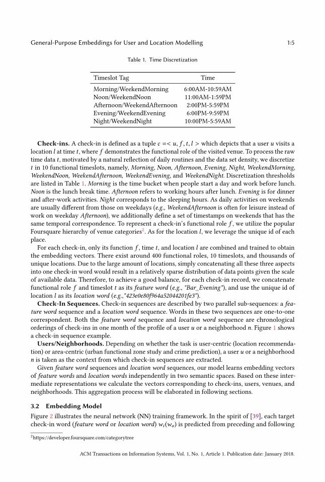
Check-ins. A check-in is defined as a tuple c =< u, f , t , l > which depicts that a user u visits alocation l at time t , where f demonstrates the functional role of the visited venue. To process the rawtime data t , motivated by a natural reflection of daily routines and the data set density, we discretizet in 10 functional timeslots, namely, Morning, Noon, Afternoon, Evening, Night,WeekendMorning,WeekendNoon,WeekendAfternoon,WeekendEvening, andWeekendNight. Discretization thresholdsare listed in Table 1. Morning is the time bucket when people start a day and work before lunch.Noon is the lunch break time. Afternoon refers to working hours after lunch. Evening is for dinnerand after-work activities. Night corresponds to the sleeping hours. As daily activities on weekendsare usually different from those on weekdays (e.g., WeekendAfternoon is often for leisure instead ofwork on weekday Afternoon), we additionally define a set of timestamps on weekends that has thesame temporal correspondence. To represent a check-in’s functional role f , we utilize the popularFoursquare hierarchy of venue categories2. As for the location l , we leverage the unique id of eachplace.
For each check-in, only its function f , time t , and location l are combined and trained to obtainthe embedding vectors. There exist around 400 functional roles, 10 timeslots, and thousands ofunique locations. Due to the large amount of locations, simply concatenating all these three aspectsinto one check-in word would result in a relatively sparse distribution of data points given the scaleof available data. Therefore, to achieve a good balance, for each check-in record, we concatenatefunctional role f and timeslot t as its feature word (e.g., "Bar_Evening"), and use the unique id oflocation l as its location word (e.g.,"423e0e80f964a52044201fe3").
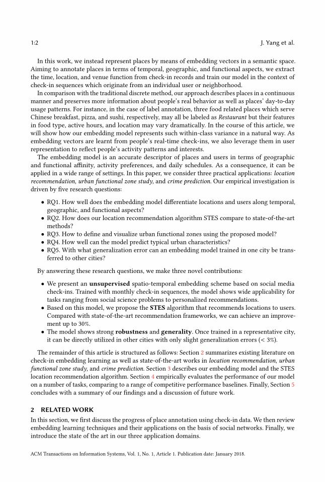
Check-In Sequences. Check-in sequences are described by two parallel sub-sequences: a fea-ture word sequence and a location word sequence. Words in these two sequences are one-to-onecorrespondent. Both the feature word sequence and location word sequence are chronologicalorderings of check-ins in one month of the profile of a user u or a neighborhood n. Figure 1 showsa check-in sequence example.
Users/Neighborhoods. Depending on whether the task is user-centric (location recommenda-tion) or area-centric (urban functional zone study and crime prediction), a user u or a neighborhoodn is taken as the context from which check-in sequences are extracted.
Given feature word sequences and location word sequences, our model learns embedding vectorsof feature words and location words independently in two semantic spaces. Based on these inter-mediate representations we calculate the vectors corresponding to check-ins, users, venues, andneighborhoods. This aggregation process will be elaborated in following sections.
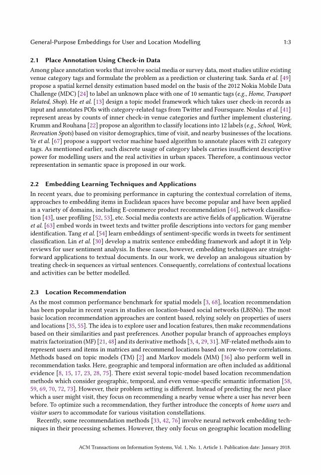
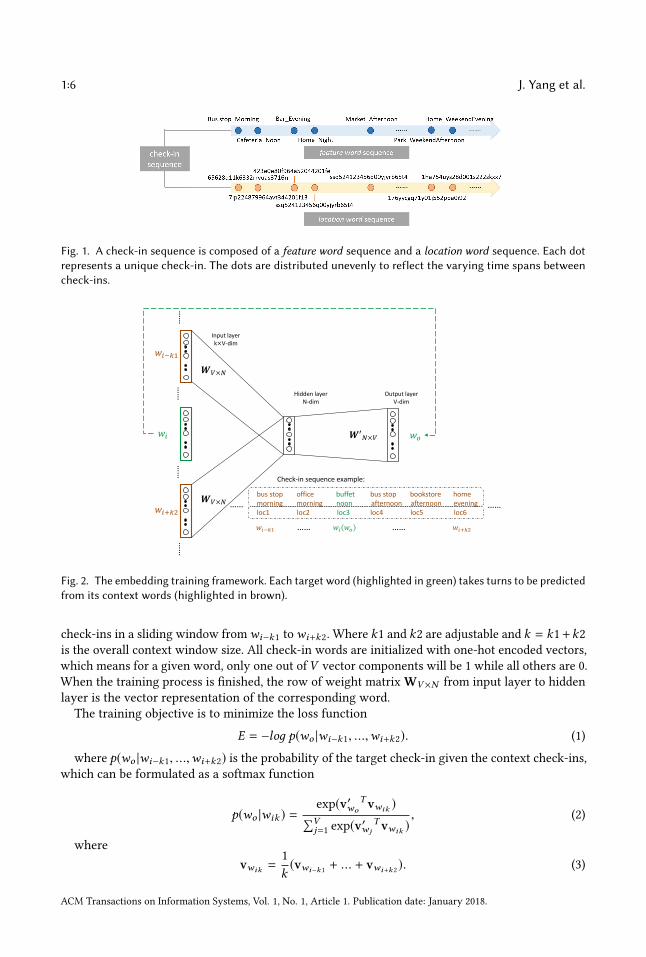
3.2 Embedding ModelFigure 2 illustrates the neural network (NN) training framework. In the spirit of [39], each targetcheck-in word (feature word or location word)wi (wo ) is predicted from preceding and following
2https://developer.foursquare.com/categorytree
ACM Transactions on Information Systems, Vol. 1, No. 1, Article 1. Publication date: January 2018.
1:6 J. Yang et al.
Fig. 1. A check-in sequence is composed of a feature word sequence and a location word sequence. Each dotrepresents a unique check-in. The dots are distributed unevenly to reflect the varying time spans betweencheck-ins.
……
…
…
Hidden layer N-dim
Output layer V-dim
𝑤𝑤𝑖𝑖
𝑤𝑤𝑖𝑖−𝑘𝑘𝑘
𝑤𝑤𝑖𝑖+𝑘𝑘𝑘
Input layer k×V-dim
𝑤𝑤𝑜𝑜
𝑾𝑾𝑉𝑉×𝑁𝑁
𝑾𝑾𝑉𝑉×𝑁𝑁
𝑾𝑾′𝑁𝑁×𝑉𝑉
bus stop office buffet bus stop bookstore home morning morning noon afternoon afternoon evening loc1 loc2 loc3 loc4 loc5 loc6
Check-in sequence example:
𝑤𝑤𝑖𝑖−𝑘𝑘𝑘 …… 𝑤𝑤𝑖𝑖 𝑤𝑤𝑜𝑜 …… 𝑤𝑤𝑖𝑖+𝑘𝑘𝑘
……
…
…
…… ……
Fig. 2. The embedding training framework. Each target word (highlighted in green) takes turns to be predictedfrom its context words (highlighted in brown).
check-ins in a sliding window fromwi−k1 towi+k2. Where k1 and k2 are adjustable and k = k1+k2is the overall context window size. All check-in words are initialized with one-hot encoded vectors,which means for a given word, only one out ofV vector components will be 1 while all others are 0.When the training process is finished, the row of weight matrix WV×N from input layer to hiddenlayer is the vector representation of the corresponding word.
The training objective is to minimize the loss function
E = −loд p(wo |wi−k1, ...,wi+k2). (1)
where p(wo |wi−k1, ...,wi+k2) is the probability of the target check-in given the context check-ins,which can be formulated as a softmax function
p(wo |wik ) =exp(v′wo
T vwik )∑Vj=1 exp(v′w j
T vwik ), (2)
wherevwik =
1k(vwi−k1 + ... + vwi+k2 ). (3)
ACM Transactions on Information Systems, Vol. 1, No. 1, Article 1. Publication date: January 2018.
General-Purpose Embeddings for User and Location Modelling 1:7
feature word sequences or/and
location word sequences
embedding model
word
vectors
sum
check-in vectors average
place/user representation
Fig. 3. Flowchart from importing check-ins to obtaining embedding vectors of places or users.
In Equation 2, v′w s comes from the columns ofW′N×V , the weight matrix connecting hidden layer
to output layer. Back-propagation is applied during the training process and both hidden-to-outputweights (W′) and input-to-hidden weights (W) are updated using stochastic gradient descent.
Also, from Equation 2, we can see that the learning process involves a traversal of all featurewords or location words, which may jeopardize model efficiency. A typical method to tackle thisproblem is to employ the hierarchical softmax algorithm as proposed in [38]. To do so, we constructa Huffman binary tree [19], in whichV vocabulary words are leaf units, and for each of them, thereexists a unique path to the root. We only consider the along-path words when calculating the lossfunction. Our preliminary experiments demonstrate that utilizing hierarchical softmax improvesthe time efficiency by around 13%. On the other hand, the location recommendation accuraciesafter using hierarchical softmax are in most cases comparable with the raw results. The largest lossis approximately 0.7%.Feature words and location words are separately trained via this model, resulting in a feature
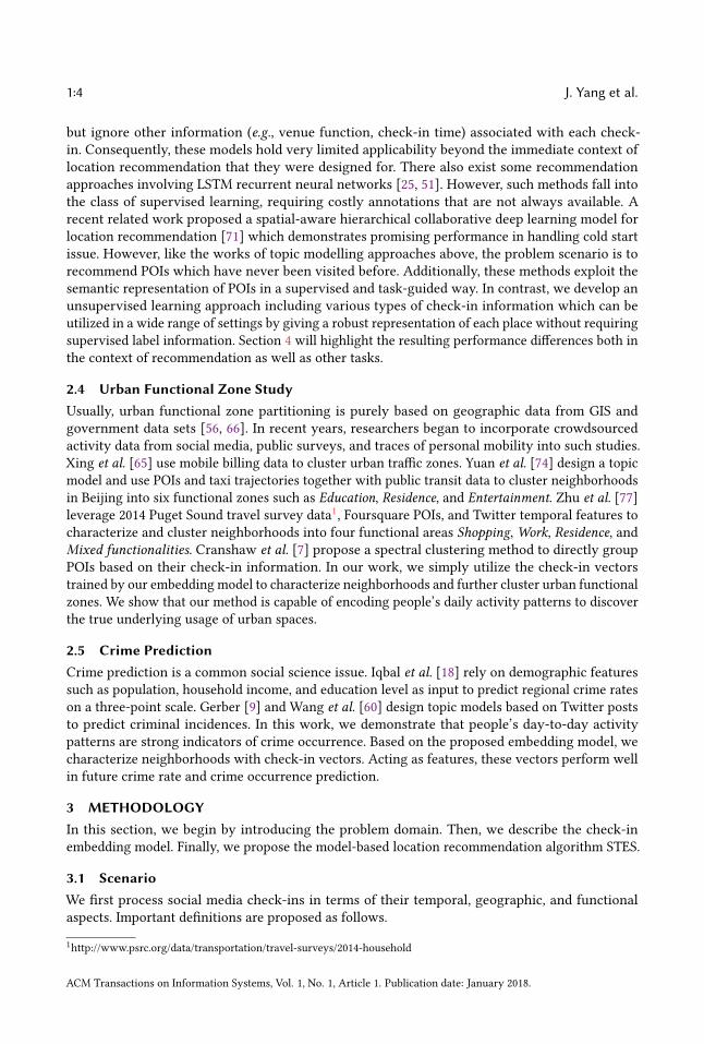
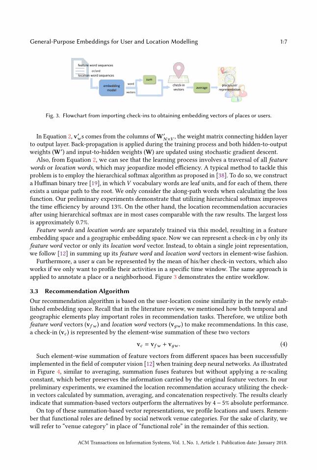
embedding space and a geographic embedding space. Now we can represent a check-in c by only itsfeature word vector or only its location word vector. Instead, to obtain a single joint representation,we follow [12] in summing up its feature word and location word vectors in element-wise fashion.
Furthermore, a user u can be represented by the mean of his/her check-in vectors, which alsoworks if we only want to profile their activities in a specific time window. The same approach isapplied to annotate a place or a neighborhood. Figure 3 demonstrates the entire workflow.
3.3 Recommendation AlgorithmOur recommendation algorithm is based on the user-location cosine similarity in the newly estab-lished embedding space. Recall that in the literature review, we mentioned how both temporal andgeographic elements play important roles in recommendation tasks. Therefore, we utilize bothfeature word vectors (vf w ) and location word vectors (vдw ) to make recommendations. In this case,a check-in (vc ) is represented by the element-wise summation of these two vectors
vc = vf w + vдw . (4)
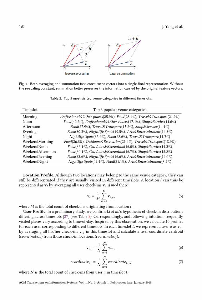
Such element-wise summation of feature vectors from different spaces has been successfullyimplemented in the field of computer vision [12] when training deep neural networks. As illustratedin Figure 4, similar to averaging, summation fuses features but without applying a re-scalingconstant, which better preserves the information carried by the original feature vectors. In ourpreliminary experiments, we examined the location recommendation accuracy utilizing the check-in vectors calculated by summation, averaging, and concatenation respectively. The results clearlyindicate that summation-based vectors outperform the alternatives by 4− 5% absolute performance.
On top of these summation-based vector representations, we profile locations and users. Remem-ber that functional roles are defined by social network venue categories. For the sake of clarity, wewill refer to “venue category” in place of “functional role” in the remainder of this section.
ACM Transactions on Information Systems, Vol. 1, No. 1, Article 1. Publication date: January 2018.
1:8 J. Yang et al.
Fig. 4. Both averaging and summation fuse constituent vectors into a single final representation. Withoutthe re-scaling constant, summation better preserves the information carried by the original feature vectors.
Table 2. Top 3 most visited venue categories in different timeslots.
Timeslot Top 3 popular venue categories
Morning Professional&Other places(25.9%), Food(23.4%), Travel&Transport(21.9%)Noon Food(40.2%), Professional&Other Places(17.1%), Shop&Service(11.6%)Afternoon Food(27.9%), Travel&Transport(15.2%), Shop&Service(14.1%)Evening Food(30.3%), Nightlife Spots(19.5%), Arts&Entertainment(14.3%)Night Nightlife Spots(35.2%), Food(22.6%), Travel&Transport(11.7%)WeekendMorning Food(26.8%), Outdoors&Recreation(21.4%), Travel&Transport(18.9%)WeekendNoon Food(36.1%), Outdoors&Recreation(16.0%), Shop&Service(14.3%)WeekendAfternoon Food(30.1%), Outdoors&Recreation(16.7%), Shop&Service(15.8%)WeekendEvening Food(33.6%), Nightlife Spots(16.6%), Arts&Entertainment(14.0%)WeekendNight Nightlife Spots(49.4%), Food(21.1%), Arts&Entertainment(8.4%)
Location Profile. Although two locations may belong to the same venue category, they canstill be differentiated if they are usually visited in different timeslots. A location l can thus berepresented as vl by averaging all user check-ins vc issued there:
vl =1M
M∑m=1
vcm , (5)
whereM is the total count of check-ins originating from location l .User Profile. In a preliminary study, we confirm Li et al.’s hypothesis of check-in distributions
differing across timeslots [27] (see Table 2). Correspondingly, and following intuition, frequentlyvisited places vary according to time-of-day. Inspired by this observation, we calculate 10 profilesfor each user corresponding to different timeslots. In each timeslot t , we represent a user u as vutby averaging all his/her check-ins vct in this timeslot and calculate a user coordinate centroid(coordinateut ) from those check-in locations (coordinatect ).
vut =1N
N∑n=1
vct,n (6)
coordinateut =1N
N∑n=1
coordinatect,n (7)
where N is the total count of check-ins from user u in timeslot t .
ACM Transactions on Information Systems, Vol. 1, No. 1, Article 1. Publication date: January 2018.
General-Purpose Embeddings for User and Location Modelling 1:9
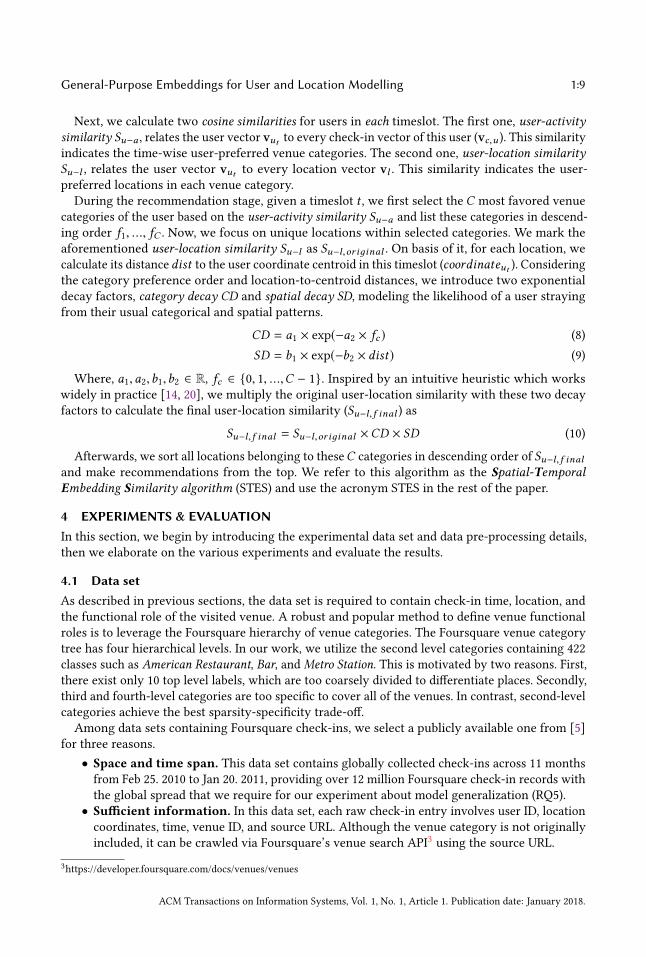
Next, we calculate two cosine similarities for users in each timeslot. The first one, user-activitysimilarity Su−a , relates the user vector vut to every check-in vector of this user (vc,u ). This similarityindicates the time-wise user-preferred venue categories. The second one, user-location similaritySu−l , relates the user vector vut to every location vector vl . This similarity indicates the user-preferred locations in each venue category.During the recommendation stage, given a timeslot t , we first select the C most favored venue
categories of the user based on the user-activity similarity Su−a and list these categories in descend-ing order f1, ..., fC . Now, we focus on unique locations within selected categories. We mark theaforementioned user-location similarity Su−l as Su−l,or iдinal . On basis of it, for each location, wecalculate its distance dist to the user coordinate centroid in this timeslot (coordinateut ). Consideringthe category preference order and location-to-centroid distances, we introduce two exponentialdecay factors, category decay CD and spatial decay SD, modeling the likelihood of a user strayingfrom their usual categorical and spatial patterns.
CD = a1 × exp(−a2 × fc ) (8)SD = b1 × exp(−b2 × dist) (9)
Where, a1,a2,b1,b2 ∈ R, fc ∈ {0, 1, ...,C − 1}. Inspired by an intuitive heuristic which workswidely in practice [14, 20], we multiply the original user-location similarity with these two decayfactors to calculate the final user-location similarity (Su−l,f inal ) as
Su−l,f inal = Su−l,or iдinal ×CD × SD (10)
Afterwards, we sort all locations belonging to theseC categories in descending order of Su−l,f inaland make recommendations from the top. We refer to this algorithm as the Spatial-TemporalEmbedding Similarity algorithm (STES) and use the acronym STES in the rest of the paper.
4 EXPERIMENTS & EVALUATIONIn this section, we begin by introducing the experimental data set and data pre-processing details,then we elaborate on the various experiments and evaluate the results.
4.1 Data setAs described in previous sections, the data set is required to contain check-in time, location, andthe functional role of the visited venue. A robust and popular method to define venue functionalroles is to leverage the Foursquare hierarchy of venue categories. The Foursquare venue categorytree has four hierarchical levels. In our work, we utilize the second level categories containing 422classes such as American Restaurant, Bar, and Metro Station. This is motivated by two reasons. First,there exist only 10 top level labels, which are too coarsely divided to differentiate places. Secondly,third and fourth-level categories are too specific to cover all of the venues. In contrast, second-levelcategories achieve the best sparsity-specificity trade-off.Among data sets containing Foursquare check-ins, we select a publicly available one from [5]
for three reasons.• Space and time span. This data set contains globally collected check-ins across 11 monthsfrom Feb 25. 2010 to Jan 20. 2011, providing over 12 million Foursquare check-in records withthe global spread that we require for our experiment about model generalization (RQ5).
• Sufficient information. In this data set, each raw check-in entry involves user ID, locationcoordinates, time, venue ID, and source URL. Although the venue category is not originallyincluded, it can be crawled via Foursquare’s venue search API3 using the source URL.
3https://developer.foursquare.com/docs/venues/venues
ACM Transactions on Information Systems, Vol. 1, No. 1, Article 1. Publication date: January 2018.
1:10 J. Yang et al.
• Comparability. This data set has been utilized in a variety of relevant works, includinglocation recommendation [16, 17, 64], urban activity pattern understanding [10, 11], location-based services with privacy awareness [46, 62], etc.
Another two Foursquare data sets from [28] and [76] are also leveraged in relevant pieces ofresearch. However, the former only contains check-ins in Singapore while the latter does notinclude any venue category. Therefore, we exclude them from our study.A common issue in check-in data streams are repeated check-ins at the same venue in an
artificially short time window during which users remain in an unchanged location and activity [26].This appears reasonable as check-ins are often posted in a casual way in which people share real-time affairs and moods. This effect is especially common in recreational and culinary activities. Forinstance, a user may check in for several times during one meal with friends, each time postingabout a newly served dish or commenting on the food. To model activity sequences most reliably,we delete such repeated check-ins from an individual staying in an unchanged activity and retainonly the first check-in at this location. To reduce noise, we further remove both users and locationswith less than 10 posts. After this pre-processing, for the example of New York City (NYC), ourdataset contains 225,782 check-ins by 6,442 users at 7,453 locations.To define urban “neighborhoods” for our area-centric tasks urban functional zone study and
crime prediction, we utilize official 2010 Census Block Group (CBG) polygons4, matching the timeperiod of the check-in data collection. A CBG may contain several Census Blocks (CBs), whichare the smallest geographic areas that the U.S. Census Bureau uses to collect and tabulate censusdata. These polygons represent the most natural segmentation of a city, given that their boundariesare defined by physical streets, railroad tracks, bodies of water as well as invisible town limits,property lines, and imaginary extensions of streets. In NYC, there are 6,493 CBGs, 1,720 of whichare populated by our denoised check-ins.
4.2 Qualitative Analysis of Embedding VectorsOur embedding vectors are designed to retain key characteristics of user activities and urban venuesso that users and places are differentiable. We set the latent embedding dimension to 200 and obtainembedding vectors for all of the feature words and location words in NYC.
To get a qualitative impression of the resulting embeddings, we first examine their overall cosinesimilarities and Euclidean distances. The cosine metric evaluates the similarity by normalizing vec-tors and measuring the in-between angle, and the Euclidean distance demonstrates the magnitudeof difference between two vectors.
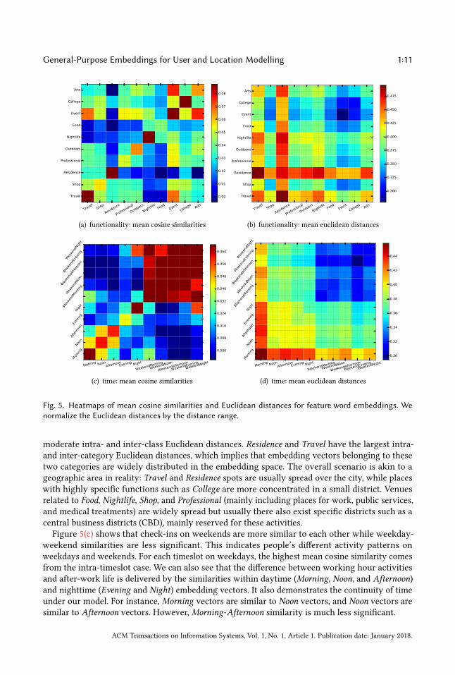
We explore feature word embedding vectors from both functionality and time perspectives. Wefirst calculate the cosine similarity and Euclidean distance for each pair of embedding vectors,then we compute the mean similarity and distance values among the timeslots and top-level venuecategories, respectively. We demonstrate the results in the form of heatmaps in Figure 5, wherefour significant tendencies can be observed.
In Figure 5(a), we can see that intra-category embedding vectors show the highest mean cosinesimilarities. The single exception Arts lists Arts-Arts similarity as second to the Arts-Event pair.Considering that Event mainly involves places for sport, musical, and arts activities, this resultappears reasonable. Categories including similar or overlapping venues also have good inter-classsimilarities, such as Food-Nightlife, College-Event, and Outdoors-Event.Turning to Figure 5(b), the mean intra-category Euclidean distances of College and Event are
smaller than inter-category distances, which indicates that these two categories have the mostcompact embedding vector clouds. Arts, Food, Nightlife, Outdoors, Professional, and Shop also have
4http://data.beta.nyc/dataset/2010-census-block-groups-polygons
ACM Transactions on Information Systems, Vol. 1, No. 1, Article 1. Publication date: January 2018.
General-Purpose Embeddings for User and Location Modelling 1:11
TravelShop
Residence
Professional
Outdoors
Nightlife
FoodEvent
College
Arts
Travel
Shop
Residence
Professional
Outdoors
Nightlife
Food
Event
College
Arts
cosine similarity heatmap of feature word embeddings
0.00
0.01
0.02
0.03
0.04
0.05
0.06
0.07
0.08
(a) functionality: mean cosine similarities
TravelShop
Residence
Professional
Outdoors
Nightlife
FoodEvent
College
Arts
Travel
Shop
Residence
Professional
Outdoors
Nightlife
Food
Event
College
Arts
euclidean distance heatmap of feature word embeddings
0.300
0.325
0.350
0.375
0.400
0.425
0.450
0.475
(b) functionality: mean euclidean distances
Morning NoonAfternoon
Evening Night
WeekendMorning
WeekendNoon
WeekendAfternoon
WeekendEvening
WeekendNight
Mor
ning
Noon
Afte
rnoo
n
Even
ing
NightW
eeke
ndM
orni
ng
Wee
kend
Noon
Wee
kend
Afte
rnoo
n
Wee
kend
Even
ing
Wee
kend
Night
0.000
0.008
0.016
0.024
0.032
0.040
0.048
0.056
0.064
(c) time: mean cosine similarities
Morning NoonAfternoon
Evening Night
WeekendMorning
WeekendNoon
WeekendAfternoon
WeekendEvening
WeekendNight
Mor
ning
Noon
Afte
rnoo
n
Even
ing
NightW
eeke
ndM
orni
ng
Wee
kend
Noon
Wee
kend
Afte
rnoo
n
Wee
kend
Even
ing
Wee
kend
Night
0.30
0.32
0.34
0.36
0.38
0.40
0.42
0.44
(d) time: mean euclidean distances
Fig. 5. Heatmaps of mean cosine similarities and Euclidean distances for feature word embeddings. Wenormalize the Euclidean distances by the distance range.
moderate intra- and inter-class Euclidean distances. Residence and Travel have the largest intra-and inter-category Euclidean distances, which implies that embedding vectors belonging to thesetwo categories are widely distributed in the embedding space. The overall scenario is akin to ageographic area in reality: Travel and Residence spots are usually spread over the city, while placeswith highly specific functions such as College are more concentrated in a small district. Venuesrelated to Food, Nightlife, Shop, and Professional (mainly including places for work, public services,and medical treatments) are widely spread but usually there also exist specific districts such as acentral business districts (CBD), mainly reserved for these activities.Figure 5(c) shows that check-ins on weekends are more similar to each other while weekday-
weekend similarities are less significant. This indicates people’s different activity patterns onweekdays and weekends. For each timeslot on weekdays, the highest mean cosine similarity comesfrom the intra-timeslot case. We can also see that the difference between working hour activitiesand after-work life is delivered by the similarities within daytime (Morning, Noon, and Afternoon)and nighttime (Evening and Night) embedding vectors. It also demonstrates the continuity of timeunder our model. For instance, Morning vectors are similar to Noon vectors, and Noon vectors aresimilar to Afternoon vectors. However, Morning-Afternoon similarity is much less significant.
ACM Transactions on Information Systems, Vol. 1, No. 1, Article 1. Publication date: January 2018.
1:12 J. Yang et al.
0 5 10 15 20 25 30 35 400.02
0.00
0.02
0.04
0.06
0.08
POI-
PO
I co
sin
e si
mila
rity
POI-POI geographic distance (km)
(a) Cosine similarity of location pairs (y-axis) with in-creasing geographic distance (x-axis)
0 5 10 15 20 25 30 35 40
0.52
0.54
0.56
0.58
0.60
POI-POI geograhic distance (km)
PO
I-P
OI E
ucl
idea
n d
ista
nce
(b) Euclidean distance of location pairs (y-axis) withincreasing geographic distance (x-axis)
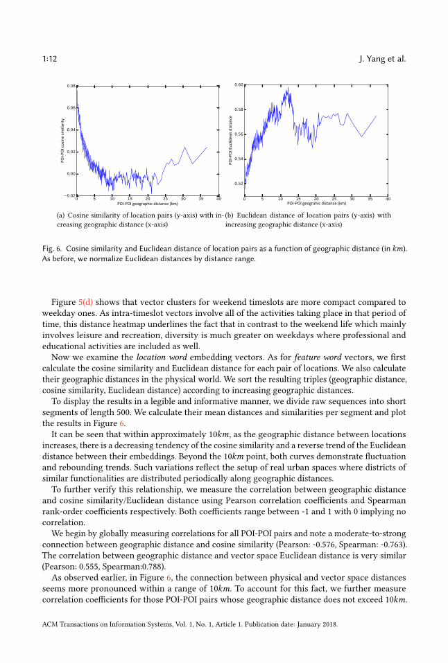
Fig. 6. Cosine similarity and Euclidean distance of location pairs as a function of geographic distance (in km).As before, we normalize Euclidean distances by distance range.
Figure 5(d) shows that vector clusters for weekend timeslots are more compact compared toweekday ones. As intra-timeslot vectors involve all of the activities taking place in that period oftime, this distance heatmap underlines the fact that in contrast to the weekend life which mainlyinvolves leisure and recreation, diversity is much greater on weekdays where professional andeducational activities are included as well.Now we examine the location word embedding vectors. As for feature word vectors, we first
calculate the cosine similarity and Euclidean distance for each pair of locations. We also calculatetheir geographic distances in the physical world. We sort the resulting triples (geographic distance,cosine similarity, Euclidean distance) according to increasing geographic distances.To display the results in a legible and informative manner, we divide raw sequences into short
segments of length 500. We calculate their mean distances and similarities per segment and plotthe results in Figure 6.It can be seen that within approximately 10km, as the geographic distance between locations
increases, there is a decreasing tendency of the cosine similarity and a reverse trend of the Euclideandistance between their embeddings. Beyond the 10km point, both curves demonstrate fluctuationand rebounding trends. Such variations reflect the setup of real urban spaces where districts ofsimilar functionalities are distributed periodically along geographic distances.To further verify this relationship, we measure the correlation between geographic distance
and cosine similarity/Euclidean distance using Pearson correlation coefficients and Spearmanrank-order coefficients respectively. Both coefficients range between -1 and 1 with 0 implying nocorrelation.
We begin by globally measuring correlations for all POI-POI pairs and note a moderate-to-strongconnection between geographic distance and cosine similarity (Pearson: -0.576, Spearman: -0.763).The correlation between geographic distance and vector space Euclidean distance is very similar(Pearson: 0.555, Spearman:0.788).
As observed earlier, in Figure 6, the connection between physical and vector space distancesseems more pronounced within a range of 10km. To account for this fact, we further measurecorrelation coefficients for those POI-POI pairs whose geographic distance does not exceed 10km.
ACM Transactions on Information Systems, Vol. 1, No. 1, Article 1. Publication date: January 2018.
General-Purpose Embeddings for User and Location Modelling 1:13
Venues in weekend evening
Hotdog joint
Cafe
Sandwich place College cafeteria
College bookstore
Library
College academic building
University
School
Office
Food
College & University
Professional Places
y-ax
is in
dow
nsca
led
two-
dim
ensio
nal s
pace
x-axis in downscaled two-dimensional space
(a) feature word embeddings
14.33km 17.12km 7.13km
Locations
423e0e80f964a52044201fe3
4c0d701c7189c9282c01d7b6 4c7e02dcd6543704bd1bc2a2
14.33km
17.12km
4a258464f964a5205e7e1fe3
7.13km
16.52km
4bf416d594af2d7f81293a72
x-axis in downscaled two-dimensional space
y-ax
is in
dow
nsca
led
two-
dim
ensio
nal s
pace
(b) location word embeddings
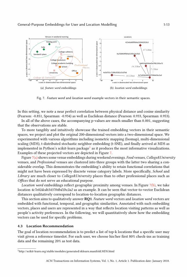
Fig. 7. Feature word and location word example vectors in their semantic spaces.
In this setting, we note a near perfect correlation between physical distance and cosine similarity(Pearson: -0.851, Spearman: -0.934) as well as Euclidean distance (Pearson: 0.933, Spearman: 0.953).
In all of the above cases, the accompanying p-values are much smaller than 0.001, suggestingthat the observations are stable.To more tangibly and intuitively showcase the trained embedding vectors in their semantic
spaces, we project and plot the original 200-dimensional vectors into a two-dimensional space. Weexperimented with various algorithms including isometric mapping (Isomap), multi-dimensionalscaling (MDS), t-distributed stochastic neighbor embedding (t-SNE), and finally arrived at MDS asimplemented in Python’s scikit-learn package1 as it produces the most informative visualizations.Examples of these projected vectors are depicted in Figure 7.
Figure 7(a) shows some venue embeddings duringweekend evenings. Food venues,College&Universityvenues, and Professional venues are clustered into three groups with the latter two sharing a con-siderable overlap. This demonstrates the embedding’s ability to retain functional correlations thatmight not have been expressed by discrete venue category labels. More specifically, School andLibrary are much closer to College&University places than to other professional places such asOffices that do not serve an educational purpose.Location word embeddings reflect geographic proximity among venues. In Figure 7(b), we take
location 4c7e02dcd6543704bd1bc2a2 as an example. It can be seen that vector-to-vector Euclideandistances qualitatively correspond to location-to-location geographic distances.
This section aims to qualitatively answerRQ1. Feature word vectors and location word vectors areembedded with functional, temporal, and geographic similarities. Annotated with such embeddingvectors, places and users are represented in a way that reflects location visiting patterns as well aspeople’s activity preferences. In the following, we will quantitatively show how the embeddingvectors can be used for specific problems.
4.3 Location RecommendationThe goal of location recommendation is to predict a list of top-k locations that a specific user mayvisit given a reference timeslot. For each user, we choose his/her first 80% check-ins as trainingdata and the remaining 20% as test data.
1http://scikit-learn.org/stable/modules/generated/sklearn.manifold.MDS.html
ACM Transactions on Information Systems, Vol. 1, No. 1, Article 1. Publication date: January 2018.
1:14 J. Yang et al.
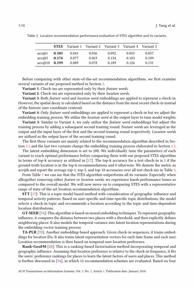
Table 3. Location recommendation performance evaluation of STES algorithm and its variants.
STES Variant 1 Variant 2 Variant 3 Variant 4 Variant 5
acc@1 0.105 0.041 0.036 0.092 0.055 0.057acc@5 0.176 0.077 0.063 0.154 0.103 0.109acc@10 0.199 0.089 0.078 0.189 0.126 0.131
Before comparing with other state-of-the-art recommendation algorithms, we first examineseveral variants of our proposed method in Section 3.
Variant 1: Check-ins are represented only by their feature words.Variant 2: Check-ins are represented only by their location words.Variant 3: Both feature word and location word embeddings are applied to represent a check-in.
However, the spatial decay is calculated based on the distance from the most recent check-in insteadof the historic user coordinate centroid.
Variant 4: Only feature word embeddings are applied to represent a check-in but we adjust theembedding training process. We utilize the location word at the output layer to tune model weights.
Variant 5: Similar to Variant 4, we only utilize the feature word embeddings but adjust thetraining process by adding a subsequent second training round. Feature words are leveraged as theoutput and the input layer of the first and the second training round respectively. Location wordsare utilized as the output layer of the second training round.The first three variants are mainly related to the recommendation algorithm described in Sec-
tion 3.3 and the last two variants change the embedding training process elaborated in Section 3.2.The latent embedding dimension is set to 200. We individually tune the parameters of each
variant to reach optimal performance before comparing them with our proposed STES algorithmin terms of top-k accuracy as utilized in [17]. The top-k accuracy for a test check-in is 1 if theground-truth location is in the top-k recommendations and 0 otherwise. We demote the metric asacc@k and report the average top-1, top-5, and top-10 accuracies over all test check-ins in Table 3.From Table 3 we can see that the STES algorithm outperforms all its variants. Especially when
alltogether removing either feature or location words, we experience harsh performance losses ascompared to the overall model. We will now move on to comparing STES with a representativerange of state-of-the-art location recommendation algorithms.
STT [17]: This is a topic model based method with consideration of geographic influence andtemporal activity patterns. Based on user-specific and time-specific topic distributions, the modelselects a check-in topic and recommends a location according to the topic and time-dependentlocation distributions.
GT-SEER [76]: This algorithm is based on neural embedding techniques. To represent geographicinfluence, it compares the distance between two places with a threshold, and then explicitly definesneighboring places. It also models the temporal variance into latent location representations duringthe embedding vector training process.
TA-PLR [33]: Another embedding-based approach. Given check-in sequences, it trains embed-dings for location IDs. It also trains latent representation vectors for each time frame and each user.Location recommendation is then based on temporal user-location preference.
Rank-GeoFM [28]: This is a ranking-based factorization method incorporating temporal andgeographic influence. Assuming that location preference is relative to the check-in frequency, it fitsthe users’ preference rankings for places to learn the latent factors of users and places. This methodis further discussed in [34], in which 12 recommendation schemes are evaluated. Based on four
ACM Transactions on Information Systems, Vol. 1, No. 1, Article 1. Publication date: January 2018.
General-Purpose Embeddings for User and Location Modelling 1:15
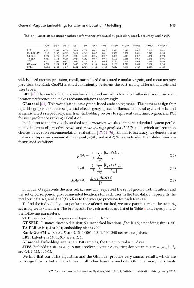
Table 4. Location recommendation performance evaluated by precision, recall, accuracy, and MAP.
p@1 p@5 p@10 r@1 r@5 r@10 acc@1 acc@5 acc@10 MAP@1 MAP@5 MAP@10
LRT 0.371 0.105 0.054 0.016 0.038 0.052 0.017 0.033 0.059 0.017 0.029 0.042Rank-GeoFM 0.42 0.152 0.069 0.019 0.046 0.067 0.021 0.051 0.077 0.021 0.045 0.058GT-SEER 0.462 0.179 0.099 0.021 0.058 0.076 0.047 0.088 0.126 0.047 0.071 0.093TA-PLR 0.457 0.184 0.096 0.025 0.062 0.087 0.045 0.101 0.143 0.045 0.074 0.091STT 0.547 0.209 0.125 0.032 0.071 0.09 0.055 0.137 0.174 0.055 0.084 0.098GEmodel 0.598 0.224 0.152 0.057 0.085 0.108 0.083 0.169 0.201 0.083 0.124 0.130STES 0.606 0.227 0.147 0.064 0.089 0.109 0.105 0.176 0.199 0.105 0.128 0.132
widely-used metrics precision, recall, normalized discounted cumulative gain, and mean averageprecision, the Rank-GeoFM method consistently performs the best among different datasets anduser types.
LRT [8]: This matrix factorization based method measures temporal influence to capture user-location preference and makes recommendations accordingly.
GEmodel [64]: This work introduces a graph-based embedding model. The authors design fourbipartite graphs to encode sequential effects, geographical influence, temporal cyclic effects, andsemantic effects respectively, and train embedding vectors to represent user, time, region, and POIfor user preference ranking calculation.
In addition to the previously studied top-k accuracy, we also compare individual system perfor-mance in terms of precision, recall, and mean average precision (MAP), all of which are commonchoices in location recommendation evaluation [17, 32, 76]. Similar to accuracy, we denote thesemetrics at top-k recommendation as p@k, r@k, and MAP@k respectively. Their definitions areformulated as follows,
p@k =1|U |
∑u ∈U
|Lдt ∩ Lr ec |k
(11)
r@k =1|U |
∑u ∈U
|Lдt ∩ Lr ec ||Lдt |
(12)
MAP@k =
∑t ∈T AveP(t)
|T | (13)
in which,U represents the user set, Lдt and Lr ec represent the set of ground truth locations andthe set of corresponding recommended locations for each user in the test data. T represents thetotal test data set, and AveP(t) refers to the average precision for each test case.To find the individually best performance of each method, we tune parameters on the training
set using cross validation. The best results for each method are listed in Table 4 and correspond tothe following parameters:
STT: Counts of latent regions and topics are both 150.GT-SEER: Distance threshold is 1km; 50 unchecked locations, β/α is 0.5; embedding size is 200.TA-PLR: α is 1; λ is 0.01; embedding size is 200.Rank-GeoFM: α ,γ , ϵ,C,K are 0.15, 0.0001, 0.3, 1, 100; 300 nearest neighbors.LRT: Latent d is 10; α , β , λ are 2, 2, 1.GEmodel: Embedding size is 100; 150 samples; the time interval is 30 days.STES: Embedding size is 200; 15 most preferred venue categories; decay parameters a1,a2,b1,b2
are 0.4, 0.025, 1, 0.95.We find that our STES algorithm and the GEmodel produce very similar results, which are
both significantly better than those of all other baseline methods. GEmodel marginally beats
ACM Transactions on Information Systems, Vol. 1, No. 1, Article 1. Publication date: January 2018.

1:16 J. Yang et al.
our algorithm in terms of precision and accuracy at top-10 recommendations while in all othercases our STES model is slightly better. However, GEmodel was specifically designed for locationrecommendation. Although the embeddings can also be utilized in other domains, it is less flexibleand general than our algorithm. In the rest of this paper, we will show how our algorithm can begracefully generalized to other tasks without any adjustments.
We confirm the statistical significance of performance differences between our method and all ofthe contesting baselines using McNemar’s test [37]. The largest mid-p-value is 1.53 × 10⁻⁴.With respect to RQ2, the results demonstrate the effectiveness of our embedding model and
the STES algorithm in user/place characterization for location recommendation. As geographicand temporal aspects are considered in these six approaches in different stages, we argue thatour improvement mainly comes from the embedding of venues’ functional roles. In addition toindicating where and when someone is, the functional information further explains why someoneis there at that time, essentially revealing a person’s activity preference beyond specific locationpreference. Consequently, we attain better relative modelling power when a user is in a regionwhich is away from his/her frequently visited area and literal check-ins at unique locations cannotbe levied. Moreover, calculating the mean of check-in vectors further leverages the continuity andsmoothness of the embedding model and thus establishes more latent correlations between usersand locations.
4.4 Urban Functional Zone StudyPrevious work has shown that dividing a city into different functional zones is a straightforwardyet informative way to define urban areas. The central information according to which to partitionfunctional zones are the inhabitants’ interactions with urban spaces. Therefore, we conduct researchin this aspect to examine model efficiency in describing people’s activities and characterizingplaces. To do so, we exclusively utilize feature word embeddings which contain second-level venuecategories and check-in timestamps. We train the embedding model on neighborhood level andrepresent each neighborhood using the mean of all contained check-in vectors. Then, we implementK-Means clustering on neighborhoods as suggested by [41] and [77].
Remember that in location recommendation, we compared our model with a baseline algorithmGEmodel. Similar to our method, GEmodel generates timestamp and venue category embeddingsas well. As an additional comparison, we also characterize neighborhoods with the mean of innercheck-in time and venue category vectors trained by GEmodel.
Zhu et al. [77] demonstrate an effective neighborhood characterization based on the normalizedcounts of demographic, temporal and spatial aspects of visits. Noulas et al. [41] show that thefunctional zones can be reliably clustered if neighborhoods are represented only by the numberof visits at each venue category. Corresponding to these two approaches, we first propose twoground-truth alternatives: (1). l2-normalized counts of feature words; (2). l2-normalized counts ofvenue categories.
To determine the most qualified ground-truth in our work, we examine the cluster assignmentsderived from the alternatives using Silhouette Index (SI) [47], which measures how compact clustersare by computing the average intra-cluster and inter-cluster distances. The SI ranges between -1 forincorrect clustering and +1 for highly dense and well separated clustering. An SI around 0 indicatesoverlapping clusters.
We increase the count of clusters from 3 to 10 and report the Silhouette indices of clusterings inTable 5.
We can see that all comparedmethods peak in performance at four or five clusters. ComparedwithGEmodel based clustering, our embedding model produces more well-defined clusters. Similarly,ground-truth alternative 1 performs better than alternative 2.
ACM Transactions on Information Systems, Vol. 1, No. 1, Article 1. Publication date: January 2018.
General-Purpose Embeddings for User and Location Modelling 1:17
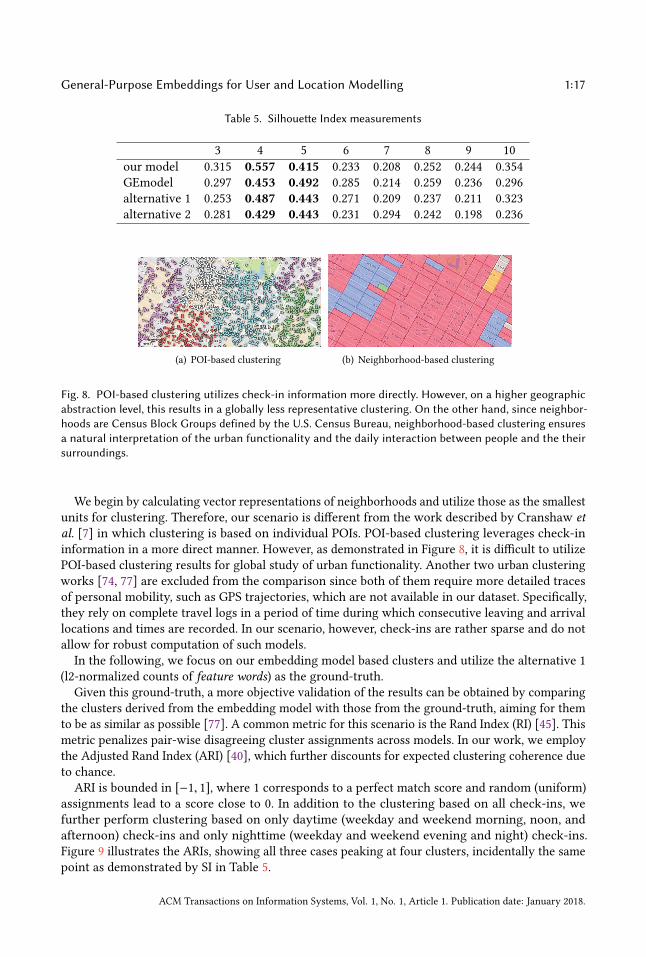
Table 5. Silhouette Index measurements
3 4 5 6 7 8 9 10our model 0.315 0.557 0.415 0.233 0.208 0.252 0.244 0.354GEmodel 0.297 0.453 0.492 0.285 0.214 0.259 0.236 0.296alternative 1 0.253 0.487 0.443 0.271 0.209 0.237 0.211 0.323alternative 2 0.281 0.429 0.443 0.231 0.294 0.242 0.198 0.236
(a) POI-based clustering (b) Neighborhood-based clustering
Fig. 8. POI-based clustering utilizes check-in information more directly. However, on a higher geographicabstraction level, this results in a globally less representative clustering. On the other hand, since neighbor-hoods are Census Block Groups defined by the U.S. Census Bureau, neighborhood-based clustering ensuresa natural interpretation of the urban functionality and the daily interaction between people and the theirsurroundings.
We begin by calculating vector representations of neighborhoods and utilize those as the smallestunits for clustering. Therefore, our scenario is different from the work described by Cranshaw etal. [7] in which clustering is based on individual POIs. POI-based clustering leverages check-ininformation in a more direct manner. However, as demonstrated in Figure 8, it is difficult to utilizePOI-based clustering results for global study of urban functionality. Another two urban clusteringworks [74, 77] are excluded from the comparison since both of them require more detailed tracesof personal mobility, such as GPS trajectories, which are not available in our dataset. Specifically,they rely on complete travel logs in a period of time during which consecutive leaving and arrivallocations and times are recorded. In our scenario, however, check-ins are rather sparse and do notallow for robust computation of such models.In the following, we focus on our embedding model based clusters and utilize the alternative 1
(l2-normalized counts of feature words) as the ground-truth.Given this ground-truth, a more objective validation of the results can be obtained by comparing
the clusters derived from the embedding model with those from the ground-truth, aiming for themto be as similar as possible [77]. A common metric for this scenario is the Rand Index (RI) [45]. Thismetric penalizes pair-wise disagreeing cluster assignments across models. In our work, we employthe Adjusted Rand Index (ARI) [40], which further discounts for expected clustering coherence dueto chance.ARI is bounded in [−1, 1], where 1 corresponds to a perfect match score and random (uniform)
assignments lead to a score close to 0. In addition to the clustering based on all check-ins, wefurther perform clustering based on only daytime (weekday and weekend morning, noon, andafternoon) check-ins and only nighttime (weekday and weekend evening and night) check-ins.Figure 9 illustrates the ARIs, showing all three cases peaking at four clusters, incidentally the samepoint as demonstrated by SI in Table 5.
ACM Transactions on Information Systems, Vol. 1, No. 1, Article 1. Publication date: January 2018.
1:18 J. Yang et al.
0.00%
10.00%
20.00%
30.00%
40.00%
50.00%
60.00%
70.00%
3 4 5 6 7 8 9 10
ARI
all-day daytime nighttime
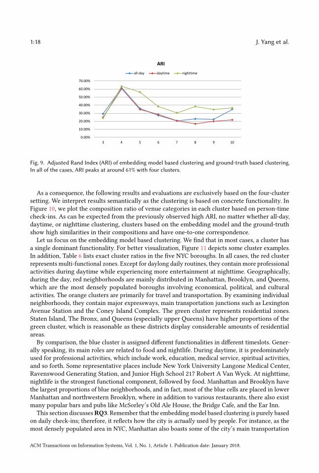
Fig. 9. Adjusted Rand Index (ARI) of embedding model based clustering and ground-truth based clustering.In all of the cases, ARI peaks at around 61% with four clusters.
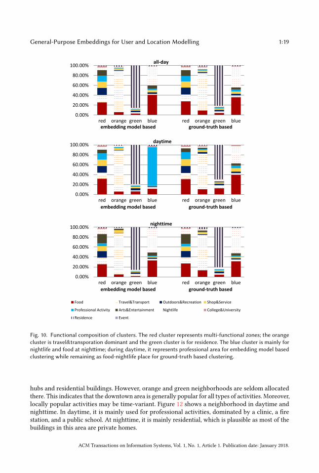
As a consequence, the following results and evaluations are exclusively based on the four-clustersetting. We interpret results semantically as the clustering is based on concrete functionality. InFigure 10, we plot the composition ratio of venue categories in each cluster based on person-timecheck-ins. As can be expected from the previously observed high ARI, no matter whether all-day,daytime, or nighttime clustering, clusters based on the embedding model and the ground-truthshow high similarities in their compositions and have one-to-one correspondence.
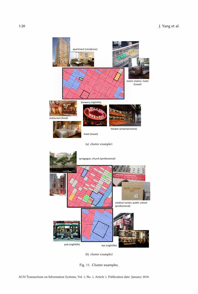
Let us focus on the embedding model based clustering. We find that in most cases, a cluster hasa single dominant functionality. For better visualization, Figure 11 depicts some cluster examples.In addition, Table 6 lists exact cluster ratios in the five NYC boroughs. In all cases, the red clusterrepresents multi-functional zones. Except for daylong daily routines, they contain more professionalactivities during daytime while experiencing more entertainment at nighttime. Geographically,during the day, red neighborhoods are mainly distributed in Manhattan, Brooklyn, and Queens,which are the most densely populated boroughs involving economical, political, and culturalactivities. The orange clusters are primarily for travel and transportation. By examining individualneighborhoods, they contain major expressways, main transportation junctions such as LexingtonAvenue Station and the Coney Island Complex. The green cluster represents residential zones.Staten Island, The Bronx, and Queens (especially upper Queens) have higher proportions of thegreen cluster, which is reasonable as these districts display considerable amounts of residentialareas.
By comparison, the blue cluster is assigned different functionalities in different timeslots. Gener-ally speaking, its main roles are related to food and nightlife. During daytime, it is predominatelyused for professional activities, which include work, education, medical service, spiritual activities,and so forth. Some representative places include New York University Langone Medical Center,Ravenswood Generating Station, and Junior High School 217 Robert A Van Wyck. At nighttime,nightlife is the strongest functional component, followed by food. Manhattan and Brooklyn havethe largest proportions of blue neighborhoods, and in fact, most of the blue cells are placed in lowerManhattan and northwestern Brooklyn, where in addition to various restaurants, there also existmany popular bars and pubs like McSorley’s Old Ale House, the Bridge Cafe, and the Ear Inn.
This section discussesRQ3. Remember that the embeddingmodel based clustering is purely basedon daily check-ins; therefore, it reflects how the city is actually used by people. For instance, as themost densely populated area in NYC, Manhattan also boasts some of the city’s main transportation
ACM Transactions on Information Systems, Vol. 1, No. 1, Article 1. Publication date: January 2018.
General-Purpose Embeddings for User and Location Modelling 1:19
0.00%
20.00%
40.00%
60.00%
80.00%
100.00%
red orange green blue red orange green blue
all-day
embedding model based ground-truth based
0.00%
20.00%
40.00%
60.00%
80.00%
100.00%
red orange green blue red orange green blue
daytime
embedding model based ground-truth based
0.00%
20.00%
40.00%
60.00%
80.00%
100.00%
red orange green blue red orange green blue
nighttime
Food Travel&Transport Outdoors&Recreation Shop&Service
Professional Activity Arts&Entertainment Nightlife College&University
Residence Event
embedding model based ground-truth based
Fig. 10. Functional composition of clusters. The red cluster represents multi-functional zones; the orangecluster is travel&transporation dominant and the green cluster is for residence. The blue cluster is mainly fornightlife and food at nighttime; during daytime, it represents professional area for embedding model basedclustering while remaining as food-nightlife place for ground-truth based clustering.
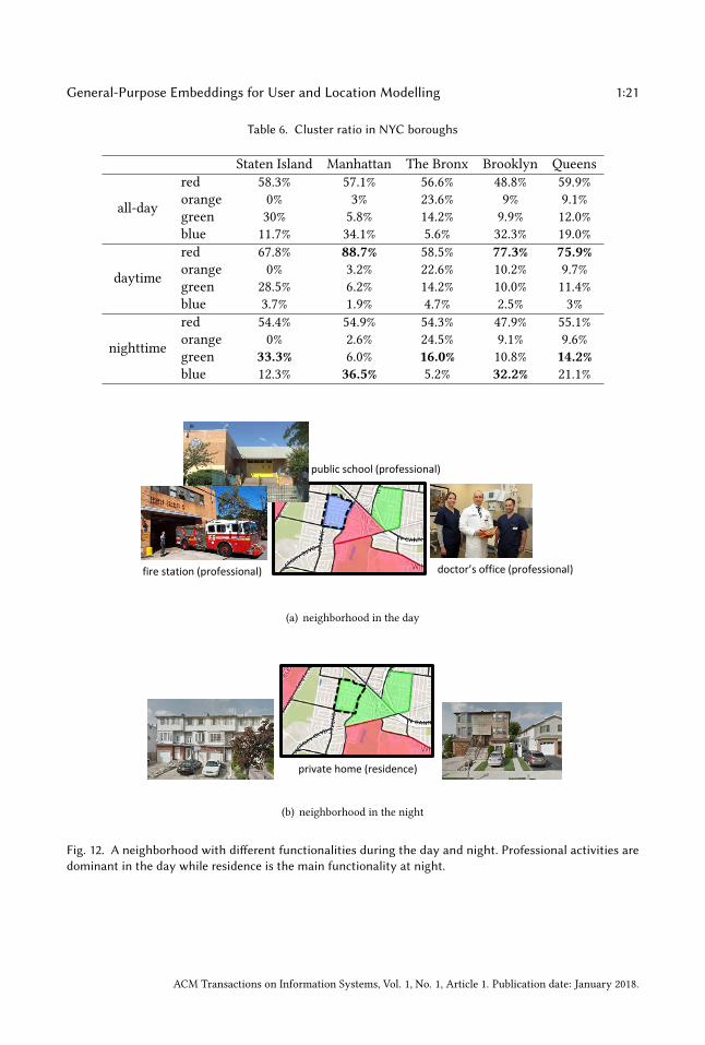
hubs and residential buildings. However, orange and green neighborhoods are seldom allocatedthere. This indicates that the downtown area is generally popular for all types of activities. Moreover,locally popular activities may be time-variant. Figure 12 shows a neighborhood in daytime andnighttime. In daytime, it is mainly used for professional activities, dominated by a clinic, a firestation, and a public school. At nighttime, it is mainly residential, which is plausible as most of thebuildings in this area are private homes.
ACM Transactions on Information Systems, Vol. 1, No. 1, Article 1. Publication date: January 2018.
1:20 J. Yang et al.
restaurant (food)
hotel (travel)
brewery (nightlife)
theater (entertainment)
apartment (residence)
metro station, hotel (travel)
(a) cluster example1
medical center, public school (professional)
synagogue, church (professional)
pub (nightlife) bar (nightlife)
(b) cluster example2
Fig. 11. Cluster examples.
ACM Transactions on Information Systems, Vol. 1, No. 1, Article 1. Publication date: January 2018.
General-Purpose Embeddings for User and Location Modelling 1:21
Table 6. Cluster ratio in NYC boroughs
Staten Island Manhattan The Bronx Brooklyn Queens
all-day
red 58.3% 57.1% 56.6% 48.8% 59.9%orange 0% 3% 23.6% 9% 9.1%green 30% 5.8% 14.2% 9.9% 12.0%blue 11.7% 34.1% 5.6% 32.3% 19.0%
daytime
red 67.8% 88.7% 58.5% 77.3% 75.9%orange 0% 3.2% 22.6% 10.2% 9.7%green 28.5% 6.2% 14.2% 10.0% 11.4%blue 3.7% 1.9% 4.7% 2.5% 3%
nighttime
red 54.4% 54.9% 54.3% 47.9% 55.1%orange 0% 2.6% 24.5% 9.1% 9.6%green 33.3% 6.0% 16.0% 10.8% 14.2%blue 12.3% 36.5% 5.2% 32.2% 21.1%
public school (professional)
fire station (professional) doctor’s office (professional)
private home (residence)
(a) neighborhood in the day
public school (professional)
fire station (professional) doctor’s office (professional)
private home (residence)
(b) neighborhood in the night
Fig. 12. A neighborhood with different functionalities during the day and night. Professional activities aredominant in the day while residence is the main functionality at night.
ACM Transactions on Information Systems, Vol. 1, No. 1, Article 1. Publication date: January 2018.
1:22 J. Yang et al.
4.5 Crime PredictionBy providing spatio-temporal embeddings for user and location characterization, our model repre-sents a proxy for the social interactions observed in an urban area. In this section, we will furtherinvestigate this capability by addressing a well-known social science problem: crime prediction.Previous work [57, 61] demonstrates that the occurrence of criminal activities is correlated withplace types and time, which are both encoded in our check-in embeddings.Similar to our urban functional zone study, neighborhoods rather than users are our study
subjects in crime prediction. We utilize feature word embeddings to characterize neighborhoods.This modification is motivated by the fact that location words are only locally descriptive. Therefore,a neighborhood cannot be described without prior training data from the exact location, but suchnew neighborhood prediction is possible if only modelled with the universally applicable featureword vectors, as long as visited venues have the same functional roles. NYC is still the representativecity for study and the crime data originates from the NYC Open Data portal5.
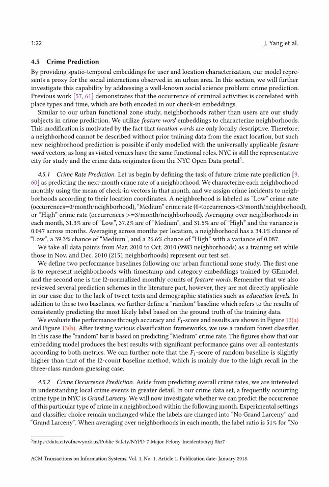
4.5.1 Crime Rate Prediction. Let us begin by defining the task of future crime rate prediction [9,60] as predicting the next-month crime rate of a neighborhood. We characterize each neighborhoodmonthly using the mean of check-in vectors in that month, and we assign crime incidents to neigh-borhoods according to their location coordinates. A neighborhood is labeled as “Low” crime rate(occurrences=0/month/neighborhood), “Medium” crime rate (0<occurrences<3/month/neighborhood),or “High” crime rate (occurrences >=3/month/neighborhood). Averaging over neighborhoods ineach month, 31.3% are of “Low”, 37.2% are of “Medium”, and 31.5% are of “High” and the variance is0.047 across months. Averaging across months per location, a neighborhood has a 34.1% chance of“Low”, a 39.3% chance of “Medium”, and a 26.6% chance of “High” with a variance of 0.087.
We take all data points from Mar. 2010 to Oct. 2010 (9983 neighborhoods) as a training set whilethose in Nov. and Dec. 2010 (2151 neighborhoods) represent our test set.We define two performance baselines following our urban functional zone study. The first one
is to represent neighborhoods with timestamp and category embeddings trained by GEmodel,and the second one is the l2-normalized monthly counts of feature words. Remember that we alsoreviewed several prediction schemes in the literature part, however, they are not directly applicablein our case due to the lack of tweet texts and demographic statistics such as education levels. Inaddition to these two baselines, we further define a “random" baseline which refers to the results ofconsistently predicting the most likely label based on the ground truth of the training data.
We evaluate the performance through accuracy and F1-score and results are shown in Figure 13(a)and Figure 13(b). After testing various classification frameworks, we use a random forest classifier.In this case the “random" bar is based on predicting “Medium" crime rate. The figures show that ourembedding model produces the best results with significant performance gains over all contestantsaccording to both metrics. We can further note that the F1-score of random baseline is slightlyhigher than that of the l2-count baseline method, which is mainly due to the high recall in thethree-class random guessing case.
4.5.2 Crime Occurrence Prediction. Aside from predicting overall crime rates, we are interestedin understanding local crime events in greater detail. In our crime data set, a frequently occurringcrime type in NYC is Grand Larceny. We will now investigate whether we can predict the occurrenceof this particular type of crime in a neighborhood within the followingmonth. Experimental settingsand classifier choice remain unchanged while the labels are changed into “No Grand Larceny” and“Grand Larceny”. When averaging over neighborhoods in each month, the label ratio is 51% for “No
5https://data.cityofnewyork.us/Public-Safety/NYPD-7-Major-Felony-Incidents/hyij-8hr7
ACM Transactions on Information Systems, Vol. 1, No. 1, Article 1. Publication date: January 2018.
General-Purpose Embeddings for User and Location Modelling 1:23
30.00%
35.00%
40.00%
45.00%
50.00%
55.00%
60.00%
random l2-count GEmodel embedding
NYC Crime Rate Prediction random baseline GEmodel embedding
(a) crime rate prediction accuracy
30.00%
35.00%
40.00%
45.00%
50.00%
55.00%
60.00%
random l2-count GEmodel embedding
NYC Crime Rate Prediction f1random baseline GEmodel embedding
(b) crime rate prediction F1 score
30.00%
35.00%
40.00%
45.00%
50.00%
55.00%
60.00%
65.00%
70.00%
random l2-count GEmodel embedding
NYC Crime Occurrence Predictionrandom baseline GEmodel embedding
(c) crime occurrence prediction accuracy
40.00%
45.00%
50.00%
55.00%
60.00%
65.00%
70.00%
75.00%
random l2-count GEmodel embedding
NYC Crime Occur Prediction f1random baseline GEmodel embedding
(d) crime occurrence prediction 1 score
Fig. 13. Average crime prediction accuracies and F1 scores in NYC.
Grand Larceny” and 49% for “Grand Larceny” with a variance of 0.027. For each neighborhood, ithas on average a 60.9% probability that this crime would occur with a variance of 0.082.
Figure 13(c) and Figure 13(d) demonstrate the average prediction accuracies and F1-scores. Similarto crime rate prediction, we can observe that our model outperforms random guessing as well asboth baselines at significance-level.
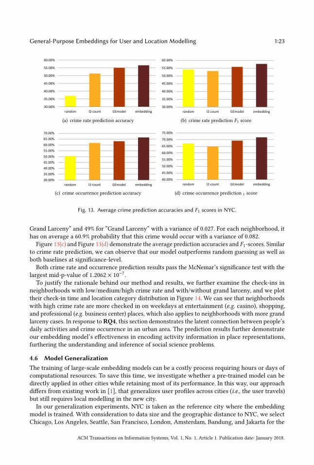
Both crime rate and occurrence prediction results pass the McNemar’s significance test with thelargest mid-p-value of 1.2062 × 10⁻⁷.To justify the rationale behind our method and results, we further examine the check-ins in
neighborhoods with low/medium/high crime rate and with/without grand larceny, and we plottheir check-in time and location category distribution in Figure 14. We can see that neighborhoodswith high crime rate are more checked in on weekdays at entertainment (e.g. casino), shopping,and professional (e.g. business center) places, which also applies to neighborhoods with more grandlarceny cases. In response toRQ4, this section demonstrates the latent connection between people’sdaily activities and crime occurrence in an urban area. The prediction results further demonstrateour embedding model’s effectiveness in encoding activity information in place representations,furthering the understanding and inference of social science problems.
4.6 Model GeneralizationThe training of large-scale embedding models can be a costly process requiring hours or days ofcomputational resources. To save this time, we investigate whether a pre-trained model can bedirectly applied in other cities while retaining most of its performance. In this way, our approachdiffers from existing work in [1], that generalizes user profiles across cities (i.e., the user travels)but still requires local modelling in the new city.In our generalization experiments, NYC is taken as the reference city where the embedding
model is trained. With consideration to data size and the geographic distance to NYC, we selectChicago, Los Angeles, Seattle, San Francisco, London, Amsterdam, Bandung, and Jakarta for the
ACM Transactions on Information Systems, Vol. 1, No. 1, Article 1. Publication date: January 2018.
1:24 J. Yang et al.
0
0.05
0.1
0.15
0.2
0.25 Low Medium High
(a) crime rate: time distribution
00.05
0.10.15
0.20.25
0.30.35 Low Medium High
(b) crime rate: category distribution
0
0.05
0.1
0.15
0.2
0.25 Grand Larceny No Grand Larceny
(c) crime occurrence: time distribution
00.05
0.10.15
0.20.25
0.3 Grand Larceny No Grand Larceny
(d) crime occurrence: category distribution
Fig. 14. Check-in time and location category distribution in neighborhoods of different labels.
ACM Transactions on Information Systems, Vol. 1, No. 1, Article 1. Publication date: January 2018.
General-Purpose Embeddings for User and Location Modelling 1:25
Table 7. Check-In Statistics
City # of check-ins # of users # of locations avg. check-ins/user (density)
Chicago (CH) 86,117 2,755 3,678 31.26Los Angeles (LA) 118,088 4,238 5,609 27.86Seattle (SE) 44,960 1,523 2,180 29.52San Francisco (SF) 84,494 3,285 3,605 25.72London (LO) 45,270 2,182 1,922 20.75Amsterdam (AM) 49,722 1,855 1,895 26.80Bandung (BA) 23,581 1,476 996 15.98Jakarta (JA) 50,875 3,123 1,995 16.29∗ NYC ∗ 225,782 ∗ 6,442 ∗ 7,453 ∗ 35.05
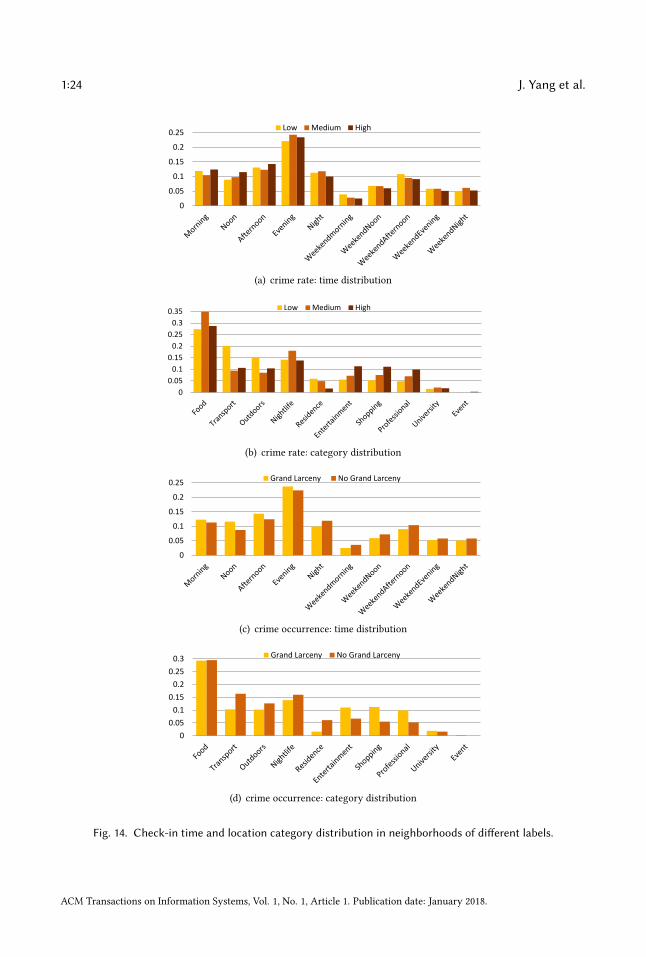
generalization test. As before, we delete repeating check-ins from individuals in artificially shorttime periods and remove both users and locations with less than 10 posts. Eight cities and theircheck-in statistics are listed in Table 7. We also list NYC statistics for reference.
4.6.1 Generalization of Location Recommendation. Recall that in our earlier investigation inSection 4.3, we relied on both feature words and location words for location recommendation.However, since location words are locally descriptive, they cannot be easily taken out of theiroriginal frame of reference. As a consequence, we only generalize the NYC-based embedding modelfor feature words, but locally train location words.Upon careful examination, none of the baseline methods can be ported across cities. GT-SEER
and TA-PLR methods exclusively focus on local POI embedding; Rank-GeoFM and LRT algorithmsrely on location vectorization; STT is dependent on local topic model; GEmodel trains embeddingvectors based on bipartite graphs but all of the graphs involve local POIs. Therefore, we have totrain the baseline methods locally when applying them to different cities.As before, we measure performance in terms of precision, recall, accuracy, and MAP and the
results are listed in Table 9. Again, GEmodel and STES(local) have very similar performances, andthe half-transferred model STES(NYC) produces close and even better results in some cases. Forinstance, in Seattle, the NYC-based STES model outperforms both GEmodel and the local STESmodel according to recall at top-1 recommendation. This can happen as a consequence of datasparsity since Seattle only offers 45k local check-ins which provide less information than the 226ktransferred ones from NYC.Let us now focus on the STES(NYC) and STES(local) models. Upon closer examination, in all
of the eight cities, the gaps between STES(NYC) and STES(local) are generally smaller than 3%.In particular, these two methods almost tie at top-1 recommendation for all U.S. cities; while inthe other four non-US cities, the NYC-based STES model produces less satisfactory performancewith respect to the local models. To further understand this observation, we plot the accuracydifferences between STES(local) and STES(NYC) in top-1, top-5, and top-10 cases in Figure 15. Fromthe figure, we can see that both the difference in local check-in density and the distance fromNYC appear to exert influence on generalization performance. While the former is less significant,the latter plays a key role in model portability as indicated by comparison among Los Angeles,Amsterdam, and San Francisco. We argue that the geographic distance from NYC is a proxy forcultural differences in the way that urban zones are used. Specifically, life style in Southeast Asia isdistinct from that in the U.S., which also applies for Europe where the difference seems smaller.
ACM Transactions on Information Systems, Vol. 1, No. 1, Article 1. Publication date: January 2018.
1:26 J. Yang et al.
Table 8. Crime Statistics in U.S. Cities
City Training Test Low:(Medium):High No:Yes
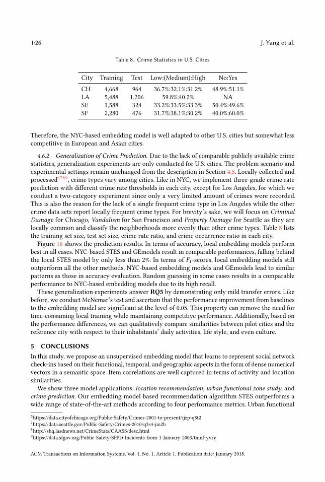
CH 4,668 964 36.7%:32.1%:31.2% 48.9%:51.1%LA 5,488 1,206 59.8%:40.2% NASE 1,588 324 33.2%:33.5%:33.3% 50.4%:49.6%SF 2,280 476 31.7%:38.1%:30.2% 40.0%:60.0%
Therefore, the NYC-based embedding model is well adapted to other U.S. cities but somewhat lesscompetitive in European and Asian cities.
4.6.2 Generalization of Crime Prediction. Due to the lack of comparable publicly available crimestatistics, generalization experiments are only conducted for U.S. cities. The problem scenario andexperimental settings remain unchanged from the description in Section 4.5. Locally collected andprocessed6789, crime types vary among cities. Like in NYC, we implement three-grade crime rateprediction with different crime rate thresholds in each city, except for Los Angeles, for which weconduct a two-category experiment since only a very limited amount of crimes were recorded.This is also the reason for the lack of a single frequent crime type in Los Angeles while the othercrime data sets report locally frequent crime types. For brevity’s sake, we will focus on CriminalDamage for Chicago, Vandalism for San Francisco and Property Damage for Seattle as they arelocally common and classify the neighborhoods more evenly than other crime types. Table 8 liststhe training set size, test set size, crime rate ratio, and crime occurrence ratio in each city.Figure 16 shows the prediction results. In terms of accuracy, local embedding models perform
best in all cases. NYC-based STES and GEmodels result in comparable performances, falling behindthe local STES model by only less than 2%. In terms of F1-scores, local embedding models stilloutperform all the other methods. NYC-based embedding models and GEmodels lead to similarpatterns as those in accuracy evaluation. Random guessing in some cases results in a comparableperformance to NYC-based embedding models due to its high recall.
These generalization experiments answer RQ5 by demonstrating only mild transfer errors. Likebefore, we conduct McNemar’s test and ascertain that the performance improvement from baselinesto the embedding model are significant at the level of 0.05. This property can remove the need fortime-consuming local training while maintaining competitive performance. Additionally, based onthe performance differences, we can qualitatively compare similarities between pilot cities and thereference city with respect to their inhabitants’ daily activities, life style, and even culture.
5 CONCLUSIONSIn this study, we propose an unsupervised embedding model that learns to represent social networkcheck-ins based on their functional, temporal, and geographic aspects in the form of dense numericalvectors in a semantic space. Item correlations are well captured in terms of activity and locationsimilarities.We show three model applications: location recommendation, urban functional zone study, and
crime prediction. Our embedding model based recommendation algorithm STES outperforms awide range of state-of-the-art methods according to four performance metrics. Urban functional
6https://data.cityofchicago.org/Public-Safety/Crimes-2001-to-present/ijzp-q8t27https://data.seattle.gov/Public-Safety/Crimes-2010/q3s4-jm2b8http://shq.lasdnews.net/CrimeStats/CAASS/desc.html9https://data.sfgov.org/Public-Safety/SFPD-Incidents-from-1-January-2003/tmnf-yvry
ACM Transactions on Information Systems, Vol. 1, No. 1, Article 1. Publication date: January 2018.
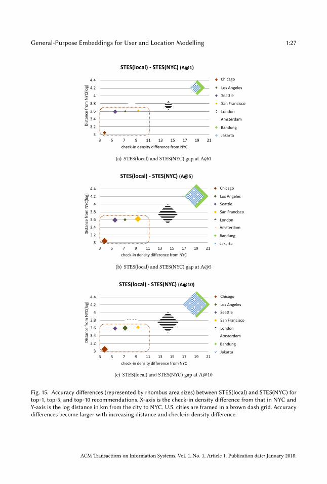
General-Purpose Embeddings for User and Location Modelling 1:27
3
3.2
3.4
3.6
3.8
4
4.2
4.4
3 5 7 9 11 13 15 17 19 21
Dist
ance
from
NYC
(log)
check-in density difference from NYC
STES(local) - STES(NYC) (A@1)
3.79
7.19
5.53
9.33
14.3
8.25
19.07
18.76
Chicago
Los Angeles
Seattle
San Francisco
London
Amsterdam
Bandung
Jakarta
(a) STES(local) and STES(NYC) gap at A@1
3
3.2
3.4
3.6
3.8
4
4.2
4.4
3 5 7 9 11 13 15 17 19 21
Dist
ance
from
NYC
(log)
check-in density difference from NYC
STES(local) - STES(NYC) (A@5)
3.79
7.19
5.53
9.33
14.3
8.25
19.07
18.76
Chicago
Los Angeles
Seattle
San Francisco
London
Amsterdam
Bandung
Jakarta
(b) STES(local) and STES(NYC) gap at A@5
3
3.2
3.4
3.6
3.8
4
4.2
4.4
3 5 7 9 11 13 15 17 19 21
Dist
ance
from
NYC
(log)
check-in density difference from NYC
STES(local) - STES(NYC) (A@10)
3.79
7.19
5.53
9.33
14.3
8.25
19.07
18.76
Chicago
Los Angeles
Seattle
San Francisco
London
Amsterdam
Bandung
Jakarta
(c) STES(local) and STES(NYC) gap at A@10
Fig. 15. Accuracy differences (represented by rhombus area sizes) between STES(local) and STES(NYC) fortop-1, top-5, and top-10 recommendations. X-axis is the check-in density difference from that in NYC andY-axis is the log distance in km from the city to NYC. U.S. cities are framed in a brown dash grid. Accuracydifferences become larger with increasing distance and check-in density difference.
ACM Transactions on Information Systems, Vol. 1, No. 1, Article 1. Publication date: January 2018.
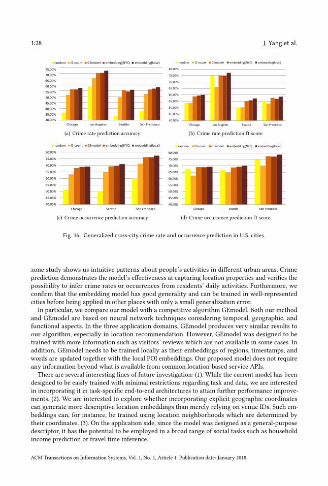
1:28 J. Yang et al.
30.00%35.00%
40.00%
45.00%
50.00%
55.00%
60.00%
65.00%
70.00%
75.00%
Chicago Los Angeles Seattle San Francisco
Crime Occur Prediction
random l2-count GEmodel embedding(NYC) embedding(local)
(a) Crime rate prediction accuracy
40.00%
45.00%
50.00%
55.00%
60.00%
65.00%
70.00%
75.00%
80.00%
Chicago Los Angeles Seattle San Francisco
Crime Rate f1 random l2-count GEmodel embedding(NYC) embedding(local)
(b) Crime rate prediction f1 score
40.00%
45.00%
50.00%
55.00%
60.00%
65.00%
70.00%
75.00%
80.00%
Chicago Seattle San Francisco
Crime Occur Prediction
random l2-count GEmodel embedding(NYC) embedding(local)
(c) Crime occurrence prediction accuracy
40.00%
45.00%
50.00%
55.00%
60.00%
65.00%
70.00%
75.00%
80.00%
Chicago Seattle San Francisco
Crime Occur f1 random l2-count GEmodel embedding(NYC) embedding(local)
(d) Crime occurrence prediction f1 score
Fig. 16. Generalized cross-city crime rate and occurrence prediction in U.S. cities.
zone study shows us intuitive patterns about people’s activities in different urban areas. Crimeprediction demonstrates the model’s effectiveness at capturing location properties and verifies thepossibility to infer crime rates or occurrences from residents’ daily activities. Furthermore, weconfirm that the embedding model has good generality and can be trained in well-representedcities before being applied in other places with only a small generalization error.In particular, we compare our model with a competitive algorithm GEmodel. Both our method
and GEmodel are based on neural network techniques considering temporal, geographic, andfunctional aspects. In the three application domains, GEmodel produces very similar results toour algorithm, especially in location recommendation. However, GEmodel was designed to betrained with more information such as visitors’ reviews which are not available in some cases. Inaddition, GEmodel needs to be trained locally as their embeddings of regions, timestamps, andwords are updated together with the local POI embeddings. Our proposed model does not requireany information beyond what is available from common location-based service APIs.
There are several interesting lines of future investigation: (1). While the current model has beendesigned to be easily trained with minimal restrictions regarding task and data, we are interestedin incorporating it in task-specific end-to-end architectures to attain further performance improve-ments. (2). We are interested to explore whether incorporating explicit geographic coordinatescan generate more descriptive location embeddings than merely relying on venue IDs. Such em-beddings can, for instance, be trained using location neighborhoods which are determined bytheir coordinates. (3). On the application side, since the model was designed as a general-purposedescriptor, it has the potential to be employed in a broad range of social tasks such as householdincome prediction or travel time inference.
ACM Transactions on Information Systems, Vol. 1, No. 1, Article 1. Publication date: January 2018.
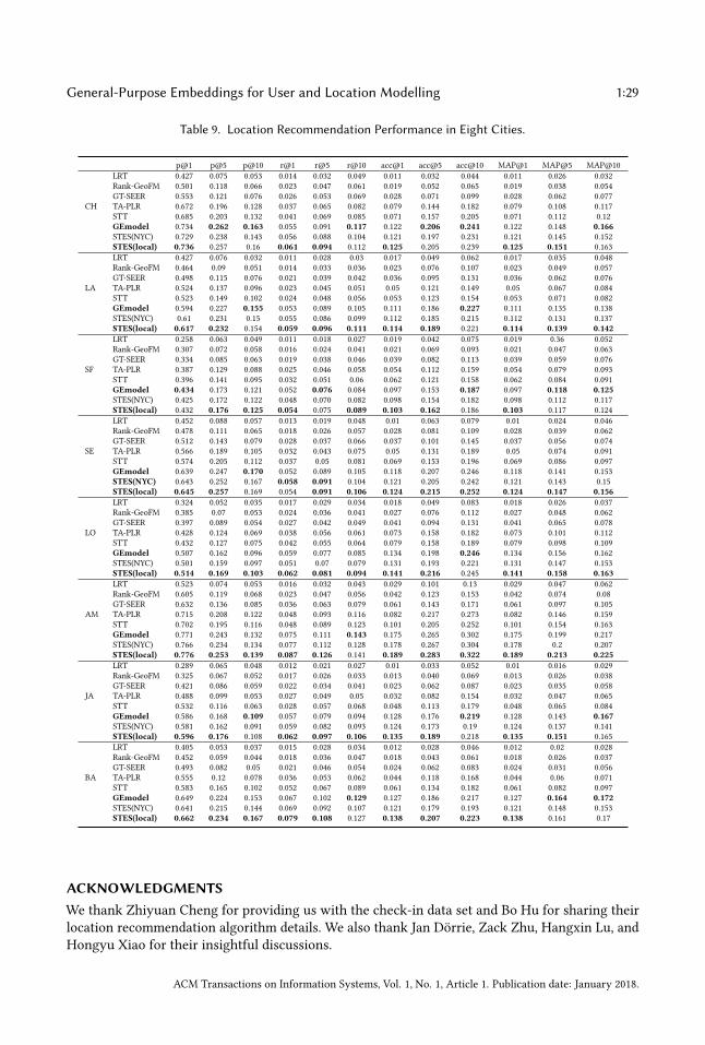
General-Purpose Embeddings for User and Location Modelling 1:29
Table 9. Location Recommendation Performance in Eight Cities.
p@1 p@5 p@10 r@1 r@5 r@10 acc@1 acc@5 acc@10 MAP@1 MAP@5 MAP@10LRT 0.427 0.075 0.053 0.014 0.032 0.049 0.011 0.032 0.044 0.011 0.026 0.032Rank-GeoFM 0.501 0.118 0.066 0.023 0.047 0.061 0.019 0.052 0.065 0.019 0.038 0.054GT-SEER 0.553 0.121 0.076 0.026 0.053 0.069 0.028 0.071 0.099 0.028 0.062 0.077
CH TA-PLR 0.672 0.196 0.128 0.037 0.065 0.082 0.079 0.144 0.182 0.079 0.108 0.117STT 0.685 0.203 0.132 0.041 0.069 0.085 0.071 0.157 0.205 0.071 0.112 0.12GEmodel 0.734 0.262 0.163 0.055 0.091 0.117 0.122 0.206 0.241 0.122 0.148 0.166STES(NYC) 0.729 0.238 0.143 0.056 0.088 0.104 0.121 0.197 0.231 0.121 0.145 0.152STES(local) 0.736 0.257 0.16 0.061 0.094 0.112 0.125 0.205 0.239 0.125 0.151 0.163LRT 0.427 0.076 0.032 0.011 0.028 0.03 0.017 0.049 0.062 0.017 0.035 0.048Rank-GeoFM 0.464 0.09 0.051 0.014 0.033 0.036 0.023 0.076 0.107 0.023 0.049 0.057GT-SEER 0.498 0.115 0.076 0.021 0.039 0.042 0.036 0.095 0.131 0.036 0.062 0.076
LA TA-PLR 0.524 0.137 0.096 0.023 0.045 0.051 0.05 0.121 0.149 0.05 0.067 0.084STT 0.523 0.149 0.102 0.024 0.048 0.056 0.053 0.123 0.154 0.053 0.071 0.082GEmodel 0.594 0.227 0.155 0.053 0.089 0.105 0.111 0.186 0.227 0.111 0.135 0.138STES(NYC) 0.61 0.231 0.15 0.055 0.086 0.099 0.112 0.185 0.215 0.112 0.131 0.137STES(local) 0.617 0.232 0.154 0.059 0.096 0.111 0.114 0.189 0.221 0.114 0.139 0.142LRT 0.258 0.063 0.049 0.011 0.018 0.027 0.019 0.042 0.075 0.019 0.36 0.052Rank-GeoFM 0.307 0.072 0.058 0.016 0.024 0.041 0.021 0.069 0.093 0.021 0.047 0.063GT-SEER 0.334 0.085 0.063 0.019 0.038 0.046 0.039 0.082 0.113 0.039 0.059 0.076
SF TA-PLR 0.387 0.129 0.088 0.025 0.046 0.058 0.054 0.112 0.159 0.054 0.079 0.093STT 0.396 0.141 0.095 0.032 0.051 0.06 0.062 0.121 0.158 0.062 0.084 0.091GEmodel 0.434 0.173 0.121 0.052 0.076 0.084 0.097 0.153 0.187 0.097 0.118 0.125STES(NYC) 0.425 0.172 0.122 0.048 0.070 0.082 0.098 0.154 0.182 0.098 0.112 0.117STES(local) 0.432 0.176 0.125 0.054 0.075 0.089 0.103 0.162 0.186 0.103 0.117 0.124LRT 0.452 0.088 0.057 0.013 0.019 0.048 0.01 0.063 0.079 0.01 0.024 0.046Rank-GeoFM 0.478 0.111 0.065 0.018 0.026 0.057 0.028 0.081 0.109 0.028 0.039 0.062GT-SEER 0.512 0.143 0.079 0.028 0.037 0.066 0.037 0.101 0.145 0.037 0.056 0.074
SE TA-PLR 0.566 0.189 0.105 0.032 0.043 0.075 0.05 0.131 0.189 0.05 0.074 0.091STT 0.574 0.205 0.112 0.037 0.05 0.081 0.069 0.153 0.196 0.069 0.086 0.097GEmodel 0.639 0.247 0.170 0.052 0.089 0.105 0.118 0.207 0.246 0.118 0.141 0.153STES(NYC) 0.643 0.252 0.167 0.058 0.091 0.104 0.121 0.205 0.242 0.121 0.143 0.15STES(local) 0.645 0.257 0.169 0.054 0.091 0.106 0.124 0.215 0.252 0.124 0.147 0.156LRT 0.324 0.052 0.035 0.017 0.029 0.034 0.018 0.049 0.083 0.018 0.026 0.037Rank-GeoFM 0.385 0.07 0.053 0.024 0.036 0.041 0.027 0.076 0.112 0.027 0.048 0.062GT-SEER 0.397 0.089 0.054 0.027 0.042 0.049 0.041 0.094 0.131 0.041 0.065 0.078
LO TA-PLR 0.428 0.124 0.069 0.038 0.056 0.061 0.073 0.158 0.182 0.073 0.101 0.112STT 0.432 0.127 0.075 0.042 0.055 0.064 0.079 0.158 0.189 0.079 0.098 0.109GEmodel 0.507 0.162 0.096 0.059 0.077 0.085 0.134 0.198 0.246 0.134 0.156 0.162STES(NYC) 0.501 0.159 0.097 0.051 0.07 0.079 0.131 0.193 0.221 0.131 0.147 0.153STES(local) 0.514 0.169 0.103 0.062 0.081 0.094 0.141 0.216 0.245 0.141 0.158 0.163LRT 0.523 0.074 0.053 0.016 0.032 0.043 0.029 0.101 0.13 0.029 0.047 0.062Rank-GeoFM 0.605 0.119 0.068 0.023 0.047 0.056 0.042 0.123 0.153 0.042 0.074 0.08GT-SEER 0.632 0.136 0.085 0.036 0.063 0.079 0.061 0.143 0.171 0.061 0.097 0.105
AM TA-PLR 0.715 0.208 0.122 0.048 0.093 0.116 0.082 0.217 0.273 0.082 0.146 0.159STT 0.702 0.195 0.116 0.048 0.089 0.123 0.101 0.205 0.252 0.101 0.154 0.163GEmodel 0.771 0.243 0.132 0.075 0.111 0.143 0.175 0.265 0.302 0.175 0.199 0.217STES(NYC) 0.766 0.234 0.134 0.077 0.112 0.128 0.178 0.267 0.304 0.178 0.2 0.207STES(local) 0.776 0.253 0.139 0.087 0.126 0.141 0.189 0.283 0.322 0.189 0.213 0.225LRT 0.289 0.065 0.048 0.012 0.021 0.027 0.01 0.033 0.052 0.01 0.016 0.029Rank-GeoFM 0.325 0.067 0.052 0.017 0.026 0.033 0.013 0.040 0.069 0.013 0.026 0.038GT-SEER 0.421 0.086 0.059 0.022 0.034 0.041 0.023 0.062 0.087 0.023 0.035 0.058
JA TA-PLR 0.488 0.099 0.053 0.027 0.049 0.05 0.032 0.082 0.154 0.032 0.047 0.065STT 0.532 0.116 0.063 0.028 0.057 0.068 0.048 0.113 0.179 0.048 0.065 0.084GEmodel 0.586 0.168 0.109 0.057 0.079 0.094 0.128 0.176 0.219 0.128 0.143 0.167STES(NYC) 0.581 0.162 0.091 0.059 0.082 0.093 0.124 0.173 0.19 0.124 0.137 0.141STES(local) 0.596 0.176 0.108 0.062 0.097 0.106 0.135 0.189 0.218 0.135 0.151 0.165LRT 0.405 0.053 0.037 0.015 0.028 0.034 0.012 0.028 0.046 0.012 0.02 0.028Rank-GeoFM 0.452 0.059 0.044 0.018 0.036 0.047 0.018 0.043 0.061 0.018 0.026 0.037GT-SEER 0.493 0.082 0.05 0.021 0.046 0.054 0.024 0.062 0.083 0.024 0.031 0.056
BA TA-PLR 0.555 0.12 0.078 0.036 0.053 0.062 0.044 0.118 0.168 0.044 0.06 0.071STT 0.583 0.165 0.102 0.052 0.067 0.089 0.061 0.134 0.182 0.061 0.082 0.097GEmodel 0.649 0.224 0.153 0.067 0.102 0.129 0.127 0.186 0.217 0.127 0.164 0.172STES(NYC) 0.641 0.215 0.144 0.069 0.092 0.107 0.121 0.179 0.193 0.121 0.148 0.153STES(local) 0.662 0.234 0.167 0.079 0.108 0.127 0.138 0.207 0.223 0.138 0.161 0.17
ACKNOWLEDGMENTSWe thank Zhiyuan Cheng for providing us with the check-in data set and Bo Hu for sharing theirlocation recommendation algorithm details. We also thank Jan Dörrie, Zack Zhu, Hangxin Lu, andHongyu Xiao for their insightful discussions.
ACM Transactions on Information Systems, Vol. 1, No. 1, Article 1. Publication date: January 2018.
1:30 J. Yang et al.
REFERENCES[1] Jie Bao, Yu Zheng, and Mohamed F Mokbel. 2012. Location-based and preference-aware recommendation using sparse
geo-social networking data. In Proceedings of the 20th international conference on advances in geographic informationsystems. ACM, 199–208.
[2] David M Blei, Andrew Y Ng, and Michael I Jordan. 2003. Latent dirichlet allocation. Journal of machine Learningresearch 3, Jan (2003), 993–1022.
[3] Chen Cheng, Haiqin Yang, Irwin King, and Michael R Lyu. 2012. Fused Matrix Factorization with Geographical andSocial Influence in Location-Based Social Networks.. In Aaai, Vol. 12. 17–23.
[4] Chen Cheng, Haiqin Yang,Michael R Lyu, and Irwin King. 2013. Where You Like to GoNext: Successive Point-of-InterestRecommendation.. In IJCAI, Vol. 13. 2605–2611.
[5] Zhiyuan Cheng, James Caverlee, Kyumin Lee, and Daniel Z Sui. 2011. Exploring Millions of Footprints in LocationSharing Services. ICWSM 2011 (2011), 81–88.
[6] Andrew Church, Martin Frost, and Keith Sullivan. 2000. Transport and social exclusion in London. Transport Policy 7,3 (2000), 195–205.
[7] Justin Cranshaw, Raz Schwartz, Jason I Hong, and Norman Sadeh. 2012. The livehoods project: Utilizing social mediato understand the dynamics of a city. (2012).
[8] Huiji Gao, Jiliang Tang, Xia Hu, and Huan Liu. 2013. Exploring temporal effects for location recommendation onlocation-based social networks. In Proceedings of the 7th ACM conference on Recommender systems. ACM, 93–100.
[9] Matthew S Gerber. 2014. Predicting crime using Twitter and kernel density estimation. Decision Support Systems 61(2014), 115–125.
[10] Samiul Hasan and Satish V Ukkusuri. 2014. Urban activity pattern classification using topic models from onlinegeo-location data. Transportation Research Part C: Emerging Technologies 44 (2014), 363–381.
[11] Samiul Hasan, Xianyuan Zhan, and Satish V Ukkusuri. 2013. Understanding urban human activity and mobility patternsusing large-scale location-based data from online social media. In Proceedings of the 2nd ACM SIGKDD internationalworkshop on urban computing. ACM, 6.
[12] Kaiming He, Xiangyu Zhang, Shaoqing Ren, and Jian Sun. 2016. Deep residual learning for image recognition. InProceedings of the IEEE conference on computer vision and pattern recognition. 770–778.
[13] Tieke He, Hongzhi Yin, Zhenyu Chen, Xiaofang Zhou, Shazia Sadiq, and Bin Luo. 2016. A Spatial-Temporal TopicModel for the Semantic Annotation of POIs in LBSNs. ACM Transactions on Intelligent Systems and Technology (TIST)8, 1 (2016), 12.
[14] Francis Heylighen and Johan Bollen. 2002. Hebbian algorithms for a digital library recommendation system. In ParallelProcessing Workshops, 2002. Proceedings. International Conference on. IEEE, 439–446.
[15] Liangjie Hong, Amr Ahmed, Siva Gurumurthy, Alexander J Smola, and Kostas Tsioutsiouliklis. 2012. Discoveringgeographical topics in the twitter stream. In Proceedings of the 21st international conference on World Wide Web. ACM,769–778.
[16] Bo Hu andMartin Ester. 2013. Spatial topic modeling in online social media for location recommendation. In Proceedingsof the 7th ACM conference on Recommender systems. ACM, 25–32.
[17] Bo Hu, Mohsen Jamali, and Martin Ester. 2013. Spatio-temporal topic modeling in mobile social media for locationrecommendation. In 2013 IEEE 13th International Conference on Data Mining. IEEE, 1073–1078.
[18] Rizwan Iqbal, Masrah Azrifah Azmi Murad, Aida Mustapha, Payam Hassany Shariat Panahy, and Nasim Khanahmadli-ravi. 2013. An experimental study of classification algorithms for crime prediction. Indian Journal of Science andTechnology 6, 3 (2013), 4219–4225.
[19] Donald E Knuth. 1985. Dynamic huffman coding. Journal of algorithms 6, 2 (1985), 163–180.[20] Yehuda Koren. 2010. Collaborative filtering with temporal dynamics. Commun. ACM 53, 4 (2010), 89–97.[21] Yehuda Koren, Robert Bell, Chris Volinsky, et al. 2009. Matrix factorization techniques for recommender systems.
Computer 42, 8 (2009), 30–37.[22] John Krumm and Dany Rouhana. 2013. Placer: semantic place labels from diary data. In Proceedings of the 2013 ACM
international joint conference on Pervasive and ubiquitous computing. ACM, 163–172.[23] Takeshi Kurashima, Tomoharu Iwata, Takahide Hoshide, Noriko Takaya, and Ko Fujimura. 2013. Geo topic model:
joint modeling of user’s activity area and interests for location recommendation. In Proceedings of the sixth ACMinternational conference on Web search and data mining. ACM, 375–384.
[24] Juha K Laurila, Daniel Gatica-Perez, Imad Aad, Olivier Bornet, Trinh-Minh-Tri Do, Olivier Dousse, Julien Eberle,Markus Miettinen, et al. 2012. The mobile data challenge: Big data for mobile computing research. In PervasiveComputing.
[25] Jia Li, Hua Xu, Xingwei He, Junhui Deng, and Xiaomin Sun. 2016. Tweet modeling with LSTM recurrent neuralnetworks for hashtag recommendation. In Neural Networks (IJCNN), 2016 International Joint Conference on. IEEE,1570–1577.
ACM Transactions on Information Systems, Vol. 1, No. 1, Article 1. Publication date: January 2018.
General-Purpose Embeddings for User and Location Modelling 1:31
[26] Wen Li, Carsten Eickhoff, and Arjen P de Vries. 2016. Probabilistic Local Expert Retrieval. In European Conference onInformation Retrieval. Springer, 227–239.
[27] Wen Li, Pavel Serdyukov, Arjen P de Vries, Carsten Eickhoff, and Martha Larson. 2011. The where in the tweet. InProceedings of the 20th ACM international conference on Information and knowledge management. ACM, 2473–2476.
[28] Xutao Li, Gao Cong, Xiao-Li Li, Tuan-Anh Nguyen Pham, and Shonali Krishnaswamy. 2015. Rank-GeoFM: a rankingbased geographical factorization method for point of interest recommendation. In Proceedings of the 38th InternationalACM SIGIR Conference on Research and Development in Information Retrieval. ACM, 433–442.
[29] Defu Lian, Cong Zhao, Xing Xie, Guangzhong Sun, Enhong Chen, and Yong Rui. 2014. GeoMF: joint geographicalmodeling and matrix factorization for point-of-interest recommendation. In Proceedings of the 20th ACM SIGKDDinternational conference on Knowledge discovery and data mining. ACM, 831–840.
[30] Zhouhan Lin, Minwei Feng, Cicero Nogueira dos Santos, Mo Yu, Bing Xiang, Bowen Zhou, and Yoshua Bengio. 2017.A Structured Self-attentive Sentence Embedding. arXiv preprint arXiv:1703.03130 (2017).
[31] Bin Liu, Yanjie Fu, Zijun Yao, and Hui Xiong. 2013. Learning geographical preferences for point-of-interest recommen-dation. In Proceedings of the 19th ACM SIGKDD international conference on Knowledge discovery and data mining. ACM,1043–1051.
[32] Qiang Liu, Shu Wu, Liang Wang, and Tieniu Tan. 2016. Predicting the Next Location: A Recurrent Model with Spatialand Temporal Contexts. In Thirtieth AAAI Conference on Artificial Intelligence.
[33] Xin Liu, Yong Liu, and Xiaoli Li. 2016. Exploring the Context of Locations for Personalized Location Recommendations.2016 (2016), 2016.
[34] Yiding Liu, Tuan-Anh Nguyen Pham, Gao Cong, and Quan Yuan. 2017. An experimental evaluation of point-of-interestrecommendation in location-based social networks. Proceedings of the VLDB Endowment 10, 10 (2017), 1010–1021.
[35] Paolo Massa and Paolo Avesani. 2007. Trust-aware recommender systems. In Proceedings of the 2007 ACM conferenceon Recommender systems. ACM, 17–24.
[36] Wesley Mathew, Ruben Raposo, and Bruno Martins. 2012. Predicting future locations with hidden Markov models. InProceedings of the 2012 ACM Conference on Ubiquitous Computing. ACM, 911–918.
[37] Quinn McNemar. 1947. Note on the sampling error of the difference between correlated proportions or percentages.Psychometrika 12, 2 (1947), 153–157.
[38] Tomas Mikolov, Quoc V Le, and Ilya Sutskever. 2013. Exploiting similarities among languages for machine translation.arXiv preprint arXiv:1309.4168 (2013).
[39] Tomas Mikolov, Ilya Sutskever, Kai Chen, Greg S Corrado, and Jeff Dean. 2013. Distributed Representations of Wordsand Phrases and their Compositionality. In Advances in Neural Information Processing Systems. 3111–3119.
[40] Glenn W Milligan and Martha C Cooper. 1985. An examination of procedures for determining the number of clustersin a data set. Psychometrika 50, 2 (1985), 159–179.
[41] Anastasios Noulas, Salvatore Scellato, Cecilia Mascolo, and Massimiliano Pontil. 2011. Exploiting Semantic Annotationsfor Clustering Geographic Areas and Users in Location-based Social Networks. The social mobile web 11 (2011), 02.
[42] Makbule Gulcin Ozsoy. 2016. From Word Embeddings to Item Recommendation. arXiv preprint arXiv:1601.01356(2016).
[43] Bryan Perozzi, Rami Al-Rfou, and Steven Skiena. 2014. Deepwalk: Online learning of social representations. InProceedings of the 20th ACM SIGKDD international conference on Knowledge discovery and data mining. ACM, 701–710.
[44] Van-Thuy Phi, Liu Chen, and Yu Hirate. 2016. Distributed Representation-based Recommender Systems in E-commerce.2016 (2016), 2016.
[45] William M Rand. 1971. Objective criteria for the evaluation of clustering methods. Journal of the American Statisticalassociation 66, 336 (1971), 846–850.
[46] Daniele Riboni and Claudio Bettini. 2013. A platform for privacy-preserving geo-social recommendation of points ofinterest. In Mobile Data Management (MDM), 2013 IEEE 14th International Conference on, Vol. 1. IEEE, 347–349.
[47] Peter J Rousseeuw. 1987. Silhouettes: a graphical aid to the interpretation and validation of cluster analysis. Journal ofcomputational and applied mathematics 20 (1987), 53–65.
[48] Ruslan Salakhutdinov and Andriy Mnih. 2011. Probabilistic matrix factorization. In NIPS, Vol. 20. 1–8.[49] Siddharth Sarda, Carsten Eickhoff, and Thomas Hofmann. 2016. Semantic Place Descriptors for Classification and Map
Discovery. arXiv preprint arXiv:1601.05952 (2016).[50] Salvatore Scellato, Anastasios Noulas, and Cecilia Mascolo. 2011. Exploiting place features in link prediction on
location-based social networks. In Proceedings of the 17th ACM SIGKDD international conference on Knowledge discoveryand data mining. ACM, 1046–1054.
[51] Yang Song, Ali Mamdouh Elkahky, and Xiaodong He. 2016. Multi-rate deep learning for temporal recommendation. InProceedings of the 39th International ACM SIGIR conference on Research and Development in Information Retrieval. ACM,909–912.
ACM Transactions on Information Systems, Vol. 1, No. 1, Article 1. Publication date: January 2018.
1:32 J. Yang et al.
[52] Duyu Tang, Bing Qin, and Ting Liu. 2015. Learning semantic representations of users and products for document levelsentiment classification. In Proc. ACL.
[53] Duyu Tang, Bing Qin, Ting Liu, and Yuekui Yang. 2015. User modeling with neural network for review rating prediction.In Proceedings of the 24th International Conference on Artificial Intelligence. AAAI Press, 1340–1346.
[54] Duyu Tang, Furu Wei, Nan Yang, Ming Zhou, Ting Liu, and Bing Qin. 2014. Learning Sentiment-Specific WordEmbedding for Twitter Sentiment Classification.. In ACL (1). 1555–1565.
[55] Mozhgan Tavakolifard and Kevin C Almeroth. 2012. Social computing: an intersection of recommender systems,trust/reputation systems, and social networks. IEEE Network 26, 4 (2012), 53–58.
[56] Guangjin Tian, Jianguo Wu, and Zhifeng Yang. 2010. Spatial pattern of urban functions in the Beijing metropolitanregion. Habitat International 34, 2 (2010), 249–255.
[57] Peter J Van Koppen and Robert WJ Jansen. 1999. The time to rob: variations in time of number of commercial robberies.Journal of Research in Crime and Delinquency 36, 1 (1999), 7–29.
[58] Weiqing Wang, Hongzhi Yin, Ling Chen, Yizhou Sun, Shazia Sadiq, and Xiaofang Zhou. 2015. Geo-sage: A geographicalsparse additive generative model for spatial item recommendation. In Proceedings of the 21th ACM SIGKDD InternationalConference on Knowledge Discovery and Data Mining. ACM, 1255–1264.
[59] Weiqing Wang, Hongzhi Yin, Shazia Sadiq, Ling Chen, Min Xie, and Xiaofang Zhou. 2016. Spore: A sequentialpersonalized spatial item recommender system. In Data Engineering (ICDE), 2016 IEEE 32nd International Conference on.IEEE, 954–965.
[60] Xiaofeng Wang, Matthew S Gerber, and Donald E Brown. 2012. Automatic crime prediction using events extractedfrom twitter posts. In International Conference on Social Computing, Behavioral-Cultural Modeling, and Prediction.Springer, 231–238.
[61] DavidWeisburd, ShawnBushway, Cynthia Lum, and Sue-Ming Yang. 2004. Trajectories of crime at places: A longitudinalstudy of street segments in the city of Seattle. Criminology 42, 2 (2004), 283–322.
[62] Marius Wernke, Frank Dürr, and Kurt Rothermel. 2012. PShare: Position sharing for location privacy based onmulti-secret sharing. In Pervasive Computing and Communications (PerCom), 2012 IEEE International Conference on.IEEE, 153–161.
[63] Sanjaya Wijeratne, Lakshika Balasuriya, Derek Doran, and Amit Sheth. 2016. Word embeddings to enhance twittergang member profile identification. In IJCAI Workshop on Semantic Machine Learning (SML 2016). New York City, NY:CEUR-WS, Vol. 7. 2016.
[64] Min Xie, Hongzhi Yin, Hao Wang, Fanjiang Xu, Weitong Chen, and Sen Wang. 2016. Learning Graph-based POIEmbedding for Location-based Recommendation. In Proceedings of the 25th ACM International on Conference onInformation and Knowledge Management. ACM, 15–24.
[65] Xingxing Xing, Wenhao Huang, Guojie Song, and Kunqing Xie. 2014. Traffic zone division using mobile billing data.In Fuzzy Systems and Knowledge Discovery (FSKD), 2014 11th International Conference on. IEEE, 692–697.
[66] Wang Yajun et al. 2006. The Functionality Analysis to Urban Green Space System structural Configuration Plan [J].Journal of Shandong Forestry Science and Technology 6 (2006), 033.
[67] Mao Ye, Dong Shou, Wang-Chien Lee, Peifeng Yin, and Krzysztof Janowicz. 2011. On the semantic annotation ofplaces in location-based social networks. In Proceedings of the 17th ACM SIGKDD international conference on Knowledgediscovery and data mining. ACM, 520–528.
[68] Mao Ye, Peifeng Yin, and Wang-Chien Lee. 2010. Location recommendation for location-based social networks. InProceedings of the 18th SIGSPATIAL international conference on advances in geographic information systems. ACM,458–461.
[69] Hongzhi Yin, Bin Cui, Yizhou Sun, Zhiting Hu, and Ling Chen. 2014. Lcars: A spatial item recommender system. ACMTransactions on Information Systems (TOIS) 32, 3 (2014), 11.
[70] Hongzhi Yin, Bin Cui, Xiaofang Zhou, Weiqing Wang, Zi Huang, and Shazia Sadiq. 2016. Joint modeling of usercheck-in behaviors for real-time point-of-interest recommendation. ACM Transactions on Information Systems (TOIS)35, 2 (2016), 11.
[71] Hongzhi Yin,WeiqingWang, HaoWang, Ling Chen, and Xiaofang Zhou. 2017. Spatial-Aware Hierarchical CollaborativeDeep Learning for POI Recommendation. IEEE Transactions on Knowledge and Data Engineering 29, 11 (2017), 2537–2551.
[72] Hongzhi Yin, Xiaofang Zhou, Bin Cui, Hao Wang, Kai Zheng, and Quoc Viet Hung Nguyen. 2016. Adapting to userinterest drift for poi recommendation. IEEE Transactions on Knowledge and Data Engineering 28, 10 (2016), 2566–2581.
[73] Hongzhi Yin, Xiaofang Zhou, Yingxia Shao, Hao Wang, and Shazia Sadiq. 2015. Joint modeling of user check-in behaviors for point-of-interest recommendation. In Proceedings of the 24th ACM International on Conference onInformation and Knowledge Management. ACM, 1631–1640.
[74] Nicholas Jing Yuan, Yu Zheng, Xing Xie, Yingzi Wang, Kai Zheng, and Hui Xiong. 2015. Discovering urban functionalzones using latent activity trajectories. IEEE Transactions on Knowledge and Data Engineering 27, 3 (2015), 712–725.
ACM Transactions on Information Systems, Vol. 1, No. 1, Article 1. Publication date: January 2018.
General-Purpose Embeddings for User and Location Modelling 1:33
[75] Jia-Dong Zhang, Chi-Yin Chow, and Yanhua Li. 2014. LORE: exploiting sequential influence for location recommenda-tions. In Proceedings of the 22nd ACM SIGSPATIAL International Conference on Advances in Geographic InformationSystems. ACM, 103–112.
[76] Shenglin Zhao, Tong Zhao, Irwin King, and Michael R Lyu. 2016. GT-SEER: Geo-Temporal SEquential EmbeddingRank for Point-of-interest Recommendation. arXiv preprint arXiv:1606.05859 (2016).
[77] Zack Zhu, Jing Yang, Chen Zhong, Julia Seiter, and Gerhard Tröster. 2015. Learning functional compositions of urbanspaces with crowd-augmented travel survey data. In Proceedings of the 23rd SIGSPATIAL International Conference onAdvances in Geographic Information Systems. ACM, 22.
Received July 2017; revised November 2017; accepted January 2018
ACM Transactions on Information Systems, Vol. 1, No. 1, Article 1. Publication date: January 2018.