Embed Size (px)
Citation preview
Jim OhlsonStern School of Business
New York University
August 2008
How to Conceptualize and Value Earnings
Growth

2
Key ResultA formula (“OJ”) that expresses value in terms of next
year expected EPS and growth in EPS
Model Variables: Value depends on EPS1: Next-year expected EPS or “forward EPS”. Year 2 vs. Year 1 growth (STG) in expected EPS Some measure of long-term growth (LTG) in
expected EPS Discount factor which reflects risk (Cost of Equity
Capital)
P0 EPS1 EPS2 LTG

3
Compelling Empirical Realities
P0 / EPS1 correlates with short-term growth in EPS, but by no means perfectly
P0 / EPS1 rates often exceed any reasonable estimate of the inverse of the cost of capital
Short-term growth in EPS often substantially exceeds any reasonable estimate of cost of capital (e.g., Google’s growth in estimated 2008 EPS vs. 2008 EPS is 28%)
Analysts typically expect that superior EPS growth rates revert to “normal” rates over time

4
Implications of Empirical Realities
The Constant (Gordon) Growth Model works only if cost of capital exceeds the perpetual growth rate.
One must model a decaying growth rate in EPS when short-term growth is relatively large.
5
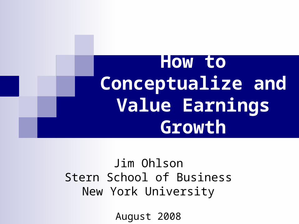
Approach to Assumptions
Short-term growth (EPS2 vs. EPS1 adjusted for DPS1) -- decays gradually to a steady state growth
also determines the rate of decay in EPS growth.
P0 equals the present value of expected DPS using the discount factor r (cost of equity capital).
Assumptions build in dividend policy irrelevancy.
LgLg

6
A Hypothetical Example
Model Dynamics:
Assuming full payout:
Numerical illustration:
These assumptions imply the following growth pattern.
1 (1 ) tLteps g eps
1
2
4%11.15
Lgepseps

7
0
3
6
9
12
15
18
2 12 22 32 42 52 62 72 82
Years
EPS Growth Rate (%)
4.18
8
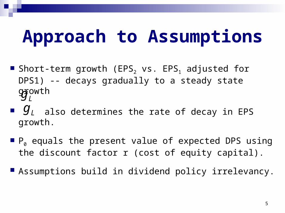
More generally, the model is determined by
where
r = cost of equity capital (8%, say)
does NOT depend on the dividend policy!
1 (1 )t L treps g reps
1 1
1 1 1 2
t t t
t t t t
reps eps r bvps
bvps eps dps bvps
treps
1
1 /t t t t
t t
reps eps r x eps dps
eps dps r

9
Basic Valuation Formula
r = cost of equity capital
= long-term EPS growth given full payout
= as
arguably approximates steady state growth in GNP
10
s L
L
g gepsP PVED
r r g
2 1 1
1 1s
eps eps r dpsg
eps eps
1
1
t t
t
eps epseps
t
Lg

10
Example: GE
Adjustments for dividends;
If and then
2 $2.10EPS 2.10 1.98
6%1.98
1 $1.98EPS
1
1
0.08 1.205%
1.98r dpseps
6% 5% 11%sg
8%r 4%Lg
0
1.98 11 4ˆ $43.310.08 8 4
P $35.50actual
1 1.20DPS

11
Example: GE
Does estimated value exceed actual price because our specification of r is too low?
Try
is evidently sensitive to r
9%r
0
1.98 11 4ˆ $30.800.09 9 4
P
0̂P
12
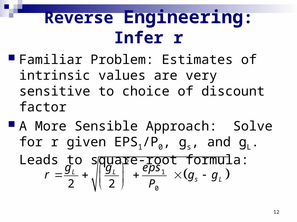
Reverse Engineering: Infer r
Familiar Problem: Estimates of intrinsic values are very sensitive to choice of discount factor
A More Sensible Approach: Solve for r given EPS1/P0, gs, and gL. Leads to square-root formula:
2
1
02 2L L
s L
g g epsr g g
P

13
Reverse Engineering: Infer r
In the case of GE,
8.56%r
20.04 0.04 1.98
0.11 0.042 2 35.5

14
Comparative analysis
r as P0 or EPS1
r as gs or gL
If gL = 0 implies
where
PEG is “Price-to-Earnings divided by Growth”:
1
rPEG
0 1
2 1
1 1
( / )P epsPEG
eps dpsr
eps eps

15
Very popular as a buy/sell signal, given risk is not a problem.
If two firms have the same and then the firm with the higher P0 / EPS1 ratio has lower risk.
sg Lg

16
What Factors Should Determine r?
In theory: r equals expected return, which depends upon risk (e.g., CAPM b).
In practice, r may be affected by the following: Broader perceptions about equity risk Market is expecting EPS1 (and/or EPS2) will
soon be revised. A high r implies an expected downward
revision in EPS, and vice versa. Mispricing

17
Can we say some about
?Lg
Why not assume
?F Lr r g
Risk (premium) and growth are now two sides of the same coin
2 1
10 1
1
/
1 /
F
F
r eps eps epsr
dpsr P eps
eps
18
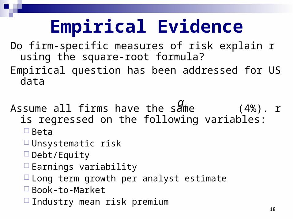
Empirical EvidenceDo firm-specific measures of risk explain r using the
square-root formula?Empirical question has been addressed for US data
Assume all firms have the same (4%). r is regressed on the following variables: Beta Unsystematic risk Debt/Equity Earnings variability Long term growth per analyst estimate Book-to-Market Industry mean risk premium
Lg
19
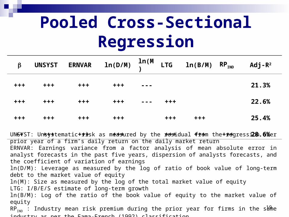
Pooled Cross-Sectional Regression
UNSYST ERNVAR ln(D/M) ln(M) LTG ln(B/M) RPIND Adj-R2
+++ +++ +++ +++ --- 21.3%
+++ +++ +++ +++ --- +++ 22.6%
+++ +++ +++ +++ +++ +++ 25.4%
++ +++ +++ +++ +++ +++ +++ 28.6%
UNSYST: Unsystematic risk as measured by the residual from the regression over prior year of a firm’s daily return on the daily market returnERNVAR: Earnings variance from a factor analysis of mean absolute error in analyst forecasts in the past five years, dispersion of analysts forecasts, and the coefficient of variation of earnings ln(D/M): Leverage as measured by the log of ratio of book value of long-term debt to the market value of equityln(M): Size as measured by the log of the total market value of equityLTG: I/B/E/S estimate of long-term growthln(B/M): Log of the ratio of the book value of equity to the market value of equityRPIND : Industry mean risk premium during the prior year for firms in the same industry as per the Fama-
French (1992) classification

20
Means of Year-by-Year Cross-Sectional Regressions
UNSYST ERNVAR ln(D/M) ln(M) LTG ln(B/M) RPIND Adj-R2
+++ + +++ +++ --- 23.6%
+++ +++ +++ --- +++ 25.4%
+++ ++ +++ +++ +++ +++ 28.5%
+ ++ +++ +++ +++ +++ +++ 30.8%
UNSYST: Unsystematic risk as measured by the residual from the regression over prior year of a firm’s daily return on the daily market returnERNVAR: Earnings variance from a factor analysis of mean absolute error in analyst forecasts in the past five years, dispersion of analysts forecasts, and the coefficient of variation of earnings ln(D/M): Leverage as measured by the log of ratio of book value of long-term debt to the market value of equityln(M): Size as measured by the log of the total market value of equityLTG: I/B/E/S estimate of long-term growthln(B/M): Log of the ratio of the book value of equity to the market value of equityRPIND : Industry mean risk premium during the prior year for firms in the same industry as per the Fama-
French (1992) classification
21
Summary Instead of using a constant growth assumption, we
derive a simple formula expressing as a function of four variables: (i) next year estimated EPS (ii) short term EPS growth (iii) long term EPS growth (iv) cost of capital.
The valuation formula is easy to implement using analysts’ forecasts.
The “square-root” formula expresses the market’s assessment of a firm’s cost of capital; it depends only on (i) P0 / EPS1, and (ii), and (iii)
Inferred cost of capital (r) are explained by (i) risk (ii) misleading “consensus” estimates of EPS1 and , (iii) market inefficiencies.
Lgsg
Sg