Embed Size (px)
Citation preview

HAL Id: tel-03447637https://tel.archives-ouvertes.fr/tel-03447637
Submitted on 24 Nov 2021
HAL is a multi-disciplinary open accessarchive for the deposit and dissemination of sci-entific research documents, whether they are pub-lished or not. The documents may come fromteaching and research institutions in France orabroad, or from public or private research centers.
L’archive ouverte pluridisciplinaire HAL, estdestinée au dépôt et à la diffusion de documentsscientifiques de niveau recherche, publiés ou non,émanant des établissements d’enseignement et derecherche français ou étrangers, des laboratoirespublics ou privés.
Supercuspidal representations of GL(n) over anon-archimedean local field : distinction by a unitary or
orthogonal subgroup, base change and automorphicinductionJiandi Zou
To cite this version:Jiandi Zou. Supercuspidal representations of GL(n) over a non-archimedean local field : distinc-tion by a unitary or orthogonal subgroup, base change and automorphic induction. Number Theory[math.NT]. Université Paris-Saclay, 2021. English. �NNT : 2021UPASM030�. �tel-03447637�

Représentations supercuspidales de GL(n) sur un corps local non archimédien:
distinction par un sous-groupe unitaire ou orthogonal, changement de base et
induction automorphe. Supercuspidal representations of GL(n) over a non-archime-
dean local field : distinction
by a unitary or orthogonal subgroup, base change and
automorphic inductions
Thèse de doctorat de l'université Paris-Saclay
Ecole Doctorale n°574, Mathématique Hadamard (EDMH)
Spécialité de doctorat : Mathématiques fondamentales
Unité de recherche : Université Paris-Saclay, UVSQ, CNRS, Laboratoire de
mathématiques de Versailles, 78000, Versailles, France
Référent : Université de Versailles Saint-Quentin-en-Yvelines
Thèse présentée et soutenue à Paris-Saclay,
le 13/07/2021, par
Jiandi ZOU Composition du Jury
Christophe BREUIL
Directeur de Recherche, Université
Paris-Saclay (LMO)
Président
Jean-François DAT
Professeur, Sorbonne Université Rapporteur & Examinateur
Fiona MURNAGHAN
Professeur, University of Toronto Rapportrice
Paul BROUSSOUS
Maître de conférences, Université de
Poitiers
Examinateur
Shaun STEVENS
Professeur, University of East Anglia Examinateur
Direction de la thèse Vincent SÉCHERRE
Professeur, Université Paris-Saclay
(LMV)
Directeur de thèse
Th
èse
de d
octo
rat
NN
T : 2
021U
PA
SM
030
01

Maison du doctorat de l’Université Paris-Saclay
2ème étage aile ouest, Ecole normale supérieure Paris-Saclay
4 avenue des Sciences,
91190 Gif sur Yvette, France

THESE DE DOCTORAT DE L’UNIVERSITE PARIS-SACLAY 1
Dedicate to my grandparents
I wish for this night-time to last for a lifetimeThe darkness around me, shores of a solar sea
Oh how I wish to go down with the sunSleeping, weeping, with you
“Sleeping sun”, Nightwish
At the end of the river the sundown beamsAll the relics of a life long lived
Here, weary traveller rest your wandSleep the journey from your eyes
“Turn loose the mermaids”, Nightwish

2
Acknowledgement
First and foremost, I would like to thank my advisor Vincent Secherre for his guidance during thepast three years and a half. I thank him for leading me to the world of Langlands program andproposing the subject of my thesis, for his enduring help and encouragement during each meeting andemail correspondence, and for his patience and pertinent advice towards my mathematical lecture andwriting. Without him, I couldn’t have found my own research interests and pursue my mathematicalcareer in the future.
It is my pleasure and honour to thank Jean-Francois Dat and Fiona Murnaghan, as experts of thecorresponding subjects in my thesis, for becoming the referees. Meanwhile, I appreciate ChristopheBreuil, Paul Broussous, Shaun Stevens for becoming part of the jury of my defence.
Concerning the context of this thesis, I thank Colin Bushnell and Guy Henniart for their adviceand encouragement. I thank Raphael Beuzart-Plessis and Nadir Matringe for helpful discussions, andalso their invitations to give talks in their universities. I thank Max Gurevich for becoming my postdochost, and for his interest in my work.
I spent three years as a PhD student in the department of mathematics of UVSQ, which is asmall but warm community for me. I thank Catherine, Christophe, Maelle and Mohamed for theirhelp concerning administrative and teaching procedures. I thank Laure, Liliane and Nadege for theirhelp and warmth as secretaries. I thank Ahmed, Andrea and Florian as former postdocs, and Alessia,Arsen, Bastien, Henry, Ilias, Louis, Melek, Monica and Sybille as former or current PhD studentsfor countless joyful moments. Especially I thank Andrea for inviting me to give a talk at Bordeauxuniversity and Sybille for her help and encouragement towards my research and postdoc application.
During my study in France, I received numerous help from my former teachers and schoolmates ofFudan university. I thank Yijun Yao for his recommendation of the project FMJH and countless help,I thank Shanwen Wang for guiding my undergraduate thesis and his encouragement. I thank ChenlinGu, Jing Yang, Junyan Cao, Xiaojun Wu, Yanbo Fang, Yicheng Zhou, Zhouhang Mao for sharingtheir useful experience in France, especially Zhouhang for various discussions as a continuation of ourfriendship.
I spent my first two years in France as a master student at Paris-Sud university, and I would like tothank An Khuong, Angelot, Duc Nam, Jingrui Niu, Kegang Liu, Ngoc Nhi, Ning Guo, Nicolas, XiaoliWei, Xu Yuan, Yi Pan, Yisheng Tian, Zechuan Zheng, Zhangchi Chen, Zhixiang Wu, Zicheng Qianfor those happy moments. Special thanks due to Ning and Xu for the foundation and development ofour “cuisine and entertainment seminar”, with infinite amusements with them.
Besides I really miss those old days before the pandemic of Covid, during which I participatedseveral “real” conferences and was acquainted with many colleagues. Especially I would like to thankRamla, Huajie Li, Jialiang Zou, Miao Gu, Yichen Qin for those memorable moments during theconference, as well as further online or face to face discussions later on.
Last but not least, I would like to thank my parents for their consistent support and encouragement.Without them, I wouldn’t have been courageous enough to pursue my childish dream as becoming aprofessional mathematician.
3

4

Contents
Introduction (Engilsh version) 9
0.1 General context . . . . . . . . . . . . . . . . . . . . . . . . . . . . . . . . . . . . . . . . 9
0.1.1 Local Langlands correspondence . . . . . . . . . . . . . . . . . . . . . . . . . . 9
0.1.2 Local Langlands functoriality . . . . . . . . . . . . . . . . . . . . . . . . . . . . 10
0.1.3 Problem of distinction . . . . . . . . . . . . . . . . . . . . . . . . . . . . . . . . 11
0.1.4 Our concrete settings . . . . . . . . . . . . . . . . . . . . . . . . . . . . . . . . 13
0.2 Introduction of chapter 1 . . . . . . . . . . . . . . . . . . . . . . . . . . . . . . . . . . 14
0.2.1 Background . . . . . . . . . . . . . . . . . . . . . . . . . . . . . . . . . . . . . . 14
0.2.2 Main results . . . . . . . . . . . . . . . . . . . . . . . . . . . . . . . . . . . . . . 16
0.2.3 Organization of the chapter 1 . . . . . . . . . . . . . . . . . . . . . . . . . . . . 17
0.3 Introduction of chapter 2 . . . . . . . . . . . . . . . . . . . . . . . . . . . . . . . . . . 19
0.3.1 Background . . . . . . . . . . . . . . . . . . . . . . . . . . . . . . . . . . . . . . 19
0.3.2 Statement of the main theorems . . . . . . . . . . . . . . . . . . . . . . . . . . 21
0.3.3 Sketch of the proof and the structure of chapter 2 . . . . . . . . . . . . . . . . 22
0.4 Introduction of chapter 3 . . . . . . . . . . . . . . . . . . . . . . . . . . . . . . . . . . 24
0.4.1 Background . . . . . . . . . . . . . . . . . . . . . . . . . . . . . . . . . . . . . . 24
0.4.2 Main results . . . . . . . . . . . . . . . . . . . . . . . . . . . . . . . . . . . . . . 26
0.4.3 Structure of the chapter 3 . . . . . . . . . . . . . . . . . . . . . . . . . . . . . . 28
Introduction (version francaise) 29
0.1 Contexte general . . . . . . . . . . . . . . . . . . . . . . . . . . . . . . . . . . . . . . . 29
0.1.1 Correspondance de Langlands locale . . . . . . . . . . . . . . . . . . . . . . . . 29
0.1.2 Fonctorialite de Langlands locale . . . . . . . . . . . . . . . . . . . . . . . . . . 30
0.1.3 Probleme de la distinction . . . . . . . . . . . . . . . . . . . . . . . . . . . . . . 31
0.1.4 Notre parametres concrets . . . . . . . . . . . . . . . . . . . . . . . . . . . . . . 33
0.2 Introduction du chapitre 1 . . . . . . . . . . . . . . . . . . . . . . . . . . . . . . . . . . 34
0.2.1 Contexte general . . . . . . . . . . . . . . . . . . . . . . . . . . . . . . . . . . . 34
0.2.2 Principaux resultats . . . . . . . . . . . . . . . . . . . . . . . . . . . . . . . . . 37
0.2.3 Organisation du chapitre 1 . . . . . . . . . . . . . . . . . . . . . . . . . . . . . 38
0.3 Introduction du chapitre 2 . . . . . . . . . . . . . . . . . . . . . . . . . . . . . . . . . . 40
0.3.1 Contexte general . . . . . . . . . . . . . . . . . . . . . . . . . . . . . . . . . . . 40
0.3.2 Enonce des principaux theoremes . . . . . . . . . . . . . . . . . . . . . . . . . . 42
0.3.3 Esquisse de la preuve et de la structure du chapitre 2 . . . . . . . . . . . . . . 43
0.4 Introduction du chapitre 3 . . . . . . . . . . . . . . . . . . . . . . . . . . . . . . . . . . 45
0.4.1 Contexte general . . . . . . . . . . . . . . . . . . . . . . . . . . . . . . . . . . . 45
0.4.2 Principaux resultats . . . . . . . . . . . . . . . . . . . . . . . . . . . . . . . . . 47
0.4.3 La structure du chapitre 3 . . . . . . . . . . . . . . . . . . . . . . . . . . . . . . 49
5
6 CONTENTS
1 Problem of distinction related to unitary subgroups of GLn(F ) and l-modular basechange lift 51
1.1 Notation and basic definitions . . . . . . . . . . . . . . . . . . . . . . . . . . . . . . . . 51
1.2 Hermitian matrices and unitary groups . . . . . . . . . . . . . . . . . . . . . . . . . . . 52
1.3 Preliminaries on simple types . . . . . . . . . . . . . . . . . . . . . . . . . . . . . . . . 53
1.3.1 Simple strata and characters . . . . . . . . . . . . . . . . . . . . . . . . . . . . 53
1.3.2 Simple types and cuspidal representations . . . . . . . . . . . . . . . . . . . . . 54
1.3.3 Endo-classes, tame parameter fields and tame lifting . . . . . . . . . . . . . . . 55
1.3.4 Supercuspidal representations . . . . . . . . . . . . . . . . . . . . . . . . . . . . 56
1.4 One direction of Theorem 0.2.1 for a supercuspidal representation . . . . . . . . . . . 56
1.5 The τ -selfdual type theorem . . . . . . . . . . . . . . . . . . . . . . . . . . . . . . . . . 59
1.5.1 Endo-class version of main results . . . . . . . . . . . . . . . . . . . . . . . . . 60
1.5.2 The maximal and totally wildly ramified case . . . . . . . . . . . . . . . . . . . 61
1.5.3 The maximal case . . . . . . . . . . . . . . . . . . . . . . . . . . . . . . . . . . 64
1.5.4 The general case . . . . . . . . . . . . . . . . . . . . . . . . . . . . . . . . . . . 66
1.6 The distinguished type theorem . . . . . . . . . . . . . . . . . . . . . . . . . . . . . . . 68
1.6.1 Double cosets contributing to the distinction of θ . . . . . . . . . . . . . . . . . 69
1.6.2 The double coset lemma . . . . . . . . . . . . . . . . . . . . . . . . . . . . . . . 69
1.6.3 Distinction of the Heisenberg representation . . . . . . . . . . . . . . . . . . . . 72
1.6.4 Distinction of extensions of the Heisenberg representation . . . . . . . . . . . . 75
1.6.5 Existence of a τ -selfdual extension of η . . . . . . . . . . . . . . . . . . . . . . . 79
1.6.6 Proof of Theorem 1.6.2 . . . . . . . . . . . . . . . . . . . . . . . . . . . . . . . 80
1.7 The supercuspidal unramified case . . . . . . . . . . . . . . . . . . . . . . . . . . . . . 83
1.7.1 The finite field case . . . . . . . . . . . . . . . . . . . . . . . . . . . . . . . . . 83
1.7.2 Distinction criterion in the unramified case . . . . . . . . . . . . . . . . . . . . 85
1.8 The supercuspidal ramified case . . . . . . . . . . . . . . . . . . . . . . . . . . . . . . . 87
1.8.1 The finite field case . . . . . . . . . . . . . . . . . . . . . . . . . . . . . . . . . 87
1.8.2 Distinction criterion in the ramified case . . . . . . . . . . . . . . . . . . . . . . 89
1.8.3 Proof of Theorem 0.2.3 . . . . . . . . . . . . . . . . . . . . . . . . . . . . . . . 91
1.9 Generalization of Theorem 1.4.1 . . . . . . . . . . . . . . . . . . . . . . . . . . . . . . 91
1.9.1 The finite analogue . . . . . . . . . . . . . . . . . . . . . . . . . . . . . . . . . . 91
1.9.2 The cuspidal case . . . . . . . . . . . . . . . . . . . . . . . . . . . . . . . . . . . 92
1.9.3 The discrete series case . . . . . . . . . . . . . . . . . . . . . . . . . . . . . . . 95
1.9.4 The generic case . . . . . . . . . . . . . . . . . . . . . . . . . . . . . . . . . . . 96
1.10 “`-modular” base change lift and applications . . . . . . . . . . . . . . . . . . . . . . . 98
1.10.1 l-modular local Langlands correspondence . . . . . . . . . . . . . . . . . . . . . 98
1.10.2 l-modular base change lift . . . . . . . . . . . . . . . . . . . . . . . . . . . . . . 103
1.10.3 Application . . . . . . . . . . . . . . . . . . . . . . . . . . . . . . . . . . . . . . 107
2 Problem of distinction related to orthogonal subgroups of GLn(F ) 113
2.1 Notation . . . . . . . . . . . . . . . . . . . . . . . . . . . . . . . . . . . . . . . . . . . . 113
2.1.1 General notation . . . . . . . . . . . . . . . . . . . . . . . . . . . . . . . . . . . 113
2.1.2 A brief recall of the simple type theory . . . . . . . . . . . . . . . . . . . . . . . 113
2.2 Symmetric matrices and orthogonal involutions . . . . . . . . . . . . . . . . . . . . . . 114
2.2.1 Orbits of symmetric matrices, orthogonal involutions and orthogonal groups . . 115
2.2.2 τ -split embedding . . . . . . . . . . . . . . . . . . . . . . . . . . . . . . . . . . 117
2.2.3 Calculation of Hilbert symbol and Hasse invariant in certain cases . . . . . . . 118
2.3 τ -selfdual type theorem . . . . . . . . . . . . . . . . . . . . . . . . . . . . . . . . . . . 124

THESE DE DOCTORAT DE L’UNIVERSITE PARIS-SACLAY 7
2.3.1 The maximal and totally wildly ramified case . . . . . . . . . . . . . . . . . . . 125
2.3.2 The maximal case . . . . . . . . . . . . . . . . . . . . . . . . . . . . . . . . . . 126
2.3.3 The general case . . . . . . . . . . . . . . . . . . . . . . . . . . . . . . . . . . . 129
2.4 Distinguished type theorem and the orbits of distinguished type . . . . . . . . . . . . . 134
2.4.1 Double cosets contributing to the distinction of θ . . . . . . . . . . . . . . . . . 135
2.4.2 The double coset lemma . . . . . . . . . . . . . . . . . . . . . . . . . . . . . . . 135
2.4.3 Distinction of the Heisenberg representation . . . . . . . . . . . . . . . . . . . . 137
2.4.4 Distinction of the extension of a Heisenberg representation . . . . . . . . . . . 138
2.4.5 Existence of a τ -selfdual extension of η . . . . . . . . . . . . . . . . . . . . . . . 139
2.4.6 Proof of Theorem 2.4.2 . . . . . . . . . . . . . . . . . . . . . . . . . . . . . . . 140
2.4.7 Double cosets contributing to the distinction of π . . . . . . . . . . . . . . . . . 141
2.5 Proof of the main theorems . . . . . . . . . . . . . . . . . . . . . . . . . . . . . . . . . 144
2.5.1 The finite field case . . . . . . . . . . . . . . . . . . . . . . . . . . . . . . . . . 145
2.5.2 Orthogonal groups contributing to the distinction of π . . . . . . . . . . . . . . 146
2.5.3 Other orthogonal groups . . . . . . . . . . . . . . . . . . . . . . . . . . . . . . . 147
3 Explicit base change lift and automorphic induction for supercuspidal representa-tions 149
3.1 General notations . . . . . . . . . . . . . . . . . . . . . . . . . . . . . . . . . . . . . . . 149
3.2 Preliminaries for the simple type theory . . . . . . . . . . . . . . . . . . . . . . . . . . 150
3.2.1 Simple strata and simple characters . . . . . . . . . . . . . . . . . . . . . . . . 150
3.2.2 Endo-class and interior tame lifting . . . . . . . . . . . . . . . . . . . . . . . . . 150
3.2.3 Full Heisenberg representation . . . . . . . . . . . . . . . . . . . . . . . . . . . 153
3.2.4 Extended maximal simple type and supercuspidal representation . . . . . . . . 153
3.3 Symplectic signs . . . . . . . . . . . . . . . . . . . . . . . . . . . . . . . . . . . . . . . 155
3.4 Cyclic base change and automorphic induction . . . . . . . . . . . . . . . . . . . . . . 156
3.4.1 Cyclic base change . . . . . . . . . . . . . . . . . . . . . . . . . . . . . . . . . . 156
3.4.2 Cyclic automorphic induction . . . . . . . . . . . . . . . . . . . . . . . . . . . . 157
3.4.3 Functorial property . . . . . . . . . . . . . . . . . . . . . . . . . . . . . . . . . . 160
3.5 Basic classification . . . . . . . . . . . . . . . . . . . . . . . . . . . . . . . . . . . . . . 161
3.5.1 Supercuspidal case . . . . . . . . . . . . . . . . . . . . . . . . . . . . . . . . . . 162
3.5.2 Non-supercuspidal case . . . . . . . . . . . . . . . . . . . . . . . . . . . . . . . 164
3.5.3 A brief summary . . . . . . . . . . . . . . . . . . . . . . . . . . . . . . . . . . . 165
3.6 Statement of the main theorems . . . . . . . . . . . . . . . . . . . . . . . . . . . . . . 166
3.6.1 Base change in supercuspidal case . . . . . . . . . . . . . . . . . . . . . . . . . 166
3.6.2 Interior automorphic induction . . . . . . . . . . . . . . . . . . . . . . . . . . . 168
3.6.3 Exterior automorphic induction . . . . . . . . . . . . . . . . . . . . . . . . . . . 168
3.6.4 base change in non-supercuspidal case . . . . . . . . . . . . . . . . . . . . . . . 170
3.7 A precise construction of the full Heisenberg representation . . . . . . . . . . . . . . . 171
3.7.1 Several results of Bushnell-Henniart . . . . . . . . . . . . . . . . . . . . . . . . 171
3.7.2 Construction in the interior automorphic induction case . . . . . . . . . . . . . 178
3.7.3 Construction in the supercuspidal base change case . . . . . . . . . . . . . . . . 179
3.7.4 Construction in the exterior automorphic induction case . . . . . . . . . . . . . 182
3.8 Proof of the main theorems . . . . . . . . . . . . . . . . . . . . . . . . . . . . . . . . . 185
3.8.1 Interior automorphic induction . . . . . . . . . . . . . . . . . . . . . . . . . . . 185
3.8.2 Base change in supercuspidal case . . . . . . . . . . . . . . . . . . . . . . . . . 186
3.8.3 Exterior automorphic induction . . . . . . . . . . . . . . . . . . . . . . . . . . . 186
3.9 Calculation of bφF/F0
θ0in the F/F0 unramified case . . . . . . . . . . . . . . . . . . . . 188

8 CONTENTS
3.9.1 Reduction to the maximal totally ramified case . . . . . . . . . . . . . . . . . . 1893.9.2 A special case of Theorem 3.9.1 . . . . . . . . . . . . . . . . . . . . . . . . . . . 1923.9.3 A reductive procedure when Γ0 is non-trivial . . . . . . . . . . . . . . . . . . . 1973.9.4 The end of the proof . . . . . . . . . . . . . . . . . . . . . . . . . . . . . . . . . 200
3.10 Contribution to the calculation of the character µT0/F0
θ0. . . . . . . . . . . . . . . . . . 201
3.10.1 Evaluating at $ps
T0. . . . . . . . . . . . . . . . . . . . . . . . . . . . . . . . . . 202
3.10.2 Epsilon factors . . . . . . . . . . . . . . . . . . . . . . . . . . . . . . . . . . . . 2033.10.3 A more detailed discussion for supercuspidal representations of Carayol type . 203

Introduction (English version)
This thesis contains three parts. In this introductory chapter, we will explain the general backgroundin the first section, and then in the following three sections we will focus on each part and providespecific introductions.
0.1 General context
Let F0 be a non-archimedean locally compact field of residue characteristic p and let R be an alge-braically closed field of characteristic l 6= p, and in particular when l > 0 we are in the “l-modularcase”. For instance, we will mainly focus on the following three cases: R being the complex numberfield C, the algebraic closure of the field of l-adic numbers denoted by Ql, or the algebraic closure ofthe finite field of l elements denoted by Fl when l 6= 0. Let G be a reductive group1 over F0 and letG be the locally profinite group consisting of the F0-rational points of G. We are interested in thecategory of smooth irreducible representations of a locally profinite group and we denote by IrrR(G)the set of isomorphism classes of smooth irreducible representations of G over R.
0.1.1 Local Langlands correspondence
First of all let us consider the case where R = C. We fix a separable closure F0 of F0, we denote byWF0 the Weil group of F0 with respect to F0 and by WDF0 =WF0 × SL2(C) the Weil-Deligne groupof F0. We define the dual group of G, denoted by G, as the complex reductive group (identified withthe complex topological group of its rational points by abuse of notation) determined by the dual ofthe root datum of G. Since the root datum of G is endowed with a WF0-action, so is the group Gafter fixing a pinning of the root datum, and we denote by LG = GoWF0 the L-group of G.
Definition 0.1.1. An L-parameter of G (over C) is a homomorphism φ : WDF0 → LG such that
• The following diagram is commutative:
WF0 × SL2(C) = WDF0
((
φ // LG = GoWF0
xxWF0
where the two unmarked arrows are canonical projections.
• φ|WF0×{1} is continuous with image consisting of semisimple elements2, and φ|{1}×SL2(C) is al-
gebraic 3 with image consisting of unipotent elements in G.
1We will only consider connected reductive groups.2An element (g, w) in LG is semisimple if for any r as a finite dimensional representation of LG, the image r((g, w))
is semisimple.3That is, it is an algebraic representation from the complex algebraic group SL2 into the complex algebraic group G .
9

10 0.1. GENERAL CONTEXT
Two L-parameters are said to be isomorphic if they are in the same G-conjugacy class, and wedenote by Φ(G) the isomorphism classes of Langlands parameters of G. The famous local Langlandscorrespondence is stated as follows.
Conjecture 0.1.2. There is a unique finite-to-one surjection
LLC : IrrR(G) −→ Φ(G)
satisfying certain desiderata.
Definition 0.1.3. For φ ∈ Φ(G), we call Πφ := LLC−1(φ) the L-packet of φ as a finite set ofirreducible representations of G.
Here we won’t specify what exactly do these desiderata mean (compatible with parabolic induction,transfer L-factors and ε-factors, etc.) but refer to [Bor79] for an expository introduction. The localLanglands correspondence for certain reductive groups is known, such as G being a torus, GLn orcertain classical groups, due to the work of Langlands [Lan97], Harris-Taylor [HT01], Arthur [Art13],etc.
Moreover, although the original conjecture of Langlands is only proposed for representations overC, for other R under our settings it is still possible to give a definition for L-parameters and to proposethe corresponding conjecture with the corresponding desiderata being adapted to the new situations.For example, there are pioneering work of Vigneras [Vig01] for G = GLn, and also recent work of Dat-Helm-Kurinczuk-Moss [DHKM20] for general reductive groups and representations over an integraldomain with p being invertible within instead of over a field R. Finally we mention the recent resultof Fargues-Scholze [FS21]. Using geometric method and under general enough settings (more generalthan ours), they constructed Φ(G) (indeed as a stack) and the local Langlands correspondence, andverified the corresponding desiderata under their settings (cf. ibid. Theorem IX.0.5).
0.1.2 Local Langlands functoriality
Now we discuss the local Langlands functoriality and we still assume that R = C. Let G0 be anotherreductive group over F0, and let G0 be the group of F0-rational points of G0. As in the previous sub-section, we may similarly define its dual group G0, its L-group LG0 = G0oWF0 and the isomorphismclasses Φ(G0).
Definition 0.1.4. A group homomorphism
ι : LG0 −→ LG
is called an L-homomorphism, if
• it is continuous, and its restriction to G0 is an algebraic representation of G0 into G.
• The following diagram is commutative
WF0 n G0 = LG0
''
ι // LG = GoWF0
xxWF0
where the two unmarked arrows are canonical projections.

THESE DE DOCTORAT DE L’UNIVERSITE PARIS-SACLAY 11
By definition, given an L-parameter φ0 in Φ(G0), the composition ι◦φ0 is an L-parameter in Φ(G).Thus we construct a map between isomorphism classes of L-parameters:
Φ(ι) : Φ(G0) −→ Φ(G), φ0 7−→ ι ◦ φ0.
If we admit the local Langlands correspondence for both G0 and G, we have the following diagram
IrrR(G0)
Π(ι)
��
LLC // Φ(G0)
Φ(ι)
��IrrR(G)
LLC// Φ(G)
The local Langlands functoriality predicts the existence of a map Π(ι), called local lifting with re-spect to ι, such that the above diagram is commutative. Moreover this map Π(ι) is expected to beconstructed independently of this diagram, but using other technical tools such as trace formula orL-function. On the one hand, understanding different local liftings maps forms an important part ofthe local Langlands program. On the other hand, it also plays a crucial role in the inductive strategy,proposed by Langlands-Shelstad [LS87] and called the method of endoscopy, of constructing the localLanglands correspondence for general reductive group, which has become a prosperous area in recentyears with fruitful results, including the work of Arthur, Kottwitz, Langlands, Laumon, Ngo, Shelstad,Waldspurger, etc.
Still we need not confine ourself in complex representations, instead we consider possible locallifting over R. For example, one expectation for the expected local lifting over Fl is that, it issupposed to be compatible with the local lifting over Ql, after we identify C with Ql via a certainalgebraic isomorphism and implement the modulo l reduction. One typical result is about the Jacquet-Langlands correspondence as one natural enough lifting between GLn and its inner form. Over Fl, theconstruction of this map and also its compatibility with the usual Jacquet-Langlands correspondencewas studied by Dat [Dat12] for special case, and then generalized by Mınguez-Secherre [MS17] forgeneral case.
0.1.3 Problem of distinction
Let H ⊂ G be a closed algebraic subgroup over F0 and we denote by H the group of F0-rationalpoints of H. For π ∈ IrrR(G) and ρ ∈ IrrR(H), we say that π is (H, ρ)-distinguished if
HomH(π, ρ) 6= 0,
or in other words, the restriction of π to H admits ρ as a quotient. In particular, when ρ is trivial,we call π distinguished by H or H-distinguished. Still for simplicity we temporarily assume R = C.
The problem of distinction is ubiquitous and plays an important role in the representation theoryof p-adic groups. For example, if G is quasisplit, we let H = U be the unipotent radical of a Borelsubgroup of G and we let ψ be a non-degenerate character of H = U , that is, its restriction to anyunipotent subgroup Uα of U related to a simple root α is non-trivial. One well-known result [Sha74]is that the vector space
HomU (π, ψ)
is of dimension smaller than or equal to one. Those π with the corresponding dimension equallingone are called generic representations. By the Frobenius reciprocity, such π can be embedded intothe space of (U,ψ)-invariant G-linear forms, which is called the Whittaker model of π and plays anprominent role in the local and global theory of L-functions. In another example we consider V as

12 0.1. GENERAL CONTEXT
a finite dimensional vector space over F0 endowed with a sesquilinear form, and W as a subspace ofV . We denote by G the group of F0-automorphisms of V and by H the group of F0-automorphismsof W , preserving the sesquilinear form. Then the corresponding problem of distinction is related tothe “branching laws”, which dates back to the representation theory of complex algebraic groups andhas been performing as an active area in decades because of the initiation and breakthrough of theGan-Gross-Prasad conjecture [GGP12] and its variants.
Under good settings, the problem of distinction is closely related to the local Langlands corre-spondence and its functoriality. In the remarkable book [SV17a], Sakellaridis and Venkatesh proposeda general framework to study the problem of distinction, in which they assume G to be split andX = H\G to be a spherical variety with X denoting its F0-rational points. Their starting point isthe construction of the dual group GX for X as a complex reductive group, under an assumption onthe roots of X, together with a canonical algebraic representation
ιX : GX × SL2(C) −→ G.
Under their conjectural proposal, roughly speaking, the H-distinguished representations of G cor-respond to the X-distinguished Arthur parameters via the local Langlands correspondence, whereArthur parameters are the analogue of L-parameters with a corresponding version of local Langlandscorrespondence related, and those Arthur parameters factoring through ιX are called X-distinguished,for which we leave ibid. section 16 for more details. So the idea behind is that, under good circum-stances, the property of being distinguished is transferred by the local Langlands correspondence.In [Pra15], Prasad considered the case where X = H\G is a symmetric space with respect to a Galoisinvolution. He constructed a quasisplit subgroup G0 (denoted by Gop in loc. cit.) over F0, a naturalL-homomorphism ι : LG0 → LG which simply comes from the restriction, and a character ωH of H.Finally he conjectured that, for π an irreducible representation of G distinguished by (H,ωH), theL-packet of π is derived from the local lifting related to ι, or more precisely there exists φ0 ∈ Φ(G0)such that π ∈ Π(ι ◦ φ0). Moreover a conjectural formula for the dimension of the space of distinctionhas been given. These two general frameworks, combining with various concrete examples being veri-fied, should be regarded as our guideline of the results we should expect under the language of localLanglands correspondence and its functoriality.
We briefly introduce some known methods of dealing with problem of distinction. One importantmethod, initiated by Jacquet and developed by himself, his students and other followers, is called therelative trace formula method, for which we name a few articles [JLR93], [JY96], [Guo96], [Mao98].The idea, roughly speaking, is first to solve the corresponding problem over a global field, and then torealize our local field F0 as a component of the ring of adeles of a global field and to use a global-to-local argument. Then one compares two different trace formulae as distributions on two spaces of testfunctions, one of which relates exactly to our global problem. After verifying the fundamental lemmaand the existence of smooth transfer, one obtains sufficient many pairs of matching test functions suchthat two trace formulae coincide. If the other trace formula is well understood, we get the informationto solve the global problem of distinction. In addition, to solve the local Gan-Gross-Prasad conjecturefor orthogonal groups, Waldspurger [Wal10], [Wal12] initiated a new method with the considerationof a local relative trace formula, such that the dimension of the space of distinction can be expressedinside, and then he used sophisticated techniques in harmonic analysis over p-adic reductive groupsto reformulate the trace formula and to obtain the result. In the last decade this method has beendeveloped and applied to different situations by some people including Beuzart-Plessis and C. Wan.For example in [BP18] using the similar method, Beuzart-Plessis solved part of the above conjectureproposed by Prasad for essentially square integrable representations.
Another possible method to study the problem of distinction is algebraic, which first studies thesame problem for supercuspidal representations as the starting point, and then applies parabolic

THESE DE DOCTORAT DE L’UNIVERSITE PARIS-SACLAY 13
induction to study more general irreducible representations. For π a supercuspidal representation ofG, a general belief is that it can be written down as the compact induction of a finite dimensionalsmooth irreducible representation, more precisely, there exists a pair (J ,Λ) such that J is a compactsubgroup of G modulo the centre, and Λ is a smooth irreducible finite dimensional representationof J such that π ∼= indGJΛ. This belief is verified for many cases, including tame supercuspidalrepresentations [Yu01], [Fin21] for tamely ramified reductive group G, and also general supercuspidalrepresentations for classical groups [BK93], [Ste08]. Then if we focus on the study of H-distinguishedsupercuspidal representation π, using the Mackey formula and the Frobenius reciprocity, it is easilyseen that
HomH(π, 1) ∼= HomH(indGJΛ, 1) ∼=∏
g∈J\G/H
HomJg∩H(Λg, 1).
Thus we only need to study those g ∈ J\G/H such that the R-vector space HomJg∩H(Λg, 1) isnon-zero, and then to study corresponding dimension. To that aim, we date back to the detailed con-struction of (J ,Λ). One typical work is [HM08], where the authors studied, for G/H as a symmetricspace, tame supercuspidal representations π of G distinguished by H using the idea mentioned aboveand the structural result of J.-K. Yu [Yu01] for such representations.
Still we are not necessarily confined in the case where R = C, but we focus on the general R inour settings. In this case the two analytic methods mentioned above become invalid. By contrastthe algebraic method remains valid, since the structural result for the (J ,Λ), once being established,usually works for general R rather that just R = C, such as [Vig96], [MS14b] and [Fin19]. Tosum up, searching the possible relation between the problem of distinction and the local Langlandscorrespondence and its functoriality for general R should be regarded as the original motivation forthis thesis.
0.1.4 Our concrete settings
Although the context above is quite general, the aim of this thesis is humble, which focuses on theunderstanding of several special examples. Fix n as a positive integer. Let F/F0 be a finite cyclicextension of non-archimedean locally compact fields of residue characteristic p of degree r, and let Gbe the Weil restriction of the reductive group GLn over F , which is a reductive group over F0. Inparticular we have G = GLn(F ). For most of the time, we will concentrate on cuspidal or supercuspidalrepresentations of G over R, which should be regarded as the building blocks for general irreduciblerepresentations. Recall that an irreducible representation of G is cuspidal (resp. supercuspidal) if itdoesn’t occur as a subrepresentation (resp. subquotient) of the parabolic induction of an irreduciblerepresentation of a proper Levi subgroup of G. When char(R) = 0 the two concepts above areequivalent, however when char(R) = l > 0, a supercuspidal representation must be cuspidal, but theexistence of counter-example manifests that the converse is false in general.
To study a cuspidal representation π ofG overR, our main tool is the simple type theory establishedby Bushnell-Kutzko [BK93] when char(R) = 0, and further generalized by Vigneras [Vig96] to thel-modular case. We refer to chapter 1, section 3 or chapter 3, section 2 for a detailed introduction forthe theory, but here we also give a brief introduction for ease of giving more details.
As indicated above, the idea of simple type theory is to realize π as the compact induction of afinite dimensional irreducible representation Λ of J , which is an open subgroup of G compact modulothe centre. Such a pair (J ,Λ) is called an extended maximal simple type which we will abbreviate tosimple type for short. The main theorem says that, any π can be constructed in this way, and thecorresponding simple type (J ,Λ) is unique up to G-conjugacy. We also mention the following mainproperties of (J ,Λ):

14 0.2. INTRODUCTION OF CHAPTER 1
(1) The group J contains a unique maximal open compact subgroup J which contains a uniquemaximal normal pro-p-subgroup J1;
(2) We have J/J1 ∼= GLm(l). Here l is the residue field of E, where E is a field extension over Fof degree d. Moreover we have n = md, where m and d are integers determined by π;
(3) We may write Λ = κ ⊗ ρ, where κ and ρ are irreducible representations of J such that therestriction κ|J1 = η is an irreducible representation of J1, called a Heisenberg representation, and ρ|Jis the inflation of a cuspidal representation of GLm(l) ∼= J/J1;
(4) There exists a pro-p-subgroup of J1 denoted by H1, and a character of H1 denoted by θ andcalled a simple character, such that the restriction of η to H1 equals the direct sum of (J1 : H1)1/2
copies of θ.
Finally we enter the introduction for our concrete work. For the first part, we study the problemof distinction related to a unitary subgroup of G and its relation with the Langlands functoriality,or embodied as the quadratic base change lift in our settings; For the second part, we study theproblem of distinction related to an orthogonal subgroup of G, and we focus only on supercuspidalrepresentations over R = C, which is the first step towards the understanding of more general irre-ducible representations; For the final part for R = C we give explicit constructions for two speciallocal liftings, the base change lift and the automorphic induction, for supercuspidal representations.
0.2 Problem of distinction related to unitary subgroups of GLn(F )and l-modular base change lift
0.2.1 Background
The first eight sections of chapter 1 is based on the preprint [Zou19]. In this subsection we assumeF/F0 to be a quadratic extension of p-adic fields of residue characteristic p, and we let σ denote itsnon-trivial automorphism. For G and G as above, we write ε for a hermitian matrix in G, that is,σ( tε) = ε with t denoting the transpose of matrices. We define
τε(x) = εσ( tx−1)ε−1
for any x ∈ G, called a unitary involution on G, which also induces an F0-automorphism on G. Wefix one τ = τε, and we denote by Gτ the subgroup of G over F0, such that Gτ is the subgroup of Gconsisting of the elements fixed by τ . Such Gτ (resp. Gτ ) is called the unitary subgroup of G (resp.G) with respect to τ .
For π a smooth irreducible representation of G over C, Jacquet proposed to study the problemof distinction related to the pair (G,Gτ ) as above, that is, to study the space of Gτ -invariant linearforms
HomGτ (π, 1)
and its dimension as a complex vector space. For n = 3 and π supercuspidal, he proved in [Jac01] byusing global argument, that π is distinguished by Gτ if and only if π is σ-invariant, that is, πσ ∼= π,where πσ := π ◦ σ. Moreover he showed that this space is of dimension one as a complex vector spacewhen the condition above is satisfied. Besides in ibid., he also sketched a similar proof when n = 2and π is supercuspidal, to give the same criterion of distinction and the same dimension one theorem.Based on these results as one of the main reasons, he conjectured that in general, π is distinguished byGτ if and only if π is σ-invariant. Moreover, the dimension of the space of Gτ -invariant linear formsis not necessary to be one in general. Under the assumption that π is σ-invariant and supercuspidalJacquet further conjectured that the dimension is one.

THESE DE DOCTORAT DE L’UNIVERSITE PARIS-SACLAY 15
In addition, an irreducible representation π of G is contained in the image of quadratic base changelift with respect to F/F0 if and only if it is σ-invariant ( [AC89]). Thus for irreducible representations,the conjecture of Jacquet gives a connection between quadratic base change lift and Gτ -distinction.
Besides the special case mentioned above, there are two more evidences which support the con-jecture. First we consider the analogue of the conjecture in the finite field case. For ρ an irreduciblecomplex representation of GLn(Fq2), Gow [Gow84] proved that ρ is distinguished by the unitary sub-group Un(Fq) if and only if ρ is isomorphic to its twist under the non-trivial element of Gal(Fq2/Fq).Under this condition, he also showed that the space of Un(Fq)-invariant linear forms is of dimen-sion one as a complex vector space. In addition, Shintani [Shi76] showed that there is a one-to-onecorrespondence between the set of irreducible representations of GLn(Fq) and that of Galois invari-ant irreducible representations of GLn(Fq2), where the correspondence, called the base change map,is characterized by a trace identity. These two results give us a clear feature between base changemap and Un(Fq)-distinction. Finally, when ρ is generic and Galois-invariant, Anandavardhanan andMatringe [AM18] recently showed that the Un(Fq)-average of Bessel function of ρ on the Whittakermodel as a Un(Fq)-invariant linear form is non-zero. Since the space of Un(Fq)-invariant linear formsis of dimension one, this result gives us a concrete characterization of the space of distinction.
The other evidence for the Jacquet conjecture is its global analogue. We assume K/K0 to be aquadratic extension of number fields and we denote by σ its non-trivial automorphism. We considerτ to be a unitary involution on GLn(K), which also gives us an involution on GLn(AK), still denotedby τ by abuse of notation, where AK denotes the ring of adeles of K. We denote by GLn(K)τ (resp.GLn(AK)τ ) the unitary subgroup of GLn(K) (resp. GLn(AK)) with respect to τ . For φ a cusp formof GLn(AK), we define
Pτ (φ) =
∫GLn(K)τ\GLn(AK)τ
φ(h)dh
to be the unitary period integral of φ with respect to τ . We say that a cuspidal automorphic represen-tation Π of GLn(AK) is GLn(AK)τ -distinguished if there exists a cusp form in the space of Π such thatPτ (φ) 6= 0. In 1990’s, Jacquet and Ye began to study the relation between GLn(AK)τ -distinction andglobal base change lift (see for example [JY96] when n = 3). For general n, Jacquet [Jac05] showedthat Π is contained in the image of quadratic base change lift (or equivalently Π is σ-invariant [AC89])with respect to K/K0 if and only if there exists a unitary involution τ such that Π is Gτ -distinguished.This result may be viewed as the global version of Jacquet conjecture for supercuspidal representations.
In fact, for the special case of the Jacquet conjecture in [Jac01], Jacquet used the global analogueof the same conjecture and relative trace formula as two main techniques to finish the proof. To say itsimple, he first proved the global analogue of the conjecture. Then he used the relative trace formulato write a non-zero unitary period integral as the product of its local components at each place of K0,where each local component characterizes the distinction of the local component of Π with respect tothe corresponding unitary group over local fields. When π is σ-invariant, he chose Π as a σ-invariantcuspidal automorphic representation of GLn(AK) and v0 as a non-archimedean place of K0 such that(Gτ , π) = (GLn(Kv0)τ ,Πv0). Then the product decomposition leads to the proof of the “if” part ofthe conjecture. The “only if” part of the conjecture, which will be discussed in chapter 1, section 4,requires the application of globalization theorem. His method was generalized by Feigon-Lapid-Offenin [FLO12] to general n and more general family of representations. They showed that the Jacquetconjecture works for generic representations of G. Moreover for the same family of representations,they were able to give a lower bound for the dimension of HomGτ (π, 1) and they further conjecturedthat the inequality they gave is actually an equality. Finally, Beuzart-Plessis [BP20] recently verifiedthe equality based on the work of Feigon-Lapid-Offen and the relative local trace formula. Thus forgeneric representations of G, the Jacquet conjecture was settled.
Instead of using global-to-local argument, there are also partial results based on the algebraic

16 0.2. INTRODUCTION OF CHAPTER 1
method we explained before. In [HM98] Hakim-Mao verified the conjecture when π is supercuspidalof level zero, that is, π is supercuspidal such that π1+pFMn(oF ) 6= 0, where oF denotes the ring ofintegers of F and pF denotes its maximal ideal. When π is supercuspidal and F/F0 is unramified,Prasad [Pra01] proved the conjecture by applying the simple type theory developed by Bushnell-Kutzko in [BK93]. When π is tame supercuspidal, that is, π is a supercuspidal representation arisingfrom the construction of Howe [How77], Hakim-Murnaghan [HM02b] verified the conjecture. Notingthat in the results of Hakim-Mao and Hakim-Murnaghan, they need the additional assumption thatthe residue characteristic p 6= 2.
The discussion above leaves us an open question: Is there any local and algebraic method that leadsto a proof of the Jacquet conjecture which works for all supercuspidal representations of G? First, thismethod will generalize the results of Hakim-Mao, Prasad and Hakim-Murnaghan which we mentionedin the last paragraph. Secondly, we are willing to consider F/F0 to be a quadratic extension ofnon-archimedean locally compact fields instead of p-adic fields. Since the result of Feigon-Lapid-Offenheavily relies on the fact that the characteristic of F equals 0, their method fails when considering non-archimedean locally compact fields of positive characteristic. Finally, instead of considering complexrepresentations, we are also willing to study l-modular representations with l 6= p. One hopes toprove an analogue of the Jacquet conjecture for l-modular supercuspidal representations, which willgeneralize the result of Feigon-Lapid-Offen for supercuspidal representations. Noting that they useglobal method in their proof, which strongly relies on the assumption that all the representations arecomplex. Thus their method doesn’t work anymore for l-modular representations.
The aim of chapter 1 is first to address the question above, and then to explore the problem ofdistinction for more general irreducible representations in the l-modular case and its relation with the“l-modular” base change lift whose construction will be given.
0.2.2 Main results
To begin with, from now on we assume F/F0 to be a quadratic extension of non-archimedean locallycompact fields of residue characteristic p instead of p-adic fields, and we assume that p 6= 2. We fixR an algebraically closed field of characteristic l 6= p, allowing that l = 0. We assume π to be anirreducible representation of G = GLn(F ) over R. Now we state our first main theorem.
Theorem 0.2.1. For π a supercuspidal representation of G and τ a unitary involution, π is distin-guished by Gτ if and only if πσ ∼= π.
Moreover, we may also calculate the dimension of the space of Gτ -invariant linear forms.
Theorem 0.2.2. For π a σ-invariant supercuspidal representation of G, we have
dimRHomGτ (π, 1) = 1.
One important corollary of Theorem 0.2.1 relates to the Ql-lift of a σ-invariant supercuspidalrepresentation of G over Fl when l > 0, where we denote by Ql, Zl and Fl the algebraic closure of anl-adic field, its ring of integers and the algebraic closure of the finite field of l elements respectively.For (π, V ) a smooth irreducible representation of G over Ql, we call it integral if it admits an integralstructure, that is, a Zl[G]-submodule LV of V such that LV ⊗Zl Ql = V . For such a representation,
the semi-simplification of LV ⊗Zl Fl doesn’t depend on the choice of LV , which we denote by rl(π)
a representation of G over Fl, called the modulo l reduction of π (see [Vig96] for more details). Thefollowing theorem which will be proved at the end of chapter 1, section 8, says that it is always possibleto find a σ-invariant Ql-lift for a σ-invariant supercuspidal representation of G over Fl.

THESE DE DOCTORAT DE L’UNIVERSITE PARIS-SACLAY 17
Theorem 0.2.3. For π a σ-invariant supercuspidal representation of G over Fl, there exists an integralσ-invariant supercuspidal representation π of G over Ql, such that rl(π) = π.
For irreducible generic representations, we are able to prove one direction of the Jacquet conjecture,which is new only if char(R) = l > 0.
Theorem 0.2.4 (see Theorem 1.9.1). Let π be an irreducible generic representation of G over R. Ifπ is distinguished by Gτ , then π is σ-invariant.
Our next goal is to characterize l-modular distinguished representations via local Langlands func-toriality, or base change lift in our settings. To that aim, first we need to construct an l-modular basechange lift. The upshot is the following theorem:
Theorem 0.2.5 (see Theorem 1.10.17). We may define the l-modular cyclic base change lift
BCFl : IrrFl(GLn(F0)) −→ Irrσ−invFl
(GLn(F ))
which satisfies and is determined by the following commutative diagram
IrrIntQl
(GLn(F0))
Jl
��
BCQl// IrrInt,σ−inv
Ql(GLn(F ))
Jl��
IrrFl(GLn(F0))BCFl // Irrσ−inv
Fl(GLn(F ))
We briefly explain the notations and leave the corresponding section for more details. Here thesuperscripts Int and σ-inv represent integral and σ-invariant respectively, BCQl represents the base
change lift of Arthur-Clozel being transferred to representations over Ql via a certain algebraic isomor-phism C ∼= Ql, and for π0 (resp. π) in IrrInt
Ql(GLn(F0)) (resp. IrrInt,σ−inv
Ql(GLn(F ))), the image Jl(π0)
(resp. Jl(π)) is the unique irreducible constituent in rl(π0) (resp. rl(π)) having the highest deriva-tive sequence. Finally as an application, we explore the distinguished cuspidal (but not necessarilysupercuspidal) representations in the l-modular case.
0.2.3 Organization of the chapter 1
Let us outline the content of chapter 1. We introduce our settings in section 1 and basic knowledgeabout hermitian matrices and unitary subgroups in section 2. Our main tool to prove the theoremswill be the simple type theory developed by Bushnell-Kutzko in [BK93], and further generalized byVigneras [Vig96] to the l-modular case. In section 3 we will give a detailed introduction of this theory.
For a given supercuspidal representation π of G, our starting point is to prove the “only if” partof Theorem 0.2.1. When R = C and char(F ) = 0, it is a standard result by using global argument,especially the globalization theorem ( [HM02a], Theorem 1). When char(F ) = p > 0, we may keep theoriginal proof except that we need a characteristic p version of the globalization theorem. Fortunatelywe can use a more general result due to Gan-Lomelı [GL18] to get the result we need. Since anysupercuspidal representation of G over a characteristic 0 algebraically closed field can be realized as arepresentation over Q up to twisting by an unramified character, we finish the proof when char(R) = 0.When R = Fl, we consider the projective envelope PΛ|J of Λ|J and we use the results in [Vig96] to study
its irreducible components and the irreducible components of its Ql-lift. Finally we show that thereexists a Ql-lift of π which is supercuspidal and Gτ -distinguished. Thus by using the characteristic0 case we finish the proof for the “only if” part for any R under our settings. The details will bepresented in section 4.

18 0.2. INTRODUCTION OF CHAPTER 1
In section 5, we prove the τ -selfdual type theorem, which says that for any given unitary involutionτ and a σ-invariant cuspidal representation of G with a technical condition (see Theorem 1.5.3), whichis automatically true at least in the supercuspidal case, we may find a simple type (J ,Λ) containedin π such that τ(J) = J and Λτ ∼= Λ∨, where ∨ denotes the contragredient. In other words, we finda “symmetric” simple type contained in π with respect to τ . Our strategy follows from [AKM+19],section 4. First we consider the case where E/F is totally wildly ramified and n = d. Then for E/Fin general with n = d, we make use of the techniques about endo-class and tame lifting developedin [BH96] to prove the theorem by reducing it to the former case. Finally by using the n = d case, weprove the general theorem.
In section 6, for a given σ-invariant cuspidal representation π and a certain unitary involution τsatisfying the technical condition, we first use our results in section 5 to choose a τ -selfdual simpletype (J ,Λ) contained in π. The main result of section 6, which we call the distinguished type theorem,says that π is distinguished by Gτ if and only if there exists a τ -selfdual and distinguished simple typeof π. More specifically, by the Frobenius reciprocity and the Mackey formula, we have
HomGτ (π, 1) ∼=∏
g∈J\G/GτHomJg∩Gτ (Λg, 1).
We concentrate on those g in the double coset such that HomJg∩Gτ (Λg, 1) 6= 0. The proof of thedistinguished type theorem also shows that there are at most two such double cosets which can bewritten down explicitly. Moreover for those g we have
HomJg∩Gτ (Λg, 1) ∼= HomJg∩Gτ (κg, χ−1)⊗R HomJg∩Gτ (ρg, χ),
where κτ ∼= κ∨ and χ is a quadratic character of Jg ∩Gτ which is trivial when restricting to J1g ∩Gτ .In the tensor product, the first term HomJg∩Gτ (κg, χ−1) is of dimension one as an R-vector space. Soessentially we only need to study the second term. If we denote by ρg the cuspidal representation ofGLm(l) ∼= Jg/J1g whose inflation equals ρg|Jg , and by χ the character of H := Jg ∩ Gτ/J1g ∩ Gτwhose inflation equals χ|Jg∩Gτ , then we further have
HomJg∩Gτ (ρg, χ) ∼= HomH(ρg, χ).
Here H could be a unitary subgroup, an orthogonal subgroup or a symplectic subgroup of GLm(l).So we reduce our problem to study the H-distinction of a supercuspidal representation of GLm(l).
Now we assume that π is supercuspidal. At the beginning of section 6, we use the result in section 5to extend σ to a non-trivial involution on E. We write E0 = Eσ, where E/E0 is a quadratic extension.When E/E0 is unramified, H is a unitary subgroup. We first use the result of Gow [Gow84] to dealwith the characteristic 0 case. For char(R) > 0, we use the same method as in section 4. When E/E0
is ramified, H is either an orthogonal subgroup or a symplectic subgroup. When H is orthogonal,we use Deligne-Lusztig theory [DL76], precisely a formula given by Hakim-Lansky [HL12] to calculatethe dimension of HomH(ρg, χ) when char(R) = 0. For char(R) > 0, we use again the same methodas in section 4 to finish the proof. When H is symplectic, we show that the space is always 0. Thesetwo cases will be dealt with in section 7 and section 8 separately. As a result, we finish the proof ofTheorem 0.2.1, Theorem 0.2.2 and Theorem 0.2.3.
The section 9 is dedicated to the proof of Theorem 0.2.4. We first deal with the cuspidal case,whose strategy follows from the same argument in section 5-8. In particular, we also give a new proofof the main result of section 4, which is purely local and doesn’t depend on the globalization theorem.And then using the parabolic induction and following the similar argument of Feigon-Lapid-Offen, wefinish the proof for the generic case.
Finally in section 10, we construct the l-modular base change map as promised in Theorem 0.2.5.The strategy of construction is quite naive. We first construct the l-modular base change lift from

THESE DE DOCTORAT DE L’UNIVERSITE PARIS-SACLAY 19
the Galois side, which corresponds to a restriction map. Then we use the l-modular local Langlandscorrespondence developed by Vigneras [Vig01] to transfer this map to the GLn side, such that itis compatible with the desired l-modular local Langlands functoriality. What remains to show isthe compatibility of the constructed map with the usual base change lift of Arthur-Clozel, whichrelies on the local Langlands correspondence over Ql and Fl and their compatibility, and the localLanglands functoriality for base change lift over Ql. However it should be pointed out that our l-modular base change lift is in some sense “artificial”, since in the theorem the map Jl is not the usualmodulo l reduction rl, and in general we cannot ensure that the modulo l reduction of an irreduciblerepresentation is irreducible. But for cuspidal representations, the definition of rl and Jl coincides,thus we could make use of our l-modular base change lift to study the distinction of l-modular cuspidalrepresentations, which will be displayed in the final subsection.
It is worth mentioning that in [Sec19], Secherre studied the σ-selfdual supercuspidal representationsof G over R, with the same notation unchanged as before. He proved the following Dichotomy Theoremand Disjunction Theorem: For π a supercuspidal representation of G, it is σ-selfdual (that is, πσ ∼= π∨)if and only if π is either distinguished by GLn(F0) or ω-distinguished, where ω denotes the uniquenon-trivial character of F×0 which is trivial on NF/F0
(F×). The method we use in this chapter is thesame as that was developed in ibid. For example, our section 5 corresponds to section 4 of [AKM+19]and our section 6 corresponds to section 6 of [Sec19], etc.
To point out the main differences in our case as the end of the introduction, first in section 5 wewill find that in a certain case, it is even impossible to find a hereditary order a such that τ(a) = a ,which isn’t a problem in section 4 of [AKM+19]. That’s why we need to add a technical condition inthe main theorem of section 5 and finally verify it for supercuspidal representations. Precisely, for aσ-invariant supercuspidal representation, we first consider the unitary involution τ = τ1 correspondingto the identity hermitian matrix In. In this case, we may use our discussion in section 5 to find aτ -selfdual type contained in π and we may further use our discussion in section 6 and section 7 toshow that m is odd when E/E0 is unramified. This affirms the technical condition we need, thus wemay repeat the procedure of section 5 and section 6 for general unitary involutions. This detouringargument also indicates that a σ-invariant cuspidal not supercuspidal representation does not alwayscontain a τ -selfdual simple type. Moreover in section 9 we also provide another method to deal withthis difficult. The rough idea is to regard a general unitary involution as a twist of a special unitaryinvolution. This idea enable us to prove Theorem 0.2.4 for cuspidal representations.
Furthermore in section 8, we may find out that the character χ mentioned above cannot alwaysbe realized as a character of J , thus cannot be assumed to be trivial a priori as in [Sec19]. It meansthat we need to consider a supercuspidal representation of the general linear group over finite fielddistinguished by a non-trivial character of an orthogonal subgroup instead of the trivial one. That’swhy the result of Hakim-Lansky ( [HL12], Theorem 3.11) shows up.
Last but not least, in section 6 a large part of our results are stated and proved for a generalinvolution instead of a unitary one. This provides the possibility to generalize this method to studythe distinction of supercuspidal representations of G by other involutions. For instance, the similarproblem for orthogonal subgroups is explored in chapter 2 of the thesis.
0.3 Problem of distinction related to orthogonal subgroups of GLn(F )
0.3.1 Background
This chapter is based on the preprint [Zou20]. Let F = F0 be a non-archimedean locally compact fieldof residue characteristic p. We will only consider the case where R = C, although the main resultsof this chapter are also expected to be true for R in general. As before we let G = GLn be as an

20 0.3. INTRODUCTION OF CHAPTER 2
algebraic group over F and we have G = GLn(F ). For ε a symmetric matrix in G, we denote by
τε(x) = ε−1 tx−1ε for any x ∈ G
the orthogonal involution with respect to ε, and by Gτε the orthogonal subgroup of G, such thatthe group of its F0-rational points, denoted by Gτε and called the orthogonal subgroup of G, is thesubgroup of G consisting of the elements fixed by τε. In this settings, we are interested in the problemof distinction related to the pair (G,Gτε), and its relation with the local Langlands correspondenceand its functoriality.
If we write S for the set of invertible symmetric matrices as a topological subspace of G, which isendowed with a continuous right G-action
ε · g := tgεg, g ∈ G, ε ∈ S,
then we have the following decomposition as G-spaces
S =⊔[ε]
Gτε\G,
where [ε] ranges over S/G, and Gτε is the orthogonal group defined by a certain representative ε inthe class [ε]. A more uniformed version of the above problem is to study the space
HomG(π, C∞(S)) ∼=⊕[ε]
HomG(π, IndGGτε1) ∼=⊕[ε]
HomGτε (π, 1), (0.3.1)
for irreducible representation π of G, and to determine a criterion for the space being non-zero andto study the corresponding dimension, where C∞(S) denotes the space of uniformly locally constantfunctions on S with complex values.
The study of this problem was first proposed by Jacquet [Jac91]. The method, as we already intro-duced before, is first to consider its global analogue, and then to initiate a global-to-local argument,and the key point is to compare two relative trace formulae: one relates to the relative trace formulafor the symmetric matrices or orthogonal groups, and the other relates to the Kuznetsov trace formulafor the two-fold metaplectic covering of GLn (see [Mao98] for a brief introduction).
We provide a brief summary for the known results. In [Off05], Offen followed Jacquet’s argumen-t [Jac03] to consider the Kloosterman-Fourier transform for orbital integrals with respect to sym-metric matrices, which might be a partial step to prove the existence for smooth transfer in thenon-archimedean case, and the corresponding archimedean case remains a mystery. For the funda-mental lemma for unit Hecke elements, Mao [Mao98] gave a proof, for n = 3, by direct calculation andDo first proved, for general n, for local fields of positive characteristic via geometric method [Do15],and then he transferred the result to p-adic fields for p large enough [Do18]. However for ease oflater application, a stronger version of fundamental lemma working with general Hecke elements isneeded but remains unknown. The spectral sides of both trace formulae are less studied. Partialresults due to Chinta and Offen [CO12], [CO13], on the one hand, shed some light on the spectralexpansions, but on the other hand, indicate the difficult of solving the full question. In particular,since the local Whittaker model for the two-fold metaplectic covering group of GLn is not unique, theterms of the spectral side of Kuznetsov trace formula are not factorizable, adding the difficulty to theglobal-to-local argument.
One subtle point of this problem is that, it is out of the reach of known general proposals, forexample the one proposed by Sakellaridis-Venkatesh as we introduced before. In fact for X = Gτ\Gwith τ a given orthogonal involution, even if X is a spherical variety, the assumption on the roots

THESE DE DOCTORAT DE L’UNIVERSITE PARIS-SACLAY 21
of X is not satisfied, which prevents us from constructing the dual group GX . If we believe in theexistence of the connection between distinction and the local Langlands functoriality as we explainedbefore, then an expected local lifting should be constructed
IrrC(G0) −→ IrrC(G),
for G0 as at least a locally profinite group, such that those distinguished representations are exactlyin its image. As already indicated in the work of Jacquet and his successors above, a general beliefis that, the group G0 should be the two-fold metaplectic covering of GLn(F ), and the correspondinglifting should be the metaplectic correspendence studied by Flicker-Kazhdan [FK86]. However to theknowledge of the author, no precise statement or conjecture has been made, which is probably due tothe lack of known cases of the problem of distinction itself. Instead of understanding the full problem,it should also be cheerful if enlightening partial results or even reasonable guesses could be made.
Another strategy starts from studying the distinction of supercuspidal representations, and thenuses parabolic induction to get at least some partial results for more general representations. For thestudy of a supercuspidal representation π, as we introduced before, the rough idea is first to regard itas the compact induction of a finite dimensional representation Λ of an open subgroup J of G whichis compact modulo its centre, and then to use the Mackey formula and the Frobenius reciprocity towrite the original distinguished space as direct product, ranging over the double cosets in J\G/H, ofdistinguished spaces with respect to Λ. Under the assumption that p 6= 2, the question is completelyaddressed by Hakim and Mao [HM99] when π is of level 0 and by Hakim and Lansky [HL12] andHakim [Hak13] when π is tamely ramified. The goal of this chapter is to generalize their results to allsupercuspidal representations of G, which we explain in the following subsection.
0.3.2 Statement of the main theorems
From now on we further assume that p 6= 2. For π a supercuspidal representation of G, we recallseveral invariants given by the simple type theory of Bushnell-Kutzko [BK93] and the theory of endo-class of Bushnell-Henniart [BH96], which we refer to §2.1.2 for more details. First of all, there is aunique tamely ramified extension T/F up to F -isomorphism, called the tame parameter field of π.We write d for the degree of the endo-class of π which divides n and is divided by [T : F ]. We writem for the integer such that n = md. Let Tm be the unramified extension of degree m over T . Here T ,d, m, Tm are intrinsically determined by π.
To give an impression of what these invariants should be, we let ϕπ be the irreducible representationof the Weil groupWF corresponding to π via the local Langlands correspondence. Then the restrictionof ϕπ to the wild inertia subgroup PF of WF is semisimple and can be written as direct sum ofirreducible representations with each irreducible component of multiplicity exactly m. We choose αto be any irreducible component of ϕπ|PF , then there exists a finite tamely ramified extension T/Fsuch that
NF (α) := {g ∈ WF |αg ∼= α}
as a subgroup of WF equals WT . And it turns out that T/F is uniquely determined up to an F -isomorphism and independent of the choice of α. We let n = dim(ϕπ), d = n/m and Tm be as above.Then T , d, m, Tm defined here from the Galois side match with those defined from the GLn sidementioned in the last paragraph (see [BH14b] for more details).
The following theorem gives a criterion for distinction.
Theorem 0.3.1. Let π be a supercuspidal representation of G and let T , d, m, Tm be as above. Thenπ is distinguished by an orthogonal group H if and only if the following two conditions hold:
1. ωπ(−1) = 1, where ωπ denotes the central character of π;

22 0.3. INTRODUCTION OF CHAPTER 2
2. Precisely one of the following conditions holds:
• NTm/F (T×m)F×2/F×2 = F×/F×2 and H is split;
• NTm/F (T×m)F×2/F×2 is a subgroup of F×/F×2 of order 2 and H is either split or H = Gτε
which is quasisplit but not split, where ε is a symmetric matrix such that (−1)n(n−1)/2det(ε)∈ NTm/F (T×m)− F×2;
• NTm/F (T×m)F×2/F×2 = {1} and H is either split or not quasisplit.
In particular, it is easily seen that:
Corollary 0.3.2. When H is split, π is distinguished by H if and only if ωπ(−1) = 1.
Moreover, the following theorem calculates the dimension of the distinguished space.
Theorem 0.3.3. Let π be a supercuspidal representation of G such that ωπ(−1) = 1 and let H be anorthogonal group satisfying the condition 2 of Theorem 0.3.1.
1. If H is not split, then dimCHomH(π, 1) = 1;
2. If H is split, then
• If NTm/F (T×m)F×2/F×2 = F×/F×2, then dimCHomH(π, 1) = 1;
• If NTm/F (T×m)F×2/F×2 is a subgroup of F×/F×2 of order 2, then dimCHomH(π, 1) = 2;
• If NTm/F (T×m)F×2/F×2 = {1}, then dimCHomH(π, 1) = 3.
Finally using (0.3.1) and the same argument in [Hak13], the following theorem holds as a corollaryof Theorem 0.3.3.
Theorem 0.3.4. For π a supercuspidal representation of G, it is distinguished by a certain orthogonalsubgroup if and only if ωπ(−1) = 1. Moreover, if this condition holds, then
dimCHomG(π, C∞(S)) = 4.
Thus for p 6= 2 and any supercuspidal representation π of G = GLn(F ), the problem of distinctionfor orthogonal subgroups is fully settled. The only restriction on π, being the triviality of its centralcharacter on −1, can also be rephrased as the triviality of the determinant character of its Langlandsparameter on −1 via the local Langlands correspondence for GLn.
0.3.3 Sketch of the proof and the structure of chapter 2
We sketch the proof and the structure of chapter 2. We briefly recall the simple type theory we needin section 1, which is indeed a proper subset of chapter 1, section 2. In section 2 we build up necessaryresults for symmetric matrices, orthogonal involutions and orthogonal groups for future use.
In section 3 we prove our first main theorem, the tau-selfdual type theorem, which says thatfor a certain well-chosen orthogonal involution τ0 depending on π, there exists a simple type (J ,Λ)compactly inducing π such that τ0(J) = J and Λ ◦ τ0 = Λ∨, where Λ∨ denotes the contragredientof Λ. In fact, for each orthogonal group H satisfying Theorem 0.3.1, condition 2, we may find a τ0
satisfying H = Gτ0 and the tau-selfdual theorem. Such a simple type is called τ0-selfdual and will beregarded as the starting point to pursue the problem of distinction.

THESE DE DOCTORAT DE L’UNIVERSITE PARIS-SACLAY 23
In section 4, we study the distinction with respect to an arbitrary orthogonal involution τ andthe corresponding orthogonal group Gτ . We fix a τ0-selfdual simple type (J ,Λ) and we may use theMackey formula and the Frobenius reciprocity to write the distinguished space as follows:
HomGτ (π, 1) ∼=∏
g∈J\G/GτHomJg∩Gτ (Λg, 1).
The distinguished type theorem says that for those double cosets g ∈ J\G/Gτ contributing to thedistinction, the simple type (Jg,Λg) is τ -selfdual. In particular, when τ = τ0 we may also give out allthe possible J -Gτ0 double cosets contributing to the distinction.
Finally in section 5, we continue to study the distinguished space HomJg∩Gτ (Λg, 1). The techniquesdeveloped in section 4 enable us to further study the distinguished space via the more delicate structuregiven by the simple type theory, and finally reduce the question to study the distinguished spaceHomH(ρ, χ), where H is an orthogonal subgroup of a finite general linear group G = GLm(Fq), and ρis a supercuspidal representation of G, and χ is a character of H of order 1 or 2. Using the Deligne-Lusztig theory, the condition for the space being non-zero is given and the dimension is at most one.The condition turns out to be the central character of π being trivial at −1. Thus for those special τ0
in section 4, we fully study the distinguished space and the corresponding dimension. Since those τ0
correspond exactly to the orthogonal groups in Theorem 0.3.1 and Theorem 0.3.3, we prove the “if”part of Theorem 0.3.1 and Theorem 0.3.3.
It remains the “only if” part of Theorem 0.3.1, of which we take advantage to explain the conditionfor the orthogonal groups or corresponding orthogonal involutions in the theorem. For Em/F anextension of degree n and τ an orthogonal involution, we call Em τ -split if there exists an embeddingι : E×m ↪→ GLn(F ) such that τ(ι(x)) = ι(x)−1 for any x ∈ E×m. The following intermediate propositiongives important information for π being distinguished by Gτ :
Proposition 0.3.5. For π a given supercuspidal representation of G with ωπ(−1) = 1, there exists afield Em of degree n over F which is totally wildly ramified over Tm, such that if π is distinguished byGτ , then Em is τ -split.
The construction of Em is derived from the construction of τ0-selfdual simple type given in section3. In particular, when τ0 corresponds to a split orthogonal group, from the “if” part of Theorem 0.3.1,Em is τ0-split. Once knowing this, it is not hard to study all the involutions τ such that Em is τ -split,which turn out to be those involutions satisfying the condition of Theorem 0.3.1, proving the “onlyif” part of the theorem.
When Tm/F is of degree n, or equivalently when π is essentially tame in the sense of Bushnell-Henniart [BH05a], which is the same as being tamely ramified in the context of Hakim [Hak13] thanksto the work of Mayeux [May20], our result gives another proof for the result of Hakim by using thesimple type theory instead of Howe’s construction for tamely ramified representations. It is worthmentioning that we also borrow many lemmas from [HM99], [HL12], [Hak13], which effectively helpus to reduce our task.
As in chapter 1, it should also be pointed out that the method we use here is not new. It has firstbeen developed by Secherre to solve the similar problem where τ is a Galois involution [AKM+19],[Sec19], and then by us for the case where τ is a unitary involution (cf. chapter 1), and then bySecherre for the case where τ is an inner involution [Sec20] (there G can also be an inner form ofGLn(F )). The sketches of the proof in different cases are similar, but one major difference in thecurrent case is worth to be mentioned, that is, we need to consider those involution τ not contributingto the distinction. In this case we cannot construct a τ -selfdual simple type (J ,Λ) using the methodin section 3. The novelty of our argument is first to consider a special involution τ0, and then toregard τ as another involution which differs from τ0 up to a G-conjugation. Thus we choose (J ,Λ)

24 0.4. INTRODUCTION OF CHAPTER 3
to be a τ0-selfdual simple type and, using the general results built up in chapter 1, we can still studythose J -Gτ double cosets contributing to the distinction. If one wants to fit the method in the abovecases to a general involution τ , one major problem encountered is to construct a τ -selfdual simpletype, which, as we explained, may be impossible if Gτ does not contribute to the distinction. Thestrategy we explained above gives a possible solution, which helps to consider the same question foran abstract involution.
0.4 Explicit base change lift and automorphic induction for super-cuspidal representations
0.4.1 Background
Let F/F0 be as in §0.1.4, and we only consider the case R = C in this chapter. We will focus ontwo special local liftings, say base change lift and automorphic induction with respect to F/F0. Moreprecisely, when F/F0 is tamely ramified and for supercuspidal representations, we will study these twomaps via the simple type theory.
First we give a brief introduction for the local Langlands correspondence for general linear groups,whose existence and properties have been known for a while ( [LRS93], [HT01], [Hen00], [Sch13]).For n′ a certain positive integer and G0 = GLn′ as a reductive group over F0, the local Langlandscorrespondence is a bijection
LLCF0 : IrrC(G0) −→ Φ(G0).
Here we keep the notations of §0.1.1 and in this case Φ(G0) consists of GLn′(C)-conjugacy classes ofhomomorphisms
φ0 = (ϕ0, λ0) :WF0 × SL2(C) −→ GLn′(C),
such that ϕ0 := φ0|WF0×{1} is a smooth representation of WF0 , and λ0 := φ0|{1}×SL2(C) is an algebraic
representation of SL2(C) of dimension n′. For n a positive integer, let G be the Weil restriction ofthe reductive group GLn over F , which is a reductive group over F0 with G = GLn(F ). Still the localLanglands correspondence is a bijection
LLCF : IrrC(G) −→ Φ(G).
Here Φ(G) is the isomorphism classes of L-parameters related to G, which can be naturally identifiedwith the isomorphism classes of L-parameters related to GLn over F . Using this identification, Φ(G)consists of GLn(C)-conjugacy classes of homomorphisms
φ = (ϕ, λ) :WF × SL2(C) −→ GLn(C),
such that ϕ := φ|WF×{1} is a smooth representation of WF , and λ := φ0|{1}×SL2(C) is an algebraicrepresentation of SL2(C) of dimension n.
Now we introduce the base change lift and automorphic induction related to F/F0. First we assumen′ = n and we define the restriction map
ResF/F0: Φ(G0) −→ Φ(G), φ0 = (ϕ0, λ0) 7−→ φ = (ϕ0|WF
, λ0),
where we notice that WF is a subgroup of WF0 . Thus the base change lift is the expected local liftingBCF/F0
: IrrC(G0)→ IrrC(G) such that the following diagram is commutative:
IrrC(G0)
BCF/F0��
LLCF0// Φ(G0)
ResF/F0��
IrrC(G)LLCF
// Φ(G)

THESE DE DOCTORAT DE L’UNIVERSITE PARIS-SACLAY 25
Secondly we assume n′ = nr and we define the induction map
IndF/F0: Φ(G) −→ Φ(G0), φ = (ϕ, λ) 7−→ φ′0 = (Ind
WF0WF
ϕ, i ◦ λ),
where i : GLn(C)→ GLnr(C) is a group embedding4. Thus the automorphic induction is the expectedlocal lifting AF/F0
: IrrC(G)→ IrrC(G0) such that the following diagram is commutative:
IrrC(G0)LLCF0// Φ(G0)
IrrC(G)LLCF
//
AF/F0
OO
Φ(G)
IndF/F0
OO
In [AC89], [HH95] and [HL11], the base change lift for all irreducible representations, and the auto-morphic induction for at least essentially unitary generic representations have been constructed viathe method of trace formula without the utilisation of the local Langlands correspondence, and thefunctoriality above have been verified.
Although for GLn the local Langlands correspondence has already been constructed as a bijectionwith desiderata being verified, it seems that the information extracted from the two sides are notequal. Let us focus on supercuspidal representations, then for any n ∈ N the correspondence can berealized as a bijection
LLCF : A0n(F ) −→ G0
n(F )
from the set of equivalence classes of supercuspidal representations of GLn(F ), to the set of equivalenceclasses of smooth irreducible representations of the Weil groupWF of dimension n, denoted by A0
n(F )and G0
n(F ) respectively. Usually we get few concrete information for irreducible representations ofWF
from the representation theory, but by contrast we have the classification theory for supercuspidalrepresentations of GLn(F ), the so-called simple type theory built up by Bushnell-Kutzko [BK93],which is down-to-earth and sophisticated. So one natural question is, can we characterize the LLCF
above using the structural theory for supercuspidal representations of GLn(F )?To answer this question, Bushnell and Henniart initiate a long-running project with the outcome
contained in a series of articles [BH96], [BH99], [BH05c] [BH03], [BH05a], [BH05b], [BH10], [BH14b],[BH17], [BH19], etc. Especially, in [BH05a], [BH05b], [BH10] they fully addressed the question abovefor a special class of supercuspidal representations, say essentially tame supercuspidal representations.To do that, they first constructed an algebraic version of local Langlands correspondence, which theycalled “naıve local Langlands correspondence”, as a bijection between same sets as LLCF and denotedby NLCF . For ϕ ∈ G0
n(F ), let Tm be defined as the tamely ramified extension of F related to ϕ as inthe last section. For µ a tamely ramified character of T×m , they constructed a certain “twist” of ϕ by µ,denoted by ϕ� µ, which is another representation in G0
n(F ). The upshot is the comparison theorem,which predicts the existence of a tamely ramified character µϕ of T×m , such that LLC−1
F (ϕ) is isomorphicto NLC−1
F (ϕ�µϕ). In the essentially tame case in the sense of [BH10], the character µϕ of T×m is of orderdividing 4 which can be calculated explicitly, thus in this case the local Langlands correspondence isfully understand in an algebraic way. In the general case as in [BH14b], the construction of the naıvelocal Langlands correspondence relies on the local Langlands correspondence in the wildly ramifiedcase as a “black box”, and the full characterization of the character µϕ remains unknown. So tofully understand the LLCF in general, we first need to understand its special case for wildly ramifiedsupercuspidal representations, which seems to be a deep enough question, and then we need to calculatethe character µϕ above, which will be discussed in chapter 3 later on.
4Using basic argument in linear algebra we may show that the definition doesn’t depend on the choice of i.

26 0.4. INTRODUCTION OF CHAPTER 3
The principal aim of this chapter is to adapt the idea of Bushnell-Henniart above to the basechange lift and automorphic induction, that is, we will construct algebraic versions of the two maps,and then will compare them with the original maps correspondingly. More details will be given in thesubsection below.
0.4.2 Main results
To give a detailed introduction, we use the basic terminologies and properties of the simple type theoryand the theory of cyclic base change and automorphic induction, for which the readers may refer tochapter 3, section 2 and section 4 respectively. For F/F0 as before, let Σ = Gal(F/F0) be the Galoisgroup and fix σ ∈ Σ a generator. For π0 a supercuspidal representation of GLn(F0), we define its basechange π := BCF/F0
(π0) as an irreducible representation of GLn(F ). We further assume that eitherπ is supercuspidal, or r divides n and there exists a supercuspidal representation π′ of GLn/r(F ) suchthat π is isomorphic to the parabolic induction
π′ × π′σ × ...× π′σr−1.
Equivalently we have π0 = AF/F0(π′) as the automorphic induction of π′ in the latter case. Our aim is
to give an explicit construction of π and π′ in the two cases respectively, using the simple type theoryand the information from π0. To that end, we need to assume the additional condition that F/F0 istamely ramified.
Let [a0, β] be a maximal simple stratum in Mn(F0), and let θ0 be a simple character of H1(a, β)contained in π0. We choose κ0 to be a full Heisenberg representation of θ0 as a representation ofJ(a0, β), and then there exists a unique representation ρ0 of J(a0, β) trivial on J1(a0, β), such that
π0 is isomorphic to the compact induction indGLn(F0)J(a0,β) (κ0 ⊗ ρ0). Here E0 = F0[β] is a field of degree d
over F0 with n = md for m an integer, and we denote by T0 its maximal tamely ramified subextensionover F0 and by T0,m the unramified extension of degree m over T0. Then the representation ρ0
can be characterized by the ∆0-orbit of a ∆0-regular tamely ramified character ξ0 of T×0,m, where∆0 = Gal(T0,m/T0).
We first consider the case where π is supercuspidal. Using the tame lifting result in [BH96]and [BH03], we construct [a, β] as a maximal simple stratum in Mn(F ), and θb as a simple character ofH1(a, β) contained in π. And such θb may be regarded as the base change lift of θ0 for simple characters.Then we determine a full Heisenberg representation κb of θb in an algebraic way, which relies only onθ0 and κ0, but not π0. Then there exists a unique representation ρb of J(a, β) trivial on J1(a, β), such
that π is isomorphic to the compact induction indGLn(F )J(a,β) (κb ⊗ ρb). Such ρb is characterized by the
∆-orbit of a ∆-regular tamely ramified character ξb of T×m , where Tm = F ⊗F0 T0,m and T = F ⊗F0 T0
are fields over F and ∆ = Gal(Tm/T ). The following comparison theorem is recorded as the maintheorem for base change.
Theorem 0.4.1 (See Theorem 3.6.2). There exists a tamely ramified character bφF/F0
θ0of T×m , such
that ξb · bφF/F0
θ0and ξ0 ◦NTm/T0,m
are in the same ∆-orbit.
Similarly we consider the case where π0 equals the automorphic induction of a supercuspidalrepresentation π′ of GLn/r(F ). To proceed, we further assume that either F is identified with asubfield of E0 via an embedding, which corresponds to the interior automorphic induction case, orE = F ⊗F0 E0 is a field of degree r over E0, which corresponds to the exterior automorphic inductioncase, and we divide the latter case into two subcases depending on E/E0 unramified or totally ramified,since in different cases the corresponding situations and methods are different. Still using the tamelifting method in [BH96] and [BH03], we construct [c, β] as a simple stratum in Mn/r(F ) and θa as a

THESE DE DOCTORAT DE L’UNIVERSITE PARIS-SACLAY 27
simple character of H1(c, β) contained in π′ And θ0 may be regarded as the automorphic induction ofθa for simple characters. Like the base change case, we determine a full Heisenberg representation κaof θa in an algebraic way depending only on θ0 and κ0, and then there exists a unique representation ρa
of J(c, β) trivial on J1(c, β), such that π′ is isomorphic to the compact induction indGLn/r(F )
J(c,β) (κa⊗ρa).In the interior automorphic induction case the representation ρa is characterized by the ∆0-orbit of a∆0-regular tamely ramified character ξa of T×0,m. In the exterior automorphic induction case we writeT = F ⊗F0 T0 as a field and we let Tm/r be the unramified extension of degree m/r over T , then for∆ = Gal(Tm/r/T ) the representation ρa is characterized by the ∆-orbit of a ∆-regular tamely ramified
character of T×m/r, still denoted by ξa. In this case if E/E0 is unramified, Tm/r is identified with T0,m
and ∆ is identified with a subgroup of ∆0, and if E/E0 is totally ramified, Tm = F ⊗F0 T0,m is a fieldof degree m over T with Tm/r being regarded as its subfield, and we write ∆′ = Gal(Tm/T ). Thefollowing comparison theorem is recorded as the main theorem for automorphic induction.
Theorem 0.4.2 (See Theorem 3.6.4, Theorem 3.6.6 and Theorem 3.6.8). (1) In the interior auto-
morphic induction case, there exists a tamely ramified character aφF/F0
θ0of T×0,m such that ξa · aφF/F0
θ0and ξ0 are in the same ∆0-orbit;
(2) In the exterior automorphic induction case, there exists a tamely ramified character aφF/F0
θ0of
T×m/r such that
• if E/E0 is unramified, ξa · aφF/F0
θ0and ξ0 are in the same ∆0-orbit;
• if E/E0 is totally ramified, (ξa · aφF/F0
θ0) ◦NTm/Tm/r and ξ0 ◦NTm/T0,m
are in the same ∆′-orbit.
We mention three applications of the above two theorems to end this subsection. The first ap-plication relates to the study of ρb and ρa via ρ0, where ρ0 is the supercuspidal representation ofGLm(kE0) ∼= J(a0, β)/J1(a0, β) whose inflation equals ρ0|J(a0,β) with kE0 denoting the residue fieldof E0, and ρb is the supercuspidal representation of GLm(kE) ∼= J(a, β)/J1(a, β) whose inflationequals ρb|J(a,β) with kE denoting the residue field of E in the base change case, and ρa is the super-cuspidal representation of GLm(kE0) ∼= J(c, β)/J1(c, β) in the interior automorphic induction case,of GLm/r(kE) ∼= J(c, β)/J1(c, β) in the exterior automorphic induction case, whose inflation equals
ρa|J(c,β). Then the restriction of bφF/F0
θ0and aφ
F/F0
θ0to those elements in the ring of integers are
quadratic characters which can be fully characterized, the representations ρb and ρa are understoodvia the theory of Green (cf. [Gre55]). In particular for E/E0 as an unramified extension of degreer in the base change case or exterior automorphic induction case, this gives a relation between theArthur-Clozel base change lift and the Shintani base change map (cf. [Shi76]) for supercuspidal rep-resentations, see Corollary 3.6.3 and Corollary 3.6.9.
The second application relates to the l-modular representations. For l a prime number differentfrom p, we fix an algebraic isomorphism Ql ∼= C, thus all the representations above can be realizedas representations over Ql. We further assume that π0 is integral, saying that it comes from a repre-sentation over a Zl-lattice by extension of scalar. Using the two theorems, we may prove that tamelyramified cyclic base change lift and automorphic induction are compatible with modulo l reduction forsupercuspidal representations. More precisely, for one such π0 with its base change π supercuspidal, πis also integral, and if we change π0 by another integral supercuspidal representation with its modulol reduction rl(π0) unchanged as a cuspidal representation over Fl, then the corresponding π is stillintegral supercuspidal with its modulo l reduction rl(π) unchanged. Similarly for one such π0 as theautomorphic induction of π′ as a supercuspidal representation, π′ is integral, and if we change π′ byanother integral supercuspidal representation with its modulo l reduction rl(π
′) unchanged as a cusp-idal representation over Fl, then the corresponding π0 is still integral supercuspidal with its modulo l

28 0.4. INTRODUCTION OF CHAPTER 3
reduction rl(π0) unchanged. The proof is direct and will not be given in this chapter, but the readersmay consult [BH14a] for a similar idea.
The final application relates to the calculation of the character µϕ related to the comparisontheorem in [BH14b] mentioned in the last subsection. The strategy is to consider a certain unramifiedbase change lift, and then to compare the corresponding characters “mu” related the two base fields,which has already been used for the essentially tame case in [BH05a]. To that end we need to study
bφF/F0
θ0in the case where F/F0 is unramified.
Theorem 0.4.3 (See Theorem 3.9.1). When F/F0 is unramified, the character bφF/F0
θ0is unramified,
and bφF/F0
θ0($ps
T0) = (−1)(t−1)(r−1), where $T0 denotes a uniformizer of T×m , and K0 denotes the
maximal unramified subextension of T0,m over F0, and t = [T0,m : K0] and [E0 : T0] = ps.
Using a special case of the theorem, that is Proposition 3.9.9, we may update the values of µϕwhich will be discussed in the last section. Our result there is obviously incomplete and not satisfactoryenough.
0.4.3 Structure of the chapter 3
We sketch the structure of chapter 3. The sections 1-4 are preliminaries, including a brief introductionand summary of the simple type theory, symplectic signs, and base change lift and automorphicinduction respectively. After the first elementary discussion in section 5, in section 6 we formulateour algebraic construction of tamely ramified cyclic base change and automorphic induction followingthe sketch mentioned in the last subsection and state Theorem 0.4.1 and Theorem 0.4.2. But theconstruction of the corresponding full Heisenberg representations remains to be done until section 7,whose strategy relies on the idea of a series of results of Bushnell-Henniart which will be recalledand reformulated there. The proof of Theorem 0.4.1 and Theorem 0.4.2 will be given in section 8which seems to be surprisingly easy, which actually relies on two highly-nontrivial ingredients: thelocal Langlands functoriality for base change lift and automorphic induction, and the comparisontheorem of Bushnell-Henniart. The section 9 is devoted to prove Theorem 0.4.3 and the section 10 isits application to calculate the character µϕ related to the comparison theorem.
The author would like to take advantage of this place to thank Colin J. Bushnell and Guy Henniartfor their enormous influence on the author and on this chapter. Actually it is better to regard thispart as a (clumsy) continuation of their work rather than an independent work, since almost all theimportant ideas and techniques are originated from their articles listed above. Moreover the authorwould like to thank them for their generous encouragements, which indeed helped a lot to a youngPhD student who was not confident and was even suspicious with the necessity of his work.

Introduction (version francaise)
Cette these contient trois parties. Dans ce chapitre introductif, nous expliquerons le contexte generaldans la premiere section, puis dans les trois sections suivantes, nous nous concentrerons sur chaquepartie et fournirons des introductions specifiques.
0.1 Contexte general
Soient F0 un corps localement compact non archimedien de caracteristique residuelle p et R un corpsalgebriquement clos de caracteristique l 6= p, et en particulier lorsque l > 0 nous dirons que noussommes dans le cas “l-modulaire”. Par exemple, nous nous concentrerons principalement sur les troiscas suivants: R est le corps des nombres complexes C, la closure algebrique du corps l-adique noteQl, ou la closure algebrique du corps fini avec l elements note Fl quand l 6= 0. Soient G un groupereductif 5 sur F0 et G le groupe localement profini constitue des F0-points rationnels de G. Nousnous interessons a la categorie des representations irreductibles lisses d’un groupe localement profiniet nous designons par IrrR(G) l’ensemble des classes d’isomorphisme de representations irreductibleslisses de G sur R.
0.1.1 Correspondance de Langlands locale
Considerons tout d’abord le cas ou R = C. Fixons une closure separable F0 de F0, et notons WF0
le groupe de Weil de F0 par rapport a F0 et WDF0 = WF0 × SL2(C) le groupe de Weil-Deligne deF0. Definissons le groupe dual de G, note G, comme le groupe reductif complexe (identifie au groupetopologique complexe de ses points rationnels par abus de notation) determine par le dual de la donneeradicielle de G. Puisque la donnee radicielle de G est munie d’une action par WF0 , il en est de memepour le groupe G en fixant un epinglage, et nous notons LG = GoWF0 le L-groupe de G.
Definition 0.1.1. Un L-parametre de G (sur C) est un homomorphisme φ : WDF0 → LG tel que
• Le diagramme suivant est commutatif:
WF0 × SL2(C) = WDF0
((
φ // LG = GoWF0
xxWF0
ou les deux fleches transversales sont les projections canoniques.
5Nous ne considererons que les groupes reductifs connexes.
29

30 0.1. CONTEXTE GENERAL
• φ|WF0×{1} est continu et d’image constituee d’elements semi-simples6, et φ|{1}×SL2(C) est al-
gebrique 7 et d’image constituee d’elements unipotents dans G.
Deux L-parametres sont dits isomorphes s’ils sont dans la meme G-classe de conjugaison, et nousnotons Φ(G) l’ensemble des classes d’isomorphisme des parametres de Langlands de G. La celebrecorrespondance de Langlands locale est enoncee comme suit.
Conjecture 0.1.2. Il y a une surjection unique
LLC : IrrC(G) −→ Φ(G)
avec fibres finies et satisfaisant certaines desiderata.
Definition 0.1.3. Pour φ ∈ Φ(G), nous appelons Πφ := LLC−1(φ) le L-paquet de φ. C’est unenemble fini de representations irreductibles de G.
Ici, nous ne precisons pas ce que signifient exactement ces desiderata (compatibilite avec l’inductionparabolique, transfert des L-facteurs et des ε-facteurs, etc.) mais nous nous referons a [Bor79] pourune introduction explicative. La correspondance de Langlands locale pour certains groupes reductifsest connue, comme pour les tores, GLn ou certains groupes classiques, grace aux travaux de Langlands[Lan97], Harris-Taylor [HT01], Arthur [Art13], etc.
De plus, bien que la conjecture de Langlands ne soit enoncee que pour les representations sur C,il est possible de l’etendre aux representations a coefficients dans R, en adaptant les definitions desL-parametres et des desiderata. Par exemple, il existe des travaux novateurs de Vigneras [Vig01] pourG = GLn, ainsi que des travaux recents de Dat-Helm-Kurinczuk-Moss [DHKM20] pour les groupesreductifs generaux et representations sur un anneau integre dans lequel p est inversible au lieu desur un corps R. Enfin, nous mentionnons le resultat recent de Fargues-Scholze [FS21]. En utilisantdes methodes geometriques et sous des parametres assez generaux (plus generaux que les notres), ilsont construit Φ(G) (en fait comme un champ) et la correspondance de Langlands locale, et verifie lesdesiderata correspondants sous leurs parametres (cf. ibid. Theorem IX.0.5).
0.1.2 Fonctorialite de Langlands locale
Maintenant nous discutons la fonctorialite de Langlands locale et nous supposons que R = C. SoientG0 un autre groupe reductif sur F0 et G0 le groupe de F0-points rationnels de G0. Comme dans lasous-section precedente, nous pouvons definir de la meme maniere son groupe dual G0, son L-groupeLG0 = G0 oWF0 et l’ensemble des classes d’isomorphisme des L-parametres Φ(G0).
Definition 0.1.4. Un homomorphisme de groupe
ι : LG0 −→ LG
est appele un L-homomorphisme, si
• il est continu, et sa restriction a G0 est une representation algebrique de G0 dans G.
6Un element (g, w) dans LG est semi-simple si pour tout r comme une representation de dimension finie de LG,l’image r((g, w)) est semi-simple.
7C’est-a-dire qu’il s’agit d’une representation algebrique du groupe algebrique complexe SL2 dans le groupe algebriquecomplexe G .

THESE DE DOCTORAT DE L’UNIVERSITE PARIS-SACLAY 31
• Le diagramme suivant est commutatif
WF0 n G0 = LG0
''
ι // LG = GoWF0
xxWF0
ou les deux fleches transversales sont des projections canoniques.
Etant donne un L-parametre φ0 dans Φ(G0), la composition ι ◦φ0 est un L-parametre dans Φ(G).Ainsi, nous construisons une application entre les classes d’isomorphisme des L-parametres:
Φ(ι) : Φ(G0) −→ Φ(G), φ0 7−→ ι ◦ φ0.
Si nous admettons la correspondance de Langlands locale pour G0 et G, nous avons le diagrammesuivant:
IrrR(G0)
Π(ι)��
LLC // Φ(G0)
Φ(ι)��
IrrR(G)LLC
// Φ(G)
La fonctorialite de Langlands locale predit l’existence d’une application Π(ι), appelee relevement localpar rapport a ι, telle que le diagramme ci-dessus est commutatif. De plus, cette application Π(ι)devrait etre construite independamment de ce diagramme, mais en utilisant d’autres outils techniquescomme la formule des traces ou les fonctions L. D’une part, la comprehension des relevements locauxconstitue une partie importante du programme de Langlands local. D’autre part, il joue egalement unrole crucial dans la strategie inductive, proposee par Langlands-Shelstad [LS87] et appelee la methoded’endoscopie, pour construire la correspondance de Langlands locale pour un groupe reductif general,qui est devenu un domaine prospere depuis quelques decennies avec des resultats fructueux, notammentles travaux d’Arthur, Kottwitz, Langlands, Laumon, Ngo, Shelstad, Waldspurger, etc.
Neanmoins, nous n’avons pas besoin de nous confiner aux representations complexes, mais nouspouvons aussi considerer un relevement local possible sur R. Par exemple, une attente pour unrelevement local sur Fl est que, il soit compatible avec le relevement local sur Ql, en identifiant Cavec Ql via un certaine isomorphisme algebrique et appliquant la reduction modulo l. Un resultattypique est la correspondance de Jacquet-Langlands qui est un relevement assez naturel entre GLn etses formes interieures. Sur Fl, la construction de cette application et aussi sa compatibilite avec lacorrespondance de Jacquet-Langlands habituelle a ete etudiee par Dat [Dat12] dans un cas particulier,puis generalisee par Mınguez-Secherre [MS17] dans le cas general.
0.1.3 Probleme de la distinction
SoitH ⊂ G un sous-groupe algebrique ferme sur F0 et nous notons H le groupe de F0-points rationnelsde H. Pour π ∈ IrrR(G) et ρ ∈ IrrR(H), nous disons que π est (H, ρ)-distinguee si
HomH(π, ρ) 6= 0,
ou en d’autres termes, la restriction de π a H admet ρ comme un quotient. En particulier, lorsqueρ est triviale, nous appelons π distinguee par H ou H-distinguee. Pour simplifier, nous supposonstemporairement R = C.
Le probleme de la distinction est omnipresent et joue un role important dans la theorie desrepresentations des groupes p-adiques. Par exemple, si G est quasi-deploye, nous notons H = U

32 0.1. CONTEXTE GENERAL
le radical unipotent d’un sous-groupe Borel de G et nous choisissons ψ comme un caractere nondegenere de H = U , c’est-a-dire que sa restriction a tout sous-groupe unipotent Uα de U lie a uneracine simple α n’est pas triviale. Un resultat bien connu [Sha74] est que l’espace vectoriel
HomU (π, ψ)
est de dimension inferieure a un. Ces π pour lesquelles cette dimension vaut un sont appeles lesrepresentations generiques. Par la reciprocite de Frobenius, une telle π peut etre plongee dans l’espacedes formes lineaires (U,ψ)-invariantes G, qui est appele le modele de Whittaker de π et joue un roleimportant dans la theorie locale et globale des L-fonctions. Dans un autre exemple, nous consideronsV comme un espace vectoriel de dimension finie sur F0 muni d’une forme sesquilineaire, et W commeun sous-espace de V . On note G le groupe de F0-automorphismes de V et H le groupe de F0-automorphismes de W , en preservant la forme sesquilineaire. Ensuite, le probleme de la distinctioncorrespondant est lie aux “lois de branchement”, qui remontent a la theorie des representations desgroupes algebriques complexes et se sont comportees comme un domaine actif depuis des decennies enraison de l’initiation et de la percee de la conjecture de Gan-Gross-Prasad [GGP12] et ses variantes.
Dans de bonnes conditions, le probleme de la distinction est etroitement lie a la correspondance deLanglands locale et a sa fonctorialite. Dans le livre remarquable [SV17a], Sakellaridis et Venkatesh ontpropose un cadre general pour etudier le probleme de la distinction, dans lequel ils supposent que Gsoit deploye et X = H\G soit une variete spherique avec X designant ses F0-points rationnels. Leurpoint de depart est la construction du groupe dual GX pour X comme un groupe reductif complexe,sous une hypothese sur les racines de X, avec une representation algebrique canonique
ιX : GX × SL2(C) −→ G.
Selon leur suggestion conjecturale, grosso modo, les representations de G distinguees par H corre-spondent aux parametres d’Arthur X-distingues via la correspondance de Langlands locale, ou lesparametres d’Arthur sont l’analogue des L-parametres avec une version correspondante de la corre-spondance de Langlands locale, et ces parametres d’Arthur factorises via ιX sont appeles X-distingues,pour lesquels nous laissons ibid. section 16 pour plus de details. L’idee sous-jacente est donc que,dans de bonnes circonstances, la propriete d’etre distinguee est preservee par la correspondance deLanglands locale. Dans [Pra15], Prasad a considere le cas ou X = H\G est un espace symetrique parrapport a une involution galoisienne. Il a construit un sous-groupe quasi-deploye G0 (note Gop dansloc. cit.) sur F0, un L-homomorphisme naturel ι : LG0 → LG qui vient simplement de la restriction,et un caractere ωH de H. Finalement, il a conjecture que, pour π une representation irreductible de Gdistinguee par (H,ωH), le L-paquet de π vient du relevement local lie a ι, ou plus precisement il existeφ0 ∈ Φ(G0) tel que π ∈ Π(ι ◦ φ0). De plus, une formule conjecturale pour la dimension de l’espace dela distinction a ete donnee. Ces deux cadres generaux, combines aux exemples divers concrets, doiventetre consideres comme notre ligne directrice des resultats auxquels nous devrions nous attendre dansle langage de la correspondance de Langlands locale et de sa fonctorialite.
Nous presentons brievement quelques methodes connues pour traiter le probleme de la distinction.Une methode importante, initiee par Jacquet et developpee par lui-meme, ses etudiants et d’autresadeptes, est appelee la methode de la formule de trace relative, pour laquelle nous nommons quelquesarticles [JLR93], [JY96], [Guo96] , [Mao98]. L’idee, grosso modo, est d’abord de resoudre le problemecorrespondant sur un corps global, puis de realiser notre corps local F0 comme un composant del’anneau des adeles d’un corps global et d’utiliser un argument global-local. Ensuite, nous comparonsdeux formules de trace differentes comme des distributions sur deux espaces de fonctions de test, dontl’une se rapporte exactement a notre probleme global. Apres avoir verifie le lemme fondamental etl’existence d’un transfert lisse, nous obtenons suffisamment de paires de fonctions de test correspon-dantes pour que deux formules de trace coıncident. Si l’autre formule de trace est bien comprise, nous

THESE DE DOCTORAT DE L’UNIVERSITE PARIS-SACLAY 33
obtenons les informations pour resoudre le probleme global de la distinction. De plus, pour resoudrela conjecture locale de Gan-Gross-Prasad pour les groupes orthogonaux, Waldspurger [Wal10], [W-al12] a lance une nouvelle methode avec la consideration d’une formule de trace relative locale, telleque la dimension de l’espace de la distinction peut etre exprimee, puis il a utilise des techniques so-phistiquees d’analyse harmonique sur des groupes reductifs p-adiques pour reformuler la formule detrace et obtenir le resultat. Au cours de la derniere decennie, cette methode a ete developpee et ap-pliquee a differentes situations par certaines personnes dont Beuzart-Plessis et C. Wan. Par exempledans [BP18] en utilisant la methode similaire, Beuzart-Plessis a resolu une partie de la conjectureci-dessus proposee par Prasad pour des representations essentiellement de carre integrable.
Une autre methode possible pour etudier le probleme de la distinction est algebrique: on etudied’abord le probleme pour les representations supercuspidales, puis on applique l’induction paraboliquepour etudier des representations irreductibles plus generales. Pour π une representation supercusp-idale de G, une croyance generale est que, elle peut etre ecrite comme l’induction compacte d’unerepresentation lisse irreductible de dimension finie. Plus precisement, il existe une paire (J ,Λ) telleque J est un sous-groupe compact de G modulo le centre, et Λ est une representation irreductiblelisse de dimension finie de J telle que π ∼= indGJΛ. Cette croyance est verifiee dans de nombreuxcas, y compris les representations supercuspidales moderees [Yu01], [Fin21] pour un groupe reductifmoderement ramifie G, et aussi les representations supercuspidales generales pour les groupes clas-siques [BK93], [Ste08]. En ce moment si nous nous concentrons sur l’etude de la representationsupercuspidale π distinguee par H, en utilisant la formule de Mackey et la reciprocite de Frobenius,on voit facilement que
HomH(π, 1) ∼= HomH(indGJΛ, 1) ∼=∏
g∈J\G/H
HomJg∩H(Λg, 1).
Il suffit donc d’etudier les g ∈ J\G/H tels que HomJg∩H(Λg, 1) est different de zero, puis d’etudier ladimension correspondante. Pour cela, nous remontons a la construction detaillee de (J ,Λ). Un travailtypique est [HM08], ou les auteurs ont etudie, pour G/H un espace symetrique, les representationssupercuspidales moderees π de G distinguees par H en utilisant l’idee mentionnee ci-dessus et leresultat structurel de J.-K. Yu [Yu01] pour de telles representations.
Pourtant, nous ne sommes pas forcement confines au cas ou R = C, mais nous nous concentrons surle general R dans nos parametres. Les deux methodes analytiques mentionnees ci-dessus deviennentinvalides. En revanche, la methode algebrique reste valide, puisque le resultat structurel pour (J ,Λ),une fois etabli, fonctionne generalement pour R general plutot que juste R = C, comme [Vig96],[MS14b] et [Fin19]. En resume, la recherche de la relation possible entre le probleme de la distinctionet la correspondance de Langlands locale et sa fonctorialite pour le R general doit etre considereecomme la motivation originelle de cette these.
0.1.4 Notre parametres concrets
Bien que le contexte ci-dessus soit assez general, le but de cette these est humble, qui se concentresur la comprehension de quelques exemples particuliers. Fixons n un entier positif. Soit F/F0 uneextension cyclique finie de corps localement compacts non archimediens de caracteristique residuellep de degre r, et soit G la restriction de Weil du groupe reductif GLn/F , qui est un groupe reductifsur F0. En particulier, nous avons G = GLn(F ). La plupart du temps, nous nous concentrerons surles representations cuspidales ou supercuspidales de G sur R, qui devraient etre considerees commeles blocs de construction des representations irreductibles generales. Rappelons qu’une representationirreductible de G est cuspidale (resp. supercuspidale) si elle ne se produit pas comme une sous-representation (resp. sous-quotient) de l’induction parabolique d’une representation irreductible d’un

34 0.2. INTRODUCTION DU CHAPITRE 1
sous-groupe de Levi propre de G. Quand char(R) = 0 les deux concepts ci-dessus sont equivalents,cependant quand char(R) = l > 0, une representation supercuspidale est cuspidale, mais l’existencede contre-exemples montre que l’inverse est faux en general.
Pour etudier une representation cuspidale π de G sur R, notre outil principal est la theorie des typessimples etablie par Bushnell-Kutzko [BK93] lorsque char(R) = 0, et generalisee par Vigneras [Vig96]au cas l-modulaire. Nous nous referons au chapitre 1, section 3 ou au chapitre 3, section 2 pour uneintroduction detaillee de la theorie, mais ici nous donnons egalement une breve introduction pourfaciliter les details.
Comme indique ci-dessus, l’idee de la theorie des types simples est de realiser π comme l’inductioncompacte d’une representation irreductible de dimension finie Λ de J , qui est un sous-groupe ouvertde G compact modulo le centre. Une telle paire (J ,Λ) est appelee un type simple maximal etendu quenous abregerons en type simple. Le theoreme principal dit que toute π peut etre construite de cettemaniere, et le type simple correspondant (J ,Λ) est unique a G-conjugaison pres. Nous mentionnonsegalement les principales proprietes suivantes de (J ,Λ):
(1) Le groupe J contient un unique maximal sous-groupe compact ouvert J qui contient un uniquemaximal pro-p-sous-groupe distingue J1;
(2) Nous avons J/J1 ∼= GLm(l). Ici l est le corps residuel de E, ou E est une extension de corpssur F de degre d. De plus, nous avons n = md, ou m et d sont entieres determines par π;
(3) On peut ecrire Λ = κ ⊗ ρ, ou κ et ρ sont des representations irreductibles de J tel que larestriction κ|J1 = η est une representation irreductible de J1, appelee representation de Heisenberg,et ρ|J est l’inflation d’une representation cuspidale de GLm(l) ∼= J/J1;
(4) Il existe un pro-p-sous-groupe de J1 note H1, et un caractere de H1 note θ et appele uncaractere simple, tels que la restriction de η a H1 egale la somme directe de (J1 : H1)1/2 copies de θ.
Enfin, nous entrons dans l’introduction pour nos travaux concrets. Pour la premiere partie, nousetudions le probleme de la distinction lie a un sous-groupe unitaire de G et sa relation avec la foncto-rialite de Langlands, ou incarne comme le changement de base quadratique dans nos contextes; Pourla deuxieme partie, nous etudions le probleme de la distinction lie a un sous-groupe orthogonal deG, et nous nous concentrons uniquement sur les representations supercuspidales sur R = C, ce quiest la premiere etape vers la comprehension de representations irreductibles plus generales; Pour lapartie finale, nous donnons des constructions explicites pour deux relevements locaux particuliers, lechangement de base et l’induction automorphe, pour les representations supercuspidales sur R = C.
0.2 Le probleme de la distinction pour le sous-groupe unitaire deGLn(F ) et le changement de base l-modulaire
0.2.1 Contexte general
Les huit premieres sections du chapitre 1 sont basees sur la prepublication [Zou19]. Dans cette sous-section, nous supposons que F/F0 est une extension quadratique de corps p-adiques de caracteristiqueresiduelle p, et nous notons σ son automorphisme non trivial. Pour G et G comme ci-dessus, nousnotons ε pour une matrice hermitienne dans G, c’est-a-dire σ( tε) = ε avec t designant la transpositiondes matrices. Nous definissons
τε(x) = εσ( tx−1)ε−1
pour tout x ∈ G, appelee une involution unitaire sur G, qui induit egalement un F0-automorphismesur G. Nous fixons une τ = τε, et nous notons Gτ le sous-groupe de G sur F0, tel que Gτ est lesous-groupe de G constitue des elements fixes par τ . Un tel Gτ (resp. Gτ ) est appele le sous-groupeunitaire de G (resp. G) par rapport a τ .

THESE DE DOCTORAT DE L’UNIVERSITE PARIS-SACLAY 35
Pour π une representation lisse irreductible de G sur C, Jacquet a propose d’etudier le probleme dela distinction lie au couple (G,Gτ ) comme ci-dessus, c’est-a-dire, d’etudier l’espace des formes lineairesGτ -invariantes
HomGτ (π, 1)
et sa dimension en tant qu’espace vectoriel complexe. Pour n = 3 et π supercuspidale, il a prouvedans [Jac01] en utilisant un argument global, que π est distinguee par Gτ si et seulement si π estσ-invariante, c’est-a-dire πσ ∼= π ou πσ := π ◦ σ. De plus, il a montre que cet espace est de dimensionun en tant qu’un espace vectoriel complexe lorsque la condition ci-dessus est satisfaite. D’ailleurs dansibid., Il a aussi esquisse une preuve similaire lorsque n = 2 et π est supercuspidale, en donnant lememe critere de la distinction et le meme theoreme de dimension un. Il a conjecture qu’en general,π est distinguee par Gτ si et seulement si π est σ-invariante. De plus, la dimension de l’espace desformes lineaires Gτ -invariantes n’est pas necessairement un en general. Sous l’hypothese que π estσ-invariante et supercuspidale, Jacquet a conjecture que la dimension est un.
De plus, une representation irreductible π de G est contenue dans l’image du changement de basequadratique par rapport a F/F0 si et seulement si elle est σ-invariante ( [AC89]). Ainsi pour lesrepresentations irreductibles, la conjecture de Jacquet donne un lien entre le changement de basequadratique et Gτ -distinction.
Outre le cas particulier mentionne ci-dessus, il existe deux autres motivations qui corroborent laconjecture. Nous considerons d’abord l’analogue de la conjecture dans le cas de corps finis. Pour ρune representation complexe irreductible de GLn(Fq2), Gow [Gow84] a prouve que ρ est distingueepar le sous-groupe unitaire Un(Fq) si et seulement si ρ est isomorphe a sa torsion par l’element nontrivial de Gal(Fq2/Fq). Sous cette condition, il a egalement montre que l’espace des formes lineairesUn(Fq)-invariantes est de dimension un en tant qu’espace vectoriel complexe. De plus, Shintani [Shi76]a montre qu’il existe une bijection entre l’ensemble des representations irreductibles de GLn(Fq) etcelle des representations irreductibles Galois-invariantes de GLn(Fq2), ou la correspondance, appeleel’application de changement de base, est caracterisee par une identite de traces. Ces deux resultats nousdonnent une caracterisation claire entre le changement de base et la distinction par Un(Fq). Enfin,lorsque ρ est generique et Galois-invariante, Anandavardhanan et Matringe [AM18] ont recemmentmontre que la Un(Fq)-moyenne de la fonction de Bessel de ρ sur le modele de Whittaker en tantque une forme lineaire Un(Fq)-invariante est non nulle. Puisque l’espace des formes lineaires Un(Fq)-invariantes est de dimension un, ce resultat nous donne une caracterisation concrete de l’espace de ladistinction.
L’autre motivation de la conjecture de Jacquet est son analogue global. Nous supposons que K/K0
est une extension quadratique de corps de nombres et nous notons σ son automorphisme non trivial.Nous considerons τ comme une involution unitaire sur GLn(K), ce qui nous donne aussi une involutionsur GLn(AK), notee τ par abus de notation, ou AK designe l’anneau des adeles de K. Nous notonsGLn(K)τ (resp. GLn(AK)τ ) le sous-groupe unitaire de GLn(K) (resp. GLn(AK)) par rapport a τ .Pour φ une forme automorphe cuspidale de GLn(AK), nous definissons
Pτ (φ) =
∫GLn(K)τ\GLn(AK)τ
φ(h)dh
comme l’integrale de periode unitaire de φ par rapport a τ . Nous disons qu’une representation auto-morphe cuspidale Π de GLn(AK) est GLn(AK)τ -distinguee s’il existe une forme automorphe cuspidaledans l’espace de Π telle que Pτ (φ) 6= 0. Dans les annees 1990, Jacquet et Ye ont commence a etudier larelation entre GLn(AK)τ -distinction et le changement de base globale (voir par exemple [JY96] quandn = 3). Pour n general, Jacquet [Jac05] a montre que Π est contenu dans l’image du changement debase quadratique (ou de maniere equivalente Π est σ-invariant [AC89]) par rapport a K/K0 si et seule-

36 0.2. INTRODUCTION DU CHAPITRE 1
ment s’il existe une involution unitaire τ telle que Π est Gτ -distinguee. Ce resultat peut etre considerecomme la version globale de la conjecture de Jacquet pour les representations supercuspidales.
En fait, pour le cas particulier de la conjecture de Jacquet dans [Jac01], Jacquet a utilise l’analogueglobal de la meme conjecture et la formule des traces relative comme deux techniques principalespour terminer la demonstration. Pour le dire simple, il a d’abord prouve l’analogue global de laconjecture. Puis il a utilise la formule des traces relative pour ecrire une integrale de periode u-nitaire non nulle comme le produit de ses composantes locales a chaque place de K0, ou chaquecomposante locale caracterise la distinction de chaque composante locale de Π par le sous-groupeunitaire correspondant. Lorsque π est σ-invariante, il choisit Π comme une representation automor-phique cuspidale σ-invariante de GLn(AK) et v0 comme une place non archimedienne de K0 telles que(Gτ , π) = (GLn(Kv0)τ ,Πv0). Ensuite, la decomposition du produit conduit a la preuve de la partie“si” de la conjecture. La partie “seulement si” de la conjecture, qui sera discutee dans chapitre 1,section 4, a besoins de l’application du theoreme de la globalisation. Sa methode a ete generaliseepar Feigon-Lapid-Offen dans [FLO12] aux n general et representations plus generales. Ils ont montreque la conjecture de Jacquet fonctionne pour des representations generiques de G. De plus pour lameme famille de representations, ils ont donne une borne inferieure pour la dimension de HomGτ (π, 1)et ils ont en outre conjectue que l’inegalite qu’ils ont donnee est en fait une egalite. Enfin, Beuzart-Plessis [BP20] a recemment verifie l’egalite sur la base des travaux de Feigon-Lapid-Offen et de laformule de trace locale relative. Ainsi pour les representations generiques de G, la conjecture deJacquet a ete resolue.
Au lieu d’utiliser l’argument global-local, il existe egalement des resultats partiels bases sur lamethode algebrique que nous avons expliquee precedemment. Dans [HM98] Hakim-Mao a verifie laconjecture lorsque π est supercuspidale de niveau zero, c’est-a-dire que π est supercuspidale telle queπ1+pFMn(oF ) 6= 0, ou oF designe l’anneau des entiers de F et pF designe son ideal maximal. Quand π estsupercuspidale et F/F0 est non ramifiee, Prasad [Pra01] a prouve la conjecture en appliquant la theoriedes types simples developpee par Bushnell-Kutzko dans [BK93]. Quand π est supercuspidale moderee,c’est-a-dire que π est une representation supercuspidale donnee par la construction de Howe [How77],Hakim-Murnaghan [HM02b] a verifie la conjecture. Notant que dans les resultats de Hakim-Maoet Hakim-Murnaghan, ils ont besoin de l’hypothese supplementaire que la caracteristique residuellep 6= 2.
La discussion ci-dessus nous laisse une question ouverte: Y a-t-il une methode locale et algebriquequi mene a une preuve de la conjecture de Jacquet qui fonctionne pour toutes les representations su-percuspidales de G? Premierement, cette methode generalisera les resultats de Hakim-Mao, Prasadet Hakim-Murnaghan dont nous avons parle dans le dernier paragraphe. Deuxiemement, nous con-siderons F/F0 comme une extension quadratique de corps localement compacts non archimediens aulieu de corps p-adiques. Puisque le resultat de Feigon-Lapid-Offen repose fortement sur le fait que lacaracteristique de F est nulle, leur methode echoue lorsqu’on considere des corps localement compactsnon archimediens de caracteristique positive. Enfin, au lieu de considerer des reprsentations complexes,nous sommes egalement disposes a etudier les representations l-modulaires avec l 6= p. Nous esperonsprouver un analogue de la conjecture de Jacquet pour les representations supercuspidales l-modulaires,qui generalisera le resultat de Feigon-Lapid-Offen pour les representations supercuspidales. Notonsqu’ils utilisent les methodes globales dans leur preuve, qui repose fortement sur l’hypothese que toutesles representations sont complexes. Ainsi leur methode ne fonctionne plus pour les representationsl-modulaires.
Le but du chapitre 1 est d’abord de repondre la question ci-dessus, puis d’explorer le problemede la distinction pour des representations irreductibles plus generales dans le cas l-modulaire et sarelation avec le changement de base “l-modulaire” dont la construction sera donnee.

THESE DE DOCTORAT DE L’UNIVERSITE PARIS-SACLAY 37
0.2.2 Principaux resultats
Pour commencer, nous supposons desormais que F/F0 est une extension quadratique de corps locale-ment compacts non archimediens de caracteristique residuelle p au lieu de corps p-adiques, et noussupposons que p 6= 2. Nous fixons R un corps algebriquement clos de caracteristique l 6= p, perme-ttant que l = 0. Nous supposons que π est une representation irreductible de G = GLn(F ) sur R.Maintenant, nous enoncons notre premier theoreme principal.
Theoreme 0.2.1. Pour π une representation supercuspidale de G et τ une involution unitaire, π estdistinguee par Gτ si et seulement si πσ ∼= π.
De plus, nous pouvons aussi calculer la dimension de l’espace de formes lineaires Gτ -invariantes.
Theoreme 0.2.2. Pour π une representation supercuspidale σ-invariante de G,
dimRHomGτ (π, 1) = 1.
Un corollaire important du Theoreme 0.2.1 concerne le Ql-relevement d’une representation super-cuspidale σ-invariante de G sur Fl quand l > 0, ou nous notons Ql, Zl et Fl la closure algebrique d’uncorps l-adique, son anneau des entiers et la closure algebrique d’un corps fini a l elements respective-ment. Pour (π, V ) une representation lisse et irreductible de G sur Ql, nous l’appelons entiere si elleadmet une structure entiere, c’est-a-dire un Zl[G]-sous-module LV de V tel que LV ⊗Zl Ql = V . Pour
une telle representation, la semi-simplification de LV ⊗Zl Fl ne depend pas du choix de LV , que nous
notons rl(π) une representation de G sur Fl, appele la reduction modulo l de π (voir [Vig96] pour plusde details). Le theoreme suivant qui sera prouve a la fin du chapitre 1, section 8, dit qu’il est toujourspossible de trouver un Ql-relevement σ-invariant pour une representation supercuspidale σ-invariantede G sur Fl.
Theoreme 0.2.3. Pour π une representation supercuspidale σ-invariante de G sur Fl, il existe unerepresentation entiere σ-invariante π de G sur Ql, telle que rl(π) = π.
Pour les representations generiques irreductibles, nous pouvons prouver une direction de la con-jecture de Jacquet, qui n’est nouvelle que si char(R) = l > 0.
Theoreme 0.2.4 (Voir Theorem 1.9.1). Soit π une representation irreductible generique de G sur R.Si π est distinguee par Gτ , alors π est σ-invariante.
Notre prochain objectif est de caracteriser les representations distinguees l-modulaires via la fonc-torialite de Langlands locale, ou le changement de base dans notre parametre. Pour ce faire, nousdevons d’abord construire un changement de base l-modulaire. Le resultat est le theoreme suivant:
Theoreme 0.2.5 (Voir Theorem 1.10.17). Nous pouvons definir le changement de base cyclique l-modulaire
BCFl : IrrFl(GLn(F0)) −→ Irrσ−invFl
(GLn(F ))
qui satisfait et est determine par le diagramme commutatif suivant
IrrIntQl
(GLn(F0))
Jl
��
BCQl// IrrInt,σ−inv
Ql(GLn(F ))
Jl��
IrrFl(GLn(F0))BCFl // Irrσ−inv
Fl(GLn(F ))

38 0.2. INTRODUCTION DU CHAPITRE 1
Nous expliquons brievement les notations et laissons la section correspondante pour plus de details.Ici, les exposants Int et σ-inv representent respectivement entier et σ-invariant, BCQl represente le
changement de base d’Arthur-Clozel aux representations sur Ql via un certain isomorphisme algebriqueC ∼= Ql, et pour π0 (resp. π) dans IrrInt
Ql(GLn(F0)) (resp. IrrInt,σ−inv
Ql(GLn(F )), l’image Jl(π0) (resp.
Jl(π)) est l’unique composant irreductible dans rl(π0) (resp. rl(π)) ayant la sequence derivee la plushaute. Enfin, en tant qu’une application, nous explorons les representations cuspidales distinguees(mais pas necessairement supercuspidales) dans le cas l-modulaire.
0.2.3 Organisation du chapitre 1
Decrivons le contenu du chapitre 1. Nous introduisons nos parametres dans la section 1 et les con-naissances de base sur les matrices hermitiennes et les sous-groupes unitaires dans la section 2. Notreprincipal outil pour prouver les theoremes sera la theorie des types simples developpee par Bushnell-Kutzko dans [BK93], et generalise par Vigneras [Vig96] au cas l-modulaire. Dans la section 3, nousdonnerons une introduction detaillee de cette theorie.
Pour une representation supercuspidale donnee π de G, notre point de depart est de prouver lapartie “seulement si” du Theoreme 0.2.1. Quand R = C et char(F ) = 0, c’est un resultat standarden utilisant un argument global, en particulier le theoreme de globalisation ( [HM02a], Theorem 1).Quand char(F ) = p > 0, nous pouvons garder la preuve originale sauf que nous avons besoin d’uneversion en caracteristique p du theoreme de globalisation. Heureusement, nous pouvons utiliser unresultat plus general en raison de Gan-Lomelı [GL18] pour obtenir le resultat dont nous avons besoin.Comme toute representation supercuspidale de G sur un corps algebriquement clos de caracteristique0 peut etre realisee comme une representation sur Q a torsion pres par un caractere non ramifie, nousterminons la demonstration lorsque char(R) = 0. Quand R = Fl, nous considerons l’enveloppe projec-tive PΛ|J de Λ|J et nous utilisons les resultats de [Vig96] pour etudier ses composants irreductibles et
les composants irreductibles de son Ql-relevement. Enfin nous montrons qu’il existe un Ql-relevementde π qui est supercuspidal et Gτ -distingue. Ainsi, en utilisant le cas de caracteristique 0, nous finissonsla preuve de la partie “seulement si” pour tout R sous nos conditions. Les details seront presentesdans la section 4.
Dans la section 5, nous prouvons le theoreme du type τ -autodual, qui dit que pour toute involutionunitaire τ et toute representation cuspidale σ-invariante de G avec une condition technique (voirTheorem 1.5.3) qui est automatiquement vraie au moins dans le cas supercuspidal, on peut trouver untype simple (J ,Λ) contenu dans π tel que τ(J) = J et Λτ ∼= Λ∨, ou ∨ designe la contragrediente. End’autres termes, nous trouvons un type simple “symetrique” contenu dans π par rapport a τ . Notrestrategie decoule de [AKM+19], section 4. Nous considerons d’abord le cas ou E/F est totalementramifiee et n = d. Ensuite, pour E/F quelconque avec n = d, nous utilisons les techniques sur l’endo-classe et le relevement modere developpees dans [BH96] pour prouver le theoreme en le reduisant aucas precedent. Enfin en utilisant le cas n = d, nous prouvons le theoreme general.
Dans la section 6, pour une representation cuspidale σ-invariante π et une certaine involutionunitaire τ satisfaisant la condition technique, nous utilisons d’abord nos resultats dans la section 5pour choisir un type simple τ -autodual (J ,Λ) contenu dans π. Le resultat principal de la section 6,que nous appelons le theoreme du type distingue, dit que π est distinguee par Gτ si et seulement s’ilexiste un type simple de π qui est τ -autodual et distingue. Plus precisement, par la reciprocite deFrobenius et la formule de Mackey, nous avons
HomGτ (π, 1) ∼=∏
g∈J\G/GτHomJg∩Gτ (Λg, 1).
Nous nous concentrons les g tels que HomJg∩Gτ (Λg, 1) 6= 0. La preuve du theoreme du type distin-

THESE DE DOCTORAT DE L’UNIVERSITE PARIS-SACLAY 39
gue montre egalement qu’il existe au plus deux doubles classes de ce type qui peuvent etre decritesexplicitement. De plus pour ces g nous avons
HomJg∩Gτ (Λg, 1) ∼= HomJg∩Gτ (κg, χ−1)⊗R HomJg∩Gτ (ρg, χ),
ou κτ ∼= κ∨ et χ est un caractere quadratique de Jg ∩ Gτ qui est trivial quand on le restreint aJ1g ∩Gτ . Dans le produit tensoriel, le premier terme HomJg∩Gτ (κg, χ−1) est de dimension un commeun espace vectoriel sur R. Donc essentiellement, nous n’avons besoin d’etudier que le deuxieme terme.Si nous notons ρg la representation cuspidale de GLm(l) ∼= Jg/J1g dont l’inflation est egale a ρg|Jg , etχ le caractere de H := Jg ∩Gτ/J1g ∩Gτ dont l’inflation est egale a χ|Jg∩Gτ , alors nous avons encore
HomJg∩Gτ (ρg, χ) ∼= HomH(ρg, χ).
Ici H est un sous-groupe unitaire, ou un sous-groupe orthogonal ou un sous-groupe symplectique deGLm(l). Nous reduisons donc notre probleme a etudier la distinction d’une representation supercus-pidale de GLm(l) par H.
Nous supposons maintenant que π est supercuspidale. Au debut de la section 6, nous utilisons leresultat de la section 5 pour etendre σ a une involution non triviale sur E. Nous ecrivons E0 = Eσ, ouE/E0 est une extension quadratique. Lorsque E/E0 n’est pas ramifiee, H est un sous-groupe unitaire.Nous utilisons d’abord le resultat de Gow [Gow84] pour traiter le cas liee de caracteristique 0. Pourchar(R) > 0, nous utilisons la meme methode que dans la section 4. Lorsque E/E0 est ramifiee, Hest soit un sous-groupe orthogonal soit un sous-groupe symplectique. Lorsque H est orthogonal, nousutilisons la theorie de Deligne-Lusztig [DL76], precisement une formule donnee par Hakim-Lansky[HL12] pour calculer la dimension de HomH(ρg, χ) quand char(R) = 0. Pour char(R) > 0 nousutilisons a nouveau la meme methode que dans la section 4 pour terminer la preuve. Lorsque H estsymplectique, nous montrons que l’espace est toujours 0. Ces deux cas seront traites separement auxsections 7 et 8. En consequence, nous terminons la demonstration du Theoreme 0.2.1, du Theoreme0.2.2 et du Theoreme 0.2.3.
La section 9 est dediee a la preuve du Theoreme 0.2.4. Nous traitons d’abord le cas cuspidal, dontla strategie decoule du meme argument dans les sections 5-8. En particulier, nous donnons egalementune nouvelle preuve du resultat principal de la section 4, qui est purement local et ne depend pas dutheoreme de globalisation. Puis en utilisant l’induction parabolique et en suivant l’argument similairede Feigon-Lapid-Offen, nous terminons la preuve pour le cas generique.
Enfin dans la section 10, nous construisons le changement de base l-modulaire comme promisdans le Theoreme 0.2.5. La strategie de construction est assez naıve. Nous construisons d’abord lechangement de base l-modulaire du cote galoisien, ce qui correspond a l’application de restriction.Ensuite, nous utilisons la correspondance locale de Langlands l-modulaire developpee par Vigneras[Vig01] pour transferer cette application au cote de GLn, de sorte qu’elle soit compatible avec lefonctorialite de Langlands local l-modulaire. Ce qui reste a montrer est la compatibilite de l’applicationconstruite avec le changement de base d’Arthur-Clozel, qui repose sur la correspondance de Langlandslocale sur Ql et Fl et leur compatibilite, et la fonctorialite de Langlands locale pour le changement debase surQl. Cependant, il faut souligner que notre changement de base l-modulaire est en quelque sorte“artificiel”, puisque dans le theoreme l’application Jl n’est pas rl, la reduction modulo l habituelle,et en general la reduction modulo l d’une representation irreductible n’est pas irreductible. Maispour les representations cuspidales, la definition de rl et Jl coıncide, donc nous pourrions utilisernotre changement de base l-modulaire pour etudier la distinction des representations cuspidales l-modulaires, qui seront exposes dans la sous-section finale.
Il est a noter que dans [Sec19], Secherre a etudie les representations supercuspidales σ-autodualesde G sur R, avec la meme notation que precedemment. Il a prouve le Theoreme de Dichotomie et

40 0.3. INTRODUCTION DU CHAPITRE 2
Theoreme de Disjonction: Pour π une representation supercuspidale de G, elle est σ-autoduale (c’est-a-dire πσ ∼= π∨) si et seulement si π est soit distinguee par GLn(F0) soit ω-distinguee, ou ω designele caractere non trivial unique de F×0 qui est trivial sur NF/F0
(F×). La methode que nous utilisonsdans ce chapitre est la meme que celle developpe dans ibid. Par exemple, notre section 5 corresponda la section 4 de [AKM+19] et notre section 6 correspond a la section 6 de [Sec19], etc.
Pour signaler les principales differences dans notre cas pour finir cette introduction, d’abord dansla section 5 nous verrons que dans un certain cas, il est impossible de trouver un ordre hereditaire a telque τ(a) = a, ce qui n’est pas un probleme dans la section 4 de [AKM+19]. C’est pourquoi nous devonsajouter une condition technique dans le theoreme principal de la section 5 et enfin la verifier pour lesrepresentations supercuspidales. Precisement, pour une representation supercuspidale σ-invariante,nous considerons d’abord l’involution unitaire τ = τ1 correspondant a la matrice hermitienne In.Dans ce cas, nous pouvons utiliser notre discussion dans la section 5 pour trouver un type simpleτ -autodual contenu dans π et nous pouvons utiliser notre discussion dans les sections 6 et 7 pourmontrer que m est impair quand E/E0 n’est pas ramifiee. Cela confirme la condition technique dontnous avons besoin, nous pouvons donc repeter la procedure des sections 5 et 6 pour les involutionsunitaires generales. Cet argument de detour indique egalement qu’une representation cuspidale nonsupercuspidale σ-invariante ne contient pas toujours un type simple τ -autodual. De plus, dans lasection 9, nous fournissons egalement une autre methode pour resoudre ce probleme. L’idee est deconsiderer une involution unitaire generale comme une torsion d’une involution unitaire particuliere.Cette idee nous permet de prouver Theoreme 0.2.4 pour les representations cuspidales.
De plus dans la section 8, nous pouvons decouvrir que le caractere χ mentionne ci-dessus ne peutpas toujours etre realise comme un caractere de J , donc ne peut pas etre suppose trivial a priori commedans [Sec19]. Cela signifie que nous devons considerer une representation supercuspidale du groupelineaire general sur un corps fini distinguee par un caractere non trivial d’un sous-groupe orthogonalau lieu du caractere trivial. C’est pourquoi le resultat de Hakim-Lansky ( [HL12], Theorem 3.11)apparaıt.
Enfin, dans la section 6, une grande partie de nos resultats sont enonces et prouves pour uneinvolution generale au lieu d’une involution unitaire. Ceci offre la possibilite de generaliser cettemethode pour etudier la distinction des representations supercuspidales de G par d’autres involutions.Par exemple, le probleme similaire pour les sous-groupes orthogonaux est explore au chapitre 2 de lathese.
0.3 Probleme de la distinction pour le sous-groupe orthogonal deGLn(F )
0.3.1 Contexte general
Ce chapitre est base sur la prepublication [Zou20]. Soit F = F0 un corps localement compact nonarchimedien de caracteristique residuelle p. Nous ne considererons que le cas ou R = C, bien queles principaux resultats de ce chapitre devraient egalement etre vrais pour R en general. Commeprecedemment, soient G = GLn comme un groupe algebrique sur F et G = GLn(F ). Pour ε unematrice symetrique dans G, nous notons
τε(x) = ε−1 tx−1ε pour tout x ∈ G
l’involution orthogonale par rapport a ε, et Gτε le sous-groupe orthogonal de G, tel que le groupe deses F0-points rationnels, note Gτε et appele le sous-groupe orthogonal de G, est le sous-groupe de Gconstitue des elements fixes par τε. Dans ce cadre, nous nous interessons au probleme de la distinctionlie au couple (G,Gτε), et sa relation avec la correspondance de Langlands locale et sa fonctorialite.

THESE DE DOCTORAT DE L’UNIVERSITE PARIS-SACLAY 41
Si nous ecrivons S pour l’ensemble des matrices symetriques inversibles comme un sous-espacetopologique de G, qui est dote d’une G-action continue a droite
ε · g := tgεg, g ∈ G, ε ∈ S,
alors nous avons la decomposition suivante comme G-espaces
S =⊔[ε]
Gτε\G,
ou [ε] parcourt S/G, et Gτε est le groupe orthogonal defini par un certain representant ε dans la classe[ε]. Une version plus uniforme du probleme ci-dessus consiste a etudier l’espace
HomG(π, C∞(S)) ∼=⊕[ε]
HomG(π, IndGGτε1) ∼=⊕[ε]
HomGτε (π, 1), (0.3.1)
pour la representation irreductible π de G, et determiner un critere pour que l’espace soit non nulet pour etudier la dimension correspondante, ou C∞(S) designe l’espace des fonctions uniformementlocalement constantes sur S a valeurs complexes.
L’etude de ce probleme a d’abord ete proposee par Jacquet [Jac91]. La methode, comme nousl’avons deja introduit precedemment, consiste d’abord a considerer son analogue global, puis a initierun argument global-local, et le point cle est de comparer deux formules de trace relatives: l’uneconcerne la formule de trace relative pour les matrices symetriques ou groupes orthogonaux, et l’autrese rapporte a la formule de trace de Kuznetsov pour le revetement metaplectique double de GLn(voir [Mao98] pour une breve introduction).
Nous fournissons un bref resume des resultats connus. Dans [Off05], Offen a suivi l’argument deJacquet [Jac03] pour considerer la transformation de Kloosterman-Fourier pour les integrales orbitalespar rapport aux matrices symetriques, ce qui pourrait etre une etape partielle pour prouver l’existenced’un transfert lisse dans le cas non-archimedien, et le cas archimedien correspondant reste un mystere.Pour le lemme fondamental pour l’unite de l’algebre de Hecke, Mao [Mao98] a donne une preuve, pourn = 3, par calcul direct et Do a d’abord prouve, pour n general, pour les corps locaux de caracteristiquepositive via la methode geometrique [Do15], puis il a transfere le resultat aux corps p-adiques pour passez grand [Do18]. Cependant, pour faciliter l’application ulterieure, une version plus forte du lemmefondamental fonctionnant pour des elements generaux dans l’algebre de Hecke est necessaire mais resteinconnu. Les cotes spectraux des deux formules de trace sont moins etudies. Des reultats partiels dusa Chinta et Offen [CO12], [CO13], d’une part, jettent un peu de lumiere sur les expansions spectrales,mais d’autre part, indiquent la difficulte de resoudre la question complete. En particulier, commele modele de Whittaker local pour le revetement metaplectique double de GLn n’est pas unique, lestermes du cote spectral de la formule de trace de Kuznetsov ne sont pas factorisables, ajoutant ladifficulte a un argument global-local.
Un point subtil de ce probleme est qu’il est hors de portee des propositions generales connues, parexemple celle proposee par Sakellaridis-Venkatesh comme nous l’avons presente precedemment. Enfait pour X = Gτ\G avec τ une involution orthogonale donnee, meme si X est une variete spherique,l’hypothese sur les racines de X n’est pas satisfaite, ce qui nous empeche de construire le groupe dualGX . Si nous croyons en l’existence du lien entre la distinction et la fonctorialite de Langlands localecomme nous l’avons explique precedemment, alors un relevement local attendu doit etre construit:
IrrC(G0) −→ IrrC(G),
pour G0 comme au moins un groupe localement profini, de sorte que les representations distingueessoient exactement dans son image. Comme deja indique dans les travaux de Jacquet et de ses suc-cesseurs ci-dessus, une croyance generale est que, le groupe G0 devrait etre le revetement metaplectique
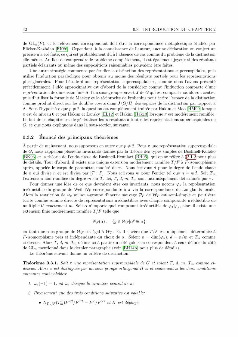
42 0.3. INTRODUCTION DU CHAPITRE 2
de GLn(F ), et le relevement correspondant doit etre la correspondance metaplectique etudiee parFlicker-Kazhdan [FK86]. Cependant, a la connaissance de l’auteur, aucune declaration ou conjectureprecise n’a ete faite, ce qui est probablement du a l’absence de cas connus du probleme de la distinctionelle-meme. Au lieu de comprendre le probleme completement, il est egalement joyeux si des resultatspartiels eclairants ou meme des suppositions raisonnables pouvaient etre faites.
Une autre strategie commence par etudier la distinction des representations supercuspidales, puisutilise l’induction parabolique pour obtenir au moins des resultats partiels pour les representationsplus generales. Pour l’etude d’une representation supercuspidale π, comme nous l’avons presenteprecedemment, l’idee approximative est d’abord de la considerer comme l’induction compacte d’unerepresentation de dimension finie Λ d’un sous-groupe ouvert J de G qui est compact modulo son centre,puis d’utiliser la formule de Mackey et la reciprocite de Frobenius pour ecrire l’espace de la distinctioncomme produit direct sur les doubles cosets dans J\G/H, des espaces de la distinction par rapport aΛ. Sous l’hypothese que p 6= 2, la question est completement traitee par Hakim et Mao [HM99] lorsqueπ est de niveau 0 et par Hakim et Lansky [HL12] et Hakim [Hak13] lorsque π est moderement ramifiee.Le but de ce chapitre est de generaliser leurs resultats a toutes les representations supercuspidales deG, ce que nous expliquons dans la sous-section suivante.
0.3.2 Enonce des principaux theoremes
A partir de maintenant, nous supposons en outre que p 6= 2. Pour π une representation supercuspidalede G, nous rappelons plusieurs invariants donnes par la theorie des types simples de Bushnell-Kutzko[BK93] et la theorie de l’endo-classe de Bushnell-Henniart [BH96], qui on se refere a §2.1.2 pour plusde details. Tout d’abord, il existe une unique extension moderement ramifiee T/F a F -isomorphismeapres, appelee le corps de parametre modere de π. Nous ecrivons d pour le degre de l’endo-classede π qui divise n et est divise par [T : F ]. Nous ecrivons m pour l’entier tel que n = md. Soit Tml’extension non ramifiee du degre m sur T . Ici, T , d, m, Tm sont intrinsequement determines par π.
Pour donner une idee de ce que devraient etre ces invariants, nous notons ϕπ la representationirreductible du groupe de Weil WF correspondante a π via la correspondance de Langlands locale.Alors la restriction de ϕπ au sous-groupe d’inertie sauvage PF de WF est semi-simple et peut etreecrite comme somme directe de representations irreductibles avec chaque composante irreductible demultiplicite exactement m. Soit α n’importe quel composant irreductible de ϕπ|PF , alors il existe uneextension finie moderement ramifiee T/F telle que
NF (α) := {g ∈ WF |αg ∼= α}
en tant que sous-groupe de WF est egal a WT . Et il s’avere que T/F est uniquement determinee aF -isomorphisme pres et independante du choix de α. Soient n = dim(ϕπ), d = n/m et Tm commeci-dessus. Alors T , d, m, Tm definis ici a partir du cote galoisien correspondent a ceux definis du cotede GLn mentionne dans le dernier paragraphe (voir [BH14b] pour plus de details).
Le theoreme suivant donne un critere de distinction.
Theoreme 0.3.1. Soit π une representation supercuspidale de G et soient T , d, m, Tm comme ci-dessus. Alors π est distinguee par un sous-groupe orthogonal H si et seulement si les deux conditionssuivantes sont valables:
1. ωπ(−1) = 1, ou ωπ designe le caractere central de π;
2. Precisement une des trois conditions suivantes est valable:
• NTm/F (T×m)F×2/F×2 = F×/F×2 et H est deploye;
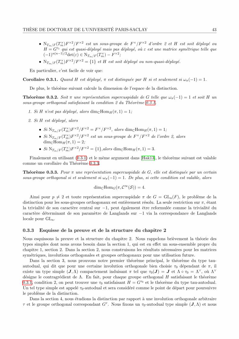
THESE DE DOCTORAT DE L’UNIVERSITE PARIS-SACLAY 43
• NTm/F (T×m)F×2/F×2 est un sous-groupe de F×/F×2 d’ordre 2 et H est soit deploye ouH = Gτε qui est quasi-deploye mais pas deploye, ou ε est une matrice symetrique telle que(−1)n(n−1)/2det(ε) ∈ NTm/F (T×m)− F×2;
• NTm/F (T×m)F×2/F×2 = {1} et H est soit deploye ou non-quasi-deploye.
En particulier, c’est facile de voir que:
Corollaire 0.3.1. Quand H est deploye, π est distinguee par H si et seulement si ωπ(−1) = 1.
De plus, le theoeme suivant calcule la dimension de l’espace de la distinction.
Theoreme 0.3.2. Soit π une representation supercuspidale de G telle que ωπ(−1) = 1 et soit H unsous-groupe orthogonal satisfaisant la condition 2 du Theoreme 0.3.1.
1. Si H n’est pas deploye, alors dimCHomH(π, 1) = 1;
2. Si H est deploye, alors
• Si NTm/F (T×m)F×2/F×2 = F×/F×2, alors dimCHomH(π, 1) = 1;
• Si NTm/F (T×m)F×2/F×2 est un sous-groupe de F×/F×2 de l’ordre 2, alorsdimCHomH(π, 1) = 2;
• Si NTm/F (T×m)F×2/F×2 = {1},alors dimCHomH(π, 1) = 3.
Finalement en utilisant (0.3.1) et le meme argument dans [Hak13], le theoreme suivant est valablecomme un corollaire du Theoreme 0.3.3.
Theoreme 0.3.3. Pour π une representation supercuspidale de G, elle est distinguee par un certainsous-groupe orthogonal si et seulement si ωπ(−1) = 1. De plus, si cette condition est valable, alors
dimCHomG(π, C∞(S)) = 4.
Ainsi pour p 6= 2 et toute representation supercuspidale π de G = GLn(F ), le probleme de ladistinction pour les sous-groupes orthogonaux est entierement resolu. La seule restriction sur π, etantla trivialite de son caractere central sur −1, peut egalement etre reformulee comme la trivialite ducaractere determinant de son parametre de Langlands sur −1 via la correspondance de Langlandslocale pour GLn.
0.3.3 Esquisse de la preuve et de la structure du chapitre 2
Nous esquissons la preuve et la structure du chapitre 2. Nous rappelons brievement la theorie destypes simples dont nous avons besoin dans la section 1, qui est en effet un sous-ensemble propre duchapitre 1, section 2. Dans la section 2, nous construisons les resultats necessaires pour les matricessymetriques, involutions orthogonales et groupes orthogonaux pour une utilisation future.
Dans la section 3, nous prouvons notre premier theoreme principal, le theoreme du type tau-autodual, qui dit que pour une certaine involution orthogonale bien choisie τ0 dependant de π, ilexiste un type simple (J ,Λ) compactement induisant π tel que τ0(J) = J et Λ ◦ τ0 = Λ∨, ou Λ∨
designe le contragredient de Λ. En fait, pour chaque groupe orthogonal H satisfaisant le theoreme0.3.1, condition 2, on peut trouver une τ0 satisfaisant H = Gτ0 et le theoreme du type tau-autodual.Un tel type simple est appele τ0-autodual et sera considere comme le point de depart pour poursuivrele probleme de la distinction.
Dans la section 4, nous etudions la distinction par rapport a une involution orthogonale arbitraireτ et le groupe orthogonal correspondant Gτ . Nous fixons un τ0-autodual type simple (J ,Λ) et nous

44 0.3. INTRODUCTION DU CHAPITRE 2
pouvons utiliser la formule de Mackey et la reciprocite de Frobenius pour ecrire l’espace de la distinctioncomme suit:
HomGτ (π, 1) ∼=∏
g∈J\G/GτHomJg∩Gτ (Λg, 1).
Le theoreme du type distingue dit que pour les doubles classes g ∈ J\G/Gτ contribuant a la distinction,le type simple (Jg,Λg) est τ -autodual. En particulier, quand τ = τ0 nous pouvons aussi donner toutesles J -Gτ0 doubles classes contribuant a la distinction.
Enfin dans la section 5, nous continuons a etudier l’espace de la distinction HomJg∩Gτ (Λg, 1). Lestechniques developpees dans la section 4 nous permettent d’etudier plus avant l’espace de la distinctionvia la structure plus delicate donnee par la theorie des types simples, et enfin de reduire la question aetudier l’espace de la distinction HomH(ρ, χ), ou H est un sous-groupe orthogonal d’un groupe lineairegeneral fini G = GLm(Fq), et ρ est une representation supercuspidale de G, et χ est un caractere deH d’ordre 1 ou 2. En utilisant la theorie de Deligne-Lusztig, la condition pour que l’espace soit nonnul est donnee et la dimension est au plus un. La condition s’avere etre le caractere central de πetant trivial a −1. Ainsi pour ces τ0 speciales dans la section 4, nous etudions entierement l’espace dela distinction et la dimension correspondante. Puisque ces τ0 correspondent exactement aux groupesorthogonaux dans les Theoreme 0.3.1 et Theoreme 0.3.2, nous prouvons la partie “si” du Theoreme0.3.1 et Theoreme 0.3.2.
Il reste la partie “seulement si” du theoreme 0.3.1, dont nous profitons pour expliquer la conditiondes groupes orthogonaux ou des involutions orthogonales correspondantes dans le theoreme. PourEm/F une extension de degre n et τ une involution orthogonale, nous appelons Em τ -deploye s’ilexiste un plongement ι : E×m ↪→ GLn(F ) tel que τ(ι(x)) = ι(x)−1 pour tout x ∈ E×m. La propositionintermediaire suivante donne des informations importantes pour que π soit distinguee par Gτ :
Proposition 0.3.2. Pour π une representation supercuspidale de G avec ωπ(−1) = 1, il existe uncorps Em de degre n sur F qui est totalement sauvagement ramifie sur Tm, tel que si π est distingueepar Gτ , alors Em est τ -deploye.
La construction de Em provient de la construction de type simple τ0-autodual donnee dans lasection 3. En particulier, lorsque τ0 correspond a un groupe orthogonal deploye, de la partie “si” duTheoreme 0.3.1, Em est τ0-deploye. En sachant cela, il n’est pas difficile d’etudier toutes les involutionsτ telles que Em est τ -deploye, qui s’averent etre involutions satisfaisant la condition du theoreme 0.3.1,prouvant la partie “seulement si” du theoreme.
Lorsque Tm/F est de degre n, ou de maniere equivalente lorsque π est essentiellement modereeau sens de Bushnell-Henniart [BH05a], ce qui revient a etre moderement ramifiee dans le contextede Hakim [Hak13] grace au travail de Mayeux [May20], notre resultat donne une autre preuve duresultat de Hakim en utilisant la theorie des types simples au lieu de la construction de Howe pourdes representations moderement ramifiees. Notons que nous empruntons egalement nombreux lemmesa [HM99], [HL12], [Hak13], qui nous aident a reduire notre tache.
Comme dans le chapitre 1, il convient egalement de souligner que la methode que nous utilisons icin’est pas nouvelle. Elle a d’abord ete developpee par Secherre pour resoudre le probleme similaire ou τest une involution galoisienne [AKM+19], [Sec19], puis par l’auteur pour le cas ou τ est une involutionunitaire (cf. chapitre 1), puis par Secherre pour le cas ou τ est une involution interieure [Sec20] (la Gpeut aussi etre une forme interieure de GLn(F )). Les strategies de preuves dans ces differents cas sontsimilaires, mais une difference majeure dans le cas actuel merite d’etre mentionnee, c’est-a-dire quenous devons considerer ces involutions τ ne contribuant pas a la distinction. En ce moment, nous nepouvons pas construire un type simple τ -autodual (J ,Λ) en utilisant la methode de la section 3. Lanouveaute de notre argument est d’abord de considerer une involution speciale τ0, puis de considererτ comme une autre involution qui differe de τ0 a G-conjugaison pres. Ainsi, nous choisissons (J ,Λ)

THESE DE DOCTORAT DE L’UNIVERSITE PARIS-SACLAY 45
comme un type simple τ0-autodual et, en utilisant les resultats generaux construits au chapitre 1, nouspouvons encore etudier les J -Gτ doubles classes contribuant a la distinction. Si l’on veut adapter lamethode dans les cas ci-dessus a une involution generale τ , un probleme majeur est de construire untype simple τ -autodual, ce qui, comme nous l’avons explique, peut etre impossible si Gτ ne contribuepas a la distinction. La strategie que nous avons expliquee ci-dessus donne une solution possible, cequi permet de considerer la meme question pour une involution abstraite.
0.4 Changement de base et induction automorphe explicites pourles representations supercuspidales
0.4.1 Contexte general
Soit F/F0 comme dans §0.1.4, et nous ne considerons que le cas R = C dans ce chapitre. Nousnous concentrerons sur deux relevements locaux speciaux, disons le changement de base et l’inductionautomorphe par rapport a F/F0. Plus precisement, lorsque F/F0 est moderement ramifiee et pour lesrepresentations supercuspidales, nous etudierons ces deux applications via la theorie des types simples.
Nous donnons d’abord une breve introduction pour la correspondance de Langlands locale pourles groupes lineaires generaux, dont l’existence et les proprietes sont connues depuis un certain temps( [LRS93], [HT01], [Hen00], [Sch13]). Pour n′ un certain entier positif et G0 = GLn′ comme un groupereductif sur F0, la correspondance de Langlands locale est une bijection
LLCF0 : IrrC(G0) −→ Φ(G0).
Ici nous gardons les notations de §0.1.1 et Φ(G0) est constitue de GLn′(C)-classes de conjugaisond’homomorphismes
φ0 = (ϕ0, λ0) :WF0 × SL2(C) −→ GLn′(C),
tels que ϕ0 := φ0|WF0×{1} est une representation lisse de WF0 , et λ0 := φ0|{1}×SL2(C) est une
representation algebrique de SL2(C) de dimension n′. Pour n un entier positif, soit G la restric-tion de Weil du groupe reductif GLn sur F , qui est un groupe reductif sur F0 avec G = GLn(F ). Lacorrespondance de Langlands locale est une bijection
LLCF : IrrC(G) −→ Φ(G).
Ici Φ(G) est constitue des classes d’isomorphisme des L-parametres lies aG, qui peuvent etre naturelle-ment identifies avec les classes d’isomorphisme des L-parametres lies a GLn over F . En utilisant cetteidentification, Φ(G) est constitue des GLn(C)-classes de conjugaison d’homomorphismes
φ = (ϕ, λ) :WF × SL2(C) −→ GLn(C),
tels que ϕ := φ|WF×{1} est une representation lisse deWF , et λ := φ0|{1}×SL2(C) est une representationalgebrique de SL2(C) de dimension n.
Nous introduisons maintenant le changement de base et l’induction automorphe lies a F/F0.D’abord nous supposons n′ = n et nous definissons l’application de restriction
ResF/F0: Φ(G0) −→ Φ(G), φ0 = (ϕ0, λ0) 7−→ φ = (ϕ0|WF
, λ0),
ou nous remarquons queWF est un sous-groupe deWF0 . Ainsi, le changement de base est le relevement

46 0.4. INTRODUCTION DU CHAPITRE 3
local BCF/F0: IrrC(G0)→ IrrC(G) tel que le diagramme suivant est commutatif:
IrrC(G0)
BCF/F0��
LLCF0// Φ(G0)
ResF/F0��
IrrC(G)LLCF
// Φ(G)
Deuxiemement, nous supposons n′ = nr et nous definissons l’application d’induction
IndF/F0: Φ(G) −→ Φ(G0), φ = (ϕ, λ) 7−→ φ′0 = (Ind
WF0WF
ϕ, i ◦ λ),
ou i : GLn(C) → GLnr(C) est un plongement des groupes 8. Ainsi l’induction automorphe est lerelevement local AF/F0
: IrrC(G)→ IrrC(G0) tel que le diagramme suivant est commutatif:
IrrC(G0)LLCF0// Φ(G0)
IrrC(G)LLCF
//
AF/F0
OO
Φ(G)
IndF/F0
OO
Dans [AC89], [HH95] et [HL11], le changement de base pour toutes les representations irreductibles, etl’induction automorphe pour au moins les representations generiques essentiellement unitaires ont eteconstruits via la methode de la formule des traces sans l’utilisation de la correspondance de Langlandslocale, et la fonctorialite ci-dessus a ete verifiee.
Bien que pour GLn la correspondance de Langlands locale ait deja ete construite comme unebijection avec les desiderata verifes, il semble que les informations extraites des deux cotes ne soien-t pas egales. Concentrons-nous sur les representations supercuspidales, alors pour tout n ∈ N lacorrespondance peut etre realisee comme une bijection
LLCF : A0n(F ) −→ G0
n(F )
de l’ensemble des classes equivalentes de representations supercuspidales de GLn(F ), dans l’ensembledes classes equivalentes de representations lisses irreductibles du groupe de Weil WF de dimension n,notes respectivement A0
n(F ) et G0n(F ). Habituellement, nous obtenons peu d’informations concretes
pour les representations irreductibles deWF a partir de la theorie des representations, mais en revanchenous avons la theorie de classification pour les representations supercuspidales de GLn(F ), la theoriedes types simples construite par Bushnell-Kutzko [BK93], qui est terre-a-terre et sophistiquee. Unequestion naturelle est donc la suivante: pouvons-nous caracteriser le LLCF ci-dessus en utilisant latheorie structurale pour les representations supercuspidales de GLn(F )?
Pour repondre a cette question, Bushnell et Henniart lancent un projet de longue haleine don-t le resultat est contenu dans une serie d’articles [BH96], [BH99], [BH05c] [BH03], [BH05a], [B-H05b], [BH10], [BH14b], [BH17], [BH19], etc. Surtout, dans [BH05a], [BH05b], [BH10] ils ont en-tierement repondu a la question ci-dessus pour une classe speciale de representations supercuspidales,les representations supercuspidales essentiellement moderees. Pour ce faire, ils ont d’abord construitune version algebrique de la correspondance de Langlands locale, qu’ils ont appelee “correspondancenaıve de Langlands locale”, comme une bijection entre les memes ensembles que LLCF et notee parNLCF . Pour ϕ ∈ G0
n(F ), definissons Tm comme l’extension moderement ramifiee de F liee a ϕ comme
8En utilisant un argument de base en algebre lineaire, nous pouvons montrer que la definition ne depend pas du choixde i.

THESE DE DOCTORAT DE L’UNIVERSITE PARIS-SACLAY 47
dans la derniere section. Pour µ un caractere moderement ramifie de T×m , ils ont construit une certaine“torsion” de ϕ par µ, notee ϕ�µ, qui est une autre representation dans G0
n(F ). Le resultat final est letheoreme de comparaison, qui predit l’existence d’un caractere moderement ramifie µϕ de T×m , tel queLLC−1
F (ϕ) est isomorphe a NLC−1F (ϕ� µϕ). Dans le cas essentiellement modere au sens de [BH10], le
caractere µϕ de T×m est d’ordre divisant 4 et peut etre calcule explicitement, donc dans ce cas la cor-respondance de Langlands locale est pleinement comprise de maniere algebrique. Dans le cas generalcomme dans [BH14b], la construction de la correspondance naıve de Langlands local s’appuyait surla correspondance de Langlands locale dans le cas sauvagement ramifie comme une “boıte noire”, etla caracterisation complete du caractere µϕ reste inconnue. Donc, pour bien comprendre le LLCF engeneral, nous devons d’abord comprendre le cas particulier pour les representations supercuspidalessauvagement ramifiees, ce qui est une question assez profonde, puis nous devons calculer le caractereµϕ ci-dessus, qui sera aborde dans le chapitre 3 plus tard.
L’objectif principal de ce chapitre est d’adapter l’idee de Bushnell-Henniart ci-dessus aux change-ment de base et induction automorphe, c’est-a-dire que nous construirons des versions algebriquesdes deux applications, puis les comparerons avec les applications originales respectivement. Plus dedetails seront donnes dans la sous-section ci-dessous.
0.4.2 Principaux resultats
Pour donner une introduction detaillee, nous utilisons les terminologies et proprietes de base de latheorie des types simples et de la theorie du changement de base et l’induction automorphe cycliques,pour lesquelles les lecteurs peuvent se referer respectivement au chapitre 3, section 2 et section 4.Pour F/F0 comme precedemment, soient Σ = Gal(F/F0) le groupe de Galois et σ ∈ Σ un generateur.Pour π0 une representation supercuspidale de GLn(F0), nous definissons son changement de baseπ := BCF/F0
(π0) comme une representation irreductible de GLn(F ). Nous supposons en outre quesoit π est supercuspidale, ou soit r divise n et qu’il existe une representation supercuspidale π′ deGLn/r(F ) telle que π est isomorphe a l’induction parabolique
π′ × π′σ × ...× π′σr−1.
De maniere equivalente, nous avons π0 = AF/F0(π′) comme l’induction automorphe de π′ dans le
dernier cas. Notre but est de donner une construction explicite de π et π′ respectivement dans lesdeux cas, en utilisant la theorie des types simples et les informations de π0. Pour cela, nous devonssupposer la condition supplementaire que F/F0 est moderement ramifiee.
Soit [a0, β] une strate simple maximale dans Mn(F0), et soit θ0 un caractere simple de H1(a, β)contenu dans π0. Nous choisissons κ0 comme une representation de Heisenberg complete (full Heisen-berg representation) de θ0 comme une representation de J(a0, β), et en ce moment il existe unerepresentation unique ρ0 de J(a0, β) triviale sur J1(a0, β), telle que π0 est isomorphe a l’induction
compacte indGLn(F0)J(a0,β) (κ0 ⊗ ρ0). Ici E0 = F0[β] est un corps de degre d sur F0 avec n = md pour m un
entier, et nous notons T0 sa sous-extension maximale moderement ramifiee sur F0 et T0,m l’extensionnon ramifiee de degre m sur T0. En ce moment, la representation ρ0 peut etre caracterisee par ∆0-orbite d’un caractere ξ0 de T×0,m qui est ∆0-regulier et moderement ramifie, ou ∆0 = Gal(T0,m/T0).
Nous considerons d’abord le cas ou π est supercuspidale. En utilisant le resultat de relevementmodere dans [BH96] et [BH03], nous construisons [a, β] comme une strate simple maximale dansMn(F ), et θb comme un caractere simple de H1(a, β) contenu dans π. Et un tel θb peut etre considerecomme le changement de base de θ0 pour des caracteres simples. Ensuite, nous determinons unerepresentation de Heisenberg complete κb de θb de maniere algebrique, qui ne depend que de θ0 et κ0,mais pas de π0. Alors il existe une representation unique ρb de J(a, β) trivial sur J1(a, β), telle que π
est isomorphe a l’induction compacte indGLn(F )J(a,β) (κb⊗ρb). Une telle ρb est caracterisee par la ∆-orbite

48 0.4. INTRODUCTION DU CHAPITRE 3
d’un caractere ∆-regulier moderement ramifie ξb de T×m , ou Tm = F ⊗F0 T0,m et T = F ⊗F0 T0 sontdes corps sur F et ∆ = Gal(Tm/T ). Le theoreme de comparaison suivant est le theoreme principalpour le changement de base.
Theoreme 0.4.1 (Voir Theorem 3.6.2). Il existe un caractere moderement ramifie bφF/F0
θ0de T×m , tel
que ξb · bφF/F0
θ0et ξ0 ◦NTm/T0,m
sont dans la meme ∆-orbite.
De meme, nous considerons le cas ou π0 est egale a l’induction automorphe d’une representationsupercuspidale π′ de GLn/r(F ). Pour continuer, nous supposons en outre que soit F est identifie avecun sous-corps de E0 via un plongement, ce qui correspond au cas de l’induction automorphe interieure,soit E = F ⊗F0 E0 est un corps de degre r sur E0, qui correspond au cas de l’induction automorpheexterieure, et nous divisons ce dernier cas en deux sous-cas en fonction de E/E0 non ramifiee outotalement ramifiee, car dans les differents cas, les situations et les methodes correspondantes sontdifferentes. En utilisant la methode de relevement modere dans [BH96] et [BH03], nous construisons[c, β] comme une strate simple dans Mn/r(F ) et θa comme un caractere simple de H1(c, β) contenu dansπ′, et θ0 peut etre considere comme l’induction automorphe de θa pour les caracteres simples. Commedans le cas de changement de base, nous determinons une representation de Heisenberg completeκa de θa de maniere algebrique qui depend seulement de θ0 et κ0, et en ce moment il existe unerepresentation unique ρa de J(c, β) triviale sur J1(c, β), telle que π′ est isomorphe a l’induction
compacte indGLn/r(F )
J(c,β) (κa⊗ρa). Dans le cas de l’induction automorphe interieure, la representation ρa
est caracterisee par la ∆0-orbite d’un caractere ∆0-regulier moderement ramifie ξa sur T×0,m. Dans lecas de l’induction automorphe exterieure, nous ecrivons T = F ⊗F0 T0 comme un corps et nous notonsTm/r l’extension non ramifiee de degre m/r sur T , alors pour ∆ = Gal(Tm/r/T ) la representation ρaest caracterisee par la ∆-orbite d’un caractere ∆-regulier moderement ramifie de T×m/r, encore designe
par ξa. En ce moment, si E/E0 n’est pas ramifiee, Tm/r est identifie avec T0,m et ∆ est identifie avecun sous-groupe de ∆0, et si E/E0 est totalement ramifiee, Tm = F ⊗F0 T0,m est un corps de degrem sur T avec Tm/r etant considere comme son sous-corps, et nous ecrivons ∆′ = Gal(Tm/T ). Letheoreme de comparaison suivant est le principal theoreme pour l’induction automorphe.
Theoreme 0.4.2 (Voir Theorem 3.6.4, Theorem 3.6.6, Theorem 3.6.8). (1) Dans le cas de l’induction
automorphe interieure, il existe un caractere moderement ramifie aφF/F0
θ0de T×0,m tel que ξa · aφF/F0
θ0et ξ0 sont dans la meme ∆0-orbite;
(2) Dans le cas de l’induction automorphe exterieure, il existe un caractere moderement ramifie
aφF/F0
θ0de T×m/r tel que
• Si E/E0 est non-ramifiee, ξa · aφF/F0
θ0et ξ0 sont dans la meme ∆0-orbite;
• Si E/E0 est totalement ramifiee, (ξa · aφF/F0
θ0) ◦ NTm/Tm/r et ξ0 ◦ NTm/T0,m
sont dans la meme
∆′-orbite.
Nous mentionnons trois applications des deux theoremes ci-dessus pour terminer cette sous-section.La premiere application concerne l’etude de ρb et ρa par ρ0, ou ρ0 est la representation supercusp-idale de GLm(kE0) ∼= J(a0, β)/J1(a0, β) dont l’inflation est egale a ρ0|J(a0,β) avec kE0 designant lecorps residuel de E0, et ρb est la representation supercuspidale de GLm(kE) ∼= J(a, β)/J1(a, β) dontl’inflation est egale a ρb|J(a,β) avec kE designant le corps residuel de E dans le cas de changementde base, et ρa est la representation supercuspidale de GLm(kE0) ∼= J(c, β)/J1(c, β) dans le cas del’induction automorphe interieure, de GLm/r(kE) ∼= J(c, β)/J1(c, β) dans le cas de l’induction au-
tomorphe exterieure, dont l’inflation est egale a ρa|J(c,β). En ce moment, les restrictions de bφF/F0
θ0

THESE DE DOCTORAT DE L’UNIVERSITE PARIS-SACLAY 49
et aφF/F0
θ0a ces elements dans l’anneau des entiers sont des caracteres quadratiques qui peuvent etre
entierement caracterises, les representations ρb et ρa sont compris via la theorie de Green (cf. [Gre55]).En particulier pour E/E0 en tant qu’une extension non ramifiee de degre r dans le cas du changementde base ou dans le cas de l’induction automorphe exterieure, cela donne une relation entre le change-ment de base d’Arthur-Clozel et l’application de changement de base de Shintani (cf. [Shi76]) pourles representations supercuspidales, voir Corollary 3.6.3 et Corollary 3.6.9.
La seconde application concerne les representations l-modulaires. Pour l un nombre premier dif-ferent de p, nous fixons un isomorphisme algebrique Ql ∼= C, ainsi toutes les representations ci-dessuspeuvent etre realisees comme des representations sur Ql. Nous supposons en outre que π0 est entiere,c’est-a-dire qu’il provient d’une representation sur un Zl-reseau par extension des scalaires. En util-isant les deux theoremes, nous pouvons prouver que le changement de base et l’induction automorphecycliques moderement ramifies sont compatibles avec la reduction modulo l pour les representationssupercuspidales. Plus precisement, pour une telle π0 avec son changement de base π supercuspidal,π est egalement entiere, et si nous changeons π0 par une autre representation supercuspidale entiereavec sa modulo l reduction rl(π0) inchangee comme une representation cuspidale sur Fl, alors la π cor-respondante est encore supercuspidale entiere avec sa modulo l reduction rl(π) inchangee. De memepour une telle π0 comme l’induction automorphe de π′ comme une representation supercuspidale en-tiere, π0 est egalement entiere, et si nous changeons π′ par une autre representation supercuspidaleentiere avec sa modulo l reduction rl(π
′) inchangee comme une representation cuspidale sur Fl, alors laπ0 correspondante est supercuspidale entiere avec sa modulo l reduction rl(π0) inchangee. La preuveest directe et ne sera pas donnee dans ce chapitre, mais les lecteurs peuvent consulter [BH14a] pourune idee similaire.
L’application finale concerne le calcul du caractere µϕ lie au theoreme de comparaison dans [BH14b]mentionne dans la derniere sous-section. La strategie est de considerer une certaine changement debase non ramifiee, puis de comparer les caracteres correspondants “mu” lies aux deux corps de base,qui a deja ete utilise pour le cas essentiellement modere dans [BH05a]. Pour cela, nous avons besoin
d’etudier bφF/F0
θ0dans le cas ou F/F0 est non-ramifiee.
Theoreme 0.4.3 (Voir Theorem 3.9.1). Quand F/F0 est non-ramifiee, le caractere bφF/F0
θ0est non-
ramifie, et bφF/F0
θ0($ps
T0) = (−1)(t−1)(r−1), ou $T0 designe une uniformisante de T×m , et K0 designe la
sous-extension maximale de T0,m sur F0, et t = [T0,m : K0] et [E0 : T0] = ps.
En utilisant un cas particulier du theoreme, c’est-a-dire la proposition 3.9.9, nous pouvons mettrea jour les valeurs de µϕ qui seront discutees dans la derniere section. Notre resultat est evidemmentincomplet et pas assez satisfaisant.
0.4.3 La structure du chapitre 3
Nous esquissons la structure du chapitre 3. Les sections 1-4 sont des preliminaires, y compris une breveintroduction et un resume de la theorie des types simples, des signes symplectiques, du changementde base et de l’induction automorphe respectivement. Apres la premiere discussion elementaire dela section 5, dans la section 6 nous formulons notre construction algebrique du changement de basecyclique et de l’induction automorphe moderement ramifies en suivant l’esquisse mentionnee dansla derniere sous-section et enoncons le theoreme 0.4.1 et le theoreme 0.4.2. Mais la constructiondes representations de Heisenberg completes correspondantes reste a faire jusqu’a la section 7, dontla strategie repose sur l’idee d’une serie de resultats de Bushnell-Henniart qui y seront rappeles etreformules. La preuve du theoreme 0.4.1 et theoreme 0.4.2 sera donnee dans la section 8 qui sembleetonnamment simple, qui repose en fait sur deux ingredients hautement non triviaux: la fonctorialite deLanglands locale pour le changement de base et l’induction automorphe, et le theoreme de comparaison

50 0.4. INTRODUCTION DU CHAPITRE 3
de Bushnell-Henniart. La section 9 est consacree a prouver le theoreme 0.4.3 et la section 10 est sonapplication pour calculer le caractere µϕ lie au theoreme de comparaison.
L’auteur tient a remercier Colin J. Bushnell et Guy Henniart pour leur enorme influence surl’auteur et sur ce chapitre. En fait, il est preferable de considerer cette partie comme une continuation(maladroite) de leur travail plutot que comme un travail independant, puisque presque toutes les ideeset techniques importantes proviennent de leurs articles enumeres ci-dessus. De plus, l’auteur tient ales remercier pour leurs genereux encouragements, qui ont en effet beaucoup aide un jeune doctorantqui n’etait pas confiant et meme etait mefiant a la necessite de son travail.

Chapter 1
Problem of distinction related tounitary subgroups of GLn(F ) andl-modular base change lift
1.1 Notation and basic definitions
Let F/F0 be a quadratic extension of non-archimedean locally compact fields of residue characteristicp 6= 2 and let σ be the unique non-trivial involution in the Galois group. Write oF and oF0 for thering of integers of F and F0 and write k and k0 for the residue field of F and F0 respectively. Theinvolution σ induces a k0-automorphism of k generating Gal(k/k0), still denoted by σ.
Let R be an algebraically closed field of characteristic l ≥ 0 different from p. If l > 0, then we arein the “modular case”.
We fix a characterψ0 : F0 → R×
trivial on the maximal ideal of oF0 but not on oF0 , and we define ψ = ψ0 ◦ trF/F0.
Let G be the locally profinite group GLn(F ) with n ≥ 1, equipped with the involution σ actingcomponentwise. Let ε be a hermitian matrix in Mn(F ), which means that ε∗ = ε. Here x∗ := σ( tx)for any x ∈ Mn(F ) with t denoting the transpose operator. Sometimes we write σ1(x) := x∗ for anyx ∈ Mn(F ) to emphasize that σ1 is an anti-involution on Mn(F ) extending σ. For ε hermitian andg ∈ G, we define τε(g) = εσ( tg−1)ε−1, called the unitary involution corresponding to ε. For τ = τε afixed unitary involution, we denote by Gτ the corresponding unitary subgroup, which consists of theelements of G fixed by τ .
By representations of a locally profinite group, we always mean smooth representations on anR-module. Given a representation π of a closed subgroup H of G, we write π∨ for the smoothcontragredient of π. We write πσ and πτ for the representations π ◦ σ and π ◦ τ of groups σ(H) andτ(H) respectively. We say that π is τ -selfdual if H is τ -stable and πτ is isomorphic to π∨. We say thatπ is σ-invariant if H is σ-stable and πσ is isomorphic to π. For g ∈ G, we write Hg = {g−1hg|h ∈ H}as a closed subgroup and we write πg : x 7→ π(gxg−1) as a representation of Hg.
For a an oF -subalgebra of Mn(F ) and τ = τε a unitary involution, we denote by
τ(a) := σε(a) = {σε(x)|x ∈ a}
an oF -subalgebra of Mn(F ), where σε(x) := εσ( tx)ε−1 is an anti-involution for any x ∈ Mn(F ). Wesay that a is τ -stable if τ(a) = a. Moreover for g ∈ G, we obtain
τ(a)g = g−1σε(a)g = σε(σε(g)aσε(g−1)) = σε(τ(g)−1aτ(g)) = τ(aτ(g))
51

52 1.2. HERMITIAN MATRICES AND UNITARY GROUPS
In other words, the notation τ(a) is compatible with G-conjugacy.For τ a unitary involution and π a representation of H as above, we say that π is H ∩ Gτ -
distinguished, or just distinguished, if the space HomH∩Gτ (π, 1) is non-zero.An irreducible representation of G is called cuspidal if it doesn’t occur as a subrepresentation
of a proper parabolically induced representation. It is called supercuspidal if it doesn’t occur as asubquotient of a proper parabolically induced representation.
1.2 Hermitian matrices and unitary groups
We make use of this subsection to introduce basic knowledge of hermitian matrices and unitary groups.The references will be [HM98] and [Jac62].
Let E/E0 be a quadratic extension of non-archimedean locally compact fields which are algebraicextension of F and F0 respectively. Write oE for the ring of integers of E and oE0 for that of E0. Letσ′ ∈ Gal(E/E0) be the unique non-trivial involution in the Galois group. For ε′ ∈ GLm(E), just as inthe last subsection, we say that ε′ is a hermitian matrix if (ε′)∗ = ε′, where we consider (·)∗ as beforewith n, F , F0, σ replaced by m, E, E0, σ′ respectively. Write $E for a uniformizer of E such that
σ′($E) =
{$E if E/E0 is unramified,
−$E if E/E0 is ramified.
Let X denote the set of all the hermitian matrices. The group G acts on X by g · x = gxg∗. Wehave the following proposition:
Proposition 1.2.1 ( [Jac62], Theorem 3.1). There are exactly two GLm(E)-orbits of X with respect tothe action given above. Furthermore, the elements in each orbit are exactly determined by the classesof their determinants in E×0 /NE/E0
(E×).
We may also consider the GLm(oE)-orbits of X . We consider sequences α = (α1, ..., αr) of certaintriples αi = (ai,mi, δi), such that a1 > ... > ar is a decreasing sequence of integers, and m1 + ...+mr =m is a partition of m by positive integers, and δ1, ..., δr are elements of E such that:
(1) If E/E0 is unramified, then δi = 1;(2) If E/E0 is ramified and ai is odd, then δi = 1 and mi is even;(3) If E/E0 is ramified and ai is even, then δi is either 1 or ε, with ε ∈ o×E0
\NE/E0(o×E) fixed.
Let A be the set of all sequences α satisfying these requirements. For each α = (α1, ..., αr) ∈ A, weintroduce a hermitian matrix $α
E = $α1E ⊕ ... ⊕ $
αrE , where $αi
E ∈ GLmi(E) is a hermitian matrix,such that:
(i) In the case (1), $αiE = $ai
E Imi ;
(ii) In the case (2), $αiE = $ai
E Jmi/2, where Jmi/2 =
(0 Imi/2
−Imi/2 0
);
(iii) In the case (3), $αiE = $ai
E diag(1, ..., 1, δi), where diag(∗, ..., ∗) denotes the diagonal matrixwith corresponding diagonal elements.
We state the following proposition which classifies all the GLm(oE)-orbits of X .
Proposition 1.2.2 ( [Jac62], Theorem 7.1, Theorem 8.2). Each class of the GLm(oE)-orbits of Xcontains a unique representative of the form $α
E for a certain α ∈ A.
Now we study unitary groups. For ε′ ∈ X , we denote by Um(ε′) the unitary group consisting ofthose g ∈ GLm(E) such that gε′g∗ = ε′. We say that two unitary groups are equivalent if and onlyif they are conjugate by some g ∈ G. Since it is easy to check that gUm(ε′)g−1 = Um(gε′g∗), byProposition 1.2.1, there are at most two equivalence classes of unitary groups, which are represented

THESE DE DOCTORAT DE L’UNIVERSITE PARIS-SACLAY 53
by Um(E/E0) := Um(Im) and U′m(E/E0) := Um(ε) for ε = diag(1, ..., 1, ε), where ε ∈ E×0 \NE/E0(E×)
is fixed.
Remark 1.2.3. We list the following result for completeness: Um(E/E0) is equivalent to U′m(E/E0)if and only if m is odd. Since we will never use it in the future, we omit the proof.
Remark 1.2.4. In the future, we only consider the following two cases. First, we consider E = F ,E0 = F0, m = n and σ′ = σ. For any two unitary involutions with the corresponding hermitianmatrices in the same GLn(F )-orbit, we already showed that the corresponding two unitary groups areequivalent. Since distinction is a property invariant up to equivalence of unitary groups, we may choosea hermitian matrix in its G-orbit such that the corresponding unitary involution τ is simple enoughto simplify the problem. Secondly, we consider E as a finite field extension of F determined by acuspidal representation π such that n = m[E : F ]. We will find out that if πσ ∼= π, then we may findan involution σ′ on E such that E0 = Eσ
′and σ′|F = σ. So we may make use of the propositions in
this subsection to study hermitian matrices and unitary groups of GLm(E).
1.3 Preliminaries on simple types
In this section, we recall the main results we will need on simple strata, characters and types [BK93],[BH96], [BH14b], [MS14b]. We mainly follow the structure of [AKM+19] and [Sec19].
1.3.1 Simple strata and characters
Let [a, β] be a simple stratum in Mn(F ) for a certain n ≥ 1. Recall that a is a hereditary order ofMn(F ) and β is in G = GLn(F ) such that:
(1) the F -algebra E = F [β] is a field with degree d over F ;(2) E× normalizes a×.The centralizer of E in Mn(F ), denoted by B, is an E-algebra isomorphic to Mm(E) with n = md.
The intersection b := a ∩B is a hereditary order of B.We denote by pa the Jacobson radical of a, and U1(a) the compact open pro-p-subgroup 1 + pa of
G. Similarly, we denote by pb the Jacobson radical of b and U1(b) the compact open pro-p-subgroup1 + pb of B×. For any x ∈ B×, we have ( [BK93], Theorem 1.6.1)
U1(a)xU1(a) ∩B× = U1(b)xU1(b). (1.3.1)
Associated with [a, β], there are open compact subgroups
H1(a, β) ⊂ J1(a, β) ⊂ J(a, β)
of a× and a finite set C(a, β) of simple characters of H1(a, β) depending on the choice of ψ. We denoteby J(a, β) a subgroup of G generated by J(a, β) and the normalizer of b× in B×.
The above definition excludes the “null” case, which we explain here. In this case for a simplestratum [a, β], conventionally we write β = 0, E = F , A = B, a = b and H1(a, β) = J1(a, β) = 1 + pa.Moreover, the set C(a, β) is a singleton consisting of the trivial character of H1(a, β). Later on all thesimple strata we consider should also include this case.
Proposition 1.3.1 ( [Sec19], Proposition 5.1). We have the following properties:(1) The group J(a, β) is the unique maximal compact subgroup of J(a, β);(2) The group J1(a, β) is the unique maximal normal pro-p-subgroup of J(a, β);(3) The group J(a, β) is generated by J1(a, β) and b×, and we have
J(a, β) ∩B× = b×, J1(a, β) ∩B× = U1(b); (1.3.2)

54 1.3. PRELIMINARIES ON SIMPLE TYPES
(4) The normalizer of any simple character θ ∈ C(a, β) in G is equal to J(a, β);
(5) The intertwining set of any θ ∈ C(a, β) in G, which we denote by IG(θ), is equal to
J1(a, β)B×J1(a, β) = J(a, β)B×J(a, β).
Remark 1.3.2. We write for short J , J1, H1 for J(a, β), J1(a, β), H1(a, β) respectively if a and βare clear to us.
When b is a maximal order in B, we call the simple stratum [a, β] and the simple characters inC(a, β) maximal. In this case we may find an isomorphism of E-algebras B ∼= Mm(E) which identifiesb with the standard maximal order, and moreover we have group isomorphisms
J(a, β)/J1(a, β) ∼= b×/U1(b) ∼= GLm(l), (1.3.3)
where l denotes the residue field of E.
1.3.2 Simple types and cuspidal representations
A pair (J ,Λ), called an extended maximal simple type in G (we always write simple type for short), ismade of a subgroup J of G which is open and compact modulo centre, and an irreducible representationΛ of J . It has been constructed in [BK93] in the characteristic 0 case and in [Vig96], [MS14b] in themodular case.
Given a simple type (J ,Λ) in G, there are a maximal simple stratum [a, β] in Mn(F ) and amaximal simple character θ ∈ C(a, β), such that J(a, β) = J and θ is contained in the restrictionof Λ to H1(a, β). Such a character θ is said to be attached to Λ. By [BK93], Proposition 5.1.1(or [MS14b], Proposition 2.1 in the modular case), the group J1(a, β) has, up to isomorphism, aunique irreducible representation η whose restriction to H1(a, β) contains θ. Such a representation η,called the Heisenberg representation associated to θ, has the following properties:
(1) the restriction of η to H1(a, β) is made of (J1(a, β) : H1(a, β))1/2 copies of θ. Here (J1(a, β) :H1(a, β))1/2 is a power of p;
(2) the direct sum of (J1(a, β) : H1(a, β))1/2 copies of η, which we denote by η(J1(a,β):H1(a,β))1/2, is
isomorphic to IndJ1
H1θ;
(3) the representation η extends to J ;
(4) the intertwining set of η, which we denote by IG(η), equals IG(θ);
(5) for h ∈ IG(η), we have dimR(HomJ1∩J1h(ηh, η)) = 1.
For any representation κ of J extending η, there exists a unique irreducible representation ρ of Jtrivial on J1(a, β) such that Λ ∼= κ⊗ ρ. Through (1.3.3), the restriction of ρ to J = J(a, β) identifieswith the inflation of a cuspidal representation of GLm(l).
Remark 1.3.3. Recall that in [BK93], Bushnell and Kutzko also assume κ0 = κ|J(a,β) to be a socalled beta-extension, which means that:
(1) κ0 is an extension of η;
(2) if we denote by IG(κ0) the intertwining set of κ0, then IG(κ0) = IG(η) = IG(θ).
However in our case, since GLm(l) is not isomorphic to GL2(F2) (p 6= 2), any character of GLm(l)factors through the determinant. It follows that any representation of J extending η is a beta-extension.So finally our consideration of κ0 coincides with the original assumption of Bushnell and Kutzko.
We now give the classification of irreducible cuspidal representations of G in terms of simple types(see [BK93], 6.2, 8.4 and [MS14b], Section 3 in the modular case).

THESE DE DOCTORAT DE L’UNIVERSITE PARIS-SACLAY 55
Proposition 1.3.4 ( [BK93], [MS14b]). Let π be a cuspidal representation of G.(1) There is a simple type (J ,Λ) such that Λ is a subrepresentation of the restriction of π to J .
It is unique up to G-conjugacy;(2) Compact induction c-IndGJ gives a bijection between the G-conjugacy classes of simple types
and the isomorphism classes of cuspidal representations of G.
1.3.3 Endo-classes, tame parameter fields and tame lifting
In this subsection, we introduce the concepts of endo-classes, tame parameter fields and tame lifting.The main references will be [BK93], [BH96] and [BH14b].
For [a, β] a simple stratum in Mn(F ) and [a′, β′] a simple stratum in Mn′(F ) with n, n′ ≥ 1, if wehave an isomorphism of F -algebras φ : F [β]→ F [β′] such that φ(β) = β′, then there exists a canonicalbijection
tβ,β′
a,a′ : C(a, β)→ C(a′, β′),
called the transfer map (see [BK93], Theorem 3.6.14).Now let [a1, β1] and [a2, β2] be simple strata of Mn1(F ) and Mn2(F ) respectively with n1, n2 ≥ 1.
We call two simple characters θ1 ∈ C(a1, β1) and θ2 ∈ C(a2, β2) endo-equivalent, if there are simplestrata [a′, β′1] and [a′, β′2] of Mn′(F ) for some n′ ≥ 1 such that θ1 and θ2 transfer to two simplecharacters θ′1 ∈ C(a′, β′1) and θ′2 ∈ C(a′, β′2) respectively which intertwine (or by [BK93], Theorem3.5.11 which are GLn′(F )-conjugate). This defines an equivalence relation on⋃
[a,β]
C(a, β),
where the union runs over all simple strata in Mn(F ) for all n ≥ 1 (see [BH96], section 8). Anequivalence class for this equivalence relation is called an endo-class.
For π a cuspidal representation of G = GLn(F ), there exist a simple stratum [a, β] and a simplecharacter θ ∈ C(a, β) contained in π. The set of simple characters θ contained in π constitutes aG-conjugacy class, thus those simple characters are endo-equivalent. So we may denote by Θπ theendo-class of π which is the endo-class determined by any θ contained in π.
Given θ ∈ C(a, β), the degree of E/F , its ramification index and its residue class degree dependonly on the endo-class of θ. They are called the degree, ramification index and residue class degreeof this endo-class. Although the field extension E/F is not uniquely determined, its maximal tamelyramified subextension is uniquely determined by the endo-class of θ up to F -isomorphisms. This fieldis called a tame parameter field of the endo-class (see [BH14b], 2.2, 2.4).
We denote by E(F ) the set of endo-classes of simple characters over F . Given a finite tamelyramified extension T of F , we have a surjection
E(T )→ E(F )
with finite fibers, which is called restriction map (see [BH14b], 2.3). Given Θ ∈ E(F ), the endo-classesΨ ∈ E(T ) restricting to Θ are called the T/F -lifts of Θ. If Θ has a tame parameter field T , thenAutF (T ) acts faithfully and transitively on the set of T/F -lifts of Θ (see [BH14b], 2.3, 2.4).
Let [a, β] be a simple stratum and let θ ∈ C(a, β) be a simple character. Let T be the maximaltamely ramified extension of F in E. Let Θ be the endo-class of θ, then T is a tame parameter fieldof Θ. Let C ∼= Mn/t(T ) denote the centralizer of T in Mn(F ), where t = [T : F ]. The intersectionc = a∩C is an order in C which gives rise to a simple stratum [c, β]. The restriction of θ to H1(c, β),denoted by θT , is a simple character associated to this simple stratum, called the interior T/F -lift ofθ. Its endo-class, denoted by Ψ, is a T/F -lift of Θ. For the origin and details of the construction ofΨ by using interior T/F -lift of θ, see [BH96].

56 1.4. ONE DIRECTION OF THEOREM 0.2.1 FOR A SUPERCUSPIDAL REPRESENTATION
We may change our choice of simple stratum [a, β] but fix T ↪→ Mn(F ) unchanged, then the map
a 7→ a ∩ C
is injective from the set of hereditary orders of Mn(F ) normalized by T× to the set of hereditary ordersof C (see [BH96], section 2). For [a, β1], [a2, θ2] two simple strata, and θ1 ∈ C(a, β1), θ2 ∈ C(a, β2) twosimple characters, such that θ1 and θ2 have the same tame parameter field T , if
C(c, β1) = C(c, β2) and (θ1)T = (θ2)T ,
then (see [BH96], Theorem 7.10, Theorem 7.15)
C(a, β1) = C(a, β2) and θ1 = θ2.
In particular, when β1 = β2 = β, the interior T/F -lift is injective from C(a, β) to C(c, β).
1.3.4 Supercuspidal representations
Let π be a cuspidal representation of G. By Proposition 1.3.4, it contains a simple type (J ,Λ). Fix amaximal simple stratum [a, β] such that J = J(a, β), and write Λ = κ⊗ ρ as in subsection 1.3.2. Letρ be the cuspidal representation of J/J1 ∼= GLm(l) whose inflation equals ρ|J . We have the followingproposition:
Proposition 1.3.5 ( [MS14a], Proposition 6.10). The representation π is supercuspidal if and only ifρ is supercuspidal.
1.4 One direction of Theorem 0.2.1 for a supercuspidal representa-tion
Let G = GLn(F ) and let Gτ be the unitary group corresponding to a unitary involution τ . We statethe following theorem which is well-known when R = C and char(F ) = 0 (see for example [HM02a],section 4, corollary or more ancient paper [HLR86] which illustrates the idea).
Theorem 1.4.1. Let π be a supercuspidal representation of G. If π is distinguished by Gτ , then π isσ-invariant.
Before proving Theorem 1.4.1, we state a useful lemma which will be used not only in the proofof the theorem, but also in the latter sections.
Lemma 1.4.2. For δ a unitary involution on G and for (J ,Λ) a simple type in G, we have J ∩Gδ =J ∩Gδ.
Proof. For x ∈ J ∩ Gδ, we have δ(x) = x which implies that σ(det(x))det(x) = 1, where we denoteby det(·) the determinant function defined on G. Thus we have det(x) ∈ o×F . Since J = E×J , we getx ∈ o×EJ ∩Gδ = J ∩Gδ. Since x is arbitrary, we finish the proof.
Moreover, we need the following lemma which says that the properties of distinction and σ-invariance are maintained up to change of base fields.

THESE DE DOCTORAT DE L’UNIVERSITE PARIS-SACLAY 57
Lemma 1.4.3. Let R1 ↪→ R2 be a fixed embedding of two algebraically closed fields of characteristicl ≥ 0. Let π0 be a supercuspidal representation of G over R1. Let π = π0⊗R1 R2 be the correspondingrepresentation of G over R2. Then:
(1) π0 is distinguished by Gτ if and only if π is distinguished by Gτ ;
(2) πσ0∼= π0 if and only if πσ ∼= π.
Proof. For (1), let (J ,Λ0) be a simple type of π0. Then (J ,Λ) := (J ,Λ0⊗R1 R2) is a simple type of πand thus π is also supercuspidal. Using the Frobenius reciprocity and the Mackey formula1, we have
HomR1[Gτ ](π0, 1) 6= 0⇐⇒ There exists g ∈ G such that HomR1[Jg∩Gτ ](Λg0, 1) 6= 0
and
HomR2[Gτ ](π, 1) 6= 0⇐⇒ There exists g ∈ G such that HomR2[Jg∩Gτ ](Λg, 1) 6= 0
By Lemma 1.4.2, Jg∩Gτ = Jg∩Gτ is a compact group, and Λg0 is a representation of finite dimension.Thus
HomR1[Jg∩Gτ ](Λg0, 1)⊗R1 R2
∼= HomR2[Jg∩Gτ ](Λg, 1)
which finishes the proof of (1). For (2), from [Vig96], Chapitre I, 6.13 we know that π0 is isomorphicto πσ0 if and only if their trace characters are equal up to a scalar in R×1 , which works similarly forπ and πσ. Since the trace characters of π0 and π are equal up to the change of scalars, which workssimilarly for πσ0 and πσ, we finish the proof of (2).
Proof of Theorem 1.4.1. First we consider R = C. For char(F ) = 0, it is a standard result proved byusing global method ( [HM02a], section 4, Corollary). Especially, their result is based on the global-ization theorem, saying a distinguished π under our settings can be realized as a local component ofa cuspidal automorphic representation Π of GLn(AK), which is distinguished by a unitary subgroupof GLn(AK) with respect to a quadratic extension of number fields K/K0 (see ibid., Theorem 1). Ifchar(F ) > 0, in order to use the proof of Hakim-Murnaghan, we only need a variant of globaliza-tion theorem for characteristic positive case. Fortunately, Gan-Lomelı already built up such kindof result for general reductive groups over function fields and locally compact fields of characteristicpositive (see [GL18], Theorem 1.3). Following their settings, we choose the reductive group H tobe RK/K0
(GLn(K)), where K/K0 is a quadratic extension of function fields, and RK/K0is the Weil
restriction. We choose V to be Mn(K) as a K0-vector space and ι : H → GL(V ) to be a representationover K0 defined by
ι(h)x = hxσ( th), x ∈ V, h ∈ H,
where σ denotes the non-trivial involution in Gal(K/K0). If we choose x0 ∈ V to be a hermitianmatrix in Mn(K) and Hx0 to be the stabilizer of x0, then Hx0 becomes a unitary subgroup of H whichsatisfies the condition of loc. cit. In order to use their result, we only need to verify the condition (a)and (b) in their theorem. For condition (a), ι is semisimple since it is the direct sum of two irreduciblesubrepresentations, composed of hermitian matrices and anti-hermitian matrices respectively 2. Forcondition (b), since we only care about the case where χ = 1, it is automatically satisfied. Thus,if we use [GL18], Theorem 1.3 to replace [HM02a], Theorem 1 and follow the proof in [HM02a],then we finish the proof when R = C and F/F0 is a quadratic extension of locally compact fields ofcharacteristic p.
1This argument will occur several times in this section, so we refer to the reader for more details in the proof ofTheorem 1.4.1.
2Here we need the assumption p 6= 2.

58 1.4. ONE DIRECTION OF THEOREM 0.2.1 FOR A SUPERCUSPIDAL REPRESENTATION
For char(R) = 0 in general, a supercuspidal representation of G can be realized as a representationover Q up to twisted by an unramified character, where Q is the algebraic closure of Q. More precisely,there exists a character χ : F× → R× such that χ|o×F = 1 and πχ can be realized as a representation
over Q. Since Gτ ∩ F× = Gτ ∩ o×F , we deduce that π is Gτ -distinguished if and only if πχ is, asa representation over R, and also as a representation over Q or C by Lemma 1.4.3.(1). Using thecomplex case, πχ is σ-invariant as a representation over C, and also as a representation over Q or Rby Lemma 1.4.3.(2). By definition, χ is σ-invariant, thus π is also σ-invariant.
For R = Fl, we write π ∼= c-IndGJΛ for a simple type (J ,Λ). Using the Mackey formula and theFrobenius reciprocity, we have
0 6= HomGτ (π, 1) ∼=∏
g∈J\G/GτHomJg∩Gτ (Λg, 1).
Thus π is distinguished if and only if there exists g ∈ G such that HomJg∩Gτ (Λg, 1) 6= 0. Letγ = τ(g)g−1 and let δ(x) = γ−1τ(x)γ for x ∈ G which is also a unitary involution, then we have
0 6= HomJg∩Gτ (Λg, 1) ∼= HomJ∩Gδ(Λ, 1) = HomJ∩Gδ(Λ0, 1) ∼= HomJ(Λ0, IndJJ∩GδFl),
where Λ0 = Λ|J and we use the fact that J ∩Gδ = J ∩Gδ by Lemma 1.4.2.Since π is supercuspidal, if we consider PΛ0 as the projective envelope of Λ0 as a Zl[J ]-module,
where we denote by Zl the ring of integers of Ql, then we have ( [Vig96], chapitre III, 4.28 and [Ser77],chapter 14, Proposition 42 for finite group case. Since Λ0 is a smooth representation of the compactgroup J of finite dimension, it can be regarded as a representation of a finite group.):
(1) PΛ0 ⊗Zl Fl is the projective envelope of Λ0 as a Fl[J ]-module, which is indecomposable of finite
length, with each irreducible component isomorphic to Λ0. Thus HomFl[J ](PΛ0 ⊗Zl Fl, IndJJ∩GδFl) 6= 0;
(2) If we write PΛ0 = PΛ0 ⊗Zl Ql as the Ql-lift of PΛ0 , then PΛ0∼=⊕
Λ0, where Λ0 in the direct
sum are Ql-lifts of Λ0 of multiplicity 1 (The multiplicity 1 statement is derived from counting the
length of PΛ0 ⊗Zl Fl, and the number of different Λ0 in PΛ0 , and then showing that they are equal.The argument is indicated in the proof of [Vig96], chapitre III, 4.28, or more precisely, ibid., chapitreIII, Theoreme 2.2 and Theoreme 2.9);
(3) In (2), each (J, Λ0) can be extended to a simple type (J , Λ) of G as a Ql-lift of (J ,Λ).Using (1), we have HomFl[J ](PΛ0 ⊗Zl Fl, IndJJ∩GδFl) 6= 0. Since PΛ0 is a projective Zl[J ]-module, it
is a free Zl-module. Since IndJJ∩GδZl is a free Zl-module,
HomZl[J ](PΛ0 , IndJJ∩GδZl)
is a free Zl-module. As a result,
HomFl[J ](PΛ0 ⊗Zl Fl, IndJJ∩GδFl) ∼= HomZl[J ](PΛ0 , IndJJ∩GδZl)⊗Zl Fl 6= 0
if and only ifHomZl[J ](PΛ0 , IndJJ∩GδZl) 6= 0
if and only if
HomQl[J ](PΛ0 , IndJJ∩GδQl) ∼= HomZl[J ](PΛ0 , IndJJ∩GδZl)⊗Zl Ql 6= 0,
So there exists Λ0 as in condition (2) such that HomQl[J ](Λ0, IndJJ∩GδQl) 6= 0. Using (3), we may choose
(J , Λ) as an extension of (J, Λ0). We write π = c-IndGJ Λ which is a supercuspidal representation of Gover Ql. By using
HomJg∩Gτ (Λg, 1) ∼= HomJ∩Gδ(Λ, 1) = HomJ∩Gδ(Λ0, 1) ∼= HomJ(Λ0, IndJJ∩GδQl) 6= 0

THESE DE DOCTORAT DE L’UNIVERSITE PARIS-SACLAY 59
and the Mackey formula and the Frobenius reciprocity as before, π is Gτ -distinguished. Using theresult of characteristic 0 case, we have πσ ∼= π. Using (3), Λ is a Ql-lift of Λ. So π is a Ql-lift of π. Sowe have πσ ∼= π.
For char(R) = l > 0 in general, as in the characteristic zero case, there exists a character χ : F× →R× such that χ|o×F = 1 and πχ can be realized as a representation over Fl. Since Gτ ∩ F× = Gτ ∩ o×F ,
we deduce that π is Gτ -distinguished if and only if πχ is, as a representation over R, and also as arepresentation over Fl by Lemma 1.4.3.(1). Using the case above, πχ is σ-invariant, as a representationover Fl, and also as a representation over R by Lemma 1.4.3.(2). By definition, χ is σ-invariant, thusπ is also σ-invariant.
Remark 1.4.4. In section 9, we will give a purely local proof (without using the result of complexsupercuspidal case) for this theorem which also works for cuspidal case.
1.5 The τ-selfdual type theorem
Let G = GLn(F ) and let τ be the unitary involution of G corresponding to a hermitian matrix ε.Let π be a cuspidal representation of G. From our settings of section 3, there exist a maximal simplestratum [a, β] and a simple character θ ∈ C(a, β) contained in π. First of all, we have the followinglemma:
Lemma 1.5.1. If π is σ-invariant, then we may choose the simple stratum above such that σ( tβ) = β.As a result, σ1 (see section 2) is an involution defined on E whose restriction to F is σ.
Let E0 = Eσ1 , where E = F [β] and β is chosen as in Lemma 1.5.1. We state the followingimportant theorem.
Theorem 1.5.2. Let π be a σ-invariant cuspidal representation of G and let τ be a unitary involution.We also assume the following additional condition:
If the hermitian matrix corresponding to τ is not in the same G-class as In in X and if there existsa maximal simple stratum [a, β] as in Lemma 1.5.1 with a θ ∈ C(a, β) contained in π, such that thecorresponding E/E0 is unramified, then m is odd.
Then there exist a maximal simple stratum [a′, β′] and a simple character θ′ ∈ C(a′, β′) containedin π such that:
(1) τ(β′) = β′−1;
(2) τ(a′) = a′ and3 τ(H1(a′, β′)) = H1(a′, β′);
(3) θ′ ◦ τ = θ′−1.
As a corollary of Theorem 1.5.2, we state the following theorem as the main theorem of this section:
Theorem 1.5.3 (The τ -selfdual type theorem). Under the same condition of Theorem 1.5.2, thereexists a simple type (J ,Λ) contained in π such that τ(J) = J and Λτ ∼= Λ∨.
In the following subsections, we will focus on the proof of the results stated.
3For the definition of τ(a′), see §1.1. Same notations work for Theorem 1.5.5 and further proofs.

60 1.5. THE τ -SELFDUAL TYPE THEOREM
1.5.1 Endo-class version of main results
To prove Theorem 1.5.2 and Theorem 1.5.3, we state their corresponding endo-class versions. LetΘ be an endo-class over F . As mentioned in section 3, we write d = deg(Θ). Moreover, its tameparameter field T as a tamely ramified extension over F is unique up to F -isomorphism.
From the definition of endo-class, we may choose a maximal simple stratum [a, β] and a simplecharacter θ ∈ C(a, β) such that θ ∈ Θ. We denote by Θσ the endo-class of θσ which doesn’t dependon the choice of θ. We denote by n the size of a, that is, a ↪→ Mn(F ) as a hereditary order. We writen = md with m a positive integer. First of all, we have the following lemma as the endo-class versionof Lemma 1.5.1 which will be proved in subsection 5.4.
Lemma 1.5.4. If Θσ = Θ, then we may choose the simple stratum above such that σ( tβ) = β. As aresult, σ1 is an involution defined on E whose restriction to F is σ.
Let E0 = Eσ1 , where E = F [β] and β is chosen as in Lemma 1.5.4. The following theorem as anendo-class version of Theorem 1.5.2 says that we may adjust our choice of simple stratum and simplecharacter such that they are τ -selfdual with respect to a unitary involution τ :
Theorem 1.5.5. Let Θ ∈ E(F ) be an endo-class over F such that Θσ = Θ. Let τ be a unitaryinvolution of G. We also assume the following additional condition:
If the hermitian matrix corresponding to τ is not in the same G-class as In in X and if there existsa maximal simple stratum [a, β] as in Lemma 1.5.4 with a θ ∈ C(a, β) contained in Θ, such that thecorresponding E/E0 is unramified, then m = n/d is odd.
Then there exist a maximal simple stratum [a′, β′] in Mn(F ) and a simple character θ′ ∈ C(a′, β′)such that:
(1) τ(β′) = β′−1;(2) τ(a′) = a′ and τ(H1(a′, β′)) = H1(a′, β′);(3) θ′ ∈ Θ and θ′ ◦ τ = θ′−1.
Later we will focus on the proof of Theorem 1.5.5. So before we begin our proof, it is necessary toillustrate how does this theorem imply Theorem 1.5.2 and Theorem 1.5.3. First, we have the followingimportant result due to Gelfand and Kazhdan (see [BZ76], Theorem 7.3 for complex case and [SV17b],Proposition 8.4 for l-modular case):
Proposition 1.5.6. For π an irreducible representation of GLn(F ), the representation defined byg 7→ π( tg−1) is isomorphic to π∨.
For π given as in Lemma 1.5.1, if we denote by Θπ the endo-class corresponding to π, then we getΘσπ = Θπ. So we may use Lemma 1.5.4 to get Lemma 1.5.1 and use Theorem 1.5.5 to get Theorem
1.5.2.Now we show that Theorem 1.5.2 implies Theorem 1.5.3. Using Proposition 1.5.6, we have πτ∨ ∼=
πσ ∼= π. Let (J ,Λ) be a simple type of π containing θ′, where θ′ is obtained from Theorem 1.5.2 suchthat θ′ ◦ τ = θ′−1. Thus τ(J) = J since they are the G-normalizers of θ′ ◦ τ and θ′−1 respectively.Since πτ∨ ∼= π, it contains both (J ,Λ) and (J ,Λτ∨). By Proposition 1.3.4, there exists g ∈ G suchthat (J ,Λτ∨) = (Jg,Λg). Since Λτ∨ ∼= Λg contains both (θ′ ◦ τ)−1 = θ′ and θ′g as simple characters,the restriction of Λg to the intersection
H1(a′, β′) ∩H1(a′, β′)g, (1.5.1)
which is a direct sum of copies of θ′g restricting to (1.5.1), contains the restriction of θ′ to (1.5.1). Itfollows that g intertwines θ′. By Proposition 1.3.1.(5), we know that g ∈ J(a′, β′)B′×J(a′, β′) with B′
the centralizer of E′ in Mn(F ). Thus we may assume g ∈ B′×. From the uniqueness of the maximal

THESE DE DOCTORAT DE L’UNIVERSITE PARIS-SACLAY 61
compact subgroup in J , we deduce that Jg = J implies J(a′, β′)g = J(a′, β′). Intersecting it with B′×
implies that b′×g = b′×. Since b′× is a maximal compact subgroup of B′× ∼= GLm(E′) and g ∈ B′×,we deduce that g ∈ E′×b′× ⊂ J . Thus (Jg,Λg) = (J ,Λ), which finishes the proof of Theorem 1.5.3.
Finally we state the following two lemmas which will be useful in our further proof:
Lemma 1.5.7. Let [a, β] be a maximal simple stratum of Mn(F ) and let Θ be a σ-invariant endo-classover F , such that there exists a simple character θ ∈ C(a, β) in Θ. Then θ ◦ τ and θ−1 are in the sameendo-class. In particular, if the hereditary order a is τ -invariant, then θ ◦ τ is conjugate to θ−1 by anelement in U(a).
Proof. We choose π as a cuspidal representation of G containing θ. Thus by definition, we haveΘπ = Θ. Using Proposition 1.5.6, we have πτ ∼= πσ∨. So θ ◦ τ ∈ Θπτ = Θπσ∨ = Θσ
π∨ and θ−1 ∈ Θπ∨ .Since Θσ = Θ, we have Θσ
π∨ = Θπ∨ , which means that θ ◦ τ and θ−1 are in the same endo-class.If τ(a) = a, then by definition and construction of endo-equivalence ( [BH96], Theorem 8.7), θ ◦ τintertwines with θ−1. By [BK93], Theorem 3.5.11, θ ◦ τ is conjugate to θ−1 by an element in U(a).
The following lemma will be used to change the choice of unitary involution up to G-action on itscorresponding hermitian matrix.
Lemma 1.5.8. Let τ = τε be the unitary involution on GLn(F ) corresponding to a hermitian matrixε, let [a, β] be a maximal simple stratum in Mn(F ) and let θ ∈ C(a, β) be a simple character, such that
τ(a) = a, θ ◦ τ = θ−1 (and τ(β) = β−1).
Then for τ ′ = τε′ the unitary involution on GLn(F ) corresponding to a hermitian matrix ε′ =g−1εσ( tg−1), we have
τ ′(ag) = ag, θg ◦ τ ′ = (θg)−1 (and τ ′(βg) = (βg)−1).
Proof. The proof is just a simple calculation. We have
τ ′(ag) = τ ′(g−1)τ ′(a)τ ′(g) = τ ′(g−1)ε′ε−1τ(a)(ε′ε−1)−1τ ′(g) = g−1τ(a)g,
where in the last step we use
(ε′ε−1)−1τ ′(g) = εσ( tg−1)ε′−1 = g.
Since τ(a) = a, we get τ ′(ag) = ag. The other two equations can be proved in a similar way.
1.5.2 The maximal and totally wildly ramified case
Now we focus on the proof of Theorem 1.5.5. We imitate the strategy in [AKM+19], section 4 whichfirst considered special case, and then used tame lifting developed by Bushnell and Henniart [BH96]and other tools developed by Bushnell and Kutzko [BK93] to generalize their result. In this subsection,we prove the following proposition as a special case of (2) and (3) of Theorem 1.5.5:
Proposition 1.5.9. Let [a, β] be a simple stratum in Mn(F ) and let θ ∈ C(a, β) such that θ ∈ Θwith Θ a σ-invariant endo-class. Let E/F be totally wildly ramified of degree n. Let τ = τ1 withτ1(x) := σ( tx−1) for any x ∈ G. Then there exist a simple stratum [a′′, β′′] and a simple characterθ′′ ∈ C(a′′, β′′) such that (a′′, θ′′) is G-conjugate to (a, θ) with the property τ(a′′) = a′′ and θ′′◦τ = θ′′−1.
Remark 1.5.10. We have [E : F ] = d = n, which is a power of p as an odd number.

62 1.5. THE τ -SELFDUAL TYPE THEOREM
Up to G-conjugacy, we may and will assume that a is standard (that is, a is made of matrices withupper triangular elements in oF and other elements in pF .). First we prove the following lemma:
Lemma 1.5.11. There exist g1 ∈ G and a1, ..., an ∈ o×F such that
τ(g1)g−11 = A :=
0 0 . . . 0 a1
0 . ..
. ..a2 0
... . ..
. ... .. ...
0 an−1 . ... ..
0an 0 . . . 0 0
.
Moreover, if we define a′ := ag1, then we have τ(a′) = a′.
Proof. First we claim that we may choose ai ∈ o×F such that A is a hermitian matrix and det(A) ∈NF/F0
(F×). To do this, noting that A∗ = A if and only if ai = σ(an+1−i) for i = 1, 2, ..., n. So
we choose ai = σ(an+1−i) ∈ o×F for i = 1, 2, ..., (n − 1)/2 and a(n+1)/2 ∈ o×F0to make sure that
det(A) ∈ NF/F0(F×). So we finish the proof of the claim.
Since A is a hermitian matrix which is in the same G-orbit as In by considering the determinant,using Proposition 1.2.1, there exists an element g1 ∈ G such that (g−1
1 )∗g−11 = A, which means that
τ(g1)g−11 = A. By definition τ(a′) = a′ if and only if τ(g−1
1 )τ(a)τ(g1) = g−11 ag1. Since a∗ = ta, we
deduce that τ(a′) = a′ if and only if A−1 taA = (τ(g1)g−11 )−1 taτ(g1)g−1
1 = a. From our choice of Aand the definition of a, this can be verified directly. So we finish the proof.
Now fix g1 as in Lemma 1.5.11. We write θ′ = θg1 and β′ = βg1 . Since a′ = ag1 , we also have:
(1) U ′i := U i(a′) = U i(a)g1 , where U i(a) := 1 + pia for i ≥ 1;
(2) J ′ := J(a′, β′) = J(a, β)g1 ;
(3) J ′1 := J1(a′, β′) = J1(a, β)g1 ;
(4) J ′ := J(a′, β′) = J(a, β)g1 ;
(5) H ′1 := H1(a′, β′) = H1(a, β)g1 ;
(6) M ′ := Mg1 , where M = o×F × ...× o×F is the subgroup of diagonal matrices contained in a.
Since a′ is τ -stable and Θσ = Θ, using Lemma 1.5.7, there exists u′ ∈ U(a′) such that θ′ ◦ τ =(θ′−1)u
′. Since θ′ = θ′ ◦ τ ◦ τ = (θ′−1)u
′ ◦ τ = θ′u′τ(u′), we deduce that u′τ(u′) normalizes θ′, which
means that u′τ(u′) ∈ J ′ ∩ U(a′) = J ′ by using Proposition 1.3.1.(4). To prove Proposition 1.5.9, we
only need to find x′ ∈ G such that a′′ := a′x′
and θ′′ := θ′x′
have the desired property. By directcalculation, it means that τ(x′)x′−1 normalizes a′ and u′τ(x′)x′−1 normalizes θ′, so using Proposition1.3.1.(4) and the fact that u′−1J ′ is contained in the normalizer of a′, it suffices to choose x′ such thatu′τ(x′)x′−1 ∈ J ′.
First we prove the following lemma:
Lemma 1.5.12. There exists y′ ∈M ′ such that u′τ(y′)y′−1 ∈ J(a′, β′)U1(a′) = o×FU1(a′).
Proof. First we write u′ = g−11 ug1 for a certain u ∈ U(a). Then u′τ(u′) ∈ J(a′, β′) implies that
uA−1(u−1)∗A ∈ J(a, β) ⊂ o×FU1(a) by direct calculation, where A is defined as in Lemma 1.5.11.
We choose y′ = g−11 yg1 with y = diag(y1, ..., yn) ∈M = o×F × ...× o×F to be determined. By direct
calculation, u′τ(y′)y′−1 ∈ J(a′, β′)U1(a′) if and only if uA−1(y−1)∗Ay−1 ∈ J(a, β)U1(a) = o×FU1(a).
We use ui, a, yi and b to denote the image of ui, a, yi, b in kF ∼= oF /pF respectively, where ui, a, b ∈ oFwill be defined in the future.
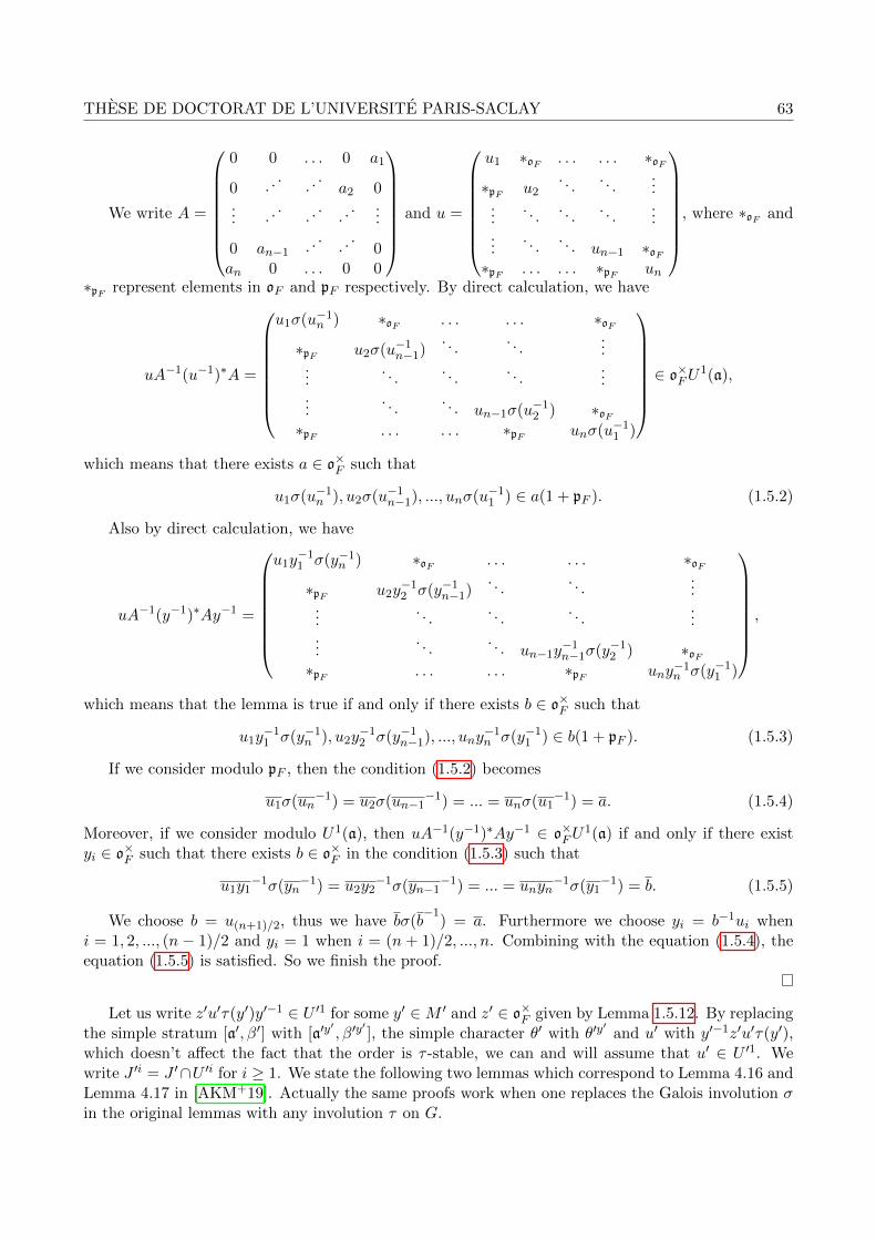
THESE DE DOCTORAT DE L’UNIVERSITE PARIS-SACLAY 63
We write A =
0 0 . . . 0 a1
0 . ..
. ..a2 0
... . ..
. ... .. ...
0 an−1 . ... ..
0an 0 . . . 0 0
and u =
u1 ∗oF . . . . . . ∗oF∗pF u2
. . .. . .
......
. . .. . .
. . ....
.... . .
. . . un−1 ∗oF∗pF . . . . . . ∗pF un
, where ∗oF and
∗pF represent elements in oF and pF respectively. By direct calculation, we have
uA−1(u−1)∗A =
u1σ(u−1n ) ∗oF . . . . . . ∗oF
∗pF u2σ(u−1n−1)
. . .. . .
......
. . .. . .
. . ....
.... . .
. . . un−1σ(u−12 ) ∗oF
∗pF . . . . . . ∗pF unσ(u−11 )
∈ o×FU
1(a),
which means that there exists a ∈ o×F such that
u1σ(u−1n ), u2σ(u−1
n−1), ..., unσ(u−11 ) ∈ a(1 + pF ). (1.5.2)
Also by direct calculation, we have
uA−1(y−1)∗Ay−1 =
u1y−11 σ(y−1
n ) ∗oF . . . . . . ∗oF∗pF u2y
−12 σ(y−1
n−1). . .
. . ....
.... . .
. . .. . .
......
. . .. . . un−1y
−1n−1σ(y−1
2 ) ∗oF∗pF . . . . . . ∗pF uny
−1n σ(y−1
1 )
,
which means that the lemma is true if and only if there exists b ∈ o×F such that
u1y−11 σ(y−1
n ), u2y−12 σ(y−1
n−1), ..., uny−1n σ(y−1
1 ) ∈ b(1 + pF ). (1.5.3)
If we consider modulo pF , then the condition (1.5.2) becomes
u1σ(un−1) = u2σ(un−1
−1) = ... = unσ(u1−1) = a. (1.5.4)
Moreover, if we consider modulo U1(a), then uA−1(y−1)∗Ay−1 ∈ o×FU1(a) if and only if there exist
yi ∈ o×F such that there exists b ∈ o×F in the condition (1.5.3) such that
u1y1−1σ(yn
−1) = u2y2−1σ(yn−1
−1) = ... = unyn−1σ(y1
−1) = b. (1.5.5)
We choose b = u(n+1)/2, thus we have bσ(b−1
) = a. Furthermore we choose yi = b−1ui wheni = 1, 2, ..., (n − 1)/2 and yi = 1 when i = (n + 1)/2, ..., n. Combining with the equation (1.5.4), theequation (1.5.5) is satisfied. So we finish the proof.
Let us write z′u′τ(y′)y′−1 ∈ U ′1 for some y′ ∈M ′ and z′ ∈ o×F given by Lemma 1.5.12. By replacingthe simple stratum [a′, β′] with [a′y
′, β′y
′], the simple character θ′ with θ′y
′and u′ with y′−1z′u′τ(y′),
which doesn’t affect the fact that the order is τ -stable, we can and will assume that u′ ∈ U ′1. Wewrite J ′i = J ′∩U ′i for i ≥ 1. We state the following two lemmas which correspond to Lemma 4.16 andLemma 4.17 in [AKM+19]. Actually the same proofs work when one replaces the Galois involution σin the original lemmas with any involution τ on G.

64 1.5. THE τ -SELFDUAL TYPE THEOREM
Lemma 1.5.13. Let v′ ∈ U ′i for some i ≥ 1 and assume that v′τ(v′) ∈ J ′i. Then there exist j′ ∈ J ′iand x′ ∈ U ′i such that j′v′τ(x′)x′−1 ∈ U ′i+1.
Using Lemma 1.5.13 to replace Lemma 4.16 in [AKM+19], we may prove the following lemma:
Lemma 1.5.14. There exists a sequence of (x′i, j′i, v′i) ∈ U ′i × J ′i × U ′i+1 for i ≥ 0, satisfying the
following conditions:
(1) (x′0, j′0, v′0) = (1, 1, u′);
(2) for all i ≥ 0, if we set y′i = x′0x′1...x
′i ∈ U ′1, then the simple character θ′i = θ′y
′i ∈ C(a′, β′y′i)
satisfies θ′i ◦ τ = (θ′−1i )v
′i;
(3) for all i ≥ 1, we have y′iv′i = j′iy
′i−1v
′i−1τ(x′i).
Let x′ ∈ U ′1 be the limit of y′i = x′0x′1...x
′i and let h′ ∈ J ′1 be that of j′i...j
′1j′0 when i tends to
infinity. By Lemma 1.5.14.(3), we have
y′iv′iτ(y′−1
i ) = j′iy′i−1v
′i−1τ(y′−1
i−1) = ... = j′i...j′1j′0u′.
Passing to the limit, we get x′τ(x′)−1 = h′u′, which implies that u′τ(x′)x′−1 = h′−1 ∈ J ′. Let(a′′, θ′′) = (a′x
′, θ′x
′), which finishes the proof of Proposition 1.5.9.
1.5.3 The maximal case
In this subsection, we generalize Proposition 1.5.9 to the following situation:
Proposition 1.5.15. Let [a, β] be a simple stratum in Mn(F ) such that [E : F ] = n and let θ ∈ C(a, β)such that θ ∈ Θ with Θ a σ-invariant endo-class. Let τ be a given unitary involution. Then thereexist a simple stratum [a′′, β′′] and a simple character θ′′ ∈ C(a′′, β′′) such that (a′′, θ′′) is G-conjugateto (a, θ) with the property τ(a′′) = a′′ and θ′′ ◦ τ = θ′′−1.
Let T be a tame parameter field of Θ. First we have the following lemma:
Lemma 1.5.16. Let Θ be a σ-invariant endo-class and let T/F be its tame parameter field. Thengiven a T/F -lift Ψ of Θ, there is a unique involution α of T extending σ such that Ψα = Ψ.
Proof. The proof of Lemma 4.8 in [AKM+19] can be used almost unchanged to our lemma. We onlyneed to consider Θ instead of Θ∨ and Ψ instead of Ψ∨.
Let α be the involution of T given by Lemma 1.5.16, and let T0 be the subfield of T fixed by α.Thus T0 ∩ F = F0. We write t = [T : F ] = [T0 : F0]. We need the following proposition due to Hakimand Murnaghan (see [HM02b], Proposition 2.1):
Proposition 1.5.17. There exists an embedding ι : T ↪→ Mt(F ) of F -algebras such that for x ∈ T , wehave ι(α(x)) = ι(x)∗ := σ( tι(x)). Consequently, ι(T0) is contained in the set of hermitian matrices.
Proof of Proposition 1.5.15. Let E = F [β] and let T be the maximal tamely ramified extension of Fin E. It is a tame parameter field of the endo-class Θ. The simple character θ gives Ψ, the endo-classof the interior T/F -lift of Θ, as we introduced in §1.3.3. Let α be defined as in Lemma 1.5.16 and letι be defined as in Proposition 1.5.17. By abuse of notation, we define
ι : Mn/t(T ) ↪→ Mn/t(Mt(F )) = Mn(F )
THESE DE DOCTORAT DE L’UNIVERSITE PARIS-SACLAY 65
with each block defined by the original ι. First we consider τ(x) = εσ( tx−1)ε−1 for any x ∈ G withε = In or diag(ι(ε), ..., ι(ε), ι(ε)), where ε ∈ T×0 \NT/T0
(T×). The determinant of the latter matrix is
NT0/F0(ε)n/t. Since
NT0/F0: T×0 → F×0
is a homomorphism which maps NT/T0(T×) to NF/F0
(F×), it leads to a group homomorphism
NT0/F0: T×0 /NT/T0
(T×)→ F×0 /NF/F0(F×)
between two groups of order 2. We state and proof the following lemma in general:
Lemma 1.5.18. Let F, F0 be defined as before. Let L0/F0 be a finite extension such that L = L0F isa field with [L : L0] = 2 and F0 = L0 ∩ F . Then the group homomorphism
NL0/F0: L×0 → F×0
induces an isomorphism
NL0/F0: L×0 /NL/L0
(L×)→ F×0 /NF/F0(F×)
of groups of order 2.
Proof. We first consider the case where L0/F0 is abelian. If on the contrary the induced homomorphismis not an isomorphism, then we get NL0/F0
(L×0 ) ⊂ NF/F0(F×) which means that F is contained in L0
by Local Class Field Theory ( [Ser79], Chapter 14, Theorem 1), which is absurd.
When L0/F0 is Galois, we may write F0 = L00 ( ... ( Lr0 = L0, such that Li+1
0 /Li0 is abelian fori = 0, ..., r − 1 ( [Ser79], Chapter 4, Proposition 7). We write Li = Li0F . Thus it is easy to show thatLi/Li0 is quadratic, Li0 = Li+1
0 ∩ Li and Li+10 Li = Li+1 for i = 0, ..., r − 1. Using the abelian case,
NLi+10 /Li0
: Li+1×0 /NLi+1/Li+1
0(Li+1×)→ Li×0 /NLi/Li0
(Li×)
is an isomorphism for i = 0, 1, ..., r − 1. Composing them together, we finish the proof.
When L0/F0 is separable, we write L′0 as the normal closure of L0 over F0. Thus L′0 contains L0
and L′0/F0 is a finite Galois extension. We write L′ = L′0F . Using the Galois case,
NL′0/F0: L′×0 /NL′/L′0
(L′×)→ F×0 /NF/F0(F×)
is an isomorphism. Since NL′0/F0(L′×0 ) ⊂ NL0/F0
(L×0 ),
NL0/F0: L×0 /NL/L0
(L×)→ F×0 /NF/F0(F×)
is also an isomorphism.
In the characteristic p case in general, we write Lsep0 for the maximal separable subextension of F0
contained in L0, thus L0/Lsep0 is purely inseparable. Thus NL0/L
sep0
(x) = xp[L0:L
sep0 ]
for any x ∈ L×0 .
Since p 6= 2 and L×0 /NL/L0(L×) is of order 2, we deduce that
NL0/Lsep0
: L×0 /NL/L0(L×)→ Lsep×0 /NLsep/Lsep0
(Lsep×)
is an isomorphism, where Lsep := LLsep0 . So we come back to the separable case which finishes theproof.

66 1.5. THE τ -SELFDUAL TYPE THEOREM
Using Lemma 1.5.18 for L0 = T0, the homomorphism above is actually an isomorphism. Since n/tis odd and ε ∈ T×0 \NT/T0
(T×), we have det(ε) = NT0/F0(ε)n/t ∈ F×0 \NF/F0
(F×). So indeed these twoinvolutions represent all the two G-classes of hermitian matrices. Thus using Lemma 1.5.8, we mayfrom now on assume τ to be the two unitary involutions we mentioned above. Furthermore, ι(T )× isnormalized by τ from the exact construction of τ and Proposition 1.5.17, where we regard T as anF -subalgebra of Mn/t(T ) given by the diagonal embedding.
Since T and ι(T ) are isomorphic as F -subalgebras contained in Mn(F ), by the Skolem-Noethertheorem, there exists g ∈ G such that ι(T ) = T g. Thus, if we write [a′, β′] = [ag, βg], θ′ = θg andE′ = F [β′], then θ′ ∈ Θ such that its tame parameter field equals ι(T ). Since τ normalizes ι(T )×, wededuce that θ′ ◦ τ and θ′−1 have the same parameter field ι(T ). If we write Ψ′ as the endo-class of theinterior ι(T )/F -lift corresponding to θ′, and if we choose α′ = ι|T ◦ α ◦ ι|−1
ι(T ), then we have Ψ′α′
= Ψ′.
Let C ′ = Mn/t(ι(T )) denote the centralizer of ι(T ) in Mn(F ). For c ∈ Mn/t(T ), we have
τ(ι(c)) = εσ( tι(c)−1)ε−1 = ε( tC′ ι(α(c))−1)ε−1 = ε(α′( tC′ ι(c))−1)ε−1 = τ ′(ι(c)),
where we denote by tC′ the transpose on C ′ = Mn/t(ι(T )) and τ ′(c′) = ε(α′( tC′ c′−1))ε−1 for anyc′ ∈ C ′× . Thus τ ′, the restriction of τ to C ′×, is the unitary involution τ1 on C ′× = GLn/t(ι(T )) withrespect to the Galois involution α′ ∈ Gal(ι(T )/F ). The intersection c′ = a′ ∩ C ′ gives rise to a simplestratum [c′, β′]. The restriction of θ′ to H1(c′, β′), denoted by θ′ι(T ), is a simple character associated
to this simple stratum with endo-class Ψ′. Since E′/ι(T ) is totally wildly ramified, using Proposition1.5.9 with G, θ, Θ, σ and τ replaced by C ′×, θ′ι(T ), Ψ′, α′ and τ ′ respectively, there exists c′ ∈ C ′×
such that τ ′(c′c′) = c′c
′and θ′c
′
ι(T ) ◦ τ′ = (θ′c
′
ι(T ))−1.
By the injectivity of a 7→ a∩C ′ between sets of hereditary orders as mentioned in §1.3.3, we knowthat a′′ := a′c
′is τ -stable. Moreover if we write θ′′ = θ′c
′, then from our construction of τ and the
definition of ι(T )/F -lift,
(θ′′ ◦ τ)ι(T ) = θ′′ ◦ τ |H1(τ(c′),τ(β′)) = θ′′ ◦ τ ′|H1(τ(c′),τ(β′)) = θ′′ι(T ) ◦ τ′
and(θ′′−1)ι(T ) = θ′′−1
ι(T )
are equal. Since the interior ι(T )/F -lift θ′′ 7→ θ′′ι(T ) is injective between sets of simple characters as
mentioned in §1.3.3, the simple character θ′′ satisfies the property θ′′ ◦ τ = θ′′−1.
1.5.4 The general case
In this subsection, we finish the proof of Lemma 1.5.4 and Theorem 1.5.5. First of all, we recall thefollowing result similar to that appearing in the paper of Stevens:
Proposition 1.5.19 ( [Ste01], Theorem 6.3). Let [a, β] be a simple stratum in Mn(F ) with σ1(a) = a.Suppose that there exists a simple character θ ∈ C(a, β) such that H1(a, β) is σ1-stable and θ ◦ σ1 = θ.Then there exists a simple stratum [a, γ] such that θ ∈ C(a, γ) and σ1(γ) = γ.
Proof. The original proof of [Ste01], Theorem 6.3 can be modified a little bit as follows, thus canbe used in our case without difficulty. For any x ∈ Mn(F ), we use −σ1(x) to replace x; we use σ1
to replace σ; for [a, β] a simple stratum, we say that it is σ1-invariant if σ1(a) = a, and σ1(β) = βand we use this concept to replace the concept skew simple stratum in the original proof. With thesereplacements, the original proof can be used directly.

THESE DE DOCTORAT DE L’UNIVERSITE PARIS-SACLAY 67
We choose [a0, β0] as a maximal simple stratum in Md(F ) and θ0 ∈ C(a0, β0) such that θ0 ∈ Θ. ByProposition 1.5.15, there are a maximal simple stratum [a′0, β
′0] and a simple character θ′0 ∈ C(a′0, β′0)
which is GLd(F )-conjugate to θ0 such that:(1) the order a′0 is τ1-stable;(2) the group H1(a′0, β
′0) is τ1-stable and θ′0 ◦ τ1 = θ′−1
0 ;Furthermore, using Proposition 1.5.19 we may assume that:(3) σ1(β′0) = β′0.We embed Md(F ) diagonally into the F -algebra Mn(F ). This gives an F -algebra homomorphism
ι′ : F [β′0] ↪→ Mn(F ). Write β′ = ι′(β′0) = β′0 ⊗ ... ⊗ β′0 and E′ = F [β′]. The centralizer B′ of E′ inMn(F ) is naturally identified with Mm(E′). We regard σ1 as an involution on E′ extending σ and wewrite E′0 = E′σ1 . Let b′ be a maximal standard hereditary order in B′ which may be identified withMm(oE′), and let a′ = Mm(a′0) be the unique hereditary order of Mn(F ) normalized by E′× such thata′ ∩ B′ = b′. Then we have [a′, β′] in Mn(F ) as a simple stratum which satisfies the requirement ofLemma 1.5.4, finishing its proof.
Now we focus on the proof of Theorem 1.5.5. By Lemma 1.5.8, we may change τ up to G-actionon its corresponding hermitian matrix which doesn’t change the content of the theorem. So if ε is inthe same G-class as In, we may simply choose τ = τ1, where τ1(x) = σ( tx−1) for any x ∈ G. If not,we fix ε ∈ E′×0 \NE′/E′0
(E′×). Regarding ε as an element in Md(F ), we have det(ε) = NE′0/F0(ε). Since
NE′0/F0: E′×0 → F×0
is a homomorphism which maps NE′/E′0(E′×) to NF/F0
(F×), by Lemma 1.5.18 with L0 = E′0, it leadsto an isomorphism
NE′0/F0: E′×0 /NE′/E′0
(E′×)→ F×0 /NF/F0(F×)
of the two groups of order 2. Thus we have NE′0/F0(ε) ∈ F×0 \NF/F0
(F×). If E′/E′0 is unramified,
we write ε = diag(ε, ..., ε). We deduce that det(ε) = NE′0/F0(ε)m ∈ F×0 \NF/F0
(F×), which is because
F×0 /NF/F0(F×) is a group of order 2, and m is odd from the condition of the theorem. If E′/E′0 is
ramified, we may further assume that ε ∈ o×E′0
. We choose ε = diag(Id, ..., Id, ε) and we have det(ε) =
NE′0/F0(ε) ∈ F×0 \NF/F0
(F×). For both two cases, τε is a unitary involution whose correspondinghermitian matrix is not in the same G-class as In. So from now on, we only consider the three unitaryinvolutions above. From our assumption of τ , the restriction of τ on GLm(E′) is also a unitaryinvolution τ ′ = τ1 or τε with ε = diag(1, ..., 1, ε). In particular, since ε is an element in E′, we knowthat ε commutes with elements in E′ and we have τ(β′) = β′−1.
Since a′0 is τ1-stable and b′ is τ ′-stable, from our assumption of τ we deduce that a′ is τ -stable, orby definition εσ1(a′)ε−1 = a′. Since σ1(β′) = β′, by direct calculation we have
τ(H1(a′, β′)) = εH1(σ1(a′), σ1(β′))−1ε−1 = H1(σ1(a′)ε−1, β′ε
−1) = H1(a′, β′ε
−1) = H1(a′, β′).
Let M be the standard Levi subgroup of G isomorphic to GLd(F )× ...×GLd(F ), let P be the standardparabolic subgroup of G generated by M and upper triangular matrices, and let N be its unipotentradical. Let N− be the unipotent radical of the parabolic subgroup opposite to P with respect to M .By [SS08], Theoreme 2.17, we have
H1(a′, β′) = (H1(a′, β′) ∩N−) · (H1(a′, β′) ∩M) · (H1(a′, β′) ∩N), (1.5.6)
H1(a′, β′) ∩M = H1(a′0, β′0)× ...×H1(a′0, β
′0). (1.5.7)
Let θ′ ∈ C(a′, β′) be the transfer of θ′0. By loc. cit., the character θ′ is trivial on H1(a′, β′) ∩N− andH1(a′, β′) ∩N , and the restriction of θ′ on H1(a′, β′) ∩M equals θ′0 ⊗ ...⊗ θ′0. We have
θ′ ◦ τ |H1(a′,β′)∩N− = θ′ ◦ τ |H1(a′,β′)∩N = θ′−1|H1(a′,β′)∩N− = θ′−1|H1(a′,β′)∩N = 1

68 1.6. THE DISTINGUISHED TYPE THEOREM
andθ′ ◦ τ |H1(a′,β′)∩M = θ′0 ◦ τ1 ⊗ ...⊗ θ′0 ◦ τ1 = θ′−1
0 ⊗ ...⊗ θ′−10 = θ′−1|H1(a′,β′)∩M
for τ = τ1 or τε with ε = diag(ε, ..., ε) or diag(1, ..., 1, ε), since ε ∈ F [β′0]× normalizes θ′0. Thus byequation (1.5.6), we have θ′ ◦ τ = θ′−1.
Remark 1.5.20. From the proof of Theorem 1.5.5, we observe that if τ is chosen as one of the threeunitary involutions mentioned in the proof, then we may choose the same simple stratum and simplecharacter which satisfy the conclusion of the theorem.
Remark 1.5.21. We give a counter-example to show that the condition in Theorem 1.5.5 is necessary.Let n = 2, F/F0 unramified, Θ is trivial and ε = diag(1, $F0). Then d = 1, m = n = 2, E = F andE0 = F0. If the theorem is true, then a = M2(oF )g for some g ∈ GL2(F ) and τ(a) = a. By directcalculation σ( tg−1)ε−1g−1 normalizes M2(oF ), which means that σ( tg−1)ε−1g−1 ∈ F×GL2(oF ). It isimpossible since det(σ( tg−1)ε−1g−1) ∈ $F0NF/F0
(F×), while det(F×GL2(oF )) ⊂ NF/F0(F×).
1.6 The distinguished type theorem
Let π be a cuspidal representation of G such that πσ ∼= π. From the statements and proofs of Theorem1.5.2, 1.5.3 and 1.5.5, we may assume the following conditions as a remark of section 5:
Remark 1.6.1. (1) For τ = τ1, there exist a simple stratum [a, β] and a simple character θ ∈ C(a, β)contained in π such that τ(a) = a, τ(H1(a, β)) = H1(a, β), θ ◦ τ = θ−1 and τ(β) = β−1, whereτ1(x) := σ( tx−1) for any x ∈ GLn(F );
(2) For τ = τ1, there exists a simple type (J ,Λ) containing θ and contained in π such that τ(J) = Jand Λτ ∼= Λ∨;
(3) σ1 is an involution on E = F [β], whose restriction to F equals σ. So by abuse of notation,we identify σ with σt. Let E0 = Eσ. We assume further in this section that if E/E0 isunramified, then m is odd4.;
(4) Write τ(x) = εσ( tx−1)ε−1 for any x ∈ G such that: when E/E0 is unramified, we assumeε = In or diag($E , ..., $E) ∈ GLm(E) ↪→ GLmd(F ) = GLn(F ); when E/E0 is ramified, we assumeε = In or diag(1, ..., 1, ε) ∈ GLm(E) ↪→ GLn(F ) with ε ∈ o×E0
\NE/E0(o×E). By Remark 1.5.20, we
assume further that for these three unitary involutions, condition (1) and (2) are also satisfied. Fromnow on until the end of this section, we assume ε to be one of these three hermitianmatrices and τ to be one of these three corresponding involutions.
(5) the element β has the block diagonal form:
β = diag(β0, ..., β0) ∈ Mm(Md(F )) = Mn(F )
for some β0 ∈ Md(F ), where d is the degree of β over F and n = md. The centralizer B of E inMn(F ) is identified with Mm(E). If we regard τ as the restriction of the original involution to B×,then it is a unitary involution with respect to B× = GLm(E), E/E0 and σ ∈ Gal(E/E0);
(6) the order b = a∩B is the standard maximal order Mm(oE) of Mm(E). Thus if we write a0 asthe hereditary order of Md(F ) normalized by E, then a is identified with Mm(a0);
(7) $E is a uniformizer of E such that:
σ($E) =
{$E if E is unramified over E0;
−$E if E is ramified over E0.
4 Although this condition seems a little bit annoying, finally in §1.7 we may find out that this condition is automaticallysatisfied for π a σ-invariant supercuspidal representation.

THESE DE DOCTORAT DE L’UNIVERSITE PARIS-SACLAY 69
Now we state the main theorem of this section:
Theorem 1.6.2 (distinguished type theorem). For π a σ-invariant cuspidal representation, it is Gτ -distinguished if and only if it contains a τ -selfdual simple type (J ,Λ) such that HomJ∩Gτ (Λ, 1) 6= 0.
Remark 1.6.3. Since every hermitian matrix is equivalent to one of the hermitian matrices mentionedin Remark 1.6.1.(4) up to G-action, and the property of distinction is invariant up to equivalenceof unitary groups, the theorem works for every unitary involution, although we only consider thoseoccurring in loc. cit.
Choose (J ,Λ) as in Remark 1.6.1, using the Mackey formula and the Frobenius reciprocity, wehave
HomGτ (π, 1) ∼=∏g
HomJg∩Gτ (Λg, 1),
where g ranges over a set of representatives of (J , Gτ )-double cosets in G. So π is Gτ -distinguished ifand only if there exists g as a representative of a (J , Gτ )-double coset such that HomJg∩Gτ (Λg, 1) 6= 0.We will study such g and will show that (Jg,Λg) is actually τ -selfdual. This will finish the proof ofthis theorem.
1.6.1 Double cosets contributing to the distinction of θ
First we have the following proposition:
Proposition 1.6.4. For g ∈ G, the character θg is trivial on H1g∩Gτ if and only if τ(g)g−1 ∈ JB×J .
Proof. We only need to use the same proof of [Sec19], Proposition 6.6, with σ replaced by τ .
As a result, since HomJg∩Gτ (Λg, 1) 6= 0 implies that HomH1g∩Gτ (θg, 1) 6= 0, using Proposition1.6.4 we have γ := τ(g)g−1 ∈ JB×J .
1.6.2 The double coset lemma
The next step is to prove the following double coset lemma:
Lemma 1.6.5. Let g ∈ G. Then γ = τ(g)g−1 ∈ JB×J if and only if g ∈ JB×Gτ .
Proof. If g ∈ JB×Gτ , one verifies immediately that γ ∈ JB×J . Conversely, suppose that γ ∈ JB×J ,first we need the following lemma:
Lemma 1.6.6. There exists an element b ∈ B× such that γ ∈ JbJ and bτ(b) = 1.
Proof. Since B×∩J = b× is a maximal compact subgroup of B×, using the Cartan decomposition overB× ∼= GLm(E), we write γ = xcy with x, y ∈ J and c = diag($a1
E Im1 , ..., $arE Imr), where a1 > ... > ar
as integers and m1 + ...+mr = m.If E/E0 is unramified, then by definition c∗ = c. So if we choose b = cε−1, then bε(b∗)−1ε−1 =
c(c∗)−1 = 1, that is, bτ(b) = 1.If E/E0 is ramified, since τ(γ)γ = 1, we know that xcy = εy∗c∗x∗ε−1 which is equivalent to
(y∗)−1ε−1xc = c∗x∗ε−1y−1. Let z = x∗ε−1y−1 ∈ J , then we have z∗c = c∗z. We regard z and c asmatrices in Mm(Md(F )). Denote by z(j) ∈ Mmj (Md(F )) the block matrix in z which is at the same
place as $ajE Imj in c. Since z∗c = c∗z, by direct calculation
(z(j))∗$ajE = (−1)aj$
ajE z
(j) for j = 1, ..., r. (1.6.1)

70 1.6. THE DISTINGUISHED TYPE THEOREM
By considering the following embedding
Mmj (Md(F )) ↪→Mm(Md(F ))
h 7→diag(0m1d, ..., 0mj−1d, h, 0mj+1d, ..., 0mrd),
we may regard Mmjd(F ) as a subalgebra of Mmd(F ) which we denote by A(j), where 0mjd represents
the zero matrix of size mjd ×mjd. We write a(j) = a ∩ A(j). By abuse of notation, we identify theelement β0 ⊗ ... ⊗ β0, which consists of mj copies of β0 and is contained in Mmj (Md(F )), with β.
By [SS08], Theoreme 2.17, since z ∈ J(a, β), we get z(j) ∈ J(a(j), β) for j = 1, ..., r. By loc. cit., if wedenote by
M = GLm1d(F )× ...×GLmrd(F )
the Levi subgroup of G corresponding to the partition n = m1d+ ...+mrd, then
M ∩ J = J(a(1), β)× ...× J(a(r), β)
and
M ∩ J1 = J1(a(1), β)× ...× J1(a(r), β).
Thus we get diag(z(1), ..., z(r)) ∈M ∩ J . And further we have
M ∩ J/M ∩ J1 ∼= J(a(1), β)/J1(a(1), β)× ...× J(a(r), β)/J1(a(r), β) ∼= GLm1(l)× ...×GLmr(l).
Since (·)∗ fixes M ∩ J and M ∩ J1, we know that (·)∗ induces a map
M ∩ J/M ∩ J1 ∼= GLm1(l)× ...×GLmr(l) −→ GLm1(l)× ...×GLmr(l)∼= M ∩ J/M ∩ J1,
(z(1), ..., z(r)) 7−→ ((z(1))∗, ..., (z(r))∗),
where l is the residue field of E and E0, and z(j) ∈ J(a(j), β)/J1(a(j), β) ∼= GLmj (l) is the image of
z(j).
We show that for any i such that 2 - ai, we have 2 | mi. Consider j = i in equation (1.6.1), we get(z(i))∗ = −$ai
E z(i)$−aiE . Since J/J1 ∼= U(b)/U1(b) on which E× acts trivially by conjugation, we get
z(i) = $aiE z
(i)$−aiE = −(z(i))∗ = − tz(i). Since there exists no anti-symmetric invertible matrix of odddimension, we must have 2|mi. Now for αj = (aj ,mj), define
$αjE =
{$ajE Imj if 2|aj ;
$ajE Jmj/2 if 2 - aj .
and c′ = diag($α1E , ..., $αr
E ), where Jmj/2 :=
(0 Imj/2
−Imj/2 0
). We have c′ = c′∗ and c′ is in the same
J-J double coset as c. Let b = c′ε−1, we get bτ(b) = 1.
Now we write γ = x′bx with x, x′ ∈ J and b ∈ B× as in Lemma 1.6.6. Replacing g by τ(x′)−1gdoes not change the double coset JgGτ but changes γ into bxτ(x′). So from now on, we will assumethat
γ = bx, bτ(b) = 1, x ∈ J, b is of the form in the proof of Lemma 1.6.6. (1.6.2)
Write K for the group J ∩ b−1Jb. Since τ(b) = b−1 and J is τ -stable, we have x ∈ K. We havethe following corollary of Lemma 1.6.6.

THESE DE DOCTORAT DE L’UNIVERSITE PARIS-SACLAY 71
Corollary 1.6.7. The map δb : k 7→ b−1τ(k)b is an involution on K.
Now for a1 > ... > ar as in the proof of Lemma 1.6.6, and M = GLm1d(F )× ...×GLmrd(F ) ⊆ G,we write P for the standard parabolic subgroup of G generated by M and upper triangular matrices.We write N and N− for the unipotent radicals of P and its opposite parabolic subgroup respectively.By definition of b, it normalizes M and we have
K = (K ∩N−) · (K ∩M) · (K ∩N).
For V = K ∩B× = U ∩ b−1Ub as a subgroup of B×, similarly we have
V = (V ∩N−) · (V ∩M) · (V ∩N),
where U = U(b) and U1 = J1 ∩B× = U1(b). By definition, V is also fixed by δb.
Lemma 1.6.8. The subsetK1 = (K ∩N−) · (J1 ∩M) · (K ∩N)
is a δb-stable normal pro-p-subgroup of K, and we have K = V K1.
Proof. The proof is the same as that in [Sec19], Lemma 6.10.
Lemma 1.6.9. Let y ∈ K such that yδb(y) = 1, then there are k ∈ K and v ∈ V such that:(1) the element v is in GLm1(oE)× ...×GLmr(oE) ⊆ B× such that vδb(v) = 1;(2) one has δb(k)yk−1 ∈ vK1.
Proof. Let V 1 = V ∩K1. We have
V 1 = (V ∩N−) · (U1 ∩M) · (V ∩N).
Thus we have canonical δb-equivariant group isomorphisms
K/K1 ∼= V/V 1 ∼= (U ∩M)/(U1 ∩M). (1.6.3)
Since B× ∩M = GLm1(E) × ... ×GLmr(E), the right side of (1.6.3) identifies with M = GLm1(l) ×... × GLmr(l), where l denotes the residue field of E. As in the proof of Lemma 1.6.6, we may writeε−1b = diag($a1
E c1, ..., $arE cr) with cj ∈ GLmj (oE). Moreover, the involution δb acts on M by
(g1, ..., gk) 7→ (c1−1σ(tg−1
1 )c1, ..., cr−1σ(tg−1
r )cr),
where we denote by cj the image of cj in GLmj (l). We denote by (g1, ..., gr) the image of y inM = GLm1(l)× ...×GLmr(l).
When E/E0 is unramified, we denote by l0 the residue field of E0. So l/l0 is quadratic and therestriction of σ to l is the non-trivial involution in Gal(l/l0). Since (b−1ε)∗ = ε(b∗)−1ε−1ε = τ(b)ε =b−1ε, we get cj
∗ = cj . If yδb(y) = 1, then we get (cjgj)∗ = g∗j cj = cjgj . We need the following lemma:
Lemma 1.6.10 ( [KL90], Proposition 2.3.1). For x = x∗ in GLs(l), there exists A ∈ GLs(l) such thatAxA∗ = Is.
Using Lemma 1.6.10, we choose kj ∈ GLmj (oE) such that its image kj in GLmj (l) satisfies
(kj∗)−1cjgjkj
−1= Imj . Choose k = diag(k1, ..., kr) and v = diag(v1, ..., vr) = diag(c−1
1 , ..., c−1r ),
we get δb(k)yk−1 ∈ vV 1 and δb(v)v = diag(c−11 c∗1c1c
−11 , ..., c−1
r c∗rcrc−1r ) = 1.
When E/E0 is ramified, the restriction of σ on l is trivial. Since (b−1ε)∗ = b−1ε, we get c∗j =(−1)ajcj and tcj = (−1)ajcj . We need the following two lemmas:

72 1.6. THE DISTINGUISHED TYPE THEOREM
Lemma 1.6.11 ( [KL90], Proposition 2.5.4). For x = tx in GLs(l), there exists A ∈ GLs(l) suchthat Ax tA is either Is or εs = diag(1, ..., 1, ε), where ε ∈ l×\l×2 with l×2 denoting the group of squareelements of l×.
Lemma 1.6.12 ( [KL90], Proposition 2.4.1). For x = − tx in GLs(l) and s even, there exists A ∈GLs(l) such that Ax tA = Js/2.
When aj is even, using Lemma 1.6.11 we may choose kj ∈ GLmj (oE) such that its image kj in
GLmj (l) satisfies that ( tkj)−1cjgjkj
−1equals either Imj or εmj , where we choose εmj = diag(1, ..., 1, ε)
∈ GLmj (oE) such that its image εmj in GLmj (l) is diag(1, ..., 1, ε) as in Lemma 1.6.11. Let vj be c−1j
or c−1j εmj in the two cases respectively.
When aj is odd mj is even from the proof of Lemma 1.6.6. Using Lemma 1.6.12, we may choose
kj ∈ GLmj (oE) such that its image kj in GLmj (l) satisfies ( tkj)−1cjgjkj
−1= Jmj/2 . We choose
vj = c−1j Jmj/2.
Choose k = diag(k1, ..., kr) and v = diag(v1, ..., vr), we know that
δb(k)yk−1 ∈ vV 1
and
δb(v)v = diag(c−11 (v∗1)−1c1v1, ..., c
−1r (v∗r )
−1crvr) = 1
by direct calculation in the two cases respectively. So no matter E/E0 is ramified or not, we finishthe proof.
Now we finish the proof of Lemma 1.6.5. Applying Lemma 1.6.9 to x gives us k ∈ K and v ∈ V ,such that bvτ(bv) = 1 and δb(k)xk−1 ∈ vK1. Thus we have τ(k)γk−1 ∈ bvK1. Therefore replacing gby kg and b by bv, we assume that γ can be written as:
γ = bx, bτ(b) = 1, x ∈ K1, b ∈ $a1E GLm1(oE)× ...×$ar
E GLmr(oE). (1.6.4)
Furthermore, we have δb(x)x = 1.
Since K1 is a δb-stable pro-p-group and p is odd, the first cohomology set of δb on K1 is trivial. Thusx = δb(y)y−1 for some y ∈ K1, hence γ = τ(y)by−1. Consider the determinant of this equation, wehave det(b) ∈ NF/F0
(F×). If we denote by detB the determinant function defined on B× = GLm(E),then we have det(b) = NE/F (detB(b)). Using Lemma 1.5.18 for L = E, we get detB(b) ∈ NE/E0
(E×)and detB(ε−1b) ∈ detB(ε−1)NE/E0
(E×). Since τ(b)b = 1, we have (ε−1b)∗ = ε−1b. Using Proposition1.2.1, there exists h ∈ B× such that ε−1b = (h∗)−1ε−1h−1. So we have b = τ(h)h−1. Thus g ∈ yhGτ ⊆JB×Gτ , which finishes the proof of Lemma 1.6.5.
1.6.3 Distinction of the Heisenberg representation
Now let η be the Heisenberg representation of J1 associated to θ. We have the following result similarto [Sec19], Proposition 6.12. by replacing σ with τ :
Proposition 1.6.13. Given g ∈ G, we have:
dimRHomJ1g∩Gτ (ηg, 1) =
{1 if g ∈ JB×Gτ ,0 otherwise.

THESE DE DOCTORAT DE L’UNIVERSITE PARIS-SACLAY 73
Proof. It is useful to recall the detail of the proof of this proposition, which will be used in the nextsubsection. We write δ(x) := γ−1τ(x)γ for any x ∈ G which is an involution on G. And for anysubgroup H ⊂ G, we have Hg ∩Gτ = (H ∩Gδ)g.
When g /∈ JB×Gτ , restricting ηg to H1g and using Proposition 1.6.4 and Lemma 1.6.5, weknow that the dimension equals 0. When g ∈ JB×Gτ , we need to prove that HomJ1g∩Gτ (ηg, 1) =HomJ1∩Gδ(η, 1) is of dimension 1. We state the following general proposition which works for a generalinvolution on G:
Proposition 1.6.14. Let δ be an involution on G such that δ(H1) = H1γ and θ ◦ δ = θ−1γ, whereγ ∈ B× such that δ(γ)γ = 1. Then we have
dimRHomJ1∩Gδ(η, 1) = 1.
Since Proposition 1.6.14 in our special case implies Proposition 1.6.13, we only need to focus onthe proof of this proposition. We only need to prove that the space
HomJ1∩Gδ(η(J1:H1)1/2
, 1) ∼= HomJ1∩Gδ(IndJ1
H1(θ), 1)
is of dimension (J1 : H1)1/2. First we prove the following lemmas which will also be used in the nextsubsection:
Lemma 1.6.15. For H a subgroup of G such that δ(H) = Hγ with δ and γ as in Proposition 1.6.14,we have
H ∩Gδ = Hγ ∩Gδ = H ∩Hγ ∩Gδ.
Proof. We have H ∩Gδ = δ(H ∩Gδ) = δ(H) ∩ δ(Gδ) = Hγ ∩Gδ which proves the lemma.
Lemma 1.6.16. Let δ and γ be as in Proposition 1.6.14, then we have the following isomorphisms offinite dimensional representations:
(1) IndJ1
H1θ|J1∩J1γ∼=⊕
H1\J1/J1∩J1γ IndJ1∩J1γ
H1∩J1γθ;
(2) IndJ1γ
H1γθγ |J1∩J1γ∼=⊕
H1γ\J1γ/J1∩J1γ IndJ1∩J1γ
J1∩H1γθγ;
(3) IndJ1
H1θ|J1∩Gδ∼=⊕
H1\J1/J1∩J1γ
⊕H1∩J1γ\J1∩J1γ/J1∩Gδ IndJ
1∩GδH1∩Gδθ;
(4) IndJ1γ
H1γθγ |J1γ∩Gδ∼=⊕
H1γ\J1γ/J1∩J1γ
⊕J1∩H1γ\J1∩J1γ/J1γ∩Gδ IndJ
1γ∩GδH1γ∩Gδθ.
Proof. We only prove (1) and (3), since the proofs of (2) and (4) are similar to the proofs of (1) and(3) respectively.
For (1), using the Mackey formula, we have
IndJ1
H1θ|J1∩J1γ∼=
⊕x∈H1\J1/J1∩J1γ
IndJ1∩J1γ
H1x∩(J1∩J1γ)θx
∼=⊕
H1\J1/J1∩J1γ
IndJ1∩J1γ
H1∩J1γθ.
The last step is because x ∈ J1 normalizes H1 and θ.

74 1.6. THE DISTINGUISHED TYPE THEOREM
For (3), using the Mackey formula again, we have
IndJ1
H1θ|J1∩Gδ∼=
⊕H1\J1/J1∩J1γ
IndJ1∩J1γ
H1∩J1γθ|J1∩Gδ
∼=⊕
H1\J1/J1∩J1γ
⊕y∈H1∩J1γ\J1∩J1γ/J1∩Gδ
IndJ1∩Gδ
(H1∩J1γ)y∩(J1∩Gδ)θy
∼=⊕
H1\J1/J1∩J1γ
⊕H1∩J1γ\J1∩J1γ/J1∩Gδ
IndJ1∩GδH1∩Gδθ.
The last step is because y ∈ J1 ∩ J1γ normalizes H1 ∩ J1γ and θ, and H1 ∩ J1γ ∩ J1 ∩Gδ = H1 ∩Gδby Lemma 1.6.15.(2) for H = J1. So we finish the proof.
Lemma 1.6.17. Let δ and γ be as in Proposition 1.6.14, then we have:
(1) |H1\J1/J1 ∩ J1γ | · |H1 ∩ J1γ\J1 ∩ J1γ/J1 ∩Gδ| = (J1 : H1)1/2;
(2) |H1γ\J1γ/J1 ∩ J1γ | · |J1 ∩H1γ\J1 ∩ J1γ/J1γ ∩Gδ| = (J1γ : H1γ)1/2;
(3) (J1 : H1)1/2 = (J1γ : H1γ)1/2 = (J1 ∩Gδ : H1 ∩Gδ).
Proof. For (3), we refer to [Sec19] subsection 6.3 for a proof, by noting that all the results and proofsfrom Lemma 6.14 to the end of subsection 6.3 in ibid. can be generalized to a general involution δof G, with τ in loc. cit. replaced by δ in our settings. For (1), since J1 normalizes H1 and J1 ∩ J1γ
normalizes H1 ∩ J1γ , we have
left hand side of (1) =(J1 : H1(J1 ∩ J1γ)) · (J1 ∩ J1γ : (H1 ∩ J1γ)(J1 ∩Gδ))=(J1 : H1) · (J1 ∩ J1γ : H1 ∩ J1γ)−1·· (J1 ∩ J1γ : H1 ∩ J1γ) · (J1 ∩Gδ : H1 ∩ J1γ ∩Gδ)−1
=(J1 : H1) · (J1 ∩Gδ : H1 ∩Gδ)−1
=(J1 : H1)1/2,
where we use Lemma 1.6.15 for H = J1γ and (3) in the last two equations. So we finish the proof of(1), and the proof of (2) is similar.
Combining Lemma 1.6.16.(3) with Lemma 1.6.17.(1)(3), we have
dimRHomJ1∩Gδ(IndJ1
H1θ, 1) = dimR
⊕H1\J1/J1∩J1γ
⊕H1∩J1γ\J1∩J1γ/J1∩Gδ
HomJ1∩Gδ(IndJ1∩GδH1∩Gδθ, 1)
= (J1 : H1)1/2dimRHomH1∩Gδ(θ|H1∩Gδ , 1)
= (J1 : H1)1/2.
For the last step, since γ intertwines θ−1 and since θ ◦ δ = θ−1γ , we know that θ is trivial on
{yδ(y)|y ∈ H1 ∩H1γ}.
This set equals H1 ∩ Gδ since the the first cohomology group of δ−1-action on H1 ∩ H1γ is trivial.Thus θ|H1∩Gδ is a trivial character. So we finish the proof.

THESE DE DOCTORAT DE L’UNIVERSITE PARIS-SACLAY 75
1.6.4 Distinction of extensions of the Heisenberg representation
Let κ be an irreducible representation of J extending η. There is a unique irreducible representationρ of J , which is trivial on J1 satisfying Λ ∼= κ⊗ ρ. First we have the following lemma:
Lemma 1.6.18. Let g ∈ JB×Gτ .(1) There is a unique character χ of Jg ∩Gτ trivial on J1g ∩Gτ such that
HomJ1g∩Gτ (ηg, 1) = HomJg∩Gτ (κg, χ−1).
(2) The canonical linear map
HomJ1g∩Gτ (ηg, 1)⊗HomJg∩Gτ (ρg, χ)→ HomJg∩Gτ (Λg, 1).
is an isomorphism.
Proof. The proof is the same as that in [Sec19], Lemma 6.20.
For g ∈ JB×Gτ , we have τ(g) ∈ τ(JB×Gτ ) = JB×Gτ , which means that we may consider thesimilar thing for τ(g) as for g in Lemma 1.6.18. Thus, there exists a unique character χ′ of Jτ(g) ∩Gτtrivial on J1τ(g) ∩Gτ such that
HomJ1τ(g)∩Gτ (ητ(g), 1) ∼= HomJτ(g)∩Gτ (κτ(g), χ′−1).
Moreover, we know that τ(J) = J , τ(J) = J , τ(J1) = J1 and τ(H1) = H1, thus using Lemma 1.4.2and Lemma 1.6.15, we have Jg ∩ Gτ = Jτ(g) ∩ Gτ = Jg ∩ Gτ = Jτ(g) ∩ Gτ , J1g ∩ Gτ = J1τ(g) ∩ Gτand H1g ∩ Gτ = H1τ(g) ∩ Gτ . As a result, χ and χ′ are characters defined on the same groupJg ∩ Gτ = Jτ(g) ∩ Gτ . A natural idea is to compare them. For the rest of this subsection, we focuson the proof of the following proposition:
Proposition 1.6.19. For χ and χ′ defined above as characters of Jg ∩ Gτ = Jτ(g) ∩ Gτ , we haveχ = χ′.
We write δ(x) = γ−1τ(x)γ for any x ∈ G with γ = τ(g)g−1. From §1.3.1, we have γ ∈ IG(η) =IG(κ0), where κ0 = κ|J . Moreover we have
dimR(HomJ∩Jγ (κ0γ , κ0)) = dimR(HomJ1∩J1γ (ηγ , η)) = 1.
Using Lemma 1.6.15, we have J1 ∩Gδ = J1γ ∩Gδ as a subgroup of J1 ∩J1γ and H1 ∩Gδ = H1γ ∩Gδ.We claim the following proposition which works for general γ and δ:
Proposition 1.6.20. Let δ and γ be as in Proposition 1.6.14, then for a non-zero homomorphismϕ ∈ HomJ1∩J1γ (ηγ , η) = HomJ∩Jγ (κ0γ , κ0), it naturally induces an R-vector space isomorphism:
fϕ : HomJ1∩Gδ(η, 1)→ HomJ1γ∩Gδ(ηγ , 1),
λ 7→ λ ◦ ϕ
First we show that how does Proposition 1.6.20 imply Proposition 1.6.19. Using Proposition 1.6.13for g and τ(g) respectively, we have dimRHomJ1g∩Gτ (ηg, 1) = dimRHomJ1τ(g)∩Gτ (ητ(g), 1) = 1. ByProposition 1.6.20, we deduce that
fϕ : HomJ1g∩Gτ (ηg, 1)→ HomJ1τ(g)∩Gτ (ητ(g), 1),
λ 7→ λ ◦ ϕ,

76 1.6. THE DISTINGUISHED TYPE THEOREM
is bijective. If we choose
0 6= λ ∈ HomJ1g∩Gτ (ηg, 1) and 0 6= λ′ := fϕ(λ) = λ ◦ ϕ ∈ HomJ1τ(g)∩Gτ (ητ(g), 1),
then for any v in the representation space of η and any x ∈ Jg ∩Gτ = Jτ(g) ∩Gτ , we have
χ′(x)−1λ′(v) = λ′(κ0τ(g)(x)v) (by Proposition 1.6.18.(1))
= λ(ϕ(κ0τ(g)(x)v)) (by definition of λ′)
= λ(κ0g(x)ϕ(v)) (since ϕ ∈ HomJg∩Jτ(g)(κ0τ(g), κ0g))
= χ(x)−1λ(ϕ(v)) (by Proposition 1.6.18.(1))
= χ(x)−1λ′(v) (by definition of λ′).
Since v and x ∈ Jg∩Gτ = Jτ(g)∩Gτ are arbitrary, we have χ′|Jτ(g)∩Gτ = χ|Jg∩Gτ which is Proposition1.6.19.
So we only need to focus on the proof of Proposition 1.6.20. First of all, we need the followingimportant lemma:
Lemma 1.6.21. Let δ and γ be as in Proposition 1.6.14, then there exist an R[J1 ∩ J1γ ]-modulehomomorphism
Φ : ηγ(J1:H1)1/2 |J1∩J1γ∼= IndJ
1γ
H1γθγ |J1∩J1γ → IndJ
1
H1θ|J1∩J1γ∼= η(J1:H1)1/2 |J1∩J1γ
and a linear form L0 ∈ HomJ1∩Gδ(η(J1:H1)1/2
, 1), such that
0 6= L0 ◦ Φ ∈ HomJ1∩Gδ(ηγ(J1γ :H1γ)1/2
, 1).
Proof. We prove this lemma by giving a direct construction of Φ and L0. First we choose our L0. Wechoose λ0 ∈ HomJ1∩Gδ(IndJ
1∩GδH1∩Gδ1, 1) ∼= R with the isomorphism given by the Frobenius reciprocity,
such that its corresponding image in R equals 1. Then we choose L0 = (λ0, ..., λ0) as a element in⊕H1\J1/J1∩J1γ
⊕H1∩J1γ\J1∩J1γ/J1∩Gδ
HomJ1∩Gδ(IndJ1∩GδH1∩Gδ1, 1) ∼= HomJ1∩Gδ(η
(J1:H1)1/2, 1),
where the isomorphism is determined by Lemma 1.6.16.(3), and by Lemma 1.6.17 the number of copiesequals (J1 : H1)1/2.
Now we focus on the construction of Φ. We define
f0(g) :=
{θγ(g1)θ(g2) if g = g1g2 ∈ (J1 ∩H1γ)(H1 ∩ J1γ)
0 if g ∈ J1 ∩ J1γ\(J1 ∩H1γ)(H1 ∩ J1γ). (1.6.5)
as a continuous function defined on J1∩J1γ with values in R. Since (J1∩H1γ)∩(H1∩J1γ) = H1∩H1γ
and θγ = θ on H1 ∩H1γ , we know that f0 is well-defined.We want to verify that f0 ∈ IndJ
1∩J1γ
H1∩J1γθ and f0 ∈ IndJ1∩J1γ
J1∩H1γθγ . Since J1 normalizes H1 and J1γ
normalizes H1γ , by direct calculation we deduce that J1 ∩ J1γ normalizes J1 ∩H1γ and H1 ∩ J1γ . Inparticular, we have (J1∩H1γ)(H1∩J1γ) = (H1∩J1γ)(J1∩H1γ). Moreover, since J1 and J1γ normalizeθ and θγ respectively, we deduce that (J1 ∩H1γ)(H1 ∩ J1γ) = (H1 ∩ J1γ)(J1 ∩H1γ) normalizes θ andθγ .
For g′1 ∈ J1 ∩H1γ , g′2 ∈ H1 ∩ J1γ and g ∈ J1 ∩ J1γ , if g /∈ (J1 ∩H1γ)(H1 ∩ J1γ), then we haveg′1g, g
′2g /∈ (J1 ∩H1γ)(H1 ∩ J1γ), thus
f0(g′1g) = f0(g′2g) = 0;

THESE DE DOCTORAT DE L’UNIVERSITE PARIS-SACLAY 77
if g = g1g2 ∈ (J1 ∩H1γ)(H1 ∩ J1γ), we have
f0(g′1g) = θγ(g′1)θγ(g1)θ(g2) = θγ(g′1)f0(g)
and
f0(g′2g) = f0(g′2g1g′−12 g′2g2) = θγ(g′2g1g
′−12 )θ(g′2)θ(g2) = θ(g′2)θγ(g1)θ(g2) = θ(g′2)f0(g).
Considering these facts, we have f0 ∈ IndJ1∩J1γ
H1∩J1γθ and f0 ∈ IndJ1∩J1γ
J1∩H1γθγ .We consider J1∩J1γ-action on f0 given by the right translation and we let 〈f0〉 be the R[J1∩J1γ ]-
subspace of both IndJ1∩J1γ
J1∩H1γθγ and IndJ1∩J1γ
H1∩J1γθ generated by f0. We choose Vf0 to be a R[J1 ∩ J1γ ]-
invariant subspace of IndJ1∩J1γ
J1∩H1γθγ such that IndJ1∩J1γ
J1∩H1γθγ = 〈f0〉 ⊕ Vf0 .We define an R[J1 ∩ J1γ ]-module homomorphism
Φ1 : IndJ1∩J1γ
J1∩H1γθγ → IndJ
1∩J1γ
H1∩J1γθ
such that Φ1(f0) = f0 and Φ1|Vf0 = 0. And we define
Φ :⊕
H1γ\J1γ/J1∩J1γ
IndJ1∩J1γ
J1∩H1γθγ →
⊕H1\J1/J1∩J1γ
IndJ1∩J1γ
H1∩J1γθ
given by Φ = diag(Φ1, 0, ..., 0) ∈ MN1(HomR[J1∩J1γ ](IndJ1∩J1γ
J1∩H1γθγ , IndJ1∩J1γ
H1∩J1γθ)), where the coordinatesare indexed by N1 := |H1γ\J1γ/J1∩J1γ | = |H1\J1/J1∩J1γ |. In particular, we let the first coordinatecorrespond to the trivial double cosets H1γ(J1 ∩ J1γ) and H1(J1 ∩ J1γ) respectively. As a result, Φgives an R[J1 ∩ J1γ ]-module homomorphism. By Lemma 1.6.16 we have
η(J1:H1)1/2 ∼= IndJ1
H1θ|J1∩J1γ∼=
⊕H1\J1/J1∩J1γ
IndJ1∩J1γ
H1∩J1γθ (1.6.6)
andηγ(J1:H1)1/2 ∼= IndJ
1γ
H1γθγ |J1∩J1γ
∼=⊕
H1γ\J1γ/J1∩J1γ
IndJ1∩J1γ
J1∩H1γθγ . (1.6.7)
With these two isomorphisms, we may regard Φ as a homomorphism from ηγ(J1:H1)1/2 |J1∩J1γ to
η(J1:H1)1/2 |J1∩J1γ .
Finally, we study L0 ◦ Φ. First we calculate
Φ1 : IndJ1∩J1γ
J1∩H1γθγ |J1∩Gδ → IndJ
1∩J1γ
H1∩J1γθ|J1∩Gδ .
We have the following isomorphism
IndJ1∩J1γ
H1∩J1γθ|J1∩Gδ∼=
⊕H1∩J1γ\J1∩J1γ/J1∩Gδ
IndJ1∩GδH1∩Gδ1. (1.6.8)
By definition of Φ1 and (1.6.5),(1.6.8), Φ1(f0|J1∩Gδ) = f0|J1∩Gδ equals
(1H1∩Gδ , ...,1H1∩Gδ , 0, ..., 0) ∈⊕
H1∩J1γ\J1∩J1γ/J1∩GδIndJ
1∩GδH1∩Gδ1, (1.6.9)
where the coordinates are indexed by the double coset H1∩J1γ\J1∩J1γ/J1∩Gδ, and those coordinateswhich equal the characteristic function 1H1∩Gδ are exactly indexed by the subset H1 ∩ J1γ\(J1 ∩H1γ)(J1 ∩H1γ)/J1 ∩Gδ.

78 1.6. THE DISTINGUISHED TYPE THEOREM
We define v0 = (f0|J1∩Gδ , 0, ..., 0) as an element in both⊕H1\J1/J1∩J1γ
IndJ1∩J1γ
J1∩H1γθγ |J1∩Gδ
and ⊕H1γ\J1γ/J1∩J1γ
IndJ1∩J1γ
H1∩J1γθ|J1∩Gδ ,
where the first coordinate corresponds to the trivial double cosets H1(J1 ∩ J1γ) and H1γ(J1 ∩ J1γ)respectively as in our definition of Φ. Thus we have
(L0 ◦ Φ)(v0) = L0((Φ1(f0|J1∩Gδ), 0, ..., 0)) = L0((f0|J1∩Gδ , 0, ..., 0))
= |H1 ∩ J1γ\(H1 ∩ J1γ)(J1 ∩H1γ)/J1 ∩Gδ|λ0(1H1∩Gδ) 6= 0,
where we use the definition of L0 and (1.6.9) for the last equation. Thus we get L0 ◦ Φ 6= 0 whichfinishes the proof.
We also need the following lemma:
Lemma 1.6.22. We keep the same notations as in Proposition 1.6.20 and we fix
0 6= λ′0 ∈ HomJ1∩Gδ(η, 1) and 0 6= λ′′0 ∈ HomJ1∩Gδ(ηγ , 1).
Then:(1) For any L ∈ HomJ1∩Gδ(η
(J1:H1)1/2, 1), there exists an R[J1 ∩ J1γ ]-homomorphism
Pr : η(J1:H1)1/2 |J1∩J1γ → η|J1∩J1γ
such that L = λ′0 ◦ Pr;
(2) For any L ∈ HomJ1∩Gδ(ηγ(J1:H1)1/2
, 1), there exists an R[J1 ∩ J1γ ]-homomorphism
s : ηγ |J1∩J1γ → ηγ(J1:H1)1/2 |J1∩J1γ
such that λ′′0 = L ◦ s.
Proof. The proof is just a simple application of linear algebra. We write N = (J1 : H1)1/2. For (1), we
define pri : η(J1:H1)1/2 |J1∩J1γ → η|J1∩J1γ as the projection with respect to the i-th coordinate. Since
λ′0 ◦ pr1,...,λ′0 ◦ prN are linearly independent, and dimRHomJ1∩Gδ(η(J1:H1)1/2
, 1) = N as an R-vector
space by Proposition 1.6.13, λ′0 ◦ pr1,...,λ′0 ◦ prN generate HomJ1∩Gδ(η(J1:H1)1/2
, 1). So we may choosePr to be a linear combination of prj which proves (1). The proof of (2) is similar.
Now we finish the proof of Proposition 1.6.20. Using Lemma 1.6.22.(1) we choose Pr such that
L0 = λ′0 ◦ Pr, where L0 is defined as in the statement of Lemma 1.6.21. Using Lemma 1.6.21, there
exists Φ such that L0 ◦Φ 6= 0. Using Lemma 1.6.22.(2) we choose s such that L0 ◦Φ ◦ s = λ′′0 6= 0. Wedefine ϕ′ = Pr ◦ Φ ◦ s and we have the following commutative diagram
ηγ(J1:H1)1/2 |J1∩J1γΦ // η(J1:H1)1/2 |J1∩J1γ
Pr
��ηγ |J1∩J1γ
s
OO
ϕ′ // η|J1∩J1γ
THESE DE DOCTORAT DE L’UNIVERSITE PARIS-SACLAY 79
By definition we have λ′0◦ϕ′ = λ′0◦Pr◦Φ◦s = λ′′0 6= 0, which means that ϕ′ 6= 0. Since HomJ1∩J1γ (ηγ , η)is of dimension 1, we deduce that ϕ equals ϕ′ multiplying with a non-zero scalar, which means thatλ′0 ◦ ϕ 6= 0. Since HomJ1∩Gδ(η, 1) and HomJ1∩Gδ(η
γ , 1) are of dimension 1, we know that fϕ is anR-vector space isomorphism which proves Proposition 1.6.20.
1.6.5 Existence of a τ-selfdual extension of η
Now our aim is to choose a simple κ as an extension of η. Specifically, under the condition of Remark1.6.1, we show that we may assume κ to be τ -selfdual, which means that κτ ∼= κ∨. First of all, wehave the following lemma whose proof is the same as that in [Sec19], Lemma 5.21:
Lemma 1.6.23. There exists a unique character µ of J trivial on J1 such that κτ∨ ∼= κµ. It satisfiesthe identity µ ◦ τ = µ.
Now we are going to prove the following important proposition:
Proposition 1.6.24. When char(R) = 0, there exists a character φ of J trivial on J1 such thatµ = φ(φ ◦ τ). Moreover for any R, we may choose κ as an extension of η such that κτ∨ ∼= κ.
Proof. First we consider the case where char(R) = 0. we need the following elementary lemma:
Lemma 1.6.25. Assume char(R) = 0. For N odd and A ∈ GLN (R) such that A2s = cIN for s ∈ Nand c ∈ R×, we have Tr(A) 6= 0.
Proof. s = 0 is trivial, so from now on we assume s ≥ 1. Let ζ2s be a primitive 2s-th root of 1 in Rand let c1/2s be a 2s-th root of c in R, then we get Tr(A) = c1/2s
∑Ni=1 ζ
ni2s with ni ∈ {0, 1, 2, ..., 2s−1}.
We know that P (x) = x2s−1+ 1 is the minimal polynomial of ζ2s in Q[x]. If Tr(A) = 0, then for
Q(x) =∑N
i=1 xni , we have Q(ζ2s) = 0. As a result, P (x)|Q(x) in Q[x] thus in Z[x] by the Gauss
lemma. However, the sum of all the coefficients of P (x) is even and the sum of all the coefficients ofQ(x) equals N which is odd. We get a contradiction. So Tr(A) 6= 0.
Come back to our proof. We choose κ as any extension of η, thus as in Lemma 1.6.23, there existsφ as a character of J such that κτ∨ ∼= κµ. If E/E0 is unramified, we let
µ : GLm(l) ∼= J/J1 → R×
be the character whose inflation is µ|J . There exists a character ϕ : l× → R× such that µ = ϕ ◦ det.Since µ◦τ = µ, we get (ϕ◦σ)ϕ = 1, or equivalently ϕ|l×0 = 1, where l0 is the residue field of E0, and σ
acts on l as the Frobenius map corresponding to l0. Let Q be the cardinality of l0, then the cardinalityof l is Q2. If we fix ζl a generator of l×, then ζQ+1
l is a generator of l×0 . So we have ϕ(ζl)Q+1 = 1.
Choose α : l× → R× as a character such that
α(ζml )Q−1 = ϕ(ζl)−m for m ∈ Z.
Sinceα(ζl)
Q2−1 = ϕ(ζl)−Q−1 = 1,
α is well-defined as a character of l×. Moreover, we get ϕ = α(α ◦ σ)−1. Choose φ0 : J → R× as theinflation of α ◦ det, we get µ|J = φ0(φ0 ◦ τ).
Since $E and J generate J , to choose φ as a character of J extending φ0, it suffices to show thatµ($E) = 1. Since µ = µ ◦ τ , we get
µ($E) = µ(τ($E)) = µ($E)−1, thus µ($E) ∈ {1,−1}.

80 1.6. THE DISTINGUISHED TYPE THEOREM
Let e be the ramification index of E/F , and let $eE = a0$F for a certain a0 ∈ o×E . We have
$e(Q−1)E = aQ−1
0 $Q−1F with aQ−1
0 ∈ 1 + pE ⊂ H1(a, β).
We write e(Q− 1) = 2su for 2 - u and s ∈ N. For A = κ($uE), we have
A2s = κ(aQ−10 $Q−1
F ) = θ(aQ−10 )ωκ($Q−1
F )IN ,
where we use the fact that the restriction of κ to H1(a, β) equals N -copies of θ with N = (J1 : H1)1/2,and ωκ is the central character of κ. Using Lemma 1.6.25 with A and c = θ(aQ−1
0 )ωκ($Q−1F ), we get
Tr(κ($uE)) 6= 0. Since κτ∨ ∼= κµ, considering the trace of both sides at $u
E , we get
Tr(κ($uE)) = Tr(κ($u
E))µ($uE),
thus µ($uE) = 1. Since u is odd and µ($E) equals either 1 or −1, we get µ($E) = 1 which finishes
the proof of this case.If E/E0 is ramified, first we show that µ|l× = 1, where we consider the embedding l× ↪→ E×. Let
Q be the cardinality of l = l0 and let ζl be a generator of l×, then we want to show that µ(ζl) = 1.Write Q− 1 = 2su with 2 - u and use Lemma 1.6.25 with A = κ(ζul ) and c = 1, we get Tr(κ(ζul )) 6= 0.Since κτ∨ ∼= κµ, we get
Tr(κ(ζul )) = Tr(κ(ζul ))µ(ζul )
after considering the trace of the isomorphism. Thus µ(ζul ) = 1. Since µ(ζl) equals either 1 or −1which can be proved as the former case and u is odd, we get µ(ζl) = 1. Thus µ|J = 1.
To finish the definition of φ : J → R× such that µ = φ(φ ◦ τ), we only need to verify the equation
µ($E) = φ($E)φ(τ($E)) = φ($E)φ(−$E))−1 = φ(−1)−1.
Since we have already showed that µ(−1) = 1, using the relation µ = µ◦τ , we get µ($2E) = µ(−$2
E) =µ($E)µ(τ($E))−1 = 1, so we deduce that µ($E) equals either 1 or −1. Choose φ(−1) = µ($E) whichis well defined, we finish the definition of φ such that µ = φ(φ ◦ τ). Let κ′ = κφ, then κ′ is τ -selfdual.
Now we suppose R = Fl. Let θ be the lift of θ to Ql given by the canonical embedding Fl×↪→ Ql
×,
then θ is a simple character and θ ◦ τ = θ−1. There is a τ -selfdual representation κ of J extending theHeisenberg representation η of J1 corresponding to θ. Moreover we can further choose κ such that the
central character of κ is integral. To do this, first we choose κ0 as a representation of J extending η.
We extend κ0 to a representation of F×J . This requires us to choose a quasi-character ω : F× → Ql×
extending ωκ0 . We choose ω such that it is integral. If we further extend this representation to κ
as a representation of J = E×J , then κ is also integral. From the proof of characteristic 0 case, wemay further assume κτ∨ ∼= κ without losing the property that κ is integral. By [MS14b], 2.11, thereduction of κ to Fl, denoted by κ, is thus a τ -selfdual representation of J extending η.
For char(R) = l > 0 in general, we fix ι : Fl ↪→ R an embedding. For θ a simple character over Ras before which is of finite image, there exists a simple character θ0 over Fl corresponding to the samesimple stratum [a, β], such that θ = ι ◦ θ0 and θ0 ◦ τ = θ−1
0 . Let η0 be the Heisenberg representationof θ0 and choose κ0 to be a τ -selfdual extension of η0 by the former case. Then κ = κ0 ⊗Fl R is whatwe want.
1.6.6 Proof of Theorem 1.6.2
Using Proposition 1.6.24, we may assume that κ is τ -selfdual. From its proof, when R = Fl, we assumefurther that κ is the reduction of a τ -selfdual representation κ of J over Ql, and when char(R) = l > 0in general, we assume κ to be realized as a Fl-representation via a certain field embedding Fl ↪→ R.

THESE DE DOCTORAT DE L’UNIVERSITE PARIS-SACLAY 81
Proposition 1.6.26. The character χ defined by Lemma 1.6.18.(1) is quadratic when restricting toJg ∩Gτ , that is, χ2|Jg∩Gτ = 1.
Proof. First we assume that char(R) = 0. We have the following isomorphisms
HomJ1τ(g)∩Gτ (ητ(g), 1) ∼= HomJ1g∩Gτ (ηg, 1)
∼= HomJg∩Gτ (κg, χ−1)∼= HomJg∩Gτ (χ,κg∨) (by the duality of contragredient)∼= HomJg∩Gτ (κg∨, χ) (since char(R) = 0)∼= HomJg∩Gτ (κg∨ ◦ τ, χ ◦ τ)
∼= HomJg∩Gτ ((κτ∨)τ(g), χ ◦ τ)
∼= HomJτ(g)∩Gτ (κτ(g), χ ◦ τ) (since κ is τ -selfdual).
Using Proposition 1.6.19 and the uniqueness of χ′ in the loc. cit., we have χ ◦ τ = χ−1. Since χ isdefined on Jg ∩Gτ which is τ -invariant, we have χ ◦ τ = χ. Thus χ2 = χ(χ ◦ τ) = 1.
If R = Fl, we denote by κ a τ -selfdual Ql-lift of κ and we denote by χ the character defined byLemma 1.6.18.(1) with respect to κ and η, where η is a J1 ∩Gτ -distinguished Ql-lift of η. Using thisproposition for Ql-representations, we get χ2 = 1. From the uniqueness of χ, we know that χ is aQl-lift of χ. As a result, we get χ2 = 1.
If char(R) = l > 0 in general, from the assumption of κ mentioned at the beginning of thissubsection, via a field embedding Fl ↪→ R, we may realize all the representations mentioned in thisproposition as representations over Fl, so we finish the proof by using the former case.
As in the proof of Lemma 1.6.5, we assume g ∈ B× and
γ = bx, bτ(b) = 1, x ∈ K1, b ∈ $a1E GLm1(oE)× ...×$ar
E GLmr(oE). (1.6.10)
There exists a unique standard hereditary order bm ⊆ b such that
U1(bm) = (U ∩ δ(U1))U1 = (U ∩ U1γ)U1,
where we define δ(y) = γ−1τ(y)γ for any y ∈ G as an involution on G. First we have the followinglemma whose proof is the same as that in [Sec19], Lemma 6.22, inspired by [HM08], Proposition 5.20:
Lemma 1.6.27. We have U1(bm) = (U1(bm) ∩Gδ)U1.
Now we state and prove the following important theorem:
Theorem 1.6.28. Let g ∈ G and suppose that HomJg∩Gτ (Λg, 1) is non-zero. Then τ(g)g−1 ∈ J .
Proof. It is enough to show that r = 1 in (1.6.10). If not, bm by definition is a proper suborder of b.Furthermore, U1(bm) := U1(bm)/U1 is a non-trivial unipotent subgroup of U/U1 ∼= GLm(l). UsingLemma 1.6.18.(2), we have
HomJ∩Gδ(ρ, χg−1
) ∼= HomJg∩Gτ (ρg, χ) 6= 0.
Restricting to U1(bm) ∩Gδ, we have
HomU1(bm)∩Gδ(ρ, χg−1
) 6= 0. (1.6.11)

82 1.6. THE DISTINGUISHED TYPE THEOREM
Using Lemma 1.6.27, we have the isomorphism
(U1(bm) ∩Gδ)U1/U1 ∼= U1(bm)/U1.
We denote by ρ the cuspidal representation of U0/U1 ∼= GLm(l) whose inflation is ρ|U0 , and χg−1 thecharacter of U1(bm) whose inflation is χg
−1. So if we consider the equation (1.6.11) modulo U1, then
we get
HomU1(bm)
(ρ, χg−1) 6= 0.
Since χg−1 |J∩Gδ is quadratic and U1(bm) is a p-group with p 6= 2, we get χg−1 = 1, thus
HomU1(bm)
(ρ, 1) 6= 0,
which contradicts the fact that ρ is cuspidal. So we finish the proof.
Proof of Theorem 1.6.2. If there exists a τ -selfdual simple type (J ,Λ) in π such that HomJ∩Gτ (Λ, 1) isnon-zero, then π is Gτ -distinguished. Conversely, there exists g ∈ G such that HomJg∩Gτ (Λg, 1) 6= 0.Using Theorem 1.6.28, we conclude that (Jg,Λg) is a τ -selfdual simple type.
Finally we state the following corollary of Theorem 1.6.28 as the end of this section:
Corollary 1.6.29. Under the assumption of Theorem 1.6.28, we have g ∈ JGτ or g ∈ Jg1Gτ , where
the latter case exists only if m is even, and g1 ∈ B× is fixed such that
τ(g1)g−11 =
{$EIm if E/E0 is unramified.
$EJm/2 if E/E0 is ramified.
As a result,HomGτ (π, 1) ∼= HomJ∩Gτ (Λ, 1)⊕HomJg1∩Gτ (Λg1 , 1).
Proof. Recall that we have already assumed that g ∈ B×. Since τ(g)g−1 ∈ J ∩ B× = E×b×, bychanging g up to multiplying an element in E× which doesn’t change the double coset it represents,we may assume (g∗)−1ε−1g−1 ∈ b× or $Eb
×, where ε equals Im for E/E0 unramified5 and ε equalsIm or diag(1, ..., 1, ε) with ε ∈ o×E0
\NE/E0(o×E) for E/E0 ramified. Using Proposition 1.2.2, we may
change g−1 up to multiplying an element in b× on the right, thus we may write (g∗)−1ε−1g−1 = $αE ,
where $αE is defined as in §1.2. Thus we get detB($α
E)/detB(ε−1) ∈ NE/E0(E×).
If (g∗)−1ε−1g−1 ∈ b×, from the definition and the uniqueness of $αE in Proposition 1.2.2, we get
$αE = ε. We may further change g−1 up to multiplying an element in b× on the right, such that
(g∗)−1ε−1g−1 = ε−1. Thus we get τ(g) = ε(g∗)−1ε−1 = g, which means that g ∈ Gτ .If (g∗)−1ε−1g−1 ∈ $Eb
×, by considering the determinant we deduce that detB((g∗)−1ε−1g−1) ∈ E×is of even order with respect to the discrete valuation of E. Since the determinant of elements in$Eb
× is of order m, we know that m is even. Thus from the definition and the uniqueness of $αE
in Proposition 1.2.2, we get $αE = $Eε when E/E0 is unramified and $α
E = $EJm/2 when E/E0 isramified. For the former case, we have ε = Im. Using Proposition 1.2.1, we may choose g1 ∈ B×
such that (g∗1)−1g−11 = $EIm = (g∗)−1g−1. Thus g ∈ g1G
τ . For the latter case, considering thedeterminant we must have detB(ε) ∈ NE/E0
(E×), thus ε = Im. Using Proposition 1.2.1, we may
choose g1 ∈ B× such that (g∗1)−1g−11 = $EJm/2 = (g∗)−1g−1, thus g ∈ g1G
τ .
5It is also possible in the unramified case that ε = diag($E , ..., $E). However ε ∈ E× which commutes with B×,thus this case can be combined into the case where ε = Im.

THESE DE DOCTORAT DE L’UNIVERSITE PARIS-SACLAY 83
1.7 The supercuspidal unramified case
In this section, we study the distinction of σ-invariant supercuspidal representations of G in the casewhere E/E0 is unramified.
1.7.1 The finite field case
In this subsection, we assume l/l0 to be a quadratic extension of finite fields with characteristic p 6= 2.Let |l0| = Q, then we have |l| = Q2. Let σ be the non-trivial involution in Gal(l/l0). For m a positiveinteger, we first consider the σ-invariant supercuspidal representation of GLm(l).
Lemma 1.7.1. (1) If there exists a σ-invariant supercuspidal representation of GLm(l), then m isodd.
(2) When char(R) = 0, the converse of (1) is true.
Proof. Let t be an extension of degree m over l. We identify t× with a maximal torus of GLm(l). By aGal(t/l)-regular (or regular for short) character ξ : t× → R×, we mean ξ|l|
i 6= ξ for any i = 1, ...,m−1.By Green [Gre55] when char(R) = 0 and James [Jam86] when char(R) = l > 0 is relatively prime top, there is a surjective map
ξ 7→ ρξ
between regular characters of t× and isomorphism classes of supercuspidal representations of GLm(l),whose fibers are Gal(t/l)-orbits. Thus, for ρ a supercuspidal representation of GLm(l), we choose ξas a regular character of t× such that ρ = ρξ.
The representation ρ is σ-invariant if and only if
ξQ2i
= ξQ for a certain i ∈ {1, ...,m}.
Applying this equality twice gives us the equality ξQ4i−2
= ξ. The regularity assumption on ξ impliesthat 2m divides 4i− 2. Since 1 ≤ i ≤ m, we get m = 2i− 1 as an odd number.
Conversely, for m = 2i− 1 and char(R) = 0, we pick a character ξ of t× of order Qm− 1. Thus wehave ξQ
2i= ξQ
m+1= ξQ and ξ is regular. Thus the corresponding ρξ is a σ-invariant supercuspidal
representation.
Let H = Um(l/l0) := Um(Im) be the unitary subgroup of GLm(l) corresponding to the hermitianmatrix Im. We have the following lemma:
Lemma 1.7.2. Suppose that m = 2i − 1 with i ≥ 1, and let ρ be a supercuspidal representation ofGLm(l). The following assertions are equivalent:
(1) The representation ρ is σ-invariant;
(2) The representation ρ is H-distinguished;
(3) The R-vector space HomH(ρ, 1) has dimension 1.
Proof. When R has characteristic 0, this is [Gow84], Theorem 2.1, Theorem 2.4. Suppose now thatR = Fl. First we prove that (1) is equivalent to (2).
For ρ a supercuspidal representation of GLm(l), we denote by Pρ the projective envelope of ρ as aZl[GLm(l)]-module, where Zl is the ring of integers of Ql. Using [Vig96], chapitre III, Theoreme 2.9and [Ser77], Proposition 42, we have:
(1) Pρ ⊗Zl Fl is the projective envelope of ρ as a Fl[GLm(l)]-module, which is indecomposable offinite length, with each irreducible component isomorphic to ρ;
84 1.7. THE SUPERCUSPIDAL UNRAMIFIED CASE
(2) If we write Pρ = Pρ ⊗Zl Ql as the Ql-lift of Pρ, then Pρ ∼=⊕ρ, where ρ in the direct sum are
supercuspidal as Ql-lifts of ρ of multiplicity 1.Using the result above, we have
HomH(ρ, 1) 6= 0;⇐⇒ HomFl[GLm(l)](ρ,Fl[H\GLm(l)]) 6= 0;
⇐⇒ HomFl[GLm(l)](Pρ ⊗Zl Fl,Fl[H\GLm(l)]) 6= 0;
⇐⇒ HomZl[GLm(l)](Pρ,Zl[H\GLm(l)]) 6= 0;
⇐⇒ HomQl[GLm(l)](Pρ,Ql[H\GLm(l)]) 6= 0;
⇐⇒ There exists ρ as above such that HomQl[GLm(l)](ρ,Ql[H\GLm(l)]) 6= 0;
⇐⇒ There exists ρ as above such that ρσ
= ρ;
⇐⇒ ρσ = ρ.
For the former equivalences, they are of the similar reason to in the proof of Theorem 1.4.1. For thesecond last equivalence we use the result for characteristic 0 case. For the last equivalence, we use theconstruction of supercuspidal representation given by Green and James in Lemma 1.7.1. Since it isalways possible to lift a σ-invariant regular character over Fl to a σ-invariant regular character overQl, it is always possible to find a σ-invariant Ql-lift ρ for a σ-invariant supercuspidal representation ρ.
Since (3) implies (2) by definition, we only need to prove (2) implies (3). We sum up the proofoccurring in [Sec19], Lemma 2.19. We have the following Fl[GLm(l)]-module decomposition
Fl[H\GLm(l)] = Vρ ⊕ V ′,
where Vρ is composed of irreducible components isomorphic to ρ, and V ′ has no irreducible componentisomorphic to ρ. First we verify that EndFl[GLm(l)](Vρ) is commutative. By [Gow84], Theorem 2.1, the
convolution algebra Zl[H\GLm(l)/H] is commutative. Modulo l we deduce that
Fl[H\GLm(l)/H] ∼= EndFl[GLm(l)](Fl[H\GLm(l)]) ∼= EndFl[GLm(l)](Vρ)⊕ EndFl[GLm(l)](V′)
is commutative, thus EndFl[GLm(l)](Vρ) is commutative.
If we write P = Pρ, then there exists a nilpotent endomorphism N ∈ EndFl(P ) such that
EndFl[GLm(l)](P ) = Fl[N ]. And there exist r ≥ 1 and n1, ..., nr positive integers such that
Vρ ∼=r⊕i=1
P/NniP.
Since EndFl[GLm(l)](Vρ) is commutative, we have r = 1 and Vρ = P/Nn1P . Thus
HomH(ρ, 1) ∼= HomGLm(l)(ρ, Vρ) = HomGLm(l)(ρ, P/Nn1P ) ∼= Fl.
Now for char(R) = l > 0 in general, there exists an equivalence of categories between represen-tations of GLm(l) over Fl, and representations of GLm(l) over R, which is given by tensor productρ0 7→ ρ0 ⊗Fl R for ρ0 a representation of GLm(l) over Fl. Thus we may use the former result to finishthe proof.
Remark 1.7.3. We give an example of a σ-invariant cuspidal non supercuspidal representation ofGLm(l) over Fl which is not distinguished by H. Assume m = 2 and l 6= 2 such that l|Q2 +1. Let B be

THESE DE DOCTORAT DE L’UNIVERSITE PARIS-SACLAY 85
the subgroup of GL2(l) consisting of upper triangular matrices. For IndGL2(l)B 1, it is a representation of
length 3, with each component of dimension 1, Q2− 1, 1. Denote by ρ the representation of dimension
Q2 − 1 as the subquotient of IndGL2(l)B 1. It is thus cuspidal (not supercuspidal) and σ-invariant. Let
ρ be a Ql-lift of ρ which is an irreducible cuspidal representation. We write ρ|H = V1 ⊕ ... ⊕ Vr itsdecomposition of irreducible components. Since |H| = Q(Q+1)(Q2−1) is prime to l, reduction modulol preserves irreducibility. So ρ|H decomposes as W1⊕ ...⊕Wr, where the irreducible representation Wi
is the reduction of Vi modulo l for each i = 1, ..., r. Suppose that ρ is distinguished. Then Wi = Fl forsome i. Thus Vi is a character which must be trivial. It implies that ρ is distinguished. It is impossibleby Lemma 1.7.1 and Lemma 1.7.2, since m = 2 is even.
Finally, we need the following finite group version of Proposition 1.5.6:
Proposition 1.7.4. For ρ an irreducible representation of GLm(l), we have ρ∨ ∼= ρ( t·−1), whereρ( t·−1) : x 7→ ρ( tx−1) for any x ∈ GLm(l).
Proof. By definition, the Brauer characters of ρ∨ and ρ( t·−1) are the same. Thus we finish the proof.
1.7.2 Distinction criterion in the unramified case
Let π be a σ-invariant supercuspidal representation of G. In this subsection we want to prove Theorem0.2.1 and Theorem 0.2.2 in the case where E/E0 is unramified. Combining with Theorem 1.4.1, weonly need to show that π is distinguished by any unitary subgroup to finish the proof of Theorem0.2.1. Since changing τ up to a G-action doesn’t change the content of the theorem, we only need toconsider two special unitary involutions as representatives of G-orbits of hermitian matrices mentionedin Remark 1.6.1. To ensure that, first we prove the following lemma:
Lemma 1.7.5. For any σ-invariant supercuspidal representation π with E/E0 unramified, m is odd.
Proof. We consider τ = τ1, where τ1(x) = σ( tx−1) for any x ∈ G. We follow the settings of Remark1.6.1. For (J ,Λ) a simple type as in Remark 1.6.1.(2), we may write Λ ∼= κ ⊗ ρ as before. UsingProposition 1.6.24, we may further assume κτ∨ ∼= κ. Since Λ and κ are τ -selfdual, we deduce that ρis τ -selfdual. Let ρ be the supercuspidal representation of GLm(l) ∼= J/J1 whose inflation equals ρ|J ,then ρτ∨ ∼= ρ when regarding τ as a unitary involution of GLm(l). Using Proposition 1.7.4, we haveρ ◦ σ ∼= ρ. Using Lemma 1.7.1, we conclude that m is odd.
With the aid of Lemma 1.7.5, we may assume as in Remark 1.6.1.(4) that τ(x) = εσ( tx−1)ε−1 forany x ∈ G with ε equalling In or diag($E , ..., $E), representing the two classes of unitary involutions.For (J ,Λ) a simple type as in Remark 1.6.1.(2), we may write Λ ∼= κ⊗ρ as before. Using Proposition1.6.24, we may further assume κτ∨ ∼= κ. Using Lemma 1.6.18 with g = 1, there exists a quadraticcharacter χ : J ∩Gτ → R× such that
dimRHomJ∩Gτ (κ, χ−1) = 1
and
HomJ∩Gτ (Λ, 1) ∼= HomJ∩Gτ (κ, χ−1)⊗R HomJ∩Gτ (ρ, χ).
We want to show that χ = 1. First we need the following lemma:
Lemma 1.7.6. The character χ can be extended to a character χ′ of J .

86 1.7. THE SUPERCUSPIDAL UNRAMIFIED CASE
Proof. Using Lemma 1.4.2, we have J ∩ Gτ = J ∩ Gτ . Write χ as the character of Um(l/l0) ∼=J ∩Gτ/J1∩Gτ whose inflation equals χ. Since it is well-known that the derived subgroup of Um(l/l0)is SUm(l/l0) := {g ∈ Um(l/l0)|det(g) = 1} (see [Cam00], Theorem 5.4 and Theorem 5.5), there exists φas a quadratic character of det(Um(l/l0)) = {x ∈ l×|xσ(x) = xQ+1 = 1}, such that χ = φ◦det|Um(l/l0).
We extend φ to a character of l× and we write χ′ = φ ◦ det which is a character of GLm(l) extendingχ. Write χ′0 as the inflation of χ′ with respect to the isomorphism GLm(l) ∼= J/J1. Finally we chooseχ′ as a character of J extending χ′0 by choosing χ′($E) 6= 0 randomly. By construction, χ′|J∩Gτ = χ.
Proposition 1.7.7. (1) When char(R) = 0, for any χ′ extending χ we have χ′(χ′ ◦ τ) = 1.(2) Furthermore, for any R we have χ = 1.
Proof. First we consider char(R) = 0. Since m is odd, Lemma 1.7.1 implies that GLm(l) possesses
a σ-invariant supercuspidal representation ρ′. Using Proposition 1.7.4, we get ρ′τ∨ ∼= ρ′. We denote
by ρ′ a representation of J trivial on J1 such that its restriction to J is the inflation of ρ′. Sinceσ($E) = $E , we have ρ′(τ($E)) = ρ′($E)−1 which means that ρ′ is τ -selfdual. By Lemma 1.7.2, itis also distinguished.
Let Λ′ denote the τ -selfdual simple type κ⊗ ρ′. The natural isomorphism
HomJ∩Gτ (Λ′, χ−1) ∼= HomJ∩Gτ (κ, χ−1)⊗R HomJ∩Gτ (ρ′, 1)
shows that Λ′ is χ−1-distinguished.By Lemma 1.7.6, there exists a character χ′ extending χ. The representation Λ′′ = Λ′χ′ is thus
a distinguished simple type. Let π′′ be the supercuspidal representation of G compactly induced by(J ,Λ′′). It is distinguished, thus τ -selfdual by Theorem 1.4.1 and Proposition 1.5.6. Since Λ′′ andΛ′′τ∨ ∼= Λ′′χ′−1(χ′−1 ◦ τ) are both contained in π′′, it follows that χ′(χ′ ◦ τ) is trivial.
We write χ = φ ◦ det with the same notation as in the proof of Lemma 1.7.6. Since χ′(χ′ ◦ τ) = 1,
we get φ(φ ◦ σ)−1 = φ1−Q
= 1. Choose ζl as a primitive root of l×, we know that ζQ−1l generates the
group det(Um(l/l0)) = {x ∈ l×|xσ(x) = xQ+1 = 1}. Since φ(ζ1−Ql ) = 1, we deduce that φ|det(Um(l/l0))
is trivial, which means that χ is trivial. Thus χ as the inflation of χ is also trivial.Now we consider R = Fl. As already mentioned in the proof of Proposition 1.6.26, if we denote by
κ the Ql-lift of κ and if we denote by χ the character defined by Lemma 1.6.18.(1) with respect to κand η, then we know that χ is a Ql-lift of χ. By using the characteristic 0 case we already proved, weget χ = 1 which implies that χ = 1.
When R = l > 0 in general, we just follow the same logic as in Proposition 1.6.26 to finish theproof.
Remark 1.7.8. In fact in Proposition 1.7.7, we proved that when m is odd and E/E0 is unramified,any τ -selfdual κ constructed in Proposition 1.6.24 as an extension of a J1∩Gτ -distinguished Heisenbergrepresentation η is J ∩Gτ -distinguished.
Now we come back to the proof of our main theorem. We have
HomJ∩Gτ (Λ, 1) ∼= HomJ∩Gτ (κ, 1)⊗R HomJ∩Gτ (ρ, 1),
where HomJ∩Gτ (κ, 1) is of dimension 1, and HomJ∩Gτ (ρ, 1) ∼= HomUm(l/l0)(ρ, 1) is also of dimension1 by Lemma 1.4.2, Lemma 1.7.2 and Proposition 1.7.4. So HomJ∩Gτ (Λ, 1) is of dimension 1, whichimplies that π is Gτ -distinguished. Thus we finish the proof of Theorem 0.2.1 when E/E0 is unramified.Using Corollary 1.6.29 and the fact that m is odd, we deduce that HomGτ (π, 1) is of dimension 1,which finishes the proof of Theorem 0.2.2 when E/E0 is unramified.

THESE DE DOCTORAT DE L’UNIVERSITE PARIS-SACLAY 87
1.8 The supercuspidal ramified case
In this section, we study the distinction of σ-invariant supercuspidal representations of G in the casewhere E/E0 is ramified. This finishes the proof of our main theorem.
1.8.1 The finite field case
Let l be a finite field of characteristic p 6= 2 and let |l| = Q. For m a positive integer, we denote byG the reductive group GLm over l. Thus by definition, G(l) = GLm(l). For ε a matrix in G(l) suchthat tε = ε, the automorphism defined by τ(x) = ε tx−1ε−1 for any x ∈ GLm(l) gives an involutionon GLm(l), which induces an involution on G. Thus Gτ is the orthogonal group corresponding toτ , which is a reductive group over l, and Gτ (l) = GLm(l)τ which is a subgroup of GLm(l). In thissubsection, for ρ a supercuspidal representation of GLm(l) and χ a character of GLm(l)τ , we state theresult mentioned in [HL12] which gives a criterion for ρ distinguished by χ.
First of all, we assume R = Ql. We recall a little bit of Deligne-Lusztig theory (see [DL76]).Let T be an elliptic maximal l-torus in G, where elliptic means that T(l) = t× and t/l is the fieldextension of degree m. Let ξ be a regular character of T(l), where regularity means the same as inthe construction of Green and James in subsection 7.1. Using [DL76], Theorem 8.3, there is a virtualcharacter RT,ξ as the character of a cuspidal representation of GLm(l). Moreover if we fix T, we knowthat ξ 7→ RT,ξ gives a bijection from the set of Galois orbits of regular characters of T to the set ofcuspidal representations of GLm(l). So we may choose ξ such that Tr(ρ) = RT,ξ. Moreover, using[DL76], Theorem 4.2, we get RT,ξ(−1) = dim(ρ)ξ(−1) with dim(ρ) = (Q − 1)(Q2 − 1)...(Qm−1 − 1).So if we denote by ωρ the central character of ρ, we get ωρ(−1) = ξ(−1).
Under the same settings, we have the following proposition due to Hakim and Lansky ( [HL12],Proposition 6.7):
Proposition 1.8.1. For τ , ρ, T and ξ above, we have:
dimR(HomGτ (l)(ρ, χ)) =
{1 if ωρ(−1) = ξ(−1) = χ(−1),
0 otherwise.
Now we consider the l-modular case and assume char(R) = l > 0.
Proposition 1.8.2. For τ above and ρ a supercuspidal representation of GLm(l) over R, the spaceHomGLm(l)τ (ρ, χ) 6= 0 if and only if ωρ(−1) = χ(−1). Moreover if the condition is satisfied, then wehave dimR(HomGLm(l)τ (ρ, χ)) = 1.
Proof. First we assume R = Fl. We use the similar proof to that in Lemma 1.7.2. Let H = GLm(l)τ
with other notations unchanged. We choose χ as a character of H lifting χ, which is defined over Zlor Ql by abuse of notation. For S = Zl,Ql, we define
S[H\GLm(l)]χ := {f |f : GLm(l)→ S, f(hg) = χ(h)f(g) for any h ∈ H, g ∈ GLm(l)}.
Especially we have
Ql[H\GLm(l)]χ = IndGLm(l)H χ
as a representation of GLm(l) over Ql, and we have Zl[H\GLm(l)]χ as a free Zl-module. If we furtherdefine
Fl[H\GLm(l)]χ = IndGLm(l)H χ,
then we haveZl[H\GLm(l)]χ ⊗Zl Fl = Fl[H\GLm(l)]χ

88 1.8. THE SUPERCUSPIDAL RAMIFIED CASE
andZl[H\GLm(l)]χ ⊗Zl Ql = Ql[H\GLm(l)]χ.
We deduce that
HomH(ρ, χ) 6= 0;⇐⇒ HomFl[GLm(l)](ρ,Fl[H\GLm(l)]χ) 6= 0;
⇐⇒ HomFl[GLm(l)](Pρ ⊗Zl Fl,Fl[H\GLm(l)]χ) 6= 0;
⇐⇒ HomZl[GLm(l)](Pρ,Zl[H\GLm(l)]χ) 6= 0;
⇐⇒ HomQl[GLm(l)](Pρ,Ql[H\GLm(l)]χ) 6= 0;
⇐⇒ There exists ρ lifting ρ such that HomQl[GLm(l)](ρ,Ql[H\GLm(l)]χ) 6= 0;
⇐⇒ There exists ρ lifting ρ such that ωρ(−1) = χ(−1);
⇐⇒ ωρ(−1) = χ(−1).
The former equivalences are of the same reason as in the proof of Lemma 1.7.2, and we use Proposition1.8.1 for the second last equivalence. For the last equivalence, the “⇒” direction is trivial. Forthe other direction, when l 6= 2, we choose ρ to be any supercuspidal Ql-lift of ρ. Thus we haveωρ(−1) = ωρ(−1) = χ(−1) = χ(−1). When l = 2, using the construction of Green and James, for ξ
a regular character over Fl corresponding to ρ, we may always find a Ql-lift ξ which is regular andsatisfies ξ(−1) = χ(−1). Thus the supercuspidal representation ρ corresponding to ξ as a lift of ρsatisfies ωρ(−1) = χ(−1). So we finish the proof of the first part.
To calculate the dimension, as in the proof of Lemma 1.7.2 if we write
Fl[H\GLm(l)]χ = Vρ ⊕ V ′,
where Vρ is composed of irreducible components isomorphic to ρ, and V ′ has no irreducible componentisomorphic to ρ, then we only need to show that EndFl[GLm(l)](Vρ) is commutative. We consider the
following Zl[GLm(l)]-module decomposition
Zl[H\GLm(l)]χ = Vρ ⊕ V ′,
where Vρ⊗Zl Ql =⊕
ρ ρ with the direct sum ranging over all the irreducible representations ρ over Qloccurring in Pρ counting the multiplicity, and V ′ denotes a Zl[GLm(l)]-complement of Vρ, such that
V ′ ⊗Zl Ql contains no irreducible component of ρ. Using Proposition 1.8.1, we know that Vρ ⊗Zl Qlis multiplicity free, which means that EndQl[GLm(l)](Vρ ⊗Zl Ql) is commutative. Since the canonical
embedding from Zl[H\GLm(l)]χ to Ql[H\GLm(l)]χ induces the following ring monomorphism
EndZl[GLm(l)](Zl[H\GLm(l)]χ) ↪→ EndQl[GLm(l)](Ql[H\GLm(l)]χ)
given by tensoring Ql, which leads to the ring monomorphism
EndZl[GLm(l)](Vρ) ↪→ EndQl[GLm(l)](Vρ ⊗Zl Ql),
thus EndZl[GLm(l)](Vρ) is also commutative.
The modulo l map from Zl[H\GLm(l)]χ to Fl[H\GLm(l)]χ induces the following ring epimorphism
EndZl[GLm(l)](Zl[H\GLm(l)]χ) � EndFl[GLm(l)](Fl[H\GLm(l)]χ),

THESE DE DOCTORAT DE L’UNIVERSITE PARIS-SACLAY 89
which leads to the ring epimorphism
EndZl[GLm(l)](Vρ) � EndFl[GLm(l)](Vρ).
Since EndZl[GLm(l)](Vρ) is commutative, we know that EndFl[GLm(l)](Vρ) is also commutative. Thus wemay use the same proof as in Lemma 1.7.2 to show that
dimFl(HomGLm(l)τ (ρ, χ)) = 1.
Finally for char(R) = l > 0 in general, we follow the corresponding proof in Lemma 1.7.2.
Remark 1.8.3. For Gτ (l) an orthogonal group with m ≥ 2, it is well-known that its derived group isalways a subgroup of Gτ0(l) of index 2 (see [Cam00], Proposition 6.5) , which means that there existsa character of Gτ (l) which isn’t trivial on Gτ0(l). It means that we cannot expect χ to be trivial onGτ0(l) in general. However, for those χ occurring in the next subsection, it is highly possible that χis trivial on Gτ0(l). For example, [HL12], Proposition 6.4 gives an evidence in the case where π istame supercuspidal. However, I don’t know how to prove it.
Now we assume that m is even. We write Jm/2 =
(0 Im/2
−Im/2 0
)and we denote by
Spm(l) = {x ∈ GLm(l)| txJm/2x = Jm/2}
the symplectic subgroup of GLm(l).
Proposition 1.8.4. For ρ a cuspidal representation of GLm(l), we have HomSpm(l)(ρ, 1) = 0.
Proof. Using [Kly84], Corollary 1.4. whose proof also works for the l-modular case, we know that anirreducible generic representation cannot be distinguished by a symplectic subgroup. Since a cuspidalrepresentation is generic, we finish the proof.
1.8.2 Distinction criterion in the ramified case
Still let π be a σ-invariant supercuspidal representation of G. In this subsection we prove Theorem0.2.1 and Theorem 0.2.2 in the case where E/E0 is ramified. Using Theorem 1.4.1, we only needto show that π is distinguished by any unitary subgroup to finish the proof of Theorem 0.2.1. Wemay change τ up to a G-action which doesn’t change the property of distinction. Thus using Remark1.6.1.(4), we may assume τ(x) = εσ( tx−1)ε−1 for any x ∈ G, where ε equals In or diag(Id, ..., Id, ε)with ε ∈ o×E0
\NE/E0(o×E), representing the two classes of unitary involutions. We denote by ε the
image of ε in GLm(l).For (J ,Λ) a simple type in Remark 1.6.1.(2), we write Λ ∼= κ ⊗ ρ. Using Proposition 1.6.24, we
may further assume κτ∨ ∼= κ. Using Lemma 1.6.18 with g = 1, there exists a quadratic characterχ : J ∩Gτ → R× such that
dimRHomJ∩Gτ (κ, χ−1) = 1 (1.8.1)
andHomJ∩Gτ (Λ, 1) ∼= HomJ∩Gτ (κ, χ−1)⊗R HomJ∩Gτ (ρ, χ). (1.8.2)
If we denote by ωκ the central character of κ defined on F×, using (1.8.1), we get ωκ = χ−1 ascharacters of F× ∩ (J ∩Gτ ). In particular, ωκ(−1) = χ−1(−1). Since κτ∨ ∼= κ, we get ωκ ◦ τ = ω−1
κ .In particular we have
ωκ($F )−1 = ωκ(τ($F )) = ωκ($F )−1ωκ(−1)−1,

90 1.8. THE SUPERCUSPIDAL RAMIFIED CASE
where we use the fact that σ($F ) = −$F . Thus we get ωκ(−1) = χ(−1) = 1.
Since Λ and κ are τ -selfdual, ρ is τ -selfdual. Using the same proof as that for κ, we get ωρ(−1) = 1.Let ρ be the supercuspidal representation of GLm(l) ∼= J/J1 whose inflation equals ρ|J and let χ bethe character of
Gτ (l) ∼= J ∩Gτ/J1 ∩Gτ
whose inflation equals χ, where τ naturally induces an orthogonal involution on G with respect to εwith the notation in subsection 1.8.1. By definition and Lemma 1.4.2 we get
HomJ∩Gτ (ρ, χ) ∼= HomGτ (l)(ρ, χ).
Since ωρ(−1) = χ(−1) = 1, using Proposition 1.8.1 and Proposition 1.8.2, the space above is non-zero.Thus by (1.8.2) we have
HomJ∩Gτ (Λ, 1) 6= 0
which means that π is distinguished by Gτ , finishing the proof of Theorem 0.2.1. Moreover usingProposition 1.8.1, Proposition 1.8.2, (1.8.1) and (1.8.2), we get
dimRHomJ∩Gτ (Λ, 1) = 1.
Now if m is even and ε = Im, we also need to study the space HomJg1∩Gτ (Λg1 , 1), where g1 isdefined in Corollary 1.6.29 such that τ(g1)g−1
1 = $EJm/2 ∈ B×. Using Lemma 1.6.18, there exists aquadratic character χ1 : Jg1 ∩Gτ → R× such that
dimRHomJg1∩Gτ (κg1 , χ−11 ) = 1. (1.8.3)
and
HomJg1∩Gτ (Λg1 , 1) ∼= HomJg1∩Gτ (κg1 , χ−11 )⊗R HomJg1∩Gτ (ρg1 , χ1). (1.8.4)
So we only need to study the space HomJg1∩Gτ (ρg1 , χ1) ∼= HomJ∩Gδg1 (ρ, χ
g−11
1 ), where
δg1(x) := (τ(g1)g−11 )−1τ(x)(τ(g1)g−1
1 ) = ($EJm/2)−1τ(x)$EJm/2
for any x ∈ G as an involution on G.
Let ρ be the supercuspidal representation of GLm(l) ∼= J/J1 whose inflation equals ρ|J and let
χg−11
1 be the character of
Spm(l) ∼= J ∩Gδg1/J1 ∩Gδg1
whose inflation equals χg−11
1 , then we get
HomJ∩Gδg1 (ρ, χ
g−11
1 ) ∼= HomSpm(l)(ρ, χg−11
1 ) = HomSpm(l)(ρ, 1),
where the last equation is because of the well-known fact that Spm(l) equals its derived group (
[Cam00], Lemma 4.8), thus χg−11
1 |Spm(l) is trivial. Using Proposition 1.8.4, we get HomSpm(l)(ρ, 1) = 0.Thus HomJg1∩Gτ (Λg1 , 1) = 0.
Using Corollary 1.6.29, we get
dimRHomGτ (π, 1) = dimRHomJ∩Gτ (Λ, 1) + dimRHomJg1∩Gτ (Λg1 , 1) = 1,
which finishes the proof of Theorem 0.2.2 when E/E0 is ramified.

THESE DE DOCTORAT DE L’UNIVERSITE PARIS-SACLAY 91
Remark 1.8.5. From the proof above, we may find out that when E/E0 is ramified, for the twoτ -selfdual simple types mentioned in Corollary 1.6.29, it is always the simple type (J ,Λ) which con-tributes to the distinction, and (Jg1 ,Λg1) never contributes to the distinction.
Remark 1.8.6. In general, if we weaken the condition for the representation π such that it is onlycuspidal, and if we still assume that it is σ-invariant such that E/E0 is totally ramified, then theargument above still works and we have
HomGτ (π, 1) ∼= HomGτ (l)(ρ, χ)
as R-vector space, where Gτ (l) is an orthogonal subgroup of GLm(l), ρ is a cuspidal representationof GLm(l) and χ is a quadratic character of Gτ (l) such that ωρ(−1) = χ(−1). Furthermore we mayprove that this space is non-zero. When char(R) = 0 it has been proved and when char(R) = l > 0we assume R = Fl without loss of generality. Using the argument of Proposition 1.8.2 we may finda cuspidal representation ρ of GLm(l) as a Ql-lift of ρ and χ as a quadratic character of Gτ (l) as aQl-lift of χ, such that ωρ(−1) = χ(−1). Then by Proposition 1.8.1 we get HomGτ (l)(ρ, χ) 6= 0 and thusHomGτ (l)(ρ, χ) 6= 0. Thus even for a σ-invariant cuspidal representation π as above, it is distinguishedby a given unitary subgroup, however in this case we don’t know the multiplicity one result.
1.8.3 Proof of Theorem 0.2.3
Let π be a σ-invariant supercuspidal representation of G over Fl. For τ a unitary involution, byTheorem 0.2.1, π is distinguished by Gτ . From the proof of Theorem 1.4.1, there exists π as adistinguished integral σ-invariant supercuspidal representation of G over Ql which lifts π. So we finishthe proof of Theorem 0.2.3.
1.9 Generalization of Theorem 1.4.1
In this section, we generalize Theorem 1.4.1 to the irreducible generic representations, while in themeantime we also give another proof of the original theorem which is purely local. Precisely, we provethe following theorem:
Theorem 1.9.1. Let π be an irreducible generic representation of G over R. If π is distinguished byGτ , then π is σ-invariant.
1.9.1 The finite analogue
To begin with, we first study the finite analogue of the theorem:
Proposition 1.9.2. Let l/l0 be a quadratic extension of finite fields of characteristic p and let ρ be anirreducible generic representation of G = GLm(l) over R. If ρ is distinguished by the unitary subgroupH of G, then it is σ-invariant.
Proof. When char(R) = 0, the proposition was proved by Gow [Gow84] for any irreducible represen-tations. So we only consider the l-modular case and without loss of generality we assume R = Fl. Wewrite Pρ for the projective envelope of ρ as a Zl[G]-module. Thus Pρ⊗ZlFl is a projective Fl[G]-module,and moreover
HomFl[H](ρ, 1) ∼=HomFl[G](ρ,Fl[H\G]) 6= 0

92 1.9. GENERALIZATION OF THEOREM 1.4.1
implies that
HomFl[G](Pρ ⊗Zl Fl,Fl[H\G]) 6= 0.
From the property of projective envelope, equivalently we have
HomQl[G](Pρ ⊗Zl Ql,Ql[H\G]) 6= 0,
and thus there exists ρ as an irreducible constituent of Pρ ⊗Zl Ql such that
HomQl[G](ρ,Ql[H\G]) 6= 0.
By [Ser77], §14.5, §15.4, ρ is a constituent of rl(ρ). Since ρ is H-distinguished, it is σ-invariant and so isrl(ρ). We choose ρ1, ..., ρk to be cuspidal representations ofG overQl, such that ρ is a subrepresentationof the parabolic induction ρ1 × ... × ρk. We write ρi = rl(ρi) as cuspidal representations of G overFl, then all the irreducible constituents of rl(ρ) are subquotients of ρ1 × ... × ρk, and in particularso is ρ. Since ρ is generic (or non-degenerate), by [Vig96], III.1.10, it is the unique non-degeneratesubquotient contained in ρ1 × ...× ρk, thus it is the unique non-degenerate constituent in rl(ρ). Thusit is σ-invariant.
1.9.2 The cuspidal case
In this subsection, we first prove the case where π is cuspidal. We choose (J ,Λ) to be a simple typeof π, then by the Frobenius reciprocity and the Mackey formula, there exists g ∈ G such that
HomJg∩Gτ (Λg, 1) 6= 0. (1.9.1)
Let H1 be the corresponding subgroup of J , let θ be the simple character of H1 contained in Λ andlet η be the Heisenberg representation of θ. Restricting (1.9.1) to H1g ∩ Gτ we get θg|H1g∩Gτ = 1.Following the proof of [Sec19], Lemma 6.5, we have
(θ ◦ τ)τ(g)|τ(H1g)∩H1g = θg ◦ τ |τ(H1g)∩H1g = (θg)−1|τ(H1g)∩H1g , (1.9.2)
or in other words, θ ◦ τ intertwines with θ−1. Using the Intertwining Theorem (cf. [BH13]), θ ◦ τ andθ−1 are endo-equivalent, which, from the argument of Lemma 1.5.7, is equivalent to Θσ = Θ, whereΘ denotes the endo-class of θ.
We let τ1 be the unitary involution corresponding to In, which in particular satisfies the conditionof Theorem 1.5.5. Since Θσ = Θ, by loc. cit., we may choose a simple stratum [a, β] and θ′ ∈ H1(a, β)with θ′ ∈ Θ, such that
τ1(β) = β−1, τ1(a) = a and θ′ ◦ τ1 = θ′−1.
Up to G-conjugacy, we may and will assume that J = J(a, β) and θ′ = θ. We write E = F [β]and B ∼= Mm(E) as the centralizer of E in Mn(F ). Using Proposition 1.6.24, we write Λ = κ ⊗ ρwith κ an extension of the Heisenberg representation η such that κτ1 ∼= κ∨. Let ε be an hermitianmatrix such that τ(x) = εσ( tx−1)ε−1 = τ1(x)ε
−1for any x ∈ G. For a fixed g ∈ G, we define
γ = ε−1τ(g)g−1 = τ1(g)ε−1g−1 and by direct calcualtion we have τ1(γ) = γ.
Proposition 1.9.3. Let g ∈ G such that HomJg∩Gτ (Λg, 1) 6= 0.(1) Changing g up to another representative in the same J-Gτ double coset, we may assume
γ ∈ B×;(2) The dimension dimRHomJ1g∩Gτ (ηg, 1) = 1;

THESE DE DOCTORAT DE L’UNIVERSITE PARIS-SACLAY 93
(3) There is a unique quadratic character χ of Jg ∩Gτ trivial on J1g ∩Gτ , such that
HomJ1g∩Gτ (ηg, 1) ∼= HomJg∩Gτ (κg, χ−1) ∼= R.
Moreover
HomJg∩Gτ (Λg, 1) ∼= HomJg∩Gτ (κg, χ−1)⊗HomJg∩Gτ (ρg, χ);
(4) The element γ ∈ J , thus under the assumption of (1) γ ∈ B× ∩ J = E×b×.
Proof. We sketch the proof which follows from that of Theorem 1.6.2 (actually the same theoremif τ = τ1). Using (1.9.2) and the fact that τ(H1g) = τ1(H1)ε
−1τ(g) = H1ε−1τ(g) and (θ ◦ τ)τ(g) =(θ ◦ τ1)ε
−1τ(g) = (θ−1)ε−1τ(g), we have
(θε−1τ(g))−1|
H1ε−1τ(g)∩H1g = (θ ◦ τ)τ(g)|τ(H1g)∩H1g = θg ◦ τ |τ(H1g)∩H1g = (θg)−1|H1ε−1τ(g)∩H1g ,
which means that γ intertwines θ, or in other words γ ∈ JB×J . The following lemma follows fromthe same proof of Lemma 1.6.5, once we replace the γ there with our γ here and τ there with τ1.
Lemma 1.9.4. There exist y ∈ J = J(a, β) and b ∈ B×, such that γ = τ1(y)by.
Thus we change g by y−1g and then the corresponding γ = b ∈ B×, which proves (1). For (2), wedenote
δ(x) := (τ(g)g−1)−1τ(x)τ(g)g−1 = γ−1τ1(x)γ for any x ∈ G
as an involution on G, then by definition we have
HomGτ (ηg, 1) ∼= HomGδ(η, 1),
and
γδ(γ) = γγ−1τ1(γ)γ = 1.
Moreover, by direct calculation we have
δ(H1) = (τ(g)g−1)−1H1ε−1τ(g)g−1 = H1γ and θ ◦ δ = (θ−1)ε
−1τ(g)g−1= (θ−1)γ .
So using Proposition 1.6.14, we finish the proof of (2).
Using (2) and the same argument of Proposition 1.6.18 we get the statement (3), except the partχ being quadratic. To finish that part, since
τ1(τ1(g)ε−1)ε−1(τ1(g)ε−1)−1 = gετ1(g)−1 = (τ1(g)ε−1g−1)−1 = γ−1 ∈ B×,
we may replace g with ε−1τ(g) = τ1(g)ε−1 in the statement (3) to get a unique character χ′ ofJε−1τ(g) ∩Gτ trivial on J1ε−1τ(g) ∩Gτ . Moreover, using the facts τ(J) = Jε
−1, τ(J) = Jε
−1, τ(J1) =
J1ε−1and τ(H1) = H1ε−1
and Lemma 1.4.2, it is easy to show that
Jg ∩Gτ = Jε−1τ(g) ∩Gτ = Jg ∩Gτ = Jε
−1τ(g) ∩Gτ (1.9.3)
As a result, χ and χ′ are characters defined on the same group Jg ∩Gτ = Jε−1τ(g) ∩Gτ . We have the
following lemma similar to Proposition 1.6.19:
Lemma 1.9.5. We have χ = χ′.
94 1.9. GENERALIZATION OF THEOREM 1.4.1
Proof. We write δ for the involution defined as above. By §1.3.2, we have γ ∈ IG(η) = IG(κ0) and
dimR(HomJ∩Jγ (κ0γ , κ0)) = dimR(HomJ1∩J1γ (ηγ , η)) = 1,
where κ0 = κ|J . By direct calculation, we have J1 ∩ Gδ = J1γ ∩ Gδ as a subgroup of J1 ∩ J1γ andH1 ∩Gδ = H1γ ∩Gδ. Using statement (2) for g and ε−1τ(g) respectively, we get
dimRHomJ1g∩Gτ (ηg, 1) = dimRHomJ1ε−1τ(g)∩Gτ (ηε
−1τ(g), 1) = 1.
By Proposition 1.6.20, for 0 6= ϕ ∈ HomJ1∩J1γ (ηγ , η) = HomJ1g∩J1ε−1τ(g)(η
ε−1τ(g), ηg), the map
fϕ : HomJ1g∩Gτ (ηg, 1) −→ HomJ1ε−1τ(g)∩Gτ (ηε
−1τ(g), 1),
λ 7−→ λ ◦ ϕ,
is bijective6. If we choose
0 6= λ ∈ HomJ1g∩Gτ (ηg, 1) and 0 6= λ′ := fϕ(λ) = λ ◦ ϕ ∈ HomJ1ε−1τ(g)∩Gτ (ηε
−1τ(g), 1),
then for any v in the representation space of η and any x ∈ Jg ∩Gτ = Jε−1τ(g) ∩Gτ , we have
χ′(x)−1λ′(v) = λ′(κ0ε−1τ(g)(x)v) (by the statement (3))
= λ(ϕ(κ0ε−1τ(g)(x)v)) (by definition of λ′)
= λ(κ0g(x)ϕ(v)) (since ϕ ∈ HomJg∩Jε−1τ(g)(κ
0ε−1τ(g), κ0g))
= χ(x)−1λ(ϕ(v)) (by the statement (3))
= χ(x)−1λ′(v) (by definition of λ′).
Since v and x ∈ Jg ∩Gτ = Jε−1τ(g) ∩Gτ are arbitrary, we have χ′|
Jε−1τ(g)∩Gτ = χ|Jg∩Gτ . Combining
with (1.9.3) we finish the proof of the lemma.
To prove that χ is quadratic, we first assume that char(R) = 0. We have the following isomorphisms
HomJ1ε−1τ(g)∩Gτ (ηε
−1τ(g), 1) ∼= HomJ1g∩Gτ (ηg, 1)
∼= HomJg∩Gτ (κg, χ−1)∼= HomJg∩Gτ (χ,κg∨) (by the duality of contragredient)∼= HomJg∩Gτ (κg∨, χ)∼= HomJg∩Gτ (κg∨ ◦ τ, χ ◦ τ)
∼= HomJg∩Gτ ((κ∨ ◦ τ1)ε−1τ(g), χ ◦ τ)
∼= HomJε−1τ(g)∩Gτ (κε
−1τ(g), χ ◦ τ) (since κ is τ1-selfdual).
Using the above lemma and the uniqueness of χ′, we have χ ◦ τ = χ−1. Since χ is defined onJg ∩ Gτ = Jg ∩ Gτ which is τ -invariant, we have χ ◦ τ = χ, thus χ2 = χ(χ ◦ τ) = 1. Whenchar(R) = l > 0 the same argument in Proposition 1.6.26 can be used directly.
Finally using (3) and the distinction of the simple type, we have HomJg∩Gτ (ρg, χ) 6= 0. Then theproof of (4) are the same of that in subsection 1.6.6, once we replace γ there with our γ here.
6Noting that J1g ∩ Gτ = J1 ∩ Gδ and J1ε−1τ(g) ∩ Gτ = J1γ ∩ Gδ, thus HomJ1g∩Gτ (ηg, 1) = HomJ1∩Gδ (η, 1) and
HomJ1ε−1τ(g)∩Gτ (ηε
−1τ(g), 1) = HomJ1γ∩Gδ (ηγ , 1)

THESE DE DOCTORAT DE L’UNIVERSITE PARIS-SACLAY 95
Corollary 1.9.6. For g ∈ G such that HomJg∩Gτ (Λg, 1) 6= 0, we may choose g up to changing therepresentative in the J-Gτ double coset, such that
γ =
{Im or $EIm if E/E0 is unramified;
Im or diag(1, ..., 1, ε) or $EJm/2 if E/E0 is ramified,
as an element in GLm(E) ∼= B× ↪→ G, where ε ∈ o×E0\NE/E0
(o×E)
Proof. We have proved that γ = τ1(g)ε−1g−1 ∈ B× ∩ J = E×b×. Changing g up to multiplying byan element in E× which doesn’t change the double coset it represents, we may assume γ ∈ b× or$Eb
×. Using Proposition 1.2.2 and changing g up to multiplying by an element in b× on the left, wemay assume that γ = $α
E , and from the uniqueness we must have $αE = Im or $EIm when E/E0 is
unramified, and $αE = Im or diag(1, ..., 1, ε) or $EJm/2 when E/E0 is totally ramified.
Thus for g ∈ G as above, we get
HomJ∩Gδ(ρ, χg−1
) ∼= HomJ∩Gδ(ρ, χg−1
) ∼= HomJg∩Gτ (ρg, χ) 6= 0.
Write H = J ∩Gδ/J1 ∩Gδ for the subgroup of G = GLm(l) ∼= J/J1, which, from the expression of γin Corollary 1.9.6, is either a unitary subgroup, or an orthogonal subgroup, or a symplectic subgroupof G. Thus we have
HomH(ρ, χ′) 6= 0,
where ρ is a cuspidal representation of G whose inflation is ρ|J and χ′ is a quadratic character of Hwhose inflation is χg
−1 |J∩Gδ .When H is unitary which also means that E/E0 is unramified, by Lemma 1.7.6 (or more precisely
its argument) χ′ can be extended to a quadratic character ofG. Thus ρχ′−1
as a cuspidal representationof G is distinguished by H, and thus it is σ-invariant by Proposition 1.9.2. Since p is odd, as a quadraticcharacter χ is σ-invariant. Thus ρ is also σ-invariant, or by Proposition 1.7.4, ρτ1 ∼= ρ∨. Thus both κand ρ are τ1-selfdual, which means that Λ and π are τ1-selfdual. By Proposition 1.5.6, π is σ-invariant.
When H is orthogonal which also means that E/E0 is totally ramified, comparing the centralcharacter as in §1.8.2 we have ρ(−Im) = id. Thus ρτ1 |J = ρ( t·−1)|J ∼= ρ|J by Proposition 1.7.4 andρ(τ1($E)) = ρ(−$E) = ρ($E), which means that ρ is τ1-selfdual, finishing the proof as above.
Finally by Proposition 1.8.4 and the fact that Spm(l) equals its derived subgroup, the case whereH is symplectic never occurs, which ends the proof of Theorem 1.9.1 when π is cuspidal.
1.9.3 The discrete series case
In the following two subsections we use the result in [FLO12] and our cuspidal result to finish theproof of Theorem 1.9.1. Since the characteristic 0 case has been proved in ibid, Theorem 6.1, we onlyconsider the case where char(R) = l > 0. In this subsection we assume that π is a discrete seriesrepresentation, of which we give the definition below.
For ρ a cuspidal representation of GLn′(F ), we denote by f(ρ) the number of unramified charactersχ such that ρχ ∼= ρ and we write q(ρ) = qf(ρ). We denote by o(ρ) the smallest positive integer suchthat l divides q(ρ)o(ρ) − 1. We let e(ρ) be the smallest integer e′ such that 1 + q(ρ) + ... + q(ρ)e
′−1
is divided by l. Thus we always have e(ρ) ≥ o(ρ) and the equality holds if and only if o(ρ) 6= 1. Wewrite ∆ρ,[a,b] for the segment {ρνa, ρνa+1, ..., ρνb}, where ν(·) = |det(·)|F , a, b ∈ Z and k = b − a + 1is a positive integer. When k is smaller than e(ρ), the normalized parabolic induction
ρνa × ρνa+1 × ...× ρνb
96 1.9. GENERALIZATION OF THEOREM 1.4.1
has a unique non-degenerate irreducible quotient ( [MS14a], Lemma 7.14, Proposition 7.21.(3), Ex-ample 8.2.), which we denote by
St(∆ρ,[a,b]).
We call it a discrete series representation.
Remark 1.9.7. Noting that in our definition a discrete series representation is always non-degenerate.One may also regard [MS14a], Definition 7.5.(2) as another possible definition for discrete seriesrepresentations, which is a larger category than ours and includes degenerate representations.
Proposition 1.9.8. If kn′ = n and π = St(∆ρ,[a,b]) as above is distinguished by Gτ , then bothSt(∆ρ,[a,b]) and ρ are σ-invariant.
Proof. Since π is distinguished byGτ , the parabolic induction ρνa×ρνa+1×...×ρνb is also distinguishedby Gτ . By [FLO12], Lemma 6.10. (note that their argument also works for l-modular case), forM = GLn′(F ) × ... ×GLn′(F ) as a Levi subgroup of G and for each i ∈ {0, 1, ..., k − 1}, either thereexists a unitary involution τ ′ of GLn′(F ) such that ρνa+i is distinguished by GLn′(F )τ
′, or ρσνa+i is
isomorphic to ρνa+i′ for another i′ ∈ {0, 1, ..., k − 1}.If for a certain i the first situation occurs, then using the theorem for the cuspidal case ρνi and ρ
are σ-invariant 7, then ρνa× ρνa+1× ...× ρνb and π are σ-invariant which finishes the proof. Thus weassume that for each i we are in the second situation, and in particular we choose i to be the smallestinteger in {0, 1, ..., k − 1} such that ρσνa ∼= ρνa+i.
If i = 0, we finish the proof as above. In particular if q(ρ) equals 1 modulo l, we have ρν ∼= ρ whichmeans that ρσνa ∼= ρνa+i ∼= ρνa, included in the i = 0 case. So we assume that i > 0 and l doesn’tdivide q(ρ)−1 indicating o(ρ) = e(ρ). We have ρνa+2i ∼= ρσνa+i ∼= ρνa and thus o(ρ) divides 2i. Sincei ≤ k < e(ρ) = o(ρ) from our assumption, we have 2i = e(ρ) > k. Then ρσνa+i−1 ∼= ρνa+i−1+i andsince ρσνa+i−1 is isomorphic to ρνa+j′ for a certain j′ ∈ {0, 1, ..., k − 1}, we know that 2i− 1− j′, asan integer between 2− k and 2i− 1 = e(ρ)− 1, is divided by e(ρ), thus 2i− 1 = j′ which implies that2i− 1 ≤ k − 1, or 2i ≤ k, contradictory! Thus we finish the proof.
1.9.4 The generic case
Finally we assume that π is generic and distinguished by Gτ . Using [MS14a], Theoreme 9.10, fori = 1, ..., r there exist ni, ki ∈ N and ai, bi ∈ Z satisfying n1k1 + ... + nrkr = n and bi − ai + 1 = ki,and ρi cuspidal representations of GLni(F ) satisfying ki < e(ρi), such that
π ∼= St(∆ρ1,[a1,b1])× ...× St(∆ρr,[ar,br]),
where for i1 6= i2, the corresponding segments ∆ρi1 ,[ai1 ,bi1 ] and ∆ρi2 ,[ai2 ,bi2 ] are not linked (lie in French)in the sense of ibid, Definition 7.3. We write ∆1, ...,∆r for those segments for short. For ∆1+...+∆r asa multisegment, we define its support to be
∑ri=1
∑bij=ai
ρiνj as a multiset of cuspidal representations.
Lemma 1.9.9. For each i there exist segments ∆i1, ...,∆iji with ∆i and ∆i1+...+∆iji having the samesupport, such that for each corresponding representation St(∆ij), either it is distinguished by a unitarysubgroup, or there exist i′ ∈ {1, ..., r}, j′ ∈ {1, ..., ji′} such that ∆σ
i′j′ = ∆ij and St(∆i′j′)σ ∼= St(∆ij).
Proof. The proof of the lemma is indicated in [FLO12], §6.2. By the geometric lemma, the restrictionπ|Gτ = St(∆ρ1,[a1,b1])× ...× St(∆ρr,[ar,br])|Gτ is written as a finite filtration of Gτ -invariant subspaces.Since π is distinguished by Gτ , there exists at least one subquotient in the filtration contributing to the
7As an unramified character ν is always σ-invariant.

THESE DE DOCTORAT DE L’UNIVERSITE PARIS-SACLAY 97
distinction. Thus by Lemma 6.4. of loc. cit., for M = GLn1k1(F )× ...×GLnrkr(F ) as a Levi subgroupof G, there exists a Levi subgroup L of M , such that the Jacquet module JL,M (St(∆ρ1,[a1,b1]) ⊗... ⊗ St(∆ρr,[ar,br])) as a representation of L is distinguished by a unitary subgroup of L. Using[MS14a], Proposition 7.16. to calculate the Jacquet module, we deduce that JL,M (St(∆ρ1,[a1,b1])⊗ ...⊗St(∆ρr,[ar,br])) must be of the form
St(∆11)⊗ ...⊗ St(∆1j1)⊗ St(∆21)⊗ ...⊗ St(∆2j2)⊗ ...⊗ St(∆r1)⊗ ...⊗ St(∆rjr),
where ∆i1,...,∆iji form a partition of ∆i. Finally by [FLO12], (6.5), each corresponding representationSt(∆ij) is either distinguished by a unitary subgroup, or there exist i′ ∈ {1, ..., r}, j′ ∈ {1, ..., ji′}such that St(∆i′j′)
σ ∼= St(∆ij). By considering the cuspidal support the latter case also implies that∆σi′j′ = ∆ij .
Lemma 1.9.10. For any multiset s of cuspidal representations, the multisegment ∆1 + ...+ ∆r suchthat
• its support is s;
• its elements are not linked;
• ki < e(ρi) for each i
is unique, if it exists.
Proof. We choose ρ to be a cuspidal representation contained in s. We let k be the largest integer,such that there exist a, b ∈ Z with ρνa, ρνa+1, ..., ρνb in s and k = b − a + 1. From the non-linkedcondition, k < e(ρ) and the multisegment contains a segment with ∆ρ,[a,b] as its subsegment, thus itcontains ∆ρ,[a,b] since k is the largest. Thus we finish the proof by eliminating ∆ρ,[a,b] and by inductionon the cardinality of s.
For ∆i as one segment given as above, if there exists one ∆ij as in the lemma such that St(∆ij) isdistinguished by a unitary subgroup, by Proposition 1.9.8 both ρi and St(∆i) are σ-invariant.
Now we consider those ∆i such that ρσi is not isomorphic to ρi. First we assume that ρσi is notisomorphic to ρi twisted by any power of ν. We let ∆i1 , ...,∆is be those segments such that each ρitis isomorphic to ρi twisted by a certain power of ν, correspondingly let ∆i′1
, ...,∆i′s′
be those segments
such that each ρi′t′
is isomorphic to ρσi twisted by a power of ν. Thus using Lemma 1.9.9 every ∆σitj
equals a certain ∆i′t′j′ . Thus ∆σ
i1+ ...+ ∆σ
isand ∆i′1
+ ...+ ∆i′s′
have the same support and are equal
to each other by Lemma 1.9.10. Thus ∆σi equals a certain ∆i′ with i′ ∈ {1, ..., r} and ρσi is isomorphic
to ρi′ twisted by a power of ν.Now we assume that ρσi is isomorphic to ρi twisted by a certain power of ν. As above we let
∆i1 , ...,∆is be those segments such that each ρit is isomorphic to ρi twisted by a power of ν, stillusing Lemma 1.9.9 every ∆σ
itjequals a certain ∆it′j
′ . Thus ∆σi1
+ ... + ∆σis
and ∆i1 + ... + ∆is havethe same support and are equal to each other by Lemma 1.9.10. Thus ∆σ
i equals a certain ∆i′ withi′ ∈ {1, ..., r}.
Thus we have proved that for each ∆i there exists i′ such that ∆σi = ∆i′ (it is possible that i′ = i),
where i and i′ range over {1, ..., r}, thus
πσ ∼= St(∆σ1 )× ...× St(∆σ
r ) ∼= St(∆1)× ...× St(∆r) ∼= π,
which finishes the proof.
Remark 1.9.11. In general it should be interesting to know whether Theorem 1.9.1 and Proposition1.9.2 are true or not for general irreducible l-modular representations.

98 1.10. “`-MODULAR” BASE CHANGE LIFT AND APPLICATIONS
1.10 “`-modular” base change lift and applications
In this section, we study a “l-modular” version of cyclic base change lift via l-modular local Langlandscorrespondence developed by Vigneras. Here we use quotation mark to indicate that our map is notalways compatible with the cyclic base change lift over Ql if we consider the usual modulo l map rl,instead we need to replace rl by another modified modulo l map Jl whose definition will be given later.As an application, we will study all the σ-invariant cuspidal representations of G = GLn(F ) over Flhaving a Ql-lift as a σ-invariant cuspidal representation of G.
1.10.1 l-modular local Langlands correspondence
We briefly recall the l-modular local Langlands correspondence developed by Vigneras [Vig01]. Let Fbe a non-archimedean locally compact field and let R be Ql or Fl. We write WF for the Weil group ofF . By representations ofWF over R, say Weil representations, we mean semisimple finite dimensionalsmooth representations. By a Weil-Deligne representation over R we mean a pair (%,N), where % is aWeil representation of WF and N is a nilpotent linear transformation defined on the space of %, suchthat
vF (w)%(w)N = N%(w)
for any w ∈ WF , where vF is given by the exact sequence
0 // IF //WFvF // Z // 0
whose evaluation at the arithmetic Frobenius map is 1. We denote by RepR(WF ) and RepR(WDF ) theequivalence classes of Weil representations and Weil-Deligne representations, by IrrR(WF ) the equiva-lence classes of irreducible Weil representations, by IrrR(WF (n)) the equivalence classes of irreducibleWeil representations of dimension n, by IrrR(GLn(F )) the equivalence classes of smooth irreduciblerepresentations of GLn(F ), by RepR(WDF (n)) the equivalence classes of Weil-Deligne representationswith the dimension of the corresponding Weil representation equaling n and by ScuspR(GLn(F )) theequivalence classes of irreducible supercuspidal representations of GLn(F ) over R. We identify Qlwith C via an algebraic isomorphism,
Theorem 1.10.1 (Laumon-Rapoport-Stuhler, Harris-Taylor, Henniart, Scholze, Vigneras [LRS93],[HT01], [Hen00], [Sch13], [Vig01]). (1) The local Langlands correspondence is defined as a bijection
LLCR : ScuspR(GLn(F )) −→ IrrR(WF (n))
determined by certain desiderata.
(2) When R = Ql, the map LLCQl can be extended to irreducible representations, which is abijection
LLCQl : IrrQl(GLn(F )) −→ RepQl(WDF (n))
determined by certain desiderata;
(3) LLCFl is compatible with LLCQl, saying that for any π as an integral supercuspidal represen-
tation of GLn(F ) over Ql with the supercuspidal support of its modulo l reduction rl(π) denoted by{π1, ..., πs} as a multiset, LLCQl(π) is also integral and ⊕si=1LLCFl(πi) = rl(LLCQl(π)).
Remark 1.10.2. Our consideration of LLCQl and LLCFl depends on the choice of the isomorphism
Ql ∼= C. Actually it only depends on the choice of a certain square root of q in Ql for q denoting thecardinality of the residue field of F ( cf. [Dat07], §2.2).

THESE DE DOCTORAT DE L’UNIVERSITE PARIS-SACLAY 99
Recall that we have defined ν = |det(·)|F as a character of GLn(F ) for any n. By abuse ofnotations we also regard ν as a character of WF defined by ν(w) = q−vF (w) for any w ∈ WF . Bya (super)cuspidal segment of GLn(F ), we mean a multiset ∆ρ,[a,b] = {ρνa, ρνa+1, ..., ρνb} with a ≤ bintegers and ρ a (super)cuspidal representation of GLn′(F ) such that n′(b − a + 1) = n. Similarlyby a segment of WF (n), we mean a multiset ∆%,[a,b] = {%νa, %νa+1, ..., %νb} with a ≤ b integers and% ∈ IrrR(WF ) such that dim(%)(b− a+ 1) = n. In both cases we call n the length of the segment, andwithout imposing on the restriction on the length we call ∆ρ,[a,b] a (super)cuspidal segment of GL(F ),and ∆%,[a,b] a segment of WF . A multisegment of GL(F ) (resp. WF ) means a multiset composed ofcuspidal segments of GL(F ) (resp. segments of WF ), whose length equals the sum of that of eachsegment. We denote by MulR(GLn(F )) the set of multisegments of GL(F ) of length n composed ofsupercuspidal segments and by MulR(WF (n)) the set of multisegments of WF of length n. Thefollowing proposition extend the local Langlands correspondence above to multisegments, whose proofis direct.
Proposition 1.10.3. For each n the local Langlands correspondence as above extends to a bijection
LLCR : MulR(GLn(F )) −→ MulR(WF (n)),
given by the relationLLCR(∆ρ,[a,b]) = ∆LLCR(ρ),[a,b]
for any a, b and ρ ∈ ScuspR(GLn′(F )), and
LLCR(∆1 + ...+ ∆r) = LLCR(∆1) + ...+ LLCR(∆r)
for ∆i segments of GL(F ).
We consider MulIntQl
(GLn(F )) as the subset of MulQl(GLn(F )) with each supercuspidal constituent
integral, and for any n we define
rl : MulIntQl
(GLn(F )) −→ MulFl(GLn(F ))
such thatrl(∆ρ,[a,b]) =
∑ρ∈SC(rl(ρ))
∆ρ,[a,b]
for any a, b and ρ ∈ ScuspIntQl
(GLn′(F )) with SC(rl(ρ)) denoting the supercuspidal support of rl(ρ),
andrl(∆1 + ...+ ∆r) = rl(∆1) + ...+ rl(∆r)
for ∆i integral segments of GL(F ) over Ql. Similarly we consider MulIntQl
(WF (n)) as the subset of
MulQl(WF (n)) with each irreducible constituent integral, and for any n we define
rl : MulIntQl
(WF (n)) −→ MulFl(WF (n))
such thatrl(∆%,[a,b]) =
∑%∈rl(%)
∆%,[a,b]
for any a, b and % ∈ IrrIntQl
(WF (n′)), and
rl(∆1 + ...+ ∆r) = rl(∆1) + ...+ rl(∆r)
for ∆i integral segments of WF over Ql.

100 1.10. “`-MODULAR” BASE CHANGE LIFT AND APPLICATIONS
Corollary 1.10.4. LLCQl maps integral multisegments to integral multisegments and we have thefollowing commutative diagram
MulIntQl
(GLn(F ))
rl
��
LLCQl //MulIntQl
(WF (n))
rl
��MulFl(GLn(F ))
LLCFl //MulFl(WF (n))
Proof. The first part is obvious and the second part follows from Theorem 1.10.1.(3).
Fix ψF : oF → Zl×
a non-trivial character and extend it to a character ψF : F → R× by extensionof scalar. For Un the standard unipotent subgroup of GLn(F ) and λ = (λ1 ≥ λ2 ≥ ... ≥ λs) a partitionof n, we define a character of Un
ψλ(u) := ψF (∑i
ui,i+1),
where the sum ranges over i 6= λ1, λ1 + λ2, ..., λ1 + λ2 + ... + λs. We have a total order λ ≥ λ′ forpartitions λ = (λ1 ≥ λ2 ≥ ... ≥ λs) and λ′ = (λ′1 ≥ λ′2 ≥ ... ≥ λ′s′) of n, saying that either λ = λ′, orthere exists k ∈ {1, 2, ..., s} such that
λ1 = λ′1, λ2 = λ′2, ... λk−1 = λ′k−1, and λ1 + ...+ λk > λ′1 + ...+ λ′k.
For π a smooth representation of GLn(F ) of finite length over R, we write λπ for the largest partitionλ such that
HomR[Un](π, ψλ) 6= 0,
called the derivative sequence of π. The dimension of the above R-vector space equals exactly thenumber of irreducible subquotients of π having the same derivative sequence. In particular, if the spaceis of dimension 1 as an R-vector space, we may associate to π with its unique irreducible subquotientπ′ such that λπ = λπ′ , that is, amongst all the subquotients of π, the subquotient π′ is unique havingthe highest derivative sequence.
For ∆ = ∆ρ,[a,b] with ρ a cuspidal representation of GLn′(F ), when R = Ql we define Z(∆) to
be the subrepresentation of ρνa × ... × ρνb which is unique up to ismorphism, such that its Jacquetmodule corresponding to the Levi subgroup GLn′(F ) × ... × GLn′(F ) equals ρνa ⊗ ... ⊗ ρνb. WhenR = Fl the above construction doesn’t work due to the lack of uniqueness, but we have the followinglemma:
Lemma 1.10.5 ( [Dat12], Proposition 2.2.3). For ρ a cuspidal representation of GLn′(F ), there existsan integral supercuspidal representation ρ of GLn′(F ) such that ρ = rl(ρ). Moreover the representationrl(Z(∆ρ,[a,b])) is irreducible and independent of the choice of ρ.
Using this lemma we define Z(∆) := rl(Z(∆ρ,[a,b])) for R = Fl. Moreover for m = ∆1 + ...+ ∆r asa multisegment of GLn(F ), the R-vector space
HomR[Un](Z(∆1)× ...× Z(∆r), ψλZ(∆1)×...×Z(∆r))
is of dimension 1, andZ(m) = Z(∆1, ...,∆r)
is defined to be the unique subquotient of Z(∆1) × ... × Z(∆r) such that λZ(∆1)×...×Z(∆r) = λZ(m)
(cf. [Dat12], §2.2.5). We have the following classification theorem for IrrR(GLn(F )).

THESE DE DOCTORAT DE L’UNIVERSITE PARIS-SACLAY 101
Proposition 1.10.6. We have the bijection
ZR : MulR(GLn(F )) −→ IrrR(GLn(F ))
m 7−→ Z(m).
Moreover when R = Ql it maps integral multisegments to integral representations and vice versa.
Proof. The first part follows from [Vig98] Theoreme, V.12. For the second part since the Jacquetfunctor and the parabolic induction maintain the property of being integral, and the subrepresentationof an integral representation is also integral ( [MS14a], §1.2), we know that an irreducible representationis integral if and only if all the representations in its cuspidal support are integral, which finishes theproof.
Corollary 1.10.7. For π an irreducible integral representation of GLn(F ) over Ql, we have λπ = λrl(π)
and HomFl[Un](rl(π), ψλrl(π)) ∼= Fl, thus we may define a map
Jl : IrrIntQl
(GLn(F )) −→ IrrFl(GLn(F ))
π 7−→ Jl(π)
with Jl(π) denoting the unique irreducible subquotient of rl(π) such that λπ = λJl(π). Moreover Jl issurjective and we have the commutative diagram
MulIntQl
(GLn(F ))
rl
��
ZQl // IrrIntQl
(GLn(F ))
Jl
��MulFl(GLn(F ))
ZFl // IrrFl(GLn(F ))
Proof. The first part follows from the fact that Un is a pro-p-group and p 6= l. The surjectivityof Jl follows from [Vig98], V.9.2. Now we prove the commutativity of the diagram. We choosem = ∆1 + ... + ∆r ∈ MulInt
Ql(GLn(F )) and we write π = Z(m) which is an irreducible representation.
By definition Jl(π) equals the unique subquotient of rl(Z(∆1)) × ... × rl(Z(∆r)) having the highestderivative sequence. By definition rl(Z(∆i)) = Z(∆i) for each i, where for ∆i = ∆ρi,[ai,bi], we write
∆i = ∆ρi,[ai,bi] as a segment over Fl with ρi = rl(ρi) cuspidal (but not necessarily supercusidal) over
Fl. Then Jl(π) is the unique subquotient of Z(∆1)×Z(∆2)× ...×Z(∆r) having the highest derivativesequence, which by definition equals Z(
∑ri=1 ∆i). Finally using [MS14a], Theoreme 9.36, we have
Z(∑r
i=1 ∆i) = Z(rl(m)) which finishes the proof.
For (%, N) ∈ RepQl(WDF (n)), we call it integral if % is integral and N is realized from an element
in EndZl(M) by extension of scalar with M denoting one Zl-lattice corresponding to %, and we definerl(%, N) := (rl(%), rl(N)). For Weil-Deligne represenations, we have the following classification theoremwhose proof is clear by definition and the utilization of Jordan normal form.
Proposition 1.10.8. We have a bijection
GR : MulR(WF (n)) −→ RepR(WDF (n))

102 1.10. “`-MODULAR” BASE CHANGE LIFT AND APPLICATIONS
determined by the relations
GR(∆%,[a,b]) :=
(%νa ⊕ %νa+1 ⊕ ...⊕ %νb,
0 In′ 0 . . . 0... 0 In′
. . ....
.... . .
. . .. . . 0
.... . .
. . . 0 In′
0 . . . . . . . . . 0
)
for any a, b and % ∈ IrrR(WF (n′)), and
GR(∆1 + ...+ ∆r) := GR(∆1)⊕ ...⊕ GR(∆r)
for ∆i segments of IrrR(WF ). Moreover if R = Ql it maps integral multisegments to integral repre-sentations and vice versa.
Corollary 1.10.9. We have the following commutative diagram:
MulIntQl
(WF (n))
rl
��
GQl // RepIntQl
(WDF (n))
rl
��MulFl(WF (n))
GFl // RepFl(WDF (n))
Proof. By definition we only need to study a single segment, which is direct.
Finally we define the so-called Zelevinsky correspondence which is analogous to the local Langlandscorrespondence and was indicated by Zelevinsky [Zel80]. We define the map
ZelR : IrrR(GLn(F )) −→ RepR(WDF )
as the composition of Z−1R , LLCR and GR which is a bijection. More precisely, for π = Z(m) with
m ∈ MulR(GLn(F )), we define ZelR(π) = GR(LLCR(m)). In particular restricting to supercuspidalrepresentations, the Zelevinsky correspondence coincides with the Langlands correspondence. We endthis subsection with the l-modular property of Zelevinsky correspondence.
Proposition 1.10.10. We have the following commutative diagram
IrrIntQl
(GLn(F ))
Jl
��
ZelQl // RepIntQl
(WDF )
rl
��IrrFl(GLn(F ))
ZelFl // RepFl(WDF )
Proof. We only need to combine the above three commutative diagrams together.

THESE DE DOCTORAT DE L’UNIVERSITE PARIS-SACLAY 103
1.10.2 l-modular base change lift
In this subsection, we make use of the Zelevinsky correspondence defined above to construct a l-modular version of cyclic base change lift. To that end, we assume F/F0 to be a cyclic extensionof degree r of non-archimedean locally compact fields of residue characteristic p 6= l. We fix σ ∈Gal(F/F0) a generator and ωF/F0
a character of F×0 with kernel NF/F0(F×) which is usually identified
with a character of GLn(F0) by composing with the determinant map. We write ν0 = |det(·)|F0 as acharacter of GLn(F0), which is also regarded as a character of WF0 by abuse of notations. And forsegments of GL(F0) (resp. GL(F )) and WF0 (resp. WF ), they are related to the character ν0 (resp.ν). We fix an algebraic isomorphism Ql ∼= C to identify this two fields. For ρ0 ∈ ScuspQl(GLn′(F0)),
let c(ρ0) be the cardinality of the set of isomorphism classes C(ρ0) := {ρ0ωkF/F0|k ∈ Z}/ ∼=. It is easy
to see that c(ρ0) divides r.
We also recall the Langlands classification, which says that for any π0 as an irreducible represen-tation of GLn(F0) over Ql, there exists a multisegment m0 = ∆0
1 + ... + ∆0k such that π0 = L(m0),
where L(m0) denotes the unique irreducible quotient of St(∆01)× ...× St(∆0
k) if m0 is rearranged suchthat ∆0
i does not precede ∆0j for i < j (see for example [MS13], Theoreme 1.4).
Theorem 1.10.11. The base change lift
BCQl : IrrQl(GLn(F0)) −→ Irrσ−invQl
(GLn(F ))
satisfies and is determined by the following properties:
• For ρ0 ∈ ScuspQl(GLn′(F0)), the integer r/c(ρ0) divides n′. And moreover there exists ρ ∈ScuspQl(GLn′c(ρ0)/r(F )) such that ρσ
i ∼= ρ if and only if i is divided by r/c(ρ0), and for anya ≤ b integers,
BCQl(St(∆ρ0,[a,b])) = St(∆ρ,[a,b])× St(∆ρ,[a,b])σ × ...× St(∆ρ,[a,b])
σr/c(ρ0)−1. (1.10.1)
Conversely let c be a positive integer dividing r with r/c dividing n′. For ρ ∈ ScuspQl(GLn′c/r(F ))
such that ρσi ∼= ρ if and only if i is divided by r/c, there exists ρ0 satisfying (1.10.1) and c(ρ0) = c,
and moreover
BC−1Ql
(St(∆ρ,[a,b])× St(∆ρ,[a,b])σ × ...× St(∆ρ,[a,b])
σr/c−1) = {St(∆ρ′0,[a,b]
)|ρ′0 ∈ C(ρ0)}.
• The base change lift is compatible with the Langlands quotient. That is, for π0 = L(m0) as above,we have
BCQl(L(m0)) = L(BCQl(m0)),
where for any segment ∆ρ0,[a,b] as above we define
BCQl(∆ρ0,[a,b]) := ∆ρ,[a,b] + ∆ρσ ,[a,b] + ...+ ∆ρσr/c(ρ0)−1
,[a,b]
as a multisegment of GL(F ), and for any multisegment m0 = ∆01 + ...+ ∆0
k we define
BCQl(m0) :=k∑i=1
BCQl(∆0i ).
In addition, it maps integral representations to integral representations.

104 1.10. “`-MODULAR” BASE CHANGE LIFT AND APPLICATIONS
Proof. All the properties are listed in [AC89], chapter 1, section 6 and [HL11], chapter 2, except the fi-nal one. Since base change lift transfers the information of central characters, it maps integral supercus-pidal representations to integral supercuspidal representations. More precisely for ρ0 a supercuspidal
representation of GLn′(F0) and BCQl(ρ0) = ρ×ρσ...×ρσr/c(ρ0)−1, we have ωρ0
=∏r/c(ρ0)−1i=0 ω
ρσi◦NF/F0
,
where ωρ0and ω
ρσidenote the central character of ρ0 and ρσ
irespectively. Thus ωρ0
is integral if and
only if ωρ is integral, which means that ρ0 is integral if and only if ρ is integral by [Vig96], II.4.12,confirming the assertion above. Finally using the first two properties listed in the theorem it mapsintegral irreducible representations to integral irreducible representations.
Remark 1.10.12. Our consideration of base change lift over Ql still depends on the choice of theisomorphism Ql ∼= C, or more precisely the choice of a certain square root of q in Ql for q denotingthe cardinality of the residue field of F0. This is unlike the Jacquet-Langlands correspondence over Qlwhich doesn’t depend on the embedding since there the local Langlands correspondences (for GLn(F )and its inner form) are over the same base field, thus once we consider their composition and changethe embedding, the changes of two local Langlands correspondences (as signs) compensate with eachother. However for base change lift since the base fields (and in particular the cardinalities of residuefields) are not the same, this kind of cancelation doesn’t happen in general (for example F/F0 isunramified and quadratic).
One important property and motivation for the consideration of cyclic base change lift is that itsatisfies the local Langlands functoriality. For (%,N) ∈ RepR(WDF0), since WF can be regarded asan open subgroup of WF0 , we define the restriction8
ResF/F0: RepR(WDF0) −→ RepR(WDF )
(%,N) −→ ((%|WF)ss, N)
Proposition 1.10.13. We have the following commutative diagram:
IrrQl(GLn(F0))
BCQl��
LLCQl // RepQl(WDF0)
ResF/F0
��IrrQl(GLn(F ))
LLCQl // RepQl(WDF )
Proof. The proof follows from the fact that the base change lift, the restriction ResF/F0and the
local Langlands correspondence transfer the information of L-factors and ε-factors, which determinesthe irreducible representations of general linear groups or Weil-Deligne representations. See [AC89],Proposition 6.9, [HL11], II.3.5 and [HT01].
In addition, the restriction is compatible with the modulo l reduction, whose proof is direct:
Proposition 1.10.14. We have the following commutative diagram:
RepIntQl
(WDF0))
rl
��
ResF/F0// RepIntQl
(WDF )
rl
��RepFl(WDF0))
ResF/F0// RepFl(WDF ))
8The superscript “ss” denotes the semi-simplification.

THESE DE DOCTORAT DE L’UNIVERSITE PARIS-SACLAY 105
For the future use, we need the functoriality with respect to the Zelevinsky correspondence. Firstwe recall the Zelevinsky involution ( [Zel80], section 9), which is an involution between multisegments
TZel : MulQl(GLn(F )) −→ MulQl(GLn(F ))
whose combinatorial definition is given by Moeglin-Waldspurger [MW86], leading to an involutionbetween irreducible representations (still called the Zelevinsky involution)
TZel : IrrQl(GLn(F )) −→ IrrQl(GLn(F ))
determined by the relationTZel(Z(m)) = Z(TZel(m))
for any multisegment m over Ql. Zelevinsky further conjectured that
LLCQl ◦ TZel = ZelQl
which is known (For example see [MS13], Proposition A.7).
Proposition 1.10.15. We have the following commutative diagram:
IrrQl(GLn(F0))
BCQl��
ZelQl // RepQl(WDF0)
ResF/F0
��IrrQl(GLn(F ))
ZelQl // RepQl(WDF )
Proof. By proposition 1.10.13 and the result mentioned above, we only need to prove that the basechange lift is compatible with the Zelevinsky involution, that is, for any π0 ∈ IrrQl(GLn(F0)) we haveBCQl(TZel(π0)) = TZel(BCQl(π0)). Using Theorem 1.10.11, we have
BCQl(L(m0)) = L(m)
for m = BCQl(m0). Moreover we have
Lemma 1.10.16. TZel(m) = BCQl(TZel(m0)).
Proof. Using the algorithm given by Moeglin-Waldspurger in [MW86], we only need to considerthe case where the elements in the support of m0 belong to {ρ0ν
i0|i ∈ Z}. We may write m =
m1 + ...+ mr/c(ρ0), where mi is the multisegment having the same combinatorial structure as m0, but
with ρ0νj0 in each segment replaced by ρσ
i−1νj . Since the algorithm is independence of the supercus-
pidal representations in each segment but only the combinatorial structure, once we replace m0 withTZel(m0), each mi is replaced with TZel(mi), which proves the lemma.
By definition and [MS13], Proposition A.7, we have
TZel(L(m0)) = L(TZel(m0)) = Z(m0) and TZel(L(m)) = L(TZel(m)) = Z(m).
Thus combining them together we have
TZel(BCQl(π0)) = TZel(BCQl(L(m0)) = TZel(L(m)) = Z(m)
and
BCQl(TZel(π0)) = BCQl(TZel(L(m0))) = BCQl(L(TZel(m0))) = L(BCQl(TZel(m0))) = L(TZel(m))
= Z(m).

106 1.10. “`-MODULAR” BASE CHANGE LIFT AND APPLICATIONS
Finally we may give our definition of l-modular base change lift. We consider the following diagram
RepIntQl
(WDF0)ResF/F0
(I)//
rl (II)
��
RepIntQl
(WDF )
rl(III)
��
IrrIntQl
(GLn(F0))
ZelQl
hh
Jl
��
BCQl
(V)// IrrInt,σ−inv
Ql(GLn(F ))
Jl��
ZelQl66
IrrFl(GLn(F0))
ZelFlvv
BCFl // Irrσ−invFl
(GLn(F ))ZelFl
))RepFl(WDF0)
ResF/F0
(IV)// RepFl(WDF )
The diagram (I) is commutative by Proposition 1.10.15 and the diagram (II) and (III) are commutativeby Propsition 1.10.10. In the diagram (IV) since ZelFl is bijective, we may define the map BCFl tomake the diagram commutative. In this case from the commutativity of (I), (II), (III), (IV) and theouter diagram via Proposition 1.10.14, by diagram chasing the inner diagram (V) is also commutative.To sum up, we have proved the following theorem:
Theorem 1.10.17. We may define the l-modular cyclic base change lift
BCFl : IrrFl(GLn(F0)) −→ Irrσ−invFl
(GLn(F ))
which satisfies and is determined by the following commutative diagram
IrrIntQl
(GLn(F0))
Jl
��
BCQl// IrrInt,σ−inv
Ql(GLn(F ))
Jl��
IrrFl(GLn(F0))BCFl // Irrσ−inv
Fl(GLn(F ))
Remark 1.10.18. Similarly we have a finite version of l-modular base change lift. Let l/l0 be anextension of finite fields of characteristic p of degree r, then we may define the l-modular cyclic basechange lift
bcFl : IrrFl(GLn(l0)) −→ Irrσ−invFl
(GLn(l))
which satisfies and is determined by the following commutative diagram
IrrQl(GLn(l0))
Jl
��
bcQl // Irrσ−invQl
(GLn(l))
Jl��
IrrFl(GLn(l0))bcFl // Irrσ−inv
Fl(GLn(l))
where bcQl denotes the Shintani base change lift as a bijection ( cf. [Shi76]) and Jl is defined in thesame manner as in the p-adic case.
To apply the above method, we use the Shintani base change lift and also its further development(for example [SZ05], Corollary 5.7.) in place of the theory of local base change lift of Arthur-Clozel,

THESE DE DOCTORAT DE L’UNIVERSITE PARIS-SACLAY 107
and we use the classification theorem of Green ( [Gre55], over Ql) and Dipper-James ( [DJ86], overFl) of finite linear groups in place of the classification theorem for irreducible representations of p-adiclinear groups and also the local Langlands correspondence. In this case the group lim←−nF
×qn plays the
role of the Weil group. Then we may simply imitate our proof above, for which we omit the detail.
1.10.3 Application
In this subsection, we assume that F/F0 is quadratic of residue characteristic p 6= 2. We are goingto classify all the σ-invariant cuspidal representations π of GLn(F ) over Fl coming from the modulo lreduction of a certain σ-invariant integral cuspidal representation π of GLn(F ) over Ql.
Proposition 1.10.19 ( [MS14a], section 6). For π a cuspidal representation of GLn(F ) over Fl,there exists a supercuspidal representation ρ of GLn/k(F ) over Fl with k being 1 or e(ρ)ls for s a
non-negative integer, such that9 π = Z(ρ, ρν, ..., ρνk−1).
Proposition 1.10.20. For ρ0 an integral cuspidal representation of GLn′(F0) over Ql such thatρ = BCQl(ρ0) is cuspidal, ρ is l-supercuspidal if and only if ρ0 is l-supercuspidal, where being l-supercuspidal means that the modulo l reduction is supercuspidal.
Proof. If ρ0 is not l-supercuspidal, then rl(ρ0) is written as Z(ρ0, ..., ρ0νk0−10 ) with ρ0 supercuspidal
for k0 > 1. Let ρ′0 be a Ql-lift of ρ0, then by Theorem 1.10.17 we get
rl(ρ) = BCFl(rl(ρ0)) = BCFl(Jl(Z(ρ′0, ..., ρ′0νk0−10 ))) = Jl(BCQl(Z(ρ′0, ..., ρ
′0νk0−10 )))
which is not supercuspidal by Theorem 1.10.11 and direct calculation. Now we focus on the otherdirection, that is, we assume ρ0 to be l-supercuspidal and we prove that ρ is l-supercuspidal. We needthe following lemma whose proof is a simple corollary of [Dat12], §2.2.4.
Lemma 1.10.21. If l doesn’t divide q(ρ)− 1, then ρ is l-supercuspidal.
We first study the l 6= 2 case. For ρ = rl(ρ), using the fuctoriality of the local Langlands corre-spondence k = e(ρ)ls equals the number of irreducible constituents of
rl(LLCQl(ρ)) = ResF/F0(rl(LLCQl(ρ0))),
where rl(LLCQl(ρ0)) is irreducible since rl(ρ0) is supercuspidal. Since [WF0 : WF ] = 2, we know
that k is smaller than 2. If k = 1, then by definition ρ is l-supercuspidal. Otherwise we must havek = o(ρ) = e(ρ) = 2 since l 6= 2. Thus l doesn’t divide q(ρ) − 1 = q(ρ) − 1, meaning that ρ isl-supercuspidal by the above lemma.
We sketch the proof of the l = 2 case using the explicit base change lift, which we refer to chapter3, section 1, section 5 and section 6 for more information. Let E0 be the a parameter field of ρ0, letd = [E0 : F0], let n′ = m′d, let l0 be the residue field of E0 and let t0 be the unramified extension ofdegree m′ over l0. Since ρ is also cuspidal, E = E0 ⊗F0 F is quadratic over E0 as a parameter field ofρ. Let l be the residue field of E and let t = t0⊗l0 l. Then there exists a Gal(t0/l0)-regular characterξ0 of t×0 over Ql characterizing the “level 0 part” of ρ0 (more precisely up to twisting a quadraticcharacter) via the theory of Green. From our assumption ρ0 is l-supercuspidal, or equivalently themodulo l reduction of ξ0 as a character of t×0 over Fl is also Gal(t0/l0)-regular. If E/E0 is unramified,then both l/l0 and t/t0 are quadratic. Using Theorem 3.6.2, ξ = ξ0 ◦ Nt/t0 is a Gal(t/l)-regular
character of t× over Ql characterizing the “level 0 part” of ρ. Moreover by direct verification the
9Here each ρνi is regarded as a segment and Z(·) is defined in §1.10.1. In [MS14a] the notation St(ρ, k) was usedinstead which is the isomorphic to the representation Z(ρ, ρν, ..., ρνk−1).

108 1.10. “`-MODULAR” BASE CHANGE LIFT AND APPLICATIONS
modulo l reduction of ξ is Gal(t/l)-regular. If E/E0 is totally ramified, then l = l0 and t = t0. Stillusing Theorem 3.6.2, ξ = ξ2
0 is a Gal(t0/l0)-regular character of t×0 over Ql characterizing the “level 0part” of ρ. Since l = 2 and the modulo l reduction of ξ0 is Gal(t0/l0)-regular, the modulo l reductionof ξ is also Gal(t0/l0)-regular. Thus in both cases ρ is l-supercuspidal.
Lemma 1.10.22. For ρ a σ-invariant supercuspidal representation of GLn(F ) over Fl, there existsa supercuspidal representation ρ0 of GLn(F0) over Fl such that BCFl(ρ0) = ρ. Furthermore, e(ρ0) isindependent of the choice of ρ0.
Proof. Using Theorem 0.2.3 we choose ρ to be a σ-invariant integral cuspidal representation of GLn(F )over Ql such that rl(ρ) = ρ. Then by Theorem 1.10.11 we choose ρ0 to be an integral cuspidalrepresentation of GLn(F0) over Ql such that BCQl(ρ0) = ρ. If we write ρ0 = rl(ρ0) which is cuspidal,by definition we have BCFl(ρ0) = ρ. Using Proposition 1.10.20, ρ0 must be supercuspidal. Finally,by [BH03], Theorem A, and the fact that modulo l reduction maintains the endo-class, the endo-classof ρ equals the unique F/F0-lift of that of ρ0. Thus the endo-class of ρ0 is independent of the choiceof ρ0, and so is e(ρ0) (cf. [MS14a], §5.2).
Lemma 1.10.23. Let π0 = Z(ρ0, ..., ρ0νk0−10 ) be a cuspidal representation of GLn(F ) over Fl with ρ0
supercuspidal, let T0 be the tame parameter field of π0 and ρ0, let π0 be a Ql-lift of π0, and let ρ0 bea Ql-lift of ρ0. Assume that T = T0 ⊗F0 F is quadratic over T0.
• If T/T0 is unramified, then BCQl(π0) being cuspidal implies that BCQl(ρ0) is cuspidal, and theconverse is true if and only if k0 is odd.
• If T/T0 is totally ramified and l 6= 2, and if ρ0 can be chosen such that BCQl(ρ0) is cuspidal,then BCQl(π0) is cuspidal.
• If T/T0 is totally ramified and l = 2, then BCQl(ρ0) is cuspidal, and BCQl(π0) is cuspidal if andonly k0 = 1, or k0 = 2 and q(ρ0) + 1 is divided by 4.
Proof. If T/T0 is unramified, using Proposition 3.5.14, BCQl(π0) is cuspidal if and only if n/[T0 : F0]is odd (noting that p 6= 2). Similarly BCQl(ρ0) is cuspidal if and only if n/k0[T0 : F0] is odd. Thusthe first claim is proved.
Now we assume that T/T0 is totally ramified. Let E0 be a parameter field of both π0 and ρ0, letd = [E0 : F0], let m = n/d which is a positive integer divided by k0, let l0 be the residue field ofE0, let t0/l0 be an extension of degree m and let t′0/l0 be its subextension of degree m/k0. Recallthat there exists a character ξ0 of t×0 over Ql which is Gal(t0/l0)-regular, characterizing the “level 0part” of π0, and moreover by loc. cit. BCQl(π0) is cuspidal if and only if ξ2
0 is also Gal(t0/l0)-regular.
Similarly, there exists a character ξ′0 of t′×0 over Ql which is Gal(t′0/l0)-regular, charactering the “level0 part” of ρ0, and moreover BCQl(ρ0) is cuspidal if and only if ξ′20 is also Gal(t′0/l0)-regular. Finally
the modulo l reduction of ξ′0 is Gal(t′0/l0)-regular as a character over Fl and the modulo l reductionof ξ0 coincides with that of ξ′0 ◦Nt0/t′0 (see [DJ86] section 3).
Let s be the maximal integer such that ls divides the cardinality of t×0 . We write ξ0 = (ξ′0◦Nt0/t′0)·ξ′1,
where ξ′1 is a character of t×0 of order a power of l to be determined, such that the order of ξ0 is dividedby ls, and let ξ1 be a character of t×0 of order ls. If l 6= 2 and ξ′20 is Gal(t′0/l0)-regular, we have10
l0[ξ′20 ] ∼= t′0. Thusl0[ξ2
0 ] = l0[(ξ′0 ◦Nt0/t′0)2, ξ21 ] ∼= t′0[ξ2
1 ],
10Here ξ′20 is identified with a root of unity in the algebraic closure of l0 of the same order (where the choice ofidentification is not important), and thus l0[ξ′20 ]/l0 is a field extension.

THESE DE DOCTORAT DE L’UNIVERSITE PARIS-SACLAY 109
and similarly since ξ0 is Gal(t0/l0)-regular, we have
t0 ∼= l0[ξ0] ∼= t′0[ξ1].
Since l is odd and ξ1 is of order a power of l, we must have t′0[ξ21 ] = t′0[ξ1], meaning that ξ2
0 isGal(t0/l0)-regular and BCQl(π0) is cuspidal. If l = 2, it is easy to see that l0[ξ′0] = l0[ξ′20 ]. Since ξ′0 is
Gal(t0/l0)-regular, ξ′20 is Gal(t0/l0)-regular, meaning that BCQl(ρ0) is cuspidal. Similarly we have
t0 ∼= l0[ξ0] ∼= t′0[ξ1] and l0[ξ20 ] ∼= t′0[ξ2
1 ].
Let Q0 be the cardinality of t′0 and recall that k0 = [t0 : t′0]. An elementary argument shows thatthere exists ξ0 as above, such that the corresponding ξ1 satisfies t′0[ξ2
1 ] = t′0[ξ1], if and only if k0 = 1,or k0 = 2 and 4 - Q0 − 1. Noting that q(ρ0) = Q0, we finish the proof.
Theorem 1.10.24. Let π be a σ-invariant cuspidal representation of GLn(F ), let T be the tameparameter field of π and let T0 be the tame parameter field11 of any supercuspidal representation ofGLn(F0) over Fl whose base change is π. Write π = Z(ρ, ρν..., ρνk−1) as in Proposition 1.10.19. forρ a supercuspidal representation of GLn/k(F ).
(1) Let ρ be σ-invariant and let ρ0 be any supercuspidal representation of GLn/k(F0) such that
BCFl(ρ0) = ρ, then π has a σ-invariant Ql-lift if and only if
• k = 1, or k > 1 and e(ρ0) = e(ρ) in the case where l 6= 2;
• k = 1 in the case where l = 2 and T/T0 is unramified;
• k = 1, or k = 2 and q(ρ) + 1 is divided by 4 in the case where l = 2 and T/T0 is totally ramified.
(2) If ρ is not σ-invariant, then π doesn’t have a σ-invariant Ql-lift if T/T0 is unramified, andconversely π always has a σ-invariant Ql-lift if T/T0 is totally ramified;
Proof. First we prove (1). To begin with we consider the case l 6= 2. We assume that π = rl(π) forπ an integral σ-invariant cuspidal representation of GLn(F ) over Ql, and we write π = BCQl(π0) for
π0 an integral cuspidal representation of GLn(F0) over Ql. We define π0 = rl(π0) which is a cuspidalrepresentation of GLn(F0) over Fl. By Proposition 1.10.19, we write π0 = Z(ρ′0, ρ
′0ν0, ..., ρ
′0νk0−10 ) with
ρ′0 supercuspidal.
If T/T0 is unramified, by Lemma 1.10.23 we choose ρ0 to be an integral cuspidal representationof GLn/k0
(F0) lifting ρ′0, such that ρ = BCQl(ρ0) is an integral cuspidal representation of GLn/k0(F ).
Thus Jl(Z(ρ0, ρ0ν0, ..., ρ0νk0−10 )) = Z(ρ′0, ρ
′0ν0, ..., ρ
′0νk0−10 ). Using Theorem 1.10.17 and the fact that
BCQl(Z(ρ0, ..., ρ0νk0−10 )) = Z(ρ, ..., ρνk0−1), for ρ′ = rl(ρ) we have
Z(ρ, ..., ρνk−1) = π = rl(π) = Jl(Z(ρ, ..., ρνk0−1)) = Z(ρ′, ..., ρ′νk0−1).
By Proposition 1.10.20 ρ′ is supercuspidal, thus we must have k0 = k and we may assume ρ = ρ′
without loss of generality (when k0 = k = 1 it is automatic). And since BCFl(ρ′0) = ρ′ we may also
assume ρ0 = ρ′0 without loss of generality. Thus if k0 6= 1, since π is cuspidal and ρ is supercuspidal,there exists a non-negative integer s such that e(ρ0)ls0 = k0 = k = e(ρ)ls. Since both e(ρ0) and e(ρ)are either equal to l or prime to l, we must have s = s0 and e(ρ) = e(ρ0). If T/T0 is totally ramified,the condition e(ρ) = e(ρ0) is automatic by direct calculation.
11By [BH03], T/T0 is a quadratic extension.
110 1.10. “`-MODULAR” BASE CHANGE LIFT AND APPLICATIONS
Conversely we show that the condition listed above is also sufficient. If k = 1, using Theorem 0.2.3there exists a σ-invariant integral cuspidal representation ρ of GLn(F ) over Ql such that rl(ρ) = ρ.If k > 1 and there exists a supercuspidal representation ρ0 of GLn/k(F0) such that BCFl(ρ0) = ρ
and e(ρ0) = e(ρ), then Z(ρ0, ..., ρ0νk−10 ) is a cuspidal representation of GLn(F0) over Fl which we
denote by π0. In particular when T/T0 is unramified we have q(ρ) = q(ρ0)2, thus e(ρ0) = e(ρ)implies that o(ρ0) = l is odd, meaning that k0 = e(ρ0)ls is odd. Choose ρ0 to be a Ql-lift of ρ0 andwrite ρ = BCQl(ρ0), then we have Jl(ρ) = ρ which is supercuspidal. Considering the supercuspidalsupport we know that ρ must be cuspidal. By Lemma 1.10.23, we choose π0 to be an integral cuspidalrepresentation of GLn(F0) over Ql lifting π0, such that π := BCQl(π0) is cuspidal. By Theorem 1.10.17we have rl(π) = π.
Now we let l = 2. For π having a σ-invariant Ql-lift, we define π, π0, π0 and ρ′0 as in the l 6= 2case. When T/T0 unramified, since k0 is either 1 or even, using Lemma 1.10.23 we have k0 = 1, sayingthat rl(π0) = ρ′0. Using Proposition 1.10.20, we must have k = 1. When T/T0 is totally ramified, byLemma 1.10.23, we have k0 = 1, or k0 = 2 and q(ρ′0) + 1 is divided by 4. Using Proposition 1.10.20and similar argument to the l 6= 2 case we have k = k0 and q(ρ′0) = q(ρ). Conversely, if k = 1,using Theorem 0.2.3 π = ρ has a Ql-lift which is σ-invariant. If k = 2, T/T0 is totally ramified andq(ρ0) + 1 = q(ρ) + 1 is not divided by 4, let π0 be an integral cuspidal representation of GLn(F0) overQl, such that rl(π0) = Z(ρ0, ρ0ν0). By Lemma 1.10.23 π = BCQl(π0) is cuspidal. Thus by Theorem1.10.17 we have rl(π) = Z(ρ, ρν) = π, finishing the proof of (1).
Finally we prove (2). Comparing the supercuspidal support, we must have o(ρ) is even andρσ ∼= ρνo(ρ)/2. In particular we have l 6= 2. When T/T0 is unramified if we assume on the contrarythat there exists a σ-invariant Ql-lift of π, then using the same argument as (1), there exists a σ-invariant supercuspidal representation ρ′ of GLn/k0
(F ), such that
Z(ρ, ..., ρνk−1) = π = Z(ρ′, ..., ρ′νk0−1).
Since both ρ and ρ′ are supercuspidal, k = k0 and ρ is isomorphic to ρ′ twisted by a power of ν,which must be σ-invariant, contradictory! When T/T0 is totally ramified, we let ρ be a Ql-lift of ρas a cuspidal representation of GLn/k(F ). Then ρσ is not isomorphic to ρ. Using Theorem 1.10.11,
there exists ρ0 as a supercuspidal representation of GL2n/k(F0) over Ql, such that BCQl(ρ0) = ρ× ρσ.We write ρ0 = rl(ρ0) as a cuspidal represenation of GL2n/k(F0). Using the same proof as the in firstparagraph of Proposition 1.10.20, ρ0 is supercuspidal. Since by definition q(ρ0) = q(ρ)2, we have2o(ρ0) = o(ρ), thus k/2 = o(ρ0)ls and Z(ρ0, ..., ρ0ν
k/2) is cuspidal.
Lemma 1.10.25. We may choose π0 to be a Ql-lift of Z(ρ0, ..., ρ0νk/2) as a cuspidal representation
of GLn(F0), such that π = BCQl(π0) is cuspial.
Proof. For l0, t0 introduced as in the proof of Lemma 1.10.23 and for ξ0 as a Gal(t0/l0)-regularcharacter of t×0 characterizing the “level 0 part” of π0, using Proposition 3.5.14, π is cuspidal ifand only if ξ2
0 is Gal(t0/l0)-regular. Let s′ be the maximal positive integer such that ls′
divides thecardinality of t×0 , then it is elementary to prove that for ζ ′ as a ls
′-th primitive root of unity, l0[ζ ′] ∼= t0.
Thus if we choose ξ1 to be a character of t×0 of order a power of l, such that the order of ξ0ξ1 is dividedby ls
′, then we have
t0 ∼= l0[ξ0ξ1] ∼= l0[(ξ0ξ1)2].
Replacing ξ0 by ξ0ξ1, the corresponding π is cuspidal.
For such π0 and π, by Theorem 1.10.17 we get rl(π) = π, which finishes the proof.

THESE DE DOCTORAT DE L’UNIVERSITE PARIS-SACLAY 111
Combining with [KM20], Theorem 3.4 and Theorem 0.2.1 for R = Ql, we have
Corollary 1.10.26. For π a cuspidal representation of G over Fl having a σ-invariant Ql-lift, thatis, satisfying the corresponding condition of Theorem 1.10.24, it is distinguished by Gτ for any τ as aunitary involution.
Remark 1.10.27. When T/T0 is totally ramified, Remark 1.8.6 indicates that all the σ-invariantcuspidal representations are distinguished, which is stronger that the corollary above. When T/T0 isunramified, it is interesting to know if the condition of being distinguished in the corollary is necessaryor not, which is beyond the scope of the author.

112 1.10. “`-MODULAR” BASE CHANGE LIFT AND APPLICATIONS

Chapter 2
Problem of distinction related toorthogonal subgroups of GLn(F )
2.1 Notation
2.1.1 General notation
Let F be a non-archimedean locally compact field of residue characteristic p 6= 2. We write oF , pF ,k for its ring of integers, the corresponding maximal ideal and its residue field respectively. We fixψF : F → C× an additive character which is trivial on pF but not on oF .
Fix n a positive integer. We write G = GLn(F ) as a locally profinite group. By representations ofG and its closed subgroups, we always mean complex smooth representations. For a closed subgroupH of G, an element g ∈ G and a representation π of H, we write Hg := {g−1hg|h ∈ H} as a subgroupof G, and πg : g 7→ π(ghg−1) as its representation. We write π∨ for the contragredient of π. Givenτ a continuous involution of G, we write πτ for the representation π ◦ τ of τ(H). We say that π isτ -selfdual if τ(H) = H and πτ ∼= τ∨.
Given π a representation of H and µ a representation of Gτ ∩H, we say that π is µ-distinguishedif HomGτ∩H(π, µ) 6= 0, where Gτ denotes the subgroup of G consisting of the elements fixed by τ . Inparticular, if µ is the trivial character, we simply call π Gτ ∩H-distinguished.
2.1.2 A brief recall of the simple type theory
In this subsection, we follow the introduction of the simple type theory given in chapter 1, section 3summarizing results of [BK93], [BH96], [BH14b]. Since it seems redundant to repeat the same wordsagain, we simply recall the necessary notation.
We write [a, β] for a simple stratum in Mn(F ), where a is a hereditary order in Mn(F ) and β is anelement in GLn(F ) such that
(1) the F -algebra E = F [β] is a field, where [E : F ] = d and n = md for a positive integer m;(2) E× normalizes a×.We write B for the centralizer of E in Mn(F ) identifying with Mm(E), and b = a ∩ B for the
hereditary order in B. We denote by pa (resp. pb) the Jacobson radical of a (resp. b), and U1(a)(resp. U1(b)) the compact open pro-p-subgroup 1 + pa (resp. 1 + pb) of GLn(F ) (resp. B×).
Associated to [a, β], there are compact open subgroups
H1(a, β) ⊂ J1(a, β) ⊂ J(a, β)
of a×, and there is a finite set C(a, β) of characters of H1(a, β), depending on the choice of ψF , calledsimple characters. We denote by J(a, β) the subgroup of G generated by J(a, β) and the normalizer of
113

114 2.2. SYMMETRIC MATRICES AND ORTHOGONAL INVOLUTIONS
b× in B× which is compact modulo the centre F×. We write J , J , J1, H1 for short for J(a, β), J(a, β),J1(a, β), H1(a, β) respectively if a and β are clear to us. When b is a maximal order in B, we call thesimple stratum [a, β] and the simple characters in C(a, β) maximal. In this case b×/1 + pb ∼= GLm(l),where l is the residue field of E.
We denote by (J ,Λ) an extended maximal simple type (we always write simple type for short)in GLn(F ), which means that there are a maximal simple stratum [a, β] in Mn(F ) and a maximalsimple character θ ∈ C(a, β) such that J(a, β) = J and θ is contained in the restriction of Λ toH1(a, β). We write η for the Heisenberg representation associated to θ. For any representation κof J extending η, there is, up to isomorphism, a unique irreducible representation ρ of J such thatΛ ∼= κ⊗ρ, and moreover ρ|J is the inflation of a supercuspidal representation of J/J1 ∼= GLm(l). Forπ a supercuspidal representation of G, there exists a unique G-conjugacy class of simple type (J ,Λ)such that π ∼=c-IndGJΛ, the compact induction of Λ.
For [a, β] a simple stratum in Mn(F ) and [a′, β′] a simple stratum in Mn′(F ) with n, n′ ≥ 1, andfor a given F -algebra isomorphism φ : F [β]→ F [β′] such that φ(β) = β′, we denote by
tβ,β′
a,a′ : C(a, β)→ C(a′, β′)
the corresponding transfer map. We use capital Greek letter Θ to denote the endo-class of a simplecharacter θ and Θπ to denote the endo-class of π, a supercuspidal representation of G. We writed = [F [β] : F ] for the degree of Θ which does not depend on the choice of [a, β] and θ, but only on Θitself.
Let Θ be as above and let T be its tame parameter field with respect to E/F , that is, the maximaltamely ramified subextension of E over F . Noting that T only depends on Θ up to F -isomorphism,so it is also called the tame parameter field of Θ. Let C ∼= Mn/t(T ) denote the centralizer of T inMn(F ), where t = [T : F ]. The intersection c = a ∩ C is an order in C, which gives rise to a simplestratum [c, β]. The restriction of θ to H1(c, β), denoted by θT and called the interior T/F -lift of θ, isa simple character associated to the simple stratum [c, β]. If we change our choice of simple stratum[a, β] but fix T ↪→ Mn(F ) unchanged, then the map
a 7→ a ∩ C
is injective from the set of hereditary orders in Mn(F ) normalized by T× to the set of hereditary ordersin C (see [BH96], section 2). For [a, β1], [a, β2] two simple strata, and θ1 ∈ C(a, β1), θ2 ∈ C(a, β2) twosimple characters, such that θ1 and θ2 have the same tame parameter field T , if
C(c, β1) = C(c, β2) and (θ1)T = (θ2)T ,
then we have
C(a, β1) = C(a, β2) and θ1 = θ2
(see [BH96], Theorem 7.10, Theorem 7.15). In particular, when β1 = β2 = β, the interior T/F -lift isinjective from C(a, β) to C(c, β).
2.2 Symmetric matrices and orthogonal involutions
In this section, we recall some basic but important results about symmetric matrices and orthogonalinvolutions. Let E be a non-archimedean locally compact field of residue characteristic p 6= 2, let $E
be a uniformizer of E and let m be a fixed positive integer.

THESE DE DOCTORAT DE L’UNIVERSITE PARIS-SACLAY 115
2.2.1 Orbits of symmetric matrices, orthogonal involutions and orthogonal groups
Let S denote the set of the symmetric matrices in GLm(E), that is
S := {ε ∈ GLm(E)| tε = ε}.
Especially, if we write
Jm :=
0 0 . . . 0 1
0 . ... ..
1 0... . .
.. ... .. ...
0 1 . ... ..
01 0 . . . 0 0
∈ Mm(E),
then it is an element in S.
We consider GLm(E)-action on S as follows:
ε · g := tgεg, g ∈ GLm(E), ε ∈ S.
We say that two elements in S are similar if they are in the same GLm(E)-orbit. For ε ∈ S, we denoteby discE(ε) its discriminant, saying the image of det(ε) in E×/E×2 which is a group isomorphic toZ/2Z× Z/2Z. We denote by1
HasseE(ε) =∏i<j
HilE(ai, aj) ∈ {1,−1}
its Hasse invariant, where diag(a1, ..., am) denotes a diagonal matrix similar to ε, and
HilE(a, b) =
{1, if ax2 + by2 = 1 has a solution (x, y) ∈ E × E;
−1, otherwise.
denotes the Hilbert symbol for a, b ∈ E×. Noting that the definition of HasseE(ε) doesn’t depend onthe choice of diag(a1, ..., am) similar to ε (see [O’M71], 63.13). When E is clear to us, we simply writedisc, Hil and Hasse instead.
The following proposition characterizes all the GLm(E)-orbits in S.
Proposition 2.2.1 ( [O’M71], Theorem 63.20). (1) When m = 1, there are four GLm(E)-orbits inS represented by elements in E×/E×2;
(2) When m ≥ 2, any two GLm(E)-orbits in S are different if and only if their discriminants orHasse invariants are different. Moreover,
• When m ≥ 3 there are eight GLm(E)-orbits;
• When m = 2, any ε ∈ S with disc(ε) = −1 satisfies Hasse(ε) = 1, and there are seven GLm(E)-orbits.
We may also consider the GLm(oE)-orbits of S. We consider α = (α1, ..., αr) of certain triplesαi = (ai,mi, εi), such that a1 > ... > ar is a decreasing sequence of integers, and m1, ...,mr are
1In [Hak13] Hakim used i ≤ j instead of i < j in the product for the definition, however in the proof of various propo-sitions (for example, Proposition 6.6. of ibid.) he indeed used the second definition (i < j). This little inconsiderationof course doesn’t affect his results and proofs.

116 2.2. SYMMETRIC MATRICES AND ORTHOGONAL INVOLUTIONS
positive integers such that m1 + ... + mr = m, and ε1, ..., εr are either 1 or ε0, where ε0 ∈ o×E\o×2E is
fixed. For each α = (α1, ..., αr) as above, we introduce a symmetric matrix
$αE = $α1
E ⊕ ...⊕$αrE ,
where$αiE := $ai
E diag(1, ..., 1, εi) ∈ GLmi(E).
The following proposition studies all the GLm(oE)-orbits.
Proposition 2.2.2 ( [O’M71], §92). Each GLm(oE)-orbit in S contains exactly one representative ofthe form $α
E defined as above.
Now for ε ∈ S a given symmetric matrix, we denote by
τε(x) := ε−1 tx−1ε for any x ∈ GLm(E)
the orthogonal involution corresponding to ε. The group GLm(E) acts on the set of orthogonalinvolutions by
g · τε = τε·g = τ tgεg.
Given ε1, ε2, it is elementary to see that τε1 = τε2 if and only if ε1E× = ε2E
×. Thus we build upa bijection between S/E× and the set of orthogonal involutions, which is given by εE× 7→ τε. Thefollowing proposition studies the GLm(E)-orbits of S/E×, thus classifies all the GLm(E)-orbits oforthogonal involutions.
Proposition 2.2.3. (1) When m = 1, there is one GLm(E)-orbit in S/E×;(2) When m ≥ 3 is odd, there are two GLm(E)-orbits in S/E×. A representative in each orbit
can be chosen to have any given discriminant, and two representatives with the same discriminantrepresent different orbits if and only if they have different Hasse invariants;
(3) When m = 2, there are four GLm(E)-orbits in S/E× determined by the discriminants;(4) When m ≥ 4 is even, the discriminant leads to a map from (S/E×)/GLm(E) to E×/E×2
which is surjective. The fiber corresponding to (−1)m(m−1)/2, the discriminant of Jm, is composedof two orbits distinguished exactly by the Hasse invariant, and the other three fibers are composed ofexactly one orbit.
Proof. The proof is a refinement of Proposition 2.2.1. For more detail, see [O’M71], §63.
For τ = τε an orthogonal involution, we denote by
GLm(E)τ := {x ∈ GLm(E)|τ(x) = x}
the orthogonal group corresponding to τ .
Lemma 2.2.4. Let τ1 and τ2 be two orthogonal involutions such that GLm(E)τ1 = GLm(E)τ2, thenτ1 = τ2. As a result, τ 7→ GLm(E)τ gives a bijection between GLm(E)-orbits of orthogonal involutionsand the set of GLm(E)-conjugacy classes of orthogonal subgroups of GLm(E).
Proof. For a proof, see [Hak13], Lemma 2.7.
Combining Proposition 2.2.3 and Lemma 2.2.4, we get all the possible GLm(E)-conjugacy classesof orthogonal groups.
THESE DE DOCTORAT DE L’UNIVERSITE PARIS-SACLAY 117
Proposition 2.2.5. (1) When m = 1, there is only one orthogonal group {1,−1};(2) When m ≥ 3 is odd, there are two GLm(E)-conjugacy classes of orthogonal groups, the one
corresponding to the symmetric matrix Jm is split, and the other one is not quasisplit;(3) When m = 2, there are four GLm(E)-conjugacy classes of orthogonal groups, the one corre-
sponding to the symmetric matrix Jm is split, and the other three are quasisplit but not split;(4) When m ≥ 4 is even, there are five GLm(E)-conjugacy classes of orthogonal groups. The one
corresponding to the symmetric matrix Jm is split, and the one whose corresponding symmetric matrixis in the same fiber as Jm but not similar to Jm, as mentioned in Proposition 2.2.3, is not quasisplit,and the other three orthogonal groups are quasisplit but not split.
2.2.2 τ-split embedding
Now for Em a field extension of degree m over E and ε ∈ S, we say that an E-algebra embeddingι : Em → Mm(E) is ε-symmetric if its image consists of ε-symmetric matrices, or in other words,
ε−1 tι(x)ε = ι(x) for any x ∈ Em.
For τ = τε an orthogonal involution, we say that Em is τ -split if there exists an embedding ι as abovesuch that it is ε-symmetric, or equivalently for any x ∈ E×m, we have τ(ι(x)) = ι(x)−1. In particular, weget τ(E×m) = E×m. We have the following important proposition which gives all the possible symmetricmatrices via a given symmetric embedding:
Proposition 2.2.6. Let τ = τε0 be a given orthogonal involution with ε0 ∈ S and let
ι0 : Em → Mm(E)
be an ε0-symmetric embedding. Then any symmetric matrix ε in S such that there exists
ι : Em → Mm(E)
as an ε-symmetric embedding is similar to an element in ε0ι0(E×m).
Proof. We follow the proof of [Hak13], Proposition 4.3. For ε ∈ S and corresponding ι satisfying ourcondition, by the Skolem-Noether theorem, there exists g ∈ GLm(E) such that
ι(x) = g−1ι0(x)g
for any x ∈ E×m. Then we have
τ0(ι0(x)) = ι0(x)−1 and τ(ι(x)) = ι(x)−1,
thusτ(g)−1ε−1ε0ι0(x)−1ε−1
0 ετ(g) = τ(g)−1τ(ι0(x))τ(g) = ι(x)−1 = g−1ι0(x)−1g,
which means thatε−1
0 ετ(g)g−1 = ε−10
tg−1εg−1
commutes with any ι0(x) ∈ ι0(E×m). Thus ε−10
tg−1εg−1 ∈ ZMm(E)(ι0(Em))\{0} = ι0(E×m), whichmeans that ε is similar to an element in ε0ι0(E×m).
In particular, we call an E-algebra embedding
ι : Em → Mm(E),
J-symmetric if it is Jm-symmetric, omitting the size of matrices. The following proposition ensuresthe existence of J-symmetric embedding when Em/E is tamely ramified.
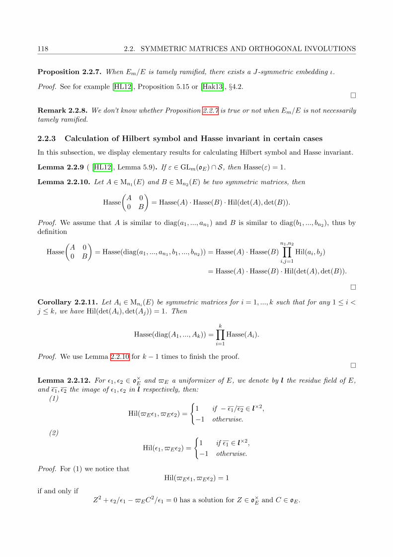
118 2.2. SYMMETRIC MATRICES AND ORTHOGONAL INVOLUTIONS
Proposition 2.2.7. When Em/E is tamely ramified, there exists a J-symmetric embedding ι.
Proof. See for example [HL12], Proposition 5.15 or [Hak13], §4.2.
Remark 2.2.8. We don’t know whether Proposition 2.2.7 is true or not when Em/E is not necessarilytamely ramified.
2.2.3 Calculation of Hilbert symbol and Hasse invariant in certain cases
In this subsection, we display elementary results for calculating Hilbert symbol and Hasse invariant.
Lemma 2.2.9 ( [HL12], Lemma 5.9). If ε ∈ GLm(oE) ∩ S, then Hasse(ε) = 1.
Lemma 2.2.10. Let A ∈ Mn1(E) and B ∈ Mn2(E) be two symmetric matrices, then
Hasse
(A 00 B
)= Hasse(A) ·Hasse(B) ·Hil(det(A),det(B)).
Proof. We assume that A is similar to diag(a1, ..., an1) and B is similar to diag(b1, ..., bn2), thus bydefinition
Hasse
(A 00 B
)= Hasse(diag(a1, ..., an1 , b1, ..., bn2)) = Hasse(A) ·Hasse(B)
n1,n2∏i,j=1
Hil(ai, bj)
= Hasse(A) ·Hasse(B) ·Hil(det(A), det(B)).
Corollary 2.2.11. Let Ai ∈ Mni(E) be symmetric matrices for i = 1, ..., k such that for any 1 ≤ i <j ≤ k, we have Hil(det(Ai), det(Aj)) = 1. Then
Hasse(diag(A1, ..., Ak)) =k∏i=1
Hasse(Ai).
Proof. We use Lemma 2.2.10 for k − 1 times to finish the proof.
Lemma 2.2.12. For ε1, ε2 ∈ o×E and $E a uniformizer of E, we denote by l the residue field of E,and ε1, ε2 the image of ε1, ε2 in l respectively, then:
(1)
Hil($Eε1, $Eε2) =
{1 if − ε1/ε2 ∈ l×2,
−1 otherwise.
(2)
Hil(ε1, $Eε2) =
{1 if ε1 ∈ l×2,
−1 otherwise.
Proof. For (1) we notice thatHil($Eε1, $Eε2) = 1
if and only ifZ2 + ε2/ε1 −$EC
2/ε1 = 0 has a solution for Z ∈ o×E and C ∈ oE .

THESE DE DOCTORAT DE L’UNIVERSITE PARIS-SACLAY 119
Since if the equation $Eε1X2 + $Eε2Y
2 = 1 has a solution, comparing the order we must haveX−1, Y −1 ∈ pE and X/Y ∈ o×E . Thus we can change the variables Z = X/Y and C = $−1
E Y −1.Using the Hensel lemma for the polynomial P (Z) = Z2 + ε2/ε1 −$EC
2/ε1 and the fact that p 6= 2,the condition above is true if and only if
Z2
= −ε2/ε1 has a solution for Z ∈ l×,
which is equivalent to −ε1/ε2 ∈ l×2. Thus we finish the proof of (1), and the proof of (2) is similar.
Remark 2.2.13. In the latter sections, we mainly consider two cases: E = F or E/F is a fieldextension of degree d given by a certain simple stratum related to a given supercuspidal representation.In the former case, we have m = n; In the latter case, we have m such that n = md with d = [E : F ].Moreover, we will simply write det, disc and Hasse for short when E = F .
From now on until the end of this section, we assume E to be a tamely ramified extension ofdegree d = ef over F , where f denotes its residue class degree and e denotes its ramification index.Using Proposition 2.2.7, we fix a J-symmetric embedding E ↪→ Md(F ). We fix ε0 ∈ o×E\o
×2E and $E
a uniformizer of E, such that E×/E×2 = {1, ε0, $E , ε0$E}. By Section 3 of [Hak13], we have threedifferent cases:
Proposition 2.2.14. (1) NE/F (E×)F×2/F×2 = {1} if and only if E contains three quadratic subex-tensions over F , and exactly one of them is unramified. Thus both e and f are even;
(2) NE/F (E×)F×2/F×2 is of order 2 if and only if E contains exactly one quadratic subextensionover F . Thus either e or f is even;
(3) NE/F (E×)F×2/F×2 = F×/F×2 if and only if E contains no quadratic subextension over F .Thus d = ef is odd.
For case (1), we have the following lemma:
Lemma 2.2.15. If NE/F (E×)F×2/F×2 = {1}, then we may further choose the uniformizer $E of E,such that
Hasse(Jd$E) = 1 and Hasse(Jd$Eε0) = −1,
where Jd$E and Jd$Eε0 are symmetric matrices in GLd(F ).
Proof. We may use [Hak13], Proposition 6.6 directly.
For case (2), first we assume that f is odd and e is even. We have:
Lemma 2.2.16. For f odd and e even, we have Hasse(Jd$E) 6= Hasse(Jd$Eε0).
Proof. We use the proof of [Hak13], Proposition 6.6 directly, except that right now f is odd insteadof being even. Our question reduces to calculate the following term
Hasse(diag(u1, ..., uf , u1$F , ..., uf$F )) (with u1, ..., uf ∈ o×F )
in the case where∏fi=1 ui ∈ F×2 or ε′0F
×2 respectively with ε′0 ∈ o×F \o×2F fixed, and to show that they
are different. From the calculation in loc. cit., we have
Hasse(diag(u1, ..., uf , u1$F , ..., uf$F )) = (
f∏i=1
Hil(ui, $F ))2f−1 ·Hil($F , $F )f(f−1)/2
= Hil(
f∏i=1
ui, $F ) ·Hil($F , $F )f(f−1)/2

120 2.2. SYMMETRIC MATRICES AND ORTHOGONAL INVOLUTIONS
Thus by Lemma 2.2.12.(2), when∏fi=1 ui ∈ F×2 or ε′0F
×2 respectively, the corresponding terms aredifferent.
Corollary 2.2.17. Under the assumption of Lemma 2.2.16, the Hasse invariants
Hasse(diag(Jd$E , ..., Jd$E , Jd$E)) and Hasse(diag(Jd$E , ..., Jd$E , Jd$Eε0))
are different, where the two matrices are in Mm(Md(F )) = Mmd(F ).
Proof. We write
A = diag(Jd$E , ..., Jd$E) ∈ Mm−1(Md(F )) = M(m−1)d(F ),
then using Lemma 2.2.10, we have
Hasse(diag(Jd$E , ..., Jd$E , Jd$E)) = Hasse(A) ·Hasse(Jd$E) ·Hil(det(A),det(Jd$E))
and
Hasse(diag(Jd$E , ..., Jd$E , Jd$Eε0)) = Hasse(A) ·Hasse(Jd$Eε0) ·Hil(det(A),det(Jd$Eε0)).
Thus using Lemma 2.2.16, we only need to show that
Hil(det(A), det(Jd$E)) = Hil(det(A), det(Jd$Eε0)),
which follows from the fact that det(ε0) = NE/F (ε0) ∈ F×2 when e is even.
Now we assume that e is odd. First we consider the case where f is even. In this case, NE/F (ε0) /∈F×2. We choose $′E to be another uniformizer of E such that NE/F ($′E) ∈ F×2.
Lemma 2.2.18. If e and m are odd and if f is even, then
Hasse(diag(Jd$E , ...Jd$E , Jd$′E)) = 1
and
Hasse(diag(Jd$Eε0, ...Jd$Eε0, Jd$′Eε0)) = −1,
where the two matrices are in Mm(Md(F )) = Mmd(F ).
Proof. To begin with, we state and proof the following general lemma which is useful not only in thisproof, but in the latter sections.
Lemma 2.2.19. Let E/L be a finite extension of non-archimedean locally compact fields of residuecharacteristic p 6= 2 with odd degree, and let
L×/L×2 → E×/E×2
be the homomorphism induced by the canonical embedding L ↪→ E, then the homomorphism aboveinduces two isomorphisms
L×/L×2 ∼= E×/E×2 and o×L/o×2L∼= o×E/o
×2E .

THESE DE DOCTORAT DE L’UNIVERSITE PARIS-SACLAY 121
Proof. The embedding L ↪→ E leads to the following embedding:
L×/E×2 ∩ L× ↪→ E×/E×2.
First we have L×2 ⊂ E×2 ∩ L×. And for x ∈ E×2 ∩ L×, let x = y2 with y ∈ E×. Thus L[y] is asubextension of E over L which is of degree 1 or 2. Since [E : L] is odd, we must have L[y] = L andy ∈ L. So x ∈ L×2, which means that E×2 ∩L× = L×2 since x is arbitrary. Thus the homomorphismin the lemma is injective, which is an isomorphism since [E× : E×2] = [L× : L×2] = 4.
Moreover, since |o×L/o×2L | = |o
×E/o
×2E | = 2, the isomorphism above also leads to an isomorphism
o×L/o×2L∼= o×E/o
×2E .
Come back to the original proof. We write L for the maximal unramified subextension of E overF , then [L : F ] = f and [E : L] = e. Since e is odd, by Lemma 2.2.19 we have an isomorphism
o×E/o×2E∼= o×L/o
×2L .
Since the result doesn’t depend on the choice of $E , $′E and ε0 as representatives in E×/E×2,we may assume that $e
E = $L is a uniformizer in L, and $′eE = $′L is a uniformizer in L suchthat NL/F ($′L) ∈ F×2, and ε0 ∈ o×L\o
×2L . From the construction of the J-symmetric embedding in
Proposition 2.2.7 (see the proof of [Hak13], Proposition 6.6 for more details), we may write
Jd$E = diag(J(e−1)f , Jf$L) and Jd$′E = diag(Je(f−1), Jf$
′L)
andJd$Eε0 = diag(J(e−1)f ε0, Jf$Lε0) and Jd$
′Eε0 = diag(Je(f−1)ε0, Jf$
′Lε0).
Since det(J(e−1)f ) ∈ o×F , and since det(diag(Jf$L, ..., Jf$L, Jf$′L)) is of even order in F×, using
Lemma 2.2.9 and Corollary 2.2.11, we get
Hasse(diag(Jd$E , ..., Jd$E , Jd$′E)) = Hasse(diag(Jf$L, ..., Jf$L, Jf$
′L)), (2.2.1)
where the matrix in the Hasse of the right hand side is of size fm. Similarly we have
Hasse(diag(Jd$Eε0, ..., Jd$Eε0, Jd$′Eε0)) = Hasse(diag(Jf$Lε0, ..., Jf$Lε0, Jf$
′Lε0)), (2.2.2)
where the matrix in the Hasse of the right hand side is also of size fm. Since L/F is unramified, wemay write $L = $F v and $′L = $F v
′ with v, v′ ∈ o×T , thus the term in (2.2.1) equals
Hasse(diag(Jfv$F , ..., Jfv$F , Jfv′$F )), (2.2.3)
and the term in (2.2.2) equals
Hasse(diag(Jfvε0$F , ..., Jfvε0$F , Jfv′ε0$F )). (2.2.4)
Since f is even, det(Jf$F ) and det(Jfv′$F ) are of even order in F×, thus by Lemma 2.2.11, (2.2.3)
equalsHasse(Jfv$F )m−1 ·Hasse(Jfv
′$F ) = Hasse(Jfv′$F )
and similarly (2.2.4) equals
Hasse(Jfvε0$F )m−1 ·Hasse(Jfv′ε0$F ) = Hasse(Jfv
′ε0$F ).

122 2.2. SYMMETRIC MATRICES AND ORTHOGONAL INVOLUTIONS
We assume that Jfv′ is similar to diag(1, ..., 1, u1) and Jfv
′ε0 is similar to diag(1, ..., 1, u2) with u1, u2 ∈o×F , then (2.2.3) equals
Hasse(diag($F , ..., $F , $Fu1)),
and (2.2.4) equals
Hasse(diag($F , ..., $F , $Fu2)).
By direct calculation, we get
det(Jfv′$F ) = (−1)f(f−1)/2NL/F ($′L) ∈ (−1)f(f−1)/2F×2
and
det(Jfv′ε0$F ) = (−1)f(f−1)/2NL/F (ε0$
′L) ∈ (−1)f(f−1)/2NL/F (ε0)F×2,
where NL/F (ε0) ∈ o×F \o×2F .
If −1 ∈ F×2 or if −1 /∈ F×2 and 4|f , then det(Jfv′) ∈ o×2
F and det(Jfv′ε0) ∈ o×F \o
×2F . We may
assume u1 = 1 and u2 ∈ o×F \o×2F , where in the latter case we may further assume u2 = −1. So by
Lemma 2.2.12.(1), when −1 ∈ F×2 we have
Hasse(diag($F , ..., $F , $Fu1)) = 1
and
Hasse(diag($F , ..., $F , $Fu2)) = (−1)f−1 = −1.
When −1 /∈ F×2 and 4|f , we have
Hasse(diag($F , ..., $F , $Fu1)) = (−1)f(f−1)/2 = 1,
and
Hasse(diag($F , ..., $F ,−$F )) = (−1)(f−1)(f−2)/2 = −1.
If −1 /∈ F×2 and 4 - f , then det(Jfv′) ∈ o×F \o
×2F and det(Jfv
′ε0) ∈ o×2F . We may assume u1 = −1
and u2 = 1 and we have
Hasse(diag($F , ..., $F ,−$F )) = (−1)(f−1)(f−2)/2 = 1
and
Hasse(diag($F , ..., $F , $F )) = (−1)f(f−1)/2 = −1.
Thus we finish the proof.
Finally, we drop the assumption that f is even.
Lemma 2.2.20. If e is odd, m is even and one of the three cases happens:
• 2|d;
• 2 - d and 4|m;
• 2 - d, 4 - m and −1 ∈ F×2,
then Hasse(diag(Jd$E , ..., Jd$E , Jd$Eε0)) = −1, where the matrix in Hasse is in Mmd(F ).

THESE DE DOCTORAT DE L’UNIVERSITE PARIS-SACLAY 123
Proof. We write L for the maximal unramified extension of F contained in E, thus [L : F ] = f and[E : L] = e. Since e is odd, by Lemma 2.2.19 we get
o×E/o×2E∼= o×L/o
×2L .
Since the result doesn’t depend on the choice of $E and ε0 as representatives in E×/E×2, we maychoose $E as a uniformizer of E such that $e
E = $L is a uniformizer in L, and ε0 ∈ o×L\o×2L . As in
Lemma 2.2.18, we may write
Jd$E = diag(J(e−1)f , Jf$L) and Jd$Eε0 = diag(Je(f−1)ε0, Jf$Lε0).
Thus by Corollary 2.2.11 and the fact that m is even, we get
Hasse(diag(Jd$E , ..., Jd$E , Jd$Eε0)) = Hasse(diag(Jf$L, ..., Jf$L, Jf$Lε0)), (2.2.5)
where the last term in the Hasse is a matrix of size fm. Since L/F is unramified, we may write$L = $F v with v ∈ o×T , thus the term in (2.2.5) equals
Hasse(diag(Jfv$F , ..., Jfv$F , Jfv$F ε0)).
If we assume that Jfv is similar to diag(1, ..., 1, u1), and Jfvε0 is similar to diag(1, ..., 1, u2), then weget u2/u1 ∈ o×F \o
×2F . Moreover we get
Hasse(diag(Jfv$F , ..., Jfv$F , Jfv$F ε0)) = Hasse(diag(Im(f−1)$F , u1$F , ..., u1$F , u2$F )), (2.2.6)
where the last diagonal matrix in Hasse is of size fm.If −1 ∈ F×2, we may choose either u1 = 1 and u2 = ε′0, or u1 = ε′0 and u2 = 1 with ε′0 ∈ o×F \o
×2F .
Thus in the former case, by Lemma 2.2.12.(1) the (2.2.6) equals
Hasse(diag(Imf−1$F , $F ε′0)) = (−1)mf−1 = −1,
and in the latter case, by Lemma 2.2.12.(1) the (2.2.6) equals
Hasse(diag(Imf−m+1$F , Im−1$F ε′0)) = (−1)(mf−m+1)(m−1) = −1.
If −1 /∈ F×2, we may assume ε′0 = −1, u1 equals 1 or −1 and u2 = −u1, and for the two casesusing Lemma 2.2.12.(1) the (2.2.6) equals
Hasse(diag(Ifm−1$F ,−$F )) = (−1)(fm−1)(fm−2)/2 = −1
orHasse(diag(I(f−1)m+1$F ,−Im−1$F )) = (−1)fm(fm−1)/2−((f−1)m+1)(m−1) = −1,
where in both cases we use the fact that 4|fm and 2|m, thus we finish the proof.
Finally we have the following lemma which completes Lemma 2.2.20.
Lemma 2.2.21. If d is odd, m is even not divided by 4 and −1 /∈ F×2, then
Hasse(diag(Jd$E , ..., Jd$E , Jd$E)) = −1,
where the matrix is in Mmd(F ).
Proof. We may follow the same proof as Lemma 2.2.20, which finally shows that
Hasse(diag(Jd$E , ..., Jd$E , Jd$E)) = Hasse(Ifm$F ).
Since −1 /∈ F×2, by Lemma 2.2.12.(1) the latter term equals (−1)fm(fm−1)/2, which is −1 since underour assumption fm ≡ 2 (mod 4). Thus we finish the proof.

124 2.3. τ -SELFDUAL TYPE THEOREM
2.3 τ-selfdual type theorem
Let π be a supercuspidal representation of G. Let τ = τε be the orthogonal involution correspondingto a symmetric matrix ε, such that for H = Gτ as the orthogonal group corresponding to τ , it satisfiesthe condition 2 of Theorem 0.3.1 with respect to π. For a an oF -subalgebra of Mn(F ), we define
τ(a) := ε−1 taε
which is an oF -subalgebra of Mn(F ). We say that a is τ -stable if τ(a) = a. For any g ∈ G, it is easyto show that τ(ag) = τ(a)τ(g).
In this section, we follow the strategy in chapter 1, section 5 to prove the following theorem:
Theorem 2.3.1. For π and τ as above, there exists a maximal simple stratum [a, β] and a simplecharacter θ ∈ C(a, β) contained in π, such that
(1) τ(a) = a and τ(H1(a, β)) = H1(a, β);
(2) θ ◦ τ = θ−1;
(3) τ(β) = β−1.
As a corollary of Theorem 2.3.1, we have the following τ -selfdual type theorem.
Theorem 2.3.2. For π and τ as above, there exists a τ -selfdual simple type (J ,Λ) that compactlyinduces π.
Proof. We only need to follow the proof of Theorem 1.5.3, with Theorem 1.5.2 replaced by Theorem2.3.1.
Now we state the following general theorem which implies Theorem 2.3.1.
Theorem 2.3.3. Let [a, β] be a maximal simple stratum in Mn(F ), let T be the maximal tamelyramified subextension of E/F , let Tm be the unramified extension of degree m over T and let θ ∈ C(a, β)be a simple character. Let τ be an orthogonal involution of G such that H = Gτ satisfies the condition 2of Theorem 0.3.1. Then there exist a maximal simple stratum [a′, β′] in Mn(F ) and a simple characterθ′ ∈ C(a′, β′) such that
(1) τ(a′) = a′ and τ(H1(a′, β′)) = H1(a′, β′);
(2) θ′ and θ are in the same endo-class and θ′ ◦ τ = θ′−1;
(3) τ(β′) = β′−1.
For π given as in Theorem 2.3.1, if we choose [a, β] to be a maximal simple stratum and θ ∈ C(a, β)to be a simple character contained in π, then Theorem 2.3.3 implies Theorem 2.3.1. So from now on,we focus on the proof of Theorem 2.3.3. We write E = F [β], d = [E : F ] and m = n/d. In thefollowing subsections, we gradually consider the following three cases: E/F is maximal and totallywildly ramified, E/F is maximal and the general case.
To begin with, we state the following lemmas which will be useful in our future proof.
Lemma 2.3.4. Let [a, β] be a maximal simple stratum in Mn(F ) and let θ ∈ C(a, β), then for τ asan orthogonal involution on G, the simple characters θ ◦ τ and θ−1 are in the same endo-class. Inparticular, if τ(a) = a, then θ ◦ τ is conjugate to θ−1 by an element in U(a).
Proof. We follow the same proof of Lemma 1.5.7, with σ in loc. cit. replaced by the trivial action.

THESE DE DOCTORAT DE L’UNIVERSITE PARIS-SACLAY 125
Lemma 2.3.5. Let τ = τε be the orthogonal involution on G corresponding to a symmetric matrix ε,let [a, β] be a maximal simple stratum in Mn(F ) and let θ ∈ C(a, β) be a simple character, such that
τ(a) = a, θ ◦ τ = θ−1 (and τ(β) = β−1).
Then for τ ′ = τε′ as the orthogonal involution on G corresponding to the symmetric matrix ε′ = tgεg,we have
τ ′(ag) = ag, θg ◦ τ ′ = (θg)−1 (and τ ′(βg) = (βg)−1).
Proof. Same proof as Lemma 1.5.8.
Lemma 2.3.6. Let [a, β] be a maximal simple stratum in Mn(F ) and let θ ∈ C(a, β) such that τ(a) = a,τ(H1(a, β)) = H1(a, β) and θ ◦ τ = θ−1. Then there exists a simple stratum [a, γ] such that θ ∈ C(a, γ)and τ(γ) = γ−1.
Proof. For τ = τε with respect to a symmetric matrix ε, we define
σε(x) := ε−1 txε for any x ∈ Mn(F )
as an anti-involution on Mn(F ). Then we may use the same argument in Proposition 1.5.19, with σtin loc. cit. replaced by σε, and the original proof in [Ste01], Theorem 6.3 works.
2.3.1 The maximal and totally wildly ramified case
In this subsection, we prove the following special case of Theorem 2.3.3.
Proposition 2.3.7. Let [a, β] be a simple stratum in Mn(F ) and let θ ∈ C(a, β) be a simple character,where n = d and E/F is totally wildly ramified. Then for τ = τIn the orthogonal involution onG, there exist a simple stratum [a′, β′] and a simple character θ′ ∈ C(a′, β′) such that (a′, θ′) is G-conjugate to (a, θ) with the property τ(a′) = a′ and θ′ ◦ τ = θ′−1. Moreover, we may further assumethat a′ ⊂ Mn(oF ).
Proof. We explain how the proof of Proposition 1.5.9 could be used directly in our case. First up toG-conjugacy, we may assume a to be the standard minimal order of Mn(F ). We have the followinglemma corresponding to Lemma 1.5.11:
Lemma 2.3.8. There exist g1 ∈ GLn(oF ) and a1, ..., an ∈ o×F such that
τ(g1)g−11 = A :=
0 0 . . . 0 a1
0 . ..
. ..a2 0
... . ..
. ... .. ...
0 an−1 . ... ..
0an 0 . . . 0 0
.
Moreover, if we define a′′ := ag1, then we have τ(a′′) = a′′.
Proof. We choose a1 = ... = a(n−1)/2 = a(n+3)/2 = ... = an = 1, and a(n+1)/2 equals 1 or −1 to makesure that det(A) = 1. Since the oF -lattice of rank n equipped with a quadratic form correspondingto A is unimodular in the sense of [O’M71], §92, by §92:1 in loc. cit., there exists g1 ∈ GLn(oF ) suchthat tg−1
1 g−11 = A, or equivalently τ(g1)g−1
1 = A. Then we may use the same proof as that in Lemma1.5.11 to obtain τ(a′′) = a′′.

126 2.3. τ -SELFDUAL TYPE THEOREM
By Lemma 2.3.8, we may choose g1 ∈ GLn(oF ) such that a′′ = ag1 is τ -invariant. Let M = o×F×...×o×F be the subgroup of GLn(oF ) via diagonal embedding, let M ′′ = Mg1 and U ′′1 = U1g1 := U1(a)g1 .Then using directly the proof of Proposition 1.5.9, with all the Galois involution in loc. cit. replacedby the trivial action, there exists x ∈ M ′′U ′′1 such that for a′ = a′′x = ag1x and θ′ = θg1x, we haveτ(a′) = a′ and θ′ ◦ τ = θ′−1. Moreover since g1x ∈ g1M
′′U ′′1 = MU1g1 ⊂ GLn(oF ) and a ⊂ Mn(oF ),we get a′ = ag1x ⊂ Mn(oF ).
2.3.2 The maximal case
In this subsection, we further use the result proved in §2.3.1 to consider the following special case ofTheorem 2.3.3.
Proposition 2.3.9. Let [a, β] be a simple stratum in Mn(F ) and let θ ∈ C(a, β) be a simple characterwith n = d. Then for an orthogonal involution τ = τε which is G-conjugate to τJn, there exist a simplestratum [a′, β′] and a simple character θ′ ∈ C(a′, β′) such that (a′, θ′) is G-conjugate to (a, θ) with theproperty τ(a′) = a′, θ′ ◦ τ = θ′−1 and τ(β′) = β′−1.
Remark 2.3.10. If we assume E/F to be totally wildly ramified, then by direct calculation and Lemma2.2.9, we have
det(In) = det(Jn) or det(−Jn) and Hasse(In) = Hasse(Jn) = Hasse(−Jn) = 1.
Thus In is G-conjugate to Jn or −Jn, which means that τIn is G-conjugate to τJn. Choosing ε = In,Proposition 2.3.9 implies Proposition 2.3.7.
Remark 2.3.11. Since τJn represents the split orthogonal group, it satisfies the condition of Theorem2.3.3, which justifies that Proposition 2.3.9 is indeed a special case of Theorem 2.3.3.
Proof. We write n = t(n/t) with t = [T : F ] and n/t a power of p as an odd number, where T is themaximal tamely ramified subextension of E over F . We define
Jt,n/t := diag(Jt, ..., Jt)
as a matrix in Mn/t(Mt(F )) = Mn(F ). Using Lemma 2.2.9, we have
Hasse(Jt,n/t) = Hasse(Jn) = Hasse(−Jn) = 1.
Moreover by direct calculation we have
det(Jt,n/t) = det(Jn) or det(−Jn).
Thus using Proposition 2.2.1, Jt,n/t is similar to Jn or −Jn. Thus τJt,n/t is G-conjugate to τJn and τε.
By Proposition 2.2.3, we may replace ε by multiplying an element in F× to make sure that ε is similarto Jt,n/t. Thus using Lemma 2.3.5, we only need to consider the case where ε = Jt,n/t and τ = τJt,n/t .So from now on we assume ε = Jt,n/t.
Using Proposition 2.2.7, we may choose
ι : T ↪→ Mt(F )
to be an F -algebra embedding which is Jt-symmetric. By abuse of notation, we consider the followingembedding
ι : Mn/t(T ) ↪→ Mn/t(Mt(F )) = Mn(F )

THESE DE DOCTORAT DE L’UNIVERSITE PARIS-SACLAY 127
given by mapping each entry T to the corresponding Mt(F ) via the original ι. If we regard T as anF -subalgebra of Mn/t(T ) given by the diagonal embedding, then ι(T )× is fixed by τ . By the Skolem-Noether theorem, we may choose g ∈ G such that ι(T ) = T g. Thus using [ag, βg] and θg to replace[a, β] and θ, we may suppose ι(T ) to be the maximal tamely ramified extension with respect to E/F .Thus we identify T with ι(T ) and omit ι.
Let C = Mn/t(T ) denote the centralizer of T in Mn(F ) and let tC denote the transpose on C. Forc = (cij)ij ∈ GLn/t(T ), we have
τ(c) = (J−1t,n/t
tcJt,n/t)−1 = ((J−1
ttcjiJt)ij)
−1 = ((cji)ij)−1 = tCc−1 = τ ′(c)
where we use the fact that ι is Jt-symmetric and we write τ ′(x) = tCx−1 for any x ∈ C×. Thus τ ′
as the restriction of τ to C× is the orthogonal involution τIn/t on C× = GLn/t(T ). As mentionedin §2.1.2, the intersection c = a ∩ C gives rise to a simple stratum [c, β] and the restriction of θ toH1(c, β), denoted by θT , is the interior T/F -lift of θ. Since E/T is totally wildly ramified, usingProposition 2.3.7 with G, θ and τ replaced by C×, θT and τ ′ respectively, there exists c ∈ C× suchthat τ ′(cc) = cc and θcT ◦ τ ′ = (θcT )−1. As a corollary, we also have τ ′(H1(cc, βc)) = H1(cc, βc) andC(cc,−βc) = C(cc, τ ′(βc)).
By the injectivity of a 7→ a ∩ C between sets of hereditary orders mentioned in §2.1.2, a′ := ac isτ -stable. Moreover if we write θ′ = θc and T ′ = T c, then from our construction of τ and the definitionof T ′/F -lift, we know that
(θ′ ◦ τ)T ′ = θ′ ◦ τ |H1(cc,βc) = θ′ ◦ τ ′|H1(cc,βc) = θ′T ′ ◦ τ ′
and(θ′−1)T ′ = θ′−1
T ′
are equal. Thus by the last paragraph of §2.1.2, the simple character θ′ satisfies the property θ′ ◦ τ =θ′−1.
Finally using Lemma 2.3.6 with ε = Jt,n/t, we may choose β′ in the simple stratum such thatθ′ ∈ C(a′, β′) and τ(β′) = β′−1, thus we finish the proof.
Before we prove the general case, we state and prove the following important lemma which studiesthe set εE′× consisting of symmetric matrices, where E′ = F [β′] with β′ chosen as in Proposition2.3.9.
Lemma 2.3.12. We may choose [a′, β′] and θ′ ∈ C(a′, β′) satisfying the conclusion of Proposition 2.3.9and T as a tame parameter field of θ′, and we may fix ι : T ↪→ Mt(F ) as a J-symmetric embeddinggiven by Proposition 2.2.7, such that for any x ∈ E′×, there exists xt ∈ T× such that εx is similar todiag(Jtι(xt), ..., Jtι(xt)).
Proof. First we assume ε = Jt,d/t. We recall that in the proof of Proposition 2.3.9, first we obtain asimple stratum [a′, β] and a simple character θ′ ∈ C(a′, β), such that τ(a′) = a′ and θ′ ◦ τ = θ′−1, thenwe use Lemma 2.3.6 to get β′. In this case we have θ′ ∈ C(a′, β) ∩ C(a′, β′), thus J1(a′, β) = J1(a′, β′)as the maximal pro-p-subgroup of the normalizer of θ. Moreover from our construction of [a′, β], for Tthe maximal tamely ramified subextension of E/F with E = F [β] and for ι : T ↪→ Mt(F ) the chosenJ-symmetric embedding, we have
T = {diag(ι(xt), ..., ι(xt)) ∈ Md/t(Mt(F )) = Md(F )|xt ∈ T}.
Thus we getεT× = {diag(Jtι(xt), ..., Jtι(xt)) ∈ Md/t(Mt(F )) = Md(F )|xt ∈ T×}.

128 2.3. τ -SELFDUAL TYPE THEOREM
We write T ′ for the maximal tamely ramified subextension of E′/F with E′ = F [β′]. By Lemma2.2.19 with E = E′ and L = T ′, the embedding T ′ ↪→ E′ induces an isomorphism
T ′×/T ′×2 ∼= E′×/E′×2.
Thus for any x ∈ E′×, there exists y ∈ E′× such that xy2 ∈ T ′×. Thus
εx = ty−1ε(xy2)y−1,
where we use the fact that ε−1 ty−1ε = y−1. Thus every element in εE′× is similar to an element inεT ′×. Thus to finish the proof, we only need to show that any element in εT ′× is similar to an elementin εT×.
Using [BH14b], Proposition 2.6, there exists j ∈ J1(a′, β) = J1(a′, β′) such that T ′ = T j . For anyx ∈ T×, we have j−1xj ∈ T ′×. Thus we get τ(x) = x−1 and τ(j−1xj) = (j−1xj)−1, which implies that
kxk−1 = τ(x−1) = x,
where k := τ(j)j−1 ∈ C ∩J1(a′, β) = J1(c′, β) ⊂ U1(c′) with C = ZMd(F )(T ) = Md/t(T ). Moreover wehave
εj−1xj = (εj−1ε−1)εxj = tτ(j)εxj = tj tkεxj,
So we only need to show that tkεx is similar to εx.
We denote by τ ′ the restriction of τ to C×, thus by definition τ ′(c) = tCc−1 for any c ∈ C×, wheretC denotes the transpose on C. Since τ(k)k = 1, we have τ ′(k)k = 1, or equivalently tCk = k. SincedetC(k) ∈ 1 + pT ⊂ T×2 and HasseT (k) = 1 by Proposition 2.3.7 and Lemma 2.2.9, by Proposition2.2.1, there exists m ∈ C× such that
tCmm = tCk or equivalently τ(m)−1m = τ(k)−1,
where we denote by detC the determinant with respect to C = Md/t(T ) and by HasseT the Hasseinvariant with respect to T . Thus
tkεx = ετ(k)−1x = ετ(m)−1mx = tmεmx = tmεxm,
which means that tkεx is similar to εx. So we finish the proof when ε = Jt,d/t.
For the general case, since τε and τJt,d/t are G-conjugate, we may choose ε up to multiplying an
element in F×, such that ε = tgJt,d/tg with a certain g ∈ G. We assume that [a′, β′] and θ′ satisfythis lemma for τ = τJt,d/t . We choose [a′′, β′′] := [a′g, β′g], θ′′ = θ′g, and by Lemma 2.3.5 we have
τε(a′′) = a′′, θ′′ ◦ τε = θ′′−1 and τε(β
′′) = β′′−1.
Moreover we have
εE′′× = tgJt,d/tgE′×g = tg(Jt,d/tE
′×)g,
which means that each element in εE′′× is similar to an element in Jt,d/tE′×. Thus [a′′, β′′], θ′′ satisfy
the condition of the lemma when τ = τε.
Remark 2.3.13. From the proof we may further observe that when ε = Jt,d/t, if we identify T withthe maximal tamely ramified subextension of E′ over F via an F -embedding, then x and xt are in thesame class of T×/T×2 ∼= E′×/E′×2 given by Lemma 2.2.19 for E = E′ and L = T .

THESE DE DOCTORAT DE L’UNIVERSITE PARIS-SACLAY 129
Finally we state and prove the following corollary, saying the results for calculating Hasse invariantin §2.2.3 can be generalized to the case where E/F is not necessarily tamely ramified, once E is well-chosen.
Corollary 2.3.14. For ε = Jd and [a′, β′], θ′ constructed in Lemma 2.3.12, the results in Lemma2.2.15, Lemma 2.2.16, Corollary 2.2.17, Lemma 2.2.18, Lemma 2.2.20, Lemma 2.2.21 hold for E =E′.
Proof. Since all the proofs are similar, we only prove Lemma 2.2.20 as an example.
First of all when d is even, by direct calculation and Lemma 2.2.9 we have det(Jt,d/t) = det(Jd)and Hasse(Jt,d/t) = Hasse(Jd) = 1. Thus Jt,d/t is similar to Jd. Using this fact and Remark 2.3.13, wededuce that when ε = Jd, we may assume x and xt in the result of Lemma 2.3.12 to be in the sameclass of E′×/E′×2 ∼= T×/T×2, where we identify T with the maximal tamely ramified subextensionof E′ over F via an embedding. In particular, when x = $E′ is a uniformizer of E′, we may assumext = $T to be a uniformizer of T in the same class as that of $E′ , and when x = $E′ε0 with ε0 anelement in o×E′\o
×2E′ , we may also assume xt = $T ε
′0 with ε′0 an element in o×T \o
×2T . Thus using Lemma
2.3.12 for x = $E′ and x = $E′ε0, we have
Hasse(diag(Jd$E′ , ..., Jd$E′ , Jd$E′ε0))
= Hasse(diag(diag(Jt$T , ..., Jt$T ), ...,diag(Jt$T , ..., Jt$T ), diag(Jt$T ε′0, ..., Jt$T ε
′0)))
= Hasse(diag(diag(Jt$T , ..., Jt$T , Jt$T ε′0), ...,diag(Jt$T , ..., Jt$T , Jt$T ε
′0)))
= Hasse(diag(Jt$T , ..., Jt$T , Jt$T ε′0))n/t
= Hasse(diag(Jt$T , ..., Jt$T , Jt$T ε′0)),
where the matrix in the third line is the direct sum of n/t copies of diag(Jt$T , ..., Jt$T , Jt$T ε′0) ∈
Mtm(F ), and for the fourth line we use the fact that det(diag(Jt$T , ..., Jt$T , Jt$T ε′0)) is of even order
in F× and Corollary 2.2.11, and for the final line we use the fact that n/t is odd. Thus we may usethe tamely ramified case to finish the proof.
When d is odd, if det(Jt,d/t) = det(Jd) we can still follow the proof above verbatim. If det(Jt,d/t) =det(−Jd), we deduce that Jt,d/t is similar to −Jd. Thus following the above proof, when x = $E′
(resp. $E′ε0) we may choose xt = −$T (resp. −$T ε′0), where $E′ , $T , ε0, ε′0 are defined as above.
Thus for $′T = −$T as a uniformizer of T and using the same calculation, we have
Hasse(diag(Jd$E′ , ..., Jd$E′ , Jd$E′ε0)) = Hasse(diag(Jt$′T , ..., Jt$
′T , Jt$
′T ε′0)).
And still we use the tamely ramified case to finish the proof.
2.3.3 The general case
In this subsection, we finish the proof of Theorem 2.3.3. For [a, β] and θ ∈ C(a, β) given as in thetheorem, we choose β0 ∈ Md(F ) such that there exists an F -algebra isomorphism F [β0]→ F [β] whichmaps β0 to β. Let a0 be the unique hereditary order of Md(F ) normalized by β0. Thus [a0, β0] is
a simple stratum of Md(F ) and we let θ0 = tβ,β0a,a0 (θ) be the transfer of θ as a simple character with
respect to [a0, β0]. Using Proposition 2.3.9, for τJd the involution on GLd(F ), there exist a simplestratum [a′0, β
′0] and a simple character θ′0 ∈ C(a′0, β′0) such that (a′0, θ
′0) is GLd(F )-conjugate to (a0, θ0)
with the following property:
(1) τJd(a′0) = a′0 and τJd(H
1(a′0, β′0)) = H1(a′0, β
′0);
(2) θ′0 ◦ τJd = θ′−10 ;

130 2.3. τ -SELFDUAL TYPE THEOREM
(3) τJd(β′0) = β′−1
0 ;
(4) Corollary 2.3.14 holds.
Now we embed Md(F ) diagonally in Mn(F ), which gives an F -algebra homomorphism ι′ : F [β′0] ↪→Mn(F ). We write β′ = ι′(β′0) = β′0 ⊗ ...⊗ β′0 and E′ = F [β′]. The centralizer of E′ in Mn(F ), denotedby B′, is naturally identified with Mm(E′). Let b′ be a maximal standard hereditary order in B′ whichmay be identified with Mm(oE′), and let a′ be the unique hereditary order in Mn(F ) normalized by E′×
such that a′∩B′ = b′. Then we obtain a simple stratum [a′, β′] in Mn(F ). Let θ′ = tβ′0,β
′
a′0,a′ (θ′0) ∈ C(a′0, β′0)
be the transfer of θ′0.
We denote by T ′ the maximal tamely ramified subextension of E′/F and we denote by T ′m anunramified extension of degree m over T ′. We denote by E′m = T ′mE
′ an unramified extension ofdegree m over E′. Since E′/T ′ and E′m/T
′m are totally wildly ramified, it is easy to check that
NT ′/F (T ′×)F×2/F×2 = NE′/F (E′×)F×2/F×2 (2.3.1)
and
NT ′m/F(T ′×m )F×2/F×2 = NE′m/F
(E′×m )F×2/F×2. (2.3.2)
The latter group is a subgroup of the former one, and both of them are subgroups of F×/F×2, whichis a group of order four.
We consider the following special orthogonal involutions τ = τε such that
Case (i) If NT ′m/F(T ′×m )F×2/F×2 = F×/F×2, then ε = Jd,m = diag(Jd, ..., Jd) ∈ Mm(Md(F )) =
Mn(F );
Case (ii) If NT ′m/F(T ′×m )F×2/F×2 is a subgroup of F×/F×2 of order two, we consider the following
two cases:
(ii.a) If 2|m, then ε equals Jd,m or diag(Jd, ...Jd, Jdε), where ε ∈ o×E′ ;
(ii.b) If 2 - m, then ε equals Jd,m or diag(Jdε, ..., Jdε), where ε ∈ E′×;
Case (iii) If NT ′m/F(T ′×m )F×2/F×2 = {1}, then ε equals Jd,m or diag(Jd$E′ , ..., Jd$E′ε), where
ε ∈ o×E′ and $E′ is a certain uniformizer of E′. We distinguish the following two cases:
(iii.a) NT ′/F (T ′×)/F×2 = {1};(iii.b) NT ′/F (T ′×)F×2/F×2 is not trivial.
We want to check that for [a′, β′], θ′ and τ = τε given as above, the conditions (1), (2) and (3)in Theorem 2.3.3 are satisfied. For each ε above, we may write ε = Jd,maεεE′ , where aε ∈ E′× andεE′ = diag(1, ..., 1, ε) ∈ GLm(E′) with ε ∈ o×E′ . Thus for x = (xij)ij ∈ GLm(E′), we have
τ(x) = ((Jd,maεεE′)−1 t((xij)ij)Jd,maεεE′)
−1 = ((ε−1E′ a
−1ε ((J−1
dtxjiJd)ij)aεεE′)
−1
= (ε−1E′ a
−1ε ((xji)ij)aεεE′)
−1 = (ε−1E′ (
tE′x)εE′)−1 = τ ′(x), (2.3.3)
where we write tE′ for the transpose on GLm(E′) and τ ′ := τεE′ for the orthogonal involution defined onGLm(E′) corresponding to εE′ , and we use the fact that the embedding E′ ↪→ Md(F ) is Jd-symmetricand aε commutes with elements in GLm(E′). Thus we proved that the restriction of τ to GLm(E′)equals τ ′ as an orthogonal involution on GLm(E′). In particular, since ε is an element in E′, we knowthat εE′ commutes with elements in E′ and we have τ(β′) = β′−1. Thus condition (3) is verified.
Since b′ is a maximal standard hereditary order in B′ which may be identified with Mm(oE′), itis τ ′-stable. Thus from our assumption of τ and construction of a′, we deduce that a′ is τ -stable. Bydefinition H1(a′, β′) is τ -stable, which means that condition (1) is verified.
Let M be the standard Levi subgroup of G isomorphic to GLd(F ) × ... × GLd(F ). Let P be thestandard parabolic subgroup of G generated by M and upper triangular matrices, and let N be itsunipotent radical. Let N− be the unipotent radical of the parabolic subgroup opposite to P with

THESE DE DOCTORAT DE L’UNIVERSITE PARIS-SACLAY 131
respect to M . By [SS08], Theoreme 2.17, we have
H1(a′, β′) = (H1(a′, β′) ∩N−) · (H1(a′, β′) ∩M) · (H1(a′, β′) ∩N), (2.3.4)
H1(a′, β′) ∩M = H1(a′0, β′0)× ...×H1(a′0, β
′0). (2.3.5)
By loc. cit., the character θ′ is trivial on H1(a′, β′) ∩N− and H1(a′, β′) ∩N , and the restriction of θ′
to H1(a′, β′) ∩M equals θ′0 ⊗ ...⊗ θ′0. We have
θ′ ◦ τ |H1(a′,β′)∩N− = θ′ ◦ τ |H1(a′,β′)∩N = θ′−1|H1(a′,β′)∩N− = θ′−1|H1(a′,β′)∩N = 1.
Moreover since τ = τε with
ε = diag(Jd, ..., Jd) or diag(Jdε, ..., Jdε) or diag(Jd, ..., Jd, Jdε) or diag(Jd$E′ , ..., Jd$E′ , Jd$E′ε),
and since ε and $E′ normalize θ′0, we have
θ′ ◦ τ |H1(a′,β′)∩M = θ′0 ◦ τJd ⊗ ...⊗ θ′0 ◦ τJd = θ′−1
0 ⊗ ...⊗ θ′−10 = θ′−1|H1(a′,β′)∩M .
Thus by equation (2.3.4), we have θ′ ◦ τ = θ′−1, which is the condition (2). Thus for those specialorthogonal involutions, we finish the proof.
Finally we show that for a given orthogonal involution τ and the corresponding orthogonal groupH = Gτ satisfying the condition of Theorem 2.3.3, τ is conjugate to one of the orthogonal involutionsmentioned in Case (i), (ii) or (iii). We consider them separately.
Case (i) By definition,
NE′m/F(E′×m )F×2/F×2 = NT ′m/F
(T ′×m )F×2/F×2 = F×/F×2 (2.3.6)
then using Proposition 2.2.14 for E = T ′m, we deduce that [T ′m : F ] is odd, thus n = [E′m : F ] is odd.By Lemma 2.2.9, we have
Hasse(Jn) = Hasse(−Jn) = Hasse(Jd,m) = 1.
And moreoverdet(Jd,m) = det(Jn) or det(Jd,m) = det(−Jn).
So by Proposition 2.2.1, Jd,m is similar to Jn or −Jn, which means that τJn and τJd,m are in the sameG-orbit.
Case (ii) By Lemma 2.2.9, we have
Hasse(Jn) = Hasse(Jd,m) = 1.
(ii.a) Since T ′m/T′ is unramified and m is even, we get
NT ′m/F(T ′×m )F×2/F×2 = NT ′/F (o×T ′)F
×2/F×2 = NT ′m/F(o×T ′m
)F×2/F×2.
Thus using equation (2.3.1) and (2.3.2) we know that
NE′m/F(o×E′m
)F×2/F×2 = NT ′m/F(o×T ′m
)F×2/F×2 = NE′/F (o×E′)F×2/F×2 = NT ′/F (o×T ′)F
×2/F×2
is a subgroup of F×/F×2 of order two. Thus there exists ε0 ∈ o×E′ such that the image of NE′/F (ε0)
in NE′/F (o×E′)F×2/F×2 is nontrivial. From now on we fix one such ε0.
(ii.a.1) If either of the three cases is true:

132 2.3. τ -SELFDUAL TYPE THEOREM
• 2|d;
• 2 - d and 4|m;
• 2 - d, 4 - m and −1 ∈ F×2,
then by direct calculation we get
1 = disc(Jd,m) = disc(Jn).
Thus by Proposition 2.2.1, Jd,m is in the same G-orbit as Jn, representing the G-conjugacy class ofsplit orthogonal group. Moreover, we have
det(Jd, ..., Jd, Jdε0) = NE′/F (ε0)
which is non-trivial in F×/F×2. Thus by Proposition 2.2.3 and Proposition 2.2.5, we know thatτε corresponds to the G-conjugacy class of orthogonal groups mentioned in Theorem 2.3.3, which isquasisplit but not split.
(ii.a.2) If 2 - d, 4 - m and −1 /∈ F×2, we get
NT ′m/F(T ′×m )F×2/F×2 = {1,−1}.
By direct calculation we get
det(diag(Jd, ..., Jd,−Jd)) = det(Jn) = −1
and
det(Jd,m) = 1.
Thus if we further choose ε = −1 and ε = diag(Jd, ..., Jd,−Jd), then by Proposition 2.2.3 and Propo-sition 2.2.5, τε and τJd,m correspond to the two G-conjugacy classes of orthogonal groups respectivelymentioned in Theorem 2.3.3, where the former class is split, and the latter class is quasisplit but notsplit.
(ii.b) Since m is odd, we deduce that
NT ′m/F(T ′×m )F×2/F×2 = NT ′/F (T ′×)F×2/F×2 = NE′/F (E′×)F×2/F×2
and d is even by Proposition 2.2.14 with E = T ′. We fix ε ∈ NE′/F (E′×) whose image in F×/F×2 isnon-trivial. By direct calculation we get
det(Jd,m) = (−1)md(d−1)/2 = (−1)md(n−1)/2 = det(Jn).
Thus by Proposition 2.2.1, Jd,m is in the same G-orbit as Jn, representing the G-conjugacy class ofsplit orthogonal group. Moreover, we have
det(Jdε, ..., Jdε) = NE′/F (ε)m
which is non-trivial in F×/F×2. Thus by Proposition 2.2.3 and Proposition 2.2.5, τε correspond tothe G-conjugacy class of orthogonal groups mentioned in Theorem 2.3.3, which is quasisplit but notsplit.
Case (iii) First of all since
NE′m/F(E′×m )F×2/F×2 = NT ′m/F
(T ′×m )F×2/F×2 = {1},

THESE DE DOCTORAT DE L’UNIVERSITE PARIS-SACLAY 133
by Proposition 2.2.14 with E = T ′m we know that 4|[T ′m : F ]. Thus 4|[E′m : F ] = n. By directcalculation, we have
det(Jd,m) = det(Jn) = 1.
Moreover, by Lemma 2.2.9 we get
Hasse(Jd,m) = Hasse(Jn) = 1.
Thus by Proposition 2.2.1, Jd,m is in the same G-orbit as Jn, representing the G-conjugacy class ofsplit orthogonal group. Thus we only need to show that for ε = diag(Jd$E′ , ..., Jd$E′ε) with $E′ andε ∈ o×E well-chosen, τ = τε corresponds to the non-quasisplit orthogonal group. By direct calculation,we have
det(ε) = (−1)n(d−1)/2NE′/F ($E′)mNE′/F (ε) = NE′/F ($E′)
mNE′/F (ε).
(iii.a) Since
NE′/F (E′×)F×2/F×2 = NT ′/F (T ′×)F×2/F×2 = {1},
det(ε) is trivial as an element in F×/F×2. Thus we only need to choose ε such that Hasse(ε) = −1.By Lemma 2.2.15 and Corollary 2.3.14, we may choose $E′ and ε0 such that Hasse(Jd$E′) = 1 andHasse(Jd$E′ε0) = −1. Then using Corollary 2.2.11 and the fact that det(Jd$E′), det(Jd$E′ε0) ∈ F×2,we get
Hasse(ε) = Hasse(Jd$E′)m−1Hasse(Jd$E′ε0) = −1.
(iii.b) Since NE′/F (E′×)F×2/F×2 is not trivial and NE′m/F(E′×m )F×2/F×2 is trivial, m is even and
there exists a uniformizer $′F of F such that
NE′/F (E′×)F×2/F×2 = {1, $′F }.
Thus
det(ε) = NE′/F ($E′)mNE′/F (ε) ≡ NE′/F (ε) (mod F×2).
Since NE′/F (ε) ∈ o×F ∩NE′/F (E′×), its image in F×/F×2 is trivial, that is, disc(ε) = 1. So as in (iii.a),
we only need to show that Hasse(ε) = −1. Fix ε0 ∈ o×E′\o×2E′ , by Corollary 2.2.17 and Corollary 2.3.14,
we may choose ε equals 1 or ε0, such that
Hasse(ε) = Hasse(diag(Jd$E′ , ..., Jd$E′ , Jd$E′ε)) = −1.
So we finish the discussion for (iii.b).
Thus for H = Gτ given as an orthogonal group in Theorem 2.3.3 with τ = τε, we have shownthat τ is G-conjugate to one of the special orthogonal involutions mentioned in Case (i), (ii) or (iii).Furthermore, we may change ε up to multiplying by an element in E′× such that ε is similar to oneof the special symmetric matrices mentioned in Case (i), (ii) or (iii). Using Lemma 2.3.5 and thespecial cases proved, we end the proof of Theorem 2.3.3.
Remark 2.3.15. In the proof of Theorem 2.3.3, we actually showed that for τ as an involution inCase (i), (ii) or (iii), the choices of [a′, β′] and θ′ are the same. Moreover, E = E′ = F [β′] satisfiesCorollary 2.3.14.

134 2.4. DISTINGUISHED TYPE THEOREM AND THE ORBITS OF DISTINGUISHED TYPE
2.4 Distinguished type theorem and the orbits of distinguished type
Let π be a supercuspidal representation of G, let T be a tame parameter field of π and let Tm be theunramified extension of degree m over T , where n = md is determined by π as before. From Theorem2.3.1, Theorem 2.3.2, Theorem 2.3.3 and Remark 2.3.15, there exist a simple stratum [a, β], a simplecharacter θ ∈ C(a, β) attached to π and a simple type (J ,Λ) containing θ and compactly inducing πsuch that
(1) τ0(a) = a and τ0(H1(a, β)) = H1(a, β);
(2) θ ◦ τ0 = θ−1;
(3) τ0(β) = β−1;
(4) τ0(J) = J and Λτ0 = Λ∨;
(5) Lemma 2.2.15, Lemma 2.2.16, Corollary 2.2.17, Lemma 2.2.18, Lemma 2.2.20, Lemma 2.2.21hold for E = F [β].
Here we assume τ0 = τε0 , where ε0 is a symmetric matrix in Mn(F ) as follows:
Case (i) If NTm/F (T×m)F×2/F×2 = F×/F×2, then ε0 = Jd,m.
Case (ii) If NTm/F (T×m)F×2/F×2 is a subgroup of F×/F×2 of order two, we consider the followingtwo cases:
(ii.a) If 2|m, then ε0 equals Jd,m or diag(Jd, ...Jd, Jdε0), where ε0 ∈ o×E\o×2E ;
(ii.b) If 2 - m, then ε0 equals Jd,m or diag(Jdε, ..., Jdε), where ε is chosen to be either a uniformizerin E or an element in o×E\o
×2E , such that NE/F (ε) ∈ NTm/F (T×m)− F×2.
Case (iii) If NTm/F (T×m)F×2/F×2 = {1}, we consider the following two cases:
(iii.a) If NT/F (T×)F×2/F×2 = {1}, then ε0 equals Jd,m or diag(Jd$E , ..., Jd$E , Jd$Eε0), where
ε0 ∈ o×E\o×2E and $E is a uniformizer of E chosen by Lemma 2.2.15, such that Hasse(Jd$E) = 1 and
Hasse(Jd$Eε0) = −1;
(iii.b) If NT/F (T×)F×2/F×2 is not trivial, then ε0 equals Jd,m or diag(Jd$E , ..., Jd$E , Jd$Eε0)
where ε0 ∈ o×E and $E is a certain uniformizer of E, such that Hasse(diag(Jd$E , ..., Jd$E , Jd$Eε0)) =−1.
Thus in different cases, Gτ0 represents all possible G-conjugacy classes of orthogonal groups men-tioned in Theorem 2.3.3 respectively.
From now on until the end of this section, we fix ε0, [a, β], θ and (J ,Λ) as above. By (2.3.3) if werestrict τ0 to B× = GLm(E), it becomes an orthogonal involution τε0E with respect to E, where ε0E
equals Im or diag(1, ..., 1, ε0) with ε0 ∈ o×E\o×2E . We fix ε a symmetric matrix in GLn(F ) and τ = τε
an orthogonal involution on G. We write u = ε−10 ε, then by direct calculation we get
τ(x) = u−1τ0(x)u for any x ∈ G
and
uτ0(u) = ε−10 εε−1
0tε0
tε−1ε0 = 1. (2.4.1)
We write γ = uτ(g)g−1. We first state the following main theorem of this section:
Theorem 2.4.1. For π a supercuspidal representation and Gτ an orthogonal group of G, the repre-sentation π is distinguished by Gτ if and only if there exists a τ -selfdual simple type (J ,Λ) of π suchthat HomJ∩Gτ (Λ, 1) 6= 0.
The “if” part of this theorem is obvious, so we only need to prove the “only if” part of this theorem.We assume π to be distinguished by Gτ and we choose (J ,Λ) to be τ0-selfdual as above. By directcalculation, we get
τ(H1) = τ0(H1)u = H1u, θτ ∼= (θτ0)u ∼= (θ−1)u and τ(β) = (β−1)u, (2.4.2)

THESE DE DOCTORAT DE L’UNIVERSITE PARIS-SACLAY 135
and
τ(J) = τ0(J)u = Ju and Λτ ∼= (Λτ0)u ∼= Λ∨u. (2.4.3)
Using the Mackey formula and the Frobenius reciprocity, we have
0 6= HomGτ (π, 1) ∼=∏
g∈J\G/GτHomJg∩Gτ (Λg, 1).
The main step is to prove the following important theorem:
Theorem 2.4.2. For g ∈ G such that HomJg∩Gτ (Λg, 1) 6= 0, we have γ = uτ(g)g−1 ∈ J .
Thus for the simple type (Jg,Λg), we get
τ(Jg) = τ0(J)uτ(g) = Jγg = Jg and (Λg)τ ∼= (Λτ0)uτ(g) ∼= (Λ∨)γg ∼= (Λg)∨,
where we use the fact that γ ∈ J normalizes J and Λ. Thus (Jg,Λg) is what we want, which finishesthe “only if” part of Theorem 2.4.1. So from now on, we focus on the proof of Theorem 2.4.2.
2.4.1 Double cosets contributing to the distinction of θ
In this subsection, we prove the following proposition:
Proposition 2.4.3. For g ∈ G, the character θg is trivial on H1g ∩Gτ if and only if γ ∈ JB×J .
Proof. We follow the proof of [Sec19], Lemma 6.5. We choose τ , χ and H in loc. cit. to be our τ , θand H1 respectively. We use the assumptions τ(H1) = H1u and θ ◦ τ = θ−1u to replace the originalassumptions τ(H) = H and χ ◦ τ = χ−1 respectively. And we use γ = uτ(g)g−1 to replace τ(g)g−1 inloc. cit. Finally we notice that γ intertwines θ if and only if γ ∈ JB×J . With the replacements andremarks mentioned above, the original proof can be used directly.
As a result, for g ∈ G such that HomJg∩Gτ (Λg, 1) 6= 0, restricting to H1g we get θg|H1g∩Gτ = 1, orequivalently γ ∈ JB×J .
2.4.2 The double coset lemma
In this section we prove the following double coset lemma:
Lemma 2.4.4. Let g ∈ G and let γ = uτ(g)g−1 ∈ JB×J . Then by changing g with another repre-sentative in JgGτ , we may assume γ ∈ B×.
Remark 2.4.5. By direct calculation, we get
γ = uτ(g)g−1 = ε−10
tg−1εg−1 = τ0(g)ug−1, (2.4.4)
and
τ0(γ)γ = gτ0(u)τ0(g)−1τ0(g)ug−1 = gτ0(u)ug−1 = 1. (2.4.5)
Since τ0(J) = J , if we change g with a new representative of JgGτ , the new γ belongs to the sameJ-J double coset represented by the original γ, that is, the property γ ∈ JB×J doesn’t depend on thechoice of g in the J-Gτ double coset.
Proof. First of all, we need the following lemma:

136 2.4. DISTINGUISHED TYPE THEOREM AND THE ORBITS OF DISTINGUISHED TYPE
Lemma 2.4.6. There exists b ∈ B× such that γ ∈ JbJ and τ0(b)b = 1.
Proof. Since b× is a maximal order of B×, using the Cartan decomposition for B× ∼= GLm(E), wemay assume γ = xcy such that x, y ∈ J and
c = diag($a1E Im1 , ..., $
arE Imr), (2.4.6)
where a1 > ... > ar as integers and m1 + ...+mr = m. By definition of ε0, the restriction of τ0 to B×
is also an orthogonal involution τ ′0 defined by
τ ′0(z) = ε−10E
tEz−1ε0E for any z ∈ B×,
where tE represents the transpose on GLm(E). If we write b = cε0E , then by definition we get
τ0(b)b = τ ′0(cε0E)cε0E = ε−10E
tEc−1 tEε−10Eε0Ecε0E = ε−1
0EtEc−1cε0E = ε−1
0Eε0E = 1.
So the choice of b satisfies our conditions.
Now we write γ = x′bx with x, x′ ∈ J , b = cε0E ∈ B× and c as in (2.4.6). Replacing g by τ0(x′)−1gdoes not change the double coset JgGτ but changes γ into bxτ0(x′). So we may and will assume thatγ = bx with x ∈ J .
Write K for the group J ∩ Jb. Since τ0(b) = b−1 and τ0(J) = J , using (2.4.5) we have x ∈ J andbxb−1 = γb−1 = τ0(γ−1)τ0(b) = τ0(x−1) ∈ J , thus x ∈ K. Moreover, we have the following corollaryof Lemma 2.4.6.
Corollary 2.4.7. The map δb : k 7→ b−1τ0(k)b is an involution on K.
For a1 > ... > ar and m1 + ...+mr = m as in (2.4.6), and M = GLm1d(F )× ...×GLmrd(F ) ⊆ G,let P be the standard parabolic subgroup of G generated by M and upper triangular matrices. LetN and N− be the unipotent radicals of P and its opposite parabolic subgroup with respect to M . Bydefinition, b normalizes M and we have
K = (K ∩N−) · (K ∩M) · (K ∩N).
We have similar properties for the subgroup V = K ∩B× = U ∩ b−1Ub of B×:
V = (V ∩N−) · (V ∩M) · (V ∩N),
where U = U(b) and U1 = J1 ∩B× = U1(b). By definition, V is also fixed by δb.
Lemma 2.4.8. The subset
K1 = (K ∩N−) · (J1 ∩M) · (K ∩N)
is a δb-stable normal pro-p-subgroup of K, and we have K = V K1.
Proof. The proof is the same as that in [Sec19], Lemma 6.10.
Lemma 2.4.9. For x ∈ K satisfying xδx(y) = 1, there exist k ∈ K and v ∈ V such that
(1) the element v is in GLm1(oE)× ...×GLmr(oE) ⊆ B× satisfying vδb(v) = 1;
(2) δb(k)xk−1 ∈ vK1.

THESE DE DOCTORAT DE L’UNIVERSITE PARIS-SACLAY 137
Proof. We may follow the same proof as Lemma 1.6.9, by replacing σ and ∗ in loc. cit. with trivialmap and t. Noting that in instead of considering the three cases separately by using Lemma 1.6.10,Lemma 1.6.11 and Lemma 1.6.12 in loc. cit., there is only one case to consider in our lemma and weonly need to use Lemma 1.6.11 in loc. cit. to finish the proof.
We finish the proof of Lemma 2.4.4. Applying Lemma 2.4.9 gives us k ∈ K and v ∈ V such thatbvτ0(bv) = 1 and δb(k)xk−1 ∈ vK1. Thus we have τ0(k)γk−1 ∈ bvK1. Therefore, replacing g by kgand b by bv, we may assume that γ is written as
γ = bx, bτ0(b) = 1, x ∈ K1, b ∈ $a1E GLm1(oE)× ...×$ar
E GLmr(oE). (2.4.7)
Furthermore, we have δb(x)x = 1.Since K1 is a δb-stable pro-p-group and p is odd, the first cohomology set of δb in K1 is trivial.
Thus x = δb(y)y−1 for some y ∈ K1, hence using (2.4.4) we have γ = τ0(g)ug−1 = τ0(y)by−1. As aresult, if we further use y−1g to replace g, we get γ = b ∈ B×, which finishes the proof of Lemma2.4.4.
Remark 2.4.10. Noting that in [Sec19] and §1.6.1, the corresponding double coset lemma says thatγ ∈ JB×J if and only if g ∈ JB×Gτ . However in our case if we assume ε = ε0 and γ = τ(g)g−1 ∈JB×J , then it is possible that g is not in JB×Gτ . We will discuss this new phenomenon and calculateall the possible J-Gτ cosets in §2.4.7 .
2.4.3 Distinction of the Heisenberg representation
Let η be the Heisenberg representation of J1 associated to θ, we have the following result as in [Sec19],Proposition 6.12 and Proposition 1.6.13.
Proposition 2.4.11. Given g ∈ G, we have
dimCHomGτ (ηg, 1) =
{1 if γ = uτ(g)g−1 ∈ JB×J,0 otherwise.
Proof. First we restrict ηg to H1g which is isomorphic to θg(J1:H1)1/2
. Using Proposition 2.4.3 whenγ /∈ JB×J , the dimension equals 0.
When γ ∈ JB×J , by Lemma 2.4.4 we may further assume γ ∈ B×. We denote
δ(x) := (τ(g)g−1)−1τ(x)τ(g)g−1 for x ∈ G
as an involution on G, then by definition and (2.4.5) we have
HomGτ (ηg, 1) ∼= HomGδ(η, 1),
andγδ(γ) = γγ−1τ0(γ)γ = 1. (2.4.8)
Moreover, using (2.4.2) we have
δ(H1) = (τ(g)g−1)−1H1uτ(g)g−1 = H1γ and θ ◦ δ = (θ−1)uτ(g)g−1= (θ−1)γ . (2.4.9)
So using Proposition 1.6.14, we finish the proof.

138 2.4. DISTINGUISHED TYPE THEOREM AND THE ORBITS OF DISTINGUISHED TYPE
2.4.4 Distinction of the extension of a Heisenberg representation
Let κ be an irreducible representation of J extending η, then there exists a unique representation ρ ofJ trivial on J1 up to isomorphism, such that Λ = κ⊗ρ. First of all we have the following proposition:
Proposition 2.4.12. Let g ∈ G such that γ ∈ JB×J .
(1) There is a unique character χ of Jg ∩Gτ trivial on J1g ∩Gτ such that
HomJ1g∩Gτ (ηg, 1) = HomJg∩Gτ (κg, χ−1).
(2) The canonical linear map
HomJ1g∩Gτ (ηg, 1)⊗HomJg∩Gτ (ρg, χ)→ HomJg∩Gτ (Λg, 1).
is an isomorphism.
Proof. With the aid of Proposition 2.4.11, the proof is the same as that in [Sec19], Lemma 6.20.
For g ∈ G such that γ = uτ(g)g−1 = τ0(g)ug−1 ∈ JB×J , using uτ(g) = τ0(g)u to replace g, wehave
τ0(τ0(g)u)u(τ0(g)u)−1 = gu−1τ0(g)−1 = (τ0(g)ug−1)−1 ∈ JB×J,
which means that we may consider uτ(g) instead of g in Proposition 2.4.12. Thus there exists a uniquecharacter χ′ of Juτ(g) ∩Gτ trivial on J1uτ(g) ∩Gτ such that
HomJ1uτ(g)∩Gτ (ηuτ(g), 1) ∼= HomJuτ(g)∩Gτ (κuτ(g), χ′−1).
Moreover, we know that τ(J) = Ju, τ(J) = Ju, τ(J1) = J1u and τ(H1) = H1u, thus as in Lemma1.4.2 and Lemma 1.6.15, it is easy to show that
Jg ∩Gτ = Juτ(g) ∩Gτ = Jg ∩Gτ = Juτ(g) ∩Gτ (2.4.10)
As a result, χ and χ′ are characters defined on the same group Jg ∩Gτ = Juτ(g) ∩Gτ .
Proposition 2.4.13. For χ and χ′ defined above as characters of Jg ∩ Gτ = Juτ(g) ∩ Gτ , we haveχ = χ′.
Proof. We write δ(x) = (τ(g)g−1)−1τ(x)τ(g)g−1 for any x ∈ G. Using the basic results in simple typetheory, we have γ = uτ(g)g−1 ∈ IG(η) = IG(κ0), where κ0 = κ|J and IG(η) (resp. IG(κ0)) denotesthe intertwining set of η (resp. κ0). Moreover we have
dimC(HomJ∩Jγ (κ0γ , κ0)) = dimC(HomJ1∩J1γ (ηγ , η)) = 1.
By direct calculation, we have J1∩Gδ = J1γ ∩Gδ as a subgroup of J1∩J1γ and H1∩Gδ = H1γ ∩Gδ.Using Proposition 1.6.20 for our γ and δ, we have:
Proposition 2.4.14. For a non-zero homomorphism ϕ ∈ HomJ1∩J1γ (ηγ , η) = HomJ∩Jγ (κ0γ , κ0), itnaturally induces a C-vector space isomorphism
fϕ : HomJ1∩Gδ(η, 1)→ HomJ1γ∩Gδ(ηγ , 1),
λ 7→ λ ◦ ϕ.

THESE DE DOCTORAT DE L’UNIVERSITE PARIS-SACLAY 139
Now we use Proposition 2.4.14 to finish the proof of Proposition 2.4.13. Using Proposition 2.4.11for g and uτ(g) respectively, we have
dimCHomJ1g∩Gτ (ηg, 1) = dimCHomJ1uτ(g)∩Gτ (ηuτ(g), 1) = 1.
By Proposition 2.4.14, for 0 6= ϕ ∈ HomJ1∩J1γ (ηγ , η) = HomJ1g∩J1uτ(g)(ηg, ηuτ(g)),
fϕ : HomJ1g∩Gτ (ηg, 1)→ HomJ1uτ(g)∩Gτ (ηuτ(g), 1),
λ 7→ λ ◦ ϕ,
is bijective. If we choose
0 6= λ ∈ HomJ1g∩Gτ (ηg, 1) and 0 6= λ′ := fϕ(λ) = λ ◦ ϕ ∈ HomJ1uτ(g)∩Gτ (ηuτ(g), 1),
then for any v in the representation space of η and any x ∈ Jg ∩Gτ = Juτ(g) ∩Gτ , we have
χ′(x)−1λ′(v) = λ′(κ0uτ(g)(x)v) (by Proposition 2.4.12.(1))
= λ(ϕ(κ0uτ(g)(x)v)) (by definition of λ′)
= λ(κ0g(x)ϕ(v)) (since ϕ ∈ HomJg∩Juτ(g)(κ0uτ(g), κ0g))
= χ(x)−1λ(ϕ(v)) (by Proposition 2.4.12.(1))
= χ(x)−1λ′(v) (by definition of λ′).
Since v and x ∈ Jg ∩ Gτ = Juτ(g) ∩ Gτ are arbitrary, we have χ′|Juτ(g)∩Gτ = χ|Jg∩Gτ , which finishesthe proof with the aid of (2.4.10).
2.4.5 Existence of a τ-selfdual extension of η
Proposition 2.4.15. There is κ as an extension of η such that κτ0∨ ∼= κ.
Proof. We refer to Proposition 1.6.24 for a proof. Noting that the restriction of τ0 to GLm(l) becomesan orthogonal involution with respect to the symmetric matrix ε0E ∈ GLm(l), where ε0E representsthe image of ε0E in GLm(l) ∼= GLm(oE)/(1 + Mm(pE)), thus if we replace σ and τ in the loc. cit. bythe trivial action and τ0, then the same proof in the case where E/E0 is ramified in loc. cit. worksfor our proposition.
From now on until the end of this section we fix κ as in Proposition 2.4.15. We have the followingcorollary:
Corollary 2.4.16. The character χ defined by Lemma 2.4.12.(1) is quadratic, that is, χ2 = 1.
Proof. We have the following isomorphisms
HomJ1uτ(g)∩Gτ (ηuτ(g), 1) ∼= HomJ1g∩Gτ (ηg, 1)
∼= HomJg∩Gτ (κg, χ−1)∼= HomJg∩Gτ (χ,κg∨) (by the duality of contragredient)∼= HomJg∩Gτ (κg∨, χ)∼= HomJg∩Gτ (κg∨ ◦ τ, χ ◦ τ)
∼= HomJg∩Gτ ((κτ0∨)uτ(g), χ ◦ τ)
∼= HomJuτ(g)∩Gτ (κuτ(g), χ ◦ τ) (since κ is τ0-selfdual).
140 2.4. DISTINGUISHED TYPE THEOREM AND THE ORBITS OF DISTINGUISHED TYPE
Using Proposition 2.4.13 and the uniqueness of χ′, we have χ ◦ τ = χ−1. Since χ is defined onJg ∩Gτ = Jg ∩Gτ which is τ -invariant, we have χ ◦ τ = χ, thus χ2 = χ(χ ◦ τ) = 1.
2.4.6 Proof of Theorem 2.4.2
In this subsection, we finish the proof of Theorem 2.4.2. For g ∈ G given as in loc. cit., by Lemma2.4.4 and Cartan decomposition, we may replace g by another representative in the same J-Gτ doublecoset, such that
γ := uτ(g)g−1 ∈ $a1E GLm1(oE)× ...×$ar
E GLmr(oE), (2.4.11)
where ai, mi are defined as in Lemma 2.4.6. Thus there exists a unique standard hereditary orderbm ⊆ b such that
U1(bm) = (U ∩ δ(U1))U1 = (U ∩ U1γ)U1,
where we define U = U(b), U1 = U1(b) and δ(x) = (τ(g)g−1)−1τ(x)τ(g)g−1 for any x ∈ G as aninvolution on G. First we have the following lemma whose proof is the same as that in [Sec19],Lemma 6.22, inspired by [HM08], Proposition 5.20:
Lemma 2.4.17. We have U1(bm) = (U1(bm) ∩Gδ)U1.
To finish the proof, it is enough to show that r = 1 in (2.4.11). If not, we know that bm bydefinition is a proper suborder of b. Furthermore, U1(bm) := U1(bm)/U1 is a non-trivial unipotentsubgroup of U/U1 ∼= GLm(l). Using Proposition 2.4.12.(2), we have
HomJ∩Gδ(ρ, χg−1
) ∼= HomJg∩Gτ (ρg, χ) 6= 0.
Restricting to U1(bm) ∩Gδ, we have
HomU1(bm)∩Gδ(ρ, χg−1
) 6= 0. (2.4.12)
Using Lemma 2.4.17, we have the isomorphism
(U1(bm) ∩Gδ)U1/U1 ∼= U1(bm)/U1.
We denote by ρ the cuspidal representation of U0/U1 ∼= GLm(l) whose inflation is ρ|U0 , and χg−1 thecharacter of U1(bm) whose inflation is χg
−1. We consider the equation (2.4.12) modulo U1 and we
have
HomU1(bm)
(ρ, χg−1) 6= 0.
Since χg−1 |J∩Gδ is quadratic and U1(bm) is a p-group with p 6= 2, we get χg−1 |
U1(bm)= 1, thus
HomU1(bm)
(ρ, 1) 6= 0
which contradicts to the fact that ρ is supercuspidal. So we finish the proof.

THESE DE DOCTORAT DE L’UNIVERSITE PARIS-SACLAY 141
2.4.7 Double cosets contributing to the distinction of π
In this subsection, we assume ε = ε0 and τ = τ0. We want to study all the possible J -Gτ doublecosets contributing to the distinction of π. Precisely, we want to study those g ∈ G such that
HomJg∩Gτ (Λg, 1) 6= 0.
By Lemma 2.4.4, we may change g with another representative in JgGτ to assume that γ = τ(g)g−1 ∈B×. Moreover, by Theorem 2.4.2 we get γ ∈ J . As a result, we have
γ ∈ J ∩B× = E×b×. (2.4.13)
First by changing g up to multiplying an element in E× on the left, which doesn’t change the doublecoset JgGτ , we may assume γ ∈ b× or $Eb
×. Since J ∩B× = b× = GLm(oE), using Proposition 2.2.2we may change g up to multiplying an element in b× on the left, which doesn’t change the doublecoset JgGτ , such that
γ = Im or diag(1, ..., 1, ε0) or diag($E , ..., $E , $E) or diag($E , ..., $E , $Eε0). (2.4.14)
By definition, we have
NE/F (detB(γ)) = det(γ) ∈ F×2, (2.4.15)
where detB denotes the determinant on B× = GLm(E). By studying different cases separately, wewill give out all the possible double cosets of g satisfying the condition (2.4.14).
Case (i) If NTm/F (T×m)F×2/F×2 = F×/F×2, then
NE/F : E×/E×2 −→ F×/F×2
is bijective. Thus (2.4.15) shows that detB(γ) ≡ 1 (mod E×2). Thus from (2.4.14) and the fact thatm is odd, we get γ = 1, which means that g ∈ Gτ . Thus in this case there is only one double cosetJGτ .
Case (ii) If NTm/F (T×m)F×2/F×2 is a subgroup of F×/F×2 of order two, we consider the followingtwo cases:
(ii.a) If 2|m, then from the same argument in §2.3.3 we have NEm/E(E×m)E×2/E×2 = {1, ε0}, where
ε0 ∈ o×E\o×2E as above. And moreover the ramification index of E/F is odd and NE/F (ε0) /∈ F×2. Using
(2.4.14) and (2.4.15), γ equals Im or diag($E , ..., $E).
(ii.a.1) We assume one of the three cases is true:
• 2|d;
• 2 - d and 4|m;
• 2 - d, 4 - m and −1 ∈ F×2.
If ε = Jd,m and ε0E = Im, then in the case where γ = τ(g)g−1 = Im, we have g ∈ Gτ . In the casewhere γ = diag($E , ..., $E), using Proposition 2.2.1 and the fact that
detB(diag($E , ..., $E)) = $mE ∈ E×2 and HasseE(diag($E , ..., $E)) = 1,
there exists g1 ∈ B× such that τ(g1)g−11 = diag($E , ..., $E), where we denote by HasseE the Hasse
invariant for the symmetric matrices in B× = GLm(E) and we use Lemma 2.2.12 to calculate theHasse invariant. Thus we have g ∈ Jg1G
τ . So there are two possible double cosets JGτ and Jg1Gτ .

142 2.4. DISTINGUISHED TYPE THEOREM AND THE ORBITS OF DISTINGUISHED TYPE
If ε = diag(Jd, ..., Jd, Jdε0) and ε0E = diag(1, ..., 1, ε0) with ε0 ∈ o×E\o×2E , then in the case where
γ = Im, we have g ∈ Gτ . In the case where γ = diag($E , ..., $E), by direct calculation we get
tg−1diag(Jd, ..., Jd, Jdε0)g−1 = diag(Jd$E , ..., Jd$E , Jd$Eε0).
Using Lemma 2.2.9 we obtain Hasse( tg−1diag(Jd, ..., Jd, Jdε0)g−1) = 1. However by Lemma 2.2.20and Corollary 2.3.14, we have Hasse(diag(Jd$E , ..., Jd$E , Jd$Eε0)) = −1, thus there doesn’t existany g ∈ G such that γ = diag($E , ..., $E , $E), so there is only one possible double coset JGτ .
(ii.a.2) If 2 - d, 4 - m and −1 /∈ F×2, then we may choose ε0 = −1 ∈ o×E\o×2E .
If ε = diag(Jd, ..., Jd,−Jd) and ε0E = diag(1, ..., 1,−1), then in the case where γ = τ(g)g−1 = Im,we have g ∈ Gτ . In the case where γ = diag($E , ..., $E), using Proposition 2.2.1 and the fact that(by Lemma 2.2.12 for example)
detB(diag($E , ...,−$E)) = −$mE ∈ ε0E×2 and HasseE(diag($E , ...,−$E)) = 1,
there exists g1 ∈ B× such that tg−11 ε0Eg
−11 = diag($E , ...,−$E), or in other words τ(g1)g−1
1 =diag($E , ..., $E , $E). Thus we have g ∈ Jg1G
τ . So there are two possible double cosets JGτ andJg1G
τ .If ε = Jd,m and ε0E = Im, then in the case where γ = Im, we have g ∈ Gτ . In the case where
γ = diag($E , ..., $E), by direct calculation we get
tg−1diag(Jd, ..., Jd, Jd)g−1 = diag(Jd$E , ..., Jd$E , Jd$E).
Using Lemma 2.2.9 we get Hasse( tg−1diag(Jd, ..., Jd, Jd)g−1) = 1. Using Lemma 2.2.21 and Corollary
2.3.14 we have Hasse(diag(Jd$E , ..., Jd$E , Jd$E)) = −1, thus there doesn’t exist any g as above suchthat γ = diag($E , ..., $E , $E), so there is only one possible double coset JGτ .
(ii.b) If 2 - m, then ε equals Jd,m or diag(Jdε, ..., Jdε), where ε ∈ E×. In this case we haveNEm/F (E×m)F×2/F×2 = NE/F (E×)F×2/F×2 and 2|d. Furthermore by Proposition 2.2.14, either theramification index or the residue class degree of E/F is odd. We further consider the following twocases:
(ii.b.1) If the ramification index of E/F is odd, then ε = ε0 ∈ o×E\o×2E such that NE/F (ε0) /∈ F×2.
By (2.4.14) and (2.4.15), we deduce that γ equals Im or diag($E , ..., $E , $′E), where $′E equals $E
or $Eε0 such that NE/F ($′E) ∈ F×2.If ε = Jd,m, we have g ∈ Gτ in the case where γ = Im. In the case where γ = diag($E , ..., $E , $
′E),
using Lemma 2.2.9, Lemma 2.2.18 and Corollary 2.3.14, we have
det(Jd,mdiag($E , ..., $E , $′E)) ∈ det(Jd,m)F×2 and Hasse(Jd,mdiag($E , ..., $E , $
′E)) = 1,
thus by Proposition 2.2.1, there exists g1 ∈ G such that
tg−11 Jd,mg
−11 = Jd,mdiag($E , ..., $E , $
′E) = Jd,mγ,
or in other words τ(g1)g−11 = γ. Thus g ∈ g1G
τ . So we get two double cosets JGτ and Jg1Gτ .
Remark 2.4.18. Since detB(diag($E , ..., $E , $′E)) = $m
E$E′ /∈ E×2, it is impossible to chooseg1 ∈ B× such that τ(g1)g1 = γ. Thus Jg1G
τ is disjoint with JB×Gτ . Similar phenomena also occurin (ii.b.2) and (iii) below.
If ε = diag(Jdε0, ..., Jdε0), we get g ∈ Gτ in the case where γ = Im. In the case where γ =diag($E , ..., $E , $
′E), by direct calculation we have
tg−1diag(Jdε0, ...Jdε0, Jdε0)g−1 = diag(Jd$Eε0, ...Jd$Eε0, Jd$′Eε0). (2.4.16)

THESE DE DOCTORAT DE L’UNIVERSITE PARIS-SACLAY 143
By Lemma 2.2.9, we get
Hasse( tg−1diag(Jdε0, ...Jdε0, Jdε0)g−1) = 1.
And by Lemma 2.2.18 and Corollary 2.3.14, we obtain Hasse(diag(Jd$Eε0, ...Jd$Eε0, Jd$′Eε0)) = −1,
thus the condition (2.4.16) is never satisfied. Thus there is only one possible double coset JGτ .
(ii.b.2) If the residue class degree of E/F is odd, then ε = $E as a uniformizer of E such thatNE/F ($E) /∈ F×2. By (2.4.14) and (2.4.15), we get NE/F (detB(γ)) ∈ F×2, thus detB(γ) equals 1 orε0, which means that γ equals Im or diag(1, ..., 1, ε0).
If ε = Jd,m, we have g ∈ Gτ in the case where γ = Im. In the case where γ = diag(1, ..., 1, ε0),using Lemma 2.2.9 we have
det(Jd,mdiag(1, ..., 1, ε0)) ∈ det(Jd,m)F×2 and Hasse(Jd,mdiag(1, ..., 1, ε0)) = Hasse(Jd,m) = 1,
thus by Proposition 2.2.1, there exists g1 ∈ G such that
tg−11 Jd,mg
−11 = Jd,mdiag(1, ..., 1, ε0),
or equivalently τ(g1)g−11 = γ. Thus g ∈ g1G
τ . So we get two double cosets JGτ and Jg1Gτ .
If ε = diag(Jd$E , ..., Jd$E), we get g ∈ Gτ in the case where γ = Im. In the case whereγ = diag(1, ..., 1, ε0), by direct calculation we have
tg−1diag(Jd$E , ...Jd$E , Jd$E)g−1 = diag(Jd$E , ...Jd$E , Jd$Eε0), (2.4.17)
However by Corollary 2.2.17 and Corollary 2.3.14, this condition is never satisfied. Thus there is onlyone possible double coset JGτ .
Case (iii) If NTm/F (T×m)F×2/F×2 = {1}, we consider the following two cases:
(iii.a) If NE/F (E×)F×2/F×2 = {1}, then ε equals Jd,m or diag(Jd$E , ..., Jd$Eε0), where ε0 ∈o×E\o
×2E and $E is a uniformizer of E satisfying Lemma 2.2.15 with E′ = E.
If ε = Jd,m, by (2.4.14) we have
tg−1Jd,mg−1 = Jd,m or diag(Jd, ..., Jd, Jdε0) or diag(Jd$E , ..., Jd$E , Jd$E)
or diag(Jd$E , ..., Jd$E , Jd$Eε0) (2.4.18)
Since the determinants of both sides of (2.4.18) are in F×2, and by Lemma 2.2.9, Lemma 2.2.15and Corollary 2.3.14, we have
Hasse(Jd,m) = Hasse(diag(Jd, ..., Jd, Jdε0)) = Hasse(diag(Jd$E , ..., Jd$E , Jd$E)) = 1,
and
Hasse(diag(Jd$E , ..., Jd$E , Jd$Eε0)) = −1,
then by Proposition 2.2.1 there exist g0 = 1, g1 and g2 which satisfy equation (2.4.18) with the firstthree terms on the right separately. Furthermore, equation (2.4.18) with the last term on the right isnever satisfied. Thus there are exactly three double cosets JGτ , Jg1G
τ and Jg2Gτ .
If ε = diag(Jd$E , ..., Jd$Eε0), then by (2.4.14) we have
tg−1εg−1 = εIm or εdiag(1, ..., 1, ε0) or εdiag($E , ..., $E , $E)
or εdiag($E , ..., $E , $Eε0) (2.4.19)

144 2.5. PROOF OF THE MAIN THEOREMS
Since the determinants of both sides of (2.4.19) are in F×2, and by Lemma 2.2.9, Lemma 2.2.15and Corollary 2.3.14, we have
Hasse(εdiag(1, ..., 1, ε0)) = Hasse(εdiag($E , ..., $E , $E))
= Hasse(εdiag($E , ..., $E , $Eε0)) = 1,
and
Hasse(ε) = −1.
Then equation (2.4.19) is never satisfied with the last three terms on the right, and g0 = 1 satisfies(2.4.19) with the first term on the right. Thus there is only one double coset JGτ .
(iii.b) If NE/F (E×)F×2/F×2 is not trivial, then ε equals Jd,m or diag(Jd$E , ..., Jd$Eε0), where
ε0 ∈ o×E and $E is a uniformizer of E. Using the similar proof as (iii.a), with Lemma 2.2.15 replacedby Corollary 2.2.17, we can show that if ε = Jd,m, there are three double cosets Jg0G
τ , Jg1Gτ and
Jg2Gτ , where g0 = 1, g1 and g2 are defined such that τ(gi)g
−1i equal three of the four terms on the
right side of equation (2.4.14). If ε = diag(Jd$E , ..., Jd$Eε0), then there is only one double cosetJGτ .
We sum up the main result of this subsection as the following proposition:
Proposition 2.4.19. Case (i) When NTm/F (T×m)F×2/F×2 = F×/F×2, the only double coset con-tributing to the distinction is Jg0G
τ0, where we write g0 = 1 here and after to normalize the notation;
Case (ii) When NTm/F (T×m)F×2/F×2 is a subgroup of F×/F×2 of order 2, if Gτ0 is quasisplitbut not split, then the only double coset contributing to the distinction is Jg0G
τ0; If Gτ0 is split,then there are two different double cosets Jg0G
τ0 and Jg1Gτ0 contributing to the distinction, where
τ0(g1)g−11 ∈ B×;
Case (iii) When NTm/F (T×m)F×2/F×2 = {1}, if Gτ0 is not quasisplit, then the only double cosetcontributing to the distinction is Jg0G
τ0; If Gτ0 is split, then there are three different double cosetsJg0G
τ0, Jg1Gτ0 and Jg2G
τ0 contributing to the distinction, where τ0(g1)g−11 , τ0(g2)g−1
2 ∈ B×.
Remark 2.4.20. The above proposition doesn’t guarantee that each of the double coset correspondsto a distinguished space, and it says nothing about the dimension. However in the next section we willfind out that each double coset indeed contributes to the distinction and the corresponding dimensionis one respectively.
Remark 2.4.21. We may also give out all the maximal simple characters contained in π that areτ0-selfdual. Let θ be a fixed maximal simple character such that θ ◦ τ0 = θ−1. Any other maximalsimple characters contained in π can be written as θg with g ∈ G. Thus θg is τ0-selfdual if and onlyif γ = τ0(g)g−1 normalizes θ, that is, γ ∈ J . Thus from the above argument, g is in the same J-Gτ0
double coset as one of the gi in Proposition 2.4.19. Thus one has a one-to-one correspondence betweenJ-Gτ0 double cosets in loc. cit. and Gτ0-orbits of τ0-selfdual maximal characters contained in π.
2.5 Proof of the main theorems
In this section, we finish the proof of our main theorem. Let π be a given supercuspidal representationof G and let τ be a given orthogonal involution on G. First of all, if π is distinguished by Gτ , thenwe restrict π to F× ∩ Gτ = {1,−1} which is contained in the centre of G and we get ωπ(−1) = 1.So ωπ(−1) = 1 is indeed a necessary condition for π to be distinguished by Gτ . So from now on weassume further that π satisfies this condition.

THESE DE DOCTORAT DE L’UNIVERSITE PARIS-SACLAY 145
2.5.1 The finite field case
Let l be a finite field of characteristic p 6= 2 and let l be a fixed algebraic closure of l. We denote byFr ∈ Gal(l/l) the arithmetic Frobenius map, then we have HFr := H(l)Fr = H(l) for any algebraicgroup H over l. For m ≥ 1, let G = GLm be the reductive group over l. Let τ be an orthogonalinvolution of G over l, which means that the symmetric matrix corresponding to τ is of coefficientsin l. Thus τ commutes with Fr and Gτ denotes the corresponding orthogonal subgroup of G as areductive group over l.
For S a maximal torus of G over l, we write Sτ = S ∩Gτ . We say that S is τ -stable if τ(S) = S.Furthermore, we say that S is τ -split if τ(x) = x−1 for any x ∈ S(l). We denote by T the setof maximal tori S of G, such that there exists a Borel subgroup B of G over l with the propertyS = B ∩ τ(B). By [Vus74], Proposition 5, the Gτ -action on T given by conjugation is transitive.Since this Gτ -action maintains the τ -split property, and since T contains a τ -split torus2, T consistsof τ -split tori.
As in [Lus90], section 2, for S a τ -stable maximal torus of G over l, we may define a character
εS : (Sτ )Fr → {±1}.
given byεS(t) = (−1)rankl(ZG((Sτ )◦))+rankl(ZG((Sτ )◦)∩ZG(t)◦),
where (·)◦ denotes the connected component of an algebraic group, ZG(·) denotes the centralizer ofan element or an algebraic group in G and rankl(·) denotes the rank of an algebraic group over l. ForT a maximal torus of G over l, we define
ΞT = {g ∈ G(l)|g−1T g is τ -stable}
as a variety over l, and we denote by ΞFrT = ΞT ∩ GFr its l-points. By definition, it consists ofTFr-(Gτ )Fr double cosets. For λ a character of TFr and χ a character of (Gτ )Fr, we define
ΞFrT,λ,χ = {g ∈ ΞFrT |λ(t) = χ(g−1tg)εg−1Tg(g−1tg) for any t ∈ T(l) such that g−1tg ∈ ((Tg)τ )Fr}.
It is a subset of ΞFrT which also consists of TFr-(Gτ )Fr double cosets.We choose lm/l to be a finite extension of degree m and we fix an embedding lm ↪→ Mm(l). We
assume T to be elliptic, which means that T(l) = l×m. By [HM99], Lemma 2, ΞFrT consists of a singleTFr-(Gτ )Fr double coset. Moreover, from its proof we know that for g ∈ ΞFrT , we have g−1Tg ∈ T ,thus g−1Tg is τ -split.
For any ρ as a supercuspidal representation of G(l), by [DL76] we may associate it to a virtualcharacter RT,λ as the trace of ρ, where λ is a non-singular character of TFr, that is, λFr
i 6= λ for anyi = 1, ...,m− 1. If
HomGτ (l)(ρ, χ) 6= 0,
then by [HL12], Theorem 3.11, we get ΞFrT,λ,χ 6= 0, which means that ΞFrT,λ,χ = ΞFrT consists of a single
TFr-(Gτ )Fr double coset. Thus for h ∈ ΞFrT,λ,χ we know that h−1Th is τ -split, which also means that
h−1lmh is τ -split. Thus we have proved the following proposition:
Proposition 2.5.1. For ρ a supercuspidal representation of G(l) and χ a character of Gτ (l), if
HomGτ (l)(ρ, χ) 6= 0,
then there exists a τ -split embedding lm ↪→ Mm(l) , where lm/l is the field extension of degree m.
2If τ = τε corresponds to the diagonal symmetric matric ε = diag(1, ..., 1, ε) with ε equalling 1 or ε0 ∈ l×\l×2, thenS0 defined as the diagonal maximal torus is τ -split which is contained in T .

146 2.5. PROOF OF THE MAIN THEOREMS
2.5.2 Orthogonal groups contributing to the distinction of π
In this subsection, we first assume that H = Gτ satisfies the condition of Theorem 0.3.1. From theproof of Theorem 2.3.3, Gτ is conjugate to Gτ0 with τ0 = τε0 defined as in the beginning of §2.4. Sincethe property of distinction doesn’t depend on the choice of the representative of a G-conjugacy class,we may suppose τ = τ0.
We choose a τ -selfdual simple type (J ,Λ) of π as in §2.4, then using the Mackey formula and theFrobenius reciprocity we get
HomGτ (π, 1) ∼=∏
g∈J\G/GτHomJg∩Gτ (Λg, 1).
In §2.4.7, we studied all the possible double cosets that contribute to the distinction. By Proposition2.4.19, we have
HomGτ (π, 1) ∼=⊕gi
HomJgi∩Gτ (Λgi , 1),
where gi runs over a finite set of representatives, depending on Case (i), Case (ii) or Case (iii) ofloc. cit.
Moreover, we may writeΛ ∼= κ⊗ ρ,
where by Proposition 2.4.15 we assume κτ∨ ∼= κ, thus we also have ρτ∨ ∼= ρ. By Proposition 2.4.12,we get
dimCHomJgi∩Gτ (κgi , χ−1i ) = 1 (2.5.1)
andHomJgi∩Gτ (Λgi , 1) ∼= HomJgi∩Gτ (κgi , χ−1
i )⊗HomJgi∩Gτ (ρgi , χi),
where χi is a quadratic character of Jgi ∩ Gτ . Thus to finish the proof for τ = τ0, we only need tocalculate
dimCHomJgi∩Gτ (ρgi , χi).
We define δi(x) = γ−1i τ(x)γi for any x ∈ G with γi = τ(gi)g
−1i , then by the exact definition of τ and
δi, the restriction of δi to GLm(l) ∼= J/J1 is an orthogonal involution, and we denote by GLm(l)δi thecorresponding orthogonal group. So we have
HomJgi∩Gτ (ρgi , χi) ∼= HomJ∩Gδi (ρ, χg−1ii ) ∼= HomGLm(l)δi (ρ, χ
g−1ii ),
where ρ and χg−1ii denote the representations of J/J1 and J ∩ Gδi/J1 ∩ Gδi whose inflations equal
ρ := ρ|J and χg−1ii respectively. Using (2.5.1) we get ωκ(−1) = χ
g−1ii (−1)−1, where ωκ denotes the
central character of κ. By [HL12], Proposition 6.7, HomGLm(l)δi (ρ, χg−1ii ) is non-zero and of dimension
1 if and only if ωρ(−1) = χg−1ii (−1), or equivalently
ωρ(−1) = χg−1ii (−1), (2.5.2)
where ωρ and ωρ denote the central character of ρ and ρ respectively. If we denote by ωΛ and ωπ thecentral character of Λ and π respectively, then we get
ωπ(−1) = ωΛ(−1) = ωκ(−1)ωρ(−1) = χg−1ii (−1)−1ωρ(−1), (2.5.3)
Combining (2.5.2) with (2.5.3), HomGLm(l)δi (ρ, χg−1ii ) is non-zero and of dimension 1 if and only if
ωπ(−1) = 1. Thus we proved the “if” part of Theorem 0.3.1 and Theorem 0.3.3.

THESE DE DOCTORAT DE L’UNIVERSITE PARIS-SACLAY 147
2.5.3 Other orthogonal groups
In this subsection, we finish the proof of Theorem 0.3.1, by showing that if π is distinguished, thenthe corresponding orthogonal group must satisfy the condition of loc. cit.
Let τ(x) = ε−1 tx−1ε for x ∈ G as an orthogonal involution and let Gτ be the correspondingorthogonal group. We assume that ε0 = Jd,m and we write τ0 = τε0 . We choose [a, β], θ and (J ,Λ) asin §2.4.
If π is distinguished by Gτ , then by Theorem 2.4.1, Theorem 2.4.2 and Lemma 2.4.4, there existsg ∈ G with γ = uτ(g)g−1 ∈ J ∩B× = E×b×, such that (Jg,Λg) is a simple type of π satisfying
τ(Jg) = Jg, (Λg)τ∨ ∼= Λg and HomGτ (Λg, 1) 6= 0.
Moreover from Proposition 2.4.12, if we write Λ = κ⊗ ρ, then there exists a character χ of Jg ∩Gτtrivial on J1g ∩Gτ such that
0 6= HomJg∩Gτ (Λg, 1) ∼= HomJg∩Gτ (κg, χ−1)⊗HomJg∩Gτ (ρg, χ),
where HomJg∩Gτ (κg, χ−1) is of dimension 1. Thus we get
HomJg∩Gτ (ρg, χ) = HomJg∩Gτ (ρg, χ) 6= 0.
If we define
δ(x) = (τ(g)g−1)−1τ(x)τ(g)g−1 = γ−1ε−10
tx−1ε0γ for any x ∈ G
as an orthogonal involution of G, then we have
J = δ(J), J1 = δ(J1), Jg ∩Gτ = (J ∩Gδ)g and J1g ∩Gτ = (J1 ∩Gδ)g.
By definition for x ∈ B×, we have δ(x) = γ−1 tEx−1γ, where tE denotes the transpose with respect toB ∼= Mm(E). Since γ ∈ E×b×, the restriction of δ induces an orthogonal involution on GLm(l) ∼= J/J1.Thus we have
HomGLm(l)δ(ρ, χg−1) = HomJ∩Gδ(ρ, χ
g−1) = HomJg∩Gτ (ρg, χ) = HomJg∩Gτ (ρg, χ) 6= 0,
where ρ and χg−1 denote the representations of J/J1 and J ∩Gδ/J1∩Gδ whose inflations equal ρ andχg−1
respectively.
By Proposition 2.5.1, there exists lm/l as a field extension of degree m and an embedding lm ↪→Mm(l) such that lm is δ-split. Using this embedding, l×m can be regarded as a δ-split subgroup of J .We denote by Em = E[l×m] the maximal unramified extension of degree m over E which is a δ-split,thus Egm is a τ -split which is F -isomorphic to Em. In other words, there exists an F -embeddingι : Em ↪→ Mn(F ) which is τ -split. We have proved Proposition 0.3.5.
Using the results in §2.5.2 we know that π is distinguished by GτJn , thus we may in particularconsider the argument above for ε = Jn and we deduce that Em is τJn-split, that is, the condition ofthe following lemma is satisfied.
Lemma 2.5.2 ( [Hak13], Lemma 6.4). Assume that there exists a J-symmetric embedding Em ↪→Mn(F ). Then for YEm/F = E×m/(E
×2m F×) and OEm the set of E×m-orbits of orthogonal involutions τ
such that Em is τ -split, the map
µEm/F : YEm/F → OEm
which sends the coset of x ∈ E×m to the orbit of τJnx is a bijection.

148 2.5. PROOF OF THE MAIN THEOREMS
In particular we have τJn , τ ∈ OEm . Since Em/Tm is totally wildly ramified, as in Lemma 2.2.19 itis easy to see that E×m/E
×2m F× ∼= T×m/T
×2m F×, and we denote by yTm/F the corresponding cardinality.
Thus by [Hak13], Lemma 6.2, yTm/F − 1 equals the number of quadratic extensions of F contained inTm. Furthermore by [Hak13], Lemma 3.8 we have
yTm/F =
1 Case (i),
2 Case (ii),
4 Case (iii).
Thus in Case (i), we have |OEm | = 1, which means that OEm consists of the E×m-orbit represented bythe split involution τJn , thus Gτ is split. In Case (ii), we have |OEm | = 2. And by direct calculation,
det(JnE×m)F×2/F×2 = (−1)n(n−1)/2NEm/F (E×m)F×2/F×2 = (−1)n(n−1)/2NTm/F (T×m)F×2/F×2,
which is of order 2. Thus OEm consists of two E×m-orbits, one of which is split, and the other isquasisplit but not split with the determinants of its corresponding symmetric matrices contained in(−1)n(n−1)/2NTm/F (T×m)F×2\(−1)n(n−1)/2F×2. Thus Gτ is either split or quasisplit that satisfies thecondition of Theorem 0.3.1. In Case (iii),
det(JnE×m)F×2/F×2 = (−1)n(n−1)/2NEm/F (E×m)F×2/F×2 = {1}.
Thus by Proposition 2.2.5, Gτ is either split or non-quasisplit. Combining these three cases together,we have shown that Gτ must satisfy the condition of Theorem 0.3.1, which finishes the “only if” partof Theorem 0.3.1.

Chapter 3
Explicit base change lift andautomorphic induction forsupercuspidal representations
3.1 General notations
For F a non-archimedean locally compact field of residue characteristic p, we denote by oF its ringof integers, by pF the maximal ideal, by kF its residual field, by µF the group of roots of unity oforder relatively prime to p in F×, by | · |F the corresponding discrete absolute value and by vF thecorresponding discrete valuation. We leave the notations AF and CF to stand for a certain F -algebraisomorphic to Mm(F ) with the positive integer m to be specified, whose exact definitions will be givenlater according to the context, and we denote by detF the determinant map and by TrAF or TrCFthe trace map. We leave the notation GF to stand for A×F or C×F according to the context. ForE/F a finite extension of non-archimedean locally compact fields, we denote by f(E/F ) its residueclass degree and by e(E/F ) its ramification index, and by NE/F and TrE/F the norm and trace maprespectively. Later without further mention, any finite separable extension E/F should be regardedas subextension in a fixed algebraic separable closure F/F . We denote by WF the Weil group of Fand by WE the Weil group of E as a subgroup of WF .
We regard GLn(F ) as a locally profinite group endowed with p-adic topology. By representationsof a locally profinite group we always mean smooth complex representations, and by characters wemean one dimensional smooth representations with complex values. We will use ∨ “check” to denotethe contragredient of a smooth representation. For a character of F×, it is called unramified if itsrestriction to o×F is trivial, and called tamely ramified if its restriction to 1 + pF is trivial.
We fix a prime number p and a non-archimedean locally compact field F0 of residue characteristicp, we fix once and for all an algebraic separable closure F0/F0, and we write |kF0 | = q. We fix acharacter ψF0 : F0 → C× of level 0, saying that it is trivial on pF0 but not on oF0 . For any F/F0 as afinite separable tamely ramified extension, we choose ψF = ψF0 ◦ TrF/F0
which is a character of F oflevel 0.
For G a group and Σ a subgroup of the group of automorphisms of G, we define the semi-directproduct Go Σ as a group via the relations
(g, σ) · (g′, σ′) = (gσ(g′), σσ′)
for any g, g′ ∈ G and σ, σ′ ∈ Σ.
149

150 3.2. PRELIMINARIES FOR THE SIMPLE TYPE THEORY
3.2 Preliminaries for the simple type theory
In this section, we briefly recall the simple type theory built up by Bushnell and Kutzko, and furtherdeveloped by Bushnell and Henniart in a series of articles. Our main reference will be [BK93], [BH96]and [BH14b].
3.2.1 Simple strata and simple characters
Let F be a non-archimedean locally compact field of residue characteristic p and let A = AF = Mn(F )for n ≥ 1 fixed. We consider a simple stratum [a,mβ, 0, β] in A defined as in [BK93], section 1, where
a is a hereditary in A, and β is an element in A× satisfying βa = p−mβa for mβ a positive integer, such
that E := F [β] is a field normalizing a. Since mβ is uniquely determined by a and β, we abbreviatethe above notation to [a, β]. We denote by B the centralizer of E in A and we write b = a ∩B whichis a hereditary order in B. We say that [a, β] is maximal if b is a maximal order in B. In particularfor E′/E a finite extension with [E′ : F ] = n, we choose an F -algebra embedding E′ ↪→ A whoserestriction to E is identity. Thus, the ideal chain of E′ gives rise to a hereditary order in A, denoted byaF (E′), and [aF (E′), β] is a simple stratum in A which is maximal if and only if E′/E is unramified.
Associated with [a, β], there is a chain of open compact subgroups (see [BK93], section 3)
H1(a, β) ⊂ J1(a, β) ⊂ J(a, β)
of a×, where J(a, β) = b×J1(a, β). We denote by J(a, β) the subgroup of A× generated by J(a, β)and the normalizer of b× in B×, which is compact modulo F×. We may write H1(a, β) = 1 + h1(a, β)and J1(a, β) = 1 + j1(a, β) for h1(a, β) and j1(a, β) sub-oF -lattices of pa.
We attach to [a, β] a finite set of characters of H1(a, β) as in [BK93], §3.2, denoted by C(a, β, ψF )and called simple characters, and we simply write C(a, β) by omitting ψF . We use small Greek letterθ (with additional superscripts and subscripts) to denote a simple character.
Given a simple stratum [a, β] and a simple character θ of H1(a, β), the normalizer of θ equalsJ(a, β), whose unique maximal compact subgroup equals J(a, β). The unique maximal normal pro-p-subgroup of J(a, β) equals J1(a, β). Thus even if we change our choice of simple stratum [a, β], thechain of subgroups
H1(a, β) ⊂ J1(a, β) ⊂ J(a, β) ⊂ J(a, β)
is only determined by θ. In particular, [a, β] is maximal if and only if J(a, β)/J1(a, β) ∼= GLm(kE),which only depends on θ. Thus we say that θ is maximal if for one maximal simple stratum [a, β] wehave θ ∈ C(a, β).
We explain our convention for the “null” case for a simple stratum [a, β]. In this case conventionallywe write β = 0, E = F , A = B, a = b and H1(a, β) = J1(a, β) = 1 + pa. Moreover, the set C(a, β) is asingleton consisting of the trivial character of H1(a, β). Later on our discussion will also include thiscase.
3.2.2 Endo-class and interior tame lifting
For [a, β] a simple stratum in Mn(F ) and [a′, β] a simple stratum in Mn′(F ), where we identify βwith an element in both Mn(F ) and Mn′(F ) via certain F -algebra embeddings, we have a bijection(see [BK93], §3.6.)
tβa,a′ : C(a, β) −→ C(a′, β)
called the transfer map. Now let [a1, β1] and [a2, β2] be simple strata in Mn1(F ) and Mn2(F ) re-spectively. We say that a simple character θ1 ∈ C(a1, β1) is endo-equivalent to another simple char-acter θ2 ∈ C(a2, β2), if there exist simple strata [a′, β1] and [a′, β2] in Mn′(F ) and simple characters
THESE DE DOCTORAT DE L’UNIVERSITE PARIS-SACLAY 151
θ′1 ∈ C(a′, β1) and θ′2 ∈ C(a′, β2), such that θ′i = tβiai,a′(θi) for i = 1, 2, and θ′1 is GLn′(F )-conjugate to θ′2.This definition does not depend on the choice of n′, [a′, β1], [a′, β2] and the embeddings, which indeedgives an equivalence relation on the set of all the simple characters (see [BH96], section 8). We usethe capital Greek letter Θ (with superscripts and subscripts) to denote the corresponding equivalenceclass, called endo-class, of a certain simple character. We use E(F ) to denote the set of endo-classesof F . For a simple stratum [a, β] and a simple character θ in the endo-class Θ, we say that θ realizesΘ and E = F [β] is a parameter field of Θ. Such a parameter field is not unique, however its degreed = [E : F ] and its maximal tamely ramified subextension T/F up to F -isomorphism are uniquelydetermined by Θ. We call d the degree of Θ and T/F the tame parameter field of Θ.
Now we consider the interior tame lifting (see [BH96], section 7). Given a simple stratum [a, β] inA, let L/F be a tamely ramified subextension in A such that L[β] is a subfield of A normalizing a. Wedenote by AL the centralizer of L in A, and we write aL = a∩A for the hereditary order in AL. Thus[aL, β] is a simple stratum in AL and we have H1(aL, β) = A×L ∩H1(a, β), J1(aL, β) = A×L ∩ J1(a, β),J(aL, β) = A×L ∩ J(a, β) and J(aL, β) = A×L ∩J(a, β). Moreover, given a simple character θ ∈ C(a, β),we know that θL := θ|H1(aL,β) is a simple character in C(aL, β). We call such θL the interior L/F -liftof θ.
In general, given a tamely ramified extension L/F , there exists a surjection (see [BH14b], §2.3)
iL/F : E(L) −→ E(F )
with finite fibers. For Θ ∈ E(F ), the elements in the finite set i−1L/F (Θ) are called the L/F -lifts of Θ.
To find out all the fibers, we choose a simple stratum [a, β] and a simple character θ ∈ C(a, β) realizingΘ. We have an F -algebra isomorphism F [β]⊗F L ∼=
∏ki=1 Li, where Li are fields over L. Then there
is a canonical bijection
{L1, ..., Lk} −→ i−1L/F (Θ)
Li 7−→ Θi,
such that Li is a parameter field of Θi. In particular, if θL is the interior L/F -lift of θ, then theendo-class of θL is a L/F -lift of that of θ.
Finally we state and proof two technical lemmas to end this subsection.
Lemma 3.2.1. Let [a, β] be a simple stratum in A, let L/F be a tamely ramified subextension in Asuch that L[β] is a field normalizing a, and let L′ be a subfield of L over F . Then for θ ∈ C(a, β), wehave (θL′)L = θL.
Proof. By definition, we have θL′ = θ|H1(aL′ ,β) and θL = θ|H1(aL,β). Since AL is also the centralizer ofL in AL′ , considering the tamely ramified extension L/L′ we have aL = (aL′)L, [aL, β] = [(aL′)L, β],H1(aL, β) = A×L ∩H1(aL′ , β) and θL = θL′ |H1(aL,β), which finishes the proof.
Lemma 3.2.2. Let [a, β] and [a, β] be two maximal simple strata in Mn(F ) and Mn′(F ) respectivelyand let L/F be a tamely ramified subextension in both Mn(F ) and Mn′(F ), such that L[β] is a subfield of
Mn(F ) and Mn′(F ) normalizing both a and a. Then for any θ ∈ C(a, β), we have (tβa,a
(θ))L = tβaL ,aL
(θL)
as a simple character in C(aL, β).
Proof. We write E′ = L[β] as a field containing E and normalizing both a and a, and we writet = [L : F ] and s = [E′ : F ]. We need to show that the following diagram is commutative:

152 3.2. PRELIMINARIES FOR THE SIMPLE TYPE THEORY
C(aL, β)tβaL,aL // C(aL, β)
C(a, β)
|H1(aL,β)
OO
tβa,a
// C(a, β)
|H1(aL,β)
OO(3.2.1)
First we assume that n = n′, thus both a and a are hereditary orders in Mn(F ). By [BK93], Theorem
3.6.1, θ := tβa,a
(θ) is the unique simple character in C(a, β) such that θ|H1(a,β)∩H1(a,β) = θ|H1(a,β)∩H1(a,β).
By definition, [aL, β] and [aL, β] are simple strata in Mn/t(L), and θL and θL are the interior L/F -lifts
of θ and θ respectively, and moreover
θL|H1(aL,β)∩H1(aL,β) = θ|GLn/t(L)∩H1(a,β)∩H1(a,β) = θ|GLn/t(L)∩H1(a,β)∩H1(a,β)
= θL|H1(aL,β)∩H1(aL,β),
thus θL = tβaL ,aL
(θL), which finishes the proof of the case n = n′.
Now we consider the case n′ = nk for k a positive integer. By [BK93], §1.2, since E′ normalizesa, there exist an E′-vector space V of dimension n/s and an oE′-lattice chain L = {Li} in V , suchthat EndF (V ) ∼= Mn(F ) induces End0
oF(L) = a, where End0
oF(L) denotes the ring of endomorphisms
of L as in loc. cit. We write V = V ⊕ ... ⊕ V of k-copies and L = L ⊕ ... ⊕ L of k-copies as aoE′-lattice chain of V , and we have End0
oF(L) ∼= a given by the isomorphism EndF (V ) ∼= Mn′(F ),
which is naturally induced by EndF (V ) ∼= Mn(F ) given above. We further assume End0oF
(L) = a. Tosimplify the notation, we write
G = GLF (V ′) and M = GLF (V )× ...×GLF (V )
of k-copies which is actually a Levi subgroup of G. Thus by [BK93], Proposition 7.1.19, we have
H1(a, β) ∩M = H1(a, β)× ...×H1(a, β)
of k-copies and for θ := tβa,a
(θ) we have
θ|H1(a,β)∩M = θ ⊗ ...⊗ θ.
Similarly we may consider interior L/F -lifts. From our construction, aL = End0oL
(L) and aL =
End0oL
(L) are hereditary orders in EndL(V ) and EndL(V ), and [aL, β] and [aL, β] are correspondingsimple strata respectively. We write
GL = GLL(V ) and ML = GLL(V )× ...×GLL(V )
as a Levi subgroup of GL, and if we denote by θL and θL the interior L/F -lifts of θ and θ respectively,by definition we have
θL|H1(aL,β)∩ML= θ|H1(a,β)∩ML
= θ|H1(a,β)∩GLL(V ) ⊗ ...⊗ θ|H1(a,β)∩GLL(V ) = θL ⊗ ...⊗ θL.
Using [BK93], Proposition 7.1.19 again, we must have θL = tβaL ,aL
(θL).
Finally we consider the general case. We choose a simple stratum [a′, β] in Mnn′/s(F ), such that a′
is determined by the oE′-lattice chain as the direct sum of n′/s-copies of the lattice chain corresponding
THESE DE DOCTORAT DE L’UNIVERSITE PARIS-SACLAY 153
to a. Similarly we choose a simple stratum [a′, β] in Mnn′/s(F ), such that a′ is determined by the oE′-lattice chain as the direct sum of n/s-copies of the lattice chain corresponding to a. Thus the followingtwo diagrams are commutative:
C(aL, β)tβaL,a
′L // C(a′L, β) C(aL, β)
tβaL,a
′L // C(a′L, β)
C(a, β)
|H1(aL,β)
OO
tβa,a′
// C(a′, β)
|H1(a′L,β)
OO
C(a, β)
|H1(aL,β)
OO
tβa,a′
// C(a′, β)
|H1(a′L,β)
OO
Since both [a′, β] and [a′, β] are simple strata in Mnn′/s(F ), using the previous case the followingdiagram is commutative:
C(a′L, β)tβa′L,a′L // C(a′L, β)
C(a′, β)
|H1(a′L,β)
OO
tβa′,a′
// C(a′, β)
|H1(a′L,β)
OO
Combining these three diagrams together we get (3.2.1), which finishes the proof.
3.2.3 Full Heisenberg representation
Let [a, β] be a simple stratum in A and let θ ∈ C(a, β) be a simple character. We denote by I(θ)the set of elements of A× which intertwine θ. There exists a unique irreducible representation η ofJ1(a, β) containing θ, called the Heisenberg representation of θ. We further consider a representationκ of J(a, β) as a extension of η. Such a representation is called a full Heisenberg representation of θ ifevery element in I(θ) also intertwines κ, whose existence is guaranteed by [BH14b], §3.2. In particularκ := κ|J(a,β) is a so-called β-extension.
3.2.4 Extended maximal simple type and supercuspidal representation
We fix a maximal simple stratum [a, β] and a simple character θ ∈ C(a, β) with E = F [β], welet T be the maximal tamely ramified subextension of E over F , and we write d = [E : F ] andn = md. We consider an extended maximal simple type1 (J ,Λ) of θ in the sense of [BK93], section6, such that J = J(a, β) and Λ is a representation of J whose restriction to H1(a, β) is a multipleof θ. We write T (θ) for the set of isomorphism classes of representations Λ of J , such that (J ,Λ)is an extended maximal simple type of θ. We denote by Tm(E) the set of isomorphism classes ofrepresentations ρ of E×GLm(oE) trivial on 1 + Mm(pE), such that ρ|GLm(oE) is the inflation of asupercuspidal representation of GLm(kE) ∼= GLm(oE)/(1 + Mm(pE)). Via the natural isomorphismJ/J1 ∼= E×GLm(oE)/(1 + Mm(pE)), we will also regard elements in Tm(E) as representations of Jtrivial on J1 = J1(a, β) without further mention.
We denote by Θ the endo-class of θ and byA0m(F,Θ) the set of isomorphism classes of supercuspidal
representations of GLmdeg(Θ)(F ) whose endo-class is Θ.
Proposition 3.2.3 ( [BH14b], §3.6, [BK93], §6.2, §8.4.). (1) Given any full Heisenberg representationκ of θ, we have the following bijection
Tm(E) −→ T (θ), ρ 7−→ κ⊗ ρ.1Later we will always write simple type for short.

154 3.2. PRELIMINARIES FOR THE SIMPLE TYPE THEORY
(2) We have the following bijection
T (θ) −→ A0m(F,Θ), Λ 7−→ indGJΛ,
where indGJ represents the compact induction.
Finally, we denote by X1(Tm) (resp. X1(Em)) the set of tamely ramified characters of T×m (resp.E×m) endowed with a ∆-action, where Tm (resp. Em) is the unramified extension of degree m over T(resp. E) and ∆ = Gal(Em/E) ∼= Gal(Tm/T ). Since Em/Tm is wildly ramified, it is easy to see that
X1(Tm) −→ X1(Em), ξ 7−→ ξE := ξ ◦NEm/Tm (3.2.2)
is a bijection. We say that ξ is ∆-regular if ξδ is not equal to ξ for any non-trivial δ ∈ ∆ andwe have a similar definition for ξE to be ∆-regular. We write X1(Tm)∆−reg (X1(Em)∆−reg) for theset of ∆-regular tamely ramified characters of T×m (resp. E×m), then it is easy to see that (3.2.2)induces a bijection between these two sets. We write ∆\X1(Tm)∆−reg (resp. ∆\X1(Em)∆−reg) for thecorresponding quotient with respect to the ∆-action.
Proposition 3.2.4 ( [BH14b], §3.5, Proposition). (1) For ξE ∈ X1(Em)∆−reg, there exists a uniquerepresentation ρξE ∈ Tm(E) such that
tr(ρξE )(zζ) = (−1)m−1ξE(z)∑δ∈∆
ξδE(ζ)
for any z ∈ E× and any ∆-regular element ζ ∈ µEm;(2) The representation ρξE depends only on the ∆-orbit of ξE, which induces the following bijection
∆\X1(Em)∆−reg −→ Tm(E), ξE 7−→ ρξE ;
(3) Combining (2) with (3.2.2), we have the following bijection
∆\X1(Tm)∆−reg −→ Tm(E), ξ 7−→ ρξE , (3.2.3)
and we write ρξ := ρξE for short.
As a corollary of the above two propositions, we have:
Corollary 3.2.5. If m = 1, then for κ a fixed full Heisenberg representation of θ and any simple type Λcontaining θ, there exists a unique tamely ramified character ξ of T×m = T×, such that Λ ∼= κ·(ξ◦NE/T ),where ξ ◦NE/T is regarded as a character of J via the canonical isomorphism J/J1 ∼= E×/(1 + pE).
Finally for π a supercuspidal representation of GLn(F ) containing θ and κ a β-extension of θ, thefinite dimensional vecter space HomJ1(κ, π) is endowed with a J/J1-action given by
g · f := π(g−1) ◦ f ◦ κ(g), g ∈ J, f ∈ HomJ1(κ, π),
thus is realized as a representation of GLm(kE) ∼= J/J1 denoted by Kκ(π), which is necessarilyirreducible and supercuspidal (cf. [SZ99]). If we choose a full Heisenberg representation κ extendingκ, then we get a ∆-regular character ξE of E×m which is trivial on 1 + pEm by the propositions above.In particular we get a Gal(kEm/kE)-regular character ξ of k×Em whose inflation equals ξE |o×Em via the
isomorphism k×Em∼= o×Em/(1 + pEm). It is easily seen that the cuspidal representation of GLm(kE)
related to ξ via Green’s theory [Gre55] and Kκ(π) coincide.
THESE DE DOCTORAT DE L’UNIVERSITE PARIS-SACLAY 155
3.3 Symplectic signs
In this section, we sum up basic results corresponding to symplectic signs, which are useful whencomparing the trace of two (full) Heisenberg representations. The main reference will be [BF83],[BH10].
Fix p a prime number and let Γ be a finite cyclic group of order relatively prime to p. We call(V, h) a symplectic Fp[Γ]-module if
(1) V is a finite Fp[Γ]-module;
(2) h is a non-degenerate, alternating, bilinear form V ×V → Fp, such that h(γv1, γv2) = h(v1, v2)for any v1, v2 ∈ V and γ ∈ Γ.
For two symplectic Fp[Γ]-modules (V1, h1) and (V2, h2), we may consider their direct sum (V1 ⊕V2, h1 ⊕ h2) which is also a symplectic Fp[Γ]-module, where
(h1 ⊕ h2)((v1, v2), (v′1, v′2)) := h1(v1, v
′1) · h2(v2, v
′2), (v1, v2), (v′1, v
′2) ∈ V1 ⊕ V2.
Usually we omit the corresponding symplectic form and write V1, V2 and V = V1 ⊕ V2 instead.In general, every Fp[Γ]-module can be written as direct sum of indecomposable Fp[Γ]-modules, andindecomposable Fp[Γ]-modules are classified into two basic types.
Given a symplectic Fp[Γ]-module V , we may define a sign t0Γ(V ) ∈ {±1} and a quadratic charactert1Γ(V ) : Γ → {±1}. Here it is unnecessary to recall the exact definition, which the interested readersmay find in [BH10]. We recall the following useful properties instead:
Proposition 3.3.1. (1) If V = V1⊕V2 as symplectic Fp[Γ]-modules, then t0Γ(V ) = t0Γ(V1) · t0Γ(V2) andt1Γ(V ) = t1Γ(V1) · t1Γ(V2);
(2) For any γ as a generator of Γ, the sign tΓ(V ) := t0Γ(V ) · t1Γ(V )(γ) doesn’t depend on the choiceof γ;
(3) For Σ a subgroup of Γ acting trivially on V and γ a generator of Γ, we have t0Γ(V ) = t0Γ/Σ(V )
and t1Γ(V )(γ) = t1Γ/Σ(V )(γ);
(4) For ∆ a subgroup of Γ such that V ∆ = V Γ and δ a generator of ∆, we have t0Γ(V ) · t1Γ(V )(δ) =t0∆(V ) · t1∆(V )(δ).
Proof. Properties (1)(2)(3) follow from direct definition, property (4) is [BH10], Proposition 5.
We call t0Γ(V ), t1Γ(V ) and tΓ(V ) in the proposition symplectic signs, although t1Γ(V ) is indeed aquadratic character. Now we focus on concrete examples. Let A = Mn(F ), let [a, β] be a maximalsimple stratum in A and let θ ∈ C(a, β). For g1, g2 ∈ J1(a, β), the pairing
〈g1, g2〉 7→ θ(g1g2g−11 g−1
2 )
induces a non-degenerate alternating bilinear form
J1(a, β)/H1(a, β)× J1(a, β)/H1(a, β)→ Fp,
which endows V = J1(a, β)/H1(a, β) with a finite dimensional symplectic space structure ( [BK93],Theorem 3.4.1). Moreover if we write g1 = 1+x and g2 = 1+y for x, y ∈ j1(a, β), then θ(g1g2g
−11 g−1
2 ) =ψF (TrA(β(xy − yx))) ( [BH05c], 6.1.1 Proposition). In other words, the symplectic structure onV = J1(a, β)/H1(a, β) ∼= j1(a, β)/h1(a, β) can also be given by
〈x, y〉 7→ ψF (TrA(β(xy − yx))). (3.3.1)

156 3.4. CYCLIC BASE CHANGE AND AUTOMORPHIC INDUCTION
Now we denote by Em the maximal unramified extension of degree m over E = F [β] and we fixan E-embedding Em ↪→ B such that o×Em is contained in GLm(oE), where n = md and B = Mm(E).Let Tm be the maximal tamely ramified subextension of Em over F . As a result, E×m is contained inJ(a, β) and thus normalizes H1(a, β), J1(a, β), V and θ. For any uniformizer $F of F , the quotientE×m/〈$F 〉 acts on V via conjugacy, which maintains the symplectic structure. Thus for any Γ as acyclic subgroup of E×m/〈$F 〉, we may endow V with a Fp[Γ] symplectic module structure.
Example 3.3.2. (1) For µTm being regarded as a subgroup of E×m/〈$F 〉, we endow V with Fp[µTm ]symplectic module structure and we have symplectic signs ε0F (µTm) := t0µTm (V), ε1F (µTm) := t1µTm (V)and εF (µTm) := tµTm (V);
(2) Let $T be a uniformizer of T and Tm, such that $F = $e(Tm/F )T ζ for ζ a root of unity in
T×. Thus the subgroup of E×m/〈$F 〉, generated by $T and denoted by 〈$T 〉/〈$F 〉, is cyclic of orderrelatively prime to p. Then we endow V with Fp[〈$T 〉/〈$F 〉] symplectic module structure and we havesymplectic signs ε0F ($T ) := t0〈$T 〉/〈$F 〉(V), ε1F ($T ) := t1〈$T 〉/〈$F 〉(V) and εF ($T ) := t〈$T 〉/〈$F 〉(V);
(3) Under the notation of (2) if we further assume ζ = 1, then we actually have 〈$T 〉/〈$F 〉 ∼=T×/F×o×T
∼= T×m/F×o×Tm. In this particular case, we use ε0T/F , ε1T/F and εT/F to denote the symplectic
signs ε0F ($T ), ε1F ($T ) and εF ($T ) instead respectively, which are independent of the choice of $T .
Moreover, for L/F as a subextension of Tm/F , we write AL for the centralizer of L in A andaL = AL ∩ a as a hereditary order in AL. Thus [aL, β] is a simple stratum in AL and θL = θ|H1(aL,β)
is the interior T/F -lift of θ. Thus VL = J1(aL, β)/H1(aL, β) is a Fp[ΓL] symplectic module, where thesymplectic structure is given by θL and ΓL is a cyclic subgroup of E×m/〈$L〉 with $L a uniformizer ofL.
Example 3.3.3. (1) We have symplectic signs ε0L(µTm) := t0µTm (VL), ε1L(µTm) := t1µTm (VL) andεL(µTm) := tµTm (VL);
(2) For $T a uniformizer of T and Tm such that $L = $e(Tm/L)T ζL for ζL a root of unity in
T×, we have symplectic signs ε0L($T ) := t0〈$T 〉/〈$L〉(VL), ε1L($T ) := t1〈$T 〉/〈$L〉(VL) and εL($T ) :=
t〈$T 〉/〈$L〉(VL);(3) If we further assume ζL = 1, we may use ε0T/L, ε1T/L and εT/L to denote the symplectic signs
ε0L($T ), ε1L($T ) and εL($T ) respectively instead, which are independent of the choice of $T .
Remark 3.3.4. As indicated in [BH14b], section 5, the symplectic signs in the above examples areindependent of the choice of the simple stratum [a, β] and the embedding Em ↪→ B, but only dependon θ and thus only depend on the endo-class of θ, since any such two maximal simple characters inthe same endo-class are conjugate.
3.4 Cyclic base change and automorphic induction
In this section, we recall the definition and basic properties of cyclic base change and automorphicinduction.
3.4.1 Cyclic base change
In this subsection, we sum up the results in [AC89], [HL11] to give a brief introduction of cyclic basechange. Let F/F ′ be a finite cyclic extension of non-archimedean locally compact fields of degree r,let Σ = Gal(F/F ′) and fix σ ∈ Σ a generator. For π an irreducible representation of GLn(F ), it iscalled σ-invariant if πσ ∼= π, or equivalently there exists an intertwining operator Iσ such that Irσ = idand π(σ(g)) ◦ Iσ = Iσ ◦ π(g) for any g ∈ GLn(F ). Once Iσ is chosen, we may also regard π as an

THESE DE DOCTORAT DE L’UNIVERSITE PARIS-SACLAY 157
irreducible representation of GF oΣ defined by π(g, σ) = π(g) ◦ Iσ acting on the same representationspace. For π0 an irreducible representation of GLn(F ′), we call π the Shintani base change lift of π0,if there exist Iσ as above and a non-zero complex number c(Iσ) depending on Iσ such that
tr(π)(g, σ) = c(Iσ) · tr(π0)(g0)
for any g ∈ GLn(F ) such that g0 := NF/F ′(g) = gσ(g)...σr−1(g) is a semisimple regular element inGLn(F ′), where tr(π) and tr(π0) denote the Harish-Chandra characters. We remark that such π,once exists, is uniquely determined by π0. We denote by Irr(GLn(F ′)) the set of equivalence classesof irreducible representations of GLn(F ′) and by Irrσ−inv(GLn(F )) the set of equivalence classes ofirreducible representations of GLn(F ) that are σ-invariant.
Theorem 3.4.1 ( [AC89], chapter I, section 6, [HL11], chapter II). We have the map
BCF/F ′ : Irr(GLn(F ′)) −→ Irrσ−inv(GLn(F ))
π0 7−→ π
such that π0 is essentially tempered if and only if π is essentially tempered. In this case π is theShintani base change lift of π0, and their central characters ωπ0 and ωπ satisfy the relation
ωπ(z) = ωπ0(NF/F ′(z))
for any z ∈ F×;
In particular, we are interested in the supercuspidal case. We fix ωF/F ′ a character of F ′× whosekernel is NF/F ′(F
×).
Proposition 3.4.2 ( [AC89], chapter I, section 6, [HL11], chapter II). (1) For π0 a supercuspidalrepresentation of GLn(F ′), let c(π0) be the cardinality of the set of isomorphism classes
C(π0) := {π0ωkF/F ′ |k ∈ Z}/ ∼=
dividing r. Then r/c(π0) divides n and there exists a supercuspidal representation π′ of GLnc(π0)/r(F )
such that π′σi ∼= π′ if and only if r/c(π0) divides i, and
BCF/F ′(π0) = π′ × π′σ × ...× π′σr/c(π0)−1. (3.4.1)
(2) Conversely for c a positive integer dividing r such that r/c divides n, and for π′ as a supercus-pidal representation of GLnc/r(F ), such that π′σ
i ∼= π′ if and only if r/c divides i, there exists π0 as asupercuspidal representation of GLn(F ′) satisfying (3.4.1), c(π0) = c and
BC−1F/F ′(π
′ × π′σ × ...× π′σr/c−1) = {π′0|π′0 ∈ C(π0)}.
Remark 3.4.3. Since we may decompose F/F ′ into a sequence of subextensions F ′ ( F1 ( ... ( Fk =F , such that Fi+1/Fi and F1/F
′ are cyclic of a prime degree, in practice we only need to focus on twospecial cases in the proposition above: either c(π0) = r or c(π0) = 1. In the former case BCF/F ′(π0)is a supercuspidal representation of GLn(F ), and in the latter case it equals the parabolic inductionπ′ × π′σ × ...× π′σr−1
with π′ a supercuspidal representation of GLn/r(F ).
3.4.2 Cyclic automorphic induction
In this subsection, we sum up the results in [HH95], [HL10], [BH10], [HL11] to give a brief introductionof cyclic automorphic induction.

158 3.4. CYCLIC BASE CHANGE AND AUTOMORPHIC INDUCTION
3.4.2.1
Let K/F be a finite cyclic extension of non-archimedean locally compact fields of degree l. We fixa certain F -algebra embedding K ↪→ Mn(F ) to identify K with an F -subalgebra of Mn(F ), thusGLn/l(K) is regarded as the centralizer of K× in GLn(F ). Moreover, we fix the following data:
(1) a generator σ0 of Σ0 = Gal(K/F );
(2) a character κK/F of F× with kernel NK/F (K×);
(3) an element el ∈ K× such that σ0(el) = (−1)n(l−1)/lel.
We call such a triple (σ0,κK/F , el) a transfer system for K/F in relative dimension n/l.
For g, g′ two elements in GLn/l(K) with eigenvalues g1, ..., gn/l and g′1, ..., g′n/l in an algebraic
closure of K, we define
rK/F (g, g′) =
n/l∏i,j=1
(gi − g′j) ∈ K,
and moreover for g a semisimple regular element in GLn/l(K), we define
∆K/F (g) =∏
0≤i<j≤l−1
rK/F (σi0(g), σj0(g)).
By definition, we have el∆K/F (g), ∆K/F (g)2 ∈ F×. We further define
∆1K/F (g) = |∆K/F (g)2|1/2F |det(g)|n(l−1)/2l
F ,
∆2K/F (g) = κK/F (el∆K/F (g)),
δK/F (g) = ∆2K/F (g)/∆1
K/F (g).
These definitions, depending on the embedding and the choice of transfer factors, will be the startingpoint of the cyclic automorphic induction.
3.4.2.2
Let π be an irreducible representation of GLn(F ) such that πκK/F ∼= π, where we identify κK/F withκK/F ◦detF as a character of GLn(F ). Equivalently, there exists a κK/F -intertwining operator Φ suchthat
Φ ◦ (π(g)κK/F (g)) = π(g) ◦ Φ, g ∈ GLn(F ),
which determines Φ up to a scalar. We define the κK/F -trace of π as a distribution of the space ofsmooth compactly supported functions on GLn(F ):
trκK/F (π) : f 7−→ tr(Φ ◦ π(f)), f ∈ C∞c (GLn(F )),
which can also be realized as a locally constant function defined on the set of semisimple regularelements of GLn(F ). Similarly for τ as an irreducible representation of GLn/l(K), we have the ordinarytrace
tr(τ) : f 7−→ tr(τ(f)), f ∈ C∞c (GLn/l(K))
which can be realized as a locally constant function defined on the set of semisimple regular elementsof GLn/l(K). We call such π a κK/F -lift of τ , if a certain relation between κK/F -trace of π and thetrace of τ is satisfied for all semisimple regular elements of GLK(K), which we shall not recall here(see [HH95], §3.11). Since such a relation, if exists, uniquely determines π, in this case we also call π

THESE DE DOCTORAT DE L’UNIVERSITE PARIS-SACLAY 159
the automorphic induction of τ and we write π = AK/F (τ). In particular, for any elliptic elements gin GLn/l(K), the above omitted relation is easy to describe and can be written as follows:
trκK/F (π)(g) = δK/F (g) · c(τ,Φ)
l−1∑i=0
tr(τ)(σi0(g)), (3.4.2)
where c(τ,Φ) is a non-zero complex number independent of g. For supercuspidal representations, wesum up the following result:
Proposition 3.4.4 ( [BH05c], §1.2.). (1) When π is supercuspidal satisfying πκK/F ∼= π, there exists
a supercuspidal representation τ such that AK/F (τ) = π. Each τ is Σ0-regular, saying that τσi0 is not
isomorphic to τ for i = 1, 2, ..., l − 1, and its Σ0-orbit is uniquely determined by π.(2) Conversely, for any supercuspidal representation τ that is Σ0-regular, its automorphic induction
π = AK/F (τ) is well defined and supercuspidal satisfying πκK/F ∼= π.(3) For (1) and (2), (3.4.2) is enough to determine π via the Σ0-orbit of τ , and vice versa.
3.4.2.3
We further assume that π = AK/F (τ) is generic. We let (U, ϑ) be a Whittaker pair, where U isthe unipotent radical of a Borel subgroup of GLn(F ), and ϑ is a nondegenerate character of U .Being generic means that the vector space HomU (π, ϑ) is of dimension 1, thus we choose λ to be anon-zero vector in this space. Since the restriction of κK/F to U is trivial, we have HomU (π, ϑ) =HomU (πκK/F , ϑ).
For Φ an intertwining operator as before, λ◦Φ is another non-zero vector in HomU (πκK/F , ϑ), thusis proportional to λ. We may change Φ up to a scalar such that λ ◦ Φ = λ and we denote by Φ(π, ϑ)this special intertwining operator. We write cK/F (ϑ) = c(τ,Φ(π, ϑ)) for the constant determined by(3.4.2), which is independent of τ and π by the main result of [HL10].
In particular, for ψ an additive character of F of level 0, we may consider the special Whittakerpair (U0, ϑψ), where U0 is the unipotent radical of the upper triangular Borel subgroup, and ϑψ(u) :=
ψ(∑n−1
i=1 uii+1) for u = (uij) ∈ U0. In this case we write cK/Fn (ψ) = cK/F (ϑψ) for the corresponding
constant. We may also compare two different constants with respect to two Whittaker pairs: for anyg ∈ GLn(F ) such that (U, ϑ) = (Ug0 , ϑ
gψ), we have (see [HL10], §3.3.)
cK/F (ϑ) = κK/F (detF (g))−1 · cK/Fn (ψ), (3.4.3)
where Ug0 := g−1U0g and ϑgψ(u) := ϑψ(gug−1) for any u ∈ Ug0 .
3.4.2.4
We further assume τ to be supercuspidal and π = AK/F (τ). Let [a, β] be a maximal simple stratum inMn(F ) and let θ be a simple character contained in π. Let Em be an unramified extension of E = F [β]of degree m such that E×m normalizes a, where n = md and d = [E : F ]. We further choose K/F to bea cyclic subextension of Em/F of degree l. We choose (J(a, β),Λ) to be an extended maximal simpletype containing θ and compactly inducing π.
We fix V a vector space of dimension n over F and an isomorphism EndF (V ) ∼= Mn(F ). By anF -flag F of V , we mean a sequence
{0} = V0 ( V1 ( V2 ( ... ( Vn = V,
where Vi is a subspace of V of dimension i for i = 1, 2, ..., n. Considering the stabilizer, we get aunipotent subgroup UF of GLn(F ). We have the following Uniform Induction Theorem:

160 3.4. CYCLIC BASE CHANGE AND AUTOMORPHIC INDUCTION
Theorem 3.4.5. (1) There exists a Whittaker pair (U, ϑ) of GLn(F ), unique up to J(a, β)-conjugacy,such that Λ|J(a,β)∩U contains ϑ|J(a,β)∩U . As a result,
• Φθπ := Φ(π, ϑ) is a κK/F -intertwining operator which acts trivially on the θ-isotypic subspace of
the representation space of π;
• (3.4.2) is satisfied for all τ supercuspidal with π = AK/F (τ) supercuspidal containing θ, and all
elliptic elements g ∈ GLn/l(K), where Φ = Φθπ. We set c
K/Fθ = c(τ,Φθ
π) for later use.
(2) There exist an F -flag F , the corresponding unipotent subgroup U = UF and a nondegeneratecharacter ϑ of U , such that
θ|U∩H1(a,β) = ϑ|U∩H1(a,β).
(3) When E/F is of degree n, the Whittaker pair in (2) satisfies the result in (1).
Proof. (1) follows from [BH14b], §1.3, §1.5, and (2) follows from [PS08], Theorem 3.3. To prove (3),since U is a pro-p-group and J(a, β) = E×J1(a, β), we have
U ∩ J(a, β) = U ∩ J(a, β) = U ∩ J1(a, β).
Thus we only need to proveHomU∩J1(a,β)(η, ϑ) 6= 0
for η the Heisenberg representation of θ. Since we have
η⊕(J1(a,β):H1(a,β))1/2 ∼= IndJ1(a,β)H1(a,β)
θ,
we only need to prove that
HomU∩J1(a,β)(IndJ1(a,β)H1(a,β)
θ, ϑ) 6= 0
or by the Mackey formula and the Frobenius reciprocity⊕H1(a,β)\J1(a,β)/U∩J1(a,β)
HomU∩H1(a,β)(θ, ϑ) 6= 0,
which follows from (2).
3.4.3 Functorial property
One of the most important motivations for the base change and automorphic induction above is thatthey satisfy the functoriality of local Langlands correspondence for general linear groups. Let K/Fbe a finite separable extension of non-archimedean locally compact fields. We denote by WF the Weilgroup with respect to F and WK the Weil group with respect to K identifying with a subgroup ofWF . For n a positive integer, we denote by A0
n(F ) (resp. A0n(K)) the set of isomorphism classes
of supercuspidal representations of GLn(F ) (resp. GLn(K)), and by G0n(F ) (resp. G0
n(K)) the set ofisomorphism classes of irreducible representations of WF (resp. WK) of dimension n. Then we havethe following local Langlands correspondence.
Theorem 3.4.6 ( [LRS93], [HT01], [Hen00], [Sch13]). For F a non-archimedean locally compact field,the local Langlands correspondence is a bijection2
LLCF : G0n(F ) −→ A0
n(F )
satisfying certain desiderata.
2We notice that the definition of LLCF here is actually the inverse of that considered in the introduction. This minormodification is more compatible with the notations in the results of Bushnell-Henniart.
THESE DE DOCTORAT DE L’UNIVERSITE PARIS-SACLAY 161
For ρ ∈ G0n(F ) and πρ = LLCF (ρ) ∈ A0
n(F ), we let ResK/F (ρ) := ρ|WK= ρ1 ⊕ ... ⊕ ρk, where
ρi ∈ G0ni(K) for i = 1, ..., k with n1 + ... + nk = n. Then πρi := LLCK(ρi) is a supercuspidal
representation of GLni(K). The following proposition is known as the functoriality for the basechange map:
Proposition 3.4.7 ( [AC89], chapter I, section 6, [HL11], chapter II). (1) The parabolic inductionπρ1 × ...× πρk is an irreducible representation of GLn(K), which we denote by BCK/F (πρ);
(2) When K/F is cyclic, the definition of BCK/F (πρ) coincide with that in §3.4.1.
Similarly for ρ′ ∈ G0n(K) and πρ′ = LLCK(ρ′) ∈ A0
n(K), we let IndK/F (ρ′) := IndWFWK
ρ′ = ρ′1⊕ ...⊕ρ′k′ , where ρ′i ∈ G0
n′i(F ) for i = 1, ..., k′ with n′1 + ... + n′k′ = n|WF /WK |. Then πρ′i := LLCF (ρ′i) is a
supercuspidal representation of GLni(F ). The following proposition is known as the functoriality forthe automorphic induction:
Proposition 3.4.8 ( [HH95]). (1) The parabolic induction πρ′1 × ...× πρ′k′ is an irreducible represen-
tation of GLn|WF /WK |(F ), which we denote by AK/F (πρ′);(2) When K/F is cyclic, the definition of AK/F (πρ′) coincides with that in §3.4.2.
Proposition 3.4.9. Let K/F and F/F ′ be finite separable extensions of non-archimedean locallycompact fields.
(1) For πF ′ ∈ A0n(F ′) such that BCK/F ′(πF ′) is supercuspidal, we have
BCK/F ′(πF ′) = BCK/F (BCF/F ′(πF ′));
(2) For πK ∈ A0n(K) such that AK/F ′(πK) is supercuspidal, we have
AK/F ′(πK) = AF/F ′(AK/F (πK));
(3) If moreover K ′ is a subfield of K over F ′ such that K ′F = K and K ′ ∩ F = F ′, and ifπK′ ∈ A0
n(K ′) such that AK/F (BCK/K′(πK′)) is supercuspidal, then
AK/F (BCK/K′(πK′)) = BCF/F ′(AK′/F ′(πK′)).
Proof. It follows from the equalities ResK/F ′ = ResK/F ◦ ResF/F ′ , IndK/F ′ = IndF/F ′ ◦ IndK/F andIndK/F ◦ ResK/K′ = ResF/F ′ ◦ IndK′/F ′ .
3.5 Basic classification
Let F/F0 be a tamely ramified cyclic extension of non-archimedean locally compact fields of degree rof residue characteristic p. We fix ωF/F0
a primitive character of the cyclic group F×0 /NF/F0(F×), and
by abuse of notation we identify it with a character of GLn(F0) by composing with the determinantmap. We write Σ = Gal(F/F0) and we fix σ ∈ Σ a generator.
For π0 a supercuspidal representation of GLn(F0), we denote by π the base change of π0 as anirreducible representation of GLn(F ). Our aim is to give an explicit construction of π via π0 usingthe simple type theory. As mentioned in Remark 3.4.3 essentially we only need to focus on twocases: either π is supercuspidal, or π is the parabolic induction of r supercuspidal representations ofGLn/r(F ).
Let [a0, β] be a maximal simple stratum in Mn(F0) and let E0 = F0[β]. We write d = [E0 : F0]and n = md. We write E0,m for the unramified extension of degree m over E0, we fix an embeddingE0,m ↪→ Mn(F0) whose restriction to E0 is identity, and we define AF0 := EndF0(E0,m) ∼= Mn(F0) as

162 3.5. BASIC CLASSIFICATION
the endomorphism ring of F -vector space E0,m and GF0 = A×F0
∼= GLn(F0). Thus up to GF0-conjugacy,we may and will assume a0 = aF0(E0,m). We choose θ0 ∈ C(a0, β) to be a simple character containedin π0, we denote by η0 the Heisenberg representations of θ0, and we choose κ0 to be a full Heisenbergrepresentation extending η0. Thus there is a unique representation ρ0 of J(a0, β) trivial on J1(a0, β)up to isomorphsim, such that Λ0 = κ0 ⊗ ρ0 compactly induces π0. Here ρ0|J(a0,β) is the inflation of asupercuspidal representation ρ0 of GLm(kE0) ∼= J(a0, β)/J1(a0, β).
3.5.1 Supercuspidal case
In this subsection we assume π to be supercuspidal. We first restate the following corollary of Propo-sition 3.4.2.
Proposition 3.5.1. π is supercuspidal if and only if π0ωiF/F0
� π0 for any i = 1, 2, ..., r − 1.
Since π0∼= ind
GF0
J(a0,β)Λ0, for i = 1, ..., r − 1 we have
π0ωiF/F0
� π0 ⇐⇒ Λ0ωiF/F0
� Λ0 ⇐⇒ ρ0ωiF/F0
� ρ0 (3.5.1)
Thus in particular we have
ωiF/F0|J(a0,β) = ωiF/F0
|NE0/F0(E×0 )mNE0/F0
(o×E0) 6= 1, i = 1, ..., r − 1 (3.5.2)
Since NE0/F0(E×0 )mNE0/F0
(o×E0) ⊂ NE0/F0
(E×0 ), finally we have
ωiF/F0|NE0/F0
(E×0 ) 6= 1, i = 1, ..., r − 1 (3.5.3)
Proposition 3.5.2. (3.5.3) is true if and only if for any non-trivial subextension F ′/F0 of F/F0, thefield F ′ is not isomorphic to any subfield of E0 over F0. Thus E = F [β] = F ⊗F0 E0 is a field andE/E0 is of degree r.
Proof. (3.5.3) is true if and only if NE0/F0(E×0 ) is not contained in the kernel of ωiF/F0
for each i, thus
NE0/F0(E×0 ) * NF ′/F0
(F ′×) for any F ′/F0 as a non-trivial subextension of F/F0. By the local classfield theory, it is equivalent to the fact that each F ′ is not isomorphic to a subfield of E0.
We write T0 (resp. T ) for the maximal tamely ramified extension of E0 (resp. E) over F0 (resp.F ), and e0 (resp. e) for the ramification index and f0 (resp. f) for the residue class degree of T0/F0
(resp. T/F ), and we have d = [E0 : F0] = [E : F ].
Proposition 3.5.3. (3.5.2) implies that:
• If F/F0 is unramified, then (r,mf0) = 1 and E/E0 is unramified;
• If F/F0 and E/E0 are totally ramified, then (r, e(E0/F0)) = 1;
• If F/F0 is totally ramified and E/E0 is unramified, then r|e0 and (r,m) = 1.
Proof. We first consider the case where r is a prime number. By (3.5.2), we know that
NE0/F0(E×0 )mNE0/F0
(o×E0) * NF/F0
(F×), (3.5.4)
which implies thatNT0/F0
(T×0 )mNT0/F0(o×T0
) * NF/F0(F×). (3.5.5)

THESE DE DOCTORAT DE L’UNIVERSITE PARIS-SACLAY 163
Choose $F0 to be a uniformizer of F0 and $T0 to be a uniformizer of T0, such that $e0T0
= $F0ζT0 fora certain ζT0 ∈ µT0 . Thus for F ′0 denoting the maximal unramified subextension of T0 over F0, the
element ζ ′0 := NF ′0/F0(ζT0) is in µF0 and we have NT0/F0
($T0) = $f0
F0ζ ′0. Moreover
NT0/F0(T×0 )mNT0/F0
(o×T0) = 〈$mf0
F0ζ ′m0 〉NT0/F0
(o×T0) = 〈$mf0
F0ζ ′m0 〉k
×e0F0
(1 + pF0).
If F/F0 is unramified, we have
NF/F0(F×) = 〈$r
F0〉o×F0
.
Thus (3.5.5) is equivalent to (r,mf0) = 1, and moreover T/T0 and E/E0 are unramified. If F/F0
is totally and tamely ramified, we have (r, p) = 1. Choose $F to be a uniformizer of F such that$rF = $F0ζ0 for a certain ζ0 ∈ k×F0
, and we have
NF/F0(F×) = 〈$F0ζ0〉NF/F0
(o×F ) = 〈$F0ζ0〉k×rF0(1 + pF0).
To ensure (3.5.5), either of the conditions is true:
• (r, e0) = 1;
• r|e0 and ζ ′m0 (ζmf00 )−1 /∈ krF0
.
In the first case T/T0 is totally ramified, since r divides the ramification index of T/T0. Thus E/E0
is also totally ramified. In the second case we must have (r,m) = 1. Moreover Xr = $F0ζT0 has asolution in T0 and Xr = $F0ζ0 has a solution in F , so we have
T ∼= T0[X]/(Xr −$F0ζ0) ∼= T0[X]/(Xr − ζ0ζ−1T0
).
As a result T/T0 is unramified, thus E/E0 is also unramified.
In general, we choose F ′/F0 to be a subextension of F/F0 of prime degree and we write E′ = F ′E0.Then the proposition follows if we consider all such F ′ using the previous result.
Remark 3.5.4. As already indicated in the proof, if F/F0 is of prime degree, then the proposition clas-sifies all the possibilities. In general, we may consider extensions F0 ⊂ F1 ⊂ F2 ⊂ F and E1 = E0F1
and E2 = E0F2, such that F1/F0 is unramified, F2/F1 is totally ramified and E2/E1 is unramified,and both F/F2 and E/E2 are totally ramified. So essentially we only need to study the three caseslisted in the proposition.
Corollary 3.5.5. In the first and second cases of Proposition 3.5.3, we have e = e0 and f = f0.
Now we assume that F/F0 and E/E0 are totally ramified.
Lemma 3.5.6. (3.5.1) implies that ρ0|J(a0,β) · ωiF/F0� ρ0|J(a0,β) for i = 1, 2, ..., r − 1.
Proof. We choose $E to be a uniformizer of E. Since E/E0 is totally ramified, $E0 = NE/E0($E)
is a uniformizer of E0. Thus by definition detF0($E0) ∈ NF/F0(F×), meaning that ωF/F0
($E0) = 1.Since J(a0, β) = 〈$E0〉J(a0, β), we finish the proof.
Since F/F0 is tamely ramified, ωF/F0is trivial on 1 + pF0 . We denote by ω the character of k×E0
whose inflation equals ωF/F0◦ NE0/F0
|o×E0
. Moreover, since ωF/F0◦ detF0 |GLm(oE0
) = ωF/F0◦ NE0/F0
◦

164 3.5. BASIC CLASSIFICATION
detE0 |GLm(oE0), we know that ωF/F0
◦ detF0 |J(a0,β) is the inflation of ω ◦ detkE0. By abuse of notation,
we identify ω with ω ◦ detkE0and we have
ρ0 · ωi � ρ0 (3.5.6)
for i = 1, 2, ..., r − 1.By definition kE0,m is the field of degree m over kE0 . We write ξ0 for a Gal(kE0,m/kE0)-regular
character of k×E0,mcorresponding to ρ0 via the theory of Green [Gre55]. Thus (3.5.6) implies that for
any k ∈ {0, 1, 2, ...,m− 1} and any i ∈ {1, 2, ..., r − 1},
ξ0 · (ω ◦NkE0,m/kE0
)i 6= ξQk
0 , (3.5.7)
where Q denotes the cardinality of kE0 .
Lemma 3.5.7. The character ω ◦NkE0,m/kE0
of k×E0,mis of order r.
Proof. By definition and direct calculation, if we write ω′ for the character of k×F0
∼= o×F0/1 + pF0
whose inflation equals ωF/F0|o×F0
, then ω ◦ NkE0,m/kE0
= (ω′ ◦ NkE0,m/kF0
)e(E0/F0). By definition ω′
has kernel k×r0 , thus it is a character of order r. Using the fact that (r, e(E0/F0)) = 1, the character(ω′ ◦NkE0,m
/kF0)e(E0/F0) is also of order r.
Corollary 3.5.8. The character ξ := ξr0 of k×E0,mis Gal(kE0,m/kE0)-regular, thus it corresponds to a
supercuspidal representation of GLm(kE0).
Proof. We assume on the contrary that there exists k ∈ {1, ...,m − 1} such that ξQk
= ξ, which
also means that ξrQk
0 = ξr0. As a result, ξQk
0 equals ξ0 multiplying by a character of k×E0,mof order
dividing r, which is of the form (ω ◦NkE0,m/kE0
)i by Lemma 3.5.7, contradicting to (3.5.7). Thus ξ is
Gal(kE0,m/kE0)-regular.
3.5.2 Non-supercuspidal case
Now we consider the following non-supercuspidal case, where there exists π′ as a supercuspidal repre-sentation of GLn/r(F ) such that
π ∼= π′ × π′σ × ...× π′σr−1.
Since π′ is σ-regular, by [BH03], (5.1.2), we have AF/F0(π′) = π0 and A−1
F/F0(π0) = {π′, π′σ, ..., π′σr−1},
where AF/F0denotes the automorphic induction.
By Proposition 3.4.2, we haveρ0ωF/F0
∼= ρ0 (3.5.8)
Restricting to J(a0, β), we haveρ0ω ∼= ρ0, (3.5.9)
where ρ0 and ω are defined as in the last subsection.We focus on two special cases: either F is isomorphic to a subfield of E0, or any non-trivial
subextension F ′/F0 of F/F0 is not isomorphic to a subfield of E0. In particular if r is a prime number,then either of the two cases happens.
For the former case, by [BH03], Theorem B, the endo-class of π′ is one of the F/F0-lifts of theendo-class of π0, which is of degree d/r. We say that π0 is the interior automorphic induction of π′.

THESE DE DOCTORAT DE L’UNIVERSITE PARIS-SACLAY 165
For the latter case, E := E0 ⊗F0 F is a field of degree r over E0. Thus σ can also be regarded asa generator of Gal(E/E0). Still by [BH03], Theorem B, the endo-class of π′ is the unique F/F0-lift ofthe endo-class of π0 which is of degree d. As a corollary we have d|(n/r), or equivalently r|m. We saythat π0 is the exterior automorphic induction of π′, which we study more precisely.
Proposition 3.5.9. For F/F0 unramified, the field extension E/E0 is also unramified, and we have(r, f0) = 1.
Proof. Since F is not isomorphic to a subfield of E0, we must have (r, f0) = 1. Thus r divides theresidue class degree of E/E0, which means that E/E0 is also unramified.
Proposition 3.5.10. For F/F0 totally ramified, (r, e0) = 1 if and only if E/E0 is totally ramified,and r|e0 if and only if E/E0 is unramified.
Proof. If (r, e0) = 1, then r divides the ramification index of E/E0, which means that E/E0 is totallyramified. If r|e0, we may choose $F0 as a uniformizer of F0 and ζT0 ∈ µT0 , such that Xr = $F0ζT0
has a solution in E0. Moreover, we may choose $F to be a uniformizer of F such that $rF = $F0ζ0,
where ζ0 ∈ k×F0. Thus E ∼= E0[X]/(Xr −$F0ζ0) ∼= E0[X]/(Xr − ζ0ζ
−1T0
), which implies that E/E0 isunramified.
For the other direction of the first equivalence if r is a prime number the proof is finished. Ingeneral we consider a certain subextension F ′/F0 of F/F0 of degree l as a prime number. If E/E0
is totally ramified, then (l, e0) = 1 from the prime case. Since F ′/F0 is arbitrary we must have(r, e0) = 1. To finish the second equivalence if E/E0 is unramified, since r divides the ramificationindex of E0/F0, we must have r|e0.
Proposition 3.5.11. For F/F0 and E/E0 totally ramified and for ξ0 a regular character of k×E0,m
corresponding to ρ0, the character ξr0 is not Gal(kE0,m/kE0)-regular.
Proof. By (3.5.9), we have ξ0ω = ξQk
0 for a certain k ∈ {1, ...,m− 1}. Since ω is a character of order
r, we have ξr(Qk−1)0 = 1, meaning that ξr0 is not Gal(kE0,m/kE0)-regular.
3.5.3 A brief summary
The following corollary gives a partial criterion for π being supercuspidal, whose proof is the com-bination of Proposition 3.5.3, Corollary 3.5.8, Proposition 3.5.9, Proposition 3.5.10 and Proposition3.5.11.
Corollary 3.5.12. For π0 and π = BCF/F0(π0) as above such that E = E0 ⊗F0 F is a field of degree
r over E,
• if F/F0 is unramified, or if F/F0 is totally ramified but E/E0 is unramifed, then π is supercus-pidal if and only if (r,m) = 1. Moreover for the F/F0 unramified case we have (r, f0) = 1;
• if both F/F0 and E/E0 are totally ramified, then (r, e0) = 1. In this case π is supercuspidal ifand only if ξr0 is Gal(kE0,m/kE0)-regular.
Remark 3.5.13. In the corollary, it is possible in the F/F0 totally ramified and E/E0 unramifiedcase that r is NOT relatively prime to f0. For example we choose r = 2 and we assume F/F0 to betotally ramified. And we may choose π0 such that e0 = f0 = 2, E0 = T0 and E0/F0 is not cyclic.

166 3.6. STATEMENT OF THE MAIN THEOREMS
Using the basic argument in the local class field theory, there exists a unique quadratic subextensionof degree 2 of E0/F0 which is unramified. In this case E = E0 ⊗F0 F must be a field, otherwise F isisomorphic to a subfield of E0 which is impossible. And E/E0 must be unramified since r|e0. Howeverr = f0 = 2.
Finally when r is a prime number, our discussion above is actually exhaustive. Precisely we havethe following proposition:
Proposition 3.5.14. Assume r prime and let π0 be a supercuspidal representation of GLn(F0).
1. If F is isomorphic to a subfield of E0, then π0 is the interior automorphic induction of a super-cuspidal representation of GLn/r(F ).
2. If F is not isomorphic to a subfield of E0, then E = F ⊗F0 E0 is a field and moreover
• if F/F0 is unramified, then E/E0 is unramified and (r, f0) = 1. If F/F0 is totally ramifiedand E/E0 is unramified, then r|e0. Moreover for these two cases (r,m) = 1 if and onlyif BCF/F0
(π0) is supercuspidal, otherwise r divides m and π0 is the exterior automorphicinduction of a supercuspidal representation of GLn/r(F ).
• if both F/F0 and E/E0 are totally ramified, then BCF/F0(π0) is supercuspidal if and only
if ξr0 is a Gal(kE0,m/kE0)-regular character of k×E0,m, otherwise r divides m and π0 is the
exterior automorphic induction of a supercuspidal representation of GLn/r(F ). Moreover(r, e0) = 1.
3.6 Statement of the main theorems
In this section we state the main theorems providing an explicit construction of tamely ramifed cyclicbase change and automorphic inductions, whose proof will be given in §3.8. Let F/F0, π0, π, [a0, β],θ0, η0, E0, E0,m, T0 be as in the last section and let T0,m be the maximal tamely ramified subextensionof E0,m over F0, and let θT0,m be the interior T0,m/F0-lift of θ0. We fix a uniformizer $F0 of F0. Wedenote by CT0,m($F0) the subgroup of T×0,m containing $F0 , such that CT0,m($F0)× U1
T0,m→ T×0,m is
bijective. By [BH14b], §5.6, Lemma 2, we refine our choice of the full Heisenberg representation κ0
extending η0 such that
CT0,m($F0) ⊂ Ker(det(κ0)) and $F0 ∈ Ker(κ0). (3.6.1)
Thus we get ρ0 as the unique representation of J(a0, β) trivial on J1(a0, β) up to isomorphism, suchthat Λ0 = κ0 ⊗ ρ0 compactly induces π0. Moreover by (3.2.3), there exists a ∆0-regular tamelyramified character ξ0 of T×0,m unique up to ∆0-action such that ρ0 = ρξ0 , where ∆0 = Gal(T0,m/T0).We denote by κ0 the restriction of κ0 to J(a0, β) as a β-extension of θ0.
3.6.1 Base change in supercuspidal case
First we assume π to be supercuspidal. Using the results in §3.5, E = F ⊗F0 E0∼= F [β] is a field
of degree r over E0, and Em = F ⊗F0 E0,m is a field of degree r over E0,m, and we define T = T0F
and Tm = T0,mF . We write AF0 := EndF0(Em) ∼= Mnr(F0) for the endomorphism ring of Em as
an F -vector space and we denote by a0 = aF0(Em) the hereditary order in AF0 given by the ideal
chain of Em, which gives a simple stratum [a0, β] in AF0 . We write θ0 for the simple character ofH1(a0, β) as the transfer of θ0. Since F/F0 is tamely ramified, we may consider the interior F/F0-liftof θ0 as follows: First let AF be the centralizer of F in AF0 , which is isomorphic to Mn(F ). We

THESE DE DOCTORAT DE L’UNIVERSITE PARIS-SACLAY 167
write a := a0 ∩ AF , which by definition is identified with aF (Em) as a hereditary order in AF . Thuswe get a simple stratum [a, β] in AF , and for GF := A×F , we have H1(a, β) = H1(a0, β) ∩ GF and
θb = θ0|H1(a,β) serving as the interior F/F0-lift of θ0. As a result, the endo-class of θb is the F/F0-lift ofthe endo-class of θ0. Using [BH03], Theorem A, the supercuspidal representation π of GF contains θb.The Galois action σ ∈ Gal(F/F0) ∼= Gal(E/E0) naturally induces an action on AF , and by definitiona and H1(a, β) are σ-invariant, σ(β) = β and θb ◦σ = θb (see [BH96], §11.3, Remark). We sum up thediscussion above as the following proposition:
Proposition 3.6.1. For π a supercuspidal representation of GLn(F ) as the base change of a super-cuspidal representation of GLn(F0), there are a simple stratum [a, β] in Mn(F ) and a simple characterθ ∈ C(a, β), such that:
(1) σ(a) = a and σ(H1(a, β)) = H1(a, β);(2) θ ◦ σ = θ;(3) σ(β) = β.
We denote by ηb the Heisenberg representation of θb, then ηb ◦ σ ∼= ηb. For $F a uniformizer ofF , we denote by CTm($F ) the subgroup of T×m containing $F such that CTm($F ) × U1
Tm→ T×m is a
bijection, where Tm is the maximal tamely ramified subextension of Em over F . In the next section,we will first choose $F , and then describe a unique way to construct a σ-invariant full Heisenbergrepresentation κb extending ηb, such that
CTm($F ) ⊂ Ker(det(κb)) and $F ∈ Ker(κb). (3.6.2)
Right now we just assume the existence of such κb.By Proposition 3.2.3, there is a unique σ-invariant representation ρb of J(a, β) trivial on J1(a, β)
up to isomorphism, such that Λb = κb ⊗ ρb compactly induces π. And by (3.2.3), we may choose ξbto be a ∆-regular tamely ramified character of T×m , unique up to ∆-action, such that ρb = ρξb , where∆ = Gal(Tm/T ) ∼= Gal(T0,m/T0) = ∆0. One interesting question is to compare ξ0 with ξb, whichequivalently gives a direct construction of an extended maximal simple type of π via that of π0.
Theorem 3.6.2. (1) There exists a tamely ramified character bφF/F0
θ0of T×m depending only on the
endo-class of θT0,m, such that ξb · bφF/F0
θ0and ξ0 ◦NTm/T0,m
are in the same ∆-orbit.
(2) bφF/F0
θ0|o×Tm is a quadratic character.
Using (2), there exists a quadratic character bϕF/F0
θ0of o×E trivial on 1 + pE such that bϕ
F/F0
θ0◦
NEm/E = bφF/F0
θ0|o×Tm ◦ NEm/Tm . The supercuspidal representation Kκ0(π0) of GLm(kE0) is given
by the regular character ξ0 of k×E0,mwhose inflation equals (ξ0 ◦ NE0,m/T0,m
)|o×E0,m
. Moreover for
κb = κb|J(a,β) and κ′b := κb · ( bϕF/F0
θ0◦ detE), the supercuspidal representation Kκ′b
(π) is given by
the regular character ξ′b of k×Em whose inflation equals ( bϕF/F0
θ0◦ NEm/E) · (ξb ◦ NEm/Tm)|o×Em , and by
definition ξ′b and (ξ0 ◦NkEm/kE0,m)e(E/E0) are in the same Gal(kEm/kE0,m)-orbit. In particular:
Corollary 3.6.3. For [a0, β], [a, β], θ0, θb as above such that E/E0 is unramified, there exist a β-extension κ0 of θ0 and a β-extension κ′b of θb such that
Kκ′b(BCF/F0
(π0)) = BCkE/kE0(Kκ0(π0))
for any π0 supercuspidal containing θ0 whose base change BCF/F0(π0) is also supercuspidal, where
BCkE/kE0denotes the Shintani base change given in [Shi76].
168 3.6. STATEMENT OF THE MAIN THEOREMS
3.6.2 Interior automorphic induction
In this subsection, we assume that F is isomorphic to a subfield of E0 over F0 and we identify F witha subfield of E0 via a certain F0-embedding. We denote by CF the centralizer of F in AF0 and weidentify GLm/r(F ) with3 GF := C×F . Thus there exists a supercuspidal representation π′ of GF such
that AF/F0(π′) = π0. By [BH03], Theorem A, the endo-classes of π′σ
irun over all the F/F0-lifts of
that of θ0 when i = 0, 1, ..., r − 1. Changing π′ by its twist with a certain σi if necessary, we furtherassume that the endo-class of π′ is that of the interior F/F0-lift of θ0.
By definition c = a0 ∩CF is a hereditary order and [c, β] is a simple stratum in CF . We also haveH1(c, β) = H1(a0, β)∩GF and θa := θ0|H1(c,β) serving as the interior F/F0-lift of θ0. Thus π′ containsθa. We denote by ηa the Heisenberg representation of θa. In the next section, we will construct a fullHeisenberg representation κa extending ηa, which in particular satisfies
CT0,m($F ) ⊂ Ker(det(κa)) and $F ∈ Ker(κa), (3.6.3)
where $F will be chosen later as a uniformizer of F . Thus there exists ρa as a representation of J(c, β)trivial on J1(c, β) unique up to isomorphism, such that Λa = κa ⊗ ρa compactly induces π′. HereJ(c, β)/J1(c, β) ∼= J(a0, β)/J1(a0, β) ∼= E×0 GLm(oE0), and in this sense we identify the representationsof J(c, β) trivial on J1(c, β) with the representations of J(a0, β) trivial on J1(a0, β). We choose ξa tobe a ∆0-regular tamely ramified character of T×0,m corresponding to ρa via (3.2.3). We denote by κathe restriction of κa to J(c, β).
Theorem 3.6.4. (1) There exists a tamely ramified character aφF/F0
θ0of T×0,m depending only on the
endo-class of θT0,m, such that ξa · aφF/F0
θ0and ξ0 are in the same ∆0-orbit.
(2) The restriction aφF/F0
θ0|o×T0,m
is quadratic. Thus there exists a quadratic character aϕF/F0
θ0of
o×E0trivial on 1 + pE0 determined by aϕ
F/F0
θ0◦ NE0,m/E0
= aφF/F0
θ0◦ NE0,m/T0,m
|o×E0,m
, and moreover
Kκ′a(π′) is isomorphic to Kκ0(π0) as a supercuspidal representation of GLm(kE0), where κ′a := κa ·( aϕ
F/F0
θ0◦ detE0).
Remark 3.6.5. In the theorem we may also consider all the representations of the form π′σi. What
we need to do is to replace the original F0-embedding F ↪→ E0 with its composition with σi. Thus thenotations CF , c, H1(c, β), J1(c, β), J(c, β) and ∆0 remain unchanged, but we replace θa, ηa, κa, ρa,Λa and ξa with θσ
i
a , ησi
a , κσi
a , ρσi
a , Λσi
a and ξσi
a respectively to obtain the corresponding theorem.
3.6.3 Exterior automorphic induction
We now consider exterior automorphic induction in this subsection. More precisely, we assume thatany non-trivial subextension of F over F0 is not isomorphic to any subfield of E0, and there existsa supercuspidal representation π′ of GLn/r(F ) such that AF/F0
(π′) = π0. In this case we writeE = E0 ⊗F0 F = F [β] as a field extension of degree r over E0. We further consider the following twocases:
3.6.3.1
Suppose that E/E0 is unramified. Since r divides m, we identify E with the subfield of E0,m which isunramified of degree r over E0. Since F/F0 is tamely ramified, for CF the centralizer of F in AF0 , and
3Indeed GF may represent A×F (for the base change case) or C×F (for the automorphic induction case) by abuse ofnotations, however since we are in different situations, we hope this abbreviation won’t cause any trouble.

THESE DE DOCTORAT DE L’UNIVERSITE PARIS-SACLAY 169
c = a0∩CF , we know that [c, β] is a simple stratum in CF . Moreover we have H1(c, β) = H1(a0, β)∩CFand θa = θ0|H1(c,β) as the interior F/F0-lift of θ0. Using [BH03], Theorem B, π′ as a supercuspidalrepresentation of GF ∼= GLn/r(F ) contains θa.
We denote by Tm/r the unramified extension of degree m/r over T which is contained in E0,m,thus by definition Tm/r = T0,m. For $F a uniformizer of F , we define CTm/r($F ) as before. In thenext section we will first specify $F , and then give a direct construction of a full Heisenberg extensionκa of J(c, β) extending ηa which satisfies
$F ∈ Ker(κa) and CTm/r($F ) ⊂ Ker(det(κa)), (3.6.4)
and we denote by κa the restriction of κa to J(c, β). Corresponding to π′, we define ρa and ξa as inthe interior case, but here ∆ = Gal(Tm/r/T ) is a subgroup of ∆0.
Theorem 3.6.6. (1) There exists a tamely ramified character aφF/F0
θ0of T×0,m depending only on the
endo-class of θT0,m, such that ξa · aφF/F0
θ0and ξ0 are in the same ∆0-orbit.
(2) The restriction aφF/F0
θ0|o×T0,m
is quadratic.
Thus there exists a quadratic character aϕF/F0
θ0of o×E trivial on 1 + pE determined by aϕ
F/F0
θ0◦
NE0,m/E = aφF/F0
θ0◦ NE0,m/T0,m
|o×E0,m
. In this case the supercuspidal representation Kκ0(π0) is given
by the regular character ξ0 of k×E0,mwhose inflation equals (ξ0 ◦ NE0,m/T0,m
)|o×E0,m
, and for κ′a :=
κa · ( aϕF/F0
θ0◦ detE), the supercuspidal representation Kκ′a(π′) is given by the regular character ξa of
k×Em/r whose inflation equals (ξa◦NEm/r/Tm/r)|o×Em/r, thus ξ0 and ξa as characters of k×E0,m
= k×Em/r are
in the same Gal(kE0,m/kE0)-orbit. Moreover, we may also change π′ above by π′σi
with i = 0, 1, ..., r−1.
Then for different i the corresponding π′σi
are inequivalent, thus the corresponding ξa are in different∆-orbits, and the corresponding ξa are in different Gal(kEm/r/kE)-orbits. As a result when i varies,ξa ranges over exactly all the Gal(kEm/r/kE)-orbits which are contained in the Gal(kE0,m/kE0)-orbitof ξ0. In other words, we have proved:
Corollary 3.6.7. The parabolic induction Kκ′a(π′)×Kκ′a(π′σ)× ...×Kκ′a(π′σr−1
) is isomorphic to theShintani base change of Kκ0(π0) related to kE/kE0.
3.6.3.2
When E/E0 is totally ramified, we write Em = E0,m ⊗E0 E for the unramified extension of degree m
over E and Em/r for its subextension of degree m/r over E. We denote by CF0 = EndF0(Em/r) theendomorphism ring of F0-vector space Em/r. Then c0 := aF0(Em/r) is a hereditary order and [c0, β] is
a simple stratum in CF0 . We define θ′0 = tβa0 ,c0
(θ0) the transfer of θ0 as a simple character of H1(c0, β).
We write CF ∼= Mn/r(F ) for the centralizer of F in CF0 . Since F/F0 is tamely ramified, c = c0 ∩ CFis a hereditary order in CF , and [c, β] is a simple stratum in CF , and H1(c, β) = H1(c0, β) ∩ CF andθa = θ′0|H1(c,β) is the interior F/F0-lift.
Using [BH03], Theorem B, the supercuspidal representation π′ of GF contains θa. We denoteby Tm/r the unramified extension of degree m/r over T which is contained in Em/r and we defineCTm/r($F ) as before. In the next section, we will specify our choice of $F and will construct afull Heisenberg extension κa of J(c, β) extending ηa which satisfies (3.6.4). Corresponding to π′,we define κa, ρa and ξa as in the E/E0 unramified case, but here ∆ = Gal(Tm/r/T ). We write∆′ := Gal(Tm/T ) ∼= Gal(T0,m/T0) = ∆0.
170 3.6. STATEMENT OF THE MAIN THEOREMS
Theorem 3.6.8. (1) There exists a tamely ramified character aφF/F0
θ0of T×m depending only on the
endo-class of θT0,m, such that (ξa ◦NTm/Tm/r) · aφF/F0
θ0and ξ0 ◦NTm/T0,m
are in the same ∆′-orbit.
(2) The restriction aφF/F0
θ0|o×Tm is quadratic. Thus there exists a quadratic character aϕ
F/F0
θ0of o×E
trivial on 1 + pE determined by aϕF/F0
θ0◦ NEm/E = aφ
F/F0
θ0◦ NEm/Tm |o×Em , such that for Kκ′a(π′) the
supercuspidal representation of GLm/r(kE) given by a regular character ξ′, and Kκ0(π0) the supercusp-idal representation of GLm(kE0) given by a regular character ξ0, the characters ξr0 and ξ′◦NkE0,m
/kEm/r
are in the same Gal(kE0,m/kE0)-orbit, where κ′a := κa · ( aϕF/F0
θ0◦ detE).
3.6.4 base change in non-supercuspidal case
Finally we finish the discussion for base change. We assume that there exists a supercuspidal repre-sentation π′ of GLn/r(F ) such that π = BCF/F0
(π0) ∼= π′ × π′σ × ... × π′σr−1. Since π′ is σ-regular,
by [BH03], (5.1.2), we have AF/F0(π′) = π and A−1
F/F0(π) = {π′, π′σ, ..., π′σr−1}. Thus the result in the
last two subsections are enough to study π.We give a “base change” version of Corollary 3.6.7 to end this section. We assume E/E0 to be
unramified of degree r and we write F ⊗F0 E0,m =∏ri=1Ei, where each Ei is isomorphic to E0,m. We
denote by a0 the hereditary order over F0 defined by the ideal chain {∏ri=1 p
kEi|k ∈ Z}, thus [a0, β] is
a simple stratum in AF0 := EndF0(F ⊗F0 E0,m) ∼= Mmr(F0). Just as in the first paragraph of §3.6.1,
we define θ0, AF , a, [a, β] and θb := θ0|H1(a,β). Moreover the flag
E1 ⊂ E1 ⊕ E2 ⊂ ... ⊂ E1 ⊕ ...⊕ Er = F ⊗F0 E0,m
gives a parabolic subgroup Pb of A×F with the corresponding Levi subgroup denoted by Mb and unipo-tent radical denoted by Ub. We write ai = aF (Ei) for the hereditary order and [ai, β] the correspondingsimple stratum in AF,i := EndF (Ei), thus by definition Mb = A×F,1 × ...×A
×F,r. We have
H1(a, β) ∩Mb = H1(a1, β)× ...×H1(ar, β)
andθb|H1(ab,β)∩Mb
= θ1 ⊗ ...⊗ θr,
where θi is the corresponding simple character of H1(ai, β). By identifying each Ei with E0,m, weidentify AF,i with CF , [ai, β] with [c, β] and θi with θa respectively. Via this identification, we furtherdenote by ηi the Heisenberg representation and κi the β-extension corresponding to ηa and κa respec-tively, and we regard π′σ
i−1as a supercuspidal representation of A×F,i. We denote by ηb the Heisenberg
extension of θb and we may choose κb to be a β-extension extending ηb, such that
Kκb ◦ IndA×FPb
= IndGLm(kE)
Pb◦ (Kκ1 ⊗ ...⊗Kκr),
as functors from the category of finite length smooth representations of Mb to that of GLm(l), wherePb is the corresponding parabolic subgroup of GLm(kE) (see [MS14b], section 5 for more details), thusin particular we have
Kκb(π′ × ...× π′σr−1
) = Kκ1(π′)×Kκ2(π′σ)× ...×Kκr(π′σr−1
).
By Corollary 3.6.7, we finally have
Kκb(π′ × ...× π′σr−1
) = BCkE/kE0(Kκ′0
(π0)).
We record this result as the following corollary:

THESE DE DOCTORAT DE L’UNIVERSITE PARIS-SACLAY 171
Corollary 3.6.9. For n = md with m divisible by r and [a0, β], [a, β], θ0, θb as above, there exist aβ-extension κ0 of θ0 and a β-extension κb of θb, such that
Kκα(BCF/F0(π0)) = BCkE/kE0
(Kκ0(π0))
for any supercuspidal representation π0 of GLn(F0) containing θ0.
3.7 A precise construction of the full Heisenberg representation
In the previous section, we stated several results related to the base change lift and automorphicinduction. More precisely, for F/F0 a cyclic tamely ramified extension of degree r, we consideredπ0 as a supercuspidal representation of GLn(F0) such that either its base change BCF/F0
(π0) asa representation of GLn(F ) is supercuspidal, or there exists a supercuspidal representation π′ ofGLn/r(F ) such that AF/F0
(π′) = π0. We fixed a simple stratum [a0, β] and a character θ0 related toπ0, and we fixed a certain full Heisenberg representation κ0 of θ0, which gives a unique representationρ0 and the corresponding ∆0-regular orbit represented by ξ0. In the base change case, we constructeda σ-invariant simple stratum [a, β] and a σ-invariant simple character θb related to π via that of π0. Inthis section, we will give an explicit construction of a σ-invariant full Heisenberg representation κb ofθb. Similarly in the automorphic induction case, we constructed a simple stratum [c, β] and a simplecharacter θa related to π via that of π0. Still in this section, we will give an explicit construction of afull Heisenberg representation κa of θa.
3.7.1 Several results of Bushnell-Henniart
In this subsection, we recall and reformulate several known results in a series of articles of Bushnell-Henniart.
3.7.1.1
First of all, we recall the result related to the base change in the wild case. Let [a0, β], [a, β], θ0, θbbe as in §3.6.1, and we assume further that n = d = ps for a certain s ∈ N and E0/F0 is totally
wildly ramified. By definition, π′0 := indGF0
J(a0,β)κ0 is a supercuspidal representation of GF0 . We fix a
uniformizer $F0 of F0 and we choose $F to be a uniformizer of F such that NF/F0($F ) ∈ 〈$F0〉µF0 .
By Corollary 3.5.12, π′ := BCF/F0(π′0) is a supercuspidal representation of GF .
Theorem 3.7.1 ( [BH96], Proposition 14.10, [BH99], Theorem 1.8, Proposition 1.8.). (1) There is aunique σ-invariant full Heisenberg representation κb of θb such that π′ ∼= indGFJ(a,β)κb;
(2) When either r or vE0(β) = −mβ is relatively prime to p, the full Heisenberg representation κbcan be constructed explicitly.
Corollary 3.7.2. For $F a uniformizer of F and $F0 a uniformizer of F0 such that NF/F0($F ) ∈
〈$F0〉µF0, the map bF/F0: κ0 7→ κb is a bijection between full Heisenberg representations of θ0 and
that of θb satisfying respectively
〈$F0〉µF0 ⊂ Ker(κ0) and 〈$F 〉µF ⊂ Ker(κb) (3.7.1)
Proof. By Theorem 3.4.1 we have ωκ0 ◦NF/F0= ωκb with ωκ0 and ωκb denoting the central characters,
thus
NF/F0(〈$F 〉µF ) ⊂ Ker(κ0) if and only if 〈$F 〉µF ⊂ Ker(κb).

172 3.7. A PRECISE CONSTRUCTION OF THE FULL HEISENBERG REPRESENTATION
Since NF/F0(〈$F 〉µF ) ⊂ 〈$F0〉µF0 , the map bF/F0
must be surjective. Moreover, by [BH14b], §5.6.,Lemma 2, both sets of the full Heisenberg representations satisfying the condition of the statementare of cardinality ps, thus bF/F0
is actually a bijection.
Let κ0 and κb be two full Heisenberg representations satisfying Theorem 3.7.1.(1) and (3.7.1). Forany supercuspidal representation π0 of GF0 containing θ0, by Corollary 3.2.5, there exists a unique
tamely ramified character ξ0 of F×0 , such that π0∼= ind
GF0
J(a0,β)(κ0 · (ξ0 ◦ NE0/F0)). We write π =
BCF/F0(π0) which is a supercuspidal representation of GF containing θb. Still by loc. cit. there exists
a unique tamely ramified character ξb of F×, such that π ∼= indGFJ(a,β)(κb ·(ξb◦NE/F )). Here ξ0◦NE0/F0
and ξb ◦ NE/F are regarded as characters of J(a0, β) and J(a, β) respectively via the isomorphisms
J(a0, β)/J1(a0, β) ∼= E×0 /1 + pE0 and J(a, β)/J1(a, β) ∼= E×/1 + pE .
Proposition 3.7.3. We have ξb = ξ0 ◦NF/F0in the setting above.
Proof. Comparing the central character of π0 and π and using Theorem 3.7.1, we get ξnb = (ξ0◦NF/F0)n,
which means that ξb and ξ0◦NF/F0coincide on (1+pF )F×n. To finish the proof, we only need to show
that ξb($F ) = ξ0(NF/F0($F )). We fix a uniformizer $E of E such that $n
E ∈ $F (1 + pF ). We fix
an integer k and we choose h0 ∈ J1(a0, β) such that h′0 := NE/E0($k
E)h0 is an elliptic element in GF0 ,and moreover tr(π′0)(h′0) 6= 0 (Using, for example, [BH14b], §9.5, Linear Independence Lemma). Sinceit is easy to see that detF0(h′0) ∈ NF/F0
(F×), we may choose h′ to be an element in F [h′0]× ⊂ GFsuch that the norm NF [h′0]/F0[h′0](h
′) = h′σ(h′)...σr−1(h′) equals h′0. By direct calculation we havevF (detF (h′)) = k.
Since κb is σ-invariant, we may choose a certain extension to regard κb as a representation ofJ(a, β)oΣ, which naturally extends π′ as a representation of GF oΣ via compact induction. Similarlysince ξb is a σ-invariant character, we realize κb · (ξb ◦NE/F ) as a representation of J(a, β)oΣ and πas a representation of GF o Σ. Using the trace formula for the cyclic base change, we have
tr(π′)(h′, σ) = c′ · tr(π′0)(h′0) and tr(π)(h′, σ) = c · tr(π0)(h′0),
where c′ and c are non-zero constants depending on the choice of the extension above.
Lemma 3.7.4. We have
tr(π0)(h′0) = tr(π′0)(h′0) · ξ0(NF/F0($k
F )) and tr(π)(h′, σ) = tr(π′)(h′, σ) · ξb($kF ).
Proof. For the first equation, using the Mackey formula4 we have
tr(π′0)(h′0) =∑
g0∈J(a0,β)\GF0,
g−10 h′0g0∈J(a0,β)
tr(κ0)(g−10 h′0g0)
andtr(π0)(h′0) =
∑g0∈J(a0,β)\GF ,g−10 h′0g0∈J(a0,β)
tr(κ0)(g−10 h′0g0) · (ξ0 ◦NE0/F0
)(g−10 h′0g0)
Since detF0(g−10 h′0g0) = detF0(h′0), it is easy to see that the images of g−1
0 h′0g0 ∈ J(a0, β) and h′0 inJ(a0, β)/J1(a0, β) ∼= E×0 /(1 + pE0) are identical. Thus
(ξ0 ◦NE0/F0)(g−1
0 h′0g0) = (ξ0 ◦NE0/F0)(h′0) = ξ0(NF/F0
($kF )),
4Note that there are only finite many non-zero terms in the sum of the right hand side, see for example [BH11],Lemma 1.2.

THESE DE DOCTORAT DE L’UNIVERSITE PARIS-SACLAY 173
finishing the first equation. For the second equation, we have
tr(π′)(h′, σ) =∑
g∈J(a,β)\GF ,g−1h′σ(g)∈J(a,β)
tr(κb)(g−1h′σ(g), σ)
andtr(π)(h′, σ) =
∑g∈J(a,β)\GF ,g−1h′σ(g)∈J(a,β)
tr(κb)(g−1h′σ(g), σ) · (ξb ◦NE/F )(g−1h′σ(g))
Since ξb is σ-invariant, there exists a character ξ′0 of F×0 such that ξb = ξ′0 ◦ NF/F0. For g ∈ GF such
that g−1h′σ(g) ∈ J(a, β) and NF/F0(h) := h′σ(h′)...σr−1(h′), we have
(ξb ◦NE/F )(g−1h′σ(g)) = (ξ′0 ◦NE0/F0)(g−1NF/F0
(h′)g) = (ξ′0 ◦NE0/F0)(NF/F0
(h′)) = (ξb ◦NE/F )(h′),
where the equation in the middle follows from the fact that detF (g−1NF/F0(h′)g) = detF (NF/F0
(h′)),and thus g−1NF/F0
(h′)g and NF/F0(h′) are identical in J(a, β)/J1(a, β) ∼= E×/(1 + pE). Thus
(ξb ◦NE/F )(g−1h′σ(g)) = (ξb ◦NE/F )(h′) = ξb($kF ),
finishing the proof of the second equation.
Using this lemma and the above equations, we get
0 6= c′ · tr(π′0)(h′0) · ξb($kF ) = c · tr(π′0)(h′0) · ξ0(NF/F0
($kF )).
Since k is arbitrary, we must have c = c′ and ξb($F ) = ξ0(NF/F0($F )), finishing the proof of the
proposition.
3.7.1.2
Now we consider unramified automorphic induction. Let [a0, β] and θ0 be as before, let K0 be themaximal unramified subextension of E0,m over F0. We denote by AK0 the centralizer of K0 in AF0 andwe write GK0 := A×K0
, thus aK0 = a0 ∩ AK0 is a hereditary order, and [aK0 , β] is a simple stratum in
AK0 . Moreover H1(aK0 , β) = H1(a0, β) ∩GK0 and θK0 = θ0|H1(aK0,β) is the interior K0/F0-lift of θ0.
We fix a uniformizer $F0 as in §3.6.1 and we choose a full Heisenberg κ0 representation of θ0 satisfying(3.6.1). The group E×0 J
1(a0, β)/〈$F0〉 has a unique pro-p-subgroup, and we denote by pJ(a0, β)($F0)its inverse image in J(a0, β). We have pJ(aK0 , β)($F0) = pJ(a0, β)($F0) ∩GK0 which is a subgroupof J(aK0 , β) = J(a0, β) ∩GK0 .
Proposition 3.7.5 ( [BH14b], §5.6, Lemma 3, Lemma 4 and Proposition). There exists a unique∆0-invariant full Heisenberg representation κK0 of J(aK0 , β) of θK0 satisfying
CT0,m($F0) ⊂ Ker(det(κK0)) and $F0 ∈ Ker(κK0), (3.7.2)
such that for any h ∈ pJ(aK0 , β)($F0) and any ζ0 ∈ µK0 which is Gal(K0/F0)-regular,
tr(κK0)(h) = ε0F0(µK0) · ε1F0
(µK0)(ζ0) · tr(κ0)(ζ0h).
( cf. Example 3.3.2) Moreover the map lurK0/F0: κ0 7→ κK0 given above induces a bijection from the
set of full Heisenberg extensions of θ0 satisfying (3.6.1) to the set of full Heisenberg extensions of θK0
satisfying (3.7.2).

174 3.7. A PRECISE CONSTRUCTION OF THE FULL HEISENBERG REPRESENTATION
Using [BH14b], §9.1, Proposition, the following unramified automorphic induction is bijective:
AK0/F0: ∆0\A0
1(K0,ΘK0)∆0−reg −→ A0m(F0,Θ0),
where ΘK0 denotes the endo-class of θK0 , and ∆0\A01(K0,ΘK0)∆0−reg denotes the ∆0-orbits of ∆0-
regular representations in A01(K0,ΘK0). Thus we may choose πK0 to be a supercuspidal representation
of GK0 containing θK0 , such that π0 = AK0/F0(πK0). Let (J(aK0 , β),ΛK0) be an extended maximal
simple type compactly inducing πK0 . By Corollary 3.2.5, there exists a unique tamely ramified char-acter ξK0 of T×0,m, such that ΛK0 = κK0 · (ξK0 ◦NE0,m/T0,m
).
Theorem 3.7.6 ( [BH14b], §9.1, Unramified Induction Theorem, §10.7, Corollary). There exists a
∆0-fixed tamely ramified character µK0/F0
θ0of T×0,m uniquely determined by the following equations ( cf.
Example 3.3.2, 3.3.3):
(1) µK0/F0
θ0|µT0,m
= ε1F0(µT0,m);
(2) µK0/F0
θ0($F0) = κK0/F0
($F0)n([K0:F0]−1)/2 = (−1)[E0,m:K0]([K0:F0]−1), where κK0/F0is a primitive
character of F×0 /NK0/F0(K×0 );
(3) For $T0 a uniformizer of T0 lying in CT0($F0) and L0 = F0[$T0 ],
µK0/F0
θ0($T0)[E0:T0] = d′ · εK0($T0) · εF0($T0) · ε0L0
(µT0,m) · ε0F0(µT0,m),
where d′ = κK0/F0($F0)n([K0:F0]−1)[E0:T0]/2 = (−1)[E0,m:K0]([K0:F0]−1)[E0:T0].
More importantly for any ξ0 and ξK0 as above, ξ0 is ∆0-conjugate to ξK0 · µK0/F0
θ0.
Remark 3.7.7. In the original statement of [BH14b], §10.7, Corollary, the sign d′ is not explicitlygiven, which is actually a simple corollary of ibid., Transfer Lemma (Using the exact value of d givenin the last paragraph of its proof), (10.4.9), (10.5.1) and (10.6.3).
3.7.1.3
Finally we consider the automorphic induction in the maximal totally ramified case, that is, we assumethat n = d and E0/F0 is totally ramified. Thus we have m = 1, E0 = E0,m and T0 = T0,m. Let AT0
be the centralizer of T0 in AF0 and let GT0 = A×T0. Similarly we define aT0 , [aT0 , β], H1(aT0 , β) and
θT0 = θ0|H1(aT0,β), where θT0 is the T0/F0-lift of θ0.
Proposition 3.7.8 ( [BH14b], §5.3, Proposition, §5.6, Lemma 2). For κ0 a full Heisenberg represen-tation of J(a0, β) of θ0, there exists a unique full Heisenberg representation κT0 of J(aT0 , β) of θT0,such that ( cf. Example 3.3.2)
tr(κT0)(x) = εT0/F0· tr(κ0)(x)
for any x ∈ J(aT0 , β) such that vT0(detT0(x)) is relatively prime to t = [T0 : F0]. The map ltrT0/F0:
κ0 7→ κT0 given above is a bijection between full Heisenberg representations of θ0 and that of θT0.Moreover,
CT0($F0) ⊂ Ker(det(κ0)) and $F0 ∈ Ker(κ0)
if and only ifCT0($F0) ⊂ Ker(κT0).
Remark 3.7.9. In the maximal totally ramified case, by definition (J(a0, β),κ0) is actually an ex-tended maximal simple type containing θ0, and every extended maximal simple type containing θ0 isof this form. Similarly, (J(aT0 , β),κT0) ranges over all the extended maximal simple type containingθT0 when κT0 ranges over all the full Heisenberg representations of θT0.

THESE DE DOCTORAT DE L’UNIVERSITE PARIS-SACLAY 175
Since T0/F0 is not always cyclic (not even Galois), we cannot use the construction of Henniart-Herb [HH95] to define the automorphic induction AT0/F0
. However in §4.3. we gave the definitionfrom the Galois side instead. We denote by WF0 the Weil group of F0 and by WT0 the Weil groupof T0 regarded as a subgroup of WF0 . Since T0/F0 is tamely ramified, we denote by PF0 = PT0 thewild inertia subgroup of WF0 (resp. WT0) and we denote by PF0 = PT0 the set of equivalence classesof smooth irreducible representations of PF0 = PT0 , which naturally endows with a WF0 (resp. WT0)-action. By [BH14b], §6.1, Ramification Theorem, there exists a unique α ∈ PT0 such that WT0 ·α = αand the following bijection is induced from the ordinary local Langlands correspondence:
LLCT0 : G01(T0, α) −→ A0
1(T0,ΘT0),
where G01(T0, α) denotes the set of irreducible representations ofWT0 whose restriction to PT0 contains
α with multiplicity 1. Since α can be naturally regarded as an element in PF0 , thus as an orbitin WF0\PF0 , by ibid., §6.1, Ramification Theorem and §6.2, Proposition, the following bijection isinduced from the ordinary local Langlands correspondence:
LLCF0 : G01(F0, α) −→ A0
1(F0,Θ0),
where G01(F0, α) denotes the set of irreducible representations ofWF0 whose restriction to PF0 overlaps
with the orbit α ∈ WF0\PF0 with multiplicity 1. By ibid., §6.3, Tame Parameter Theorem and §1.5,Proposition, we have the following bijection:
IndT0/F0: G0
1(T0, α) −→ G01(F0, α).
Combining these together, the automorphic induction AT0/F0leads to a bijection
AT0/F0: A0
1(T0,ΘT0) −→ A01(F0,Θ0),
such that the following diagram is commutative:
G01(T0, α)
IndT0/F0��
LLCT0 // A01(T0,ΘT0)
AT0/F0��
G01(F0, α)
LLCF0 // A01(F0,Θ0)
We fix κ0 as a full Heisenberg representation of θ0 and we let κT0 be the full Heisenberg representationof θT0 given by Proposition 3.7.8. Let π0 be a supercuspidal representation of GF0 containing θ0, orin other words, π0 ∈ A0
1(F0,Θ0). By Corollary 3.2.5, there exists a unique tamely ramified characterξ0 of T×0 such that
indGF0
J(a0,β)(κ0 · (ξ0 ◦NE0/T0)) ∼= π0.
We choose πT0 to be the supercuspidal representation ofGT0 containing θT0 such that AT0/F0(πT0) = π0.
Still by Corollary 3.2.5, there exists a unique tamely ramified character ξT0 of T×0 such that
indGT0
J(aT0,β)(κT0 · (ξT0 ◦NE0/T0
)) ∼= πT0 .
Proposition 3.7.10 ( [BH14b], §8.2, Corollary). There exists a unique tamely ramified character
µT0/F0
θ0of T×0 depending only on the endo-class of θT0, such that ξ0 = ξT0 · µ
T0/F0
θ0.

176 3.7. A PRECISE CONSTRUCTION OF THE FULL HEISENBERG REPRESENTATION
We further let L0 be a subfield of T0 over F0, let AL0 be the centralizer of L0 in AF0 and letGL0 = A×L0
. We define aL0 , [aL0 , β], H1(aL0 , β) and θL0 = θ0|H1(aL0,β) in the similar way. By
definition θT0 = θL0 |H1(aT0,β), and by Proposition 3.7.8 with F0 replaced by L0, there exists a full
Heisenberg κL0 of θL0 , such that
tr(κT0)(x) = εT0/L0· tr(κL0)(x)
for any x ∈ J(aT0 , β) such that vT0(detT0(x)) is relatively prime to [T0 : L0]. Thus we have thefollowing corollary of Proposition 3.7.8:
Corollary 3.7.11. For κ0 as a full Heisenberg representation of J(a0, β) containing θ0, there existsa unique Heisenberg representation κL0 of J(aL0 , β) containing θL0, such that
εT0/L0· tr(κL0)(x) = εT0/F0
· tr(κ0)(x)
for all x ∈ J(aT0 , β) such that vT0(detT0(x)) is relative to [T0 : F0], and the map atrL0/F0: κ0 7→ κL0
given above is a bijection between full Heisenberg representations containing θ0 and those containingθL0. Moreover for $L0 a uniformizer of L0 such that CT0($F0) = CT0($L0),
CT0($F0) ⊂ Ker(det(κ0)) and $F0 ∈ Ker(κ0)
if and only ifCT0($L0) ⊂ Ker(det(κL0)) and $L0 ∈ Ker(κL0).
With F0 replaced by L0, we similarly consider the bijection AT0/L0: A0
1(T0,ΘT0) → A01(L0,ΘL0).
Using Proposition 3.4.9 we haveAT0/F0= AL0/F0
◦AT0/L0as a bijection fromA0
1(T0,ΘT0) toA01(F0,Θ0).
We denote by πL0 the supercuspidal representation of GL0 containing θL0 , such that AL0/F0(πL0) = π0.
Thus we also have AT0/L0(πT0) = πL0 . By Corollary 3.2.5, there exists a unique tamely ramified char-
acter ξL0 of T×0 such that
indGL0
J(aL0,β)(κL0 · (ξL0 ◦NE0/T0
)) ∼= πL0 .
Using Proposition 3.7.10 with F0 replaced by L0, we may define a tamely ramified character µT0/L0
θL0of
T×0 . When L0/F0 is cyclic of degree l, we fix a related transfer system (σ0,κL0/F0, el), and we consider
∆L0/F0, ∆1
L0/F0, ∆2
L0/F0and δL0/F0
as in §3.4.2.
Proposition 3.7.12. For L0/F0 cyclic and of prime degree l, there exists a unique tamely ramified
character χL0/F0
θ0of T×0 such that
χL0/F0
θ0(detT0(h0)) = εT0/L0
· εT0/F0· cL0/F0
θ0· δL0/F0
(h0) (3.7.3)
for all h0 ∈ J(aT0 , β) with vT0(detT0(h0)) relatively prime to n, where cL0/F0
θ0is the constant occurring
Theorem 3.4.5. Moreover we have
ξ0 = ξL0 · χL0/F0
θ0and µ
T0/F0
θ0= µ
T0/L0
θL0· χL0/F0
θ0.
Proof. This proposition is morally [BH14b], §8.9, Corollary, except that in loc. cit. they assume l tobe the largest prime divisor of |Γ0|, where Γ0 = Aut(T0/F0). We explain how this assumption can beweakened to our settings.
As indicated in ibid., §8.6, for any γ ∈ Γ0 we may choose gγ contained in the normalizer of T×0 inGF0 , such that g−1
γ xgγ = xγ for every x ∈ T0 and det(gγ) equals 1 or −1. Thus
κ : γ 7→ κL0/F0(det(gγ))

THESE DE DOCTORAT DE L’UNIVERSITE PARIS-SACLAY 177
is a character of Γ0 of order dividing 2. By definition, κ is trivial except when
l = 2, q ≡ 3 (mod 4) and [T0 : F0] ≡ |Γ0| ≡ 2 (mod 4). (3.7.4)
Using the same argument of ibid. (8.7.3), we may prove that
εT0/F0
∑γ∈Γ0
χL0/F0
θ0(detT0(hγ0)) · tr(πT0)(hγ0) · κ(γ) = εT0/L0
· cL0/F0
θ0· δL0/F0
(h0)∑γ∈Γ0
tr(πT0)(hγ0)
for any elliptic h0 ∈ J(aT0 , β) such that vT0(detT0(h0)) is relatively prime to n. When the condition
(3.7.4) fails, as in ibid. §8.7. we deduce that χL0/F0
θ0(detT0(h0)) = χ
L0/F0
θ0(detT0(hγ0)), and χ
L0/F0
θ0|µT0
and κ are trivial. When the condition (3.7.4) holds, κT0/F0(−1) = −1 and κ is a character of order 2.
By ibid. §8.8, Lemma 1 and Lemma 2, we deduce that χL0/F0
θ0|µT0
is of order 2 and χL0/F0
θ0(detT0(h0)) =
χL0/F0
θ0(detT0(hγ0)) · κ(γ). Thus in both cases we have
εT0/F0· χL0/F0
θ0(detT0(h0))
∑γ∈Γ0
tr(πT0)(hγ0) = εT0/L0· cL0/F0
θ0· δL0/F0
(h0)∑γ∈Γ0
tr(πT0)(hγ0).
Thus for those h0 satisfying∑
γ∈Γ0tr(πT0)(hγ0) 6= 0, we have
χL0/F0
θ0(detT0(h0)) = εT0/F0
· εT0/L0· cL0/F0
θ0· δL0/F0
(h0). (3.7.5)
Finally for any h′0 ∈ J(aT0 , β) with vT0(detT0(h0)) relatively prime to n, by ibid. §8.1. Corol-lary we may choose h0 ∈ J(aT0 , β) elliptic, such that
∑γ∈Γ0
tr(πT0)(hγ0) 6= 0 and vT0(detT0(h0)) =vT0(detT0(h′0)). Using ibid., §8.5 Transfer Lemma, the last paragraph of §8.7 and §8.8 Lemma 1, wehave
δL0/F0(h0)/δL0/F0
(h′0) = χL0/F0
θ0(detT0(h0))/χ
L0/F0
θ0(detT0(h′0)).
Combining with (3.7.5) we have
χL0/F0
θ0(detT0(h′0)) = εT0/F0
· εT0/L0· cL0/F0
θ0· δL0/F0
(h′0),
which finishes the proof.
Corollary 3.7.13. When l is odd, for p 6= 2 the character χL0/F0
θ0defined above is trivial, and for
p = 2, the character χL0/F0
θ0is unramified such that χ
L0/F0
θ0($
[E0:T0]T0
) = 1.
Proof. First we have the following lemma:
Lemma 3.7.14. For l odd, $E0 a uniformizer of E0 such that $nE0/$F0 ∈ 1 + pF0 and a an integer
relatively prime to p, the value δL0/F0($a
E0) is independent of a.
Proof. Let E′0/F0 be a Galois extension containing E0 and all the n-th roots of unity. Using thecalculation in [BH05a], Lemma 4.5, we may prove that
∆L0/F0($a
E0) = $
an(l−1)/2lF0
· ε ·Π · u0,
where Π is the product of certain differences of two different n-th roots of unity as an element in E′0independent of a, whose exact expression is not important here, ε is a sign and u0 ∈ 1 + pE′0 . Thus
el ·Π · u0 is an element in F×. By definition ∆1L0/F0
($aE0
) = 1 and
∆2L0/F0
($aE0
) = κL0/F0($
an(l−1)/2lF0
· ε) · κL0/F0(el ·Π · u0).

178 3.7. A PRECISE CONSTRUCTION OF THE FULL HEISENBERG REPRESENTATION
Since $F0 ∈ NT0/F0(T×0 ) and l is odd, κT0/F0
($an(l−1)/2lF0
· ε) = κT0/F0(ε) = 1. Moreover since κL0/F0
is tamely ramified, κL0/F0(el ·Π · u0) is independent of u0, and thus independent of a. Thus
δL0/F0($a
E0) = κL0/F0
(el ·Π · u0)
is independent of a.
As a by-product of the proof of Proposition 3.7.12 , the character χL0/F0
θ0is unramified when l is
odd. If p 6= 2, we choose h1 = $E0 and h2 = $2E0
, then using the above lemma and Proposition 3.7.12,
we obtain χL0/F0
θ0(detT0(h2h
−11 )) = 1, meaning that χ
L0/F0
θ0is trivial on a uniformizer of T0, thus it is
trivial. For p = 2 and [E0 : T0] = 2s, the case s = 0 is trivial. And for s ≥ 1, we choose h−1 = $−1E0
and h1 = $E0 , thus using the same argument we get χL0/F0
θ0(detT0(h1h
−1−1)) = 1, which implies that
χL0/F0
θ0($2
T0) = 1.
When l = 2 correspondingly we have:
Corollary 3.7.15. For l = 2, the character χL0/F0
θ0|µT0
is of order 2.
Proof. It follows from [BH14b], §8.8, Lemma 1.
Corollary 3.7.16. For the character µT0/F0
θ0of T×0 in Proposition 3.7.10, its restriction to µT0 is
quadratic.
Proof. We may choose a sequence of field extensions F0 ⊂ F1 ⊂ ... ⊂ Fk ⊂ T0, such that Fi/Fi−1 iscyclic and of prime order, and Aut(T0/Fk) = {1}. Thus by Proposition 3.7.12
µT0/F0
θ0= µ
T0/FkθFk
·k∏i=1
χFi/Fi−1
θFi−1,
where θF0 := θ0 and θFi denotes the interior Fi/F0-lift of θ0. By [BH14b], §8.3, Remark, µT0/FkθFk
is
unramified, and combining with Corollary 3.7.13 and Corollary 3.7.15 we finish the proof.
3.7.2 Construction in the interior automorphic induction case
In this subsection, we follow the same setting as §3.6.2. We give an exact construction of the fullHeisenberg representation κa.
3.7.2.1
When F/F0 is unramified, F is also a subfield of K0 and T0. We choose $F = $F0 to be a uniformizerof F . We denote by AK0 the centralizer of K0 in AF0 and we write aK0 = a0 ∩ AK0 as a hereditaryorder in AK0 , thus [aK0 , β] is a simple stratum in AK0 . Moreover H1(aK0 , β) = H1(a0, β) ∩ GK0
and θK0 = θ0|H1(aK0,β) is the interior K0/F0-lift of θ0. Using Proposition 3.7.5, there exists a unique
∆0-invariant full Heisenberg representation κK0 of θK0 , such that lurK0/F0(κ0) = κK0 . Moreover AK0
is also the centralizer of K0 in CF . By definition, aK0 = c ∩ AK0 , H1(aK0 , β) = H1(c, β) ∩ GK0 andθK0 is the interior K0/F -lift of θa. Thus replacing F0 by F in Proposition 3.7.5, there exists a unique

THESE DE DOCTORAT DE L’UNIVERSITE PARIS-SACLAY 179
κa as a full Heisenberg extension of θa, such that lurK0/F(κa) = κK0 . This gives the construction of κa
in the unramified case. For ease of reference, we write aurF/F0: κ0 7→ κa for the above correspondence
which is a bijection between those κ0 satisfying (3.6.1) and those κa satisfying (3.6.3).
κK0
(lurK0/F
)−1
��
K0
mf0/r
κa Fr
κ0
aurF/F0
OOlurK0/F0
XX
F0
3.7.2.2
When F/F0 is totally ramified, we choose $F to be any uniformizer of F , such that $rF /$F0 is in
µF , and in particular CT0,m($F0) = CT0,m($F ). We denote by K the maximal unramified subfield ofT0,m over F , thus K/K0 is a totally tamely ramified extension of degree r. As in the previous case,we define aK0 , [aK0 , β], H1(aK0 , β) and θK0 . Similarly we write CK for the centralizer of K in CF andwe write cK = c ∩ CK , thus [cK , β] is a simple stratum in CK . Moreover H1(cK , β) = H1(c, β) ∩GKand θK = θa|H1(cK ,β) is the interior K/F -lift of θa. By definition we also have θK = θK0 |H1(cK ,β),which means that θK is the interior K/K0-lift of θK0 . By Proposition 3.7.5 as above, there exists aunique ∆0-invariant full Heisenberg representation κK0 of θK0 such that lurK0/F0
(κ0) = κK0 , which in
particular satisfies (3.7.2). Since E0,m = K0[β] is a totally ramified extension of degree n/[K0 : F0]over K0, by Corollary 3.7.11 with L0 = K and F0 = K0, there exists a full Heisenberg extension κKof J(cK , β) containing θK such that atrK/K0
(κK0) = κK , and in particular we have
CT0,m($F ) ⊂ Ker(det(κK)) and $F ∈ Ker(κK). (3.7.6)
Using Proposition 3.7.5 for F0 = F and K0 = K, there exists a unique full Heisenberg representationκa of θa satisfying equation (3.6.3), such that lurK/F (κa) = κK . This gives the contruction of κa in the
totally ramified case. For ease of reference, we write atrF/F0: κ0 7→ κa for the above correspondence,
which is actually in accordance with the notation in Corollary 3.7.11. Such atrF/F0is a bijection between
those κ0 satisfying (3.6.1) and those κa satisfying (3.6.3).
κK(lurK/F
)−1
��
κK0
atrK/K0oo K
mf
rK0
mf0
κa κ0atrF/F0
oo
lurK0/F0
OO
Fr
F0
3.7.2.3
In general, we let F1/F0 be the maximal unramified subextension of F/F0. We choose $F1 = $F0
as a uniformizer of F1 and F0, and $F as a uniformizer of F such that $[F :F1]F /$F0 is in µF . Thus
combining the above two cases together, we obtain aF/F0= atrF/F1
◦ aurF1/F0as a bijection between
those κ0 of θ0 satisfying (3.6.1) and those κa of θa satisfying (3.6.3).
3.7.3 Construction in the supercuspidal base change case
In this subsection, we follow the same setting as §3.6.1. Our aim is to construct the full Heisenbergextension κb of J(a, β) of θb.

180 3.7. A PRECISE CONSTRUCTION OF THE FULL HEISENBERG REPRESENTATION
Lemma 3.7.17. We may choose $F as a uniformizer of F , and $T0 and $T as uniformizers of T0
and T respectively satisfying $F0 ∈ µT0〈$T0〉, $F ∈ µT 〈$T 〉 and NT/T0($T ) ∈ µT0〈$T0〉.
Proof. We consider a sequence of field extensions F0 ⊂ F1 ⊂ F2 ⊂ F , such that for E1 = F1E0
and E2 = F2E0, both E1/E0 and F1/F0 are unramified, E2/E1 is unramified and F2/F1 is totallyramified, and both E/E2 and F/F2 are totally ramified. We write T1 = F1T0 and T2 = F2T0 and wehave e0 = e(T0/F0) = e(T1/F1), and e = e(T2/F2) = e(T/F ) = e0/[F2 : F1].
Using Hensel lemma, we choose $T0 to be a uniformizer of T0 such that $F0 = $e0T0ζT0 for a certain
ζT0 ∈ µT0 , and $F2 to be a uniformizer of F2 such that $F0 = $[F2:F1]F2
ζF2 for a certain ζF2 ∈ µF0 , andfinally $T2 to be a uniformizer of T2 such that $F2 = $e
T2ζT2 for a certain ζT2 ∈ µT2 . By definition,
($T2/$T0)e0 = ζT0/ζF2ζ[F2:F1]T2
which is a root of unity in µT2 , thus $T2/$T0 must be a root of unityin µT2 which we denote by ζ ′T2
. Still using Hensel lemma, we choose $F to be a uniformizer of F such
that $F2 = $[F :F2]F ζF for a certain ζF ∈ µF , and $T to be a uniformizer of T such that $F = $e
T ζT
for a certain ζT ∈ µT . Thus by definition, ($[F :F2]T /$T2)e = ζT2/ζF ζ
[F :F2]T which is a root of unity in
µT . Thus $[F :F2]T /$T2 must be a root of unity in µT = µT2 which we denote by ζ ′T . By definition we
get $F0 ∈ µT0〈$T0〉, $F ∈ µT 〈$T 〉, and moreover
NT/T0($T ) = NT2/T0
(NT/T2($T )) = NT2/T0
($T2ζ′T ) = NT2/T0
(ζ ′T ζ′T2
)$[F2:F0]T0
∈ µT0〈$T0〉
We choose $F , $T0 and $T as in the above lemma. For K0 the maximal unramified subextensionof E0,m over F0, let AK0 , aK0 , [aK0 , β], H1(aK0 , β) and θK0 be as in the last subsection. UsingProposition 3.7.5 there exists a full Heisenberg representation κK0 = lurK0/F0
(κ0) of θK0 satisfying
(3.7.2). For the simple stratum [aK0 , β] and simple character θK0 , we are in the totally ramifiedmaximal case, that is, E0,m = K0[β] is totally ramified over K0 of degree n/[K0 : F0]. Let AT0,m be thecentralizer of T0,m in AF0 and let aT0,m = aK0 ∩AT0,m . Thus [aT0,m , β] is a simple stratum in AT0,m andH1(aT0,m , β) = H1(aK0 , β)∩GT0,m . Moreover since T0,m/K0 is tamely ramified, θT0,m = θK0 |H1(aT0,m
,β)
is the interior T0,m/K0-lift of θK0 . Using Proposition 3.7.8 for T0 = T0,m and F0 = K0, there exists aunique full Heisenberg representation κT0,m = ltrT0,m/K0
(κK0) of θT0,m satisfying
µT0,m〈$T0〉 = CT0,m($F0) ⊂ Ker(κT0,m) (3.7.7)
The composition of the two maps given above
κ0�lurK0/F0 // κK0
�ltrT0,m/K0// κT0,m
is a bijection between those κ0 satisfying (3.6.1) and those κT0,m satisfying (3.7.7).
The above argument also works for [a, β] and θb. Let AK be the centralizer of K in AF . Wesimilarly define aK , [aK , β], H1(aK , β) and θK = θb|H1(aK ,β). For any full Heisenberg representationκb of J(a, β) of θb satisfying (3.6.2), by Proposition 3.7.5 with F0 = F and K0 = K, there exists aunique full Heisenberg representation κK = lurK/F (κb) of θK , which satisfies (3.7.6). For [aK , β] and θK ,
we are also in the totally ramified maximal case. We similarly define ATm , aTm , [aTm , β], H1(aTm , β)and θTm = θK |H1(aTm ,β). Thus by Proposition 3.7.8 with F0 = K and T0 = Tm, there exists a unique
full Heisenberg representation κTm = ltrTm/K(κK) of θTm satisfying
µTm〈$T 〉 = CTm($F ) ⊂ Ker(κTm). (3.7.8)

THESE DE DOCTORAT DE L’UNIVERSITE PARIS-SACLAY 181
The composition of the two maps given above
κb� l
urK/F // κK
� ltrTm/K // κTm (3.7.9)
is a bijection between those κb satisfying (3.6.1) and those κTm satisfying (3.7.8). To connect the twosides, we need the following lemma:
Lemma 3.7.18. We have θTm = (θT0,m)b, where (θT0,m)b is the simple character in C(aTm , β) con-structed by the procedure in §3.6.1. In particular, the endo-class of θTm is the Tm/T0,m-lift of that ofθT0,m.
Proof. We write AF0 = EndF0(Em) and a0 = aF0(Em) as a hereditary order in AF0 . From theconstruction, we have
θTm = (θb)Tm = ((tβa0 ,a0
(θ0))F )Tm .
Using Lemma 3.2.1 for the tamely ramified field extensions Tm/F/F0 and Tm/T0,m/F0, we have
θTm = ((tβa0 ,a0
(θ0))F )Tm = (tβa0 ,a0
(θ0))Tm = ((tβa0 ,a0
(θ0))T0,m)Tm .
On the other hand, we write AT0,m = EndT0,m(Em) and aT0,m = aT0,m(Em) as a hereditary order in
AT0,m . From the construction, we have
(θT0,m)b = (tβaT0,m
,aT0,m(θT0,m))Tm .
Using Lemma 3.2.2 for F = F0, L = T0,m, a = a0 and a = a0, combining with the fact that(a0)T0,m = aT0,m and (a0)T0,m = aT0,m , we get
tβaT0,m
,aT0,m(θT0,m) = (tβ
a0 ,a0(θ0))T0,m .
Combining these equations together, we finally get (θT0,m)b = θTm .
Remark 3.7.19. To sum up, we actually proved that each block in the following diagram is commu-tative:
C(a0, β)tβa0,a0 //
|H1(aT0,m,β)
��
C(a0, β)|H1(a,β) //
|H1(aT0,m,β)
��
C(a, β)
|H1(aTm,β)
��C(aT0,m , β)
tβaT0,m
,aT0,m
// C(aT0,m , β)|H1(aTm
,β)
// C(aTm , β)
Combining this lemma with Theorem 3.7.1 for the extension Tm/T0,m, we choose κTm to be theunique full Heisenberg extension extending θTm , such that
BCTm/T0,m
(ind
GT0,m
J(aT0,m,β)(κT0,m)
)= ind
GTmJ(aTm ,β)
(κTm
).
By Corollary 3.7.2, such κTm satisfies (3.7.8). Thus by (3.7.9) we get the corresponding full Heisenbergrepresentation κb of θb which satisfies (3.6.2). The map κ0 7→ κb given above is a bijection between

182 3.7. A PRECISE CONSTRUCTION OF THE FULL HEISENBERG REPRESENTATION
those κ0 satisfying (3.6.1) and those κb satisfying (3.6.2), which we denote by bF/F0for ease of
reference.
κTm(ltrTm/K
)−1
��
κT0,m
bTm/T0,moo Tme
rT0,m
e0
κK(lurK/F
)−1
��
κK0
ltrT0,m/K0
OO
K
mf
K0
mf0
κb κ0bF/F0
oo
lurK0/F0
OO
Fr
F0
3.7.4 Construction in the exterior automorphic induction case
In this subsection, we follow the same setting as §3.6.3. We will construct the full Heisenberg extensionκa in the exterior automorphic induction case.
3.7.4.1
First we consider the case where E/E0 is unramified and we follow the setting of 3.6.3.1. We write K0
for the maximal unramified subfield of T0,m over F0 and we denote by AK0 the centralizer of K0 in AF0 .As before we define aK0 , [aK0 , β], H1(aK0 , β) and θK0 = θ0|H1(aK0
,β). Similarly we write K for themaximal unramified subfield of Tm/r over F . Thus K0 is a subfield of K by noting that T0,m = Tm/r,and in particular K0 = K if and only if F/F0 is unramified. Regarding K/F0 as a tamely ramifiedsubextension of T0,m/F0, we may denote by AK the centralizer of K in AF and we may similarlydefine aK , [aK , β], H1(aK , β) and θK = θ0|H1(aK ,β). Thus by definition θK0 |H1(aK ,β) = θK , meaningthat θK is the interior K/K0-lift of θK0 .
On the other hand, we denote by CK the centralizer of K in CF . Thus cK = cF ∩ CK is ahereditary order, and [cK , β] is a simple stratum in CK . By direct definition, we actually have AK =CK = EndK(E0,m), aK = cK = aK(E0,m). Using Lemma 3.2.1, we have θK = θa|H1(cK ,β) as theK/F -interior lift of θa.
We choose $F to be a uniformizer of F , such that $e(F/F0)F /$F0 is in µF . In particular we
have CT0,m($F0) = CTm/r($F ). For κ0 a full Heisenberg representation of θ0 satisfying (3.6.1), byProposition 3.7.5, there exists a full Heisenberg representation κK0 = lurK0/F0
(κ0) of θK0 satisfying
(3.7.2). Then using Corollary 3.7.11 with F0 = K0 and L0 = K, we get a full Heisenberg representationκK = atrK/K0
(κK0) of θK satisfying
CTm/r($F ) ⊂ Ker(det(κK)) and $F ∈ Ker(κK). (3.7.10)
Finally using Proposition 3.7.5 again, there exists a full Heisenberg representation κa = (lurK/F )−1(κK)
satisfying (3.6.4). Thus we obtain a bijection from those κ0 satisfying (3.6.1) to those κa satisfying(3.6.4), which is denoted by eaurF/F0
.
κK(lurK/F
)−1
��
κK0
atrK/K0oo K
mf/r
f/f0K0
mf0
κa κ0
lurK0/F0
OO
eaurF/F0
oo Fr
F0
3.7.4.2
Then we consider the case where both E/E0 and F/F0 are totally ramified. Using Lemma 3.7.17 (whichalso works for our settings here), we choose $F as a uniformizer of F , and $T0 and $T as uniformizers

THESE DE DOCTORAT DE L’UNIVERSITE PARIS-SACLAY 183
of T0 and T respectively satisfying $F0 ∈ µT0〈$T0〉, $F ∈ µT 〈$T 〉 and NT/T0($T ) ∈ µT0〈$T0〉. Let
K0 be the maximal unramified subfield of T0,m over F0 and let K be the maximal unramified subfieldof Tm/r over F . Then for K ′ = KK0 as a subfield of Em, both K ′/K0 and K ′/K are cyclic extensionsof degree r. The former is totally ramified, and the latter is unramified.
Let [a0, β], θ0 be given as before. Still we write AK0 for the centralizer of K0 in AF0 , and wedefine aK0 , [aK0 , β], H1(aK0 , β) and θK0 = θ0|H1(aK0
,β) as before. We write AK0 = EndK0(Em) and
aK0 = aK0(Em) its hereditary order. Thus [aK0 , β] is a simple stratum in AK0 and we denote by
θK0 the tranfer of θK0 which is a simple character of H1(aK0 , β). Furthermore we write AK′ for thecentralizer of K ′ in AK0 and aK′ = aK0∩AK′ for its hereditary order. Thus [aK′ , β] is a simple stratum
in AK′ and H1(aK′ , β) = H1(aK0 , β) ∩GK′ . Moreover θK0 |H1(aK′ ,β) is the interior K ′/K0-lift of θK0 .
On the other hand, let CF , c, [c, β], θa be defined as in §3.6.3 in the case where E/E0 is totallyramified. We write CK for the centralizer of K in CF and we may similarly define cK , [cK , β], H1(cK , β)and θK = θa|H1(cK ,β). We write CK = EndK(Em) and cK = aK(Em) its hereditary order. Let θKbe the transfer of θK which is a simple character of H1(cK , β). Furthermore we write CK′ for thecentralizer of K ′ in CK and cK′ = cK ∩ CK′ for its hereditary order. By definition we actually haveCK′ = AK′ = EndK′(Em), cK′ = aK′ = aK′(Em) and [cK′ , β] = [aK′ , β] as a simple stratum in AK′ .Then θK |H1(cK′ ,β) is a simple character which is the interior K ′/K-lift of θK .
Lemma 3.7.20. We have θK0 |H1(aK′ ,β) = θK |H1(cK′ ,β), which we denote by θK′ as a simple character
of H1(aK′ , β) = H1(cK′ , β).
Proof. From the construction, we have
θK0 |H1(aK′ ,β) = tβaK0
,aK0(θK0)|H1(aK′ ,β) = (tβ
aK0,aK0
(θK0))K′ .
Using Lemma 3.2.2 for F = F0, L = K0, a = a0 and a = a0 := aF0(Em), and noting that (a0)K0 = aK0
and (a0)K0 = aK0 := aK0(Em), we get
tβaK0
,aK0(θK0) = (tβ
a0 ,a0(θ0))K0 .
Recall that c0 := aF0(Em/r) is a hereditary order in CF0 := EndF0(Em/r). Using the transitivity ofthe transfer map, we have
tβc0 ,a0
(tβa0 ,c0
(θ0)) = tβa0 ,a0
(θ0) =: θ0
as a simple character in C(a0, β). Using Lemma 3.2.1 for the tamely ramified extensions K ′/K0/F0
and K ′/K/F0, we get
((θ0)K0)K′ = (θ0)K′ = ((θ0)K)K′ .
Combining these equations together we get
θK0 |H1(aK′ ,β) = ((tβc0 ,a0
(θ′0))K)K′ ,
where by definition θ′0 := tβa0 ,c0
(θ0) is a simple character in C (c0, β). We use Lemma 3.2.2 for another
time with F = F0, L = K, a = c0 and a0, and noting that by definition (c0)K = cK := aK(Em/r) and(a0)K = cK := aK(Em), we get
(tβc0 ,a0
(θ′0))K = tβcK ,cK
((θ′0)K),
thus
θK0 |H1(aK′ ,β) = (tβcK ,cK
((tβa0 ,c0
(θ0))K))K′ .

184 3.7. A PRECISE CONSTRUCTION OF THE FULL HEISENBERG REPRESENTATION
On the other hand, by definition we have
θK |H1(cK′ ,β) = (tβcK ,cK
((θa)K))K′ = (tβcK ,cK
(((tβa0 ,c0
(θ0))F )K))K′ .
Using Lemma 3.2.1 with the tamely ramified extensions K/F/F0, we get
(tβa0 ,c0
(θ0))K = ((tβa0 ,c0
(θ0))F )K
which finally shows that
θK0 |H1(aK′ ,β) = θK |H1(cK′ ,β).
Remark 3.7.21. In the above proof, we actually showed that each block in the following diagram iscommutative:
C(a0, β)tβa0 ,c0 //
tβa0,a0
))|H1(aK0
,β)
��
C(c0, β)
tβc0,a0��
|H1(c,β) // C(c, β)|H1(cK,β) // C(cK , β)
tβcK,cK��
C(a0, β)|H1(cK,β) //
|H1(aK0,β)
��
C(cK , β)
|H1(cK′ ,β)
��C(aK0 , β)
tβaK0
,aK0 // C(aK0 , β)|H1(cK′ ,β)
// C(cK′ , β)
Given κ0 a full Heisenberg representation of θ0 satisfying (3.6.1), by Proposition 3.7.5, we obtaina ∆0-invariant full Heisenberg representation κK0 = lurK0/F0
(κ0), where ∆0 = Gal(T0,m/T0). Then
using §3.7.3 for the unramified extension K ′/K0, we obtain a full Heisenberg representation κK′ =bK′/K0
(κK0) of θK′ . In particuler, such κK′ satisfies
CTm($F ) ⊂ Ker(det(κK′)) and $F ∈ Ker(κK′) (3.7.11)
We use §3.7.3 again for the unramified extension K ′/K to get a unique full Heisenberg representationof θK , such that bK′/K(κK) = κK′ . Finally using Proposition 3.7.5 for the unramified extension K/F ,there exists a unique full Heisenberg representation κa of θa satisfying (3.6.3) such that lurK/F (κa) = κK .
We denote by eatrF/F0the above map from those full Heisenberg representations κ0 satisfying (3.6.1)
to those full Heisenberg representations κa satisfying (3.6.3). From the construction it is a bijection.
κK′
(bK′/K)−1
��
κK0
bK′/K0oo K ′
r
rK0
mf0κK(lurK/F
)−1
��
K
mf/r
κa κ0eatrF/F0
oo
lurK0/F0
OO
Fr
F0
Remark 3.7.22. In defining aurF/F0, atrF/F0
, aF/F0, bF/F0
, eaurF/F0and eatrF/F0
, we always precise theuniformizers $F0 and $F at the beginning, however the definitions of those maps do not rely on ourchoice of the uniformizers. It is because those maps are combinations of the bijections between thefull Heisenberg representations considered in Theorem 3.7.1, Proposition 3.7.5 and Proposition 3.7.8,whose definitions are independent of the choice of the uniformizers.

THESE DE DOCTORAT DE L’UNIVERSITE PARIS-SACLAY 185
3.8 Proof of the main theorems
In this section, we prove the results mentioned in section 3.6.
3.8.1 Interior automorphic induction
We follow the setting of §3.6.2 and §3.7.2, and we will prove Theorem 3.6.4.
3.8.1.1
When F/F0 is unramified, by §3.7.1.2 we choose πK0 to be a supercuspidal representation of GK0
containing θK0 , such that AK0/F (πK0) = π′. Since AF/F0◦ AK0/F = AK0/F0
by Proposition 3.4.9.(2),we also have AK0/F0
(πK0) = π0. Moreover by Corollary 3.2.5, there exists a unique ∆0-regular tamely
ramified character ξK0 of T×0,m, such that
πK0∼= ind
GK0
J(aK0,β)(κK0 · (ξK0 ◦NE0,m/T0,m
)).
Using Theorem 3.7.6 for K0/F0 and K0/F , both ξ0 · (µK0/F0
θ0)−1 and ξa · (µK0/F
θa)−1 are in the same
∆0-orbit as ξK0 . Thus
aφF/F0
θ0:= (µ
K0/Fθa
)−1 · µK0/F0
θ0
as a tamely ramified character of T×0,m satisfies the condition (1) of the theorem.
3.8.1.2
When F/F0 is totally ramified, we choose πK0 to be a supercuspidal representation of GK0 such thatAK0/F0
(πK0) = π0. Since K/K0 is totally ramified, by §3.7.1.3 we choose πK to be a supercuspidalrepresentation of GK containing θK , such that AK/K0
(πK) = πK0 . Since
π0 = AK0/F0(AK/K0
(πK)) = AK/F0(πK) = AF/F0
(AK/F (πK))
by Proposition 3.4.9.(2), AK/F (πK) equals π′σi
for a certain i. Moreover, the endo-class of AK/F (πK)must be that of θa, thus we have AK/F (πK) = π′. By Corollary 3.2.5, there exist unique tamely
ramified characters ξK0 and ξK of T×0,m, such that respectively
πK0∼= ind
GK0
J(aK0,β)(κK0 · (ξK0 ◦NE0,m/T0,m
)) and πK ∼= indGKJ(cK ,β)(κK · (ξK ◦NE0,m/T0,m)).
Using Theorem 3.7.6 for K0/F0 and K/F , we deduce that ξ0 (resp. ξa) is in the same ∆0-orbit as
ξK0 · µK0/F0
θ0(resp. ξK · µK/Fθa
). Moreover by Proposition 3.7.10 for T0,m/K0 and T0,m/K, we have
ξK0 = ξK · µT0,m/K0
θK0· (µT0,m/K
θK)−1. Thus
aφF/F0
θ0:= (µ
K/Fθa
)−1 · (µT0,m/KθK
)−1 · µT0,m/K0
θK0· µK0/F0
θ0
as a tamely ramified character of T×0,m satisfies the condition (1) of the theorem.
3.8.1.3
In general, we consider the extensions F/F1/F0, such that F1/F0 is unramified, and F/F1 is totallyramified. In this case, the character
aφF/F0
θ0:= aφ
F/F1
θF1· aφF1/F0
θ0
satisfies the statement (1), where θF1 denotes the interior F1/F0-lift of θ0. Moreover the statement(2) follows from Theorem 3.7.6 and Corollary 3.7.16.
186 3.8. PROOF OF THE MAIN THEOREMS
3.8.2 Base change in supercuspidal case
We follow the setting of §3.6.1 and §3.7.3 and we will prove Theorem 3.6.2. By §3.7.1.2 and §3.7.1.3,we choose πK0 to be a ∆0-regular supercuspidal representation of GK0 containing θK0 such thatAK0/F0
(πK0) = π0, and then πT0,m to be a supercuspidal representation of GT0,m containing θT0,m suchthat AT0,m/K0
(πT0,m) = πK0 , where AT0,m/K0is defined as in §3.4.3 since T0,m/K0 is not necessarily
cyclic. We write πTm = BCTm/T0,m(πT0,m) for the base change of πT0,m which is a supercuspidal
representation of GTm by Corollary 3.5.12 and we write πK = ATm/K(πTm) for the automorphicinduction of πTm defined as in §3.4.3 as a representation of GK . Using Proposition 3.4.9.(3), we haveπK = BCK/K0
(πK0) which is supercuspidal by Corollary 3.5.12. Still using Proposition 3.4.9.(3) wehave π = AK/F (πK).
Now it is not difficult to study the relation between ξ0 and ξb. By Corollary 3.2.5 we choose ξK0
and ξK to be the unique tamely ramified characters of T×0,m and T×m respectively, such that
πK0∼= ind
GK0
J(aK0,β)(κK0 · (ξK0 ◦NE0,m/T0,m
) and πK ∼= indGKJ(aK ,β)(κK · (ξK ◦NEm/Tm)).
And similarly we choose ξT0,m and ξTm to be the unique tamely ramified characters of T×0,m and T×mrespectively such that
πT0,m∼= ind
GT0,m
J(aT0,m,β)(κT0,m · (ξT0,m ◦NE0,m/T0,m
)) and πTm∼= ind
GTmJ(aTm ,β)(κTm · (ξTm ◦NEm/Tm)).
Thus by Theorem 3.7.6, ξ0 equals ξK0 · µK0/F0
θ0up to a ∆0-action and ξb equals ξK · µK/Fθb
up to a
∆-action. Moreover by Proposition 3.7.10, ξK0 = ξT0,m · µT0,m/K0
θK0and ξK = ξTm · µ
Tm/KθK
. Finally by
Proposition 3.7.3, ξT0,m ◦NTm/T0,m= ξTm . Combining these together, if we write
bφF/F0
θ0= (µ
K/Fθb· µTm/KθK
)−1 · (µK0/F0
θ0· µT0,m/K0
θK0) ◦NTm/T0,m
,
then ξb · bφF/F0
θ0and ξ0 ◦NTm/T0,m
are in the same ∆-orbit, finishing the proof of statement (1) in thiscase. The statement (2) follows from Theorem 3.7.6 and Corollary 3.7.16.
3.8.3 Exterior automorphic induction
Finally we follow the setting of §3.6.3 and §3.7.4, and we will prove Theorem 3.6.6 and Theorem 3.6.8.
3.8.3.1
First we consider the case where E/E0 is unramified. Let πK be a supercuspidal representationof GK containing θK such that AK/F (πK) = π′. Let πK0 = AK/K0
(πK) which is a supercuspidalrepresentation of GK0 containing θK0 by Proposition 3.4.4 and [BH03], Theorem B. By Proposition3.4.9.(2), we have
π0 = AF/F0(AK/F (πK)) = AK0/F0
(AK/K0(πK)) = AK0/F0
(πK0).
By Corollary 3.2.5, we choose ξK0 (resp. ξK) to be a tamely ramified character of T×0,m = T×m/r suchthat
πK0∼= ind
GK0
J(aK0,β)(κK0 · (ξK0 ◦NE0,m/T0,m
)) (resp. πK ∼= indGKJ(cK ,β)(κK · (ξK ◦NEm/r/Tm/r))).
By Theorem 3.7.6 for K0/F0 and K/F , we have a tamely ramified character µK0/F0
θ0(resp. µ
K/Fθa
) of
T×0,m = T×m/r such that ξK0 · µK0/F0
θ0(resp. ξK · µK/Fθa
) and ξ0 (resp. ξa) are in the same ∆0 (resp.
THESE DE DOCTORAT DE L’UNIVERSITE PARIS-SACLAY 187
∆)-orbit. Furthermore using Theorem 3.6.4 for F0 = K0 and F = K, the characters ξK · aφK/K0
θK0and
ξK0 are in the same ∆0-orbit. Thus if we define
aφF/F0
θ0:= (µ
K/Fθa
)−1 · aφK/K0
θK0· µK0/F0
θ0
as a tamely ramified character of T×0,m, we conclude that ξa · aφF/F0
θ0and ξ0 are in the same ∆0-orbit.
Finally using Theorem 3.7.6 and Corollary 3.7.16, we finish the proof of Theorem 3.6.6.
3.8.3.2
Then we assume that both F/F0 and E/E0 are totally ramified and we will prove Theorem 3.6.8.By §3.7.1.2 we choose πK to be a supercuspidal representation of GK = C×K containing θK suchthat AK/F (πK) = π′. By Corollary 3.5.12 πK′ := BCK′/K(πK) is a supercuspidal representation of
GK′ = C×K′ = A×K′ containing θK′ .
Lemma 3.8.1. There exists a supercuspidal representation πK0 of GK0 containing θK0, such thatAK0/F0
(πK0) = π0 and BCK′/K0(πK0) = πK′.
Proof. We consider the equation
AF/F0(AK/F (AK′/K(πK′))) = AK0/F0
(AK′/K0(πK′))
which follows from [BH03], Lemma 6.2.(2). We choose κK′/K0as a character of K×0 whose kernel is
NK′/K0(K ′×), and κK′/K as a character of K× whose kernel is NK′/K(K ′×), and κF/F0
the character
of F×0 satisfying κF/F0◦ NK0/F0
= κK′/K0whose kernel is NF/F0
(F×). Using ibid., Theorem B and(5.1.2), there exists a supercuspidal representation π′K0
of GK0 containing θK0 , such that
AK′/K0(πK′) = π′K0
× π′K0· κK′/K0
× ...× π′K0· κr−1
K′/K0.
Let π′0 := AK0/F0(π′K0
) which is a supercuspidal representation of GF0 , thus by ibid. (5.1.1) and thefact that automorphic induction commutes with parabolic induction for generic representations (seefor example [HH95], section 5), we get
AK0/F0(AK′/K0
(πK′)) = π′0 × π′0 · κF/F0× ...× π′0 · κr−1
F/F0
as an irreducible representation of GF0 . On the other hand using [BH03] again, we have
AK′/K(πK′) = πK × πK · κK′/K × ...× πK · κr−1K′/K ,
thus
AK0/F0(AK′/K0
(πK′)) = AF/F0(AK/F (AK′/K(πK′))) = π0 × πc0,
where π0 = AF/F0(AK/F (πK)) from the construction and πc0 := AF/F0
(AK/F (πK · κK′/K × ... × πK ·κr−1K′/K)). Since the factorization of an irreducible generic representation as parabolic induction of
discrete series representations is unique, we get π0∼= π′0 · κiF/F0
for a certain i ∈ {0, 1, ..., r − 1}. Let
πK0 := π′K0· κiK′/K0
be as a supercuspidal representation of GK0 , then AK0/F0(πK0) = π0. Finally
by [BH03], (5.1.2) and (5.1.3), we have BCK′/K0(πK0) = πK′ .

188 3.9. CALCULATION OF BφF/F0
θ0IN THE F/F0 UNRAMIFIED CASE
Choose πK0 as in the lemma. By Corollary 3.2.5, we choose ξK0 (resp. ξK) to be the uniquetamely unramified character of T×0,m (resp. T×m/r) such that
πK0∼= ind
GK0
J(aK0,β)(κK0 · (ξK0 ◦NE0,m/T0,m
)) (resp. πK ∼= indGKJ(cK ,β)(κK · (ξK ◦NEm/r/Tm/r)))
and we choose ξK′ to be the unique tamely unramified character of T×m such that
πK′ ∼= indGK′J(cK′ ,β)(κK′ · (ξK′ ◦NEm/Tm)).
Using Theorem 3.7.6, we have a tamely ramified character µK0/F0
θ0(resp. µ
K/Fθa
) of T×0,m (resp. T×m/r)
such that ξ0 (resp. ξa) and ξK0 · µK0/F0
θ0(resp. ξK · µK/Fθa
) are in the same ∆0 (resp. ∆)-orbit. SinceπK′ = BCK′/K0
(πK0) = BCK′/K(πK), by Theorem 3.6.2 there exists a tamely ramified character
bφK′/K0
θK0(resp. bφ
K′/KθK
) of T×m such that ξK′ · bφK′/K0
θK0(resp. ξK′ · bφ
K′/KθK
) equals ξK0 ◦NTm/T0,m(resp.
ξK ◦NTm/Tm/r). Thus if we write
aφF/F0
θ0:= (µ
K/Fθa◦NTm/Tm/r)
−1 · ( bφK′/KθK
)−1 · bφK′/K0
θK0· (µK0/F0
θ0◦NTm/T0,m
)
as a tamely ramified character of T×m , then (ξa ◦NTm/Tm/r) · aφF/F0
θ0and ξ0 ◦NTm/T0,m
are in the same
∆′ = Gal(Tm/T )-orbit, finishing the proof of Theorem 3.6.8.(1), and the statement (2) follows fromTheorem 3.7.6 and Corollary 3.7.16.
3.9 Calculation of bφF/F0
θ0in the F/F0 unramified case
In the previous section, we proved the main theorems of §3.6. However, it should be more interestingto calculate the corresponding characters, which in practice gives the explicit construction of base
change and automorphic induction5. In this section, we focus on the calculation of bφF/F0
θ0when F/F0
is unramified.The motivation for concentrating on this special case is two-fold. On the one hand, the values of
this character are expected to be simple, since the symplectic signs in the definition compensate witheach others, which is not the case when F/F0 is not unramified or when we consider the automorphicinduction instead of base change, and which can also be expected from the known results of Bushnell-Henniart in the essentially tame case [BH05a], [BH05b], [BH10]. On the other hand, this specialcase is quite useful. For example, it will help us to update the values of the character related to the
Comparison Theorem in [BH14b], or more concretely the character µT0/F0
θ0in Proposition 3.7.10, which
will be explained in the next section. Here comes the main theorem:
Theorem 3.9.1. When F/F0 is unramified, the character bφF/F0
θ0in Theorem 3.6.2 is unramified,
and moreover bφF/F0
θ0($ps
T0) = (−1)(t−1)(r−1), where t = [T0,m : K0] and [E0 : T0] = ps.
Remark 3.9.2. In particular when E0/F0 is totally and tamely ramified, we return to the knownresult [BH05b], Corollary 2.3.
From now on until the end of this section, we will follow the settings of §3.6.1, §3.7.3 and §3.8.2,and we always assume that F/F0 is unramified.
5More precisely, we still need to admit the explicit construction of the full Heisenberg representation κb in Theorem3.7.1 as a black box. Or in other words, we assume that the explicit construction of base change map in the totallywildly ramified case is fully understood.

THESE DE DOCTORAT DE L’UNIVERSITE PARIS-SACLAY 189
3.9.1 Reduction to the maximal totally ramified case
In this subsection, we will show that Theorem 3.9.1 can be reduced to the maximal and totally ramifiedcase.
3.9.1.1
Proposition 3.9.3. µK0/F0
θ0◦ NTm/T0,m
= µK/Fθb
as tamely ramified characters of T×m , where µK0/F0
θ0
and µK/Fθb
are defined as in Theorem 3.7.6.
Proof. We use the exact formula of the two characters given in Theorem 3.7.6. By Proposition 3.5.3,r is relatively prime to mf0, thus by definition K/K0 is unramified of degree r, and [K : F ] = [K0 :F0] = mf0. Moreover since [Em : F ] = [E0,m : F0] = n, we have [Em : K] = [E0,m : K0]. Thus
µK0/F0
θ0($F0) = (−1)[E0,m:K0]([K0:F0]−1) = (−1)[Em:K]([K:F ]−1) = µ
K/Fθb
($F0)
and
d′F := (−1)[E0,m:K0]([K0:F0]−1)ps = (−1)[Em:K]([K:F ]−1)ps =: d′F0.
If r is odd, then
(−1)r[E0,m:K0]([K0:F0]−1) = (−1)[Em:K]([K:F ]−1)
and
(−1)r[E0,m:K0]([K0:F0]−1)ps = (−1)[Em:K]([K:F ]−1)ps .
If r is even, then [K0 : F0] = [K : F ] is odd and thus
(−1)r[E0,m:K0]([K0:F0]−1) = (−1)[Em:K]([K:F ]−1) = 1
and
(−1)r[E0,m:K0]([K0:F0]−1)ps = (−1)[Em:K]([K:F ]−1)ps = 1.
Therefore we have
µK0/F0
θ0(NTm/T0,m
($F0)) = µK0/F0
θ0($F0)r = µ
K/Fθb
($F0) and d′F = (d′F0)r.
To finish the proof, it is enough to prove the following proposition:
Proposition 3.9.4. (1) ε1F (µTm) = ε1F0(µT0,m) ◦NTm/T0,m
as quadratic characters of µTm;
(2) ε0F (µTm) = ε0F0(µT0,m)r and ε0L(µTm) = ε0L0
(µT0,m)r, where L0 = F0[$T0 ] for $T0 a uniformizerof T0 lying in CT0($F0) and L = F [$T0 ];
(3) εF ($T0) = εF0($T0)r and εL($T0) = εL0($T0)r.
Recall that all the symplectic signs in this proposition have been defined in Example 3.3.2 and3.3.3. Once this proposition is proved, we further have
µK0/F0
θ0◦NTm/T0,m
|µTm = µK/Fθb|µTm
and
µK0/F0
θ0(NTm/T0,m
($T0)ps) = µ
K/Fθb
($ps
T0),
finishing the proof of Proposition 3.9.3.

190 3.9. CALCULATION OF BφF/F0
θ0IN THE F/F0 UNRAMIFIED CASE
3.9.1.2
Thus we only need to prove Proposition 3.9.4. We refer to §3.2.1 for the definition of j1(a, β), j1(a0, β),h1(a, β), h1(a0, β) in the lemma below.
Lemma 3.9.5 ( [BH96], Proposition 11.14). We have the isomorphisms j1(a, β) ∼= j1(a0, β) ⊗oF0oF ,
h1(a, β) ∼= h1(a0, β)⊗oF0oF and j1(a, β)/h1(a, β) ∼= j1(a0, β)/h1(a0, β)⊗kF0
kF .
We choose {v1, ..., vr} to be a basis of oF as a oF0-lattice, such that TrF/F0(vivj) = δij for 1 ≤
i, j ≤ r, where δij equals 1 for i = j or 0 otherwise, which is possible for unramified extension F/F0.Thus using the above lemma we have
j1(a, β) ∼=r⊕i=1
j1(a0, β)⊗oF0vi and h1(a, β) ∼=
r⊕i=1
h1(a0, β)⊗oF0vi (3.9.1)
as oF0-modules. Moreover, for any xi, xj ∈ j1(a0, β), we have
ψF(TrAF
(β((xi ⊗ vi) · (xj ⊗ vj)− (xj ⊗ vj) · (xi ⊗ vi)
)))=
ψF0
(TrAF0
(β(xixj ⊗ TrF/F0
(vivj)− xjxi ⊗ TrF/F0(vjvi)
)))= δij · ψF0
(TrAF0
(β(xixj − xjxi)
)).
Combining with (3.3.1) we proved that:
Lemma 3.9.6. (3.9.1) gives an isomorphism of symplectic spaces over Fp:
j1(a, β)/h1(a, β) ∼=r⊕i=1
j1(a0, β)/h1(a0, β)⊗kF0vi, (3.9.2)
where the right hand side is the orthogonal direct sum of j1(a0, β)/h1(a0, β) ⊗oF0vi identifying with
j1(a0, β)/h1(a0, β) as symplectic spaces via x⊗ vi 7→ x.
We study a finite cyclic group Γ acting on both sides of (3.9.2). First we consider Γ = 〈$T0〉/〈$F0〉,where $T0 is a uniformizer of T0 lying in CT0($F0) and the action on the left hand side is given byconjugation. We regard j1(a0, β)/h1(a0, β) ⊗kF0
vi as a symplectic Fp[Γ]-module with the Γ-actiongiving by conjugation on the first coordinate of the tensor product, which is naturally isomorphic tothe symplectic Fp[Γ]-module j1(a0, β)/h1(a0, β). We define the Γ-action on the right hand side of (3.9.2)by acting on each summand j1(a0, β)/h1(a0, β)⊗kF0
vi together. Thus comparing the symplectic signsof both sides, we get εF ($T0) = εF0($T0)r, finishing the proof of the first statement of Proposition3.9.4.(3).
We fix ζ0 a given generator of µT0,m and ζ a generator of µTm such that NTm/T0,m(ζ) = ζ0.
Lemma 3.9.7. For ζ ′ ∈ µF ∼= k×F a generator, x0 := ζ0 ⊗ ζ ′ being regarded as an element inµTm
∼= k×Tm via the isomorphism kT0,m ⊗kF0kF ∼= kTm satisfies x0 = ζu for an odd u.
Proof. Recall that q is the cardinality of kF0 . Since ζ0 is a generator of µT0,m , its order is exactlyqmf0 − 1. Similarly the order of ζ ′ is qr − 1, and thus the order of x0 is the least common divisor ofqmf0 − 1 and qr − 1, denoted by [qmf0 − 1, qr − 1]. To finish the proof, we only need to show that[qmf0−1, qr−1] and qmf0r−1 have the same maximal divisor as a power of 2, which is an easy exerciseby noting that (mf0, r) = 1.

THESE DE DOCTORAT DE L’UNIVERSITE PARIS-SACLAY 191
Now we let Γ = 〈x0〉 be as a subgroup of µTm for x0 as in the lemma above, and we consider itsaction on (3.9.2). Still on the left hand side the Γ-action is given by conjugation, and on the right handside it is given by Γ conjugation on each summand j1(a0, β)/h1(a0, β) ⊗kF0
vi together. Comparingthe symplectic signs we have:
t0Γ(j1(a, β)/h1(a, β)) =r∏i=1
t0Γ(j1(a0, β)/h1(a0, β)⊗kF0vi) (3.9.3)
and
t1Γ(j1(a, β)/h1(a, β)) =r∏i=1
t1Γ(j1(a0, β)/h1(a0, β)⊗kF0vi) (3.9.4)
Since ζ0 is a generator of k×T0,m, it is easily seen that
kF [x0] = kF [ζ0] = kTm = kF [ζ20 ] = kF [x2
0],
which implies that for Γ′ := 〈x20〉 as a subgroup of Γ,
(j1(a, β)/h1(a, β))Γ′ = (j1(a, β)/h1(a, β))Γ = (j1(a, β)/h1(a, β))µTm
Thus by Proposition 3.3.1.(4) and the equation x0 = ζu with u being odd, we get
t0Γ(j1(a, β)/h1(a, β)) · t1Γ(j1(a, β)/h1(a, β))(x0) = ε0F (µTm) · ε1F (µTm)(x0) = ε0F (µTm) · ε1F (µTm)(ζ)
and
t0Γ(j1(a, β)/h1(a, β)) · t1Γ(j1(a, β)/h1(a, β))(x20) = t0Γ′(j
1(a, β)/h1(a, β)) · t1Γ′(j1(a, β)/h1(a, β))(x20)
= ε0F (µTm) · ε1F (µTm)(x20) = ε0F (µTm) · ε1F (µTm)(ζ2),
which imply that
t0Γ(j1(a, β)/h1(a, β)) = ε0F (µTm) and t1Γ(j1(a, β)/h1(a, β))(x0) = ε1F (µTm)(ζ). (3.9.5)
Moreover Ξ := 〈x|µT0,m
|0 〉 = 〈1⊗ζ ′|µT0,m
|〉 as a subgroup of Γ acts trivially on j1(a0, β)/h1(a0, β)⊗kF0vi.
And by definition, the symplectic Fp[Γ/Ξ]-module j1(a0, β)/h1(a0, β) ⊗kF0vi is identified with the
symplectic Fp[µT0,m ]-module j1(a0, β)/h1(a0, β) via the group isomorphism Γ/Ξ → µT0,m , x0 7→ ζ0.Thus by Proposition 3.3.1.(3), we have
t0Γ(j1(a0, β)/h1(a0, β)⊗kF0vi) = ε0F0
(µT0,m)
t1Γ(j1(a0, β)/h1(a0, β)⊗kF0vi)(x0) = ε1F0
(µT0,m)(ζ0). (3.9.6)
Combining (3.9.3), (3.9.4), (3.9.5), (3.9.6) together, we have
ε0F (µTm) = ε0F0(µT0,m)r and ε1F (µTm)(ζ) = ε1F0
(µT0,m)(ζr0).
So the first part of Proposition 3.9.4.(2) is proved, and noting that ζ generates µTm and ζ0 =NTm/T0,m
(ζ), we further have
ε1F (µTm) = (ε1F0(µT0,m) ◦NTm/T0,m
)r.
When r is odd, we have
ε1F (µTm) = (ε1F0(µT0,m) ◦NTm/T0,m
)r = ε1F0(µT0,m) ◦NTm/T0,m
.
192 3.9. CALCULATION OF BφF/F0
θ0IN THE F/F0 UNRAMIFIED CASE
When r is even, ε1F (µTm) = (ε1F0(µT0,m) ◦ NTm/T0,m
)r = 1 and [kT0,m : kF0 ] = [K0 : F0] is relatively
prime to r which is odd. Thus |µT0,m/µF0 | = |k×T0,m/k×F0
| is odd. Using Proposition 3.3.1.(3), we have
ε1F0(µT0,m)(ζ0) = t1µT0,m
/µF0(j1(a0, β)/h1(a0, β))(ζ0) = 1,
implying that
ε1F (µTm) = ε1F0(µT0,m) ◦NTm/T0,m
= 1.
Thus Proposition 3.9.4.(1) is proved no matter r is odd or even. Finally, for all the symplectic signswith respect to L0 and L, we use L0, [aL0 , β], θL0 , L, [aL, β], θL to replace F0, [a0, β], θ0, F, [a, β], θbrespectively and the rest of the statements in Proposition 3.9.4 can be proved using the same argumentas above.
3.9.1.3
We finish this subsection by explaining that to deal with Theorem 3.9.1, we only need to deal with themaximal and totally ramified case. We consider πK0 , πK exactly as in §3.8.2 and the corresponding
character bφK/K0
θK0. Thus from the construction of bφ
K/K0
θK0and bφ
F/F0
θ0there and Proposition 3.9.3, we
have
bφF/F0
θ0= (µ
K/Fθb
)−1 · bφK/K0
θK0· (µK0/F0
θ0◦NTm/T0,m
) = bφK/K0
θK0.
So we only need to consider πK0 and πK = BCK/K0(πK0) instead. Then K0[β] = E0,m is totally
ramified over K0, thus we reduce the theorem to the maximal and totally ramified case.
3.9.2 A special case of Theorem 3.9.1
From the argument of the previous subsection, from now on until the end of this section we mayand will assume that m = 1 and E0/F0 is totally ramified in the statement of Theorem3.9.1. In this subsection, we expect the following result is true:
Conjecture 3.9.8. If F/F0 is unramified, t = [T0 : F0] is odd and (r, t) = 1, then bφF/F0
θ0is a trivial
character of T×.
However due to the incompleteness of a key step which we will explain later, we could only provethe following special case:
Proposition 3.9.9. If F/F0 is unramifed, t = [T0 : F0] is odd and (r, t) = 1, then bφF/F0
θ0is an
unramified character of T×, and moreover bφF/F0
θ0($ps
T0) = 1, where ps = [E0 : T0].
3.9.2.1
We first recall our notations in §3.7.3 and §3.8.2 in the maximal and totally ramified case. Let θ0 and θbbe the simple characters contained in π0 and π respectively as before, let θT0 be the interior T0/F0-liftof θ0 and let θT be the interior T/F -lift of θb. For κ0 a full Heisenberg representation of θ0 satisfying(3.6.1), we use Proposition 3.7.8 to construct the full Heisenberg representation κT0 = ltrT0/F0
(κ0) of
θT0 . And then we use Theorem 3.7.1 to construct the full Heisenberg representation κT = bT/T0(κT0) of
θT . Finally using Proposition 3.7.8 again we get the full Heisenberg representation κb = (ltrT/F )−1(κT )of θb. In particular, κb and κT are σ-invariant.
To calculate bφF/F0
θ0, we only need to choose a special supercuspidal representation π0. Thus in
particular we assume π0∼= ind
GF0
J(a0,β)κ0, or in other words, we assume ξ0 = 1. Thus by Theorem 3.6.2,

THESE DE DOCTORAT DE L’UNIVERSITE PARIS-SACLAY 193
we have π ∼= indGFJ(a,β)κ′b with κ′b := κb·( bφ
F/F0
θ0)−1, where by abuse of notations we identify bφ
F/F0
θ0with
the corresponding character of J(a, β)/J1(a, β) as in Corollary 3.2.5. We write πT0 := indGT0
J(aT0,β)κT0 as
a supercuspidal representation of GT0 = A×T0and πT := indGTJ(aT ,β)κT as a supercuspidal representation
of GT = A×T , so we further have BCT/T0(πT0) = πT . For J(a0, β), J(aT0 , β), J(a, β), J(aT , β), we will
write JF0 , JT0 , JF , JT for short respectively. Similar abbreviation for groups as J1F0
and H1F0
workswithout further mention.
By construction the central characters of κ0 and κb are trivial, thus the central character of π0 istrivial. Using the formula for the central characters of base change, the central character of π is alsotrivial. From the construction in the maximal case, every extended maximal simple type containingθb and having trivial central character equals κb twisted by a character of JF /F
×J1F , which is a cyclic
group of order dividing n (see for example [BK93], Proposition 6.1.2). Thus:
Proposition 3.9.10. bφF/F0
θ0is an unramified character of order dividing n.
3.9.2.2
Since κb is σ-invariant, we fix a representation κb of JF o Σ such that κb|JF = κb, where Σ =Gal(F/F0). We have the following proposition as a generalization of Proposition 3.7.8.
Proposition 3.9.11. There exists a representation κT of JT o Σ extending κT , such that
tr(κT )(g, σi) = εT/F · tr(κb)(g, σi)
( cf. Example 3.3.2) for all g ∈ JT such that (vT (detT (g)), t) = 1 and all integers i.
Proof. We follow exactly the same proof of [BH14b], §5.3, Proposition. We write pJF = pJF ($F0)for the subgroup of JF such that pJF /〈$F0〉 is the Sylow pro-p-subgroup of JF /〈$F0〉, and we write
pJT = pJF ∩JT . Since CF ($F0) ⊂ F× ⊂ Ker(κb), we may view κb as the inflation of a representationof CT ($F0)/CF ($F0) n ( pJF /〈$F0〉 o Σ). The group CT ($F0)/CF ($F0) ∼= T×/o×T F
× is of order t,which is relatively prime to the order of pJF /〈$F0〉oΣ, thus using the Glauberman correspondence,we get a representation κT of pJT /〈$F0〉o Σ such that
tr(κT )(x, σi) = ε · tr(κb)(ζ · (x, σi))
for any x ∈ pJT /〈$F0〉, any integer i and any generator ζ of CT ($F0)/CF ($F0). Moreover if we restrictboth sides to pJT /〈$F0〉 × {1}, we come back to the trace formula in loc. cit., which implies thatκT | pJT = κT | pJT and ε = εT/F . We extend κT trivially to a representation of CT ($F0)/CF ($F0) ×( pJT /〈$F0〉 o Σ) and inflate it to a representation of CT ($F0) · ( pJT /〈$F0〉 o Σ) = JT o Σ, stilldenoted by κT . This representation satisfies the condition of the proposition.
Since bφF/F0
θ0is σ-invariant and has been identified with a character of JF /J
1F as we explained
before, it extends to a character of JF oΣ whose restriction to Σ is trivial. Thus κ′b := κb · ( bφF/F0
θ0)−1
is a representation of JF o Σ extending κ′b. Let π = indGFoΣJFoΣ κ
′b be a representation of GF o Σ and
let πT = indGToΣJToΣ κT be a representation of GT o Σ. Thus π extends π and πT extends πT .
3.9.2.3
We denote by NT0 (resp. NT ) the normalizer of T×0 (resp. T×) in GF0 (resp. GF ), and we write Γ0 =Aut(T0/F0) (resp. Γ = Aut(T/F )). Thus by definition we have Γ0
∼= NT0/GT0 (resp. Γ ∼= NT /GT ).The following conjecture is expected to be true in general, although we cannot give a proof.
194 3.9. CALCULATION OF BφF/F0
θ0IN THE F/F0 UNRAMIFIED CASE
Conjecture 3.9.12. Let a be an integer relatively prime to t. There exists an elliptic regular elementh0 ∈ JT0 such that
• vT0(detT0(h0)) = vF0(detF0(h0)) = a;
• F0[h0]/F0 is totally ramified with T0/F0 its maximal tamely ramified subextension;
• tr(π0)(h0) = εT0/F0
∑γ∈Γ0
tr(πT0)(hγ0) 6= 0 ( cf. Example 3.3.2).
Instead we will use and prove the following special case:
Proposition 3.9.13. If moreover a is either relatively prime to n, or it is divisible by ps, then theconjecture above is true.
Proof. When a is relatively prime to n, it is derived from [BH14b], §8.1. When a = a′ps for an integera′, we explain how the similar idea works. Using the principal theorem (which is due to Howe [How77]when char(F0) = 0) of [BHL10], for any elliptic element h′0 ∈ GT0 sufficiently close to 1, the tracetr(π0)(h′0) is a non-zero constant C. We choose one such h′0 such that F0[h′0]/F0 is totally ramifiedof degree n and h′0 ∈ J1(a, β), which is possible since J1(a, β) is open. We write h0 = $a′
T0h′0 as an
element in JT0 . By definition T0 is contained in the centralizer of F0[h0], which is F0[h0] itself, thusF0[h0]/F0 is a totally ramified field extension of degree n with T0/F0 its maximal tamely ramifiedsubextension, and vT0(detT0(h0)) = a′ps = a. Moreover
εT0/F0
∑γ∈Γ0
tr(πT0)(hγ0) = εT0/F0· C · |Γ0| 6= 0,
and we only need to show that it equals tr(π0)(h0). This follows from [BH14b], §8.1, Proposition,whose proof can be adapted here, since in loc. cit. the condition (n, a) = 1 is only needed to proveLemma 1 there, which is actually our second condition for h0 in our proposition and has been verified.
We choose b to be an integer relatively prime to t, such that a = br satisfies the condition ofProposition 3.9.13. We fix h0 ∈ JT0 in loc. cit., thus detF0(h0) ∈ NF/F0
(F×) since F/F0 is unramifiedof degree r. Using [AC89], Lemma 1.4, there exists h ∈ GT such that NF/F0
(h) = NT/T0(h) = h0.
Proposition 3.9.14. For h ∈ GT such that NF/F0(h) = h0, we have
tr(π)(h, σ) = εT/F · bφF/F0
θ0(detT (h))−1
∑γ∈Γ0
tr(πT )(hγ , σ),
where Γ0 is naturally identified with a subgroup of Γ = Aut(T/F ).
Proof. Using the Mackey formula, we have
tr(π)(h, σ) =∑
g∈GF /JF ,g−1hσ(g)∈JF
tr(κ′b)(g−1hσ(g), σ).
For g−1hσ(g) ∈ JF , we further have NF/F0(g−1hσ(g)) = g−1h0g ∈ JF .
Lemma 3.9.15. For g ∈ GF such that g−1h0g ∈ JF , there exists y ∈ NT such that yJT = gJF ∩NT ,thus γy(t) := y−1ty for any t ∈ T is an element in Γ. Moreover if g−1hσ(g) ∈ JF , we further haveγy ∈ Γ0.

THESE DE DOCTORAT DE L’UNIVERSITE PARIS-SACLAY 195
Proof. As indicated in the proof of [BH14b], §8.1, Lemma 2, we may use ibid. §2.6, Conjugacy Lemmaand §5.5, Lemma to choose y ∈ gJF such that y−1h0y ∈ JT . By definition, T is contained in thecentralizer of y−1h0y in AF , which is F [y−1h0y]. Thus both yTy−1 and T are contained in F [h0] andtamely ramified over F , implying that y−1Ty = T and y ∈ NT and proving the first statement.
Since h ∈ GT , the conjugation by y−1σ(y) restricting to T equals the conjugation by y−1hσ(y)restricting to T , which gives an action in Γ. Since y−1hσ(y) ∈ JF = E×J1
F , where E× is commutativewith T× and J1
F is a pro-p-group with p relatively prime to |Γ|, the above two conjugations restrictingto T give the trivial action in Γ. Thus
x = (y−1σ(y))−1ty−1σ(y) = σ ◦ γy ◦ σ−1 ◦ γ−1y (x) (3.9.7)
for all x ∈ T by direct calculation. In particular, if we consider $T0 as a uniformizer of T0 such that$tT0
= $F0 is a uniformizer of F0, then γy($T0) = ζ$T0 for a certain ζ ∈ µF . Choose x = $T0 in(3.9.7), we get σ(ζ)ζ−1$T0 = $T0 , which means that ζ ∈ µF0 . Since T0 = F0[$T0 ], the restriction ofγy to T0 is in Γ0 = Aut(T0/F0) which finishes the proof.
Using this lemma and Proposition 3.9.11, we further have
tr(π)(h, σ) =∑
y∈NT /JT ,y−1hσ(y)∈JT
tr(κ′b)(y−1hσ(y), σ)
=∑γ∈Γ0
∑g∈GT /JT ,g−1hγσ(g)∈JT
tr(κ′b)(g−1hγσ(g), σ)
=∑γ∈Γ0
∑g∈GT /JT ,g−1hγσ(g)∈JT
εT/F · ( bφF/F0
θ0(detT (g−1hγσ(g))))−1 · tr(κT )(g−1hγσ(g), σ)
Lemma 3.9.16. For g ∈ GT such that g−1hγσ(g) ∈ JT , we have bφF/F0
θ0(detT (g−1hγσ(g))) =
bφF/F0
θ0(detT (hγ)).
Proof. First we have NT/T0(g−1hγσ(g)) = g−1NT/T0
(hγ)g ∈ JT , as a result it is easy to see that
NT/T0(g−1hγσ(g)) ≡ NT/T0
(hγ) (mod J1T ). We write hγ ≡ $k
E0ζ (mod J1
T ) for k ∈ N and ζ ∈ µE , thus
by direct calculation we have NT/T0(hγ) ≡ NE/E0
($kE0ζ) (mod J1
T ). Similarly if we write g−1hγσ(g) ≡$k′E0ζ ′ (mod J1
T ) for k′ ∈ N and ζ ′ ∈ µE , then we have NT/T0(g−1hγσ(g)) ≡ NE/E0
($k′E0ζ ′) (mod J1
T ).
As a result, we must have k = k′ and NE/E0(ζ) = NE/E0
(ζ ′). Since bφF/F0
θ0is unramified, we have
bφF/F0
θ0(detT (g−1hγσ(g))) = bφ
F/F0
θ0(NE/T ($k
E0ζ ′)) = bφ
F/F0
θ0(NE/T ($k
E0ζ)) = bφ
F/F0
θ0(detT (hγ)).
Lemma 3.9.17. We have ( bφF/F0
θ0)γ = bφ
F/F0
θ0as characters of T× for any γ ∈ Γ.
Proof. Since the action γ maps a certain uniformizer $T to its multiplication with a certain root of
unity, we finish the proof by using the fact that bφF/F0
θ0is unramified.
Using these two lemmas and the Mackey formula again, we finish the calculation:

196 3.9. CALCULATION OF BφF/F0
θ0IN THE F/F0 UNRAMIFIED CASE
tr(π)(h, σ) = εT/F · ( bφF/F0
θ0(detT (h)))−1
∑γ∈Γ0
∑g∈GT /JT ,g−1hγσ(g)∈JT
tr(κT )(g−1hγσ(g), σ)
= εT/F · ( bφF/F0
θ0(detT (h)))−1
∑γ∈Γ0
tr(πT )(hγ , σ)
3.9.2.4
We choose h0 and h as before. For π0 and π = BCF/F0(π0), using the trace formula of base change,
there exists a non-zero constant c independent of the choice of h0 and h, such that
tr(π)(h, σ) = c · tr(π0)(h0). (3.9.8)
Similarly for πT0 and πT = BCT/T0(πT0), using the trace formula of base change there exists a non-zero
constant c′, independent of the choice of h0 and h, such that
tr(πT )(h, σ) = c′ · tr(πT0)(h0).
For γ ∈ Γ0 ⊂ Γ, using hγ0 and hγ to replace h0 and h respectively, we further have:
tr(πT )(hγ , σ) = c′ · tr(πT0)(hγ0). (3.9.9)
Combining Proposition 3.9.13, Proposition 3.9.14, (3.9.8), (3.9.9) together, we get:
c · εT0/F0· tr(π0)(h0) = εT/F · bφ
F/F0
θ0(detT (h))−1 · c′ · tr(π0)(h0),
which implies that
bφF/F0
θ0(detT (h)) = εT/F · εT0/F0
· c′ · c−1, (3.9.10)
where vT (detT (h)) = vF (detF (h)) = b is relatively prime to t. Since t is odd, for b = ps and b = 2ps,which in particular guarantee the condition of Proposition 3.9.13 for a, there exist h = h1 and h = h2
respectively such that (3.9.10) is satisfied. As a result we get
bφF/F0
θ0(detT (h2/h1)) = 1 with vT (detT (h2/h1)) = ps,
concluding that bφF/F0
θ0($ps
T0) = 1 and finishing the proof of Proposition 3.9.9.
Remark 3.9.18. If Conjecture 3.9.12 is proved, we may use it to replace Proposition 3.9.13, and thenwe may choose b = 1 and 2 in the argument instead to prove Conjecture 3.9.8 with the same proof.
Remark 3.9.19. Moreover the assumption t being odd in Conjecture 3.9.8 Proposition 3.9.9 can bedropped. When t is even, which implies that r is odd since (r, t) = 1, using Proposition 3.9.4.(3) wehave εT/F = εT0/F0
. Moreover we may use the Whittaker model to regularize our choice of κb and πto make sure that c = 1 (see [AC89], §1.2.). Then we can show that κT and πT are also “regularized”by the Whittaker model as extensions of κT and πT respectively, meaning that c′ = 1. Thus the righthand side of (3.9.10) is 1, and the introduction of h2 is avoided whose existence relies on the fact that(2, t) = 1.

THESE DE DOCTORAT DE L’UNIVERSITE PARIS-SACLAY 197
3.9.3 A reductive procedure when Γ0 is non-trivial
In this subsection, we consider the case where Γ0 = Aut(T0/F0) is non-trivial. We fix a prime numberl dividing |Γ0|. We choose L0 to be the unique cyclic subextension of T0 of degree l over F0 and wewrite L = L0F which is a subfield of T of degree l over F . We write θL0 for the interior L0/F0-lift of
θ0. We want to compare bφF/F0
θ0with bφ
L/L0
θL0. More concretely, we will prove the following proposition,
which permits us to reduce the degree t = [T0 : F0] to t/l = [T0 : L0] by replacing F0 with L0.
Proposition 3.9.20. bφF/F0
θ0· ( bφ
L/L0
θL0)−1 is an unramified character of T×, and moreover
bφF/F0
θ0($T0) · ( bφ
L/L0
θL0($T0))−1 = (−1)(r−1)(l−1)n/l.
3.9.3.1
We choose πT0 and πT as in §3.8.2 (here T0 = T0,m and T = Tm). We choose πL0 to be the supercuspidalrepresentaion πL0 = AT0/L0
(πT0) of GL0 := A×L0, where AL0 is the centralizer of L0 in AF0 . Thus πL0
contains θL0 . Using Proposition 3.4.9.(3) and Corollary 3.5.12,
πL = BCL/L0(πL0) = AT/L(πT )
is a supercuspidal representation of GL := A×L , where AL is the centralizer of L in AF . Again usingProposition 3.4.9.(3), we have
π = BCF/F0(AL0/F0
(πL0)) = AL/F (πL).
We write θL for the interior L/F -lift of θb. From the exact formula in §3.8.2, we have
bφF/F0
θ0= (µ
T/Fθb
)−1 · (µT0/F0
θ0◦NT/T0
) and bφL/L0
θL0= (µ
T/LθL
)−1 · (µT0/L0
θL0◦NT/T0
).
Using Proposition 3.7.12, we finally have
bφF/F0
θ0· ( bφ
L/L0
θL0)−1 = (χ
L/Fθb
)−1 · (χL0/F0
θ0◦NT/T0
), (3.9.11)
where for L0/F0 we fix a transfer system (σ0,κL0/F0, el) and for L/F we fix the transfer system
(σ0,κL/F , el), with σ0 a generator of Gal(L/F ) ∼= Gal(L0/F0), and κL/F := κL0/F0◦ NF/F0
and
el ∈ L×0 such that σ0(el) = (−1)(l−1)n/l. Moreover χL0/F0
θ0and χ
L/Fθb
are determined by the formula(3.7.3).
3.9.3.2
We fix a regular elliptic element h0 ∈ JT0 such that vT0(detT0(h0)) = 1. We want to show that
χL/Fθb
(detT (h0)) = (χL0/F0
θ0(detT0(h0)))r · (−1)(r−1)(l−1)n/l. (3.9.12)
Combining this equation with (3.9.11), we have
bφF/F0
θ0($T0) · ( bφ
L/L0
θL0($T0))−1 = bφ
F/F0
θ0(detT (h0)) · ( bφ
L/L0
θL0(detT (h0)))−1 = (−1)(r−1)(l−1)n/l,
finishing the proof of Proposition 3.9.20. So we focus on the proof of (3.9.12).

198 3.9. CALCULATION OF BφF/F0
θ0IN THE F/F0 UNRAMIFIED CASE
3.9.3.3
Using (3.7.3), we have
χL/Fθb
(detT (h0)) = εT/L · εT/F · cL/Fθb· δL/F (h0)
andχL0/F0
θ0(detT0(h0)) = εT0/L0
· εT0/F0· cL0/F0
θ0· δL0/F0
(h0).
Using Proposition 3.9.4.(3) (also with F and F0 replaced by L and L0), we have
εT/L = εrT0/L0and εT/F = εrT0/F0
.
By direct calculation we have (cf. §3.4.2)
∆L/F (h0) = ∆L0/F0(h0) and el∆L/F (h0) = el∆L0/F0
(h0) ∈ F×0 .
Since | · |F = | · |rF0, we get ∆1
L/F (h0) = ∆1L0/F0
(h0)r. And since κL/F := κL0/F0◦ NF/F0
, by directcalculation we get
∆2L/F (h0) = κL/F (el∆L/F (h0)) = κL0/F0
(NF/F0(el∆L0/F0
(h0))) = ∆2L0/F0
(h0)r.
Thus finally
δL/F (h0) = ∆2L/F (h0)/∆1
L/F (h0) = ∆2L0/F0
(h0)r/∆1L0/F0
(h0)r = δL0/F0(h0)r.
Thus to finish the proof, we only need to show that cL/Fθb
= (−1)(r−1)(l−1)n/l · (cL0/F0
θ0)r
3.9.3.4
For a given F0-algebra isomorphism AF0∼= EndF0(E0) and the induced isomorphism AF ∼= F⊗F0AF0
∼=EndF (F ⊗F0 E0) ∼= EndF (E), we consider the flag
F : 0 = V0 ( V1 ( V2 ( ... ( Vn = E0
of the F0-vector space E0, also being regarded as a flag of the F -vector space E by extension of scalars,and then we get the corresponding unipotent subgroup U(F0) of GF0 and the unipotent subgroup U(F )of GF . Moreover by Theorem 3.4.5.(2), there exists a non-degenerate character ϑ0 of U(F0), such that(U(F0), ϑ0) is a Whittaker pair of GF0 satisfying
θ0|H1(a0,β)∩U(F0) = ϑ0|H1(a0,β)∩U(F0).
By extension of scalars we get a Whittaker pair (U(F ), ϑ) of GF . To be more precise, the characterϑ is realized as follows: The norm map induces the following group homomorphism
NF/F0: U(F )/Uder(F ) −→ U(F0)/Uder(F0),
where Uder denotes the derived subgroup of U , thus
ϑ(u) = ϑ0(NF/F0(u))
for any u ∈ U(F ), where u and NF/F0(u) should be regarded as in U(F )/Uder(F ) and U(F0)/Uder(F0)
respectively. Then by definition and [BH96], Theorem 12.6. the following condition is satisfied:
θb|H1(a,β)∩U(F ) = ϑ|H1(a,β)∩U(F ).

THESE DE DOCTORAT DE L’UNIVERSITE PARIS-SACLAY 199
By Theorem 3.4.5.(3), we have
cL/Fθb
= cL/F (ϑ) and cL0/F0
θ0= cL0/F0(ϑ0).
Moreover, we choose a certain element g0 ∈ GF0 such that (U(F0), ϑ0) = (U0(F0)g0 , ϑg0
ψF0), where
U0(F0) is the upper triangular unipotent radical of GF0 . Here g0 can be realized as the base changematrix, which is invariant up to extension of scalar. In other words, we also have (U(F ), ϑ) =(U0(F )g0 , ϑg0
ψF), where U0(F ) is the upper triangular unipotent radical of GF . By (3.4.3), we have
cL0/F0(ϑ0) = cL0/F0n (ψF0) · (κL0/F0
(detF0(g0)))−1
andcL/F (ϑ) = cL/Fn (ψF ) · (κL/F (detF (g0)))−1 = cL/Fn (ψF ) · (κL0/F0
(detF0(g0))r)−1.
Thus we actually proved that
cL/Fθb
/(cL0/F0
θ0)r = cL/Fn (ψF )/cL0/F0
n (ψF0)r,
so we only need to calculate the latter term.Finally we also point out that this ratio is independent of the choice of the embedding L0 ↪→
AF0 , since by the Skolem-Noether Theorem, any two embeddings are conjugate by a certain g′ ∈GF0 . Thus when we change one embedding to the other, the above ratio varies by multiplyingκL0/F0
(detF0(g′))r/κL/F (detF (g′)) = 1 ( [HL10], §3.3.) and remains unchanged. Similarly usingibid. §3.2. this ratio is also independent of the choice of the transfer system (σ0,κL0/F0
, el).
3.9.3.5
We first calculate cL/Fn (ψF )/c
L0/F0n (ψF0)r in a special case. We temporarily assume E0 = L0 and
E = L. In this case the supercuspidal representation π0 and π are essentially tame, saying that E0/F0
and E/F are tamely ramified. Moreover, πL0 (resp. πL) are Γ0-regular (resp. Γ-regular) characters ofGL0 = L×0 (resp. GL = L×) for Γ0 = Gal(L0/F0) (resp. Γ = Gal(L/F )). Moreover πL = πL0 ◦NL/L0
.
Using [BH05b] Corollary 2.3, we get bφF/F0
θ0($T0) = (−1)(r−1)(l−1) with $T0 a uniformizer of T0
and bφL/L0
θL0is trivial (noting that in the essentially tame case, our character bφ
F/F0
θ0coincides with
the character ν in loc. cit.). If we choose the transfer system for L0/F0 and L/F to be (σ0,κL0/F0, e′l)
and (σ0,κL/F , e′l) respectively, where σ0, κL0/F0, κL/F are as before, and e′l is an element in L×0 such
that σ0(e′l) = (−1)l−1. Thus using the previous argument, we have
(−1)(r−1)(l−1) = bφF/F0
θ0($T0)/ bφ
L/L0
θL0($T0) = c
L/Fl (ψF )/c
L0/F0
l (ψF0)r (3.9.13)
3.9.3.6
Finally we come back to the general case. We let ξL0 be a Γ0-regular character of L×0 , thus π′0 =AL0/F0
(ξL0) is a supercuspidal representation of AutF0(L0) ∼= GLl(F0). Since the automorphic induc-tion maintains the parabolic induction, for τ0 := ξL0 × ... × ξL0 as a generic representation of GL0
∼=GLn/l(L0), the automorphic induction AL/F (τ0) is exactly the parabolic induction π0 := π′0 × ...× π′0as a generic representation of GF0
∼= GLn(F0). For τ0 and π0, using [HL10], Proposition 3.7, we have
cL0/F0n (ψF0) = ζ0 · cL0/F0
l (ψF0)n/l, (3.9.14)
where ζ0 = κL0/F0(ς0) and ς0 := (−1)n(n/l−1)(l−1)/4 · (e′l)n/l/el is an element in F×0 .

200 3.9. CALCULATION OF BφF/F0
θ0IN THE F/F0 UNRAMIFIED CASE
Correspondingly, we consider the L/F -side and we have
cL/Fn (ψF ) = ζ · cL/Fl (ψF )n/l, (3.9.15)
where ζ = κL/F (ς0). Since
ζ = κL/F (ς0) = κL0/F0(ς0)r = ζr0 ,
using (3.9.13), (3.9.14), (3.9.15), we finally have
cL/Fn (ψF )/cL0/F0n (ψF0)r = (−1)(r−1)(l−1)n/l,
finishing the proof of Proposition 3.9.20. We note the following interesting by-product as a corollaryfor ease of reference:
Corollary 3.9.21. Let F , F0 be as before, let L0/F0 be a cyclic totally ramified extension of degreel and let L = FL0. For n divisible by l, we fix an F0-embedding L0 ↪→ Mn(F0) which induces an F -embedding L ↪→ Mn(F ) by extension of scalars, which respectively induces an embedding GLn/l(L0) ↪→GLn(F0) and an embedding GLn/l(L) ↪→ GLn(F ) by taking the centralizer, and we fix a transfer system(σ0,κL0/F0
, el) for L0/F0 and the transfer system (σ0,κL/F , el) for L/F with κL0/F0◦NF/F0
= κL/F ,then we have
cL/Fn (ψF )/cL0/F0n (ψF0)r = (−1)(r−1)(l−1)n/l.
3.9.4 The end of the proof
Finally we finish the proof of Theorem 3.9.1. As before we assume that m = 1 and E0/F0 is totallyramified.
We initiate by induction on t = [T0 : F0]. When t = 1 we are in the wildly ramified case, and by
definition bφF/F0
θ0is trivial. We assume the theorem is true for [T0 : F0] smaller than t, and we will
prove the theorem for [T0 : F0] = t > 1.
3.9.4.1
First we assume that Γ0 is non-trivial. We choose a prime number l dividing |Γ0|, we let L0/F0 bethe unique cyclic subsection of T0 over F0 of degree l and we let L = FL0. We define πL0 and πL
as before. Since [T0 : L0] = t/l < t, using the induction hypothesis the unramified character bφL/L0
θL0
satisfies
bφL/L0
θL0($ps
T0) = (−1)(t/l−1)(r−1).
Combining with Proposition 3.9.20, the unramified character bφF/F0
θ0satisfies
bφF/F0
θ0($ps
T0) = (−1)(t/l−1)(r−1)+ps(r−1)(l−1)n/l.
If ps is odd we have
(−1)(t/l−1)(r−1)+ps(r−1)(l−1)n/l = (−1)(t/l−1)(r−1)+(r−1)(l−1)t/l = (−1)(r−1)(t−1),
and if ps is even both t− 1 and t/l − 1 are even, thus
(−1)(t/l−1)(r−1)+ps(r−1)(l−1)n/l = (−1)(r−1)(t−1) = 1,
which finishes the proof.

THESE DE DOCTORAT DE L’UNIVERSITE PARIS-SACLAY 201
3.9.4.2
Now we assume that Γ0 is trivial, then t = [T0 : F0] is odd. We choose l to be the minimal prime divisorof t. We let F ′0/F0 be the unramified extension of degree l − 1, and we let F ′/F ′0 be the unramifiedextension of degree r, such that F ′/F is unramified of degree l − 1. We further write T ′0 = T0F
′0 and
T ′ = TF ′.
F ′
l−1
rF ′0
l−1
T ′
l−1
rT ′0
l−1
F r F0 T r T0
We consider the base change lifts for unramified extensions F ′/F , F/F0, F ′/F ′0, F ′0/F0 and F ′/F0.Using the exact construction in §3.8.2, we have:
bφF ′/F0
θ0= bφ
F ′/F ′0θF ′0
· ( bφF ′0/F0
θ0◦NT ′/T ′0
) = bφF ′/Fθb
· ( bφF/F0
θ0◦NT ′/T ),
where θF ′0 denotes the simple character constructed in §3.6.1 (θb in loc. cit.) with F replaced by F ′0.
Since l is minimal, l− 1 is relatively prime to t. Thus using Proposition 3.9.9 we have bφF ′/Fθb
($ps
T0) =
bφF ′0/F0
θ0($ps
T0) = 1, and we obtain
bφF ′/F ′0θF ′0
($ps
T0) = bφ
F/F0
θ0(NT ′/T ($ps
T0)). (3.9.16)
Since l divides ql−1 − 1, which also means that l divides |Γ′0| for Γ′0 = Aut(T ′0/F′0), we may use the
above result to show that bφF ′/F ′0θF ′0
($ps
T0) = (−1)(t−1)(r−1)n/t = 1 (since t − 1 is even). By (3.9.16) we
have bφF/F0
θ0($
(l−1)ps
T0) = 1.
Since bφF/F0
θ0is an unramified character of order dividing n = pst, where t is relatively prime to
l − 1, we finally have bφF/F0
θ0($ps
T0) = 1 which finishes the proof.
Remark 3.9.22. In general our method here is not enough to give a full characterization of bφF/F0
θ0, or
equivalently to calculate bφF/F0
θ0($T0). Indeed in the above argument, it is possible that l−1 is divisible
by ps′
for a certain s′. Thus even if we have proved Conjecture 3.9.8 and have got the equation
bφF ′/F ′0θF ′0
= bφF/F0
θ0◦NT ′/T
in place of (3.9.16), it only provides information of bφF/F0
θ0evaluating at $ps
′
T0instead of $T0 itself.
3.10 Contribution to the calculation of the character µT0/F0
θ0.
In this section as before we let θ0 be a simple character of degree d with respect to a simple stratum[a0, β] in Mn(F0), let θT0 be the interior T0/F0-lift of θ0. We further assume that n = d and E0/F0 is
totally ramified. Our aim is to update the information of the character µT0/F0
θ0given by Proposition
3.7.10, which is closely related to the explicit Langlands correspondence in the totally ramified case6,however not well understood from the GLn side, see [BH14b], §8.9. for a brief summary.
6Reducing from the general case to the totally ramified case is fully understood, which is Theorem 3.7.6.

202 3.10. CONTRIBUTION TO THE CALCULATION OF THE CHARACTER µT0/F0
θ0.
To do that, we choose π0 = indGF0JF0κ0 as a supercuspidal representation of GF0 and we write
πT0 = indGT0JT0
(κT0 · (µT0/F0
θ0)−1) which is the supercuspidal representation of GT0
∼= GLps(T0) satisfying
AT0/F0(πT0) = π0, where κ0 is a full Heisenberg representation of θ0 satisfying (3.6.1), and κT0 is a
full Heisenberg representation of θT0 , which is uniquely determined by Proposition 3.7.8.Later we will focus on the case where t is odd. Indeed, in general we choose a sequence of field
extensionsF0 ( F1 ( ... ( Fk ( T0
such that Fi/Fi−1 is cyclic of prime degree, and Aut(T0/Fk) is trivial. For θ0 the simple charactercontained in π0 as before, let θFi be the interior Fi/F0-lift of θ0. Thus using Proposition 3.7.12, weget
µT0/F0
θ0= µ
T0/FkθFk
·k∏i=1
χFi/Fi−1
θFi−1.
Those characters χFi/Fi−1
θFi−1are completely characterized by the formula given in loc. cit., albeit not
always having a simple expression, which can be regarded as “known”. As a result, essentially we only
need to study the character µT0/FkθFk
, whence [T0 : Fk] is odd.
3.10.1 Evaluating at $ps
T0
Comparing the central character of π0 and πT0 , we have
1 = ωπ0 = det(LLC−1F0
(π0)) = det(IndT0/F0(LLC−1
T0(πT0)))
= (dT0/F0)t · det(LLC−1
T0(πT0))
= (dT0/F0)t · ωπT0
|F×0 = (dT0/F0)t · ((µT0/F0
θ0)ps |F×0 )−1,
or to sum up
(µT0/F0
θ0)ps |F×0 = (dT0/F0
)t,
where dT0/F0denotes the character det(IndT0/F0
1WT0) of F×0 , and from the first line to the second line
we use [BH06], Proposition 29.2. If t is odd, dT0/F0is exactly the unramified quadratic character with
the value on a uniformizer equalling to the Jacobi symbol ( qt ). As a result,
Proposition 3.10.1. When t is odd, µT0/F0
θ0is an unramified character of F×0 order 2n.
Moreover we have the following proposition:
Proposition 3.10.2. When t is odd, we have µT0/F0
θ0($ps
T0) = ( qt ).
Proof. We prove this proposition by induction on t. We first consider the case where Γ0 = Aut(T0/F0)is non-trivial. We choose l to be a prime divisor of |Γ0| and we let L0/F0 be the cyclic subextension of
T0/F0 of degree l. As before we have µT0/F0
θ0= χ
L0/F0
θ0·µT0/L0
θL0and using Corollary 3.7.13 we know that
χL0/F0
θ0($ps
T0) = 1. Thus using the induction hypothesis for T0/L0, we get µ
T0/F0
θ0($ps
T0) = µ
T0/L0
θM0($ps
T0) =
( qt/l ) = ( qt ), since l|q − 1 and thus ( ql ) = 1.
Now we assume that Γ0 is trivial. We let l be the minimal prime divisor of t. We choose F/F0 tobe an unramified extension of degree l − 1 and we write T = T0F which is a totally tamely ramifiedextension of degree t over F . We write πT = BCT/T0
(πT0) as a supercuspidal representation of GTand π = BCF/F0
(π0) as a supercuspidal representation of GF . Thus using Propsition 3.4.9.(3) we have

THESE DE DOCTORAT DE L’UNIVERSITE PARIS-SACLAY 203
AT/F (πT ) = π. Using Theorem 3.6.2 and the exact definition of the corresponding character, we get
bφF/F0
θ0= (µ
T/Fθb
)−1 · (µT0/F0
θ0◦ NT/T0
). Since (l − 1, t) = 1 and t is odd, by Proposition 3.9.9 we have
bφF/F0
θ0($ps
T0) = 1, thus µ
T/Fθb
($ps
T0) = µ
T0/F0
θ0(NT/T0
($ps
T0)). Since l|ql−1 − 1 which also means that l||Γ|
for Γ = Aut(T/F ), using the previous case we know that µT/Fθb
($ps
T0) = ( q
l−1
t ), which also means that
µT0/F0
θ0($
(l−1)ps
T0) = ( qt )
l−1. Since (µT0/F0
θ0)ps
is a character of order 2t and l− 1 is relatively prime to t,
we must have µT0/F0
θ0($ps
T0)2 = ( qt )
2. Finally since µT0/F0
θ0($ps
T0)t = µ
T0/F0
θ0($ps
F0) = ( qt ) = ( qt )
t, we have
µT0/F0
θ0($ps
T0) = ( qt ).
3.10.2 Epsilon factors
For π′0 (resp. π′T0) a supercuspidal representation of GF0 (resp. GT0), we denote by ε(π′0) :=
ε(π′0, 1/2, ψF0) (resp. ε(π′T0) := ε(π′T0
, 1/2, ψT0)) the corresponding epsilon factors evaluating at 1/2.
Lemma 3.10.3. We haveε(π0) = ε(πT0) · λtT0/F0
,
where λT0/F0:= λT0/F0
(ψF0) denotes the Langlands constant.
Proof. It follows from [BH06], (30.4.2) and the fact that the local Langlands correspondence maintainsepsilon factors.
Now we define π′T0= ind
GT0JT0
(κT0), then
Lemma 3.10.4 ( [BH99], Theorem 1.4.). ε(π′T0) · µT0/F0
θ0(NE0/T0
(β)) = ε(πT0).
We write mβ = −vE0(β), which by definition is a positive integer. Thus vT0(NE0/T0(β)) = −mβ.
Combining with the above two lemmas, we get
µT0/F0
θ0($T0)mβ = ε(π′T0
) · λtT0/F0/ε(π0) = (
q
t) · ε(π′T0
)/ε(π0), (3.10.1)
where we use the fact that t is odd and [BH05b], Lemma 1.5.(2) for the last equation.
3.10.3 A more detailed discussion for supercuspidal representations of Carayoltype
In this subsection we assume that t is odd and mβ is relatively prime to p and we call the supercuspidalrepresentation π0 with one corresponding simple stratum satisfying the latter condition of Carayol type.
In this case Proposition 3.10.2 and (3.10.1) together give a full characterization of µT0/F0
θ0. However
the right hand side of equation (3.10.1) is quite vague, thus we will provide more details.We denote by ZVF0
(β) (resp. ZVT0(β)) the group of fixed points of β (with β acting by conjugation)
in VF0 := J1(a0, β)/H1(a0, β) (resp. VT0 := J1(aT0 , β)/H1(aT0 , β)) and we define ψAF0:= ψF0 ◦TrAF0
(resp. ψAT0:= ψT0 ◦ TrAT0
).
Proposition 3.10.5. We assume that E0 6= T0.
• When mβ is odd, we have
ε(π0) = tr(κ∨0 )(β) · ψAF0(β)/|ZVF0
(β)|1/2 and ε(π′T0) = tr(κ∨T0
)(β) · ψAT0(β)/|ZVT0
(β)|1/2,

204 3.10. CONTRIBUTION TO THE CALCULATION OF THE CHARACTER µT0/F0
θ0.
• When mβ is even, there exist h0 ∈ 1 + pmβ/2a0 and h′0 ∈ 1 + p
mβ/2aT0
, such that
tr(κ∨0 )(βh0) 6= 0 and tr(κ∨T0)(βh′0) 6= 0,
and for any such h0, h′0, we have
ε(π0) = tr(κ∨0 )(βh0) · ψAF0(βh0)/|ZVF0
(β)|1/2
and
ε(π′T0) = tr(κ∨T0
)(βh′0) · ψAT0(βh′0)/|ZVT0
(β)|1/2.
Proof. The case where mβ is odd follows directly from [BH99], §6.1, Lemma 2 and §6.3, Proposition1. The case where mβ is even follows from ibid. §6.1, Lemma 2 and §6.3, Proposition 2, and we onlyneed to prove that the condition of §6.3, Proposition 2 is satisfied. For [a0,mβ,mβ − 1, α] a simplestratum equivalent to [a0,mβ,mβ − 1, β], we need to prove that F0[α]/F0 is not tamely ramified.By [BK93], Theorem 2.4.1, we know that e(F0[α]/F0) divides e(E0/F0) and f(F0[α]/F0) = 1, andmoreover vF0[α](α)/e(F0[α]/F0) = vE0(β)/e(E0/F0) = −mβ/e(E0/F0), thus e(F0[α]/F0) is divisibleby ps, otherwise p divides mβ, contradictory! Thus F0[α]/F0 is not tamely ramified since E0 6= T0 ands ≥ 1. For [aT0 ,mβ,mβ − 1, α′] a simple stratum equivalent to [aT0 ,mβ,mβ − 1, β], similarly we provethat T0[α′]/T0 is not tamely ramified, verifying the condition of §6.3, Proposition 2.
Corollary 3.10.6. Let k be an integer such that kps −mβ is relatively prime to t.
• When mβ is odd, then
µT0/F0
θ0($T0)mβ = (
q
t) ·|ZVF0
(β)|1/2
|ZVT0(β)|1/2
·tr(κ∨0 )(β$k
T0)
tr(κ∨0 )(β).
• When mβ is even, then for h0 and h′0 as in the proposition,
µT0/F0
θ0($T0)mβ = (
q
t) ·|ZVF0
(β)|1/2
|ZVT0(β)|1/2
·tr(κ∨0 )(βh′0$
kT0
)
tr(κ∨0 )(βh0)·ψAF0
(βh′0)
ψAF0(βh0)
.
Proof. We only prove the second case, whence the first case is similar and simpler. By constructionwe know that ψAT0
(βh′0) = ψAF0(βh′0). Since $T0 ∈ CT0($F0) ⊂ Ker(κ∨T0
), we have κ∨T0(βh′0) =
κ∨T0(βh′0$
kT0
). Since vT0(detT0(βh′0$kT0
)) = kps −mβ is relatively prime to t, using Proposition 3.7.8
with κ0 and κT0 replaced by κ∨0 and κ∨T0, we get tr(κ∨T0
)(βh′0) = tr(κ∨0 )(βh′0$kT0
). Thus the prooffollows from (3.10.1) and the above proposition.
Unfortunately the author doesn’t know how to proceed to simplify the result in the corollary. Forexample, the right hand side of the two equations should be a 2n-th root of unity, which seems notclear from the expression itself. Instead we consider the following special case to end our discussion.
Corollary 3.10.7. If mβ is relatively prime to n, then µT0/F0
θ0($T0) = ( qt ).

THESE DE DOCTORAT DE L’UNIVERSITE PARIS-SACLAY 205
Proof. We may choose k = 0, and h0 = h′0 if mβ is even, then we get
µT0/F0
θ0($T0)mβ = (
q
t) ·|ZVF0
(β)|1/2
|ZVT0(β)|1/2
.
Since µT0/F0
θ0($T0)mβ is a root of unity, we must have
|ZVF0(β)|1/2 = |ZVT0
(β)|1/2 and µT0/F0
θ0($T0)mβ = (
q
t).
Combining with Proposition 3.10.2 we finish the proof.
206 3.10. CONTRIBUTION TO THE CALCULATION OF THE CHARACTER µT0/F0
θ0.

Bibliography
[AC89] J. Arthur and L. Clozel. Simple algebras, base change, and the advanced theory of thetrace formula. Annals of Mathematics Studies 120, Princeton University Press, 1989.
[AKM+19] U. K. Anandavardhanan, R. Kurinczuk, N. Matringe, V. Secherre, and S. Stevens. Galoisself-dual cuspidal types and Asai local factors. arXiv preprint arXiv:1807.07755v3, 2019.
[AM18] U. K. Anandavardhanan and N. Matringe. Test vectors for finite periods and base change.arXiv preprint arXiv:1805.04047, 2018.
[Art13] J. Arthur. The Endoscopic Classification of Representations. Orthogonal and symplecticgroups. American Mathematical Society Colloquium Publications, volume 61. AmericanMathematical Society, Providence, 2013.
[BF83] C. J. Bushnell and A. Frohlich. Gauss sums and p-adic division algebras. Lecture Notesin Mathematics, 987. Springer-Verlag, Berlin-New York, 1983.
[BH96] C. J. Bushnell and G. Henniart. Local tame lifting for GL(N). I. Simple characters. Inst.Hautes Etudes Sci. Publ. Math., 83:105–233, 1996.
[BH99] C. J. Bushnell and G. Henniart. Local tame lifting for GL(n) II: wildly ramified super-cuspidals. Asterisque No. 254, 1999.
[BH03] C. J. Bushnell and G. Henniart. Local tame lifting for GL(n) IV: simple characters andbase change. Proc. London Math. Soc. (3), 87(2):337–362, 2003.
[BH05a] C. J. Bushnell and G. Henniart. The essentially tame local Langlands correspondence, I.J. Amer. Math. Soc., 18(3):685–710, 2005.
[BH05b] C. J. Bushnell and G. Henniart. The essentially tame local Langlands correspondence, II:totally ramified representations. Compos. Math., 141(4):979–1011, 2005.
[BH05c] C. J. Bushnell and G. Henniart. Local tame lifting for GL(N). III. Explicit base changeand Jacquet-Langlands correspondence. J. Reine Angew. Math., (580):39–100, 2005.
[BH06] C. J. Bushnell and G. Henniart. The local Langlands conjecture for GL(2), volume 335.Springer-Verlag, Berlin, 2006.
[BH10] C. J. Bushnell and G. Henniart. The essentially tame local langlands correspondence, III:the general case. Proc. Lond. Math. Soc. (3), 101(2):497–553, 2010.
[BH11] C. J. Bushnell and G. Henniart. The essentially tame Jacquet-Langlands correspondencefor inner forms of GL(n). Pure Appl. Math. Q., 7(3):469–538, 2011.
207

208 BIBLIOGRAPHY
[BH13] C. J Bushnell and G. Henniart. Intertwining of simple characters in GL(n). Int. Math.Res. Not. IMRN, 2013(17):3977–3987, 2013.
[BH14a] C. J. Bushnell and G. Henniart. Modular local Langlands correspondence for GLn. Int.Math. Res. Not. IMRN 2014, (15):4124–4145, 2014.
[BH14b] C. J. Bushnell and G. Henniart. To an effective local Langlands correspondence. Mem.Amer. Math. Soc., 231(1087):1–88, 2014.
[BH17] C. J. Bushnell and G. Henniart. Higher ramification and the local Langlands correspon-dence. Ann. of Math. (2), 185(3):919–955, 2017.
[BH19] C. J. Bushnell and G. Henniart. Local langlands correspondence and ramification forCarayol representations. Compos. Math., 155(10):1959–2038, 2019.
[BHL10] C. J. Bushnell, G. Henniart, and B. Lemaire. Caractere et degre formel pour les formesinterieures de GL(n) sur un corps local de caracteristique non nulle. Manuscripta Math.,131(1–2):11–24, 2010.
[BK93] C. J. Bushnell and P. C. Kutzko. The admissible dual of GL(N) via compact opensubgroups. Annals of Mathematics Studies, 129, 1993.
[Bor79] A. Borel. Automorphic L-functions. Automorphic forms, representations and L-functions(Proc. Sympos. Pure Math., Oregon State Univ., Corvallis, Ore., 1977), Part 2, pages27–61, 1979.
[BP18] R. Beuzart-Plessis. On distinguished square-integrable representations for galois pairs anda conjecture of prasad. Invent. Math., 214(1):437–521, 2018.
[BP20] R. Beuzart-Plessis. Multiplicities and Plancherel formula for the space of nondegenerateHermitian matrices. arXiv preprint arXiv:2008.05036, 2020.
[BZ76] I. N. Bernstein and A. V. Zelevinskii. Representations of the group GL(n, F ), where F isa non-archimedean local field. Uspehi Mat. Nauk, 31(3):5–70, 1976.
[Cam00] P. J. Cameron. Notes on classical groups. Queen Mary and Westfield College, 2000.
[CO12] G. Chinta and O. Offen. Orthogonal Period of a GL3(Z) Eisenstein Series. Representationtheory, complex analysis, and integral geometry, pages 41–59, 2012.
[CO13] G. Chinta and O. Offen. A metaplectic Casselman-Shalika formula for GLr. Amer. J.Math., 135(2):403–441, 2013.
[Dat07] J.-F. Dat. Theorie de Lubin-Tate non-abelienne et representations elliptiques. Invent.Math., 169(1):75–152, 2007.
[Dat12] J.-F. Dat. Un cas simple de correspondance de Jacquet-Langlands modulo l. Proc. Lond.Math. Soc. (3), 104(4):690–727, 2012.
[DHKM20] J.-F. Dat, D. Helm, R. Kurinczuk, and G. Moss. Moduli of Langlands parameters. arXivpreprint arXiv:2009.06708, 2020.
[DJ86] R. Dipper and G. James. Identification of the irreducible modular representations ofGLn(q). J. Algebra, 104(2):266–288, 1986.

THESE DE DOCTORAT DE L’UNIVERSITE PARIS-SACLAY 209
[DL76] P. Deligne and G. Lusztig. Representations of reductive groups over finite fields. Ann. ofMath. (2), 103(1):103–161, 1976.
[Do15] V. C. Do. Le lemme fondamental metaplectique de Jacquet et Mao en egales carac-teristiques. Bull. Soc. Math. France, 143(1):125–196, 2015.
[Do18] V. C. Do. Transfer to Characteristic Zero of the Jacquet–Mao’s Metaplectic FundamentalLemma. Int. Math. Res. Not. IMRN 2018, 2018.
[Fin19] J. Fintzen. Tame cuspidal representations in non-defining characteristics. arXiv preprintarXiv:1905.06374, 2019.
[Fin21] J. Fintzen. Types for tame p-adic groups. Ann. of Math. (2), 193(1):303–346, 2021.
[FK86] Y. Z. Flicker and D. A. Kazhdan. Metaplectic correspondence. Inst. Hautes Etudes Sci.Publ. Math., 64:53–110, 1986.
[FLO12] B. Feigon, E. Lapid, and O. Offen. On representations distinguished by unitary groups.Publ. Math. Inst. Hautes Etudes Sci., 115(1):185–323, 2012.
[FS21] L. Fargues and P. Scholze. Geometrization of the local Langlands correspondence. arXivpreprint arXiv:2102.13459, 2021.
[GGP12] W. T. Gan, B. H. Gross, and D. Prasad. Symplectic local root numbers, central critical L-values, and restriction problems in the representation theory of classical groups. Asterisque,346:1–109, 2012.
[GL18] W. T. Gan and L. Lomelı. Globalization of supercuspidal representations over functionfields and applications. J. Eur. Math. Soc. (JEMS), 20(11):2813–2858, 2018.
[Gow84] R. Gow. Two multiplicity-free permutation representations of the general linear groupGL(n,q2). Math. Z., 188(1):45–54, 1984.
[Gre55] J. A. Green. The characters of the finite general linear groups. Trans. Amer. Math. Soc.,80:402–447, 1955.
[Guo96] J. Guo. On a generalization of a result of Waldspurger. Canad. J. Math., 48(1):105–142,1996.
[Hak13] J. Hakim. Tame supercuspidal representations of GLn distinguished by orthogonal invo-lutions. Represent. Theory, 17:120–175, 2013.
[Hen00] G. Henniart. Une preuve simple des conjectures de langlands pour GL(n) sur un corpsp-adique. Invent. Math., 139(2):439–455, 2000.
[HH95] G. Henniart and R. Herb. Automorphic induction for GL(n) (over local nonarchimedeanfields). Duke Math. J., 78(1):131–192, 1995.
[HL10] G. Henniart and B. Lemaire. Formules de caracteres pour l’induction automorphe. J.Reine Angew. Math., (645):41–84, 2010.
[HL11] G. Henniart and B. Lemaire. Changement de base et induction automorphe pour GLn encaracteristique non nulle. Mem. Soc. Math. Fr. (N.S.), (124), 2011.

210 BIBLIOGRAPHY
[HL12] J. Hakim and J. Lansky. Distinguished tame supercuspidal representations and odd or-thogonal periods. Represent. Theory, 16:276–316, 2012.
[HLR86] G. Harder, R. P. Langlands, and M. Rapoport. Algebraische Zyklen auf Hilbert-Blumenthal-Flachen. J. Reine Angew. Math., 366:53–120, 1986.
[HM98] J. Hakim and Z. Mao. Supercuspidal representations of GL(n) distinguished by a unitarysubgroup. Pacific J. Math., 185(1):149–162, 1998.
[HM99] J. Hakim and Z. Mao. Cuspidal representations associated to (GL(n), O(n)) over finitefields and p-adic fields. J. Algebra, 213(1):129–143, 1999.
[HM02a] J. Hakim and F. Murnaghan. Globalization of distinguished supercuspidal representationsof GL(n). Canad. Math. Bull., 45(2):220–230, 2002.
[HM02b] J. Hakim and F. Murnaghan. Tame supercuspidal representations of GL(n) distinguishedby a unitary group. Compositio Math., 133(2):199–244, 2002.
[HM08] J. Hakim and F. Murnaghan. Distinguished tame supercuspidal representations. Int.Math. Res. Pap. IMRP 2008, (2):1–166, 2008.
[How77] R. Howe. Tamely ramified supercuspidal representations of Gln. Pacific J. Math.,73(2):437–460, 1977.
[HT01] M. Harris and R. Taylor. The Geometry and Cohomology of Some Simple Shimura Va-rieties. With an appendix by Vladimir G. Berkovich., volume 151. Princeton universitypress, 2001.
[Jac62] R. Jacobowitz. Hermitian forms over local fields. Amer. J. Math., 84:441–465, 1962.
[Jac91] H. Jacquet. Representations distinguees pour le groupe orthogonal. C. R. Acad. Sci. ParisSer. I Math., 312(13):957–961, 1991.
[Jac01] H. Jacquet. Factorization of period integrals. J. Number Theory, 87(1):109–143, 2001.
[Jac03] H. Jacquet. Smooth transfer of Kloosterman integrals. Duke Math. J., 120(1):121–152,2003.
[Jac05] H. Jacquet. Kloosterman identities over a quadratic extension. II. Ann. Sci. Ecole Norm.Sup., 38(4):609–669, 2005.
[Jam86] G. James. The irreducible representations of the finite general linear groups. Proc. LondonMath. Soc. (3), 52(2):236–268, 1986.
[JLR93] H. Jacquet, K. F. Lai, and S. Rallis. A trace formula for symmetric spaces. Duke Math.J., 70(2):305–372, 1993.
[JY96] H. Jacquet and Y. Ye. Distinguished representations and quadratic base change for GL(3).Trans. Amer. Math. Soc., 348(3):913–939, 1996.
[KL90] P. B. Kleidman and M. W. Liebeck. The subgroup structure of the finite classical groups.London Mathematical Society Lecture Note Series, 129. Cambridge University Press, 1990.
[Kly84] A. A. Klyachko. Models for the complex representations of the groups GL(n, q). Math.USSR-Sb., 48:365–379, 1984.

THESE DE DOCTORAT DE L’UNIVERSITE PARIS-SACLAY 211
[KM20] R. Kurinczuk and N. Matringe. Characterisation of the poles of the l-modular Asai l-factor.Bull. Soc. Math. France, 148(3):481–514, 2020.
[Lan97] R. P. Langlands. Representations of abelian algebraic groups. Olga Taussky-Todd: inmemoriam. Pacific J. Math., Special Issue, pages 231–250, 1997.
[LRS93] G. Laumon, M. Rapoport, and U. Stuhler. D-elliptic sheaves and the Langlands corre-spondence. Invent. Math., 113(2):217–338, 1993.
[LS87] R. P. Langlands and D. Shelstad. On the definition of transfer factors. Math. Ann.,278(1-4):219–271, 1987.
[Lus90] G. Lusztig. Symmetric spaces over a finite field. The Grothendieck Festschrift, Vol. III,Progr. Math., 88:57–81, 1990.
[Mao98] Z. Mao. A fundamental lemma for metaplectic correspondence. J. Reine Angew. Math.,496:107–129, 1998.
[May20] A. Mayeux. Comparison of Bushnell-Kutzko and Yu’s constructions of supercuspidal rep-resentations. arXiv preprint arXiv:2001.06259, 2020.
[MS13] A. Minguez and V. Secherre. Representations banales de GLm(D). Compos. Math.,149(4):679–704, 2013.
[MS14a] A. Mınguez and V. Secherre. Representations lisses modulo l de GLm(D). Duke Math. J.,163(4):795–887, 2014.
[MS14b] A. Mınguez and V. Secherre. Types modulo l pour les formes interieures de GLn sur uncorps local non archimedien. Proc. Lond. Math. Soc. (3), 109(4):823–891, 2014.
[MS17] A. Mınguez and V. Secherre. Correspondance de Jacquet-Langlands locale et congruencesmodulo l. Invent. Math., 208(2):552–631, 2017.
[MW86] C. Moeglin and J.-L. Waldspurger. Sur l’involution de Zelevinski. J. Reine Angew. Math.,1986(372):136–177, 1986.
[Off05] O. Offen. Kloosterman-Fourier inversion for symmetric matrices. Bull. Soc. Math. France,133(3):331–348, 2005.
[O’M71] O. T. O’Meara. Introduction to quadratic forms. Die Grundlehren der mathematischenWissenschaften, Band 117. Springer-Verlag, New York-Heidelberg, 1971.
[Pra01] D. Prasad. On a conjecture of Jacquet about distinguished representations of GL(n). DukeMath. J., 109(1):67–78, 2001.
[Pra15] D. Prasad. A ‘relative’ local Langlands correspondence. arXiv preprint arXiv:1512.04347,2015.
[PS08] V. Paskunas and S. Stevens. On the realization of maximal simple types and epsilonfactors of pairs. Amer. J. Math., 130(5):1211–1261, 2008.
[Sch13] P. Scholze. The local Langlands correspondence for GLn over p-adic fields. Invent. Math.,192(3):663–715, 2013.
212 BIBLIOGRAPHY
[Sec19] V. Secherre. Supercuspidal representations of GLn(F ) distinguished by a Galois involution.Algebra Number Theory, 13(7):1677–1733, 2019.
[Sec20] V. Secherre. Representations cuspidales de GL(r,D) distinguees par une involution in-terieure. arXiv preprint arXiv:2005.05615, 2020.
[Ser77] J.-P. Serre. Linear representations of finite groups, volume 42. Springer-Verlag, NewYork-Heidelberg, 1977.
[Ser79] J.-P. Serre. Local fields, volume 67. Springer-Verlag, New York-Berlin, 1979.
[Sha74] J. A. Shalika. The multiplicity one theorem for GLn. Ann. of Math., 100(2):171–193, 1974.
[Shi76] T. Shintani. Two remarks on irreducible characters of finite general linear groups. J.Math. Soc. Japan, 28(2):396–414, 1976.
[SS08] V. Secherre and S. Stevens. Representations lisses de GLn(D) IV: Representations super-cuspidales. J. Inst. Math. Jussieu, 7(3):527–574, 2008.
[Ste01] S. Stevens. Intertwining and supercuspidal types for p-adic classical groups. Proc. LondonMath. Soc. (3), 83(1):120–140, 2001.
[Ste08] S. Stevens. The supercuspidal representations of p-adic classical groups. Invent. Math.,172(2):289–352, 2008.
[SV17a] Y. Sakellaridis and A. Venkatesh. Periods and harmonic analysis on spherical varieties.Asterisque No. 396, 2017.
[SV17b] V. Secherre and C. G. Venketasubramanian. Modular representations of GL(n) distin-guished by GL(n− 1) over p-adic field. Int. Math. Res. Not. IMRN 2017, (14):4435–4492,2017.
[SZ99] P. Schneider and E-W. Zink. K-types for the tempered components of a p-adic generallinear group (With an Appendix by P. Schneider, U. Stuhler). J. Reine Angew. Math.,1999(517):161–208, 1999.
[SZ05] A. J. Silberger and E.-W. Zink. An explicit matching theorem for level zero discrete seriesof unit groups of p-adic simple algebras. J. Reine Angew. Math., 2005(585):173–235, 2005.
[Vig96] M.-F. Vigneras. Representations l-modulaires d’un groupe reductif p-adique avec l 6= p,volume 137. Progress in Mathematics, Birkhauser Boston, 1996.
[Vig98] M.-F. Vigneras. Induced r-representations of p-adic reductive groups. Selecta Math. (N.S.),4:549–623, 1998.
[Vig01] M.-F. Vigneras. Correspondance de Langlands semi-simple pour GL(n, F ) modulo l 6= p.Invent. Math., 144(1):177–223, 2001.
[Vus74] T. Vust. Operation de groupes reductifs dans un type de cones presque homogenes. Bull.Soc. Math. France., 102:317–333, 1974.
[Wal10] J.-L. Waldspurger. Une formule integrale reliee a la conjecture locale de Gross–Prasad.Compos. Math., 146(5):1180–1290, 2010.

THESE DE DOCTORAT DE L’UNIVERSITE PARIS-SACLAY 213
[Wal12] J.-L. Waldspurger. Une formule integrale reliee a la conjecture locale de Gross-Prasad, 2epartie: extension aux representations temperees. Asterisque, (346):171–312, 2012.
[Yu01] J.-K. Yu. Construction of tame supercuspidal representations. J. Amer. Math. Soc.,14(3):579–622, 2001.
[Zel80] A. V. Zelevinsky. Induced representations of reductive p-adic groups. II. On irreduciblerepresentations of GL(n). Ann. Sci. Ecole Norm. Sup., 13(2):165–210, 1980.
[Zou19] J. Zou. Supercuspidal representations of GLn(F ) distinguished by a unitary involution.arXiv preprint arXiv:1909.10450, 2019.
[Zou20] J. Zou. Supercuspidal representations of GLn(F ) distinguished by an orthogonal involu-tion. arXiv preprint arXiv:2011.07349, 2020.


Titre : Représentations supercuspidales de GLpnq sur un corps local non archimédien : distinc-tion par un sous-groupe unitaire ou orthogonal, changement de base et induction automorphe.
Mots clés : groupes réductifs p-adiques, théorie des représentations, correspondance de Langlandslocale, fonctorialité de Langlands locale, problème de la distinction, représentations modulaires, théoriedes types simples
Résumé : Dans cette thèse, nous considéronsquelques exemples concrets de la relation entre lacorrespondance de Langlands locale, sa fonctorialitéet le problème de la distinction. Soit F {F0 une exten-sion cyclique finie de corps localement compacts non-archimédiens de caractéristique résiduelle p et soitR un corps algébriquement clos de caractéristiquel ‰ p. Dans la première partie, nous supposons queF {F0 est quadratique et p ‰ 2, et nous étudions lesreprésentations irréductibles de GLnpF q sur R dis-tinguées par un sous-groupe unitaire. Nous résolvonscomplètement le problème pour les représentations
supercuspidales et obtenons des résultats partielspour les représentations génériques. Nous définissonségalement une version l-modulaire du changementde base cyclique. Dans la deuxième partie, nous sup-posons F “ F0 et p ‰ 2, et nous caractérisons com-plètement les représentations supercuspidales com-plexes de GLnpF q distinguées par un sous-groupeorthogonal. Dans la dernière partie pour F {F0 mod-érément ramifiée, nous étudions le changement debase et l’induction automorphe pour des représen-tations supercuspidales complexes via la théorie destypes simples.
Title : Supercuspidal representations of GLpnq over a non-archimedean local field : distinctionby a unitary or orthogonal subgroup, base change and automorphic induction
Keywords : p-adic reductive groups, representation theory, local Langlands correspondence, local Lang-lands functoriality, problem of distinction, modular representations, simple type theory
Abstract : In this thesis, we consider several con-crete examples of the relation among the local Lang-lands correspondence, its functoriality and the prob-lem of distinction. Let F {F0 be a finite cyclic ex-tension of non-archimedean locally compact fields ofresidue characteristic p and let R be an algebraicallyclosed field of characteristic l ‰ p. In the first part,we assume F {F0 to be quadratic and p ‰ 2, and westudy the irreducible representations of GLnpF q overR distinguished by a unitary subgroup. We com-pletely solve the problem for supercuspidal represen-
tations and get partial results for generic representa-tions. Meanwhile we also define an l-modular versionof the cyclic base change lift. In the second part, weassume F “ F0 and p ‰ 2, and we fully charac-terize the complex supercuspidal representations ofGLnpF q distinguished by an orthogonal subgroup. Inthe final part for F {F0 tamely ramified, we study thebase change lift and the automorphic induction forcomplex supercuspidal representations via the sim-ple type theory.
Maison du doctorat de l’Université Paris-Saclay,
2ème étage aile ouest, Ecole normale supérieure Paris-Saclay
4 avenue des Sciences,
91190 Gif sur Yvette, France