Embed Size (px)
Citation preview

Kasetsart Journal : N
atural Science A
pril - June 2005 Volum
e 39 Num
ber 2
April - June 2005
Volume 39 Number 2http://www.rdi.ku.ac.th

The Kasetsart Journal
Advisor : Samakkee Boonyawat
Rangsit Suwanketnikom
Editor-in-Chief : Ed Sarobol
Associate Editors : Wanchai Chanprasert, Natural Science
Suparp Chatraphorn, Social Science
Editorial Board : Natural Sciences Social Sciences
Amara Thongpan Suwanna Thuvachote
Pornsri Chairatanayuth Pongpan Trimongkholkul
Onanong Naivikul Matrini Ruktanonchai
Praparat Hormchan Nongnuch Sriussadaporn
Korchoke Chantawarangul Patana Sukprasert
Aree Thunyakijjanukij
Overseas Members
G. Baker (Mississippi State University, USA.)
A. Bruce Bishop (Utah State University, USA.)
John Hampton (Lincoln University, New Zealand)
Helen H. Keenan (University of Stathclyde, Scotland)
Chitochi Miki (Tokyo Institute of Technology, Japan)
Eiji Nawata (Kyoto University, Japan)
Manager : Orawan Wongwanich
Assistant Managers : Surai Suwannarat
Business Office : Kasetsart University Research and Development Institute (KURDI)
Kasetsart University, Chatuchak, Bangkok 10900.
The Kasetsart Journal is a publication of Kasetsart University intended to make available the results
of technical work in the natural and the social sciences. Articles are contributed by Kasetsart University faculty
members as well as by those from other institutions. The Kasetsart Journal : Natural Sciences edition is issued
four times per year in March, June, September and December while The Kasetsart Journal : Social Sciences
edition is issued twice a year in June and December.
Exchange publications should be addressed to
The Librarian,
Main Library,
Kasetsart University,
Bangkok 10900, Thailand.
KASETSART JOURNALNATURAL SCIENCE
The publication of Kasetsart University
VOLUME 39 April - June 2005 NUMBER 2
Response of Weeds and Yield of Dry Direct Seeded Rice to Tillage and Weed Management
................................................ Jagat Devi Ranjit and Rungsit Suwanketnikom 165
Screening and Selection for Physiological Characters Contributing to Salinity Tolerance in Rice
................... Duangjai Suriya-arunroj, Nopporn Supapoj, Apichart Vanavichit
.................................................................................... and Theerayut Toojinda 174
Weed Control Measures and Moisture Conservation Practices Effects on Seedbank Composition
and Vertical Distribution in the Soil
............... Girma Woldetsadik, Sombat Chinawong, Rungsit Suwanketnikom,
.............................................................Sunanta Juntakool and Visoot Verasan 186
Genetic Diversity of Elite and Exotic Oilseed Meadowfoam Germplasm using AFLP Markers
....................................................... Sureeporn Katengam and Steven J. Knapp 194
Effects of Gramma Radiation on Azuki Bean Weevil, Callosobruchus chinensis (L.)
...................... Jakarpong Supawan, Praparat Hormchan, Manon Sutantawong
............................................................................... and Arunee Wongpiyasatid 206
Occurrence and Distribution of Major Seedborne Fungi Associated with Phaseolus Bean
Seeds in Ethiopia
....................................................... Mohammed Yesuf and Somsiri Sangchote 216
Short-Term Stressor Effects of Water Deprivation Prior to the Onset of Lay on Subsequent
Reproductive Performance of ISA Brown Pullets
............................................. Nirat Gongruttananun and Ratana Chotesangasa 226
Pharmacokinetics and Withdrawal Times of Enrofloxacin in Ducks
................... Natthasit Tansakul, Amnart Poapolathep, Naruamol Klangkaew,
.............................................. Napasorn Phaochoosak and Wanida Passudaruk 235
Antimicrobial Resistance of Campylobacter jejuni Isolated from Chicken in Nakhon Pathom
Province, Thailand
.............. Jananya Sukhapesna, Patamaporn Amavisit, Worawidh Wajjwalku,
.......................................Arinthip Thamchaipenet and Thavajchai Sukpuaram 240
Hematology, Cytochemistry and Ultrastructure of Blood Cells in Asiatic Black Bear
(Ursus thibetanus)
......................... Chaleow Salakij, Jarernsak Salakij, Nual-Anong Narkkong,
............................................ Ludda Trongwonsa and Rattapan Pattanarangsan 247

Probiotic Properties of Bacillus pumilus, Bacillus sphaericus and Bacillus subtilis
in Black Tiger Shrimp (Penaeus monodon Fabricius) Culture
.......... Watchariya Purivirojkul, Monchan Maketon and Nontawith Areechon 262
Extracts of Thai Indigenous Vegetables as Rancid Inhibitor in a Model System
......................................... Plernchai Tangkanakul, Gassinee Trakoontivakorn
....................................................................... and Chansuda Jariyavattanavijit 274
Screening and Characterization of Lactic Acid Bacteria Producing Antimicrobial Substance
against Staphylococcus aureus
........ Chatinan Ratanapibulsawat, Pumrussiri Kroujkaew, Ohmomo Sadahiro
................................................................................... and Sunee Nitisinprasert 284
Studies on Nham-Pla’s Processing by Using Rock Salt and Solar Salt
. Mathana Sangjindavong, Pranisa Chuapoehuk and Daungdoen Vareevanich 294
Product Development of Crocodile Jerky
........... Sinee Nongtaodum, Nongnuch Raksakulthai and Mayuree Chaiyawat 300
Utilization of Fish Flour in Canned Concentrated Seasoning Stock for Thai Foods Preparation
......... Plernchai Tangkanakul, Payom Auttaviboonkul, Patcharee Tungtrakul,
....................... Mantana Ruamrux Chidchom Hiraga, Kanjanarat Thaveesook
................................................................................... and Montatip Yunchalad 308
Lightning Surge Response of Concrete Pole due to Effect of the Electrical Properties
of Concrete based on the Electromagnetic Field Method
....................................................... Samroeng Hintamai and Jamnarn Hokierti 319

Kasetsart J. (Nat. Sci.) 39 : 165 - 173 (2005)
Response of Weeds and Yield of Dry Direct Seeded Rice to Tillageand Weed Management
Jagat Devi Ranjit1 and Rungsit Suwanketnikom2
ABSTRACT
The study was initiated to assess the performance of rice (Oryza sativa) under dry direct seeded
environment with two tillage systems of conventional tillage and minimum tillage and five weed
management treatments namely unweeded control, handweeding twice 25 and 45 days after seeding,
anilophos + one handweeding, bispyribac-sodium, and straw mulch + bispyribac-sodium as an alternate
method of transplanting in the mid-hill ecology. Both anilophos and bispyribac–sodium were found to
reduce narrowleaf and broadleaf weeds compared to unweeded control. However, anilophos reduced
Cyperus difformis, C. sanguinolentus, and C. iria 4 weeks after seeding (WAS) but not Ammania sp. and
Dopatrium junceum 8 WAS. Bispyribac–sodium and straw mulch + bispyribac-sodium reduced the
population of Alternanthera philoxeroides, Ammania sp., Commelina diffusa, C. difformis, C. iria, and
D. junceum 8 WAS. No phytotoxic effect on the rice plants was observed due to both herbicides. Yield
and yield attributes were not affected by the tillage systems. The weed managements were found to affect
the numbers of tiller per square meter and grain yield. The increasing number of weed did not affect the
plant height of rice (Khumal-4). The numbers of tiller and grain yield highly affected the increasing
number of weed population. Anilophos plus one handweeding, straw mulch plus bispyribac-sodium,
handweeded twice and bispyribac–sodium alone gave higher yield compared to unweeded control.
Promising grain yield could be achieved with the anilophos or bispyribac-sodium with additional physical
or mechanical control methods in dry direct seeded rice.
Key words: dry direct seeded rice, bispyribac-sodium, anilophos, tillage, weed flora
INTRODUCTION
Transplanting is the popular rice
establishment practice throughout Nepal with very
little in direct seeding in some pocket areas. But
with the ascending problem of labor and time,
alternate method of rice culture may be beneficial
in the future. However, direct seeding will be an
alternate option to transplanting. Puddling for rice
transplanting also makes land preparation difficult
for wheat crop in rice–wheat rotation resulting in
1 Agronomy Division, Nepal Agriculture Research Council, GPO 404, Kathmandu, Nepal.2 Department of Agronomy, Faculty of Agriculture, Kasetsart University, Bangkok 10900, Thailand.
Received date : 06/07/04 Accepted date : 01/03/05
cloddy soil structure, loss of soil moisture, delayed
and inadequate seed soil contact (Sharma and De
Datta, 1985). Weeds are one of the limiting factors
in direct seeded rice in reducing the yield. Weeds
account for 50-80% yield reduction in rainfed
uplands (Ranjit et al., 1989; Sinha et al., 1996).
Yield reduction in rice is even higher (97%) due to
competition of Echinochloa crusgalli (Kurchania
et al., 1991). However, Echinochloa spp. was
reported to be more competitive causing greater
loss in growth and yield of rice compared to C.

166 Kasetsart J. (Nat. Sci.) 39 (2)
difformis, Eclipta alba, Marsilia minuta, and
Paspalum distichum (Srinivasan and Palaniappon,
1994). The yield losses caused by different weeds
depends on the type of rice culture, weed infestation,
density and weed species prevalence.
Hand weeding is the most popular method
of weed management in Nepal as well as in many
parts of the world. Besides hand pulling and hand
weeding, a number of herbicides have been
developed and tested for the direct seeded rice
around the world. Herbicides such as butachlor,
thiobencarb, pendimethalin, oxyfluorfen, propanil,
quinclorac, ioxynil, 2,4-D, piperophos +
sulfonylurea, bentazone, molinate and bispyribac-
sodium have been tested in direct seeded rice in the
past research (Biswas et al., 1992; Chin, 1999;
Crawford and Jordan, 1995; Im, et al., 1999;
Ranjit et al., 1989). Many factors affected cause
the change of weed communities. Weed flora in
the rainfed ecosystem has been reported to be the
most complex compared to irrigated rice, but the
weed management is the most important and can
fill up at least 15% yield gap in different growing
conditions (Moody, 1982). This study aimed to
assess the responses of weed and yield attributes of
dry direct seeded rice to tillage and weed
management with bispyribac-sodium and
anilophos herbicide and straw mulch in the mid-
hill ecology.
MATERIALS AND METHODS
This experiment was conducted in the
lowland field at Agronomy farm, Khumaltar, Nepal
in a split plot design with RCBD replicated 4 times
during the summer season of 2002. The main plots
and sub plots were compiled of tillage and weed
management respectively. The plot size was 4m ¥5m (20m2) and row spacing 20 cm. The field was
located at an elevation of 1360 m above mean sea
level on 27∞ 40’N latitude and 85∞ 20’E longitude.
Land preparation was done with 2 ploughing
and 2 harrowing in case of conventional tillage
(CT). But, for minimum tillage (MT), about 5-7
cm deep ploughing (only one time) was undertaken
by the Chinese Seed Drill. Rice seeding was done
after wheat harvest.
Planting was carried out after making a line
with hand hoe for both tillage systems. Planting
and harvesting were conducted in June and October
respectively.
The variety used was Khumal-4. Seed rate
was 90 kg/ha. Chemical fertilizer was applied at
100 kg nitrogen, 50 kg phosphorus, and 30 kg
potash per hectare. Nitrogen was splitted in two
halves. The 1st half was given as basal dose during
planting and 2nd half during top dressing 45 days
after planting. Chopped rice straw at 4 t/ha was
used for the mulch treatment one day after rice
seeding.
Weed count was initiated from 0.50 m2
placing 50 cm by 50 cm quadrat at 2 places in each
plot. Weed count was performed 3 times first 4
weeks after rice seeding (WAS), the second one 8
WAS and the 3rd at milking stage of rice (MSR).
The first and second weed counts were carried out
from the same spots in each plot but the third count
was done from the different spot in each plot to see
the changes in weed flora during the reproductive
stage of rice. Individual weed species was counted.
Weeds were pulled during the second and third
counts and biomass was recorded after separating
and cutting the roots of the narrowleaf and broadleaf
weeds.
Chopped rice straw @ 4t/ha was used for
the mulch treatment one day after rice seeding.
There were 5 weed management treatments namely
unweeded control (W1), twice hand weeding 25
and 45 days after sowing (DAS) (W2),
preemergence application of anilophos [S[N(4-
chloro-phenyl-)-N-isopropyl-carbamoyl-methyl-]-
o, o-dimethyl-dithiophosphate, trade name =
Arozin“ 30EC] @ 0.4kg ai/ha (W3),
postemergence application of bispyribac-sodium
[ 2,6-bis{(4,6-dimethoxypyrimidin-2-yl)
oxy}benzoate, trade name = Nominee“10 EC] @

Kasetsart J. (Nat. Sci.) 39 (2) 167
50 g ai (W4), and rice straw mulch @ 4 t/ha +
postemergence application of bispyribac-sodium
@ 40 g ai /ha 40 days after seeding (DAS) (W5).
Bispyribac-sodium was applied after
mixing with 1/1 v/v surfactant. Anilophos was
applied one day after rice sowing. Aspee backpack
sprayer with 4 flat fan nozzles (8002) was used for
herbicide spray. The spray volume was 500 l/ha.
The weather during herbicide spray was sunny sky
with patches of cloud and mild wind.
Plant height (cm), tillers per square meter,
seeds per panicle, thousand seed weight (g) and
grain yield (kg/ha) were recorded. Plant height
was recorded from the averages of 5 plant in each
plot. Tillers were recorded from one square meter
in each plot. Harvesting was done from 9.60 square
meter (3m ¥ 3.20m). Grain yield was adjusted at
14 percent moisture contents.
The mean minimum temperature during
the rice crop ranged from 20.3∞C (June) to 12.8∞C(October) and the maximum temperature ranged
from 28.5∞C (June) to 24.7∞C (October). The total
rainfall was 993.5 mm from June to October. The
percent soil moisture during the rice crop was 40-
53.
RESULTS AND DISCUSSION
Weeds were categorized in narrowleaf
(grass and sedge), broadleaf (monocot and dicot)
and pteridophyte. The important species were A.
philoxeroides, C. diffusa, C. difformis, C. iria, C.
sanguinolentus, Ceratopteris thalictroides, E.
colona, F. miliacea, Lindernia procumbens, and
P. distichum (Table1).
Response of weeds and weed biomass to tillageand management
Both narrowleaf and broadleaf weeds and
their biomass were found not to be different due to
tillage in all counts. However, P. distichum was
noticed to be more in minimum tillage 8 WAS and
Table 1 Weed species recorded in the experimental field at different stages of direct seeded rice.
Weeds species Family Weeds species Family
Narrowleaf weeds : Alternanthera philoxeroides (Mart) Griseb. Amaranthaceae
Ammania baccifera L. Lythraceae
Cynodon dactylon L. Pers Poaceae Dopatrium junceum Hamilt. Scrophulariaceae
Cyperus difformis L. Cyperaceae Lindernia procumbens Philcox Scrophulariaceae
C. dilutus L Cyperaceae Polygonum hydropiper L. Polygonaceae
C. iria L Cyperaceae Rotola indica Koehne Lythraceae
C. sanguinolentus Vahl. Cyperaceae Rorrippa indica Brassicaceae
Echinochloa colona L. (Link) Poaceae Vandellia angustifolia Benth. Scrophulariaceae
E. crusgalli (L) P. Beauv. Poaceae
Eriocaulan sp. Eriocaulaceae Broadleaf weeds (Monocot) :
Eriocaulan sieboldtianum Sieb.et Zucc Eriocaulaceae
Fimbristylis miliacea Vahl. Cyperaceae Commelina diffusa Burm.f Commelinaceae
Paspalum distichum L. Poaceae Murdania sp. Commelinaceae
Panium sp. Poaceae Monochoria vaginalis Presl. Pontederiaceae
Scirpus juncoides Roxb. Cyperaceae Sagittaria guayanensis H.B.K Alismataceae
Broadleaf weeds (Dicot) : Pteridophyte :
Ageratum conyzoides L. Asteraceae Ceratopteris thalictroides (L) Brongn Parkeriaceae
Eclipta prostrata L. Asteraceae
Erigeron sp. Asteraceae

168 Kasetsart J. (Nat. Sci.) 39 (2)
MSR although the population was not high. But
the number of C. sanguinolentus was less in
minimum tillage 8 WAS (Figure 1).
It has been reported that different tillage
systems have different rates of weed suppression.
Reduced tillage (one round tillage + leveling)
resulted in heavy infestation of F. miliacea. But
conventional tillage increased the amount of M.
vaginalis. A seeding rate of 100 kg/ha significantly
reduced sedges and broadleaf biomass 60 days
after planting but not E. crusgalli (Azmi and
Mortimer, 1999). However, the tillage did not
affect the total populations of weed in the study. It
might need a few years to see the change in weed
population and species (Table 2).
Total number of weed was different due to
weed management treatments in all counts except
broadleaf weeds 4 WAS. Preemergence application
of anilophos + handweeding, straw mulch +
bispyribac-sodium and bispyribac-sodium alone
(a) Cyperus sanguinolentus
0
5
10
15
20
25
4 WAS 8 WAS MSR
Plan
ts/0
.50
m2
CT
MT
a
b
(b) Paspalum distichum
0
5
10
15
4 WAS 8 WAS MSR
Plan
ts/0
.50
m2
CT
MTb
aa
b
Figure 1 Weed species response to conventional
tillage (CT) and minimum tillage (MT)
at 4 WAS, 8 WAS, and MSR. Values in
the bars with the same letters above are
not significantly different at the 0.05
level. Bars without letter are not signifi-
cantly different.
reduced the narrowleaf weeds in all counts (Table
2). Among the individual species, anilophos and
straw mulch suppressed more amount of C.
difformis and C. sanguinolentus than the unweeded
control 4 WAS (Figure 2). All weed control
treatments were found to suppress both narrowleaf
and broadleaf weeds 8 WAS, and MSR (Table 2).
Post-emergence application of bispyribac-
sodium alone and straw mulch + bispyribac-sodium
were found to suppress both types of weed namely
Ammania sp. and D. junceum, but both of them
were not suppressed by anilophos when compared
to the unweeded control 8 WAS (Figure 2). The
number of these weeds decreased during the
maturity stage of rice. Weeds like Cyperus spp., C.
diffusa, and D. junceum were suppressed by
bispyribac-sodium alone and in combination with
straw mulch (Figure 2).
Narrowleaf and broadleaf weed biomasses
were significantly different due to weed
management 8 WAS and MSR. Higher weed
biomass was recorded in the unweeded control.
The rest of the weed management treatments
lowered the weed biomass in the same range. The
herbicide application was also equally effective as
twice handweeding (Table 3).
Earlier researches also reported that
bispyribac–sodium controlled many narrowleaf
and broadleaf weeds such as C. diffusa, C. iria, E.
crusgalli, Fimbristyllis spp., Leersia oryzoides,
Murdania sp., P. distichum, Polygonum sp.,
Sagittaria spp., Scirpus spp., and Sphenoclea
zeylanica (Han, 2001; Kobayashi et al., 1995;
Shinohara et al., 1994; Tachikawa et al., 1997;
Yokohama et al., 1993). A. philoxiroides,
Aeschenomene indica, Ammania coccinea, and
Heteranthera limosa were also controlled by KIH
2023 (bispyribac–soduim) (Braverman and Jordan,
1996). Anilophos + ethoxysulfuron or anilophos
alone controlled the most dominant weed Cyperus
sp., F. miliacia and also Saccolepis interrupta
(Moorthy et al., 1999; Screedevi and Thomas,
1993).

Kasetsart J. (Nat. Sci.) 39 (2) 169
(a) Cyperus difformis
0
50
100
150
4WAS 8WAS MSR
Plan
ts/0
.50m
2
W1
W2
W3
W4
W5
a a
b
ab
ba a
b a b
(b) Cyperus iria
0
5
10
15
20
4WAS 8WAS MSR
Plan
ts/0
.50m
2
W1
W2
W3
W4
W5
a
b bb
b ab b a
b
(c) Cyperus sanguinolentus
0
10
20
30
40
50
4WAS 8WAS MSR
Plan
ts/0
.502
W1
W2
W3
W4
W5a a ba
b
a
b
c
bc
bc
a
bb b b
(d) Commelina diffusa
0
5
10
15
20
25
4WAS 8WAS MSR
Plan
ts/0
.50m
2
W1
W2
W3
W4
W5
a
bb b b
a
b b b b
Table 2 Narrowleaf and broadleaf weeds as affected by tillage and weed management.
Treatment Narrowleaf weeds Broadleaf weeds
4 WAS 8 WAS MSR 4 WAS 8 WAS MSR
------------------------ (Plants/0.50 m2)------------------------
Tillage :
Conventional tillage (CT) 921 65 31 23 45 11
Minimum tillage (MT) 145 79 43 36 45 11
Weed management :
Unweeded control (W1) 172 a 117 a 58 a 27 25 c 30 a
Handweeding twice (W2) 161 a 90 ab 48 ab 32 56 b 7 b
Anilophos + handweeding one (W3) 63 b 59 bc 34 bc 28 107 a 7 b
Bisbyribac-sodium (W4) 127 ab 55 c 21 c 35 12 c 5 b
Straw mulch + bisbyribac-sodium (W5) 70 b 40 c 23 c 24 25 c 7 b
Tillage (T) NS2 NS NS NS NS NS
Weed management (W) ** ** ** NS ** **
T x W NS NS * NS NS NS
1 Means within the same column and grouping followed by the same letters are not different according to Fisher’s protected test
P=0.05.2 Treatment effects and interactions were significant at 5% (*), significant at 1% (**) or nonsignificant (NS).
Figure 2 Weed species responses to different weed managements of W1 (unweeded control), W2
(handweeded twice), W3 (anilophos + one weeding), W4 (bispyribac-sodium), and W5 (straw
mulch + bispyribac-sodium) at 4 WAS, 8 WAS, and MSR. Values in the bars with the same
letters above are not significantly different at 0.05 level. Bars without letters are not
significantly different.

170 Kasetsart J. (Nat. Sci.) 39 (2)
Response of yield attributes of rice to tillageThere were no significant differences on
plant height, tillers per square meter, thousand
seed weight and grain yield due to tillage. It
showed that dry direct seeding rice in conventional
and minimum tillage did not affect the yield
attributes and could be planted in both tillage
systems (Table 4). Hobbs et al. (2002) also reported
that rice yield was in the same range in both
puddled and unpuddled rice cultures. This might
be due to the condition under the unpuddled rice
culture where the weeds were more properly
controlled, since, in general, weeds in unpuddled
rice culture were more serious problem than in
puddled rice culture.
Response of yields attributes to weedmanagement
Tillers per square meter, grain yield and
dry straw weight were significantly different due
to weed management, but not plant height, number
of seeds per panicle, and thousand seed weight. It
showed that higher numbers of weed did not affect
plant height because the plant height in other weed
management treatments was in the same range of
the unweeded control. Number of tillers per square
meter ranged from 205 in unweeded control to 335
in straw mulch + bispyribac-sodium. Higher yield
(6,708 kg/ha) was recorded in handweeding twice,
straw mulch + bispyribac-sodium (6,445 kg/ha),
and anilophos + one handweeding (6,416 kg/ha)
which were at par to each other. Bispyribac-sodium
alone yielded 5,469 kg/ha which was higher than
that in unweeded control (2,136 kg/ha) (Table 4).
All weed management treatments except unweeded
control in this experiment gave promising yields
up to 670 kg/ha. In the study, both herbicides did
not show any phytotoxic effect on rice plants.
However, the phytotoxic effect of these herbicides
on different agroecological rice cultivars needs to
Table 3 Effects of weed management on dry weed biomass at different stages of rice.
8 Weeks after sowing (WAS) Maturity stage of rice (MSR)
Treatments Narrowleaf Broadleaf Narrowleaf Broadleaf
--------------------------------(g/0.50 m2)------------------------------
Tillage :
Conventional tillage (CT) 35.61 5.8 30.5 13.4
Minimum tillage (MT) 48.7 8.2 43.9 13.7
Weed management :
Unweeded control (W1) 113.1 a 18.1 a 88.3a 50.8 a
Handweeding twice (W2) 20.9 b 4.6 b 11.1 b 2.4 b
Anilophos + handweeding one (W3) 14.5 b 4.5 b 24.4 b 3.7 b
Bisbyribac-sodium (W4) 38.4 b 2.3 b 35.5 b 5.3 b
Straw mulch + bisbyribac- 24.0 b 5.6 b 26.8 b 5.5 b
sodium (W5)
Tillage (T) NS2 NS NS NS
Weed management (W) ** ** ** **
T ¥ W NS NS NS NS
1 Means within the same column and grouping followed by the same letters are not different according to Fisher’s protected test
P=0.05.2 Treatment effects and interactions were significant at 5% (*), significant at 1% (**) or nonsignificant (NS).

Kasetsart J. (Nat. Sci.) 39 (2) 171
be assessed in the future. The rotational effect of
these herbicides to wheat herbicides should be
studied in depth in different agroecological
environments to find the effect on crop and weed
shifts in the future.
With the increasing number of narrowleaf
weed population, both tillers per square meter and
grain yield decreased (Table 2, 4, and Figure 3). In
this study Cyperus spp. were the found to be
dominant narrowleaf weed. Broadleaf weed like
D. junceum did not affect the rice yields (Figure 3).
Because the yield in anilophos treatment was
higher, even the broadleaf weeds was not
suppressed. The yield reduction might be depended
on weed species.
However, the low yield in bispyribac-
sodium alone compared to other treatments W2,
W3 and W5 was actually not known although it
suppressed both narrowleaf and broadleaf weeds
(Figure 3). This herbicide might need to be assessed
with regard to time, rate and the cultivar in different
agroecological environments for more seasons.
CONCLUSION
Most common weeds associated with dry
direct seeded rice were A. philoxiroides, C.
difformis, C. iria, C. sanguinolentus, C. diffusa, D.
junceum, E. colona, and Lindernia sp. Both
narrowleaf and broadleaf weeds were not
significantly different due to tillage, but was
significantly different due to weed management.
Both narrowleaf and broadleaf weeds were reduced
by bispyribac-sodium. Weeds like A. philoxiroides,
Cyperus spp., and D. junceum were significantly
reduced. However, Ammania sp. and D. junceum
were not suppressed by anilophos. No phytotoxic
effect on rice plants has been observed due to both
herbicides. This study showed that both herbicides
could be applied in dry direct seeded rice culture in
the mid hill ecology. The weed managements
showed significant impact on tillers and grain
Table 4 Effects of tillage and weed management on plant height, tillers, seeds/panicle, thousand seed
weight, grain yield and dry straw weight of dry direct seeded rice.
Treatments Plant Tiller Seed/panicle 1000 Grain Straw
height Filled Unfilled seed wt. yield biomass
(cm) (no./ m2) ----(no./panicle)---- (g) (kg/ha) (kg/ha)
Tillage :
Conventional tillage (CT) 127.61 281 146 12 18.7 5630 7395
Minimum tillage (MT) 127.8 256 126 11 19.4 5239 6432
Weed management :
Unweeded control (W1) 127.4 205c 106 11 19.1 2136c 3989b
Handweeding twice (W2) 127.2 258ab 138 11 19.3 6708a 7701a
Anilophos + handweeding one (W3) 128.5 277ab 170 11 18.9 6416a 7541a
Bisbyribac-sodium (W4) 127.5 270abc 128 10 19.2 5469b 7195a
Straw mulch + bisbyribac-sodium (W5) 128.0 335a 139 15 18.8 6445a 8140a
Tillage (T) NS2 NS NS NS NS NS NS
Weed management (W) NS NS * NS NS ** **
T ¥ W NS NS NS NS NS NS NS
1 Means within the same column and grouping followed by the same letters are not different according to Fisher’s protected test
P=0.05.2 Treatment effects and interactions were significant at 5% (*), significant at 1% (**) or nonsignificant (NS).

172 Kasetsart J. (Nat. Sci.) 39 (2)
Figure 3 Grain yields of rice as affected by narrow leaf (NL) and broadleaf weed (BL) under different
weed managements of W1 of (unweeded control), W2 (handweeded twice), W3 (anilophos +
1 weeding), W4 (bispyribac-sodium), and W5 (straw mulch + bispyribac-sodium) 8 WAS and
MSR.
8 WAS
0
2000
4000
6000
8000
W1 W2 W3 W4 W5
Yie
ld k
g/ha
0
50
100
150
Plan
ts/0
.50
m2
YL
NL
0.05
0.05
8 WAS
0
2000
4000
6000
8000
W1 W2 W3 W4 W5
Yie
ld k
g/ha
0
50
100
150
Plan
ts/0
.50
m2
YL
BL0.05
0.05
MSR
0
2000
4000
6000
8000
W1 W2 W3 W4 W5
Yie
ld k
g/ha
0
10
20
30
40
Plan
ts/0
.50
m2
YL
BL 0.05
0.05
LSD= 593
LSD= 9
MSR
0
2000
4000
6000
8000
W1 W2 W3 W4 W5
Yie
ld k
g/ha
0
20
40
60
80
Plan
ts/0
.50
m2
YL
NL
0.05
0.05
LSD= 593
LSD= 16
LSD= 593
LSD= 32
LSD= 593
LSD= 27
yield. With the increasing number of weed
population, the numbers of tiller and grain yields
decreased. All weed management gave comparable
yields to twice handweeding. With the proper
weed management 150-200 percent rice yield could
be increased so that the drudgery operation like
seedbed preparation and transplanting could be
avoided in dry direct seeded rice culture.
ACKNOWLEDGEMENTS
The authors would like to give their sincere
thanks to Chief and the staffs of the Agronomy
Division for providing the field and other facilities
to conduct this research. We are thankful to Dr. P.
R. Hobbs, former regional agronomist CIMMYT/
Nepal, Rice – Wheat Consortium New Delhi and
Kumiai Chemical Company, Japan for their
cooperation in providing the rice herbicides for
this research. Nepal Agricultural Research Council,
Nepal supported this program.
LITERATURE CITED
Azmi, M.and A.M. Mortimer. 1999. Effect of
tillage practices, seeding rates and herbicides
on weed infestations in direct seeded rice, pp.
199-204. In Proc. 17th Asian Pacific WeedScience Society Conference, Bangkok,
Thailand.
Biswas, J.C., S.A. Sattar, and S.B. Siddique. 1992.
Evaluation of herbicides in direct seeded rice
in Bangladesh. Bangladesh Rice Journal.2(1-2): 40-43.
Braverman, M.P. and D.L Jordan. 1996. Efficacy
of KIH-2023 in dry–and water seeded rice

Kasetsart J. (Nat. Sci.) 39 (2) 173
(Oryza sativa). Weed Tech. 10: 876-882.Chin, D.V. 1999. Bispyribac-sodium, a new
selective rice herbicide in direct seeded rice inVietnam, pp. 443-446. In Proc. 17th AsianPacific Weed Science Society Conference.Bangkok, Thailand.
Crawford, S.H. and D.L. Jordan. 1995. Comparisonof single and multiple applications of propaniland residual herbicides in dry seeded rice(Oryza sativa). Weed Tech. 9(1): 153-157.
Han, F.C. 2001. Effect of Nominee (Bispyribac-sodium) on rice cutgrass (Leersia oryzoides)in water seeded rice in Heilongjiang, China,pp. 787-792. In Proc. of 18th Asian PacificWeed Science Society Conference, Beijing,China.
Hobbs, P.R., Y. Singh, G.S. Giri, J.G. Lauren, andJ.M. Duxbury. 2002. Direct seeding andreduced tillage options in the rice-wheatsystems of the Indo-Gangetic plains of SouthAsia, pp. 201-215. In Pandey, S., M. Mortimer,I. Wade, T.P. Tuong, K. Lopez and B. Hardy(eds). Direct seeding: research issues andopportunities. In Proc. of the InternationalWorkshop on Direct Seeding in Asian RiceSystems: Strategic Research Issues andOpportunities, Bangkok, Thailand,International Rice Research Institute, LosBanos, Philippines.
Im, I.B., C.K. Kang, S.S. Han, and S.Y. Cho, 1999.Weed control by weed emergence types in drydirect seeded rice fields. Korean Journal ofWeed Science. 19(1): 7-14.
Kobayashi, K., M. Yokohama, O. Watanabe, H.Sadohara, and N. Wada. 1995. KIH 2023 anew post emergence herbicide in rice (Oryzasativa), pp. 221-226. In Proc. 15th AsianPacific Weed Science Society Conference.Tsukuba, Japan.
Kurchania, S.P., J.P. Tiwari, and N.R. Paradkar.1991. Weed control in rice (Oryza sativa)–wheat (Triticum sativum) cropping system.Indian Jour. Agric. Sci. 61(10): 720-725.
Moody, K. 1982. The status of weed control in rice
in Asia. FAO Plant Protection Bulletin. 30:1-10.
Moorthy, B.T.S., S. Saha and S. Sanjoy. 1999.Relative efficacy of different herbicides forweed control in direct seeded rice in puddledsoil. Indian Jour. of Weed Sci. 31(3-4): 210-213.
Ranjit, J.D., K.P. Bhurer, K.P. Koirala, Y. Thakur,and D.N. Choudhary. 1989. Screening ofherbicides in upland and transplanted rice, pp.129-139. In Proc. 14th Summer cropsworkshop. Parwanipur, Nepal.
Screedevi, P. and C.G. Thomas. 1993. Control ofSaccolepis interrupta (Wild) Stapf in dryseeded rice in Kerela, pp.10-12. In Proc.Indian Society of Weed ScienceInternational Symposium. India.
Sharma, P.K. and S.K. De Datta. 1985. Effects ofpuddling on soil physical properties andprocesses. In Soil Physics and Rice. IRRIpublications.
Shinohara, T., M Yokoyama, O. Watanabe, K.Kawano, and S. Shigematsu. 1994. KIH 2023,A new post –emergence herbicide in rice, p 8.In Proc. Weed Science Society of America,Abstract.
Sinha, P.K., C.V. Singh, R.K. Mishra, D. Maiti,V.D. Shukla and M. Variar. 1996. Rainfedupland rice–future strategies. IndianFarming. 66(9): 25-29.
Srinivasan, G. and S. Palaniappon. 1994. Effect ofmajor weed species on growth and yield ofrice. Indian Jour. Agron. 69(1): 13-15.
Tachikawa, S., T. Miyazawa, and H. Sadohara.1997. Vegetation management by KIH-2023in rice levees and highways and railroad right-of-ways, pp. 114-117. In Proc. 16th AsianPacific Weed Science Society Conference.Kualalumpur, Malaysia.
Yokohama, M.,O. Watanabe, K. Kawano, S.Shigematsu and N. Wada. 1993. KIH-2023,A new post-emergence herbicide in rice pp.61-66. In Brighton Crop ProtectionConference-Weeds.

Kasetsart J. (Nat. Sci.) 39 : 174 - 185 (2005)
Screening and Selection for Physiological CharactersContributing to Salinity Tolerance in Rice
Duangjai Suriya-arunroj1 ,Nopporn Supapoj1, Apichart Vanavichit2
and Theerayut Toojinda3
ABSTRACT
Two screening techniques, one initial screening using nutrient solution culture at young seedling
stage and the other using soil in pots at vegetative stage, were used for identification of genotypes for
salinity tolerance. Sixteen rice lines and cultivars were screened initially at seedling stage. Germinated
seeds were placed on styrofoam plates floated on nutrient solution in a plastic container. After 14 days
of sowing, the seedlings were subjected to salinization. The results showed that there were 3 groups of
rice with different levels of response to salinity ; tolerant group consisted of Pokkali, FL496 and FL530,
moderately tolerant group consisted of FL358, FL367, FL411, FL416, FL434, FL443, FL478, FL523,
FL563, KMK and DDG, and susceptible group were KDML105 and RD6. To confirm the reliability of
this initial screening technique, the visual salt-injury symptom was compared with the mean performance
of salinity damage rating, Na+, K+ content and Na+/K+ absorption ratio in young leaves , old leaves and
stem to identify physiological characters contributing to salinity tolerance in rice in the vegetative
experiment. Eight lines/cultivars of rice were selected from the seedling screening to further investigate
tolerant ability at vegetative stage in soil medium. In this test, 21 day-old seedling were subjected to 3
levels of salinity, 4,8 and 12 dS /m. The results showed visual scores to match with the Na+/K+ ratio, the
cultivars with low Na+/K+ ratio had high tolerant ability and the susceptible one had high Na+/K+ ratio.
The two selected salt tolerant recombinant inbred lines were FL496 and FL478 and two landrace cultivars
selected were DDG and KMK which will be used as donors to introgress salt tolerant QTL into target
cultivars (KDML105 and RD6) in salt tolerance breeding program.
Key words: rice, salt tolerant rice, salt tolerance screening, Na+/K+ ratio
INTRODUCTION
Soil salinity is the single most widespread
soil toxicity problem in rice growing countries.
Thus, an increase in salinity resistance in rice is
necessary for further expansion of rice growing
area because good agricultural land is limited
1 Ubon Ratchathani Rice Research Center, Ubon Ratchathani 34000, Thailand.2 Rice Genome Project, Kasetsart University Khampaeng Saen Campus, Nakhon Pathom 74130, Thailand.3 BIOTEC, National Center for Genetic Engineering and Biotechnology. Kasetsart University, Khampaeng Saen Campus,
Nakhon Prathom 74130, Thailand.
Received date : 21/09/04 Accepted date : 21/02/05
(Toenniessen, 1984). Breeding for salinity
tolerance in rice requires reliable screening
techniques and must be rapid to keep pace with a
large amount of breeding materials. Salt sensitivity
of rice varies not only among genotypes but also
among developmental stages of the plant (Akbar
and Yabuno, 1974). According to Pearson and

Ayers (1960), rice is very tolerant to salt during
germination, but very sensitive during the early
seedling stages. Once panicles have developed in
the leaf sheaths, subsequent phases of development
are not sensitive to salt (Kaddah et al., 1973).
Two screening techniques were developed
(Gregorio et al., 1997) for use at seedling stage
and vegetative and reproductive stages. In this
study the second techniques used was only for
vegetative stage. The two screening techniques
adopted were 1. screening at seedling stage in
which salinity was imposed to medium solution 14
days after growing in the solution and 2. screening
at vegetative stage where the rice plants in pots
were salinized 21 days after sowing. The purpose
of the latter was to confirm the result of the first
screening and also to identify physiological traits
associated with salinity tolerance. Physiological
mechanisms confering Na+ exclusion and
selectivity for K+ and Na+ have been described for
salt tolerant ability of plant. Thus the visual salt-
injury symptoms were compared with Na+, K+
content and Na+/K+ ratio in young leaf, old leaf
and stem of selected lines and cultivars. Rice
plants maintain the leaf water content to avoid the
injury from drought stress which is the early phase
of salt stress (Munns,1993) or osmotic phase. K+
and organic solutes accumulate in the cytoplasm
and organelles to balance the osmotic pressure of
ions in the vacuoles (Munns and James, 2003).
Mechanisms of salt tolerance at the cellular level
involve keeping the salt out of cytoplasm and
sequestering it in the vacuoles of the cell. The
objectives of this study were to elucidate how
some rice cultivars had an ability to grow in
salinity conditions, with particular emphasis on
phenological development, leaf injury (salt tolerant
scoring), dry matter growth, plant height, Na+ and
K+ concentration in plant parts and relative water
content, to identify physiological traits for salinity
tolerance and to select salt tolerant cultivars/lines.
The information obtained from this work would
assist in identifying traits which could be used as
selection criteria for salt tolerance in rice.
MATERIALS AND METHODS
1. Tested materialsAt seedling stage, 16 rice lines/cultivars
were used; IR66946-3R-58-1-1(FL358), IR66946-
3R-67-1-1(FL367), IR66946-3R-111-1-1
(FL411), IR66946-3R-116-1-1(FL416), IR66946-
3R-134-1-1(FL434), IR66946-3R-143-1-1
(FL443), IR66946-3R-178-1-1(FL478), IR66946-
3R-196-1-1(FL496), IR66946-3R-223-1-1
(FL523), IR66946-3R-230-1-1(FL530), IR66946-
3R-263-1-1(FL563) (the progenies of the cross
Pokkali/IR29 which were selected based on
different salinity tolerant abilities classified by
Gregorio (1997), Khao Mahk Khaek (KMK),
Daeng Dawk Gok (DDG), RD6, Khao Dawk
Mali105 (KDML105)(Thai landrace cultivars),
and Pokkali(tolerant cultivar). Since KDML105
and RD6 were moderately sensitive to salt (score
7) so these cultivars were used as susceptible
checks. The lines and cultivars used for vegetative
stage screening were selected from the lines or
cultivar found to vary on tolerance to salinity
during seedling stage. The 8 lines and cultivars
selected were Pokkali (tolerant check), IR29
(susceptible check), KMK, KDML105, FL478,
FL496, DDG, and RD6.
2. Screening at seedling stageSeeds of the 16 lines/cultivar were surface
sterilized with 10% Clorox (5.25%w/w sodium
hypochlorite) for 30 minutes, then rinsed with
distilled water. Sterilized seeds were incubated in
petridishes at room temperature (38-42∞C) for 5-7
days to germinate. Germinated seeds were placed
at 1 seed per a small hole on a styrofoam plate with
a nylon net supported at the bottom. The plates
were floated on a nutrient solution recommended
by Yoshida et al.(1976). After 14 days of growth,
the seedlings were subjected to salinization (EC 6
dS /m) by adding NaCl to the nutrient solution.
Kasetsart J. (Nat. Sci.) 39 (2) 175

176 Kasetsart J. (Nat. Sci.) 39 (2)
The nutrient solution was renewed once a week,
and its pH was maintained daily at 5.5 (adjusted by
adding either 1N NaOH or HCl). The seedlings
were grown in screenhouse at Ubon Ratchathani
Rice Research Center, Ubon Ratchathani, Thailand.
The experimental design was a 16 ¥ 2
factorial in RCB design with 3 replications. The
treatments consisted of 16 rice cultivars and 2
salinity levels of 0 and 6 dS /m. Each experimental
unit consisted of 18 plants. The salt tolerant scoring
(Table 1) was recorded 16 days after salinization
(Gregorio et al.,1997). At the same time, leaf and
shoot samples were taken for relative water content
and Na+ and K+ content determination,
respectively. For relative water content, the
youngest fully expanded leaf was used. One
centimeter long leaf sample cut at 1/3 of the leaf
from the leaf tip was taken. Two samples were
weighed to determine fresh weight (FW), then
soaked in distilled water at 25∞C for 4 hrs and
weighed again to record the turgid weight (TW)
and oven-dried at 80∞C for 24 hrs to determine the
dry weight (DW). The Relative Water Content
(RWC) was computed as follows
%RWC = FW DW
TW DW
--
¥100
Shoot samples for Na+ and K+ content
analysis were oven-dried for 3 days at 80∞C.
Dried samples were finely ground, and 0.3 g
powder from each sample was taken for
Na+ and K + analysis using atomic absorption
spectrophotometer.
3. Screening at vegetative stageThe purposes of this study were to confirm
the reliability of the screening at seedling stage
and to determine the differential responses to
salinity of the parents and progenies for
physiological characters including Na+/K+ ratio
in young leaves (1-4 leaves from the top), old
leaves(below the 4th leaves from the top) and
stems, RWC and salt tolerant scoring.
Preparation of pots : Black plastic bags
with 15 cm ¥ 15 cm surface area and 17 cm height
were used as experimental pots. Holes with 3-4
mm in diameter, were made at 2-cm spacing on the
side wall of these bags to allow movement of the
salinized water into the soil. A cotton bag was
placed inside each plastic bag and filled with
fertilized soil (45 mg N, 27 mg P2O5 and depending
on K treatment 18, 22, or 36 mg K2O /kg of soil
used)up to 2 cm below the rim of the bag. The
cotton bags were used once only. Then the bags
were placed in the plastic container filled up with
tap water to the same level as soil in plastic bags.
Six pregerminated seeds of each entry were
placed on soil surface of each bag. Two weeks
after seeding, seedlings were thinned to three per
bag. Water level was then raised to 1 cm above the
soil surface and maintained daily. Pesticides were
Table 1 Modified standard evaluation score (SES) of visual salt injury (Gregorio et al., 1997).
Score Observation Tolerance level
1 Normal growth Highly tolerant
3 Nearly normal growth;
leaf tips or few leaves whitish and rolled Tolerant
5 Growth severely retarded;
most leaves rolled; only a few are elongating Moderately tolerant
7 Complete cessation of growth ;
most leaves dry; some plants dying Susceptible
9 Almost all plant dead or dying Highly susceptible

Kasetsart J. (Nat. Sci.) 39 (2) 177
applied to the plants as necessary.
Salinization : when the seedlings were 21
days old, water was siphoned from the contaniers;
3-hours elapsed before all water was drained out of
the bags. Salinized water solutions with
concentration of 4, 8 and 12 dS /m were prepared
by dissolving table salt (NaCl) in water while
stirring. The plastic container was filled up with
salinized water solution. The solution level was
maintained at 1 cm above soil surface by adding
tap water and salinity levels were monitored for
each treatment. Plants were exposed to different
salinity levels for 12 weeks when the experiment
was completed. The experiment was laid out in a
split plot design: Main plots were arranged as
4 ¥ 3 factorials ;
Factor 1: salinity levels = 4 levels ; 0, 4, 8,
and 12 dS /m
Factor 2: Potassium(K) application rates =
3 rates ; 31.25, 43.75, and 68.75 kg K2O /ha which
represented low, reccommended and high rate,
respectively. The purpose of different levels of K
application was to determine whether K level
affected Na absorption and hence salt tolerant
scoring of rice plants.
Sub plots were 8 lines/cultivars of rice
selected for difference in salinity tolerance from
screening at seedling stage. They were Pokkali,
IR29, KMK, KDML105, FL478, FL496, DDG
and RD.
The experiment was conducted in a
screenhouse at Ubon Ratchathani Rice Research
Center, Ubon Ratchathani, Thailand, during
June – September 2001. The average surrounding
temperature of the screenhouse was (day/night
temperature) 37/29∞C.
RESULTS
1. Seedling stage screeningThere was no significant difference in salt
tolerant scoring, RWC and Na+/K+ ratio when
seedlings were grown at the normal nutrient
solution(data not shown). Physiological traits
contributing to salt tolerance of rice grown in 6 dS/
m solution are shown in Table 2.
Visual symptom observation illustrated that
the lines which had low scores (salt tolerant)
compared to Pokkali(tolerant check) were FL416,
FL478, FL496, and FL530(Table 2). The lines
identified as moderately susceptible to salinity
(with intermediate scores) were FL358, FL367,
FL411, FL434, FL443, FL523, and FL563, while
the susceptible cultivars were RD6 and KDML105.
Genotypic ranking for RWC determined at
midday was similar to that determined at predawn.
The liness FL478, FL496 and FL530 had high
RWC compared to Pokkali (Table 2). The two
landrace cultivars, KMK and DDG, and FL416,
FL434, FL443, FL523, FL358, FL367, FL411,
FL563, and Pokkali were rated as having
moderately high RWC. Cultivars with low RWC
were RD6 and KDML105.
In this experiment, the lines FL496 and
FL530 had low Na+/K+ indicating that these lines
were tolerant to salinity compared to Pokkali with
respect to Na+/K+ ratio. The moderately tolerant
lines and cultivars were FL358, FL367, FL411,
FL416, FL434, FL443, FL478, FL523, FL563,
KMK and DDG, while the cultivars RD6 and
KDML105 were susceptible to salinity (with high
Na+/K+ ratio, Table 2).
2. Vegetative stage screening1 week after salinization (WAS), most rice
cultivars were scored 1 at salinity level of 4 dS/m
(Table 3). This indicated that at this salinity level
the salt content has mild effects on rice growth
except for IR29 (score 2). At 8 dS/m, IR29 was the
most susceptible (score 4) while KDML105 was
the second most susceptible (score 3). The tolerant
lines/cultivars identified were Pokkali, FL496 and
DDG which scored 1. At the salinity level of 12
dS/m, most lines scored 3 except for IR29 and
KDML105 which scored 5 and 4, respectively.
Similar trends were obtained 2 WAS at 4 dS/m. At

178 Kasetsart J. (Nat. Sci.) 39 (2)
8 and 12 dS/m, salt affected these lines and cultivars
more severely than at 4 ds/m. After 12 weeks of
salinization, the rice plants were severely damaged
by the salt at these levels. Most susceptible
cultivatrs, such as IR29, RD6 and KDML105 were
dead or nearly dead, at 8 dS/m. While young leaves
of Pokkali, KMK and DDG were still green, old
leaves were dead. All plants were dead after
Table 3 Salinity tolerant scoring at 4 salinty levels recorded 1,2 and 12 weeks after salinization.
Variety 1 WAS 2 WAS 12 WAS0 dS/m 4 dS/m 8 dS/m 12 dS/m 0 dS/m 4 dS/m 8 dS/m 12 dS/m 0 dS/m 4 dS/m 8 dS/m 12 dS/m
Pokkali 1 a 1 b 1 e 3 cd 1 a 1 cd 2 d 3 d 1 a 1 bc 3 e 6 b
FL 496 1 a 1 b 1 e 3 cd 1 a 1 cd 3 c 4 c 1 a 2 b 7 c 8 a
DDG 1 a 1 b 1 e 3 cd 1 a 2 bc 3 c 4 c 1 a 1 bc 6 d 9 a
KMK 1 a 1 b 2 cd 3 cd 1 a 1 cd 3 c 4 c 1 a 1 bc 5 d 9 a
FL 478 1 a 1 b 2 cd 3 cd 1 a 2 bc 4 b 5 b 1 a 1 bc 7 c 9 a
KDML105 1 a 1 b 3 b 4 b 1 a 2 bc 4 b 5 b 1 a 1 bc 8 b 9 a
RD6 1 a 1 b 2 cd 3 cd 1 a 2 bc 4 b 5 b 1 a 1 bc 9 a 9 a
IR 29 1 a 2 a 4 a 5 a 1 a 3 a 5 a 7 a 1 a 7 a 9 a 9 a
Mean 1 1 2 3 1 2 4 5 1 2 7 9
CV (%) 37.1 24.1 23.0
Table 2 Physiological traits contributing to salinity tolerance in rice grown at salinity level of 6 dS/m.
Salt Plant Plant Relative water content (%)1/
tolerance weight (g) height (cm)
Lines/cultivars scoring* At 6 dS/m At 6 dS/m Midday Predawn Na+/K+ ratio*
FL358 5.7 b 0.638 bcd 71.85 ab 85.80 bc 84.28 de 0.246 bc
FL367 5.0 bcd 0.748 a-d 66.76 b-e 86.98 abc 87.35 b-e 0.266 bc
FL411 5.7 b 0.607 bcd 70.06 a-d 87.94 abc 91.61 a-d 0.241 bc
FL416 3.3 de 0.462 cd 51.96 fg 91.96 ab 94.11 ab 0.169 bc
FL434 5.3 bc 0.565 bcd 78.07 a 88.50 ab 86.73 b-e 0.182 bc
FL443 5.3 bc 0.578 bcd 64.41 cde 88.90 ab 85.04 cde 0.232 bc
FL478 3.0 e 0.665 a-d 55.72 efg 94.16 a 97.93 a 0.183 bc
FL496 3.0 e 0.523 bcd 60.68 c-f 94.28 a 96.68 a 0.158 c
FL523 4.7 b-e 0.633 bcd 78.73 a 91.06 ab 92.51 abc 0.200 bc
FL530 3.7 cde 0.506 cd 48.53 g 93.91 a 96.39 a 0.126 c
FL563 5.0 bcd 0.593 bcd 77.39 ab 86.04 bc 90.75 a-d 0.318 b
KMK 4.3 b-e 0.855 abc 63.42 cde 91.08 ab 90.34 a-d 0.209 bc
DDG 4.3 b-e 1.049 a 65.58 cde 92.00 ab 90.18 a-d 0.233 bc
RD6 7.7 a 0.338 d 59.83 def 81.35 c 82.06 e 0.729 a
KDML105 7.7 a 0.557 bcd 61.53 c-f 75.00 d 81.80 e 0.668 a
Pokkali 3.0 e 0.940 ab 80.61 a 93.27 a 94.12 ab 0.236 bc
CV(%) 32.3 29.0 8.5 4.2 4.5 71.8
1/ The data were collected 16 days after salinization

Kasetsart J. (Nat. Sci.) 39 (2) 179
salinization at 12 dS/m for 12 weeks.
The results from this experiment indicated
that at salinity level of 4 dS/m, there was slight or
no effect on rice growth compared to that grown in
normal condition. Screening salt tolerant rice at
this condition(day/night temperature = 32-37/23-
29∞C) should not be at this level. Therefore the
screening was based on the data obtained from
salinity levels of 8 dS/m and 12 dS/m 2 weeks after
salinization. The line and cultivars which were
tolerant to these conditions were Pokkali, KMK,
FL496 and DDG. Moderately tolerant line and
cultivars were KDML105, FL478, and RD6. The
susceptible cultivar was IR29.
Total dry weight and total Na+ and K+ uptakePokkali had the highest total dry weight
(TDW) and high total Na+ and K+ uptake (Table 4)
rendering this cultivar to have balance Na+ and K+
in its cell. This implied that Pokkali had high salt
tolerant ability because of dilution effect. On the
other hand, some lines/cultivars had high Na+
uptake but low K+ uptake resulting in imbalance
Na+ and K+ in their cells. These lines/cultivars
included KDML105, RD6 and IR29 which were
rated as salt susceptible.
Effect of Potassium(K) application rateThere was no significant difference in salt
tolerant scoring among potassium application rates
of 31.25, 43.75, and 68.75 kg K2O ha-1(K1, K2,
and K3). This result indicated that the 3 potassium
application rates, which represented low,
recommended and high rate, had no significant
effect on salinity tolerance (Munns et al., 2002).
This suggested that some rice genotypes might
have some mechanisms, such as Na+ exclusion,
which allowed plants to handle high levels of salt
accumulation in their leaves to maintain low Na+/
K+ ratio(Gregorio and Senadhira,1993).
Tab
le 4
Tot
al d
ry w
eigh
t and
tota
l Na+
and
K+ u
ptak
e of
8 r
ice
lines
/cul
tivar
s at
4 s
alin
ity le
vels
.
Lin
es/c
ultiu
ars
Tot
al d
ry w
eigh
t (g/
plan
t)T
otal
Na+
upt
ake
(g/p
lant
)T
otal
K+ u
ptak
e (g
/pla
nt)
0 dS
/m4
dS /m
8 dS
/m12
dS
/m0
dS /m
4 dS
/m8
dS /m
12 d
S /m
0 dS
/m4
dS /m
8 dS
/m12
dS
/m
Pokk
ali
2.44
2 a
2.62
2 a
2.51
9 a
2.32
7 a
0.02
24 a
0.02
91 a
b0.
0393
a0.
0399
ab
0.03
24 a
0.03
26 a
0.02
91 a
0.02
39 a
IR 2
91.
375
a1.
108
c1.
696
b1.
713
ab0.
0111
a0.
0112
c0.
0301
ab
0.04
05 a
b0.
0148
c0.
0109
d0.
0156
b0.
0154
b
KM
K1.
661
a1.
584
bc2.
028
ab1.
588
ab0.
0139
a0.
0201
abc
0.03
34 a
b0.
0296
abc
0.02
01 b
c0.
0176
bcd
0.01
97 b
0.01
29 b
KD
ML
105
1.61
9 a
2.41
1 a
1.77
1 ab
1.53
0 b
0.01
35 a
0.03
35 a
0.03
39 a
b0.
0389
ab
0.01
99 b
c0.
0245
b0.
0152
b0.
0116
b
FL 4
781.
631
a1.
625
bc1.
768
ab1.
601
ab0.
0138
a0.
0185
bc
0.02
72 a
b0.
0346
abc
0.01
96 b
c0.
0172
bcd
0.01
76 b
0.01
47 b
FL 4
961.
319
a1.
981
ab1.
761
ab1.
467
b0.
0104
a0,
0204
abc
0.02
43 b
0.02
19 c
0.01
63 b
c0.
0199
bc
0.01
83 b
0.01
45 b
DD
G1.
177
a 1
.386
bc
1.65
9 b
1.51
3 b
0.00
82 a
0.01
55 b
c0.
0248
ab
0.02
70 b
c0.
0135
c0.
0152
cd
0.01
52 b
0.01
30 b
RD
61.
855
a2.
007
ab1.
781
ab1.
843
ab0.
0155
a0.
0257
ab
0.03
08 a
b0.
0439
a0.
0236
b0.
0216
bc
0.01
49 b
0.01
53 b
cv (
%)
23.8
30.1
25.7

180 Kasetsart J. (Nat. Sci.) 39 (2)
Sodium concentrations in different parts ofrice plant
In young leaves, at 8 dS/ m and 12 dS/ m
levels of salinity, high Na+ concentration was
found in cultivars IR29, KMK, KDML105 and
RD6. Moderately high Na+ concentration was
found in FL478 and DDG, and low Na+
concentration were found in Pokkali and FL496.
In old leaves, similar trends were obtained; high
Na+ concentration was found in the cultivars IR29,
KDML105 and KMK. FL478 and DDG had
accumulated medium of Na+ concentration, while
Pokkali and FL496 had low Na+ concentration in
old leaves. In stems, a high concentration of Na+
was found at high salinity level (12 dS/ m) in IR29,
KMK, KDML105 FL478, and RD6. On the other
hand, DDG had moderately low Na+ concentration
and Pokkali and FL496 had low Na+ concentration
in stems (data not shown).
Potassium concentrations in different parts ofrice plant
There were high K+ concentrations in
young leaves of KMK, FL496 and RD6 at 0 dS /m
of salinity (Table 5). At 4 dS /m salinity level,
KMK had the highest K+ concentration, however
it was not significantly different from Pokkali,
FL496, DDG and RD6. At 8 and 12 dS /m, IR29
had the highest K+ concentration. In most salinity
levels, KDML105 had the lowest K+ concentration.
In the old leaves, for all salinity levels, Pokkali had
the highest K+ concentration except at 12 dS /m
where FL496 had the highest K+ concentration.
IR29 had the lowest K+ concentration in all cases
studied. In stems, the lines and cultivars which had
high K+ concentration at 0 dS /m were FL478,
Pokkali, KMK, FL496 and DDG, while RD6 had
moderately high K+ concentration IR29 and
KDML105 had low K+ concentration. Similar
trend was observed in stems of rice plant grown at
4, 8 and 12 dS /m where Pokkali had the highest K+
concentration, and KMK, FL478, FL496 and DDG
had moderately high K+ concentration. In all Tab
le 5
K+ c
once
ntra
tion
(%)
in 3
par
ts o
f r
ice
pla
nt a
t 1
wee
k a
fter
sal
iniz
atio
n.
Lin
es/c
ultiu
ars
You
ng l
eave
s (1
-4 le
aves
fro
m t
he t
op)
Old
lea
ves
(af
ter
the
4 th
lea
f f
rom
the
top
)St
em
0 dS
/m4
dS /m
8 dS
/m12
dS
/m0
dS /m
4 dS
/m8
dS /m
12 d
S /m
0 dS
/ m4
dS /m
8 dS
/m12
dS
/m
Pokk
ali
1.07
8 b
1.12
2 ab
c1.
062
ab1.
168
b1.
458
a1.
443
a1.
357
a1.
308
a1.
206
ab1.
056
a0.
926
a0.
888
a
IR 2
91.
125
b1.
038
bcd
1.12
9 a
1.34
4 a
1.21
5 b
0.94
5 c
0.93
5 d
1.00
3 b
0.97
0 d
0.69
5 e
0.55
7 d
0.48
2 e
KM
K1.
295
a1.
156
a1.
031
abc
0.98
4 de
1.30
4 ab
1.18
6 b
1.21
5 ab
c1.
024
b1.
182
ab0.
888
b0.
657
c0.
610
cd
KD
ML
105
1.13
3 b
0.95
1 d
0.85
8 d
0.90
4 e
1.33
0 ab
1.07
0 bc
0.97
3 d
1.09
3 b
1.08
5 c
0.75
6 de
0.62
2 cd
0.53
0 de
FL 4
781.
153
b1.
029
cd0.
988
bc1.
098
bc1.
331
ab1.
079
bc1.
173
bc1.
068
b1.
221
a0.
859
bc0.
751
b0.
640
c
FL 4
961.
265
a1.
070
abc
1.02
8 ab
c1.
129
bc1.
349
ab1.
218
b1.
327
ab1.
348
a1.
168
abc
0.85
1 bc
0.74
2 b
0.72
5 b
DD
G1.
142
b1.
061
abc
0.96
0 bc
1.07
2 bc
d1.
346
ab1.
205
b1.
079
cd0.
993
b1.
134
abc
0.83
4 bc
d0.
627
cd0.
630
c
RD
61.
263
a1.
143
ab0.
950
cd1.
043
cd1.
356
ab1.
210
b1.
087
cd1.
072
b1.
123
abc
0.78
0 cd
e0.
579
cd0.
591
cd
cv (
%)
9.5
1510
.8

Kasetsart J. (Nat. Sci.) 39 (2) 181
salinity levels tested, IR29, KDML105 and RD6
had low K+ concentration (Table 5).
Sodium/Potassium ratios (Na+/K+ ratio) indifferent parts of rice plant
As for Na+/K+ ratios in young leaves, there
were no significant genotypic differences in Na+/
K+ ratio at 0 dS /m and 4 dS /m. The different
response appeared at salinity levels of 8 and 12 dS
/m. Low Na+/K+ ratios were found in the leaves of
Pokkali, FL478, FL496 and DDG, while high
Na+/K+ ratio was found in KDML105, RD6, KMK
and IR29 (Table 6). In the old leaves, at 0 dS /m
and 4 dS /m, Na+/K+ ratios of all lines and cultivars
did not show significant difference. At 8 and 12 dS
/m, there was tendency of low Na+/K+ in Pokkali,
FL478, FL496, KMK and DDG, which were
tolerant to salinity (low Na+/K+ ratio Table 6),
while high ratios were found in KDML105, RD6
and IR29. In stems, the Na+/K+ ratio appeared to
be higher than those in young and old leaves.
Pokkali expressed the lowest Na+/K+ ratio at 4, 8
and 12 dS /m while KDML105 had the highest
Na+/K+ ratio at 4 dS /m. At 8 and 12 dS/m, only
Pokkali and FL496 had low Na+/K+ ratio, while
FL478, DDG and KMK had intermediate Na+/K+
ratios, while IR29, KDML105 and RD6 had high
Na+/K+ ratios compared to Pokkali (Table 6).
DISCUSSION
The results of the study indicated that there
was slight or no effect of salinity on rice growth at
salinity level of 4 dS/m . This level might not be
suitable for screening salt tolerance in rice.
However, at 8 dS /m (day/night temperature = 37/
29∞C) most rice plants were dead 12 WAS.
Therefore, the screening should be conducted at
salinity level of 8 dS /m and 12 dS /m and data
should be collected 2 WAS. The shoot Na+/K+
ratio is considered to be a reliable parameter used
to evaluate salt tolerance ability of rice cultivars
(Gregorio et al., 1997; Chotechuen, 2001; Mishra Tab
le 6
Na+
/K+ r
atio
in
3 p
arts
of
ric
e p
lant
at
1 w
eek
aft
er s
alin
izat
ion.
Lin
es/c
ultiu
ars
You
ng l
eave
s (1
-4 le
aves
fro
m t
he t
op)
Old
lea
ves
(af
ter
the
4 th
lea
f f
rom
the
top
)St
em
0 dS
/m4
dS/ m
8 dS
/m12
dS
/m0
dS /m
4 dS
/m8
dS /m
12 d
S /m
0 dS
/m4
dS /m
8 dS
/m12
dS
/m
Pokk
ali
0.24
5 a
0.26
2 b
0.39
8 de
0.38
5 f
0.82
2 a
1.09
3 b
1.55
0 d
1.70
4 c
1.05
6 a
1.51
6 c
2.28
4 c
2.52
0 d
IR 2
90.
226
a0.
297
ab0.
571
bcd
0.80
8 cd
0.91
2 a
1.70
2 ab
3.06
9 a
3.05
8 ab
1.04
2 a
2.21
3 ab
c4.
077
a5.
671
a
KM
K0.
225
a0.
353
ab0.
619
bc1.
028
b0.
870
a1.
634
ab2.
230
bc2.
573
b1.
058
a2.
200
abc
3.50
4 ab
4.64
1 bc
KD
ML
105
0.19
5 a
0.47
2 a
0.99
3 a
1.26
9 a
0.86
8 a
1.92
6 a
3.19
6 a
3.58
3 a
1.31
9 a
2.63
6 a
3.98
2 a
5.60
5 a
FL 4
780.
201
a0.
336
ab0.
433
de0.
666
de0.
763
a1.
582
ab2.
085
cd2.
814
b0.
975
a2.
009
abc
2.89
4 bc
4.78
8 b
FL 4
960.
178
a0.
269
b0.
369
e0.
404
f0.
835
a1.
212
b1.
545
d1.
807
c0.
944
a1.
702
bc2.
682
c3.
138
d
DD
G0.
212
a0.
326
ab0.
491
cde
0.56
6 e
0.87
1 a
1.36
9 ab
2.33
5 bc
2.69
7 b
0.96
4 a
1.91
1 ab
c3.
428
ab4.
008
c
RD
60.
193
a0.
320
ab0.
739
b0.
920
bc0.
830
a1.
636
ab2.
742
ab3.
214
ab1.
044
a2.
356
ab4.
086
a4.
512
bc
cv (
%)
37.5
34.9
26.4

182 Kasetsart J. (Nat. Sci.) 39 (2)
et al., 1998). Cultivars with low Na+/K+ ratio
usually have an ability to adjust the Na+ content in
parts of the plant to prevent toxicity of the ions. At
the same time, the rice plant also has K+ absorption
capacity to balance the Na+ in the cell (Gregorio et
al., 1993). Therefore, the cultivars which have the
ability of Na+/K+ balance (low Na+/K+ ratio) is
classified as salt tolerant cultivars. In this work, a
strong positive correlation (r = 0.84**) between
Na+/K+ ratio and salt tolerant scoring (Figure1a)
and negative correlation (r = - 0.71**) between
Na+/K+ ratio and relative water content (Figure1b)
in rice plant were found. Usually, when rice plants
are subjected to stress conditions caused by salinity,
the tolerant plants will markedly accumulate a
number of solute particles, i.e., proline, glycine
betain (Bray et al., 2000) and also K+ which is an
essential element in many enzyme activators or
cofactors and catalysts in plant mechanism(Evans
and Sorgor 1966). In general, many researchers
point out that in plants, high affinity K+ uptake
transporter correlates with low Na+ uptake. In
other words, the lower the Na+ uptake, the higher
the K+ uptake when rice plants are under
stresses(Munns et al., 2002; Amtmann and Sanders,
1999, Blumwald, 2000; Munns et al., 2003).
Therefore, the concentrations of proline and glycine
betain in plant cells are high. In this situation, the
percentages of water in the cells were also high due
to the osmotic adjustment. This was demonstrated
by high relaltive water content in plant under such
conditions. It could be concluded that under stress
conditions, plants with low Na+/K+ ratio or high
K+/Na+ ratio and high relative water content were
salinity tolerant.
At 8, and 12 dS /m, there were high external
Na+ concentrations which affected rice growth as
also reported by Greenway (1972) on its effect to
reduce availability of essential elements such as
K+ by nutrient deficiency. Sodium can partially
substitute K+ in a number of crops, while
substitution is minimally effective in others.
However, the critical level of K+ in plant tissue is
relatively high (about 200 ppm), and nearly all K+
are absorbed during vegetative growth (Gardner et
al., 1985). In this experiment, a higher level of K+
application (68.75 kg /ha as compared to 43.75 kg
/ha) was not able to compete with the high Na+
concentration (at 8 and 12 dS /m) and had no effect
on K+ concentration and salt tolerant ability. Salt
tolerant was also defined as genotypic differences
in biomass production in saline versus non-saline
condition over prolonged period of 3-4 weeks.
Short term experiment (1 week) measuring of
plant size revealed large decrease in growth rate
but little genotypic different (Munns and James,
Na+/K+ ratio
0.0 .1 .2 .3 .4 .5 .6 .7 .8
Salt
tole
ranc
e sc
orin
g
2
3
4
5
6
7
8
9
r = .84**
Na+/K+ ratio
0.0 .1 .2 .3 .4 .5 .6 .7 .8
%R
WC
7880828486889092949698
100
r = - 0.71**
Figure 1a Relationship between Na+/K+ ratio and
salt tolerant scoring of 16 rice cultivars/
lines grown in nutrient solution at 6
dS/m.
Figure 1b Relationship between Na+/K+ ratio and
%RWC of 16 rice cultivars/lines grown
in nutrient solution at 6 dS/m.

Kasetsart J. (Nat. Sci.) 39 (2) 183
2003). Therefore, additional application of K
fertilizer in Northeast Thailand soil which is very
low in nutrient contents may not be enough to cope
with the high Na+ concentration in salinized soil
condition. The relation of salt tolerant lines to
plant size (both plant weight and plant height) in
this experiment indicated that there were 2 types of
salt tolerance ; the first type was associated with
the large plant size such as Pokkali (Table 2) with
plant weight of 0.940 g/plant, plant height of 80.61
cm, moderately low RWC, Na+/K+ ratio and salt
tolerant scoring of 3, 2 WAS. This salt tolerant
capability was a dilution effect of the large volume
of the vegetative shoot (Yeo and Flower, 1984)
and the ability of higher K+ uptake, resulting in
low Na+/K+ ratios in shoot and root (Neue, 1991).
The second type of salt tolerant mechanism was
observed in the lines FL478, FL496, and FL530
which had small plant sizes but high RWC both at
predawn and midday. Low Na+/K+ ratio and low
salt tolerant scoring indicated that these lines had
the mechanism to protect the water loss of stressed
plants. This was the type reported by Bolhar-Nor
Denkampf and Draxler (1993) in which they
clarified that during stomata opening, the starch in
chloroplast of guard cell, was degraded. This caused
K+ to move from subsidiary cells to enhance
osmotic value in vacuoles (osmotic adjustment)
and subsequently increased turgor pressure (leaf
water potential). The reduction of nutrient uptake
and Na+ accumulation in plants grown under high
saline medium were also found in long-term
response (Munns and Termat, 1986). The long-
term effect resulted from the accumulation of salt
within expanded leaves (Yeo et al., 1991). Yeo
and Flower (1986) also reported that the salinity
resistance was not conferred by a single factor, but
was indeed the sum of many contributory
physiological traits, which were not necessary
linked. Pokkali resistant ability, therefore, was
contributed not only by dilution effect but also by
second type of salt tolerant mechanism i.e. Na+
exclusion. Pokkali plant size itself rendered dilution
effect to contribute predominately, while in RILs
derived from Pokkali and IR29, Na+ exclusion
mechanism (Munns et al., 2002) was predominant.
The selection for salt tolerant parents can
be made using nutrient solution for screening at
seedling stage. The relationship between salinity
tolerant scoring and Na+/K+ ratio was also taken
into consideration because Na+/K+ ratio rather
than Na+ alone has been used as an index of
salinity tolerance for cultivars comparison in rice
(Asch et al., 2000; Zhu et al.,2001). The cultivars
selected in this manner were confirmed to be also
adapted well to salinized soil condition during
vegetative stage. The Na+/K+ ratio also indicated
that the tolerant cultivar/lines were Pokkali and
FL496. Moderately tolerant cultivar/lines were
FL478, DDG and KMK and susceptible cultivars
were IR29, KDML105 and RD6.
CONCLUSION
Screening for salt tolerant parent materials
was conducted based on physiological characters,
visual symptom(salt tolerant scoring), relative
water content, Na+ and K+ concentrations and
Na+/K+ ratios in shoot and different parts of rice
plant. The screening at seedling stage using nutrient
solution culture was the most appropriate and
reliable technique for a large number of plant
materials generated in each year. The screening at
vegetative stage confirmed that the lines were
salinity tolerant when grown in pots. In this study,
the lines identified as salt tolerant donors were
FL478, FL496 and FL530. KMK and DDG were
moderately tolerant donors (landrace cultivars)
and KDML105 and RD6 were salt susceptible
cultivars. The lines and cultivars which were salt
tolerant and moderately tolerant will be used as
salt tolerant parent in breeding program.
ACKNOWLEDGEMEMTS
We are grateful to Rockefeller Foundation,

184 Kasetsart J. (Nat. Sci.) 39 (2)
for granting the scholarship and we would like to
acknowledge Dr. Shu Fukai (School of Land and
Food Science, the University of Queensland) for
editing this manuscript.
LITERATURE CITED
Akbar, M. and Yabuno, T. 1974. Breeding for
saline-resistant variety of rice. II. Comparative
performance of some rice varieties to salinity
during early development stage. Japan J.Breed. 24 : 176-181.
Amtmann, A. and Sanders, D. 1999. Mechanisms
of Na+ uptake by plant cells. Adv. Bot. Res.
29 : 76 –112.
Asch, F., Dingkuhn, M., Dorffing, K. and Meizan,
K. 2000. Leaf K/Na ratio predicts salinity
induced yield loss in irrigated rice. Euphytica113: 109-118.
Blumwald, E. 2000. Sodium transport and salt
tolerance in plant cells. Curr. Opin. Cell Biol.12 : 431 – 434.
Bolhar-Nor Denkampf, H. R. and Draxler, G.
1993. Functional leaf anatomy In D.O. Hall,
J.M. O. SCURLOCK, H.R. Bolhar-Nor
Denkampf, R.C. Leegood and S.P. Long (eds.)
Photosynthesis and Production in a Changing
Environment. A Field and LaboratoryManual. Chapman and Hall, London. pp.
99-112.
Bray, A.E., Bailey-Serres, J. and Weretilnyk, E.
2000. Responses to abiotic stresses. In B.
Buchanan, W. Gruissem,R. Jones, (eds.)
Biochemistry & Molecular Biology ofPlants. Rockville, Marryland, pp. 1158 -
1175.
Chotechuen,S. 2001. Responses of rice (Oryza
sativa L.) to salt stress. Paper presented to the
Rice Research Seminars held by Prachinburi
Rice Research Center and Ayutthaya Rice
Experiment Station on 5-6 March 2001 at
Aran Mermaid Hotel, Sra Kaew, Thailand.
pp.34-77.
Evan, H.J. and Sorger, G.J. 1966. Role of mineral
elements with emphasis on the univalent
cations. Annu. Rev. Plant Physiol.17: 47–76.
Gardner, F.P., Pearce, R.B. and Michell, R.L.
1985. Physiology of Crop Plants. The Iowa
State University Press, Ames, Iowa. pp.98-
131.
Greenway, H. 1972. Salinity plant growth and
metabolism. J. Aust. Insti. Agri. Sci. 39 : 24
– 34.
Gregorio, G.B. 1997. Tagging salinity tolerance
genes in rice using amplified fragment length
polymorphism (AFLP). UPLB, Ph.D Thesis,
118 p.
Gregorio, G.B., Dharmawansa, S. and Mendoza,
R.D. 1997. Screening rice for salinity
tolerance. IRRI Discussion Paper Series
NO.22 International Rice Research Institute,
Manila, Philippines. pp.2-23.
Gregorio, G.B. and Dharmawansa, S.1993. Genetic
analysis of salinity tolerance in rice (Oryza
sativa L.) Theor. Appl. Gen. 86 : 333-338.
Kaddah, M.T., Lehman, W.F. and Robinson, F.E.
1973. Tolerance of rice (Oryza sativa L.) to
salt during boot, flowering, and grain filling
stages, Agronomy J. 65: 845 – 847.
Mishra, B., Singh, R.K. and Jetly, V.1998.
Inheritance pattern of salinity tolerance in
rice. J. Genet. Breed. 52: 325-331.
Munns, R. and Termat, A. 1986. Whole plant
responses to salinity. Aust. J. Plant Physiol.13: 143 – 160.
Munns, R.1993. Physiological processes limiting
plant growth in saline soil : some dogmas and
hypothesis. Plant Cell Enviro.16 :15 – 24.
Munns, R., Hussain, S., Rivelli, A.R., James,
R.A., Condon, A.G., Linsay, M.P., Lagudah,
E.S., Schachtman, D.P. and Hare, R.A. 2002.
Avenues for increasing salt tolerance of crops,
and the role of physiological based selection
traits. Plant and Soil 247: 93-105.
Munns, R. and James, R.A. 2003. Screening

Kasetsart J. (Nat. Sci.) 39 (2) 185
methods for salinity tolerance : a case study
with tetraploid wheat. Plant and Soil 253:
201-218.
Neue, H. U. 1991. Adverse soil tolerance of rice :
Mechanisms and screening techniques. pp.
243-250. In P. Deturck and F.N.
Ponnamperuma (eds.) Rice Production on
Acid Soil of the Tropics. Institute of
Fundamental Studies, Kandy, Sri Lanka.
Pearson, G.A. and Ayers, A. D. 1960. Rice as a
crop for salt-affected soil in process of
reclamation. U.S. Agri. Prod. Rep. 43 : 1-13.
Toenniessen, G.A. 1984. Review of the world
food situation and the role of salt-tolerant
plants. pp.399-413. In R.C. Staples, G.A.
Toenniessen (eds.) Salinity Tolerance in Plants
– Strategies for Crop Improvement. Wiley,
New York.
Yeo, A.R. and Flowers, T.J.1984. Mechanisms of
salinity resistance in rice and their role as
physiological criteria in plant breeding.
pp.151-170. In R.C. Staples, and G.A.
Toenniessen (eds.) Salinity Tolerance in
Plants–Strategies for Crop Improvement.
Wiley,New York.
Yeo, A. R. and Flowers, T. J. 1986. Salinity
resistance in rice (Oryza sativa L.) and a
pyramiding approach to breeding varieties
for saline soils. Aust. J. Plant Physiol. 13:
161 –173.
Yeo, A. R., Lee, K. S., Izard, P., Boursier, P. J. and
Flowers, T. J. 1991. Short and long – term
effects of salinity on leaf growth in rice (Oryza
sativa L.). J. Exp. Bot. 42: 881 – 889.
Yoshida, S., Forno, O. A., Cock, J. H. and Gomez,
K. A. 1976. Laboratory Manual for
Physiological Studies of Rice. International
Rice Research Institute. Manila. pp.61 –66.
Zhu, G.Y.,Kinet, J.M. and Lutts, S. 2001.
Characterisation of rice (Oryza sativa L.) F3
populations selected for salt resistance. I
Physiological behaviour during vegetative
growth. Euphytica 121: 25-263.

Kasetsart J. (Nat. Sci.) 39 : 186 - 193 (2005)
Weed Control Measures and Moisture Conservation PracticesEffects on Seedbank Composition and Vertical Distribution
in the Soil
Girma Woldetsadik1, Sombat Chinawong2, Rungsit Suwanketnikom3,Sunanta Juntakool3 and Visoot Verasan4
ABSTRACT
Change in the weed seedbank due to crop production practices is an important determination of
subsequent weed problems. Research was conducted to compare weed seed bank composition and
vertical distribution of weed seed in the soil among four weed control measures and four moisture
conservation practices at Dera Sub-Center and Melkassa Agricultural Research Center.
Seed numbers at 45 cm depth were lower in pre-emergence of primagram at the rate of 3 L/ha
treatment (137 seeds/m-2) and pre- and post-emergence of primagram at the rate of 3 L/ha plus 2, 4-D at
the rate of 1 L/ha (105 seeds/m-2) at Dera and Melkassa, respectively. More than 60% of the weed seed
bank was concentrated in the upper 15 cm of soil layer in post-emergence treatment at Dera and pre plus
post-emergence at Melkassa site. The seed bank of the moisture conservation treatments was more
uniformly distributed over depth and greater than the other systems. Chenopodium fasciulosum, Cyprus
rotundus, Eragrostis aspera, and Sorghum arundenanceum were the most commonly found in the seed
bank.
Key words: moisture conservation, flat bed, ridge, vertical distribution, and furrow
INTRODUCTION
The weed seed bank, which comprises of
viable seeds in the soil and on its surface, is the
principal source of annual weeds in the field crops.
Size and composition of the seed bank as well as
above ground weed flora reflect past and present
weed, crop, and soil management (Roberts et al.,
1981). Reducing the size of weed seed bank has
been a long-term goal of weed management
strategies, especially for field cropped continuously
(Schweizer et al., 1984). Additions and losses of
1 Bako Agricultural Research Center, P.O. Box-3, Bako, Ethiopia.2 Faculty of Agriculture at Kamphaeng Saen, Department of Agronomy, Kasetsart University, Nakom Pathom 73140, Thailand.3 Faculty of Agriculture, Department of Agronomy, Kasetsart University, Bangkok 10900, Thailand.
Received date : 04/10/04 Accepted date : 31/01/05
seed from the seed bank are affected by physical,
biological and management factors that interact
over time to result in shifts in weed flora (Cavers
and Benoit,1989).
Many weed infestations in cropping seasons
arise from the weed seed bank, so changes in the
seed bank due to agricultural management practices
ultimately result in changing in observed weed
flora. However, seed bank changes must be of
sufficient magnitude to produce detectable changes
in weed flora since only a small percentage of seed
residing in soil is expressed as flora during any

given growing season (Roberts, 1963; Harper,
1977).
Weed control by herbicides and mulch are
two primary practices that have an impact on weed
seed banks. Recognizing the importance of
herbicide and mulching in altering species
composition in the weed seed bank can lead to
improved strategies for weed management.
Weed seed depth in the soil influences
germination and seedling. Seed at or just below the
soil surface often germinate more than seed buried
deeper in the soil (Chepil, 1946; Herr et al., 1970).
Seed placed deep by plowing may remain dormant
until further tillage places them where germination
may occur. Weed species with long dormancy are
favored by plowing. Seed buried deep in the soil
also takes longer to emerge and develops seedling
characteristics than weed placed shallow (Mester
and Buhler, 1990). Weak seedlings are easier to
kill by chemical or mechanical methods than more
vigorous plants (Herr et al., 1970, Mester and
Buhler, 1990). Depth for optimum germination
and development varies among species. Thus, it is
very important to analyze the seed bank in the soil,
because seed density estimates is useful for
predicting weed infestation and enables a minimum
use of herbicides (Buhler et al., 1992).
Effective weed management is critical for
successful maize production. The use of herbicides
can also influence the species composition of the
seed bank, and may increase or decrease it,
depending on the chemicals used (Ball et al.,
1989), and they can also cause species shifting
(Roberts, 1968). In general, it can be said that
interactions among herbicides, land preparation
and cultural practice have altered the sizes and
natures of seed bank (Roberts, 1981). One key
factor that can influence herbicide effectiveness is
the propertied weed populations in a field. The
numbers of weed seed found in the soil seed bank
determine the propertied weed population in a
field. The seed bank is a continuous fluctuation
due to introductions of new weed seed and losses
of seed from germination or decay (Maxwell and
Ghersa, 1992). The soil seed bank population
declined by more than 90% after five years of
continuous maize with excellent control (Schweizer
et al., 1984). However, the seed bank rapidly
increased when the level of weed management
reduced. The level of input required to obtain
acceptable weed control is related to the size of the
seed bank.
Little work has been done quantifying depth
distribution of weed seed by herbicide and moisture
conservation practices under field conditions. No
previous work in herbicide and mulch effects on
seed germination was found in Ethiopia. This
experiment evaluated effects of herbicide and weed
management on numbers, depth distribution, and
viability of the soil weed seed bank.
The objective of this study was to compare
weed seed bank composition and vertical
distribution of weed seed in the soil among four
weed control measures and four moisture
conservation practices.
MATERIALS AND METHODS
Study site and agronomic practicesA field experiment was conducted at Dera
sub-Center and Melkassa Agricultural Research
Center during the rainy season of 2003. The soil
types at Dera and Melkassa are diverse, most of
them are shallow and the organic matter content is
quite low between 0 and 2% in most areas, resulting
in poor water–holding capacity. The soils are
generally brown, grayish brown or light brown.
The textures of the soil are either clay loam, loam
or sandy loam. The experiment was laid out in a
split- split - plot design, comprising 3 levels of soil
depth [0-15 cm, 15-30 cm, and 30- 45 cm] in main
plots, 4 levels of fertilizer [N0, Control, N1, 10, N2,
20, and N3, 30 kg N/ha] in sub-plots and 4 weed
control treatments [W0, weedy check, W1,
primagram Gold 660 SC 3 L/ha (pre-emergence);
W2, primagram Gold 660 SC 3 L/ha and 2, 4-D 1
Kasetsart J. (Nat. Sci.) 39 (2) 187
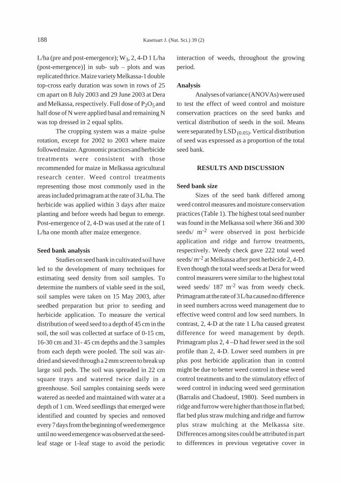
188 Kasetsart J. (Nat. Sci.) 39 (2)
L/ha (pre and post-emergence); W3, 2, 4-D 1 L/ha
(post-emergence)] in sub- sub – plots and was
replicated thrice. Maize variety Melkassa-1 double
top-cross early duration was sown in rows of 25
cm apart on 8 July 2003 and 29 June 2003 at Dera
and Melkassa, respectively. Full dose of P2O5 and
half dose of N were applied basal and remaining N
was top dressed in 2 equal splits.
The cropping system was a maize -pulse
rotation, except for 2002 to 2003 where maize
followed maize. Agronomic practices and herbicide
treatments were consistent with those
recommended for maize in Melkassa agricultural
research center. Weed control treatments
representing those most commonly used in the
areas included primagram at the rate of 3 L/ha. The
herbicide was applied within 3 days after maize
planting and before weeds had begun to emerge.
Post-emergence of 2, 4-D was used at the rate of 1
L/ha one month after maize emergence.
Seed bank analysisStudies on seed bank in cultivated soil have
led to the development of many techniques for
estimating seed density from soil samples. To
determine the numbers of viable seed in the soil,
soil samples were taken on 15 May 2003, after
seedbed preparation but prior to seeding and
herbicide application. To measure the vertical
distribution of weed seed to a depth of 45 cm in the
soil, the soil was collected at surface of 0-15 cm,
16-30 cm and 31- 45 cm depths and the 3 samples
from each depth were pooled. The soil was air-
dried and sieved through a 2 mm screen to break up
large soil peds. The soil was spreaded in 22 cm
square trays and watered twice daily in a
greenhouse. Soil samples containing seeds were
watered as needed and maintained with water at a
depth of 1 cm. Weed seedlings that emerged were
identified and counted by species and removed
every 7 days from the beginning of weed emergence
until no weed emergence was observed at the seed-
leaf stage or 1-leaf stage to avoid the periodic
interaction of weeds, throughout the growing
period.
AnalysisAnalyses of variance (ANOVAs) were used
to test the effect of weed control and moisture
conservation practices on the seed banks and
vertical distribution of seeds in the soil. Means
were separated by LSD (0.05). Vertical distribution
of seed was expressed as a proportion of the total
seed bank.
RESULTS AND DISCUSSION
Seed bank sizeSizes of the seed bank differed among
weed control measures and moisture conservation
practices (Table 1). The highest total seed number
was found in the Melkassa soil where 366 and 300
seeds/ m-2 were observed in post herbicide
application and ridge and furrow treatments,
respectively. Weedy check gave 222 total weed
seeds/ m-2 at Melkassa after post herbicide 2, 4-D.
Even though the total weed seeds at Dera for weed
control measurers were similar to the highest total
weed seeds/ 187 m-2 was from weedy check.
Primagram at the rate of 3 L/ha caused no difference
in seed numbers across weed management due to
effective weed control and low seed numbers. In
contrast, 2, 4-D at the rate 1 L/ha caused greatest
difference for weed management by depth.
Primagram plus 2, 4 –D had fewer seed in the soil
profile than 2, 4-D. Lower seed numbers in pre
plus post herbicide application than in control
might be due to better weed control in these weed
control treatments and to the stimulatory effect of
weed control in inducing weed seed germination
(Barralis and Chadoeuf, 1980). Seed numbers in
ridge and furrow were higher than those in flat bed;
flat bed plus straw mulching and ridge and furrow
plus straw mulching at the Melkassa site.
Differences among sites could be attributed in part
to differences in previous vegetative cover in

Kasetsart J. (Nat. Sci.) 39 (2) 189
addition to differences in soil type. Pre-emergence
of primagram plus post-emergence of 2, 4-D at
both sites were best to suppress weeds from weed
control measures. The effect of mulch to control
weeds was found effective only at Melkassa.
Vertical distributionThe vertical distributions of seed in the soil
varied among weed control treatments (Table 2).
The top 0-15 cm of soil contained 43.5, 40.2, 40,
and 61 % of the seed bank in weedy check,
primagram, primagram plus 2, 4-D, and 2, 4-D at
Dera, respectively. At Melkasaa, the top 0-15 cm
of soil contained 59.1, 56.8, 62.7, and 58.3 % in
weedy check, primagram, primagram plus 2, 4-D
and 2, 4-D weed control measures, respectively
which were greater as compared to those at Dera
site. The highest concentrations of weed seed were
found in 0-15 cm layer. In 16-30 cm, distribution
of weed seeds in the soil declined and were found
in the ranges from 18.4 in post-emergence of 2, 4-
D to 46.5% in pre-emergence of primagram at
Dera and from 19.7 in post-emergence of 2, 4-D to
33.5% in pre-emergence of primagram at Melkassa,
which were almost similar in weed seeds in the soil
among the four weed management systems. Seeds
in 31-45 cm soil depth declined steadily and were
found in the range from 13.3 in pre-emergence of
primagram to 22.7 % in pre plus post-emergence
of primagram plus 2, 4-D at Dera in the order of
primagram at the rate of 3 L/ha, weedy check, 2, 4-
D at the rate of 1 L/ha and primagram @ 3 L/ha
plus 2, 4-D at the rate of 1 L/ha, respectively.
In moisture conservation practice, at Dera
flat bed plus straw mulching recorded the lowest
percent of weed seed at 0-15 cm soil depth and the
highest at 16-30 cm were recorded. Ridge and
furrow recorded the highest weed seed at 0-15 cm
and the lowest at 31-45 cm, while ridge and furrow
plus straw mulching recorded the lowest percent
of weed seed at 16-30 cm and the highest at 31-45
cm. At Melkassa flat bed plus straw mulching
showed the lowest percent of weed seed at 0-15 cm
and 31- 45 cm and the highest at 16-30 cm where
as flat bed without straw mulching treatment
recorded the highest percent of weed seed at 16-30
cm and the lowest at 16-30 cm. Ridge and furrow
with and without straw mulching expressed
medium percents of weed seed at the three depths
and which were not different from one another. At
both sites, flat bed plus straw mulching recorded
the lowest percentage of weed seed at 0-15 cm
layer.
The highest number of weed seed among
the four weed control measures was obtained from
weedy check followed by primagram @ 3 L/ha
treated plots (Table 3). Ridge and furrow also gave
the highest total weed seed followed by flat bed.
The control measure with mulch gave less number
of weed seed as compared to without mulch. Over
52.7% seeds were concentrated in the top 0-15 cm
layer in 2, 4-D @ 1 L/ha herbicide applied treatment
and flat bed planting method (Table 3). Weed
control measurers ranked 2, 4- D > weedy check >
primagram > primagram + 2, 4-D for total seed in
the top 45 cm soil depth. Depths by weed control
interaction were also significant at both sites.
Species compositionAt four weed control measures, twenty-
eight weed species were identified in the seed bank
or in the field. Almost all of the species observed
only in seed bank samples were relatively common
at the experimental site; hence it was surprising
that these species appeared in the soil samples.
Over 90 % of each seed bank among weed control
treatments and soils were composed of fewer
weed species with 18 species being common to
both sites (Table 4). The weeds in different
combinations were found at each seed bank. The
results showed that the weed seed bank was mainly
composed of Chenopodium fasciulosum,
Eragrostis aspera, Cyperus rotundus, Sorghum
arundenanceum, Flaveria trinerva, Argemone
mexicana, Hetilotropium cineraseioen,
Amaranthus hybridus, Anagalis arvensis, Nicandra

190 Kasetsart J. (Nat. Sci.) 39 (2)
phylasoides, Datura stramonium, Galinsoga
parviflora, Euphorbia heterophylla, Launea
comuta, Portulaca oleracea, Foeum vulgare, etc.
at the two sites. Chenopodium fasciulosum was the
only species present in each weed control treated
plots constituted 21.7 % of the total seed bank
across two locations and consistently made up
greater percentages of the seed bank in pre-, pre -
plus post- and post- emergences than weedy check.
Cyprus rotundus, Eragrostis aspera and Sorghum
arundenanceum were the next most abundant
species at each site. Galinsoga parviflora was
Table 1 Numbers of seed per m2 at a depth of 45 cm in four-weed control measures and averaged
moisture conservation practices.
Total weed seeds Dera Melkassa
Weed control measures
W0 (weedy check) 187 222
W1 (Primagram) 184 144
W2 (Primagram + 2, 4-D) 137 105
W3 (2, 4-D) 135 366
LSD (0.05) 29.92 66.51
Moisture conservation practices
FB (Flat bed) 154 262
R & F (Ridge and furrow) 160 300
FB + SM (Flat bed + straw mulch) 167 168
R & F + SM (Ridge and furrow + straw mulch) 152 203
LSD (0.05) 35.22 37.08
Table 2 Influences of weed control measure and moisture conservation practices on vertical distributions
of total weed seed (%) to a 45 cm soil depth after maize cropping.
Dera Melkassa
Depth (cm)Weed control measures
W0 W1 W2 W3 W0 W1 W2 W3
0-15 43.5 40.2 40 61 59.1 56.8 62.7 58.3
15-30 39.8 46.5 37.3 18.4 28.7 33.5 22.9 19.7
30-45 16.8 13.3 22.7 20.6 12.2 9.7 14.4 22
Moisture conservation practices
Depth (cm) FB R & F FB + SM R & F + SM FB R & F FB + SM R and F + SM
0-15 48.8 51.8 36.5 48.6 61.3 59.2 58.8 55.9
15-30 31 33.8 46.9 30.3 23.2 28.7 30.4 26
30-45 20.2 10.6 10.8 21.1 15.5 12.1 10.8 18.1
W0 = weedy check, W1= primagram @ 3 L/ha, W2 = primagram @ 3 L/ha + 2, 4-D @ 1 L/ha, and W3 = 2, 4-D @ 1 L/ha. FB =
flat bed, R & F = ridge and furrow, FB + SM= flat bed + straw mulch, and R & F + SM = ridge and furrow + straw mulch. L1
= Dera and L2 = Melkassa

Kasetsart J. (Nat. Sci.) 39 (2) 191
found in all weed control measures at both sites but
was not present in post herbicide treatment.
Commelina benghalensis, Agenatum spp,
Convolvulus spp were very small in number and
commonly found in Dera while Euphorbia
heterophylla, Leucas martini, Sidaalba spp, Tagets
minuta, Tribulus spp, and Portulaca oleracea
were found only in Melkassa.
CONCLUSION
In this study, the herbicides and residues
Table 3 Distribution of weed seed by soil depth as affected by weed control and moisture conservation
practices.
Weed seed as affected by depth (cm)
Weed control Moisture Dera Melkassa
conservation 0-15 16-30 31-45 0-15 16-30 31-45
No m-2
Weedy check (control)FB 35 18 3 42 16 14
R & F 24 20 5 31 11 6
FB + SM 28 14 5 21 10 16
R & F +SM 23 7 5 29 14 12
Primagram @ 3 L/ha (pre-emergence)FB 23 15 1 18 12 8
R & F 42 16 12 17 10 5
FB + SM 25 12 4 15 13 4
R & F + SM 12 20 2 27 7 8
Primagram @ 3 L/ha and 2, 4-D @ 1 L/ha (pre and post-emergence)FB 6 87 3 13 7 7
R & F 15 7 2 19 8 5
FB + SM 37 12 6 11 5 4
R & F + SM 16 19 6 15 5 6
2, 4-D @ 1 L/ha (post-emergence)
FB 33 4 5 85 22 19
R & F 13 8 6 82 25 25
FB + SM 14 8 2 13 8 7
R & F + SM 21 15 6 45 20 15
FB = flat bed, R & F = ridge and furrow, FB + SM= flat bed + straw mulch, and R & F + SM = Ridge and furrow + straw mulch.
L1 = Dera and L2 = Melkassa
could influence weed population levels, the rate of
population growth and species composition. This
might indicate that herbicides and residues were
effective enough to prevent excessive weed seed
production. This result was obtained from one-
year data, the long–term effects of herbicide and
residue on weed populations were not studied.
Further studies are needed to examine the
interaction effects of herbicide with residue
application, allelophaty and shading effects and
may result in reduced weed seedling emergence. It
also needs further study on farmer’s field where

192 Kasetsart J. (Nat. Sci.) 39 (2)
Table 4 Seed bank compositions (45 cm deep) in two sites after one year of maize cropping with four
weed control measures.
Seed bank composition as affected by soil and weed control
Species Dera Melkassa
W0 W1 W2 W3 W0 W1 W2 W3
Chenopodium fasciulosum 43 89 56 55 10 30 9 11
Flaveria trinerva 12 3 1 1 24 13 7 12
Cyperus rotundus 26 19 7 2 12 6 1 27
Amaranthus hybridus 2 2 4 1 5 14 11 6
Eragrostis aspera 19 9 36 24 5 3 6 19
Argemone mexicana 15 9 7 3 16 7 5 3
Sorghum arundenanceum 26 13 3 22 9 2 1 19
Nicandra physaloides 1 3 5 3 3 4 12 6
Heliotropism cineraseioen 7 13 8 11 5 8 6 2
Anagalis arvensis 12 3 2 7 9 3 2 3
Datura stramonium 3 7 0 0 3 7 0 0
Euphorbia heterophylla * * * * 4 1 0 2
Galinsoga parviflora 1 3 1 0 1 3 1 0
Launea comuta 2 0 1 2 2 1 1 1
Portulaca oleracea * * * * 1 1 1 0
Foeum vulgare 1 1 1 2 0 0 0 2
Tagetes minuta * * * * 0 2 0 0
Erucastrum arabicum 2 3 3 4 0 1 1 0
Setaria pumila 1 1 1 0 0 1 1 0
Eleusine indica 0 1 0 0 0 1 0 0
Xanthium strumarium 2 0 2 0 1 0 0 0
Commelina benghalensis 1 0 0 0 * * * *
Ageratum conyzoides 1 3 0 1 * * * *
Convolvulus arvensis 3 0 0 1 * * * *
Leucas martini * * * * 0 1 0 1
Sidaalba spinosa * * * * 0 0 0 1
Tribulus terrestris * * * * 1 1 1 1
Values are means of 3 replications at Melkassa and Dera sites.* Species not found at that site;W0 = weedy check (control); W1 =
Primagram 660 SC @ 3 L/ha (pre emergence); W2 = Primagram 660 SC @ 3 L/ha and 2, 4-D @ 1 L/ha (pre and post emergence);
W3 = 2, 4-D @ 1 L/ha (post emergence). L1 = Dera and L2 = Melkassa
herbicides and residues were rarely or not applied.
The results and information obtained would
expedite the development of management strategies
to reduce populations of weed with seed bank
regeneration strategies and to manage the
successional dynamics of weed in weed control
measures.

Kasetsart J. (Nat. Sci.) 39 (2) 193
LITERATURE CITED
Ball, D. A. and S. D. Miller. 1989. A composition
of techniques for estimation of arable soil
seed banks and relationship to weed flora.
Weed Res. 29: 365-373.
Barralis, G. and R. Chadoeuf. 1980. Etude de la
dynanique d’ une communaute adventice. 1.
Evolution de la flora adventice au course du
cycle vegetative d’une culture. Weed Res.20: 231-237.
Buhler, D. D., J. L. Gunsolus and D. F. Ralston.
1992. Integrated weed management
techniques to reduce herbicide inputs in
Soybean. Agron. J. 84: 973-978.
Burnside , O. C., R. S. Moomaw, F. W. Roeth, G.
A. Wicks and R. G. Wilson. 1986. Weed seed
demise in soil in weed free corn (Zea mays L.)
production across Nebraska. Weed Sci. 34:
248-251.
Cavers, P. B. and D. L. Benoit 1989. Seed banks
in arable land. pp 309-328 in M. A. Leck, V.
T. Parker and R. L. Simpson, eds. Ecology of
Soil Seed Banks. Academic Press New YorkChepil, W. S. 1946. Germination of weed seeds:
11. The influence of tillage treatments on
germination. Science. Agric 8: 347-357.
Harper, C. A. 1977.The seed bank, pp 83-110. In:
Population Biology of plants. AcademicPress, London.
Herr, D. E. and E. W. Stroube. 1970. Velvetleaf
control as influenced by herbicide placement
and seed depth. Weed Sci. 18: 459-461.
Maxwell, B.D. and C. Ghersa. 1992. The influence
of weed seed dispersion versus the effect of
competition on crop yield. Weed Techn. 6:
196-204.
Mester, J. C. and D. D.Buhler.1990. Effect of
seedling depth on Velvetleaf seedling
development and response to cynazine. WeedSci. 38: 34-38.
Roberts, H. A. 1963. Studies ion the weeds of
vegetable crops. 111. Effect of different t
primary cultivation on the w weed seeds in the
soil. J. of Ecology 51: 83-95.
Roberts, H. A. 1968. The changing population of
viable weeds seeds in an arable soil. WeedRes. 8: 253-256.
Roberts, H. A. and J. E. Neilson. 1981. Seed banks
in soils. Adv. Appl. Biology 6: 1-55.
Schweitzer, E. E. and R. L. Zimdahl. 1984. Weed
seed decline in irrigated soil after six years of
continuous corn (Zea mays L.) and herbicides.
Weed Sci. 32: 76-3.

Kasetsart J. (Nat. Sci.) 39 : 194 - 205 (2005)
Genetic Diversity of Elite and Exotic Oilseed MeadowfoamGermplasm using AFLP Markers
Sureeporn Katengam1 and Steven J. Knapp2
ABSTRACT
Amplified fragment length polymorphism (AFLP) is a PCR-based marker, which is suitable for
DNA fingerprinting. The AFLP fingerprinting has not been described in meadowfoam. This powerful
method was utilized to access genetic diversity of 41 meadowfoam accessions belonging to the genus
Limnanthes. The objectives were to estimate polymorphic information contents (PIC) for AFLP markers
and genetic distance among germplasm, and to assess the pattern of genetic diversity in meadowfoam
germplasm. One hundred and seventy six polymorphic AFLP markers were produced using 6 primer
combinations across 41 accessions. The PIC value ranged from 0.0 to 0.5 and 42 % of germplasm showed
high PIC scores in a range between 0.45 and 0.5. Genetic distance ranged from 0.14 to 0.55 with an
average of 0.44. The UPGMA clustering phenogram based on the distance matrix was consistent with
the known taxonomic classification. The first three principal coordinate analyses accounted for 37 % of
total variation of genetic distance estimated. Cluster analysis and principal component analysis clearly
separated L. floccosa from L. alba. Within L. alba, subspecies alba and versicolor were distinctly
separated into two groups. The results suggested genetic diversity among meadowfoam germplasm was
very high. This information is useful to layout framework for meadowfoam improvement thereby
enhancing productivity and performance of cultivated meadowfoam.
Key words: meadowfoam, Limnanthes sp., genetic diversity, DNA fingerprinting, AFLP
INTRODUCTION
Meadowfoam (Limnanthes sp.) is an annual
oil seed crop, native to Southern Oregon and
California (Mason, 1952). Seed oil of meadowfoam
contains unique unsaturated very long chain fatty
acids (C20 and C22) with outstanding oxidative
stability (Isbell, 1997). Cultivated meadowfoam
which belongs to section Inflexae, family
Limnanthaceae is based on Limnanthes alba. The
section Inflexae comprises of 4 species, namely L.
1 Department of Agronomy, Faculty of Agriculture, Ubon Ratchathani University, Ubon Ratchathani 34190, Thailand.
[email protected] Department of Crop and Soil Science, Oregon State University, Corvallis, OR, 97331 USA.
Received date : 18/06/04 Accepted date : 28/02/05
alba, L. floccosa, L. gracilis and L. montana. The
primary gene pool of L. alba is composed of L.
alba ssp. alba and L. alba ssp. versicolor, whereas
L. floccosa, L. gracilis, and L. montana are
identified as a secondary gene pool of L. alba.
Meadowfoam has been domesticated since
1973 (Jain, 1986). The L. alba was evaluated as
the most promising species in this genus for its
lower moisture requirements, adaptation to wide
ranges of environments, and high seed yield (Gentry
and Miller, 1965). The first non- shattering cultivar,

Foamore, developed for commercial production
was released in 1974 (Calhoun and Crane, 1975).
Breeding and cultivars development is underway
at the Oregon State University with the main goal
of increasing the productivity of meadowfoam by
developing superior cultivars, discovering and
developing novel phenotypes, and advancing our
understanding of the genetics of economically
important traits (Knapp and Crane, 1999).
Knowledge of the genetic diversity and
relationships among germplasm is essential to the
improvement of meadowfoam. Generally, the
genetic diversity of germplasm collections can be
obtained from pedigree records, morphological
traits, isozyme and DNA markers (Smith et al.,
1990; Mumm and Dudley, 1994). However, a
small number of polymorphic markers obtained
from isozyme markers and unfavorable phenotypic
expressions of some morphological traits due to
the environmental effects are known as limitations
of these markers (Smith et al., 1990). The advent
of DNA markers opens the ways to solve this
problem since DNA markers can reveal tremendous
number of genetic loci and they are phenotypic
neutral and not subjected to environmental effects.
A variety of DNA markers have been applied to
cultivar improvement and germplasm
management. Owing to its capacity to reveal a
large number of marker loci in a short period of
time (Vos et al., 1995), AFLP (Amplified fragment
length polymorphism) appears to be the leading
DNA-based marker systems for DNA fingerprints.
AFLP has shown to be a powerful tool for genetic
diversity study in many plant species such as
soybean (Maughan et al., 1996), barley (Ellis et
al., 1997), and rice (Zhu et al., 1998).
The high throughout AFLP markers were
employed to evaluate the genetic diversity among
recent meadowfoam germplasm. The objectives
were (1) to estimate polymorphic information
contents (PIC) for AFLP markers and estimate
genetic distance among inbreds, open-pollinated
cultivars, wild population and all genotypes, (2) to
assess the pattern of genetic diversity and
relationships of meadowfoam germplasm using
UPGMA cluster analysis and principal coordinate
analysis.
MATERIAL AND METHODS
Plant materialsA total of 41 meadowfoam accessions
representing nine inbred lines, eight open-
pollinated cultivars, and 24 wild populations were
included in this diversity study (Table1). The
meadowfoam seeds were germinated and grown
as described by Katengam et al. (2002). Leaves
from 50 to 55 day-old plants were harvested,
immediately frozen, and stored at -80∞C prior to
DNA extraction.
AFLP fingerprintsGenomic DNA was extracted from frozen
tissue using a protocol similar to Lodhi et al.
(1994) with minor modification. AFLP analysis
was carried out essentially as developed by
Keygene (Waeningen, NL) with the minor
modification that the selection of a subset of
fragments on steptavidin beads was omitted (Vos
et al., 1995). AFLP fingerprints were produced
using six MseI-EcoRI primer pairs with three
selective nucleotides (Table 2).
Data analysisGene diversity was used to describe the
relative value of AFLP marker with respect to the
degree of polymorphism exhibited for each
polymorphic locus. Thus,
Gene diversity = piik 2
1=Âwhere pi is the frequency of ith allele and k is the
number of alleles (Ott, 1991). Anderson et. al.
(1993) indicated that gene diversity was essentially
the same as the polymorphic information content
(PIC) as used by Botstein et al. (1980). This
parameter is sometimes called heterozygosity. Due
Kasetsart J. (Nat. Sci.) 39 (2) 195

196 Kasetsart J. (Nat. Sci.) 39 (2)
Table 1 Meadowfoam germplasm (41 accessions) for AFLP fingerprinting.
Accessions Description
1. OMF63 S5 Self-pollinated inbred line (Selected from OMF159)2. OMF64 S5 Self-pollinated inbred line (Selected from OMF160)3. OMF66 S5 Self-pollinated inbred line (Selected from OMF66)4. OMF109-1 Self-pollinated inbred line (Selected from Mermaid x OMF62/ OMF64)5. OMF109-2 Self-pollinated inbred line (Selected from Mermaid x OMF62/ OMF64)6. OMF109-3 Self-pollinated inbred line (Selected from Mermaid x OMF62/ OMF64)7. OMF40-11 (Mermaid S5) Insect-pollinated L. alba ssp. alba inbred line (Selected from PI
283703)8. LAG109 F4 Self-pollinated Mermaid x L. gracilis ssp. parishii inbred line9. LAG111 F4 Self-pollinated Mermaid x L. gracilis ssp. parishii inbred line
10. OMF66 (Redding) Wild L. alba ssp. versicolor population11. OMF 158 Wild L. alba ssp. versicolor population (Recollected PI 283705)12. OMF159 Wild L. alba ssp. versicolor population (Recollected PI 374791)13. OMF160 Wild L. alba ssp. versicolor population (Recollected PI 374801)14. OMF161 Wild L. alba ssp. versicolor population (Recollected PI 374802)15. OMF57 Wild L. alba ssp. versicolor population (UC328 or UC457)16. OMF52 Wild L. alba ssp. alba population (UC- Calaveras)17. OMF53 Wild L. alba ssp. alba population (UC-Sonoma)18. PI 374793 Wild L. alba ssp. alba population (Placer county)19. PI 374794 Wild L. alba ssp. alba population (Placer county)20. PI 374795 Wild L. alba ssp. alba population (Placer county)21. PI 374796 Wild L. alba ssp. alba population (Butte county)22. PI 374797 Wild L. alba ssp. alba population (Butte county)23. PI 374798 Wild L. alba ssp. alba population (Butte county)24. PI 367900 Wild L. alba ssp. alba population (Sacremento county)25. PI 374792 Wild L. alba ssp. alba population (Shasta county)26. Foamore Open-pollinated cultivar (Selected from PI 283704)27. Mermaid Open-pollinated cultivar (Selected from PI 283703)28. Floral Open-pollinated cultivar (Mermaid x L. floccosa ssp. grandiflora)29. Knowles (OMF69) Open-pollinated cultivar (Selected from bulk of L. alba ssp. alba)30. OMF86 Open-pollinated cultivar (Selected from Knowles)31. OMF78 Open-pollinated cultivar (Selected from intermating between L. alba
ssp.alba and ssp. versicolor)32. OMF87 High oil open-pollinated population (Selected from OMF62)33. PI 283724 L. gracilis ssp. parishii (Wild species)34. PI 420137 L. gracilis ssp. gracilis (Wild species)35. PI 283720 L. floccosa ssp. bellingeriana (Wild species)36. PI 420133 L. floccosa ssp. grandiflora (Wild species)37. PI 283719 L. floccosa ssp. floccosa (Wild species)38. OSU-LF-4 L. floccosa ssp. californica (Wild species)39. PI 283721 L. floccosa ssp. pumila (Wild species)40. PI 283725 L. montana (Wild species)41. OMF62-92 High oil open-pollinated population (L. alba ssp. alba)
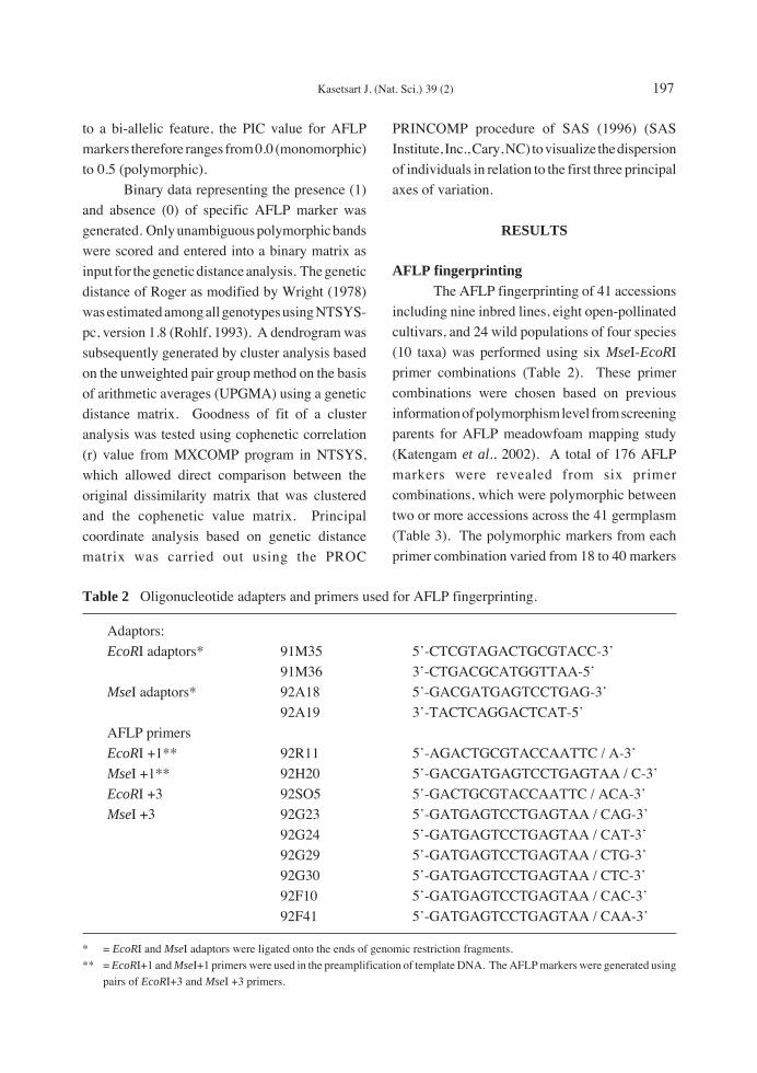
Kasetsart J. (Nat. Sci.) 39 (2) 197
to a bi-allelic feature, the PIC value for AFLP
markers therefore ranges from 0.0 (monomorphic)
to 0.5 (polymorphic).
Binary data representing the presence (1)
and absence (0) of specific AFLP marker was
generated. Only unambiguous polymorphic bands
were scored and entered into a binary matrix as
input for the genetic distance analysis. The genetic
distance of Roger as modified by Wright (1978)
was estimated among all genotypes using NTSYS-
pc, version 1.8 (Rohlf, 1993). A dendrogram was
subsequently generated by cluster analysis based
on the unweighted pair group method on the basis
of arithmetic averages (UPGMA) using a genetic
distance matrix. Goodness of fit of a cluster
analysis was tested using cophenetic correlation
(r) value from MXCOMP program in NTSYS,
which allowed direct comparison between the
original dissimilarity matrix that was clustered
and the cophenetic value matrix. Principal
coordinate analysis based on genetic distance
matrix was carried out using the PROC
PRINCOMP procedure of SAS (1996) (SAS
Institute, Inc., Cary, NC) to visualize the dispersion
of individuals in relation to the first three principal
axes of variation.
RESULTS
AFLP fingerprintingThe AFLP fingerprinting of 41 accessions
including nine inbred lines, eight open-pollinated
cultivars, and 24 wild populations of four species
(10 taxa) was performed using six MseI-EcoRI
primer combinations (Table 2). These primer
combinations were chosen based on previous
information of polymorphism level from screening
parents for AFLP meadowfoam mapping study
(Katengam et al., 2002). A total of 176 AFLP
markers were revealed from six primer
combinations, which were polymorphic between
two or more accessions across the 41 germplasm
(Table 3). The polymorphic markers from each
primer combination varied from 18 to 40 markers
Table 2 Oligonucleotide adapters and primers used for AFLP fingerprinting.
Adaptors:
EcoRI adaptors* 91M35 5’-CTCGTAGACTGCGTACC-3’
91M36 3’-CTGACGCATGGTTAA-5’
MseI adaptors* 92A18 5’-GACGATGAGTCCTGAG-3’
92A19 3’-TACTCAGGACTCAT-5’
AFLP primers
EcoRI +1** 92R11 5’-AGACTGCGTACCAATTC / A-3’
MseI +1** 92H20 5’-GACGATGAGTCCTGAGTAA / C-3’
EcoRI +3 92SO5 5’-GACTGCGTACCAATTC / ACA-3’
MseI +3 92G23 5’-GATGAGTCCTGAGTAA / CAG-3’
92G24 5’-GATGAGTCCTGAGTAA / CAT-3’
92G29 5’-GATGAGTCCTGAGTAA / CTG-3’
92G30 5’-GATGAGTCCTGAGTAA / CTC-3’
92F10 5’-GATGAGTCCTGAGTAA / CAC-3’
92F41 5’-GATGAGTCCTGAGTAA / CAA-3’
* = EcoRI and MseI adaptors were ligated onto the ends of genomic restriction fragments.
** = EcoRI+1 and MseI+1 primers were used in the preamplification of template DNA. The AFLP markers were generated using
pairs of EcoRI+3 and MseI +3 primers.

198 Kasetsart J. (Nat. Sci.) 39 (2)
with an average of 29 markers per primer pair. The
sizes of these markers ranged from 50 to 250 bp.
Out of 176 AFLP markers, 142 and 138 AFLP
markers showed polymorphism in at least two
inbred lines and two cultivars, respectively,
whereas 175 AFLP markers revealed
polymorphism in at least two wild populations of
meadowfoam.
Gene diversity (Polymorphic informationcontent, PIC)
Estimation of gene diversity in
meadowfoam germplasm was represented by
polymorphic information content (PIC) value
which showed the probability of polymorphism
between two randomly lines. The PIC scores for
176 AFLP markers ranged from 0.0 to 0.5 (Figure1).
Mean PIC scores was 0.31 for inbred lines, 0.30
for open-pollinated cultivars, 0.40 for wild
populations, and 0.39 for all genotypes based on
142, 138, 175, and 176 polymorphic AFLP markers
respectively. The distribution of PIC score was
dramatically increased from 0.0 to 0.5. Nearly
half of markers (42.61%) showed maximum PIC
scores with a range of 0.45 - 0.50, indicating a high
genetic diversity in meadowfoam germplasm.
Distance analysisGenetic distance among 41 accessions
based on 176 AFLP markers was estimated using
Rogers genetic distance as modified by Wright
(1978), ranging from 0.14 to 0.55, with an average
of 0.44 (Table 4). The distances estimated among
nine inbred lines varied from 0.14 (between
OMF109-1 and OMF109-3) to 0.47 (between
LAG109F4 and OMF109-1, OMF109-2, and
OMF109-3) with an average of 0.39. OMF109-1,
OMF109-2 and OMF109-3 were related as they
were developed from the same cross (Mermaid x
OMF62/ OMF64), but were selected for different
fatty acid concentration profiles. OMF109-2 was
Table 3 Total numbers of informative AFLP marker detected with six primer combinations (one
EcoRI+3 primers (ACA) and six MseI+3 primers) used in diversity study.
Primers combinations (EcoRI+3 / MseI+3) Total polymorphic AFLP markers
ACACTC 28
ACACAG 38
ACACTG 40
ACACAC 35
ACACAA 18
ACACAT 20
Total 176
Average 29.33
Polymorphic information content
0.05
0.05-0.1
0.1-0.15
0.15-0.2
0.2-0.25
0.25-0.3
0.3-0.35
0.35-0.4
0.4-0.45
0.45-0.5
No.
of
AFL
P m
arke
rs
0
10
20
30
40
50
60
70
80
Figure 1 Distribution of polymorphic informa-
tion content (PIC ) scored for 176 AFLP
markers among 41 meadowfoam ac-
cessions.

Kasetsart J. (Nat. Sci.) 39 (2) 199T
able
4
Gen
etic
dis
tanc
e m
atri
x es
timat
ed b
y R
oger
-W f
rom
AFL
P fi
nger
prin
ts o
f 41
mea
dow
foam
acc
essi
ons.
12
34
56
78
910
1112
1314
1516
1718
1920
1. O
MF6
3S5
02.
OM
F64S
50.
310
3. O
MF6
6S5
0.33
0.44
04
OM
F109
-10.
370.
390.
460
5 O
MF1
09-2
0.37
0.38
0.46
0.25
06
OM
F109
-30.
360.
390.
450.
140.
270
7 O
MF4
0-11
0.35
0.43
0.42
0.42
0.43
0.43
08
LA
G10
9F4
0.41
0.44
0.45
0.47
0.47
0.47
0.38
09
LA
G11
1F4
0.35
0.42
0.40
0.44
0.44
0.44
0.42
0.30
010
OM
F66
0.31
0.41
0.32
0.42
0.43
0.43
0.41
0.45
0.42
011
OM
F158
0.30
0.38
0.35
0.42
0.42
0.42
0.41
0.43
0.38
0.32
012
OM
F159
0.33
0.41
0.39
0.42
0.42
0.42
0.40
0.47
0.41
0.37
0.35
013
OM
F160
0.32
0.38
0.38
0.41
0.42
0.41
0.41
0.46
0.42
0.35
0.37
0.34
014
OM
F161
0.32
0.38
0.38
0.37
0.37
0.36
0.44
0.47
0.41
0.34
0.34
0.38
0.38
015
OM
F57
0.43
0.49
0.47
0.47
0.47
0.49
0.43
0.44
0.44
0.47
0.45
0.46
0.47
0.46
016
OM
F52
0.43
0.49
0.45
0.49
0.48
0.50
0.42
0.47
0.44
0.47
0.47
0.48
0.48
0.48
0.42
017
OM
F53
0.38
0.44
0.43
0.46
0.46
0.46
0.40
0.47
0.44
0.42
0.43
0.44
0.42
0.43
0.47
0.44
018
PI
3747
930.
380.
460.
390.
450.
460.
450.
330.
410.
380.
410.
410.
430.
380.
410.
440.
440.
410
19 P
I 37
4794
0.39
0.49
0.39
0.45
0.44
0.46
0.42
0.47
0.43
0.41
0.43
0.45
0.43
0.43
0.47
0.44
0.44
0.36
020
PI
3747
950.
400.
470.
450.
500.
460.
490.
410.
450.
450.
440.
470.
460.
430.
440.
490.
470.
460.
420.
400
21 P
I 37
4796
0.38
0.46
0.41
0.47
0.45
0.48
0.41
0.46
0.42
0.40
0.41
0.43
0.41
0.43
0.45
0.48
0.46
0.34
0.38
0.39
22 P
I 37
4797
0.37
0.43
0.40
0.46
0.44
0.47
0.40
0.45
0.41
0.38
0.40
0.42
0.39
0.43
0.45
0.46
0.40
0.38
0.38
0.43
23 P
I 37
4798
0.37
0.40
0.42
0.46
0.45
0.46
0.42
0.47
0.44
0.40
0.40
0.40
0.39
0.43
0.49
0.46
0.43
0.40
0.42
0.42
24 P
I 36
7900
0.38
0.47
0.43
0.46
0.45
0.47
0.43
0.48
0.45
0.44
0.44
0.46
0.44
0.44
0.47
0.43
0.40
0.40
0.41
0.45
25 P
I 37
4792
0.38
0.42
0.40
0.42
0.43
0.42
0.41
0.46
0.42
0.40
0.38
0.36
0.37
0.39
0.46
0.43
0.43
0.41
0.41
0.47
26 F
oam
ore
0.37
0.45
0.40
0.46
0.46
0.45
0.43
0.49
0.43
0.44
0.41
0.41
0.38
0.45
0.49
0.44
0.44
0.38
0.40
0.42
27 M
erm
aid
0.40
0.46
0.43
0.49
0.48
0.49
0.37
0.48
0.42
0.46
0.43
0.44
0.42
0.46
0.46
0.45
0.43
0.40
0.41
0.44
28 F
lora
l0.
380.
430.
440.
450.
430.
460.
370.
410.
380.
420.
420.
400.
390.
450.
460.
420.
420.
400.
450.
4429
Kno
wle
s0.
400.
390.
440.
440.
430.
450.
400.
470.
430.
440.
430.
440.
400.
430.
460.
430.
430.
400.
440.
4230
OM
F86
0.37
0.39
0.42
0.41
0.43
0.42
0.38
0.46
0.45
0.41
0.41
0.42
0.37
0.42
0.47
0.47
0.40
0.40
0.46
0.44
31 O
MF7
80.
350.
400.
430.
390.
410.
400.
400.
490.
450.
410.
400.
400.
410.
400.
460.
460.
420.
390.
430.
4732
OM
F87
0.36
0.41
0.43
0.42
0.42
0.42
0.39
0.47
0.43
0.40
0.41
0.41
0.41
0.43
0.49
0.46
0.43
0.41
0.44
0.44
33 P
I 28
3724
0.47
0.51
0.49
0.49
0.48
0.50
0.47
0.46
0.44
0.52
0.48
0.49
0.50
0.49
0.45
0.48
0.45
0.47
0.47
0.51
34 P
I 42
0137
0.38
0.47
0.44
0.46
0.47
0.46
0.41
0.45
0.41
0.46
0.43
0.42
0.43
0.43
0.49
0.47
0.44
0.38
0.46
0.44
35 P
I 28
3720
0.47
0.52
0.49
0.49
0.50
0.50
0.48
0.48
0.46
0.53
0.51
0.54
0.52
0.52
0.47
0.46
0.47
0.49
0.45
0.49
36 P
I 42
0133
0.46
0.52
0.51
0.50
0.52
0.51
0.47
0.50
0.46
0.51
0.49
0.52
0.50
0.53
0.48
0.48
0.49
0.51
0.47
0.49
37 P
I 28
3719
0.46
0.52
0.51
0.50
0.51
0.49
0.49
0.46
0.45
0.49
0.49
0.55
0.51
0.52
0.48
0.48
0.50
0.49
0.47
0.49
38 O
SU-L
F 40.
470.
520.
500.
480.
490.
480.
480.
510.
480.
520.
520.
520.
510.
520.
480.
490.
510.
490.
460.
5139
PI
2837
210.
450.
490.
460.
460.
460.
460.
460.
490.
450.
470.
460.
490.
470.
470.
470.
450.
510.
480.
450.
4940
PI
2837
250.
380.
410.
430.
460.
450.
450.
430.
450.
400.
460.
390.
380.
440.
400.
460.
470.
410.
420.
460.
4441
OM
F622
90.
390.
420.
440.
430.
420.
440.
390.
450.
420.
460.
470.
450.
450.
460.
470.
440.
440.
450.
450.
47

200 Kasetsart J. (Nat. Sci.) 39 (2)T
able
4C
ontin
ued.
2122
2324
2526
2728
2930
3132
3334
3536
3738
3940
41
21 P
I 37
4796
0
22 P
I 37
4797
0.35
0
23 P
I 37
4798
0.37
0.39
0
24 P
I 36
7900
0.43
0.41
0.39
0
25 P
I 37
4792
0.42
0.41
0.40
0.40
0
26 F
oam
ore
0.40
0.40
0.35
0.40
0.40
0
27 M
erm
aid
0.43
0.42
0.43
0.44
0.42
0.41
0
28 F
lora
l0.
430.
420.
410.
420.
420.
410.
410
29 K
now
les
0.43
0.42
0.39
0.43
0.38
0.41
0.39
0.38
0
30 O
MF8
60.
440.
410.
380.
420.
400.
440.
380.
390.
340
31 O
MF7
80.
430.
430.
390.
430.
410.
400.
410.
360.
400.
340
32 O
MF8
70.
430.
400.
350.
420.
400.
420.
400.
410.
400.
380.
370
33 P
I 28
3724
0.47
0.49
0.48
0.45
0.46
0.46
0.46
0.47
0.48
0.47
0.49
0.49
0
34 P
I 42
0137
0.43
0.43
0.39
0.42
0.42
0.38
0.41
0.42
0.40
0.43
0.41
0.40
0.47
0
35 P
I 28
3720
0.51
0.49
0.49
0.46
0.49
0.52
0.49
0.51
0.50
0.48
0.52
0.50
0.44
0.49
0
36 P
I 42
0133
0.49
0.49
0.49
0.49
0.49
0.49
0.45
0.50
0.51
0.50
0.51
0.48
0.48
0.50
0.40
0
37 P
I 28
3719
0.50
0.48
0.51
0.51
0.50
0.51
0.48
0.52
0.51
0.50
0.51
0.49
0.48
0.51
0.32
0.41
0
38 O
SU-L
F 40.
520.
520.
500.
490.
480.
510.
480.
530.
490.
500.
520.
490.
490.
480.
390.
340.
410
39 P
I 28
3721
0.47
0.46
0.48
0.48
0.44
0.47
0.46
0.48
0.47
0.49
0.49
0.45
0.49
0.49
0.44
0.33
0.43
0.33
0
40 P
I 28
3725
0.44
0.42
0.41
0.44
0.39
0.41
0.40
0.43
0.40
0.40
0.42
0.38
0.46
0.39
0.52
0.51
0.52
0.49
0.48
0
41 O
MF6
229
0.49
0.46
0.45
0.46
0.44
0.46
0.44
0.41
0.42
0.43
0.42
0.40
0.47
0.47
0.49
0.49
0.49
0.47
0.40
0.43
0

Kasetsart J. (Nat. Sci.) 39 (2) 201
selected for L. alba ssp. versicolor fatty acid
profile, which had high dienoic (22:2 D5D13) and
low erucic acid (22:1D13) content while OMF
109-3 was selected based on L. alba ssp. alba fatty
acid profile, which had high erucic acid but low
dienoic acid content. OMF109-1 was selected
based on heterozygote progeny, which had fatty
acid profiles between these two subspecies. In
contrast to OMF109 inbred lines, LAG109F4 was
derived from an interspecific cross between L.
alba (Mermaid) and L. gracilis ssp. parishii,
therefore it showed the greatest distance to those
derived from intersubspecific (L. alba) crosses.
Amongst the eight open-pollinated
cultivars, the distance estimated varied from 0.34
to 0.46 with an average of 0.40. The greatest
distance was found between Foamore and OMF62-
29, whereas the least distance or close relationship
was found between OMF86 and Knowles and
OMF86 and OMF78.
Among 24 wild meadowfoam populations,
the greatest distance (0.55) was found between
OMF159 (L. alba ssp. versicolor) and PI 283719
(L. floccosa ssp. floccosa). The least distance
(0.32) was found between two wild populations of
L. alba ssp. versicolor. The average genetic
distance among wild population was 0.45 indicating
high genetic diversity in these wild populations.
Cluster analysisCluster analysis using UPGMA
(unweighted pair group method based on arithmetic
mean) was performed to examine genetic
relationships among meadowfoam germplasms.
A phenogram was produced from the UPGMA
cluster analysis of genetic distance matrix for 41
accessions based on mean AFLP data from each
accession (Figure 2). There were three major
diverse clusters. The first cluster (I) was comprised
of L. alba ssp. versicolor. Wild populations of L.
alba ssp. versicolor and inbred lines derived from
them tended to group together in this cluster. The
second and largest cluster (II) was primarily
comprised of L. alba ssp. alba with two distinct
subclusters. The first subcluster included wild
populations of L. alba ssp. alba and the other
consisted of all elite germplasm (open-pollinated
cultivars) and wild populations of L. alba ssp. alba
(PI 374798), L. gracilis spp. gracilis (PI 420137),
and L. montana (PI 283725). The third cluster (III)
was composed of five taxa of L. floccosa including
subspecies bellingeriana, floccosa, grandiflora,
california and pumila (PI 283720, PI 283719, PI
420133, OSU-LF4 and PI 283721, respectively).
Three inbred lines (OMF62-29, LAG109-
F4 and LAG111-F4), separately formed a small
cluster far from the others (cluster IV). OMF62-
29 was high oil content enhanced germplasm
derived from L. alba ssp. alba, while LAG109-F4
and LAG111-F4 were inbred lines derived from
interspecific cross between L. alba ssp. alba
(Mermaid) and L. gracilis ssp. parishii. This
phenogram showed that these two inbred lines
were in between Mermaid and L. gracilis ssp.
parishii indicating that they were equally related
to their parents. The remaining two small clusters
(V and VI) consisted of two wild populations of L.
alba ssp. alba, OMF53 and PI 367900 and two
wild populations of L. alba alba (OMF52) and L.
alba versicolor (OMF57), respectively. The latter
was distantly related to their groups (Figure 2).
The goodness of fit of this UPGMA cluster
analysis was performed based on the cophenetic
correlation (r) value between the cophenetic value
matrix and the original distance matrix. The
cophenetic correlation was high (r = 0.85)
indicating a good fit of the UPGMA cluster analysis
performed.
Principal coordinate analysis (PCA)A two-dimensional presentation of genetic
distance produced by principal coordinate analysis
is shown in Figure 3. The first three principal
coordinates accounted for 37 % of the total variation
in AFLP-based genetic distance (the first, second,
and the third eigenvalues were 0.22, 0.09, and

202 Kasetsart J. (Nat. Sci.) 39 (2)
0.5 0.4 0.3 0.2 0.1
OMF63 S5
OMF158OMF66OMF66 S5
OMF161OMF159OMF160PI 374792OMF64 S5OMF109-1OMF109-3OMF109-2OMF40-11PI 374793PI 374794
PI 374797PI 374795PI 374798OMF87FoamorePI 420137PI 283725MermaidFloralOMF78Knowles
PI 367900LAG109-F4LAG111-F4
OMF62-29OMF57OMF52PI 283724PI 283720PI 283719PI 420133OSU-LF4PI 283721
I
II
III
IV
V
VI
PI 374796
OMF86OMF53
Figure 2 A dendrogram produced by UPGMA clustering of Roger-W genetic distance based on AFLP
data among 41 meadowfoam accessions.
0.06, respectively). The first and the second as
well as the first and the third coordinate clearly
separated the wild populations of L. floccosa from
the other populations. Within wild populations of
L. alba, L. alba ssp. versicolor were clustered and
separated from the L. alba ssp. alba.
DISCUSSION
In this study, 41 accessions of meadowfoam
was fingerprinted including nine inbred lines, eight
open-pollinated cultivars and 24 wild populations.
One hundred seventy six polymorphic AFLP
makers were produced from six primer
combinations in 41 accessions whereas 141 and
138 AFLP markers were polymorphic among
inbred lines and open-pollinated cultivars,
respectively). Abundant of AFLP markers
providing an efficient mean to UPGMA cluster
analysis (Rohlf, 1993) with the cophenetic
correlation (r) of 0.84 suggested that a good fit of
cluster analysis was performed. The dendrogram
produced from UPGMA cluster analysis showed
concordance with the taxonomic classification
(Mason, 1952) and previous systematic and
phylogeny studies using morphological traits and
allozyme markers (McNeill and Jain, 1983).
The principal component analysis provided
three-dimensional presentation of estimated
genetic distance and supported the results of the

Kasetsart J. (Nat. Sci.) 39 (2) 203
Limnanthes species contains a wide range
of mating systems from cleistogamy involving
full autogamy in L. floccosa through intermediate
stage in L. gracilis ssp. parishii, L. graclilis ssp.
gracilis, and L. montana, to L. alba with dominantly
protandous, showy, insect-pollinated flower and
with the lowest autofertility in the section Inflexae
(Mason, 1952; Arroyo, 1973). L. alba Benth. has
been domesticated since 1971, and several open-
pollinated cultivars have been developed for
commercial production. These results revealed
two distinct clusters including wild populations of
L. alba ssp. alba and L. alba spp versicolor (Figure
2) which was consistent with taxonomic
classification. Commercial open-pollinated
cultivars formed a subgroup within L.alba ssp.
alba cluster. Foamore was the first meadowfoam
cultivar developed (Calhoun and Crane, 1975),
followed by Mermaid and Floral (Calhoun and
Crane, 1984). All cultivars were developed by
mass selection. Knowles and OMF86 were closely
related since they were derived from OMF58 by
one and two cycles of recurrent half-sib family
selection, respectively. OMF78 was developed by
one cycle of recurrent half-sib family selection in
OMF59. The result from genetic distance showed
that all three cultivars were closely related.
L. alba was addressed as an outcrossing
species and primarily consisted of two subspecies,
alba and versicolor (Arroyo, 1973; Brown et al.,
1979). The mating systems of this species and the
other species in section Inflexae have been widely
investigated (Arroyo, 1975; McNeill and Jain,
1983). Several studies reported the presence of
self-pollinated progeny in wild populations of L.
alba (Arroyo, 1975). Knapp and Crane (1997)
screened 26 accessions of L. alba for self-pollinated
phenotypes and found that six populations of L.
alba ssp. versicolor produced seed in a high
percentage of flowers, which indicated that these
geographically isolated populations seemed to have
allelic diversity for self-pollination. L. alba ssp.
versicolor is distributed from ~37 to 41∞N and ~
Figure 3 Principal coordinate plots of 41
meadowfoam germplasm for the first,
second and third principal coordinates
estimated with 176 AFLP markers, us-
ing Roger-W distance matrix. ∑, L. alba
ssp. alba; , L. alba ssp. versicolor; D,
L. floccosa; —, L. glacillis and L.
montana; ¥¥¥¥¥, Interspecific hybrid.
UPGMA cluster analysis. L. floccosa subspecies
were distinctly separated from the others. Within
L. floccosa, two subgroups were clearly
distinguished in which L. floccosa subspecies
floccosa and bellingeriana were closely related
with genetic distance estimated at 0.32 (Table 4),
while the other members of this species,
grandiflora, californica, and pumila formed a
more distantly related groups. This result is not
only in agreement with previous studies of allozyme
markers and morphological traits (McNeill and
Jain, 1983) but agreed with morphological or
taxonomical classification of this species as
described by Mason (1952) and Arroyo (1973).
The subspecies floccosa and bellingeriana were
classified as fully autogamous, producing
cleistogamous flowers, while the remaining three
subspecies, grandiflora, californica, and pumila,
were assigned as semi-autogamous due to their
relatively more chasmogamous flowers and the
presence of a small degree of protandry.

204 Kasetsart J. (Nat. Sci.) 39 (2)
120 to 123 ∞W in central and northern California
(Brown et al., 1979; McNeill and Jain, 1983).
Self- pollination seems to be concentrated in
populations originating near Redding California
(40.5 ∞N, 122.4 ∞W), and OMF66 (Redding) was
found to be a source of self-pollinated phenotypes
(Knapp and Crane, 1997). Self-pollinated inbred
lines have been developed from OMF66 and two
other wild populations of L. alba ssp. versicolor
(OMF159 and OMF160) (Table 1). The self-
pollinated inbred lines developed from these
species provide useful resources for developing
elite meadowfoam cultivars (Table 1).
CONCLUSION
AFLP fingerprinting was proven to be a
promising approach for evaluating genetic diversity
in addition to constructing a genetic linkage map
in meadowform. AFLPs revealed the great
diversity among meadowfoam germplasm, which
broadened the opportunity for meadowfoam
improvement. Wild species primarily contained
sources of many desirable genes underlying
important agronomic and quality traits.
Interspecific and intersubspecific hybridization
among meadowfoam germplasm provided an
opportunity to broaden the genetic base of
meadowfoam cultivars. Molecular breeding and
genome mapping underlying economically
important traits, particularly fatty acid
concentration (low erucic acid content) and self-
pollination traits, are underway in the laboratory,
and this information will be used in marker-assisted
selection for meadowfoam cultivar improvement.
ACKNOWLEDGEMENTS
This research was funded by the Paul C.
Berger Endowment and USDA (#58-5114-8-1021
and # 58-3620-8-107).
LITERATURE CITED
Anderson J.A., G.A. Churchill, J.E. Autrique,
S.D. Tankslay, and M.E. Sorrells. 1993.
Optimizing parental selection for genetic
linkage maps. Genome 36: 181-186.
Arroyo M.T.K. 1973. A taximmetric study of
intraspecific variation in autogamous
Limnanthes floccosa (Limnanthaceae).
Brittonia 25:177-191.
Arroyo M.T.K. 1975. Electrophoretic studies of
genetic variation in natural populations of
allogamous Limnanthes alba and autogamous
Limnanthes floccosa (Limnanthaceae).
Heredity 35(2):153-164.
Botstein D., R.L.White, M. Skolnick and R. Davis.
1980. Construction of genetic linkage map in
human using restriction fragment length
polymorphism. Am. J. Hum. Genet. 32:314-
331.
Brown C.R., H. Hauptli and S.K. Jain. 1979.
Variation in Limnanthes alba: A biosystematic
survey of germ plasm resources. Eco. Bot.33:267-274.
Calhoun W. and J.M. Crane. 1975. Registrationof ‘Foamore’ meadowfoam. Oregon Agr.
Exp. Sta., Corvallis.
Calhoun W. and J.M. Crane. 1984. Registrationof ‘Mermaid’ Meadowfoam. Oregon Agr.
Exp. Sta., Corvallis.
Ellis R.P., J.W. McNiclo, E. Baird, A. Booth, P.
Lawrence, B. Thomus and W. Powell. 1997.
The use of AFLP to examine genetic
relatedness in barley. Mol. breeding 3:359-
369.
Gentry H.S. and R.W Miller. 1965. The search for
new industrial crops. IV. Perspectives of
Limnanthes. Eco. Bot. 19:25-32.
Isbell T.A. 1997. Development of meadowfoam
as industrial crop through novel fatty acid
derivatives. Lipid Technol. 9:140-144.
Jain S. 1986. Domestication of Limnanthes
(Meadowfoam) as a new oil crop. In FAO/

Kasetsart J. (Nat. Sci.) 39 (2) 205
IAEA (ed.) Plant domestication inducedmutation. Proceedings of an advisory group
meeting on the possible use of mutation
breeding for rapid domestication of new crop
plants. p 121-134, Vienna, Austria.
Katengam S., J.M. Crane and S.J. Knapp. 2002.
The development of a genetic map for
meadowfoam comprised of amplified
fragment length polymorphisms. Theor.Appl. Genet. 104:92-96.
Knapp S.J. and J.M. Crane. 1997. The development
of self-pollinated inbred lines of meadowfoam
by direct selection in open-pollinated. CropSci. 37:1770-1775.
Knapp S.J. and J.M. Crane. 1999. Breeding
advances and germplasm resources in
meadowfoam: A novel very long-chain
oilseed. In Janick J pp. 222-233. Perspectiveson new crops and uses. Ashs Press,
Alexandria, VA.
Lodhi M.A., G.-N. Ye, N.F. Weeden and B.I.
Reisch. 1994. A simple and efficient method
for DNA extraction from grapevine cultivars
and Vitis species. Plant Mol. Biol. Rep.12(1):6-13.
Mason C.T. 1952. A systematic study of the genus
Limnanthes. Bot. Publ. 25:455-512.
Maughan P.J., M.A. Saghai Maroof, G.R. Buss
and G.M. Huestis. 1996. Amplified fragment
length polymorphism (AFLP) in soybean:
species, diversity, inheritance, and near-
isogenic line analysis. Theor. Appl. Genet.93:392-401.
McNeill C.I. and S.K. Jain. 1983 Genetic
differentiation studies and phylogenetic
inference in the plant genus Limnanthes
(section Inflexae). Theor. Appl. Genet.66:257-269.
Mumm R.H. and J.W. Dudley. 1994. A
classification of 148 U.S. maize inbreds: I.
Cluster analysis based on RFLPs. Crop Sci.34:842-851.
Ott J. 1991. Analysis of human genetic linkage.John Hopkins University Press, Baltimore,
Maryland.
Rohlf F.J. 1993. NTSYS-pc numerical taxonomyand multivariate analysis system. Version
1.8. Exster Software, Setauket, New York.
SAS 6.12. 1996. SAS User’s guide. SAS institute
Inc. Cary, North Carolina.
Smith O.S., J.S.C. Smith, S.L. Bowen, R.A.
Tenborg and S.J. Wall, 1990. Similarities
among a group of elite inbreds as measured by
pedigree, F1 grain yield, grain yield, heterosis,
and RFLPs. Theor. Appl. Genet. 80:833-
840.
Vos P., R. Hoger, M. Bleeker, M. Reijans, T. van
de Lee, M. Hornes, A. Frijters, J. Pot, J.
Peleman, M. Kuiper, and M. Zabeau. 1995.
AFLP: a new technique for DNA
fingerprinting. Nucleic Acids. Res. 23(21):
4407-4414.
Wright S. 1978. Evolutions and the genetics ofpopulations. Vol.4 Variability within and
among natural populations. University of
Chicago Press, Chicago.
Zhu J., M.D.Gale, S. Quarrie, M.T. Jackson and
G.J. Bryan, 1998. AFLP markers for the study
of rice biodiversity. Theor. Appl. Genet.96:602-611.

Kasetsart J. (Nat. Sci.) 39 : 206 - 215 (2005)
Effects of Gramma Radiation on Azuki Bean Weevil,Callosobruchus chinensis (L.)
Jakarpong Supawan1, Praparat Hormchan1, Manon Sutantawong2
and Arunee Wongpiyasatid3
ABSTRACT
Effects of gamma radiation at various doses on eggs, larvae, pupae and adults of azuki bean weevil,
Callosobruchus chinensis (L.) were studied. It was found that there were no significant differences
between percent egg mortalities at 40 and 80 Gy and among 120, 160 and 180 Gy. As for the larvae,
percent mortalities at all doses were significantly different from that of the control. Significant differences
were also found among tested doses from that of the control in percent pupal mortality. After 4 and 7 days
of irradiation, percent adult mortalities were found to be significantly different from those of the control
at every dose. No significant differences were found among percent mortalities at all tested doses between
4 and 7 days. Percent sterilities at 100 and 120 Gy were not significantly different. When untreated male
mating with treated female, there were significant differences in fecundity from the control and from
among one another. In treated larvae at 100, 300 and 500 Gy, of all doses the degrees of melanization
decreased with the increasing dose. The percent phenoloxidase (PO) activities of the treated larvae
reduced compared with that of the control.
Key words: gamma radiation, azuki bean weevil, Callosobruchus chinensis, melanization, phenoloxidase
activity
INTRODUCTION
Irradiation of insect has received wide
attention in all aspects, from the fundamentals of
genetics, through the different approaches of
exploratory development to technology and
successful application to limited areas or to country-
wide insect-pest eradication programs. Radiation
studies on specific effects have been carried out on
male and female germ cells in Diptera,
Hymenoptera, Coleoptera and Hemiptera in order
to measure variation in response and sensitivity to
1 Department of Entomology, Faculty of Agriculture, Kasetsart University, Bangkok 10900, Thailand.2 Biological Science Division, Office of Atoms for Peace, Bangkok 10900, Thailand.3 Department of Applied Radiation and Isotopes, Faculty of Science, Kasetsart University, Bangkok 10900, Thailand.
Received date : 17/02/05 Accepted date : 27/04/05
radiation at different stages of oogenesis and
spermatogenesis (IAEA, 1963).
Many species of stored-product pests are
cosmopolitan, but other serious pests such as the
khapra beetle (Trogoderma granarium), the larger
grain borer (Prostephanus truncatus), and various
species of legume weevil (Bruchidae) are not.
Irradiation has been proposed as a possible
quarantine treatment for various species of fruit
fly, mango seed weevil, and codling moth but not
for stored-product pests. However, irradiation has
good potential for control of these pests, especially

since the radiosensitivity of many of them is well
documented (Brower and Tilton, 1985).
The genera Bruchus and Callosobruchus
are particularly serious, and moderate to heavy
infestations have been reported in the region,
because the insects pass a major portion of their
life-cycles inside the seeds (Quraishi and Metin,
1963). The most serious of these species in Asia
are azuki bean weevil (Callosobruchus chinensis),
cowpea weevil (Callobruchus maculatus) and
graham bean weevil (Callosobruchus analis). The
three bruchid pests have different distribution
ranges. C. chinensis occurs in Asia, where it is a
pest on azuki bean, chickpea, cowpea, mungbean,
peanut, soybean and other grain legumes. The
aims of the study were to investigate the effects of
gamma radiation on various developmental stages
and reproduction of C. chinensis and to determine
if change in melanization of irradiated C. chinensis
larvae could be used to indicate irradiation exposure
including analysis of phenoloxidase activity.
MATERIALS AND METHODS
Laboratory rearing of C. chinensisThe culture was started with eggs of
Callosobruchus chinensis (obtained from Stored
Pest Division, DOA) on Vigna angularis Sayi
seeds kept at room temperature of 27 ± 2∞C, 70 ±
10 %, relative humidity (RH) and 10 : 14 (light :
dark) photoperiod. This included the rearing of
larvae and pupae as well as the adults in azuki bean
seeds. All life stages were used in various
experiments.
Effects of gamma radiation on variousdevelopmental stages of C. chinensis
Eggs: four-day-old eggs from laboratory
culture were irradiated with 0, 40, 60, 120, 160 and
180 Gy in a Cobalt 60 gamma irradiator (Gamma
Cell 220) at the Office of Atoms for Peace. In each
replication, 100 eggs were taken and each dose
treatment was replicated three times. After
irradiation, the eggs were reared in petri dishes (1
cm tall ¥ 9 cm diameter). The viabilities of irradiated
and control egg were recorded at the end of ten
days. Wherever hatching occurred, the larvae were
provided with azuki bean seeds and allowed to
complete development.
Larvae: Seeds of 10-day-old egg laying
with larvae inside were irradiated with doses of 0,
100, 300, 500 and 800 Gy. For each dose, three
replications of 100 larvae each, were used. After
irradiation, the larvae were dissected from seeds,
reared in petri dishes (1 cm tall ¥ 9 cm diameter),
released over azuki bean seeds and kept at 27∞C.
Pupae: Seeds of 22-day-old egg laying
with pupae inside were irradiated with doses of 0,
100, 300, 500 and 800 Gy. Each group of irradiated
pupae consisted of 100 individuals dissected from
seeds. Replications were conducted the same way
as in the larvae.
After hatching, counts of dead and living
insects were recorded every day, together with
development and reproduction changes.
Adults: Approximately two-day-old adults
of C. chinensis were irradiated at 0, 300, 600 and
800 Gy. After irradiation, they were mated into
their groups. Data on insect emergence, insect
deformation and longevity were recorded.
Percent mortality was corrected using
Abbott’s formula. Duncan’s new multiple range
test (DNMRT) was used in statistical analysis.
Effects of gamma radiation on reproduction ofC. chinensis females
Mature females were irradiated with doses
of 0, 40, 60 and 80 Gy while males were irradiated
with 0, 50, 100 and 120 Gy respectively. Treated
and untreated adults were held in the same
conditions previously described. Fecundities and
percent sterilities of female were recorded from
the following crosses for each radiation dose.
Three replications were administered.
1. In each replication, 10 untreated males
were crossed with 10 untreated females (The
Kasetsart J. (Nat. Sci.) 39 (2) 207

208 Kasetsart J. (Nat. Sci.) 39 (2)
control)
UTM X UTF
2. 10 treated males of different doses were
crossed with 10 untreated females
TM X UTF
3. 10 treated females of different doses
were crossed with 10 untreated males
TF X UTM
Where UT stands for untreated, T stands
for treated, M stands for male and F stands for
female.
The fecundity was determined by counting
the eggs laid and the sterility by the percentages of
unhatching egg. The numbers of adult emerged in
each case were recorded as percentages of the
number emerged from the controls.
Effects of gamma radiation on melanization of10 days old C. chinensis
Mungbean seeds of 10 day-old egg laying
with larvae inside were irradiated with doses of 0,
100, 300 and 500 Gy. After irradiation, the larvae
were reared singly in petri dishes. The larvae were
cold-killed by placing in freezer (-20±1∞C) for 24
hours after irradiation of 1, 2, 3 weeks. They were
then removed from the freezer and kept at room
temperature. Melanization was evaluated visually.
The observations on melanization process were
made using stereomicroscope (30X). The color of
melanized body portion (black color) was shown
by photo.
Effects of gamma radiation on phenoloxidase(PO) activity in C. chinensis
Control and irradiated 10-day-old larvae
with 300 and 500 Gy were killed by placing them
in a freezer (-20±1∞C) for a few days. Larvae were
then removed from the freezer until used in the
experiments. PO activity was to be determined by
homogenizing each larval instar individually in
150 ml 0.1 M phosphate buffer solution (pH 6.5) in
glass apparatus. The tissue homogenate was added
with polyvinylpyrrolidone (oxidation protection)
and centrifuged at 12000 x g for 10 min. The
supernatant was used as the enzyme source.
Enzyme preparations were kept on ice until tested
to avoid possible auto oxidation. The substrate
was 3 mg/ml of L-dihydroxyphenylalanine (2-
methyl dopa, Sigma) in 0.1 M phosphate buffer
solution (pH 6.5). One hundred microlitre of the
supernatant was added to 150 ml substrate solution
and 750 ml 0.5 M phosphate buffer, mixed for few
seconds and incubated at 25∞C for 30 min. The
intensity of the red color produced was measured
by light absorption at 490 nm using a 6400
Spectrophotometer (Jenway). One unit of PO
activity was defined as the amount of enzyme, at
pH 6.5, producing a change of one absorbance unit
a 490 nm. Specific activity was measured as units
per milligram of protein (units/mg protein). Data
from spectrophotometric analyses were statistically
analyzed at 0.05 level of significance and means
separated by the Duncan’s new multiple range test
(DNMRT).
RESULTS AND DISCUSSION
Effects of gamma radiation on variousdevelopmental stages of C. chinensis
EggsResults on egg irradiation at different doses
after 10 days are shown in Table 1. It was found
that the mortality of 4 days old egg increased with
the increasing dose. Percentages of mortality at 0,
40, 80, 120, 160 Gy were 0, 40.6, 75.2, 93.7, 98.3
respectively and no egg hatched after treated with
180 Gy. There were no significant differences
between percent mortalities of egg irradiated at 40
and 80 Gy and among those at 120, 160 and 180
Gy. Percent egg mortalities at every dose were
also found to be significantly different from that of
the control.
The experiment showed the eggs of C.
chinensis with 100 percent mortality at 180 Gy
which was in agreement with Sutantawong (1991)
who found that a dose of 180 Gy caused 100%

Kasetsart J. (Nat. Sci.) 39 (2) 209
mortality in C. maculatus eggs.
LarvaeResults on larval irradiation at different
doses are shown in Table 2. The mortalities of 10
days old C. chinensis larvae were also found to
vary directly with the radiation doses. Larval
mortalities of full-grown larvae following
irradiation at 0, 100, 300, 500 and 800 Gy were 0,
27.37, 83.86, 96.14 and 100 % respectively. At
every dose, percent larval mortalities were noticed
to be significantly different from that of the control.
While there was no significant difference between
percent larval mortalities at 500 and 800 Gy, both
were significantly different from those at 100 and
300 Gy.
In the experiment, a dose of 800 Gy caused
100% larval mortality while OAEP (1968) and
Quraishi and Metin (1963) reported 16000 rad
(160 Gy) and 200 Gy respectively to cause 100%
mortality of 16 days old C. chinensis larvae after
hatching from eggs. Yet, the result was similar to
that reported by Sutantawong (1991) which found
500 Gy to cause 100% mortality of 7-10 days old
C. maculatus. It was possible that the different
result from that of Quraishi and Metin (1963) was
in the different ages of larvae used. The 8-day-old
larvae in their experiment, compared to the 10-day
old as in this study, were more sensitive to radiation
as suggested by Molin (2001). Hence, lower dose
(200 Gy) than the dose in the experiment was
required to cause 100% mortality.
PupaeThe results on the pupal irradiation are
shown in Table 3. The mortality of pupal irradiation
also increased with increasing dose. Percentages
of pupal mortality at 0, 100, 300, 500 and 800 Gy
were 0, 44.33, 69.41, 92.09 and 100 % respectively.
Some pupae were found dead inside the seeds,
hence they were not used in the treatments.
Table 1 Effects of gamma irradiation on percent
mortalities of 4-day-old egg of C.
chinensis 10 days after irradiation.
Dose (Gy) % mortality1/
0 0 a
40 40.6 b
80 75.2 b
120 93.7 c
160 98.3 c
180 100 c
1/ Means in column followed by the same letters are not
significantly different at 5% level as determined by
DNMRT.
Table 2 Effects of gamma irradiation on the
mortalities of 10-day-old C. chinensis
larvae 10 days after irradiation.
Dose (Gy) % larval mortality1/
0 0 a
100 27.37 b
300 83.86 c
500 96.14 d
800 100 d
1/ Means in column followed by the same letters are not
significantly different at 5% level as determined by
DNMRT.
Table 3 Effects of gamma irradiation on the
mortalities of 4-day-old C. chinensis
pupae 10 days after irradiation.
Dose (Gy) % pupal mortality1/
0 0 a
100 44.33 b
300 69.41 b
500 92.09 c
800 100 c
1/ Means in column followed by the same letters are not
significantly different at 5% level as determined by
DNMRT.

210 Kasetsart J. (Nat. Sci.) 39 (2)
Significant differences were found among all doses
from that of the control in percent pupal mortality.
It was also found that between 500 and 800 Gy, the
percent pupal mortality did not significantly
different from each other. There was no significant
difference of percent pupal mortality at 100 and
300 Gy as well.
The result was similar to those of
Sutantawong (1991) and Quraishi and Metin (1963)
which reported 100 percent pupal mortality of C.
maculatus and C. chinensis found at 500 and 470
Gy respectively. This study also agreed with Bhuiya
et al. (1985) who found 100 percent pupal mortality
of C. chinensis at 800 Gy.
AdultsTable 4 expresses the adult mortality to
increase when irradiated at higher doses. Four
days after irradiation, the 2-day old adults irradiated
at 0, 300, 600 and 800 Gy were noticed to have
percentages of mortality of 0, 16, 86.5 and 97
respectively, while after 7 days after irradiation
percent mortalities were 0, 81, 100 and 100
respectively. At every dose after 4 and 7 days of
irradiation, percent adult mortalities were found to
be significantly different from those of the control.
While percent mortalities at 600 and 800 Gy were
not significantly different from each other, they
were from that at 300 Gy 4 days after irradiation.
No significant differences among tested doses
after 7 days of irradiation were noticed.
Table 5 shows the percent mortalities of C.
chinensis adult between 4 and 7 days after
irradiation at various doses. It was revealed that
there were significant differences in percent
mortality between 4 and 7 days at 300 and 600 but
not at 800 Gy according to t-test analysis.
According to the results of Table 4 & 5, 800
Gy at 4 and 7 days or 600 Gy at 7 days after
irradiation should be recommended as the killing
doses and times for complete control of this insect.
However, from an economical point of view, 600
Gy at 7 days of irradiation is likely to cause less
expense since higher dose means greater cost
while longer checking days does not increase as
much expense.
Similar results were reported by
Sutantawong (1991) who revealed a dose of 1000
Gy 7 days after irradiated to give C. maculatus
100% mortality. The study also agreed with Kovacs
and Kiss (1985) who reported that with a treatment
of 0.8 kGy all imagoes of T. confusum were dead
7 days after irradiation.
As stated by Molin (2001), the effect of
radiation on insects are many and varied depending
primarily on the species, stage, age and physical
factor and the younger metamorphic stages of
insect are most radiosensitive than the older stages.Table 4 Effects of gamma irradiation on the
mortalities of 2-day-old C. chinensis
adults 4 and 7 days after irradiation.
Dose (Gy) % mortality after irradiation1/
4 days 7 days
0 0 a 0 a
300 16 b 81 b
600 86 c 100 b
800 97 c 100 b
1/ Means in each column followed by the same letters are not
significantly different at 5% level as determined by
DNMRT.
Table 5 Effects of gamma irradiation on the
mortalities of 2-day-old C. chinensis
adult between 4 and 7 days after
irradiation.
Dose (Gy) % mortality after irradiation
4 days 7 days t value
300 16 81 -6.40*
600 86 100 -2.96*
800 97 100 -1.73
* Significant at .05 level.

Kasetsart J. (Nat. Sci.) 39 (2) 211
Thus, eggs, larvae and young pupae are quite
easily killed within a reasonable period of time
after treatment, the old pupae and young adults are
relatively resistant to the lethal effects of irradiation.
Eggs are most sensitive to radiation. This was to
explain egg mortality occurring at lower doses as
in this study compared to the mortalities of other
stages at higher doses. Physical factors also have
an influence on the effects of radiation on insects.
The differences in temperature and humidity,
hence, caused different results to even 2-day old
difference in age as between larval mortality in the
study of Quraishi and Metin (1963) and this
experiment.
Effects of gamma radiation on fecundity andsterility of C. chinensis females
The effects of gamma irradiation with 2-
day-old C. chinensis males (TM) on the fecundities
and sterilities of untreated female (UTF) compared
with the control (UTF X UTM) are shown in Table
6. It was found that the numbers of egg/female at
each dose of untreated females were not
significantly different from the control or from
one another. While the percent sterilities at 100
and 120 Gy were not significantly different they
differed from that at 50 Gy.
When untreated male (UTM) mating with
treated female (TF) (Table 7), it was revealed that
at various doses of radiation the fecundity of
treated female decreased resulting in increased
percent sterilities from 0 to 80 Gy with dose of 80
Gy gave 100% sterility in female. When female
exposed to this dose was paired with a normal
adult of the opposite sex, eggs were laid on the
seeds but the eggs failed to hatch. It was also found
that there were significant differences in fecundity
from the control and among one another at all
doses. Percent sterilities at every tested dose were
significantly different from that of the control (0
Gy) but not among one another.
In sterility of female, the results agreed
with that of Brower and Tilton (1985) who showed
the doses required to sterilize stored-product insects
to vary widely from 70 Gy for the cowpea weevil,
C. chinensis and the female appeared more
susceptible than the male in all cases in the same
insects (OAEP, 1968). The result also agreed with
Sutantawong (1991) who suggested that female of
C. maculatus was susceptible than male at 40, 60
and 80 Gy.
According to the results in Table 6 & 7, the
lower dose in obtaining complete mortality in
females than males was required, hence, irradiated
Table 6 Effects of gamma irradiated 2-day-old
C. chinensis males mated with untreated
females (TM ¥ UTF) on the fecundities
and sterilities of untreated female.
Dose (Gy) Fecundity1/
(Eggs / female) % Sterility2/
0 32.93 a 76.15 a
50 33.23 a 79.67 b
100 28.63 a 90.40 c
120 28.53 a 91.47 c
1/2/ Means in each column followed by the same letters are not
significantly different at 5% level as determined by
DNMRT.
Table 7 Effects of gamma irradiated 2-day-old
C. chinensis females mated with
untreated males (TF ¥ UTM) on their
fecundities and sterilities.
Dose (Gy) Fecundity1/ % Sterility2/
(Eggs / female)
0 32.93 a 76.15 a
40 24.93 b 98.34 b
60 21.22 c 99.67 b
80 8.66 d 100 b
1/2/ Means in each column followed by the same letters are not
significantly different at 5% level as determined by
DNMRT.

212 Kasetsart J. (Nat. Sci.) 39 (2)
females should be employed in SIT (Sterile Insect
Technique) program. However, since the females
in the nature are needed to reduce their fecundities,
it is more practical to release the irradiated males
in order to mate with these wild females even
though, in economical point of view, the expense
will be higher.
In most SIT program, however, both sexes
are released and the response of both males and
females to the sterilizing doses has to be assessed.
In some species the males are the more sensitive
sex, e.g., the screw-worm, Cochliomyia
hominivorax, in other species the females are, e.g.,
the medfly, Ceratitis capitata. In case where the
male is the more sensitive sex it would be very
advantage to have a system for the removal of
females so that a lower radiation dose could be
given to the male (Rechcigl and Rechcigl, 1998).
As suggested by Molin (2001), low
radiation doses cause insect sterilization or
genetically deformed gametes, which higher doses
required to induce insect death. In these
experiments, 600-800 Gy caused complete
mortality while only 100-120 Gy induced complete
sterility in C. chinensis adults. Higher radiation
doses cause multiple breaks in the chromosomes,
thus causing death or sterility.
Effects of gamma radiation on melanizationprocess of 10 days old C. chinensis larvae
Figure 1 presents the color of C. chinensis
at different doses. When larvae were treated with
various doses (0-500 Gy), the color variation of
the larvae ranged from black to creamy white. The
degree of melanization in treated larvae decreased
with the increasing doses.
Figure 1 Degrees of darkening in the larvae of azuki bean weevil, C. chinensis 3 days after treatment.
A. Control (30X)
B. Treated with 100 Gy (30X)
C. Treated with 300 Gy (30X)
D. Treated with 500 Gy (30X)

Kasetsart J. (Nat. Sci.) 39 (2) 213
The results similarly agreed with Kongrat-
arpon (2002) who reported melanization occurred
in untreated young larvae of cigarette beetle larvae
after killing by freezing. Some parts of larvae body
became dark brown to black while the rest of the
body was yellow-white or grayed-yellow. In the
treated young larvae, non-melanization to slight
melanization occurred at 100, 300 and 500 Gy.
The degree of melanization in treated young larvae
decreased with the increasing dose. Ignatiwicz
and Banasik-Solgala (1997) reported that after the
irradiation treatment with doses ranging from 0.1
to 0.5 Gy, the melanization process was
significantly inhibited in young larvae cold-killed
after irradiation and old larvae of khapra beetle
melanized slowly after their death, so that some
visible in the body color were noted as late as after
24 hours. With similarity of this study to such
report, the change in melanization of the azuki
bean weevil, C. chinensis larvae could not be used
for indicating previous exposure of these insects to
irradiation, because of the great variability in
response of the melanization process to the
irradiation treatment.
Ignatowicz and Ibrahim (1996) found that
the melanization in irradiated young larvae of the
confused flour beetle, Tribolium confusum
DUAVL., was reduced in the first week after
treatment and completely inhibited in the second
week. Great variation of melanization in the
untreated old larvae partially obscured the effects
of gamma radiation on this process. However, the
melanization was considerably reduced in all
experiments involving old larvae. Banasik-solgala
and Stanislaw (1997) found that the degree of
melanization differed significantly between treated
and untreated the Indian meal moth (Plodia
interpunctella HBN), the Mediterranean flour moth
(Ephestia (Anagasta) kuehniella ZELL) and the
almond moth (Cadra cautella WLK).
Effects of gamma radiation on phenoloxidase(PO) activity in C. chinensis
Results of the experiment on the effects of
radiation on PO in larvae of azuki bean weevil, C.
chinensis, indicated variability of the response of
enzyme activity to gamma radiation. Three sets of
experiment were conducted to determine PO
activity spectrophotometrically. In this assay, the
frozen larvae were used to increase the activity of
the PO system (Mansour and Franz, 1996). The
results of PO activity measurement are shown in
Table 8.
The preliminary analysis of PO in the
irradiated larvae at 0, 100, 300 and 500 Gy showed
low activities of PO which was difficult to detect
because the larvae had small sizes that were not
easy in homogenizing. At 0, 100, 300 and 500 Gy,
PO activities of larva were found to be 2.500,
1.867, 0.851 and 0.409 units/mg protein
respectively.
The values obtained for PO activity showed
that with the increasing dose from 0 to 100, 300
and 500 Gy, PO activity decreased. The PO activity
was found to be significantly different between 0
and 500 Gy, while not differed from those at 100
and 300 Gy. No significant differences were found
among PO activities at 100, 300 and 500 Gy.
Percent reduction of PO activity also
decreased with the increasing dose where the
highest (83.67%) was at 500 Gy and lowest
(25.33%) at 100 Gy.
Irradiation was found to reduce or eliminate
melanization after death and reduced
phenoloxidase activity in the fourth instar of C.
chinensis larvae. The irradiation dose at which
melanization was essentially prevented was from
100 Gy up.
The result agreed with Lupa and Ignatowicz
(1999) who showed the highest doses to inhibit
enzyme activities in larvae of Mediterranean flour
moth and the confused flour beetle after irradiated.
There was a decreasing of PO activity and
significant difference when larvae were treated

214 Kasetsart J. (Nat. Sci.) 39 (2)
with 0.3 (kGy) or higher dose of gamma radiation.
Lupa (2000), also reported that the
phenoloxidase activity in fourth instar of kaphra
beetle (Trogoderma granarium) larvae was
inhibited by 50 and 150 Gy after 1 week and larvae
irradiated with 100 and 300 Gy exhibited higher
enzyme activity compared to the control. Surisan
(2004) reported the changes in the effect of radiation
on PO activity on each instar of cotton bollworm.
At 75 and 150 Gy the irradiated insects were found
to have PO activities significantly less than that of
the control and percent reduction of PO activity
also increased from 4th to 1st instar. According to
Hara et al. (1991) the active units of cuticle-bound
phenoloxidase should be measured during
metamorphosis along with hemolymphatic
phenoloxidase activity in order to better understand
the physiological role of phenoloxidase in cuticle
tanning and sclerotization.
CONCLUSION
The egg, larval, pupal and adult mortalities
increased with the increasing dose with the egg
being the most sensitive. Sterilities of irradiated
male mating with untreated female were
significantly different at all doses while those of
irradiated female mating with untreated male
significantly different between 0 and other doses.
Lower dose was used for female than for male in
obtaining complete mortality. Melanization in
irradiated larvae decreased with increasing dose
and could not be used in detecting radiation
exposure due to great variability in response of the
process to irradiation. Percent PO activity decreased
with the increasing dose.
LITERATURE CITED
Banasik-Solgala, K. and I. Stanislaw. 1997.
Melanization process in irradiated larvae of
stored product moth. Polish J. Entomal. 66:
125-134.
Bhuiya, A.D., M. Ahmed, R. Rezaur, D.R. Seal, G.
Nahar, M.M. Islam and M.S. Islam. 1985.
Insect disinfestation of pulses by irradiation,
pp. 214-221. In J.H. Moy (ed.). RadiationDisinfestation of Food and AgriculturalProduct. University of Hawaii Press,
America.
Dobie, P., C.P. Harines, R.J. Hodges and P.F.
Prevett. 1991. Insects and Arachinids of
Table 8 Phenoloxidase (PO) activity and percent reduction of irradiated 10-day-old larvae of C.
chinensis at different radiation doses.
Dose (Gy) Mean of PO activity (units/mg protein) 1/2/
(% Reduction)
0 (control) 2.500 a
100 1.867 ab
(25.32)
300 0.851 ab
(65.96)
500 0.409 b
(83.67)
1/ Means followed by the same types of letter in the same columns are not significantly different from one another as determined
by DNMRT at 0.05 level.2/ Units of phenoloxidase at 490 nm.

Kasetsart J. (Nat. Sci.) 39 (2) 215
Tropical Stored Products: Their Biologyand Identification (A Training Manual).Storage Department Tropical Development
and Research Institute. UK. 273 p.
Hara, T., T. Tsukamoto, K. Wantanabe, N.
Yamasaki and M. Funatsu. 1991. Properties
of cuticular phenoloxidase from pupae of the
housefly, Musca domestica L. Agric. Biol.Chem. 55(1): 13-17.
IAEA. 1963. Radiation and RadioisotopesApplied to Insects of AgriculturalImportance. International Atomic Energy
Agency, Vienna, Austria. 508 p.
Ignatowicz, S. and H.Z. Ibrahim. 1996. Reduced
melanization after death in larvae of the
confused flour beetle, Trogoderma confusum,
as a result of the irradiation treatment. PolishJ. Entomal. 65: 51-59.
Ignatowicz, S. and K. Banasik-Solgala. 1997.
Reduced melanization after death in larvae of
the khapra beetle, Trogoderma granarium, as
a result of the irradiation treatment.
Radiobiology 42: 801-802.
Kongrat-arpon, T. 2002. Effect of GammaRadiation on the Cigarette Beetle,Lasioderma serricorne (F.). M.S. Thesis,
Kasetsart University, Bangkok.
Kovacs, E. and I. Kiss. 1985. Disinfestation of
wheat germ, wheat, and dried mushrooms by
irradiation. pp. 189-198. In J.H. Moy (ed.).
Radiation Disinfestation of Food andAgricultural Product. University of Hawaii
Press, America.
Lupa, D.A. 2000. Reduced activity of
phenoloxidase after treatment with gamma
radiation in larvae of the kaphra beetle
(Trogoderma granarium Everts), as an easy
method to detect irradiated and nonirradiated
insects. Ann. Warsan Agri. Univ. Hort.
(Landscape Architecture) 21: 9-16.
Lupa, D.A. and S. Ignatowicz. 1999. Change of
phenoloxidase activity in stored product pest
treated with ionization radiation. Progress inPlant Protection 39(2): 458-462.
Mansour, M. and G. Franz. 1996. Effect of gamma
ray radiation on the biology of the Periplaneta
americana. Restaurator 21(1): 41-54.
Molin, R.A. 2001. Food Irradiation: Principlesand Applications. John Wiley and Sons,
Inc., New York. 469 p.
OAEP. 1968. Studies on the Use of GammaRadiation in the Control of Pea Weevil,Callosobruchus chinensis L. Bangkok,
Thailand. 18 p.
Quraishi, M.S and M. Metin. 1963. Radiosensitivity
of various stages of Callosobruchus chinensis
L., pp. 479-484. In International Atomic
Energy Agency. Radiation andRadioisotopes Applied to Insects ofAgricultural Importance. IAEA, Austria.
Rechcigl, J.E. and N.A. Rechcigl. 1998. Biologicaland Biotechnological Control of InsectPests. Lewis Publishers, America. 374 p.
Ress, D.P. 1960. Coleoptera, pp. 1 - 40. In B.
Subramanyam and D.W. Hagstrum (eds.).
Integrated Management of Insect in StoredProducts. Marcel Dekker, Inc., America.
Surisan, S. 2004. Gamma Radiation-InducedChanges in Haemocytes,Melanization and Phenoloxidase Activityof Cotton Bollworm, Heliothis armigeraHübner. M.S. Thesis, Kasetsart University,
Bangkok.
Sutantawong, M. 1991. Disinfestation of theCowpea Weevil, Callosobruchus maculatusF. in Stored Mungbean by GammaIrradiation. Office of Atomic Energy for
Peace, Bangkok 16 p.

Kasetsart J. (Nat. Sci.) 39 : 216 - 225 (2005)
Occurrence and Distribution of Major Seedborne Fungi Associatedwith Phaseolus Bean Seeds in Ethiopia
Mohammed Yesuf1 and Somsiri Sangchote2
ABSTRACT
A total of 245 seed samples of Phaseolus bean; 172 common beans, 51 climbing beans and 22
green beans were collected from various bean growing areas during 2003 crop season. The incidence and
severity of seed infection by the major fungal diseases of bean varied between localities, bean types and
cropping practices. Thirteen seed-borne fungal pathogens of different genus were identified from seed
samples collected from the major bean growing regions of Ethiopia. The incidence of different seedborne
fungi ranging between 0.2 to 14.5% was found to vary from location to location and growing conditions.
Among them, Colletotrichum lindemuthianum, Phaeoisariopsis griseola, and Ascochyta phaseolorum
were the most widespread and damaging seedborne fungal pathogens associated with Phaseolus bean
seeds in Ethiopia. From the total seed samples collected, 26.2%, 19.6% and 13.6% of common bean,
climbing bean and green bean respectively were infected by C. lindemuthianum, whereas infection by P.
griseola was 18.6% and 15.7% on common bean and climbing beans seeds respectively. Green bean seeds
were not infected by the latter two fungi. Seeds collected from south, southwest, and western part of
Ethiopia showed heavy seed infection by these major fungal pathogens, whereas seeds produced in dry
areas with minimum rainfall or under irrigation showed very low seed infection. Phytophthora rot of
beans caused by Phytophthora sp. was also detected from green bean pods and immature seeds produced
under irrigation in the central rift valley of the country. The geographic distribution of major seed-borne
fungi of Phaseolus beans was mapped.
Key words: Phaseolus beans, seedborne fungi, distribution, Ethiopia
INTRODUCTION
Different types of Phaseolus beans are
widely cultivated in various agro-ecological regions
of Ethiopia. The most important Phaseolus beans
grown in the country are dry common beans
(Phaseolus vulgaris L), climbing beans (Phaseolus
coccineus) and French/green beans (Phaseolus
vulgaris). The area covered by dry common bean
production alone in Ethiopia is estimated to be
1 Melkassa Agricultural Research Center, P. O. Box 436, Nazareth, Ethiopia.2 Department of Plant Pathology, Faculty of Agriculture, Kasetsart University, Bangkok 10900, Thailand.
Received date : 30/09/04 Accepted date : 30/12/04
more than 200,000 hectare annually (CSA, 2000).
Among the biotic stresses of Phaseolus
bean production in the country, diseases are
considered the major production threats. Under
optimum crop production management practices
of Ethiopia, there is a potential to produce common
beans of 2.5 - 3.0 tons/hectare (Amare, 1987).
However, the national average of bean yield in
Ethiopia is very low (0.6 - 0.7 ton/ha). The major
limiting factor for low yield is thought to be

diseases (Habtu et al., 1996). Seedborne fungi are
among the most important plant pathogens that
cause direct and indirect losses of the bean crop
throughout the world (Schwartz and Galvez, 1980;
Hall, 1994; Abdelmonem, 2000). Losses are
associated with high disease epidemic in the field
consequently causes reduced seed yield and quality
attributing to discoloration and blemish of seeds
and green pods (Hellene, 1988). Moreover,
seedborne pathogens play an important role for the
dispersal and dissemination of several
economically important diseases in the production
field within the country and between countries
(Agarwal and Sinclair, 1997). In a bean production
system like in Ethiopia where there is no seed
health and certification scheme, the risk of seed
infection by seedborne fungi could be high.
Different types of fungal diseases are
reported to cause damage on the bean plant in the
field. Among others, bean anthracnose
(Colletotrichum lindemuthianum), angular leaf spot
(Phaeoisariopsis griseola), aschochyta blight
(Ascochyta phaseolorum), ashy stem blight
(Macrophomina phaseolina) are reported to be the
major fungal pathogens causing foliar diseases of
Phaseolus beans under field condition in Ethiopia
(Habtu and Abiy, 1995, Habtu, et al., 1996).
However, the association of these major fungal
pathogens and other fungi with Phaseolus bean
seeds has not been adequately investigated.
Survey and identification of plant pathogens
is important to understand the association of
pathogens with a specific host plant and to describe
their geographic distribution (Agrios, 1997).
Application of GIS on plant disease distribution
map is helpful to store and refer spatially referenced
point data (Nelson, et al., 1999). Mathur (1995)
emphasised the need of surveys of seedborne
pathogen by having good amounts of sample unit
of different crop species and cultivars so that it
enables researchers to set research priorities. Detail
understanding of the type, occurrence, association
with seed, and geographic distribution of major
pathogens is a prerequisite to formulate rational
integrated and sustainable disease management
practices in different agro-ecologies. Therefore,
the occurrence of major seedborne fungi of
Phaseolus beans and their geographic distribution
are needed to be investigated.
The objective of this study was to investigate
the occurrence, and to map the geographic
distribution of major seedborne fungal pathogens
associated with Phaseolus bean seeds in various
bean growing agro-ecological regions of Ethiopia.
MATERIALS AND METHODS
Survey areas and sample collectionDisease survey was carried out in the major
bean growing regions of Ethiopia representing the
lowlands (central rift valley), mid altitudes (north
and southern part) and highlands (north-west and
western part of the country) during the 2003 crop
season. A total of 245 Phaseolus bean seed samples
(172, 51, and 22) of common bean, climbing bean
and green bean respectively were collected from
the major bean-growing areas of the country. The
seed samples were collected from various sources
and cropping practices. These included farmers’
fields, experimental fields, large-scale commercial
farms and local markets. Geographic features like
latitude, longitude and altitude were recorded from
all surveyed areas using handheld Global
Positioning System (GPS), “Garmen” with 12
channels to trace back the specific locations and
types of seedborne fungi. All collected seed samples
were kept at +5 ∞C in a refrigerator. The seed
samples of different Phaseolus bean collected
from various agro-ecologies were tested for seed-
borne fungi by the standard blotter method
(International Seed Testing Association, 1993)
and agar plate method.
Detection of seedborne fungi using standardblotter method
Four hundred untreated and 1% sodium
Kasetsart J. (Nat. Sci.) 39 (2) 217

218 Kasetsart J. (Nat. Sci.) 39 (2)
hypochlorite pre-treated seeds were plated on four
layers of water soaked blotter, 10 seeds per petri
dish. The dishes were then incubated for seven
days in a growth chamber SGC097.C with
programmer, controller and sensor of combined
temperature 24 ± 1∞C and humidity probe under
95% humidity and 12 hours photoperiod of pre-
programmed light conditions (Maden et al., 1975).
The bottom of the compartment was filled with
clean water covered by a glass plate. Slight air
current was forced through a plastic pipe in the
center at the bottom against the underside of the
glass. Such high air humidity enabled the blotters
remoistened during incubation and facilitated
fungal sporulation. After seven days of incubation
samples were examined using stereomicroscope
with 20-30x magnification for the growth of fungi.
The habit characters of various fungi associated
with seeds was recorded. Further identification of
fungi was made using compound microscope.
Detection of seedborne fungi using agar platemethod
Seeds of Phaseolus bean treated with 1%
sodium hypochlorite were plated on potato dextrose
agar (PDA), and then incubated as it was done in
the standard blotter method. Microscopic
examination was made after seven days of
incubation. Comparison on the efficiency of
standard blotter and agar plate methods was also
made by using naturally infected seed lots of
common bean seed by the three major seed borne
fungi (C. lindemuthianum, A. phaseolorum, and P.
griseola).
Geographic distribution of major seedbornefungi of phaseolus beans
Important geographic features such as
latitude, longitude, and altitude were recorded
with the help of handheld Global Positioning
System (GPS) “Garmen” with 12 channels. Satellite
signals were received using the GPS and position
of the coordinates was recorded. The collected
coordinate information was downloaded into the
computer and all necessary descriptive information
were incorporated. Consequently, using the latitude
and longitude coordinates the survey route and
geographic distribution of major seedborne fungi
maps were prepared using Geographic Information
System (GIS) software (Arc view GIS) version
8.2.
RESULTS AND DISCUSSION
Detection and identification of seedborne fungiof phaseolus beans
Symptoms of seed infection by seedborne
fungi varied depending on bean types and severity
of infection. Common bean seeds with severe
infection by C. lindemuthianum showed dark brown
spot associated with characteristic symptoms of
depressed sunken lesion both on pod and seed
surface (Figure 3 C & D). When seed infection was
not severe, it was difficult to differentiate symptoms
of different pathogen by the naked eyes.
This study showed that Phaseolus bean
seeds could be attacked by several economically
important seedborne fungal pathogens. A total of
thirteen seed-borne fungi of different genus was
identified. Seed infection levels of Phaseolus bean
with different seedborne fungi ranges between 0.2
- 14.5%. Bean seed infection levels varied between
localities, growing conditions, and bean types.
Seeds of common bean were more susceptible to
all major seedborne fungal pathogens than climbing
beans and green beans. High number of fungal
microflora was also associated with common bean
seeds (Table 1). The severity of seed infection by
the major pathogens was very high on seeds
collected from fields of small-scale farmer. This
was mainly because small-scale farmers did not
have the access to improve disease free seeds.
Instead, they used to grow their own saved seeds
from the previous harvests, without prior
knowledge on the primary inoculum present in the
seeds.

Kasetsart J. (Nat. Sci.) 39 (2) 219
Bean anthracnose was found to be the most
widespread with high percent seed infection. C.
lindemuthianum was recovered from 26.2%, 19.6,
and 13.6% of the seed samples of common bean,
climbing bean and green bean respectively; whereas
P. griseola was recovered from 18.6% and 15.7%
of common bean and climbing bean respectively.
P. griseola and A. phaseolorum were not detected
from green bean seeds (Figure 1).
All these fungal pathogens are also
economically important seedborne pathogens of
beans in many parts of the world (Richardson,
1979). C. lindemuthianum is found to be the most
important seedborne pathogen and is found in high
frequency with severe crop damage followed by P.
griseola and A. phaseolorum in many bean growing
areas of Ethiopia. Chang et al., (2001) reported
that several species of fungal microflora were
isolated from naturally infected common bean
seeds in Canada and C. lindemuthianum was found
to be the most predominant fungus associated with
bean seeds.
In the western part of Ethiopia, small-scale
farmers grow climbing bean (Phaseolus coccineus)
in their gardens. All three major seed borne fungi
identified from common beans were also isolated
from climbing beans and all the isolates proved to
Phaseolus beans
Infe
cted
sam
ples
(%
)
0
5
10
15
20
25
30
C. lindemuthianum
P. griseola
A. phaseolorum
Com
mon
bea
ns
Clim
bing
bea
ns
Gre
en b
eans
26.2
18.6
9.9
19.6
15.7
9.8
13.6
0 0
Table 1 Numbers of infected seed sample and incidences (%) of seedborne fungi of common bean
(Phaseolus vulgaris) seed obtained from different agro-ecologies of Ethiopia during 2003 crop
season.
Fungi Numbers of infected sample Seed infection (%)
Range Average
Colletotrichum lindemuthianum 45 1.2-14.5 8.4
Phaeoisariopsis griseola 32 0.5-12.3 5.6
Ascochyta phaseolorum 17 0.6-7.4 3.7
Macrophomina phaseoli 10 0.3-4.5 2.8
Fusarium moniliforme 3 0.2-2.5 0.8
Fusarium oxysporum 5 0.3-2.3 0.9
Aspergillus sp. 6 1.2-4.5 2.4
Botrytis sp. 1 0.3-2.3 0.4
Phoma exigua 4 0.4-2.6 1.0
Sclerotinia sp. 1 0.6 0.6
Trichotecium sp. 3 0.2-1.6 0.5
Alternaria alternta 4 0.4-1.2 1.3
Figure 1 Infected samples (%) of Phaseolus bean
seeds by major seedborne fungi during
2003 crop season.

220 Kasetsart J. (Nat. Sci.) 39 (2)
attack Phaseolus vulgaris. Since climbing bean is
a long duration crop and sometimes it can be
grown throughout the year as a garden crop, it
could serve as a primary source of inoculum of
these major seed borne pathogens from season to
season. Whereas, in the central rift valley of the
country where 60% of the country’s common bean
production is grown (Aleligne, 1990), green beans
are cultivated in state owned large commercial
farms and also private investors under irrigation in
continuous planting throughout the year. This type
of cropping system also creates favourable
condition for the survival and dissemination of
important seed borne pathogens such as C.
lindemuthianum. Noitalics rot of beans which is
caused by Phytophthora sp. was detected from
green bean pods and immature seeds collected
from commercial bean farms in the central rift
valley. This disease is common and causes damage
to the bean plant in the South and Central America
(Hall, 1994). In this study, Phytophthora rot of
beans caused by Phytophthora sp. was reported
for the first time in Ethiopia.
Detection of major seedborne pathogens
using the standard blotter method gave the higher
amount of seed infection (P < 0.01) as compared to
the agar plate method (Figure 4). This might be
due to the availability of free moisture on the moist
blotter papers than the agar plates. The bean seed
coat absorbed more water from the wet blotters
and enabled the fungi to easily grow and sporulate,
whereas on the agar plates, the bean seeds became
dry and sporulation of the fungus reduced as
compared to the standard blotter method. Blotter
method was the easiest, efficient and economical
detection technique for Colletotrichum
lindemuthianum, Ascochyta phaseolorum, and
Phaeoisariopsis griseola from naturally infected
Phaseolus bean seeds.
Geographic distribution of major seedbornefungi of Phaseolus beans
A total of thirteen seedborne fungi of
different genera were identified from samples
collected from various bean growing agro-
ecologies of Ethiopia (Table 1 & 2). Seed infection
of individual samples by different seedborne fungi
ranged from 0.2-14.5% and the most widespread
Table 2 Number of infected seed samples and infection percentage of climbing bean and green bean
seeds by different seedborne fungi obtained from different agro-ecologies of Ethiopia during
2003 crop season.
Seed infection (%)
Number of infected samples Range Average
Fungi Climbing Green Climbing Green Climbing Green
bean bean bean bean bean bean
Colletotrichum lindemuthianum 10 3 2.0 - 8.6 1.0 - 4.2 4.8 2.6
Phaeoisariopsis griseola 8 0 0.8 - 10.4 0 5.2 0
Ascochyta phaseolorum 5 0 1.1 - 6.4 0 3.2 0
Macrophomina phaseolina 4 0 0.4 - 2.4 0 1.2 0
Fusarium moniliforme 2 1 0.4 -1.8 0.9 1.0 0
Aspergillus sp. 4 2 1.6 - 5.8 1.1 - 2.6 3.2 1.4
Botrytis sp. 0 2 0 1.0 - 2.8 0 1.6
Tricotecium sp. 2 0 1.2 - 2.6 0 1.8 0
Phytophthora sp. 0 6 0 1.5 - 4.8 0 3.1
Alternaria alternata 6 2 1.8 - 6.5 1.0 - 2.3 3.4 1.7

Kasetsart J. (Nat. Sci.) 39 (2) 221
seedborne fungi of Phaseolus beans were C.
lindemuthianum, P. griseola, and A. phaseolorum.
These pathogens attack major Phaseolus beans
and widely distributed in many of bean growing
areas of Ethiopia. The south, west, and north-
western part of the country is characterized with
high rainfall, whereas the central and eastern part
get low and erratic rainfall. However, during the
2003 crop season, there was high rainfall in all
parts of the country. This created favourable
condition for the development of some of the
seedborne pathogens even in the semi-arid areas.
In the western part of the country, where there is
high and frequent rainfall, all these pathogens
were found simultaneously in the same area or
bean field (Figure. 2). Bean anthracnose was the
most widespread and predominant fungal pathogen
in almost all bean growing areas of the country
including the lowland arid areas where there was
low and erratic rainfall during the crop season.
Even though there was field infection of beans by
bean anthracnose in the semi arid areas of the
central rift valley, seed infection by C.
lindemuthianum was very low. This might be due
to the late appearance of the disease in the field and
unfavourable environmental conditions during the
active growth stage of the bean plant. Angular leaf
spot and ascochyta blight were more abundant in
areas with high rainfall and humidity particularly
to the southern and western part of Ethiopia such
as Ambo, Bako, Pawe, Areka and Jimma area
(Figure 2). These fungi were not detected from
seeds collected from the central rift valley where
the bulk of dry common bean production is found
(Table 3).
Figure 2 Geographic distribution of major seedborne fungi of Phaseolus beans in Ethiopia during the
2003 main crop season (1- Colletotrichum lindemuthianum, 2-Phaeoisariopsis griseola, 3-
Ascochyta phaseolorum).

222 Kasetsart J. (Nat. Sci.) 39 (2)
Table 3 Geographic distribution and severity of major seed borne fungi of common bean at different
bean growing areas during 2003 crop season.
Geographic Altitude Severity of major seedborne fungi
Location locations (M.a.s.l) C. lindemuthianum P. griseola A. phaseolorum
Melkassa 39 ∞.50' E 8 ∞.60' N 1650 ++ - -
Debrezeit 39 ∞.19' E 8 ∞.91' N 1940 ++ - -
Dejen 38 ∞.15' E 10 ∞.37' N 2476 + + -
Markos 37 ∞.91' E 10 ∞.58' N 2470 ++ + -
Finoteselam 37 ∞.43' E 10 ∞.84' N 1875 ++ ++ -
Chagni1 37 ∞.58' E 11 ∞.01' N 1665 ++ ++ -
Pawe1 36 ∞.60' E 11 ∞.50' N 1126 ++ +++ +
Bure1 37 ∞.21' E 10 ∞.77' N 2150 ++ +++ -
Guten 36 ∞.81' E 9 ∞.68’N 1404 + + -
Nekemt1 36 ∞.71' E 9 ∞.14' N 2130 +++ +++ ++
Bako1 37 ∞.23' E 9 ∞.11' N 1650 +++ +++ +++
Ambo1 37 ∞.86' E 8 ∞.64' N 2200 +++ +++ +++
Arjo1 36 ∞.71' E 8 ∞.75' N 2526 ++ + +
Bedele1 36 ∞.40' E 8 ∞.50' N 2027 ++ ++ +
Agaro1 36 ∞.64' E 7 ∞.89' N 1684 ++ +++ +
Jimma1 38 ∞.88' E 7 ∞.74' N 1750 ++ +++ ++
Wolkite1 37 ∞.96' E 8 ∞.42' N 1845 ++ ++ -
Areka1 37 ∞.78' E 7 ∞.08' N 1768 ++ +++ +
Sodo1 37 ∞.81' E 6 ∞.92' N 1850 ++ +++ -
Awassa1 38 ∞.52' E 7 ∞.30' N 1730 ++ +++ -
Shashemene 38 ∞.51' E 7 ∞.33’N 1940 ++ + -
Arssinegelle 38 ∞.79' E 7 ∞.41' N 1960 ++ + -
Ziway 38 ∞.94' E 8 ∞.06' N 1660 ++ + -
Meki 38 ∞.82' E 8 ∞.27' N 1675 + + -
Meisso 40 ∞.76' E 9 ∞.19' N 1350 + + -
Alemaya 42 ∞.27' E 9 ∞.43' N 2050 +++ - -
Shoarobit 40 ∞.00' E10 ∞.06' N 1260 ++ + -
Kemissie 39 ∞.97' E 10 ∞.14' N 1780 ++ + -
Kombolcha 39 ∞.85' E 11 ∞.11' N 1900 ++ ++ -
Dessie 39 ∞.70' E 11 ∞.08' N 1950 ++ + -
Kobbo 39 ∞.72' E 12 ∞.30' N 1450 ++ - -
1 - Areas with high rainfall
- = No disease; + = Slight; ++ = Moderate; +++ = Severe
M.a.s.l. - Meters above sea level

Kasetsart J. (Nat. Sci.) 39 (2) 223
Figure 3 Symptoms of major seedborne fungal diseases under field condition on pods and seeds of
common beans, Paseolus vulgaris L. (A & B- Angular leaf spot, C & D-Anthracnose, E & F-
Ascochyta blight).
CONCLUSION
Basic information on the occurrences and
geographic distribution of major plant disease,
and their association with seeds is very important
for setting research priorities for further disease
management strategies in different agro-ecologies.
From this study, it could be concluded that several
seed borne fungi were highly associated with bean
seeds. The majority of fungi identified in this
study were known to be seed transmitted and
caused heavy crop loss in different bean growing
parts of the world. The presence of different seed
borne pathogens in bean seeds warrants for research
attention in the area of seed pathology. Seed
certification schemes must be strengthen during
production, and release of improved bean varieties
to the growers. Infection of bean seeds by large
number of seedborne fungi also implies the
importance of inspecting seed lots of Phaseolus
beans for potential seedborne pathogens in local
germplasm maintenance, introduction or exchange

224 Kasetsart J. (Nat. Sci.) 39 (2)
Major seedborne fungal pathogens
Seed
infe
ctio
n (%
)
0
2
4
6
8
10
12
14
16
18
20Blotter methodAgar plate method
C. l
inde
mut
hian
um
P. g
rise
ola
A. p
hase
olor
um
a
b
a
b
a
b
Figure 4 Comparison of standard blotter and agar
plate methods for the detection of
seedborne fungi using naturally infected
common bean seeds.
between institutions and countries. Since there is
a change or shift in types and occurrence of plant
pathogens in different agro-ecologies, routine
disease surveys and identification work is important
for better understanding of fungal myco-flora
associated with Phaseolus bean seeds. Distribution
maps along with illustrations of the spread and
spatial patterns of diseases across regions should
be emphasised.
ACKNOWLEDGMENTS
The authors would like to acknowledge
Mr. Demeke Nigusse for his assistance on mapping
of survey routes and geographic distribution of
major seed borne fungi using GIS software.
This study was financed by the Ethiopian
Agricultural Research Organization (EARO)
through the Agricultural Research and Training
Project (ARTP).
LITERATURE CITED
Abdelmonem, A.M. 2000. Status of seed pathology
and seed health testing in Egypt. SeedSci. & Technol. 28: 533-547.
Agrios, G.N. 1997. Plant pathology. 4th ed.,
Academic Press, San Diego, 635p.
Agarwal, V.K. and J.B. Sinclair, 1997. Principlesof seed pathology, 2nd ed. CRC Lewis
publishers, New York. 539p.
Aleligne K. 1990. Farm survey and on-farm
research in haricot bean in the middle rift
valley of Ethiopia. In: Proceedings of anational workshop on research on haricotbean in Ethiopia, pp. 3-7, Addis Ababa,
Ethiopia, 1-3 October, 1990.
Amare, 1987. Haricot bean (Phaseolus vulgaris
L.) varieties performance and recommended
methods of production. pp. 229-251 In:
Proceedings of the 19th National CropImprovement Conference, Institute of
Agricultural Research, Addis Ababa, Ethiopia.
Central Statistical Authority (CSA). 2000. Area
under production of major crops. StatisticalBulletin No. 245, Addis Ababa, Ethiopia.
Chang, K.F., Y. yang, R. Conner, S.F. Hwang, and
R.J. Hward, 2001. Relationship of bean
seed infection with anthracnose to disease
development and seed microflora (Abstr.).
Can. J. Plant Pathol. 23: 196.
Habtu, A. and T. Abiy, 1995. Disease management
in lowland pulses: Progress and possibilities
for an integrated approach. In Habtu Assefa
(ed.). Proceedings of the 25th anniversaryof Nazareth Agricultural Research Center:
25 years of experience in lowland crops
research, 20-23 September 1995. Nazareth,
Ethiopia.
Habtu, A., S. Ivan, and J.C. Zadoks, 1996. Survey
of cropping practices and foliar disease of
common beans in Ethiopia. Crop Protection,
15 (2): 179-186.
Hall, R. 1994. Compendium of bean diseases.

Kasetsart J. (Nat. Sci.) 39 (2) 225
2nd edition. APS Press, the American
Phytopathological Society, St. Paul,
Minnesota, 73p.
Hellene, R.D. 1988. Bean anthracnose fact sheet.Department of Plant pathology, New York
State Agricultural Experiment Station, Geneva
Cornell University, pp. 729-740.
International Seed Testing Association (ISTA)
1993. International rules for seed testing. SeedSci & Technol., 21, (Supplement), 288p.
Maden, S., D. Singh, S.B. Mathur, and P.
Neergaard, 1975. Detection and location of
seed-borne inoculum of Ascochyta rabiei and
its transmission in chickpea (Cicer arietinum).
Seed Sci. & Technol. 3: 667-681.
Maude, R.B. 1996. Seed-borne diseases and theircontrol: Principles and practices. CAB
International, University press, Cambridge,
280p.
Mathur, S.B. 1995. Some aspects of seed pathology
that deserve immediate attention. Indian J.Mycol. pl. Pathol. 25: 13-24.
Neergaard, P. 1977. Seed Pathology. Vol. I & II.
The Macmillan Press Ltd., London and
Asingstoke. 1187p.
Nelson, M.R., T.V. Orum, and R. Jaime-Garcia
1999. Application of Geographic Information
Systems and Geostatistics in Plant Disease
Epidemiology and management. Plant Dis.
83: 308-319.
Richardson, M.J. 1979. An annotated list ofseedborne diseases, Third edition,
Commonwealth Mycological Institute, Kew
Surrey, 320p.
Schwartz, H.F. and G.E. Galvez. 1980. Beanproduction problems: Diseases, insect, soil
and climate constraints of Phaseolus vulgaris,
Cali, Colombia, 424 p.
Kasetsart J. (Nat. Sci.) 39 : 226 - 234 (2005)
Short-Term Stressor Effects of Water Deprivation Priorto the Onset of Lay on Subsequent Reproductive Performance
of ISA Brown Pullets
Nirat Gongruttananun and Ratana Chotesangasa
ABSTRACT
The influence of water deprivation prior to the onset of production on sexual maturity and
subsequent reproductive performance was investigated in commercial pullets. Three hundred 16-week-
old ISA Brown pullets were used in this study. The birds were housed in cages (100 cages of 3 birds/cage)
situated in an open sided poultry shed and randomly divided into three treatment groups. The 3 groups
were 1) control (received feed with water at all times) 2) dehydrated and 3) dehydrated+NH4Cl.
Following an acclimatization period of 4 weeks, the birds in all groups were placed on a commercial layer
ration and the treatments began. In the dehydrated and dehydrated+NH4Cl groups, the drinking water was
removed completely from the pullets for 48 hours of dehydration but feed available at all times. The water
was then returned to the birds following the water withdrawal period, and thereafter until the end of the
trial. The pullets in the dehydrated+NH4Cl group were fed on the layer diet supplemented with 1%NH4Cl
throughout the experimental period. It was found that feed intake dropped rapidly, by approximately 50%,
when the birds were subjected to water deprivation. Neither age at first egg nor at 50-60 % of production
was influenced by the interruption of drinking water supply. Little difference in egg weight at first egg
was noted between the dehydrated birds and the normally hydrated hens. Pullets deprived of water were
slower coming into egg production especially during the first 2 weeks of production period, however,
thereafter egg production was similar among all treatment groups with numerical advantages for the
normally hydrated hens. There were no carryover effects of water deprivation on subsequent egg weight,
albumen weight, Haugh units, yolk weight or yolk color throughout the entire 12 weeks of the test. Body
weights were not different either before the treatment or at the end of the study (P>0.05).
The results might be interpreted as indicating that an interruption of drinking water supply for 2
days prior to the commencement of egg production induced transient effects of nutrient deficiency
resulted in retardation of reproductive development. The acidified layer ration failed to show any positive
effects on reproductive performance for the first 12 weeks of lay. The pullets, however, appeared to
overcome the detrimental effects as they approached sexual maturity.
Key words: water deprivation, sexual maturity, ammonium chloride, onset of lay, egg weight, egg
production
Department of Animal Science, Faculty of Agriculture, Kasetsart University, Bangkok 10900, Thailand.
Received date : 18/10/04 Accepted date : 27/04/05
INTRODUCTION
Water is recognized as a vitally important
nutrient for chickens. Lacking of drinking water
can have a disastrous effect on the performance of
the birds. Interruptions of the water supply could
happen as a result of failure of watering systems.
As cited by Marsden et al. (1965), there was an
occurrence of water deprivation at a turkey breeding
flock station due to the weekend attendant failing
to refill the water in the water supply. A mortality
rate of 13% was observed in older poults and 28%
in young birds deprived of drinking water for 2
days. Generally, the birds were weak, unsteady on
their feet, and some were dead. Symptoms were
ataxia and convulsions including violent flopping,
head retraction, gasping, falling over backwards,
and lying on their side or back, kicking and died.
The removal of drinking water in laying hens even
for a few days appears to have a long-term effect
on subsequent egg production. Sunde (1962)
reported that lack of drinking water for 36 hours
had a long term detrimental effect on body weight
and egg production. This author indicated that the
lowest egg production occurred on the fifth day
following water deprivation. Bierer et al. (1965)
found reduced feed intake and a sudden drop in
egg production in White Leghorn hens deprived of
water for 48 hours on Days 3 and 4 following water
deprivation. Adams (1973) deprived White
Leghorn laying hens of water for 48 to 72 hours
and found an 8-week period of declined egg
production. This finding was consistent with that
reported by Sunde (1962) who observed adverse
effects on egg production for 10 weeks in water-
deprived hens. Prolonged water deprivation has
been reported that severely affected the avian
kidneys resulting in renal failure and sudden death
(Siller, 1981). Glahn et al. (1988) demonstrated
that adding ammonium chloride in the diet could
reduce the incidence of kidney damages without
deleterious effects on egg production. However,
the many works reported have been conducted
with hens that had been in production for some
time and, thus, little or no information is available
on the influence of the dehydration mentioned on
sexual maturity.
The objective of the study was to determine
the effects of water deprivation for 48 hours, at the
point of lay, on sexual maturity and subsequent
reproduction performance in commercial pullets.
In addition, the use of a diet acidified with NH4Cl
in dehydrated birds was also examined, to
determine if dietary acidification could be effective
in preventing performance damages.
MATERIALS AND METHODS
Three hundred ISA Brown pullets, 16 weeks
of age, were used in this study. The birds were
randomly divided and assigned into three treatment
groups as follows: 1) control, 2) dehydrated, and
3) dehydrated+NH4Cl. The pullets were allotted
to cages (100 cages of 3 birds/cage) placed in an
open-sided layer house, and received 16 hours of
light per day. An acclimatization period of 4
weeks was allowed. In the control group, the
pullets were provided food and water ad libitum
throughout the experimental period. In the
dehydrated and dehydrated+NH4Cl groups, the
drinking water was withdrawn completely for 48
hours of dehydration but feed was available at all
times. The water was then returned (rehydration)
to the dehydrated and dehydrated+NH4Cl groups
following the water withdrawal period. The pullets
in both control and dehydrated groups were fed a
layer diet, the birds in the dehydrated+NH4Cl
group received the layer diet supplemented with
1%NH4Cl throughout the study. The layer ration
used in this study was a mash commercial corn-
soybean ration, formulated to have a calculated
analysis of 3.25% Ca, 0.5% available phosphorous
(aP), and an ME value of 2,851 cal/kg. The acidified
layer diet was made by adding 0.45 kg of NH4Cl
to 44.9 kg of the layer diet (Glahn et al., 1988).
Observations of sexual maturity and subsequent
Kasetsart J. (Nat. Sci.) 39 (2) 227

228 Kasetsart J. (Nat. Sci.) 39 (2)
production performance of the experimental birds
were made and recorded. Daily egg production
was recorded and presented as the numbers of egg
per hen per 100 days (percentage of hen-day), and
feed intakes were determined during the 2 days of
water deprival period, and then biweekly thereafter
until 32 weeks of age. All eggs obtained from the
last day of each two weeks were assessed
individually for egg weight, albumen weight,
albumen height (Haugh units), yolk weight and
yolk color. Mean body weights of the experimental
bird were recorded at the beginning and the
termination of the trial.
The experiment was commenced in July,
2003 and terminated in December, 2003. The
average of minimum and maximum ambient
temperatures were 26.04 ± 1.98 ∞C and 33.29 ±0.66 ∞C, respectively. The statistical evaluation of
the data was performed by analysis of variance.
Repeated measures ANOVA was used where
appropriate. Mean values were compared using
Duncan’s multiple range test to determine
significance (Snedecor and Cochran, 1980).
Significance was assumed if P<0.05.
RESULTS
Generally, no deaths occurred during the
experimental period. The birds remained seemingly
in good health. During the water withdrawal period,
aggressive behavior was observed in the birds in
the water deprived groups, such as head movement
and nonnutritive pecking. On Day 2 of water
withdrawal, the dehydrated pullets appeared to
increase their alertness. The degree of aggression,
however, disappeared gradually as the drinking
water was reintroduced. Birds deprived of water
drank rapidly and avidly after the water was
returned.
Table 1 shows mean values of feed intake
of all treatment groups during and after water
deprivation. Feed intakes of the pullet in the two
groups of dehydration reduced sharply when the
drinking water was removed for 48 hours (P<0.05).
However, feed consumption of the dehydrated
hens caught up, and was similar to that of the
normally hydrated birds after 2 weeks of
replenishment of the drinking water and remained
so until the end of the experimental period (P>0.05).
Effects of water deprivation on ages at the onset of
lay and at 50% of production are illustrated in
Figure 1. Although the significant difference was
not noticed, the first egg of the control hens (144.7
days) was laid earlier than that of the dehydrated
birds (150 days) and dehydrated+NH4Cl hens
(148 days). However, the birds in all groups came
to 50% of egg production at the same age (P>0.05).
The size of the first egg was significantly affected
by the treatments as shown in Figure 2. It was
apparent that egg weight of the first egg of the
Table 1 Feed consumption during water deprivation and rehydration in the different treatment groups.
Group 48 hours-of Rehydration (weeks)
dehydration 2 4 6 8 10 12
Feed intake
(g/bird/2days) Feed intake (g/bird/d)
Control 155.0±12.5a 72.7±4.1 80.0±3.3 89.6±3.8 96.5±4.4 100.5±5.0 107.0±3.3
Dehydrated 77.0±8.3b 73.7±2.9 81.2±4.1 91.5±3.9 94.1±2.0 101.2±6.1 108.5±6.2
Dehydrated 62.5±7.9c 72.9±3.8 80.3±2.4 88.9±2.7 92.4±3.5 100.9±3.6 106.6±2.7
+NH4Cl
a-c Means with no common superscript differ significantly among groups (P<0.05).

Kasetsart J. (Nat. Sci.) 39 (2) 229
control pullets (43.9 g) was similar to that of the
dehydrated birds (42.7 g), which was significantly
heavier than that of the dehydrated+NH4Cl hens
(39.3 g) (P<0.05). Influences of water deprivation
for 48 hours at the point of lay on subsequent egg
production are represented in Table 2. Obviously,
withdrawal of drinking water adversely affected
hen-day egg production during the initial state of
the production period. The dehydrated pullets laid
at a lower rate than did the normally hydrated
birds’ interval 20-22 weeks of age (P<0.05) whereas
egg production of the birds in the
dehydrated+NH4Cl group was not significantly
different from that of the birds in the control group.
However, thereafter egg production did not
significantly differ for all groups until the end of
the study. Details of egg quality measurement of
the different treatment groups for the first 12
weeks of production are summarized in Table 3.
Deprival of drinking water did not significantly
affect subsequent egg weight, or any aspect of egg
quality parameters throughout the experimental
period (P>0.05). Figure 4 presents mean values of
body weight of the different treatment hens at the
130
135
140
145
150
155
160
165
170
175
Age
(da
ys)
At first egg At 50% of lay
Group
control
dehydrated
dehydrated+ammonium chloride
Figure 1 Averages of age at the onset of lay and 50% of production of the different treatment hens.
36
37
38
39
40
41
42
43
44
45
46
Egg
wei
ght
(g)
Group
controldehydrateddehydrated+ammonium chloride
Figure 2 Averages of egg weight at first egg of the different treatment hens.

230 Kasetsart J. (Nat. Sci.) 39 (2)
Table 3 Influences of interruption of drinking water supply for 48 hours prior to the onset of lay on
subsequent egg quality parameters in the different treatment groups.
Group Age (weeks)
22 24 26 28 30 32
Egg weight (g)
Control 48.7±2.6 50.8±1.0 54.9±1.3 56.4±2.6 55.6±1.9 56.1±3.3
Dehydrated 47.4±3.6 51.9±1.5 53.7±1.5 55.3±1.7 54.8±1.4 54.4±1.0
Dehydrated+NH4Cl 46.4±2.7 49.9±2.6 52.9±2.0 56.4±1.9 55.4±2.5 55.6±3.3
Haugh units
Control 93.6±4.5 96.8±5.2 91.8±2.4 88.7±4.2 90.0±2.2 87.1±6.0
Dehydrated 94.3±6.4 98.0±2.2 94.3±2.1 90.2±0.7 91.3±2.4 89.0±1.0
Dehydrated+NH4Cl 95.2±4.1 95.9±2.7 94.0±3.7 92.1±3.2 88.7±4.2 86.5±4.7
Yolk color
Control 10.1±0.8 11.8±0.3 11.9±0.3 12.5±0.2 11.8±0.3 12.1±0.1
Dehydrated 10.4±0.4 12.2±0.3 12.4±0.3 12.2±0.2 12.2±0.1 12.1±0.2
Dehydrated+NH4Cl 10.3±0.4 12.3±0.4 12.2±0.2 12.2±0.2 11.8±0.3 12.1±0.2
Yolk weight (%)
Control 22.5±1.2 22.5±0.8 22.7±0.4 22.9±0.4 23.2±1.2 22.6±0.3
Dehydrated 21.3±1.2 22.1±0.9 22.2±0.2 23.4±0.2 22.6±0.6 23.1±0.6
Dehydrated+NH4Cl 23.3±1.9 22.6±0.9 23.0±0.9 23.0±0.2 23.1±0.2 23.6±1.5
Albumen weight (%)
Control 67.8±1.4 68.1±0.6 67.8±0.7 67.7±0.8 67.5±0.8 67.3±0.7
Dehydrated 69.4±1.5 68.2±0.8 68.3±0.7 67.1±0.6 68.1±0.7 67.1±0.6
Dehydrated+NH4Cl 67.2±2.1 68.5±0.8 67.9±0.7 67.5±0.3 67.4±0.2 66.6±1.7
There were no significant differences between groups (P>0.05).
All data in the tables are given as mean ± standard deviation.
Table 2 Effects of water deprivation for 2 days during the pullet-laying transition period on subsequent
egg production in the different treatment groups.
Group Age interval (weeks)
20-22 22-24 24-26 26-28 28-30 30-32
Egg production (%)
Control 11.4±6.5a 34.8±8.5 58.8±7.8 74.9±4.2 74.6±6.3 82.8±3.5
Dehydrated 3.8±1.1b 32.3±10.6 54.2±8.9 71.9±7.3 73.0±6.3 82.2±3.8
Dehydrated+NH4Cl 6.8±4.8ab 24.4±14.0 49.5±13.5 74.6±3.8 73.7±7.2 80.2±6.0
a-b Means with no common superscript differ significantly among groups (P<0.05).

Kasetsart J. (Nat. Sci.) 39 (2) 231
beginning and the end of the investigation. No
significant differences were observed in body
weight among groups before the treatment or at the
end of the experiment.
DISCUSSION
No adverse effects of water deprivation for
2 days at the onset of lay were observed on body
weights of the bird as illustrated in Figure 4.
However, the hens in the study were not weighed
during the water removal. The water deprival
period of 48 hours caused no apparent behavioral
ill effects on the hens, except for an aggressive
behavior. The pullets in both dehydration groups
showed an increase in aggressive pecks during the
water withdrawal period, especially on Day 2 of
water deprivation. The increased degree of
aggression might arise from frustration (Duncan
and Wood-Gush, 1971) resulting from hens
expecting the availability of drinking water but not
finding it. The finding of aggressive behavior in
the dehydrated hens in the study was similar to that
observed in White Leghorn laying hens deprived
of food (Simonsen, 1979). It is well documented
that deprivation of food or water enhances levels
of plasma corticosterone in avian species (Freeman
et al., 1980; Arnason et al., 1986). Corticosterone
hormone is secreted from the adrenal glands,
located anterior and medial to the cephalic lobe of
the avian kidneys (Ringer and Meyer, 1976).
Freeman et al. (1980) indicated that starvation was
a strong stimulus for the releasing of corticosterone
in domestic birds.
The findings of this study, that removal of
drinking water for 48 hours prior to the onset of lay
reduces feed intake, were consistent with those
reported by several workers (Sunde, 1962; Adams,
1973). Korr (1939) reported that the birds
responded to water deprivation by reducing
glomerular filtration rates (GFR) and urine flow
rates, and increasing the osmotic pressure of blood
and urine. Later, dehydration was reported to
induce an increase in plasma osmotic
concentrations (Koike et al., 1983). These findings
were consistent with those reported by Roberts
(1991).
Sexual maturity of the experimental pullets,
as estimated from age at first egg and at 50%
production, was not significantly affected by
interruption of drinking water which would be a
reflection of a similar body weight of the
experimental birds (Figure 4). Several reports
from previous studies (Summers et al., 1987;
Summers and Leeson, 1994) have shown that
there is a specific body weight threshold for the
onset of production of birds. The investigators
suggested that pullets must achieve the certain
body weight in order to trigger the onset of
production. It was well documented from previous
several studies (Brody et al., 1980; Leeson and
Caston, 1991) that regardless of feed or
management regimen, if the pullet had the chance
to consume diets at all times, the animal could
quickly catch up in body weight so that a uniform
weight was obtained at the onset of lay. The results
from the study indicated that, as the drinking water
was withheld, feed intake decreased markedly by
approximately 50-60 % comparing with that
consumed by the normally hydrated hens (Table
1). This might be comparable to the circumstance
of feed restriction for 2 days. However, it was of
interest to notice that feed intake in the two
dehydration groups increased rapidly and returned
to the normal value within 2 weeks after the birds
were allowed access to the drinking water again.
This demonstrated the ability of the pullets to
increase feed consumption in an attempt to achieve
a mature body weight as they approached sexual
maturity.
The results from this study revealed that
the interruption of drinking water for 48 hours at
the point of lay had minor effects on subsequent
reproductive performance due to feed restriction.
If one compared feed intake of the experimental
birds during water deprivation (Table 1) with the

232 Kasetsart J. (Nat. Sci.) 39 (2)
average of egg weight at first egg (Figure 2), it was
likely that the amount of nutrient intake supported
egg size at the initial phase of lay. In addition, the
dehydrated pullets were coming into production
slowly than the conventionally reared birds as
evidenced by hen-day egg production during the
first 2 weeks of production period (Table 2), and
age at first egg. It did appear to be a trend in the
dehydrated birds for requirement of much more
times to be ready-to-lay pullets as compared with
the control pullets (Figure 1). Likewise, the trend
for slightly lower production was evident for the
hens in the two groups of water withdrawal as
depicted in Figure 3, confirming by the experiences
of others (Isaacks et al., 1960; Brake et al., 1985;
Summers et al., 1991) that feed restriction during
the prelaying phase had only a slightly adverse
effect on subsequent egg production. Summers et
al. (1991) deprived White Leghorn pullets of food
for 6 days at 17 weeks of age, they found that the
6-day feed withdrawal period delayed sexual
maturity and reduced egg weight only during the
first 2 weeks of production. Brake et al. (1985)
stated that nutrient intake during the prelay period
was a main factor influencing performance of
hens. These authors suggested that protein intake
0
10
20
30
40
50
60
70
80
90
20-22 22-24 24-26 26-28 28-30 30-32
Age interval (weeks)
Hen
-day
pro
duct
ion
(%)
control
dehydrated
dehydrated+ammonium chloride
1.1
1.2
1.3
1.4
1.5
1.6
Bod
y w
eigh
t (kg
)
At the beginning At the end
Age
controldehydrateddehydrated+ammonium chloride
Figure 4 Averages of body weight at the beginning and the end of the experiment of the different
treatment birds.
Figure 3 Hen-day egg production of hens on the different treatments from 20 to 32 weeks of age.

Kasetsart J. (Nat. Sci.) 39 (2) 233
was the major factor allowing accumulation of
protein reserves in the body, which resulted in
increased egg production and egg weight.
Presumably, in this study, the dehydrated birds
consumed inadequate amount of nutrients
especially protein intakes, resulting from a
reduction of feed intake during 2 days of water
deprivation, in which the degrees of nutrient
deficiency would be so much severely that affected
reproductive development. This would indicate
that such conditions adversely affect carrying
reserves of body composition of the pullets at the
point of lay, thereby poor production and small
egg size at first egg were observed in the laying
house. Unfortunately, the data of gonads of the
birds in the current experiment were not
determined. Additional studies are needed to
conduct whether water deprivation influences the
development of reproductive organs of the domestic
fowl.
The results obtained from the study
indicated that withdrawal of drinking water supply
for 48 hours prior to the onset of egg production
had transiently adverse effects on subsequent
reproductive performance as evidenced by reducing
of egg weight at first egg and egg production
during the initial state of lay, suggesting that due
to reduced feed intake during the dehydration
period resulted in protein and/or nutrient
deficiencies, therefore growth and reproductive
development was retarded. However, the pullets
deprived of water tended to overcome the nutrient
restricted stress effect as they approached sexual
maturity. This would be a reflection of the ability
of the animals to compensate for such circumstance
by increasing feed intake and body composition.
Acidification diets with NH4Cl did not exhibit any
beneficial effects on sexual performance for the 12
weeks of observation period. These results were in
agreement with the results reported by Glahn et al.
(1988). The workers demonstrated that dietary
acidification with NH4Cl at a level of 1% did not
affect production performance. They also indicated
that a major advantage of the NH4Cl acidified diet
was that it reduced the incidence of kidney lesions.
CONCLUSION
Lacking of drinking water for 48 hours,
prior to the onset of lay, did not affect sexual
maturity, body weight, egg weight or subsequent
reproductive performance. However, the pullets
deprived of water commenced to lay slightly late
during the initial period of production. Obviously,
feed consumption of the birds dropped abruptly as
the birds were subjected to water deprivation. It
was possible that dehydration induced a short-
term stressor, leading to a reduction in feed intake.
Reduced feed consumption resulted in nutrient
deficiencies and retardation of reproductive
development. No beneficial effects on reproductive
performance of adding 1%NH4Cl to feed were
evident.
ACKNOWLEDGEMENTS
The authors wish to acknowledge the
financial support of the Kasetsart University
Research and Development Institute (KURDI) in
the carrying out of this work.
LITERATURE CITED
Adams, A.W. 1973. Consequences of depriving
laying hens of water a short time. Poultry Sci.52: 1221-1223.
Arnason, S.S., G.E. Rice, A. Chadwick and E.
Skadhauge. 1986. Plasma levels of arginine
vasotocin, prolactin, aldosterone and
corticosterone during prolonged dehydration
in the domestic fowl: effect of dietary NaCl.
J. Comp. Physiol B156:383-397.
Bierer, B.W., T.H. Eleazer and D.E. Roebuck.
1965. Effect of feed and water deprivation on
chickens of various ages. Poultry Sci. 44:
1351.

234 Kasetsart J. (Nat. Sci.) 39 (2)
Brody, T., Y. Eitan, M. Soller, N. Nir and Z.
Nitsan. 1980. Compensatory growth and
sexual maturity in breeder females reared
under severe food restriction from day of
hatching. Br. Poultry Sci. 21: 437-446.
Brake, J., J.D. Garlich and E.D. Peebles. 1985.
Effect of protein and energy intake by broiler
breeders during the prebreeder transition
period on subsequent reproductive
performance. Poultry Sci. 64: 2335-2340.
Duncan, I.J.H. and D.G.M. Wood-Gush. 1971.
Frustration and aggression in the domestic
fowl. Anim. Behav. 19: 500-504.
Freeman, B.M., A.C.C. Manning and I.H. Flack.
1980. Short-term stressor effects of food
withdrawal on the immature fowl. Comp.Biochem. Physiol. 67A: 569-571.
Glahn, R.P., R.F. Wideman, Jr. and B.S. Cowen.
1988. Effect of dietary acidification and
alkalinization on urolith formation and renal
function in single comb white leghorn laying
hens. Poultry Sci. 67: 1694-1701.
Isaacks, R.E., B.L. Reid, R.E. Davies, J.H.
Quisenberry and J.R. Couch. 1960. Restricted
feeding of broiler type replacement stock.
Poultry Sci. 39: 339-346.
Koike, T.I., L.R. Pryor and H.L. Neldon. 1983.
Plasma volume and electrolytes during
progressive water deprivation in chickens
(Gallus domesticus). Comp. Biochem.Physiol. 74A: 83-87.
Korr, I.M. 1939. The osmotic function of the
chicken kidney. J. Cell. Comp. Physiol. 13:
175-179.
Leeson, S. and L.J. Caston. 1991. Growth and
development of Leghorn pullets subjected to
abrupt changes in environment temperature
and dietary energy level. Poultry Sci. 70:
1732-1738.
Marsden, S.J., G.S. McKee and M.L. Crandall.
1965. Water deprival and replenishment in
poults. Poultry Sci. 44: 793-797.
Ringer, R.K. and D.C. Meyer. 1976. Parathyroids,
Ultimobrachial Bodies, and the Pineal, pp.
359-371. In P.D. Sturkie (ed.). AvianPhysiology 3rd ed. Springer-Verlag, New
York.
Roberts, J.R. 1991. Effects of water deprivation on
renal function and plasma arginine vasotocin
in the feral chicken Gallus gallus
(Phasianidae). Aust. J. Zool. 39:439-446.
Siller, W.G. 1981. Renal pathology of the fowl –
A review. Avian Patho. 10: 187- 262.
Simonsen, H.B. 1979. Effect of feed withdrawal
on behavior and egg production in white
leghorns on litter and wire. Br. Vet. J. 135:
364-369.
Snedecor, G.W. and W.G. Cochran. 1980.
Statistical Methods 7th ed. The Iowa State
University Press, Ames, Iowa, USA.
Summers, J.D. and S. Leeson. 1994. Laying hen
performance as influenced by protein intake
to sixteen weeks of age and body weight at
point of lay. Poultry Sci. 73: 495-501.
Summers, J.D., S. Leeson and D. Spratt. 1987.
Rearing early maturing pullets. Poultry Sci.66:1750-1757.
Summers, J.D., D. Spratt and J.L. Atkinson. 1991.
Delaying sexual maturity of pullets by nutrient
restriction at the onset of production. Can. J.Anim. Sci. 71: 1215-1221.
Sunde, M.L. 1962. Amino acids, proteins, and
stuff. Poultry Sci. 41: 1688.

Kasetsart J. (Nat. Sci.) 39 : 235 - 239 (2005)
Pharmacokinetics and Withdrawal Times of Enrofloxacin in Ducks
Natthasit Tansakul1, Amnart Poapolathep1, Naruamol Klangkaew1,Napasorn Phaochoosak1 and Wanida Passudaruk2
ABSTRACT
The pharmacokinetic properties of enrofloxacin (EFX) were investigated in healthy ducks
following a single administration of EFX with a dose of 10 mg/kg of body weight by intravenous (i.v.),
intramuscular (i.m.), subcutaneous (s.c.) or oral (p.o.) route. The plasma concentration-time curve was
analyzed using a two compartment model. Mean peak plasma concentration of EFX was 11.49 ± 1.17,
5.65 ± 0.36, 4.99 ± 0.87 and 4.87 ± 0.69 mg/ml after i.v., i.m., s.c. and p.o. administration, respectively.
After a single i.v. administration, the pharmacokinetic parameters were found as follow; the elimination
half-life (t1/2b) = 6.47 ± 2.85 h, the elimination rate constant (Kel ) = 0.70 ± 0.06 h-1,the apparent volume
of distribution Vd(area) = 1.30 ± 0.22 L/kg and the total body clearance (ClB) = 0.89 ± 0.07 L/kg/h.
Difference enrofloxacin bioavailability following i.m., s.c. and p.o. administration were 98.77 ± 0.05 %,
85.11 ± 2.71 % and 80.35 ± 0.29%, respectively. The results of pharmacokinetic properties of EFX in
ducks should be provided with the dosage regimen, preslaughter withdrawal times and maximum residue
limits for ducks.
Key words: pharmacokinetic, withdrawal time, antibiotic, enrofloxacin, duck species
INTRODUCTION
Enrofloxacin (1-cyclopropyl-6-fluoro-1,4-
dihydro-4-oxo-7-[4-ethyl-1-piperazinyl] -3-
quinoline carboxylic acid) is an antimicrobial
substance which belongs to the fluoroquinolones
groups. This agent reportedly has excellent
activities against a wide range of aerobic gram-
negative bacteria. It is also active against gram-
positive bacteria and Mycoplasma spp. Therefore,
EFX is commercialized for animal use and potential
therapeutic application for many types of infection
(García-ovando et al.,1999). Similar to that of
1 Department of Pharmacology, Faculty of Veterinary Medicine, Kasetsart University, Bangkok 10900. Thailand.2 Department of Microbiology and Immunology, Faculty of Veterinary Medicine, Kasetsart University, Bangkok 10900.
Thailand.
Received date : 24/10/03 Accepted date : 15/07/04
other quinolones, these compounds act on inhibition
of DNA gyrase and exhibit a bactericidal and
mycoplasmacidal activity at low concentrations.
The efficacy of EFX reportedly inhibits in vivo
replication of certain organisms that are resistant
to antibacterial substances i.e., beta-lactam
antibiotics, aminoglycosides, tetracyclines, folic
acid antagonists and macrolides (Anadón et al.,
1995). Limited information is available on
disposition, metabolism and safety of EFX use in
commercial ducks. The objective of the present
study was to investigate the fundamental
pharmacokinetic value of EFX on ducks following

236 Kasetsart J. (Nat. Sci.) 39 (2)
intravenous (i.v.), intramuscular (i.m.),
subcutaneous (s.c.) and oral (p.o.) administration.
Thereafter, the proper therapeutic regimen of EFX
should be concerned for ducks.
MATERIALS AND METHODS
AnimalsHealthy ducks of an average 1.09 ± 0.24 kg
body weight, without previous treatment, were
used in the study. Ducks were separated into four
groups (30 ducks per group). The animals were fed
with a commercial standard diet that was free from
any chemotherapeutics three times per day. Water
supply was provided ad libitum. Throughout the
study they were housed in the animal cage at
Division of Experimental Animal, Faculty of
Veterinary Medicine, Kasetsart University.
Drug administration and sample collectionCommercial enrofloxacin containing 50
mg/ml (Baytril“ 5% sterile solution, Bayer AG,
Leverkusen,Germany) was prepared for i.v., i.m.,
s.c. and p.o. administrations at the same dose of 10
mg/kg body weight for each duck. Randomized
2.5 ml of heparinized blood were taken from the
brachial vein in the following preset times:0.0,
0.15, 0.30, 1, 2, 3, 4, 5, 6, 8, 10, 12, 20, 24, 30, 48,
54, 72, 78 and 92 h. Blood samples were collected
and centrifuged (3000 X g) for 15 min to collect
the plasma (García-ovando et al.,1999), placed in
a 1.5 ml Eppendorf vial (Laboratory Product, Inc.,
Rochester, NY.) and stored at -20∞C until analysis.
Method of analysisThe concentration of EFX was analyzed
using a microbiological diffusion method (Bennett
et al.,1966; Anhalt,1985; Limpoka,1992). The
method used Escherichia coli ATCC 25922
(Scientific and Technology Institute of Thailand)
as test organisms. Standard dose-response curves
were obtained using buffer EFX solution. The
motten agars were prepared by inoculated with the
organisms in broth. Then the medium was poured
32 ml into each 10 ¥ 15 cm glass plate. After
hardened, 10 mm diameter wells were punched 8
holes per plate. Then the plasma samples and
standard control (2 holes) were examined. The
samples were allowed to diffuse for 45 min at
room temperature prior to incubation for 24 h at
37∞C. Thereafter, the inhibition zone of the standard
preparations and samples were measured using a
caliper vernia. The concentrations were recorded
from plots of log concentration plus zone diameter
of plasma.
Calculation of pharmacokinetic parametersThe pharmacokinetic values of EFX on
plasma concentrations after a single i.v.
administration were evaluated by a semilogarithm
modified standard technique. A bi-exponential
equation was selected for all ducks having been
given the drug by the i.v. route and consequently
the data were described by a two-compartment
open model based on the criteria of improvement
in the sum square by plotting of residuals. The
following pharmacokinetic parameters were
obtained according to the conventional equations
previously described by Baggot (1977), Limpoka
(1992) and Craigmill et al. (1994).
The following equations were used to obtain
these pharmacokinetic parameters for a two-
compartment pharmacokinetic model.
t1/2a = ln 2/at1/2b = ln 2/bK21 = A(b) + B(a)/ A+B
Kel = (a)(b)/ K21
K12 = a+b- K21 - Kel
Vd(area) = Dose/Cpo
AUC = (A/a) + (B/b)
F = AUCother / AUCi.v
ClB = (Kel) (Vc)
The term of Cpo is the extrapolated plasma
concentration to determined the zero- time profile.
B was calculated from the elimination phase (B-
slope). A was calculated by the residual method
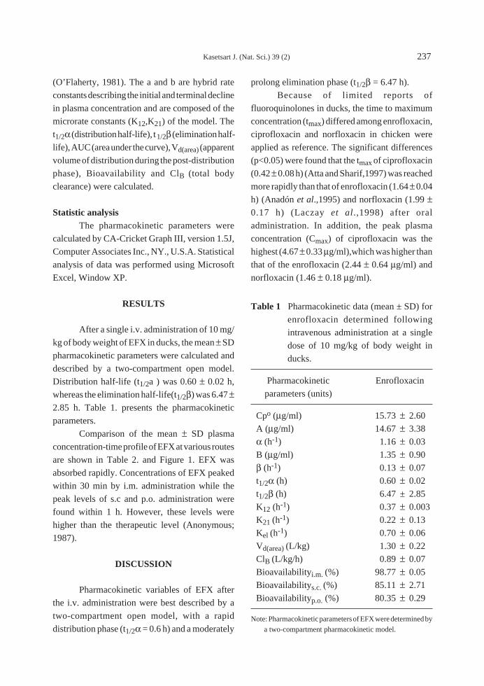
Kasetsart J. (Nat. Sci.) 39 (2) 237
(O’Flaherty, 1981). The a and b are hybrid rate
constants describing the initial and terminal decline
in plasma concentration and are composed of the
microrate constants (K12,K21) of the model. The
t1/2a (distribution half-life), t1/2b (elimination half-
life), AUC (area under the curve), Vd(area) (apparent
volume of distribution during the post-distribution
phase), Bioavailability and ClB (total body
clearance) were calculated.
Statistic analysisThe pharmacokinetic parameters were
calculated by CA-Cricket Graph III, version 1.5J,
Computer Associates Inc., NY., U.S.A. Statistical
analysis of data was performed using Microsoft
Excel, Window XP.
RESULTS
After a single i.v. administration of 10 mg/
kg of body weight of EFX in ducks, the mean ± SD
pharmacokinetic parameters were calculated and
described by a two-compartment open model.
Distribution half-life (t1/2a ) was 0.60 ± 0.02 h,
whereas the elimination half-life(t1/2b) was 6.47 ±2.85 h. Table 1. presents the pharmacokinetic
parameters.
Comparison of the mean ± SD plasma
concentration-time profile of EFX at various routes
are shown in Table 2. and Figure 1. EFX was
absorbed rapidly. Concentrations of EFX peaked
within 30 min by i.m. administration while the
peak levels of s.c and p.o. administration were
found within 1 h. However, these levels were
higher than the therapeutic level (Anonymous;
1987).
DISCUSSION
Pharmacokinetic variables of EFX after
the i.v. administration were best described by a
two-compartment open model, with a rapid
distribution phase (t1/2a = 0.6 h) and a moderately
prolong elimination phase (t1/2b = 6.47 h).
Because of limited reports of
fluoroquinolones in ducks, the time to maximum
concentration (tmax) differed among enrofloxacin,
ciprofloxacin and norfloxacin in chicken were
applied as reference. The significant differences
(p<0.05) were found that the tmax of ciprofloxacin
(0.42 ± 0.08 h) (Atta and Sharif,1997) was reached
more rapidly than that of enrofloxacin (1.64 ± 0.04
h) (Anadón et al.,1995) and norfloxacin (1.99 ±0.17 h) (Laczay et al.,1998) after oral
administration. In addition, the peak plasma
concentration (Cmax) of ciprofloxacin was the
highest (4.67 ± 0.33 mg/ml),which was higher than
that of the enrofloxacin (2.44 ± 0.64 mg/ml) and
norfloxacin (1.46 ± 0.18 mg/ml).
Table 1 Pharmacokinetic data (mean ± SD) for
enrofloxacin determined following
intravenous administration at a single
dose of 10 mg/kg of body weight in
ducks.
Pharmacokinetic Enrofloxacin
parameters (units)
Cpo (mg/ml) 15.73 ± 2.60
A (mg/ml) 14.67 ± 3.38
a (h-1) 1.16 ± 0.03
B (mg/ml) 1.35 ± 0.90
b (h-1) 0.13 ± 0.07
t1/2a (h) 0.60 ± 0.02
t1/2b (h) 6.47 ± 2.85
K12 (h-1) 0.37 ± 0.003
K21 (h-1) 0.22 ± 0.13
Kel (h-1) 0.70 ± 0.06
Vd(area) (L/kg) 1.30 ± 0.22
ClB (L/kg/h) 0.89 ± 0.07
Bioavailabilityi.m. (%) 98.77 ± 0.05
Bioavailabilitys.c. (%) 85.11 ± 2.71
Bioavailabilityp.o. (%) 80.35 ± 0.29
Note: Pharmacokinetic parameters of EFX were determined by
a two-compartment pharmacokinetic model.

238 Kasetsart J. (Nat. Sci.) 39 (2)
Table 2 Mean ± SD plasma concentrations of enrofloxacin in ducks following i.v., i.m., s.c. or p.o.
administration at a single dose of 10 mg/kg of body weight.
Hours after dosing Plasma concentrations (mg/ml)
i.v. i.m. s.c. p.o.
0.15 11.49 ± 1.17 5.65 ± 0.36 4.99 ± 0.87 4.87 ± 0.69
0.30 10.46 ± 1.85 8.97 ± 1.33 6.48 ± 1.07 5.55 ± 0.70
1.00 5.59 ± 0.28 7.99 ± 0.63 8.29 ± 0.62 7.61 ± 1.20
2.00 4.00 ± 0.25 7.60 ± 0.68 7.19 ± 1.12 5.99 ± 0.34
3.00 2.08 ± 0.36 6.76 ± 0.99 7.06 ± 0.58 5.74 ± 0.60
4.00 1.97 ± 0.15 5.72 ± 0.58 6.67 ± 0.73 4.62 ± 0.39
5.00 1.06 ± 0.16 3.90 ± 0.35 4.44 ± 0.68 4.43 ± 0.59
6.00 0.86 ± 0.19 3.57 ± 0.41 2.95 ± 1.13 3.99 ± 0.73
8.00 0.47 ± 0.07 1.51 ± 0.17 1.46 ± 0.10 2.28 ± 0.21
10.00 0.43 ± 0.04 1.43 ± 0.17 1.42 ± 0.25 2.06 ± 0.43
Figure 1 Comparative mean plasma concentration-time profile of enrofloxacin (EFX) following single
i.v.,i.m.,s.c.and p.o. administrations of 10 mg/kg b.w. in ducks.
Hour after dosing (hr.)
0 1 2 3 6 8 10
Plas
ma
conc
entr
atio
ns (u
g/m
l)
0
2
4
6
8
10
12
14
i.v.i.m.s.c.p.o.
4 5 7 9
A similar kinetic profile was also observed
in chickens after the i.v. administration, the biphasic
nature of the plasma concentration-time curve has
been reported for EFX (Anadón et al.,1995;García-
ovando et al.,1999). In the present study, the
elimination half-life (6.47 ± 2.85 h) was also
higher than that recorded in healthy dogs (3.4 h),
cattle (1.7h), sheep (3.7 h), horses (5.0 h) and pigs
(5.5 h) (Baggot,2001). However, this parameter
was lower than that previously reported in chickens
(6.99 ± 0.48 h) (García-ovando et al.,1999).
Fluoroquinolones are lipid-soluble
chemical agents, and their typical Vd values are 2-
4 L/kg (Brown,1996). Nevertheless, lower Vd
values i.e., 1.94 ± 0.14 L/kg have been reported for
EFX in chickens (García-ovando et al.,1999)

Kasetsart J. (Nat. Sci.) 39 (2) 239
The mean ± SD bioavailability of EFX inducks was 98.77 ± 0.05% after the i.m.administration, therefore it is likely that the doseof EFX was almost completely absorbed. Thebioavailability value of the i.m. administrationwas also higher than those of the s.c. (85.11 ±2.71%) and p.o. (80.35 ± 0.29%). Moreover, thedrug was detected and remained in the plasma upto 20 h after the s.c. and i.m. administrations whileit was up to 24h after the i.v. and p.o.administrations.
In conclusion, The biphasic nature of plasmaconcentration-time curve suggested that a two-compartment pharmacokinetic model wouldprovide an accurate description of pharmacokineticbehaviors. The pattern of plasma concentration-time profiles between EFX and the otherfluoroquinolones were identical following i.m.,s.c. or p.o. administration . According to the resultsof this study a dose of 10 mg/kg body weight ofenrofloxacin in ducks may be appropriate for theroutes investigated. However, the tissue residuesshould be further determined by an HPLC assay toget insight into the tissue uptake and the properwithdrawal times of EFX in ducks.
ACKNOWLEDGEMENTS
This study was financially supported bythe Kasetsart University Research andDevelopment Institute (KURDI), THAILAND.The researchers wish to thank Prof. Dr. MalineeLimpoka for her advice on the method of analysis.Special thanks are extended to Kanokwan Bangnoiand Sasithorn Limsuwan for their advice on theuse of computer program.
LITERATURE CITED
Anadón, A., M.R. Martinez-Larranaga, M.J. Diaz,P. Bringas, M.A. Martinez, M.L. Fernandez-Cruz, M.C. Fernandez and R. Fernandez.1995.Pharmacokinetics and residues of enrofloxacinin chickens.Amer. J. of Vet. 56: 501-505.
Anhalt, J.P. 1985. Antimicrobial assays. In
Laboratory Procedures in ClinicalMicrobiology. 2nd ed., J.A. Sprinter Verlag,Washington, New York. 691 p.
Anonymous .1987. Baytril“ Broad-spectrumAntiinfective for the treatment of BacterialDiseases in Animals. Product information.Bayer Veterinary Department, Leverkusen,Germany. 27 p.
Atta, A.H. and L. Sharif. 1997. Pharmacokineticsof ciprofloxacin following intravenous andoral administration in broiler chickens. J. vet.Pharmacol. Therap. 20: 326-329.
Baggot, J.D.1977.Principles of Drug in DomesticAnimals.W.B. Saunders, Philadelphia. 238p.
Baggot, J.D.2001. The Physiological Basis ofVeterinary Clinical Pharmacology. IowaState University Press. 283p.
Bennett, J.V., J.L. Brodie, E.Benner and W.M.M.Kirby. 1966. Simplified, accurate method forantibiotic assay of clinical specimens. AppliedMicrobiology. 14: 170-175.
Brown, S.A. 1996. Fluoroquinolones in animalhealth. J.Vet.Pharmacol.Therap.19: 1-14.
Craigmill, A.L., S.F. Sundlof and J.E. Riviere.1994. Handbook of ComparativePharmacokinetics and Residues ofVeterinary Therapeutic Drugs, CRC Press,Inc., Boca Raton, Fla. 665 p.
García- ovando, H., N. Gorla, C. Luders, G. Poloni,C. Errecalde, G. Prieto and I. Puelles. 1999.Comparative pharmacokinetics ofenrofloxacin and ciprofloxacin in chickens.J. Vet. Pharmacol. Therap. 22: 209-212.
Laczay, P., G. Semjen and J. Lehel .1998.Comparative studies on the pharmacokineticsof norfloxacin in chickens,turkeys and geeseafter a single oral administration. J. Vet.Pharmacol. Therap. 21: 161-164.
Limpoka, M. 1992. Principle Pharmacokineticin Animals. Charulsanitwong, Bangkok. 195p.
O’ Flaherty, E. 1981.Toxicants and Drug:Kinetics and Dynamics.A Wiley IntersciencePublication, New York. 398 p.

Kasetsart J. (Nat. Sci.) 39 : 240 - 246 (2005)
Antimicrobial Resistance of Campylobacter jejuni Isolated fromChicken in Nakhon Pathom Province, Thailand
Jananya Sukhapesna1, Patamaporn Amavisit2, Worawidh Wajjwalku3,Arinthip Thamchaipenet4 and Thavajchai Sukpuaram5
ABSTRACT
Campylobacter jejuni isolated from retail market-chicken in Nakhon Pathom province were
determined for resistance to quinolone and other antimicrobial agents by broth microdilution method.
Sixty-eight C. jejuni strains were resistant to quinolone drugs including nalidixic acid (69.12%),
norfloxacin (69.12%), ciprofloxacin (58.82%) and marbofloxacin (25.00%). High proportions of the
isolates were resistant to tetracycline (77.94%), sulfamethoxazole (72.06%), kanamycin (51.47%),
ampicillin 47.06% and streptomycin (42.65%). Low proportions of the isolates were found resistance to
gentamycin (16.18%) and erythromycin (13.23%). Nearly 97% of the isolates were multiple resistances
to more than 4 antimicrobial agents tested.
Key words: Campylobacter jejuni, broth microdilution method, MICs
INTRODUCTION
Infection with Campylobacter species has
emerged worldwide as one of the leading causes of
diarrhea (Rautelin et al., 2003). C. jejuni is one of
the main species involved in human infection
(Saenz et al., 2000). The genotyping and serotyping
analysis revealed that poultry can be a source of
Campylobacter infection and the contamination
occurred by direct ingestion of undercooked food
or cross contamination of raw poultry to other
foods (Engberg et al.,2001).
Fluoroquinolones and macrolides have been
widely used for treatment of Campylobacter
1 Center for Agricultural Biotechnology, Kasetsart University, Kamphaengsean Campus, Nakhon Pathom 73140, Thailand.2 Department of Microbiology and Immunology, Faculty of Veterinary Medicine, Kasetsart University, Bangkok 10900,
Thailand.3 Department of Pathology, Faculty of Veterinary Medicine, Kasetsart University, Kamphaengsean Campus, Nakhon Pathom
73140, Thailand.4 Department of Genetics, Faculty of Science, Kasetsart University, Bangkok 10900, Thailand.5 Department of Public Health, Faculty of Veterinary Medicine, Kasetsart University, Kamphaengsean Campus, Nakhon
Pathom 73140, Thailand.
Received date : 06/01/05 Accepted date : 04/04/05
infections (Aquino et al., 2002). The increasing
proportions of Campylobacter isolates have been
reported to be resistant to these drugs (Endtz et al.,
1991). The over uses of antimicrobial agents in
veterinary medicine or as feed additives might
result in the emergence and spread of resistance
among Campylobacter strains. This caused
potentially serious effects on food safety and
affected to both veterinary and human health
(Piddock et al., 2000).
In this study we determined the
antimicrobial resistance patterns of sixty-eight
C. jejuni isolated from chicken in Nakhon Pathom
province and evaluated the range of their minimum

inhibitory concentrations (MICs) using broth
microdilution method.
MATERIALS AND METHODS
Bacterial strainsSixty-eight C. jejuni were isolated from
retail market-chicken in Nakhon Pathom province.
They were identified at Kamphaengsean Animal
Diagnostic Laboratory, Faculty of Veterinary
Medicine, Kasetsart University. These isolates
were confirmed to be C. jejuni by using PCR assay
following the method of Stucki et al. (1995). The
isolates were cultured on Columbia agar plate with
5% lysed horse blood and were incubated at 42∞Cfor 48 h in microaerophilic atmosphere. C. jejuni
colonies were transferred into 5 ml of Mueller-
Hinton broth and then incubated at 37∞C for 24 h
in microaerophilic atmosphere to produce a
suspension of 6 to 7 log CFU/ml.
Antimicrobial agentsSix groups of antimicrobial agents including
aminoglycoside (gentamycin, kanamycin and
streptomycin), macrolide (erythromycin),
penicillin (ampicillin), quinolone (ciprofloxacin,
marbofloxacin, nalidixic acid and norfloxacin),
sulfanamide (sulfamethoxazole) and tetracycline,
were used for this study.
Test procedureOne hundred microliters of two-fold
dilution of each antimicrobial agent ranging from
0.007 to 128 ml/ml was filled in each well of 96
wells sterile microtiter plates (Luber et al., 2003).
Each well for susceptibility testing was filled with
100 ml of 6 to 7 log CFU/ml of bacterial suspension,
and mixed gently. The plates were incubated at
37∞C under microaerophilic condition. The MICs
was evaluated at 24 hours later.
RESULTS AND DISCUSSION
Minimum Inhibitory Concentrations
(MICs) were defined as the lowest concentration
that exhibits no growth of C. jejuni by visible
reading. The MICs of antimicrobial agents for C.
jejuni is presented in Table 1.
Each of isolates had different MICs in each
antimicrobial agents and different range of MICs.
The MICs range of gentamycin, kanamycin,
streptomycin, erythromycin, ampicillin,
ciprofloxacin, marbofloxacin, norfloxacin and
sulfamethoxazole were 0.03-2, 1-128, 0.12-16,
0.5-64, 0.25-64, 0.12-16, 0.007-8, 0.06-8 and
0.5-128 mg/ml, respectively. Nalidixic acid and
tetracycline had the same MICs range at 0.25-128
mg/ml. The MICs values of tetracycline, nalidixic
acid, kanamycin and sulfamethoxazole were higher
than other antimicrobial agents.
At present, there is no internationally
accepted criterion for susceptibility testing of
Campylobacter. Resistant breakpoint following
EUCAST (2000) method was used in this study. It
was classified as susceptibility or resistance
according to their individual MICs distribution of
each agent. When two or more sub-populations
were found, isolates with lower MICs were
classified as susceptibility, whereas those from
sub-populations with higher MICs were classified
as resistance.
The distribution of MICs of antimicrobial
agents against sixty-eight isolates of C. jejuni is
shown in Figure 1. The MICs of these antimicrobial
agents was a bimodal distribution. C. jejuni isolates
were categorized as resistance when MICs of
erythromycin, kanamycin, and sulfamethoxazole
exceeded 32 mg/ml; ampicillin and tetracycline
exceeded 16 mg/ml; nalidixic acid and streptomycin
exceeded 8 mg/ml; ciprofloxacin and
marbofloxacin exceeded 4 mg/ml, whereas C.
jejuni isolates were found as low resistance, when
MICs of gentamycin and norfloxacin exceeded 1
and 2 mg/ml, respectively.
Kasetsart J. (Nat. Sci.) 39 (2) 241

242 Kasetsart J. (Nat. Sci.) 39 (2)
Table 1 MICs of 11 antimicrobial agents against sixty-eight isolates of C. jejuni by broth microdilution
method.
MICs (mg/ml)
Agent1 128 64 32 16 8 4 2 1 0.5 0.25 0.12 0.06 0.03 0.015 0.007
GEN � � � � � � 2 9 � � 45 9 3
KAN 1 9 25 � � � 27 6�
STR � � � 8 21 � � � � 35 4
ERY � 3 6 � � 5 14 33 7
AMP � 4 8 20 � � � � 35 1
CIP � � � 8 11 21 � � � 23 5
MAR � � � � 3 14 � � � � � 7 33 10 1
NAL 1 9 7 22 8 4 9 4 2 2
NOR � � � � 1 9 37 � � � 13 8
SMX 12 35 2 � � � � 3 16
TET 8 7 32 6 � � � 1 10 4
1 GEN = gentamycin, KAN = kanamycin, STR = streptomycin, ERY = erythromycin, AMP = ampicillin, CIP = ciprofloxacin,
MAR = marbofloxacin, NAL = nalidixic acid, NOR = norfloxacin, SMX = sulfamethoxazole, TET = tetracycline2 MICs = Minimum Inhibitory Concentrations
Antimicrobial concentration ranges,
MIC50, MIC90, breakpoints of resistance and
percentage of resistance for C. jejuni are presented
in Table 2. MIC50 and MIC90 were MIC at which
50% and 90% of the isolates were inhibited,
respectively. The data indicated that
sulfamethoxazole had MIC50 and MIC90 higher
than other agents at 64 and 128 mg/ml, respectively,
Table 2 Antimicrobial agents, range of MICs, MIC50, MIC90, breakpoint of resistance and percentage
of resistance from sixty-eight C. jejuni isolates as determination by broth microdilution.
MIC (mg/ml) Break point of Percentage of
Agent Range MIC50 MIC90 resistance (mg/ml) resistance
Gentamycin 0.03-2 0.12 1 1 16.18%
Kanamycin 1-128 32 64 32 51.47%
Streptomycin 0.12-16 0.25 16 8 42.65%
Erythromycin 0.5-64 1 32 32 13.23%
Ampicillin 0.25-64 0.5 32 16 47.06%
Ciprofloxacin 0.12-16 4 8 4 58.82%
Marbofloxacin 0.007-8 0.03 4 4 25.00%
Nalidixic acid 0.25-128 16 64 8 69.12%
Norfloxacin 0.06-8 2 8 2 69.12%
Sulfamethoxazole 0.5-128 64 128 32 72.06%
Tetracycline 0.25-128 32 128 16 77.94%

Kasetsart J. (Nat. Sci.) 39 (2) 243
while gentamycin had lowest values at 0.12 and 1
mg/ml, respectively.
Resistance to antimicrobial agents was
commonly detected among sixty eight C. jejuni
isolates. Resistance to four quinolones including
ciprofloxacin, marbofloxacin, nalidixic acid and
norfloxacin was found at 58.82, 25.00, 69.12 and
69.12%, respectively. The high prevalence of
quinolone resistant C. jejuni isolates was similar to
the finding of Engberg et al. (2001). However, the
prevalence of marbofloxacin resistant isolates of
C. jejuni in this study was relatively low (25.00%).
The reason was possibly due to marbofloxacin is
not commonly used as the other drugs in this
group. Endtz et al. (1991) reported that certain
isolates of C. jejuni were cross-resistant to various
Erythromycin
0
20
40
60
80
100
0.03 0.25 2 16 128
MIC (ug/ml)
% is
olat
es
Kanamycin
0
20
40
60
80
100
0.03 0.25 2 16 128
MIC (ug/ml)
% is
olat
esSulfamethoxazole
0
20
40
60
80
100
0.03 0.25 2 16 128
MIC (ug/ml)
% is
olat
esAmpicillin
0
20
40
60
80
100
0.03 0.25 2 16 128
MIC (ug/ml)
% is
olat
es
Tetracycline
0
20
40
60
80
100
0.03 0.25 2 16 128
MIC (ug/ml)
% is
olat
es
Nalidixic acid
0
20
40
60
80
100
0.03 0.25 2 16 128
MIC (ug/ml)
% is
olat
es
Streptomycin
0
20
40
60
80
100
0.03 0.25 2 16 128
MIC (ug/ml)
% is
olat
es
Ciprofloxacin
0
20
40
60
80
100
0.03 0.25 2 16 128
MIC (ug/ml)
% is
olat
es
Marbofloxacin
0
20
40
60
80
100
0.01 0.06 0.5 4 32
MIC (ug/ml)
% is
olat
es
Gentamycin
0
20
40
60
80
100
0.03 0.25 2 16 128
MIC (ug/ml)
% is
olat
es
Norfloxacin
0
20
40
60
80
100
0.03 0.25 2 16 128
MIC (ug/ml)
% is
olat
es
Figure 1 Distribution of MICs of 11 antimicrobial agents against sixty-eight isolates of C. jejuni from
chicken. Arrow indicated break point of resistance.

244 Kasetsart J. (Nat. Sci.) 39 (2)
quinolones. Most nalidixic acid-resistant isolates
have been reported to be cross-resistant to one,
two or three drugs in this group (Reina et al.,
1995).
In Thailand, prevalence of quinolone
resistant Campylobacter species in broiler
farms was found to increase from 0% in 1987 to
84% in 1995 (Hoge et al., 1998). In addition,
Daniel et al. (2002) found that C. jejuni isolated
from Thai population was resistant to ciprofloxacin
in high proportion (77%). Quinolone-resistant
Campylobacter isolates in human and poultry
meat were also found in other countries, including
Canada (Gaunt and Piddock, 1996), Spain (Prats
et al., 2000), Senegal (Cardinale, 2003) and Taiwan
(Engberg et al., 2001). A fluoroquinolone-resistant
C. jejuni infection has also been associated with
foreign travel to many countries (Cardinale, 2003).
It was reported that most clinical isolates of C.
jejuni from U.S. troops in Thailand were resistant
to ciprofloxacin (Murphy et al., 1996).
Regarding the proportion of aminoglyco-
side resistance, the percentage of isolate resistance
in kanamycin was 51.47%, gentamycin was
16.18% and streptomycin was 42.65%. There was
a report previously indicated that aminoglycosides
resistance was less common in C. jejuni (Trieber
and Taylor, 2000). Campylobacter species isolated
from humans, pigs, cattle, and broilers were very
low in resistance to streptomycin (1%) (Fallon et
al., 2003). Moreover, it was demonstrated that
there was no Campylobacter from chicken isolates
that was resistant to aminoglycosides (Cabrita et
al., 1992). The contrary of aminoglycosides
resistance of C. jejuni from this work to the others
was possibly due to the administration of these
antimicrobial agents in veterinary medicine under
certain conditions in Thailand. Therefore,
resistances of these agents were found to increase
in certain isolates of C. jejuni.
In this study, the high proportions of C.
jejuni isolates were also resistant to other
antimicrobial agents including ampicillin
(47.06%), sulfamethozaxole (72.06%) and
tetracycline (77.94%). These results are in
accordance with the previous report that resistances
to ampicillin, chloramphenicol, sulfamethozaxole
and tetracycline of C. jejuni were commonly found
in Thailand (Daniel et al., 2002).
Low resistant level of erythromycin and
gentamycin was found in 9 and 11 isolates of C.
jejuni, respectively. However, MIC values of these
agents were different (Table 2). Since gentamycin
showed a very low MIC90, it seems reasonable to
consider this drug as an alternative for treatment of
C. jejuni infections under certain conditions in
Nakhon Pathom province, Thailand. Therefore, it
is necessary to select the antimicrobial wisely for
its effectiveness.
Resistance of C. jejuni isolates to a number
of antimicrobial agents is presented in Table 3.
Antimicrobial resistance (4 to 8 antimicrobial
agents) was detected in sixty-six isolates (97.06%).
Resistance to four or more of the drugs tested was
Table 3 Multi-antimicrobial resistant profiles of C. jejuni.
Number of antimicrobial agents Number of resistance isolates (%)
0 2 (2.94%)
4 10 (14.70%)
5 19 (27.94%)
6 26 (38.24%)
7 9 (13.24%)
8 2 (2.94%)

Kasetsart J. (Nat. Sci.) 39 (2) 245
defined as multiple resistances. Only two isolates
of C. jejuni (2.94%) were susceptible to all
antimicrobial agents. All of multiple resistance of
C. jejuni was consisted of quinolone resistance.
One common resistance of this group was nalidixic
acid.
Most C. jejuni strains were resistant to
multi-antimicrobial agents tested. This was
possibly due to some development by genetic
change or physiological adaptation of the organisms
to increase antimicrobial tolerances in consequence
of previous exposure to antimicrobials. Therefore,
discontinuing the practice of routinely adding
growth promoters to animal feeds would reduce
the resistant strains of C. jejuni in animals in
Thailand. Long-term surveillance data are needed
to further evaluate the impact of any intervention
in antimicrobial usages. Moreover, antimicrobial
susceptibility testing methods for Campylobacter
species are needed to be harmonized and
standardized for predication that bacteria will
respond to treatment from an appropriate agent.
CONCLUSION
Quinolone–resistant Campylobactor is a
concerning issue in human medicine because of
failure in treatment of diarrhea cases with
quinolone. Scientists are monitoring the import
meat products to protect the consumers from this
organism. Most, C. jejuni of Thai–isolates have
shown high proportion of multiple resistance to
many kinds of antimicrobial agent used in the test
including quinolone. Erythromycin and
gentamycin are alternative drugs for treatment of
these cases. Good farming practice should be
implemented to reduce the usage of antimicrobials.
ACKNOWLEDGEMENTS
This work was supported by funding from
Center for Agricultural Biotechnology, Kasetsart
University, Kamphaengsean Campus. Gratitude
is expressed to Srisamai Viriyarampa for her
advices in microbiological techniques. We also
acknowledge the Faculty of Veterinary Medicine,
Kasetsart University for equipment supporting.
LITERATURE CITED
Aquino, M.H.C., A.L.L. Filgueiras, M.C.S. Ferreira
and S.S. Oliveinia. 2002. Antimicrobial
resistance and plasmid profiles of C. jejuni
and C. coli from human and animal sources.
Lett. Appl. Microbiol. 34: 149-153.
Cabrita, J.J., J. Rodrigues, F. Bragance, C. Morgado
and A. Goncalves. 1992. Prevalence biotypes,
plasmid profiles and antimicrobial resistance
of Campylobacter isolated from wild and
domestic animals from Northeast Portugal. J.Appl. Bacteriol. 73: 279-285.
Cardinale, E.J., A. Dromigny, F. Tall, M. Ndiaye,
M. Konte and J.D. Perrier. 2003.
Fluoroquinolone susceptibility of
Campylobacter strains, Senegal. Antimicrob.Agents Chemother. 58: 178-190.
Daniel, W.I., C.W. Hoge, P. Chittima, L. Bodhidatta
and K.W. Hickey. 2002. Competitive
antibiotic resistance of diarrheal pathogens
from Vietnam and Thailand, 1996-99. Emerg.Infect. Dis. 8: 175-201.
Endtz, H.P., G.J. Rujis, B. Klingeren, W. H. Jansen
and. R.P.Mouton. 1991. Quinolone resistance
in Campylobacter isolated from man and
poultry following the introduction of
fluoroquinolone in veterinary medicine. J.Antimicrob. Chemother. 27: 199-208.
Engberg, J., F.M. Aurestrup, D.E. Taylor and I.
Nachamkin. 2001. Quinolone and macrolide
resistance in C. jejuni and C. coli resistance
mechanisms and trend in human isolates.
Emerg. Infect. Dis. 7: 24-34.
EUCAST. 2000. Terminology relating to methods
for the determination of susceptibility of
bacteria to antimicrobial agents. Clin.Microbiol. Infect. 6: 503-508.

246 Kasetsart J. (Nat. Sci.) 39 (2)
Fallon, R., N. Sullivan, M. Maher and C. Carroll.
2003. Antimicrobial resistance of C. jejuni
and C. coli isolates from broiler chickens
isolated at an Irish poultry processing plant.
Lett. Appl. Microbiol. 36: 277-281.
Gaunt, P.N. and L.J.V. Piddock. 1996.
Ciprofloxacin resistant Campylobacter spp.
In humans: an epidemiological and
laboratory study. J. Antimicrob. Chemother.37: 747-757.
Hoge, C.W., J.M. Gambel, C. Pitarangsri and P.
Echeverria. 1998. Trends in antibiotic
resistance diarrhea pathogens isolated in
Thailand over 15 years. Clin. Infect. Dis. 26:
341-345.
Luber, P., E. Bartelt, E. Genschow, J. Wagner and
H. Hahn. 2003. Comparison of broth
microdilution, E Test, and agar dilution
methods for antibiotic susceptibility testing
of Campylobacter jejuni and Campylobacter
coli. J. Clin. Microbiol. 41: 1062-8.
Murphy, G., P. Echeverria, L. Jackon, M. Arness
and C. Leboon. 1996. Ciprofloxacin and
azithromycin resistant Campylobacter causing
travelers’ s diarrhea in US troops deployed to
Thai in 1994. Clin. Infect. Dis. 22: 864-869.
Piddock, L.J.V., V. Ricci, K. Stanley and K.Jones.
2000. Activity of antibiotics used in human
medicine for C. jejuni isolated from farm
animals and their environment in Lancashire,
U.K. J. Antimicrob. Chemother. 46: 303-
306.
Prats, G., B. Mirelis, T. Lovet, C. Munoz, E. Miro
and F. Navarro. 2000. Antibiotic resistance
trends in enteropathogenic bacteria isolated
in 1985-1987 and 1995-1998 in Barcelona.
Antimicrob. Agents Chemother. 44: 1140-
1145.
Rautelin, H., A. Vierikko, M.L. Hanninen and M.
Vaara. 2003. Antimicrobial susceptibility of
Campylobacter strains isolated from Finnish
subjects infected domestically or from those
infected abroad. Antimicrob. AgentsChemother. 47: 102-105.
Reina, J., M.J. Ros and V. Fernandez-Baca. 1995.
Resistance to erythromycin in
fluoroquinolone-resistant Campylobacter
jejuni strains isolated from human feces. J.Antimicrob. Chemother. 35: 351-352.
Saenz, Y., M. Zarazaga, M. Lantero and F. Baquero.
2000. Antibiotic resistance in Campylobacter
strains isolated from animals, foods, and
human in Spain in 1997-1998. Antimicrob.Agents Chemother. 44: 267-271.
Stucki, U., J. Frey, J. Nicolet and A.P. Burnens.
1995. Identification of Campylobacter jejuni
on the basis of a species-specific gene that
encodes a membrane protein. J. Clin.Microbiol. 33: 855–859.
Trieber, C.A. and D.E.Taylor. 2000. Mechanisms
of antibiotic resistance in Campylobacter.
Am. Soc. Microbiol. 54: 441-454.

Kasetsart J. (Nat. Sci.) 39 : 247 - 261 (2005)
Hematology, Cytochemistry and Ultrastructure of Blood Cellsin Asiatic Black Bear (Ursus thibetanus)
Chaleow Salakij1, Jarernsak Salakij1, Nual-Anong Narkkong2,Ludda Trongwonsa3 and Rattapan Pattanarangsan4
ABSTRACT
Blood cells from adult Asiatic black bear (Ursus thibetanus) were examined and measured after
stainning with modified Wright stain and cytochemical stains, including Sudan Black B (SBB), Periodic
acid Schiff’s reaction (PAS), a-naphthyl acetate esterase (ANAE), acid phospatase (AcP) and b-
glucuronidase (b-glu). Red blood cells were uniform in shape, with 7.3 mm mean diameter in size and easy
to form rouleaux. Using scanning electron microscopic (SEM) examinations revealed normal and
abnormal red blood cell surfaces. Neutrophils contained several vacuoles as detected by light microscope
and revealed themselves as large granules under transmission electron microscope. Neutrophils stained
strongly positive with SBB, ANAE; weak positive with PAS and negative with AcP and b-glu. Using
SEM, neutrophil surfaces revealed several microvilli and some micropores. Eosinophils contained
numerous small round red refractive granules with some vacuoles. Eosinophils stained strongly positive
with SBB and ANAE but negative with PAS and b-glu. Basophils had variable numbers of intense
basophilic granules that obscured the very long lobulated nucleus. Basophils stained moderately positive
with SBB but strongly positive with ANAE. Lymphocytes were negative with SBB but have 3 patterns
of reactivity with ANAE, AcP and b-glu, including negative, focal dot and fine granular stainings.
Monocytes stained moderately with SBB and moderately to strongly with for ANAE and b-glu. The SEM
examinations could differentiate white blood cells by their surface contours. Transmission electron
microscopic examinations revealed organelles within all blood cells.
Key words: Asiatic black bear, blood cell, cytochemistry, morphology, ultrastucture
INTRODUCTION
Asiatic black bear (Ursus thibetanus) has
shaggy black fur with white crescent on the chest,
considerably larger than Malayan sun bear (Ursus
malayanus). Asiatic black bear has suffered from
habitat loss and is now rare in many areas (Francis,
2001). So this endangered species has been studied
1 Faculty of Veterinary Medicine, Kasetsart University, Kamphaengsaen, Nakorn Pathom 73140, Thailand.2 Central Instruments Center, Faculty of Science, Mahasarakarm University, Mahasarskarm 44150, Thailand.3 National Institute of Animal Health, Kasetklang, Jatujuk, Bangkok 10900, Thailand.4 Faculty of Veterinary Science, Mahidol University, Salaya, Nakorn Pathom 73170, Thailand.
Received date : 19/01/05 Accepted date : 03/05/05
intensively to determine the health status of the
individuals. Veterinary hematology serves as a
screening procedure to assess general health, the
body’s ability to fight infection in adjunct to patient
evaluation or diagnosis (Jain, 1993).
Differential white blood cell count is very
useful not only in numbering the white blood cells
but also provide evidence of anemic condition or

248 Kasetsart J. (Nat. Sci.) 39 (2)
reveal the pathogenesis. Blood smear examinations
provide more information on morphology of red
blood cell, white blood cell and platelets (Mills,
1998). Cytochemical method is useful in diagnosis
of acute leukemia in human (Apibal, 1987;
Khemtonglang et al., 1997). The purpose of the
present study was to characterize the morphology,
cytochemical reaction and ultrastrucrure of blood
cells in Asiatic black bear.
MATERIALS AND METHODS
From February to June 2003, five clinically
healthy Asiatic black bears in Khao Kheaw Open
Zoo were chemical restrained with xylaxine
(Rompun®) and ketamine. Two millilitres of blood
samples were collected from the jugular vein and
transferred to tubes containing ethylenediamine
tetraacetic acid (EDTA). Some of the blood without
anticoagulant was directly smeared on the slides.
Two Asiatic black bears were adult males and
three were adult females aging between 3-5 years
old. Hematology, plasma protein and fibrinogen
were determined by manual technique (Schalm et
al., 1975) within two hours after blood collection.
Two direct blood smears from each bear were
stained with a modified Wright and Wright’s stains.
A minimum of 200 leukocytes were counted for
differential leukocyte determinations. The
anticoagulated blood was used for reticulocyte
count by staining with new methylene blue stain
(Schalm et al., 1975). The percentage of
reticulocyte presented in 1,000 red blood cells
(RBC) was determined. For each hematologic
parameter, means, variances and standard errors
were calculated using SPSS® for Window™
(Norusis, 1993).
Cytochemical staining characteristics of
blood cells were evaluated using air-dried blood
smears from three Asiatic black bears. Cells were
stained with periodic acid Schiff’s reaction (PAS),
Sudan black B (SBB), a–naphthyl acetate
esterase (ANAE), acid phosphatase (AcP) and b–
glucuronidase (b–glu). Cytochemical procedures
used were the same as those previously described
(Salakij et al., 2002). Positive– and negative-
stained cells were differentiated by counting 500
cells on each of the cytochemically stained smears.
For scanning electron microscopy (SEM)
and transmission electron microscopy (TEM),
blood cells from three Asiatic black bears were
processed as described by Salakij et al. (2002).
Identification of blood cells by SEM and TEM was
based on the relative number, size, shape and
distribution of granules and on nuclear appearance.
RESULTS
There was no blood parasite detected in all
bears. Hematological data of Asiatic black bear
was tabulated (Table 1). White blood cell
differential counts were shown in Table 2. Blood
cell diameters were observed and calculated (Table
3). Cytochemical staining patterns of blood cells
were summarized (Table 4). The morphology under
light microscope, SEM, TEM and cytochemical
characteristics of individual blood cells were
evaluated, as described below.
ErythrocytesRed blood cells (RBCs) or erythrocytes
under light microscope showed uniform in shape
(Figure 1), slightly biconcave and slightly central
pallor as observed by SEM (Figure 4a, 4b) with 7.3
mm mean diameter in size (Table 3) and easy to
forming rouleaux. Some defected RBCs (Figure
4c), crenated RBCs (Figure 4d), echinocyte (Figure
5a, 5b), rubricyte (Figure 8b) and metarubricyte
(Figure 8c) were also observed. Mature red blood
cells were negative for all cytochemical stainings.
Ultrastructurally, mature RBC showed only
hemoglobin (Figure 8a) while the metarubricytes
showed some organelles (Figure 8c) and the
rubricytes showed more mitochondria (Figure 8b).

Kasetsart J. (Nat. Sci.) 39 (2) 249
PlateletsBear platelets were approximately 1/5 to 1/
2 of RBC and had prominent reddish-purple
granules which were easily seen in modified Wright
stain (Figure 1d, f). Plateletes were not stained
with SBB but were moderately to strongly positive
with ANAE (Figure 3m). These platelets were
seldom seen on RBCs (Figure 5b), but gave rosette
formation on monocyte (Figure 5c) and aggregation
(Figure 5d). Ultrastructurally, platelets showed
dense granules, alpha-granules, glycogen granules
and microtubule (Figure 8d).
NeutrophilsNeutrophils were the most prevalent
leukocyte in Asiatic black bear (Table 2) with
neutrophil : lymphocyte ratio equal to 62 : 26.
With modified Wright stain, neutrophils showed
the same size as basophil (Table 3). Neutrophils
showed faintly stained cytoplasm which contained
indistinct pale granules and several vacuoles
Table 1 Hematology of Asiatic black bear.
Hematology Asiatic black bear (n = 5)
PCV (%) 41.4 ± 1.8
Hemoglobin (g/dL) 13.3 ± 0.6
RBC (1012/L) 6.08 ± 0.39
MCV (fL) 68.5 ± 2.1
MCHC (g/dL) 32.1 ± 0.6
WBC (1011/L) 6.99 ± 0.59
Band neutrophils (109/L) 0.11 ± 0.09
Segmented neutrophils (109/L) 4.15 ± 0.19
Lymphocytes (109/L) 1.84 ± 0.28
Monocytes (109/L) 0.13 ± 0.04
Eosinophils (109/L) 0.73 ± 0.18
Basophils (109/L) 0.03 ± 0.02
Band neutrophils (%) 1.7 ± 1.4
Segmented neutrophils (%) 60.3 ± 3.4
Lymphocytes (%) 25.8 ± 1.7
Monocytes (%) 1.8 ± 0.5
Eosinophils (%) 10.0 ± 1.5
Basophils (%) 0.4 ± 0.2
Plasma protein (g/dL) 8.1 ± 0.3
Fibrinogen (mg/dL) 220 ± 49
Reticulocyte (%) 0.0 ± 0.0
Table 2 White blood cell differential count in
Asiatic black bear.
Hematology Asiatic black bear
(n = 5)
Band neutrophils (%) 1.7 ± 1.4
Segmented neutrophils (%) 60.3 ± 3.4
Lymphocytes (%) 25.8 ± 1.7
Monocytes (%) 1.8 ± 0.5
Eosinophils (%) 10.0 ± 1.5
Basophils (%) 0.4 ± 0.2

250 Kasetsart J. (Nat. Sci.) 39 (2)
(Figure 1a, 2a). Neutrophils have tight constricted
and multilobulated nuclei (Figure 1a, 2a). These
vacuoles shown in light microscope were revealed
as large granules in TEM (Figure 9a-d). Some
neutrophils (2-5%) of the female revealed sex
chromatin lobe.
Neutrophils stained strongly positive with
SBB (Figure 3a), moderately stained with ANAE
(Figure 3i) and negative with b-glu (Figure 3o).
Using SEM, neutrophil surfaces revealed several
microvilli and some micropores (Figure 6a, 6b,
6d). Ultrastructurally, neutrophils showed lobed
nuclei, small specific granules (Figure 11a, b),
large electron-dense granules (Figure 9a-c) and
glycogen granules (Figure 9d) were also detected.
EosinophilsEosinophils varied from 10 to 16 mm
(average 14 mm) in diameter (Table 3). Eosinophils
contained numerous small round red refractive
granules with some vacuoles (Figure 1b, 2b).
Eosinopil nuclei were less lobulated than those of
neutrophils, and tetralobed, trilobed or band-
shaped. Eosinophils stained moderately positive
with SBB (Figure 3b) and ANAE (Figure 3j) but
weak positive with b-glu (Table 4). Under SEM,
eosinophil surfaces revealed larger granule contour
(Figure 6c, 6d) than those of basophils (Figure 6e,
6f). Ultrastructurally, eosinophils showed lobed
nuclei, large pleomorphic granules with bar-shape
structures in some granules, Golgi apparatus, RER
and ribosomes (Figure 10a, 10b).
Table 4 Cytochemical staining patterns of blood cells from Asiatic black bear.
Cell type SBB PAS ANAE Acid phosphatase b-glucuronidase
Neutrophils + + + ++ - ±±
Eosinophils + - +++ - +
Basophils + + - ++ - -
Lymphocytes - - - / focal dot / fine granular - / focal dot / fine granular - / focal dot / fine granular
Monocytes + - + + - +
Platelets - - ++ - -
SBB indicates sudan black B; PAS, periodic acid-Schiff; and ANAE, a-naphthyl acetate esterase. Staining was scored as negative
(-), weak (±±, few positive cells), moderate (+), moderate to strong (++), or strong (+++).
Table 3 Mean ± SD of blood cell diameters (mm) in Asiatic black bear.
Cell type No. Asiatic black bear
Red blood cells 50 7.30 ± 0.84
Segmented Neutrophils 50 13.42 ± 1.10
Eosinophils 50 14.09 ± 1.66
Basophils 18 13.06 ± 1.95
Lymphocytes
small 50 8.28 ± 0.78
medium 50 11.02 ± 1.11
large 17 14.40 ± 0.48
Monocytes 50 15.28 ± 2.14

Kasetsart J. (Nat. Sci.) 39 (2) 251
Figure 1 Light micrographs of blood cells in Asiatic black bear stained with modified Wright stain. a.
A segmented neutrophil with many cytoplasmic vacuoles. b. An eosinophil. c. A basophil (left)
and a segmented neutrophil. d. A lymphocyte (right) and a segmented neutrophil. e. A
monocyte. f. A basophil (right) and a segmented neutrophil.
Figure 2 Light micrographs of blood cells in Asiatic black bear stained with Wright’s stain (a-d). a. A
segmented neutrophil with some cytoplasmic vacuoles. b. An eosinophil. c. A basophil. d. A
lymphocyte (right) and a basophil. e. A leukocyte stained with new methylene blue whilst there
was no reticulocyte.

252 Kasetsart J. (Nat. Sci.) 39 (2)
Figure 3 Cytochemical staining of blood cells in Asiatic black bear a. Sudan black-B (SBB) positive
segmented neutrophil. b. SBB positive in the periphery of the granules of the eosinophil. c.
SBB positive in basophil. d. Some small dots of SBB positive in a 14 mm monocyte. e. PAS
positive in segmented neutrophil. f. PAS positive in two segmented neutrophils and negative
in an eosinophil. g. PAS negative in a basophil comparing with PAS positive in two segmented
neutrophils. h. PAS negative in lymphocyte (lower right) and monocyte (upper left). i.-m.
ANAE reactivity in a segmented neutrophil (i), eosinophil (j), basophil (right) (k), monocyte
(upper right) (l) and in platelets (m). n. Negative AcP in a segmented neutrophil and a
monocyte. o. Negative b-glu in a segmented neutrophil and a basophil. p. Focal dot positive
of b-glu in a lymphocyte.

Kasetsart J. (Nat. Sci.) 39 (2) 253
Figure 4 Scanning electron micrographs (SEM) of red blood cells (RBCs) in Asiatic black bear. a. A
cluster of RBCs showing bicocave disk and crenations. b. Higer magnification of crenated
RBCs. c. Defective RBCs. d. A cluster of four echinocytes.
Figure 5 SEM of RBCs and platelets in Asiatic black bear. a. An echinocyte. b. A platelet on an
echinocyte. c. Plateletes rosetting on a monocyte. d. Platelets aggregation next to neutrophil.

254 Kasetsart J. (Nat. Sci.) 39 (2)
Figure 6 SEM of granulocytels in Asiatic black bear. a. A neutrophil showing short microvilli and some
micropores. b. A neutrophil with three micropores. c. An eosinophil. d. An eosinophil (right)
and a monocyte (left). e. A basophil showing small granule contour. f. A basophil.
Figure 7 SEM of agranulocytes in Asiatic black bear. a. A lymphocyte with several cytoplasmic blebs.
b. A monocyte with deep surface fissures.

Kasetsart J. (Nat. Sci.) 39 (2) 255
Figure 8 Transmission electron micrographs (TEM) of blood cells in Asiatic black bear. a. Mature
erythrocytes. b. A rubricyte with some mitochondria (arrows). c. A metarubricyte. d. Platelets
containing mitochondria, vacuoles (v) and dense granules (*).

256 Kasetsart J. (Nat. Sci.) 39 (2)
Figure 9 TEM of neutrophils in Asiatic black bear. a. A segmented neutrophil showing nucleus (N)
many fine granules and large granules (L). b. A segmented neutrophil showing two lobed
neucleus (N) with heterogeneous granule density of large granules (L). c. A segmented
neutrophil (N) with homogeneous granule density of large granules (L). d. A segmented
neutrophil (N) with many glycogen granules (arrows).

Kasetsart J. (Nat. Sci.) 39 (2) 257
Figure 10 TEM of eosinophils and basophils in Asiatic black bear. a. An eosinophil showing neucleus
(N) and many granules. b. Higher magnification of eosinophil in (a) showing bar-shape
structures (arrows) in their granules. c., d. Basophils showing bilobed neuclei (N) and many
small heterogenous granules.

258 Kasetsart J. (Nat. Sci.) 39 (2)
Figure 11 TEM of lymphocytes and monocytes in Asiatic black bear. a. A lymphocyte showing round
neucleus (N) and three mitochondria (arrows). b. A lymphocyte with round nucleus (N). c.
A monocyte with kidney-shaped nucleus (N). d. A monocyte with nucleus (N), many
mitochondria (MT), ribosomes, vacuoles (v) and pseudopodia (arrows).

Kasetsart J. (Nat. Sci.) 39 (2) 259
BasophilsBasophils in were not frequently observed.
They varied from 11 to 15 mm (average 13 mm).
Basophils contained variable numbers of intensely
basophilic granules (Figure 1c, 1f, 2c, 2d) which
obscured the very long lobe nucleus. Basophil
granules stained with SBB more faintly than
granules of neutrophil (Figure 3c). Basophil
granules appeared red-brown when stained with
ANAE (Figure 3k) but weak positive or negative
with b-glu (Figure 3o). Under SEM, basophil
surfaces revealed smaller granule contour (Figure
6e, 6f) than those of eosinophils (Figure 6c, 6d).
Ultrastructurally, basophils showed lobed nuclei,
small heterogenous electron density granules, some
dense granules (Figure 10c) and some mitochondria
(Figure 10d).
LymphocytesLymphocytes in bears were variable in size
(7 to 16 mm diameter). Most lymphocytes were
small (Figure 1d, 2d) and medium size. Some
lymphocytes contained small azurophilic granules
in their cytoplasm. Lymphocytes were negative
for SBB but had 3 patterns of reactivity for ANAE
and b-glu, including negative, focal dot and fine
granular stainings. Under SEM, lymphocyte
surfaces revealed smooth bulging contour of round
nuclei (Figure 7a) with variable numbers of cell
membrane blebs. Ultrastructurally, lymphocytes
showed round nuclei with peripheral clumps of
heterochromatin and some mitochodria (Figure
11a, 11b).
MonocytesMonocytes in bears varied from 13 to 17
mm in diameter (Table 4). They are the largest
white blood cells with variable shape. The nuclei
were extremely variable but usually have lacy
chromatin (Figure 1e). The cytoplasm was blue-
gray and contained variable size of vacuoles (Figure
1e). Monocytes stained moderately positive with
SBB with faintly black, small granules scattered in
the cytoplasm (Figure 3d). They were moderately
to strongly positive with ANAE showing red-
brown fine granular pattern (Figure 3l), but they
were negative for PAS (Figure 3h) and b-glu.
Under SEM, monocyte surfaces revealed more
smooth membrane than those of neutrophil (Figure
7b) with deep fissure and micropores.
Ultrastructurally, monocytes showed variable
shape of nuclei with several mitochodria and
pseudopodia (Figure 11c, 11d).
DISCUSSION
In this report, we described the light
microscope, cytochemical features and
ultrastructure of blood cells in Asiatic black bear.
Although the erythrocytes in bears has special
features such as uniform in shape with central
pallor similar to those of dog, they are larger in
mean diameter (Jain, 1993) and easy to form
rouleaux. The RBC parameters of Asiatic black
bear in this study was similar to but had lower
number of leukocytes than those of Asiatic black
bear in the zoo of Czechoslovakia (Pospisil et al.,
1987). There was no blood parasite found in Asiatic
black bear of this study while there was a report of
filarid worm (Dirofilaria ursi) found in the
esophageal and tracheal connective tissue of the
male Asiatic black bear on Kyushu island
(Yokohata et al., 1990).
Ultrastructure of platelets in Asiatic black
bear were similar to those in bovine (Fern, 2000)
and African elephant (Du Plessis and Stevens,
2002). Platelets in Asiatic black bear were negative
for SBB which were the same as those in bovine,
cat, dog, horse and green sea turtle (Raskin and
Valenciano, 2000). Platelets in Asiatic black bear
positively stained with ANAE which were similar
to those of dog that were also positively stained
with non-specific esterase (Raskin and Valenciano,
2000). And they were similar to platelets in Asian
wild dog that were positive with ANAE and b-glu
(Salakij et al., 2000). So the ANAE stain would be

260 Kasetsart J. (Nat. Sci.) 39 (2)
useful to differentiate megakaryocytic leukemia
in the bears when using with the other non-specific
esterase stains like those in human (Apibal, 1987).
The neutrophils in Asiatic black bear
contained large granules that were unstained similar
to vacuoles under light microscopy that were
characteristic of neutrophils in Asiatic black bear.
These vacuoles were large and variable in electron
density as shown by TEM. This characteristic was
not found in goat (Kramer, 2000) or in reindeer
(Henkel et al., 1999).
Characteristic features of basophils in
Asiatic black bear were similar to those in dog;
including having a long polymorphonuclear-
shaped nucleus that is longer than those of
neutrophil and thinner than those of most monocyte
(Willard et al., 1994). Basophils of Asiatic black
bear are the same size as neutrophils but smaller
than eosinophils (Table 2). These findings may be
useful in differentiation of degranulated basophils
from netrophils in Asiatic black bear.
The strongest reactivity of ANAE was found
in eosinophils which was different from eosinophils
in Asian wild dogs that were negative for ANAE
(Salakij et al., 2000). The bar-shape structures
found in some granules of the eosinophil in Asiatic
black bear by TEM were different from eosinophils
of dog, cat (Young, 2000), goat (Kramer, 2000)
and reindeer (Henkel et al., 1999).
In the Asiatic black bear, granulocytes and
monocytes stained with SBB. These findings are
useful in differentiating acute myelogenous
leukemia from acute lymphoblastic leukemia like
those in human (Apibal, 1987). ANAE, AcP and
b-glu staining characteristics of lymphocytes were
similar to those reported in human that can
differentiate T-lymphocytes (dot staining) from
non T-lymphocytes (negative or fine granular
staining) (Apibal, 1987; Khemtonglang et al.,
1997).
The basophils in Asiatic black bear were
strongly positive with SBB and ANAE which is
similar to reindeer basophils (Henkel et al., 1999).
The basophils in Asian wild dog were stained
strongly positive with SBB, ANAE and b-glu
(Salakij et al., 2000). So in the Asiatic black bear,
the SBB and ANAE are useful in the diagnosis
between basophilic leukemia and megakaryocytic
leukemia.
The ultrastructure of basophils in Asiatic
black bear showed smaller granules than those in
goat (Kramer, 2000) and in reindeer (Henkel et al.,
1999). The ultrastructure of lymphocytes and
monocytes in Asiatic black bear were not different
from those in pig (Steffens III, 2000) and in
reindeer (Henkel et al., 1999). Under SEM, the
eosinophils revealed large granule contour which
were easy to differentiate from basophils and
neutrophils. This is the first report on the surfaces
of blood cells in Asiatic black bear that could
demonstrate abnormal shape of red blood cells and
differentiation of white blood cells.
CONCLUSIONS
The neutrophils in Asiatic black bear
contained large granules that were unstained and
similar to vacuoles under light microscopy. This is
characteristic of neutrophils in Asiatic black bear.
The basophils in Asiatic black bear contained
many small granules that not stained metachromatic
with modified Wright stain so their nuclear outline
were clearly defied. The results of this study
provide more information on the morphology,
cytochemical staining and ultrastructural
characteristics of blood cells in Asiatic black bear.
This information adds to our understanding of
blood cells in healthy Asiatic black bears.
ACKNOWLEDGEMENTS
This research was supported in part by the
Kasetsart University Research and Development
Institute.

Kasetsart J. (Nat. Sci.) 39 (2) 261
LlTERATURE CITED
Apibal, S. 1987. Laboratory diagnosis of acute
leukemia. J. Med. Tech. Assoc. Thailand15: 69-75.
du Plessis, L. and K. Stevens. 2002. Blood platelets
of the African elephant. J. Comp. Patho.127: 208-210.
Francis, C. M. 2001. A Photographic Guide toMammals of Thailand & South-East Asia.ASIABOOKS. Bangkok. 127 p.
Khemtonglang, N., C. Kitpetcharatana, B.
Petsuriya, K. Rukseree and A. Sriinsut. 1997.
Pattern of b-glucuronidase staining in acute
leukemias. J. Med. Tech. Assoc. Thailand25:66-78.
Kramer, J. W. 2000. Normal hematology of cattle,
sheep and goat, pp. 1075-1084. In B. F.
Feldman, J. G. Zinkl and N. C. Jain (eds.).
Schalm’s Veterinary Hematology 5thed.
Lippincott Williams and Wilkins,
Philadelphia.
Henkel, K. A., C. L. Swenson, B. Richardson and
R. Common. 1999. Morphology, cytochemical
staining and ultrastructure characteristics of
reindeer (Rangifer tarandus) leukocytes. Vet.Clin. Path. 28: 8-15.
Jain, N.C. 1993. Essentials of VeterinaryHematology. Lea and Febiger. Philadelphia,
417 p.
Mills, J. 1998. Interpreting blood smears (or What
blood smears are trying to tell you !). Aust.Vet. J. 76 : 596-600.
Norusis, M. J. 1993. SPSS“““““ for Window‘‘‘‘‘ BaseSystem User’s Guide Release 6.0. SPSS
Inc., Chicago, Illinois. 828 p.
Pospisil, J., F. Kaset and J. Vahara. 1987. Basic
haematological values in carnivores-I. The
Canidae, the Hyaenidae and the Ursidae.
Comp. Bioche. Physio. 86: 649-652.
Raskin, R. E. and A Valemciano. 2000.
Cytochemistry of normal leukocytes. pp. 327-
346. In B. F. Feldman, J. G. Zinkl and N. C.
Jain (eds.). Schalm’s VeterinaryHematology. 5thed. Lippincott Williams and
Wilkins, Philadelphia.
Salakij, C., J. Salakij, J. Rattanakunuprakarn, N.
Tengchaisri, W. Tunwattana and S. Apibal.
2000. Morphology and cytochemistry of blood
cells from Asian wild dog (Cuon alpinus).
Kasetsat J. (Nat. Sci.). 34:518-525.
Salakij, C., J. Salakij, S. Apibal, N. Narkkong, L.
Chanhome and N. Rochanapat. 2002.
Hematology, morphology, cytochemical
staining, and ultrastructural characteristics of
blood cells in King cobras (Ophiophagus
hannah). Vet. Clin. Path. 31 : 116-126.
Schalm, O. W., N. C. Jain and D. J. Carrol. 1975.
Schalm’s Veterinary Hematology. 3rded.
Lea and Febiger. Philadelphia. 807 p.
Steffens III WL. 2000. Ultrastructural features of
leukocytes, pp. 326-336. In B. F. Feldman, J.
G. Zinkl and N. C. Jain (eds.). Schalm’sVeterinary Hematology. 5thed. Lippincott
Williams and Wilkins, Philadelphia.
Willard, M. D., H. Tvedten and G. H. Turnwald.
1994. Small Animal Clinical Diagnosis byLaboratory Methods. 2nded. W. B. Saunders
Company. Philadelphia. 377 p.
Yokohata, Y., O., Fujita, M. Kamiya, T. Fujita, K.
Kaneko and M. Ohbayashi. 1990. Parasites
from the Asiatic black bear (Ursus thibetanus)
on Kyushu island, Japan. Journal of WildlifeDiseases. 26: 137-138.

Kasetsart J. (Nat. Sci.) 39 : 262 - 273 (2005)
Probiotic Properties of Bacillus pumilus, Bacillus sphaericusand Bacillus subtilis in Black Tiger Shrimp
(Penaeus monodon Fabricius) Culture
Watchariya Purivirojkul1, Monchan Maketon1 and Nontawith Areechon2
ABSTRACT
Three species of the genus Bacillus namely B. pumilus,B. sphaericus, and B. subtilis were isolated
from the intestine of Penaeus monodon and tested for possible potential as a probiotic in black tiger shrimp
rearing. The competition, colonization and inhibition activities of Bacillus spp. on Vibrio harveyi, a
known pathogen in black tiger shrimp aquaculture were conducted. Transmission electron microscope
observations showed the size of V. harveyi’s cell colonized by B. pumilus, B. sphaericus and B. subtilis
to be smaller compare with its normal cell. This morphological deviation was permanently changed in
every generation of V. harveyi. In addition, three species of the Bacillus could be grown in a wild range
of conditions, these include salinity between 0-8 % NaCl, pH from 4 to 11 and temperature ranging of
25-50 ∞C except B. sphaericus which was not amenable to grow at 50 ∞C. Therefore, B. pumilus, B.
sphaericus and B. subtilis showed promising potential to be used as a probiotic in black tiger shrimp.
As for probiotic properties in black tiger shrimp, the results shown that number of bacteria in
intestinal tracts of the shrimps were increased in all treatments from 216 to 803% of the control group,
and the amount of V. harveyi, were found reduced from 87.53 to 99.76% of the control, as also confirmed
by scanning electron microscope observations. B. subtilis, the mixture of B. sphaericus + B. subtilis, and
B. pumilus + B. sphaericus + B. subtilis in culture media showed immunostimulatory features measured
by total hemocytes, phenol oxidase, superoxide anion, clearance ability and bactericidal activity which
increased by 20.02-23.10, 26.02-39.43, 53.45-66.04, 44.68-59.57 and 50.00%, respectively.
Key words: Bacillus pumilus, Bacillus sphaericus, Bacillus subtilis, probiotic, Penaeus monodon
INTRODUCTION
Black tiger shrimp (Penaeus monodon
Fabricius) has been one of the important export
products of Thailand for more than a decade.
However, in 2002, Thai shrimp production fell
about 40 percent from 2001 to approximately
160,000 tons due to several diseases outbreak at
the beginning of the year. Farmers utilized a large
1 Department of Zoology, Faculty of Science, Kasetsart University, Bangkok 10900, Thailand.2 Department of Aquaculture, Faculty of Fisheries, Kasetsart University, Bangkok 10900, Thailand.
Received date : 03/11/04 Accepted date : 01/03/05
quantities of antibiotics in trying to solve this
problem. Some antibiotic such as chloramphenicol
was found as a residue in shrimps exported from
China, Viet Nam, Indonesia and Thailand.
Recently, the European communities are focusing
in antibiotic residues in shrimp products by strictly
inspection for all shrimp products imported from
Asian countries.
The use of probiotic bacteria and some

immunostimulant substances such as glucan and
peptidoglycan have become popular methods
developed for fighting againt diseases since the
past decade (Fuller, 1992). Many genus of bacteria
were used as probiotic such as Vibrio (Gullian et
al., 2004) Bacillus spp. (Moriarty, 1998; Rengpipat
et al., 2000; Gullian et al., 2004), especially those
bacteria isolated from the intestine of Penaeus
monodon (Rengpipat et al., 2000). There are several
mechanisms of probiotic, these include production
of inhibitory compounds, competition for
chemicals or available energy, competition for
adhesion sites, enhancement of the immune
response and improvement of water quality
(Verschuere et al., 2000)
In our studies, we conducted both in vitro
and in vivo experiments by focusing on competitive
and inhibitive capabilities of bacteria in the genus
Bacillus in term of probiotic against Vibrio harveyi.
Moreover, we continued study these bacteria on
their effectiveness as probiotic properties in P.
monodon in terms of growth and immune response
indicated by total hemocytes, phenoloxidase
activity, superoxide anion, bactericidal activity
and clearance ability. Changing of bacterial
community in shrimp intestines when feed with
Bacillus spp. were also investigated by counting
the number of Bacillus spp. and Vibrio spp.,
scanning electron microscope (SEM) was used for
confirmation.
MATERIALS AND METHODS
This research was performed in both in
vitro and in vivo systems.
Isolation and identification of Bacillus spp.Bacillus spp. were isolated from the
intestine of Penaeus monodon harvested from
shrimp farms in Chachoengsao province. Two
hundred samples of shrimp were investigated.
Intestine were dissolved in 5 ml of 1.5% NaCl per
animal and heat shock on water bath at 80 ∞C for
20 min followed by cold shock with normal tap
water. Then the solution was spreaded on plates
using spread plate technique on Nutrient agar
(NA) supplemented with 1.5% NaCl (w/v). These
plates were incubated at 35 ∞C for 24 h. Isolates
were purified by streaking on NA supplemented
with 1.5% NaCl (w/v). Catalase test were used for
identifying Bacillus species. Species identification
were done by VITEK 32 Bacillus (Biomérieux).
1. Colonization and inhibition activities of threebacteria on Vibrio harveyi in vitro
V. harveyi was isolated from black tiger
shrimp and streaked on TCBS (Thiosulfate Citrate
Bile Sucrose) agar. Bacillus spp. were cultured on
nutrient agar supplemented with 1.5% NaCl (w/
v), and both were incubated at 35 ∞C for 24 h.
Colonization activities tests were done on NA
supplemented with 1.5% NaCl (w/v) by cross
streak method. V. harveyi was streaked in the first
line and then Bacillus spp. was streaked
perpendicular to it. Each type of bacterium streaking
was done in triplicate and they were incubated at
room temperature for 24 h.
1.1 Morphological change of V. harveyiafter colonization
V. harveyi was isolated from the
colonization area, especially from the cross
streaking point as well as from the control. All
samples were cultured on TCBS agar and incubated
at 35 ∞C for 24 h. Growth rates of the experimental
V. harveyi were compared with the normal one.
Single colony was used to determine
morphological deviation by transmission electron
microscope (TEM)
1.2 Investigation for the possibility of V.harveyi to return to its normal shape
All V. harveyi samples isolated from the
cross streaking point were cultured on TCBS agar.
These plates were incubated at 35 ∞C for 24 h and
morphological change was determined. The
samples were then subcultured every 24 h for three
consecutive times. TEM was used to observe the
Kasetsart J. (Nat. Sci.) 39 (2) 263

264 Kasetsart J. (Nat. Sci.) 39 (2)
change of shapes during the subculture times for
investigation o the recovery.
1.3 Bacillus spp. growth in differentconditions
Temperature, salinity and pH were tested
for the effect on the growth of Bacillus spp. The
bacteria were prepared on NA supplemented with
1.5% NaCl (w/v) and incubated at 35 ∞C for 24
hours. For temperature study, a single colony was
selected from the plate and streaked on the NA
supplemented with 1.5% NaCl (w/v) and incubated
at 25 ∞C, 35 ∞C and 50 ∞C for 24 h. The single
colony of Bacillus spp. from the plate was
inoculated in NB supplemented with 1.5% NaCl
(w/v). 0, 1, 2, 3, 4, 5, 6, 7, 8, 9, and 10% NaCl were
added to the media for salinity study and the pH to
3, 4, 5, 6, 7, 8, 9, 10, 11, and 12 for pH study. Test
materials were incubated at 35 ∞C for 24 hours.
2. Probiotic and immunology properties of threebacteria against V. harveyi in vivo
Penaeus monodon was obtained from
shrimp farm in Chachoengsao Province, Thailand.
Shrimp with a mean fresh weight of approximately
8-12 g per animal were used. They were
acclimatised in an aerated aquarium system at 25
ppt and change water every week before testing.
2.1 Probiotic properties studyThree strains of Bacillus, they were B.
pumilus, B. sphaericus, B. subtilis. Each bacterium
was formulated at the concentration of 1011-1012
cfu/g powder using clay as a filter. The experiment
was designed as a CRD with 8 treatments and 3
replications each as shown in Table 1.
Each treatment was blended with the
shrimp’s feed, at the ratio of 5 g : 1 kg. feed and
then fed at 3% of the body weight, three times
daily. The growth rate were observed at 4 weeks
after feeding. Scanning electron microscope (SEM)
was used to confirm the present of Bacillus in
shrimp intestine.
2.2 Immunology studyPreparation of hemolymph samples0.5 ml of hemolymph from each sample
was withdrawn from base of the third walking leg
of the shrimp using a syrynge containing 1.5 ml
anticoagulant (K-199 + 5% L-cysteine) at 4 weeks
after feeding.
2.2.1 Total hemocytesAfter collected hemolymph, hemocytes
were counted using a hemocytometer and
calculated as number of blood cells (total hemocytes
per cubic millimeter)
2.2.2 Phenoloxidase activity assayThe method was modified from
Supamattaya et al. (2000).After the blood was
withdrawn, the hemocytes were washed three times
with shrimp saline (1000 rpm. 4 ∞C 10 min).
Hemocyte lysate (HLS) was prepared from
hemocytes in a cacodylate buffer pH 7.4 by using
Table 1 Eight treatments of probiotic properties study.
Treatment Species of Bacillus spp.
1 B. pumilus
2 B. sphaericus
3 B. subtilis
4 B. pumilus + B. sphaericus (1:1)
5 B. pumilus + B. subtilis (1:1)
6 B. sphaericus + B. subtilis (1:1)
7 B. pumilus + B. sphaericus + B. subtilis (1:1:1)
8 No Bacillus (control)

Kasetsart J. (Nat. Sci.) 39 (2) 265
the sonicator at 30 amplitute for 5 second and the
suspension was then centrifuged at 10,000 rpm.,
4∞C for 20 min. The supernatant was collected as
HLS. Then 200 ml of trypsin 0.1% in cacodylate
buffer was mixed to the 200 ml HLS followed by
200 ml of L-dihydroxyphenylalanine (L-DOPA) 4
mg/ml as the substrate. Enzyme activity was
measured as the absorbance of dopachrome at 490
nm wavelength. Measurement of protein content
in HLS was made by using the method of Lowry
et al. (1951). The phenoloxidase activity was
calculated as the increasing of optimum density
(OD) per minute per mg of protein as :
1 unit of phenoloxidase = D OD490 / min/
mg protein
2.2.3 Superoxide anion (O2-)
The method was modified from
Supamattaya et al. (2000). The O2- was detected
by reduction of redox dye, nitroblue tetrazolium
(NBT). By this method, hemocytes were washed 3
times in K-199 solution. Living cells were separated
by using trypan blue solution and adjusted to
1¥107 cell/ml suspension. 200 ml of the cell
suspension of each sample was dropped into well
of a 96 microwell sterile plate. The plate was left
for 45 min at room temperature for incubation
period. Unattached cells were washed out by K-
199 solution. 100 ml of the reaction mixture (0.5
mg zymozan in 0.5 ml serum + 20 mg NBT in 1 ml
DMSO + K-199) was added to each well and the
reaction mixture incubated at 25 ∞C 60 min. NBT
was reduced by O2- during incubation period into
a water insoluable blue formozan. The reaction
was inhibited by putting 70% methanol into the
samples for 3 min and the samples were then
allowed to air dry. 120 ml of 2M NaOH and 140 ml
of dimethyl sulfoxide (DMSO) were added to each
well in order to dissolve the formozan. The
concentration of the prussian-blue-colored solution
was measured at 620 nm, KOH/DMSO was used
as a blank control. The amount of O2- was indicated
by the increasing in absorbance at 620 nm of 0.001
from control.
2.2.4 Clearance abilityThe method of study the clearance ability
was modified from Martin et al. (1993). The
bacterial pathogen V. harveyi was subcultured in
TSA (Tryptic Soy Agar) with 1.5% NaCl and
incubated at 35∞C for 24 hours. A single colony of
V. harveyi was solved in the 1.5% NaCl sterile
water. The suspension with the OD of 0.13
(2.45 ¥ 108 cfu/ml) measured by absorbance value
at 640 nm was used to count for the number of
bacteria after cultured on TCBS agar by spread
plate technique. Then 0.1 ml of the bacterial
suspension with the counted number was injected
to each tested shrimp while the control was injected
with saline water. Three hours after injections, 0.5
ml of the blood from each shrimp was withdrawn
for counting the number of bacteria by spread plate
technique and calculated for the difference.
2.2.5 Bactericidal activitySerum was separated from hemolymph of
each shrimp sample and diluted by 2.6% NaCl in
the proportion of 1:2, 1:4, 1:8, 1:16 and 1:32 serum
to NaCl. The 0.5 ml of each serum dilution and 0.5
ml of NaCl as the control were used in the study.
0.5 ml of bacterial suspension, V. harveyi, prepared
from the method as in number 2.2.4 was put into
each serum dilution including the control. The
treatments were incubated at room temperature
for 3 hours before counting the number of bacteria
made by a spread plate technique. Recording of
the results were made for the dilution that could
decrease 50% V. harveyi compared to the control.
2.3 Study for the bacterial concentrationin shrimps intestine
The average concentration of both probiotic
bacteria and V. harveyi were determined after 4
weeks of feeding. Scanning Electron Microscope
(SEM) was used for confirmation the results.
RESULTS
Isolation and identification of Bacillus spp.Out of twenty isolates from shrimp

266 Kasetsart J. (Nat. Sci.) 39 (2)
intestines, there were only three species belong to
the genus Bacillus and were identified as B. pumilus,
B. sphaericus and B. subtilis. The percentage of
each species were shown in Table 2
1. Study on the colonization and inhibitionactivities of three bacteria on Vibrio harveyi invitro
The results showed that only 12 hours after
the tested, B. pumilus had inhibition effect against
V. harveyi as shown in Figure 1.1. On the test plate,
some clear zone area were existed and more
colonization areas were observed after 24 hours as
shown in Figure 1.2. On the other hand, the clear
zone did not appear in the colonized plates of both
B. sphaericus and B. subtilis.
1.1 Study on the morphological changedof V. harveyi after colonization
The cross streaking point between V.
harveyi and each colonizing Bacillus spp. on the
TCBS agar was isolated for V. harveyi. Results
showed that V. harveyi colonized by B. pumilus
had slower growth compare with the control but
the others two V. harveyi colonized by B. sphaericus
and B. subtilis had normal growth with slightly
change as shown by TEM (Figure 2)
In addition, the cell of V. harveyi colonized
by B. pumilus, was almost destroyed as shown in
Figure 2.2, this might occurred from some
metabolites produced from B. pumilus. The size of
normal V. harveyi and those colonized by B.
pumilus, B. sphaericus and B. subtilis were about
0.71 ¥ 1.54 mm, 0.50 ¥ 0.78 mm, 0.68 ¥ 0.96 mm
Table 2 The result of isolate Bacillus spp. from shrimp intestine by VITEK 32.
Species of Bacillus spp. Number of isolated Percent
Bacillus pumilus 1 5
Bacillus sphaericus 2 10
Bacillus subtilis 3 15
Non Bacillus species 14 70
Total 20 100
Figure 1 Colonization activities of Bacillus spp.
3 species on V. harveyi in vitro.
1.1 inhibition effect of B. pumilus
against Vibrio harveyi after 12 hours.
1.2 inhibition effect of B. pumilus
against Vibrio harveyi after 24 hours.
1.3 colonization activities of B.
sphaericus against Vibrio harveyi after 24 hours.
1.4 colonization activities of B. subtilis
against Vibrio harveyi after 24 hours.
and 0.68 ¥ 1.07 mm as shown in Figure 2.1, 2.2, 2.3
and 2.5 respectively.
1.2 Investigation for the possibility of V.harveyi to return to its normal shape
After three consecutive subcultures those
deviated V. harveyi colonized from each bacterium
on the TCBS agar at every 24 hours confirmed that
their morphologies were permanently changed

Kasetsart J. (Nat. Sci.) 39 (2) 267
compare with the control. Thus, it might not
possible for the colonized V. harveyi to return to its
regular size and shape again as shown in Figure
2.3, 2.5 and 2.7
1.3 Bacillus spp. growth in differentconditions
Table 3 showed that B. pumilus and B.
subtilis could grow at 25-50 ∞C but B. sphaericus
could not grow at 50 ∞C. All three Bacillus species
could grow in the salinity ranging between 0-10%
and pH ranging from 4 to 11.
2. Study on the probiotic and immunologyproperties of three bacteria against V. harveyiin vivo
2.1 Probiotic properties study
Percent mean weight increasing of shrimps
after 4 weeks fed by the mixture of B. sphaericus
+ B. subtilis (55.72 ± 24.43) is significantly higher
(P<0.05) than the single formulation of B. pumilus,
B. sphaericus, B. subtilis and the mixture of B.
pumilus + B. sphaericus, the mixture of B. pumilus
+ B. subtilis, the mixture of B. pumilus + B.
sphaericus + B. subtilis and control which percent
mean weight increasing were 9.99 ± 5.71, 19.44 ±9.62, 24.17 ± 23.46, 19.94 ± 4.25, 13.63 ± 7.27,
18.77 ± 7.64 and 12.46 ± 3.22, respectively as
shown in Figure 3.
2.2 Immunology study2.2.1 Total hemocytesMean of total hemocytes from shrimp
hemolymph after cultured with 8 feeds for 4 weeks
Figure 2 Morphological structure of normal V. harveyi compared with those deviated from colonization
by TEM.
2.1 normal V. harveyi
2.2 V. harveyi colonized by B. pumilus
2.3 V. harveyi colonized by B. pumilus after three consecutive subcultures
2.4 V. harveyi colonized by B. sphaericus
2.5 V. harveyi colonized by B. sphaericus after three consecutive subcultures
2.6 V. harveyi colonized by B. subtilis
2.7 V. harveyi colonized by B. subtilis after three consecutive subcultures
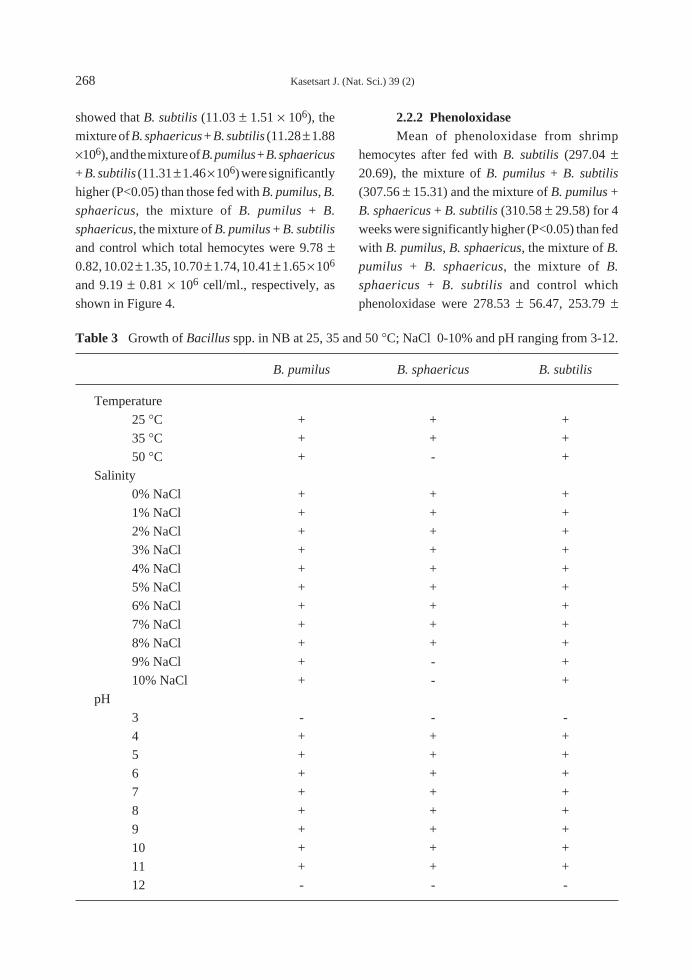
268 Kasetsart J. (Nat. Sci.) 39 (2)
showed that B. subtilis (11.03 ± 1.51 ¥ 106), the
mixture of B. sphaericus + B. subtilis (11.28 ± 1.88
¥106), and the mixture of B. pumilus + B. sphaericus
+ B. subtilis (11.31 ± 1.46 ¥ 106) were significantly
higher (P<0.05) than those fed with B. pumilus, B.
sphaericus, the mixture of B. pumilus + B.
sphaericus, the mixture of B. pumilus + B. subtilis
and control which total hemocytes were 9.78 ±0.82, 10.02 ± 1.35, 10.70 ± 1.74, 10.41 ± 1.65 ¥ 106
and 9.19 ± 0.81 ¥ 106 cell/ml., respectively, as
shown in Figure 4.
2.2.2 PhenoloxidaseMean of phenoloxidase from shrimp
hemocytes after fed with B. subtilis (297.04 ±20.69), the mixture of B. pumilus + B. subtilis
(307.56 ± 15.31) and the mixture of B. pumilus +
B. sphaericus + B. subtilis (310.58 ± 29.58) for 4
weeks were significantly higher (P<0.05) than fed
with B. pumilus, B. sphaericus, the mixture of B.
pumilus + B. sphaericus, the mixture of B.
sphaericus + B. subtilis and control which
phenoloxidase were 278.53 ± 56.47, 253.79 ±
Table 3 Growth of Bacillus spp. in NB at 25, 35 and 50 ∞C; NaCl 0-10% and pH ranging from 3-12.
B. pumilus B. sphaericus B. subtilis
Temperature
25 ∞C + + +
35 ∞C + + +
50 ∞C + - +
Salinity
0% NaCl + + +
1% NaCl + + +
2% NaCl + + +
3% NaCl + + +
4% NaCl + + +
5% NaCl + + +
6% NaCl + + +
7% NaCl + + +
8% NaCl + + +
9% NaCl + - +
10% NaCl + - +
pH
3 - - -
4 + + +
5 + + +
6 + + +
7 + + +
8 + + +
9 + + +
10 + + +
11 + + +
12 - - -

Kasetsart J. (Nat. Sci.) 39 (2) 269
0
20
40
60
80
100
control 1 2 3 4 5 6 7
feeds
b bb
b
b bb
a 1 = B.pumilus 2 = B.sphaericus 3 = B.subtilis, 4 = B.pumilus + B. sphaericus 5 = B.pumilus + B. subtilis 6 = B.sphaericus + B. subtilis 7 = B.pumilus + B. sphaericus +
B.subtilis
Weight increasing (%)
x 106 cells/ml
0
5
10
15
control 1 2 3 4 5 6 7
feeds
bbb
b ba a aunit/min/mg.protein
0
100
200
300
400
control 1 2 3 4 5 6 7feeds
b
aa a
b
a aa
28.92, 234.52 ± 26.77, 280.70 ± 30.64 and 222.75
± 15.34, respectively, as shown in Figure 5.
2.2.3 Superoxide anionMean of superoxide anion from shrimp
hemocytes after fed with B. subtilis (8.13 ± 2.16),
the mixture of B. pumilus + B. sphaericus (8.33 ±1.66), the mixture of B. sphaericus + B. subtilis
(8.40 ± 1.41) and the mixture of B. pumilus + B.
sphaericus + B. subtilis (8.80 ± 1.31) for 4 weeks
were significantly higher (P<0.05) from B. pumilus,
B. sphaericus, the mixture of B. pumilus + B.
subtilis and control which superoxide anion were
5.63 ± 1.22, 4.60 ± 1.35, 7.63 ± 0.91 and 5.30 ±0.92, respectively, as shown in Figure 6.
2.2.4 Clearance abilityClearance ability of shrimp blood
circulation system after fed with 8 feeds for 4
weeks and then injected with V. harveyi found that
shrimp fed with B. subtilis (346.67 ± 70.95), the
mixture of B. sphaericus + B. subtilis (253.33 ±122.20) and the mixture of B. pumilus + B.
sphaericus + B. subtilis (320.00 ± 98.49) could
reduce V. harveyi in hemolymph significantly
different (P<0.05) from shrimp fed with B. pumilus,
B. sphaericus, the mixture of B. pumilus + B.
sphaericus, the mixture of B. pumilus + B. subtilis
and control which amount of V. harveyi cells were
456.67 ± 85.05, 660.00 ± 105.36, 483.33 ± 201.08,
420.00 ± 40.00 and 626.67 ± 192.96 cfu/ml,
respectively, as shown in Figure 7.
2.2.5 Bactericidal activityBactericidal activity from shrimp serum at
4 weeks after fed with B. sphaericus, the mixture
of B. pumilus + B. subtilis , the mixture of B.
sphaericus + B. subtilis and the mixture of B.
pumilus + B. sphaericus + B. subtilis (8.80 ± 1.31)
at the dilution ratio of 1:8 serum to brine could
killed 50 percent of V. harveyi. While, shrimp fed
Figure 3 Percent weight increase of the P. monodon after 4 weeks cultured with 8 feeds.
Figure 4 Average of the P. monodon hemocytes
after 4 weeks cultured with 8 feeds.
Figure 5 Average of the P. monodon
phenoloxidase after 4 weeks cultured
with 8 feeds.

270 Kasetsart J. (Nat. Sci.) 39 (2)
with B. pumilus, B. subtilis, the mixture of B.
pumilus + B. sphaericus and control killed 50
percent of V. harveyi at the dilution ratio of 1:4, as
shown in Figure 8.
2.3 Study for the bacterial concentrationin shrimps intestine
2.3.1 Bacillus spp.The number of Bacillus spp. in shrimp
intestine after fed with B. pumilus (803.33 ±395.01), B. sphaericus (536.67 + 310.86), B.
subtilis (359.00 ± 270.63), the mixture of B. pumilus
+ B. sphaericus (373.33 ± 156.31), the mixture of
B. pumilus + B. subtilis (216.33 ± 94.87), the
mixture of B. sphaericus + B. subtilis (493.33 ±187.17) and the mixture of B. pumilus + B.
sphaericus + B. subtilis (476.00 ± 234.03) for 4
weeks were significantly different (P<0.05) from
control which number of Bacillus spp. average
was 1.00 ± 1.73 ¥ 104 cfu/g, as shown in Figure 9.
2.3.2 Vibrio spp.The number of Vibrio spp. in shrimp
intestine at 4 weeks after fed with normal feed
(control) (970.00 ± 285.13 cfu/g) was significantly
different (P<0.05) from shrimp fed with B. pumilus,
cfu/ml.
0
200
400
600
800
1000
control 1 2 3 4 5 6 7
feeds
b
a
b
a
a
aa a
unit
0
2
4
6
8
10
12
control 1 2 3 4 5 6 7
feeds
bcdd
ab aabc
a a
cd
feeds
% of V. harveyi decreased
0
50
100
1: 2
1: 4
1: 8
1: 1
6 1
: 32
1: 2
1: 4
1: 8
1: 1
6 1
: 32
1: 2
1: 4
1: 8
1: 1
6 1
: 32
1: 2
1: 4
1: 8
1: 1
6 1
: 32
1: 2
1: 4
1: 8
1: 1
6 1
: 32
1: 2
1: 4
1: 8
1: 1
6 1
: 32
1: 2
1: 4
1: 8
1: 1
6 1
: 32
1: 2
1: 4
1: 8
1: 1
6 1
: 32
control 1 2 3 4 5 6 7 * * * * * * * *
Figure 6 Average of the P. monodon superoxide
anion after 4 weeks cultured with 8
feeds.
Figure 7 Cells of V. harveyi from P. monodon
hemolymph after infected with V.
harveyi 3 hours after 4 weeks cultured
with 8 feeds.
Figure 8 Value of diluted serum to kill V. harveyi 50% (*) of P. monodon after 4 weeks of culture when
provided with 8 feeds (1 = B. pumilus, 2 = B. sphaericus, 3 = B. subtilis, 4 = B. pumilus + B.
sphaericus, 5 = B. pumilus + B. subtilis, 6 = B. sphaericus + B. subtilis, 7 = B. pumilus + B.
sphaericus + B. subtilis).

Kasetsart J. (Nat. Sci.) 39 (2) 271
B. sphaericus, B. subtilis, the mixture of B. pumilus
+ B. sphaericus, the mixture of B. pumilus + B.
subtilis, the mixture of B. sphaericus + B. subtilis
and the mixture of B. pumilus + B. sphaericus + B.
subtilis which the number of Vibrio spp. in shrimp
intestine were 11.33 ± 1.16, 121.67 ± 11.50, 8.00
± 1.00, 26.00 ± 3.00, 32.00 ± 3.61, 10.00 ± 3.00,
2.33 ± 1.53 cfu/g, respectively, as shown in Figure
10.
2.3.3 Scanning electron microscopeSEM revealed that Bacillus spp. could
survived in shrimp intestine after treated with
either individual isolation or mixtures of two and
three of B. pumilus, B. sphaericus and B. subtilis
as shown in Figure 11.1. While, in control group,
only Vibrio spp. was observed in shrimp intestine
as shown in Figure 11.2.
DISCUSSION
Isolation of Bacillus spp. from shrimp
intestine found three species namely B. pumilus,
B. sphaericus and B. subtilis. Original of those
bacteria might came from water, soil, food or
normal flora in the intestine. Bonde (1981) reported
that in seawater dominated by B. licheniformis
followed by B. subtilis and B. pumilus. Other
species encountered in low numbers include B.
0
200
400
600
800
1000
1200
1400
Control 1 2 3 4 5 6 7
x 104 cfu/g
c
a
ab
abab
abab
b
feeds
Figure 9 The number of Bacillus spp. in P.
monodon intestine after 4 weeks of
culture when provided with 8 feeds.
Figure 11 Scanning Electron Microscope picture.
11.1 Scanning Electron Microscope picture of Bacillus spp. in shrimp intestine after fed
with mixture of B. pumilus, B. sphaericus and B. subtilis ( ¥ 10,000)
11.2 Scanning Electron Microscope picture of Vibrio spp. in shrimp intestine (control
group) (¥ 15,000)
0
500
1000
1500
Control 1 2 3 4 5 6 7
cfu/g
feedsaa
aa a a a
b
Figure 10 The number of Vibrio spp. in P.
monodon intestine after 4 weeks of
culture when provided with 8 feeds.

272 Kasetsart J. (Nat. Sci.) 39 (2)
brevis, B. firmus and B. sphaericus, largely in
nonpolluted areas. In a numerical study of North
Sea sediments, Boeyé and Herts (1976) found that
B. subtilis, B. licheniformis and B. firmus strains
predominated. So, it was possible for B. pumilus,
B. sphaericus and B. subtilis to contaminate in
intestinal of shrimp by sea water.
In vitro production of inhibitory compounds
toward known pathogens for the considered species
has often been used in the selection of putative
probiotic strains (Verschuere et al., 2000). In this
study we demonstrated that the isolated Bacillus
spp. from intestinal of black tiger shrimp are
potential competitors for V. harveyi, the results
showed colonization effect of each Bacillus spp. to
V. harveyi in 24 hours. Special results we received
from this experiment, the effective of B. pumilus
could produce some substance and effective to
destroy V. harveyi confirm this result by clear
zone area in the test plates. The inhibition of B.
pumilus to V. harveyi observed clear zone of V.
harveyi colony in 12 hours and eradicate all of V.
harveyi colony in 48-72 hours. Although B.
sphaericus and B. subtilis did not show colonization
effect but they showed some inhibition effect to V.
harveyi, which confirmed by distorted shape of V.
harveyi by TEM the shape of V. harveyi had
smaller size and some area of cell wall was
destroyed. The abnormal shape of V. harveyi were
permanently changes confirmed with three
consecutive subcultures. Bacillus spp. might
produced some metabolites for instance antibiotic
(Williams and Vickers, 1986) or enzymes for
inhibition and/or digestion (Bruno and Montville,
1993)
Regarding to the growth of Bacillus spp.,
this experiment might confirmed that Bacillus
spp. could grow in a wide range of environment,
such as salinity up to 8% NaCl, pH 4-11 and
temperature up to 50 ∞C, althought B. sphaericus
could not grow at 50 ∞C but in the real culture,
water temperature never raise so high as 50 ∞C.
Using B. subtilis mixed with B. sphaericus
could increase weight of shrimp significantly
difference (P<0.05) from control and other
experiment groups, while others treatments had no
significant different from the control (P>0.05).
About immunoenhancement ability of
Bacillus spp., Bacillus had peptidoglycan in its
cell wall which could increase immune of shrimp
(Boonyaratpalin et al., 2000). In this research, B.
subtilis had highest efficiency to improve immune
parameters of black tiger shrimp consists of total
hemocyte, phenol oxidase, superoxide anion and
clearance ability. Others treatments containing B.
subtilis in the mixtures also increased immune
parameters significantly difference from the control
as well. These results were similar to Rengpipat et
al. (2000). But in our research we measured
superoxide anion instead of phagocytic activity
because superoxide anion produced in phagocytosis
process (Bell and Smith, 1993).
Furthermore, after fed shrimp with Bacillus
spp. for 4 weeks revealed that Bacillus spp. showed
superiority in competition and colonization to
Vibrio spp. in shrimp intestine.
CONCLUSIONS
In summary, it had been demonstrated that
B. pumilus, B. sphaericus and B. subtilis had good
properties to be used as probiotic for black tiger
shrimp. B. pumilus showed colonization activity
and produce inhibitory compounds while B.
sphaericus and B. subtilis showed only inhibitory
effects to V. harveyi. TEM studied found that cell
morphology of V. harveyi colonized by B. pumilus,
B. sphaericus and B. subtilis changed to smaller
sizes compared with normal cell. Moreover, three
species of Bacillus spp. could grow in a different
environment, including salinity 0-8% NaCl, pH 4-
11 and temperature 25-50 ∞C except B. sphaericus
which could not grow at 50 ∞C. When fed shrimp
with these Bacillus spp. showed
immunoenhancement capability and also
colonization and inhibition on V. harveyi in shrimp

Kasetsart J. (Nat. Sci.) 39 (2) 273
intestine. Therefore, these Bacillus spp. might be
applied as good probiotic in shrimp aquaculture.
ACKNOWLEDGEMENTS
This research was supported by Kasetsart
University Research and Development Institute
(KURDI). We thank Professor Dr. Toshiaki Itami,
Miyazaki University for immune techniques.
Assoc. Prof. Kidchakarn Supamattaya, Prince of
Songkla University, Thailand for chemical formula.
Ms.Kanokphan Srimanopach, Department of
Fisheries for VITEK 32 instrument, Ms. Patcharee
Umrung, Central lab KU for TEM and Ms. Yuppade
Paowpan, Central lab KU for SEM.
LITERATURE CITED
Bell, K. L. and V. J. Smith. 1993. In vitro superoxide
production by hyaline cells of the shore crab
Carcinus maenas Dev. Comp. Immunol.17: 211-219.
Boeyé, A. and M. Herts. 1976. Numerical
taxonomy of Bacillus isolates from North Sea
sediments. Int. J. Syst. Bacteriol. 26:427-
441.
Bonde, G. J. 1981. Bacillus from marine habitats
: Allocation to phena established by
numerical Techniques, pp. 181-215. In R. C.
W. Berkeley and M. Goodfellow (eds.). TheAerobic Endospore-Forming Bacteria :Classification and Identification, Academic
Press, London.
Boonyaratpalin, M., K. Supamattaya, J.
Pongmaneerat, S. Boonyaratpalin and
Y. Toride. 2000. The stimulatory effect of
high and low molecule peptidoglycan
(PG) on immune responses in black
tiger shrimp, Penaeus monodon Fabricius.
Songklanakarin J. Sci. Technol. 22 (Suppl.)
: 689-696.
Bruno, M. E. C. and T. J. Montville. 1993. Common
mechanistic action of bacteriocins from lactic
acidbacteria. Appl. Environ. Microbiol.59:3003– 3010.
Fuller R. 1992. Probiotics. The Scientific Basis.
Chapman and Hall, London. 398 p.
Gullian, M., F. Thompson and J. Rodriguez. 2004.
Selection of probiotic bacteria and study on
their immunostimulatory effect in Penaeus
vannamei. Aquaculture 233: 1-14.
Lowry, O.H., N. J. Rosebrough, A. L. Farr and R.
J. Randall. 1951. Protein measurement with
the folin phenol reagent. J. Biol. Chem. 193:
265-275.
Martin, G. G., D. Poole, C. Poole, J. E. Hose, M.
Arias, L. Reynolds, N. Mckrell and A. Whang.
1993. Clearance of bacteria injected into the
hemolymph of the Penaeid shrimp, Sicyonia
ingentis. J. Inver. Pathol. 62: 308-315.
Moriarty, D.J.W. 1998. Control of luminous Vibrio
species in penaeid aquaculture ponds.
Aquaculture 164: 351-358.
Rengpipat, S., S. Rukpratanporn, S.
Piyatirativarakul and P. Menasveta. 2000.
Immunity enhancement in black tiger shrimp
(Penaeus monodon) by a probiont bacterium
(Bacillus S11). Aquaculture 191: 271-288.
Supamattaya, K., J. Pongmaneerat and T.
Klowklieng. 2000. The effect of b–glucan
(MacroGard®) on growth performance,
immune response and disease resistance in
black tiger shrimp, Penaeus monodon
Fabricius. Songklanakarin J. Sci. Technol.22 : 677-688.
Verschuere, L., G. Rombaut, P. Sorgeloos and W.
Verstraete. 2000. Probiotic Bacteria as
Biological Control Agents in Aquaculture.
Microbiol. Mol. Biol. R. 64: 655–671.
Williams, S. T., and J. C. Vickers. 1986. The
ecology of antibiotic production. Microb.Ecol. 12:43–52.
Kasetsart J. (Nat. Sci.) 39 : 274 - 283 (2005)
Extracts of Thai Indigenous Vegetables as Rancid Inhibitorin a Model System
Plernchai Tangkanakul, Gassinee Trakoontivakornand Chansuda Jariyavattanavijit
ABSTRACT
The antioxidant property of twenty five vegetables extracted with ethanolic and water was
determined by monitoring their capacities to scavenge the stable free- radicals DPPH. Oxidative rancidity
in oil-in-water emulsion model was evaluated by ferric thiocyanate (FTC) method. Total phenolic content
was also determined by Folin-Ciocalteu method. The ethanolic extracts were found to exhibit a higher
phenolic content as well as DPPH radical scavenging activities than the water extracts. However, the data
indicated that both ethanolic and water extracts had dramatically antioxidant activity determined by FTC
method. Sixteen and eighteen plants of ethanolic and water extracts, respectively, performed greater
rancid inhibition than synthetic antioxidant (BHA, 10 ppm). This study found no relationship between
antioxidant activities through the DPPH radicals scavenging or through lipid radicals scavenging.
Key words: vegetables, antioxidant capacity, free radical scavenging activity, total phenolics, rancidity
INTRODUCTION
Synthetic antioxidants have been applied
for decreasing lipid oxidation during storage of
processed food products. The use of chemical
additives has raised questions regarding food safety
and toxicity (Chang et al., 1977). Many research
works have been directed toward safe antioxidants
with high antioxidative activity from natural
sources. The antioxidant properties of herbs and
spices, cinnamon, turmeric, clove, black pepper,
nutmeg, dry ginger, rosemary, sage and paprika
were continuously reported (Chang et al., 1977;
Nakatani et al., 1986; Kikuzaki and Nakatani.,
1993; Tomaino et al., 2005). Many plant extracts
were revealed on antioxidation efficiency when
applied in oils, fats and fat containing foods, meat
Institute of Food Research and Product Development, Kasetsart University, Bangkok 10900, Thailand.
Received date : 19/01/05 Accepted date : 21/04/05
products (Karpin′ska et al., 2001). For example,
rosemary and sage prolong the induction period in
chicken fat and show antioxidant activity
comparable with butylated hydroxyanisole (BHA)
and butylated hydroxytoluene (BHT) (Bracco et
al., 1981).
For Thai local vegetables, study on
antioxidant activity was reported regarding to the
potency of over 100 varieties by using b-carotene
bleaching method ((Nakahara and
Trakoontivakorn, 1999; Trakoontivakorn and
Saksitpitak, 2000; Na Thalang et al., 2001). More
than fifty varieties were reported to contain
antioxidant more than 100 mg BHA equivalent in
100g fresh weight. With their high potential and
lack in information for rancid inhibition, the present
study was aimed to evaluate 25 Thai vegetables for

anti-rancidity in a model system. Extract solvents,
water and ethanol, were taken into a consideration.
Total phenolic content was examined to find a
relationship between phenolic content and
antioxidant activity of crude extracts from both
solvents.
Presenting antioxidant activity of plant
crude extract was expressed in many aspects.
These methods revealed differently on mechanisms
of antioxidant defense system, i.e., inhibition of
lipid peroxidation, reduction of lipid peroxyl
radicals or scavenging of oxygen and hydroxyl
radicals (Tsushida et al., 1994; Velioglu et al.,
1998; Kähkönen et al., 1999; Pulido et al., 2000).
Stable free radicals, frequently applied to study
natural antioxidant efficiency were 2,2’-azino-
b i s (3 - e thy lbenzo th i azo l i ne -6 - su l fon i c
acid (ABTS), DPPH or N,N-Dimethyl-p-
phenylenediamine dihydrochloride (DMPD).
Koleva et al. (2002) recommended using DPPH
due to being simple, rapid, convenient and
independent of sample polarity.
Antioxidant capacity was another
perspective to present antioxidant activity, applying
different methodologies such as TEAC (Trolox
equivalent antioxidant capacity, Cook et al., 1998),
b-carotene bleaching method expressed as BHA
content (Tsushida et al., 1994), stable radical
ABTS or DPPH expressed as vitamin C (Kim et al,
2002). These antioxidant capacity methods were
developed in an attempt to have a meaningful
interpretation relating to health. In this study,
rancid inhibition was concerned, therefore,
scavengers of DPPH were stated in equivalent to
BHA content.
MATERIALS AND METHODS
Sample preparationTwenty five Thai indigenous vegetables
were either purchased from local markets or
collected from nature (Table 1). Edible portions of
vegetable were weighed in 10 g/plastic bags and
kept at -20 ∞C until extracting.
Vegetable extractionIndividual vegetable was extracted with 2
different solvents, 95% aqueous ethanol and
distilled water. The 10 g of frozen vegetables were
homogenized (Ultra Turrax) in 40 ml 95% aqueous
ethanol or distilled water at room temperature for
1 min. and centrifuged at 10000 g for 10 min. The
residue was re-extracted with either 95% aqueous
ethanol or distilled water and extracts were pooled
and made to 100 ml. The extracts were stored in
capped bottles and kept at -20∞C until further use
for antioxidant capacity and total phenolics
determinations and rancid inhibition test.
DPPH Radical scavenging activity andantioxidant capacity
DPPH scavenging activity was determined
using a modified method of Onichi et al. (1994).
The free radical scavenging activity of vegetable
extracts were tested, indicated as bleaching of the
stable 1,1 –diphenyl-2-picrylhydrazyl radical
(DPPH). A diluted extract of the right concentration
to posses not more than 60% scavenging activity
(%SA), 0.15 ml, was added to 0.9 ml of 0.1 mM
DPPH dissolved in 95% ethanolic solution. The
mixture was vertexed and allowed to stand at room
temperature. After 20 min., the absorbance was
recorded at 517 nm. 95% aqueous ethanol was
used as a control. Percentage of DPPH scavenging
activity (%SA) was calculated from this equation
(C-X)100/C, where C = absorbance of control and
X =absorbance of extract.
In order to express antioxidant activity of
plant extract to an easily understood manner,
antioxidant capacity as mg t-butylated
hydroxyanisole equivalent (BHAE) /g fresh
vegetable was introduced. A standard curve of t-
butylated hydroxyanisole (BHA) was obtained
from DPPH %SA (x) plotted against various BHA
concentrations (y). Prepared concentrations of
BHA solution were 0.1, 0.25, 0.5, 1.0, 2.5 and 5.0
Kasetsart J. (Nat. Sci.) 39 (2) 275

276 Kasetsart J. (Nat. Sci.) 39 (2)T
able
1A
ntio
xida
nt c
apac
ity (
AC
), r
epor
ted
as B
HA
equ
ival
ent (
BH
AE
), a
nd to
tal p
heno
lic (
TP)
con
tent
, rep
orte
d as
gal
lic a
cid
equi
vale
nt (
GA
E),
of
vege
tabl
es.
Bot
anic
al n
ame
Loc
al n
ame
Tes
ted
Plac
e an
d tim
eD
ryE
than
olic
ext
ract
Wat
er e
xtra
ctR
atio
of
part
of
colle
ctio
n m
atte
rA
CT
PA
CT
PA
C,
(%)
(mg
BH
AE
(mg
GA
E/
(mg
BH
AE
(mg
GA
E/
EtO
H/w
ater
/g F
W)
g FW
)/g
FW
)g
FW)
Aga
nosm
a m
argi
nata
Sato
nL
eaf
Ubo
n R
atch
atha
ni,
31.1
613
1.72±1
4.38
42.1
6±5.
4917
.73±
3.15
18.4
6 ±0.
067.
4M
arch
Ana
card
ium
occ
iden
tale
Mam
uang
Lea
fSu
rat T
hani
, Mar
ch23
.06
176.
48±3
2.07
51.3
3±4.
4268
.25±
9.86
30.0
8±10
.67
2.6
him
apha
nA
rchi
dend
ron
jiri
nga
Nie
ngFr
uit
Sura
t Tha
ni, M
arch
28.8
615
.09±
7.64
6.71
±3.8
44.
78±3
.50
3.53
±1.3
73.
2B
arri
ngto
nea
acut
angu
laK
rado
n na
mL
eaf
Ubo
n R
atch
atha
ni,
19.6
131
.85 ±
0.81
11.8
6±0.
1119
.75±
1.76
7.12
±0.6
41.
6M
arch
Car
eya
spha
eric
aK
rado
n bo
gL
eaf
Sako
n N
akor
n,28
.15
174.
18±1
4.67
54.0
2±9.
4534
.63±
7.43
17.6
8 ±1.
145.
0Fe
brua
ryC
ente
lla
asia
tica
Bai
bua
bog
Lea
fSu
rat T
hani
, Mar
ch8.
721.
24±0
.15
1.18
±0.2
20.
14±0
.01
0.46
±0.0
58.
7C
olub
rina
asi
atic
aG
an to
ngL
eaf
Lam
pang
, Apr
il21
.94
4.06
±0.0
94.
94±0
.69
1.05±0
.23
3.86
±0.5
43.
9C
rato
xylu
m fo
rmos
umT
ewFl
ower
Sako
n N
akor
n,18
.74
53.9
1±0.
9733
.77±
3.54
31.0
4±6.
7116
.35 ±
1.95
1.7
Febr
uary
Cym
bopo
gon
citr
atus
.T
a ka
iSt
emB
angk
ok, M
ay17
.18
1.95
±0.0
31.
25±0
.04
0.51±0
.26
0.36
±0.0
23.
8D
rege
a vo
lubi
lis
Hua
nL
eaf
Lam
pang
, Apr
il14
.26
3.39
±0.0
73.
39±0
.08
1.56±0
.73
1.95
±0.0
52.
2E
ugen
ia g
rata
Sa m
egL
eaf
Sako
n N
akor
n,17
.60
88.7
2±0.
9525
.34±
4.96
46.7
7±9.
9111
.27±
0.91
1.9
Febr
uary
Fer
onie
lla
luci
daM
a su
ngFl
ower
Sako
n N
akor
n,24
.32
25.3
4±0.
3434
.51±
1.14
4.78±0
.59
12.8
7±2.
205.
3Fe
brua
ryG
linu
s op
posi
tifo
lius
Khe
e kh
omW
hole
Sako
n N
akor
n,8.
380.
03±0
.00
0.62
±0.0
30.
03±0
.03
0.38
±0.0
01.
0Fe
brua
ryG
loch
idio
n w
alli
chia
num
Mun
pu
Lea
fSu
rat T
hani
, Mar
ch25
.48
167.
22±1
9.06
49.0
6±7.
3233
.86±
4.15
11.4
3±0.
114.
9G
netu
m g
nem
onL
ieng
Lea
fSu
rat T
hani
, Mar
ch20
.14
1.20
±0.0
71.
76±0
.10
0.18±0
.06
1.74
±0.2
76.
7G
ymne
ma
inod
orum
Chi
engd
aL
eaf
Lam
pang
, Apr
il16
.76
1.77
±0.0
83.
61±0
.15
1.51±0
.88
3.60
±0.4
21.
2Ip
omoe
a aq
uati
caPh
ak b
ung
thai
Lea
f, s
tem
Ban
gkok
, May
8.22
9.56
±0.0
25.
74±0
.66
1.56±0
.05
1.91
±0.0
86.
1L
asia
spi
nosa
Phak
nha
mL
eaf,
ste
mSa
kon
Nak
orn,
8.16
1.65
±0.0
71.
11±0
.08
0.45±0
.02
0.73
±0.0
93.
7Fe
brua
ryL
euca
ena
leuc
ocep
hala
Kra
tinL
eaf,
ste
mB
angk
ok, M
ay16
.33
12.8
2±0.
157.
28±0
.37
4.60±1
.83
13.1
3±0.
302.
8L
imon
ophi
la a
rom
atic
aPh
ak k
a yh
eng
Lea
f, s
tem
Ubo
n R
atch
atha
ni,
9.76
10.4
8±0.
976.
51±0
.29
0.34±0
.15
0.97
±0.0
531
.2M
arch
Man
gife
ra in
dica
Ma
mua
ngL
eaf
Lam
pang
, Apr
il22
.47
114.
36±8
.39
40.2
2±4.
2737
.51±
8.06
12.5
1±1.
893.
0M
icro
mel
um m
inut
umM
hui
Lea
fSu
rat T
hani
, Mar
ch25
.18
24.7
6±2.
1312
.64±
0.49
6.13±0
.56
12.5
5±3.
264.
0P
arki
a sp
ecio
saSa
tor
Lea
fSu
rat T
hani
, Mar
ch26
.26
23.4
4±3.
7511
.73±
0.30
15.0
8±3.
115.
95±0
.34
1.6
Pas
sifl
ora
foet
ida
Ka
tok
rok
Lea
fU
bon
Rat
chat
hani
,19
.19
7.82±2
.80
5.02
±0.4
72.
55±0
.59
2.59
±0.5
03.
1M
arch
Spir
ogyr
a sp
.T
aoFi
lam
ents
Sako
n N
akor
n,3.
9014
.71±
2.17
4.08
±0.0
66.
74±0
.09
1.70
±0.1
12.
2Fe
brua
ry

Kasetsart J. (Nat. Sci.) 39 (2) 277
mg/100 ml 95% ethanol. The regression line was
y = 0.0832x - 0.0469.
Determination of total phenolic contentsTotal phenolics were determined using the
Folin-Ciocalteau reagent, adopted from Singleton
and Rossi (1965). Two millilitres of suitable diluted
vegetable extracts was transferred and reacted
with 10 ml of Folin-Ciocalteau reagent (previously
diluted 10 fold with distilled water) in 25 ml
volumetric flask. After 30 sec. and before 8 min.,
8 ml of 7.5% of sodium carbonate was added and
mixed, and the contents of the flask made to
volume with distilled water. Solutions were heated
in a 40∞C water bath for 30 min. The color was
developed and absorbance measured at 765 nm.
The standard curve was prepared using 0, 0.5, 1.0
and 1.5 ml of gallate stock solution (8 mg/100ml)
in 25 ml volumetric flask. The regression line
between absorbance (y) and gallic acid content (x)
was y = 0.0046x + 0.0163. The results were
expressed as mg gallic acid equivalent / g of fresh
vegetable.
Antioxidative assay in model systemThe lipid oxidation was monitored by ferric
thiocyanate (FTC) method described by Kikuzaki
and Nakatani (1993). A 20 ml experimental mixture
made of 4 ml of an ethanolic extract (0.4 g fresh
vegetable), 4.1 ml of 2.51% linoleic acid in 99.5%
ethanol, 8 ml of 0.05 M phosphate buffer (pH 7.0)
and 3.9 ml of water was placed in a plastic bottle
(25 mm diameter, 60 mm height) with a screw cap.
For water extract, an assay mixture was prepared
the same as above except 3.9 ml of water was
replaced by 99.5% ethanol. The mixtures were
placed in an oven at 40∞C in the dark. FTC was
carried out by adding 0.1 ml of incubated mixture,
9.7 ml of 75% ethanol and 0.1 ml of 30%
ammonium thiocyanate into a test tube. Precisely
3 min after addition of 0.1 ml of 0.02M ferrous
chloride in 3.5% hydrochloric acid to the reaction
mixture, the absorbance of red color was measured
at 500 nm. Antioxidative assay was carried out
with 7 days interval until the absorbance of the
tested mixture reached maximum or 142 days.
BHA at concentration of 1.0 mg/100 ml and 5.0
mg/100 ml were used as a control.
RESULTS AND DISCUSSION
Antioxidant capacityWithin twenty five vegetables, ethanolic
extract was found to obtain more antioxidant
capacity than water extract (Table 1). The result
agreed with Kaur and Kapoor (2000) who applied
b-carotene bleaching test. Ratio of antioxidant
capacity of components soluble in ethanol to water
of 25 tested vegetables varied in a range of 31.2 to
1.0, with mean 4.7 and median of 3.2. Limonophila
aromatica was the one that contained antioxidants
most susceptible to dissolve in ethanol. And it was
also revealed that antioxidant capacity of ethanolic
extracts was in different order from that of water
extracts, however, not dramatically.
A large variation in the antioxidant capacity
was observed in ethanolic extracts, ranging from
as high as 176.48 mg BHAE /g fresh weight of
Anacardium occidentale to as low as 0.03 mg
BHAE /g fresh weight of Glinus oppositifolius.
The ranking of five vegetables possessing high
antioxidant capacity through ethanol extraction
was Anacardium occidentale, Careya sphaerica,
Glochidion wallichianum, Aganosma marginata
and Mangifera indica. The result agreed to
Trakoontivakorn and Saksitpitak (2000) who
reported that methanolic extracts of Anacardium
occidentale, Careya sphaerica, Glochidion
wallichianum and Mangifera indica contained great
amount of antioxidants analyzed by b-carotene
bleaching method. The results of water extract
were found to have antioxidant capacities between
0.03 - 68.25 mg BHAE /g fresh vegetable. The five
greatest antioxidant capacities were Anacardium
occidentale, Eugenia grata, Mangifera indica,
Careya sphaerica and Glochidion wallichianum.

278 Kasetsart J. (Nat. Sci.) 39 (2)
Total phenolic contentThe results of phenolic analysis of twenty
five vegetables are exhibited in Table 1. The
phenolic contents of the vegetable in ethanol
extraction varied from 0.62 mg GAE/g fresh weight
of Glinus oppositifolius to 54.02 mg GAE/g
fresh weight of Careya sphaerica. The ethanolic
extractable phenolic compounds greater than
25 mg GAE/g fresh vegetable were found
in Anacardium occidentale, Glochidion
wallichianum, Aganosma marginata, Mangifera
indica, Feroniella lucida, Cratoxylum formosum
and Eugenia grata. In water extraction, the total
phenolic contents was found highest in Anacardium
occidentale, 30.08 mg GAE/g fresh weight,
followed by Aganosma marginata, Careya
sphaerica, Cratoxylum formosum and Leucaena
leucocephala as 18.46, 17.68, 16.35 and 13.13 mg
GAE/g fresh weight, respectively. The present
study demonstrated that total phenolics in tested
Thai vegetables generally were greater than those
of Western herbs, 0.23 -17.51 mg GAE/g fresh
weight, reported by Zheng and Wang (2001).
Phenolic compounds were found to be
generally susceptible to dissolve more in ethanol
than in water. An exception was observed in
Leucaena leucocephala where extractable phenolic
compounds were almost double in water extract
than in ethanolic extract. Micromelum minutum,
Gymnema inodorum and Gnetum gnemon
possessed similar phenolic contents in both extract
media. A study reported on phenolic components
extracting ability that ethanol was less effective
than acetone when applied in Greek oregano and
summer savory. However, acetone extracts
exhibited incredible low in DPPH scavenging
activity (Exarchou et al., 2002). With this detection,
therefore, an extract medium should be taking into
account in order to obtain antioxidative compounds.
Phenolic contents existed in these twenty
five Thai indigenous vegetables were considered
as moderate to high. Converting vegetable weight
into dry weight basis, ethanolic extractable phenolic
compounds ranged from 7.28 mg GAE/g dry weight
in Cymbopogon citratus to 222.59 mg GAE/g dry
weight in Anacardium occidentale. Comparing to
the result of Kähkönen et al. (1999), the selected
cereals and vegetables contained greatly lower
amount of phenolics, 0.2 – 6.6 mg GAE/ g dry
weight and in moderate level in herb extracts, 9.1
– 23.1 mg GAE/g dry weight.
A relationship between phenolic content
and antioxidant activity was extensively
investigated, and both positive and negative
correlationships were demonstrated. Velioglu et
al. (1998), Rapisarda et al. (1999), Zheng and
Wang (2001), and many other research groups
stated that there was a positive correlation. In the
mean time, a few evidences of no significant
correlation were confronted (Heinonen et al., 1998;
Kähkönen et al., 1999). In this study, the regression
analysis was done separately on the extracting
medium, ethanol and water. The results revealed
that both ethanolic (R2 = 0.8893) and water extracts
(R2 = 0.6601) held a positive linear relationship
between phenolic content and antioxidant capacity
as displayed in Figure 1. The degree of correlation
coefficient pronounced greatly in ethanolic extracts
(R = 0.9430) and lesser in water extracts (R =
0.8125).
Antioxidative effect in model systemThe oxidation of oil-in-water emulsion was
monitored by the ferric thiocyanate (FTC) method.
The FTC method was used to measure the amount
of peroxide in initial stages of lipid oxidation.
Peroxide oxidizes ferrous iron to the ferric state
resulted in the formation of a red thiocyanate
complex. The determined values at 500 nm with
low absorbance indicated a high ability to delay
rancidity. On the contrary, if high absorbance
values and sharp increasing curve were noted, an
uncontrollable lipid oxidation stage was
confronted. In this study, extracts from 25
vegetables were analyzed and illustrated separately
by the extracting media (Figure 2).

Kasetsart J. (Nat. Sci.) 39 (2) 279
R2 = 0.6601
R2 = 0.8893
0.00
10.00
20.00
30.00
40.00
50.00
60.00
0.00 50.00 100.00 150.00 200.00
Antioxidant capacity (mg BHAE/g FW)
Tot
al p
heno
lics
(mg
GA
E/g
FW
)
Ethanolic extracts
Water extracts
Figure 1 Relationship between total phenolic content and antioxidant capacity of 25 vegetables,
extracted by ethanol and water.
Within 142 days of rancid inhibiting
evaluation, only 9 vegetable ethanol extracts were
lost or deteriorated in their abilities indicated by
reaching an absorbance of 0.4 (Figure 2a). They
were Cratoxylum formosum, Aganosma marginata,
Anacardium occidentale, Glinus oppositifolius,
Feroniella lucida, Micromelum minutum, Careya
sphaerica, Spirogyra sp. and Gnetum gnemon.
Absorbance of the control, no antioxidant in the
system, reached absorbance of 0.4 after day 7.
Seven out of 9 vegetables and 0.04 mg BHA
reached absorbance of 0.4 within 60 days. From
the whole experiment, only the extracts from Glinus
oppositifolius, Spirogyra sp., Gnetum gnemon,
0.04 mg BHA and 0.2 mg BHA displayed a sharp
raise curve similar to the control. A sharp changing
in absorbance is a common oxidation pattern
monitored by FTC method as shown in other
studies (Kikuzaki and Nakatani, 1993; Chen and
Ho, 1997). The indicator used to monitor the
generation of rancid odor from oil oxidation during
incubation was the absorbance of 0.4 by FTC as
reported by Chen and Ho (1997). Extract of
Anacardium occidentale and Careya sphaerica
could retain absorbance values around 0.4
indicating potential antioxidant plants, and there
were other 16 vegetables performed better than 0.2
mg BHA. The plant extracts that exhibited
substantial ability in rancid inhibition were
Gymnema inodorum, Dregea volubilis,
Cymbopogon citratus, Colubrina asiatica,
Passiflora foetida, Lasia spinosa and Centella
asiatica.
Water extracts illustrated a good result as
rancid inhibitors as well (Figure 2b). The plants
that possessed this property were Leucaena
leucocephala, Gymnema inodorum, Dregea
volubilis, Archidendron jiringa, Ipomoea aquatica,
Passiflora foetida and Spirogyra sp.. Water extracts
of plant that could not inhibit rancidity were
Glinus oppositifolius, Cratoxylum formosum,
Aganosma marginata, Gnetum gnemon, Lasia
spinosa, Cymbopogon citratus, Limonophila
aromatica and Centella asiatica.
It was interesting to point out that some
plants performed oppositely in controlling rancidity
in this model system. Water extract of Spirogyra
sp. contained effective antioxidants but not in
ethanolic extract. Whiles, ethanolic extracts of
Centella asiatica, Lasia spinosa and Cymbopogon
citratus were effective antioxidant, they became
ineffective when extracted with water. The plants

280 Kasetsart J. (Nat. Sci.) 39 (2)
0
0.1
0.2
0.3
0.4
0.5
0.6
0.7
0.8
0 20 40 60 80 100 120 140
Time (days)
Abs
orba
nce
500
nm
AM
AO
AJ
BA
CS
CAU
CAB
CF
CC
DV
EG
FL
GO
GW
GG
GI
IA
LS
LL
LA
MI
MM
PS
PF
S
Control
BHA 0.04 mg
BHA 0.2 mg
a
0
0.1
0.2
0.3
0.4
0.5
0.6
0.7
0.8
0 20 40 60 80 100 120 140
Time (days)
Abs
orba
nce
500
nm
AM
AO
AJ
BA
CS
CAU
CAB
CF
CC
DV
EG
FL
GO
GW
GG
GI
IA
LS
LL
LA
MI
MM
PS
PF
S
Control
BHA 0.04 mg
BHA 0.2 mg
b
Figure 2 Oxidation of oil-in-water emulsion monitored by the ferric thiocyanate method (a) ethanol
extraction (b) water extraction. Aganosma marginata (AM), Anacardium occidentale (AO),
Archidendron jiringa (AJ), Barringtonea acutangula (BA), Careya sphaerica (CS), Centella
asiatica (CAU), Colubrina asiatica (CAB), Cratoxylum formosum (CF), Cymbopogon
citrates (CC), Dregea volubilis (DV), Eugenia grata (EG), Feroniella lucida (FL), Glinus
oppositifolius (GO), Glochidion wallichianum (GW), Gnetum gnemon (GG), Gymnema
inodorum (GI), Ipomoea aquatica (IA), Lasia spinosa (LS), Leucaena leucocephala (LL),
Limonophila aromatica (LA), Mangifera indica (MI), Micromelum minutum (MM), Parkia
speciosa (PS), Passiflora foetida (PF), Spirogyra sp.(S)

Kasetsart J. (Nat. Sci.) 39 (2) 281
that displayed as a good antioxidant sources when
either extracted with water or ethanol were
Passiflora foetida, Dregea volubilis and Gymnema
inodorum.
Results from the model system experiment
revealed that plant extracts good in scavenging
DPPH radical was not always good in scavenging
lipid radicals. A relationship between BHAE
content and incubation time (reached absorbance
of 0.4) was investigated. BHAE content of tested
vegetables calculated from antioxidant capacity
which used DPPH scavenging method as a tool.
The regression values of ethanolic extract and
water extract were 0.093 and 0.0122, respectively
(Figure 3).
CONCLUSION
It was apparent from the study that plant
extracted by different solvents scavenged DPPH
radical and lipid radicals differently. Water extracts
of some vegetables were efficient comparable to
their ethanolic extracts for oxidative rancidity
inhibition. And the model of scavenging DPPH
radical could not be used to predict lipid oxidative
inhibition. This study also found that extractable
antioxidants from 0.4 g of some vegetables
demonstrated stronger rancid inhibition than the
synthetic antioxidant, 10 ppm BHA. It thus
constitutes an interesting source for use as natural
protecting agent to prevent oxidative deterioration
of food.
ACKNOWLEDGMENTS
Kasetsart University Research and
Development Institute (KURDI) financially
supported this research.
LITERATURE CITED
Bracco, U., J. Loliger and Viret J.L. 1981.
Production and use of natural antioxidans.
J. Am. Oil Chem. Soc. 58:686-690.Chang, S.S., B. Ostric-Matijasevic, O.A. Hsieh
and C.L. Chang. 1977. Natural antioxidants
from rosemary and sage. J. Food Sci. 42:1102-
1106.
Figure 3 Relationship between BHAE content obtained from antioxidant capacity and incubation time
to reach an absorbance of 0.4 by ferric thiocyanate method of 25 vegetables, extracted by
ethanol and water.
0
10
20
30
40
50
60
70
80
0 20 40 60 80 100 120 140 160 180 200
Incubation time (days)
BH
AE
con
tent
(m
g)
Ethanolic extracts
Water extracts

282 Kasetsart J. (Nat. Sci.) 39 (2)
Chen, J.H. and C-T Ho. 1997. Antioxidant activities
of caffeic acid and its related hydroxycinnamic
acid compounds. J. Agric. Food Chem.
45:2374-2378.
Cook, J.A., D.J. Vanderjagt, A. Dasgupta, G.
Mounkaila, R.S. Glew, W. Blackwell and
R.H. Glew. 1998. Use of the Trolox assay to
estimate the antioxidant content of seventeen
edible wild plants of Niger. Life Sci. 63:105-
110.
Exarchou, V., N. Nenadis, M. Tsimidou, I.P.
Gerothanassis, A. Troganis and D. Boskou.
2002. Antioxidant activities and phenolic
composition of extracts from Greek oregano,
Greek sage and summer savory. J. Agric.Food Chem. 50:5294-5299.
Heinonen, M., P.J. Lehtonen and A. Hopia. 1998.
Antioxidative activity of berry and fruit wines
and liquor. J. Agric. Food Chem. 46:25-31.
Karpin′ska, M., J. Borowski and M. Danowska-
Oziewicz. 2001. The use of natural
antioxidants in ready-to-serve food. FoodChemistry 72:5-9.
Kaur, C. and H.C. Kapoor. 2002. Anti-oxidant
activity and total phenolic content of some
Asian vegetables. Inter. J. Food Sci. Tech.
37:153-161.
Kähkönen, M.P., A.L. Hopia, H.J. Vuorela, J-P.
Rauha, K. Pihlaja, T.S. Kujala and M.
Heinonen. 1999. Antioxidant activity of plant
extracts containing phenolic compounds.
J. Agric. Food Chem. 47:3954-3962.
Kikuzaki, H. and N. Nakatani. 1993. Antioxidant
effects of some ginger constituents. J. FoodSci. 58:1407-1410.
Kim, D-O., W.L. Ki, H.J. Lee and C.Y. Lee. 2002.
Vitamin Cequivalent antioxidant capacity
(VCEAC) of phenolic phytochemicals.
J. Agric. Food Chem. 50:3713-3717.
Koleva, I.I., T.A. van Beek, J.P.H. Linssen, A. de
Groot and L.N. Evstatieva. 2002. Screening
of plant extracts for antioxidant activity: a
comparative study on three testing methods.
Phytochemical Analysis 13:8-17.
Na Thalang, V., G. Trakoontivakorn and
K.Nakahara. 2001. Determination of
antioxidant activity of some commonly
consumed leafy vegetables in Thailand.
JIRCAS J. 9:39-46.
Nakahara, K. and G.Trakoontivakorn. 1999.
Antioxidative and autimutagenic properties
of some local agricultural products in Thailand.
In Highlight of Collaborative ResearchAcfivities between Thai ResearchOrganizations and JIRCAS. Provided for
JIRCAS Seminar in Bangkok 1999, Bangkok,
Thailand 3 March 1999. pp.141
Nakatani, N., R. Inatani, H. Ohta and A. Nishioka.
1986. Chemical constitutents of pepper and
application of food preservation, naturally
occurring antioxidative compounds.
Environmental Health Perspectives.
67:135-141.
Ohnishi, M., H. Morishita, H. Iwahashi, S. Toda,
Y. Shirataki, M. Kimura and R. Kido. 1994.
Inhibitory effects of chlorogenic acids on
linoleic acid peroxidation and haemolysis.
Phytochemistry 36 (3):579-583.
Pulido, R., L. Bravo and F. Saura-Calixto. 2000.
Antioxidant activity of dietary polyphenols
as determined by a modified ferric reducing/
antioxidant power assay. J. Agric. FoodChem. 48:3396-3402.
Rapisarda, P., A. Tomaino, R.L. Cascio, F. Bonina,
A. De Pasquale and A. Saija. 1999. Antioxidant
effectiveness as influenced by phenolic content
of fresh orange juices. J. Agric. Food Chem.
47:4718-4723.
Singleton, V.L. and J.A. Rossi. 1965. Colorimetry
of total phenolics with phosphomolybdic-
phosphotungstic acid reagents. Am. J. Enol.Vitic. 16:144-158.
Tomaino, A., F. Cimino, V. Zimbalatti, V. Venuti,
V. Sulfaro, A. De Pasquale and A. Saija.
2005. Influence of heating on antioxidant
activity and the chemical composition of some

Kasetsart J. (Nat. Sci.) 39 (2) 283
spice essential oils. Food Chemistry 89:549-
554
Trakoontivakorn, G. and J. Saksitpitak. 2000.
Antioxidative potential of Thai indigenous
vegetable extracts. Food 30:164-176.
Tsushida, T., M. Suzuki and M. Kurogi. 1994.
Evaluation of antioxidant activity extracts
and determination of some active compounds.
Nippon Shokuhin Kogyo Gakhaishi.
41:611-618.
Velioglu, Y.S., G. Mazza, L. Gao and B.D. Oomah.
1998. Antioxidant activity and total phenolics
in selected fruits, vegetables and grain
products. J. Agric. Food Chem 46:4113-
4117.
Zheng, W. and S.Y. Wang. 2001. Antioxidant
activity and phenolic compounds in selected
herbs. J. Agric. Food Chem. 49:5165-5170.

Kasetsart J. (Nat. Sci.) 39 : 284 - 293 (2005)
Screening and Characterization of Lactic Acid Bacteria ProducingAntimicrobial Substance against Staphylococcus aureus
Chatinan Ratanapibulsawat1, Pumrussiri Kroujkaew2,Ohmomo Sadahiro2 and Sunee Nitisinprasert1
ABSTRACT
One isolate of lactic acid bacteria (LAB) producing antimicrobial substance (AMS) against
Staphylococcus aureus was selected and designed as LS2-30. Morphological, physical and biochemical
tests, and 16S rRNA analysis were performed and revealed that it was Pediococcus acidilactici. Optimal
conditions for growth and AMS production were determined. The optimum temperature and initial pH
for both growth and AMS production were 45 ∞C and pH 6, respectively. Cell-free culture fluid of LS2-
30 showed an inhibitory action against Staphylococcus aureus, Salmonella sp., Bacillus sp., and E. coli
but no activity against all LAB tested. When mode of action was studied, the cell-free culture fluid
exhibited a bactericidal mode of action but did not lyse its cells. After removing organic acids, partial
purified antimicrobial substance at pH 3 showed inhibitory activity as bactericidal action. Hydrolytic
enzyme treatment suggested that AMS structure was neither proteinaceous, starch nor lipid moiety in
nature. Therefore, the nature of inhibitory compound secreted by P. acidilactici LS2-30 was still unclear.
Key words: antimicrobial substance, lactic acid bacteria, Staphylococcus aureus
INTRODUCTION
Staphylococcus aureus is an important
opportunistic pathogen that causes a variety of
diseases in humans and animals. It is widely
recognized that antibiotic therapies formulated for
intramammary use are generally unsuccessful in
eliminating existing S. aureus infections or in
preventing the establishment of chronic udder
disease (Leitnera et al., 2003). Currently, more
than 95% of infectant with S. aureus infections
worldwide do not respond to first-line antibiotics
such as penicillin or ampicillin (Rubin et al.,
1999). Moreover, with increasing public concern
over food safety, there is regulatory pressure to
1 Department of Biotechnology, Faculty of Agro-Industry, Kasetsart University, Bangkok 10900, Thailand.2 Department of Animal Products, National Institute of Animal Industry (NIAI), Tsukuba, Ibaraki, 305-0901 Japan.
Received date : 28/12/04 Accepted date : 28/04/05
justify the use of therapeutic drugs in dairy cattle
and to reduce the incidence of residues in milk.
The emergence and spread of drug-resistant
staphylococci underscores the need to find new
modes of prevention and alternative non-antibiotic
treatment.
In a recent in vitro study, various substances
have been found and shown antimicrobial activity
against S. aureus, like, lactose chitosan derivative
against S. aureus CCRC 12657 (Chen and Chou,
2005), the extract of Panax ginseng root
(ginsenoside) (Hu et al., 2003) and lactoferrin with
penicillin G (Diarra et al., 2002). In addition, many
anti-S. aureus substances producing LAB have
been a great interest because most of the LAB are

considered as “Generally Recognized as Safe”
microorganism (Holzapfel et al., 1995). Several
LAB species were found to be a potent anti-S.
aureus substance producer such as Lactobacillus
plantarum BS, Lb. salivarius, Lb. plantarum 35d
(Messi et al., 2001), P. acidilactici F
(Osmanagaoglu et al., 1998) and Lb. acidophilus
LA1 (Bernet-camard et al., 1997). However, most
of them produced the substances that inhibited
themselves as well. Therefore, it is still important
to isolate a novel anti-S. aureus substance with
new properties and without significant inhibitory
activity against its host.
The objective of this study was to
characterize LAB producing antimicrobial
substance against S. aureus. The antibacterial
spectrum and their mode of action were described
as well.
MATERIALS AND METHODS
Bacterial strains and growth conditionsAntimicrobial substance (AMS) producing
lactic acid bacteria isolated from silage and
fermented pork (Nham) were obtained from the
culture collection of Department of Biotechnology,
Kasetsart University (Thailand). They were
anaerobically grown in De Man Rogosa and Shape
(MRS, Merck) at 45 ∞C. All strains of S. aureus
isolated from mastitis cow milk from the National
Institute of Animal Health (Thailand) and
pathogenic bacteria used as indicator strains were
grown in Nutrient broth at 37 ∞C while LAB was
done in MRS at 37 ∞C. E. coli DH5a used as a host
for cloning PCR-amplified 16S rDNA was grown
in Luria broth at 37 ∞C. All strains were stored at
-80 ∞C in desirable media containing 20% (v/v)
glycerol, and propagated twice before experimental
use.
Screening of antimicrobial substance producingLAB
Bacterial cells were removed from the
overnight cultures by centrifugation at 10,956 g
for 15 min at 4∞C. Cell-free culture supernatant
(CFS) obtained was filter-sterilized with a 0.2 mm
pore size filter membrane and further assayed for
antimicrobial activity.
Determination of antimicrobial activityThe spot-on-lawn method was used to
determine antimicrobial activity. The desired
medium agar plates were overlaid with 5 ml of soft
medium agar containing 50 ml of an overnight
culture of the indicator strain. 10 ml of sample was
spotted onto the overlaid surface. The plates were
incubated for 6 and 12 h at 37∞C and determined
for antimicrobial substance (AMS) production.
The AMS titre was determined by the serial twofold
dilution method previously described by Mayr-
Harting et al. (1972). The activity was defined as
the reciprocal of the dilution after the last serial
dilution giving a zone of inhibition and expressed
as activity units (AU) per milliliter.
Identification of the LABSixteen-hour culture solution was
determined for morphology, gram stain, catalase
reaction and motility according to Axelsson (1998).
Growth of LAB in MRS broth at the temperatures
of 10, 45, 50 and 55 ∞C and NaCl concentration of
6% and 18% were determined by turbidity
measurement at 600 nm. CO2 production from
glucose was examined by the method of Gerhardt
et al. (1981). Carbohydrate fermentation patterns
were determined by API CHL50 tests (API,
BioMeriuex, France) as described by the
manufacturer. 16S rRNA analysis was done by the
modified method of Nitisinprasert et al. (2000).
Primer 1407B (5’-GACGGGCGGTGTGTAC-3’)
and 8UA (5’-AGAGTTTGATCCTGGCTC AG-
3’) were used as forward and reverse primers,
respectively. Amplification was carried out in a
thermo-cycler (Hybaid, UK) with annealing for 2
min at 55 ∞C. The purified DNA fragment was
ligated into pGEM-T® Easy vector (Promega,
Kasetsart J. (Nat. Sci.) 39 (2) 285

286 Kasetsart J. (Nat. Sci.) 39 (2)
USA) and then transformed into E. coli DH5acompetent cells. The presence of the PCR product
ligated to the plasmid was confirmed by whole cell
PCR reaction (Nitisinprasert et al., 2000) and
restriction analysis with EcoRI under standard
condition. Nucleotide sequences were determined
by Bioservice unit (BSU, Thailand). The sequences
of 16S rDNA clone were aligned with data from
GenBank by BLAST analysis.
Optimization of growth and AMS productionTo determine the effect of temperature and
pH on growth and AMS production, the culture
solution in MRS medium was incubated at the
temperatures of 30, 37, 45, 50 and 55∞C, and the
pH of 4, 5, 6, 7 and 8. Culture solution was sampled
every 2 h until 24 h and then determined the values
of turbidity at 600 nm, viable cell numbers, pH and
AMS activity against S. aureus TM67.
Preparation of partial purified AMS (ppAMS)Partially purified AMS (ppAMS) was
prepared by vacuum evaporator and cation
exchange chromatography. The CFS was
concentrated to 10-fold by vacuum evaporator.
One mililiter of 10-fold concentrated CFS was
loaded onto a Sephadex fast flow column
equilibrated with 20 mM sodium citrate buffer
(pH 3.0). After initial washing with 20 mM sodium
citrate buffer (pH 3.0), AMS was eluted with 1 M
NaCl in the same buffer at a flow rate of 1 ml/min.
The ppAMS obtained was free from lactic acid and
acetic acid tested by HPLC with an Aminex HPX-
87H cation exchanger. The acids were eluted with
8 mM sulphuric acid at the flow rate of 0.5 ml/min
and tartaric acid was used as internal standard.
Mode of actionTo determine the mode of action of CFS
and ppAMS, 1% (v/v) of the overnight culture
solution of S. aureus was inoculated into NB and
cultivated at 37∞C until the cells reached
logarithmic phase. Then, CFS at the concentrations
of 100, 200 and 300 AU/ml was added into the
culture broth and further cultivated at 37∞C. For
control, equal amount of sterile distilled water was
added instead of CFS. Viable cell numbers and
turbidity at 600 nm were monitored at 1-h intervals.
For ppAMS, 100 AU/ml of ppAMS was
directly added into 102 CFU/ml of S. aureus and
the number of viable cell was determined at 1-h
intervals. twenty mM sodium citrate buffer (pH
3.0) used instead of ppAMS was performed as a
control.
Structural determination by enzyme treatmentA ppAMS was treated with various enzymes
including pepsin, trypsin, proteinase K, protease,
a-chymotrypsin, papain, a-amylase and lipase.
Each enzyme was added to the ppAMS (100 AU/
ml) to obtain a final concentration of 1 mg/ml. The
mixture was incubated at the optimum temperature
of each enzyme for 18 h. At the end of incubation,
the residual activity of AMS was assayed.
RESULTS
Screening of AMS-producing lactic acidbacteria
Fifteen LAB strains isolated from silage
and fermented pork were screened for AMS
production as shown in Table 1. All CFS exhibited
higher inhibition number activity than CFS adjusted
pH to 5 and 6. It indicated a synergistic effect
between antimicrobial substance and organic acids.
The isolate designed as LS2-30 displayed the
highest inhibition number against 9 S. aureus
strains at different conditions of CFS, CFS adjusted
to pH 5 (CFS-5) and CFS adjusted to pH 6 (CFS-
6). Moreover, the AMS of LS2-30 was active
against food-borne and pathogenic bacteria not
only gram positive, S. aureus and Bacillus sp., but
also gram negative such as E. coli as shown in
Table 2. The inhibition activity against those
strains appeared at the range of 100 – 300 AU/ml
(data not shown). The highest activity obtained

Kasetsart J. (Nat. Sci.) 39 (2) 287
was against S. aureus, Salmonella sp., Sal.
Typhimurium, B. cereus, and B. subtilis.
Interestingly, its AMS was not active against all
LAB, M. luteus, and L. innocua.
Identification of the strain LS2-30Morphological and biochemical tests were
used to identify this isolate. LS2-30 was gram-
positive, coccus-shaped, tetrad formed, without
catalase activity, non-motile and no spore forming.
It grew at high temperatures of 45, 50 and 55∞C,
and did not produce gas indicated as
homofermentative LAB. It also grew in MRS
broth with the pH adjusted to 4.5 and 9.6, and NaCl
concentration to 6% but not to 18%. Based on
Bergey’s Manual of systematic of bacteriology,
this isolate was tentatively assigned to the genus
Pediococcus. For species determination,
carbohydrate fermentation using API 50 CHL was
performed and analyzed by APILAB program.
The results showed that LS2-30 was similar to P.
pentosaceus at 92.8%. However, the difference in
maltose fermentation was found as shown in Table
3. Therefore, 1,500 bp of the 16S rRNA of LS2-30
was analyzed and the result showed 97% identity
to P. acidilactici B1104 (accession no. AJ
305322.1).
Optimization of growth and AMS productionThe effects of temperature and the initial
pH of medium on growth and AMS production
were monitored at various conditions. The
temperature effect was performed at 30, 37, 45, 50
and 55∞C as shown in Figure 1. Similar growth
profile was observed at 37 and 45∞C, however, the
maximum activity of 300 AU/ml obtained at 45 ∞C was greater and even maintained for longer time
of 24 h. At high temperature of 50 ∞C, both growth
and AMS activity reached the maximum after
18 h and then dropped dramatically while the one
of 55 ∞C was clearly inhibited after 6 h. It seems
that AMS produced after 6 h actively killed all
viable target cells at high temperature of 55 ∞C.
The initial pH of 4, 5, 6, 7 and 8 displayed
a significant effect on AMS production but not on
its growth as shown in Figure 2. At initial pH of 4,
5 and 6, AMS production started immediately
after growth began and reached a maximum of
200-300 AU/ml during stationary phase. The
maximum of AMS activity was observed after 8 h
of cultivation at initial pH of 6. At the higher pH of
7, only low activity of 100 AU/ml was detected
after 12 h while there was no AMS production
found at the initial pH of 8.
Mode of actionTo determine whether the AMS had
bactericidal or bacteriostatic effect on the sensitive
strains, the AMS treated condition of 100, 200 and
300 AU/ml and a control (without AMS) were
performed as shown in Figure 3. Comparing to the
control, the number of viable indicator cell from
Table 1 The antimicrobial activity of LAB 15
isolates against S. aureus 9 strains.
LAB %Inhibition number1/
CFS CFS-5 CFS-6
CS1-10 100 0 22.2
CS1-11 100 55.5 0
CS4-10 100 66.7 0
CS4-11 100 22.2 11.1
LG1-1 100 11.1 0
LG1-2 100 55.5 0
LG2-1 100 0 0
LS2-30 100 77.8 55.6
LS2-31 100 22.2 0
LS2-32 100 44.4 11.1
N1-9 100 44.4 0
SG1-1 100 22.2 0
SG1-2 100 11.1 0
SK1-3 100 55.6 11.1
SK1-4 100 11.1 0
1/ % Inhibition number = the number of inhibited S. aureus
/ total S. aureus tested

288 Kasetsart J. (Nat. Sci.) 39 (2)
Table 2 The antibacterial spectrum of LS2-30.
Indicator strain Strain tested/inhibited
Staphylococcus aureus 9/9
Escherichia coli 13/13
Salmonella sp. 3/3
Salmonella Typhimurium TISTR 292 (ATCC 13311) 1/1
Bacillus cereus (isolated from silage) 1/1
Bacillus subtilis TISTR 025 1/1
Bacillus coagulans JCM2257 1/1
Bacillus subtilis JCM1465 1/1
Bacillus circulans JCM2504 1/0
Micrococcus luteus IFO12708 1/0
Listeria innocua (ATCC33090) 1/0
Pediococcus pentosaceus JCM5885 1/0
Enterococcus faecalis JCM5803 1/0
Lactococcus lactis ssp. lactis (ATCC19435) 1/0
Lactococcus lactis ssp. cremoris TUA1344L 1/0
Lactobacillus plantarum (ATCC14917) 1/0
Lactobacillus sakei subsp. sakei JCM1157 1/0
Leuconostoc mesenteroides ssp. mesenteroides JCM6124 1/0
the treated condition decreased immediately while
the optical density of cell suspension still remained.
This indicated that CFS of LS2-30 was bactericidal
without cell lysis.
For ppAMS (Figure 4), the viable cell of
2.5 log CFU/ml decreased to less than 10 cfu/ml
after 1 h incubation while the control declined
slowly. This confirmed bactericidal effect against
S. aureus TM67 while low pH of 3 displayed slight
inhibition of its growth.
Determination of compound structure byenzyme treatment
The structure of ppAMS produced from
LS2-30 was examined by various enzymes as
shown in Table 4. The antimicrobial activity of
ppAMS was not affected after treatment with
proteinase K, protease type XIII, papain, pepsin A,
trypsin type I, a-chymotrypsin type II, a-amylase
type X-A and lipase indicating that the ppAMS
was neither proteinaceous, starch nor lipid moiety
in nature.
DISCUSSION
Isolate LS2-30, obtained from silage and
identified as P. acidilactici, was selected to study
as an AMS producing strain. Recently, a number
of antagonistic substances from P. acidilactici
were reported, for example, lactic acid (Stiles,
1996), pediocin PA-1, pediocin AcH, pediocin
JD, pediocin SJ-1 (Schved et al., 1994), pediocin
5, pediocin L50, pediocin F (Osmanagaoglu et al.,
1998), pediocin AcM (Elegado et al., 1997). They
all, except lactic acid, had proteinaceous structure.
However, the AMS of LS2-30 seems to be different
from the results of various enzyme treatments, it
didn’t show the structure of either protein or
complex compounds of protein, starch or lipid
belonging to bacteriocin group IV. Therefore, it

Kasetsart J. (Nat. Sci.) 39 (2) 289
Table 3 Carbohydrate fermentation pattern of
LS2-30 compared with P. pentosaceus.
Carbohydrate P. pentosaceus LS2-30
Glycerol ± -
Arabinose + +
Ribose + +
Xylose ± +
Galactose + +
Glucose + +
Fructose + +
Mannose + +
Rhamnose ± ?
Mannitol - -
Sorbitol - -
Amygdalin + +
Salicin + +
Cellubiose + +
Maltose + +
Lactose + ?
Melibiose ± -
Trehalose + +
Inulin ± -
Melezitose - -
Raffinose ± -
+ = positive; - = negative; ? = doubtful
closely related species (Klaenhammer, 1993),
therefore, it was possible that the AMS found was
not bacteriocin which correspond to above result
of structure determination. This was the first report
of non-bacteriocin substance excluding organic
acid produced by homofermentative lactic acid
bacteria. This property is an advantage to use this
compound as a biological preservative in the dairy
product and fermented food without any effect to
LAB used as a starter culture.
The AMS from this isolate were secreted
into culture medium at the beginning of the
logarithmic growth phase and reached the
maximum level during the early stationary phase
at 45∞C. Thus, the production of AMS from LS2-
30 was growth-associated. The same pattern
occurred with most of active compound produced
by other LAB, such as carnocin U149, leucocin S
and plancitaricin S. The initial optimum pH of
AMS production was pH 6 which was similar to
the previous reports (Mortvedt-Abildgaard et al.,
1995). In addition, this strain clearly showed that
the inhibitory activity remained stable although
the pH was down to pH 4 after prolonging
incubation, suggesting that the antimicrobial
substance was unaffected under acidic conditions.
This could be an important asset allowing its use
under acidic conditions such as fermented food.
Table 4 Factors affecting antimicrobial activity
of ppAMS.
Enzyme Activity (AU/ml)
Proteinase K 100
Protease type XIII 100
Papain 100
Pepsin A 100
trypsin type I 100
a-Chymotrypsin type II 100
a-Amylase type X-A 100
Lipase 100
Control 100
could be either tolerate to enzyme or new compound
structure.
Considering the inhibition ability, LS2-30
has shown the ability to secrete broad spectrum
AMS against different non-related genera,
including food-borne pathogens such as S. aureus,
Bacillus sp., Salmonella sp., and E. coli.
Interestingly, no inhibitory activity of LS2-30 was
observed against LAB tested. Most bacteriocins
produced by P. acidilactici displayed inhibitory
effect to both LAB and some pathogenic
microorganisms for example nisin, pediocin AcH
(Kalchayanand et al., 1992), salivacin 140 and
plantaricin 35d (Messi et al., 2001). Since the
definition of bacteriocin indicated that it will inhibit
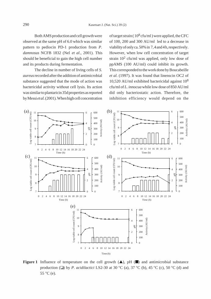
290 Kasetsart J. (Nat. Sci.) 39 (2)
Time (h)0 2 4 6 8 10 12 14 16 18 20 22 24
7
8
9
10
11
pH
0
2
4
6
Act
ivity
(AU
/ml)
0
100
200
300
400
500
600
Log
via
ble
cell
coun
t (C
FU/m
l)
Time (h)
0 2 4 6 8 10 12 14 16 18 20 22 24
Log
via
ble
cell
coun
t (C
FU/m
l)
7
8
9
10
11
pH
0
2
4
6
Act
ivity
(A
U/m
l)
0
100
200
300
400
500
600
Time (h)0 2 4 6 8 10 12 14 16 18 20 22 24
Log
via
ble
cell
coun
t (C
FU/m
l)
7
8
9
10
11
pH
0
2
4
6
Act
ivity
(A
U/m
l)
0
100
200
300
400
500
600
Time (h)0 2 4 6 8 10 12 14 16 18 20 22 24
Log
via
ble
cell
coun
t (C
FU/m
l)
7
8
9
10
11
pH
0
2
4
6
Act
ivity
(A
U/m
l)
0
100
200
300
400
500
600
Time (h)
0 2 4 6 8 10 12 14 16 18 20 22 24
Log
via
ble
cell
coun
t (C
FU/m
l)
7
8
9
10
11
pH
0
2
4
6
Act
ivity
(AU
/ml)
0
100
200
300
400
500
600
(a) (b)
(c) (d)
(e)
Figure 1 Influence of temperature on the cell growth (▲), pH (■ ) and antimicrobial substance
production (❏ ) by P. acidilactici LS2-30 at 30 ∞C (a), 37 ∞C (b), 45 ∞C (c), 50 ∞C (d) and
55 ∞C (e).
Both AMS production and cell growth were
observed at the same pH of 6.0 which was similar
pattern to pediocin PD-1 production from P.
damnosus NCFB 1832 (Nel et al., 2001). This
should be beneficial to gain the high cell number
and its products during fermentation.
The decline in number of living cells of S.
aureus recorded after the addition of antimicrobial
substance suggested that the mode of action was
bactericidal activity without cell lysis. Its action
was similar to plantaricin 35d properties as reported
by Messi et al. (2001). When high cell concentration
of target strain ( 108 cfu/ml ) were applied, the CFC
of 100, 200 and 300 AU/ml led to a decrease in
viability of only ca. 50% in 7, 4 and 4 h, respectively.
However, when low cell concentration of target
strain 102 cfu/ml was applied, only low dose of
ppAMS (100 AU/ml) could inhibit its growth.
This corresponded to the work done by Boucabeille
et al. (1997). It was found that linenscin OC2 of
10,520 AU/ml exhibited bactericidal against 108
cfu/ml of L. innocua while low dose of 850 AU/ml
did only bacteriostatic action. Therefore, the
inhibition efficiency would depend on the
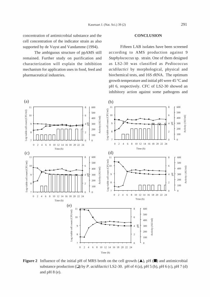
Kasetsart J. (Nat. Sci.) 39 (2) 291
Time (h)
0 2 4 6 8 10 12 14 16 18 20 22 24
Log
via
ble
cell
coun
t (C
FU/m
l)
7
8
9
10
11
pH
0
2
4
6
8
Act
ivity
(AU
/ml)
0
100
200
300
400
500
600
Time (h)
0 2 4 6 8 10 12 14 16 18 20 22 24
Log
via
ble
cell
coun
t (C
FU/m
l)
7
8
9
10
11
pH
0
2
4
6
8
Act
ivity
(A
U/m
l)
0
100
200
300
400
500
600
Time (h)
0 2 4 6 8 10 12 14 16 18 20 22 24
Log
via
ble
cell
coun
t (C
FU/m
l)
7
8
9
10
11
pH
0
2
4
6
8
Act
ivity
(AU
/ml)
0
100
200
300
400
500
600
Time (h)
0 2 4 6 8 10 12 14 16 18 20 22 24
Log
via
ble
cell
coun
t (C
FU/m
l)
7
8
9
10
11
pH
0
2
4
6
8
Act
ivity
(A
U/m
l)
0
100
200
300
400
500
600
Time (h)
0 2 4 6 8 10 12 14 16 18 20 22 24
Log
via
ble
cell
coun
t (C
FU/m
l)
7
8
9
10
11
pH
0
2
4
6
8
Act
ivity
(AU
/ml)
0
100
200
300
400
500
600
(a) (b)
(c) (d)
(e)
Figure 2 Influence of the initial pH of MRS broth on the cell growth (▲), pH (■ ) and antimicrobial
substance production (❏ ) by P. acidilactici LS2-30. pH of 4 (a), pH 5 (b), pH 6 (c), pH 7 (d)
and pH 8 (e).
concentration of antimicrobial substance and the
cell concentration of the indicator strain as also
supported by de Vuyst and Vandamme (1994).
The ambiguous structure of ppAMS still
remained. Further study on purification and
characterization will explain the inhibition
mechanism for application uses in food, feed and
pharmaceutical industries.
CONCLUSION
Fifteen LAB isolates have been screened
according to AMS production against 9
Staphylococcus sp. strain. One of them designed
as LS2-30 was classified as Pediococcus
acidilactici by morphological, physical and
biochemical tests, and 16S rRNA. The optimum
growth temperature and initial pH were 45 ∞C and
pH 6, respectively. CFC of LS2-30 showed an
inhibitory action against some pathogens and

292 Kasetsart J. (Nat. Sci.) 39 (2)
Time (h)
0
Log
via
ble
coun
t
(cfu
/ml)
8
9
10
X X
X
X X X
0
0.5
1
1.5
2
0 2 4 6 8
Time (h)
OD
600
1 2 3 4 5 6 7 8 1 3 5 7
Time (h)
0
Log
via
ble
coun
t(c
fu/m
l)
1
2
3
1 2 3
Figure 3 Effect of LS2-30 CFS on the viability (a) and absorbance at 600 nm (b) of S. aureus. CFS was
added (arrow) at a final dose of 100 AU/ml (■ ), 200 AU/ml (▲), 300 AU/ml (X) and control
(◆ ).
Figure 4 Effect of ppAMS of LS2-30 on the
viability of S. aureus at 102 cfu/ml.
ppAMS was added at 100 AU/ml (▲)
and 20 mM sodium citrate buffer (pH
3.0) as control (◆ ).
foodborne bacteria such as S. aureus, Salmonella
sp., Bacillus sp., and E. coli . However, it didn’t
exhibit activity against all LAB tested. When
mode of action was studied, the CFS displayed a
bactericidal mode of action without cell lysis. The
ppAMS at pH 3.0 showed inhibitory activity as
bactericidal action at low concentration of 100
AU/ml against 102 CFU/ml of target strain. By
various hydrolytic enzymes treatment, it suggested
that the AMS was neither proteinaceous, starch
nor lipid moiety in nature. Therefore, the nature of
inhibitory compound secreted by P. acidilactici
LS2-30 is still unclear.
ACKNOWLEDGEMENTS
This work was supported in part by a
research grant from Graduated School, Kasetsart
University. The authors gratefully acknowledge
National Institutes of Animal Health, Ministry of
Agriculture and Cooperatives, for S. aureus used
as indicator strains.
LITERATURE CITED
Axelsson, L. 1998. Lactic acid bacteria:classification and physiology, pp. 1-72. In S.Salminen and A Von Wright (eds). LacticAcid Bacteria: Microbiology andFunctional Aspect. Marcel Dekker, Inc.,
New York.Bernet-Camard, M.F, V. Lievin, D. Brassart, J.R.
Neeser, A.L. Servin and S. Hudault. 1997.The human Lactobacillus acidophilus strainLA1 secretes a nonbacteriocin antimicrobialsubstance(s) active in vitro and in vivo. Appl.Environ. Microbiol. 63: 2747-2753.
Boucabeille, C., D. Mengin-Lecreulx, G. Henkes,J.M. Simonet and J. van Heijenoort. 1997.Antibacterial and hemolytic activities oflinenscin OC2, a hydrophobic substanceproduced by Brevibacterium linens OC2.FEMS Microbiol. Lett. 153: 295-301.
Chen, Y.L. and C.C. Chou. 2005. Factors affecting

Kasetsart J. (Nat. Sci.) 39 (2) 293
the susceptibility of Staphylococcus aureusCCRC 12657 to water soluble lactose chitosanderivative. Food Microbiol. 22: 29–35.
Diarra, M.S., D. Petitclerc and P. Lacasse. 2002.Effect of lactoferrin in combination withpenicillin on the morphology and thephysiology of Staphylococcus aureus isolatedfrom bovine mastitis. J. Dairy Sci. 85:1141–1149.
Elegado, F.B., W.J. Kim and D.Y. Kwon. 1997.Rapid purification, partial characterization,and antimicrobial spectrum of the bacteriocin,Pediocin ACM, from Pediococcus acidilacticiM. Int. J. Food Microbiol. 37: 1-11.
Gerhardt, P., R.G.E. Murray, R.N. Costilow, E.W.Nester, W.A. Wood, N.R. Krieg, and G.B.Phillips. 1981. Manual of Methods forGeneral Bacteriology. Washington:American Society for Microbiology. P. 415.
Holzapfel, W.H., R. Geisen and U. Schillinger.1995. Biological preservation of foods withreference to protective cultures, bacteriocinsand food-grade enzymes. Int. J. FoodMicrobiol. 24: 343–62.
Hu, S., C. Concha, F. Lin and K.P. Waller. 2003.Adjuvant effect of ginseng extract on theimmune responses to immunization againstStaphylococcus aureus in dairy cattle. Vet.Immunol. 91: 29-37.
Kalchayanand, N., M.B. Hanilin and B. Ray. 1992.Sublethal injury makes Gram-negativebacteria sensitive to the bacteriocin, pediocinAcH and nisin. Lett. Appl. Microbiol. 15:239-243.
Klaenhammer, T.R. 1993. Genetics of bacteriocinsproduced by lactic acid bacteria. FEMSMicrobiol. Rev. 12: 39-86.
Leitnera, G., E. Lubashevskyb and Z. Traininb.2003. Staphylococcus aureus vaccine againstmastitis in dairy cows, composition andevaluation of its immunogenicity in a mousemodel. Vet. Immunol. Immunopathol. 93:159–167.
Mayr-Harting, A., A.J. Hedges and R.C.W.Berkeley. 1972. Methods for studyingbacteriocins, pp. 313-342. In J.R. Norris andD.W. Ribbon (eds.) Methods inMicrobiology (7a). Academic Press, NewYork.
Messi, P., M. Bondi, C. Sabia, R. Battini and G.Manicardi. 2001. Detection and preliminarycharacterization of a bacteriocin (plantaricin35d) produced by a Lactobacillus plantarumstrain. Int. J. Food Microbiol. 64: 193-198.
Mortvedt-Abildgaard, C.I., J. Nissen-Meyer, B.Jelle, B. Grenov, M. Skaugen and I.F Nes.1995. Production and pH-dependentbactericidal activity of lactocin S, a lantibioticfrom Lactobacillus sake L45. Appl. Environ.Microbiol. 61: 175-179.
Nitisinprasert, S., V. Nilphai, P. Bunyun, P. Sukyai,K. Doi and K. Sonomoto. 2000. Screeningand identification of effective thermotolerantlactic acid bacteria producing antimicrobialactivity against Escherichia coli andSalmonella sp. resistant to antibiotics.Kasetsart J. 34: 387-400.
Nel, H.A., R. Bauer, E.J. Vandamme and L.M.T.Dicks. 2001. Growth optimization ofPediococcus damnosus NCFB 1832 and theinfluence of pH and nutrients on the productionof pediocin PD-1. J. Appl. Microbiol. 91:1131-1138.
Osmanagaoglu, O., U. Gunduz, Y. Beyatli and C.Cokmus. 1998. Purification andcharacterization of pediocin F, a bacteriocinproduced by Pediococcus acidilactici F. Tr.J. Biol. 22: 217-228.
Rubin, R.J., C.A. Harrington, A. Poon, K. Dietrich,J.A. Greene and A. Moiduddin. 1999. Theeconomic impact of Staphylococcus aureusinfection in New York City hospitals. Emerg.Infect. Dis. 5: 9 –17.
Schved, F., Y. Henis and B.J. Juven. 1994.Response of spheroplasts and chelator-permeabilized cells of Gram-negative bacteriato the action of the bacteriocins pediocin SJ-1 and nisin. Inter. J. Food Microbiol. 21: 305-314.
Stiles, M. E. 1996. Biopreservation by lactic acidbacteria. Antonie Leeuwenhoek. 70: 331-345.
de Vuyst, L. and E.J. Vandamme. 1994.Bacteriocin of Lactic Acid Bacteria:Microbiology, Genetics and ApplicationsBlackie Academic and Professional, London,536 p.

Kasetsart J. (Nat. Sci.) 39 : 294 - 299 (2005)
Studies on Nham-Pla’s Processing by Using Rock Saltand Solar Salt
Mathana Sangjindavong, Pranisa Chuapoehuk and Daungdoen Vareevanich
ABSTRACT
Nham-Pla (fermented fish cakes) were made from striped snake-head fish (Channa striata), Nile
tilapia (Oreochromis niloticus), striped catfish (Pangasius hypophthalmus), and hybrid catfish (Clarias
macrocephalus x Clarias gariepinus). The results of the organoleptic test of uncooked Nham-Pla
prepared from rock salt showed differences (p<0.05) in appearance, texture, odor and average acceptability
scores with the exception for dark meat flesh from hybrid catfish which received the lowest acceptability
score of color. The organoleptic tests of cooked Nham-Pla prepared by using rock salt revealed that
Nham-Pla made from striped catfish received the highest acceptability score for the appearance
characteristic and there were no differences in odor, taste and average acceptability score for both samples
prepared from rock salt and solar salt. Nham-Pla made from Nile tilapia with solar salt received the lowest
acceptability score, but they received the highest acceptability score for texture. Nham-Pla made from
snake-head fish using solar salt received better acceptability scores than Nham-Pla prepared by using
rock salt. According to the results, rock salt and solar salt were important for Nham-Pla preparation based
on species of fresh water fish and some of their characteristics.
Key words: Nham-Pla, rock salt, solar salt
INTRODUCTION
Nham-Pla or sour fish cake is one of
fermented fishery products processed from mostly
fresh-water fish. Nham-Pla made from Notopterus
chitala are found in the market but the shapes of
the product and the ingredients were the same as
Som-Fug. Usually Som-Fug is made from minced
fresh water fish and the ingredients are salt, minced
garlic and cooked rice, but for Nham-Pla some
sliced pork skin are added the same as Nham-Moo
and carrot is used for decorating the products.
Because there were a lot of reservoirs in the country,
the people who live around that area have the great
chance to use some common fresh-water fish such
Department of Fishery Products, Faculty of Fisheries, Kasetsart University, Bangkok 10900, Thailand.
Received date : 03/11/04 Accepted date : 15/02/05
as Oreochromis niloticus, Pangasius
hypophthalmus, Channa striata, Clarias spp.,
Notopterus chitala and Notopterus notopterus for
Nham-Pla’s processing. Sangjindavong et al.
(2000) made a preliminary study on Nham-Pla
made from fresh water fish and marine fish. Sensory
evaluation tests showed that Nham-Pla made from
the fresh water fish had a higher acceptability
score than Nham-Pla made from marine fish.
Fermented fish products are divided into three
main categories (Amano, 1962): 1) Traditional
products with high salt content which involve
enzymes from fish muscle and intestinal organ.
Fish sauce and fish paste are categorized in this
group. 2) Traditional products with two steps

reaction: the first step involves enzymes from fish
muscle and the second step mainly adds
carbohydrate or microbial to start the final reaction.
Pla-Ra and Pickled fish are samples of this group.
3) Non-traditional products: acid such as
hydrochloric acid (HCI) is added in the processing
of fish sauce products.
Rock salt as a mineral occurs naturally in
the ground. It contains 98-99% sodium chloride
and it has a water insolubility level of about 0.5-
1.5%, being mainly calcium sulphate. Solar salt as
a natural product is obtained mainly through
evaporation of seawater. It contains 85% sodium
chloride and has a water insolubility level of less
than 0.03%. (http://www.lentech. Com/water-
softener-FAQ.htm)
The objective of this study was therefore to
assess the quality characteristics of fermented fish
cake prepared from four common varieties of
freshwater fish by comparing Nham-Pla which
using rock salt and solar salt.
MATERIALS AND METHODS
Completely randomized design (CRD)
method with four treatments was adopted for this
research. Four kilograms of striped snake-head
fish (Channa striata), Nile tilapia (Oreochromis
niloticus), striped catfish (Pangasius
hypophthalmus), and hybrid catfish (Clarias
macrocephalus x C. gariepinus) were bought from
the market, cleaned, gutted and filleted, followed
by grinding for 10 minutes using Kitchen Aid.
Small amount of rock salt or solar salt, up to 30
grams, was added to 1,000 grams of fish minced
during the grinding process. All other ingredients
(Table 1) were added after grinding and then the
samples, weighing about 130-150 grams each,
were put into 6”¥9” plastic tubes, wrapped with
rubber bands on both ends, placed on trays and
kept at ambient temperature (28∞C-30∞C) for 4
days. Sensory evaluation, chemical analysis and
microbiological tests were conducted at
fermentation period of 4 days. Flow diagram of
Nham-Pla processing is shown in Figure 1.
Quality examinationSensory evaluationA sensory panel consisting of 10 persons
from the department of Fishery Products was
established. Hedonic scale ranged from 1 to 5 was
used to indicate the degree of acceptability of each
sample (1 = most unacceptable, 5 = most
acceptable). The evaluation criteria was manily
focused on appearance, color, odor, flavor and
texture (Watt et al., 1989). Statistical analyses
Table 1 Ingredients used in Nham-Pla
processing.
Ingredients Total weight (gms)
Fish minced 1,000
Pork skin, sliced 300
Rice, cooked 100
Carrot, sliced 150
Garlic, minced 150
Salt (Rock salt, Solar salt) 30
Chilli 10-20
Raw material
↓Filleting
↓Addition of salt while grinding for 10-15 minutes
↓Addition of other ingredients and mixed
↓Filling in plastic tubes (size 6”x9”) about 130-150 gms each
↓Fermentation
↓at ambient temperature (28 oC - 30 oC) for 4 days
↓Analysis
Figure 1 Flow diagram of Nham-Pla.
Kasetsart J. (Nat. Sci.) 39 (2) 295

296 Kasetsart J. (Nat. Sci.) 39 (2)
were carried out using Randomized completed
block design (RCBD) method. The mean from 3
replicates was compared by the methods of
Duncan’s new multiple range test (DMRT)
(Khuantham, 1996).
Chemical analysisThe value of pH was measured from 1:10
diluted samples (Metrohm 744 pH meter). Lactic
acid, expressed as total acid, was examined from
titrating diluted samples with 0.1 N standard NaOH,
using phenolphthaline as pH indicator and
calculating the lactic acid concentration using the
equation % lactic acid = (ml alkali x normality
alkali ¥ 9)/ weight of samples in grams (Frazier et
al., 1968). NaCl content was determined according
to Volhard (AOAC, 1990). Protein, fat and
moisture content were determined according to
AOAC (1984).
Microbiological analysisTotal viable aerobic counts (TVC) were
performed on Plate count agar (Merck KGaA),
and lactic acid bacteria counted on MRS agar
(Merck KGaA). Plates were incubated at 35-37∞C for 3 days (TVC count) and incubated at 25∞Cfor 3 days (lactic acid bacteria counted). Strains of
lactic acid bacteria were identified according to
Sharpe et al. (1966).
RESULTS
Chemical analysis
Proximate compositions of Nham-Pla are
shown in Table 2. and 3. Sensory evaluation are
shown in Table 7 and 8.
Microbiological analysisMicrobiological studied are shown in Table
4, 5 and 6
DISCUSSION
The effect of rock salt and solar salt on
Nham-Pla depended on the species of fish and salt
characteristics. Flavor of Nham-Pla related to
some lactic acid bacteria which might be found in
salt. Sangjindavong (1982) reported that 4 genera
of bacteria such as Staphylococcus sp., Bacillus
sp. Arthrobacter sp. and Corynebacterium sp.
were isolated from solar salt. Sangjindavong et al.
(2000) studied on Nham-Pla prepared from striped
catfish and Nile tilapia and lactic acid bacteria
were isolated namely :- Leuconostoc
mesenteroides, Lactobacillus plantarum,
Pediococcus damnosus, Lactobacillus leichmanii,
Lactobacillus delbruekii, Lactobacillus brevis and
Lactobacillus acidophilus. For this study, lactic
acid bacteria isolated from Nham-Pla were
Lactobacillus pentosus, Lactobacillus plantarum,
Lactobacillus brevis, Lactobacillus acidophilus
and Pediococcus pentosaceus. Some pathogenic
bacteria such as Staphylococcus aureus,
Clostridium perfringens, Salmonella spp., and
fungi were not detected from Nham-Pla.
Table 2 Chemical composition of Nham-Pla using rock salt.
Kinds of Nham-Pla Moisture pH Lactic acid Salt Protein Fat Ash
(%) (%) (%) (%) (%) (%)
Nile tilapia 75.11 3.81 2.37 1.63 15.58 1.06 2.14
Hybrid catfish 68.02 4.03 1.78 1.72 17.23 2.15 2.49
Striped snake-head fish 72.73 4.06 2.81 1.76 18.17 0.94 2.06
Striped catfish 71.26 4.05 2.17 1.73 16.97 3.25 2.24

Kasetsart J. (Nat. Sci.) 39 (2) 297
Table 4 Total lactic acid bacteria in Nham-Pla.
Kinds of Nham-Pla Total lactic acid bacteria (CFU/g)
Rock salt Solar salt
Nile tilapia >300 >300
Hybrid catfish >300 >300
Striped snake-head fish >300 >300
Striped catfish >300 >300
Table 5 Total viable aerobic counts.
Kinds of Nham-Pla Total viable aerobic counts (CFU/g)
Rock salt Solar salt
Nile tilapia 4.65 ¥ 108 2.90 ¥ 109
Hybrid catfish 5.65 ¥ 108 9.25 ¥ 108
Striped snake-head fish 3.95 ¥ 108 6.10 ¥ 108
Striped catfish 1.64 ¥ 109 3.40 ¥ 108
Table 3 Chemical composition of Nham-Pla using solar salt.
Kinds of Nham-Pla Moisture pH Lactic acid Salt Protein Fat Ash
(%) (%) (%) (%) (%) (%)
Nile tilapia 75.58 4.06 2.48 1.59 17.12 1.07 2.33
Hybrid catfish 73.49 4.09 2.58 1.70 16.62 2.19 2.56
Striped snake-head fish 73.67 4.10 2.68 1.67 17.22 1.03 2.26
Striped catfish 73.16 4.09 2.32 1.8 17.52 3.01 2.35
Table 6 Coliforms, faecal coliforms and Escherichia coli in Nham-Pla.
Kinds of Nham-Pla Coliforms Faecal coliforms Escherichia coli
(MPN/gm) (MPN/gm) (MPN/gm)
Rock salt Solar salt Rock salt Solar salt Rock salt Solar salt
Nile tilapia >1100 >1100 <3 <3 <3 <3
Hybrid catfish >1100 >1100 <3 <3 <3 <3
Striped snake-head fish >1100 >1100 <3 <3 <3 <3
Striped catfish>1100 >1100 <3 <3 <3 <3

298 Kasetsart J. (Nat. Sci.) 39 (2)
Table 7 Comparative sensory scores of uncooked Nham-Pla using rock salt and solar salt, fermented
at ambient temperature for 4 days.
Sensory properties
Kinds of Nham-Pla Appearance Texture Color Odor Average
acceptability
1. Striped snake-head fish 4.21a ± 0.11 3.00b ± 1.18 4.36a ± 0.11 3.93a ± 0.83 3.57abc ± 1.22
2. Striped catfish 4.04a ± 0.50 3.71a ± 0.83 3.82ab ± 0.54 3.68a ± 0.77 4.14a ± 0.53
3. Nile tilapia 3.43ab ± 0.65 3.57ab ± 0.65 3.82ab ± 0.88 2.96b ± 0.97 3.50abc ± 0.52
4. Hybrid catfish 3.54ab ± 1.04 4.07a ± 0.73 3.54b ± 1.05 3.43ab ± 1.16 3.71b ± 0.61
5. Striped snake-head fish 3.71ab ± 0.83 3.43ab ± 0.65 3.57b ± 0.94 3.00b ± 1.11 3.21bc ± 1.05
6. Striped catfish 3.15b ± 0.86 3.46ab ± 0.63 2.71c ± 1.00 2.86b ± 0.86 2.93c ± 0.62
7. Nile tilapia 3.79ab ± 1.05 3.43ab ± 0.76 3.85ab ± 0.95 3.36 ab ± 0.84 3.57abc ± 0.85
8. Hybrid catfish 3.86a ± 0.85 3.36 ab ± 0.84 3.79ab ± 0.89 3.21ab ± 0.89 3.64ab ± 0.93
Means followed by different letter are significantly different (P<0.05)
1-4 Nham-Pla; Using Rock salt
5-8 Nham-Pla; Using Solar salt
Table 8 Comparative sensory scores of cooked Nham-Pla using rock salt and solar salt, fermented at
ambient temperature for 4 days.
Sensory properties
Kinds of Nham-Pla Appearance Texture Color Odor Flavor Average
acceptability
1. Striped snake-head fish 3.93ab± 0.96 2.87c ± 1.25 4.00a± 0.85 3.30ab± 1.19 3.13ab± 1.25 3.30ab± 1.10
2. Striped catfish 4.20a ± 0.41 3.67ab± 0.90 4.00a± 0.53 3.60a ± 0.83 3.80a± 0.94 3.63a± 0.80
3. Nile tilapia 3.90ab ± 0.84 4.00a ± 0.85 3.90a± 0.93 3.40ab± 0.91 3.23ab± 1.24 3.63a± 1.01
4. Hybrid catfish 3.47b ± 0.83 3.67ab± 0.90 3.13b± 0.74 3.60a± 0.74 3.93a± 0.70 3.53a± 0.64
5. Striped snake-head fish 4.00ab ± 0.76 3.53b ± 0.92 3.87a± 0.83 3.32ab± 1.14 3.47 ab± 0.99 3.57a± 0.90
6. Striped catfish 3.73ab ± 0.70 3.20ac± 0.85 3.40ab± 0.83 3.50ab± 1.12 3.33 ab± 0.98 3.30ab± 0.88
7. Nile tilapia 2.66c ± 0.82 3.33bc ± 0.90 2.53c ± 0.74 2.73b ± 0.59 2.80b ± 0.86 2.67b ± 0.72
8. Hybrid catfish 4.00ab± 0.65 3.27bc ± 0.80 3.67ab ± 0.72 3.00ab± 1.13 3.27ab± 0.80 3.40a± 0.74
Means followed by different letter are significantly different (P<0.05)
1-4 Nham-Pla; Using Rock salt
5-8 Nham-Pla; Using Solar salt
CONCLUSIONS
Sensory properties of uncooked Nham-Pla
prepared from striped snake-head fish and striped
catfish using rock salt were highest based on the
criteria of appearance, color and odor at
fermentation period of 4 days while Nham-Pla
made from striped catfish using rock salt gave the
highest average acceptability. Sensory evaluation
of cooked Nham-Pla prepared from striped catfish
and Nile tilapia both using rock salt showed the
highest average acceptability. Nham-Pla made

Kasetsart J. (Nat. Sci.) 39 (2) 299
from hybrid catfish using rock salt and Nham-Pla
made from Nile tilapia using solar salt gave the
lowest acceptability. Nham-Pla made from striped
snaked-head fish using rock salt had better texure
than using rock salt.
LITERATURE CITED
Amano, K. 1962. The influence of fermentation
on the nutritive value of fish with special
reference to fermented fish products of
Southeast Asia, pp. 180-200. In E. Heen and
R. Kruezer (eds.). Fish in Nutrition. Fishing
News (Books), London.
AOAC. 1984. Official Methods of Analysis. 14th
edition. Association of Official Analytical
Chemistry. Washington. D.C. 1141 p.
AOAC. 1990. Official Methods of Analysis. 15th
edition. Association of Official Analytical
Chemistry. Washington. D.C. 1296 p.
Frazier, W. C., E. H. Marth and R. H. Diebel. 1968.
Laboratory Manual for Food Microbiology.
4th edition. Burgess Publishing Companys
Minneapolis, MN. 122 p.
Horie, S. and N. Hinago. 1924. Bacterial flora in
imported solar salt. Bulletin of the JapaneseSociety of Scientific Fisheries 40(10) : 1059-
1062.
Khuantham, A. 1996. Principles of ExperimentalDesigns. Department of Statistics, Faculty of
Science, Kasetsart University, Bangkok. 227
p.
Saisithi, P. 1987. Traditional fermented fish
products with special reference to Thai
Products. Asean Food Journal 3(1) : 3-10.
Sangjindavong, M, P. Chuapoehuk and N.
Raksakulthai. 2000. Quality characteristics
of fermented sour fish cake (Nham-pla).
International Journal of Food Properties3(3) : 407-419.
Sangjindavong, M. 1982. Studies on bacteria
isolated from solar salt selling at Bangkok’s
market. Food. Jan-March : 56-63.
Watt, B. M., G. I. Ylimalei, L. E. Jefferg and L. G.
Elias. 1989. Basic Sensory Methods forFood Evaluation. The International
Development Research Center, Ottawa,
Canada. 160 p.
Water softener FAQ. http://www.lentech.com/
water-softener-FAQ.htm. (2/14/2005)

Kasetsart J. (Nat. Sci.) 39 : 300 - 307 (2005)
Product Development of Crocodile Jerky
Sinee Nongtaodum1, Nongnuch Raksakulthai2 and Mayuree Chaiyawat2
ABSTRACT
Crocodile jerky was developed from freshwater crocodile (Crocodylus siamensis) tail meat. The
Ratio Profile Test (RPT) was used to find the most acceptable product. Seasonings (soy sauce, sugar, and
pepper) and processing conditions (drying time and temperature, frying time and temperature) were
varied. The jerky sample with 8 % soy sauce, 6.5 % sugar, 2.5 % pepper and 3 % white sesame seed, dried
at 60∞C for 2 hours and fried at 160∞C for 1 minute received the highest acceptability score (P £ 0.05).
The shear force, L*, a*, b* values and aw of the prepared product were 25.8 N., 41.5, 5.3, 9.4 and 0.63,
respectively. The proximate composition of the fresh meat was 72.3 % moisture, 20.2 % protein, 5.5 %
fat, 1.0 % ash and 0.9 % carbohydrates, and the total viable bacterial count was 1.48 ¥ 106 CFU/g. The
proximate composition of the jerky was 13.9 % moisture, 48.2 % protein, 14.7 % fat, 5.3 % ash and 17.9
% carbohydrates. No microorganism was found in the jerky. The product shelf life was determined
according to the thiobarbituric acid number set at 2.5 mg malonaldehyde/Kg by accelerated temperature
test. The product was stored in aluminum foil laminated plastic (OPP/LDPE/Al/LDPE/OPP) bags at
ambient temperature (30±3∞C) under different conditions. The results showed that shelf life was 7 weeks
when packed under air, 9 weeks under air with moisture absorber, 14 weeks under air with oxygen
absorber and 13 weeks under modified atmosphere of 100 % nitrogen.
Key words: crocodile meat, crocodile jerky
INTRODUCTION
Freshwater, marine and hybrid crocodiles
are farm-raised successfully in Thailand. The most
commonly bred species is the freshwater crocodile
(Crocodylus siamensis). At present, the number of
crocodile farms is increasing. The main purpose of
farming is to produce and export crocodile leather
products. Crocodile meat, especially from the tail
part, is believed to be a nutraceutical and can be
cooked with herbs to cure asthma (Maneenopphol,
1998). It is popular among Chinese, Taiwanese,
and Korean tourists. Furthermore, canned stew,
1 Department of Food Technology, Faculty of Engineering and Industrial Technology, Silpakorn University, Sanamchandra
Palace Campus, Nakorn Pathom 73000, Thailand.2 Department of Fishery Products, Faculty of Fisheries, Kasetsart University, Bangkok 10900, Thailand.
Received date : 18/10/04 Accepted date : 18/02/05
soup and dried crocodile meat have been processed.
In Australia, there are many kinds of crocodile
products such as burgers and jerky (Rattanakorn,
1994). Jerky is a product rather similar to Thai
semi-dried beef or pork. Since it is light-weight
and shelf-stable, making crocodile jerky with a
Thai-style taste and flavor might expand the uses
of crocodile meat. Therefore, the objectives of this
study are as follows:
1. To determine the proximate
composition of fresh crocodile meat and prepared
crocodile jerky.
2. To develop a process for Thai-style

crocodile jerky.
3. To set up the thiobarbituric acid (TBA)
number as a quality index for the prepared crocodile
jerky.
4. To find the shelf life of the prepared
crocodile jerky under different storage conditions
at ambient temperature.
MATERIALS AND METHODS
Process development of crocodile jerkyFrozen crocodile meat was sliced into thin
sheets of approximately 3 ¥ 6 ¥ 0.5 cm and
marinated with seasonings at 4-6∞C for 16 hours
before drying. The dried product was fried at 160∞C for 1 minute.
The Ratio Profile Test (RPT) of product
using soy sauce (6.0 %), sugar (4.5 %), ground
pepper (1.5 %) and sesame seeds (3.0 %) as in
semi-dried catfish sticks (Department of Fishery
Products, 2000) was conducted. The marinated
crocodile meat was dried at 60∞C for 3 hours then
fried at 160∞C for 1 minute. Sensory evaluation by
10-trained panelists for color, spice odor, hardness,
toughness, sweetness, saltiness and aftertaste was
carried out.
To develop the most acceptable product,
appropriate amounts of seasoning and spice were
studied by varying one factor at a time. The
variables were soy sauce (8, 8.5 and 9.0 % w/w of
crocodile meat); sugar (5.0, 6.5 and 8.0 % w/w)
and pepper (1.5, 2.0 and 2.5 % w/w). The prepared
samples were sensory evaluated by 30 panelists
for appearance, color, odor, taste, texture and
overall acceptability using a 9-point hedonic scale
(1 = dislike extremely and 9 = like extremely). The
experimental design used was a randomized
completely block design. The scores were
statistically analyzed for ANOVA, and Duncan’s
new multiple range tests were employed for
comparison among sample means.
Optimal drying temperature and time of
product with the highest acceptability score were
determined at 50 and 60∞C for 1.5 and 2 hours. The
experimental design was 2¥2 factorial. The samples
were sensory evaluated as above.
Quality of crocodile jerkyShear force of the prepared crocodile jerky
with the highest acceptability score was measured
with the TA-HD Texture Analyzer. L*, a* and b*
were measured by the Minolta CM-3500. aw was
measured with a Thermoconstanter Novasina TH
200.
Proximate compositions of fresh crocodile
meat and crocodile jerky were analyzed according
to AOAC (1984).
Total viable bacterial and Salmonella counts
were determined according to FDA (1984).
Deterioration at an accelerated temperatureThe prepared crocodile jerky was placed
on a glass plate with a cover and stored at 50∞C.
Samples were taken for the TBA number analysis
(Woods and Aurand, 1977; Shibata and Kinumaki,
1979) and the rancid odor was determined by 5
trained panelists every day. The TBA number at
the point that rancidity could be detected by the
panelists was considered as the end of storage
time.
ShelflifeSamples (20 g each) of prepared crocodile
jerky were packed in 12 ¥ 18 cm aluminum foil
laminated plastic bags (OPP/PE/Al/PE/OPP of
20/25/7/20/30 microns thickness) and stored at
ambient temperature (30±3∞C) under different
conditions namely: air, air with a moisture absorber
bag (silica gel), air with an oxygen absorber bag
(ferric) and modified atmosphere of 100 % nitrogen.
Samples were taken once a week for the
TBA number analysis until TBA number exceeded
the predetermined value. The experimental design
was a split plot with packaging conditions as a
main plot and storage time as a subplot.
Kasetsart J. (Nat. Sci.) 39 (2) 301

302 Kasetsart J. (Nat. Sci.) 39 (2)
RESULTS AND DISCUSSION
Process development of crocodile jerkyRPT results are shown in Table 1. The
ratios of ideal and sample scores on toughness and
hardness were higher than 1.0, but those of spice
odor, sweetness and saltiness were lower than 1.0.
Therefore, drying time and temperature, amount
of spice and seasonings were adjusted in the next
step.
Sensory evaluation of samples prepared
with varying amounts of soy sauce, sugar and
pepper contents are shown in Tables 2-4. It may be
concluded that the appropriate amounts of soy
sauce, sugar and pepper were 8, 6.5 and 2.5% by
weight of the crocodile meat, respectively.
It was found that drying time and
temperature significantly affected the texture of
the product (P £ 0.05). Shear force of products
dried at 50 and 60∞C is shown in Table 5. Sensory
evaluation of samples is shown in Table 6. The
sample dried at 60∞C for 2 hours received the
highest sensory score for texture with the highest
shear force. The appearance, color and overall
acceptability scores were the highest as well.
It was recommended that jerky with the
size of 12.5 ¥ 5 ¥ 0.6 cm should be dried at a
temperature between 60 and 65∞C for at least 4 h
to keep it from spoiling (http://www.alljerky.com/
wwwboard/wwwboard.html).�The size of samples
in this study were smaller, thus the drying time
required at the same drying temperature was only
2 h.
Quality of crocodile jerky
Proximate compositions, total bacterial,
Salmonella counts of fresh crocodile meat, and
prepared crocodile jerky are shown in Table 7.
Mitchell et al. (1995) reported that the average
proximate compositions of fresh meat of
Crocodylus porosus and C. johnstoni were 75.9 %
moisture content, 21.1 % protein, 1.9 % fat and
0.95 % ash while Baek and Cadwallader (1997)
reported the proximate composition of the tail
meat of Alligator mississippiensis to be 29.1 %
protein and 2.9 % fat. The fat content of Crocodylus
siamensis from our study was as high as 5.5 %
which might be due to its feed. However, it could
be observed that the fat layer was separated from
the muscle.
It was found that the process of crocodile
jerky was effectively in reducing the number of
bacteria. The product had a shear force, L*, a* and
b* and aw of 25.8 N, 41.5, 5.3, 9.4 and 0.63,
respectively.
Deterioration at an accelerated temperatureThe TBA number was chosen as a quality
index in this study since it has been generally used
to test rancidity in meat (Green and Cumeze,
1982). In general, the acceptable TBA value in
food is less than 20 mg malonaldehyde/Kg sample
(Shamberger et al., 1977). However, different
types of food have different TBA values for a
threshold of rancid odor, e.g., in cooked ground
pork and beef, the values are 0.5-1.0 and 0.6-2.0
mg malonaldehyde/Kg, respectively (Tarladgis et
al. 1960). For frozen and canned fish, it was
reported as good quality when the TBA number
was less than 3.0, however they were still acceptable
when the number increased to 4-27 mg
malonaldehyde/Kg (Shamberger et al. 1977). For
fishmeal, the initial TBA number was reported at
21, and a strong rancid odor was found at around
300 mg malonaldehyde/Kg (Green and Cumeze,
1982). Rancid odor in semi-dried catfish sticks
could be detected when the TBA number exceeded
2.1 mg malonaldehyde/Kg (Pongchawee, 1994).
The initial TBA number of dried fish was 3.1
(Pigott and Tucker, 1990). The panelists accepted
fried pork sticks if the TBA number was lower
than 3.54 mg malonaldehyde/Kg (Niyomkiatkul,
1986).
It was found that panelists could detect a
rancid odor when the TBA number of the prepared

Kasetsart J. (Nat. Sci.) 39 (2) 303
Table 2 Sensory evaluation scores of crocodile jerky with different soy sauce contents.
Sensory attribute Sensory evaluation score NS
Soy sauce content
8.0 % 8.5 % 9.0 %
Appearance 6.9 6.8 6.8
Color 7.0 6.9 6.8
Odor 6.9 6.8 6.8
Flavor 7.0 6.9 6.8
Texture 6.8 6.8 7.0
Overall acceptability 7.1 6.9 6.8
NS Not significantly different.
Table 1 Ratio Profile Test of crocodile jerky.
Attribute Ideal score (I) Sample score (S) S/I
Color 5.70 6.12 1.08
Spice odor 6.57 5.18 0.78
Toughness 4.40 5.00 1.14
Hardness 4.12 5.73 1.43
Sweetness 5.51 4.32 0.79
Saltiness 5.21 4.73 0.91
Aftertaste 0.50 0.52 1.04
jerky exceeded 2.5 mg malonaldehyde/Kg.
Therefore, this value was used as an index of
quality during the shelf life study.
ShelflifeTBA numbers of crocodile jerky stored
under different conditions are shown in Figure 1.
Packaging conditions and storage time significantly
affected the TBA number (P £ 0.05). The TBA
values of sample stored under air showed a trend
to be higher than those stored under air with
moisture absorber, under modified atmosphere
with nitrogen or under air with oxygen absorber. It
was also found that the TBA values of samples
stored under air with oxygen absorber during the
12, 13 and 14th week were not significantly different
(P > 0.05). According to the predetermined value
of TBA from the accelerated storage condition, the
shelf life of the products packed under air, air with
a moisture absorber, air with an oxygen absorber
and 100 % nitrogen were 7, 9, 14 and 13 weeks,
with the TBA numbers of 2.53, 2.63, 2.52 and 2.55
mg malonaldehyde/Kg samples, respectively. The
crocodile jerky product of Australia with 2 % fat
was reported to have a shelflife of at least 1 year
(www.alljerky.com/jerky_product.html). The
shorter shelflife of our products was resulted from
the higher fat content (14.7 %).
CONCLUSION
Thai-style crocodile jerky can be prepared
from the tail meat of cultured freshwater crocodile
with the acceptability scores of 7-8 (like moderately

304 Kasetsart J. (Nat. Sci.) 39 (2)
Table 3 Sensory evaluation scores of crocodile jerky with different sugar contents.
Sensory attribute Sensory evaluation score1
Sugar content
5.0 % 6.5 % 8.0 %
Appearance 7.1 a 7.2 a 7.3 a
Color 7.1 a 7.2 a 7.2 a
Odor 7.0 a 7.2 a 7.2 a
Flavor 7.2 b 7.5 a 7.4 a
Texture 7.2 a 7.3 a 7.2 a
Overall acceptability 7.2 b 7.5 a 7.4 a
1Values in the same row followed by different letters are significantly different (P £ 0.05).
Table 5 Shear force of fried crocodile jerky dried at 50 or 60∞C for 1.5 or 2.0 hours.
Shear force (Newton)1
Drying temperature Drying time (hours)
50 ∞C 60 ∞C
1.5 12.4 d 14.1 c
2.0 16.0 b 20.4 a
1 Values followed by different letters are significantly different (P £ 0.05).
Table 4 Sensory evaluation scores of crocodile jerky with different pepper contents.
Sensory attribute Sensory evaluation score1
Pepper content
1.5 % 2.0 % 2.5 %
Appearance 7.4 a 7.4 a 7.4 a
Color 7.3 a 7.3 a 7.4 a
Odor 7.3 b 7.3 b 7.6 a
Flavor 7.1 c 7.4 b 7.8 a
Texture 7.1 a 7.1 a 7.2 a
Overall acceptability 7.1 c 7.4 b 7.7 a
1 Values in the same row followed by different letters are significantly different (P £ 0.05).
to like very much). TBA number can be used
effectively as a quality index. Product packed in
OPP/PE/Al/PE/OPP bag with oxygen absorber
could be kept for 14 weeks. However, since
deterioration of crocodile jerky is found to result
from rancidity, the use of vacuum packaging might
be able to extend shelf life of this product for
longer than 14 weeks.

Kasetsart J. (Nat. Sci.) 39 (2) 305
Table 7 Proximate compositions and microbiological quality of crocodile meat and jerky.
Composition and microbiological quality Crocodile meat Crocodile jerky
Moisture (%) 72.3 13.9
Protein (%) 20.2 48.2
Fat (%) 5.5 14.7
Ash (%) 1.0 5.3
Carbohydrate (%) 0.9 17.9
Total bacterial count (CFU/g) 1.48 ¥ 106 N.D.
Salmonella (CFU/g) N.D. N.D.
N.D. not detected.
Table 6 Sensory evaluation scores of fried crocodile jerky dried at different times and temperatures.
Sensory attribute Sensory evaluation score
Drying temperature
50 ∞C 60 ∞C Means
Appearance
Drying time 1.5 h 6.7 6.9 6.8 b
2.0 h 7.0 7.5 7.3 a
Means 6.9 B 7.2 A
Color
Drying time 1.5 h 6.2 6.7 6.5 b
2.0 h 6.8 7.6 7.2 a
Means 6.5 B 7.1 A
Odor
Drying time 1.5 h 7.2 7.2 7.2
2.0 h 7.2 7.3 7.2
Means 7.2 7.2
Flavor
Drying time 1.5 h 7.3 7.4 7.4
2.0 h 7.3 7.5 7.4
Means 7.3 7.4
Texture
Drying time 1.5 h 6.5 6.8 6.6 b
2.0 h 6.9 7.4 7.2 a
Means 6.7 B 7.1 A
Overall acceptability
Drying time 1.5 h 6.9 7.1 7.0 b
2.0 h 7.0 7.3 7.2 a
Means 7.0 B 7.2 A
Means in the same row followed by different letters (A, B) are significantly different (P £ 0.05).
Means in the same column followed by different letters (a, b) are significantly different (P £ 0.05).

306 Kasetsart J. (Nat. Sci.) 39 (2)
LITERATURE CITED
AOAC. 1984. Official Methods of Analysis. 14th
ed.; Association of Analytical Chemists,
Washington D.C. 1141 p.
Baek, H.H., and K.R. Cadwallader. 1997. Aroma
volatile in cooked alligator meat. J. Food Sci.62(2): 321-325
Department of Fishery Products. 2000. FreshwaterFish Processing. Faculty of Fisheries,
Kasetsart University 48 p.
FDA. 1984. Bacteriological Analytical Manualfor Food. 16th ed. Bureau of Food, Division
of Microbiology. Washington D.C. 224 p.
Green, B. E. and T. H. Cumeze. 1982. Relationship
between TBA numbers and inexperienced
panelists’ assessment of oxidized flavor in
cooked beef. J. Food Sci. 47: 52-54, 58.
http://www.alljerky.com/jerky_product.html. 11
Feb. 2005.
h t t p : / / w w w . a l l j e r k y . c o m / w w w b o a r d /
wwwboard.html. 11 Feb. 2005.
Maneenopphol, P. 1998. Basic knowledge in
crocodile farming. Modern Kaset. 8(3):1-
10.
Mitchell, G.E., A.W. Reed and D.B. Houlihan.
1995. Composition of crocodile meat
(Crocodylus porosus and C. johnstoni). FoodAustralia 47:321-325.
Niyomkiatkul, J. 1986. Effect of ButylatedHydroxy Anisole, Butylated HydroxyToluene and Sorbate on Quality of PorkStick. M.S. Thesis. Kasetsart University.
Bangkok.
Pigott, G. M. and B. W. Tucker. 1990. Seafood:Effects of Technology on Nutrition. Marcel
Dekker, Inc. New York. 362 p.
Pongchawee, K. 1994. Production of Semi-driedCatfish Stick and Shelf Life under ModifiedAtmosphere Packaging. M.S. Thesis.
Kasetsart University. Bangkok.
Rattanakorn, P. 1994. Utilization of crocodile.
Crocodile News 3(2): 5.
Shamberger, R.G., B. A. Shamberger and C. E.
Willis. 1977. Malonaldehyde content of food.
J. Nutr. 107: 1404-1409.
Figure 1 Change of TBA number of crocodile jerky stored under different conditions at ambient
temperature.
0 1 2 3 4 5 6 7 8 9 10 11 12 13 14 15 16 17
TB
A N
umbe
r (m
g m
alon
alde
hyde
/kg)
1
2
3
4air
air + moisture absorber
100 % nitrogen
air + oxygen absorber
Storage time (week)

Kasetsart J. (Nat. Sci.) 39 (2) 307
Shibata, N. and T. Kinumaki. 1979. An
improvement of TBA procedure as the
measure of the oxidative determination
occurring in fish oil: II- Intactsample
procedure. Bull. Jap. Soc. Sci. Fish. 45: 505-
509.
Tarladgis, B.G., B.M. Watt, M.T. Younathan and
L.R. Dugan, Jr. 1960. A distillation method
for quantitative determination of
malonaldehyde in rancid foods. J. Am. Chem.Soc. 37: 44-48.
Woods, A.E. and L.W. Aurand. 1977. LaboratoryManual in Food Chemistry. TheAVI
Publishing Co., Inc., Westport, Connecticut.
72 p.

Kasetsart J. (Nat. Sci.) 39 : 308 - 318 (2005)
Utilization of Fish Flour in Canned Concentrated Seasoning Stockfor Thai Foods Preparation
Plernchai Tangkanakul, Payom Auttaviboonkul, Patcharee Tungtrakul, Mantana RuamruxChidchom Hiraga, Kanjanarat Thaveesook and Montatip Yunchalad
ABSTRACT
Herring fish flour possessed high contents of protein, calcium and phosphorus at 64.70 g/100 g,
2,576 mg/100 g and 1,531 mg/100 g, respectively. Herring fish flour was used to replace fresh or
dehydrated fish meat in developing five canned concentrated seasoning stocks for Thai food; Nam Ya Pla
(fish curry sauce), Kaeng Som (spicy sour mixed vegetable), Kaeng Tai Pla (southern hot curry), Kaeng
Kua Fag (red curry with wax gourd), and Kaeng Tae Po (red curry with swamp morning glory). Sensory
test exhibited that a suitable amount of herring fish flour incorporated was 15% or 18% of curry paste,
that accounted for 2.6-5.1% in the recipe. It was determined that 100 g canned stocks provided protein,
calcium and phosphorus as 4.32 – 6.00 g, 126.5 – 136.4 mg and 83.9 – 108.6 mg, respectively. Calcium
content of fish flour incorporated dishes was high, supplying 10-25% of the adult Recommended Daily
Dietary Allowance in a 100 g portion.
Key words: fish powder, Thai curry, Thai dishes, processed foods, calcium, canned concentrated
seasoning stock
INTRODUCTION
Fish and fish products attracted food
technologists in development of varieties of food
due to their marvellous potential and health benefits
(Kinsella, 1986; Kinsella et al., 1990). Fish is an
excellent source of protein and rich in vitamins and
minerals (Guthrie, 1983). In Thailand, it was
reported that over 40 % of animal proteins
consumed were derived from fish, since a wide
spreading in rivers, lakes and rice fields (FAO,
1982). Besides its wide distribution, the price is
relatively lower than other animal proteins.
Surprisingly, in 58 developing countries, more
than 20% of animal protein supply came from fish
(FAO, 1982). It implied that there must be
Institute of Food Research and Product Development, Kasetsart University, Bangkok 10900, Thailand.
Received date : 27/05/04 Accepted date : 23/08/04
thousands of recipes prepared from fishes available
around the world.
Micronutrients in fish are renowned,
however, with different quantities depending on
the type of fishes. For example, cod, a white meat
fish, contains 60 mg sodium, 9 mg calcium and 0.1
mg iron, where as 123 mg, 60 mg and 1.2 mg,
respectively, were found in herring, which
determined from 100 g raw edible portion (Holland
et al., 1993). A gutted herring contained calcium
as high as 231-597 mg per 100 g fresh weight
(Tahvonen et al., 2000). Common fishes used in
Thai cooking are fresh water fishes, such as snake-
head fish, catfish and common silver barb. These
fishes contained calcium in a range of 18–32 mg,
0.6–1.0 mg iron and 189–287 mg phosphorus per

100 g raw edible portion (Institute of Nutrition,
1999). In Thailand, the sources of calcium could
come from dark green vegetables, dried shrimp
and small fishes. A national survey on dietary
intake of mineral in 1995 reported that calcium
consumption per day per person for Thai people
was 344 mg (Department of Health, 1995), while
the recommendation amount is 800 mg (Committee
on Recommended Daily Dietary Allowances,
1989). Thus, if there is herring in a convenient
form available in a market, it could supply as a
good source of calcium in fish-containing Thai
dishes. From health information, it is well-known
that calcium is related to health due to a property
on reducing the risk of developing osteoporosis.
At present, Thai people are concerned more
about food safety and health foods. And food
producers trend to produce easy-to-cook/
convenience products, serving a modern life style.
Hence, the objectives of this study were to evaluate
potential of utilizing herring fish flour into ten
different Thai dishes and to develop five most
accepted dishes into canned concentrated seasoning
stocks.
MATERIALS AND METHODS
Herring fish flour was obtained from the
Norwegian Herring Oil and Meal Industry Research
Institute and kept at –18∞C until used. Ten popular
dishes of Thai foods were selected; Kaeng Luang
(yellow curry), Pad Thai (stir fried rice noodles),
Kaeng Pa (spicy curry without coconut milk), Pad
Khee Mao (spicy stir fried noodles), Kaeng Tai Pla
(southern hot curry), Kaeng Kua Fag (red curry
with wax gourd), Nam Ya Pla (fish curry sauce),
Kaeng Liang (spicy vegetable soup), Kaeng Som
(spicy sour mixed vegetable) and Kaeng Tae Po
(red curry with swamp morning glory). The nature
of these ten dishes was possible to add a fish
ingredient. Dish description and their major
ingredients were presented as followed:
Kaeng Luang Soup-type dish; dried chilli,
turmeric root, garlic, shallot,
shrimp paste, tamarind juice,
palm sugar, fish sauce, raw
papaya, fish.
Pad Thai Stirred-fried dish; rice noodle,
fish flour, hard tofu, fresh bean
sprouts, Chinese chive.
Kaeng Pa Soup-type dish; chilli, shallot,
garlic, shrimp paste, lemon
grass, galanga, coriander root,
kaffir lime peel, coriander seed,
cumin, pepper, fish, bamboo
shoot, long-yard bean, baby
corn, brinjal, fingerroot
(krachai), holy basil leaves.
Pad Khee Mao Stirred-fried dish; rice noodle,
pepper, garlic, fish flour, onion,
tomato, baby corn, cabbage, holy
basil leaves.
Kaeng Tai Pla Soup-type dish; chilli, shallot,
garlic, lemon grass, galanga,
kaffir lime peel, turmeric, shrimp
paste, fish, fermented fish
viscera, bamboo shoot, brinjal,
plate brush eggplant, long-yard
bean.
Kaeng Kua Fag Soup-type dish with coconut
milk; chilli, shallot, garlic,
galanga, lemon grass, shrimp
paste, coconut milk, dried fish,
wax gourd, kaffir lime leaves.
Nam Ya Pla Sauce with coconut milk; chilli,
shallot, fingerroot, garlic,
galanga, lemon grass, shrimp
paste, coconut milk, fish.
Kaeng Liang Soup-type dish; shallot, pepper,
shrimp paste, fingerroot, angled
gourd, straw mushroom,
pumpkin, baby corn, ivy gourd
leaves, hairy basil leaves, fish.
Kaeng Som Soup-type dish; dried red chilli,
shallot, fingerroot, shrimp paste,
Kasetsart J. (Nat. Sci.) 39 (2) 309

310 Kasetsart J. (Nat. Sci.) 39 (2)
fish, tamarind juice, Chinese
radish, long-yard bean, Chinese
cabbage.
Kaeng Tae Po Soup-type dish with coconut
milk; dried red chilli, shallot,
garlic, galanga, lemon grass,
pepper, kaffir lime peel,
coriander root, shrimp paste,
coconut milk, dried fish,
tamarind juice, kaffir lime juice,
swamp morning glory, kaffir
lime leaves.
Sensory evaluation of fish flour incorporatedThai dishes
Sensory evaluation was carried out using
25 panellists with a 9-hedonic scale method (9 =
like extremely, 8 = like very much, 7 = like
moderately, 6 = like slightly, 5 = neither like nor
dislike, 4 = dislike slightly, 3 = dislike moderately,
2 = dislike very much, 1 = dislike extremely). Two
sensory tests were carried out. The interested
attributes were colour, consistency, odour, taste,
texture and overall acceptance. The first test was
examined when ten dishes at any four different
percentages of fish flour; 6, 8, 10, 12, 15 or 18% of
curry paste were added. The result was used to
indicate five most acceptant dishes at the best
incorporated amount of fish flour. The second test
was run to evaluate taste preference of five selected
dishes prepared from canned concentrated
seasoning stock and their controls, the traditional
dishes. Five dishes which were prepared from
canned concentrated seasoning stock were mixed
with vegetables and water as shown in Table 1.
Processing concentrated seasoning stocksConcentrated seasoning stocks of five most
satisfied dishes, Nam Ya Pla, Kaeng Som, Kaeng
Tai Pla, Kaeng Kua Fag and Kaeng Tae Po, were
selected for canning. The pHs of the five dishes
were 5.97, 4.37, 5.73, 5.99 and 5.07, respectively.
The ingredients of five fish flour incorporated
concentrated seasoning stock are shown in Table
2. All concentrated stocks were packed in lacquered
tinplate can size No. 2 (307¥409) and processed at
Table 1 Preparation of five Thai dishes from canned concentrated seasoning stocks.
Product Seasoning stock,1 can (g) Water (g) Vegetables (g)
Nam Ya Pla 560 100 -
Kaeng Som 580 120 520
Kaeng Tai Pla 570 150 515
Kaeng Kua Fag 565 150 400
Kaeng Tae Po 580 100 275
Table 2 Ingredients of five canned concentrated seasoning stocks (g/100g total weight).
Product Fish flour Spices Condiment Coconut milk Chicken stock
Nam Ya Pla 4.5 10.0 4.8 80.7 -
Kaeng Som 4.6 10.0 20.0 - 65.4
Kaeng Tai Pla 5.1 11.6 17.4 - 65.9
Kaeng Kua Fag 4.0 8.2 8.5 79.3 -
Kaeng Tae Po 2.6 7.1 18.7 71.5 -

Kasetsart J. (Nat. Sci.) 39 (2) 311
121∞C for 60 min, except Kaeng Som which was
processed for 30 min.
Chemical analysisHerring fish flour, canned concentrated
seasoning stock, foods prepared from concentrated
seasoning stock and its control recipe of five Thai
dishes were analyzed for nutritional compositions.
Proximate compositions; protein, fat, ash
and moisture content were determined by methods
of AOAC (1984). Total dietary fibre was carried
out by enzymatic–gravimetric method (Faulks and
Timms, 1985; Prosky et al., 1985).
The level of potassium, sodium, iron,
copper, zinc, cadmium, lead, calcium and
magnesium were analyzed through Atomic
Absorption Spectrophotometric method followed
AOAC (2000). The phosphorus content was
determined by means of colourimetric method
(AOAC, 1998).
Consumer testTwo hundred and eighty test subjects were
randomly selected for an acceptance test. Three
groups of people: 150 students, 80 teachers and 50
workers, were recruited. Each food prepared from
canned fish flour concentrated seasoning stock
(Table 1) was evaluated for its attributes of colour,
odour, taste and overall acceptability. Verbal scale
with 5 categories as follows: like very much, like,
neither like nor dislike, dislike, dislike very much,
was used for colour, odour and taste. For overall
acceptability, only 3 categories scale was used,
i.e., accepted, neither accepted nor unaccepted and
unaccepted.
Statistical analysisOne way analysis of variance and Duncan’s
multiple range test were applied to the results of
sensory data by using IRRISTAT software package
(IRRISTAT version 90-1). Significance of
differences of five dishes between control and its
herring fish flour incorporated dish was evaluated
using student’s t-test at levels of 0.01 and 0.05.
RESULTS AND DISCUSSION
Nutrients of herring fish flourProximate analysis of herring fish flour is
shown in Table 3. Herring fish flour contained
64.70 g protein/100 g which exhibits a good protein
source. However, not only the protein content but
also the quality of protein is important to health.
Essential amino acid score is generally considered
the most logical method to assess protein quality.
The pattern of essential amino acids in herring fish
flour protein compared to the reference protein
according to FAO/WHO (1973) revealed that all
of essential amino acid contents are greater than
80% of FAO/WHO suggestion (data not shown).
It could be implied that incorporating fish flour
into food products would help improving nutritional
status to combat malnutrition problem. Fat content
was 10.52 g/100 g which was higher than fresh
water fish such as dried snake-head fish, 7.0 g/100
g (Ministry of Public Health, 1987).
Ash content was substantially high which
had a direct correlation with the quantities of the
minerals present (Table 4). Among them calcium
and phosphorus level were substantially high.
Thus, herring fish flour would be useful as a source
of many important minerals. Phithakpol (1984)
studied on calcium and phosphorus contents of
roller dried fish from sardine and threadfin bream.
The results showed that both minerals were
noticeably lower than those in the herring fish
flour (Table 4). The level of harmful heavy metals,
cadmium and lead, in tested herring fish flour was
low.
Sensory evaluation of ten Thai foods utilizingherring fish flour
Ten different Thai dishes which
incorporated with four various percentages of
herring fish flour were studied for sensory
evaluation on six attributes; colour, consistency,

312 Kasetsart J. (Nat. Sci.) 39 (2)
Table 3 Proximate analysis of fish flours, processed foods and foods (per 100 g sample).
Raw material Moisture Protein Fat Ash Dietary fibre CHO* Energy
(g) (g) (g) (g) (g) (g) (Kcal)
Fish flour
Herring 9.31 64.70 10.52 10.81 4.13 0.53 355.60
Sardinea 5.55 75.20 5.26 5.19 0.72** 8.80 -
Threadfin breama 6.59 74.51 7.41 5.15 0.10** 6.34 -
Canned concentrated seasoning stocks
Nam Ya Pla 77.92 4.97 11.23 2.25 3.34 0.29 122.11
Kaeng Som 84.15 4.59 1.41 3.29 1.78 4.78 40.40
Kaeng Tai Pla 83.70 6.00 1.67 4.20 1.52 2.91 50.67
Kaeng Kua Fag 75.36 5.09 12.46 3.10 2.25 1.74 139.46
Kaeng Tae Po 65.65 4.32 13.85 2.70 2.47 11.01 185.97
Foods prepared from canned concentrated seasoning stocks
Nam Ya Pla 76.86 5.49 11.04 2.31 3.89 0.41 122.96
Kaeng Som 87.91 3.13 0.79 2.10 1.66 4.41 37.25
Kaeng Tai Pla 86.77 4.05 1.30 2.24 1.44 4.20 44.70
Kaeng Kua Fag 82.92 3.56 6.05 1.78 2.31 3.38 82.21
Kaeng Tae Po 76.20 3.74 7.47 2.42 2.22 7.95 113.99
Traditional foods (control)
Nam Ya Pla 80.14 3.74 11.23 1.86 2.76 0.27 117.11
Kaeng Som 89.11 2.58 0.54 1.83 1.99 3.95 30.98
Kaeng Tai Pla 87.71 3.68 1.09 2.01 1.39 4.12 41.01
Kaeng Kua Fag 85.34 2.88 5.38 1.62 2.14 2.64 70.50
Kaeng Tae Po 75.92 3.16 7.24 2.29 2.33 9.06 114.04
* carbohydrate, expressed as : 100 – (protein + fat + ash + dietary fibre + moisture)
** crude fibrea source: Phithakpol, 1984
odour, taste, texture and acceptability (Table 5).
Percentages of added herring fish flour in the
selected dishes were varied depending on the
nature of each dish. It was found that there were
many limitations for amount of herring fish flour
adding. Foods with small amount of herbs and
spices could incorporate less fish flour than foods
with high amount of spices, which could be
observed in Pad Thai and Pad Khee Mao. Colour
of most dishes was darkened when greater amount
of herring fish flour was added, lead to lower
acceptability, for example, Pad Thai, Pad Khee
Mao, Nam Ya Pla and Kaeng Som. From the
results, herring fish flour odour was detected in
two dishes of stirred fried noodle, Pad Thai and
Pad Khee Mao. Fish flour odour in soup-type
dishes were not substantially detected as indicated
by less score variation. Texture of both stirred
fried noodle dishes was influenced by high
percentage of fish flour. The effect was
mouthcoating of fish flour particles on the tongue.
For soup–type dishes, sandy mouth feel was
reported when high amount of fish flour was
applied. This effect was less pronounced in the

Kasetsart J. (Nat. Sci.) 39 (2) 313
Table 4 Minerals contents in fish flours, processed foods and foods (mg per 100 g sample).
Raw material Na Ca P Fe Cu Pb K Mg Zn Cd
Fish flour
Herring 706.9 2,576 1,531 10.66 1.69 0.0064 904.4 140.25 11.36 0.03
Sardine a n/d 970 708 5.66 0.80 0.20 n/d n/d 4.52 0.05
Threadfin bream a n/d 514 692 1.59 0.40 0.21 n/d n/d 3.50 0.02
Canned concentrated seasoning stocks
Nam Ya Pla 506.6 126.5 102.4 1.21 0.11 n/d n/d n/d n/d n/d
Kaeng Som 861.2 135.1 83.9 0.86 0.08 n/d n/d n/d n/d n/d
Kaeng Tai Pla 1,000.6 136.4 92.9 1.82 0.10 n/d n/d n/d n/d n/d
Kaeng Kua Fag 734.6 129.8 108.6 1.04 0.17 n/d n/d n/d n/d n/d
Kaeng Tae Po 591.8 135.3 87.1 1.00 0.21 n/d n/d n/d n/d n/d
Foods prepared from canned concentrated seasoning stocks
Nam Ya Pla 1,055.0 204.8 175.8 1.83 0.20 n/d n/d n/d n/d n/d
Kaeng Som 971.0 122.3 123.4 1.26 0.10 n/d n/d n/d n/d n/d
Kaeng Tai Pla 1,144.0 142.5 111.8 1.28 0.23 n/d n/d n/d n/d n/d
Kaeng Kua Fag 754.0 90.9 109.9 1.10 0.19 n/d n/d n/d n/d n/d
Kaeng Tae Po 1,112.0 119.3 144.2 2.31 0.34 n/d n/d n/d n/d n/d
Traditional foods (control)
Nam Ya Pla 1,008.6 106.6 138.3 1.46 0.14 n/d n/d n/d n/d n/d
Kaeng Som 822.3 70.2 75.4 1.03 0.13 n/d n/d n/d n/d n/d
Kaeng Tai Pla 1,037.3 104.0 109.0 1.32 0.11 n/d n/d n/d n/d n/d
Kaeng Kua Fag 736.9 63.3 83.9 0.89 0.18 n/d n/d n/d n/d n/d
Kaeng Tae Po 996.6 47.6 68.7 1.44 0.31 n/d n/d n/d n/d n/d
a source: Phithakpol, 1984
n/d = not determined
dishes with coconut milk.
Overall acceptability was evaluated. And
dishes from top five at the highest incorporated
percentage (Table 5) were selected for further
canning process of concentrated seasoning stock.
The result of selected dishes with fish flour content
were Nam Ya Pla, 18% fish flour; Kaeng Tae Po,
15% fish flour; Kaeng Tai Pla, 15% fish flour;
Kaeng Kua Fag, 15% fish flour and Kaeng Som,
15% fish flour.
It was found that herring flour applied in
this study did not have any critical characteristic
on taste, odour or consistency of the dishes. A
similar research work was done in 1981 by
Phithakpol et al., demonstrated that the
incorporated roller-dried sardine and threadfin
bream had more effect on taste and odour than on
colour and consistency.
Chemical compositionsCanned concentrated seasoning stock
Nutrient compositions of the five canned
concentrated seasoning stock at zero month are
exhibited in Table 3. Protein content of all products
fell in the range of 4.32 – 6.00 g/100 g. Kaeng Tai
Pla contained the highest protein content. When

314 Kasetsart J. (Nat. Sci.) 39 (2)
Table 5 Sensory evaluation of fish flour incorporated in 10 kinds of Thai dishes.
% Fish flour in curry paste Colour Consistency Odour Taste Texture Acceptability
Kaeng Luang8% 7.34a 6.86a 7.05a 7.02a 6.86a 6.95a
10% 7.14ab 6.50a 6.79ab 6.64a 6.76a 6.64a
12% 7.24ab 6.86a 6.98ab 6.79a 6.88a 6.81a
15% 6.95b 6.71a 6.68b 6.62a 6.52a 6.57a
Pad Thai6% 7.53a 6.78a 7.20a 7.32a 7.22a 7.32a
8% 7.40a 6.70a 7.05a 7.10a 6.85a 7.03a
10% 6.32b 5.88b 6.38b 6.65b 6.07b 6.30b
12% 5.60c 5.55b 6.00b 6.30b 5.65b 5.50c
Kaeng Pa8% 7.35a 7.10a 7.28a 7.35a 7.20a 7.34a
10% 7.40a 6.95a 7.03a 7.20ab 6.90a 7.05a
12% 7.38a 7.07a 7.03a 7.35a 7.00a 7.20a
15% 7.25a 6.75a 6.60a 6.93b 6.20b 6.43b
Pad Khee Mao6% 7.55a 7.34a 7.26a 7.24a 7.34a 7.24a
8% 7.24a 7.03a 6.97a 7.16a 6.71b 6.76a
10% 6.68b 6.03b 6.42b 6.63b 5.66c 5.74b
12% 6.13c 5.68b 5.95b 6.24b 5.18c 5.32b
Kaeng Tai Pla8% 7.58ab 7.53a 7.53a 7.74a 7.63ab 7.61a
10% 7.76a 7.71a 7.66a 7.82a 7.74a 7.76a
12% 7.45ab 7.68a 7.45a 7.63a 7.26bc 7.42ab
15% 7.37b 7.58a 7.37a 7.55a 6.95c 7.11b
Kaeng Kua Fag8% 7.35bc 7.53a 7.57a 7.63a 7.55a 7.60a
10% 7.72a 7.53a 7.55a 7.43ab 7.47a 7.55a
12% 7.50ab 7.47a 7.47a 7.53ab 7.45a 7.35a
15% 7.13c 7.32a 7.22a 7.22b 6.85b 6.88b
Nam Ya Pla10% 8.02a 8.00a 8.20a 8.24a 8.11a 8.39a
12% 7.70b 7.91a 7.87b 7.98b 7.65b 7.78b
15% 7.41b 7.96a 7.80bc 7.91b 7.35b 7.67b
18% 7.07c 7.89a 7.57c 7.72b 6.98c 7.35c
Kaeng Liang8% 7.40a 7.02a 7.43a 7.31a 7.43a 7.25a
10% 7.31a 7.14a 7.14ab 7.24a 7.05b 7.17b12% 7.45a 7.05a 7.02bc 6.76b 6.36c 6.74c
15% 7.43a 7.05a 6.79c 6.79b 6.38c 6.57c
Kaeng Som8% 7.97a 7.22a 7.56a 7.72a 7.61a 7.72a
10% 7.61b 7.06ab 7.25b 7.58ab 7.56a 7.56a
12% 7.03c 6.86b 7.25b 7.33bc 6.92b 6.94b
15% 6.89c 6.83b 6.86c 7.28c 6.47b 6.58b
Kaeng Tae Po8% 8.07a 7.52a 7.80a 7.75a 7.91a 8.02a
10% 7.73b 7.45a 7.55ab 7.45b 7.52b 7.50b
12% 7.66b 7.52a 7.52ab 7.50ab 7.50b 7.45b
15% 7.57b 7.48a 7.30b 7.41b 7.07c 7.25b
In a column, means for each attribute followed by a same letter are not significantly different at the 5 % level by DMRT

Kasetsart J. (Nat. Sci.) 39 (2) 315
using coconut milk as an ingredient, fat content in
the products was markedly increased. Coconut
milk contained dishes, namely Kaeng Tae Po,
Kaeng Kua Fag and Nam Ya Pla, exhibited 11.23-
13.85 g fat in 100 g. Non coconut milk dishes,
Kaeng Som and Kaeng Tai Pla contained fat
dramatically lower of 1.41 and 1.67 g/100g,
respectively. Thus, the products without coconut
milk provided low calories which were 40.40 Kcal
for Kaeng Som and 50.67 Kcal for Kaeng Tai Pla.
As shown in Table 4, calcium and
phosphorus contents of all products fall in the
range of 126.5 – 136.4 mg/100 g and 83.9 – 108.6
mg/100 g, respectively. The ratio of calcium and
phosphorus in the products was 1.2-1.6:1. The
relationship between calcium and phosphorus in
the diet plays an important role in the absorption of
both minerals. A dietary ratio of 2 parts calcium to
1 to 2 parts phosphorus was known to promote the
highest level of calcium absorption (Guthrie, 1983).
Sodium content appeared to be high as
expected in canned concentrated seasoning stock.
The sodium level in Kaeng Tai Pla was found to be
the highest as 1000.6 mg in 100 g. The reason
might come from applying tai–pla (fermented fish
viscera), which contained 15,000 mg sodium in
100g (Institute of Nutrition, 1999), as an ingredient
in the dish. Iron contents ranged from 0.86-1.82
mg/100 g while copper level fell in the range of
0.08-0.21 mg/100 g.
Fish flour incorporated foods and controls
The contents of protein and ash were greater
in foods prepared from canned concentrated
seasoning stocks than their controls (Table 3). Fat,
dietary fibre and carbohydrate of five dishes
incorporating fish flour were comparable to their
controls recipes. The determined minerals in this
section were sodium, calcium, phosphorus, iron
and copper. In general, minerals level was higher
in fish flour incorporated foods than their control.
And there was a distinction in case of calcium
which the contents appeared to be 1.4 - 2.5 times
higher in all dishes using fish flour than those in
the controls (Table 4). The present calcium contents
were 90.9, 119.3, 122.3, 142.5 and 204.8 mg in
100g of Kaeng Kua Fag, Kaeng Tae Po, Kaeng
Som, Kaeng Tai Pla and Nam Ya Pla, respectively.
The Thai Recommended Daily Dietary Allowances
for adult on calcium is 800 mg (Committee on
Recommended Daily Dietary Allowances, 1989).
Therefore, consuming 100g portion of the above
dishes obtained calcium about 10-25% of RDA.
Sensory evaluation and nutrient of five selectedherring fish flour incorporated foods and theircontrols
Dishes prepared from seasoning stock
contained herring fish flour were tested along with
their controls (Table 6). There was no significant
differences found in all aspects on Kaeng Tai Pla
at P>0.01. While the control dishes of Nam Ya Pla
and Kaeng Som received significantly better scores
of all attributes (P<0.01). The results demonstrated
that colour was the renowned deteriorate factors.
Attributes on taste of the control did not alter much
from the fish flour incorporated seasoning stock in
Kaeng Tae Po and Kaeng Kua Fag. Even though
many attributes were not as good as the control, the
verbal explanation of foods contained herring fish
flour was positive expression as better than ‘like
slightly’. The overall acceptability scores of control
and fish flour incorporated food were relatively
good ranging from 7.43-7.91 and 6.61 – 7.64,
respectively.
Consumer testFoods prepared from five different
concentrate seasoning stocks were evaluated by
280 panelists (Figure 1). The ratings of colour for
the top 2 boxes (combined percentages of like very
much and like) for Kaeng Tae Po, Kaeng Tai Pla,
Kaeng Kua Fag, Keang Som and Nam Ya Pla were
75.7, 69.2, 64.6, 60.3 and 58.5%, respectively.
The result of the bottom 2 boxes scores
corresponded to dislike and dislike very much due

316 Kasetsart J. (Nat. Sci.) 39 (2)
to off colour (Figure 1). For traditional recipe of
Nam Ya Pla, steamed snake-head fish meat which
is white in colour was used. Therefore, applying
fish flour in Nam Ya Pla was strongly affected the
colour. On the contrary, Kaeng Tai Pla had the
least effect since it contained fermented fish viscera,
which naturally dark in colour.
Odour of fish flour did not affect all five
recipes. The panelists responded to the odour of
products as like and like very much in a range of
62.3 – 76.8 %. Spices incorporated in curry pastes
probably masked the fish flour odour in addition to
a fish sensation that supposed to exist in the dishes.
The taste rating for the top 2 boxes was
great in Kaeng Tae Po, Nam Ya Pla, Kaeng Kua
Fag and Kaeng Som, while, Kaeng Tai Pla was
verbally indicated as most dislike among these
five dishes. However, the dislike reasons came
from chilli hotness or saltiness of product, not
from the taste of fish flour.
Considering the overall acceptability,
Kaeng Tae Po, Nam Ya Pla, Kaeng Som and
Kaeng Kua Fag obtained high percentage of 80.5,
78.3, 74.0 and 68.8, respectively, in the top 2
boxes. The sandy mouth feel was mentioned to
cause unacceptability in dishes without coconut
milk.
CONCLUSION
It was possible to use herring fish flour for
Thai food preparations. Applying amount was
varied due to the nature of foods. Some limitations
could be concluded as darken colour, fish flour
odour, cooking style, liquid available, coconut
milk present or sandy mouth feel.
Nutritious wise, herring fish flour possessed
good quality protein and high calcium content, in
addition to many minerals. The five selected Thai
dishes prepared by incorporating fish flour provided
90.9 – 204.8 mg of calcium per 100g, which were
1.4-2.5 times of the traditional dishes and
contributed 10-25% of RDA for calcium.
Table 6 Sensory evaluation of five herring fish flour incorporated dishes and their controls.
Food Mean±S.D.
Colour Consistency Odour Taste Texture Acceptability
Nam Ya Pla
Control 7.95±0.58 7.68±0.48 7.93±0.47 7.61±0.72 7.86±0.56 7.91±0.59
18% fish flour 6.23±0.83** 7.23±0.75** 6.64±0.68** 6.70±0.96** 6.86±0.85** 6.61±1.00**
Kaeng Som
Control 8.02±0.53 7.83±0.49 7.56±0.77 7.41±0.83 7.72±0.54 7.43±0.86
15% fish flour 6.33±0.83** 7.28±0.65** 6.65±1.00** 6.56±1.04** 6.74±0.80** 6.37±1.00**
Kaeng Tai Pla
Control 7.82±0.52 7.82±0.39 7.64±0.80 7.70±0.61 7.68±±0.65 7.80±0.65
15% fish flour 7.52±0.64* 7.75±0.43 7.54±0.58 7.70±0.70 7.34±0.50* 7.64±0.54
Kagng Kua Fag
Control 7.98±0.49 7.72±0.45 7.63±0.80 7.76±0.56 7.67±0.56 7.83±0.70
15% fish flour 7.04±0.66** 7.54±0.56* 7.11±0.81** 7.28±0.77* 6.87±1.02** 7.20±060**
Kaeng Tae Po
Control 7.68±0.73 7.68±0.48 7.48±0.63 7.30±0.84 7.64±0.49 7.54±0.69
15% fish flour 6.82±0.78** 7.41±0.57** 6.91±0.70** 6.98±0.97 7.04±0.72** 6.93±1.04*
** Significantly different at µ = 0.01 by student’s t-test
* Significantly different at µ = 0.05 by student’s t-test

Kasetsart J. (Nat. Sci.) 39 (2) 317
Fig
ure
1Pe
rcen
tage
of
cons
umer
s on
pre
fere
nce
and
acce
ptan
ce to
war
d fi
ve T
hai d
ishe
s pr
epar
ed f
rom
can
ned
conc
entr
ated
sea
soni
ng s
tock
s.
020406080100
Nam
Ya
Pla
Kae
ng S
omK
aeng
Tai
Pla
Kae
ng K
ua F
agK
aeng
Tae
Po
% Consumers
colo
ur
020406080100
Nam
Ya
Pla
Kae
ng S
omK
aeng
Tai
Pla
Kae
ng K
ua F
agK
aeng
Tae
Po
% Consumers
tast
e
020406080100
Nam
Ya
Pla
Kae
ng S
omK
aeng
Tai
Pla
Kae
ng K
ua F
agK
aeng
Tae
Po
%Consumers
Lik
e ve
ry m
uch
+ li
ke
Nei
ther
like
nor
dis
like
Dis
like
+ d
islik
e ve
ry m
uch
odou
r
020406080100
Nam
Ya
Pla
Kae
ng S
omK
aeng
Tai
Pla
Kae
ng K
ua F
agK
aeng
Tae
Po
%Consumers
Acc
ept
Nei
ther
acc
ept n
or u
nacc
ept
Una
ccep
t
over
all a
ccep
tabi
lity

318 Kasetsart J. (Nat. Sci.) 39 (2)
ACKNOWLEDGEMENTS
This study was carried out under theresearch project “Utilization of Fish Flour in SomeFood Products” funded by Norwegian Herring Oiland Meal Industry Research Institute.
LITERATURE CITED
Association of Official Analytical Chemists. 1984.Official method of analysis. (14th ed.)Arlington, Virginia.
Association of Official Analytical Chemists. 1998.Official method of analysis. (16th ed.) (P)method 995.11. Arlington, Virginia.
Association of Official Analytical Chemists. 2000.Official method of analysis. (17th ed.) (K)method 973.53, (Na) method 973.54, (Fe,Cu,Zn, Cd, Pb) method 999.11 (Ca, Mg) method.991.25. Gaithersburg, Maryland.
Committee on Recommended Daily DietaryAllowances, Department of Health, Ministryof Public Health. 1989. Recommended DailyDietary Allowances for Healthy Thais. TheWar Veterans Association of ThailandPublishing Co., Bangkok.
Department of Health, 1995. The 4th Nationalfood and nutrition survey. Ministry of PublicHealth, Thailand.
FAO 1982. Fishery products and the consumer indeveloping countries. Report of the FAO/NORAD round table discussion, FrazersHill,Malaysia 11-16 June 1982. FAO Fish.Rep. 271, 37 p.
FAO/WHO 1973. Energy and proteinrequirements. Report of a joint FAO/WHOAd Hoc Expert Committee. WHOTechnical report series no. 522; FAONutrition Meetings Report Series 52. WorldHealth Organization, Geneva.
Faulks, R.M. and S.B. Timms, 1985. A rapidmethod for determining the carbohydratecomponent of dietary fibre. Food Chemistry17:273-287.
Guthrie, H.A.1983. Introductory Nutrition, 5thed. St.Louis, Missouri, The C.V. MosbyCompany. pp.135, 614.
Holland B., J. Brown and D.H. Buss. 1993. Fishand Fish Products. Third supplement to 5thedition of McCance and Widdowson’s TheComposition of Foods. Royal Society ofChemistry, Cambridge.
Institute of Nutrition. 1999. Thai FoodComposition Tables. 1st ed. Bangkok,Thailand: Paluk Tai Co., Ltd.150 p.
Kinsella,J.A. 1986. Food components withpotential therapeutic benefits: The n-3polyunsaturated fatty acids of fish oils. FoodTechnology 4:89-97.
Kinsella, J.E., B. Lokesh and R.A. Stone. 1990.Dietary n – 3 polyunsaturated fatty acids andamelioration of cardiovascular disease:possible mechanisms. The American Journalof Clinical Nutrition 52:1 – 28.
Ministry of Public Health, Thailand. 1987. FoodComposition Table for Use in Thailand.Nutrition Division, Department of Health,Ministry of Public Health. 48 p.
Phithakpol, B., S. Sringam, N. Sarikaputi and T.Panayotou. 1981. Report on the acceptabilitytesting of fish protein concentrate type B androller – dried fish in Thailand. Institute ofFood Research and Product Development,Kasetsart University, Bangkok. Report forthe Food and Agricultural Organization ofthe United Nations Rome. 123 p.
Phithakpol, B. 1984. Marketability and feasibilityof pilot plant production of roller dried fish inThailand. Institute of Food Research andProduct Development, Kasetsart University,Bangkok. Report for the Food andAgricultural Organization of the UnitedNations Rome. 74 p.
Prosky, L., N. G. Asp, L. Furda, J.W. De Vries, T.F. Schweizer and B.F. Harland, 1985.Determination of total dietary fibre in foodsand food products: Collaborative study.Journal of the Association of OfficialAnalytical Chemists 68:677-679.
Tahvonen, R., T. Aro, J. Nurmi and H. Kallio.2000. Mineral content in Baltic herring andBaltic herring products. Journal of FoodComposition and Analysis 13:893-903.

Kasetsart J. (Nat. Sci.) 39 : 319 - 328 (2005)
Lightning Surge Response of Concrete Pole due to Effectof the Electrical Properties of Concrete based
on the Electromagnetic Field Method
Samroeng Hintamai and Jamnarn Hokierti
ABSTRACT
Lightning performance of overhead distribution line affects the cost of line construction. For
economical insulation coordination in distribution line design, it is necessary to accurately predict the
lightning surge overvoltage that occurs in the electric power system. In particularly, tower or pole surge
impedance is one of the most important parameters for lightning surge analysis of distribution lines. This
paper presents the lightning surge response of reinforced concrete pole due to the electrical properties of
concrete based on the electromagnetic field theory, which has never been considered in the previous
lightning surge analysis. The electrical properties of concrete were measured over the frequency of range
from 100 Hz to 40 MHz during 86 days after pouring. The concrete sample was mixed according to a
construction standard of the electrical distribution pole of Provincial Electricity Authority (PEA). The
cement/sand/aggregate ratio was about 1:1.5:3 and water/cement ratio was approximately 0.3. It was
found that the electrical properties of concrete varied significantly over the frequencies and time after
pouring. Therefore, lightning surge response of reinforced concrete pole depended on the electrical
properties of concrete. The results showed that surge impedance calculated by the proposed formula
agreed well with the other measured value obtained from reduced- scale test.
Key words: concrete pole, electromagnetic field method, electrical properties of concrete, lightning
surge response, surge impedance
INTRODUCTION
Thailand is in a tropical zone and has the
highest number of thunderstorm days in this zone,
about 50-120 days per year. For protection of
equipments in the electric power system, a lightning
overvoltage is a significant factor. Thus, lightning
surge analysis is essential for insulation design of
the electric power system. Particularly, tower surge
impedance is an important factor in the insulation
1 Bako Agricultural Research Center, Ethiopia.2 Department of Agronomy, Faculty of Agriculture at Kamphaeng Saen, Kasetsart University, Nakhon Pathom 73140, Thailand.3 Department of Agronomy, Faculty of Agriculture, Kasetsart University,Bangkok 10900, Thailand.
Received date : 17/09/04 Accepted date : 27/12/04
coordination design for transmission/distribution
lines. A number of experimental and theoretical
studies on tower surge impedance have been carried
out (Motoyama and Matsubara, 2000). However,
surge impedance of concrete pole has not been
studied enough for lightning surge analysis.
Representative methods to investigate the
tower surge characteristics include measurement
on real towers, measurement on reduced-scale
models, analytical study on simplified geometry

320 Kasetsart J. (Nat. Sci.) 39 (2)
and numerical analysis based on the
electromagnetic theory.
The first theoretical formulation of tower
surge impedance was proposed by Jordan (1934).
In this formulation, based on Neumann’s
inductance formula, it was assumed that the current
distribution inside the tower was uniform from the
tower bottom.
Theoretical formulations of tower surge
impedance based on the electromagnetic field
theory were proposed by Lundholm et al.(1958),
Wagner and Hileman(1959), Sargent and
Darveniza (1969) and Okumura and Kijima(1985),
considering effects of the vector potential generated
by the injection current into the tower only.
Propagation velocity inside the tower was assumed
at the speed of light to the top of the tower.
However, the effect of return stroke current was
neglected. The tower was approximated as a vertical
cylinder having a height equal to the tower, and a
radius equal to the mean equivalent radius of the
tower. Propagation velocity inside the tower was
assumed at the speed of light.
Measurements of the surge impedance of
actual transmission towers were reported by Breuer
et al.(1958) and Caswell et al. (1958). In both
cases, a reflection method was used, and similar
impedance values of 165 ohms were obtained at
the tower top. Measured propagation velocity inside
the tower was almost the speed of light.
Another experimental value for actual
transmission towers was reported by Kawai (1964).
He used a direct method to measure tower surge
impedance, and obtained an impedance value of
100 ohms at the tower top. His experimental
results showed that the tower response to a vertical
current is different from the response to a horizontal
current. Measured propagation velocity inside the
tower was 70–80% of the speed of light.
Scale-model measurements were reported
by Chisholm (1983) and Wahab et al.(1987).
Chisholm used the time-domain reflectometry
(TDR) method to measure tower surge impedance.
These measurements were performed using both
horizontal and vertical current injection. Measured
propagation velocity inside the tower was the
speed of light. Wahab et al.(1987) used the direct
method to measure tower surge impedance for
various angles of current injection. Measured
propagation velocity inside the tower was 80–90%
of the speed of light. These results showed that the
tower surge impedance was strongly influenced
by the angle of current injection.
Field measurements of full-scale tower
impedance using the direct method were reported
by Ishii et al.(1991) and Yamada et al.(1995).
These measurements were performed using
inclined and horizontal current injection. Both
papers proposed a surge impedance of the tower
based on the Electromagnetic Transient
Program(EMTP). Propagation velocity inside the
tower was assumed at the speed of light.
Measurements of surge response of a
transmission tower to actual lightning were reported
by Matsumoto et al.(1995), Shinjo et al.(1997)
and Motoyama et al.(1997). All of them estimated
the surge impedance of the tower based on the
measurements, and proposed a model of the tower
based on the EMTP. The results showed that surge
response and surge impedance of the tower
depended on the lightning discharge path direction.
Theoretical work was reported by Ishii and
Baba(1997). They estimated the surge response of
a tower by numerical electromagnetic field analysis.
The calculated results were compared with field
test results (Yamada et al., 1995). The analysis
showed that surge response and surge impedance
of the tower depended on the arrangement of the
current lead.
Theoretical formulation of tower surge
impedance based on the electromagnetic field
theory was proposed by Motoyama and
Matsubara(2000). The analysis showed that the
tower surge impedance depended on the direction
and velocity of return stroke current.
Recently, theoretical formulation of pole

Kasetsart J. (Nat. Sci.) 39 (2) 321
surge impedance of concrete pole based on the
electromagnetic field theory, including the effect
of direction and velocity of the return stroke current
and the electrical properties of concrete, was
proposed by Hintamai and Hokierti(2003). The
calculated result showed that surge impedance of
concrete pole depended on the electrical properties
of concrete.
In this paper, a new formula of surge
impedance of reinforced concrete pole based on
the electromagnetic field theory by taking the
effect of the electrical properties of concrete is
proposed. The electrical properties of concrete
were measured over the frequency range from 100
Hz to 40 MHz during 86 days after pouring.
MATERIALS AND METHODS
1. Model of lightning return stroke currentIn this model, as the downward leader
nears the earth, an upward leader (or the return
stroke) is initiated progresses upwards with a
velocity vR neutralizing the charge lowered by the
preceding steeped leader (Chowdhuri et al., 2001).
The lightning channel then consists of a vertical
column; the lower part, containing current, is
rapidly expanding upwards, and the upper part,
containing the residual charge of the proceeding
steeped leader, is diminishing rapidly, as shown in
Figure 1.
The surge impedance of the return stroke is
a function of the height and the velocity of the
return stroke. However, the conservative
assumption that the stroke is a constant current
source is almost universally used, i.e., the surge
impedance of the stroke is infinite.
2. Electric field produced by a step currentThe geometry adopted for the calculation
of electromagnetic filed is shown in Figure 2. This
configuration is a crude approximation to the
lightning return stroke which travel up with a
propagation velocity vR in lossy dielectric medium
from the earth while removing negative charge
from the channel previously formed by a downward
moving, negative charged, cloud-to-ground leader.
From the electromagnetic field theory, the
general solution for electric fields in cylindrical
coordination at any point (r,f,z) is defined as
(Rubinstein and Uman, 1989),
EA
t= - - ∂
∂f , (1)
where
E : electric field intensity, V/m,f : scalar electric potential, V and
A : vector magnetic potential, Wb/m .From the Lorentz condition,
earth
cloud
residualcharge
returnstrokei
vR
Figure 1 Model of lightning return stroke.
h
z'
-z'
dz' i(z',t )
(r, φ, z)R
Rl
Perfectly Conducting ground
ˆxa
ˆya
ˆza
aφ
ˆra
ˆza
aφ
aθ
ˆsr
a
sr
rφ
θ
image
Figure 2 Geometry of a vertical conductor above
a perfectly conducting ground.

322 Kasetsart J. (Nat. Sci.) 39 (2)
— + ∂∂
=.At
me f0 , (2)
where
m : permeability of medium, H/m and
e : complex permittivity of medium, F/m.
It can be shown that the inhomogeneous solutions
are
A r tI r t R c
Rdz
z
,, /( ) =
¢ -( ) ¢¢
Úmp4
0
, (3)
fpe
rr t
r t R c
Rdz
z
,, /( ) =
¢ -( ) ¢¢
Ú1
40
, (4)
where
z¢ : traveling distance of the current, m,
r¢ : observation coordinates,
r : source coordinates,
R r r= - ¢ : distance between and , m,
c : propagation velocity of the current in
medium, m/s,
r : line charge density, C/m and
I : current distribution, A.
The medium of the vertical structure being
considered here have conductivity s, a dielectric
constant eR and permeability m. Thus, the complex
permittivity is defined as (Plonus, 1988),
e e e s w= -0 R j / . (5)
The dipole technique uses infinitesimal
time-varying as the source of the electric and
magnetic fields. Since the vector potential A r can
be found from the current alone, expression f in
terms of A allows us to write (1) in terms of the
current distribution alone. By solving the Lorentz
condition, we obtain,
fme
fr t Adt tt
, . .( ) = - — + = -•( )Ú1
0
(6)
Substituting (6) into (1), we obtain
E r t A dtA
t
t
, . .( ) = — —( ) - ∂∂Ú
1
0me
(7)
where f(t=–•) since the current and charge
distributions are zeros for times less than a certain
time t0 .
In this analysis, a step current of magnitude
I0 is traveling up in the positive direction inside
the concrete pole at velocity vR. It is convenient to
use a mathematical expression describing both the
real current distribution and its image at the same
time as (Rubinstein and Uman, 1989),
i z t I u t z vR¢( ) = - ¢( ), / .0 (8)
The function u(x) is called the Heaviside
function and is defined as,
u xxx
( ) =≥
ÏÌÓ
◊0, < 0
1, 1
We allow for the presence of the conducting
plane by using the method of images. The vector
potential Ar in cylindrical coordination at any
point (r,f, z) can be integrated to yield,
AI h z h z r
z z r=
-( ) + -( ) +
- + +ÊË
ˆ¯
mp0
2 2
2 24ln . (9)
The heightcan be found by setting the
argument of the Heaviside function to zero. Solving
for and inserting into (9), the vector potential Ar
can be obtained as,
AI v t z v t z r
z z rr
R R=-( ) + -( ) +
- + +ÊË
ˆ¯
mp0
2 2
2 24ln . (10)
Meanwhile, we can calculate vector
potential at the same point from the image channel.
Since to change the actual channel to the image
channel all we can change z to –z, it is readily seen
that
AI v t z v t z r
z z ri
R R=+( ) + +( ) +
+ +ÊË
ˆ¯
mp0
2 2
2 24ln . (11)

Kasetsart J. (Nat. Sci.) 39 (2) 323
The sign of the vector potential from image
is the same as from the source because the directions
of current are the same for both. The total vector
potential is then given by,
A z A z A zr i( ) = ( ) + -( ). (12)
Substituting (12) into (7), we obtain the
total electric field intensity in cylindrical
coordination at any (r,f, z) point as,
EI
j z rz
R= -
- +
Ê
ËÁ
ˆ
¯˜
60 10
0 2 2e s e w/. (13)
3. Surge impedance of concrete pole3.1 Single conductor modelIf the lightning stroke starts from the top of
the pole at, t=0 the pole top voltage Vtop is obtained
by,
V E dztop z
h
= -Ú 0
. (14)
For 0£t<(r/c), the wave front of the
electromagnetic wave does not pass the point.
Therefore,
Vtop = 0 . (15)
For (r/c) £ t <(h/vR + r/c), the wave front of
electromagnetic wave passes through the point
(r,f,z). Therefore,
VI
j
h h r
rtopR
=-
+ +Ê
ËÁÁ
ˆ
¯˜
60 0
0
2 2
e s e w/ln . (16)
For, t > h/vR + r/c the electromagnetic
wave reflected on the ground surface reaches the
pole top. Therefore,
V t V h v r ctop top R( ) = +( )/ / . (17)
Since the voltage Vtop is produced by the
vertical return stroke current I0, the pole surge
impedance Zpole is defined as,
ZV
I
jIn
h h r
r
t h r c
V h r c t h r c
poletop
R
R
top R R
=
=
£ ( )
-+ +Ê
ËÁÁ
ˆ
¯˜
( ) £ < +( )+( ) < +( )
Ï
Ì
ÔÔÔÔ
Ó
ÔÔÔÔ
0
0
2 2
0
60
,
/,
/ /
/ / , / /
0 t < r / c
r / c
e s e w
n
n n
(18)
Finally, the surge impedance of concrete
pole Zpole can be obtained as,
Zj
h h r
rpoleR
=-
+ +Ê
ËÁÁ
ˆ
¯˜
60
0
2 2
e s e w/ln , (19)
where h is the height of the pole.
3.2 Multiconductor modelAn actual concrete pole is composed of
multiconductor as shown in Figure 3. The five
conductors being short-circuited at its boundary
(top and/or bottom), the total impedance seen from
the top is given considering the mutual impedances
between the conductors by
Z Z Z Z Z
j
d
r
d
r
d
r r
j
h
d
pole
r
g GMR st
GMR st g
r
= + + +( )
=-( )
Ê
ËÁÁ
ˆ
¯˜
Ê
ËÁˆ
¯
Ê
ËÁ
ˆ
¯˜
+-( )
ÊËÁ
ˆ¯
11 12 13 15
05
4
0
2
60 2 4 2
16 2
60 2 2
e s e w
e s e w
/
ln ln
ln
/ln
,
,
(21)
where r r d d d dGMR st st st st st st, .= +( )1 2 1 22 24
If it is tedious to calculate each component
of the above equation, the total surge impedance is
easily evaluated as the impedance of an equivalent
circular single conductor with the following
geometrical mean radius

324 Kasetsart J. (Nat. Sci.) 39 (2)
Zj
h h R
RpoleR
GMR
GMR=
-+ +Ê
ËÁÁ
ˆ
¯˜˜
60
0
2 2
e s e w/ln ,
(22)
where R r r dGMR g GMR st= ( ) ( )1 5 1 5 45 /,
/.
RESULTS AND DISCUSSION
1. Electrical properties of concreteThe electrical properties of concrete were
measured over the frequency range from 100 Hz to
40 MHz during 86 days after pouring, using
Impedance/Gain-Phase Analyzer Hewlett Packard
4164A with an accuracy of 0.17 percent as shown
in Figure 3. The concrete sample was formed by
placing aluminum plate electrode about 1 cm in
thickness. The cement/sand/aggregate ratio in
preparing the concrete specimen was about 1:1.5:3
and the water/cement ratio was near 0.3.
Capacitance and dissipation factor were measured
by impedance analyzer. Dielectric constant and
electrical conductivity were calculated from the
measured values. Change of the dielectric constant
and the electrical conductivity with the curing
time and frequency are shown in Figures 5 and 6.
In the first 3 days, dielectric constant and
electrical conductivity decreased rapidly. After 10
days, their changes become very slow. These
changes show good consistency with the chemical
change and water content in the hardening period
of concrete. Therefore, frequency of lightning
current of the first strokes is 25 kHz (10/350 ms),
dielectric constant of concrete is about 16 and
electrical conductivity is about 0.01 mS/m. Another
frequency of lightning current of the subsequent
strokes is 1 MHz (0.25/100 ms), dielectric constant
of concrete is about 8 and electrical conductivity is
about 0.122 mS/m.
2. Propagation velocity of waveThe propagation velocity of return stroke
current inside a medium of complex permittivity eis varied inversely to the square root of the complex
permittivity as (Morshedy, 2000),
yx
z I
a) structure inside of concrete pole
b) cross section area
Figure 3 Multiconductor model of concrete pole.
Figure 4 Measurement of the electrical proper-
ties of concrete.

Kasetsart J. (Nat. Sci.) 39 (2) 325
0
20
40
60
80
100
120
140
160
180
0.1 0.6 4.0 25.1 158.5 1000.0 6309.6 39810.7freq.(kHz)
diel
ectr
ic c
onst
ant
1st day
3rd day
6th day
10th day
15th day
20th day
28th day
55th day
86th day tf ( µs) 2500 416.6 62.5 10 1.57 0.25 0.04 0.006
Figure 5 Change of dielectric constant of concrete.
0.000
0.005
0.010
0.015
0.020
0.025
0.1 0.6 4.0 25.1 158.5 1000.0 6309.6 39810.7freq.(kHz)
cond
uctiv
ity(S
/m)
1st day
3rd day
6th day
10th day
15th day
20th day
28th day
55th day
86th day tf (µs) 2500 416 63 10 1.5 0.25 0.04 0.006
Figure 6 Change of electrical conductivity of concrete.
velocityjR
= ¥-
3 108
0e s e w/. (23)
The propagation velocity of return stroke
current inside the concrete pole is shown in Figure
7.
In Figure 7, the propagation velocity of
wave inside the concrete pole is about 70 to 103.6
m/ms as the frequency of lightning current is
between 25 kHz to 1 MHz.
3. Comparison between calculated result andmeasured result
To clarify the effectiveness of the proposed
formula, we show the comparison of surge
impedance of reinforced concrete pole calculated
by the proposed formula with the measured result
(Yamamoto et al., 1997). The surge impedance of
reinforced concrete pole was measured by scale
model technique. The height of reinforced concrete
pole is 14 m and a radius of 0.377 m. The hollow
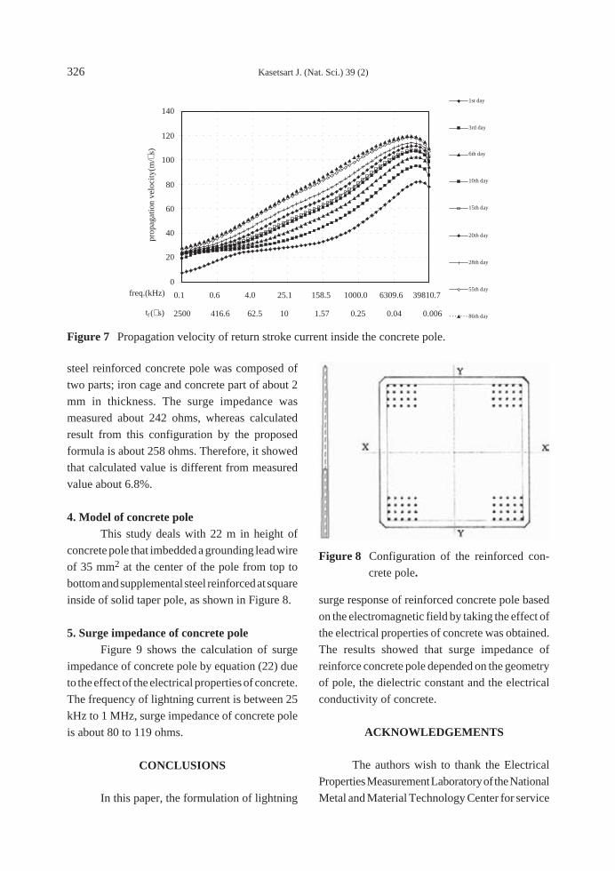
326 Kasetsart J. (Nat. Sci.) 39 (2)
steel reinforced concrete pole was composed of
two parts; iron cage and concrete part of about 2
mm in thickness. The surge impedance was
measured about 242 ohms, whereas calculated
result from this configuration by the proposed
formula is about 258 ohms. Therefore, it showed
that calculated value is different from measured
value about 6.8%.
4. Model of concrete poleThis study deals with 22 m in height of
concrete pole that imbedded a grounding lead wire
of 35 mm2 at the center of the pole from top to
bottom and supplemental steel reinforced at square
inside of solid taper pole, as shown in Figure 8.
5. Surge impedance of concrete poleFigure 9 shows the calculation of surge
impedance of concrete pole by equation (22) due
to the effect of the electrical properties of concrete.
The frequency of lightning current is between 25
kHz to 1 MHz, surge impedance of concrete pole
is about 80 to 119 ohms.
CONCLUSIONS
In this paper, the formulation of lightning
0
20
40
60
80
100
120
140
0.1 0.6 4.0 25.1 158.5 1000.0 6309.6 39810.7freq.(kHz)
prop
agat
ion
velo
city
(m/µ
s)
1st day
3rd day
6th day
10th day
15th day
20th day
28th day
55th day
86th day tf (µs) 2500 416.6 62.5 10 1.57 0.25 0.04 0.006
Figure 7 Propagation velocity of return stroke current inside the concrete pole.
Figure 8 Configuration of the reinforced con-
crete pole.
surge response of reinforced concrete pole based
on the electromagnetic field by taking the effect of
the electrical properties of concrete was obtained.
The results showed that surge impedance of
reinforce concrete pole depended on the geometry
of pole, the dielectric constant and the electrical
conductivity of concrete.
ACKNOWLEDGEMENTS
The authors wish to thank the Electrical
Properties Measurement Laboratory of the National
Metal and Material Technology Center for service

Kasetsart J. (Nat. Sci.) 39 (2) 327
of the concrete electrical properties of
measurement.
LITERATURE CITED
Jordan, C.A. 1934. Lightning computations for
transmission lines with overhead ground wires
Part II. General Electric Review 34: 180-
185.
Lundholm, R., R.B. Finn, Jr. and W.S. Price. 1958.
Calculation of transmission line lightning
voltage by field concepts. AIEE Trans. PT.
77: 1271-1283.
Wagner, C.F. and A.R. Hileman. 1960. A new
approach to calculation of lightning
performance of transmission lines. AIEETrans. PT. 79: 589-603.
Sargent, A. and M. Darveniza. 1969. Tower surge
impedance. IEEE Trans. PAS. 88: 680-687
Okumura, K. and A. Kijima. 1985. A method for
computing surge impedance of transmission
line tower by electromagnetic field theory.
IEE of Japan Trans. B. 105: 733-740.
Breuer,G.D., A.J. Schultz, R.H. Schlomann and
W. S. Price. 1958. Field studies of the surge
response of a 345-kV transmission tower and
ground wire. AIEE Trans. PT. 77:
1392–1396.
Caswell, R.W., I.B. Johnson, E.F. Koncel, Jr. and
N. R. Schultz. 1958. Lightning performance
of 138-kV twin-circuit transmission lines of
Commonwealth Edison company—operating
experience and field studies. IEEE Trans.PT. 77: 1480–1491.
Kawai, M. 1964. Studies of the surge response on
a transmission line tower. IEEE Trans. PAS.
83: 30–34.
Chisholm,W.A., Y.L. Chow and K.D. Srivastava.
1983. Lightning surge response of
transmission towers. IEEE Trans. PAS. 102:
3232–3242.
Chisholm W.A. and Y.L. Chow. 1985. Travel time
of transmission towers. IEEE Trans. PAS.
104: 2922–2928.
Wahab, M.A.A., I. Matsubara and H. Kinoshita.
1987. An experimental evaluation of some
factors affecting tower surge impedance. IEEof Japan Trans. 107: 171–177.
Ishii M., T. Kawamura, T. Kouno, E. Ohsaki, K.
Murotani and T. Higuchi. 1991. Multistory
transmission tower model for lightning surge
analysis. IEEE Trans. PWRD. 6: 1327–1335.
Yamada T., A. Mochizuki, J. Sawada, E. Zaima,
T. Kawamura, A. Ametani, M. Ishii and S.
Kato. 1995. Experimental evaluation of a
UHV tower model for lightning surge analysis.
Figure 9 Surge impedance of concrete pole.
0
20
40
60
80
100
120
140
160
0.1 0.6 4.0 25.1 158.5 1000.0 6309.6 39810.7freq.(kHz)
surg
e im
peda
nce(
ohm
s)
1st day
3rd day
6th day
10th day
15th day
20th day
28th day
55th day
86th day tf ( µs) 2500 416.6 62.5 10 1.57 0.25 0.04 0.006

328 Kasetsart J. (Nat. Sci.) 39 (2)
IEEE Trans. PWRD. 10: 393–402.
Matsumoto Y., O. Sakuma, K. Shinjo, M. Saiki, T.
Wakai, T. Sakai, N.Nagasaka, H. Motoyama
and M. Ishii. 1995. Measuring of lightning
surges on test transmission line equipped with
arresters struck by natural and triggered
lightning. IEEE Trans. PWRD. 11:
996–1002.
Shinjo K., Y. Matsumoto, O. Sakuma, T. Wakai,
T. Sakai, M. Ishii and H. Motoyama. 1997.
Characteristics of transient response of
okushishiku test transmission line struck by
natural and triggered lightning. IEE of JapanTrans. 117-B: 478–487.
Motoyama H., K. Shinjo, Y. Matsumoto and N.
Itamoto. 1998. Observation and analysis of
multiphase back flashover on the okushishiku
test transmission line caused by winter
lightning. IEEE Trans. PWRD. 13: 1319-
1398.
Ishii M. and Y. Baba. 1997. Numerical
electromagnetic field analysis of tower surge
response. IEEE Trans. PWRD. 12: 483–488.
Motoyama, H. and H.Matsubara. 2000. Analytical
and experimental study on surge response of
transmission tower. IEEE Trans. PowerDelivery 15: 812-819.
Hintamai, S. and J. Hokierti. 2003. Lightning
surge response analysis of concrete pole using
the electromagnetic field method, pp. 568-
573. In Transmission and DistributionConference and Exposition. Dallas Texas.
Chowdhuri, P. S. Li and P. Yan. 2001. Review of
research on lightning-induced voltages on an
overhead line. IEE Proc.-Gener. Transm.Distrib. 148: 91-95.
Rubinstein, M. and M.A.Uman. 1989. Methods
for calculating the electromagnetic fields from
a known source distribution: application to
lightning. IEEE Trans. Electromag.Compat. 31: 183-189.
Plonus, M.A. 1988. Applied Electromagnetics.International Editions. New York: McGraw-
Hill.
Morshedy, A.El. 2000. High-Voltage EngineerngTheory and Practice. New York: Marcel
Dekker, Inc.
Yamamoto, K., Z. Kawasaki, K. Matsuura, S.
Sekioka and S. Yokoyama. 1997. Study on
surge impedance of reinforced concrete pole
and grounding lead wire on distribution line
by experimental on reduced scale model, pp.
209-212. In Proc. 10th Int. Symp. HighVoltage Eng.


