ACTIVE NOISE CONTROL USING MODALLY

TUNED PHASE-COMPENSATED FILTERS

by

Jesse B. Bisnette

BS, University of Pittsburgh, 2002

Submitted to the Graduate Faculty of

the School of Engineering in partial fulfillment

of the requirements for the degree of

Master of Science

University of Pittsburgh

2003

UNIVERSITY OF PITTSBURGH

SCHOOL OF ENGINEERING

This thesis was presented

by

Jesse B. Bisnette

It was defended on

25 November 2003

and approved by

Jeffery S. Vipperman, Assistant Professor, Mechanical Engineering

Danial D. Budny, Associate Professor, Civil Engineering

William W. Clark, Associate Professor, Mechanical Engineering

Thesis Advisor: Jeffery S. Vipperman, Assistant Professor, Mechanical Engineering

ii

ACTIVE NOISE CONTROL USING MODALLY TUNED

PHASE-COMPENSATED FILTERS

Jesse B. Bisnette, MS

University of Pittsburgh, 2003

An active noise control device or an active noise absorber (ANA) that is based on either

resonant 2nd-order or 4th-order Butterworth filters is developed and demonstrated. This

control method is similar to structural positive position feedback (PPF) control, with two

exceptions: 1) acoustic transducers (microphone and speaker) cannot be truly colocated, and

2) the acoustic actuator (loudspeaker) has significant dynamics that can affect performance

and stability. Acoustic modal control approaches are typically not sought, however, there are

a number of applications where controlling a few room modes is adequate. A model of a duct

with speakers at each end is developed and used to demonstrate the control method, including

the impact of the speaker dynamics. An all-pass filter is used to provide phase compensation

and to improve controller performance. Two companion experimental studies validated the

simulation results. A single mode case using a resonant band-pass filter demonstrated nearly

10 dB of control in the first duct, while a multimodal case using two 4th-order Butterworth

band-pass filters show both 10 dB of reduction in the fundamental mode and nearly 8.0 dB

in the second.

iii

TABLE OF CONTENTS

1.0 INTRODUCTION . . . . . . . . . . . . . . . . . . . . . . . . . . . . . . . . . 1

2.0 MODELING THE SYSTEM . . . . . . . . . . . . . . . . . . . . . . . . . . 7

2.1 Analytical Model . . . . . . . . . . . . . . . . . . . . . . . . . . . . . . . . . 7

2.1.1 Acoustic Duct . . . . . . . . . . . . . . . . . . . . . . . . . . . . . . . 8

2.1.2 Loudspeakers . . . . . . . . . . . . . . . . . . . . . . . . . . . . . . . . 10

2.2 State Space Representation and Model Verification . . . . . . . . . . . . . . 11

2.2.1 Acoustic Duct State Matrices . . . . . . . . . . . . . . . . . . . . . . . 13

2.2.2 Loudspeaker State Matrices . . . . . . . . . . . . . . . . . . . . . . . . 16

2.3 Simulated Plant Response and Model Verification . . . . . . . . . . . . . . . 17

3.0 COMPENSATOR DESIGN . . . . . . . . . . . . . . . . . . . . . . . . . . . 19

3.1 Feedback Configuration . . . . . . . . . . . . . . . . . . . . . . . . . . . . . 19

3.2 Resonant Filter Design . . . . . . . . . . . . . . . . . . . . . . . . . . . . . . 21

3.2.1 Phase Compensation . . . . . . . . . . . . . . . . . . . . . . . . . . . 24

3.2.2 Resonant Filter Control Simulation . . . . . . . . . . . . . . . . . . . 25

3.3 Fourth-order Compensators . . . . . . . . . . . . . . . . . . . . . . . . . . . 29

3.4 Control with Non-collocated Sensor/Actuator Pair . . . . . . . . . . . . . . 32

3.5 Multimodal Control . . . . . . . . . . . . . . . . . . . . . . . . . . . . . . . 35

4.0 EXPERIMENTAL DEMONSTRATIONS . . . . . . . . . . . . . . . . . . 40

4.1 Design and Response of Second-order Controller . . . . . . . . . . . . . . . . 40

4.1.1 Compensator Design . . . . . . . . . . . . . . . . . . . . . . . . . . . 40

4.1.2 Closed-loop Response . . . . . . . . . . . . . . . . . . . . . . . . . . . 42

4.2 Design and Response of Multimodal Controller . . . . . . . . . . . . . . . . 43

iv

5.0 CONCLUDING REMARKS . . . . . . . . . . . . . . . . . . . . . . . . . . 49

APPENDIX A. MATLABTM CODE FOR DUCT . . . . . . . . . . . . . . . 51

APPENDIX B. MATLABTM CODE FOR LOUDSPEAKERS . . . . . . . . 54

APPENDIX C. MATLABTM CODE UTILIZING DESIGN PROCEDURE 56

BIBLIOGRAPHY . . . . . . . . . . . . . . . . . . . . . . . . . . . . . . . . . . . . 62

v

LIST OF TABLES

1 Plant parameters used in simulation. . . . . . . . . . . . . . . . . . . . . . . . 18

2 Dual mode controller design parameters. . . . . . . . . . . . . . . . . . . . . . 38

3 Compensator parameters. . . . . . . . . . . . . . . . . . . . . . . . . . . . . . 42

4 Multimodal Butterworth filter compensator parameters. . . . . . . . . . . . . 46

vi

LIST OF FIGURES

1 Block diagram of PPF controller. . . . . . . . . . . . . . . . . . . . . . . . . . 4

2 Response of a single mode structure and PPF filter. . . . . . . . . . . . . . . 5

3 Disturbance/Controlled response for a single mode structure. . . . . . . . . . 5

4 Rigid walled acoustic duct setup. . . . . . . . . . . . . . . . . . . . . . . . . . 7

5 Loudspeaker schematic. . . . . . . . . . . . . . . . . . . . . . . . . . . . . . . 10

6 Plant schematic showing system conventions. . . . . . . . . . . . . . . . . . . 12

7 Simulated and experimental results for disturbance-path. . . . . . . . . . . . 18

8 Closed-loop system schematic. . . . . . . . . . . . . . . . . . . . . . . . . . . 20

9 Fully coupled feedback model of controller. . . . . . . . . . . . . . . . . . . . 20

10 Simplified feedback model of controller. . . . . . . . . . . . . . . . . . . . . . 21

11 Frequency response of control speaker, duct, and duct+loudspeaker. . . . . . 22

12 Frequency response of control-path and low/band-pass filter. . . . . . . . . . 23

13 Predicted disturbance-path/closed-loop response without speaker dynamics. . 26

14 Predicted disturbance-path/closed-loop response with speaker dynamics. . . . 27

15 Root locus analysis of first mode controller . . . . . . . . . . . . . . . . . . . 28

16 Predicted disturbance-path/closed-loop response using all-pass filter. . . . . . 28

17 Root locus analysis of second mode controller . . . . . . . . . . . . . . . . . . 29

18 Predicted disturbance-path/closed-loop response for control over mode 2. . . 30

19 Butterworth response tuned to second duct mode. . . . . . . . . . . . . . . . 31

20 Predicted control-path response. . . . . . . . . . . . . . . . . . . . . . . . . . 33

21 Root-locus of control-path with Butterworth filter. . . . . . . . . . . . . . . . 33

22 Predicted closed-loop response with control over mode 2. . . . . . . . . . . . 34

vii

23 Illustration of sensor placement using duct mode shapes . . . . . . . . . . . . 35

24 Predicted results of duct+loudspeaker when xsen = x1. . . . . . . . . . . . . . 36

25 Predicted disturbance-path/closed-loop results when xsen = x1, xe = x2. . . . 36

26 Schematic of multimodal controller. . . . . . . . . . . . . . . . . . . . . . . . 37

27 Predicted control-path response tuned to modes 1 and 2. . . . . . . . . . . . 39

28 Predicted disturbance-path/closed-loop response for control over modes 1 and 2. 39

29 Experimental test bed. . . . . . . . . . . . . . . . . . . . . . . . . . . . . . . 41

30 Schematic for inverting all-pass filter network. . . . . . . . . . . . . . . . . . . 42

31 Measured fully compensated control-path. . . . . . . . . . . . . . . . . . . . . 43

32 Measured disturbance-path/closed-loop response for various gain values. . . . 44

33 Measured Disturbance-path/closed-loop response over 500 Hz frequency range. 45

34 Measured fully compensated multimodal control-path. . . . . . . . . . . . . . 46

35 Measured disturbance-path/closed-loop response for various gain combinations. 48

36 Measured disturbance-path/closed-loop response for gain value G3. . . . . . . 48

viii

NOMENCLATURE

Symbols

l : Length

w : Width

h : Height

V : Volume of duct

A : Area of speaker cone

x : Position

R : Resistance

L : Inductance

C : Capacitance

I : Current

m : Mass of loudspeaker cone

b : Damping ratio of loudspeaker

k : Stiffness of loudspeaker

Bl : Electro-mechanical coupling coefficient

c : Sound speed in air

N : Number of modes

t : Time

f : Frequency

v(t) : Applied voltage

y(t) : Speaker displacement function

p(x, t) : Pressure function

A : State-space A matrix

ix

B : State-space B matrix

C : State-space C matrix

D : State-space D matrix

U : State input vector

F : Force

H : Transfer function

S : Laplace variable

G : Filter gain

z : Filter zero

p : Filter pole

µ : State variable

ϕ : State output vector

ρo : Density of air at room temperature

Ψ : Eigenfunction of duct

φ : Structural/acoustical coupling coefficient

β : State duct model input coefficients

γ : State duct model pressure output coefficents

ω : Circular frequency

ζ : Damping ratio

θ : Phase angle

Subscripts

n : Mode index, or referring to noise speaker

j : Speaker index

co : Cuttoff frequency

d : Referring to duct

e : Referring to error signal

s : Referring to loudspeaker

sen : Referring to sensor signal

x

c : Referring to compensator, or control speaker

f : Referring to generic filter

a : Referring to all-pass filter

g : Referring to gain circuit

LP : Low-pass filter

BP : Band-pass filter

AP : All-pass filter

Superscripts

˙ : First derivative, ddt

¨: Second Derivative, d2

dt2

xi

1.0 INTRODUCTION

Engineering noise control typically entails reducing sound by modifying acoustic sources,

augmenting transmission paths, or removing the object or subject being exposed to noise.

Within a reverberant enclosure, both passive and active control technologies can be applied

either separately or in combination [1].

Passive control techniques are an attractive solution when a power source is either un-

wanted or impractical. Often, passive control is achieved by adding absorptive materials

such as foam insulation or ceiling tiles to the system so that the material disrupts the re-

flection of the disturbance sound field. Another popular method used in passive control

is the Helmholtz resonator, in which a mechanical band-stop filter is achieved by adding

a small opening in a cavity such as a duct or pipe which leads to a fixed volume chamber

tuned to a given frequency [2, 3]. Some implementations of Helmholtz resonators include the

ability to actively tailor the passive properties and provide tuning mechanisms [4, 5]. One

recent report uses active electronics to tune a passive speaker, which serves as an acoustic

absorber [6]. Typically, passive techniques are employed for mid to high frequency distur-

bances. At low frequencies, however, these techniques become bulky and heavy, thus making

them undesirable. For these situations, active controllers can be more practical.

There are many considerations for implementing active noise control (ANC) [8]. Foremost

is the control topology: feedforward vs. feedback. In feedforward control, “anti-noise”

signals are created which can completely control plane waves or notch out zones of silence

in harmonic, 3-dimensional sound fields. For this topology, a sensor, such as a microphone

or accelerometer, is placed downstream from the disturbance source. This signal is then

used to drive an electronic controller, typically an adaptive filter network, which is fed to

an electormechanical transducer further downstream. Another sensor is incorporated in

1

feedforward design to measure the error at the control point and is used it improve the

controller’s performance. The first work in feedforward noise control dates to 1934 when

Paul Lueg first proposed using interference sound waves to control noise in rigid walled

ducts and tubes [8].

Often adaptive feedforward algorithms, which are implemented using digital finite im-

pulse response (FIR) filters and digital signal processing (DSP) boards, are required along

with some form of system identification. Such algorithms typically employ an iterative pro-

cess that gradually generates new sets of FIR coefficients at every iteration so that the

mean-squared error in the zone of silence is reduced over time. One popular example of

this method is the least-mean-square algorithm, or LMS, which is based on a gradient de-

scent algorithm. Updating the filter coefficients, however, is often computationally intensive.

Therefore, works such as Douglas [10] have proposed algorithms, where the coefficients are

only partially updated at every sample time, thus reducing the complexity of the overall

system, up to 50%, when compared to a standard LMS controller. This makes these fast al-

gorithms much more suitable for real time applications. Another recent feedforward method

has utilized fuzzy logic for controlling a distributed source of broadband noise [11].

The second topology used in ANC is feedback control. For this method, a disturbance

pressure field is detected by using a sensor microphone, which is used as an input to an

electronic controller that conditions the magnitude and phase of the signal. The controller’s

output is then amplified and converted to an output pressure field at the sensor microphone.

This conditioned “control” signal is then added to the disturbance field. These controllers

have been used to create zones of silence using servo control [12] or to augment the dynamics

(i.e. add damping) of an enclosed sound field. Implementations range from dissipative output

feedback to robust and optimal model-based control designs [8]. Acoustic feeback control

has a limited bandwidth because of the transducer dynamics and the time delay between

the sensor and actuator.

For these reasons, this topology is far less popular in ANC than feedforward designs.

In enclosed sound fields, these problems are compounded by high modal density of the

enclosure and thus feedback control is seldom used in such circumstances [9]. However,

there are cases where controlling a few modes is beneficial, such as ducts or mufflers or for

2

controlling transmission loss in finite structures [13, 14, 19, 20]. Control of low-frequency

acoustic modes proves to be important for protecting payloads in launch vehicles. In these

situations, the complications described above must be taken into consideration.

Feedback control of structural and acoustic systems are very similar while also having

important differences. For example, unlike for structures, perfectly collocated sensor (mi-

crophone) and actuator (loudspeaker) pairs can not be achieved since the spatial aperture

of the two transducers differ. By centering the microphone at the face of the loudspeaker,

a “substantially collocated” transducer pair is achieved. However, unlike piezoceramic ac-

tuators used in structural control problems, the loudspeaker has significant dynamics which

can be destabilizing and therefore erode controller performance. One report indicated that

a 10% phase shift can reduce control effectiveness by 70% [25]. Several methods have been

deduced which compensate for loudspeaker dynamics, two of which are described here.

One method for overcoming the effects of transducer dynamics in acoustic systems is to

created a band-limited volume-velocity source, which was also used to demonstrate dissipa-

tive feedback control. In this procedure, the motion (either position, velocity, or acceleration)

of the cone is measured and negatively fed back to the input voltage. By doing so, the poles,

thus dynamics, are moved further to the left in the complex plane, thereby yielding nearly

constant phase and magnitude response in low frequency regions. One issue with this tech-

nique, however, is that by adding the feedback loop, the overall gain of the loudspeaker is

greatly reduced [15].

A second method was proposed to eliminate the loudspeaker dynamics in systems that

have strong pressure coupling with the plant. However, in this case, the procedure de-

scribed above is not as effective, since it only takes into account the internal dynamics of

the loudspeaker. To address this problem, a velocity sensor which takes into account both

the secondary coil voltage due to the motion of the loudspeaker cone and the primary coil

current can be developed and used in conjunction with a proportional feedback controller.

Doing so can result in an actuator that obtains nearly flat magnitude and phase response in

the 20− 200 Hz frequency range [16].

An example of a relatively simple, yet effective structural feedback control approach

is positive position feedback (PPF) [17]. In PPF, a control sensor and actuator that are

3

essentially free of dynamics at low frequencies (e.g., piezoceramic patches) are selected and

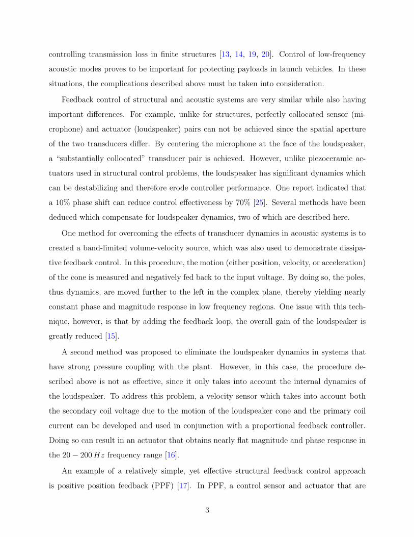
collocated, which ensures that the control path is minimum phase. A simple block diagram

of a PPF controller is given in Figure 1.

Figure 1: Block diagram of PPF controller.

The control signal is formed by feeding back structural displacement signals through a

damped, resonant low-pass filter that is tuned to the desired structural resonance frequency

[17, 18]. For a collocated sensor/actuator configuration, both the structure and low-pass filter

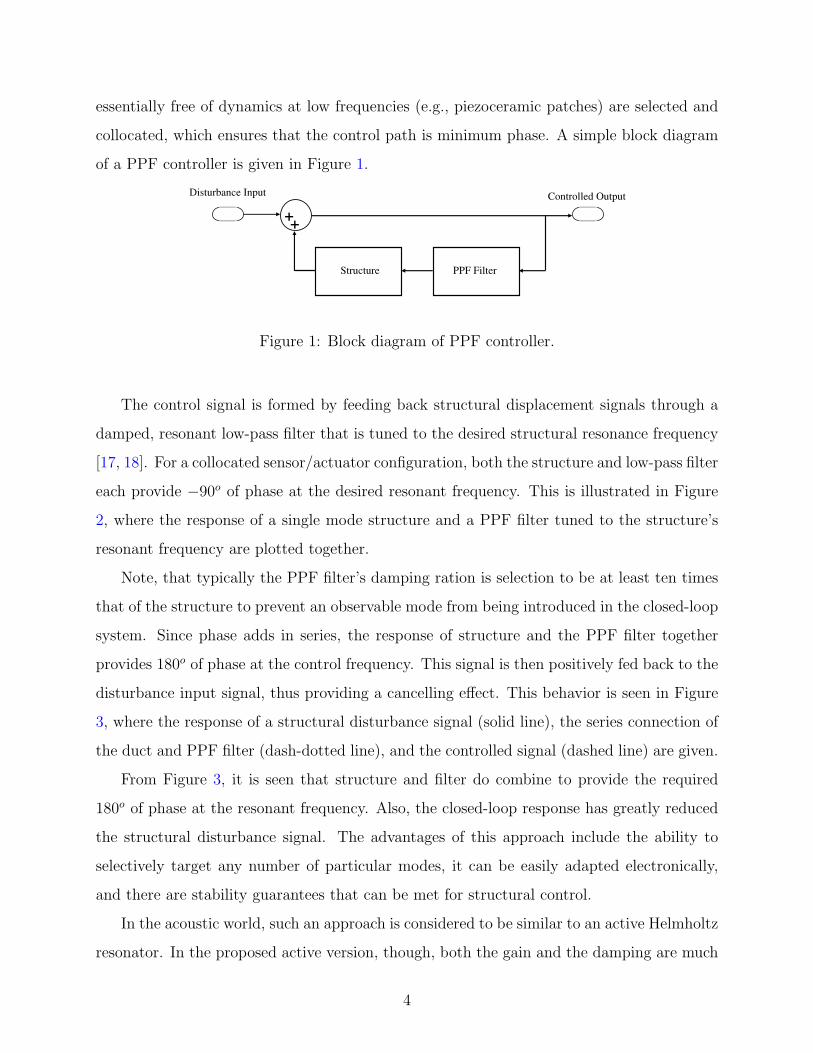
each provide −90o of phase at the desired resonant frequency. This is illustrated in Figure

2, where the response of a single mode structure and a PPF filter tuned to the structure’s

resonant frequency are plotted together.

Note, that typically the PPF filter’s damping ration is selection to be at least ten times

that of the structure to prevent an observable mode from being introduced in the closed-loop

system. Since phase adds in series, the response of structure and the PPF filter together

provides 180o of phase at the control frequency. This signal is then positively fed back to the

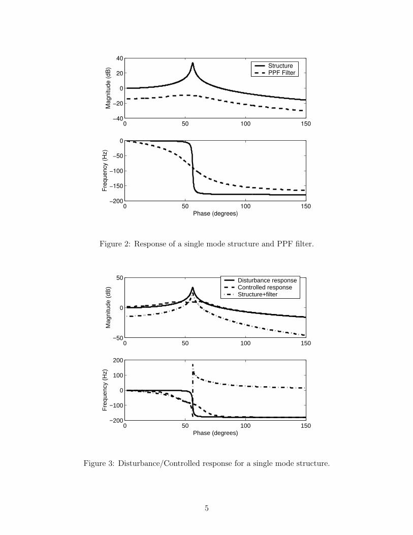
disturbance input signal, thus providing a cancelling effect. This behavior is seen in Figure

3, where the response of a structural disturbance signal (solid line), the series connection of

the duct and PPF filter (dash-dotted line), and the controlled signal (dashed line) are given.

From Figure 3, it is seen that structure and filter do combine to provide the required

180o of phase at the resonant frequency. Also, the closed-loop response has greatly reduced

the structural disturbance signal. The advantages of this approach include the ability to

selectively target any number of particular modes, it can be easily adapted electronically,

and there are stability guarantees that can be met for structural control.

In the acoustic world, such an approach is considered to be similar to an active Helmholtz

resonator. In the proposed active version, though, both the gain and the damping are much

4

0 50 100 150−40

−20

0

20

40

Mag

nitu

de (d

B)

0 50 100 150−200

−150

−100

−50

0

Phase (degrees)

Freq

uenc

y (H

z)

StructurePPF Filter

Figure 2: Response of a single mode structure and PPF filter.

0 50 100 150−50

0

50

Mag

nitu

de (

dB)

0 50 100 150−200

−100

0

100

200

Phase (degrees)

Fre

quen

cy (

Hz)

Disturbance responseControlled responseStructure+filter

Figure 3: Disturbance/Controlled response for a single mode structure.

5

higher than for the passive counterpart. There is one report [26] that demonstrated PPF for

acoustic control. By only targeting modes at frequencies above the loudspeaker’s dynamics,

its dynamics were neglected. This paper develops the theory for an active noise control device

similar to PPF that includes a method to compensate the phase response of the loudspeaker

actuator, thereby, permitting control in frequency regions where the loudspeaker dynamics

are dominant. Although previously referred to as an “actively tuned acoustic absorber”

[21], it will hence be referred to as an active noise absorber (ANA), to differentiate it from

passive absorbers that are actively tuned [4, 5, 16]. A method to correct phase and provide

performance and stability improvements will be presented, along with stability analysis using

root locus techniques.

First, a theoretical model of a duct/loudspeaker system is developed. Next,control of the

first two duct modes is demonstrated. Unlike Farinholt [26], where only non-inverting low-

pass filters were utilized, this work does not place limitations on the chosen filter. Rather,

gross phase compensation (± 90) of the loudspeaker dynamics is achieved by choosing either

an inverting or non-inverting low-pass or band-pass resonant filter. It will also be shown that

the bandpass provides more optimal magnitude response and thus will be favored. Instead

of utilizing one of the above techniques which eliminate phase dynamics of the loudspeaker,

here fine phase adjustments at the control frequency are accomplished by including an all-

pass filter in the control-path. Once this technique is demonstrated with resonant 2nd-order

filters, the design is extended to utilize 4th-order Butterworth bandpass filters, which are used

to develop a multimodal controller. A previous publication of this study [27] focused only

on collocated sensor/actuator pairs. This thesis will also consider the use of non-collocated

choices, which is a benefit of using the all-pass filter. Finally, two companion experimental

studies are provided that demonstrate control using a resonant filter over the fundamental

duct mode and also demonstrates multimodal control in the fundamental and second duct

modes.

6

2.0 MODELING THE SYSTEM

2.1 ANALYTICAL MODEL

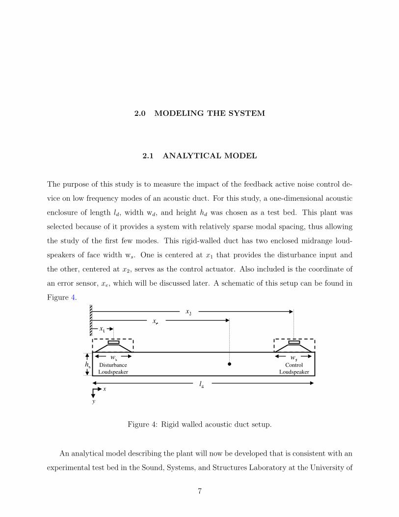
The purpose of this study is to measure the impact of the feedback active noise control de-

vice on low frequency modes of an acoustic duct. For this study, a one-dimensional acoustic

enclosure of length ld, width wd, and height hd was chosen as a test bed. This plant was

selected because of it provides a system with relatively sparse modal spacing, thus allowing

the study of the first few modes. This rigid-walled duct has two enclosed midrange loud-

speakers of face width ws. One is centered at x1 that provides the disturbance input and

the other, centered at x2, serves as the control actuator. Also included is the coordinate of

an error sensor, xe, which will be discussed later. A schematic of this setup can be found in

Figure 4.

Figure 4: Rigid walled acoustic duct setup.

An analytical model describing the plant will now be developed that is consistent with an

experimental test bed in the Sound, Systems, and Structures Laboratory at the University of

7

Pittsburgh. In the following sections, the governing equations for the midrange loudspeakers

and the acoustic duct will be presented. For a more detailed derivation of these equations

see Fahy [22].

2.1.1 Acoustic Duct

To model the duct, the inhomogeneous wave equation, in terms of pressure, is used. The

general form of the equation can be written as

∇2p(x, t)− 1

c2

∂2p(x, t)

∂t2= ρo

J∑j=1

∂2yj(t)

∂t2, n = 1 . . .∞, (2.1)

where p(x, t) is the time dependent acoustic pressure at a point x inside the duct; c is the

speed of sound in air; and ρo is the air density. In addition, the speaker is modeled as a

piston where yj(t) is the displacement function of the jth speaker. The acoustic response of

the duct can be represented in modal coordinates as

p(x, t) =∞∑

n=1

pn(t)Ψn(x), (2.2)

where pn and Ψn are the nth pressure mode and eigenfunction of the enclosure respectively

[22]. By applying the closed-closed boundary conditions and a volume normalization, Ψn is

written as

Ψn =2

ldcos

(nπx

ld

), (2.3)

where x is an arbitrary point inside the duct. Applying the orthogonality condition and

substituting Equations (2.3) and (2.2) into (2.1) and integrating the resulting equation over

the fluid volume, the duct pressure in modal coordinates becomes

pn + ω2npn = ρoc

2

J∑j=1

∫Aj

Ψn(xj)yj dA, (2.4)

where

ωn =nπc

ld(2.5)

8

is the natural frequency of the nth duct pressure mode and Aj is the area of the jth loud-

speaker. By assuming the speaker’s cross sectional area can be treated as as square, the

right hand side of Equation (2.4) can now be written as

2ρoc2ws

ld

2∑j=1

∫ xj2

xj1

Ψn(xj)yj dx, (2.6)

where ws is the speaker face width and xj1 and xj2 indicate the left and right edges of the

disturbance (j = 1) and control (j = 2) loudspeaker, respectively. Performing the integration

in Equation (2.6) and substituting Equation (2.3) into the result gives the final governing

equation for the duct

pn + ζdωnpn + ω2npn =

2ρoc2A

ld

2∑j=1

yjφj, (2.7)

where

φj(n) =2ws

nπA

[sin

(nπxj2

ld

)− sin

(nπxj1

ld

)], n = 1 . . . N, j = 1, 2. (2.8)

Equation (2.7) also includes the duct damping ratio, ζd. This is introduced to represent the

internal dissipation and to properly bound the model. Notice that the infinite summation

over n is truncated to N , where N is large enough for the model to converge over the

bandwidth of interest. The one-dimensional model is valid if the applied system is operated

below the lowest cutoff frequency, fco [7]. For the experimental setup in question, the cutoff

frequency can be calculated by

fco =c

2wd

=343

.3302 s= 1039Hz. (2.9)

Thus, Equation (2.7) provides a set of uncoupled equations that completely describe the low

frequency behavior of the duct.

9

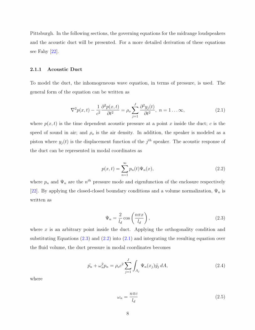
2.1.2 Loudspeakers

The next step is to develop the mathematical models for the loudspeakers. As shown in

Figure 4, both the acoustic disturbance signal and the control signal excite the duct via

midrange loudspeakers. A generic schematic for a cone speaker is provided in Figure 5.

Figure 5: Loudspeaker schematic.

The two inputs for each loudspeaker include the pressure acting on the speaker face and

the voltage to the coil; the output is the acceleration of the speaker cone, which acoustically

excites the duct. Since loudspeakers are coupled electro-mechanical systems, two differential

equations are needed to describe their behavior. The mechanical equation of motion for both

of the loudspeakers, (Figure 5(a)) is

yj +b

myj +

k

myj =

Bl

mIj −

A

mp(xj, t), (2.10)

where m and A are the the mass and cross sectional area of the loudspeaker cone, and b and k

are the damping ratios and the stiffness of the loudspeaker respectively. The input pressure,

which acts on the cone area, is given by p(xj, t) and the electro-mechanical coupling, which

creates an applied force that opposes the input pressure, is given by the product of the Bl

constant and the current through the coil, Ij.

10

Using the acoustic/mechanical coupling given in (2.8) along with Equations (2.2) and

(2.3), the modal form of Equation (2.10) can be written as

yj +b

myj +

k

myj =

Bl

mIj −

A

m

N∑n=1

pn(t)φj, j = 1, 2. (2.11)

To complete the mathematical representation, the electrical equation must also be included.

By summing the voltages around the loop in Figure 5(b), the equation that describes the

electrical behavior is given by

Ij +Rs

Ls

Ij =vj(t)

Ls

− Bl

Ls

yj, j = 1, 2, (2.12)

where, Ls and Rs are the internal inductance and resistance of the loudspeaker and vj(t)

is the input voltage. In this case, the Bl term produces a voltage in proportion to the

loudspeaker voice coil velocity (vemf = Blyj), which opposes the applied voltage.

2.2 STATE SPACE REPRESENTATION AND MODEL VERIFICATION

The above governing equations (2.7, 2.11, 2.12) can now be used to derive a state space model

to describe the experimental setup (less control speaker for uncontrolled case). However, it is

first necessary to present the system topology in order to determine the inputs and outputs

of the plant. A schematic showing the chosen plant topology, is seen in Figure 6.

The duct model shown in Figure 6 includes two acceleration inputs: y1 is the acceleration

from the disturbance loudspeaker, which is considered to be a component of the uncontrolled

plant system, while y2 is the acceleration output from the acoustic controller, which will be

discussed in detail later. The duct is also developed to include four outputs. The first and

last outputs, F (x1, t) and F (x2, t), are the integrated forces acting on the disturbance and

control loudspeakers, respectively. The second output, p(xe, t), represents the point error

pressure response at position xe, and can be set to record any point within the duct. The

final output, p(xsen, t) is the point sensor pressure for the controller and is set to xsen = x2

for a substantially colocated sensor/actuator pair. Notice that the block diagram for the

duct has been partitioned into two sections: one designated the disturbance duct, which

11

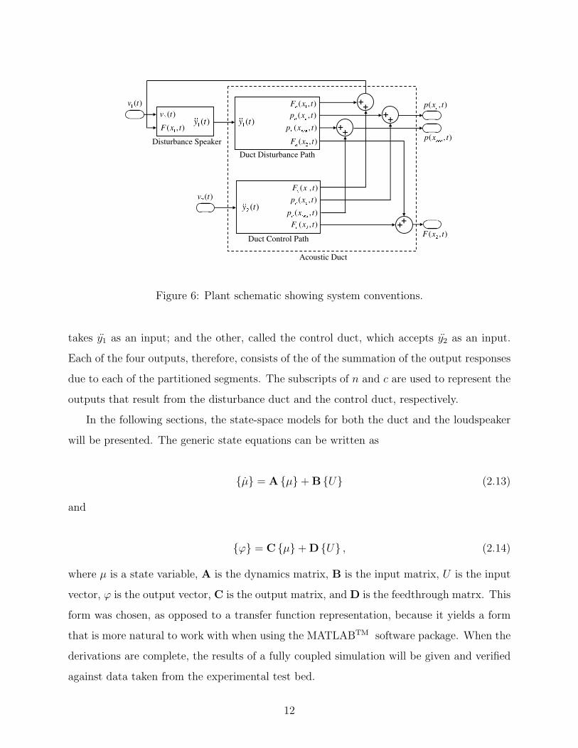
Figure 6: Plant schematic showing system conventions.

takes y1 as an input; and the other, called the control duct, which accepts y2 as an input.

Each of the four outputs, therefore, consists of the of the summation of the output responses

due to each of the partitioned segments. The subscripts of n and c are used to represent the

outputs that result from the disturbance duct and the control duct, respectively.

In the following sections, the state-space models for both the duct and the loudspeaker

will be presented. The generic state equations can be written as

µ = A µ+ B U (2.13)

and

ϕ = C µ+ D U , (2.14)

where µ is a state variable, A is the dynamics matrix, B is the input matrix, U is the input

vector, ϕ is the output vector, C is the output matrix, and D is the feedthrough matrx. This

form was chosen, as opposed to a transfer function representation, because it yields a form

that is more natural to work with when using the MATLABTM software package. When the

derivations are complete, the results of a fully coupled simulation will be given and verified

against data taken from the experimental test bed.

12

2.2.1 Acoustic Duct State Matrices

To begin the developement of the duct model, consider Equation (2.7), which provides the

information regarding the inputs and the internal dynamics of the duct and Equations (2.2)

and (2.3), which will provide the information regarding the outputs of the duct. For the

system shown in Figure 6, the inputs to the duct will consist of the two accelerations from

each of the loudspeakers and the outputs of the duct will be two point pressures and two

distributed forces.

This set of equations can be used to derive the Ad matrix and the Bd matrices of the

state-space model. However, to alleviate the derivation, some simplifications in notation are

first presented. The first simplification is made by combining the constant terms on the right

side of Equation (2.7) with equation (2.8). This combination, which is called βj(n) can be

written as

βj(n) =2ρoc

2

ldφj(n), j = 1, 2. (2.15)

Second, since the acceleration terms are the input variables, the yj notation can be dropped

in favor of the more conventional Uj notation. Finally, as stated in the previous chapter, the

number of the modes can be truncated to a finite number, N , such that N is large enough to

guarantee convergence to the experimental response. Making these substitutions and solving

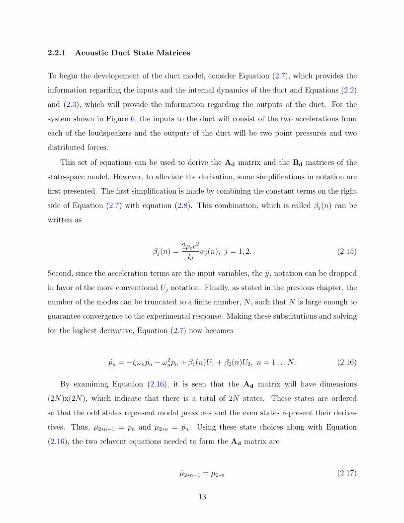
for the highest derivative, Equation (2.7) now becomes

pn = −ζωnpn − ω2npn + β1(n)U1 + β2(n)U2, n = 1 . . . N. (2.16)

By examining Equation (2.16), it is seen that the Ad matrix will have dimensions

(2N)x(2N), which indicate that there is a total of 2N states. These states are ordered

so that the odd states represent modal pressures and the even states represent their deriva-

tives. Thus, µ2∗n−1 = pn and µ2∗n = pn. Using these state choices along with Equation

(2.16), the two relavent equations needed to form the Ad matrix are

µ2∗n−1 = µ2∗n (2.17)

13

and

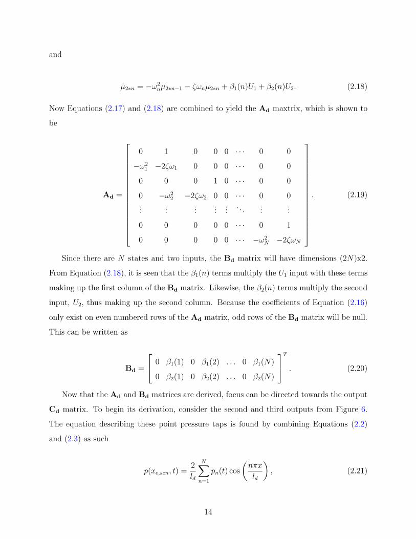
µ2∗n = −ω2nµ2∗n−1 − ζωnµ2∗n + β1(n)U1 + β2(n)U2. (2.18)

Now Equations (2.17) and (2.18) are combined to yield the Ad maxtrix, which is shown to

be

Ad =

0 1 0 0 0 · · · 0 0

−ω21 −2ζω1 0 0 0 · · · 0 0

0 0 0 1 0 · · · 0 0

0 −ω22 −2ζω2 0 0 · · · 0 0

......

......

.... . .

......

0 0 0 0 0 · · · 0 1

0 0 0 0 0 · · · −ω2N −2ζωN

. (2.19)

Since there are N states and two inputs, the Bd matrix will have dimensions (2N)x2.

From Equation (2.18), it is seen that the β1(n) terms multiply the U1 input with these terms

making up the first column of the Bd matrix. Likewise, the β2(n) terms multiply the second

input, U2, thus making up the second column. Because the coefficients of Equation (2.16)

only exist on even numbered rows of the Ad matrix, odd rows of the Bd matrix will be null.

This can be written as

Bd =

0 β1(1) 0 β1(2) . . . 0 β1(N)

0 β2(1) 0 β2(2) . . . 0 β2(N)

T

. (2.20)

Now that the Ad and Bd matrices are derived, focus can be directed towards the output

Cd matrix. To begin its derivation, consider the second and third outputs from Figure 6.

The equation describing these point pressure taps is found by combining Equations (2.2)

and (2.3) as such

p(xe,sen, t) =2

ld

N∑n=1

pn(t) cos

(nπx

ld

), (2.21)

14

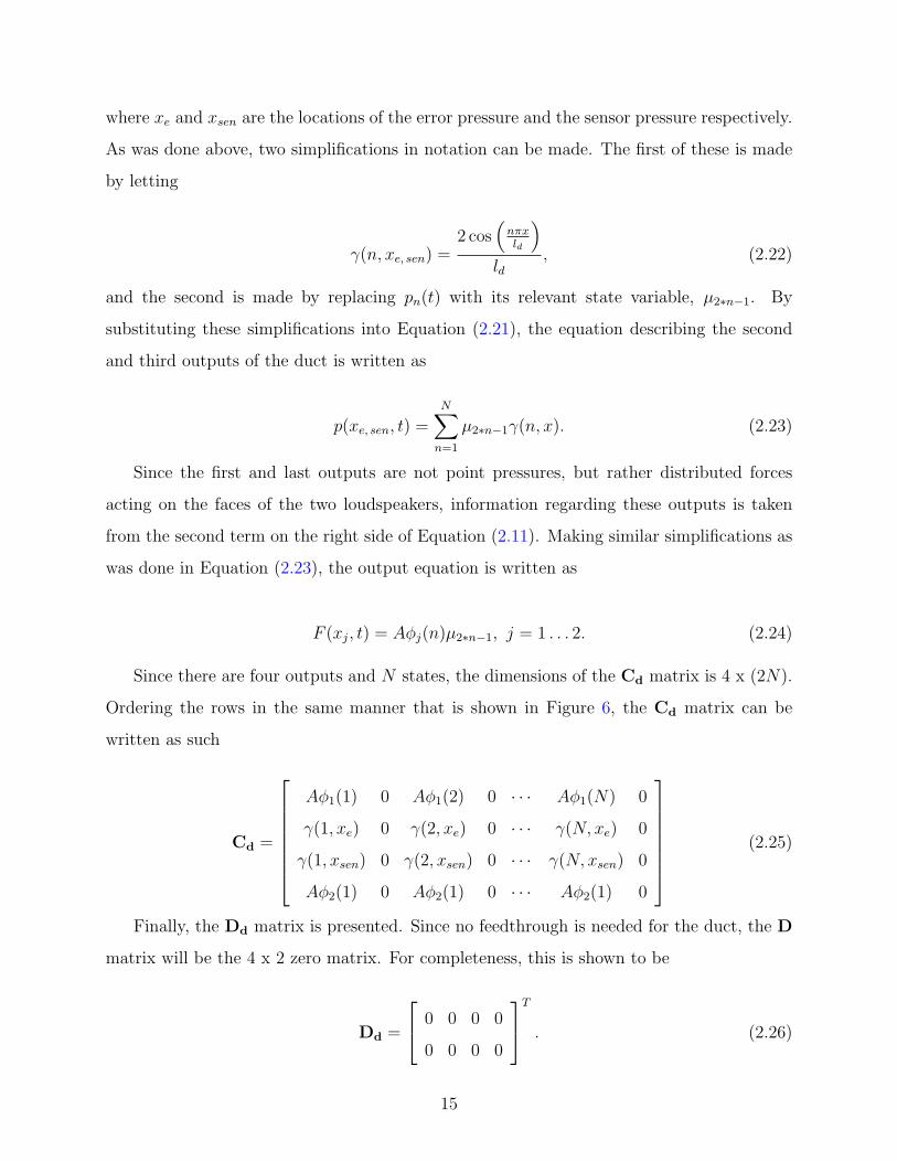
where xe and xsen are the locations of the error pressure and the sensor pressure respectively.

As was done above, two simplifications in notation can be made. The first of these is made

by letting

γ(n, xe, sen) =2 cos

(nπxld

)ld

, (2.22)

and the second is made by replacing pn(t) with its relevant state variable, µ2∗n−1. By

substituting these simplifications into Equation (2.21), the equation describing the second

and third outputs of the duct is written as

p(xe, sen, t) =N∑

n=1

µ2∗n−1γ(n, x). (2.23)

Since the first and last outputs are not point pressures, but rather distributed forces

acting on the faces of the two loudspeakers, information regarding these outputs is taken

from the second term on the right side of Equation (2.11). Making similar simplifications as

was done in Equation (2.23), the output equation is written as

F (xj, t) = Aφj(n)µ2∗n−1, j = 1 . . . 2. (2.24)

Since there are four outputs and N states, the dimensions of the Cd matrix is 4 x (2N).

Ordering the rows in the same manner that is shown in Figure 6, the Cd matrix can be

written as such

Cd =

Aφ1(1) 0 Aφ1(2) 0 · · · Aφ1(N) 0

γ(1, xe) 0 γ(2, xe) 0 · · · γ(N, xe) 0

γ(1, xsen) 0 γ(2, xsen) 0 · · · γ(N, xsen) 0

Aφ2(1) 0 Aφ2(1) 0 · · · Aφ2(1) 0

(2.25)

Finally, the Dd matrix is presented. Since no feedthrough is needed for the duct, the D

matrix will be the 4 x 2 zero matrix. For completeness, this is shown to be

Dd =

0 0 0 0

0 0 0 0

T

. (2.26)

15

The four state matrices presented above can be substituted into Equations (2.13) and

(2.14) to form the final state-space model describing the duct, which will be used for simula-

tion purposes. In the next section, the same process will be used to form the state matrices

for the two loudspeakers.

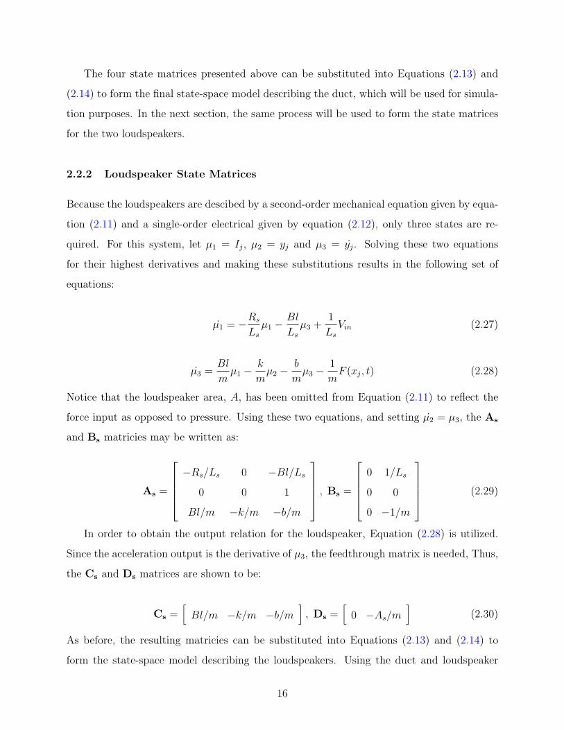
2.2.2 Loudspeaker State Matrices

Because the loudspeakers are descibed by a second-order mechanical equation given by equa-

tion (2.11) and a single-order electrical given by equation (2.12), only three states are re-

quired. For this system, let µ1 = Ij, µ2 = yj and µ3 = yj. Solving these two equations

for their highest derivatives and making these substitutions results in the following set of

equations:

µ1 = −Rs

Ls

µ1 −Bl

Ls

µ3 +1

Ls

Vin (2.27)

µ3 =Bl

mµ1 −

k

mµ2 −

b

mµ3 −

1

mF (xj, t) (2.28)

Notice that the loudspeaker area, A, has been omitted from Equation (2.11) to reflect the

force input as opposed to pressure. Using these two equations, and setting µ2 = µ3, the As

and Bs matricies may be written as:

As =

−Rs/Ls 0 −Bl/Ls

0 0 1

Bl/m −k/m −b/m

, Bs =

0 1/Ls

0 0

0 −1/m

(2.29)

In order to obtain the output relation for the loudspeaker, Equation (2.28) is utilized.

Since the acceleration output is the derivative of µ3, the feedthrough matrix is needed, Thus,

the Cs and Ds matrices are shown to be:

Cs =[

Bl/m −k/m −b/m], Ds =

[0 −As/m

](2.30)

As before, the resulting matricies can be substituted into Equations (2.13) and (2.14) to

form the state-space model describing the loudspeakers. Using the duct and loudspeaker

16

models, a simulation of the coupled plant is now presented and verified against data taken

from the experimental test bed.

2.3 SIMULATED PLANT RESPONSE AND MODEL VERIFICATION

The plant model was assembled and simulated in MATLABTM using the state-space repre-

sentations of the duct and speaker models derived in the previous sections. To be consistent

with the experimental test bed, the internal dimensions of the duct and the parameters for

the Peerless 832592 loudspeakers are used in the simulation. These values, along with the

properties of air, are listed in Table 1. The MATLABTM code pertaining to the duct is

presented in Appendix A, and code for the loudspeaker is presented in Appendix B.

In order to verify the MATLABTM model, the analytical frequency response between

v1(t) and p(xe, t) with xe set to x2 is plotted against measured results from the test bed

as shown in Figure 7. This response consists of the combination of the disturbance loud-

speaker and the duct disturbance-path, but will be referred to simply as the disturbance-path.

Through a trial and error approach, the low-frequency model from 0 − 500 Hz is found to

converge with N ≥ 36, and thus N = 40 is chosen.

It is seen that the simulated results predict the behavior of the experimental test bed

reasonably well. The discrepancy in the analytical model with the experimental data will

not inhibit the development of a design procedure for an ANA controller. Thus focus is now

directed to developing a compensator that will selectively control one of the duct modes

observed in Figure 7.

17

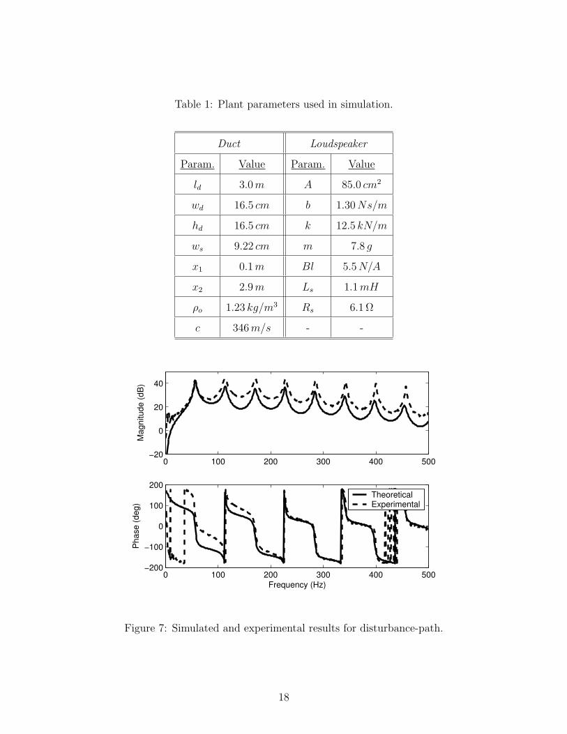
Table 1: Plant parameters used in simulation.

Duct Loudspeaker

Param. Value Param. Value

ld 3.0 m A 85.0 cm2

wd 16.5 cm b 1.30 Ns/m

hd 16.5 cm k 12.5 kN/m

ws 9.22 cm m 7.8 g

x1 0.1 m Bl 5.5 N/A

x2 2.9 m Ls 1.1 mH

ρo 1.23 kg/m3 Rs 6.1 Ω

c 346 m/s - -

0 100 200 300 400 500−20

0

20

40

Mag

nitu

de (d

B)

0 100 200 300 400 500−200

−100

0

100

200

Pha

se (d

eg)

Frequency (Hz)

TheoreticalExperimental

Figure 7: Simulated and experimental results for disturbance-path.

18

3.0 COMPENSATOR DESIGN

In this chapter, a design process is developed that will target and control one of the duct

modes shown in Figure 7. To perform this control, a device called an active noise absorber

(ANA) similar to ones used for structural PPF [17], is designed and used to control the

acoustic pressure modes. The controller uses a reference pressure as an input and feeds

back an output pressure to the duct. As with structural PPF, described in [17, 18], both

a collocated sensor/actuator pair and a tuned 2nd-order filter are initially used to generate

an output signal that is perfectly out of phase (180o) with the input at the desired control

frequency, ωc. Unlike the structural PPF examples [17, 18], however, the dynamics of the

acoustic loudspeaker will add phase to the control path, which affects the performance and

stability of the closed-loop system. To produce the required 180o of phase, these added

dynamics must be accounted for.

Once the procedure is shown using resonant 2nd-order filters, the design will be then

extended to use 4th-order Butterworth band-pass filters. It will also be shown that the

phase compensation technique has the added benefit of allowing the use of non-collocated

sensor/actuator pairs. Finally, a multimodal case is illustrated where control over the fun-

damental and second duct mode is achieved.

3.1 FEEDBACK CONFIGURATION

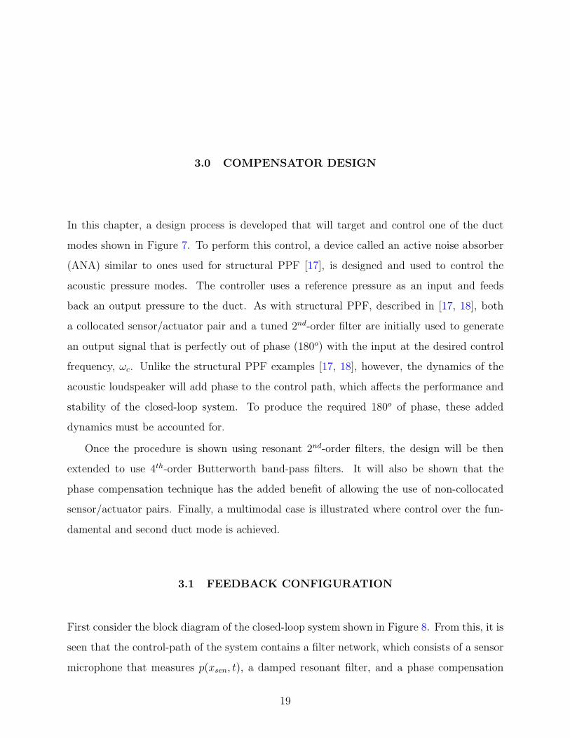
First consider the block diagram of the closed-loop system shown in Figure 8. From this, it is

seen that the control-path of the system contains a filter network, which consists of a sensor

microphone that measures p(xsen, t), a damped resonant filter, and a phase compensation

19

filter; a control speaker; and the duct transfer function between y2 and p(xsen, t), where xsen

is collocated with x2 and thus y2.

Figure 8: Closed-loop system schematic.

In order to gain more insight into the controller’s topology, which will aide in the design

of filter network, it is now advantageous to develop a simplified model of the controller cast

in a feedback setting. In addition, many classical feedback techniques, such as root-locus

analysis, may be utilized when the controller is in this form. With that being said, now

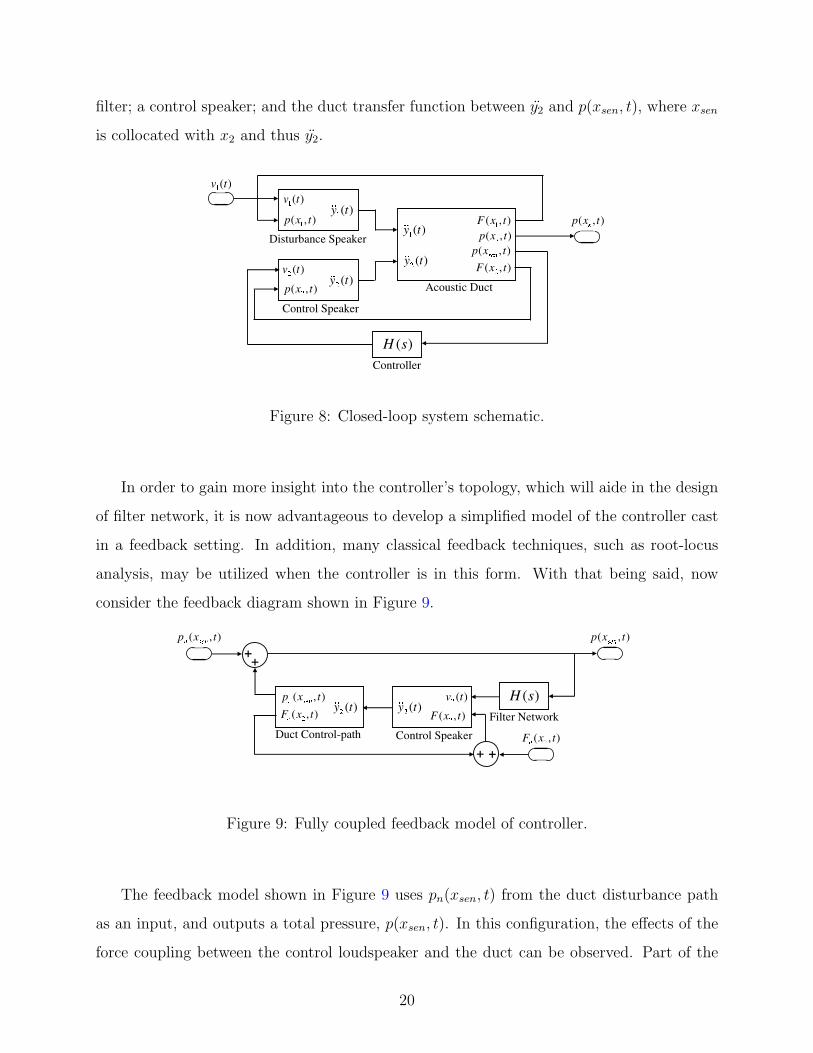
consider the feedback diagram shown in Figure 9.

Figure 9: Fully coupled feedback model of controller.

The feedback model shown in Figure 9 uses pn(xsen, t) from the duct disturbance path

as an input, and outputs a total pressure, p(xsen, t). In this configuration, the effects of the

force coupling between the control loudspeaker and the duct can be observed. Part of the

20

input force acting on the control loudspeaker cone is due to back coupling from the duct

control-path, Fc(x2, t), while the remainder, Fn(x2, t), is due to the influence of the duct

disturbance-path. The latter force is unwanted and may be treated as a noise input to the

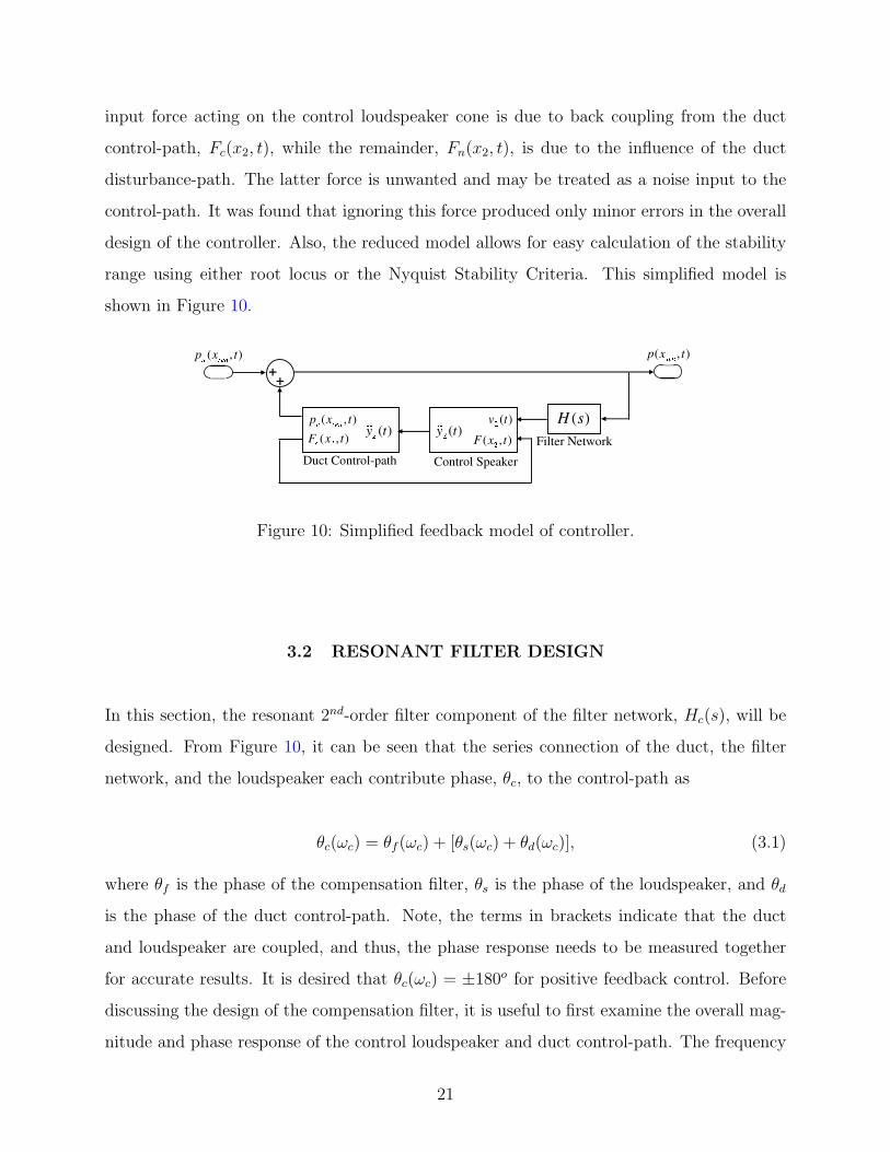
control-path. It was found that ignoring this force produced only minor errors in the overall

design of the controller. Also, the reduced model allows for easy calculation of the stability

range using either root locus or the Nyquist Stability Criteria. This simplified model is

shown in Figure 10.

Figure 10: Simplified feedback model of controller.

3.2 RESONANT FILTER DESIGN

In this section, the resonant 2nd-order filter component of the filter network, Hc(s), will be

designed. From Figure 10, it can be seen that the series connection of the duct, the filter

network, and the loudspeaker each contribute phase, θc, to the control-path as

θc(ωc) = θf (ωc) + [θs(ωc) + θd(ωc)], (3.1)

where θf is the phase of the compensation filter, θs is the phase of the loudspeaker, and θd

is the phase of the duct control-path. Note, the terms in brackets indicate that the duct

and loudspeaker are coupled, and thus, the phase response needs to be measured together

for accurate results. It is desired that θc(ωc) = ±180o for positive feedback control. Before

discussing the design of the compensation filter, it is useful to first examine the overall mag-

nitude and phase response of the control loudspeaker and duct control-path. The frequency

21

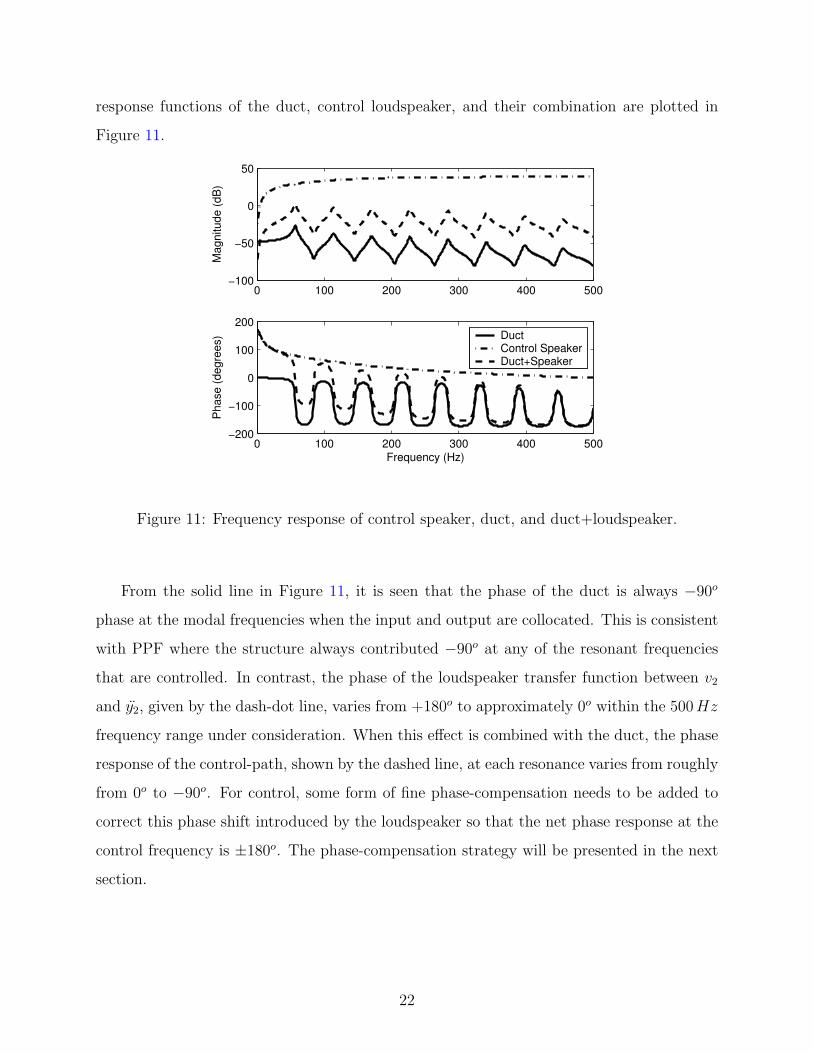
response functions of the duct, control loudspeaker, and their combination are plotted in

Figure 11.

0 100 200 300 400 500−100

−50

0

50

Mag

nitu

de (d

B)

0 100 200 300 400 500−200

−100

0

100

200

Frequency (Hz)

Pha

se (d

egre

es) Duct

Control SpeakerDuct+Speaker

Figure 11: Frequency response of control speaker, duct, and duct+loudspeaker.

From the solid line in Figure 11, it is seen that the phase of the duct is always −90o

phase at the modal frequencies when the input and output are collocated. This is consistent

with PPF where the structure always contributed −90o at any of the resonant frequencies

that are controlled. In contrast, the phase of the loudspeaker transfer function between v2

and y2, given by the dash-dot line, varies from +180o to approximately 0o within the 500 Hz

frequency range under consideration. When this effect is combined with the duct, the phase

response of the control-path, shown by the dashed line, at each resonance varies from roughly

from 0o to −90o. For control, some form of fine phase-compensation needs to be added to

correct this phase shift introduced by the loudspeaker so that the net phase response at the

control frequency is ±180o. The phase-compensation strategy will be presented in the next

section.

22

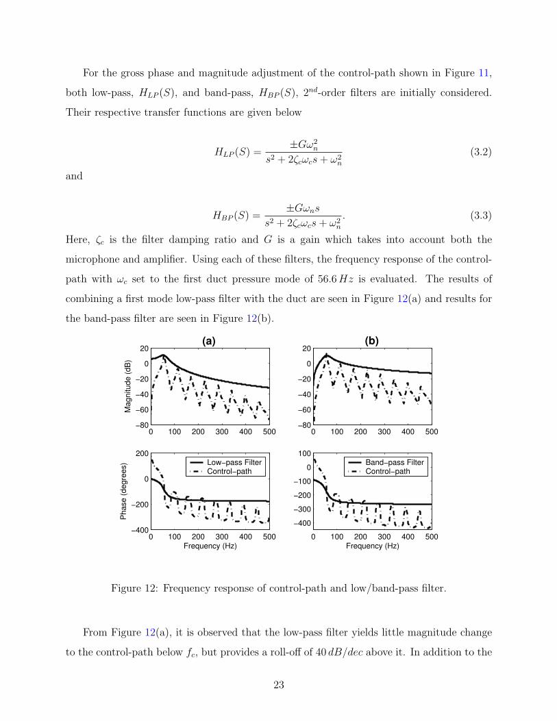
For the gross phase and magnitude adjustment of the control-path shown in Figure 11,

both low-pass, HLP (S), and band-pass, HBP (S), 2nd-order filters are initially considered.

Their respective transfer functions are given below

HLP (S) =±Gω2

n

s2 + 2ζcωcs + ω2n

(3.2)

and

HBP (S) =±Gωns

s2 + 2ζcωcs + ω2n

. (3.3)

Here, ζc is the filter damping ratio and G is a gain which takes into account both the

microphone and amplifier. Using each of these filters, the frequency response of the control-

path with ωc set to the first duct pressure mode of 56.6 Hz is evaluated. The results of

combining a first mode low-pass filter with the duct are seen in Figure 12(a) and results for

the band-pass filter are seen in Figure 12(b).

0 100 200 300 400 500−80

−60

−40

−20

0

20(a)

Mag

nitu

de (d

B)

0 100 200 300 400 500−400

−200

0

200

Frequency (Hz)

Pha

se (d

egre

es)

0 100 200 300 400 500−80

−60

−40

−20

0

20(b)

0 100 200 300 400 500

−400

−300

−200

−100

0

100

Frequency (Hz)

Low−pass FilterControl−path

Band−pass FilterControl−path

Figure 12: Frequency response of control-path and low/band-pass filter.

From Figure 12(a), it is observed that the low-pass filter yields little magnitude change

to the control-path below fc, but provides a roll-off of 40 dB/dec above it. In addition to the

23

magnitude characteristics, the low-pass filter also contributes a phase adjustment of −90o

at the targeted mode: 90o if inverting. In contrast, the band-pass filter seen in Figure 12(b)

provides for attenuation in both the low and high frequency regions to either side of fc. The

high-frequency roll-off of 20 dB/dec, however, is slower than the low-pass filter. It is also

seen that the phase adjustment of the band-pass filter at ωc is 0o: 180o if inverting. These

characteristics, in addition to the phase response of the loudspeaker determine the range of

G before instability occurs at either modes above or below fc.

The damping ratio and gain of the filters can have an impact on both performance and

stability of the controller, primarily through the gain at fc, and also by introducing an

observable mode if ζc << 1.0. To maintain stability, the maximum gain of any in-phase

region (0o) of the control-path must always be less than 1. This ensures the gain margin will

be positive and is consistent with the Nyquist stability criteria.

3.2.1 Phase Compensation

As mentioned previously, the phase shift introduced by the loudspeaker, θs(ωc), can prevent

the control-path phase, θc(ωc), in Equation (3.1) from being a multiple of 180o. The resonant

filters given by Equation (3.2) and (3.3) can only adjust the phase in 90o multiples, and thus

are used to provide a gross phase adjustment. There are, however, several possible methods

for correcting the phase of the speaker. Examples include lead-lag compensation, building

an approximate volume-velocity control loudspeaker [15], or using an all-pass phase-shaping

circuit. Since both the volume velocity approach and lead-lag compensation may adversely

impact the magnitude of the control loop, the all-pass filter is chosen. An all-pass filter has

unity gain and can provide a phase shift ranging from 0−180o if non-inverting, or 180−360o

if inverting. The transfer function of the all-pass filter is written as

HAP (S) =±(s− z)

s + p, (3.4)

where, z is the zero location of the all-pass filter and p is the pole location [23], where the

pole and zero must be equal, (z = p). Considering Figures 12(a) and 12(b), the desired

24

all-pass filter phase is chosen to be the supplemental angle of θc(ωc) as

θa = 180− θc(ωc) = 180− θf (ωc) + [θs(ωc) + θd(ωc)] . (3.5)

If 0 < θa < 180, then a non-inverting all-pass is used and the pole/zero location is calculated

using

p = z =ωc

cot(

πθa

360

) . (3.6)

However, if 180 < θa < 360, then an inverting all-pass is used and the pole/zero location is

calculated using

p = z = − ωc

tan(

πθa

360

) . (3.7)

Once the all-pass pole/zero is calculated, the filter is then added to the control-path

to create a compensator that will produce a perfectly out-of-phase modal control signal.

The following five-step algorithm summarizes the steps required to design the appropriate

controller.

1. Determine the targeted mode of control.2. Obtain the phase response of duct control-path and loudspeaker combination.3. Choose the best filter to provide gross phase and magnitude compensation .4. Obtain the phase response of the duct, controller, and resonant filter.5. If the phase response is not within ±2% of 180o, perform the following:

• Use Equation (3.5) to find the required phase compensation, θa.• Calculate the all-pass filter pole using either Equation (3.6) if 0 < θa < 180, or

Equation (3.7) if 180 < θa < 360.

3.2.2 Resonant Filter Control Simulation

A full controller is now developed and simulated using the techniques described above. First,

consider the case where the loudspeaker is not present (θs = 0o) in the controller. Since

θd = −90o, it is seen from Equation 3.1 that the required phase of the compensator is −90o,

which is realized with a non-inverting low-pass filter. Choosing the first pressure mode as the

target of control, ωc in Equation 3.2 is 356 rad/s (56.6 Hz). A filter gain of G = 10.0 and a

damping ratio of ζc = 0.35 are heuristically chosen for this step, however, a stability analysis

25

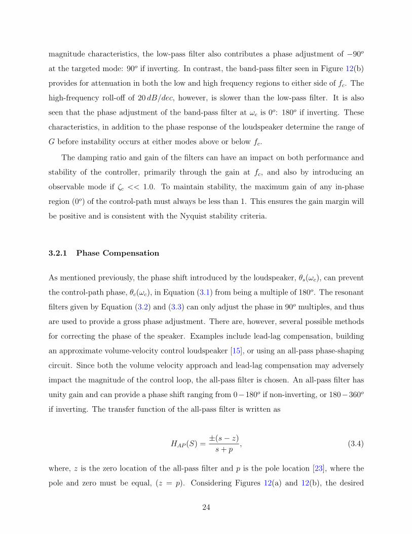
will be performed before the final controller is developed. Figure 13 shows the resulting

disturbance-path/closed-loop response for a transfer function between x1 and p(xe, t) with

xe = x2. Also included is the control-path transfer function.

20 40 60 80 100 120 140−60

−40

−20

0

Mag

nitu

de (d

B)

20 40 60 80 100 120 140−500

−400

−300

−200

−100

0

Frequency (Hz)

Pha

se (d

egre

es)

Duct disturbance−pathClosed−loopControl−path

−180 degrees

Figure 13: Predicted disturbance-path/closed-loop response without speaker dynamics.

Notice that the control-path frequency response, given by the dashed-dotted line, does

indeed have −180o phase at the first pressure mode (f1 = 56.6 Hz). Also, note that about

5 dB of attenuation has been predicted when comparing the disturbance-path (dashed line)

and closed-loop response (solid line), which are taken between the disturbance input, v1(t),

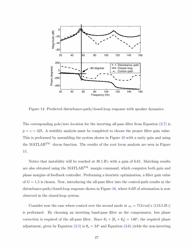
and the error sensor, xe = x2. Now contrast these results with those given in Figure 14, where

the loudspeaker dynamics are included. Note, that for this simulation, the filter gain, G, is

reduced to 1.0 to maintain stability as a result of the added speaker dynamics. It is seen from

the dashed-dotted line representing the control-path that the uncompensated loudspeaker

shifted the resonant phase from −180o to −80o. Rather than attenuating the first mode,

mass is effectively added and the closed-loop resonant frequency shifted downward, while

damping is relatively unaffected.

Next, phase adjustment is accomplished through the addition of an all-pass filter. Since

θf + [θs + θd] = −800, the required phase correction, using Equation (3.5), is θa = 280o.

26

20 40 60 80 100 120 140 160

−60

−40

−20

0

Mag

nitu

de (d

B)

20 40 60 80 100 120 140 160

−400

−200

0

200

Frequency (Hz)

Pha

se (d

egre

es) Disturbance−path

Closed−loopControl−path

−80 degrees

Figure 14: Predicted disturbance-path/closed-loop response with speaker dynamics.

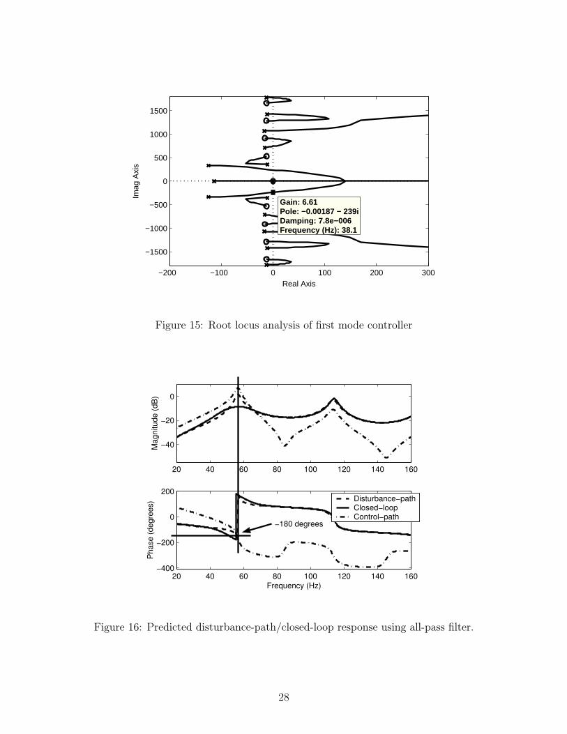
The corresponding pole/zero location for the inverting all-pass filter from Equation (3.7) is

p = z = 425. A stability analysis must be completed to choose the proper filter gain value.

This is performed by assembling the system shown in Figure 10 with a unity gain and using

the MATLABTM rlocus function. The results of the root locus analysis are seen in Figure

15.

Notice that instability will be reached at 38.1 Hz with a gain of 6.61. Matching results

are also obtained using the MATLABTM margin command, which computes both gain and

phase margins of feedback controller. Performing a heuristic optimization, a filter gain value

of G = 1.5 is chosen. Now, introducing the all-pass filter into the control-path results in the

disturbance-path/closed-loop response shown in Figure 16, where 8 dB of attenuation is now

observed in the closed-loop system.

Consider now the case where control over the second mode at ωc = 713 rad/s (113.5 Hz)

is performed. By choosing an inverting band-pass filter as the compensator, less phase

correction is required of the all-pass filter. Since θf + [θs + θd] = 146o, the required phase

adjustment, given by Equation (3.5) is θa = 34o and Equation (3.6) yields the non-inverting

27

Real Axis

Imag

Axi

s

−200 −100 0 100 200 300

−1500

−1000

−500

0

500

1000

1500

Gain: 6.61 Pole: −0.00187 − 239i Damping: 7.8e−006 Frequency (Hz): 38.1

Figure 15: Root locus analysis of first mode controller

20 40 60 80 100 120 140 160

−40

−20

0

Mag

nitu

de (d

B)

20 40 60 80 100 120 140 160−400

−200

0

200

Frequency (Hz)

Pha

se (d

egre

es) Disturbance−path

Closed−loopControl−path

−180 degrees

Figure 16: Predicted disturbance-path/closed-loop response using all-pass filter.

28

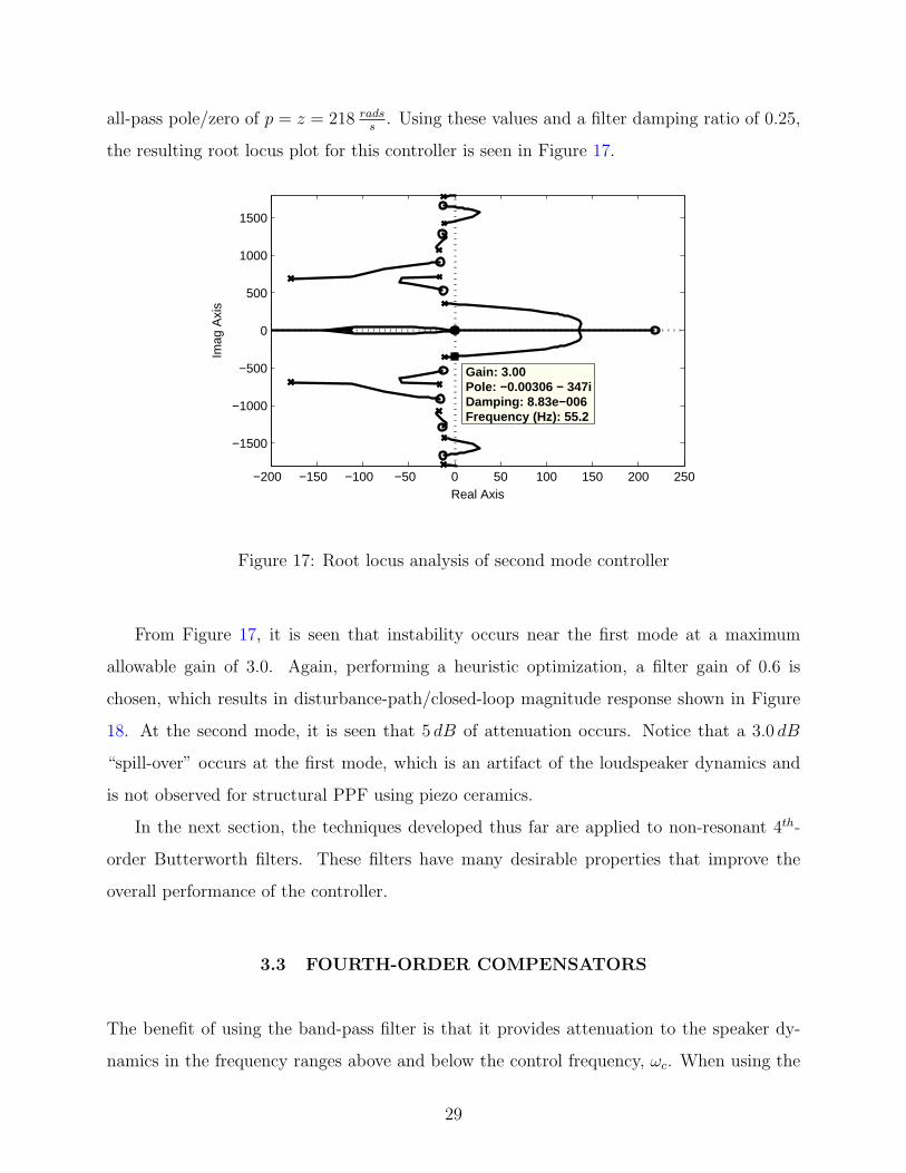
all-pass pole/zero of p = z = 218 radss

. Using these values and a filter damping ratio of 0.25,

the resulting root locus plot for this controller is seen in Figure 17.

Real Axis

Imag

Axi

s

−200 −150 −100 −50 0 50 100 150 200 250

−1500

−1000

−500

0

500

1000

1500

Gain: 3.00 Pole: −0.00306 − 347i Damping: 8.83e−006 Frequency (Hz): 55.2

Figure 17: Root locus analysis of second mode controller

From Figure 17, it is seen that instability occurs near the first mode at a maximum

allowable gain of 3.0. Again, performing a heuristic optimization, a filter gain of 0.6 is

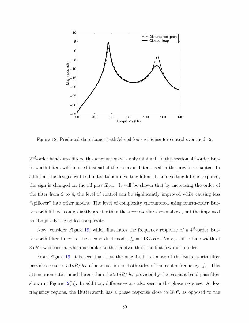
chosen, which results in disturbance-path/closed-loop magnitude response shown in Figure

18. At the second mode, it is seen that 5 dB of attenuation occurs. Notice that a 3.0 dB

“spill-over” occurs at the first mode, which is an artifact of the loudspeaker dynamics and

is not observed for structural PPF using piezo ceramics.

In the next section, the techniques developed thus far are applied to non-resonant 4th-

order Butterworth filters. These filters have many desirable properties that improve the

overall performance of the controller.

3.3 FOURTH-ORDER COMPENSATORS

The benefit of using the band-pass filter is that it provides attenuation to the speaker dy-

namics in the frequency ranges above and below the control frequency, ωc. When using the

29

20 40 60 80 100 120 140−35

−30

−25

−20

−15

−10

−5

0

5

10

Mag

nitu

de (d

B)

Frequency (Hz)

Disturbance−pathClosed−loop

Figure 18: Predicted disturbance-path/closed-loop response for control over mode 2.

2nd-order band-pass filters, this attenuation was only minimal. In this section, 4th-order But-

terworth filters will be used instead of the resonant filters used in the previous chapter. In

addition, the designs will be limited to non-inverting filters. If an inverting filter is required,

the sign is changed on the all-pass filter. It will be shown that by increasing the order of

the filter from 2 to 4, the level of control can be significantly improved while causing less

“spillover” into other modes. The level of complexity encountered using fourth-order But-

terworth filters is only slightly greater than the second-order shown above, but the improved

results justify the added complexity.

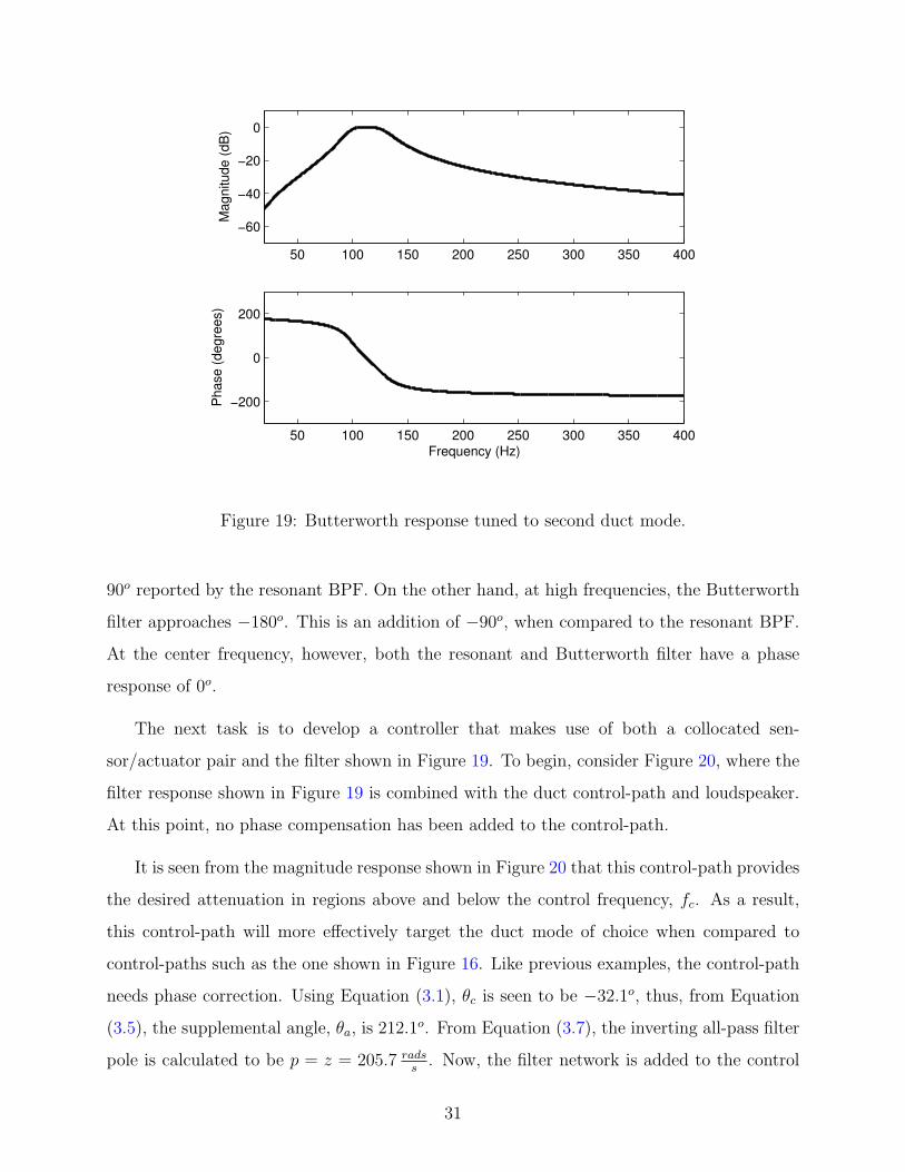
Now, consider Figure 19, which illustrates the frequency response of a 4th-order But-

terworth filter tuned to the second duct mode, fc = 113.5 Hz. Note, a filter bandwidth of

35 Hz was chosen, which is similar to the bandwidth of the first few duct modes.

From Figure 19, it is seen that that the magnitude response of the Butterworth filter

provides close to 50 dB/dec of attenuation on both sides of the center frequency, fc. This

attenuation rate is much larger than the 20 dB/dec provided by the resonant band-pass filter

shown in Figure 12(b). In addition, differences are also seen in the phase response. At low

frequency regions, the Butterworth has a phase response close to 180o, as opposed to the

30

50 100 150 200 250 300 350 400

−60

−40

−20

0

Mag

nitu

de (d

B)

50 100 150 200 250 300 350 400

−200

0

200

Frequency (Hz)

Pha

se (d

egre

es)

Figure 19: Butterworth response tuned to second duct mode.

90o reported by the resonant BPF. On the other hand, at high frequencies, the Butterworth

filter approaches −180o. This is an addition of −90o, when compared to the resonant BPF.

At the center frequency, however, both the resonant and Butterworth filter have a phase

response of 0o.

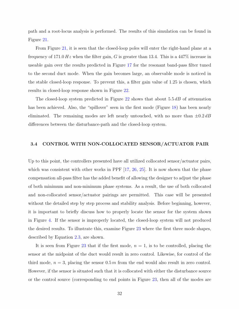
The next task is to develop a controller that makes use of both a collocated sen-

sor/actuator pair and the filter shown in Figure 19. To begin, consider Figure 20, where the

filter response shown in Figure 19 is combined with the duct control-path and loudspeaker.

At this point, no phase compensation has been added to the control-path.

It is seen from the magnitude response shown in Figure 20 that this control-path provides

the desired attenuation in regions above and below the control frequency, fc. As a result,

this control-path will more effectively target the duct mode of choice when compared to

control-paths such as the one shown in Figure 16. Like previous examples, the control-path

needs phase correction. Using Equation (3.1), θc is seen to be −32.1o, thus, from Equation

(3.5), the supplemental angle, θa, is 212.1o. From Equation (3.7), the inverting all-pass filter

pole is calculated to be p = z = 205.7 radss

. Now, the filter network is added to the control

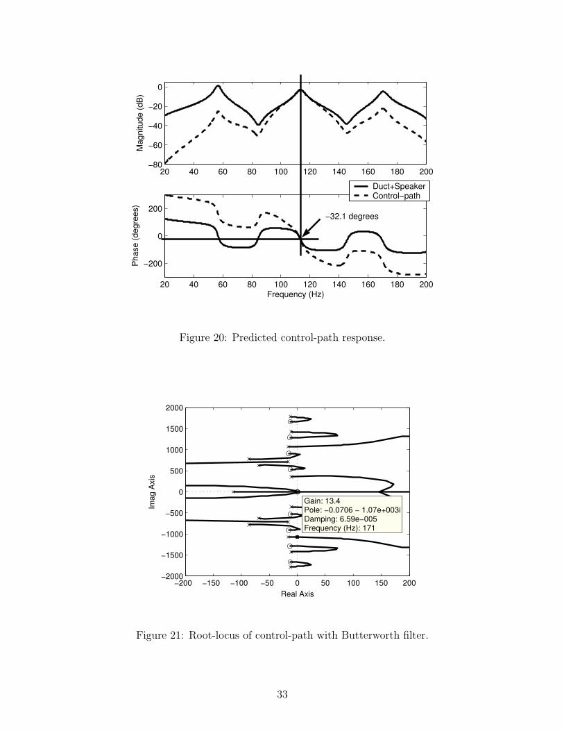
31

path and a root-locus analysis is performed. The results of this simulation can be found in

Figure 21.

From Figure 21, it is seen that the closed-loop poles will enter the right-hand plane at a

frequency of 171.0 Hz when the filter gain, G is greater than 13.4. This is a 447% increase in

useable gain over the results predicted in Figure 17 for the resonant band-pass filter tuned

to the second duct mode. When the gain becomes large, an observable mode is noticed in

the stable closed-loop response. To prevent this, a filter gain value of 1.25 is chosen, which

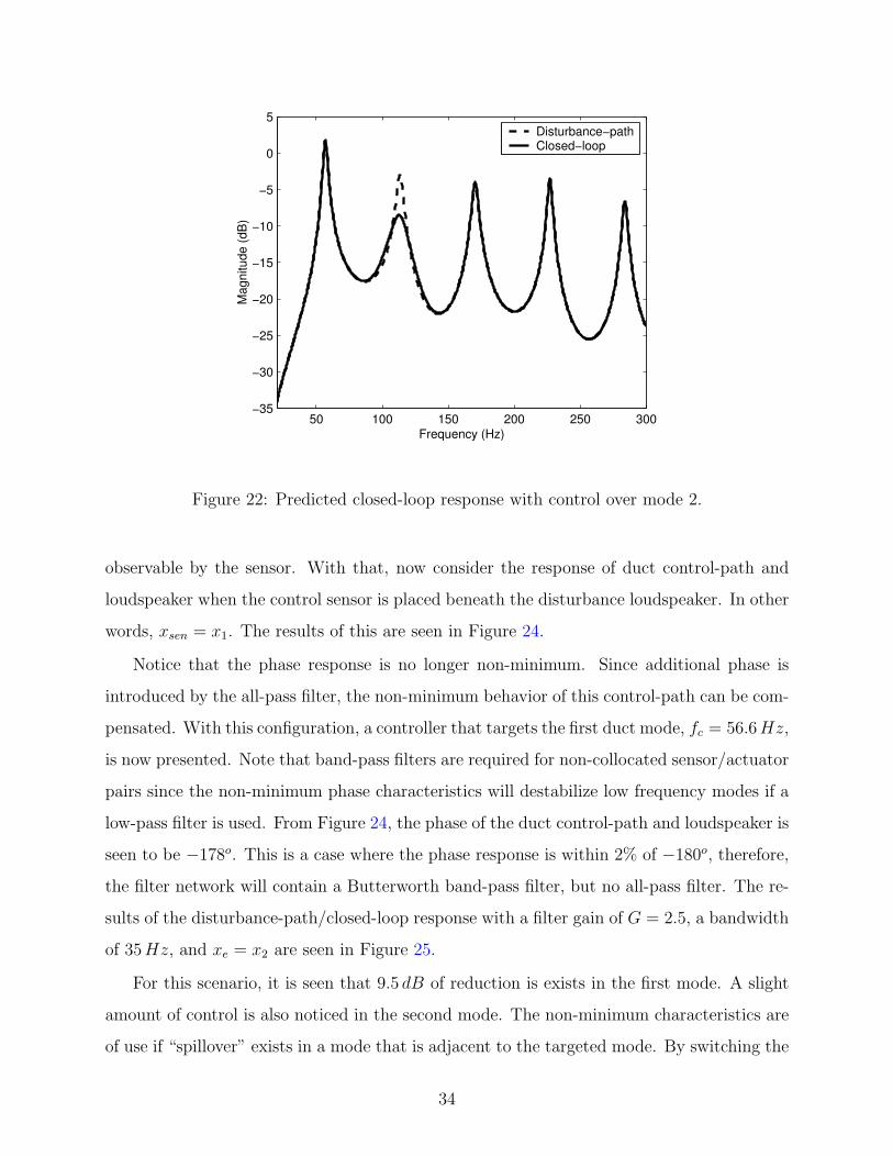
results in closed-loop response shown in Figure 22.

The closed-loop system predicted in Figure 22 shows that about 5.5 dB of attenuation

has been achieved. Also, the “spillover” seen in the first mode (Figure 18) has been nearly

eliminated. The remaining modes are left nearly untouched, with no more than ±0.2 dB

differences between the disturbance-path and the closed-loop system.

3.4 CONTROL WITH NON-COLLOCATED SENSOR/ACTUATOR PAIR

Up to this point, the controllers presented have all utilized collocated sensor/actuator pairs,

which was consistent with other works in PPF [17, 26, 25]. It is now shown that the phase

compensation all-pass filter has the added benefit of allowing the designer to adjust the phase

of both minimum and non-minimum phase systems. As a result, the use of both collocated

and non-collocated sensor/actuator pairings are permitted. This case will be presented

without the detailed step by step process and stability analysis. Before beginning, however,

it is important to briefly discuss how to properly locate the sensor for the system shown

in Figure 4. If the sensor is improperly located, the closed-loop system will not produced

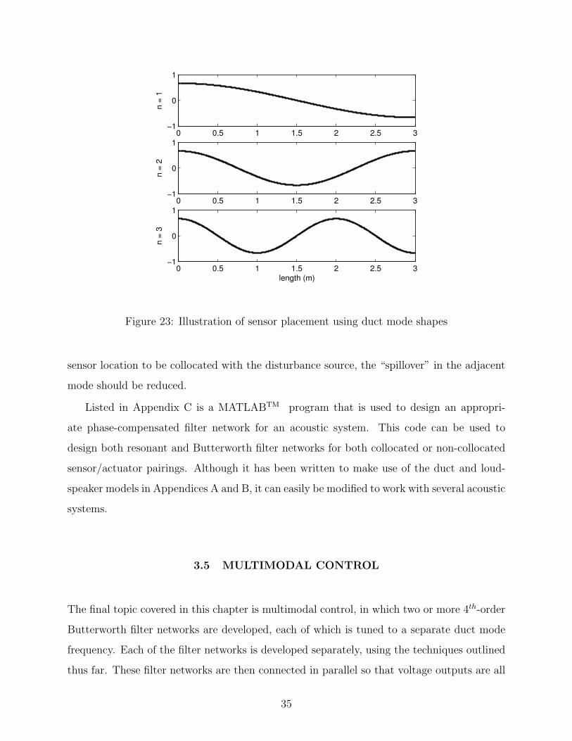
the desired results. To illustrate this, examine Figure 23 where the first three mode shapes,

described by Equation 2.3, are shown.

It is seen from Figure 23 that if the first mode, n = 1, is to be controlled, placing the

sensor at the midpoint of the duct would result in zero control. Likewise, for control of the

third mode, n = 3, placing the sensor 0.5 m from the end would also result in zero control.

However, if the sensor is situated such that it is collocated with either the disturbance source

or the control source (corresponding to end points in Figure 23, then all of the modes are

32

20 40 60 80 100 120 140 160 180 200−80

−60

−40

−20

0

Mag

nitu

de (d

B)

20 40 60 80 100 120 140 160 180 200

−200

0

200

Frequency (Hz)

Pha

se (d

egre

es)

Duct+SpeakerControl−path

−32.1 degrees

Figure 20: Predicted control-path response.

Real Axis

Imag

Axi

s

−200 −150 −100 −50 0 50 100 150 200−2000

−1500

−1000

−500

0

500

1000

1500

2000

Gain: 13.4 Pole: −0.0706 − 1.07e+003i Damping: 6.59e−005 Frequency (Hz): 171

Figure 21: Root-locus of control-path with Butterworth filter.

33

50 100 150 200 250 300−35

−30

−25

−20

−15

−10

−5

0

5

Frequency (Hz)

Mag

nitu

de (d

B)

Disturbance−pathClosed−loop

Figure 22: Predicted closed-loop response with control over mode 2.

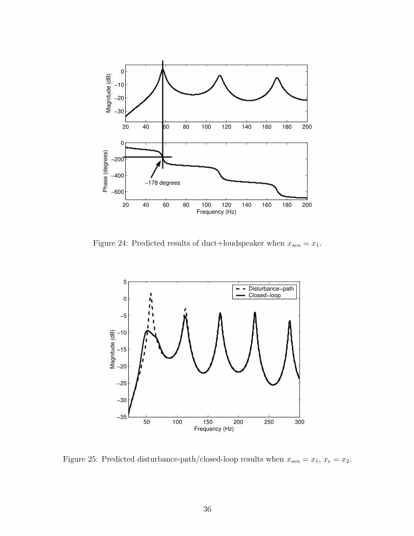
observable by the sensor. With that, now consider the response of duct control-path and

loudspeaker when the control sensor is placed beneath the disturbance loudspeaker. In other

words, xsen = x1. The results of this are seen in Figure 24.

Notice that the phase response is no longer non-minimum. Since additional phase is

introduced by the all-pass filter, the non-minimum behavior of this control-path can be com-

pensated. With this configuration, a controller that targets the first duct mode, fc = 56.6 Hz,

is now presented. Note that band-pass filters are required for non-collocated sensor/actuator

pairs since the non-minimum phase characteristics will destabilize low frequency modes if a

low-pass filter is used. From Figure 24, the phase of the duct control-path and loudspeaker is

seen to be −178o. This is a case where the phase response is within 2% of −180o, therefore,

the filter network will contain a Butterworth band-pass filter, but no all-pass filter. The re-

sults of the disturbance-path/closed-loop response with a filter gain of G = 2.5, a bandwidth

of 35 Hz, and xe = x2 are seen in Figure 25.

For this scenario, it is seen that 9.5 dB of reduction is exists in the first mode. A slight

amount of control is also noticed in the second mode. The non-minimum characteristics are

of use if “spillover” exists in a mode that is adjacent to the targeted mode. By switching the

34

0 0.5 1 1.5 2 2.5 3−1

0

1

n =

1

0 0.5 1 1.5 2 2.5 3−1

0

1

n =

2

0 0.5 1 1.5 2 2.5 3−1

0

1

n =

3

length (m)

Figure 23: Illustration of sensor placement using duct mode shapes

sensor location to be collocated with the disturbance source, the “spillover” in the adjacent

mode should be reduced.

Listed in Appendix C is a MATLABTM program that is used to design an appropri-

ate phase-compensated filter network for an acoustic system. This code can be used to

design both resonant and Butterworth filter networks for both collocated or non-collocated

sensor/actuator pairings. Although it has been written to make use of the duct and loud-

speaker models in Appendices A and B, it can easily be modified to work with several acoustic

systems.

3.5 MULTIMODAL CONTROL

The final topic covered in this chapter is multimodal control, in which two or more 4th-order

Butterworth filter networks are developed, each of which is tuned to a separate duct mode

frequency. Each of the filter networks is developed separately, using the techniques outlined

thus far. These filter networks are then connected in parallel so that voltage outputs are all

35

20 40 60 80 100 120 140 160 180 200

−30

−20

−10

0

Mag

nitu

de (d

B)

20 40 60 80 100 120 140 160 180 200

−600

−400

−200

0

Frequency (Hz)

Pha

se (d

egre

es)

−178 degrees

Figure 24: Predicted results of duct+loudspeaker when xsen = x1.

50 100 150 200 250 300−35

−30

−25

−20

−15

−10

−5

0

5

Frequency (Hz)

Mag

nitu

de (d

B)

Disturbance−pathClosed−loop

Figure 25: Predicted disturbance-path/closed-loop results when xsen = x1, xe = x2.

36

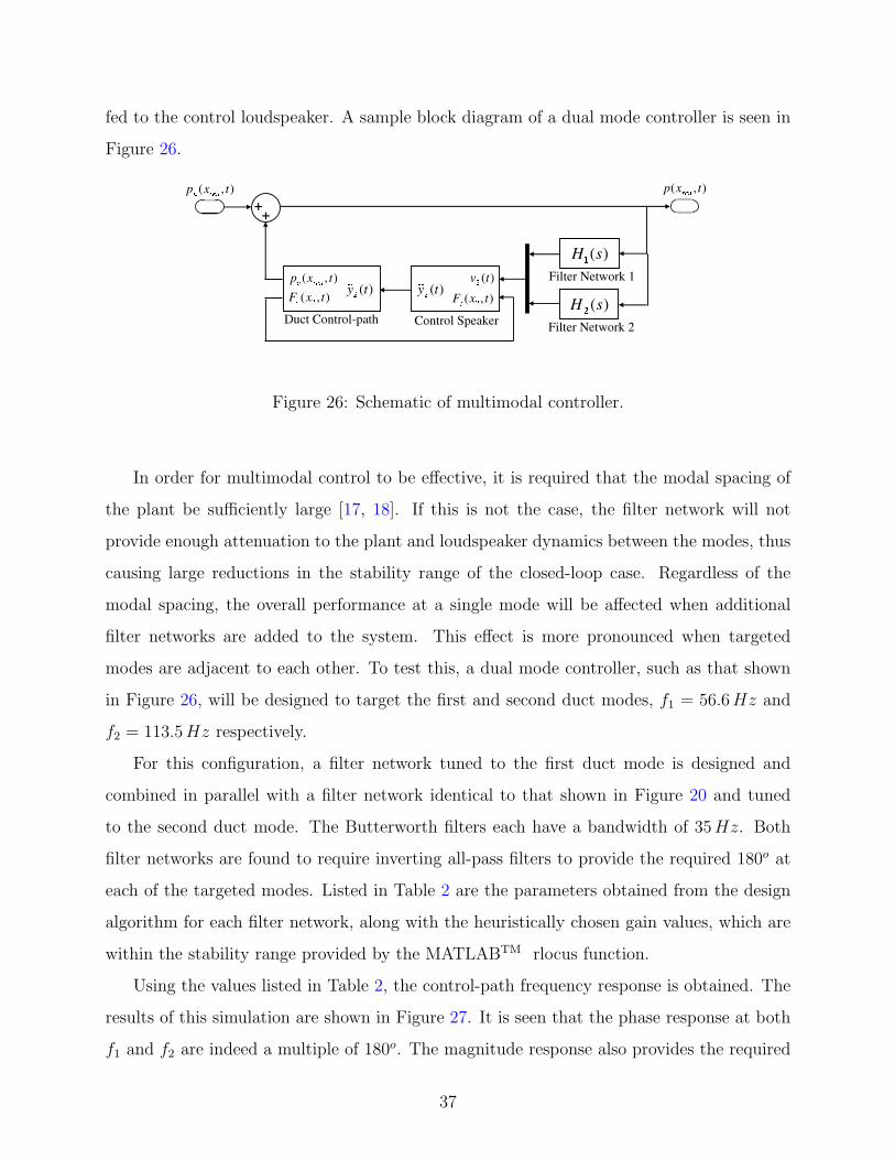
fed to the control loudspeaker. A sample block diagram of a dual mode controller is seen in

Figure 26.

Figure 26: Schematic of multimodal controller.

In order for multimodal control to be effective, it is required that the modal spacing of

the plant be sufficiently large [17, 18]. If this is not the case, the filter network will not

provide enough attenuation to the plant and loudspeaker dynamics between the modes, thus

causing large reductions in the stability range of the closed-loop case. Regardless of the

modal spacing, the overall performance at a single mode will be affected when additional

filter networks are added to the system. This effect is more pronounced when targeted

modes are adjacent to each other. To test this, a dual mode controller, such as that shown

in Figure 26, will be designed to target the first and second duct modes, f1 = 56.6 Hz and

f2 = 113.5 Hz respectively.

For this configuration, a filter network tuned to the first duct mode is designed and

combined in parallel with a filter network identical to that shown in Figure 20 and tuned

to the second duct mode. The Butterworth filters each have a bandwidth of 35 Hz. Both

filter networks are found to require inverting all-pass filters to provide the required 180o at

each of the targeted modes. Listed in Table 2 are the parameters obtained from the design

algorithm for each filter network, along with the heuristically chosen gain values, which are

within the stability range provided by the MATLABTM rlocus function.

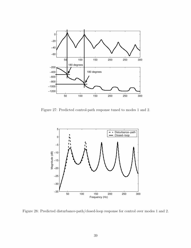
Using the values listed in Table 2, the control-path frequency response is obtained. The

results of this simulation are shown in Figure 27. It is seen that the phase response at both

f1 and f2 are indeed a multiple of 180o. The magnitude response also provides the required

37

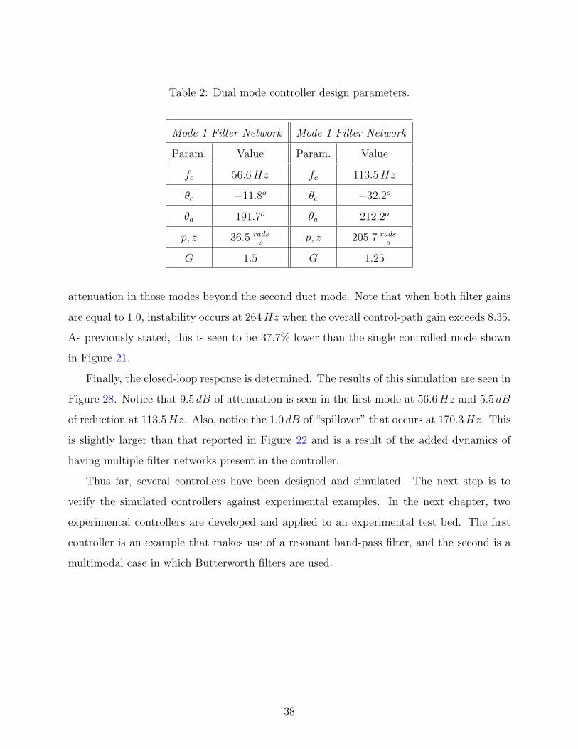
Table 2: Dual mode controller design parameters.

Mode 1 Filter Network Mode 1 Filter Network

Param. Value Param. Value

fc 56.6 Hz fc 113.5 Hz

θc −11.8o θc −32.2o

θa 191.7o θa 212.2o

p, z 36.5 radss

p, z 205.7 radss

G 1.5 G 1.25

attenuation in those modes beyond the second duct mode. Note that when both filter gains

are equal to 1.0, instability occurs at 264 Hz when the overall control-path gain exceeds 8.35.

As previously stated, this is seen to be 37.7% lower than the single controlled mode shown

in Figure 21.

Finally, the closed-loop response is determined. The results of this simulation are seen in

Figure 28. Notice that 9.5 dB of attenuation is seen in the first mode at 56.6 Hz and 5.5 dB

of reduction at 113.5 Hz. Also, notice the 1.0 dB of “spillover” that occurs at 170.3 Hz. This

is slightly larger than that reported in Figure 22 and is a result of the added dynamics of

having multiple filter networks present in the controller.

Thus far, several controllers have been designed and simulated. The next step is to

verify the simulated controllers against experimental examples. In the next chapter, two

experimental controllers are developed and applied to an experimental test bed. The first

controller is an example that makes use of a resonant band-pass filter, and the second is a

multimodal case in which Butterworth filters are used.

38

50 100 150 200 250 300

−60

−40

−20

0

50 100 150 200 250 300

−1200

−1000

−800

−600

−400

−200180 degrees

180 degrees

Figure 27: Predicted control-path response tuned to modes 1 and 2.

50 100 150 200 250 300−35

−30

−25

−20

−15

−10

−5

0

5

Frequency (Hz)

Mag

nitu

de (d

B)

Disturbance−pathClosed−loop

Figure 28: Predicted disturbance-path/closed-loop response for control over modes 1 and 2.

39

4.0 EXPERIMENTAL DEMONSTRATIONS

4.1 DESIGN AND RESPONSE OF SECOND-ORDER CONTROLLER

In order to verify the ANC method discussed in this paper, an ANA compensator was de-

signed to control the first acoustic mode of the experimental test bed shown in Figure 29.

The duct is constructed of 1.9 cm thick hard plywood and is sealed with silicone caulking.

The internal dimensions are consistent with the simulated model and are provided in Table

1. Both the disturbance and control loudspeakers (Peerless 832592) are mounted in iden-

tical sealed boxes having an internal volume of 2, 304 cm3. Ten equidistant, sealable ports

are located along the top edge of the duct for error measurement purposes, and another

port is collocated with the center of the control loudspeaker to provide the input signal to

the controller. Model Mike-28 microphones by All Electrocics Corp were used for pressure

measurements.

The measured frequency response for the uncontrolled plant was presented in Figure

7. The input to the disturbance loudspeaker was a white noise signal with a bandwidth of

1000 Hz, and the output was a pressure measurement at x2. All data for the experiments

were collected using a SigLab MC-2084 signal analyzer.

4.1.1 Compensator Design

For the experiment, an inverting band-pass filter was found to provide the optimum gross

phase adjustment for the first frequency mode, fc = f1. By examining the experimental open-

loop data from Figure 7, f1 was found to be 54.8 Hz, which is 3.28% lower than the predicted

value used in the simulation. In order to realize the 2nd-order band-pass filter, a Burr-Brown

40

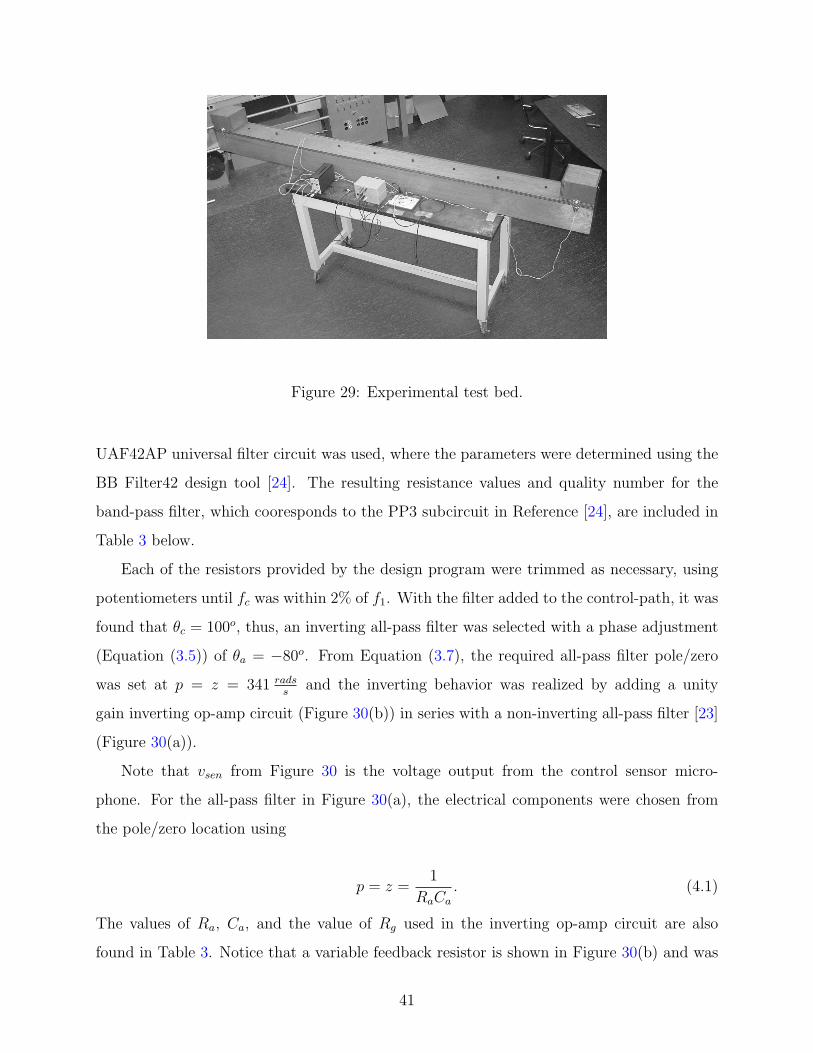
Figure 29: Experimental test bed.

UAF42AP universal filter circuit was used, where the parameters were determined using the

BB Filter42 design tool [24]. The resulting resistance values and quality number for the

band-pass filter, which cooresponds to the PP3 subcircuit in Reference [24], are included in

Table 3 below.

Each of the resistors provided by the design program were trimmed as necessary, using

potentiometers until fc was within 2% of f1. With the filter added to the control-path, it was

found that θc = 100o, thus, an inverting all-pass filter was selected with a phase adjustment

(Equation (3.5)) of θa = −80o. From Equation (3.7), the required all-pass filter pole/zero

was set at p = z = 341 radss

and the inverting behavior was realized by adding a unity

gain inverting op-amp circuit (Figure 30(b)) in series with a non-inverting all-pass filter [23]

(Figure 30(a)).

Note that vsen from Figure 30 is the voltage output from the control sensor micro-

phone. For the all-pass filter in Figure 30(a), the electrical components were chosen from

the pole/zero location using

p = z =1

RaCa

. (4.1)

The values of Ra, Ca, and the value of Rg used in the inverting op-amp circuit are also

found in Table 3. Notice that a variable feedback resistor is shown in Figure 30(b) and was

41

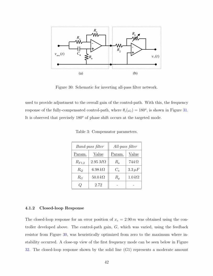
Figure 30: Schematic for inverting all-pass filter network.

used to provide adjustment to the overall gain of the control-path. With this, the frequency

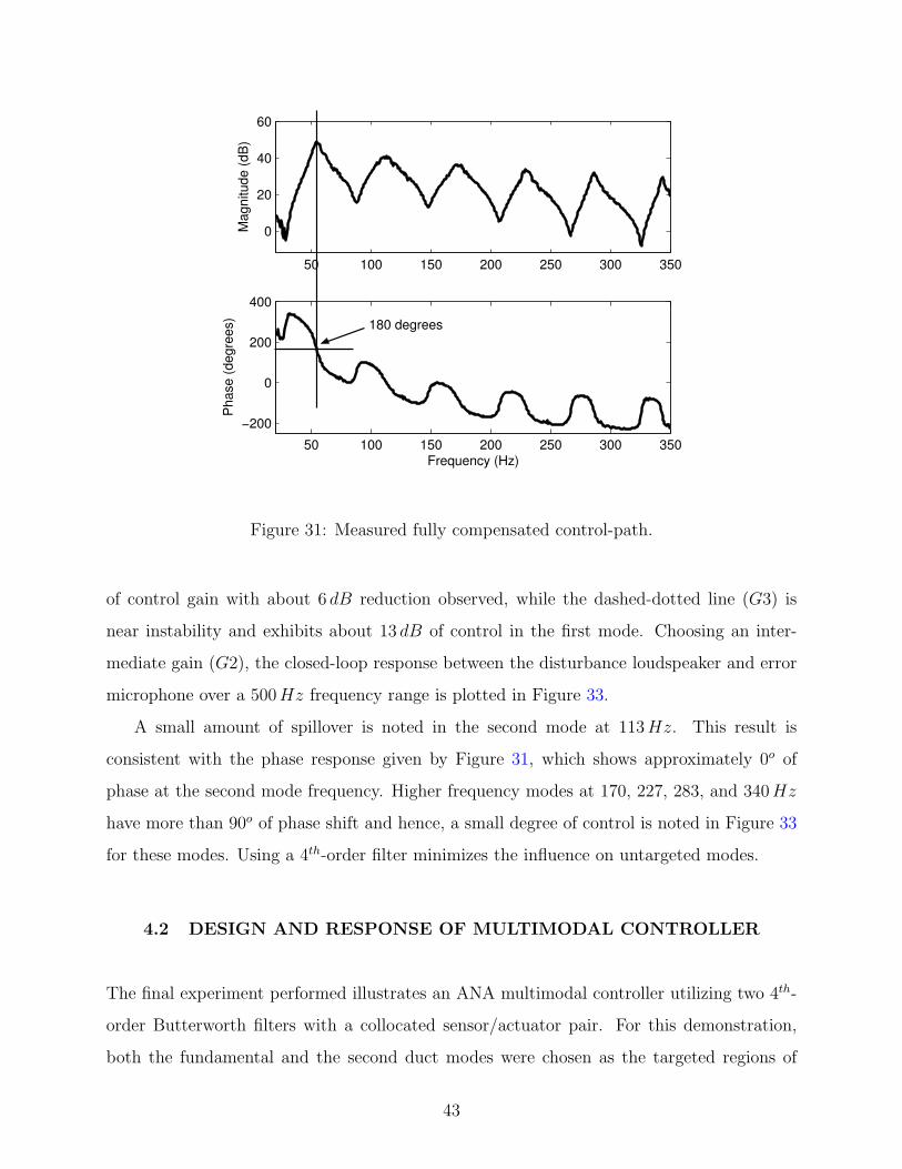
response of the fully-compensated control-path, where θc(ωc) = 180o, is shown in Figure 31.

It is observed that precisely 180o of phase shift occurs at the targeted mode.

Table 3: Compensator parameters.

Band-pass filter All-pass filter

Param. Value Param. Value

RF1,2 2.95 MΩ Ra 744 Ω

RQ 6.98 kΩ Ca 3.3 µF

RG 50.0 kΩ Rg 1.0 kΩ

Q 2.72 - -

4.1.2 Closed-loop Response

The closed-loop response for an error position of xe = 2.90 m was obtained using the con-

troller developed above. The control-path gain, G, which was varied, using the feedback

resistor from Figure 30, was heuristically optimized from zero to the maximum where in-

stability occurred. A close-up view of the first frequency mode can be seen below in Figure

32. The closed-loop response shown by the solid line (G1) represents a moderate amount

42

50 100 150 200 250 300 350

0

20

40

60

Mag

nitu

de (d

B)

50 100 150 200 250 300 350

−200

0

200

400

Frequency (Hz)

Pha

se (d

egre

es) 180 degrees

Figure 31: Measured fully compensated control-path.

of control gain with about 6 dB reduction observed, while the dashed-dotted line (G3) is

near instability and exhibits about 13 dB of control in the first mode. Choosing an inter-

mediate gain (G2), the closed-loop response between the disturbance loudspeaker and error

microphone over a 500 Hz frequency range is plotted in Figure 33.

A small amount of spillover is noted in the second mode at 113 Hz. This result is

consistent with the phase response given by Figure 31, which shows approximately 0o of

phase at the second mode frequency. Higher frequency modes at 170, 227, 283, and 340 Hz

have more than 90o of phase shift and hence, a small degree of control is noted in Figure 33

for these modes. Using a 4th-order filter minimizes the influence on untargeted modes.

4.2 DESIGN AND RESPONSE OF MULTIMODAL CONTROLLER

The final experiment performed illustrates an ANA multimodal controller utilizing two 4th-

order Butterworth filters with a collocated sensor/actuator pair. For this demonstration,

both the fundamental and the second duct modes were chosen as the targeted regions of

43

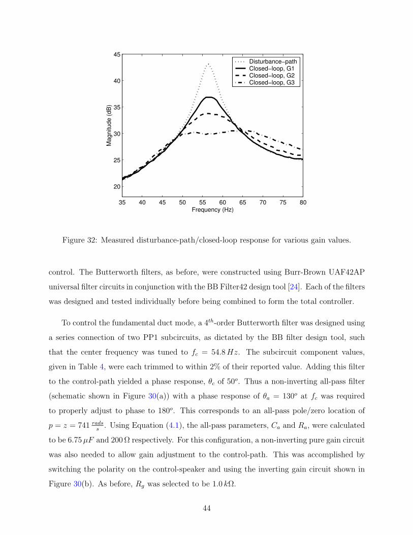
35 40 45 50 55 60 65 70 75 80

20

25

30

35

40

45

Frequency (Hz)

Mag

nitu

de (d

B)

Disturbance−pathClosed−loop, G1Closed−loop, G2Closed−loop, G3

Figure 32: Measured disturbance-path/closed-loop response for various gain values.

control. The Butterworth filters, as before, were constructed using Burr-Brown UAF42AP

universal filter circuits in conjunction with the BB Filter42 design tool [24]. Each of the filters

was designed and tested individually before being combined to form the total controller.

To control the fundamental duct mode, a 4th-order Butterworth filter was designed using

a series connection of two PP1 subcircuits, as dictated by the BB filter design tool, such

that the center frequency was tuned to fc = 54.8 Hz. The subcircuit component values,

given in Table 4, were each trimmed to within 2% of their reported value. Adding this filter

to the control-path yielded a phase response, θc of 50o. Thus a non-inverting all-pass filter

(schematic shown in Figure 30(a)) with a phase response of θa = 130o at fc was required

to properly adjust to phase to 180o. This corresponds to an all-pass pole/zero location of

p = z = 741 radss

. Using Equation (4.1), the all-pass parameters, Ca and Ra, were calculated

to be 6.75 µF and 200 Ω respectively. For this configuration, a non-inverting pure gain circuit

was also needed to allow gain adjustment to the control-path. This was accomplished by

switching the polarity on the control-speaker and using the inverting gain circuit shown in

Figure 30(b). As before, Rg was selected to be 1.0 kΩ.

44

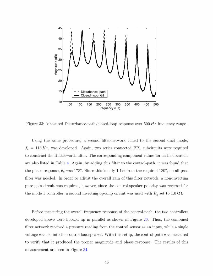
50 100 150 200 250 300 350 400 450 50010

15

20

25

30

35

40

45

Frequency (Hz)

Mag

nitu

de (d

B)

Disturbance−pathClosed−loop, G2

Figure 33: Measured Disturbance-path/closed-loop response over 500 Hz frequency range.

Using the same procedure, a second filter-network tuned to the second duct mode,

fc = 113 Hz, was developed. Again, two series connected PP1 subcircuits were required

to construct the Butterworth filter. The corresponding component values for each subcircuit

are also listed in Table 4. Again, by adding this filter to the control-path, it was found that

the phase response, θa was 178o. Since this is only 1.1% from the required 180o, no all-pass

filter was needed. In order to adjust the overall gain of this filter network, a non-inverting

pure gain circuit was required, however, since the control-speaker polarity was reversed for

the mode 1 controller, a second inverting op-amp circuit was used with Rg set to 1.0 kΩ.

Before measuring the overall frequency response of the control-path, the two controllers

developed above were hooked up in parallel as shown in Figure 26. Thus, the combined

filter network received a pressure reading from the control sensor as an input, while a single

voltage was fed into the control loudspeaker. With this setup, the control-path was measured

to verify that it produced the proper magnitude and phase response. The results of this

measurement are seen in Figure 34.

45

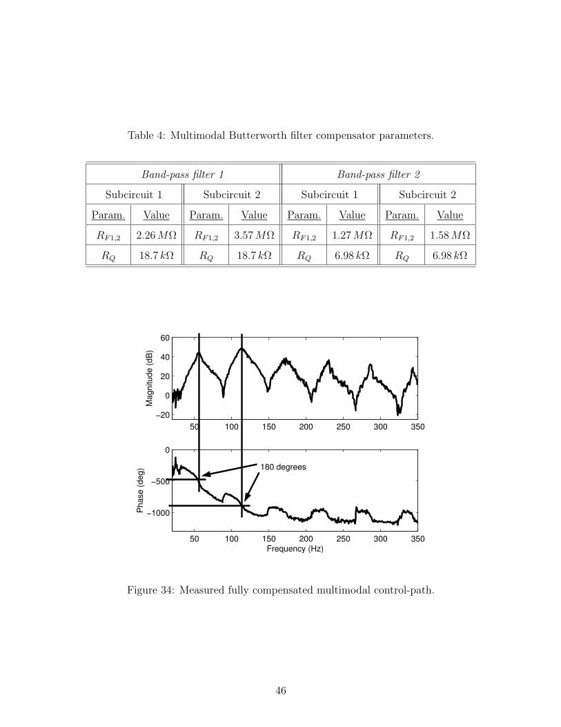
Table 4: Multimodal Butterworth filter compensator parameters.

Band-pass filter 1 Band-pass filter 2

Subcircuit 1 Subcircuit 2 Subcircuit 1 Subcircuit 2

Param. Value Param. Value Param. Value Param. Value

RF1,2 2.26 MΩ RF1,2 3.57 MΩ RF1,2 1.27 MΩ RF1,2 1.58 MΩ

RQ 18.7 kΩ RQ 18.7 kΩ RQ 6.98 kΩ RQ 6.98 kΩ

50 100 150 200 250 300 350−20

0

20

40

60

Mag

nitu

de (d

B)

50 100 150 200 250 300 350

−1000

−500

0

Frequency (Hz)

Pha

se (d

eg) 180 degrees

Figure 34: Measured fully compensated multimodal control-path.

46

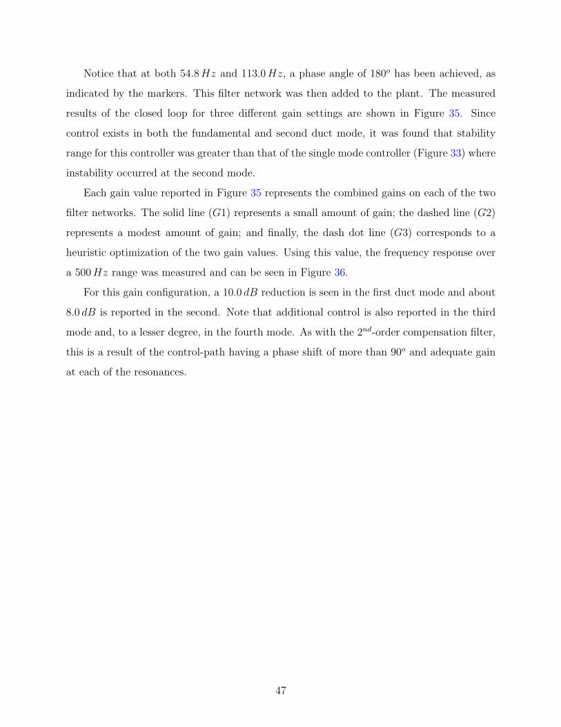
Notice that at both 54.8 Hz and 113.0 Hz, a phase angle of 180o has been achieved, as

indicated by the markers. This filter network was then added to the plant. The measured

results of the closed loop for three different gain settings are shown in Figure 35. Since

control exists in both the fundamental and second duct mode, it was found that stability

range for this controller was greater than that of the single mode controller (Figure 33) where

instability occurred at the second mode.

Each gain value reported in Figure 35 represents the combined gains on each of the two

filter networks. The solid line (G1) represents a small amount of gain; the dashed line (G2)

represents a modest amount of gain; and finally, the dash dot line (G3) corresponds to a

heuristic optimization of the two gain values. Using this value, the frequency response over

a 500 Hz range was measured and can be seen in Figure 36.

For this gain configuration, a 10.0 dB reduction is seen in the first duct mode and about

8.0 dB is reported in the second. Note that additional control is also reported in the third

mode and, to a lesser degree, in the fourth mode. As with the 2nd-order compensation filter,

this is a result of the control-path having a phase shift of more than 90o and adequate gain

at each of the resonances.

47

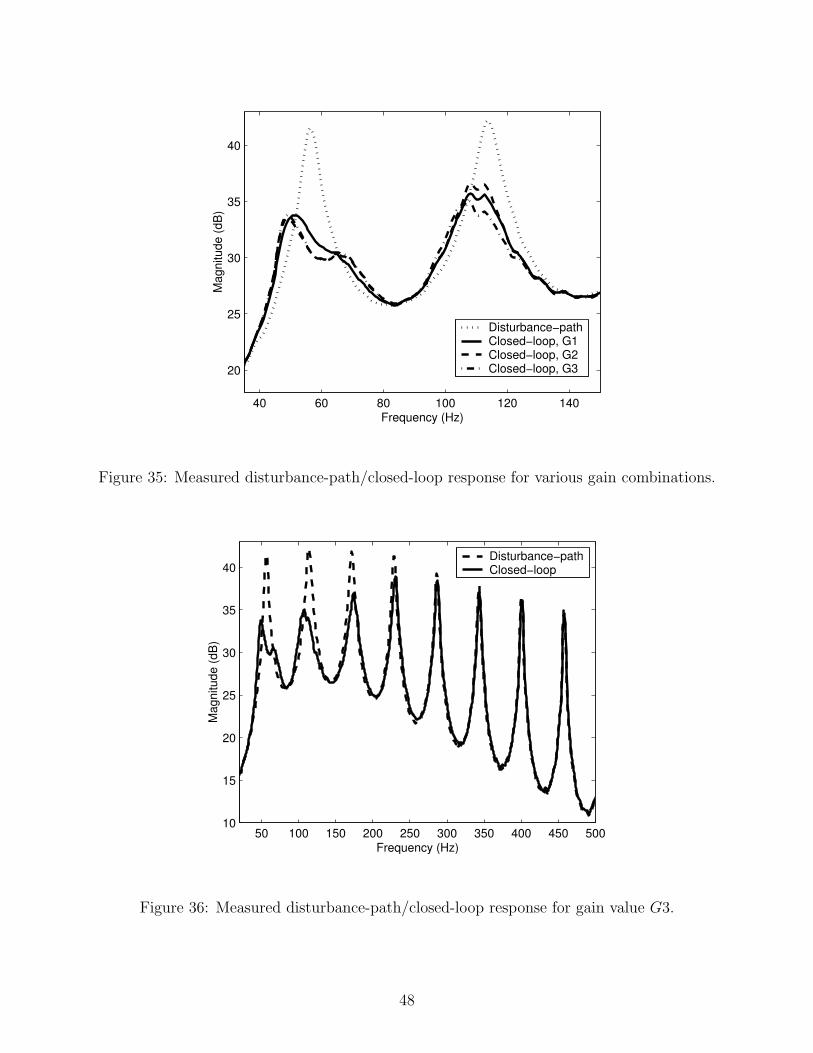
40 60 80 100 120 140

20

25

30

35

40

Frequency (Hz)

Mag

nitu

de (d

B)

Disturbance−pathClosed−loop, G1Closed−loop, G2Closed−loop, G3

Figure 35: Measured disturbance-path/closed-loop response for various gain combinations.

50 100 150 200 250 300 350 400 450 50010

15

20

25

30

35

40

Frequency (Hz)

Mag

nitu

de (d

B)

Disturbance−pathClosed−loop

Figure 36: Measured disturbance-path/closed-loop response for gain value G3.

48

5.0 CONCLUDING REMARKS

A new technique has been developed for controlling single or multiple modes in acoustic

enclosures. This device is referred to as an active noise absorber (ANA). Similar to pos-

itive position feedback (PPF) for structures, an ANA control compensator can make use

of damped, resonant filters as control compensators. However, it is shown that improved

performace is obtained by using 4th-order Butterworth filters. Unlike structural cases in

PPF, where the piezo crystal actuators are virtually dynamicless in the low frequency re-

gion, acoustic actuators (loudspeakers) add dynamics to the closed-loop system. The phase

response of the added dynamics degrade both the performace and stability of the control sys-

tem and must be compensated. Phase compensation for an ANA is achieved by combining

an all-pass filter with the control filter so that the control-path provides ±180o of phase at

the desired control frequency. A method of gross phase compensation (within ±90o of target)

is achieved by choosing either a BPF or LPF filter, which may be combined with an invert-

ing circuit. Low-pass filters are found to work well for the fundamental duct mode, while

band-pass filters are found to work for higher frequency modes where the phase response of

the loudspeaker is more pronounced.

The phase-compensation abilities of the all-pass filter are found to have a second ben-

efit. Unlike previous examples in PPF, an ANA controller does not require collocated sen-

sor/actuator pairs. The phase-shaping characteristics of the all-pass filter allow for the com-

pensation of non-minimum phase response that results when non-collocated sensor/actuator

pairings are used.

To illustrate the design and response of the ANA controller, a duct model that has a

control speaker at one end and a disturbance speaker at the other was created. Simulated

results demonstrate individual control of the first two modes using 2nd-order compensators,

49

while multimodal control of the first and second modes is achieved using a 4th-order But-

terworth network. One experimental demonstrations targeted the first duct mode using a

2nd-order BPF. The gains were heuristically chosen to provide a 10 dB reduction. Some

control in adjacent modes was also observed. Spillover was minimal, presumably due to the

roll-off of the band-pass filter in the control compensator. A second experimental demon-

stration provided simultaneous control of the first two duct modes using a pair of 4th-order

Butterworth band-pass filters. The roll-off provided by the 4th-order filter helped minimize

effects of the controller on non-targeted modes.

50

APPENDIX A

MATLABTM CODE FOR DUCT

function sys=ductFreq(xLoc,X,Ly,xSen)

%%% Duct properties %%%

Lg = 10*12*.0254; % m, duct length

c = 346; % m/s, sound speed

rho = 1.225; % kg/m^3, density

zeta = 0.008; % duct damping ratio

N = 20; % number of pressure modes...

n = 1:N;

Wn = pi*c/Lg*(1:1:N); % vector of duct natural frequencies

bnP = (4*rho*c^2*Ly)/(Lg*pi)*(sin(Wn/c*X.X12)-sin(Wn/c*X.X11))./n;

dnP = (2*Ly)/pi*(sin(Wn/c*X.X12)-sin(Wn/c*X.X11))./n;

bn = (4*rho*c^2*Ly)/(Lg*pi)*(sin(Wn/c*X.X22)-sin(Wn/c*X.X21))./n;

dn = (2*Ly)/pi*(sin(Wn/c*X.X22)-sin(Wn/c*X.X21))./n;

n = 1:N;

numRows = (N*2);

51

% create A matrix and ones along I,J diaganal

AA = zeros(numRows);

for I = 2:2:numRows

AA(I-1,I) = 1;

end

zeta = [linspace(0.03,0.008,4) 0.007*ones(1,size(Wn,2)-4)];

%zeta = linspace(0.005,0.0001,size(Wn,2));

for I = 1:2:numRows-1

% ductDamp = 2*zeta*Wn((I+1)/2);

ductDamp = 2*zeta((I+1)/2)*Wn((I+1)/2);

Wn_sq = Wn((I+1)/2)^2;

AA(I+1,I) = -Wn_sq;

AA(I+1,I+1) = -ductDamp;

end

BB = zeros(numRows,2);

for I = 1:2:numRows-1

BB(I+1,1) = bnP((I+1)/2);

BB(I+1,2) = bn((I+1)/2);

end

DD = zeros(4,2);

bs = (2/Lg)*cos(n*pi*xLoc/Lg);

bsSen = (2/Lg)*cos(n*pi*xSen/Lg);

CC = zeros(3,numRows);

52

for I=1:2:numRows-1

% X.X11, X.X12, Pressure output to the noise Speaker

CC(1,I) = dnP((I+1)/2);

% xLoc, Error signal at a point

CC(2,I) = bs((I+1)/2);

% xSens, Pressure output to the sensor

CC(3,I) = bsSen((I+1)/2);

% X.X21, X.X22, Pressure output to the control Speaker

CC(4,I) = dn((I+1)/2);

end

sys = ss(AA,BB,CC,DD);

53

APPENDIX B

MATLABTM CODE FOR LOUDSPEAKERS

function sys = noiseSpeak

% Box parameters

L = 20/100-6/100;

W = L;

H = 15/100-6/100;

Vb = L*W*H; % box volume

% physical parameters

rho = 1.225; % kg/m^3, density

c = 346; % m/s, sound speed

% speaker parameters

Ms=9.2/1000; % mass of speaker cone (kg)

Bl=6.7; % Bl constant (N/A)

Rs=8; % system resistance (Ohms)

Ls=.9/1000; % total system inductance (Henreys)

Km = (1/0.85)*1000; % speaker spring constant (N/m)

Bm = 1.74; % damping constant (N*s/m)

Sk = pi*(10.4/100)^2/4; % speaker area (m^2)

54

Kb = (pi*Sk^2)^2*(rho*c*c)/Vb;

Ks = Km + Kb;

Vas = 8.7*.001; % volume eq

alpha = Vas/Vb;

Qtc = sqrt(alpha + 1)*.34;

Wn = sqrt(Ks/Ms);

Bb = Ms*Wn/Qtc;

Bs = Bm+Bb;

ASpN = [0 1 0 0;

0 -Rs/Ls 0 -Bl/Ls;

0 0 0 1;

0 Bl/Ms -Ks/Ms -Bs/Ms];

%BSpN = [0 0;1/Ls 0;0 0;0 -Sk/Ms]; % input matrix

BSpN = [0 0;1/Ls 0;0 0;0 -1/Ms]; % input matrix (voltage, pressure)

CSpN = [0 Bl/Ms -Ks/Ms -Bs/Ms]; % output matrix (acceleration observer)

%DSpN = [0 -Sk/Ms]; % feedthrough matrix

DSpN = [0 -1/Ms]; % feedthrough matrix

sys = ss(ASpN,BSpN,CSpN,DSpN);

55

APPENDIX C

MATLABTM CODE UTILIZING DESIGN PROCEDURE

%%%%%%%%%%%%%%%%%%%%%%%%%%%%%%%%%%%%%%%%%%%%%%%%%%%%%%%%%%%%

% M file that generates the appropriate control filter and %

% all-pass filter for duct system %

%%%%%%%%%%%%%%%%%%%%%%%%%%%%%%%%%%%%%%%%%%%%%%%%%%%%%%%%%%%%

close all; clear all;

x1 = 4*.0254; % m, location of speaker 1 (noise)

x2 = 116*.0254; % m, location of speaker 2 (control)

X = struct(’X11’, x1-0.0461, ’X12’, x1+0.0461, ...

’X21’, x2-0.0461, ’X22’, x2+0.0461);

Ly = .0922;

%% get sensor and error locations

senLoc = input(’Enter the location of the sensor as a multiple of x2 (eg x2/3): ’);

errLoc = input(’Enter point of measure as a multiple of x2: ’);

%% get sysetm models

sysD = ductFreq(errLoc,X,Ly,senLoc);

sysC = noiseSpeak;

56

sysN = noiseSpeak;

%% create openloop system.

sysTemp = append(1,sysN,sysD);

Q = [2 1;3 3;4 2];

sysOL = connect(sysTemp,Q,1,4);

%% get control frequency

Wns = unique(sort(abs(pole(sysD))));

index = input(’Enter mode number to control: ’);

ctrFreq = Wns(index);

disp([’ Control Frequency: ’ num2str(ctrFreq/2/pi) ’ Hz’]);

disp(’ ’);

%% get phase of plant and control speaker

Q = [2 5;4 4];

sysCD = connect(append(sysD,sysC),Q,3,3);

[Mcd,PHcd] = bode(sysCD,ctrFreq);

%% create filter

order = input(’Enter an even butterworth filter order: ’);

BWhz = input(’Enter filter bandwidth in Hz: ’);

BWrad = BWhz*2*pi;

[B,A] = butter(order/2,[(ctrFreq-BWrad/2) (ctrFreq+BWrad/2)], ’s’);

sysF = tf(B,A);

%% get filter phase

[Mf,PHf] = bode(sysF,ctrFreq);

thetaC = PHcd + PHf;

57

%% Find required phase correction

thetaA = 180 - thetaC;

%% make sure angle is 0 < thetaA < 360

if thetaA > 360 | thetaA < -360

thetaA = thetaA - floor(thetaA/360)*360;

end

%% convert angle to radians for all-pass filter pole calculation

taRad = thetaA*pi/180;

if thetaA > 0 & thetaA < 180

filtPole = ctrFreq/cot(taRad/2);

G = 1;

num = [1 -filtPole];

den = [1 filtPole];

sysF2 = tf(num,den);

elseif thetaA > 180 & thetaA < 360

taRad = taRad - 2*pi;

filtPole = -ctrFreq/tan(taRad/2);

G = 1;

num = [1 -filtPole];

den = [1 filtPole];

sysF2 = tf(-num,den);

elseif thetaA == 180

disp(’No all pass required’);

filtPole = 0;

G = 1;

sysF2 = 1;

else

58

disp(’No all pass required, inverting gain value needed’);

filtPole = 0;

G = -1;

sysF2 = 1;

end

Q1 = [2 1;3 6;5 2];

sysCLb = connect(append(series(series(sysF,sysF2),G),sysC,sysD),Q1,1,5);

sysCLc = connect(append(1,sysC,sysD),Q1,1,5);

figure(1)

pzmap(sysCLc);

title(’Pole Zero Map of Open-loop System’);

figure(2);

rlocus(-sysCLb);

title(’Root Locus of Control Path’);

axis([-400 200 -2500 2500]);

%% get filter gain

absG = input(’Enter absolute filter from Root Locus plot: ’);

filtG = G*absG;

%% Display filter transfer functions.

disp(’ ’);

disp(’Control Filter TF function: ’)

sysF

if filtPole

disp(’All-pass filter TF function: ’);

59

sysF2

end

%% Generate OL/CL frequency response plots.

sysTemp = append(sysD,sysN,sysC,series(series(sysF,sysF2),filtG),1);

Q = [1 5;2 6;4 1;5 7;6 4;7 8;8 3];

sys = connect(sysTemp,Q,3,2);

if ~isempty(find(real(pole(sys))>0))

disp(’System unstable: choose a lower gain value’);

else

disp(’System Stable’);

freqT = linspace(10,2*pi*300,1000);

f = freqT/2/pi;

[MTmp,PHTmp] = bode(sysOL,freqT);

Mol = 20*log10(abs(squeeze(mp2h(MTmp,PHTmp))));

PHol = angle(squeeze(mp2h(MTmp,PHTmp)))*180/pi;

[MTmp,PHTmp] = bode(sys,freqT);

M = 20*log10(abs(squeeze(mp2h(MTmp,PHTmp))));

PH = angle(squeeze(mp2h(MTmp,PHTmp)))*180/pi;

figure(3);

plot(f,Mol,f,M);

xlabel(’Frequency (Hz)’),ylabel(’Magnitude (dB)’);

axis([20 300 -45 10]);

title(’Bode diagram’);

legend(’forward-path’,’closed-loop’);

60

T = 0:6.1e-05:.5;

U = cos(Wns(1)*T);

figure(4);

lsim(sys,sysOL,U,T);

legend(’cl’,’ol’,’input’);

end

61

BIBLIOGRAPHY

[1] David A. Bies and Colin Hansen. Engineering Noise Control: Theory and Practice.Taylor and Francis Group, New York, NY, 2003.

[2] Lord J.W.S. Rayleigh. The Theory of Sound. Dover Publicaions, Inc., New York, NY,1945.

[3] U. Ingard. On the theory and design of acoustic resonators. JASA, 25(6):1037–1061,1953.

[4] Theodore-M Kostek. Combining adaptive-passive and fully active noise control in ducts.In ASME IMECE 1997, volume 24, pages 293–8, Fairfield, NJ, 1997.

[5] K. Nagaya, Y. Hano, and A. Suda. Silencer consisting of two-stage helmholtz resonatorwith auto-tuning control. JASA, 110(1):289–95, 2001.

[6] Jonathan D. Kemp and Robert L. Clark. Noise reduction in a launch vehicle fairingusing actively tuned loudspeakers. JASA, 113(4):1986–94, 2003.

[7] L. E. Kinsler,A. R. Frey,A. B. Coppens, and J. V. Sanders, Fundamentals of Acoustics.John Wiley and Sons, Inc.,New York, NY, 1982.

[8] P. A. Nelson and S. J. Elliott. Active Control of Sound. Academic Press, New York,NY, 1992.

[9] H. Boonen and P. Sas. Stability Improvement for Feedback Noise Control in DuctsUsing A Time Delay Compensator. International Conference On Noise and VibrationEngineering, volume 25, pages 9–14, Katholieke Universiteit Leuven, Belgium, 2000.

[10] S. C. Douglas. Adaptive Filters Employing Partial Updates. IEEE Transactions onAnalog and Digital Signal Processing, 44(3): 209–216, 1997.

[11] O. Kipersztok and R. Hammond. The Use Of Fuzzy Logic In Active Noise Control.In 3rd International Symposium on Uncertainty Modelling and Analysis, College Park,MD, March 17-20 1995.

[12] H. F. Olson and E. G. May. Electronic sound absorber. JASA, 25(1):1130–6, 1953.

62

[13] Jeffrey S. Vipperman, Deyu Li, Ilya Avdeev, and Steven Lane. Investigation of thesound transmission into an advanced grid-stiffened structure. JVA, 125(3):257–266,2003.

[14] Deyu Li and Jeffrey S. Vipperman. Noise transmission control studies on a chambercore composite cylinder. In ASME IMECE 2002, number IMECE-33069, New Orleans,LA, November 17-22 2002.

[15] Steven A. Lane and Robert L. Clark. Dissipative feedback control of a reverberantenclosure using a constant volume velocity source. JVA, 120(3):987–993, 1998.

[16] C. B. Birdsong and C. J. Radcliffe. A compensated acoustic actuator for systems withstrong dynamics pressure coupling. JVA, 121(1):89–94, 1999.

[17] J. L. Fanson and T. K. Caughey. Positive position feedback control for large spacestructures. AIAA Journal, 28(4):717–724, April 1990.

[18] James L. Fanson. An Experimental Investigation of Vibration Suppression in LargeSpace Structures Using Positive Position Feedback. PhD thesis, California Institute ofTechnology, Pasadena, CA, 1986.

[19] Steven Griffin and Collin Hansen and Ben Cazzolato. Feedback Control of StructurallyRadiated Sound Into Enclosed Spaces Using Structural Sensing. JASA, 106(5):2621–2628, 1999.

[20] Steven Griffin and Keith K. Denoyer and Alok Das. Passive Vibroacoustic Isolation forPayload Containers. JIMSS, 10(5):83–87, 1999.

[21] Jesse B. Bisnette, Jeffrey S. Vipperman, and Daniel D. Budny. Active noise controlusing damped resonant filters. Abstract only. JASA, 113(4):2228, 2003.

[22] F. Fahy. Sound and Structural Vibration. Academic Press, Inc., New York, 1985.

[23] M. E. Van Valkenburg. Analog Filter Design. Oxford University Press, New York, 1982.

[24] Texas Instruments, Inc. Application Bulletin: Filter Design Program for the UAF42Universal Active Filter, 2000.

[25] Mark A. McEver. Optimal Vibration Suppression Using On-line Pole/Zero Identifica-tion. MS thesis, Virginia Polytechnic Institute and State University, Blacksburg, VA,1999.

[26] Kevin. Farinholt. Modal and Impedance Modeling of a Conical Bore for Control Appli-cation. MS thesis, Virginia Polytechnic Institute and State University, Blacksburg, VA,2001.

63

[27] Jesse B. Bisnette, Jeffrey S. Vipperman, and Daniel D. Budny. Active Noise ControlUsing Phase-compensated, Damped Resonant Filters. In ASME IMECE 2002, numberIMECE2003-41831, Washington, D.C., November 15-21 2003.

64