Jeroen K. Vermunt* - Statistical Innovations · The model is also similar to the multilevel item response theory ... is the probability of observing response s k on item k given that

7MULTILEVEL LATENT CLASSMODELS

Jeroen K. Vermunt*

The latent class (LC) models that have been developed so far

assume that observations are independent. Parametric and non-

parametric random-coefficient LC models are proposed here,

which will make it possible to modify this assumption. For

example, the models can be used for the analysis of data col-

lected with complex sampling designs, data with a multilevel

structure, and multiple-group data for more than a few groups.

An adapted EM algorithm is presented that makes maximum-

likelihood estimation feasible. The new model is illustrated with

examples from organizational, educational, and cross-national

comparative research.

1. INTRODUCTION

In the past decade, latent class (LC) analysis (Lazarsfeld 1950;

Goodman, 1974) has become a more widely used technique in social

science research. One of its applications is clustering or constructing

typologies with observed categorical variables. Another related applica-

tion is dealing with measurement error in nominal and ordinal indicators.

An important limitation of the LC models developed so far is, however,

that they assume that observations are independent, an assumption that is

often violated. This paper presents a random-coefficients or multilevel

LC model that makes it possible to modify this assumption.

*Tilburg University

213

Random-coefficients models can be used to deal with various

types of dependent observations (Agresti et al. 2000). An example is

dependent observations in data sets collected by two-stage cluster

sampling or longitudinal designs. A more theory-based use of random-

coefficients models that is popular in fields such as educational and

organizational research is often referred to as multilevel or hierarchical

modeling, a method that is intended to disentangle group-level from

individual-level effects (Bryk and Raudenbush 1992; Goldstein 1995;

Snijders and Bosker 1999). Another interesting application of these

methods is in the context of multiple-group analysis, such as in cross-

national comparative research based on data from a large number of

countries (for example, see Wong and Mason 1985).

In a standard LC model, it is assumed that the model param-

eters are the same for all persons (level-1 units). The basic idea of a

multilevel LC model is that some of the model parameters are allowed

to differ across groups, clusters, or level-2 units. For example, the

probability of belonging to a certain latent class may differ across

organizations or countries. Such differences can be modeled by

including group dummies in the model, as is done in multiple-group

LC analysis (Clogg and Goodman 1984), which amounts to using

what is called a fixed-effects approach. Alternatively, in a random-

effects approach, the group-specific coefficients are assumed to come

from a particular distribution, whose parameters should be estimated.

Depending on whether the form of the mixing distribution is specified

or not, either a parametric or a nonparametric random-effects

approach is obtained.

The proposed multilevel LC model is similar to a random-

coefficients logistic regression model (Wong and Mason 1985;

Hedeker and Gibbons 1996; Hedeker, 1999; Agresti et al. 2000).

A difference between the two models is that the dependent variable

is not directly observed but rather is a latent variable with several

observed indicators. The model can therefore be seen as an extension

of a random-coefficients logistic regression model in which there is

measurement error in the dependent variable. It is well-known that

LC models can be used to combine the information contained in

multiple outcome variables (Bandeen-Roche et al. 1997).

The model is also similar to the multilevel item response theory

(IRT) model that was recently proposed by Fox and Glas (2001). A

conceptual difference is, however, that in IRT models the underlying

214 JEROEN K. VERMUNT

latent variables are assumed to be continuous instead of discrete.

Because of the similarity between LC and IRT models (for example,

see Heinen 1996), it is not surprising that restricted multilevel LC

models can be used to approximate multilevel IRT models.

The idea of introducing random effects in LC analysis is not

new, as has been shown, for example, in Qu, Tan, and Kutner (1996)

and Lenk and DeSarbo (2000). The models proposed by these authors

are, however, not multilevel models, and therefore conceptually and

mathematically very different from the models described in this

paper. Although there is no option for combining LC structures

with random effects in the current version of the GLLAMM program

of Rabe-Hesketh, Pickles, and Skrondal (2001), the model proposed

here fits very naturally into the general multilevel modeling frame-

work developed by these authors.

The multilevel LC model can be represented as a graphical or

path model containing one latent variable per random coefficient and

one latent variable per level-1 unit within a level-2 unit. The fact that

the model contains so many latent variables makes the use of a

standard EM algorithm for maximum-likelihood (ML) estimation

impractical. The ML estimation problem can, however, be solved by

making use of the conditional independence assumptions implied by

the graphical model. More precisely, I adapted the E step of the EM

algorithm to the structure of the multilevel LC model.

The next section describes the multilevel LC model. Section 3

will then focus on estimation issues that are specific for this new

model. Section 4 presents applications from organizational, educa-

tional, and cross-national comparative research. The paper ends with

a short discussion.

2. THE MULTILEVEL LC MODEL

Let Yijk denote the response of individual or level-1 unit i within

group or level-2 unit j on indicator or item k. The number of level-2

units is denoted by J, the number of level-1 units within level-2 unit j

by nj, and the number of items by K. A particular level of item k is

denoted by sk and its number of categories by Sk. The latent class

variable is denoted by Xij, a particular latent class by t, and the

number of latent classes by T. Notation Yij is used to refer to the

MULTILEVEL LATENT CLASS MODELS 215

full vector of responses of case i in group j, and s to refer to a possible

answer pattern.

The probability structure defining a simple LC model can be

expressed as follows:

P(Yij ¼ s) ¼XTt¼1

P(Xij ¼ t)P(Yij ¼ sjXij ¼ t)

¼XTt¼1

P(Xij ¼ t)YKk¼1

P(Yijk ¼ skjXij ¼ t):

(1)

The probability of observing a particular response pattern, P(Yij¼ s),

is a weighted average of class-specific probabilities P(Yij¼ s|Xij¼ t).

The weight P(Xij¼ t) is the probability that person i in group j belongs

to latent class t. As can be seen from the second line, the indicators

Yijk are assumed to be independent of each other given class member-

ship, which is often referred to as the local independence assumption.

The term P(Yijk¼ sk|Xij¼ t) is the probability of observing response skon item k given that the person concerned belongs to latent class t.

These conditional response probabilities are used to name the latent

classes.

The general definition in equation (1) applies to both the

standard and the multilevel LC model. In order to be able to

distinguish the two, the model probabilities have to be written in the

form of logit equations. In the standard LC model,

P(Xij ¼ t) ¼ exp (�t)

�Tr¼1 exp (�r)

(2)

P(Yijk ¼ skjXij ¼ t) ¼exp (�k

skt)

�Sk

r¼1 exp (�krt)

: (3)

As always, identifying constraints have to be imposed on the logit

parameters—for example, �1 ¼ �k1t ¼ 0.

The fact that the � and � parameters appearing in equations (2)

and (3) do not have an index j indicates that their values are assumed

to be independent of the group to which one belongs. Taking into

account the multilevel structure involves modifying this assumption.

The most general multilevel LC model is obtained by assuming that

all model parameters are group specific; that is,


P(Xij ¼ t) ¼ exp (�tj)

�Tr¼1 exp (�rj)

(4)

P(Yijk ¼ skjXij ¼ t) ¼exp (�k

sktj)

�Sk

r¼1 exp (�krtj)

: (5)

Without further restrictions, this model is equivalent to an unrest-

ricted multiple-group LC model (Clogg and Goodman 1984). A more

restricted multiple-group LC model is obtained by assuming that the

item conditional probabilities do not depend on the level-2 unit—that

is, by combining specifications (4) and (3). In practice, such a partially

heterogeneous model assuming invariant measurement error is the

most useful specification, although it is not a problem to modify

this assumption for some of the indicators.

It will, however, be clear that such a multiple-group or fixed-

effects approach may be problematic if there are more than a few

groups because group-specific estimates have to be obtained for cer-

tain model parameters. It is not only the number of parameters to be

estimated that increases rapidly with the number of level-2 units; the

estimates may also be very unstable with group sizes that are typical

in multilevel research. Another disadvantage of the fixed-effects

approach is that all group differences are ‘‘explained’’ by the group

dummies, making it impossible to determine the effects of level-2

covariates on the probability of belonging to a certain latent class.

The next section shows how to include such covariates in the model.

2.1. A Parametric Approach

The problems associated with the multiple-group approach can be

tackled by adopting a random-effects approach: Rather than estimating

a separate set of parameters for each group, the group-specific effects

are assumed to come from a certain distribution. Let us look at

the simplest case: a two-class model with group-specific class-

membership probabilities as defined by equation (4), and with �1j¼ 0

for identification. Typically, random coefficients are assumed to come

from a normal distribution, yielding a LC model in which

�2j ¼ �2 þ �2 � uj; (6)


with uj�N(0,1). Note that this amounts to assuming that the

between-group variation in the log-odds of belonging to the second

instead of the first latent class follows a normal distribution with a

mean equal to �2 and a standard deviation equal to �2.With more than two latent classes, one has to specify the

distribution of the T� 1 random-intercept terms �tj. One possibility

is to work with a (T� 1) dimensional normal distribution. Another

option is to use more a restricted structure of the form

�tj ¼ �t þ �t � uj; (7)

with uj�N(0,1) and with one identifying constraint on the �tand another on the � t: for example, �1¼ �1¼ 0. This specification

was also used by Hedeker (1999) in the context of random-effects

multinomial logistic regression analysis. The implicit assumption

that is made is that the random components in the various �tj areperfectly correlated. More specifically, the same random effect uj is

scaled in a different manner for each t by the unknown � t. This

formulation, which is equivalent to Bock’s nominal response model

(Bock 1972), is based on the assumption that each nominal category is

related to an underlying latent response tendency. Whether such a

restricted structure suffices or a more general formulation is needed is

an empirical issue. Note that (7) reduces to (6) if T¼ 2.

A measure that is often of interest in random-effects models

is the intraclass correlation. It is defined as the proportion of the

total variance accounted for by the level-2 units, where the total

variance equals the sum of the level-1 and level-2 variances. Hedeker

(forthcoming) showed how to compute the intraclass correlation in

random-coefficients multinomial logistic regression models. The same

method can be used in multilevel LC models; that is,

rIt ¼�2t

�2t þ �2=3: (8)

This formula makes use of the fact that the level-1 variance can be

set equal to the variance of the logistic distribution, which equals

�2/3� 3.29. Notice that T� 1 independent intraclass correlations

can be computed.


2.2. A Nonparametric Approach

A disadvantage of the presented random-effects approach is that it

makes quite strong assumptions about the mixing distribution. An

attractive alternative is therefore to work with a discrete unspecified

mixing distribution. This yields a nonparametric random-coefficients

LC model in which there are not only latent classes of level-1 units but

also latent classes of level-2 units sharing the same parameter values.

Such an approach does not only have the advantage of less strong

distributional assumptions and less computational burden (Vermunt

and Van Dijk 2001), it may also fit better with the substantive

research problem at hand. In many settings, it is more natural to

classify groups (for example, countries) into a small number of types

than to place them on a continuous scale.

It should be noted that the term nonparametric does not mean

‘‘distribution free.’’ In fact, the normal distribution assumption is

replaced by a multinomial distribution assumption. According to

Laird (1978), a nonparametric characterization of the mixing distri-

bution is obtained by increasing the number of mass points until a

saturation point is reached. In practice, however, one will work with

fewer latent classes than the maximum number that can be identified.

Let Wj denote the value of group j on the latent class variable

defining the discrete mixing distribution. In a nonparametric

approach, the model for the latent class probability equals

P(Xij ¼ tjWj ¼ m) ¼ exp (�tm)

�Tr¼1 exp (�rm)

; (9)

where m denotes a particular mixture component. Besides the M

component-specific coefficients, we have to estimate the size of each

component, denoted by �m. Note that we can write �tm as

�tm ¼ �t þ utm; (10)

where the utm come from an unspecified distribution withMmass points.

2.3. Covariates

A natural extension of the random-coefficient LC model involves

including level-1 and level-2 covariates to predict class membership.


Suppose that there is one level-2 covariate Z1j and one level-1

covariate Z2ij. A multinomial logistic regression model for Xij with a

random intercept is obtained by

P(Xij ¼ tjZ1j;Z2ij) ¼exp (�0tj þ �1tZ1j þ �2tZ2ij)

�Tr¼1 exp (�0rj þ �1rZ1j þ �2rZ2ij)

:

This model is an extension of the LC model with concomitant vari-

ables proposed by Dayton and McReady (1988)—that is, a model

containing fixed as well as random effects.

Not only the intercept but also the effects of the level-1 covariates

may be assumed to be random coefficients. A model with a random

slope is obtained by replacing �2t with �2tj, and making certain distri-

butional assumptions about �2tj. In fact, any multilevel model that can

be specified for an observed nominal outcome variable can also be

applied with the latent class variable, which is in fact an indirectly

observed nominal outcome variable.

Also the nonparametric approach can easily be extended to

include level-1 and level-2 covariates. An example is

P(Xij ¼ tjZ1j;Z2ij;Wj ¼ m) ¼ exp (�0tm þ �1tZ1j þ �2tmZ2ij)

�Tr¼1 exp (�0rm þ �1rZ1j þ �2rmZ2ij)

:

In this model, both the intercept and the slope of the level-1 covariate

are assumed to depend on the mixture variable Wj.

2.4. Item Bias

The last extension to be discussed here is the possibility of allowing

for group differences in the class-specific conditional response

probabilities, as was already indicated in equation (5). It may happen

that individuals belonging to different groups respond to certain

items in a different manner, a phenomenon that is sometimes referred

to as item bias.

A random-effects specification for the item bias in item k can,

for example, be of the form

�ksktj

¼ �kskt

þ �s � ej;

where the �s are category-specific parameters, and ej�N(0,1).

One identifying constraint has to be imposed on the �kskt

and on


the �t parameters—for example, �k1t ¼ �1 ¼ 0. Note that this

specification is similar to the one that was proposed for �tj in

equation (7). The terms uj and ej can be assumed to be correlated or

uncorrelated.

In the nonparametric approach, item bias can be dealt with by

allowing the conditional response probabilities to depend on the

mixture variable—that is,

P(Yijk ¼ skjXij ¼ t;Wj ¼ m) ¼exp (�k

sktm)PSk

r¼1 exp (�krtm)

:

In such a specification, latent classes of groups not only differ with

respect to the latent class distribution of individuals but also with

respect to item distributions within latent classes of individuals.

3. MAXIMUM-LIKELIHOOD ESTIMATION

The parameters of the multilevel LC model can be estimated by

maximum likelihood (ML). The likelihood function is based on the

probability density for the data of a complete level-2 unit, denoted by

P(Yj|Zj). It should be noted that these are independent observations

while observations within a level-2 unit are not assumed to be

independent. The log-likelihood to be maximized equals

logL ¼XJj¼1

logP(YjjZj):

In a parametric random-coefficient LC model, the relevant

probability density equals

P(YjjZj) ¼Zu

P(YjjZj; u; q)f (ujq)du

¼Zu

Ynji¼1

P(YijjZij; u; q)

( )f (ujq)du; (11)

where q denotes the complete set of unknown parameters to be

estimated and f(u|q) the multivariate normal mixing distribution.

As can be seen, the responses of the nj level-1 units within level-2

unit j are assumed to be independent of one another given the random


coefficients. Of course, the contributions of the level-1 units have the

form of a LC model; that is,

P(YijjZij; u; q) ¼XTt¼1

P(Xij ¼ t;YijjZij; u; q)

¼XTt¼1

P(Xij ¼ tjZij ; u; q)YKk¼1

P(YijkjXij ¼ t;Zij; u; q):

The integral on the right-hand side of equation (11) can be evaluated

by the Gauss-Hermite quadrature numerical integration method

(Stroud and Secrest 1966; Bock and Aitkin 1981). After orthonormal-

izing the random coefficients, the multivariate normal mixing distri-

bution is approximated by a limited number of M discrete points.

Hedeker (1999) provided a detailed description of the implementation

of this method in the estimation of random-coefficients multinomial

logistic regression models. An equivalent approach is used here.

The basic idea is that the integral is replaced by a summation over

M quadrature points,

P(YjjZj) ¼XMm¼1

P(YjjZj; um; q)�m

¼XMm¼1

Ynji¼1

P(YijjZij; um; q)

( )�m: (12)

Here, um and �m denote the fixed optimal quadrature nodes and

weights corresponding to the (multivariate) normal density of interest.

These can be obtained from published tables (for example, see Stroud

and Secrest 1966). The integral can be approximated to any practical

degree of accuracy by setting M sufficiently large.

As was explained above, it is also possible to use an

unspecified discrete mixing distribution. The probability density

corresponding to a nonparametric model with M components is

similar to the approximate density defined in equation (12). A differ-

ence is, however, that now um and �m are unknown parameters to be

estimated, and that the parameter vector q no longer contains the

variances and covariances of the random coefficients. Equation (10)

defines um for the nonparametric case.


3.1. Implementation of the EM Algorithm

ML estimates of the model parameters can be obtained by an EM

algorithm with an E step that is especially adapted to the problem

at hand. A standard implementation of the E step would involve

computing the joint conditional expectation of nj latent class variables

and the latent variables representing the random effects—that is, a

posterior distribution with M � Tnj entries P(Wj¼m, Xj¼ t|Yj, Zj). It

will be clear that this is not practical when there are more than a few

level-1 units per level-2 unit.

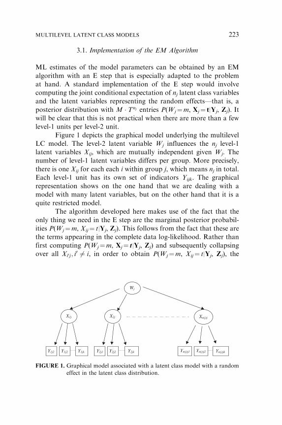
Figure 1 depicts the graphical model underlying the multilevel

LC model. The level-2 latent variable Wj influences the nj level-1

latent variables Xij, which are mutually independent given Wj. The

number of level-1 latent variables differs per group. More precisely,

there is one Xij for each each i within group j, which means nj in total.

Each level-1 unit has its own set of indicators Yijk. The graphical

representation shows on the one hand that we are dealing with a

model with many latent variables, but on the other hand that it is a

quite restricted model.

The algorithm developed here makes use of the fact that the

only thing we need in the E step are the marginal posterior probabil-

ities P(Wj¼m, Xij¼ t|Yj, Zj). This follows from the fact that these are

the terms appearing in the complete data log-likelihood. Rather than

first computing P(Wj¼m, Xj¼ t|Yj, Zj) and subsequently collapsing

over all Xi0j; i0 6¼ i, in order to obtain P(Wj¼m, Xij¼ t|Yj, Zj), the

Wj

X2jX1j Xn(j)j

Y1j2 Y1jk Y2j1 Y2j2 Y2jk Yn(j)j1 Yn(j)j2 Yn(j)jkY1j2

FIGURE 1. Graphical model associated with a latent class model with a random

effect in the latent class distribution.


latter term is computed directly. The procedure makes use of the

conditional independence assumptions underlying the graphical

model associated with the density defined in equation (12). This yields

an algorithm in which computation time increases linearly rather than

exponentially with nj. The proposed method is similar to the forward-

backward algorithm for the estimation of hidden Markov models for

large numbers of time points (Baum et al. 1970; Juang and Rabiner

1991). As will become clear below, the method proposed here could

be called an upward-downward algorithm. Latent variables are inte-

grated or summed out by going from the lower- to the higher-level

units, and the marginal posteriors are subsequently obtained by going

from the higher- to the lower-level units.

The marginal posterior probabilities P(Wj¼m, Xij¼ t|Yj, Zj)

needed to perform the E step can be obtained using the following

simple decomposition:

P(Wj ¼ m;Xij ¼ tjYj;Zj) ¼ P(Wj ¼ mjYj;Zj)P(Xij ¼ tjWj ¼ m;Yj;Zj)

The proposed efficient algorithm makes use of the fact that in the

multilevel LC model

P(Xij ¼ tjWj ¼ m;Yj;Zj) ¼ P(Xij ¼ tjWj ¼ m;Yij;Zij):

That is, given Wj, Xij is independent of the observed (and latent)

variables of the other level-1 units within the same level-2 unit.

This is the result of the fact that level-1 observations are mutually

independent given the random coefficients (given the value of Wj), as

is expressed in the density function described in equation (11).

This can also be seen from Figure 1, which depicts the conditional

independence assumptions underlying the multilevel LC model.

Using this important result, we get the following slightly simplified

decomposition:

P(Wj ¼ m;Xij ¼ tjYj;Zj) ¼ P(Wj ¼ m; jYj;Zj)P(Xij ¼ tjWj ¼ m;Yij ;Zij):

(13)

This shows that the problem of obtaining the marginal

posterior probabilities reduces to the computation of the two terms

at the right-hand side of this equation. Using the short-hand notation

�ij|m for P(Yij|Zij,um,q) and �ijt|m for P(Xij¼ t,Yij|Zij,um,q),and noting that �ijjm ¼

PTt¼1 �ijtjm, we obtain


P(Wj ¼ mjYj ;Zj) ¼�m

Qnji¼1 �ijjmPM

m¼1 �mQnj

i¼1 �ijjm(14)

P(Xij ¼ tjWj ¼ m;Yij;Zij) ¼�ijtjmPTt¼1 �ijtjm

¼�ijtjm�ijjm

:

As can be seen, the basic operation that has to be performed is the

computation of �ijt|m for each i, j, t, and m. In the upward step, the njsets of �ijt|m terms are used to obtain P(Wj¼m|Yj, Zj). The downward

step involves the computation of P(Xij¼ t|Wj¼m, Yij, Zij), as well as

P(Wj¼m, Xij¼ t|Yj, Zj) via equation (13). In the upward-downward

algorithm, computation time increases linearly with the number of

level-1 observations instead of exponentially, as would be the case in a

standard E step. Computation time can be decreased somewhat more

by grouping records with the same values for the observed variables

within level-2 units—that is, records with the same value for �ijt|m.

The remaining part of the implementation of the EM algo-

rithm is as usual. In the E step, the P(Wj¼m|Yj, Zj) and P(Wj¼m,

Xij¼ t|Yj, Zj) are used to obtain improved estimates for the observed

cell entries in the relevant marginal tables. Suppose that we have a

multilevel LC model in which the latent class probabilities contain

random coefficients and are influenced by covariates Z. Denoting a

particular covariate pattern by r, the relevant marginal tables have

entries f Wm ; f WXZmtr , and f XYk

tsk , which can be obtained as follows:

f Wm ¼XJj¼1

P(Wj ¼ mjYj;Zj)

f WXZmtr ¼

XJj¼1

Xnji¼1

P(Wj ¼ m;Xij ¼ tjYj;Zj)I(Zj ¼ r)

f XYktsk

¼XMm¼1

XJj¼1

Xnji¼1

P(Wj ¼ m;Xij ¼ tjYj;Zj)I(Yijk ¼ sk);

where I(Yijk¼ sk) and I(Zj¼ r) are 1 if the corresponding condition is

fulfilled, and 0 otherwise.

In the M step, standard complete data methods for the estima-

tion of logistic regression models can be used to update the parameter

estimates using the completed data as if it were observed.


A practical problem in the above implementation of the ML

estimation of the multilevel LC model is that underflows may occur in

the computation of P(Wj¼m|Yj, Zj). More precisely, because it may

involve multiplication of a large number (1þ nj �K) of probabilities,the numerator of equation (14) may become equal to zero for each m.

Such underflows can, however, easily be prevented by working on a

log scale. Letting ajm ¼ logð�mÞ þPnj

i logð�ijjmÞ and bj¼max(ajm),

P(Wj¼m|Yj, Zj) can be obtained by

P(Wj ¼ mjYj;Zj) ¼exp [ajm � bj]PMr exp [ajr � bj)]

:

3.2. Posterior Means

One of the objectives of a multilevel analysis may be to obtain

estimates of the group-specific parameters. Suppose we are interested

in the value of �tj for each level-2 unit. A simple estimator is the

posterior mean, denoted by ��tj. It is computed as follows:

��tj ¼ �t þ �t � �uuj

¼ �t þ �t �XMm¼1

umP(Wj ¼ mjYj;Zj): (15)

Here, um denotes the value of the mth quadrature node and

P(Wj¼m|Yj) the posterior probability associated with this node.

The quantity ��tj can subsequently be used to calculate the group-

specific latent class distributions by means of equation (4).

In the nonparametric approach, ��tj is defined as

��tj ¼XMm¼1

�tmP(Wj ¼ mjYj;Zj); (16)

that is, it is a weighted average of the parameters of the M mixture

components.

3.3. Standard Errors

Contrary to Newton-like methods, the EM algorithm does not

provide standard errors of the model parameters as a by-product.


Estimated asymptotic standard errors can be obtained by computing

the observed information matrix, the matrix of second-order deriva-

tives of the log-likelihood function toward all model parameters. The

inverse of this matrix is the estimated variance-covariance matrix. For

the examples presented in the next section, the necessary derivatives

are computed numerically.

The information matrix can also be used to check identifiability.

A sufficient condition for local identification is that all the eigenvalues

of the information matrix are larger than zero.

3.4. Software Implementation

The multilevel LC model cannot be estimated with standard software

for LC analysis. The upward-downward algorithm described in this

section was implemented in an experimental version of the Latent

GOLD program (Vermunt and Magidson 2000). The method will

become available in a subsequent version of this program for LC

analysis.

4. THREE APPLICATIONS

Three applications of the proposed new method are presented. These

illustrate not only three interesting application fields but also the most

important model specification options. The first example uses data

from a Dutch survey in which employees of various teams are asked

about their work conditions. Multilevel LC analysis is used to con-

struct a task-variety scale and to determine the between-team hetero-

geneity of the latent class probabilities. The second example uses a

Dutch data set containing information on the mathematical skills of

eighth grade students from various schools. The research question of

interest is to determine whether school differences remain after con-

trolling for individual characteristics such as nonverbal intelligence

and socioeconomic status of the family. The third example uses data

from the 1999 European Values Survey. Country differences in the

proportion of postmaterialists are modeled by means of random

effects. Contrary to the previous applications, we focus here not

only on the overall between-group differences but also on the latent

distribution for each of the groups (countries).


4.1. Organizational Research

In a Dutch study on the effect of autonomous teams on individual

work conditions, data were collected from 41 teams within two organ-

izations, a nursing home and a domiciliary care organization. These

teams contained 886 employees. The example contains five dichot-

omized items of a scale measuring perceived task variety (Van Mierlo

et al. 2002). The item wording is as follows (translated from Dutch):

1. Do you always do the same things in your work?

2. Does your work require creativity?

3. Is your work diverse?

4. Does your work make enough usage of your skills and capacities?

5. Is there enough variation in your work?

The original items contained four answer categories. In order

to simplify the analysis, the first two and the last two categories have

been collapsed. Because some respondents had missing values on one

or more of the indicators, the ML estimation procedure has been

adapted to deal with such partially observed indicators.

Using LC analysis for this data set, we can assume that the

researcher is interested in building a typology of employees based on

their perceived task variety. On the other hand, if we were interested

in constructing a continuous scale, a latent trait analysis would be

more appropriate. Of course, also in that situation the multilevel

structure should be taken into account.

In the analysis of this data set, a simple unrestricted LC model

has been combined with three types of specifications for the between-

team variation in the class-membership probabilities: no random

effects, parametric random effects as defined in equation (6), and

nonparametric random effects as defined in equation (9).

Table 1 reports the log-likelihood (LL) value, the number of

parameters, and the BIC value for the models that were estimated.

The models were first estimated without random effects. The BIC

values for the one to three class model (Models 1–3) without random

effects show that a solution with two classes suffices. Subsequently,

random effects were introduced in the two-class model (Models 4–6).

From the results obtained with Models 4 and 5, it can be seen that

there is clear evidence for between-team variation in the latent


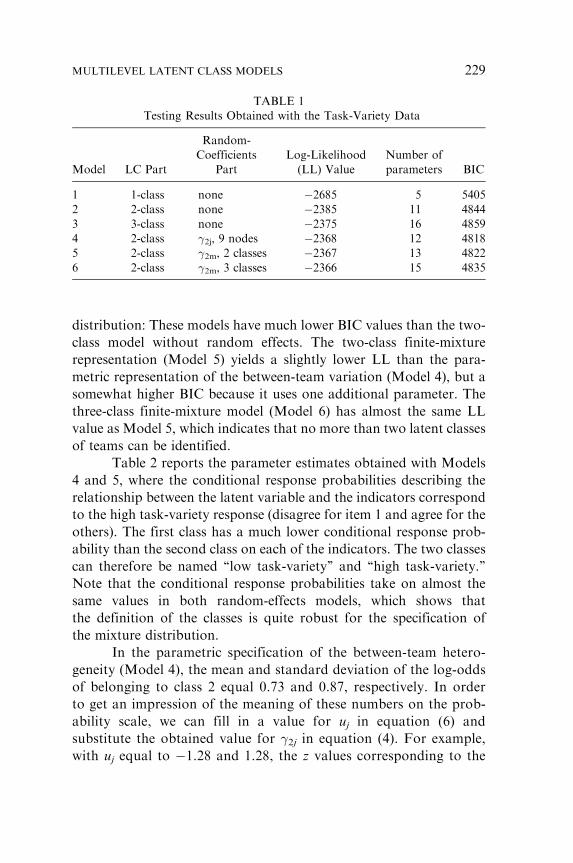
distribution: These models have much lower BIC values than the two-

class model without random effects. The two-class finite-mixture

representation (Model 5) yields a slightly lower LL than the para-

metric representation of the between-team variation (Model 4), but a

somewhat higher BIC because it uses one additional parameter. The

three-class finite-mixture model (Model 6) has almost the same LL

value as Model 5, which indicates that no more than two latent classes

of teams can be identified.

Table 2 reports the parameter estimates obtained with Models

4 and 5, where the conditional response probabilities describing the

relationship between the latent variable and the indicators correspond

to the high task-variety response (disagree for item 1 and agree for the

others). The first class has a much lower conditional response prob-

ability than the second class on each of the indicators. The two classes

can therefore be named ‘‘low task-variety’’ and ‘‘high task-variety.’’

Note that the conditional response probabilities take on almost the

same values in both random-effects models, which shows that

the definition of the classes is quite robust for the specification of

the mixture distribution.

In the parametric specification of the between-team hetero-

geneity (Model 4), the mean and standard deviation of the log-odds

of belonging to class 2 equal 0.73 and 0.87, respectively. In order

to get an impression of the meaning of these numbers on the prob-

ability scale, we can fill in a value for uj in equation (6) and

substitute the obtained value for �2j in equation (4). For example,

with uj equal to �1.28 and 1.28, the z values corresponding to the

TABLE 1

Testing Results Obtained with the Task-Variety Data

Model LC Part

Random-

Coefficients

Part

Log-Likelihood

(LL) Value

Number of

parameters BIC

1 1-class none �2685 5 5405

2 2-class none �2385 11 4844

3 3-class none �2375 16 4859

4 2-class �2j, 9 nodes �2368 12 4818

5 2-class �2m, 2 classes �2367 13 4822

6 2-class �2m, 3 classes �2366 15 4835


lower and upper 10 percent tails of the normal distribution, we get

latent class probabilities of .41 and .86. These numbers indicate that

there is a quite large team effect on the perceived task variety. The

intraclass correlation obtained with equation (8) equals .19, which

means that 19 per cent of the total variance is explained by team

membership.

The mixture components in the two-class finite-mixture model

(Model 5) contained 37 and 63 percent of the teams. Their log-odds of

belonging to the high task-variety class are �.35 and 1.29, respect-

ively. These log-odds correspond to probabilities of .41 and .78.

Although the parametric and nonparametric approach capture the

variation across teams in a somewhat different manner, both show

that there are large between-team differences in the individual percep-

tion of the variety of the work. The substantive conclusion based on

Model 5 would be that there are two types of employees and two

types of teams. The two types of teams differ with respect to the

distribution of the team members over the two types of employees.

TABLE 2

Estimated Parameter Values of Models 4 and 5 (Task-Variety Data)

Model 4 (parametric) Model 5 (nonparametric)

t¼ 1 t¼ 2 t¼ 1 t¼ 2

Parameter Value

Standard

Error Value

Standard

Error Value

Standard

Error Value

Standard

Error

Latent logit

mean (�2) 0.73 0.15

Latent logit

standard

deviation (�2) 0.87 0.14

Latent logit for

m¼ 1 (�21) �0.35 0.20

Latent logit for

m¼ 2 (�22) 1.29 0.18

P(Yij1¼ 1) 0.17 0.03 0.54 0.02 0.17 0.03 0.54 0.02

P(Yij2¼ 2) 0.30 0.03 0.71 0.02 0.30 0.03 0.71 0.02

P(Yij3¼ 2) 0.21 0.04 0.97 0.01 0.22 0.04 0.97 0.01

P(Yij4¼ 2) 0.44 0.03 0.83 0.02 0.44 0.03 0.83 0.02

P(Yij5¼ 2) 0.17 0.03 0.94 0.02 0.17 0.03 0.94 0.02


4.2. Educational Research

The second example uses data from a Dutch study comparing the

mathematical skills of eighth grade students across schools (Doolaard

1999). A mathematical test consisting of 18 items was given to 2156

students in a sample of 97 schools. The 18 dichotomous (correct/

incorrect) items are used to construct an LC model measuring individ-

ual skills. There is also information on the individual-level covariates

socioeconomic status (SES; standardized), nonverbal intelligence (ISI;

standardized), and gender (0¼male, 1¼ female), and a school-level

covariate indicating whether a school participates in the national

school leaving examination (CITO; 0¼ no, 1¼ yes).

Again the assumption is that the researcher is interested in

constructing a latent typology, in this case of types of students who

differ in their mathematical skills. It can be expected that schools

differ with respect to the mathematical ability of their students. How-

ever, in the Dutch educational context in which schools are assumed

to be more or less of the same quality, one would expect that the

school effect decreases or may even disappear if one controls for the

composition of the groups. The availability of individual-level covari-

ates that can be expected to be strongly related to mathematical

ability makes it possible to control for such composition effects.

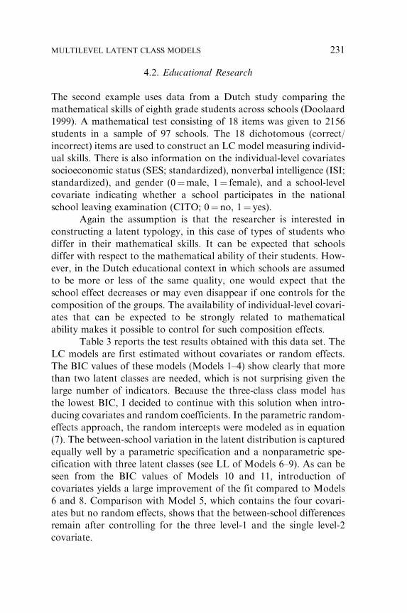
Table 3 reports the test results obtained with this data set. The

LC models are first estimated without covariates or random effects.

The BIC values of these models (Models 1–4) show clearly that more

than two latent classes are needed, which is not surprising given the

large number of indicators. Because the three-class class model has

the lowest BIC, I decided to continue with this solution when intro-

ducing covariates and random coefficients. In the parametric random-

effects approach, the random intercepts were modeled as in equation

(7). The between-school variation in the latent distribution is captured

equally well by a parametric specification and a nonparametric spe-

cification with three latent classes (see LL of Models 6–9). As can be

seen from the BIC values of Models 10 and 11, introduction of

covariates yields a large improvement of the fit compared to Models

6 and 8. Comparison with Model 5, which contains the four covari-

ates but no random effects, shows that the between-school differences

remain after controlling for the three level-1 and the single level-2

covariate.


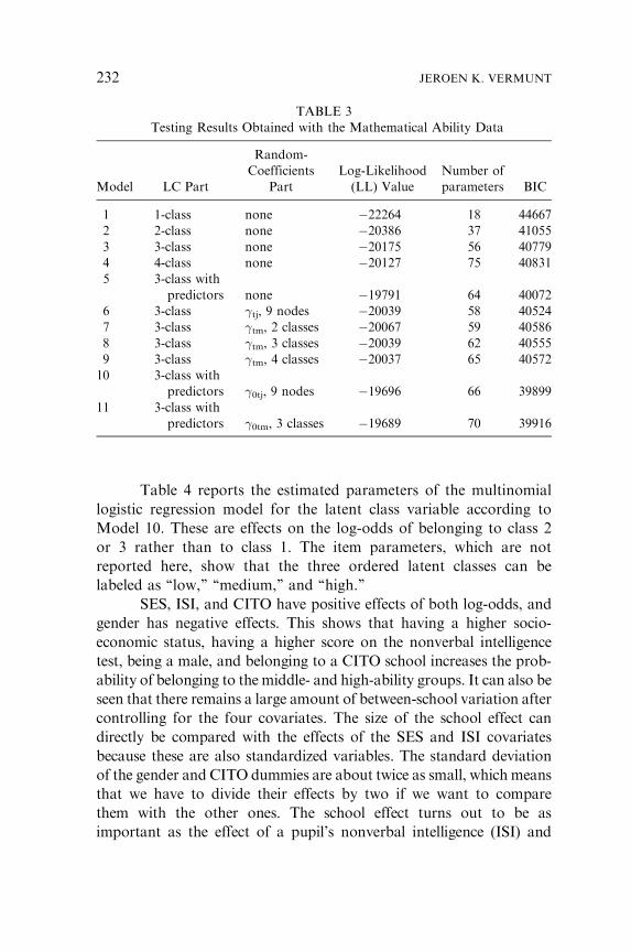
Table 4 reports the estimated parameters of the multinomial

logistic regression model for the latent class variable according to

Model 10. These are effects on the log-odds of belonging to class 2

or 3 rather than to class 1. The item parameters, which are not

reported here, show that the three ordered latent classes can be

labeled as ‘‘low,’’ ‘‘medium,’’ and ‘‘high.’’

SES, ISI, and CITO have positive effects of both log-odds, and

gender has negative effects. This shows that having a higher socio-

economic status, having a higher score on the nonverbal intelligence

test, being a male, and belonging to a CITO school increases the prob-

ability of belonging to the middle- and high-ability groups. It can also be

seen that there remains a large amount of between-school variation after

controlling for the four covariates. The size of the school effect can

directly be compared with the effects of the SES and ISI covariates

because these are also standardized variables. The standard deviation

of the gender and CITO dummies are about twice as small, which means

that we have to divide their effects by two if we want to compare

them with the other ones. The school effect turns out to be as

important as the effect of a pupil’s nonverbal intelligence (ISI) and

TABLE 3

Testing Results Obtained with the Mathematical Ability Data

Model LC Part

Random-

Coefficients

Part

Log-Likelihood

(LL) Value

Number of

parameters BIC

1 1-class none �22264 18 44667

2 2-class none �20386 37 41055

3 3-class none �20175 56 40779

4 4-class none �20127 75 40831

5 3-class with

predictors none �19791 64 40072

6 3-class �tj, 9 nodes �20039 58 40524

7 3-class �tm, 2 classes �20067 59 40586

8 3-class �tm, 3 classes �20039 62 40555

9 3-class �tm, 4 classes �20037 65 40572

10 3-class with

predictors �0tj, 9 nodes �19696 66 39899

11 3-class with

predictors �0tm, 3 classes �19689 70 39916


more important than the other covariates. The differences between

schools cannot be explained by differences in the composition of their

populations.

4.3. Comparative Research

The third example makes use of data from the 1999 European Values

Study (EVS), which contains information from 32 countries. A sam-

ple was obtained from 10 per cent of the available cases per country,

yielding 3584 valid cases. A popular scale in the survey is the post-

materialism scale developed by Inglehart (1977). An important issue

has always been the comparison of countries on the basis of the

individual-level responses, something that can be done in an elegant

manner using the multilevel LC model.

The Inglehart scale consists of making a first (Yij1) and second

(Yij2) choice out of a set of four alternatives. Respondents indicate

what they think should be the most and next most important aim

of their country for the next ten years. There are four alternatives:

(1) maintaining order in the nation, (2) giving people more say in

important government decisions, (3) fighting rising prices, and

(4) protecting freedom of speech. The two observed indicators can

be modeled by the LC model for (partial) rankings proposed by

Croon (1989), in which P(Yij1¼ s1, Yij2¼ s2) is assumed to be equal to

P(Yij1 ¼ s1;Yij2 ¼ s2) ¼XTt¼1

P(Xij ¼ t)exp (�s1t)

�4r¼1 exp (�rt)

exp (�s2t)

�r 6¼s1 exp (�rt)

TABLE 4

Estimated Parameter Values of Parametric Model 10 (Mathematical Ability Data)

t¼ 2 t¼ 3

Parameter Value

Standard

Error Value

Standard

Error

Intercept/mean (�0t) 0.82 0.26 �0.70 0.38

SES (�1t) 0.83 0.11 1.36 0.13

ISI (�2t) 1.15 0.12 2.28 0.12

Gender (�3t) �0.61 0.18 �1.03 0.21

CITO (�4t) 1.85 0.29 3.08 0.42

Standard deviation (� t) 1.11 0.18 2.25 0.27


for s1 6¼ s2, and 0 otherwise. This model differs from a standard LC

model in that the � parameters are equal for the two items and that

the probability of giving the same response on the two items is

structurally zero. This is a way to take into account that the prefer-

ences remain the same in both choices and that the second choice

cannot be the same as the first one. The � parameters can be inter-

preted as the class-specific utilities of the alternative concerned. The

alternative with the largest positive utility has the highest probability

to be selected, and the one with the largest negative value the lowest

probability.

The multilevel structure is used to model country differences in

the latent distribution. Both a continuous and a discrete mixture

distribution will again be used in order to be able to see the effect of

the specification of this part of the model on the final results. From a

substantive point of view, the finite mixture approach yielding a

typology of countries is the more natural one in this application.

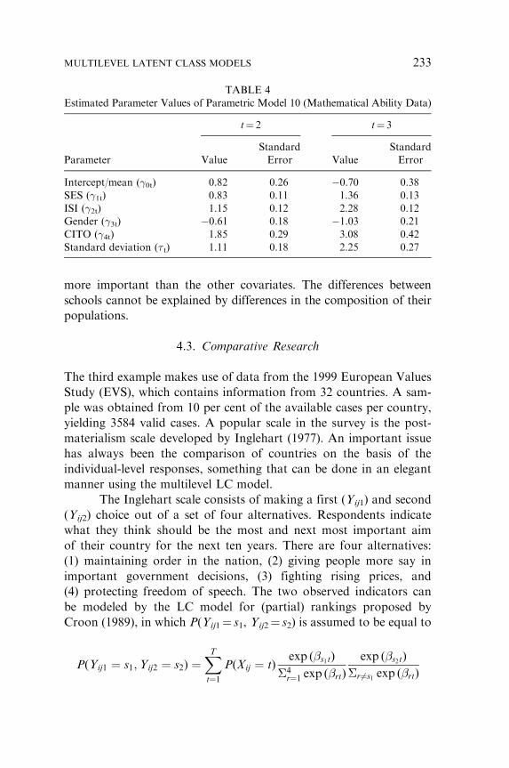
Table 5 reports the test results obtained with the EVS data.

Again models were estimated without random effects. Comparison of

the BIC values of Models 1, 2, and 3 shows that a two-class model

should be preferred for this data set. Note that this is in agreement

with the intension of this scale, which should make a distinction

between materialists and postmaterialists. The much lower BIC values

obtained with the two-class models with a random log-odds of

belonging to the postmaterialist class (Models 4–7) indicate that there

is considerable between-country variation in the latent distribution.

TABLE 5

Test Results Obtained with the European Valves Study (EVS) Data

Model LC Part

Random-

Coefficients

Part

Log-Likelihood

(LL) Value

Number of

parameters BIC

1 1-class none �8392 3 16809

2 2-class none �8259 7 16576

3 3-class none �8248 11 16587

4 2-class �2j, 9 nodes �8158 8 16382

5 2-class �2m, 2 classes �8191 9 16457

6 2-class �2m, 3 classes �8156 11 16402

7 2-class �2m, 4 classes �8151 13 16409


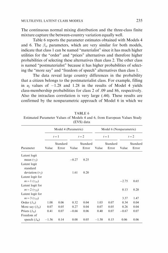
The continuous normal mixing distribution and the three-class finite

mixture capture the between-country variation equally well.

Table 6 reports the parameter estimates obtained with Models 4

and 6. The �st parameters, which are very similar for both models,

indicate that class 1 can be named ‘‘materialist’’ since it has much higher

utilities for the ‘‘order’’ and ‘‘prices’’ alternatives and therefore higher

probabilities of selecting these alternatives than class 2. The other class

is named ‘‘postmaterialist’’ because it has higher probabilities of select-

ing the ‘‘more say’’ and ‘‘freedom of speech’’ alternatives than class 1.

The data reveal large country differences in the probability

that a citizen belongs to the postmaterialist class. For example, filling

in uj values of �1.28 and 1.28 in the results of Model 4 yields

class-membership probabilities for class 2 of .09 and 86, respectively.

Also the intraclass correlation is very large (.44). These results are

confirmed by the nonparametric approach of Model 6 in which we

TABLE 6

Estimated Parameter Values of Models 4 and 6, from European Values Study

(EVS) data

Model 4 (Parametric) Model 6 (Nonparametric)

t¼ 1 t¼ 2 t¼ 1 t¼ 2

Parameter Value

Standard

Error Value

Standard

Error Value

Standard

Error Value

Standard

Error

Latent logit

mean (�2) �0.27 0.25

Latent logit

standard

deviation (�2) 1.61 0.20

Latent logit for

m¼ 1 (�21) �2.75 0.65

Latent logit for

m¼ 2 (�22) 0.13 0.20

Latent logit for

m¼ 3 (�23) 3.37 1.47

Order (�1t) 1.08 0.06 0.32 0.04 1.03 0.07 0.34 0.04

More say (�2t) 0.07 0.05 0.27 0.04 0.07 0.05 0.26 0.04

Prices (�3t) 0.41 0.07 �0.66 0.06 0.40 0.07 �0.67 0.07

Freedom of

speech (�4t) �1.56 0.14 0.08 0.05 �1.50 0.15 0.06 0.06


see large differences in the logit of belonging to class 2 between the

three mixture components. The three logits correspond to probabilities

of 0.06, 0.53, and 0.97, respectively.

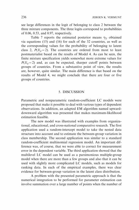
Table 7 reports the estimated posterior means ��2j obtained

via equations (15) and (16) for each of the 32 countries, as well as

the corresponding values for the probability of belonging to latent

class 2, P(Xij¼ 2). The countries are ordered from most to least

postmaterialist based on the results of Model 4. As can be seen, the

finite mixture specification yields somewhat more extreme values for

P(Xij¼ 2) and, as can be expected, sharper cutoff points between

groups of countries. From a substantive point of view, the results

are, however, quite similar. The main difference is that based on the

results of Model 4, we might conclude that there are four or five

groups of countries.

5. DISCUSSION

Parametric and nonparametric random-coefficient LC models were

proposed that make it possible to deal with various types of dependent

observations. In addition, an adapted EM algorithm named upward-

downward algorithm was presented that makes maximum-likelihood

estimation feasible.

The new model was illustrated with examples from organiza-

tional, educational, and cross-national comparative research. The first

application used a random-intercept model to take the nested data

structure into account and to estimate the between-group variation in

class membership. The second application was similar to a standard

random-coefficient multinomial regression model. An important dif-

ference was, of course, that we were able to correct for measurement

error in the dependent variable. The third application showed that the

multilevel LC model can be used as a parsimonious multiple-group

model when there are more than a few groups and also that it can be

used with slightly more complicated LC models, such as models for

ranking data. In each of the empirical examples, there was clear

evidence for between-group variation in the latent class distribution.

A problem with the presented parametric approach is that the

numerical integration to be performed for parameter estimation can

involve summation over a large number of points when the number of


random coefficients is increased. It should be noted that the total

number of quadrature points equals the product of the number of

points used for each dimension. Despite the fact that the number of

points per dimension can be somewhat reduced with multiple random

TABLE 7

Posterior Means of Random Effects and the Corresponding Proportion of

Postmaterialists for the 32 Countries (Models 4 and 6, EVS data)

Model 4 (Parametric) Model 6 (Nonparametric)

Country �tj P(Xij¼ 2) �tj P(Xij¼ 2)

Italy 3.14 0.96 3.37 0.97

Sweden 2.99 0.95 3.37 0.97

Denmark 2.96 0.95 3.37 0.97

Austria 2.83 0.94 3.37 0.97

Netherlands 2.81 0.94 3.37 0.97

Croatia 1.67 0.84 3.29 0.96

Belgium 1.43 0.81 3.36 0.97

Greece 1.35 0.79 0.41 0.60

France 1.35 0.79 0.13 0.53

Spain 1.24 0.78 0.14 0.54

Northern Ireland 1.15 0.76 0.14 0.54

Ireland 1.06 0.74 0.16 0.54

Luxembourg 0.02 0.51 0.13 0.53

Slovenia �0.16 0.46 0.13 0.53

Czechnia �0.23 0.44 0.13 0.53

Iceland �0.27 0.43 0.13 0.53

Finland �0.27 0.43 0.13 0.53

West Germany �0.27 0.43 0.13 0.53

Portugal �0.28 0.43 0.13 0.53

Romania �0.29 0.43 0.13 0.53

Malta �0.29 0.43 0.11 0.53

East Germany �0.31 0.42 0.12 0.53

Bulgaria �0.31 0.42 0.12 0.53

Lithuania �1.83 0.14 �2.71 0.06

Latvia �1.87 0.13 �2.74 0.06

Poland �1.91 0.13 �2.75 0.06

Estonia �1.96 0.12 �2.75 0.06

Belarus �2.21 0.10 �2.75 0.06

Slovakia �2.24 0.10 �2.75 0.06

Hungary �2.39 0.08 �2.75 0.06

Ukraine �2.78 0.06 �2.75 0.06

Russia �3.75 0.02 �2.75 0.06


coefficients, computational burden becomes enormous with more

than five or six random coefficients. There exist other methods for

computing high-dimensional integrals, such as Bayesian simulation

and simulated maximum-likelihood methods, but these are also com-

putationally intensive. As shown by Vermunt and Van Dijk (2001),

these problems can be circumvented by adopting a nonparametric

approach in which the computation burden is much less dependent

on the number of random coefficients. The finite mixture specification

is not only interesting on its own, but it can also be used to approxi-

mate a multivariate continuous mixture distribution.

REFERENCES

Agresti, Alan, James G. Booth, James P. Hobert, and Brian Caffo. 2000.

‘‘Random-Effects Modeling of Categorical Response Data.’’ Pp. 27–80 in

Sociological Methodology 2000, edited by Michael E. Sobel and Mark P.

Becker. Cambridge, MA: Blackwell Publisher.

Bandeen-Roche, Karen J., Diana L. Miglioretti, Scott L. Zeger, and Paul J.

Rathouz. 1997. ‘‘Latent Variable Regression for Multiple Discrete Outcomes.’’

Journal of the American Statistical Association 92:1375–86.

Baum, Leonard E., Ted Petrie, George Soules, and Norman Weiss. 1970. ‘‘A

Maximization Technique Occurring in the Statistical Analysis of Probabilistic

Functions of Markov Chains.’’ Annals of Mathematical Statistics 41:164–71.

Bock, R. Darroll. 1972. ‘‘Estimating Item Parameters and Latent Ability When

Responses are Scored in Two or More Nominal Categories.’’ Psychometrika

37:29–51.

Bock, R. Darroll, and Murray Aitkin. 1981. ‘‘Marginal Maximum-Likelihood

Estimation of Item Parameters.’’ Psychometrika 46:443–59.

Bryk, Anthony S., and Stephen W. Raudenbush. 1992. Hierarchical Linear

Models: Application and Data Analysis. Newbury Park, CA: Sage.

Clogg, Clifford C., and Leo A. Goodman. 1984. ‘‘Latent Structure Analysis of a

Set of Multidimensional Contingency Tables.’’ Journal of the American

Statistical Association 79:762–71.

Croon, Marcel A. 1989. ‘‘Latent Class Models for the Analysis of Rankings.’’

Pp. 99–121 in New Developments in Psychological Choice Modeling, edited by

G. De Soete, H. Feger, and K.C. Klauer. Amsterdam, Netherlands: Elsevier

Science Publishers.

Dayton, C. Mitchell, and George B. Macready. 1988. ‘‘Concomitant-Variable

Latent-Class Models.’’ Journal of the American Statistical Association 83:173–78.

Doolaard, Simone. 1999. ‘‘Schools in Change or School in Chain.’’ Ph.D.

dissertation, University of Twente, The Netherlands.

Fox, Jean-Paul, and Cees A.W. Glas. 2001. ‘‘Bayesian Estimation of a Multilevel

IRT Model Using Gibbs Sampling.’’ Psychometrika 66:269–86.


Goldstein, Harvey. 1995. Multilevel Statistical Models. New York: Halsted Press.

Goodman, Leo A. 1974. ‘‘The Analysis of Systems of Qualitative Variables When

Some of the Variables Are Unobservable. Part I: A Modified Latent Structure

Approach.’’ American Journal of Sociology 79:1179–259.

Hedeker, Donald. 1999. ‘‘MIXNO: A Computer Program for Mixed-Effects

Nominal Logistic Regression.’’ Journal of Statistical Software 4:1–92.

Hedeker, Donald. Forthcoming. ‘‘A Mixed-Effects Multinomial Logistic

Regression Model.’’ Statistics in Medicine.

Hedeker, Donald, and Robert D. Gibbons. 1996. ‘‘MIXOR: A Computer

Program for Mixed-Effects Ordinal Regression Analysis.’’ Computer Methods

and Programs in Biomedicine 49:157–76.

Heinen, Ton. 1996. Latent Class and Discrete Latent Trait Models: Similarities

and Differences. Thousand Oaks, CA: Sage.

Inglehart, Ronald. 1977. The Silent Revolution. Princeton, NJ: Princeton

University Press.

Juang, Biing Hwang, and Laurence R. Rabiner. 1991. ‘‘Hidden Markov Models

for Speech Recognition.’’ Technometrics 33:251–72.

Laird, Nan. 1978. ‘‘Nonparametric Maximum-Likelihood Estimation of a Mixture

Distribution.’’ Journal of the American Statistical Association 73:805–11.

Lazarsfeld, Paul F. 1950. ‘‘The Logical and Mathematical Foundation of Latent

Structure Analysis and the Interpretation and Mathematical Foundation of

Latent Structure Analysis.’’ Pp. 362–472 in Measurement and Prediction,

edited by S. A. Stouffer et al. Princeton, NJ: Princeton University Press.

Lenk, Peter J., and Wayne S. DeSarbo. 2000. ‘‘Bayesian Inference for Finite

Mixture Models of Generalized Linear Models with Random Effects.’’

Psychometrika 65:93–119.

Qu, Yinsheng, Ming Tan, and Michael H. Kutner. 1996. ‘‘Random Effects

Models in Latent Class Analysis for Evaluating Accuracy of Diagnostic

Tests.’’ Biometrics 52:797–810.

Rabe-Hesketh, Sophia, Andrew Pickles, and Anders Skrondal. 2001.

‘‘GLLAMM: A General Class of Multilevel Models and a Stata Program.’’

Multilevel Modelling Newsletter 13:17–23.

Snijders, Tom A. B., and Roel J. Bosker. 1999. Multilevel Analysis. London: Sage.

Stroud, Arthur H., and Don Secrest. 1966. Gaussian Quadrature Formulas.

Englewood Cliffs, NJ: Prentice Hall.

Van Mierlo, Heleen, Jeroen K. Vermunt, and Cristel Rutte. 2002. ‘‘Using

Individual Level Survey Data to Measure Group Constructs: A Comparison

of Items with Reference to the Individual and to the Group in a Job Design

Context.’’ Manuscript submitted for publication.

Vermunt, Jeroen K., and Liesbet Van Dijk. 2001. ‘‘A Nonparametric Random-

Coefficients Approach: The Latent Class Regression Model.’’ Multilevel

Modelling Newsletter 13:6–13.

Vermunt, Jeroen K., and Jay Magidson. 2000. Latent GOLD User’s Manual.

Boston, MA: Statistical Innovations.

Wong, George Y., and William M. Mason. 1985. ‘‘Hierarchical Logistic Models for

Multilevel Analysis.’’ Journal of the American Statistical Association 80:513–24.


Documents

Jeroen K. Vermunt* - Statistical Innovations · The model is also similar to the multilevel item response theory ... is the probability of observing response s k on item k given that