Jens Suedekum International Trade RGS Econ + DICE · Bangladesh 10.0 3.5 1.7 3.4 8.0 ... → Monopoly, oligopoly, monopolistic competition ... for example, for linear demand curve)

Jens Suedekum International Trade RGS Econ + DICE

1

Trade with imperfect competition Heckscher-Ohlin, Ricardo, Ricardo-Viner: Neoclassical trade theory → Perfect competition, constant returns to scale → Theories of intra-industry trade Stylized fact: A significant part of world trade (particularly among developed countries) is intra-industry trade, i.e., two way trade in similar products Example: German cars ↔ French cars

Both countries (D and F) export and import, at the same time, similar yet not completely identical products

→ Measuring intra-industry trade: Grubel-Lloyd-Index


2

Grubel-Lloyd-Index Exports from H to F, Sector i:

1 i ii

i i

Ex ImGL

Ex Im

→ In neoclassical trade theory: Exi=0 or Imi=0, hence GLi=0 → When export- and import volume in sector i between H and F are the same

(in world market prices): GLi = 1. → International Standard Industrial Classification (ISIC), UNO


3

© van Marrewijk (2004)

Table 10.1 International trade between The Philippines (RP) and Japan; 1998*

SITC Exports

from RP

Imports

into RP

GL index

8 Miscellaneous manufactured articles 383,167 576,412 0.80

81 Prefabricated buildings 4,147 2,186 0.69

82 Furniture and parts thereof 42,332 6,155 0.25

83 Travel goods, handbags and similar containers 4,804 67 0.03

84 Articles of apparel and clothing accessories 115,627 3,255 0.05

85 Footwear 13,283 920 0.13

87 Prof. scientific & controlling instruments 24,091 175,018 0.24

88 Photographic apparatus 72,174 123,333 0.74

89 Miscellaneous manufactured articles 106,709 265,477 0.57


4

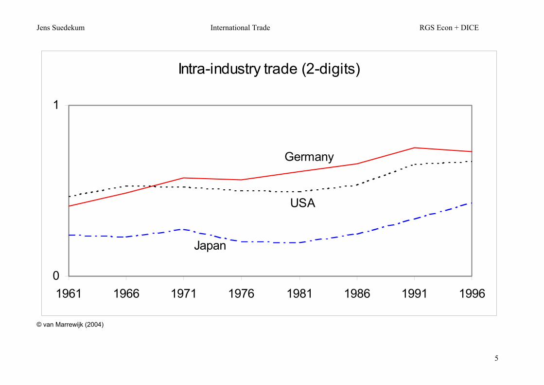
→ Intra-industry trade mostly between high-income countries

Table 10.2 Intra-industry trade, GL-index manufacturing sector 1995 (3-digit level, %)

Country World OECD 22 NAFTA East Asia Dev. Latin America

Australia 36.6 17.5 16.0 39.2 41.6

Bangladesh 10.0 3.5 1.7 3.4 8.0

Chile 25.7 10.1 11.5 3.6 47.8

France 83.5 86.7 62.7 38.7 22.9

Germany 75.3 80.1 61.2 36.2 22.8

Japan 42.3 47.6 45.7 36.1 7.0

Malaysia 60.4 48.5 57.9 75.0 10.4

Hong Kong 28.4 20.2 25.2 19.9 13.6

UK 85.4 84.0 72.5 46.6 38.6

USA 71.7 74.0 73.5 41.4 66.0

Source: NAPES website, http://napes.anu.edu.au/


5

© van Marrewijk (2004)

Intra-industry trade (2-digits)

0

1

1961 1966 1971 1976 1981 1986 1991 1996

Japan

USA

Germany


6

„Old“ vs. „new“ trade theory: Basics Neoclassical trade theory: Perfect competition Atomistic market structure Price taking behaviour Homogeneous products Zero profits due to free entry

Imperfect competition → Monopoly, oligopoly, monopolistic competition Non-atomistic market structure Firms have price setting power → Mark-ups on marginal costs


7

Oligopoly Monopolistic competition (typical setup)

Few firms (n≥2)

Many, but not infinitely many firms

Homogeneous or heterogeneous products

Product differentiation is a necessary feature of this market form

Firms are symmetrical or asymmetrical

Firms supply differentiated products but are typically symmetrical

Barriers to market entry → Existence of pure profits

Free entry in the long run → Zero profits

Operating profits (p>MC) exceed fixed costs

Operating profits (p>MC) cover only fixed costs

Strategic Interaction is crucial! → Industrial organization

No strategic interaction between competitors! (as firms are small relative to the market)

Trade with oligopoly: Brander (1980), Brander/Krugman (1981), Brander/Spencer (1984)

Trade with monopolistic competition: Krugman (1979, 1980), Ethier (1982), Helpman/Krugman (1985)


8

The simplest version of the Krugman-Model

© Princeton University

Nobel price in Economics, 2008!


9

Krugman-Model: Autarky Population: L identical consumers/workers One sector, consisting of a large number (N) of differentiated but

symmetrical products („varieties“) One variety ↔ one firm Production function:

x 0,0 1 x – Output, – Workers per firm. 0 : Fixed labor requirement

C x w x , MC dC x dx w

AC C x x w w x → decreasing av.costs = IRS

x

MC=βw

AC=βw+αw/x


10

Profit maximization

x p x x w x

0 1

d x dp x dp xxp x x w p x wdx dx p x dx

11p x w

with

0

dx p pdp x p

(price elasticity of demand)

1

p x w mark-up pricing

Mark-up depends negatively on the price elasticity (in absolute terms).


11

Dixit-Stiglitz preferences

1

N

ii

U c

0 1 → love for variety (e.g., 51/2 + 51/2 = 4,47 > 101/2=3,16)

Effect is stronger the lower is θ Utility maximization (w=wage):

1 ,..., 1 1N

N N

i i ic c i iMax c w p cZ

111 0 1,...,i i i i

i

Z c p c p for i Nc


12

(1) Equilibrium condition: Firms maximize profits

01

d xp w

dx

Elasticity with the utility/demand function specified above:

1 1 11 1

11

1 1 11 1 1

i i ii i i

i i

i

dc p pc p pdp c

p

→ Price setting rule: 1*p w

→ Fixed mark-up! Independent of the number of competitors!

Assumption: λ is fixed! → Chamberlain’s large group assumption → no effects of dpi on the shadow price of income!


13

(2) Equilibrium condition: Zero long-run profits (Entry of new competitors if π*>0)

0 wx p x x w x w x w

*

1x

Output per firm

* *

1x

Workers per firm

→ All firms identical


14

(3) Equilibrium condition: Labor market clearing 1

* **

LLL N N

Larger countries have more firms, more product varieties (L↑ → N*↑) (4) Equilibrium condition: Product market clearing

** * *

1xx L c cL L

c* = consumption per capita per variety L↑ → N↑, c*↓ → V*↑ , see problem set 1! → More varieties in larger countries (under autarky); consumers split income

over a larger set of varieties. This increases welfare („love for variety“)!


15

Autarky → Trade Starting point: Two countries (H and F) in autarky (population sizes LH, LF) Varieties under autarky: NH*, NF* (LH>LF → NH* > NF*) Country F produces different varieties than country H! → With perfectly free trade: (NH*+NF*) varieties available in both countries → Emergence of intra-industry trade! → Trade generates a welfare gain for both countries due to an increase in

consumption variety. → The welfare gain is stronger for the smaller country. → The source of the welfare gain is entirely different than in neoclassical trade

models of the Heckscher-Ohlin-type (~ gains from specialization according to comp. advantage) → No effects of trade on firm-level variables: x*, * constant → Introduction of free trade and increases in country size (LH↑) have analogous

implications in this model


16

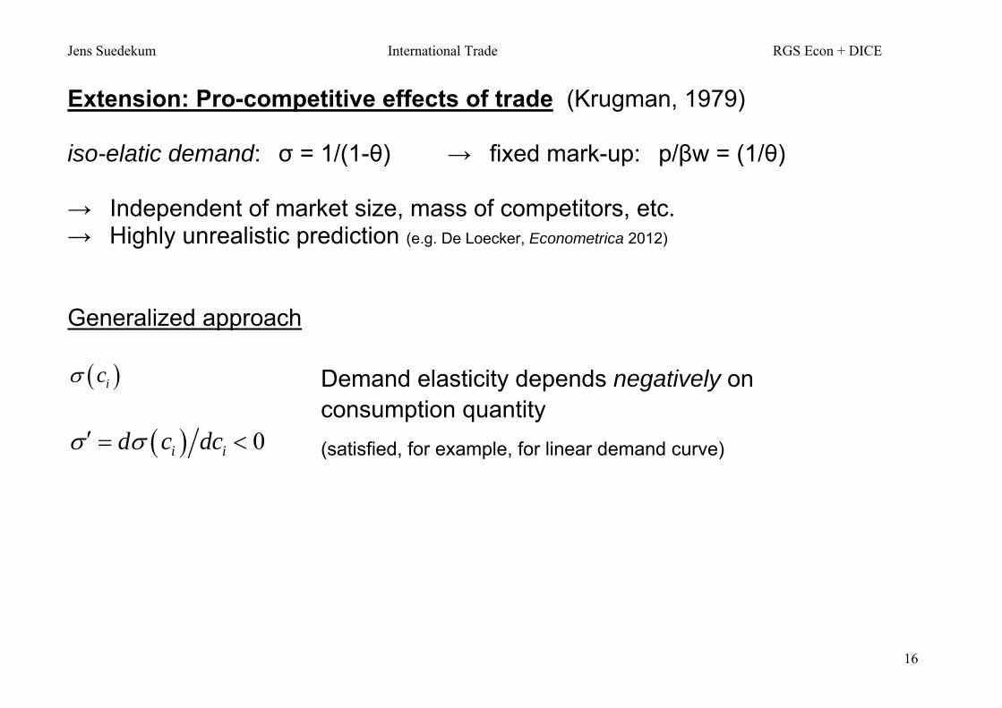
Extension: Pro-competitive effects of trade (Krugman, 1979) iso-elatic demand: σ = 1/(1-θ) → fixed mark-up: p/βw = (1/θ) → Independent of market size, mass of competitors, etc. → Highly unrealistic prediction (e.g. De Loecker, Econometrica 2012) Generalized approach ic Demand elasticity depends negatively on

consumption quantity 0i id c dc (satisfied, for example, for linear demand curve)


17

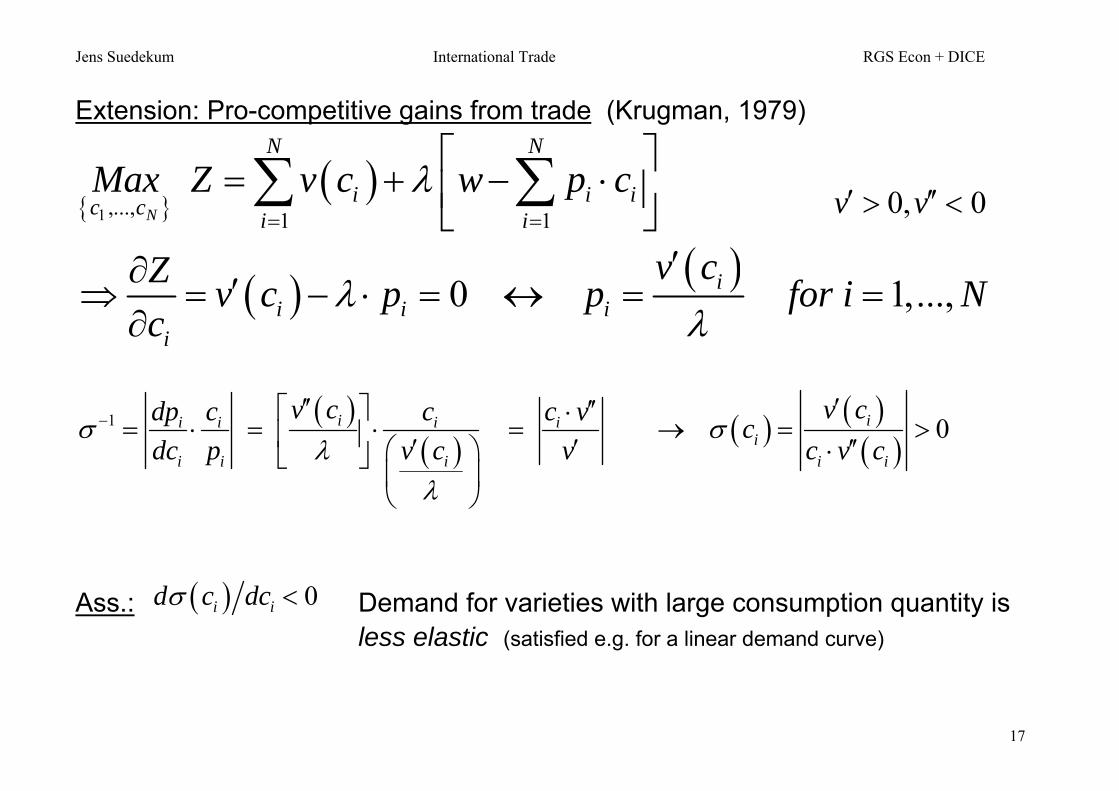
Extension: Pro-competitive gains from trade (Krugman, 1979)

1 ,..., 1 1N

N N

i i ic c i iMax Z v c w p c

0, 0v v

0 1,...,ii i i

i

v cZ v c p p for i Nc

1 0i ii i i ii

ii i i i

v c v cdp c c c v cv cdc p v c v c

Ass.: 0i id c dc Demand for varieties with large consumption quantity is

less elastic (satisfied e.g. for a linear demand curve)


18

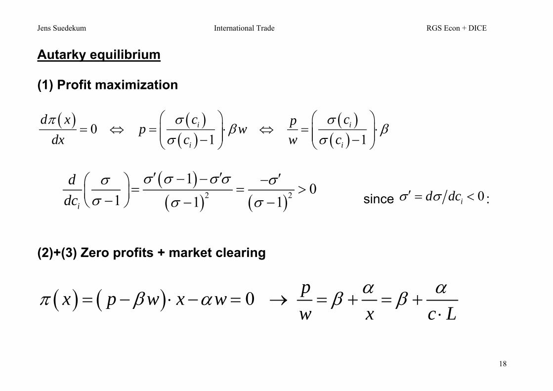
Autarky equilibrium (1) Profit maximization

01 1

i i

i i

d x c cpp wdx c w c

2 2

10

1 1 1i

ddc

since 0id dc :

(2)+(3) Zero profits + market clearing

0 px p w x ww x c L


19

pw

c*c

*pw

1pw

pw c L

Autarky equilibriumEquilibrium

*, *c p w Hence,

* *x L c

* *x

** *

1*

L LNL c

L c


20

pw

c*c

*pw

1pw

pw c L

The effects of trade (i.e., L↑) Effects:

* , *c p w

1*

*N

L c

Welfare gains from trade due to -- gains in consumption variety -- pro-competitive gains The latter do not arise in the model with constant price elasticity of demand!


21

Two-sector, two-country model - Homogenous good agriculture A (price pA=1 is the numéraire) - Manufacturing good M, consists of N differentiated varieties Utility function of the representative consumer:

(1) 1( , )U M A M A 0 1

With sub-utility function

(2)

1

0

( ) 0 1N

M m i di

“CES”-function

The representative household maximizes (1) and (2) subject to:

(3) 0

( ) ( )N

A p i m i di Y Y = income


22

Maximization problem solved in two steps Step 1

(4) 1

1

,..., 0 0

( ) ( ) . . ( )N

N N

m mMin Z p i m i di s t m i di M

→ N+1 FOCs: for all pairs of varieties mi, mj MRS equals relative price

(5) 1

1 (1 )1

( ) ( ( )) ( ) ( ) ( ) ( )( ) ( ( ))

p i m i m i m j p j p ip j m j

Plugging into budget constraint (FOC # N+1) we get:

(6) 1

1 (1 )

0

N

j j im p p di M


23

Rewrite (6) as a Hicks demand function for the j-th good (mj):

(7)

1 ( 1)

1

/( 1)

0

( )( )

( )N

p jm j M

p i di

( 1)

1

/( 1)

0

( )( ) ( )

( )N

p jp j m j M

p i di

Integrating over all varieties j:

(8)

( 1)

/( 1) /( 1)1

0 0 0/( 1)

0

( ) ( ) ( ) ( )

( )

N N N

N

Mp j m j dj p j dj p k dk M

p i di

Define for notational convenience:

(9)

( 1) 1 1

/( 1) 1

0 0

( ) ( )N N

P p k dk p k dk

with 1 1


24

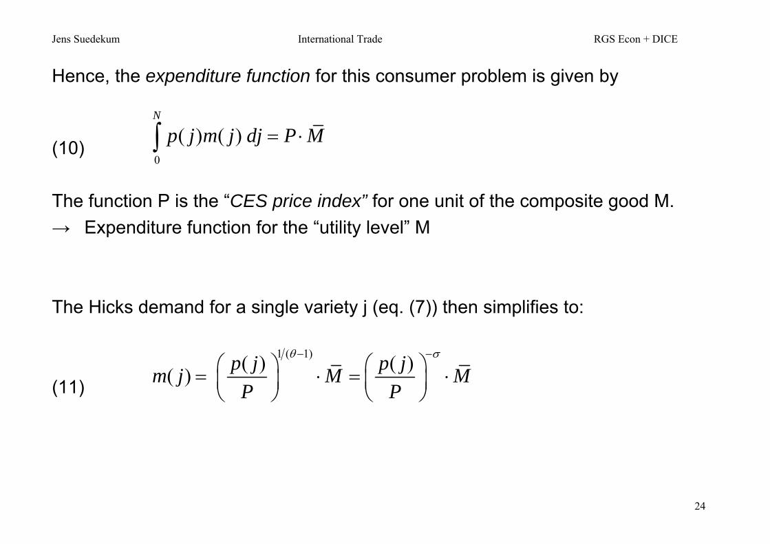
Hence, the expenditure function for this consumer problem is given by

(10) 0

( ) ( )N

p j m j dj P M

The function P is the “CES price index” for one unit of the composite good M. → Expenditure function for the “utility level” M The Hicks demand for a single variety j (eq. (7)) then simplifies to:

(11)

1 ( 1)( ) ( )( ) p j p jm j M MP P


25

Second step Optimal allocation of exogenous income over A and M

1( , ) . .Max U M A M A s t A P M Y Standard utility maximization problem with Cobb-Douglas-preferences: constant expenditure shares (Please verify this!)

(12) M Y P (1 ) (1 )AA Y p Y Marshall demand function for variety m(j) is given by:

(13) (1 ) 1 ( 1) 1( ) ( ) ( )m j Y P p j Y P p j 0,j N

Note: constant price elasticity of demand: 1 (1 ) (in absolute terms)


26

Indirect utility (using (12) in (1))

(14) (1 )(1 )V Y P

“Love for variety” Let ( ) 0,p i p i N :

(15) ( 1)( 1) ( 1)P N p P N p

because 0<θ<1: ∂P/∂N < 0. Since ∂V/∂P<0 → ∂V/∂N >0 Note: The “upper tier utility function” need not be Cobb-Douglas! Other example:

( , ) lnU M A A M ,M P A Y 1( ) ( )m j P p j

Quasi-linear preferences → no income effects of demand for M-varieties!


27

The Supply Side “Agricultural good” A: perfect competition, constant returns of scale

AA L Hence, 1A Ap w “Manufacturing sector” M: See above!

( ) ( ) ( ) ( )MMax j p j x j w x j 1s.t. ( ) ( )x j Y P p j

FOC

( ) ( ) ( )( ) ( ) 0 ( ) 1( ) ( ) ( ) 1

M M Mdp j x j dp jp j x j w p j w p j wdx j p j dx j

The Chamberlian “large group assumption”: Each firm takes the price index P as given and neglects the effect of p(j) on P. ~ absence of strategic interactions in monopolistic competition models


28

Due to the constant price elasticity of demand 1 (1 ) :

(16) * Mp w

identical for all firms!

→ Producers charge constant mark-up 1 over the marginal costs, Mw

Zero long-run profits !

0M M Mp x w x x w w

(17) *(1 )

X

equilibrium firm size

(18) * * (1 )X equilibrium labour demand per firm

(19) (1 )*

*

M ML LN

equilibrium number of firms (=varieties)

(20) ( 1)* ( *) *P N p LM↑ → N*↑, p* const. → P* ↓ → V*↑


29

Spatial version: Two regions with transport costs

(21)

1

0 0

( ) ( ) 0 1r r s

sr NNM m i di m j dj

→ Elasticity of substitution between two varieties does not depend on where

the good has been produced Demand for a variety j produced and consumed in region r (mrr(j)), and respect., for a variety k produced in region s and consumed in region r (msr(k)):

1( ) ( ) ( )rr r r rrm j Y P p j 1( ) ( ) ( )sr r r srm k Y P p k

Note: Same price elasticity of demand for local and imported varieties, 1 (1 )

Price index in region r:

1 1

1 1

0 0

( ) ( )r rr sr

sr NNP p j dj p k dk


30

Iceberg transport costs and “mill pricing” Agricultural good No transport costs (neither within, nor across regions). Provided the A-good is produced in both regions (if μ is sufficiently small):

1 2 1A Ap p (numéraire) Manufacturing varieties Shipping one unit from one region to the other, only a part (1/T) arrives (T ≥ 1). No transport costs for M-varieties within a region Consider the consumer price in region r for a variety j produced in s ( ( )srp k ): → Producers charge constant mark-up (due to constant price elasticity) → Effective marginal costs for one unit to arrive in region r is M

sT w

→ ( ) 1 ( )M Msr s s ssp k T w T w T p k

The consumer price in region r for the region-s variety is just T times the consumer price of that variety in region s.


31

Since all firms are symmetrical, we have the following demands:

(22) 1

rr r r rm Y P p for r=1,2 (local varieties)

(23) 1sr r r sm Y P Tp for r,s=1,2; r≠s (imported varieties)

Total sales for a firm from region r (notice the “double impact” of T):

(24) 11 1r rr rs r r r s sx m T m p Y P Y P T

1 1Mr r r s sw Y P Y P

1 ( 1)( ) ( ) 0,1T T “trade freeness” (inverse measure of trade costs)

The CES-price indices in the two regions are given by:

(25) 1 1 1 11 1 1 1

1 1 1 2 2 1 1 2 2( ) ( ) ( ) ( )M MP N p N Tp N w N w

1 1 1 11 1 1 1

2 1 1 2 2 1 1 2 2( ) ( ) ( ) ( )M MP N Tp N p N w N w


32

The Home Market Effect

To pin down the equilibrium, we need to specify factor endowments. In particular, are workers mobile across sectors and across regions? Krugman (1980): - Total labour endowment Lr

- Labor perfectly mobile across sectors within region r - No regional labor mobility between regions r and s

Note: These assumptions ensure that

1 1,2A Mr r rw w w for r

A necessary condition for this factor price equalization across regions and industries it that the agricultural good is produced in equilibrium in both regions. This is the case if μ (the expenditure share for manufacturing goods) is sufficiently small and, hence, the expenditure share for agricultural goods sufficiently large because both regions then have to produce the A-good.


33

With wages equal to one everywhere, we have:

(26) 1 1Y L 2 2Y L 1 2p p p Rewriting equation (25), the CES price indices become:

(27) 1 11 1 2P N N

1 12 1 2P N N

Total sales of a firm in region r simplify to:

(28) 1 1r r r s sx L P L P

In equilibrium, total sales must equal firm supply x* which is determined by the zero long-run profit condition (see eq. (17) above):

(29) *(1 )

X

Hence, we must have X*=xr for r=1,2


34

Setting (28) equal to (29) for r=1,2 and using (26) and (27), we obtain:

(30) 1 2

1 2 1 2(1 )L L

N N N N

1 2

1 2 1 2(1 )L L

N N N N

These are two equations with two unknowns: N1 and N2 (given the exogenous population sizes L1 and L2 and “geography” captured by )

1 1 1 2/( )Ls L L L is the exogenous share of the total population living in region 1, with 2 2 1 2 1/ ( ) 1L Ls L L L s . Furthermore, 1 1 1 2/ ( )Ns N N N is the endogenous share of manufacturing production in region 1 (with 2 11N Ns s ). We can then rewrite the equilibrium condition as follows:

(31)

1 2 1 1 1 1

1 2 1 1 1 1 1 1 1 1

(1 ) (1 )(1 ) (1 ) (1 ) (1 ) (1 )

L L L L

N N N N N N N N

N N s s s sL L s s s s s s s s


35

After some algebra we can express the endogenous variable 1Ns in terms of 1

Ls :

(32) 1 11

1 1N Ls s

(i) 1 1

1 12 2L Ns s

If the two regions are equally large, they host 50% of the world M-production. (ii) 1 1 21 0, 1L N Ns s s , 1 1 21 1 1, 0L N Ns s s If regions differ sufficiently strongly in size (relative to trade freeness), the larger region will host all M-production! The smaller region specializes in agriculture.

(iii) 1

11 1

1 2

1 1: 11 1 1

NL

LLs

dssds

(„Home market effect“)

With diversified production: An increase in the population share in region 1 leads to an over-proportional increase in the manufacturing production in that region!


36

The “Home market effect” (HME) ( 1 1 2,Ls L L ) -- Effective market size in region 1 expands: More consumers can purchase the local varieties without having to pay transport costs. There is less demand from consumers in region 2, but effectively demand for every firm in region 1 shifts outwards. This raises profitability of firms in region 1 and reduces it in region 2. -- To restore zero long-run profits there must be entry of firms in region 1 and exit in region 2, which causes inward shifts of demand curves for all existing firms in region 1 (and outward shifts in region 2). The impact of this market crowding is weaker than the initial market size effect, so we need changes in the number of firms that are relatively stronger than the initial population change. Formally, a diversified equilibrium requires both equations in (30) to hold:

1 2

1 2 1 2(1 )L L

N N N N

1 2

1 2 1 2(1 )L L

N N N N

L1↑, L2↓ represents the direct market size effect, which implies an increase in effective market size in region 1 and a decrease in region 2 (since 0 1 ). For both equations to hold, it is required that N1↑, N2↓ (with ∆N1/N1 > ∆L1/L1)


37

The HME implies that the larger region is a net exporter of M-varieties and a net importer of the agricultural good (vice versa for the small region). The HME furthermore implies that the larger region has the lower CES price index since more varieties are produced locally. Thus, the larger region has higher welfare!

Recall: 1 11 1 2P N N

1 12 1 2P N N

(1 )(1 )r rV P

Hence, 1 2 1 2 1 2 1 2L L N N P P V V

1Ls 1/2

1/2

0

0

1

1

1Ns


38

The HME in a multi-country world (Behrens et al. 2007; Südekum 2007) World consists of i=1,…,M countries. World population: 1 2 ... ML L L L

Population shares: i iL L FPE across countries due to costless trade of the A-good

1ij - iceberg costs for transport from country i to j (with 1ii ) Aggregate demand from country j for a variety produced in country i:

(33) 1ij

ij jj

px Y

P

ijp - delivered price (inclusive iceberg trade costs)

(34) (1 1 )

1j i ij

iP n p

Profit function for a firm in country i (Note: Yj=Lj since w=1)

(35) 1ij

i ij ij jj j

pp L

P

( 1)

ijij ijp


39

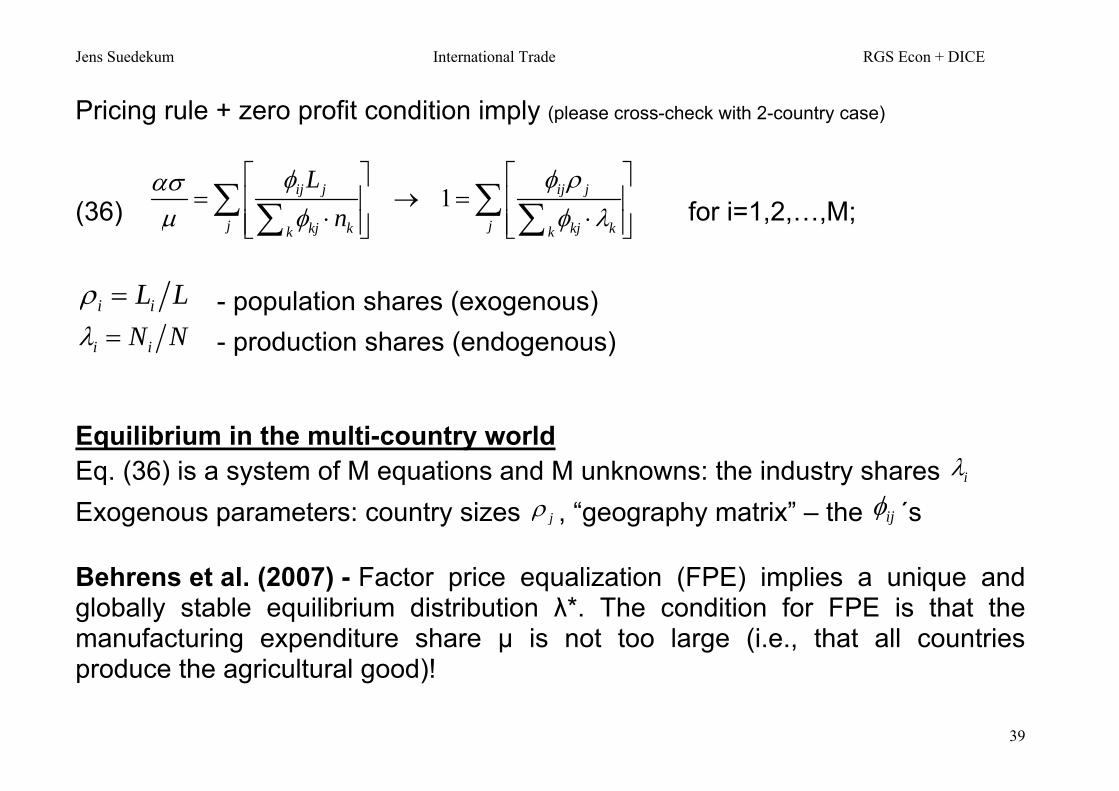
Pricing rule + zero profit condition imply (please cross-check with 2-country case)

(36) 1ij j ij j

j jkj k kj kk k

Ln

for i=1,2,…,M;

i iL L - population shares (exogenous)

i iN N - production shares (endogenous) Equilibrium in the multi-country world Eq. (36) is a system of M equations and M unknowns: the industry shares i Exogenous parameters: country sizes j , “geography matrix” – the ij ´s Behrens et al. (2007) - Factor price equalization (FPE) implies a unique and globally stable equilibrium distribution λ*. The condition for FPE is that the manufacturing expenditure share μ is not too large (i.e., that all countries produce the agricultural good)!


40

Suedekum (2007) - The three-country case (M=3). (37) 1 11 1 12 2 13 3* I I I (analogous expressions for λ2* and λ3*)

(38) 2

2311 2

12 13 12 23 13 23 23

1 ( )1 ( )

I

(39) 12 13 2312 2

12 12 13 13 23 23 13

( )1 ( )

I

(40) 13 12 23

13 212 12 13 13 23 23 121 ( )

I

Assumptions on the (3 3 )-geography matrix: -- 1ii

-- ij ji (symmetric trade costs)

-- ij ik kj ij ik kj for all i,j,k “triangle inequality”: It is not cheaper for producers from country i to ship goods to j via country k.

LEMMA 1: (i) 11 0I , 12 130, 0I I (ii) If 12 13 , then 12 13I I . If, 12 13 then 12 13I I .

If 12 13 , then 12 13 0I I .


41

Third country effects: Foreign expenditure shift Let 2 3dE dE dE . With 1 0dE the effect on the domestic industry share is:

12 131* I I

d dEE

Assume 0dE , 12 13 : expenditure shift away from the more remote foreign country 3 towards the better accessible foreign country 2. Effects: -- Effective market size for firms in country 1 expands, as more consumers are now located closer by → raises profitability, induces entry of firms in country 1 -- Home consumers demand more foreign varieties as transport costs are now lower on average. Price index P1 decreases, inward shift of demand for local varieties → reduces profitability, induces exit of firms in country 1


42

Which effect dominates? Using lemma 1: 12 13 12 13 0I I → Foreign expenditure shift towards the better accessible foreign country negatively affects the domestic industry share! Manifestation of the HME: The shift 0dE will induce the HME in country 2. I.e., the change in the number of firms in country 2 will be relatively stronger than the change in population. This is the intuition why the effect of foreign competition “moving closer” (N2↑, N3↓) dominates the effect that domestic firms have now better access to foreign consumers (L2↑, L3↓), since relatively more firms than consumers/workers change location!


43

The “hub effect” Consider equally large countries (ρ1=ρ2=ρ3=1/3), and suppose the “geography matrix” looks like this:

12 13

12 23

13 23

1 1 0.5 0.31 0.5 1 0.5

1 0.3 0.5 1

→ Country 2 is a “hub”: Trade with country 2 is freer both countries 1 and 3 than trade between countries 1 and 3 (yet, the triangle inequality holds!). Using (37)-(40) and the analogous expressions for λ2* and λ3* one obtains: λ1*= 0.111, λ2*=0.777, λ3*= 0.111 → The hub country hosts a larger industry share than the two non-hub countries! Even though country 2 is not directly larger than countries 1 and 3, it has an advantage in its market potential as foreign demand is not so much distorted by trade costs. This raises the profitability, and thus induces entry of M-firms!

Jens Südekum International Trade RGS Econ + DICE

1

NEW ECONOMIC GEOGRAPHY -- two regions: r=1,2 -- two sectors: A (homogeneous good, CRS, freely traded, pA=1) M (differentiated varieties, Set of Nr firms = varieties in region r, iceberg trade costs) -- two types of workers: L (unskilled labor; works either in A or as the variable input in M; regionally immobile) H (skilled labor; fixed input for a M-firm: 1# of H = 1 firm=1 variety; regionally mobile) Note: This setup is not exactly as in Krugman (1991), who assumes sector specific inputs L↔A, H↔M. But this setup yields similar results as the original Krugman (1991)-model, but is analytically better tractable.1 Profit function of a manufacturing firm in region r is:

,( ) ( ) ( ) ( )M M L Hr r r rj p j x j x j w w

Demand for single varieties, CES price indices are as given above (iso-elastic):

1( ) ( )rr r r rm j Y P p j for r=1,2 local varieties

1( ) ( )rs s s rm j Y P Tp j for r,s=1,2; r≠s imported vars. 1 11 1( ) ( )r r r s sP N p N p

for r,s=1,2; r≠s

1 The fomal equalivalence of Krugman’s core-periphery model and this “footloose entrepreneur”-model by Forslid/Ottaviano (2003) is proven in: Robert-Nicoud, Frederic (2005), “The structure of simple ´new economic geography´ models (or, on identical twins)”, Journal of Economic Geography, Vol. 5, pp. 201-234.


2

Due to isoelastic demand for variety j (both from home and from abroad), we obtain again constant mark-ups ,1( ) , ( ) ( )M L

r r rs rp j w p j T p j

Normalization: β=θ ,( ) M L

r rp j w

Unskilled workers are mobile across industries: ,1A A M L

r r rp w w r=1,2 (Provided both regions produce A)

Hence, manufacturing prices are ( ) 1r rp j p for r=1,2 and for all varieties j The CES price indices simplify to:

(1) 1 11 1 2P N N 1 1

2 1 2P N N Zero-profit condition for a single firm in M-sector implies that wages for skilled workers equal the firm’s operating profits:

(2) ( ) ( ) 0 1 ( ) 1 ( ) ( )M H Hr r rx j x j w w x j x j x j

Market clearing condition for a single variety ( ( ) ( ) ( )rr rsx j m j T m j ):

(3) 1 1* srr r r r s s

r s r s

YYx p Y P Y PN N N N

Hence, wages for skilled workers in region r=1,2 are given by:

(4) 1 2

11 2 1 2

H Y YwN N N N

1 22

1 2 1 2

H Y YwN N N N


3

Specification of factor endowments Let L be the total number of unskilled workers in the country. They are equally split across the two regions, so ρ=L/2 is the fixed factor endowment of both regions with unskilled workers. Let H be the total number of skilled workers (=of M-firms) in the country, where units are chosen such that H=1. The share λ of H initially lives in region 1, the share (1-λ) lives in region 2. In the long-run λ will be endogenous (see below). We have:

(5) 1 1HN L 2 2 (1 )HN L

(6) 1 1HY w 2 21 HY w

The CES price indices P1, P2 from (1) are then given by:

(7) 1 11 1P

1 1

2 1P The CES price indices depend on σ, the trade freeness and on the distribution of skilled workers across regions (on λ). In particular, λ↑ implies P1↓ and P2↑ The more skilled workers (=firms) are located in region 1, the more varieties are produced locally, the fewer varieties have to be imported subject to trade costs; Hence, the lower is the overall price index! → price index effect, supply linkage In the short-run, the location of skilled workers λ is given. In the long-run, skilled workers are mobile across regions and move in response to utility differences. Indirect utility for a skilled worker is given by:

(8)

11H

H rr

r

wVP

The above mentioned supply linkage is thus an agglomeration force!

λ↑ → P1↓ → V1H↑ But what about w1

H?


4

Determination of equilibrium Using (5), (6) in (4) the wage equations simplify to

(9) 21 1

(1 )(1 ) (1 )

HH H ww w

12 2(1 )

(1 ) (1 )

HH Hww w

The two equations in (9) can be solved explicitly for the wages 1

Hw , 2Hw

(10) 1 1* * , , , ,H Hw w 2 2* * , , , ,H Hw w These solutions are complicated and not very revealing (we will see a simpler model below). Yet, recall from (3) that:

1 1*( ) * ( ), ( )H Hr r r r r r s sw w Y P Y P Y P

Let λ=1/2: P1=P2, w1=w2, Y1=Y2, V1=V2 (leaving the superscript “H” from now on for notational convenience) Consider: dλ>0 (λ↑, marginal increase in the number of skilled workers=firms in region 1) → λ↑ → P1↓ P2↑ → ceteris paribus: V1>V2

(“cost-of-living effect”, “supply linkage”, agglomerative) → λ↑ → Y1↑, Y2↓ → w1↑, w2↓ → ceteris paribus: V1>V2

(“market size effect”, “demand linkage”, agglomerative) → P1↓, P2↑→ w1↓, w2↑ → ceteris paribus: V1<V2

(“market crowding effect”, “competition effect”, dispersive)


5

Agglomeration of workers in region 1: -- Lowers consumer price index (more goods are produced locally) -- Increases demand for varieties produced in region 1due to larger market size BALANCE OF EFFECTS DEPENDS ON -- Decreases demand for varieties produced in region 1due to market crowding Using (10) together with (7) in (8) we can also derive an explicit expression for the utility difference:

(11)

1 2

1 2

( , , ), ( , , ), ( , , ), ( , , ),, ,

, , , ,

H Hr r r rw Y P w Y P

P P

“Ad-hoc” dynamics: (1 ) with > 0

Spatial equilibrium A spatial structure λ is an equilibrium if

i) 0 1 and 0 1 20 H HV V symmetry or partial agglomeration

ii) 1, 0 1 2H HV V full agglomeration in region 1

iii) 0, 0 1 2H HV V full agglomeration in region 2

Notice: λ=1/2 is always an equilibrium due to the symmetrical setup of the model!

→ This equilibrium is not necessarily stable! (I.e., the system does not necessarily converge back to λ=1/2 after a small shock dλ>0)


6

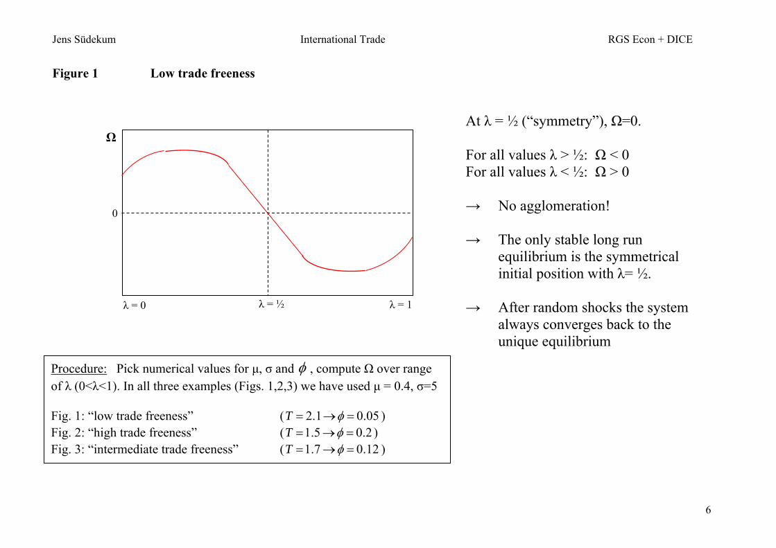
Figure 1 Low trade freeness

0

Ω

λ = 0 λ = 1 λ = ½

At λ = ½ (“symmetry”), Ω=0. For all values λ > ½: Ω < 0 For all values λ < ½: Ω > 0 → No agglomeration! → The only stable long run

equilibrium is the symmetrical initial position with λ= ½.

→ After random shocks the system

always converges back to the unique equilibrium

Procedure: Pick numerical values for μ, σ and , compute Ω over range of λ (0<λ<1). In all three examples (Figs. 1,2,3) we have used μ = 0.4, σ=5 Fig. 1: “low trade freeness” ( 2.1 0.05T ) Fig. 2: “high trade freeness” ( 1.5 0.2T ) Fig. 3: “intermediate trade freeness” ( 1.7 0.12T )


7

Figure 2 “High trade freeness“

0

Ω

λ = 0 λ = 1 λ = ½

At λ = ½ (“symmetry”), Ω=0. For all values λ > ½: Ω > 0 For all values λ < ½: Ω < 0 → Symmetrical equilibrium is

unstable! → Even after a very small random

shock dλ the system converges to a corner equilibrium

→ Indeterminacy in which region

there will be full agglomeration!

→ Cumulative causation! Myrdal, 1957


8

Figure 3 “Intermediate trade freeness“

0

Ω

λ = 0 λ = 1 λ = ½

At λ = ½ (“symmetry”), Ω=0. → Symmetrical equilibrium is

locally stable! → Two unstable equilibria with

partial agglomeration → Multiple (locally) stable equilibria → Path dependency!

Symmetry stable for small shocks, unstable for large shocks


9

Figure 4: Bifurcation diagram Globalization: Exogenous increase of trade freeness. Leads endogenously to agglomeration at the critical

level break (the “break point“), starting from ex-ante identical regions! Reversal of trade integration will not restore symmetry if breaksustain (“history matters“)

½

0

1

sust

The area sust corresponds with Figure 1, the area break with Figure 2, the area sust break with Figure 3. Solid lines : stable equilibra Broken lines : unstable equilibria

break

“Globalization”


10

Analytical derivations of the critical trade freeness levels Since there exists an explicit analytical expression for the utility differential , , (see eq. (11)) we can explicitly compute the following threshold level of

-- the break point: 1

2 ,0 break

This corresponds to the trade freeness level at the transition from fig. 1 to fig. 2 where , , is flat at the symmetrical configuration λ=1/2. We can also analyze the following threshold level:

-- the sustain point: 1, 0 sustain With a tomahawk bifurcation pattern we should have sustain break and this can in fact be verified → See problem set 2 and the corresponding MATHEMATICA-computation!


11

The quasi-linear “footloose entrepreneur” Model of Pflüger (RSUE, 2004) Model identical to footloose entrepreneur-model from Forslid/Ottaviano, with one difference: Functional form of the upper tier utility function. Instead of the Cobb-Douglas type utility function U(M,A), which is used by Krugman and Forslid/Ottaviano, the following quasi linear function is used:

(12) ( , ) ln( )U M A M A μ>0 This assumption implies that all income effect of demand for M-Goods are eliminated. Aggregate demands in region r are: (13) r rM P r rA Y Hence, indirect utility for a mobile “entrepreneur” (with income H

rw in region r) is given by:

(14) ln( ) ln( ) 1H Hr r rV w P

The long-run location decision of mobile entrepreneurs is determined by the regional utility differential:

(15) 1 2 1 2 1 2lnH H H HV V w w P P The same ad-hoc dynamics (1 ) apply.

As before we ensure that , 1L M A A

r r rw w p and that ( ) 1 1rp j


12

Demand for single varieties Recall that the Hicks-demand for a single variety is given by (see lecture notes 1)

( )( ) srsr r

r

p jm j MP

where psr(j)=pr(j) if r=s and psr(j)=Tps(j) if r≠s

Substituting r rM P and using ( ) 1rp j we obtain the following individual Marshall demand functions:

(16) 1( )rr rm j P

1( )rs sm j T P where we have

(17) 1 11 (1 )P 1 1

2 (1 )P Notice that there are no income effects of demand for manufacturing varieties. All income effects arise with the A-good! From the zero profit condition we know that * H

rx w , as in (2). The market clearing condition now commands that:

(18) 1 1 11 2 12 1* Hx L m T L m w 2 2 22 1 21 2* Hx L m T L m w Total population sizes L1 and L2 are incorporated in the market clearing conditions, because the demand curves (16) are for single individuals! Total population sizes are given

(19) 1L 2 1L


13

Analytical solution of the model

Using (16) in (18), the wages 1Hw and 2

Hw are determined as follows:

(20) 1 2

1 1 11 2

H L LwP P

2 12 1 1

2 1

H L LwP P

Using (17) and (19) in (20) we can compute the following simple closed-form solutions for the wages

(21) 1( 1 )

(1 ) 1Hw

2

( ) 1(1 ) 1

Hw

Plugging (21) and (17) in (15) yields an explicit expression for the utility difference Ω , which determines the long-run spatial equilibrium structure:

(22) 1 (1 ), , , (1 ) ln(1 ) 1 1 (1 )

1 2

H Hw w 1 2ln G G


14

Simulation of Eq. (22) – parameter combination: μ=0.3, σ=2, ρ=1

a) Low degree of trade freeness ( 0.01 ) c) intermediate degree of trade freeness ( 0.11 )

b) High degree of trade freeness ( 0.3 )

0.2 0.4 0.6 0.8 1

-2

-1

1

2

0.2 0.4 0.6 0.8 1

-0.075

-0.05

-0.025

0.025

0.05

0.075

0.2 0.4 0.6 0.8 1

-0.0075

-0.005

-0.0025

0.0025

0.005

0.0075

Comparison of the figure c) with the Figure 3 above: With intermediate trade freeness, the symmetrical equilibrium (λ= ½ ) is now locally unstable, and there are two stable equilibria with partial agglomeration (0<λ*< ½, ½<λ*< 1)!


15

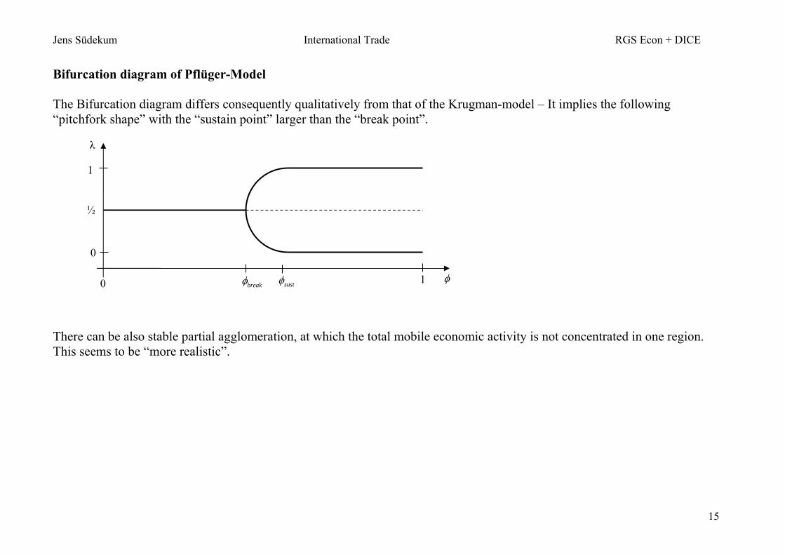
Bifurcation diagram of Pflüger-Model The Bifurcation diagram differs consequently qualitatively from that of the Krugman-model – It implies the following “pitchfork shape” with the “sustain point” larger than the “break point”.

There can be also stable partial agglomeration, at which the total mobile economic activity is not concentrated in one region. This seems to be “more realistic”.

0 break

0

1

½

1

λ

sust


16

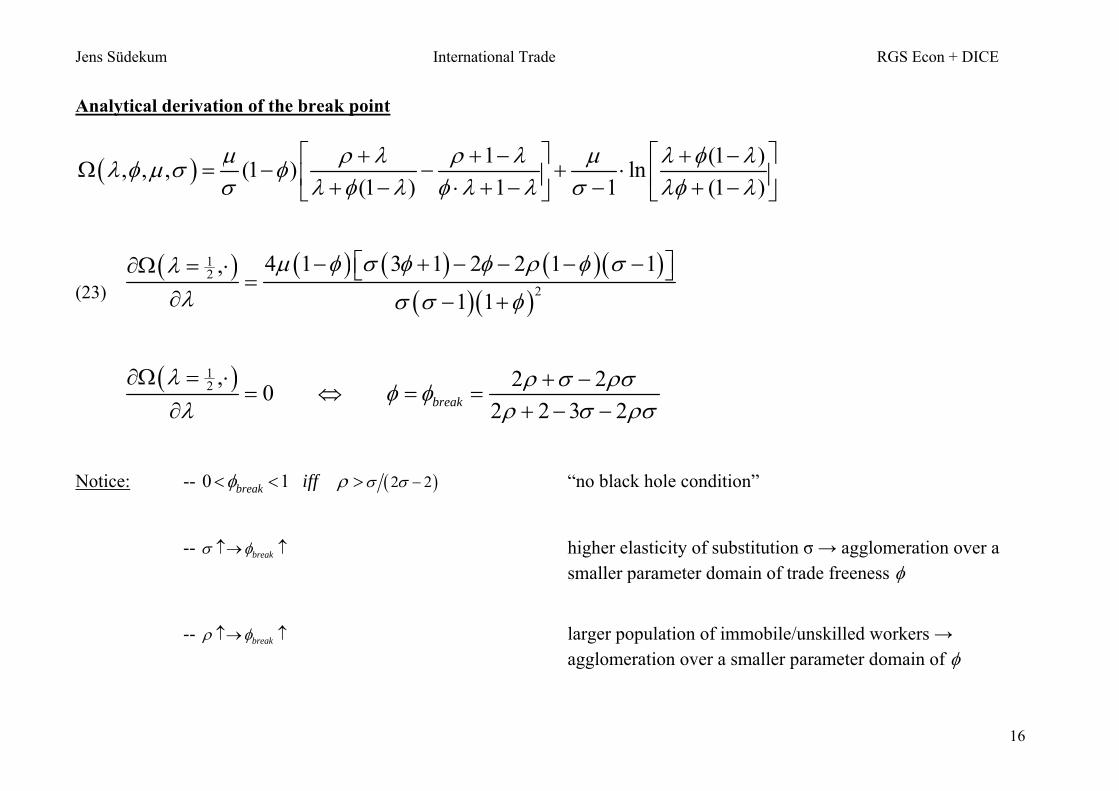
Analytical derivation of the break point

1 (1 ), , , (1 ) ln(1 ) 1 1 (1 )

(23)

12

2

4 1 3 1 2 2 1 1,1 1

1

2 , 2 202 2 3 2break

Notice: -- 2 20 1break iff “no black hole condition” -- break higher elasticity of substitution σ → agglomeration over a smaller parameter domain of trade freeness -- break larger population of immobile/unskilled workers → agglomeration over a smaller parameter domain of


17

Decomposition of the break point analysis Supply Linkage

(24)

1 2

1/2

ln / 4 10

1 1d P P

d

→ “cost-of-living”-effect is agglomerative! An increase in λ lower CES price index in region 1, increases it in region 2.

Demand Linkage and Competition Effect:

(25)

1 2

2

1/2

8 1 1

1

H Hd w wd

Sign unclear!

Eq. (25) is negative if 0 1 , positive if 1 1 , and zero if 1 or 1 .

Reason

1 21 1 1

1 2

H L LwG G

„Demand linkage“, increasing in λ → Agglomerative

“Competition effect”, decreasing in λ → Dispersive


18

Supply Linkage:

4 1

01 1

0.2 0.4 0.6 0.8 1

Demand Linkage:

4 10

1

0.2 0.4 0.6 0.8 1

Competition Effect:

2

2

4 2 1 10

1

0.2 0.4 0.6 0.8 1


19

Interaction of agglomeration- and dispersion forces

Single location forces – components of 1

2 ,

Mb

Supply linkage

Demand linkage + competition effect = nominal wage differential

Housing congestion

Private NAF: Supply linkage + demand linkage + competition effect

Mr 1ˆ


20

Extensions: Housing congestion (Pflüger/Südekum, JUE, 2008) Let B be an immobile housing stock (B=buildings) owned by “absentee landlords”

(26) ( , , ) ln( ) ln( )U M B A M B A This assumption implies that all income effect of demand for M-Goods are eliminated. Aggregate demands in country i are:

(27) r rM P H

r rH p r rA Y Hence, indirect utility for a mobile “entrepreneur” (with income H

r rY w in region r) is given by:

(28) ln( ) ln( )H H Hr r r rV w P p

The long-run location decision of mobile entrepreneurs is determined by regional utility differences:

(29) 1 2 1 2 1 2 1 2ln lnH H H H H HV V w w P P p p Housing market

1 2

1 2

1,H HB B

p p

1

2

ln ln1

H

H

pp

(assuming 1 2B B )


21

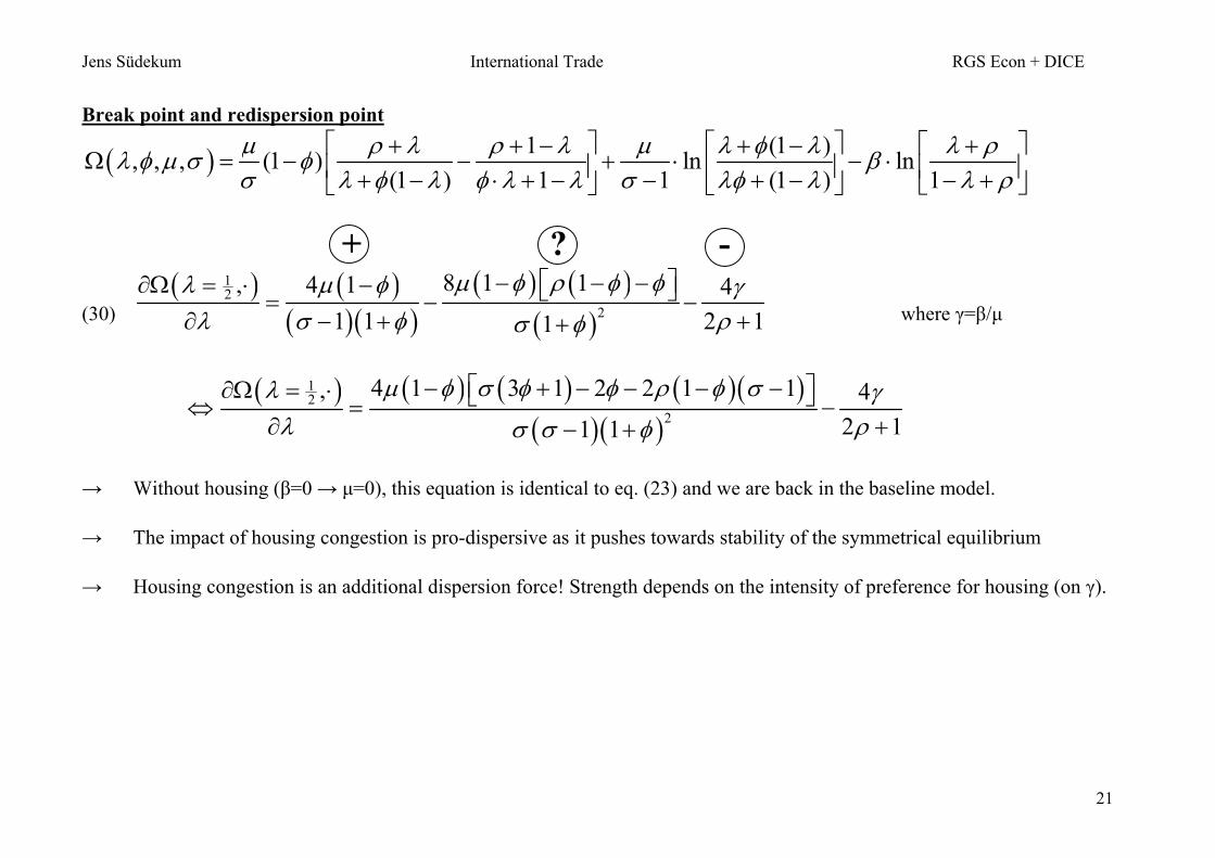
Break point and redispersion point

1 (1 ), , , (1 ) ln ln(1 ) 1 1 (1 ) 1

+ ? -

(30)

12

2

8 1 1, 4 1 41 1 2 11

where γ=β/μ

12

2

4 1 3 1 2 2 1 1, 42 11 1

→ Without housing (β=0 → μ=0), this equation is identical to eq. (23) and we are back in the baseline model.

→ The impact of housing congestion is pro-dispersive as it pushes towards stability of the symmetrical equilibrium

→ Housing congestion is an additional dispersion force! Strength depends on the intensity of preference for housing (on γ).


22

Supply Linkage:

4 1

01 1

0.2 0.4 0.6 0.8 1

Demand Linkage:

4 10

1

0.2 0.4 0.6 0.8 1

Competition Effect:

2

2

4 2 1 10

1

0.2 0.4 0.6 0.8 1

Housing Congestion: 02 1

0.2 0.4 0.6 0.8 1


23

Interaction of agglomeration- and dispersion forces

Mb

Supply linkage

Demand linkage + competition effect = nominal wage differential

Housing congestion

Private NAF: Supply linkage + demand linkage + competition effect

Mr 1ˆ


24

The bubble-shaped bifurcation pattern

12 ,

0 ,break redisp

2

2

1 2 1 2 1 1 4 1 1 1

1 2 1 2 1 2 1Mbreak

2

2

1 2 1 2 1 1 4 1 1 1

1 2 1 2 1 2 1Mredisp

with 0 1M Mbreak redisp iff / 2 2 1 1 0 ; 1 0M

redisp if

Mr

0

1

½

λ

=0 Mb

→ First, globalization endogenously leads to agglomeration; later on to re-dispersion! The initial agglomeration is due to the fact that supply+demand linkage exceed the competition effect beyond a certain level of trade freeness (the break point). As trade becomes even freer, location continues to matter ever less. Yet, the centre has higher housing prices. Beyond a certain point (the redispersion point) it is no longer beneficial for skilled workers (=firms) to concentrate in a single region.

Documents

Jens Suedekum International Trade RGS Econ + DICE · Bangladesh 10.0 3.5 1.7 3.4 8.0 ... → Monopoly, oligopoly, monopolistic competition ... for example, for linear demand curve)