Embed Size (px)
Citation preview
1
Jeffrey Schaller Eastern Connecticut State University
Department of Business Administration 83 Windham St.
Willimantic, CT 06226-2295 [email protected]
(860) 465 - 5226
Jorge M. S. Valente Faculdade de Economia, Universidade do Porto
Rua Dr. Roberto Frias, 4200-464 Porto Portugal
AN EVALUATION OF HEURISTICS FOR SCHEDULING A PERMUTATION FLOW SHOP WITH FAMILY SETUPS TO MINIMIZE TOTAL EARLINESS AND
TARDINESS
ABSTRACT
This paper presents several procedures for developing non-delay schedules for a permutation flow shop with family setups when the objective is to minimize total earliness and tardiness. These procedures consist of heuristics that were found to be effective for minimizing total tardiness in flow shops without family setups, modified to consider family setups and the total earliness and tardiness objective. These procedures are tested on several problem sets with varying conditions. The results show that variable greedy algorithms are effective when solving small problems but using a genetic algorithm that includes a neighborhood defined by the sequence of batches of jobs belonging to the same setup family is effective when solving medium or large sized problems. The results also show that if setup times can be reduced a significant reduction in total earliness and tardiness could result.
Keywords: Scheduling, Flow Shop, Heuristics, Family Setups

2
An Evaluation of Heuristics for Scheduling a Permutation Flow Shop with Family Setups to Minimize Total Earliness and Tardiness 1. Introduction
In many operations obtaining economies of scale is a critical element in achieving
success. Economies of scale are efficiencies in production in which per-unit production
costs increase at a slower rate than production volume. In scheduling, efficiencies that
lead to economies of scale are gained by grouping similar jobs together. The motivation
for grouping sometimes relates to change-over times, or setup times, on the machines.
For example, jobs may belong to families where the jobs in each family tend to be similar
in some way, such as their required tooling. As a result of this similarity, a job does not
need a setup when following another job from the same family, but a known “family
setup time” is required when a job follows a member of some other family. Typically,
there are a large number of jobs, but a relatively small number of families.
The widespread adoption of lean production methods has caused customers to
view early delivery of products as well as tardy delivery to be undesirable. Early
deliveries result in unnecessary inventory that ties up cash as well as space and resources
needed to maintain and manage inventory. Therefore, an important consideration when
sequencing and scheduling a set of jobs is completing each job on the customer’s due
date.
To address these considerations, this paper seeks to identify and compare methods
for sequencing a set of jobs in a permutation flow shop with significant family setup
times that will minimize the total earliness and tardiness of the jobs. Most research on
flow shops has assumed the sequence of jobs to process will be the same on each
machine. These schedules are referred to as permutation schedules. This is done for two
3
reasons. First it simplifies the computational effort and second it is often not practical to
change the sequence of jobs from one machine to the next. In this research only
permutation schedules are considered.
Formally, suppose there is a set of n jobs belonging to F setup families to be
processed in a flowshop consisting of M machines. Let fj, and dj represent the setup
family and the due date of job j (j = 1, …, n) respectively. Let pjm, Sjm, and Cjm represent
the processing time, setup time, and completion time of job j (j = 1, …, n) on machine m
(m = 1, …, M). The earliness of job j, Ej, is defined as: Ej = max {dj – CjM, 0}, for j =
1,…, n and the tardiness of job j, Tj, is defined as: Tj = max {CjM – dj, 0}, for j = 1,…, n.
The objective function, Z, can be expressed as: Z = ∑=
n
j 1
Ej + Tj.
Since the objective in the problem is non-regular, inserting idle time into a
schedule for the jobs can help to reduce the earliness of some jobs and thus improve the
objective. However, in certain production environments, the insertion of idle time may
actually be undesirable, or even impossible. For instance, idle time should be avoided
when the capacity of the shop is limited when compared with the demand. Also, idle time
should not be inserted when the machine has a high operating cost, and / or when starting
a new production run involves high setup costs or times. Some specific examples of
production environments where the insertion of idle time is undesirable have been given
by Korman (1994) and Landis (1993). In this research only non-delay schedules without
unforced inserted idle time are considered. Also, setups for a machine can be performed
in anticipation of a job arriving at a machine, therefore if the job to be sequenced in
position j is denoted as [j] and C[0]1 = 0 then C[j]1 = C[j – 1]1 + p[j]1 if f[j] = f[j – 1] and C[j]1 =
4
C[j – 1]1 + S[j]1 + p[j]1 if f[j] ≠ f[j – 1], and C[j]m = max {C[j]m-1, C[j – 1]m} + p[j]m if f[j] = f[j – 1] and
max { C[j]m-1, C[j – 1]m + S[jm]} + p[j]m if f[j] ≠ f[j – 1] for m = 2, …, M.
Streams of literature that are most relevant to the problem addressed in this paper
are minimizing total earliness and tardiness in a flow shop and scheduling flow shops
with family setup times. A large number of papers have been published on scheduling
models with earliness and tardiness costs. Baker and Scudder (1990) provide an excellent
survey of the initial work on early/tardy scheduling. A recent survey of multi-criteria
scheduling which includes problems with earliness and tardiness penalties is given in
Hoogeveen (2005). Most of the research with an objective based on early and tardy job
completion costs deals with single machine environments. Recent research for single
machine environments with an early/tardy objective and no idle time is summarized in
Valente (2009). Scheduling models with inserted idle time, on the other hand, are
reviewed in Kanet and Sridharan (2000).
Only three papers address objectives based on earliness and tardiness costs in
flow shops. Moslehi et al. (2009) present an optimal procedure for minimizing the sum of
maximum earliness and tardiness in a two-machine flow shop. Chandra et al. (2009)
present approaches for permutation flow shop scheduling with earliness and tardiness
penalties when all the jobs have a common due date. Madhushini et al. (2009) present
branch-and-bound algorithms for scheduling permutation flow shops for a variety of
objectives including minimizing earliness and tardiness without inserted idle time.
An objective that is partially related to the objective considered in this paper is
minimizing total tardiness. The reason the objectives are related is that our objective
includes total tardiness. Vallada et al. (2008) reviewed and tested over 40 heuristic
5
methods for the m-machine flow shop problem with the objective of minimizing total
tardiness. Based on their tests Vallada et al. (2008) found that the neighborhood searches
developed by Kim et al (1996) were the best heuristics and the simulated annealing
algorithms developed by Parthasarathy and Rajendran (1997) and Hasiji and Rajendran
(2004) were the best meta-heuristics. Framinan and Leisten (2008) developed a variable
greedy algorithm for the problem and found it to be more effective in minimizing total
tardiness than the simulated annealing algorithms developed by Parthasarathy and
Rajendran (1997) and Hasija and Rajendran (2004). Vallada and Ruiz (2010) proposed
three genetic algorithms for minimizing total tardiness in permutation flowshops and
performed computational tests for these algorithms and other metaheuristics including
those by Parthasarathy and Rajendran (1997) and Hasija and Rajendran (2004). They
found that two of the genetic algorithms performed the best.
Cheng, Gupta, and Wang (2000) provide a review of flowshop scheduling
research with setup times. Most of the papers identified in this review consider the
objective of minimizing makespan. The only paper that considered an objective that
included total earliness and tardiness was Jorden (1996). In this paper a genetic algorithm
was developed for a two-machine flowshop with family setup times to minimize the sum
of weighted earliness and tardiness penalties.
Section two of the paper describes the proposed scheduling procedures. Section
three presents the computational tests of the procedures as well as the results of the tests.
Section four describes a test to measure the effect of a reduction in setup times and
presents the results. Section five concludes the paper.
6
2. Heuristic Procedures
Six heuristic procedures that are based on procedures that were found to be
effective for minimizing total tardiness in flow shops without family setups are described
in this section. The first two procedures are neighborhood search procedures. Two
procedures are variable greedy algorithms and two are genetic algorithms.
2.1 Neighborhood Search Procedures
Kim et al (1996) developed two neighborhood searches for minimizing total
tardiness in flow shops without family setups. One of the searches used an exchange
operator to define the neighborhood and the other used an insert operator. Two
neighborhood search procedures are presented in this section. The first uses both of the
neighborhood operators developed by Kim et al (1996). This procedure is referred to as
NS in this paper. The second uses the exchange and insert operators on individual jobs
and also uses the exchange and insert operators as well as a consolidate operator on
batches of jobs to define neighborhoods. This procedure is referred to as BNS in this
paper.
In both procedures an initial sequence is developed and then the sequence is
improved by using the neighborhood search operators. The neighborhood search
operators are repeated until none of the moves in a neighborhood offer an improvement.
The algorithms both use the same procedure to find an initial sequence. The initial
sequence is found using a method that is similar to that used in Kim et al (1996) with a
modification to the objective. This procedure is referred to as the IS procedure.
2.1.1 Initial Sequence (IS procedure)
The initial sequence is created in two steps. First a list of the jobs is created. Then,
7
an insertion algorithm is used to create a sequence. To create a list of the jobs they are
first sorted in non-decreasing order of due dates. The insertion algorithm starts by
selecting the first two jobs on the list and two sequences are formed consisting of these
jobs (each job is placed first once and second once). The total earliness and tardiness is
calculated for each of these sequences and the sequence with the lower total earliness and
tardiness is selected as the initial sequence. The insertion step is then repeated n – 2 times
to sequence the remaining jobs. Let k = 3 be the first time the insertion step is performed.
The insertion step is performed as follows. Pick the kth job from the initial list and create
k sequences by inserting this job into each possible position of the sequence while
keeping the relative order of the jobs from the k-1st iteration. The total earliness and
tardiness is then calculated for each of these new sequences. The sequence with the
lowest total earliness and tardiness is selected. If k < n then let k = k + 1 and the insertion
step is repeated with the sequence just selected as the initial sequence. If k = n the phase
stops.
2.1.2 NS Neighborhood Search Improvement Procedure
The NS neighborhood search improvement procedure attempts to improve a
sequence by performing neighborhood searches. The two neighborhood searches used in
Kim et al (1996) are performed. The first search looks at all of the possible exchanges of
pairs of jobs. A sequence of jobs σ is converted into a sequence σ’ by exchanging the
positions of two jobs j and k. If the total earliness and tardiness of sequence σ’ is less
than the total earliness and tardiness of the best sequence found so far (incumbent
sequence) then the incumbent is updated. The second search is an insertion search. Each
job is removed from a sequence σ and then n sequences are created by inserting the job

8
into each possible position while maintaining the relative order of the other jobs. If the
total earliness and tardiness of a sequence is less than the total earliness and tardiness of
the incumbent sequence, then the incumbent is updated.
The two searches are repeated until either of two conditions occurs: 1) both
searches fail to obtain an improvement or 2) a time limit is exceeded. The time limit is set
to n*(M/2)*0.125 seconds. This time limit was based on preliminary computational
experiments and was set for all of the procedures described in this section.
2.1.3 BNS Neighborhood Search Improvement Procedure
The BNS neighborhood search improvement procedure also attempts to improve a
sequence by performing neighborhood searches. Five neighborhood searches are
performed in this procedure. The first two searches are the job exchange and insertion
searches used in Kim et al (1996) and in the NS procedure described in the previous
subsection. The other three searches use search operators that explore the neighborhood
of a sequence based on the batches of jobs in the sequence. A batch of jobs is defined as a
succession of jobs in a sequence that belongs to the same setup family. Let β be a
sequence of batches and TET (β) be the resulting total earliness and tardiness of sequence
β. Let nβ be the number of batches in the sequence β. Three operators are used to explore
the neighborhood of sequence β: Consol, BE and BI.
The Consol operator consolidates batches to eliminate setups. A sequence β’ is
formed using this operator by combining two batches in β and inserting the combined
batch into a position of a batch sequence that maintains the relative order of the non-
combined batches of β. Each possible position for the combined batch is checked. If the
best of the neighborhood batch sequences results in a lower total earliness and tardiness

9
than the batch sequence β then the best batch sequence is retained. The Consol operator is
repeated until it fails to find a better batch sequence.
The BE operator attempts to improve a sequence by exchanging pairs of batches.
A sequence β is converted to a sequence of batches β’ by exchanging the positions of two
batches b1 and b2. If the total earliness and tardiness of the sequence resulting from the
change is less than the total earliness and tardiness of the original sequence the exchange
is retained, otherwise the exchange is reversed.
The BI operator is similar to the job insertion operator. Each batch is removed
from the sequence β and then nβ batch sequences are created by inserting the batch into
each possible position while maintaining the relative order of the other batches. If the
best of the neighborhood batch sequences results in a lower total earliness and tardiness
than the batch sequence β, then the best batch sequence is retained.
A small example with eight jobs and two families is used to demonstrate how the
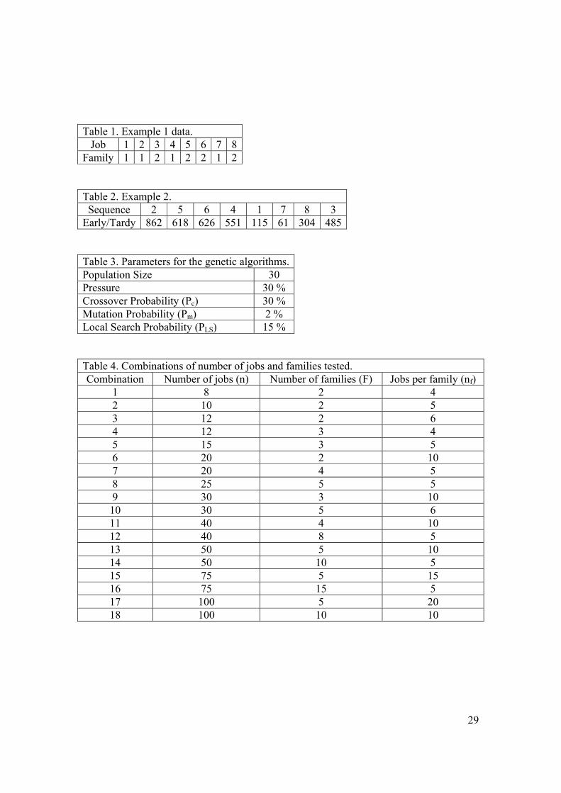
three batch operators create neighborhoods. Table 1 shows the setup family for each job.
[Insert table 1 around here]
If the current sequence is: 5 – 3 – 7 – 1 – 8 – 4 – 2 then there are four batches consisting 5
– 3 (b1), 7 – 1 (b2), 8 – 6 (b3) and 4 – 2 (b4). If the consol operator is to be performed on
batches 2 and 4 (b2 and b4) a new batch is formed 7 – 1 – 4 – 2 and the following three
sequences are checked.
7 – 1 – 4 – 2 – 5 – 3 – 8 – 6
5 – 3 – 7 – 1 – 4 – 2 – 8 – 6
5 – 3 – 8 – 6 – 7 – 1 – 4 – 2

10
The lowest total earliness and tardiness among the sequences above is compared to the
total earliness and tardiness of the current sequence and if it is lower the current sequence
is updated.
If the BE operator is to be performed on batches 2 and 4 then the sequence 5 – 3 – 4 – 2 –
8 – 6 – 7 – 1 is created and checked to see if its total earliness and tardiness is less than
the current sequence’s and if so the current sequence is updated.
If the BI operator is to be performed on batch 2 (b2) then the following sequences are
created.
7 – 1 – 5 – 3 – 8 – 6 – 4 – 2
5 – 3 – 7 – 1 – 8 – 6 – 4 – 2
5 – 3 – 8 – 6 – 7 – 1 – 4 – 2
5 – 3 – 8 – 6 – 4 – 2 – 7 – 1
The lowest total earliness and tardiness among the sequences above is compared to the
total earliness and tardiness of the current sequence and if it is lower the current sequence
is updated.
The five operators are repeated until either of two conditions occurs: 1) all five
operators fail to obtain an improvement or 2) a time limit is exceeded.
2.2 Variable Greedy Algorithm Based on Framinan and Leisten’s (2008) Variable Greedy
Algorithm
A variable greedy algorithm combines features of both the variable neighborhood
search (VNS) and the iterated greedy (IG) algorithm meta-heuristics. An IG algorithm
generates solutions by using a destruction phase and a construction phase on a
constructive heuristic. During the destruction phase k elements are removed from a

11
solution to form a partial solution. During the construction phase a greedy constructive
heuristic obtains a potential new solution by adding the previously removed elements. A
VNS is used to overcome the problem of the IG stalling in a local optimum. When a VNS
is used the size of the neighborhood that will be searched varies or, in the case of
combining VNS with IG, the number of elements k that will be removed and then added
back varies.
Let σ be a sequence and Cj(σ) the completion time of job j in the sequence σ.
Define etj(σ) as the slack of job j in the sequence σ, with etj(σ) = max{dj – Cj(σ), Cj(σ) –
dj}. The following early/tardy-based greedy algorithm, which is based on Framinan and
Leisten (2008)’s slack-based greedy algorithm, is used to obtain a sequence σ’ from
another sequence σ:
1. Remove from σ the k jobs with the largest etj(σ). Sort them in non-increasing
order of etj(σ) and store them in Rk. Let μ be the remaining subsequence after
removing the k jobs.
2. For each job r belonging to Rk, repeat:
2.1 Insert job r in all possible positions of μ. Let υ be the best subsequence
obtained, and b the position of job r in υ.
2.2 Perform an adjacent pairwise exchange among all jobs in positions b + 1 to (n
– k + 1). Let π be the best sequence obtained by this approach. If π is better
than υ then π becomes μ, otherwise υ becomes μ.
3. Set σ’ equal to μ.
12
A small example with eight jobs used to demonstrate the early/tardy-based greedy
algorithm with k = 2. Table 2 shows the sequence σ and the resulting earliness or
tardiness of each job in the sequence.
[Insert table 2 around here]
Since k = 2 R2 = {2, 6} and the initial subsequence is 5 – 4 – 1 – 7 – 8 – 3. Job 2 is
inserted into each possible position of the subsequence creating the following
subsequences: 2 – 5 – 4 – 1 – 7 – 8 – 3, 5 – 2 – 4 – 1 – 7 – 8 – 3, 5 – 4 – 2 – 1 – 7 – 8 – 3,
5 – 4 – 1 – 2 – 7 – 8 – 3, 5 – 4 – 1 – 7 – 2 – 8 – 3, 5 – 4 – 1 – 7 – 8 – 2 – 3, and
5 – 4 – 1 – 7 – 8 – 3 – 2. The subsequence 5 – 4 – 1 – 7 – 8 – 3 – 2 had the lowest total
earliness and tardiness so then job 6 is inserted into each possible position of this
subsequence creating the following sequences: 6 – 5 – 4 – 1 – 7 – 8 – 3 – 2,
5 – 6 – 4 – 1 – 7 – 8 – 3 – 2, 5 – 4 – 6 – 1 – 7 – 8 – 3 – 2, 5 – 4 – 1 – 6 – 7 – 8 – 3 – 2,
5 – 4 – 1 – 7 – 6 – 8 – 3 – 2, 5 – 4 – 1 – 7 – 8 – 6 – 3 – 2, 5 – 4 – 1 – 7 – 8 – 3 – 6 – 2, and
5 – 4 – 1 – 7 – 8 – 3 – 2 – 6. The sequence 5 – 4 – 1 – 7 – 8 – 3 – 2 – 6 had the lowest
total earliness and tardiness so σ is updated to this sequence.
In order to improve the solution generated by the early/tardy-based greedy
algorithm an insertion-based local search is used. The local search generates n positions
at random (without repetition), and for each position the job occupying this position is
removed and inserted in all possible positions.
This variable greedy algorithm is referred to as VGA in this paper. The algorithm
starts with a solution developed by using the IS procedure described in subsection 2.1.1
and performs the early/tardy-based greedy algorithm with k = 1 and the insertion-based
local search. If a better solution is not found k is increased by 1 and the two steps
13
(early/tardy-based greedy algorithm and local search) are repeated. This continues until a
better solution is found or k = n. If a better solution is found, k is set equal to 1. If k = n,
then a random solution is generated and k is set to 1. There are two stopping criteria for
the procedure: 1) if a solution is found with zero total earliness and tardiness the
procedure stops or 2) if a time limit is exceeded the procedure stops.
A second version of the variable greedy algorithm is also proposed. This
algorithm, referred to as VGAB in this paper differs from the VGA procedure by
including the batch insertion neighborhood search (BI) used in the BNS neighborhood
search in addition to the insertion-based local search after the early/tardy-based greedy
algorithm is performed.
2.3 Genetic Algorithms Based on Vallada and Ruiz’s (2010) Genetic Algorithms
A genetic algorithm is a meta-heuristic search procedure that uses a multiple
solution search technique. This approach has been found to quickly generate good
solutions for a wide variety of scheduling problems. In a genetic algorithm, an initial
population of chromosomes is first created, and then successive populations (or
generations) of chromosomes are created using some methodology until a stopping
condition is met. A chromosome corresponds to a solution for the problem. For this
problem, solutions can be represented by a permutation sequence of the jobs. The jth
gene in a chromosome corresponds to the job in the jth position of a sequence.
Vallada and Ruiz (2010) proposed three genetic algorithms for minimizing total
tardiness in permutation flowshops and performed computational tests for these
algorithms and other metaheuristics. They found that the genetic algorithm that used a
crossover operator to generate individuals, called offspring, from two selected
14
progenitors performed the best. Elements of this algorithm include initialization of the
population, a selection mechanism, a crossover operator, mutation operator, generational
scheme, local search, a restart mechanism based on the diversity of the population and the
stopping condition. These elements are described in the following subsection.
2.3.1 Parameters for the genetic algorithms
In each algorithm an initial population of chromosomes (permutation sequences)
is created. Two methods for creating chromosomes are used. The first method is to
randomly generate chromosomes. Each chromosome (sequence) is created by first
generating a random number between 0 and 1 for each job and then sorting the numbers
corresponding to each job (lowest to highest) to create the sequence of jobs
(chromosome). In the second method chromosomes are created by using a heuristic
procedure. This method is used to seed the population with some good individuals. The
proposed algorithm generates one chromosome using the earliest due date (EDD)
dispatching rule and one chromosome using the NEHedd heuristic (Kim 1993b) and the
remaining chromosomes are generated randomly.
A selection operator called n-tournament is used in these algorithms. With this
approach a percentage of individuals, a parameter called “pressure”, is selected and the
individual with the lowest total earliness and tardiness among these individuals is
selected for the mating process.
The mating operator used is one point crossover. The crossover operator is
applied with a Pc probability. Two individuals are generated, called offspring, from two
progenitors (chromosomes) that were selected using the selection operator described in
the previous subsection. First a crossover point is randomly generated using a uniform
15
integer distribution [1, n]. Then, each offspring directly inherits all the jobs from one of
the parents up to the randomly generated crossover point. The last step is to copy the jobs
that are missing from each offspring from the other parent in the same relative order as in
the parent. For example if the crossover point is three and the sequences associated with
the two parents are:
Parent 1 4 – 5 – 2 – 3 – 1 – 6
Parent 2 1 – 2 – 3 – 6 – 5 – 4
The resulting children sequences are:
Child 1 4 – 5 – 2 – 1 – 3 – 6
Child 2 1 – 2 – 3 – 4 – 5 – 6
A shift mutation operator is used. With this operator, each job in a permutation
sequence is extracted with a Pm probability and is inserted in a randomly selected
different position in the sequence.
Two local searches are used in the genetic algorithms. The first local search is the
job insertion search used in the neighborhood search procedures. This search is referred
to as JI. In this search, a job is removed from the sequence and is inserted into all n
positions. The final position of the job is the position that results in the lowest total
earliness and tardiness. This search is carried out for all n jobs of each generated
offspring after the mating and mutation operators have been applied. The JI search is also
applied to the best individual found in the initial generation of the population. All of the
genetic algorithms proposed in this research use the JI local search. The second local
search is the batch insertion search used in the BNS neighborhood search. This local
search is referred to as BI. Each batch is removed from the sequence of batches and then

16
nβ batch sequences are created by inserting the batch into each possible position while
maintaining the relative order of the other batches. The final position of the batch is the
position that results in the lowest total earliness and tardiness. If this search is
incorporated in a genetic algorithm it is carried out after the JI local search has been
performed. The local searches are applied with a PLS probability.
There are two criteria for accepting generated offspring into the population: 1) an
offspring must be better (have a lower total earliness and tardiness) than the worst
individual in the population and 2) the offspring has a unique sequence (there are no
other individuals in the population with the same sequence).
A diversity measure is used to determine if a restart mechanism should be
initiated for the algorithm. If the individuals in a population become too similar the
algorithm may fail to evolve to better solutions. To avoid this condition the population is
reinitialized by randomly generating new individuals with the exception of the
individuals created in the initial population with heuristics. This occurs when the
diversity measure falls below a certain value. See Vallada and Ruiz (2010) for a
description of the diversity measure.
Two stopping criteria are used: 1) if a solution is found with zero total earliness
and tardiness the procedure stops and 2) if the time limit is exceeded when a generation is
completed the procedure stops.
Vallada and Ruiz (2010) conducted a statistical experiment to select the values for
the genetic algorithm to minimize total tardiness. After doing some preliminary
computational experiments we found that the parameters used by Vallada and Ruiz

17
(2010) are also effective for minimizing total earliness and tardiness with family setups.
The values for the parameters are shown in table 3.
[Insert table 3 around here]
2.3.2 Genetic Algorithms
Two versions of the genetic algorithm are proposed. The procedure referred to as
GADV is Vallada and Ruiz (2010)’s genetic algorithm that uses the one point crossover
mating operator but is modified to incorporate family setups and the total earliness and
tardiness objective. The GADVB procedure is the same as the GADV procedure except
that both the JI and BI local searches are used.
3. Computational Tests of the Procedures
3.1 Data and Performance Measures
The procedures described in the previous section were tested on problems of
various sizes in terms of the number of jobs, number of families and jobs within each
family, number of machines, for six sets of distributions of due date range and tightness,
and three sets of distributions for family setup times. Each problem set consists of 10
problems. The problems within a problem set have the same number of jobs, number of
families, number of jobs per family, same number of machines, family setup times are
drawn from the same distribution, and the due dates for the jobs are generated using the
same distribution.
Eleven levels of number of jobs (n) were included in the test. Some levels of job
number had two levels of number of families (F) and jobs per family (nf). This resulted in
eighteen combinations which are shown in table 4.
[Insert Table 4 around Here]
18
Three levels of number of machines were tested: m = 5, m = 10 and m = 15.
The processing times of the jobs for each machine were generated using a uniform
distribution over the integers 1 and 100. The setup times on each machine for each family
were randomly generated using a uniform distribution. Three setup distributions were
used. The first setup distribution (1) generated setups over the integers 1 and 50, the
second (2), over the integers 1 and 100, and the third (3), over the integers 1 and 200. The
due dates for the jobs were also randomly generated using a uniform distribution over the
integers MS (1 – r – R/2) and MS (1 – r + R/2), where MS is an estimated minimum
makespan found for the problem using a heuristic developed by Schaller (2000), and R
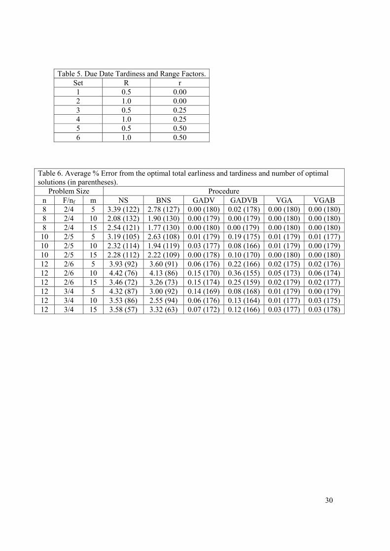
and r are two parameters called due date range and tardiness factors. Six sets of these
parameters were used for each n, F, nf, and m combination and are shown in table 5.
[Insert Table 5 around Here]
The levels of the test factors result in (18*3*6*3*10) 9720 problems in the test. The
procedures were coded in Turbo Pascal and were tested on a Dell Inspiron 1525 1.6 GHz
Lap Top computer for all of the problem sets.
For small sized problems (n = 8, 10 and 12) a branch and bound algorithm was
used to obtain the optimal total earliness and tardiness. The measures of performance
used to evaluate the procedures for the test problems are CPU time required to generate a
solution, the percentage error (% Error) of the total earliness and tardiness of the solution
generated by each procedure compared to the optimal total earliness and tardiness for the
problem and the number of optimal solutions generated by each procedure for the small
sized problems, and the percentage difference (% Diff) of the total earliness and tardiness
of the solution generated by each procedure compared to the total earliness and tardiness
19
of the solution generated by NS procedure for the large sized problems. The percentage
error calculates the percentage the total earliness and tardiness of the solution obtained by
the heuristic procedure is greater than the optimal total earliness and tardiness. % Error =
[(Zh - ZO)/ ZO] * 100, where ZO = optimal the total earliness and tardiness for the
problem, and Zh = the total earliness and tardiness of the solutions generated by the
heuristic procedures. % Diff = [(Zh - ZNS)/ ZNS] * 100, where ZNS = the total earliness and
tardiness for the problem obtained by the NS procedure, and Zh = the total earliness and
tardiness of the solutions generated by the other heuristic procedures.
3.2 Results of the Test
Table 6 shows the average percentage the total earliness and tardiness of each
procedure’s solutions are greater than the total earliness and tardiness of the optimal
solution for each of the small problem sizes (n = 8, 10 and 12) and the number of times
each procedure generated an optimal solution for each problem size.
[Insert Table 6 around Here]
The two versions of the variable greedy algorithm performed best for these
problem sizes and had average percent errors of less than one tenth of one percent for
each of these problem sizes. The variable greedy algorithms also found the most optimal
solutions. Both of the variable greedy algorithms found optimal solutions for over 95% of
the problems on each of these problem sizes. The two versions of the Genetic algorithm
also performed very well. The GADV procedure had average percent errors of less than
0.2 percent for each of these problem sizes and solved over 95% of the problems
optimally, and the GADVB procedure had average percent errors of less than 0.4 percent,
and solved over 93% of the problems optimally. The two neighborhood search

20
procedures found optimal solutions for less than 75% of the problems for each problem
size and had percent errors between one and five percent for each problem size.
One of the reasons the variable greedy and genetic algorithms performed better
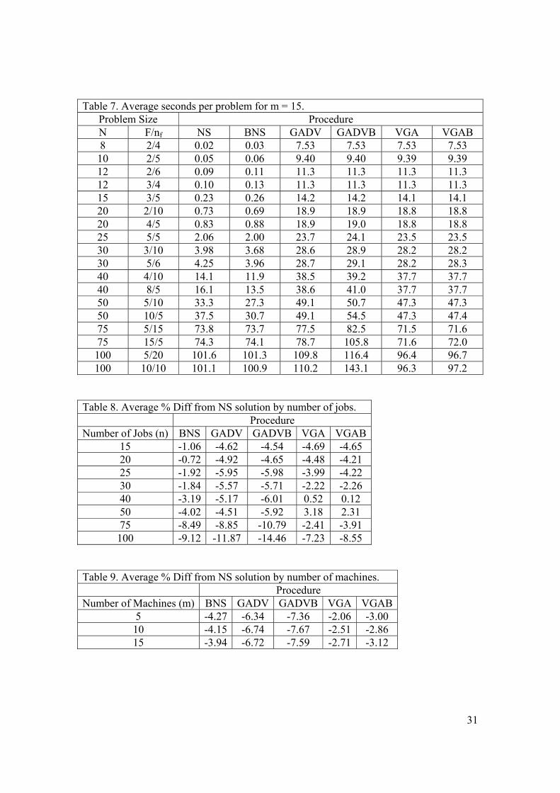
for the small problem sizes is that they used more time to generate solutions. Table 7
shows the average number of seconds per problem each procedure used to generate a
solution for each problem size when m = 15.
[Insert Table 7 around Here]
Since the time required by each of the procedures to generate solutions was relatively
linear with respect to the number of machines the results for m = 5 and 10 are omitted.
The variable greedy and genetic algorithms continue until the time limit criteria for
stopping is reached whereas the neighborhood searches terminate much more quickly on
the small problem sizes. The neighborhood searches usually terminate before the time
limit stopping criteria is reached for problem sizes consisting of 50 jobs or less.
Table 8 shows the Average % Diff measure for each level of n for problems with
15 or more jobs.
[Insert table 8 around here]
Figure 1 plots these results. For problem sizes up to 20 jobs the genetic and variable
greedy algorithms perform best and are relatively close. When n > 20, the genetic
algorithms performed the best. As n increases the relative performance of the GADVB
procedure improves and is the best when n ≥ 25. When n = 75 or 100 the % Diff for the
GADVB procedure was greater than 10%. Although the variable greedy algorithms are
best when n is low their performance decline rapidly as n initially is increased and for n =
40 and 50 were worse than even the NS procedure.
21
The use of a batch neighborhood search proved to be beneficial as problem size
increased. The BNS procedure outperformed the NS procedure for all problem sizes. The
GADVB procedure outperformed the GADV procedure when n ≥ 25 and the VGAB
procedure also outperformed the VGA procedure when n ≥ 25.
Table 9 shows the Average % Diff measure for each level of number of machines
(m).
[Insert table 9 around here]
Figure 2 plots these results. The number of machines did not appear to affect the relative
quality of the solutions generated by the procedures as the average % Diff’s of the
procedures are consistent across the three levels of machines. For each level of m the
ranking of the procedures is: 1) GADVB, 2) GADV, 3) BNS, 4) VGAB, and 5) VGA.
These results also show the advantage of including batch neighborhood searches as the
procedures that included a batch neighborhood search outperformed the corresponding
procedure that did not.
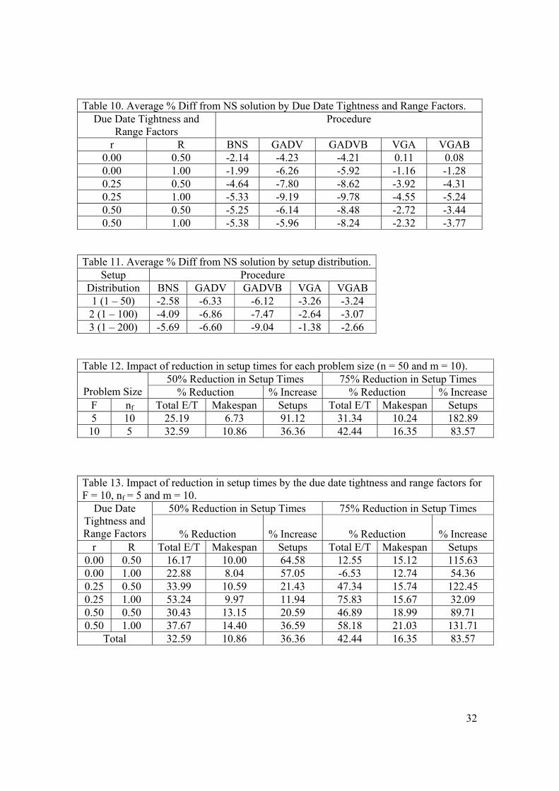
Table 10 shows the Average % Diff measure for each of the due date tightness
and range factors.
[Insert table 10 around here]
Figure 3 plots the results for the Average % Diff measure by due date tightness factor and
figure 4, by due date range factor. These results also show that the genetic algorithms
performed best followed by the BNS procedure. The performance of the procedures
compared to the NS procedure improves when R = 1.00 and when r > 0.00.
Table 11 shows the Average % Diff measure for each level setup distribution.
[Insert table 11 around here]
22
Figure 5 plots these results. These results also show that the genetic algorithms perform
best. It can also be seen that including a batch neighborhood search becomes more
beneficial as the size of setups are increased as the relative performance of procedures
with a batch neighborhood search improves compared to their counterparts without a
batch neighborhood search.
To summarize the results the genetic and variable greedy algorithms generate the
best solutions for small sized problems but as the number of jobs increases the GADVB
procedure generates the best solutions. The GADVB procedure was also consistently best
over all levels of number of machines and setup distributions and the genetic algorithms
were best for all the due date tightness and range factors. Procedures with a batch
neighborhood search consistently outperformed the corresponding procedure that did not
include a batch neighborhood search.
4. Impact of a Reduction in Setup Times on Total Earliness and Tardiness
It is commonly recognized that the existence of long setup times is a negative
factor in production operations. Long setup times are associated with increased costs for
performing the setups, and since production equipment is not producing during the setup,
long setup times also reduce production capacity, which represents an opportunity cost.
To help offset the cost and reduction of production capacity caused by long family
setups, jobs belonging to the same setup families are batched and produced together,
thereby reducing the total number of setups and the time spent setting up. This batching
of jobs makes it difficult to match the production of individual jobs with their due dates.
Some jobs in a batch are produced before their due dates and have to be held in inventory
which is a form of waste. Also these early jobs are using production capacity that could
23
be used to produce jobs that have current due dates and hence are delayed so that they
become tardy. This is another form of waste. Shingo (1985) developed a set of principles
called Single Minute Exchange of Die (SMED) to reduce setup times. These principles
are relatively easy to implement and have been widely utilized to reduce setup times.
Setup time reductions of 50% to 75% are very common utilizing this approach. This
section describes a test to help determine how reducing setup times using methods such
as SMED in permutation flow shops affects the total earliness and tardiness incurred.
Data for the test was created in a fashion similar to that described in section 3.1.
Problems were created for the problem size parameters: n = 50, F = 5, nf = 10 for all f = 1
to F, m = 10; and n = 50, F = 10, nf = 5 for all f = 1 to F, and m = 10. Each problem set
consisted of 10 problems. The processing times for the jobs in each problem were
generated as described in section 3.1 with a uniform distribution over the integers 1 and
100. Setup times for each family on each machine were generated in two steps. In the
first step a number is generated using a uniform distribution over the integers 1 and 50.
Then in the second step the number generated is multiplied by four to obtain the setup
time. The due dates for the jobs were randomly generated using the approach described in
section 3.1 and the same six sets of due date range and tightness were used. For each
problem that was created, two additional problems were created. Both of the additional
problems consisted of the same data as the original problem with the exception of the
setup times. One problem was created by copying the data from the original problem and
dividing the setup times by two (a 50% reduction) and the other problem was created by
copying the data from the original problem and dividing the setup times by four (a 75%
reduction).

24
Since the GADVB procedure performed the best for the problems with 50 jobs (n
= 50), it was used to generate a solution for each problem and the resulting total earliness
and tardiness, makespan and the number of setups were recorded. Table 12 shows results
for each problem size.
[Insert Table 12 around Here]
The table shows the percent reduction in total earliness and tardiness and
makespan and the percent increase in the total number of setups when the setup times
were reduced 50% and 75%. The results show that there were large decreases in total
earliness and tardiness and large increases in the number of setups for each problem size
when there was a 50% reduction in setup times. When the reduction in setup times was
75% there was a further reduction in total earliness and tardiness and the increase in the
number of setups was significant even when compared to those of the 50% reduction in
setup times. The makespan was decreased with the 50% reduction in setup times and was
further decreased with the 75% reduction in setup times but not as significantly as the
decrease in total earliness and tardiness. The reason why the makespans did not decrease
by a larger amount can be attributed to the increase in the number of setups which offsets
some of the reduction in setup times.
The due date tightness and range factors affects these results. To illustrate how
these factors affect total earliness and tardiness, makespan and the number of setups as
setup time is reduced, table 13 shows the results for each set of due date range and
tightness factors for the F = 10, nf = 5 and m = 10 problem size.
[Insert Table 13 around Here]
25
The results in this table show the due date tightness and range factors affect the results in
terms of total earliness and tardiness obtained when setup times are reduced. When the
due date tightness factor is very low (r = 0.00) the reduction in total earliness and
tardiness when setup times are reduced by 50% is considerably less than when the due
date tightness factor is set at higher levels (r = 0.25 or 0.50). When r = 0.00 and setup
times are reduced by 75% the total earliness and tardiness actually increases compared to
the 50% setup reduction and in the case of r = 0.00 and R = 1.00 the total earliness and
tardiness is higher than when there is no reduction in setup times. When the due date
tightness factor is set at 0.25 or 0.50 the reduction in total earliness and tardiness is very
high with a 50% reduction in setup times and is substantially higher when the reduction
in setup times is 75%. Also, the reduction in total earliness and tardiness is greater when
R = 1.00. The restriction that only non-delay schedules are considered is an important
factor contributing to these results. When due dates are loose and there is excess capacity
then as setup times are reduced there is even greater excess capacity and several jobs are
completed earlier even if additional setups are used causing the early completion penalty
to increase. It would be interesting to see how removing the restriction that only non-
delay schedules are considered affects total earliness and tardiness when setup times are
reduced. The results of the current test show that when capacity is reasonably matched
with the demand, a reduction in setup times allows for a better matching of production of
jobs with their due dates enabling a much lower total earliness and tardiness to be
achieved.
26
5. Conclusion
In this paper several heuristics that were based on procedures found to be
effective for minimizing total tardiness in permutation flow shops were proposed for
minimizing total earliness and tardiness for permutation flow shops with family setups.
These heuristics included neighborhood searches, variable greedy algorithms and genetic
algorithms.
The proposed procedures were tested on problems of various sizes in terms of the
number of jobs, number of families included, and the number of machines. Also
considered were three distributions of family setups and six sets of distributions that
determine the tightness and range of due dates. The solutions generated were compared
against optimal solutions for small sized problems and the solutions found by one of the
procedures for large sized problems.
The results of the tests showed that the variable greedy algorithms were very
effective for the small sized problems. The best performing procedure for larger sized
problems was a genetic algorithm (GADVB) that included a neighborhood of batch
sequences in addition to a neighborhood search for job sequences. Also, incorporating a
batch sequence local search into the various algorithms improved their performance.
A test was also conducted to see the effect of reducing setup times on the total
earliness and tardiness obtained in scheduling. It was found that if setup times are
reduced, then total earliness and tardiness can be significantly reduced. The reduction in
total earliness and tardiness is achieved not only from additional effective capacity
obtained by reducing setup times, but also utilizing the resources more effectively by
scheduling smaller batches of jobs belonging to each family so that production of
27
individual jobs is better matched to their due dates. The test also showed that the
tightness of the due dates affected the reduction in total earliness and tardiness when
setup times are reduced. When there was excess capacity and due dates were not tight
reducing setup times did not impact earliness and tardiness as much as when capacity was
tighter. This could be due in large part to the restriction that only non-delay schedules
were considered. It would be interesting to approach the problem where non-delay
schedules are considered and the use of unforced inserted idle time is permitted. This
would be a productive area for future work.
References
Baker, K.R. and Scudder, G.D. (1990) ‘Sequencing with earliness and tardiness penalties: a review’, Operations Research, Vol. 38, pp.22–36. Chandra, P., P. Mehta, and D. Tirupati, (2009). Permutation flow shop scheduling with earliness and tardiness penalties, International Journal of Production Research, 47 (20): 5591 – 5610. Cheng, T. C. E., J. N. D. Gupta, and G Wang, (2000). A review of flowshop scheduling research with setup times, Production and Operations Management, 9 (3): 262 – 282. Framinan, J. M., and R. Leisten, (2008). Total tardiness minimization in permutation flowshops: a simple approach based on a variable greedy algorithm, International Journal of Production Research, 46 (22): 6479 – 6498. Hasija, S., and C. Rajendran, Scheduling in flowshops to minimize total tardiness of jobs, (2004). International Journal of Production Research, 42: 2289 – 2301. Hoogeveen, H. (2005) Multicriteria scheduling, European Journal of Operational Research, Vol. 167, pp.592–623. Jorden, C., (1996). Batching and Scheduling: Models and Methods for Several Problem Classes, Springer, Berlin, Germany, 1996. Kanet, J.J. and Sridharan, V. (2000) ‘Scheduling with inserted idle time: problem taxonomy and literature review’, Operations Research, Vol. 48, pp.99–110. Kim, Y., (1993b). Heuristics for flowshop scheduling problems minimizing mean tardiness, Journal of Operational Research Society, 44:19 – 28.
28
Kim, Y., H. G. Lim, and M. W. Park, (1996). Search heuristics for a flowshop scheduling problem in a printed circuit board assembly process, European Journal of Operational Research, 91: 124 – 143. Korman, K. (1994) ‘A pressing matter’, Video, pp.46–50. Landis, K. (1993) Group Technology and Cellular Manufacturing in the Westvaco Los Angeles VH Department, Project report in IOM 581, School of Business, University of Southern California. Madhushini, N., C. Rajendran, and Y. Deepa, (2009). Branch-and-bound algorithms for scheduling in permutation flowshops to minimize the sum of weighted flowtime/sum of weighted tardiness/sum of weighted flowtime and weighted tardiness/sum of weighted flowtime, weighted tardiness and weighted earliness of jobs, Journal of the Operational Research Society, 60: 991 – 1004. Moslehi, G., Mirzaee, M., Vasei, M., and A. Azaron, Two-machine flow shop scheduling to minimize the sum of maximum earliness and tardiness, International Journal of Production Economics, 2009; 122: 763 – 773. Parthasarathy, S., and C. Rajendran, (1997). A simulated annealing heuristic for scheduling to minimize mean weighted tardiness in a flowshop with sequence-dependent setup times of jobs – A case study. Production Planning and Control, 8: 475 – 483. Schaller, J. E., (2000). A comparison of heuristics for family and job scheduling in a flow-line manufacturing cell, International Journal of Production Research, 38: 287 – 308. Valente, J. M. S., Beam search heuristics for the single machine scheduling problem with linear earliness and quadratic tardiness costs, Asia-Pacific Journal of Operational Research, 2009; 26: 319 – 339. Vallada, E., R. Ruiz, and G. Minella, (2008). Minimising total tardiness in the m-machine flowshop problem: A review and evaluation of heuristics and metaheuristics, Computers & Operations Research, 4: 1350. Vallada, E., and R. Ruiz, (2010). Genetic algorithms with path relinking for the minimum tardiness permutation flowshop problem, Omega, 38: 57 – 67.
29
Table 1. Example 1 data. Job 1 2 3 4 5 6 7 8
Family 1 1 2 1 2 2 1 2
Table 2. Example 2. Sequence 2 5 6 4 1 7 8 3
Early/Tardy 862 618 626 551 115 61 304 485
Table 3. Parameters for the genetic algorithms.Population Size 30 Pressure 30 % Crossover Probability (Pc) 30 % Mutation Probability (Pm) 2 % Local Search Probability (PLS) 15 % Table 4. Combinations of number of jobs and families tested. Combination Number of jobs (n) Number of families (F) Jobs per family (nf)
1 8 2 4 2 10 2 5 3 12 2 6 4 12 3 4 5 15 3 5 6 20 2 10 7 20 4 5 8 25 5 5 9 30 3 10
10 30 5 6 11 40 4 10 12 40 8 5 13 50 5 10 14 50 10 5 15 75 5 15 16 75 15 5 17 100 5 20 18 100 10 10
30
Table 5. Due Date Tardiness and Range Factors.Set R r 1 0.5 0.00 2 1.0 0.00 3 0.5 0.25 4 1.0 0.25 5 0.5 0.50 6 1.0 0.50
Table 6. Average % Error from the optimal total earliness and tardiness and number of optimal solutions (in parentheses).
Problem Size Procedure n F/nf m NS BNS GADV GADVB VGA VGAB 8 2/4 5 3.39 (122) 2.78 (127) 0.00 (180) 0.02 (178) 0.00 (180) 0.00 (180) 8 2/4 10 2.08 (132) 1.90 (130) 0.00 (179) 0.00 (179) 0.00 (180) 0.00 (180) 8 2/4 15 2.54 (121) 1.77 (130) 0.00 (180) 0.00 (179) 0.00 (180) 0.00 (180) 10 2/5 5 3.19 (105) 2.63 (108) 0.01 (179) 0.19 (175) 0.01 (179) 0.01 (177) 10 2/5 10 2.32 (114) 1.94 (119) 0.03 (177) 0.08 (166) 0.01 (179) 0.00 (179) 10 2/5 15 2.28 (112) 2.22 (109) 0.00 (178) 0.10 (170) 0.00 (180) 0.00 (180) 12 2/6 5 3.93 (92) 3.60 (91) 0.06 (176) 0.22 (166) 0.02 (175) 0.02 (176) 12 2/6 10 4.42 (76) 4.13 (86) 0.15 (170) 0.36 (155) 0.05 (173) 0.06 (174) 12 2/6 15 3.46 (72) 3.26 (73) 0.15 (174) 0.25 (159) 0.02 (179) 0.02 (177) 12 3/4 5 4.32 (87) 3.00 (92) 0.14 (169) 0.08 (168) 0.01 (179) 0.00 (179) 12 3/4 10 3.53 (86) 2.55 (94) 0.06 (176) 0.13 (164) 0.01 (177) 0.03 (175) 12 3/4 15 3.58 (57) 3.32 (63) 0.07 (172) 0.12 (166) 0.03 (177) 0.03 (178)
31
Table 7. Average seconds per problem for m = 15. Problem Size Procedure N F/nf NS BNS GADV GADVB VGA VGAB 8 2/4 0.02 0.03 7.53 7.53 7.53 7.53
10 2/5 0.05 0.06 9.40 9.40 9.39 9.39 12 2/6 0.09 0.11 11.3 11.3 11.3 11.3 12 3/4 0.10 0.13 11.3 11.3 11.3 11.3 15 3/5 0.23 0.26 14.2 14.2 14.1 14.1 20 2/10 0.73 0.69 18.9 18.9 18.8 18.8 20 4/5 0.83 0.88 18.9 19.0 18.8 18.8 25 5/5 2.06 2.00 23.7 24.1 23.5 23.5 30 3/10 3.98 3.68 28.6 28.9 28.2 28.2 30 5/6 4.25 3.96 28.7 29.1 28.2 28.3 40 4/10 14.1 11.9 38.5 39.2 37.7 37.7 40 8/5 16.1 13.5 38.6 41.0 37.7 37.7 50 5/10 33.3 27.3 49.1 50.7 47.3 47.3 50 10/5 37.5 30.7 49.1 54.5 47.3 47.4 75 5/15 73.8 73.7 77.5 82.5 71.5 71.6 75 15/5 74.3 74.1 78.7 105.8 71.6 72.0 100 5/20 101.6 101.3 109.8 116.4 96.4 96.7 100 10/10 101.1 100.9 110.2 143.1 96.3 97.2
Table 8. Average % Diff from NS solution by number of jobs.
Procedure Number of Jobs (n) BNS GADV GADVB VGA VGAB
15 -1.06 -4.62 -4.54 -4.69 -4.65 20 -0.72 -4.92 -4.65 -4.48 -4.21 25 -1.92 -5.95 -5.98 -3.99 -4.22 30 -1.84 -5.57 -5.71 -2.22 -2.26 40 -3.19 -5.17 -6.01 0.52 0.12 50 -4.02 -4.51 -5.92 3.18 2.31 75 -8.49 -8.85 -10.79 -2.41 -3.91
100 -9.12 -11.87 -14.46 -7.23 -8.55 Table 9. Average % Diff from NS solution by number of machines.
Procedure Number of Machines (m) BNS GADV GADVB VGA VGAB
5 -4.27 -6.34 -7.36 -2.06 -3.00 10 -4.15 -6.74 -7.67 -2.51 -2.86 15 -3.94 -6.72 -7.59 -2.71 -3.12
32
Table 10. Average % Diff from NS solution by Due Date Tightness and Range Factors. Due Date Tightness and
Range Factors Procedure
r R BNS GADV GADVB VGA VGAB 0.00 0.50 -2.14 -4.23 -4.21 0.11 0.08 0.00 1.00 -1.99 -6.26 -5.92 -1.16 -1.28 0.25 0.50 -4.64 -7.80 -8.62 -3.92 -4.31 0.25 1.00 -5.33 -9.19 -9.78 -4.55 -5.24 0.50 0.50 -5.25 -6.14 -8.48 -2.72 -3.440.50 1.00 -5.38 -5.96 -8.24 -2.32 -3.77
Table 11. Average % Diff from NS solution by setup distribution.
Setup Procedure Distribution BNS GADV GADVB VGA VGAB 1 (1 – 50) -2.58 -6.33 -6.12 -3.26 -3.24
2 (1 – 100) -4.09 -6.86 -7.47 -2.64 -3.07 3 (1 – 200) -5.69 -6.60 -9.04 -1.38 -2.66
Table 12. Impact of reduction in setup times for each problem size (n = 50 and m = 10).
Problem Size
50% Reduction in Setup Times 75% Reduction in Setup Times % Reduction % Increase % Reduction % Increase
F nf Total E/T Makespan Setups Total E/T Makespan Setups 5 10 25.19 6.73 91.12 31.34 10.24 182.89 10 5 32.59 10.86 36.36 42.44 16.35 83.57
Table 13. Impact of reduction in setup times by the due date tightness and range factors for F = 10, nf = 5 and m = 10.
Due Date Tightness and Range Factors
50% Reduction in Setup Times 75% Reduction in Setup Times
% Reduction
% Increase
% Reduction
% Increase r R Total E/T Makespan Setups Total E/T Makespan Setups
0.00 0.50 16.17 10.00 64.58 12.55 15.12 115.63 0.00 1.00 22.88 8.04 57.05 -6.53 12.74 54.36 0.25 0.50 33.99 10.59 21.43 47.34 15.74 122.45 0.25 1.00 53.24 9.97 11.94 75.83 15.67 32.09 0.50 0.50 30.43 13.15 20.59 46.89 18.99 89.71 0.50 1.00 37.67 14.40 36.59 58.18 21.03 131.71
Total 32.59 10.86 36.36 42.44 16.35 83.57
33
34
35