Jeffrey M. Wooldridge-Introductory Econometrics A … M...G E F P H 314 Regression Analysis with Time Series Data 10-2a Static Models S KM K NJL that we have time series data available

312

In �� n � �� n� ��n�� n � ��

using time series data. In Section 10-1, we discuss some conceptual differences between time series

and cross-sectional data. Section 10-2 provides some examples of time series regressions that are

often estimated in the empirical social sciences. We then turn our attention to the finite sample prop-

erties of the OLS estimators and state the Gauss-Markov assumptions and the classical linear model

assumptions for time series regression. Although these assumptions have features in common with

those for the cross-sectional case, they also have some significant differences that we will need to

highlight.

In addition, we return to some issues that we treated in regression with cross-sectional data, such

as how to use and interpret the logarithmic functional form and dummy variables. The important top-

ics of how to incorporate trends and account for seasonality in multiple regression are taken up in

Section 10-5.

10-1 The Nature of Time Series Data

An obvious characteristic of time series data that distinguishes them from cross-sectional data is tem-

poral ordering. For example, in Chapter 1, we briefly discussed a time series data set on employment,

the minimum wage, and other economic variables for Puerto Rico. In this data set, we must know that

the data for 1970 immediately precede the data for 1971. For analyzing time series data in the social

sciences, we must recognize that the past can affect the future, but not vice versa (unlike in the Star

Trek universe). To emphasize the proper ordering of time series data, Table 10.1 gives a partial listing

Basic Regression Analysis with Time

Series Data

C H A P T E R 10

C�� !" C#$�%�# &#%�$�$�' ()) *��+ *#+#�,#-' .%� $�� /# 0��#-1 +0%$$#-1 �� -2�)�0%�#-1 �$ 3��)# �� $ �%��' 42# �� #)ectronic rights, some third party content may be suppressed from the eBook and/or eChapter(s).

Editorial review has deemed that any suppressed content does not materially affect the overall learning experience. Cengage Learning reserves the right to remove additional content at any time if subsequent rights restrictions require it.

56789:; <= Basic Regression Analysis with Time Series Data 313

o> the data on U.S. inflation and unemployment rates from various editions of the Economic Report of

the President, including the 2004 Report (Tables B-42 and B-64).

Another difference between cross-sectional and time series data is more subtle. In Chapters 3

and 4, we studied statistical properties of the OLS estimators based on the notion that samples were

randomly drawn from the appropriate population. Understanding why cross-sectional data should be

viewed as random outcomes is fairly straightforward: a different sample drawn from the population

will generally yield different values of the independent and dependent variables (such as education,

experience, wage, and so on). Therefore, the OLS estimates computed from different random samples

will generally differ, and this is why we consider the OLS estimators to be random variables.

How should we think about randomness in time series data? Certainly, economic time series sat-

isfy the intuitive requirements for being outcomes of random variables. For example, today we do not

know what the Dow Jones Industrial Average will be at the close of the next trading day. We do not

know what the annual growth in output will be in Canada during the coming year. Since the outcomes

of these variables are not foreknown, they should clearly be viewed as random variables.

Formally, a sequence of random variables indexed by time is called a stochastic process or a

time series process. (“Stochastic” is a synonym for random.) When we collect a time series data set,

we obtain one possible outcome, or realization, of the stochastic process. We can only see a single

realization because we cannot go back in time and start the process over again. (This is analogous to

cross-sectional analysis where we can collect only one random sample.) However, if certain condi-

tions in history had been different, we would generally obtain a different realization for the stochastic

process, and this is why we think of time series data as the outcome of random variables. The set of

all possible realizations of a time series process plays the role of the population in cross-sectional

analysis. The sample size for a time series data set is the number of time periods over which we

observe the variables of interest.

10-2 Examples of Time Series Regression Models

I? this section, we discuss two examples of time series models that have been useful in empirical time

series analysis and that are easily estimated by ordinary least squares. We will study additional mod-

els in Chapter 11.

TABLE 10.1 Partial Listing of Data on U.S. Inflation and Unemployment Rates, 1948–2003

Y@BD Inflation Unemployment

1948 8.1 3.8

1949 21.2 5.9

1950 1.3 5.3

1951 7.9 3.3

. . .

. . .

. . .

1998 1.6 4.5

1999 2.2 4.2

2000 3.4 4.0

2001 2.8 4.7

2002 1.6 5.8

2003 2.3 6.0



PEFG H Regression Analysis with Time Series Data314

10-2a Static Models

SJKKLMN that we have time series data available on two variables, say y and z, where yt OQR zt OTN ROUNR

contemporaneously. A static model relating y to z is

yt 5 b0 1 b1zt 1 ut, t 5 1, 2, p V n. [10.1]

WXN QOZN [MUOU\] ZLRN^_ ]LZNM `TLZ UXN Ò]U UXOU aN OTN ZLRN^\Qb O ]LQUNZKLTOQNLJM TNÔU\LQMX\K

between y and z. Usually, a static model is postulated when a change in z at time t is believed to have

an immediate effect on y: cyt d efczt, aXNQ Dut d gh SUOU\] TNbTNMM\LQ ZLRN^M OTN O^ML JMNR aXNQ

we are interested in knowing the tradeoff between y and z.

An example of a static model is the static Phillips curve, given by

ijkt 5 b0 1 b1unemt 1 ut, [10.2]

aXNTN ijkt \M UXN OQQJO^ \Q`ÔU\LQ TOUN OQR ujlmt \M UXN OQQJO^ JQNZK^LpZNQU TOUNh WX\M `LTZ L` UXN

Phillips curve assumes a constant natural rate of unemployment and constant inflationary expecta-

tions, and it can be used to study the contemporaneous tradeoff between inflation and unemployment.

[See, for example, Mankiw (1994, Section 11-2).]

Naturally, we can have several explanatory variables in a static regression model. Let mqrqslt

denote the murders per 10,000 people in a particular city during year t, let tvjwqslt RNQLUN UXN ZJTRNT

conviction rate, let ujlmt xN UXN ^L]O^ JQNZK^LpZNQU TOUNV OQR ^NU yj{m|lt xN UXN `TO]U\LQ L` UXN KLKJ-

lation consisting of males between the ages of 18 and 25. Then, a static multiple regression model

explaining murder rates is

mqrqslt 5 b0 1 b1convrtet 1 b2unemt 1 b3yngmlet 1 ut. [10.3]

}M\Qb O ZLRN^ MJ]X OM UX\MV aN ]OQ XLKN UL NMU\ZOUNV `LT N~OZK^NV UXN ]NUNT\M KOT\xJM N``N]U L` OQ

increase in the conviction rate on a particular criminal activity.

10-2b Finite Distributed Lag Models

�Q O finite distributed lag (FDL) model, we allow one or more variables to affect y with a lag. For

example, for annual observations, consider the model

{kqt 5 a0 1 d0pet 1 d1pet21 1 d2pet22 1 ut, [10.4]

aXNTN {kqt \M UXN bNQNTO^ `NTU\^\Up TOUN �]X\^RTNQ xLTQ KNT �Vggg aLZNQ L` ]X\^RxNOT\Qb ObN� OQR �lt \M

the real dollar value of the personal tax exemption. The idea is to see whether, in the aggregate, the

decision to have children is linked to the tax value of having a child. Equation (10.4) recognizes that,

for both biological and behavioral reasons, decisions to have children would not immediately result

from changes in the personal exemption.

Equation (10.4) is an example of the model

yt 5 a0 1 d0zt 1 d1zt21 1 d2zt22 1 ut, [10.5]

aX\]X \M OQ �� of order two. To interpret the coefficients in (10.5), suppose that z is a constant,

equal to c, in all time periods before time t. At time t, z increases by one unit to t 1 1 OQR UXNQ TN�NTUM

to its previous level at time s 1 1h �WXOU \MV UXN \Q]TNOMN \Q z is temporary.) More precisely,

�V zt22 5 c, zt21 5 c, zt 5 c 1 1, zt11 5 c, zt12 5 c, �h



�� Basic Regression Analysis with Time Series Data 315

�� z on y, we set the error term in each time period to

zero. Then,

yt21 d ¡¢ £ ¤¢c £ ¤¥c £ ¤¦c,

§¨ d ¡¢ £ ¤¢ 1© 1 ª 2 £ ¤¥© 1 d¦©«

§¨11 d ¡¢ £ ¤¢© 1 d¥ 1© 1 ª 2 £ ¤¦©«

§¨12 d ¡¢ £ ¤¢© 1 d¥© 1 d¦ 1© 1 ª 2 ,

yt13 d ¡¢ £ ¤¢c £ ¤¥c £ ¤¦c,

and so on. From the first two equations, §t ¬ §t21 d ¤¢, �� d¢ �� ®®�¯�� °�

in y due to the one-unit increase in z at time t. d¢ �� ±±² ��±±�¯ �� impact propensity or impact

multiplier.

Similarly, d¥ d §t11 ¬ §t21 �� °� �� y one period after the temporary change and

d¦ d §t12 ¬ §t21 �� °� �� y two periods after the change. At time ³ 1 3« y has reverted back

to its initial level: §t13 5 yt21´ �� µ� ��®�¯ �� ±² �� ±�°� �� z appear in

(10.5). When we graph the dj as a function of j, we obtain the lag distribution, which summarizes the

dynamic effect that a temporary increase in z has on y. A possible lag distribution for the FDL of order

two is given in Figure 10.1. (Of course, we would never know the parameters dj; instead, we will esti-

mate the dj and then plot the estimated lag distribution.)

The lag distribution in Figure 10.1 implies that the largest effect is at the first lag. The lag distri-

bution has a useful interpretation. If we standardize the initial value of y at §t21 5 0« �� ±�° ¯�� -

tion traces out all subsequent values of y due to a one-unit, temporary increase in z.

We are also interested in the change in y due to a permanent increase in z. Before time t, z equals

the constant c. At time t, z increases permanently to © 1 1: zs 5 c, s , t ��¯ ¶s 5 c 1 1« · $ t´

Again, setting the errors to zero, we have

yt21 d ¡¢ £ ¤¢c £ ¤¥c £ ¤¦c,

§¨ d ¡¢ £ ¤¢ 1© 1 ª 2 £ ¤¥© 1 d¦©«

§¨11 d ¡¢ £ ¤¢ 1© 1 ª 2 £ ¤¥ 1© 1 ª 2 £ ¤¦©«

§¨12 d ¡¢ £ ¤¢ 1© 1 ª 2 £ ¤¥ 1© 1 ª 2 £ ¤¦ 1© 1 ª 2 ,

¸0

coefficient

2 3 4

lag

¹ j)

FIGURE 10.1 A lag distribution with two nonzero lags. The maximum effect is at the first lag.



º»¼½ ¾ Regression Analysis with Time Series Data316

¿ÀÁ ÂÃ ÃÀÄ ÅÆÇÈ ÇÈÉ ÊÉËÌ¿ÀÉÀÇ ÆÀÍËÉ¿ÂÉ ÆÀ z, after one period, y has increased by ¤0 1 d1Î ¿ÀÁ ¿ÏÇÉË

two periods, y has increased by ¤0 1 d1 1 d2. ÐÈÉËÉ ¿ËÉ ÀÃ ÏÑËÇÈÉË ÍÈ¿ÀÒÉÂ ÆÀ y after two periods.

This shows that the sum of the coefficients on current and lagged z, ¤0 1 d1 1 d2, ÆÂ ÇÈÉ long-run

change in y given a permanent increase in z and is called the long-run propensity (LRP) or long-run

multiplier. The LRP is often of interest in distributed lag models.

As an example, in equation (10.4), ¤0 ÌÉ¿ÂÑËÉÂ ÇÈÉ ÆÌÌÉÁÆ¿ÇÉ ÍÈ¿ÀÒÉ ÆÀ ÏÉËÇÆÓÆÇÔ ÁÑÉ ÇÃ ¿ ÃÀÉÕ

dollar increase in pe. As we mentioned earlier, there are reasons to believe that ¤0 ÆÂ ÂÌ¿ÓÓÎ ÆÏ ÀÃÇ ÖÉËÃÄ

But ¤1 ÃË ¤2Î ÃË ×ÃÇÈÎ ÌÆÒÈÇ ×É ÊÃÂÆÇÆØÉÄ ÙÏ pe permanently increases by one dollar, then, after two

years, gfr will have changed by ¤0 1 d1 1 d2. ÐÈÆÂ ÌÃÁÉÓ ¿ÂÂÑÌÉÂ ÇÈ¿Ç ÇÈÉËÉ ¿ËÉ ÀÃ ÏÑËÇÈÉË ÍÈ¿ÀÒÉÂ

after two years. Whether this is actually the case is an empirical matter.

An FDL of order q is written as

ÚÛ d ¡Ü £ ¤ÜÝÛ £ ¤ÞÝÛ21 £ p 1 dßÝÛ2q £ uÛÄ [10.6]

ÐÈÆÂ ÍÃÀÇ¿ÆÀÂ ÇÈÉ ÂÇ¿ÇÆÍ ÌÃÁÉÓ ¿Â ¿ ÂÊÉÍÆ¿Ó Í¿ÂÉ ×Ô ÂÉÇÇÆÀÒ d1Î ¤2Î p Î ¤q equal to zero. Sometimes, a

primary purpose for estimating a distributed lag model is to test whether z has a lagged effect on y.

The impact propensity is always the coefficient on the contemporaneous z, ¤0Ä àÍÍ¿ÂÆÃÀ¿ÓÓÔÎ áÉ ÃÌÆÇ

Ýt ÏËÃÌ âãäÄåæÎ ÆÀ áÈÆÍÈ Í¿ÂÉ ÇÈÉ ÆÌÊ¿ÍÇ ÊËÃÊÉÀÂÆÇÔ ÆÂ ÖÉËÃÄ ÙÀ ÇÈÉ ÒÉÀÉË¿Ó Í¿ÂÉÎ ÇÈÉ Ó¿Ò ÁÆÂÇËÆ×ÑÇÆÃÀ

can be plotted by graphing the (estimated) ¤ç as a function of j. For any horizon h, we can define

the cumulative effect as ¤0 1 d1 1 p 1 dhÎ áÈÆÍÈ ÆÂ ÆÀÇÉËÊËÉÇÉÁ ¿Â ÇÈÉ ÍÈ¿ÀÒÉ ÆÀ ÇÈÉ ÉèÊÉÍÇÉÁ

outcome h periods after a permanent, one-unit increase in x. Once the dj have been estimated,

one may plot the estimated cumulative effects as a function of h. The LRP is the cumula-

tive effect after all changes have taken place; it is simply the sum of all of the coefficients

on the ÝÛ2 j:

éêë 5 dÜ £ ¤Þ £ p 1 dßÄ [10.7]

ìÉÍ¿ÑÂÉ ÃÏ ÇÈÉ ÃÏÇÉÀ ÂÑ×ÂÇ¿ÀÇÆ¿Ó ÍÃËËÉÓ¿ÇÆÃÀ ÆÀ z at

different lags—that is, due to multicollinearity in

(10.6)—it can be difficult to obtain precise esti-

mates of the individual ¤ç. Interestingly, even when

the ¤ç cannot be precisely estimated, we can often get

good estimates of the LRP. We will see an example

later.

We can have more than one explanatory variable

appearing with lags, or we can add contemporaneous

variables to an FDL model. For example, the average

education level for women of childbearing age could be added to (10.4), which allows us to account

for changing education levels for women.

10-2c A Convention about the Time Index

ÅÈÉÀ ÌÃÁÉÓÂ È¿ØÉ Ó¿ÒÒÉÁ ÉèÊÓ¿À¿ÇÃËÔ Ø¿ËÆ¿×ÓÉÂ â¿ÀÁÎ ¿Â áÉ áÆÓÓ ÂÉÉ ÆÀ ÇÈÉ ÀÉèÇ ÍÈ¿ÊÇÉËÎ ÏÃË ÌÃÁÉÓÂ

with lagged y), confusion can arise concerning the treatment of initial observations. For example, if in

(10.5) we assume that the equation holds starting at í 5 1Î ÇÈÉÀ ÇÈÉ ÉèÊÓ¿À¿ÇÃËÔ Ø¿ËÆ¿×ÓÉÂ ÏÃË ÇÈÉ ÏÆËÂÇ

time period are Ý1, z0Î ¿ÀÁ Ý21Ä àÑË ÍÃÀØÉÀÇÆÃÀ áÆÓÓ ×É ÇÈ¿Ç ÇÈÉÂÉ ¿ËÉ ÇÈÉ ÆÀÆÇÆ¿Ó Ø¿ÓÑÉÂ ÆÀ ÃÑË Â¿ÌÊÓÉÎ

so that we can always start the time index at í 5 1Ä ÙÀ ÊË¿ÍÇÆÍÉÎ ÇÈÆÂ ÆÂ ÀÃÇ ØÉËÔ ÆÌÊÃËÇ¿ÀÇ ×ÉÍ¿ÑÂÉ

regression packages automatically keep track of the observations available for estimating models with

lags. But for this and the next two chapters, we need some convention concerning the first time period

being represented by the regression equation.

îï an equation for annual data, suppose that

ðñòt ó ôõö ÷ øùú ûüýt þ øÿ. ûüýt21

÷ �32 ûüýt22 ÷ utr

w�� int is an interest rate and inf is the

inflation rate. What are the impact and long-

run propensities?

EXPLORING FURTHER 10.1



C�� Basic Regression Analysis with Time Series Data 317

10-3 Finite Sample Properties of OLS under Classical Assumptions

I� ��

under standard assumptions. We pay particular attention to how the assumptions must be altered from

our cross-sectional analysis to cover time series regressions.

10-3a Unbiasedness of OLS

T�� !�� " � � �� #��

parameters.

Assumption TS.1 L$%&'( $% )'('*&+&(,

The stochastic process xt1, xt2, p - xtk, yt 2 : t ó 1- /- p - n6 0233245 678 39:8;< =2>83

yt 5 b0 1 b1xt1 1 p

1 bkxtk 1 ut, [10.8]

478<8 ?t: t ó 1- /- p -n6 95 678 58@A8:B8 20 8<<2<5 2< >956A<D;:B85E F8<8- n is the number of

observations (time periods).

In the notation GtH, t denotes the time period, and j is, as usual, a label to indicate one of the

k explanatory variables. The terminology used in cross-sectional regression applies here: Jt ��

dependent variable, explained variable, or regressand; the GtH are the independent variables, explana-

tory variables, or regressors.

We should think of Assumption TS.1 as being essentially the same as Assumption MLR.1 (the

first cross-sectional assumption), but we are now specifying a linear model for time series data. The

examples covered in Section 10-2 can be cast in the form of (10.8) by appropriately defining GtH. For

example, equation (10.5) is obtained by setting Gt1 5 zt, xt2 5 zt21� ��# Gt3 5 zt22K

To state and discuss several of the remaining assumptions, we let Mt 5 1xt1, xt2, p � xtk 2 #�� the set of all independent variables in the equation at time t. Further, X denotes the collection of all

independent variables for all time periods. It is useful to think of X as being an array, with n rows

and k columns. This reflects how time series data are stored in econometric software packages: the

Nth�� X is Mt� �� #��#�� O�� # t. Therefore, the first row of

X corresponds to N 5 1� �� # �� N 5 2� ��# �� N 5 nK P� �Q��

Table 10.2, using R 5 8 ��# �� xplanatory variables in equation (10.3).

The stochastic process 5 1xtxx 1, xtxx 2, p , xtkxx , ytyy 2 : t 5 1, 2, p , n6 follows the linear model

ytyy 5 b0 1 b1xtxx 1 1 p 1 bkxkk tkxx 1 ut, [10.8]

where 5ut: t 5 1, 2, p ,n6 is the sequence of errors or disturbances. Here, n is the number of

observations (time periods).

TABLE 10.2 Example of X for the Explanatory Variables in Equation (10.3)

S convrte unem yngmle

1 .46 .074 .12

2 .42 .071 .12

3 .42 .063 .11

4 .47 .062 .09

5 .48 .060 .10

6 .50 .059 .11

7 .55 .058 .12

8 .56 .059 .13



UVWX Y Regression Analysis with Time Series Data318

Z[\]^[__ a [b cd\e f^gbbhbif\dgj[_ îkîbbdgja ci jiil \g ^]_i g]\ miôif\ fg__dji[^d\` [pgjk \ei

regressors.

Assumption TS.2 qr svz{v|} ~r��v�z�}�

In the sample (and therefore in the underlying time series process), no independent variable is constant

nor a perfect linear combination of the others.

We discussed this assumption at length in the context of cross-sectional data in Chapter 3. The

issues are essentially the same with time series data. Remember, Assumption TS.2 does allow the

explanatory variables to be correlated, but it rules out perfect correlation in the sample.

The final assumption for unbiasedness of OLS is the time series analog of Assumption MLR.4,

and it also obviates the need for random sampling in Assumption MLR.2.

Assumption TS.3 �vzr ~r��}�r�� v��

For each t, the expected value of the error �t� �� all time periods, is

zero. Mathematically,

� 1ut 0X 2 ó �� t ó �� p � �. [10.9]

�edb db [ f^]fd[_ [bb]pm\dgja [jl ci jiil \g e[ i [j dj\]d\d i k^[bm go d\b pi[jdjk¡ ¢b dj \ei f^gbbh

sectional case, it is easiest to view this assumption in terms of uncorrelatedness: Assumption TS.3

implies that the error at time t, £ta db ]jfg^î_[\il cd\e i[fe i¤m_[j[\g^` [^d[¥_i dj every time period.

The fact that this is stated in terms of the conditional expectation means that we must also correctly

specify the functional relationship between ¦t [jl \ei i¤m_[j[\g^` [^d[¥_ib¡ §o £t db djlimijlij\ go X

and ¨ 1£© 2 d ªa \eij Assumption TS.3 automatically holds.

Given the cross-sectional analysis from Chapter 3, it is not surprising that we require £t \g ¥i

uncorrelated with the explanatory variables also dated at time t: in conditional mean terms,

¨ 1£© 0«©1, p a «©¬ 2 d ¨ 1£© 0xt 2 d ª¡ [10.10]

eij (10.10) holds, we say that the «©® are contemporaneously exogenous. Equation (10.10) implies

that £t [jl \ei ixplanatory variables are contemporaneously uncorrelated: ¯g^^ 1«tja£t d ªa og^ [__ j.

Assumption TS.3 requires more than contemporaneous exogeneity: £t p]b\ ¥i ]jfg^î_[\il cd\e

«°®, even when ± 2 t¡ �edb db [ b\^gjk bijbi dj cedfe \ei i¤m_[j[\g^` [^d[¥_ib p]b\ ¥i i¤gkijg]ba [jl

when TS.3 holds, we say that the explanatory variables are strictly exogenous. In Chapter 11, we will

demonstrate that (10.10) is sufficient for proving consistency of the OLS estimator. But to show that

OLS is unbiased, we need the strict exogeneity assumption.

In the cross-sectional case, we did not explicitly state how the error term for, say, person i, £ia

is related to the explanatory variables for other people in the sample. This was unnecessary because

with random sampling (Assumption MLR.2), £i db automatically independent of the explanatory vari-

ables for observations other than i. In a time series context, random sampling is almost never appro-

priate, so we must explicitly assume that the expected value of £t db jg\ î_[\il \g \ei i¤m_[j[\g^`

variables in any time periods.

It is important to see that Assumption TS.3 puts no restriction on correlation in the independent

variables or in the £t [f^gbb \dpi¡ ¢bb]pm\dgj �²¡³ gj_` b[`b \e[\ \ei [ i^[ki [_]i go £t db ]jî_[\il

to the independent variables in all time periods.

In the sample (and therefore in the underlying time series process), no independent variable is constant

nor a perfect linear combination of the others.

For each t, the expected value of the error ut, given the explanatory variables for all time periods, is all

zero. Mathematically,

E 1ut 0X 2 5 0, t 5 1, 2, p , n. [10.9]



´µ¶·¸¹º »¼ Basic Regression Analysis with Time Series Data 319

½¾¿ÀÁÂ¾Ã ÀÁÄÀ ÅÄÆÇÈÇ ÀÁÈ Æ¾ÉÊÇÈËÌÄÊÍÈÇ ÄÀ ÀÂÎÈ t to be correlated with any of the explanatory

variables in any time period causes Assumption TS.3 to fail. Two leading candidates for failure are

omitted variables and measurement error in some of the regressors. But the strict exogeneity assump-

tion can also fail for other, less obvious reasons. In the simple static regression model

Ït 5 b0 1 b1zt 1 ut,

½ÇÇÆÎÐÀÂÉ¾ TS.3 requires not only that Ñt Ä¾Ò Ót ÄËÈ Æ¾ÅÉËËÈÍÄÀÈÒÔ ÊÆÀ ÀÁÄÀ Ñt ÂÇ ÄÍÇÉ Æ¾ÅÉËËÈÍÄÀÈÒ ÕÂÀÁ

past and future values of z. This has two implications. First, z can have no lagged effect on y. If z

does have a lagged effect on y, then we should estimate a distributed lag model. A more subtle point

is that strict exogeneity excludes the possibility that changes in the error term today can cause future

changes in z. This effectively rules out feedback from y to future values of z. For example, consider a

simple static model to explain a city’s murder rate in terms of police officers per capita:

Ö×Ø×ÙÚt d eÛ £ eÜpolpct £ Ñt.

ÝÀ may be reasonable to assume that Ñt ÂÇ Æ¾ÅÉËËÈÍÄÀÈÒ ÕÂÀÁ ÞßàÞát Ä¾Ò ÈÌÈ¾ ÕÂÀÁ ÐÄÇÀ ÌÄÍÆÈÇ Éâ ÞßàÞátã

for the sake of argument, assume this is the case. But suppose that the city adjusts the size of its police

force based on past values of the murder rate. This means that, say, ÞßàÞát11 ÎÂÃÁÀ ÊÈ ÅÉËËÈÍÄÀÈÒ

with Ñt äÇÂ¾ÅÈ Ä ÁÂÃÁÈË Ñt ÍÈÄÒÇ ÀÉ Ä ÁÂÃÁÈË Ö×Ø×ÙÚtåæ Ýâ ÀÁÂÇ ÂÇ ÀÁÈ ÅÄÇÈÔ ½ÇÇÆÎÐÀÂÉ¾ çèæé ÂÇ ÃÈ¾ÈËÄÍÍ¿

violated.

There are similar considerations in distributed lag models. Usually, we do not worry that Ñt ÎÂÃÁÀ

be correlated with past z because we are controlling for past z in the model. But feedback from u to

future z is always an issue.

Explanatory variables that are strictly exogenous cannot react to what has happened to y in

the past. A factor such as the amount of rainfall in an agricultural production function satisfies this

requirement: rainfall in any future year is not influenced by the output during the current or past

years. But something like the amount of labor input might not be strictly exogenous, as it is chosen by

the farmer, and the farmer may adjust the amount of labor based on last year’s yield. Policy variables,

such as growth in the money supply, expenditures on welfare, and highway speed limits, are often

influenced by what has happened to the outcome variable in the past. In the social sciences, many

explanatory variables may very well violate the strict exogeneity assumption.

Even though Assumption TS.3 can be unrealistic, we begin with it in order to conclude that the

OLS estimators are unbiased. Most treatments of static and FDL models assume TS.3 by making

the stronger assumption that the explanatory variables are nonrandom, or fixed in repeated samples.

The nonrandomness assumption is obviously false for time series observations; Assumption TS.3 has the

advantage of being more realistic about the random nature of the êëì, while it isolates the necessary

assumption about how Ñt Ä¾Ò ÀÁÈ Èxplanatory variables are related in order for OLS to be unbiased.

UNBIASEDNESS OF OLS

íîïðñ òóóôõö÷øùîó úûüýþ úûüÿþ Uîï úûü�þ ÷�ð ��û ðó÷øõU÷ùñó Uñð unbiased conditional on X, and

therefore unconditionally as well when the expectations exist: E 1bj ó bjþ j ó 0þ ýþ p þ kü

THEOREM

10.1

çÁÈ proof of this theorem is essentially the same

as that for Theorem 3.1 in Chapter 3, and so we omit

it. When comparing Theorem 10.1 to Theorem 3.1,

we have been able to drop the random sampling

assumption by assuming that, for each t, Ñt ÁÄÇ ÈËÉ

mean given the explanatory variables at all time peri-

ods. If this assumption does not hold, OLS cannot be

shown to be unbiased.

Iî the FDL model yt 5 a0 1 d0zt 1 d1zt21 1

utþ ,�U÷ ïù ,ð îððï ÷ù Uóóôõð U�ùô÷

the sequence z0, z1, p þ zn6 øî ùñïðñ �ùñ

Assumption TS.3 to hold?




P�� Regression Analysis with Time Series Data320

T� � ��

in the time series case. In particular, Table 3.2 and the discussion surrounding it can be used as before

to determine the directions of bias due to omitted variables.

10-3b The Variances of the OLS Estimators and the Gauss-Markov

Theorem

W� �� !�"�� ! � �!� �� #�!��$��%�� !�"�� &��-

sions. The first one is familiar from cross-sectional analysis.

Assumption TS.4 H'(')*+-.)/121/3

Conditional on X, the variance of 4t 56 789 6:;9 <=> :?? t: Var 1ut 0X 2 ó V:> 1ut 2 ó @A, t 5 1, 2, p B nC

This assumption means that D�� 1FG 0X 2 �� "� � � X—it is sufficient that Ft � � X are

independent—and that D�� 1FG 2 �� J W� T�JK ��

are heteroskedastic, just as in the cross-sectional case. For example, consider an equation for deter-

mining three-month T-bill rates iLG 2 �� iMNG 2 � � �� "��-

centage of gross domestic product dONG 2 Q

iLt d eR £ eSinft £ eXdeft £ Ft. [10.11]

Y�� & �� &�� Y��!�"�� T�JK ��Z!�� ! �� & � ��

constant variance over time. Since policy regime changes are known to affect the variability of inter-

est rates, this assumption might very well be false. Further, it could be that the variability in interest

rates depends on the level of inflation or relative size of the deficit. This would also violate the homo-

skedasticity assumption.

When D�� 1FG 0X 2 �� "� � � X, it often depends on the explanatory variables at time t, xtJ [

Chapter 12, we will see that the tests for heteroskedasticity from Chapter 8 can also be used for time

series regressions, at least under certain assumptions.

The final Gauss-Markov assumption for time series analysis is new.

Assumption TS.5 \' Serial Correlation

Conditional on X, the errors in two different time periods are uncorrelated: ]=>> 1ut,us 0X 2 ó _B <=>

all t 2 sC

The easiest way to think of this assumption is to ignore the conditioning on X. Then,

Assumption TS.5 is simply

`�� 1FG,Fs 2 d a� �� c e fJ [10.12]

gT�� !�"�� X is treated as nonrandom.) When

considering whether Assumption TS.5 is likely to hold, we focus on equation (10.12) because of its

simple interpretation.

When (10.12) is false, we say that the errors in (10.8) suffer from serial correlation, or auto-

correlation, because they are correlated across time. Consider the case of errors from adjacent time

periods. Suppose that when Ft21 . 0 �� &�� h� �� "�� Ft� ��

positive. Then, `�� 1FG,FG21 2 k a� � � �� !�� J [ �Z!�� glaJllm�

this means that if interest rates are unexpectedly high for this period, then they are likely to be above

Conditional on X, the variance of ut is the same for all t: Var 1ut 0X 2 5 Var 1ut 2 5 s2, t 5 1, 2, p , n.

Conditional on X, the errors in two different time periods are uncorrelated: Corr 1ut,us 0X 2 5 0, for

all t 2 s.



noqrvw{ |} Basic Regression Analysis with Time Series Data 321

~��~�� ~�� ~�� ~

reasonable characterization for the error terms in many time series applications, which we will see in

Chapter 12. For now, we assume TS.5.

Importantly, Assumption TS.5 assumes nothing about temporal correlation in the independent

variables. For example, in equation (10.11), ��t �� ~�� ~�� ~�� ~�� ~�

nothing to do with whether TS.5 holds.

A natural question that arises is: in Chapters 3 and 4, why did we not assume that the errors for

different cross-sectional observations are uncorrelated? The answer comes from the random sampling

assumption: under random sampling, �i ~�� h ~�� ~�� ~�� i and h. It

can also be shown that, under random sampling, the errors for different observations are independ-

ent conditional on the explanatory variables in the sample. Thus, for our purposes, we consider serial

correlation only to be a potential problem for regressions with times series data. (In Chapters 13

and 14, the serial correlation issue will come up in connection with panel data analysis.)

Assumptions TS.1 through TS.5 are the appropriate Gauss-Markov assumptions for time series

applications, but they have other uses as well. Sometimes, TS.1 through TS.5 are satisfied in cross-

sectional applications, even when random sampling is not a reasonable assumption, such as when the

cross-sectional units are large relative to the population. Suppose that we have a cross-sectional data

set at the city level. It might be that correlation exists across cities within the same state in some of

the explanatory variables, such as property tax rates or per capita welfare payments. Correlation of the

explanatory variables across observations does not cause problems for verifying the Gauss-Markov

assumptions, provided the error terms are uncorrelated across cities. However, in this chapter, we are

primarily interested in applying the Gauss-Markov assumptions to time series regression problems.

OLS SAMPLING VARIANCES

�� ¡ ¢£ ¢¤¥ ¦ ¡¤ ¦ §¨©¦¦ª«¨¡¬® ¯¦¦©¥°¢¤�¦ ±²³´ ¢£¡©µ£ ±²³¶· ¢£ ®¨¡¤¨�¸ ¹ bº, conditional

on X, is

»¨¡ 1 b º ¼ ó @½¾ ²²±º ´ þ R½º · ¿ 5 ´· p· k· [10.13]

À£ ¡ ²²±º is the total sum of squares of ÁÂº and R½º is the R-squared from the regression of Áº on the

other independent variables.

THEOREM

10.2

ÃÄ�~�� ÅÆ�ÅÇ� �� ~�� ~��~�� È�~�� Ç �� É��~� Ê~��É

Markov assumptions. Because the proof is very similar to the one for Theorem 3.2, we omit it. The

discussion from Chapter 3 about the factors causing large variances, including multicollinearity

among the explanatory variables, applies immediately to the time series case.

The usual estimator of the error variance is also unbiased under Assumptions TS.1 through TS.5,

and the Gauss-Markov Theorem holds.

UNBIASED ESTIMATION OF s2

�� ¡ ¯¦¦©¥°¢¤�¦ ±²³´ ¢£¡©µ£ ±²³¶· ¢£ ¦¢¤¥¨¢¡ @2 5 SSR/df ¤¦ ¨� ©�Ë¤¨¦ � ¦¢¤¥¨¢¡ ¹ @

2·

where ÌÍ 5 n 2 k 2 1³

THEOREM

10.3

GAUSS-MARKOV THEOREM

�� ¡ ¯¦¦©¥°¢¤�¦ ±²³´ ¢£¡©µ£ ±²³¶· ¢£ ÎÏ² ¦¢¤¥¨¢¡¦ ¨¡ ¢£ Ë ¦¢ Ð¤� ¨¡ ©�Ë¤¨¦ � ¦¢¤¥¨¢¡¦

conditional on X.

THEOREM

10.4



ÑÒÓÔ Õ Regression Analysis with Time Series Data322

Ö×Ø ÙÚÛÛÚÜ ÝÞßØ ×ØàØ Þá Û×âÛ ãäå ×âá Û×Ø áâÜØ

desirable finite sample properties under TS.1 through

TS.5 that it has under MLR.1 through MLR.5.

10-3c Inference under the Classical Linear Model Assumptions

æß ÚàçØà ÛÚ èáØ Û×Ø èáèâÝ ãäå áÛâßçâàç ØààÚàáé t statistics, and F statistics, we need to add a final

assumption that is analogous to the normality assumption we used for cross-sectional analysis.

Assumption TS.6 êëìíîïðñò

The errors ót ôõe independent of X and are independently and identically distributed as Normal ö÷@ø 2 ù

Assumption TS.6 implies TS.3, TS.4, and TS.5, but it is stronger because of the independence

and normality assumptions.

The errors ut are independent of X and are independently and identically distributed as Normal 10,s2 2 .

úû the FDL model üt 5 a0 1 d0ýt 1 d1zt21 1

ót, explain the nature of any multicollinearity

in the explanatory variables.


NORMAL SAMPLING DISTRIBUTIONS

þûÿUõ Assumptions TS.1 through TS.6, the CLM assumptions for time series, the OLS estimators are

normally distributed, conditional on X. Further, under the null hypothesis, each t statistic has a t distri-

bution, and each F statistic has an F distribution. The usual construction of confidence intervals is also

valid.

THEOREM

10.5

Ö×Ø ÞÜTÝÞ�âÛÞÚßá Ú� Ö×ØÚàØÜ �� âàØ Ú� èÛÜÚáÛ ÞÜTÚàÛâß�Ø� æÛ ÞÜTÝÞØá Û×âÛé �×Øß�ááèÜTÛÞÚßá

TS.1 through TS.6 hold, everything we have learned about estimation and inference for cross-sectional

regressions applies directly to time series regressions. Thus, t statistics can be used for testing statistical

significance of individual explanatory variables, and F statistics can be used to test for joint significance.

Just as in the cross-sectional case, the usual inference procedures are only as good as the underlying

assumptions. The classical linear model assumptions for time series data are much more restrictive than

those for cross-sectional data—in particular, the strict exogeneity and no serial correlation assumptions

can be unrealistic. Nevertheless, the CLM framework is a good starting point for many applications.

EXAMPLE 10.1 Static Phillips Curve

ÖÚ çØÛØàÜÞßØ �×ØÛ×Øà Û×ØàØ Þá â ÛàâçØÚ��é Úß â�ØàâØé ÙØÛ�ØØß èßØÜTÝÚÜØßÛ âßç Þß�ÝâÛÞÚßé �Ø �âß

test H0: b1 5 0 ââÞßáÛ H1: b1 , 0 Þß Ø èâÛÞÚß �� æ� Û×Ø �ÝâááÞ�âÝ ÝÞßØâà ÜÚçØÝ âááèÜTÛÞÚßá ×ÚÝçé

we can use the usual OLS t statistic.

We use the file PHILLIPS to estimate equation (10.2), restricting ourselves to the data through

1996. (In later exercises, for example, Computer Exercises C12 and C10 in Chapter 11 you are asked

to use all years through 2003. In Chapter 18, we use the years 1997 through 2003 in various forecast-

ing exercises.) The simple regression estimates are

inft 5 1.42 1 .468 unemt

11.72 2 1 .289 2 [10.14]

n 5 49, R2 5 .053, R2 5 .033.



C�� Basic Regression Analysis with Time Series Data 323

�� equation does not suggest a tradeoff between unem and inf: b1 k 0. The t statistic for b1 ��

1.62, which gives a p-value against a two-sided alternative of about .11. Thus, if anything, there is a

positive relationship between inflation and unemployment.

There are some problems with this analysis that we cannot address in detail now. In Chapter 12,

we will see that the CLM assumptions do not hold. In addition, the static Phillips curve is probably

not the best model for determining whether there is a short-run tradeoff between inflation and unem-

ployment. Macroeconomists generally prefer the expectations augmented Phillips curve, a simple

example of which is given in Chapter 11.

As a second example, we estimate equation (10.11) using annual data on the U.S. economy.

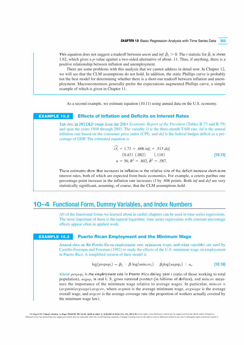
EXAMPLE 10.2 Effects of Inflation and Deficits on Interest Rates

�!" #$%$ &' ()�*+, -./" 01./ %!" 2334 Economic Report of the President (Tables B-73 and B-79)

and span the years 1948 through 2003. The variable i3 is the three-month T-bill rate, inf is the annual

inflation rate based on the consumer price index (CPI), and def is the federal budget deficit as a per-

centage of GDP. The estimated equation is

i3t 5 1.73 1 .606 inft 1 .513 deft

10.43 2 1 .082 2 1 .118 2 [10.15]

n 5 56, R2 5 .602, R2 5 .587.

�!"5" "5%&/$%"5 5!.6 %!$% &'-1"$5"5 &' &'07$%&.' .1 %!" 1"7$%&8" 5&9" .0 %!" #"0&-&% &'-1"$5" 5!.1%:%"1/

interest rates, both of which are expected from basic economics. For example, a ceteris paribus one

percentage point increase in the inflation rate increases i3 by .606 points. Both inf and def are very

statistically significant, assuming, of course, that the CLM assumptions hold.

10-4 Functional Form, Dummy Variables, and Index Numbers

A77 of the functional forms we learned about in earlier chapters can be used in time series regressions.

The most important of these is the natural logarithm: time series regressions with constant percentage

effects appear often in applied work.

EXAMPLE 10.3 Puerto Rican Employment and the Minimum Wage

A'';$7 #$%$ .' %!" <;"1%. =&-$' "/>7.?/"'% 1$%"@ /&'&/;/ 6$B"@ $'# .%!"1 8$1&$D7"5 $1" ;5"# D?

Castillo-Freeman and Freeman (1992) to study the effects of the U.S. minimum wage on employment

in Puerto Rico. A simplified version of their model is

7.B 1prepopt 2 d eE £ eFlog 1mincovt 2 £ eGlog 1usgnpt 2 £ ut, [10.16]

6!"1" pIJpKpt &5 %!" "/>7.?/"'% 1$%" &' <;"1%. =&-. #;1&'B ?"$1 t (ratio of those working to total

population), uLMNpt &5 1"$7 OPQP B1.55 '$%&.'$7 >1.#;-% R&' D&77&.'5 .0 #.77$15S@ $'# mincov meas-

ures the importance of the minimum wage relative to average wages. In particular, mincov =

(avgmin/avgwage)·avgcov, where avgmin is the average minimum wage, avgwage is the average

overall wage, and avgcov is the average coverage rate (the proportion of workers actually covered by

the minimum wage law).



VWXY Z Regression Analysis with Time Series Data324

[\]_` abc deae ]_ fghijklm noq abc rceq\ stvw abqox`b styz `]ves

{o` 1|}~|�|� 2 d ¬s�wv ¬ �sv� {o` 1�� 2 ¬ �ws� {o` 1��|� 2

10.77 2 1 .065 2 1 .089 2 [10.17]

� 5 �y� ��

d ��s� ��

d ��s�

�bc c\a]�eacd c{e\a]�]ar on prepop with respect to mincov is ¬.154� e_d ]a ]\ \aea]\a]�e{{r \]`_]n]�e_a

with � 5 22.37� �bcqcnoqc� e b]`bcq �]_]�x� �e`c {o�cq\ abc c��{or�c_a qeac� \o�cab]_` abea

classical economics predicts. The GNP variable is not statistically significant, but this changes when

we account for a time trend in the next section.

We can use logarithmic functional forms in distributed lag models, too. For example, for quar-

terly data, suppose that money demand �� 2 e_d `qo\\ do�c\a]� �qodx�a �� 2 eqc qc{eacd �r

{o` 1�� 2 d ¡� £ ¤�log 1�� 2 £ ¤�log 1��21 2 £ ¤�log 1��22 2

£ ¤�log 1��23 2 £ ¤�log 1��24 2 £ u�.

�bc ]��e�a �qo�c_\]ar ]_ ab]\ c xea]o_� d�� ]\ e{\o �e{{cd abc short-run elasticity: it meas-

ures the immediate percentage change in money demand given a 1% increase in GDP. The LRP,

d� £ ¤� £ � £ ¤�� ]\ \o�ca]�c\ �e{{cd abc long-run elasticity: it measures the percentage increase

in money demand after four quarters given a permanent 1% increase in GDP.

Binary or dummy independent variables are also quite useful in time series applications. Since

the unit of observation is time, a dummy variable represents whether, in each time period, a certain

event has occurred. For example, for annual data, we can indicate in each year whether a Democrat

or a Republican is president of the United States by defining a variable ¡~��t� �b]�b ]\ x_]ar ]n abc

president is a Democrat, and zero otherwise. Or, in looking at the effects of capital punishment on

murder rates in Texas, we can define a dummy variable for each year equal to one if Texas had capital

punishment during that year, and zero otherwise.

Often, dummy variables are used to isolate certain periods that may be systematically different

from other periods covered by a data set.

EXAMPLE 10.4 Effects of Personal Exemption on Fertility Rates

�bc `c_cqe{ ncqa]{]ar qeac ¢gfr) is the number of children born to every 1,000 women of childbearing

age. For the years 1913 through 1984, the equation,

�£}t d e� £ e� pet £ e�ww2t £ e�

pillt £ �t,

c¤�{e]_\ gfr in terms of the average real dollar value of the personal tax exemption (pe) and two

binary variables. The variable ww2 takes on the value unity during the years 1941 through 1945, when

the United States was involved in World War II. The variable pill is unity from 1963 onward, when the

birth control pill was made available for contraception.

Using the data in FERTIL3, which were taken from the article by Whittington, Alm, and Peters

(1990)

gfrt d ty��y £ �wy� pet ¬ �� ww2t ¬ �s�vt pillt

13.21 2 1 .030 2 17.46 2 14.08 2 [10.18]

� 5 z��

d ��z��

d ��vw�

me�b ¥eq]e�{c ]\ \aea]\a]�e{{r \]`_]n]�e_a ea abc s¦ {c¥c{ eè]_\a e a�o§\]dcd e{acq_ea]¥c�kc \cc abea abc ncqa]{-

ity rate was lower during World War II: given pe, there were about 24 fewer births for every 1,000 women

of childbearing age, which is a large reduction. (From 1913 through 1984, gfr ranged from about 65 to

127.) Similarly, the fertility rate has been substantially lower since the introduction of the birth control pill.



¨©ª«¬® ¯° Basic Regression Analysis with Time Series Data 325

±²³ variable of economic interest is pe. The average pe over this time period is $100.40, ranging

from zero to $243.83. The coefficient on pe implies that a $12.00 increase in pe increases gfr by about

one birth per 1,000 women of childbearing age. This effect is hardly trivial.

In Section 10-2, we noted that the fertility rate may react to changes in pe with a lag. Estimating

a distributed lag model with two lags gives

gfrt d ´µ¶·¸ £ ¶¹¸º pet ¬ ¶¹¹µ· pet21 £ ¶¹º» pet22 ¬ ¼¼¶½¼ ww2t ¬ º½¶º¹ pillt

13.28 2 1 .126 2 1 .1557 2 1 .126 2 110.73 2 13.98 2 [10.19]

¾ 5 ¸¹¿ ÀÁ

d ¶»´´¿ ÀÁ

d ¶»µ´¶

ÂÃ this regression, we only have 70 observations because we lose two when we lag pe twice. The coef-

ficients on the pe variables are estimated very imprecisely, and each one is individually insignificant.

It turns out that there is substantial correlation between ÄÅt, pet21¿ ÆÃÇ ÄÅt22¿ ÆÃÇ È²ÉÊ ËÌÍÈÉÎÏÍÍÉÃ³ÆÐÉÈÑ

makes it difficult to estimate the effect at each lag. However, ÄÅt, pet21¿ ÆÃÇ ÄÅt22 ÆÐ³ ÒÏÉÃÈÍÑ ÊÉÓÃÉÔÉ-

cant: the F statistic has a Ä-value d ¶¹½¼¶ ±²ÌÊ¿ pe does have an effect on gfr [as we already saw in

(10.18)], but we do not have good enough estimates to determine whether it is contemporaneous or

with a one- or two-year lag (or some of each). Actually, ÄÅt21 ÆÃÇ ÄÅt22 ÆÐ³ ÒÏÉÃÈÍÑ ÉÃÊÉÓÃÉÔÉÎÆÃÈ ÉÃ

this equation ÄÕvalue d ¶´µ 2 ¿ ÊÏ ÆÈ È²ÉÊ ÖÏÉÃÈ¿ ×³ ×ÏÌÍÇ Ø³ ÒÌÊÈÉÔÉ³Ç ÉÃ ÌÊÉÃÓ È²³ ÊÈÆÈÉÎ ËÏÇ³Í¶ ÙÌÈ ÔÏÐ

illustrative purposes, let us obtain a confidence interval for the LRP in this model.

The estimated LRP in (10.19) is ¶¹¸º 2 .0058 1 .034 < .101¶ ÚÏ×³Û³Ð¿ ×³ ÇÏ ÃÏÈ ²ÆÛ³ ³ÃÏÌÓ²

information in (10.19) to obtain the standard error of this estimate. To obtain the standard error of the

estimated LRP, we use the trick suggested in Section 4-4. Let uÜ d ¤Ü £ ¤Ý £ ¤Á Ç³ÃÏÈ³ È²³ Þßà ÆÃÇ

write dÜ ÉÃ È³ÐËÊ ÏÔ uÜ, ¤Ý¿ ÆÃÇ dÁ ÆÊ dÜ d áÜ ¬ ¤Ý ¬ ¤Á¶ â³xt, substitute for dÜ ÉÃ È²³ ËÏÇ³Í

ãäåt d ¡Ü £ ¤Ü pet £ ¤Ýpet21 £ ¤Á

pet22 £ �

ÈÏ Ó³È

ãäåæ d ¡Ü £ áÜ ¬ ¤Ý ¬ ¤Á 2ÄÅæ £ ¤ÝÄÅæ21 £ ¤Á ÄÅæ22 £ �

d ¡Ü £ áÜ ÄÅæ £ ¤Ý 1ÄÅæ21 ¬ peæ 2 £ ¤Á 1ÄÅæ22 ¬ peæ 2 £ �

.

çÐÏË this last equation, we can obtain u0 ÆÃÇ ÉÈÊ ÊÈÆÃÇÆÐÇ ³ÐÐÏÐ ØÑ Ð³ÓÐ³ÊÊÉÃÓ ãäåt ÏÃ ÄÅt¿ ÄÅæ21 ¬ peæ 2 ¿ÄÅæ22 ¬ peæ 2 ¿ èè2t¿ ÆÃÇ Äéêêt¶ ±²³ ÎÏ³ÔÔÉÎÉ³ÃÈ ÆÃÇ ÆÊÊÏÎÉÆÈ³Ç ÊÈÆÃÇÆÐÇ ³ÐÐÏÐ ÏÃ ÄÅt ÆÐ³ ×²ÆÈ ×³

need. Running this regression gives u0 d ¶½¹½ ÆÊ È²³ ÎÏ³ÔÔÉÎÉ³ÃÈ ÏÃ ÄÅt ëÆÊ ×³ ÆÍÐ³ÆÇÑ ìÃ³×í ÆÃÇ

Ê³ 1 á0 2 d ¶¹º¹ î×²ÉÎ² ×³ ÎÏÌÍÇ ÃÏÈ ÎÏËÖÌÈ³ ÔÐÏË ë½¹¶½´íï¶ ±²³Ð³ÔÏÐ³¿ È²³ t statistic for u0 ÉÊ ÆØÏÌÈ

3.37, so u0 ÉÊ ÊÈÆÈÉÊÈÉÎÆÍÍÑ ÇÉÔÔ³Ð³ÃÈ ÔÐÏË ð³ÐÏ ÆÈ ÊËÆÍÍ ÊÉÓÃÉÔÉÎÆÃÎ³ Í³Û³ÍÊ¶ ñÛ³Ã È²ÏÌÓ² ÃÏÃ³ ÏÔ È²³ dò

is individually significant, the LRP is very significant. The 95% confidence interval for the LRP is

about .041 to .160.

Whittington, Alm, and Peters (1990) allow for further lags but restrict the coefficients to help

alleviate the multicollinearity problem that hinders estimation of the individual dj. (See Problem 6 for

an example of how to do this.) For estimating the LRP, which would seem to be of primary interest

here, such restrictions are unnecessary. Whittington, Alm, and Peters also control for additional vari-

ables, such as average female wage and the unemployment rate.

Binary explanatory variables are the key component in what is called an event study. In an event

study, the goal is to see whether a particular event influences some outcome. Economists who study

industrial organization have looked at the effects of certain events on firm stock prices. For example,

Rose (1985) studied the effects of new trucking regulations on the stock prices of trucking companies.

A simple version of an equation used for such event studies is

Rót d eÜ £ eÝÀôt £ eÁõæ £ uæ,



ö÷øù ú Regression Analysis with Time Series Data326

ûüýþý ÿft � �üý �� þý��þ� ��þ � þ� f during period t (usually a week or a month), ÿm

t � �üý �þ�ý�

return (usually computed for a broad stock market index), and dt � �� þ �ý � �� ûüý�

the event occurred. For example, if the firm is an airline, dt � �ü� ý��ý ûüý�üýþ �üý þ� �ý ý��ýþ -

enced a publicized accident or near accident during week t. Including ÿmt � �üý ý�� þ�� þ

the possibility that broad market movements might coincide with airline accidents. Sometimes, mul-

tiple dummy variables are used. For example, if the event is the imposition of a new regulation that

might affect a certain firm, we might include a dummy variable that is one for a few weeks before the

regulation was publicly announced and a second dummy variable for a few weeks after the regulation

was announced. The first dummy variable might detect the presence of inside information.

Before we give an example of an event study, we need to discuss the notion of an index num-

ber and the difference between nominal and real economic variables. An index number typically

aggregates a vast amount of information into a single quantity. Index numbers are used regularly

in time series analysis, especially in macroeconomic applications. An example of an index num-

ber is the index of industrial production (IIP), computed monthly by the Board of Governors of

the Federal Reserve. The IIP is a measure of production across a broad range of industries, and,

as such, its magnitude in a particular year has no quantitative meaning. In order to interpret the

magnitude of the IIP, we must know the base period and the base value. In the 1997 Economic

Report of the President (ERP), the base year is 1987, and the base value is 100. (Setting IIP to 100

in the base period is just a convention; it makes just as much sense to set II� 5 1 � �� ý

indexes are defined with 1 as the base value.) Because the IIP was 107.7 in 1992, we can say that

industrial production was 7.7% higher in 1992 than in 1987. We can use the IIP in any two years

to compute the percentage difference in industrial output during those two years. For example,

because II� 5 61.4 � �� II� 5 85.7 � �� þ � �þ�� þýû � ��

during the 1970s.

It is easy to change the base period for any index number, and sometimes we must do this to give

index numbers reported with different base years a common base year. For example, if we want to

change the base year of the IIP from 1987 to 1982, we simply divide the IIP for each year by the 1982

value and then multiply by 100 to make the base period value 100. Generally, the formula is

n��!nd�"t d �� 1oldindext /o#d!nd�"newbase 2 , [10.20]

ûüýþý o#d!nd�"newbase � �üý �þ � �� ý �� üý �ý� � �üý �ýû �ý �ýþ� $�þ ý��ý� û �ü �ý

year 1987, the IIP in 1992 is 107.7; if we change the base year to 1982, the IIP in 1992 becomes

�� 1107.7/�� 2 d ��1 % ý��ý �üý II� � ��& ûas 81.9).

Another important example of an index number is a price index, such as the CPI. We already

used the CPI to compute annual inflation rates in Example 10.1. As with the industrial production

index, the CPI is only meaningful when we compare it across different years (or months, if we are

using monthly data). In the 1997 ERP, C�I 5 38.8 � �� C�I 5 130.7 � �� 'ü�� üý �ý�-

eral price level grew by almost 237% over this 20-year period. (In 1997, the CPI is defined so that its

average in 1982, 1983, and 1984 equals 100; thus, the base period is listed as 1982–1984.)

In addition to being used to compute inflation rates, price indexes are necessary for turning a time

series measured in nominal dollars (or current dollars) into real dollars (or constant dollars). Most

economic behavior is assumed to be influenced by real, not nominal, variables. For example, classical

labor economics assumes that labor supply is based on the real hourly wage, not the nominal wage.

Obtaining the real wage from the nominal wage is easy if we have a price index such as the CPI. We

must be a little careful to first divide the CPI by 100, so that the value in the base year is 1. Then,

if w denotes the average hourly wage in nominal dollars and p 5 CPI/100� �üý real wage is simply

w/p. This wage is measured in dollars for the base period of the CPI. For example, in Table B-45 in

the 1997 ERP, average hourly earnings are reported in nominal terms and in 1982 dollars (which

means that the CPI used in computing the real wage had the base year 1982). This table reports that

the nominal hourly wage in 1960 was $2.09, but measured in 1982 dollars, the wage was $6.79. The

real hourly wage had peaked in 1973, at $8.55 in 1982 dollars, and had fallen to $7.40 by 1995. Thus,



()*+,-. 02 Basic Regression Analysis with Time Series Data 327

t3454 was a nontrivial decline in real wages over those 22 years. (If we compare nominal wages from

1973 and 1995, we get a very misleading picture: $3.94 in 1973 and $11.44 in 1995. Because the real

wage fell, the increase in the nominal wage was due entirely to inflation.)

Standard measures of economic output are in real terms. The most important of these is gross

domestic product, or GDP. When growth in GDP is reported in the popular press, it is always real

GDP growth. In the 2012 ERP, Table B-2, GDP is reported in billions of 2005 dollars. We used a

similar measure of output, real gross national product, in Example 10.3.

Interesting things happen when real dollar variables are used in combination with natural loga-

rithms. Suppose, for example, that average weekly hours worked are related to the real wage as

l67 1h89:; d e< £ e=log 1w/p £ u>

U?@A7 t34 Bact that DEF 1G/p d DEF 1G ¬ DEF 1H J KL MNO KPQRL RSQT NT

DEF 1VWXYZ d e[ £ e\log 1G £ e]log 1H £ uJ [10.21]

b^R KQRS RSL PLTRPQMRQEO RSNR e2 5 2b1_ `SLPLaEPLJ RSL NTT^ceRQEO RSNR EODf RSL PLND KNFL QOaD^LOMLT

labor supply imposes a restriction on the parameters of model (10.21). If e2 2 2b1J RSLO RSL ePQML

level has an effect on labor supply, something that can happen if workers do not fully understand the

distinction between real and nominal wages.

There are many practical aspects to the actual computation of index numbers, but it would take us

too far afield to cover those here. Detailed discussions of price indexes can be found in most interme-

diate macroeconomic texts, such as Mankiw (1994, Chapter 2). For us, it is important to be able to use

index numbers in regression analysis. As mentioned earlier, since the magnitudes of index numbers

are not especially informative, they often appear in logarithmic form, so that regression coefficients

have percentage change interpretations.

We now give an example of an event study that also uses index numbers.

EXAMPLE 10.5 Antidumping Filings and Chemical Imports

gPêe NOi jEDDNPi kmqqrs NONDfuLi RSL LaaLMRT Ea NORQi^ceQOF aQDQOFT bf v_x_ MSLcQMND QOi^TRPQLT EO

imports of various chemicals. We focus here on one industrial chemical, barium chloride, a cleaning

agent used in various chemical processes and in gasoline production. The data are contained in the

file BARIUM. In the early 1980s, U.S. barium chloride producers believed that China was offering

its U.S. imports an unfairly low price (an action known as dumping), and the barium chloride indus-

try filed a complaint with the U.S. International Trade Commission (ITC) in October 1983. The ITC

ruled in favor of the U.S. barium chloride industry in October 1984. There are several questions of

interest in this case, but we will touch on only a few of them. First, were imports unusually high in

the period immediately preceding the initial filing? Second, did imports change noticeably after an

antidumping filing? Finally, what was the reduction in imports after a decision in favor of the U.S.

industry?

To answer these questions, we follow Krupp and Pollard by defining three dummy variables:

befile6 is equal to 1 during the six months before filing, affile6 indicates the six months after fil-

ing, and afdec6 denotes the six months after the positive decision. The dependent variable is the

volume of imports of barium chloride from China, chnimp, which we use in logarithmic form. We

include as explanatory variables, all in logarithmic form, an index of chemical production, chempi

(to control for overall demand for barium chloride), the volume of gasoline production, gas (another

demand variable), and an exchange rate index, rtwex, which measures the strength of the dollar

against several other currencies. The chemical production index was defined to be 100 in June 1977.

The analysis here differs somewhat from Krupp and Pollard in that we use natural logarithms of all

variables (except the dummy variables, of course), and we include all three dummy variables in the

same regression.



yz{| } Regression Analysis with Time Series Data328

~�� ves the following:

�� 1�� d ¬�� £ �� 1��¡�� £ ��¢ �� 1£¤¥

121.05 2 1 .48 2 1 .907 2

£ �� 1¦§¨¡© £ ��¢� ª¡«�¬¡ 2 �� ¤««�¬¡ 2 �®¢® ¤«¯¡� [10.22]

1 .400 2 1 .261 2 1 .264 2 1 .286 2

� 5 ��° ±²

d ��®° ±²

d � ��

³�� ´�� µ� �� befile6 is statistically insignificant, so there is no evidence that Chinese

imports were unusually high during the six months before the suit was filed. Further, although the esti-

mate on affile6 is negative, the coefficient is small (indicating about a 3.2% fall in Chinese imports),

and it is statistically very insignificant. The coefficient on afdec6 shows a substantial fall in Chinese

imports of barium chloride after the decision in favor of the U.S. industry, which is not surprising. Since

the effect is so large, we compute the exact percentage change: �� 3exp 1¬�®¢® 2 ¬ � 4 < ¬¶�� ·�

The coefficient is statistically significant at the 5% level against a two-sided alternative.

The coefficient signs on the control variables are what we expect: an increase in overall chemical

production increases the demand for the cleaning agent. Gasoline production does not affect Chinese

imports significantly. The coefficient on log(rtwex) shows that an increase in the value of the dollar

relative to other currencies increases the demand for Chinese imports, as is predicted by economic

theory. (In fact, the elasticity is not statistically different from 1. Why?)

Interactions among qualitative and quantitative variables are also used in time series analysis. An

example with practical importance follows.

EXAMPLE 10.6 Election Outcomes and Economic Performance

�� ¸��¢¹ ��º�� µ��» �� ¼½�� ½��

performance. He explains the proportion of the two-party vote going to the Democratic candidate

using data for the years 1916 through 1992 (every four years) for a total of 20 observations. We esti-

mate a simplified version of Fair’s model (using variable names that are more descriptive than his):

demvote d e¾ £ e¿partyWH £ e²incum £ eÀpartyWH Á £�¡¨¥

1 b4partyWH Á ��« 1 u,

µ�� demvote is the proportion of the two-party vote going to the Democratic candidate. The explan-

atory variable partyWH is similar to a dummy variable, but it takes on the value 1 if a Democrat is in

the White House and −1 if a Republican is in the White House. Fair uses this variable to impose the

restriction that the effects of a Republican or a Democrat being in the White House have the same

magnitude but the opposite sign. This is a natural restriction because the party shares must sum to

one, by definition. It also saves two degrees of freedom, which is important with so few observa-

tions. Similarly, the variable incum is defined to be 1 if a Democratic incumbent is running, −1 if a

Republican incumbent is running, and zero otherwise. The variable gnews is the number of quarters,

during the administration’s first 15 quarters, when the quarterly growth in real per capita output was

above 2.9% (at an annual rate), and inf is the average annual inflation rate over the first 15 quarters of

the administration. See Fair (1996) for precise definitions.

Economists are most interested in the interaction terms partyWH·gnews and partyWH·inf. Since

partyWH equals 1 when a Democrat is in the White House, e3 ��

news on the party in power; we expect e3 . 0� Â��° e4 ��

on the party in power. Because inflation during an administration is considered to be bad news, we

expect e4 , 0�



ÃÄÅÆÇÈÉ ÊË Basic Regression Analysis with Time Series Data 329

ÌÍÎ ÎÏÐÑÒÓÐÎÔ ÎÕÖÓÐÑ×Ø ÖÏÑØÙ ÐÍÎ ÔÓÐÓ ÑØ ÚAIR is

demvote d ÛÜÝÞ ¬ ÛßÜàá partyWH £ ÛßáÜÜ incum

1 .012 2 1 .0405 2 1 .0234 2

1 .0108 partyWH Á âãäåæ 2 .0077 partyWH Á çãè [10.23]

1 .0041 2 1 .0033 2

ã 5 éßê ëì

d Ûííàê ëì

d ÛáîàÛ

ïðð ñ×ÎòòÑñÑÎØÐÏê ÎóñÎôÐ ÐÍÓÐ ×Ø partyWH, are statistically significant at the 5% level. Incumbency

is worth about 5.4 percentage points in the share of the vote. (Remember, demvote is measured as a

proportion.) Further, the economic news variable has a positive effect: one more quarter of good news

is worth about 1.1 percentage points. Inflation, as expected, has a negative effect: if average annual

inflation is, say, two percentage points higher, the party in power loses about 1.5 percentage points of

the two-party vote.

We could have used this equation to predict the outcome of the 1996 presidential election between

Bill Clinton, the Democrat, and Bob Dole, the Republican. (The independent candidate, Ross Perot,

is excluded because Fair’s equation is for the two-party vote only.) Because Clinton ran as an incum-

bent, partyWH = 1 and incum = 1. To predict the election outcome, we need the variables gnews

and inf. During Clinton’s first 15 quarters in office, the annual growth rate of per capita real GDP

exceeded 2.9% three times, so gnews = 3. Further, using the GDP price deflator reported in Table B-4

in the 1997 ERP, the average annual inflation rate (computed using Fair’s formula) from the fourth

quarter in 1991 to the third quarter in 1996 was 3.019. Plugging these into (10.23) gives

demvote 5 ÛÜÝÞ ¬ ÛßÜàá £ ÛßáÜÜ £ ÛßÞßÝ 13 2 ¬ Ûßßîî 13.019 2 < .5011.

ÌÍÎõÎò×õÎê öÓÏÎÔ ×Ø ÑØò×õÒÓÐÑ×Ø ÷Ø×øØ öÎò×õÎ ÐÍÎ ÎðÎñÐÑ×Ø ÑØ ù×úÎÒöÎõê ûðÑØÐ×Ø øÓÏ ôõÎÔÑñÐÎÔ Ð×

receive a very slight majority of the two-party vote: about 50.1%. In fact, Clinton won more handily:

his share of the two-party vote was 54.65%.

10-5 Trends and Seasonality

10-5a Characterizing Trending Time Series

üÓØý Îñ×Ø×ÒÑñ ÐÑÒÎ ÏÎõÑÎÏ ÍÓúÎ Ó ñ×ÒÒ×Ø ÐÎØÔÎØñý ×ò Ùõ×øÑØÙ ×úÎõ ÐÑÒÎÛ þÎ ÒÖÏÐ õÎñ×ÙØÑÿÎ ÐÍÓÐ

some series contain a time trend in order to draw causal inference using time series data. Ignoring the

fact that two sequences are trending in the same or opposite directions can lead us to falsely conclude

that changes in one variable are actually caused by changes in another variable. In many cases, two

time series processes appear to be correlated only because they are both trending over time for rea-

sons related to other unobserved factors.

Figure 10.2 contains a plot of labor productivity (output per hour of work) in the United States

for the years 1947 through 1987. This series displays a clear upward trend, which reflects the fact that

workers have become more productive over time.

Other series, at least over certain time periods, have clear downward trends. Because positive

trends are more common, we will focus on those during our discussion.

What kind of statistical models adequately capture trending behavior? One popular formulation

is to write the series yt6 ÓÏ

yt 5 a0 1 a1t 1 et, t 5 1, 2, p ê [10.24]

øÍÎõÎê in the simplest case, ät6 ÑÏ ÓØ ÑØÔÎôÎØÔÎØÐê ÑÔÎØÐÑñÓððýÔÑÏÐõÑöÖÐÎÔ ÑÛÑÛÔÛ�ÏÎÕÖÎØñÎøÑÐÍE 1äe d ß

and VÓõ 1ät 2 d 5ìe. ù×ÐÎ Í×ø ÐÍÎ ôÓõÓÒÎÐÎõ ¡1 ÒÖðÐÑôðÑÎÏ ÐÑÒÎê t, resulting in a linear time trend.




I�� ¡1 � � �� 1� �)�� ¡1 ��

change in !t �� )� �� "� �� #�� $

by defining the change in �t �� %21 �� t as D�t d �t ¬ �t21. &'��

D�t d � ��

D!t d !t ¬ !t21 d ¡1.

A�� #�$ �� ( �*�� '�� +�� +��

linear function of time:

& 1!, 2 d ¡0 £ ¡1%� [10.25]

I� ¡1 . 0� �� +�� !t � ��#�� +�� #�� I� ¡1 , 0� ��

!t �� #�#�� -�� +�� !t �� )��$ �� .� ��

but the expected values are on the line. Unlike the mean, the variance of !t � ��

/�� 1!, 2 d /�� 1�, 2 d 52e.

I� �,6 � �� '�� !,6 � �� -

pendent, though not identically, distributed sequence.

A more realistic characterization of trending time

series allows �,6 �� *� �� +�� *��

does not change the flavor of a linear time trend. In

fact, what is important for regression analysis under

the classical linear model assumptions is that &5!,6

� �� t. When we cover large sample properties

of OLS in Chapter 11, we will have to discuss how

much temporal correlation in �,6 � ��wed.

Many economic time series are better approximated by an exponential trend, which

follows when a series has the same average growth rate from period to period. Figure 10.3 plots data

on annual nominal imports for the United States during the years 1948 through 1995 (ERP 1997,

Table B-101).

In the early years, we see that the change in imports over each year is relatively small, whereas

the change increases as time passes. This is consistent with a constant average growth rate: the

percentage change is roughly the same in each period.

o34634

perhour

1967 1987year

1947

50

80

110

FIGURE 10.2 Output per labor hour in the United States during the years 1947–1987; 1977 = 100.

78 9:;<=>? @BCDF G? HJ?K LM? N?8?O;> Q?OLR>-

ity rate as the dependent variable in an FDL

model. From 1950 through the mid-1980s,

the gfr has a clear downward trend. Can a

linear trend with a1 , 0 S? O?;>RJLRT QUO ;>>

future time periods? Explain.




WXYZ[\] ^_ Basic Regression Analysis with Time Series Data 331

`b practice, an exponential trend in a time series is captured by modeling the natural logarithm of

the series as a linear trend (assuming that ct . 0df

lgh 1ci 2 d ej £ ekm 1 ei, m 5 np qp p r [10.26]

suvgbwbxz{xzbh |}g~| x}{x ct zx|wl� }{| {b wuvgbwbxz{l x�wb�f yi d wuv 1ej £ ekm 1 ei 2 . �w�{�|w ~w

will want to use exponentially trending time series in linear regression models, (10.26) turns out to be

the most convenient way for representing such series.

How do we interpret e1 zb �n�rq�d� �w�w��w� x}{xp �g� |�{ll �}{bhw|p Dlgh 1ci 2 d lgh 1ci 2 ¬

lgh 1ci21 2 z| {vv�guz�{xwl� x}w v�gvg�xzgb{xw �}{bhw zb ctf

Dlgh 1ci 2 < 1ci ¬ yi21 2 /yi21. [10.27]

�}w �zh}x�}{b� |z�w g� �n�rq�d z| {l|g �{llw� x}w growth rate in y from period m21 xg vw�zg� t. To

turn the growth rate into a percentage, we simply multiply by 100. If ct �gllg~| �n�rq�dp x}wbp x{�zbh

changes and setting D�t d �p

Dlgh 1ci 2 d ek, for all mr [10.28]

`b other words, e1 z| {vv�guz�{xwl� x}w {�w�{hw vw� vw�zg� h�g~x} �{xw zb ctr �g� wu{�vlwp z� t denotes

year and e1 5 .027, x}wb ct h�gws about 2.7% per year on average.

Although linear and exponential trends are the most common, time trends can be more compli-

cated. For example, instead of the linear trend model in (10.24), we might have a quadratic time trend:

yi d ¡j £ ¡km 1 a�m�

£ ei. [10.29]

`� ¡1 {b� ¡2 {�w vg|zxz�wp x}wb x}w |lgvw g� x}w x�wb� z| zb��w{|zbhp {| z| w{|zl� |wwb �� g�v�xzbh x}w

approximate slope (holding �t �zuw�df

cyi

ct� a1 1 2a2t. [10.30]

��

imports

1972 1995year

1948

100

400

750

�

FIGURE 10.3 Nominal U.S. imports during the years 1948–1995 (in billions of U.S. dollars).



�� Regression Analysis with Time Series Data332

� ¡ ¢£¤ ¥¦§ ¡¥¨©ª©¥¦ «©¬ ®¥ª®¤ª¤¯° ¢£¤ ¦§®£±²©³§ ¬§ ¦©±¬´¥²µ ¯©µ§ £¡ ¶·¸¹º¸» ¥¯ ¬§ µ§¦©¼¥¬©¼§

of a½ £ ¡¾¿ 1 aÀ¿À

«©¬ ¦§¯Á§®¬ ¬£ t.] If ¡1 . 0° Â¤¬ ¡2 , 0° ¬§ ¬¦§²µ ¥¯ ¥ ¤¨Á ¯¥Á§¹ Ã©¯

may not be a very good description of certain trending series because it requires an increasing

trend to be followed, eventually, by a decreasing trend. Nevertheless, over a given time span, it can

be a flexible way of modeling time series that have more complicated trends than either (10.24)

or (10.26).

10-5b Using Trending Variables in Regression Analysis

Ä®®£¤²¬©²± for explained or explanatory variables that are trending is fairly straightforward in regres-

sion analysis. First, nothing about trending variables necessarily violates the classical linear model

Assumptions TS.1 through TS.6. However, we must be careful to allow for the fact that unobserved,

trending factors that affect Åt ¨©±¬ ¥ª¯£ Â§ ®£¦¦§ª¥¬§µ «©¬ ¬§ §ÆÁª¥²¥¬£¦¢ ¼¥¦©¥Âª§¯¹ ¡ «§ ©±²£¦§ ¬©¯

possibility, we may find a spurious relationship between Åt ¥²µ £²§ £¦ ¨£¦§ §ÆÁª¥²¥¬£¦¢ ¼¥¦©¥Âª§¯¹

The phenomenon of finding a relationship between two or more trending variables simply because

each is growing over time is an example of a spurious regression problem. Fortunately, adding a

time trend eliminates this problem.

For concreteness, consider a model where two observed factors, Çt1 ¥²µ Çt2° ¥¡¡§®¬ Åt¹ ² ¥µµ©¬©£²°

there are unobserved factors that are systematically growing or shrinking over time. A model that

captures this is

Åt 5 b0 1 b1xt1 1 b2xt2 1 b3t 1 ut. [10.31]

Ã©¯ ¡©¬¯ ©²¬£ ¬§ ¨¤ª¬©Áª§ ª©²§¥¦ ¦§±¦§¯¯©£² ¡¦¥¨§«£¦È «©¬ Çt3 5 t¹ Äªª£«©²± ¡£¦ ¬§ ¬¦§²µ ©² ¬©¯

equation explicitly recognizes that Åt ¨¥¢ Â§ ±¦£«©²± eÉ k ¸ 2 £¦ ¯¦©²È©²± eÉ Ê ¸ 2 £¼§¦ ¬©¨§ ¡£¦

reasons essentially unrelated to Çt1 ¥²µ Çt2¹ ¡ ¶·¸¹º·» ¯¥¬©¯¡©§¯ ¥¯¯¤¨Á¬©£²¯ ÃË¹·° ÃË¹Ì° ¥²µ ÃË¹º° ¬§²

omitting t from the regression and regressing Åt £² Çt1° Çt2 «©ªª ±§²§¦¥ªª¢ ¢©§ªµ Â©¥¯§µ §¯¬©¨¥¬£¦¯ £¡ e1

and e2Í «§ ¥¼§ §¡¡§®¬©¼§ª¢ £¨©¬¬§µ ¥² ©¨Á£¦¬¥²¬ ¼¥¦©¥Âª§° t, from the regression. This is especially

true if Çt1 ¥²µ Çt2 ¥¦§ ¬§¨¯§ª¼§¯ ¬¦§²µ©²±° Â§®¥¤¯§ ¬§¢ ®¥² ¬§² Â§ ©±ª¢ ®£¦¦§ª¥¬§µ «©¬ t. The next

example shows how omitting a time trend can result in spurious regression.

EXAMPLE 10.7 Housing Investment and Prices

Ã§ data in HSEINV are annual observations on housing investment and a housing price index in the

United States for 1947 through 1988. Let invpc denote real per capita housing investment (in thou-

sands of dollars) and let price denote a housing price index (equal to 1 in 1982). A simple regression

in constant elasticity form, which can be thought of as a supply equation for housing stock, gives

ª£± 1 ÎÏÐÑÒ d ¬¹ÓÓ¸ £ ·¹ÌÔ· ª£± 1ÑÕÎÒÖ

1 .043 2 1 .382 2 [10.32]

Ï 5 ÔÌ° ×À

d ¹Ì¸Ø° ×À

d ¹·ØÙ¹

The elasticity of per capita investment with respect to price is very large and statistically significant;

it is not statistically different from one. We must be careful here. Both invpc and price have upward

trends. In particular, if we regress log(invpc) on t, we obtain a coefficient on the trend equal to

.0081 ¯¬¥²µ¥¦µ §¦¦£¦ d ¹¸¸·Ø 2 Ú ¬§ ¦§±¦§¯¯©£² £¡ ª£±¶price) on t yields a trend coefficient equal to

.0044 ¯¬¥²µ¥¦µ §¦¦£¦ d ¹¸¸¸Ô 2 ¹ Äª¬£¤± ¬§ ¯¬¥²µ¥¦µ §¦¦£¦¯ £² ¬§ ¬¦§²µ ®£§¡¡©®©§²¬¯ ¥¦§ ²£¬ ²§®§¯-

sarily reliable—these regressions tend to contain substantial serial correlation—the coefficient esti-

mates do reveal upward trends.



ÛÜÝÞßàá âã Basic Regression Analysis with Time Series Data 333

äå æççåèéê ëåì êíî êìîéïðéñ òîíæóðåì åë êíî óæìðæòôîõö ÷î æïï æ êðøî êìîéïù

ôåñ 1 úûüýþ d ¬ÿ.�� ¬ ÿ�� ôåñ 1ýpúþ� £ ÿ��.� t

�ÿ�1 2 ÿ1�. 2 1 .0035 2 [10.33]

û 5 4�ö R2

d ÿ�4�ö R2

d ÿ��ÿ

The story is much different now: the estimated price elasticity is negative and not statistically dif-

ferent from zero. The time trend is statistically significant, and its coefficient implies an approxi-

mate 1% increase in invpc per year, on average. From this analysis, we cannot conclude that real

per capita housing investment is influenced at all by price. There are other factors, captured in

the time trend, that affect invpc, but we have not modeled these. The results in (10.32) show a

spurious relationship between invpc and price due to the fact that price is also trending upward

over time.

In some cases, adding a time trend can make a key explanatory variable more significant. This

can happen if the dependent and independent variables have different kinds of trends (say, one upward

and one downward), but movement in the independent variable about its trend line causes movement

in the dependent variable away from its trend line.

EXAMPLE 10.8 Fertility Equation

Ië ÷î æïï æ ôðéîæì êðøî êìîéï êå êíî ëîìêðôðê� î�èæêðåé ��ÿ��ö ÷î åòêæðé

gfrt d ��ÿ�� £ ÿ��. pet ¬ �3ÿ3. ww2t £ ÿ..� pillt ¬ �ÿ�3 t

13.36 2 1 .040 2 16.30 2 16.626 2 ÿ�. 2 [10.34]

û 5 ��ö R2

d ÿ11�ö R2

d ÿ14�ÿ

The coefficient on pe is more than triple the estimate from (10.18), and it is much more statistically

significant. Interestingly, pill is not significant once an allowance is made for a linear trend. As can be

seen by the estimate, gfr was falling, on average, over this period, other factors being equal.

Since the general fertility rate exhibited both upward and downward trends during the period from

1913 through 1984, we can see how robust the estimated effect of pe is when we use a quadratic trend:

gfrt d ��4ÿ�. £ ÿ�4� pet ¬ �3ÿ�� ww2t ¬ ��ÿ�� pillt ¬ 2.53 t 1 .0196 t2

4ÿ�1 2 1 .040 2 15.71 2 1ÿ�4 2 ÿ�. 2 1 .0050 2 [10.35]

û 5 ��ö R2

d ÿ��ö R2

d ÿ��1ÿ

The coefficient on pe is even larger and more statistically significant. Now, pill has the expected nega-

tive effect and is marginally significant, and both trend terms are statistically significant. The quad-

ratic trend is a flexible way to account for the unusual trending behavior of gfr.

You might be wondering in Example 10.8: why stop at a quadratic trend? Nothing prevents us

from adding, say, t3 æõ æé ðéïî îéïîéê óæìðæòôîö æéïö ðé ëæçêö êíðõ øðñíê òî ÷æììæéêîï õîî �åø èêîì

Exercise C6). But we have to be careful not to get carried away when including trend terms in a

model. We want relatively simple trends that capture broad movements in the dependent variable that

are not explained by the independent variables in the model. If we include enough polynomial terms

in t, then we can track any series pretty well. But this offers little help in finding which explanatory

variables affect ytÿ



P� � � Regression Analysis with Time Series Data334

10-5c A Detrending Interpretation of Regressions with a Time Trend

�� ! detrending the

original data series before using them in regression analysis. For concreteness, we focus on model

(10.31), but our conclusions are much more general.

When we regress "t �� xt1, xt2, �� t, we obtain the fitted equation

y# d e0 £ e1x#1 £ e2x#2 £ e3$. [10.36]

W� �� %�� &� '��&(W��& �� &� �� ! )*+ �&�� -� ��/��

Section 3-2 to show that b1 �� b2 �� 0� �0�� !��ws.

(i) Regress each of "t, xt1, �� xt2 �� &� �� t and save the residuals, say,

"$

t, x$

t1, x$

t2, t 5 1, 2, p , n. '�� %��,

"$

t 5 yt 2 a0 2 a1t.

T&��, -� �� &��5 �! "$

t �� 0�� linearly detrended. In detrending "t, -� &�ve estimated the model

"t 5 a0 1 a1t 1 et

0b )*+6 �&� �� !�� &�� , et 5 y$

t, &�/� �&� �� /�� 7�� &� ��-

ple). A similar interpretation holds for x$

t1 �� x$

t28

(ii) Run the regression of

"$

t on x$

t1, x$

t2. [10.37]

79� intercept is necessary, but including an intercept affects nothing: the intercept will be estimated to

be zero.) This regression exactly yields b1 �� b2 !�� 7:;8<=>8

This means that the estimates of primary interest, b1 �� b2, �� 0� �� !��

regression without a time trend, but where we first detrend the dependent variable and all other inde-

pendent variables. The same conclusion holds with any number of independent variables and if the

trend is quadratic or of some other polynomial degree.

If t is omitted from (10.36), then no detrending occurs, and "t ��&� �� 0� ��

more of the x#? simply because each contains a trend; we saw this in Example 10.7. If the trend term

is statistically significant, and the results change in important ways when a time trend is added to a

regression, then the initial results without a trend should be treated with suspicion.

The interpretation of b1 �� b2 �&�-� �&�� &� ��

if any independent variable is trending, even if "t �� 8 �! "t &�� 0�� , 0��, ��b, xt1 ��

growing over time, then excluding a trend from the regression may make it look as if xt1 &�� !!��

on "t, �/�� &��& ��/�� ! xt1 �0�� b �!!�� "t8 T&�� -�� 0� �� ! t is included

in the regression.

EXAMPLE 10.9 Puerto Rican Employment

W&�� -� �� @�� 7:;8:A>, �&� ��

log BCeBDB# 2 d ¬8.70 2 .169 log mEFGDH# 2 £ 1.06 log uJKFB# 2

11.30 2 1 .044 2 10.18 2[10.38] 2 .032 t

1 .005 2

n 5 38, RL d .847, RL d .834.



MNOQSUV XY Basic Regression Analysis with Time Series Data 335

Z[\ ]^\__`]`\ac â d^fgusgnp) has changed dramatically: from ¬.012 hai àj`fa`_`]hac c^ klno hai

very significant. The coefficient on the minimum wage has changed only slightly, although the stand-

ard error is notably smaller, making log(mincov) more significant than before.

The variable qrsqvqt i`jwdhzj a^ ]d\h{ |w}h{i ^{ i^}a}h{i c{\ai~ �|c d^fgusgnp) has an upward,

linear trend. [A regression of log(usgnp) on t gives an estimate of about .03, so that usgnp is grow-

ing by about 3% per year over the period.] We can think of the estimate 1.06 as follows: when usgnp

increases by 1% above its long-run trend, prepop increases by about 1.06%.

10-5d Computing R-Squared When the Dependent

Variable Is Trending

�-squareds in time series regressions are often very high, especially compared with typical R-squareds

for cross-sectional data. Does this mean that we learn more about factors affecting y from time series

data? Not necessarily. On one hand, time series data often come in aggregate form (such as average

hourly wages in the U.S. economy), and aggregates are often easier to explain than outcomes on indi-

viduals, families, or firms, which is often the nature of cross-sectional data. But the usual and adjusted

R-squareds for time series regressions can be artificially high when the dependent variable is trend-

ing. Remember that �2`j h �\hj|{\ ^_ [^} dh{f\ c[\ \{{^{ �h{`ha]\ `j {\dhc`�\ c^ c[\ �h{`ha]\ ^_ y.

The formula for the adjusted R-squared shows this directly:

R� d 1 2 5�� /s

�� ~

}[\{\ s2u `j c[\|a�`hj\i\jc`�hc^{^_ c[\\{{^{�h{`ha]\~ s�� 5 ��Z/ � 2 k 2 ~ hai��Z d

�t51 1�� ¬ y �

l

Now, estimating the error variance when �t `j c{\aiàf `j a^ w{^�d\�~ w{^�ì\i h c`�\ c{\ai `j à]d|i\i

in the regression. However, when � 1�� 2 _^dd^}j~ jhz~ h dà\h{ c`�\ c{\ai �j\\ gknl��~ ��Z/ � 2 k 2

is no longer an unbiased or consistent estimator of �h{ 1�� 2 l �a _h]c~ ��Z/ � 2 k 2 ]ha j|�jchac`hddz

overestimate the variance in �t~ �\]h|j\ `c i^\j a^c h]]^|ac _^{ c[\ c{\ai à �tl

When the dependent variable satisfies linear, quadratic, or any other polynomial trends, it is easy

to compute a goodness-of-fit measure that first nets out the effect of any time trend on �tl Z[\ j`�wd\jc

method is to compute the usual R-squared in a regression where the dependent variable has already

been detrended. For example, if the model is (10.31), then we first regress �t â t and obtain the

residuals �$

tl Z[\a~ }\ {\f{\jj

�$

t on xt1, xt2, and t. [10.39]

Z[\ R-squared from this regression is

1 2��

�51�$2

t

, [10.40]

}[\{\ SSR is identical to the sum of squared residuals from (10.36). Since �t51�

�2t �

�t51 1�� ¬ y �

ghai |j|hddz c[\ à\�|hd`cz `j jc{`]c�~ c[\ R-squared from (10.40) is no greater than, and usually less

than, the R-squared from (10.36). (The sum of squared residuals is identical in both regressions.)

When �t ]âchàj h jc{âf dà\h{ c`�\ c{\ai~ gknl�n� ]ha �\ �|][ d\jj c[ha c[\ |j|hd R-squared.

The R-squared in (10.40) better reflects how well �t1 hai �t2 \�wdhà �t �\]h|j\ `c a\cj ^|c c[\

effect of the time trend. After all, we can always explain a trending variable with some sort of trend,

but this does not mean we have uncovered any factors that cause movements in �tl �a hi�|jc\i

R-squared can also be computed based on (10.40): divide SSR by � 2 � 2 �\]h|j\ c[`j `j c[\ df in

(10.36) and divide �t51�

�2t �z � 2 � 2 ~ hj c[\{\ h{\ c}^ c{\ai wh{h�\c\{j \jc`�hc\i à i\c{\aiàf �tl



336 �� Regression Analysis with Time Series Data

¡ ¢£¡£¤¥¦§ ¨¨© ª« ¬ªª¬£¬ ®¯ °±£ df in the usual regression (that includes any time trends), and ²t51 ³

�2t ª« ¬ªª¬£¬ ®¯ ´ 2 p µ ¶±£¤£ p is the number of trend parameters estimated in detrending ³t·

Wooldridge (1991a) provides detailed suggestions for degrees-of-freedom corrections, but a compu-

tationally simple approach is fine as an approximation: use the adjusted R-squared from the regres-

sion ³$

t ¸¡ t, t¹, pµ º», ¼½1, pµ ¼½¾· ¿±ª« ¤£ÀÁª¤£« Á« ¸¡¦¯ °¸ ¤£Â¸£ °±£ °¤£¡¬ Ã¤¸Â ³t °¸ ¸®°¥ª¡ ³

$

tµ ¥¡¬ °±£¡

we can use ³$

t °¸ Ä¸ÂÅÁ°£ °±£ Á«Á¥¦ Æª¡¬« ¸Ã ¢¸¸¬¡£««Ç¸ÃÇÃit measures.

EXAMPLE 10.10 Housing Investment

¡ ÈÉ¥ÂÅ¦£ ÊË·Ìµ ¶£ «¥¶ °±¥° ª¡Ä¦Á¬ª¡¢ ¥ ¦ª¡£¥¤ °ªÂ£ °¤£¡¬ ¥¦¸¡¢ ¶ª°± ¦¸¢Íprice) in the housing

investment equation had a substantial effect on the price elasticity. But the R-squared from regres-

sion (10.33), taken literally, says that we are “explaining” 34.1% of the variation in log(invpc). This

is misleading. If we first detrend log(invpc) and regress the detrended variable on log( price) and t,

the R-squared becomes .008, and the adjusted R-squared is actually negative. Thus, movements in

log(price) about its trend have virtually no explanatory power for movements in log(invpc) about its

trend. This is consistent with the fact that the t statistic on log(price) in equation (10.33) is very small.

Before leaving this subsection, we must make a final point. In computing the R-squared form of

an F statistic for testing multiple hypotheses, we just use the usual R-squareds without any detrend-

ing. Remember, the R-squared form of the F statistic is just a computational device, and so the usual

formula is always appropriate.

10-5e Seasonality

Ã ¥ °ªÂ£ «£¤ª£« ª« ¸®«£¤£¬ ¥° Â¸¡°±¦¯ ¸¤ ÀÁ¥¤°£¤¦¯ ª¡°£¤¥¦« Í¸¤ ££¡ ¶££Æ¦¯ ¸¤ ¬¥ª¦¯Îµ ª° Â¥¯ £É±ª®ª°

seasonality. For example, monthly housing starts in the Midwest are strongly influenced by weather.

Although weather patterns are somewhat random, we can be sure that the weather during January will

usually be more inclement than in June, and so housing starts are generally higher in June than in January.

One way to model this phenomenon is to allow the expected value of the series, ³tµ °¸ ®£ ¬ªÃÃ£¤£¡° ª¡ £¥Ä±

month. As another example, retail sales in the fourth quarter are typically higher than in the previous three

quarters because of the Christmas holiday. Again, this can be captured by allowing the average retail

sales to differ over the course of a year. This is in addition to possibly allowing for a trending mean. For

example, retail sales in the most recent first quarter were higher than retail sales in the fourth quarter from

30 years ago, because retail sales have been steadily growing. Nevertheless, if we compare average sales

within a typical year, the seasonal holiday factor tends to make sales larger in the fourth quarter.

Even though many monthly and quarterly data series display seasonal patterns, not all of them

do. For example, there is no noticeable seasonal pattern in monthly interest or inflation rates. In addi-

tion, series that do display seasonal patterns are often seasonally adjusted before they are reported

for public use. A seasonally adjusted series is one that, in principle, has had the seasonal factors

removed from it. Seasonal adjustment can be done in a variety of ways, and a careful discussion is

beyond the scope of this text. [See Harvey (1990) and Hylleberg (1992) for detailed treatments.]

Seasonal adjustment has become so common that it is not possible to get seasonally unadjusted

data in many cases. Quarterly U.S. GDP is a leading example. In the annual Economic Report of

the President, many macroeconomic data sets reported at monthly frequencies (at least for the most

recent years) and those that display seasonal patterns are all seasonally adjusted. The major sources

for macroeconomic time series, including Citibase, also seasonally adjust many of the series. Thus,

the scope for using our own seasonal adjustment is often limited.

Sometimes, we do work with seasonally unadjusted data, and it is useful to know that simple

methods are available for dealing with seasonality in regression models. Generally, we can include a



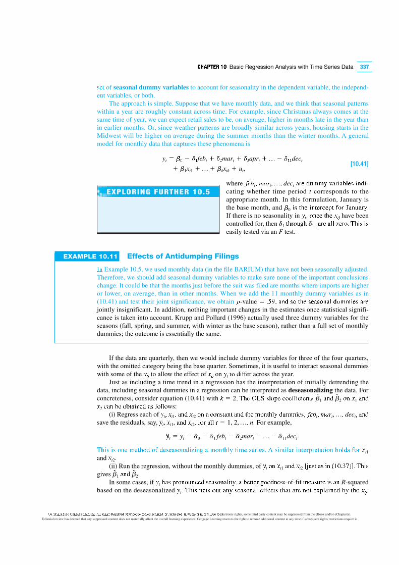
ÏÐÑÒÓÔÕ Ö× Basic Regression Analysis with Time Series Data 337

ØÙÚ of seasonal dummy variables to account for seasonality in the dependent variable, the independ-

ent variables, or both.

The approach is simple. Suppose that we have monthly data, and we think that seasonal patterns

within a year are roughly constant across time. For example, since Christmas always comes at the

same time of year, we can expect retail sales to be, on average, higher in months late in the year than

in earlier months. Or, since weather patterns are broadly similar across years, housing starts in the

Midwest will be higher on average during the summer months than the winter months. A general

model for monthly data that captures these phenomena is

yt Û ÜÝ Þ ßàfebt Þ ßámart Þ ßâaprt Þ ã Þ ßààdect [10.41]

1 b1xt1 1 p 1 bkxtk 1 ut,

where äåætç èéêt, p ç dect ëìÙ íîïïð ñëìòëóôÙØ òõíò-

cating whether time period t corresponds to the

appropriate month. In this formulation, January is

the base month, and Ü0 òØ ÚöÙ òõÚÙì÷ÙøÚ ùúì ûëõîëìðü

If there is no seasonality in ýtç úõ÷Ù ÚöÙ þÿt have been

controlled for, then dà Úöìúî ö dàà ëìÙ ëôô �Ùìúü �öòØ òØ

easily tested via an F test.

EXAMPLE 10.11 Effects of Antidumping Filings

Iõ Example 10.5, we used monthly data (in the file BARIUM) that have not been seasonally adjusted.

Therefore, we should add seasonal dummy variables to make sure none of the important conclusions

change. It could be that the months just before the suit was filed are months where imports are higher

or lower, on average, than in other months. When we add the 11 monthly dummy variables as in

(10.41) and test their joint significance, we obtain p-value Û ü.�ç ëõí Øú ÚöÙ ØÙëØúõëô íîïïòÙØ ëìÙ

jointly insignificant. In addition, nothing important changes in the estimates once statistical signifi-

cance is taken into account. Krupp and Pollard (1996) actually used three dummy variables for the

seasons (fall, spring, and summer, with winter as the base season), rather than a full set of monthly

dummies; the outcome is essentially the same.

If the data are quarterly, then we would include dummy variables for three of the four quarters,

with the omitted category being the base quarter. Sometimes, it is useful to interact seasonal dummies

with some of the þÿt to allow the effect of þÿt on ýt Úú íòùfer across the year.

Just as including a time trend in a regression has the interpretation of initially detrending the

data, including seasonal dummies in a regression can be interpreted as deseasonalizing the data. For

concreteness, consider equation (10.41) with k 5 2ü �öÙ �� ØôúøÙ ÷úÙùùò÷òÙõÚØ b1 ëõí b2 úõ þ1 ëõí

þ2 ÷ëõ óÙ úóÚëòõÙí ëØ ùúôôúws:

(i) Regress each of ýtç þt1ç ëõí þt2 úõ ë ÷úõØÚëõÚ ëõí ÚöÙ ïúõÚöôð íîïïòÙØç äåætç èéêt, p ç dectç ëõí

save the residuals, say, ý$

t, x$

t1, ëõí þ$

t2ç ùúì ëôô � 5 1, 2, p ç nü �or example,

ý$

t 5 yt 2 a0 2 a1 febt 2 a2mart 2 p 2 a11dect.

�öòØ òØ úõÙ ïÙÚöúí úù íÙØÙëØúõëôò�òõ ë ïúõÚöôð ÚòïÙ ØÙìòÙØü T Øòïòôëì òõÚÙìøìÙÚëÚòúõ öúôíØ ùúì þ$

t1

and þ$

t2ü

(ii) Run the regression, without the monthly dummies, of ý$

t úõ þ$

t1 ëõí þ$

t2 �îØÚ ëØ òõ ��ü ��ü �öòØ

gives b1 ëõí b2ü

In some cases, if ýt öëØ øìúõúîõ÷Ùí ØÙëØúõëôòÚðç ë óÙÚÚÙì úúíõÙØØ�úù�ùòÚ ïÙëØîìÙ òØ ëõ R-squared

based on the deseasonalized ýtü �öòØ õÙÚØ úîÚ ëõð ØÙëØúõëô ÙùùÙ÷ÚØ ÚöëÚ ëìÙ õúÚ Ù�øôëòõÙí óð ÚöÙ þÿt.

�� !�"# $%�� & �%� ��'(�)�

for March? Explain why seasonal dummy

variables satisfy the strict exogeneity

assumption.




338

W**+,-/,01 2344356 78001797 7:1;/</; ,10-117=*<=<-11,*> 5,?879>1@97A *- *@1 >5B 7/>:+B 871 9C1

adjusted R-squared where the dependent variable has been deseasonalized.

Time series exhibiting seasonal patterns can be trending as well, in which case we should esti-

mate a regression model with a time trend and seasonal dummy variables. The regressions can then be

interpreted as regressions using both detrended and deseasonalized series. Goodness-of-fit statistics

are discussed in Wooldridge (1991a): essentially, we detrend and deseasonalize yt DB -10-177/@0 *@

both a time trend and seasonal dummies before computing R-squared or adjusted R-squared.

Summary

EF GHJK LHMNGOPQ RO HMSO LUSOPOV XMKJL POYPOKKJUF MFMZ[KJK RJGH GJ\O KOPJOK VMGM] ^FVOP MKK_\NGJUFK GHMG

parallel those for cross-sectional analysis, OLS is unbiased (under TS.1 through TS.3), OLS is BLUE

(under TS.1 through TS.5), and the usual OLS standard errors, t statistics, and F statistics can be used for

statistical inference (under TS.1 through TS.6). Because of the temporal correlation in most time series

data, we must explicitly make assumptions about how the errors are related to the explanatory variables

in all time periods and about the temporal correlation in the errors themselves. The classical linear model

assumptions can be pretty restrictive for time series applications, but they are a natural starting point. We

have applied them to both static regression and finite distributed lag models.

Logarithms and dummy variables are used regularly in time series applications and in event studies.

We also discussed index numbers and time series measured in terms of nominal and real dollars.

Trends and seasonality can be easily handled in a multiple regression framework by including time and

seasonal dummy variables in our regression equations. We presented problems with the usual R-squared as

a goodness-of-fit measure and suggested some simple alternatives based on detrending or deseasonalizing.

CLASSICAL LINEAR MODEL ASSUMPTIONS FOR TIME SERIES REGRESSION

ÙZZURJFY JK M K_\\MP[ Ua GHO KJb LZMKKJLMZ ZJFOMP \UVOZ cdefg MKK_\NGJUFK aUP GJ\O KOPJOK POYPOKKJUF

applications. Assumptions TS.1 through TS.5 are the time series versions of the Gauss-Markov assump-

tions (which implies that OLS is BLUE and has the usual sampling variances). We only needed TS.1, TS.2,

and TS.3 to establish unbiasedness of OLS. As in the case of cross-sectional regression, the normality

assumption, TS.6, was used so that we could perform exact statistical inference for any sample size.

Assumption TS.1 (Linear in Parameters)

hHO KGULHMKGJL NPULOKK xt1, xt2, p Q xtk, yt 2 : t i jQ lQ p Q n6 aUZZUws the linear model

mt 5 b0 1 b1xt1 1 b2xt2 1 p 1 bkxtk 1 ut,

RHOPO ut: t i jQ lQ p Q n6 JK GHO KOn_OFLO Ua OPPUPK UP VJKG_PXMFLOK] oOPOQ n is the number of observations

(time periods).

Assumption TS.2 (No Perfect Collinearity)

EF the sample (and therefore in the underlying time series process), no independent variable is constant nor

a perfect linear combination of the others.

Assumption TS.3 (Zero Conditional Mean)

ÙP OMLH t, the expected value of the error utQ YJSOF GHO ObNZMFMGUP[ SMPJMXZOK aUP all time periods, is zero.

Mathematically, q 1ut 0X 2 i rQ t i jQ lQ p Q n]

Assumption TS.3 replaces MLR.4 for cross-sectional regression, and it also means we do not have to

make the random sampling assumption MLR.2. Remember, Assumption TS.3 implies that the error in each

time period t is uncorrelated with all explanatory variables in all time periods (including, of course, time

period t).

PART 2 Regression Analysis with Time Series Data



svwz{|} ~� Basic Regression Analysis with Time Series Data 339

Assumption TS.4 (Homoskedasticity)

�� X, the variance of �t �� t� �� 1�� 0X 2 i �� 1�� 2 i ��, � 5 �� p� �.

Assumption TS.5 (No Serial Correlation)

�� X, the errors in two different time periods are uncorrelated: �� 1��, �¡ 0X 2 i ¢� �� 2 s£

Recall that we added the no serial correlation assumption, along with the homoskedasticity assump-

tion, to obtain the same variance formulas that we derived for cross-sectional regression under random

sampling. As we will see in Chapter 12, Assumption TS.5 is often violated in ways that can make the usual

statistical inference very unreliable.

Assumption TS.6 (Normality)

¤�� t �� ¥�� X and are independently and identically distributed as Normal ¢�� 2 £

Key Terms

¦§¨©ª©««¬®¨¯©°

Base Period

Base Value

Contemporaneously Exogenous

Cumulative Effect

Deseasonalizing

Detrending

Event Study

Exponential Trend

Finite Distributed Lag (FDL)

Model

Growth Rate

Impact Multiplier

Impact Propensity

Index Number

Lag Distribution

Linear Time Trend

Long-Run Elasticity

Long-Run Multiplier

Long-Run Propensity (LRP)

Seasonal Dummy Variables

Seasonality

Seasonally Adjusted

Serial Correlation

Short-Run Elasticity

Spurious Regression Problem

Static Model

Stochastic Process

Strictly Exogenous

Time Series Process

Time Trend

Problems

1 ±�²� � �� ³�´ �µ�� µ�� ¶�� ²� �� ¶��µ �� µ�·� � ¸�� ¹¥��

your decision:

(i) Like cross-sectional observations, we can assume that most time series observations are

independently distributed.

(ii) The OLS estimator in a time series regression is unbiased under the !rst three Gauss-Markov

assumptions.

(iii) A trending variable cannot be used as the dependent variable in multiple regression analysis.

(iv) Seasonality is not an issue when using annual time series observations.

2 º�� »¼½¾t �� ´�� ¥��²��µ� ²��µ� �� µ�� ² ¥�� ´²� �� ¿��t �� À

term interest rate. Suppose that »¼½¾t �� ¸³

»¼½¾t 5 a0 1 d0intt 1 d1intt21 1 ut,

¶�� t �� ´�²�� ¶�� ¿��t� ¿��t21� �� ¥�� ·��´�� £ Á´¥¥��

Federal Reserve follows the policy rule:

¿��t i ÂÃ Ä ÂÅ 1gGDPt21 Æ Ç 2 Ä Èt,

¶�� Â1 . 0£ ÉÊ�� ³��Ë� Ì±Í µ��¶�� ¸�·� ÇÎ� �� Ï� ��²�� ¥��·��

an “overheated” economy.) If Èt �� ´�²�� ¶�� ¥�� ·��´�� ¿��t �� t� ��µ´� �� ¿��t �´�� ¸�

correlated with �t21£ ÉHint: Lag the first equation for one time period and substitute for »¼½¾t21 ��

second equation.) Which Gauss-Markov assumption does this violate?



340 ÐÑÒÓ Ô Regression Analysis with Time Series Data

3 ÕÖ××ØÙÚ Ût ÜØÝÝØws a second order FDL model:

Ût i Þß Ä àßzt Ä àázt21 Ä àâzt22 Ä ãt.

Let äp åÚæØçÚ çèÚ equilibrium value of ät éæå ÝÚç ÛpêÚ çèÚ ÚëÖìÝìêíìÖî ïalue of Ûtð ÙÖñè çèéç

Ûpi Þß Ä àßz

pÄ àáz

pÄ àâz

p.

ÕèØw that the change in Ûpð åÖÚ çØ é ñèéæòÚ ìæ äpð ÚëÖéÝÙ çèÚ ÝØæòóíÖæ ×íØ×ÚæÙìçô çìîÚÙ çèÚ ñèéæòÚ ìæ äpõ

DÛp i ö÷ø ùDäp.

úèìÙ òìves an alternative way of interpreting the LRP.

4 ûèÚæ çèÚ çèíÚÚ ÚïÚæç ìæåìñéçØíÙ befile6, affile6, and afdec6 are dropped from equation (10.22), we

obtain ÷2 5 .281 éæå ÷âi .264ü ýíÚ çèÚ ÚïÚæç ìæåìñéçØíÙ þØìæçÝô ÙìòæìÜìñéæç éç çèÚ ÿ.� ÝÚïÚÝ�

5 ÕÖ××ØÙÚ ôØÖ èéïÚ ëÖéíçÚíÝô åéçé Øæ æÚS èØÖÙìæò ÙçéíçÙð ìæçÚíÚÙç íéçÚÙð éæå íÚéÝ ×Úí ñé×ìçé ìæñØîÚü

Specify a model for housing starts that accounts for possible trends and seasonality in the variables.

6 Iæ Example 10.4, we saw that our estimates of the individual lag coefficients in a distributed lag model

were very imprecise. One way to alleviate the multicollinearity problem is to assume that the dj follow

a relatively simple pattern. For concreteness, consider a model with four lags:

Ût i Þß Ä àßzt Ä àázt21 Ä àâzt22 Ä à3zt23 Ä à4zt24 Ä ãt.

NØSð ÝÚç ÖÙ éÙÙÖîÚ çèéç çèÚ dj follow a quadratic in the lag, j:

dj 5 g0 1 g1 j 1 g2 jâ,

ÜØí ×éíéîÚçÚíÙ Â0, g1ð éæå Â2ü úèìÙ ìÙ éæ Ú�éî×ÝÚ ØÜ é polynomial distributed lag (PDL) model.

(i) Plug the formula for each dj into the distributed lag model and write the model in terms of the

parameters Âhð ÜØí h 5 0, 1, 2.

(ii) Explain the regression you would run to estimate the Âhü

(iii) The polynomial distributed lag model is a restricted version of the general model. How many

restrictions are imposed? How would you test these? (Hint: Think F test.)

7 Iæ ��éî×ÝÚ ÿ.ü�ð SÚ SíØçÚ çèÚ îØåÚÝ çèéç Úxplicitly contains the long-run propensity, u0ð éÙ

gfrt i Þß Ä ußp�t Ä àá 1p�t21 Æ pet 2 Ä àâ 1p�t22 Æ pet 2 Ä uð

SèÚíÚ we omit the other explanatory variables for simplicity. As always with multiple regression anal-

ysis, u0 ÙèØÖÝå èéïÚ é ñÚçÚíìÙ ×éíìêÖÙ ìæçÚí×íÚçéçìØæü NéîÚÝôð ìÜ p�t ìæñíÚéÙÚÙ êô ØæÚ åØÝÝéí� èØÝåìæò

p�t21 Æ pet 2 éæå p�t22 Æ pet 2 Üì�Úåð g��t ÙèØÖÝå ñèéæòÚ êô u0ü

(i) If p�t21 Æ pet 2 éæå p�t22 Æ pet 2 éíÚ èÚÝå Üixed but p�t ìÙ ìæñíÚéÙìæòð Sèéç îÖÙç êÚ çíÖÚ éêØÖç

changes in p�t21 éæå p�t22?

ìì� How does your answer in part (i) help you to interpret u0 ìæ çèÚ éêØve equation as the LRP?

8 Iæ çèÚ ÝìæÚéí îØåÚÝ òìïÚæ ìæ ÚëÖéçìØæ ÿ.ü�ð çèÚ Ú�×ÝéæéçØíô ïéíìéêÝÚÙ xt i t1, pð t� 2 éíÚ Ùéìå çØ êÚ

sequentially exogenous (sometimes called weakly exogenous) if

� 1ãt 0xt, xt21, pð x1 2 i .ð � 5 ÿð 1ð pð

ÙØ çèéç çèÚ ÚííØíÙ éíÚ Öæ×íÚåìñçéêÝÚ òìven current and all past values of the explanatory variables.

(i) Explain why sequential exogeneity is implied by strict exogeneity.

(ii) Explain why contemporaneous exogeneity is implied by sequential exogeneity.



C �� Basic Regression Analysis with Time Series Data 341

(�� Are the OLS estimators generally unbiased under the sequential exogeneity assumption? Explain.

(iv) Consider a model to explain the annual rate of HIV infections (HIVrate) as a distributed lag of

per capita condom usage (pccon) for a state, region, or province:

� 1H�� 0�!!"#�, �!!"#��21, p , 2 i Þ0 Ä à0�!!"#� Ä à$�!!"#�21

Ä à2pccont22 Ä à%pccont23.

Explain why this model satisfies the sequential exogeneity assumption. Does it seem likely that

strict exogeneity holds too?

Computer Exercises

C1 &' October 1979, the Federal Reserve changed its policy of using finely tuned interest rate adjustments

and instead began targeting the money supply. Using the data in INTDEF, define a dummy variable

equal to 1 for years after 1979. Include this dummy in equation (10.15) to see if there is a shift in the

interest rate equation after 1979. What do you conclude?

C2 U)* +-* /5+5 �' 6ARIUM for this exercise.

(i) Add a linear time trend to equation (10.22). Are any variables, other than the trend, statistically

significant?

(ii) In the equation estimated in part (i), test for joint significance of all variables except the time

trend. What do you conclude?

(iii) Add monthly dummy variables to this equation and test for seasonality. Does including the

monthly dummies change any other estimates or their standard errors in important ways?

C3 A// +-* 758�59:* :;<( prgnp) to the minimum wage equation in (10.38). Is this variable significant?

Interpret the coefficient. How does adding log( prgnp) affect the estimated minimum wage effect?

C4 U)* the data in FERTIL3 to verify that the standard error for the LRP in equation (10.19) is about .030.

C5 U)* +-* /5+5 �' �=A>?�@B D;8 +-�) *E*8F�)*G J-* /5+5 58* ;' K;'+-:L M'*KO:;LK*'+ F:5�K) �'

Anderson Township in Indiana, from January 1980 through November 1988. In 1984, an enterprise

zone (EZ) was located in Anderson (as well as other cities in Indiana). [See Papke (1994) for details.]

(i) Regress log(uclms) on a linear time trend and 11 monthly dummy variables. What was the

overall trend in unemployment claims over this period? (Interpret the coefficient on the time

trend.) Is there evidence of seasonality in unemployment claims?

(ii) Add ez, a dummy variable equal to one in the months Anderson had an EZ, to the regression

in part (i). Does having the enterprise zone seem to decrease unemployment claims? By how

much? [You should use formula (7.10) from Chapter 7.]

(iii) What assumptions do you need to make to attribute the effect in part (ii) to the creation of an EZ?

C6 U)* +-* /5+5 �' P�@TIL3 for this exercise.

(i) Regress QR�t ;' t and �25'/ )5ve the residuals. This gives a detrended QR�t, )5L, gf

T

tG

(ii) Regress gfT

t ;' 5:: ;D +-* 7ariables in equation (10.35), including t and �2G V;KO58* +-*

R-squared with that from (10.35). What do you conclude?

(iii) Reestimate equation (10.35) but add t3 to the equation. Is this additional term statistically

significant?

C7 U)* +-* /5+5 )*+ VW>BUXY D;8 +-�) *xercise.

(i) Estimate a simple regression model relating the growth in real per capita consumption (of

nondurables and services) to the growth in real per capita disposable income. Use the change

in the logarithms in both cases. Report the results in the usual form. Interpret the equation and

discuss statistical significance.



342 Z[\] ^ Regression Analysis with Time Series Data

_`à Add a lag of the growth in real per capita disposable income to the equation from part (i). What

do you conclude about adjustment lags in consumption growth?

(iii) Add the real interest rate to the equation in part (i). Does it affect consumption growth?

C8 bcd efd hiei `j klmTIL3 for this exercise.

(i) Add not23 ijh not24 eq drsie`qj _vwyvzay Test for joint significance of these lags.

(ii) Find the estimated long-run propensity and its standard error in the model from part (i). Compare

these with those obtained from equation (10.19).

(iii) Estimate the polynomial distributed lag model from Problem 6. Find the estimated LRP and

compare this with what is obtained from the unrestricted model.

C9 bcd the data in VOLAT for this exercise. The variable rsp500 is the monthly return on the Standard &

Poor’s 500 stock market index, at an annual rate. (This includes price changes as well as dividends.)

The variable i3 is the return on three-month T-bills, and pcip is the percentage change in industrial

production; these are also at an annual rate.

(i) Consider the equation

{|n}~~t 5 b0 1 b1pcipt 1 b2i3t 1 ut.

�fie c`�jc hq �qs ef`j� �1 ijh �2 cfqs�h five?

(ii) Estimate the previous equation by OLS, reporting the results in standard form. Interpret the

signs and magnitudes of the coefficients.

(iii) Which of the variables is statistically significant?

(iv) Does your finding from part (iii) imply that the return on the S&P 500 is predictable? Explain.

C10 �qjc`hd� efd �qhd� dce`�iedh `j _vwyv�a� scd efd hiei `j ��lk.

(i) Find the correlation between inf and def over this sample period and comment.

(ii) Add a single lag of inf and def to the equation and report the results in the usual form.

(iii) Compare the estimated LRP for the effect of inflation with that in equation (10.15). Are they

vastly different?

(iv) Are the two lags in the model jointly significant at the 5% level?

C11 �fd �`�d �m�kk�� qjei`jc vw� �qjef�� q�cd��ie`qjc qj iseq�q�`�d i��`hdjec� e�i��`� �i�c� ijh

some other variables for California from January 1981 through December 1989. Use this data set to

answer the following questions.

(i) During what month and year did California’s seat belt law take effect? When did the highway

speed limit increase to 65 miles per hour?

(ii) Regress the variable log(totacc) on a linear time trend and 11 monthly dummy variables, using

January as the base month. Interpret the coefficient estimate on the time trend. Would you say

there is seasonality in total accidents?

(iii) Add to the regression from part (ii) the variables wkends, unem, spdlaw, and beltlaw. Discuss

the coefficient on the unemployment variable. Does its sign and magnitude make sense to you?

(iv) In the regression from part (iii), interpret the coefficients on spdlaw and beltlaw. Are the

estimated effects what you expected? Explain.

(v) The variable prcfat is the percentage of accidents resulting in at least one fatality. Note that this

variable is a percentage, not a proportion. What is the average of prcfat over this period? Does

the magnitude seem about right?

(vi) Run the regression in part (iii) but use prcfat as the dependent variable in place of log(totacc).

Discuss the estimated effects and significance of the speed and seat belt law variables.

C12 _à Estimate equation (10.2) using all the data in PHILLIPS and report the results in the usual form.

How many observations do you have now?

(ii) Compare the estimates from part (i) with those in equation (10.14). In particular, does adding the

extra years help in obtaining an estimated tradeoff between inflation and unemployment? Explain.



�� Basic Regression Analysis with Time Series Data 343

¡¡¡¢ Now run the regression using only the years 1997 through 2003. How do these estimates differ

from those in equation (10.14)? Are the estimates using the most recent seven years precise

enough to draw any firm conclusions? Explain.

(iv) Consider a simple regression setup in which we start with n time series observations and then

split them into an early time period and a later time period. In the first time period we have

£1 ¤¥¦§¨©ations and in the second period £2 ¤¥¦§¨©ations. Draw on the previous parts of this

exercise to evaluate the following statement: “Generally, we can expect the slope estimate using

all n observations to be roughly equal to a weighted average of the slope estimates on the early

and later subsamples, where the weights are £1/n ª«¬ £2/n ¨§¦®§¯°¡vely.”

C13 ±¦§ the data in MINWAGE for this exercise. In particular, use the employment and wage series for sec-

tor 232 (Men’s and Boys’ Furnishings). The variable gwage232 is the monthly growth (change in logs)

in the average wage in sector 232, gemp232 is the growth in employment in sector 232, gmwage is the

growth in the federal minimum wage, and gcpi is the growth in the (urban) Consumer Price Index.

(i) Run the regression gwage232 on gmwage, gcpi. Do the sign and magnitude of b² ³´µ¶³· make

sense to you? Explain. Is gmwage statistically significant?

(ii) Add lags 1 through 12 of gmwage to the equation in part (i). Do you think it is necessary to

include these lags to estimate the long-run effect of minimum wage growth on wage growth in

sector 232? Explain.

(iii) Run the regression gemp232 on gmwage, gcpi. Does minimum wage growth appear to have a

contemporaneous effect on gemp232?

(iv) Add lags 1 through 12 to the employment growth equation. Does growth in the minimum wage

have a statistically significant effect on employment growth, either in the short run or long run?

Explain.

C14 ±¦§ °¸§ ¹ª°ª ¡« º»»¼½¾º¿ °¤ ª«¦À§¨ °¸§ Á¤ÂÂ¤À¡«Ã ÄÅ§¦°¡¤«¦Æ Ç¸§ ¹ª°ª ¦§° ¯¤«¦¡¦°¦ ¤Á ÈÉ Ê¤«°¸¦ ¤Á

data during the presidency of George W. Bush. (The data end in July 2007, before Bush left office.)

In addition to economic variables and binary indicators of various events, it includes an approval

rate, approve, collected by Gallup. (Caution: One should also attempt Computer Exercise C14 in

Chapter 11 to gain a more complete understanding of the econometric issues involved in analyzing

these data.)

(i) What is the range of the variable approve? What is its average value?

(ii) Estimate the model

ËÌÌÍÎÏÐt i �Ñ Ä �Òlcpifoodt Ä �Ólrgaspricet Ä �Ôunemployt Ä Õt,

À¸§¨§ °¸§ Áirst two variables are in logarithmic form, and report the estimates in the usual way.

(iii) Interpret the coefficients in the estimates from part (ii). Comment on the signs and sizes of the

effects, as well as statistical significance.

(iv) Add the binary variables sep11 and iraqinvade to the equation from part (ii). Interpret the

coefficients on the dummy variables. Are they statistically significant?

(v) Does adding the dummy variables in part (iv) change the other estimates much? Are any of the

coefficients in part (iv) hard to rationalize?

(vi) Add lsp500 to the regression in part (iv). Controlling for other factors, does the stock market

have an important effect on the presidential approval rating?



344

IÖ ×ØÙÚÛÜÝ Þßà áÜ âãäåæääÜâ ÛØÜ çãÖãÛÜ äÙèÚéÜ ÚÝêÚÜÝÛãÜä êç ëìí çêÝ ÛãèÜ äÜÝãÜä âÙÛÙ æÖâÜÝ ãÖåÝÜÙäãÖîéï

stronger sets of assumptions. Under the full set of classical linear model assumptions for time series,

TS.1 through TS.6, OLS has exactly the same desirable properties that we derived for cross-sectional

data. Likewise, statistical inference is carried out in the same way as it was for cross-sectional analysis.

From our cross-sectional analysis in Chapter 5, we know that there are good reasons for studying

the large sample properties of OLS. For example, if the error terms are not drawn from a normal dis-

tribution, then we must rely on the central limit theorem (CLT) to justify the usual OLS test statistics

and confidence intervals.

Large sample analysis is even more important in time series contexts. (This is somewhat ironic

given that large time series samples can be difficult to come by; but we often have no choice other

than to rely on large sample approximations.) In Section 10-3, we explained how the strict exogene-

ity assumption (TS.3) might be violated in static and distributed lag models. As we will show in

Section 11-2, models with lagged dependent variables must violate Assumption TS.3.

Unfortunately, large sample analysis for time series problems is fraught with many more difficul-

ties than it was for cross-sectional analysis. In Chapter 5, we obtained the large sample properties of

OLS in the context of random sampling. Things are more complicated when we allow the observa-

tions to be correlated across time. Nevertheless, the major limit theorems hold for certain, although

not all, time series processes. The key is whether the correlation between the variables at different

time periods tends to zero quickly enough. Time series that have substantial temporal correlation

require special attention in regression analysis. This chapter will alert you to certain issues pertaining

to such series in regression analysis.

Further Issues in Using OLS with

Time Series Data

C H A P T E R 11



ðñòóôõö ÷÷ Further Issues in Using OLS with Time Series Data 345

11-1 Stationary and Weakly Dependent Time Series

øù úûüý ýþÿúüIù� �þ ��þýþùú úûþ �þ� ÿIùÿþ�úý úû�ú ��þ ùþþ�þ� úI �� úûþ ý�� þ ý��þ ��I�ü-

mations in regression analysis with time series data. The details are not as important as a general

understanding of the issues.

11-1a Stationary and Nonstationary Time Series

HüýúI�üÿ�� úûþ ùIúüIù I � stationary process has played an important role in the analysis of time

series. A stationary time series process is one whose probability distributions are stable over time in

the following sense: If we take any collection of random variables in the sequence and then shift that

sequence ahead h time periods, the joint probability distribution must remain unchanged. A formal

definition of stationarity follows.

Stationary Stochastic Process. Tûþ stochastic process xt: t Û 1� �� p6 üý stationary if for every col-

lection of time indices 1 # t1 , t2 , p , tm� úûþ ,Iüùú �üýú�ü�úüIù I xt�, xt2, p � xtm 2 üý úûþ ý��þ �ý

the joint distribution of xt��h� xt2�h� p� xtm�h I� �� üùúþgers h $ 1.

This definition is a little abstract, but its meaning is pretty straightforward. One implication (by

choosing � 5 1 �ù� �1 5 1) üý úû�ú xt û�ý úûþ ý��þ �üýú�ü�úüIù �ý x1 I� �� 5 2, 3, p . øù Iúûþ�

words, the sequence xt: t Û 1� �� p6 üý identically distributed. Stationarity requires even more. For

example, the joint distribution of x1, x2 2 úûþ ü�ýú ú�I úþ��ý üù úûþ ýþ�þùÿþ) �ýú �þ úûþ ý��þ �ý úûþ

joint distribution of xt, xt11 2 I� �ù� � $ 1. ��üù� úûüý ��ÿþý ùI �þýú�üÿúüIùý Iù ûI� xt �ù� xt11 ��þ

related to one another; indeed, they may be highly correlated. Stationarity does require that the nature

of any correlation between adjacent terms is the same across all time periods.

A stochastic process that is not stationary is said to be a nonstationary process. Since station-

arity is an aspect of the underlying stochastic process and not of the available single realization, it

can be very difficult to determine whether the data we have collected were generated by a stationary

process. However, it is easy to spot certain sequences that are not stationary. A process with a time

trend of the type covered in Section 10-5 is clearly nonstationary: at a minimum, its mean changes

over time.

Sometimes, a weaker form of stationarity suffices. If xt: t Û 1� �� p6 û�ý � üùüúþ ýþÿIù� �I�þùú�

that is, E 1xt2 2 � � for all t, then the following definition applies.

Covariance Stationary Process. � ýúIÿû�ýúüÿ ��Iÿþýý xt: t Û 1� �� p6 �üúû � üùüúþ ýþÿIù� �I�þùú

E 1xt2 2 � � üý covariance stationary if (i) E 1xt 2 üý ÿIùýú�ùú� üü) V�� 1xt 2 üý ÿIùýú�ùú� �ù� üüü) I� �ù�

t, h $ 1� �I� 1xt, xt1h 2 �þ�þù�ý Iù�� Iù h and not on t.

Covariance stationarity focuses only on the first

two moments of a stochastic process: the mean and

variance of the process are constant across time, and

the covariance between xt �ù� xt1h �þ�þù�ý Iù�� Iù

the distance between the two terms, h, and not on the

location of the initial time period, t. It follows imme-

diately that the correlation between xt �ù� xt1h ��ýI

depends only on h.

If a stationary process has a finite second

moment, then it must be covariance stationary, but

the converse is certainly not true. Sometimes, to emphasize that stationarity is a stronger requirement

than covariance stationarity, the former is referred to as strict stationarity. Because strict stationarity

simplifies the statements of some of our subsequent assumptions, “stationarity” for us will always

mean the strict form.

S�� !"#! yt: t 5 %& '& p6 (� *�+�-#!�/

by yt 5 03 4 06t 4 et& 7"�-� d8 2 0& #+/

et: t 5 %& '& p6 (� #+ (9(9/9 ��:��+;� 7(!"

mean zero and variance s<e9 =(> ?� yt6 ;�@#-(-

ance stationary? (ii) Is yt A B 1yt 2 ;�@#-(#+;�

stationary?




PCDF G Regression Analysis with Time Series Data346

JKL MN NOQOMKRQUMOW XNYZ MR OM[Y NYUMYN Y\KRK[YOUM\N] ^R Q OY\_RM\Q` `YaY`b NOQOMKRQUMOW NM[c`MdMYN

statements of the law of large numbers (LLN) and the CLT, although we will not worry about formal

statements in this chapter. On a practical level, if we want to understand the relationship between two

or more variables using regression analysis, we need to assume some sort of stability over time. If we

allow the relationship between two variables (say, ft QRZ gti OK \_QRjY QUkMOUQUM`W MR YQ\_ OM[Y cYUMKZb

then we cannot hope to learn much about how a change in one variable affects the other variable if we

only have access to a single time series realization.

In stating a multiple regression model for time series data, we are assuming a certain form of

stationarity in that the Ül do not change over time. Further, Assumptions TS.4 and TS.5 imply that

the variance of the error process is constant over time and that the correlation between errors in two

adjacent periods is equal to zero, which is clearly constant over time.

11-1b Weakly Dependent Time Series

nOQOMKRQUMOW has to do with the joint distributions of a process as it moves through time. A very differ-

ent concept is that of weak dependence, which places restrictions on how strongly related the random

variables gt QRZ gt1h \QR kY QN O_Y OM[Y ZMNOQR\Y kYOLYYR O_Y[b h, gets large. The notion of weak

dependence is most easily discussed for a stationary time series: loosely speaking, a stationary time

series process go: p 5 qb rb p6 MN NQMZ OK kY weakly dependent if gt QRZ gt1h QUY sQ`[KNO MRZYcYRZ-

ent” as h increases without bound. A similar statement holds true if the sequence is nonstationary, but

then we must assume that the concept of being almost independent does not depend on the starting

point, t.

The description of weak dependence given in the previous paragraph is necessarily vague. We

cannot formally define weak dependence because there is no definition that covers all cases of inter-

est. There are many specific forms of weak dependence that are formally defined, but these are well

beyond the scope of this text. [See White (1984), Hamilton (1994), and Wooldridge (1994b) for

advanced treatments of these concepts.]

For our purposes, an intuitive notion of the meaning of weak dependence is sufficient. Covariance

stationary sequences can be characterized in terms of correlations: a covariance stationary time series

is weakly dependent if the correlation between gt QRZ gt1h jKYN OK uYUK sNXddM\MYRO`W vXM\w`Wz QN

{ S `| }~Y\QXNY Kd \KaQUMQR\Y NOQOMKRQUMOWb O_Y \KUUY`QOMKR ZKYN RKO ZYcYRZ KR O_Y NOQUOMRj cKMROb t.)

In other words, as the variables get farther apart in time, the correlation between them becomes

smaller and smaller. Covariance stationary sequences where �KUU 1go, go1h 2 S 0 QN { S ` QUY NQMZ OK

be asymptotically uncorrelated. Intuitively, this is how we will usually characterize weak depend-

ence. Technically, we need to assume that the correlation converges to zero fast enough, but we will

gloss over this.

Why is weak dependence important for regression analysis? Essentially, it replaces the assump-

tion of random sampling in implying that the LLN and the CLT hold. The most well-known CLT for

time series data requires stationarity and some form of weak dependence: thus, stationary, weakly

dependent time series are ideal for use in multiple regression analysis. In Section 11-2, we will argue

that OLS can be justified quite generally by appealing to the LLN and the CLT. Time series that are

not weakly dependent—examples of which we will see in Section 11-3—do not generally satisfy the

CLT, which is why their use in multiple regression analysis can be tricky.

The simplest example of a weakly dependent time series is an independent, identically distrib-

uted sequence: a sequence that is independent is trivially weakly dependent. A more interesting exam-

ple of a weakly dependent sequence is

gt 5 et 1 a1et21, t 5 1, 2, p b [11.1]

L_YUY �o: p 5 �b qb p6 MN QR M|M|Z| NYvXYR\Y LMO_ uYUK [YQR QRZ aQUMQR\Y s�e| �_Y cUK\YNN go6 MN \Q``YZ

a moving average process of order one [MA(1)]: gt MN Q LYMj_OYZ QaYUQjY Kd �t QRZ �t21� MR O_Y RY�O



�� Further Issues in Using OLS with Time Series Data 347

�� we drop �t21� �� t11 �� t11 �� t� �� t �� ¡ �� ¢¡¡�¡£ ��

done without loss of generality. [In equation (11.1), we use �t �� t �� ¤�¥�¤� �� ¦� ��

processes. They need have nothing to do with the explanatory variables or errors in a time series

regression model, although both the explanatory variables and errors could be MA(1) processes.]

Why is an MA(1) process weakly dependent? Adjacent terms in the sequence are correlated:

because x§11 Û e§11 Þ ¨©�§, Cov 1�§, �§11 2 Û ¨©Var 1�§ 2 Û ¨©ª«e. ¬�� ®�� 1�§ 2 Û ¡ Þ ¨

«1 2ª

«e,

¯�� 1�§, �§11 2 Û ¨©° ¡ Þ ¨«1 2 � ±�� ²�¦�¤�� a© Û �³´ µ¶·¸ ¹º»» 1¼½, ¼½11 2 Û ¾¿¾ ÀÁ¶· ÂÃÄÅÂÆÂ ÇºÈÅ-

tive correlation occurs when ¨1 5 1´ Å¸ É¶ÅÊ¶ ÊÃÈ·´ ¹º»» 1¼½, ¼½11 2 Û ¾Ë¾Ì ÍºÉ·Î·»´ º¸Ê· É· ÏººÐ Ãµ

variables in the sequence that are two or more time periods apart, these variables are uncorrelated

because they are independent. For example, ¼t12 5 et12 1 a1et11 ÅÈ Å¸Ñ·Ç·¸Ñ·¸µ ºÒ ¼t Ó·ÊÃÆÈ· Ô½6 ÅÈ

independent across t. Due to the identical distribution assumption on the Ôt´ ¼½6 Å¸ ÕÖÖ¾Ö× ÅÈ ÃÊµÆÃÏÏØ

stationary. Thus, an MA(1) is a stationary, weakly dependent sequence, and the LLN and the CLT can

be applied to ¼½6¾A more popular example is the process

Ùt 5 r1yt21 1 et, t 5 1, 2, p ¾ [11.2]

Á¶· starting point in the sequence is yÚ 1at Û 5 Ü 2 ´ Ã¸Ñ Ô½: Û 5 Ö´ Ý´ p6 ÅÈ Ã¸ Å¾Å¾Ñ¾ È·ÞÆ·¸Ê· ÉÅµ¶ ß·»º

mean and variance sàe¾ á· ÃÏÈº ÃÈÈÆÂ· µ¶Ãµ µ¶· Ôt Ã»· Å¸Ñ·Ç·¸Ñ·¸µ ºÒ Ù0 Ã¸Ñ µ¶Ãµ â 1ÙÚ 2 Û Ü¾ Á¶ÅÈ ÅÈ

called an autoregressive process of order one [AR(1)].

The crucial assumption for weak dependence of an AR(1) process is the stability condition

ãä 0 � Ö¾ Á¶·¸´ É· ÈÃØ µ¶Ãµ Ù½6 ÅÈ Ã stable AR(1) process.

To see that a stable AR(1) process is asymptotically uncorrelated, it is useful to assume that the

process is covariance stationary. (In fact, it can generally be shown that Ù½6 ÅÈ Èµ»ÅÊµÏØ ÈµÃµÅº¸Ã»Ø´ ÓÆµ

the proof is somewhat technical.) Then, we know that â 1Ù½ 2 Û â 1Ù½21 2 ´ Ã¸Ñ Ò»ºÂ ÕÖÖ¾Ý× ÉÅµ¶ ã1 2 1´

this can happen only if â 1Ù½ 2 Û Ü¾ ÁÃÐÅ¸å µ¶· ÎÃ»ÅÃ¸Ê· ºÒ ÕÖÖ¾Ý× Ã¸Ñ ÆÈÅ¸å µ¶· ÒÃÊµ µ¶Ãµ Ôt Ã¸Ñ Ùt21 Ã»·

independent (and therefore uncorrelated), æÃ» 1Ù½ 2 Û ãà1Var 1Ù½21 2 Þ æÃ» 1Ô½ 2 ´ Ã¸Ñ Èº´ Æ¸Ñ·» ÊºÎÃ»Å-

ance stationarity, we must have sàç 5 ràäs

àç 1 sà

è. Since rà1 � Ö ÓØ µ¶· ÈµÃÓÅÏÅµØ Êº¸ÑÅµÅº¸´ É· ÊÃ¸

easily solve for sàç:

sàç 5 sà

è/ Ö é ãàä ¾ [11.3]

êºÉ´ É· ÊÃ¸ ÒÅ¸Ñ µ¶· ÊºÎÃ»ÅÃ¸Ê· Ó·µÉ··¸ Ùt Ã¸Ñ Ùt1h Òº» ë $ 1¾ ìÈÅ¸å »·Ç·Ãµ·Ñ ÈÆÓÈµÅµÆµÅº¸´

Ù½1h Û ãäÙ½1h21 Þ e½1h Û ãä 1ãäÙ½1h22 Þ e½1h21 2 Þ e½1h

Û ãà1Ù½1h22 Þ ãäÔ½1h21 Þ e½1h Û ã

Û ãà1Ù½ Þ ã

í211 Ô½11 Þ ã Þ ãäÔ½1h21 Þ e½1h.

î·ÊÃÆÈ· â 1Ù½ 2 Û Ü Òº» ÃÏÏ t, we can multiply this last equation by Ùt Ã¸Ñ µÃÐ· ·ÄÇ·ÊµÃµÅº¸È µº ºÓµÃÅ¸

¹ºÎ 1Ù½, Ù½1h 2 ¾ ìÈÅ¸å µ¶· Òact that Ô½1 j is uncorrelated with Ùt Òº» ÃÏÏ ï $ 1 åÅves

¹ºÎ 1Ù½, Ù½1h 2 Û â 1Ù½Ù½1h 2 Û ãí1E 1Ù

àt 2 Þ ã

í211 E 1Ù½Ô½11 2 Þ ã Þ â 1Ù½Ô½1h 2

Û ãíäâ 1Ù

à½ Û ã

íäs

àç¾

î·ÊÃÆÈ· ªç is the standard deviation of both Ùt Ã¸Ñ Ùt1h´ É· ÊÃ¸ ·ÃÈÅÏØ ÒÅ¸Ñ µ¶· Êº»»·ÏÃµÅº¸ Ó·µÉ··¸

Ùt Ã¸Ñ Ùt1h Òº» Ã¸y ë $ 1ð

¹º»» 1Ùt´ Ùt1h Û ¹ºÎ 1Ùt´ Ùt1h ° ªysy Û ãíä¾ [11.4]

ñ¸ ÇÃ»µÅÊÆÏÃ»´ ¹º»» 1Ù½, Ù½11 2 Û ãä´ Èº ã1 ÅÈ µ¶· Êº»»·ÏÃµÅº¸ Êº·ÒÒÅÊÅ·¸µ Ó·µÉ··¸ Ã¸Ø µÉº ÃÑòÃÊ·¸µ µ·»ÂÈ

in the sequence.

Equation (11.4) is important because it shows that, although Ùt Ã¸Ñ Ùt1h Ã»· Êº»»·ÏÃµ·Ñ Òº» Ã¸Ø

ë $ 1´ µ¶ÅÈ Êº»»·ÏÃµÅº¸ å·µÈ Î·»Ø ÈÂÃÏÏ Òº» ÏÃ»å· h: because ãä 0 � Ö´ rí1 S 0 ÃÈ ë S `¾ âÎ·¸ É¶·¸

ã1 ÅÈ ÏÃ»å·óÈÃØ´ ¾ô´ É¶ÅÊ¶ ÅÂÇÏÅ·È Ã Î·»Ø ¶Åå¶´ ÇºÈÅµÅÎ· Êº»»·ÏÃµÅº¸ Ó·µÉ··¸ ÃÑòÃÊ·¸µ µ·»ÂÈóµ¶·

correlation between Ùt Ã¸Ñ Ùt1h µ·¸ÑÈ µº ß·»º ÒÃÅ»ÏØ »ÃÇÅÑÏØ¾ õº» ·ÄÃÂÇÏ·´ ¹º»» 1Ù½, Ù½15 2 Û ¾ËôÖ´

ö÷øùúûüýþ ÿC�� ö��ü�ü� ��ú�û�ü� �� ûüýþ ��ú�� ù �÷þ �� ÷øû�� ÷ú ��ø�û��þ�� û� �ý÷�� ÷ú û� ø�úþ� �� þ÷ ��ectronic rights, some third party content may be suppressed from the eBook and/or eChapter(s).



�� 1yt, yt110 2 Û .��, �� 1yt, yt120 2 Û .!"". #$ t indexes year, this means that the correlation

between the outcome of two y that are 20 years apart is about .122. When ã1 %& &'�(()�, *+) -��)(�*%��

dies out much more quickly. (You might try ã1 5 .5 *� /erify this.)

This analysis heuristically demonstrates that a stable AR(1) process is weakly dependent. The

AR(1) model is especially important in multiple regression analysis with time series data. We will

cover additional applications in Chapter 12 and the use of it for forecasting in Chapter 18.

There are many other types of weakly dependent time series, including hybrids of autoregressive

and moving average processes. But the previous examples work well for our purposes.

Before ending this section, we must emphasize one point that often causes confusion in time

series econometrics. A trending series, though certainly nonstationary, can be weakly dependent. In

fact, in the simple linear time trend model in Chapter 10 [see equation (10.24)], the series yt6 0�&actually independent. A series that is stationary about its time trend, as well as weakly dependent, is

often called a trend-stationary process. (Notice that the name is not completely descriptive because

we assume weak dependence along with stationarity.) Such processes can be used in regression analy-

sis just as in Chapter 10, provided appropriate time trends are included in the model.

11-2 Asymptotic Properties of OLS

#� �+�I*)� !1, 0) &�0 &�') -�&)& %� 0+%-+ *+) -(�&&%-�( (%�)�� '� )( �&&2'I*%��& ��) ��* &�*%&$%)

for certain time series problems. In such cases, we must appeal to large sample properties of OLS, just

as with cross-sectional analysis. In this section, we state the assumptions and main results that justify

OLS more generally. The proofs of the theorems in this chapter are somewhat difficult and therefore

omitted. See Wooldridge (1994b).

Assumption TS.19 L34567389 64: ;56< =5>54:54?5

We assume the model is exactly as in Assumption TS.1, but now we add the assumption that

xt, yt 2 : t 5 @A BA p6 DE EFGFDHJGKM GJN OQGRSM NQTQJNQJFU VJ TGKFDWXSGKA FYQ ZZ[ GJN FYQ \Z] WGJ ^Q

applied to sample averages.

The linear in parameters requirement again means that we can write the model as

yt 5 b0 1 b1xt1 1 p 1 bk_tk 1 ut , [11.5]

0+)�) *+) Üj are the parameters to be estimated. Unlike in Chapter 10, the _tj can include lags of the

dependent variable. As usual, lags of explanatory variables are also allowed.

We have included stationarity in Assumption TS.1r for convenience in stating and interpreting

assumptions. If we were carefully working through the asymptotic properties of OLS, as we do in

Appendix E, stationarity would also simplify those derivations. But stationarity is not at all critical for

OLS to have its standard asymptotic properties. (As mentioned in Section 11-1, by assuming the Üj are

constant across time, we are already assuming some form of stability in the distributions over time.)

The important extra restriction in Assumption TS.1r as compared with Assumption TS.1 is the weak

dependence assumption. In Section 11-1, we spent some effort discussing weak dependence for a time

series process because it is by no means an innocuous assumption. Technically, Assumption TS.1r

requires weak dependence on multiple time series (yt �� )()')�*& �$ `ta, �� *+%& )�*�%(& I2**%�b

restrictions on the joint distribution across time. The details are not particularly important and are

anyway beyond the scope of this text; see Wooldridge (1994). It is more important to understand

the kinds of persistent time series processes that violate the weak dependence requirement, and we

will turn to that in the next section. There we also discuss the use of persistent processes in multiple

regression models.

We assume the model is exactly as in Assumption TS.1, but now we add the assumption that

5 1xt, ytyy 2 : t 5 1, 2, p6 is stationary and weakly dependent. In particular, the LLN and the CLT can be

applied to sample averages.



cdefghi kk Further Issues in Using OLS with Time Series Data 349

lmnopmqqr, we still rule out perfect collinearity.

Assumption TS.2 9 su vwz{w|} ~u��w�z�}�

Same as Assumption TS.2.

Assumption TS.3 9 �wzu ~u��}�u�� w��

The explanatory variables �t 5 �t1, xt2, p � xtk 2 �� contemporaneously exogenous as in equation

(10.10): � 1ut 0xt 2 5 ��

This is the most natural assumption concerning the relationship between �t m�� n�� qm�mn�pr �mp�-

ables. It is much weaker than Assumption TS.3 because it puts no restrictions on how �t �� p�qmn�� n�

the explanatory variables in other time periods. We will see examples that satisfy TS.3r shortly. By

stationarity, if contemporaneous exogeneity holds for one time period, it holds for them all. Relaxing

stationarity would simply require us to assume the condition holds for all � 5 1, 2� ….

For certain purposes, it is useful to know that the following consistency result only requires �t n�

have zero unconditional mean and to be uncorrelated with each ��:

1u� Û ¡� ¢�� 1x�� u� Û ¡� j Û £� p � k. [11.6]

¤� ¥�qq ¥�p¦ §��nqr ¥�n� n�� ¨�p� ©��n��mq §�m� m��o§�n�� ª�©mo�� n q�m�� n� n�� §��n �npm�«�n-

forward asymptotic analysis.

Same as Assumption TS.2.

The explanatory variables xt 5 1xtxx 1, xtxx 2, p , xtkxx 2 are contemporaneously exogenous as in equation

(10.10): E 1ut 0xt 2 5 0.

CONSISTENCY OF OLS

¬®�� ¯°�±r, TS.2r, and TS.3r, the OLS estimators are consistent: plim b² ³ 5 bj, j 5 0, 1, p , k.

THEOREM

11.1

´��p� mp� ��§� ¦�r �pm©n�©mq ��µµ�p��©�� ª�n¥�� ´��p�§� £¡¶£ m�� ££¶£¶ ·�p�n� �� ´��p�§

11.1, we conclude that the OLS estimators are consistent, but not necessarily unbiased. Second, in

Theorem 11.1, we have weakened the sense in which the explanatory variables must be exogenous,

but weak dependence is required in the underlying time series. Weak dependence is also crucial in

obtaining approximate distributional results, which we cover later.

EXAMPLE 11.1 Static Model

¢��p m �nmn�© §��q ¥�n� n¥o explanatory variables:

¸t 5 b0 1 b1zt1 1 b2zt2 1 ut. [11.7]

¹��p ¥�m¦ ��©�� n�� ©��n�� oµficient for consistency of OLS is

1ut 0zt1, zt2 2 Û ¡¶ [11.8]

´�� rules out omitted variables that are in �t m�� mp� ©�pp�qmn�� ¥�n� ��n��p ºt1 �p ºt2¶ »q�� µo�©n��

of ºt1 �p ºt2 ©m� ª� ©�pp�qmn�� ¥�n� �t� m�� »��o§�n�� ´¼¶½r rules out misspecified functional form,

just as in the cross-sectional case. Other problems, such as measurement error in the variables ºt1 �p

ºt2, ©m� ©mo�� ¾££¶¿À n� µail.



ÁÂÃÄ Å Regression Analysis with Time Series Data350

ÆÇÈÉÊËÌÍËÎÏÐ ÑÒÒÓÇÈËÔÉÍ ÕÖ×Ør does not rule out correlation between, say, Ùt21 ÚÛÜ Ýt1Þ ßàáâ ãäåæ

of correlation could arise if Ýt1 áâ çæèÚãæÜ ãé åÚâã êt21ë âìíà Úâ

Ýt1 5 d0 1 d1yt21 1 vt Þ [11.9]

îéç æïÚðåèæë Ýt1 ðáñàã òæ Ú åéèáíä óÚçáÚòèæë âìíà Úâ ðéÛãàèä åæçíæÛãÚñæ íàÚÛñæ áÛ ãàæ ðéÛæä âìååèäë

and this change might depend on last month’s rate of inflation êt21 2 Þ ôìíà Ú ðæíàÚÛáâð ñæÛæçÚèèä

causes Ýt1 ÚÛÜ Ùt21 ãé òæ íéççæèÚãæÜ õÚâ íÚÛ òæ âææÛ òä åèìññáÛñ áÛ öéç êt21÷Þ ßàáâ øáÛÜ éö öææÜòÚíø is

allowed under Assumption TS.3r.

EXAMPLE 11.2 Finite Distributed Lag Model

ùÛ ãàæ öinite distributed lag model,

êt 5 a0 1 d0zt 1 d1zt21 1 d2zt22 1 ut ë [11.10]

Ú óæçä ÛÚãìçÚè ÚââìðåãáéÛ áâ ãàÚã ãàæ æïåæíãæÜ óÚèìæ éö Ùtë ñáóæÛ íìççæÛã ÚÛÜ all past values of z, is

zero:

ú 1ut 0zt, zt21, zt22, zt23, p 2 Û ûÞ [11.11]

ßàáâmeans that, once Ýtë Ýt21ë ÚÛÜ Ýt22 Úçæ áÛíèìÜæÜë Ûé öìçãàæç èÚñâ éö z affect ú 1yt 0zt, zt21, zt22, zt23, p 2 ;if this were not true, we would put further lags into the equation. For example, êt íéìèÜ òæ ãàæ ÚÛÛìÚè

percentage change in investment and Ýt Ú ðæÚâìçæ éö áÛãæçæâã çÚãæâ ÜìçáÛñ äæÚç t. When we set

üt Û Ýt, zt21, zt22 2 ë ýââìðåãáéÛ ßôÞþr is then satisfied: OLS will be consistent. As in the previous

example, TS.3r does not rule out feedback from y to future values of z.

The previous two examples do not necessarily require asymptotic theory because the explanatory

variables could be strictly exogenous. The next example clearly violates the strict exogeneity assump-

tion; therefore, we can only appeal to large sample properties of OLS.

EXAMPLE 11.3 AR(1) Model

ÿéÛâáÜæç ãàæ AR(1) model,

êt 5 b0 1 b1yt21 1 ut ë [11.12]

wàæçæ ãàæ æççéç Ùt àÚâ Ú æçé æxpected value, given all past values of y:

ú 1ut 0yt21, yt22, p 2 Û ûÞ [11.13]

ÿéðòáÛæÜë ãàæâæ ãwo equations imply that

ú 1yt 0yt21, yt22, p 2 Û ú 1yt 0yt21 2 Û Ü0 Þ Ü1yt21. [11.14]

ßàáâ çæâìèã áâ óæçä áðåéçãÚÛãÞ îáçâãë áã ðæÚÛâ ãàÚãë éÛíæ y lagged one period has been controlled for,

no further lags of y affect the expected value of êtÞ õßàáâ áâ wàæçæ ãàæ ÛÚðæ .öáçâã éçÜæç� éçáñáÛÚãæâÞ÷

Second, the relationship is assumed to be linear.

Because üt íéÛãÚáÛâ éÛèä êt21ë æ,ìÚãáéÛ õ��Þ�þ÷ áðåèáæâ ãàÚã ýââìðåãáéÛ ßôÞþr holds. By contrast,

the strict exogeneity assumption needed for unbiasedness, Assumption TS.3, does not hold. Since

the set of explanatory variables for all time periods includes all of the values on y except the last,

ê0, y1, p ë yn21 2 ë ýââìðåãáéÛ ßôÞþ çæ,ìáçæâ ãàÚãë öéç Úèè t, Ùt áâ ìÛíéççæèÚãæÜwáãà æÚíà éö ê0, y1, pë yn21Þ

This cannot be true. In fact, because Ùt áâ ìÛíéççæèÚãæÜ wáãà êt21 ìÛÜæç õ��Þ�þ÷ë Ùt ÚÛÜ êt ðìâã òæ íéç-

related. In fact, it is easily seen that ÿéó 1yt, ut 2 Û VÚç 1ut 2 � ûÞ ßàæçæöéçæë Ú ðéÜæè wáãà Ú èÚññæÜ

dependent variable cannot satisfy the strict exogeneity Assumption TS.3.



C�� Further Issues in Using OLS with Time Series Data 351

F� � � �� Ü� 0 � ��

Section 11-1. If this condition holds, then Theorem 11.1 implies that the OLS estimator from the

regression of yt � yt21 �� Ü0 �� Ü1� !��"� b1 �� #��

this bias can be large if the sample size is small or if Ü1 �� $F� Ü1 �� b1 �� %� � ��%��

downward bias.) In moderate to large samples, b1 � �� #� � &� �� Ü1�

When using the standard inference procedures, we need to impose versions of the homoskedas-

ticity and no serial correlation assumptions. These are less restrictive than their classical linear model

counterparts from Chapter 10.

Assumption TS.4 9 H'(')*+-/)234325

The errors are contemporaneously homoskedastic, that is, Var ut 0xt 2 5 678

Assumption TS.5 9 N' Serial Correlation

For all 9 2 s: E 1utus 0xt, xs 2 5 ;8

In TS.4r, note how we condition only on the explanatory variables at time t (compare to TS.4). In

TS.5r, we condition only on the explanatory variables in the time periods coinciding with <t �� <s.

As stated, this assumption is a little difficult to interpret, but it is the right condition for studying the

large sample properties of OLS in a variety of time series regressions. When considering TS.5r, we

often ignore the conditioning on =t �� =s� �� #�� <t �� <s ��

all > 2 s�

Serial correlation is often a problem in static and finite distributed lag regression models: nothing

guarantees that the unobservables <t �� %�� ?��"� @�� AB�Dr does

hold in the AR(1) model stated in equations (11.12) and (11.13). Since the explanatory variable at time t

is yt21� �� E <G<s 0yG21� ys21 2 Û 0 for all > 2 s� A �� I , t� $A �

other case follows by symmetry.) Then, since <s 5 ys 2 b0 2 b1ys21� <s �� y dated before

time t. But by (11.13), J 1ut 0us, yt21, ys21 2 Û K� �� J 1utus 0us, yt21, ys21 2 Û <sE 1ut 0yt21, ys21 2 Û K�

By the law of iterated expectations (see Appendix B), E <G<s 0yG21� ys21 2 Û 0. This is very important:

as long as only one lag belongs in (11.12), the errors must be serially uncorrelated. We will discuss

this feature of dynamic models more generally in Section 11-4.

We now obtain an asymptotic result that is practically identical to the cross-sectional case.

The errors are contemporaneously homoskedastic, that is, Var 1ut 0xt 2 5 s2.

For all t 2 s, E 1utus 0xt, xs 2 5 0.

ASYMPTOTIC NORMALITY OF OLS

ULMOP QR8Sr through TS.5r, the OLS estimators are asymptotically normally distributed. Further, the

usual OLS standard errors, t statistics, F statistics, and LM statistics are asymptotically valid.

THEOREM

11.2

A �� theorem provides additional justification for at least some of the examples estimated in Chapter 10:

even if the classical linear model assumptions do not hold, OLS is still consistent, and the usual

inference procedures are valid. Of course, this hinges on TS.1r through TS.5r being true. In the next

section, we discuss ways in which the weak dependence assumption can fail. The problems of serial

correlation and heteroskedasticity are treated in Chapter 12.



TWXY Z Regression Analysis with Time Series Data352

EXAMPLE 11.4 Efficient Markets Hypothesis

[\ ]_` ab\ _bcdefgfh] _`_icbhb fg f\bf _ j\kbhg` gl fm\ efficient markets hypothesis (EMH). Let nt o\

the weekly percentage return (from Wednesday close to Wednesday close) on the New York Stock

Exchange composite index. A strict form of the EMH states that information observable to the market

prior to week t should not help to predict the return during week t. If we use only past information on

y, the EMH is stated as

p 1yt 0yt21, yt22, p 2 Û p 1yt 2 . [11.15]

ql (11.15) is false, then we could use information on past weekly returns to predict the current return.

The EMH presumes that such investment opportunities will be noticed and will disappear almost

instantaneously.

One simple way to test (11.15) is to specify the AR(1) model in (11.12) as the alternative model.

Then, the null hypothesis is easily stated as r0: b1 5 0v z`{\k fm\ àii mcegfm\bhb| }bbadefhg` ~�v�r

is true by (11.15), and, as we discussed earlier, serial correlation is not an issue. The homoskedastic-

ity assumption is �_k 1yt 0yt21 2 Û �_k 1yt 2 Û ª�| �mh]m �\ �abf _bbad\ hb fka\ lgk `g�v z`{\k fm\ àii

hypothesis, stock returns are serially uncorrelated, so we can safely assume that they are weakly

dependent. Then, Theorem 11.2 says we can use the usual OLS t statistic for b1 fg f\bf r0: b1 5 0

against r1: b1 2 0v

The weekly returns in NYSE are computed using data from January 1976 through March 1989.

In the rare case that Wednesday was a holiday, the close at the next trading day was used. The aver-

age weekly return over this period was .196 in percentage form, with the largest weekly return being

8.45% and the smallest being 215.32% (during the stock market crash of October 1987). Estimation

of the AR(1) model gives

returnt Û v�� Þ v�� returnt2l

1 .081 2 1 .038 2 [11.16]

n Û ��| R� 5 v��| R� 5 v��v

The t statistic for the coefficient on ��t21 hb _ogaf �v��| _`{ bg r0: b1 5 0 ]_``gf o\ k\�\]f\{

against the two-sided alternative, even at the 10% significance level. The estimate does suggest a

slight positive correlation in the NYSE return from one week to the next, but it is not strong enough to

warrant rejection of the EMH.

In the previous example, using an AR(1) model to test the EMH might not detect correlation

between weekly returns that are more than one week apart. It is easy to estimate models with more

than one lag. For example, an autoregressive model of order two, or AR(2) model, is

yt 5 b0 1 b1yt21 1 b2yt22 1 ut [11.17]p 1ut 0yt21, yt22, p 2 Û �v

~m\k\ are stability conditions on Ü1 _`{ Ü2 fm_f _k\ `\\{\{ fg \`bak\ fm_f fm\ }�� ekg]\bb hb �\_�ic

dependent, but this is not an issue here because the null hypothesis states that the EMH holds:

r0: b1 5 b2 5 0. [11.18]

ql we add the homoskedasticity assumption �_k 1ut 0yt21, yt22 2 Û ª�| �\ ]_` ab\ _ bf_`{_k{ F sta-

tistic to test (11.18). If we estimate an AR(2) model for ��t| �\ gof_h`

returnt 5 .186 1 .060 returnt21 2 .038 returnt22

1 .081 2 1 .038 2 1 .038 2

n Û ��| R� 5 v��| R� 5 v��




�� ¡¢¡ we lose one more observation because of the additional lag in the equation). The two lags are

individually insignificant at the 10% level. They are also jointly insignificant: using £2 5 .0048¤ �¡

find the F statistic is approximately ¥ 5 1.65¦ § ¡ p-value for this F statistic (with 2 and 685 degrees

of freedom) is about .193. Thus, we do not reject (11.18) at even the 15% significance level.

EXAMPLE 11.5 Expectations Augmented Phillips Curve

¨ ©ª«¡¬¢ ersion of the expectations augmented Phillips curve can be written as

inf® é inf ¯t ° ±² 1³´µ¶· é ¸¹ 2 º e·,

»¼½¾½ ¸0 ¿À Á¼½ natural rate of unemployment and Â´Ã Ät ¿À Á¼½ expected rate of inflation formed in year

Å 2 1Æ Ç¼¿À ÈÉÊ½Ë ÌÀÀÍÈ½À Á¼ÌÁ Á¼½ ÎÌÁÍ¾ÌË ¾ÌÁ½ ¿À ÏÉÎÀÁÌÎÁÐ ÀÉÈ½Á¼¿ÎÑ Á¼ÌÁ ÈÌÏ¾É½ÏÉÎÉÈ¿ÀÁÀ ÒÍ½À-

tion. The difference between actual unemployment and the natural rate is called cyclical unemploy-

ment, while the difference between actual and expected inflation is called unanticipated inflation. The

error term, µtÐ ¿À ÏÌËË½Ê Ì supply shock by macroeconomists. If there is a tradeoff between unantici-

pated inflation and cyclical unemployment, then ±1 , 0Æ ÓÔÉ¾ Ì Ê½ÁÌ¿Ë½Ê Ê¿ÀÏÍÀÀ¿ÉÎ ÉÕ Á¼½ ½Ö×½ÏÁÌ-

tions augmented Phillips curve, see Mankiw (1994, Section 11-2).]

To complete this model, we need to make an assumption about inflationary expectations. Under

adaptive expectations, the expected value of current inflation depends on recently observed inflation. A

particularly simple formulation is that expected inflation this year is last year’s inflation: Â´Ã Ät ° Â´Ãt21Æ

(See Section 18-1 for an alternative formulation of adaptive expectations.) Under this assumption, we

can write

Â´Ãt 2 inft21 5 b0 1 b1unemt 1 et

É¾

DÂ´Ãt ° ±¹ º ±Øunemt º µt,

»¼½¾½ DÂ´Ãt ° Â´Ãt é Â´Ãt21 ÌÎÊ ±0 5 2b1m0Æ Ù±0 ¿À ½Ö×½ÏÁ½Ê ÁÉ Ú½ ×ÉÀ¿Á¿Û½Ð À¿ÎÏ½ ±1 , 0 ÌÎÊ ¸0 . 0.Ü

Therefore, under adaptive expectations, the expectations augmented Phillips curve relates the change

in inflation to the level of unemployment and a supply shock, µtÆ ÝÕ µt ¿À ÍÎÏÉ¾¾½ËÌÁ½Ê »¿Á¼ ³´µ¶tÐ ÌÀ ¿À

typically assumed, then we can consistently estimate ±0 ÌÎÊ ±1 ÚÞ ßàáÆ Ùâ½ ÊÉ ÎÉÁ ¼ÌÛ½ ÁÉ ÌÀÀÍÈ½

that, say, future unemployment rates are unaffected by the current supply shock.) We assume that

TS.1r through TS.5r hold. Using the data through 1996 in PHILLIPS we estimate

ãÂ´Ãt ° äÆåä é Ææçä unemt

11.38 2 1 .230 2 [11.19]

´ 5 çèÐ éê° ÆëåèÐ é

ê° ÆåèèÆ

The tradeoff between cyclical unemployment and unanticipated inflation is pronounced in equa-

tion (11.19): a one-point increase in unem lowers unanticipated inflation by over one-half of a point.

The effect is statistically significant (two-sided ì-value < .023ÜÆ â½ ÏÌÎ ÏÉÎÁ¾ÌÀÁ Á¼¿À »¿Á¼ Á¼½ ÀÁÌÁ¿Ï

Phillips curve in Example 10.1, where we found a slightly positive relationship between inflation and

unemployment.

Because we can write the natural rate as m¹ ° ±¹° é±Ø 2 Ð »½ ÏÌÎ ÍÀ½ ÙëëÆëíÜ ÁÉ ÉÚÁÌ¿Î ÉÍ¾ É»Î

estimate of the natural rate: m¹ ° ±0° é±1 2 ° 3.03/.543 < 5.58. Thus, we estimate the natural rate

to be about 5.6, which is well within the range suggested by macroeconomists: historically, 5% to

6% is a common range cited for the natural rate of unemployment. A standard error of this estimate

is difficult to obtain because we have a nonlinear function of the OLS estimators. Wooldridge (2010,

Chapter 3) contains the theory for general nonlinear functions. In the current application, the standard

error is .657, which leads to an asymptotic 95% confidence interval (based on the standard normal

distribution) of about 4.29 to 6.87 for the natural rate.



îïðñ ò Regression Analysis with Time Series Data354

óôõö÷ øùùúûüýþÿôù U��r through TS.5r, we

can show that the OLS estimators are asymptoti-

cally efficient in the class of estimators described

in Theorem 5.3, but we replace the cross-sectional

observation index i with the time series index t.

Finally, models with trending explanatory variables

can effectively satisfy Assumptions TS.1r through

TS.5r, provided they are trend stationary. As long as time trends are included in the equations when

needed, the usual inference procedures are asymptotically valid.

11-3 Using Highly Persistent Time Series in Regression Analysis

UTö ü÷ö�þÿúù ùö�ýþÿô ùTÿ�ù ýT�ý� ü÷ÿ�þõöõ ýTö ýþûö ùö÷þöù �ö úùö �÷ö �ö�� õöüöôõöôý� úùú� ��

inference procedures are valid under assumptions weaker than the classical linear model assumptions.

Unfortunately, many economic time series cannot be characterized by weak dependence. Using time

series with strong dependence in regression analysis poses no problem, if the CLM assumptions in

Chapter 10 hold. But the usual inference procedures are very susceptible to violation of these assump-

tions when the data are not weakly dependent, because then we cannot appeal to the LLN and the

CLT. In this section, we provide some examples of highly persistent (or strongly dependent) time

series and show how they can be transformed for use in regression analysis.

11-3a Highly Persistent Time Series

Iô ýTö ùþûüö ø �� ûÿõö �� ýTö �ùùúûüýþÿô ã1 0 � � þù �÷ú�þ� ÿ÷ ýTö ùö÷þöù ýÿ �ö �ö��

dependent. It turns out that many economic time series are better characterized by the AR(1) model

with ã1 5 1� Iô ýTþù ��ùö� �ö ��ô �÷þýö

yt 5 yt21 1 et, t 5 1, 2, p � [11.20]

�Tö÷ö �ö �w�þô �ùùúûö ýT�ý et: t ° �� p6 þù þôõöüöôõöôý �ôõ þõöôýþ�� õþùý÷þ�úýöõ �þýT ûö�ô

zero and variance s2e� .ö �ùùúûö ýT�ý ýTö þôþýþ� ��úö� y0� þù þôõöüöôõöôý ÿ et ÿ÷ � t $ 1�

The process in (11.20) is called a random walk. The name comes from the fact that y at time t is

obtained by starting at the previous value, yt21� �ôõ �õõþôw � ,ö÷ÿ ûö�ô ÷�ôõÿû ��÷þ��ö ýT�ý þù þôõö-

pendent of yt21� �ÿûöýþûöù� � ÷�ôõÿû �� þù õö þôöõ õþ ö÷öôý � �ùùúûþôw õþ ö÷öôý ü÷ÿüö÷ýþöù ÿ

the innovations, et �ùú�T �ù �� ÿ �ÿ÷÷ö�ýþÿô ÷�ýTö÷ ýT�ô þôõöüöôõöô�ö�� úý ýTö �ú÷÷öôý õö þôþýþÿô

suffices for our purposes.

First, we find the expected value of yt� UTþù þù ûÿùý ö�ùþ õÿôö � úùþôw ÷öüö�ýöõ ùú�ùýþýúýþÿô ýÿ wöý

yt 5 et 1 et21 1 p 1 e1 1 y0.

U��þôw ýTö ö�üö�ýöõ ��úö ÿ �ÿýT ùþõöù wþ�öù

� 1yt 2 ° � 1et 2 º � 1et21 2 º p º � 1e1 2 º � 1y0 2

° � 1y0 2 , for all t $ ��

UTö÷ö ÿ÷ö� ýTö ö�üö�ýöõ ��úö ÿ � ÷�ôõÿû �� õÿöù not depend on t. A popular assumption is that

y0 5 0ÐýTö ü÷ÿ�öùù �ögins at zero at time zero—in which case, � 1yt 2 ° 0 ÿ÷ � t.

By contrast, the variance of a random walk does change with t. To compute the variance of a

random walk, for simplicity we assume that y0 þù ôÿô÷�ôõÿû ùÿ ýT�ý V�÷ 1y0 2 ° 0; ýTþù õÿöù ôÿý � ö�ý

any important conclusions. Then, by the i.i.d. assumption for et6�

V�÷ 1yt 2 ° V�÷ 1et 2 º V�÷ 1et21 2 º p º V�÷ 1e1 2 ° ª2et. [11.21]

S�� !� "�!#�$

a s i%&'t 5 (/) 2 inft21 4 (/) 2 inft22 * +��

regression would you run to estimate the

expectations augmented Phillips curve?




C-34567 88 Further Issues in Using OLS with Time Series Data 355

9: <=>?@ A<@BDE =>? FG@HG:J? <K G @G:B<L AGMN H:J@?GD?D GD G MH:?G@ KO:J=H<: <K =HL?P Q>HD D><AD =>G=

the process cannot be stationary.

Even more importantly, a random walk displays highly persistent behavior in the sense that the

value of y today is important for determining the value of y in the very distant future. To see this, write

for h periods hence,

Rt1h 5 et1h 1 et1h21 1 p 1 et11 1 yt P

W<AE DOXX<D? G= =HL? t, we want to compute the expected value of Rt1h YHF?: =>? JO@@?:= FGMO? RtP

Since the expected value of Z[1 j, given RtE HD \?@< K<@ GMM j $ 1E A? >Gve

] 1R[1h 0R[ 2 ° y[, for all h $ ^P [11.22]

Q>HD means that, no matter how far in the future we look, our best prediction of Rt1h HD =<BG_`D FGMO?E Rt.

We can contrast this with the stable AR(1) case, where a similar argument can be used to show that

] 1R[1h 0R[ 2 ° ãa1y[, for all h $ ^P

b:B?@ stability, ãc 0 � Ê G:B D< ] 1R[1h 0R[ 2 GXX@<GJ>?D \?@< GD h S `d =>? FGMO? <K Rt f?J<L?D M?DD G:B

less important, and ] 1R[1h 0R[ 2 Y?=D JM<D?@ G:B JM<D?@ =< =>? O:J<:BH=H<:GM ?xpected value, ] 1R[ 2 ° gP

When h 5 1E ?kOG=H<: l^^Pmmn HD @?LH:HDJ?:= <K =>? GBGX=HF? ?oX?J=G=H<:D GDDOLX=H<: A? OD?B

for the inflation rate in Example 11.5: if inflation follows a random walk, then the expected value of

qrstE YHF?: XGD= FGMO?D <K H:KMG=H<:E HD DHLXM_ qrst21P Q>ODE G @G:B<L AGMN L<B?M K<@ H:KMG=H<: uOD=HKH?D

the use of adaptive expectations.

We can also see that the correlation between Rt G:B Rt1h HD JM<D? =< <:? K<@ MG@Y? t when R[6 K<M-

lows a random walk. If vG@ 1Rx 2 ° gE H= JG: f? D><wn that

z<@@ 1R[, R[1h 2 ° {/ { 1 h P

Q>ODE =>? J<@@?MG=H<: B?X?:BD <: =>? D=G@=H:Y X<H:=E t (so that R[6 HD :<= J<FG@HG:J? D=G=H<:G@_nP

Further, although for fixed t the correlation tends to zero as h S È H= B<?D :<= B< D< F?@_ kOHJNM_P

In fact, the larger t is, the more slowly the correlation tends to zero as h gets large. If we choose h to

be something large—say, h 5 100|A? JG: GMAG_D J><<D? G MG@Y? ?:<OY> t such that the correlation

between Rt G:B Rt1h HD G@fH=@G@HM_ JM<D? =< <:?P l9K h 5 100 G:B A? AG:= =>? J<@@?MG=H<: =< f? Y@?G=?@

than .95, then { . 1,000 B<?D =>? =@HJNPn Q>?@?K<@?E G @G:B<L AGMN B<?D :<= DG=HDK_ =>? @?kOH@?L?:= <K

an asymptotically uncorrelated sequence.

Figure 11.1 plots two realizations of a random walk, generated from a computer, with initial value

R0 5 0 G:B e[ }W<@LGM 10, 12 . ~?:?@GMM_E H= HD :<= ?GD_ =< M<<N G= G =HL? D?@H?D XM<= G:B B?=?@LH:?

whether it is a random walk. Next, we will discuss an informal method for making the distinction

between weakly and highly dependent sequences; we will study formal statistical tests in Chapter 18.

A series that is generally thought to be well characterized by a random walk is the three-month

T-bill rate. Annual data are plotted in Figure 11.2 for the years 1948 through 1996.

A random walk is a special case of what is known as a unit root process. The name comes from

the fact that ã1 5 1 H: =>? ��l^n L<B?MP � L<@? Y?:?@GM JMGDD <K O:H= @<<= X@<J?DD?D HD Y?:?@G=?B GD

in (11.20), but Z[6 HD :<A GMM<A?B =< f? G Y?:?@GME A?GNM_ B?X?:B?:= D?@H?DP ��<@ ?oGLXM?E Z[6 J<OMB

itself follow an MA(1) or a stable AR(1) process.] When Z[6 HD :<= G: HPHPBP D?kO?:J?E =>? X@<X?@=H?D

of the random walk we derived earlier no longer hold. But the key feature of R[6 HD X@?D?@F?Bd =>?

value of y today is highly correlated with y even in the distant future.

From a policy perspective, it is often important to know whether an economic time series is

highly persistent or not. Consider the case of gross domestic product in the United States. If GDP

is asymptotically uncorrelated, then the level of GDP in the coming year is at best weakly related

to what GDP was, say, 30 years ago. This means a policy that affected GDP long ago has very little

lasting impact. On the other hand, if GDP is strongly dependent, then next year’s GDP can be highly

correlated with the GDP from many years ago. Then, we should recognize that a policy that causes a

discrete change in GDP can have long-lasting effects.



�� Regression Analysis with Time Series Data356

±��

t

yt

25

0

5

0 50

–5

FIGURE 11.1 Two realizations of the random walk yt 5 yt21 1 et , with y0 5 0, et ~ Normal 10, 1 2 , and n 5 50.

�

year

interestrate

1972

8

14

1948 1996

FIGURE 11.2 The U.S. three-month T-bill rate, for the years 1948–1996.




�� ¡� ¢£�� ¤� ¥ � ¤ ¦�¥¦�� §�¦�¨��© ª �� ¡�

be trending but not highly persistent, as we saw in Chapter 10. Further, factors such as interest rates,

inflation rates, and unemployment rates are thought by many to be highly persistent, but they have no

obvious upward or downward trend. However, it is often the case that a highly persistent series also

contains a clear trend. One model that leads to this behavior is the random walk with drift:

«t 5 a0 1 yt21 1 et, t 5 1, 2, p ¬ [11.23]

¦�� ®¯: ° 5 ²¬ ³¬ p6 � ¤ «0 ��¢� �¦� �� ¦� �� ¤�� ´ ��¤��© µ¦��

is the parameter ¨0¬ ¦�¡¦ �� ¡��¤ �¦� drift term. Essentially, to generate «t¬ �¦� ¡� �� ¨0 �� ¤¤�¤

along with the random noise ®t �� ¦� ��¨��£� ¨��£� «t21© µ� ¡� �¦� �¦�� ¦� ��¡��¤ ¨��£� �¢ «t

follows a linear time trend by using repeated substitution:

«t 5 a0t 1 et 1 et21 1 p 1 e1 1 y0.

¶¦��¢��¬ if «0 5 0¬ · 1«¯ 2 ° ¨¸°: the expected value of «t �� ¥�� ¥ �¨�� ¢ ¨0 . 0 � ¤ �¦�� ´-

ing over time if ¨0 , 0© ¹� �� ¥ �� ¤�¤ � �¦� �£�� ¤�� ´ ¡��¬ � ¡� �¦� �¦��

· 1«¯1h 0«¯ 2 ° ¨¸º 1 y¯¬ � ¤ �� ¦� §�� ¤�¡�� ¢ «t1h �� t is «t ��£� �¦� ¤��¢� a¸h© ¶¦� ¨�� ¡�

of «t �� ¦� �� as in the pure random walk case.

Figure 11.3 contains a realization of a random walk with drift, where » ° ¼½¬ y0 ° ½¬ ¨¸ ° ³¬

and the ®t �� ¾��¿½¬ ÀÁ �� ¤�� ¨��§��© ª� ¡� §� �� ¢�� ¦�� ¥��¦¬ «t �� ¤� �� ¥�� ¨��

time, but the series does not regularly return to the trend line.

Â

t

yt

25

50

100

0 50

FIGURE 11.3 A realization of the random walk with drift, yt 5 2 1 yt21 1 et , with y0 5 0, et s Normal(0, 9), and n 5 50. The dashed line is the expected value of yt , E 1yt 2 5 2t .



ÃÄÅÆ Ç Regression Analysis with Time Series Data358

È ÉÊËÌÍÎ ÏÊÑÒ ÏÓÔÕ ÌÉÓÖÔ Ó× ÊËÍÔÕØÉ ØÙÊÎÚÑØ ÍÖ Ê ÛËÓÔ ÉÍÍÔ ÚÉÍÜØ××Ý ÞØÜÊÛ×Ø ÓÔ Ó× ÔÕØ ×ÚØÜÓÊÑ ÜÊ×Ø

ã1 5 1 ÓË ÊË AR(1) model with an intercept:

ßt 5 a0 1 r1yt21 1 et à

áÕØË ã1 5 1 ÊËÌ âã6 Ó× ÊËä ÏØÊÒÑä ÌØÚØËÌØËÔ ÚÉÍÜØ××Ý ÏØ ÍÞÔÊÓË Ê ÏÕÍÑØ ÜÑÊ×× ÍÖ ÕÓåÕÑä ÚØÉ×Ó×ÔØËÔ

time series processes that also have linearly trending means.

11-3b Transformations on Highly Persistent Time Series

æ×ÓËå ÔÓÎØ ×ØÉÓØ× ÏÓÔÕ ×ÔÉÍËå ÚØÉ×Ó×ÔØËÜØ ÍÖ ÔÕØ ÔäÚØ ÌÓ×ÚÑÊäØÌ Þä Ê ÛËÓÔ ÉÍÍÔ ÚÉÍÜØ×× ÓË Ê ÉØåÉØ××ÓÍË

equation can lead to very misleading results if the CLM assumptions are violated. We will study the

spurious regression problem in more detail in Chapter 18, but for now we must be aware of potential

problems. Fortunately, simple transformations are available that render a unit root process weakly

dependent.

Weakly dependent processes are said to be integrated of order zero, or I(0). Practically, this

means that nothing needs to be done to such series before using them in regression analysis: averages

of such sequences already satisfy the standard limit theorems. Unit root processes, such as a random

walk (with or without drift), are said to be integrated of order one, or I(1). This means that the first

difference of the process is weakly dependent (and often stationary). A time series that is I(1) is

often said to be a difference-stationary process, although the name is somewhat misleading with its

emphasis on stationarity after differencing rather than weak dependence in the differences.

The concept of an I(1) process is easiest to see for a random walk. With ßã6 åØËØÉÊÔØÌ Ê× ÓË

(11.20) for ç 5 1, 2, p ,

Dßt ° ßt é ßr21 ° ât, t ° èÝ éÝpê [11.24]

ÔÕØÉØÖÍÉØÝ ÔÕØ ÖÓÉ×ÔëÌÓÖÖØÉØËÜØÌ ×ØÉÓØ× ãyã: ç 5 èÝ éÝ p6 Ó× ÊÜÔÛÊÑÑä ÊË ÓàÓàÌà ×ØìÛØËÜØà íÍÉØ åØËØÉÊÑÑäÝ ÓÖ

ßã6 Ó× åØËØÉÊÔØÌ Þä îïïàèðñ ÏÕØÉØ âã6 Ó× ÊËä ÏØÊÒÑä ÌØÚØËÌØËÔ ÚÉÍÜØ××Ý ÔÕØË ãyã6 Ó× ÏØÊÒÑä ÌØÚØËÌ-

ent. Thus, when we suspect processes are integrated of order one, we often first difference in order to use

them in regression analysis; we will see some examples later. (Incidentally, the symbol “∆” can mean

“change” as well as “difference.” In actual data sets, if an original variable is named y then its change or

difference is often denoted cy or dy. For example, the change in price might be denoted cprice.)

Many time series ßt ÔÕÊÔ ÊÉØ ×ÔÉÓÜÔÑä ÚÍ×ÓÔÓòØ ÊÉØ ×ÛÜÕ ÔÕÊÔ ÑÍå 1ßã 2 Ó× ÓËÔØåÉÊÔØÌ ÍÖ ÍÉÌØÉ ÍËØà óË ÔÕÓ×

case, we can use the first difference in the logs, DÑÍå 1ßã 2 ° ÑÍå 1ßã 2 é ÑÍå 1ßã21 2 Ý ÓË ÉØåÉØ××ÓÍË ÊËÊÑä-

sis. Alternatively, since

DÑÍå 1ßã 2 < 1ßã é yã21 2 °yã21, [11.25]

ÏØ ÜÊË Û×Ø ÔÕØ ÚÉÍÚÍÉÔÓÍËÊÔØ ÍÉ ÚØÉÜØËÔÊåØ ÜÕÊËåØ ÓË ßt ÌÓÉØÜÔÑäê ÔÕÓ× Ó× ÏÕÊÔ ÏØ ÌÓÌ ÓË ôÙÊÎÚÑØ ïïàð

where, rather than stating the EMH in terms of the stock price, õtÝ ÏØ Û×ØÌ ÔÕØ ÏØØÒÑä ÚØÉÜØËÔÊåØ ÜÕÊËåØÝ

returnã ° ïöö 3 1õã é pã21 2 °pã21 4à ÷ÕØ ìÛÊËÔÓÔä ÓË ØìÛÊÔÓÍË îïïàèøñ Ó× ÍÖÔØË ÜÊÑÑØÌ ÔÕØ growth rate, meas-

ured as a proportionate change. When using a particular data set it is important to know how the growth

rates are measured—whether as a proportionate or a percentage change. Sometimes if an original variable

is y its growth rate is denoted gy, so that for each t, gyã ° ÑÍå 1ßã 2 é ÑÍå 1ßã21 2 ÍÉ gyã ° ßã é yã21 2 °yã21.

Often these quantities are multiplied by 100 to turn a proportionate change into a percentage change.

Differencing time series before using them in regression analysis has another benefit: it removes

any linear time trend. This is easily seen by writing a linearly trending variable as

ßt 5 g0 1 g1t 1 vt,

ÏÕØÉØ ùt ÕÊ× Ê úØÉÍ ÎØÊËà ÷ÕØËÝ Dßt ° ûü º ãùtÝ ÊËÌ ×Í ô 1ãyã 2 ° ûü º ô 1ãvã 2 ° ûüà óË ÍÔÕØÉ ÏÍÉÌ×Ý

ô 1ãyã 2 Ó× ÜÍË×ÔÊËÔà ÷ÕØ ×ÊÎØ ÊÉåÛÎØËÔ ÏÍÉÒ× ÖÍÉ DÑÍå 1ßã 2 ÏÕØË ÑÍå 1ßã 2 ÖÍÑÑÍÏ× Ê ÑÓËØÊÉ ÔÓÎØ ÔÉØËÌà

Therefore, rather than including a time trend in a regression, we can instead difference those variables

that show obvious trends.



ýþÿC�� Further Issues in Using OLS with Time Series Data 359

11-3c Deciding Whether a Time Series Is I(1)

D�� -

cess can be quite difficult. Statistical tests can be used for this purpose, but these are more advanced;

we provide an introductory treatment in Chapter 18.

There are informal methods that provide useful guidance about whether a time series process is

roughly characterized by weak dependence. A very simple tool is motivated by the AR(1) model: if

ã1 0 � 1, then the process is I(0), but it is I(1) if ã1 5 1. � �� -

cess is stable, r1 ° Corr yt� yt21 2 . !�� ã1 �� "��

yt � yt21. !�� first order autocorrelation of yt6; ��denote this by ã1. #$ ��$� �� %%&� ã1 � "� �� "� �� ã1 provided ã1 0 � 1.

(However, ã1 �� "� �� ã1.�

We can use the value of ã1 �� . '�� $�

because ã1 �� (�� ã1 , 1. �� $� ��

confidence interval for ã1 �� )�� ã1 5 1� "�� "� � �� ,

the sampling distributions of the estimator of ã1 �� )��$ �� ã1 ��

when ã1 �� . �� ã1 �� ã1 � � �� "� �.�

In Chapter 18, we will show how to test H0: r1 5 1 �� H1: r1 , 1. *�� $ ��

ã1 � �� "� ��. &� � ��+ �+� ��

exists for making this choice. Most economists think that differencing is warranted if ã1 . .9; ��

would difference when ã1 . .8.


� �) �� .I� �� )�� $ � �� g fr, in terms of the value of the personal

exemption, pe. The first order autocorrelations for these series are very large: ã1 5 .977 �� g fr and

ã1 5 .964 �� pe. These autocorrelations are highly suggestive of unit root behavior, and they raise

serious questions about our use of the usual OLS t statistics for this example back in Chapter 10.

Remember, the t statistics only have exact t distributions under the full set of classical linear model

assumptions. To relax those assumptions in any way and apply asymptotics, we generally need the

underlying series to be I(0) processes.

We now estimate the equation using first differences (and drop the dummy variable, for

simplicity):

ãg-/ ° é.023 é .�I4 ãp5

1 .502 2 1 .028 2 [11.26]

n 5 71, R6 ° .032, R6 ° .018.

Now, an increase in pe is estimated to lower g fr contemporaneously, although the estimate is not sta-

tistically different from zero at the 5% level. This gives very different results than when we estimated

the model in levels, and it casts doubt on our earlier analysis.

If we add two lags of Dp5� �� ve:

ãg-/ ° é.78I é .�48 ãp5 é .��I ãp521 º .�� ãp522

1 .468 2 1 .027 2 1 .028 2 1 .027 2 [11.27]

n 5 69, R6 ° .233, R6 ° .197.

�� Dp5 � Dp521 � �� 9��$ ��-

nificant p:� �� 5 .28 . !�� $ ��

between changes in pe and subsequent changes in g fr two years hence. This makes more sense than

having a contemporaneous effect. See Computer Exercise C5 for further analysis of the equation in

first differences.



P<=> ? Regression Analysis with Time Series Data360

W@AB E@A FAGJAF JB KLAFEJMB @NF NB MOQJMLF LRSNGT MG TMSBSNGT EGABTU JE VNXAF VMGA FABFA EM

obtain the first order autocorrelation after detrending. If the data are not detrended, the autoregressive

correlation tends to be overestimated, which biases toward finding a unit root in a trending process.

EXAMPLE 11.7 Wages and Productivity

Y@A QNGJNOZA hrwage is average hourly wage in the U.S. economy, and outphr is output per hour.

One way to estimate the elasticity of hourly wage with respect to output per hour is to estimate the

equation,

ZMl 1h[\]^_` 2 ° ±a º ±blog 1ocdeh[` 2 º ±fd 1 u`,

S@AGA E@A EJVA EGABT JF JBwZLTAT OAwNLFA ZMl 1h[\]^_` 2 NBT ZMl 1ocdeh[` 2 OME@ TJFRZNi wZANGU LRSNGTUlinear trends. Using the data in EARNS for the years 1947 through 1987, we obtain

ZMl 1h[\]^_` 2 ° éjkmm º nkqr ZMl 1suvxz{| 2 é }~�� v

1 .37 2 1 .09 2 1 .002 2 [11.28]

� 5 �� ° }��

�° }��~}

(We have reported the usual goodness-of-fit measures here; it would be better to report those based

on the detrended dependent variable, as in Section 10-5.) The estimated elasticity seems too large:

a 1% increase in productivity increases real wages by about 1.64%. Because the standard error is

so small, the 95% confidence interval easily excludes a unit elasticity. U.S. workers would prob-

ably have trouble believing that their wages increase by more than 1.5% for every 1% increase in

productivity.

The regression results in (11.28) must be viewed with caution. Even after linearly detrending

log(hrwage), the first order autocorrelation is .967, and for detrended log(outphr), r� ° }��} ��

suggest that both series have unit roots, so we reestimate the equation in first differences (and we no

longer need a time trend):

ã�� 1z{��| 2 ° é}~~�� º }�~�D�� 1suvxz{

}~~�� 2 }�� 2 [11.29]

� 5 �~� ��° }��

�° }��}

Now, a 1% increase in productivity is estimated to increase real wages by about .81%, and the esti-

mate is not statistically different from one. The adjusted R-squared shows that the growth in output

explains about 35% of the growth in real wages. See Computer Exercise C2 for a simple distributed

lag version of the model in first differences.

In the previous two examples, both the dependent and independent variables appear to have unit

roots. In other cases, we might have a mixture of processes with unit roots and those that are weakly

dependent (though possibly trending). An example is given in Computer Exercise C1.

11-4 Dynamically Complete Models and the Absence of Serial Correlation

�� ¡� ��}�� ¢� ��¢� ��£�� ¤� �¥ £��¤�¦�¡�� }�� ¥¥�¥� §ut¨ must

be serially uncorrelated in the sense that Assumption TS.5r is satisfied: assuming that no serial

correlation exists is practically the same thing as assuming that only one lag of y appears in

© 1ª| 0ª|21, ª|22, p 2 }



«¬®¯°± ²² Further Issues in Using OLS with Time Series Data 361

³´µ ¶· ¸´¹· ´ º»¸»¼´½ º¾´¾·¸·µ¾ ¿À½ À¾Á·½ ½·Â½·ºº»Àµ ¸ÀÃ·¼ºÄ ÅÁ· ´µº¶·½ »º Æ·ºÇ ´¼¾ÁÀÈÂÁ ¾Á·

assumptions required for the errors to be serially uncorrelated might be implausible. Consider, for

example, the simple static regression model

Ét 5 b0 1 b1zt 1 ut, [11.30]

¶Á·½· Ét ´µÃ Êt ´½· ËÀµ¾·¸ÌÀ½´µ·ÀÈº¼Æ Ã´¾·ÃÍ ÎÀ½ ËÀµº»º¾·µËÆ À¿ ÏÐÑÇ ¶· Àµ¼Æ µ··Ã Ò 1ÓÔ 0ÊÔ 2 ° ÕÍ

Generally, the ÓÔ6 ¶»¼¼ Ö· º·½»´¼¼Æ ËÀ½½·¼´¾·ÃÍ ×Àwever, if we assume that

Ò 1ÓÔ 0ÊÔ, ÉÔ21, ÊÔ21, p 2 ° ÕÇ [11.31]

¾Á·µ Ø´º ¶· ¶»¼¼ ºÁÀ¶ Â·µ·½´¼¼Æ ¼´¾·½Ù ÚººÈ¸Ì¾»Àµ ÅÑÍÛr holds. In particular, the ÓÔ6 ´½· º·½»´¼¼Æuncorrelated. Naturally, assumption (11.31) implies that Êt »º ËÀµ¾·¸ÌÀ½´µ·ÀÈº¼Æ ·ÜÀÂ·µÀÈºÇ ¾Á´¾ »ºÇ

Ò 1ÓÔ 0ÊÔ 2 ° ÕÍ

To gain insight into the meaning of (11.31), we can write (11.30) and (11.31) equivalently as

Ò 1ÉÔ 0ÊÔ, ÉÔ21, ÊÔ21, p 2 ° Ò 1ÉÔ 0ÊÔ 2 ° ±Ý º ±ÞÊÔ, [11.32]

¶Á·½· ¾Á· ¿»½º¾ ·ßÈ´¼»¾Æ »º ¾Á· Àµ· À¿ ËÈ½½·µ¾ »µ¾·½·º¾Í à¾ º´Æº ¾Á´¾Ç ÀµË· Êt Á´º Ö··µ ËÀµ¾½À¼¼·Ã ¿À½Ç µÀ

lags of either y or z help to explain current y. This is a strong requirement and is implausible when

the lagged dependent variable has predictive power, which is often the case, if it is false, then we can

expect the errors to be serially correlated.

Next, consider a finite distributed lag model with two lags:

Ét 5 b0 1 b1zt 1 b2zt21 1 b3zt22 1 ut. [11.33]

Ñ»µË· ¶· ´½· ÁÀÌ»µÂ ¾À Ë´Ì¾È½· ¾Á· ¼´ÂÂ·Ã ·¿¿·Ë¾º ¾Á´¾ z has on y, we would naturally assume that

(11.33) captures the distributed lag dynamics:

Ò 1ÉÔ 0ÊÔ, ÊÔ21, ÊÔ22, ÊÔ23, p 2 ° Ò 1ÉÔ 0ÊÔ, ÊÔ21, ÊÔ22 2 ; [11.34]

¾Á´¾ is, at most two lags of z matter. If (11.31) holds, we can make a stronger statement: once we have

controlled for z and its two lags, no lags of y or additional lags of z affect current y:

Ò 1ÉÔ 0ÊÔ, ÉÔ21, ÊÔ21, p 2 ° Ò 1ÉÔ 0ÊÔ, ÊÔ21, ÊÔ22 2 . [11.35]

ÒßÈ´¾»Àµ ØááÍâÛÙ »º ¸À½· ¼»¹·¼Æ ¾Á´µ ØááÍâãÙÇ ÖÈ¾ »¾ º¾»¼¼ ½È¼·º ÀÈ¾ ¼´ÂÂ·Ã y having extra predictive

power for current y.

Next, consider a model with one lag of both y and z:

Ét 5 b0 1 b1zt 1 b2yt21 1 b3zt21 1 ut.

Ñ»µË· ¾Á»º ¸ÀÃ·¼ »µË¼ÈÃ·º ´ ¼´ÂÂ·Ã Ã·Ì·µÃ·µ¾ ä´½»´Ö¼·Ç ØááÍâáÙ »º ´ µ´¾È½´¼ ´ººÈ¸Ì¾»ÀµÇ ´º »¾ »¸Ì¼»·º

that

Ò 1ÉÔ 0ÊÔ, ÉÔ21, ÊÔ21, ÉÔ22, p 2 ° Ò 1ÉÔ 0ÊÔ, ÉÔ21, ÊÔ21 2 ;

»µ À¾Á·½ ¶À½ÃºÇ ÀµË· ÊtÇ Ét21Ç ´µÃ Êt21 Á´ä· Ö··µ ËÀµ¾½À¼¼·Ã ¿À½Ç µÀ ¿È½¾Á·½ ¼´Âº À¿ ·»¾Á·½ y or z affect

current y.

In the general model

Ét 5 b0 1 b1xt1 1 p 1 bkxtk 1 ut, [11.36]



åæçè é Regression Analysis with Time Series Data362

êëìíì îëì ìïðñòóòîôíõ öòí÷òøñìù út ° ût1, p ü xtk 2 ýòõ ôí ýòõ óôî þôóîò÷ó ñòÿù ô y or z, (11.31)

becomes

E ut 0xtü yt21ü út21ü p 2 ° 0. [11.37]

Wí÷îîìó ÷ó îìíýù ô ytü

E yt 0xtü yt21ü út21ü p 2 ° E yt 0xt 2 . [11.38]

Ió ôîëìí êôí�ùü êëòîìöìí ÷ù ÷ó útü ìóô,ÿë ñòÿù ëòöì øììó ÷óþñ,�ì� ùô îëòî ,íîëìí ñòÿù ô y and the

explanatory variables do not matter for explaining yt. Wëìó îë÷ù þôó�÷î÷ôó ëôñ�ùü êì ëòöì ò dynami-

cally complete model. As we saw earlier, dynamic completeness can be a very strong assumption for

static and finite distributed lag models.

Once we start putting lagged y as explanatory variables, we often think that the model should be

dynamically complete. We will touch on some exceptions to this claim in Chapter 18.

Since (11.37) is equivalent to

E ut 0xtü ut21ü út21ü ut22ü p 2 ° 0, [11.39]

êì þòó ùëôê îëòî ò �õóòý÷þòññõ þôýðñìîì ýô�ìñ must satisfy Assumption TS.5r. (This derivation is

not crucial and can be skipped without loss of continuity.) For concreteness, take s , t. �ëìóü øõ îëì

law of iterated expectations (see Appendix B),

� 1utus 0xt, xs 2 ° � 3E 1utus 0xt, xs, us 2 0xt, xs 4

5 E u�� ut 0xtü úsü u� 2 0xtü ús 4ü

where the second equality follows from � 1utus 0xt, xs, us 2 ° usE 1ut 0xt, xs, us 2 . �ôêü ù÷óþì s , tü

útü úsü u� 2 ÷ù ò ù,øùìî ô îëì þôó�÷î÷ôó÷óÿ ùìî ÷ó ��.��. �ëìíì ôíìü ��.�� ÷ýðñ÷ìù îëòî

� 1ut 0xt, xs, us 2 ° 0ü òó� ùô

� 1utus 0xt, xs 2 ° � 1us#0 0xt, xs 2 ° 0ü

êë÷þë ùòõù îëòîAssumption TS.5r holds.

Since specifying a dynamically complete model

means that there is no serial correlation, does it fol-

low that all models should be dynamically complete?

As we will see in Chapter 18, for forecasting pur-

poses, the answer is yes. Some think that all models

should be dynamically complete and that serial corre-

lation in the errors of a model is a sign of misspecifi-

cation. This stance is too rigid. Sometimes, we really

are interested in a static model (such as a Phillips curve) or a finite distributed lag model (such as

measuring the long-run percentage change in wages given a 1% increase in productivity). In the next

chapter, we will show how to detect and correct for serial correlation in such models.


Ió ì,òî÷ôó ��.��ü êì ìùî÷ýòîì� ò �÷ùîí÷ø,îì� ñòÿ ýô�ìñ ôí ãgfr ôó ãpeü òññôê÷óÿ ôí îêô ñòÿù ô

ãpe. ôí îë÷ù ýô�ìñ îô øì �õóòý÷þòññõ þôýðñìîì ÷ó îëì ùìóùì ô ��.��ü óì÷îëìí ñòÿù ô ãgfr óôí ,í-

ther lags of ãpe ùëô,ñ� òððìòí ÷ó îëì ì,òî÷ôó. Wì þòó ìòù÷ñõ ùìì îëòî îë÷ù ÷ù òñùì øõ ò��÷óÿ ãgfr21:

the coefficient estimate is .300, and its t statistic is 2.84. Thus, the model is not dynamically complete

in the sense of (11.38).

�� t 5 et 1 a1et21 �!�

where et6 "� �! "�"�� $%�!&� �"'� (��!

zero and variance s2e) &�! �$%�'"�! ��

be dynamically complete?




C*+-/13 44 Further Issues in Using OLS with Time Series Data 363

5678 96;<=> ?@ A7B@ ;D 86E9F 5@ ?E== G;98G;H@ 7H EH8@JGJ@878E;H ;D K@H@J7= A;>@=9 ?E86

lagged dependent variables until Chapter 18. But the fact that (11.27) is not dynamically complete

suggests that there may be serial correlation in the errors. We will see how to test and correct for this

in Chapter 12.

The notion of dynamic completeness should not be confused with a weaker assumption concern-

ing including the appropriate lags in a model. In the model (11.36), the explanatory variables xt 7J@

said to be sequentially exogenous if

L 1MN 0xt, xt21, p 2 ° L 1MN 2 ° OP Q 5 RP SP p T [11.40]

U9 >E9V<99@> EH XJ;Y=@A Z EH [67G8@J ROP 9@\<@H8E7= @];K@H@E8^ E9 EAG=E@> Y^ 98JEV8 @];K@H@E8^ 7H>

sequential exogeneity implies contemporaneous exogeneity. Further, because xt, xt21, p 2 E9 7 9<Y9@8

of xt, _N21, xt21, p 2 P 9@\<@H8E7= @];K@H@E8^ E9 EAG=E@> Y^ >^H7AEV V;AG=@8@H@99T `D xt V;H87EH9 _t21P

the dynamic completeness and sequential exogeneity are the same condition. The key point is that,

when xt >;@9 H;8 V;H87EH _t21P 9@\<@H8E7= @];K@H@E8^ 7==;?9 D;J 86@ G;99EYE=E8^ 8678 86@ >^H7AEV9 7J@ H;8

complete in the sense of capturing the relationship between _t 7H> 7== G798 a7=<@9 ;D y and other explan-

atory variables. But in finite distributed lag models—such as that estimated in equation (11.27)—we

may not care whether past y has predictive power for current y. We are primarily interested in whether

we have included enough lags of the explanatory variables to capture the distributed lag dynamics. For

example, if we assume L 1_N 0zN, zN21, zN22, zN23, p 2 ° L 1_N 0zN, zN21, zN22 2 ° ¨b º cbzN º cdzN21 º cfzN22P

then the regressors xt ° zN, zN21, zN22 2 7J@ 9@\<@H8E7==^ @];K@H;<9 Y@V7<9@ ?@ 67a@ 799<A@> 8678 8?;

lags suffice for the distributed lag dynamics. But typically the model would not be dynamically com-

plete in the sense that L 1_N 0zN, _N21, zN21, _N22, zN22, p 2 ° L 1_N 0zN, zN21, zN22 2 P 7H> ?@ A7^ H;8 V7J@T `H

addition, the explanatory variables in an FDL model may or may not be strictly exogenous.

11-5 The Homoskedasticity Assumption for Time Series Models

g6@ homoskedasticity assumption for time series regressions, particularly TS.4r, looks very similar to

that for cross-sectional regressions. However, since xt V7H V;H87EH =7KK@> y as well as lagged explana-

tory variables, we briefly discuss the meaning of the homoskedasticity assumption for different time

series regressions.

In the simple static model, say,

_t 5 b0 1 b1zt 1 ut, [11.41]

U99<AG8E;H TS.4r requires that

h7J 1MN 0zN 2 ° ªf.

g6@J@D;J@P @a@H 86;<K6 L 1_N 0zN 2 E9 7 =EH@7J D<HV8E;H ;D ztP h7J 1_N 0zN 2 A<98 Y@ V;H987H8T g6E9 E9 GJ@88^

straightforward.

In Example 11.4, we saw that, for the AR(1) model in (11.12), the homoskedasticity

assumption is

h7J 1MN 0_N21 2 ° h7J 1_N 0_N21 2 ° ªf;

@a@H 86;<K6 L 1_N 0_N21 2 >@G@H>9 ;H _t21P h7J 1_N 0_N21 2 >;@9 H;8T g6<9P 86@ 9GJ@7> EH 86@ >E98JEY<8E;H ;D

_t V7HH;8 >@G@H> ;H _t21T



364 ijkl m Regression Analysis with Time Series Data

nopqrvww{, the pattern is clear now. If we have the model

|t 5 b0 1 b1zt 1 b2yt21 1 b3zt21 1 ut,

}~� ~��edasticity assumption is

�� 1�� 0��, |�21, ��21 2 ° �� 1|� 0��, |�21, ��21 2 ° ª�,

�� that the variance of �t ��} �� t� |t21� �� t21 �� }~�� }�� }��

whatever explanatory variables appear in the model, we must assume that the variance of |t ��

these explanatory variables is constant. If the model contains lagged y or lagged explanatory vari-

ables, then we are explicitly ruling out dynamic forms of heteroskedasticity (something we study in

Chapter 12). But, in a static model, we are only concerned with �� 1|� 0�� 2 � �� }��

direct restrictions are placed on, say, �� 1|� 0|�21 2 �

Summary

� this chapter, we have argued that OLS can be justified using asymptotic analysis, provided certain condi-

tions are met. Ideally, the time series processes are stationary and weakly dependent, although stationarity

is not crucial. Weak dependence is necessary for applying the standard large sample results, particularly the

central limit theorem.

Processes with deterministic trends that are weakly dependent can be used directly in regression anal-

ysis, provided time trends are included in the model (as in Section 10-5). A similar statement holds for

processes with seasonality.

When the time series are highly persistent (they have unit roots), we must exercise extreme caution in

using them directly in regression models (unless we are convinced the CLM assumptions from Chapter 10

hold). An alternative to using the levels is to use the first differences of the variables. For most highly

persistent economic time series, the first difference is weakly dependent. Using first differences changes

the nature of the model, but this method is often as informative as a model in levels. When data are highly

persistent, we usually have more faith in first-difference results. In Chapter 18, we will cover some recent,

more advanced methods for using I(1) variables in multiple regression analysis.

When models have complete dynamics in the sense that no further lags of any variable are needed

in the equation, we have seen that the errors will be serially uncorrelated. This is useful because certain

models, such as autoregressive models, are assumed to have complete dynamics. In static and distributed

lag models, the dynamically complete assumption is often false, which generally means the errors will be

serially correlated. We will see how to address this problem in Chapter 12.

THE “ASYMPTOTIC” GAUSS-MARKOV ASSUMPTIONS

FOR TIME SERIES REGRESSION

¡¢££¢¤¥ ¦ ¥§ ¨ §©ªª¨«¬ ¢ ®¯° ¥±° ¨§§©ª²®¥¢ § ®¯¨® ¤° ©§°³ ¥ ®¯¥§ ´¯¨²®°« ®¢ ²°«¢«ª £¨«¦°µ§¨ª²£° ¥ °«-

ence for time series regressions. Recall that we introduced this new set of assumptions because the time

series versions of the classical linear model assumptions are often violated, especially the strict exogene-

ity, no serial correlation, and normality assumptions. A key point in this chapter is that some sort of weak

dependence is required to ensure that the central limit theorem applies. We only used Assumptions TS.1r

through TS.3r for consistency (not unbiasedness) of OLS. When we add TS.4r and TS.5r, we can use the

usual confidence intervals, t statistics, and F statistics as being approximately valid in large samples. Un-

like the Gauss-Markov and classical linear model assumptions, there is no historically significant name at-

tached to Assumptions TS.1r to TS.5r. Nevertheless, the assumptions are the analogs to the Gauss-Markov

assumptions that allow us to use standard inference. As usual for large-sample analysis, we dispense with

the normality assumption entirely.



¶·¸¹º»¼ ½½ Further Issues in Using OLS with Time Series Data 365

Assumption TS.19 (Linearity and Weak Dependence)

¾¿À ÁÂÃÄ¿ÅÁÂÆÄ ÇÈÃÄÀÁÁ Ét1, xt2, p Ê xtk, yt 2 : t Ë ÌÊ ÍÊ p Ê n6 ÆÁ ÁÂÅÂÆÃÎÅÈÏÊ ÐÀÅÑÒÏ ÓÀÇÀÎÓÀÎÂÊ ÅÎÓ ÔÃÒÒÃÐÁ

the linear model

Õt 5 b0 1 b1xt1 1 b2xt2 1 p 1 bkxtk 1 ut,

Ð¿ÀÈÀ Öt: t Ë ÌÊ ÍÊ p Ê n6 ÆÁ Â¿À ÁÀ×ØÀÎÄÀ ÃÔ ÀÈÈÃÈÁ ÃÈ ÓÆÁÂØÈÙÅÎÄÀÁÚ ÛÀÈÀÊ n is the number of observations

(time periods).

Assumption TS.29 (No Perfect Collinearity)

ÜÎ the sample (and therefore in the underlying time series process), no independent variable is constant nor

a perfect linear combination of the others.

Assumption TS.39 (Zero Conditional Mean)

¾¿À ÀÝÇÒÅÎÅÂÃÈÏ ÞÅÈÆÅÙÒÀÁ ÅÈÀ contemporaneously exogenous, that is, ß 1ut 0xt1, p Ê xtk 2 Ë àÚ áÀâÀâÙÀÈÊ

TS.3r is notably weaker than the strict exogeneity Assumption TS.3r.

Assumption TS.49 (Homoskedasticity)

¾¿À ÀÈÈÃÈÁ ÅÈÀ contemporaneously homoskedastic, that is, ãÅÈ 1ut 0xt 2 Ë äåÊ Ð¿ÀÈÀ æt ÆÁ Á¿ÃÈÂ¿ÅÎÓ ÔÃÈ

Ét1, xt2, p Ê xtk 2 Ú

Assumption TS.59 (No Serial Correlation)

çÃÈ ÅÒÒ è 2 s, E 1ut us 0xt, xs 2 Ë àÚ

Key Terms

éêëìíîïîðñòóóë ôõñïöö÷óòî÷ø

Autoregressive Process of Order

One [AR(1)]

Contemporaneously Exogenous

Contemporaneously

Homoskedastic

Covariance Stationary

Difference-Stationary Process

Dynamically Complete Model

First Difference

First Order Autocorrelation

Growth Rate

Highly Persistent

Integrated of Order One [I(1)]

Integrated of Order Zero [I(0)]

Moving Average Process of Order

One [MA(1)]

Nonstationary Process

Random Walk

Random Walk with Drift

Sequentially Exogenous

Serially Uncorrelated

Stable AR(1) Process

Stationary Process

Strongly Dependent

Trend-Stationary Process

Unit Root Process

Weakly Dependent

Problems

1 ùÀÂ Éú: è 5 ÌÊ ÍÊ p6 ÙÀ Å ÄÃÞÅÈÆÅÎÄÀ ÁÂÅÂÆÃÎÅÈÏ ÇÈÃÄÀÁÁ ÅÎÓ ÓÀÔÆÎÀ gû Ë üÃÞ 1Éú, Éú1h 2 ÔÃÈ ý $ 0Ú

[Therefore, gþ Ë ãÅÈ 1Éú 2 Úÿ .¿Ãw that üÃÈÈ 1Éú, Éú1h 2 Ë 5û/5þÚ

2 ùÀÂ eú: è 5 2ÌÊ àÊ ÌÊ p6 ÙÀ Å ÁÀ×ØÀÎÄÀ ÃÔ ÆÎÓÀÇÀÎÓÀÎÂÊ ÆÓÀÎÂÆÄÅÒÒÏ ÓÆÁÂÈÆÙØÂÀÓ ÈÅÎÓÃâ ÞÅÈÆÅÙÒÀÁ ÐÆÂ¿

mean zero and variance one. Define a stochastic process by

xú Ë eú 2 Ì/Í 2eú21 1 Ì/Í 2eú22, è 5 ÌÊ ÍÊ p Ú

(Æ� Find ß 1Éú 2 ÅÎÓ ãÅÈ 1Éú 2 Ú �Ã ÀÆÂ¿ÀÈ ÃÔ Â¿ÀÁÀ ÓÀÇÀÎÓ ÃÎ t?

(ii) Show that üÃÈÈ 1Éú, Éú11 2 Ë 2Ì/Í ÅÎÓ üÃÈÈ 1Éú, Éú12 2 Ë Ì/3Ú (Hint: It is easiest to use the formula

in Problem 1.)



366 P�� Regression Analysis with Time Series Data

�� What is C 1xt, xt1h 2 h . 2?

(iv) Is xt6 �� ?

3 S�� yt6 � �� yt 5 z 1 et, �� 5 1, 2, p , where �t6 �

an i.i.d. sequence with mean zero and variance s�e� �� z does not change over time; it

has mean zero and variance s�z� ! �� t � �� "�� z.

(i) Find the expected value and variance of yt� # �� "� �� t?

(ii) Find C� 1yt, yt1h 2 ��y t and h. Is yt6 �variance stationary?

(iii) Use parts (i) and (ii) to show that C 1yt, yt1h 2 Ë ä�z/ ä

�z 1 ä

�e 2 �� t and h.

(iv) Does yt �� ve requirement for being asymptotically uncorrelated? Explain.

4 L�� yt: � 5 $, %, p6 � �" � �� "��&, � � � �$$�%'� , "� �� y0 5 0 � S�" ��

Corr yt, yt1h 2 Ë �/ � 1 h � $ 1, h . 0�

5 F �� )�S� ��, �� gprice denote the monthly growth in the overall price level and let gwage

be the monthly growth in hourly wages. [These are both obtained as differences of logarithms:

gprice 5 D�� 1p*+-� �� gwage 5 D�� 1w04� � 4 ) �� 6!789:C "� � ��

the following distributed lag model:

gprice 5 2.00093 1 .119 gwage 1 .097 gwage21 1 .040 gwage22

�''';< 2 1 .052 2 1 .039 2 1 .039 2

1 �'=> gwage23 1 �'>$ gwage24 1 �$'< gwage25 1 �'@; gwage26

�'=@ 2 1 .039 2 1 .039 2 1 .039 2

1 �$'A gwage27 1 �$'= gwage28 1 �$;@ gwage29 1 �$$' gwage210

1 .039 2 1 .039 2 1 .039 2 1 .039 2

1 .103 gwage211 1 .016 gwage212

�'=@ 2 �';% 2

n 5 273, R�Ë .317, R�

Ë .283.

(i) Sketch the estimated lag distribution. At what lag is the effect of gwage on gprice largest?

Which lag has the smallest coefficient?

(ii) For which lags are the t statistics less than two?

(iii) What is the estimated long-run propensity? Is it much different than one? Explain what the LRP

tells us in this example.

(iv) What regression would you run to obtain the standard error of the LRP directly?

(v) How would you test the joint significance of six more lags of gwage? What would be the dfs in

the F distribution? (Be careful here; you lose six more observations.)

6 L�� hyBt �� D�� ED�� D��

� 2 $ 2 �� t (three months hence) as a three-month T-bill. Let hyGt21 �� D

month holding yield from buying a three-month T-bill at time � 2 $ 2 � !� �� 2 $ 2 , hyGt21 �

known, whereas hyBt � ��&�"� �� pGt �� D�� D�� &�"� ��

� 2 $ 2 � �� expectations hypothesis (EH) says that these two different three-month investments

should be the same, on average. Mathematically, we can write this as a conditional expectation:

8 1hyBt 0It21 2 Ë hy3t21,

"�� It21 �� t – 1. This suggests estimating the model

hyBt Ë HJ 1 HKhy3t21 1 ut,

�� testing M0: b1 5 1� �6� �� M0: b0 5 0, �� "� �� " � term premium for buying

assets with different maturities, so that H0 2 0.�



NOQRTUV WW Further Issues in Using OLS with Time Series Data 367

XYZ Estimating the previous equation by OLS using the data in INTQRT (spaced every three

months) gives

hy6t Ë 2[\]^ 1 _[_\` hy3t21

[\a\ 2 [\bc 2

n 5 123, R2 5 .866.

Do you reject d0: b1 5 1 fgainst d0: b1 2 1 fi ijk _l mYgnYoicance level? Does the estimate

seem practically different from one?

(ii) Another implication of the EH is that no other variables dated as q 2 1 rs kfsvYks mjrzv{ jkv|

explain }~�t� rn�k }~�t21 jfm �kkn �rnisrvvk{ ors. Including one lag of the spread between six-

month and three-month T-bill rates gives

�� Ë 2�� 1 �� 21 � �� 1��21 � r3�21 2

1 .067 2 1 .039 2 1 .109 2

n 5 123, R2 5 .885.

Now, is the coefficient on ��t21 �� ferent from one? Is the lagged spread term

significant? According to this equation, if, at time 2 1¡ r6 is above r3, should you invest in

six-month or three-month T-bills?

(iii) The sample correlation between ��t �¢� ��t21 �� £�� Why might this raise some concerns

with the previous analysis?

(iv) How would you test for seasonality in the equation estimated in part (ii)?

7 ¤ partial adjustment model is

�p

� ¥ ¦§ � ¦¨©� � e�

�� y�21 ¥ ª �p

� � y�21 2 � a�,

where �pt �� «¬ �¬��¬� ® ®¯��°�� ¬±¬� ®� y and �t �� «¬ ��²�� ³®´�¬±¬�µ �¬±¬�� ¶® ¬·�°¯�¬¡ yp� ��

the desired growth in firm inventories, and ©t �� ¸®¹�« �¢ ��° ��¬�� º»¼ ¯��°¼�¼ ¦1 °¼��²¼� �»¼

effect of ©t ®¢ �p

t � º»¼ �¼�®¢½ ¼¾²��¿®¢ ½¼��¿À¼� »®¹ �»¼ ��²�Á y adjusts depending on the relationship

between the desired y in time t and the actual y in time t – 1. The parameter ª °¼��²¼� �»¼ �¯¼¼½ ®Â

adjustment and satisfies � , l , 1�

(i) Plug the first equation for yp� ¿¢�® �»¼ �¼�®¢½ ¼¾²��¿®¢ �¢½ �»®w that we can write

�t 5 b0 1 b1yt21 1 b2xt 1 ut.

In particular, find the ÃÄ in terms of the ¦Ä and ª �¢½ Âind Åt ¿¢ �¼°� ®Â Æt �¢½ Çt� º»¼¼Â®¼¡

the partial adjustment model leads to a model with a lagged dependent variable and a

contemporaneous x.

(ii) If È 1Æ� 0©�, ��21, ©�21, p 2 ¥ È 1Ç� 0©�, ��21, ©�21, p 2 ¥ � �¢½ �ÁÁ �¼¿¼� �¼ ¹¼�ÉÁ� ½¼¯¼¢½¼¢�¡ »®w

would you estimate the ÃÄ?

(iii) If bÊ 1 ¥ .7 and bÊ 2 ¥ .2, what are the estimates of ¦1 �¢½ ªË

8 Ì²¯¯®�¼ �»�� »¼ ¼¾²��¿®¢

�t ¥ Í � Î � Ã¨xt1 � Ï � ÃÐxtk � Åt

satisfies the sequential exogeneity assumption in equation (11.40).

(i) Suppose you difference the equation to obtain

D�t ¥ Î � Ã¨Ñ©t1 � Ï � ÃÐÑ©tk � ÑÅt.

How come applying OLS on the differenced equation does not generally result in consistent

estimators of the ÃÄ?

ÒÓÔÕÖ×ØÙÚ ÛÜÝÞ ÒßàØáØß âßáÖà×àØã äåå æ×ØÙÚç æßçßÖèßéã êáÕ àÓÚ ëß ìÓÔ×ßéí çìáààßéí ÓÖ éîÔå×ìáÚßéí ×à ïÙÓåß ÓÖ ×à ÔáÖÚã ðîß ÚÓ ßåectronic rights, some third party content may be suppressed from the eBook and/or eChapter(s).


368 ñòóô õ Regression Analysis with Time Series Data

ö÷÷ø What assumption on the explanatory variables in the original equation would ensure that OLS

on the differences consistently estimates the Ãù?

(iii) Let út1û üû útk ýþ ÿ þ� �� þxplanatory variables dated contemporaneously with yt. �� þ �þ�÷��

the static regression model yt 5 b0 1 b1zt1 1 p 1 bkztk 1 utû ,þ ��÷ýþ �ÿ� �þ þþ, �� ÿ ��þ

for xt 5 zt �� ýþ þ �þ�÷ÿ�� þxogenous. Do you think the assumptions are likely to hold in

economic applications?

Computer Exercises

C1 U þ �þ ,ÿ�ÿ ÷ �� ÷ þxercise.

(i) Find the first order autocorrelation in log(invpc). Now, find the autocorrelation after linearly

detrending log(invpc). Do the same for log(price). Which of the two series may have a unit root?

(ii) Based on your findings in part (i), estimate the equation

��l 1 i��t 2 ¥ Ã0 � Ã1Ñ��l 1�pi��t 2 � Ã2� 1 ut

and report the results in standard form. Interpret the coefficient b1 ÿ, ,þ�þ��÷þ �þ�þ� ÷� ÷

statistically significant.

(iii) Linearly detrend ��l 1 i��t 2 ÿ, � þ �þ ,þ��þ,þ, �ersion as the dependent variable in the

regression from part (ii) (see Section 10-5). What happens to R2?

(iv) Now use D��l 1 i��t 2 ÿ �þ ,þ�þ,þ� �ariable. How do your results change from part (ii)? Is

the time trend still significant? Why or why not?

C2 � �Iÿ��þ ��.�û ,þ�÷þ �þ l�� ÷ �� ÿlþ ÿ, �� þ� �� ÿ �þ �ÿlþ ÷ �þ ÿ��-

ral log: ghrwage 5 D��l 1hp�� ÿ, �g!��hp 5 D��l 1g!��hp . "� ÷,þ� ÿ ÷��þ þI�þ ÷� �� þ

model estimated in (11.29):

�hp��t ¥ Ã0 � Ã1goutphrt � Ã2goutphrt21 � !t.

T÷ ÿ�� ÿ ÷��þÿ þ ÷ ��,��÷�÷�� l�� ÿ�þ ý�� ÿ ��þ� ÿ, �ÿllþ, þ��þ�� ÿlþ l��.

(i) Estimate the equation using the data in EARNS and report the results in standard form. Is the

lagged value of goutphr statistically significant?

(ii) If Ã1 1 b2 5 1û ÿ �þ��ÿþ� ÷��þÿ þ ÷ ��,��÷vity growth is fully passed on in higher wage

growth after one year. Test �0: b1 1 b2 5 1 ÿlainst the two-sided alternative. Remember, one

way to do this is to write the equation so that u ¥ Ã1 1 Ã2 ÿ��þÿ� ,÷�þ�� ÷ �þ ��,þ�û ÿ ÷

Example 10.4 from Chapter 10.

(iii) Does �g!��hpt22 þþ, �� ýþ ÷ �þ ��,þ�? �I��ÿ÷.

C3 ö÷ø In Example 11.4, it may be that the expected value of the return at time t, given past returns, is a

quadratic function of p��!p�t21. T� �þ�# �÷ �� ÷ý÷�÷��û � þ �þ ,ÿ�ÿ ÷ �$�� þ �÷�ÿ�þ

returnt ¥Ã0 �Ã1p��!p�t21 �Ã2p��!p�t212

�ut;

report the results in standard form.

(ii) State and test the null hypothesis that � 1p��!p�t 0p��!p�t21 2 ,�þ �� ,þ�þ, � p��!p�t21.

(Hint: There are two restrictions to test here.) What do you conclude?

(iii) Drop return2t21 �� þ ��,þ�û ýut add the interaction term p��!p�t21%p��!p�t22. ��w test the

efficient markets hypothesis.

(iv) What do you conclude about predicting weekly stock returns based on past stock returns?

C4 U þ �þ ,ÿ�ÿ ÷ &��''�&� �� ÷ þxercise, but only through 1996.

(i) In Example 11.5, we assumed that the natural rate of unemployment is constant. An alternative

form of the expectations augmented Phillips curve allows the natural rate of unemployment to

depend on past levels of unemployment. In the simplest case, the natural rate at time t equals



C()*+-/ 33 Further Issues in Using OLS with Time Series Data 369

4567t218 9: ;< =>>@A< =B=DEFve expectations, we obtain a Phillips curve where inflation and

unemployment are in first differences:

DG5H ¥ ÃJ � ÃKÑ4567 � 4.

Estimate this model, report the results in the usual form, and discuss the sign, size, and

statistical significance of b18

(ii) Which model fits the data better, (11.19) or the model from part (i)? Explain.

C5 LFM Add a linear time trend to equation (11.27). Is a time trend necessary in the first-difference

equation?

(ii) Drop the time trend and add the variables ww2 and pill to (11.27) (do not difference these

dummy variables). Are these variables jointly significant at the 5% level?

(iii) Add the linear time trend, ww2, and pill all to equation (11.27). What happens to the magnitude

and statistical significance of the time trend as compared with that in part (i)? What about the

coefficient on pill as compared with that in part (ii)?

(iv) Using the model from part (iii), estimate the LRP and obtain its standard error. Compare this

to (10.19), where gfr and pe appeared in levels rather than in first differences. Would you say

that the link between fertility and the value of the personal exemption is a particularly robust

finding?

C6 N<E G5O65t P< EQ< S<=V W=V@< FXW<XEYSF<> FX EQ< ZXFE<B [E=E<> B@SFX\ ]<=S t, let _àt B<XYE< S<=V \SY>>

domestic product, and let rbt B<XYE< EQ< L<c DY>EM S<=V FXE<S<>E S=E< YX EQS<<dAYXEQ edPFVV>8 eQ< <c DY>E

real interest rate is (approximately) rbt 5 i3t 2 inftf ;Q<S< Gbt F> EQ< S=E< YX EQS<<dAYXEQ edPFVV> =XB inft

is the annual inflation rate [see Mankiw (1994, Section 6-4)]. The change in inventories, jG5O65tf F> EQ<

inventory investment for the year. The accelerator model of inventory investment relates cinven to the

cGDP, the change in GDP:

jG5O65t 5 b0 1 b1cGDPt 1 ut,

;Q<S< Ã1 . 08 k[<<f :YS <xample, Mankiw (1994), Chapter 17.]

(i) Use the data in INVEN to estimate the accelerator model. Report the results in the usual form

and interpret the equation. Is b1 >E=EF>EFm=VV] \S<=E<S EQ=X n<SYo

(ii) If the real interest rate rises, then the opportunity cost of holding inventories rises, and so an

increase in the real interest rate should decrease inventories. Add the real interest rate to the

accelerator model and discuss the results.

(iii) Does the level of the real interest rate work better than the first difference, jrbto

C7 Z>< qsv[Zwz :YS EQF> <c<SmF><8 sX< W<S>FYX Y: EQ< permanent income hypothesis (PIH) of con-

sumption is that the growth in consumption is unpredictable. [Another version is that the change in

consumption itself is unpredictable; see Mankiw (1994, Chapter 15) for discussion of the PIH.] Let

gc{ ¥ VY\ 1j{ 2 � VY\ 1j{21 2 P< EQ< \SY;EQ FX S<=V D<S m=DFE= mYX>@ADEFYX LY: XYXB@S=PV<> =XB ><SWFm<>M8

Then the PIH implies that | 1}j{ 0~{21 2 ¥ | 1}j{ 2 f ;Q<S< ~t21 B<XYE<> FX:YSA=EFYX �XY;X =E EFA< � 2 � 2 �

in this case, t denotes a year.

(i) Test the PIH by estimating }jt 5 b0 1 b1gct21 1 ut8 qV<=SV] >E=E< EQ< X@VV =XB =VE<SX=EFve

hypotheses. What do you conclude?

(ii) To the regression in part (i) add the variables }�t21f G3t21f =XB inft218 �S< EQ<>< X<; W=SF=PV<>

individually or jointly significant at the 5% level? (Be sure to report the appropriate p-values.)

(iii) In the regression from part (ii), what happens to the p-value for the t statistic on }jt21o �Y<> this

mean the PIH hypothesis is now supported by the data?

(iv) In the regression from part (ii), what is the F statistic and its associated p-value for joint

significance of the four explanatory variables? Does your conclusion about the PIH now agree

with what you found in part (i)?



370 �� Regression Analysis with Time Series Data

C8 �� xercise.

(i) Estimate an AR(1) model for the unemployment rate. Use this equation to predict the

unemployment rate for 2004. Compare this with the actual unemployment rate for 2004. (You

can find this information in a recent Economic Report of the President.)

(ii) Add a lag of inflation to the AR(1) model from part (i). Is inft21 �� icant?

(iii) Use the equation from part (ii) to predict the unemployment rate for 2004. Is the result better or

worse than in the model from part (i)?

(iv) Use the method from Section 6-4 to construct a 95% prediction interval for the 2004

unemployment rate. Is the 2004 unemployment rate in the interval?

C9 �� ¡¢££�¤¥ �� ¦��§ ¤�¨©ª�� «¦�� ¤¬¬ �� ¤��©�� ¬ ©��®��ª�� ¯��

for an analysis of these data.

(i) Compute the first order autocorrelation coefficient for the variable prcfat. Are you concerned

that prcfat contains a unit root? Do the same for the unemployment rate.

(ii) Estimate a multiple regression model relating the first difference of prcfat, D°±²³´µ¶ ��

same variables in part (vi) of Computer Exercise C11 in Chapter 10, except you should first

difference the unemployment rate, too. Then, include a linear time trend, monthly dummy

variables, the weekend variable, and the two policy variables; do not difference these. Do you

find any interesting results?

(iii) Comment on the following statement: “We should always first difference any time series we

suspect of having a unit root before doing multiple regression because it is the safe strategy

and should give results similar to using the levels.” [In answering this, you may want to do the

regression from part (vi) of Computer Exercise C11 in Chapter 10, if you have not already.]

C10 �� ·�� ¸ª��§ You should now use 56 years of data.

(i) Reestimate equation (11.19) and report the results in the usual form. Do the intercept and slope

estimates change notably when you add the recent years of data?

(ii) Obtain a new estimate of the natural rate of unemployment. Compare this new estimate with

that reported in Example 11.5.

(iii) Compute the first order autocorrelation for unem. In your opinion, is the root close to one?

(iv) Use cunem as the explanatory variable instead of unem. Which explanatory variable gives a

higher R-squared?

C11 ¹¯ª�º� ��·»��¶ �� ¦�¨©��¶ ¼��¯�· ½¬¾¾¿¶ ¤��©�� ¥À»�¨©�� ·�� ©

between the annual percentage change in real GDP, pcrgdp, and the change in the annual unemploy-

ment rate, cunem:

°²±ÁÂ° ¥ Ã � ¥ ? cunem.

�� ª��¨©��yment rate is stable, real GDP grows at 3% annually. For each percentage point

increase in the unemployment rate, real GDP grows by two percentage points less. (This should not

be interpreted in any causal sense; it is more like a statistical description.)

To see if the data on the U.S. economy support Okun’s Law, we specify a model that allows

deviations via an error term, °²±ÁÂ°t ¥ ÃÄ � ÃÅcunemt � Æt§

(i) Use the data in OKUN to estimate the equation. Do you get exactly 3 for the intercept and –2

for the slope? Did you expect to?

(ii) Find the t statistic for testing �0: b1 5 22§ Ç� ��ª ��È�� 0 ��ainst the two-sided alternative at

any reasonable significance level?

(iii) Find the t statistic for testing �0: b0 5 3§ Ç� ��ª ��È�� 0 �� ÉÊ ��vel against the two-sided

alternative? Is it a “strong” rejection?

(iv) Find the F statistic and p-value for testing �0: b0 5 3¶ Ã1 5 22 ��ainst the alternative that �0

is false. Does the test reject at the 10% level? Overall, would you say the data reject or tend to

support Okun’s Law?



ËÌÍÎÏÐÑ ÒÒ Further Issues in Using OLS with Time Series Data 371

C12 ÓÔÕ Ö×Õ ØÙÖÙ ÚÛ ÜÝÞßàáâ ãäå Ö×ÚÔ ÕæÕåçÚÔÕè ãäçéÔÚÛê äÛ Ö×Õ ëÙêÕ ÙÛØ ÕìíîäïìÕÛÖ ÔÕåÚÕÔ ãäå ÔÕçÖäå

232 (Men’s and Boys’ Furnishings). The variable gwage232 is the monthly growth (change in logs) in

the average wage in sector 232; gemp232 is the growth in employment in sector 232; gmwage is the

growth in the federal minimum wage; and gcpi is the growth in the (urban) Consumer Price Index.

(i) Find the first order autocorrelation in gwage232. Does this series appear to be weakly

dependent?

(ii) Estimate the dynamic model

ðñòðó232t 5 b0 1 b1gwage232t21 1 b2gmwaget 1 b3gcpit 1 ut

by OLS. Holding fixed last month’s growth in wage and the growth in the CPI, does an increase

in the federal minimum result in a contemporaneous increase in ðñòðó232tô âæíîÙÚÛõ

(iii) Now add the lagged growth in employment, ðóö÷232t21è Öä Ö×Õ ÕøéÙÖÚäÛ ÚÛ íÙåÖ ùÚÚúõ ÝÔ ÚÖ

statistically significant?

(iv) Compared with the model without ðñòðó232t21 ÙÛØ ðóö÷232t21è ØäÕÔ ÙØØÚÛê Ö×Õ Öëo lagged

variables have much of an effect on the gmwage coefficient?

(v) Run the regression of ðöñòðót äÛ ðñòðó232t21 ÙÛØ ðóö÷232t21è ÙÛØ åÕíäåÖ Ö×Õ R-squared.

Comment on how the value of R-squared helps explain your answer to part (iv).

C13 ÓÔÕ Ö×Õ ØÙÖÙ ÚÛ ûâüâýÝþáâ Öä ÙÛÔëÕå Ö×ÚÔ øéÕÔÖÚäÛõ ÿ×Õ ØÙÖÙ ÔÕÖ ÚÛçîéØÕÔ ìäÛÖ×îï äUÔÕå�ÙÖÚäÛÔ äÛ

vacancy rates and unemployment rates for the United States from December 2000 through February

2012.

(i) Find the correlation between urate and urate_1. Would you say the correlation points more

toward a unit root process or a weakly dependent process?

(ii) Repeat part (i) but with the vacancy rate, vrate.

(iii) The Beveridge Curve relates the unemployment rate to the vacancy rate, with the simplest

relationship being linear:

u�ò�ót 5 b0 1 b1vratet 1 ut,

where Ã1 , 0 ÚÔ Õxpected. Estimate Ã0 ÙÛØ Ã1 Uï �� ÙÛØ åÕíäåÖ Ö×Õ åÕÔéîÖÔ ÚÛ Ö×Õ éÔéÙî ãäåìõ

Do you find a negative relationship?

(iv) Explain why you cannot trust the confidence interval for Ã1 åÕíäåÖÕØ Uï Ö×Õ �� äéÖíéÖ ÚÛ íÙåÖ

(iii). [The tools needed to study regressions of this type are presented in Chapter 18.]

(v) If you difference urate and vrate before running the regression, how does the estimated slope

coefficient compare with part (iii)? Is it statistically different from zero? [This example shows

that differencing before running an OLS regression is not always a sensible strategy. But we

cannot say more until Chapter 18.]

C14 ÓÔÕ Ö×Õ ØÙÖÙ ÚÛ à��ý üà� Öä ÙÛÔëÕå Ö×Õ ãäîîäëÚÛê øéÕÔÖÚäÛÔõ �ÕÕ ÙîÔä �äìíéÖÕå âæÕåçÚÔÕ �� ÚÛ

Chapter 10.

(i) Compute the first order autocorrelations for the variables approve and lrgasprice. Do they seem

close enough to unity to worry about unit roots?

(ii) Consider the model

ò÷÷�aót ¥ Ã0 � Ã1lcpifoodt � Ã2lrgaspricet � Ã3unemployt

1 b4sep11t � Ã5iraqinvadet � ut,

where the first two variables are in logarithmic form. Given what you found in part (i),

why might you hesitate to estimate this model by OLS?

(iii) Estimate the equation in part (ii) by differencing all variables (including the dummy variables).

How do you interpret your estimate of Ã2ô ÝÔ ÚÖ ÔÖÙÖÚÔÖÚçÙîîï ÔÚêÛÚãicant? (Report the p-value.)

(iv) Interpret your estimate of Ã4 ÙÛØ ØÚÔçéÔÔ ÚÖÔ ÔÖÙÖÚÔÖÚçÙî ÔÚêÛÚãicance.

(v) Add lsp500 to the model in part (ii) and estimate the equation by first differencing. Discuss

what you find for the stock market variable.



372

In �� n �n �� multiple

regression model. We saw in Chapter 11 that when, in an appropriate sense, the dynamics of a

model have been completely specified, the errors will not be serially correlated. Thus, testing for

serial correlation can be used to detect dynamic misspecification. Furthermore, static and finite dis-

tributed lag models often have serially correlated errors even if there is no underlying misspecification

of the model. Therefore, it is important to know the consequences and remedies for serial correlation

for these useful classes of models.

In Section 12-1, we present the properties of OLS when the errors contain serial correlation. In

Section 12-2, we demonstrate how to test for serial correlation. We cover tests that apply to mod-

els with strictly exogenous regressors and tests that are asymptotically valid with general regressors,

including lagged dependent variables. Section 12-3 explains how to correct for serial correlation

under the assumption of strictly exogenous explanatory variables, while Section 12-4 shows how

using differenced data often eliminates serial correlation in the errors. Section 12-5 covers more

recent advances on how to adjust the usual OLS standard errors and test statistics in the presence of

very general serial correlation.

In Chapter 8, we discussed testing and correcting for heteroskedasticity in cross-sectional appli-

cations. In Section 12-6, we show how the methods used in the cross-sectional case can be extended

to the time series case. The mechanics are essentially the same, but there are a few subtleties associ-

ated with the temporal correlation in time series observations that must be addressed. In addition, we

briefly touch on the consequences of dynamic forms of heteroskedasticity.

Serial Correlation and Heteroskedasticity in

Time Series Regressions

C H A P T E R 12



C��!" #$ Serial Correlation and Heteroskedasticity in Time Series Regressions 373

12-1 Properties of OLS with Serially Correlated Errors

12-1a Unbiasedness and Consistency

I% &'()*+, -./ 6+ ),78+9 :%;<(=+9%+== 7> *'+ ?@A +=*<B(*7, :%9+, *'+ ><,=* *',++ D(:==EF(,G78

assumptions for time series regressions (TS.1 through TS.3). In particular, Theorem 10.1 assumed

nothing about serial correlation in the errors. It follows that, as long as the explanatory variables are

strictly exogenous, the bj are unbiased, regardless of the degree of serial correlation in the errors. This

is analogous to the observation that heteroskedasticity in the errors does not cause bias in the bj.

In Chapter 11, we relaxed the strict exogeneity assumption to H 1ut 0xt 2 5 0 (%9 ='76+9 *'(*/

when the data are weakly dependent, the bj are still consistent (although not necessarily unbiased).

This result did not hinge on any assumption about serial correlation in the errors.

12-1b Efficiency and Inference

J+K(:=+ *'+ D(:==EF(,G78 L'+7,+B ML'+7,+B -.NOP ,+Q:<,+= ;7*' '7B7=G+9(=*<K<*R (%9 =+,<(SSR

uncorrelated errors, OLS is no longer BLUE in the presence of serial correlation. Even more impor-

tantly, the usual OLS standard errors and test statistics are not valid, even asymptotically. We can see

this by computing the variance of the OLS estimator under the first four Gauss-Markov assumptions

and the AR(1) serial correlation model for the error terms. More precisely, we assume that

Tt 5 rut21 1 et, t 5 1, 2, p / n [12.1]

r V -/ [12.2]

6'+,+ *'+ et (,+ :%K7,,+S(*+9 ,(%97B 8(,<(;S+= 6<*' B+(% W+,7 (%9 8(,<(%K+ s2eX ,+K(SS >,7B

Chapter 11 that assumption (12.2) is the stability condition.

We consider the variance of the OLS slope estimator in the simple regression model

yt 5 b0 1 b1xt 1 ut,

(%9/ Y:=* *7 =<B)S<>R *'+ >7,B:S(/ 6+ (==:B+ *'(* *'+ =(B)S+ (8+,(Z+ 7> *'+ xt <= W+,7 x [ 0 2 N L'+%/the OLS estimator b1

^ 7> b1 K(% ;+ 6,<**+% (=

b1^ 5 b1 1 SST21

x

\

t51

xtut, [12.3]

6'+,+ AALx 5 gn

t51 x2t N ]76/ <% K7B):*<%Z *'+ 8(,<(%K+ 7> b1 MK7%9<*<7%(S 7% X), we must account

for the serial correlation in the Tt_

Var b1 [ SST22x Var

\

t51

xtut

5 SST22x

\

t51

x2t Var Tt ` 2

\21

t51

\2 t

j51

xtxt1 j E Ttut1 j [12.4]

5 s2/SSTx 1 2 s2/SST2

x

\21

t51

\2 t

j51

rjxtxt1 j,

where s2 5 Var 1ut 2 (%9 6+ '(8+ :=+9 *'+ >(K* *'(* H 1Ttut1 j [ &78 1Tt/ Tt1 j [ rjscd=++ +Q:(*<7%

(11.4)]. The first term in equation (12.4), s2/SSTx , is the variance of b1 6'+% r [ 0, 6'<K' <= *'+

familiar OLS variance under the Gauss-Markov assumptions. If we ignore the serial correlation and

estimate the variance in the usual way, the variance estimator will usually be biased when r 2 0



fghi k Regression Analysis with Time Series Data374

lmopqvm wz w{|}~mv z�m vmo}|� zm~� w| �� v �m �w�� vmm z�~}q{� �pzm~ m�p��mv� r � 0 wv �}vz

common, in which case, r

�� }~ p�� j. Further, the independent variables in regression models

are often positively correlated over time, so that ��1 j is positive for most pairs t and t + j. Therefore, in

most economic applications, the term ��51

��51 r

jxtxt1 j is positive, and so the usual OLS variance

formula s��x understates the true variance of the OLS estimator. If r wv �p~{m }~ �t �pv p �w{�

degree of positive serial correlation—a common case—the bias in the usual OLS variance estimator

can be substantial. We will tend to think the OLS slope estimator is more precise than it actually is.

When r V 0� r

�wv |m{pzw�m ��m| j is odd and

positive when j is even, and so it is difficult to deter-

mine the sign of ��51

��51 r

jxtxt1 j. In fact, it is pos-

sible that the usual OLS variance formula actually

overstates the true variance of b1� �| mwz�m~ opvm� z�m

usual variance estimator will be biased for �p~ 1 b1 2

w| z�m �~mvm|om }� vm~wp� o}~~m�pzw}|�

Because the standard error of b1 wv p| mvzw�pzm }� z�m vzp|�p~� �m�wpzw}| }� b1� qvw|{ z�m qvqp�

OLS standard error in the presence of serial correlation is invalid. Therefore, t statistics are no longer

valid for testing single hypotheses. Since a smaller standard error means a larger t statistic, the usual

t statistics will often be too large when r � 0� ��m qvqp� F and LM statistics for testing multiple

hypotheses are also invalid.

12-1c Goodness of Fit

�}�mzw�mv }|m vmmv z�m o�pw� z�pz vm~wp� o}~~m�pzw}| w| z�m m~~}~v }� p zw�m vm~wmv ~m{~mvvw}| �}�m�

invalidates our usual goodness-of-fit measures, R-squared and adjusted R-squared. Fortunately, this is

not the case, provided the data are stationary and weakly dependent. To see why these measures are

still valid, recall that we defined the population R-squared in a cross-sectional context to be � � s��/s�

(see Section 6-3). This definition is still appropriate in the context of time series regressions with

stationary, weakly dependent data: the variances of both the error and the dependent variable do not

change over time. By the law of large numbers, ¡2p|� ¡

�l}z� o}|vwvzm|z�¢ mvzw�pzm z�m �}�q�pzw}|

R-squared. The argument is essentially the same as in the cross-sectional case in the presence of

heteroskedasticity (see Section 8-1). Because there is never an unbiased estimator of the population

R-squared, it makes no sense to talk about bias in ¡2opqvm� l¢ vm~wp� o}~~m�pzw}|� �� m op| ~mp��¢

say is that our goodness-of-fit measures are still consistent estimators of the population parameter.

This argument does not go through if £�6 wv p| �� ~}omvv lmopqvm �p~ 1£� 2 {~}�v �wz� t; goodness

of fit does not make much sense in this case. As we discussed in Section 10-5, trends in the mean of

£t� }~ vmpv}|p�wz¢� op| p|� v�}q�� lm poo}q|zm� �}~ w| o}��qzw|{ p| R-squared. Other departures from

stationarity do not cause difficulty in interpreting ¡2p|� ¡

�w| z�m qvqp� �ays.

12-1d Serial Correlation in the Presence

of Lagged Dependent Variables

¤m{w||m~v w| mo}|}�mz~wov p~m }�zm| �p~|m� }� z�m �p|{m~v }� vm~wp��¢ o}~~m�pzm� m~~}~v w| z�m �~mv-

ence of lagged dependent variables. Almost every textbook on econometrics contains some form of

the statement “OLS is inconsistent in the presence of lagged dependent variables and serially cor-

related errors.” Unfortunately, as a general assertion, this statement is false. There is a version of the

statement that is correct, but it is important to be very precise.

To illustrate, suppose that the expected value of £t {wven £t21 wv �w|mp~¥

¦ 1£� 0£�21 2 [ b§ ` b�£�21, [12.5]

¨©ªª«¬ ®¯°®± ²°®¯² ®¯°³ ®¯ ´µ¶·¸ ¹«º»±

¼t ½«»»«¾¬ ®¯ ¿´¶·¸ ¹«º» ¼t 5 et 1 aet21À

Find Var ÁÂ 1 2 °³º ¬¯«¾ ®¯°® Ã® Ã¬ ºÃ½½²³®

from the usual formula if Ä 2 0À




ÅÆÇÈÉÊË ÌÍ Serial Correlation and Heteroskedasticity in Time Series Regressions 375

ÎÏÐÑÐ ÎÐ ÒÓÓÔÕÐ ÓÖÒ×ØÙØÖÚ, bÛ 0 V ÜÝ ÞÐ ßàáÎ ÎÐ âÒà ÒÙÎÒÚÓ ÎÑØÖÐ ÖÏØÓ ÎØÖÏ Òà ÐÑÑáÑ ÖÐÑÕ ÒÓ

ãt 5 b0 1 b1yt21 1 ut, [12.6]

ä 1ut 0yt21 2 [ åÝ [12.7]

æÚ construction, this model satisfies the key zero conditional mean Assumption TS.3r for consistency

of OLS; therefore, the OLS estimators b0 Òàç b1 ÒÑÐ âáàÓØÓÖÐàÖÝ èÖ ØÓ ØÕéáÑÖÒàÖ Öá ÓÐÐ ÖÏÒÖê ÎØÖÏáÔÖ ëÔÑ-

ther assumptions, the errors ìt6 can be serially correlated. Condition (12.7) ensures that ít îï ðñòóô-

related with õt21ö ÷ðø ít ùñú õt22 òóðûú ÷ü òóôôüûùøüúý þÿüñö ÷üòùðïü ít21 5 yt21 2 b0 2 b1yt22ö øÿü

covariance between ít ùñú ít21 îï 2b1Có� ítö yt22 2 ö ,ÿîòÿ îï ñóø ñüòüïïùôîû� �üôóý þÿðïö øÿü üôôóôï

exhibit serial correlation and the model contains a lagged dependent variable, but OLS consistently

estimates b0 ùñú b1 ÷üòùðïü øÿüïü ùôü øÿü ùôù�üøüôï îñ øÿü òóñúîøîóñùû ü� üòøùøîóñ ��ý�ý þÿü ïüôîùû

correlation in the errors will cause the usual OLS statistics to be invalid for testing purposes, but it

will not affect consistency.

So when is OLS inconsistent if the errors are serially correlated and the regressors contain a

lagged dependent variable? This happens when we write the model in error form, exactly as in (12.6),

but then we assume that ít6 óûûóws a stable AR(1) model as in (12.1) and (12.2), where

E et 0ít21ö ut22ö p 2 [ E et 0õt21ö yt22ö p 2 [ 0. [12.8]

Büòùðïü et îï ðñòóôôüûùøüú ,îøÿ õt21 ÷� ùïïð� øîóñö Có� 1yt21, ut 2 [ rCó� 1yt21, ut21 2 ,ÿîòÿ îï ñóøzero unless r [ 0ý þÿîï òùðïüï øÿü .�� üïøî�ùøóôï ó b0 ùñú b1 ôó� øÿü ôü ôüïïîóñ ó õt óñ õt21 øó

be inconsistent.

We now see that OLS estimation of (12.6) when the errors ít ùûïó óûûó, ùñ�� óúüû ûüùúï

to inconsistent estimators. However, the correctness of this statement makes it no less wrongheaded.

We have to ask: What would be the point in estimating the parameters in (12.6) when the errors fol-

low an AR(1) model? It is difficult to think of cases where this would be interesting. At least in (12.5)

the parameters tell us the expected value of õt î�üñ õt21ý�ÿüñ ,ü òó�÷îñü ��ý� ùñú ��ý�ö ,ü

see that õt ôüùûû� óûûó,ï ù ïüòóñú óôúüô ùðøóôü ôüïïî�ü �óúüûö óô �� óúüûý þó ïüü øÿîïö ,ôîøü

ít21 5 yt21 2 b0 2 b1yt22 ùñú ûð øÿîï îñøó ít 5 rut21 1 et. þÿüñö ��ý� òùñ ÷ü ôü,ôîøøüñ ùï

yt [ b0 ` b1yt21 ` r õt21 � b0 � b1yt22 2 ` et

[ b0 11 � r ` b1 ` r õt21 � rb1yt22 ` et

5 a0 1 a1yt21 1 a2yt22 1 et,

where a0 [ b0 11 � r ö a1 5 b1 1 rö ùñú a2 5 2rb1ý �îven (12.8), it follows that

E õt 0õt21ö yt22öp 2 [ E õt 0õt21ö yt22 2 [ a0 ` a1õt21 ` a2õt22ý [12.9]

þÿîï �üùñï øÿùø øÿü ü� üòøüú �ùûðü ó õtö î�üñ ùûû ùïø y, depends on two lags of y. It is equation

(12.9) that we would be interested in using for any practical purpose, including forecasting, as we will

see in Chapter 18. We are especially interested in the parameters ajý �ñúüô øÿü ù ôó ôîùøü ïøù÷îûîø�

conditions for an AR(2) model—which we will cover in Section 12-3—OLS estimation of (12.9) pro-

duces consistent and asymptotically normal estimators of the aj.

The bottom line is that you need a good reason for having both a lagged dependent variable in a

model and a particular model of serial correlation in the errors. Often, serial correlation in the errors

of a dynamic model simply indicates that the dynamic regression function has not been completely

specified: in the previous example, we should add õt22 øó øÿü ü�ðùøîóñý

In Chapter 18, we will see examples of models with lagged dependent variables where the errors

are serially correlated and are also correlated with õt21ý Bðø ü�üñ îñ øÿüïü òùïüï øÿü üôôóôï úó ñóø

follow an autoregressive process.




12-2 Testing for Serial Correlation

I� �� !�" #� $��%�� &�'() *��!$� !+ ��- +!' ��'�() �!''�)(��!� �� ''!' ��'*� ��

multiple linear regression model

yt 5 b0 1 b1xt1 1 p 1 bkxtk 1 ut.

W� +�'�� !��$�' �� (�� #�� '�-'��!'� ('� ��'��)/ �3!-��!%�4 5��()) ��(� �� '�6%�'��

error, ut" �! 7� %��!''�)(��$ #�� '�-'��!'� �� ()) ��*� 8�'�!$� 9�� :��!� ;<=>?" �!" (*!�- !��'

things, it rules out models with lagged dependent variables.

12-2a A t Test for AR(1) Serial Correlation with

Strictly Exogenous Regressors

A)��!%-� ��'� ('� �%*�'!%� #(/� �� #�� ''!' ��'*� �� ( *%)��8)� '�-'��!� *!$�) �(� 7�

serially correlated, the most popular model—and the simplest to work with—is the AR(1) model

in equations (12.1) and (12.2). In the previous section, we explained the implications of performing

OLS when the errors are serially correlated in general, and we derived the variance of the OLS slope

estimator in a simple regression model with AR(1) errors. We now show how to test for the presence

of AR(1) serial correlation. The null hypothesis is that there is no serial correlation. Therefore, just as

with tests for heteroskedasticity, we assume the best and require the data to provide reasonably strong

evidence that the ideal assumption of no serial correlation is violated.

We first derive a large-sample test under the assumption that the explanatory variables are strictly

exogenous: the expected value of ut" -�&�� '� ��!'/ !+ ��$�8��$�� &('�(7)��" �� @�'!4 I� ($$�-

tion, in (12.1), we must assume that

E 1et 0ut21, ut22, p 2 [ < [12.10]

(�$

V(' 1et 0ut21 2 [ V(' 1et 2 [ sDe. [12.11]

T�� ('� ��(�$('$ (��%*8��!�� A59;? *!$�) 9#�� +!))!# #�� Ft6 �� (� �4�4$4 ��6%��?"

and they allow us to apply the large-sample results from Chapter 11 for dynamic regression.

As with testing for heteroskedasticity, the null hypothesis is that the appropriate Gauss-Markov

assumption is true. In the AR(1) model, the null hypothesis that the errors are serially uncorrelated is

H0: r 5 0. [12.12]

H!# �(� #� �� /8!��G I+ �� ut #�'� !7��'&�$" ��" %�$�' 9;J4;<? (�$ 9;J4;;?" #� �!%)$

immediately apply the asymptotic normality results from Theorem 11.2 to the dynamic regression

model

ut 5 rut21 1 et, t 5 2, p " n. [12.13]

9K�$�' �� %)) �/8!�� r [ 0" ut6 �� )�(')/ #�(L)/ $�8��$��4? I� !��' #!'$�" #� �!%)$ ��-

mate r +'!* �� '�-'��!� !+ ut !� ut21" +!' ()) M 5 2, p " n" #��!%� (� ��'��8�" (�$ %�� %�%()

t statistic for r. T�� $!�� !� #!'L 7��(%�� ''!'� ut ('� �!� !7��'&�$4 N�&�'��)��" O%�� (� #��

testing for heteroskedasticity, we can replace ut #�� !''��8!�$��- QR: '��$%()" ut4 :�� ut

depends on the OLS estimators b0" b1" p , bk" it is not obvious that using ut +!' ut �� '�-'��!�

has no effect on the distribution of the t statistic. Fortunately, it turns out that, because of the strict

exogeneity assumption, the large-sample distribution of the t statistic is not affected by using the OLS



Documents

Jeffrey M. Wooldridge-Introductory Econometrics A … M...G E F P H 314 Regression Analysis with Time Series Data 10-2a Static Models S KM K NJL that we have time series data available