jef4-2004-9

8/13/2019 jef4-2004-9

http://slidepdf.com/reader/full/jef4-2004-9 1/12

NOMINAL AND REAL STYLIZED FACTSOF THE BUSINESS CYCLES IN THE

ROMANIAN ECONOMY

Petre CARAIANI*

Abstract

This paper analyses the nominal and real characteristics of the Romanian business

cycles over the period 1994-2003. As a proxy for the aggregate fluctuations, we usethe index of the industrial production. The results confirm the great role of nominal andreal rigidities in the mechanism of the business cycles in the Romanian economy.

1. Introduction

The field of the business cycles is one of the most dynamic and controversial in theeconomics. That is because the explanation of the shocks that produce them and ofthe propagation mechanisms through which they work it is the true test for anymacroeconomics school of thought.

In the recent years, in the economics fluctuations theory the debate is dominated bythe New Keynesian school (NK henceforth) and the Real Business Cycle school (RBChenceforth). On the one hand, we have a central role for the nominal rigidities that

make the business cycles possible due to the sluggish adjustments. Thus, accordingto the NK the monetary disturbances that affect only the demand can causefluctuations in the economic activity.

The RBC theory supports the view that the fluctuations can be explained in aWalrasian framework - a competitive model where markets are clearing, there is lackof imperfections, externalities or asymmetries. According to the RBC, the shocks thattrigger the business cycles are the technological shocks, while the aggregatefluctuations are the results of the aggregated optimal decisions of the representativehousehold.

Most of the business cycles studies were made for the G7 countries, many of thestylized facts being common for most of these countries. In the last two decades, thetopic of business cycles has started to be studied in the case of the emergingeconomies, too. For the emerging economies, the usual assumption is that of a smallopen economy. Potentially, the assumption of small open economy coupled with that ofa developing economy leads to some characteristics that play a role in the fluctuations:

* Institute of Economic Forecasting, Bucharest, Romania.

9999....

8/13/2019 jef4-2004-9


the economy is more unstable, there is vulnerability to the exchange rate shocks, thefinancial sector of the economy is underdeveloped.

In this paper we will look for the specific of the business cycles in Romania, trying toexplain them in the context of transition and the changing structures of the economy.

2. The Methodology

We will follow the Kydland and Prescott (1990) approach, studying the behavior of real(output, employment, wages) and nominal variables (monetary variables, prices,exchange rates) for the Romanian economy.

In our study of the business cycles, we will consider the modern definition of thebusiness cycles, as Lucas (1977) had defined them – where the aggregate cycles arethe deviations of the real output from its trend. The term trend comes from the fact thatin the industrialized countries the output has a long-run tendency to increase slowly.

The traditional identification of trend has been the Hodrick–Prescott technique(henceforth HP), the recent years giving us a larger set of possibilities. The HPtechnique emerged in the context of the formation of RBC school.

The HP consists in a filter that extracts the long-run component of a given series. Theseries is assumed to be de-seasoned and is expressed in logarithms. The necessity ofexpressing the series in natural logarithms comes from two advantages given by thismethod: we are interested in the percentage deviations of the series from its smoothtrend and we also obtain by applying logarithms series that are linear over time,assuming that the initial series are exponentially growing in time.

The mathematical representation of this filter is:

∑ ∑=

−

=

−+ −−−+−

T

i

T

t

t t t t t t ggggg y1

1

2

2

11

2)]()[()( λ

where λ penalizes the variation in the growth component.A lot of debate has aroused regarding the optimal values of the λ , which has anessential role in obtaining the cycle component. Hodrick and Prescott have argued thatstarting from the fact that a 5% variation in the cycle component is large enough as it isone-eighth of a percent change in the quarterly growth component; one can deduct thevalue of lambda as:

cycle

trend

σ λ

σ =

obtaining λ =1600 for quarterly data. Some studies have questioned the applicability toother countries as this value was obtained for the US data. For the monthly time serieswe use the default value λ =14400, as given in Eviews.

After we identify the cycle component for the reference series (industrial production)

and for the main macroeconomic variables, we test their stationarity by using unit roottests. The results show us that all the cyclical components obtained are stationary.

The final stage consists in studying the economic fluctuation by their volatility, degreeof comovement of the cyclical component of the macroeconomic variables (real or

8/13/2019 jef4-2004-9


nominal) with the cyclical component of the aggregate fluctuation, proxied by the cycleof the industrial production, and of the phase shifting with respect to the economiccycles.

We use the contemporaneous correlation coefficient to detect the comovement of thecyclical variable. For a negative contemporaneous correlation coefficient, we say thatthe series is countercyclical, for a positive one, procyclical, while a correlationcoefficient closed to zero tells us that the series is acyclical.

We will use the correlation coefficient at log j where j∈(±1,±2,…,±12) to detect thecyclical behavior of the series in regard with their phase shifting. For a procyclicalseries, we say that the series is leading or lagging if the lag with the highest positivecorrelation coefficient is negative or positive, respectively. For a countercyclical series,we say that the series is leading or lagging if the lag with the highest negativecorrelation coefficient is negative or positive, respectively.

3. Dating the business cycles in Romania

In the developed countries, as a measure of the aggregate fluctuations usually oneuses the quarterly real GDP. Since this economic indicator it is not available forRomania before 1997, we will make use of the monthly index of industrial productionas a measure of the aggregate activity. This is the indicator used in most of the studiesof business cycles in the emergent economies, for similar reasons.

One possible criticism to this choice is the fact that the share of the industry has fallenin the total GDP, but it can be argued that we use the cycle component of the series,the trend being eliminated. Another possible negative aspect is the fact that thefluctuations in the industrial production are much more pronounced that those in theaggregated activity, but this is more difficult to demonstrate.

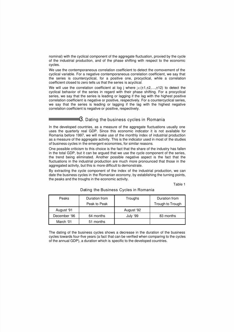
By extracting the cycle component of the index of the industrial production, we can

date the business cycles in the Romanian economy, by establishing the turning points,the peaks and the troughs in the economic activity.

Table 1

Dating the Business Cycles in Romania

Peaks Duration from

Peak to Peak

Troughs Duration from

Trough to Trough

August ‘91 August ‘92

December ‘96 64 months July ‘99 83 months

March ‘01 51 months

The dating of the business cycles shows a decrease in the duration of the businesscycles towards four-five years (a fact that can be verified when comparing to the cyclesof the annual GDP), a duration which is specific to the developed countries.

8/13/2019 jef4-2004-9


Figure 1Business Cycles in the Romanian Economy

- . 1 5

- . 1 0

- . 0 5

. 0 0

. 0 5

. 1 0

. 1 5

1 9 9 2 1 9 9 4 1 9 9 6 1 9 9 8 2 0 0 0 2 0 0 2

C Y C L E

Since the period is small for analyzing the business cycles, we cannot but assume thatthe period of large swings is over, and except some huge shocks, the aggregatefluctuations in Romania will tend to look similar to those in the developed countries asregards persistence, volatility and asymmetry between expansions and recessions.

The volatility of the business cycles is higher than in the developed countries, a factcaused by the large shifts in the structure of the economy and the restructuringprocess that took place. It is expected that the volatility will tend towards levelscommon to the developing economies, given the absence of large shocks (seeMcDermott (1999)).

4. Nominal and Real Characteristics of the

Romanian Business Cycles

4.1. The Prices

As a measure of prices, two different variables are used: the level of prices (and onecan use either the CPI or the GDP deflator) or the inflation rate. The difference mayseem unimportant but as the studies of the cyclical behavior of the prices in thedeveloped countries show, contrasting results for the two variables are quite oftenobtained.

We will study both the cyclical properties of the level of prices and of the inflation rate.

Figure 2

CPI and Industrial Product ion Cycles

8/13/2019 jef4-2004-9


- . 3

- . 2

- . 1

. 0

. 1

. 2

9 4 9 5 9 6 9 7 9 8 9 9 0 0 0 1 0 2 0 3

C Y C L E _ I P C Y C L E _ C P I

The results show us that while the prices are countercyclical (R(0)=-0.35) and leadingby ten months, the inflation rate is acyclical, while having a much larger volatility.

We will consider only the results for the level of prices, as showing us the behavior ofprices.

In Keynes’ “General Theory”, prices are flexible and taken as procyclical, thishypothesis playing a central role in this theory of short run fluctuations. As thestatistical tests have shown, the prices were indeed procyclical in the pre WW2 period.Nevertheless, the economists have continued to assume the procyclicity of the pricesin the post war period, without testing it, and here the famous Koopman critique (1947)on the reporting of business cycles facts without any theory to back up them has

played an essential role.More recently, this prevailing view has been contradicted by the RBC school. Kydlandand Prescott (1990) have shown that in the post Korean war period, in the UnitedStates the prices have been “clearly countercyclical”.

Their finding was confirmed by other studies – Cooley and Ohanian (1991), Backusand Kehoe (1992) and Smith (1992). While there appears an agreement on the factthat the level of prices is countercyclical, some other studies have showed that theinflation rate is procyclical for the most developed countries.

Some studies were undertaken for the developing countries, too. McDermott (1999)finds for some countries countercyclical price behavior, while for other he finds aprocyclical pattern.

The countercyclical pattern of the prices is usually interpreted as a reason against thedemand–driven models.

8/13/2019 jef4-2004-9


4.2. The WagesWe will use two measures of the wages – the nominal average wage per month andthe real average wage per month (the nominal wage deflated by the CPI).

Figure 3

Real Wages and Industrial Production Cycles

- . 3

- . 2

- . 1

. 0

. 1

. 2

9 4 9 5 9 6 9 7 9 8 9 9 0 0 0 1 0 2 0 3

C Y C L E _ I P C Y C L E _ W R

The results for the cyclical properties of the wages, both real and nominal show amuch clearer picture. Both of them are leading (the nominal wage by four months whilethe real wage is leading the economic fluctuations by five months) and countercyclical(the nominal wage has a stronger countercyclical character).

These results dismiss a possible real business cycle approach to the understanding

and modeling of the business cycles in Romania. In the RBC framework, the real wageis procyclical, and theoretical it should show a strong procyclicity (close to one). Theevidence from the developed countries (especially US) shows a moderate to weakprocyclical character.

The Keynesian explanation of the business cycles makes the central point from thenominal rigidities. In the initial form of the “General Theory” (1936), Keynes expressedthe view that the nominal wages are rigid in the short run and the prices are flexible.Thus, in the case of a recession, the prices are going down and given the short runrigidity of the nominal wage, the real wage becomes countercyclical. The hypothesis ofthe countercyclical real wage has been contradicted by the statistical tests on the realdata that were undertaken a short while after the publication of the Keynes’scontribution. It has also been proven that in the post war period, in the developedcountries the real wages have been proven proczclical.

McDermott (1999) in the study on the emerging economies business cycles also findsa prociclicity of the real wages in most of the countries included in the sample.

As a response to the early studies on the cyclical behavior of the real wage, Keynes(1939) has formulated a new view in which the nominal wage is rigid, the nominal

8/13/2019 jef4-2004-9


prices are flexible but there are some imperfections also in the goods market. Thehypothesis that the goods market has some rigidity is expressed by the fact that theprice is a markup over the price. Given the well known fact the markups arecountercyclical (Rotember and Woodford (1999)), which means that they are lower inexpansions than in the recessions, the real wage may become procyclical.

The countercyclical behavior of the nominal and real wage confirms the rigidities of theRomanian economy’s labor market.

4.3. The Role of th e Money

One of the fundamental questions regarding the nature of business cycles is about therole of the money, or to use the well-known expression – whether the money areneutral.

Up to the apparition of the RBC school there was a consensus on the fact that moneydo matter. The debate was between what was a good monetary policy and what was a

bad monetary policy and, in the mainstream thinking, the place of the money in thebusiness cycles theory was well established.

In the RBC theory, where the impulses that trigger the business cycle are thetechnological shocks and the propagation mechanism is by the intertemporal allocationof leisure and hours of working, changes in the monetary variables do not change thereal variables but just the nominal ones. Therefore, the monetary shocks do not haveany influence on the real economy.

The New Keynesian school admits a role to the monetary side of the economy,because the monetary shocks do influence the real activity due to the rigidities in theshort run of the prices and wages.

Figure 4

Real Money Supply and Industrial Production Cycles

- . 1 5

- . 1 0

- . 0 5

. 0 0

. 0 5

. 1 0

. 1 5

. 2 0

9 4 9 5 9 6 9 7 9 8 9 9 0 0 0 1 0 2 0 3

C Y C L E _ I P C Y C L E _ M 2 R

8/13/2019 jef4-2004-9


We obtain contrasting results for the cyclical behavior of the money supply, dependingon the fact whether it is real or nominal. For the nominal money supply we get a veryweak countercyclical behavior, close to an acyclical one, with a leading tendency offive months. Meanwhile, the real money supply has a moderate procyclical behaviorand is leading the aggregate fluctuations by ten months.

Given the large fluctuations in the level of prices and the clearer pattern for the realbalance of money, we consider that the real M2 gives us the measure of the behaviorof the monetary side of the economy.

Theoretically, a leading and procyclical character of the money would sustain a NKapproach but the RBC proponents have their explanation for the procyclical characterof the money (in the US the monetary aggregates are procyclical but they lag thebusiness cycles). They argue that M2 responds endogenously to the outputfluctuations, because the rise in productivity during the booms leads to a rise in thedemand for transaction services, the result being that the banking sector responds by

increasing the money supply.This sale of the money can be underlined by the cyclical properties of the real non-government debt, which is moderately procyclical and is leading the business cycle by12 months. The obvious role of the credit in the business cycles is a characteristic of adeveloping country, due to the lack of development of the financial markets. Thisstylized fact is confirmed for some other emergent economies by McDermott (1999).

The leading and procyclical character of the real monetary variables suggests apossible money output causality relationship for Romania, which should be furtherinvestigated.

Figure 5

Real Non-Government debt and Industr ial Production Cycles

- . 4

- . 3

- . 2

- . 1

. 0

. 1

. 2

. 3

. 4

9 4 9 5 9 6 9 7 9 8 9 9 0 0 0 1 0 2 0 3

C Y C L E _ I P C Y C L E _ D B T

8/13/2019 jef4-2004-9


4.4. Other v ariables4.4.1. The employment

In order to measure the fluctuations in the labor market we used two variables – thenumbers of employed and of unemployed persons, both in thousands persons.

The two variables perform quite asymmetrical during the cycle. If the employment isalmost acyclical the unemployment, measured by the number of unemployed persons,yields an obvious countercyclical behavior, with the contemporaneous correlationcoefficient of -0.54, while it lags the cycle with five months.

The explanation for this behavior rests in the fact that during the ‘90’s a continuousprocess of restructuring in the labor market took place and many workers had to leave jobs in the inefficient companies. That is why the employment continued to fall evenduring the expansion periods, given the need for restructuring. As many of the peoplewho lost their jobs received retirement packages, the number of unemployed did not

take a pattern in line with the employment variable. Thus, the numbers of employedshows a weak to acyclical behavior, which cannot but give a partial confirmation of therigidity of the labor market in Romania, contradicted by the countercyclical pattern ofthe unemployment.

Figure 6

Unemployment and Industr ial Production Cycles

- . 3

- . 2

- . 1

. 0

. 1

. 2

9 4 9 5 9 6 9 7 9 8 9 9 0 0 0 1 0 2 0 3

C Y C L E _ I P C Y C L E _ U N E M

4.4.2. The exchange rate

The recent Asian crisis shows that the exchange rates can play an important role asshocks that may cause business cycles, through the various channels by which theyoperate.

As a variable we have chosen the real exchange rate, which is the nominal exchangerate deflated by the consumer price index.

8/13/2019 jef4-2004-9


8/13/2019 jef4-2004-9


Variables R((X(t),Y(t+j))*Nominal M2 -0.27 -0.29 -0.32 -0.36 -0.17 0.06 0.27 0.31 0.32

Real M2 0.55 0.57 0.54 0.46 0.34 0.05 -0.18 -0.25 -0.27

RealNon-governmentDebt

0.43 0.41 0.37 0.34 0.23 0.00 -0.26

-0.35 -0.34

Nominal wages -0.48 -0.55 -0.59 -0.64 -0.50 -0.17 0.17 0.31 0.37

Real wages -0.03 -0.09 -0.12 -0.14 -0.24 -0.39 -0.36 -0.23 -0.06

Nominal Exchange Rate

RealExchange Rate

0.39 0.46 0.48 0.41 0.38 0.37 0.21 0.06 -0.12

Employment -0.34 -0.30 -0.24 -0.06 0.15 0.35 0.44 0.49 0.54

Unemployment 0.25 0.16 0.04 -0.30 -0.54 -0.66 -0.58 -0.49 -0.41

* Where X(t) is the cyclical component of the industrial production and Y(t+j) is the cycle of thevariable selected.

B ibliography

Abraham, Katharine G., and John C. Haltiwanger, 1995, “Real Wages and the BusinessCycle”, Journal of Economic Literature , Vol. 33, pp. 1215-64.

Albu, Lucian Liviu, Pelinescu, Elena and Scutaru, Cornelia, 2003, Short-term modelsand forecastings. Applications for Romania , Expert Publishing House,Romanian Academy.

Ahmed, Shaguil and Kae H. Park, 1994, “Sources of Macroeconomic Fluctuations inSmall Open Economies”, Journal of Macroeconomics , Vol. 16 (Spring),1-36.

Backus, David K., and Patrick J. Kehoe, 1992, “International Evidence on the HistoricalProperties of Business Cycle”, American Economic Review , Vol. 82(September), 864-88.

Baxter, Marianne, and Robert G. King, 1995, Approximate Band Pass Filters forEconomic Time Series , National Bureau of Economic Research,Working Paper No. 5022 (February).

Blackburn, Keith, and Morten O. Ravn, 1991, Univariate Detrending of MacroeconomicTime Series , Working Paper No. 22, Aarhus University (March).

Canova, Fabio, 1998, “Detrending and Business Cycles Facts”, Journal of MonetaryEconomics , Vol. 41 (June) 475-512.

Chadha, Bankim, and Eswar Prasad, 1994, “Are Prices Countercyclical? Evidence fromthe G7”, Journal of Monetary Economics , Vol. 34 (October), 239-57.

Cooley, Thomas F., and Lee E. Ohanian, 1991, “The Cyclical Behavior of Prices”,Journal of Monetary Economics , Vol. 28 (August), 25-60.

8/13/2019 jef4-2004-9


Fiorito, Riccardo, and Tryphon Kollintzas, 1994, “Stylized Facts of Business Cycles inthe G7 from a Real Business Cycle Perspective,” European EconomicReview , Vol. 38 (February), 235-69.

Gavin, William T., and Finn E. Kydland, 1995, Endogenous Money Supply and theBusiness Cycle , Discussion Paper 95-010A, Federal Reserve Bank ofSt. Louis (July).

Hodrick, Robert J., and Edward C. Prescott, 1997, “Postwar U.S. Business Cycles: AnEmpirical Investigation”, Journal of Money, Credit and Banking , Vol. 29(February), 1-16.

Judd, John P., and Bharat Trehan, 1995, “The Cyclical Behavior of Prices: Interpretingthe Evidence”, Journal of Money, Credit and Banking , Vol. 27 (August),789-97.

Kim, Yang Woo, 1996, Are Prices Counter Cyclical? Evidence from East Asian

Countries , Review of Federal Reserve Bank of St. Louis.King, Robert G., and Plosser, Charles I., 1984, “Money, Credit and Prices in a Real

Business Cycle”, American Economic Review , Vol. 74 (June), 363-80.

Kydland, Finn E. and Edward C. Prescott, 1994, “Business Cycles: Real Facts and aMonetary Myth”, Federal Reserve Bank of Minneapolis QuarterlyReview 14(2), Spring 1990, pp. 3-18.

Mankiw, N. Gregory, 1989, “Real Business Cycles: A new Keynesian perspective,”Journal of Economic Perspectives 3(3), pp. 79-90.

McDermott John C., Agenor Pierre-Richard and Prasad Eswar S., 1999,Macroeconomic Fluctuations in Developing Countries: Some StylizedFacts , International Monetary Fund, Working Paper, 99/35.

Taylor, Mark P., 1995, “The Economics of Exchange Rate”, Journal of EconomicLiterature , Vol. 33 (March), 13-47.

Watson, W. Mark and Stock, James H., 1998, Business Cycle Fluctuations in U.S.Macroeconomic Time Series , NBER Working Paper 6528.

Documents

jef4-2004-9