Embed Size (px)
Citation preview

A Space-Time Modeling Approach toAssess the E�ects of El NinoJe�rey W. Stein, Fred W. Hu�er, and Xufeng Niu �AbstractWe consider monitoring station data consisting of meteorological climate mea-surements (e.g. temperature) recorded repeatedly over time, always at the samelocations. The locations of the monitoring stations form an irregular lattice,making it di�cult to use space-time models which require the speci�cation of ahierarchical spatial neighborhood system. Our goal is to test for the presence of\factor e�ects" in such data. We accomplish this goal using models which are likestandard ANOVA models except that the \error" terms are allowed to exhibitboth spatial and temporal correlations. The spatial correlations are modeled asa decreasing function of the inter-station distances using a Mat�ern covariancestructure. The temporal correlations are modeled using a vector AR(p) process.We use modi�cations of the usual ANOVA inference procedures to test for theexistence of factor e�ects. To increase the exibility of our models, we allowthe parameters of the vector AR(p) process to vary by region, and we providean objective method for grouping the stations into regions for this purpose. Asan application of our methodology, we examine the e�ect of El Nino-SouthernOscillation (ENSO) events on the winter temperature across the southern UnitedStates.�Je�rey W. Stein is a Statistician at the General Electric Corporate Research and DevelopmentCenter in Schenectady, NY, 12309; Fred W. Hu�er is an Associate Professor, and Xufeng Niu is anAssociate Professor at the Department of Statistics, Florida State University, Tallahassee, FL. Thisresearch was funded in part by the US Army Research Grant, Contract No. DAAH04-93-G-0333. Weare grateful to Dr. James O`Brien for providing us with the data set.Key words: Space-TimeModels; Likelihood Ratio Tests; Simulated Annealing, Mat�ern CovarianceFunction. 1

1 IntroductionEl Nino-Southern Oscillation, or ENSO has been described as a disruption in thenormal ow of life in the Paci�c Ocean region. The 1997-1998 El Nino disruption hasreceived worldwide attention for its impact on global weather patterns. The 1998-1999year may wreak a di�erent sort of havoc on global temperature and precipitation asit is predicted to be a La Nina or El Viejo year. El Nino (El Viejo) refers to theoccurrence of warm (cool) water along the equator in the Paci�c Ocean. The globale�ects of these two di�erent yet recurrent sets of ENSO climate conditions have beenwell documented (e.g. Rasmusson and Carpenter, 1982). It is also widely recognizedthat the climate variability of certain geographical regions is strongly a�ected by theseENSO events. For example, Kiladis and Diaz (1989) and Sittel (1994) showed (viat-tests on individual station data) there exists winter temperature anomalies during ElNino and El Viejo events during this season in the southeastern United States. Kiladisand Diaz (1989) also mapped t-values of the ENSO temperature anomalies in di�erentseasons for each monitoring station and subjectively identi�ed regional temperaturepatterns of ENSO events by visual inspection. Quantifying the ENSO temperaturepatterns is of great value to those whose economic livelihood is in uenced by any year-to-year climate uctuations. In particular, Adams et al. (1995) estimate the annualvalue of perfect ENSO prediction to be $323 million for the agricultural industry.An ENSO year is de�ned as the period from October to the following September.Based upon the extent of the sea-surface temperature anomalies in the equatorialPaci�c Ocean during this period, an index de�ned by the Japan Meteorological Agency(JMA, 1991) may be used to classify each year as El Nino, El Viejo, or Neutral (seeTable 1). Given this year classi�cation scheme, we develop a comprehensive approach2

Table 1: List of ENSO categorized years between 1948-1986El Nino Neutral El Viejo1951 1950 1974 19481957 1952 1977 19491963 1953 1978 19541965 1958 1989 19551969 1959 1980 19561972 1960 1981 19641976 1961 1983 19671982 1962 1984 19701986 1966 1985 19711968 19731975in this paper to statistically determine if there exists an overall e�ect of ENSO eventson the winter temperature across the southern United States. In particular, we areinterested in determining if the ENSO e�ect is uniform across this geographical region.Our proposed methodology improves upon the t-test approach in three obvious ways:1) We capture the extent of spatial correlation present in monitoring station data bymodeling it, 2) We are able to provide a more reliable estimate of the standard errorof the ENSO winter temperature di�erences by incorporating all of the data in themonitoring station network, and 3) We are able to determine the signi�cance levelof an ENSO e�ect by station location interaction by specifying one comprehensiveANOVA model rather than performing multiple t-tests.Because monitoring station data form temporally and (irregularly spaced) spa-tially dependent systems, our comprehensive approach to examining the ENSO wintertemperature patterns requires the formulation of a sophisticated mathematical model.Two popular classes of space-time models for regular and irregular lattice data arethe STARMA models of Cli� et al. (1975) and the conditionally speci�ed models ofBartlett (1955) and Besag (1974). One limitation of these modeling approaches is therequired speci�cation of a hierarchical spatial neighborhood system. This speci�cation3

is a tricky issue for irregularly spaced spatial data. Also, Pfeifer and Deutsch (1980)chart the behavior of the theoretical space-time autocorrelation function for �rst-orderSTAR(1) models; the decay is either oscillatory or geometrical. However, Whittle(1954) suggests that a slower rate than geometrical spatial decay is more natural fordata arising in two dimensions. Other parametric space-time modeling approaches ap-pear in Martin and Oeppen (1975), Handcock and Wallis (1994), and Niu and Tiao(1995).We propose a space-time model for a time series of spatial random �elds whichdoes not require the speci�cation of a spatial neighborhood scheme. Speci�cally, letfYi(t) : i = 1; 2; : : : ; n; t = 1; 2; : : : ; Tg denote the collection of observed data for nlocations at T equally spaced time periods. De�neY (t) = [Y1(t); Y2(t); : : : ; Yn(t)]0; and �(t) = [�1(t); �2(t); : : : ; �n(t)]0:Our proposed family of space-time models takes the formY (t) = X(t)� + �(t); (1)where X(t)� is a regression function and f�(t)g is a stationary vector AR(p) temporalprocess, �(t) = pXl=1�l�(t � l) + "(t); t = 1; 2; : : : ; T: (2)The nonsingular n x n matrices �l, l = 1; 2; : : : ; p are assumed to be diagonal. Theprocess, f"(t)g, is assumed to be a multivariate Gaussian zero-mean white noise processwith non-diagonal covariance matrix function,E("(t)"(t + h)0) = ( �(�) if h = 0;0 otherwise;4

where �(�) is a positive de�nite, symmetric matrix which depends upon a vector ofparameters, �. Our approach di�ers from the approach of Cli� et al. (1975) in that wemodel the spatial correlation in the covariance function of the white noise componentterm, f"(t)g, rather than model the spatial correlation as a weighted linear function ofthe response variable, Y (t). We refer to the model described in (1) and (2) as a spatialvector AR(p), or SVAR(p) model.The seasonal climate variable, Y (t), considered in our study is the average dailymaximum temperature (�C) over the three winter months, December, January, andFebruary. This measure was chosen because it has been shown in previous studies (e.g.Sittel, 1994, Ropelewski and Halpert, 1989) that ENSO temperature anomalies aregreatest during the winter season in the southern United States. The winter temper-ature data was collected for 39 years on a historical climatology network (HCN) of 36monitoring stations in this region (see Figure 1 on p. 15).To address our research questions, the regression function, X(t)�, is speci�ed ina two way �xed-e�ects analysis of variance framework allowing for interactions. An-other more parsimonious expression for the regression function would involve usinglatitude and longitude coordinates for each station as covariates. However, our resultsindicate that no systematic di�erences in the winter temperature measurements wereattributable to the latitude and longitude coordinates of the monitoring stations.The main e�ect terms in our ANOVA modeling framework consist of a \treatment"factor with three levels corresponding to e�ects of the three ENSO categories, and a\site" factor with 36 levels corresponding to e�ects of the n = 36 station locations.The degrees of freedom for main e�ects are k = 38 (1 for the mean correction factor,2 for the treatments and 35 for the sites). The degrees of freedom for interactions are5

2 � 35 = 70. We partition the mean function, X(t)�, asX(t) = [X(1)(t)j X(2)(t)] and � = " �1�2 # ; (3)whereX(1)(t)�1 andX (2)(t)�2 represent the main e�ect and interaction terms, respec-tively. We denote dim(X (1)(t)) = n x k and dim(X (2)(t)) = n x (m � k), where them x 1 vector of mean function parameters, �, is partitioned accordingly. For our dataset, n = 36; k = 38; and m = 108. One common hypothesis tested in an analysis ofvariance is the equality of treatment means. However, if the treatment means dependupon the spatial location, then treatment e�ects should be examined separately foreach site.The paper is organized as follows. In Section 2, we discuss some basic propertiesas well as various covariance structures of spatial vector AR(p) processes. Parameterestimation is discussed brie y in Section 3. An objective method to form contiguousgroups of monitoring stations that are homogeneous with respect to the temporalvariations in the climate measurements is presented in Section 4. In Section 5 weapply the proposed methodology to the winter temperature data. Our hypothesistesting results indicate that ENSO winter temperature e�ects depend upon the spatiallocation. Estimated ENSO winter temperature anomalies are found in Section 6. Adiscussion appears in Section 7.2 Basic Properties of the SVAR(p) ModelIn this section we discuss some basic properties of the SVAR(p) model, (1) and(2), as well as the stationarity assumptions of this model in both the space and thetime domains. First, we note a few special cases of the SVAR(p) model. In the ab-sence of temporal correlation (i.e. �l = 0 for l = 1; 2; : : : ; p so that �(t) = "(t)) the6

Ordinary Least Squares (OLS) model is obtained when �(�) = �2In. When �(t) ="(t) and the white noise covariance matrix, �(�), is non-diagonal, a spatial MANOVAmodel is obtained where the errors, "(t), are contemporaneously correlated but un-correlated between time periods. When �l = diag(�l1; �l2; : : : ; �ln) for l = 1; 2; : : : ; pand �(�) = �2In, we obtain n independent univariate AR(p) processes. Our model isquite similar to Niu and Tiao's (1995) STAR(q; p) model when their (Wn) matrixequals the identity matrix, In. In this case, their f"(t)g process has periodic covariancematrices, �2(t)In, whereas our f"(t)g process has the same covariance matrix, �(�),for each t.2.1 Stationarity Conditions for the Space and Time DomainsAn equivalent representation of (2) is�(B)�(t) = "(t) (4)where the backshift operator, B, operates on t such that Bl�(t) = �(t� l) and �(B) =In�Ppl=1�lBl. This process is temporally stationary if the zeros of the determinantalpolynomial, j�(B)j, lie outside the unit circle. In this case, it can be shown (seeBrockwell and Davis, 1991) that the unique stationary solution to (4) is�(t) = 1Xj=0j"(t� j) (5)where the matrices, fjg, are determined recursively by0 = In; j = jXl=1�lj�l; j = 1; 2; : : : ; (6)and �l = 0, for l > p. 7

To model the spatial covariance of the residual process, f"(t)g, we chose a four-parameter isotropic model from the Mat�ern class of covariance functions,Cov("i(t); "j(t + h)) = 8>><>>: c0 + �2 r = 0; h = 0�22�2�1�(�2)(r�1)�2K�2(r�1) r > 0; h = 00 h 6= 0; (7)where K�2(�) is the modi�ed Bessel function of the second kind of order �2 (Abramowitzand Stegun, 1964). For more details on this class of covariance functions, see Mat�ern(1986) and Handcock and Wallis (1994). The covariance function (7) contains twovariance components: c0 is a nugget e�ect (Matheron, 1963) and �2 is the point measureof variability of the maximum winter temperature. This Mat�ern model was �t to ourwinter temperature data both with and without the nugget term, c0; we retained thisnugget term in the covariance model because it was statistically signi�cant and becausea better �t was obtained with the presence of this parameter. We denote the entirevector of spatial covariance parameters by � = (c0; �2; �1; �2).To estimate and make inferences on the spatial covariance model parameters, �,some assumptions must be imposed on the f"(t)g process. We assume f"i(t) : i � Dg,when viewed as a spatial random �eld, is isotropic and second-order stationary for allt. That is, the covariance between "i(t) and "j(t) depends only upon a scalar distancemeasure, r = dij, where dij is the distance between stations i and j. Directional spatialvariograms (see Cressie, 1990) estimated using the OLS residuals indicate the isotropyassumption is reasonable.2.2 Covariance Matrix Function of the SVAR(p) ProcessIf we use the representation in (5) and note that E("(t+h)"(t)0)=0 for h 6= 0, thenthe covariance matrix function, �(h) � E(�(t+ h)�(t)0), of the f�(t)g process may be8

expressed as �(h) = 1Xk=0h+k�0k; h = 0;�1;�2; : : : ; (8)where �(�h) = �0(h) and k is de�ned in (6). A spatial vector AR(1) process hascovariance matrix function,�(h) = 1Xk=0�h+k1 ��0k1 ; h = 0; 1; 2; : : : : (9)It readily follows that the SVAR(1) process with common AR coe�cient, �1, acrossthe n components of �(t) (i.e. �1 = �1In) has covariance matrix function,Cov(�j(t + h); �k(t)) = � �h1�jk1��21 for h = 0; 1; 2; : : : j; k = 1; 2; : : : ; n: (10)When �1 = diag(�1; �2; : : : ; �n), the covariance matrix function isCov(�j(t+ h); �k(t)) = � �hj �jk1��j�k for h = 0; 1; 2; : : : j; k = 1; 2; : : : ; n; (11)where �jk denotes the (j; k)th element of �(�). However, the covariance function (11)is no longer isotropic because the covariance between observations at stations j and kdepends upon the values, �j and �k, in addition to the distance between the stations.The covariance function (11) is also not very parsimonious because each site hasa parameter, �j, associated with it. Suppose the region, D, may be partitioned suchthat D = Sgk=1Dk is a disjoint union of subregions, fDk : k = 1; 2; : : : ; gg, eachcontaining nk sites. It may be reasonable to assume the components of �(t) withinthe kth subregion share similar temporal statistical properties. For example, supposethe stations numbered 1; 2; : : : ; n1 belong to the �rst region, stations numbered n1 +1; : : : ; n2 belong to the second region, etc. To construct a parsimonious SVAR(1) modelfor this example, we partition the n x 1 vector as�(t) = [�(1)(t); �(2)(t); : : : ; �(g)(t)]0; (12)9

and the white noise covariance matrix function, �(�), as�(�) = 0BBBB@ �11 �12 � � � �1g�12 �22 � � � �2g� � � � � � . . . � � ��1g �2g � � � �gg 1CCCCA : (13)The corresponding matrix, �1, has a block diagonal form given by�1 = diag(�1In1; �2In2; : : : ; �gIng)and the covariance matrix function of the noise process, f�(t)g, is for h = 0; 1; 2; : : :,Cov(�(j)(t + h); �(k)(t)) = � �hj1��j�k�jk j 6= k j; k = 1; 2; : : : ; g: (14)An objective procedure is presented in Section 4 to group together monitoring stationswhere the stations in each group share similar temporal statistical properties.3 Parameter EstimationThe derivation of the exact log-likelihood function for our SVAR(p) model isanalogous to the derivation presented in Niu and Tiao (1995) for their STAR(q; p)model when (Wn) = In in their model. Speci�cally, let�0� = [�(1)0; �(2)0; : : : ; �(p)0];�0 = [�(p+ 1)0; �(p+ 2)0; : : : ; �(T )0];"0 = ["(p+ 1)0; "(p+ 2)0; : : : ; "(T )0]:As in Niu and Tiao (1995), we de�ne UlT�p to be a (T � p) x (T � p) lower triangularmatrix with 1's on the lth lower diagonal where U0T�p = IT�p. We also de�neC = 0BBBBBBBBBBB@ �1 �2 � � � �p�1 �p�2 �3 � � � �p 0� � � � � � � � � � � � � � ��p 0 � � � 0 00 0 � � � 0 0� � � � � � � � � � � � � � �0 0 � � � 0 01CCCCCCCCCCCAn(T�p) x npand 10

D = pXl=1UlT�p �l:By de�ning A = In(T�p) in Niu and Tiao's (1995) model, we may express our model inthe same compact form (A�D)� = "+C��; (15)but where " has covariance matrix I(T�p) �. Here, �� is multivariate Gaussian withmean 0 and np x np covariance matrix �� where�� = 0BBBB@ �(0) �(1) �(2) � � � �(p� 1)�(�1) �(0) �(1) � � � �(p� 2)... . . . . . . � � � ...�(�p+ 1) � � � � � � �(�1) �(0) 1CCCCA :When the regression parameters are considered, the exact log-likelihood function forthe parameters islT (�;�;�jY ) = �nT2 log(2�)� (T�p)2 log(j�j) � p2 log(j��j)�12(Y � �X��)0��1� (Y � �X��)� 12S(Y �X�); (16)where Y � = [Y (1)0;Y (2)0; : : : ;Y (p)0]0; Y = [Y (1)0;Y (2)0; : : : ;Y (T )0]0;X� = [X(1)0;X(2)0; : : : ;X(p)0]0; X = [X(1)0;X(2)0; : : : ;X(T )0]0;M = [�C (A �D)]0(IT�p ��1)[�C (A�D)]; (17)and S(Y �X�) = (Y �X�)0M(Y �X�): (18)The conditional log-likelihood function (given Y �) is computationally more tractableto solve for the parameter estimates and is given byl�T (�;�;�jY ) = �n(T � p)2 log(2�)� (T � p)2 log(j�j) � 12S(Y �X�): (19)11

Parameter estimates must be obtained for both the exact and conditional log-likelihoodfunctions using an iterative estimation procedure. We applied the scoring algorithm(see e.g. Mardia and Marshall, 1984) because of the complexity in evaluating the partialderivatives of the modi�ed Bessel functions. The FORTRAN subroutines, RKBESLand RIBESL, obtained from the SPECFUN library (Cody, 1987) of NETLIB (Dongarraand Du Croz, 1985) were used in our research to evaluate the Bessel functions.4 Delineation of Contiguous ZonesIf a monitoring station network is spread over a large geographic area, it may beunreasonable to assume the temporal correlation is the same for each station (i.e. thediagonal elements (�l1; �l2; : : : ; �ln) of �l are all equal for each l = 1; 2; : : : ; p in theSVAR(p) model, (1) and (2)). However, too little data may exist to allow the temporalcorrelation in the temperature measurements to be di�erent for each station (i.e. thediagonal elements (�l1; �l2; : : : ; �ln) are all di�erent). A preliminary analysis of theOLS residuals indicated some evidence that the �li values are not equal and varied byregion. In order to obtain a rigorous test for the existence of interactions between theENSO e�ects and site locations, we need to account for the varying autocorrelationparameter values. Therefore, we were interested in a �nding an objective approachto put the stations into groups which are fairly homogeneous with respect to theseautocorrelation parameter values for the purpose of obtaining a more accurate modelwith which to test the signi�cance of the regression parameters, �. The grouping ofthese regions was not intended for any other use as we would have applied a stationgrouping algorithm in some other way (perhaps using the � values).We provide a solution to the station grouping problem by assuming that nearbystations have the same temporal autocorrelation parameter values (i.e. �lj = �lk if12

stations j and k belong to the same group). A formal de�nition of station groupingswill be given later in this section. Earlier approaches to solve similar regionalizationproblems were somewhat informal and often required a degree of subjective judgementin forming the groups (e.g. Gregory, 1975, and Gadgil et al., 1993). In contrast,our approach is completely automatic, requires no subjective judgement, and maybe regarded as more objective than these other approaches.We view the station grouping problem as a large combinatorial optimization prob-lem for which the simulated annealing algorithm is applied (Kirkpatrick et al., 1982).This algorithm is commonly used to minimize a cost function over a very large numberof possible system con�gurations. In our problem a system con�guration simply cor-responds to a grouping of stations. To ensure that the station groups do not overlapand do not have odd shapes, we de�ne valid system con�gurations as groupings ofstations (D1; D2; : : : ; Dg) for which the convex hulls (S1; S2; : : : ; Sg) are disjoint, whereSk denotes the convex hull of f(xi; yi) : i � Dkg, the locations of the stations in group k.The cost function we prefer to minimize is the SBC model selection criterion(Schwarz, 1978), SBC = �2lT + (pg + q +m)log(nT ); (20)where p, q, and m are the number of temporal, spatial, and regression parameters,respectively in the SVAR(p) model. It is too computationally expensive to maximizethe exact log-likelihood function, lT (see (16)) for each system con�guration in theannealing algorithm. Instead, we approximate (20) by substituting the conditionallog-likelihood function, l�T (see (19)) for lT and by �xing the values of � and � at themaximum likelihood estimates obtained from �tting the MANOVA model.The minimization of this approximation to (20) is equivalent to the minimization13

of the following cost function,E = S(Y �X�̂;�(�̂); �̂1; : : : ; �̂p) + pg log(nT ): (21)The values, �̂1; : : : ; �̂p, in (21) are those which minimize S(Y � X�̂; �̂; �̂1; : : : ; �̂p)with �̂ and �̂ set equal to the maximum likelihood estimates obtained from �ttingthe MANOVA model. The �lk values which minimize the sum of squared errors,S(Y �X�̂), are found quickly by solving a multivariate system of p linear equations.Embedded in the annealing algorithm is the Metropolis algorithm (Metropolis etal., 1953) which is a Monte Carlo method of simulating the evolution of a system to astate of equilibrium. To randomly generate a sequence of valid system recon�gurations,a station grouping con�guration (D1; D2; : : : ; Dg) is perturbed by selecting a station atrandom and moving it from its current group into one of the other g�1 groups (selectedat random). If the new grouping is not valid, we try again until a valid grouping ofstations is obtained.Minimization of the cost function for an SVAR(1) model, E = S(Y �X�̂;�(�̂); �̂1)+g log(nT ), produced the con�guration of six station groups in Figure 1. The FOR-TRAN subroutine, CONVEX, written by Eddy (1977) and obtained from NETLIB(Dongarra and Du Croz, 1985), was used to �nd the vertices of the convex hulls ofstation groups. The algorithm we used to detect the intersection of two convex hullsis found in O'Rourke (1994).5 Application to Monitoring Station DataWe apply the previously outlined methodology in this section to analyze the wintertemperature data. A preliminary analysis of the OLS residuals was conducted todetermine the extent of both spatial and temporal correlations. Univariate empirical14

105 100 95 90 85 80 75
24
26
28
30
32
34
36
38
1
2
3
4
5
6
7
8
9
1011
12
13
14
1516
17
18
19
20
21
2223
24
2526
2728
29
30
31
32
33
34
35
36
A Six Region Zonal Configuration
Longitude
Latitu
de
Figure 1: Final station grouping con�guration produced by the simulated annealingalgorithm 15

ACF and PACF plots of the OLS residuals from each station revealed a signi�cant�rst partial autocorrelation coe�cient for 14 of the 36 time series, but non-signi�cantcoe�cients for p > 1, indicating p = 1 is appropriate.To assess the spatial correlation, isotropic variograms were estimated for each ofthe 39 years using the method of moments variogram estimator (Cressie, 1993). Anaverage variogram, constructed by averaging these 39 variograms, guided us to considerthe Mat�ern covariance model (7). Directional variograms (Cressie, 1993) were alsoplotted, but provided little evidence of directional anisotropy.5.1 Parameter Estimation ResultsFour models, all special cases of (1) and (2), were �t to the data: The ordinaryleast squares (OLS) model, the MANOVAmodel (see Section 2), a spatial vector AR(1)model (SVAR(1)-1) where �1 = �1I36, and a regionally isotropic model (SVAR(1)-6)with six temporal parameters, identi�ed by the simulated annealing algorithm (seeTable 2). Table 2: Station numbers for six region station groupingsRegion 1 Region 2 Region 3 Region 4 Region 5 Region 61 12 7 9 11 18 20 262 14 8 10 15 30 21 273 32 9 16 17 36 22 284 34 13 19 23 295 35 24 316 25 33Table 3 presents parameter estimates (and estimated standard errors) of the spatialcovariance parameters for these four models obtained by maximizing the exact log-likelihood function, lT , in (16). The estimated standard errors in Table 3 were obtained16
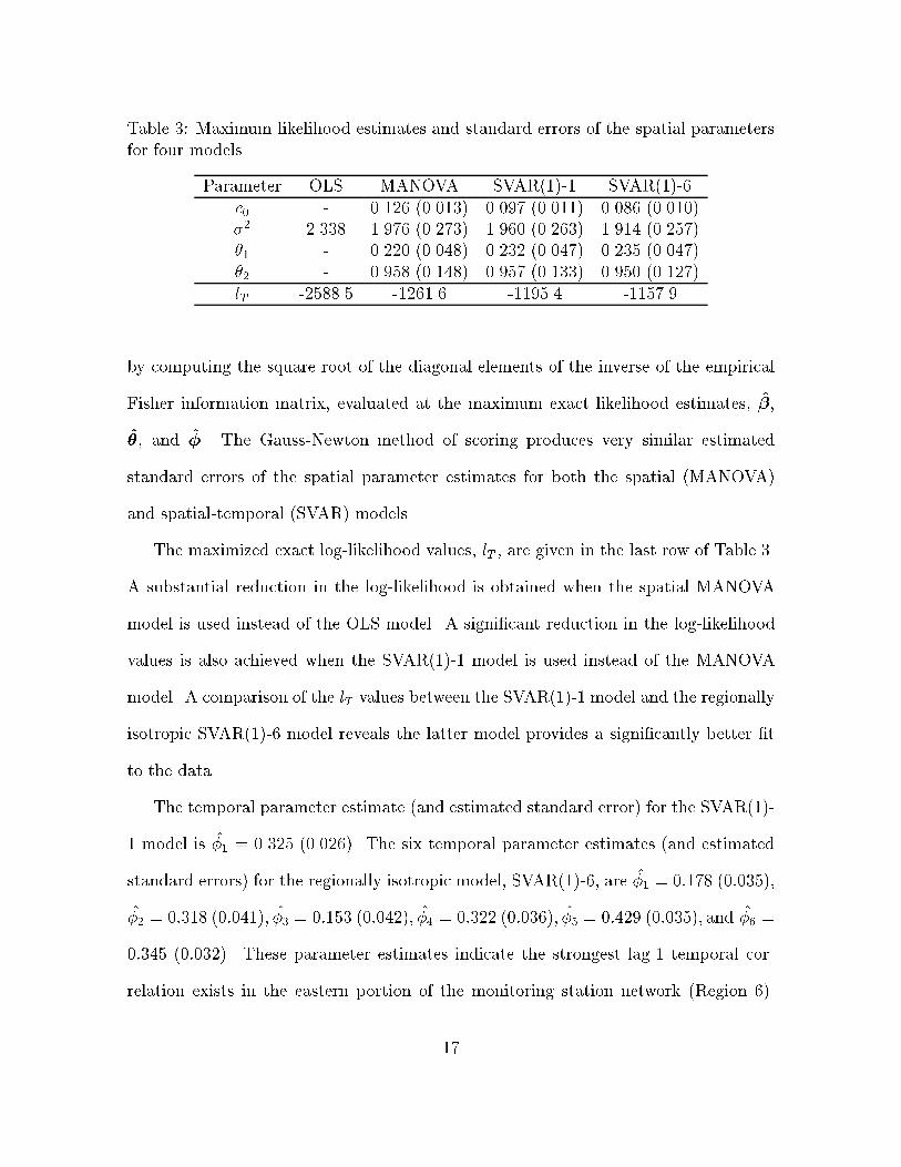
Table 3: Maximum likelihood estimates and standard errors of the spatial parametersfor four modelsParameter OLS MANOVA SVAR(1)-1 SVAR(1)-6c0 - 0.126 (0.013) 0.097 (0.011) 0.086 (0.010)�2 2.338 1.976 (0.273) 1.960 (0.263) 1.914 (0.257)�1 - 0.220 (0.048) 0.232 (0.047) 0.235 (0.047)�2 - 0.958 (0.148) 0.957 (0.133) 0.950 (0.127)lT -2588.5 -1261.6 -1195.4 -1157.9by computing the square root of the diagonal elements of the inverse of the empiricalFisher information matrix, evaluated at the maximum exact likelihood estimates, �̂,�̂, and �̂. The Gauss-Newton method of scoring produces very similar estimatedstandard errors of the spatial parameter estimates for both the spatial (MANOVA)and spatial-temporal (SVAR) models.The maximized exact log-likelihood values, lT , are given in the last row of Table 3.A substantial reduction in the log-likelihood is obtained when the spatial MANOVAmodel is used instead of the OLS model. A signi�cant reduction in the log-likelihoodvalues is also achieved when the SVAR(1)-1 model is used instead of the MANOVAmodel. A comparison of the lT values between the SVAR(1)-1 model and the regionallyisotropic SVAR(1)-6 model reveals the latter model provides a signi�cantly better �tto the data.The temporal parameter estimate (and estimated standard error) for the SVAR(1)-1 model is �̂1 = 0.325 (0.026). The six temporal parameter estimates (and estimatedstandard errors) for the regionally isotropic model, SVAR(1)-6, are �̂1 = 0:178 (0:035),�̂2 = 0:318 (0:041); �̂3 = 0:153 (0:042); �̂4 = 0:322 (0:036); �̂5 = 0:429 (0:035); and �̂6 =0:345 (0:032). These parameter estimates indicate the strongest lag-1 temporal cor-relation exists in the eastern portion of the monitoring station network (Region 6).17

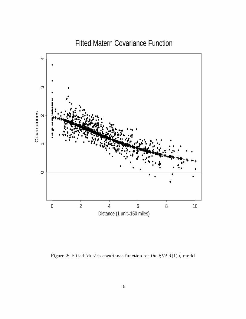
Regions 1 and 3 exhibit the weakest lag-1 temporal autocorrelation.5.2 Spatial Vector AR(p) Model Diagnostic MethodsIn this section, we propose some diagnostic methods to examine the adequacy ofthe �tted models. We apply these methods to the empirical residuals de�ned in (22)from the MANOVA, SVAR(1)-1, and SVAR(1)-6 models."̂(t) = y(t)�X(t)�̂ t = 1"̂(t) = [y(t)�X(t)�̂]� �̂1[y(t � 1)�X(t � 1)�̂] t = 2; 3; : : : ; T: (22)The empirical residuals for the MANOVA model are obtained by taking �̂1 to be thezero matrix, where �̂1 denotes �1 evaluated at the maximum exact likelihood functionestimate, �̂.A plot of the �tted covariance function versus the inter-station distances provides asummary of the spatial properties of the (isotropic) winter temperature random �eldsover the 39 year time period. In particular, this plot provides a visual description ofthe range of spatial correlation for the maximum winter temperature. The empiricalresidual covariances, de�ned by V = 1T TXt=1 "̂(t)"̂(t)0; (23)may be biased, correlated, and heteroskedastic. Consequently, graphing the �ttedcovariance function along with the empirical residual covariances may not be the bestmethod to determine the adequacy of the �t of the covariance function. However, sucha plot may reveal anomalies of the proposed model. A graph of the �tted Mat�erncovariance function for the SVAR(1)-6 model is presented in Figure 2. Empiricalresidual covariances (i.e., the (i; j)th elements of V in (23)) for stations i and j fromthis model are also plotted versus the inter-station distances, dij .18
+
++
++ +
++
+++
++ + ++
+ +++
+++ ++++ +++ +
++ ++
+
+
++
++++
++
+ ++++
+++++
+++++++
++
+++++ ++
++
++
+++
++
++ +
+++
++ +++
+++++++
++
+++++
++
+
+
++
+
++++ + +
+ ++ +
+++ ++
++++ ++++ +
++ +++
++
+
+ + ++
+
+ +++ +
++++
++ +++
++++ +++
+ ++++
++ ++
+
++++
+
++
+++
+++ +
+++
+++
+++ ++++
+++ +
++++
+
+
++
++
++
+ + ++
++
+ +++ ++
++++ ++++ +
++ +++
++
+
+
++
+
+
++
+++
+
++
++++++
++++ ++++ +
+++
++++
+
+++ +
+
++++
++
++
++++ ++
+
+++ +++
++
+++
++++
+++
+++
++++
++
++
+++
++++
++++
+++ +++
+++
++
+++
+ ++
+++
+++
++
+
+++++
+
+++
++++
+++
+++
++
+
+
++
+ +
+++
++
+
+++
+++
+++
+++++++
++++
++++
+
+
++
++
+++
+++
++
+ ++ +++
+++++++
++
++ +
++++
+
+
++
+ +
+++
+++
+ ++
+++++
+++++++
++
+++
++++
+
++
++
+
+ ++++
+ +++
+ ++++
+
+++ +++
++
+++
++
++
+
++
++
+
+ +++ +
+ +++
+++ ++
+
+++ +++
++
+++
++++
+
+
++
+ +
+++
+ ++
+++
+++
+ ++
+++++++
+++
++
++
+
++
++
+
+ ++
+++ ++ +
+ ++
++
+
+++ ++++ +
++
++
+
+ +
+
++
++
+
+ ++
+++
+++
++ ++
++
+++
++++ +
++
++
+
+ +
+
+++
++
+++
+++
++ +
+++
+++
+++
+++
++++
++
+
+ +
+
++++ +
+ ++++
+ + + +
+ ++++
+
++ + +++
++
++++
+
++
+
++++ +
+++++
++ + +
+ ++++
+++
++++
++++
+ ++
++
+
++++ +
+ ++++
++ + +
+ ++++
++++
+++
++++
+ ++
++
+
+++
+ ++ ++
++++ ++
+ ++
+ +++ ++
+++
++
+ + +++
++
+
+++
+ ++ ++
++++ + +
+ +++ +
+++++++
++ +++ +
+
++
+
+++
+ ++ ++
++++ + +
+ +++ ++++++++
+++++ +
+
++
+
++
++ +
+ +++ +
++
++++
++ + + ++++++
+++ ++
++
+ +
+
+++
+ ++ ++
++++++
+ +++ +++++
+++++
+ ++ ++
++
+
++
++ +
+ ++++
++ + +
+ ++
+ ++
+++++++ +
++
++
+
+ +
+
++
++
+
+ ++
+++ + + +
+ +++ +
+
+++ ++++ +
++
++
+
+ +
+
+
++
+ ++
+++ +
+
+++++
++ +
+ ++++++
+++ +
+
++++
+
+
+++ +
+ +++ +
++
+++++ + + ++ ++
+++
+++ +
+
+++ +
+
+++
+ ++ ++
+ ++
+++
++++ +++ ++
+ ++++
+ +++
+
+++
+++
+ ++ ++
+ ++
+++++
+ + +++ ++
+++
+++ +
+
++
++
+
+
++++
+ +++ +
+
++
+ +++
+ + ++ +++ ++
+++ +
++
+
++
+
+
++
+ +
+++
+ ++
+++++
++ +
+++++++
+++ +
+
++++
+
Distance (1 unit=150 miles)
Covariances
0 2 4 6 8 10
01
23
4
•
••
••
•
•
•••
••
•• •
•
• ••
• ••
• •••• •••
•••
••
•
•
•
••
••
•
••
••
•
••
••• •
•
••
••
•••
••
••
•••
••
••
••••
••
••• ••
•• ••
• ••
• ••
••••
••
••
•••
••
•
• ••
•
•
••
•
••
• •
•
•••
• ••
••
•• •••• •
••
••
•
••
•
•
•
••
•
••
•
•• •
•••
••• •
•
••
••
•••
• •••• •
••
•
•
•
•••
•
••
••
• ••
•
•••
• ••
• ••• •••
••
••
••
••
•
•
•••
•
•
•
••
• •
•
•
•
•
••
• ••
••
•• ••••
•
••
•••
••
•
•
•
•
•
•
•
•
•
••
•
•
•
•
••
••
•
••••
•••
••
••
•
••••
•
•••
•
•
•••
•• •
•
•
•
••
•••
• ••• •••••
••
••
•••
•
••
••
•
••
•
••
•
•
•
•
••
••
•
• ••••
••••
••
•••
••
•
•
•• •
•
••
•••
•
•
•
•
••
•••
• ••••
••••
••
•
••
••
• •
••
• ••
•
•
••
•
••• ••• •
•
• •
••
•••
•••
•
••
•
••
•
•
•••
•
•
••
••
••
•
• ••• •
•
••
•• •
•••
•••
••
•
••
•
•
••
• ••
•
•
••
•
• ••
••• ••
••
••
•••
•••
•
••
•
••
•
•
•••
•
•
•••
•
• •••
••
••
•
• •
•• ••
••
••
•
••
•
••
•
•
•••
•
•
•••
•
• •••
••• ••
• •
•• •••
••
••
••
•
••
•
•
••
• •
•
•
•
••
•
•••
••
••
•• •
••
•••
• ••••
••
••
•
•
••
• •
•
••
••
•
• • ••
••
•
•• •
•• •
••• •
••
••
•
••
•
•
•••
•
•
••
••
• •• ••
• ••
•
• ••
• ••
•• ••
•
••
•
• •
•
•
••
• •
•
••
••
••• •
• •••
••
••• •••
•••
•
• ••
• •
•
•
••
• •
•
••
••
•• • •
••
••
••
•
• • ••• •• ••
••
•
• •
•
•
•••
•
••
•••
•• • •
• ••••••• •
••• ••
••
••
•
• •
•
•
•••
•
•••
••
• • • •• ••
••
• •••
••• ••
••
••
•
• •
•
•
••
••
•
•
•
••
•
•••
••
•••
••
••
• ••
•• • •••
•
• •
•
•
••• •
•
••
••
•• • •
••
••
•
••
•••
••
••••
••
•
• •
•
•
•• • •
•••
••
•• • •• •
••
••
••
• ••• •• ••
••
•
• •
•
•
••
••
•
•
•
••
•
••••
•
•••
• •
••
•••
••• ••
•
•
• •
•
•
••
•••
•
•
••
•
••••
•
••••
•
••
• ••
••
• •• •
•
• •
•
•
••
• •
•
••
••
•• • •
••
••
•• •
•••
••
• •• •
••
•
• •
•
•
••
••
•
••
••
•• • •
•••
•
••
•
•• •
••• •
•
•
••
•
••
•
•
•••
••
•
•
••
•
••
•• •
• ••
• •
••
•••
• •• •••
•
• •
•
•
•••
••
•
•
• •
•
••
•• •• •
• •••
•• •
•
••• ••
• •
• • •
•
••
•••
•
•
••
•
•
•
••
•
••••
•
••
• ••
••• •••
•
• •
•
•
•••
••
•
•
• •
•
••
•• •• •
• ••••
•••
••• •
•• •
•• •
•
•••
••
••
• ••
••
• • •• • • ••
•••
•••• • •
•• •••
•
•
••
•••
•
•
••
•
••
•••
• ••
••
••
•••
• •• ••
•
•
••
•
Fitted Matern Covariance Function
Figure 2: Fitted Mat�ern covariance function for the SVAR(1)-6 model19

If the f�(t)g process is generated by an SVAR(1) model, then the MANOVAmodel will not account for the temporally correlated observations. Let �"i(k) =corr("i(t); "i(t + k)) denote the univariate lag-k autocorrelations for station i (i =1,2,. . . ,36). If the model is correct, then the sample autocorrelations of the residualsfor each station, �̂"i(k) = PT�kt=1 ("̂i(t) � "i)("̂i(t + k)� "i)PTt=1("̂i(t) � "i)2 (24)should exihibit a mean of zero and approximate standard error of 1/pT , where "i =1T PTt=1 "̂i(t). The boxplots in Figure 5.2 show the ranges of the 36 estimated �̂"i(k)values for each of lags k = 1; 2; : : : ; 9, for the MANOVA, SVAR(1)-1, and SVAR(1)-6models, respectively. The horizontal band in the graphs represents approximate mar-gins of errors, �2=pT , around a mean of zero. The MANOVA model has clearlynot accounted for the lag-l autocorrelation as evidenced by a large number of signif-icant sample lag-1 autocorrelation coe�cients. However, both SVAR(1) models havesuccessfully removed the temporal correlation.5.3 Hypothesis Testing of ANOVA Factor E�ectsIn this section, we test for the existence of treatment (ENSO e�ect) by siteinteractions to determine if the ENSO events a�ect the winter temperature uniformlyacross the southern U.S. region of study. For our proposed model, this corresponds totesting the hypothesis, H0 : �2 = 0 vs: H1 : �2 6= 0; (25)where �2 is an (m� k) x 1 vector of treatment by site interaction terms.20

-1.0
-0.5
0.0
0.5
1.0
Lag
AC
F
1 2 3 4 5 6 7 8 9
(a) SACF of Residuals from MANOVA Model
-1.0
-0.5
0.0
0.5
1.0
Lag
AC
F
1 2 3 4 5 6 7 8 9
(b) SACF of Residuals from SVAR(1)-1 Model
-1.0
-0.5
0.0
0.5
1.0
Lag
AC
F
1 2 3 4 5 6 7 8 9
(c) SACF of Residuals from SVAR(1)-6 Model
Figure 3: Boxplots of the sample autocorrelation values computed using the residualsfrom the (a) MANOVA, (b) SVAR(1)-1, and (c) SVAR(1)-6 models21

5.3.1 Likelihood-Ratio Test StatisticsDenote lT and l(0)T to be the values obtained by maximizing the exact log-likelihoodfunction for the full model and the model with �2 = 0, respectively. Under H0 thestatistic, X2 = �2(l(0)T �lT ); approximately follows a �2 distribution with m�k degreesof freedom for large T . Our simulations have shown the sample size, T = 39, is notlarge enough for the asymptotic theory to provide an adequate approximation. Inparticular, the X2 statistic produces values which are larger than expected under thenull hypothesis. Therefore, use of this statistic for small T will yield the rejection ofthe null hypothesis more times than the data warrants.We have experimented with two modi�cations of the basicX2 statistic which usuallyhave better distributional properties under H0. The �rst is motivated by consideringthe F -statistic used to test the hypothesis, (25) for the OLS model,F (OLS) = (nT �m)(m� k) (SSE(Reduced)SSE(Full) � 1) ;where SSE(�) denotes the usual sum of squared errors. For the OLS model, therelationship between this F statistic and the X2 statistic isF = (nT �m)(m� k) (exp X2nT !� 1) ; (26)which exactly follows an F distribution with m � k and nT �m degrees of freedomunder the null hypothesis.Our second modi�ed X2 statistic is motivated by performing a one step Taylorseries expansion for exp(X2nT ) in (26) and using the fact that, for large nT � m, therandom variable, (m�k)F , will approximately follow a �2m�k distribution for the OLSmodel under the null hypothesis. This leads to the statistic,U = (nT �m)nT X2; (27)22

which is just a scaled version of X2. For the OLS model, both F and U are closer totheir nominal Fm�k;nT�m and �2m�k distributions, respectively under H0 than is X2.Monte Carlo simulation experiments were performed to study the null distributionsof X2, F , and U for the MANOVA and SVAR(1)-1 models. The �ndings were similarfor both models so only the SVAR(1)-1 results will be presented. For each iteration,39 years of simulated data were generated from the reduced model with �2 = 0 forour network of 36 sites. The values, (c0; �2; �1; �2; �1) = (0.097, 1.96, 0.232, 0.957,0.325), were used to generate data from the SVAR(1)-1 model. The full and reducedmodels were then �t to the simulated data and the proposed statistics were calculated.This process was repeated 500 times for the SVAR(1)-1 model. Figure 4 displays thequantile-quantile probability plots for the 500 X2, F , and U statistics which werecomputed for the simulated data from the SVAR(1)-1 model.Graph (a) shows the simulated X2 values are larger than expected under the nullhypothesis. The plot in graph (b) indicates that the scaling factor of (nT �m)=nTin the U statistic is a little too \strong" in the sense that the U values are smallerthan expected under the null hypothesis. The plot in graph (c) indicates that the Fstatistic gives the closest approximation to its nominal sampling distribution of thethree statistics being considered in our example.Table 4 lists the maximized exact log-likelihood values, lT and l(0)T , for the fulland reduced models, respectively, along with the computed X2, F , and U statistics.For this data set, m � k = 70 and nT �m = 1296. The observed signi�cance levelsassociated with the hypothesis tests, which were computed using the nominal samplingdistribution of the corresponding statistics under the null hypothesis, are listed inparentheses in the last three rows of Table 4. Although the same conclusions wouldbe reached in our example based upon the small observed levels of signi�cance for each23

Expected Chi-square values
Sim
ula
ted X
2 V
alu
es
40 60 80 100 120
40
60
80
100
120
•••••••••••
••••••••••••••••••••••••••••••••••••••••••••••••••••••••••••••••••••••••••••••••••••••••••••
••••••••••••••••••••••••••••••••••••••••••••••••••••••••••••••••••••••••••••••••••••••••••••••••••••••••••••••••••••••••••••••••
••••••••••••••••••••••••••••••••••••••••••••••••••••••••••••••••••••••••••••••••••••••••••••••••••••••••••••••••••••••••••••••••
••••••••••••••••••••••••••••••••••••••••••••••••••
•••••••••••••
•• •
(a) X^2: SVAR(1)-1
Expected Chi-square valuesS
imula
ted U
Valu
es
40 60 80 100 120
40
60
80
100
120
••••••••••••••••••••••••••••••••••••••••••••••••••••••••••••
••••••••••••••••••••••••••••••••••••••••••••••••••••••••••••••••••••••••••••••••••••••••••••••••••••••••••••••••••••••••••••••••••
••••••••••••••••••••••••••••••••••••••••••••••••••••••••••••••••••••••••••••••••••••••••••••••••••••••••••••••••••••••••••••••••••••••••••••••
••••••••••••••••••••••••••••••••••••••••••••••••••••••••••••••••
•••••••••••••••••
•• •
(b) U: SVAR(1)-1
Expected F values
Sim
ula
ted F
Valu
es
0.4 0.6 0.8 1.0 1.2 1.4 1.6 1.8
0.4
0.8
1.2
1.6
•••••••••••••••••••••••••••••••••••••••••••••••
•••••••••••••••••••••••••••••••••••••••••••••••••••••••••••••••••••••••••••••••••••••••••••••••••••••••••••••••••••••••••••••••••••
•••••••••••••••••••••••••••••••••••••••••••••••••••••••••••••••••••••••••••••••••••••••••••••••••••••••••••••••••••••••••••••••••••••••••••••••••••
••••••••••••••••••••••••••••••••••••••••••••••••••••••••••••••••••••
•••••••••••••••••••••••
•• •
(c) F: SVAR(1)-1
Figure 4: Quantile-Quantile plots of the X2, F , and U values from the SVAR(1)-1model simulations 24

Table 4: Test statistics for the OLS, MANOVA, SVAR(1)-1, and SVAR(1)-6 modelsStatistic OLS MANOVA SVAR(1)-1 SVAR(1)-6lT -2588.52 -1261.63 -1195.35 -1157.92l(0)T -2605.66 -1312.84 -1251.49 -1216.15X2 34.28 (1.000) 102.42 (0.007) 112.28 (0.001) 116.46 (0.0004)F 0.458 (1.000) 1.401 (0.018) 1.541 (0.003) 1.601 (0.0015)U 31.64 (1.000) 94.54 (0.027) 103.64 (0.006) 107.50 (0.0027)of the three likelihood ratio statistics for the two SVAR(1) models, it is clear that hadthe interaction e�ect not been as large as the one observed, con icting results wouldbe obtained.6 ENSOWinter Temperature Anomaly EstimationAn assessment of the ENSO temperature anomalies is given using the maximumexact likelihood estimate of �,�̂ = (X(1)0�̂�1X(1) +X0M̂X)�1(X(1)0�̂�1Y(1) +X0M̂Y); (28)from the SVAR(1)-6 model, where �̂�1 and M̂ are evaluated at the maximum exactlikelihood values, (�̂; �̂). The covariance matrix of �̂ is approximately (X(1)0�̂�1X(1)+X0M̂X)�1. Figure 5 lists the estimated average (El Nino � Neutral) di�erences inmaximum winter temperature (�C) for each site. The estimated standard errors ofthese di�erences ranges between 0.41 and 0.51 (�C). Figure 6 lists the estimatedaverage (El Viejo � Neutral) di�erences in maximum winter temperature (�C). Thecorresponding estimated standard errors of these di�erences ranged between 0.39 and0.49 (�C). Except for site 5 (Fort Stockton, TX), the absolute magnitude of the average(El Viejo � Neutral) di�erences is larger than the absolute magnitude of the average(El Nino � Neutral) di�erences for all sites. Also, the estimated average (El Nino �25

-0.7
-0.7
-0.5
-0.7
-1.3
-0.2
-0.5
0.5
0.2
-0.10.2
-0.6
-0.3
-0.6
-0.1-0.2
-0.6
-0.5-0.4
-0.3
-0.4
-0.4-0.7
-0.7
-0.9-0.6
-0.9-1
-0.7-0.6
-0.6
-1
-0.9
-0.7
-0.4
-0.7
Estimated (El Nino - Neutral) Differences
105 100 95 90 85 80 75
24
26
28
30
32
34
36
38
Longitude
Latitu
de
Figure 5: Estimated average El Nino � Neutral di�erences in maximum winter tem-perature 26

1.5
2
2
1.5
1.2
1.7
1.1
1.6
1.8
1.61.9
2.4
2.4
2.6
2.22.3
2.4
2.12.2
1.9
2.3
1.81.8
2.3
2.12
2.22.2
2.12.2
2.1
1.5
2.6
0.9
1.4
2.5
Estimated (El Viejo - Neutral) Differences
105 100 95 90 85 80 75
24
26
28
30
32
34
36
38
Longitude
Latitu
de
Figure 6: Estimated average El Viejo � Neutral di�erences in maximum winter tem-perature 27

Neutral) di�erences for sites 8, 9, and 11 (Newkirk, OK; Poteau, OK; and Pocahontas,AR) are positive whereas these average di�erences for all other sites are negative; thesesites may be causing the hypothesis of no treatment by site interactions to be rejected.7 Summary and DiscussionA methodology was proposed in this paper to model a series of spatial random�elds exhibiting an autoregressive temporal structure. Our techniques were applied toanalyze winter temperature climate data recorded on an irregularly spaced monitoringstation network. The procedure outlined in this paper is appropriate to rigorously andstatistically examine the e�ect of ENSO events on temperature across a geographicalregion.In general, the El Nino winters are cooler than Neutral winters, whereas the El Viejowinters are over 2�C warmer on average than Neutral winters in some portions of themonitoring station network. The estimated temperature di�erences (via t-tests) are0:1�C smaller than those estimated from the SVAR(1)-6 model for (El Nino - Neutral)but 0:3�C larger for (El Viejo - Neutral). However, the standard errors of the di�erences(via t-tests) range from 0:42�C to 0:82�C for (El Viejo - Neutral) and from 0:45�C to0:87�C for (El Nino - Neutral). One surprising conclusion drawn from this study is thesigni�cant temporal correlation present after taking into account the e�ects of ENSOevents and station locations. Our results indicate that erroneous conclusions may bedrawn if the spatial and temporal nature of the data is ignored.Modi�cations of the usual ANOVA inference procedures were also presented to testfor the existence of factor e�ects for small sample sizes when the observations exhibitspatial and temporal dependence. Through Monte Carlo simulations, the sampling dis-tributions of some proposed likelihood-ratio and Wald test statistics were compared to28

their nominal null distributions. The sampling distribution of a proposed F statistic,analogous to the F statistic for standard regression models, seemed to yield a closeapproximation to its nominal F distribution for the spatial MANOVA and SVAR(1)models. The results of our simulated examples are promising; more research is neces-sary to determine if the close approximation holds in general.Lastly, we mention the class of space-time models proposed in this paper was in-tended primarily for purposes of hypothesis testing and explanation rather than ofprediction. A more parsimonious mean structure which includes covariates represent-ing spatial characteristics of the site such as latitude, longitude, and elevation, could beused if spatial interpolation (kriging) and/or temporal prediction is the primary goal.REFERENCESAbramowitz, M. and Stegun, I.A. (1964) Handbook of Mathematical Functions. NewYork: Dover.Adams, R.A., Bryant, K.J., McCarl, B.A., Legler, D.M., O'Brien, J.J., Solow, A.,and Weiher, R. (1995) The Value of Improved Long-Range Weather Infor-mation: Southeastern US ENSO Forecasts as they In uence US Agriculture.Contemporary Economic Policy, 13, 10-19.Bartlett, M.S. (1955) An Introduction to Stochastic Processes. Cambridge: CambridgeUniversity Press.Besag, J.E. (1974) Spatial Interaction and the Statistical Analysis of Lattice Systems.Journal of the Royal Statistical Society Series B, 36, 192-225.Brockwell, P.J. and Davis, R.A. (1991) Time Series: Theory and Methods, Second29

Edition. New York: Springer.Cli�, A.D., Haggett, P., Ord, J.K., Bassett, K.A., and Davies, R.B. (1975) Elementsof Spatial Structure: A Quantitative Approach. Cambridge: Cambridge Uni-versity Press.Cody, W.J. (1987) New Computing Environments: Microcomputers in Large-ScaleScienti�c Computing. city: SIAM.Cressie, N. (1993) Statistics for Spatial Data (Revised Edition). New York: Wiley.Dongarra, J.J. and Du Croz, J. (1985) Distribution of Mathematical Software ViaElectronic Email. city: Technical Report MCS-TM-48, Argonne NationalLaboratory, Mathematics and Computer Science Division.Eddy, W.F. (1977) CONVEX. ACM TOMS, 3, 411-412.Gadgil, S., Joshi, Y., and Joshi, N.V. (1993) Coherent Rainfall Zones of the IndianRegion. Journal of Climatology, 13, 547-566.Gregory, S. (1975) On the Delimitation of Regional Patterns of Recent Climatic Fluc-tuations. Weather, 30, 276-287.Handcock, M.S. and Wallis, J.R. (1994) An Approach to Statistical Spatial-TemporalModeling of Meteorological Fields. Journal of the American Statistical Asso-ciation, 89, 368-378.JMA (1991) Climate Charts of Sea Surface Temperatures of the Western North Paci�cand the Global Ocean. city: Japan Meteorological Agency Marine Division.Kiladis, G.N. and Diaz, H.F. (1989) Global Climatic Anomalies Associated with Ex-tremes in the Southern Oscillation. Journal of Climate, 2, 1069-1090.30

Kirkpatrick, S., Gelatt, C.D. Jr., and Vecchi, M.P. (1982) Optimization by SimulatedAnnealing. city: IGM Research Report RC 9355.Mardia, K.V. and Marshall, R.J. (1984) Maximum Likelihood Estimation of Modelsfor Residual Covariance in Spatial Regression. Biometrika, 71, 135-146.Martin, R.L. and Oeppen, J.E. (1975) The Identi�cation of Regional Forecasting Mod-els Using Space-Time Correlation Functions. Transactions of the Institute ofBritish Geographers, 66, 95-118.Mat�ern, B. (1986) Spatial Variation, Second Edition, Lecture Notes in Statistics. NewYork: Springer.Matheron, G. (1963) Principles of Geostatistics. Economic Geology, 58, 1246-1266.Metropolis, N., Rosenbluth, A., Rosenbluth, M., Teller, A., and Teller, E. (1953) Equa-tion of State Calculations by Fast Computing Machines. Journal of ChemicalPhysics, 21, 1087-1092.Niu, X. and Tiao, G.C. (1995) Modeling Satellite Ozone Data. Journal of the AmericanStatistical Association, 90, 969-983.O'Rourke, J. (1994) Computational Geometry in C. Cambridge: Cambridge UniversityPress.Pfeifer, P.E. and Deutsch, S.J. (1980) Identi�cation and Interpretation of First-OrderSpace-Time ARMA Models. Technometrics, 22, 397-408.Rasmusson, E.M. and Carpenter, T.H. (1982) Variation in Tropical Sea Surface Tem-perature and Surface Wind Fields Associated with the Southern Oscillation-El Nino. Monthly Weather Review, 110, 354-384.31

Ropelewski, C.F. and Halpert, M.S. (1989) Precipitation Patterns Associated with theHigh Index Phase of the Southern Oscillation. Journal of Climate, 2, 268-284.Schwarz, G. (1978) Estimating the Dimension of a Model. Annals of Statistics, 6,461-464.Sittel, M. (1994) Marginal Probability Distributions of the Extremes of ENSO Eventsfor Temperature and Precipitation in the Southeastern United States. Talla-hassee: Master's Thesis, Department of Meteorology, Florida State Univer-sity, unpublished.Whittle, P. (1954) On Stationary Processes in the Plane. Biometrika, 41, 434-449.Wilks, S.S. (1938) The Large-Sample Distribution of the Likelihood Ratio for TestingComposite Hypotheses. Annals Mathematical Statistics, 9, 60-62.
32