Embed Size (px)
Citation preview
AISM (2006) 58: 1–20DOI 10.1007/s10463-005-0007-7
Arijit Chakrabarti · Jayanta K. Ghosh
Optimality of AIC in inferenceabout Brownian motion
Received: 12 February 2004/Accepted: 10 December 2004 / Published online: 25 March 2006© The Institute of Statistical Mathematics, Tokyo 2006
Abstract In the usual Gaussian White-Noise model, we consider the problem ofestimating the unknown square-integrable drift function of the standard Brownianmotion using the partial sums of its Fourier series expansion generated by an ortho-normal basis. Using the squared L2 distance loss, this problem is known to be thesame as estimating the mean of an infinite dimensional random vector with l2 loss,where the coordinates are independently normally distributed with the unknownFourier coefficients as the means and the same variance. In this modified versionof the problem, we show that Akaike Information Criterion for model selection,followed by least squares estimation, attains the minimax rate of convergence.
Keywords Nonparametric regression · Minimax · AIC · Oracle · Brownianmotion · White-noise
1 Introduction
The Akaike Information Criterion (AIC), the now well-known penalized likeli-hood model selection criterion, was introduced and studied byAkaike (1973,1978).Different asymptotic optimality properties of AIC have been proved in the litera-ture by several authors in the last three decades. In the first line of work, Shibata(1981, 1983) proved the optimality of AIC as a model selection rule in the infinitedimensional problem of nonparametric regression, where the goal is to find out
A. Chakrabarti (B)Applied Statistics Unit, Indian Statistical Institute, 203 B.T. Road,Calcutta 700108, IndiaE-mail: arijit [email protected]
J. K. GhoshDepartment of Statistics, Purdue University, 150 North University Street,West Lafayette, IN 47907-2067, USAStatistics and Mathematics Unit, Indian Statistical Institute,203 B.T.Road, Calcutta 700108, India
2 A. Chakrabarti and J. K. Ghosh
the optimum number of terms to retain, for the purpose of prediction, in the Fou-rier series expansion of the unknown function generated by a given orthonormalsequence. Shibata (1983) has shown that AIC does as well as an oracle introducedby him in this problem. In a second line of work, Li (1987) and Shao (1997) provedthe asymptotic optimality of AIC as a model selection rule in the context of selec-tion of variables from a given set of variables in a Linear model setup. But theoptimal rate of convergence of AIC has not been studied in the literature. The nov-elty of our paper is to show that model selection by AIC followed by least squaresestimation achieves the minimax rate of convergence in one form of nonparametricfunction estimation problem.
We study AIC in the following problem of inference about an unknown signalor drift f ∈ L2[0, 1] of a Brownian motion and prove it attains the optimal rate ofconvergence in two different senses. Given n, one observes {Z(t)} given by
dZ(t) = f (t)dt + dB(t)√n
, 0 ≤ t ≤ 1, (1)
where B(t) is the standard Brownian motion. This is essentially the problem(Eq. 31) of Ibragimov and Has’minskii (1981, p. 345). In problem (Eq. 1), weconsider a complete orthonormal basis {φi, i = 1, 2, . . . } of L2[0, 1]. Then onecan write
f (t) =∞∑
i=1
θiφi(t), (2)
with equality in the sense of L2 convergence, where θi’s are the Fourier coefficientsgiven by
θi =1∫
0
φi(t)f (t) dt, and∞∑
i=1
θ2i < ∞. (3)
Then we need to study the somewhat simpler problem as follows:
yi = θi + εi√n, εi
i.i.d.∼ N(0, 1), (4)
where yi =1∫
0φi(t) dZ(t) for i = 1, 2, . . . .
Let θ̂ = {θ̂i} be an estimate of θ and let f̂ (t) =∞∑i=1
θ̂iφi(t) the corresponding
estimate of f . Then by Parseval’s theorem,
‖f − f̂ ‖2 =∞∑
i=1
(θi − θ̂i )2, (5)
where ‖.‖ is the usual L2 norm. So estimating f in model (Eq. 1) is the same as esti-mating θ in model Eq. (4) in terms of the above losses. We use the setup of Eq. (4)in this paper and use the squared error l2 loss. We show that model selection by AIC

AIC in inference about Brownian motion 3
followed by least squares estimates attains the minimax rate of convergence forconvergence in probability over the usual Sobolev balls Eq(B) (defined in Sect. 2),for any B > 0. This result is based on a strong property of AIC with lower trunca-tion. Under lower truncation it is shown that AIC is asymptotically equivalent toan oracle uniformly in Eq(B), where the oracle provides a lower bound to the lossin a certain class of decision rules. We also show that model selection by AIC withupper truncation followed by least squares estimation, attains the minimax rate ofconvergence, i.e, n−2q/2q+1, over the Sobolev balls mentioned before.
It is worthwhile to mention here that the definition of AIC [see Eq. (7)] does notrequire the knowledge of the order of smoothness q or the constant B appearingin the definition Eq(B) (in Sect. 2) of the class of functions being considered. Yetmodel selection by AIC followed by least squares estimation yields the minimaxrate over Eq(B); showing that AIC is adaptive.
It is not hard to show that the Bayes Information Criterion (BIC) cannot havethis kind of optimality. A counter-example is presented in Sect. 4.
Problem (1) has been shown in Brown and Low (1996) to be an equivalentversion in a decision theoretic sense, upto the minimax rate of convergence, of thefollowing nonparametric regression problem
Yi = f
(i
n + 1
)+ εi, εi
i.i.d∼ N(0, 1), i = 1, 2, . . . , n. (6)
Using Eq. (1) through Eq. (6), Zhao (2000) has pointed out that nonparametricregression can in principle be studied through the yi’s. Her main result is to intro-duce a hierarchical prior on the parameter space and show that the correspondingBayes estimator achieves the minimax rate of convergence. The relation betweenEqs. (1) and (6) suggests that ourAIC for Eq. (1) can be lifted in principle to providean asymptotically minimax method of estimation for nonparametric regression.This is discussed in the last section.
Section 4 also includes a discussion on how to use the theoretical results derivedfor continuous path data, when one observes the process {Z(t)} only at a finite num-ber of equally spaced points.
2 Preliminaries, notations and theorems
Suppose, as in Eq. (4), one has random variable yi’s which are independentN(θi, 1/n), i = 1, 2, 3, . . . , where
∑∞i=1 θ2
i < ∞. Using yi’s one has to comeup with estimates θ̂i and the loss is L =∑∞
i=1(θ̂i − θi)2. We consider a restricted
parameter space in our study, as in Zhao (2000), which is a Sobolev-type subspaceof l2 given by Eq = {θ = {θi} :
∑∞i=1 i2qθ2
i < ∞}, q > 1/2. We then studythe asymptotic rate of convergence of model selection by AIC followed by leastsquares estimation in the Sobolev ball
Eq(B) ={
θ :∞∑
i=1
i2qθ2i ≤ B
}.
4 A. Chakrabarti and J. K. Ghosh
With respect to the usual trigonometric basis, for q an integer, Eq correspondsto all periodic L2[0, 1] functions with absolutely continuous (q − 1)th derivativesand q-th derivatives with bounded L2 norm.
The AIC is not well defined in this case since we have an infinite sequence ofobservations. However, if we take θ̂i = 0 for all i > n, the contribution to error forθ in Eq(B) is
∑
i>n
θ2i =∑
i>n
i2qθ2i
i2q≤ B(n + 1)−2q = o
(n
− 2q
2q+1
)as n → ∞,
since θ ∈ Eq(B). So at least for the problem of finding decision rules thatattain the minimax rate, we can ignore observations beyond the nth. With thismodification one can define AIC as follows. Let
mAIC = argmin1≤m≤n
S(m) where S(m) =n∑
m+1
y2i + 2m
n. (7)
The estimate of θi is yi for i ≤ mAIC and zero thereafter. The loss is∑mAIC
1
(yi − θi)2 +∑n
mAIC+1θ2i +∑∞
n+1 θ2i .
One may interpret this as first choosing a model Mm for which θi = 0 for i > mand then estimating θi by least squares, i.e., by yi for i ≤ m.
We will now introduce some notations before we state our theorems. DefineLn(m) by
Ln(m) =m∑
1
(yi − θi)2 +
∞∑
m+1
θ2i , 1 ≤ m ≤ n, (8)
the loss in choosing model Mm and then using least squares estimates. Let
rm(θ) = m
n+
∞∑
m+1
θ2i , (9)
the risk of the estimate described above.We next define two oracles based on Ln(m) and rm(θ) as follows.Define m1 as
m1 = argmin1≤m≤n
Ln(m). (10)
Note that Ln(m1) is a lower bound to the loss of any decision rule that firstpicks a model Mm and then estimates θi by zero if i > m and by yi for i ≤ m.
Define the second oracle m0 as
m0 = argmin1≤m≤n
rm(θ). (11)
Intuitively one expects m1 and m0 to be close but m0 is easier to deal with. Notethat both m0 and m1 depend on θ .

AIC in inference about Brownian motion 5
Let AICu be the model selection procedure which is AIC with upper truncation.It chooses the model Mmu where
mu = argmin1≤m≤[n
12q+1 ]
S(m). (12)
where [n1/2q+1] denotes the largest integer less than or equal to n1/2q+1.Notation. Henceforth “an ∼ bn asymptotically”, will mean that there exist
positive constants 0 < k1 < k2 such that for all sufficiently large n, k1bn ≤ an ≤k2bn.
Consider now any sequence {mn} of integers such that mn → ∞ as n → ∞as slowly as we wish but mn ≤ m∗ where m∗ ∼ n1/2q+1 asymptotically, and isdefined in the proof of Theorem 2.1.
Now define ml0 and ml
1 as
ml0 = argmin
mn≤m≤n
rm(θ), ml1 = argmin
mn≤m≤n
Ln(m) (13)
and define ml as
ml = argminmn≤m≤n
S(m). (14)
So ml is the model chosen by AICl , the model selection procedure which isAIC with lower truncation as described in Eq. (14).
We now state the main results proved in this paper. (Note that we are suppressingthe dependence of θ̂ on n for notational convenience.)
Theorem 2.1 For the case m ≥ mn, we have, (a)
Ln(ml)(1 + op(1)) ≤ Ln(m
l0)(1 + op(1)), (15)
where the op(1) terms on both sides of Eq. (15) tend to 0 in probability as n → ∞uniformly in θ ∈ Eq(B), and
Ln(ml) = Ln(m
l1)(1 + op(1)), (16)
where the equality Eq. (16) holds on a set whose probability tends to 1 as n → ∞uniformly in θ ∈ Eq(B) and the op(1) term on the r.h.s. of Eq. (16) tends to 0 inprobability as n → ∞ uniformly in θ ∈ Eq(B).
Also, for this case,
(b) n2q
2q+1 Ln(ml) = Op(1) uniformly in θ ∈ Eq(B).
Theorem 2.2 Uniformly in θ ∈ Eq(B), we have
n2q
2q+1 Ln(mAIC) = Op(1).

6 A. Chakrabarti and J. K. Ghosh
Theorem 2.3 Let θ̂ be the estimate of θ after a model is chosen by AICu, i.e.,θ̂i = 0 for i > mu and θ̂i = yi for i ≤ mu. Then θ̂ achieves the minimax rate ofconvergence, i.e., for any B < ∞,
lim supn→∞ θ∈Eq(B)
n2q
2q+1 E(||θ̂ − θ ||2) < ∞.
Remark The lower truncation in Theorem 2.1 cannot be removed. This is easy tosee by considering what happens for θn = (1/
√n, 0, 0, . . . ).
Proofs are given in the next section.
3 Proofs
Proof of Theorem 2.1. In the following, ei = yi − θi, i = 1, 2, . . . and B = 1without any loss of generality. The proof has been divided into three steps for thepurpose of clarity.
Step 1. In this step we will look at a simple minimax rule as follows. Considerrule rm for a fixed m: For m ≤ n, estimate θi by yi for 1 ≤ i ≤ m and for i > m,estimate θi by 0.
Risk of rm at θ is rm(θ) as defined in Eq. (3). Note that we can write
rm(θ) = m
n+
∞∑
m+1
1
i2qi2qθ2
i .
Then,
supθ∈Eq(1)
rm(θ) = m
n+ sup
θ∈Eq(1)
( ∞∑
m+1
1
i2qi2qθ2
i
)= m
n+ 1
(m + 1)2q.
Now choose m∗ as
m∗ = argmin1≤m≤n
{m
n+ 1
(m + 1)2q
}. (17)
It is easy to show that m∗ ∼ n1/2q+1 asymptotically, whence the maximum risk ofthe rule rm∗ is
supθ∈Eq(1)
rm∗(θ) = m∗
n+ 1
(m∗ + 1)2q∼n
−2q
(2q+1) asymptotically,
i.e., limn→∞ n
−2q
(2q+1) supθ∈Eq(1)
rm∗(θ)<∞. (18)
Thus rm∗ is a rule which attains the asymptotic minimax rate of convergence. Nownote that rm0(θ) ≤ rm∗(θ), ∀θ ∈ Eq(1), i.e.,
supθ∈Eq(1)
rm0(θ) ≤ supθ∈Eq(1)
rm∗(θ) ∼ n−2q
(2q+1) asymptotically, (19)
whence the rule rm0 based on the oracle m0 does at least as well as the rule rm∗
asymptotically.

AIC in inference about Brownian motion 7
Step 2. In this step we will consider the lower truncated AIC and derive severalproperties associated with it.
First recall the definitions of Ln(m) and S(m) from Eqs. (8) and (7) respectively.Note,
Ln(m) =m∑
1
e2i +
∞∑
m+1
θ2i = rm(θ) +
(m∑
1
e2i − m
n
).
Again,
S(m) =n∑
m+1
e2i +
n∑
m+1
θ2i + 2
n∑
m+1
θiei + 2m
n
=n∑
1
e2i −
m∑
1
e2i +
n∑
m+1
θ2i + 2
n∑
m+1
θiei + 2m
n
= Ln(m) + Rn(m) +n∑
1
e2i −
∞∑
n+1
θ2i
= Ln(m) + Rn(m) + (“constants” independent of m),
where
Rn(m) = 2n∑
m+1
θiei − 2
(m∑
1
e2i − m
n
).
Hence, minimizing S(m) with respect to m is equivalent to minimizing Ln(m) +Rn(m) over m. So we have, with ml , ml
0 and ml1 as in Eqs. (13) and (14),
Ln(ml) + Rn(m
l) ≤ Ln(ml0) + Rn(m
l0) (20)
and
Ln(ml) + Rn(m
l) ≤ Ln(ml1) + Rn(m
l1). (21)
Let us now prove three lemmas which essentially show that the remainder termsRn(m
l), Rn(ml0) and Rn(m
l1) in Eqs. (20) and (21) are negligible. These lemmas
are crucial for proving the theorem.
Lemma 3.1m∑
1
e2i − m
n= op(rm(θ)) (22)
andn∑
m+1
θiei = op(rm(θ)), (23)

8 A. Chakrabarti and J. K. Ghosh
uniformly θ ∈ Eq(1) and for mn ≤ m ≤ n as n → ∞.
So, for such a sequence {mn}, we also have,
Rn(m) = op(rm(θ)) (24)
uniformly in θ ∈ Eq(1) and for mn ≤ m ≤ n as n → ∞.
Proof E(∑m
1 e2i − m/n
) = 0. Fix ε > 0. Then,
P
(∣∣∣∣
∑m1 e2
i − m/n
rm(θ)
∣∣∣∣ > ε
)≤ E
(∑m1 e2
i − m/n)2
ε2r2m(θ)
.
But,
E
(m∑
1
e2i − m
n
)2
= Var
(m∑
1
e2i −m
n
)= mVar
(e2i
) = 2m
n2.
Also,
r2m(θ) =
( ∞∑
m+1
θ2i
)2
+ m2
n2+ 2m
n
( ∞∑
m+1
θ2i
).
So,
E(∑m
1 e2i − m/n
)2
ε2r2m(θ)
= 1
ε2· 2m/n2
(∑∞m+1 θ2
i
)2 + m2/n2 + 2m/n(∑∞
m+1 θ2i
)
<2
ε2m≤ 2
ε2mn
→ 0 as n → ∞,
for each θ ∈ Eq(1), proving Eq. (22). Similarly,
E
(n∑
m+1
θiei
)= 0 and Var
(n∑
m+1
θiei
)=(
n∑
m+1
θ2i
)1
n,
whereby
Var(∑n
m+1 θiei
)
r2m(θ)
=(∑n
m+1 θ2i
)1n
m2/n2 + (∑∞m+1 θ2
i
)2 + 2m/n(∑∞
m+1 θ2i
)
<1
2m≤ 1
2mn
→ 0 as n → ∞,
for each θ ∈ Eq(1), proving Eq. (23). Equation (24) now follows trivially fromEqs. (22) and (23) as
Rn(m) = 2n∑
m+1
θiei − 2
(m∑
1
e2i − m
n
).
So, Lemma 3.1 is proved. ��

AIC in inference about Brownian motion 9
Corollary 3.1
Ln(ml1)(1 + op(1)) = rml
0(θ)(1 + op(1)) (25)
almost surely, where the op(1) terms on both sides of Eq. (25) tend to zero inprobability as n → ∞ uniformly in θ ∈ Eq(B).
Proof Using Lemma 3.1, we get
Ln(m) = rm(θ) +(
m∑
1
e2i − m
n
)= rm(θ)(1 + op(1)),
uniformly in θ ∈ Eq(1) and for mn ≤ m ≤ n as n → ∞.As ml
0 is a nonrandom integer in [mn, n], it also follows from the above obser-vation that
Ln(ml0) = rml
0(θ) +
ml
0∑
1
e2i − ml
0
n
= rml0(θ)(1 + op(1)) uniformly in θ ∈ Eq(1) as n → ∞.
Now observe that, from definition, Ln(ml1) ≤ Ln(m
l0), rml
0(θ) ≤ rml
1(θ). Also note
that
ml1∑
1
e2i − ml
1
n= op(rml
1(θ)), uniformly in θ ∈ Eq(1) as n → ∞.
The last statement follows using the same argument employed in provingRn1(ml) =
op(rml (θ)) uniformly in θ ∈ Eq(1) as n → ∞ in Lemma 3.3. Combining all theabove facts, one gets after some algebra,
Ln(ml1) ≤ rml
0(θ)(1 + op(1)) ≤ rml
1(θ)(1 + op(1))
= Ln(ml1)(1 + op(1)) almost surely,
where all the op(1) terms tend to 0 in probability as n → ∞ uniformly in θ ∈Eq(B). The proof of Eq. (25) now follows immediately from the above sequenceof inequalities. ��Lemma 3.2 Rn(m) = op(Ln(m)) uniformly in θ ∈ Eq(1) and for mn ≤ m ≤ nand as n → ∞.
Proof Fix 0 < ε < 1.
P
{∣∣∣∣Rn(m)
Ln(m)
∣∣∣∣ > ε
}= P
{∣∣∣∣Rn(m)
Ln(m)
∣∣∣∣ > ε,
∣∣∣∣Ln(m)
rm(θ)
∣∣∣∣ < 1 − ε
}
+P
{∣∣∣∣Rn(m)
Ln(m)
∣∣∣∣ > ε,
∣∣∣∣Ln(m)
rm(θ)
∣∣∣∣ > 1 + ε
}
+P
{∣∣∣∣Rn(m)
Ln(m)
∣∣∣∣ > ε, 1 − ε ≤∣∣∣∣Ln(m)
rm(θ)
∣∣∣∣ ≤ 1 + ε
}. (26)

10 A. Chakrabarti and J. K. Ghosh
The first two terms on the r.h.s. of Eq. (26) converge to zero as Ln(m)/rm(θ) =1 + op(1), uniformly in θ ∈ Eq(1) and for mn ≤ m ≤ n as n → ∞. The thirdterm is less than
P
{∣∣∣∣Rn(m)
rm(θ)
∣∣∣∣ > ε(1 − ε)
}→ 0 as n → ∞,
by Lemma 3.1 uniformly in θ ∈ Eq(1) and for mn ≤ m ≤ n. This provesLemma 3.2.
Lemma 3.3 Rn(ml) = op(Ln(m
l)) uniformly in θ ∈ Eq(1) as n → ∞.
Proof We first prove that
Rn(ml) = op(rml (θ)), uniformly in θεEq(1) as n → ∞. (27)
Now write,
Rn(m) = Rn1(m) + Rn2(m),
where
Rn1(m) = −2
(m∑
1
e2i − m
n
)and Rn2(m) = 2
n∑
m+1
θiei .
Fix ε > 0. Then,
P
{∣∣∣∣Rn1(m
l)
rml (θ)
∣∣∣∣ > ε
}≤ P
{max
mn≤m≤n
∣∣∣∣Rn1(m)
rm(θ)
∣∣∣∣ > ε
}
≤∑
mn≤m≤n
P
{∣∣∣∣Rn1(m)
rm(θ)
∣∣∣∣ > ε
}≤∑
mn≤m≤n
1
ε4
E(R4n1(m))
r4m(θ)
.
Noting that{∑m
1 e2i − m/n, m ≥ 1
}is a Martingale, we have, by a result
proved in Dharmadhikari et al. (1968),
E
(m∑
1
e2i − m
n
)4
≤ D1m2E
(e2
1 − 1
n
)4
for a positive constant D1
= D1m2
n4E(ne2
1 − 1)4
= D2m2
n4, for some new constant D2 as ne2
1 ∼ χ2(1).
In the above χ2(1) refers to a central chi-square distribution with one degree of
freedom.
So,∑
mn≤m≤n
E(R4n1(m))
r4m(θ)
≤∑
mn≤m≤n
16D2m2/n4
(m/n +∑∞
m+1θ2i
)4
≤∑
mn≤m≤n
16D2
m2→ 0

AIC in inference about Brownian motion 11
as n → ∞, whence Rn1(ml) = op(rml (θ)), uniformly in θ ∈ Eq(1) as n → ∞.
Now consider Rn2(m) and note that
1
2Rn2(m) =
n∑
m+1
θiei ∼ N
(0,
(n∑
m+1
θ2i
)1
n
).
So we get, E(∑n
m+1 θiei
)4 = 3(∑n
m+1 θ2i
)2 · 1/n2. This implies, by a simplealgebra, that
E
(∑nm+1 θiei
)4
r4m(θ)
<1
2m2.
Using the last inequality in the same way as we did for Rn1(ml), we have Rn2(m
l) =op(rml (θ)) uniformly in θ ∈ Eq(1) as n → ∞, proving Eq. (27).
We are done if we can show that Ln(ml) = rml (θ)(1 + op(1)) uniformly in
θ ∈ Eq(1) as n → ∞, because then Rn(ml) = op(Ln(m
l)) will follow by usingexactly the same logic as in the proof of Lemma 3.2.
Fix ε > 0. Then, by a simple argument,
P
{∣∣∣∣Ln(m
l)
rml (θ)− 1
∣∣∣∣ > ε
}≤∑
mn≤m≤n
1
ε4· E(∑m
1 e2i − m/n
)4
r4m(θ)
→ 0
as n → ∞ for all θ ∈ Eq(1), as already shown before. So, Lemma 3.3 is proved.��
Step 3. In this step we combine the results in Step 1 and Step 2 to finally proveTheorem 2.1.
Equation (15) of Part (a) of Theorem 2.1 follows by applying Lemma 3.3 tothe left-hand side of Eq. (20) and Lemma 3.2 to the right-hand side of Eq. (20), byjust noting that ml
0 is a nonrandom integer in [mn, n].Equation (16) is then proved as follows. By Eqs. (15), (25) and the facts that
Ln(ml0) = rml
0(1 + op(1)) uniformly in θ ∈ Eq(1) as n → ∞ and Ln(m
l1) ≤
Ln(ml), one has
Ln(ml1)(1+op(1))≤Ln(m
l)(1+op(1))≤rml0(1+op(1))=Ln(m
l1)(1+op(1)),
where the above holds on a set whose probability tends to 1 as n → ∞ uniformlyin θ ∈ Eq(B). (Note that all the op(1) terms in the above statement tend to 0in probability as n → ∞ uniformly in θ ∈ Eq(B).) Equation (16) then followsimmediately from the above.
We shall now prove Part (b) of Theorem 2.1. To prove this, we first recall thedefinitions of ml
0, m∗ and the asymptotic minimaxity property of rm∗ as in Eqs. (13),(17) and (18) respectively. Then it follows that
rml0(θ) ≤ rm∗(θ) ≤ Dn−2q/(2q+1)
for some D > 0 for each θ ∈ Eq(1) for all sufficiently large n in the same way asone shows in Eq. (19). Part (b) then follows easily by applying this fact togetherwith Corollary 3.1 in part (a) of Theorem 2.1.

12 A. Chakrabarti and J. K. Ghosh
Remark If we choose mn = m∗ in Theorem 2.1 and then combine with it the resultof Theorem 2.3, Theorem 2.2 follows immediately. To see this one has to note that
(i) P{n
2q
2q+1 Ln(mu) > K
}≤ n
2q
2q+1E(Ln(m
u))
K, for each K > 0,
(ii) n2q
2q+1 E(Ln(mu)) is bounded for each θ ∈ Eq(1) for each n, and
(iii) Ln(mAIC) ≤ max
{Ln(m
u), Ln(ml),Ln
(mAIC
[n1
2q+1]<m<m∗
)}if m∗>n
12q+1,
Ln(mAIC) ≤ max
{Ln(m
u), Ln(ml)}
if m∗ ≤ n1
2q+1 ,
and E(Ln(m)) ≤ Fn− 2q
2q+1 for all large enough n, if [n1
2q+1 ] < m < m∗,
where F is a positive number. In the above,
mAIC
[n1
2q+1 ]<m<m∗= argmin
[n1
2q+1 ]<m<m∗
S(m),
where S(m) is as in Eq. (7). ��But we present a more direct proof of Theorem 2.2 which does not require
Theorem 2.3 and which explains the interesting behaviour of AIC for relativelysmall m.
Proof of Theorem 2.2 Fix ε > 0 and η > 0 arbitrary. We can choose m̃ largeenough such that
P
{2
∣∣∣∣n∑
m̃+1
θiei
∣∣∣∣ < εLn(m̃)
}> 1 − η
6, ∀n ≥ m̃, ∀θ ∈ Eq(B)
and
P{n
2q
2q+1 Ln
(mAIC
m≥m̃
) ≤ Kε
}> 1 − η, for all large enough n > m̃, ∀θ ∈ Eq(B)
for some suitably chosen Kε , where mAICm≥m̃
is defined as
mAICm≥m̃ = argmin
m̃≤m≤n
S(m).
The above two probability statements follow directly from the arguments used inthe proof of Theorem 2.1. We shall henceforth write mAIC
old = mAICm≥m̃
. For eachθ ∈ Eq(B), define
K(θ) = max
{I :
m̃∑
i=I
θ2i > εn−2q/(2q+1)
},
where the maximum is taken over the range [1, m̃].Now note, for each θ ∈ Eq(B), the following two cases occur.

AIC in inference about Brownian motion 13
Case 1.m̃∑
m1+1θ2i > εn−2q/(2q+1) if 1 ≤ m1 ≤ K(θ) − 1.
Case 2.m̃∑
m1+1θ2i ≤ εn−2q/(2q+1) if K(θ) ≤ m1 < m̃.
Consider Case 2 first. Let m̃ > m1 ≥ K(θ). Then
Ln(m1) = Ln(m̃) − R1
n(m1), where
R1n(m
1) =m̃∑
m1+1
(yi − θi)2 −
m̃∑
m1+1
θ2i .
Now fix η1 > 0, arbitrarily small. It is easy to show, by noting that n∑m̃
m1+1(yi−θi)
2 ∼ χ2(m̃−m1)
and m̃ is fixed, that for all large enough n,
P
{∣∣∣∣n2q/(2q+1)R1
n(m1)
∣∣∣∣ ≤ 2ε
}> 1 − η1, ∀θ ∈ Eq(B) and K(θ) ≤ m1 < m̃.
Letting S̃(m) = S(m) − (∑n1 e2
i −∑∞n+1 θ2
i
), henceforth, we have
S̃(m1) = Ln(m1) + 2
m̃∑
m1+1
θiei + 2n∑
m̃+1
θiei − 2
m1∑
1
e2i − m1
n
.
Now note that m̃ is a fixed number, θiei ∼ N(0, θ2i /n) independently and e2
i −1/n
are independently distributed with mean 0 and variance 2/n2. Using these factsand the last equality, it is easy to show that
n2q/(2q+1)Ln(m1) ≤ n2q/(2q+1)S̃(m1) + 2ε + 2n2q/(2q+1)
∣∣∣∣n∑
m̃+1
θiei
∣∣∣∣,
for all large enough n with probability at least 1 − 2η1, for each θ ∈ Eq(B) andK(θ) ≤ m1 < m̃.
We now consider Case 1. Note that
S(m̃) = S(m1) +
2
(m̃ − m1
n
)−
m̃∑
m1+1
y2i
and
m̃∑
m1+1
y2i − 2
(m̃ − m1
n
)D=1
n
{χ2
(m̃−m1−1) + W 2 − 2(m̃ − m1
)}
where
W ∼ N
√√√√n
m̃∑
m1+1
θ2i , 1
.

14 A. Chakrabarti and J. K. Ghosh
Since, m1 ≤ K(θ) − 1, n∑m̃
m1+1 θ2i > εn1/(2q+1) → ∞ as n → ∞. So, again, we
can choose n large enough so that
P
m̃∑
m1+1
y2i − 2
(m̃ − m1
)
n> 0
> 1 − η1,
for all θεEq(B) and 1 ≤ m1 ≤ K(θ) − 1, implying
S(m̃) < S(m1), i.e., mAICnew,m1 = mAIC
old ,
where mAICnew,m1 = argmin
m≥m̃,
m=m1
S(m), with
probability bigger than 1 − η1 each 1 ≤ m1 ≤ K(θ) − 1.Finally note that the fact S̃(mAIC
old ) = Ln(mAICold ) + Rn(m
AICold ), where Rn(m) is
as defined in the proof of Theorem 2.1, implies, by an easy argument, that each ofthe following events
n2q
2q+1 Ln
(mAIC
old
) ≤ n2q
2q+11
1 − εS̃(mAIC
old
)+ 4ε
1 − ε
and
S̃(mAIC
old
) ≤ (1 + ε)Ln
(mAIC
old
)
holds with probability bigger than 1 − η/3, for all θ ∈ Eq(B) and ∀n ≥ m̃.Now, consider, for each θ ∈ Eq(B), the probability of the following occurring
simultaneously
{n
2q
2q+1 Ln
(m1) ≤ n
2q
2q+1 S̃(m1)+2ε+2n2q
2q+1
∣∣∣∣n∑
m̃+1
θiei
∣∣∣∣ for all K(θ)≤m1 <m̃,
∣∣∣∣n2q
2q+1 R1n
(m1) ∣∣∣∣ ≤ 2ε for all K(θ) ≤ m1 < m̃,
Ln
(mAIC
new,m1
) = Ln
(mAIC
old
)for 1 ≤ m1 ≤ K(θ) − 1,
n2q
2q+1 Ln
(mAIC
old
) ≤ n2q
2q+11
1 − εS̃(mAIC
old
)+ 4ε
1 − ε,
2
∣∣∣∣n∑
m̃+1
θiei
∣∣∣∣ < εLn(m̃), n2q
2q+1 Ln
(mAIC
old
) ≤ Kε,
S̃(mAICold ) ≤ (1 + ε)Ln(m
AICold )}.
The probability of this event can be shown to be larger than 1 − 11/6η − 4m̃η1
for all large enough n for each θ ∈ Eq(B). So the above event, in turn implies, thefollowing event,
n2q
2q+1 Ln
(mAIC
) ≤ 1 + ε
1 − εKε + 4ε
1 − ε.

AIC in inference about Brownian motion 15
The above statement follows by observing that
mAIC = mAICold or mAIC
new,m1 for some 1 ≤ m1 < m̃.
Now we are done, as m̃ is a fixed number for a given η and ε and so η1 can bechosen to be η/24m̃, to start with, making the quantity 1 − 11/6η − 4m̃n1 equalto 1 − 2η. This completes the proof of Theorem 2.2. ��
Proof of Theorem 2.3 Fix any C > 0. Define λ(θ) as in Zhao (2000), i.e.,
λ(θ) = max
{I :
∞∑
i=I
θ2i ≥ (B + C)n
− 2q
2q+1
}.
It is easy to see, vide Zhao (2000), that λ(θ) ≤ n1/(2q+1).
Now recall the definition of mu from Eq. (12). Note that
E(||θ̂ − θ ||2
)= E(Ln(m
u))
= E
{mu∑
1
(yi − θi)2 +
∞∑
mu+1
θ2i
}.
Now E(Ln(mu)) = E(Ln(m
u)1(mu≤λ(θ))) + E(Ln(mu)1(mu>λ(θ))). But,
E(Ln(mu)1(mu>λ(θ))) = E
{mu∑
1
(yi − θi)21(mu>λ(θ))
}
+E
{( ∞∑
mu+1
θ2i
)1(mu>λ(θ))
}. (28)
The second term in the r.h.s. of Eq. (28) is trivially less than (B + C)n−2q/(2q+1).
The first term is less than or equal to E{∑[n1/2q+1]
1 (yi − θi)2}
= [n1/(2q+1)]/n
≤ n−2q/(2q+1), whence E(Ln(mu)1(mu>λ(θ))) < (B + C + 1)n−2q/(2q+1).
Again,
E(Ln(mu)1(mu≤λ(θ))) = E
mu∑
1
(yi − θi)2 +
λ(θ)∑
mu+1
θi2 +
∞∑
λ(θ)+1
θ2i
1(mu≤λ(θ))
< (B + C + 1)n− 2q
2q+1 + E
{(λ(θ)∑
mu+1
θ2i
)1(mu≤λ(θ))
}. (29)

16 A. Chakrabarti and J. K. Ghosh
Now consider any number K >√
2. The second expression in Eq. (29) equals
E
{(λ(θ)∑
mu+1
θ2i
)1(
mu≤λ(θ),∑λ(θ)
mu+1 θ2i ≤K2n−2q/(2q+1)
)
}
+E
{(λ(θ)∑
mu+1
θ2i
)1(
mu≤λ(θ),∑λ(θ)
mu+1 θ2i >K2n−2q/(2q+1)
)
}
≤ K2n− 2q
2q+1 + E
{(λ(θ)∑
mu+1
θ2i
)1(
mu<λ(θ),∑λ(θ)
mu+1 θ2i >K2n−2q/(2q+1)
)
}
≤ K2n− 2q
2q+1 +λ(θ)−1∑
m=1
BP(mu = m)I
(λ(θ)∑
m+1
θ2i > K2n−2q/(2q+1)
),
as θ ∈ Eq(B).
Now for any m < λ(θ),
P (mu = m) ≤ P {S(λ(θ)) > S(m)} = P
{n
λ(θ)∑
m+1
y2i < 2(λ(θ) − m)
}. (30)
Noting that n∑λ(θ)
m+1 y2i
D= χ2(λ(θ)−m−1) + W 2, where W ∼ N
(√n∑λ(θ)
m+1 θ2i , 1
),
the expression in Eq. (30) is less than
P{W <
√2√
λ(θ) − m}
≤ P{Z < (
√2 − K)n
12(1+2q)
},
where Z ∼ N(0, 1), using the fact that∑λ(θ)
m+1 θ2i > K2n−2q/(2q+1) and λ(θ) ≤
n1/(2q+1). But,
P{Z < (
√2 − K)n1/[2(1+2q)]
}
≤ 1/√
2π exp{−1/2(K−√2)2n1/(1+2q)}
(K−√2)n1/2(1+2q)
.
So,
λ(θ)−1∑
m=1
BP(mu = m)I
(λ(θ)∑
m+1
θ2i > K2n−2q/(2q+1)
)
≤ Bn1/[2(1+2q)]
√2π(K − √
2) exp{1/2(K − √2)2n1/(1+2q)} ≤ C1n−2q/(2q+1),
for some constant C1. Hence Theorem 2.3 is proved. ��
AIC in inference about Brownian motion 17
4 Discussion
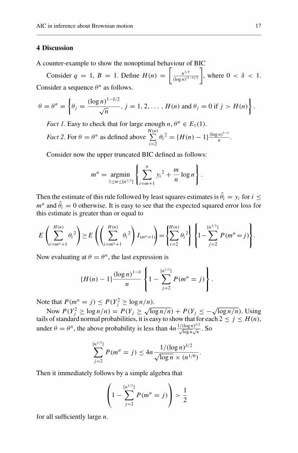
A counter-example to show the nonoptimal behaviour of BIC
Consider q = 1, B = 1. Define H(n) =[
n1/3
(log n)(1−δ)/2
], where 0 < δ < 1.
Consider a sequence θn as follows.
θ = θn ={θj = (log n)1−δ/2
√n
, j = 1, 2, . . . , H(n) and θj = 0 if j > H(n)
}.
Fact 1. Easy to check that for large enough n, θn ∈ E1(1).
Fact 2. For θ = θn as defined aboveH(n)∑i=2
θi2 = {H(n) − 1} (log n)1−δ
n.
Consider now the upper truncated BIC defined as follows:
mu = argmin1≤m≤[n1/3]
{n∑
i=m+1
yi2 + m
nlog n
}.
Then the estimate of this rule followed by least squares estimates is θ̂i = yi for i ≤mu and θ̂i = 0 otherwise. It is easy to see that the expected squared error loss forthis estimate is greater than or equal to
E
(H(n)∑
i=mu+1
θi2
)≥E
((H(n)∑
i=mu+1
θi2
)I(mu=1)
)={
H(n)∑
i=2
θi2
}
1−[n1/3]∑
j=2
P(mu =j)
.
Now evaluating at θ = θn, the last expression is
{H(n) − 1} (log n)1−δ
n
1 −[n1/3]∑
j=2
P(mu = j)
.
Note that P(mu = j) ≤ P(Y 2j ≥ log n/n).
Now P(Y 2j ≥ log n/n) = P(Yj ≥ √
log n/n) + P(Yj ≤ −√log n/n). Using
tails of standard normal probabilities, it is easy to show that for each 2 ≤ j ≤ H(n),under θ = θn, the above probability is less than 4n
1/(log n)δ/2√log n
√n
. So
[n1/3]∑
j=2
P(mu = j) ≤ 4n1/(log n)δ/2
√log n × (n1/6)
.
Then it immediately follows by a simple algebra that
1 −[n1/3]∑
j=2
P(mu = j)
>1
2
for all sufficiently large n.

18 A. Chakrabarti and J. K. Ghosh
But note that
n2/3{H(n) − 1} (log n)1−δ
n→ ∞ as n → ∞.
Using the above facts it follows that limn→∞ sup
θ∈E1(1)
n2/3E(∑∞
i=1(θ̂i − θi)2)
= ∞.
So the upper truncated BIC does not achieve the minimax rate of convergence.In fact, a careful inspection reveals that this same sequence θn can be used
to show that BIC does not attain the minimax rate of convergence for any kindof upper truncation. More importantly, the same sequence can be used to showunrestricted BIC followed by least squares also does not achieve the minimax rate,even in the sense of convergence in probability as shown to be true for AIC. Butwe do not present those arguments in the present paper.
We explore below the connection between the problem studied in our paperand nonparametric regression, vide Eq. (7). Define
f̄ (t) = f
(i
n + 1
), if
i − 1
n≤ t <
i
nfor i = 1, 2, . . . , n − 1
= f
(n
n + 1
)if
n − 1
n≤ t ≤ 1.
It is shown in Brown and Low (1996) that under certain conditions, estimating{f (t)} in problem (1.1) through {Z(t)} is asymptotically equivalent to estimating{f̄ (t)} through {Z̄(t)}, where
dZ̄(t) = f̄ (t)dt + dB(t)√n
, 0 ≤ t ≤ 1.
They also observe that {Si = n(Z̄i/n − Z̄i−1/n
), i=1,2, . . . , n} are sufficient for
Z̄(t). Now note that n(Z̄i/n − Z̄i−1/n)D= Yi , i = 1, 2, . . . , n, and the Yi’s are
trivially sufficient for the problem (Eq. 7). So any decision rule based on Si’s canbe replaced by the same decision rule based on the Yi’s and both will have the sameproperties. It is also easy to verify, at least heuristically, that the minimization cri-terion for AIC studied in our theorems is close (up to Op(1/n)) in distribution tothe minimization criterion for AIC based on the Yis and so the models selected byAIC in these two problems are also expected to be close.
We briefly explain below how the theoretical results about the rate optimalityof AIC obtained for continuous path data can be applied to the situation when oneobserves the process {Z(t)} only at points {tK = K/N : K = 0, 1, . . . , N}, whereN = Nn; i.e, N depends on n.
Let {φi : i ≥ 1} be the usual Fourier basis of L2[0, 1]. Analogous to the yis, letus define
y ′i =
N∑
K=1
φi
(K
N
)(Z
(K
N
)− Z
(K − 1
N
)),
i = 1, . . . , n; which can be rewritten as
y ′i = θ ′
i + ε′i; i = 1, . . . , n
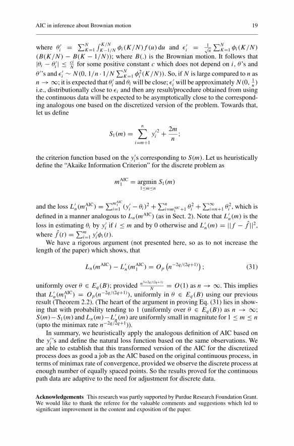
AIC in inference about Brownian motion 19
where θ ′i = ∑N
K=1
∫ K/N
K−1/Nφi(K/N)f (u) du and ε′
i = 1√n
∑NK=1 φi(K/N)
(B(K/N) − B(K − 1/N)); where B(.) is the Brownian motion. It follows that|θi − θ ′
i | ≤ ciN
for some positive constant c which does not depend on i, θ ’s and
θ ′’s and ε′i ∼ N(0, 1/n · 1/N
∑NK=1 φ2
i (K/N)). So, if N is large compared to n asn → ∞; it is expected that θ ′
i and θi will be close; ε′i will be approximately N(0, 1
n)
i.e., distributionally close to εi and then any result/procedure obtained from usingthe continuous data will be expected to be asymptotically close to the correspond-ing analogous one based on the discretized version of the problem. Towards that,let us define
S1(m) =n∑
i=m+1
y ′i
2 + 2m
n;
the criterion function based on the y ′is corresponding to S(m). Let us heuristically
define the “Akaike Information Criterion” for the discrete problem as
mAIC1 = argmin
1≤m≤n
S1(m)
and the loss L′n(m
AIC1 ) =∑mAIC
1i=1 (y ′
i − θi)2 +∑n
i=mAIC1 +1 θ2
i +∑∞i=n+1 θ2
i , which is
defined in a manner analogous to Ln(mAIC) (as in Sect. 2). Note that L′
n(m) is theloss in estimating θi by y ′
i if i ≤ m and by 0 otherwise and L′n(m) = ||f − f̂ ||2,
where f̂ (t) =∑mi=1 y ′
iφi(t).We have a rigorous argument (not presented here, so as to not increase the
length of the paper) which shows, that
Ln(mAIC) − L′
n(mAIC1 ) = Op
(n−2q/(2q+1)
) ; (31)
uniformly over θ ∈ Eq(B); provided n3+2q/(2q+1)
N= O(1) as n → ∞. This implies
that L′n(m
AIC1 ) = Op(n−2q/(2q+1)), uniformly in θ ∈ Eq(B) using our previous
result (Theorem 2.2). (The heart of the argument in proving Eq. (31) lies in show-ing that with probability tending to 1 (uniformly over θ ∈ Eq(B)) as n → ∞;S(m)−S1(m) and Ln(m)−L′
n(m) are uniformly small in magnitute for 1 ≤ m ≤ n(upto the minimax rate n−2q/2q+1)).
In summary, we heuristically apply the analogous definition of AIC based onthe y ′
i’s and define the natural loss function based on the same observations. Weare able to establish that this transformed version of the AIC for the discretizedprocess does as good a job as the AIC based on the original continuous process, interms of minimax rate of convergence, provided we observe the discrete process atenough number of equally spaced points. So the results proved for the continuouspath data are adaptive to the need for adjustment for discrete data.
Acknowledgements This research was partly supported by Purdue Research Foundation Grant.We would like to thank the referee for the valuable comments and suggestions which led tosignificant improvement in the content and exposition of the paper.

20 A. Chakrabarti and J. K. Ghosh
References
Akaike, H. (1973). Information theory and an extension of the maximum likelihood principle.In: B.N. Petrov & J.O. Berger (Eds.), Second international symposium on information theory.Budapest: Akademia Kiado. pp 267–281.
Akaike, H. (1978). A Bayesian analysis of the minimum aic procedure. Annals of the Institute ofStatistical Mathematics, 30, 9–14.
Brown, L.D., Low, M.G. (1996). Asymptotic equivalence of nonparametric regression and whitenoise. The Annals of Statistics, 24, 2384–2398.
Dharmadhikari, S.W., Fabian, V., Jogdeo, K. (1968). Bounds on the moments of martingales. TheAnnals of Mathematical Statistics, 39, 1719–1723.
Ibragimov, I.A., Has’minskii, R.Z. (1981). Statistical estimation: asymptotic theory. New York:Springer-Verlag.
Li, K.C. (1987). Asymptotic optimality for cp, cl , cross validation and generalized cross valida-tion: discrete index set. The Annals of Statistics, 15, 958–975.
Shao, J. (1997). An asymptotic theory for linear model selection. Statistica Sinica, 7, 221–264.Shibata, R. (1981). An optimal selection of regression variables. Biometrika, 68, 45–54.Shibata, R. (1983). Asymptotic mean efficiency of a selection of regression variables. Annals of
the Institute of Statistical Mathematics, 35, 415–423.Zhao, L.H. (2000). Bayesian aspects of some nonparametric problems. The Annals of Statistics,
28, 532–552.

AISMDOI 10.1007/s10463-006-0092-2
E R R AT U M
Optimality of AIC in inference about Brownian motion
Arijit Chakrabarti · Jayanta K. Ghosh
© The Institute of Statistical Mathematics, Tokyo 2006
Erratum to: AISM 58: 1–20DOI 10.1007/s10463-005-0007-7
The original version of the history unfortunately contained a mistake. The cor-rect approval history is given here.
Received: 12 February 2004 / Revised: 10 December 2004
The online version of the original article can be foundat http://dx.doi.org/10.1007/s10463-005-0007-7.
A. Chakrabarti (B)Applied Statistics Unit, Indian Statistical Institute, 203 B.T. Road,Calcutta 700108, Indiae-mail: [email protected]
J. K. GhoshDepartment of Statistics, Purdue University, 150 North University Street,West Lafayette, IN 47907-2067, USA
J. K. GhoshStatistics and Mathematics Unit, Indian Statistical Institute,203 B.T.Road, Calcutta 700108, India