The Future of Spanish Pensions:Technical Appendix∗

Javier Dıaz-GimenezIESE Business School

<jdiaz@iese.edu>

Julian Dıaz-SaavedraUniversidad de Granada

<julianalbertodiaz@ugr.es>

February 11, 2016

∗We thank Juan Carlos Conesa for an early version of the code and we thank Fernando Gil for his researchassistance. Dıaz-Gimenez gratefully acknowledges the financial support of the Spanish Ministerio de Ciencia y Tec-nologıa (ECO2012-37742) and of the Centro de Investigaciones Financieras. Dıaz-Saavedra gratefully acknowledgesthe financial support of the Spanish Ministerio de Ciencia y Tecnologıa (ECO2011-25737).

Contents

1 The Model Economy 1

1.1 The Households . . . . . . . . . . . . . . . . . . . . . . . . . . . . . . . . . . . . . . . 1

1.2 The Representative Firm . . . . . . . . . . . . . . . . . . . . . . . . . . . . . . . . . 4

1.3 The Government . . . . . . . . . . . . . . . . . . . . . . . . . . . . . . . . . . . . . . 5

1.4 The Pension System . . . . . . . . . . . . . . . . . . . . . . . . . . . . . . . . . . . . 6

1.5 The Households’ Decision Problem . . . . . . . . . . . . . . . . . . . . . . . . . . . . 9

1.6 Definition of Equilibrium . . . . . . . . . . . . . . . . . . . . . . . . . . . . . . . . . 10

2 Calibration 13

2.1 Initial conditions . . . . . . . . . . . . . . . . . . . . . . . . . . . . . . . . . . . . . . 13

2.2 Parameters . . . . . . . . . . . . . . . . . . . . . . . . . . . . . . . . . . . . . . . . . 13

2.3 Equations . . . . . . . . . . . . . . . . . . . . . . . . . . . . . . . . . . . . . . . . . . 13

2.4 The expenditure ratios . . . . . . . . . . . . . . . . . . . . . . . . . . . . . . . . . . . 18

2.5 The government policy ratios . . . . . . . . . . . . . . . . . . . . . . . . . . . . . . . 19

2.6 The initial distribution of households . . . . . . . . . . . . . . . . . . . . . . . . . . . 20

2.7 The demographic transition . . . . . . . . . . . . . . . . . . . . . . . . . . . . . . . . 21

2.8 The educational transition . . . . . . . . . . . . . . . . . . . . . . . . . . . . . . . . . 21

2.9 Results . . . . . . . . . . . . . . . . . . . . . . . . . . . . . . . . . . . . . . . . . . . . 21

3 Computation 27

4 Literature Review 30

1 The Model Economy

We study an overlapping generations model economy with heterogeneous households, a represen-

tative firm, and a government, which we describe below.1

1.1 The Households

Households2 in our model economy are heterogeneous and they differ in their age, j ∈ J ; in their

education, h ∈ H; in their employment status, e ∈ E ; in their assets, a ∈ A; in their pension rights,

bt ∈ Bt, and in their disability and retirement pensions, pdt and pt ∈ Pt. Sets J , H, E , A, Bt,

and Pt are all finite sets which we describe below. We use µj,h,e,a,b,p,t to denote the measure of

households of type (j, h, e, a, b, p) at period t. For convenience, whenever we integrate the measure

of households over some dimension, we drop the corresponding subscript.

Age. Households enter the economy at age 20, the duration of their lifetimes is random, and they

exit the economy at age 100 at the latest. Consequently, J = {20, 21, . . . , 100}. Parameter ψjt

denotes the conditional probability of surviving from age j to age j+1. This probability depends

on the household’s age and it varies with time, but it does not depend on the household’s education

level.

Fertility and immigration. In our model economy fertility rates and immigration flows are exoge-

nous.

Education. Households can either be high school dropouts, high school graduates who have not

completed college, or college graduates. The education level of a household that has dropped out

of high school is h=1. The education level of a household that has has completed high school but

has not completed college is h=2. And the education level of college graduates is h=3. Therefore,

H = {1, 2, 3}. The education decision is exogenous and the education level of every household is

determined forever when it enters the economy.

Employment status. Households in our economy are either workers, disabled households, or retirees.

We denote workers by ω, disabled households by d, and retirees by ρ. Consequently, E = {ω, d, ρ}.Every household enters the economy as a worker and every worker faces a positive probability of

becoming disabled at the end of each period of their working lives. Once a household has reached

1This model economy is an enhancement of the model economy that we presented in Dıaz-Gimenez and Dıaz-Saavedra (2009).

2To calibrate our model economy, we use data per person older than 20. Therefore our model economy householdsare really individual people.

1

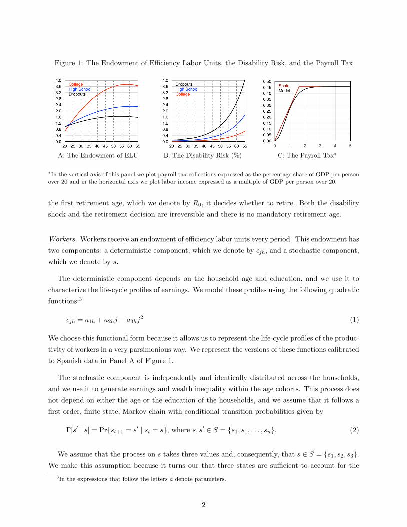
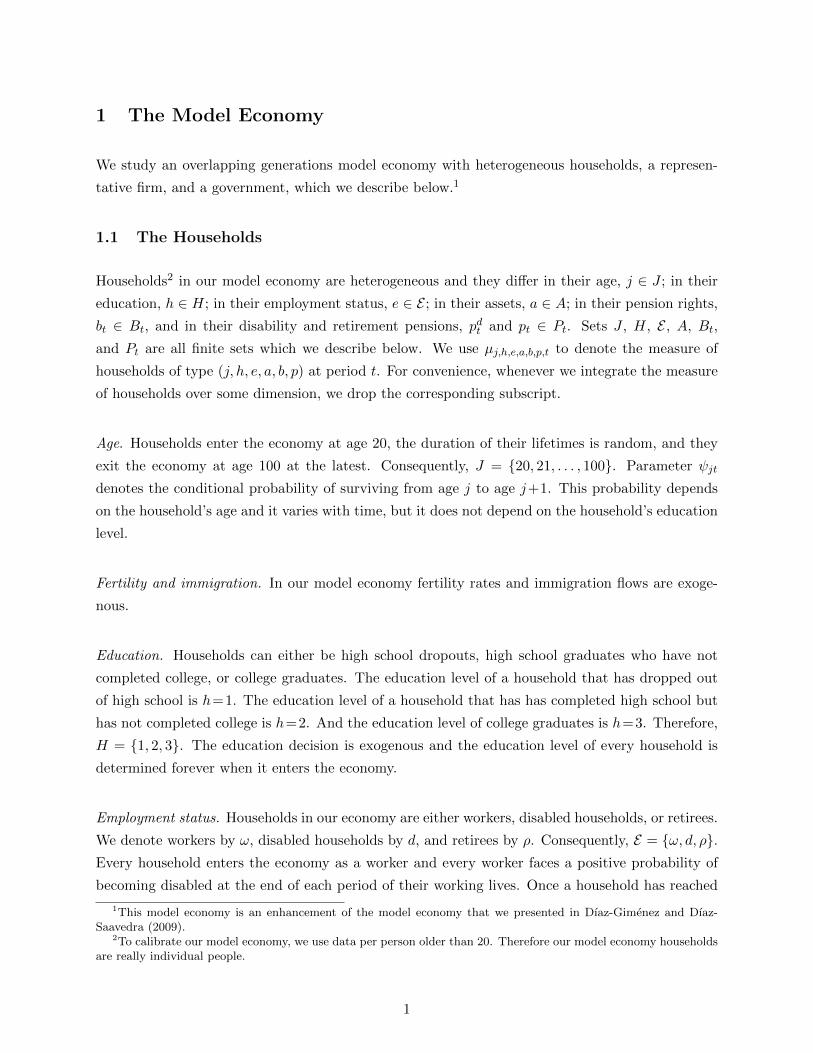
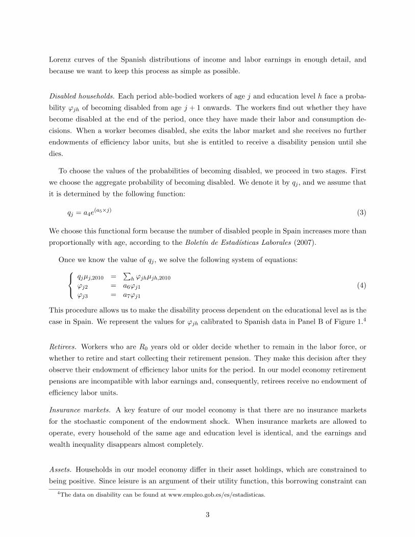
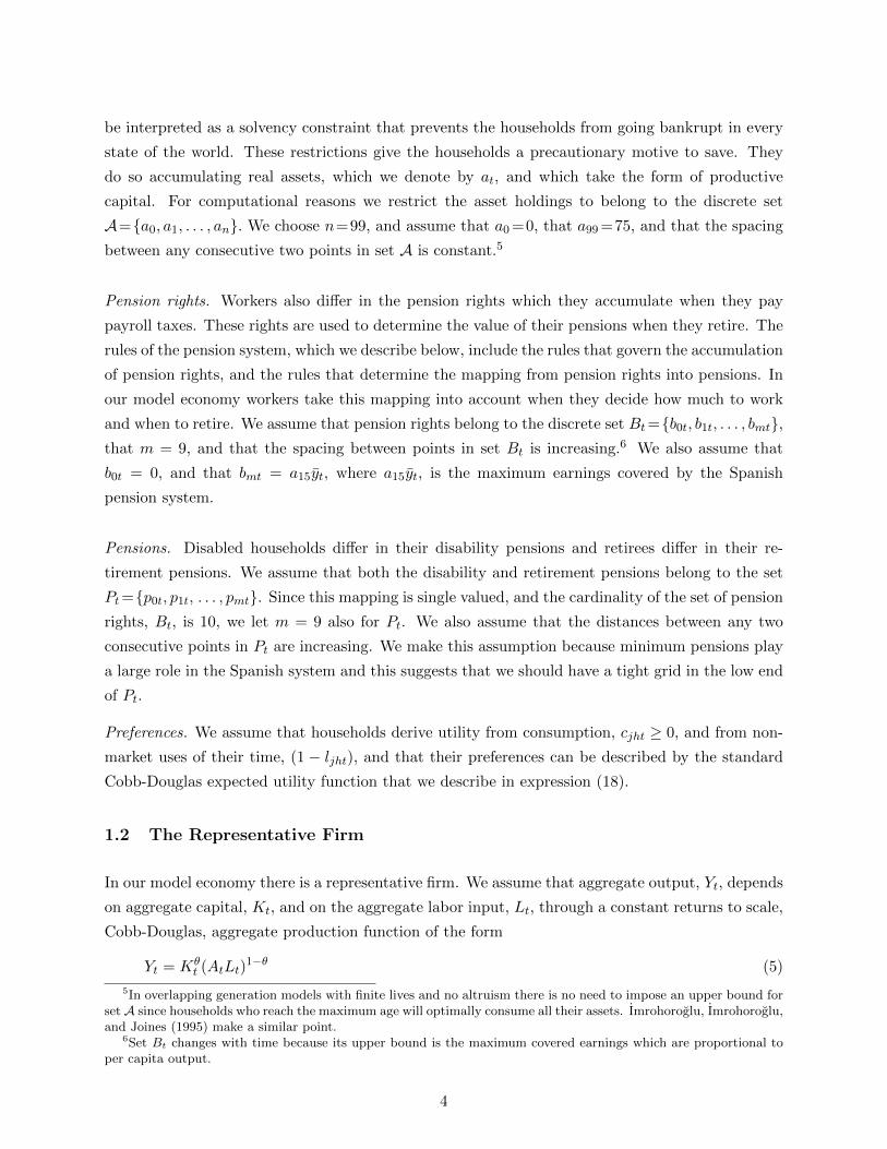
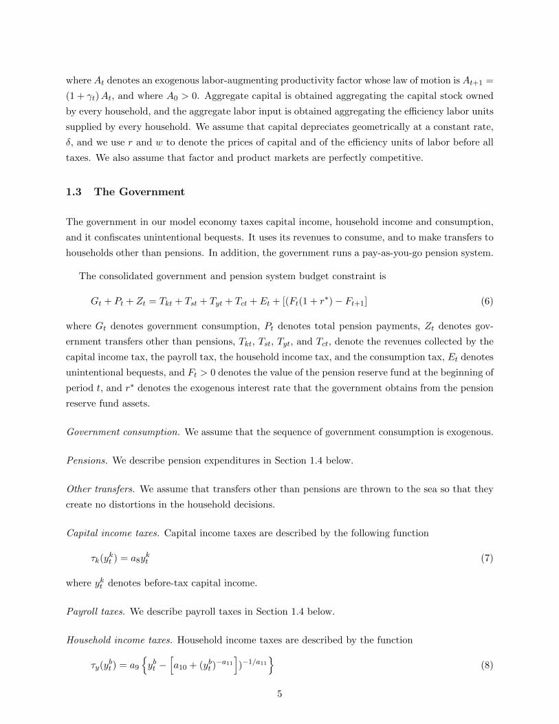
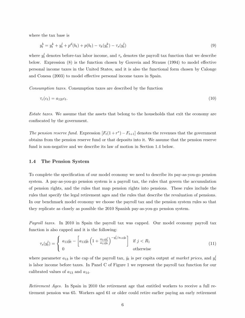
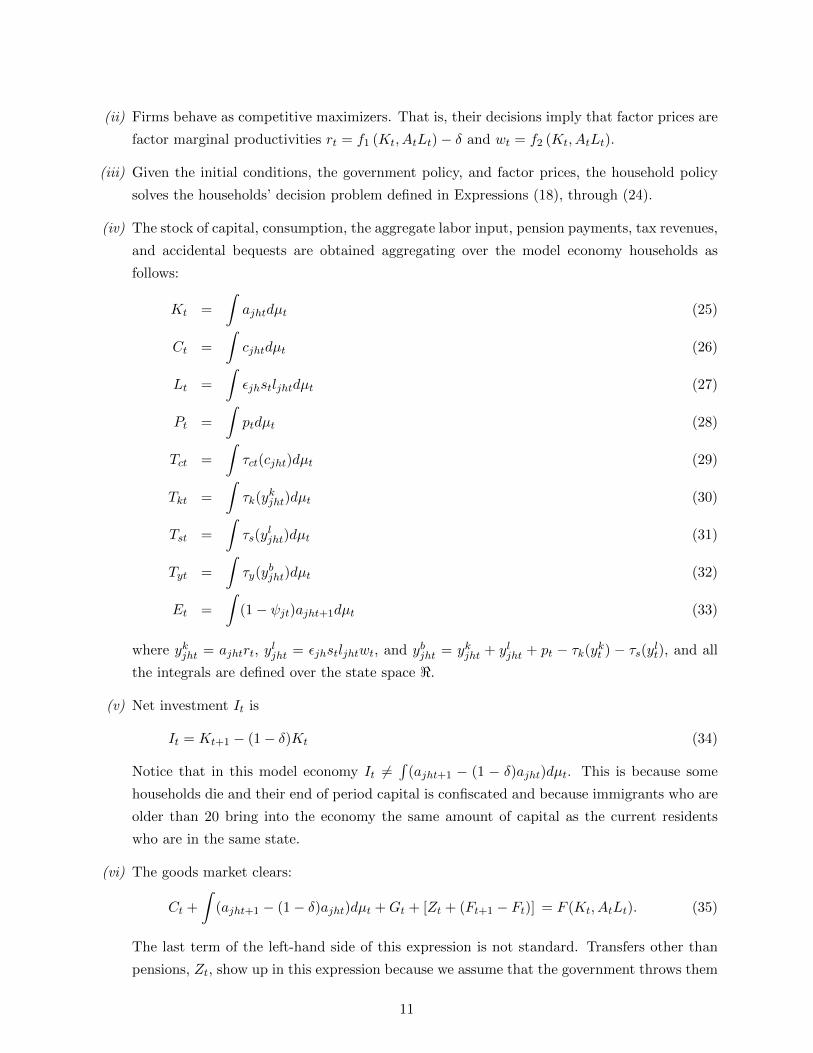
Figure 1: The Endowment of Efficiency Labor Units, the Disability Risk, and the Payroll Tax

A: The Endowment of ELU B: The Disability Risk (%) C: The Payroll Tax∗

∗In the vertical axis of this panel we plot payroll tax collections expressed as the percentage share of GDP per personover 20 and in the horizontal axis we plot labor income expressed as a multiple of GDP per person over 20.

the first retirement age, which we denote by R0, it decides whether to retire. Both the disability

shock and the retirement decision are irreversible and there is no mandatory retirement age.

Workers. Workers receive an endowment of efficiency labor units every period. This endowment has

two components: a deterministic component, which we denote by εjh, and a stochastic component,

which we denote by s.

The deterministic component depends on the household age and education, and we use it to

characterize the life-cycle profiles of earnings. We model these profiles using the following quadratic

functions:3

εjh = a1h + a2hj − a3hj2 (1)

We choose this functional form because it allows us to represent the life-cycle profiles of the produc-

tivity of workers in a very parsimonious way. We represent the versions of these functions calibrated

to Spanish data in Panel A of Figure 1.

The stochastic component is independently and identically distributed across the households,

and we use it to generate earnings and wealth inequality within the age cohorts. This process does

not depend on either the age or the education of the households, and we assume that it follows a

first order, finite state, Markov chain with conditional transition probabilities given by

Γ[s′ | s] = Pr{st+1 = s′ | st = s}, where s, s′ ∈ S = {s1, s1, . . . , sn}. (2)

We assume that the process on s takes three values and, consequently, that s ∈ S = {s1, s2, s3}.We make this assumption because it turns our that three states are sufficient to account for the

3In the expressions that follow the letters a denote parameters.

2

Lorenz curves of the Spanish distributions of income and labor earnings in enough detail, and

because we want to keep this process as simple as possible.

Disabled households. Each period able-bodied workers of age j and education level h face a proba-

bility ϕjh of becoming disabled from age j + 1 onwards. The workers find out whether they have

become disabled at the end of the period, once they have made their labor and consumption de-

cisions. When a worker becomes disabled, she exits the labor market and she receives no further

endowments of efficiency labor units, but she is entitled to receive a disability pension until she

dies.

To choose the values of the probabilities of becoming disabled, we proceed in two stages. First

we choose the aggregate probability of becoming disabled. We denote it by qj , and we assume that

it is determined by the following function:

qj = a4e(a5×j) (3)

We choose this functional form because the number of disabled people in Spain increases more than

proportionally with age, according to the Boletın de Estadısticas Laborales (2007).

Once we know the value of qj , we solve the following system of equations:qjµj,2010 =

∑h ϕjhµjh,2010

ϕj2 = a6ϕj1ϕj3 = a7ϕj1

(4)

This procedure allows us to make the disability process dependent on the educational level as is the

case in Spain. We represent the values for ϕjh calibrated to Spanish data in Panel B of Figure 1.4

Retirees. Workers who are R0 years old or older decide whether to remain in the labor force, or

whether to retire and start collecting their retirement pension. They make this decision after they

observe their endowment of efficiency labor units for the period. In our model economy retirement

pensions are incompatible with labor earnings and, consequently, retirees receive no endowment of

efficiency labor units.

Insurance markets. A key feature of our model economy is that there are no insurance markets

for the stochastic component of the endowment shock. When insurance markets are allowed to

operate, every household of the same age and education level is identical, and the earnings and

wealth inequality disappears almost completely.

Assets. Households in our model economy differ in their asset holdings, which are constrained to

being positive. Since leisure is an argument of their utility function, this borrowing constraint can

4The data on disability can be found at www.empleo.gob.es/es/estadisticas.

3

be interpreted as a solvency constraint that prevents the households from going bankrupt in every

state of the world. These restrictions give the households a precautionary motive to save. They

do so accumulating real assets, which we denote by at, and which take the form of productive

capital. For computational reasons we restrict the asset holdings to belong to the discrete set

A={a0, a1, . . . , an}. We choose n=99, and assume that a0 =0, that a99 =75, and that the spacing

between any consecutive two points in set A is constant.5

Pension rights. Workers also differ in the pension rights which they accumulate when they pay

payroll taxes. These rights are used to determine the value of their pensions when they retire. The

rules of the pension system, which we describe below, include the rules that govern the accumulation

of pension rights, and the rules that determine the mapping from pension rights into pensions. In

our model economy workers take this mapping into account when they decide how much to work

and when to retire. We assume that pension rights belong to the discrete set Bt={b0t, b1t, . . . , bmt},that m = 9, and that the spacing between points in set Bt is increasing.6 We also assume that

b0t = 0, and that bmt = a15yt, where a15yt, is the maximum earnings covered by the Spanish

pension system.

Pensions. Disabled households differ in their disability pensions and retirees differ in their re-

tirement pensions. We assume that both the disability and retirement pensions belong to the set

Pt={p0t, p1t, . . . , pmt}. Since this mapping is single valued, and the cardinality of the set of pension

rights, Bt, is 10, we let m = 9 also for Pt. We also assume that the distances between any two

consecutive points in Pt are increasing. We make this assumption because minimum pensions play

a large role in the Spanish system and this suggests that we should have a tight grid in the low end

of Pt.

Preferences. We assume that households derive utility from consumption, cjht ≥ 0, and from non-

market uses of their time, (1 − ljht), and that their preferences can be described by the standard

Cobb-Douglas expected utility function that we describe in expression (18).

1.2 The Representative Firm

In our model economy there is a representative firm. We assume that aggregate output, Yt, depends

on aggregate capital, Kt, and on the aggregate labor input, Lt, through a constant returns to scale,

Cobb-Douglas, aggregate production function of the form

Yt = Kθt (AtLt)

1−θ (5)

5In overlapping generation models with finite lives and no altruism there is no need to impose an upper bound forset A since households who reach the maximum age will optimally consume all their assets. Imrohoroglu, Imrohoroglu,and Joines (1995) make a similar point.

6Set Bt changes with time because its upper bound is the maximum covered earnings which are proportional toper capita output.

4

where At denotes an exogenous labor-augmenting productivity factor whose law of motion is At+1 =

(1 + γt)At, and where A0 > 0. Aggregate capital is obtained aggregating the capital stock owned

by every household, and the aggregate labor input is obtained aggregating the efficiency labor units

supplied by every household. We assume that capital depreciates geometrically at a constant rate,

δ, and we use r and w to denote the prices of capital and of the efficiency units of labor before all

taxes. We also assume that factor and product markets are perfectly competitive.

1.3 The Government

The government in our model economy taxes capital income, household income and consumption,

and it confiscates unintentional bequests. It uses its revenues to consume, and to make transfers to

households other than pensions. In addition, the government runs a pay-as-you-go pension system.

The consolidated government and pension system budget constraint is

Gt + Pt + Zt = Tkt + Tst + Tyt + Tct + Et + [(Ft(1 + r∗)− Ft+1] (6)

where Gt denotes government consumption, Pt denotes total pension payments, Zt denotes gov-

ernment transfers other than pensions, Tkt, Tst, Tyt, and Tct, denote the revenues collected by the

capital income tax, the payroll tax, the household income tax, and the consumption tax, Et denotes

unintentional bequests, and Ft > 0 denotes the value of the pension reserve fund at the beginning of

period t, and r∗ denotes the exogenous interest rate that the government obtains from the pension

reserve fund assets.

Government consumption. We assume that the sequence of government consumption is exogenous.

Pensions. We describe pension expenditures in Section 1.4 below.

Other transfers. We assume that transfers other than pensions are thrown to the sea so that they

create no distortions in the household decisions.

Capital income taxes. Capital income taxes are described by the following function

τk(ykt ) = a8y

kt (7)

where ykt denotes before-tax capital income.

Payroll taxes. We describe payroll taxes in Section 1.4 below.

Household income taxes. Household income taxes are described by the function

τy(ybt ) = a9

{ybt −

[a10 + (ybt )

−a11])−1/a11

}(8)

5

where the tax base is

ybt = ykt + ylt + pd(bt) + p(bt)− τk(ykt )− τs(ylt) (9)

where ylt denotes before-tax labor income, and τs denotes the payroll tax function that we describe

below. Expression (8) is the function chosen by Gouveia and Strauss (1994) to model effective

personal income taxes in the United States, and it is also the functional form chosen by Calonge

and Conesa (2003) to model effective personal income taxes in Spain.

Consumption taxes. Consumption taxes are described by the function

τc(ct) = a12tct. (10)

Estate taxes. We assume that the assets that belong to the households that exit the economy are

confiscated by the government.

The pension reserve fund. Expression [Ft(1 + r∗)−Ft+1] denotes the revenues that the government

obtains from the pension reserve fund or that deposits into it. We assume that the pension reserve

fund is non-negative and we describe its law of motion in Section 1.4 below.

1.4 The Pension System

To complete the specification of our model economy we need to describe its pay-as-you-go pension

system. A pay-as-you-go pension system is a payroll tax, the rules that govern the accumulation

of pension rights, and the rules that map pension rights into pensions. These rules include the

rules that specify the legal retirement ages and the rules that describe the revaluation of pensions.

In our benchmark model economy we choose the payroll tax and the pension system rules so that

they replicate as closely as possible the 2010 Spanish pay-as-you-go pension system.

Payroll taxes. In 2010 in Spain the payroll tax was capped. Our model economy payroll tax

function is also capped and it is the following:

τs(ylt) =

a13yt −[a13yt

(1 +

a14ylta13yt

)−ylt/a13yt]if j < R1

0 otherwise(11)

where parameter a13 is the cap of the payroll tax, yt is per capita output at market prices, and ylt

is labor income before taxes. In Panel C of Figure 1 we represent the payroll tax function for our

calibrated values of a13 and a14.

Retirement Ages. In Spain in 2010 the retirement age that entitled workers to receive a full re-

tirement pension was 65. Workers aged 61 or older could retire earlier paying an early retirement

6

penalty, as long as they had contributed to the pension system for at least 30 years. Exceptionally,

workers who had entered the system before 1967 could retire at age 60.

In the case of early retirement, the pension benefits of households with between 30 and 40 years

of contributions were reduced by 7.5 percent for every year or fraction of year before 65. When a

household had contributed for more than 40 years the penalty was reduced to 6 percent per year.

For those who are allowed to retire at age 60, the pension benefit was reduced by 8 percent per

year.

In our model economy the normal retirement age is R1 and the early retirement age is R0.7

Workers who choose to retire early pay a penalty, λj , which is determined by the following function

λj =

{a16 − a17(j −R0) if j < R1

0 if j ≥ R1(12)

where a16 and a17 are parameters which we choose to replicate the Spanish early retirement penal-

ties.

Retirement Pensions. In Spain, in 2010, at least 15 years of contributions were required to receive

a contributory retirement pension. In general, these pensions were incompatible with labor income.

The method used to calculate the pensions was earnings-based. Pension benefits depended both

on the amounts contributed and on the number of years of contributions. If the number of years of

contributions was equal to 15, the pension was 50 percent of the regulatory base. This percentage

increased by 3 percentage points for each one of the next 10 years of contributions and by 2

percentage points for each one of the following 10. Each year worked after age 65, increased this

percentage by 2 or 3 points depending on the length of the contributory career.8

In 2010 the regulatory base was defined as the average labor earnings of the last 15 years before

retirement. Labor income earned in the last two years prior to retirement entered the calculation in

nominal terms. The earnings of the remaining years were revaluated using the rate of change of the

Spanish Consumer Price Index. Finally contributive pensions in Spain were bound by a minimum

and a maximum pension.

In 2010 in Spain pensions were calculated using the following formula:

pt = φ(N)(1.03)v(1− λj)1

Nb

j−1∑t=j−Nb

min{ylt, ymax,t} (13)

In this formula, function φ(N) denotes the pension system replacement rate which dependes on N ,

the number of years of contributions, in a way that we have described above; parameter v denotes

7To replicate the delay the early retirement age that resulted in Spain from regulatory changes enacted before2010, in our benchmark model economy we change the early retirement age from 60 to 61 in 2015.

8This late retirement premium was introduced in the 2002 reform of the Spanish public pension system.

7

the number of years that the worker remains in the labor force after reaching the normal retirement

age; parameter Nb denotes the number of consecutive years immediately before retirement that are

used to compute the retirement pension; and ymax denotes the maximum covered earnings.

In our model economy we calculate the retirement pensions using the following formula:

pt(bt) = φ(1.03)v(1− λj)bt (14)

Expression (14) replicates most of the features of Spanish retirement pensions. The main dif-

ference is that in our model economy the pension replacement rate is independent of the number

of years of contributions. We abstract from this feature of Spanish pensions because it requires an

additional state variable and because, in our benchmark model economy, 99.6 percent of all workers

aged 20-64 in choose to work in our calibration year. This suggests that the number of workers

who would have been penalized for having short working histories is very small.9

Pension Rights. In our model economy we choose the law of motion of pension rights so that

it replicates the rules used to calculate pensions in Spain. Formally, the pension rights evolve

according to the following expression:

bt+1 =

0 if j < R0 −Nb

(bt + min{ylt, ymax,t})/[j − (R0 −Nb − 1)] if R0 −Nb ≤ j < R0,[bt(Nb − 1) + min{ylt, ymax,t}]/Nb if j ≥ R0,

(15)

In this expression Nb denotes the number of years of contributions that are taken into account to

calculate the pension, and ymax,t = a15yt is the maximum covered earnings. Then, when a worker’s

age is R0 −Nb < j < R0, the bt record the average labor income earned by that worker since age

R0 −Nb. And when a worker is older than R0, the bt record the average labor income earned by

that worker during the previous Nb years.

Disability Pensions. We model disability pensions explicitly for two reasons: because they represent

a large share of all Spanish pensions (in 2010, 10.7 percent of all contributive pensions and 16.5

percent of the sum of the retirement and disability pensions paid by the Regimen General), and

because disability pensions are used as an alternative route to early retirement in many cases.10 To

replicate the current Spanish rules, we assume that there is a minimum disability pension which

coincides with the minimum retirement pension. And that the disability pensions are 75 percent

of the households’ retirement claims. Formally, we compute the disability pensions as follows:

pdt (bt) = max{p0t, 0.75bt}. (16)

9We also abstract from partial retirement. In our model economy retirees cannot work because they receive noendowment of efficiency labor units. In Spain a limited form of partial retirement is possible but many restrictionsapply.

10See Boldrin and Jimenez-Martın (2003) for an elaboration of this argument.

8

Minimum and Maximum Pensions. In 2010 in Spain contributive pensions were bounded by a

minimum pension and a maximum pension. Our model economy replicates this feature. Formally,

we require that p0t ≤ pt ≤ pmt, where p0t denotes the minimum pension and pmt denotes the

maximum pension.

The Revaluation of Pensions. In 2010 in Spain pensions were fully indexed to price inflation, as

measured by the consumer price index. In our benchmark model economy the real value of pensions

remains unchanged, and we update the values of the minimum and the maximum pensions so that

they remain a constant proportion of output per capita.11

The Pension Reserve Fund. Since the year 2000, Spain has had a pension reserve fund which is

invested in fixed income assets and which is financed with part of the pension system surpluses.

The assets of this fund have been used to finance the pension system deficits when needed.

In our model economy, we assume that pension system surpluses, (Tst−Pt), are deposited into

a pension reserve fund which evolves according to

Ft+1 = (1 + r∗)Ft + Tst − Pt (17)

We require the pension reserve fund to be non-negative. We assume that the pension fund assets are

used to finance the pension system deficits and that, when they ran out, the government changes

the consumption tax rate as needed to finance the pensions.

1.5 The Households’ Decision Problem

We assume that the households in our model economy solve the following decision problem:

maxE

100∑j=20

βj−20 ψjt (1− ϕjh) [cαjht(1− ljht)(1−α)](1−σ)/1− σ

(18)

subject to

cjht + ajht+1 + τjht = yjht + ajht (19)

11In Spain in 2010, pensions and the maximum pension were revaluated using the inflation rate and minimumpensions were increased discretionally. In the first decade of the century the Spanish minimum pension has roughlykept up with per capita GDP, and that the maximum pension and normal pensions have decreased as a share of percapita GDP. This little known fact is known as the silent reform of Spanish pensions.

9

where

τjht = τkykjht + τy(y

bjht) + τst(y

ljht) + τctcjht (20)

yjht = ykjht + yljht + pdt (bt) + pt(bt) (21)

ykjht = ajhtrt (22)

yljht = εjhstljhtwt (23)

ajht ∈ A, pt(bt) and pdt (bt) ∈ Pt, st ∈ S for all t, and ajh0 is given, (24)

and where parameter β > 0 denotes the time-discount factor, function τy is defined in expression (8),

variable ybjht is defined in expression (9), function τs is defined in expression (11), function p is

defined in expression (14), the law of motion of bt is defined in expression (15), and function pd is

defined in expression (16).

Notice that every household can earn capital income, that only workers can earn labor income,

that only disabled households receive disability pensions, and that only retirees receive retirement

pensions. As we have already mentioned, an important feature of the households decision problem

that we have omitted here is that households decide optimally when to retire, once they have

reached age R0. This decision depends on their state variables, j, h, at, st, and bt, and on the

expected benefits and costs of continuing to work. The benefits are the labor earnings and, possibly,

the reduction of the early retirement penalties or the late retirement premium, and the costs are

the forgone leisure and the forgone pension. They also take into account the change in their pension

rights, bt+1− bt, which could be a benefit or a cost depending on the values of bt and of the current

and expected future endowments of efficiency labor units.

1.6 Definition of Equilibrium

Let j∈J , h∈H, e∈E , a∈A, bt∈Bt, and pt∈Pt, and let µj,h,e,a,b,p,t be a probability measure defined

on < = J×H×E×A×Bt×Pt.12 Then, given initial conditions µ0, A0, E0, F0, and K0, a competitive

equilibrium for this economy is a government policy, {Gt, Pt, Zt, Tkt, Tst, Tyt, Tct, Et+1, Ft+1}∞t=0,

a household policy, {ct(j, h, e, a, b, p), lt(j, h, e, a, b, p), at+1(j, h, e, a, b, p)}∞t=0, a sequence of mea-

sures, {µt}∞t=0, a sequence of factor prices, {rt, wt}∞t=0, a sequence of macroeconomic aggregates,

{Ct,It,Yt,Kt+1,Lt}∞t=0, a function, Q, and a number, r∗, such that:

(i) The government policy and r∗ satisfy the consolidated government and pension system budget

constraint described in Expression (6) and the the law of motion of the pension system fund

described in Expression (17).

12Recall that, for convenience, whenever we integrate the measure of households over some dimension, we drop thecorresponding subscript.

10

(ii) Firms behave as competitive maximizers. That is, their decisions imply that factor prices are

factor marginal productivities rt = f1 (Kt, AtLt)− δ and wt = f2 (Kt, AtLt).

(iii) Given the initial conditions, the government policy, and factor prices, the household policy

solves the households’ decision problem defined in Expressions (18), through (24).

(iv) The stock of capital, consumption, the aggregate labor input, pension payments, tax revenues,

and accidental bequests are obtained aggregating over the model economy households as

follows:

Kt =

∫ajhtdµt (25)

Ct =

∫cjhtdµt (26)

Lt =

∫εjhstljhtdµt (27)

Pt =

∫ptdµt (28)

Tct =

∫τct(cjht)dµt (29)

Tkt =

∫τk(y

kjht)dµt (30)

Tst =

∫τs(y

ljht)dµt (31)

Tyt =

∫τy(y

bjht)dµt (32)

Et =

∫(1− ψjt)ajht+1dµt (33)

where ykjht = ajhtrt, yljht = εjhstljhtwt, and ybjht = ykjht + yljht + pt − τk(ykt ) − τs(ylt), and all

the integrals are defined over the state space <.

(v) Net investment It is

It = Kt+1 − (1− δ)Kt (34)

Notice that in this model economy It 6=∫

(ajht+1 − (1 − δ)ajht)dµt. This is because some

households die and their end of period capital is confiscated and because immigrants who are

older than 20 bring into the economy the same amount of capital as the current residents

who are in the same state.

(vi) The goods market clears:

Ct +

∫(ajht+1 − (1− δ)ajht)dµt +Gt + [Zt + (Ft+1 − Ft)] = F (Kt, AtLt). (35)

The last term of the left-hand side of this expression is not standard. Transfers other than

pensions, Zt, show up in this expression because we assume that the government throws them

11

into the sea. And the change in the value of the pension reserve fund, (Ft+1 − Ft) shows up

because pension system surpluses are invested in the pension fund and pension system deficits

are financed with the fund until it is depleted.13

(vii) The law of motion for µt is:

µt+1 =

∫<Qtdµt. (36)

Describing function Q formally is complicated because it specifies the transitions of the mea-

sure of households along its six dimensions: age, education level, employment status, assets

holdings, pension rights, and pensions. An informal description of this function is the follow-

ing:

We assume that new-entrants, who are 20 years old, enter the economy as able-bodied workers,

that they draw the stochastic component of their endowment of efficiency labor units from

its invariant distribution, and that they own zero assets and zero pension rights. Their

educational shares are exogenous and they determine the evolution of µht. We also assume

that new-entrants who are older than 20 replicate the age, education, employment status,

wealth, pension rights, and pensions share distribution of the existing population.

The evolution of µjht is exogenous, it replicates the Spanish demographic projections, and

we compute it following a procedure that we describe in Section 2.6 below. The evolution of

µet is governed by the conditional transition probability matrix of its stochastic component,

by the probability of becoming disabled, and by the optimal decision to retire. The evolution

of µat is determined by the optimal savings decision and by the changes in the population.

The evolution of µbt is determined by the rules of the Spanish public pension system which

we have described in Section 1.1.

13The last term of the left-hand side of Expression (35) would show up as net exports in the standard nationalincome and product accounts.

12

2 Calibration

To calibrate our model economy we do the following: First, we choose a calibration target country —

Spain in this article— and a calibration target year —2010 in this article. Then we choose the initial

conditions and the parameter values that allow our model economy to replicate as closely as possible

selected macroeconomic aggregates and ratios, distributional statistics, and the institutional details

of our chosen country in our target year. We describe these steps in the subsections below.

2.1 Initial conditions

To determine the initial conditions, first we choose an initial distribution of households, µ0. In

Section 2.6 we provide a detailed description about how we obtain that distribution. The initial

distribution of households implies an initial value for the capital stock. This value is K2010 =

12.2115. The initial distribution of households and the initial survival probabilities determine

the initial value of unintentional bequests, E2010. We must also specify the initial values for the

productivity process, A2010, and for the pension reserve fund F2010. Since A2010 determines the

units which we use to measure output and does nothing else, we choose A2010 = 1.0. Finally, our

choice for the initial value of the pension reserve fund is F2010 = 0.0612 Y ∗2010, where Y ∗t denotes

output at market prices, which we define as Y ∗t = Yt+Tct. Our choice for F2010 replicates the value

of the Spanish pension reserve fund at the end of 2010.

2.2 Parameters

Once the initial conditions are specified, to characterize our model economy fully, we must choose

the values of a total of 50 parameters. Of these 50 parameters, 3 describe the household preferences,

21 the process on the endowment of efficiency labor units, 4 the disability risk, 3 the production

technology, 12 the pension system rules, and 7 the remaining components of the government policy.

To choose the values of these 50 parameters we need 50 equations or calibration targets which we

describe below.

2.3 Equations

To determine the values of the 50 parameters that identify our model economy, we do the following.

First, we determine the values of a group of 31 parameters directly using equations that involve

either one parameter only, or one parameter and our guesses for (K,L). To determine the values

of the remaining 19 parameters we construct a system of 19 non-linear equations. Most of these

equations require that various statistics in our model economy replicate the values of the corre-

sponding Spanish statistics in 2010. We describe the determination of both sets of parameters in

13

the subsections below.

2.3.1 Parameters determined solving single equations

The life-cycle profile of earnings. We measure the deterministic component of the process on the

endowment of efficiency labor units independently of the rest of the model. We estimate the values

of the parameters of the three quadratic functions that we describe in Expression (1), using the

age and educational distributions of hourly wages reported by the Instituto Nacional de Estadıstica

(INE) in the Encuesta de Estructura Salarial (2010) for Spain.14 This procedure allows us to

identify the values of 9 parameters directly.

The disability risk. We want the probability of becoming disabled to approximate the data reported

by the Boletın de Estadısticas Laborales (2007) for the Spanish economy. We use this dataset to

estimate the values of parameters a4 and a5 of Expression (3) using an ordinary least squares

regression of qj on j. According to the Instituto de Mayores y Servicios Sociales, in 2008 in Spain

62.6 percent of the total number of disabled people aged 25 to 44 years old had not completed high

school, 26.9 percent had completed high school, and the remaining 10.5 percent had completed

college. We use these shares to determine the values of parameters a6 and a7 of Expression (4).

Specifically, we choose a6 = 0.269/0.626 = 0.4297 and a7 = 0.105/0.626 = 0.1677. This procedure

allows us determine the values of 4 parameters directly.

The pension system. In 2010 in Spain, the payroll tax rate paid by households was 28.3 percent

and it was levied only on the first 44,772 euros of annual gross labor income. Hence, the maximum

contribution was 12,670 euros which correspond to 45,53 percent of the Spanish GDP per person

who was 20 or older. To replicate this feature of the Spanish pension system we choose the value

of parameter a13 of our payroll tax function to be a13 = 0.4553.

Our choice for the number of years used to compute the retirement pensions in our benchmark

model economy is Nb = 15. This is because in 2010 the Spanish Regimen General de la Seguridad

Social took into account the last 15 years of contributions prior to retirement to compute the

pension.

We assume that the minimum pension, the maximum pension, and the maximum covered earn-

ings are directly proportional to per capita income. Our targets for the proportionality coefficients

are b0t = 0.1731yt, bmt = 1.2567yt, and a15 = 1.6089. These numbers correspond to their values in

2010 .15

14Since we only have data until age 64, we estimate the quadratic functions for workers in the 20–64 age cohortand we project the resulting functions from age 65 onwards.

15Specifically, in 2010 the minimum retirement pension in Spain was 4,817 euros, the maximum pension was 34,970euros, the maximum covered earnings were 44,772 euros, and GDP per person who was 20 or older was 27,827 euros.All these data are yearly.

14

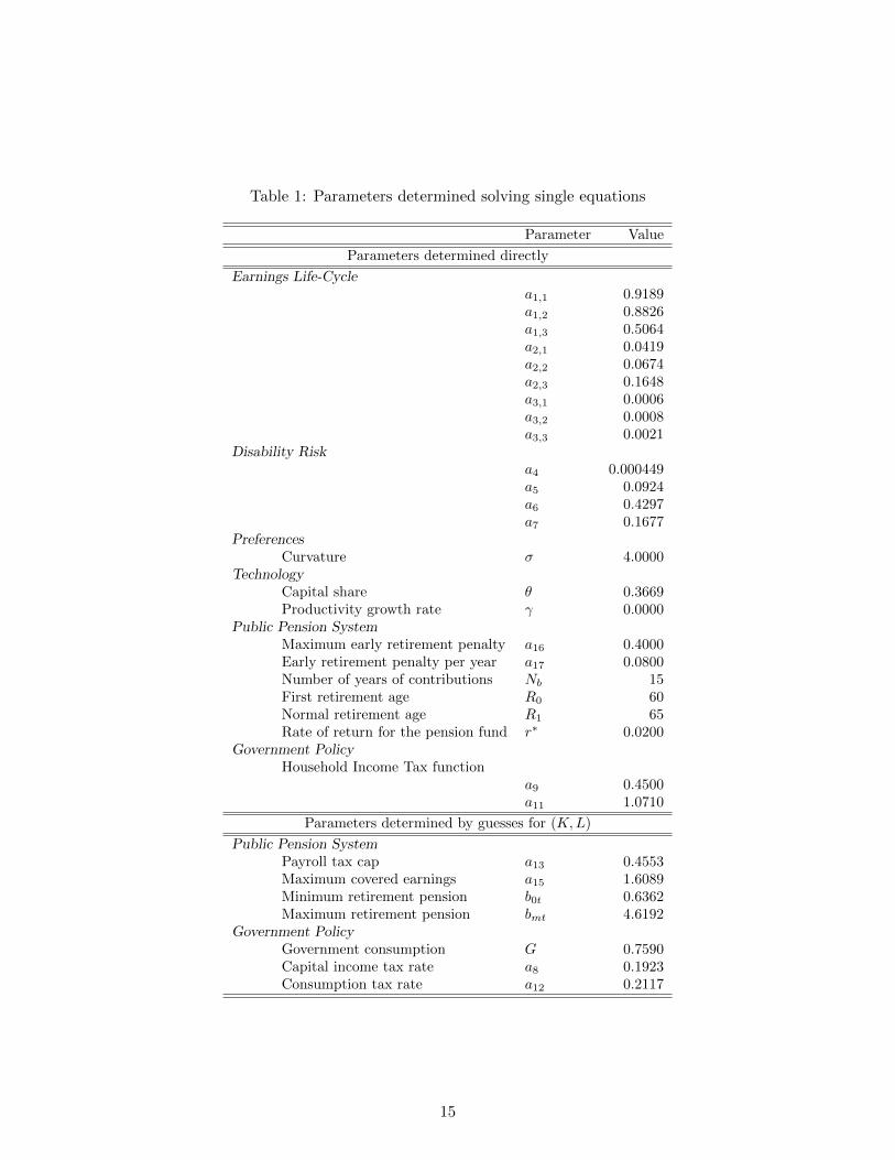
Table 1: Parameters determined solving single equations

Parameter Value

Parameters determined directly

Earnings Life-Cyclea1,1 0.9189a1,2 0.8826a1,3 0.5064a2,1 0.0419a2,2 0.0674a2,3 0.1648a3,1 0.0006a3,2 0.0008a3,3 0.0021

Disability Riska4 0.000449a5 0.0924a6 0.4297a7 0.1677

PreferencesCurvature σ 4.0000

TechnologyCapital share θ 0.3669Productivity growth rate γ 0.0000

Public Pension SystemMaximum early retirement penalty a16 0.4000Early retirement penalty per year a17 0.0800Number of years of contributions Nb 15First retirement age R0 60Normal retirement age R1 65Rate of return for the pension fund r∗ 0.0200

Government PolicyHousehold Income Tax function

a9 0.4500a11 1.0710

Parameters determined by guesses for (K,L)

Public Pension SystemPayroll tax cap a13 0.4553Maximum covered earnings a15 1.6089Minimum retirement pension b0t 0.6362Maximum retirement pension bmt 4.6192

Government PolicyGovernment consumption G 0.7590Capital income tax rate a8 0.1923Consumption tax rate a12 0.2117

15

In the benchmark model economy we choose the first and the normal retirement ages to be

R0 = 60 and R1 = 65. In Spain the first retirement age was 60 until 2002. This rule was changed

in 2002 when the first retirement age was changed to 61, with some exceptions. We choose R0 = 60

because in 2010 a large number of workers were still retiring at that age.16

To identify the early retirement penalty function, we choose a16 = 0.4, and a17 = 0.08. This

is because we have chosen R0 = 60, and because in Spain the penalties for early retirement are 8

percent for every year before age 65. Finally, for the rate of return on the pension reserve fund’s

assets we choose r∗ = 0.02.17 These choices allow us to determine the values of 10 parameters.

Government policy. To specify the government policy, we must choose the values of government

consumption, Gt, of the tax rate on capital income, a8, of parameters a9 and a11 of the household

income tax function, and of the tax rate on consumption, a12t. We describe our procedure to choose

the value of these 5 parameters in Section 2.5.

Preferences. Of the four parameters in the utility function, we choose the value of only σ directly.

Specifically, we choose σ = 4.0. This choice and the value of the share of consumption in the utility

function, imply that the relative risk aversion in consumption is 1.8937, which falls within the 1.5-3

range which is standard in the literature.

Technology. According to the OECD data, the capital income share in Spanish GDP was 0.3669

in 2008. Consequently, we choose θ = 0.3669. We also choose the growth rate of total factor

productivity directly. We discuss this choices for the growth rate scenarios in the main body of the

paper.

Adding up. So far we have determined the values of 31 parameters either directly or as functions

of our guesses for (K,L) only. We report their values in the first two blocks of Table 1.

2.3.2 Parameters determined solving a system of equations

We still have to determine the values of 19 parameters. To find the values of those 19 parameters we

need 19 equations. Of those equations, 14 require that model economy statistics replicate the value

of the corresponding statistics for the Spanish economy in 2010, 4 are normalization conditions,

and the last one is the government budget constraint that allows us to determine the value of Z/Y ∗

residually.

16In 2010 in Spain 22.4 percent of the people who opted for early retirement were 60 years old or younger. And5.78 percent of the total number of retirees were 60 or younger. See Ministerio de Trabajo e Inmigracion (MTIN),Anuario de Estadısticas 2010 (http://www.empleo.gob.es/estadisticas/ANUARIO2010/PEN/index.htm).

17In Dıaz-Gimenez and Dıaz-Saavedra (2009) we also run simulations for r∗ = 1, 3, and 4 percent. We found that

16

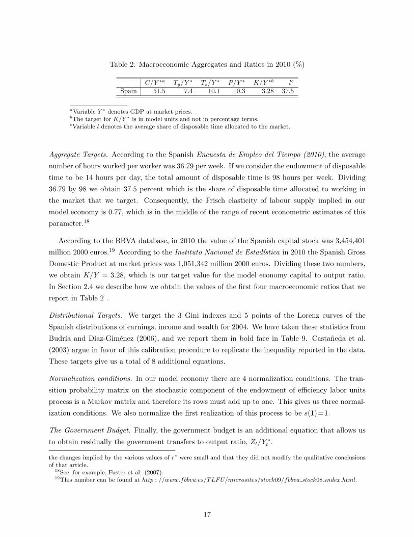
Table 2: Macroeconomic Aggregates and Ratios in 2010 (%)

C/Y ∗a Ty/Y∗ Ts/Y

∗ P/Y ∗ K/Y ∗b lc

Spain 51.5 7.4 10.1 10.3 3.28 37.5

aVariable Y ∗ denotes GDP at market prices.bThe target for K/Y ∗ is in model units and not in percentage terms.cVariable l denotes the average share of disposable time allocated to the market.

Aggregate Targets. According to the Spanish Encuesta de Empleo del Tiempo (2010), the average

number of hours worked per worker was 36.79 per week. If we consider the endowment of disposable

time to be 14 hours per day, the total amount of disposable time is 98 hours per week. Dividing

36.79 by 98 we obtain 37.5 percent which is the share of disposable time allocated to working in

the market that we target. Consequently, the Frisch elasticity of labour supply implied in our

model economy is 0.77, which is in the middle of the range of recent econometric estimates of this

parameter.18

According to the BBVA database, in 2010 the value of the Spanish capital stock was 3,454,401

million 2000 euros.19 According to the Instituto Nacional de Estadıstica in 2010 the Spanish Gross

Domestic Product at market prices was 1,051,342 million 2000 euros. Dividing these two numbers,

we obtain K/Y = 3.28, which is our target value for the model economy capital to output ratio.

In Section 2.4 we describe how we obtain the values of the first four macroeconomic ratios that we

report in Table 2 .

Distributional Targets. We target the 3 Gini indexes and 5 points of the Lorenz curves of the

Spanish distributions of earnings, income and wealth for 2004. We have taken these statistics from

Budrıa and Dıaz-Gimenez (2006), and we report them in bold face in Table 9. Castaneda et al.

(2003) argue in favor of this calibration procedure to replicate the inequality reported in the data.

These targets give us a total of 8 additional equations.

Normalization conditions. In our model economy there are 4 normalization conditions. The tran-

sition probability matrix on the stochastic component of the endowment of efficiency labor units

process is a Markov matrix and therefore its rows must add up to one. This gives us three normal-

ization conditions. We also normalize the first realization of this process to be s(1)=1.

The Government Budget. Finally, the government budget is an additional equation that allows us

to obtain residually the government transfers to output ratio, Zt/Y∗t .

the changes implied by the various values of r∗ were small and that they did not modify the qualitative conclusionsof that article.

18See, for example, Fuster et al. (2007).19This number can be found at http : //www.fbbva.es/TLFU/microsites/stock09/fbbva stock08 index.html.

17

2.4 The expenditure ratios

The Spanish National Income and Product Data reported by the Instituto Nacional de Estadıstica

(INE) for 2010 are the following:

Table 3: Spanish GDP and its Components for 2010 at Current Market Prices

Millon Euros Shares of GDP (%)

Private Consumption 596,322 56.72Public Consumption 221,715 21.08Consumption of Non-Profits 10,589 1.00Gross Capital Formation 244,987 23.30Exports 283,936 27.00Imports 306,207 29.12

Total (GDP) 1,051,342 100.00

We adjust the amounts reported in Table 3 according to Cooley and Prescott (1995) and we

obtain the following numbers:

– Adjusted Private Consumption: Private Consumption – Private Consumption of Durables +

Consumption of Non-Profits = 596, 322− 54, 127 + 10, 589 = 552, 784 million euros.

– Adjusted Public Consumption: Public Consumption = 221,715 million euros.

– Adjusted Investment (Private and Public): Gross Capital Formation + Private Consumption

of Durables = 244, 987 + 54, 127 = 299, 114 million euros.

The next adjustment is to allocate Net Exports to our measures of C, I, and G. To that purpose,

we compute the shares of each of those three variables in the sum of the three and we allocate Net

Exports according to those shares. The sum of the three variables is 1,073,613 million euros and

the shares of C, I, and G are 51.49, 27.86, and 20.65 percent.

Net Exports are –22,271 million euros. When we allocate them to C, I, and G we obtain the

final adjusted values for C, I, and G which are 541,317, 217,116, and 292,909. Naturally, this new

adjusted values now add to Total GDP but the adjusted shares remain unchanged and they are

51.49, 27.86, y 20.65 percent of GDP.

Next we redefine the model economy’s output and consumption from factor cost to market prices

as follows: Y ∗ = Y + Tc, where Y ∗ is the model economy’s output at market prices and Tc is the

consumption tax collections, and C∗ = C + Tc, where C∗ is the model economy’s consumption at

market prices. Finally we use C∗/Y ∗ = 51.49 and G/Y ∗ = 20.65 as targets.

18

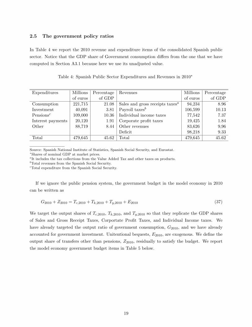
2.5 The government policy ratios

In Table 4 we report the 2010 revenue and expenditure items of the consolidated Spanish public

sector. Notice that the GDP share of Government consumption differs from the one that we have

computed in Section A3.1 because here we use its unadjusted value.

Table 4: Spanish Public Sector Expenditures and Revenues in 2010∗

Expenditures Millions Percentage Revenues Millions Percentageof euros of GDP of euros of GDP

Consumption 221,715 21.08 Sales and gross receipts taxesa 94,234 8.96Investment 40,091 3.81 Payroll taxesb 106,599 10.13Pensionsc 109,000 10.36 Individual income taxes 77,542 7.37Interest payments 20,120 1.91 Corporate profit taxes 19,425 1.84Other 88,719 8.44 Other revenues 83,626 9,96

Deficit 98,218 9.33

Total 479,645 45.62 Total 479,645 45.62

Source: Spanish National Institute of Statistics, Spanish Social Security, and Eurostat.∗Shares of nominal GDP at market prices.aIt includes the tax collections from the Value Added Tax and other taxes on products.bTotal revenues from the Spanish Social Security.cTotal expenditure from the Spanish Social Security.

If we ignore the public pension system, the government budget in the model economy in 2010

can be written as

G2010 + Z2010 = Tc,2010 + Tk,2010 + Ty,2010 + E2010 (37)

We target the output shares of Tc,2010, Tk,2010, and Ty,2010 so that they replicate the GDP shares

of Sales and Gross Receipt Taxes, Corportate Profit Taxes, and Individual Income taxes. We

have already targeted the output ratio of government consumption, G2010, and we have already

accounted for government investment. Unitentional bequests, E2010, are exogenous. We define the

output share of transfers other than pensions, Z2010, residually to satisfy the budget. We report

the model economy government budget items in Table 5 below.

19

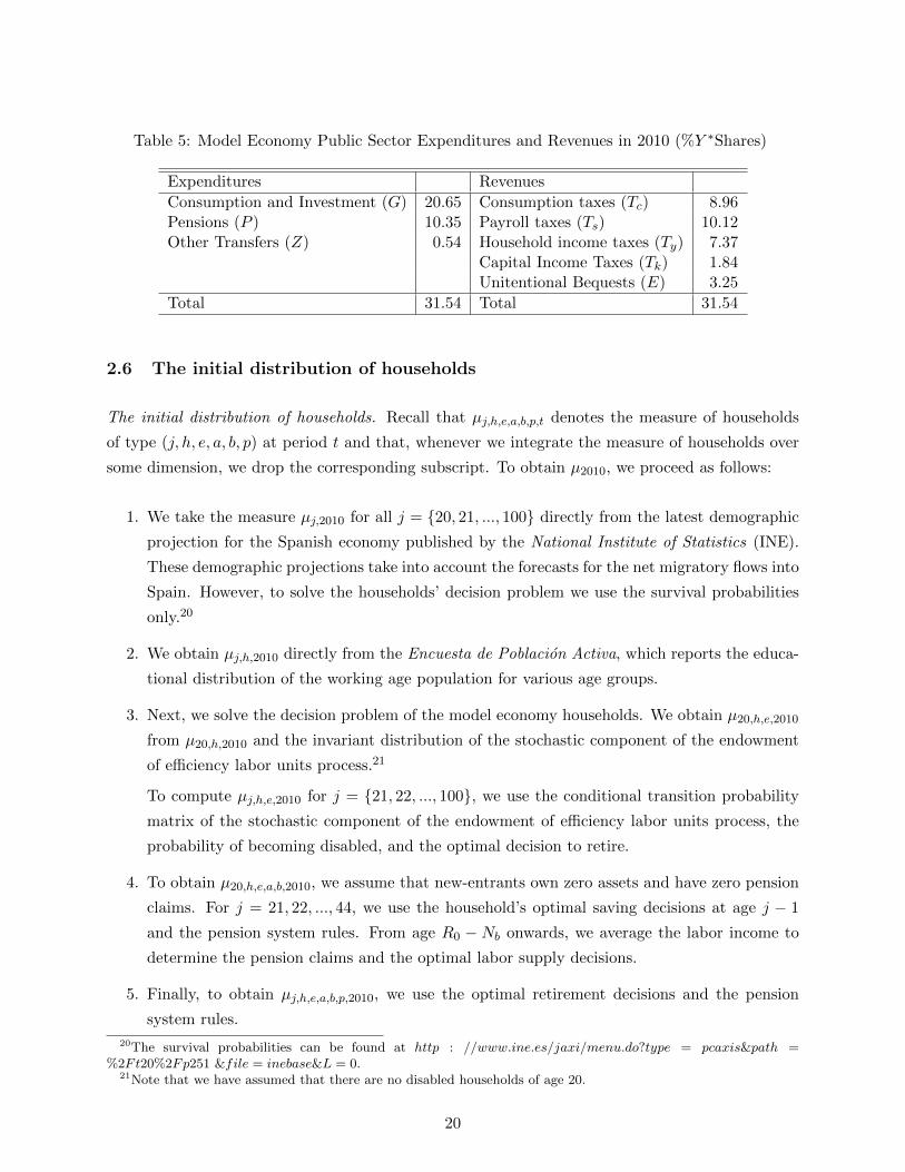
Table 5: Model Economy Public Sector Expenditures and Revenues in 2010 (%Y ∗Shares)

Expenditures Revenues

Consumption and Investment (G) 20.65 Consumption taxes (Tc) 8.96Pensions (P ) 10.35 Payroll taxes (Ts) 10.12Other Transfers (Z) 0.54 Household income taxes (Ty) 7.37

Capital Income Taxes (Tk) 1.84Unitentional Bequests (E) 3.25

Total 31.54 Total 31.54

2.6 The initial distribution of households

The initial distribution of households. Recall that µj,h,e,a,b,p,t denotes the measure of households

of type (j, h, e, a, b, p) at period t and that, whenever we integrate the measure of households over

some dimension, we drop the corresponding subscript. To obtain µ2010, we proceed as follows:

1. We take the measure µj,2010 for all j = {20, 21, ..., 100} directly from the latest demographic

projection for the Spanish economy published by the National Institute of Statistics (INE).

These demographic projections take into account the forecasts for the net migratory flows into

Spain. However, to solve the households’ decision problem we use the survival probabilities

only.20

2. We obtain µj,h,2010 directly from the Encuesta de Poblacion Activa, which reports the educa-

tional distribution of the working age population for various age groups.

3. Next, we solve the decision problem of the model economy households. We obtain µ20,h,e,2010

from µ20,h,2010 and the invariant distribution of the stochastic component of the endowment

of efficiency labor units process.21

To compute µj,h,e,2010 for j = {21, 22, ..., 100}, we use the conditional transition probability

matrix of the stochastic component of the endowment of efficiency labor units process, the

probability of becoming disabled, and the optimal decision to retire.

4. To obtain µ20,h,e,a,b,2010, we assume that new-entrants own zero assets and have zero pension

claims. For j = 21, 22, ..., 44, we use the household’s optimal saving decisions at age j − 1

and the pension system rules. From age R0 − Nb onwards, we average the labor income to

determine the pension claims and the optimal labor supply decisions.

5. Finally, to obtain µj,h,e,a,b,p,2010, we use the optimal retirement decisions and the pension

system rules.

20The survival probabilities can be found at http : //www.ine.es/jaxi/menu.do?type = pcaxis&path =%2Ft20%2Fp251 &file = inebase&L = 0.

21Note that we have assumed that there are no disabled households of age 20.

20

Notice that steps 3, 4 and 5 must be computed simultaneously in the same loop.

2.7 The demographic transition

We use the latest demographic projections of the Instituto Nacional de Estadıstica which correspond

to 2012. The INE reports and projects the age distribution of Spanish residents from 2010 to 2052

for people aged from zero to 100 and more. Call those age cohorts Njt and let Nt =∑100+

j=20 Njt.

Then, the age distribution of the households in our model economy is µjt = Njt/Nt for j =

20, 21, ..., 99, 100+ and for t = 2010, 2011, ...., 2052.22

2.8 The educational transition

To update the distribution of education, we assume that from 2011 onwards, 8.65 percent of the 20

year-old entrants have not completed their secondary education, that 63.53 percent have completed

their secondary education, and that 27.82 percent have completed college. This was the educational

distribution of Spanish households born between 1980 and 1984, which was the most educated

cohort in 2010.23 We also assume that immigrants have the same educational distribution as the

residents of the same age.

2.9 Results

In this section we show that our calibrated, benchmark model economy replicates reasonably well

most of the Spanish statistics that we target in our calibration procedure.

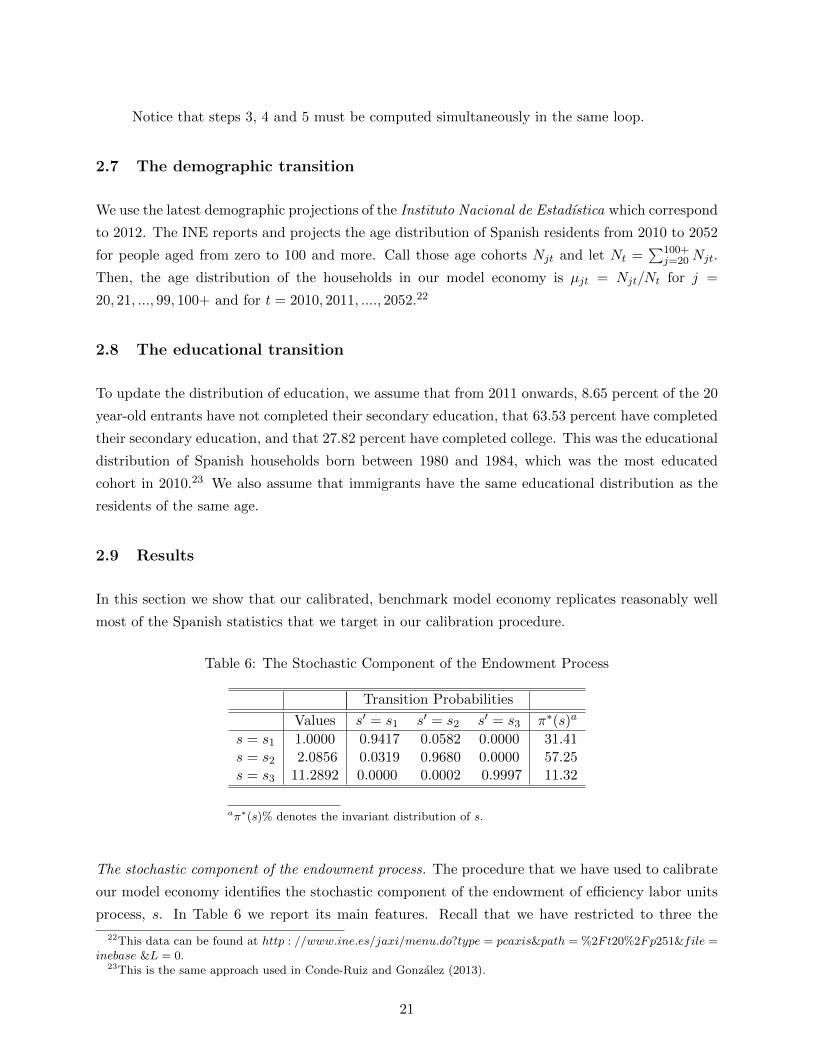
Table 6: The Stochastic Component of the Endowment Process

Transition Probabilities

Values s′ = s1 s′ = s2 s′ = s3 π∗(s)a

s = s1 1.0000 0.9417 0.0582 0.0000 31.41s = s2 2.0856 0.0319 0.9680 0.0000 57.25s = s3 11.2892 0.0000 0.0002 0.9997 11.32

aπ∗(s)% denotes the invariant distribution of s.

The stochastic component of the endowment process. The procedure that we have used to calibrate

our model economy identifies the stochastic component of the endowment of efficiency labor units

process, s. In Table 6 we report its main features. Recall that we have restricted to three the

22This data can be found at http : //www.ine.es/jaxi/menu.do?type = pcaxis&path = %2Ft20%2Fp251&file =inebase &L = 0.

23This is the same approach used in Conde-Ruiz and Gonzalez (2013).

21

number of realizations of s. We find that the value of the highest realization of s is 11.3 times that

of its lowest value. We find also that the process on s is very persistent. Specifically, the expected

durations of the shocks are 17.2, 31.3, and an astonishing 3333.3 years. In the last column of

Table 6 we report the invariant distributions of the shocks. We find that approximately 89 percent

of the workers are either in state s = s1 or in state s = s2 , and that about 11 percent are in state

s = s3.24 These features allow us to replicate reasonably well the Lorenz curves of the Spanish

income and earnings distributions, as we report below.

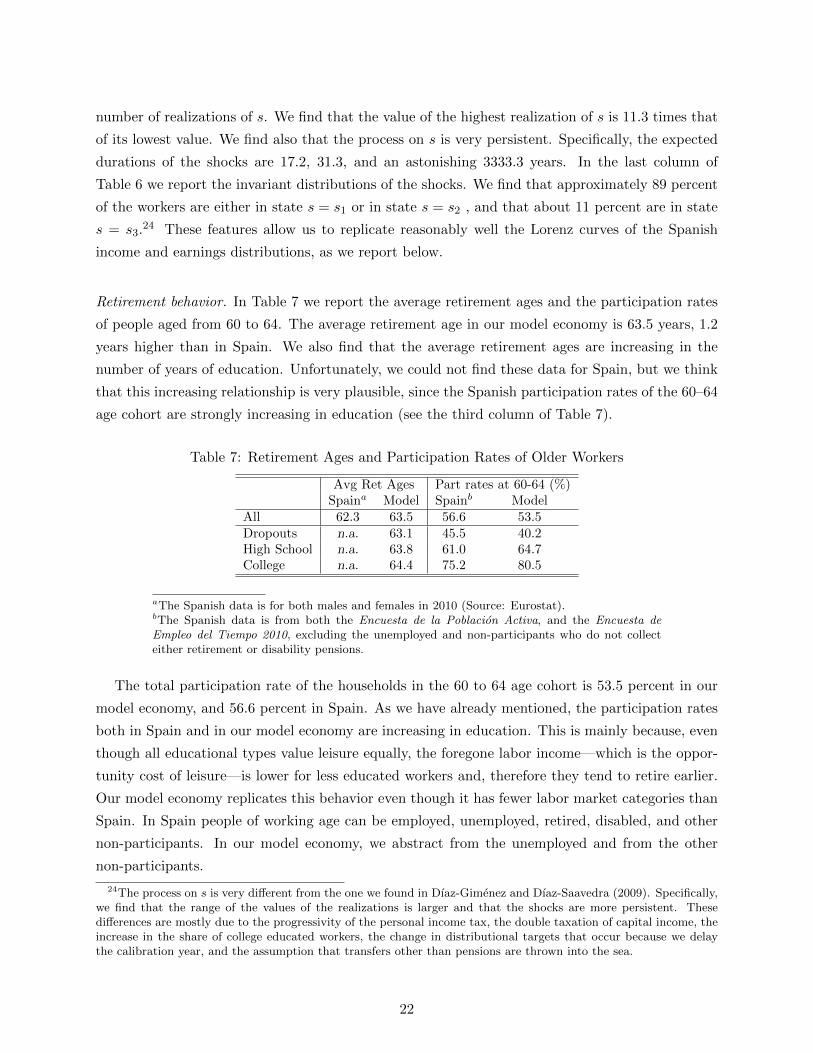
Retirement behavior. In Table 7 we report the average retirement ages and the participation rates

of people aged from 60 to 64. The average retirement age in our model economy is 63.5 years, 1.2

years higher than in Spain. We also find that the average retirement ages are increasing in the

number of years of education. Unfortunately, we could not find these data for Spain, but we think

that this increasing relationship is very plausible, since the Spanish participation rates of the 60–64

age cohort are strongly increasing in education (see the third column of Table 7).

Table 7: Retirement Ages and Participation Rates of Older Workers

Avg Ret Ages Part rates at 60-64 (%)Spaina Model Spainb Model

All 62.3 63.5 56.6 53.5Dropouts n.a. 63.1 45.5 40.2High School n.a. 63.8 61.0 64.7College n.a. 64.4 75.2 80.5

aThe Spanish data is for both males and females in 2010 (Source: Eurostat).bThe Spanish data is from both the Encuesta de la Poblacion Activa, and the Encuesta deEmpleo del Tiempo 2010, excluding the unemployed and non-participants who do not collecteither retirement or disability pensions.

The total participation rate of the households in the 60 to 64 age cohort is 53.5 percent in our

model economy, and 56.6 percent in Spain. As we have already mentioned, the participation rates

both in Spain and in our model economy are increasing in education. This is mainly because, even

though all educational types value leisure equally, the foregone labor income—which is the oppor-

tunity cost of leisure—is lower for less educated workers and, therefore they tend to retire earlier.

Our model economy replicates this behavior even though it has fewer labor market categories than

Spain. In Spain people of working age can be employed, unemployed, retired, disabled, and other

non-participants. In our model economy, we abstract from the unemployed and from the other

non-participants.

24The process on s is very different from the one we found in Dıaz-Gimenez and Dıaz-Saavedra (2009). Specifically,we find that the range of the values of the realizations is larger and that the shocks are more persistent. Thesedifferences are mostly due to the progressivity of the personal income tax, the double taxation of capital income, theincrease in the share of college educated workers, the change in distributional targets that occur because we delaythe calibration year, and the assumption that transfers other than pensions are thrown into the sea.

22

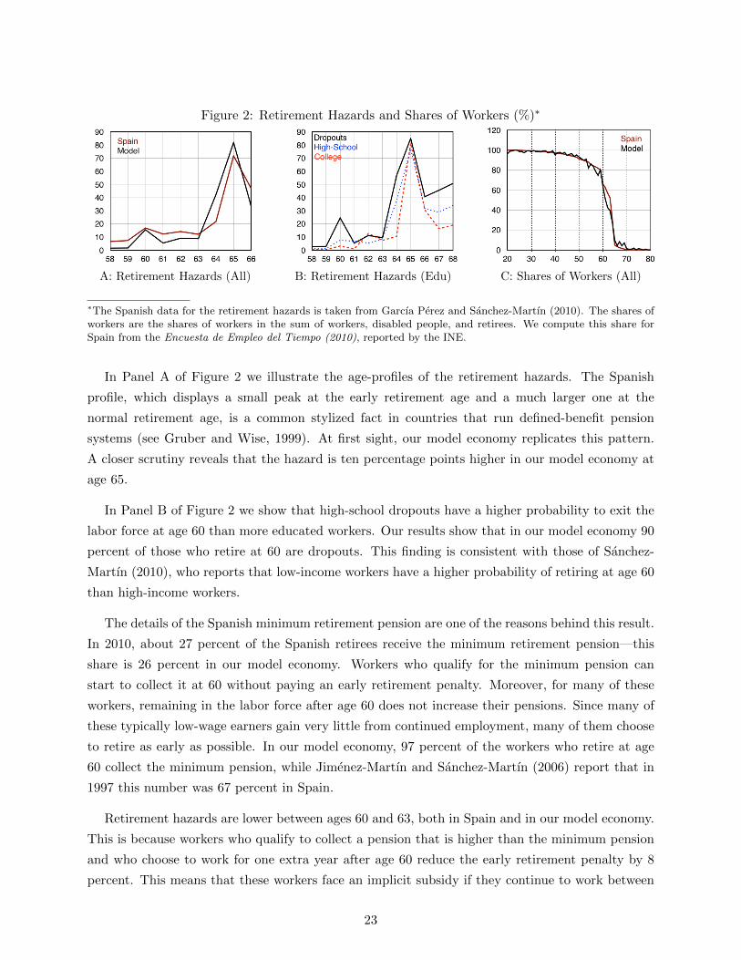
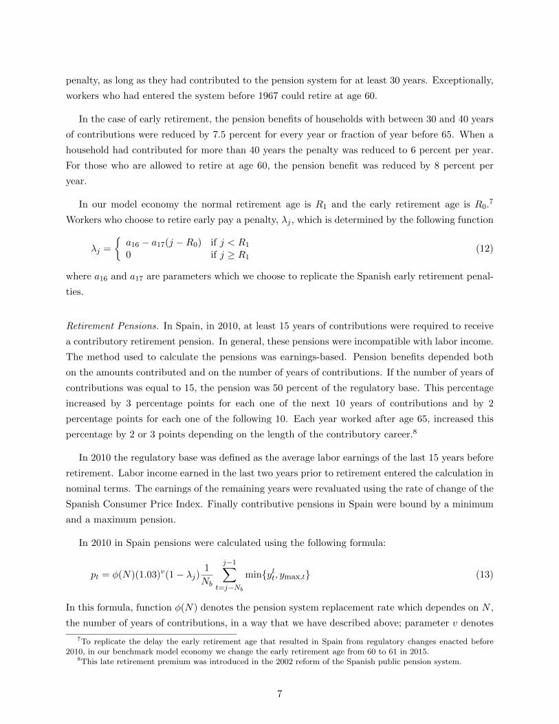
Figure 2: Retirement Hazards and Shares of Workers (%)∗

A: Retirement Hazards (All) B: Retirement Hazards (Edu) C: Shares of Workers (All)

∗The Spanish data for the retirement hazards is taken from Garcıa Perez and Sanchez-Martın (2010). The shares ofworkers are the shares of workers in the sum of workers, disabled people, and retirees. We compute this share forSpain from the Encuesta de Empleo del Tiempo (2010), reported by the INE.

In Panel A of Figure 2 we illustrate the age-profiles of the retirement hazards. The Spanish

profile, which displays a small peak at the early retirement age and a much larger one at the

normal retirement age, is a common stylized fact in countries that run defined-benefit pension

systems (see Gruber and Wise, 1999). At first sight, our model economy replicates this pattern.

A closer scrutiny reveals that the hazard is ten percentage points higher in our model economy at

age 65.

In Panel B of Figure 2 we show that high-school dropouts have a higher probability to exit the

labor force at age 60 than more educated workers. Our results show that in our model economy 90

percent of those who retire at 60 are dropouts. This finding is consistent with those of Sanchez-

Martın (2010), who reports that low-income workers have a higher probability of retiring at age 60

than high-income workers.

The details of the Spanish minimum retirement pension are one of the reasons behind this result.

In 2010, about 27 percent of the Spanish retirees receive the minimum retirement pension—this

share is 26 percent in our model economy. Workers who qualify for the minimum pension can

start to collect it at 60 without paying an early retirement penalty. Moreover, for many of these

workers, remaining in the labor force after age 60 does not increase their pensions. Since many of

these typically low-wage earners gain very little from continued employment, many of them choose

to retire as early as possible. In our model economy, 97 percent of the workers who retire at age

60 collect the minimum pension, while Jimenez-Martın and Sanchez-Martın (2006) report that in

1997 this number was 67 percent in Spain.

Retirement hazards are lower between ages 60 and 63, both in Spain and in our model economy.

This is because workers who qualify to collect a pension that is higher than the minimum pension

and who choose to work for one extra year after age 60 reduce the early retirement penalty by 8

percent. This means that these workers face an implicit subsidy if they continue to work between

23

ages 60 and 64, and this subsidy may amount to as much as 25 percent of their net yearly salary,

as shown by Boldrin et al. (1997)25.

This behavior changes at age 65. This is because the incentives provided by the Spanish pension

system to delay retirement beyond this age are small relative to the reduction in pension rights

that results from the downward sloping life-cycle profile of earnings. Therefore, most workers who

continue to work after age 65 face an implicit tax on doing so and many choose to leave the labor

force at 65 to avoid this tax. Finally, Boldrin et al. (1997), Argimon et al. (2009), and Sanchez-

Martın (2010) find that the probability of retiring at age 65 is independent of salary level, and our

model economy replicates this stylized fact. Panel B of Figure 2 shows that retirement hazards at

65 are similar for the three educational groups, and that they are larger than 77 percent for all of

them.

In Panel C of Figure 2 we report the shares of workers in the sum of workers, disabled people

and retirees. We find that the age distribution of this ratio is almost identical in Spain and in the

benchmark model economy.

Overall, we find these results very encouraging. A trustworthy answer to the questions that

we ask in this paper requires a model economy that captures the key institutional and economic

forces that affect the retirement decision. Our model economy replicates in great detail both the

Spanish tax system and the rules of the Spanish public pension system. Moreover, our calibration

procedure allows us to obtain an earnings process that allows us to replicate the earnings, income

and wealth inequality observed in Spain, as we discuss below. And we have just shown that our

model economy replicates many of the features of retirement behavior found in Spanish data. This

result is particularly remarkable, since we did not target explicitly any of these retirement behavior

facts in our calibration procedure.

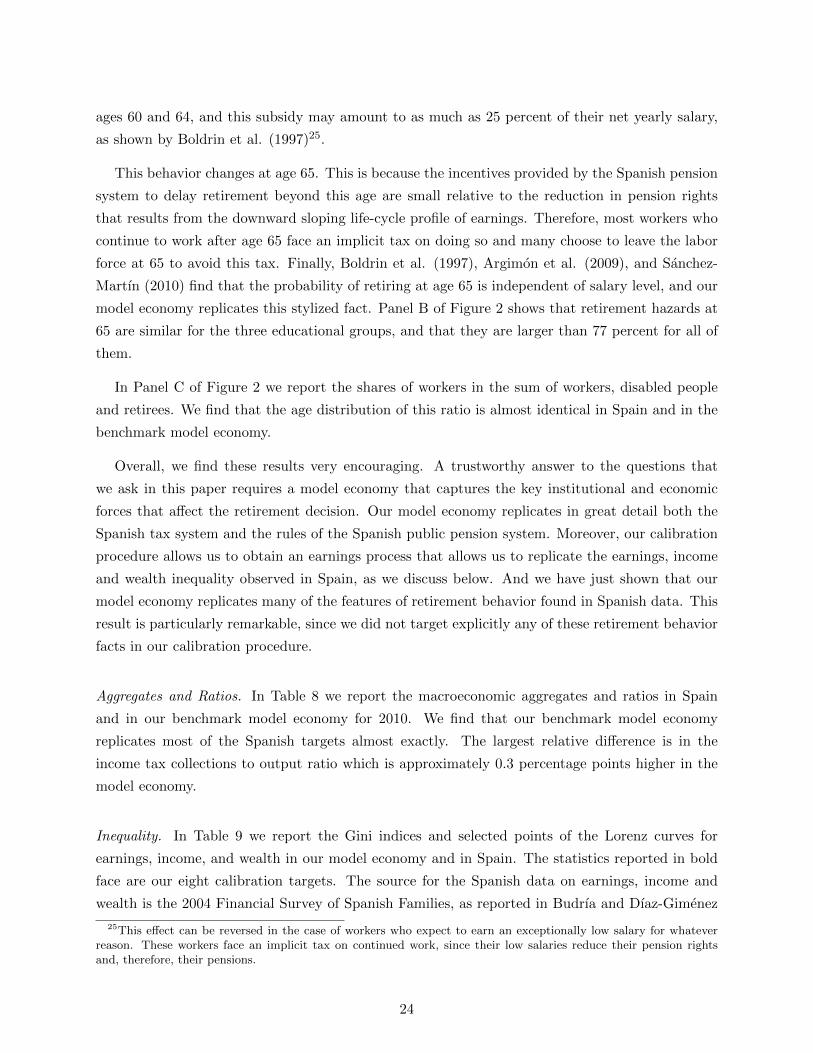
Aggregates and Ratios. In Table 8 we report the macroeconomic aggregates and ratios in Spain

and in our benchmark model economy for 2010. We find that our benchmark model economy

replicates most of the Spanish targets almost exactly. The largest relative difference is in the

income tax collections to output ratio which is approximately 0.3 percentage points higher in the

model economy.

Inequality. In Table 9 we report the Gini indices and selected points of the Lorenz curves for

earnings, income, and wealth in our model economy and in Spain. The statistics reported in bold

face are our eight calibration targets. The source for the Spanish data on earnings, income and

wealth is the 2004 Financial Survey of Spanish Families, as reported in Budrıa and Dıaz-Gimenez

25This effect can be reversed in the case of workers who expect to earn an exceptionally low salary for whateverreason. These workers face an implicit tax on continued work, since their low salaries reduce their pension rightsand, therefore, their pensions.

24

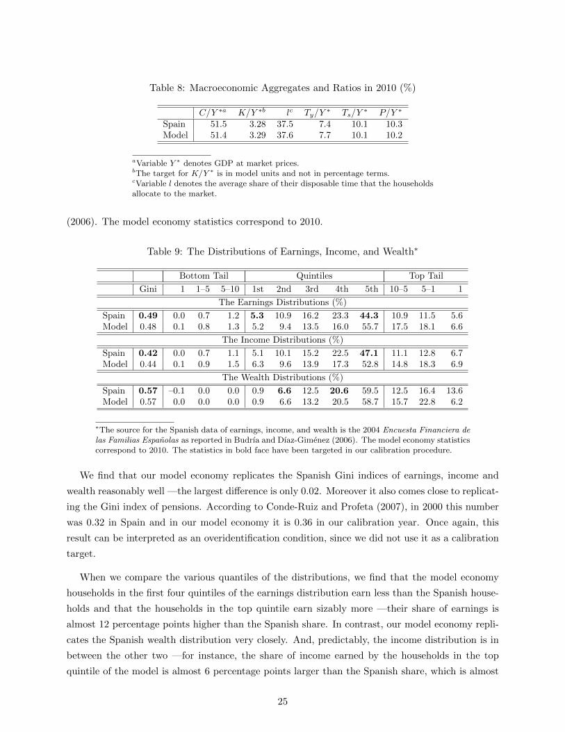
Table 8: Macroeconomic Aggregates and Ratios in 2010 (%)

C/Y ∗a K/Y ∗b lc Ty/Y∗ Ts/Y

∗ P/Y ∗

Spain 51.5 3.28 37.5 7.4 10.1 10.3Model 51.4 3.29 37.6 7.7 10.1 10.2

aVariable Y ∗ denotes GDP at market prices.bThe target for K/Y ∗ is in model units and not in percentage terms.cVariable l denotes the average share of their disposable time that the householdsallocate to the market.

(2006). The model economy statistics correspond to 2010.

Table 9: The Distributions of Earnings, Income, and Wealth∗

Bottom Tail Quintiles Top Tail

Gini 1 1–5 5–10 1st 2nd 3rd 4th 5th 10–5 5–1 1

The Earnings Distributions (%)

Spain 0.49 0.0 0.7 1.2 5.3 10.9 16.2 23.3 44.3 10.9 11.5 5.6Model 0.48 0.1 0.8 1.3 5.2 9.4 13.5 16.0 55.7 17.5 18.1 6.6

The Income Distributions (%)

Spain 0.42 0.0 0.7 1.1 5.1 10.1 15.2 22.5 47.1 11.1 12.8 6.7Model 0.44 0.1 0.9 1.5 6.3 9.6 13.9 17.3 52.8 14.8 18.3 6.9

The Wealth Distributions (%)

Spain 0.57 –0.1 0.0 0.0 0.9 6.6 12.5 20.6 59.5 12.5 16.4 13.6Model 0.57 0.0 0.0 0.0 0.9 6.6 13.2 20.5 58.7 15.7 22.8 6.2

∗The source for the Spanish data of earnings, income, and wealth is the 2004 Encuesta Financiera delas Familias Espanolas as reported in Budrıa and Dıaz-Gimenez (2006). The model economy statisticscorrespond to 2010. The statistics in bold face have been targeted in our calibration procedure.

We find that our model economy replicates the Spanish Gini indices of earnings, income and

wealth reasonably well —the largest difference is only 0.02. Moreover it also comes close to replicat-

ing the Gini index of pensions. According to Conde-Ruiz and Profeta (2007), in 2000 this number

was 0.32 in Spain and in our model economy it is 0.36 in our calibration year. Once again, this

result can be interpreted as an overidentification condition, since we did not use it as a calibration

target.

When we compare the various quantiles of the distributions, we find that the model economy

households in the first four quintiles of the earnings distribution earn less than the Spanish house-

holds and that the households in the top quintile earn sizably more —their share of earnings is

almost 12 percentage points higher than the Spanish share. In contrast, our model economy repli-

cates the Spanish wealth distribution very closely. And, predictably, the income distribution is in

between the other two —for instance, the share of income earned by the households in the top

quintile of the model is almost 6 percentage points larger than the Spanish share, which is almost

25

half way between 12 and -1.

When we look at the top tails of the distributions we find that the share of wealth owned by

the top 1 percent of the wealth distribution is 7.4 percentage points higher in Spain. This disparity

was to be expected, because it is a well-known result that overlapping generation model economies

that abstract from bequests fail to account for the large shares of wealth owned by the very richest

households in the data.26

26See Castaneda et al. (2003) for an elaboration of this argument.

26

3 Computation

To solve our model economy, we must choose the values of 50 parameters. As we have already

mentioned, we the obtain the values of 31 of these parameters directly because they are functions

of single targets. Another 4 parameters normalization conditions and 1 is obtained residually from

the government budget constraint. This gives us a total of 36 parameters and leaves us with 14 to

be determined. To do so, we solve a system of 14 non-linear equations.

The 14 parameters determined by this system are the following:

• Preferences: β and γ.

• Technology: δ.

• Stochastic process for labor productivity: s(2), s(3), s11, s12, s21, s22, s32, and s33.

• Pension system: φ and a14.

• Fiscal policy: a10.

To solve this system of equations we use a standard non-linear equation solver. Specifically, we

use a modification of Powell’s hybrid method, implemented in subroutine DNSQ from the SLATEC

package.

The DNSQ routine works as follows

1. Choose the weights that define the loss function that has to be minimized

2. Choose a vector of initial values for the 14 unknown parameters

3. Solve the model economy

4. Update the vector of parameters

5. Iterate until no further improvemets of the loss function can be found.

To solve the model economy, we proceed as follows:

1. We guess values for the interest rate, r, and for the effective labor input, N . Then, using the

optimality conditions from the firm’s maximization problem and the production function, we

obtain the implied values for productive capital, K, output, Y , and the wage rate, w.

27

2. The value of output determines the values of the fiscal policy ratios, the values of the max-

imum and minimum pensions, and the pension grid, These variables, the tax rates already

determined uniquely by single targets, and the remaining 3 government variables which are

unknowns determine the government policy.

3. Given the factor prices, the government policy, the age-dependent probabilities of surviving,

and the initial values of the parameters that describe preferences and the stochastic pro-

cess for labor productivity, we solve the household’s decision problem backwards and obtain

household’s optimal decisions.

4. We aggregate these optimal decisions and obtain the implied values for the government rev-

enue items (tax collections and accidental bequests), pension payments, and the new values

for K,N, r, w and Y .

5. Finally, we update N and r, and we iterate until convergence.

Once that the model economy is solved, DNSQ compares the relevant statistics of the model

economy with the corresponding targets, and changes the initial values of the parameters to re-

duce the values of the loss function. This procedure continues until DNSQ cannot find further

improvements of the loss function. At this point, the iteration stops and we have found a solution

for the values of the 14 unknown parameters. Since the solutions to these very non-linear systems

of equations are not guaranteed to exist and, when they do exist, they are not guaranteed to be

unique, we try many different initial values for the 14 parameters and vectors of weights and we

stop when we are convinced that we have found the best possible parameterization.

28

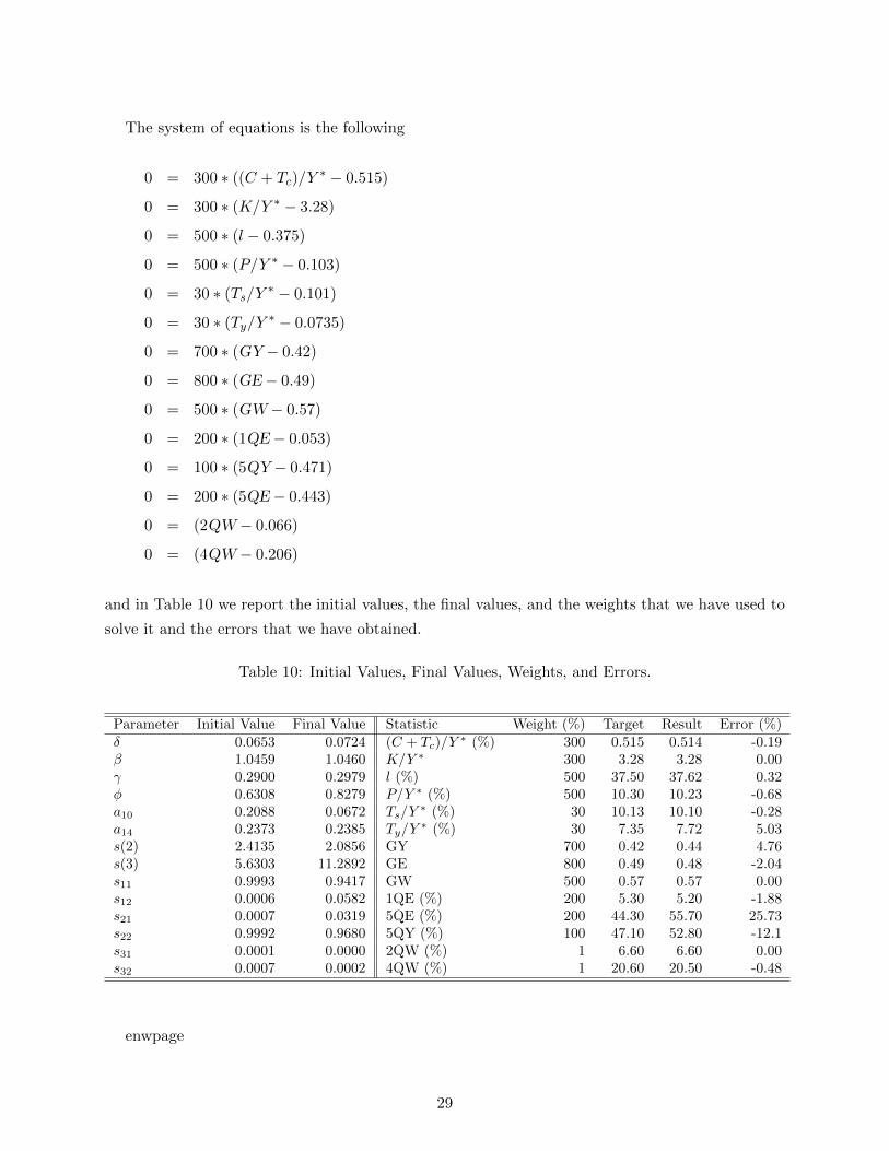
The system of equations is the following

0 = 300 ∗ ((C + Tc)/Y∗ − 0.515)

0 = 300 ∗ (K/Y ∗ − 3.28)

0 = 500 ∗ (l − 0.375)

0 = 500 ∗ (P/Y ∗ − 0.103)

0 = 30 ∗ (Ts/Y∗ − 0.101)

0 = 30 ∗ (Ty/Y∗ − 0.0735)

0 = 700 ∗ (GY− 0.42)

0 = 800 ∗ (GE− 0.49)

0 = 500 ∗ (GW− 0.57)

0 = 200 ∗ (1QE− 0.053)

0 = 100 ∗ (5QY− 0.471)

0 = 200 ∗ (5QE− 0.443)

0 = (2QW− 0.066)

0 = (4QW− 0.206)

and in Table 10 we report the initial values, the final values, and the weights that we have used to

solve it and the errors that we have obtained.

Table 10: Initial Values, Final Values, Weights, and Errors.

Parameter Initial Value Final Value Statistic Weight (%) Target Result Error (%)δ 0.0653 0.0724 (C + Tc)/Y

∗ (%) 300 0.515 0.514 -0.19β 1.0459 1.0460 K/Y ∗ 300 3.28 3.28 0.00γ 0.2900 0.2979 l (%) 500 37.50 37.62 0.32φ 0.6308 0.8279 P/Y ∗ (%) 500 10.30 10.23 -0.68a10 0.2088 0.0672 Ts/Y

∗ (%) 30 10.13 10.10 -0.28a14 0.2373 0.2385 Ty/Y

∗ (%) 30 7.35 7.72 5.03s(2) 2.4135 2.0856 GY 700 0.42 0.44 4.76s(3) 5.6303 11.2892 GE 800 0.49 0.48 -2.04s11 0.9993 0.9417 GW 500 0.57 0.57 0.00s12 0.0006 0.0582 1QE (%) 200 5.30 5.20 -1.88s21 0.0007 0.0319 5QE (%) 200 44.30 55.70 25.73s22 0.9992 0.9680 5QY (%) 100 47.10 52.80 -12.1s31 0.0001 0.0000 2QW (%) 1 6.60 6.60 0.00s32 0.0007 0.0002 4QW (%) 1 20.60 20.50 -0.48

enwpage

29

4 Literature Review

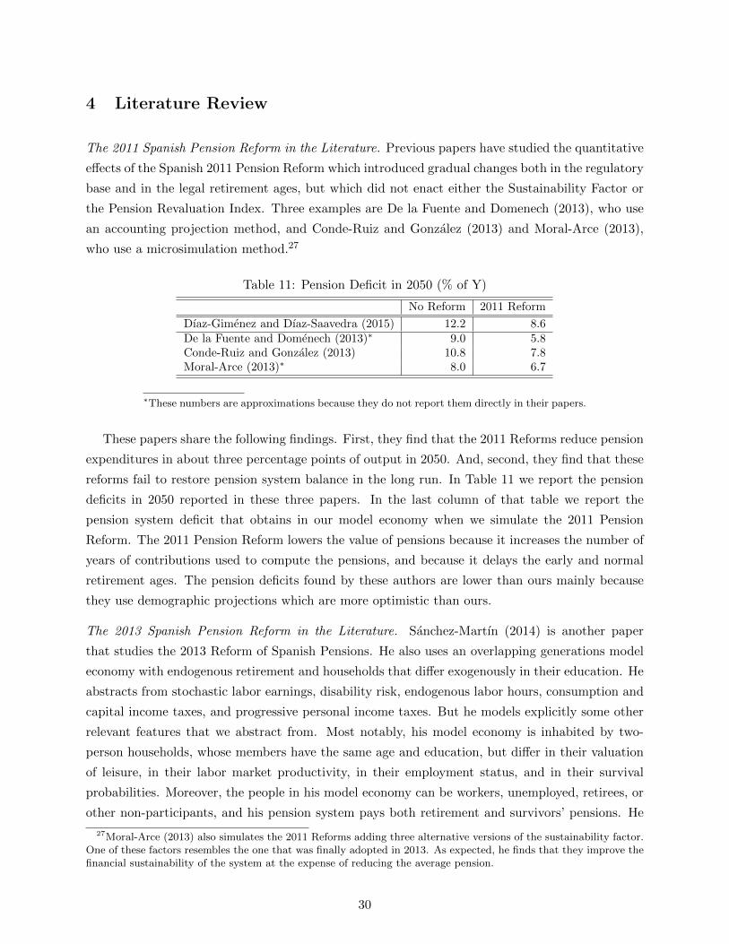
The 2011 Spanish Pension Reform in the Literature. Previous papers have studied the quantitative

effects of the Spanish 2011 Pension Reform which introduced gradual changes both in the regulatory

base and in the legal retirement ages, but which did not enact either the Sustainability Factor or

the Pension Revaluation Index. Three examples are De la Fuente and Domenech (2013), who use

an accounting projection method, and Conde-Ruiz and Gonzalez (2013) and Moral-Arce (2013),

who use a microsimulation method.27

Table 11: Pension Deficit in 2050 (% of Y)

No Reform 2011 Reform

Dıaz-Gimenez and Dıaz-Saavedra (2015) 12.2 8.6De la Fuente and Domenech (2013)∗ 9.0 5.8Conde-Ruiz and Gonzalez (2013) 10.8 7.8Moral-Arce (2013)∗ 8.0 6.7

∗These numbers are approximations because they do not report them directly in their papers.

These papers share the following findings. First, they find that the 2011 Reforms reduce pension

expenditures in about three percentage points of output in 2050. And, second, they find that these

reforms fail to restore pension system balance in the long run. In Table 11 we report the pension

deficits in 2050 reported in these three papers. In the last column of that table we report the

pension system deficit that obtains in our model economy when we simulate the 2011 Pension

Reform. The 2011 Pension Reform lowers the value of pensions because it increases the number of

years of contributions used to compute the pensions, and because it delays the early and normal

retirement ages. The pension deficits found by these authors are lower than ours mainly because

they use demographic projections which are more optimistic than ours.

The 2013 Spanish Pension Reform in the Literature. Sanchez-Martın (2014) is another paper

that studies the 2013 Reform of Spanish Pensions. He also uses an overlapping generations model

economy with endogenous retirement and households that differ exogenously in their education. He

abstracts from stochastic labor earnings, disability risk, endogenous labor hours, consumption and

capital income taxes, and progressive personal income taxes. But he models explicitly some other

relevant features that we abstract from. Most notably, his model economy is inhabited by two-

person households, whose members have the same age and education, but differ in their valuation

of leisure, in their labor market productivity, in their employment status, and in their survival

probabilities. Moreover, the people in his model economy can be workers, unemployed, retirees, or

other non-participants, and his pension system pays both retirement and survivors’ pensions. He

27Moral-Arce (2013) also simulates the 2011 Reforms adding three alternative versions of the sustainability factor.One of these factors resembles the one that was finally adopted in 2013. As expected, he finds that they improve thefinancial sustainability of the system at the expense of reducing the average pension.

30

also assumes that households can borrow and that the government can issue debt.

His demographic scenario is more optimistic than ours, because his baseline simulation uses the

Eurostat 2012 population projection. His educational transition is similar to ours and the growth

rate scenarios are hard to compare because he assumes that the labor market participation of

women increases and that the unemployment rate falls, and we abstract from these two changes.

Finally, his forecast for the inflation rate is 2.5 percent while ours is 2.0 percent.

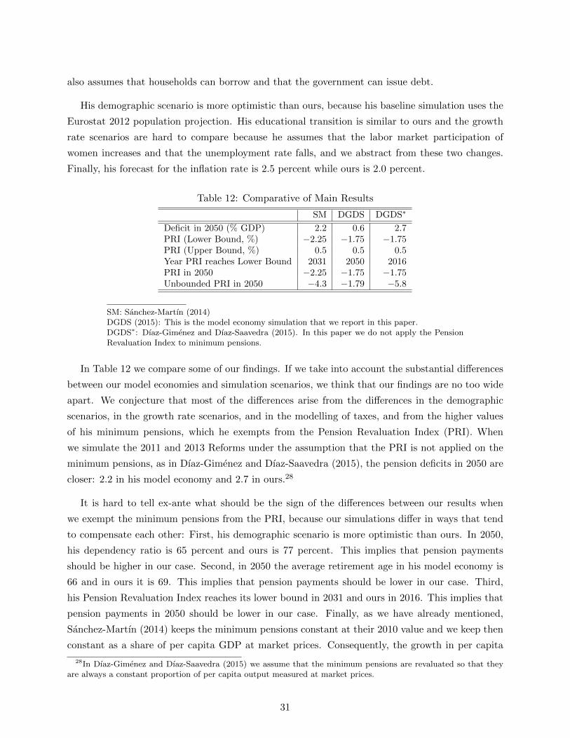
Table 12: Comparative of Main Results

SM DGDS DGDS∗

Deficit in 2050 (% GDP) 2.2 0.6 2.7PRI (Lower Bound, %) −2.25 −1.75 −1.75PRI (Upper Bound, %) 0.5 0.5 0.5Year PRI reaches Lower Bound 2031 2050 2016PRI in 2050 −2.25 −1.75 −1.75Unbounded PRI in 2050 −4.3 −1.79 −5.8

SM: Sanchez-Martın (2014)DGDS (2015): This is the model economy simulation that we report in this paper.DGDS∗: Dıaz-Gimenez and Dıaz-Saavedra (2015). In this paper we do not apply the PensionRevaluation Index to minimum pensions.

In Table 12 we compare some of our findings. If we take into account the substantial differences

between our model economies and simulation scenarios, we think that our findings are no too wide

apart. We conjecture that most of the differences arise from the differences in the demographic

scenarios, in the growth rate scenarios, and in the modelling of taxes, and from the higher values

of his minimum pensions, which he exempts from the Pension Revaluation Index (PRI). When

we simulate the 2011 and 2013 Reforms under the assumption that the PRI is not applied on the

minimum pensions, as in Dıaz-Gimenez and Dıaz-Saavedra (2015), the pension deficits in 2050 are

closer: 2.2 in his model economy and 2.7 in ours.28

It is hard to tell ex-ante what should be the sign of the differences between our results when

we exempt the minimum pensions from the PRI, because our simulations differ in ways that tend

to compensate each other: First, his demographic scenario is more optimistic than ours. In 2050,

his dependency ratio is 65 percent and ours is 77 percent. This implies that pension payments

should be higher in our case. Second, in 2050 the average retirement age in his model economy is

66 and in ours it is 69. This implies that pension payments should be lower in our case. Third,

his Pension Revaluation Index reaches its lower bound in 2031 and ours in 2016. This implies that

pension payments in 2050 should be lower in our case. Finally, as we have already mentioned,

Sanchez-Martın (2014) keeps the minimum pensions constant at their 2010 value and we keep then

constant as a share of per capita GDP at market prices. Consequently, the growth in per capita

28In Dıaz-Gimenez and Dıaz-Saavedra (2015) we assume that the minimum pensions are revaluated so that theyare always a constant proportion of per capita output measured at market prices.

31

GDP makes pension payments higher in 2050 in our case.

As in our case, the improved sustainability of his pension system is achieved reducing the value

of pensions. He defines the pension replacement rate as the ratio between the average pension

and the average output per employee, and it decreases from 0.2 to 0.124 or, approximately, by 37

percent between 2010 and 2050. In our model economy the pension replacement rate decreases

50.9 percent to 28.0 percent or by, approximately, 45 percent during that same period, but in

our definition of the pension replacement rate we use as the denominator the average earnings of

households in the 60-64 age cohort.

Finally, Sanchez-Martın (2014)’s welfare comparison differs from ours because he adjusts the

household income tax rate to finance the pension deficits and we adjust the consumption tax rate.

In spite of these differences, we reach a similar conclusion regarding the welfare costs born by the

households who are alive at the moment of the reform: if we ignore disabled households, which

Sanchez-Martın does not model, the 2013 Pension Reform imposes the highest welfare costs on

older workers. More importantly, however, our results differ from those of Sanchez-Martın when

we consider future cohorts. He finds that they are better-off and this is because his model economy

does not consider the role played by minimum pensions as an insurance mechanism against disability

risk and we do.

32

References

[1] Argimon I., M. Botella, C. Gonzalez, and R. Vegas, (2009). Retirement Behaviour and RetirementIncentives in Spain, Banco de Espana, Documentos de Trabajo, n 0913.

[2] Boldrin M., and S. Jimenez-Martın, (2003). Evaluating Spanish Pension Expenditure Under AlternativeReform Scenarios. In Gruber and Wise eds, Social Security Programs and Retirement Around the World:Fiscal Implications of Reform. NBER, University of Chicago Press.

[3] Boldrin M., S. Jimenez, and F. Peracchi, (1997). Social Security and Retirement in Spain. NBER, WP6136.

[4] Budrıa S., and J. Dıaz-Gimenez, (2006). Earnings, Income and Wealth Inequality in Spain: La EncuestaFinanciera de las Familias Espanolas (EFF). Mimeo.

[5] Castaneda A., J. Dıaz-Gimenez and J. V. Rıos-Rull (2003). Accounting for the U.S. Earnings andWealth Inequality. Journal of Political Economy 4, 818–855.

[6] Calonge S., and J. C. Conesa, (2003). Progressivity and Effective Income Taxation in Spain: 1990 and1995. Centre de Recerca en Economia del Benestar.

[7] Conde-Ruiz J. I., and C. I. Gonzalez, (2013). Reforma de Pensiones 2011 en Espana. Hacienda PublicaEspanola, IEF, 204(1), 9–44.

[8] Conde-Ruiz I., and P. Profeta, (2007). The Redistributive Design of Social Security Systems, EconomicJournal, 117, 686–712.

[9] Cooley T., and E. Prescott, (1995). Economic Growth and Business Cycles. In Frontiers of BusinessCycle Research, T. Cooley (ed), Princeton University Press.

[10] De La Fuente A., and R. Domenech, (2013). The Financial Impact of Spanish Pension Reform: A QuickEstimate. Journal of Pension Economics and Finance, 12(01), 111–137.

[11] Dıaz-Gimenez J., and J. Dıaz-Saavedra, (2009). Delaying Retirement in Spain. Review of EconomicDynamics, 12, 147–167.

[12] Dıaz-Gimenez J., and J. Dıaz-Saavedra, (2015). Spanish Minimum Pensions After The 2013 PensionReform. Estudios de Economıa Aplicada, 33, 717–734.

[13] Fuster L., A. Imrohoroglu, and S. Imrohoroglu, (2007). Elimination of Social Security in a DynasticFramework. Review of Economic Studies, 74, pp 113-145.

[14] Garcıa Perez J. I., and A. R. Sanchez-Martın, (2010). Social Security and the Job Search Behavior ofWorkers Approaching Retirement. Working Papers 2010-26, FEDEA.

[15] Gouveia M., and R. P. Strauss, (1994). Effective Federal Individual Income Tax Functions: An Ex-ploratory Empirical Analysis. National Tax Journal, 47, 2, 317–339.

[16] Gruber J., and D. A. Wise, (1999). Social Security and Retirement around the World. NBER Books,National Bureau of Economic Research, Inc.

[17] Imrohoroglu A., S. Imrohoroglu, and D. Joines, (1995). A Life Cycle Analysis of Social Security. Eco-nomic Theory, 6, 83-114.

[18] Jimenez-Martın S., and A. R. Sanchez-Martın, (2006). An Evaluation of the Life-cycle Effects of Mini-mum Pensions on Retirement Behavior: Extended Version. Working Papers 06.23, Universidad Pablode Olavide, Department of Economics.

[19] Moral-Arce I., (2013). Aplicacion de Factores de Sostenibilidad en el Sistema de Pensiones Espanol:Previsiones Para el Perıodo 2012-2050. Instituto de Estudios Fiscales, P.T. 4/2013.

[20] Sanchez-Martın A. R., (2010). Endogenous Retirement and Public Pension System Reform in Spain.Economic Modelling, 27, 336–349.

[21] Sanchez-Martın A. R., (2014). The Automatic Adjustment of Pension Expenditures in Spain: An

Evaluation of the 2013 Pension Reform. Banco de Espana, Documento de Trabajo 1420.

33