Embed Size (px)
Citation preview
Intro Structural Limits Representations Stone Interpretations Near the Limit Modelings Perspectives
Structural Limits
Jaroslav Nešetřil Patrice Ossona de Mendez
Charles UniversityPraha, Czech Republic LIA STRUCO CAMS, CNRS/EHESS
Paris, France
— Warwick(
2
(22
2
)
2
)—
Intro Structural Limits Representations Stone Interpretations Near the Limit Modelings Perspectives
Contents
Introduction
Structural Limits
General Representation Theorems
Stone Spaces
Interpretations
Near the Limit
Modelings
Perspectives
Intro Structural Limits Representations Stone Interpretations Near the Limit Modelings Perspectives
Introduction
Intro Structural Limits Representations Stone Interpretations Near the Limit Modelings Perspectives
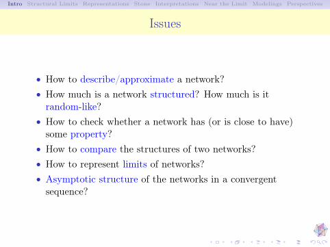
Issues
• How to describe/approximate a network?• How much is a network structured? How much is itrandom-like?
• How to check whether a network has (or is close to have)some property?
• How to compare the structures of two networks?• How to represent limits of networks?• Asymptotic structure of the networks in a convergentsequence?
Intro Structural Limits Representations Stone Interpretations Near the Limit Modelings Perspectives
Structural Limits
Intro Structural Limits Representations Stone Interpretations Near the Limit Modelings Perspectives
Structural Limits
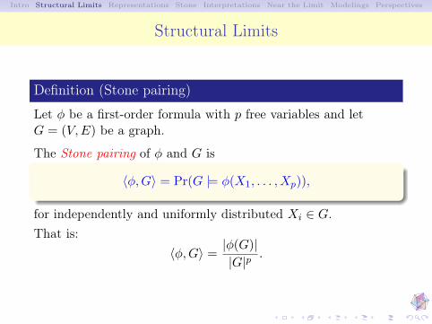
Definition (Stone pairing)
Let φ be a first-order formula with p free variables and letG = (V,E) be a graph.
The Stone pairing of φ and G is
〈φ,G〉 = Pr(G |= φ(X1, . . . , Xp)),
for independently and uniformly distributed Xi ∈ G.That is:
〈φ,G〉 =|φ(G)||G|p .
Intro Structural Limits Representations Stone Interpretations Near the Limit Modelings Perspectives
Structural Limits
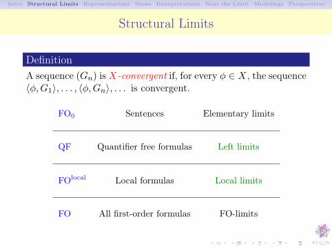
DefinitionA sequence (Gn) isX-convergent if, for every φ ∈ X, the sequence〈φ,G1〉, . . . , 〈φ,Gn〉, . . . is convergent.
FO0 Sentences Elementary limits
QF Quantifier free formulas Left limits
FOlocal Local formulas Local limits
FO All first-order formulas FO-limits
Intro Structural Limits Representations Stone Interpretations Near the Limit Modelings Perspectives
General Representation Theorems
Intro Structural Limits Representations Stone Interpretations Near the Limit Modelings Perspectives
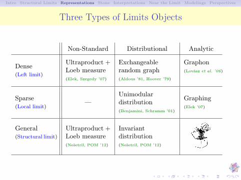
Three Types of Limits Objects
Non-Standard Distributional Analytic
Dense(Left limit)
Ultraproduct +Loeb measure(Elek, Szegedy ’07)
Exchangeablerandom graph(Aldous ’81, Hoover ’79)
Graphon(Lovász et al. ’06)
Sparse(Local limit)
—Unimodulardistribution(Benjamini, Schramm ’01)
Graphing(Elek ’07)
General(Structural limit)
Ultraproduct +Loeb measure(Nešetril, POM ’12)
Invariantdistribution(Nešetril, POM ’12)

Intro Structural Limits Representations Stone Interpretations Near the Limit Modelings Perspectives
Non-Standard Limit: Ultraproduct with Loeb Measure
Theorem (Nešetril, POM 2012)
Let (Gn)n∈N be FO-convergent and let U be a non-principalultrafilter on N. Then there exists a probability measure ν onthe ultraproduct
∏U Gn such that for every first-order formula φ
with p free variables it holds:
∫· · ·∫
(∏U Gn)p
1φ([x1], . . . , [xp]) dν([x1]) . . . dν([xp]) = limU〈ψ,Gi〉.
Not product σ-algebra, but Fubini-like properties
(Follows Elek, Szegedy ’07; See also Keisler ’77)
Intro Structural Limits Representations Stone Interpretations Near the Limit Modelings Perspectives
Distributionual Limit
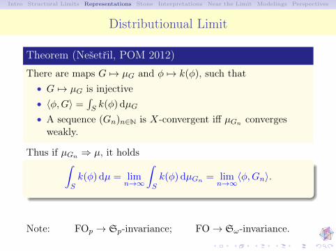
Theorem (Nešetřil, POM 2012)
There are maps G 7→ µG and φ 7→ k(φ), such that• G 7→ µG is injective• 〈φ,G〉 =
∫S k(φ) dµG
• A sequence (Gn)n∈N is X-convergent iff µGn convergesweakly.
Thus if µGn ⇒ µ, it holds∫
Sk(φ) dµ = lim
n→∞
∫
Sk(φ) dµGn = lim
n→∞〈φ,Gn〉.
Note: FOp → Sp-invariance; FO→ Sω-invariance.
Intro Structural Limits Representations Stone Interpretations Near the Limit Modelings Perspectives
Stone Spaces
Intro Structural Limits Representations Stone Interpretations Near the Limit Modelings Perspectives
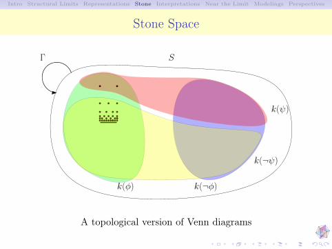
Stone Space
S
k(φ) k(¬φ)
Γ
k(ψ)
k(¬ψ)
A topological version of Venn diagrams
Intro Structural Limits Representations Stone Interpretations Near the Limit Modelings Perspectives
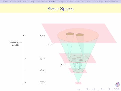
Stone Spaces
S(FO)
S(FOp)
S(FO0)
number of freevariables
S(FO1)
0
1
p
ω
Sω
Sp
Intro Structural Limits Representations Stone Interpretations Near the Limit Modelings Perspectives
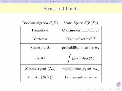
Structural Limits
Boolean algebra B(X) Stone Space S(B(X))
Formula φ Continuous function fφ
Vertex v “Type of vertex” T
Structure A probability measure µA
〈φ,A〉∫fφ(T ) dµA(T )
X-convergent (An) weakly convergent µAn
Γ = Aut(B(X)) Γ-invariant measure
Intro Structural Limits Representations Stone Interpretations Near the Limit Modelings Perspectives
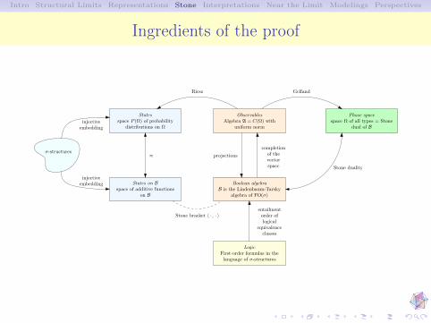
Ingredients of the proof
ObservablesAlgebra A = C(Ω) with
uniform norm
Statesspace P (Ω) of probability
distributions on Ω
Phase spacespace Ω of all types = Stone
dual of B
Boolean algebraB is the Lindenbaum-Tarsky
algebra of FO(σ)
Stone duality
projections
completionof thevectorspace
injectiveembedding
entailmentorder oflogical
equivalenceclasses
States on Bspace of additive functions
on B
≈σ-structures
injectiveembedding
Stone bracket 〈 · , · 〉
GelfandRiesz
LogicFirst-order formulas in thelanguage of σ-structures
Intro Structural Limits Representations Stone Interpretations Near the Limit Modelings Perspectives
The Elementary Convergence Case
Intro Structural Limits Representations Stone Interpretations Near the Limit Modelings Perspectives
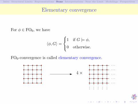
Elementary convergence
For φ ∈ FO0, we have
〈φ,G〉 =
1 if G |= φ,
0 otherwise.
FO0-convergence is called elementary convergence.
4×. . .
. . .
. . .
. . .
. . ....
......
......
Intro Structural Limits Representations Stone Interpretations Near the Limit Modelings Perspectives
Limit Object
Proposition (Gödel+Löwenheim–Skolem)
Every elementarily convergent sequence of finite graphs has alimit, which is an at most countable graph.
Complete theories with Finite Model Property form a closedsubset of the Stone dual of FO0 but . . .
No characterization of elementary limits
Trakhtenbrot’s theorem states that the problem of existence of afinite model for a single first-order sentence is undecidable.
Intro Structural Limits Representations Stone Interpretations Near the Limit Modelings Perspectives
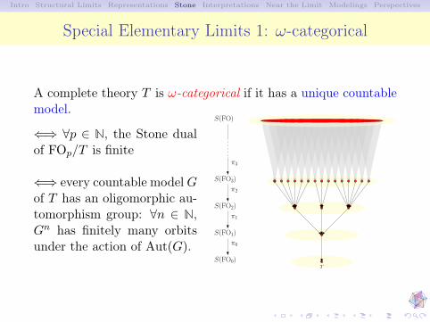
Special Elementary Limits 1: ω-categorical
A complete theory T is ω-categorical if it has a unique countablemodel.
⇐⇒ ∀p ∈ N, the Stone dualof FOp/T is finite
⇐⇒ every countable modelGof T has an oligomorphic au-tomorphism group: ∀n ∈ N,Gn has finitely many orbitsunder the action of Aut(G).
S(FO0)T
S(FO1)
S(FO2)
S(FO3)
S(FO)
π2
π1
π0
π3
Intro Structural Limits Representations Stone Interpretations Near the Limit Modelings Perspectives
Special Elementary Limits 2: Ultrahomogeneous
A graph G is ultrahomogeneous if every isomorphism between twoof its induced subgraphs can be extended to an automorphism.The only countably infinite homogeneous graphs are:• ωKn, nKω, ωKω, and complements;• the Rado graph;• the Henson graphs and complements.
Proposition
If (Gn)n∈N is elementarily convergent to an ultrahomogeneousgraph, then (Gn)n∈N is FO-convergent if and only if (Gn)n∈N isQF-convergent.
Intro Structural Limits Representations Stone Interpretations Near the Limit Modelings Perspectives
Example
Theorem (Nešetril, Ossona de Mendez)
Let 0 < p < 1 and let Gn ∈ G(n, p) be independent randomgraphs with edge probability p. Then (Gn)n∈N is almost surelyFO-convergent.
Proof.(Gn)n∈N almost surely converges elementarily to the Rado graph,and almost surely QF-converges.
Problem (Cherlin)
Is the generic countable triangle-free graph elementary limit offinite graphs?
Intro Structural Limits Representations Stone Interpretations Near the Limit Modelings Perspectives
The Quantifier-Free Case
Intro Structural Limits Representations Stone Interpretations Near the Limit Modelings Perspectives
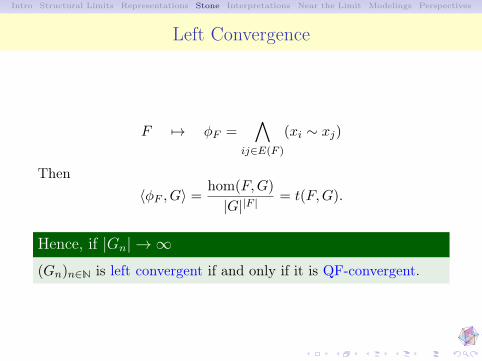
Left Convergence
F 7→ φF =∧
ij∈E(F )
(xi ∼ xj)
Then〈φF , G〉 =
hom(F,G)
|G||F | = t(F,G).
Hence, if |Gn| → ∞(Gn)n∈N is left convergent if and only if it is QF-convergent.
Intro Structural Limits Representations Stone Interpretations Near the Limit Modelings Perspectives
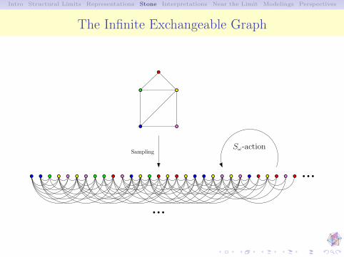
The Infinite Exchangeable Graph
SamplingSω-action
Intro Structural Limits Representations Stone Interpretations Near the Limit Modelings Perspectives
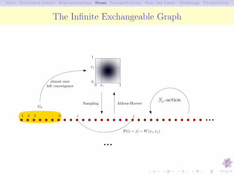
The Infinite Exchangeable Graph
1 2 3 i j
0 10
1
xi
xj
Pr(i ∼ j) =W (xi, xj)
Sampling Aldous-Hoover
k
Gk
almost sureleft convergence
Sω-action
Intro Structural Limits Representations Stone Interpretations Near the Limit Modelings Perspectives
Extensions
4 colored, directed, decorated graphs (Lovász, Szegedy ’10);4 regular hypergraphs (Elek, Szegedy ’12; Zhao ’14);4 relational structures (Aroskar ’12; Aroskar, Cummings ’14);* algebraic structures.
Intro Structural Limits Representations Stone Interpretations Near the Limit Modelings Perspectives
Algebraic Structures
Signature σ = (f0, . . . , fd), fi involution
−→ encodes graphs with maximum degree d;−→ QF1-limit equivalent to local limit;−→ limit object with same signature, fi measure preserving
involution (= graphing).
Thus. . .General QF-convergence extends both left limits and local limitsof graphs with bounded degrees.
Intro Structural Limits Representations Stone Interpretations Near the Limit Modelings Perspectives
The Local Case
Intro Structural Limits Representations Stone Interpretations Near the Limit Modelings Perspectives
Local Formulas
DefinitionA formula φ is local if there exists r such that satisfaction of φonly depends on the r-neighborhood of the free variables:
G |= φ(v1, . . . , vp) ⇐⇒ G[Nr(v1, . . . , vp)] |= φ(v1, . . . , vp).
DefinitionA sequence (Gn) is local-convergent if, for every φ ∈ FOlocal, thesequence 〈φ,G1〉, . . . , 〈φ,Gn〉, . . . is convergent.
(Gn) is local-convergent if, for every local formula φ, the prob-ability that Gn satisfies φ for a random assignment of the freevariables converges.
Intro Structural Limits Representations Stone Interpretations Near the Limit Modelings Perspectives
Local Convergent Sequence of Bounded Degree Graphs
For a sequence (Gn)n∈N of graphs with degree ≤ d the followingare equivalent:1. the sequence (Gn)n∈N is local convergent (in the sense of
Benjamini and Schramm);2. the sequence (Gn)n∈N is FOlocal
1 -convergent;3. the sequence (Gn)n∈N is local-convergent (in our sense).
Intro Structural Limits Representations Stone Interpretations Near the Limit Modelings Perspectives
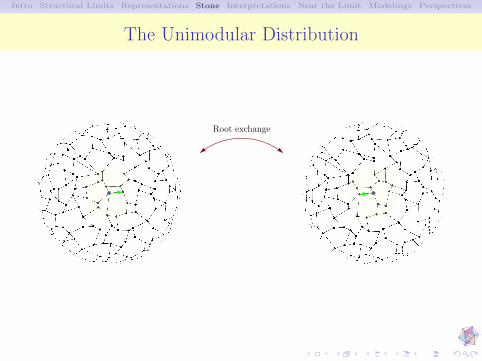
The Unimodular Distribution
Root exchange
Intro Structural Limits Representations Stone Interpretations Near the Limit Modelings Perspectives
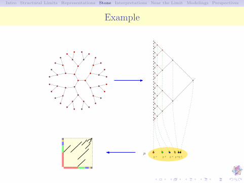
Example
2−1 2−2 2−3 2−42−5. . .
µ
Intro Structural Limits Representations Stone Interpretations Near the Limit Modelings Perspectives
Why Formulas?
Consider extension of local convergence: (Gn)n∈N converges if,for every d and rooted (F, r) there is some td(F ) such that
Pr[Bd(Gn, X) ' (F, r)] −→ td(F ).
No limit probability distribution!
Example: Gn any n-regular graph. Then for every d and every(F, r) it holds
Pr[Bd(Gn, X) ' (F, r)] −→ 0.
Intro Structural Limits Representations Stone Interpretations Near the Limit Modelings Perspectives
Why Local Convergence?
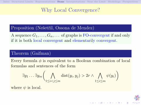
Proposition (Nešetřil, Ossona de Mendez)
A sequence G1, . . . , Gn, . . . of graphs is FO-convergent if and onlyif it is both local convergent and elementarily convergent.
Theorem (Gaifman)
Every formula φ is equivalent to a Boolean combination of localformulas and sentences of the form
∃y1 . . . ∃ym( ∧
1≤i<j≤mdist(yi, yj) > 2r ∧
∧
1≤i≤mψ(yi)
)
where ψ is local.
Intro Structural Limits Representations Stone Interpretations Near the Limit Modelings Perspectives
Interpretations
Intro Structural Limits Representations Stone Interpretations Near the Limit Modelings Perspectives
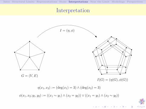
Interpretation
G = (V,E)I(G) = (η(G), φ(G))
I = (η, φ)
η(x1, x2) := (deg(x1) = 3) ∧ (deg(x2) = 3)
φ(x1, x2; y1, y2) := ((x1 ∼ y1) ∧ (x2 = y2)) ∨ ((x1 = y1) ∧ (x2 ∼ y2))
Intro Structural Limits Representations Stone Interpretations Near the Limit Modelings Perspectives
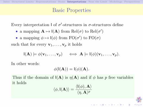
Basic Properties
Every interpretation I of σ′-structures in σ-structures define• a mapping A 7→ I(A) from Rel(σ) to Rel(σ′)
• a mapping φ 7→ I(φ) from FO(σ′) to FO(σ)
such that for every v1, . . . ,vp it holds
I(A) |= φ(v1, . . . ,vp) ⇐⇒ A |= I(φ)(v1, . . . ,vp).
In other words:φ(I(A)) = I(φ)(A).
Thus if the domain of I(A) is η(A) and if φ has p free variablesit holds
〈φ, I(A)〉 =〈I(φ),A〉〈η,A〉p
Intro Structural Limits Representations Stone Interpretations Near the Limit Modelings Perspectives
Near the Limit
Intro Structural Limits Representations Stone Interpretations Near the Limit Modelings Perspectives
Negligible Sequences
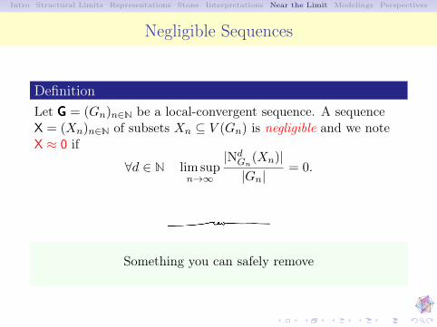
DefinitionLet GGG = (Gn)n∈N be a local-convergent sequence. A sequenceX = (Xn)n∈N of subsets Xn ⊆ V (Gn) is negligible and we noteX ≈ 0 if
∀d ∈ N lim supn→∞
|NdGn
(Xn)||Gn|
= 0.
Something you can safely remove
Intro Structural Limits Representations Stone Interpretations Near the Limit Modelings Perspectives
What is a cluster?
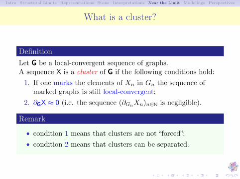
DefinitionLet GGG be a local-convergent sequence of graphs.A sequence X is a cluster of GGG if the following conditions hold:1. If one marks the elements of Xn in Gn the sequence of
marked graphs is still local-convergent;2. ∂GGGX ≈ 0 (i.e. the sequence (∂GnXn)n∈N is negligible).
Remark
• condition 1 means that clusters are not “forced”;• condition 2 means that clusters can be separated.
Intro Structural Limits Representations Stone Interpretations Near the Limit Modelings Perspectives
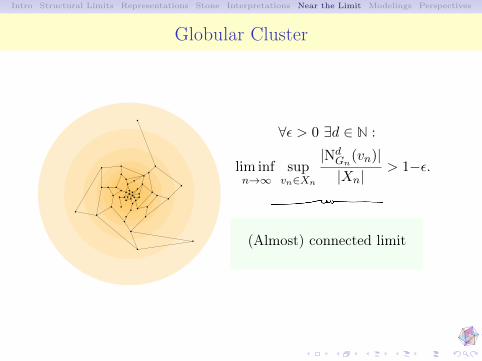
Globular Cluster
∀ε > 0 ∃d ∈ N :
lim infn→∞
supvn∈Xn
|NdGn
(vn)||Xn|
> 1−ε.
(Almost) connected limit
Intro Structural Limits Representations Stone Interpretations Near the Limit Modelings Perspectives
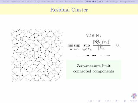
Residual Cluster
∀d ∈ N :
lim supn→∞
supvn∈Xn
|NdGn
(vn)||Xn|
= 0.
Zero-measure limitconnected components
Intro Structural Limits Representations Stone Interpretations Near the Limit Modelings Perspectives
Marking of all Globular Clusters
Theorem (Nešetřil, Ossona de Mendez, 2015+)
Let GGG be a local convergent sequence of graphs. Then there exists(for all n) a marking G+
n of Gn by S,R,M1, . . . ,Mi, . . . such that
• marks S,R,M1, . . . ,Mi, . . . induce a partition of V (Gn)and each mark Mi marks one of the connected componentsof Gn \ S;
• the sequence GGG+ is local convergent;• S(GGG) is negligible in GGG+;• Mi(GGG) is a globular cluster of GGG+;• R(GGG) is a residual cluster of GGG+.
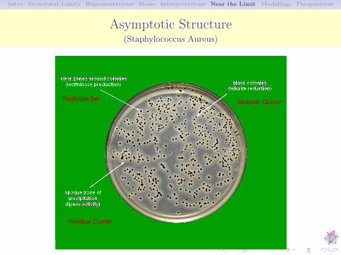
Intro Structural Limits Representations Stone Interpretations Near the Limit Modelings Perspectives
Asymptotic Structure(Staphylococcus Aureus)
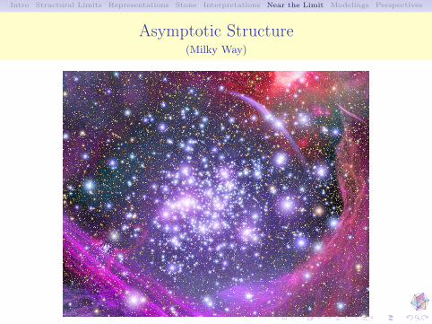
Intro Structural Limits Representations Stone Interpretations Near the Limit Modelings Perspectives
Asymptotic Structure(Milky Way)
Intro Structural Limits Representations Stone Interpretations Near the Limit Modelings Perspectives
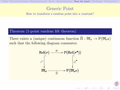
Generic PointHow to transform a random point into a constant?
Theorem (1-point random lift theorem)
There exists a (unique) continuous function Π : Mσ → P(Mσ•)such that the following diagram commutes:
Mσ P(Mσ•)Π
//
Rel(σ)
Mσ
_
ισ
Rel(σ) P(Rel(σ•))Π // P(Rel(σ•))
P(Mσ•)
_
ισ•∗
Intro Structural Limits Representations Stone Interpretations Near the Limit Modelings Perspectives
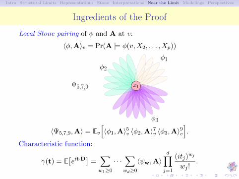
Ingredients of the Proof
Local Stone pairing of φ and A at v:
〈φ,A〉v = Pr(A |= φ(v,X2, . . . , Xp))
x1
φ1
φ2
φ3
Ψ5,7,9
〈Ψ5,7,9,A〉 = Ev[〈φ1,A〉5v 〈φ2,A〉7v 〈φ3,A〉9v
].
Characteristic function:
γ(t) = E[eit·D
]=∑
w1≥0
· · ·∑
wd≥0
〈ψw,A〉d∏
j=1
(itj)wj
wj !.
Intro Structural Limits Representations Stone Interpretations Near the Limit Modelings Perspectives
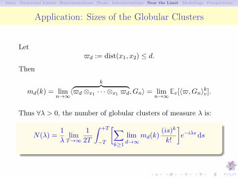
Application: Sizes of the Globular Clusters
Let$d := dist(x1, x2) ≤ d.
Then
md(k) = limn→∞
〈k︷ ︸︸ ︷
$d ⊗x1 · · · ⊗x1 $d, Gn〉 = limn→∞
Ev[〈$,Gn〉kv ].
Thus ∀λ > 0, the number of globular clusters of measure λ is:
N(λ) =1
λlimT→∞
1
2T
∫ +T
−T
[∑
k≥1
limd→∞
md(k)(is)k
k!
]e−iλs ds
Intro Structural Limits Representations Stone Interpretations Near the Limit Modelings Perspectives
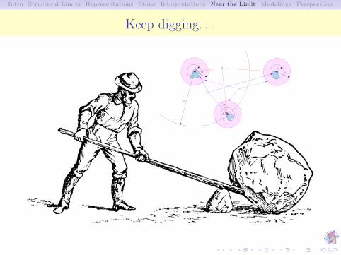
Keep digging. . .
8δz
2δz
δz
δz
2δz
δz
2δz
Zλ,zn
Sλn
Cλn
Intro Structural Limits Representations Stone Interpretations Near the Limit Modelings Perspectives
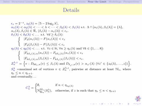
Details
εz = 2−z , z0(λ) = d5− 2 log2 λe,α1(λ) < α2(λ) < · · · < λ < · · · < β2(λ) < β1(λ) s.t. Λ ∩ [α1(λ), β1(λ)] = λ,αz(λ), βz(λ) ∈ R, |βz(λ)− αz(λ)| < εz .δ1(λ) < δ2(λ) < . . . s.t. ∀d ≥ δz(λ):
|Fd(αz(λ))− F (αz(λ))| < εz
|Fd(βz(λ))− F (βz(λ))| < εzη1(λ) < η2(λ) < . . . s.t. ∀z ∈ N, ∀n ≥ ηz(λ) and ∀k ∈ 1, . . . 8:
|Fkδz(λ),n(αz(λ))− Fkδz(λ)(αz(λ))| < εz
|Fkδz(λ),n(βz(λ))− Fkδz(λ)(βz(λ))| < εz .
Zλ,zn =v : D8δz ,n(v) ≤ βz(λ) and Dδz′ ,n(v) > αz′ (λ) (∀z′ ∈ z0(λ), . . . , z)
.
Sλn =maximal set of vertices v ∈ Zλ,zn , pairwise at distance at least 7δz , whereηz ≤ n < ηz+1.and eventually. . .
Cλn =
∅, if n < ηz0(λ)
N2δzGn
(Sλn), otherwise, if z is such that ηz ≤ n < ηz+1
Intro Structural Limits Representations Stone Interpretations Near the Limit Modelings Perspectives
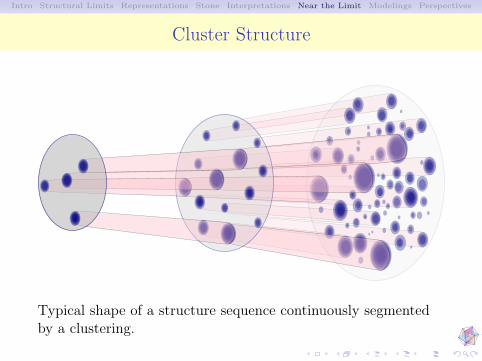
Cluster Structure
Typical shape of a structure sequence continuously segmentedby a clustering.
Intro Structural Limits Representations Stone Interpretations Near the Limit Modelings Perspectives
Modelings
Intro Structural Limits Representations Stone Interpretations Near the Limit Modelings Perspectives
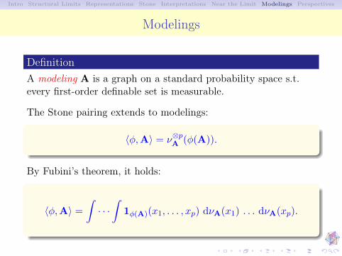
Modelings
DefinitionA modeling A is a graph on a standard probability space s.t.every first-order definable set is measurable.
The Stone pairing extends to modelings:
〈φ,A〉 = ν⊗pA (φ(A)).
By Fubini’s theorem, it holds:
〈φ,A〉 =
∫· · ·∫
1φ(A)(x1, . . . , xp) dνA(x1) . . . dνA(xp).
Intro Structural Limits Representations Stone Interpretations Near the Limit Modelings Perspectives
Modelings as FO-limits?
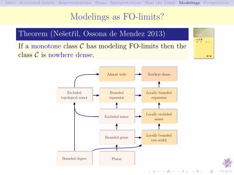
Theorem (Nešetřil, Ossona de Mendez 2013)
If a monotone class C has modeling FO-limits then theclass C is nowhere dense.
Nowhere denseAlmost wide
Bounded
expansion
Excluded
topological minor
Locally bounded
expansion
Locally excluded
minorExcluded minor
Bounded genusLocally bounded
tree-width
PlanarBounded degree
Intro Structural Limits Representations Stone Interpretations Near the Limit Modelings Perspectives
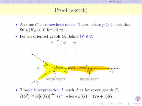
Proof (sketch)
• Assume C is somewhere dense. There exists p ≥ 1 such thatSubp(Kn) ∈ C for all n;
• For an oriented graph G, define G′ ∈ C:
p
p
G
p
p
x y
x′ y′
︷ ︸︸ ︷(2p+ 1)(|G| − dG(x))− 1
︷ ︸︸ ︷(2p+ 1)(|G| − dG(y))− 1
p︷ ︸︸ ︷ p︷ ︸︸ ︷ p︷ ︸︸ ︷G′
• ∃ basic interpretation I, such that for every graph G,I(G′) ∼= G[k(G)]
def= G+, where k(G) = (2p+ 1)|G|.
Intro Structural Limits Representations Stone Interpretations Near the Limit Modelings Perspectives
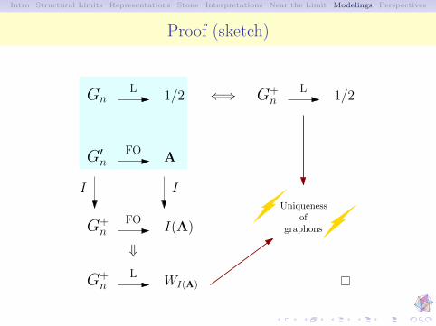
Proof (sketch)
Gn
G′n
L
FO
1/2
A
I I
G+n
FOI(A)
G+n WI(A)
L
⇓
⇐⇒ G+n
L1/2
Uniquenessof
graphons
Intro Structural Limits Representations Stone Interpretations Near the Limit Modelings Perspectives
Modelings as FO-limits?
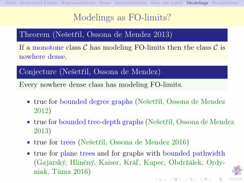
Theorem (Nešetřil, Ossona de Mendez 2013)
If a monotone class C has modeling FO-limits then the class C isnowhere dense.
Conjecture (Nešetřil, Ossona de Mendez)
Every nowhere dense class has modeling FO-limits.
• true for bounded degree graphs (Nešetřil, Ossona de Mendez2012)
• true for bounded tree-depth graphs (Nešetřil, Ossona de Mendez2013)
• true for trees (Nešetřil, Ossona de Mendez 2016)• true for plane trees and for graphs with bounded pathwidth(Gajarský, Hliněný, Kaiser, Kráľ, Kupec, Obdržálek, Ordy-niak, Tůma 2016)
Intro Structural Limits Representations Stone Interpretations Near the Limit Modelings Perspectives
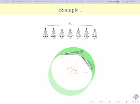
Example I
θ0
x
θ0
√n
√n
√n
√n
√n
√n
√n
√n
Intro Structural Limits Representations Stone Interpretations Near the Limit Modelings Perspectives
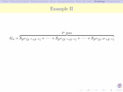
Example II
Gn =
2n stars︷ ︸︸ ︷S22n (2−1+2−n) + · · · + S22n (2−i+2−n) + · · · + S22n (2−2n+2−n)
Bigcomponents
Smallcomponents
Intro Structural Limits Representations Stone Interpretations Near the Limit Modelings Perspectives
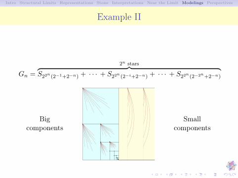
Example II
Gn =
2n stars︷ ︸︸ ︷S22n (2−1+2−n) + · · · + S22n (2−i+2−n) + · · · + S22n (2−2n+2−n)
Bigcomponents
Smallcomponents
Intro Structural Limits Representations Stone Interpretations Near the Limit Modelings Perspectives
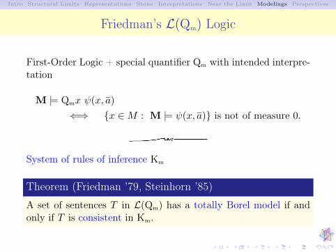
Friedman’s L(Qm) Logic
First-Order Logic + special quantifier Qm with intended interpre-tation
M |= Qmx ψ(x, a)
⇐⇒ x ∈M : M |= ψ(x, a) is not of measure 0.
System of rules of inference Km
Theorem (Friedman ’79, Steinhorn ’85)
A set of sentences T in L(Qm) has a totally Borel model if andonly if T is consistent in Km.
Intro Structural Limits Representations Stone Interpretations Near the Limit Modelings Perspectives
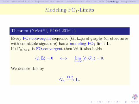
Modeling FO1-Limits
Theorem (Nešetřil, POM 2016+)
Every FO1-convergent sequence (Gn)n∈N of graphs (or structureswith countable signature) has a modeling FO1-limit L.If (Gn)n∈N is FO-convergent then ∀φ it also holds
〈φ,L〉 = 0 ⇐⇒ limn→∞
〈φ,Gn〉 = 0.
We denote this by
GnFO∗1−−→ L.
Intro Structural Limits Representations Stone Interpretations Near the Limit Modelings Perspectives
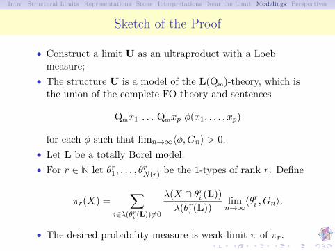
Sketch of the Proof
• Construct a limit U as an ultraproduct with a Loebmeasure;
• The structure U is a model of the L(Qm)-theory, which isthe union of the complete FO theory and sentences
Qmx1 . . . Qmxp φ(x1, . . . , xp)
for each φ such that limn→∞〈φ,Gn〉 > 0.• Let L be a totally Borel model.• For r ∈ N let θr1, . . . , θrN(r) be the 1-types of rank r. Define
πr(X) =∑
i∈λ(θri (L)) 6=0
λ(X ∩ θri (L))
λ(θri (L))limn→∞
〈θri , Gn〉.
• The desired probability measure is weak limit π of πr.
Intro Structural Limits Representations Stone Interpretations Near the Limit Modelings Perspectives
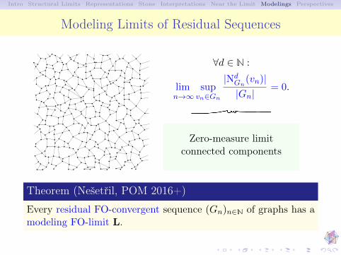
Modeling Limits of Residual Sequences
∀d ∈ N :
limn→∞
supvn∈Gn
|NdGn
(vn)||Gn|
= 0.
Zero-measure limitconnected components
Theorem (Nešetřil, POM 2016+)
Every residual FO-convergent sequence (Gn)n∈N of graphs has amodeling FO-limit L.
Intro Structural Limits Representations Stone Interpretations Near the Limit Modelings Perspectives
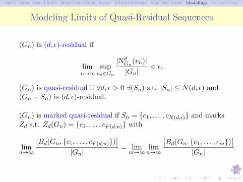
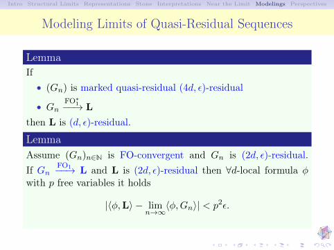
Modeling Limits of Quasi-Residual Sequences
(Gn) is (d, ε)-residual if
limn→∞
supvn∈Gn
|NdGn
(vn)||Gn|
< ε.
(Gn) is quasi-residual if ∀d, ε > 0 ∃(Sn) s.t. |Sn| ≤ N(d, ε) and(Gn − Sn) is (d, ε)-residual.
(Gn) is marked quasi-residual if Sn = c1, . . . , cN(d,ε) and marksZd s.t. Zd(Gn) = c1, . . . , cF (d,n) with
limn→∞
∣∣Bd(Gn, c1, . . . , cF (d,n))∣∣
|Gn|= lim
m→∞limn→∞
∣∣Bd(Gn, c1, . . . , cm)∣∣
|Gn|.
Intro Structural Limits Representations Stone Interpretations Near the Limit Modelings Perspectives
Modeling Limits of Quasi-Residual Sequences
LemmaIf• (Gn) is marked quasi-residual (4d, ε)-residual
• GnFO∗1−−→ L
then L is (d, ε)-residual.
LemmaAssume (Gn)n∈N is FO-convergent and Gn is (2d, ε)-residual.If Gn
FO1−−→ L and L is (2d, ε)-residual then ∀d-local formula φwith p free variables it holds
|〈φ,L〉 − limn→∞
〈φ,Gn〉| < p2ε.
Intro Structural Limits Representations Stone Interpretations Near the Limit Modelings Perspectives
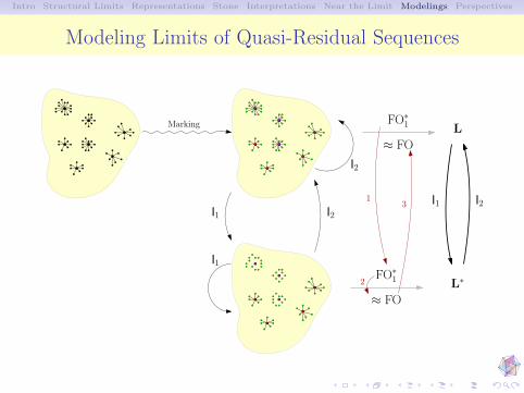
Modeling Limits of Quasi-Residual Sequences
I1 I2
I2
I1
FO∗1 L
I1
L∗FO∗1
≈ FO
I21
2
≈ FO
3
Marking
Intro Structural Limits Representations Stone Interpretations Near the Limit Modelings Perspectives
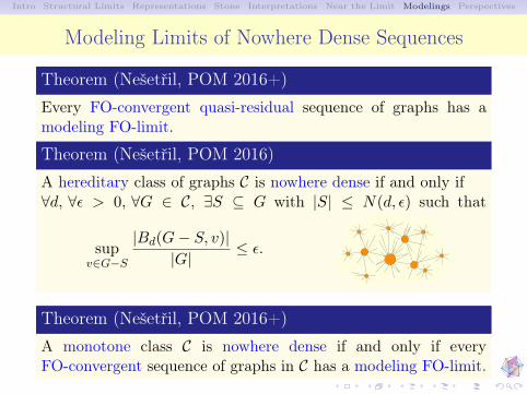
Modeling Limits of Nowhere Dense Sequences
Theorem (Nešetřil, POM 2016+)
Every FO-convergent quasi-residual sequence of graphs has amodeling FO-limit.
Theorem (Nešetřil, POM 2016)
A hereditary class of graphs C is nowhere dense if and only if∀d, ∀ε > 0, ∀G ∈ C, ∃S ⊆ G with |S| ≤ N(d, ε) such that
supv∈G−S
|Bd(G− S, v)||G| ≤ ε.
Theorem (Nešetřil, POM 2016+)
A monotone class C is nowhere dense if and only if everyFO-convergent sequence of graphs in C has a modeling FO-limit.
Intro Structural Limits Representations Stone Interpretations Near the Limit Modelings Perspectives
Perspectives
Intro Structural Limits Representations Stone Interpretations Near the Limit Modelings Perspectives
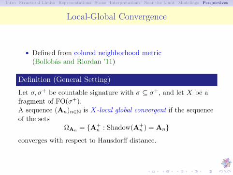
Local-Global Convergence
• Defined from colored neighborhood metric(Bollobás and Riordan ’11)
Definition (General Setting)
Let σ, σ+ be countable signature with σ ⊆ σ+, and let X be afragment of FO(σ+).A sequence (An)n∈N is X-local global convergent if the sequenceof the sets
ΩAn = A+n : Shadow(A+
n ) = Anconverges with respect to Hausdorff distance.
Intro Structural Limits Representations Stone Interpretations Near the Limit Modelings Perspectives
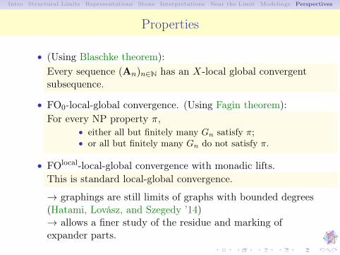
Properties
• (Using Blaschke theorem):Every sequence (An)n∈N has an X-local global convergentsubsequence.
• FO0-local-global convergence. (Using Fagin theorem):For every NP property π,
• either all but finitely many Gn satisfy π;• or all but finitely many Gn do not satisfy π.
• FOlocal-local-global convergence with monadic lifts.This is standard local-global convergence.
→ graphings are still limits of graphs with bounded degrees(Hatami, Lovász, and Szegedy ’14)→ allows a finer study of the residue and marking ofexpander parts.
Intro Structural Limits Representations Stone Interpretations Near the Limit Modelings Perspectives
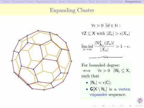
Expanding Cluster
∀ε > 0 ∃d ∈ N :
∀Z ⊆ X with |Zn| > ε|Xn|
lim infn→∞
|NdAn
(Zn)||Xn|
> 1− ε.
For bounded degree:⇐⇒ ∀ε > 0 ∃Nε ⊆ X,such that• |Nε| < ε|C|;• GGG[X \ Nε] is a vertexexpander sequence.
Intro Structural Limits Representations Stone Interpretations Near the Limit Modelings Perspectives
Thank you for yourattention.
![Layouts of Expander Graphs - University of Chicagocjtcs.cs.uchicago.edu/articles/2016/1/cj16-01.pdf · Layouts of Expander Graphs ... Nešetˇril, Ossona de Mendez and Wood [37] proved](https://img.pdfslide.us/doc/110x75/5ba64b1009d3f22f1b8b9cae/layouts-of-expander-graphs-university-of-layouts-of-expander-graphs-nesetril.jpg)
![public.gettysburg.edupublic.gettysburg.edu/~franpe02/files/[Baela_Bajnok]_Additive... · Series Editors Miklos Bona Donald L. Kreher Douglas West Patrice Ossona de Mendez Introduction](https://img.pdfslide.us/doc/110x75/5fd20622fccad917db184e30/franpe02filesbaelabajnokadditive-series-editors-miklos-bona-donald-l.jpg)


![Abstract. N G arXiv:2003.03605v1 [cs.DM] 7 Mar 2020 · arXiv:2003.03605v1 [cs.DM] 7 Mar 2020. 2 JAROSLAV NE SET RIL, PATRICE OSSONA DE MENDEZ, MICHAL PILIPCZUK, AND XUDING ZHU inspired](https://img.pdfslide.us/doc/110x75/5f6286398d335728d919d0be/abstract-n-g-arxiv200303605v1-csdm-7-mar-2020-arxiv200303605v1-csdm-7.jpg)

![lecture24-1 - Massachusetts Institute of Technologycourses.csail.mit.edu/6.889/fall11/lectures/L24.pdf · [Nd05] J. Ne set ril and P. Ossona de Mendez. Tree depth, subgraph col-oring](https://img.pdfslide.us/doc/110x75/5ba64b1009d3f22f1b8b9c9e/lecture24-1-massachusetts-institute-of-nd05-j-ne-set-ril-and-p-ossona.jpg)


![MENDEZ] [CARLOS - carlos mendez](https://img.pdfslide.us/doc/110x75/620652ca8c2f7b173006a76f/mendez-carlos-carlos-mendez.jpg)