Japanese foreign exchange intervention: A tale of pattern, size, or frequency

Japan and the World Economy 24 (2012) 184–192

Japanese foreign exchange intervention: A tale of pattern, size, or frequency

Marwa Hassan *

Faculty of Commerce, Alexandria University, Alexandria, Egypt

A R T I C L E I N F O

Article history:

Received 23 May 2010

Received in revised form 26 April 2011

Accepted 29 March 2012

Available online 8 April 2012

JEL classification:

E5

F3

Keywords:

Foreign exchange intervention

Frequency

size

GARCH models

A B S T R A C T

This paper contributes to the debate of the efficacy of different patterns of foreign exchange intervention

(FXI). Daily data on the Japanese foreign exchange intervention and the Yen/Dollar exchange rates

among other macroeconomic variables over the period 1992–2004, in an EGARCH time series model is

used to measure the impact of intervention on both the level and volatility of the exchange rate. This

paper offers two important results in regard to the effectiveness of the Japanese FXI. First, this study tests

whether the pattern of FXI leads to conflicting outcomes with respect to the desired level and volatility of

the exchange rates. Second, this study examines the asymmetric impact of the frequency and size of the

Japanese FXI on the level and volatility of the exchange rate. This paper finds that successful depreciation

of the yen has always been achieved at the expense of higher volatility, a result that supports the

conflicting outcomes of the Japanese FXI. In addition, the frequency of intervention is found to be a

crucial factor in affecting the level of the exchange rate while the size of intervention is more influential

in affecting its volatility.

� 2012 Elsevier B.V. All rights reserved.

Contents lists available at SciVerse ScienceDirect

Japan and the World Economy

jo ur n al h o mep ag e: www .e lsev ier . c om / loc ate / jw e

1 According to Dominguez (1998), Journal of International Money and Finance 17

(1998), p. 162, ‘‘It was not until 1977 that the IMF Executive Board provided its

member countries three guiding principles for intervention policy: (1) countries

1. Introduction

Despite the move to floating exchange rates after thebreakdown of the Bretton Woods fixed exchange rate system inthe early 1970s, foreign exchange intervention (FXI) had beenseriously used as a tool for influencing exchange rates in mostdeveloped economies. Japan had been the most heavily interven-ing industrialized country in the nineties to purchase the US dollar.The higher tendency towards purchasing US dollars reflects theattempt of the Japanese authorities to counter or slow theappreciation of the yen. Had the Japanese Monetary authorities(JMA) been effective in its intervention operations? Had the JMAbeen successful in depreciating the yen? How about the volatilityof the yen was it a point of interest to the JMA? If FXI was effective,why would JMA change its policy over time, why did JMA stopintervening after March 2004?

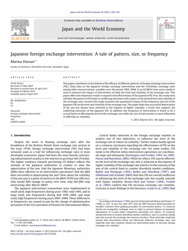
The Japanese intervention transactions were implemented insmall sized, high frequencies during years 1992–mid 1995, and inlarge sized, low frequencies during mid 1995–2002, and largesized, high frequencies during years 2003–2004. These differencesin frequencies are caused in part by the change of administrativepersonnel of the Vice president of Finance for International Affairs.

* Corresponding author at: 11 Tived Lane, Edison, NJ 08837, United States.

Tel.: +1 347 249 2606.

E-mail address: [email protected].

0922-1425/$ – see front matter � 2012 Elsevier B.V. All rights reserved.

http://dx.doi.org/10.1016/j.japwor.2012.03.002

Central banks intervene in the foreign exchange markets toachieve one of two objectives; to influence the level of theexchange rate or reduce its volatility.1 Earlier studies hardly agreedon a common conclusion regarding the effectiveness of FXI on thelevel and volatility of the exchange rate. For some studies, FXItends to be effective when intervention operations are coordinat-ed, large and infrequent (Dominguez and Frankel, 1993; Ito, 2002;Fatum and Hutchison, 2003). While for others, FXI may be effectiveon the level of the exchange rate, this is achieved at the expense ofhigher volatility of the exchange rate which is to the contrary of theaim of the central bank to counter disorderly market conditions.Baillie and Humpage (1992), Baillie and Osterberg (1997), andHillebrand and Schnabl (2004) find that FXI are overall ineffectivein influencing the level of the exchange rate, but usually coincidewith higher volatility. Bonser-Neal and Tanner (1996), Frenkelet al. (2003) confirm that FXI increases exchange rate volatility.Contrary to most findings in the literature, Galati et al. (2005) find

should not manipulate exchange rates in order to prevent balance of payments

adjustments or to gain unfair competitive advantage over others; (2) countries

should intervene to counter disorderly market conditions; and (3) countries should

take into account the exchange rate interests of others. These principles implicitly

assume that intervention policy can effectively influence exchange rates, and

explicitly state that countries should use intervention policy to decrease foreign

exchange rate volatility’’.


mailto:[email protected]

http://www.sciencedirect.com/science/journal/09221425


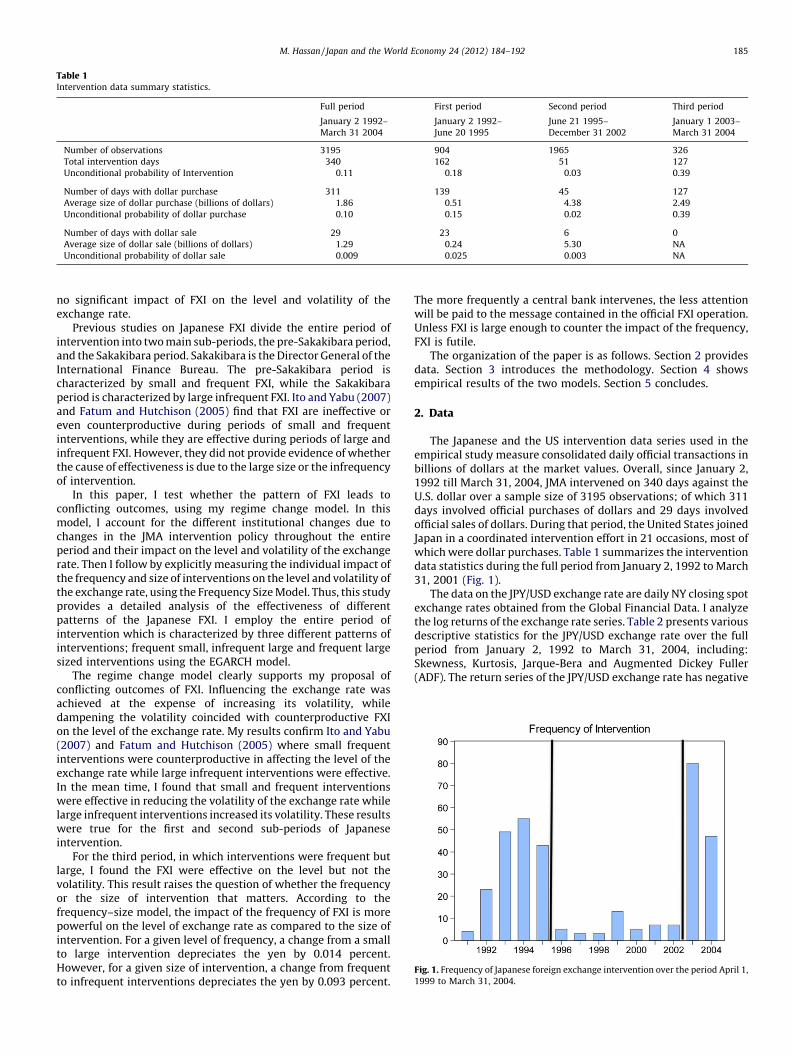
Table 1Intervention data summary statistics.

Full period First period Second period Third period

January 2 1992–

March 31 2004

January 2 1992–

June 20 1995

June 21 1995–

December 31 2002

January 1 2003–

March 31 2004

Number of observations 3195 904 1965 326

Total intervention days 340 162 51 127

Unconditional probability of Intervention 0.11 0.18 0.03 0.39

Number of days with dollar purchase 311 139 45 127

Average size of dollar purchase (billions of dollars) 1.86 0.51 4.38 2.49

Unconditional probability of dollar purchase 0.10 0.15 0.02 0.39

Number of days with dollar sale 29 23 6 0

Average size of dollar sale (billions of dollars) 1.29 0.24 5.30 NA

Unconditional probability of dollar sale 0.009 0.025 0.003 NA

Fig. 1. Frequency of Japanese foreign exchange intervention over the period April 1,

1999 to March 31, 2004.

M. Hassan / Japan and the World Economy 24 (2012) 184–192 185

no significant impact of FXI on the level and volatility of theexchange rate.

Previous studies on Japanese FXI divide the entire period ofintervention into two main sub-periods, the pre-Sakakibara period,and the Sakakibara period. Sakakibara is the Director General of theInternational Finance Bureau. The pre-Sakakibara period ischaracterized by small and frequent FXI, while the Sakakibaraperiod is characterized by large infrequent FXI. Ito and Yabu (2007)and Fatum and Hutchison (2005) find that FXI are ineffective oreven counterproductive during periods of small and frequentinterventions, while they are effective during periods of large andinfrequent FXI. However, they did not provide evidence of whetherthe cause of effectiveness is due to the large size or the infrequencyof intervention.

In this paper, I test whether the pattern of FXI leads toconflicting outcomes, using my regime change model. In thismodel, I account for the different institutional changes due tochanges in the JMA intervention policy throughout the entireperiod and their impact on the level and volatility of the exchangerate. Then I follow by explicitly measuring the individual impact ofthe frequency and size of interventions on the level and volatility ofthe exchange rate, using the Frequency Size Model. Thus, this studyprovides a detailed analysis of the effectiveness of differentpatterns of the Japanese FXI. I employ the entire period ofintervention which is characterized by three different patterns ofinterventions; frequent small, infrequent large and frequent largesized interventions using the EGARCH model.

The regime change model clearly supports my proposal ofconflicting outcomes of FXI. Influencing the exchange rate wasachieved at the expense of increasing its volatility, whiledampening the volatility coincided with counterproductive FXIon the level of the exchange rate. My results confirm Ito and Yabu(2007) and Fatum and Hutchison (2005) where small frequentinterventions were counterproductive in affecting the level of theexchange rate while large infrequent interventions were effective.In the mean time, I found that small and frequent interventionswere effective in reducing the volatility of the exchange rate whilelarge infrequent interventions increased its volatility. These resultswere true for the first and second sub-periods of Japaneseintervention.

For the third period, in which interventions were frequent butlarge, I found the FXI were effective on the level but not thevolatility. This result raises the question of whether the frequencyor the size of intervention that matters. According to thefrequency–size model, the impact of the frequency of FXI is morepowerful on the level of exchange rate as compared to the size ofintervention. For a given level of frequency, a change from a smallto large intervention depreciates the yen by 0.014 percent.However, for a given size of intervention, a change from frequentto infrequent interventions depreciates the yen by 0.093 percent.

The more frequently a central bank intervenes, the less attentionwill be paid to the message contained in the official FXI operation.Unless FXI is large enough to counter the impact of the frequency,FXI is futile.

The organization of the paper is as follows. Section 2 providesdata. Section 3 introduces the methodology. Section 4 showsempirical results of the two models. Section 5 concludes.

2. Data

The Japanese and the US intervention data series used in theempirical study measure consolidated daily official transactions inbillions of dollars at the market values. Overall, since January 2,1992 till March 31, 2004, JMA intervened on 340 days against theU.S. dollar over a sample size of 3195 observations; of which 311days involved official purchases of dollars and 29 days involvedofficial sales of dollars. During that period, the United States joinedJapan in a coordinated intervention effort in 21 occasions, most ofwhich were dollar purchases. Table 1 summarizes the interventiondata statistics during the full period from January 2, 1992 to March31, 2001 (Fig. 1).

The data on the JPY/USD exchange rate are daily NY closing spotexchange rates obtained from the Global Financial Data. I analyzethe log returns of the exchange rate series. Table 2 presents variousdescriptive statistics for the JPY/USD exchange rate over the fullperiod from January 2, 1992 to March 31, 2004, including:Skewness, Kurtosis, Jarque-Bera and Augmented Dickey Fuller(ADF). The return series of the JPY/USD exchange rate has negative

Table 2Descriptive statistics of daily returns of the JPY/USD exchange rate.

Full period

1/2/1992–3/31/2004

St ln St dst

Mean 114.70 4.74 0.00

Std. Dev. 11.57 0.10 0.01

Skewness �0.14 �0.47 �0.60

Kurtosis 3.016 3.41 8.90

Jarque-Bera 10.70 138.36 4827.32

Probability 0.00 0.00 0.00

Observations 3196 3195 3195

ADF (level) �1.94

ADF (1st diff) �56.11

Notes: dst = ln(St/St�1), skewness is a measure of asymmetry of the distribution of the

series around its mean. Kurtosis measures the peakedness or flatness of the

distribution of the series.

Jarque-Bera is a test statistic for testing whether the series is normally distributed.

ADF regressions include intercept but not trend. I employ ADF test on the

logarithms of stock indices.

ADF critical values: (1 percent) �3.4334, (5 percent) �2.8627, (10 percent) �2.5674.

70

80

90

100

110

120

130

140

150

160

170

-24

-20

-16

-12

-8

-4

0

4

8

12

16

92 93 94 95 96 97 98 99 00 01 02 03

JPY/USD Exchang e Ra teImpli cit Target 125 JPY /USDVolume of JMA Interventions in Doll ars

80

90

100

110

120

130

140

150

160

-1.00

-0.75

-0.50

-0.25

0.00

0.25

0.50

0.75

1.00

92 93 94 95 96 97 98 99 00 01 02 03

JPY /USD Exchang e RateImpli cit Target 125 JPY /USDVolume of USMA Interventions in Doll ars

Fig. 2. The behavior of the JPY/USD exchange rate around the Japanese and U.S. FXI

operations, and the 125 USD/JPY level of the exchange rate during the full period

January 2, 1992 to March 31, 2004.

M. Hassan / Japan and the World Economy 24 (2012) 184–192186

mean and skewness2 representing the prevailing yen appreciationpressure against the dollar. The values for kurtosis are high (closeto three) in all cases. So, the distributions are peaked relative tonormal. The Jarque-Bera test rejects normality at the 5 percentlevel for all distributions. So, the samples have all financialcharacteristics: volatility clustering and leptokurtosis. Further-more, in terms of stationarity, the results from the ADF testsindicate that the series is I (1), and therefore, time-series modelscan be used to examine the behavior of volatility over time.

Fig. 2 depicts the behavior of the JPY/USD exchange rate roundthe Japanese and the U.S. foreign exchange intervention opera-tions. Fig. 3 presents the plots of JPY/USD exchange rate returnsand volatilities (defined as squared returns) over time showing thehigh volatility clustering.

3. Methodology

3.1. The regime change model

To examine the conflicting outcomes of FXI I employ regimechange model that provides a detailed analysis of the effectivenessof different patterns of the Japanese FXI. I employ the entire periodof intervention which is characterized by three different patternsof interventions; frequent small, infrequent large and frequentlarge sized interventions using EGARCH model.3

The Regime-change model accounts for the different institu-tional changes in intervention that occurred throughout the entireperiod by introducing three dummy variables S1, S2 and S3 thatrepresent the first, second and third subsamples. S1, S2 and S3 take

2 Negative skewness implies that the distribution has a long left tail.3 EGARCH model is an asymmetric model that controls the leverage effect. The

leverage effect means that a fall in returns is accompanied by an increase in

volatility greater than the volatility induced by an increase in returns. In other

words, bad news tends to increase the volatility of the exchange rate than good

news. The motivation for implementing the EGARCH model is based on a model

selection criterion among different GARCH models; GARCH(1,1), GARCH(p,q),

GARCH in mean(p,q), TGARCH(p,q) and EGARCH(p,q). For all models other than

traditional GARCH(1,1), lags have been assigned according to the value of

information criteria, such that Q test on the standardized and squared residuals

with 5, 10, or 20 lags for the standardized squared residuals is insignificant at the 95

percent confidence level. Once lags are assigned, the choice of the model per sample

period is based on both in sample and out of sample evaluation criterion. The best

model is the one that satisfies the following measures: minimizes the Akaike

information criterion (AIC) and the Bayesian Information Criterion (BIC), maximizes

the log likelihood (LL), and if conflict is to occur, models with the minimum out of

sample root mean square error (RMSE) and mean absolute error (MAE) are chosen.

the value of one when operating in the first, second and thirdsubsample, respectively, and zero otherwise. The coefficient ofintervention shows the impact of intervention in the firstsubsample. Multiplying S1, S2 or S3, to the intervention variablerefers to the impact of intervention in the first subsample, secondsubsample, or the third subsample, respectively. I expect that thecoefficient of purchase intervention in the first subsample to benegative, in the second and third subsamples to be positive.

Eq. (1) represents the regime change model.

dst ¼ m þ S1ða1INVJPBuy;t þ a2INVUSBuy;t þ a3INVJPSell;t

þ a4INVUSSell;tÞ þ S2ða1INVJPBuy;t þ a2INVUSBuy;t þ a3INVJPSell;t

þ a4INVUSsell;tÞ þ S3ða1INVJPBuy;tÞ þ a5DOWt þ a6Nikkeit

þ a7ðit�1 � i�t�1Þ þ et

et Vt�1j � Nð0; htÞ

ln ht ¼ v þ aet�1ffiffiffiffiffiffiffiffiffiht�1

p

��

��þ g

et�1ffiffiffiffiffiffiffiffiffiht�1

p þbi ln ht�1 þ S1ðb1INVJPBuy;t

þ b2INVUSBuy;t þ b3INVJPSell;t þ b4INVUSSell;tÞ þ S2ðb1INVJPBuy;t

þ b2INVUSBuy;t þ b3INVJPSell;t þ b4INVUSsell;tÞ þ S3 � b1INVJPBuy;t

(1)

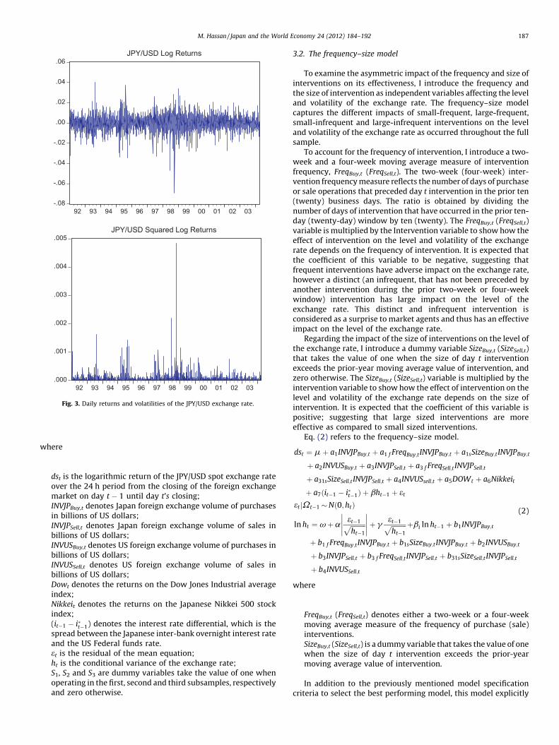
-.08

-.06

-.04

-.02

.00

.02

.04

.06

92 93 94 95 96 97 98 99 00 01 02 03

JPY/USD Log Returns

.000

.001

.002

.003

.004

.005

92 93 94 95 96 97 98 99 00 01 02 03

JPY/USD Squared Log Returns

Fig. 3. Daily returns and volatilities of the JPY/USD exchange rate.


where

dst is the logarithmic return of the JPY/USD spot exchange rateover the 24 h period from the closing of the foreign exchangemarket on day t � 1 until day t’s closing;INVJPBuy,t denotes Japan foreign exchange volume of purchasesin billions of US dollars;INVJPSell,t denotes Japan foreign exchange volume of sales inbillions of US dollars;INVUSBuy,t denotes US foreign exchange volume of purchases inbillions of US dollars;INVUSSell,t denotes US foreign exchange volume of sales inbillions of US dollars;Dowt denotes the returns on the Dow Jones Industrial averageindex;Nikkeit denotes the returns on the Japanese Nikkei 500 stockindex;(it�1 � i�t�1) denotes the interest rate differential, which is thespread between the Japanese inter-bank overnight interest rateand the US Federal funds rate.et is the residual of the mean equation;ht is the conditional variance of the exchange rate;S1, S2 and S3 are dummy variables take the value of one whenoperating in the first, second and third subsamples, respectivelyand zero otherwise.

3.2. The frequency–size model

To examine the asymmetric impact of the frequency and size ofinterventions on its effectiveness, I introduce the frequency andthe size of intervention as independent variables affecting the leveland volatility of the exchange rate. The frequency–size modelcaptures the different impacts of small-frequent, large-frequent,small-infrequent and large-infrequent interventions on the leveland volatility of the exchange rate as occurred throughout the fullsample.

To account for the frequency of intervention, I introduce a two-week and a four-week moving average measure of interventionfrequency, FreqBuy,t (FreqSell,t). The two-week (four-week) inter-vention frequency measure reflects the number of days of purchaseor sale operations that preceded day t intervention in the prior ten(twenty) business days. The ratio is obtained by dividing thenumber of days of intervention that have occurred in the prior ten-day (twenty-day) window by ten (twenty). The FreqBuy,t (FreqSell,t)variable is multiplied by the Intervention variable to show how theeffect of intervention on the level and volatility of the exchangerate depends on the frequency of intervention. It is expected thatthe coefficient of this variable to be negative, suggesting thatfrequent interventions have adverse impact on the exchange rate,however a distinct (an infrequent, that has not been preceded byanother intervention during the prior two-week or four-weekwindow) intervention has large impact on the level of theexchange rate. This distinct and infrequent intervention isconsidered as a surprise to market agents and thus has an effectiveimpact on the level of the exchange rate.

Regarding the impact of the size of interventions on the level ofthe exchange rate, I introduce a dummy variable SizeBuy,t (SizeSell,t)that takes the value of one when the size of day t interventionexceeds the prior-year moving average value of intervention, andzero otherwise. The SizeBuy,t (SizeSell,t) variable is multiplied by theintervention variable to show how the effect of intervention on thelevel and volatility of the exchange rate depends on the size ofintervention. It is expected that the coefficient of this variable ispositive; suggesting that large sized interventions are moreeffective as compared to small sized interventions.

Eq. (2) refers to the frequency–size model.

dst ¼ m þ a1INVJPBuy;t þ a1 f FreqBuy;tINVJPBuy;t þ a1sSizeBuy;tINVJPBuy;t

þ a2INVUSBuy;t þ a3INVJPSell;t þ a3 f FreqSell;t INVJPSell;t

þ a31sSizeSell;tINVJPSell;t þ a4INVUSsell;t þ a5DOWt þ a6Nikkeit

þ a7ðit�1 � i�t�1Þ þ bht�1 þ et

et Vt�1j � Nð0; htÞ

ln ht ¼ v þ aet�1ffiffiffiffiffiffiffiffiffiht�1

p

��

��þ g

et�1ffiffiffiffiffiffiffiffiffiht�1

p þbi ln ht�1 þ b1INVJPBuy;t

þ b1 f FreqBuy;tINVJPBuy;t þ b1sSizeBuy;tINVJPBuy;t þ b2INVUSBuy;t

þ b3INVJPSell;t þ b3 f FreqSell;tINVJPSell;t þ b31sSizeSell;tINVJPSell;t

þ b4INVUSSell;t

(2)

where

FreqBuy,t (FreqSell,t) denotes either a two-week or a four-weekmoving average measure of the frequency of purchase (sale)interventions.SizeBuy,t (SizeSell,t) is a dummy variable that takes the value of onewhen the size of day t intervention exceeds the prior-yearmoving average value of intervention.

In addition to the previously mentioned model specificationcriteria to select the best performing model, this model explicitly

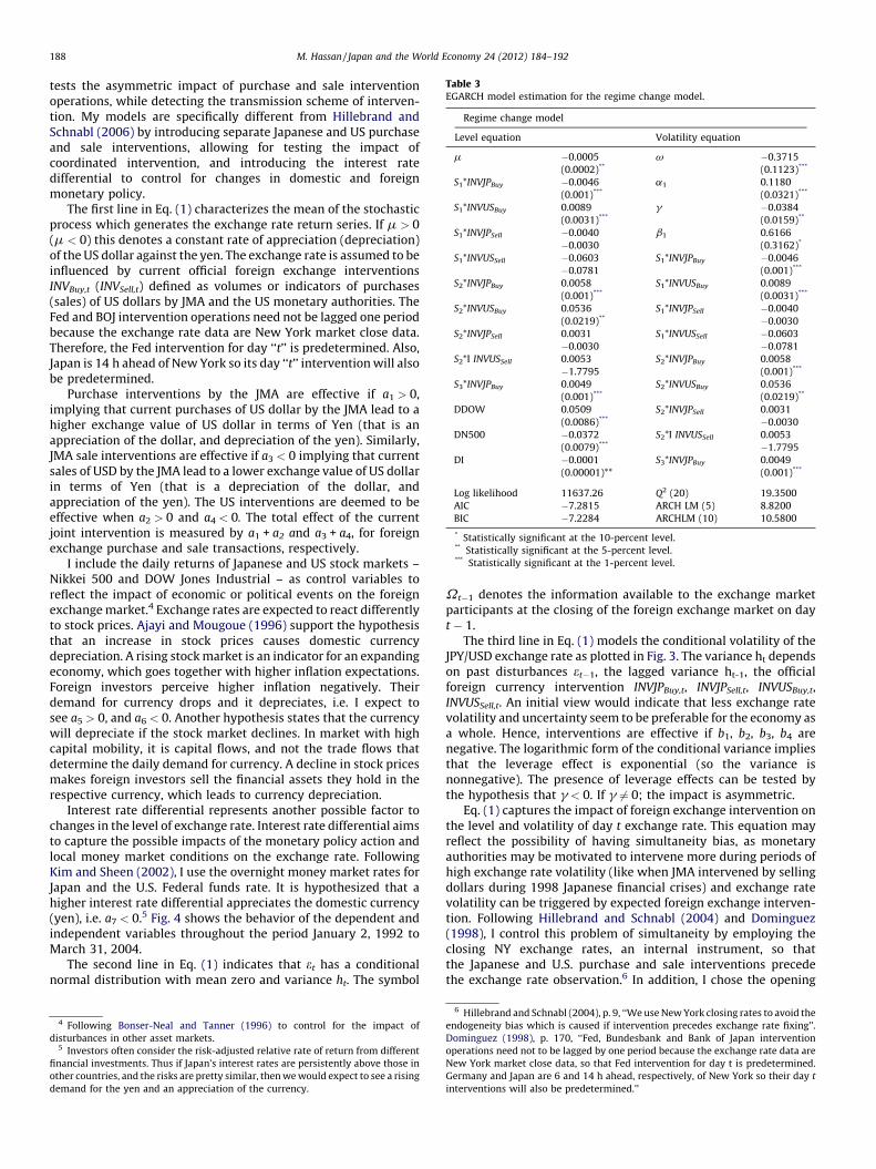
Table 3EGARCH model estimation for the regime change model.

Regime change model

Level equation Volatility equation

m �0.0005 v �0.3715

(0.0002)** (0.1123)***

S1*INVJPBuy �0.0046 a1 0.1180

(0.001)*** (0.0321)***

S1*INVUSBuy 0.0089 g �0.0384

(0.0031)*** (0.0159)**

S1*INVJPSell �0.0040 b1 0.6166

�0.0030 (0.3162)*

S1*INVUSSell �0.0603 S1*INVJPBuy �0.0046

�0.0781 (0.001)***

S2*INVJPBuy 0.0058 S1*INVUSBuy 0.0089

(0.001)*** (0.0031)***

S2*INVUSBuy 0.0536 S1*INVJPSell �0.0040

(0.0219)** �0.0030

S2*INVJPSell 0.0031 S1*INVUSSell �0.0603

�0.0030 �0.0781

S2*I INVUSSell 0.0053 S2*INVJPBuy 0.0058

�1.7795 (0.001)***

S3*INVJPBuy 0.0049 S2*INVUSBuy 0.0536

(0.001)*** (0.0219)**

DDOW 0.0509 S2*INVJPSell 0.0031

(0.0086)*** �0.0030

DN500 �0.0372 S2*I INVUSSell 0.0053

(0.0079)*** �1.7795

DI �0.0001 S3*INVJPBuy 0.0049

(0.00001)** (0.001)***

Log likelihood 11637.26 Q2 (20) 19.3500

AIC �7.2815 ARCH LM (5) 8.8200

BIC �7.2284 ARCHLM (10) 10.5800

* Statistically significant at the 10-percent level.** Statistically significant at the 5-percent level.*** Statistically significant at the 1-percent level.


tests the asymmetric impact of purchase and sale interventionoperations, while detecting the transmission scheme of interven-tion. My models are specifically different from Hillebrand andSchnabl (2006) by introducing separate Japanese and US purchaseand sale interventions, allowing for testing the impact ofcoordinated intervention, and introducing the interest ratedifferential to control for changes in domestic and foreignmonetary policy.

The first line in Eq. (1) characterizes the mean of the stochasticprocess which generates the exchange rate return series. If m > 0(m < 0) this denotes a constant rate of appreciation (depreciation)of the US dollar against the yen. The exchange rate is assumed to beinfluenced by current official foreign exchange interventionsINVBuy,t (INVSell,t) defined as volumes or indicators of purchases(sales) of US dollars by JMA and the US monetary authorities. TheFed and BOJ intervention operations need not be lagged one periodbecause the exchange rate data are New York market close data.Therefore, the Fed intervention for day ‘‘t’’ is predetermined. Also,Japan is 14 h ahead of New York so its day ‘‘t’’ intervention will alsobe predetermined.

Purchase interventions by the JMA are effective if a1 > 0,implying that current purchases of US dollar by the JMA lead to ahigher exchange value of US dollar in terms of Yen (that is anappreciation of the dollar, and depreciation of the yen). Similarly,JMA sale interventions are effective if a3 < 0 implying that currentsales of USD by the JMA lead to a lower exchange value of US dollarin terms of Yen (that is a depreciation of the dollar, andappreciation of the yen). The US interventions are deemed to beeffective when a2 > 0 and a4 < 0. The total effect of the currentjoint intervention is measured by a1 + a2 and a3 + a4, for foreignexchange purchase and sale transactions, respectively.

I include the daily returns of Japanese and US stock markets –Nikkei 500 and DOW Jones Industrial – as control variables toreflect the impact of economic or political events on the foreignexchange market.4 Exchange rates are expected to react differentlyto stock prices. Ajayi and Mougoue (1996) support the hypothesisthat an increase in stock prices causes domestic currencydepreciation. A rising stock market is an indicator for an expandingeconomy, which goes together with higher inflation expectations.Foreign investors perceive higher inflation negatively. Theirdemand for currency drops and it depreciates, i.e. I expect tosee a5 > 0, and a6 < 0. Another hypothesis states that the currencywill depreciate if the stock market declines. In market with highcapital mobility, it is capital flows, and not the trade flows thatdetermine the daily demand for currency. A decline in stock pricesmakes foreign investors sell the financial assets they hold in therespective currency, which leads to currency depreciation.

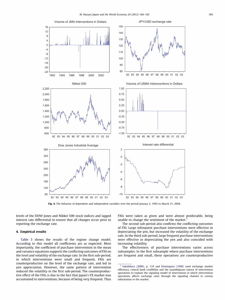
Interest rate differential represents another possible factor tochanges in the level of exchange rate. Interest rate differential aimsto capture the possible impacts of the monetary policy action andlocal money market conditions on the exchange rate. FollowingKim and Sheen (2002), I use the overnight money market rates forJapan and the U.S. Federal funds rate. It is hypothesized that ahigher interest rate differential appreciates the domestic currency(yen), i.e. a7 < 0.5 Fig. 4 shows the behavior of the dependent andindependent variables throughout the period January 2, 1992 toMarch 31, 2004.

The second line in Eq. (1) indicates that et has a conditionalnormal distribution with mean zero and variance ht. The symbol

4 Following Bonser-Neal and Tanner (1996) to control for the impact of

disturbances in other asset markets.5 Investors often consider the risk-adjusted relative rate of return from different

financial investments. Thus if Japan’s interest rates are persistently above those in

other countries, and the risks are pretty similar, then we would expect to see a rising

demand for the yen and an appreciation of the currency.

Vt�1 denotes the information available to the exchange marketparticipants at the closing of the foreign exchange market on dayt � 1.

The third line in Eq. (1) models the conditional volatility of theJPY/USD exchange rate as plotted in Fig. 3. The variance ht dependson past disturbances et�1, the lagged variance ht-1, the officialforeign currency intervention INVJPBuy,t, INVJPSell,t, INVUSBuy,t,INVUSSell,t. An initial view would indicate that less exchange ratevolatility and uncertainty seem to be preferable for the economy asa whole. Hence, interventions are effective if b1, b2, b3, b4 arenegative. The logarithmic form of the conditional variance impliesthat the leverage effect is exponential (so the variance isnonnegative). The presence of leverage effects can be tested bythe hypothesis that g < 0. If g 6¼ 0; the impact is asymmetric.

Eq. (1) captures the impact of foreign exchange intervention onthe level and volatility of day t exchange rate. This equation mayreflect the possibility of having simultaneity bias, as monetaryauthorities may be motivated to intervene more during periods ofhigh exchange rate volatility (like when JMA intervened by sellingdollars during 1998 Japanese financial crises) and exchange ratevolatility can be triggered by expected foreign exchange interven-tion. Following Hillebrand and Schnabl (2004) and Dominguez(1998), I control this problem of simultaneity by employing theclosing NY exchange rates, an internal instrument, so thatthe Japanese and U.S. purchase and sale interventions precedethe exchange rate observation.6 In addition, I chose the opening

6 Hillebrand and Schnabl (2004), p. 9, ‘‘We use New York closing rates to avoid the

endogeneity bias which is caused if intervention precedes exchange rate fixing’’.

Dominguez (1998), p. 170, ‘‘Fed, Bundesbank and Bank of Japan intervention

operations need not to be lagged by one period because the exchange rate data are

New York market close data, so that Fed intervention for day t is predetermined.

Germany and Japan are 6 and 14 h ahead, respectively, of New York so their day t

interventions will also be predetermined.’’

-24

-20

-16

-12

-8

-4

0

4

8

12

16

19941992 19 96 199 8 200 0 200 2

Volume of JMA Interventions in Dollars

80

90

100

110

120

130

140

150

9392 94 95 96 97 98 99 00 01 02 03

JPY/USD exchange rate

600

800

1,000

1,200

1,400

1,600

1,800

2,000

2,200

9392 94 95 96 97 98 99 00 01 02 03

Nikkei 500

-1.00

-0.75

-0.50

-0.25

0.00

0.25

0.50

0.75

1.00

9392 94 95 96 97 98 99 00 01 02 03

Volume of USMA Intereventions in Dollars

80

120

160

200

240

280

320

360

9392 94 95 96 97 98 99 00 01 02 03

Dow Jones Industrial Average

-10

-8

-6

-4

-2

0

2

9392 94 95 96 97 98 99 00 01 02 03

Interest rate differential

Fig. 4. The behavior of dependent and independent variables over the period January 2, 1992 to March 31, 2004.

7 Sakakibara (2000), p. 119 and Dominguez (1998) used exchange market

efficiency, central bank credibility and the unambiguous nature of intervention

operations to explain the signaling model of intervention in which intervention

operations affects exchange rates through the signaling channel to convey

information to the market.


levels of the DOW Jones and Nikkei 500 stock indices and laggedinterest rate differential to ensure that all changes occur prior toreporting the exchange rate.

4. Empirical results

Table 3 shows the results of the regime change model.According to this model all coefficients are as expected. Mostimportantly, the coefficient of purchase intervention in the meanand variance equations supports the conflicting outcomes of FXI onthe level and volatility of the exchange rate. In the first sub-period,in which interventions were small and frequent, FXIs arecounterproductive on the level of the exchange rate, and led toyen appreciation. However, the same pattern of interventionreduced the volatility in the first sub-period. The counterproduc-tive effect of the FXIs is due to the fact that Japan’s FX market wasaccustomed to interventions, because of being very frequent. Thus

FXIs were taken as given and were almost predictable, beingunable to change the sentiment of the market.7

The second sub-period also confirms the conflicting outcomesof FXI. Large infrequent purchase interventions were effective indepreciating the yen, but increased the volatility of the exchangerate. In the third sub-period, large frequent purchase interventionswere effective in depreciating the yen and also coincided withincreasing volatility.

The effectiveness of purchase interventions varies acrosssubsamples. In the first subsample where purchase interventionsare frequent and small, these operations are counterproductive

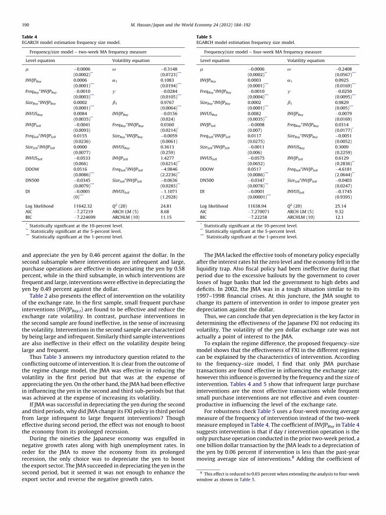
Table 5EGARCH model estimation frequency size model.

Frequency/size model – four-week MA frequency measure


m �0.0006 v �0.2408

(0.0002)** (0.0567)***

INVJPBuy 0.0003 a1 0.0925

(0.0001)*** (0.0169)***

FreqBuy*INVJPBuy �0.0010 g �0.0250

(0.0004)*** (0.0095)***

SizeBuy*INVJPBuy 0.0002 b1 0.9829

(0.0001)*** (0.005)***

INVUSBuy 0.0082 INVJPBuy �0.0079

(0.0035)** (0.0169)

INVJPSell �0.0008 FreqBuy*INVJPBuy 0.0314

(0.007) (0.0177)*

FreqSell*INVJPSell 0.0117 SizeBuy*INVJPBuy �0.0051

(0.0275) (0.0052)

SizeSell*INVJPSell �0.0011 INVUSBuy 0.3009

(0.006) (0.2259)

INVUSSell �0.0575 INVJPSell 0.6129

(0.0652) (0.2836)**

DDOW 0.0517 FreqSell*INVJPSell �4.6181

(0.0086)*** (2.0644)**

DN500 �0.0347 SizeSell*INVJPSell �0.0403

(0.0078)*** (0.0247)

DI �0.0001 INVUSSell �0.1745

(0.00001)*** (0.9395)

Log likelihood 11638.94 Q2 (20) 25.14

AIC �7.270071 ARCH LM (5) 9.32

BIC �7.22258 ARCHLM (10) 12.1


Table 4EGARCH model estimation frequency size model.

Frequency/size model – two-week MA frequency measure


m �0.0006 v �0.3148

(0.0002)** (0.0723)***

INVJPBuy 0.0006 a1 0.1083

(0.0001)*** (0.0194)***

FreqBuy*INVJPBuy �0.0010 g �0.0284

(0.0003)*** (0.0105)***

SizeBuy*INVJPBuy 0.0002 b1 0.9767

(0.0001)*** (0.0064)***

INVUSBuy 0.0084 INVJPBuy �0.0156

(0.0035)** (0.024)

INVJPSell �0.0041 FreqBuy*INVJPBuy 0.0360

(0.0093) (0.0214)*

FreqSell*INVJPSell 0.0155 SizeBuy*INVJPBuy �0.0059

(0.0236) (0.0061)

SizeSell*INVJPSell 0.0000 INVUSBuy 0.3613

(0.0077) (0.259)

INVUSSell �0.0533 INVJPSell 1.4277

(0.066) (0.6214)**

DDOW 0.0516 FreqSell*INVJPSell �4.9846

(0.0086)*** (2.2236)**

DN500 �0.0345 SizeSell*INVJPSell �0.0636

(0.0079)*** (0.0285)**

DI �0.0001 INVUSSell �1.1071

(0)*** (1.2928)

Log likelihood 11642.32 Q2 (20) 24.81

AIC �7.27219 ARCH LM (5) 8.68

BIC �7.224699 ARCHLM (10) 11.15


8 This effect is reduced to 0.03 percent when extending the analysis to four-week

window as shown in Table 5.


and appreciate the yen by 0.46 percent against the dollar. In thesecond subsample where interventions are infrequent and large,purchase operations are effective in depreciating the yen by 0.58percent, while in the third subsample, in which interventions arefrequent and large, interventions were effective in depreciating theyen by 0.49 percent against the dollar.

Table 2 also presents the effect of intervention on the volatilityof the exchange rate. In the first sample, small frequent purchaseinterventions (INVJPBuy,t) are found to be effective and reduce theexchange rate volatility. In contrast, purchase interventions inthe second sample are found ineffective, in the sense of increasingthe volatility. Interventions in the second sample are characterizedby being large and infrequent. Similarly third sample interventionsare also ineffective in their effect on the volatility despite beinglarge and frequent.

Thus Table 3 answers my introductory question related to theconflicting outcome of intervention. It is clear from the outcome ofthe regime change model, the JMA was effective in reducing thevolatility in the first period but that was at the expense ofappreciating the yen. On the other hand, the JMA had been effectivein influencing the yen in the second and third sub-periods but thatwas achieved at the expense of increasing its volatility.

If JMA was successful in depreciating the yen during the secondand third periods, why did JMA change its FXI policy in third periodfrom large infrequent to large frequent interventions? Thougheffective during second period, the effect was not enough to boostthe economy from its prolonged recession.

During the nineties the Japanese economy was engulfed innegative growth rates along with high unemployment rates. Inorder for the JMA to move the economy from its prolongedrecession, the only choice was to depreciate the yen to boostthe export sector. The JMA succeeded in depreciating the yen in thesecond period, but it seemed it was not enough to enhance theexport sector and reverse the negative growth rates.

The JMA lacked the effective tools of monetary policy especiallyafter the interest rates hit the zero level and the economy fell in theliquidity trap. Also fiscal policy had been ineffective during thatperiod due to the excessive bailouts by the government to coverlosses of huge banks that led the government to high debts anddeficits. In 2002, the JMA was in a tough situation similar to its1997–1998 financial crises. At this juncture, the JMA sought tochange its pattern of intervention in order to impose greater yendepreciation against the dollar.

Thus, we can conclude that yen depreciation is the key factor indetermining the effectiveness of the Japanese FXI not reducing itsvolatility. The volatility of the yen dollar exchange rate was notactually a point of interest to the JMA.

To explain the regime difference, the proposed frequency–sizemodel shows that the effectiveness of FXI in the different regimescan be explained by the characteristics of intervention. Accordingto the frequency–size model, I find that only JMA purchasetransactions are found effective in influencing the exchange rate;however this influence is governed by the frequency and the size ofintervention. Tables 4 and 5 show that infrequent large purchaseinterventions are the most effective transactions while frequentsmall purchase interventions are not effective and even counter-productive in influencing the level of the exchange rate.

For robustness check Table 5 uses a four-week moving averagemeasure of the frequency of intervention instead of the two-weekmeasure employed in Table 4. The coefficient of INVJPBuy in Table 4suggests intervention is that if day t intervention operation is theonly purchase operation conducted in the prior two-week period, aone billion dollar transaction by the JMA leads to a depreciation ofthe yen by 0.06 percent if intervention is less than the past-yearmoving average size of interventions.8 Adding the coefficient of

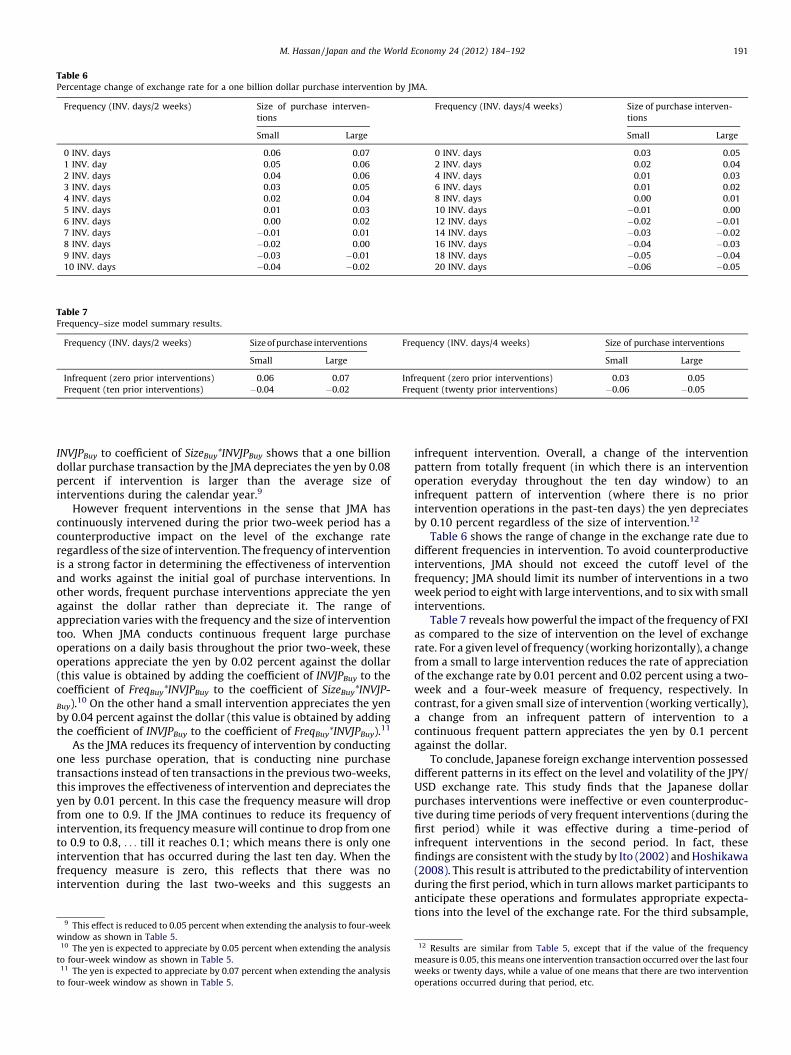
Table 6Percentage change of exchange rate for a one billion dollar purchase intervention by JMA.

Frequency (INV. days/2 weeks) Size of purchase interven-

tions

Frequency (INV. days/4 weeks) Size of purchase interven-

tions

Small Large Small Large

0 INV. days 0.06 0.07 0 INV. days 0.03 0.05

1 INV. day 0.05 0.06 2 INV. days 0.02 0.04

2 INV. days 0.04 0.06 4 INV. days 0.01 0.03

3 INV. days 0.03 0.05 6 INV. days 0.01 0.02

4 INV. days 0.02 0.04 8 INV. days 0.00 0.01

5 INV. days 0.01 0.03 10 INV. days �0.01 0.00

6 INV. days 0.00 0.02 12 INV. days �0.02 �0.01

7 INV. days �0.01 0.01 14 INV. days �0.03 �0.02

8 INV. days �0.02 0.00 16 INV. days �0.04 �0.03

9 INV. days �0.03 �0.01 18 INV. days �0.05 �0.04

10 INV. days �0.04 �0.02 20 INV. days �0.06 �0.05

Table 7Frequency–size model summary results.

Frequency (INV. days/2 weeks) Size of purchase interventions Frequency (INV. days/4 weeks) Size of purchase interventions

Small Large Small Large

Infrequent (zero prior interventions) 0.06 0.07 Infrequent (zero prior interventions) 0.03 0.05

Frequent (ten prior interventions) �0.04 �0.02 Frequent (twenty prior interventions) �0.06 �0.05


INVJPBuy to coefficient of SizeBuy*INVJPBuy shows that a one billiondollar purchase transaction by the JMA depreciates the yen by 0.08percent if intervention is larger than the average size ofinterventions during the calendar year.9

However frequent interventions in the sense that JMA hascontinuously intervened during the prior two-week period has acounterproductive impact on the level of the exchange rateregardless of the size of intervention. The frequency of interventionis a strong factor in determining the effectiveness of interventionand works against the initial goal of purchase interventions. Inother words, frequent purchase interventions appreciate the yenagainst the dollar rather than depreciate it. The range ofappreciation varies with the frequency and the size of interventiontoo. When JMA conducts continuous frequent large purchaseoperations on a daily basis throughout the prior two-week, theseoperations appreciate the yen by 0.02 percent against the dollar(this value is obtained by adding the coefficient of INVJPBuy to thecoefficient of FreqBuy*INVJPBuy to the coefficient of SizeBuy*INVJP-

Buy).10 On the other hand a small intervention appreciates the yenby 0.04 percent against the dollar (this value is obtained by addingthe coefficient of INVJPBuy to the coefficient of FreqBuy*INVJPBuy).11

As the JMA reduces its frequency of intervention by conductingone less purchase operation, that is conducting nine purchasetransactions instead of ten transactions in the previous two-weeks,this improves the effectiveness of intervention and depreciates theyen by 0.01 percent. In this case the frequency measure will dropfrom one to 0.9. If the JMA continues to reduce its frequency ofintervention, its frequency measure will continue to drop from oneto 0.9 to 0.8, . . . till it reaches 0.1; which means there is only oneintervention that has occurred during the last ten day. When thefrequency measure is zero, this reflects that there was nointervention during the last two-weeks and this suggests an

9 This effect is reduced to 0.05 percent when extending the analysis to four-week

window as shown in Table 5.10 The yen is expected to appreciate by 0.05 percent when extending the analysis

to four-week window as shown in Table 5.11 The yen is expected to appreciate by 0.07 percent when extending the analysis

to four-week window as shown in Table 5.

infrequent intervention. Overall, a change of the interventionpattern from totally frequent (in which there is an interventionoperation everyday throughout the ten day window) to aninfrequent pattern of intervention (where there is no priorintervention operations in the past-ten days) the yen depreciatesby 0.10 percent regardless of the size of intervention.12

Table 6 shows the range of change in the exchange rate due todifferent frequencies in intervention. To avoid counterproductiveinterventions, JMA should not exceed the cutoff level of thefrequency; JMA should limit its number of interventions in a twoweek period to eight with large interventions, and to six with smallinterventions.

Table 7 reveals how powerful the impact of the frequency of FXIas compared to the size of intervention on the level of exchangerate. For a given level of frequency (working horizontally), a changefrom a small to large intervention reduces the rate of appreciationof the exchange rate by 0.01 percent and 0.02 percent using a two-week and a four-week measure of frequency, respectively. Incontrast, for a given small size of intervention (working vertically),a change from an infrequent pattern of intervention to acontinuous frequent pattern appreciates the yen by 0.1 percentagainst the dollar.

To conclude, Japanese foreign exchange intervention possesseddifferent patterns in its effect on the level and volatility of the JPY/USD exchange rate. This study finds that the Japanese dollarpurchases interventions were ineffective or even counterproduc-tive during time periods of very frequent interventions (during thefirst period) while it was effective during a time-period ofinfrequent interventions in the second period. In fact, thesefindings are consistent with the study by Ito (2002) and Hoshikawa(2008). This result is attributed to the predictability of interventionduring the first period, which in turn allows market participants toanticipate these operations and formulates appropriate expecta-tions into the level of the exchange rate. For the third subsample,

12 Results are similar from Table 5, except that if the value of the frequency

measure is 0.05, this means one intervention transaction occurred over the last four

weeks or twenty days, while a value of one means that there are two intervention

operations occurred during that period, etc.


both the size and the frequency of intervention are effective indepreciating the level of the exchange rate.

These results support Almekinders (1995) view that, the morefrequently a central bank intervenes, the less attention will be paidto the message contained in the official foreign currencyoperations. It follows that the central bank is faced with a tradeoff.It can choose to intervene more frequently in the present with a(small) chance of driving the current spot rate closer to the targetrate and/or limiting the conditional volatility of the spot rate. Thiswill go at the cost of lowering the news–content and thus thepotential effectiveness of future interventions. Thus, the centralbanks would better intervene to confront serious instability toproduce the intended effect on the exchange rates and refrain fromintervention in the face of small changes in the exchange rate andnormal levels of conditional volatility.

In the two models, the EGARCH leverage effect term g isnegative and significant, indicating that the leverage effect existsand that increases in volatility are associated more often with largenegative returns or bad news (unexpected yen appreciation) thanwith equally large positive returns.

5. Conclusion

This study provides a detailed analysis of the impact of differentpatterns of the FXI. The pattern of the Japanese FXI leads toconflicting outcomes on the level and volatility of the exchangerate. In other words, one objective may be achieved at the expenseof forgoing the other objective. Successful depreciation of the yenhas been always achieved at the expense of higher volatility.

One appealing contribution to this paper is the findings of FXI tothe exchange rate volatility. Contrary to Frenkel et al. (2005), thispaper finds that FXI reduces the volatility in the first period.Consistent to the literature, the paper also confirms the effective-ness in the first regime is different from the second and the thirdregimes. To explain the regime difference, the paper proposes afrequency–size model of FXI that explicitly distinguish betweenthe impact of the frequency and size of interventions on the leveland volatility of the exchange rate, providing a detailed analysis ofthe effectiveness of different patterns of the Japanese FXI.

I find that the impact of the frequency of FXI is more importanton the level of exchange rate while it is less important on thevolatility as compared to the size of intervention. For a given levelof frequency, a change from a small to large intervention reducesthe rate of appreciation of the exchange rate by 0.01 percent.However, for a given size of intervention, a change from perfectlyfrequent to perfectly infrequent interventions improves the rate ofdepreciation by 0.1 percent, providing more evidence of whyinfrequent large interventions during the second period were more

effective as compared to the frequent large interventions in thethird period. On the other hand small frequent interventionreduces the volatility while large frequent interventions increasedthe exchange rate volatility.

Extending this approach of studying the effectiveness of FXI toemerging market economies while taking into consideration thespillover effects of changes in other related exchange rates in a VARframework might be the direction of future research.

References

Ajayi, R.A., Mougoue, M., 1996. On the dynamic relation between stock prices andExchange rates. Journal of Financial Research 19, 193–207.

Almekinders, G.J., 1995. Foreign Exchange Intervention: Theory and Evidence. Elgar,Brookfield, VT.

Baillie, R.T., Osterberg, W.P., 1997. Central Bank Intervention and Risk in theForward Premium. Journal of International Economics 43, 483–497.

Baillie, R.T., Humpage, O.F., 1992. Post-Louvre intervention: did targetzones stabilize the dollar? Working Paper 9203, Federal Reserve Bank ofCleveland.

Bonser-Neal, C., Tanner, G., 1996. Central bank intervention and the volatility offoreign exchange rates: evidence from the options market. Journal of Interna-tional Money and Finance 15 (6), 853–878.

Dominguez, K.M., 1998. Central bank intervention and exchange rate volatility.Journal of International Money and Finance 18, 161–190.

Dominguez, K., Frankel, J., 1993. Does foreign exchange intervention matter? Theportfolio effect. American Economic Review 83, 1356–1369.

Fatum, R., Hutchison, M.M., 2003. Effectiveness of official daily foreign-exchange-market intervention operations in Japan. NBER Working Paper 9648.

Fatum, R., Hutchison, M.M., 2005. Foreign Exchange Intervention and MonetaryPolicy in Japan, 2003–04. Bank of Japan.

Frenkel, M., Pierdzioch, C., Stadtmann, G., 2005. The effects of Japanese foreignexchange market intervention on the yen/U.S. dollar exchange rate volatility.International Review of Economics and Finance 14, 27–40.

Frenkel, M., Pierdzioch, C., Stadtmann, G., 2003. The effects of Japanese foreignexchange market interventions on the yen/us dollar exchange rate volatility.Kiel Working Paper No. 1165.

Galati, G., Melick, W., Micu, M., 2005. Foreign-exchange market intervention andexpectations: an empirical study of the dollar/yen exchange rate. Journal ofInternational Money and Finance.

Hillebrand, E., Schnabl, G., 2006. A structural Break in the effects of Japanese foreignexchange intervention on yen/dollar exchange rate volatility. European CentralBank Working Paper Series No 650.

Hillebrand, E., Schnabl, G., 2004. The Effects of Japanese Foreign Exchange Inter-vention: GARCH Estimation and Change Point Detection, International Finance0410008, EconWPA.

Hoshikawa, T., 2008. The effect of intervention frequency on the foreign exchangemarket: the Japanese experience. Journal of International Money and Finance27 (2008), 547–559.

Ito, T., 2002. Is foreign exchange intervention effective? The Japanese experiences inthe 1990. NBER Working Paper 8914.

Ito, T., Yabu, T., 2007. What prompts Japan to intervene in the FX market? A newapproach to a reaction function. Journal of International Money and Finance 26,193–212.

Kim, S., Sheen, J., 2002. The determinants of Foreign exchange Intervention byCentral Banks: evidence from Australia. Journal of International Money andFinance 21 (4).

Sakakibara, E., 2000. The Day Japan and the World Shuddered: Establishment ofCyber-capitalism. Chuo-Koron Shin Sha.

Documents

Japanese foreign exchange intervention: A tale of pattern, size, or frequency