Jamming:

Comparision of Soft- and Hard-Spheres

T.N. Shendruk

May 21, 2011

0.1 Introduction: Jamming

In class, we have studied a variety of materials which can be described as visco-elastic fluids. They arematerials that can not simply be descibed as fluids or solids; instead, they have a mixture of viscous andelastic behaviours as described by the shear modulus.

A class of fluids we did not get the chance to explore are granular media. Granular media are variedclass of materials. It may even feel odd to even refer to them as a material since their constituentsare clearly descernable as individuals. The actual length scale is immaterial: They can be magascopicbodies like a pile of bolders or a solution of nanoparticles. This differs from our classical paradigm thatmaterials are made of atomic or molecular consituents that form materials that are for all intensivepurposes continuous.

And yet granular media are materials. They have fluid phase and can flow. They can crystalize byforming ordered arrays. They can have a phase change from a fluid to a solid that is density, shearand effective temperature dependent. It’s easy to imagine a crystal of hard spheres or an amorphousglass of beads and so it is tempting to think of granular media as simply macroscopic/toy-models of realmaterials. But not only is understanding granular media of practicle importance for industry but alsofascinating in it’s own right.

Granular materials have fundamentally different behaviour from classical materials. They possess aless than obvious disordered phase. Grains can jam. Some researchers contend that jammed systemsactually constitute a completely novel phase, neither fluid nor solid, which has been designated fragilematter . Even the simplest granular materials near the jamming transition have rheolgical behaviour thatone can not strictly describe as visco-elastic.

0.2 Introduction: Soft-Colloids

Let’s talk about the particles that make up a granular material. Us physicists have a series of approxi-mations for particles that we often fall back on:

• If at all possible we describe particles as point-like.

• If we absolutely can’t use a point-particle formulation, we talk about hard-spheres.

• From time to time we admit that spherical particles aren’t perfectly hard but can be compressed.

• God forbid that we have to treat non-spherical particles or particles with rough surfaces.

It’s clear that a point-particle formulation will never be sufficient to describe jamming. However, we alsocan’t use hard-spheres. This isn’t at all obvious. At first one might assume that it’s just a computationalissue: an algorithm that allows an ensemble of particles to interact through an infinitely large step-potential will necassarily freeze-up computationally at densities high enough that some particles willalways be in contact. But there is physical reason why real, spherical, frictionless beads can not jamwithout compressibility. Demonstrating why this is is a main goal of this report and will be discussed in§ 0.6 . In this report we will limit ourselfs to this simplest formulation although deviations from sphericaland friction are an important area of modern research into jamming and granular materials in general.

So then let us discuss soft-spheres. Although there are many other soft-colloids (cells, nanogels,etc. ), we choose to focus on inorganic composites consisting of hard nanoparticle cores with polymericcoatings. Nanoparticles have all kinds of interesting properties (you name your favourite material physicsinterest and nanoparticles will offer novel behaviour) which all arise because of their large surface-to-volume ratio (SVR). However, specifically because of their high SVR, nanoparticles tend to agglomerate.If agglomeration occurs, the structure they form has a reduced SVR and so is often accompanied by areduction in their interesting properties.

One of the only practicle strategies to overcoming agglomeration while preserving the character of thenanoparticles is to modify the surface. And by far the most common surface modification for combatingagglomoration is to attach polymers. Polymers can be chemically tethered to the surface or be moreweakly adsorbed. In either case, as the distance between nanoparticle surfaces decreases, the polymercoronas sterically repulse each other. Different short-range models for this repulsive interaction will bediscussed in § 0.3 .

1

Figure 1: Although we aren’t talking about charged spheres this is a stolen, compulsary schematic ofsoft colloids.

There are a variety of ways to synthesize such core-shell nanoparticles. A nice review was recentlypublished by Achilleos and Vamvakaki [1]. Homopolymers with a strongly attractive head-group ordiblock copolymers can be strongly anchored to the nanoparticle surface by covalent bonds. Or initiatingmoieties can induced to form on the surface and then the hairy polymers can be grown right on thesurface. Either method creates a densly tethered polymer brush at the surface. The grafting density hasa profound effect on the “softness” of the particle.

Despite my chosen focus, you are encouraged to keep in mind that many of the systems that jamare extremely soft. It is natural to envision jamming of grains or cars; of marbles or powders. Jammingoccurs are large density but that is a number density not a statement about massive constituents. Infact, foams jam when the density of voids increases to the critical density. Mayonesse ceases to flowwhen the density of oil droplets cause the emulsion to jam.

0.3 Interaction Potentials

If we wish to discuss the importance of how hard or soft the particles are to jamming transitions thenwe must model their interactions. This was discussed in the lectures for polymer coatings; however, Iwould like to discuss some historical models, give more detail about the polymer models and present thegeneric models used by the granular/jamming science community.

0.3.1 Hard-Spheres

The potential between two hard-spheres (labeled i and j) is discontinuous

V (rij) =

{∞ if rij < 2a

0 if rij > 2a(1)

where rij is the distance between centres and a is the particles’ radii. An algorithm for hard-spheregases was created for and has been used in the last couple of years of the graduate Statistical Mechanicscourse. In § 0.5 the code will be expanded for use in this project. The reasons precluding this potentialfrom being useful were already mentioned in part in § 0.2 .

0.3.2 Square-Well

In 1957, Alder and Wainwright added a square-well to the hard-sphere potential

V (rij) =

∞ if rij < 2a

−ε if 2a < rij < 2γa

0 if rij > 2γa

(2)

where γ is the width of the well (typically γ ≈ 1.5). In fact, the first application of this potential was tostudy a phase transition as indicated by a discrete jump in pressure [2].

2

0.3.3 Mackor

Often when we say soft-colloid, we mean a nano-composite object with a hard, solid-state core and apolymeric halo or coating. It was recognized quite early on that the interaction mechanism was stericrepulsion. Perhaps the first attempt at treating such an interaction was sixty years ago by Mackor [13].Mackor modelled the anchored chains as rigid rods of length δ attached to the surface by a hinge.Consider what occurs when a bare surface approaches a single rod. The surface reduces the number ofstates that the rod can take. The original number of states was proportional to the an accessible regionavailable to the rod W∞ ∝ πδ2/2 but when the plates are a distance h < δ apart the number of statesis reduced to W (h) ∝ πδh/2 and so the Helmholtz free energy is

∆A(h) = T (S∞ − S(h))

= kBT ln

(W∞W (h)

)= kBT ln

(h

δ

)≈ kBT

(1− h

δ

). (3)

Of course this model does not take into account the internal degrees of freedom of the flexible tetheredpolymer chain or the solvent quality. Nevertheless, if we are determined to take this model to theextreme, we can add a rod the other surface which just rescales h so that the interaction energy becomes∆A ≈ kBT (1− h/(2δ)). If there is more than one rod then the free energies simply sum (assumingthe rods hinged to the same surface are dilute enough that they are noninteracting) so that ∆A ≈ϕkBT (1− h/(2δ)) where ϕ is the surface density. If the surface concentration is too high then W∞ mustincorporate ϕ.

0.3.4 Flory-Huggins/Alexander Model

As stated at the beginning of this section, we discussed this model and the next in class so we simplystate the results of that derivation. We make two conflicting assumptions: 1) The polymer coating isdense enough that an Alexander model of constant monomer density is good 2) the brush is dilute enoughthat they interpenetrate perfectly and can be modelled as a dilute polymer solution by Flury-Hugginstheory. For planar surfaces, this results in an interaction energy per unit area of

V (h)

area= 2kBTB2c

2 (2δ − h) (4)

where B2 is the second virial coefficient which can come from Flory-Huggins theory or be a fittingparameter and c is the monomer concentration in the unperturbed Alexander brush. The virial coefficientcan be written in terms of the χ-parameter which in Flory-Huggins theory describes the solvent quality.

This analysis is ported to interacting spheres by changing the overlap volume. The interaction energybetween spheres is

V (h) =4πkBT

3B2c

2 (δ − h/2)2

(3R+ 2δ + h/2) . (5)

This type of interaction is attributed to Fischer [7].

0.3.5 Compression

The other extreme discussed in the lecture was when the brushes are too dense to allow penetrationi.e. have a large grafting density ϕ. In this case, the brushes must compress each other as non-linearsprings (which has both an entropic and enthalpic contribution). The free energy of compressing twodense brushes of equilibrium height δ is

∆A(h) ≈ δ√ϕkBT

[(δ

h

)1/(3ν−1)

+

(h

δ

)(1−4ν)/(1−3ν)]

3

where ν is the solvent quality. For a good solvent ν = 3/5 [14]

∆A(h) ≈ δ√ϕkBT

[(δ

h

)5/4

+

(h

δ

)7/4]

(6)

0.3.6 Jackel-Hertz

The other extreme is to ignore the constituent polymers in the coating and model the soft-sphere macro-scopically with some elastic modulus E. At the end of the 19th century Heinrich Hertz turn his attentionaway from electromagnetism and laid down the foundation for contact mechanics. One of the primaryproblems he considered was the collision of two elastic spheres. Our coated nanoparticles can be thoughtof as composite objects consisting of a hard core of radius R and an elastic outerlayer of thickness δ.Keeping the same notation as previously h is the surface separation distance (i.e. not centre-to-centredistance). The elastic energy of compression is [15]

V (h) =3E

4

(δ − h

2

)5/2

(R+ δ) . (7)

When talking about polymeric coatings, this model seems to be more reasonable for coatings of cross-linked gels than for brushes. Notice this still does not include solvent quality unless it is arbitarilyincluded in the elastic modulus E somehow.

0.3.7 Theoretical

A detailed (if somewhat more involved) interaction potential is given in Russel’s book “Colloidal disper-sions” [18]. This interaction energy is given in terms of G(~r, ~r′, s), the density of configurations availableto s segments of chain starting at some position in space ~r′ and ending at ~r through the partition function

Z(h) =

∫ ∞0

G(x, b/2, N)dx.

To actually solve for G requires an iterative self-consistant field theory since it obeys a nonlinear, integro-differential equation which we won’t discuss here. But techniqually the potential is

V (h) = −2ϕkBT ln (Z)− kBT∫ ∞0

(νc(x)2

2+wc(x)3

3

)dx−A∞ (8)

where A∞ is the free energy of the layers when isolated. ν and w are the two- and three-body interactioncoefficients so the second term (the integral) is a virial expansion of the free energy of interaction (and aspreviously c is the concentration but c now varies with x). Without knowing the configuration densityEq. (8) is pretty useles. However, there are a couple of limits:

1. Ideal solution and small separations h� 1

V (h) ≈ ϕkBT[π2

3

Nb2

h2+ ln

(3

8π

h2

Nb2

)]limh→0

V (h)→ ϕkBTπ2

3

Nb2

h2(9)

2. Good solution with dense coverage (i.e. large ϕ). For slight interpenetration (h >√

2N1/2b [18]i.e. before compression) the potential goes like

V (h) ≈ 34/3

22/3NϕkBT

(ϕνb

)2/3 [1−

(3

4

)1/3h

Nb

(b

ϕν

)1/3]2

(10)

4

0.3.8 Exponential Approximations

Above we considered a techniqually correct solution for the interaction energy that isn’t very convenient.Now we consider practicle potentials that are easy to work with but are more pedagogical in nature. In thelimit of very low surface coverage (non-interacting grafted chains) and over separations of 2 < h/Rg < 8the repulsive energy can be adequately approximated as a series of exponentials [8]

V (h) = 2ϕkBTe−h2/4R2

g + . . .

≈ 36ϕkBTe−h/Rg (11)

where the radius of gyration can be for ideal or good solvent. Israelachvili [8] claims that over separationsof 0.2 < h/2δ < 0.9 Eq. (6) also looks exponential

V (h) ≈ 100δ

πϕ√ϕkBTe

−πh/δ. (12)

Presonally, I don’t see how this could be a great approximation.

0.3.9 General Repulsive Potential

All the potentials presented above are an attempt to capture the physical mechanism creating the poten-tial. They are all repulsive (except § 0.3.7 that can have a small global minimum if ν < 0 although thisminimum is always much less than kBT in magnitude [15]) and they all plummet at large. separations.

If we only want to model a plummeting repulsion then more heuristic potentials may be exceptable.We’ve already seen some basis for an exponential function:

V (h) = ε0 exp (−h/∆) . (13)

Here ∆ isn’t really the thickness of the brush ∆ but together with V0 just controls the softness of thepotential [8]. We discussed this as a good model for low surface density but apparently, an exponentialfunction has a little justification when considering steric repulsion due to loops of weakly adsorbedpolymers as well [15]. Less well justified but even more convenient is a power-law potential

V (h) = ε0

(1− rij

Ri +Rj

)α(14)

= ε0σαij (15)

where α now controls the growth of the repulsion when particles overlap. Sometimes researchers refer tothe overlap parameter

σij = 1− rijRi +Rj

= h/ (Ri +Rj) . (16)

When α = 2 Eq. (15) corresponds to a harmonic potential. When α = 5/2 it is the Hertzian potentialfrom Eq. (7) . The case α = 3/2 (which is less than 2 and so corresponds to a potential that weakenswith compression) has also been studied with regard to jamming [17]. Theoretically, one can also claimthat α =∞ is a hard potential.

Because of it’s simplicity and flexibility (we are free to chose α), we will use Eq. (15) to modelthe interactions of jammed particles. V (and especially α) sets many of the mechanical properties ofmaterials close to the jamming transition.

0.4 Derjaquin Approximation

Some of the potentials in § 0.3 were given for spherical particles (§ 0.3.1 ,§ 0.3.6 ,§ 0.3.4 and § 0.3.9) but the more complicated potentials were derived for planar surfaces (§ 0.3.3 ,§ 0.3.5 and § 0.3.7) and rederiving them for spherical surfaces is a daunting task. Fortunately, we can approximate theforce between two spherical objects from the planar interaction energy. This proceedure is the DerjaquinApproximation.

5

Consider two spheres of radii R1 and R2 whose surfaces are very close together (h� R1, R2). Whatis the force F (h) between these spheres? Let the force per unit area be called f(X) between two flatrings (of area 2πxdx) that are separated by some distance X = h+ x1 + x2 (which means x1, x2 are thedistance of the ring from point of closest approach). The total force is the integral over all these rings:

F (h) =

∫ X=h+R1+R2

X=h

2πf(X)xdx

≈ 2π

∫ X=∞

X=h

f(X)xdx.

The radius of the ring x can be estimated by the Chord Theorem [8]: x2 = (2R1 − x1)x1 ≈ 2R1x1 =2R2x2. This means that the rings are a distance

X = h+ x1 + x2

= h+x2

2

(1

R1+

1

R2

)and therefore

dX =

(1

R1+

1

R2

)xdx.

The total force is then

F (h) ≈ 2π

∫ X=∞

X=h

f(X)xdx

= 2π

∫ X=∞

X=h

11R1

+ 1R2

f(X)dX = 2πR1R2

R1 +R2

∫ X=∞

X=h

f(X)dX

= 2πR1R2

R1 +R2V (h) (17)

which is a really clean result. In the important case, when the two particles are the same size the forceis simply

F (h) = πRV (h). (18)

For the reader’s convenience we make a list of all the forces for spherical particles of radius R, withpolymer brush that is δ thick and with centre-to-centre separation rij (i.e. not surface separation h):

F (r) =

−πkBTRϕ(

1− rij−2R2δ

)Mackor

− 15E16

(δ +R− rij

2

)3/2(R+ δ) Jackel-Hertz

−πkBT2 B2c2[r2ij − 4 (R+ δ)

2]

Alexander

−πkBTRδ√ϕ

[(δ

rij−2R

)5/4+(rij−2R

δ

)7/4]Compression

−π3kBT3 Rϕ Nb2

(rij−2R)2Ideal solution, small separations

−π34/3

22/3RNϕkBT

(ϕνb

)2/3 [1−

(34

)1/3 hNb

(bϕν

)1/3]2Good solvent, slight interpenetration

−36πRϕkBT exp(

2R−rijRg

)Low surface coverage

−100Rδϕ3/2kBT exp(π(

2R−rijδ

))Exp. Approx.

−αε0σα−1ij Repulsive

(19)

6

0.0 0.5 1.0 1.5 2.0 2.5 3.0

ρVF(%)

0

20

40

60

80

100

p(%

)

Probability of Acceptance

Figure 2: The probablity of acceptence rate for initial configurations as a function of density for a 2Dhas of hard-disks. The partion function of a hard-sphere gas is directly proportional to p.

0.5 Hard-Sphere Fluid

The hard-sphere potential was introduced in § 0.3.1 . It mentioned that a code for simulating hard-spheregases was previously written. As is, that code is useless for studying jamming.

Since the potential in Eq. (1) is discontinuous, simulations can not numerically integrate the forcebetween particles as would be done for continuous potentials. Instead, the algorithm streams particlesbetween collision events. When collisions do occur between the perfectly elastic particles, the velocitiesare solved for through the impulse. In this way, this algorithm is continous unlike the MD-algorithm (tobe discussed presently) that operates discretely in time

As a model for a hard-sphere gas, this algorithm works quite well but an obvious problem arisesas the density is increased to the critical density i.e. particles will be in contact perminantly and thecomputation time will explode.

Luckily, we aren’t interested in the evolution of the particles’ trajectories. We can get informationabout the jamming transition from the initialization of this algorithm. By counting the number ofattempts it takes to initialize the system information about the partition function. This is shown for 2Ddisks in Fig. 2 .

For this project, the algorithm was extended to handle a heat bath and piston system i.e. the NPT-ensemble. That is to say, the algorithm could now operate at constant pressure although as stated we areonly interested in the configuration space. Following Krauth [9] we compare two Monte Carlo algorithmand chose the most efficient one for our studies.

Direct Sampling Algorithm (DSA) This algorithm, chooses a random configuration of particlesand calculates the volume that a Maxwell-bath would need for that many particles (N) at a given pressureP and temperature β = 1/kBT from the partition function

Z =

∫ ∞0

dV

∫ ∞0

d~r1 . . .

∫ ∞0

d~rN exp (−βPV ) . (20)

If the random configuration is acceptable (i.e. none of the hard-spheres overlap) then the volume isrecorded. Otherwise, the configuration is rejected until an acceptable random set is generated. This isvery accurate but slow.

The results of placing these hard-spheres can be seen in Fig. 3 . It should be noted that althoughthe number of discs is only a half dozen or so, the direct sampling method took upwards of 20 hours toinitialize enough systems to get the data shown in Fig. 3 . All this at pressures way below the transitionpressure.

7

2.0 2.5 3.0 3.5 4.0 4.5

V0.0

0.5

1.0

1.5

2.0

Inst

ance

Likelihood of Volumen=8 2.76±0.25

n=103.21±0.26

Figure 3: The distribution of volume for relatively small simulations of N = 6, 8 2D particles at Pβ = 2.

Volume Rescaling Algorithm (VRA) If instead of tossing out the d × N random numbers thatwere generated for an illegal configuration, the volume is rescaled to accept the set then the process ofsampling configuration space can be greatly sped up. Of course, we can’t just scale the volume to makethe configuration fit. The partition function is rewritten to remove V dependence of ~ri i.e. instead ofgenerating a set of random positions ~ri we generate a random configuration and scale it by volume toget the set of positions

Z =

∫ ∞0

dV

∫ ∞0

d~r1 . . .

∫ ∞0

d~rNe−βPV

=

∫ ∞0

V Ne−βPV dV

∫ ∞0

d~α1 . . .

∫ ∞0

d~αN

= ΓN (V )

∫ ∞0

d~α1 . . .

∫ ∞0

d~αN (21)

where we have defined the Γ-distribution for N particles in a volume V . The trick is that Γ lookspretty exponential at large V . A second Monte Carlo algorithm is employed to randomly accept andreject volume rescalings from a Γ probablity distribution. Let’s call the minimum volume at which theconfiguration would fit Vcut and rescale any volumes that are greater. The rescaled volume is distributedaccording to the probability density

ρ =

{ΓN (βPV ) if V > Vcut

0 otherwise.(22)

The code that I wrote for both these algorithms has been included in § .1 .The VRA algorithm certainly is fast . . . but it fails entirely to reproduce the volume distribution. As

can be seen in Fig. 4 , for small N the volume rescaling algorithm is unusable. Alot of time was spenttrying to get this algorithm to work and it follows Krauth [9] exactly but I have to admit after-the-factthat I don’t understand how any volume rescaling algorithm wouldn’t shift the distribution to largervolumes.

In conclusion, let us discuss what we had hoped to find using this algorithm. If we could simulatemany disks then we could approach a bulk-like granular material (as few as 100 disks is acceptable [9]).

8

5 10 15 20

V0.0

0.2

0.4

0.6

0.8

1.0

1.2

1.4

1.6

Inst

ance

Likelihood of VolumeSmart 16.29±23.32

Direct 3.21±0.26

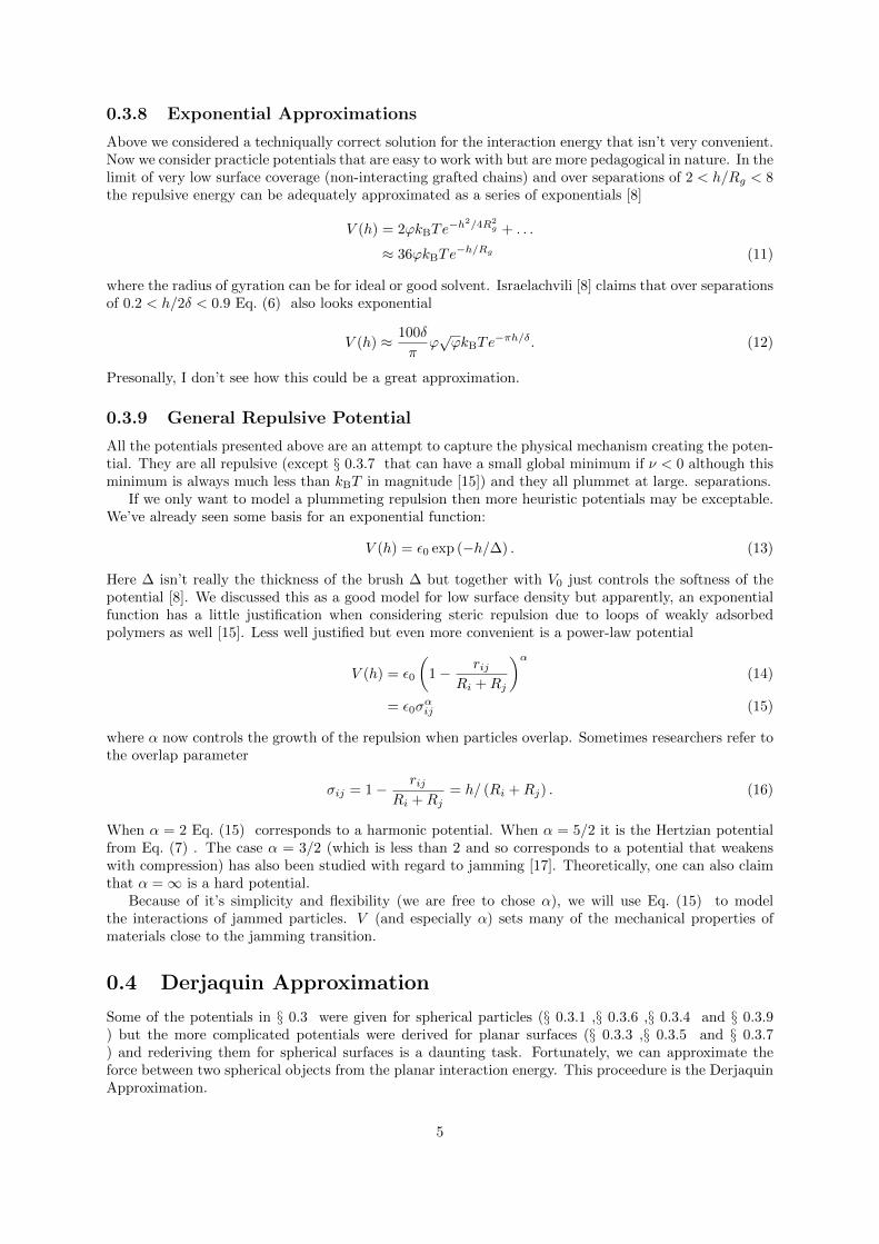
Figure 4: The distribution of volume for N = 8 disks at Pβ = 2. Clearly the “smart” algorithm failsentirely.

As the pressure is increased the volume is decreased. At a critical pressure (around Pβ ≈ 8 for 100disks) there is a discontinuous jump from one volume to another signalling a phase change from a fluidto a solid-like phase. Computations near the transition are extremely expensive (even with a workingVRA) and the DSA is prohibitively slow (even N = 10) but they do find a double peak in the volumedistribution.

0.6 Jamming

Investigations of the phase transition in hard-sphere gases is an ancient art (on the time scale of com-putational physics). § 0.3 mentioned that the first simulations of square-well potentials focused on theliquid-solid transition. But this is not quite the same thing as a jamming transition and the difference isa little subtle. It may seem a little pendantic but the properties of marginally jammed solids (i.e. justabove the transition) are different fram ordinary elastic solids. The reason is because they have markedlydifferent vibrational normal modes that they can sustain. Unfortunately, we won’t be able to discusshow the vibrational spectrum (especially the low-frequency modes at the transition) are different fromordinary solids but in § 0.7 we will discuss the elastic, compression and shear moduli. The results areimportant for understanding amorphous systems like glasses at low temperatures [11]. Although stud-ies like those shown in Fig. 5 [3] can carefully map-out the difference between true solids, marginallyjammed solids (and in fact three types of jammed systems: locally jammed , collectively jammed andstrictly jammed [20]), for our purposes we can have a very clear, practicle differentition:

• Jammed materials are fragile. Unlike for an actual solid phase, if the direction of an applied stresschanges even by a small amount, the jam will break and the entire network of forces that give thematerial its rigidity are lost.

Although the jam can support a load along the axis of the jam, it can’t hold up to stress in any otherdirection (Now would be a good time to recall that we are only discussing jamming of frictionless spheres.For jamming of more complicated objects see [12] (notice this reference was clearly writen as a chapterfor some book but I could only find the arXiv information)). As an anzats there can be no obviousrelation connecting stress to strain throughout the material [10]. The example often give is a pile of

9

(a) A schematic phase diagram in density-disorderspace. φ is the density and ψ is the order metric.

(b) This snapshot shows a random packing (φ =0.82) with locally jammed points but that is notcollectively jammed.

Figure 5: Carefully exploring jamming transitions shows that care is needed in defining what is and isn’ta jammed system [3].

sand. It appears solid because it sustains it’s shape against the force of gravity but tilting or vibratingthe table that the pile sits on immediately “melts” the so-called solid.

But our simple example has just introduced another element. Random noise or stresses on thegranular material can change the phase and so any “phase diagram” for jamming must include density,effective temperature and applied stress. This idea of a jammed phase is actually quite modern and onlya decade ago was a qualitative phase diagram (Fig. 6 ) for granular media formulated [10]. The jammingtransition is thought to be a function of the temperature, the applied stress and the density. Of principleinterest is the zero temperature and zero applied stress case. The point at which the jamming transitionoccurs in this case is called the J-point and is prominant in Fig. 6

At the end of the § 0.5 , we discussed the jump in volume with pressure near the transition butan equivalent point-of-view is a discontinuity in pressure as the volume containing the grains is shrunk.It is more convenient for this section to imagine the latter. Below the critical packing density φ theinstantaneous pressure is zero as shown in Fig. 7 (of course over a some finite window of time we couldmeasure the pressure of the hard sphere gas but instantaneously the contact forces are zero and sothen is the pressure). At the J-point φc the particles are only just touching and as φ > φc the pressureincreases. Despite what’s shown in Fig. 7 , the pressure does not grow linearly with the distance fromthe J-point ∆φ = φ−φc. ∆φ is the packing fraction about the transition and so it measures the amountof compression or overlap. The overlap parameter σ was defined in Eq. (16) and of course scales linearlywith excess density ∆φ.

So if the pressure does not grow linearly with ∆φ, how does it grow? Well that obviously dependson the interaction potential. In § 0.3 , we introduced many models and in § 0.4 we approximated theforce F between pairs of particles and listed them in Eq. (19) . The pressure depends on the interactionforces between particles

P ∼ F (σ)− ∂V

∂σ.

We can chose any force that we wish (or is appropriate for the ensemble of particles). To move forwardwe must chose one and we choose a simple one; the last one introduced; the repulsive potential (§ 0.3.9and Eq. (15) ). With this particular choise then the pressure above φc grows as

P ∼ F (σ) ∼ σα−1 ∼ (∆φ)α−1

. (23)

The granular material requires contacts to support stress. If there are not enough contacts, thematerial can not maintain stability. Determining marginal stability (and so then the jamming transition)

10

Figure 6: Jamming phase diagram [11]. The shaded green region represents the jammed phase outsideof which the system can flow. The J-point is a point worth considering since it marks the jammingtransition for a system at zero temperature and zero applied stress.

Figure 7: Transition around the J-point as seen by measuring (obviously the figure is an heuristicschematic) pressure [19]. The linear growth is too naive and not true. See the text.

11

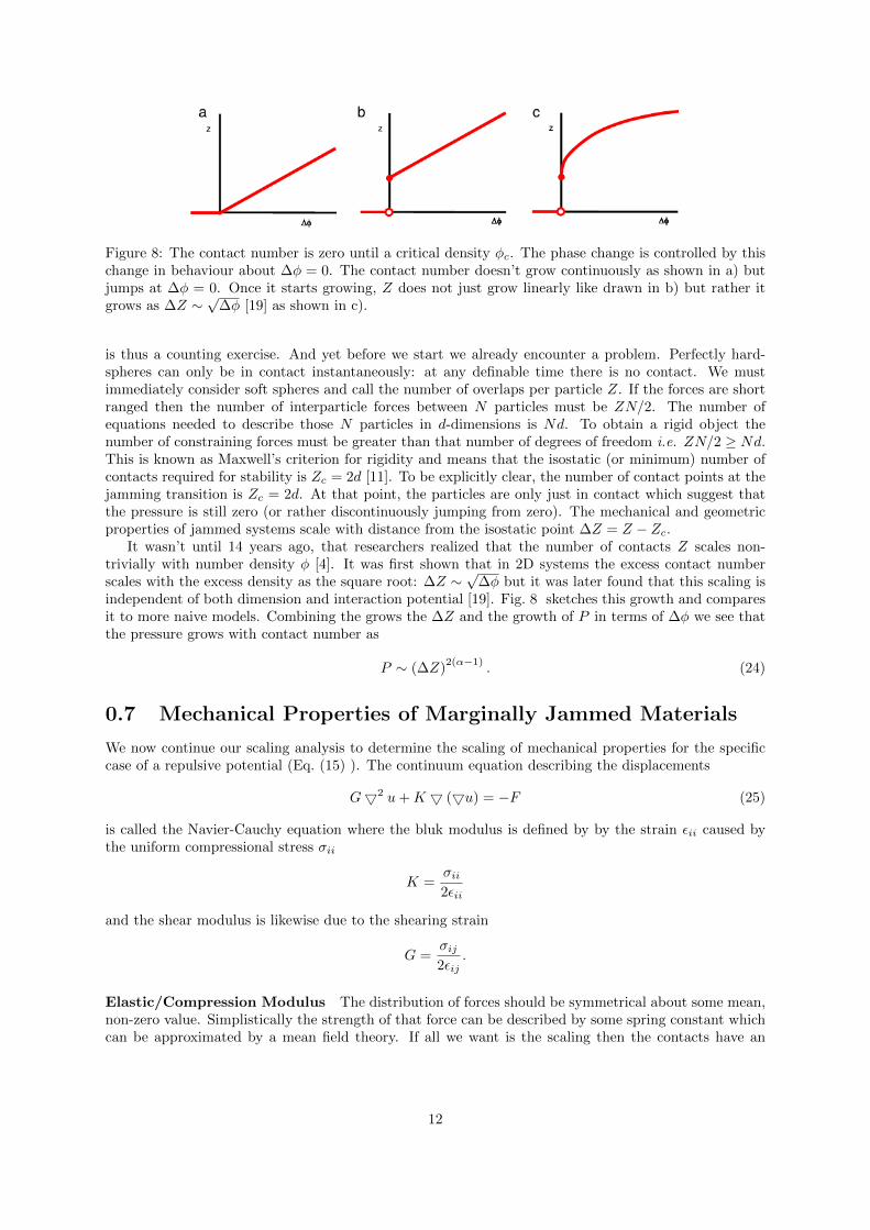
Figure 8: The contact number is zero until a critical density φc. The phase change is controlled by thischange in behaviour about ∆φ = 0. The contact number doesn’t grow continuously as shown in a) butjumps at ∆φ = 0. Once it starts growing, Z does not just grow linearly like drawn in b) but rather itgrows as ∆Z ∼

√∆φ [19] as shown in c).

is thus a counting exercise. And yet before we start we already encounter a problem. Perfectly hard-spheres can only be in contact instantaneously: at any definable time there is no contact. We mustimmediately consider soft spheres and call the number of overlaps per particle Z. If the forces are shortranged then the number of interparticle forces between N particles must be ZN/2. The number ofequations needed to describe those N particles in d-dimensions is Nd. To obtain a rigid object thenumber of constraining forces must be greater than that number of degrees of freedom i.e. ZN/2 ≥ Nd.This is known as Maxwell’s criterion for rigidity and means that the isostatic (or minimum) number ofcontacts required for stability is Zc = 2d [11]. To be explicitly clear, the number of contact points at thejamming transition is Zc = 2d. At that point, the particles are only just in contact which suggest thatthe pressure is still zero (or rather discontinuously jumping from zero). The mechanical and geometricproperties of jammed systems scale with distance from the isostatic point ∆Z = Z − Zc.

It wasn’t until 14 years ago, that researchers realized that the number of contacts Z scales non-trivially with number density φ [4]. It was first shown that in 2D systems the excess contact numberscales with the excess density as the square root: ∆Z ∼

√∆φ but it was later found that this scaling is

independent of both dimension and interaction potential [19]. Fig. 8 sketches this growth and comparesit to more naive models. Combining the grows the ∆Z and the growth of P in terms of ∆φ we see thatthe pressure grows with contact number as

P ∼ (∆Z)2(α−1)

. (24)

0.7 Mechanical Properties of Marginally Jammed Materials

We now continue our scaling analysis to determine the scaling of mechanical properties for the specificcase of a repulsive potential (Eq. (15) ). The continuum equation describing the displacements

G52 u+K 5 (5u) = −F (25)

is called the Navier-Cauchy equation where the bluk modulus is defined by by the strain εii caused bythe uniform compressional stress σii

K =σii2εii

and the shear modulus is likewise due to the shearing strain

G =σij2εij

.

Elastic/Compression Modulus The distribution of forces should be symmetrical about some mean,non-zero value. Simplistically the strength of that force can be described by some spring constant whichcan be approximated by a mean field theory. If all we want is the scaling then the contacts have an

12

Figure 9: Simulations of Hertzian disks [5] compare well to the mean field theory for mechanical modulidescribed in this section.

effective spring constant

k =∂2V

∂σ2

∼ σα−2 ∼ (∆φ)α−2 ∼ (∆Z)

2(α−2). (26)

The bulk modulus B describes the resistance to homogeneous compressio and so scales with k [11]. Sothen for marginally jammed repulsive systems, the bulk modulus goes as

B ∼ k ∼ σα−2 ∼ (∆φ)α−2 ∼ (∆Z)

2(α−2). (27)

Shear Modulus From a scaling point-of-view of Eq. (25) , the resistance to pure shear G scales exactlylike the elastic modulus. Therefore

G ∼ (∆φ)α−2 ∼ (∆Z)

2(α−2).

Effective medium theories come to the same conclusion [19, 5] but this is where the difference betweentradional solids and marginally jammed systems arises. Simulations show a very different scaling be-haviour for G [19]. Instead

G ∼ k∆Z ∼ (∆Z)2α−3

. (28)

The reason for this difference doesn’t seem to be perfectly understood at this time although randomnetwork theory may offer some insight [6].

Ratio We conclude this brief section by noting that the elastic and shear moduli depend on the specificforce law and so are not universal but the ratio is (at least for repulsive forces)

G

B∼ (∆φ)

1/2 ∼ ∆Z. (29)

Despite it’s simplicity, this model compares well to simulations of Hertzian disks near the jamming pointas is seen in Fig. 9 [5].

0.8 Rheology Near Jamming

We conclude this review by presenting some extremely new research on the rheology of jammed systemsnear the transition i.e. small ∆φ [16]. Studying the rheology of jammed systems has been notoriouslydifficult. This is for two reasons:

1. Experiments are limited to hard-spheres while theory is most definitely for soft spheres.

13

(a) Shear needed to obtain strain rate for a varietyof small excess densities (that is near the jammingtransition) for a suspension of gel microparticles.

(b) Non-dimensionalized shear verses strain rate.The data collapses onto two distinct curves for sys-tems below and above the critical density φc.

2. Wall slip and shear banding in common rheometers disguises the results.

Nordstrom et al. [16] solved these issues by:

1. Using a dense aqueous suspension of colloidal N-isopropylacrylamide gel microparticles (the sizeand therefore φ could be controlled by temperature).

2. Building a custom micro-rheometer that takes video tracking the particles’ positions in a microflu-idic channel and the velocity profile gives the strain rate γ. The shear stress is known for pressuredriven (∆P ) parabolic flow in a channel of length L to be σ = ∆P/L.

Using this device, Nordstrom et al. [16] measured the strain rate at different shears for a varied ofdensities near the critical value φc ≈ 0.64. Some were below and some were above the J-point. The datais shown in Fig. 10a . They describe it with a different set of variables than we’ve been using

• the shear-thinning exponent β = 0.48± 0.03the shear-thinning exponent

• a scaling exponent related to the steepness of the repulsive interaction (simply as ∆ = α − 1/2)which was measured to be ∆ = 2.1± 0.2.

These exponents can both be calculated for a given α. Nordstrom et al. assumed their gel microparticleswere Hertzian and so expected α = 5/2, ∆ = 2 and β = 1/2. Their measurements are in quite goodagreement and so, using the theoretical values, they plotted their data in terms of dimensionless unitsas shown in Fig. 10b . Amazingly, the data all collapses onto one of two curves corresponding to φ < φcand φ > φc. This universality was expected by § 0.7 but had been observed until last year.

0.9 Conclusion

The field of marginally jammed solids was over ripe for understanding and it is only in this last decadethat the intellectual harvest has begun. Initially, the field was viewed as trivial but very quickly the vastvariety of behaviours swamped researchers and impedied a universal understanding. However, recentunification in the field has resulted in a burst of forward thinking. Jammed materials were recognized asa novel phase of matter, a phase diagram was postulated for jamming, some of the statistical argumentsof such a system are now entrenched and unrefutable, scaling laws resulted, and now even the rheologicalproperties of this fragile yet beautiful state of matter are coming to light.

Likewise this project evolved. Initially I thought a simulation would be fun but soon realized thatsuch simulations are non-trivial and no one set of simulations can offer adquit insight into the nature ofjammed materials. Only by taking a curvy and wandering path through the field could I be satisfied.

PS. Sorry that I get this to you before I left.

14

Bibliography

[1] Demetra S. Achilleos and Maria Vamvakaki. End-grafted polymer chains onto inorganic nano-objects. Materials, 3:1981 – 2026, 2010.

[2] B. J. Alder and T. E. Wainwright. Phase transition for a hard sphere system. The Journal ofChemical Physics, 27(5):1208–1209, 1957.

[3] Aleksandar Donev, Salvatore Torquato, Frank H. Stillinger, and Robert Connelly. Jamming in hardsphere and disk packings. JOURNAL OF APPLIED PHYSICS, 95(2):989–999, 2004.

[4] D.J. Durian. Phys. Rev. Lett., 75:4780, 1997.

[5] W. G. Ellenbroek, M. van Hecke, and W. van Saarloos. Jammed frictionless disks: Connecting localand global response. Phys. Rev. E, 80:061307, 2009.

[6] W. G. Ellenbroek, Z. Zeravcic, W. van Saarloos, and M. van Hecke. EPL, 87:34004, 2009.

[7] E. Fischer. Elektronenmikroskopische untersuchungen zur stabilitat von suspensionen in makro-molekularen losungen. Colloid &; Polymer Science, 160:120–141, 1958. 10.1007/BF01503288.

[8] J.N. Israelachvili. Intermolecular and surface forces, volume 450. Academic press London, 1992.

[9] W. Krauth. Statistical Mechanics: Algorithms and computations. Oxford University Press, NewYork, 2006.

[10] Andrea J. Liu and Sidney R. Nagel. Jamming is not just cool any more. Nature, 396(5):21, 1998.

[11] Andrea J. Liu and Sidney R. Nagel. The jamming transition and the marginally jammed solid.Annu. Rev. Condens. Matter Phys., 1:347–369, 2010.

[12] Andrea J. Liu, Sidney R. Nagel, and Wim van Saarloos Matthieu Wyart. The jamming scenario—an introduction and outlook. arXiv, 2011.

[13] E.L Mackor. A theoretical approach of the colloid-chemical stability of dispersions in hydrocarbons.Journal of Colloid Science, 6(5):492 – 495, 1951.

[14] S. T. Milner. Polymer brushes. Science, 251(4996):905–914, 1991.

[15] D.H. Napper. Polymeric stabilization of colloidal dispersions, volume 7. Academic Press London,1983.

[16] K. N. Nordstrom, E. Verneuil, P. E. Arratia, A. Basu, Z. Zhang, A. G. Yodh, J. P. Gollub, andD. J. Durian. Microfluidic rheology of soft colloids above and below jamming. October 2010.

[17] Corey S. O’Hern, Leonardo E. Silbert, Andrea J. Liu, and Sidney R. Nagel. Jamming at zerotemperature and zero applied stress: The epitome of disorder. Phys. Rev. E, 68(1):011306, Jul2003.

[18] W.B. Russel, WB Russel, D.A. Saville, and W.R. Schowalter. Colloidal dispersions. CambridgeUniv Pr, 1992.

15

[19] Alexander O.N. Siemens and Martin van Hecke. Jamming: A simple introduction. Physica A,389:4255–4264, 2010.

[20] S. Torquato and F.H. Stillinger. Multiplicity of generation, selection, and classification proceduresfor jammed hard-particle packings. J. Phys. Chem. B, 5105:11849–11853, 2001.

16

.1 Hard-Core Monte Carlo Code

Both the direct sampling and the volume rescaling algorithm discussed in § 0.5 are included here.

/∗∗∗∗∗∗∗∗∗∗∗∗∗∗∗∗∗∗∗∗∗∗∗∗∗∗∗∗∗∗∗∗∗∗∗∗∗∗∗∗∗∗∗∗∗∗∗∗∗∗∗∗∗∗∗∗∗∗∗∗∗∗∗∗∗∗∗∗∗∗∗∗ Hard−shere NPT−ensemble code ∗∗∗∗∗∗∗∗∗∗∗∗∗∗∗∗∗∗∗∗∗∗∗∗∗∗∗∗∗∗∗∗∗∗∗∗∗∗∗∗∗∗∗∗∗∗∗∗∗∗∗∗∗∗∗∗∗∗∗∗∗∗∗∗∗∗∗∗∗∗∗∗//∗ C−headers ∗/#include <s t d l i b . h>#include <s t d i o . h>#include <uni s td . h>#include <s t r i n g . h>#include <math . h>#include <time . h>

/∗∗∗∗∗∗∗∗∗∗∗∗∗∗∗∗∗∗∗∗∗∗∗∗∗∗∗∗∗∗∗∗∗∗∗∗∗∗∗∗∗∗∗∗∗∗∗∗∗∗∗∗∗∗∗∗∗∗∗∗∗∗∗∗∗∗∗∗∗∗∗∗ Global va r i a b l e s ∗∗∗∗∗∗∗∗∗∗∗∗∗∗∗∗∗∗∗∗∗∗∗∗∗∗∗∗∗∗∗∗∗∗∗∗∗∗∗∗∗∗∗∗∗∗∗∗∗∗∗∗∗∗∗∗∗∗∗∗∗∗∗∗∗∗∗∗∗∗∗∗/int DIM;int POP;int ACCEPT;double RADIUS;double MASS;double PRESSURE;double TEMPERATURE;char FOUT[ 5 0 0 ] ;

/∗∗∗∗∗∗∗∗∗∗∗∗∗∗∗∗∗∗∗∗∗∗∗∗∗∗∗∗∗∗∗∗∗∗∗∗∗∗∗∗∗∗∗∗∗∗∗∗∗∗∗∗∗∗∗∗∗∗∗∗∗∗∗∗∗∗∗∗∗∗∗∗ I n i t i a l i z e subrout ines ∗∗∗∗∗∗∗∗∗∗∗∗∗∗∗∗∗∗∗∗∗∗∗∗∗∗∗∗∗∗∗∗∗∗∗∗∗∗∗∗∗∗∗∗∗∗∗∗∗∗∗∗∗∗∗∗∗∗∗∗∗∗∗∗∗∗∗∗∗∗∗∗/double dRand(void ) ;double s e tPosP i s tonDi r ec t (double ∗∗pos ) ;double setPosPistonSmart (double ∗∗pos ) ;double r e s c a l eVo l ( double length , double ∗∗pos ) ;double cut ( double inCut ) ;void cmmndln( int argc , char∗ argv [ ] ) ;/∗∗∗∗∗∗∗∗∗∗∗∗∗∗∗∗∗∗∗∗∗∗∗∗∗∗∗∗∗∗∗∗∗∗∗∗∗∗∗∗∗∗∗∗∗∗∗∗∗∗∗∗∗∗∗∗∗∗∗∗∗∗∗∗∗∗∗∗∗∗∗∗ main() funct ion ∗∗∗∗∗∗∗∗∗∗∗∗∗∗∗∗∗∗∗∗∗∗∗∗∗∗∗∗∗∗∗∗∗∗∗∗∗∗∗∗∗∗∗∗∗∗∗∗∗∗∗∗∗∗∗∗∗∗∗∗∗∗∗∗∗∗∗∗∗∗∗∗/int main ( int argc , char∗ argv [ ] ){// double pos [POP] [DIM] ;

double ∗∗pos ;double var l ength = 0 . ;int i ;FILE ∗ f i l e V o l ;

/∗ I n i t i a l i z e va r i a b l e s ∗/cmmndln( argc , argv ) ;//Al locate memory for pos [POP] [DIM]pos = (double∗∗) mal loc ( POP ∗ s izeof ( double∗ ) ) ;for ( i =0; i<POP; i++ ) pos [ i ] = (double∗) mal loc ( DIM ∗ s izeof ( double ) ) ;

p r i n t f ( ”%s\n” ,FOUT ) ;f i l e V o l=fopen (FOUT, ”w +” ) ;

/∗ I n i t i a l i z e random number generator ∗/p r i n t f ( ” I n i t i a l i z e system . . . \ n” ) ;srand ( (unsigned ) time (NULL) ) ;

p r i n t f ( ”Sample c on f i gu r a t i on space . . . \ n” ) ;for ( i =0; i<ACCEPT; i++) {

/∗ I n i t i a l i z e pos i t i ons ∗/// var leng th = setPosPistonDirect ( pos ) ;

var l ength = setPosPistonSmart ( pos ) ;f p r i n t f ( f i l eVo l , ”%e\n” , var l ength ) ;

}

f c l o s e ( f i l e V o l ) ;return 0 ;

}

/∗∗∗∗∗∗∗∗∗∗∗∗∗∗∗∗∗∗∗∗∗∗∗∗∗∗∗∗∗∗∗∗∗∗∗∗∗∗∗∗∗∗∗∗∗∗∗∗∗∗∗∗∗∗∗∗∗∗∗∗∗∗∗∗∗∗∗∗∗∗∗∗ dRand() returns a type double random number ∗∗∗∗∗∗∗∗∗∗∗∗∗∗∗∗∗∗∗∗∗∗∗∗∗∗∗∗∗∗∗∗∗∗∗∗∗∗∗∗∗∗∗∗∗∗∗∗∗∗∗∗∗∗∗∗∗∗∗∗∗∗∗∗∗∗∗∗∗∗∗∗/double dRand(void ) {

return rand ( ) / ( ( double ) (RANDMAX) ) ;}

/∗∗∗∗∗∗∗∗∗∗∗∗∗∗∗∗∗∗∗∗∗∗∗∗∗∗∗∗∗∗∗∗∗∗∗∗∗∗∗∗∗∗∗∗∗∗∗∗∗∗∗∗∗∗∗∗∗∗∗∗∗∗∗∗∗∗∗∗∗∗∗∗ setPosPistonDirect () randomly i n i t i a l i z e s the p a r t i c l e pos i t i ons ∗∗∗∗∗∗∗∗∗∗∗∗∗∗∗∗∗∗∗∗∗∗∗∗∗∗∗∗∗∗∗∗∗∗∗∗∗∗∗∗∗∗∗∗∗∗∗∗∗∗∗∗∗∗∗∗∗∗∗∗∗∗∗∗∗∗∗∗∗∗∗∗/

17

double s e tPosP i s tonDi r ec t (double ∗∗pos ) {int i , j , k ;int check ;double length , d i s t , gamma;double alpha [POP] [DIM ] ;

do {gamma = dRand ( ) ;for ( i =0; i<POP; i++) {

for ( j =0; j<DIM; j++) alpha [ i ] [ j ] = dRand ( ) ;gamma = gamma∗dRand ( ) ;

}l ength = sq r t ( −1.∗ l og (gamma)∗TEMPERATURE/PRESSURE ) ;/∗ Set pos i t i on ∗/for ( i =0; i<POP; i++) for ( j =0; j<DIM; j++) pos [ i ] [ j ] = alpha [ i ] [ j ]∗ l ength ;

check = 0 ;/∗ Check en t i r e conf igurat ion ∗/for ( i =0; i<POP; i++) for ( j =0; j<i ; j++) {

d i s t = 0 . ;for ( k=0;k<DIM; k++) d i s t += ( pos [ i ] [ k]−pos [ j ] [ k ] ) ∗ ( pos [ i ] [ k]−pos [ j ] [ k ] ) ;d i s t = sq r t ( d i s t ) ;i f ( d i s t < 2 .∗RADIUS) check = 1 ;

}} while ( check ) ;

return l ength ;}

/∗∗∗∗∗∗∗∗∗∗∗∗∗∗∗∗∗∗∗∗∗∗∗∗∗∗∗∗∗∗∗∗∗∗∗∗∗∗∗∗∗∗∗∗∗∗∗∗∗∗∗∗∗∗∗∗∗∗∗∗∗∗∗∗∗∗∗∗∗∗∗∗ setPosPistonSmart () i n i t i a l i z e s p a r t i c l e pos i t i ons by MC ∗∗∗∗∗∗∗∗∗∗∗∗∗∗∗∗∗∗∗∗∗∗∗∗∗∗∗∗∗∗∗∗∗∗∗∗∗∗∗∗∗∗∗∗∗∗∗∗∗∗∗∗∗∗∗∗∗∗∗∗∗∗∗∗∗∗∗∗∗∗∗∗/double setPosPistonSmart (double ∗∗pos ) {

int i , j ;double length , gamma;double alpha [POP] [DIM ] ;

gamma = dRand ( ) ;for ( i =0; i<POP; i++) {

for ( j =0; j<DIM; j++) alpha [ i ] [ j ] = dRand ( ) ;gamma = gamma∗dRand ( ) ;

}l ength = sq r t ( −1.∗ l og (gamma)∗TEMPERATURE/PRESSURE ) ;/∗ Set pos i t i on ∗/for ( i =0; i<POP; i++) for ( j =0; j<DIM; j++) pos [ i ] [ j ] = alpha [ i ] [ j ]∗ l ength ;

l ength = re s c a l eVo l ( length , pos ) ;

return l ength ;}

/∗∗∗∗∗∗∗∗∗∗∗∗∗∗∗∗∗∗∗∗∗∗∗∗∗∗∗∗∗∗∗∗∗∗∗∗∗∗∗∗∗∗∗∗∗∗∗∗∗∗∗∗∗∗∗∗∗∗∗∗∗∗∗∗∗∗∗∗∗∗∗∗ Instead of regenerat ing a new i n i t i a l conf igurat ion , r e s ca l e data ∗∗∗∗∗∗∗∗∗∗∗∗∗∗∗∗∗∗∗∗∗∗∗∗∗∗∗∗∗∗∗∗∗∗∗∗∗∗∗∗∗∗∗∗∗∗∗∗∗∗∗∗∗∗∗∗∗∗∗∗∗∗∗∗∗∗∗∗∗∗∗∗/double r e s c a l eVo l ( double length , double ∗∗pos ) {

double newVol , oldVol = pow( length , ( double )DIM) ;double d i s t , min , radCut , s c a l i n g ;int i , j , k ;min=length ∗100000 . ;

/∗ Check en t i r e conf igurat ion ∗/for ( i =0; i<POP; i++) for ( j =0; j<i ; j++) {

d i s t = 0 . ;for ( k=0;k<DIM; k++) d i s t += ( pos [ i ] [ k]−pos [ j ] [ k ] ) ∗ ( pos [ i ] [ k]−pos [ j ] [ k ] ) ;d i s t = sq r t ( d i s t ) ;i f ( d i s t < min) min=d i s t ;

}

i f ( min>2.∗RADIUS ) s c a l i n g = 1 . ;else {

radCut = PRESSURE∗oldVol∗pow( RADIUS/min , (double )DIM )/TEMPERATURE;newVol = cut ( radCut ) ∗ TEMPERATURE / PRESSURE;s c a l i n g = pow( ( newVol/ oldVol ) , 1 . / (double )DIM ) ;

}

for ( i =0; i<POP; i++) for ( j =0; j<DIM; j++) pos [ i ] [ j ]=pos [ i ] [ j ]∗ s c a l i n g ;return l ength ∗ s c a l i n g ;

}

/∗∗∗∗∗∗∗∗∗∗∗∗∗∗∗∗∗∗∗∗∗∗∗∗∗∗∗∗∗∗∗∗∗∗∗∗∗∗∗∗∗∗∗∗∗∗∗∗∗∗∗∗∗∗∗∗∗∗∗∗∗∗∗∗∗∗∗∗∗∗∗∗ Used to sample qu i c k l y ∗∗∗∗∗∗∗∗∗∗∗∗∗∗∗∗∗∗∗∗∗∗∗∗∗∗∗∗∗∗∗∗∗∗∗∗∗∗∗∗∗∗∗∗∗∗∗∗∗∗∗∗∗∗∗∗∗∗∗∗∗∗∗∗∗∗∗∗∗∗∗∗/double cut ( double inCut ) {

18

double prob ;double s h i f t , randScale ;int r e j e c t ;

prob = 1.−((double )POP)/ inCut ;s h i f t =0. ;i f ( prob>0. ) {

do {r e j e c t = 0 ;s h i f t = −1.∗ l og ( dRand ( ) ) / prob ;randScale = pow( ( inCut+s h i f t )/ inCut , (double )POP ) ∗ exp ( −1.∗(1.−prob )∗ s h i f t ) ;i f ( dRand()> randScale ) r e j e c t =1;

} while ( r e j e c t ) ;}return inCut+s h i f t ;

}

/∗∗∗∗∗∗∗∗∗∗∗∗∗∗∗∗∗∗∗∗∗∗∗∗∗∗∗∗∗∗∗∗∗∗∗∗∗∗∗∗∗∗∗∗∗∗∗∗∗∗∗∗∗∗∗∗∗∗∗∗∗∗∗∗∗∗∗∗∗∗∗∗ Set g l o b a l va r i a b l e s ∗∗∗∗∗∗∗∗∗∗∗∗∗∗∗∗∗∗∗∗∗∗∗∗∗∗∗∗∗∗∗∗∗∗∗∗∗∗∗∗∗∗∗∗∗∗∗∗∗∗∗∗∗∗∗∗∗∗∗∗∗∗∗∗∗∗∗∗∗∗∗∗/void cmmndln( int argc , char∗ argv [ ] ) {

int arg ;

/∗ Check en t i r e conf igurat ion ∗/DIM=2;POP=4;RADIUS=1. ;MASS=1. ;PRESSURE=1;TEMPERATURE=1. ;ACCEPT=10;s p r i n t f (FOUT, ”volume . dat” ) ;

for ( arg=1; arg<argc ; arg++) i f ( argv [ arg ] [0]== ’− ’ ) switch ( argv [ arg ] [ 1 ] ) {case ’ h ’ :

p r i n t f ( ”Sample NPT ensembles o f hard−sphere s \nWritten by Tyler Shendruk\n” ) ;p r i n t f ( ”Usage :\n\ tFo l lowing the launch command ,\n” ) ;p r i n t f ( ”\ ttype ’− ’ then one o f the f o l l ow i ng commands .\n” ) ;p r i n t f ( ”\n\t−h\ tThis menu\n\t−d\ td imens i ona l i t y \n\n” ) ;p r i n t f ( ”\t−n\tnumber o f p a r t i c l e s \n\t−a\tnumber o f t imes to sample\n” ) ;p r i n t f ( ”\t−r\ t r ad iu s \n\t−m\ tmass\n\t−p\ t p r e s su r e \n” ) ;p r i n t f ( ”\t−t\ ttemperature \n\t−f \ toutput f i l e name\n” ) ;e x i t (EXIT SUCCESS ) ;break ;

case ’ d ’ :arg++;DIM=ato i ( argv [ arg ] ) ;break ;

case ’ n ’ :arg++;POP=ato i ( argv [ arg ] ) ;break ;

case ’ a ’ :arg++;ACCEPT=ato i ( argv [ arg ] ) ;break ;

case ’ r ’ :arg++;RADIUS=ato f ( argv [ arg ] ) ;break ;

case ’m’ :arg++;MASS=ato f ( argv [ arg ] ) ;break ;

case ’ p ’ :arg++;PRESSURE=ato f ( argv [ arg ] ) ;break ;

case ’ t ’ :arg++;TEMPERATURE=ato f ( argv [ arg ] ) ;break ;

case ’ f ’ :arg++;s p r i n t f (FOUT, argv [ arg ] ) ;break ;

default :p r i n t f ( ”ERROR:\n∗∗ I nva l i d arument : %s\n∗∗ Try −h\n” , argv [ arg ] ) ;e x i t (EXIT FAILURE ) ;

}p r i n t f ( ” Input :\n” ) ;p r i n t f ( ”\ tSave to :\ t%s\n\ tDimens iona l i ty :\ t%d\n” ,FOUT,DIM) ;p r i n t f ( ”\ tPopulat ion :\ t%d\n\ tSamples :\ t%d\n” ,POP,ACCEPT) ;

19

p r i n t f ( ”\ tRadius :\ t\ t%l f \n\tMass :\ t\ t%l f \n” ,RADIUS,MASS) ;p r i n t f ( ”\ tPre s sure :\ t%l f \n\ tTemperature :\ t%l f \n” ,PRESSURE,TEMPERATURE) ;

}

20