Embed Size (px)
Citation preview
Undergraduate Lecture Notes in Physics
Jakob Schwichtenberg
Physics from Symmetry Second Edition

Undergraduate Lecture Notes in Physics
Undergraduate Lecture Notes in Physics (ULNP) publishes authoritative texts covering topicsthroughout pure and applied physics. Each title in the series is suitable as a basis forundergraduate instruction, typically containing practice problems, worked examples, chaptersummaries, and suggestions for further reading.
ULNP titles must provide at least one of the following:
• An exceptionally clear and concise treatment of a standard undergraduate subject.• A solid undergraduate-level introduction to a graduate, advanced, or non-standard subject.• A novel perspective or an unusual approach to teaching a subject.
ULNP especially encourages new, original, and idiosyncratic approaches to physics teachingat the undergraduate level.
The purpose of ULNP is to provide intriguing, absorbing books that will continue to be thereader’s preferred reference throughout their academic career.
Series editors
Neil AshbyUniversity of Colorado, Boulder, CO, USA
William BrantleyDepartment of Physics, Furman University, Greenville, SC, USA
Matthew DeadyPhysics Program, Bard College, Annandale-on-Hudson, NY, USA
Michael FowlerDepartment of Physics, University of Virginia, Charlottesville, VA, USA
Morten Hjorth-JensenDepartment of Physics, University of Oslo, Oslo, Norway
Michael InglisSUNY Suffolk County Community College, Long Island, NY, USA
More information about this series at http://www.springer.com/series/8917
Jakob Schwichtenberg
Physics from SymmetrySecond Edition
123
Jakob SchwichtenbergKarlsruheGermany
ISSN 2192-4791 ISSN 2192-4805 (electronic)Undergraduate Lecture Notes in PhysicsISBN 978-3-319-66630-3 ISBN 978-3-319-66631-0 (eBook)https://doi.org/10.1007/978-3-319-66631-0
Library of Congress Control Number: 2017959156
1st edition: © Springer International Publishing Switzerland 20152nd edition: © Springer International Publishing AG 2018This work is subject to copyright. All rights are reserved by the Publisher, whether the whole or part of the material isconcerned, specifically the rights of translation, reprinting, reuse of illustrations, recitation, broadcasting, reproductionon microfilms or in any other physical way, and transmission or information storage and retrieval, electronicadaptation, computer software, or by similar or dissimilar methodology now known or hereafter developed.The use of general descriptive names, registered names, trademarks, service marks, etc. in this publication does notimply, even in the absence of a specific statement, that such names are exempt from the relevant protective laws andregulations and therefore free for general use.The publisher, the authors and the editors are safe to assume that the advice and information in this book are believedto be true and accurate at the date of publication. Neither the publisher nor the authors or the editors give a warranty,express or implied, with respect to the material contained herein or for any errors or omissions that may have beenmade. The publisher remains neutral with regard to jurisdictional claims in published maps and institutionalaffiliations.
Printed on acid-free paper
This Springer imprint is published by Springer NatureThe registered company is Springer International Publishing AGThe registered company address is: Gewerbestrasse 11, 6330 Cham, Switzerland

N AT U R E A LW AY S C R E AT E S T H E B E S T O F A L L O P T I O N S
A R I S T O T L E
A S FA R A S I S E E , A L L A P R I O R I S TAT E M E N T S I N P H Y S I C S H AV E T H E I R
O R I G I N I N S Y M M E T R Y.
H E R M A N N W E Y L
T H E I M P O R TA N T T H I N G I N S C I E N C E I S N O T S O M U C H T O O B TA I N N E W FA C T S
A S T O D I S C O V E R N E W W AY S O F T H I N K I N G A B O U T T H E M .
W I L L I A M L A W R E N C E B R A G G

Dedicated to my parents
Preface to the Second Edition
In the two years since the first edition of this book was published I’vereceived numerous messages from readers all around the world. Iwas surprised by this large number of responses and how positivemost of them were. Of course, I was cautiously confident that read-ers would like the book. Otherwise I wouldn’t have spent so manymonths writing it. However, there is certainly no shortage of bookson group theory or on the role of symmetries in physics. To quotePredrag Cvitanovic1 1 Predrag Cvitanovic. Group Theory:
Birdtracks, Lie’s, and Exceptional Groups.Princeton University Press, 7 2008.ISBN 9780691118369
Almost anybody whose research requires sustained use of grouptheory (and it is hard to think of a physical or mathematical problemthat is wholly devoid of symmetry) writes a book about it.
Moreover, I’m not a world renowned expert. Therefore, I knew noone would buy the book because my name is written on the cover. Sothe chances were high that "Physics from Symmetry" would simplydrown in the flood of new textbooks that are published every year.
Therefore, it’s reasonable to wonder: Why and how did "Physicsfrom Symmetry" avoid this fate?
I think the main reason for the success of the first edition is what Iframed as something negative above: it wasn’t written by a worldrenowned expert. I wrote the book while I was still a student and,as I remarked in the preface to the first edition, "I wrote the book Iwished had existed when I started my journey in physics". So mymotivation for writing the book wasn’t to create an authoritative ref-erence or a concise text that experts would love. Instead, my only fo-cus was to write a book that helps students understand. As a studentmyself I always had still fresh in memory what I found confusingand what finally helped me understand.
This point of view is nicely summarized in the following quote byC.S. Lewis2 2 C. S. Lewis. Reflections on the Psalms.
HarperOne, reprint edition, 2 2017.ISBN 9780062565488It often happens that two schoolboys can solve difficulties in their work
for one another better than the master can. When you took the problem
to a master, as we all remember, he was very likely to explain whatyou understood already, to add a great deal of information which youdidn’t want, and say nothing at all about the thing that was puzzlingyou. [...] The fellow-pupil can help more than the master becausehe knows less. The difficulty we want him to explain is one he hasrecently met. The expert met it so long ago he has forgotten. He seesthe whole subject, by now, in a different light that he cannot conceivewhat is really troubling the pupil; he sees a dozen other difficultieswhich ought to be troubling him but aren’t.
While most readers liked the student-friendly spirit of the first edi-tion, it was, of course, not perfect. Several readers pointed out typosand paragraphs with confusing notation or explanations. This feed-back guided me during the preparation of this second edition. Ifocused on correcting typos, improving the notation and I rewroteentire sections that were causing confusion.
I hope these changes make "Physics from Symmetry" even morestudent-friendly and useful3.3 No book is ever perfect and I’m al-
ways happy to receive feedback. So ifyou find an error, have an idea for im-provement or simply want to commenton something, always feel free to writeme at [email protected]
Karlsruhe, September 2017 Jakob Schwichtenberg
X
Preface to the First Edition
The most incomprehensible thing about the world is that it is at allcomprehensible.
- Albert Einstein4 4 As quoted in Jon Fripp, DeborahFripp, and Michael Fripp. Speaking ofScience. Newnes, 1st edition, 4 2000.ISBN 9781878707512In the course of studying physics I became, like any student of
physics, familiar with many fundamental equations and their solu-tions, but I wasn’t really able to see their connection.
I was thrilled when I understood that most of them have a com-mon origin: symmetry. To me, the most beautiful thing in physics iswhen something incomprehensible, suddenly becomes comprehen-sible, because of a deep explanation. That’s why I fell in love withsymmetries.
For example, for quite some time I couldn’t really understandspin, which is some kind of curious internal angular momentum thatalmost all fundamental particles carry. Then I learned that spin isa direct consequence of a symmetry, called Lorentz symmetry, andeverything started to make sense.
Experiences like this were the motivation for this book and insome sense, I wrote the book I wished had existed when I started myjourney in physics. Symmetries are beautiful explanations for manyotherwise incomprehensible physical phenomena and this book isbased on the idea that we can derive the fundamental theories ofphysics from symmetry.
One could say that this book’s approach to physics starts at theend: Before we even talk about classical mechanics or non-relativisticquantum mechanics, we will use the (as far as we know) exact sym-metries of nature to derive the fundamental equations of quantumfield theory. Despite its unconventional approach, this book is aboutstandard physics. We will not talk about speculative, experimentallyunverified theories. We are going to use standard assumptions anddevelop standard theories.
XII
Depending on the reader’s experience in physics, the book can beused in two different ways:
• It can be used as a quick primer for those who are relatively newto physics. The starting points for classical mechanics, electro-dynamics, quantum mechanics, special relativity and quantumfield theory are explained and after reading, the reader can decidewhich topics are worth studying in more detail. There are manygood books that cover every topic mentioned here in greater depthand at the end of each chapter some further reading recommen-dations are listed. If you feel you fit into this category, you areencouraged to start with the mathematical appendices at the endof the book5 before going any further.5 Starting with Chapter A. In addition,
the corresponding appendix chaptersare mentioned when a new mathemati-cal concept is used in the text.
• Alternatively, this book can be used to connect loose ends for moreexperienced students. Many things that may seem arbitrary or alittle wild when learnt for the first time using the usual historicalapproach, can be seen as being inevitable and straightforwardwhen studied from the symmetry point of view.
In any case, you are encouraged to read this book from cover tocover, because the chapters build on one another.
We start with a short chapter about special relativity, which is thefoundation for everything that follows. We will see that one of themost powerful constraints is that our theories must respect specialrelativity. The second part develops the mathematics required toutilize symmetry ideas in a physical context. Most of these mathe-matical tools come from a branch of mathematics called group theory.Afterwards, the Lagrangian formalism is introduced, which makesworking with symmetries in a physical context straightforward. Inthe fifth and sixth chapters the basic equations of modern physicsare derived using the two tools introduced earlier: The Lagrangianformalism and group theory. In the final part of this book these equa-tions are put into action. Considering a particle theory we end upwith quantum mechanics, considering a field theory we end up withquantum field theory. Then we look at the non-relativistic and classi-cal limits of these theories, which leads us to classical mechanics andelectrodynamics.
Every chapter begins with a brief summary of the chapter. If youcatch yourself thinking: "Why exactly are we doing this?", returnto the summary at the beginning of the chapter and take a look athow this specific step fits into the bigger picture of the chapter. Everypage has a big margin, so you can scribble down your own notes andideas while reading6.6 On many pages I included in the
margin some further information orpictures.

XIII
I hope you enjoy reading this book as much as I have enjoyed writingit.
Karlsruhe, January 2015 Jakob Schwichtenberg

Acknowledgments
I want to thank everyone who helped me create this book. I am espe-cially grateful to Fritz Waitz, whose comments, ideas and correctionshave made this book so much better. I am also very indebted to ArneBecker and Daniel Hilpert for their invaluable suggestions, commentsand careful proofreading. I thank Robert Sadlier for his proofreading,Jakob Karalus for his comments and Marcel Köpke and Paul Tremperfor many insightful discussions.
I also want to thank Silvia Schwichtenberg, Christian Nawroth,Ulrich Nierste and my editor at Springer, Angela Lahee, for theirsupport.
Many thanks are due to all readers of the first edition who sug-gested improvements and pointed out mistakes, especially MeirKrukowsky, Jonathan Jones, Li Zeyang, Rob Casey, Ethan C. Jahns,Bart Pastoor, Zheru Qiu, Rudy Blyweert, Bruno Jacobs, Joey Ooi,Henry Carnes, Jandro Kirkish, Vicente Iranzo, Rohit Chaki, JonathanWermelinger, Achim Schmetz, RubingBai, Markus Pernow, GlebKlimovitch, Enric Arcadia, Cassiano Cattan, Martin Wong, MarcoSmolla, Alexander Zeng, Mohammad Mahdi AlTakach, JonathanHobson, Peter Freed, Daniel Ciobotu, Telmo Cunha, Jia-Ji Zhu, An-drew J. Sutter, Rutwig Campoamor-Stursberg and Andreas Wipf.
Finally, my greatest debt is to my parents who always supportedme and taught me to value education above all else.
If you find an error in the text I would appreciate a short emailto [email protected]. All known errors are listed athttp://physicsfromsymmetry.com/errata .
Contents
Part I Foundations
1 Introduction 31.1 What we Cannot Derive . . . . . . . . . . . . . . . . . . . 31.2 Book Overview . . . . . . . . . . . . . . . . . . . . . . . . 51.3 Elementary Particles and Fundamental Forces . . . . . . 7
2 Special Relativity 112.1 The Invariant of Special Relativity . . . . . . . . . . . . . 122.2 Proper Time . . . . . . . . . . . . . . . . . . . . . . . . . . 142.3 Upper Speed Limit . . . . . . . . . . . . . . . . . . . . . . 162.4 The Minkowski Notation . . . . . . . . . . . . . . . . . . 172.5 Lorentz Transformations . . . . . . . . . . . . . . . . . . . 192.6 Invariance, Symmetry and Covariance . . . . . . . . . . . 21
Part II Symmetry Tools
3 Lie Group Theory 253.1 Groups . . . . . . . . . . . . . . . . . . . . . . . . . . . . . 263.2 Rotations in two Dimensions . . . . . . . . . . . . . . . . 29
3.2.1 Rotations with Unit Complex Numbers . . . . . . 313.3 Rotations in three Dimensions . . . . . . . . . . . . . . . 33
3.3.1 Quaternions . . . . . . . . . . . . . . . . . . . . . . 343.4 Lie Algebras . . . . . . . . . . . . . . . . . . . . . . . . . . 38
3.4.1 The Generators and Lie Algebra of SO(3) . . . . 423.4.2 The Abstract Definition of a Lie Algebra . . . . . 453.4.3 The Generators and Lie Algebra of SU(2) . . . . 463.4.4 The Abstract Definition of a Lie Group . . . . . . 47
3.5 Representation Theory . . . . . . . . . . . . . . . . . . . . 503.6 SU(2) . . . . . . . . . . . . . . . . . . . . . . . . . . . . . 54
3.6.1 The Finite-dimensional Irreducible Representationsof SU(2) . . . . . . . . . . . . . . . . . . . . . . . . 54
XVIII
3.6.2 The Representation of SU(2) in one Dimension . 61
3.6.3 The Representation of SU(2) in two Dimensions 61
3.6.4 The Representation of SU(2) in three Dimensions 62
3.7 The Lorentz Group O(1, 3) . . . . . . . . . . . . . . . . . . 62
3.7.1 One Representation of the Lorentz Group . . . . 66
3.7.2 Generators of the Other Components of theLorentz Group . . . . . . . . . . . . . . . . . . . . 69
3.7.3 The Lie Algebra of the Proper OrthochronousLorentz Group . . . . . . . . . . . . . . . . . . . . 70
3.7.4 The (0, 0) Representation . . . . . . . . . . . . . . 72
3.7.5 The ( 12 , 0) Representation . . . . . . . . . . . . . . 72
3.7.6 The (0, 12 ) Representation . . . . . . . . . . . . . . 74
3.7.7 Van der Waerden Notation . . . . . . . . . . . . . 75
3.7.8 The ( 12 , 1
2 ) Representation . . . . . . . . . . . . . . 80
3.7.9 Spinors and Parity . . . . . . . . . . . . . . . . . . 84
3.7.10 Spinors and Charge Conjugation . . . . . . . . . . 86
3.7.11 Infinite-Dimensional Representations . . . . . . . 87
3.8 The Poincaré Group . . . . . . . . . . . . . . . . . . . . . 89
3.9 Elementary Particles . . . . . . . . . . . . . . . . . . . . . 91
3.10 Appendix: Rotations in a Complex Vector Space . . . . . 92
3.11 Appendix: Manifolds . . . . . . . . . . . . . . . . . . . . . 93
4 The Framework 954.1 Lagrangian Formalism . . . . . . . . . . . . . . . . . . . . 95
4.1.1 Fermat’s Principle . . . . . . . . . . . . . . . . . . 96
4.1.2 Variational Calculus - the Basic Idea . . . . . . . . 96
4.2 Restrictions . . . . . . . . . . . . . . . . . . . . . . . . . . . 97
4.3 Particle Theories vs. Field Theories . . . . . . . . . . . . . 98
4.4 Euler-Lagrange Equation . . . . . . . . . . . . . . . . . . . 99
4.5 Noether’s Theorem . . . . . . . . . . . . . . . . . . . . . . 101
4.5.1 Noether’s Theorem for Particle Theories . . . . . 101
4.5.2 Noether’s Theorem for Field Theories - SpacetimeSymmetries . . . . . . . . . . . . . . . . . . . . . . 105
4.5.3 Rotations and Boosts . . . . . . . . . . . . . . . . . 108
4.5.4 Spin . . . . . . . . . . . . . . . . . . . . . . . . . . . 110
4.5.5 Noether’s Theorem for Field Theories - InternalSymmetries . . . . . . . . . . . . . . . . . . . . . . 110
4.6 Appendix: Conserved Quantity from Boost Invariancefor Particle Theories . . . . . . . . . . . . . . . . . . . . . 113
4.7 Appendix: Conserved Quantity from Boost Invariancefor Field Theories . . . . . . . . . . . . . . . . . . . . . . . 114
XIX
Part III The Equations of Nature
5 Measuring Nature 1175.1 The Operators of Quantum Mechanics . . . . . . . . . . . 117
5.1.1 Spin and Angular Momentum . . . . . . . . . . . 1185.2 The Operators of Quantum Field Theory . . . . . . . . . 119
6 Free Theory 1216.1 Lorentz Covariance and Invariance . . . . . . . . . . . . . 1216.2 Klein-Gordon Equation . . . . . . . . . . . . . . . . . . . . 122
6.2.1 Complex Klein-Gordon Field . . . . . . . . . . . . 1246.3 Dirac Equation . . . . . . . . . . . . . . . . . . . . . . . . 1246.4 Proca Equation . . . . . . . . . . . . . . . . . . . . . . . . 127
7 Interaction Theory 1317.1 U(1) Interactions . . . . . . . . . . . . . . . . . . . . . . . 133
7.1.1 Internal Symmetry of Free Spin 12 Fields . . . . . 134
7.1.2 Internal Symmetry of Free Spin 1 Fields . . . . . 1357.1.3 Putting the Puzzle Pieces Together . . . . . . . . . 1367.1.4 Inhomogeneous Maxwell Equations and Minimal
Coupling . . . . . . . . . . . . . . . . . . . . . . . . 1397.1.5 Charge Conjugation, Again . . . . . . . . . . . . . 1407.1.6 Noether’s Theorem for Internal U(1) Symmetry . 1417.1.7 Interaction of Massive Spin 0 Fields . . . . . . . . 1427.1.8 Interaction of Massive Spin 1 Fields . . . . . . . . 143
7.2 SU(2) Interactions . . . . . . . . . . . . . . . . . . . . . . 1437.3 Mass Terms and "Unification" of SU(2) and U(1) . . . . 1507.4 Parity Violation . . . . . . . . . . . . . . . . . . . . . . . . 1587.5 Lepton Mass Terms . . . . . . . . . . . . . . . . . . . . . . 1627.6 Quark Mass Terms . . . . . . . . . . . . . . . . . . . . . . 1657.7 Isospin . . . . . . . . . . . . . . . . . . . . . . . . . . . . . 166
7.7.1 Labelling States . . . . . . . . . . . . . . . . . . . . 1687.8 SU(3) Interactions . . . . . . . . . . . . . . . . . . . . . . 170
7.8.1 Color . . . . . . . . . . . . . . . . . . . . . . . . . . 1727.8.2 Quark Description . . . . . . . . . . . . . . . . . . 173
7.9 The Interplay Between Fermions and Bosons . . . . . . . 174
Part IV Applications
8 Quantum Mechanics 1778.1 Particle Theory Identifications . . . . . . . . . . . . . . . . 1788.2 Relativistic Energy-Momentum Relation . . . . . . . . . . 1788.3 The Quantum Formalism . . . . . . . . . . . . . . . . . . 179
8.3.1 Expectation Value . . . . . . . . . . . . . . . . . . 181
XX
8.4 The Schrödinger Equation . . . . . . . . . . . . . . . . . . 1828.4.1 Schrödinger Equation with an External Field . . . 185
8.5 From Wave Equations to Particle Motion . . . . . . . . . 1858.5.1 Example: Free Particle . . . . . . . . . . . . . . . . 1858.5.2 Example: Particle in a Box . . . . . . . . . . . . . . 1868.5.3 Dirac Notation . . . . . . . . . . . . . . . . . . . . 1898.5.4 Example: Particle in a Box, Again . . . . . . . . . 1918.5.5 Spin . . . . . . . . . . . . . . . . . . . . . . . . . . . 192
8.6 Heisenberg’s Uncertainty Principle . . . . . . . . . . . . . 1968.7 Comments on Interpretations . . . . . . . . . . . . . . . . 1978.8 Appendix: Interpretation of the Dirac Spinor
Components . . . . . . . . . . . . . . . . . . . . . . . . . . 1988.9 Appendix: Solving the Dirac Equation . . . . . . . . . . . 2038.10 Appendix: Dirac Spinors in Different Bases . . . . . . . . 205
8.10.1 Solutions of the Dirac Equation in the Mass Basis 207
9 Quantum Field Theory 2099.1 Field Theory Identifications . . . . . . . . . . . . . . . . . 2109.2 Free Spin 0 Field Theory . . . . . . . . . . . . . . . . . . . 2119.3 Free Spin 1
2 Field Theory . . . . . . . . . . . . . . . . . . . 2169.4 Free Spin 1 Field Theory . . . . . . . . . . . . . . . . . . . 2199.5 Interacting Field Theory . . . . . . . . . . . . . . . . . . . 219
9.5.1 Scatter Amplitudes . . . . . . . . . . . . . . . . . . 2209.5.2 Time Evolution of States . . . . . . . . . . . . . . . 2209.5.3 Dyson Series . . . . . . . . . . . . . . . . . . . . . 2249.5.4 Evaluating the Series . . . . . . . . . . . . . . . . . 225
9.6 Appendix: Most General Solution of the Klein-GordonEquation . . . . . . . . . . . . . . . . . . . . . . . . . . . . 229
10 Classical Mechanics 23310.1 Relativistic Mechanics . . . . . . . . . . . . . . . . . . . . 23510.2 The Lagrangian of Non-Relativistic Mechanics . . . . . . 236
11 Electrodynamics 23911.1 The Homogeneous Maxwell Equations . . . . . . . . . . 24011.2 The Lorentz Force . . . . . . . . . . . . . . . . . . . . . . . 24111.3 Coulomb Potential . . . . . . . . . . . . . . . . . . . . . . 243
12 Gravity 245
13 Closing Words 251
Part V Appendices
A Vector calculus 255
XXI
A.1 Basis Vectors . . . . . . . . . . . . . . . . . . . . . . . . . . 256A.2 Change of Coordinate Systems . . . . . . . . . . . . . . . 257A.3 Matrix Multiplication . . . . . . . . . . . . . . . . . . . . . 259A.4 Scalars . . . . . . . . . . . . . . . . . . . . . . . . . . . . . 260A.5 Right-handed and Left-handed Coordinate Systems . . . 260
B Calculus 263B.1 Product Rule . . . . . . . . . . . . . . . . . . . . . . . . . . 263B.2 Integration by Parts . . . . . . . . . . . . . . . . . . . . . . 263B.3 The Taylor Series . . . . . . . . . . . . . . . . . . . . . . . 264B.4 Series . . . . . . . . . . . . . . . . . . . . . . . . . . . . . . 266
B.4.1 Important Series . . . . . . . . . . . . . . . . . . . 266B.4.2 Splitting Sums . . . . . . . . . . . . . . . . . . . . 268B.4.3 Einstein’s Sum Convention . . . . . . . . . . . . . 269
B.5 Index Notation . . . . . . . . . . . . . . . . . . . . . . . . 269B.5.1 Dummy Indices . . . . . . . . . . . . . . . . . . . . 269B.5.2 Objects with more than One Index . . . . . . . . . 270B.5.3 Symmetric and Antisymmetric Indices . . . . . . 270B.5.4 Antisymmetric × Symmetric Sums . . . . . . . . 271B.5.5 Two Important Symbols . . . . . . . . . . . . . . . 272
C Linear Algebra 273C.1 Basic Transformations . . . . . . . . . . . . . . . . . . . . 273C.2 Matrix Exponential Function . . . . . . . . . . . . . . . . 274C.3 Determinants . . . . . . . . . . . . . . . . . . . . . . . . . 274C.4 Eigenvalues and Eigenvectors . . . . . . . . . . . . . . . . 275C.5 Diagonalization . . . . . . . . . . . . . . . . . . . . . . . . 275
D Additional Mathematical Notions 277D.1 Fourier Transform . . . . . . . . . . . . . . . . . . . . . . . 277D.2 Delta Distribution . . . . . . . . . . . . . . . . . . . . . . . 278
Bibliography 281
Index 285
Part IFoundations
"The truth always turns out to be simpler than you thought."
Richard P. Feynmanas quoted by
K. C. Cole. Sympathetic Vibrations.Bantam, reprint edition, 10 1985.
ISBN 9780553342345
1
Introduction
1.1 What we Cannot Derive
Before we talk about what we can derive from symmetry, let’s clarifywhat we need to put into the theories by hand. First of all, there ispresently no theory that is able to derive the constants of nature.These constants need to be extracted from experiments. Examples arethe coupling constants of the various interactions and the masses ofthe elementary particles.
Besides that, there is something else we cannot explain: The num-ber three. This should not be some kind of number mysticism, butwe cannot explain all sorts of restrictions that are directly connectedwith the number three. For instance,
• there are three gauge theories1, corresponding to the three fun- 1 Don’t worry if you don’t understandsome terms, like gauge theory ordouble cover, in this introduction. Allthese terms will be explained in greatdetail later in this book and they areincluded here only for completeness.
damental forces described by the standard model: The electro-magnetic, the weak and the strong force. These forces are de-scribed by gauge theories that correspond to the symmetry groupsU(1), SU(2) and SU(3). Why is there no fundamental force follow-ing from SU(4)? Nobody knows!
• There are three lepton generations and three quark generations.Why isn’t there a fourth? We only know from experiments withhigh accuracy that there is no fourth generation2. 2 For example, the element abundance
in the present universe depends on thenumber of generations. In addition,there are strong evidence from colliderexperiments. (See e.g. Phys. Rev. Lett.109, 241802) .
• We only include the three lowest orders in Φ in the Lagrangian(Φ0, Φ1, Φ2), where Φ denotes here something generic that de-scribes our physical system and the Lagrangian is the object weuse to derive our theory from, in order to get a sensible theorydescribing free (=non-interacting) fields/particles.
• We only use the three lowest-dimensional representations of thedouble cover of the Poincaré group, which correspond to spin 0, 1
2
© Springer International Publishing AG 2018J. Schwichtenberg, Physics from Symmetry, UndergraduateLecture Notes in Physics, https://doi.org/10.1007/978-3-319-66631-0_1
4 physics from symmetry
and 1, respectively, to describe fundamental particles. There is nofundamental particle with spin 3
2 .
In the present theory, these things are assumptions we have toput in by hand. We know that they are correct from experiments,but there is presently no deeper principle why we have to stop afterthree.
In addition, there is one thing that can’t be derived from symme-try, but which must be taken into account in order to get a sensibletheory:
We are only allowed to include the lowest-possible, non-trivial orderin the differential operator ∂μ in the Lagrangian. For some theoriesthese are first order derivatives ∂μ, for other theories Lorentz in-variance forbids first order derivatives and therefore second orderderivatives ∂μ∂μ are the lowest-possible, non-trivial order. Otherwise,we don’t get a sensible theory. Theories with higher order derivativesare unbounded from below, which means that the energy in such the-ories can be arbitrarily negative. Therefore states in such theories canalways transition into lower energy states and are never stable.
Finally, there is another thing we cannot derive in the way we de-rive the other theories in this book: gravity. Of course there is a beau-tiful and correct theory of gravity, called general relativity. But thistheory works quite differently than the other theories and a completederivation lies beyond the scope of this book. Quantum gravity, as anattempt to fit gravity into the same scheme as the other theories, isstill a theory under construction that no one has successfully derived.Nevertheless, some comments regarding gravity will be made in thelast chapter.
introduction 5
1.2 Book Overview
Double Cover of the Poincaré Group
Irreducible Representations
��
�� �� ��(0, 0) : Spin 0 Rep
acts on��
( 12 , 0)⊕ (0, 1
2 ) : Spin 12 Rep
acts on��
( 12 , 1
2 ) : Spin 1 Rep
acts on��
Scalars
Constraint that Lagrangian is invariant��
Spinors
Constraint that Lagrangian is invariant��
Vectors
Constraint that Lagrangian is invariant��
Free Spin 0 Lagrangian
Euler-Lagrange equations��
Free Spin 12 Lagrangian
Euler-Lagrange equations��
Free Spin 1 Lagrangian
Euler-Lagrange equations��
Klein-Gordon equation Dirac equation Proka equation
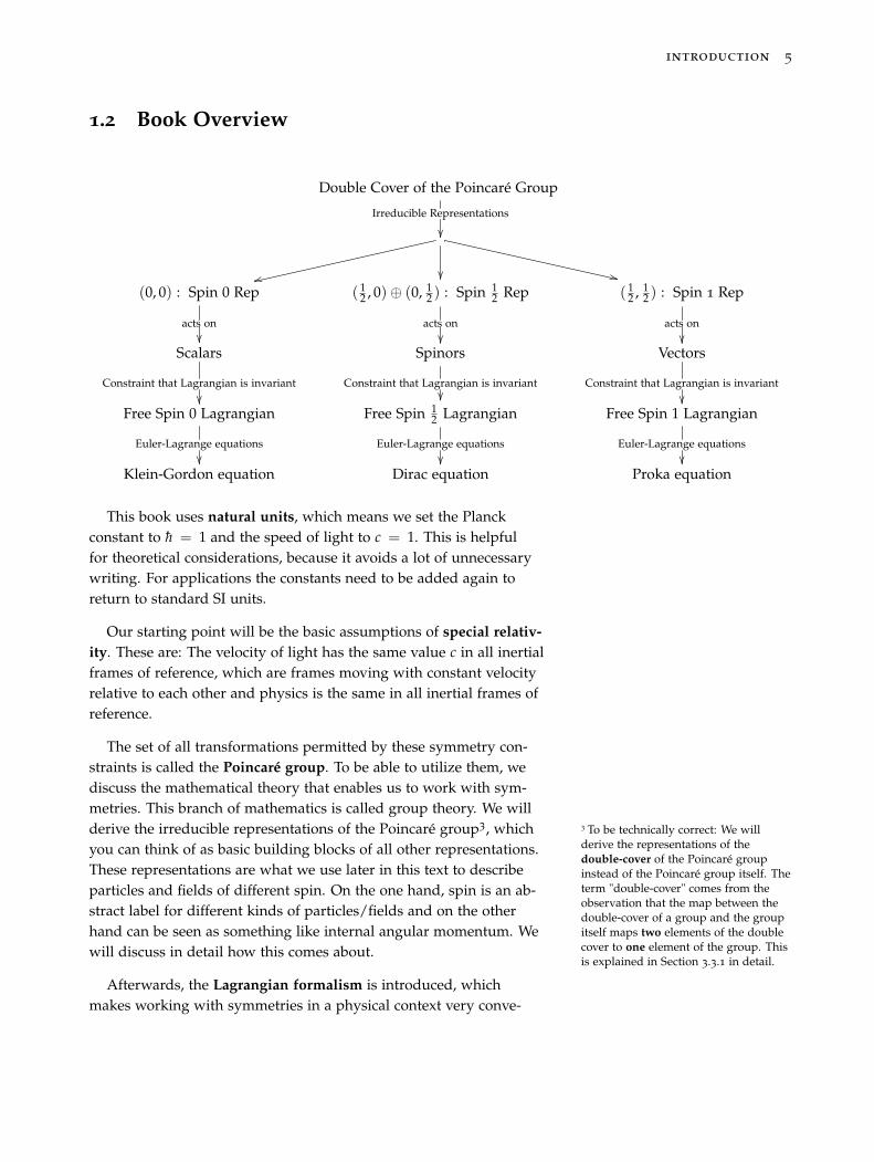
This book uses natural units, which means we set the Planckconstant to h = 1 and the speed of light to c = 1. This is helpfulfor theoretical considerations, because it avoids a lot of unnecessarywriting. For applications the constants need to be added again toreturn to standard SI units.
Our starting point will be the basic assumptions of special relativ-ity. These are: The velocity of light has the same value c in all inertialframes of reference, which are frames moving with constant velocityrelative to each other and physics is the same in all inertial frames ofreference.
The set of all transformations permitted by these symmetry con-straints is called the Poincaré group. To be able to utilize them, wediscuss the mathematical theory that enables us to work with sym-metries. This branch of mathematics is called group theory. We willderive the irreducible representations of the Poincaré group3, which 3 To be technically correct: We will
derive the representations of thedouble-cover of the Poincaré groupinstead of the Poincaré group itself. Theterm "double-cover" comes from theobservation that the map between thedouble-cover of a group and the groupitself maps two elements of the doublecover to one element of the group. Thisis explained in Section 3.3.1 in detail.
you can think of as basic building blocks of all other representations.These representations are what we use later in this text to describeparticles and fields of different spin. On the one hand, spin is an ab-stract label for different kinds of particles/fields and on the otherhand can be seen as something like internal angular momentum. Wewill discuss in detail how this comes about.
Afterwards, the Lagrangian formalism is introduced, whichmakes working with symmetries in a physical context very conve-
6 physics from symmetry
nient. The central object is the Lagrangian. Different Lagrangiansdescribe different physical systems and we will derive several La-grangians using symmetry considerations. In addition, the Euler-Lagrange equations are derived. These enable us to derive the equa-tions of motion from a given Lagrangian. Using the irreducible rep-resentations of the Poincaré group, the fundamental equations ofmotion for fields and particles with different spin can be derived.
The central idea here is that the Lagrangian must be invariant(=does not change) under any transformation of the Poincaré group.This makes sure the equations of motion take the same form in allframes of reference, which we stated above as "physics is the same inall inertial frames".
Then, we will discover another symmetry of the Lagrangian forfree spin 1
2 fields: Invariance under U(1) transformations. Similarlyan internal symmetry for spin 1 fields can be found. Demandinglocal U(1) symmetry will lead us to coupling terms between spin 1
2and spin 1 fields. The Lagrangian with this coupling term is the cor-rect Lagrangian for quantum electrodynamics. A similar procedurefor local SU(2) and SU(3) transformations will lead us to the correctLagrangian for weak and strong interactions.
In addition, we discuss symmetry breaking and a special way tobreak symmetries called the Higgs mechanism. The Higgs mecha-nism enables us to describe particles with mass4.4 Without the Higgs mechanism, terms
describing mass in the Lagrangianspoil the symmetry and are thereforeforbidden.
Afterwards, Noether’s theorem is derived, which reveals a deepconnection between symmetries and conserved quantities. We willutilize this connection by identifying each physical quantity withthe corresponding symmetry generator. This leads us to the mostimportant equation of quantum mechanics
[xi, pj] = iδij (1.1)
and quantum field theory
[Φ(x), π(y)] = iδ(x − y). (1.2)
We continue by taking the non-relativistic5 limit of the equation5 Non-relativistic means that everythingmoves slowly compared to the speed oflight and therefore especially curiousfeatures of special relativity are toosmall to be measurable.
of motion for spin 0 particles, called Klein-Gordon equation, whichresult in the famous Schrödinger equation. This, together with theidentifications we made between physical quantities and the genera-tors of the corresponding symmetries, is the foundation of quantummechanics.
Then we take a look at free quantum field theory, by starting
introduction 7
with the solutions of the different equations of motion6 and Eq. 1.2. 6 The Klein-Gordon, Dirac, Proka andMaxwell equations.Afterwards, we take interactions into account, by taking a closer look
at the Lagrangians with coupling terms between fields of differentspin. This enables us to discuss how the probability amplitude forscattering processes can be derived.
By deriving the Ehrenfest theorem the connection between quan-tum and classical mechanics is revealed. Furthermore, the fun-damental equations of classical electrodynamics, including theMaxwell equations and the Lorentz force law, are derived.
Finally, the basic structure of the modern theory of gravity, calledgeneral relativity, is briefly introduced and some remarks regardingthe difficulties in the derivation of a quantum theory of gravity aremade.
The major part of this book is about the tools we need to workwith symmetries mathematically and about the derivation of what iscommonly known as the standard model. The standard model usesquantum field theory to describe the behavior of all known elemen-tary particles. Until the present day, all experimental predictions ofthe standard model have been correct. Every other theory introducedhere can then be seen to follow from the standard model as a specialcase. For example in the limit of macroscopic objects we get classicalmechanics or in the limit of elementary particles with low energy,we get quantum mechanics. For those readers who have never heardabout the presently-known elementary particles and their interac-tions, a really quick overview is included in the next section.
1.3 Elementary Particles and Fundamental Forces
There are two major categories for elementary particles: bosons andfermions. There can be never two fermions in exactly the same state,which is known as Pauli’s exclusion principle, but infinitely manybosons. This curious fact of nature leads to the completely differentbehavior of these particles:
• fermions are responsible for matter
• bosons for the forces of nature.
This means, for example, that atoms consist of fermions7, but the 7 Atoms consist of electrons, protonsand neutrons, which are all fermions.But take note that protons and neutronsare not fundamental and consist ofquarks, which are fermions, too.
electromagnetic-force is mediated by bosons. The bosons that areresponsible for electromagnetic interactions are called photons. Oneof the most dramatic consequences of thie exclusion principle is thatthere is stable matter at all. If there could be infinitely many fermionsin the same state, there would be no stable matter8. 8 We will discuss this in Chapter 6
8 physics from symmetry
There are four presently known fundamental forces
• The electromagnetic force, which is mediated by massless photons.
• The weak force, which is mediated by massive W+, W− and Z-bosons.
• The strong force, which is mediated by massless gluons.
• Gravity, which is (maybe) mediated by gravitons.
Some of the these bosons are massless and some are not and thistells us something deep about nature. We will fully understand thisafter setting up the appropriate framework. For the moment, justtake note that each force is closely related to a symmetry. The factthat the bosons mediating the weak force are massive means therelated symmetry is broken. This process of spontaneous symmetrybreaking is responsible for the masses of all elementary particles.We will see later that this is possible through the coupling to anotherfundamental boson, the Higgs boson.
Fundamental particles interact via some force if they carry thecorresponding charge9.9 All charges have a beautiful common
origin that will be discussed in Chapter7. • For the electromagnetic force this is the electric charge and conse-
quently only electrically charged particles take part in electromag-netic interactions.
• For the weak force, the charge is called isospin10. All known10 Often the charge of the weak forcecarries the extra prefix "weak", i.e. iscalled weak isospin, because thereis another concept called isospin forcomposite objects that interact via thestrong force. Nevertheless, this is not afundamental charge and in this bookthe prefix "weak" is omitted.
fermions carry isospin and therefore interact via the weak force.
• The charge of the strong force is called color, because of somecurious features it shares with the humanly visible colors. Don’tlet this name confuse you, because this charge has nothing to dowith the colors you see in everyday life.
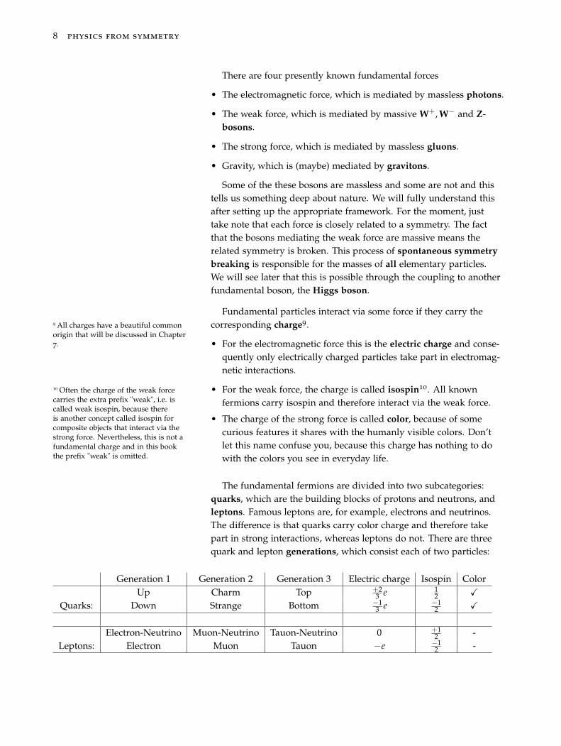
The fundamental fermions are divided into two subcategories:quarks, which are the building blocks of protons and neutrons, andleptons. Famous leptons are, for example, electrons and neutrinos.The difference is that quarks carry color charge and therefore takepart in strong interactions, whereas leptons do not. There are threequark and lepton generations, which consist each of two particles:
Generation 1 Generation 2 Generation 3 Electric charge Isospin ColorUp Charm Top +2
3 e 12 �
Quarks: Down Strange Bottom −13 e −1
2 �
Electron-Neutrino Muon-Neutrino Tauon-Neutrino 0 +12 -
Leptons: Electron Muon Tauon −e −12 -
introduction 9
Different particles can be identified through labels. In additionto the charges and the mass there is another incredibly importantlabel called spin, which can be seen as some kind of internal angularmomentum. Bosons carry integer spin, whereas fermions carry half-integer spin. The fundamental fermions we listed above have spin12 and almost all fundamental bosons have spin 1. There is only oneknown fundamental particle with spin 0: the Higgs boson.
There is an anti-particle for each particle, which carries exactly thesame labels with opposite sign11. For the electron the anti-particle 11 Maybe except for the mass label.
This is currently under experimentalinvestigation, for example at the AEGIS,the ATRAP and the ALPHA exper-iment, located at CERN in Geneva,Switzerland.
is called positron, but in general there is no extra name and only aprefix "anti". For example, the antiparticle corresponding to an up-quark is called anti-up-quark. Some particles, like the photon12 are
12 And maybe the neutrinos, which iscurrently under experimental investi-gation in many experiments that searchfor a neutrinoless double-beta decay.
their own anti-particle.
All these notions will be explained in more detail later in this text.Now it’s time to start with the derivation of the theory that describescorrectly the interplay of the different characters in this particle zoo.The first cornerstone towards this goal is Einstein’s famous theory ofspecial relativity, which is the topic of the next chapter.
2
Special Relativity
The famous Michelson-Morley experiment discovered that the speedof light has the same value in all reference frames1. Albert Einstein 1 The speed of objects we observe in
everyday life depend on the frameof reference. For example, when anobserver standing at a train stationmeasures that a train moves with50 km
h , another observer running with15 km
h next to the same train, measuresthat the train moves with 35 km
h . Incontrast, light always moves with1, 08 · 109 km
h , no matter how you moverelative to it.
recognized the far reaching consequences of this observation andaround this curious fact of nature he built the theory of special rela-tivity. Starting from the constant speed of light, Einstein was able topredict many interesting and strange consequences that all provedto be true. We will see how powerful this idea is, but first let’s clarifywhat special relativity is all about. The two basic postulates are
• The principle of relativity: Physics is the same in all inertialframes of reference, i.e. frames moving with constant velocityrelative to each other.
• The invariance of the speed of light: The velocity of light has thesame value c in all inertial frames of reference.
In addition, we will assume that the stage our physical laws act onis homogeneous and isotropic. This means it does not matter where(=homogeneity) we perform an experiment and how it is oriented(=isotropy), the laws of physics stay the same. For example, if twophysicists, one in New-York and the other one in Tokyo, perform ex-actly the same experiment, they would find the same2 physical laws. 2 Besides from changing constants,
as, for example, the gravitationalacceleration
Equally a physicist on planet Mars would find the same physicallaws.
The laws of physics, formulated correctly, shouldn’t change ifyou look at the experiment from a different perspective or repeatit tomorrow. In addition, the first postulate tells us that a physicalexperiment should come up with the same result regardless of ifyou perform it on a wagon moving with constant speed or at rest ina laboratory. These things coincide with everyday experience. Forexample, if you close your eyes in a car moving with constant speed,there is no way to tell if you are really moving or if you’re at rest.
© Springer International Publishing AG 2018J. Schwichtenberg, Physics from Symmetry, UndergraduateLecture Notes in Physics, https://doi.org/10.1007/978-3-319-66631-0_2
12 physics from symmetry
Without homogeneity and isotropy physics would be in deeptrouble: If the laws of nature we deduce from experiment would holdonly at one point in space, for a specific orientation of the experimentsuch laws would be rather useless.
The only unintuitive thing is the second postulate, which is con-trary to all everyday experience. Nevertheless, all experiments untilthe present day show that it is correct.
2.1 The Invariant of Special Relativity
Before we dive into the details, here’s a short summary of what wewant to do in the following sections. We use the postulates of specialrelativity to derive the Minkowski metric, which tells us how to com-pute the "distance" between two physical events. Another name forphysical events in this context is points in Minkowski space, whichis how the stage the laws of special relativity act on is called. It thenfollows that all transformations connecting different inertial frames ofreference must leave the Minkowski metric unchanged. This is howwe are able to find all transformations that connect allowed framesof reference, i.e. frames with a constant speed of light. In the rest ofthe book we will use the knowledge of these transformations, to findequations that are unchanged by these transformations. Let’s startwith a thought experiment that enables us to derive one of the mostfundamental consequences of the postulates of special relativity.
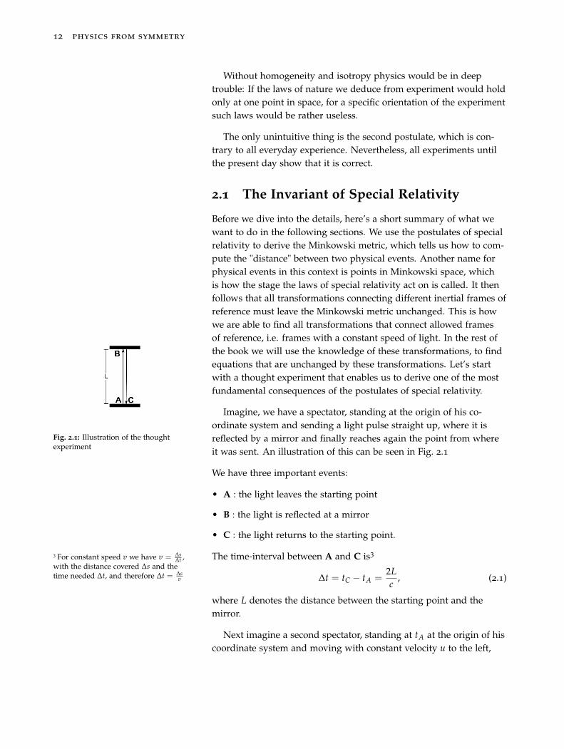
Fig. 2.1: Illustration of the thoughtexperiment
Imagine, we have a spectator, standing at the origin of his co-ordinate system and sending a light pulse straight up, where it isreflected by a mirror and finally reaches again the point from whereit was sent. An illustration of this can be seen in Fig. 2.1
We have three important events:
• A : the light leaves the starting point
• B : the light is reflected at a mirror
• C : the light returns to the starting point.
The time-interval between A and C is33 For constant speed v we have v = ΔsΔt ,
with the distance covered Δs and thetime needed Δt, and therefore Δt = Δs
v Δt = tC − tA =2Lc
, (2.1)
where L denotes the distance between the starting point and themirror.
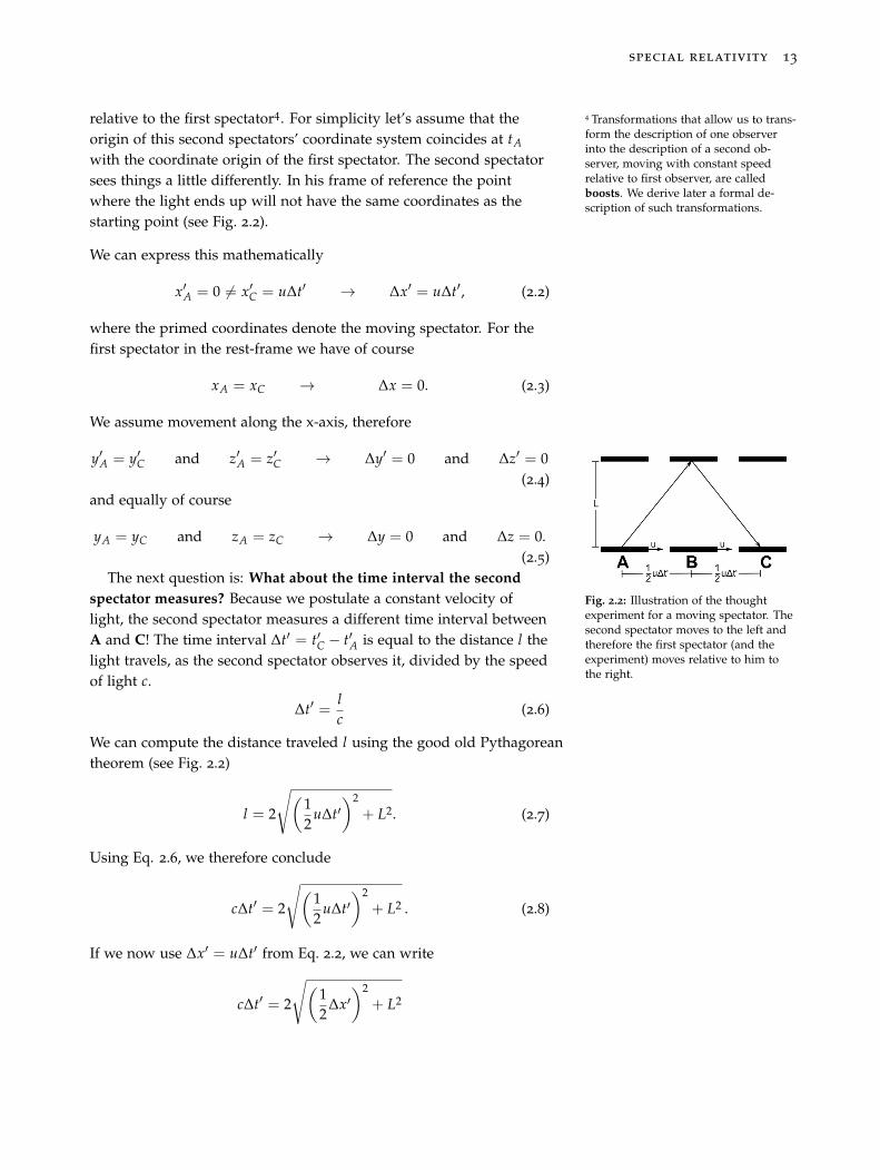
Next imagine a second spectator, standing at tA at the origin of hiscoordinate system and moving with constant velocity u to the left,
special relativity 13
relative to the first spectator4. For simplicity let’s assume that the 4 Transformations that allow us to trans-form the description of one observerinto the description of a second ob-server, moving with constant speedrelative to first observer, are calledboosts. We derive later a formal de-scription of such transformations.
origin of this second spectators’ coordinate system coincides at tA
with the coordinate origin of the first spectator. The second spectatorsees things a little differently. In his frame of reference the pointwhere the light ends up will not have the same coordinates as thestarting point (see Fig. 2.2).
We can express this mathematically
x′A = 0 �= x′C = uΔt′ → Δx′ = uΔt′, (2.2)
where the primed coordinates denote the moving spectator. For thefirst spectator in the rest-frame we have of course
xA = xC → Δx = 0. (2.3)
We assume movement along the x-axis, therefore
y′A = y′C and z′A = z′C → Δy′ = 0 and Δz′ = 0(2.4)
and equally of course
yA = yC and zA = zC → Δy = 0 and Δz = 0.(2.5)
Fig. 2.2: Illustration of the thoughtexperiment for a moving spectator. Thesecond spectator moves to the left andtherefore the first spectator (and theexperiment) moves relative to him tothe right.
The next question is: What about the time interval the secondspectator measures? Because we postulate a constant velocity oflight, the second spectator measures a different time interval betweenA and C! The time interval Δt′ = t′C − t′A is equal to the distance l thelight travels, as the second spectator observes it, divided by the speedof light c.
Δt′ = lc
(2.6)
We can compute the distance traveled l using the good old Pythagoreantheorem (see Fig. 2.2)
l = 2
√(12
uΔt′)2
+ L2. (2.7)
Using Eq. 2.6, we therefore conclude
cΔt′ = 2
√(12
uΔt′)2
+ L2 . (2.8)
If we now use Δx′ = uΔt′ from Eq. 2.2, we can write
cΔt′ = 2
√(12
Δx′)2
+ L2
14 physics from symmetry
→ (cΔt′)2 = 4
((12
Δx′)2
+ L2
)
→ (cΔt′)2 − (Δx′)2 = 4
((12
Δx′)2
+ L2
)− (Δx′)2 = 4L2 (2.9)
and now recalling from Eq. 2.1 that Δt = 2Lc , we can write
(cΔt′)2 − (Δx′)2 = 4L2 = (cΔt)2 = (Δtc)2 − (Δx)2︸ ︷︷ ︸=0 see Eq. 2.3
. (2.10)
So finally, we arrive5 at5 Take note that what we are doing hereis just the shortest path to the result,because we chose the origins of thetwo coordinate systems to coincideat tA. Nevertheless, the same can bedone, with more effort, for arbitrarychoices, because physics is the samein all inertial frames. We used thisfreedom to choose two inertial frameswhere the computation is easy. Inan arbitrarily moving second inertialsystem we do not have Δy′ = 0 andΔz′ = 0. Nevertheless, the equationholds, because physics is the same in allinertial frames.
(cΔt′)2 − (Δx′)2 − (Δy′)2︸ ︷︷ ︸=0
− (Δz′)2︸ ︷︷ ︸=0
= (cΔt)2 − (Δx)2︸ ︷︷ ︸=0
− (Δy)2︸ ︷︷ ︸=0
− (Δz)2︸ ︷︷ ︸=0
.
(2.11)Considering a third observer, moving with a different velocity rela-tive to the first observer, we can use the same reasoning to arrive at
(cΔt′′)2 − (Δx′′)2 − (Δy′′)2 − (Δz′′)2 = (cΔt)2 − (Δx)2 − (Δy)2 − (Δz)2
(2.12)Therefore, we have found something which is the same for allobservers: the quadratic form
(Δs)2 ≡ (cΔt)2 − (Δx)2 − (Δy)2 − (Δz)2. (2.13)
In addition, we learned in this section that (Δx)2 + (Δy)2 + (Δz)2
or (cΔt)2 aren’t the same for different observers. We will talk aboutthe implications of this curious property in the next section.
2.2 Proper Time
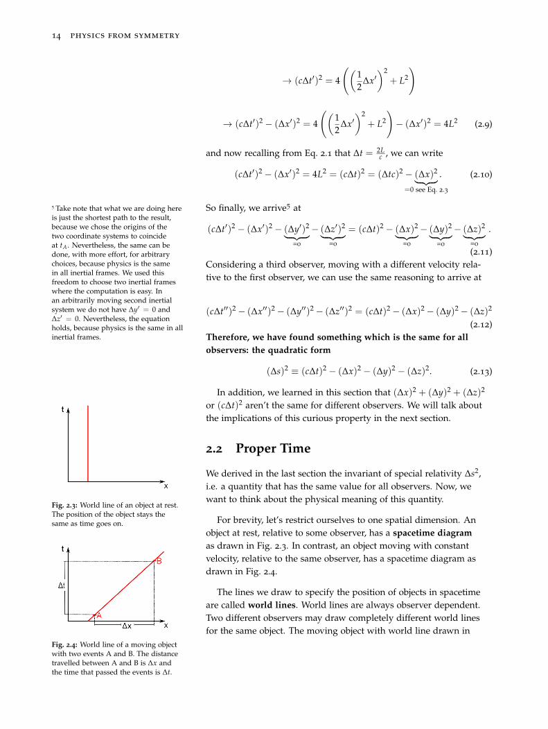
Fig. 2.3: World line of an object at rest.The position of the object stays thesame as time goes on.
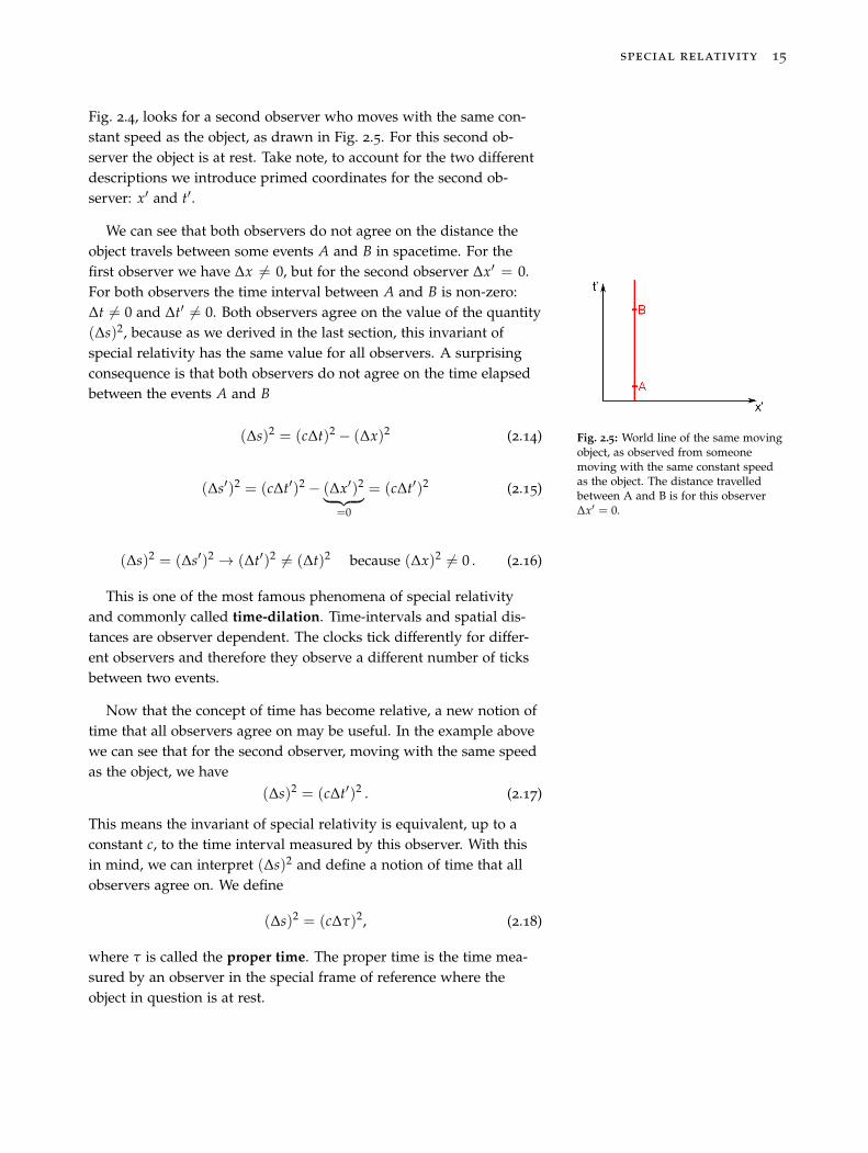
Fig. 2.4: World line of a moving objectwith two events A and B. The distancetravelled between A and B is Δx andthe time that passed the events is Δt.
We derived in the last section the invariant of special relativity Δs2,i.e. a quantity that has the same value for all observers. Now, wewant to think about the physical meaning of this quantity.
For brevity, let’s restrict ourselves to one spatial dimension. Anobject at rest, relative to some observer, has a spacetime diagramas drawn in Fig. 2.3. In contrast, an object moving with constantvelocity, relative to the same observer, has a spacetime diagram asdrawn in Fig. 2.4.
The lines we draw to specify the position of objects in spacetimeare called world lines. World lines are always observer dependent.Two different observers may draw completely different world linesfor the same object. The moving object with world line drawn in
special relativity 15
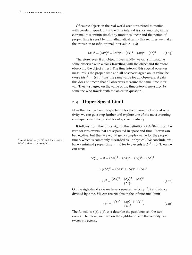
Fig. 2.4, looks for a second observer who moves with the same con-stant speed as the object, as drawn in Fig. 2.5. For this second ob-server the object is at rest. Take note, to account for the two differentdescriptions we introduce primed coordinates for the second ob-server: x′ and t′.
We can see that both observers do not agree on the distance theobject travels between some events A and B in spacetime. For thefirst observer we have Δx �= 0, but for the second observer Δx′ = 0.For both observers the time interval between A and B is non-zero:Δt �= 0 and Δt′ �= 0. Both observers agree on the value of the quantity(Δs)2, because as we derived in the last section, this invariant ofspecial relativity has the same value for all observers. A surprisingconsequence is that both observers do not agree on the time elapsedbetween the events A and B
Fig. 2.5: World line of the same movingobject, as observed from someonemoving with the same constant speedas the object. The distance travelledbetween A and B is for this observerΔx′ = 0.
(Δs)2 = (cΔt)2 − (Δx)2 (2.14)
(Δs′)2 = (cΔt′)2 − (Δx′)2︸ ︷︷ ︸=0
= (cΔt′)2 (2.15)
(Δs)2 = (Δs′)2 → (Δt′)2 �= (Δt)2 because (Δx)2 �= 0 . (2.16)
This is one of the most famous phenomena of special relativityand commonly called time-dilation. Time-intervals and spatial dis-tances are observer dependent. The clocks tick differently for differ-ent observers and therefore they observe a different number of ticksbetween two events.
Now that the concept of time has become relative, a new notion oftime that all observers agree on may be useful. In the example abovewe can see that for the second observer, moving with the same speedas the object, we have
(Δs)2 = (cΔt′)2 . (2.17)
This means the invariant of special relativity is equivalent, up to aconstant c, to the time interval measured by this observer. With thisin mind, we can interpret (Δs)2 and define a notion of time that allobservers agree on. We define
(Δs)2 = (cΔτ)2, (2.18)
where τ is called the proper time. The proper time is the time mea-sured by an observer in the special frame of reference where theobject in question is at rest.
16 physics from symmetry
Of course objects in the real world aren’t restricted to motionwith constant speed, but if the time interval is short enough, in theextremal case infinitesimal, any motion is linear and the notion ofproper time is sensible. In mathematical terms this requires we makethe transition to infinitesimal intervals Δ → d:
(ds)2 = (cdτ)2 = (cdt)2 − (dx)2 − (dy)2 − (dz)2. (2.19)
Therefore, even if an object moves wildly, we can still imaginesome observer with a clock travelling with the object and thereforeobserving the object at rest. The time interval this special observermeasures is the proper time and all observers agree on its value, be-cause (ds)2 = (cdτ)2 has the same value for all observers. Again,this does not mean that all observers measure the same time inter-val! They just agree on the value of the time interval measured bysomeone who travels with the object in question.
2.3 Upper Speed Limit
Now that we have an interpretation for the invariant of special rela-tivity, we can go a step further and explore one of the most stunningconsequences of the postulates of special relativity.
It follows from the minus sign in the definition of Δs2that it can bezero for two events that are separated in space and time. It even canbe negative, but then we would get a complex value for the propertime6, which is commonly discarded as unphysical. We conclude, we6 Recall (ds)2 = (cdτ)2 and therefore if
(ds)2 < 0 → dτ is complex. have a minimal proper time τ = 0 for two events if Δs2 = 0. Then wecan write
Δs2min = 0 = (cΔt)2 − (Δx)2 − (Δy)2 − (Δz)2
→ (cΔt)2 = (Δx)2 + (Δy)2 + (Δz)2
→ c2 =(Δx)2 + (Δy)2 + (Δz)2
(Δt)2 . (2.20)
On the right-hand side we have a squared velocity v2, i.e. distancedivided by time. We can rewrite this in the infinitesimal limit
→ c2 =(dx)2 + (dy)2 + (dz)2
(dt)2 . (2.21)
The functions x(t), y(t), z(t) describe the path between the twoevents. Therefore, we have on the right-hand side the velocity be-tween the events.
special relativity 17
We conclude the lowest value for the proper time is measured bysomeone travelling with speed
→ c2 = v2. (2.22)
This means nothing can move with a velocity larger than c! Wehave an upper speed limit for everything in physics. Two eventsin spacetime can’t be connected by anything faster than c.
From this observation follows the principle of locality, whichmeans that everything in physics can only be influenced by its imme-diate surroundings. Every interaction must be local and there can beno action at a distance, because everything in physics needs time totravel from some point to another.
2.4 The Minkowski Notation
Henceforth space by itself, and time by itself, are doomed to fade awayinto mere shadows, and only a kind of union of the two will preservean independent reality.
- Hermann Minkowski7 7 In a speech at the 80th Assemblyof German Natural Scientists andPhysicians (21 September 1908)We can rewrite the invariant of special relativity
ds2 = (cdt)2 − (dx)2 − (dy)2 − (dz)2 (2.23)
by using a new notation, which looks quite complicated at first sight,but will prove to be invaluable:
ds2 = ημνdxμdxν = η00(dx0)2 + η11(dx1)
2 + η22(dx2)2 + η33(dx3)
2
= (dx0)2 − (dx1)
2 − (dx2)2 − (dx3)
2 = (cdt)2 − (dx)2 − (dy)2 − (dz)2.(2.24)
Here we use several new notations and conventions one needs tobecome familiar with, because they are used everywhere in modernphysics:
• Einsteins summation convention: If an index occurs twice, a sumis implicitly assumed : ∑3
i=1 aibi = aibi = a1b1 + a2b2 + a3b3, but∑3
i=1 aibj = a1bj + a2bj + a3bj �= aibj
• Greek indices8, like μ, ν or σ, are always summed from 0 to 3: 8 In contrast, Roman indices like i, j, kare always summed: xixi ≡ ∑3
i xixifrom 1 to 3. Much later in the bookwe will use capital Roman letters likeA, B, C that are summed from 1 to 8.
xμyμ = ∑3μ=0 xμyμ.
• Renaming of the variables x0 ≡ ct, x1 ≡ x, x2 ≡ y and x3 ≡ z, tomake it obvious that time and space are now treated equally andto be able to use the rules introduced above
18 physics from symmetry
• Introduction of the Minkowski metric η00 = 1, η11 = −1, η22 = −1,η33 = −1 and ημν = 0 for μ �= ν ( an equal way of writing this is9
9 η =
⎛⎜⎜⎝1 0 0 00 −1 0 00 0 −1 00 0 0 −1
⎞⎟⎟⎠ η = diag(1,−1,−1,−1) )
In addition, it’s conventional to introduce the notion of a four-vector
dxμ =
⎛⎜⎜⎜⎝dx0
dx1
dx2
dx3
⎞⎟⎟⎟⎠ , (2.25)
because the equation above can be written equally using four-vectorsand the Minkowski metric in matrix form
(ds)2 = dxμημνdxν =(
dx0 dx1 dx2 dx3
)⎛⎜⎜⎜⎝1 0 0 00 −1 0 00 0 −1 00 0 0 −1
⎞⎟⎟⎟⎠⎛⎜⎜⎜⎝
dx0
dx1
dx2
dx3
⎞⎟⎟⎟⎠= dx2
0 − dx21 − dx2
2 − dx23 (2.26)
This is really just a clever way of writing things. A physical in-terpretation of ds is that it is the "distance" between two events inspacetime. Take note that we don’t mean here only the spatial dis-tance, but also have to consider a separation in time. If we consider3-dimensional Euclidean10 space the squared (shortest) distance be-10 3-dimensional Euclidean space is just
the space of classical physics, wheretime was treated differently from spaceand therefore it was not included intothe geometric considerations. Thenotion of spacetime, with time as afourth coordinate was introduced withspecial relativity, which enables mixingof time and space coordinates as wewill see.
tween two points is given by11
11 The Kronecker delta δij, which is theidentity matrix in index notation, isdefined in Appendix B.5.5.
(ds)2 = dxiδijdxj =(
dx1 dx2 dx3
)⎛⎜⎝1 0 00 1 00 0 1
⎞⎟⎠⎛⎜⎝dx1
dx2
dx3
⎞⎟⎠= (ds)2 = (dx1)
2 + (dx2)2 + (dx3)
2 (2.27)
The mathematical tool that tells us the distance between two in-finitesimal separated points is called metric. In boring Euclideanspace the metric is just the identity matrix δ. In the curved space-time of general relativity much more complicated metrics can occur.The geometry of the spacetime of special relativity is encoded in therelatively simple Minkowski metric η. Because the metric is the toolto compute length, we need it to define the length of a four-vector,which is given by the scalar product of the vector with itself1212 The same is true in Euclidean space:
length2(v) = �v · �v = v21 + v2
2 + v23,
because the metric is here simply
δ =
⎛⎝1 0 00 1 00 0 1
⎞⎠.
x2 = x · x ≡ xμxνημν .
Analogously, the scalar product of two arbitrary four-vectors is
special relativity 19
defined by
x · y ≡ xμyνημν. (2.28)
There is another, notational convention to make computationsmore streamlined. We define a four-vector with upper index as13 13 Four-vectors with a lower index are
often called covariant and four-vectorswith an upper index contravariant.
xμ ≡ ημνxν (2.29)
or equally
yν ≡ ημνyμ =︸︷︷︸The Minkowski metric is symmetric ημν=ηνμ
ηνμyμ . (2.30)
Therefore, we can write the scalar product of two four-vectors as14 14 The name of the index makes nodifference. For more information aboutthis have a look at Appendix B.5.1.
x · y ≡ xμyνημν = xμyμ = xνyν. (2.31)
It doesn’t matter which index we transform to an upper index. Thisis just a way of avoiding writing the Minkowski metric all the time,just as Einstein’s summation convention is introduced to avoid writ-ing the summation sign.
2.5 Lorentz Transformations
Next, we try to figure out in what ways we can transform our de-scription in a given frame of reference without violating the postu-lates of special-relativity. We learned above that it follows directlyfrom the two postulates that ds2 = ημνdxμdxν is the same in all iner-tial frames of reference:
ds′2 = dx′μdx′νημν = ds2 = dxμdxνημν. (2.32)
Therefore, allowed transformations are those which leave this quadraticform or equally the scalar product of Minkowski spacetime invariant.Denoting a generic transformation that transforms the description inone frame of reference into the description in another frame with Λ,the transformed coordinates dx′μ can be written as:
dxμ → dx′μ = Λ σμ dxσ. (2.33)
Then we can write the invariance condition as
20 physics from symmetry
(ds)2 = (ds′)2
→ dx · dx != dx′ · dx′
→ dxμdxνημν != dx′μdx′νημν =︸︷︷︸
Eq. 2.33
Λ σμ dxσΛ γ
ν dxγημν
→︸︷︷︸Renaming dummy indices
dxμdxνημν != Λ μ
σ dxμΛ νγ dxνησγ
→︸︷︷︸Because the equation holds for arbitrary dxμ
ημν != Λ μ
σ ησγΛ νγ . (2.34)
Or written in matrix notation1515 If you wonder about the transposehere have a look at Appendix C.1.
η = ΛTηΛ (2.35)
This is the condition that transformations Λ between allowedframes of reference must fulfil.
If this seems strange at this point don’t worry, because we will seethat such a condition is a quite natural thing. In the next chapter wewill learn that, for example, rotations in ordinary Euclidean space aredefined as those transformations O that leave the scalar product ofEuclidean space invariant1616 The · is used for the scalar product of
vectors, which corresponds to�a ·�b =
�aT�b for ordinary matrix multiplication,where a vector is an 1 × 3 matrix. Thefact (Oa)T = aTOT is explained inAppendix C.1, specifically Eq. C.3.
�a ·�b !=�a′ ·�b′ =︸︷︷︸
Take note that (Oa)T=aTOT
�aTOTO�b. (2.36)
Therefore17 OT1O != 1 and we can see that the metric of Euclidean
17 This condition is often called orthog-onality, hence the symbol O. A matrixsatisfying OTO = 1 is called orthogonal,because its columns are orthogonalto each other. In other words: Eachcolumn of a matrix can be thought ofas a vector and the orthogonality condi-tion for matrices means that each suchvector is orthogonal to all other columnvectors.
space, which is just the unit matrix 1, plays the same role as theMinkowski metric in Eq. 2.35. This is one part of the definition forrotations, because the defining feature of rotations is that they leavethe length of a vector unchanged, which corresponds mathematicallyto the invariance of the scalar product18. Additionally we must in-
18 Recall that the length of a vector isgiven by the scalar product of a vectorwith itself.
clude that rotations do not change the orientation19 of our coordinate
19 This is explained in Appendix A.5.
system, which means mathematically det O != 1, because there are
other transformations which leave the length of any vector invariant:spatial inversions20
20 A spatial inversion is simply a map�x → −�x. Mathematically such trans-formations are characterized by the
conditions det O != −1 and OTO = 1.
Therefore, if we only want to talk aboutrotations we have the extra conditiondet O !
= 1. Another name for spatialinversions are parity transformations.
We define the Lorentz transformations as those transformationsthat leave the scalar product of Minkowski spacetime invariant. Inphysical terms this means that Lorentz transformations describechanges between frames of references that respect the postulatesof special relativity. In turn this does mean, of course, that every-time we want to get a term that does not change under Lorentztransformations, we must combine an upper with a lower index:
special relativity 21
xμyμ = xμyνημν. We will construct explicit matrices for the allowedtransformations in the next chapter, after we have learned some veryelegant techniques for dealing with conditions like this.
2.6 Invariance, Symmetry and Covariance
Before we move on, we have to talk about some very important no-tions. Firstly, we call something invariant, if it does not change undertransformations. For instance, let’s consider something arbitrary likeF = F(A, B, C, ...) that depends on different quantities A, B, C, .... Ifwe transform A, B, C, ... → A′, B′, C′, ... and we have
F(A′, B′, C′, ...) = F(A, B, C, ...) (2.37)
F is called invariant under this transformation. We can express thisdifferently using the word symmetry. Symmetry is defined as in-variance under a transformation or class of transformations. Forexample, some physical system is symmetric under rotations if wecan rotate it arbitrarily and it always stays exactly the same. Anotherexample would be a room with constant temperature. The quantitytemperature does not depend on the position of measurement. Inother words, the quantity temperature is invariant under translations.A translation means that we move every point a given distance in aspecified direction. Therefore, we have translational symmetry withinthis room.
Covariance means something similar, but may not be confusedwith invariance. An equation is called covariant, if it takes the sameform when the objects in it are transformed. For instance, if we havean equation
E1 = aA2 + bBA + cC4
and after the transformation this equation reads
E′1 = aA′2 + bB′A′ + cC′4
the equation is called covariant, because the form stayed the same.Another equation
E2 = x2 + 4axy + z
that after a transformation looks like
E′2 = y′3 + 4az′y′ + y′2 + 8z′x′
is not covariant, because it changed its form completely.
22 physics from symmetry
All physical laws must be covariant under Lorentz transformations,because only such laws are valid in all reference frames. Formulat-ing the laws of physics in a non-covariant way would be a very badidea, because such laws would only hold in one frame of reference.The laws of physics would look differently in Tokyo and New York.There is no preferred frame of reference and we therefore want ourlaws to hold in all reference frames. We will learn later how we canformulate the laws of physics in a covariant manner.
special relativity 23
Further Reading Tips
• E. Taylor and J. Wheeler - Spacetime Physics: Introduction toSpecial Relativity21 is a very good book to start with. 21 Edwin F. Taylor and John Archibald
Wheeler. Spacetime Physics. W. H.Freeman, 2nd edition, 3 1992. ISBN9780716723271
• D. Fleisch - A Student’s Guide to Vectors and Tensors22 has very
22 Daniel Fleisch. A Student’s Guideto Vectors and Tensors. CambridgeUniversity Press, 1st edition, 11 2011.ISBN 9780521171908
creative explanations for the tensor formalism used in specialrelativity, for example, for the differences between covariant andcontravariant components.
• N. Jeevanjee - An Introduction to Tensors and Group Theory forPhysicists23 is another good source for the mathematics needed in
23 Nadir Jeevanjee. An Introduction toTensors and Group Theory for Physicists.Birkhaeuser, 1st edition, August 2011.ISBN 978-0817647148
special relativity.
• A. Zee - Einstein Gravity in a nutshell24 is a book about gen-
24 Anthony Zee. Einstein Gravity in aNutshell. Princeton University Press, 1stedition, 5 2013. ISBN 9780691145587
eral relativity, but has many great explanations regarding specialrelativity, too.
Part IISymmetry Tools
"Numbers measure size, groups measure symmetry."
Mark A. Armstrongin Groups and Symmetry.
Springer, 2nd edition, 2 1997.ISBN 9780387966755
3
Lie Group Theory
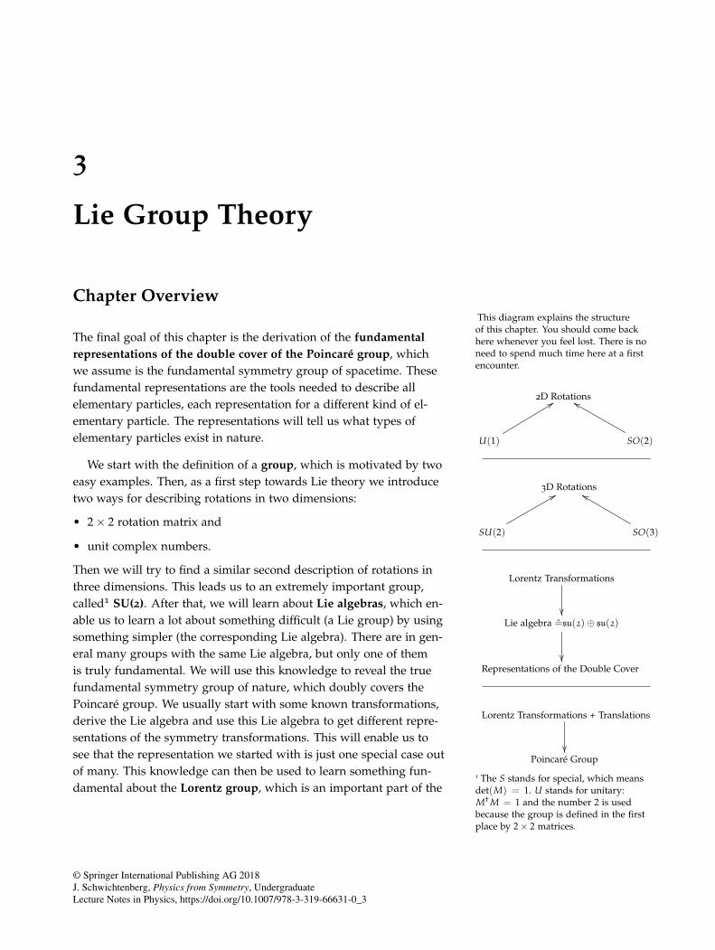
Chapter OverviewThis diagram explains the structureof this chapter. You should come backhere whenever you feel lost. There is noneed to spend much time here at a firstencounter.
2D Rotations
U(1)
��
SO(2)
��
3D Rotations
SU(2)
��
SO(3)
��
Lorentz Transformations
��Lie algebra =su(2)⊕ su(2)
��Representations of the Double Cover
Lorentz Transformations + Translations
��Poincaré Group
The final goal of this chapter is the derivation of the fundamentalrepresentations of the double cover of the Poincaré group, whichwe assume is the fundamental symmetry group of spacetime. Thesefundamental representations are the tools needed to describe allelementary particles, each representation for a different kind of el-ementary particle. The representations will tell us what types ofelementary particles exist in nature.
We start with the definition of a group, which is motivated by twoeasy examples. Then, as a first step towards Lie theory we introducetwo ways for describing rotations in two dimensions:
• 2 × 2 rotation matrix and
• unit complex numbers.
Then we will try to find a similar second description of rotations inthree dimensions. This leads us to an extremely important group,called1 SU(2). After that, we will learn about Lie algebras, which en-
1 The S stands for special, which meansdet(M) = 1. U stands for unitary:M† M = 1 and the number 2 is usedbecause the group is defined in the firstplace by 2 × 2 matrices.
able us to learn a lot about something difficult (a Lie group) by usingsomething simpler (the corresponding Lie algebra). There are in gen-eral many groups with the same Lie algebra, but only one of themis truly fundamental. We will use this knowledge to reveal the truefundamental symmetry group of nature, which doubly covers thePoincaré group. We usually start with some known transformations,derive the Lie algebra and use this Lie algebra to get different repre-sentations of the symmetry transformations. This will enable us tosee that the representation we started with is just one special case outof many. This knowledge can then be used to learn something fun-damental about the Lorentz group, which is an important part of the
© Springer International Publishing AG 2018J. Schwichtenberg, Physics from Symmetry, UndergraduateLecture Notes in Physics, https://doi.org/10.1007/978-3-319-66631-0_3
26 physics from symmetry
Poincaré group. We will see that the Lie algebra of the double coverof the Lorentz group consists of two copies of the SU(2) Lie algebra.Therefore, we can directly use everything we learned about SU(2).Finally, we include translations into the considerations, which leadsus to the Poincaré group. The Poincaré group is the Lorentz groupplus translations. At this point, we will have everything at hand toclassify the fundamental representations of the double cover of thePoincaré group. We use these fundamental representations in laterchapters to derive the fundamental laws of physics.
3.1 Groups
If we want to utilize the power of symmetry, we need a frameworkto deal with symmetries mathematically. The branch of mathematicsthat deals with symmetries is called group theory. A special branchof group theory that deals with continuous symmetries is Lie The-ory.
Symmetry is defined as invariance under a set of of transforma-tions and therefore, one defines a group as a collection of transforma-tions. Let us get started with two easy examples to get a feel for whatwe want to do:
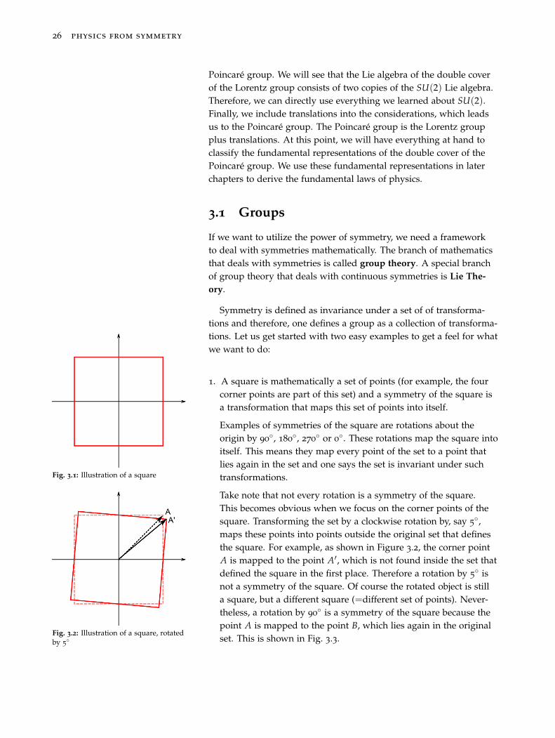
1. A square is mathematically a set of points (for example, the fourcorner points are part of this set) and a symmetry of the square isa transformation that maps this set of points into itself.
Fig. 3.1: Illustration of a square
Examples of symmetries of the square are rotations about theorigin by 90◦, 180◦, 270◦ or 0◦. These rotations map the square intoitself. This means they map every point of the set to a point thatlies again in the set and one says the set is invariant under suchtransformations.
Fig. 3.2: Illustration of a square, rotatedby 5◦
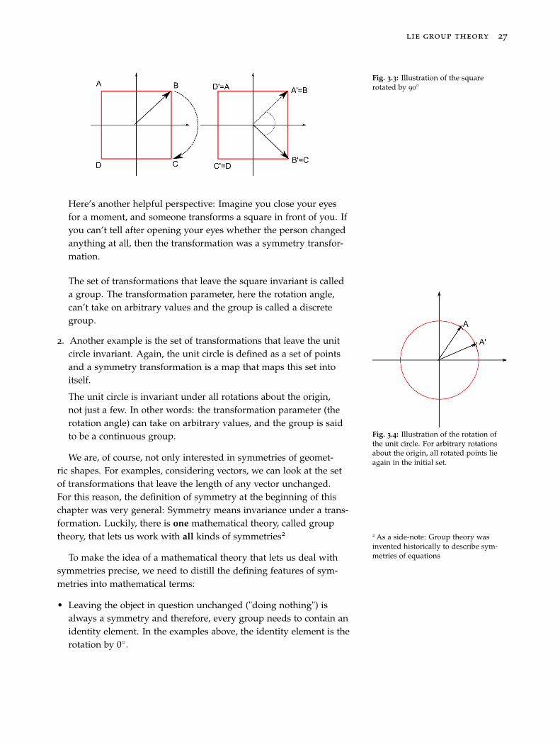
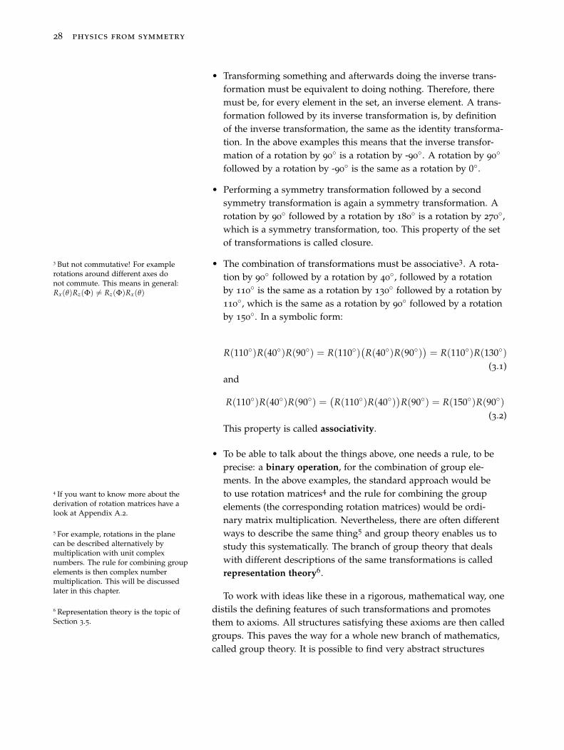
Take note that not every rotation is a symmetry of the square.This becomes obvious when we focus on the corner points of thesquare. Transforming the set by a clockwise rotation by, say 5◦,maps these points into points outside the original set that definesthe square. For example, as shown in Figure 3.2, the corner pointA is mapped to the point A′, which is not found inside the set thatdefined the square in the first place. Therefore a rotation by 5◦ isnot a symmetry of the square. Of course the rotated object is stilla square, but a different square (=different set of points). Never-theless, a rotation by 90◦ is a symmetry of the square because thepoint A is mapped to the point B, which lies again in the originalset. This is shown in Fig. 3.3.
lie group theory 27
Fig. 3.3: Illustration of the squarerotated by 90◦
Here’s another helpful perspective: Imagine you close your eyesfor a moment, and someone transforms a square in front of you. Ifyou can’t tell after opening your eyes whether the person changedanything at all, then the transformation was a symmetry transfor-mation.
The set of transformations that leave the square invariant is calleda group. The transformation parameter, here the rotation angle,can’t take on arbitrary values and the group is called a discretegroup.
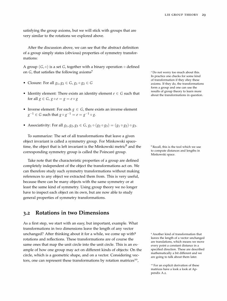
2. Another example is the set of transformations that leave the unitcircle invariant. Again, the unit circle is defined as a set of pointsand a symmetry transformation is a map that maps this set intoitself.
Fig. 3.4: Illustration of the rotation ofthe unit circle. For arbitrary rotationsabout the origin, all rotated points lieagain in the initial set.
The unit circle is invariant under all rotations about the origin,not just a few. In other words: the transformation parameter (therotation angle) can take on arbitrary values, and the group is saidto be a continuous group.
We are, of course, not only interested in symmetries of geomet-ric shapes. For examples, considering vectors, we can look at the setof transformations that leave the length of any vector unchanged.For this reason, the definition of symmetry at the beginning of thischapter was very general: Symmetry means invariance under a trans-formation. Luckily, there is one mathematical theory, called grouptheory, that lets us work with all kinds of symmetries2 2 As a side-note: Group theory was
invented historically to describe sym-metries of equationsTo make the idea of a mathematical theory that lets us deal with
symmetries precise, we need to distill the defining features of sym-metries into mathematical terms:
• Leaving the object in question unchanged ("doing nothing") isalways a symmetry and therefore, every group needs to contain anidentity element. In the examples above, the identity element is therotation by 0◦.
28 physics from symmetry
• Transforming something and afterwards doing the inverse trans-formation must be equivalent to doing nothing. Therefore, theremust be, for every element in the set, an inverse element. A trans-formation followed by its inverse transformation is, by definitionof the inverse transformation, the same as the identity transforma-tion. In the above examples this means that the inverse transfor-mation of a rotation by 90◦ is a rotation by -90◦. A rotation by 90◦
followed by a rotation by -90◦ is the same as a rotation by 0◦.
• Performing a symmetry transformation followed by a secondsymmetry transformation is again a symmetry transformation. Arotation by 90◦ followed by a rotation by 180◦ is a rotation by 270◦,which is a symmetry transformation, too. This property of the setof transformations is called closure.
• The combination of transformations must be associative3. A rota-3 But not commutative! For examplerotations around different axes donot commute. This means in general:Rx(θ)Rz(Φ) �= Rz(Φ)Rx(θ)
tion by 90◦ followed by a rotation by 40◦, followed by a rotationby 110◦ is the same as a rotation by 130◦ followed by a rotation by110◦, which is the same as a rotation by 90◦ followed by a rotationby 150◦. In a symbolic form:
R(110◦)R(40◦)R(90◦) = R(110◦)(
R(40◦)R(90◦))= R(110◦)R(130◦)
(3.1)and
R(110◦)R(40◦)R(90◦) =(
R(110◦)R(40◦))
R(90◦) = R(150◦)R(90◦)(3.2)
This property is called associativity.
• To be able to talk about the things above, one needs a rule, to beprecise: a binary operation, for the combination of group ele-ments. In the above examples, the standard approach would beto use rotation matrices4 and the rule for combining the group4 If you want to know more about the
derivation of rotation matrices have alook at Appendix A.2.
elements (the corresponding rotation matrices) would be ordi-nary matrix multiplication. Nevertheless, there are often differentways to describe the same thing5 and group theory enables us to5 For example, rotations in the plane
can be described alternatively bymultiplication with unit complexnumbers. The rule for combining groupelements is then complex numbermultiplication. This will be discussedlater in this chapter.
study this systematically. The branch of group theory that dealswith different descriptions of the same transformations is calledrepresentation theory6.
6 Representation theory is the topic ofSection 3.5.
To work with ideas like these in a rigorous, mathematical way, onedistils the defining features of such transformations and promotesthem to axioms. All structures satisfying these axioms are then calledgroups. This paves the way for a whole new branch of mathematics,called group theory. It is possible to find very abstract structures
lie group theory 29
satisfying the group axioms, but we will stick with groups that arevery similar to the rotations we explored above.
After the discussion above, we can see that the abstract definitionof a group simply states (obvious) properties of symmetry transfor-mations:
A group (G, ◦) is a set G, together with a binary operation ◦ definedon G, that satisfies the following axioms7 7 Do not worry too much about this.
In practice one checks for some kindof transformation if they obey theseaxioms. If they do, the transformationsform a group and one can use theresults of group theory to learn moreabout the transformations in question.
• Closure: For all g1, g2 ∈ G, g1 ◦ g2 ∈ G
• Identity element: There exists an identity element e ∈ G such thatfor all g ∈ G, g ◦ e = g = e ◦ g
• Inverse element: For each g ∈ G, there exists an inverse elementg−1 ∈ G such that g ◦ g−1 = e = g−1 ◦ g.
• Associativity: For all g1, g2, g3 ∈ G, g1 ◦ (g2 ◦ g3) = (g1 ◦ g2) ◦ g3.
To summarize: The set of all transformations that leave a givenobject invariant is called a symmetry group. For Minkowski space-time, the object that is left invariant is the Minkowski metric8 and the 8 Recall, this is the tool which we use
to compute distances and lengths inMinkowski space.
corresponding symmetry group is called the Poincaré group.
Take note that the characteristic properties of a group are definedcompletely independent of the object the transformations act on. Wecan therefore study such symmetry transformations without makingreferences to any object we extracted them from. This is very useful,because there can be many objects with the same symmetry or atleast the same kind of symmetry. Using group theory we no longerhave to inspect each object on its own, but are now able to studygeneral properties of symmetry transformations.
3.2 Rotations in two Dimensions
As a first step, we start with an easy, but important, example. Whattransformations in two dimensions leave the length of any vectorunchanged? After thinking about it for a while, we come up with9 9 Another kind of transformation that
leaves the length of a vector unchangedare translations, which means we moveevery point a constant distance in aspecified direction. These are describedmathematically a bit different and weare going to talk about them later.
rotations and reflections. These transformations are of course thesame ones that map the unit circle into the unit circle. This is an ex-ample of how one group may act on different kinds of objects: On thecircle, which is a geometric shape, and on a vector. Considering vec-tors, one can represent these transformations by rotation matrices10,
10 For an explicit derivation of thesematrices have a look a look at Ap-pendix A.2.
30 physics from symmetry
which are of the form
Rθ =
(cos(θ) − sin(θ)sin(θ) cos(θ)
)(3.3)
and describe two-dimensional rotations about the origin by angle θ.Reflections at the axes can be performed using the matrices:
Px =
(−1 00 1
)Py =
(1 00 −1
). (3.4)
You can check that these matrices, together with the ordinarymatrix multiplication as binary operation ◦, satisfy the group axiomsand therefore these transformations form a group.
We can formulate the task of finding "all transformations in twodimensions that leave the length of any vector unchanged" in a moreabstract way. The length of a vector is given by the scalar product ofthe vector with itself. If the length of the vector is the same after thetransformation a → a′, the equation
a′ · a′ != a · a (3.5)
must hold. We denote the transformation with O and write the trans-formed vector as a → a′ = Oa. Thus
a · a = aTa → a′Ta′ = (Oa)TOa = aTOTOa != aTa = a · a, (3.6)
where we can see the condition a transformation must fulfil to leavethe length of a vector unchanged is
OTO = I, (3.7)
where I denotes the unit matrix11. You can check that the well-11 I =(
1 00 1
)known rotation and reflection matrices we cited above fulfil exactlythis condition12. This condition for two dimensional matrices defines12 With the matrix from
Eq. 3.3 we have RTθ R =(
cos(θ) − sin(θ)sin(θ) cos(θ)
)(cos(θ) sin(θ)− sin(θ) cos(θ)
)=(
cos2(θ) + sin2(θ) 00 sin2(θ) + cos2(θ)
)=(
1 00 1
)�
the group O(2), which is the group of all13 orthogonal 2 × 2 matrices.
13 Every orthogonal 2 × 2 matrix canbe written either in the form of Eq. 3.3,as in Eq. 3.4, or as a product of thesematrices.
We can find a subgroup of this group that includes only rotations, byobserving that it follows from the condition in Eq. 3.7 that
det(OTO)!= det(I) = 1
→ det(OTO) = det(OT)det(O)!= det(I) = 1
→ (det(O))2 != 1 → det(O)
!= ±1 . (3.8)
The transformations of the group with det(O) = 1 are rotations14 and14 As can be easily seen by looking atthe matrices in Eq. 3.3 and Eq. 3.4.The matrices with det O = −1 arereflections.
the two conditionsOTO = I (3.9)
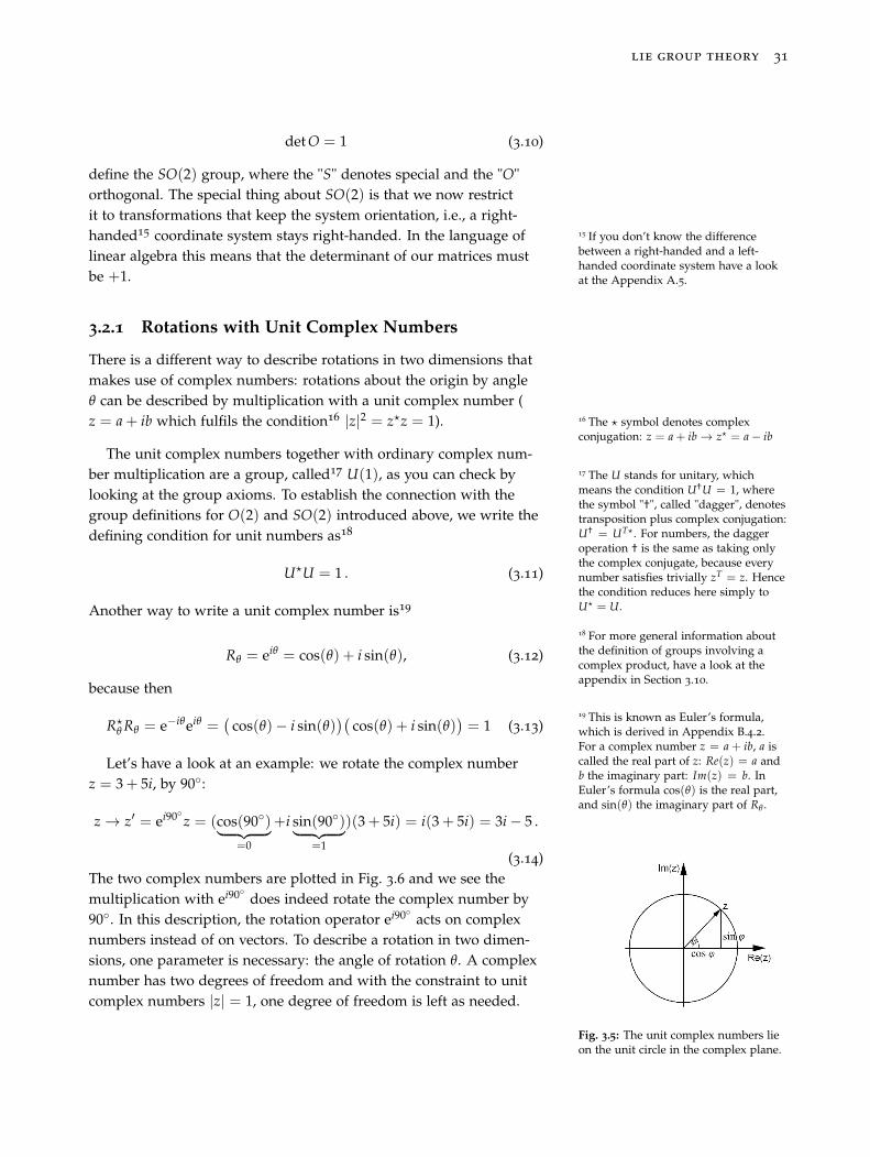
lie group theory 31
det O = 1 (3.10)
define the SO(2) group, where the "S" denotes special and the "O"orthogonal. The special thing about SO(2) is that we now restrictit to transformations that keep the system orientation, i.e., a right-handed15 coordinate system stays right-handed. In the language of 15 If you don’t know the difference
between a right-handed and a left-handed coordinate system have a lookat the Appendix A.5.
linear algebra this means that the determinant of our matrices mustbe +1.
3.2.1 Rotations with Unit Complex Numbers
There is a different way to describe rotations in two dimensions thatmakes use of complex numbers: rotations about the origin by angleθ can be described by multiplication with a unit complex number (z = a + ib which fulfils the condition16 |z|2 = z�z = 1). 16 The � symbol denotes complex
conjugation: z = a + ib → z� = a − ib
The unit complex numbers together with ordinary complex num-ber multiplication are a group, called17 U(1), as you can check by 17 The U stands for unitary, which
means the condition U†U = 1, wherethe symbol "†", called "dagger", denotestransposition plus complex conjugation:U† = UT�. For numbers, the daggeroperation † is the same as taking onlythe complex conjugate, because everynumber satisfies trivially zT = z. Hencethe condition reduces here simply toU� = U.
looking at the group axioms. To establish the connection with thegroup definitions for O(2) and SO(2) introduced above, we write thedefining condition for unit numbers as18
18 For more general information aboutthe definition of groups involving acomplex product, have a look at theappendix in Section 3.10.
U�U = 1 . (3.11)
Another way to write a unit complex number is19
19 This is known as Euler’s formula,which is derived in Appendix B.4.2.For a complex number z = a + ib, a iscalled the real part of z: Re(z) = a andb the imaginary part: Im(z) = b. InEuler’s formula cos(θ) is the real part,and sin(θ) the imaginary part of Rθ .
Fig. 3.5: The unit complex numbers lieon the unit circle in the complex plane.
Rθ = eiθ = cos(θ) + i sin(θ), (3.12)
because then
R�θ Rθ = e−iθeiθ =
(cos(θ)− i sin(θ)
)(cos(θ) + i sin(θ)
)= 1 (3.13)
Let’s have a look at an example: we rotate the complex numberz = 3 + 5i, by 90◦:
z → z′ = ei90◦z = (cos(90◦)︸ ︷︷ ︸=0
+i sin(90◦)︸ ︷︷ ︸=1
)(3 + 5i) = i(3 + 5i) = 3i − 5 .
(3.14)The two complex numbers are plotted in Fig. 3.6 and we see themultiplication with ei90◦ does indeed rotate the complex number by90◦. In this description, the rotation operator ei90◦ acts on complexnumbers instead of on vectors. To describe a rotation in two dimen-sions, one parameter is necessary: the angle of rotation θ. A complexnumber has two degrees of freedom and with the constraint to unitcomplex numbers |z| = 1, one degree of freedom is left as needed.
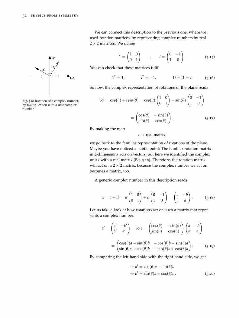
32 physics from symmetry
We can connect this description to the previous one, where weused rotation matrices, by representing complex numbers by real2 × 2 matrices. We define
1 =
(1 00 1
), i =
(0 −11 0
). (3.15)
You can check that these matrices fulfil
12 = 1, i2 = −1, 1i = i1 = i. (3.16)
Fig. 3.6: Rotation of a complex number,by multiplication with a unit complexnumber
So now, the complex representation of rotations of the plane reads
Rθ = cos(θ) + i sin(θ) = cos(θ)
(1 00 1
)+ sin(θ)
(0 −11 0
)
=
(cos(θ) − sin(θ)sin(θ) cos(θ)
). (3.17)
By making the mapi → real matrix,
we go back to the familiar representation of rotations of the plane.Maybe you have noticed a subtle point: The familiar rotation matrixin 2-dimensions acts on vectors, but here we identified the complexunit i with a real matrix (Eq. 3.15). Therefore, the rotation matrixwill act on a 2 × 2 matrix, because the complex number we act onbecomes a matrix, too.
A generic complex number in this description reads
z = a + ib = a
(1 00 1
)+ b
(0 −11 0
)=
(a −bb a
). (3.18)
Let us take a look at how rotations act on such a matrix that repre-sents a complex number:
z′ =(
a′ −b′
b′ a′
)= Rθz =
(cos(θ) − sin(θ)sin(θ) cos(θ)
)(a −bb a
)
=
(cos(θ)a − sin(θ)b − cos(θ)b − sin(θ)asin(θ)a + cos(θ)b − sin(θ)b + cos(θ)a
). (3.19)
By comparing the left-hand side with the right-hand side, we get
→ a′ = cos(θ)a − sin(θ)b
→ b′ = sin(θ)a + cos(θ)b , (3.20)
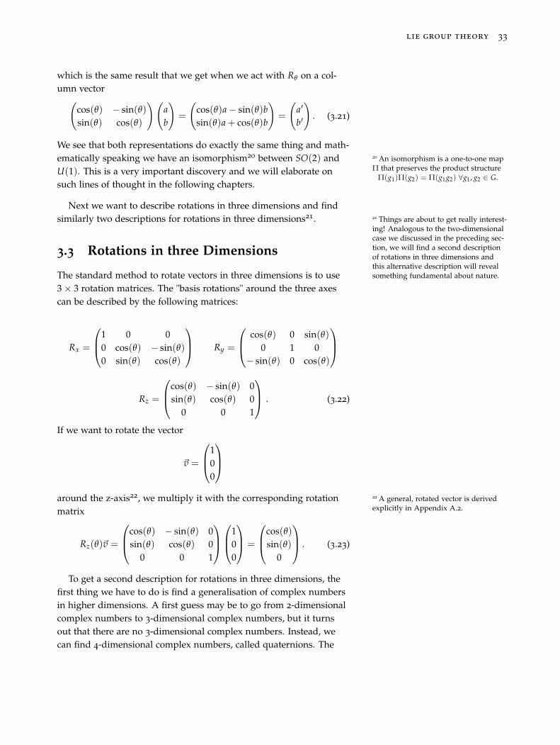
lie group theory 33
which is the same result that we get when we act with Rθ on a col-umn vector(
cos(θ) − sin(θ)sin(θ) cos(θ)
)(ab
)=
(cos(θ)a − sin(θ)bsin(θ)a + cos(θ)b
)=
(a′
b′
). (3.21)
We see that both representations do exactly the same thing and math-ematically speaking we have an isomorphism20 between SO(2) and 20 An isomorphism is a one-to-one map
Π that preserves the product structureΠ(g1)Π(g2) = Π(g1g2) ∀g1, g2 ∈ G.
U(1). This is a very important discovery and we will elaborate onsuch lines of thought in the following chapters.
Next we want to describe rotations in three dimensions and findsimilarly two descriptions for rotations in three dimensions21. 21 Things are about to get really interest-
ing! Analogous to the two-dimensionalcase we discussed in the preceding sec-tion, we will find a second descriptionof rotations in three dimensions andthis alternative description will revealsomething fundamental about nature.
3.3 Rotations in three Dimensions
The standard method to rotate vectors in three dimensions is to use3 × 3 rotation matrices. The "basis rotations" around the three axescan be described by the following matrices:
Rx =
⎛⎜⎝1 0 00 cos(θ) − sin(θ)0 sin(θ) cos(θ)
⎞⎟⎠ Ry =
⎛⎜⎝ cos(θ) 0 sin(θ)0 1 0
− sin(θ) 0 cos(θ)
⎞⎟⎠
Rz =
⎛⎜⎝cos(θ) − sin(θ) 0sin(θ) cos(θ) 0
0 0 1
⎞⎟⎠ . (3.22)
If we want to rotate the vector
�v =
⎛⎜⎝100
⎞⎟⎠around the z-axis22, we multiply it with the corresponding rotation 22 A general, rotated vector is derived
explicitly in Appendix A.2.matrix
Rz(θ)�v =
⎛⎜⎝cos(θ) − sin(θ) 0sin(θ) cos(θ) 0
0 0 1
⎞⎟⎠⎛⎜⎝1
00
⎞⎟⎠ =
⎛⎜⎝cos(θ)sin(θ)
0
⎞⎟⎠ . (3.23)
To get a second description for rotations in three dimensions, thefirst thing we have to do is find a generalisation of complex numbersin higher dimensions. A first guess may be to go from 2-dimensionalcomplex numbers to 3-dimensional complex numbers, but it turnsout that there are no 3-dimensional complex numbers. Instead, wecan find 4-dimensional complex numbers, called quaternions. The
34 physics from symmetry
quaternions will prove to be the correct second tool to describe rota-tions in 3-dimensions and the fact that this tool is 4-dimensional re-veals something deep about the universe. We could have anticipatedthis result, because to describe an arbitrary rotation in 3-dimensions,3 parameters are needed. Four dimensional complex numbers, withthe constraint to unit quaternions23, have exactly 3 degrees of free-23 Remember that we used the con-
straint to unit complex numbers in thetwo dimensional case, too.
dom.
3.3.1 Quaternions
The 4-dimensional complex numbers can be constructed analogousto the 2-dimensional complex numbers. Instead of just one complex"unit" we introduce three, named i, j, k. These fulfil
i2 = j2 = k2 = −1. (3.24)
Then a 4-dimensional complex number, called a quaternion, can bewritten as
q = a1 + bi + cj + dk. (3.25)
We now need multiplication rules for ij =? etc., because productslike this will occur when one multiplies two quaternions. The extracondition
ijk = −1 (3.26)
suffices to compute all needed relations, for example ij=k followsfrom multiplying Eq. 3.26 with k:
ij kk︸︷︷︸=−1
= −k → ij=k. (3.27)
The set of unit quaternions q = a1 + bi + cj + dk satisfy thecondition2424 The symbol †, here is called "dagger"
and denotes transposition plus complexconjugation: a† = (a�)T . The ordinaryscalar product always includes a trans-position a · b = aTb, because matrixmultiplication requires that we multiplya row with a column. In addition, forcomplex entities we include complexconjugation that makes sure we getsomething real, which is important ifwe want to interpret things in terms oflength.
q†q != 1
→ (a1 − bi − cj − dk)(a1 + bi + cj + dk) = a2 + b2 + c2 + d2 != 1.
(3.28)
Exactly as the unit complex numbers formed a group under complexnumber multiplication, the unit quaternions form a group underquaternion multiplication.
Analogous to what we did for two-dimensional complex numbers,we now represent each of the three complex units with a matrix.There are different ways of doing this, but one choice that does thejob is as complex 2 × 2 matrices:
lie group theory 35
1 =
(1 00 1
), i =
(0 1−1 0
)
j =
(0 ii 0
), k =
(i 00 −i
). (3.29)
You can check that these matrices fulfil the defining conditions inEq. 3.24 and Eq. 3.26. Using these matrices a generic quaternion canthen be written
q = a1 + bi + cj + dk =
(a + di b + ci−b + ci a − di
). (3.30)
Furthermore, we have
det(q) = a2 + b2 + c2 + d2. (3.31)
Comparing this with Eq. 3.28 tells us that the set of unit quaternionsis given by matrices of the above form with unit determinant. Theunit quaternions, written as complex 2 × 2 matrices therefore fulfilthe conditions
U†U = 1 and det(U) = 1. (3.32)
Take note that the way we define SU(2) here, is analogously to howwe defined SO(2). The S denotes special, which means det(U) = 1and U stands for unitary, which means the property25 U†U = 1. 25 For some more information about
this, have a look at the Appendix 3.10 atthe end of this chapter.
Through the map in Eq. 3.29, every unit quaternion can be identifiedwith an element of SU(2).
Now, how is SU(2) and with it the unit quaternions related torotations? Unfortunately, the map between SU(2) and26 SO(3) is not 26 Recall that SO(3) is the set of the
usual rotation matrices acting on 3dimensional vectors.
as simple as the one between U(1) and SO(2).
In 2-dimensions the 2 parameters of a complex number z = a + ibcould be easily identified with the two spatial axes, i.e. v = x + iy.The restriction to unit complex numbers automatically makes surethat the resulting matrix preserves the length of any vector27 27 Recall that here R is a unit complex
number, because complex numberscan be rotated by multiplication withunit complex numbers. Therefore wehave U�U = 1, which is the definingcondition for unit complex numbers.
(Uz)�Uz = z�U�Uz = z�z.
The quaternions have 4 parameters, so the identification with the 3coordinates of a three-dimensional vector is not obvious. When wedefine
v ≡ xi + yj + zk (3.33)
and use the matrix representation of the quaternions (Eq. 3.29), wecan compute
det(v) = x2 + y2 + z2. (3.34)
36 physics from symmetry
Therefore, if we want to consider transformations that preserve thelength of the vector (x, y, z), we must use matrix transformations thatpreserve determinants. Therefore the restriction to unit quaternionsmeans that we must restrict to matrices with unit determinant28.28 This follows from the general rule
det(BA) = det(B)det(A). Therefore, ifB has determinant 1, the product matrixBA has the same determinant as A.
Everything may now seem straight forward, but there is a subtlepoint. A first guess would be that a unit quaternion u induces arotation on v simply by multiplication. This is not the case, becausethe product of u and v may not belong to Ri +Rj +Rk. Therefore,the transformed vector can have a component we are not able tointerpret29. Instead the transformation that does the job is given by29 We identify our spatial components
x, y, z as components in the subspaceRi + Rj + Rk. If, as a result of atransformation, we end up with acoefficient that does not belong to thissubspace, i.e. does not appear togetherwith i, j or k, we can’t interpret it.
v′ = qvq−1. (3.35)
It turns out that by making this identification unit quaternions candescribe rotations in 3-dimensions.
Let’s take a look at an explicit example: To make the connectionto our example in two dimensions, we define u as a unit quaternionthat only takes values in Ri + Rj + Rk and denote a general unitquaternion with
t = cos(θ) + sin(θ)u. (3.36)
Using Eq. 3.33 a generic vector can be written
�v = (vx, vy, vz)T = vxi + vyj + vzk =︸︷︷︸
Eq. 3.30
(ivz vx + ivy
−vx + ivy −ivz
).
(3.37)With the identifications made above, we want to rotate, as an ex-ample, a vector �v = (1, 0, 0)T around the z-axis. We will make aparticular choice for the vector and for the quaternion representingthe rotation and show that it works. We write, using quaternions intheir matrix representation (Eq. 3.29)
�v = (1, 0, 0)T → v = 1i + 0j + 0k =
(0 1−1 0
). (3.38)
In addition, we use the following quaternion
Rz(θ) = cos(θ)1 + sin(θ)k =
(cos(θ) + i sin(θ) 0
0 cos(θ)− i sin(θ)
),
(3.39)and then calculate that it is the correct quaternion that describes arotation around the z-axis. We can rewrite Rz using Euler’s formula3030 For a derivation have a look at Ap-
pendix B.4.2. eix = cos(x) + i sin(x):
⇒ Rz(θ) =
(eiθ 00 e−iθ
). (3.40)
lie group theory 37
Inverting the quaternion rotation matrix yields
Rz(θ)−1 =
(cos(θ)− i sin(θ) 0
0 cos(θ) + i sin(θ)
)=
(e−iθ 0
0 eiθ
).
(3.41)Using Eq. 3.35 the rotated vector reads
v′ = Rz(θ)vR−1z (θ) =
(eiθ 00 e−iθ
)(0 1−1 0
)(e−iθ 0
0 eiθ
)
=
(0 ei2θ
−e−2iθ 0
)=
(0 cos(2θ) + i sin(2θ)
− cos(2θ) + i sin(2θ) 0
).
(3.42)On the other hand, an arbitrary vector can be written in our
quaternion notation (Eq. 3.37)
v′ =(
iv′z v′x + iv′y−v′x + iv′y −iv′z
), (3.43)
which we now compare with Eq. 3.42. This yields
v′x = cos(2θ) , v′y = sin(2θ) , v′z = 0. (3.44)
Therefore, written again in the conventional vector notation
→ �v′ = (cos(2θ), sin(2θ), 0)T . (3.45)
Our identifications do indeed induce rotations31, but something 31 See the example in Eq. 3.23 where werotated the vector, using the conven-tional rotation matrix
needs our attention. We haven’t rotated �v by θ, but by 2θ. Therefore,we define φ ≡ 2θ, because then φ really represents the angle werotate. Using this definition we rewrite Eq. 3.36, which yields
t = cos(φ
2) + sin(
φ
2)u . (3.46)
We can now see that the identifications we made are not one-to-one, but rather we have two unit-quaternions describing the samerotation. For example32 32 A rotation by π is the same as a
rotation by 3π = 2π + π for ordinaryvectors, because 2π = 360◦ is a fullrotation. In other words: We can seethat two quaternions u and −u can beused to rotate a vector by π.
tφ=π = u
��
tφ=3π = −u
Vector Rotation by π
This is the reason SU(2) is called the double-cover of SO(3). It isalways possible to go unambiguously from SU(2) to SO(3) but not
38 physics from symmetry
vice versa. One may think this is just a mathematical side-note, butwe will understand later that groups which cover other groups areindeed more fundamental33.33 To spoil the surprise: We will use
the double cover of the Lorentz group,instead of the Lorentz group itself,because otherwise we miss somethingimportant: Spin. Spin is some kindof internal momentum and one of themost important particle labels. This isdiscussed in detail in Section 4.5.4 andSection 8.5.5.
To be able to discover the group that covers a given group, weneed to introduce the most important tool of Lie theory: Lie algebras.This is the topic of the next section.
Take note that the fact we had one quaternion parameter toomany, may be interpreted as a hint towards relativity. One may ar-gue that a more natural identification would have been, as in thetwo-dimensional case, v = t1 + xi + yj + zk. We see that pure math-ematics pushes us towards the idea of using a 4th component andwhat could it be, if not time? If we now want to describe rotationsin 4-dimensions, because we know that the universe we live in is4-dimensional, we have two choices:
• We could search for even higher dimensional complex numbers or
• we could again try to work with quaternions.
From the last paragraph it may seem that quaternions have some-thing to say about rotations in 4 dimensions, too. An arbitrary ro-tation in 4 dimensions is described by34 6 parameters. There is no34 Using ordinary matrices, we need
in four dimensions 4 × 4 matrices.The two conditions OTO = 1 anddet(O) = 1 reduce the 16 componentsof an arbitrary 4 × 4 matrix to sixindependent components.
7-dimensional generalisation of complex numbers, which togetherwith the constraint to unit objects would have 6 free parameters.However, two unit quaternions have exactly 6 free parameters. There-fore, maybe it’s possible to describe a rotation in 4-dimensions by twoquaternions? We will learn later that there is indeed a close connec-tion between two copies of SU(2) and rotations in four dimensions.
3.4 Lie Algebras
Lie theory is all about continuous symmetries. An example is thecontinuous symmetry of the unit circle we discussed at the beginningof this chapter. Continuous here means that there are infinitely manysymmetry transformations, that can be parametrized continuouslyby one or several parameters. For example, the rotation angle φ inthe circle example can be any value: 0.1◦, 0.11◦, 0.11991◦, . . ... Incontrast, for discrete symmetries like a reflection symmetry there isno continuous transformation parameter.
An important observation in Lie theory is that for continuous sym-metries there are elements of the group which are arbitrarily close tothe identity transformation35. In contrast, for a discrete group there35 The identity transformation is the
transformation that changes nothing atall. For example, a rotation by 0◦ is anidentity transformation.
is no continuous transformation parameter and therefore no elementarbitrarily close to the identity. Consider again the symmetries of a
lie group theory 39
square. A rotation by 0,000001◦, which is very close to the identitytransformation (= a rotation by 0◦), is not in the set of symmetrytransformations of the square. In contrast, a rotation by 0,000001◦ is asymmetry of the circle. The symmetry group of a circle is continuous,because the rotation parameter (the rotation angle) can take on arbi-trary (continuous) values. Mathematically, with the identity denotedI, an element g close to the identity is denoted
g(ε) = I + εX , (3.47)
where ε is, as always in mathematics, a really, really small numberand X is an object, called generator, we will talk about in a moment.Such small transformations, when acting on some object changebarely anything. In the smallest possible case such transformationsare called infinitesimal transformation. Nevertheless, repeating suchan infinitesimal transformation often, results in a finite transforma-tion. Think about rotations: many small rotations in one direction areequivalent to one big rotation in the same direction. Mathematically,we can write the idea of repeating a small transformation many times
h(θ) = (I + εX)(I + εX)(I + εX)... = (I + εX)k, (3.48)
where k denotes how often we repeat the small transformation. Ifθ denotes some finite transformation parameter, e.g. 50◦ or so, andN is some really big number which makes sure we are close to theidentity, we can write the element close to the identity as
g(θ) = I +θ
NX. (3.49)
The transformations we want to consider are the smallest possible,which means N must be the biggest possible number, i.e. N → ∞. Toget a finite transformation from such a infinitesimal transformation,one has to repeat the infinitesimal transformation infinitely. Mathe-matically
h(θ) = limN→∞
(I +θ
NX)N , (3.50)
which is in the limit just the exponential function36 36 This is often used as a definitionof the exponential function. A proof,showing the equivalence of this limitand the exponential series we derive inAppendix B.4.1, can be found in mostbooks about analysis.
h(θ) = limN→∞
(I +θ
NX)N = eθX . (3.51)
In some sense the object X generates the finite transformation h,which is why it’s called the generator.
If we want to calculate the generator X of a given transformation,we can differentiate the above formula
40 physics from symmetry
ddθ
h(θ) =ddθ
eθX = XeθX . (3.52)
Thus, if we evaluate this formula at θ = 0, we get
X =dh(θ)
dθ
∣∣∣θ=0
. (3.53)
The idea behind such lines of thought is that one can learn a lotabout a group by looking at the important part of the infinitesimalelements (denoted X above): the generators. This will be made moreprecise in a moment, but first let’s look at this from another perspec-tive that makes it even clearer in what sense the generators generatea finite transformation:
If we consider a continuous group of transformations that aregiven by matrices, we can make a Taylor expansion37 of an element37 If you’ve never heard of the Taylor
expansion, or Taylor series before,you are encouraged to have a look atAppendix B.3.
of the group about the identity. The Taylor series is given by
h(θ) = I +dhdθ
.|θ=0θ +12
d2hdθ2 .|θ=0θ2 + ... = ∑
n
1n!
dnhdθn
∣∣θ=0θn. (3.54)
This shows nicely how the generators generate transformations.
For matrix Lie groups one defines the corresponding Lie algebraas the collection of objects that give an element of the group whenexponentiated. This is an easy definition one can use when restrict-ing to matrix Lie groups. Later we will introduce a more generaldefinition. In mathematical terms3838 The Lie algebra which belongs to a
group G is conventionally denoted bythe corresponding "Fraktur" letter g For a Lie Group G (given by n × n matrices), the Lie algebra g of
G is given by those n × n matrices X such that etX ∈ G for t ∈ R,together with an operation, called the Lie bracket [, ] that tells us howwe can combine these matrices.
The last part of this definition can be a bit confusing and thus wenow spent some time discussing it.
We know from the definition of a group, that a group is morethan just a collection of transformations. The definition of a groupincludes a binary operation ◦ that tells us how to combine groupelements. For matrix Lie groups this is just ordinary matrix multi-plication. Naively one may think that the same combination rule ◦is valid for elements of the Lie algebra, but this is not the case! Theelements of the Lie algebra are given by matrices39, but the multipli-39 A famous theorem of Lie group
theory, called Ado’s Theorem, statesthat every Lie algebra is isomorphic to amatrix Lie algebra.
cation of two Lie algebra elements doesn’t need to be an element ofthe Lie algebra. Instead there is another combination rule for the Lie
lie group theory 41
algebra, already mentioned in the definition above, that is directlyconnected to the combination rule of the corresponding Lie group.
The connection between the combination rule of the Lie groupand the combination rule of the Lie algebra is given by the famousBaker-Campbell-Hausdorff formula40 40 We will not talk about the proof of
this formula in this book. Proofs can befound in most books about Lie theory,for example in William Fulton and JoeHarris. Representation Theory: A FirstCourse. Springer, 1st corrected edition, 81999. ISBN 9780387974958
eX ◦ eY = eX+Y+ 12 [X,Y]+ 1
12 [X,[X,Y]]− 112 [Y,[X,Y]]+... (3.55)
On the left hand side, we have the multiplication of two elements ofthe Lie group, let’s name them g and h, which we can write in termsof the corresponding generators (=elements of the Lie algebra)
g︸︷︷︸∈G
◦ h︸︷︷︸∈G
= eX ◦ eY = eX+Y+ 12 [X,Y]+ 1
12 [X,[X,Y]]− 112 [Y,[X,Y]]+...︸ ︷︷ ︸
∈G
(3.56)
with the generators41 X, Y ∈ g. On the right-hand side we have a sin- 41 The Lie algebra which belongs to agroup G is conventionally denoted bythe corresponding "Fraktur" letter g.
gle object of the group and the multiplication of the group elementshave been translated to a sum of Lie algebra elements. The new sym-bol in this sum [ , ] is called Lie bracket and for matrix Lie groupsit is given by [X, Y] = XY − YX, which is called the commutatorof X and Y. The elements XY and YX need not to be part of the Liealgebra, but their difference always is42! 42 A very illuminating proof of this fact
can be found in John Stillwell. Naive LieTheory. Springer, 1st edition, August2008. ISBN 978-0387782140
We learn from the Baker-Campbell-Hausdorff-Formula that thenatural product of the Lie algebra is, not as one would naively think,ordinary matrix multiplication, but the Lie bracket [, ]. One says,the Lie algebra is closed under the Lie bracket, just as the groupis closed under the corresponding composition rule ◦, e.g. matrixmultiplication. Closure means that the composition of two elementslies again in the same set43. 43 For group elements g, h ∈ G we have
g ◦ h ∈ G. For elements of the Liealgebra X, Y ∈ g we have [X, Y] ∈ g andin general X ◦ Y �∈ g
After looking at an example to illustrate these new notions, wewill have a look at the modern definition of a Lie algebra. The maincomponent of this definition is how the generators of a group behavewhen put into the Lie bracket. By using this general definition wewill see that it is possible to say that different groups have the sameLie algebra. With the definition above saying something like thiswould make little sense. Nevertheless, this new way of thinkingabout Lie algebras will enable us to reveal the most fundamentaldescription corresponding to a given transformation. This is possiblebecause there is a theorem in Lie theory that tells us that there isexactly one distinguished Lie group for each Lie algebra. The Liealgebra however, according to the abstract definition, corresponds tomany Lie groups. We will make this more concrete after introducingthe modern definition of a Lie group.
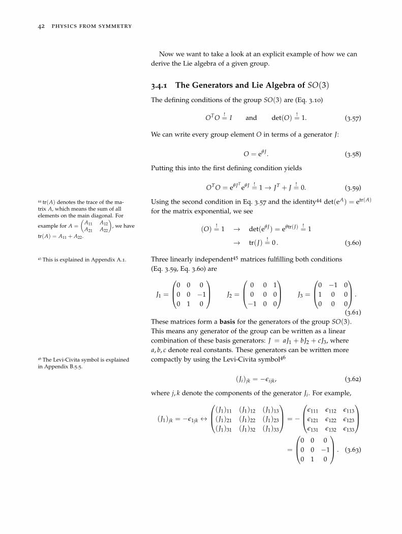
42 physics from symmetry
Now we want to take a look at an explicit example of how we canderive the Lie algebra of a given group.
3.4.1 The Generators and Lie Algebra of SO(3)
The defining conditions of the group SO(3) are (Eq. 3.10)
OTO != I and det(O)
!= 1. (3.57)
We can write every group element O in terms of a generator J:
O = eθ J . (3.58)
Putting this into the first defining condition yields
OTO = eθ JTeθ J !
= 1 → JT + J != 0. (3.59)
Using the second condition in Eq. 3.57 and the identity44 det(eA) = etr(A)44 tr(A) denotes the trace of the ma-trix A, which means the sum of allelements on the main diagonal. For
example for A =
(A11 A12A21 A22
), we have
tr(A) = A11 + A22.
for the matrix exponential, we see
(O)!= 1 → det(eθ J) = eθtr(J) !
= 1
→ tr(J) != 0 . (3.60)
Three linearly independent45 matrices fulfilling both conditions45 This is explained in Appendix A.1.
(Eq. 3.59, Eq. 3.60) are
J1 =
⎛⎜⎝0 0 00 0 −10 1 0
⎞⎟⎠ J2 =
⎛⎜⎝ 0 0 10 0 0−1 0 0
⎞⎟⎠ J3 =
⎛⎜⎝0 −1 01 0 00 0 0
⎞⎟⎠ .
(3.61)These matrices form a basis for the generators of the group SO(3).This means any generator of the group can be written as a linearcombination of these basis generators: J = aJ1 + bJ2 + cJ3, wherea, b, c denote real constants. These generators can be written morecompactly by using the Levi-Civita symbol4646 The Levi-Civita symbol is explained
in Appendix B.5.5.
(Ji)jk = −εijk, (3.62)
where j, k denote the components of the generator Ji. For example,
(J1)jk = −ε1jk ↔
⎛⎜⎝(J1)11 (J1)12 (J1)13
(J1)21 (J1)22 (J1)23
(J1)31 (J1)32 (J1)33
⎞⎟⎠ = −
⎛⎜⎝ε111 ε112 ε113
ε121 ε122 ε123
ε131 ε132 ε133
⎞⎟⎠=
⎛⎜⎝0 0 00 0 −10 1 0
⎞⎟⎠ . (3.63)
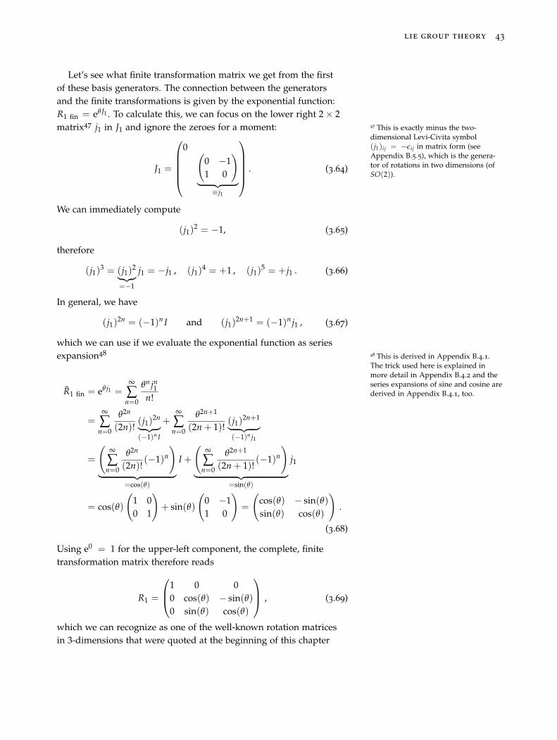
lie group theory 43
Let’s see what finite transformation matrix we get from the firstof these basis generators. The connection between the generatorsand the finite transformations is given by the exponential function:R1 fin = eθ J1 . To calculate this, we can focus on the lower right 2 × 2matrix47 j1 in J1 and ignore the zeroes for a moment: 47 This is exactly minus the two-
dimensional Levi-Civita symbol(j1)ij = −εij in matrix form (seeAppendix B.5.5), which is the genera-tor of rotations in two dimensions (ofSO(2)).
J1 =
⎛⎜⎜⎜⎜⎝0 (
0 −11 0
)︸ ︷︷ ︸
≡j1
⎞⎟⎟⎟⎟⎠ . (3.64)
We can immediately compute
(j1)2 = −1, (3.65)
therefore
(j1)3 = (j1)2︸︷︷︸=−1
j1 = −j1 , (j1)4 = +1 , (j1)5 = +j1 . (3.66)
In general, we have
(j1)2n = (−1)n I and (j1)2n+1 = (−1)n j1 , (3.67)
which we can use if we evaluate the exponential function as seriesexpansion48 48 This is derived in Appendix B.4.1.
The trick used here is explained inmore detail in Appendix B.4.2 and theseries expansions of sine and cosine arederived in Appendix B.4.1, too.R1 fin = eθ j1 =
∞
∑n=0
θn jn1n!
=∞
∑n=0
θ2n
(2n)!(j1)2n︸ ︷︷ ︸(−1)n I
+∞
∑n=0
θ2n+1
(2n + 1)!(j1)2n+1︸ ︷︷ ︸(−1)n j1
=
(∞
∑n=0
θ2n
(2n)!(−1)n
)︸ ︷︷ ︸
=cos(θ)
I +
(∞
∑n=0
θ2n+1
(2n + 1)!(−1)n
)︸ ︷︷ ︸
=sin(θ)
j1
= cos(θ)
(1 00 1
)+ sin(θ)
(0 −11 0
)=
(cos(θ) − sin(θ)sin(θ) cos(θ)
).
(3.68)
Using e0 = 1 for the upper-left component, the complete, finitetransformation matrix therefore reads
R1 =
⎛⎜⎝1 0 00 cos(θ) − sin(θ)0 sin(θ) cos(θ)
⎞⎟⎠ , (3.69)
which we can recognize as one of the well-known rotation matricesin 3-dimensions that were quoted at the beginning of this chapter
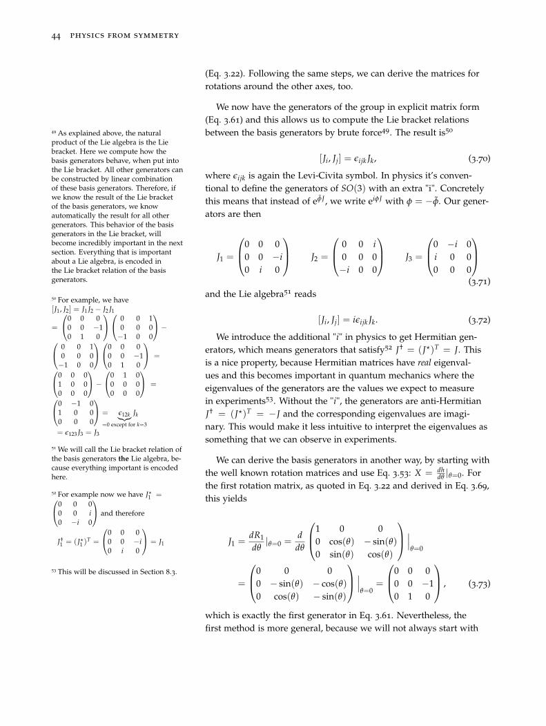
44 physics from symmetry
(Eq. 3.22). Following the same steps, we can derive the matrices forrotations around the other axes, too.
We now have the generators of the group in explicit matrix form(Eq. 3.61) and this allows us to compute the Lie bracket relationsbetween the basis generators by brute force49. The result is5049 As explained above, the natural
product of the Lie algebra is the Liebracket. Here we compute how thebasis generators behave, when put intothe Lie bracket. All other generators canbe constructed by linear combinationof these basis generators. Therefore, ifwe know the result of the Lie bracketof the basis generators, we knowautomatically the result for all othergenerators. This behavior of the basisgenerators in the Lie bracket, willbecome incredibly important in the nextsection. Everything that is importantabout a Lie algebra, is encoded inthe Lie bracket relation of the basisgenerators.
50 For example, we have[J1, J2] = J1 J2 − J2 J1
=
⎛⎝0 0 00 0 −10 1 0
⎞⎠⎛⎝ 0 0 10 0 0−1 0 0
⎞⎠ −⎛⎝ 0 0 1
0 0 0−1 0 0
⎞⎠⎛⎝0 0 00 0 −10 1 0
⎞⎠ =
⎛⎝0 0 01 0 00 0 0
⎞⎠ −⎛⎝0 1 0
0 0 00 0 0
⎞⎠ =
⎛⎝0 −1 01 0 00 0 0
⎞⎠ = ε12k︸︷︷︸=0 except for k=3
Jk
= ε123 J3 = J3
[Ji, Jj] = εijk Jk, (3.70)
where εijk is again the Levi-Civita symbol. In physics it’s conven-tional to define the generators of SO(3) with an extra "i". Concretelythis means that instead of eφJ , we write eiφJ with φ = −φ. Our gener-ators are then
J1 =
⎛⎜⎝0 0 00 0 −i0 i 0
⎞⎟⎠ J2 =
⎛⎜⎝ 0 0 i0 0 0−i 0 0
⎞⎟⎠ J3 =
⎛⎜⎝0 −i 0i 0 00 0 0
⎞⎟⎠(3.71)
and the Lie algebra51 reads
51 We will call the Lie bracket relation ofthe basis generators the Lie algebra, be-cause everything important is encodedhere.
[Ji, Jj] = iεijk Jk. (3.72)
We introduce the additional "i" in physics to get Hermitian gen-erators, which means generators that satisfy52 J† = (J�)T = J. This
52 For example now we have J�1 =⎛⎝0 0 00 0 i0 −i 0
⎞⎠ and therefore
J†1 = (J�1 )
T =
⎛⎝0 0 00 0 −i0 i 0
⎞⎠ = J1
is a nice property, because Hermitian matrices have real eigenval-ues and this becomes important in quantum mechanics where theeigenvalues of the generators are the values we expect to measurein experiments53. Without the "i", the generators are anti-Hermitian
53 This will be discussed in Section 8.3.
J† = (J�)T = −J and the corresponding eigenvalues are imagi-nary. This would make it less intuitive to interpret the eigenvalues assomething that we can observe in experiments.
We can derive the basis generators in another way, by starting withthe well known rotation matrices and use Eq. 3.53: X = dh
dθ |θ=0. Forthe first rotation matrix, as quoted in Eq. 3.22 and derived in Eq. 3.69,this yields
J1 =dR1
dθ|θ=0 =
ddθ
⎛⎜⎝1 0 00 cos(θ) − sin(θ)0 sin(θ) cos(θ)
⎞⎟⎠ ∣∣∣θ=0
=
⎛⎜⎝0 0 00 − sin(θ) − cos(θ)0 cos(θ) − sin(θ)
⎞⎟⎠ ∣∣∣θ=0
=
⎛⎜⎝0 0 00 0 −10 1 0
⎞⎟⎠ , (3.73)
which is exactly the first generator in Eq. 3.61. Nevertheless, thefirst method is more general, because we will not always start with
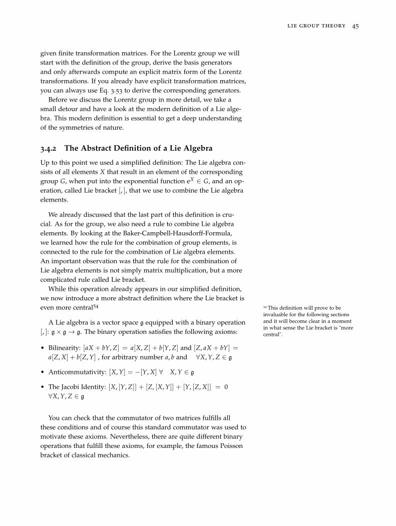
lie group theory 45
given finite transformation matrices. For the Lorentz group we willstart with the definition of the group, derive the basis generatorsand only afterwards compute an explicit matrix form of the Lorentztransformations. If you already have explicit transformation matrices,you can always use Eq. 3.53 to derive the corresponding generators.
Before we discuss the Lorentz group in more detail, we take asmall detour and have a look at the modern definition of a Lie alge-bra. This modern definition is essential to get a deep understandingof the symmetries of nature.
3.4.2 The Abstract Definition of a Lie Algebra
Up to this point we used a simplified definition: The Lie algebra con-sists of all elements X that result in an element of the correspondinggroup G, when put into the exponential function eX ∈ G, and an op-eration, called Lie bracket [, ], that we use to combine the Lie algebraelements.
We already discussed that the last part of this definition is cru-cial. As for the group, we also need a rule to combine Lie algebraelements. By looking at the Baker-Campbell-Hausdorff-Formula,we learned how the rule for the combination of group elements, isconnected to the rule for the combination of Lie algebra elements.An important observation was that the rule for the combination ofLie algebra elements is not simply matrix multiplication, but a morecomplicated rule called Lie bracket.
While this operation already appears in our simplified definition,we now introduce a more abstract definition where the Lie bracket iseven more central54 54 This definition will prove to be
invaluable for the following sectionsand it will become clear in a momentin what sense the Lie bracket is "morecentral".
A Lie algebra is a vector space g equipped with a binary operation[, ]: g× g → g. The binary operation satisfies the following axioms:
• Bilinearity: [aX + bY, Z] = a[X, Z] + b[Y, Z] and [Z, aX + bY] =a[Z, X] + b[Z, Y] , for arbitrary number a, b and ∀X, Y, Z ∈ g
• Anticommutativity: [X, Y] = −[Y, X] ∀ X, Y ∈ g
• The Jacobi Identity: [X, [Y, Z]] + [Z, [X, Y]] + [Y, [Z, X]] = 0∀X, Y, Z ∈ g
You can check that the commutator of two matrices fulfills allthese conditions and of course this standard commutator was used tomotivate these axioms. Nevertheless, there are quite different binaryoperations that fulfill these axioms, for example, the famous Poissonbracket of classical mechanics.
46 physics from symmetry
The important point is that this definition makes no reference toany Lie group. The definition of a Lie algebra stands on its own andwe will see that this makes a lot of sense. In the next section we willhave a look at the generators of SU(2) and find that the basis gener-ators, which is the set of generators we can use to construct all othergenerators by linear combinations, fulfill the same Lie bracket rela-tion as the basis generators of SO(3) (Eq. 3.72). This is interpreted asSU(2) and SO(3) having the same Lie algebra. This is an incrediblyimportant result and it will tell us a lot about SU(2) and SO(3).
3.4.3 The Generators and Lie Algebra of SU(2)
We stumbled upon SU(2) while trying to describe rotations inthree dimensions and discovered that SU(2) is the double cover5555 Recall that this means that the map
from SU(2) to SO(3) identifies twoelements of SU(2) with the sameelement of SO(3).
of SO(3).
Remember that SU(2) is the group of unitary 2 × 2 matrices withunit determinant56 :56 This is what the "S" stands for:
Special = unit determinant.
U†U = UU† = 1 (3.74)
det(U) = 1 . (3.75)
The first thing we now want to take a look at is the Lie algebra ofthis group. Writing the defining conditions of the group in terms ofthe generators J1, J2, . . . yields5757 As discussed above, we now work
with an extra "i" in the exponent, inorder to get Hermitian matrices, whichguarantees that we get real numbers aspredictions for experiments in quantummechanics.
U†U = (ei Ji )†ei Ji != 1 (3.76)
det(U) = det(ei Ji )!= 1 (3.77)
The first condition tells us, using the Baker-Campbell-Hausdorfftheorem (Eq. 3.55) and [Ji, Ji] = 0
(ei Ji )†ei Ji = e−i J†i ei Ji !
= 1
→ e−i J†i +i Ji+
12 [J
†i ,Ji ]+... !
= 1
→︸︷︷︸e0=1
J†i
!= Ji. (3.78)
A matrix fulfilling the condition J†i = Ji is called Hermitian and we
therefore learn here that the generators of SU(2) must be Hermitian.
Using the identity det(eA) = etr(A), we see that the second conditionyields
det(ei Ji ) = eitr(Ji) = 1 →︸︷︷︸e0=1
tr(Ji)!= 0. (3.79)
lie group theory 47
We conclude that the generators of SU(2) must be Hermitiantraceless matrices. A basis for Hermitian traceless 2 × 2 matrices isgiven by the following 3 matrices58: 58 A complex 2× 2 matrix has 4 complex
entries and therefore 8 degrees offreedom. Because of the two conditionsthe degrees of freedom are reduced to3.σ1 =
(0 11 0
), σ2 =
(0 −ii 0
), σ3 =
(1 00 −1
). (3.80)
This means every Hermitian traceless 2 × 2 matrix can be written as alinear combination of these matrices that are called Pauli matrices.
We can put these explicit matrices for the basis generators into theLie bracket and this yields
[σi, σj] = 2iεijkσk, (3.81)
where εijk is again the Levi-Civita symbol. To get rid of the nasty 2 itis conventional to define the generators of SU(2) as Ji ≡ 1
2 σi. The Liealgebra then reads
[Ji, Jj] = iεijk Jk . (3.82)
Take note that this is exactly the same Lie bracket relation we de-rived for SO(3) (Eq. 3.72)! Therefore one says that SU(2) and SO(3)have the same Lie algebra, because we define Lie algebras by theirLie bracket. We will use the abstract definition of this Lie algebra,to get different descriptions for the transformations described bySU(2). We will learn that an SU(2) transformation doesn’t need tobe described by 2 × 2 matrices. To make sense of things like this, weneed a more abstract definition of a Lie group. At this point SU(2) isdefined as a set of 2 × 2 matrices, and a description of SU(2) by, forexample, 3 × 3 matrices, makes little sense. The abstract definition ofa Lie group will enable us to see the connection between different de-scriptions of the same transformation. We will identify with each Liegroup a geometrical object (a manifold) and use this abstract object todefine a group. This may seem like a strange thought, but will makea lot of sense after taking a second look at two examples we alreadyencountered in earlier sections.
3.4.4 The Abstract Definition of a Lie Group
One of the first Lie groups we discussed was U(1), the unit complexnumbers. These are defined as complex numbers that satisfy z�z = 1.If we write z = a + ib this condition reads
z�z = (a + ib)�(a + ib) = (a − ib)(a + ib) = a2 + b2 = 1. (3.83)
This is exactly the defining condition of the unit circle59. The set 59 The unit circle S1 is the set of allpoints in two dimensions with distance1 from the origin. In mathematicalterms this means all points (x1, x2)fulfilling x2
1 + x22 = 1.
48 physics from symmetry
of unit-complex numbers is the unit circle in the complex plane.Furthermore, we found that there is a one-to-one map60 between60 To be precise: an isomorphism. To
say two things are isomorphic is themathematical way of saying that theyare "the same thing". Two things arecalled isomorphic if there exists anisomorphism between them.
elements of U(1) and SO(2). Therefore, for these groups it is easyto identify them with a geometric object: the unit circle. Instead oftalking about different descriptions for SO(2) or U(1), which aredefined by objects of given dimension, it can help to think about thisgroup as the unit-circle. Rotations in two-dimensions are, as a Liegroup, the unit-circle and we can represent these transformationsby elements of SO(2), i.e. 2 × 2 matrices or elements of U(1), i.e.unit-complex numbers.
The next groups we discussed were SO(3) and SU(2). Remem-ber that we found a one-to-one map between SU(2) and the unitquaternions. The unit quaternions are defined as those quaternionsq = a1 + bi + cj + dk that satisfy the condition (Eq. 3.28)
a2 + b2 + c2 + d2 != 1, (3.84)
which is the same condition that defines61 the three sphere S3! There-
61 Recall that the unit circle S1 is definedas the set of points that satisfy thecondition x2
1 + x22 = 1. Equally, the two-
sphere S2 is defined by the conditionx2
1 + x22 + x2
3 = 1 and analogously thethree sphere S3 by x2
1 + x22 + x2
3 + x24 = 1.
The number that follows the S denotesthe dimension. In two dimensions,with one condition we get a one-dimensional object: S1. Equally weget in four dimensions, with onecondition x2
1 + x22 + x2
3 + x24 = 1 a three
dimensional object S3. S3 is the surfaceof the four-dimensional ball.
fore the quaternions provide us with a map between SU(2) and thethree sphere S3. This map is an isomorphism (1-1 and onto) andtherefore we can really think of SU(2) as the three sphere S3.
These observations motivate the modern definition of a Lie group62:
62 The technical details that follow aren’timportant for what we want to do inthis book. Especially, don’t worry if theexact meaning of notions like "induces"or "differentiable" is not clear. Theimportant message to take away is: Liegroup = manifold.
A Lie group is a group, which is also a differentiable manifold63. Further-
63 A manifold is a set of points, for ex-ample a sphere that looks locally likeflat Euclidean space Rn. Another way ofthinking about a n-dimensional mani-fold is that it’s a set which can be givenn independent coordinates in someneighborhood of any point. For somemore information about manifolds, seethe appendix in Section 3.11 at the endof this chapter.
more, the group operation ◦ must induce a differentiable map of the manifoldinto itself. This is a compatibility requirement that ensures that the groupproperty is compatible with the manifold property. Concretely this meansthat every group element, say A induces a map that takes any element of thegroup B to another element of the group C = AB and this map must bedifferentiable. Using coordinates this means that the coordinates of AB mustbe differentiable functions of the coordinates of B.
We can now understand the remark at the end of Section 3.4:
"... there is precisely one distinguished Lie group for each Lie alge-bra."
a bit better64. From the geometric perspective, the distinguished
64 Recall that we already discovered thatdifferent groups can have the same Liealgebra. For example, using the abstractdefinition of a Lie algebra, we say thatSO(3) and SU(2) have the same Liealgebra (Eq. 3.82).
group has the property of being simply connected. This means that,if we use the modern definition of a Lie group as a manifold, anyclosed curve on this manifold can be shrunk smoothly to a point65.
65 We will not discuss this any further,but you are encouraged to read aboutit, for example in the books recom-mended at the end of this chapter.For the purpose of this book it suf-fices to know that there is always onedistinguished group.
To emphasize this important point:66
66 A proof can be found, for example,in Michael Spivak. A ComprehensiveIntroduction to Differential Geometry, Vol.1, 3rd Edition. Publish or Perish, 3rdedition, 1 1999. ISBN 9780914098706
There is precisely one simply-connected Lie group correspondingto each Lie algebra.
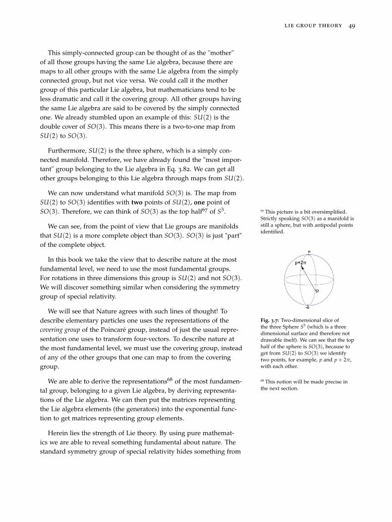
lie group theory 49
This simply-connected group can be thought of as the "mother"of all those groups having the same Lie algebra, because there aremaps to all other groups with the same Lie algebra from the simplyconnected group, but not vice versa. We could call it the mothergroup of this particular Lie algebra, but mathematicians tend to beless dramatic and call it the covering group. All other groups havingthe same Lie algebra are said to be covered by the simply connectedone. We already stumbled upon an example of this: SU(2) is thedouble cover of SO(3). This means there is a two-to-one map fromSU(2) to SO(3).
Furthermore, SU(2) is the three sphere, which is a simply con-nected manifold. Therefore, we have already found the "most impor-tant" group belonging to the Lie algebra in Eq. 3.82. We can get allother groups belonging to this Lie algebra through maps from SU(2).
We can now understand what manifold SO(3) is. The map fromSU(2) to SO(3) identifies with two points of SU(2), one point ofSO(3). Therefore, we can think of SO(3) as the top half67 of S3. 67 This picture is a bit oversimplified.
Strictly speaking SO(3) as a manifold isstill a sphere, but with antipodal pointsidentified.
Fig. 3.7: Two-dimensional slice ofthe three Sphere S3 (which is a threedimensional surface and therefore notdrawable itself). We can see that the tophalf of the sphere is SO(3), because toget from SU(2) to SO(3) we identifytwo points, for example, p and p + 2π,with each other.
We can see, from the point of view that Lie groups are manifoldsthat SU(2) is a more complete object than SO(3). SO(3) is just "part"of the complete object.
In this book we take the view that to describe nature at the mostfundamental level, we need to use the most fundamental groups.For rotations in three dimensions this group is SU(2) and not SO(3).We will discover something similar when considering the symmetrygroup of special relativity.
We will see that Nature agrees with such lines of thought! Todescribe elementary particles one uses the representations of thecovering group of the Poincaré group, instead of just the usual repre-sentation one uses to transform four-vectors. To describe nature atthe most fundamental level, we must use the covering group, insteadof any of the other groups that one can map to from the coveringgroup.
We are able to derive the representations68 of the most fundamen- 68 This notion will be made precise inthe next section.tal group, belonging to a given Lie algebra, by deriving representa-
tions of the Lie algebra. We can then put the matrices representingthe Lie algebra elements (the generators) into the exponential func-tion to get matrices representing group elements.
Herein lies the strength of Lie theory. By using pure mathemat-ics we are able to reveal something fundamental about nature. Thestandard symmetry group of special relativity hides something from
50 physics from symmetry
us, because it is not the most fundamental group belonging to thissymmetry69. The covering group of the Poincaré group is the funda-69 For those who already know some
quantum mechanics: the standardsymmetry group hides spin from us!
mental group and therefore we will use it to describe nature70.
70 In the following, we will use onerepresentation of the Poincaré group toderive the corresponding Lie algebra.Then we will use this Lie algebra toderive the representations of the onedistinguished group that belongs to thisLie algebra, which doubly covers thePoincaré group.
To summarize71
71 Maybe you wonder why S2, the sur-face of the sphere in three dimensions,is missing. S2 is not a Lie group andthis is closely related to the fact thatthere are no three-dimensional complexnumbers. Recall that we had to movefrom two-dimensional complex num-bers with just i to the four-dimensionalquaternions with i,j,k.
• S1=U(1) ↔︸︷︷︸one-to-one
SO(2)
• S3=SU(2) →︸︷︷︸two-to-one
SO(3)= "half" of S3
⇒ SU(2) is the distinguished group belonging to the Lie algebra[Ji, Jj] = iεijk Jk (Eq. 3.82), because S3 is simply connected.
Next, we will introduce another important branch of Lie theory,called representation theory. It is representation theory that enablesus to derive from a given Lie group the tools that we need to describenature at the most fundamental level.
3.5 Representation Theory
The important thing about group theory is that it is able to describetransformations without referring to any objects in the real world.
For theoretical considerations it is often useful to regard any groupas an abstract group. This means defining the group by its manifoldstructure and the group operation. For example SU(2) is the threesphere S3, the elements of the group are points of the manifold andthe rule associating a product point ab with any two points b and asatisfies the usual group axioms. In physical applications one is moreinterested in what the group actually does, i.e. the group action.
An important idea is that one group can act on many differentkinds of objects72. This idea motivates the definition of a representa-72 This will make much more sense in a
moment. tion: A representation is a map73 between any group element g of a73 The mathematical term for a mapwith these special properties is ho-momorphism. The definition of anisomorphism is then a homomorphism,which is in addition one-to-one.
group G and a linear transformation74 R(g) of some vector-space V
74 In the context of this book this willalways mean that we map each groupelement to a matrix. Each group ele-ment is then given by a matrix that actsby usual matrix multiplication on theelements of some vector space.
g →︸︷︷︸R
R(g) (3.85)
in such a way that the group properties are preserved:
• R(e) = I (The identity element of the group transforms nothing atall)
• R(g−1) =(
R(g))−1 (Every inverse element is mapped to the
corresponding inverse transformation)
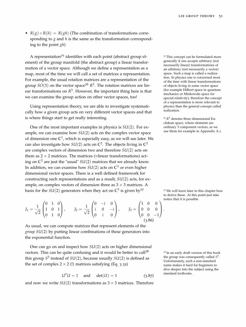
lie group theory 51
• R(g) ◦ R(h) = R(gh) (The combination of transformations corre-sponding to g and h is the same as the transformation correspond-ing to the point gh)
A representation75 identifies with each point (abstract group el- 75 This concept can be formulated moregenerally if one accepts arbitrary (notnecessarily linear) transformations ofan arbitrary (not necessarily a vector)space. Such a map is called a realiza-tion. In physics one is concerned mostof the time with linear transformationsof objects living in some vector space(for example Hilbert space in quantummechanics or Minkowski space forspecial relativity), therefore the conceptof a representation is more relevant tophysics than the general concept calledrealization.
ement) of the group manifold (the abstract group) a linear transfor-mation of a vector space. Although we define a representation as amap, most of the time we will call a set of matrices a representation.For example, the usual rotation matrices are a representation of thegroup SO(3) on the vector space76 R3. The rotation matrices are lin-
76 R3 denotes three dimensional Eu-clidean space, where elements areordinary 3 component vectors, as weuse them for example in Appendix A.1.
ear transformations on R3. However, the important thing here is thatwe can examine the group action on other vector spaces, too!
Using representation theory, we are able to investigate systemati-cally how a given group acts on very different vector spaces and thatis where things start to get really interesting.
One of the most important examples in physics is SU(2). For ex-ample, we can examine how SU(2) acts on the complex vector spaceof dimension one C1, which is especially easy, as we will see later. Wecan also investigate how SU(2) acts on C2. The objects living in C2
are complex vectors of dimension two and therefore SU(2) acts onthem as 2 × 2 matrices. The matrices (=linear transformations) act-ing on C2 are just the "usual" SU(2) matrices that we already know.In addition, we can examine how SU(2) acts on C3 or even higherdimensional vector spaces. There is a well defined framework forconstructing such representations and as a result, SU(2) acts, for ex-ample, on complex vectors of dimension three as 3 × 3 matrices. Abasis for the SU(2) generators when they act on C3 is given by77 77 We will learn later in this chapter how
to derive these. At this point just takenotice that it is possible.
J1 =1√2
⎛⎜⎝0 1 01 0 10 1 0
⎞⎟⎠ , J2 =1√2
⎛⎜⎝0 −i 0i 0 −i0 i 0
⎞⎟⎠ , J3 =
⎛⎜⎝1 0 00 0 00 0 −1
⎞⎟⎠ .
(3.86)As usual, we can compute matrices that represent elements of thegroup SU(2) by putting linear combinations of these generators intothe exponential function.
One can go on and inspect how SU(2) acts on higher dimensionalvectors. This can be quite confusing and it would be better to call78 78 In an early draft version of this book
the group was consequently called S3.Unfortunately, such a non-standardname makes it hard for beginners todive deeper into the subject using thestandard textbooks.
this group S3 instead of SU(2), because usually SU(2) is defined asthe set of complex 2 × 2 (!) matrices satisfying (Eq. 3.32)
U†U = 1 and det(U) = 1 (3.87)
and now we write SU(2) transformations as 3 × 3 matrices. Therefore
52 physics from symmetry
one must always keep in mind that we mean the abstract group, in-stead of the 2 × 2 definition, when we talk about higher dimensionalrepresentation of SU(2) or any other group.
Typically a group is defined in the first place with the help of anexplicit representation. For example, we began our discussion ofSU(2) with explicit 2 × 2 matrices. This approach enables us to studythe group properties concretely, as we did in the preceding sections.After this initial study it’s often more helpful to regard the groupas an abstract group79, because it’s possible to find other, useful79 For SU(2) this means using S3.
representations of the group.
Before we move on to examples we need to define some abstract,but useful, notions. These notions will clarify the hierarchy of rep-resentations, because not every possible representation is equallyfundamental.
The first notion we want to talk about is called similarity trans-formation. Given a matrix R and an invertible80 matrix S then a80 A matrix S is called invertible, if
there exists a matrix T, such thatST = TS = 1. The inverse matrix isusually denoted S−1.
transformation of the form
R → R′ = S−1RS (3.88)
is called a similarity transformation. The usefulness of this kind oftransformation in this context lies in the fact that if we have a rep-resentation R(G) of a group G, then S−1RS is also a representation.This follows directly from the definition of a representation: Supposewe have two group elements g1, g2 and a map R: G ⇒ GL(V), i.e.R(g1) and R(g2). This is a representation if
R(g1)R(g2) = R(g1g2) (3.89)
If we now look at the similarity transformation of the representa-tion
S−1R(g1) SS−1︸ ︷︷ ︸=1
R(g2)S = S−1R(g1)R(g2)S = S−1R(g1g2)S , (3.90)
we see that this is a representation, too. Speaking colloquially, thismeans that if we have a representation, we can transform its elementswildly with literally any non-singular matrix S to get nicer matri-ces81.81 The freedom to perform similarity
transformations correspond to ourfreedom to choose a basis for the vectorspace our group acts on.
The next notion we want to introduce is called invariant subspace.When we have a representation R of a group G on a vector spaceV, we call V′ ⊆ V an invariant subspace if for82 v ∈ V′ we have82 Of course v ∈ V, too. The vector
space V ′ must be part of the vectorspace V, which is mathematicallydenoted by V ′ ⊆ V. In other words thismeans that every element of V′ is at thesame time an element of V.
R(g)v ∈ V′ for all g ∈ G. This means, if we have a vector in thesubspace V′ and we act on it with arbitrary group elements, the
lie group theory 53
transformed vector will always be again part of the subspace V′. Ifwe find such an invariant subspace we can define a representation R′
of G on V′, called a subrepresentation of R, by
R′(g)v = R(g)v (3.91)
for all v ∈ V′. Therefore, one is led to the thought that the represen-tation R, we talked about in the first place, is not fundamental, but acomposite of smaller building blocks, called subrepresentations.
This leads us to the very important notion irreducible represen-tation. An irreducible representation is a representation of a groupG on a vector space V that has no invariant subspaces besides thezero space {0} and V itself83. Such representations can be thought 83 The subspace consisting solely of the
identity element is always, trivially aninvariant subspace.
of as truly fundamental, because they are not made up by smallerrepresentations. The irreducible representations of a group are thebuilding blocks from which we can build up all other representa-tions. There is another way to think about irreducible representation:An irreducible representation cannot be rewritten, using a similaritytransformation, in block diagonal form84. In contrast, a reducible 84 An example for a matrix in block-
diagonal form is
⎛⎝a b 0c d 00 0 e
⎞⎠.representation can be rewritten in block-diagonal form through sim-ilarity transformations. These notions are important because we useirreducible representations to describe elementary particles85. We will
85 What else?see later that the behavior of elementary particles under transforma-tions is described by irreducible representations of the correspondingsymmetry group.
There are many possible representations for each group86, how do 86 For example we already know twodifferent representations for rotationsin two-dimensions. One using complexnumbers and one using 2 × 2 matrices.Both are representations of S1 as agroup.
we know which one to choose to describe nature? There is an ideathat is based on the Casimir elements. A Casimir element C is builtfrom generators of the Lie algebra and its defining feature is that itcommutes with every generator X of the group
[C, X] = 0. (3.92)
What does this mean? A famous Lemma, called Schur’s Lemma87, 87 A basic result of group theory, whichyou can look up in any book aboutgroup theory. For example, Schur’slemma is proven at page 239 in NadirJeevanjee. An Introduction to Tensors andGroup Theory for Physicists. Birkhaeuser,1st edition, August 2011. ISBN 978-0817647148.
tells us that if we have an irreducible representation R : g → GL(V),any linear operator T : V → V that commutes with all operatorsR(X) must be a scalar multiple of the identity operator. Therefore,the Casimir elements give us linear operators with constant valuesfor each representation. As we will see, these values provide us witha way of labelling representations naturally.88 We can therefore start
88 This will become much clearer assoon as we look at an example.to investigate the irreducible representations, by starting with the
representation with the lowest possible scalar value for the Casimirelement.
Is there anything we can say about the vector space V mentioned
54 physics from symmetry
in the definition of a representation above? An important observationthat helps us to make sense of the vector space, is that for any Liegroup, one or several of the corresponding generators can be diag-onalized using similarity transformations. In physics we use thesediagonal generators to get labels for the basis vectors that span ourvector space. We use the eigenvectors of these diagonal generatorsas basis for our vector space and the corresponding eigenvalues aslabels. This idea is incredibly important to actually understand thephysical implications of a given group. If there is just one gener-ator that can be diagonalized simultaneously, each basis vector islabelled by just one number: the corresponding eigenvalue. If thereare several generators that can be diagonalized simultaneously, weget several numbers as labels for each basic vector. Each such numberis simply the eigenvalue of a given diagonal generator that belongsto this basic vector (=eigenvector). In particular this is where the"charge labels" for elementary particles: electric charge, weak charge,color charge, come from. This idea will make a lot more sense, oncewe are ready to look at some explicit examples89.
89 A bit more background information:The set of diagonal generators is calledCartan subalgebra, and the correspond-ing generators Cartan generators. Asalready mentioned, these generatorsplay a big role in elementary particlephysics, because the eigenvalues ofthe Cartan generators are used to givecharge labels to elementary particles.For example, to derive quantum chro-modynamics, we use the group SU(3),as we will see later, and there are twoSU(3) Cartan generators. Therefore,each particle that interacts via chromo-dynamics, carries two charge labels.Conventionally instead of writing twonumbers, one uses the words red, blue,green, and calls the correspondingcharge colour. Analogous, the theory ofweak interactions uses the group SU(2),which has only one Cartan generator.Therefore, each particle is labelled bythe corresponding eigenvalue of thisCartan generator.
In the next sections, we will derive the irreducible representationsof the Lie algebra of SU(2), because, as we will see, the Lie algebraof the Lorentz group can be thought of as two copies of the algebrasu(2)90. The Lorentz group is part of the Poincaré group and there-
90 Technically it’s the complexification ofthe Lie algebra of the Lorentz groupthat can be understood as two copiesof the complexification of the Lie algebrasu(2).
fore we will talk about these groups in this order.
3.6 SU(2)
We used in Section 3.4.3 specific matrices (=a specific representation)to identify how the generators of SU(2) behave, when put into theLie bracket91. We can use this knowledge to find further represen-
91 Recall that this is what we use todefine the Lie algebra of a group inabstract terms. The final result wasEq. 3.82.
tations. Unsurprisingly, we will derive again the representation thatwe started with, i.e. the set of unitary 2 × 2 matrices with unit deter-minant. However, we are then able to see that this is just one specialcase. Before we tackle this task, we want to take a moment to thinkabout what representations we can expect.
3.6.1 The Finite-dimensional Irreducible Representationsof SU(2)
As noted earlier, there are special operators that we can build froma given set of generators that are useful to understand the repre-sentations of the Lie algebra in question. These operators are calledCasimir operators and have the special property that they commutewith all generators of the given Lie algebra. For the Lie algebra su(2)there is one such operator9292 We restrict ourselves here to quadratic
Casimir operators, which means opera-tors that are quadratic in the generators.There are also higher order Casimiroperators, but here we always meanquadratic Casimir operators.
lie group theory 55
J2 = J21 + J2
2 + J33 . (3.93)
To illustrate this, let’s consider again the 3-dimensional represen-tation93, as shown in Eq. 3.86. For, this representation the Casimir 93 So far, we have not discussed where
this representation comes from. We willunderstand this in a moment. Here weonly use the final result to explain thebasic idea behind the use of the Casimiroperator J2.
operator is
J23-dim =
⎛⎜⎝ 2 0 00 2 00 0 2
⎞⎟⎠ . (3.94)
In other words, the Casimir operator is simply two times the 3 × 3identity matrix. In contrast, for the 2-dimensional representation, asgiven by Ji =
12 σi, where σi are the Pauli matrices (Eq. 3.80), we get
J22-dim =
(34 00 3
4
). (3.95)
This illustrates that if the generators J1, J2, J3 are given in some rep-resentation, we can calculate the corresponding Casimir operatorexplicitly. If we act with this Casimir operator on any element ofthe vector space that our generators act on94, we get a number. This 94 Recall that a representation is a map
of the abstract group or Lie algebraelements to the linear operators that acton some vector space.
number is what we use to label different representations.In addition to this label for different representations, we use addi-
tional special operators to label the different elements of the vectorspace that our groups acts on. The operators we use for this purposeare known as Cartan elements of the Lie algebra. In other words,while Casimir elements operators provide labels for different repre-sentations, the Cartan element provide labels within a given repre-sentation. The Cartan elements are all those generators that can bediagonalized simultaneously. For su(2) there is only one such ele-ment and it is conventional to choose J3 as diagonal generator95. In 95 As noted above, for other algebras
like su(3), there is more than oneCartan element and therefore we getmultiple labels for each vector.
the 3-dimensional representation (Eq. 3.86) it is given by
J3 =
⎛⎜⎝1 0 00 0 00 0 −1
⎞⎟⎠ (3.96)
and in the 2-dimensional representation it is given by
J3 =
(12 00 − 1
2
). (3.97)
We use for each representation the eigenvectors of the diagonal gen-erator J3 as basis vectors for the vector space that our representationacts on. This means that every such basis vector is labeled by twonumbers96 96 We use here an abstract notation for
the elements of the vector space thatour generators act on. This notationsemphasizes the labels that we use todistinguish different elements andis extremely popular in quantummechanics, as will be discussed inSection 8.5.3.
J2 |b, m〉 = b |b, m〉J3 |b, m〉 = m |b, m〉 . (3.98)
56 physics from symmetry
The first label is the value of the quadratic Casimir operator J2 forthe representation in question and the second label corresponds tothe value that we get when we act with the Cartan element J3 on thevector. By looking at Eq. 3.95 and Eq. 3.97, we can see that the basisvectors for the 2-dimensional representation in this notation are9797 Take note that in the usual, non-
abstract vector notation, we can useas basis vectors for the 2-dimensional
representation(
10
)and
(01
).
| 34 , 1
2 〉 , | 34 ,− 1
2 〉. Analogously, by looking at Eq. 3.94 and Eq. 3.96, wecan see that the basis vectors for the 3-dimensional representationare98 |2, 1〉 , |2, 0〉 , |2,−1〉.
98 Equally, in the usual, non-abstractvector notation we can use as ourbasis vectors for the 3-dimensional
representation
⎛⎝100
⎞⎠,
⎛⎝010
⎞⎠ and
⎛⎝001
⎞⎠.
After this preliminary discussion we are finally ready to under-stand the representations of SU(2). To learn something about whatfinite-dimensional, irreducible representations of SU(2) are possible,we define new operators from the ones we used in Section 3.4.3:99
99 Take note that we use a complex lin-ear combination here. This process ofconsidering a complex linear combina-tion, instead of the original generatorsis called a complexification, becauseusually we only allow real linear combi-nations of the generators. So from hereon, we consider the complexificationof the Lie algebra su(2), which is alsocalled sl(2, C).
J+ = J1 + i J2 (3.99)
J− = J1 − i J2 . (3.100)
These new operators obey the following commutation relations, asyou can check by using the commutator relations in Eq. 3.82100
100 We can always diagonalize one ofthe generators. As mentioned above,we choose J3 as diagonal and thereforeyielding the basis vectors for our vectorspace.
[J3, J±] = ±J± (3.101)
[J+, J−] = 2J3. (3.102)
If we now investigate how these operators act on an eigenvector|b, m〉 of J3 with eigenvalue101 m, we discover something remarkable:
101 This means J3 |b, m〉 = m |b, m〉 asexplained in Appendix C.4.
J3(J± |b, m〉) = J3(J± |b, m〉) + J± J3 |b, m〉 − J± J3 |b, m〉︸ ︷︷ ︸=0
= J± J3 |b, m〉︸ ︷︷ ︸=J±m|b,m〉
+ J3 J± |b, m〉 − J± J3 |b, m〉︸ ︷︷ ︸=[J3,J± ]|b,m〉
=︸︷︷︸Eq. 3.101
(m ± 1)J± |b, m〉 . (3.103)
We conclude that J± |b, m〉 is again an eigenvector of J3, but witheigenvalue (m ± 1) and thus we write102 J± |b, m〉 ≡ C |b, m ± 1〉:102 To be general, we include here
a constant C. This constant will bediscussed in a moment.
J3 |b, m ± 1〉 = (m ± 1) |b, m ± 1〉 . (3.104)
The operators J− and J+ are called raising and lowering opera-tors or ladder operators. Starting from one J3 eigenvector, we canconstruct more and more J3 eigenvectors using the ladder operatorsJ± repeatedly. This process must come to an end, because eigenvec-tors with different eigenvalues are linearly independent and we aredealing with finite-dimensional representations. This means that thecorresponding vector space is finite-dimensional and therefore wecan only find a finite number of linearly independent vectors.
lie group theory 57
We conclude that there must be an eigenvector with a maximumeigenvalue that we call j. For this maximum eigenvector, we musthave
J+ |b, j〉 = 0 , (3.105)
because the only other possibility would be that, according to Eq. 3.103,we produce a new eigenvector with eigenvalue j + 1 and thus jwouldn’t be the maximum eigenvalue. We can calculate a relation-ship between this maximum J3 eigenvalue j and the label b for thewhole representation by using103 103 This follows from J2 = J2
1 + J22 + J3
3→ J2
1 + J22 = J2 − J2
3 .
J− J+ = (J1 − i J2)(J1 + i J2)
= = J21 + J2
2︸ ︷︷ ︸=J2−J2
3
+i (J1 J2 − J2 J1)︸ ︷︷ ︸=[J1,J2]=i J3 (Eq. 3.82)
= J2 − J23 − J3 . (3.106)
Using this expression, we can write
0 =︸︷︷︸Eq 3.105
J− J+ |b, j〉 =︸︷︷︸Eq 3.106 and Eq 3.98
(b − j2 − j) |b, j〉 . (3.107)
Therefore, we can conclude b − j2 − j = 0 and thus
b = j(j + 1) . (3.108)
Completely analogous to how we concluded that there is an eigen-vector of J3 with maximum eigenvalue j, we can conclude that thereis an eigenvector with minimal eigenvalue. We call this minimaleigenvalue k and we must have J− |b, k〉 = 0, because otherwise kwould not be the minimal eigenvalue. Analogous to the calculationin Eq. 3.107, we can calculate
0 = J+ J− |b, k〉 = (b − k2 + k) |b, k〉 . (3.109)
Therefore, we have (b − k2 + k) = 0 and can conclude
b = −k(−k + 1) . (3.110)
By comparing Eq. 3.108 with Eq. 3.110, we can conclude
k = −j . (3.111)
Now it’s time to recall our discussion from the beginning of thissection. We have one label b coming from the quadratic Casimir op-erator J2, which we use to distinguish different representations. Inaddition, we have another label m coming from the diagonal gener-ator J3, which we use to label different elements of the vector spaceour representation acts on. We have derived above that for finite di-mensional representations, there is a maximal value for m, which
58 physics from symmetry
we called j. We introduced ladder operators J± that act on a given|b, m〉 and yield a new eigenvector of J3 with eigenvalue m ± 1. Inpractice, this means we can start with the eigenvector with maxi-mum J3 eigenvalue |b, j〉 for a given representation and then "movedown the ladder" using J−. The repeated application of J− yieldsnew eigenvectors of J3. However, this process must come to an endat some eigenvector |b, k〉 with lowest J3 eigenvalue k, because we aredealing with a finite dimensional representation and there can not beinfinitely many eigenvectors. Acting with J− on this eigenvector withminimal eigenvalue |b, k〉 yields simply zero. We calculated that thisminimal eigenvalue is k = −j.
In summary, for each SU(2) representation, labeled by b = j(j +1) (Eq. 3.108), we get a set of J3 eigenvectors with integer spacedeigenvalues in the range −j ≤ m ≤ j. As mentioned above, we canstart climbing down the ladder at the vector |b, j〉 with maximum J3
eigenvalue and get to the vector with minimum eigenvalue |b,−j〉 byrepeated application of the operator J−. After each application theeigenvalue is lowered by one. Therefore, the difference between themaximum J3 eigenvalue j and the minimal value −j is an integer:j − (−j) = integer. From this we can conclude immediately
2j = integer → j =integer
2. (3.112)
This is an incredibly important insight, because it allows us to under-stand the possible finite-dimensional representations of su(2). If wesimply start plugging in the allowed values of j = 0, 1/2, 1, 3/2, . . .,we get all possible su(2) representations. In addition, we can usewhat learned above to understand and construct these representa-tions explicitly. This explicit construction will be the topic of the nextsections. It is particular instructive to have a look at the possible J3
eigenvalues m for the different allowed values of j and the value ofthe quadratic Casimir operator J2 for these representations104104 In Eq. 3.98 we called the eigenvalue
that belongs to J2 simply b. However inEq. 3.108, we calculated that we expressb through the maximum J3 eigenvaluethat we called j: b = j(j + 1). j = 0 , m = 0 , j(j + 1) = 0
j = 1/2 , m = 1/2,−1/2 , j(j + 1) = 3/4
j = 1 , m = 1, 0, 1 , j(j + 1) = 2
j = 3/2 , m = 3/2, 1/2,−1/2,−3/2 , j(j + 1) = 15/4
. . . (3.113)
We learn here that the j = 0 representation is one-dimensional, thej = 1/2 representation is two-dimensional, the j = 1 representa-tion is three-dimensional and the j = 3/2 representation is four-dimensional105. Take note that the values for the quadratic Casimir105 We use the eigenvectors of the Cartan
generator, here J3, as basis vectors forthe vector space that our representationacts on. For example, if there are twopossible eigenvalues of J3, i.e. m values,we have two basis vectors and thusthe corresponding representation istwo-dimensional.
lie group theory 59
operator J2 for the two-dimensional and the three-dimensional repre-sentation are exactly those that we calculated at the beginning of thissection.
There is one more thing we need to discuss, before we can moveon to the actual explicit construction of these various representations.We calculated in Eq. 3.103 that if we act with J+ on a given J3 eigen-vector |b, m〉, we get a new J3 eigenvector with a higher eigenvalue:J3 J+ |b, m〉 = (m + 1)J+ |b, m〉. However, we can not simply concludethat J+ |b, m〉 = |b, m + 1〉. Instead, we only know that J+ |b, m〉 isproportional to |b, m + 1〉 and therefore we write
J+ |b, m〉 = C |b, m + 1〉 , (3.114)
where C is some constant. We now want to calculate this constant,because only then we have fully understood the action of the ladderoperators and can actually use them to construct the representationsexplicitly. The thing is that we want to work with normalized basisvectors and hence want that |b, m〉 and |b, m + 1〉 are normalized:
|b, m〉† |b, m〉 = 1
|b, m + 1〉† |b, m + 1〉 = 1 . (3.115)
If we act with J+ or equally with J− on a normalized basis vector like|b, m〉 the result will be, in general, not normalized. If we wouldn’tcare about normalization, we could write J+ |b, m〉 = |b, m + 1〉. How-ever, for us a basis vector like |b, m + 1〉 means always a normalizedbasis vector and hence we need to include the additional constant C.
From the definition106 of J− and J+ it follows that J†− = J+ and 106 Eq. 3.99 and Eq. 3.100:J+ = 1√
2(J1 + i J2) and
J− = 1√2(J1 − i J2)
J†+ = J−. Thus if we calculate the norm107 of Eq. 3.114, we get
107 It will become clear in a second whythis is a clever thing to do.(J+ |b, m〉)† J+ |b, m〉 = |C|2 |b, m + 1〉† |b, m + 1〉︸ ︷︷ ︸
=1 (Eq. 3.115)
|b, m〉† J†+ J+ |b, m〉 = |C|2
|b, m〉† J− J+︸ ︷︷ ︸=J2−J2
3−J3 (Eq. 3.106)
|b, m〉 = |C|2
|b, m〉† (J2 − J23 − J3) |b, m〉︸ ︷︷ ︸
=(b−m2−m)|b,m〉 (Eq. 3.98)
= |C|2
|b, m〉† ( b︸︷︷︸=j(j+1) (Eq. 3.108)
−m2 − m) |b, m〉 = |C|2
60 physics from symmetry
|b, m〉† |b, m〉︸ ︷︷ ︸=1 (Eq. 3.115)
(j(j + 1)− m2 − m) = |C|2
(j(j + 1)− m2 − m) = |C|2 . (3.116)
The final result of this calculation expresses the norm of the previ-ously unknown constant C in terms of the labels j and m that we useto characterize our representation and the vectors within a represen-tation. We can conclude108 from Eq. 3.116:108 A possible complex phase of the
constant C is irrelevant and we chose itto be real and positive.
√(j(j + 1)− m2 − m) = C . (3.117)
Thus, for a given representation, which means a given j and a givenbasis vector, which means given m, we can use Eq. 3.117 to calculatethe full result of what happens if we act with J+ on a given eigenvec-tor:
J+ |j(j + 1), m〉 = C |j(j + 1), m + 1〉=︸︷︷︸
Eq. 3.117
√(j(j + 1)− m2 − m) |j(j + 1), m + 1〉 . (3.118)
We already argued above that if we act with J+ on the eigenvectorwith maximum J3 eigenvalue |j(j + 1), j〉, we must get zero. If wenow plug in m = j in Eq. 3.117 we can see that this indeed happens:√
(j(j + 1)− j2 − j) = C√j2 + j − j2 − j = C
0 = C . (3.119)
In addition, following exactly the same steps as above, we can calcu-late the constant C that we get if we act with J− on a given eigenvec-tor. The result is
J− |j(j + 1), m〉 = C |j(j + 1), m + 1〉=
√(j(j + 1)− m2 + m) |j(j + 1), m + 1〉 . (3.120)
We have now everything we need to calculate explicit matrix ex-pressions for the various SU(2) representations. In fact, it’s possi-ble to show that every irreducible representation of SU(2) must beequivalent to one of these that we can construct by using the tools de-scribed above109. There is one small thing we need to discuss before109 See, for example, page 190 in: Nadir
Jeevanjee. An Introduction to Tensors andGroup Theory for Physicists. Birkhaeuser,1st edition, August 2011. ISBN 978-0817647148
we move on. The label j(j + 1) takes a lot of space and is somewhatredundant. It is therefore conventional to use simply j as a label in-stead. This means, we use |j, m〉 instead of |j(j + 1), m〉.
Now we look at specific examples for the representations. We start,of course, with the lowest dimensional representation.
lie group theory 61
3.6.2 The Representation of SU(2) in one Dimension
The lowest possible value for j is zero. As already mentioned above,this representation acts on a one-dimensional vector space. We cansee that this representation is trivial, because the only 1 × 1 "ma-trix" that fulfills the commutation relations of the SU(2) Lie algebra[Jl , Jm] = iεlmn Jn, are the number 0. If we exponentiate the generator0, we always get the transformation U = e0 = 1, which changesnothing at all.
3.6.3 The Representation of SU(2) in two Dimensions
We now take a look at the next possible value j = 12 . This representa-
tion is 2 12 + 1 = 2 dimensional110. The generator J3 has eigenvalues 1
2110 See Eq. 3.113.
and 12 − 1 = − 1
2 , as can be seen from Eq. 3.113 and is therefore givenby
J3 =12
(1 00 −1
), (3.121)
because we choose J3 to be the diagonal generator111. The eigenvec- 111 For SU(2) only one generator isdiagonal, because of the commutationrelations. Furthermore, remember thatwe are able to transform the generatorsusing similarity transformations andcould therefore easily make anothergenerator diagonal.
tors corresponding to the eigenvalues + 12 and − 1
2 are112
112 As mentioned above, we use, forbrevity, |j, m〉 instead of |j(j + 1), m〉.Here j = 1/2.
|1/2, 1/2〉 =(
10
)and |1/2,−1/2〉 =
(01
). (3.122)
We can find the explicit matrix form of the other two SU(2) gen-erators J1 and J2 in this basis by rewriting them using the ladderoperators
J1 =12(J− + J+) (3.123)
J2 =i2(J− − J+), (3.124)
which we get directly from inverting the definitions of J± in Eq. 3.100and Eq. 3.99. Recall that a basis for the vector space of this represen-tation is given by the eigenvectors of J3 and we therefore express thegenerators J1 and J2 in this basis. In other words, in this basis J1 andJ2 are defined by their action on the eigenvectors of J3. We compute
J1 |1/2, 1/2〉 = 12(J− + J+) |1/2, 1/2〉
=12(J− |1/2, 1/2〉+ J+ |1/2, 1/2〉︸ ︷︷ ︸
=0
)
=12
J− |1/2, 1/2〉
=︸︷︷︸Eq. 3.120 with C=1
12|1/2,−1/2〉 , (3.125)
62 physics from symmetry
where we used that 1/2 is already the maximum J3 eigenvalue andwe cannot go higher. Similarly we get
J1 |1/2,−1/2〉 = 12(J− + J+) |1/2,−1/2〉 = 1
2|1/2, 1/2〉 . (3.126)
Using Eq. 3.125 and Eq. 3.126, we can write J1 in matrix form:
J1 =12
(0 11 0
). (3.127)
You can check that this matrix has the correct action on the basisvectors that we derived above113. In the same way, we find113 We derived in Eq. 3.125:
J1 |1/2, 1/2〉 = 12 |1/2,−1/2〉. Using the
explicit matrix form of J1 we get
J1 |1/2, 1/2〉 = 12
(0 11 0
)(10
)=
12
(01
)= 1
2 |1/2,−1/2〉 �.
J2 =12
(0 −ii 0
). (3.128)
These are the same generators Ji =12 σi, with the Pauli matrices σi, we
found while investigating the Lie algebra of SU(2) at the beginningof this chapter (Eq. 3.80). We can now see that the representation weused there was exactly this two dimensional representation. Never-theless, there are many more, for example, in three-dimensions as wewill see in the next section114.114 Again, don’t get confused by the
name SU(2), which we originally de-fined as the set of unitary 2 × 2 matriceswith unit determinant. Here we meanthe abstract group, defined by the cor-responding manifold S3 and we aregoing to talk about higher dimensionalrepresentations of this group, whichresult in, for example, a representationwith 3 × 3 matrices. It would help ifwe could give this structure a differentname (For example, using the name ofthe corresponding manifold S3), butunfortunately SU(2) is the conventionalname.
3.6.4 The Representation of SU(2) in three Dimensions
Following the same procedure115 as in two-dimensions, we find:
115 Again we start with the diagonalgenerator J3, which we can write downimmediately because we know itseigenvalues (1, 0,−1) from Eq. 3.113.Afterwards, the other two generatorsJ1, J2 can be derived by looking at howthey act on the basis vectors, i.e. theeigenvectors of J3. To calculate this, weuse again that we can write J1 and J2 interms of J±.
J1 =1√2
⎛⎜⎝0 1 01 0 10 1 0
⎞⎟⎠ , J2 =1√2
⎛⎜⎝0 −i 0i 0 −i0 i 0
⎞⎟⎠ , J3 =
⎛⎜⎝1 0 00 0 00 0 −1
⎞⎟⎠(3.129)
This is the representation of the generators of SU(2) in three di-mensions. If you’re interested, you can derive the correspondingrepresentation for the group elements of SU(2) in three dimensions,by putting these generators into the exponential function. We willnot go any further and derive even higher dimensional representa-tions, because at this point we already have everything we need tounderstand the most important representations of the Lorentz group.
3.7 The Lorentz Group O(1, 3)
"To arrive at abstraction, it is always necessary to begin with a concretereality . . . You must always start with something. Afterward you canremove all traces of reality."
- Pablo Picasso116116 As quoted in Robert S. Root-Bernstein and Michele M. Root-Bernstein. Sparks of Genius. MarinerBooks, 1st edition, 8 2001. ISBN9780618127450

lie group theory 63
In this section we will derive one well-known representation ofthe Lorentz group. Then we will use this familiar representation toderive the Lie algebra of the Lorentz group. This is exactly the sameroute we followed for SU(2). There we started with explicit 2 × 2 ma-trices to derive the corresponding Lie algebra. We will find that thecomplexified Lie algebra of the Lorentz group consists of two copiesof the Lie algebra su(2). This fact can be used to discover furtherrepresentations of the Lorentz group, whereas the well-known vec-tor representation, which is the representation of the Lorentz groupby 4 × 4 matrices acting on four-vectors, will prove to be one of therepresentations. The new representations will provide us with toolsto describe physical systems that cannot be described by the vectorrepresentation. This shows the power of Lie theory. Using Lie theorywe are able to identify the hidden abstract structure of a symmetryand by using this knowledge, we are able to describe nature at themost fundamental level with the required tools.
We start with a characterisation of the Lorentz group and its sub-groups. The Lorentz group is the set of all transformations that pre-serve the inner product of Minkowski space117 117 This was derived in Chapter 2. Recall
that this definition is analogous toour definition of rotations and spatialreflections in Euclidean space, whichpreserve the inner product of Euclideanspace.
xμxμ = xμημνxν = (x0)2 − (x1)2 − (x2)2 − (x3)2 (3.130)
where ημν denotes the metric of Minkowski space
ημν =
⎛⎜⎜⎜⎝1 0 0 00 −1 0 00 0 −1 00 0 0 −1
⎞⎟⎟⎟⎠ . (3.131)
This is the reason why we call the Lorentz group O(1, 3). The groupO(4) preserves (x0)2 + (x1)2 + (x2)2 + (x3)2. Let’s see what restrictionthis imposes. The conventional name for a Lorentz transformation isΛ ("lambda"). For the moment, Λ is just a name and we will derivenow how these transformations look like explicitly. If we transformxμ → x′μ = Λμ
ν xν, we get the product
xμημνxν → x′σησρx′ρ = (xμΛσμ)ησρ(Λ
ρνxν)
!= xμημνxν (3.132)
and because this must hold for arbitrary xμ we conclude
ΛσμησρΛρ
ν!= ημν (3.133)
or written in matrix form118 118 Recall that in order to write the prod-uct of two vectors in matrix notation,the left vector is transposed. Thereforewe get here ΛT .
ΛTηΛ != η. (3.134)
64 physics from symmetry
This is how the Lorentz transformations Λ are defined!
Starting from this definition, we will now derive a useful classifica-tion for all Lorentz transformations.
If we take the determinant of Eq. 3.133 and use det(AB) = det(A)det(B),we get the condition
det(Λ)det(η)︸ ︷︷ ︸=−1
det(Λ)!= det(η)︸ ︷︷ ︸
=−1
→ det(Λ)2 != 1 (3.135)
→ det(Λ)!= ±1 . (3.136)
Furthermore, if we look at the μ = ν = 0 component in Eq. 3.133119,119 We will see in a minute why this isuseful. we get
Λσ0 ησρΛρ
0!= η00︸︷︷︸
=1
→ Λσ0 ησρΛρ
0 = (Λ00)
2 − ∑i(Λi
0)2 != 1 (3.137)
and thus conclude
Λ00
!= ±
√1 + ∑
i(Λi
0)2. (3.138)
We now divide the Lorentz transformations into four "sub-categories",depending on the signs in Eq. 3.136 and Eq. 3.138:
L↑+ : det(Λ) = +1; Λ0
0 ≥ 1
L↑− : det(Λ) = −1; Λ0
0 ≥ 1
L↓+ : det(Λ) = +1; Λ0
0 ≤ −1
L↓− : det(Λ) = −1; Λ0
0 ≤ −1 . (3.139)
This classification is useful, because, as we will see in a moment, onlythe transformations in one of these categories120, L↑
+, can be gen-120 The technical term for this mostimportant category L↑
+ is proper,orthochronous Lorentz group. "Proper"refers to the property det (Λ) = +1,which in physical terms means thattransformations in this category donot change the spatial orientation. Forexample, a right-handed coordinatesystem stays right-handed and does notbecome a left-handed one. The word"orthochronous" refers to the propertyΛ0
0 ≥ 1 and means in physical termsthat transformations with this propertydo not change the direction of time.
erated through infinitesimal transformations. We, want to use thepower of Lie theory and in particular learn as much as possible fromthe Lie algebra that belongs to a given group. Thus we focus on thissub-category L↑
+ and try to learn as much as possible using the cor-responding generators. The transformations in the other categoriesare a combination of the transformations in this special category andone or both of two special transformations known as time-reversalΛT and space-inversion ΛP, where121
121 At least for one representation, theseoperators look like this. We will seelater that for different representations,these operators look quite different.The subscript P here denotes "parity"which is another name for space-inversion. In physical terms a paritytransformation is a reflection at thespatial axes, whereas a time-reversaltransformation is a reflection at the timeaxis.
ΛP =
⎛⎜⎜⎜⎝1 0 0 00 −1 0 00 0 −1 00 0 0 −1
⎞⎟⎟⎟⎠ (3.140)
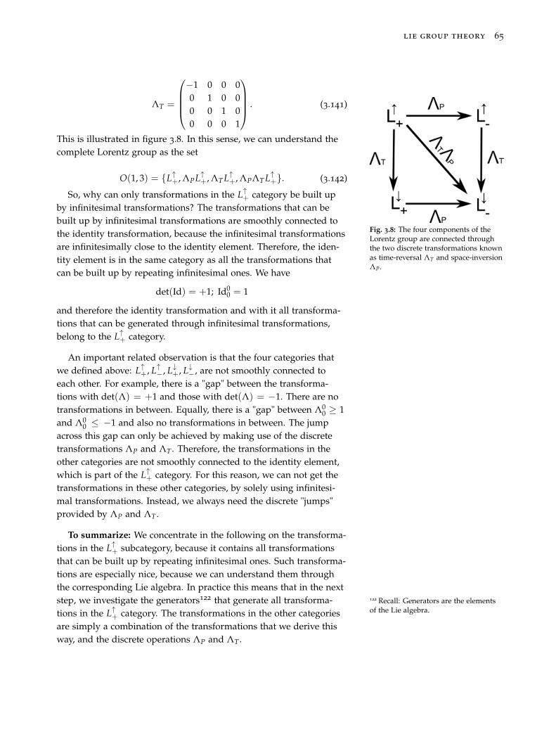
lie group theory 65
ΛT =
⎛⎜⎜⎜⎝−1 0 0 00 1 0 00 0 1 00 0 0 1
⎞⎟⎟⎟⎠ . (3.141)
This is illustrated in figure 3.8. In this sense, we can understand thecomplete Lorentz group as the set
O(1, 3) = {L↑+, ΛPL↑
+, ΛT L↑+, ΛPΛT L↑
+}. (3.142)
Fig. 3.8: The four components of theLorentz group are connected throughthe two discrete transformations knownas time-reversal ΛT and space-inversionΛP.
So, why can only transformations in the L↑+ category be built up
by infinitesimal transformations? The transformations that can bebuilt up by infinitesimal transformations are smoothly connected tothe identity transformation, because the infinitesimal transformationsare infinitesimally close to the identity element. Therefore, the iden-tity element is in the same category as all the transformations thatcan be built up by repeating infinitesimal ones. We have
det(Id) = +1; Id00 = 1
and therefore the identity transformation and with it all transforma-tions that can be generated through infinitesimal transformations,belong to the L↑
+ category.
An important related observation is that the four categories thatwe defined above: L↑
+, L↑−, L↓
+, L↓−, are not smoothly connected to
each other. For example, there is a "gap" between the transforma-tions with det(Λ) = +1 and those with det(Λ) = −1. There are notransformations in between. Equally, there is a "gap" between Λ0
0 ≥ 1and Λ0
0 ≤ −1 and also no transformations in between. The jumpacross this gap can only be achieved by making use of the discretetransformations ΛP and ΛT . Therefore, the transformations in theother categories are not smoothly connected to the identity element,which is part of the L↑
+ category. For this reason, we can not get thetransformations in these other categories, by solely using infinitesi-mal transformations. Instead, we always need the discrete "jumps"provided by ΛP and ΛT .
To summarize: We concentrate in the following on the transforma-tions in the L↑
+ subcategory, because it contains all transformationsthat can be built up by repeating infinitesimal ones. Such transforma-tions are especially nice, because we can understand them throughthe corresponding Lie algebra. In practice this means that in the nextstep, we investigate the generators122 that generate all transforma- 122 Recall: Generators are the elements
of the Lie algebra.tions in the L↑+ category. The transformations in the other categories
are simply a combination of the transformations that we derive thisway, and the discrete operations ΛP and ΛT .
66 physics from symmetry
3.7.1 One Representation of the Lorentz Group
Let’s see how we can use the defining condition of the Lorentz group(Eq. 3.133) to construct an explicit matrix representation of the al-lowed transformations. First let’s think a moment about what we aretrying to find. The Lorentz group, when acting on 4-vectors123, is123 The usual vector space of special
relativity is the real, four-dimensionalMinkowski space R(1,3). We will lookat the representation on this vectorspace first, because the Lorentz groupis defined there in the first place, i.e. asthe set of transformations that preservethe 4 × 4 metric. Equivalently SU(2)was defined as complex 2 × 2 matricesin the first place and we tried to learnas much as possible about SU(2) fromthese matrices, in order to derive otherrepresentations later .
given by real 4 × 4 matrices. The matrices must be real, because wewant to know how they act on elements of the real Minkowski spaceR(1,3). A generic, real 4 × 4 matrix has 16 parameters. The definingcondition of the Lorentz group, which is in fact 10 conditions124, re-
124 You can see this, by putting a generic4 × 4 matrix Λ, in ΛTηΛ = η.
stricts this to 6 parameters. In other words, to describe a most generalLorentz transformation, 6 parameters are needed. Therefore, if wefind 6 linearly independent generators, we have found a completebasis for the Lie algebra of this group. This means every other gener-ator can be written as a linear combination of these basis generators.In addition, we are then able to compute how these basis genera-tors behave when put into the Lie bracket and therefore to derive theabstract definition of this Lie algebra.
First note that the rotation matrices of 3-dimensional Euclideanspace, which involve only space and leave the time unchanged, fulfilthe condition in Eq. 3.133125. This follows because the spatial part126125 Λσ
μησρΛρν
!= ημν
126 The spatial part are the componentsμ = 1, 2, 3. Commonly this is denotedby ηij, because Latin indices, like i, jalways run from 1 to 3 and Greekindices, like μ and ν, run from 0 to 3.
of the Minkowski metric is proportional to the 3 × 3 identity ma-trix127 and therefore for transformations involving only space, we
127 Recall η11 = η22 = η33 = −1 andηij = 0 for i �= j.
have from Eq. 3.133 the condition
−RT I3×3R = −RT R != −I3×3
→ RT I3×3R = RT R != I3×3.
This is exactly the defining condition of O(3). Together with thecondition (Eq. 3.139)
det(Λ)!= 1
these are the defining conditions of SO(3). We conclude that thecorresponding Lorentz transformations are given by
Λrot =
(1
R3×3
)
with the rotation matrices R3×3 shown in Eq. 3.22 and derived inSection 3.4.1. The corresponding generators are therefore analogousto those we derived for three spatial dimensions in Section 3.4.1:
Ji =
(0
J3dimi
). (3.143)
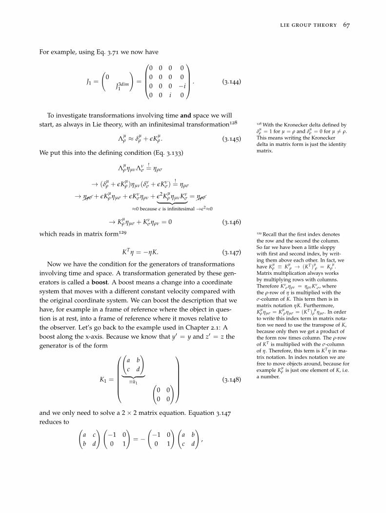
lie group theory 67
For example, using Eq. 3.71 we now have
J1 =
(0
J3dim1
)=
⎛⎜⎜⎜⎝0 0 0 00 0 0 00 0 0 −i0 0 i 0
⎞⎟⎟⎟⎠ . (3.144)
To investigate transformations involving time and space we willstart, as always in Lie theory, with an infinitesimal transformation128 128 With the Kronecker delta defined by
δμρ = 1 for μ = ρ and δ
μρ = 0 for μ �= ρ.
This means writing the Kroneckerdelta in matrix form is just the identitymatrix.
Λμρ ≈ δ
μρ + εKμ
ρ . (3.145)
We put this into the defining condition (Eq. 3.133)
Λμρ ημνΛν
σ!= ηρσ
→ (δμρ + εKμ
ρ )ημν(δνσ + εKν
σ)!= ηρσ
→��ηρσ + εKμρ ημσ + εKν
σηρν + ε2Kμρ ημνKν
σ︸ ︷︷ ︸≈0 because ε is infinitesimal →ε2≈0
=��ηρσ
→ Kμρ ημσ + Kν
σηρν = 0 (3.146)
which reads in matrix form129 129 Recall that the first index denotesthe row and the second the column.So far we have been a little sloppywith first and second index, by writ-ing them above each other. In fact, wehave Kμ
ρ ≡ Kμρ → (KT)
μρ = K μ
ρ .Matrix multiplication always worksby multiplying rows with columns.Therefore Kν
σηρν = ηρνKνσ , where
the ρ-row of η is multiplied with theσ-column of K. This term then is inmatrix notation ηK. Furthermore,Kμ
ρ ημσ = Kμρημσ = (KT)
μρ ημσ . In order
to write this index term in matrix nota-tion we need to use the transpose of K,because only then we get a product ofthe form row times column. The ρ-rowof KT is multiplied with the σ-columnof η. Therefore, this term is KTη in ma-trix notation. In index notation we arefree to move objects around, because forexample Kμ
ρ is just one element of K, i.e.a number.
KTη = −ηK. (3.147)
Now we have the condition for the generators of transformationsinvolving time and space. A transformation generated by these gen-erators is called a boost. A boost means a change into a coordinatesystem that moves with a different constant velocity compared withthe original coordinate system. We can boost the description that wehave, for example in a frame of reference where the object in ques-tion is at rest, into a frame of reference where it moves relative tothe observer. Let’s go back to the example used in Chapter 2.1: Aboost along the x-axis. Because we know that y′ = y and z′ = z thegenerator is of the form
K1 =
⎛⎜⎜⎜⎜⎜⎜⎝
(a bc d
)︸ ︷︷ ︸
≡k1 (0 00 0
)⎞⎟⎟⎟⎟⎟⎟⎠ (3.148)
and we only need to solve a 2 × 2 matrix equation. Equation 3.147reduces to (
a cb d
)(−1 00 1
)= −
(−1 00 1
)(a bc d
),
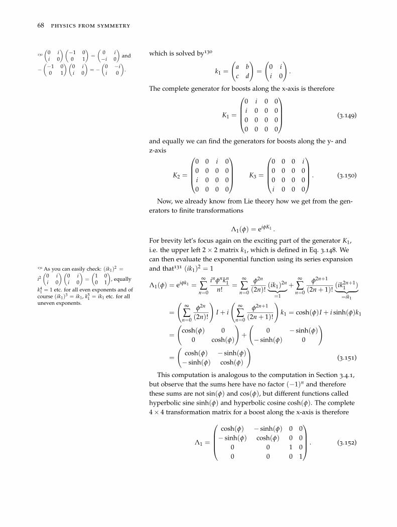
68 physics from symmetry
which is solved by130130
(0 ii 0
)(−1 00 1
)=
(0 i−i 0
)and
−(−1 0
0 1
)(0 ii 0
)= −
(0 −ii 0
). k1 =
(a bc d
)=
(0 ii 0
).
The complete generator for boosts along the x-axis is therefore
K1 =
⎛⎜⎜⎜⎝0 i 0 0i 0 0 00 0 0 00 0 0 0
⎞⎟⎟⎟⎠ (3.149)
and equally we can find the generators for boosts along the y- andz-axis
K2 =
⎛⎜⎜⎜⎝0 0 i 00 0 0 0i 0 0 00 0 0 0
⎞⎟⎟⎟⎠ K3 =
⎛⎜⎜⎜⎝0 0 0 i0 0 0 00 0 0 0i 0 0 0
⎞⎟⎟⎟⎠ . (3.150)
Now, we already know from Lie theory how we get from the gen-erators to finite transformations
Λ1(φ) = eiφK1 .
For brevity let’s focus again on the exciting part of the generator K1,i.e. the upper left 2 × 2 matrix k1, which is defined in Eq. 3.148. Wecan then evaluate the exponential function using its series expansionand that131 (ik1)
2 = 1131 As you can easily check: (ik1)2 =
i2(
0 ii 0
)(0 ii 0
)=
(1 00 1
), equally
k41 = 1 etc. for all even exponents and of
course (ik1)3 = ik1, k5
1 = ik1 etc. for alluneven exponents.
Λ1(φ) = eiφk1 =∞
∑n=0
inφnkn1
n!=
∞
∑n=0
φ2n
(2n)!(ik1)
2n︸ ︷︷ ︸=1
+∞
∑n=0
φ2n+1
(2n + 1)!(ik2n+1
1 )︸ ︷︷ ︸=ik1
=
(∞
∑n=0
φ2n
(2n)!
)I + i
(∞
∑n=0
φ2n+1
(2n + 1)!
)k1 = cosh(φ)I + i sinh(φ)k1
=
(cosh(φ) 0
0 cosh(φ)
)+
(0 − sinh(φ)
− sinh(φ) 0
)
=
(cosh(φ) − sinh(φ)− sinh(φ) cosh(φ)
)(3.151)
This computation is analogous to the computation in Section 3.4.1,but observe that the sums here have no factor (−1)n and thereforethese sums are not sin(φ) and cos(φ), but different functions calledhyperbolic sine sinh(φ) and hyperbolic cosine cosh(φ). The complete4 × 4 transformation matrix for a boost along the x-axis is therefore
Λ1 =
⎛⎜⎜⎜⎝cosh(φ) − sinh(φ) 0 0− sinh(φ) cosh(φ) 0 0
0 0 1 00 0 0 1
⎞⎟⎟⎟⎠ . (3.152)
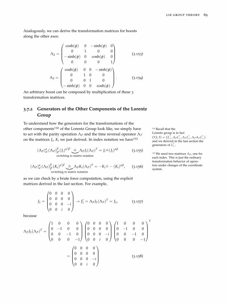
lie group theory 69
Analogously, we can derive the transformation matrices for boostsalong the other axes:
Λ2 =
⎛⎜⎜⎜⎝cosh(φ) 0 − sinh(φ) 0
0 1 0 0− sinh(φ) 0 cosh(φ) 0
0 0 0 1
⎞⎟⎟⎟⎠ (3.153)
Λ3 =
⎛⎜⎜⎜⎝cosh(φ) 0 0 − sinh(φ)
0 1 0 00 0 1 0
− sinh(φ) 0 0 cosh(φ)
⎞⎟⎟⎟⎠ . (3.154)
An arbitrary boost can be composed by multiplication of these 3transformation matrices.
3.7.2 Generators of the Other Components of the LorentzGroup
To understand how the generators for the transformations of theother components132 of the Lorentz Group look like, we simply have 132 Recall that the
Lorentz group is in factO(1, 3) = {L↑
+, ΛP L↑+, ΛT L↑
+, ΛPΛT L↑+}
and we derived in the last section thegenerators of L↑
+.
to act with the parity operation ΛP and the time reversal operator ΛT
on the matrices Ji, Ki we just derived. In index notation we have133
133 We need two matrices ΛP, one foreach index. This is just the ordinarytransformation behavior of opera-tors under changes of the coordinatesystem.
(ΛP)αα′(ΛP)
ββ′(Ji)
α′β′ =︸︷︷︸switching to matrix notation
ΛP Ji(ΛP)T = Ji=(Ji)
αβ (3.155)
(ΛP)αα′(ΛP)
ββ′(Ki)
α′β′ =︸︷︷︸switching to matrix notation
ΛPKi(ΛP)T = −Ki=− (Ki)
αβ, (3.156)
as we can check by a brute force computation, using the explicitmatrices derived in the last section. For example,
J1 =
⎛⎜⎜⎜⎝0 0 0 00 0 0 00 0 0 −i0 0 i 0
⎞⎟⎟⎟⎠ → J′1 = ΛP J1(ΛP)T = J1, (3.157)
because
ΛP J1(ΛP)T =
⎛⎜⎜⎜⎝1 0 0 00 −1 0 00 0 −1 00 0 0 −1
⎞⎟⎟⎟⎠⎛⎜⎜⎜⎝
0 0 0 00 0 0 00 0 0 −i0 0 i 0
⎞⎟⎟⎟⎠⎛⎜⎜⎜⎝
1 0 0 00 −1 0 00 0 −1 00 0 0 −1
⎞⎟⎟⎟⎠T
=
⎛⎜⎜⎜⎝0 0 0 00 0 0 00 0 0 −i0 0 i 0
⎞⎟⎟⎟⎠ (3.158)
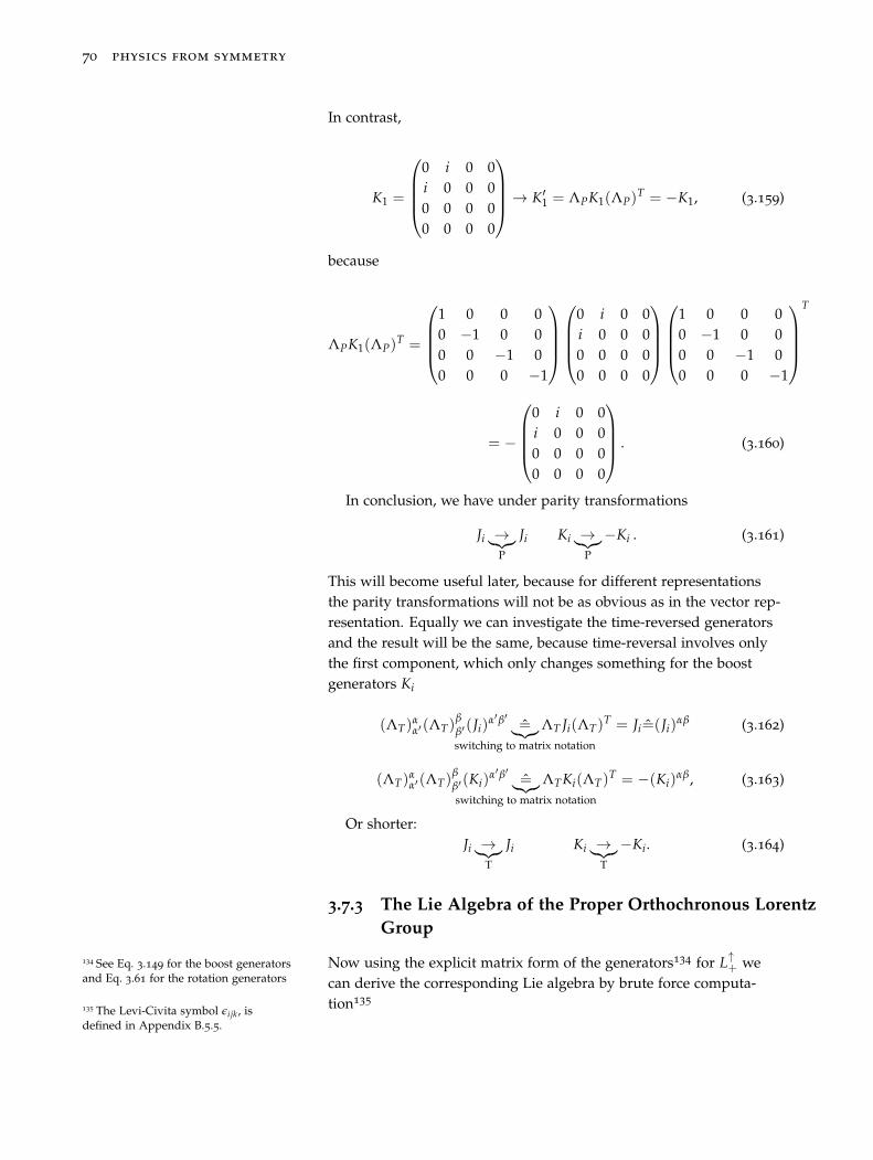
70 physics from symmetry
In contrast,
K1 =
⎛⎜⎜⎜⎝0 i 0 0i 0 0 00 0 0 00 0 0 0
⎞⎟⎟⎟⎠ → K′1 = ΛPK1(ΛP)
T = −K1, (3.159)
because
ΛPK1(ΛP)T =
⎛⎜⎜⎜⎝1 0 0 00 −1 0 00 0 −1 00 0 0 −1
⎞⎟⎟⎟⎠⎛⎜⎜⎜⎝
0 i 0 0i 0 0 00 0 0 00 0 0 0
⎞⎟⎟⎟⎠⎛⎜⎜⎜⎝
1 0 0 00 −1 0 00 0 −1 00 0 0 −1
⎞⎟⎟⎟⎠T
= −
⎛⎜⎜⎜⎝0 i 0 0i 0 0 00 0 0 00 0 0 0
⎞⎟⎟⎟⎠ . (3.160)
In conclusion, we have under parity transformations
Ji →︸︷︷︸P
Ji Ki →︸︷︷︸P
−Ki . (3.161)
This will become useful later, because for different representationsthe parity transformations will not be as obvious as in the vector rep-resentation. Equally we can investigate the time-reversed generatorsand the result will be the same, because time-reversal involves onlythe first component, which only changes something for the boostgenerators Ki
(ΛT)αα′(ΛT)
ββ′(Ji)
α′β′ =︸︷︷︸switching to matrix notation
ΛT Ji(ΛT)T = Ji=(Ji)
αβ (3.162)
(ΛT)αα′(ΛT)
ββ′(Ki)
α′β′ =︸︷︷︸switching to matrix notation
ΛTKi(ΛT)T = −(Ki)
αβ, (3.163)
Or shorter:Ji →︸︷︷︸
T
Ji Ki →︸︷︷︸T
−Ki. (3.164)
3.7.3 The Lie Algebra of the Proper Orthochronous LorentzGroup
Now using the explicit matrix form of the generators134 for L↑+ we134 See Eq. 3.149 for the boost generators
and Eq. 3.61 for the rotation generators can derive the corresponding Lie algebra by brute force computa-tion135
135 The Levi-Civita symbol εijk , isdefined in Appendix B.5.5.
lie group theory 71
[Ji, Jj] = iεijk Jk (3.165)
[Ji, Kj] = iεijkKk (3.166)
[Ki, Kj] = −iεijk Jk , (3.167)
where again Ji denotes the generators of rotations and Ki are thegenerators of boosts. A general Lorentz transformation is of the form
Λ = ei�J·�θ+i�K·�Φ (3.168)
Equation 3.166 tells us that the two types of generator (Ji and Ki)do not commute with each other. While the rotation generators areclosed under commutation136, the boost generators are not137. We 136 Closed under commutation means
that the commutator [Ji , Jj] = Ji Jj − Jj Ji ,is again a rotation generator. FromEq. 3.165 we can see that this is thecase.
137 Eq. 3.167 tells us that the commutatorof two boost generators Ki and Kj isn’tanother boost generator, but a generatorof rotations.
can now define two new operator types from the old ones that areclosed under commutation and commute with each other138
138 Again, take note that we use acomplex linear combination here andrecall that this process of consideringa complex linear combination, insteadof the original generators is called acomplexification. Usually we onlyallow real linear combinations ofthe generators. So from here on, weconsider the complexification of the Liealgebra of the Lorentz group.
N±i =
12(Ji ± iKi). (3.169)
Working out the commutation relations yields
[N+i , N+
j ] = iεijk N+k (3.170)
[N−i , N−
j ] = iεijk N−k (3.171)
[N+i , N−
j ] = 0. (3.172)
These are precisely the commutation relations for the Lie algebra ofSU(2) and we have therefore discovered that the complexified Liealgebra of L↑
+ consists of two copies of the Lie algebra su(2)139. 139 Recall that when we discussedthe representations of the Lie al-gebra su(2), we also used the cor-responding complexification. Thecomplexification of su(2) is sl(2, C)and therefore technically we haveso(1, 3)C
∼= sl(2, C) ⊕ sl(2, C), whereso(1, 3)C denotes the complexificationof the Lorentz group Lie algebra.
This is great news, because we already know how to constructall irreducible representations of the Lie algebra of su(2). Howeverwe must be careful. The Lorentz group is, like SO(3), not simply-connected140 and Lie theory tells us that, for groups that aren’t sim-
140 We will use this simply as a fact here,because a proof would lead us too farapart.
ply connected, there is no one-to-one correspondence between theirreducible representations of the Lie algebra and representations ofthe corresponding group141. Instead, by deriving the irreducible
141 This can be quite confusing, butremember that there is always onedistinguished group that belongs to aLie algebra. This group is distinguishedbecause it is simply connected. If wederive the irreducible representationof a Lie algebra, we get, by puttingthose Lie algebra elements (= thegenerators) in the exponential function,representations of the simply connected(= covering) group. Only for the simplyconnected group there is a one-to-onecorrespondence.
representations of the complexified Lie algebra of the Lorentzgroup, we find the irreducible representations of the coveringgroup of the Lorentz group, if we put the corresponding genera-tors into the exponential function. Some of these representations willbe representations of the Lorentz group, but we will find more thanthat. This is good, because we need these additional representationsto describe certain elementary particles.
72 physics from symmetry
For brevity, we will continue to call the representations we will derive,representations of the Lorentz group instead of representations of the Liealgebra of the Lorentz group or representations of the double cover of theLorentz group.
Each irreducible representation of the Lie algebra su(2) can belabeled by the scalar value j of the su(2) Casimir operator142. There-142 To be precise: the scalar value that
we get from the quadratic Casimiroperator is j(j + 1). However, forbrevity, we simply use j instead.
fore, we now know that we can label the irreducible representationsof the covering group143 of the Lorentz group by two integer or half
143 The covering group of the properorthochronous Lorentz group L↑
+ isSL(2, C), which is defined as the set of2 × 2 matrices with unit determinantand complex entries. The relationshipSL(2, C) → L↑
+ ≡ SO(1, 3)↑+ is similarto the relationship SU(2) → SO(3) wediscovered earlier in this text.
integer numbers: j1 and j2. This means we will look at the (j1, j2) rep-resentations and use the j1, j2 = 0, 1
2 , 1 . . . representations for the twosu(2) copies, which we derived earlier.
It is conventional to write the Lorentz algebra in a more compactway by introducing a new symbol Mμν, which is defined through theequations
Ji =12
εijk Mjk. (3.173)
Ki = M0i . (3.174)
With this new definition the Lorentz algebra reads
[Mμν, Mρσ] = i(ημρ Mνσ − ημσ Mνρ − ηνρ Mμσ + ηνσ Mμρ). (3.175)
Next, we investigate different representations of the complexified Liealgebra of the Lorentz group and hence of the double cover of theLorentz group in detail.
3.7.4 The (0, 0) Representation
The lowest dimensional representation is, as it is for SU(2), trivial,because the vector space is one-dimensional for both copies of su(2).Our generators must therefore be 1 × 1 matrices and the only 1 × 1"matrix" that fulfills the commutation relations is the number 0:
N+i = N−
i = 0 → eiN+i = eiN−
i = e0 = 1 (3.176)
Therefore we conclude that the (0, 0) representation of the Lorentzgroup acts on objects that do not change under Lorentz transforma-tions. This representation is called the scalar representation.
3.7.5 The (12 , 0) Representation
In this representation we use the144 2 dimensional representation144 Recall that the dimension of our vec-tor space is given by 2j + 1. Thereforewe have here 2 1
2 + 1 = 2 dimensions.for one copy of the SU(2) Lie algebra N+
i , i.e. N+i = σi
2 and the 1
lie group theory 73
dimensional representation for the other N−i , i.e. N−
i = 0. From thedefinition of N− in Eq. 3.169 we conclude
N−i =
12(Ji − iKi) = 0 (3.177)
→ Ji = iKi. (3.178)
Furthermore, we can use that we already derived in Section 3.6.3 thetwo dimensional representation of SU(2):
N+i =
σi2
, (3.179)
where σi denotes once more the Pauli matrices, which were definedin Eq. 3.80. On the other hand, we have
N+i =︸︷︷︸Eq. 3.169
12(Ji + iKi) =︸︷︷︸
Eq. 3.178
12(iKi + iKi) = iKi (3.180)
Comparing Eq. 3.179 with Eq. 3.180 tells us that
iKi =σi2
→ Ki =σi2i
=iσi2i2
=−i2
σi (3.181)
Eq. 3.178 → Ji = iKi =−i2
2σi =
12
σi. (3.182)
We conclude that a Lorentz rotation in this representation is given by
Rθ = ei�θ·�J = ei�θ·�σ2 (3.183)
and a Lorentz boost by
Bφ = ei�φ·�K = e�φ·�σ2 . (3.184)
By writing out the exponential function as series expansion we caneasily get the representation of the double cover of the Lorentz groupfrom the representation of the generators. For example, rotationsabout the x-axis e.g. are given by
Rx(θ) = eiθ J1 = eiθ 12 σ1 = 1 +
i2
θσ1 +12
(i2
θσ1
)2+ . . . (3.185)
And if we use the explicit matrix form of σ1 (Eq. 3.80), together withthe fact that σ2
1 = 1, we get145 145 The steps are completely analogousto what we did in Section 3.4.1
Rx(θ) =
(1 00 1
)+
i2
θ
(0 11 0
)− 1
2
(θ
2
)2(
1 00 1
)+ . . .
=
(cos( θ
2 ) i sin( θ2 )
i sin( θ2 ) cos( θ
2 )
). (3.186)
74 physics from symmetry
Analogously, we can compute the transformation matrix for rota-tions around other axes or boosts. One important thing to notice isthat we have here complex 2 × 2 matrices, representing the Lorentztransformations. These transformations certainly do not act on thefour-vectors of Minkowski space, because these have 4 components.The two-component146 objects this representation acts on are called146 We will learn later that these two
components correspond to spin-up andspin-down states.
left-chiral spinors147:
147 This name will make more senseafter the definition of right-chiralspinors. Then we can see that paritytransformations transform a left-chiralspinor transformation into a right-chiral spinor transformation and viceversa. These spinors are often calledleft-handed and right-handed, but thiscan be confusing, because these termscorrespond originally to a conceptcalled helicity, which is not the sameas chirality. Recall what the parityoperator does: changing a left-handedcoordinate system into a right-handedcoordinate system and vice versa.Hence the name.
χL =
((χL)1
(χL)2 .
)(3.187)
Spinors in this context are two component objects. A possibledefinition for left-chiral spinors is that they are objects that transformunder Lorentz transformations according to the ( 1
2 , 0) representationof the Lorentz group. Take note that this is not just another way todescribe the same thing, because spinors have properties that usualvectors do not have. For instance, the factor 1
2 in the exponent. Thisfactor shows us that a spinor is after a rotation by 2π not the same,but gets a minus sign148. This is a pretty crazy property, because we
148 There is much more one can sayabout spinors. See, for example, chapter3.2 in J. J. Sakurai. Modern QuantumMechanics. Addison Wesley, 1st edition,9 1993. ISBN 9780201539295
usually expect that objects are exactly the same after a rotation by360◦ = 2π.
In the last section, we saw that the lowest-dimensional representa-tion is trivial. The next representation in the "hierarchy" of represen-tations is the spinor representation that we discovered in this section.In this sense, we can say that
". . . a spinor is the most basic sort of mathematical object that can beLorentz-transformed."
- A. M. Steane149149 Andrew M. Steane. An introductionto spinors. ArXiv e-prints, December2013
3.7.6 The (0, 12) Representation
This representation can be constructed analogous to the ( 12 , 0) repre-
sentation but this time we use the 1 dimensional representation forN+
i , i.e. N+i = 0 and the two dimensional representation for N−
i , i.e.N−
i = 12 σi . A first guess could be that this representation looks ex-
actly like the ( 12 , 0) representation, but this is not the case! This time
we get from the definition of N+ in Eq. 3.169
N+i =
12(Ji + iKi) = 0 (3.188)
→ Ji = −iKi. (3.189)
Take notice of the minus sign. Using the two-dimensional represen-tation of su(2) for N+, which was derived in Section 3.6.3, yields
lie group theory 75
N−i =
12
σi =12(Ji − iKi) =︸︷︷︸
Eq. 3.189
12(−iKi − iKi) = −iKi . (3.190)
Using this we can deduce the (0, 12 ) representation of the boost gener-
ators
−iKi =12
σi → Ki =−12i
σi =−i2i2
σi =i2
σi. (3.191)
In addition, from Eq. 3.189 we get
Ji = −iKi =12
σi . (3.192)
We conclude that in this representation a Lorentz rotation is given by
Rθ = ei�θ·�J = ei�θ·�σ2 (3.193)
and a Lorentz boost by
Bφ = ei�φ·�K = e−�φ·�σ2 . (3.194)
Therefore, rotations are the same as in the ( 12 , 0) representation, but
boosts differ by a minus sign in the exponent. We conclude bothrepresentations act on objects that are similar but not the same. Wecall the objects the (0, 1
2 ) representation of the Lorentz group acts onright-chiral spinors:
χR =
((χR)
1
(χR)2
)(3.195)
The generic name for left- and right-chiral spinors is Weyl spinors.
3.7.7 Van der Waerden Notation
Now we introduce a notation that makes working with spinors veryconvenient. We know that we have two kinds of objects that trans-form differently and therefore must be distinguished. In the lastsection we learned that they are different, but not too different. Ina moment we will learn that there is a connection between the ob-jects transforming according to the ( 1
2 , 0) representation (left-chiralspinors) and the objects transforming according to the (0, 1
2 ) repre-sentation (right-chiral spinors). To be able to describe these differentobjects using one notation we introduce the notions of dotted andundotted indices, sometimes called Van der Waerden notation, aftertheir inventor. This will help us to keep track of which object trans-forms in what way. This will become much clearer in a minute, assoon as we have set up the full formalism.
76 physics from symmetry
Let’s define that a left-chiral spinor χL has a lower, undotted index
χL = χa (3.196)
and a right-chiral spinor χR has an upper, dotted index
χR = χa. (3.197)
Next, we introduce the "spinor metric". The spinor metric enablesus to transform a right-chiral spinor into a left-chiral and vice versa,but not alone as we will see. We define the spinor metric150 as
150 Take note that this is the Levi-Civitasymbol in two dimensions as defined inAppendix B.5.5.
εab =
(0 1−1 0
)(3.198)
and show that it has the desired properties. Furthermore, we de-fine151151 Maybe a short comment on the
strange notation χCL is in order. The su-
perscript C denotes charge conjugation,as will be explained in Section 3.7.10 inmore detail. Here we see that this op-eration flips one label, i.e. a left-chiralspinor becomes right-chiral. Later wewill see this operation flips all labels,including, for example, the electriccharge.
χCL ≡ εχ�
L (3.199)
where the � denotes complex conjugation. We will now inspect howχC
L transforms under Lorentz transformations and see that it trans-forms precisely as a right-chiral spinor. The defining feature of aright-chiral spinor is its transformation behavior and therefore wewill conclude that χC
L is a right-chiral spinor. Let us have a look athow χC
L transforms under boosts, where we use
(−ε)(ε) = 1 (3.200)
and(ε)σ�
i (−ε) = −σi (3.201)
for each Pauli matrix σi, as you can check by using Eq. 3.198. Trans-forming χC
L yields152152 We use the notation �φ�σ =
∑i φiσi =︸︷︷︸summation convention
φiσi . The "vector"�σ
shouldn’t be taken too seriously, be-cause it’s just a shorthand, conventionalnotation.
χCL → χ′C
L = ε(χ′)�L
= ε
((e
�φ2�σχL
)�
= ε
(e�φ2�σ (−ε)(ε)︸ ︷︷ ︸
=1 (Eq. 3.200)
χL
)�
= εe�φ2�σ
�(−ε)︸ ︷︷ ︸=e−
�φ2�σ (Eq. 3.201)
(ε)χ�L
= e−�φ2�σ εχ�
L︸︷︷︸=χC
L
= e−�φ2�σχC
L , (3.202)
lie group theory 77
which is exactly the transformation behavior of a right-chiral spinor153. 153 The transformation behavior ofright-chiral spinors under boosts was
derived in Eq. 3.194: Bθ = ei�φ�K = e−�φ�σ2 .
Compare this to how left-chiral spinorstransform under boosts, as derived inEq. 3.184: Bθ = ei�φ�K = e�φ
�σ2
To get to the fifth line, we use the series expansion of e�φ2�σ and Eq. 3.201
on every term. You can check in the same way that the behavior un-der rotations is not changed by complex conjugation and multiplica-tion with ε, as it should be, because χL and χR transform in the sameway under rotations:
χCL → χ′C
L = ε(χ′)�L = ε(ei�θ2�σχ)�L = e
i�θ2�σε(χL)
� = ei�θ2�σχC
L . (3.203)
Furthermore, you can check that ε is invariant under all transforma-tions and that if we want to go the other way round, i.e. transform aright-chiral spinor into a left-chiral spinor, we have to use (-ε).
Therefore, we define in analogy with the tensor notation of specialrelativity that our "metric" raises and lowers indices
εχL =︸︷︷︸written in index notation
εacχc = χa , (3.204)
where summation over identical indices is implicitly assumed (Ein-stein summation convention). Furthermore, we know that if we wantto get χR from χL we need to use complex conjugation as well
χR = εχL� . (3.205)
This means that complex conjugation transforms an undotted indexinto a dotted index:
χR = εχL� = χa. (3.206)
Therefore, we can get a lower, dotted index by complex conjugatingχL:
χL� = χa
� = χa (3.207)
and an upper, undotted index, by complex conjugating χR
χR� = (χa)� = χa . (3.208)
It is instructive to investigate how χa and χa transform, becausethese objects are needed to construct terms from spinors, which donot change under Lorentz transformations. Terms like this are incred-ibly important, because we need them to derive physical laws thatare the same in all frames of reference. This will be made explicit in amoment. From the transformation behavior of a left-chiral spinor
χL = χa → χ′a =
(ei�θ�σ2 +�φ
�σ2
)b
aχb , (3.209)
we can derive how a spinor with lower, dotted index transforms:
78 physics from symmetry
χ�L = χ�
a = χa → χ′a = (χ′
a)� =
((ei�θ�σ2 +�φ
�σ2
)b
a
)�
χ�b
=
(e−i�θ �σ�2 +�φ
�σ�2
)b
aχb (3.210)
Analogously, we use that we know how a right-chiral spinor trans-forms:
χR → χ′R = χ′a =
(ei�θ�σ2 −�φ�σ2
)a
bχb (3.211)
to derive how a spinor with upper, undotted index transforms:
χ�R = (χa)� = χa → χ′a = (χ′a)� =
((ei�θ�σ2 −�φ�σ2
)a
b
)�
(χb)�
=
(e−i�θ �σ�2 −�φ �σ�
2
)a
bχb . (3.212)
To be able to write products of spinors that do not change underLorentz transformations, we need one more ingredient. Recall howthe scalar product of two vectors is defined: �a ·�b = �aT�b. In the samespirit we should transpose one of the spinors in a spinor product.We can see this, because at the moment we have the complex con-
jugate of the Pauli matrices σ�i in the exponent, for example, e−i�θ �σ�2 .
Together with transposing this becomes the Hermitian conjugate:σ†
i = (σ�i )
T , where the symbol † is called "dagger". The Hermitianconjugate of every Pauli matrix, is again the same Pauli matrix
σ†i = (σ�
i )T = σi, (3.213)
as you can easily check by looking at the explicit form of the Paulimatrices (Eq. 3.80).
By comparing Eq. 3.209 with Eq. 3.212 and using Eq. 3.213, wesee that the transformation behavior of a transposed spinor withlower, undotted index is exactly the opposite of a spinor with upper,undotted index. This means a term of the form (χa)Tχa is invariant(=does not change) under Lorentz transformations, because154154 As explained in Appendix B.5.5, the
symbol δcb is called Kronecker symbol
and denotes the unit matrix in indexnotation. This means δc
b = 1 for b = cand δc
b = 0 for b �= c.
lie group theory 79
(χa)Tχa → (χ′a)Tχ′a =
((e−i�θ�σ
�
2 −�φ�σ�
2
)a
bχb
)T (ei�θ�σ2 +�φ
�σ2
)c
aχc
= (χb)T(
e−i�θ�σ�T2 −�φ�σ�T
2
)a
b
(ei�θ�σ2 +�φ
�σ2
)c
aχc
=︸︷︷︸Eq. 3.213
(χb)T(
e−i�θ�σ2 −�φ�σ2)a
b
(ei�θ�σ2 +�φ
�σ2
)c
a︸ ︷︷ ︸=δc
b
χc
= (χc)Tχc . (3.214)
In the same way we can combine an upper, dotted index with alower, dotted index as you can verify by comparing Eq. 3.210 withEq. 3.211. In contrast, a term of the form (χa)Tχa=χT
RχL isn’t invari-ant under Lorentz transformations, because
χTRχL = (χa)Tχa → (χ′a)Tχ′
a = χb(
ei�θ�σT2 −�φ �σT
2
)a
b
(ei�θ�σ2 +�φ
�σ2
)c
a︸ ︷︷ ︸�=δc
b
χc
(3.215)Therefore a term combining a left-chiral with a right-chiral spinor
is not Lorentz invariant. We conclude, we must always combine anupper with a lower index of the same type155 in order to get Lorentz 155 In this context dotted a
aor undotted a
a .invariant terms. Or formulated differently, we must combine theHermitian conjugate of a right-chiral spinor with a left-chiral spinorχ†
RχL = (χ�R)
TχL=(χa)Tχa, or the Hermitian conjugate of a left-chiralspinor with a right-chiral spinor χ†
LχR = (χ�L)
TχR = (χa)Tχa to getLorentz invariant terms. We will use this later, when need invariantterms that we can use to formulate our laws of nature.
In addition, we have now another justification for calling εab thespinor metric, because the invariant spinor product in Eq. 3.214, canbe written as
χTa χa =︸︷︷︸
Eq. 3.204
χTa εabχb. (3.216)
Compare this to how we defined in Eq. 2.31 the invariant product ofMinkowsi space by using the Minkowski metric ημν:
xμyμ = xμημνyν. (3.217)
The spinor metric is for spinors indeed what the Minkowski metric isfor four-vectors156.
156 Don’t get confused why we haveno transposition for the four-vectorshere. These equations can be read intwo ways. On the one hand as vectorequations and on the other hand ascomponent equations. It’s conventionaland sometimes confusing to use thesame symbol xμ for a four-vectorand its components. If we read theequation as a component equation weneed no transposition. The same is ofcourse true for our spinor products.Nevertheless, we have seen above thatwe mustn’t forget to transpose and inorder to avoid errors we included theexplicit superscript T, although thespinor equation here can be read ascomponent equation that do not need it.In contrast, for three component vectorsthere is a clear distinction using thelittle arrow: �a has components ai .
After setting up this notation, we can now write the spinor "met-
80 physics from symmetry
ric" with lowered indices
εab =
(0 −11 0
), (3.218)
because we need157 (−ε) to get from χR to χL. In addition, we can157 You can check this yourself, but it’snot very important for what follows. now write the two transformation operators as one object Λ. For
example, when it has dotted indices we know it multiplies with aright-chiral spinor and we know which transformation operator tochoose:
χR → χ′R = χ′a = Λa
bχb =(
ei�θ�σ2 −�φ�σ2)a
bχb (3.219)
and analogously for left-chiral spinors
χL → χ′L = χ′
a = Λ ba χb =
(ei�θ�σ2 +�φ
�σ2
) b
aχb . (3.220)
Therefore:
Λ( 12 ,0) =
(ei�θ�σ2 +�φ
�σ2
)=Λ b
a (3.221)
and
Λ(0, 12 )
=(
ei�θ�σ2 −�φ�σ2)=Λa
b (3.222)
This notation is useful, because, as we have seen, the two differentobjects χL and χR aren’t so different after all. In fact we can trans-form them into each other and a unified notation is the logical result.
Now we move on to the next irreducible representation, which willturn out to be an old acquaintance.
3.7.8 The (12 , 1
2) Representation
For this representation we use the 2-dimensional representation forboth copies of the SU(2) Lie algebra158 N+
i and N−i . This time let’s158 Mathematically we have
( 12 , 1
2 ) = ( 12 , 0)⊗ (0, 1
2 ). have a look at what kind of object our representation is going to acton first. The copies will not interfere with each other, because N+
iand N−
i commute, i.e. [N+i , N−
j ] = 0 (Eq. 3.172). Therefore, ourobjects will transform separately under both copies. Let’s name theobject we want to examine v. This object will have 2 indices vb
a, eachtransforming under a separate two-dimensional copy of su(2). Herethe notation we introduced in the last section comes in handy.
We know that our object v will have 4 components, because eachrepresentation is 2 dimensional and this means that both indices cantake on two values ( 1
2 and − 12 ). Therefore, the objects can be 2 × 2
matrices, but it’s also possible to enforce a four component vectorform, as we will see159.
159 Remember that when we talkedabout rotations of the plane we were inthe same situation. The rotation couldbe described by complex numbersacting on complex numbers. Doingthe map to real matrices we had realmatrices acting on real matrices, butthe same action could be described by areal matrix acting on a column vector.
lie group theory 81
First, let’s look at the complex matrix choice. A general 2 × 2matrix has 4 complex entries and therefore 8 free parameters. Asnoted above, we only need 4. We can write every complex matrix Mas a sum of a Hermitian (H† = H) and an anti-Hermitian (A† = −A)matrix: M = H + A. Both Hermitian and anti-Hermitian matriceshave 4 free parameters. In addition, we will see in a moment that ourtransformations in this representation always transform a Hermitian2 × 2 matrix into another Hermitian 2 × 2 matrix and equivalentlyan anti-Hermitian matrix into another anti-Hermitian matrix. Thismeans Hermitian and anti-Hermitian matrices are invariant subsets.As explained in Section 3.5 this means that working with a generalmatrix here, corresponds to having a reducible representation. Puttingthese observations together, we conclude that we can assume thatour irreducible representation acts on Hermitian 2 × 2 matrices. Abasis160 for Hermitian 2 × 2 matrices is given by the Pauli matrices 160 This means that an arbitrary Her-
mitian 2 × 2 matrix can be writtenas a linear combination of the form:a01 + aiσi
together with the identity matrix.
Instead of examining vba, we will have a look at vab, because then
we can use the Pauli matrices as defined in Eq. 3.80. Take note that vba
and vab can be transformed into each other by multiplication with εbc
and therefore if you want to work with vba, you simply have to use the
Pauli matrices that have been multiplied with ε.
If we define σ0 = I2×2 =
(1 00 1
), we can write
vab = vνσνab = v0
(1 00 1
)+ v1
(0 11 0
)+ v2
(0 −ii 0
)+ v3
(1 00 −1
).
(3.223)As explained above, we could use161 vb
a = vμσμacεbc instead, which 161 This is really just a basis choice and
here we choose the basis that givesus with our definition of the Paulimatrices, the transformation behaviorwe derived earlier for vectors.
means we would use the basis (σba )
μ = σμacεbc. We therefore write a
general Hermitian matrix as
vab =
(v0 + v3 v1 − iv2
v1 + iv2 v0 − v3
). (3.224)
Remember that we have learned in the last section that differentindices transform differently. For example, a lower dotted indextransforms differently than a lower undotted index.
Now we have a look at how vab transforms and use the transforma-
82 physics from symmetry
tion operators that we derived in the last sections
v → v′ = v′ab =(
ei�θ�σ2 +�φ�σ2
) c
avcd
((e−i�θ �σ�2 +�φ
�σ�2
)d
b
)T
=(
ei�θ�σ2 +�φ�σ2
) c
avcd
(e−i�θ
�σ†2 +�φ
�σ†2
)d
b
=︸︷︷︸σ†
i =σi
(ei�θ�σ2 +�φ
�σ2
) c
avcd
(e−i�θ�σ2 +�φ
�σ2
)d
b. (3.225)
We can now see that a Hermitian matrix is after such a transforma-tion still Hermitian, as promised above162
162 Exactly the same computationshows that an anti-Hermitian matrixis still anti-Hermitian after such atransformation. To see this, use inthe last step instead of v†
cd= vcd that
v†cd
= −vcd.
(ei�θ�σ2 +�φ
�σ2
) c
avcd
(e−i�θ�σ2 +�φ
�σ2
)d
b→
((ei�θ�σ2 +�φ
�σ2
) c
avcd
(e−i�θ�σ2 +�φ
�σ2
)d
b
)†
=︸︷︷︸(ABC)†=C†B† A†
((e−i�θ�σ2 +�φ
�σ2
)d
b
)†
v†cd
((ei�θ�σ2 +�φ
�σ2
) c
a
)†
=
(ei�θ
�σ†2 +�φ
�σ†2
)d
bv†
cd
(e−i�θ
�σ†2 +�φ
�σ†2
) c
a
=︸︷︷︸if v†
cd=vcd
(ei�θ�σ2 +�φ
�σ2
) c
avcd
(e−i�θ�σ2 +�φ
�σ2
)d
b�
(3.226)
The explicit computation for an arbitrary transformation is longand tedious163 so instead, we will look at one specific example. Let’s163 See, for example, page 128 in
Matthew Robinson. Symmetry andthe Standard Model. Springer, 1st edition,August 2011. ISBN 978-1-4419-8267-4
boost v along the z-axis164
164 This means �φ = (0, 0, φ)T . Such aboost is the easiest because σ3 is diag-onal. For boosts along other axes theexponential series must be evaluated indetail.
vab → v′ab =(
eφσ32
)c
avcd
(eφ
σ32
)d
b
=
(e
φ2 0
0 e−φ2
)(v0 + v3 v1 − iv2
v1 + iv2 v0 − v3
)(e
φ2 0
0 e−φ2
)
=
(eφ(v0 + v3) v1 − iv2
v1 + iv2 e−φ(v0 − v3)
), (3.227)
where we have used the fact that σ3 is diagonal165 and that eA =
(eA11 0
0 eA22
)165 σ3 =
(1 00 −1
)holds for every diagonal matrix. We now compare the transformedobject that we calculated in Eq. 3.227 with a generic object v′:
v′ab =
(v′0 + v′3 v′1 − iv′2v′1 + iv′2 v′0 − v′3
)=
(eφ(v0 + v3) v1 − iv2
v1 + iv2 e−φ(v0 − v3)
).
This tells us how the components of the transformed object are re-lated to the untransformed components166
166 We rewrite the equations usingthe connection between the hyper-bolic sine, the hyperbolic cosinefunction and the exponential func-tion e−φ = (cosh (φ)− sinh (φ)) andeφ = (cosh (φ) + sinh (φ)), which isconventional in this context. If you areunfamiliar with these functions youcan either take notice of their defini-tions: cosh (φ) ≡ 1
2
(eφ + e−φ
)and
sinh (φ) ≡ 12
(eφ − e−φ
)or rewrite the
few equations here in terms of eφ ande−φ, which is equally good.
lie group theory 83
→ v′0 + v′3 = eφ(v0 + v3) = (cosh (φ) + sinh (φ)) (v0 + v3)
→ v′0 − v′3 = e−φ(v0 − v3) = (cosh (φ)− sinh (φ)) (v0 − v3).
The addition and subtraction of both equations yields
→ v′0 = cosh(φ)v0 + sinh(φ)v3
→ v′3 = sinh(φ)v0 + cosh(φ)v3 . (3.228)
This is exactly what we get using the 4-vector formalism167 167 See 3.154 for the explicit form of thematrix for a boost along the z-axis.⎛⎜⎜⎜⎝
v′0v′1v′2v′3
⎞⎟⎟⎟⎠ =
⎛⎜⎜⎜⎝cosh(φ) 0 0 sinh(φ)
0 1 0 00 0 1 0
sinh(φ) 0 0 cosh(φ)
⎞⎟⎟⎟⎠⎛⎜⎜⎜⎝
v0
v1
v2
v3
⎞⎟⎟⎟⎠
=
⎛⎜⎜⎜⎝cosh(φ)v0 + sinh(φ)v3
v1
v2
sinh(φ)v0 + cosh(φ)v3
⎞⎟⎟⎟⎠ . (3.229)
This is true for arbitrary Lorentz transformations, as you can checkby computing the other possibilities. What we have shown here isthat the ( 1
2 , 12 ) representation is the vector representation. We can
simplify our transformation laws by using the enforced vector form,because multiplying a matrix with a vector is simpler than the multi-plication of three matrices. Nevertheless, we have seen how the famil-iar 4-vector is related to the more fundamental spinors. A 4-vector isa rank-2 spinor, which means a spinor with 2 indices that transformsaccording to the ( 1
2 , 12 ) representation of the Lorentz group. Further-
more, we can now see that 4-vectors aren’t appropriate to describeevery physical system on a fundamental level, because they aren’tfundamental. There are physical systems they cannot describe.
We can now understand why some people say that "spinors arethe square root of vectors". This is meant in the same way as vectorsare the square root of rank-2 tensors168. A rank-2 tensor has two 168 A rank-2 tensor is simply a matrix
Mμν.vector indices and a vector has two spinor indices. Therefore, themost basic object that can be Lorentz transformed is indeed a spinor.
When we started our studies of the Lorentz group, we noted that itconsists of four components169. These components are connected by 169 Eq. 3.142: O(1, 3) =
{L↑+, ΛP L↑
+, ΛT L↑+, ΛPΛT L↑
+}.the parity and the time-reversal operator170. Therefore, to be able to
170 See Eq. 3.142describe all transformations that preserve the speed of light, we needto find the parity and time-reversal transformation for each repre-sentation. In this text we restrict ourselves to parity transformations,
84 physics from symmetry
because the discussion for the time-reversal transformation is verysimilar. We will discuss in in a later section that nature isn’t alwayssymmetric under parity transformations171.171 Nature isn’t invariant under time-
reversal transformations either, but asatisfying discussion of this curious factlies beyond the scope of this book. 3.7.9 Spinors and Parity
Up to this point, there is no justification why we call the objectstransforming according to the ( 1
2 , 0) representation left-chiral andthe objects transforming according to the (0, 1
2 ) representation right-chiral. After talking a bit about parity transformation, this will makesense.
Recall that we already know the behavior of the generators ofthe Lorentz group under parity transformations. The result wasEq. 3.161, which we recite here for convenience
Ji →︸︷︷︸P
Ji Ki →︸︷︷︸P
−Ki . (3.230)
By looking at the definition of the generators N± in Eq. 3.169, whichwe also recite here
N±i =
12(Ji ± iKi) . (3.231)
we can see that under parity transformations N+ ↔ N−. There-fore, the (0, 1
2 ) representation of a transformation, becomes the ( 12 , 0)
representation of this transformation and vice versa under paritytransformations. This is the reason for talking about left- and right-chiral spinors172. Just as a right-handed coordinate system changes172 The conventional name is left- and
right-handed spinors, but this canbe quite confusing, because the no-tions left-handed and right-handedare directly related to a concept calledhelicity, which is different from chi-rality. Anyway the name should makesome sense, because something left ischanged into something right underparity transformations.
into a left-handed coordinate system under parity transformations,these two representations change into each other.
Rotations are the same for both representations, but boost trans-formations differ by a sign and it is easy to make the above statementexplicit:
(Λ�K)( 12 ,0) = e�φ�K →︸︷︷︸
P
e−�φ�K = (Λ�K)(0, 12 )
(3.232)
(Λ�K)(0, 12 )
= e−�φ�K →︸︷︷︸P
e�φ�K = (Λ�K)( 12 ,0). (3.233)
We learn here that if we want to describe a physical system thatis invariant under parity transformations, we will always need right-chiral and left-chiral spinors. The easiest thing to do is to write thembelow each other into a single object called Dirac spinor
Ψ =
(χL
ξR
)=
(χa
ξ a
). (3.234)
lie group theory 85
Recalling that the generic name for left- and right-chiral spinors isWeyl spinors, we can say that a Dirac spinor Ψ consists of two Weylspinors χL and ξR. Note that we want to stay general here and don’tassume any a priori connection between χ and ξ. A Dirac spinor ofthe form
ΨM =
(χL
χR
)(3.235)
is a special case, called Majorana spinor. A Dirac is not a four-vector,because it transforms completely different173. A Dirac spinor trans- 173 Equally, a Majorana spinor is not a
vector.forms according to the ( 12 , 0)⊕ (0, 1
2 ) representation174 of the Lorentz174 This a reducible representation,which is obvious because of theblock-diagonal form of the trans-formation matrix. In contrast, four-vectors transform according to the( 1
2 , 12 ) = ( 1
2 , 0)⊗ (0, 12 ) representation.
group, which means nothing more than writing the correspondingtransformations in block-diagonal form into one big matrix:
Ψ → Ψ′ = Λ( 12 ,0)⊕(0, 1
2 )Ψ =
(Λ( 1
2 ,0) 0
0 Λ(0, 12 )
)(χL
ξR
). (3.236)
For example, a boost transformation is in this representation
Ψ → Ψ′ =
⎛⎝e�φ2�σ 0
0 e−�φ2 �σ
⎞⎠(χL
ξR
). (3.237)
It is instructive to investigate how Dirac spinors behave underparity transformations, because once we know how Dirac spinorstransform under parity transformations, we can check if a giventheory is invariant under such transformations. We can’t expect thata Dirac spinor is after a parity transformation still a Dirac spinor (anobject transforming according to the ( 1
2 , 0) ⊕ (0, 12 ) representation),
because we know that under parity transformations N+ ↔ N− andtherefore (
0,12
)↔︸︷︷︸P
(12
, 0)
. (3.238)
We conclude that if a Dirac spinor transforms according to the( 1
2 , 0)⊕ (0, 12 ) representation, the parity transformed object trans-
forms according to the (0, 12 )⊕ ( 1
2 , 0) representation.
ΨP → (ΨP)′ = Λ(0, 12 )⊕( 1
2 ,0)ΨP =
(Λ(0, 1
2 )0
0 Λ( 12 ,0)
)(ξR
χL
). (3.239)
Therefore
Ψ =
(χL
ξR
)→ ΨP =
(ξR
χL
). (3.240)
86 physics from symmetry
A parity transformed Dirac spinor contains the same objects ξR, χL
as the untransformed Dirac spinor, only written differently. A paritytransformation does nothing like ξL → ξR, which is a different kindof transformation we will talk about in the next section.
3.7.10 Spinors and Charge Conjugation
In Section 3.7.7 we stumbled upon a transformation, which yieldsχL → χR and ξR → ξL. The transformation is achieved by χL → χC
L =
εχ�L = χR and analogously for a right-chiral spinor ξR → ξC
R =
(−ε)ξ�R = ξL. We are now able to understand it from a quite differentperspective.
Up to this point, we used this transformation merely as a compu-tational trick in order to raise and lower indices. Now, how does aDirac spinor transform under such a transformation? Naively we get:
Ψ =
(χL
ξR
)→ Ψ =
(χC
LξC
R
)=
(χR
ξL
). (3.241)
Unfortunately, this object does not transform like a Dirac spinor175,175 Unlike for parity transformations,we have a choice here and we preferto keep working with the same kind ofobject. The object Ψ can then be seenas a Dirac spinor that has been paritytransformed and charge conjugated.
which transform under boosts as follows
Ψ → Ψ′ =
⎛⎝e�θ2�σ 0
0 e−�θ2 �σ
⎞⎠(χL
ξR
). (3.242)
In contrast, the object Ψ we get from the naive operation, transformsas
Ψ → Ψ′ =
⎛⎝e−�θ2�σ 0
0 e�θ2�σ
⎞⎠(χL
ξR
). (3.243)
This is a different kind of object, because it transforms according to adifferent representation of the Lorentz group. Therefore we write
Ψ =
(χL
ξR
)→ ΨC =
(ξC
RχC
L
)=
(ξL
χR
), (3.244)
which incorporates the transformation behavior we observed ear-lier and transforms like a Dirac spinor. This operation is commonlycalled charge conjugation, which can be a little misleading. We knowthat this transformation transforms a left-chiral spinor into a right-chiral, i.e. flips one label we use to describe our elementary parti-cles176. Later we will learn that this operator flips not only one, but176 For the more advanced reader: Recall
that each Weyl spinor we are talkingabout here, is in fact a two componentobject. Later we will define a physicalmeasurable quantity, called spin, thatis described by 1
2 σ3. The matrix ε, flipsan object with eigenvalue + 1
2 for thespin operator 1
2 σ3 into an object witheigenvalue − 1
2 . This is commonlyinterpreted as spin flip, which means anobject with spin 1
2 , becomes an objectwith spin − 1
2 .
all labels we use to describe fundamental particles. One such label iselectric charge, hence the name charge conjugation, but before we areable to show this, we need of course to understand first what electric
lie group theory 87
charge is. Nevertheless, it’s always important to remember that alllabels get flipped, not only electric charge.
We could now go on and derive higher-dimensional representa-tions of the Lorentz group, but at this point we already have everyfinite-dimensional irreducible representation we need for the purposeof this text. Nevertheless, there is another representation, the infinite-dimensional representation, that is especially interesting, becausewe need it to transform fields, like, for example, the electromagneticfield.
3.7.11 Infinite-Dimensional Representations
In the last sections, we talked about finite-dimensional representa-tions of the Lorentz group and learned how we can classify them.These finite-dimensional representations acted on constant one-,two- or four-component objects. In physics the objects we are deal-ing with are dynamically changing in space and time, so we need tounderstand how such objects transform. So far, we have dealt withtransformations of the form
Φa → Φ′a = Mab(Λ)Φb , (3.245)
where Mab(Λ) denotes the matrix of the particular finite-dimensionalrepresentation of the Lorentz transformation Λ. This means Mab(Λ)
is a matrix that acts, for example, on a two-component object like aWeyl spinor. The result of the multiplication with this matrix is sim-ply that the components of the object in question get mixed and aremultiplied with constant factors. If our object Φ changes in space andtime, it is a function of coordinates177 Φ = Φ(x) and these coordi- 177 Here x is a shorthand notation for all
spacetime coordinates t, x, y, znates are affected by the Lorentz transformations, too. In general wehave
xμ → Λμν xν, (3.246)
where Λμν denotes the vector representation (= ( 1
2 , 12 ) representation)
of the Lorentz transformation in question. We have in this case178 178 Most books use the Wigner con-vention for symmetry operators:Φa(x) → Mab(Λ)Φb(Λ−1x), butunfortunately there is at this point noway to motivate this convention.
Φa(x) → Mab(Λ)Φb(Λx). (3.247)
Our transformation will therefore consist of two parts. One part, rep-resented by a finite-dimensional representation, acting on Φa and asecond part that transforms the spacetime coordinates x. This sec-ond part will act on an infinite-dimensional179 vector space and we
179 Each component of Φ is now afunction of x. The correspondingoperators act on Φa(x), i.e. functionsof the coordinates and the space offunctions is in this context infinite-dimensional. The reason that the spaceof functions is infinite-dimensionalis that we need an infinite number ofbasis functions. The expansion of anarbitrary function in terms of such aninfinite number of basis functions is theidea behind the Fourier transform asexplained in Appendix D.1.
therefore need an infinite-dimensional representation. The infinite-dimensional representation of the Lorentz group is given by differen-tial operators180
180 The symbols ∂ν are a shorthandnotation for the partial derivative ∂
∂ν.
Minfμν = i(xμ∂ν − xν∂μ) . (3.248)
88 physics from symmetry
You can check by a straightforward computation that Minfμν satisfies
the Lorentz algebra (Eq. 3.175) and transforms the coordinates asdesired.
The transformation of the coordinates is now given by181181 Recall the definition of Mμν inEq. 3.173. The components of ωμν canthen be directly related to the usualrotation angles θi = 1
2 εijkωjk and theboost parameters φi = ω0i .
Φ′(Λx) = e−i ωμν
2 Minfμν Φ(x), (3.249)
where the exponential function is, as usual, understood in termsof its series expansion. The complete transformation is then a com-bination of a transformation generated by the finite-dimensionalrepresentation Mfin
μν and a transformation generated by the infinite-dimensional representation Minf
μν of the generators:
Φa(x) →(
e−i ωμν
2 Mfinμν
)b
ae−i ωμν
2 Minfμν Φb(x). (3.250)
Because our matrices Mfinμν are finite-dimensional and constant we can
put the two exponents together
Φa(x) →(
e−i ωμν
2 Mμν
)b
aΦb(x) (3.251)
with Mμν = Mfinμν + Minf
μν . This representation of the generators of theLorentz group is called field representation.
We can now talk about a different kind of transformation: transla-tions, which means transformations to another location in spacetime.Translations do not mix the components and therefore, we need nofinite-dimensional representation. However, it’s quite easy to findthe infinite-dimensional representation for translations. These arenot part of the Lorentz group, but the laws of nature should be lo-cation independent. The Lorentz group (boosts and rotations) plustranslations is called the Poincaré group, which is the topic of thenext section. Nevertheless, we will introduce the infinite-dimensionalrepresentation of translations already here. For simplicity, we restrictourselves to one dimension. In this case an infinitesimal translationof a function, along the x-axis is given by182182 For a non-infinitesimal ε, we would
get here infinitely many terms. But foran infinitesimal ε, we use ε2 ≈ 0 andtherefore neglect all higher order terms.
Φ(x) → Φ(x + ε) = Φ(x) + ∂xΦ(x)︸ ︷︷ ︸"rate of change" along the x-axis
ε,
which is, of course, the first term of the Taylor series expansion. It isconventional in physics to add an extra −i to the generator and wetherefore define
Pi ≡ −i∂i. (3.252)
With this definition an arbitrary, finite translation is183183 Using i2 = −1.
lie group theory 89
Φ(x) → Φ(x + a) = e−iai Pi Φ(x) = e−ai∂i Φ(x) ,
where ai denotes the amount we want to translate in each direction.If we write the exponential function as Taylor series184, this equation 184 This is derived in Appendix B.4.1.
can simply be seen as the Taylor expansion185 for Φ(x + a). If we185 This is derived in Appendix B.3.want to transform to another point in time we use P0 = i∂0, for a
different location we use Pi = −i∂i.
Now, let’s move on to the full spacetime symmetry group of na-ture: the Poincaré group.
3.8 The Poincaré Group
The Lorentz group includes rotations and boosts. Further transforma-tions that leave the speed of light invariant are translations in spaceand time, because measuring the speed of light at a different point inspacetime does not change its value. If we add these symmetries tothe Lorentz group we get the Poincaré group186 186 The Poincaré group is not the direct,
but the semi-direct, sum of the Lorentzgroup and translations, but for thepurpose of this text we can neglect thistechnical detail.Poincaré group = Lorentz group plus translations
= Rotations plus boosts plus translations (3.253)
The generators of the Poincaré group are the generators of theLorentz group Ji, Ki plus the generators of translations Pμ.
In terms of Ji, Ki and Pμ the Lie algebra reads187 187 This is not very enlightening, butincluded for completeness.
[Ji, Jj] = iεijk Jk (3.254)
[Ji, Kj] = iεijkKk (3.255)
[Ki, Kj] = −iεijk Jk (3.256)
[Ji, Pj] = iεijkPk (3.257)
[Ji, P0] = 0 (3.258)
[Ki, Pj] = iδijP0 (3.259)
[Ki, P0] = −iPi . (3.260)
90 physics from symmetry
Because this looks like a huge mess it is conventional to write this interms of Mμν, which was defined by
Ji =12
εijk Mjk (3.261)
Ki = M0i. (3.262)
With Mμν the Poincaré algebra reads
[Pμ, Pν] = 0 (3.263)
[Mμν, Pρ] = i(ημρPν − ηνρPμ) (3.264)
and of course still have
[Mμν, Mρσ] = i(ημρ Mνσ − ημσ Mνρ − ηνρ Mμσ + ηνσ Mμρ) . (3.265)
For this quite complicated group it is very useful to label the rep-resentations by using the fixed scalar values of the Casimir operators.The Poincaré group has two Casimir operators188 . The first one is:188 Recall that a Casimir operator is
defined as an operator, constructedfrom the generators, that commuteswith all other generators. PμPμ =: m2. (3.266)
We give the scalar value the suggestive name m2, because we willlearn later that it coincides with the mass of particles189.189 Don’t worry, this will make much
more sense later.
The second Casimir operator is WμWμ, where190190 εμνρσ is the four-dimensional Levi-Civita symbol, which is defined inAppendix B.5.5. Wμ =
12
εμνρσPν Mρσ (3.267)
which is called the Pauli-Lubanski four-vector. In a lengthy com-putation it can be justified, that in addition to m, we use the numberj ≡ j1 + j2 as a label. This label is commonly called spin. For themoment this is just a name. Later we will understand why the namespin is appropriate. Exactly as for the Lorentz group, we have one jifor each of the two191 representations of the SU(2) algebra.191 Recall that the complexified Lie al-
gebra of the Lorentz group could beseen to consist of two copies of the Liealgebra of SU(2). The representationsof SU(2) could be labelled by a numberj and consequently we used for repre-sentations of the double cover of theLorentz group two numbers (j1, j2).
For example, the (j1, j2) = (0, 0) representation is called spin 0representation192. The (j1, j2) = ( 1
2 , 0) and (j1, j2) = (0, 12 ) are both
192 j1 + j2 = 0 + 0 = 0
called spin 12 representations193 and analogously the (j1, j2) = ( 1
2 , 12 )
193 j1 + j2 = 12 + 0 = 0 + 1
2 = 12
representation is called spin 1 representation194.
194 j1 + j2 = 12 + 1
2 = 1
The message to take away is that each representation is labelled bytwo scalar values: m and j. While m can take on arbitrary values, j isrestricted to half-integer or integer values.
lie group theory 91
3.9 Elementary Particles
The labels for the irreducible representations of double cover of thePoincaré group, mass m and by their spin (= j here), are how ele-mentary particles are labeled in physics195. An elementary particle 195 Some physicists go even farther
and say that elementary particles arethe irreducible representations of thePoincaré group.
with given labels m and spin, say j = 12 , is described by an object,
which transforms according to the m, spin 12 representation of the
Poincaré group.
More labels, called charges, will follow later from internal sym-metries. These labels are used to define an elementary particle. Forexample, an electron is defined by the following labels
• mass: 9, 109 · 10−31 kg,
• spin: 12 ,
• electric charge: 1, 602 · 10−19 C,
• weak charge, called weak isospin: − 12 ,
• strong charge, called color charge: 0.
These labels determine how a given elementary particle behavesin experiments. The representations we derived in this chapter definehow we can describe them mathematically. An elementary particlewith196 196 Remember that in the introductory
remarks about what we can’t derive,it was said there is no real reason tostop here after three representations.We could go on to higher dimensionalrepresentations, but there are no ele-mentary particles, for example, withspin 3
2 . Nevertheless, such representa-tions can be used to describe compositeobjects. In addition, there are manyphysicists that believe the fundamen-tal particle mediating gravity, calledgraviton, has spin 2 and therefore acorresponding higher dimensionalrepresentation must be used to describeit.
• spin 0 is described by an object Φ, called scalar, that transformsaccording to the (0, 0), called spin 0 representation or scalar repre-sentation. For example, the Higgs particle is described by a scalarfield.
• spin 12 is described by an object Ψ, called spinor, that transforms
according to the ( 12 , 0) ⊕ (0, 1
2 ) representation, called spin 12 rep-
resentation or spinor representation. For example, electrons andquarks are described by spinors.
• spin 1 is described by an object A, called vector, that transformsaccording to the ( 1
2 , 12 ), called spin 1 representation or vector
representation. For example photons are described by vectors.
This is an incredibly important, deep and beautiful insight, soagain:
What we get from deriving the irreducible representations of thePoincaré group are the mathematical tools we need to describe allelementary particles. To describe spin 0 particles, like the HiggsBoson, we use mathematical objects, called scalars, that transform
92 physics from symmetry
according to the spin 0 representation. To describe spin 12 particles
like electrons, neutrinos, quarks etc. we use mathematical objects,called spinors, that transform according to the spin 1
2 representation.To describe photons or other particles with spin 1 we use objects,called vectors, transforming according to the spin 1 representation.
An explanation for the very suggestive name spin, will be givenin Section 8.5.5, after we talked about how and what we measure inexperiments. We first have to know how we are able to find out ifsomething is spinning, before we can justify the name spin. At thispoint, spin is merely a label.
Further Reading Tips
• John Stillwell - Naive Lie Theory197 is a very readable, math197 John Stillwell. Naive Lie Theory.Springer, 1st edition, August 2008. ISBN978-0387782140
orientated introduction to Lie Theory.
• Nadir Jeevanjee - An Introduction to Tensors and Group Theoryfor Physicists198 is a very good introduction, with strong focus on198 Nadir Jeevanjee. An Introduction to
Tensors and Group Theory for Physicists.Birkhaeuser, 1st edition, August 2011.ISBN 978-0817647148
the usage of group theory in physics.
• Howard Georgi - Lie Algebras In Particle Physics199 is a great
199 Howard Georgi. Lie Algebras InParticle Physics: from Isospin To UnifiedTheories (Frontiers in Physics). West-view Press, 2 edition, 10 1999. ISBN9780738202334
book to learn more about the parts of Lie group theory that arerelevant for particle physics.
3.10 Appendix: Rotations in a Complex VectorSpace
The concept of transformations that preserve the inner product canalso be used in complex vector spaces. We want the inner productof a vector with itself to be a real number, because by definition thisshould result in the squared length of the vector. A complex numberwould make little sense as the length of the vector. Therefore, theinner product of complex vector spaces is defined with additionalcomplex conjugation200200 Because for z = a + ib we have
z� = a − ib and thereforez�z = (a + ib)(a − ib) = a2 + b2, which
is real.a · a = (aT)�a = a†a. (3.268)
The symbol †, called dagger, denotes Hermitian conjugation, whichmeans complex conjugation and transposing. We see that a trans-formation that preserves this inner product must fulfil the conditionU†U = 1:
(Ua) · (Ua) = a†U†Ua = a†a . (3.269)
Transformations like these form groups that are called U(n), where ndenotes the dimensions of the complex vector space and "U" stands
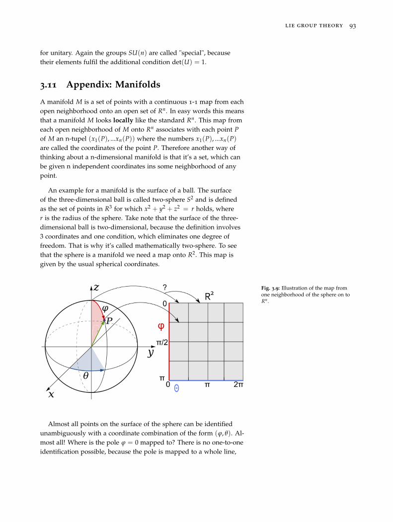
lie group theory 93
for unitary. Again the groups SU(n) are called "special", becausetheir elements fulfil the additional condition det(U) = 1.
3.11 Appendix: Manifolds
A manifold M is a set of points with a continuous 1-1 map from eachopen neighborhood onto an open set of Rn. In easy words this meansthat a manifold M looks locally like the standard Rn. This map fromeach open neighborhood of M onto Rn associates with each point Pof M an n-tupel (x1(P), ...xn(P)) where the numbers x1(P), ...xn(P)are called the coordinates of the point P. Therefore another way ofthinking about a n-dimensional manifold is that it’s a set, which canbe given n independent coordinates ins some neighborhood of anypoint.
An example for a manifold is the surface of a ball. The surfaceof the three-dimensional ball is called two-sphere S2 and is definedas the set of points in R3 for which x2 + y2 + z2 = r holds, wherer is the radius of the sphere. Take note that the surface of the three-dimensional ball is two-dimensional, because the definition involves3 coordinates and one condition, which eliminates one degree offreedom. That is why it’s called mathematically two-sphere. To seethat the sphere is a manifold we need a map onto R2. This map isgiven by the usual spherical coordinates.
Fig. 3.9: Illustration of the map fromone neighborhood of the sphere on toRn.
Almost all points on the surface of the sphere can be identifiedunambiguously with a coordinate combination of the form (ϕ, θ). Al-most all! Where is the pole ϕ = 0 mapped to? There is no one-to-oneidentification possible, because the pole is mapped to a whole line,
94 physics from symmetry
as indicated in the image. Therefore this map does not work for thecomplete sphere and we need another map in the neighborhood ofthe pole to describe things there. A similar problem occurs for themap on the semicircle θ = 0. Each point can be mapped in the R2
to θ = 0 and θ = 2π, which is again not a one-to-one map. Thisillustrates the fact that for manifolds there is in general not one coor-dinate system for all points of the manifold, only local coordinates,which are valid in some neighborhood. This is no problem becausethe defining feature of a manifold is that it looks locally like Rn.
The spherical coordinate map is only valid in the open neighbor-hood 0 < ϕ < π, 0 < θ < 2π and we need a second map to coverthe whole sphere. We can use, for example, a second spherical coor-dinate system with different orientation, such that the problematicpoles lie at different points for this map and no longer at ϕ = 0. Withthis second map every point of the sphere has a map onto R2 and thetwo-sphere can be seen to be a manifold.
A trivial example for a manifold is of course Rn.
4
The Framework
The basic idea of this chapter is that we get the correct equationsof nature, by minimizing something. What could this something be?One thing is for sure: the object shouldn’t change under Lorentztransformations, because otherwise we get different laws of naturefor different frames of reference. In mathematical terms this meansthe object we are searching for must be a scalar, which is an objecttransforming according to the (0, 0) representation of the Lorentzgroup. Together with the restriction to the simplest possible choicethis will be enough to derive the correct equations of nature. Naturelikes it simple.
Starting with this idea, we will introduce a framework called theLagrangian formalism. By minimizing the central object of the the-ory we get the equations of motion that describe the physical systemin question. The result of this minimization procedure is called theEuler-Lagrange equations.
The Lagrangian formalism enables us to derive one of the most-important theorems of modern physics: Noether’s Theorem. Thistheorem reveals the deep connection between symmetries and con-served quantities1. We will use this connection in the next chapter to
1 A conserved quantity is a quantitythat does not change in time. Famousexamples are the energy or the momen-tum of a given system. In mathematicalterms this means ∂tQ = 0 → Q =const.
understand how the quantities that we measure in experiments canbe described by the theory.
4.1 Lagrangian Formalism
The Lagrangian formalism is an incredibly powerful framework2 that
2 There are of course other frameworks,e.g. the Hamiltonian formalism, whichhas the Hamiltonian as its centralobject. The problem with the Hamilto-nian is that it is not Lorentz invariant,because the energy, it represents, isjust one component of the covariantenergy-impulse vector.
is used in most parts of fundamental physics. It is relatively simple,because the fundamental object, the Lagrangian, is a scalar3. The
3 A scalar is an object transformingaccording to the (0, 0) representationof the Lorentz group. This means thatit does not change at all under Lorentztransformations.
formalism is extremely useful if we want to use symmetry consider-ations. If we demand the action, the integral over the Lagrangian, to
© Springer International Publishing AG 2018J. Schwichtenberg, Physics from Symmetry, UndergraduateLecture Notes in Physics, https://doi.org/10.1007/978-3-319-66631-0_4
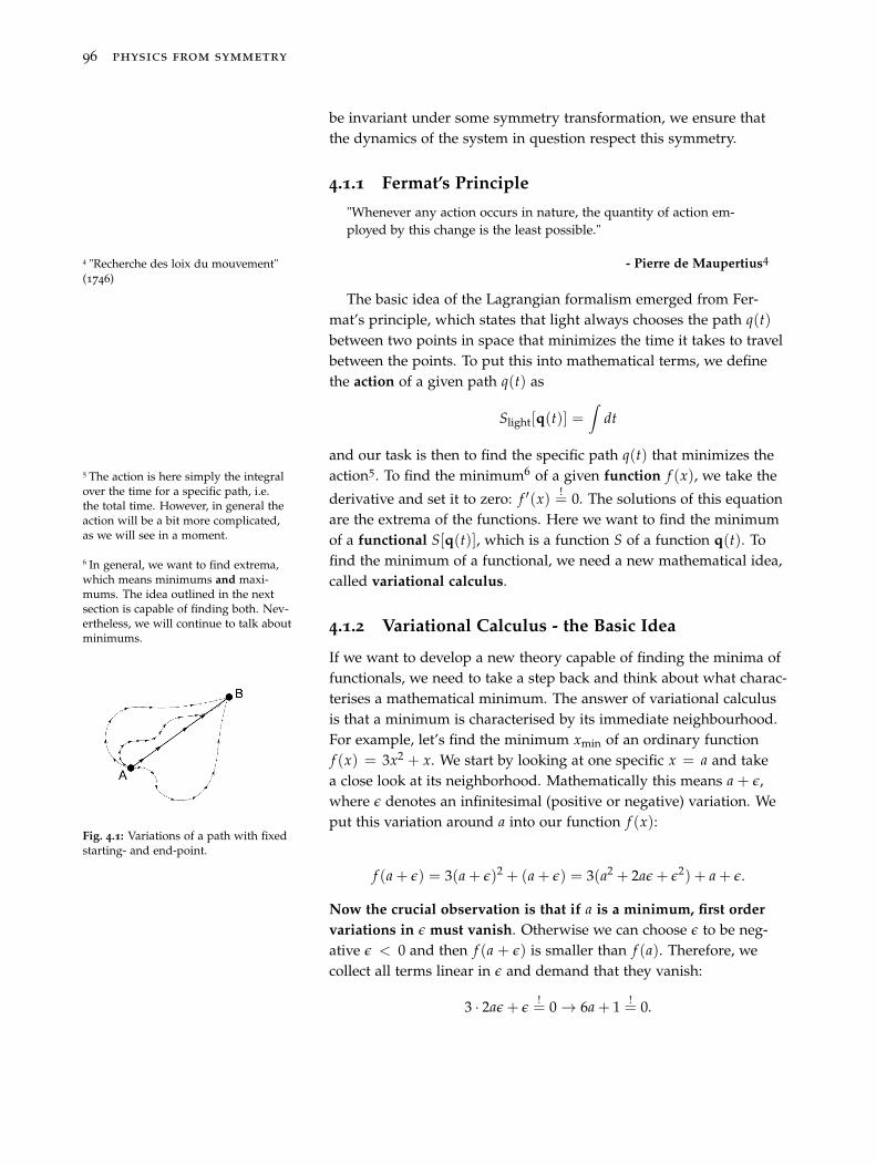
96 physics from symmetry
be invariant under some symmetry transformation, we ensure thatthe dynamics of the system in question respect this symmetry.
4.1.1 Fermat’s Principle
"Whenever any action occurs in nature, the quantity of action em-ployed by this change is the least possible."
- Pierre de Maupertius44 "Recherche des loix du mouvement"(1746)
The basic idea of the Lagrangian formalism emerged from Fer-mat’s principle, which states that light always chooses the path q(t)between two points in space that minimizes the time it takes to travelbetween the points. To put this into mathematical terms, we definethe action of a given path q(t) as
Slight[q(t)] =∫
dt
and our task is then to find the specific path q(t) that minimizes theaction5. To find the minimum6 of a given function f (x), we take the5 The action is here simply the integral
over the time for a specific path, i.e.the total time. However, in general theaction will be a bit more complicated,as we will see in a moment.
6 In general, we want to find extrema,which means minimums and maxi-mums. The idea outlined in the nextsection is capable of finding both. Nev-ertheless, we will continue to talk aboutminimums.
derivative and set it to zero: f ′(x) != 0. The solutions of this equation
are the extrema of the functions. Here we want to find the minimumof a functional S[q(t)], which is a function S of a function q(t). Tofind the minimum of a functional, we need a new mathematical idea,called variational calculus.
Fig. 4.1: Variations of a path with fixedstarting- and end-point.
4.1.2 Variational Calculus - the Basic Idea
If we want to develop a new theory capable of finding the minima offunctionals, we need to take a step back and think about what charac-terises a mathematical minimum. The answer of variational calculusis that a minimum is characterised by its immediate neighbourhood.For example, let’s find the minimum xmin of an ordinary functionf (x) = 3x2 + x. We start by looking at one specific x = a and takea close look at its neighborhood. Mathematically this means a + ε,where ε denotes an infinitesimal (positive or negative) variation. Weput this variation around a into our function f (x):
f (a + ε) = 3(a + ε)2 + (a + ε) = 3(a2 + 2aε + ε2) + a + ε.
Now the crucial observation is that if a is a minimum, first ordervariations in ε must vanish. Otherwise we can choose ε to be neg-ative ε < 0 and then f (a + ε) is smaller than f (a). Therefore, wecollect all terms linear in ε and demand that they vanish:
3 · 2aε + ε!= 0 → 6a + 1 !
= 0.
the framework 97
This equation is solved by
xmin = a =−16
.
This is, of course, exactly the same result that we get if we take thederivative f (x) = 3x2 + x → f ′(x) = 6x + 1 and demand this to bezero. In terms of ordinary functions this is just another way of doingthe same thing. However, variational calculus is additionally able tofind the extrema of functionals. We will see in a moment how thisworks for a general action functional.
The idea of the Lagrangian formalism is that a principle like theFermat principle for light exists for massive objects, too. Unfortu-nately, massive objects do not simply obey Fermat’s principle. Yet, wecan try a more general ansatz
S[q(t)] =∫
L dt,
where L is, in general, a non-constant function called the Lagrangian.This function happens to be constant for light, but a general La-grangian is a function of the position q(t) of the object in question.In addition, the Lagrangian can depend on the velocity of the object:L = L(q(t), ∂
∂t q(t)). This will be discussed in more detail in the nextsection7. Before we take a closer look at the usage of the variational 7 Our task will be to find the path q(t)
with lowest possible action for a givenLagrangian and given initial conditions.Before we are able to do that, weneed to find the correct Lagrangian,describing the physical system inquestion. Here is where the symmetrieswe talked about in the last chapterscome in handy. Demanding that theLagrangian is invariant under alltransformations of the Lorentz group,will lead us to the correct Lagrangians.
calculus idea for a functional like this, we need to talk about twosmall things.
4.2 Restrictions
As already noted in Chapter 1.1 there are restrictions to our presenttheories, that, so far, we can’t motivate from first principles. We onlyknow that we must respect them to get a sensible theory.
One important restriction is that we are only allowed to use thelowest, non-trivial derivatives in the Lagrangian. Trivial in this con-text means with no influence of the dynamics of the system, i.e. onthe equations of motion. For some theories this will be first orderand for others second order derivatives. The lowest order of a giventheory is determined by the condition that the Lagrangian must beLorentz invariant8, because otherwise we would get different equa- 8 In fact, the action must be Lorentz
invariant, but if the Lagrangian isLorentz invariant, the action certainlyis, too.
tions of motions for different frames of reference. For some theorieswe can’t get an invariant term with first order derivatives and there-fore second order derivatives are the lowest possible order.
We simply do not know how to work with theories includinghigher order derivatives and there are deep systematic problems
98 physics from symmetry
with such theories9. In addition, higher order derivatives in the La-9 These problems are known as Os-trogradski instabilities. The energyin theories with higher order deriva-tives can be arbitrarily negative, whichwould mean that every state in suchtheory would always decay into lowerenergy states. There are no stable statesin such theories.
grangian lead to higher order derivatives in the equations of motionand therefore more initial conditions would be required.
It is sometimes claimed that the constraint to first order derivativesis a consequence of our demand to get a local10 theory, but this only
10 Locality is a consequence of the basispostulates of special relativity, as shownin Section 2.4.
rules out an infinite number of derivatives. A non-local interaction isof the form11
11 We will discuss Lagrangians forparticle theories, where we search forparticle paths and Lagrangians forfield theories, where we search for fieldconfigurations Φ(x). This is the topic ofthe next section.
Φ(x − h)Φ(x), (4.1)
that is, two fields interacting with each other at two different pointsin spacetime with arbitrary distance h. Using the Taylor expansionwe can write
Φ(x − h) =∞
∑k=0
((∂
∂x
)kΦ(x)
∣∣∣x=h
)(h)k
k!, (4.2)
which shows that allowing an infinite number of derivatives wouldresult in a non-local interaction theory.
Another restriction is that in order to get a theory describing free(=non-interacting) fields/particles we must stop at second order inthe field Φ(x). This means we only include the terms1212 From another perspective, this means
again that we only include the lowestpossible, non-trivial terms. Termswith Φ0 and Φ1 do not lead to termsproportional to Φ in the Lagrangian,as we will see later and therefore weuse once more only the lowest possible,non-trivial order, now in Φ.
Φ0, Φ1, Φ2
into our considerations. For example, a term of the form Φ2∂μΦ is ofthird order in Φ and therefore not included in the Lagrangian for ourfree theory.
4.3 Particle Theories vs. Field Theories
Currently we have two frameworks to describe nature. On the onehand, we have particle theories that describe physical systems interms of positions of particles depending on time, i.e. �q = �q(t). Weuse the symbol q instead of x, because there is no need to describenature in terms of Cartesian coordinates13. For such theories the13 Another possibility are, for example,
spherical coordinates. Lagrangian depends on the position �q, the velocity ∂t�q and the time t:
L = L(�q, ∂t�q, t). (4.3)
A famous example is the Lagrangian L = 12 m�q2, from which we
can derive Newton’s equation of motion for classical mechanics. Thiswill be discussed later in great detail.
On the other hand, we have field theories that do not use thelocation �q(t) of individual particles to describe nature, but fields14. In
14 An especially beautiful feature ofquantum field theory is how particlesemerge. In Chapter 6 we will see thatfields are able to create and destroyparticles.
the framework 99
such theories space and time form the stage the fields Φ(�x, t) act on.Using the restrictions we get15 15 The usage of a different symbol L
here is intentional, because in fieldtheories we will work most of the timewith the Lagrangian density L . TheLagrangian density is related to theLagrangian via L =
∫d3xL .
L = L (Φ(�x, t), ∂μΦ(�x, t),�x, t) (4.4)
A famous example is the Lagrangian L = 12 (∂μΦ∂μΦ − m2Φ2),
from which we will derive the Klein-Gordon equation.
The big advantage of field theories is that they treat space andtime on an equal footing. In a particle theory we use the space coor-dinates �q(t) to describe our particle as a function of time. Notably,there is no term like ∂�qt in the Lagrangian and if it would be there,how should we interpret it? It is clear what we mean when we talkabout the location of a particle, but there is no obvious way to makesense of a similar sentence for time.
Having discussed all this, we are able to return to the originalminimizing problem, proposed at the beginning of this chapter. Wewant to find the minimum of some functional
S[q(t)] =∫
Ldt,
which will give us the correct equations of motion.
The solutions of these equations are for particles the correct pathsthat minimize the functional. For a field theory the solutions are thecorrect field configurations.
For the moment, do not worry about the object L, because wewill describe in the following chapters in great detail how we canderive the correct Lagrangian L for the systems in question. Here, wework with a general L and use the machinery of variational calculus,introduced above, to derive the minimum of the functional S[q(t)].This minimization procedure will give us the equations of motion forthe system.
4.4 Euler-Lagrange Equation
We start with particle theory and this means, we want to find outhow a particle moves between two fixed points. The mathematicalproblem we have to solve is to find the function q(t) for which theaction
S =∫ t2
t1
L(
q(t),dq(t)
dt, t)
dt
is an extremum (maximum or minimum). We use the notation
q(t) ≡ dq(t)dt
.
100 physics from symmetry
Analogous to the example above, we fix q(t) = a(t) and vary thisparticle path a little bit
a(t) + ε(t)
where ε is again infinitesimal. Considering a particle, we are not onlyable to vary the path, but in the same way we can vary the velocitya(t) + ε(t) with ε(t) = dε(t)
dt .At the boundary, the transformed path must be equivalent to the
untransformed path:
0 = ε(t1) = ε(t2), (4.5)
because we are searching for the path between two fixed points thatextremizes the action integral.This variation of the fixed function results in the functional
S =∫ t2
t1
dtL(q + ε, q + ε, t).
Analogous to the example above, where we searched for the mini-mum of a function, we will demand here that the terms linear in thevariation ε vanish. Because we work with a general L, we expand itas Taylor series16 and demand that the first order terms vanish16 We are using a generalization of the
formula, derived in Appendix B.3 forfunctions with more than one variable:L(q + ε, q + ε, t) = L(q) + (q + ε − q) ∂L
∂q
+(q + ε − q) ∂L∂q + . . .
= L(q) + ε ∂L∂q + ε ∂L
∂q + . . .
∫ t2
t1
dt[
ε(t)∂L∂q
+
(ddt
ε(t))
∂L∂q
]!= 0. (4.6)
To proceed further, we need to find a way to bracket ε(t) out. This isnecessary, because ε(t) is an arbitrary variation and when we bracketit out, we know that everything inside the brackets has to vanish ifthe total result is zero. So far we have one term that gets multipliedwith ε(t) and a second term that gets multiplied with d
dt ε(t). Tobracket ε(t) out, we need get rid of the derivative. To achieve this, weintegrate the last term by parts17, which yields17 Integration by parts is a direct conse-
quence of the product rule and derivedin Appendix B.2. ∫ t2
t1
dt(
ddt
ε(t))
∂L(q, q, t)∂q
= ε(t)∂L(q, q, t)
∂q
∣∣∣∣t2
t1
−∫ t2
t1
dtε(t)ddt
(∂L(q, q, t)
∂q
).
Using Eq. 4.5 we have
ε(t)∂L(q, q, t)
∂q
∣∣∣∣t2
t1
= 0 .
So, we can rewrite Eq. 4.6 as∫ t2
t1
dtε(t)[
∂L(q, q, t)∂q
− ddt(
∂L(q, q, t)∂q
)
]!= 0
the framework 101
and we can see that this only vanishes for arbitrary variations ε(t)if the expression in the square bracket [ ] is identically zero. Thisyields18 18 Maybe you wonder about the two
different symbols for derivatives. ddt is
called the total derivative with respectto t, whereas ∂
∂t is called the partialderivative. The total derivative givesus the total change, which is for afunction f given by sum of the changerates, also known as partial derivatives,times the change of the quantity itself.For example, the total change of afunction f (x(t), y(t), z(t)) in threedimensional space is given by d f
dt =∂ f∂x
∂x∂t +
∂ f∂y
∂y∂t +
∂ f∂z
∂z∂t +
∂ f∂t
∂t∂t . The change
rate times the distance it is changed.In contrast the partial derivative is justone part of this total change. For afunction that does not explicitly dependon t the partial derivative is zero. Forexample, for f (x(t), y(t)) = x2y + y3,we have ∂ f
∂t = 0, but ∂ f∂x = 2xy �= 0
and ∂ f∂y = x2 + 3y2 �= 0. Therefore,
d fdt = 2xy ∂x
∂t + (x2 + 3y2) ∂y∂t . In contrast
for another function g(x(t), y(t), t) =
x2t + y we have ∂g∂t = x2.
∂L(q, q, t)∂q
− ddt
(∂L(q, q, t)
∂q
)= 0 , (4.7)
which is the famous Euler-Lagrange equation.
For a field theory we can follow a similar route. First notice that inthis case we treat time and space equally. Therefore, we introduce theLagrangian density L :
L =∫
d3xL (Φi, ∂μΦi) (4.8)
and we can write the action in terms of this Lagrangian density
S =∫
dtL =∫
d4xL (Φi, ∂μΦi) . (4.9)
Following the same steps as above, we get the equations19 of motion
19 Plural because we get one equa-tion for each field component, i.e.Φ1, Φ2, . . ..
for a field theory:
∂L
∂Φi − ∂μ
(∂L
∂(∂μΦi)
)= 0 . (4.10)
In the next section we will derive, using the Lagrangian formalism,one of the most important theorems of modern physics. We needthis theorem to see the deep connection between symmetries andconserved quantities. The conserved quantities are the appropriatequantities20 to describe nature and from this theorem we learn how 20 We can see them as anchors in an
otherwise extremely complicatedworld. While everything changes, theconserved quantities stay the same.
we can work with them in a theoretical context.
4.5 Noether’s Theorem
Noether’s theorem shows that each symmetry of the Lagrangian isdirectly related to one conserved quantity. Or formulated slightlydifferent: The notions physicists commonly use to describe nature(the conserved quantities) are directly connected to symmetries. Thisis one of the most beautiful insights in the history of science.
4.5.1 Noether’s Theorem for Particle Theories
Let’s have a look at what we can say about conserved quantities inparticle theories. We will restrict to continuous symmetries, becausethen we can look at infinitesimal changes. As we have seen in earlierchapters, we can build up finite changes by repetition of infinitesimal
102 physics from symmetry
changes. The invariance of the Lagrangian under an infinitesimaltransformation21 q → q′ = q + δq can be expressed mathematically21 The symbol for a small variation δ
may not be confused with the symbolfor partial derivatives ∂.
δL = L(
q,dqdt
, t)−L
(q + δq,
d(q + δq)dt
, t)
= L(
q,dqdt
, t)−L
(q + δq,
dqdt
+dδqdt
, t)
!= 0. (4.11)
Demanding that the Lagrangian is invariant can be too restrictive.What really needs to be invariant for the dynamics to stay the sameis the action and not the Lagrangian. Of course, if the Lagrangian isinvariant, the action is automatically invariant:
δS =∫
dtL(
q,dqdt
, t)−
∫dtL
(q + δq,
dqdt
+dδqdt
, t)=
∫dtδL =︸︷︷︸
if δL=0
0 .
(4.12)
How can the Lagrangian change, while the action stays the same? Itturns out we can always add the total time derivative of a function Gto the Lagrangian
L → L+dGdt
without changing the action, because2222 Using δG = ∂G∂q δq, because G = G(q)
and we vary q. Therefore the variationof G is given by the rate of change ∂G
∂qtimes the variation of q.
δS → δS′ = δS +∫ t2
t1dt
ddt
δG = δS +∂G∂q
δq∣∣t2t1︸ ︷︷ ︸
=0 because δq(t1)=δq(t2)=0
.
In the last step, we use that the variation δq vanishes at the initial andfinal times (t1, t2). We conclude, there is no need for us to demandthat the variation of the Lagrangian δL vanishes, rather we have theless restrictive condition
δL !=
dGdt
. (4.13)
This means the Lagrangian can change in this way without chang-ing the action. Therefore the equation of motion stay the same eventhough the Lagrangian changes, as long as the change can be writtenas total derivative of some function: dG
dt . Rewriting Eq. 4.11, now withdGdt instead of 0 on the right hand side yields
δL = L(
q,dqdt
, t)−L
(q + δq,
dqdt
+dδqdt
, t)
!=
dGdt
(4.14)
We expand the second term as Taylor series and keep only terms thatare first order in δq, because δq is infinitesimal, and use the notationdqdt = q:
→ δL = L−L− ∂L∂q
δq − ∂L∂q
δq !=
dGdt
the framework 103
→ δL = −∂L∂q
δq − ∂L∂q
δq !=
dGdt
. (4.15)
We can rewrite Eq. 4.15 by using the Euler-Lagrange equation23. This 23 Eq. 4.7: ∂L∂q = d
dt
(∂L∂q
)yields
→ δL = − ddt
(∂L∂q
)δq − ∂L
∂qδq =
dGdt
.
This can be rewritten, using the product rule24 24 If you’re unsure about the productrule, have a look at Appendix B.1.
→ δL = − ddt
(∂L∂q
δq)=
dGdt
→ ddt
(∂L∂q
δq + G)
︸ ︷︷ ︸≡J
= 0. (4.16)
Therefore, we have found a quantity J that is conserved in time:
J =∂L∂q
δq + G, (4.17)
because we haveddt
J = 0 → J = const.
To illustrate this, we will use one later result from Section 10.2:Newton’s second law for a free particle with constant mass25 25 If q denotes the position of some ob-
ject, dqdt = q is the velocity of the object
and ddt
dqdt = d2q
dt2 = q the acceleration.m�q = 0. (4.18)
The Lagrangian that reproduces this famous equation of motion is26 26 We work now with more than onespatial dimension, which means insteadof q and a, we use vectors �q and�a.L =
12
m�q2 (4.19)
as you can check, by putting it into the Euler-Lagrange equation(Eq. 4.7).
Let us compute for different symmetries of this Lagrangian thecorresponding conserved quantities. Our Lagrangian is invariant(δL = 0) under spatial translations �q → �q′ = �q +�a, where�a denotessome constant vector, because L = 1
2 m�q2 does not depend on �q. Thecorresponding conserved quantity reads27 27 Here G = 0, which certainly fulfils the
condition in Eq. 4.13.
Jtrans =∂L∂�q
�a = m�q�a = �p�a, (4.20)
where �p = m�q is what we usually call momentum in classical me-chanics. The equation d
dt J = 0 holds for arbitrary�a and thereforemomentum is conserved, because the Lagrangian is invariant underspatial translations.
104 physics from symmetry
We now want to look at rotations and therefore need more thanone dimension, because a rotation in one dimension makes no sense.It is useful to use an index notation instead of the usual vector no-tation here, because then we can simply rewrite all equations withq → qi to be able to incorporate changes in more than one dimension.Let’s have a look at an infinitesimal rotation28 qi → q′i = qi + εijkqjak
28 Here we write the generator ofrotations by using the Levi-Civitasymbol. This was explained in the textbelow Eq. 3.62.
and therefore δqi = εijkqjak. Our Lagrangian is invariant under suchtransformations, because again, L = 1
2 m�q2 does not depend on q, andthe corresponding conserved quantity is29
29 This was derived in Eq. 4.16, again wework here with G = 0.
Jrot =∂L(qi, qi, t)
∂qiδqi =
∂L(qi, qi, t)∂qi
εijkqjak
= mqiεijkqjak = piεijkqjak
→ Jrot = (�p ×�q) ·�a ≡ �L ·�a . (4.21)
In the last step we rewrite our term in vector notation, where × iscalled the cross product and �L is what we usually call angular mo-mentum in classical mechanics. Therefore, invariance under rota-tions leads us to conservation of angular momentum.
Next let’s have a look at invariance under time translations30. An30 This means that physics doesn’t careabout if we perform an experimentyesterday, today or in 50 years, giventhe same initial conditions, the physicallaws stay the same.
infinitesimal time displacement t → t′ = t + ε has the effect
δL = L(
q(t),dq(t)
dt, t)−L
(q(t + ε),
dq(t + ε)
dt, t + ε
)
= −∂L∂q
∂q∂t
ε − ∂L∂q
∂q∂t
ε − ∂L∂t
ε =︸︷︷︸this is exactly the total derivative
−dLdt
ε, (4.22)
which tells us that in general δL �= 0, but the condition in Eq. 4.13 isfulfilled anyway with G = −L.
We can put this into Eq. 4.16, which yields
ddt
(∂L∂q
q −L)
︸ ︷︷ ︸≡H
= 0 . (4.23)
The conserved quantity H is called the Hamiltonian and representsthe total energy of the system. For our example Lagrangian, we have
H =∂L∂q
q −L =
(∂
∂q12
mq2)
︸ ︷︷ ︸=mq
q − 12
mq2
= mq2 − 12
mq2 =12
mq2, (4.24)
which is exactly the kinetic energy of our system. The kinetic energyis the total energy, because we worked without a potential/external
the framework 105
force. The Lagrangian that leads to Newton’s second law for a parti-cle in an external potential: mq = dV
dq is
L =12
mq2 − V(q).
The Hamiltonian is then
H =12
mq2 + V
which is the correct total energy=kinetic energy+potential energy.
The conserved quantity that follows from boost invariance israther strange and the corresponding computation can be found inthe appendix Section 4.6. The resulting conserved quantity is
Jboost = pt − 12
mvt︸ ︷︷ ︸≡ pt
−mq = pt − mq. (4.25)
We can see that this quantity depends on the starting time and bychoosing the starting time appropriately we can make it zero. Be-cause this quantity is conserved, this conservation law tells us thatzero stays zero for all times.
To summarize for particle theories we have the following connec-tions:
• translational invariance in space ⇒ conservation of momentum,
• boost invariance31 ⇒ conservation of pt − mq, 31 Another name for a boost is transla-tion in momentum space, because thetransformation q → q + vt, changes themomentum to mq → m(q + v).
• rotational invariance ⇒ conservation of angular momentum,
• translational invariance in time ⇒ conservation of energy.
Noether’s theorem shows us why these notions32 are used in every 32 Except for the conserved quantityfollowing from boost invariance.physical theory of nature in one or another form. As long as we
have the usual spacetime symmetries of our physical laws, we havemomentum, energy and angular momentum as conserved quantities.
It is instructive to repeat the above discussion for field theories.In field theories we have two kinds of symmetries. On the one hand,our Lagrangian can be invariant under spacetime transformations,which means a transformation like a rotation. On the other hand, wecan have invariance under transformations of the field itself, whichare called internal symmetries.
4.5.2 Noether’s Theorem for Field Theories - SpacetimeSymmetries
For fields one has to distinguish between different kinds of changesthat can happen under spacetime transformations. Observer S′ sees
106 physics from symmetry
the field Ψ′(x′) whereas observer S sees the field Ψ(x). This is thesame field, just from another perspective and the two observers donot see the same numerical field components. The two differentdescriptions are related by the appropriate transformations of theLorentz group. We introduced in Section 3.7.11 the field representa-tion, which we will be using now. The (infinite-dimensional) differ-ential operator representation changes x → x′. This means by usingthis representation we can compute the field components at a differ-ent point in spacetime or in a rotated frame. The finite-dimensionalrepresentation of the Lorentz group changes Ψ → Ψ′, i.e. mixes thefield components33.33 Remember for example, that a Weyl
spinor has two- and a vector fieldhas four-components. If we look at
the vector field Aμ =
⎛⎜⎜⎝A0A1A2A3
⎞⎟⎟⎠ from a
different perspective, i.e. describe it ina rotated coordinate system it can look
like A′μ =
⎛⎜⎜⎝A′
0A′
1A′
2A′
3
⎞⎟⎟⎠ =
⎛⎜⎜⎝A0−A2A1A3
⎞⎟⎟⎠. A′μ and
Aμ describe the same field in coordinatesystems that are rotated by 90◦ aroundthe z-axis relative to each other.
A complete transformation, for a field that depends on spacetime,needs to consist of both parts. We will look at these parts separately,starting with the change x → x′. For rotations the conserved quantitythat follows is not really conserved, because we neglected the secondpart of the transformation, i.e. the mixing of the field components.Only the sum of the two conserved quantities that follow from x →x′ and Ψ → Ψ′ is conserved.
To make this more concrete consider a general Lagrangian densityL ((Φ(xμ), ∂μΦ(xμ), xμ). Symmetry means we have
L ((Φ(xμ), ∂μΦ(xμ), xμ) = L ((Φ′(x′μ), ∂μΦ′(x′μ), x′μ). (4.26)
In general, the total change of a function-of-a-function, when theindependent functions are changed and the point at which they areevaluated is also changed, is given by3434 If this is new to you: This is often
called the total derivative. The totalchange is given by the sum of thechange rates, also known as derivatives,times the change of the quantity itself.For example, the total change of afunction f (x, y, z) in three dimensionalspace is given by ∂ f
∂x δx + ∂ f∂y δy + ∂ f
∂z δz.The change rate times the distance itis changed. We consider infinitesimalchanges and therefore this can beseen as the first terms in the Taylorexpansion, where we can neglect higherorder terms.
d f (g(x), h(x), ...) =∂ f∂g
δg +∂ f∂h
δh + ... +∂ f∂x
δx. (4.27)
Applying this to the Lagrangian yields
δL =∂L
∂ΦδΦ +
∂L
∂(∂μΦ)δ(∂μΦ) +
∂L
∂xμδxμ, (4.28)
which we can rewrite using the Euler-Lagrange equations35
35 See Eq. 4.10: ∂L∂Φ = ∂μ(
∂L∂(∂μΦ)
)
δL = ∂μ
(∂L
∂(∂μΦ)
)δΦ +
∂L
∂(∂μΦ)δ(∂μΦ)︸ ︷︷ ︸=∂μδΦ
+∂L
∂xμδxμ
=︸︷︷︸Product rule
∂μ
(∂L
∂(∂μΦ)δΦ
)+
∂L
∂xμδxμ . (4.29)
The variation δΦ has now two parts
δΦ = εμνSμνΦ(x)− ∂Φ(x)∂xμ
δxμ, (4.30)
the framework 107
with the transformation parameters εμν, the transformation operatorSμν in the corresponding finite-dimensional representation and aconventional minus sign. Sμν is related to the generators of rotationsby Ji =
12 εijkSjk and to the generators of boosts by Ki = S0i, analogous
to the definition of Mμν in Eq. 3.173. This definition of the quantitySμν enables us to work with the generators of rotations and boosts atthe same time.
The first part is only important for rotations and boosts, becausetranslations do not mix the field components. For boosts the con-served quantity will not be very enlightening, just as in the particlecase, so in fact this term will become only relevant for rotationalsymmetry.
Let’s start with the simplest field transformation: a translation inspacetime
xμ → x′μ = xμ + δxμ = xμ + aμ. (4.31)
For translations we have εμν = 0, because field components do notmix under translations and therefore Eq. 4.30 reads
δΦ = − ∂Φ∂xμ
δxμ .
Thus if we want to investigate the consequences of invariance (δL = 0),we get from Eq. 4.29
−∂ν
(∂L
∂(∂νΦ)
∂Φ∂xμ
δxμ
)+
∂L
∂xμδxμ = 0 (4.32)
→ −∂ν
(∂L
∂(∂νΦ)
∂Φ∂xμ
− δνμL
)δxμ = 0 . (4.33)
From Eq. 4.31 we have δxμ = aμ, which we now put into Eq. 4.33.This yields
−∂ν
(∂L
∂(∂νΦ)
∂(Φ)
∂xμ− δν
μL
)aμ = 0, (4.34)
and this motivates us to define the energy-momentum tensor
Tνμ :=
∂L
∂(∂νΦ)
∂(Φ)
∂xμ− δν
μL . (4.35)
Equation 4.34 tells us that each component μ of Tνμ fulfils a continuity
equation, because aμ is arbitrary36
36 Take note that we have here a plussign ∂νTν
μ = ∂0T0μ + ∂iTi
μ, although wehave AμBμ = AμημνBν = A0B0 − Ai Bi .We defined a four-vector with alower index without minus signsAμ = (A0, A1, A2, A3)
T and afour-vector with an upper index asBμ ≡ ημνBν = (B0,−B1,−B2,−B3)
T .The minus signs here are a result ofthe minus signs in the Minkowskimetric ημν = diag(1,−1,−1,−1).The reason for the plus sign inEq. 4.37 is that ∂μ is defined as∂μ ≡ ∂
∂xμ = ( ∂∂x0 ,− ∂
∂x1 ,− ∂∂x2 ,− ∂
∂x3 )T .
The minus signs here cancel with theminus signs that appear through theupper index of Tν
μ and we get an overallplus sign.
∂νTνμ = 0 (4.36)
→ ∂νTνμ = ∂0T0
μ + ∂iTiμ = 0 . (4.37)
108 physics from symmetry
This tells us directly that we have conserved quantities, because, forexample, for μ = 0 we get3737 Using ∂0 = ∂t and ∂iT0
i = ∇�Tand the famous divergence theorem∫
V d3x∇A =∫
δV d2xA, which enablesus to rewrite the integral over somevolume V, as an integral over the cor-responding surface δV. A very illumi-nating proof of the divergence theorem,there called Gauss’ theorem, can befound at http://www.feynmanlectures.caltech.edu/II_03.html which isChapter 3 of the freely online avail-able Richard P. Feynman, Robert B.Leighton, and Matthew Sands. TheFeynman Lectures on Physics: Volume 2.Addison-Wesley, 1st edition, 2 1977.ISBN 9780201021172
∂0T00 + ∂iTi
0 = 0 → ∂0T00 = −∂iTi
0
∂tT00 = −∇�T →︸︷︷︸
Integrating over some infinite volume V
∫V
d3x∂tT00 = −
∫V
d3x∇�T
→ ∂t
∫V
d3xT00 = −
∫V
d3x∇�TDivergence theorem; δV denotes the surface of the volume V︷︸︸︷
= −∫
δVd2x�T =︸︷︷︸
Because fields vanish at infinity
0 (4.38)
→ ∂t
∫V
d3xT00 = 0 . (4.39)
In the last step we use that if we have an infinite volume V, likea sphere with infinite radius r, and we have to integrate over thesurface of this volume δV, we need to evaluate our fields at r = ∞.Fields must vanish at infinity, because otherwise the total field energywould be infinite and field configurations with infinite energy arenon-physical38.38 Take note that strictly speaking this is
only true for spin 0 and spin 1/2 fields.For spin 1 fields, only the field-strengthtensor Fμν must vanish to guaranteefinite energy, while the "basic fields" Aμ
(with Fμν := ∂μ Aν − ∂ν Aμ) can be non-zero "at infinity". (The field strengthtensor will be defined in Eq. 6.23).This observation leads to the non-trivial vacuum picture in non-abeliangauge theories. Unfortunately, a properdiscussion lies far beyond the scope ofthis book.
We conclude: the invariance under translations in spacetime leadsus to 4 conserved quantities39, one for each component μ . Equation
39 Because ∂0T0μ aμ = ∂0T0
0 a0 − ∂0T0i ai =
0, with arbitrary aμ we get a separatecontinuity equation for each compo-nent.
4.39 tells us these are
E =∫
d3xT00 (4.40)
Pi =∫
d3xT0i , (4.41)
where as always i = 1, 2, 3. These quantities are called the total en-ergy E of the system, which is conserved because we have invarianceunder time-translations x0 → x0 + a0 and the total momentumof the field configuration Pi, which is conserved because we haveinvariance under spatial-translations xi → xi + ai.
4.5.3 Rotations and Boosts
Next, we take a look at invariance under rotations and boosts. Wewill start with the second part of Eq. 4.30 and then look afterwardsat the implications of the first part. We will get a quantity from thefirst part and a quantity from the second part, which are togetherconserved. A scalar field has no components that could mix, hencefor a scalar field the first part is zero. In other words, for scalars weuse the 1-dimensional representation of the generators of the Lorentzgroup Sμν = 0, which was derived in Section 3.7.4. Therefore whatwe derive in this section is the complete conserved quantity for ascalar field.
the framework 109
The second part of the transformation is given by
xμ → x′μ = xμ + δxμ = xμ + Mσμxσ (4.42)
where Mσμ are the generators of rotations and boost in their infinite-
dimensional representation. This means they are represented bydifferential operators, as defined in Eq. 3.248.
From Eq. 4.42, we see that the change of the coordinates is givenby δxμ = Mσ
μxσ. Putting this into Eq. 4.33 yields
∂ν
(∂L
∂(∂νΦ)
∂(Φ)
∂xμ− δν
μL
)Mμσxσ = 0 (4.43)
→︸︷︷︸Eq. 4.35
∂νTνμ Mμσxσ = 0 .
We can write this a little differently to bring it into the conventionalform
=12(∂νTμ
ν Mμσxσ + ∂νTμν Mμσ︸︷︷︸=−Mσμ
xσ) =12(∂νTμ
ν Mμσxσ − ∂νTμν Mσμxσ)
=︸︷︷︸Renaming dummy indices
12(∂νTμ
ν Mμσxσ − ∂νTσν Mμσxμ) =
12(∂νTμ
ν xσ − ∂νTσν xμ)Mμσ
=12
∂ν(Tμνxσ − Tσνxμ)Mμσ = 0
→ with (Jν)σμ ≡ Tμνxσ − Tσνxμ → ∂ν(Jν)σμ = 0. (4.44)
The quantity Jν we introduced in the last step is called Noethercurrent. Note that, because of the anti-symmetry of Mμσ = −Mσμ,which follows from the definition in Eq. 3.173, we have Mμμ = 0.Therefore, we found 6 different continuity equations ∂ν(Jν) = 0, onefor each non-vanishing Mμσ. With the same arguments from Eq. 4.39we conclude that the quantities conserved in time are
Qμσ =∫
d3x(Tμ0xσ − Tσ0xμ) . (4.45)
For rotational invariance40, we therefore have the conserved quanti- 40 Recall the connection between thegenerator of rotations Ji and Mμν
from Eq. 3.173: Ji = 12 εijk Mjk , which
means we now restrict to the spatialcomponents i = j = {1, 2, 3} here andwrite i, j instead of μ = ν = {0, 1, 2, 3}.
ties
Liorbit =
12
εijkQjk =12
εijk∫
d3x(Tj0xk − Tk0xj), (4.46)
which we call the orbital angular momentum of our field41.41 The prefix "orbital" will make sensein a moment, because actually this isjust one part of the complete angularmomentum. We will have a look at themissing part in a moment.
Equivalently, we have the conserved quantity for boosts42
42 Recall the connection between theboost generators Ki and Mμν: Ki = M0i .
Q0i =∫
d3x(T00xi − Ti0x0), (4.47)
which is discussed a bit more in the appendix Section 4.7.
110 physics from symmetry
4.5.4 Spin
Next, we want to take a look at the implications of the first part ofEq. 4.30, which is what we missed in our previous derivation of theconserved quantity that follows from rotations. We now consider
δΦ = εμνSμνΦ(x), (4.48)
where Sμν is the appropriate finite-dimensional representation of thetransformation in question43. This gives us in Eq. 4.29 the extra term43 The finite-dimensional representa-
tions are responsible for the mixing ofthe field components. For example, thetwo dimensional representation of therotation generators: Ji =
12 σi , mix the
components of Weyl spinors.
∂ρ
(∂L
∂(∂ρΦ)εμνSμνΦ(x)
), (4.49)
which leads to an additional term in Eq. 4.46. The complete con-served quantity then reads
Li =12
εijkQjk =12
εijk∫
d3x(
∂L
∂(∂0Φ)SjkΦ(x) + (Tj0xk − Tk0xj)
)(4.50)
and therefore we write
Li = Lispin + Li
orbit . (4.51)
The first part is something new, but needs to be similar to theusual orbital angular momentum we previously considered, becausethe two terms are added and appear when considering the sameinvariance. The standard point of view is that the first part of thisconserved quantity is some-kind of internal angular momentum44.44 We will see later that fields create
and destroy particles. A spin 12 field
creates spin 12 particles, which is an un-
changeable property of an elementaryparticle. Hence the usage of the word"internal". Orbital angular momentumis a quantity that describes how twoor more particles revolve around eachother.
Recall that we label the representations of the Poincaré group bysomething we call spin, too. Now this notion appears again. We willlearn in the next chapter and in great detail in Section 8.5.5, how weare able to measure this new kind of angular momentum, called spinand see later that it indeed coincides with the label we use for therepresentations of the Poincaré group.
4.5.5 Noether’s Theorem for Field Theories- Internal Symmetries
We now take a look at internal symmetries45. The invariance of a45 Internal symmetries will be incrediblyimportant for interacting field theories.In addition, one conserved quantity,following from one of the easiestinternal symmetries will provide uswith the starting point for quantumfield theory.
Lagrangian (δL = 0) under some infinitesimal transformation of thefield itself
Φi → Φ′i = Φi + δΦi (4.52)
can be written mathematically
δL = L (Φi, ∂μΦi)−L (Φi + δΦi, ∂μ(Φi + δΦi))
the framework 111
= −∂L (Φi, ∂μΦi)
∂Φi δΦi − ∂L (Φi, ∂μΦi)
∂(∂μΦi)∂μδΦi !
= 0, (4.53)
where we used the Taylor expansion to get to the second line andonly keep terms of first order in δΦi, because the transformation isinfinitesimal. From the Euler-Lagrange equation (Eq. 4.10) for fieldswe know
∂L
∂Φi = ∂μ
(∂L
∂(∂μΦi)
).
Putting this into Eq. 4.53, we get
δL = −∂μ
(∂L
∂(∂μΦi)
)δΦi − ∂L
∂(∂μΦi)∂μδΦi = 0
which is, using the product rule, the same as
∂μ
(∂L
∂(∂μΦi)δΦi
)= 0 . (4.54)
This means, if the Lagrangian is invariant under the transforma-tion Φi → Φ′i = Φi + δΦi, we get again a quantity, called Noethercurrent
Jμ ≡ ∂L
∂(∂μΦi)δΦi, (4.55)
which fulfils the continuity equation
Eq. 4.54 → ∂μ Jμ = 0. (4.56)
Furthermore, following the same steps as in Eq. 4.39, we are able toderive a quantity that is conserved in time
∂t
∫d3xJ0 = 0. (4.57)
Let’s have a look at one very important example: invariance underdisplacements of the field itself46, which means δΦ = −iε in Eq. 4.52: 46 Take note that at this point we made
no assumptions about the field beingcomplex or real. The constant ε is arbi-trary and could be entirely imaginaryif we want to move our field by a realvalue. The i is included at this point tomake the generator Hermitian (which isby no means obvious at this point) andtherefore the eigenvalues real, as will beshown later. Don’t get confused at thispoint. You could simply see this extra ias a convention, because we could justas well absorb it into the constant bydefining ε′ := iε.
Φ → Φ′ = Φ − iε (4.58)
or for more than one field component
Φi → Φ′i = Φi − iεi. (4.59)
The generator of this transformation is −i ∂∂Φ , because
Φ′ = e−iε ∂∂Φ Φ =
(1 − iε
∂
∂Φ+ . . .
)Φ ≈ Φ − iε (4.60)
The corresponding conserved quantity is called conjugate momen-tum Π. With Eq. 4.54 and Eq. 4.57 we get47 47 The δΦ in Eq. 4.55 becomes a constant
ε and because the quantity is conservedfor arbitrary ε we define our conservedquantity without it.
112 physics from symmetry
∂tΠ = 0 → ∂tΠ = ∂t
∫d3xJ0 = ∂t
∫d3xπ = 0
with J0 = π =∂L
∂(∂0Φ)(4.61)
The quantity π here is called the conjugate momentum density48.48 This rather abstract quantity is one ofthe most important notions in quantumfield theory, as we will see in Chapter 6.
Take note that this is different from the physical momentum densityof the field, which arises from the invariance under spatial transla-tions Φ(x) → Φ(x′) = Φ(x + ε) and is given by
pi = T0i =∂L
∂(∂0Φ)
∂Φ∂xi
,
which we derived in Eq. 4.41. In later chapters we will look at manymore internal symmetries, which will prove to be invaluable whenwe develop a theory that describes interactions. Now let’s summarizewhat we learned about symmetries and conserved quantities in fieldtheories:
• translational invariance in space ⇒ conservation of physical mo-mentum Pi =
∫d3xT0i =
∫d3x ∂L
∂(∂0Φ)∂Φ∂xi
,
• boost invariance49 ⇒ constant velocity of the center of energy,49 Another name for a boost is a transla-tion in momentum space.
• rotational invariance ⇒ conservation of the total angular mo-mentum Li = 1
2 εijk ∫ d3x(
∂L∂(∂0Φ)
SjkΦ(x) + (Tk0xj − Tj0xk))
=
Lispin + Li
orbit consisting of spin and orbital angular momentum,
• translational invariance in time ⇒ conservation of energyE =
∫d3xT00 =
∫d3x
(∂L
∂(∂0Φ)∂Φ∂x0
−L)
,
• displacement invariance of the field itself ⇒ conservation of theconjugate momentum Π =
∫d3x ∂L
∂(∂0Φ)=
∫d3xπ.
Further Reading Tips
• Cornelius Lanczos - The Variational Principles of Mechanics5050 Cornelius Lanczos. The VariationalPrinciples of Mechanics. Dover Pub-lications, 4th edition, 3 1986. ISBN9780486650678
is a brilliant book about the usage of the Lagrangian formalism inclassical mechanics.
• David Morin - Introduction to Classical Mechanics51 is an ex-51 David Morin. Introduction to ClassicalMechanics: With Problems and Solutions.Cambridge University Press, 1 edition,2 2008. ISBN 9780521876223
tremely student friendly book that carefully explains how theLagrangian framework is used in classical mechanics.
• Herbert Goldstein - Classical Mechanics52 is the standard book52 Herbert Goldstein, Charles P. PooleJr., and John L. Safko. Classical Mechan-ics. Addison-Wesley, 3rd edition, 6 2001.ISBN 9780201657029
about classical mechanics with many great explanations regardingthe Lagrangian formalism.
the framework 113
4.6 Appendix: Conserved Quantity from BoostInvariance for Particle Theories
In this appendix we want to find the conserved quantity that followsfor our example Lagrangian L = 1
2 m�q2 from boost invariance. Aboost transformation is q → q′ = q + δq = q + vt, where v denotes aconstant velocity. Our Lagrangian is not invariant under boosts, butthis is no problem at all, as we have seen above:For our equations of motion to be unchanged under transformationsthe Lagrangian is allowed to change up to the total derivative of anarbitrary function. This condition is clearly fulfilled for our boosttransformation q → q′ = q + vt ⇒︸︷︷︸
v=const!
q′ = q + v and therefore our
Lagrangian
L =12
mq2
is changed by
δL = L(q, q, t)−L(q′, q′, t) =12
mq2 − 12
mq′2
=12
mq2 − 12
m(q + v)2 = −mqv − 12
mv2,
which is the total derivative of the function53 53 dGdt = d
dt (−mqv − 12 mv2t) = −mqv −
12 mv2, because v and m are constant.
−G ≡ −mqv − 12
mv2t.
We conclude that our equations of motion stay unchanged and wecan find a conserved quantity54. 54 Another way to see this is by looking
directly at the equation of motion:mq = 0. We have the transformation
q → q′ = q + vt, with v =constand therefore q → q′ = q + v andq → q′ = q.
For boosts, the conserved quantity is (Eq. 4.16)
Jboost =∂L∂q︸︷︷︸≡p
δq︸︷︷︸=vt
−G = pvt − mvq − 12
mv2t,
where we can cancel one v from every term, because in Eq. 4.16 wehave a zero on the right hand side. This gives us
Jboost = pt − 12
mvt︸ ︷︷ ︸≡ pt
−mq = pt − mq . (4.62)
This is a rather strange conserved quantity because its value de-pends on the starting time. We can choose a suitable zero time, whichmakes this quantity zero. Because it is conserved, this zero stays zerofor all times.
114 physics from symmetry
4.7 Appendix: Conserved Quantity from BoostInvariance for Field Theories
For invariance under boosts in a field theory we have the conservedquantities
Q0i =∫
d3x(T00xi − Ti0x0), (4.63)
which we derived in Eq. 4.47, using Ki = M0i.
How can we interpret this quantity? Q0i is conserved, whichmeans
0 =∂Q0i
∂t=
∫d3x
∂Ti0
∂tx0︸ ︷︷ ︸
=x0 ∂∂t
∫d3xTi0
+∫
d3xTi0 ∂x0
∂t︸︷︷︸=1 because x0=t
− ∂
∂t
∫d3x
∂T00
∂txi
= t∂Pi
∂t+ Pi − ∂
∂t
∫d3xT00xi.
From Eq. 4.20 we know that Pi is conserved ∂Pi
∂t = 0 → Pi = const.and we can conclude
∂
∂t
∫d3xT00xi = Pi = const. (4.64)
Therefore this conservation law tells us55 that the center of energy55 Don’t worry about the meaning ofthis term too much, because this isn’treally a useful conserved quantity likethe others we derived so far.
travels with constant velocity. Or from a different perspective: Themomentum equals the total energy times the velocity of the centre-of-mass energy.
Nevertheless, the conserved quantity derived in Eq. 4.47 remainsstrange. By a suitable choice of the starting time the quantity can bechosen to be zero. Because it is conserved, this zero stays zero in allinstances.
Part IIIThe Equations of Nature
"If one is working from the point of view of getting beauty into one’sequation, ...one is on a sure line of progress."
Paul A. M. Diracin The evolution of the
physicist’s picture of nature.Scientific American, vol. 208
Issue 5, pp. 45-53.Publication Date: 05/1963
5
Measuring Nature
Now that we have discovered the connection between symmetriesand conserved quantities, we can utilize this connection. In moretechnical terms, Noether’s Theorem establishes a connection betweenthe generator of a symmetry transformation and a conserved quan-tity. In this chapter we will utilize this connection.
Conserved quantities are what physicists commonly use to de-scribe physical systems, because no matter how complicated thesystem changes, the conserved quantities stay the same. For exam-ple, to describe what is happening in an experiment physicists usethe momentum, energy and angular momentum. Noether’s theoremhints us towards an incredibly important idea:
We identify the quantities that we use to describe nature with thecorresponding generators:
physical quantity ⇒ generator of the corresponding symmetry. (5.1)
As we will see, this identification naturally guide us towards quan-tum theory. Let’s make this concrete by considering a particle theory.
5.1 The Operators of Quantum Mechanics
The invariance of the Lagrangian under the action of the generatorof spatial-translations leads us to the conservation of momentum.Therefore, we make the identification
momentum pi → generator of spatial-translations − i∂i
It is conventional to use a hat: O to denote an operator.
Analogously, the invariance under the action of the generatorof time-translations leads us to the conservation of energy. Conse-
© Springer International Publishing AG 2018J. Schwichtenberg, Physics from Symmetry, UndergraduateLecture Notes in Physics, https://doi.org/10.1007/978-3-319-66631-0_5
118 physics from symmetry
quently
energy E → generator of time-translations i∂o.
There is no symmetry corresponding to the "conservation of loca-tion" and therefore the location is not identified with a generator. Wesimply have1
1 Alternatively, we can see this bylooking at the conserved quantitycorresponding to invariance underboosts. Take note that we derived inSection 4.6 the conserved quantitycorresponding to a non-relativisticGalilei boost, because we started witha non-relativistic Lagrangian. Nev-ertheless, we can do the same for therelativistic Lagrangian and end upwith the conserved quantity t�p − �xE.The relativistic energy is given byE =
√m2 + p2. In the non-relativistic
limit c → ∞ we get E ≈ m and thereforerecover the formula we derived for aGalilei boost from the Lorentz boostconserved quantity. The conservedquantity for a particle theory is thenMi = (tpi − xiE) . The generator ofboosts is (see Eq. 3.248 with Ki = M0i)Ki = i(x0∂i − xi∂0). Comparing the twoequations, with of course x0 = t, yieldsMi = (tpi − xiE) ↔ Ki = i(t∂i − xi∂0)The identification is now, with theidentifications we made earlier, straight-forward. Location xi → xi .
location xi → xi.
The physical quantities we want to use in our theory to describenature are now given by (differential) operators. The logical nextthing to ask is: What do they act on and where is the connection tothings we can measure in experiments? We will discuss this in a laterchapter in detail. At this point it is sufficient to note that our physicalquantities, now operators, need to act on something. Here we want tomove on with an abstract thing that the operators act on. Let’s nameit Ψ. We will explore later what this something is.
At this point, we are able to derive one of the most important2
2 If you don’t know anything aboutquantum mechanics, it may seemstrange to you why this little equationis so important, but maybe you haveheard of the Heisenberg uncertaintyprinciple. In Section 8.3 we will take acloser look at the formalism of quantummechanics. Then we will be able to seethat this equation tells us that we aren’table to measure the momentum andthe location of a particle with arbitraryprecision. Our physical quantities areinterpreted as measurement opera-tors and this equation tells us that ameasurement of location followed by ameasurement of momentum is not thesame as a measurement of momentumfollowed by a measurement of location.
equations of quantum mechanics. As explained above, we assumethat our operators act on something abstract Ψ. Then we have
[ pi, xj]Ψ = ( pi xj − xj pi)Ψ = (−i∂i xj + xji∂i)Ψ
=︸︷︷︸product rule
−(i∂i xj)Ψ −����xj(i∂iΨ) +���xji∂iΨ =︸︷︷︸because ∂i xj=
∂xj∂xi
−iδijΨ. (5.2)
This equation holds for arbitrary Ψ, because we made no assump-tions about it and therefore we can write the equation without Ψ3:
3 If this is a new idea to you, take notethat we could rewrite every vectorequation as an equation that involvesonly numbers. For example Newton’ssecond law: �F = m�x, could be writtenas �F�C = m�x�C, which is certainly truefor any vector �C. Nevertheless, if theequation is true for any �C, writing it allthe time makes little sense.
[ pi, xj] = −iδij. (5.3)
5.1.1 Spin and Angular Momentum
In the last chapter (Section 4.5.4) we saw that the conserved quan-tity that resulted from rotational invariance has two parts. The sec-ond part was identified with the orbital angular momentum andwe therefore make the identification with the infinite dimensionalrepresentation of the generator
orb. angular mom. Li → gen. of rot. (inf. dim. rep. ) i12
εijk(xj∂k − xk∂j)
Analogously we identify the first part, called spin, with the corre-sponding finite dimensional representation of the generators4
4 Recall that this was the part of theconserved quantity that resulted fromthe invariance under mixing of thefield components. Hence the finite-dimensional representation.
spin Si → generators of rotations (fin. dim. rep.) Si.
measuring nature 119
As explained in the text below Eq. 4.30 the relation between Sμν andthe generator of rotations Si is Si =
12 εijkSjk.
For example, when we consider a spin 12 field, we have to use the
two-dimensional representation which we derived in Section 3.7.5:
Si = iσi2
, (5.4)
where once more σi denotes the Pauli matrices. We will return tothis very interesting and very strange type of angular momentum inSection 8.5.5, after we learned how to work with the operators thatwe derive in this chapter. It is important to keep in mind that onlythe sum of spin and orbital angular momentum is conserved.
5.2 The Operators of Quantum Field Theory
The central objects in a field theory are, of course, fields. A field isa function of the location in space and time5 Φ = Φ(x). Later we 5 Here x = x0, x1, x2, x3 includes time
x0 = t.want to describe interactions at points in spacetime and thereforework with the densities of our dynamical variables π = π(x) and notthe total quantities that we get by integrating the densities over allspace Π =
∫dx3π(x) �= Π(x).
We discovered in the last chapter for invariance under displace-ments of the field itself Φ → Φ − iε a new conserved quantity, calledconjugate momentum Π. Analogous to the identifications we madein the last section, we identify the conjugate momentum density withthe corresponding generator (Eq. 4.60)
conj. mom. density π(x) → gen. of displ. of the field itself : − i∂
∂Φ(x).
We could now go on, like we did for a particle theory, and identifymomentum, angular momentum and energy with the correspondinggenerators. However, we will see later that quantum field theoryworks a little differently and the identification we make here willprove to be sufficient.
For the same reasons discussed in the last section, we need some-thing our operators act on. Thus again, we work again with an ab-stract Ψ, that we will specify in a later chapter. We are then againable to derive an incredibly important equation, this time of quantumfield theory6 6 For the last step we use the analogue
to ∂xi∂xj
= δij for the delta distribution∂ f (xi)∂ f (xj)
= δ(xi − xj), which can be shown
in a rigorous way. For some more infor-mation have a look at Appendix D.2.
[Φ(x), π(y)]Ψ =
[Φ(x),−i
∂
∂Φ(y)
]Ψ
120 physics from symmetry
=︸︷︷︸product rule
�������−iΦ(x)∂Ψ
∂Φ(y)+��������iΦ(x)
(∂Ψ
∂Φ(y)
)+ i
(∂Φ(x)∂Φ(y)
)Ψ = iδ(x − y)Ψ .
(5.5)Again, the equations hold for arbitrary Ψ and we can therefore write
[Φ(x), π(y)] = iδ(x − y) . (5.6)
Analogously we have for more than one field component
[Φi(x), πj(y)] = iδ(x − y)δij. (5.7)
As we will see later, almost everything in quantum field theoryfollows from this little equation.
6
Free Theory
In this chapter we will derive the basic equations for a physical the-ory of free (=non-interacting) fields1 from symmetry. We will 1 Although we specify here for fields
we will see in a later chapter how theequations we derive here can be used todescribe particles, too.
• derive the Klein-Gordon equation using the (0, 0) representation ofthe Lorentz group,
• derive the Dirac equation using the ( 12 , 0)⊕ (0, 1
2 ) representation ofthe Lorentz group,
• derive the Proca equations from the vector ( 12 , 1
2 ) representation ofthe Lorentz group which in the massless limit become the famousMaxwell equations.
6.1 Lorentz Covariance and Invariance
In the following sections, we will derive the fundamental equationsof motion of the standard model of particle physics, which is the bestphysical theory that we have. We want that these equations are thesame in all inertial frames, because otherwise would have a differentequation for each possible frame of reference. This would be uselessbecause there is no preferred frame of reference in special relativity.The technical term for an equation that looks the same in all iner-tial frames of reference is Lorentz covariant equation. An object isLorentz covariant if it transforms under a given representation ofthe Lorentz group. For example, a vector Aμ, transforms accordingto the ( 1
2 , 12 ) representation and is therefore Lorentz covariant. This
means Aμ → A′μ, but not something completely different. On the
other hand, for example, a term of the form A1 + A3 is not Lorentzcovariant, because it does not transform according to a representationof the Lorentz group. This does not mean that we do not know howit transforms. The transformation properties can be easily derivedfrom the transformation laws for Aμ, but nevertheless this term looks
© Springer International Publishing AG 2018J. Schwichtenberg, Physics from Symmetry, UndergraduateLecture Notes in Physics, https://doi.org/10.1007/978-3-319-66631-0_6
122 physics from symmetry
completely different in different inertial frames. In a boosted frame,it may look like A2 + A4. An equation that involves only Lorentzcovariant objects is called a Lorentz covariant equation. For example,
Aμ + 7Bμ + Cν AνDμ = 0
is a Lorentz covariant equation, because in another coordinate systemit reads
Λνμ Aν + 7Λν
μBν + ΛρνCρΛν
η AηΛσμDσ = A′
μ + 7B′μ + C′
ν A′νD′μ = 0.
We see that it looks the same. An equation containing only somecomponents of such objects is, in general, not Lorentz covariant andtherefore looks completely different in each inertial frame.
To make sure we only end up with Lorentz covariant equations,we require the action S to be Lorentz invariant. This means it shouldonly contain terms that stay exactly the same when changing theframe of reference. In other words: The action is only allowed to con-tain terms that do not change under Lorentz transformations. We getthe equations of motion from the action2 S. Now if S depends on the2 Recall that we minimize the action and
the result of this minimization proce-dure is the Euler-Lagrange equation,which yields the equation of motion forour system.
frame of reference, so would the terms in the equations that followfrom it and therefore these equations can not be Lorentz covariant.
As already discussed in the last chapter, we can use the morerestrictive requirement that the Lagrangian should be invariant, be-cause if the Lagrangian is invariant the action is, too.
6.2 Klein-Gordon Equation
We now start with the simplest possible case: scalars, which trans-form according to the (0, 0) representation of the Lorentz group. Tospecify the equation of motion for scalars we need to find the corre-sponding Lagrangian. A general Lagrangian that is compatible withour restrictions3 is3 Discussed in Section 4.2: We only con-
sider terms of order 0, 1 and 2 in Φ. Theterm with the lowest possible derivativewill become clear in a moment.
L = AΦ0 + BΦ + CΦ2 + D∂μΦ + E∂μΦ∂μΦ + FΦ∂μΦ . (6.1)
Firstly, take note that we are considering the Lagrangian densityL and not L itself and we get our physical theory from the action
S =∫
dxL , (6.2)
where dx is to be understood as the integral over space and time.Therefore a term like Φ∂μ∂μΦ would be redundant, because it isequivalent to the term ∂μΦ∂μΦ, as we can see if we integrate byparts4.4 The boundary terms, as usual, vanish,
because fields vanish at infinity. Recallthat this follows, because field config-urations that do not vanish at infinitycorrespond to infinite field energy,which is non-physical (Section 2.3).
free theory 123
In addition, Lorentz invariance restricts the Lagrangian to be ascalar. Therefore, all odd powers in ∂μ, like in ∂μΦ are forbidden.What about the constants i.e. a and c etc. having a Lorentz index?This would mean that a, c are four-vectors, specifying a directionin spacetime and therefore violating the assumption of isotropy ofspace. We can neglect the constant term, i.e. A = 0, because we getour physical theory from the Euler-Lagrange equation and a constantin the Lagrangian has no influence on the equation of motion5. In 5 See Eq. 4.10: ∂L
∂Φ − ∂μ
(∂L
∂(∂μΦ)
)= 0
and therefore L → L + A withsome constant A does not change
anything: ∂(L+A)∂Φ − ∂μ
(∂(L+A)
∂(∂μΦ)
)=
∂L∂Φ − ∂μ
(∂L
∂(∂μΦ)
)addition, we ignore the term linear in Φ, i.e. B = 0, because it leads,using the Euler-Lagrange equation, to a constant in our equationsof motion6. At least in a free theory, the absolute value of the field
6 L → L + BΦ yields∂(L+BΦ)
∂Φ − ∂μ
(∂(L+BΦ)
∂(∂μΦ)
)= ∂L
∂Φ −∂μ
(∂L
∂(∂μΦ)
)+ B = 0, which is just an
additional constant in the equation ofmotion.
has no relevance and thus we can always perform a redefinitionΦ → Φ′ = Φ + const. such that the constant term vanishes from theequation of motion7. What remains is
7 However take note that if the fieldinteracts with other fields, this is nolonger true, because such a field shiftthen also affects the terms that de-scribe the coupling between the fields.This will be discussed in detail in Sec-tion. 7.3 in the context of spontaneoussymmetry breaking.
L = CΦ2 + E∂μΦ∂μΦ . (6.3)
As the heading of this chapter indicates we want to develop a freetheory, which means there is just one Φ and no terms of the formΦ1Φ2. Terms like this will be investigated in the next chapter, whenwe develop a theory describing interactions.
There is one last thing to note: we are left with only two constantsC and E. By using variational calculus we are able to combine theseinto just one constant, because an overall constant in the Lagrangianhas no influence on the physics8. Nevertheless, it is conventional to 8 L → CL yields
∂(CL )∂Φ − ∂μ
(∂(CL )∂(∂μΦ)
)= 0
�∂(L )
∂Φ − ∂μ
(∂(L )
∂(∂μΦ)
)= 0
include an overall factor 12 into the Lagrangian and call the remaining
constant9 −m2. Therefore, we are finally left with
9 The suggestive name of this constantwill become clear later, because we willsee that it coincides with the mass ofparticles described by this Lagrangian.
L =12(∂μΦ∂μΦ − m2Φ2) . (6.4)
If we now use the variational calculus machinery, which meansputting this Lagrangian into the Euler-Lagrange equation (Eq. 4.10),we get the equation of motion
0 =∂L
∂Φ− ∂μ
(∂L
∂(∂μΦ)
)→ 0 =
∂
∂Φ
(12(∂μΦ∂μΦ − m2Φ2)
)− ∂μ
(∂
∂(∂μΦ)
(12(∂μΦ∂μΦ − m2Φ2)
))→ 0 = (∂μ∂μ + m2)Φ . (6.5)
This is the famous Klein-Gordon equation, which is the correctequation of motion to describe free spin 0 fields and particles.
124 physics from symmetry
6.2.1 Complex Klein-Gordon Field
For spin 0 fields, we are able to construct a Lorentz invariant La-grangian without using the complex conjugate of the scalar field.This will not be the case for spin 1
2 fields Ψ and this curious fact willhave very interesting consequences10. Nevertheless, nothing prevents10 To spoil the surprise: there is an an-
tiparticle for each spin 12 particle. Using
complex fields is the same as consid-ering two fields at the same time asexplained in the text below. Thereforewe are forced by Lorentz invariance touse two (closely connected) fields atthe same time, which are commonlyinterpreted as particle and antiparticlefields.
us from investigating the equally Lorentz invariant Lagrangian
L = ∂μφ†∂μφ − m2φ†φ
as many textbooks do. This is simply the same as investigating twoscalar fields of equal mass at the same time
L =12
∂μφ1∂μφ1 − 12
m2φ21 +
12
∂μφ2∂μφ2 − 12
m2φ22 ,
because we haveφ ≡ 1√
2(φ1 + iφ2) .
Again Lorentz symmetry dictates the form of the Lagrangian. Ele-mentary scalar (=spin 0) particles are very rare. In fact, only one isexperimentally verified: the Higgs boson. However this Lagrangiancan also be used to describe composite systems like mesons. We willnot investigate this Lagrangian any further and most textbooks use itonly for "training purposes".
6.3 Dirac Equation
Another story told of Dirac is that when he first met Richard Feynman,he said after a long silence "I have an equation. Do you have one too?"
- Anthony Zee1111 Anthony Zee. Quantum Field Theory ina Nutshell. Princeton University Press,1st edition, 3 2003. ISBN 9780691010199 In this section we want to find the equation of motion for free spin 1
2fields/particles. We will use the ( 1
2 , 0)⊕ (0, 12 ) representation of the
Lorentz group, because a theory that respects symmetry under paritytransformations must include the ( 1
2 , 0) and (0, 12 ) representations at
the same time12. The objects transforming under this representation12 We showed in Section 3.7.9 that aparity transformation transforms the( 1
2 , 0) representation, into the (0, 12 )
representation.
are called Dirac spinors and combine right-chiral and left-chiral Weylspinors into one object13:
13 This was discussion in Section 3.7.9.Ψ ≡
(χL
ξR
)=
(χa
ξ a
). (6.6)
Now, we need to search for Lorentz invariant objects constructedfrom Dirac spinors, which we can then put into the Lagrangian. Thefirst step is to search for invariants constructed from our left-chiraland right-chiral Weyl spinors.
free theory 125
We will use the Van-der-Waerden notation, which was introducedin Section 3.7.7. Two possibly invariants are14 14 There are two other possibilities,
which go by the name Majorana massterms. We already know how we canmove spinor indices up and downby using the spinor "metric" ε. Wecan write down a Lorentz invariantterm of the form ε(χL)
†χL, becauseε(χL)
† = χa has an upper-undottedindex. ε(χL)
† transforms like a right-chiral spinor, but by writing a term likethis we have less degrees of freedom.ξR and χL both have two components,and therefore we have four degrees offreedom in a term like (ξR)
†χL. In theterm ε(χL)
†χL = χaχa, the object thattransforms like a right-chiral spinor isnot independent of χL and we thereforeonly have two degrees of freedom here.There is a lot more one can say aboutMajorana spinors and it is currentlyunder (experimental) investigationwhich type of term is the correct onefor neutrinos. One more thing is worthnoting: a Majorana spinor is a "real"Dirac spinor. I put real into quotationmarks, because usually real means
Ψ� != Ψ. For spinors this condition
is not Lorentz invariant (because theLorentz transformations are complexin this representation). If we impose
the standard condition (Ψ� != Ψ)
in one frame, it will, in general, nothold in another frame. Instead, it ispossible to derive a Lorentz invariant"reality" condition for Dirac spinors:(
0 ε−ε 0
)Ψ� !
= Ψ, which is commonly
interpreted as charge conjugation. Thisinterpretation will be explained inSection 7.1.5. Therefore, a Majoranaspinor describes a particle which isequivalent to its charge conjugatedparticle, commonly called anti-particle.Majorana particles are their own anti-particles and a Majorana spinor is aDirac spinor with an extra-condition:
ΨM ≡(
χLεχ�
L
)or ΨM ≡
(−εξ�RξR
)
I1 := χTa ξ a = (χ�
a)Tξ a = (χa)
†ξ a = (χL)†ξR (6.7)
and
I2 := (ξa)Tχa = ((ξ a)�)Tχa = (ξR)†χL, (6.8)
because we always need to combine a lower dotted with an upperdotted and a lower undotted with an upper undotted index, in orderto get a Lorentz invariant term. This was shown explicitly in Sec-tion 3.7.7. Here we see again that right-chiral and left-chiral spinorsare needed in pairs.
Furthermore, we can construct two Lorentz-invariant combinationsinvolving first order derivatives, as we will see in a moment. But firstwe need to understand how we can write the derivative of a spinor.We learned in Section 3.7.8 how we can construct four-vectors fromspinors
vab = vνσνab ,
where vν transforms like a four-vector. The differentiation operator istherefore in the spinor formalism
∂ab = ∂νσνab . (6.9)
It is conventional to define σ0 = I2×2, σi = −σi and using this we canconstruct the following Lorentz invariant terms
I3 := (χa)T∂μ(σ
μ)abχb = (χL)†∂μσμχL (6.10)
and
I4 := (ξa)T∂μ(σμ)abξ b = (ξR)
†∂μσμξR . (6.11)
In addition to (σμ)ab, we need here also (σμ)ab. The first index mustbe dotted and the second index undotted to combine properly withthe other spinor indices. We get (σμ)ab by using the spinor metrictwice:
(σμ)ab = ((σμ)T)ba = εbc((σμ)T)cd(εad)T
=
(0 1−1 0
)(σμ)T
(0 1−1 0
)T
=
(0 1−1 0
)(σμ)T
(0 −11 0
)= σμ . (6.12)
126 physics from symmetry
For example, for σ3, we have(0 1−1 0
)(1 00 −1
)︸ ︷︷ ︸
=σT3
(0 −11 0
)=
(−1 00 1
)︸ ︷︷ ︸=σ3=−σ3
.
Don’t let yourself get confused why ∂μ acts only on one spinor. Weare going to use these invariants in Lagrangians, which we alwaysevaluate inside of integrals15 and therefore, we can always integrate15 Remember that we get the equations
of motion from the action, which is theintegral over the Lagrangian.
by parts to get the other possibility. Therefore, our choice here is norestriction16.
16 We will see this more clearly whenwe derive the corresponding equationsof motion. We get the same equationsregardless of where we put ∂μ and wecould put both possibilities into theLagrangian. This would be longer, butdoesn’t gives us anything new.
When we introduce the matrices17
17 We get the matrix with lowered indexby using the metric: γμ = ημνγν =
ημν
(0 σν
σν 0
)=
(0 ημνσν
ημνσν 0
)=(
0 σμ
σμ 0
), because ημνσν =⎛⎜⎜⎝
1 0 0 00 −1 0 00 0 −1 00 0 0 −1
⎞⎟⎟⎠⎛⎜⎜⎝
σ0
σ1
σ2
σ3
⎞⎟⎟⎠
=
⎛⎜⎜⎝σ0
−σ1
−σ2
−σ3
⎞⎟⎟⎠ = σμ.
γμ =
(0 σμ
σμ 0
)→ γμ =
(0 σμ
σμ 0
), (6.13)
we can write the invariants we just found using the Dirac spinorformalism. Using the matrices γμ and Dirac spinors our invariantscan be written as
Ψ†γ0Ψ and Ψ†γ0γμ∂μΨ, (6.14)
because
Ψ†γ0Ψ =((χL)
† (ξR)†)(
0 σ0
σ0 0
)(χL
ξR
)= (χL)
†σ0ξR︸ ︷︷ ︸=I1
+ (ξR)†σ0χL︸ ︷︷ ︸=I2
.
These are exactly the first two invariants we found earlier and18
18 Remember that σ0 is just the unitmatrix and we have σ0 = σ0.
Ψ†γ0γμ∂μΨ =((χL)
† (ξR)†)(
0 σ0
σ0 0
)(0 σμ∂μ
σμ∂μ 0
)(χL
ξR
)
= (χL)†σ0σμ∂μχL︸ ︷︷ ︸=I3
+ (ξR)†σ0σμ∂μξR︸ ︷︷ ︸=I4
gives the other two invariants19, as promised. To avoid writing γ0 all19 Take note that σμ∂μ = ∂μσμ, becauseσμ are constant matrices. the time it is conventional to introduce the notation
Ψ := (Ψ)†γ0. (6.15)
Now we have everything we need to construct a Lorentz-invariantLagrangian using Dirac spinors that is in agreement with the restric-tions20 discussed in Section 4.2:20 Recall that these were: maximum
order two in Ψ and only the lowest,non-trivial order in ∂μ, which is hereorder 1.
L = AΨ†γ0Ψ + BΨ†γ0γμ∂μΨ = AΨΨ + BΨγμ∂μΨ.
free theory 127
Putting in the constants (A = −m, B = i) gives us the final Dirac-Lagrangian
LDirac = −mΨΨ + iΨγμ∂μΨ = Ψ(iγμ∂μ − m)Ψ. (6.16)
Take note that what appears here in our Lagrangian are two distinctfields, because Ψ is complex21. This is a requirement, because other- 21 Therefore the left-chiral and right-
chiral spinors inside each Dirac spinor,are complex, too.
wise we can’t get something Lorentz invariant. More explicitly, wehave
Ψ = Ψ1 + iΨ2
with two real fields Ψ1 and Ψ2. Instead of working with two realfields it is conventional to work with two complex fields Ψ and Ψ, astwo distinct fields.
Now, if we put this Lagrangian into the Euler-Lagrange equation,which we recite here for convenience
∂L
∂Ψ− ∂μ
(∂L
∂(∂μΨ)
)= 0
we get−mΨ − i∂μΨγμ = 0 → (i∂μΨγμ + mΨ) = 0 . (6.17)
With the Euler-Lagrange equation for the field Ψ
∂L
∂Ψ− ∂μ
(∂L
∂(∂μΨ)
)= 0
we get the equation of motion for Ψ
(iγμ∂μ − m)Ψ = 0 . (6.18)
This is the famous Dirac equation, which is the equation of motionfor spin 1
2 particles and fields. Take note that this is exactly what weget if we integrate the Lagrangian by parts
−mΨΨ + iΨγμ∂μΨ =︸︷︷︸Integrate by parts. Just imagine here the action integral.
−mΨΨ − (i∂μΨ)γμΨ
and then use the Euler-Lagrange equation,
→ −mΨ + i∂μγμΨ = 0 .
So it really makes no difference and the way we wrote the Lagrangianis no restriction, despite its asymmetry22. 22 You are free to use the longer La-
grangian that includes both possibili-ties, but the results are the same.
6.4 Proca Equation
Now, we want to find the equation of motion for an object transform-ing according to the ( 1
2 , 12 ) representation of the Lorentz group. We
128 physics from symmetry
already saw that this representation is the vector representation andtherefore this task is easy. We simply take an arbitrary vector fieldAμ and construct all possible Lorentz-invariants from it that are inagreement with the restrictions from Section 4.2. We must combinean upper with a lower index, because we defined the scalar productof Minkowski space in Section 2.4 this way and scalars are what weneed in the Lagrangian. The possible invariants are2323 Again, a term of the form ∂μ∂μ Aν Aν
is redundant, because we can integrateby parts and get ∂μ Aν∂μ Aν.
I1 = ∂μ Aν∂μ Aν , I2 = ∂μ Aν∂ν Aμ
I3 = Aμ Aμ , I4 = ∂μ Aμ
and the Lagrangian reads
LProka = C1∂μ Aν∂μ Aν + C2∂μ Aν∂ν Aμ + C3 Aμ Aμ + C4∂μ Aμ. (6.19)
We can neglect the term ∂μ Aμ, because has no influence on the equa-tions of motion, as can be seen by looking at the Euler-Lagrangeequation24. Therefore order 1 in ∂μ is trivial.24 ∂σ
(∂(C4∂μ Aμ)
∂(∂σ Aρ)
)= 0.
If we now want to compute the equations of motion using theEuler-Lagrange equation for each field component independently
∂L
∂Aρ= ∂σ
(∂L
∂(∂σ Aρ)
),
we need to be very careful about the indices. Let us take a look atthe right-hand side of the Euler-Lagrange equation and pick the terminvolving C1:
∂σ
(∂
∂(∂σ Aρ)(C1∂μ Aν∂μ Aν)
)=︸︷︷︸
product rule
C1∂σ
((∂μ Aν)
∂(∂μ Aν)
∂(∂σ Aρ)+ (∂μ Aν)
∂(∂μ Aν)
∂(∂σ Aρ)
)
=︸︷︷︸lowering indices with the metric
C1∂σ
((∂μ Aν)gμκ gνλ ∂(∂κ Aλ)
∂(∂σ Aρ)+ (∂μ Aν)
∂(∂μ Aν)
∂(∂σ Aρ)
)= C1∂σ
((∂μ Aν)gμκ gνλδσ
κ δρλ + (∂μ Aν)δσ
μδρν
)= C1∂σ (∂
σ Aρ + ∂σ Aρ)
= 2C1∂σ∂σ Aρ . (6.20)
Following similar steps we can compute
∂σ
(∂
∂(∂σ Aρ)(C2∂μ Aν∂ν Aμ)
)= 2C2∂ρ(∂σ Aσ) .
Therefore the equation of motion, following from the Lagrangian inEq. 6.19 reads
2C3 Aρ = 2C1∂σ∂σ Aρ + 2C2∂ρ(∂σ Aσ) ,
free theory 129
which gives us, when we put in the conventional constants25 25 Maybe you wonder why we useC1 = −C2. The reason for this it thatwith C1 = −C2 the Lagrangian inEq. 6.19 has a special internal symme-try. This symmetry will be crucial inour discussion of how different fields orparticles interact with each other. Thiswill be discussed in Section 7.1.2 ff.
→ m2 Aρ = ∂σ(∂σ Aρ − ∂ρ Aσ). (6.21)
This is called the Proca equation, which is the equation of motionfor massive spin 1 particles and fields. For massless (m = 0) spin 1particles, e.g. photons, the equation reads
→ 0 = ∂σ(∂σ Aρ − ∂ρ Aσ). (6.22)
This is the inhomogeneous Maxwell equation in absence of electriccurrents. To unclutter the notation it is conventional to define theelectromagnetic tensor
Fσρ := ∂σ Aρ − ∂ρ Aσ. (6.23)
Then the inhomogeneous Maxwell-equations read
∂σFσρ = 0 (6.24)
and we can rewrite the Lagrangian for massless spin 1 fields
LMaxwell =12(∂μ Aν∂μ Aν − ∂μ Aν∂ν Aμ)
as
LMaxwell =14
FμνFμν
=14(∂μ Aν − ∂ν Aμ)(∂μ Aν − ∂ν Aμ)
=14(∂μ Aν∂μ Aν − ∂μ Aν∂ν Aμ − ∂ν Aμ∂μ Aν + ∂ν Aμ∂ν Aμ)
=︸︷︷︸renaming dummy indices
14(∂μ Aν∂μ Aν − ∂μ Aν∂ν Aμ − ∂μ Aν∂ν Aμ + ∂μ Aν∂μ Aν)
=14(2∂μ Aν∂μ Aν − 2∂μ Aν∂ν Aμ)
=12(∂μ Aν∂μ Aν − ∂μ Aν∂ν Aμ) �. (6.25)
LMaxwell =14 FμνFμν is the conventional way to write the Lagrangian.
Equivalently, the Lagrangian for a massive spin 1 field can be writtenas
LProca =14
FμνFμν +m2 Aμ Aμ =12(∂μ Aν∂μ Aν − ∂μ Aν∂ν Aμ)+m2 Aμ Aμ.
(6.26)In this chapter we derived the equations of motion that describe
free fields and particles. We want to understand what we can do withthese equations in order to get predictions for experiments. However

130 physics from symmetry
first, we need to derive some more equations, because experimentsalways work through interactions. For example, we are only able todetect an electron if we use another particle, like a photon. Therefore,in the next chapter we will derive Lagrangians that describe theinteraction between different fields and particles.
7
Interaction Theory
Summary
In this chapter we will derive how different fields and particles inter-act with each other. This will enable us, for example, to describe howelectrons, interact with photons1. 1 From a different point of view: how
the electron field (= a massive spin 12
field) interacts with the photon field (=a massless spin 1 field).
We will be guided to the correct form of the Lagrangians by inter-nal symmetries, which are in this context often called gauge symme-tries2. The starting point will be local U(1) symmetry3 and we end up 2 This name will be explained in a
moment.
3 This means we multiply the field ateach point in spacetime with a differentfactor: eiα(x), instead of using thesame transformation everywhere: eiα.In other words: the transformationparameter α = α(x) is now a function ofx and has therefore a different value fordifferent points in spacetime.
with the Lagrangian
L = −mΨΨ + iΨγμ∂μΨ + AμΨγμΨ +12(∂μ Aν∂μ Aν − ∂μ Aν∂ν Aμ
).
This is the Lagrangian of quantum electrodynamics. This Lagrangiandescribes the interaction between charged, massive spin 1
2 fields anda massless spin 1 field (the photon field). The Lagrangian is only thenlocally U(1) invariant, if we avoid "mass terms" of the form mAμ Aμ
in the Lagrangian. This coincides with the experimental fact thatphotons, described by Aμ, are massless. Using Noether’s theorem, wecan derive a new conserved quantity from U(1) symmetry, which iscommonly interpreted as electric charge.
Then we move on to local SU(2) symmetry. For this purpose a twocomponent object
Ψ :=(
ψ1 ψ2
),
called doublet, is introduced. Such a doublet contains two spin 12
fields, for example, the electron and the electron neutrino field thatare "rotated" by SU(2) transformations into each other.
Using this doublet notation we are able to write down a locallySU(2) invariant Lagrangian4
4 The object Wμνj is for the three fields
Wμj what Fμν is for the U(1) gauge field
Aμ.
© Springer International Publishing AG 2018J. Schwichtenberg, Physics from Symmetry, UndergraduateLecture Notes in Physics, https://doi.org/10.1007/978-3-319-66631-0_7
132 physics from symmetry
L = iΨγμ (∂μ − igWμ)Ψ − 1
4Tr
(WμνWμν),
which contains three spin 1 fields Wμ ≡ (Wμ)iσi
2 , with i = 1, 2, 3.We need three fields to make the Lagrangian locally SU(2) invariant,because we have three SU(2) basis generators: Ji = σi
2 . We willsee that local SU(2) symmetry can only be achieved without "massterms" of the form mΨΨ, mWμWμ, with some arbitrary mass matrixm, because Ψ is now a two-component object. So this time not onlyare the spin 1 fields (Wμ)i required to be massless, but the spin 1
2fields, too. Also allowed are equal masses for the two spin 1
2 fields,but from experiments we know that this is not the case: The electronmass is much bigger than the electron-neutrino mass. In addition,we know from experiments that the three spin 1 fields (Wμ)i are notmassless. This is commonly interpreted as the SU(2) symmetry beingbroken.
This idea is the starting point for the Higgs formalism, which isintroduced afterwards. This formalism enables us to get a locallySU(2) invariant Lagrangian that includes mass terms. This works byadding the interaction with a spin 0 field, called Higgs field, into ourconsiderations. The final locally SU(2)× U(1) invariant interactionLagrangian describes the so called electroweak interactions. The no-tion electroweak interactions contains the electromagnetic interactionand a new type of interaction called the weak interaction. Throughthe Higgs formalism the SU(2)× U(1) is broken to a remnant U(1)symmetry. The weak interaction is mediated by three massive spin1 fields, called W+,W− and Z and the remnant U(1) symmetry byone massless spin 1 field γ. Using Noether’s theorem we will be ableto derive from SU(2) symmetry a new conserved quantity, calledisospin, which is the charge of weak interactions analogous to elec-tric charge for electromagnetic interactions.
Lastly, we will consider internal local SU(3) symmetry, which willlead us to a Lagrangian describing another new interaction, called thestrong interaction. For this purpose, we will introduce triplet objects
Q =
⎛⎜⎝q1
q2
q3
⎞⎟⎠ ,
that are transformed by SU(3) transformations and which containthree spin 1
2 fields. These three spin 12 fields are interpreted as quarks
carrying different color, which is the strong interaction analogue tothe electrical charge of the electromagnetic interaction or isospin ofthe weak interaction. Again, mass terms are forbidden, but this timethis coincides with the experimental fact that the 8 corresponding
interaction theory 133
bosons5, called gluons, are massless. In addition, we know from ex- 5 8 because SU(3) has 8 basis genera-tors.periments that the fields inside a SU(3) triplet have the same mass,
This is a good thing, because local SU(3) symmetry forbids a termwith arbitrary mass matrix m for terms like mQQ, but allows a term
of the form Q
(m 00 m
)Q, which means that the terms in the triplet
have the same mass. Therefore local SU(3) invariance provides nonew obstacles regarding mass terms in the Lagrangian and we there-fore say the SU(3) symmetry is unbroken. From experiments weknow that only quarks (spin 1
2 ) and gluons (spin 1) carry color. Theresulting Lagrangian
L = −14GαβGαβ + Q(i(∂μ − igGμ)γ
μ − m)Q
will only be cited, because the derivation is completely analogous towhat we did before.
To summarize the summary:
U(1) 1 gauge field massless photons electric charge
SU(2) 3 gauge fields massive W- and Z-bosons (Higgs needed) isospin
SU(3) 8 gauge fields massless gluons color charge
7.1 U(1) Interactions
To derive the correct interaction terms in the Lagrangian, we aregoing to use internal symmetrie that are usually called gauge sym-metries. The notion gauge symmetry, is used for historic reasons anddoesn’t make much sense for the type of symmetry we are consider-ing here. Weyl tried to derive electromagnetism6 6 Frank Wilczek. Riemann-einstein
structure from volume and gauge sym-metry. Phys. Rev. Lett., 80:4851–4854, Jun1998. doi: 10.1103/PhysRevLett.80.4851
"as a consequence of spacetime symmetry, specifically symmetry underlocal changes of length scale."
Naming this kind of symmetry gauge symmetry makes sense, be-cause this means, for example, that we can change the platinum barthat defines a standard meter (and which was used to gauge objectsthat measure length in experiments), arbitrarily without changingphysics. This attempt was unsuccessful, but some time later, Weylfound the correct symmetry to derive electromagnetism and thename was kept.
134 physics from symmetry
7.1.1 Internal Symmetry of Free Spin 12 Fields
Let’s have a look again at the Lagrangian that we derived for a freespin 1
2 theory (Eq. 6.16)
LDirac = −mΨΨ + iΨγμ∂μΨ = Ψ(iγμ∂μ − m)Ψ. (7.1)
We derived it by demanding Lorentz symmetry, but if we take asharp look we can discover another symmetry of this Lagrangian.The Lagrangian does not change if we transform the field Ψ as fol-lows
Ψ → Ψ′ = eiaΨ
if we take into account that this implies that Ψ also gets transformed
⇒ Ψ → Ψ′ = Ψ′†γ0 = (eiaΨ)†γ0 = Ψe−ia . (7.2)
The minus sign comes from the complex conjugation7 and a is an7 Remember: Ψ = Ψ†γ0.
arbitrary real number. To see that the Lagrangian is invariant underthis transformation, we transform the Lagrangian explicitly:
L ′Dirac = −mΨ′Ψ′ + iΨ′γμ∂μΨ′
= −m(Ψe−ia)(eiaΨ) + i(Ψe−ia)γμ∂μ(eiaΨ)
= −mΨΨ e−iaeia︸ ︷︷ ︸=1
+iΨγμ∂μΨ e−iaeia︸ ︷︷ ︸=1
= −mΨΨ + iΨγμ∂μΨ = LDirac, (7.3)
where we used that eia is just a complex number, which we can movearound freely8. Remembering that we learned in Chapter 3 that all8 Speaking more technically: A complex
number commutes with every matrix,like, for example, γμ.
unit complex numbers can be written as eia and form a group calledU(1), we can put what we just discovered into mathematical terms,by saying that the Lagrangian is U(1) invariant. This symmetry is aninternal symmetry, because it is clearly no spacetime transformationand therefore transforms the field internally. This internal symmetrydoes not look like a big thing. At a first glance it may seem like anice, but rather useless, mathematical side note. However, quite sur-prisingly we will see in a moment that this observation is incrediblyimportant!
Now let’s have a deeper look at what we just discovered. Weshowed that we are free to multiply our field with an arbitrary unitcomplex number without changing anything. The symmetry transfor-mation Ψ → Ψ′ = eiaΨ is called a global transformation, because wemultiply the field Ψ = Ψ(x) at every point x with the same factor eia.
Now, why should this factor at one point in spacetime be cor-related to the factor at another point in spacetime? The choice at
interaction theory 135
one point in spacetime shouldn’t fix this immediately in the wholeuniverse. This would be strange, because special relativity tells usthat no information can spread faster than light, as was shown inSection 2.4. For a global symmetry the choice would be fixed imme-diately for any point in the whole universe.
Let’s check if our Lagrangian is invariant if we transform eachpoint in spacetime with a different factor a = a(x). This is called alocal transformation.
If we transform
Ψ → Ψ′ = eia(x)Ψ
⇒Ψ → Ψ′ = e−ia(x)Ψ, (7.4)
where the factor a = a(x) now depends on the position, we get thetransformed Lagrangian9 9 Maybe you wonder if the Lagrangian
that includes both possible derivatives,which we neglected for brevity, islocally U(1) invariant: L = −mΨΨ +iΨγμ∂μΨ + i(∂μΨ)γμΨ. This Lagrangianis indeed locally U(1) invariant, asyou can check, but take note that theaddition of the second and the thirdterm yields zero:
iΨγμ∂μΨ + i(∂μΨ)γμΨ
=︸︷︷︸integration by parts
i(∂μΨ)γμΨ − i(∂μΨ)γμΨ = 0.
The correct Lagrangian that includesboth possible derivatives has a minussign between those terms:LDirac =−mΨΨ + iΨγμ∂μΨ − i(∂μΨ)γμΨ and istherefore not locally U(1) invariant.
L ′Dirac = −mΨ′Ψ′ + iΨ′γμ∂μΨ′
= −m(Ψ e−ia(x))(eia(x)︸ ︷︷ ︸=1
Ψ) + i(Ψe−ia(x))γμ∂μ(eia(x)Ψ)
=︸︷︷︸Product rule
−mΨΨ + iΨγμ(∂μΨ) e−ia(x)eia(x)︸ ︷︷ ︸
=1
+i(e−ia(x)Ψ)γμΨ(∂μeia(x))
= −mΨΨ + iΨγμ∂μΨ + i2(∂μa(x))ΨγμΨ �= LDirac (7.5)
Therefore, our Lagrangian is not invariant under local U(1) symme-try, because the product rule produces an extra term. As discussedabove, our Lagrangian should be locally invariant, but we just foundout that it isn’t. There is something we can do about it, but first wemust investigate another symmetry.
7.1.2 Internal Symmetry of Free Spin 1 Fields
Next, let’s take a look at the Lagrangian we derived for free spin 1particles10 10 See Eq. 6.26 and take note that we
neglect, for brevity, a conventionalfactor 1
2 here.LProca = ∂μ Aν∂μ Aν − ∂μ Aν∂ν Aμ + m2 Aμ Aμ. (7.6)
We can discover a global internal symmetry here, too. If we trans-form
Aμ → A′μ = Aμ + aμ (7.7)
with some arbitrary constants aμ11, the Lagrangian reads12 11 Remember, as always, μ = 0, 1, 2, 3.
12 The aμ are constants and therefore∂μaν = 0 etc.L ′
Proca = (∂μ A′ν∂μ A′ν − ∂μ A′ν∂ν A′
μ) + m2 A′μ A′μ
= ∂μ(Aν + aν)∂μ(Aν + aν)− ∂μ(Aν + aν)∂ν(Aμ + aμ)) + m2(Aμ + aμ)(Aμ + aμ)
= ∂μ Aν∂μ Aν − ∂μ Aν∂ν Aμ + m2(Aμ + aμ)(Aμ + aμ). (7.8)
136 physics from symmetry
We conclude this transformation is a global symmetry transforma-tion of this Lagrangian, if we restrict ourselves to massless fields, i.e.m = 0.
What about local symmetry here? We transform
Aμ → A′μ = Aμ + aμ(x) (7.9)
and the transformed massless Lagrangian reads
L ′Maxwell = (∂μ A′ν∂μ A′
ν − ∂μ A′ν∂ν A′μ)
= ∂μ(Aν + aν(x))∂μ(Aν + aν(x))− ∂μ(Aν + aν(x))∂ν(Aμ + aμ(x))
= ∂μ Aν∂μ Aν + ∂μaν∂μ Aν + ∂μ Aν∂μaν(x) + ∂μaν(x)∂μaν(x)
− ∂μ Aν∂ν Aμ − ∂μ Aν∂νaμ(x)− ∂μaν(x)∂ν Aμ − ∂μaν(x)∂νaμ(x) ,(7.10)
which shows that Aμ → A′μ = Aμ + aμ(x) is not a local internal sym-
metry .
Nevertheless, we can find a local internal symmetry by consideringthe transformation Aμ → A′
μ = Aμ + ∂μa(x) instead. This meanswe add the derivative of some arbitrary function ∂μa(x) instead of anarbitrary function. This transformation has the following effect on theLagrangian1313 The symmetry of partial deriva-
tives ∂ν∂μ = ∂μ∂ν is also known as"Schwarz’s theorem".
∂ν∂μ=∂μ∂ν and renaming dummy indices
We see this is indeed an internal local symmetry transformation.Again this may look like a technical side note. Okay, we found someinternal, local symmetry; so what?
7.1.3 Putting the Puzzle Pieces Together
Let’s summarize what we found out so far:
• We discovered the Lagrangian for free spin 12 fields has an internal
global symmetry Ψ → Ψ′ = eiaΨ. Formulated differently: theLagrangian for free spin 1
2 fields is invariant under global U(1)transformations.
L ′Maxwell = ∂μ A′ν∂μ A′
ν − ∂μ A′ν∂ν A′μ
= ∂μ(Aν + ∂νa(x))∂μ(Aν + ∂νa(x))− ∂μ(Aν + ∂νa(x))∂ν(Aμ + ∂μa(x))
= ∂μ Aν∂μ Aν + ∂μ(∂νa(x))∂μ Aν + ∂μ Aν∂μ(∂νa(x)) + ∂μ(∂νa(x))∂μ(∂νa(x))
− ∂μ Aν∂ν Aμ − ∂μ Aν∂ν(∂μa(x))− ∂μ(∂νa(x))∂ν Aμ − ∂μ(∂νa(x))∂ν(∂μa(x))
=︸︷︷︸ ∂μ Aν∂μ Aν − ∂μ Aν∂ν Aμ = LMaxwell . (7.11)
interaction theory 137
• We saw that this symmetry is not local (although it should be),because for a = a(x), we get an extra term in the Lagrangian of theform (Eq. 7.5).
−(∂μa(x))ΨγμΨ. (7.12)
In other words: The Lagrangian isn’t locally U(1) invariant.
• In the last section we found an internal local symmetry for mass-less spin 1 fields
Aμ → A′μ = Aμ + ∂μa(x), (7.13)
which is only a local symmetry if we add the derivative of anarbitrary function ∂μa(x), instead of an arbitrary function aμ(x).
This really looks like two pieces of a puzzle we should put to-gether. When we transform Ψ, Ψ and Aμ simultaneously, an addi-tional term AμΨγμΨ in the Lagrangian becomes
AμΨγμΨ → (Aμ + ∂μa(x))ΨγμΨ = AμΨγμΨ + ∂μa(x)ΨγμΨ . (7.14)
Compare the second term here to Eq. 7.12. The new term in the La-grangian, coupling Ψ, Ψ and Aμ together, therefore cancels exactlythe term which stopped the Lagrangian for free spin 1
2 from beinglocally U(1) invariant. In other words: By adding this new term wecan make the Lagrangian locally U(1) invariant.
Let’s study this in more detail. First take note that it’s conventionalto factor out a constant g in the exponent of the local U(1) transfor-mation: eiga(x). Then the extra term becomes
−(∂μa(x))ΨγμΨ → −g(∂μa(x))ΨγμΨ. (7.15)
This extra factor g accounts for an arbitrary coupling constant14, as 14 A coupling constant always tells ushow strong a given interaction is. Herewe are talking about electromagneticinteractions and g determines itsstrength.
we will see now. We then add to the Lagrangian for free spin 12 fields
the new term
gAμΨγμΨ,
where we included γμ to make the term Lorentz invariant15 and 15 Otherwise Aμ has an unmatchedindex μ and therefore wouldn’t beLorentz invariant.
inserted the coupling constant16 g. This yields the Lagrangian
16 We can see here that g determineshow strong Ψ, Ψ and Aμ couple to-gether.
LDirac+Extra-Term = −mΨΨ + iΨγμ∂μΨ + gAμΨγμΨ.
Transforming this Lagrangian according to the rules for local trans-formations of Ψ, Ψ and Aμ yields17
17 The combined transformation ofΨ, Ψ and Aμ is called U(1) gaugetransformation.
138 physics from symmetry
L ′Dirac+Extra-Term = −mΨ′Ψ′ + iΨ′γμ∂μΨ′ + gA′
μΨ′γμΨ′
=︸︷︷︸See Eq. 7.5
−mΨΨ + iΨγμ∂μΨ − g(∂μa(x))ΨγμΨ + gA′μΨ′γμΨ′
= −mΨΨ + iΨγμ∂μΨ − g(∂μa(x))ΨγμΨ
+ g(Aμ + ∂μa(x))(e−iga(x)Ψ)γμ(eiga(x)Ψ)
= −mΨΨ + iΨγμ∂μΨ −��������g(∂μa(x))ΨγμΨ
+ gAμΨγμΨ + g�������(∂μa(x))ΨγμΨ︸ ︷︷ ︸=(∂μa(x))ΨγμΨ
= −mΨΨ + iΨγμ∂μΨ + gAμΨγμΨ = LDirac+Extra-Term.(7.16)
Therefore, by adding an extra term we get a locally U(1) invariantLagrangian. To describe a system consisting of massive spin 1
2 andmassless spin 1 fields we must add the Lagrangian for free masslessspin 1 fields to the Lagrangian as well. This gives us the completeLagrangian1818 We use here the conventional "nor-
malization" with an additional factor 12
in front of the last terms. LDirac+Extra-Term+Maxwell =− mΨΨ + iΨγμ∂μΨ + gAμΨγμΨ
− 12(∂μ Aν∂μ Aν − ∂μ Aν∂ν Aμ). (7.17)
To unclutter the notation it is conventional to introduce a newsymbol
Dμ ≡ i∂μ − igAμ, (7.18)
called covariant derivative. The Lagrangian then reads
LDirac+Extra-Term+Maxwell = −mΨΨ + iΨγμ (∂μ − igAμ)︸ ︷︷ ︸
≡Dμ
Ψ
− 12(∂μ Aν∂μ Aν − ∂μ Aν∂ν Aμ)
= −mΨΨ + iΨγμDμΨ
− 12(∂μ Aν∂μ Aν − ∂μ Aν∂ν Aμ). (7.19)
This is the correct Lagrangian for the quantum field theory of elec-trodynamics, commonly called quantum electrodynamics. We areable to derive this Lagrangian simply by making use of internal sym-metries of the Lagrangians describing free spin 1
2 fields and free spin1 fields.
The next question we have to answer is: What equations of motionfollow from this Lagrangian?
interaction theory 139
7.1.4 Inhomogeneous Maxwell Equations andMinimal Coupling
To spoil the surprise: This Lagrangian gives us the inhomogeneousMaxwell equations in the presence of currents.
The process is again straightforward: we simply put the La-grangian (Eq. 7.17)
LDirac+Extra-Term+Maxwell =− mΨΨ + iΨγμ∂μΨ + gAμΨγμΨ
− 12(∂μ Aν∂μ Aν − ∂μ Aν∂ν Aμ).
into the Euler-Lagrange equation for each field
∂L
∂Ψ− ∂μ
(∂L
∂(∂μΨ)
)= 0
∂L
∂Ψ− ∂μ
(∂L
∂(∂μΨ)
)= 0
∂L
∂Aρ− ∂σ
(∂L
∂(∂σ Aρ)
)= 0.
This yieldsΨ(iγμ∂μ + m) + gAμΨγμ = 0 (7.20)
(iγμ∂μ − m)Ψ + gAμγμΨ = 0 (7.21)
∂ν(∂ν Aμ − ∂μ Aν) + gΨγμΨ = 0 . (7.22)
The first two equations describe the behavior of spin 12 particles/fields
in an external electromagnetic field. In many books the derivation ofthese equations uses the notion minimal coupling, by which is meantthat in the presence of an external field the derivative ∂μ has to bechanged into the covariant derivative
∂μ → Dμ = ∂μ − igAμ (7.23)
to yield the correct equations. The word "minimal" is used, becauseonly one gauge field Aμ, with four components μ = 0, 1, 2, 3, is used.
Now that we have the equation that describes how Dirac spinorsbehave in the presence of an external electromagnetic field (Eq. 7.21),we can show something that we promised in Section 3.7.10. Therewe claimed that a transformation, which we called very sugges-tively charge conjugation, changes the electric charge of the objectit describes. In other words, if Ψ describes something of charge +e,the charge conjugate spinor ΨC describes something of charge −e.
140 physics from symmetry
Electrical charge determines the coupling strength of spin 12 parti-
cles/fields to an external spin 1 field and we therefore investigatenow, which equation of motion holds for ΨC. Afterwards we will talkabout the third equation, i.e. Eq. 7.22.
7.1.5 Charge Conjugation, Again
Before we can derive the corresponding equation, we need to find anexplicit form of the charge conjugation operator for Dirac spinors. Wederived in Section 3.7.10 the transformation (Eq. 3.244)
Ψ =
(χL
ξR
)→ ΨC =
(ξL
χR
). (7.24)
This transformation can now be described easily with the help of oneof the γμ matrices. Using the definition of γ2 in Eq. 6.13, we have
ΨC = iγ2Ψ� = i
(0 σ2
−σ2 0
)(χ�
Lξ�R
), (7.25)
because we can rewrite this, using that iσ2 = ε is exactly the spinormetric
=
(0 ε
−ε 0
)(χ�
Lξ�R
)=
(εξ�R−εχ�
L
). (7.26)
This is equivalent to
=
(ξL
χR
), (7.27)
as was shown in Section 3.7.7, specifically Eq. 3.202. Therefore westart with Eq. 7.21:
(iγμ∂μ − m)Ψ + gAμγμΨ =(γμ(i∂μ + gAμ)− m
)Ψ = 0, (7.28)
and complex conjugate this equation, as a first step towards an equa-tion for ΨC:
→ (γ�
μ(−i∂μ + gAμ)− m)Ψ� = 0. (7.29)
Now, we multiply this equation from the left-hand side with γ2 andadd a 1 = γ−1
2 γ2 in front of Ψ�:
→ γ2(γ�
μ(−i∂μ + gAμ)− m)
γ−12 γ2︸ ︷︷ ︸=1
Ψ� = 0 (7.30)
→ (γ2γ�
μγ−12︸ ︷︷ ︸
=−γμ
(−i∂μ + gAμ)− mγ2γ−12
)γ2Ψ� = 0 (7.31)
interaction theory 141
→︸︷︷︸Multiplying the equation with i
(− γμ(−i∂μ + gAμ)− m)
iγ2Ψ�︸ ︷︷ ︸=ΨC see Eq. 7.25
= 0 (7.32)
→ ((γμ(i∂μ − gAμ)− m
)ΨC = 0 . (7.33)
This is exactly the same equation of motion as for Ψ, but with op-posite coupling strength g → −g. This justifies the name chargeconjugation19. 19 It is important to note that Ψc �=
Ψ. Ψc = iγ2Ψ� and Ψ = Ψ†γ0 =(Ψ�)Tγ0. Charge conjugation is thecorrect transformation that enablesus to interpret things in terms ofantiparticles, as we will discuss later indetail.
Next, we turn to the third equation of motion derived in the lastsection (Eq. 7.22) which is called inhomogeneous Maxwell equationin the presence of an electric current. To make the notion "electriccurrent" precise we need again Noether’s theorem.
7.1.6 Noether’s Theorem for Internal U(1) Symmetry
In Section 4.5.5 we learned that Noether’s theorem connects eachinternal symmetry with a conserved quantity. What conserved quan-tity follows from the U(1) symmetry we just discovered? Noether’stheorem for internal symmetries tells us that a transformation of theform
Ψ → Ψ′ = Ψ + δΨ
leads to a Noether current
Jμ =∂L
∂(∂μΨ)δΨ
which fulfils a continuity equation
∂μ Jμ = 0. (7.34)
A global20 U(1) transformation is 20 Recall that the Lagrangian for freespin 1
2 fields was only globally U(1)invariant. The final Lagrangian of thelast section was locally U(1) invariant.Global symmetry is a special case oflocal symmetry with a =const. There-fore, if we have a locally U(1) invariantLagrangian, it is automatically globallyU(1) invariant, too. Considering globalU(1) symmetry here will give us aquantity that is conserved for free andinteracting fields.
Ψ → Ψ′ = eigaΨ = (1 + iga + . . .)Ψ.
We stop the series expansion of the exponential function, as usual,after the first term, because U(1) is a Lie group and arbitrary trans-formations can be built of infinitesimal ones. An infinitesimal trans-formation reads
Ψ → Ψ′ = Ψ + igaΨ.
Therefore we have δΨ = igaΨ and as we derived in Section 4.5.5 thecorresponding Noether current is
Jμ =∂L
∂(∂μΨ)δΨ
=∂(−mΨΨ + iΨγμ∂μΨ)
∂(∂μΨ)igaΨ
= −ΨγμgaΨ = −gaΨγμΨ. (7.35)
142 physics from symmetry
We can ignore21 the arbitrary constant a, because the continuity equa-21 We keep the conventional constantg, which is not arbitrary but has onefixed value that is determined inexperiments.
tion holds for arbitrary a and therefore, we define
Jμ ≡ −gΨγμΨ . (7.36)
This is usually called the electric four-current. The zeroth componentis the electric charge density, which gives us if we integrate it, aquantity that is conserved in time2222 This can be seen by following the
same steps as in Eq. 4.39.
Q =∫
d3x ρ︸︷︷︸Charge density
=∫
d3xJ0 = −g∫
d3xΨγ0Ψ. (7.37)
In the quantum framework the objects Ψ will be related to probabilityamplitudes and this interpretation requires that
∫d3xΨγ0Ψ = 1,
because the overall probability must be 100% = 1. Therefore, theconserved quantity is in fact the coupling strength g, which is forelectromagnetism the electric charge. Therefore, global U(1) symme-try leads to the conservation of electric charge.
If we now take a look again at Eq. 7.22, we can write it, using thedefinition in Eq. 7.36, as
∂ν(∂ν Aμ − ∂μ Aν) + gΨγμΨ︸ ︷︷ ︸
=−Jμ
= 0
→ ∂ν(∂ν Aμ − ∂μ Aν) = Jμ. (7.38)
Using the electromagnetic tensor as defined in Eq. 6.23 this equationreads
∂νFνμ = Jμ. (7.39)
These are the inhomogeneous Maxwell equations in the presenceof an external electromagnetic current. These equations23, together23 Plural, because we have an equation
for each component μ. with the homogeneous Maxwell equations, which follow immediatelyfrom the definition of Fνμ, are the basis for the classical theory ofelectrodynamics24.24 We will see this explicitly in Chap-
ter 11.
Next we take a quick look at interactions of massive spin 1 andspin 0 fields.
7.1.7 Interaction of Massive Spin 0 Fields
Take note that the Lagrangian we derived for spin 0 fields
L =12(∂μΦ∂μΦ − m2Φ2)
is not U(1) invariant, as we can see by transforming Φ → Φ′ = eiaΦ.Nevertheless, the complex scalar theory
L =12(∂μΦ�∂μΦ − m2Φ�Φ). (7.40)
interaction theory 143
has U(1) symmetry, because then we have Φ → Φ′ = eiaΦ andΦ� → (Φ�)′ = e−iaΦ�. Therefore it is possible to derive, analogous towhat we did in Section 7.1 for spin 1
2 fields, an interaction theory forthis Lagrangian. The derivation is completely analogous25 and one 25 The correct Lagrangian can
be computed by substituting∂μ → Dμ = ∂μ − igAμ as introduced inEq. 7.23.
gets
L =12(((∂μ + iqAμ)Φ�
)((∂μ − iqAμ)Φ)− m2Φ�Φ) . (7.41)
Using the Euler-Lagrange equation
∂L
∂Φ�− ∂μ
(∂L
∂(∂μΦ�)
)= 0,
we find the corresponding equation of motion
(∂μ − iqAμ)(∂μ − iqAμ)Φ − m2Φ = 0, (7.42)
which describes a charged spin 0 field coupled to a massless spin 1field.
7.1.8 Interaction of Massive Spin 1 Fields
The interaction of a massive spin 1 field with a massless spin 1 fieldis dictated by symmetry, too. The Lagrangian for massless spin 1fields is given by (Eq. 6.25)
LMaxwell = −14
FμνFμν.
To distinguish between a massless and a massive spin 1 field, wename the massive field Bμ and define
Gμν := ∂μBν − ∂νBμ.
The Lagrangian for this massive spin 1 field reads (Eq. 6.19)
LProca = −14
GμνGμν + m2BμBμ.
Lorentz symmetry dictates the interaction term in the Lagrangian tobe of the form
LProca-interaction = CGμνFμν,
with a coupling constant C that we need to measure in experiments.If you’re interested you can derive yourself the corresponding equa-tions of motion, by using the Euler-Lagrange equations.
7.2 SU(2) Interactions
Motivated by the success with U(1) symmetry we want to answer thequestion: Is U(1) the only internal symmetry of our Lagrangians?
144 physics from symmetry
It turns out that we can find an internal symmetry for two mass-less spin
1
2 fields. We get the Lagrangian for two spin1
2 fields byadding two copies of the Lagrangian that we derived in Section 6.3.The final Lagrangian can be found in Eq. 6.16 and we recite it herefor convenience:
LDirac = ψ(iγμ∂μ − m)ψ.
Here we neglect mass terms, which means m = 0, because other-wise the Lagrangian isn’t invariant as we will see in a moment. Wewill see later how we can include mass terms, without spoiling thesymmetry. The addition yields
LD1+D2 = iψ1γμ∂μψ1 + iψ2γμ∂μψ2 . (7.43)
This can be rewritten, if we define
Ψ :=
(ψ1
ψ2
)
→ Ψ :=(
ψ1 ψ2
),
where the newly defined object Ψ is called a doublet:
LD1+D2 = iΨγμ∂μΨ. (7.44)
This Lagrangian is invariant under global SU(2) transformations2626 To calculate the transformationbehavior of Ψ, we use σ†
i = σi , whichwe already noted in Eq. 3.213. Ψ → Ψ′ = eiai
σi2 Ψ (7.45)
⇒Ψ → Ψ′ = Ψe−iaiσi2 , (7.46)
where a sum over the index "i" is implicitly assumed, ai denotesarbitrary real constants and σi
2 are the usual generators of SU(2),with the Pauli matrices σi.
To see the invariance we take a look at the transformed Lagrangian27
27 We neglect mass terms here, becausethey are, in general, not invariant underSU(2) transformations. The mass termswould be −m1Ψ1Ψ1 and −m2Ψ2Ψ2and we could write them, using thetwo component definition for Ψ and bydefining
m :=(
m1 00 m2
)as
LD1+D2 = −ΨmΨ.
Such a term is not invariant underSU(2) transformations, because, ingeneral,
LD1+D2 = −Ψ′mΨ′ = Ψ e−iaiσi2 meiai
σi2︸ ︷︷ ︸
�=m
Ψ.
For equal masses m1 = m2 it wouldbe invariant, but we are going to seehow we can include arbitrary massterms without violating this symmetry.We know from experiments that thetwo fields in the doublet do not createparticles of equal mass, i.e. m1 �= m2.This will be discussed later in detail.
L ′D1+D2 = iΨ′γμ∂μΨ′
= iΨe−iaiσi2 γμ∂μeiai
σi2 Ψ
= iΨγμ∂μΨ = LD1+D2, � (7.47)
where we got to the last line because our transformation eiaiσi2 acts
on our newly defined two-component object Ψ, whereas γμ acts onthe objects in our doublet, i.e. the Dirac spinors. We can express thisusing indices[(
e−iaiσi2)
abδαβ
] [δbcγ
βδμ
] [(eiai
σi2)
cdδδε
]=
[δadγαε
μ
].
interaction theory 145
This symmetry should be a local symmetry, too. The SU(2) trans-formations mix the two components of the doublet. Later we willgive these two fields names like electron and electron-neutrino field.Our symmetry here tells us that it does not matter what we callelectron and what electron-neutrino field, because by using SU(2)transformations we can mix them as we like. If this is only a globalsymmetry, as soon as we fix one choice28, which means we decide 28 This is known as choosing a gauge.
what we call electron and what electron-neutrino field, this choicewould be fixed immediately for the complete universe. Therefore weinvestigate if this is a local symmetry. Again we find that it isn’t, butas for local U(1) symmetry, we will do everything we can to makethe Lagrangian locally SU(2) invariant.
The problem here is again the derivative, which produces an extraterm. To unclutter the notation, we define U(x) ≡ e−iai(x) σi
2 :
Ψ → Ψ′ = U(x)Ψ (7.48)
⇒ Ψ → Ψ′ = ΨU†(x). (7.49)
Our transformed Lagrangian then reads
L ′D1+D2 = iΨ′γμ∂μΨ′
= iΨU†(x)γμ∂μ(U(x)Ψ)
=︸︷︷︸product rule
iΨγμ∂μΨ + iΨγμU†(x)(∂μU(x))Ψ �= LD1+D2. (7.50)
We can see that the Lagrangian is not invariant because we get anadditional term, iΨγμU†(x)(∂μU(x))Ψ, after the transformation.
So how can we modify our Lagrangian LD1+D2 such that is in-variant under local SU(2) transformations? In principle the samemethod that we discovered in the last sections to ensure local U(1)works again. However, some details are a bit more complicated. Wealready noted in Eq. 7.23 that the essence of how we need to changeour Lagrangian can be summarized through the replacement of theordinary derivative ∂μ, with a "covariant derivative" Dμ = ∂μ − igAμ.With this in mind, we replace the derivative ∂μ in our LagrangianLD1+D2 with a new object Dμ and then try to derive how Dμ lookslike in order to ensure local SU(2) invariance.
Concretely, we now write
LD1+D2 = iΨγμDμΨ (7.51)
and under a local SU(2) transformation this Lagrangian becomes
146 physics from symmetry
L ′D1+D2 = iΨ′γμ(DμΨ)′
= iΨU†(x)γμ(DμΨ)′
!= LD1+D2. (7.52)
We can see here that this new Lagrangian is invariant under the localSU(2) transformation U(x) = e−iai(x) σi
2 if (DμΨ)′ = U(x)DμΨ,because then2929 The reason that we can change the
positions of U†(x) and γμ, as alreadydiscussed in the text below Eq. 7.47,is that γμ is a matrix that acts on thecomponents of the Dirac spinors,whereas the SU(2) transformationmixes the two Dirac spinors ψ1 and ψ2inside the doublet Ψ.
L ′D1+D2 = iΨ′γμ(DμΨ)′
= iΨU†(x)γμ(DμΨ)′
= iΨγμ U†(x)U(x)︸ ︷︷ ︸=1
DμΨ
= LD1+D2 �. (7.53)
So our goal is to find an object Dμ that has exactly this transforma-tion behavior (DμΨ)′ = U(x)DμΨ. Take note that this property isthe reason why we call Dμ the "covariant derivative"30. The covariant30 The notion "covariance" was dis-
cussed in Section 2.6 and meansroughly that the form of an equa-tion or an object is not changed under agiven transformation.
derivative of Ψ, which we denote by DμΨ, transforms exactly likeΨ, i.e. Ψ′ = U(x)Ψ. Thus the form stays the same and we don’t getadditional terms, like we do if we use the ordinary derivative ∂μ31.
31 This was demonstrated in Eq. 7.50. From our experience with local U(1) symmetry, we already knowthat the crucial trick is to make use of spin 1 fields. However, thereis one crucial difference. We saw in Eq. 7.50 that again the reasonfor the non-invariance is that the derivative ∂μ produces an ex-tra term iΨγμU†(x)(∂μU(x))Ψ. Our local SU(2) transformations
U(x) ≡ e−iai(x) σi2 are a bit more complicated than local U(1) trans-
formations U(x) ≡ e−iα(x), because of the generators σi/2 in theexponent. For local SU(2) transformations, we have
∂μU(x) = ∂μe−iai(x) σi2 = −i(∂μai(x))
σi2
e−iai(x) σi2 . (7.54)
We can see here that we actually get three extra terms32, one for32 We have here an implicit sum, inthe sense of Einstein’s summationconvention, over the index i.
each Pauli matrix σi. Thus in contrast to the U(1) case, to make theLagrangian locally SU(2) invariant we don’t need one additional spin1 field, but three! In addition, we can see that the troublesome terms,that are produced through the derivative in the Lagrangian ∂μ, areproportional to the generators σi
2 .
To summarize: we need three spin 1 fields to cancel the terms thatmake our Lagrangian non-invariant under local SU(2) transforma-tions and must introduce these new fields in such a way that they areable to cancel terms that involve the generators σi
2 .
interaction theory 147
We therefore try
Dμ = ∂μ − igσa
2Wμ
a , (7.55)
where σa are the Pauli matrices and a = 1, 2, 3. With this ansatz,the requirement (DμΨ)′ !
= U(x)DμΨ, can now be translated into atransformation law for the spin 1 fields Wμ
a :
(DμΨ)′ != U(x)DμΨ
→︸︷︷︸Eq. 7.55
((∂μ − igσa
2Wμ
a )Ψ)′ != U(x)(∂μ − ig
σa
2Wμ
a )Ψ
→ ∂μΨ′ − igσa
2W ′μ
a Ψ′ != U(x)(∂μ − ig
σa
2Wμ
a )Ψ
→︸︷︷︸Eq. 7.48
∂μ(U(x)Ψ)− igσa
2W ′μ
a U(x)Ψ != U(x)(∂μ − ig
σa
2Wμ
a )Ψ
→︸︷︷︸product rule
(∂μU(x))Ψ +������U(x)(∂μΨ)− ig
σa
2W ′μ
a U(x)Ψ !=�����U(x)∂μΨ − igU(x)
σa
2Wμ
a Ψ
→ (∂μU(x))Ψ − igσa
2W ′μ
a U(x)Ψ != −igU(x)
σa
2Wμ
a Ψ .
(7.56)
The Lagrangian should be invariant for arbitrary Ψ and therefore, wewrite the last line in Eq. 7.56 without it
(∂μU(x))− igσa
2W ′μ
a U(x) != −igU(x)
σa
2Wμ
a . (7.57)
We can now calculate the correct transformation behavior of the spin1 fields W ′μ
a by "solving" this equation for W ′μa . To achieve this we
multiply Eq. 7.57 from the right with U−1(x), which yields
(∂μU(x))U−1(x)− igσa
2W ′μ
a U(x)U−1(x)︸ ︷︷ ︸=1
!= −igU(x)
σa
2Wμ
a U(x)−1
→σa
2W ′μ
a!= U(x)
σa
2Wμ
a U−1(x)− 1ig︸︷︷︸
= ii2g
=− ig
(∂μU(x))U−1(x)
→σa
2W ′μ
a!= U(x)
σa
2Wμ
a U−1(x) +ig(∂μU(x))U−1(x) (7.58)
This is how our gauge fields W ′μa , that we introduced in Eq. 7.55 as
part of the covariant derivative Dμ = ∂μ − ig σa
2 Wμa , need to trans-
form such that (DμΨ)′ = U(x)DμΨ. We saw in Eq. 7.53 that thistransformation behavior is needed to get a locally SU(2) invariantLagrangian.
148 physics from symmetry
There is one last thing, we need to take care of. We introducedthree new spin 1 fields Wμ
a and we saw that they need to have veryspecific transformation properties when we want a locally SU(2)invariant Lagrangian. However, the "naive" Lagrangian for these spin1 fields (Eq. 6.25)
L3xMaxwell =14(Wμν)1(Wμν)1 +
14(Wμν)2(Wμν)2 +
14(Wμν)3(Wμν)3
=14(Wμν)i(Wμν)i (7.59)
with(Wμν)i = ∂μ(Wν)i − ∂ν(Wμ)i
is not invariant under such transformations33.33 This can be seen by using the ex-plicit transformation behavior that wederived in Eq. 7.58. We saw above that the demand for local U(1) symmetry was pow-
erful and yielded the correct Lagrangian that describes electromag-netic interactions. Thus instead of discarding the transformationbehavior that successfully makes the spin 1
2 part of of the Lagrangianinvariant under local SU(2) transformations, because it is not a sym-metry of the free spin 1 field Lagrangian, we try to find a better La-grangian for these spin 1 fields which has the desired symmetry. Inother words, our final task is to derive a Lagrangian that describeshow these new spin 1 fields behave when they are on their own thatis invariant under the transformation in Eq. 7.58.
To find this Lagrangian, we need to note several things:
1. The new spin 1 fields (Wμ)i always appeared in the previous
Lagrangians34 in combination with the generators σi
2 . It is thus34 See, e.g. Eq. 7.58.
useful to introduce a new object Wμ ≡ (Wμ)iσi
2 . Next, we mighttry to use this new object Wμ instead of (Wμ)i in the LagrangianEq. 7.5935. The important difference is that Wμ is a matrix, because35 It will become clear in a moment,
why this is useful, although at a firstglance it seems to make things muchmore complicated.
the generators are matrices. Therefore, when we define our fieldstrength tensor in terms of the new object Wμ:
Wμν = ∂μWν − ∂νWμ , (7.60)
it becomes a matrix, too.
2. We want a Lagrangian that is invariant under local SU(2) trans-formations, and therefore need to combine our fields in such a waythat their transformation behavior cancels exactly. Now that wehave new objects (Wμ,Wμν) that are matrices, we can try to makeuse of the following nice property of the trace of matrices3636 This property is known as "cyclic
property" of the trace. In words itmeans that the trace stays the samewhen we perform cyclic permutationsamong the matrices A, B, C, D thatappear here. We always take the lastelement that appears in the product andput it at the beginning. However, takenote that arbitrary permutations do notlead to the same trace. For example,Tr(ACBD) �= Tr(ABCD).
Tr(ABCD) = Tr(DABC) = Tr(CDAB) = Tr(BCDA) . (7.61)
interaction theory 149
If we somehow manage that our field strength tensor transformsas Wμν → U(x)WμνU−1(x), the term Tr(WμνWμν) would beinvariant, because37 37 To get to the second line, we use the
cyclic property of the trace.
Tr(WμνWμν
) →Tr(U(x)WμνU−1(x)U(x)WμνU−1(x)
)=︸︷︷︸
Eq. 7.61
Tr(
U−1(x)U(x)︸ ︷︷ ︸=1
Wμν U−1(x)U(x)︸ ︷︷ ︸=1
Wμν
)= Tr
(WμνWμν
)� . (7.62)
3. Unfortunately, the naive field strength tensor that we wrotedown in Eq. 7.60 does not transform so nicely. However, wecan construct a different field strength tensor that has exactlythe needed transformation behavior. Above, we derived the co-variant derivative Dμ that transforms exactly in the way weneed it to get a locally SU(2) invariant Lagrangian for the spin12 fields: (DμΨ)′ = U(x)DμΨ. The spin 1
2 doublet Ψ transformsas38 Ψ → U(x)Ψ. Therefore, we can conclude that the covariant 38 See Eq. 7.48.
derivative transforms as Dμ → U(x)DμU−1(x), because
(DμΨ)′ = D′μΨ′
= U(x)Dμ U−1(x)U(x)︸ ︷︷ ︸=1
Ψ
= U(x)DμΨ � (7.63)
Now the final crucial trick to get a locally SU(2) invariant La-grangian for the spin 1 fields is the observation that the object39
39 At this point the way we introducethis correct field strength tensor mayseem a bit like magic. However, ofcourse, there is a deep reason why thecorrect field strength tensor must be thecommutator of the covariant derivative.Unfortunately, a proper discussion liesbeyond the scope of this text. It willbecome clear in the a moment, why weincluded the additional factor i
g here.
Wμν ≡ ig[Dμ, Dν] =
ig(
DμDν − DνDμ)
(7.64)
has exactly the correct transformation behavior40 Wμν → U(x)WμνU−1(x):
40 Maybe you wonder why we useDμDν − DνDμ and not just DμDν. Inshort: we need to include all terms thatare allowed by our restrictions in theLagrangian. For the spin 1 fields thismeans that we not only need ∂μWν
but also ∂νWμ. To correctly account forboth these possibilities, we need to usenot only DμDν, but also DνDμ. Thiswill be made explicit below.
giWμν = DμDν − DνDμ
→ U(x)Dμ U−1(x)U(x)︸ ︷︷ ︸=1
DνU−1 − U(x)Dν U−1(x)U(x)︸ ︷︷ ︸=1
DμU−1
= U(x)DμDνU−1 − U(x)DνDμU−1
= U(x)(
DμDν − DνDμ)U−1
= U(x)WμνU−1 � (7.65)
4. When we now calculate explicitly how our field strength tensorlooks like in terms of the fields Wμ, we can see what we missed inour naive definition in Eq. 7.6041 41 We include here an arbitrary test
function f (x), because our derivativesmust act on something.
150 physics from symmetry
Wμν f (x) =ig(
DμDν − DνDμ)
f (x)
=
(ig(∂μ − igWμ)(∂ν − igWν)− i
g(∂ν − igWν)(∂μ − igWμ)
)f (x)
=
(���i
g∂μ∂ν + ∂μWν +Wμ∂ν − igWμWν
− (���i
g∂ν∂μ + ∂νWμ +Wν∂μ − igWνWμ)
)f (x)
=︸︷︷︸product rule
(∂μWν +���Wν∂μ +���Wμ∂ν − igWμWν
− (∂νWμ +���Wμ∂ν +���Wν∂μ − igWνWμ)
)f (x)
=
(∂μWν − ∂νWμ − igWμWν + igWνWμ)
)f (x)
=(∂μWν − ∂νWμ − ig[Wμ,Wν]) f (x) . (7.66)
The last term here is what we missed previously42. It is important42 In addition, we can see here, why weincluded the factor i
g in the definitionof Wμν. this factor is exactly what weneed to cancel the factors that comefrom the definition of Dμ.
for local SU(2) symmetry, because the Wμ are now matrices andtherefore WμWν �= WνWμ. In contrast, in order to ensure localU(1) symmetry there was no need for such a term. There wasjust one spin 1 field, hence no matrix and therefore this last termvanishes.
This was quite a long journey, but now we have everything weneed to write down a Lagrangian that is invariant under local SU(2)transformations:
Llocally SU(2) invariant = iΨγμDμΨ − 14
Tr(WμνWμν
), (7.67)
where
Dμ ≡ ∂μ − igWμ
Wμν ≡ ∂μWν − ∂νWμ − ig[Wμ,Wν]
Wμ ≡ (Wμ)iσi
2. (7.68)
7.3 Mass Terms and "Unification" of SU(2) andU(1)
In the last section we couldn’t add mass terms like m1ΨΨ and m2(Wμ)i(Wμ)i
to the Lagrangian without destroying the SU(2) symmetry. From ex-periments we know that the corresponding particles43 have mass43 For example, the electron e− and
the electron-neutrino νe, described byΨ and the three bosons, described by(Wμ)i .
and this is conventionally interpreted as the SU(2) symmetry being
interaction theory 151
broken. This means the symmetry exists at high energy and sponta-neously breaks at lower energies.
So far we derived a locally U(1) invariant Lagrangian and in thiscontext it’s conventional to name the corresponding spin 1 field Bμ:
Llocally U(1) invariant = −mψψ + iψγμ(∂μ − igBμ)ψ − 1
4BμνBμν (7.69)
withBμν := ∂μBν − ∂νBμ
The spin 1 field Bμ is often called U(1) gauge field, because it makesthe Lagrangian U(1) invariant.
The locally SU(2) invariant Lagrangian is (Eq. 7.67)
Llocally SU(2) invariant = iΨγμDμΨ − 14
Tr(WμνWμν
). (7.70)
As above, the three spin 1 fields (Wν)i are called the SU(2) gaugefields, because they make the Lagrangian locally SU(2) invariant.
We can combine them into one locally U(1) and locally SU(2)invariant Lagrangian44 44 We use here again the notation
Wμ =σj2 Wμ
j .
LSU(2) and U(1) = iΨγμ(∂μ − igBμ − ig′Wμ)Ψ− 1
4Tr
(WμνWμν)− 1
4BμνBμν.
(7.71)Now, how can we add mass terms to this Lagrangian without
spoiling the SU(2) symmetry? The only ingredient we haven’t usedso far is a spin 0 field; so let’s see. The globally U(1) invariant La-grangian for a complex spin 0 field is given by (Eq. 7.40)
Lspin0 =12
(∂μφ†∂μφ − m2φ†φ
). (7.72)
We can add to this Lagrangian the next higher power in φ withoutviolating any symmetry constraints45. Thus we write, renaming the 45 Recall that only higher order deriva-
tives were really forbidden in order toget a sensible theory. Higher powersof φ describe the self-interaction of thefield φ and were omitted in order to geta "free" theory.
constants to their conventional names
Lspin0+extraTerm = ∂μφ†∂μφ + ρ2φ†φ − λ(φ†φ)2. (7.73)
We already know from Eq. 7.41 how we can add a coupling termbetween this spin 0 field and a U(1) gauge field Bμ, which makes theLagrangian locally U(1) invariant:
Lspin0+extraTerm+spin1Coupling =((∂μ + igBμ)φ
†)(
(∂μ − igBμ)φ)
+ ρ2φ†φ − λ(φ†φ)2 (7.74)
with the symmetries46 46 See Eq. 7.13 and recall that an overallconstant in the Lagrangian has noinfluence.
152 physics from symmetry
Bμ → B′μ = Bμ + ∂μa(x) (7.75)
φ(x) → φ′(x) = eia(x)φ(x). (7.76)
In the same way how we derived in the last chapter the locallySU(2) invariant Lagrangian for spin 1
2 fields, we can write a locallySU(2) invariant Lagrangian for doublets of spin 0 fields47 as47 Φ =
(φ1φ2
)
LSU(2) and U(1) =((∂μ + ig′Wμ + igBμ)Φ†
)((∂μ − ig′Wμ − igBμ)Φ
)+ ρ2Φ†Φ − λ(Φ†Φ)2︸ ︷︷ ︸
≡−V(Φ)
(7.77)
with the doublet Φ :=
(φ1
φ2
)and the symmetries48 (Eq. 7.58)48 We use again the abbreviation
U(x) = eibi(x)σi2 for our local SU(2)
transformations.Wμ → Wμ = U(x)WμU−1(x) +
ig(∂μU(x))U−1(x) (7.78)
andΦ → Φ′ = U(x)Φ , Φ → Φ′
= ΦU†(x) . (7.79)
We start with this locally SU(2) invariant Lagrangian and investigatein the following how this Lagrangian gives us mass terms for thefields Wμ = Wμ
iσi2 and Bμ. Adding mass terms "by hand" to the
Lagrangian does not work, because these terms spoil the symmetryand this leads to an insensible theory49.49 The reason is quite complicated and
will not be discussed in this book. Intechnical terms: We need a locallySU(2) symmetric Lagrangian to geta renormalizable theory. You areencouraged to read about this in thebooks mentioned at the end of thischapter.
The term we defined above
V(Φ) = −ρ2Φ†Φ + λ(Φ†Φ)2
= −ρ2φ†1φ1 + λ(φ†
1φ1)2 − ρ2φ†
2φ2 + λ(φ†2φ2)
2
= V1(φ1) + V2(φ2) (7.80)
is often called Higgs potential. A two-dimensional plot for differentvalues of ρ, with λ > 0 can be seen in Fig. 7.1.
The idea is that at very high temperatures, e.g. in the early uni-verse, the potential looks like in the image to the left. The minimum,in this context called the vacuum expectation value, is without am-biguity at φ = 0. With sinking temperature the parameters λ and ρ
change, and with them the shape of the potential. After the temper-ature dropped below some critical value the potential no longer hasits minimum at φ = 0, as indicated in the pictures to the right. Nowthere is not only one location with the minimum value, but many.
Fig. 7.1: Two-dimensional illustration ofthe Higgs potential for different valuesof ρ, which is believed to have changedas the universe cooled down as aresult of the expansion of the universe.Figure adapted from "Spontaneoussymmetry breaking" by FT2 (WikimediaCommons) released under a CC BY-SA3.0 licence: http://creativecommons.org/licenses/by-sa/3.0/deed.en.URL: http://commons.wikimedia.org/wiki/File:Spontaneous_symmetry_
breaking_(explanatory_diagram).png ,Accessed: 8.12.2014
In fact, the potential has an infinite number of possible minima. Theminima of the potential can be computed in the usual way
V(φ) = −ρ2φ†φ + λ(φ†φ)(φ†φ) (7.81)
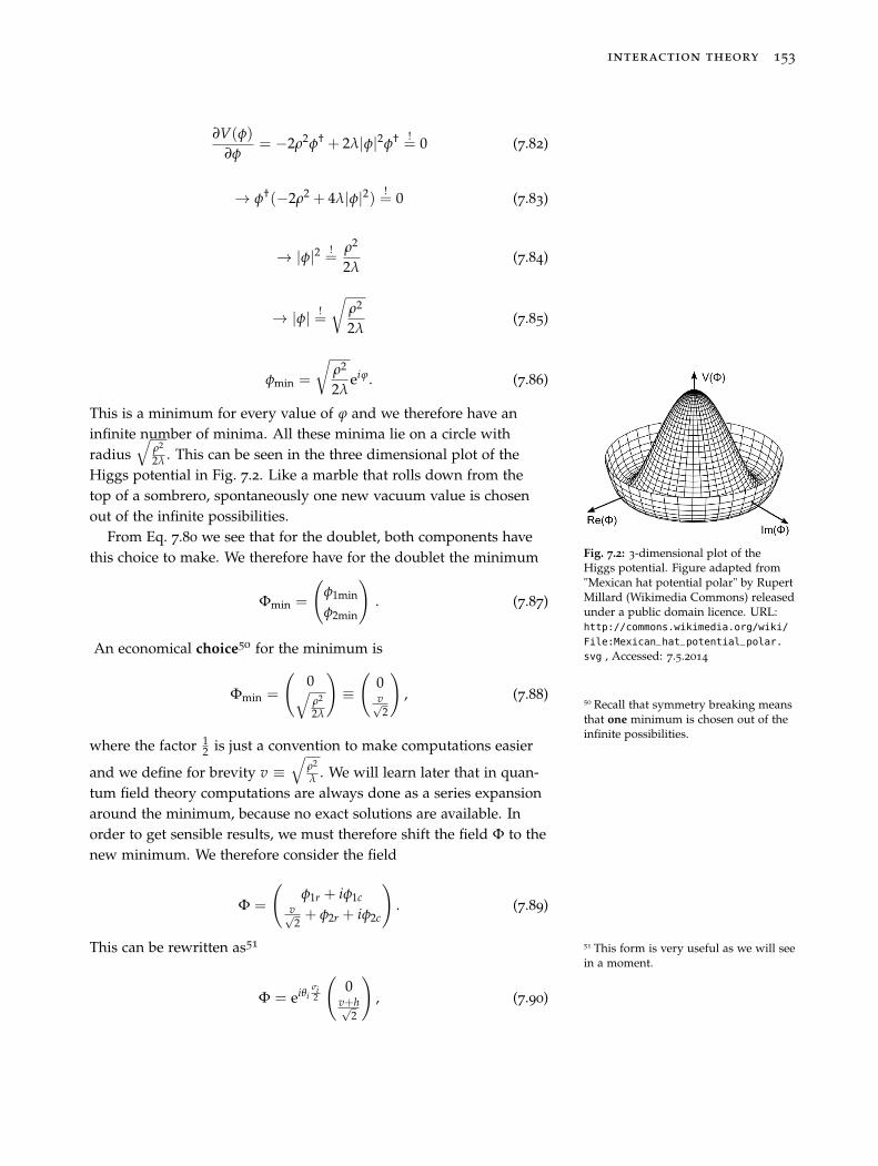
interaction theory 153
∂V(φ)
∂φ= −2ρ2φ† + 2λ|φ|2φ† !
= 0 (7.82)
→ φ†(−2ρ2 + 4λ|φ|2) != 0 (7.83)
→ |φ|2 !=
ρ2
2λ(7.84)
→ |φ| !=
√ρ2
2λ(7.85)
φmin =
√ρ2
2λeiϕ. (7.86)
This is a minimum for every value of ϕ and we therefore have aninfinite number of minima. All these minima lie on a circle withradius
√ρ2
2λ . This can be seen in the three dimensional plot of theHiggs potential in Fig. 7.2. Like a marble that rolls down from thetop of a sombrero, spontaneously one new vacuum value is chosenout of the infinite possibilities.
Fig. 7.2: 3-dimensional plot of theHiggs potential. Figure adapted from"Mexican hat potential polar" by RupertMillard (Wikimedia Commons) releasedunder a public domain licence. URL:http://commons.wikimedia.org/wiki/
File:Mexican_hat_potential_polar.
svg , Accessed: 7.5.2014
From Eq. 7.80 we see that for the doublet, both components havethis choice to make. We therefore have for the doublet the minimum
Φmin =
(φ1min
φ2min
). (7.87)
An economical choice50 for the minimum is
50 Recall that symmetry breaking meansthat one minimum is chosen out of theinfinite possibilities.
Φmin =
(0√
ρ2
2λ
)≡
(0v√2
), (7.88)
where the factor 12 is just a convention to make computations easier
and we define for brevity v ≡√
ρ2
λ . We will learn later that in quan-tum field theory computations are always done as a series expansionaround the minimum, because no exact solutions are available. Inorder to get sensible results, we must therefore shift the field Φ to thenew minimum. We therefore consider the field
Φ =
(φ1r + iφ1c
v√2+ φ2r + iφ2c
). (7.89)
This can be rewritten as51 51 This form is very useful as we will seein a moment.
Φ = eiθiσi2
(0
v+h√2
), (7.90)
154 physics from symmetry
because if we consider the series expansion of the exponential func-tion and the explicit form of the Pauli matrices σi (Eq. 3.80), we cansee that in first order
eiθiσi2
(0
v+h√2
)≈ (1 + i
12
θiσi)
(0
v+h√2
)
= (1 + i12
θ1σ1 + i12
θ2σ2 + i12
θ3σ3)
(0
v+h√2
)
=
(1 + i 1
2 θ3 i 12 θ1 +
12 θ2
i 12 θ1 − 1
2 θ2 1 − i 12 θ3
)(0
v+h√2
)
=
((i 1
2 θ1 +12 θ2)
v+h√2
(1 − i 12 θ3)
v+h√2
)
redefinitions → ≡(
φ1r + iφ1cv√2+ φ2r + iφ2c
).
(7.91)
Writing the complex spin 0 doublet in this form is useful, becausewe can now use the local SU(2) (gauge) symmetry to make com-putations simpler. In order to get physical results one gauge mustbe chosen and we prefer to work with a gauge that makes life theeasiest52.52 For different computations, different
gauges can be useful. Here we willwork with what is called the unitarygauge, that is particularly useful tounderstand the physical particle contentof a theory.
A general local SU(2) transformation is
Φ → Φ′ = eibi(x) σi2 Φ, (7.92)
which enables us to eliminate the exponential factor in Eq. 7.90, bychoosing appropriate bi(x). The complex scalar doublet is then, inthis unitary gauge
Φun =
(0
v+h√2
). (7.93)
Another possible way to understand this is that of the original fourcomponents that appeared in our complex scalar doublet, three areequivalent to our SU(2) gauge freedom53. Therefore, these three
53 Take note that this is only possible,because we have a local SU(2) theory,because our fields θ = θ(x), of coursedepend on the location in spacetime.For a global symmetry, these compo-nents can’t be gauged away, and arecommonly interpreted as masslessbosons, called Goldstone bosons.
fields aren’t physical54 and can’t be measured in experiments. What
54 The local SU(2) symmetry is nothingthat can be measured in experiments.This is merely a symmetry of our equa-tions and the gauge freedom disappearsfrom everything that is measurable inexperiments. Otherwise there wouldbe no possible way to make predictionsfrom our theory, because we wouldhave an infinite number of equivalentlypossible predictions (that are connectedby SU(2) transformations). Neverthe-less, this symmetry is far from beinguseless, because it guides us to thecorrect form of the Lagrangian.
remains is one physical field h, which is called the Higgs field.
Next, we want to take a look at the implications of this symmetrybreaking on the Lagrangian. We recite here the Lagrangian in ques-tion for convenience, which was derived in Eq. 7.74 and include anadditional factor 1
2 in front of the field Bμ to unclutter the notation inthe calculations that follow55
55 Such a factor changes nothing, be-cause it corresponds simply to a redefi-nition of the coupling constant 1
2 g ≡ g.Thus, strictly speaking, we should useg here instead of g. However, the nameof the constant doesn’t matter and wecontinue to call the coupling constantsimply g.
interaction theory 155
L =((∂μ + ig′ σi
2(Wμ)i + i
12
gBμ)Φ†)(
(∂μ − ig′ σi2(Wμ)i − i
12
gBμ)Φ)
− V(Φ) . (7.94)
We now substitute the field Φ with the shifted field in the unitarygauge, which was defined in Eq. 7.93. Of particular interest for uswill be the newly appearing terms that include the constant vacuumvalue v. The other terms describe the self-interaction of the Higgs-field and the interaction of the Higgs field with the other fields,which we will not examine any further. If we put in the minimum
value Φ → Φmin =
(0v√2
), which means we ignore h, we get
((∂μ + i
σi2
g′(Wμ)i + i12
gBμ)Φ†min
)((∂μ − ig′ σi
2(Wμ)i − i
12
gBμ)Φmin
)=
∣∣∣((∂μ + ig′ σi2(Wμ)i + i
12
gBμ)Φmin
)∣∣∣2
=∣∣∣((∂μ + ig′ σi
2(Wμ)i + i
12
gBμ)
√12
(0v
))∣∣∣2
=v2
8
∣∣∣((g′σi(Wμ)i + gBμ)
(01
))∣∣∣2.
Now using that we have behind Bμ an implicit 2 × 2 identity matrixand the explicit form of the Pauli matrices56 σi yields 56 σiWi =
(W3 W1 − iW2
W1 + iW2 −W3
)
=v2
8
∣∣∣ ( g′Wμ3 + gBμ g′Wμ
1 − ig′Wμ2
g′Wμ1 + ig′Wμ
2 −g′Wμ3 + gBμ
)(01
) ∣∣∣2
=v2
8
∣∣∣( (g′Wμ
1 − ig′Wμ2
−g′Wμ3 + gBμ
))∣∣∣2
=v2
8
((g′)2
((Wμ
1 )2 + (Wμ
2 )2)+ (g′Wμ
3 − gBμ)2)
(7.95)
Next we define two new spin 1 fields from the old ones we havebeen using so far
Wμ+ ≡ 1√
2(Wμ
1 − iWμ2 ) (7.96)
Wμ− ≡ 1√
2(Wμ
1 + iWμ2 ), (7.97)
where Wμ+ is the complex conjugate of Wμ
−. The first term in Eq. 7.95is then
(Wμ1 )
2 + (Wμ2 )
2 = 2(W+)μ(W−)μ (7.98)
156 physics from symmetry
and thus we have, including the constants,⎛⎜⎜⎝ g′v2︸︷︷︸
≡mW
⎞⎟⎟⎠2
(W+)μ(W−)μ (7.99)
which then looks like a typical "mass" term.
The second term in Eq. 7.95 can be written in matrix form
(g′Wμ3 − gBμ)2 =
(Wμ
3 , Bμ
)(g′2 −gg′
−gg′ g2
)︸ ︷︷ ︸
≡G
(Wμ
3Bμ
). (7.100)
In order to be able to interpret this as mass-terms, we need to diag-onalize57 the matrix G. The standard linear-algebra way to do this57 We will see in a moment that a
diagonalized matrix gives us termsthat look exactly like the other massterms. This enables us to interpret thecorresponding fields as physical fieldsthat can be observed in experiments.We could work with fields Wμ
3 and Bμ,but the physical interpretation wouldbe much harder.
needs the eigenvalues λ1, λ2 and normalized58 eigenvectors �v1,�v2 of
58 Which means length 1, i.e. �v ·�v = 1.
the matrix G, which are
λ1 = 0 → �v1 =1√
g2 + g′2
(gg′
)
λ2 = (g2 + g′2) → �v2 =1√
g2 + g′2
(g′
−g
).
The matrix G is then diagonalized by the matrix M build from theeigenvectors as its columns, i.e. Gdiag = M−1GM, with
M =1√
g2 + g′2
(g g′
g′ −g
)(7.101)
and
Gdiag =
(λ1 00 λ2
)=
(0 00 (g2 + g′2)
). (7.102)
The matrix M is orthogonal (MT = M−1), because we work withnormalized eigenvectors:
MT M =1√
g2 + g′2
(g g′
g′ −g
)1√
g2 + g′2
(g g′
g′ −g
)
=1
(g2 + g′2)
(g2 + g′2 gg′ − gg′
gg′ − gg′ g2 + g′2
)=
(1 00 1
). (7.103)
We therefore add two unit matrices 1 = MT M, into Eq. 7.100:
(Wμ
3 , Bμ
)MMT︸ ︷︷ ︸=1
G MMT︸ ︷︷ ︸=1
(Wμ
3Bμ
)=
(Wμ
3 , Bμ
)M MTGM︸ ︷︷ ︸
=Gdiag
MT
(Wμ
3Bμ
).
(7.104)
interaction theory 157
The remaining task is then to evaluate MT
(Wμ
3Bμ
), in order to get the
definition of two new fields, which have easily interpretable massterms in the Lagrangian:
MT
(Wμ
3Bμ
)=
1√g2 + g′2
(g g′
g′ −g
)(Wμ
3Bμ
)
=1√
g2 + g′2
((gWμ
3 + g′Bμ)
(g′Wμ3 − gBμ)
)≡
(Aμ
Zμ
). (7.105)
We can therefore write the second term as
(Aμ Zμ
)Gdiag
(Aμ
Zμ
)=
(Aμ Zμ
)(0 00 (g2 + g′2)
)(Aμ
Zμ
)
= (g2 + g′2)(Zμ)2 + 0 · (Aμ)2. (7.106)
To summarize: We started with a Lagrangian, without mass termsfor the spin 1 fields Wμ
i and Bμ (Eq. 7.71)
LSU(2) and U(1) = iΨγμ(∂μ − igBμ − ig′Wμ)Ψ− 1
4Tr
(WμνWμν)− 1
4BμνBμν.
(7.107)Then we included interactions with a doublet of spin 0 fields (Eq. 7.77)and after the process of spontaneous symmetry breaking, we havenew terms in the Lagrangian that are interpreted as mass terms59 59 For the first term here, we combine
Eq. 7.95 with Eq. 7.98.
14
v2g′2︸ ︷︷ ︸=M2
W
(W+)μ(W−)μ +18
v2(g2 + g′2)︸ ︷︷ ︸= 1
2 M2Z
Z2μ +
18
v20︸ ︷︷ ︸photon mass =0
·A2μ . (7.108)
We can see that one of the spin 1 fields Aμ remains massless afterspontaneous symmetry breaking. This is the photon field of electro-magnetism and all experiments up to now verify that the photon ismassless 60. An important observation is that the field responsible for 60 Take note that I omitted some very
important notions in this section:Hypercharge and the Weinberg angle.The Weinberg angle θW is simplydefined as cos(θW) = g√
g2+g′2or
sin(θW) = g′√g2+g′2
. This can be used
to simplify some of the definitionsmentioned in this section. Hyperchargeis a bit more complicated to explainand those who want to dig deeperare referred to the standard textsabout quantum field theory, some ofwhich are recommended at the end ofChapter 9.
Z-bosons Zμ and the field responsible for photons Aμ are orthogonallinear combinations of the fields Bμ and W3
μ. Therefore we can seethat both have a common origin!
The same formalism can be used to get mass terms for spin 12
fields without spoiling the local SU(2) symmetry, but before wediscuss this, we need to talk about one very curious fact of nature:parity violation.
158 physics from symmetry
7.4 Parity Violation
One of the biggest discoveries in the history of science was that na-ture is not invariant under parity transformations. In layman’s termsthis means that some experiments behave differently than their mir-rored analogue. The experiment that discovered the violation ofparity symmetry was the Wu experiment. A full description of thisexperiment, although fascinating, strays from our current subject, solet’s just discuss the final result.
The Wu experiment discovered that the particles mediating theweak force (the W+, W−, Z bosons) only couple to left-chiral parti-cles. In other words: only left-chiral particles interact via the weakforce61. All particles produced in weak interactions are left-chiral.61 We will discuss at the end of this
section why this means that parity isviolated
Neutrinos interact exclusively via the weak force and therefore it ispossible that there are no right-chiral neutrinos62. All other particles
62 We will see in a moment that massive,left-chiral particles always get a right-chiral component during propagation.It is known from experiments thatneutrinos have mass and therefore wewould expect a right-chiral neutrinocomponent. Nevertheless, this right-chiral component does not participatein any known interaction.
can be produced via other interactions and therefore can be right-chiral, too.
Up to this point, we used left-chiral and right-chiral as labels forobjects transforming according to different representations of theLorentz group. Although this seems like something very abstract, wecan measure the chirality of particles, because there is a correlation toa more intuitive concept called helicity63.
63 We will not discuss this here, becausethe details make no difference for thepurpose of the text. The message totake away is that it can be done. A verynice discussion of these matters canbe found in Alessandro Bettini. Intro-duction to Elementary Particle Physics.Cambridge University Press, 2nd edi-tion, 4 2014. ISBN 9781107050402
In fact, most of the time particles do not have a specified chirality,which means they aren’t definitely left-chiral or right-chiral and thecorresponding Dirac spinor Ψ has both components. Parity viola-tion was no prediction of the theory and a total surprise for everyphysicist. Until the present day, no one knows why nature behaves sostrangely. Nevertheless, it’s easy to accommodate this discovery intoour framework. We only need something that makes sure we alwaysdeal with left-chiral spinors when we describe weak interactions.
Recall that the symbols χ and ξ denote Weyl spinors (two compo-nent objects), ψ Dirac spinors (four component objects, consisting oftwo Weyl spinors)
ψ =
(χL
ξR
)(7.109)
and Ψ doublets of Dirac spinors
Ψ =
(ψ1
ψ2
). (7.110)
Then the "something" we need is the projection operator PL:
PLψ = PL
(χL
ξR
)=
(χL
0
)≡ ψL. (7.111)
interaction theory 159
Such a projection operator can be constructed using the matrix64 64 Recall the definition of the γμ matri-ces in Eq. 6.13 and don’t let yourself getconfused about the missing γ4 matrix.There is an alternative convention thatuses γ4 instead of γ0 and to avoid inter-ference between those conventions, thematrix here is commonly called γ5.
γ5 = iγ0γ1γ2γ3 =
(−1 00 1
). (7.112)
The matrix γ5 is called the chirality operator, because states of pure
chirality
(χL
0
)or
(0
ξR
)are eigenstates of γ5 with eigenvalue −1
and +1 respectively.
The projection operator PL can then be written65 65 Maybe you wonder why we define PLas so complicated and do not start withthe explicit matrix form right away. Wedo this, because it’s possible to workin a different basis where the matricesγμ look completely different. (For moreinformation about this have a lookat Section 8.10). Take note that in theLagrangian the Dirac spinors appear al-ways in combination with the matricesγμ. We can always add a 1 = U−1U,with some arbitrary invertible ma-trix U, between them. For example,∂μΨγμΨ = ∂μΨ U−1U︸ ︷︷ ︸
=1
γμ U−1U︸ ︷︷ ︸=1
Ψ =
∂μ ΨU−1︸ ︷︷ ︸=Ψ′
UγμU−1︸ ︷︷ ︸γ′
μ
UΨ︸︷︷︸Ψ′
. Physics is of
course completely independent of suchtransformations, but we can use this tosimplify computations. The basis weprefer to work with in this text is calledWeyl Basis. In other bases the two com-ponents of a Dirac spinor are mixturesof χL and ξR. Nevertheless, the projec-tion operator defined as PL = 1−γ5
2 ,always projects out the left-chiralcomponent, because PWeyl
L ΨWeyl =
ΨWeylL ⇒ P′
LΨ′ =1−γ′
52 Ψ′︸︷︷︸
UΨWeyl
=
1−Uiγ0U−1Uγ1U−1Uγ2U−1Uγ3U−1
2 UΨWeyl =U−Uiγ0γ1γ2γ3
2 ΨWeyl = U(
1−γ52
)ΨWeyl =
UΨWeylL = Ψ′
L �
PL =1 − γ5
2=
(1 00 0
)(7.113)
and we can define analogously
PR =1 + γ5
2=
(0 00 1
). (7.114)
Now, in order to accommodate for the fact that only left-chiralparticles interact via the weak force, we must simply include PL intoall terms of the Lagrangian that describe the interaction of W±
μ andZμ with different fields. The corresponding terms were derived inSection 7.2, and the final result was Eq. 7.67, which we recite here forconvenience:
Llocally SU(2) invariant = iΨγμDμΨ − 14
Tr(WμνWμν
)= iΨγμ(∂
μ − igWμ)Ψ − 14
Tr(WμνWμν
). (7.115)
The relevant term that describes the interaction is gΨγμWμΨ and wesimply add PL:
→ L = iΨγμ(∂μ − igWμPL)Ψ − 1
4Tr
(WμνWμν). (7.116)
Here PL acts on a doublet and is therefore
PLΨ =
(PL 00 PL
)(ψ1
ψ2
)=
((ψ1)L
(ψ2)L
). (7.117)
One PL is enough to project the left-chiral component out of bothdoublets Ψ and Ψ. To see this we need three identities:
• (PL)2 = PL, which is obvious from the explicit matrix form and
because every projection operator must have this property66. Pro- 66 Another defining condition of anyprojection operator is PLPR = PRPL = 0,which is here fulfilled as you can checkby using the explicit form of PL,PR andγ5.
jecting twice must be the same as projecting one time.
160 physics from symmetry
• {γ5, γμ} = γ5γμ + γμγ5 = 0, which you can check by brute forcecomputation67.
67 Or using another identity {γμ, γν} =
γμγν + γνγμ = 12 ημν, where ημν is the
Minkowski metric and the definitionγ5 = iγ0γ1γ2γ3.
• (PL)† = PL, because γ5 is real, as can be seen from the explicit
matrix form: γ5 =
(−1 00 1
)
The second identity simply tells us that γ5γμ = −γμγ5, i.e. thatwe can switch the position of γ5 and any γμ matrix, as long as weinclude a minus sign. This tells us
γμPL = γμ1 − γ5
2=
1 + γ5
2γμ = PRγμ. (7.118)
We can now rewrite the relevant term of Eq. 7.116:
gΨγμWμPLΨ = gΨγμWμ P2L︸︷︷︸
=PL
Ψ
= g Ψ︸︷︷︸Ψ†γ0
γμPL︸ ︷︷ ︸PRγμ
Wμ PLΨ︸︷︷︸ΨL
= gΨ† γ0PR︸ ︷︷ ︸PLγ0
γμWμΨL
=︸︷︷︸Using P†
L=PL and (AB)†=((AB)T)�=(BT AT)�=B† A†
(PLΨ)†γ0γμWμΨL
= g(PLΨ︸︷︷︸=ΨL
)†γ0γμWμΨL
= gΨLγμWμΨL � (7.119)
We can see here that one projection operator is really enough toguarantee that both Ψ and Ψ are left-chiral.
Now we know how we can describe mathematically that only left-chiral fields interact via the weak force, but why does this mean thatparity is violated? To understand this we need to parity transformthis term, because if it isn’t invariant, the physical system in questionis different from its mirror image68. Here we need the parity operator
68 This means an experiment, whoseoutcome depends on this term ofthe Lagrangian, will find a differentoutcome if everything in the experimentis arranged mirrored.
for spinors69 Pspinor and vectors70 Pvector. The transformation yields69 The parity operator for spinors wasderived in Section 3.7.9. Using theγμ matrices, we can write the parityoperator derived there as P = γ0 =(
0 σ0σ0 0
)=
(0 11 0
)70 The parity operator for vectors is
simply Pvector =
⎛⎜⎜⎝1 0 0 00 −1 0 00 0 −1 00 0 0 −1
⎞⎟⎟⎠as already mentioned in Eq. 3.140.
Ψ︸︷︷︸=Ψ†γ0
γμWμPLΨ → (PspinorΨ)†γ0γμ(PvectorWμ)PL(PspinorΨ)
= (Ψ)†γ0γ0γμ(PvectorWμ)PLγ0Ψ
=︸︷︷︸using {γ5, γ0} = 0 and PL = 1−γ5
2
(Ψ)†γ0γ0γμγ0(PvectorWμ)PRΨ. (7.120)
interaction theory 161
Then we can use γ0γ0γ0 = γ0 and γ0γiγ0 = −γi, as you can checkby looking at the explicit form of the matrices. Furthermore, we havePvectorW0 = W0 and PvectorWi = −Wi, which follows from the explicitform of Pvector. We conclude these two minus signs cancel each otherand the parity transformed term of the Lagrangian reads:
(PspinorΨ)†γ0γμ(PvectorWμ)PL(PspinorΨ) = ΨγμWμPRΨ �= ΨγμWμPLΨ(7.121)
Therefore this term is not invariant and parity is violated.
Parity violation has another important implication. Recall thatwe always write things below each other between two big bracketsif they can transform into each other71. For example, we use four- 71 This is explained in Appendix A.
vectors, because their components can transform into each otherthrough rotations or boosts. In this section we learned that only left-chiral particles interact via the weak force and the correct term in theLagrangian is ΨγμWμPLΨ = ΨLγμWμΨL. In physical terms thisterm means that the components of the left-chiral doublets, whichmeans the two spin 1
2 fields (ψ1)L and (ψ2)L can transform into eachother through weak-interactions. Right-chiral fields do not interactvia the weak force and therefore (ψ1)R, (ψ2)R aren’t transformed intoeach other. Therefore writing them below each other between twobig brackets makes no sense. In mathematical terms this means thatright-chiral fields form SU(2) singlets, i.e. are objects transformingaccording to the 1 dimensional representation of SU(2), which do notchange at all72. So let’s summarize: 72 This was explained in Section 3.6.2.
• Left-chiral fields are written as SU(2) doublets: ΨL =
((ψ1)L
(ψ2)L
),
because they interact via the weak force and therefore can trans-form into each other. They transform under the two-dimensionalrepresentation of SU(2):
ΨL → Ψ′L = ei�a�σ2 ΨL . (7.122)
• Right-chiral fields are described by SU(2) singlets: (ψ1)R, (ψ2)R,because they do not interact via the weak force and therefore can’ttransform into each other. Therefore they transform under theone-dimensional representation of SU(2):
(ψ1)R → (ψ1)′R = e0(ψ1)R = (ψ1)R
(ψ2)R → (ψ2)′R = e0(ψ2)R = (ψ2)R . (7.123)
Now we move on and try to understand how mass terms for spin12 particles can be added in the Lagrangian without spoiling anycrucial symmetry.
162 physics from symmetry
7.5 Lepton Mass Terms
At the beginning of Section 7.2, we discovered that we can’t includearbitrary mass terms ΨmΨ without spoiling the SU(2) symmetry.Now we will see that parity violation makes this problem even big-ger. After discussing the problem, we will see that again the Higgsmechanism is a solution.
In the last section we talked a bit about the chirality of the cou-pling term: ΨγμσjW
μj PLΨ. What about the chirality of a mass term?
Take a look again at the invariants without derivatives for spinors,which we derived in Eq. 6.7 and Eq. 6.8:
I1 := (χa)Tξ a = (χL)
†ξR and I2 := (ξa)Tχa = (ξR)†χL (7.124)
We can write these invariants using Dirac spinors as7373 The Dirac spinors ψL and ψR aredefined using the chiral-projectionoperators introduced in the last section:ψL = PLψ and ψR = PRψ. And we haveas always ψ = ψ†γ0.
ψψ = ψLψR + ψRψL
=(
χ†L 0
)(0 σ0
σ0 0
)(0
ξR
)+
(0 ξ†
R
)(0 σ0
σ0 0
)(χL
0
)= χ†
LξR + ξ†RχL � (7.125)
We can see that Lorentz invariant mass terms always combine left-chiral with right-chiral fields. This is a problem, because left-chiraland right-chiral fields transform differently under SU(2) transfor-mations, as explained at the end of the last section. The left-chiralfields are doublets, whereas the right-chiral fields are singlets. Themultiplication of a doublet and singlet is not SU(2) invariant. Forexample
ΨL︸︷︷︸doublet
ψR︸︷︷︸singlet
→ Ψ′Lψ′
R = ΨLe−ibiσi2 ψR �= ΨLψR (7.126)
From the experience with mass terms for spin 1 fields, we knowwhat to do: Instead of considering terms as above, we add SU(2)invariant coupling terms with 0 fields to the Lagrangian. Then, bychoosing the vacuum value for the spin 0 field we break the symme-try and generate mass terms.
A SU(2), U(1) and Lorentz invariant term, coupling a spin 0 dou-blet and our spin 1
2 fields together, is given by
ΨLΦψR. (7.127)
To see the invariance we transform this term with a SU(2) trans-formation7474 Remember ΦL → Φ′
L = eibi(x)σi ΦLand σ†
i = σi
interaction theory 163
ΨLΦψR → Ψ′LΦ′ψR = ΨLe−ibi(x)σi eibi(x)σi ΦψR = ΨLΦψR �
and equally for a U(1) transformation:
ΨLΦψR → Ψ′LΦψ′
R = ΨLe−ia(x)Φeia(x)ψR = ΨLΦψR �
The spin 0 field does not transform at all under Lorentz transfor-mations75 and therefore the term is Lorentz invariant, because we 75 By definition a spin 0 field transforms
according to the (0, 0) representationof the Lorentz group. In this represen-tation all Lorentz transformations aretrivially the identity transformation.This was derived in Section 3.7.4.
have the same Lorentz invariant terms as in Eq. 7.125.
This kind of term is called Yukawa term and we add it, with theequally allowed Hermitian conjugate to the Lagrangian76 −λ2
76 The strange name −λ2 and why onlyadd ψ2R here will become clear in amoment, because terms including ψ1Rand −λ1 will be discussed afterwards.
L = −λ2(ΨLΦψ2R + ψ2RΦΨL). (7.128)
The coupling constant λ2 is called a Yukawa coupling. This extraterm does not only describe the interaction between the fermions andthe Higgs field, but also leads to mass terms for the spin 1
2 fields afterthe symmetry breaking. We put the expansion around the vacuumexpectation value (Eq. 7.88)
Φ =
√12
(0
v + h
)
into the Lagrangian, which yields
L = − λ2√2
((Ψ1L, Ψ2L
)(0
v + h
)ψ2R + ψ2R
(0, v + h
)(Ψ1L
Ψ2L
))
= −λ2(v + h)√2
(Ψ2Lψ2R + ψ2RΨ2L) . (7.129)
Equation 7.125 tells us this is equivalent to
= −λ2(v + h)√2
ψ2ψ2 (7.130)
= −λ2v√2(ψ2ψ2)︸ ︷︷ ︸
Fermion mass term
− λ f h√2(ψ2ψ2)︸ ︷︷ ︸
Fermion-Higgs interaction
. (7.131)
We see that through the Higgs mechanism we get indeed the re-quired mass terms. Again, we used symmetry constraints to add aterm to the Lagrangian and this yields after spontaneous symmetrybreaking mass terms for the spin 1
2 fields. Take note that we onlygenerated mass terms for the second field inside the doublet ψ2.What about mass terms for the first field ψ1?
To get mass terms for the first field ψ1 we need to consider cou-pling terms to the charge-conjugated77 Higgs field Φ = εΦ�, because 77 Charge conjugation is explained in
Section 3.7.10.
164 physics from symmetry
Φ =
(0
v+h√2
)→ Φ = εΦ� =
(0 1−1 0
)(0
v+h√2
)=
(v+h√
20
). (7.132)
Following the same steps as above with the charge conjugated Higgsfield leads to mass terms for ψ1:
L = −λ f (ΨLΦψ1R + ψ1R˜ΦΨL)
= − λ1√2
((Ψ1L, Ψ2L
)(v+h√
20
)Ψ1R + Ψ1R
(v+h√
20
)(Ψ1L
Ψ2L
))
= −λ1(v + h)√2
(Ψ1LΨ1R + Ψ1RΨ1L) . (7.133)
To understand the rather abstract spin 12 doublets better, we
rewrite them more suggestively7878 A neutrino is always denoted by a ν.In this step we simply give the twofields in the doublet ψ1 and ψ2 theirconventional names: electron field e andelectron-neutrino field νe. Ψ =
(νe
e
)(7.134)
and equivalently for the other leptons μ, νμ and τ, ντ . This form ofthe doublets is suggested by experiments, because an electron e isalways transformed by weak interactions into another electron e, withpossibly different momentum, or an electron-neutrino ve plus otherparticles. In weak interactions e and νe (equivalently μ and νμ or τ
and ντ) always appear in pairs. This can be understood by lookingat the coupling term ΨγμWμPLΨ = Ψγμ(Wμ)i
σi
2 PLΨ. As discussedin the last section this can be rewritten using the explicit matrix formof the Pauli matrices79 σi, which then gives us terms coupling the79 This gives us once more
σiWμi =
(Wμ
3 Wμ1 − iWμ
2Wμ
1 + iWμ2 −Wμ
3
)which we can rewrite using
W± = 1√2(W1 ∓ W2):
⇒ σiWμi =
(Wμ
3
√2W+√
2W− −Wμ3
)components of the doublets together:
ΨγμσjWμj PLΨ =
(νe e
)γμ
(Wμ
3
√2W+√
2W− −Wμ3
)PL
(νe
e
)
=︸︷︷︸using Eq. 7.116
((νe)L (e)L
)γμ
(Wμ
3
√2W+√
2W− −Wμ3
)((νe)L
(e)L
)
= (νe)LγμWμ3 (νe)L + (νe)Lγμ
√2W+(e)L
+ (e)Lγμ
√2W−(νe)L − (e)LγμWμ
3 (e)L. (7.135)
If we want to consider all lepton generations at once, i.e. e, μ and τ,we need to write down three terms like this into the Lagrangian:
ΨeγμσjWμj PLΨe + ΨμγμσjW
μj PLΨμ + ΨτγμσjW
μj PLΨτ , (7.136)
interaction theory 165
which can be written more compactly by introducing Ψl =
(νl
l
),
where l = e, μ, τ:ΨlγμσjW
μj PLΨl .
Using the notation l =
(lL
lR
)the coupling term between the spin 0
and the electrically charged spin 12 fields after spontaneous symmetry
breaking reads
− λlv√2︸︷︷︸
Fermion mass mL
(ll) − λlh√2︸︷︷︸
Fermion-Higgs interaction strength cL
(ll) .
The terms for the corresponding neutrinos follow analogously80. 80 As already mentioned above, wecan only write down such mass termsif there are right-chiral neutrinos.However, so far right-chiral neutrinoswere never observed in experiments,although we know that neutrinos havemass. This is one of the open problemsof the standard model.
This Lagrangian enables us to predict something about the Higgsfield h that can be tested in experiments. For a given lepton l, themass is given by
ml =λlv√
2→ λl =
ml√
2v
(7.137)
and the coupling strength of this lepton to the Higgs is given by
cl =λlh√
2=︸︷︷︸
Eq. 7.137
mlhv
. (7.138)
The last equation means that the coupling strength of the Higgsto a lepton is proportional to the mass of the lepton. The heavier thelepton the stronger the coupling. The same is true for all particlesand the derivation is completely analogous.
There are other spin 12 particles, called quarks, that interact via
the weak force. In addition, quarks interact via a third force, calledthe strong force and this will be the topic of Section 7.8, but firstwe want to talk about mass terms for quarks. Luckily, these can beincorporated analogous to the lepton mass terms.
7.6 Quark Mass Terms
We learned in the last section that an SU(2) doublet contains theparticles that are transformed into each other via the weak force. Forquarks81 these are the up- and down quark: 81 If you’ve never heard of quarks
before, have a look at Section 1.3.
q =
(ud
)(7.139)
166 physics from symmetry
and equally for the strange and charm or top and bottom quarks.
Again, we must incorporate the experimental fact that only left-chiral particles interact via the weak force. Therefore, we have left-chiral doublets and right-chiral singlets:
qL︸︷︷︸doublet
=
(uL
dL
)→ eiai
σi2 qL (7.140)
uR︸︷︷︸singlet
→ uR
dR︸︷︷︸singlet
→ dR. (7.141)
Again, right-chiral particles do not interact via the weak force andtherefore they aren’t transformed into anything and form a SU(2)singlet (=one component object).
The problem is the same as for leptons: To get something Lorentzinvariant, we need to combine left-chiral with right-chiral spinors.Such a combination is not SU(2) invariant and we use again theHiggs mechanism. This means, instead of terms like
qLuR + qLdR + uRqL + dRqL, (7.142)
which aren’t SU(2) invariant, we consider the coupling of the quarksto a spin 0 field doublet Φ:
λuqLΦuR + λdqLΦdR + λuuRΦqL + λddRΦqL, (7.143)
with coupling constants λu, λd and the charge conjugated Higgsdoublet82 which is needed in order to get mass terms for the up
82 This is defined in Eq. 7.132:
Φ = εΦ� =︸︷︷︸(
v+h√2
0
).
quarks83.83 We defined the doublets as(
ud
).
Multiplication of this doublet with
Φ =
(0
v+h√2
)always results in terms
proportional to d.
Then, everything is analogous to the lepton case: We put theexpansion of the Higgs field around its minimum84 into the La-
84 Φ =
(0
v+h√2
)and equivalently for the
charge-conjugated Higgs field.
grangian, which gives us mass terms plus quark-Higgs couplingterms.
7.7 Isospin
Now it’s time we talk about the conserved quantity that follows fromSU(2) symmetry. The free Lagrangians are only globally invari-ant and we need interaction terms to make them locally symmet-ric. Recall that global symmetry is a special case of local symmetry.Therefore we have global symmetry in every locally invariant La-grangian and the corresponding conserved quantity is conserved for
interaction theory 167
both cases. The result will be that global SU(2) invariance gives usthrough Noether’s theorem, a new conserved quantity called isospin.This is similar to electric charge, which is the conserved quantity thatfollows from global U(1) invariance.
Noether’s theorem for internal symmetry (Section 4.5.5, especiallyEq. 4.57) tells us that
∂0
∫d3x
∂L
∂(∂0Ψ)δΨ︸ ︷︷ ︸
=Q
= 0 (7.144)
The Lagrangian is invariant under transformations of the form
Ψ → eiaiσi2 Ψ = (1 + iai
σi2+ . . .)Ψ (7.145)
Therefore our infinitesimal variation is δΨ = iaiσi2 Ψ, with arbitrary
ai. This tells us we get one conserved quantity for each generator,because the Lagrangian is invariant regardless of if two of the threeai are zero and one isn’t. For example, a2 = a3 = 0 and a1 �= 0 ora1 = a2 = 0 and a3 �= 0. Of course we get another conserved quantityfor a1 �= 0, a2 �= 0 and a3 �= 0, which is just the sum of the conservedquantities we get from the individual generators. In other words: weget three independently conserved quantities, one for each generatorof SU(2).
The globally invariant, free Lagrangian (Eq. 7.44) is
LD1+D2 = iΨγμ∂μΨ.
The corresponding conserved quantities Qi, for example for theelectron-neutrino doublet, are85 85 See Eq. 7.144 and as always defined
without the arbitrary constants ai .
Qi = iΨγ0σi2
Ψ
=
(ve
e
)†
γ0γ0︸︷︷︸=1
σi2
(ve
e
). (7.146)
Recall that only σ3 is diagonal. This means we are only able toassign a definite value to the two components of the doublet (ve, e)for the conserved quantity i = 3. For the other generators, σ1 and σ2,our two components ve and e aren’t eigenstates. We are of course freeto choose a different basis, where for example σ2 is diagonal. Thenwe can simply redefine what we call ve and e and get the same result.The thing to take away is that although we have three conservedquantities, one for each generator, we can only use one at a time tolabel our particles/states.
168 physics from symmetry
For i = 3 we have
Q3 =
(ve
e
)†σ3
2
(ve
e
)
=12
(ve
e
)† (1 00 −1
)(ve
e
)
=12
v†e ve − 1
2e†e (7.147)
This means we can assign Q3(ve) = 12 and Q3(e) = − 1
2 as newparticle labels. In contrast for i = 1, we have
Q1 =
(ve
e
)†σ1
2
(ve
e
)
=12
(ve
e
)† (0 11 0
)(ve
e
)
=12
v†e e +
12
e†ve (7.148)
and we can’t assign any particle labels here, because the matrix σ1
isn’t diagonal.
7.7.1 Labelling States
Recall that in Section 3.5, we introduced the notion of Cartan genera-tors, which is the set of diagonal generators of a given group. In thelast section we learned that these generators become especially use-ful if we want to give new labels to our particles inside a doublet8686 In a later section we will learn that
the same can be done for triplets andthe conserved quantities following fromSU(3) invariance.
object. A typical SU(2) doublet is of the form(ve
e
). (7.149)
We can’t diagonalize two or more elements of the Lie algebra su(2)
at the same time and thus the "Cartan subalgebra" consists of onlyonly one element87. It is conventional to choose J3 = 1
2 σ3 as diagonal.87 This can be seen by noting that thereare no commuting generators in su(2).Only commuting generators can bediagonalized at the same time.
The corresponding eigenvalues are + 12 and − 1
2 . A left-chiral neutrino(ve
0
)is an eigenstate of this generator, with eigenvalue + 1
2 and a
left-chiral electron
(0e
)an eigenstate of this generator, with eigen-
value − 12 . These are new particle labels, which are called the isospin
of the neutrino and the electron.
interaction theory 169
Following the same line of thoughts we can assign an isospinvalue to the right-chiral singlets. These transform according to theone-dimensional representation of SU(2), and the generators arein this representation simply zero88: Ji = 0. Therefore, in this one- 88 The right-chiral singlets do not trans-
form at all as explained in Section 3.7.4.dimensional representation, the singlets are eigenstates of the Cartangenerator J3 with eigenvalue zero. The right-chiral singlets, like eR
carry isospin zero. This coincides with the remarks above that right-chiral fields do not interact via the weak force. Just as electricallyuncharged objects do not interact via electromagnetic interactions,fields without isospin do not take part in weak interactions.
Finally, we can assign isospin values to the three gauge fieldsWμ
+, Wμ−, Wμ
3 . The three gauge fields form a SU(2) triplet
Wμ =
⎛⎜⎝Wμ+
Wμ−
Wμ3
⎞⎟⎠ , (7.150)
which transforms according to the three dimensional representationof SU(2). In this representation the Cartan generator J3 has eigenval-ues89 +1,−1, 0 and therefore we assign Q3(W
μ+) = 1, Q3(W
μ−) = −1, 89 This can be seen directly from the
explicit matrix form of J3 in Eq. 3.129:
J3 =
⎛⎝1 0 00 0 00 0 −1
⎞⎠.
Q3(Wμ3 ) = 0. This is the isospin of the W+ and the W− bosons.
Take note that the triplet(
Wμ1 Wμ
2 Wμ3
)simply belongs to a differ-
ent basis, where J3 isn’t diagonal. This can be seen as another reasonfor our introduction of Wμ
±.
If this is unclear, have a look at how we introduced the three gaugefields Wμ
i . They were included into the Lagrangian in combinationwith the generators σiW
μi . This can be seen as a basis expansion of
some objects Wμ in terms of the basis σi:
Wμ = σiWμi = σ1Wμ
1 + σ2Wμ2 + σ3Wμ
3 ,
analogous to how we can write a vector in terms of basis vectors:
�v = v1�e1 + v2�e2 + v3�e3.
The generators σi live in the Lie algebra90 of SU(2) and consequently 90 The Lie algebra is a vector space!
our object Wμ lives there, too. Therefore, if we want to know howWμ transforms, we need to know the representation of SU(2) on thisvector space, i.e. on its own Lie algebra. In other words: We need toknow how the group elements of SU(2) act on their own Lie algebraelements, i.e. its generators. This may seem like a strange idea atfirst, but actually is a quite natural idea. Recall how we defined arepresentation: a representation is a map91 from the group to the 91 To be precise: A homomorphism,
which is a map that satisfies somespecial conditions.
space of linear operators over a vector space. So far we only looked
170 physics from symmetry
at "external" vector spaces like Minkowski space. The only intrinsicvector space that comes with a group is its Lie algebra92 ! Therefore
92 A group itself is in general no vectorspace. Although we can take a look athow the group acts on itself, this is nota representation, but a realization of thegroup.
it isn’t that strange to ask what a group representation on this vectorspace looks like. This very important representation is called theadjoint representation.
Gauge fields (like W+, W−, W3) are said to live in the adjoint rep-resentation of the corresponding group. For SU(2) the Lie algebra isthree dimensional, because we have three basis generators and there-fore the adjoint representation is three dimensional. Exactly how weare able to write the components of a vector between two brackets93,
93�v =
⎛⎝v1v2v3
⎞⎠we can write the component of Wμ between two brackets94, which is
94 Wμ =
⎛⎝Wμ1
Wμ2
Wμ3
⎞⎠what we call a triplet . The generators in the adjoint representationare connected to the three dimensional generator we derived earlierthrough a basis transformation.
In the following section we move on to the "next higher" internalsymmetry group SU(3). Demanding local SU(3) invariance of theLagrangian gives us the correct Lagrangian which describes stronginteractions.
7.8 SU(3) Interactions
For three fermion fields we can find a locally SU(3) invariant La-grangian in exactly the same way we did in the last chapter for twofields and SU(2). This symmetry is not broken and the correspond-ing spin 1 fields, called gluon fields, are massless. SU(3) is the groupof all unitary 3 × 3 matrices with unit determinant, i.e.
U†U = UU† = 1 det U = 1. (7.151)
As usual for Lie groups we can write this as an exponential func-tion9595 As already noted in Section 2.4,
Capital Roman letters A, B, . . . arealways summed from 1 to 8. U = eiTAθA . (7.152)
The defining equations (Eq. 7.151) of the group require, as for96
96 See Eq. 3.79 and the following textplus equations, where the basis wasgiven by the 2 × 2 Pauli matrices.
SU(2), the generators to be Hermitian and traceless
T†A = TA (7.153)
tr(TA) = 0 . (7.154)
A basis for those traceless, Hermitian generators is, at least in onerepresentation, given by eight97 3 × 3 matrices, called Gell-Mann97 It can be shown that in general for
SU(N) the Lie-Algebra is N2 − 1dimensional.
matrices:
interaction theory 171
λ1 =
⎛⎜⎝ 0 1 01 0 00 0 0
⎞⎟⎠ λ2 =
⎛⎜⎝ 0 −i 0i 0 00 0 0
⎞⎟⎠ λ3 =
⎛⎜⎝ 1 0 00 −1 00 0 0
⎞⎟⎠λ4 =
⎛⎜⎝ 0 0 10 0 01 0 0
⎞⎟⎠ λ5 =
⎛⎜⎝ 0 0 i0 0 0−i 0 0
⎞⎟⎠ λ6 =
⎛⎜⎝ 0 0 00 0 10 1 0
⎞⎟⎠λ7 =
⎛⎜⎝ 0 0 00 0 −i0 i 0
⎞⎟⎠ λ8 =1√3
⎛⎜⎝ 1 0 00 1 00 0 −2
⎞⎟⎠ . (7.155)
The generators of the group are connected to these Gell-Mann ma-trices, just as the Pauli matrices were connected to the generators98 98 Ji =
σi2 , see Eq. 3.81 and the explana-
tions there.of the SU(2) group via TA = 12 λA. The Lie algebra for this group is
given by[TA, TB] = i f ABCTC, (7.156)
where we adopted the standard convention that capital letters likeA, B, C can take on every value from 1 to 8. f ABC are called the struc-ture constants of SU(3), which for SU(2) were given by the Levi-Civita symbol εijk. They can be computed by brute-force computa-tion, which yields99 99 This is not very enlightening, but we
list it here for completeness.f 123 = 1 (7.157)
f 147 = − f 156 = f 246 = f 257 = f 345 = − f 367 =12
(7.158)
f 458 = f 678 =
√3
2, (7.159)
where all others can be computed from the fact that the structureconstants f ABC are antisymmetric under permutation of any twoindices. For example
f ABC = − f BAC = − f CBA. (7.160)
All other possibilities, which cannot be computed by permutation,vanish.
Analogous to what we did for SU(2) in Section 7.2, we introduce atriplet of spin 1
2 fields
Q =
⎛⎜⎝q1
q2
q3
⎞⎟⎠ (7.161)
and exactly as for SU(2) we get new labels for the objects inside thistriplet. We will discuss these new labels in the next section.
172 physics from symmetry
To make the Lagrangian
L = iQ∂μγμQ − QmQ (7.162)
locally SU(3) invariant, one again adds coupling terms between thespin 1
2 fields and new spin 1 fields. The derivation is analogous as forSU(2), but the computations are quite cumbersome, so we just quotethe final Lagrangian100100 Remember: the sum over capital
letters (A, B, C, ...) runs from 1 to 8
L = −14GαβGαβ + Q(iDμγμ − m)Q, (7.163)
and the field strength tensor Gαβ for the spin 1 gluon fields Gα ≡ TCGCα
is defined asGαβ = ∂αGβ − ∂βGα − g[Gα,Gβ] . (7.164)
Here TC denotes the generators of SU(3) that were defined at thebeginning of this section. Furthermore, Dα is defined as
Dα = ∂α − igTCGCα = ∂α − igGα . (7.165)
As you can check every term here is completely analogous to theSU(2) case, except we now have different generators with differentcommutation properties.
7.8.1 Color
From global SU(3) symmetry we get through Noether’s theoremnew conserved quantities. This is analogous to what we discussedfor SU(2) in Section 7.7. Following the same lines of thought as forSU(2) tells us that we have 8 conserved quantities, one for each gen-erator. Again, we can only use the conserved quantities that belongto the diagonal generators as particle labels. SU(3) has two Cartan101101 Recall, Cartan generators = diagonal
generators. generators 12 λ3 and 1
2 λ8. Therefore, every particle that interacts viathe strong force carries two additional labels, corresponding to theeigenvalues of the Cartan generators.
The eigenvalues102 of 12 λ3 = 1
2
⎛⎜⎝ 1 0 00 −1 00 0 0
⎞⎟⎠ are + 12 ,− 1
2 , 0. For102 The eigenvectors are of course
⎛⎝100
⎞⎠,
⎛⎝010
⎞⎠ and
⎛⎝001
⎞⎠. λ8 = 12√
3
⎛⎜⎝ 1 0 00 1 00 0 −2
⎞⎟⎠ the eigenvalues103 are 12√
3, 1
2√
3, −1√
3. There-
103 Corresponding to the same eigenvec-
tors
⎛⎝100
⎞⎠,
⎛⎝010
⎞⎠ and
⎛⎝001
⎞⎠.
fore if we arrange the strong interacting fermions into triplets (in thebasis spanned by the eigenvectors of the Cartan generators), we canassign them the following labels, with some arbitrary spinor ψ:
(+
12
,1
2√
3
)for
⎛⎜⎝100
⎞⎟⎠ ψ,
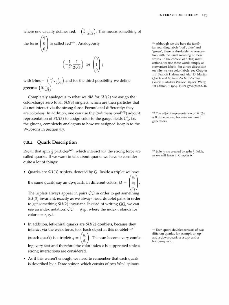
interaction theory 173
where one usually defines red:=(
12 , 1
2√
3
). This means something of
the form
⎛⎜⎝Ψ00
⎞⎟⎠ is called red104. Analogously 104 Although we use here the famil-iar sounding labels "red", blue" and"green", there is absolutely no connec-tion with the usual meaning of thesewords. In the context of SU(3) inter-actions, we use these words simply asconvenient labels. For a nice discussionon why we use color labels, see Chapter1 in Francis Halzen and Alan D. Martin.Quarks and Leptons: An IntroductoryCourse in Modern Particle Physics. Wiley,1st edition, 1 1984. ISBN 9780471887416.
(−1
2,
12√
3
)for
⎛⎜⎝010
⎞⎟⎠ ψ
with blue:=(−12 , 1
2√
3
)and for the third possibility we define
green:=(
0, −1√3
).
Completely analogous to what we did for SU(2) we assign thecolor-charge zero to all SU(3) singlets, which are then particles thatdo not interact via the strong force. Formulated differently: theyare colorless. In addition, one can use the (8-dimensional105) adjoint 105 The adjoint representation of SU(3)
is 8 dimensional, because we have 8generators.
representation of SU(3) to assign color to the gauge fields GμA, i.e.
the gluons, completely analogous to how we assigned isospin to theW-Bosons in Section 7.7.
7.8.2 Quark Description
Recall that spin 12 particles106, which interact via the strong force are 106 Spin 1
2 are created by spin 12 fields,
as we will learn in Chapter 6.called quarks. If we want to talk about quarks we have to considerquite a lot of things:
• Quarks are SU(3) triplets, denoted by Q. Inside a triplet we have
the same quark, say an up-quark, in different colors: U =
⎛⎜⎝ur
ub
ug
⎞⎟⎠.
The triplets always appear in pairs QQ in order to get somethingSU(3) invariant, exactly as we always need doublet pairs in orderto get something SU(2) invariant. Instead of writing QQ, we canuse an index notation: QQ = qcqc, where the index c stands forcolor c = r, g, b.
• In addition, left-chiral quarks are SU(2) doublets, because theyinteract via the weak force, too. Each object in this doublet107 107 Each quark doublet consists of two
different quarks, for example an up-and a down-quark or a top- and abottom-quark.
(=each quark) is a triplet: q =
(uc
dc
). This can become very confus-
ing, very fast and therefore the color index c is suppressed unlessstrong interactions are considered.
• As if this weren’t enough, we need to remember that each quarkis described by a Dirac spinor, which consits of two Weyl spinors
174 physics from symmetry
uc =
((χL
u)c
(ξRu )c
). The upper Weyl-Spinor describes a left-chiral and
the lower component the same quark with right-chirality.
Having talked about this, let’s return to SU(3) interactions. Hap-pily, there is no experimental need for mass terms for the gaugebosons in the Lagrangian, because all experiments indicate that thegauge bosons of SU(3), called gluons, are massless. Therefore SU(3)is not broken.
Furthermore, the SU(3) symmetry poses no new problems regard-ing mass terms for the fermions in the triplet, because a term of theform
QmQ (7.166)
is SU(3) invariant, as long as all particles in the triplet have equalmass. This means m is proportional to the unit matrix108. The objects
108 m = m
⎛⎝1 0 00 1 00 0 1
⎞⎠, instead of
m = m
⎛⎝m1 0 00 m2 00 0 m3
⎞⎠inside a triplet describe the same quark in different colors, whichindeed have equal mass. For example, for an up-quark the triplet is
U =
⎛⎜⎝ur
ub
ug
⎞⎟⎠ , (7.167)
where ur denotes a red, ub a blue and ug green up-quark, which allhave the same mass.
The other spin 12 particles, like electrons or neutrinos, do not carry
color and therefore do not couple to gluons. The interactions fol-lowing from local SU(3) invariance are called strong interactions,because the coupling constant is much bigger than for electromag-netic (U(1)) or weak (SU(2)) interactions.
7.9 The Interplay Between Fermions and Bosons
This section summarizes what we discovered in this chapter andputs it in a more physical context. We will learn later that spin 1
2fields create and destroy spin 1
2 particles. Analogously, spin 1 fieldscreate and destroy spin 1 particles. In this chapter we derived theLagrangians that describe how different fields and therefore particlesinteract with each other.
As already mentioned in Section 1.3 we call spin 12 particles
fermions and spin 1 particles bosons. The standard interpretationis that fermions make up matter and bosons mediate the forces be-tween matter. We can now understand how this comes about.
interaction theory 175
We started the chapter with Lagrangians describing free fields,which we derived in Chapter 6. Then we discovered internal sym-metries for the Lagrangian describing one, two or three free spin 1
2fields. These internal symmetries are only global symmetries, whichis quite unconvincing because of special relativity. More naturalwould be local symmetries.
We then discovered that we could make the Lagrangians locallyinvariant by introducing additional coupling terms. These couplingterms describe the interaction of our spin 1
2 fields with new spin 1fields. For historic reasons the internal symmetries here are calledgauge symmetries and we therefore call these new spin 1 fields,gauge fields. Through Noether’s theorem we get for each inter-nal symmetry new conserved quantities. These are interpreted ascharges, analogous to electric charge that follows for U(1) symmetry.
• To get a locally U(1) invariant Lagrangian, we need one gaugefield Aμ. The final Lagrangian describes correctly electromagneticinteractions. U(1) symmetry tells us that electric charge is con-served.
• To get a locally SU(2) invariant Lagrangian, we need three gaugefields Wμ
1 , Wμ2 , Wμ
3 . The final Lagrangian describes correctly weakinteractions. SU(2) symmetry tells us that isospin is conserved.
• To get a locally SU(3) invariant Lagrangian, we need eight suchfields Gμ
1 , Gμ2 , . . .. The final Lagrangian describes correctly strong
interactions. SU(3) symmetry tells us that color is conserved.
Different gauge bosons (spin 1 particles) are responsible for adifferent kind of force. The electromagnetic force is mediated byphotons, which is created by the U(1) gauge field Aμ. The weakforce is mediated by W+, W− and Z bosons and the strong force by 8different gluons, which are created by the corresponding SU(2) andSU(3) gauge fields.
In addition, we discovered that SU(2) symmetry forbids massterms in the Lagrangian. From experiments we know this is incorrect.The solution that enables us to include mass terms without spoilingany symmetry is the Higgs mechanism. It works by including addi-tional terms, describing coupling of our spin 1 and spin 1
2 fields to anew spin 0 field, called the Higgs field. By breaking SU(2) symme-try spontaneously and expanding the Higgs field around a new, nolonger symmetric minimum, we get the required mass terms in theLagrangian.

Part IVApplications
"There is nothing truly beautiful but that which can never be of any usewhatsoever; everything useful is ugly."
Theophile Gautierin Mademoiselle de Maupin.
Wildside Press, 11 2007 .ISBN 9781434495556
8
Quantum Mechanics
Summary
In this chapter we will talk about quantum mechanics. The founda-tion for everything here are the identifications we discussed in Chap-ter 5. As a first result, we derive the relativistic energy-momentumrelation.
After a discussion of how the quantum formalism works, we takethe non-relativistic limit of the Klein-Gordon equation, because thisis the equation of motion for the simplest type of particles: scalars.This results in the famous Schrödinger equation. The solution of thisequation is interpreted as a probability amplitude and two simpleexamples are analysed using this wave-mechanic approach.
Afterwards, the Dirac notation is introduced, which is useful tounderstand the general structure of quantum mechanics. In this no-tation, the initial state of a system is denoted by an abstract statevector |i〉, called ket. The probability amplitude for measuring thisinitial state in a specific final state can then be computed formallyby multiplying it with a bra, denoted 〈 f |. The combination of a brawith a ket results in a complex number that is interpreted as prob-ability amplitude A for the process i → f . The probability for thisprocess is |A|2. Then we talk about projection operators. We willsee how they can be used, together with the completeness relation,to expand an arbitrary state in the eigenstate basis of an arbitraryoperator. The previously used wave-mechanics can then be seen asa special case, where we expand the states in the location basis. Inthe Dirac notation the Schrödinger equation is used to compute thetime-evolution of states. To make the connection explicit, we use theDirac notation to reanalyze an example which we already solvedusing wave-mechanics.
© Springer International Publishing AG 2018J. Schwichtenberg, Physics from Symmetry, UndergraduateLecture Notes in Physics, https://doi.org/10.1007/978-3-319-66631-0_8
178 physics from symmetry
8.1 Particle Theory Identifications
The equations we derived so far1 can be used in particle- and field-1 The Klein-Gordon, Dirac, Proka andMaxwell equations theories. In this chapter we want to investigate how they can be used
in a particle-theory. Our dynamic variables are then the location, theangular momentum, the energy and the momentum of the particlein question. As explained in Chapter 5, we identify these with thegenerators of the corresponding symmetry2:2 See Eq. 3.248, Eq. 3.252 and Chapter 5
• momentum pi = −i∂i,
• location xi = xi,
• energy E = i∂0,
• angular momentum Li = i 12 εijk(xj∂k − xk∂j).
Before we discuss how these operators are used in quantum me-chanics, we use them to derive one of the most important equationsof modern physics.
8.2 Relativistic Energy-Momentum Relation
In Section 6.2 we derived the equation of motion for a free spin 0particle, the Klein-Gordon equation:
(∂μ∂μ + m2)Φ = 0.
With the identifications reiterated above this equation reads3
3 Using pμ =
⎛⎜⎜⎝p0p1p2p3
⎞⎟⎟⎠ =
(p0�p
)=
(E�p
)(∂μ∂μ + m2)Φ = (∂0∂0 − ∂i∂i + m2)Φ
=
((1i
E)(
1i
E)−
(−1
ipi
)(−1
ipi
)+ m2
)Φ
= (−E2 + �p2 + m2)Φ = 0 . (8.1)
Therefore
→ E2 = �p2 + m2 or using four-vectors pμ pμ = m2 , (8.2)
which is the famous energy-momentum relation of special-relativity.For a particle at rest (�p = 0) this gives us Einstein’s famous equation
E2 = m2 ↔ E = mc2
where we restored c2 for clarity. We can now understand why wegave the scalar value of the first Casimir operator of the Poincarégroup pμ pμ the suggestive name m2 (Eq. 3.266). The combinationpμ pμ is indeed the squared mass of the particle in question, whichcan be measured in experiments, for example, by measuring theenergy and momentum of the particle: m =
√E2 − �p2. For the same
reason, we understand now why the constant in the Lagrangian wederived in Section 6.2 is also called m2.
quantum mechanics 179
8.3 The Quantum Formalism
Now that our physical quantities are given by operators, we needsomething they can act on. First take note that we have for eachoperator a set of eigenfunctions, which is completely analogous tothe eigenvectors of matrices. Matrices are finite-dimensional andtherefore we get finite dimensional eigenvectors. Here our operatorsact on an infinite-dimensional vector space and we therefore haveeigenfunctions. For example, the equation we must solve to get theeigenfunctions of the momentum operator is
−i∂i︸︷︷︸operator
Ψ = pi︸︷︷︸eigenvalue
eigenfunction︷︸︸︷Ψ , (8.3)
with some number pi. A solution is
Ψ = C︸︷︷︸=const
eipixi because
→ −i∂iCeipixi = piCeipixi � (8.4)
but take note that this a solution for arbitrary pi. Therefore we havefound an infinite number of eigenfunctions for the momentum opera-tor pi = −i∂i. Equivalently, we can search for energy eigenfunctions
i∂0Φ = EΦ (8.5)
or angular momentum eigenfunctions4. Analogous to eigenvectors 4 The discussion for angular momentumeigenfunctions is a bit more compli-cated, because the operator is morecomplicated than the others. We can’tfind a set of eigenfunctions for all threecomponents at the same time, because[Li , Lj] �= 0. This will be discussed ina moment. The final result of a lengthydiscussion is that the correspondingeigenfunctions of the third componentof the angular momentum operator L3(and of the squared angular momentumoperator L2, which commutes with allcomponents [L2, Lj] = 0) are the famousspherical harmonics. These form anorthonormal basis.
for matrices, these eigenfunctions are bases for the corresponding ab-stract vector space5. This means we can expand an arbitrary function
5 Recall that for matrices the eigenvec-tors are a basis for the correspondingvector space.
Ψ in terms of eigenfunctions. For example, we can expand Ψ in termsof momentum eigenfunctions6 (for brevity in one dimension)
6 Take note that this is exactly theFourier transform of a function Ψ,which is introduced in Appendix D.1and the factor 1√
2πis a matter of
convention.
Ψ =1√2π
∫ ∞
−∞dpΨpe−ipx, (8.6)
where Ψp are the coefficients in this expansion analogous to v1, v2, v3
in �v = v1�e1 + v2�e2 + v3�e3.
For some systems we have boundary conditions such that wehave a discrete instead of a continuous basis. Then we can expandan arbitrary state, for example, in terms of discrete set of energyeigenfunctions ΦEn :
Ψ = ∑n
cnΦEn . (8.7)
An important observation is that, in general, a set of eigenfunctionsfor one operator is not a set of eigenfunctions for another operator.
180 physics from symmetry
Only for operators that commute [A, B] = AB − BA = 0, we can finda simultaneous set of eigenfunctions for both operators. We don’tprove this here, but to see the connection between a common set ofeigenfunctions and the commutator property, let’s assume we havetwo commutating operators [A, B] = 0 → AB = BA. For the set ofeigenfunctions Ψi that belong to A, we have AΨi = aiΨi, where ai
denotes the corresponding eigenvalues. Now, we can calculate77 The brackets () are used here solelyfor illustrative purposes.
A(BΨi) =︸︷︷︸AB=BA
BAΨi =︸︷︷︸AΨi=aiΨi
BaiΨi
ai is just a number︷︸︸︷= ai(BΨi) . (8.8)
This shows that (BΨi) is also an eigenfunction of A for all Ψi, withexactly the same eigenvalues ai. Therefore the only difference be-tween (BΨi) and Ψi can be a constant: BΨi = biΨi. We conclude thatthe A eigenfunctions Ψi are also eigenfunctions of B if AB = BAholds.
In general our operators act on something we call8 Ψ, which de-8 The usage of Ψ is conventional inquantum mechanics and we use it here,although we used it so far exclusivelyfor spinors, to describe spin 0 particles,too.
notes the state of the physical system in question. We get this Ψ, bysolving the corresponding equation of motion.
Usually, such a solution will have more than one term if we expandit in some basis. For example, consider a state that can be written interms of two energy eigenstates9 Ψ = c1ΦE1 + c2ΦE2 . Acting with the9 This means all other coefficients in the
expansion Ψ = ∑n cnΦEn are zero. energy operator on this state yields
EΨ = E(c1ΦE1 + c2ΦE2) = c1E1ΦE1 + c2E2ΦE2 �= E(c1ΦE1 + c2ΦE2).(8.9)
A superposition of states with different energy is therefore, in gen-eral, no eigenstate of the energy operator, because for an eigenstatewe have by definition EΨ = EΨ for some number E. But what isthen the energy of the system described by Ψ? What does it meanthat a state is a superposition of two energy eigenstates? How can weinterpret all this in physical terms?
A first hint towards an interpretation is the U(1) symmetry ofour Lagrangians, which shows us that the solution of an equationof motion Ψ cannot be directly physically relevant10. Secondly, we10 If we assume that Ψ describes our
particle directly in some way, whatwould the U(1) transformed solutionΨ′ = eiαΨ, which is equally allowed,describe?
observe that a solution to any equation of motion we derived so far isa function of11 �x and t, i.e. Ψ = Ψ(�x, t).
11 This will be made explicit in the nextsections.
The standard interpretation is that the absolute value squared|Ψ(�x, t)|2 of the wave function Ψ(�x, t) gives the probability densityof its location. Observe that the U(1) symmetry has no influence onthis quantity |Ψ|2 = Ψ†Ψ → (Ψ′)†(Ψ)′ = Ψ†e−iαeiαΨ = Ψ†Ψ. In
quantum mechanics 181
other words: Ψ(x, t) is the probability amplitude that a measurementof the location gives a value in the interval [x, x + dx]. Consequentlywe have, if we integrate over all space∫
dxΨ�(x, t)Ψ(x, t) != 1, (8.10)
which is called the normalization prescription, because the probabil-ity for finding the particle anywhere in space must be 100% = 1.
If we want to make predictions about any other physical quantity,we must expand the wave-function in terms of the correspondingbasis. For example, we can expand it in terms of energy eigenfunc-tions: Ψ = c1ΦE1 + c2ΦE2 + . . .. Then, the standard interpretation ofquantum mechanics is: the probability for measuring a given energyvalue E1 for the system described by Ψ is given by the absolute valuesquared of the overlap between Ψ and ΦE1
P(E1) =∣∣∣ ∫ dxΦ�
E1(x, t)Ψ(x, t)
∣∣∣2.
In the example above this means
P(E1) =∣∣∣ ∫ dxΦ�
E1(x, t)Ψ(x, t)
∣∣∣2=
∣∣∣ ∫ dxΦ�E1(x, t)
(c1ΦE1 + c2ΦE2
) ∣∣∣2
=∣∣∣c1
∫dxΦ�
E1(x, t)ΦE1︸ ︷︷ ︸
=1 as explained above
+ c2
∫dxΦ�
E1(x, t)ΦE2︸ ︷︷ ︸
=0 because eigenstates are orthogonal
∣∣∣2
= |c1|2 . (8.11)
Analogously, when we expand some other Ψ(�x, t) in terms of mo-mentum eigenfunctions
Ψ(�x, t) =1√2π
∫ ∞
−∞dpΨ(�p, t)e−i�p�x,
we have Ψ(�p, t) as the probability amplitude for finding the systemwith momentum in the interval [p, p + dp].
This interpretation can be used to make probabilistic predictionsabout the system, for example using the statistical expectation value,which is the topic of the next section. Afterwards we will derive theequation of motion for non-relativistic quantum mechanics and lookat two examples.
8.3.1 Expectation Value
In statistics the expectation value is defined in analogy to the weightedaverage. For example, if tossing a dice ten times results in 2, 4, 1, 3, 3,
182 physics from symmetry
6, 3, 1, 4, 5, the average value is
〈x〉 = (2 + 4 + 1 + 3 + 3 + 6 + 3 + 1 + 4 + 5) · 110
= 3.2.
An alternative way of computing this is to collect equal results andweighing them by their empirical probability:
〈x〉 = 210
· 1 +1
10· 2 +
310
· 3 +2
10· 4 +
110
· 5 +1
10· 6 = 3.2.
We can write this in general as
〈x〉 = ∑i
ρixi (8.12)
where ρi denotes the probability. Equally for a continuous distribu-tion we have
〈x〉 =∫
dxρ(x)x (8.13)
In quantum mechanics the expectation value for a physical quan-tity O is defined analogously
〈O〉 =∫
d3xΨ�OΨ. (8.14)
In general, we must expand Ψ in terms of eigenfunctions of O, forexample momentum eigenfunctions. Then, acting with the operatorO on these states yields the corresponding eigenvalues and we get aweighted sum.
For example, the expectation value for the location of some parti-cle is
〈x〉 =∫
d3xΨ� xΨ =∫
d3xΨ�xΨ =∫
d3xx Ψ�Ψ︸︷︷︸probability density of its location
. (8.15)
In the next section, we consider the non-relativistic limit of theKlein-Gordon equation and will derive this way the equation of mo-tion of non-relativistic quantum mechanics12.12 It is also possible to consider the non-
relativistic limit of the other equationsthat we have derived so far. For exam-ple, the Dirac equation becomes in thenon-relativistic limit the Pauli equation.However, these additional equationsare less important for the goals of thisbook.
8.4 The Schrödinger Equation
The Klein-Gordon equation is solved by plane waves
Φ = e±ipμxμ ≡ e±ip·x ,
where pμ = (E,�p)T is the conserved four-momentum of the particle.We check
0 = (∂μ∂μ + m2)Φ
= (∂μ∂μ + m2)e±ipμxμ
= (i2 pμ pμ + m2)e±ipμxμ= 0
= (−m2 + m2)e±ipμxμ= 0 � (8.16)
quantum mechanics 183
We now write the solution with a minus sign a little differently
Φ = e−ipμxμ= Φ = ei(−Et+�p·�x)
and then we see that the time dependence is given by e−iEt, i.e.Φ ∝ e−iEt. From Eq. 8.2 we know the energy is
E =√�p2 + m2 =
√m2(
�p2
m2 + 1) = m
√�p2
m2 + 1.
In the non-relativistic limit |�p| � m, i.e. for an object that movesmuch slower than the speed of light, which implies that its momen-tum is much smaller than its mass, we can approximate the energyusing the Taylor-series as
E = m
√�p2
m2 + 1
= m(1 +12�p2
m2 + . . .)
≈ m︸︷︷︸rest-mass
+�p2
2m︸︷︷︸kinetic energy
. (8.17)
We can therefore write
Φ = ei(−Et+�p·�x) ≈ e−imt ei�p·�x−i(�p2/2m)t︸ ︷︷ ︸≡φ(�x,t)
= e−imtφ(�x, t). (8.18)
From |�p| � m it follows that the rest-mass is much bigger thanthe kinetic energy and therefore the remaining time dependence inφ(�x, t) oscillates more slowly than e−imt. If we put our ansatz into theKlein-Gordon equation we get
(∂μ∂μ + m2)e−imtφ(�x, t) = (∂t∂t − ∂i∂
i + m2)e−imtφ(�x, t) = 0.
Then we use ∂te−imt(. . .) = e−imt(−im + ∂t)(. . .), which is just theproduct rule, twice. This yields
e−imt((−im + ∂t)2 − ∂i∂
i + m2)φ(�x, t) = 0,
which we can divide by e−imt, because this never becomes zero.Therefore
→ ((−im + ∂t)2 −∇2 + m2)φ(�x, t) = 0
→ (−m2 − 2im∂t + (∂t)2 −∇2 + m2)φ(�x, t) = 0 .
Comparing now the third term
(∂t)2φ(�x, t) = (∂t)
2 exp[i�p ·�x − i(�p2/2m)t
]= (�p2/2m)2 exp
[i�p ·�x − i(�p2/2m)t
]∝
p4
m2 (8.19)
184 physics from symmetry
with the second term
im∂tφ(�x, t) = im∂t exp[i�p ·�x − i(�p2/2m)t
]= m(�p2/2m) exp
[i�p ·�x − i(�p2/2m)t
]∝ p2 (8.20)
shows us that, because of |�p| � m, we can neglect the third term inthis limit. Therefore
(−2im∂t −∇2)φ(�x, t) = 0
→︸︷︷︸dividing by (-2m)
(i∂t +1
2m∇2)φ(�x, t) = 0
→ (i∂t +∇2
2m)φ(�x, t) = 0, (8.21)
which is the famous Schrödinger equation. When we now makethe identifications we recited at the beginning of this chapter, theequation reads
→ (E − �p2
2m︸︷︷︸=kinetic energy
)φ(�x, t) = 0
→ E =�p2
2m, (8.22)
which is the usual non-relativistic energy-momentum relation.From this point-of-view, it is easy to see how we can include an exter-nal potential, because movement in an external potential simply addsa term describing the potential energy to the energy equation:
→ E =�p2
2m+ V
A famous example is the potential of a harmonic oscillator V = −kx2.It is conventional to rewrite the Schrödinger equation, using theHamiltonian operator H, which collects all contributing energy op-erators, for example, the operator for the kinetic energy ∇2
2m and theoperator for the potential energy V. Then we have
i∂tφ(�x, t) =(∇2
2m+ V
)︸ ︷︷ ︸
≡H
φ(�x, t) → i∂tφ(�x, t) = Hφ(�x, t). (8.23)
This is the standard way to write the Schrödinger equation.
quantum mechanics 185
8.4.1 Schrödinger Equation with an External Field
We can also follow the same procedure as in the last section andderive the non-relativistic limit of the interacting Klein-Gordon equa-tion (Eq. 7.42), i.e. the equation that describes the interaction betweena massive spin 0 field φ and a massless spin 1 field Aμ (the photonfield). The resulting equation is(
i∂t − 12m
(∇− iq�A
)2 − qA0
)φ(�x, t) = 0 . (8.24)
8.5 From Wave Equations to Particle Motion
Now, let’s look at two examples of how the standard interpretation ofquantum mechanics works in practice.
8.5.1 Example: Free Particle
A solution for the free (without external potential) Schrödinger equa-tion (Eq. 8.21) is given by
Ψ = e−i(Et−�p�x) (8.25)
because
i∂te−i(Et−�p�x) != −∇2
2me−i(Et−�p�x)
→ Ee−i(Et−�p�x) !=
�p2
2me−i(Et−�p�x) � , (8.26)
where E is just the numerical value for the total energy of the free
particle, which was derived in Eq. 8.22 as E =�p2
2m . A more generalsolution is a linear combination
Ψ = Ae−i(Et−�p�x) + Be−i(E′t−�p′�x) + . . . .
Fig. 8.1: Free wave-packet with Gaus-sian envelope. Figure by Inductiveload(Wikimedia Commons) released undera public domain licence. URL: http://commons.wikimedia.org/wiki/File:
Travelling_Particle_Wavepacket.svg ,Accessed: 4.5.2014
We interpret the wave-function as a probability amplitude andtherefore it must be normalized, because the total probability forfinding the particle must be 100% = 1. This is not possible for thewave-function above which spreads out over all of space. To describean individual free particle we have to use a suited linear combination,called a wave-packet:
ΨWP(�x, t) =∫
dp3 A(�p)ei(�p�x−Et), (8.27)
where the complex numbers A(�p) have to be chosen in a way thatmakes the wave packet normalizable. One possibility is a Gaussian
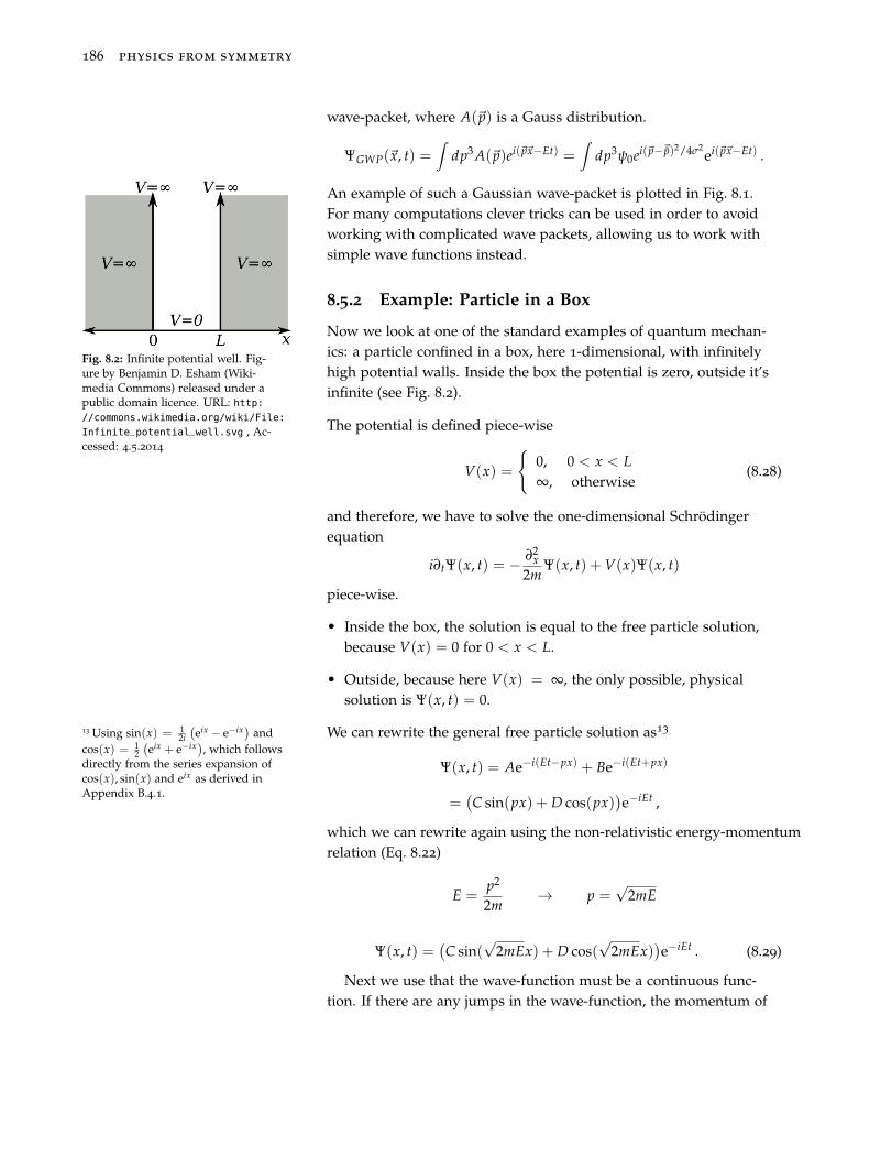
186 physics from symmetry
wave-packet, where A(�p) is a Gauss distribution.
ΨGWP(�x, t) =∫
dp3 A(�p)ei(�p�x−Et) =∫
dp3ψ0ei(�p−�p)2/4σ2ei(�p�x−Et) .
An example of such a Gaussian wave-packet is plotted in Fig. 8.1.For many computations clever tricks can be used in order to avoidworking with complicated wave packets, allowing us to work withsimple wave functions instead.
8.5.2 Example: Particle in a Box
Fig. 8.2: Infinite potential well. Fig-ure by Benjamin D. Esham (Wiki-media Commons) released under apublic domain licence. URL: http://commons.wikimedia.org/wiki/File:
Infinite_potential_well.svg , Ac-cessed: 4.5.2014
Now we look at one of the standard examples of quantum mechan-ics: a particle confined in a box, here 1-dimensional, with infinitelyhigh potential walls. Inside the box the potential is zero, outside it’sinfinite (see Fig. 8.2).
The potential is defined piece-wise
V(x) =
{0, 0 < x < L∞, otherwise
(8.28)
and therefore, we have to solve the one-dimensional Schrödingerequation
i∂tΨ(x, t) = − ∂2x
2mΨ(x, t) + V(x)Ψ(x, t)
piece-wise.
• Inside the box, the solution is equal to the free particle solution,because V(x) = 0 for 0 < x < L.
• Outside, because here V(x) = ∞, the only possible, physicalsolution is Ψ(x, t) = 0.
We can rewrite the general free particle solution as1313 Using sin(x) = 12i
(eix − e−ix) and
cos(x) = 12
(eix + e−ix), which follows
directly from the series expansion ofcos(x), sin(x) and eix as derived inAppendix B.4.1.
Ψ(x, t) = Ae−i(Et−px) + Be−i(Et+px)
=(C sin(px) + D cos(px)
)e−iEt ,
which we can rewrite again using the non-relativistic energy-momentumrelation (Eq. 8.22)
E =p2
2m→ p =
√2mE
Ψ(x, t) =(C sin(
√2mEx) + D cos(
√2mEx)
)e−iEt . (8.29)
Next we use that the wave-function must be a continuous func-tion. If there are any jumps in the wave-function, the momentum of
quantum mechanics 187
the particle pxΨ = −i∂xΨ is infinite, because the derivative at thejump would be infinite. Therefore, we have the boundary conditions
Ψ(0) = Ψ(L) != 0. Because cos(0) = 1, we see that we have D !
= 0.Furthermore, we see that these conditions impose
√2mEn
!=
nπ
L, (8.30)
with arbitrary integer n. This follows because for14 14 Take note that we put an index n onour wave-function, because we have adifferent solution for each n.
Φn(x, t) = C sin(nπ
Lx)e−iEnt (8.31)
both boundary conditions are satisfied
→ Φn(L, t) = C sin(nπ
LL)e−iEnt = C sin(nπ)e−iEnt = 0 �
→ Φn(0, t) = C sin(nπ
L0)e−iEnt = C sin(0)e−iEnt = 0 �
The normalization constant C, can be found to be C =√
2L , because
the probability for finding the particle anywhere inside the box mustbe 100% = 1 and the probability outside is zero, because there wehave Ψ = 0. Therefore
P =∫ L
0dx�
n(x, t)Φn(x, t) != 1
P =∫ L
0dxC2 sin(
nπ
Lx)e+iEnt sin(
nπ
Lx)e−iEnt
= C2∫ L
0dx sin2(
nπ
Lx) = C2
[x2− sin( 2nπ
L x)4 nπ
L
]L
0
= C2
(L2− sin( 2nπ
L L)4 nπ
L
)= C2 L
2!= 1
→ C2 !=
2L
.
We can now solve Eq. 8.30 for the energy E
En!=
n2π2
L22m. (8.32)
We see here that the possible energies are quantized, which meansthat only a discrete set of values is allowed and not arbitrary continu-ous values15. Hence the name quantum mechanics. 15 Recall that n is necessarily an integer.
The possible energy values are π2
L22mtimes this integer squared.Take note that we have a solution for each n and linear combina-
tions of the form
Φ(x, t) = AΦ1(x, t) + BΦ2(x, t) + ...
188 physics from symmetry
are solutions, too. These solutions have to be normalised again be-cause of the probabilistic interpretation16.16 A probability of more than 1 = 100%
doesn’t make sense.
Next we can ask17, what is the probability for measuring the parti-17 Instead of what’s the probability tofind a particle at place x. cle having Energy E = E2 = 22π2
L22m . Say our particle is in the normal-ized state given by
Ψ(x, t) =
√35
Φ2(x, t) +
√25
Φ3(x, t).
The answer in the conventional interpretation of quantum mechanicsis: it is the absolute value squared of the overlap between Ψ and Φ2
P(
E =22π2
L22m
)=
∣∣∣ ∫ dxΦ�2(x, t)Ψ(x, t)
∣∣∣2,
where the overlap can be seen as a scalar product18 of Φ2 and Ψ:18 In fact, this is the scalar product ofthe Hilbert space in which our statevectors Ψ, Φn live.
(Φ2, Ψ) =∫
dxΦ�2Ψ = c︸︷︷︸
complex number
.
The computation is easy, because the solutions we found are orthogo-nal, i.e. ∫
dxΦ�n(x, t)Φn′(x, t) = δnn′ .
For example19,19 You can check this easily usingintegration by parts or something likeWolframalpha.com ∫ L
0dx�
2Φ3(x, t) =∫ L
0dxC sin(
2π
Lx)e+iEtC sin(
3π
Lx)e−iEt
= C2∫ L
0dx sin(
2π
Lx) sin(
3π
Lx) = 0.
Therefore, we get the probability for finding the energy E = 22π2
L22m
P(
E =22π2
L22m
)=
∣∣∣ ∫ dxΦ�2(x, t)Ψ(x, t)
∣∣∣2
=∣∣∣ ∫ dxΦ�
2(x, t)
(√35
Φ2(x, t) +
√25
Φ3(x, t)
) ∣∣∣2
=∣∣∣ ∫ dx
⎛⎜⎝√35
Φ�2(x, t)Φ2(x, t)︸ ︷︷ ︸=1 if integrated
+
√25
Φ�2(x, t)Φ3(x, t)︸ ︷︷ ︸=0 if integrated
⎞⎟⎠ ∣∣∣2
=
(√35
)2
. (8.33)
Take note that we are able to call the functions we just found inEq. 8.31, eigenstates of the energy operator i∂t or equivalently of the
Hamiltonian20 H ≡ − ∂2x
2m , because20 This follows directly fromthe Schrödinger equation
i∂tΦ = − ∂2x
2m Φ ≡ HΦ.
quantum mechanics 189
HΦn = EnΦn. (8.34)
If we act with the energy operator on an eigenstate, we get the samestate multiplied with a constant, which we call energy of the state. Incontrast, an arbitrary state is changed when the energy operator orthe Hamiltonian operator H act on it. For example, if we take a lookat the linear combination
Ψ =
√35
Φ2 +
√25
Φ3
we see that
HΨ = H
(√35
Φ2 +
√25
Φ3
)=︸︷︷︸
Eq. 8.34
√35
E2Φ1 +
√25
E3Φ3
which cannot be written as multiple of Ψ because E2 �= E3. There-fore, Ψ is not an eigenstate of the energy operator. Nevertheless,every wave function can be expressed in terms of the eigenstates Φn,because they form a complete basis set.
Next we want to introduce a useful notation invented by Dirac,which extremely helpful to understand the structure of quantummechanics.
8.5.3 Dirac Notation
In the Dirac notation the state of a physical system is denoted ab-stractly by
|Ψ〉 , (8.35)
which is called a ket21. For example, if we prepare a particle in a box 21 The pun will become clear in asecond.in an energy eigenstate we have
H |Φn〉 = En |Φn〉 .
To each ket we can define a bra, denoted by 〈Ψ| which is given by
〈Ψ| = |Ψ〉† , (8.36)
where the † symbol (called dagger) denotes the Hermitian conjugate,i.e. transposing plus complex conjugation. A bra is an object that actson a ket. We can define an inner product as follows:
(|Φ〉 , |Ψ〉) ≡ 〈Φ|Ψ〉 .
If a ket is multiplied with a bra from the left-hand side, the result is acomplex number
〈Φ|Ψ〉 = c . (8.37)
190 physics from symmetry
This complex number is the probability amplitude for a physical sys-tem in the state |Ψ〉 to be measured in the state |Φ〉. Consequently,the probability is given by | 〈Φ|Ψ〉 |2. For example, the probabil-ity amplitude for finding a particle in the state |Ψ〉 in the interval[x, x + dx] is given by
〈x|Ψ〉 ≡ Ψ(x).
This is the wave function we used in the last chapters. Furthermore,we could ask: What’s the probability amplitude for finding the sameparticle with momentum in the interval [p, p + dp]? The answer inthe Dirac notation is
〈p|Ψ〉 ≡ Ψ(p).
Recall that our states must fulfil a normalization condition, be-cause we are using a probabilistic interpretation22. For example, we22 The probability for finding the par-
ticle anywhere must be 100% = 1 orequally the probability for finding theparticle with any momentum must be100% = 1. In other words: the sum ofprobabilities for all possible outcomesmust add up to 1.
have ∫dx|Ψ(x, t)|2 =
∫dxΨ�(x, t)Ψ(x, t) !
= 1 (8.38)
and equally ∫dp|Φ(p, t)|2 =
∫dpΦ�(p, t)Φ(p, t) !
= 1 (8.39)
or written in our new notation∫dx| 〈x|Ψ〉 |2 =
∫dx(〈x|Ψ〉)† 〈x|Ψ〉 =
∫dx 〈Ψ|x〉 〈x|Ψ〉 !
= 1 (8.40)
and∫dp| 〈p|Φ〉 |2 =
∫dp(〈p|Φ〉)† 〈p|Φ〉 =
∫dp 〈Φ|p〉 〈p|Φ〉 !
= 1 . (8.41)
We can see here a new kind of operator: |p〉 〈p| and |x〉 〈x|, whichare called projection operators23. They are operators because they23 Exactly like the projection operators
for left-chiral and right-chiral spinorswe introduced earlier, these projectionoperators fulfil the defining conditionP2 = P.
transform a ket into another ket. For example,
|x〉 〈x|Ψ〉︸ ︷︷ ︸=some complex function we call Ψ(x)
= |x〉Ψ(x),
which is again a ket, because the product of a complex function witha ket is again a ket. In general, an operator is any object that acts ona ket to generate another ket. Looking at Eq. 8.40 motivates us tointroduce another operator∫
dx 〈Ψ|x〉 〈x|Ψ〉 = 〈Ψ|(∫
dx |x〉 〈x|)
︸ ︷︷ ︸≡ I
|Ψ〉 = 〈Ψ| I |Ψ〉 != 1. (8.42)
From this we can conclude
I |Ψ〉 != |Ψ〉 (8.43)
quantum mechanics 191
for an arbitrary ket |Ψ〉, because 〈Ψ|Ψ〉 = 1. This follows, becausethe probability for a system prepared in state the |Ψ〉 to be foundin the state |Ψ〉, must be, of course, 100% = 1. For example, if weprepare a particle to be at some point x0, the probability for findingit at point x0 is 1. Therefore, 〈x0|x0〉 = 1. Because of this, I is calledthe unit operator and plays the same role as the number 1 in themultiplication of numbers. The result∫
dx |x〉 〈x| = I (8.44)
or for a discrete basis
∑i|i〉 〈i| = I (8.45)
are called completeness relations. In general, we say the componentof a ket |a〉 in the basis |i〉 is
|i〉† |a〉 ≡ 〈i|a〉 ≡ ai,
which is a complex number. Using the completeness relation, i.e.∑i |i〉 〈i| = I, we can write
|a〉 = ∑i|i〉 〈i|a〉 = ∑
i|i〉 ai.
This can be seen as the series expansion24 of the ket |a〉 in terms of 24 Analogous to how we can writea vector in terms of a given basis:�v = v1�e1 + v2�e2 + v3�e3, as explained inAppendix A.1.
the basis |i〉. Consequently, the complex numbers ai can be seen asthe expansion coefficients. Equally for a continuous complete basis,we have
|Ψ〉 =∫
dx |x〉 〈x|Ψ〉︸ ︷︷ ︸≡Ψ(x) complex number
=∫
dx |x〉Ψ(x).
The expectation value we introduced in Section 8.3.1 is in the Diracnotation given by
〈O〉 = 〈Ψ| O |Ψ〉 .
Now let’s return to the example of the particle in a box, and solve itusing the Dirac notation.
8.5.4 Example: Particle in a Box, Again
The question we asked was: What is the probability for finding theparticle having energy E = E2 = n2π2
2mL2 ? This question can be an-swered in the Dirac notation in a very natural way. The probability isgiven by
P(E2) =∣∣ 〈E =
n2π2
2mL2 |Ψ〉 ∣∣2=
∣∣ 〈E =n2π2
2mL2 |(∫
dx |x〉 〈x|)
︸ ︷︷ ︸= I
|Ψ〉 ∣∣2
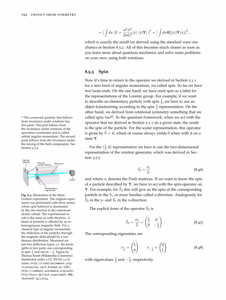
192 physics from symmetry
=∣∣ ∫ dx 〈E =
n2π2
2mL2 |x〉 〈x|Ψ〉 ∣∣2=
∣∣ ∫ dxΦ�2(x)Ψ(x)
∣∣2 ,
which is exactly the result we derived using the standard wave me-chanics in Section 8.5.2. All of this becomes much clearer as soon asyou learn more about quantum mechanics and solve some problemson your own, using both notations.
8.5.5 Spin
Now it’s time to return to the operator we derived in Section 5.1.1for a new kind of angular momentum, we called spin. So far we havetwo loose ends. On the one hand, we have used spin as a label forthe representations of the Lorentz group. For example, if we wantto describe an elementary particle with spin 1
2 , we have to use anobject transforming according to the spin 1
2 representation. On theother hand, we derived from rotational symmetry something that wecalled spin, too25. In the quantum framework, when we act with the25 The conserved quantity that follows
from invariance under rotations hastwo parts. One part follows fromthe invariance under rotations of thespacetime coordinates and is calledorbital angular momentum. The secondparts follows from the invariance underthe mixing of the field components. SeeSection 4.5.4.
operator that we derived in Section 5.1.1 on a given state, the resultis the spin of the particle. For the scalar representation, this operatoris given by S = 0, which of course always yields 0 when with it on astate Ψ.
For the ( 12 , 0) representation we have to use the two-dimensional
representation of the rotation generator, which was derived in Sec-tion 3.7.5
Si =σi2
(8.46)
and where σi denotes the Pauli matrices. If we want to know the spinof a particle described by Ψ, we have to act with the spin-operator onΨ. For example, for S3 this will give us the spin of the correspondingparticle in the 3-, or more familiar called z-direction. Analogously forS2 in the y- and S1 in the x-direction.
The explicit form of the operator S3 is
Fig. 8.3: Illustration of the Stern-Gerlach experiment. The original exper-iment was performed with silver atoms,whose spin behavior is dominatedby the one electron in the outermostatomic orbital. The experimental re-sult is the same as with electrons. Abeam of particles is affected by an in-homogeneous magnetic field. For aclassical type of angular momentumthe deflection of the particles throughthe magnetic field should be a con-tinuous distribution. Measured arejust two deflection types, i.e. the beamsplits in two parts, one correspondingto spin 1
2 and one to − 12 . Figure by
Theresa Knott (Wikimedia Commons)distributed under a CC BY-SA 3.0 li-cense: http://creativecommons.org/licenses/by-sa/3.0/deed.en. URL:http://commons.wikimedia.org/wiki/
File:Stern-Gerlach_experiment.PNG ,Accessed: 24.5.2014.
S3 =σ3
2=
(12 00 − 1
2
)(8.47)
The corresponding eigenstates are
v 12=
(10
)v− 1
2=
(01
)(8.48)
with eigenvalues 12 and − 1
2 , respectively.
quantum mechanics 193
This means a particle described by a spinor26 has spin 12 , which can 26 Recall that a spinor is an object
transforming according to the ( 12 , 0), the
(0, 12 ) or ( 1
2 , 0)⊕ (0, 12 ) representation.
be aligned or anti-aligned to some arbitrary measurement axis. Thisis why we call this representation spin 1
2 representation27. In the27 Analogous statements can be madefor the spin 1 or other higher represen-tations.
quantum framework this is interpreted by saying that a measurementof spin can only result in 1
2 and − 12 . In Section 4.5.4 we learned that
spin is something similar to orbital angular momentum, becauseboth notions arise from rotational invariance. Here we can see thatthis kind of angular momentum gives quite surprising results, whenmeasured. The most famous experiment proving this curious fact ofnature is the Stern-Gerlach experiment (see Fig. 8.3).
The same is true for a measurement of spin in any direction. Ameasurement of the spin in the x-,y- or z-direction can only result in12 and − 1
2 .
Let’s look at one concrete example of how a spin-measurementworks in the quantum formalism. As mentioned above, the explicitform of the spin operator (Eq. 5.4), say for a measurement along thez-axis, is
Sz =12
σ3 =
(12 00 − 1
2
). (8.49)
The eigenstates are | 12 〉z =
(10
)and |− 1
2 〉z =
(01
), where the sub-
script z denotes that we are dealing with eigenstates of Sz. A gen-eral spinor is not a spin-eigenstate, but a superposition |X〉 =
a | 12 〉z + b |− 1
2 〉z. The coefficients depend on how we prepare a givenparticle. If we did a measurement of the spin along the z-axis andfiltered out all particles with spin − 1
2 , the coefficient b would be zeroand a would be 1. Without any measurement and filtering the co-efficients are a = b = 1√
2, which means probability28 1
2 for each 28 The coefficients are directly relatedto the probability amplitude whichwe need to square in order to get theprobability. This will be shown in amoment.
possibility. Things get interesting if we make a measurement alongthe z-axis and afterwards a measurement, for example, along the x-axis. Even if we did filter out all − 1
2 components along the z-axis,there will be particles with spin − 1
2 along the x-axis.
Acting with the spin operator Sz on a state means measuring spinalong the z-axis. For a general state |X〉 both outcomes + 1
2 and − 12
are possible and the probability is directly related to the factors a andb. If we want to know the probability for measuring − 1
2 , the quan-tum formalism tells us that the corresponding probability amplitudeis
z〈−1
2|X〉 = a
z〈−1
2|12〉
z︸ ︷︷ ︸=0
+bz〈1
2| − 1
2〉
z︸ ︷︷ ︸=1
= b (8.50)
194 physics from symmetry
Therefore, the probability for measuring spin − 12 along the z-axis is
Pz=− 12= |b|2. If we want to measure the spin along another axis, say
the x-axis, we need to expand our two states in terms of the eigen-states of Sx, which reads in explicit matrix form (Eq. 5.4)
Sx =
(0 1
212 0
)(8.51)
and the corresponding normalized eigenstates are | 12 〉x =
1√2
(11
)and
|− 12 〉x =
1√2
(1−1
). If we want to know the probability for measuring
spin − 12 along the x-axis, we need to rewrite | 1
2 〉z and |− 12 〉z in terms
of | 12 〉x and |− 1
2 〉x:
|12〉
z︸︷︷︸⎛⎝10
⎞⎠=
1√2
(|12〉
x︸︷︷︸1√2
⎛⎝11
⎞⎠+ |−1
2〉
x︸ ︷︷ ︸1√2
⎛⎝ 1−1
⎞⎠
)(8.52)
|−12〉
z︸ ︷︷ ︸⎛⎝01
⎞⎠=
1√2
(|12〉
x︸︷︷︸1√2
⎛⎝11
⎞⎠− |−1
2〉
x︸ ︷︷ ︸1√2
⎛⎝ 1−1
⎞⎠
). (8.53)
And therefore
|X〉 = a |12〉
z+ b |−1
2〉
z= a
1√2
(|12〉
x+ |−1
2〉
x
)+ b
1√2
(|12〉
x−|−1
2〉
x
).
(8.54)The probability amplitude for measuring − 1
2 for the spin along thex-axis is then
x〈−1
2|X〉 =
x〈−1
2|(
a1√2
(|12〉
x+ |−1
2〉
x
)+ b
1√2
(|12〉
x− |−1
2〉
x
))
=a√2− b√
2(8.55)
and the probability is Px=− 12= | a√
2− b√
2|2.
Now, let’s come back to the example outlined at the beginning ofthis computation. If we filter out all particles with spin − 1
2 along thez-axis the state |X〉 is
|X〉after z-axis filtering = |12〉
z. (8.56)
quantum mechanics 195
This means a = 1 and b = 0 and we get a non-zero probability formeasuring spin − 1
2 along the x-axis Px=− 12= | 1√
2− 0√
2|2 = 1
2 . If we
now filter out all particles with spin − 12 along the x-axis and repeat
our measurement of spin along the z-axis we notice something quiteremarkable. After filtering the particles with spin − 1
2 along the x-axiswe have the state
|X〉after x-axis filtering = |12〉
x. (8.57)
If we want to know the probability for measuring spin − 12 along the
z-axis, we need to write | 12 〉x in terms of | 1
2 〉z and |− 12 〉z:
|X〉after x-axis filtering = |12〉
x︸︷︷︸1√2
⎛⎝11
⎞⎠=
1√2
(|12〉
z︸︷︷︸⎛⎝10
⎞⎠+ |−1
2〉
z︸ ︷︷ ︸⎛⎝01
⎞⎠
)(8.58)
and we get the probability Pz=− 12= | z〈− 1
2 |X〉|2 = 12 .
To summarize, this means:
• We start with a spin measurement along the z-axis and filter outall particles with − 1
2 . This leaves us with a state
|X〉after z-axis filtering = |12〉
z. (8.59)
• If we now measure again the spin along the z-axis we get a veryunsurprising result: The probability for measuring spin − 1
2 is zeroand for spin + 1
2 the probability is 100%.
z〈1
2|X〉
after z-axis filtering= 1 , (8.60)
z〈−1
2|X〉
after z-axis filtering= 0 . (8.61)
• If we then measure the spin along the x-axis, for our z-filtered par-ticle stream, we get a probability of 1
2 = 50% for a measurementof + 1
2 . Equivalently, we have a probability of 12 = 50% for a mea-
surement of − 12 . If we then filter out all components with spin − 1
2along the x-axis we are in the state |X〉after x-axis filtering = | 1
2 〉x.
• Now measuring the spin along the z-axis again, gives us thesurprising result that the probability for measuring spin − 1
2 is12 = 50%. The measurement along the x-axis did change the stateand therefore we are again getting components with spin − 1
2along the z-axis, even though we did filter these out in the firststep!
A brilliant discussion of these matters, involving real measuringdevices, can be found in the Feynman Lectures29 Vol. 3. 29 Richard P. Feynman, Robert B.
Leighton, and Matthew Sands. TheFeynman Lectures on Physics, Volume 3.Addison Wesley, 1st edition, 1 1971.ISBN 9780201021189
196 physics from symmetry
8.6 Heisenberg’s Uncertainty Principle
Now it’s time to talk about one of the most curious features of quan-tum mechanics. We learned in the last section that a measurement ofspin in the x-direction makes everything we knew previously aboutspin along the z-direction useless. This kind of thing happens formany observables in quantum mechanics. We can trace this behaviorback to the fact that30 SxSz �= SzSx. This means that a measurement30 Recall that we identify the spin
operators with the correspondingfinite-dimensional representations forthe rotation generators. These fulfilthe commutator relation [Ji , Jj] =Ji Jj − Jj Ji = iεijk Jk �= 0 → Ji Jj �= Jj Ji . Forexample, if we describe spin 1
2 particles,we must use the two-dimensionalrepresentation Ji =
σi2 .
of spin along the z-axis followed by a measurement of spin alongthe x-axis is different from a measurement of spin along the x-axisfollowed by a measurement of spin along the z-axis. After measur-ing the spin along the z-axis the system is in an eigenstate of Sz andafter a measurement of spin along the x-axis, in an eigenstate of Sx.The eigenstates for Sz and Sx are all different and therefore this is nosurprise.
We can look at this from a different perspective: We aren’t ableto know the spin of a system along the z-axis and the x-axis at thesame time! Each time we measure spin along the z-axis the spinalong the x-axis becomes undetermined and vice-versa. The sameis true for spin along the z-axis/x-axis and spin along the y-axis.Spin may be something really strange, but we can observe the samebehavior for measurements of position and momentum. Take a lookagain at Eq. 5.3, which we recite here for convenience:
[ pi, xj] = pi xj − xj pi = iδij. (8.62)
Following the line of thought as above tells us that a measurement ofmomentum in the x-direction changes what we can expect for a mea-surement of position on the x-axis. In other words this means thatwe can’t know position and momentum in the same direction at thesame time with arbitrary precision. Take note that the commutator isonly non-zero for measurements along the same axis31. A measure-31 The Kronecker delta δij is zero for
i �= j and one for i = j as defined inAppendix B.5.5.
ment of momentum in the y-direction has no influence on what wecan expect for the position on the x-axis.
Everytime we measure momentum the position becomes uncertainand vice versa. This is known as Heisenberg’s uncertainty principle.Analogous observations can be made for angular momentum alongdifferent axes, because the commutator for the corresponding oper-ator is non-zero, too. In general, we can check for any two physicalquantities if they commute with each other. If they don’t, we knowthat they can’t be measured at the same time with arbitrary precision.
Maybe this shouldn’t surprise us. Quantum mechanics uses thegenerators of the corresponding symmetries as measurement oper-
quantum mechanics 197
ators. For instance, this has the consequence that a measurement ofmomentum is equivalent to the action of the translation generator32. 32 Recall that invariance under trans-
lations leads us to conservation ofmomentum.
The translation generator moves our system a little bit and there-fore the location is changed. What is more surprising is that natureactually works this way. Over the years there have been many experi-mental tests of the Heisenberg’s uncertainty principle and all provedit to be correct.
8.7 Comments on Interpretations
The interpretation and notations described in this chapter are thestandard ones. Nevertheless, there are other formalisms equallypowerful. For example, the Feynman path integral formalism33 is, 33 To learn more about this see for
example, Richard P. Feynman andAlbert R. Hibbs. Quantum Mechanics andPath Integrals: Emended Edition. DoverPublications, emended editon edition, 72010. ISBN 9780486477220
in terms of results, completely equivalent to the wave mechanics,we described in this chapter. Yet computations in this formalismare completely different. If we want to compute the probability fora particle to get from point a to point b, we have to sum over allpossible paths that a particle can go between a and b. As absurd as itsounds, this approach leads to the same result, which can be provedformally as well. Freeman Dyson once told the story34 34 Harry Woolf, editor. Some Strangeness
in the Proportion. Addison-Wesley, 1stedition, 2 1981. ISBN 9780201099249
Dick Feynman told me about his "sum over histories" version of quan-tum mechanics. "The electron does anything it likes," he said. "It justgoes in any direction at any speed, forward or backward in time, how-ever it likes, and then you add up the amplitudes and it gives you thewavefunction." I said to him, "You’re crazy." But he isn’t.
Another interpretation for the basic equations of quantum me-chanics, further away from the mainstream, is Bohmian Mechanics.The starting point is to put the ansatz: ReSt into the Schrödingerequation. Separating the imaginary and real part results in twoequations, one of which can be seen as completely analogous to theHamilton-Jacobi equation of classical mechanics plus an additionalterm. This additional term can be interpreted as an extra potential,which is responsible for the strange quantum effects. Further com-putations are completely analogous to classical mechanics. A newforce is computed from the extra potential using the gradient, whichis then put into Newton’s classical equation: F = ma. Therefore, inBohmian mechanics one still has classical particle trajectories. Theresults from this approach are, as far as I know, equal to those com-puted by standard non-relativistic quantum mechanics. Nevertheless,this approach has fallen into disfavour because the extra potentialundergoes non-local changes.
198 physics from symmetry
Further Reading Tips
• Richard P. Feynman - The Feynman Lectures on Physics, Vol. 33535 Richard P. Feynman, Robert B.Leighton, and Matthew Sands. TheFeynman Lectures on Physics, Volume 3.Addison Wesley, 1st edition, 1 1971.ISBN 9780201021189
is a great book to start learning about quantum mechanics. Mostconcepts of quantum mechanics are explained here more lucidlythan anywhere else.
• David J. Griffiths - Introduction to Quantum Mechanics36 is a36 David J. Griffiths. Introduction toQuantum Mechanics. Pearson Pren-tice Hall, 2nd edition, 4 2004. ISBN9780131118928
very readable and enlightening book.
• J. J. Sakurai - Modern Quantum Mechanics37 is a brilliant book,
37 J. J. Sakurai. Modern Quantum Mechan-ics. Addison Wesley, 1st edition, 9 1993.ISBN 9780201539295
which often offers a unique perspective on the concepts of quan-tum mechanics.
• Paul A. M. Dirac - Lectures on Quantum Mechanics38 is an old38 Paul A. M. Dirac and Physics. Lec-tures on Quantum Mechanics. DoverPublications, 1st edition, 3 2001. ISBN9780486417134
book by one of the fathers of quantum mechanics. Highly recom-mended, because reading about ideas by the person who discov-ered them is always a good idea.
• You can find a detailed discussion of the interpretation of thecomponents of a Dirac spinor in Appendix 8.8.
8.8 Appendix: Interpretation of the Dirac SpinorComponents
In this and the corresponding appendices, u and v denote two-componentobjects inside a Dirac spinor and u and v four-component objects. For exam-ple u1 and u2 describe two different four-component objects. For a generalfour-component object u, we denote the two two-component objects by u1
and u2, i.e. u =
(u1
u2
).
Up to this point we have been relatively vague about the two Weylspinors inside a Dirac spinor. What do they stand for? How can theybe interpreted? In addition, each such Weyl spinor inside a Diracspinor consists of two components. How to interpret these? Now, weare finally in the position to give answers to these questions.
In short:
• The two Weyl spinors χL, ξR inside a Dirac spinor ψ =
(χL
ξR
)describe "different particles". Nevertheless, it’s conventional tocall them the same particle, for example an electron, with differentchirality:
– χL describes a left-chiral electron,
– ξR describes a right-chiral electron,
quantum mechanics 199
but the crucial point is that these are really distinct particles/fields39, 39 They are labelled by different quan-tum numbers and therefore behavedifferently in experiments!
because they aren’t related by a parity transformation or chargeconjugation. This is why we use different symbols. There is, ofcourse, some sort of connection between them, which is why wewrite them in one object. This will be discussed in detail in a mo-ment.
• The two components of each Weyl spinor describe different spinconfigurations40 of the corresponding particle. 40 This was discussed in Section 8.5.5.
Recall that spin can be measuredlike angular momentum, but for aspin 1
2 particle the result of such ameasurement can only be + 1
2 or − 12 ,
no matter what axis we choose. Thesetwo measurement results are commonlycalled spin up and spin down.
– A Weyl spinor proportional to
(10
)describes a particle with
spin up
– A Weyl spinor proportional to
(01
)describes a particle with
spin down
– Any other Weyl spinor is simply a mixture of spin up and spindown.
Let’s see how this comes about in detail:
The important thing we learn from weak interactions and parityviolation is that left-chiral and right-chiral particles are really differ-ent particles. Left-chiral particles carry weak charge (isospin) andtherefore interact via the weak force. Right chiral particles do not,which was explained in Section 7.7.1.
We have for every particle in nature a corresponding antiparticleand in general, we get the antiparticle description through chargeconjugation. Charge conjugation flips all particle labels, which in-cludes isospin. Let’s see what particles we can expect that are relatedto, say electrons. We have
• A left-chiral electron χL, with isospin − 12 and electric charge −e,
which is part of a doublet.
• A right-chiral anti-left-chiral-electron (χL)c = χR with isospin 1
2 ,electric charge +e, which is part of a doublet, too. This propertydoes not simply vanish through charge conjugation. This may beconfusing at the moment, but so far we have only talked about thecoupling of the weak force to particles. It turns out that the weakforce couples to right-chiral antiparticles as well.
• A right-chiral electron ξR with isospin 0 and electric charge −e
• A left-chiral anti-right-chiral-electron (ξR)c = ξL with isospin 0 and
electric charge +e
200 physics from symmetry
Therefore, when talking about electrons, we have in fact four differ-ent "things" we need to consider. These are all really different par-ticles and we need to give them different names! Usually one talksabout just two particles related to an electron: The electron and thepositron and we will see how this comes about in a moment.
We restrict the following discussion to the rest frame of the particlesin question. In other frames the discussion works analogous but is morecumbersome.
The objects inside a Dirac spinor and its charge conjugate aredirectly related to these four particles. The physical electron and thephysical positron are commonly identified as the solutions of theDirac equation. The Dirac equation is an equation of motion, i.e. anequation that determines the dynamics of the particles in question.The explicit solutions are Dirac spinors that evolve in time. We needsuch Dirac spinors with a definite time-evolution in order to describehow our particles evolve in time. As we will see this requires that wealways use two of the particles listed above at once.
An explicit derivation of the solutions of the Dirac equation can befound in the appendix Section 8.9. Here we just use the results. Thereare four independent solutions of the Dirac equation and two are ofthe form
ψi =
(ui
ui
)(8.63)
with for example41 u1 =
(10
)e−imt and u2 =
(01
)e−imt and two41 This is a basis choice. The only
requirement is that they are linearlyindependent. solutions are of the form
ψi =
(−vi
vi
), (8.64)
with for example v1 =
(10
)e+imt and v2 =
(01
)e+imt
The Dirac equation tells us that the spin configuration of the twoparticles described by the upper and lower Weyl spinors inside aDirac spinor, are directly related. In addition, their time depen-dence must be the same. These solutions describe what is commonlyknown as a physical electron and a physical positron, with differentspin configurations42.42 Take note that the connection between
these objects is charge conjugation. Thiscan be seen by using the explicit formof the charge conjugation operator:ψc
1 = iγ2ψ�1 . Therefore: (ψ1)
c = ψ2 and(ψ2)
c = ψ1.
• ψ1 is an electron with spin up
• ψ2 is an electron with spin down
quantum mechanics 201
• ψ1 is a positron with spin up
• ψ2 is a positron with spin down
We can see nicely that a physical electron has a left-chiral (the up-per two components) and a right-chiral part (the lower two compo-nents). For a physical electron the spin configuration of the left-chiraland the right-chiral part and the time-dependence must be the samefor both parts. As discussed above, this left-chiral and right-chiralparts are really different, because they have different weak charge!Nevertheless, in order to describe a dynamical, physical electron wealways need both parts.
Take note that these solutions do not mean that the object we useto describe a physical electron consists of exactly the same upper andlower two-component objects. Only their spin configuration and theirtime dependence must be equivalent. The upper object is still partof a doublet, whereas the lower object isn’t. The upper object trans-forms under SU(2) transformations and the lower doesn’t. Using thenotation from above we have
physical electron =
(χL
ξR
)∝
(uu
). (8.65)
This does not mean that χL = ξR. The Weyl spinor χL is part of adoublet and describes a particle with isospin, whereas the particledescribed by ξR has isospin zero. In addition, we already know thatthe upper and lower Weyl spinor inside a Dirac spinor transform dif-ferently under Lorentz boosts. Therefore it is important that we usedifferent symbols. In other words: The object describing a left-chiralelectron χL carries an additional SU(2) index, because χL transformsas part of a doublet under SU(2) transformations. ξR has no suchindex and transforms as a singlet under SU(2) transformations.
Equivalently we have
physical positron =
(−ξL
χR
)∝
(−vv
)(8.66)
which we can see through charge conjugation43 43 See Section 7.1.5 and use the ex-plicit form of the matrix as defined
in Eq. 6.13: γ2 =
(0 σ2σ2 0
)=(
0 −σ2σ2 0
).(physical electron)c = iγ2
(χL
ξR
)�
=
(−ξL
χR
)∝ iγ2
(uu
)�
=
(−uc
uc
)= physical positron (8.67)
The message to take away is that the physical electron we observein nature most of the time is a mixture of two different particles: The
202 physics from symmetry
left-chiral electron that carries isospin and the right-chiral electronwith isospin zero! Equivalently the physical positron is a mixture ofan anti-left-chiral electron, which carries isospin and an anti-right-chiral electron with isospin zero.
The solutions of the Dirac equation tell us how our particles evolvein time. Let’s say we start with an electron with spin up that wascreated in a weak interaction and is therefore purely left-chiral. Howdoes this particle evolve in time? A purely left-chiral electron withspin up
e↑L =
⎛⎜⎜⎜⎝1000
⎞⎟⎟⎟⎠ (8.68)
is not a solution of the Dirac equation and therefore, in order to de-termine its time evolution, we must rewrite this in terms of solutionsof the Dirac equation.
e↑L =
⎛⎜⎜⎜⎝1000
⎞⎟⎟⎟⎠ =12
⎛⎜⎜⎜⎝⎛⎜⎜⎜⎝
1010
⎞⎟⎟⎟⎠−
⎛⎜⎜⎜⎝−1010
⎞⎟⎟⎟⎠⎞⎟⎟⎟⎠ = Ψ1(t = 0)− Ψ1(t = 0) . (8.69)
We know how Ψ1 and Ψ1 evolve in time
Ψ1(t)− Ψ1(t) =→ 12
⎛⎜⎜⎜⎝⎛⎜⎜⎜⎝
1010
⎞⎟⎟⎟⎠ e−imt −
⎛⎜⎜⎜⎝−1010
⎞⎟⎟⎟⎠ eimt
⎞⎟⎟⎟⎠ (8.70)
For t = 0 this reduces to the left-chiral state as it should be, but astime evolves, say t = π
2m we have
→ 12
⎛⎜⎜⎜⎝⎛⎜⎜⎜⎝
1010
⎞⎟⎟⎟⎠ e−i π2︸︷︷︸
=-i
−
⎛⎜⎜⎜⎝−1010
⎞⎟⎟⎟⎠ ei π2︸︷︷︸
=i
⎞⎟⎟⎟⎠ =i2
⎛⎜⎜⎜⎝⎛⎜⎜⎜⎝−10−10
⎞⎟⎟⎟⎠−
⎛⎜⎜⎜⎝−1010
⎞⎟⎟⎟⎠⎞⎟⎟⎟⎠
= −i
⎛⎜⎜⎜⎝0010
⎞⎟⎟⎟⎠ = −ie↑R (8.71)
which describes a right-chiral electron with spin up! The lesson hereis that as time evolves, a left-chiral particle changes into a right-chiral
quantum mechanics 203
particle and vice versa. To describe the time-evolution of a particlelike an electron we need eL and eR, which is why we wrote themtogether in one object: the Dirac spinor. The same is true for thepositron.
Recall that the two different particles eL and eR, carry differentweak charge, i.e. isospin. Nevertheless as time evolves these twoparticles can transform into each other. Most of the time it will be amixture of both and not a definite eigenstate. Isospin and chiralityare therefore not conserved as time evolves, only in interactions.
We can now see that the notation with Dirac spinors is necessary,because we have a close, dynamical connection between each twoparticles of the four particles listed at the beginning of this section.Chirality and therefore isospin are not conserved during propagation.A propagating electron can sometimes be found as left-chiral andsometimes as right-chiral.
8.9 Appendix: Solving the Dirac Equation
As explained at the beginning of the last section, we use here the symbolsu and v for the two-component objects inside a Dirac spinor, and u and vfor four-component objects. This means, for example u1 and u2 describetwo different four-component objects. If we don’t want to be specific andwant to consider both four-component objects at the same time we simplywrite u. Then u1 and u2 are the two two-component objects inside such a
four-component object u =
(u1
u2
)
In this appendix we will solve the Dirac equation in the rest framein the chiral basis. The solution for an arbitrary frame can be com-puted by acting with a boost transformation on the solution derivedin this section. In addition to the discussion in the last section, wewill use these solutions in Chapter 9, when we talk about quantumfield theory. The Dirac equation is
(i∂μγμ − m)ψ = 0. (8.72)
Anticipating plane wave solutions, we make the ansatz Ψ = ue−ipx,with some four-component object u, because the matrices γμ in theequation are 4 × 4. In the rest frame, which means momentum zero�p = 0, the exponent reduces to −ipx = −i(p0x0 − �p�x) = −ip0x0.Now using the relativistic energy-momentum relation E =
√�p + m2,
which we derived at the beginning of this chapter, and using that
204 physics from symmetry
p0 = E and x0 = t, we have −ipx = −iEt = −i√
�p︸︷︷︸=0
+m2t = −imt.
Putting this ansatz into the Dirac equation yields
(i∂μγμ − m)ue−imt = 0
→ (i(∂0γ0 + ∂iγi)− m)ue−imt = 0
→ i((−im)γ0 − m)ue−imt = 0
→ (mγ0 − m)u = 0
→︸︷︷︸dividing by m
((0 11 0
)−
(1 00 1
))c = 0
→(−1 11 −1
)(u1
u2
)= 0
→(−u1 + u2
u1 − u2
)= 0 (8.73)
The 1 inside the remaining matrix here is the 2 × 2 unit matrix andtherefore u1 and u2 are two-component objects. We see that ouransatz solves the equation, if u1 = u2. Therefore, we have foundtwo linearly independent solutions of the Dirac equation
Ψ1 =
⎛⎜⎜⎜⎝1010
⎞⎟⎟⎟⎠ e−imt Ψ2 =
⎛⎜⎜⎜⎝0101
⎞⎟⎟⎟⎠ e−imt (8.74)
We can find two other solutions by making the ansatz Ψ = veipx,which analogously reduces in the rest frame to Ψ = veimt. Thisansatz yields
(i∂μγμ − m)veimt = 0
→ (−mγ0 − m)v = 0
→(−1 −1−1 −1
)(v1
v2
)= 0
→(−v1 − v2
−v1 − v2
)= 0. (8.75)
We therefore conclude that we have a solution with time depen-dence eimt, if the upper and lower two-component objects in theDirac spinor are related by −v1 = v2. Two linearly independent
quantum mechanics 205
solutions following from this ansatz are
Ψ1 =
⎛⎜⎜⎜⎝10−10
⎞⎟⎟⎟⎠ eimt Ψ2 =
⎛⎜⎜⎜⎝010−1
⎞⎟⎟⎟⎠ eimt. (8.76)
8.10 Appendix: Dirac Spinors in DifferentBases
In the Lagrangian the Dirac spinors ψ appear always in combinationwith the matrices γμ. This can be used to simplify computations, byswitching to a different basis. This works, because we can add termsof the form 1 = N−1N, with some arbitrary invertible matrix N,between ψ and γμ and then redefine both. For example
∂μψγμψ = ∂μψ N−1N︸ ︷︷ ︸=1
γμ N−1N︸ ︷︷ ︸=1
ψ = ∂μ ψN−1︸ ︷︷ ︸≡ψ′
NγμN−1︸ ︷︷ ︸≡γ′
μ
Nψ︸︷︷︸≡ψ′
= ∂μψ′γ′μψ′.
(8.77)The basis we worked with in this text so far is called the chiral basisor Weyl basis. Conventionally the Dirac equation is solved in anotherbasis, called mass basis or Dirac basis. In the chiral basis we workedwith so far, the Dirac Lagrangian
LD = iχ†Lσμ∂μχL + iξ†
Rσμ∂μξR − mχ†LξR − mξ†
RχL (8.78)
has non-diagonal mass terms, i.e. mass terms that mix differentstates. We can use the freedom to choose a basis to pick a basiswhere the mass terms are diagonal, which is then called mass ba-sis.
This means we want a mass term ψ†mψ, with m =
(m1 00 m2
),
which gives us mass terms of the form
ψ′M′ψ′ = ψ†γ′0M′ψ′ =
(u′
v′
)† (m1 00 m2
)(u′
v′
)= (u′)†m1u′+(v′)†m2v′,
(8.79)whereas at the moment we are dealing with
ψMψ = ψ†γ0Mψ =
(χL
ξR
)† (0 mm 0
)(χL
ξR
)= mχ†
LξR + mξ†RχL.
(8.80)
206 physics from symmetry
The latter basis, which we worked with so far, makes it easy to inter-pret things in terms of chirality, whereas it’s easier for Dirac spinorsin the mass basis to make the connection to physical propagatingparticles.
To find the connection between the second and the first form, we
need to diagonalize the matrix M =
(0 mm 0
)= m
(0 11 0
). The
matrix is diagonalized through the matrix N = 1√2
(−1 11 1
):
N−1
(−m 0
0 m
)︸ ︷︷ ︸
≡M′
N = M (8.81)
→ m1√2
(−1 11 1
)−1 (−1 00 1
)1√2
(−1 11 1
)= m
(0 11 0
)(8.82)
and therefore we redefine the Dirac spinors accordingly
ψMψ = ψ NN−1︸ ︷︷ ︸=1
M NN−1︸ ︷︷ ︸=1
ψ
= ψN︸︷︷︸≡ψ′
N−1MN︸ ︷︷ ︸≡M′
N−1ψ︸ ︷︷ ︸≡ψ′
= ψ′M′ψ′. (8.83)
It is instructive to have a look at the chiral projection operatorsPL = 1−γ5
2 in this basis. We need to calculate how the matrix γ5 lookslike in this new basis
γ5 = N−1γ5N =1√2
(1 11 −1
)(1 00 −1
)1√2
(1 11 −1
)
=12
(1 11 −1
)(1 1−1 1
)
=
(0 11 0
). (8.84)
The corresponding eigenvectors are 1√2
(1−1
)and 1√
2
(11
). This
means a chiral eigenstate is now described by a Dirac spinor withupper and lower components. For example, a left-chiral state is in
this basis of the form 1√2
(1−1
). In contrast, in the chiral basis γ5
quantum mechanics 207
was diagonal and a left-chiral eigenstate was given by a Dirac spinor
with upper components only ψL =
(χL
0
), and a right-chiral Dirac
spinor with lower components only ψR =
(0
ξR
).
The chiral projection operator is in this basis
PL =1 − γ5
2=
12
(1 −1−1 1
). (8.85)
8.10.1 Solutions of the Dirac Equation in the Mass Basis
We can solve the Dirac equation in the mass basis
(iγμ∂μ − m
)Ψ = 0 (8.86)
by making the ansatz ψ = ue−ipx, which yields
(γμ pμ − m
)ue−ipx = 0
→ ((γμ pμ − m
)u = 0 . (8.87)
Equivalently we can make the ansatz ψ = veipx, which yields(− γμ pμ − m)veipx = 0
→ (− γμ pμ − m)v = 0.
Analogously to our solution in the chiral basis, we work in the restframe, i.e. �p = 0. We are allowed to make such a choice, becausephysics is the same in all frames of reference and therefore we canpick one that fits our needs best. In this frame of reference, withpi = 0, we have
→ (γ0 p0 − m
)u = 0
→ (− γ0 p0 − m)v = 0.
In addition, we have p0 = E and we can use the relativistic energy-momentum relation, which we derived at the beginning of this chap-ter (Eq. 8.2). In the rest frame we have E =
√(pi)2 + m2 = m. We
now use the explicit form of γ0 in the mass basis, which can be com-puted using the matrix N from above and the transformation lawγ′
0 = N−1γ0N. Remember that we have an implicit unit matrix be-hind m and therefore
→((
1 00 −1
)m − m
(1 00 1
))u = 0
208 physics from symmetry
→(−
(1 00 −1
)m − m
(1 00 1
))v = 0
→(
0 00 −2
)u = 0
→(−2 00 0
)v = 0.
Recalling that each Dirac spinor consists of two two-component ob-jects, we conclude that the lower two-component object of u and theupper two-component object of v must be zero:
→(
0 00 −2
)(u1
u2
)=
(0
−2u2
)= 0 → u2 = 0
→(−2 00 0
)(v1
v2
)=
(−2v1
0
)= 0 → v1 = 0.
We can see that in this basis the physical propagating particles(=solutions of the Dirac equation) are described by spinors withupper components only or equivalently for antiparticles with lowercomponents only. We therefore have again four linearly independentsolutions
Ψ′1 =
⎛⎜⎜⎜⎝1000
⎞⎟⎟⎟⎠ e−imt Ψ′2 =
⎛⎜⎜⎜⎝0100
⎞⎟⎟⎟⎠ e−imt (8.88)
and
Ψ′1 =
⎛⎜⎜⎜⎝0010
⎞⎟⎟⎟⎠ eimt Ψ′2 =
⎛⎜⎜⎜⎝0001
⎞⎟⎟⎟⎠ eimt. (8.89)
A general solution in this frame, in this basis, is a linear combina-tion
ψ = ue−ipx + veipx =
(u1
0
)e−ipx +
(0v1
)eipx (8.90)
and we get the solution in an arbitrary frame by transforming thissolution with a Lorentz boost. In addition, the most general solutionis a superposition of all possible momenta and spin configurations4444 Recall that the two components of
a Weyl spinor represent different spinstates.
Ψ = ∑r
√m
(2π)3
∫ d3 p√Ep
(cr(p)ur(p)e−ipx + d†
r (p)vr(p)e+ipx)
(8.91)
9
Quantum Field Theory
Summary
In this chapter the framework of quantum field theory is introduced.Starting with the equation derived in Chapter 5
[Φ(x), π(y)] = iδ(x − y),
we are able to see that the fields themselves are operators. The so-lutions of the equations of motion for spin 0, 1
2 and 1 are written interms of their Fourier expansions1. Using the commutation rela- 1 The idea behind the Fourier transform
is explained in Appendix D.1.tion, cited above, we discover that the Fourier coefficients are nowoperators. Afterwards, we will see how these operators, and withthem of course the fields, create and annihilate particles. Using theLagrangian for the corresponding fields, we are able to derive theHamiltonian operator representing energy.
Afterwards, we start developing interaction theory, which is whatquantum field theory is all about. We will see that in interaction the-ory, the Hamiltonian is given by a linear combination of the Hamilto-nian for the free field plus an interaction Hamiltonian. This insightcan then be used in the interaction picture, where the time evolu-tion of the fields is governed by the free Hamiltonian and the timeevolution of the states by the interaction Hamiltonian. Using this pic-ture, we are able to derive the probability amplitudes for scatteringprocesses. These are denoted in the Dirac notation
〈 f | S |i〉 ,
where S denotes the operator describing the scattering process, |i〉is the initial state and 〈 f | is the final state. We will discover that theoperator S can be written in terms of the interaction Hamiltonian HI :
S(t, ti) = e−i
∫ tti
dt′HI .
© Springer International Publishing AG 2018J. Schwichtenberg, Physics from Symmetry, UndergraduateLecture Notes in Physics, https://doi.org/10.1007/978-3-319-66631-0_9
210 physics from symmetry
This can’t be solved and therefore we evaluate the exponentialin terms of its series expansions. For most experiments the first fewterms suffice to get an accurate description.
Each term in this series expansion can be interpreted physicallyas describing a different kind of scattering process. The interactionHamiltonian contains linear combinations of the fields, which createand annihilate particles as mentioned above. For the first non-trivialorder, we get 8 terms and we will see that the first term describes ascattering process of the form e−e+ → γ. This means we start with aninitial state |e−e+〉 consisting of an electron and a positron, which areannihilated by the field operators of the spin 1
2 fields and afterwardsa photon 〈γ| is created by the photon field. The other terms result inzero when operating on this initial state |e−e+〉.
The next order in the series expansion consists of many, manyterms and we will take a look at just one of them. Again, we startwith an initial state |e−e+〉 and we will see that one term describesthe process e−e+ → γ → e−e+, where the initial and final electronand positron have, in general, completely different momenta.
In exactly the same way, all terms can be interpreted for all inter-action Hamiltonians. A pictorial way to simplify these kinds of com-putations are the famous Feynman diagrams. Each line and vertex insuch a diagram represents a factor of the kind mentioned above.
9.1 Field Theory Identifications
In this section, we want to understand how the Lagrangians that wederived from symmetry constraints can be used in a field theoret-ical framework. The first step in deriving a field theory describingnature is combining the Lagrangians we found with the result fromChapter 5, specifically Eq. 5.5, which we recite here for convenience:
[Φ(x), π(y)] = iδ(x − y), (9.1)
where the conjugate momentum density π(y) is given by
π(y) =∂L
∂(∂0Φ(y)). (9.2)
quantum field theory 211
9.2 Free Spin 0 Field Theory
"Every act of creation is first of all an act of destruction."
- Pablo Picasso2 2 As quoted in Rollo May. The Courageto Create. W. W. Norton and Com-pany, reprint edition, 3 1994. ISBN9780393311068Again, let’s start with the simplest possible case: free spin 0 fields.
We describe such fields with scalars, which are objects that do notchange at all under Lorentz transformations3. We already derived in 3 This was derived in Section 3.7.4
Chapter 6.2 the corresponding Lagrangian
L =12(∂μΦ∂μΦ − m2Φ2) (9.3)
and the equation of motion, called Klein-Gordon equation
(∂μ∂μ + m2)Φ = 0. (9.4)
Using the Lagrangian in Eq. 9.3, we can calculate the conjugate mo-mentum
π(x) =∂L
∂(∂0Φ(x))=
∂
∂(∂0Φ(x))12(∂μΦ(x)∂μΦ(x)−m2Φ2(x)) = ∂0Φ(x) .
The most general solution of the Klein-Gordon equation can be writ-ten in terms of its Fourier-expansion4 4 See the appendix in Section 9.6 at
the end of this chapter for a detailedcomputation of the integral measureand a justification for writing thesolution like this.
Φ(x) =∫
dk3 1(2π)32ωk
(a(k)e−i(kx) + b(k)ei(kx)
), (9.5)
with (ωk)2 ≡�k2 + m2. For real scalar fields we can rewrite this as
Φ(x) =∫
dk3 1(2π)32ωk
(a(k)e−i(kx) + a†(k)ei(kx)
)(9.6)
because c + c† = Re(c) + i · Im(c)︸ ︷︷ ︸c
+Re(c)− i · Im(c)︸ ︷︷ ︸c†
= 2Re(c).
Now we are having a look at the implications of Eq. 9.1, i.e. thenon vanishing commutator [Φ(x), π(y)] �= 0. This means that Φ(x)and π(y) cannot be ordinary functions, but must be operators, be-cause ordinary functions commute: (3 + x)(7xy) = (7xy)(3 + x).By looking at Eq. 9.6, we conclude that the Fourier-coefficients a(k)and a(k)† are operators, because e±i(kx) is just a complex number andcomplex numbers commute.
Using Eq. 9.1 we can compute5 5 See for example chapter 4.1 inLewis H. Ryder. Quantum Field The-ory. Cambridge University Press, 2ndedition, 6 1996. ISBN 9780521478144
[a(k), a†(k′)] = (2π)3δ3(�k −�k′) (9.7)
and[a(k), a(k′)] = 0 (9.8)
212 physics from symmetry
[a†(k), a†(k′)] = 0 . (9.9)
Now that we know that our field itself is an operator, the logicalnext thing to ask is: What does it operate on? In a particle theory,we identify the dynamical variables as operators acting on somethingdescribing a particle (the wavefunction, an abstract Dirac vector, etc.).In a field theory we have up to now nothing to describe a particle.At this point, it is completely unclear how particles appear in a fieldtheory. Nevertheless, let’s have a look at how our field coefficentsa(k) and a†(k) act on something abstract and by doing this, we learnhow the fields act on something abstract. To get some intuition aboutwhat is going on here, let’s first have a look at something we arefamiliar with: energy.
The energy E of a scalar field is given by66 We derived this in Eq. 4.40 fromtime-translation invariance.
E =∫
d3xT00
=∫
d3x
⎛⎜⎜⎜⎝ ∂L
∂(∂0Φ)
∂Φ∂x0︸︷︷︸=∂0Φ
−L
⎞⎟⎟⎟⎠=
∫d3x
((∂0Φ)2 − 1
2(∂μΦ∂μΦ − m2Φ2)
)=︸︷︷︸
∂μ∂μ=∂0∂0−∂i∂i
12
∫d3x
((∂0Φ)2 + (∂iΦ)2 + m2Φ2
)(9.10)
By substituting Eq. 9.6 into Eq. 9.10 and using the commutationrelations (Eq. 9.7-9.9), we can write
E =12
∫dk3 1
(2π)3 ωk
(a†(k)a(k) + a(k)a†(k)
)=︸︷︷︸
Eq. 9.7
∫dk3 1
(2π)3 ωk
(a†(k)a(k) +
12(2π)3δ3(0)
)(9.11)
At this point we can see that our theory explodes. The secondterm in the integral is infinite. We could stop at this point and saythat this kind of theory does not work. Nevertheless, some bravephysicists dug deeper, ignoring this infinite term and discovered atheory describing nature very accurately. There is no explanation forthis and the standard way of continuing from here on is to ignore thesecond term. The crux here is that this term appears in the energyof every system and we are only able to measure energy differences.Therefore, this constant infinite term appears in none of our measure-ments.
quantum field theory 213
Conventionally, the energy written as an operator is called Hamil-tonian H. We can compute the commutator7 of H and the Fourier 7 It will become clear in a moment why
this is useful.coefficents a(k) and a†(k). We get
[H, a†(k′)] =∫
dk3 1(2π)3 ωk[a†(k)a(k), a†(k′)]
=︸︷︷︸[a†(k),a†(k′)]=0
∫dk3 1
(2π)3 ωka†(k)[a(k), a†(k′)]
=∫
dk3ωka†(k)δ3(k − k′)
=︸︷︷︸See Appendix D.2
ωk′ a†(k′)
(9.12)
and equally[H, a(k′)] = −ωk′ a(k
′) . (9.13)
The quantum formalism works by operating with operators onsomething that describes the physical system8. Here, if we act with 8 This was explained in Section 8.3.
the energy operator, i.e. the Hamiltonian H, on something abstract|?〉 describing our physical system, we get the energy of the system:
H |?〉 = E |?〉 (9.14)
Now we return to our starting question: How does a field9 act 9 Remember: Field=Operator!
on our system? Let’s have a look at the effect of the first Fouriercoefficient, now an operator, on the energy E of the system10: 10 We will do something very clever
here, which was first discovered byDirac while solving the problem ofthe harmonic oscillator in quantummechanics.H
(a(k′) |?〉) =
⎛⎜⎝a(k′)H + Ha(k′)− a(k′)H︸ ︷︷ ︸[H,a(k′)]
⎞⎟⎠ |?〉
= a(k′) H |?〉︸ ︷︷ ︸=E|?〉
+[H, a(k′)] |?〉
=(
a(k′)E + [H, a(k′)])|?〉
=︸︷︷︸Eq. 9.13
(a(k′)E − ωk′ a(k
′))|?〉
=(
E − ωk′)(a(k′) |?〉) (9.15)
and equally for the second Fourier coefficent
Ha†(k′) |?〉 = (E + ωk′)a†(k′) |?〉 . (9.16)
How can we interpret this? We see that a(k′) |?〉 can be interpretedas a new system with energy E − ωk. To make this more concrete wedefine
|?2〉 ≡ a(k′) |?〉
214 physics from symmetry
withH |?2〉 =︸︷︷︸
Using Eq. 9.15
(E − ωk′) |?2〉 .
This suggests how we should interpret what the field does. Imag-ine a completely empty system |0〉, with, by definition H |0〉 = 0 |0〉.If we now act with a†(k′) on |0〉, we know that this transforms ourempty system into a system having energy ωk′
Ha†(k′) |0〉 =︸︷︷︸Using Eq. 9.16
ωk′ a†(k′) |0〉 . (9.17)
We see that a†(k′) creates something in the completely empty systemwith energy ωk′ , which is what we call a particle with momentumk′! If we act a second time on this system with a†(k′) we create asecond particle with the same momentum. If we act on it with a†(k′′)we create a particle with momentum k′′ and so on. Therefore, wecall a†(k′) a creation operator. Similarly to a†(k′), we can interpreta(k′): a(k′) destroys or annihilates a particle of energy ωk′ and istherefore called annihilation or destruction operator. To make thismore concrete we introduce a new notation for particle states
a†(k) |0〉 ≡ |1k〉 (9.18)
a†(k) |1k〉 ≡ |2k〉 (9.19)
a†(k′) |2k〉 ≡ |2k, 1k′ 〉 (9.20)
Take a look at the energy again:
E =∫
dk3 1(2π)3 ωka†(k)a(k) .
What happens if this operator acts on a state like |2k1, k2〉? The resultshould be
E = 2ωk1 + ωk2 ,
which is the energy of two particles with energy ωk1 and one particlewith energy ωk2 . Therefore, the operator
N(k) ≡ a†(k)a(k) (9.21)
appearing here is a number operator, denoted N(k) that extracts thenumber of particles with momentum k from a state:
N(k) |nk, n′k, . . .〉 = nk |nk, n′
k, . . .〉 (9.22)
The energy operator can then be written as
E =∫
dk3 1(2π)3 ωk N(k).
quantum field theory 215
Furthermore, take note that there are physical systems, where themomentum spectrum is not continuous, but discrete11. For such 11 Remember the particle in a box
example. It is an often used trick inquantum field theory to assume thesystem in question is restricted to avolume V. This results in a discretemomentum spectrum. At the end of thecomputation the limit limV→∞ is taken.
systems all integrals change to sums, for example, the energy is thenof the form
E = ∑k
ωk N(k)
and the commutation relation changes to
[a(k), a†(k′)] = δk,k′ . (9.23)
Take note that quantum field theory is, like quantum mechanics, atheory making probabilistic predictions. Therefore, our states need to
be normalized 〈k, k′, ..|k, k′, ..〉 != 1, because a probability of more than
100% = 1 doesn’t make sense. If we act with an operator like a(k) ona ket, the new ket does not necessarily have unit norm12. Therefore, 12 Exactly the same line of though
was discussed in Section 3.6.1, wherewe derived the finite-dimensionalsu(2) representations. There, we alsointroduced "ladder operators" J± andderived the constants that we emergewhen we act with these operators on agiven vector.
we writea†(k) |nk〉 = C |nk + 1〉 , (9.24)
where nk denotes the number of particles with momentum k and C issome number. From this we get13
13 Recall that |nk〉† = 〈nk | and we haveof course (a†)† = a.
(a†(k) |nk〉)† = (C |nk + 1〉)†
→ 〈nk| a(k) = 〈nk + 1|C†. (9.25)
We can therefore write
〈nk| a(k)︸ ︷︷ ︸9.25
a†(k) |nk〉︸ ︷︷ ︸9.24
= 〈nk + 1| C†C︸︷︷︸a number and no operator
|nk + 1〉 = C†C 〈nk + 1|nk + 1〉︸ ︷︷ ︸=1
(9.26)or using the discrete commutation relation (Eq. 9.23)
〈nk| a(k)a†(k) |nk〉 = 〈nk|(
a†(k)a(k)︸ ︷︷ ︸=N(k) Eq. 9.21
+ δk,k︸︷︷︸=1
)|nk〉
Eq. 9.22︷︸︸︷= 〈nk| (nk + 1)︸ ︷︷ ︸
a number and no operator
|nk〉 = (nk + 1) 〈nk|nk〉︸ ︷︷ ︸=1
. (9.27)
Putting Eq. 9.26 and Eq. 9.27 together yields
C†C = nk + 1 → C =√
nk + 1 (9.28)
and we therefore have
a†(k) |nk〉 =√
nk + 1 |nk + 1〉 . (9.29)
Following the same steps we can derive
a(k) |nk〉 =√
nk |nk − 1〉 . (9.30)
Two questions may pop up at this point.
216 physics from symmetry
1. What happens if we want to annihilate a particle in a completelyempty system?
2. What about energy or charge conservation? How can we createsomething from nothing without violating conservation laws?
The conservation laws are, of course, never violated, but how thiscomes about will only become clear when we develop the theoryfurther. Maybe it helps to see that at this point Richard Feynman hadthe same problem1414 Feynman’s Nobel Lecture (December
11, 1965)
I remember that when someone had started to teach me about creationand annihilation operators, that this operator creates an electron, I said,"how do you create an electron? It disagrees with the conservationof charge", and in that way, I blocked my mind from learning a verypractical scheme of calculation.
Secondly, we are never able to destroy something which is notthere in the first place. If we act with the destruction operator a(k) ona completely empty state |0〉 we get, using Eq. 9.30
a(k) |0k〉 =√
0 |0k − 1k〉 = 0 (9.31)
or equally
a(k′) |1k〉 =√
0 |1k, 0k′ − 1k′〉 = 0. (9.32)
We can see that if we act with an annihilation operator a(k′) on aket, like |k〉 that does not include a particle with this momentum k′,the theory produces a zero. The creation and annihilation operatorsappear in the Fourier expansion of the fields, which includes anintegral (or sum) over all possible momenta. Therefore, if these fieldsact on a ket like |k〉, only one annihilation operator will result insomething non-zero. This will be of great importance when we try todescribe interactions using quantum field theory.
Before we move on to interactions, we take a brief look at free spin12 and spin 1 fields.
9.3 Free Spin 12 Field Theory
The equation of motion for free spin 12 fields is the Dirac equation1515 We derived the Dirac equation in
Section 6.3.
(iγμ∂μ − m)Ψ = 0 .
The general solution of the Dirac equation can be written in theform1616 The Dirac equation is solved in
Section 8.9. The general solution is thenwritten analogous to the solution of theKlein-Gordon equation, discussed inthe last section.
quantum field theory 217
Ψ = ∑r
√m
(2π)3
∫ d3 p√wp
(cr(p)ur(p)e−ipx + dr(p)vr(p)e+ipx
)= Ψ+ + Ψ−, (9.33)
but this time we do not restrict to real fields, because we saw in Sec-tion 6.3 that a Lorentz invariant Lagrangian needs complex spin 1
2fields. In addition, we follow the standard convention and write thesolutions as
Ψ = ∑r
√m
(2π)3
∫ d3 p√wp
(cr(p)ur(p)e−ipx + d†
r (p)vr(p)e+ipx)
, (9.34)
because in this way, d†r (p) can be seen to create an anti-particle. If
we would name it dr(p) in the solution, this could lead to confusion,because for particles c†
r (p) creates and cr(p) annihilates. Namingthe Fourier coefficient d†
r (p) instead of dr(p), leads to an analogousinterpretation for anti-particles: d†
r (p) creates and dr(p) annihilates.
Analogously, we have for the adjoint Dirac equation
(i∂μΨγμ + mΨ) = 0,
which was also derived in Section 6.3, the solution
Ψ = ∑r
√m
(2π)3
∫ d3 p√wp
(c†
r (p)ur(p)e+ipx + dr(p)vr(p)e−ipx)
≡ Ψ+ + Ψ− . (9.35)
In these solutions u1, u2, v1, v3 denote the "basis spinors" in an arbi-trary frame17 17 We derived these spinors in the rest
frame (pi = 0) in Section 8.10. The basisspinors in an arbitrary frame can becomputed from the basis spinors in therest frame by a boost transformation.
u1 =
√E + m
2m
⎛⎜⎜⎜⎜⎜⎝10p3
E+m
p1+ip2E+m
⎞⎟⎟⎟⎟⎟⎠ u2 =
√E + m
2m
⎛⎜⎜⎜⎜⎜⎝01
p1−ip2E+m
−p3E+m
⎞⎟⎟⎟⎟⎟⎠ (9.36)
v1 =
√E + m
2m
⎛⎜⎜⎜⎜⎜⎝p1−ip2E+m
−p3E+m
01
⎞⎟⎟⎟⎟⎟⎠ v2 =
√E + m
2m
⎛⎜⎜⎜⎜⎜⎝p3
E+m
p1+ip2E+m
10
⎞⎟⎟⎟⎟⎟⎠ . (9.37)
The rest of the theory for free spin 12 fields can be developed simi-
larly to the scalar theory, but there is one small difference18. Let’s try 18 With incredible huge consequences!In fact, nothing in this universe wouldbe stable if the spin 1
2 theory wouldwork exactly like the scalar theory.
218 physics from symmetry
what we get when we use the formula
[Ψ(x), π(y)] = iδ(x − y) (9.38)
for spin 12 fields, too. In the general solution for the equation of mo-
tion, i.e. the Dirac equation, we have two different coefficients: c†
creates particles, whereas d† creates anti-particles. When we nowcompute the Hamiltonian for a spin 1
2 field, using the commutationrelation19, we get something of the form19 [Ψ(x), π(y)]
= Ψ(x)π(y)− π(y)Ψ(x) = iδ(x − y)
H ∼∫
c†c − d†d .
This shows that the energy of anti-particles is then negative. This is aserious problem because every state could forever decay to lower en-ergy states and nothing in this universe would be stable. The Hamil-tonian is not bounded from below, in contrast to the scalar case.
However, when we use instead the anticommutation relation
{Ψ(x), π(y)} = Ψ(x)π(y) + π(y)Ψ(x) = −iδ(x − y),
the term involving the anti-particle creation and annihilation opera-tors comes out positive and the problem is therefore solved.
This has very interesting consequences. For example, we thenhave2020 Analogous to Eq. 9.9 for scalars, but
now with the anticommutator insteadof the commutator [, ] → {, }. {c†(p), c†(p′)} = 0
from which we can conclude
{c†(p), c†(p)} = c†(p)c†(p) + c†(p)c†(p) = 2c†(p)c†(p) = 0.
⇒ c†(p)c†(p) = 0 (9.39)
The action of two equal creation operators21always results in a21 For spin 0 fields the correspond-ing equation isn’t very surpris-ing, because there we use thecommutator: [c†(p), c†(p)] =c†(p)c†(p)− c†(p)c†(p) = 0 .
zero! This means we cannot create two equal spin 12 particles and this
is famously called Pauli-exclusion principle.
The other anti-commutation relations for the Fourier coefficientscan be derived from the anti-commutator of the field and the conju-gate momentum to be:
{cr(p), c†s (p′)} = δrsδ(p− p′) {dr(p), d†
s (p′)} = δrsδ(p− p′) (9.40)
and all other possible combinations equal zero. Therefore, these coef-ficients can be seen to have the same properties as those we derivedin the last section for the spin 0 field. They create and destroy, with
quantum field theory 219
the difference that acting twice with the same operator on a state re-sults in a zero. The Hamiltonian for a free spin 1
2 field can be derivedanalogous to the Hamiltonian for a free spin 0 field
H12free =
∫d3x(−iΨγi∂
iΨ − mΨΨ) (9.41)
or expressed in terms of the Fourier coefficients
H12
free = ∑r
∫d3 p wp
(c†
r (p)cr(p) + d†r (p)dr(p) + const
), (9.42)
where again the constant term leads to an infinite term and wechoose to ignore this.
9.4 Free Spin 1 Field Theory
The solution for the equation of motion for free spin 1 fields, theProca equation22 22 We derived the Proca equation in
Section 6.4.
m2 Aρ =12
∂σ(∂σ Aρ − ∂ρ Aσ) (9.43)
is, analogous to the spin 0 field solution, of the form
Aμ =∫ d3k√
(2π)32ωk
(εr,μ(k)ar(k)e−ikx + εr,μ(k)a†
r (k)eikx
)≡ A+
μ + A−μ (9.44)
where εr,μ(k) are basis vectors, called polarization vectors. For spin1 fields we are again able to use the commutator instead of the anti-commutator. We are therefore able to derive that the coefficients ar, a†
rhave the same properties as the coefficients for spin 0 fields.
9.5 Interacting Field Theory
The next step is to look at interactions between fields of differentspin. The corresponding Lagrangians were derived in earlier chaptersfrom Lorentz and gauge symmetry. For example, for the interactionbetween a massive spin 1
2 field and one massless spin 1 field, we havethe Lagrangian (Eq. 7.17)
LDirac+Extra-Term = −mΨΨ + iΨγμ∂μΨ + gAμΨγμΨ (9.45)
from which we derive the corresponding Hamiltonian23 23 We will use this Hamiltonian in amoment!
220 physics from symmetry
H =∫
d3xT00
=∫
d3x( ∂L
∂(∂0Ψ)︸ ︷︷ ︸=iΨγ0
∂0Ψ −L)
=∫
d3x(
iΨγ0∂0Ψ + mΨΨ − iΨ γμ∂μ︸ ︷︷ ︸=γ0∂0−γi∂i
Ψ − gAμΨγμΨ)
=∫
d3x(mΨΨ + iΨγi∂iΨ)︸ ︷︷ ︸=H
12
free
−∫
d3x(
gAμΨγμΨ)
︸ ︷︷ ︸≡−HI
= H12free + HI (9.46)
9.5.1 Scatter Amplitudes
One of the main goals in quantum field theory is to compute theprobability for a fixed number n of particles with defined24 momenta24 This is what physicists prepare in
collider experiments. p1, p2, .., pn to transform into a (possibly different) number of (pos-sibly different) particles n′ with momenta q1, q2, .., qn′ . We can writethis using Dirac’s notation
〈q1, q2, .., qn′ | S |p1, p2, .., pn〉 , (9.47)
where S is the operator describing the scattering. We will derivehow this operator looks concretely in the next section. Formulateddifferently, we have some particles at initial time ti at some points inspace xi and after the interaction, i.e. at the final time t f , (possiblydifferent) particles at a possibly different location x f .
Therefore, the first question we have to answer is: What can wesay about the time evolution of states in quantum field theory?
9.5.2 Time Evolution of States
To answer this question we observe that the energy operator is givenon the one hand by the identification with the generator of time-translations i∂0 and on the other hand by the Hamiltonian. For exam-ple, for the free spin 0 theory we derived (Eq. 9.10)
H0free =
12
∫d3x
((∂0Φ)2 + (∂iΦ)2 + mΦ2
), (9.48)
while for the free spin 12 theory we have (Eq. 9.41)
H12free =
∫d3x(mΨΨ + iΨγi∂
iΨ). (9.49)
quantum field theory 221
Both identifications are operators in a field theory, representing en-ergy, and we therefore write
i∂0 |?(t)〉 = H |?(t)〉 , (9.50)
which is the equation governing the time evolution of a state in quan-tum field theory. We can use this equation to define a time-evolutionoperator U that transforms the state from one point in time to an-other. If we choose, for brevity, the start time t = 0 we have25 25 In general |?(t)〉 = U(t − t′) |?(t′)〉.
|?(t)〉 = U(t) |?(0)〉 . (9.51)
Putting this ansatz into Eq. 9.50 yields
i∂0U(t) |?(0)〉 = HU(t) |?(0)〉 . (9.52)
This equation holds for arbitrary |?(0)〉 and therefore
i∂0U(t) = HU(t). (9.53)
The general solution of this equation is
U(t) = e−i∫ t
0 dx0 H (9.54)
as we can check
i∂0U(t) = HU(t) → i∂0e−i∫ t
0 dx0 H = He−i∫ t
0 dx0 H
→ i(−iH)e−i∫ t
0 dx0 H = He−i∫ t
0 dx0 H
→ He−i∫ t
0 dx0 H = He−i∫ t
0 dx0 H � (9.55)
In experiments we never measure a ket |?(t)〉, but always the com-binations of a bra with a ket. In general, we have objects of the form
〈 f (t)| O |i(t)〉 , (9.56)
with some operator O, initial state |i(t)〉 and final state 〈 f (t)|. Herethe states evolve in time, as described by the operator U, and theoperators are time independent. This somewhat arbitrary choice iscalled Schrödinger picture and in the following we will talk aboutdifferent possible choices, i.e. different "pictures".
Writing Eq. 9.56 in terms of the time-evolution operator leads usto26 26 Remember 〈 f | = | f 〉†
〈 f (0)|U†(t)OU(t) |i(0)〉 . (9.57)
An important idea is that we can switch our perspective and say theoperator O evolves in time, according to the rule U†(t)OU(t) and
222 physics from symmetry
the bra and ket are time-independent. This new perspective is calledHeisenberg picture.
There is a similar, very useful trick that is helpful in interactiontheory. The Hamiltonian is always the sum of the free Hamiltonianand the interaction Hamiltonian (Eq. 9.46)
H = Hfree + HI . (9.58)
The trick is to use a mixture of the two perspectives introducedabove. We let the states evolve according to HI and the operators2727 Recall that in quantum field theory
the fields are our operators. according to Hfree. This is incredibly useful, because then we canreuse all results we already derived for free fields. This type of per-spective is called interaction picture. We define a state in the interac-tion picture
|i(t)〉I ≡ U†free |i(t)〉S , (9.59)
where Ufree = e−i∫ t
0 dx0 Hfree and the index S stands for Schrödingerpicture, which is the name for the standard perspective where thestates evolve according to the full Hamiltonian and the operators aretime-independent.
Putting now Eq. 9.59 into Eq. 9.50 we get28 the time-evolution28 The equation holds in this form forthe Schrödinger picture. Therefore, wehave to solve |i(t)〉I ≡ U†
free |i(t)〉S for|i(t)〉S. We multiply the equation withUfree and use UfreeU†
free = 1. This yields|i(t)〉S = Ufree |i(t)〉I , which we can thenput into Eq. 9.50.
equation in the interaction picture:
i∂0 |i(t)〉S = H |i(t)〉S
→ i∂0Ufree |i(t)〉I = HUfree |i(t)〉I
→ i∂0e−i∫ t
0 dx0 Hfree |i(t)〉I = (Hfree + HI)e−i∫ t
0 dx0 Hfree |i(t)〉I
→︸︷︷︸product rule
�����������Hfreee−i
∫ t0 dx0 Hfree |i(t)〉I + ie−i
∫ t0 dx0 Hfree ∂0 |i(t)〉I = (���Hfree + HI)e−i
∫ t0 dx0 Hfree |i(t)〉I
→ ie−i∫ t
0 dx0 Hfree ∂0 |i(t)〉I = HIe−i∫ t
0 dx0 Hfree |i(t)〉I
→ i∂0 |i(t)〉I = ei∫ t
0 dx0 Hfree HIe−i∫ t
0 dx0 Hfree︸ ︷︷ ︸=Hint
I = the interaction Hamiltonian in the interaction picture.
|i(t)〉I
→ i∂0 |i(t)〉I = HintI |i(t)〉I (9.60)
We conclude that the time-evolution of the states is now indeedgoverned by the interaction Hamiltonian Hint
I . This little equationwill be incredibly important for everything that follows.
Now we are able to return to the starting question: How can wecompute scattering processes
〈 f (t f )| S(t f , ti) |i(ti)〉 ? (9.61)
quantum field theory 223
The operator S(t f , ti) transforms the initial state |i(ti)〉 at time ti intothe final state |Ψ(t f )〉 at time (t f ). In general, the final state is notone specific particle state, but a linear combination of many possibleoutcomes. If this would be not the case particle physics would beboring. An interaction would always result in one specific outcome.We are more general here and allow arbitrary linear combinations.After we specify the operator S we will see that this is actually thecase.
Concretely this means that S transforms an initial state into alinear combination of final states. To avoid confusion we will call thefinal time in the following simply t instead of t f . Then we have29 29 This can be seen as a series expansion
of the state |Ψ(t)〉 in terms of ourparticle states | f (t)〉.S(t, ti) |i(ti)〉 = |Ψ(t)〉 = ∑
fS f i︸︷︷︸
complex numbers
| f (t)〉 . (9.62)
The multiplication with one specific 〈 f ′(t)| from the left-hand sideterminates all but one term of the sum:
〈 f ′(t)|∑f
S f i | f (t)〉 = ∑f
S f i 〈 f ′(t)| f (t)〉︸ ︷︷ ︸=δ f f ′ because basis states are orthogonal
= ∑f
S f iδ f f ′ = S f ′i. (9.63)
Therefore, the probability for this process to happen is |S f ′i|2.
Now we specify the scatter operator S. For this purpose we take alook again at the time-evolution equation that we derived above30 30 Eq. 9.60 and in order to avoid nota-
tional clutter we suppress the super-script "int", which denotes that we areworking in the interaction picture here.i∂t |Ψ(t)〉I = HI |Ψ(t)〉I . (9.64)
We can rewrite this in terms of our initial state and the operator Susing Eq. 9.62
→ i∂tS(t, ti) |i(ti)〉I = HIS |i(ti)〉I
→︸︷︷︸product rule
i(∂tS(t, ti)) |i(ti)〉I + iS(t, ti) ∂t |i(ti)〉I︸ ︷︷ ︸=0 because |i(ti)〉I does not depend on t
= HIS |i(ti)〉I .
Now using that this equation holds for arbitrary initial states we canwrite
i∂tS(t, ti) = HIS (9.65)
with the general solution31 31 We omitted something very importanthere, called time ordering, which wewill discuss in the next section.
S(t, ti) = e−i
∫ tti
dt′HI (9.66)
At a first glance the problem is easy now. We know HI and "justhave to solve the integral". This gives the operator S(t, ti) and byacting with it on our initial states we get the probability amplitudesfor different processes. Unfortunately, the integral cannot be solved
224 physics from symmetry
and we therefore have to use an approximation method. To simplifythe problem mathematically, the initial time is taken to be ti = −∞and the final time t = ∞. By doing this we avoid our probabilityamplitudes depending on time. For example, if we scatter particles,the probability that a certain process has happened 10−24 secondsafter the assumed "collision" is different than 2 · 10−24 seconds afterthe "collision", because the interaction is still happening! By takingthe time values to be very large we avoid these kind of complications.What we measure is usually always a result after all the interactionshave happened.
9.5.3 Dyson Series
Because there is no analytic solution for the exponentiated integral,we expand it in a Taylor series3232 This is derived in Appendix B.4.1:
ex = 1 + x + x2
2! +x3
3! +x4
4! + ...
S(∞,−∞) = e−i∫ ∞−∞ dt′HI(t′)
= 1 − i∫ ∞
−∞dt1HI(t1)
− 12!
(∫ ∞
−∞dt1HI(t1)
)(∫ ∞
−∞dt2HI(t2)
)+ ... (9.67)
This is called the Dyson series. We need to take a careful look atthe third term. HI(t1) and HI(t2) are not just numeric values, butoperators acting on a ket to their right. Therefore, we need to makesure that the earlier time operator acts on the ket before the later timeoperator. The operators need to operate on the ket in a time orderedmanner. It makes no sense if we act on a state with HI(t = 5 s) andafter that with HI(t = 2 s). In the series above, we need for t1 < t2
(∫ ∞
−∞dt2HI(t2)
)(∫ ∞
−∞dt1HI(t1)
)
and for t2 < t1 (∫ ∞
−∞dt1HI(t1)
)(∫ ∞
−∞dt2HI(t2)
)
For this purpose an abstract time-ordering operator T is introduced,which is defined by
T {A(x)B(y)} :=A(t1)B(t2) if t1 > t2
B(t2)A(t1) if t1 < t2.(9.68)
quantum field theory 225
Therefore we write, giving a name to each term of the series expan-sion,
S(∞,−∞) = 1︸︷︷︸S(0)
−i∫ ∞
−∞dt1HI(t1)︸ ︷︷ ︸
S(1)
− 12!
T
{(∫ ∞
−∞dt1HI(t1)
)(∫ ∞
−∞dt2HI(t2)
)}︸ ︷︷ ︸
S(2)
+... (9.69)
or written as a sum
S(∞,−∞) =∞
∑n=0
(−i)n
n!
∫ ∞
−∞...
∫ ∞
−∞T
{(∫ ∞
−∞dt1HI(t1)
)(∫ ∞
−∞dt2HI(t2)
)...
(∫ ∞
−∞dtnHI(tn)
)}
=∞
∑n=0
S(n). (9.70)
This is useful because HI has a numerical factor33 in it, the cou- 33 See Eq. 9.46.
pling constant of the corresponding interaction, i.e. HI ∝ g . Thiscoupling constant is, for example, for electromagnetic interactions,smaller than one. Therefore, the second term in the expansion S(2) ∝(HI)
2 ∝ g2 contributes less than the first term S(1) ∝ g. The higher or-der terms in the expansion contribute even less: g > g2 > g3 > . . .. Todescribe the system in question it often suffices to evaluate the firstfew terms of the series expansion. Higher order terms often delivercorrections that lie outside the possibility of measurement.
Unfortunately, going further from this point needs many pages ofheavy algebra. The first step is Wick’s-Theorem which enables oneto express the time ordering in terms of commutators. Furthermore,these commutators need to be computed, which results in the famousFeynman propagators. Nevertheless, we want to go further34, so we 34 Because now, the fun is about to
begin!are going to use these results without proofs. The interested reader isreferred to the standard texts on quantum field theory35. 35 Some recommended books will be
listed in the last section of this chapter.
9.5.4 Evaluating the Series
We will now return to the example introduced at the beginning ofthis chapter: The interaction between a massive spin 1
2 field and amassless spin 0 field. The corresponding interaction Hamiltonian is(Eq. 9.46)
HI = −∫
d3xgAμΨγμΨ.
As explained above, we will look at each term of the series in Eq. 9.70individually.
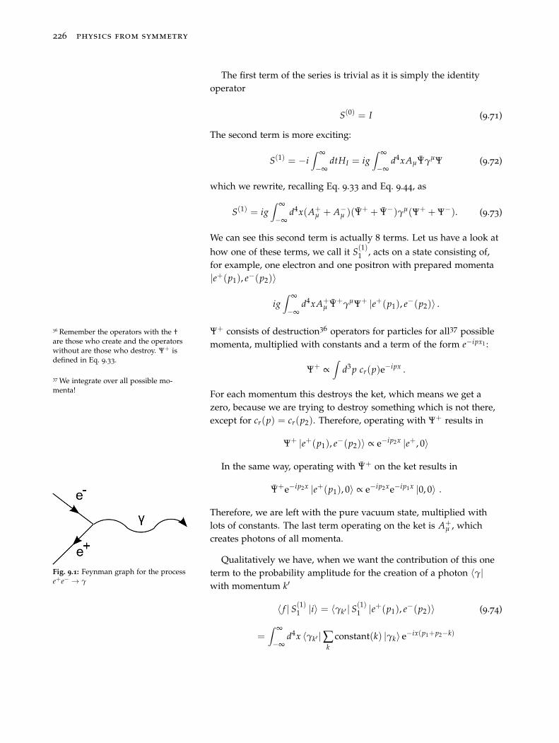
226 physics from symmetry
The first term of the series is trivial as it is simply the identityoperator
S(0) = I (9.71)
The second term is more exciting:
S(1) = −i∫ ∞
−∞dtHI = ig
∫ ∞
−∞d4xAμΨγμΨ (9.72)
which we rewrite, recalling Eq. 9.33 and Eq. 9.44, as
S(1) = ig∫ ∞
−∞d4x(A+
μ + A−μ )(Ψ
+ + Ψ−)γμ(Ψ+ + Ψ−). (9.73)
We can see this second term is actually 8 terms. Let us have a look athow one of these terms, we call it S(1)
1 , acts on a state consisting of,for example, one electron and one positron with prepared momenta|e+(p1), e−(p2)〉
ig∫ ∞
−∞d4xA+
μ Ψ+γμΨ+ |e+(p1), e−(p2)〉 .
Ψ+ consists of destruction36 operators for particles for all37 possible36 Remember the operators with the †are those who create and the operatorswithout are those who destroy. Ψ+ isdefined in Eq. 9.33.
37 We integrate over all possible mo-menta!
momenta, multiplied with constants and a term of the form e−ipx1 :
Ψ+ ∝∫
d3 p cr(p)e−ipx .
For each momentum this destroys the ket, which means we get azero, because we are trying to destroy something which is not there,except for cr(p) = cr(p2). Therefore, operating with Ψ+ results in
Ψ+ |e+(p1), e−(p2)〉 ∝ e−ip2x |e+, 0〉
In the same way, operating with Ψ+ on the ket results in
Ψ+e−ip2x |e+(p1), 0〉 ∝ e−ip2xe−ip1x |0, 0〉 .
Therefore, we are left with the pure vacuum state, multiplied withlots of constants. The last term operating on the ket is A+
μ , whichcreates photons of all momenta.
Fig. 9.1: Feynman graph for the processe+e− → γ
Qualitatively we have, when we want the contribution of this oneterm to the probability amplitude for the creation of a photon 〈γ|with momentum k′
〈 f | S(1)1 |i〉 = 〈γk′ | S(1)
1 |e+(p1), e−(p2)〉 (9.74)
=∫ ∞
−∞d4x 〈γk′ |∑
kconstant(k) |γk〉 e−ix(p1+p2−k)
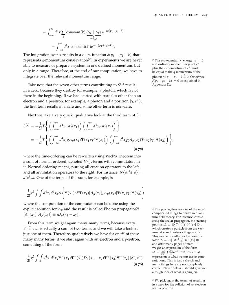
quantum field theory 227
=∫ ∞
−∞d4x ∑
kconstant(k) 〈γk′ | |γk〉︸ ︷︷ ︸
=δkk′
e−ix(p1+p2−k)
=∫ ∞
−∞d4x constant(k′)e−ix(p1+p2−k′).
The integration over x results in a delta function δ(p1 + p2 − k) thatrepresents 4-momentum conservation38. In experiments we are never 38 The 4-momentum (=energy p0 = E
and ordinary momentum pi) of e−plus the 4-momentum of e+ mustbe equal to the 4-momentum of the
photon γ: p1 + p2 − k != 0. Otherwise
δ(p1 + p2 − k) = 0 as explained inAppendix D.2.
able to measure or prepare a system in one defined momentum, butonly in a range. Therefore, at the end of our computation, we have tointegrate over the relevant momentum range.
Take note that the seven other terms contributing to S(1) resultin a zero, because they destroy for example, a photon, which is notthere in the beginning. If we had started with particles other than anelectron and a positron, for example, a photon and a positron |γ, e+〉,the first term results in a zero and some other term is non-zero.
Next we take a very quick, qualitative look at the third term of S:
S(2) = − 12!
T
{(∫ ∞
−∞d4x1HI(x1)
)(∫ ∞
−∞d4x2HI(x2)
)}
= − 12!
T
{(∫ ∞
−∞d4x1gAμ(x1)Ψ(x1)γ
μΨ(x1)
)(∫ ∞
−∞d4x2gAμ(x2)Ψ(x2)γ
μΨ(x2)
)},
(9.75)
where the time-ordering can be rewritten using Wick’s Theorem intoa sum of normal-ordered, denoted N{}, terms with commutators init. Normal ordering means, putting all creation operators to the left,and all annihilation operators to the right. For instance, N{aa†a†a} =
a†a†aa. One of the terms of this sum, for example, is
− 12!
g2∫ ∫
d4x1d4x2N
{Ψ(x1)γ
μΨ(x1)[Aμ(x1), Aμ(x2)]Ψ(x2)γμΨ(x2)
}where the computation of the commutator can be done using theexplicit solution for Aμ and the result is called Photon propagator39 39 The propagators are one of the most
complicated things to derive in quan-tum field theory. For instance, consid-ering the scalar propagator, the startingpoint is iΔ ≡ 〈0| T{Φ(x)Φ†(y)} |0〉,which creates a particle from the vac-uum at y and destroys it again at x.This can be rewritten as the commu-tator iΔ = 〈0| [Φ+†(y), Φ−(x)] |0〉and after many pages of mathwe get an expression of the formiΔ = −i
2π3
∫ d3kωk
e−ik(x−y). This finalexpression is what we can use in com-putations. This is just a sketch andmany things here are not completelycorrect. Nevertheless it should give youa rough idea of what is going on.
[Aμ(x1), Aμ(x2)] ≡ iDμ(x1 − x2) .
From this term we get again many, many terms, because everyΨ, Ψ etc. is actually a sum of two terms, and we will take a look atjust one of them. Therefore, qualitatively we have for one40 of these
40 We pick again the term not resultingin a zero for the collision of an electronwith a positron.
many many terms, if we start again with an electron and a positron,something of the form
− 12!
g2∫ ∫
d4x1d4x2Ψ−(x1)Ψ−(x1)Dμ(x1 − x2)Ψ+(x2)Ψ+(x2) |e+, e−〉(9.76)
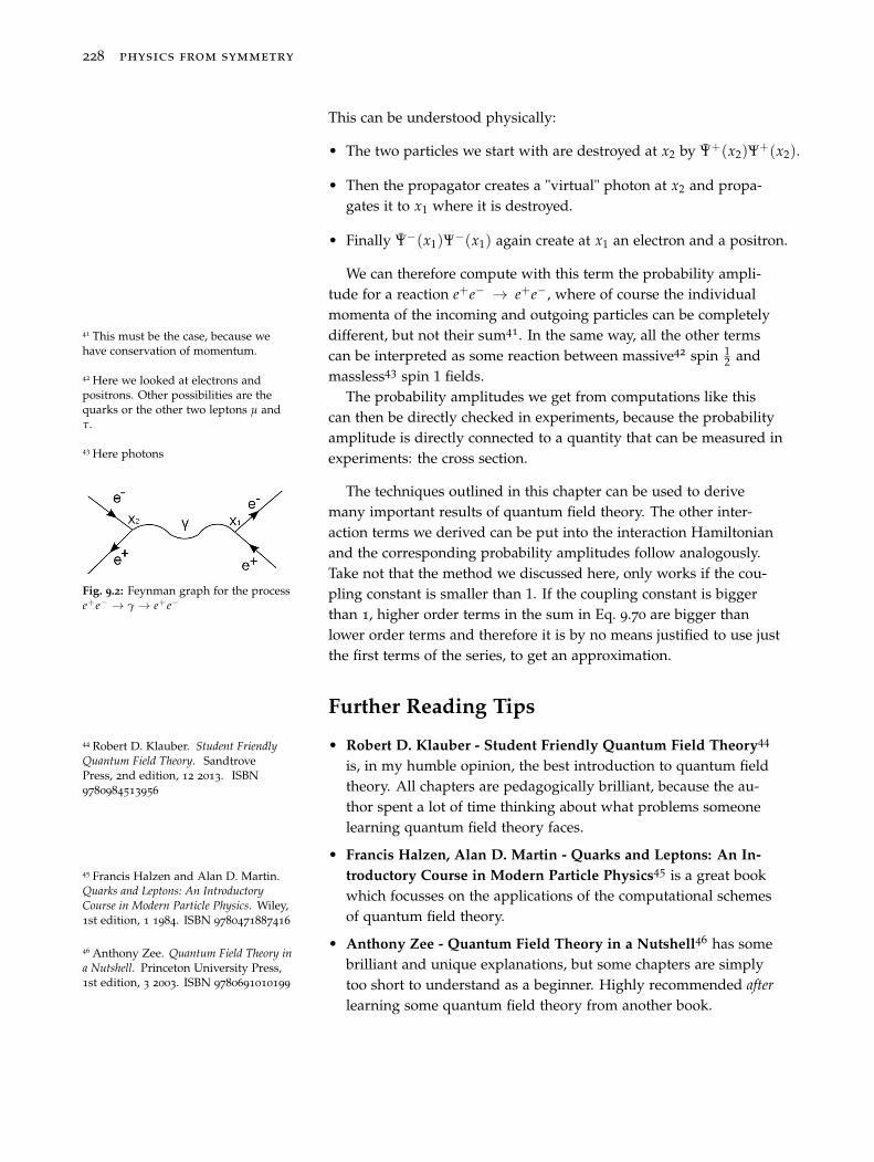
228 physics from symmetry
This can be understood physically:
• The two particles we start with are destroyed at x2 by Ψ+(x2)Ψ+(x2).
• Then the propagator creates a "virtual" photon at x2 and propa-gates it to x1 where it is destroyed.
• Finally Ψ−(x1)Ψ−(x1) again create at x1 an electron and a positron.
We can therefore compute with this term the probability ampli-tude for a reaction e+e− → e+e−, where of course the individualmomenta of the incoming and outgoing particles can be completelydifferent, but not their sum41. In the same way, all the other terms41 This must be the case, because we
have conservation of momentum. can be interpreted as some reaction between massive42 spin 12 and
42 Here we looked at electrons andpositrons. Other possibilities are thequarks or the other two leptons μ andτ.
massless43 spin 1 fields.
43 Here photons
Fig. 9.2: Feynman graph for the processe+e− → γ → e+e−
The probability amplitudes we get from computations like thiscan then be directly checked in experiments, because the probabilityamplitude is directly connected to a quantity that can be measured inexperiments: the cross section.
The techniques outlined in this chapter can be used to derivemany important results of quantum field theory. The other inter-action terms we derived can be put into the interaction Hamiltonianand the corresponding probability amplitudes follow analogously.Take not that the method we discussed here, only works if the cou-pling constant is smaller than 1. If the coupling constant is biggerthan 1, higher order terms in the sum in Eq. 9.70 are bigger thanlower order terms and therefore it is by no means justified to use justthe first terms of the series, to get an approximation.
Further Reading Tips
• Robert D. Klauber - Student Friendly Quantum Field Theory4444 Robert D. Klauber. Student FriendlyQuantum Field Theory. SandtrovePress, 2nd edition, 12 2013. ISBN9780984513956
is, in my humble opinion, the best introduction to quantum fieldtheory. All chapters are pedagogically brilliant, because the au-thor spent a lot of time thinking about what problems someonelearning quantum field theory faces.
• Francis Halzen, Alan D. Martin - Quarks and Leptons: An In-troductory Course in Modern Particle Physics45 is a great book45 Francis Halzen and Alan D. Martin.
Quarks and Leptons: An IntroductoryCourse in Modern Particle Physics. Wiley,1st edition, 1 1984. ISBN 9780471887416
which focusses on the applications of the computational schemesof quantum field theory.
• Anthony Zee - Quantum Field Theory in a Nutshell46 has some46 Anthony Zee. Quantum Field Theory ina Nutshell. Princeton University Press,1st edition, 3 2003. ISBN 9780691010199
brilliant and unique explanations, but some chapters are simplytoo short to understand as a beginner. Highly recommended afterlearning some quantum field theory from another book.
quantum field theory 229
• Franz Mandl, Graham Shaw - Quantum Field Theory47 is a very 47 Franz Mandl and Graham Shaw.Quantum Field Theory. Wiley, 2ndedition, 5 2010. ISBN 9780471496847
good starting point regarding weak and strong interaction theory
• Michele Maggiore - A Modern Introduction to Quantum FieldTheory48 is a great introduction with a strong focus on group 48 Michele Maggiore. A Modern Intro-
duction to Quantum Field Theory. OxfordUniversity Press, 1st edition, 2 2005.ISBN 9780198520740
theoretical concepts.
• Matthew Schwartz - Quantum Field Theory and the StandardModel49 offers illuminating explanations on many advanced top- 49 Matthew D. Schwartz. Quantum
Field Theory and the Standard Model.Cambridge University Press, 1 edition,12 2013. ISBN 9781107034730
ics.
9.6 Appendix: Most General Solution of theKlein-Gordon Equation
It is not too hard to find one solution of the Klein-Gordon equation.Certainly plane waves
Φ(x) = aei(px−Et) = ae−i(pμxμ)
do the job, because of the energy-momentum relation of special rela-tivity (Eq. 8.2)
E2 = �p2 + m2 → pμ pμ = m2
as we can check:
(∂μ∂μ + m2)Φ = (∂μ∂μ + m2)e−i(pμxμ)
= (−pμ pμ + m2)e−i(pμxμ)
= (−m2 + m2)e−i(pμxμ)
= 0 � (9.77)
Because we differentiate the field twice the sign in the exponent doesnot matter. Equally
Φ†(x) = a†e−i(px−Et) = a†ei(pμxμ)
is a solution. Further solutions can be built as linear combinations.A general solution is given by superposition of all possible solutions,which can be seen as Fourier expansion50 50 That’s were the factors of 2π come
from. Another way of seeing this isdemanding the solutions to form anorthonormal set:
∫dkeikxe−ikx′ =∫
dkeik(x−x′) = 2πδ(x − x′). Therefore,the factors of 2π are normalisationconstants.
Φ(x) =∫ dp4
(2π)4 (a(p)e−i(pμxμ) + a†(p)ei(pμxμ))
Take note that we wrote a = a(p) because we can have a differentmultiplication factor for each value of p and each term in the summa-tion is a solution on its own.
In this context it is conventional to work with the wave numberki ≡ pi
h and the frequency k0 = w ≡ Eh instead of the energy and
230 physics from symmetry
momentum. Because we work with h = 1 we simply have to renameour variables to get the standard textbook expressions. Furthermoreit’s conventional to abbreviate kx ≡ kμxμ. We therefore write
Φ(x) =∫ dk4
(2π)4
(a(k)e−i(kx) + a†(k)ei(kx)
)Take note that not all solutions of the Klein-Gordon equation are
suited to describe nature, because we have the "mass-shell" condi-tion
pμ pμ = kμkμ = m2 → k20 − k2
i!= m2 → k2 !
= m2. (9.78)
Only solutions satisfying the mass-shell condition are in agreementwith the relativistic energy-momentum relation (Eq. 8.2). We canbuild this condition into our equation, excluding all non-physical(off-shell) solutions with a delta distribution5151 This is explained in Appendix D.2.
Φ(x)physical =∫ dk4
(2π)4 2πδ(k2 − m2)(
a(k)e−i(kx) + a†(k)ei(kx))
Besides that, only positive energy solutions are physical, because asexplained earlier, otherwise the energy would be unbounded frombelow and nothing would be stable. We can built this constraint onour solutions into the equation by using a Heaviside function θ(k0),being zero for k0 < 0 and 1 for k0 ≥ 0. Our integral then reads
Φ(x)physical =∫ 1
(2π)3 dk4δ(k2 − m2)θ(k0)︸ ︷︷ ︸measure
(a(k)e−i(kx) + a†(k)ei(kx)
)
where we can rewrite the measure as follows
dk4δ(k2 − m2)θ(k0) = dk4δ(k20 −�k2 − m2︸ ︷︷ ︸
≡−ω2k (definition)
)θ(k0)
= dk4δ(k20 − ω2
k)θ(k0)
= dk4δ((k0 − ωk)(k0 + ωk)
)θ(k0)
=︸︷︷︸using δ
(f (x)
)=∑i
δ(x−ai)∣∣∣∣ d fdx (ai)
∣∣∣∣ where ai denotes the roots, i.e. f (ai)=0, of the function f (x)
dk4 12k0
(δ(k0 − ωk) + δ(k0 + ωk)
)θ(k0)
=︸︷︷︸because the argument of δ(k0+ωk) never becomes zero with k0≥0
dk4 12k0
δ(k0 − ωk)
= dk3dk01
2k0δ(k0 − ωk)
=︸︷︷︸Integrating over k0
dk3 12ωk
. (9.79)
quantum field theory 231
So finally the general and physical solution of the Klein-Gordonequation reads
Φ(x) =∫
dk3 1(2π)32ωk
(a(k)e−i(kx) + a†(k)ei(kx)
). (9.80)
10
Classical Mechanics
In this chapter we want to explore the connection between quan-tum and classical mechanics. We will see that the time derivative ofthe expectation value for the momentum operator gives us exactlyNewton’s second law, which is one of the foundations of classicalmechanics.
Starting with the expectation value for an operator (Eq. 8.14)
〈O〉 =∫
d3xΨ�OΨ
and the Schrödinger equation for a particle in an external potential(Eq. 8.23)
(iddt
− ∇2
2m)Ψ − VΨ = 0
→ iddt
Ψ =
(∇2
2m+ V
)︸ ︷︷ ︸
=:H
Ψ
→ ddt
Ψ =1i
HΨ
→︸︷︷︸Because H†=H
ddt
Ψ� = −1i
Ψ�︸︷︷︸Here Ψ†=Ψ�
H .
Taking the time derivative of the expectation value yields
ddt〈O〉 =
∫d3x
((ddt
Ψ�
)OΨ + Ψ�
(ddt
O)
Ψ + Ψ�O(
ddt
Ψ))
.
We use now ddt O = 0, which is true for most operators. For example,
for O = �p = −i�∇ �= O(t). In addition, we use the Schrödingerequation to rewrite the time derivatives of the wave function and its
© Springer International Publishing AG 2018J. Schwichtenberg, Physics from Symmetry, UndergraduateLecture Notes in Physics, https://doi.org/10.1007/978-3-319-66631-0_10
234 physics from symmetry
complex conjugate. This yields
ddt〈O〉 =
∫d3x
((−1
i�H
)OΨ + Ψ�O
(1i
HΨ))
=1i
∫d3x
(− Ψ�HOΨ + Ψ�OHΨ)
=1i
∫d3xΨ�[O, H]Ψ
=1i〈[O, H]〉, (10.1)
which is known as Ehrenfest theorem. If we specify O = p and use
H = p2
2m + V, we get
ddt〈 p〉 = 1
i〈[ p, H]〉
=1i〈[ p,
p2
2m+ V]〉
=1i〈[ p,
p2
2m]︸ ︷︷ ︸
=0
+[ p, V]〉
=1i〈[ p, V]〉
=1i
∫d3xΨ�[ p, V]Ψ
=1i
∫d3xΨ� pVΨ − 1
i
∫d3xΨ�VpΨ
=1i
∫d3xΨ�(−i∇)VΨ − 1
i
∫d3xΨ�V(−i∇)Ψ
=︸︷︷︸Product rule
−∫
d3xΨ�(∇V)Ψ −∫
d3xΨ�V∇Ψ +∫
d3xΨ�V∇Ψ
= −∫
d3xΨ�(∇V)Ψ
= 〈−∇V〉 = 〈F〉. (10.2)
In words this means that the time derivative (of the expectationvalue) of the momentum equals the (expectation value of the) nega-tive gradient of the potential, which is known as force. This is exactlyNewton’s second law1. This equation can be used to compute the1 Recall that we used this equation,
without a derivation, to illustrate theconserved quantities following fromNoether’s theorem in Section 4.5. Herewe deliver the derivation, as promised.
trajectories of macroscopic objects. Historically the force laws werededuced phenomenologically from experiments. All forces acting onan object were added linearly on the right-hand side of the equation.By using the phenomenologically deduced momentum pmak = mv,we can write the left-hand side as d
dt pmak = ddt mv, which equals for
an object with constant mass m ddt v. The velocity is the time-derivative
of the location2 and we therefore have2 In other words, the velocity v =ddt x(t) = x(t) is the change-rate of theposition of the object and equally theacceleration a d
dtddt x(t) = d
dt v = x(t) isthe change-rate of the velocity.
md2
dt2 x = F1 + F2 + ... (10.3)
classical mechanics 235
This is the differential equation one must solve for x = x(t) to get thetrajectory of the object in question. An example for such a classicalforce will be derived in the next chapter.
10.1 Relativistic Mechanics
Using the Lagrangian formalism, we can look at classical mechanicsfrom quite a different perspective. We need an equation that de-scribes the motion of individual particles. As always in this book,we assume that we can derive the correct equation if we minimizesomething. We already discussed at the beginning of Chapter 4 thatthis something must be invariant under all Lorentz transformations,because otherwise we don’t get the same equations of motion in allframes of reference.
Luckily, we already know something that is invariant under allLorentz transformations: the invariant of special relativity, which wasderived in Section 2.1:
(ds)2 = (cdτ)2 = (cdt)2 − (dx)2 − (dy)2 − (dz)2, (10.4)
where τ is the proper time as explained in Section 2.2. Equally thesquare root of this is invariant and therefore the simplest possiblething we can minimize is
S =∫
Cdτ (10.5)
with some constant C and
dτ =1c
√(cdt)2 − (dx)2 − (dy)2 − (dz)2 . (10.6)
The correct constant turns out to be C = −mc2 and therefore we needto minimize
S = −mc2∫
dτ. (10.7)
For brevity we will restrict the following discussion to one dimen-sion. Then we can write
dτ =1c
√(cdt)2 − (dx)2 =
1c
√(cdt)2
(1 − (dx)2
c2(dt)2
)
=1c(cdt)
√1 − 1
c2
(dxdt
)2=︸︷︷︸
dxdt =x is the velocity of the particle in question
dt
√1 − x2
c2 . (10.8)
236 physics from symmetry
Putting this into Eq. 10.7 yields
S =∫
−mc2
√1 − x2
c2︸ ︷︷ ︸≡L
dt. (10.9)
As always, we can find the extremal action by putting the Lagrangianinto the Euler-Lagrange equation (Eq. 4.7):
0 =∂L∂x
− ddt
(∂L∂x
)→ 0 =
∂
∂x
(−mc2
√1 − x2
c2
)︸ ︷︷ ︸
=0
− ddt
(∂
∂x
(−mc2
√1 − x2
c2
))
→ 0 = c2 ddt
⎛⎝ −m xc2√
1 − x2
c2
⎞⎠→ 0 =
ddt
⎛⎝ mx√1 − x2
c2
⎞⎠ . (10.10)
This is the correct relativistic equation for a free particle. If the par-ticle moves in an external potential V(x), we must simply add thispotential to the Lagrangian33 We add −V(x) instead of V(x),
because then we get in the formulafor the total energy of the system,which we can compute using Noether’stheorem, the potential energy term+V(x).
L = −mc2
√1 − (x)2
c2 − V(x) . (10.11)
For this Lagrangian the Euler-Lagrange equation yields
ddt
⎛⎝ mx√1 − x2
c2
⎞⎠ = −dVdx
≡ F. (10.12)
Take note that in the non-relativistic limit (x � c) we have√
1 − (x)2
c2 ≈ 1and the equation is exactly the equation of motion we derived in thelast section (Eq. 10.3).
10.2 The Lagrangian of Non-RelativisticMechanics
It is instructive to have a look at the non-relativistic limit of theLagrangian we derived in the last section (Eq. 10.9). The "non-relativistic limit" means, we consider a situation where the particlemoves slowly compared with the speed of light: x � c. We can thenuse the Taylor formula for the Lagrangian44 See Appendix B.3
classical mechanics 237
−mc2
√1 − x2
c2 = −mc2(
1 − 12
x2
c2 + . . .)
. (10.13)
In the limit x � c we can neglect higher order terms and the La-grangian reads
L = −mc2 +12
mx2 − V(x) . (10.14)
We already know that a constant like −mc2 has no influence on theequation of motion and therefore the Lagrangian for non-relativisticmechanics reads
L =12
mx2 − V(x). (10.15)
Without the external potential, i.e. V(x) = 0, this is exactly theLagrangian we used in section 4.5.1 to illustrate the conserved quan-tities that follow from Noether’s theorem. Putting this Lagrangianinto the Euler-Lagrange equation (Eq. 4.7) yields
∂L∂x
− ddt
(∂L∂x
)= 0
→ ∂
∂x
(12
mx2 − V(x))− d
dt
(∂
∂x
(12
mx2 − V(x)))
= 0
→ − ∂
∂xV(x)− d
dtmx = 0
→ ddt
mx = − ∂
∂xV(x)
(10.16)
This is once more exactly the equation of motion we derived at thebeginning of this chapter (Eq. 10.3).
11
Electrodynamics
We already derived in Chapter 7 one of the most important equationsof classical electrodynamics: the inhomogeneous Maxwell equations(Eq. 7.22)
∂σ(∂σ Aρ − ∂ρ Aσ) = Jρ (11.1)
or in a more compact form using the electromagnetic tensor1 1 Fσρ ≡ (∂σ Aρ − ∂ρ Aσ)
∂σFσρ = Jρ. (11.2)
We discovered in Section 7.1.6 that Jρ is a Noether current, i.e. ∂ρ Jρ =
0. In a macroscopic theory this conserved current is the electric four-current. The tensor Fσρ is antisymmetric Fσρ = −Fρσ , which canbe seen directly from the definition Fσρ = ∂σ Aρ − ∂ρ Aσ , and hastherefore 6 independent components. Three are
Fi0 = ∂i A0 − ∂0 Ai (11.3)
with i = 1, 2, 3 and the three other are
Fij = ∂i Aj − ∂j Ai = (δilδ
jm − δi
mδjl )∂
l Am =︸︷︷︸This is a standard relation for the multiplication of two ε with one coinciding index
εijkεklm∂l Am . (11.4)
The standard way to label these components is
∂i A0 − ∂0 Ai ≡ Ei (11.5)
εijk∂j Ak ≡ −Bi (11.6)
and thereforeFi0 = Ei (11.7)
Fij = εijkεklm∂l Am = −εijkBk . (11.8)
If we now rewrite the inhomogeneous Maxwell equations2 as 2 Plural because we have one equationfor each component ρ.
© Springer International Publishing AG 2018J. Schwichtenberg, Physics from Symmetry, UndergraduateLecture Notes in Physics, https://doi.org/10.1007/978-3-319-66631-0_11
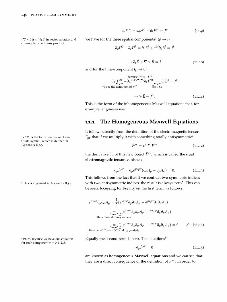
240 physics from symmetry
∂σFρσ = ∂0Fρ0 − ∂kFρk = Jρ (11.9)
we have for the three spatial components3 (ρ → i)3 ∇× �B is εikl∂kBl in vector notation andcommonly called cross product.
∂0Fi0 − ∂kFik = ∂0Ei + εikl∂kBl = Ji
→ ∂t�E +∇× �B = �J (11.10)
and for the time-component (ρ → 0)
∂0 F00︸︷︷︸=0 see the definition of Fρσ
−∂kF0kBecause Fμν=−Fνμ︷︸︸︷
= ∂kFk0 =︸︷︷︸Eq. 11.7
∂kEk = J0
→ ∇�E = J0 . (11.11)
This is the form of the inhomogeneous Maxwell equations that, forexample, engineers use.
11.1 The Homogeneous Maxwell Equations
It follows directly from the definition of the electromagnetic tensorFμν that if we multiply it with something totally antisymmetric44 εμνρσ is the four-dimensional Levi-
Civita symbol, which is defined inAppendix B.5.5. Fμν = εμνρσFρσ (11.12)
the derivative ∂μ of this new object Fμν, which is called the dualelectromagnetic tensor, vanishes:
∂μ Fμν = ∂μεμνρσ(∂σ Aρ − ∂ρ Aσ) = 0. (11.13)
This follows from the fact that if we contract two symmetric indiceswith two antisymmetric indices, the result is always zero5. This can5 This is explained in Appendix B.5.4.
be seen, focussing for brevity on the first term, as follows
εμνρσ∂μ∂σ Aρ =12(εμνρσ∂μ∂σ Aρ + εμνρσ∂μ∂σ Aρ)
=︸︷︷︸Renaming dummy indices
12(εμνρσ∂μ∂σ Aρ + εσνρμ∂σ∂μ Aρ)
=︸︷︷︸Because εμνρσ=−εσνρμ and ∂μ∂σ=∂σ∂μ
12(εμνρσ∂μ∂σ Aρ − εμνρσ∂μ∂σ Aρ) = 0 � (11.14)
Equally the second term is zero. The equations66 Plural because we have one equationfor each component v = 0, 1, 2, 3.
∂μ Fμν = 0 (11.15)
are known as homogeneous Maxwell equations and we can see thatthey are a direct consequence of the definition of Fμν. In order to
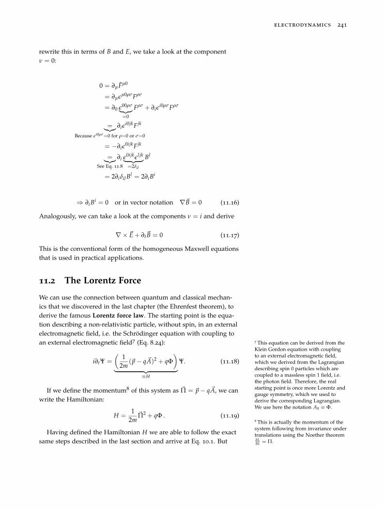
electrodynamics 241
rewrite this in terms of B and E, we take a look at the componentν = 0:
0 = ∂μ Fμ0
= ∂μεμ0ρσFρσ
= ∂0 ε00ρσ︸ ︷︷ ︸=0
Fρσ + ∂iεi0ρσFρσ
=︸︷︷︸Because εi0ρσ=0 for ρ=0 or σ=0
∂iεi0jkFjk
= −∂iε0ijkFjk
=︸︷︷︸See Eq. 11.8
∂i ε0ijkεl jk︸ ︷︷ ︸=2δil
Bl
= 2∂iδil Bl = 2∂iBi
⇒ ∂iBi = 0 or in vector notation ∇�B = 0 (11.16)
Analogously, we can take a look at the components ν = i and derive
∇× �E + ∂t�B = 0 (11.17)
This is the conventional form of the homogeneous Maxwell equationsthat is used in practical applications.
11.2 The Lorentz Force
We can use the connection between quantum and classical mechan-ics that we discovered in the last chapter (the Ehrenfest theorem), toderive the famous Lorentz force law. The starting point is the equa-tion describing a non-relativistic particle, without spin, in an externalelectromagnetic field, i.e. the Schrödinger equation with coupling toan external electromagnetic field7 (Eq. 8.24): 7 This equation can be derived from the
Klein Gordon equation with couplingto an external electromagnetic field,which we derived from the Lagrangiandescribing spin 0 particles which arecoupled to a massless spin 1 field, i.e.the photon field. Therefore, the realstarting point is once more Lorentz andgauge symmetry, which we used toderive the corresponding Lagrangian.We use here the notation A0 ≡ Φ.
i∂tΨ =
(1
2m(�p − q�A)2 + qΦ
)︸ ︷︷ ︸
≡H
Ψ. (11.18)
If we define the momentum8 of this system as �Π = �p − q�A, we can
8 This is actually the momentum of thesystem following from invariance undertranslations using the Noether theorem∂L∂x = Π.
write the Hamiltonian:
H =1
2m�Π2 + qΦ . (11.19)
Having defined the Hamiltonian H we are able to follow the exactsame steps described in the last section and arrive at Eq. 10.1. But
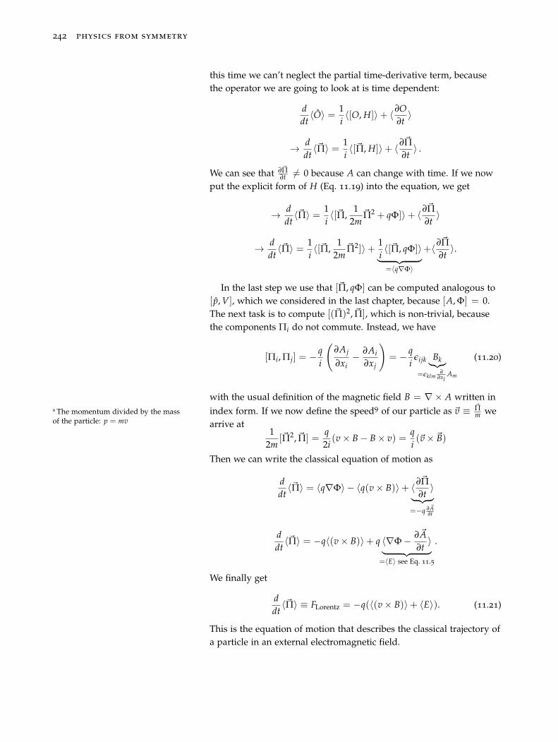
242 physics from symmetry
this time we can’t neglect the partial time-derivative term, becausethe operator we are going to look at is time dependent:
ddt〈O〉 = 1
i〈[O, H]〉+ 〈∂O
∂t〉
→ ddt〈�Π〉 = 1
i〈[�Π, H]〉+ 〈∂�Π
∂t〉 .
We can see that ∂�Π∂t �= 0 because A can change with time. If we now
put the explicit form of H (Eq. 11.19) into the equation, we get
→ ddt〈�Π〉 = 1
i〈[�Π,
12m
�Π2 + qΦ]〉+ 〈∂�Π∂t
〉
→ ddt〈�Π〉 = 1
i〈[�Π,
12m
�Π2]〉+ 1i〈[�Π, qΦ]〉︸ ︷︷ ︸=〈q∇Φ〉
+〈∂�Π∂t
〉.
In the last step we use that [�Π, qΦ] can be computed analogous to[ p, V], which we considered in the last chapter, because [A, Φ] = 0.The next task is to compute [(�Π)2, �Π], which is non-trivial, becausethe components Πi do not commute. Instead, we have
[Πi, Πj] = − qi
(∂Aj
∂xi− ∂Ai
∂xj
)= − q
iεijk Bk︸︷︷︸=εklm
∂∂xl
Am
(11.20)
with the usual definition of the magnetic field B = ∇× A written inindex form. If we now define the speed9 of our particle as �v ≡ �Π
m we9 The momentum divided by the massof the particle: p = mv arrive at
12m
[�Π2, �Π] =q2i(v × B − B × v) =
qi(�v × �B)
Then we can write the classical equation of motion as
ddt〈�Π〉 = 〈q∇Φ〉 − 〈q(v × B)〉+ 〈∂�Π
∂t〉︸ ︷︷ ︸
=−q ∂�A∂t
ddt〈�Π〉 = −q〈(v × B)〉+ q 〈∇Φ − ∂�A
∂t〉︸ ︷︷ ︸
=〈E〉 see Eq. 11.5
.
We finally get
ddt〈�Π〉 ≡ FLorentz = −q(〈(v × B)〉+ 〈E〉). (11.21)
This is the equation of motion that describes the classical trajectory ofa particle in an external electromagnetic field.
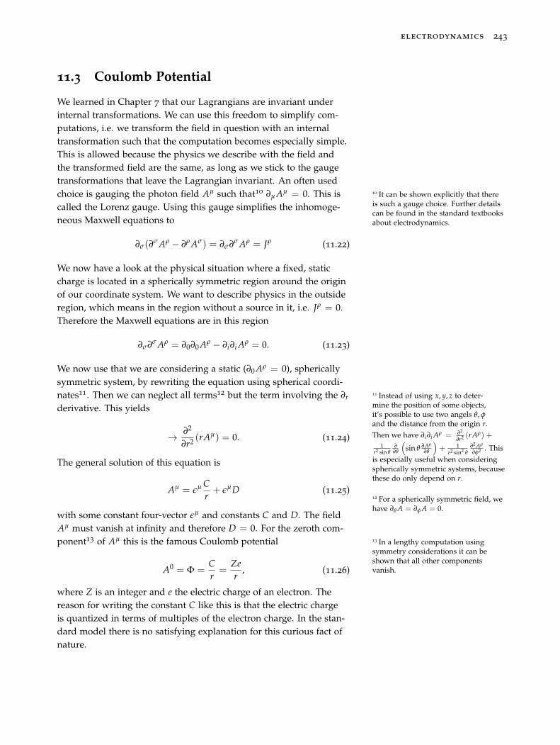
electrodynamics 243
11.3 Coulomb Potential
We learned in Chapter 7 that our Lagrangians are invariant underinternal transformations. We can use this freedom to simplify com-putations, i.e. we transform the field in question with an internaltransformation such that the computation becomes especially simple.This is allowed because the physics we describe with the field andthe transformed field are the same, as long as we stick to the gaugetransformations that leave the Lagrangian invariant. An often usedchoice is gauging the photon field Aμ such that10 ∂μ Aμ = 0. This is 10 It can be shown explicitly that there
is such a gauge choice. Further detailscan be found in the standard textbooksabout electrodynamics.
called the Lorenz gauge. Using this gauge simplifies the inhomoge-neous Maxwell equations to
∂σ(∂σ Aρ − ∂ρ Aσ) = ∂σ∂σ Aρ = Jρ (11.22)
We now have a look at the physical situation where a fixed, staticcharge is located in a spherically symmetric region around the originof our coordinate system. We want to describe physics in the outsideregion, which means in the region without a source in it, i.e. Jρ = 0.Therefore the Maxwell equations are in this region
∂σ∂σ Aρ = ∂0∂0 Aρ − ∂i∂i Aρ = 0. (11.23)
We now use that we are considering a static (∂0 Aρ = 0), sphericallysymmetric system, by rewriting the equation using spherical coordi-nates11. Then we can neglect all terms12 but the term involving the ∂r 11 Instead of using x, y, z to deter-
mine the position of some objects,it’s possible to use two angels θ, φand the distance from the origin r.Then we have ∂i∂i Aρ = ∂2
∂r2 (rAρ) +
1r2 sin θ
∂∂θ
(sin θ ∂Aρ
∂θ
)+ 1
r2 sin2 θ∂2 Aρ
∂φ2 . Thisis especially useful when consideringspherically symmetric systems, becausethese do only depend on r.
12 For a spherically symmetric field, wehave ∂θ A = ∂φ A = 0.
derivative. This yields
→ ∂2
∂r2 (rAμ) = 0. (11.24)
The general solution of this equation is
Aμ = εμ Cr+ εμD (11.25)
with some constant four-vector εμ and constants C and D. The fieldAμ must vanish at infinity and therefore D = 0. For the zeroth com-ponent13 of Aμ this is the famous Coulomb potential 13 In a lengthy computation using
symmetry considerations it can beshown that all other componentsvanish.A0 = Φ =
Cr=
Zer
, (11.26)
where Z is an integer and e the electric charge of an electron. Thereason for writing the constant C like this is that the electric chargeis quantized in terms of multiples of the electron charge. In the stan-dard model there is no satisfying explanation for this curious fact ofnature.
244 physics from symmetry
Further Reading Tips
• Richard P. Feynman - The Feynman Lectures on PhysicsVolume 214 is a great book to start learning electrodynamics.14 Richard P. Feynman, Robert B.
Leighton, and Matthew Sands. TheFeynman Lectures on Physics: Volume 2.Addison-Wesley, 1st edition, 2 1977.ISBN 9780201021172
• David J. Griffiths - Introduction to Electrodynamics15 is another
15 David J. Griffiths. Introduction toElectrodynamics. Addison-Wesley, 4thedition, 10 2012. ISBN 9780321856562
great book to learn more about the concepts of electrodynamics.
12
Gravity
Unfortunately, the best theory of gravity we have does not fit into the pic-ture outlined in the rest of this book. This is one of the biggest problems ofmodern physics and the following paragraphs try to give you a first impres-sion.
The modern theory of gravity is Einstein’s general relativity.The fundamental idea is that gravity is a result of the curvature ofspacetime. Mass and energy change the curvature of spacetime andin turn the changed curvature influences the movement of mass andenergy. This interplay between energy and curvature is described bythe famous Einstein equation
Gμν = 8πGTμν. (12.1)
On the left-hand side is the Einstein tensor Gμν, which describesthe curvature and on the right-hand side is the energy-momentumtensor1 Tμν. G is the gravitation constant. 1 Recall that the energy-momentum
tensor is the quantity which is directlyrelated to translational symmetry(Eq. 4.36).
From the idea gravity = curvature of spacetime, the derivationof the Einstein equation is, from a modern point of view, relativelystraightforward2. Firstly, one of the most important laws of physics 2 Einstein needed 100 years ago ca. 6
years for the derivation of the correctequation. Today, with the power ofhindsight we are much faster.
is the conservation of energy and momentum, which as we saw,follows directly when considering a homogeneous spacetime. Ina homogeneous spacetime the laws of physics are invariant undertranslations in space and time and using Noether’s theorem, wecan derive the conservation of momentum and energy. Therefore,one of the most basic assumptions of physics is that spacetime ishomogeneous and therefore energy and momentum are conserved.In mathematical terms this conservation law is expressed as (Eq. 4.36)
∂μTμν = 0. (12.2)
© Springer International Publishing AG 2018J. Schwichtenberg, Physics from Symmetry, UndergraduateLecture Notes in Physics, https://doi.org/10.1007/978-3-319-66631-0_12
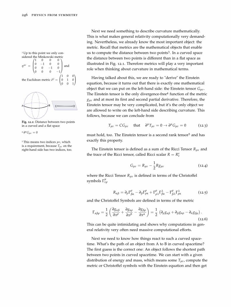
246 physics from symmetry
Next we need something to describe curvature mathematically.This is what makes general relativity computationally very demand-ing. Nevertheless, we already know the most important object: themetric. Recall that metrics are the mathematical objects that enableus to compute the distance between two points3. In a curved space3 Up to this point we only con-
sidered the Minkowski metric
ημν =
⎛⎜⎜⎝1 0 0 00 −1 0 00 0 −1 00 0 0 −1
⎞⎟⎟⎠ and
the Euclidean metric δij =
⎛⎝1 0 00 1 00 0 1
⎞⎠
the distance between two points is different than in a flat space asillustrated in Fig. 12.1. Therefore metrics will play a very importantrole when thinking about curvature in mathematical terms.
Fig. 12.1: Distance between two pointsin a curved and a flat space
Having talked about this, we are ready to "derive" the Einsteinequation, because it turns out that there is exactly one mathematicalobject that we can put on the left-hand side: the Einstein tensor Gμν.The Einstein tensor is the only divergence-free4 function of the metric
4 ∂μGμν = 0
gμν and at most its first and second partial derivative. Therefore, theEinstein tensor may be very complicated, but it’s the only object weare allowed to write on the left-hand side describing curvature. Thisfollows, because we can conclude from
Tμν = CGμν that ∂μTμν = 0 → ∂μGμν = 0 (12.3)
must hold, too. The Einstein tensor is a second rank tensor5 and has5 This means two indices μν, whichis a requirement, because Tμν on theright-hand side has two indices, too.
exactly this property.
The Einstein tensor is defined as a sum of the Ricci Tensor Rμν andthe trace of the Ricci tensor, called Ricci scalar R = Rν
ν
Gμν = Rμν − 12
Rgμν (12.4)
where the Ricci Tensor Rμν is defined in terms of the Christoffelsymbols Γμ
νρ
Rαβ = ∂ρΓρβα − ∂βΓρ
ρα + ΓρρλΓλ
βα − ΓρβλΓλ
ρα (12.5)
and the Christoffel Symbols are defined in terms of the metric
Γαβρ =12
(∂gαβ
∂xρ +∂gαρ
∂xβ− ∂gβρ
∂xα
)=
12
(∂ρgαβ + ∂βgαρ − ∂αgβρ
).
(12.6)This can be quite intimidating and shows why computations in gen-eral relativity very often need massive computational efforts.
Next we need to know how things react to such a curved space-time. What’s the path of an object from A to B in curved spacetime?The first guess is the correct one: An object follows the shortest pathbetween two points in curved spacetime. We can start with a givendistribution of energy and mass, which means some Tμν, compute themetric or Christoffel symbols with the Einstein equation and then get
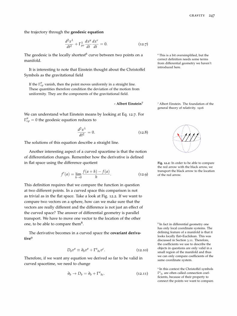
gravity 247
the trajectory through the geodesic equation
d2xλ
dt2 + Γλμν
dxμ
dtdxν
dt= 0. (12.7)
The geodesic is the locally shortest6 curve between two points on a 6 This is a bit oversimplified, but thecorrect definition needs some termsfrom differential geometry we haven’tintroduced here.
manifold.
It is interesting to note that Einstein thought about the ChristoffelSymbols as the gravitational field
If the Γμνρ vanish, then the point moves uniformly in a straight line.
These quantities therefore condition the deviation of the motion fromuniformity. They are the components of the gravitational field.
- Albert Einstein7 7 Albert Einstein. The foundation of thegeneral theory of relativity. 1916
We can understand what Einstein means by looking at Eq. 12.7. ForΓμ
νρ = 0 the geodesic equation reduces to
d2xλ
dt2 = 0. (12.8)
The solutions of this equation describe a straight line.
Fig. 12.2: In order to be able to comparethe red arrow with the black arrow, wetransport the black arrow to the locationof the red arrow.
Another interesting aspect of a curved spacetime is that the notionof differentiation changes. Remember how the derivative is definedin flat space using the difference quotient
f ′(a) = limh→0
f (a + h)− f (a)h
. (12.9)
This definition requires that we compare the function in questionat two different points. In a curved space this comparison is notas trivial as in the flat space. Take a look at Fig. 12.2. If we want tocompare two vectors on a sphere, how can we make sure that thevectors are really different and the difference is not just an effect ofthe curved space? The answer of differential geometry is paralleltransport. We have to move one vector to the location of the otherone, to be able to compare them8. 8 In fact in differential geometry one
has only local coordinate systems. Thedefining feature of a manifold is that itlooks locally flat=Euclidean. This wasdiscussed in Section 3.11. Therefore,the coefficients we use to describe theobjects in questions are only valid in asmall region of the manifold and thuswe can only compare coefficients of thesame coordinate system.
The derivative becomes in a curved space the covariant deriva-tive9
9 In this context the Christoffel symbolsΓa
bc are often called connection coef-ficients, because of their property toconnect the points we want to compare.
Dbva ≡ ∂bva + Γabcvc. (12.10)
Therefore, if we want any equation we derived so far to be valid incurved spacetime, we need to change
∂b → Db = ∂b + Γabc. (12.11)
248 physics from symmetry
Does this look familiar? Take a look again at Eq. 7.18. We learned inan earlier chapter that a locally U(1) invariant Lagrangian for spin 0or spin 1
2 fields required a specific coupling with a spin 1 field. Thisspecific coupling can be summarized by the prescription
∂μ → Dμ ≡ ∂μ + ieAμ. (12.12)
Remember that this wasn’t just a mathematical gimmick. This pre-scription gives us the correct theory of electromagnetism. The same istrue for weak
∂μ → Dμ ≡ ∂μ − ig Wμ︸︷︷︸=Wi
μσi
(12.13)
and strong interactions (see Eq. 7.165)
∂μ → Dμ = ∂μ − ig′ Gμ︸︷︷︸=TCGC
μ
. (12.14)
Although things look quite similar here, there is for many reasons noformulation of gravity that is compatible with the quantum descrip-tion of all other forces. All other forces are described in a quantumtheory and one can only make probability predictions. In contrast,general relativity is a classical theory, because particles follow de-fined trajectories and there is no need for probability predictions.To make things worse, at the current time no experiment can shineany light on the interplay between those forces. The effects of gravityon elementary particles is too weak to be measured. Because of this,the standard model, which ignores gravity entirely and only takesthe weak, the strong and the electromagnetic interactions into ac-count, works very well. The effects of general relativity only becomemeasurable with very heavy objects. For such quantum effects playno role, because massive objects consist of many, many elementaryparticles and all quantum effects get averaged out. We discovered inChapter 10 that the equation of motion for the average value is justthe classical one and no quantum effects are measurable. One canmake a long list of things that make constructing a quantum theoryof gravity so difficult, but Einstein formulated the difference betweengravity and all other forces very concisely:
...according to the general theory of relativity, gravitation occupiesan exceptional position with regard to other forces, particularly theelectromagnetic forces, since the ten functions representing the gravita-tional field at the same time define the metrical properties of the spacemeasured.
- Albert Einstein1010 Albert Einstein and Francis A. Davis.The Principle of Relativity. Dover Publi-cations, reprint edition, 6 1952. ISBN9780486600819
gravity 249
We are able do describe quantum particles in a curved space, bychanging the derivative to the covariant derivative. But this is ofcourse no dynamical theory of gravity. We could make the right-hand side of the Einstein equation quantum, if we make the usualidentification with the corresponding generator, but what aboutthe left-hand side? The Einstein tensor in terms of the ChristoffelSymbols is
Gαβ = (δγα δ
ζβ −
12
gαβgγζ)(∂εΓεγζ − ∂ζ Γε
γε + ΓεεσΓσ
γζ − ΓεζσΓσ
εγ). (12.15)
Thus maybe we can think of the Einstein equation as the field equa-tion11 for Γε
ζσ, and the terms generated by the prescription 11 Analogous to the Maxwell equationfor the electromagnetic field.
∂b → Db = ∂b + Γabc
as the corresponding coupling between the gravitational field Γεζσ and
the other fields?
Regardless of if you prefer to think of the metric or the Christof-fel symbols as the gravitational field, the two or three vector indicesindicate that we may need to investigate the (1, 1) or even higherrepresentations, which we would call consequently spin 2, 3, . . . rep-resentation of the Poincaré group. In fact most physicists believe thatthe boson responsible for gravitational attraction, the graviton, hasspin 2.
Until the present day, there is no working12 theory of quantum 12 Many attempts result in an infinitenumber of infinity terms, which is quitebad for probability predictions.
gravity and for further information have a look at the books men-tioned in the next section.
Further Reading Tips
For more information about the standard theory of gravity, Einstein’sgeneral relativity, see
• Ta-Pei Cheng - Relativity, Gravitation and Cosmology13 is a 13 Ta-Pei Cheng. Relativity, Gravitationand Cosmology: A Basic Introduction.Oxford University Press, 2nd edition, 12010. ISBN 9780199573646
great, rather low-level introduction to general relativity with manyvery enlightening explanations. Perfect to get a quick overview.
• A. Zee - Einstein Gravity in a Nutshell14, is the best book to learn 14 Anthony Zee. Einstein Gravity in aNutshell. Princeton University Press, 1stedition, 5 2013. ISBN 9780691145587
about general relativity. It really starts at the beginning, avoidsunnecessary, confusing mathematical tools and does a great jobexplaining the origin and usage of general relativity.
• Charles W. Misner, Kip S. Thorne, John Archibald Wheeler -Gravitation15 is a really, really big book, but often offers in depth 15 Charles W. Misner, Kip S. Thorne, and
John Archibald Wheeler. Gravitation. W.H. Freeman, 1st edition, 9 1973. ISBN9780716703440
explanations for points that remain unclear in most other books.
250 physics from symmetry
For more information about attempts to quantize gravity have alook at
• Lee Smolin -Three Roads to Quantum Gravity16, which is bril-16 Lee Smolin. Three Roads to QuantumGravity. Basic Books, 3 edition, 8 2017.ISBN 9780465094547
liant popular science book that summarizes the various attemptsto quantize gravity.
• John C. Baez, Javier P. Muniain - Gauge Fields, Knots, andGravity17 which is a magnificent book. The focus lies on intro-17 John C. Baez and Javier P. Muniain.
Gauge Fields, Knots, and Gravity. WorldScientific Pub Co Inc, 1st edition, 91994. ISBN 9789810220341
ducing the mathematical tools needed to understand attempts toquantize gravity in a way that physicists understand.

13
Closing Words
In my humble opinion we are a long way from a theory that is ableto explain all the things that we would like. Even the beautiful theorywe developed in the major part of this book still has many looseends that need clarification. In addition, we still have no clue how toderive the correct quantum theory of gravity as discussed in the lastchapter.
Besides that there is experimental evidence, mostly from cosmol-ogy and astroparticle physics (Dark Matter and Dark Energy), whichindicates that the present theories are not the end of the story.
I personally think there is still much to come and maybe a com-pletely new framework is needed to overcome the present obstacles.Anyway, the future developments will be very interesting and I hopeyou will continue following the story and maybe contribute some-thing yourself.
© Springer International Publishing AG 2018J. Schwichtenberg, Physics from Symmetry, UndergraduateLecture Notes in Physics, https://doi.org/10.1007/978-3-319-66631-0_13

Part VAppendices
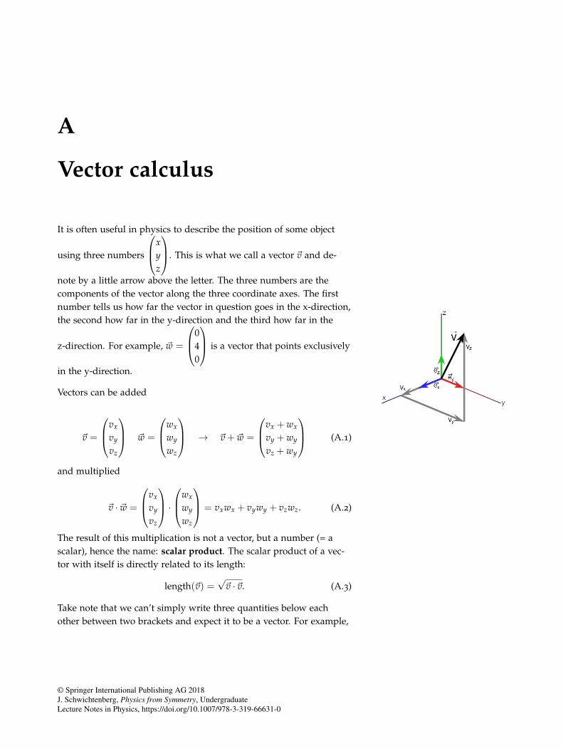
A
Vector calculus
It is often useful in physics to describe the position of some object
using three numbers
⎛⎜⎝xyz
⎞⎟⎠. This is what we call a vector �v and de-
note by a little arrow above the letter. The three numbers are thecomponents of the vector along the three coordinate axes. The firstnumber tells us how far the vector in question goes in the x-direction,the second how far in the y-direction and the third how far in the
z-direction. For example, �w =
⎛⎜⎝040
⎞⎟⎠ is a vector that points exclusively
in the y-direction.
Vectors can be added
�v =
⎛⎜⎝vx
vy
vz
⎞⎟⎠ �w =
⎛⎜⎝wx
wy
wz
⎞⎟⎠ → �v + �w =
⎛⎜⎝vx + wx
vy + wy
vz + wy
⎞⎟⎠ (A.1)
and multiplied
�v · �w =
⎛⎜⎝vx
vy
vz
⎞⎟⎠ ·
⎛⎜⎝wx
wy
wz
⎞⎟⎠ = vxwx + vywy + vzwz. (A.2)
The result of this multiplication is not a vector, but a number (= ascalar), hence the name: scalar product. The scalar product of a vec-tor with itself is directly related to its length:
length(�v) =√�v ·�v. (A.3)
Take note that we can’t simply write three quantities below eachother between two brackets and expect it to be a vector. For example,
© Springer International Publishing AG 2018J. Schwichtenberg, Physics from Symmetry, UndergraduateLecture Notes in Physics, https://doi.org/10.1007/978-3-319-66631-0
256 physics from symmetry
let’s say we put the temperature T, the pressure P and the humidityH of a room between two brackets:
⎛⎜⎝TPH
⎞⎟⎠ . (A.4)
Nothing prevents us from doing so, but the result would be ratherpointless and definitely not a vector, because there is no linear con-nection between these quantities that could lead to the mixing ofthese quantities. In contrast, the three position coordinates transforminto each other, for example if we look at the vector from a differentperspective1. Therefore writing the coordinates below each other1 This will be made explicit in a mo-
ment. between two big brackets is useful. Another example would be themomentum of some object. Again, the components mix if we look atthe object from a different perspective and therefore writing it likethe position vector is useful.
For the moment let’s say a vector is a quantity that transformsexactly like the position vector �v. This means, if under some trans-formation we have �v → �v′ = M�v any quantity that transforms like�w → �w′ = M�w is a vector. Examples are the momentum or accelera-tion of some object.
We will encounter this idea quite often in physics. If we writequantities below each other between two brackets, they aren’t nec-essarily vectors, but the quantities can transform into each otherthrough some linear operation. This is often expressed by multiplica-tion with a matrix.
A.1 Basis Vectors
We can make the idea of components along the coordinate axes moregeneral by introducing basis vectors. Basis vectors are linearly inde-pendent2 vectors of length one. In three dimensions we need three2 A set of vectors {�a,�b,�c} is called
linearly independent if the equationc1�a + c2�b + c3�c = 0 is only true forc1 = c2 = c3 = 0. This means thatno vector can be written as a linearcombination of the other vectors,because if we have c1�a + c2�b + c3�c = 0for numbers different than zero, we canwrite c1�a + c2�b = −c3�c.
basis vectors and we can write every vector in terms of these basisvectors. An obvious choice is:
�e1 =
⎛⎜⎝100
⎞⎟⎠ , �e2 =
⎛⎜⎝010
⎞⎟⎠ , �e3 =
⎛⎜⎝001
⎞⎟⎠ (A.5)
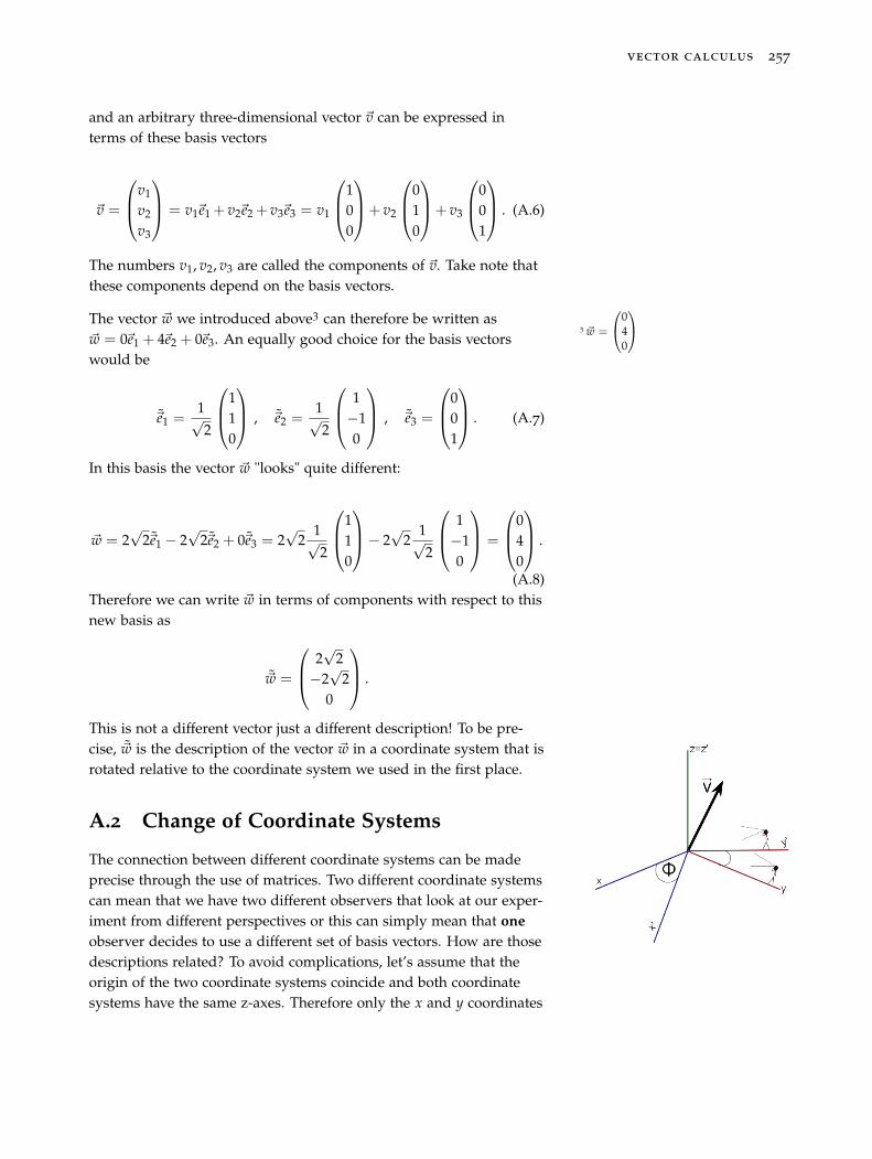
vector calculus 257
and an arbitrary three-dimensional vector �v can be expressed interms of these basis vectors
�v =
⎛⎜⎝v1
v2
v3
⎞⎟⎠ = v1�e1 + v2�e2 + v3�e3 = v1
⎛⎜⎝100
⎞⎟⎠+ v2
⎛⎜⎝010
⎞⎟⎠+ v3
⎛⎜⎝001
⎞⎟⎠ . (A.6)
The numbers v1, v2, v3 are called the components of �v. Take note thatthese components depend on the basis vectors.
The vector �w we introduced above3 can therefore be written as3 �w =
⎛⎝040
⎞⎠�w = 0�e1 + 4�e2 + 0�e3. An equally good choice for the basis vectorswould be
�e1 =1√2
⎛⎜⎝110
⎞⎟⎠ , �e2 =1√2
⎛⎜⎝ 1−10
⎞⎟⎠ , �e3 =
⎛⎜⎝001
⎞⎟⎠ . (A.7)
In this basis the vector �w "looks" quite different:
�w = 2√
2�e1 − 2√
2�e2 + 0�e3 = 2√
21√2
⎛⎜⎝110
⎞⎟⎠− 2√
21√2
⎛⎜⎝ 1−10
⎞⎟⎠ =
⎛⎜⎝040
⎞⎟⎠ .
(A.8)Therefore we can write �w in terms of components with respect to thisnew basis as
�w =
⎛⎜⎝ 2√
2−2
√2
0
⎞⎟⎠ .
This is not a different vector just a different description! To be pre-cise, �w is the description of the vector �w in a coordinate system that isrotated relative to the coordinate system we used in the first place.
A.2 Change of Coordinate Systems
The connection between different coordinate systems can be madeprecise through the use of matrices. Two different coordinate systemscan mean that we have two different observers that look at our exper-iment from different perspectives or this can simply mean that oneobserver decides to use a different set of basis vectors. How are thosedescriptions related? To avoid complications, let’s assume that theorigin of the two coordinate systems coincide and both coordinatesystems have the same z-axes. Therefore only the x and y coordinates
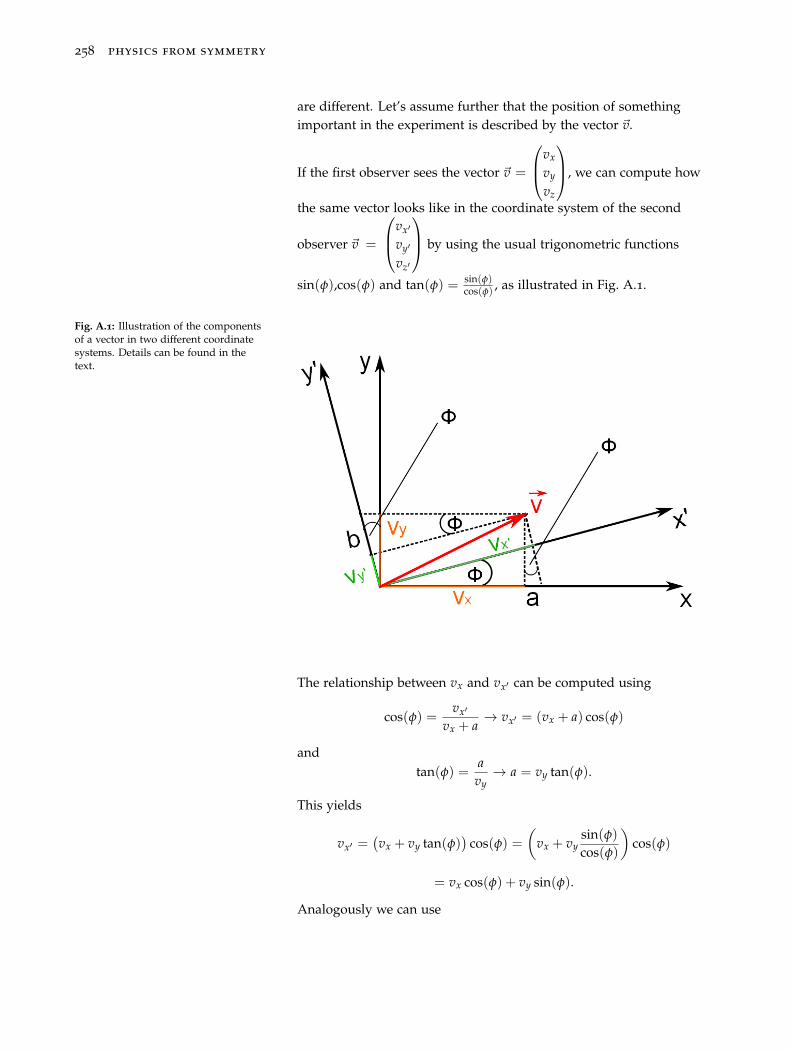
258 physics from symmetry
are different. Let’s assume further that the position of somethingimportant in the experiment is described by the vector �v.
If the first observer sees the vector �v =
⎛⎜⎝vx
vy
vz
⎞⎟⎠, we can compute how
the same vector looks like in the coordinate system of the second
observer �v =
⎛⎜⎝vx′
vy′
vz′
⎞⎟⎠ by using the usual trigonometric functions
sin(φ),cos(φ) and tan(φ) = sin(φ)cos(φ) , as illustrated in Fig. A.1.
Fig. A.1: Illustration of the componentsof a vector in two different coordinatesystems. Details can be found in thetext.
The relationship between vx and vx′ can be computed using
cos(φ) =vx′
vx + a→ vx′ = (vx + a) cos(φ)
andtan(φ) =
avy
→ a = vy tan(φ).
This yields
vx′ =(vx + vy tan(φ)
)cos(φ) =
(vx + vy
sin(φ)cos(φ)
)cos(φ)
= vx cos(φ) + vy sin(φ).
Analogously we can use
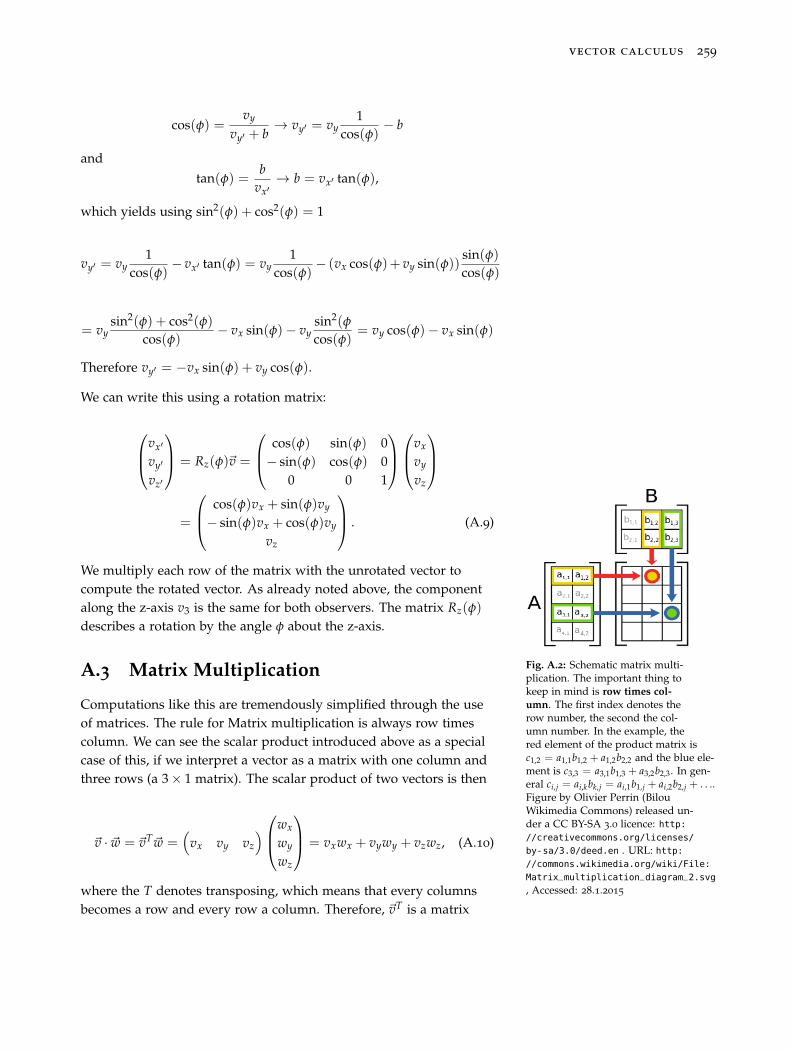
vector calculus 259
cos(φ) =vy
vy′ + b→ vy′ = vy
1cos(φ)
− b
andtan(φ) =
bvx′
→ b = vx′ tan(φ),
which yields using sin2(φ) + cos2(φ) = 1
vy′ = vy1
cos(φ)− vx′ tan(φ) = vy
1cos(φ)
− (vx cos(φ)+ vy sin(φ))sin(φ)cos(φ)
= vysin2(φ) + cos2(φ)
cos(φ)− vx sin(φ)− vy
sin2(φ
cos(φ)= vy cos(φ)− vx sin(φ)
Therefore vy′ = −vx sin(φ) + vy cos(φ).
We can write this using a rotation matrix:
⎛⎜⎝vx′
vy′
vz′
⎞⎟⎠ = Rz(φ)�v =
⎛⎜⎝ cos(φ) sin(φ) 0− sin(φ) cos(φ) 0
0 0 1
⎞⎟⎠⎛⎜⎝vx
vy
vz
⎞⎟⎠=
⎛⎜⎝ cos(φ)vx + sin(φ)vy
− sin(φ)vx + cos(φ)vy
vz
⎞⎟⎠ . (A.9)
We multiply each row of the matrix with the unrotated vector tocompute the rotated vector. As already noted above, the componentalong the z-axis v3 is the same for both observers. The matrix Rz(φ)
describes a rotation by the angle φ about the z-axis.
A.3 Matrix Multiplication Fig. A.2: Schematic matrix multi-plication. The important thing tokeep in mind is row times col-umn. The first index denotes therow number, the second the col-umn number. In the example, thered element of the product matrix isc1,2 = a1,1b1,2 + a1,2b2,2 and the blue ele-ment is c3,3 = a3,1b1,3 + a3,2b2,3. In gen-eral ci,j = ai,kbk,j = ai,1b1,j + ai,2b2,j + . . ..Figure by Olivier Perrin (BilouWikimedia Commons) released un-der a CC BY-SA 3.0 licence: http://creativecommons.org/licenses/
by-sa/3.0/deed.en . URL: http://commons.wikimedia.org/wiki/File:
Matrix_multiplication_diagram_2.svg
, Accessed: 28.1.2015
Computations like this are tremendously simplified through the useof matrices. The rule for Matrix multiplication is always row timescolumn. We can see the scalar product introduced above as a specialcase of this, if we interpret a vector as a matrix with one column andthree rows (a 3 × 1 matrix). The scalar product of two vectors is then
�v · �w = �vT�w =(
vx vy vz
)⎛⎜⎝wx
wy
wz
⎞⎟⎠ = vxwx + vywy + vzwz, (A.10)
where the T denotes transposing, which means that every columnsbecomes a row and every row a column. Therefore, �vT is a matrix
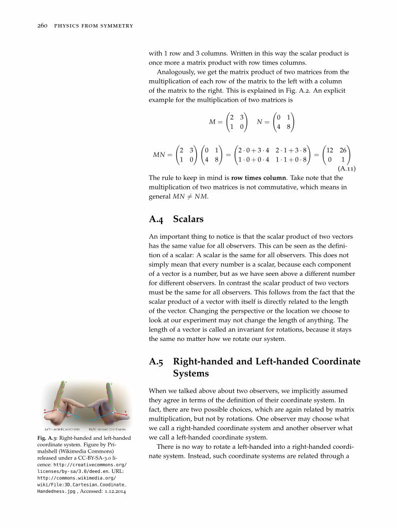
260 physics from symmetry
with 1 row and 3 columns. Written in this way the scalar product isonce more a matrix product with row times columns.
Analogously, we get the matrix product of two matrices from themultiplication of each row of the matrix to the left with a columnof the matrix to the right. This is explained in Fig. A.2. An explicitexample for the multiplication of two matrices is
M =
(2 31 0
)N =
(0 14 8
)
MN =
(2 31 0
)(0 14 8
)=
(2 · 0 + 3 · 4 2 · 1 + 3 · 81 · 0 + 0 · 4 1 · 1 + 0 · 8
)=
(12 260 1
)(A.11)
The rule to keep in mind is row times column. Take note that themultiplication of two matrices is not commutative, which means ingeneral MN �= NM.
A.4 Scalars
An important thing to notice is that the scalar product of two vectorshas the same value for all observers. This can be seen as the defini-tion of a scalar: A scalar is the same for all observers. This does notsimply mean that every number is a scalar, because each componentof a vector is a number, but as we have seen above a different numberfor different observers. In contrast the scalar product of two vectorsmust be the same for all observers. This follows from the fact that thescalar product of a vector with itself is directly related to the lengthof the vector. Changing the perspective or the location we choose tolook at our experiment may not change the length of anything. Thelength of a vector is called an invariant for rotations, because it staysthe same no matter how we rotate our system.
A.5 Right-handed and Left-handed CoordinateSystems
When we talked above about two observers, we implicitly assumedthey agree in terms of the definition of their coordinate system. Infact, there are two possible choices, which are again related by matrixmultiplication, but not by rotations. One observer may choose whatwe call a right-handed coordinate system and another observer whatwe call a left-handed coordinate system.Fig. A.3: Right-handed and left-handed
coordinate system. Figure by Pri-malshell (Wikimedia Commons)released under a CC-BY-SA-3.0 li-cence: http://creativecommons.org/licenses/by-sa/3.0/deed.en. URL:http://commons.wikimedia.org/
wiki/File:3D_Cartesian_Coodinate_
Handedness.jpg , Accessed: 1.12.2014
There is no way to rotate a left-handed into a right-handed coordi-nate system. Instead, such coordinate systems are related through a
vector calculus 261
reflection in a mirror. This means the descriptions in a right-handedand a left-handed coordinate system are related by a transformationof the form ⎛⎜⎝v1
v2
v3
⎞⎟⎠ →
⎛⎜⎝−v1
−v2
−v3
⎞⎟⎠ , (A.12)
which means we flip the sign of all spatial coordinates. The conven-tional name for this kind of transformation is parity transformation.We can describe a parity transformation by
�v → �v′ = P�v =
⎛⎜⎝−1 0 00 −1 00 0 −1
⎞⎟⎠⎛⎜⎝v1
v2
v3
⎞⎟⎠ =
⎛⎜⎝−v1
−v2
−v3
⎞⎟⎠ . (A.13)
B
Calculus
B.1 Product Rule
The product rule
d(
f (x)g(x))
dx=
(d f (x)dx
)g(x) + f (x)
(dg(x)dx
)≡ f ′g + f g′ (B.1)
follows directly from the definition of derivatives
ddx
[ f (x)g(x)] = limh→0
f (x + h)g(x + h)− f (x)g(x)h
= limh→0
[ f (x + h)g(x + h)− f (x + h)g(x)] + [ f (x + h)g(x)− f (x)g(x)]h
= limh→0
f (x + h)g(x + h)− g(x)
h+ g(x)
f (x + h)− f (x)h
= f (x)g′(x) + g(x) f ′(x)
B.2 Integration by Parts
A (likely apocryphal) story goes: when Peter Lax was awarded theNational Medal of Science, the other recipients (presumably non-mathematicians) asked him what he did to deserve the Medal. Laxresponded: " I integrated by parts."
- Willie Wong1 1 Told on www.math.stackexchange.com
An important rule for integrals follows directly from the productrule. Integrating the product rule2 2 See Eq. B.1 and we then use for the
first term the fundamental theorem ofcalculus
∫ ba dx h′(x) = h(b)− h(a).
© Springer International Publishing AG 2018J. Schwichtenberg, Physics from Symmetry, UndergraduateLecture Notes in Physics, https://doi.org/10.1007/978-3-319-66631-0
264 physics from symmetry
∫ b
adx
d(
f (x)g(x))
dx︸ ︷︷ ︸= f (x)g(x)
∣∣b
a
=∫ b
adx
(d f (x)dx
)g(x) +
∫ b
adx f (x)
(dg(x)dx
)(B.2)
and rearranging the terms yields
∫ b
adx
(d f (x)dx
)g(x) = f (x)g(x)
∣∣∣b
a−
∫ b
adx f (x)
(dg(x)dx
). (B.3)
This rule is particularly useful in physics when working with fields,because if we integrate over all space, i.e. a = −∞,b = ∞, the bound-
ary term vanishes f (x)g(x)∣∣∣b=∞
a=−∞= 0, because all fields must vanish
at infinity3.3 This follows, because otherwise thetotal field energy would be infinityand such field configurations are non-physical. B.3 The Taylor Series
The Taylor series is a formula that enables us to write any infinitelydifferentiable function in terms of a power series
f (x) = f (a) + (x − a) f ′(a) +12(x − a)2 f ′′(a) + . . . (B.4)
• On the one hand we can use it if we want to know how we canwrite some function in terms of a series. This can be used forexample to show that eix = cos(x) + i sin(x).
• On the other hand we can use the Taylor series to get approxi-mations for a function about a point. This is useful when we canneglect for some reasons higher order terms and don’t need toconsider infinitely many terms. If we want to evaluate a functionf (x) in some neighbouring point of a point y, say y + Δy, we canwrite44 Don’t let yourself get confused by
the names of our variables here. In theformula above we want to evaluate thefunction at x by doing computationsat a. Here we want to know somethingabout f at y + Δy, by using informationat y. To make the connection precise:x = y + Δy and a = y.
f (y + Δy) = f (y) + (y + Δy − y) f ′(y) + . . . = f (y) + Δy f ′(y) + . . . .(B.5)
This means we get an approximation for the function value aty + Δy, by evaluating the function at y. In the extreme case of aninfinitesimal neighbourhood Δy → ε, the change of the functioncan be written by one (the linear) term of the Taylor series.
Δ f = f (y + ε)− f (y) = f (y) + ε f ′(y) + . . . − f (y) = ε f ′(y) + . . .︸︷︷︸≈0 for ε2≈0
(B.6)
calculus 265
This formula is one of the most useful mathematical tools andwe can derive it using the fundamental theorem of calculus andintegration by parts. The fundamental theorem tells us
∫ x
adt f ′(t) = f (x)− f (a) → f (x) = f (a) +
∫ x
adt f ′(t). (B.7)
We can rewrite the second term by integrating by parts, becausewe have of course an implicit 1 in front of f ′(t) = 1 f ′(t), whichwe can use as a second function in Eq. B.3: g′(t) = 1. The rule forintegration by parts tells us that we can rewrite an integral
∫ ba v′u =
vu|ba +∫
vu′ by integrating one term and differentiating the other.Here we integrate g′(t) = 1 and differentiate f ′(t), i.e. in the formulag′ = v′ and f ′ = u. This yields
f (x) = f (a) +∫ x
adt f ′(t) = f (a) + g(t) f ′(t)
∣∣∣x
a−
∫ x
adt g(t) f ′′(t).
(B.8)Now we need to know what g(t) is. At this point the only infor-
mation we have is g′(t) = 1, but there are infinitely many functionswith this derivative: For any constant c the function g = t + c satisfiesg′(t) = 1. Our formula becomes particularly useful5 for g = t − x, i.e. 5 The equation holds for arbitrary c
and of course you’re free to choosesomething different, but you won’t getour formula. We choose the constant csuch that we get a useful formula forf (x). Otherwise f (x) would appear onthe left- and right-hand side.
we use minus the upper integration boundary −x as our constant c.Then we have for the second term in the equation above
g(t) f ′(t)∣∣∣x
a= (t− x) f ′(t)
∣∣∣x
a= (x − x)︸ ︷︷ ︸
=0
f ′(x)− (a− x) f ′(a) = (x− a) f ′(a)
(B.9)and the formula now reads
f (x) = f (a) + (x − a) f ′(a) +∫ x
adt (x − t) f ′′(t). (B.10)
We can then evaluate the last term once more using integration byparts, now with6 v′ = (x − t) and u = f ′′(t): 6 Take note that integrating v′ = (x − t)
yields a minus sign: → v = − 12 (x −
t)2 + d, because our variable here is tand with some constant d we choose tobe zero.
→∫ x
adt (x − t)︸ ︷︷ ︸
=v′
f ′′(t)︸ ︷︷ ︸=u
= −12(x − t)2︸ ︷︷ ︸=v
f ′′(t)︸ ︷︷ ︸=u
∣∣∣x
a−
∫ x
adt
(− 1
2(x − t)2
)︸ ︷︷ ︸
=v
f ′′′(t)︸ ︷︷ ︸=u′
where the boundary term is again simple
−12(x − t)2 f ′′(t)
∣∣∣x
a= −1
2(x − x)2︸ ︷︷ ︸
=0
f ′′(x) +12(x − a)2 f ′′(a).
This gives us the formula
f (x) = f (a) + (x − a) f ′(a) +12(x − a)2 f ′′(a) +
∫ x
adt
12(x − t)2 f ′′′(t).
(B.11)
266 physics from symmetry
We could go on and integrate the last term by parts, but the patternshould be visible by now. The Taylor series can be written in a morecompact form using the mathematical sign for a sum ∑:
f (x) =∞
∑n=0
f (n)(a)(x − a)n
n!
=f (0)(a)(x − a)0
0!+
f (1)(a)(x − a)1
1!+
f (2)(a)(x − a)2
2!
+f (3)(a)(x − a)3
3!+ . . . , (B.12)
where f (n) denotes the n-th derivative of f , e.g. f (2) = f ′′ and n! isthe factorial of n, i.e. n! = 1 · 2 · 3 . . . n. For example for n = 5 we have5! = 5 · 4 · 3 · 2 · 1 = 120, 2! = 2 · 1 = 2 and by definition 0! = 1. Seriesare the topic of the next section.
B.4 Series
In the last section we stumbled upon a very important formula thatincludes an infinite sum. In this section some basic tricks for summanipulation and some very important series will be introduced.
B.4.1 Important Series
In the last section we learned that we can write every infinitely differ-entiable function as a series. Let’s start with maybe the most impor-tant function: The exponential function ex. The Taylor series for theexponential function can be written right away
ex =∞
∑n=0
xn
n!, (B.13)
by using the defining feature of the exponential function that thederivative is the exponential function itself: (ex)′ = ex, evaluating theTaylor series about a = 0 and using e0 = 1. This yields the Taylorseries (Eq. B.12) for the exponential function:
ex =∞
∑n=0
e0(x − 0)n
n!=
∞
∑n=0
xn
n!(B.14)
This series can be seen as a definition of ex.
Two other important, infinitely differentiable functions are sin(x)and cos(x). We can compute the Taylor series for these functions,by using (sin(x))′ = cos(x), (cos(x))′ = − sin(x), cos(0) = 1 and
calculus 267
sin(0) = 0.
sin(x) =∞
∑n=0
sin(n)(0)(x − 0)n
n!.
Because of sin(0) = 0 every term with even n vanishes, which we canuse if we split the sum. Observe that
∞
∑n=0
n =∞
∑n=0
(2n + 1) +∞
∑n=0
(2n)
1 + 2 + 3 + 4 + 5 + 6 . . . = 1 + 3 + 5 + . . . + 2 + 4 + 6 + . . . (B.15)
Splitting the sum for sin(x) yields
sin(x) =∞
∑n=0
sin(2n+1)(0)(x − 0)2n+1
(2n + 1)!+
∞
∑n=0
sin(2n)(0)(x − 0)2n
(2n)!︸ ︷︷ ︸=0
=∞
∑n=0
sin(2n+1)(0)(x − 0)2n+1
(2n + 1)!. (B.16)
Every even derivative of sin(x), i.e. sin(2n) is again sin(x) (with pos-sibly a minus sign in front of it) and therefore the second term van-ishes because of sin(0) = 0. Every uneven derivative of sin(x) iscos(x), with possibly a minus sign in front of it. We have
sin(x)(1) = cos(x)
sin(x)(2) = cos′(x) = − sin(x)
sin(x)(3) = − sin′(x) = − cos(x)
sin(x)(4) = − cos′(x) = sin(x)
sin(x)(5) = sin′(x) = cos(x) . (B.17)
The pattern is therefore sin(2n+1)(x) = (−1)n cos(x), as you cancheck by putting some integer values for n into the formula7. We can 7 sin(1)(x) = sin(2·0+1)(x) =
(−1)·0 cos(x) = cos(x), sin(3)(x) =sin(2·1+1)(x) = (−1)1 cos(x) = − cos(x)
therefore rewrite Eq. B.16 as
sin(x) =∞
∑n=0
sin(2n+1)(0)(x − 0)2n+1
(2n + 1)!
=∞
∑n=0
(−1)n cos(0)(x − 0)2n+1
(2n + 1)!
=︸︷︷︸cos(0)=1
∞
∑n=0
(−1)n(x)2n+1
(2n + 1)!. (B.18)
268 physics from symmetry
This is the Taylor series for sin(x), which again can be seen as a defi-nition of sin(x). Analogous we can derive
cos(x) =∞
∑n=0
(−1)n(x)2n
(2n)!, (B.19)
because this time uneven derivatives are proportional to sin(0) = 0.
B.4.2 Splitting Sums
In the last section we used a trick that is quite useful in many compu-tations. There we used the example
∞
∑n=0
n =∞
∑n=0
(2n + 1) +∞
∑n=0
(2n)
1 + 2 + 3 + 4 + 5 + 6 . . . = 1 + 3 + 5 + . . . + 2 + 4 + 6 + . . . , (B.20)
to motivate how we can split any sum in terms of even and unevenintegers. 2n is always an even integer, whereas 2n + 1 is always anuneven integer. We already saw in the last section that this can beuseful, but let’s look at another example. What happens if we splitthe exponential series with complex argument ix?
eix =∞
∑n=0
(ix)n
n!
=∞
∑n=0
(ix)2n
(2n)!+
∞
∑n=0
(ix)2n+1
(2n + 1)!. (B.21)
This can be rewritten using that (ix)2n = i2nx2n and i2n = (i2)n =
(−1)n. In addition we have of course i2n+1 = i · i2n = i(−1)n. Thenwe have
eix =∞
∑n=0
(ix)n
n!
=∞
∑n=0
(−1)n(x)2n
(2n)!+ i
∞
∑n=0
(−1)n(x)2n+1
(2n + 1)!
=∞
∑n=0
(−1)n(x)2n
(2n)!︸ ︷︷ ︸=cos(x) see Eq. B.19
+i∞
∑n=0
(−1)n(x)2n+1
(2n + 1)!︸ ︷︷ ︸=sin(x) see Eq. B.18
= cos(x) + i sin(x) . (B.22)
This is famously known as Euler’s formula.
calculus 269
B.4.3 Einstein’s Sum Convention
Sums are very common in physics and writing the big sum sign ∑all the time can be quite cumbersome. For this reason a clever manintroduced a convention, called Einstein sum convention. Accordingto this convention every time an index appears twice in some term,like n in the sums above, an implicit sum is understood. This means
anbn ≡ ∑n
anbn. (B.23)
Other examples are
anbncm ≡ ∑n
anbncm. (B.24)
ambncm ≡ ∑m
ambncm. (B.25)
but
anbm �= ∑n
anbm, (B.26)
because in general m �= n. An index without a partner is called a freeindex, an index with a partner a dummy index, for reasons that willbe explained in the next section.
For example in the sum anbncm ≡ ∑n anbncm, the index n is adummy index, but m is a free index. Equivalently, in ambncm ≡ ∑m ambncm,the index m is a dummy index and n is free.
B.5 Index Notation
B.5.1 Dummy Indices
It is important to take note that the name of indices with a partnerplays absolutely no role. Renaming n → k, changes absolutely noth-ing8, as long as n is contracted 8 Of course we can’t change an index
into another type of index. For ex-ample, we can change i → j but noti → μ, because Greek indices like μ arealways summed from 0 to 3 and Romanindices, like i from 1 to 3.
anbncm = akbkcm ≡ ∑n
anbncm ≡ ∑k
akbkcm. (B.27)
On the other hand free indices can not be renamed freely. For exam-ple, m → q can make quite a difference because there must be someterm on the other side of the equation with the same free index. Thismeans when we look at a term like anbncm isolated, we must alwaystake into account that there might be other terms with the same freeindex m that must be renamed, too. Let’s look at an example
Fi = εijkajbk. (B.28)
270 physics from symmetry
A new thing that appears here is that some object, here εijk, is al-lowed to carry more than one index, but don’t let that bother you,because we will come back to this in a moment. Therefore, if we lookat εijkajbk we can change the names of j and k as we like, becausethese indices are contracted. For example j → u, k → z, which yieldsεiuzaubz is really the same. On the other hand i is not a dummy indexand we can’t rename it i → m: εmuzaubz , because then our equationwould read
Fi = εmuzaubz. (B.29)
This may seem pedantic at this point, because it is clear that we needto rename i at Fi, too in order to get something sensible, but moreoften than not will we look at isolated terms and it is important toknow what we are allowed to do without changing anything.
B.5.2 Objects with more than One Index
Now, let’s talk about objects with more than one index. Objects withtwo indices are simply matrices. The first index tells us which rowand the second index which column we should pick our value from.For example
Mij ≡(
M11 M12
M21 M22
). (B.30)
This means for example that M12 is the object in the first row in thesecond column.
We can use this to write matrix multiplication using indices. Theproduct of two matrices is
MN ≡ (MN)ij = Mik Nkj. (B.31)
On the left hand side we have the element in row i in column j ofthe product matrix (MN), which we get from multiplying the i-throw of M with the j-th column of N. The index k appears twice andtherefore an implicit sum is assumed. One can give names to objectswith three or more indices (tensors). For the purpose of this booktwo are enough and we will discuss only one exception, which is thetopic of one of the next sections.
B.5.3 Symmetric and Antisymmetric Indices
A matrix is said to be symmetric if Mij = Mji. This means in our twodimensional example M12 = M21 and an example for a symmetric
calculus 271
matrix is
(9 33 17
). (B.32)
A matrix is called totally antisymmetric if Mij = −Mji for all i, jholds. An example would be.
(0 3−3 0
). (B.33)
Take note that the diagonal elements must vanish here, becauseM11 = −M11, which is only satisfied for M11 = 0 and analogously forM22.
B.5.4 Antisymmetric × Symmetric Sums
An important observation is that every time we have a sum oversomething symmetric in its indices multiplied with something anti-symmetric in the same indices, the result is zero:
∑ij
aijbij = 0 (B.34)
if aij = −aji and bij = bji holds for all i, j. We can see this by writing
∑ij
aijbij =12
(∑ij
aijbij + ∑ij
aijbij
)(B.35)
As explained earlier we are free to rename our dummy indices i → jand j → i, which we use in the second term
→ ∑ij
aijbij =12
(∑ij
aijbij + ∑ij
ajibji
)(B.36)
Then we use the symmetry of bij and antisymmetry of aij, to switchthe indices in the second term, which yields9 9 If this looks like a cheap trick to you,
you should compute some explicitexamples to see that this is really true.
→ ∑ij
aijbij =12
(∑ij
aijbij + ∑ij
aji︸︷︷︸=−aij
bji︸︷︷︸=bij
)
=12
(∑ij
aijbij − ∑ij
aijbij
)= 0 . (B.37)
272 physics from symmetry
B.5.5 Two Important Symbols
One of the most important matrices is of course the unit matrix. Intwo dimensions we have
1 =
(1 00 1
). (B.38)
In index notation the unit matrix is called the Kronecker symbol,denoted δij, which is then defined for arbitrary dimensions by
δij =
⎧⎨⎩1 if i = j,
0 if i �= j .(B.39)
The Kronecker symbol is symmetric because δij = δji.
Equally important is the Levi-Civita symbol εijk, which is definedin two dimensions as follows:
εij =
⎧⎪⎪⎨⎪⎪⎩1 if (i, j) = {(1, 2)},
0 if i = j ,
−1 if (i, j) = {(2, 1)}.
(B.40)
In matrix form, we can write it as
εij =
(0 1−1 0
)(B.41)
In three dimensions the Levi-Civita symbol is
εijk =
⎧⎪⎪⎨⎪⎪⎩1 if (i, j, k) = {(1, 2, 3), (2, 3, 1), (3, 1, 2)},
0 if i = j or j = k or k = i,
−1 if (i, j, k) = {(1, 3, 2), (3, 2, 1), (2, 1, 3)}.
(B.42)
and in four dimensions
εijkl =
⎧⎪⎪⎨⎪⎪⎩1 if (i, j, k, l) is an even permutation of{(1, 2, 3, 4)},
−1 if (i, j, k, l) is an uneven permutation of{(1, 2, 3, 4)},
0 otherwise.(B.43)
For example (1, 2, 4, 3) is an uneven (because we make one change)and (2, 1, 4, 3) is an even permutation (because we make two changes)of (1, 2, 3, 4).
The Levi-Civita symbol is totally anti-symmetric because if wechange two indices, we always get, by definition, a minus sign:εijk = −εjik, εijk = −εikj etc. or in two dimensions εij = −εji.
C
Linear Algebra
Many computations can be simplified by using matrices and tricksfrom the linear algebra toolbox. Therefore, let’s look at some basictransformations.
C.1 Basic Transformations
The complex conjugate of a matrix is defined as
M�ij =
(M�
11 M�12
M�21 M�
22
), (C.1)
which means we simply take the complex conjugate of each ele-ment1. 1 Recall that the complex conjugate of a
complex number z = a + ib, where a isthe real part and b the imaginary part,is simply z� = a − ib.
The transpose of a matrix is defined by MTij = Mji, in matrix form
Mij =
(M11 M12
M21 M22
)→ MT
ij =
(M11 M21
M12 M22
), (C.2)
which means we swap columns and rows of the matrix. An impor-tant consequence of this definition and the definition of the prod-uct of two matrices is that we have (MN)T �= MT NT . Instead(MN)T = NT MT , which means by transposing we switch the po-sition of two matrices in a product. We can see this directly in indexnotation
MN ≡ (MN)ij = Mik Nkj
(MN)T ≡ ((MN)ij)T = (MN)ji = (Mik Nkj)
T
(Mik Nkj)T = MT
ik NTkj = Mki Njk = Njk Mki ≡ NT MT , (C.3)
© Springer International Publishing AG 2018J. Schwichtenberg, Physics from Symmetry, UndergraduateLecture Notes in Physics, https://doi.org/10.1007/978-3-319-66631-0
274 physics from symmetry
where in the last step we use the general rule that in matrix notationwe always multiply rows of the left matrix with columns of the rightmatrix. To write this in matrix notation, we change the position of thetwo terms to Njk Mki, which is rows of the left matrix times columnsof the right matrix, as it should be and we can write in matrix nota-tion NT MT .
Take note that in index notation we can always change the positionof the objects in question freely, because for example Mki and Njk arejust individual elements of the matrices, i.e. ordinary numbers.
C.2 Matrix Exponential Function
We already derived how the exponential function looks as a series,and therefore we can define what we mean when we put a matrixinto the exponential function:
eM, with an arbitrary matrix M, is defined by the series
eM =∞
∑n=0
Mn
n!. (C.4)
It is important to take note that in general eMeN �= eM+N . The iden-tity eMeN = eM+N is only correct if MN = NM.
C.3 Determinants
The determinant of a matrix is a rather unintuitive, but immenselyuseful notion. For example, if the determinant of some matrix isnon-zero, we automatically know that the matrix is invertible2. Un-2 A matrix M is invertible, if we can find
an inverse matrix, denoted by M−1,with M−1 M = 1.
fortunately proving this lies beyond the scope of this text and theinterested reader is referred to the standard texts about linear alge-bra.
The determinant of a 3 × 3 matrix can be defined using the Levi-Civita symbol
det(A) =3
∑i=1
3
∑j=1
3
∑k=1
εijk A1i A2j A3k (C.5)
and analogously for n-dimensions
det(A) =n
∑i1=1
n
∑i2=1
. . .n
∑in=1
εi1i2...in A1i1 A2i2 . . . Anin . (C.6)
It is instructive to look at an explicit example in two dimensions:
linear algebra 275
det(A) = det
(3 15 2
)= (3 · 2)− (5 · 1) = 1 .
For a general three dimensional matrix, we have
det
⎛⎜⎝a1 a2 a3
b1 b2 b3
c1 c2 c3
⎞⎟⎠ = a1(b2c3 − b3c2)− a2(b1c3 − b3c1)+ a3(b1c2 − b2c1) .
(C.7)
C.4 Eigenvalues and Eigenvectors
Two very important notions from linear algebra that are used all overphysics are eigenvalues and eigenvectors. The eigenvectors �v andeigenvalues λ are defined for each matrix M by the equation
M�v = λ�v. (C.8)
The important thing is that we have on both sides of the equationthe same vector �v. In words this equation means that the vector �vremains, up to a constant λ, unchanged if multiplied with the matrixM. To each eigenvector we have a corresponding eigenvalue. Thereare quite sophisticated computational schemes for finding the eigen-vectors and eigenvalues of a matrix and the details can be found inany book about linear algebra.
To get a feeling for the importance of these notions think aboutrotations. We can describe rotations by matrices and the eigenvectorof a rotation matrix defines the rotational axis.
C.5 Diagonalization
Eigenvectors and eigenvalues can be used to bring matrices into diag-onal form, which can be quite useful for computations and physicalinterpretations. It can be shown that any diagonalizable matrix Mcan be rewritten in the form3 3 In general, a transformation of the
form M′ = N−1 MN refers to a basischange. M′ is the matrix M in anothercoordinate system. Therefore, the resultof this section is that we can find a basiswhere M is particularly simple, i.e.diagonal.
M = N−1DN, (C.9)
where the matrix N consists of the eigenvectors as its column and Dis diagonal with the eigenvalues of M on its diagonal:
(M11 M12
M21 M22
)= N−1
(λ1 00 λ2
)N =
(�v1,�v2
)−1(
λ1 00 λ2
)(�v1,�v2
).
(C.10)
D
Additional MathematicalNotions
D.1 Fourier Transform
The idea of the Fourier transform is similar to the idea that we canexpress any vector �v in terms of basis vectors1 ( �e1, �e2, �e3). In ordinary 1 This is explained in more detail in
Appendix A.1.Euclidean space the most common choice is
�e1 =
⎛⎜⎝100
⎞⎟⎠ , �e2 =
⎛⎜⎝010
⎞⎟⎠ , �e3 =
⎛⎜⎝001
⎞⎟⎠ (D.1)
and an arbitrary three-dimensional vector �v can be expressed interms of these basis vectors
�v =
⎛⎜⎝v1
v2
v3
⎞⎟⎠ = v1�e1 + v2�e2 + v3�e3 = v1
⎛⎜⎝100
⎞⎟⎠+ v2
⎛⎜⎝010
⎞⎟⎠+ v3
⎛⎜⎝001
⎞⎟⎠ (D.2)
The idea of the Fourier transform is that we can do the samething with functions2. For periodic functions such a basis is given
2 In a more abstract sense, functionsare abstract vectors. This is meant inthe sense that functions are elements ofsome vector space. For different kindsof functions a different vector space.Such abstract vector spaces are definedsimilar to the usual Euclidean vectorspace, where our ordinary positionvectors live (those with the little arrow� ). For example, take note that we canadd two functions, just as we can addtwo vectors, and get another function.In addition, it’s possible to define ascalar product.
by sin(kx) and cos(kx). This means we can write every periodic func-tion f (x) as
f (x) =∞
∑k=0
(ak cos(kx) + bk sin(kx)) (D.3)
with constant coefficients ak and bk.
An arbitrary (not necessarily periodic) function can be writtenin terms of the basis eikx and e−ikx, but this time with an integralinstead of a sum3 3 Recall that an integral is just the limit
of a sum, where the discrete k in ∑kbecomes a continuous variable in
∫dk.
© Springer International Publishing AG 2018J. Schwichtenberg, Physics from Symmetry, UndergraduateLecture Notes in Physics, https://doi.org/10.1007/978-3-319-66631-0
278 physics from symmetry
f (x) =∫ ∞
0dk
(akeikx + bke−ikx
), (D.4)
which we can also write as
f (x) =∫ ∞
−∞dk fke−ikx. (D.5)
The expansion coefficients fk are often denoted f (k), which is thencalled the Fourier transform of f (x).
D.2 Delta Distribution
In some sense, the delta distribution is to integrals what the Kro-necker delta4 is to sums. We can use the Kronecker delta δij to pick4 The Kronecker delta is defined in
Appendix B.5.5. one specific term of any sum. For example, consider
3
∑i=1
aibj = a1bj + a2bj + a3bj (D.6)
and let’s say we want to pick the second term of the sum. We can dothis using the Kronecker delta δ2i, because then
3
∑i=1
δ2iaibj = δ21︸︷︷︸=0
a1bj + δ22︸︷︷︸=1
a2bj + δ23︸︷︷︸=0
a3bj = a2bj. (D.7)
Or more general
3
∑i=1
δikaibj = akbj. (D.8)
The delta distribution δ(x − y) is defined as an object that has exactlythis property: ∫
dx f (x)δ(x − y) = f (y). (D.9)
Completely analogous to the Kronecker delta, the delta distributionpicks one term from the integral5. In addition, we can use this anal-5 The term where x = y. For example,∫
dx f (x)δ(x − 2) = f (2). ogy to motivate from the equality
∂xi∂xj
= δij (D.10)
the equality∂ f (xi)
∂ f (xj)= δ(xi − xj). (D.11)
This is of course by no means a proof, but this equality can be shownin a rigorous way, too. There is a lot more one can say about this ob-ject, but for the purpose of this book it is enough to understand what

additional mathematical notions 279
the delta distribution does. In fact, this is how the delta distributionwas introduced in the first place by Dirac.
Bibliography
John C. Baez and Javier P. Muniain. Gauge Fields, Knots, andGravity. World Scientific Pub Co Inc, 1st edition, 9 1994. ISBN9789810220341.
Alessandro Bettini. Introduction to Elementary Particle Physics. Cam-bridge University Press, 2nd edition, 4 2014. ISBN 9781107050402.
Ta-Pei Cheng. Relativity, Gravitation and Cosmology: A Basic In-troduction. Oxford University Press, 2nd edition, 1 2010. ISBN9780199573646.
Predrag Cvitanovic. Group Theory: Birdtracks, Lie’s, and ExceptionalGroups. Princeton University Press, 7 2008. ISBN 9780691118369.
Paul A. M. Dirac and Physics. Lectures on Quantum Mechanics. DoverPublications, 1st edition, 3 2001. ISBN 9780486417134.
Albert Einstein. The foundation of the general theory of relativity.1916.
Albert Einstein and Francis A. Davis. The Principle of Relativity.Dover Publications, reprint edition, 6 1952. ISBN 9780486600819.
Richard P. Feynman and Albert R. Hibbs. Quantum Mechanics andPath Integrals: Emended Edition. Dover Publications, emended editonedition, 7 2010. ISBN 9780486477220.
Richard P. Feynman, Robert B. Leighton, and Matthew Sands. TheFeynman Lectures on Physics, Volume 3. Addison Wesley, 1st edition, 11971. ISBN 9780201021189.
Richard P. Feynman, Robert B. Leighton, and Matthew Sands. TheFeynman Lectures on Physics: Volume 2. Addison-Wesley, 1st edition,2 1977. ISBN 9780201021172.
Daniel Fleisch. A Student’s Guide to Vectors and Tensors. CambridgeUniversity Press, 1st edition, 11 2011. ISBN 9780521171908.
© Springer International Publishing AG 2018J. Schwichtenberg, Physics from Symmetry, UndergraduateLecture Notes in Physics, https://doi.org/10.1007/978-3-319-66631-0
282 physics from symmetry
Jon Fripp, Deborah Fripp, and Michael Fripp. Speaking of Science.Newnes, 1st edition, 4 2000. ISBN 9781878707512.
William Fulton and Joe Harris. Representation Theory: A First Course.Springer, 1st corrected edition, 8 1999. ISBN 9780387974958.
Howard Georgi. Lie Algebras In Particle Physics: from Isospin To Uni-fied Theories (Frontiers in Physics). Westview Press, 2 edition, 10 1999.ISBN 9780738202334.
Herbert Goldstein, Charles P. Poole Jr., and John L. Safko. Clas-sical Mechanics. Addison-Wesley, 3rd edition, 6 2001. ISBN9780201657029.
David J. Griffiths. Introduction to Quantum Mechanics. PearsonPrentice Hall, 2nd edition, 4 2004. ISBN 9780131118928.
David J. Griffiths. Introduction to Electrodynamics. Addison-Wesley,4th edition, 10 2012. ISBN 9780321856562.
Francis Halzen and Alan D. Martin. Quarks and Leptons: An Intro-ductory Course in Modern Particle Physics. Wiley, 1st edition, 1 1984.ISBN 9780471887416.
Nadir Jeevanjee. An Introduction to Tensors and Group Theory forPhysicists. Birkhaeuser, 1st edition, August 2011. ISBN 978-0817647148.
Robert D. Klauber. Student Friendly Quantum Field Theory. SandtrovePress, 2nd edition, 12 2013. ISBN 9780984513956.
Cornelius Lanczos. The Variational Principles of Mechanics. DoverPublications, 4th edition, 3 1986. ISBN 9780486650678.
C. S. Lewis. Reflections on the Psalms. HarperOne, reprint edition, 22017. ISBN 9780062565488.
Michele Maggiore. A Modern Introduction to Quantum Field Theory.Oxford University Press, 1st edition, 2 2005. ISBN 9780198520740.
Franz Mandl and Graham Shaw. Quantum Field Theory. Wiley, 2ndedition, 5 2010. ISBN 9780471496847.
Rollo May. The Courage to Create. W. W. Norton and Company,reprint edition, 3 1994. ISBN 9780393311068.
Charles W. Misner, Kip S. Thorne, and John Archibald Wheeler.Gravitation. W. H. Freeman, 1st edition, 9 1973. ISBN 9780716703440.
bibliography 283
David Morin. Introduction to Classical Mechanics: With Problems andSolutions. Cambridge University Press, 1 edition, 2 2008. ISBN9780521876223.
Matthew Robinson. Symmetry and the Standard Model. Springer, 1stedition, August 2011. ISBN 978-1-4419-8267-4.
Robert S. Root-Bernstein and Michele M. Root-Bernstein. Sparks ofGenius. Mariner Books, 1st edition, 8 2001. ISBN 9780618127450.
Lewis H. Ryder. Quantum Field Theory. Cambridge University Press,2nd edition, 6 1996. ISBN 9780521478144.
J. J. Sakurai. Modern Quantum Mechanics. Addison Wesley, 1stedition, 9 1993. ISBN 9780201539295.
Matthew D. Schwartz. Quantum Field Theory and the StandardModel. Cambridge University Press, 1 edition, 12 2013. ISBN9781107034730.
Lee Smolin. Three Roads to Quantum Gravity. Basic Books, 3 edition,8 2017. ISBN 9780465094547.
Michael Spivak. A Comprehensive Introduction to Differential Geometry,Vol. 1, 3rd Edition. Publish or Perish, 3rd edition, 1 1999. ISBN9780914098706.
Andrew M. Steane. An introduction to spinors. ArXiv e-prints,December 2013.
John Stillwell. Naive Lie Theory. Springer, 1st edition, August 2008.ISBN 978-0387782140.
Edwin F. Taylor and John Archibald Wheeler. Spacetime Physics. W.H. Freeman, 2nd edition, 3 1992. ISBN 9780716723271.
Frank Wilczek. Riemann-einstein structure from volume andgauge symmetry. Phys. Rev. Lett., 80:4851–4854, Jun 1998. doi:10.1103/PhysRevLett.80.4851.
Harry Woolf, editor. Some Strangeness in the Proportion. Addison-Wesley, 1st edition, 2 1981. ISBN 9780201099249.
Anthony Zee. Quantum Field Theory in a Nutshell. Princeton Univer-sity Press, 1st edition, 3 2003. ISBN 9780691010199.
Anthony Zee. Einstein Gravity in a Nutshell. Princeton UniversityPress, 1st edition, 5 2013. ISBN 9780691145587.
Index
action, 96adjoint representation, 170angular momentum, 104annihilation operator, 214anticommutator, 218
B field, 239Baker-Campbell-Hausdorff formula,
41basis generators, 42basis spinors, 217Bohmian mechanics, 197boost, 67boost x-axis matrix, 68boost y-axis matrix, 68boost z-axis matrix, 68boson, 174bra, 189broken symmetry, 153
Cartan generators, 53Casimir elements, 53Casimir operator SU(2), 54charge conjugation, 86classical electrodynamics, 239closure, 41commutator, 41commutator quantum field theory,
120commutator quantum mechanics, 118complex Klein-Gordon field, 124conjugate momentum, 111, 119, 211continuous symmetry, 26Coulomb potential, 243coupling constants, 123covariance, 21, 122covariant derivative, 138creation operator, 214
dagger, 34, 92delta distribution, 278determinant, 274diagonalization, 275Dirac equation, 127Dirac equation solution, 216dotted index, 75doublet, 131, 144Dyson series, 224
E field, 239Ehrenfest theorem, 234eigenvalue, 275eigenvector, 275Einstein, 11Einstein summation convention, 17Einstein’s Sum Convention, 269electric charge, 142electric charge density, 142electric field, 239electric four-current, 142, 239electrodynamics, 239elementary particles, 90energy-momentum relation, 178energy-momentum tensor, 107Euclidean space, 20Euler’s formula, 268Euler-Lagrange equation, 99
field theory, 101particle theory, 101
expectation value, 181, 233extrema of functionals, 97
Fermat’s principle, 96fermion, 174fermion mass, 162field energy, 108field momentum, 108field-strength tensor, 239
© Springer International Publishing AG 2018J. Schwichtenberg, Physics from Symmetry, UndergraduateLecture Notes in Physics, https://doi.org/10.1007/978-3-319-66631-0
286 physics from symmetry
four-vector, 18Fourier transform, 277frame of reference, 5free Hamiltonian, 220functional, 96
gamma matrices, 126gauge field, 151gauge symmetry, 133Gaussian wave-packet, 185Gell-Mann matrices, 170general relativity, 245generator, 38generator boost x-axis, 68generator boost y-axis, 68generator boost z-axis, 68generators, 40generators SO(3), 42generators SU(2), 47global symmetry, 135gluons, 174Goldstone bosons, 154gravity, 245Greek indices, 17group axioms, 29groups, 26
Hamiltonian, 104Hamiltonian scalar field, 212Heisenberg picture, 222Higgs potential, 152Higgs-field, 154homogeneity, 11homogeneous Maxwell equations,
142
inertial frame, 11infinitesimal transformation, 38inhomogeneous Maxwell equations,
129, 139, 239interaction Hamiltonian, 220interaction picture, 222internal symmetry, 110invariance, 21, 122invariant of special-Relativity, 14invariant of special-relativity, 12invariant subspace, 52irreducible representation, 53isotropy, 11
ket, 189
Klein-Gordon equation, 123, 211solution, 211
Kronecker symbol, 272
ladder operators, 56Lagrangian formalism, 97left-chiral spinor, 74Levi-Civita symbol, 272Lie algebra
definition, 40Lorentz group, 70modern definition, 45Poincaré group, 89SO(3), 44SU(2), 47
Lie bracket, 41local symmetry, 135Lorentz force, 241Lorentz group, 63Lorentz group components, 64Lorentz transformations, 19
magnetic field, 239Majorana mass terms, 125mass-shell condition, 230matrix multiplication, 259metric, 18minimal coupling, 139Minkowski metric, 17momentum, 103momentum field, 108
natural units, 5Newton’s second law, 234Noether current, 109Noether’s Theorem, 101non-continuous symmetry, 26
operators of quantum mechanics, 178
parity, 64, 84particle in a box, 186, 191path integral formalism, 197Pauli matrices, 47Pauli-exclusion principle, 218Pauli-Lubanski four-vector, 90Poincaré group, 29, 89principle of locality, 17principle of relativity, 11probabilistic interpretation, 180probability amplitude, 180
index 287
Proca equation, 129solution, 219
quantum gravity, 250quantum mechanics, 177quantum operators, 178quaternions, 33
relativity, 11representation
definition, 50Lorentz group, 66
(0,0), 72(0,0)(1/2,0), 72(0,1/2), 74(1/2,1/2), 80spin 0, 91spin 1, 91spin 1/2, 91
SU(2), 54right-chiral spinor, 75rotation matrices, 33rotational symmetry, 26rotations in Euclidean space, 20rotations with quaternions, 36
scalar field energy, 212scalar product, 255scalar representation, 91scatter amplitude, 220Schrödinger picture, 222Schur’s Lemma, 53similarity transformation, 52SO(2), 29SO(3), 42special relativity, 11, 12spin, 90spin representation, 90
spinor, 74spinor metric, 76spinor representation, 91Standard Model, 7strong interaction, 174SU(2), 35, 46, 143SU(3), 170SU(n), 92subrepresentation, 52sum over histories, 197summation convention, 17superposition, 180symmetry, 21symmetry group, 29
time evolution of states, 220total derivative, 106trace, 42triplet, 171
U(1), 31, 134unit complex number, 31unit complex numbers, 134unit matrix, 272unit quaternions, 33unitary gauge, 154
vacuum state, 154vacuum value, 155Van der Waerden notation, 75variational calculus, 96vector representation, 91
wave function, 180, 190Weyl spinor, 75, 85
Yukawa coupling, 163


![Moves towards the Incomprehensible Wild[1]](https://img.pdfslide.us/doc/110x75/6278a5dad03f2a399d529f75/moves-towards-the-incomprehensible-wild1.jpg)