Introduction to Simulation - Lecture 5

QR Factorization

Jacob White

Thanks to Deepak Ramaswamy, Michal Rewienski, and Karen Veroy

SMA-HPC ©2003 MIT

Singular ExampleQR FactorizationLU Factorization Fails

Strut

Joint

Load force

The resulting nodal matrix is SINGULAR, but a solution exists!

SMA-HPC ©2003 MIT

Singular ExampleQR FactorizationLU Factorization Fails

1v1 v2 v3 v4

1

The resulting nodal matrix is SINGULAR, but a solution exists!

SMA-HPC ©2003 MIT

Singular ExampleQR FactorizationRecall weighted sum of columns view of

systems of equations

1 1

2 21 2 N

N N

x bx b

M M M

x b

⎡ ⎤ ⎡ ⎤⎡ ⎤↑ ↑ ↑ ⎢ ⎥ ⎢ ⎥⎢ ⎥ ⎢ ⎥ ⎢ ⎥=⎢ ⎥ ⎢ ⎥ ⎢ ⎥⎢ ⎥↓ ↓ ↓ ⎢ ⎥ ⎢ ⎥⎣ ⎦ ⎣ ⎦ ⎣ ⎦

1 1 2 2 N Nx M x M x M b+ + + =

M is singular but b is in the span of the columns of M

SMA-HPC ©2003 MIT

OrthogonalizationQR FactorizationIf M has orthogonal columns

0i jM M i j• = ≠Multiplying the weighted columns equation by ith column:

Orthogonal columns implies:

( )1 1 2 2i N N iM x M x M x M M b• + + + = •

Simplifying using orthogonality:

( ) ( )i

i i i i ii i

M bx M M M b xM M

•• = • ⇒ =

•

SMA-HPC ©2003 MIT

OrthogonalizationQR FactorizationOrthonormal M - Picture

0 and 1i j i iM M i j M M• = ≠ • =M is orthonormal if:

Picture for the two-dimensional case

1M 1M

b b

Orthogonal Case2x1x

2M 2M

Non-orthogonal Case

SMA-HPC ©2003 MIT

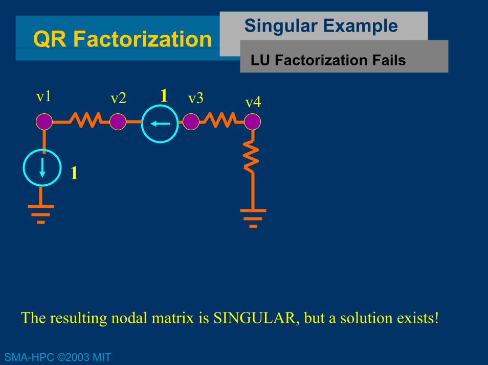
OrthogonalizationQR FactorizationQR Algorithm Key Idea

1 1

2 21 2 N

N N

x bx b

M M M

x bOriginal Matrix

⎡ ⎤ ⎡ ⎤⎡ ⎤↑ ↑ ↑ ⎢ ⎥ ⎢ ⎥⎢ ⎥ ⎢ ⎥ ⎢ ⎥=⎢ ⎥ ⎢ ⎥ ⎢ ⎥⎢ ⎥↓ ↓ ↓ ⎢ ⎥ ⎢ ⎥⎣ ⎦ ⎢ ⎥ ⎢ ⎥⎣ ⎦ ⎣ ⎦

1 1

2 21 2 N

N N

y by b

Q Q Q

y bMatrix withOrthonormalColumns

⎡ ⎤ ⎡ ⎤⎡ ⎤↑ ↑ ↑ ⎢ ⎥ ⎢ ⎥⎢ ⎥ ⎢ ⎥ ⎢ ⎥=⎢ ⎥ ⎢ ⎥ ⎢ ⎥⎢ ⎥↓ ↓ ↓ ⎢ ⎥ ⎢ ⎥⎢ ⎥⎣ ⎦ ⎢ ⎥ ⎢ ⎥⎣ ⎦ ⎣ ⎦

TQy b y Q b= ⇒ =

How to perform the conversion?

SMA-HPC ©2003 MIT

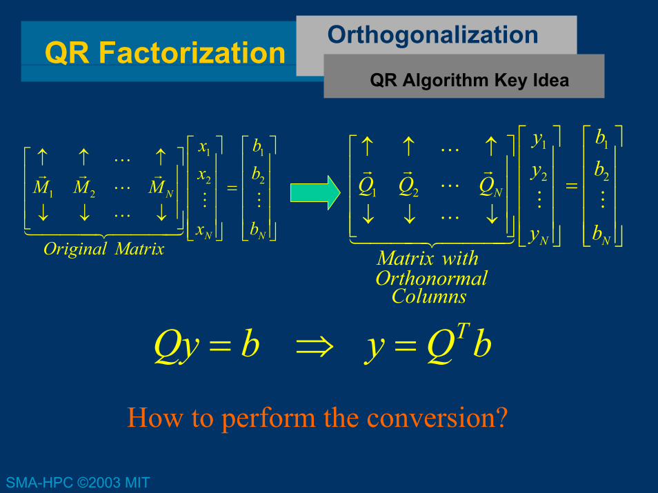
OrthogonalizationQR FactorizationProjection Formula

1 2 2 2 12 1Given , find so that, =M M Q M r M−

( )1 2 1 2 12 1 0 M Q M M r M• = • − =

1 212

1 1

M MrM M

•=

•

2M2Q 1M

12r

SMA-HPC ©2003 MIT

OrthogonalizationQR FactorizationNormalization

1 1 1 1

1 111

1

11 1Q M M Q QM M r

= = ⇒ • =•

Formulas simplify if we normalize

1 2122 2 1=Now find so that 0rQ M Q Q Q− • =

12 1 2r Q M= •

2 2 2

222

2

Fi 1 al 1 n ly r

Q Q QQ Q

= =•

SMA-HPC ©2003 MIT

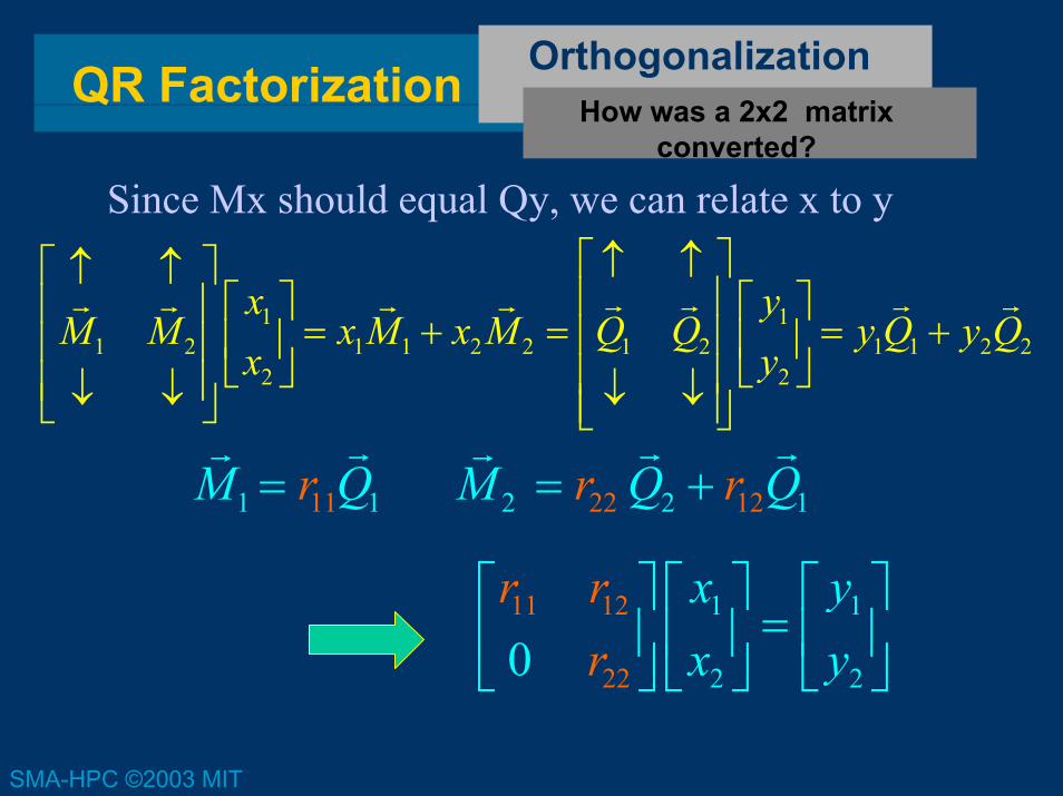
OrthogonalizationQR Factorization How was a 2x2 matrix converted?

1 11 2 1 1 2 2 1 2 1 1 2 2

2 2

x yM M x M x M Q Q y Q y Q

x y

⎡ ⎤↑ ↑⎡ ⎤↑ ↑⎢ ⎥⎡ ⎤ ⎡ ⎤⎢ ⎥ = + = = +⎢ ⎥⎢ ⎥ ⎢ ⎥⎢ ⎥

⎣ ⎦ ⎣ ⎦⎢ ⎥⎢ ⎥↓ ↓ ↓ ↓⎣ ⎦ ⎢ ⎥⎣ ⎦

1 1 2 2 111 22 12M Q M Q Qr r r= = +

Since Mx should equal Qy, we can relate x to y

11 12 1 1

2 2220x yx

r rr y

⎡ ⎤ ⎡ ⎤ ⎡ ⎤=⎢ ⎥ ⎢ ⎥ ⎢ ⎥

⎣ ⎦ ⎣ ⎦ ⎣ ⎦

SMA-HPC ©2003 MIT

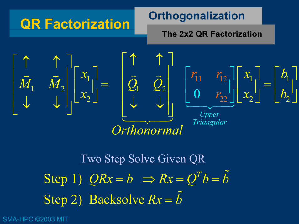
OrthogonalizationQR FactorizationThe 2x2 QR Factorization

1 1 11 2 1 2

2 2 2

11 12

220Upper

Triangular

x x bM M Q Q

x x b

Orthonormal

r rr

⎡ ⎤↑ ↑⎡ ⎤↑ ↑⎢ ⎥⎡ ⎤ ⎡ ⎤ ⎡ ⎤⎢ ⎥ = =⎢ ⎥⎢ ⎥ ⎢ ⎥ ⎢ ⎥⎢ ⎥

⎣ ⎦ ⎣ ⎦ ⎣ ⎦⎢ ⎥⎢ ⎥↓ ↓ ↓ ↓⎣ ⎦ ⎢ ⎥⎣ ⎦

⎡ ⎤⎢ ⎥⎣ ⎦

Two Step Solve Given QR

Step 1) TQRx b Rx Q b b= ⇒ = =

Step 2) Backsolve Rx b=

SMA-HPC ©2003 MIT

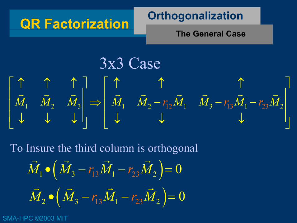
OrthogonalizationQR FactorizationThe General Case

3x3 Case

12 11 2 3 1 2 1 3 3 231 2rM M M M M M M rMr M⎡ ⎤ ⎡ ⎤↑ ↑ ↑ ↑ ↑ ↑⎢ ⎥ ⎢ ⎥⇒ − − −⎢ ⎥ ⎢ ⎥⎢ ⎥ ⎢ ⎥↓ ↓ ↓ ↓ ↓ ↓⎣ ⎦ ⎣ ⎦

( )13 21 3 1 23 0M M M Mr r• − − =

(

To Insure the third column is orthogonal

)13 22 3 1 23 0M M M Mr r• − − =

SMA-HPC ©2003 MIT

OrthogonalizationQR Factorization Must Solve Equations for Coefficients in 3x3 Case

( )13 21 3 1 23 0M M M Mr r• − − =

( )13 22 3 1 23 0M M M Mr r• − − =

1 31 1 1 2

2 32

1

1 2

3

232

M MM M M MM MM M M

rM r

⎡ ⎤⎡ ⎤ ⎡ ⎤ •• •= ⎢ ⎥⎢ ⎥ ⎢ ⎥ •• • ⎣ ⎦⎣ ⎦ ⎣ ⎦

SMA-HPC ©2003 MIT

OrthogonalizationQR Factorization Must Solve Equations for Coefficients

To Orthogonalize the Nth Vector

1,1 1 1 1 1

1 1 ,1 1 11

N N

N N N N N

N

N N

M M M M M M

M M M M M M

r

r

−

− − − −−

⎡ ⎤ ⎡ ⎤⎡ ⎤• • •⎢ ⎥ ⎢ ⎥⎢ ⎥ =⎢ ⎥ ⎢ ⎥⎢ ⎥⎢ ⎥ ⎢ ⎥⎢ ⎥• • •⎣ ⎦⎣ ⎦ ⎣ ⎦

2 3 inner products requires workN N

SMA-HPC ©2003 MIT

OrthogonalizationQR Factorization Use previously orthogonalized vectors

11 2 3 2 13 21 3 1 232 1M M M M M Q M Q Qr r r

⎡ ⎤↑ ↑ ↑⎡ ⎤↑ ↑ ↑⎢ ⎥⎢ ⎥ ⇒ − − −⎢ ⎥⎢ ⎥⎢ ⎥⎢ ⎥↓ ↓ ↓ ↓ ↓ ↓⎣ ⎦ ⎢ ⎥⎣ ⎦

3x3 Case

( )1 3 1 213 23 13 1 30Q M Q Q Mr Qr r• − − = ⇒ = •

To Insure the third column is orthogonal

( )2 3 1 213 23 23 2 30Q M Q Q Mr Qr r• − − = ⇒ = •

SMA-HPC ©2003 MIT

QR Factorization“Modified Gram-Schmidt”

Basic Algorithm

For i = 1 to N “For each Source Column”

For j = i+1 to N { “For each target Column right of source”

1

ii i

irQ M=

jij iMr Q← •

iii iMr M•=Normalize

j jj i iM M Qr⇐ −

2

1

2 2 operationsN

i

N N=

≈∑

3

1

( )2 operationsN

i

N i N N=

− ≈∑

SMA-HPC ©2003 MIT

QR Factorization“By Picture”

Basic Algorithm

1 2 3 NQ Q Q Q

⎡ ⎤↑ ↑ ↑ ↑⎢ ⎥⎢ ⎥⎢ ⎥↓ ↓ ↓ ↓⎢ ⎥⎣ ⎦

11 12 13 1

22 23 2

33 3

00 0

0 0 0

N

N

N

NN

r r r rr r r

r r

r

⎡ ⎤⎢ ⎥⎢ ⎥⎢ ⎥⎢ ⎥⎢ ⎥⎢ ⎥⎣ ⎦

SMA-HPC ©2003 MIT

QR Factorization“By Picture”

Basic Algorithm

4M↑

↓3M

↑

↓2M

↑

↓1M

↑

↓1Q

↑

↓2Q

↑

↓3Q

↑

↓4Q

↑

↓

11r 12 13 14r r r

22r 23 24r r

33r

44r34r

SMA-HPC ©2003 MIT

QR FactorizationZero Column

Basic Algorithm

1 3

0

00

NMQ M

⎡ ⎤↑ ↑⎢ ⎥⎢ ⎥⎢ ⎥↓ ↓⎢ ⎥⎣↓

⎦

↑What if a Column becomes Zero?

11 12 13 1

0 0 0 00 0 0 0

Nr r r r⎡ ⎤⎢ ⎥⎢ ⎥⎢ ⎥⎣ ⎦

Matrix MUST BE Singular!

1) Do not try to normalize the column.2) Do not use the column as a source for orthogonalization.3) Perform backward substitution as well as possible

SMA-HPC ©2003 MIT

QR FactorizationZero Column Continued

Basic Algorithm

Resulting QR Factorization

1 3

0

00

NQ Q Q

↑ ↑ ↑

↓

⎡ ⎤⎢ ⎥⎢ ⎥⎢ ⎥⎢ ⎥⎣ ⎦↓ ↓

11 12 13 1

33 3

0 0 0 00 00 0 00 0 0

N

N

NN

r r r r

r r

r

⎡ ⎤⎢ ⎥⎢ ⎥⎢ ⎥⎢ ⎥⎢ ⎥⎢ ⎥⎣ ⎦

SMA-HPC ©2003 MIT

Singular ExampleQR FactorizationRecall weighted sum of columns view of

systems of equations

1 1

2 21 2 N

N N

x bx b

M M M

x b

⎡ ⎤ ⎡ ⎤⎡ ⎤↑ ↑ ↑ ⎢ ⎥ ⎢ ⎥⎢ ⎥ ⎢ ⎥ ⎢ ⎥=⎢ ⎥ ⎢ ⎥ ⎢ ⎥⎢ ⎥↓ ↓ ↓ ⎢ ⎥ ⎢ ⎥⎣ ⎦ ⎣ ⎦ ⎣ ⎦

1 1 2 2 N Nx M x M x M b+ + + =

1 1Case 1) { ,.., } { ,.., }N Nb span M M b span Q Q∈ ⇒ ∈

Two Cases when M is singular

1Case 2) { ,.., }, How accurate is ?Nb span M M x∉

SMA-HPC ©2003 MIT

QR FactorizationAlternative Formulations

Minimization View

( )Definition of the Residual R: R x b Mx≡ −

Find x which satisfiesMx b=

( ) ( ) ( )( )2

1

Minimize over all xN

Ti

iR x R x R x

=

= ∑

( ){ }Equivalent if b span cols M∈

( ) ( ) and min 0TMx b R x R xx⇒ = =

Minimization extends to non-singular or nonsquare case!

SMA-HPC ©2003 MIT

QR FactorizationOne-dimensional

Minimization

Minimization View

1 1 1 1 1 1Suppose and therefo rex x e Mx x Me x M= = =

( ) ( ) ( ) ( )1 1 1 1T TR x R x b x Me b x Me= − −

One dimensional Minimization

( ) ( )21 1 1 1 12 TT Tb b x b Me x Me Me= − +

( ) ( ) ( ) ( )1 1 1 12 2 0T TTd b Me x MR x R Mxx

e ed

= − + =

11

1 1

T

T T

b Mexe M Me

=Normalization

SMA-HPC ©2003 MIT

QR FactorizationOne-dimensional

Minimization, Picture

Minimization View

1 1Me M=

b

1e

1x 11

1 1

T

T T

b Mexe M Me

=

One dimensional minimization yields same result as projection on the column!

SMA-HPC ©2003 MIT

QR FactorizationTwo-dimensional

Minimization

Minimization View

1 1 2 2 1 1 2 2Now and x x e x e Mx x Me x Me= + = +

Residual Minimization

( ) ( ) ( ) ( )1 1 2 2 1 1 2 2T TR x R x b x Me x Me b x Me x Me= − − − −

( ) ( )21 1 1 1 12 TT Tx b Me xb eb Me M= − +

( ) ( )22 2 2 2 22 TTx b Me x Me Me− +

( ) ( )1 2 1 22 Tx x Me Me+CouplingTerm

SMA-HPC ©2003 MIT

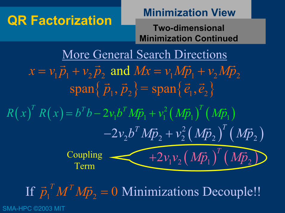
QR FactorizationTwo-dimensional

Minimization Continued

Minimization View

1 1 2 2 1 1 2 2and x v p v p Mx v Mp v Mp= + = +

( ) ( ) ( ) ( )21 1 1 1 12 TTT TR x R x b v b Mp v Mp Mb p− +=

More General Search Directions

( ) ( )22 2 2 2 22 TTv b Mp v Mp Mp− +

( ) ( )1 2 1 22 Tv v Mp Mp+

{ } { }1 2 1 2 span , = span ,p p e e

CouplingTerm

1 2If Minimization 0 s D ecouple!!T Tp M Mp =

SMA-HPC ©2003 MIT

QR FactorizationForming MTM orthogonal Minimization Directions

Minimization View

ith search direction equals MTM orthogonalized unit vector1

10

iT T

i i ji j i jj

p e r p p M Mp−

=

= − =∑Use previous orthogonalized

Search directions

( ) ( )( ) ( )

T

j iji T

j j

Mp Mer

Mp Mp⇒ =

SMA-HPC ©2003 MIT

QR FactorizationMinimizing in the Search

Direction

Minimization View

Decoupled minimizations done individually

( ) ( )2Minimize: 2T Ti i i i iv Mp Mp v b Mp−

( ) ( )Differentiating 2 0 2: T Ti i i iv Mp Mp b Mp− =

( ) ( )

Ti

i Ti i

b MpvMp Mp

⇒ =

SMA-HPC ©2003 MIT

QR FactorizationMinimization Algorithm

Minimization View

For i = 1 to N “For each Target Column”

For j = 1 to i-1 “For each Source Column left of target”

1

ii i

irp p⇐

iii iMpr Mp•=Normalize search direction

i ix x v p= +

i ip e=

Tjj

Tiir p M Mp←

i ji i jp p pr⇐ −Orthogonalize Search Direction

SMA-HPC ©2003 MIT

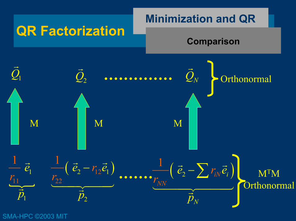
QR FactorizationComparison

Minimization and QR

1

1

11

1 e

pr

( )2 11222

2

1 e er

p

r− ( )21

iN

N

iNN

rr

e e

p

−∑

1Q NQ2Q Orthonormal

M M M

MTMOrthonormal

SMA-HPC ©2003 MIT

QR FactorizationSearch Direction

{ }1 2 , , , Unit Vectors

Ne e e…Orthogonalized unit vectors search directions

{ }1 , , Search Directions

Np p…MTM

Orthogonalization

{ }2 , , ,

Krylov-Subspace

b Mb M b…Could use other sets of starting vectors

{ }1, , Search Directions

Np p…MTM

Orthogonalization

Why?

SMA-HPC ©2003 MIT

Summary

• QR Algorithm– Projection Formulas– Orthonormalizing the columns as you go– Modified Gram-Schmidt Algorithm

• QR and Singular Matrices– Matrix is singular, column of Q is zero.

• Minimization View of QR– Basic Minimization approach– Orthogonalized Search Directions– QR and Length minimization produce identical results

• Mentioned changing the search directions