1

Jack Simons, Henry Eyring Scientist and ProfessorChemistry Department

University of Utah

Electronic Structure Electronic Structure TheoryTheory

Session 12Session 12

2

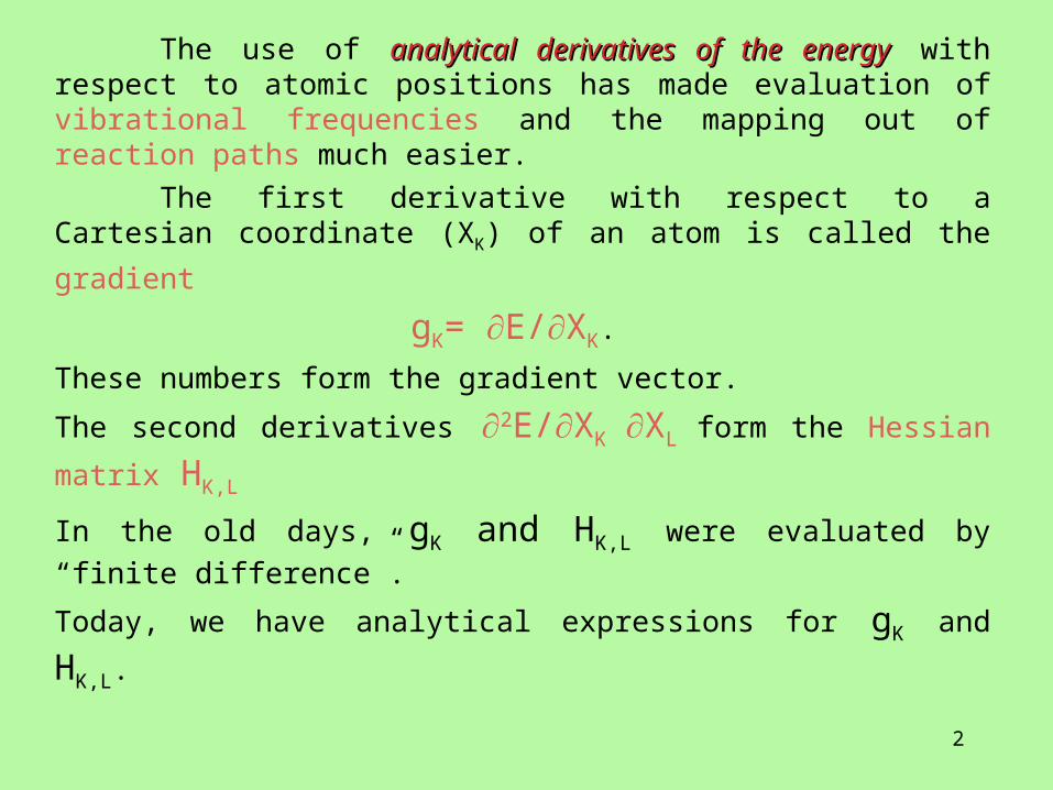
The use of analytical derivatives of the energyanalytical derivatives of the energy with respect to atomic positions has made evaluation of vibrational frequencies and the mapping out of reaction paths much easier.

The first derivative with respect to a Cartesian coordinate (XK) of an

atom is called the gradient

gK= E/XK.

These numbers form the gradient vector.

The second derivatives 2E/XK XL form the Hessian matrix HK,L

In the old days, gK and HK,L were evaluated by “finite difference”.

Today, we have analytical expressions for gK and HK,L.

3

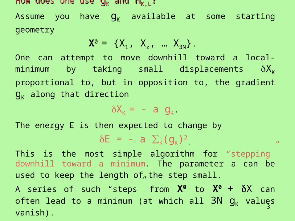
How does one useHow does one use g gKK and and H HK,LK,L??

Assume you have gK available at some starting geometry

X0 = {X1, Xz, … X3N}.

One can attempt to move downhill toward a local-minimum by taking small

displacements XK proportional to, but in opposition to, the gradient gK along that direction

XK = - a gK.

The energy E is then expected to change by

E = - a ∑K(gK)2.

This is the most simple algorithm for “stepping” downhill toward a minimum.

The parameter a can be used to keep the length of the step small.

A series of such “steps” from X0 to X0 + X can often lead to a minimum (at

which all 3N gK values vanish).

4

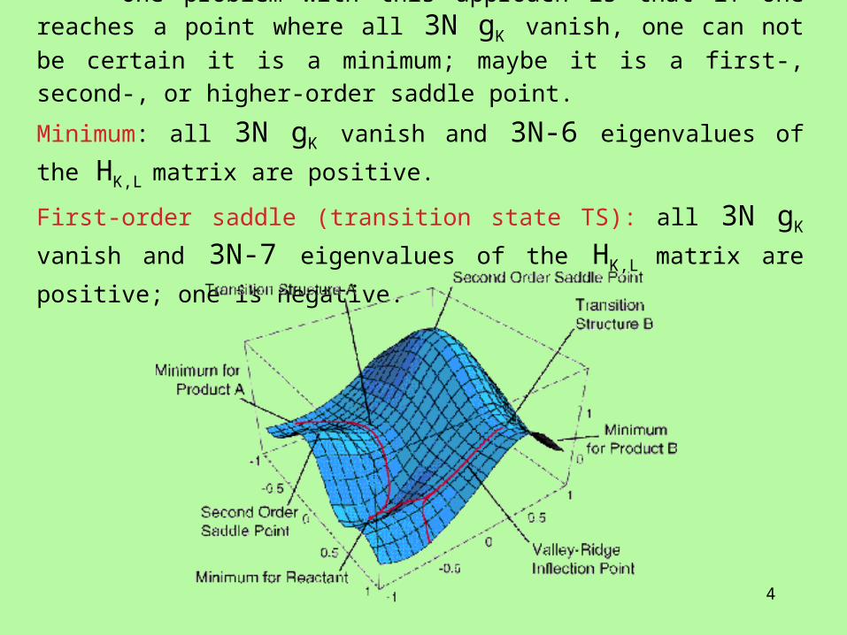
One problem with this approach is that if one reaches a point where all 3N gK vanish, one can not be certain it is a minimum; maybe it is a first-,

second-, or higher-order saddle point.

Minimum: all 3N gK vanish and 3N-6 eigenvalues of the HK,L matrix are

positive.

First-order saddle (transition state TS): all 3N gK vanish and 3N-7 eigenvalues

of the HK,L matrix are positive; one is negative.

5

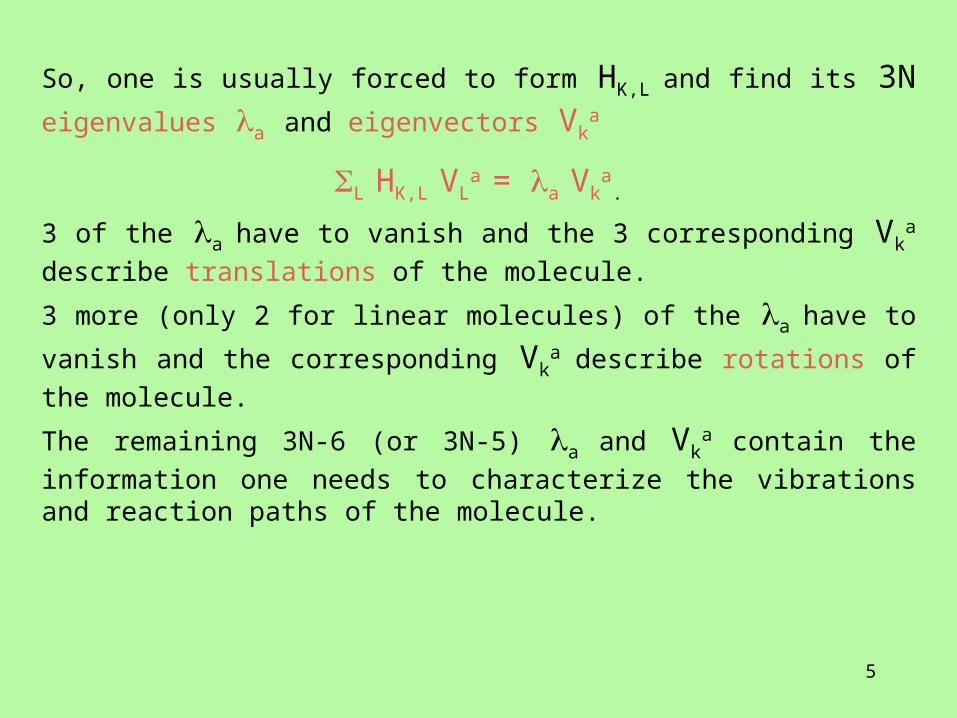
So, one is usually forced to form HK,L and find its 3N eigenvalues a and

eigenvectors Vka

L HK,L VLa = a Vk

a.

3 of the a have to vanish and the 3 corresponding Vka describe translations of

the molecule.

3 more (only 2 for linear molecules) of the a have to vanish and the

corresponding Vka describe rotations of the molecule.

The remaining 3N-6 (or 3N-5) a and Vka contain the information one needs to

characterize the vibrations and reaction paths of the molecule.

6

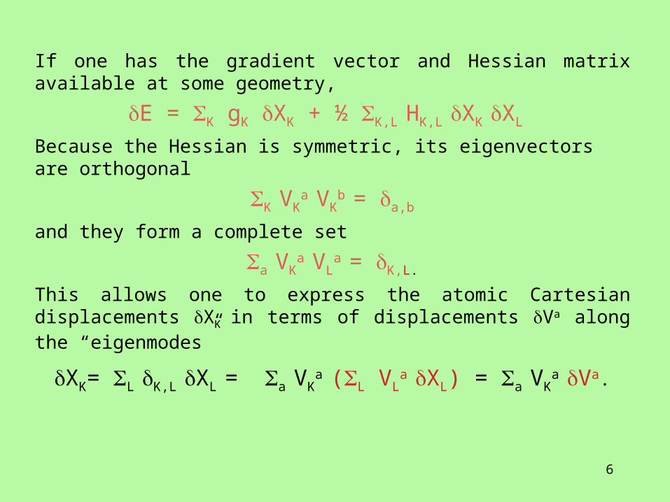
If one has the gradient vector and Hessian matrix available at some geometry,

E = K gK XK + ½ K,L HK,L XK XL

Because the Hessian is symmetric, its eigenvectors are orthogonal

K VKa VK

b = a,b

and they form a complete set

a VKa VL

a = K,L.

This allows one to express the atomic Cartesian displacements XK in terms of displacements Va along the “eigenmodes”

XK= L K,L XL = a VKa (L VL

a XL) = a VKa Va.

7

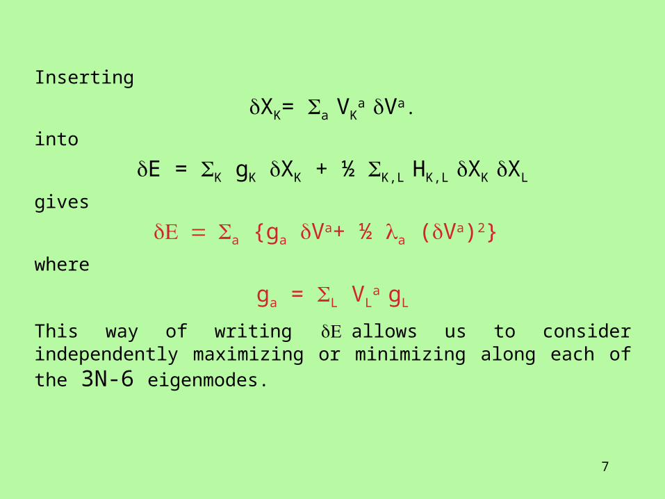
Inserting

XK= a VKa Va.

into

E = K gK XK + ½ K,L HK,L XK XL

gives

a {ga Va+ ½ a (Va)2}

where

ga = L VLa gL

This way of writing allows us to consider independently maximizing or

minimizing along each of the 3N-6 eigenmodes.

8

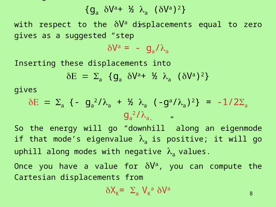
Setting the derivative of

{ga Va+ ½ a (Va)2}

with respect to the Va displacements equal to zero gives as a suggested “step”

Va = - ga/a

Inserting these displacements into

a {ga Va+ ½ a (Va)2}

gives

a{- ga2/a + ½ a (-ga/a)2} = -1/2a ga

2/a.

So the energy will go “downhill” along an eigenmode if that mode’s eigenvalue a is positive; it will go uphill along modes with negative a values.

Once you have a value for Va, you can compute the Cartesian displacements

from

XK= a VKa Va

9

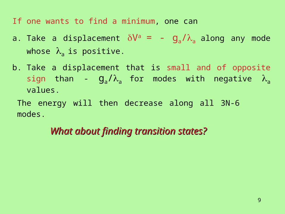
If one wants to find a minimum, one can

a. Take a displacement Va = - ga/a along any mode whose a is positive.

b. Take a displacement that is small and of opposite sign than - ga/a for

modes with negative a values.

The energy will then decrease along all 3N-6 modes.

What about finding transition states?What about finding transition states?

10

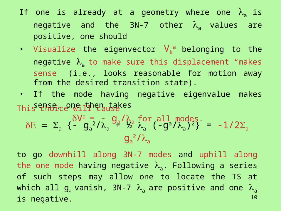
If one is already at a geometry where one a is negative and the 3N-7 other

a values are positive, one should

• Visualize the eigenvector Vka belonging to the negative a to make sure

this displacement “makes sense” (i.e., looks reasonable for motion away from the desired transition state).

• If the mode having negative eigenvalue makes sense, one then takes

Va = - ga/a for all modes.

This choice will cause

a{- ga2/a + ½ a (-ga/a)2} = -1/2a ga

2/a

to go downhill along 3N-7 modes and uphill along the one mode having

negative a. Following a series of such steps may allow one to locate the TS

at which all ga vanish, 3N-7 a are positive and one a is negative.

11

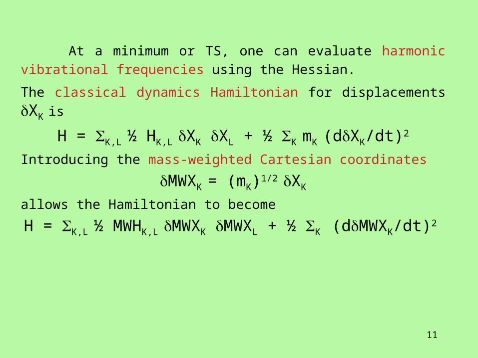
At a minimum or TS, one can evaluate harmonic vibrational

frequencies using the Hessian.

The classical dynamics Hamiltonian for displacements XK is

H = K,L ½ HK,L XK XL + ½ K mK (dXK/dt)2

Introducing the mass-weighted Cartesian coordinates

MWXK = (mK)1/2 XK

allows the Hamiltonian to become

H = K,L ½ MWHK,L MWXK MWXL + ½ K (dMWXK/dt)2

12

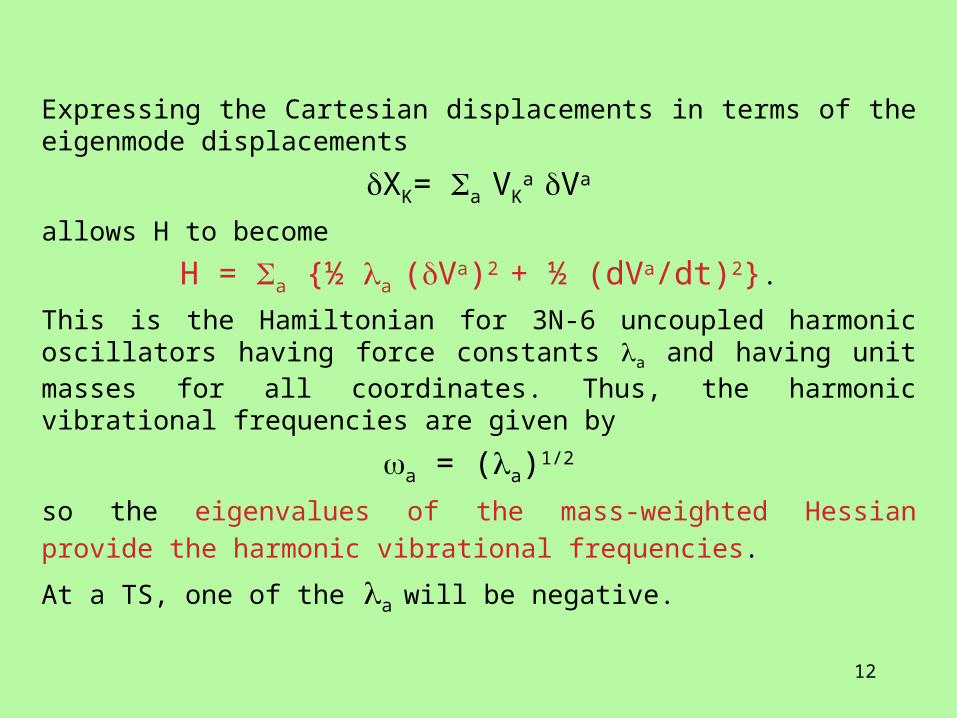
Expressing the Cartesian displacements in terms of the eigenmode displacements

XK= a VKa Va

allows H to become

H = a {½ a (Va)2 + ½ (dVa/dt)2}.

This is the Hamiltonian for 3N-6 uncoupled harmonic oscillators having force constants a and having unit masses for all coordinates. Thus, the harmonic vibrational frequencies are given by

a = (a)1/2

so the eigenvalues of the mass-weighted Hessian provide the harmonic

vibrational frequencies.

At a TS, one of the a will be negative.

13

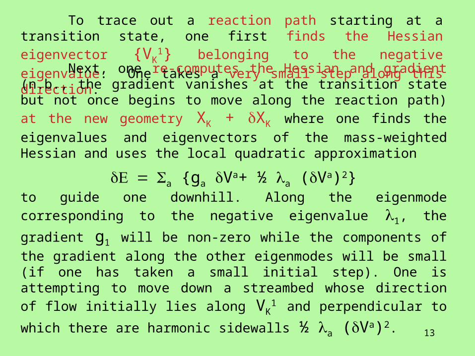
To trace out a reaction path starting at a transition state, one first finds

the Hessian eigenvector {VK1} belonging to the negative eigenvalue. One

takes a very small step along this direction.

Next, one re-computes the Hessian and gradient (n.b., the gradient vanishes at the transition state but not once begins to move along the reaction

path) at the new geometry XK + XK where one finds the eigenvalues and

eigenvectors of the mass-weighted Hessian and uses the local quadratic approximation

a {ga Va+ ½ a (Va)2}to guide one downhill. Along the eigenmode corresponding to the negative

eigenvalue 1, the gradient g1 will be non-zero while the components of the

gradient along the other eigenmodes will be small (if one has taken a small initial step). One is attempting to move down a streambed whose direction of

flow initially lies along VK1 and perpendicular to which there are harmonic

sidewalls ½ a (Va)2.

14

One performs a series of displacements by

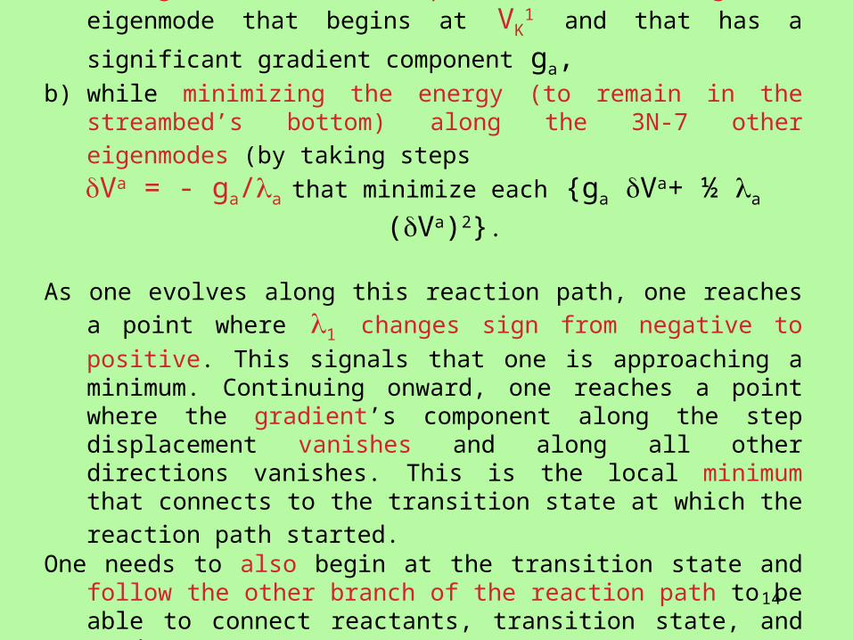
a) moving (in small steps) downhill along the eigenmode that begins at VK1

and that has a significant gradient component ga, b) while minimizing the energy (to remain in the streambed’s bottom) along

the 3N-7 other eigenmodes (by taking steps Va = - ga/a that minimize each {ga Va+ ½ a (Va)2}.

As one evolves along this reaction path, one reaches a point where 1 changes

sign from negative to positive. This signals that one is approaching a minimum. Continuing onward, one reaches a point where the gradient’s component along the step displacement vanishes and along all other directions vanishes. This is the local minimum that connects to the

transition state at which the reaction path started. One needs to also begin at the transition state and follow the other branch of

the reaction path to be able to connect reactants, transition state, and products.

15

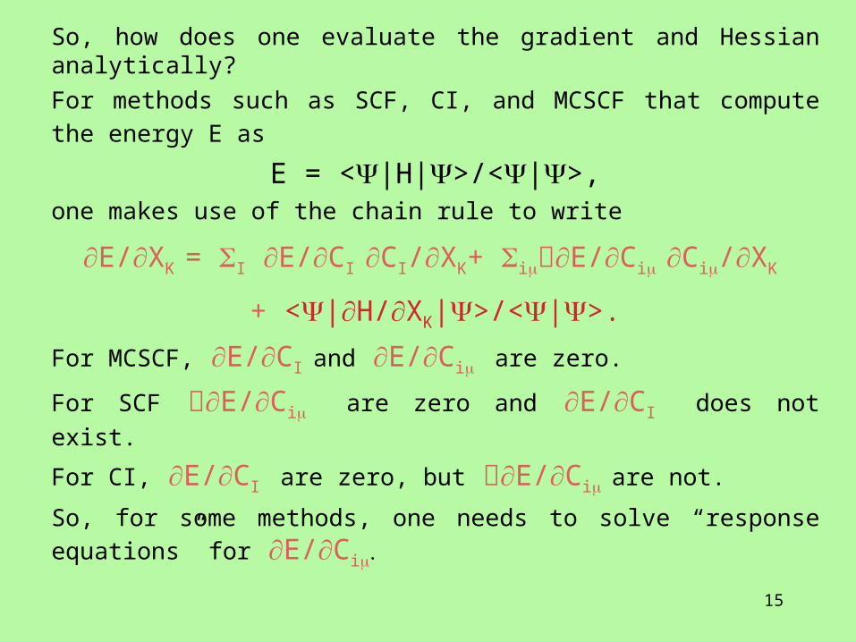
So, how does one evaluate the gradient and Hessian analytically?

For methods such as SCF, CI, and MCSCF that compute the energy E as

E = <|H|>/<|>,one makes use of the chain rule to write

E/XK = I E/CI CI/XK+ iE/Ci Ci/XK

+ <|H/XK|>/<|>.

For MCSCF, E/CI and E/Ci are zero.

For SCF E/Ci are zero and E/CI does not exist.

For CI, E/CI are zero, but E/Ci are not.

So, for some methods, one needs to solve “response equations” for E/Ci

16

What is <|H/XK|>/<|>?

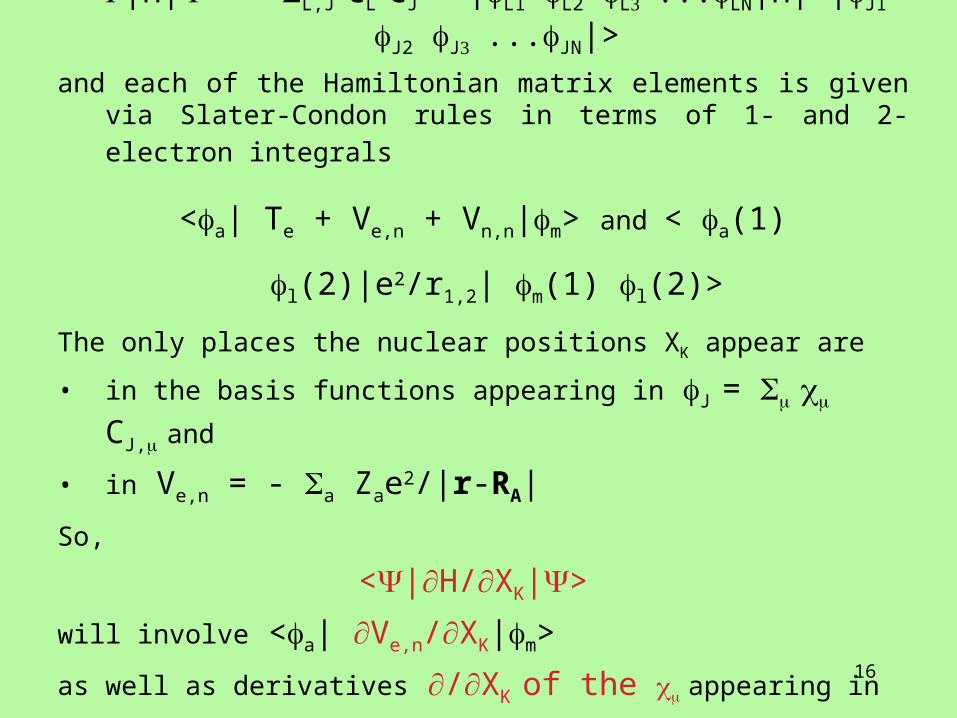
<|H|> = L,J CL CJ < |L1 L2 L...LN|H| |J1 J2 J...JN|>

and each of the Hamiltonian matrix elements is given via Slater-Condon rules

in terms of 1- and 2- electron integrals

<a| Te + Ve,n + Vn,n|m> and < a(1) l(2)|e2/r1,2| m(1) l(2)>

The only places the nuclear positions XK appear are

• in the basis functions appearing in J = CJ,and

• in Ve,n = - a Zae2/|r-RA|

So,

<|H/XK|>

will involve <a| Ve,n/XK|m>

as well as derivatives /XK of the appearing in

<a| Te + Ve,n + Vn,n|m> and in < a(1) l(2)|e2/r1,2| m(1) l(2)>

17

/XA Ve,n = - a Za (x-XA) e2/|r-RA|3

When put back into <a| Ve,n/XK|m> and into the Slater-Condon

formulas, these terms give the Hellmann-Feynman contributions to the gradient. These are not “difficult” integrals, but they are new ones that need to be added to the usual 1- electron integrals.

The /XK derivatives of the appearing in

<| –2/2m 2 |> + a<| -Zae2/|ra |> and in

<(r) (r’) |(e2/|r-r’|) | (r) (r’)>

present major new difficulties because they involve new integrals

< /XK | –2/2m 2 |> + a< /XK | -Zae2/|ra |>

< /XK (r) (r’) |(e2/|r-r’|) | (r) (r’)>

18

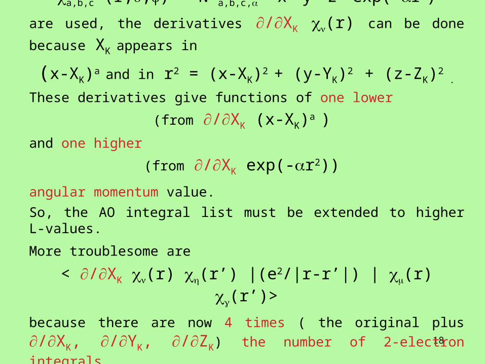
When Cartesian Gaussians

a,b,c (r,,) = N'a,b,c, xa yb zc exp(-r2)

are used, the derivatives /XK (r) can be done because XK appears in

(x-XK)a and in r2 = (x-XK)2 + (y-YK)2 + (z-ZK)2 .

These derivatives give functions of one lower

(from /XK (x-XK)a )

and one higher

(from /XK exp(-r2))

angular momentum value. So, the AO integral list must be extended to higher L-values.

More troublesome are

< /XK (r) (r’) |(e2/|r-r’|) | (r) (r’)>

because there are now 4 times ( the original plus /XK, /YK, /ZK) the

number of 2-electron integrals.

19

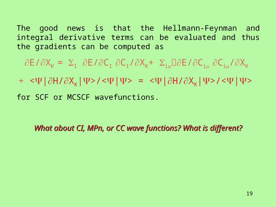
The good news is that the Hellmann-Feynman and integral derivative terms can be evaluated and thus the gradients can be computed as

E/XK = I E/CI CI/XK+ iE/Ci Ci/XK

+ <|H/XK|>/<|> = <|H/XK|>/<|>

for SCF or MCSCF wavefunctions.

What about CI, MPn, or CC wave functions? What is different?What about CI, MPn, or CC wave functions? What is different?

20

E/XK = I E/CI CI/XK+ iE/Ci Ci/XK

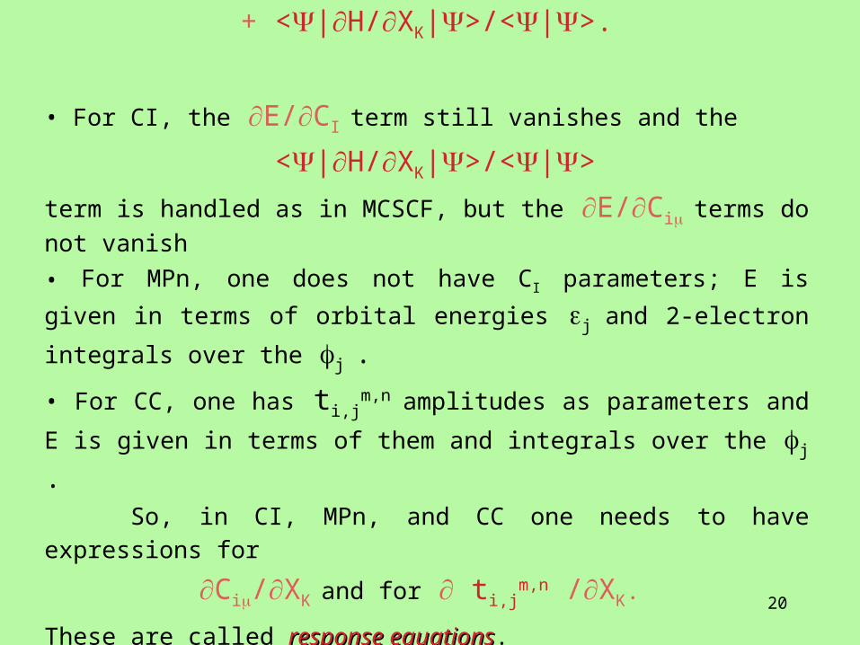
+ <|H/XK|>/<|>.

• For CI, the E/CI term still vanishes and the

<|H/XK|>/<|>

term is handled as in MCSCF, but the E/Ci terms do not vanish

• For MPn, one does not have CI parameters; E is given in terms of orbital

energies j and 2-electron integrals over the j .

• For CC, one has ti,jm,n amplitudes as parameters and E is given in terms of

them and integrals over the j .

So, in CI, MPn, and CC one needs to have expressions for

Ci/XK and for ti,jm,n /XK.

These are called response equationsresponse equations.

21

The response equations for Ci/XK are obtained by taking the /XK

derivative of the Fock equations that determined the Ci,

/XK |he| > CJ, = /XK J <|> CJ,

This gives

[ |he| >- J<|>] /XK CJ,

/XK[ |he| >- J <|>] CJ,

Because all the machinery to evaluate the terms in

/XK[ |he| >- J <|>]

exists as does the matrix

|he| >- J<|>,

one can solve for /XK CJ,

22

A similar, but more complicated strategy can be used to derive

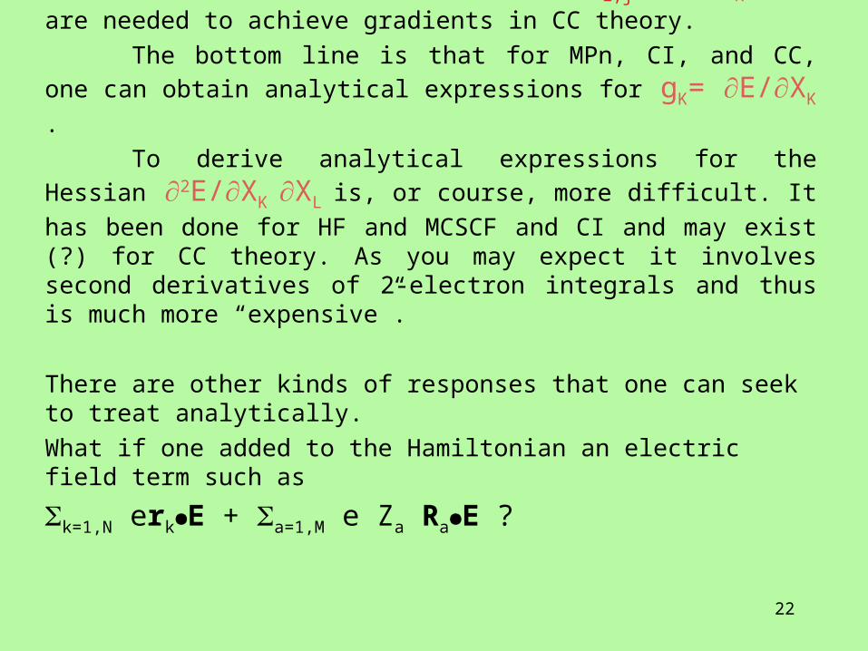
equations for the ti,jm,n /XK that are needed to achieve gradients in CC

theory.

The bottom line is that for MPn, CI, and CC, one can obtain analytical

expressions for gK= E/XK .

To derive analytical expressions for the Hessian 2E/XK XL is, or

course, more difficult. It has been done for HF and MCSCF and CI and may exist (?) for CC theory. As you may expect it involves second derivatives of 2-electron integrals and thus is much more “expensive”.

There are other kinds of responses that one can seek to treat analytically.

What if one added to the Hamiltonian an electric field term such as

k=1,N erkE + a=1,M e Za RaE ?

23

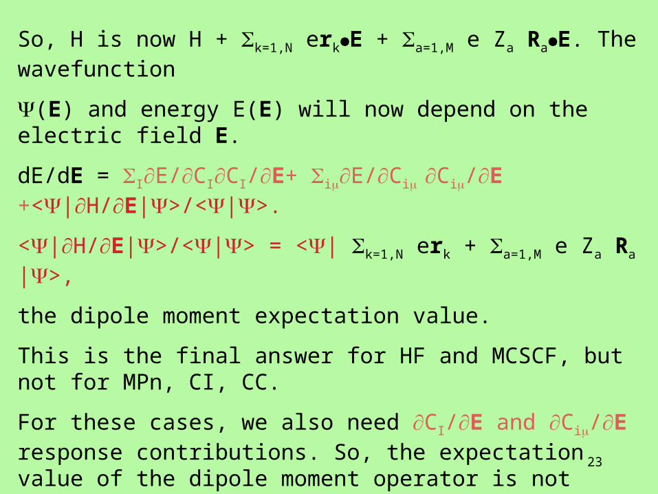
So, H is now H + k=1,N erkE + a=1,M e Za RaE. The wavefunction

(E) and energy E(E) will now depend on the electric field E.

dE/dE = IE/CICI/E+ iE/Ci Ci/E +<|H/E|>/<|>.

<|H/E|>/<|> = <| k=1,N erk + a=1,M e Za Ra |>,

the dipole moment expectation value.

This is the final answer for HF and MCSCF, but not for MPn, CI, CC.

For these cases, we also need CI/E and Ci/E response contributions. So, the expectation value of the dipole moment operator is not always the correct dipole moment!