REAR-INFLOW STRUCTURE IN SEVERE AND NON-SEVERE BOW-ECHOES

OBSERVED BY AIRBORNE DOPPLER RADAR DURING BAMEX

David P. Jorgensen*

NOAA/National Severe Storms Laboratory Norman, Oklahoma

Hanne V. Murphey and Roger M. Wakimoto

University of California, Los Angeles Los Angeles, California

1. INTRODUCTION

Bow-echoes have been of scientific and operational interest since Fujita (1978) showed their structure in relation to surface wind damage. The Bow-Echo and Mesoscale Convective Vortex Experiment (BAMEX) focused on bow-echoes, using highly mobile platforms, in the Midwest U.S. The field exercise ran during the late spring/early summer of 2003 from a main base of operations at MidAmerica Airport near St. Louis, MO. BAMEX has two principal foci: 1) improve understanding and improve prediction of bow echoes, principally those which produce damaging surface winds and last at least 4 hours and (2) document the mesoscale processes which produce long lived mesoscale convective vortices (MCVs). More information concerning the science objectives and the observational strategies of BAMEX are contained in the scientific overview document: http://www.mmm.ucar.edu/bamex/science.html. A more complete description of the BAMEX IOPs, including data set availability, can be found on the University Corporation for Atmospheric Research/Joint Office for Science Support (UCAR/JOSS) projects catalog web site: http://www.joss.ucar.edu/bamex/catalog/.

Two principal ideas have been advanced to explain the source of strong surface winds associated with the passage of bow-echoes (e.g., Przybylinski, 1995; Atkins et al. 2005). One idea involves the descent of the rear-inflow jet (Weisman 1993), the other concerns the relationship between damage patterns with the development of strong low-level mesovortices near the apex of the bow or just to the north of the apex (Weisman and Trapp 2003). In the Weisman and Trapp (2003) simulations of bow-shaped mesoscale features, the intense low- level winds

*Corresponding author address: David P. Jorgensen, NOAA/National Severe Storms Laboratory, Norman, OK 73069; e-mail: David.P.Jorgensen@noaa.gov.

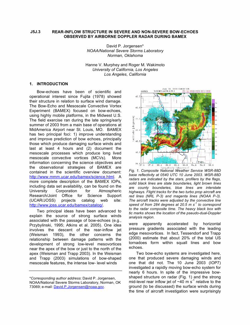
Fig. 1. Composite National Weather Service WSR-88D base reflectivity at 0540 UTC 10 June 2003. WSR-88D radars are indicated by the stars, profilers by the flags, solid black lines are state boundaries, light brown lines

are county boundaries, blue lines are interstate highways. Flight tracks for the two turbo prop aircraft are red lines (NRL P-3) and magenta lines (NOAA P-3). The aircraft tracks were adjusted by the convective line speed of from 284 degrees at 20.5 m s

-1 to correspond

to the radar composite time. The heavy black box with tic marks shows the location of the pseudo-dual-Doppler analysis region.

were apparently accelerated by horizontal pressure gradients associated with the leading edge mesovortices. In fact, Tessendorf and Trapp (2000) estimate that about 20% of the total US tornadoes form within squall lines and bow echoes.

Two bow-echo systems are investigated here, one that produced severe damaging winds and one that did not. The 10 June 2003 (IOP7) investigated a rapidly moving bow-echo system for nearly 6 hours. In spite of the impressive bow-shaped structure on radar (Fig. 1) and the strong mid-level rear inflow jet of ~40 m s

-1 relative to the

ground (to be discussed) the surface winds during the time of aircraft investigation were surprisingly

J5J.3

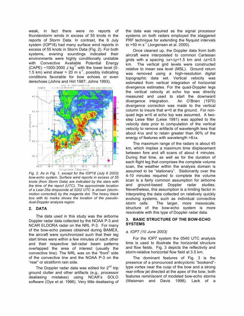
weak, in fact there were no reports of thunderstorm winds in excess of 55 knots in the reports of Storm Data. In contrast, the 6 July system (IOP18) had many surface wind reports in excess of 55 knots in Storm Data (Fig. 2). For both systems, evening soundings indicated their environments were highly conditionally unstable with Convective Available Potential Energy (CAPE) ~1000-3000 J kg

-1 with the lower level (0-

1.5 km) wind shear > 20 m s-1

, possibly indicating conditions favorable for bow echoes or even derechoes (Johns and Hirt 1987; Johns 1993).

Fig. 2. As in Fig. 1, except for the IOP18 (July 6 2003) bow-echo system. Surface wind reports in excess of 55

knots (from Storm Data) are indicated by the stars with the time of the report (UTC). The approximate location of a Lear-35a dropsonde at 0202 UTC is shown (storm-motion corrected) by the magenta dot. The heavy black box with tic marks shows the location of the pseudo-dual-Doppler analysis region.

2. DATA

The data used in this study was the airborne Doppler radar data collected by the NOAA P-3 and NCAR ELDORA radar on the NRL P-3. For many of the bow-echo passes obtained during BAMEX, the aircraft were synchronized such that their leg start times were within a few minutes of each other and their respective tail-radar beam patterns overlapped the area of interest (usually the convective line). The NRL was on the “front” side of the convective line and the NOAA P-3 on the “rear” or stratiform rain side.

The Doppler radar data was edited for 2nd

trip ground clutter and other artifacts (e.g., processor dealiasing mistakes) using NCAR’s SOLO software (Oye et al. 1996). Very little dealiasing of

the data was required as the signal processor systems on both radars employed the staggered PRF technique for extending the Nyquist intervals to >50 m s

-1 (Jorgensen et al. 2000).

Once cleaned up, the Doppler data from both aircraft were interpolated to common Cartesian grids with a spacing !x=!y=1.5 km and !z=0.5 km. The vertical grid levels were constructed relative to mean sea level (MSL). Ground return was removed using a high-resolution digital topographic data set. Vertical velocity was estimated from vertical integration of horizontal divergence estimates. For the quad-Doppler legs the vertical velocity at echo top was directly measured and used to start the downward divergence integration. An O’Brien (1970) divergence correction was made to the vertical column to insure that w=0 at the ground. For non-quad legs w=0 at echo top was assumed. A two-step Leise filter (Leise 1981) was applied to the velocity data prior to computation of the vertical velocity to remove artifacts of wavelength less that about 4!x and to retain greater than 90% of the energy of features with wavelength >8!x.

The maximum range of the radars is about 45 km, which implies a maximum time displacement between fore and aft scans of about 4 minutes. During that time, as well as for the duration of each flight leg that comprises the complete volume scan, the weather within the analysis domain is assumed to be “stationary”. Stationarity over the 4-10 minutes required to complete the volume scan is a fairly common assumption for airborne and ground-based Doppler radar studies. Nevertheless, this assumption is a limiting factor in interpreting the data collected on relatively quickly evolving systems, such as individual convective storm cells. The larger, more mesoscale, structure of the bow-echo system is more resolvable with this type of Doppler radar data.

3. BASIC STRUCTURE OF THE BOW-ECHO

SYSTEMS

a. IOP7 (10 June 2003)

For the IOP7 system the 0540 UTC analysis time is used to illustrate the horizontal structure and flow fields. Fig. 3 depicts the reflectivity and storm-relative horizontal flow field at 3.5 km.

The dominant features of Fig. 3 is the presence of a pronounced anticyclonic “bookend”-type vortex near the cusp of the bow and a strong rear-inflow jet directed at the apex of the bow, both features reminiscent of modeled bow-echo storms (Weisman and Davis 1998). Lack of a

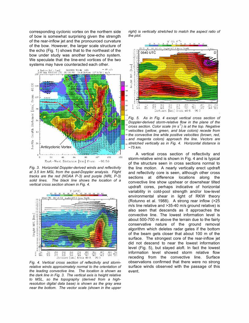
corresponding cyclonic vortex on the northern side of bow is somewhat surprising given the strength of the rear-inflow jet and the pronounced curvature of the bow. However, the larger scale structure of the echo (Fig. 1) shows that to the northeast of the bow under study was another bow-echo system. We speculate that the line-end vortices of the two systems may have counteracted each other.

Fig. 3. Horizontal Doppler-derived winds and reflectivity

at 3.5 km MSL from the quad-Doppler analysis. Flight tracks are the red (NOAA P-3) and purple (NRL P-3) solid lines. The black line shows the location of a vertical cross section shown in Fig. 4.

Fig. 4. Vertical cross section of reflectivity and storm-relative winds approximately normal to the orientation of the leading convective line. The location is shown as the dark line in Fig. 3. The vertical axis is height relative to MSL, so the topography (derived from a high-resolution digital data base) is shown as the gray area near the bottom. The vector scale (shown in the upper

right) is vertically stretched to match the aspect ratio of the plot.

Fig. 5. As in Fig. 4 except vertical cross section of Doppler-derived storm-relative flow in the plane of the cross section. Color scale (m s

-1) is at the top. Negative

velocities (yellow, green, and blue colors) recede from the convective line while positive velocities (brown, red, and magenta colors) approach the line. Vectors are stretched vertically as in Fig. 4. Horizontal distance is ~75 km.

A vertical cross section of reflectivity and storm-relative wind is shown in Fig. 4 and is typical of the structure seen in cross sections normal to the line motion. A nearly vertically erect updraft and reflectivity core is seen, although other cross sections at difference locations along the convective line show upshear or downshear tilted updraft cores, perhaps indicative of horizontal variability in cold-pool strength and/or low-level environmental shear in light of RKW theory (Rotunno et al. 1988). A strong rear inflow (>25 m/s line relative and >35-40 m/s ground relative) is also seen that descends as it approaches the convective line. The lowest information level is about 500-700 m above the terrain due to the fairly conservative nature of the ground removal algorithm which deletes radar gates if the bottom of the beam gets closer that about 100 m of the surface. The strongest core of the rear-inflow jet did not descend to near the lowest information level (Fig. 5), but stayed aloft. In fact the lowest information level showed storm relative flow receding from the convective line. Surface observations confirmed that there were no strong surface winds observed with the passage of this event.

Fig. 6. Horizontal Doppler-derived winds and reflectivity at 3.0 km MSL from the quad-Doppler analysis. Flight tracks are the red (NOAA P-3) and purple (NRL P-3) solid lines. The black line shows the location of a vertical cross section shown in Fig. 7.

b. IOP18 (6 July 2003)

Fig. 6 depicts the reflectivity and storm-relative horizontal flow field at 3.0 km MSL for the 6 July bow-echo system. Unlike the IOP7 bow-echo this mid-level horizontal flow shows the dominance of a cyclonic vortex in its northern extent rather than an anticyclonic vortex. Relatively strong rear inflow is also seen behind the convective line. A vertical cross section of reflectivity and storm-relative wind vectors is shown in Fig. 7.

Fig. 7. As in Fig. 4 but for the IOP18 bow-echo.

As with the IOP7 bow-echo, an erect updraft at the leading line is seen as well as the rear-inflow jet. This jet is most pronounced in the ground-relative isotachs shown in Fig. 8. Unlike the IOP7 case the strongest core of the jet did descend to the lowest information level, about 400 m above the ground (~1 km MSL). The core of the ground-relative flow was > 35 m/s.

Fig. 8. Ground relative wind contours for the cross section shown in Fig. 7. The gap in coverage near the middle of the figure is caused by too great a separation between the NRL and NOAA P-3 aircraft.

5. SOUNDINGS

In spite of the impressive bow-shaped structure on radar imagery of the IOP7 bow echo and storm relative rear-inflow jet magnitudes of ~20-25 m s

-1, there were no strong surface wind

reports from this system during the period of aircraft investigation. There is evidence that strong rear inflow jets can descend to the surface and contribute to straight-line wind damage from bow-echo (and longer-lived derecho systems) (John and Hirt 1987; Johns 1993). However, damaging winds can also occur in conjunction with individual rotating cells and tornadoes along the leading edge (Tessendoff and Trapp 2000). This case apparently lacked either of these two processes. One potential clue to the reason the rear the rear inflow didn’t penetrate to the surface may be evident in the soundings collected ahead of the system by the BAMEX dropsonde aircraft, a Lear-35. Figure 9 shows the locations of the two dropsondes as well as the soundings. In both drops, approximately 100 km apart, there has been substantial overturning of the lower 3 km layer from about 700 mb downward. Substantial stabilization had occurred relative to the Topeka 0000 UTC sounding, e.g., approximately the 730 mb level warmed several degrees C while the near

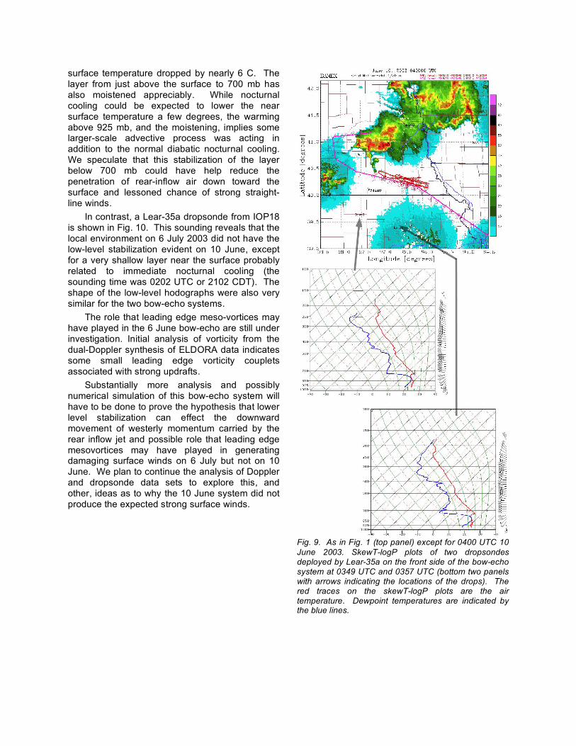
surface temperature dropped by nearly 6 C. The layer from just above the surface to 700 mb has also moistened appreciably. While nocturnal cooling could be expected to lower the near surface temperature a few degrees, the warming above 925 mb, and the moistening, implies some larger-scale advective process was acting in addition to the normal diabatic nocturnal cooling. We speculate that this stabilization of the layer below 700 mb could have help reduce the penetration of rear-inflow air down toward the surface and lessoned chance of strong straight-line winds.

In contrast, a Lear-35a dropsonde from IOP18 is shown in Fig. 10. This sounding reveals that the local environment on 6 July 2003 did not have the low-level stabilization evident on 10 June, except for a very shallow layer near the surface probably related to immediate nocturnal cooling (the sounding time was 0202 UTC or 2102 CDT). The shape of the low-level hodographs were also very similar for the two bow-echo systems.

The role that leading edge meso-vortices may have played in the 6 June bow-echo are still under investigation. Initial analysis of vorticity from the dual-Doppler synthesis of ELDORA data indicates some small leading edge vorticity couplets associated with strong updrafts.

Substantially more analysis and possibly numerical simulation of this bow-echo system will have to be done to prove the hypothesis that lower level stabilization can effect the downward movement of westerly momentum carried by the rear inflow jet and possible role that leading edge mesovortices may have played in generating damaging surface winds on 6 July but not on 10 June. We plan to continue the analysis of Doppler and dropsonde data sets to explore this, and other, ideas as to why the 10 June system did not produce the expected strong surface winds.

Fig. 9. As in Fig. 1 (top panel) except for 0400 UTC 10

June 2003. SkewT-logP plots of two dropsondes deployed by Lear-35a on the front side of the bow-echo system at 0349 UTC and 0357 UTC (bottom two panels with arrows indicating the locations of the drops). The red traces on the skewT-logP plots are the air temperature. Dewpoint temperatures are indicated by the blue lines.

Fig.10. SkewT-logP plots of a dropsonde deployed by Lear-35a on the front side of the bow-echo system at 0202 UTC. The magenta trace is the air temperature. Dewpoint temperature is indicated by the green dashed line.

Acknowledgments. We would like to the flight crews of the NOAA P-3, NRL P-3, and Lear-35a aircraft for their dedicated support in the execution of often hazardous flight patterns. The sounding data was supplied by the UCAR/JOSS web site. Lastly, we thank Dr. John Daugherty for his tireless efforts in managing the NOAA P-3 aircraft data sets.

References

Atkins, N. T., C. S. Bouchard, R. W. Przybylinski, R. J. Trapp,

and G. Schmocker, 2005: Damaging surface wind mechanisms within the 10 June 2003 Saint Louis Bow Echo during BAMEX. Mon. Wea. Rev., 133, 2275-2296.

Fujita, T. T., 1978: Manual of downburst identification for project NIMROD. Satellite and Mesometeorology Research

Paper No. 156, Department of Geophysical Sciences, University of Chicago, 104 pp.

Hildebrand, Peter H., Lee, Wen-Chau, Walther, Craig A., Frush, Charles, Randall, Mitchell, Loew, Eric, Neitzel,

Richard, Parsons, Richard, Testud, Jacques, Baudin, François, LeCornec, Alain. 1996: The ELDORA/ASTRAIA Airborne Doppler Weather Radar: High-Resolution

Observations from TOGA COARE. Bull. Amer. Meteor. Soc., 77, 213–232.

Johns, R.H., 1993: Meteorological conditions associated with bow echo development in convective storms. Wea. Forecasting, 8, 294-299.

Johns, R.H. and W.D. Hirt, 1987: Derechos: widespread

convectively induced windstorms. Wea. Forecasting, 2, 32—49.

Jorgensen, D. P., P. H. Hildebrand, and C. L. Frush, 1983: Feasibility test of an airborne pulse-Doppler meteorological radar. J. Climate Appl. Meteor., 22, 744–757.

Jorgensen, D. P., T. Matejka, and J. D. DuGranrut, 1996: Multi-beam techniques for deriving wind fields from airborne Doppler radars. Meteor. Atmos. Phys., 59, 83-104.

Jorgensen, D. P., T. R. Shepherd, and A. Goldstein, 2000: A

multiple pulse repetition frequency scheme for extending the unambiguous Doppler velocity of the NOAA P-3 airborne Doppler radar. J. Atmos. Oceanic Techol., 17, 585-594.

Leise, J. A., 1981: A multidimensional scale-telescoped filter and data extension package. NOAA Tech. Memo. ERL WPL-82, 18 pp, (NTIS PB82-164104).

O’Brien, J. J., 1970: Alternative solutions to the classical vertical velocity problem. J. Appl. Meteor., 9, 197-203.

Oye, R., R. C. Mueller, and S. Smith, 1995: Software for radar

translation, visualization, editing, and interpolation. Preprints, 27th Conf. on Radar Meteorology, Vail, CO, Amer. Meteor. Soc., 359–364.

Przybylinski, R.W., 1995: The bow echo: Obser-vations, numerical simulations, and severe weather detection

methods. Wea. Forecasting, 10, 203-218.

Rotunno, R., J. B. Klemp and M. L. Weisman, 1988: A theory for strong, long-lived squall lines. J. Atmos. Sci., 45, 463--485.

Tessendorf, S.A. and R.J. Trapp, 2000: On the climatological

distribution of tornadoes within quasi-linear convective systems. Preprints, 20th Conf. on Severe Local Storms, Orlando, Fl., Amer. Meteor. Soc., 134-137.

Weisman, M.L., 1993: The genesis of severe, long- lived bow echoes. J. Atmos. Sci., 50, 645-670.

Weisam, M.L., and R.J. Trapp, 2003: Low-level mesovortices

within squall lines and bow echoes. Part I: Overview and sensitivity to environmental wind shear. Mon. Wea. Rev., 131, 2779-2803.