J. Zheng, Z.-H. Li, A. W. Jasper, D. A. Bonhommeau, R. Valero, R. Meana-Pañeda, S. L. Mielke, and D. G. Truhlar, ANT, version 2016, University of Minnesota, Minneapolis, 2017. http://comp.chem.umn.edu/ant

ANT

A Program for Adiabatic and Nonadiabatic Trajectories Department of Chemistry, University of Minnesota

Manual for version 2017

Jingjing Zheng,a Zhen Hua Li,a Ahren W. Jasper,a,b David A. Bonhommeau,a

Rosendo Valero,a Rubén Meana-Pañeda,a Steven L. Mielke,a and Donald G. Truhlara aDepartment of Chemistry, University of Minnesota, Minneapolis, MN, USA

bCombustion Research Facility, Sandia National Laboratories, Livermore, CA, USA

Version 2017 was finalized on July 13, 2017 This document was most recently updated on July 14, 2017

Abstract ............................................................................................................................. 4

General notes about this manual ....................................................................................... 6 I. Code summary ....................................................................................................................... 7

II. Recommended citation .......................................................................................................... 9

III. Potential energy surfaces and surface couplings ............................................................... 10

III.A. Sample potential energy subroutines .................................................................... 10 III.B. Standardized calling protocol ............................................................................... 10 III.C. Diatomic potential ................................................................................................ 15 III.D. Direct Dynamics ................................................................................................... 16

IV. Initial conditions ................................................................................................................ 20

IV.A. General description for preparing each Atom Group (AG) ................................. 21 IV.A.1. Rotational orientation .................................................................................... 21 IV.A.2. Initial conditions on momenta ....................................................................... 21 IV.A.3. Rotational states ............................................................................................ 22 IV.A.4. Vibrational states ........................................................................................... 22 IV.A.5. Removal of overall angular momentum ........................................................ 22

IV.B. Unimolecular processes ........................................................................................ 23 IV.B.1. State-selected initial conditions ..................................................................... 23 IV.B.2. Vertical excitation initial conditions ............................................................. 27 IV.B.3. Fixed-energy initial conditions ...................................................................... 29 IV.B.4. Fixed-temperature initial conditions .............................................................. 29

IV.C. Bimolecular collisions .......................................................................................... 30 IV.C.1. General bimolecular collision initial conditions ............................................ 30

IV.C.1.a. State-selected run .................................................................................... 30 IV.C.1.b. Initial conditions provided by an equilibration run ................................ 31

2

IV.C.1.c. State-selected initial conditions for part of initial quantum states .......... 32 IV.C.2. Atom-diatom collision initial conditions ....................................................... 32

IV.C.2.a. Initial conditions corresponding to specified initial quantized rotational and vibrational energies and a fixed initial relative translations energy ................ 32 IV.C.2.b. General atom-diatom initial conditions .................................................. 33

IV.C.2.b.1 State-selected run .............................................................................. 34 IV.C.2.b.2 Initial conditions provided by an equilibration run .......................... 34 IV.C.2.b.3 State-selected initial conditions for part of initial quantum states ... 35

IV.C.3. Diatom-diatom collision initial conditions .................................................... 35 V. Integration ........................................................................................................................... 36

VI. Non-Born-Oppenheimer trajectory methods ..................................................................... 38

VII. The TRAPZ and mTRAPZ methods for maintaining zero-point energy ......................... 40

VII.A. Description of the TRAPZ method ..................................................................... 40 VII.B. The mTRAPZ method ......................................................................................... 42 VII.C. Problems with TRAPZ-like methods .................................................................. 42

VIII. Army ants tunneling algorithm ....................................................................................... 43

VIII.A. Computation of the turning point ...................................................................... 43 VIII.B. Evaluation of the imaginary action integral for electronically adiabatic tunneling path ................................................................................................................. 45 VIII.C. Evaluation of the imaginary action integral for electronically nonadiabatic tunneling path ................................................................................................................. 47 VIII.D. Army ants algorithm for branching ................................................................... 47

IX. Special options ................................................................................................................... 50

IX.A. TFLAG1 options ..................................................................................................... 50 IX.B. Starting trajectories at a saddle point .................................................................... 50

X. Final-state analysis routines ................................................................................................ 52

XI. Installation, compilation, and compatibility ...................................................................... 54

XI.A. Content of the ANT distribution .......................................................................... 54 XI.B. Compilation and Compatibility ............................................................................ 59

XI.B.1. Compilation of SPRNG random number generator ...................................... 59 XI.B.2. Compilation using analytic potential energy surfaces ................................... 59 XI.B.3. Compilation for direct dynamics ................................................................... 60

XII. Input file ........................................................................................................................... 61

XII.A. $CONTROL input deck .......................................................................................... 61 XII.B. $CELL input deck ................................................................................................. 63 XII.C. $RXCOLLISION input deck .................................................................................... 64 XII.D. $ATOMDIATOM input deck ................................................................................... 65 XII.E. $SURFACE input deck ........................................................................................... 66 XII.F. $TERMCON input deck .......................................................................................... 68 XII.G. $TRAJECT input deck ........................................................................................... 71 XII.H. $TUNNELING input deck ....................................................................................... 75 XII.I. $OUTPUT input deck .............................................................................................. 77

3

XII.J. $ANALYSIS input deck ........................................................................................... 77 XII.K. $DATA input deck ................................................................................................ 78 XII.L. $COMXX input deck .............................................................................................. 84 XII.M. $COMPP input deck .............................................................................................. 84

XIII. Output files ...................................................................................................................... 85

XIV. Test suite ......................................................................................................................... 95

XIV.A. Test suite for bimolecular processes using analytic potential energy surfaces . 95 XIV.B. Test suite for unimolecular processes using analytic potential energy surfaces 97 XIV.C. Direct dynamics test suite ................................................................................ 101

XV. Bibliography .................................................................................................................. 103

XVI. Parallelization ............................................................................................................... 105

XVII. Platforms, operating systems, and compilers ................................................................ 106

XVIII. Program authors and old version names ....................................................................... 108

XVIII.A. Old version names ........................................................................................ 108 XVIII.B. Distribution ................................................................................................... 108 XVIII.C. Authors and updates ...................................................................................... 108

XIX. Revision history ............................................................................................................ 110

Appendices ............................................................................................................................... 122

A1. Generation of initial conditions (appendix to sections IV.A and IV.C) ............................ 122

A2. Choice of thermostats ........................................................................................................ 128

A3. Description of potential interfaces (appendix to section III.B) ......................................... 133

A3.1 HO-MM-0 interface ............................................................................................. 133 A3.2 HO-MM-1 ............................................................................................................ 134 A3.3. POTLIB-2001 ..................................................................................................... 135 A3.4. NH3 ..................................................................................................................... 146 A3.5. HBr ..................................................................................................................... 148 A3.6. BrCH2Cl ............................................................................................................. 151

A4. SPRNG documentation ..................................................................................................... 155

A5. Gaussian09 documentation ............................................................................................... 155

A6. Molpro documentation ...................................................................................................... 155

A7. Surface couplings in non-BO calculations ........................................................................ 156

A8. Computation of the reduced nonadiabatic couplings ........................................................ 156

A9. Wigner distribution of a ground-state harmonic oscillator ................................................ 160

4

Abstract ANT ("Adiabatic and Nonadiabatic Trajectories”) is a Fortran 90 molecular dynamics program designed with emphasis on treating the dynamics of atoms, molecules, and clusters in the gas phase. It has the following major capabilities:

• ANT can be used for dynamics governed either by a single potential energy surface (electronically adiabatic processes) or by two or more coupled potential energy surfaces (electronically nonadiabatic processes).

• For an electronically adiabatic process, there are two options: (1) the user can supply an analytic potential energy surface as a subroutine or (2) the code can calculate direct dynamics in which energies and gradients are obtained directly from one of the following electronic structure packages: Gaussian09, Molpro, or MOPAC-mn (which must be obtained separately). The direct dynamics option for Molpro is not fully tested yet and should be considered to be code for developers only in the present release.

• For an electronically nonadiabatic process the user must supply two or more surfaces and their couplings in analytic form as subroutines or may employ adiabatic or diabatic input for direct dynamics. Electronically nonadiabatic processes can be treated in either the adiabatic or diabatic representation by a variety of methods including • surface hopping by the fewest switches with time uncertainty (FSTU) algorithm, • FSTU with stochastic decoherence (FSTU/SD), • the semiclassical Ehrenfest (SE) method, • coherent switches with decay of mixing (CSDM), or • other decay-of-mixing algorithms. When one uses the electronically adiabatic representation, the user may either provide the adiabatic surfaces and nonadiabatic couplings by direct dynamics, or the program may calculate them from the diabatic surfaces and diabatic couplings, which may either be analytic or direct. One can also use analytic fits to the surfaces and couplings to carry out calculations entirely in the diabatic representation.

• The army ants tunneling algorithm is implemented for both electronically adiabatic and electronically nonadiabatic trajectories on unimolecular reactions or any other unimolecular process. For electronically nonadiabatic processes, the army ant tunneling algorithm is only implemented for mean-field methods, e.g., CSDM and SE methods. The tunneling path can be along any of the valence internal coordinates or a combination of two stretch coordinates.

• ANT can handle • bimolecular reactive collisions, • inelastic collisions, and • unimolecular processes with various initial conditions. It can calculate cross sections and rate constants.

• ANT can be run at fixed energy with various initial conditions or for thermal ensembles. Collision processes between an atom and a diatom can be carried out by a more advance treatment of initial conditions specialized for that particular case. Another option is that one may begin trajectories at a dividing surface passing through a saddle point as used for unified dynamical model calculations.

5

• A limited set of final-state analysis options is available. Or one can let program write initial and final coordinates and momenta and selected other information to a file for external (post-trajectory) analysis.

• Three methods (TRAPZ, mTRAPZ, and mTRAPZ* methods) are available to ensure zero-point energy maintenance in classical trajectory simulations, if desired.

• The program can handle periodic boundary conditions (cubic or cuboid only) if a periodic potential is given.

• The program can also optimize geometry by following a steepest-descents trajectory in Cartesian coordinates.

6

General notes about this manual

All keywords are in SMALL CAPS. Subroutine names are in normal caps. Keywords in input sections are listed in alphabetical order. The sections about initial conditions in this manual are organized for bimolecular collisions and unimolecular processes separately, and issues affecting both are repeated so users need refer to only one or another of them for their purposes. The test runs are also sorted into a section for unimolecular processes and another section for bimolecular processes.

In the present version of the code, coupled-surface dynamics can be carried out by either direct dynamics or by using potential energy surface routines provided by the user. Section III of the manual discusses how one uses either potential energy surface routines or surfaces-and-couplings routines provided by the user or direct dynamics information for either single-surface or coupled-surface calculations. Note that potential energy surface may also be called electronic energies. We use the usual convention that when we say electronic energies, it also includes nuclear repulsion. It is useful to clarify a few points of notation and procedure that apply to all cases where coupled potential energy surfaces are used. There are two possible representations that may be used for coupled-surface processes: the electronically adiabatic representation and the electronically diabatic representation. When one uses the electronically adiabatic representation, one requires the adiabatic potential energy surfaces and their couplings. In the electronically adiabatic representation, the couplings are vectors (3Natom-dimensional vectors in atomic Cartesian coordinates, where Natom is the number of atoms), and they are called the nonadiabatic couplings. When one uses the electronically diabatic representation, one requires the diabatic potential energy surfaces and their couplings. In the electronically diabatic representation, the couplings are scalars, and they are called the diabatic couplings; the diabatic couplings are the off–diagonal elements of the diabatic potential energy matrix, which has the diabatic surfaces on the diagonal. We often use the word "polyatomic" to refer to a molecule with three or more atoms. References cited in the manual are in Section XV. The recommended citation for publications using the code is given in section II.

7

I. Code summary

ANT is a computer program written in Fortran 90 for calculating electronically adiabatic and electronically nonadiabatic trajectories by classical and semiclassical methods. The program can simulate unimolecular reactions, bimolecular nonreactive collisions, and bimolecular reactive collisions, and it can calculate inelastic or reactive collision cross sections and bimolecular or unimolecular reaction rate constants. All simulated processes are assumed to be gas-phase processes except in a few places where periodic boundary conditions are discussed.

Knowledge of the keywords is essential for proper use of the ANT input files. At the

beginning of most of the sections of this manual we present the list of input keywords that will be explained in that section.

The code is designed to be as modular as possible.

Potential energy surfaces can be calculated either from an analytic function (subroutine) or by direct dynamics (the latter option is sometimes called “on-the-fly” and it refers to requesting energies and gradients as needed from a quantum chemistry electronic structure program). In the present version of ANT, direct dynamics simulations are accomplished by an interface with one of following quantum chemistry packages: Gaussian09, Molpro, or MOPAC-mn. The integration with Gaussian09 and Molpro is loose, i.e., an external script is used to run the quantum chemistry package; the integration with MOPAC-mn is tight, i.e., MOPAC-mn subroutines are directly called from ANT code. The main reason for using a semiempirical program like MOPAC-mn is to reduce computer time (as compared to using nonempirical wave function calculations or using density functional calculations), but much of the possible computational efficiency would be lost if one used a loose interface.

For runs based on an analytic potential function, the user provides a potential energy subroutine that returns the electronic energy (or energies and couplings in the case of electronically nonadiabatic processes) and gradients when a nuclear geometry is passed to it. A selection of potential energy subroutines is available at POTLIB-online (http://comp.chem.umn.edu/potlib). ANT supports several potential energy subroutine interfaces. These are described in Section III and in the appendix (Section A.3).

As part of setting up the simulation of a particular process, the user specifies one atom group (AG) for unimolecular processes and two AGs for bimolecular processes. Each AG is treated as an isolated group of atoms, and initial conditions for each AG are prepared by ANT before integrating the equations of motion. For bimolecular processes, before integrating the equations of motion, one must also set up the initial collision parameters. In this context, collision parameters are parameters that control the relative location and relative motion of the two collision partners; this includes impact parameter and molecular and rotational orientation) Different AGs may be prepared using different initial condition prescriptions, and several initial condition prescriptions are supported. The program can handle periodic boundary conditions if a periodic potential is given. See Section IV for details of setting initial conditions.

8

Collision processes between an atom and a diatom can be carried out by special algorithms

for the initial conditions, as described in Ref. 15. Both atom-diatom calculations and more general bimolecular calculations (atom–polyatom and molecule–molecule collisions) may be treated using a general method that is applicable to any type of bimolecular system. The general method treats the reactants and products by the harmonic oscillator, rigid rotor approximation, whereas the special atom-diatom option can use more accurate methods.

Three kinds of thermostat and one kind of barostat are available for simulations of NVT

(canonical) or NPT (isothermal-isobaric) ensembles. See Section IV and the appendix for details.

The classical equations of motion are integrated in Hamiltonian form. Variable and fixed-step-size integration options are available. See Section V for details.

Nuclear propagation may be carried out electronically adiabatically (i.e., on a single potential energy surface) or electronically nonadiabatically if excited-state surfaces and their couplings are available. Several options exist for incorporating electronic transitions into trajectory simulations including the semiclassical Ehrenfest method, several surface hopping methods, and several decay of mixing methods, including the recommended CSDM method. See Section VI for details.

The methods for preparing initial reaction conditions are explained in Section IV. The TRAPZ (TRAjectory Projection onto ZPE orbit), mTRAPZ (minimal TRAPZ), and

mTRAPZ* methods that constrain the trajectory to maintain the total zero-point energy of a molecule in classical or semiclassical trajectories have been implemented. See Section VII for details.

The army ants tunneling algorithm is implemented for both electronically adiabatic and electronically nonadiabatic trajectories of unimolecular reactions. The tunneling path can be either a single valence internal coordinates or a combination of two stretch coordinates. See Section IX for details.

A limited number of special options are available. For example, the momenta may be zeroed at every step, resulting in a steepest-descent trajectory. As another example, the nuclear kinetic energy may be rescaled at regular intervals to simulate heating or cooling. See Section IX.A for details.

Another option is that one may begin trajectories at a dividing surface passing through the

saddle point. See Section X.B for details. Trajectories are propagated until a termination condition is met. Several options for

termination are available, including running trajectories for a fixed time, monitoring bond-breaking events, or monitoring AG fragmentation and association (the latter was found to be

9

very useful for reactions between metal clusters. See the input file section, Section XII for details.

A limited set of final-state analysis options is available. See Section X for details.

Propagation of nuclear coordinates can be carried out electronically adiabatically, i.e., on a

single potential energy surface, or electronically nonadiabatically, i.e., on coupled surfaces; the latter requires that two or more potential energy surfaces and their couplings be available. Electronically nonadiabatic calculations are also called non-Born-Oppenheimer calculations, multi-surface calculations, or coupled-surface calculations; these calculations involve transitions between surfaces, either as discontinuous hops or by continuous switching. Several options exist for incorporating electronic transitions into the trajectory simulations, including the semiclassical Ehrenfest method (coherent switches without decoherence), several surface hopping methods (with or without time-uncertainty and with or without stochastic decoherence), and several decay of mixing methods, including the recommended coherent switches with decay of mixing (CSDM) method. See Section VI for details.

When one uses the electronically adiabatic representation, the user may either provide the

adiabatic surfaces and nonadiabatic couplings as such, or the program may calculate them from the diabatic surfaces and diabatic couplings.

II. Recommended citation All published work based on the ANT program should give the ANT reference. The recommended citation for the current ANT package is: J. Zheng, Z.-H. Li, A. W. Jasper, D. A. Bonhommeau, R. Valero, R. Meana-Pañeda, S. L. Mielke, and D. G. Truhlar, ANT, version 2017, University of Minnesota, Minneapolis, 2017. http://comp.chem.umn.edu/ant

10

III. Potential energy surfaces and surface couplings Input keywords presented in this section: POTFLAG. III.A. Sample potential energy subroutines

To perform any dynamics simulation, ANT either needs a potential energy subroutine, or it needs a quantum chemistry package for direct dynamics. The subroutine GETPEM (src/getpem.f) collects all potential energy subroutine calls including direct dynamics.

The ANT distribution contains sample potential energy subroutines for several systems;

these are provided in the directory pot/. The user can also pick up other potential energy subroutines at POTLIB-online:

http://comp.chem.umn.edu/potlib/ Any additional potential energy subroutines provided by the user should be moved into the directory pot/, and the coordinates, energies, and gradients for input and output to such routines should be in atomic units (hartrees and bohrs).

Note that each run calls the subroutine PREPOT once. This call can be used to set up

quantities that need to be initialized for subsequent potential calls. The user must supply a dummy routine if this call is not needed. The PREPOT subroutine should be included in the same file as the potential energy subroutine (so it is recognized by the compiler).

III.B. Standardized calling protocol

Calculations in ANT are carried out using unscaled Cartesian coordinates (without removing overall translation), but it is often convenient to use other sets of coordinates when expressing the potential energy. An interface between the two coordinate systems (Cartesians and the one used for the potential) is therefore required. A series of potential energy subroutine interfaces are provided to handle the coordinate transformations (and those for the derivatives) for several system types. In addition to handling coordinate transformations, these interfaces also handle potential energy surface conventions such as the specific ordering of atoms, etc.

For electronically nonadiabatic dynamics, potential energy surface subroutines provide the

energies and gradients in the adiabatic representation, in the diabatic representation, or in both representations. One available option, if needed, is that the nonadiabatic couplings (see page 6 for definitions) can be calculated from the diabatic surfaces and diabatic couplings by subroutines provided as part of the ANT program.

The user selects the interface to be used with the input variable POTFLAG. The following interfaces are currently supported: POTFLAG=0: HO-MM-1 interface. This interface is described at POTLIB-online, http://t1.chem.umn.edu/potlib. This is a single-surface (adiabatic), homonuclear, molecular mechanics (i.e., variable number of atoms) interface. Subroutine calls with this interface have the general form:

11

POT(X, Y, Z, E, DEDX, DEDY, DEDZ, NATOM, MAXATOM)

for a non-periodic potential and POT(X, Y, Z, E, DEDX, DEDY, DEDZ, CELL, NATOM, MAXATOM) for a periodic potential. The user can prepare his or her own periodic boundary conditions in the potential routine, or call SUBROUTINE PERIODIMAGE(DX,DY,DZ,CELL) before calculating distances. This subroutine returns the new DX, DY, and DZ (the differences in Cartesian coordinates between the two atoms whose distance will be calculated.). Currently, the subroutine can only deal with cubic or cuboid cells. The meanings of the parameters are as follows:

NATOM (input, integer) The number of atoms. MAXATOM (input, integer) Sets the dimensions of the variables X, Y, Z, DEDX, DEDY,

and DEDZ. Must be greater than or equal to NATOM. X, Y, Z (input, double precision) One-dimensional arrays containing the Cartesian

components of NATOM atoms. E (output, double precision) The potential energy. DEDX, DEDY, DEDZ (output, double precision) One-dimensional arrays containing the

first derivatives of the energy with respect to the Cartesian coordinates. CELL(6): The six cell parameters a, b, c, α, β, and γ.

POTFLAG=1: 3-2V interface. This interface is described at POTLIB-online, http://t1.chem.umn.edu/potlib. This interface returns a 2 x 2 diabatic potential energy surface matrix for a triatomic system. PREPOT is called once, and POT is called when an energy and/or gradient is needed. Subroutine calls with this interface have the general form:

CALL POT( R, E, DE, NVALS, NSURF)

The meanings of the parameters are as follows:

NVALS (input, integer) The energy and derivatives are computed for NVALS different geometries.

NSURF (input, integer) Labels the potential energy surface. For a single-surface potential, NSURF = 1. For a two-state potential, NSURF = 1 and 3 for the two diagonal diabatic potential energy surfaces, and NSURF = 2 for the diabatic coupling surface.

R (input, double precision) A two-dimensional array containing the internuclear bond distances. The first index labels the NVALS different geometries, and the second index labels the three internuclear distances.

E (output, double precision) An array containing the potential energies of surface NSURF at NVALS geometries.

12

DE (output, double precision) A two-dimensional array of the first derivatives of surface NSURF with respect to the three internuclear distances. The first index labels the three internuclear distances, and the second index labels the NVALS different geometries.

POTFLAG=2: HE-MM-1 interface. This interface is described at POTLIB-online, http://t1.chem.umn.edu/potlib. This is a single-surface (adiabatic), heteronuclear, molecular mechanics (i.e., variable number of atoms) interface. Subroutine calls with this interface have the general form: CALL POT(SYMB, X, Y, Z, E, DEDX, DEDY, DEDZ, NATOM, MAXATOM) for a non-periodic potential and CALL POT(SYMB, X, Y, Z, E, DEDX, DEDY, DEDZ, CELL, NATOM, MAXATOM) for a periodic potential. The arguments are the same as for POTFLAG=0, except for SYMB (input, character*2) One-dimensional array containing the atomic symbols of all the atoms. POTFLAG=3: NH3 potential interface. This interface is described at POTLIB-online, http://t1.chem.umn.edu/potlib. This is a two-surface (adiabatic and diabatic), heteronuclear, 4-body interaction interface. Subroutine calls with this interface have the general form:

call pot(Xcart,U11,U22,U12,V1,V2,gcartU11,gcartU22,gcartU12,gcartV1,gcartV2)

Xcart: A one dimensional array of coordinate in an order of x1, y1, z1, x2, y2, z2, x3, y3, z3, x4, y4, z4.

U11, U22, U12: Ground state energy, excited state energy, and the cross-term of the two states in a diabatic representation.

V1, V2: Ground state energy, and excited state energy in an adiabatic representation. Gcart-terms: The one dimensional derivatives of the corresponding energies.

POTFLAG=4: 4-XS interface This interface is described at POTLIB-online, http://t1.chem.umn.edu/potlib. This is a single-surface (adiabatic), heteronuclear, 4-body interaction interface. Subroutine calls with this interface have the general form:

CALL POT(X, Y, Z, E, DEDX, DEDY, DEDZ)

In this potential, there is a special ordering of atoms, for example for the OH+H2 potential, the ordering is O, H, H, H, i.e. oxygen atom must be the first atom. In a reactive collision run, the current program can deal with reactants OH+H2 and OH3+H, but not O+H3, which seems not a possible combination of reactants.

13

POTFLAG=5: Same as HE-MM-1 interface, but transfers atomic numbers instead of atomic symbols, i.e. SYMB is replaced with INDATOM, which is a one-dimensional array containing the atomic numbers of all the atoms. POTFLAG=6: HBr potential interface. This interface is described at POTLIB-online, http://t1.chem.umn.edu/potlib. This is a twelve-surface (adiabatic and diabatic), heteronuclear, 2-body interaction interface. Subroutine calls with this interface have the general form:

call pot(Xcart,UI,UIJ,VI, gUI,gUIJ,gVI,dvec)

where the items in the parameter list have the following meanings: Xcart: A one dimensional array of coordinates in the order x1, y1, z1, x2, y2, z2, where

atom 1 is H and atom 2 is Br. UI: Array with the energies of the 12 diabatic states. The diagonal elements of this matrix

are zero. UIJ: 12×12 matrix with the diabatic couplings. VI: Array with the energies of the 12 adiabatic states. gUI: Array with the nuclear derivatives of the 12 diabatic energies. gUIJ: 12×12 matrix with the nuclear derivatives of the diabatic couplings. The diagonal

elements of this matrix are zero. gVI: Array with the nuclear derivatives of the 12 adiabatic energies. dvec: nonadiabatic coupling vector.

POTFLAG=7: BrCH2Cl potential interface. This interface is described at POTLIB-online, http://t1.chem.umn.edu/potlib. This is a twenty-four-surface (adiabatic and diabatic, where the adiabatic surfaces are optionally calculated by diagonalizing the diabatic potential matrix), heteronuclear, 5-body interaction interface. Subroutine calls with this interface have the general form:

call pot(Xcart7,UI,UIJ,VI, gUI,gUIJ,gVI,dvec,icall) where the items in the parameter list have the following meanings:

Xcart7: A one dimensional array of coordinates in the order x1, y1, z1, x2, y2, z2, x3, y3, z3, x4, y4, z4, x5, y5, z5, where atom 1 is Br, atom 2 is C, atom 3 is Cl, atom 4 is H1, and atom 5 is H2.

UI: Array with the energies of the 24 diabatic states. UIJ: 24×24 matrix with the diabatic couplings. VI: Array with the energies of the 24 adiabatic states. gUI: Array with the nuclear derivatives of the 24 diabatic energies. gUIJ: 24×24 matrix with the nuclear derivatives of the diabatic couplings. gVI: Array with the nuclear derivatives of the 24 adiabatic energies. dvec: nonadiabatic coupling vector. icall: variable that controls the calculation of adiabatic energies (only with icall = 1 will

they be calculated).

14

POTFLAG=8: This is a standard interface for a single adiabatic surface. Current examples among the distributed potentials include HN2.f, N2O-3Ap-gpip.f, and N2O-3App-gpip.f. The potential can be called as follows Call pot(V, X, GRAD) where the items in the parameter list have the following meanings:

V: Potential energy in hartrees. X: A one-dimensional array of Cartesian coordinates in the order of x1, y1, z1, x2, y2, z2,

x3, y3, etc.. The units are bohr. GRAD: A one-dimensional array of gradients. Its order is the same as the Cartesian

coordinate array X.

For any new routines, the user should also provide a print statement in the prepot routine that prints an identification line for the potential and any references that should appear in the main output file.

POTFLAG=9: HX2 potential interface. This is a two surfaces interface for the model system HX2, where H and X are model atoms. The potential can be called as follow

Call pot(Xnat,UIJnat,VInat,gUIJnat,gVInat,dvecnat,cchx2)

Xnat : a one-dimensional array of Cartesian coordinates in the order of x1, y1, z1, x2, y2, z2, x3, y3, where atom 1 is H, atom 2 and 3 are X. Unit is bohr.

UIJnat: 2×2 matrix with the diabatic energies and couplings. VInat: array with the adiabatic energy in ascending order. gUIJnat: 2×2 matrix of the nuclear derivatives with respect to the diabatic energies and

couplings. gVInat: array of the nuclear derivative with respect to the adiabatic energies dvecnat: nonadiabatic coupling vector cchx2: matrix that transform diabatic energies to adiabatic energies.

POTFLAG=10: phenol potential interface. This is coupled 33-dimensional potential energy surfaces for electronically nonadiabatic photodissociation of phenol to make phenoxyl radical and a hydrogen atom.. This potential energy surface is described in K. R. Yang, X. Xu, J. Zheng, and D. G. Truhlar, Chemical Science 2014, in press. dx.doi.org/10.1039/c4sc01967a. The potential can be called as

call pot(igrad,x,uu,guu,vv,gvv,dvec,ccph,repflag)

igrad: integer to control calculation for energy only (igrad=0) or for energy and gradients (igrad=1)

x: a two-dimension array of Cartesian coordinates, i.e. x(3, 13). The first dimension denotes x, y, and z, and the second dimension denotes the atom number. The numbering of atoms is C1, C2, C3, C4, C5, C6, O7, H8, H9, H10, H11, H12, H13

15

uu: 3×3 matrix with the diabatic energies and couplings guu: a four dimensional array defined as guu(3,13,3,3) for the nuclear derivatives with

respect to the diabatic energies and couplings. The first dimension denotes the x, y, and z components; the second dimension denotes the atom number; the third and the fourth dimension denote the diabatic state.

vv: a one dimensional array for adiabatic energies in ascending order gvv: a three dimensional array defined as gvv(3,13,3) for the nuclear derivatives with

respect to the adiabatic energies. The first dimension denotes the x, y, and z components; the second dimension denotes the atom number; the third denotes the adiabatic state.

dvec: nonadiabatic coupling vector ccph: matrix that transform diabatic energies to adiabatic energies. repflag: integer that denotes representation: repflag = 0 for adiabatic state and repflag = 1

for diabatic state. III.C. Diatomic potential The polyatomic potential energy surface subroutines could include specific subroutines to compute the potential of diatoms that are needed to calculate the initial conditions of atom-diatom and diatom-diatom calculations. To use this option, a subroutine call diapot_int should be included in the source code previous to compile the code. It is recommended to include these subroutines in the corresponding PES file located in the pot directory. An example of the diapot_int subroutine is the following: subroutine diapot_int(r,arr,nsurf,v) implicit none integer arr,nsurf double precision r,v C Diatomic arrangement: C 1 AB C 2 BC C 3 AC C 4 AD C 5 BD C 6 CD if (arr.eq.1) then call evfarr1(r,v,nsurf) else if (arr.eq.2) then call evfarr2(r,v,nsurf) else if (arr.eq.3) then call evfarr3(r,v,nsurf) else if (arr.eq.4) then call evfarr4(r,v,nsurf) else if (arr.eq.5) then call evfarr5(r,v,nsurf)

16

else if (arr.eq.6) then call evfarr6(r,v,nsurf) else write(6,*) 'ERROR in diapot_int: arr = ',arr,' is not supported' stop endif end subroutine diapot_int where r is the interatomic distance in borh, arr defines the diatomic arrangement, v is the diatomic potential in hartree and nsurf is the number of the adiabatic potential energy surface. The user must comment out the following lines in the diapot.f90 file located in the src directory of the ANT code before compiling the code: C subroutine diapot_int(r,im,nsurf,v) C implicit none C double precision r,v C integer im,nsurf C return C end The keyword FLAGDIAT has to be included in the $ATOMDIATOM input deck. Note that the current version of the code only uses this option for the atom-diatom method (see Section IV.C.3). III.D. Direct Dynamics POTFLAG=-1: direct dynamics using Gaussian09 or Molpro

The subroutines in pot/dd.f provide a common interface for direct dynamics calls to either Gaussian09 or Molpro. The keyword POTFLAG=-1turns on the direct dynamics interface. The keyword QCPACK is to choose the quantum chemistry package; QCPACK=1 is for Gaussian09 and QCPACK=2 is for Molpro. The direct dynamics option for Molpro is not fully tested yet and should be considered to be code for developers only in the present release.

To run a direct dynamics calculation, one needs to give the following set of files in the working directory together along with the ANT input file.

________________________________________________________________________ File Explanation ________________________________________________________________________ Direct dynamics with Molpro m.x An executable file that contains commands to run a Molpro job qc.molpro A template file for Molpro input Direct dynamics with Gaussian09 g.x An executable file that contains commands to run a Molpro job qc.gaussian A template file for Gaussian09 input

17

_______________________________________________________________________ Examples: m.x file: (with executable extension)

molpro -n 8 -o qc.out -s qc.in > system.out g.x file: (with executable extension)

g09 < qc.in > qc.out qc.molpro:

***,title print,orbitals,civector memory,200,m nosym noorient geometry={ GEOMETRY } basis=svp nn(1)=1 nn(2)=2 nn(3)=3 {rhf;wf,14,1,0} {multi;occ,12;closed,3;wf,13,1,1; state, 2 cpmcscf,grad,1.1,spin=0.5,accu=1.d-7,record=5101.1 cpmcscf,grad,2.1,spin=0.5,accu=1.d-7,record=5102.1 cpmcscf,nacm,1.1,2.1,accu=1.d-7,record=5103.1} molpro_energy=energy(1) {force samc,5101.1;varsav} text,MOLGRAD table,nn,gradx,grady,gradz ftyp,f,d,d,d molpro_energy=energy(2) {force samc,5102.1;varsav} text,MOLGRAD table,nn,gradx,grady,gradz

18

ftyp,f,d,d,d {force samc,5103.1;varsav} text,MOLD table,nn,gradx,grady,gradz ftyp,f,d,d,d

The ANT program will replace the GEOMETRY placeholder in the qc.molpro file with the proper Cartesian coordinates. This example is for running a nonadiabatic dynamics calculation with two surfaces. Note that the following lines in this example are essential for the ability of the ANT program to exact the energy, gradients, and nonadiabatic coupling from the tabulated values in the Molpro output file

molpro_energy=energy(1) text,MOLGRAD table,nn,gradx,grady,gradz text,MOLD table,nn,gradx,grady,gradz

It is important to include the keywords “nosym” and “noorient” in order to avoid Molpro reordering the atoms in the output file. qc.gaussian file

%nprocs=8 %mem=1000mb #mp2/6-31g* force fchk NoSym Units=bohr scf=(tight,xqc)

Title

0 2 GEOMETRY

The ANT program will replace the GEOMETRY placeholder in the qc.gaussian file with the proper Cartesian coordinates. This example is for running electronically adiabatic dynamics with one surface. The ANT program reads the energy and gradient from the formatted checkpoint file Test.Fchk. POTFLAG=-2: direct dynamics using MOPAC-mn

The subroutines in pot/potmopac.f provide an interface for direct dynamics to call MOPAC-mn subroutines directly for energy and gradient calculations instead of using a script to run external MOPAC calculations. By calling MOPAC-mn subroutines in the Fortran code directly, this interface reduces the overhead of running external jobs.

To run a direct dynamics calculation, a file named mopac.in is needed to provide all keywords used in MOPAC calculations. The file mopac.in is a MOPAC input file and the geometry in this file can be any reasonable geometry because this MOPAC input file is only run once to set up all variables used in the MOPAC calculation.

19

Note that direct dynamics with MOPAC-mn is currently only implemented for unimolecular reactions.

20

IV. Initial conditions

The user will first have to make some choices about the type of initial conditions; the first of these choices is to choose unimolecular processes or bimolecular processes. In the table below, the first run type is bimolecular, and the second run type is unimolecular. The table also lists three or four subtypes for each type, and user also has to choose one of these subtypes. Then the user will have to decide which particular initial conditions of a given type and subtype are to be used. __________________________________________________________________________ run type subtype description Applicability __________________________________________________________________________

1 Unimolecular processes 1.1 State-selected initial conditions single surface or multiple surfaces 1.2 Vertical excitation multiple surfaces 1.3 Fixed energy initial conditions single surface or multiple surfaces 1.4 Fixed temperature initial conditions single surface

2 Bimolecular collision

2.1 General bimolecular collisions single surface or multiple surfaces 2.2 Atom-diatom collisions single surface 2.3 Diatom-diatom collisions single surface

__________________________________________________________________________ In the above table, the two major types of initial conditions supported by the ANT program are bimolecular collisions and unimolecular processes. In this section, we will explain these two types and the related input keywords. Some examples are used to illustrate how to set up initial conditions for different modes. In subsection A, we will give some general descriptions of initial rotational orientation, initial coordinates, and initial momenta of atom groups; this material applies to both modes, where the initial conditions for a bimolecular collision involve two atom groups, and the initial conditions for a unimolecular process involve one atom group. The descriptions for how to set up each individual mode are in the rest of the subsections. For a bimolecular collision (run type 2), one needs to specify $NMOL = 2, give two atom groups in the $DATA input deck, and give either the input deck $RXCOLLISION or the input deck $ATOMDIATOM. For a unimolecular process (run type 1) one needs to specify $NMOL = 1 and give only one atom group. The $RXCOLLISION and $ATOMDIATOM input decks are used only for bimolecular collisions. The $TUNNELING input deck is only tested for unimolecular processes so far, and $CELL is for systems with periodic condition (which is a special case of unimolecular processes). The other input decks are generally applicable for any of the run types.

21

Note that subtype 2.1 can be used for atom-diatom and diatom-diatom collisions as well as for collisions of polyatomics. IV.A. General description for preparing each Atom Group (AG)

Quantities required for computing the initial conditions that are the same for all trajectories are pre-computed by ANT by calling PREMOL. The specific initial conditions for each trajectory are determined by calling INITMOL. An atom group is defined as a collection of atoms; atom groups are used for initial state preparation. For example, each molecule in a bimolecular collision is an atom group and unimolecular processes have only one atom group.

INITX and INITP are keywords to control the method of providing initial geometry and to control how to select the method for generating initial momenta, respectively. When there is more than one atom group, the scheme used to prepare one AG need not be the same as that used to prepare the other. The input section (Section XII) gives the descriptions of INITX and INITP, but we also explain them in this section for reader’s convenience. This subsection focuses on how to prepare the initial conditions for rotational orientation, rotational states (or energies), and vibrational states in general. Note that capitalized words are subroutine names.

IV.A.1. Rotational orientation This subsection applies to all run types except subtypes 2.2 and 2.3. After the initial coordinates are provided by the user or generated by random sphere, cuboid, or other methods.

1. The AG is rotated to its own coordinate system of principal axes of rotation by first calling ROTPRIN (to calculate the principal axes of rotation) and then a rotation transformation by calling ROTTRAN using the vectors of the principal axes of rotation as rotation transformation matrix.

2. A random orientation represented by a rotation transformation matrix is generated by calling RANROT. For general reactive collisions, the transformation matrix is generated by randomly changing the 3 Euler angles directly, while for other cases it is generated using a quaternion method (see http://mathworld.wolfram.com/EulerParameters.html, and Ref. 1 of Section XV).

3. The AG is rotated to this new orientation generated in step 2 by calling ROTTRAN, and the momenta of the atoms in this AG are subsequently transformed to the new orientation by calling ROTTRAN.

IV.A.2. Initial conditions on momenta

There are three options for generating the initial momenta of an AG, as determined by the

value of the input parameter INITP. INITP=0: Zero initial momentum The initial momenta are set to zero.

22

INITP=1: Random thermal distribution 1. The user supplies a target temperature T [TEMP0IM] in Kelvin. Steps 2 and 3 are performed in RANTHERM subroutine. 2. 3Natom random numbers (xij) are selected from a normalized Gaussian distribution. 3. The momentum is assigned according to

jbijij TMkP ξ= [PP]

where Mj is the mass of atom j. INITP=-1: Initial momentum is decided by other choices, such as VIBSELECT, ROTSTATES. See Section XII for details.

IV.A.3. Rotational states

At present, state selection on rotational states can only be done for linear AGs. This is done after the AG is rotated to its own principal axes of rotation and its overall momentum of rotation is removed. The aim of the procedure consists in adding rotational components⊥ to momenta pi. These components are estimated by randomly generating rotational states with an energy Erot. The relationship between Erot and the angular momentum J then enables to determine pi⊥. The whole procedure is described in Appendix A1.

IV.A.4. Vibrational states

In the case of the simulations for which the user desires a normal mode analysis to provide initial conditions, if vibrational quantum states or vibrational energies are not provided, the program will randomly generate a set of vibrational quantum numbers according to Boltzmann distribution (The structures provided must be local minima.). The whole procedure is described in Appendix A1.

IV.A.5. Removal of overall angular momentum

After the coordinates and momenta are assigned for each AG, the center of mass is placed

at the origin, and center of mass motion is removed. Angular motion is (approximately) removed by first computing angular velocity ω JIω 1−= , where I is the inertial tensor matrix, and J is the total angular momentum. The momentum for atom j and direction i (i = x, y, or z) is adjusted according to jijijij MPP ][ xω×−= . Note: 1) For non-symmetric structures, this scheme only approximately removes angular motion. In the current program, this procedure is repeated until the total angular motion falls below a hard-coded small value. 2) For linear AGs, this procedure cannot be used because I-1 cannot be calculated for linear AGs since the determinant of I is zero. Instead, the overall angular momentum is removed by removing the momentum component of every atom in the AG that is perpendicular to the direction of the linear AG.

23

This procedure is done for each AG separately in the INITMOL subroutine and also for the whole AG (except for reactive collision run) before entering the simulation. IV.B. Unimolecular processes The user will provide an initial structure, which should be the optimized geometry of a local minimum by using INITX=0. IV.B.1. State-selected initial conditions This initial condition can be applied for both single-surface trajectories and nonadiabatic trajectories with multiple coupled surfaces. Here “state-selected” refers to vibrational state. For a nonadiabatic trajectory, the initial electronic state can be any electronic state. The representation used for nonadiabatic trajectory propagation is adiabatic by default, but the representation used for propagation can be changed to diabatic by using the keyword DIABATIC. However, we suggest to use the adiabatic representation to set up initial condition. To set up initial condition based on adiabatic representation, one has to add the specific potential energy surface called in ADTOD subroutine to get the transformation matrix between two representations. When the keyword DIABATIC is used, the propagation of the trajectory will be carried out in the diabatic representation by transforming the electronic coefficients of the adiabatic representation into electronic coefficients in the diabatic representation after the initial conditions are determined and before the propagation of the trajectory is started. There are two choices to be made: 1. how much initial energy to put in each mode. This is determined by the

keyword VIBSELECT. 2. how to distribute the coordinates and momenta consistent with the energy

determined by choice 1. This is determined by the keyword VIBDIST. Here are all options of keyword VIBSELECT. VIBSELECT: The initial energy in vibrational mode m is called Em. There are several

choices, and they are all based in one way or another on using the harmonic approximation, but in different ways.

0: Default: Determined by other choices. For example, using keywords INITX=0, INITP = 1, and TE0FIXED = E, the program uses a fixed input geometry for all trajectories and the momenta are randomly determined based on the total energy E.

1: The user provides vibrational quantum numbers by the keyword VIBSTATE= (n 1, n2, ..., n3N–6) for a local minimum VIBSTATE= (n 1, n2, ..., n3N–7) for a saddle point

The amount of energy in each mode m equals Em = (0.5 + nm)hυ, where nm is a quantum number, and υ is the vibrational frequency.

2. This option only applies to minimum-energy structures (not saddle points). The program assigns vibrational quantum numbers at random, selected out of a Boltzmann distribution at a user-specified temperature that is specified by

24

the keyword TEMP0IM. 3. This option only applies to minimum-energy structures (not saddle points). The

program performs a normal mode frequency analysis and uses it to generate an initial velocity from a Maxwell thermal distribution at a given temperature TEMP0. This option should be combined with the keyword INITP=1. This is an option for canonical ensemble, not an option for state-selected ensemble.

4: The amount of energy in each mode is the same for each mode and is E1. Set VIBENE = E1. The unit for E1 is eV.

5: The amount of energy in mode m is Em, which can be different for each mode. Set VIBENE = (E1, E2, ..., E3N–6) or VIBENE = (E1, E2, ..., E3N–7). The units for Em are eV.

6: Like VIBSELECT = 4 except that Em is calculated by the program as min[(0.5 hυm,input E1)]

7: Like VIBSELECT = 5 except that Em is calculated by the program as min[(0.5 hυm,input Em)]

When using the VIBSTATE or VIBENE keywords, note that the vibrational modes are in order of decreasing magnitude of their frequencies, independent of symmetries. Note that only VIBSELECT = 1, 4, 5, 6, or 7 should be used for state-selected initial conditions. VIBDIST: VIBDIST determines the type of phase space distribution for initial

conditions prepared with normal mode analysis (see Section IV and Section A1 for more details). When VIBDIST is 0, 1, or 2, all the modes are treated in the same way.

0: Default: classical or quasiclassical distribution. This distribution is quasiclassical if VIBSELECT = 1 or 2, and it is classical if VIBSELECT ≥ 4. With this option, the initial displacements are distributed between −qturn,m

and +qturn,m in the same way as for a classical harmonic oscillator with the

energy specified by VIBENE, where qturn,m is the magnitude of the turning

point determined by

12kmqturn,m

2 = Em

where qm is the normal mode displacement coordinate, and km is the force constant. When this option is selected, the following steps are taken: (i) a random number λ is chosen (random numbers are always evenly

distributed between 0 and 1), and the initial displacement is qm = qturn,m cos(2πλ)

25

(ii) The potential energy is evaluated with the actual potential function. If V(qm) – V(0) > Em , then | qm| is decreased by 10%, and this is repeated if necessary until V(qm) ≤ V (0)+ Em .

Note that V(0) denotes all the modes m´ not yet assigned at q !m = 0, those modes already assigned at their assigned values, and the current mode m at qm = 0, whereas V(qm ) denotes modes m´ not

yet assigned at q !m = 0, those modes already assigned at their

assigned values, and the current mode m at qm . Because of this complication, the results depend on the order that the modes are assigned. For each trajectory the modes are assigned in a different order, as determined by random numbers.

(iii) Another random number λ´ is chosen to determine the sign of the momentum pm in mode m.

(iv) The momentum is assigned as

pm = sign( !λ ) 2µ Em − V (qm)−V (0)!" #$( )

where m is the normal-mode reduced mass. 1: If VIBSELECT=1, this option should be used only when nm is 0. It may be

called the ground-state harmonic oscillator distribution. Using a random number, the coordinate qm is selected from the quantum mechanical harmonic oscillator coordinate distribution, which is the square of the ground-state wave function and is a Gaussian. This means that

Δq = σx −2ln(λ1) cos(2πλ2) where λ1 and λ2 are two random numbers, and

σx = Em / km . Then steps ii, iii, and iv above are repeated.

2: If VIBSELECT=1, this option should be used only when nm is 0. A Wigner distribution obtained from the separable harmonic oscillator wave function in the normal mode representation. The distribution is generated using the Box-Muller algorithm for normal mode coordinate displacement and momentum. In particular the normal mode displacement and momentum is calculated as

qm = σx −2ln(λ1) cos(2πλ2)

pm =σ p −2 ln(λ1) cos(2πλ2) σ p =1/ (2σ x ) and

σx = Em / km .

26

Note that we use the same set of random numbers λ1 and λ2 in determining displacement and momentum.

9: This option allows one to use select option 1, 2, or 3 individually for each mode. If VIBDIST = 9, the one must supply another keyword VIBDISTN = (vibdist1,vibdist2,...,vibdist3N–6)

for minima and VIBDISTN = (vibdist1,vibdist2,...,vibdist3N–7) for saddle points.

Here is an example to illustrate how to set up state-selected initial condition for nonadiabatic trajectories Example: It starts a trajectory on adiabatic surface 2 with 0.02 eV in stretch modes and 0.01 eV in other modes. Note that "X Y Z" in the geometry used in this example should be filled in with the local minimum on the excited state (adiabatic state 2) before using this input sample. $control potflag=10 hstep0=0.5 ranseed=31415926 bulstointhack eps=1.d-8 $end $output outflag=4 22 10 11 20 21 maxprint nprint=200 minprinticon $end $surface nsurfi=2 nsurf0=2 nsurft=3 methflag=4 tinyrho=1e-4 $end $termcon termflag=3 t_stime=20000 nbondbreak=1 7 13 6.0 $end $traject ntraj=2 tflag1=0 $end $data nmol=1 natom=13 initx=0 initp=-1 vibselect=6 vibdist=1 0 1 # One should fill the X, Y, and Z using the local minimum on excited state 2 C 12.000000 X Y Z C 12.000000 X Y Z C 12.000000 X Y Z C 12.000000 X Y Z C 12.000000 X Y Z C 12.000000 X Y Z O 15.994915 X Y Z H 1.0079400 X Y Z H 1.0079400 X Y Z H 1.0079400 X Y Z H 1.0079400 X Y Z H 1.0079400 X Y Z H 1.0079400 X Y Z

27

vibene 0.02 0.02 0.02 0.02 0.02 0.02 0.01 0.01 0.01 0.01 0.01 0.02 0.01 0.01 0.01 0.01 0.01 0.01 0.01 0.01 0.01 0.01 0.01 0.01 0.01 0.01 0.01 0.01 0.01 0.01 0.01 0.01 0.01 $end IV.B.2. Vertical excitation initial conditions Vertical excitation initial conditions have two options. Vertical excitation Option 1 (VEO1): White light vertical excitation

1. Use options for initial conditions in state-selected systems to generate a ground-state distribution. One needs to input the ground-state minimum-energy geometry and use the keyword “NSURFI=1” to tell the program do the normal mode analysis for the ground state.

2. Use the keyword “nsurf0” to tell which surface to start propagating the trajectory, e.g., use “NSURF0=N” to start the trajectory on surface N.

With this option, the phase space distribution is determined on the ground state surface (NSURFI=1) and then the system is lifted vertically to the chosen excited state (specified by NSURF0), without changing the coordinates or momenta, where the lack of change of coordinates and momenta is the Franck-Condon principle. In practice this would occur only if the photon beam contained all frequencies (i.e., white light) since the energy gap between the surfaces varies with geometry.

Vertical excitation Option 2 (VEO2): Vertical excitation by photons with energies in a small window centered at a given fixed energy

This option is the same as option 1 except one uses the keyword VERTE to specify a photon energy (in eV) and the keyword BANDWD to specify the bandwidth of the photon energy (also in eV). Only excitations where the potential energy increases by an amount within the specified energy range (verte ± bandwd) are accepted. Other phase space points are discarded.

Here are examples to illustrate the vertical excitation options. Example: The program does normal-mode analysis on adiabatic surface 1 and determines the phase space distribution on adiabatic surface 1; then the system is lifted vertically to adiabatic surface 2 with white light (VEO1). This phase space distribution is determined by the keyword VIBSELECT=6 and VIBDIST=1 with 0.02 eV energy for each vibrational mode. Then, although the initial state is determined in the adiabatic representation, the trajectory will be carried out in the diabatic representation by transforming the electronic coefficients of the adiabatic representation into electronic coefficients in the diabatic representation after the initial conditions are determined and before the propagation of the trajectory is started. $control potflag=10 hstep0=0.5 ranseed=31415926 bulstointhack eps=1.d-8 diabatic $end $output outflag=4

28

22 10 11 20 21 maxprint nprint=200 minprinticon $end $surface nsurfi=1 nsurf0=2 nsurft=3 methflag=4 tinyrho=1e-4 $end $termcon termflag=3 t_stime=20000 nbondbreak=1 7 13 6.0 $end $traject ntraj=2 tflag1=0 $end $data nmol=1 natom=13 initx=0 initp=-1 vibselect=6 vibdist=1 0 1 C 12.000000 0.000000000 0.937824000 0.000000000 C 12.000000 -1.205700000 0.234366000 0.000000000 C 12.000000 -1.188436000 -1.160295000 0.000000000 C 12.000000 0.019898000 -1.854419000 0.000000000 C 12.000000 1.218764000 -1.138023000 0.000000000 C 12.000000 1.217257000 0.253677000 0.000000000 O 15.994915 0.052145000 2.302309000 0.000000000 H 1.0079400 -2.153827000 0.775630000 0.000000000 H 1.0079400 -2.132277000 -1.705333000 0.000000000 H 1.0079400 0.028771000 -2.943124000 0.000000000 H 1.0079400 2.170159000 -1.669900000 0.000000000 H 1.0079400 2.143024000 0.827143000 0.000000000 H 1.0079400 -0.912397652 2.641373527 0.000000000 vibene 0.02 $end Example: The initialization on the lower surface (where the photon is absorbed) is like example 2, but this example uses option VEO2 with verte=4.5 and bandwd=0.2. The initial distribution corresponds to a pure adiabatic state, and the trajectory will be carried out in the diabatic representation by transforming the electronic coefficients of the adiabatic representation into electronic coefficients in the diabatic representation after the initial conditions are determined and before the propagation of the trajectory is started. $control potflag=10 hstep0=0.5 ranseed=31415926 bulstointhack eps=1.d-8 diabatic $end $output outflag=4 22 10 11 20 21 maxprint nprint=200 minprinticon $end $surface nsurfi=1 nsurf0=2 nsurft=3 methflag=4 tinyrho=1e-4 $end $termcon termflag=3 t_stime=20000 nbondbreak=1

29

7 13 6.0 $end $traject ntraj=2 tflag1=0 $end $data nmol=1 natom=13 initx=0 initp=-1 vibselect=6 vibdist=1 verte=4.5 bandwd=0.2 0 1 C 12.000000 0.000000000 0.937824000 0.000000000 C 12.000000 -1.205700000 0.234366000 0.000000000 C 12.000000 -1.188436000 -1.160295000 0.000000000 C 12.000000 0.019898000 -1.854419000 0.000000000 C 12.000000 1.218764000 -1.138023000 0.000000000 C 12.000000 1.217257000 0.253677000 0.000000000 O 15.994915 0.052145000 2.302309000 0.000000000 H 1.0079400 -2.153827000 0.775630000 0.000000000 H 1.0079400 -2.132277000 -1.705333000 0.000000000 H 1.0079400 0.028771000 -2.943124000 0.000000000 H 1.0079400 2.170159000 -1.669900000 0.000000000 H 1.0079400 2.143024000 0.827143000 0.000000000 H 1.0079400 -0.912397652 2.641373527 0.000000000 vibene 0.02 $end IV.B.3. Fixed-energy initial conditions One could use the input options described in the subsection IV.B.1 to prepare a state-selected initial condition or subsection IV.B.2. to prepare a vertical excitation, but also add another keyword TE0FIXED to specify a total energy E0 for the system. Note that the system total energy given by a state-selected initial condition or a vertical excitation initial condition could differ with the desired total energy E0. Therefore the code prepares a fixed-energy initial condition using two steps: (1) calculate the initial geometry and momenta based on the input state-selected initial conditions or input vertical excitation initial condition; (2) calculate the potential energy (PE), kinetic energy (KE), and adjust momentum to satisfy the desired total energy (TE) by the following criteria:

a) If PE > E0, re-generate initial geometry and momentum. b) If PE ≤ E0 then, keep the geometry, but scale the momentum by

)()(

old

0oldnew P

XKE

PEEPP ijij −

← .

Note this two-step procedure is performed internally by the code using a single input file. IV.B.4. Fixed-temperature initial conditions To set up an ensemble at a constant temperature, the keywords NVT and TEMP0 in $CONTROL input deck should be used to specify the system at constant temperature TEMP0. In the

30

$TRAJECT input deck, one should specify a thermostat by using the keyword IADJTEMP. The available thermostats are Berendsen thermostat (default), Andersen thermostat, Nosé-Hoover two-chain thermostat, and a simple thermostat by scaling the momentum with a factor of T0 /T (T0 is the target temperature and T is the current temperature). User can see the

Section XII for more details of these thermostats. The keyword INITP=1 should be given to generate random thermal distribution for momenta. The current code is only designed to generate random geometries for metal clusters for initial geometries in a fixed temperature run. For example, use INITX=1, 2 or 3 to generate random atom coordinates. IV.C. Bimolecular collisions ANT has three methods to simulate bimolecular reactive collisions. One method is only for atom-diatom systems, and it has been thoroughly discussed in the book chapter of Ref. 15 (all cited references are in Section XV). The special initial conditions for the atom-diatom case are controlled in the $ATOMDIATOM input deck. Another method is an extension of this option to diatom-diatom conditions; this special option is not available yet, but when it is available it will be controlled in the $DIATOMDIATOM input deck. The third method for setting initial conditions is very general; it works for general collisions of an atom with a polyatomic molecule or for general molecule-molecule collisions as well as for atom-diatom and diatom-diatom collisions, although for the latter we recommend the use of the special atom-diatom and (when available) diatom-diatoms methods. For this general bimolecular collision method, the user may refer to general discussions of how to simulate reactive cross sections and rate constants in, for example, Refs. 15 and 16. IV.C.1. General bimolecular collision initial conditions The program follows a general convention, which involves shooting a second Atom Group (AG) toward the first AG, where the two AGs are initially separated by a distance R0COLLISION. Then the initial conditions (such as the orientation of the first AG, the initial relative translational energy (if translational energy is thermal), and the vibrational and rotational phases of the two colliding AGs) are sampled by a Monte Carlo method. The maximum allowed distance (R0COLLISION) between the two AGs is provided by the user in the $RXCOLLISION input deck or automatically generated by the program. Other initial conditions can be prepared by the following methods:

IV.C.1.a. State-selected run User provides vibrational states, rotational states for linear AG or rotational energies for non-linear AG, and relative translational energies. The combination of the keywords and input for this method is:

a. In the $RXCOLLISION input deck, write keyword STATESELECT b. In the $DATA input deck, in the same line providing INITX, INITP, specify a

VIBSELECT value (see more details in the next subsection for choice of

31

VIBSELECT), and provide relative translational energy ERELTRANS between the two AGs by for example ERELTRANS=0.5 (unit: kBT).

c. In the $DATA input deck, right after the geometry of each AG, provide information of how much energy for each vibrational state, e.g. vibrational quantum numbers and rotational quantum number (for linear AG only) or three rotational energies (for non-linear AG; unit: kBT). The following is an example:

VIBSTATES 1 0 1 0 1 ROTSTATE 1

Or: VIBSTATES 1 0 1 0 1 ROTENERGIES 0.5 1.0 2.0

IV.C.1.b. Initial conditions provided by an equilibration run a. In the $RXCOLLISION input deck, write keyword EQUILIBRIUM. b. In the $TRAJECT input deck, specify the beginning step and probability to save

the initial conditions by specifying for example ITOSAVE=1000 and PICKTHR=0.5 (PICKTHR=1.0 will save at every step). The integration time step used for the equilibration run is equal to the global time step specified in the $CONTROL input deck.

c. The user can still provide vibrational states, but these values are only used for preparing the initial conditions for the equilibration run.

d. The program will save NTRAJ structures and momenta in the file unit 60 (coordinate) and 61 (momentum) for the first AG, 62 and 63 for the second AG if there are. The user can specify three methods to choose these points to be saved: IPICKTRJ=0 (default): If the program finds that the original AG is fragmented before the NTRAJ points are saved, the equilibration will restart from the very beginning, discarding previous saved points and repeating this procedure until all NTRAJ points are all saved in one equilibration run; IPICKTRJ=1: Once equilibration fails (AG fragmented), do not abandon previously saved points and repeat the equilibration from very beginning until all NTRAJ points are saved; IPICKTRJ=2: Effectively put a soft wall before an atom if it breaks bonds with all other atoms by reversing its radial momentum against the center of mass of the whole AG in the equilibration. The last two methods can allow the user to save points with energy higher than the dissociation limit.

e. The program will read from file unit 60-63 for initial geometries and momenta. f. After initial structures are read, the AG is transformed to its own coordinate

system of principal axes of rotation. g. Initial rotational states (or energies) of each AG are either fixed if provided by

the user or randomly generated according to Boltzmann distribution. h. Initial rotational orientation of AG is randomly determined.

32

i. The relative translational energy between the two AGs is either fixed if provided by the user or randomly generated according to Boltzmann distribution.

It should be noted that randomly generated clusters are not local minima and thus the program cannot perform a vibrational state-selected run starting from these clusters. For these random clusters, VIBSELECT can only be specified as 0 (The program will abort in this situation.).

IV.C.1.c. State-selected initial conditions for part of initial quantum states User can choose to provide some of quantum states, e.g. vibrational states, rotational states (or energies for non-linear AGs) or relative translational energy, by specifying a state-selected run in the $RXCOLLISION (write keyword STATESELECT), but the other quantum states are generated randomly. The values provided for selected states will be fixed during the simulation. For example, the user can specify VIBSELECT=2 to tell the program to randomly generate initial vibrational states according to Boltzmann distribution. For randomly generated structures, the user can specify INITP=1 to randomly generate thermally distributed initial momenta for the atoms in the AG. See the Input file section (Section XII) of this manual for more details.

IV.C.2. Atom-diatom collision initial conditions The initial conditions for atom-diatom collisions can be set up by the user by using either of two different procedures:

1. Atom-diatom collisions corresponding to specified initial quantized rotational and vibrational energies and either a fixed initial relative translational energy or a fixed total energy.

2. A general method for bimolecular collisions that can also be used for polyatomics, as described in the previous section.

Note carefully that the two methods will not yield identical results because different algorithms are used (e.g., WKB is used to assign vibrational state energies if $ATOMDIATOM is chosen, whereas the harmonic approximation is used in the more-general treatment).

IV.C.2.a. Initial conditions corresponding to specified initial quantized rotational and vibrational energies and a fixed initial relative translations energy The user can specify different initial conditions for collisions of an atom with some selected vibrational-rotational state (n,j) of the diatom at some fixed center-of-mass collisions energy Erel. The different input options for special atom-diatom simulations are provided by the user in the $ATOMDIATOM input deck. The available keywords are:

a. Use the $ATOMDIATOM input deck for special atom-diatom simulations. b. ESCATAD: The total energy in eV. This is also called the scattering energy, i.e. the

energy of collision plus the internal energy of the diatom in the rotational-vibrational state (n,j):

Escat = Ecol +Eint

33

c. ECOL: The initial collision energy in eV. d. JZERO: An impact parameter appropriate for J = 0 scattering will be randomly

chosen e. B_MIN: The lower bound on a randomly chosen impact parameter f. B_MAX: The upper bound on a randomly chosen impact parameter g. VVAD: Initial vibrational quantum number for the diatom. h. JJAD: Initial rotational quantum number for the diatom. i. RRAD0: Initial atom-diatom separation in Å. j. ARRAD: Integer input: Initial molecular arrangement.

1: AB+C. 2: BC+A. 3: AC+B.

Note that in the atom-diatom simulation input only one AG is specified in the $DATA input deck.

k. In the $DATA input deck, INITX=4 and INITP=−1, i.e. the Cartesian coordinates and initial momenta are determined by the parameters described above.

One must provide either a total energy (ESCATAD) or a collision energy (ECOL). Additionally, one must choose one of two options for assigning an impact parameter, b; either JZERO or B_MIN and B_MAX. The user may set B_MIN = B_MAX in order to choose a specific value of b. The five collision parameters that characterize a collision, i.e.:

a. b : impact parameter. b. θ : the initial azimuthal orientation angle of the diatom internuclear axis. c. φ : the initial polar orientation angle of the diatom internuclear axis. d. η : the initial orientation of the diatom angular momentum. e. ξ : the initial phase angle of the diatom vibration.

are selected by Monte Carlo before integrating every classical trajectory. In general, the impact parameter b should be selected in a range from 0 to some maximum value large enough to compute cross sections and rate constants by the methods described in Ref. 15.

IV.C.2.b. General atom-diatom initial conditions The second method to choose the initial conditions of the atom-diatom collision is a general method that also works for polyatomics. The program follows a general convention, which involves shooting a second Atom Group (AG) toward the first AG, where the atom and the diatom are initially separated by a distance R0COLLISION. Then the initial conditions (such as the orientation of the diatom, the initial relative translational energy (if translational energy is thermal), and the vibrational and rotational phases of the diatom) are sampled by a Monte Carlo method.

34

The maximum allowed distance (R0COLLISION) between the atom and the diatom is provided by the user in the $RXCOLLISION input deck or automatically generated by the program. Other initial conditions can be prepared by the following methods:

IV.C.2.b.1 State-selected run User provides vibrational states, rotational states for the diatom, and relative translational energies. The combination of the keywords and input for this method is:

a. In the $RXCOLLISION input deck, write keyword STATESELECT b. In the $DATA input deck, in the same line providing INITX, INITP, specify a

VIBSELECT value (see more details in the next subsection for choice of VIBSELECT), and provide relative translational energy ERELTRANS between the atom and the diatom by for example ERELTRANS=0.5 (unit: kBT).

c. In the $DATA input deck, right after the geometry of diatom, provide information of how much energy for each vibrational state, e.g. vibrational quantum numbers and rotational quantum number (for the diatom only). The following is an example:

1. VIBSTATES 2. 1 0 1 0 1 3. ROTSTATE 4. 1

IV.C.2.b.2 Initial conditions provided by an equilibration run

a. In the $RXCOLLISION input deck, write keyword EQUILIBRIUM. b. In $CONTROL input deck, TEMP0 defines the temperature of the run. The user

can provide temperatures different from the global temperature in the $control deck by providing a TEMP0IM input when the initial momenta of the diatom are selected by using a random thermal distribution (initp=1).

c. In the $TRAJECT input deck, specify the beginning step and probability to save the initial conditions by specifying for example ITOSAVE=1000 and PICKTHR=0.5 (PICKTHR=1.0 will save at every step). The integration time step used for the equilibration run is equal to the global time step specified in the $CONTROL input deck.

d. The user can still provide vibrational states, but these values are only used for preparing the initial conditions for the equilibration run.

e. The program will save NTRAJ structures and momenta in the file unit 60 (coordinate) and 61 (momentum) for the first AG, 62 and 63 for the second AG. The user can specify three methods to choose these points to be saved: IPICKTRJ=0 (default): If the program finds that the original diatom is fragmented before the NTRAJ points are saved, the equilibration will restart from the very beginning, discarding previous saved points and repeating this procedure until all NTRAJ points are all saved in one equilibration run; IPICKTRJ=1: Once equilibration fails (AG fragmented), do not abandon previously saved points and repeat the equilibration from very beginning until all NTRAJ points are saved; IPICKTRJ=2: Effectively put a soft wall

35

before an atom if it breaks bonds with all other atoms by reversing its radial momentum against the center of mass of the whole AG in the equilibration. The last two methods can allow the user to save points with energy higher than the dissociation limit.

f. The program will read from file unit 60-63 for initial geometries and momenta.

g. After initial structures are read, the diatom is transformed to its own coordinate system of principal axes of rotation.

h. Initial rotational states of the diatom are either fixed if provided by the user or randomly generated according to Boltzmann distribution.

i. Initial rotational orientation of the diatom is randomly determined. j. The relative translational energy between the atom and the diatom is either

fixed if provided by the user or randomly generated according to Boltzmann distribution.

IV.C.2.b.3 State-selected initial conditions for part of initial quantum states User can choose to provide some of quantum states, e.g. vibrational states, rotational states or relative translational energy, by specifying a state-selected run in the $RXCOLLISION (write keyword STATESELECT), but the other quantum states are generated randomly. The values provided for selected states will be fixed during the simulation. For example, the user can specify VIBSELECT=2 to tell the program to randomly generate initial vibrational states according to Boltzmann distribution. For randomly generated structures, the user can specify INITP=1 to randomly generate thermally distributed initial momenta for the atoms in the diatom. See the Input file section (Section XII) of this manual for more details.

IV.C.3. Diatom-diatom collision initial conditions Currently diatom-diatom collisions must be treated as general bimolecular collisions. In a later version, we will enable the treatment of diatom-diatom collisions by more advanced methods like those explained in Ref. 15 for atom–diatom collisions.

36

V. Integration

Input keywords presented in this section: BULSTOINTHACK, BULSTOINT, RUNKUT4, VERLET0, VVERLET, BEEMAN, LIOUVILLE. All 3Natom Cartesian coordinates and momenta for the nuclei, the real and imaginary parts of the electronic wave function (for electronically nonadiabatic simulations), and other quantities are integrated in the subroutine TAKESTEP. The integration algorithm calls DERIVS whenever a set of time derivatives is needed. DERIVS packs the nuclear and electronic coordinates into a single array Y, calls GETGRAD to obtain the information necessary to compute the time derivatives of Y (called DY) and returns DY. The integrator then uses one or more values of Y and DY to advance the system in time. Several integration schemes are available, and the desired integration scheme is controlled by the following input keywords. BULSTOINTHACK: The Bulirsch-Stoer method with adaptive step size and an accurate scheme for hopping or switching probabilities. See Numerical Recipes for details [Ref. 2 in Section XV] of the Bulirsch-Stoer integration scheme. The accurate scheme for calculation of hopping or switching probabilities is described in Hack et al. [Ref. 4 in Section XV]. This option is used for all the electronically nonadiabatic methods except for the semiclassical Ehrenfest (SE) method, which does not use hopping or switching probabilities. The user supplies an initial step size (in fs) and an algorithmic tolerance (in atomic units). A value of 10–7 for the integrator tolerance is recommended as an initial guess. For serious production runs, this value should be optimized with respect to both CPU time and conservation of total energy and total angular momentum. This is the only method recommended for electronically nonadiabatic calculations. BULSTOINT: The Bulirsch-Stoer method with adaptive step size. For more than one potential surface, this keyword activates an approximate method for calculation of hopping/switching probabilities. Use of this option is only recommended for single-surface calculations and the semiclassical Ehrenfest method for nonadiabatic processes. In electronically nonadiabatic calculations this scheme typically requires a very small value of the integrator tolerance and convergence is not guaranteed. Therefore, if used for nonadiabatic calculations it should be used only for testing and debugging purposes or not at all. RUNKUT4: The 4th order Runge-Kutta method with fixed step size. See Numerical Recipes for details [Ref. 2 in Section XV]. The user supplies a step size (in fs). VERLET0: The simple Verlet integrator. VVERLET: The velocity Verlet integrator. BEEMAN: The Beeman integrator.

37

LIOUVILLE: The Liouville approach to the velocity Verlet integrator, which can be coupled with Nosé-Hoover (NH) thermostat.

38

VI. Non-Born-Oppenheimer trajectory methods Input keywords presented in this section: ADIABATIC, DIABATIC, METHFLAG. For systems where multiple potential energy surfaces and their couplings are available, non-Born–Oppenheimer (non-BO) trajectory methods may be used. Non-Born–Oppenheimer trajectories involve electronic and nuclear motions. All of the non-BO methods are coded in terms of the electronic wave function (rather than the electronic density matrix). The coefficients of the electronic wave functions are propagated along the classical trajectory as the solution to the classical path electronic Schrödinger equation. The details of the non-Born-Oppenheimer methods in ANT are fully described in Ref. 30, which is a book chapter that summarizes many details from the original publications in a single place and also present a few details that were not previously published. Either the adiabatic or diabatic electronic representation may be used. The input keywords ADIABATIC (default) and DIABATIC are used to select which set of potential energy surfaces (adiabatic or diabatic) to use for setting up the initial conditions and for propagating the nuclear and electronic variables. Note: The classical path equations for the electronic state populations neglect the “kinetic energy” nonadiabatic coupling term. In this formulation, the adiabatic and diabatic representations are equivalent (for a given nuclear trajectory) for two electronic states only. ADIABATIC: Adiabatic representation (default). DIABATIC: Diabatic representation. The specific non-BO algorithm is selected using the input keyword METHFLAG. METHFLAG=0: Single-surface propagation. METHFLAG=1: Tully’s fewest switches (FS) method. See Ref. 5 in Section XV, for a discussion of the FS method. Frustrated hops are ignored. METHFLAG=2: Semiclassical Ehrenfest (SE) method. Note: The final state analysis for the vibrational action does not work properly for this method. The code assumes that the system is in a single electronic state, which is not, in general, the case for this method. Only the vibrational action is affected. See Ref. 6 in Section XV, for a discussion of the SE method. METHFLAG=3: Self-consistent decay of mixing (SCDM) method. The decay lifetime is computed with E0 = 0.1 Eh and C = 1.

39

See Ref. 6 in Section XV, for a discussion of the SCDM method. METHFLAG=4: Coherent switches with decay of mixing (CSDM) method. The decay lifetime is computed with E0 = 0.1 Eh and C = 1 as default. See Ref. 6 in Section XV, for the description of the CSDM method. METHFLAG=5: Fewest switches with time uncertainty (FSTU) method. See Ref. 7 in Section XV, for a discussion of the FSTU method. Frustrated hops can be ignored, reflected, or treated using the gradV method. See Ref. 8 in Section XV, for a discussion of the gradV method. Note 1: The stochastic decoherence (SD) scheme (see Refs. 9, 10, and 13 in Section XV) can be used with either FSTU or FS. Its use is recommended in combination with FSTU (FSTU/SD method). Usage of SD is activated setting ‘STODECOFLAG=1’ in the $surface input deck. See Section XII below. Note 2: The TRAPZ (TRAjectory Projection onto ZPE orbit), mTRAPZ (minimal TRAPZ), and mTRAPZ* methods can be used to impose ZPE maintenance during surface-hopping simulations (FS, FSTU, and FSTU/SD methods). These three methods may also be used in combination with initial normal mode analysis obtained from a projected or an unprojected Hessian. Calls of these methods as well as calls of projected or unprojected Hessians are controlled by the keyword ‘NTRAPZ=0, 1, 2, or 3’ in the $SURFACE input deck. See Section XII below. For a description of the TRAPZ, mTRAPZ, and mTRAPZ* methods see Refs. 11, 12, and 13 in Section XV, and for a description of the Projected Hessian algorithm see Ref. 14 in Section XV.

40

VII. The TRAPZ and mTRAPZ methods for maintaining zero-point energy The mTRAPZ (minimal TRAPZ) method is an improvement of the TRAPZ (Trajectory Projection onto ZPE orbit) method. The mTRAPZ method ensures local zero-point energy (ZPE) maintenance during semiclassical simulations. The implementation of the method is based on Refs. 11, 12, and 13 in Section XV, especially on the third article in which the mTRAPZ algorithm is applied to a photoreactive molecular system, i.e., NH3. VII.A. Description of the TRAPZ method In what follows, the local number of atoms is denoted NATOMS2. The TRAPZ method involves seven steps: 1. Calculation of mass-scaled coordinates and momenta [PMS(3*NATOMS2)] according to

cij

jJ x

mx

µ=~

cij

jJ p

mp µ=~

where J is defined as 3(j-1)+i, xc and pc are Cartesian coordinates and linear momenta. 2. Mass-scaled coordinates are used to determine the instantaneous projected Hessian. Diagonalizing this Hessian matrix allows one to determine the instantaneous frequency of each mode k, denoted Ωk [FREQ2(3*NATOMS2)], as well as the instantaneous normal modes Lk [NMVEC2(3*NATOMS2, 3*NATOMS2)]. See Refs. 13 and 14 for more details about this point. 3. Determination of the mass-scaled vector of first derivatives [FMOD(3*NATOMS2)] according to

cijj

J dxdV

mf µ=

where J is defined as 3(j-1)+i, and xc are Cartesian unscaled coordinates. 4. Calculation of the instantaneous vibrational energy Ek [EMOD(3*NATOMS2-6) or EMOD(3*NATOMS2-5)] for each mode k at the current time t0 as follows

⎥⎥⎦

⎤

⎢⎢⎣

⎡⎟⎟⎠

⎞⎜⎜⎝

⎛Ω

+=2

0

020 )(

)(21)(

ttD

PtEk

kkk µ

41

where

∑=

=N

jj

jkpk ptLP

3

10~)( [PMOD(3*NATOMS2)]

and

∑=

=N

jj

jkpk ftLD

3

10 )( [DMOD(3*NATOMS2)],

In the rest of the explanation, we assume that the molecule is not linear. Therefore, there are, at most, 3N – 6 real positive frequencies. In general some frequencies may be imaginary and there are only 3N – q(t0) real positive frequencies, with q(t0) ≥ 6.

5. If )(21)( 00 ttE kk Ω< ! then

2

0

00

'

)()(

)()( ⎟⎟⎠

⎞⎜⎜⎝

⎛Ω

−Ω=ttD

tPsignPk

kkkk !µ [PMODP(3*NATOMS2)]

Otherwise,

kk VV β=' with

∑

∑ ∑−

+=

−

= =

−= )(3

1)(

2

)(3

1

)(

1

2'2

0

0

0 0

tqN

tnkk

tqN

k

tn

kkk

P

PPβ ,

where n(t0) is the number of modes that violate the ZPE maintenance. Remark: if β is not real then

kk VV γ=' , with

∑

∑

=

−

== )(

1

2

)(3

1

2

0

0

tn

kk

tqN

kk

P

Pγ

when )(21)( 00 ttE kk Ω< ! and 0' =kP otherwise.

6. After determining P’ we build new mass-scaled momenta [PNEW(3*NATOMS2)] according to

42

∑ ∑∑−

= =+−=

+=)(3

1

3

1

3

1)(3

'0

0

0

)(tqN

j

N

ii

ijp

kjp

N

tqNjj

kjp

newk PLLPtLp

The first term corresponds to the contribution of modified momenta, and the second term is the translational and rotational contribution (this last contribution should be zero when working in the center-of-mass frame without overall rotation, J = 0). 7. We then reverse the mass-scaling to get new Cartesian linear momenta [PPM(3,NATOMS2)]

newJ

jnewcij p

mp

µ=,

where J is defined as 3(j-1)+i, and pc,new are the new Cartesian linear momenta. VII.B. The mTRAPZ method The TRAPZ method is applied whenever the instantaneous vibrational energy of any mode drops below its local ZPE. This criterion was found to be too restrictive and to lead to unphysical results for ammonia. A better choice consists in applying momenta transformations when the total instantaneous vibrational energy drops below the total local ZPE (mTRAPZ method) or the total local product ZPE (mTRAPZ* method). These methods were shown to give much better results (see Ref. 13). VII.C. Problems with TRAPZ-like methods Several problems were brought to light when applying the TRAPZ-like methods:

a) The center-of-mass location and linear momentum were not properly conserved during the dynamics. This is, at least partly, due to the limited accuracy of the eigenvectors that are used to generate the new momenta. The RMVCOM subroutine is used at each time step to alleviate this issue.

b) The projected Hessian seemed not to be properly calculated at some NH3 geometries. This is the consequence of using Cartesian coordinates. True rotational motions have to be expressed in curvilinear rather than Cartesian coordinates. The unphysical nature of Cartesian rotational eigenvectors is directly transmitted to the projected Hessian. However, discarding all these geometries is impractical and we have thus decided to apply TRAPZ-like methods only when the number of modes is above 3N -6 (resp. 3N -5) for nonlinear geometries (resp. linear geometries). On the one hand, this criterion does not corrupt the ZPE maintenance at all and, on the other hand, it has the advantage to significantly remove the problems concerning the total angular momentum (see Ref. 29). We have indeed noticed (see Ref. 13) that the total angular momentum was not well conserved for some trajectories (always below 1-2 %) when trying to discard all the geometries for which the projected Hessian was not properly determined, certainly because of the impossibility to remove all these geometries.

43

VIII. Army ants tunneling algorithm The present version of ANT contains the army ants tunneling algorithm for use either in single-surface (i.e., electronically adiabatic) trajectories or nonadiabatic trajectories of unimolecular processes (including unimolecular dissociation). For nonadiabatic processes, army ant tunneling algorithm is only implemented for the mean-field methods, not for surface-hopping methods. This algorithm is explained in "Army Ants Tunneling for Classical Simulations, " J. Zheng, X. Xu, R. Meana-Pañeda, and D. G. Truhlar, Chemical Science 5, 2091-2099 (2014). "Including Tunneling in Non-Born-Oppenheimer Simulations," J. Zheng, R. Meana-Pañeda, and D. G. Truhlar, Journal of Physical Chemistry Letters 5, 2039-2043 (2014). These are Refs. 31 and 32 in Section XV. VIII.A. Computation of the turning point Let x be a vector whose components are the 3N Cartesian coordinates of the system. Note: in other sections of this manual, N is often called Natom. The trajectory is monitored at every integration step to see if it reaches a turning point of the tunneling coordinate (coordinate i), where that coordinate reaches a maximum or minimum, i.e., where p ⋅d1 is zero, where p is the momentum and d1 is the unit vector along the tunneling direction; both p and d1 are in 3N-dimensional (unscaled) Cartesian coordinates. To find these turning points the code uses one of these two criteria:

i) the value of the product p ⋅d1 is very small, or ii) the value of p ⋅d1 has changed sign from the previous step to the current one.

In the latter case we re-integrate from the previous step with a smaller time step to find the turning point more precisely. Note that d1 depends on x0 and x1 , where x0 is the geometry of the turning point in Cartesian coordinates, and x1 is a new geometry in the tunneling direction. The unit vector d1 defines the initial direction of the tunneling in Cartesian coordinates, and it is computed as the difference between two geometries along the tunneling path:

d1 =x1 − x0( )x1 − x0

(1)

The geometry x1 is obtained by the following procedure: 1. Evaluate of the internal coordinates q0 of the turning point. 2. Compute the internal-coordinate displacement vector

Δq1 = q1 −q0 (2) where all elements are zero except a small displacement ζ associated with the internal coordinate i. Because d1 is a Cartesian coordinate, the displacement of internal coordinate Δq1 should be small enough.

44

3. Calculate Wilson’s B and A matrices. Wilson’s A matrix is the generalized inverse of the B matrix

A=UBT(BUBT )−1 (3) where in principle U is any nonsingular 3N by 3N matrix (with N being the number

of nuclei), but we take U as a diagonal matrix with the reciprocals of the atomic

masses as the diagonal elements. Note that B and A depend on the coordinates, and

for the first iteration they are evaluated at the turning point.

4. The first order equation x1 = x0 +A(q1 −q0) (4)

provides the Cartesian coordinates of x1. This equation is solved iteratively where the A matrix is updated at each iteration until the geometry x1 converges.

45

VIII.B. Evaluation of the imaginary action integral for electronically adiabatic tunneling path When a turning point is found the next step is to evaluate the value of the imaginary action integral. We present two algorithms below, and only the general algorithm is implemented in the current ANT code for electronically adiabatic tunneling path. VIII.B.1. Algorithm for the case in which the tunneling coordinate is a bond stretch This first method only works when the tunneling coordinate is a single stretching coordinate. The reason that this case is simpler is that the tunneling path is a straight line in both internal coordinate and isoinertial coordinates. All geometries of the trajectory along the tunneling path are computed by

x = x0 +ξ d (5) where ξ is the distance along the path from x0 to x , and d is the tunneling direction along a bond. New geometries are calculated until the difference of the potential with respect to the energy of the turning point,

ΔV =V (x0+ξd)−V (xo ) (6) becomes negative (i.e. it is zero at the beginning of the tunneling path, then positive, then comes back to zero at the end of the tunneling path and then is negative). To search the value ξmax at which ΔV = 0 we use the bisection method starting from the first point where ΔV < 0 and the last point where ΔV > 0 . The geometry of the turning point at the end of the tunneling path in Cartesian coordinates is given by

xend = x0 +ξmax d (7) Both geometries x0 and xend may be converted to isoinertial coordinates by

x =m1 2 x /µ1 2 (8) where we have defined coordinates x and distances ξ without a tilde as being in Cartesian coordinates, and x and ξ with a tilde will denote coordinates and distances in isoinertial coordinates. Note that isoinertial coordinates may also be called mass-scaled coordinates, and we will use the fact that the isoinertial coordinate system has the same reduced mass µ in all directions of 3N-dimensional space. For the present case where the tunneling coordinate is a single bond stretch, the distance along the tunneling path in isoinertial coordinates is ξmax = xend − x0 (9)

and the direction of the tunneling path in isoinertial coordinates is

d =x− x0( )x− x0

(10)

With these definitions, we can compute the imaginary action integral

θ =1

2µ V ( x0 + ξ d)−V ( x0 )"#

$%

0

ξmax∫ d ξ (11)

46

using the Gauss-Legendre method. VIII.B.2. General Algorithm This is a general method and it works for when the tunneling coordinate is any internal coordinate or any linear combination of internal coordinates. Note that in the general case, when a tunneling path is along an internal coordinate, it is not a straight line in either Cartesian coordinates or isoinertial coordinates. The imaginary action integral is calculated by

θ =1

2µ V ( x)−V ( x0 )"#

$%

0

ξmax∫ d ξ (12)

where the ξ is the arc length of position x from the starting point x0 of the tunneling

path. Before calculating a tunneling path, its length ξmax is unknown. To compute the imaginary action integral we need to calculate the length of tunneling path and to calculate the geometry and potential at given quadrature nodes x . We accomplish this by a sequence of two steps: Step 1: First we predefine a long enough tunneling path (this path should be longer than any actual tunneling path we expect to encounter) and divide this predefined path into segments. The potential energy of the end point of each segment relative to the starting point of the tunneling path is calculated, and if the relative potential energy is positive, the segment should be fully included in the real tunneling path; if segment M is the first segment whose end point has negative energy, a small step (for example, 10-3 bohr for bond length and 0.1 degree for torsion angle) is used to search the precise ending point of the tunneling path. Note that the Cartesian coordinates for any point along tunneling path are calculated by using Wilson’s A matrix iteratively. Step 2: To calculate the distances ξi of points i from the start of a curved path in isoinertial coordinates, an evenly spaced fine grid is created in internal coordinates along the tunneling path, and the distance ξi

int in internal coordinates is calculated for each

grid point. Then ξi in isoinertial coordinates is approximated as a sum of small chord

lengths, i.e. ξi = x j − x j−1j=1

i∑ . Gauss-Legendre quadrature is applied to the whole

tunneling path. For a given Gauss-Legendre node ξk that falls between ξi and ξi−1 , we

use linear interpolation to calculate the corresponding length in internal coordinate ξkint ,

i.e., ξkint =

(ξk −ξi−1)ξiint + (ξi −ξk )ξi−1

int

ξi −ξi−1. Once the ξk

int is known, the Cartesian

coordinates of node k are calculated using Wilson’s A matrix iteratively, and then the potential energy is calculated for that Cartesian geometry.

47

VIII.C. Evaluation of the imaginary action integral for electronically nonadiabatic tunneling path In mean-field and decay-of-mixing methods, the nuclear motion is governed by an effective potential V , which is a function not only of nuclear position q but also of the coefficients ci in the expansion of the multi-configurational electronic wave function in terms of either adiabatic or diabatic states. When propagating trajectory along a nonadiabatic tunneling path, we assume electronic wave functions are fully coherent, i.e. semiclassical Ehrenfest (SE) method is used that is independent with the method used to propagating trajectories in classical allowed region. The new issue is that we need to convert the time derivatives ci of the SE electronic wave function coefficients to their rate of change along the tunneling path, which requires assigning a time to each point on the tunneling path. The WKB approximation is used to resolve the question of traversal time for a tunneling particle, which gives traversal time for tunneling of a particle with mass µ

Δt = Δξ

2 V −V0( ) /µ (13)

where ξ is again the distance along the tunneling path in isoinertial coordinates scaled to mass µ , V is the potential energy at Δξ in the tunneling path, and V0 is the energy of the turning point. Then it yields

dcidξ

=ci

2 V (q)−V (q0)( ) /µ (14)

Since we have to propagate both tunneling coordinates and electronic coefficients at the same time, the Gauss-Legendre quadrature cannot be applied in nonadiabatic tunneling path. Instead we use the Trapezoidal rule integral for imaginary action integral by taking small step size, e.g. 10-3 bohr for Δξ . For each step, the electronic coefficients are integrated by using the 4th order of Runge-Kutta method. VIII.D. Army ants algorithm for branching The tunneling probability is Pt = e

−2θ . When a tunneling probability Pt is calculated for a possible tunneling path, one computes γ = max(η,Pt ) where η is a parameter (taken here as 0.95 as the default, but it can be changed by the user with the keyword ETA in the $tunneling section), and picks a random number λ1. If λ1 > γ, there is no tunneling, and the classical trajectory continues with unit weight. If λ1 < γ, one picks another random number λ2, and if λ2 > 0.5, there is still no tunneling, but the weight of the trajectory is decreased by a factor 2(1 – Pt /γ). However if λ2 < 0.5, one accepts the tunneling path and weights it 2Pt /γ. Consequently we follow tunneling events about half the time, but they are weighted to ensure that the result converges to the same probability of tunneling as in the anteater method. Since, very

48

often, Pt << 0.5, the statistics on tunneling events are greatly improved, and we can efficiently explore regions of space reached only by tunneling. To conserve total angular momentum and total energy at the end of the tunneling path, the final atomic momenta are adjusted to satisfy

!xi × !pii=1

N∑ = x0,i ×p0,i

i=1

N∑ (15)

!pi = p0,i i = 1, …, N (16)

where x0,i and p0,i denote respectively the initial position vector of atom i in the unscaled Cartesian coordinates and the initial momentum of atom i. The primed variables in eqs. 15 and 16 denote the same quantities as x0,i and p0,i but at the end of the tunneling step. The adjustment is accomplished as follows. The total angular momentum J, which must be conserved, is

J = xi ×pii=1

N∑ (17)

where xi can be x0,i or !x and where pi can be p0,i or !pi . The change of Cartesian coordinates for atom i along the whole tunneling path is Δxi so that

!xi = x0,i +Δxi i = 1, …, N (18)

Equation 16 conserves the magnitudes of the atomic momenta, but not their directions. We denote the initial and final atomic momenta as

p0,i = p0,i u0,i = p0,iu0,i i = 1, …, N (19)

!pi = p0,i !ui = p0,i !ui i = 1, …, N (20)

where we have used eq. 16, and where u0,i and !ui are unit vectors. We choose to minimize the changes in direction subject to the constraints of eqs. 15 and 16. Thus we minimize the quantity

f = u0,i − "ui2

i=1

N∑

= u0,iγ − "uiγ( )2γ=x,y,z∑

i=1

N∑

(21)

subject to the constraint of eq. 15. Note that u0,iγ and u 'iγ are direction cosines. Adding three Lagrange multipliers (λi, i =1,2,3 ) to enforce the constraint gives a new objective function:

49

g = u0,iγ − "uiγ( )2γ=x,y,z∑

i∑ +λ1 Jx − p0,i( "xiy "uiz − "xiz "uiy )

i∑

$

%&

'

()

+λ2 Jy − p0,i( "xiz "uix − "xix "uiz )i∑

$

%&

'

()+λ3 Jz − p0,i( "xix "uiy − "xiy "uix )

i∑

$

%&

'

()

(22)

Then we combine all the final direction cosines into a single algebraic vector: v1 = !u1x, v2 = !u1y,  v3 = !u1z,  v4 = !u2x,  etc. (23)

Then the equations to be solved for the final direction cosines !uiγ are

∂g∂v j

= 0, j = 1, …, 3N (24)

∂g∂λk

= 0. k = 1, 2, 3 (25)

Equations 24 and 25 constitute 3N + 3 nonlinear equations, and they can be solved iteratively by the Newton-Raphson method for the 3N component of v and the three components of λ. Using the resulting v along with eqs. 20 and 23, one obtains the momentum components after the tunneling event.

50

IX. Special options IX.A. TFLAG1 options Special options are indicated using keywords TFLAG1. The following options are supported. TFLAG1=0: No special options (default). TFLAG1=1: Steepest-descent minimization. The momenta are zeroed at every step. TFLAG1=2: Momentum ramping. After each interval of N_RAMP + NEQUILRAMP steps, the momenta are scaled by a factor of RAMPFACT. The momenta are scaled NRAMP times before the trajectory ends. When this option is selected, unit 40 is written, which records information between rescalings. The time is reset at each temperature rescaling. TFLAG1=3: Simulated annealing (heating/cooling). After each interval of N_RAMP + NEQUILRAMP steps, the temperature is changed by RAMPFACT K. The temperatures are changed NRAMP times before the trajectory ends. When this option is selected, unit 40 is written, which records information between temperatures changes. The time is reset at each temperature changes. TFLAG1=4: Same as TFLAG1=3 except the program will do an extra geometry optimization using the BFGS method when the heating/cooling ends. TFLAG1=5: Same as TFLAG1=3 except the program will do extra geometry optimizations at intermediate steps using the BFGS method: at each step the program will generate a uniformly distributed random number (0-1), if it is smaller than or equal to PICKTHR, a geometry optimization is performed. The program will save the optimized geometries in file unit 28 and print out the lowest energy structure at the end of the trajectory. This is designed to search for global minimum using a simulated annealing method. IX.B. Starting trajectories at a saddle point Another option in the code is that one may start trajectories at a rectilinear hypersurface that passes through saddle point and is normal to the imaginary-frequency normal mode. This kind of calculation may be run for various purposes, for example, for calculations by the trajectory method of Anderson [33] or for calculations by the unified dynamical theory [34]. This type of calculation is selected by setting VIBTYPE=1. The user must provide the geometry of a first order saddle point. The quasiclassical initial conditions scheme discussed in section IV is used for the 3N–7 (or 3N–6 for a linear molecule) bound degrees of freedom. The remaining internal degree of freedom is associated with the

51

imaginary frequency and with the local reaction coordinate. The user may choose to add energy along this degree of freedom. The initial coordinate in the unbound direction is not displaced from its saddle point value. See the keywords VIBTYPE and VIBSTATES for details.

52

X. Final-state analysis routines A small selection of final-state analysis routines is provided in the analysis/ subdirectory. A brief description is given here. ANT30.pl Analyzes fort.30, which contains information for the atom-diatom

scattering. Computes average probabilities, rovibrational moments (using histogramming), and internal energies.

minE.pl For use with the steepest-descent option (INITp = 0). Analyzes unit 20 and

prints the energy, the number of times this energy was obtained during the entire simulation, and the geometry of the minimum-energy structure.

raddist.pl Computes the radial distribution function RDF from unit 10 or unit 20,

averaged over all of the structures. Execute using

analysis/raddist.pl FILE N where FILE is the output file to be analyzed and N is the number of particles. Output is the bin number i, value of the radial distance at the center of the bin Ri, and value of the RDF for that bin. The code counts bonds for each bin and normalizes each bin by dividing by

dRRNN i2

atomstruct 4π , where Nstruct is the number of structures, Natom is the number of atoms, and dR is the width of the bin.

cn.pl Computes coordination number information from unit 10 or unit 20.

Execute using

analysis/cn.pl FILE N where FILE is the output file to be analyzed and N is the number of particles. The code produces the following information for each structure: Structure number, energy per atom in eV, diameter (defined as the largest atom-atom distance) in Å, average coordination number, number of interior atoms (defined as having a distance from the origin less than some number), average coordination number for the interior atoms, and a list of the number of atoms in the structure with each coordination number. The parameter that is used to count neighbors (RNN) and the interior atom cutoff distance (RCUT) are hard-coded as 2.4 and 5 Å, respectively. Structures are sorted by energy.

treat.tar.gz Gathers several scripts and codes (in fortran 77) to treat data (Generated

directory: TREAT-DATA/). This suite of codes aims at providing the user with some basic tools to (i) concatenate several batches of trajectories, (ii) extract some information from the ANT08 output file, and (iii) plot distributions by using the moment method based on Legendre

53

polynomials. A description of the content of this directory is indicated in the README.txt file located in TREAT-DATA/.

phenol_FinalStateAnaly.tgz This a collection of all scripts and codes to do the final state analysis for

phenol photodissociation trajectories. The detailed explanation of each code is written in the beginning of each script/code.

54

XI. Installation, compilation, and compatibility ANT is distributed as a tar.gz file, which may be untarred by executing tar -zxvf ANT.tar.gz Before running test runs it is advisable to check that the distribution is complete. The next section provides details of the contents of the directories provided. XI.A. Content of the ANT distribution The ANT distribution contains the following directories:

analysis/ A collection of analysis routines. doc/ Contains the corresponding ANT manual. exe/ Initially empty; contains executables when they are compiled. mopac_src/ Initially empty; contains MOPAC-mn source code for direct

dynamics, which needs to be obtained separately. pot/ Contains potential energy subroutines. sprng/ SPRNG random number generator routines. src/ Source code and Makefile. tests_biomol/ Sample input and output files for bimolecular test runs using

analytic potential energy surfaces tests_unimol/ Sample input and output files for unimolecular test runs using

analytic potential energy surfaces testruns_dd/ Sample input and output files for direct dynamics

Directory

Content of the directory

analysis/

6 files: ANT30.pl, cn.pl, lowE.pl, raddist.pl, treat.tar.gz, phenol_FinalStateAnaly.tgz

doc/

1 files: ANT12-Manual.pdf

exe/

Initially empty

mopac_src/

Initially empty

pot/

23 files: ER2d.f, HBrpot.f, HalPd.f, LiFHJ.f, MCH_SB.f, MCH_TL.f, NP-Ad-li.f, NP-Ad-p.f, NP-Ad.f, NP-Bd-p.f, NP-Bd-v3-OpenMP.f, NP-Bd-v3.f, NP-Bd.f, VBO-al-del13.f, nh3potg-new.f, nh3potg.f,

55

nh3potnocg.f, oh3.f, phoh_aprp.f reGold.f, tb101AJ.f, tb101AJ_Nate.f, tb101WM.f, yrh_0.2.f

sprng/

54 files: CHANGES.TEXT, Makefile, README, VERSION, check.ccmrg, check.clcg, check.clcg64, check.clfg, check.cmlfg, check.fcmrg, check.flcg, check.flcg64, check.flfg, check.fmlfg, check_ptr.ccmrg, check_ptr.clcg, check_ptr.clcg64, check_ptr.clfg, check_ptr.cmlfg, check_ptr.fcmrg, check_ptr.flcg, check_ptr.flcg64, check_ptr.flfg, check_ptr.fmlfg, check_sim.ccmrg, check_sim.clcg, check_sim.clcg64, check_sim.clfg, check_sim.cmlfg, check_sim.fcmrg, check_sim.flcg, check_sim.flcg64, check_sim.flfg, check_sim.fmlfg, checksprng, cmrg.data, lcg.data, lcg64.data, lfg.data, make.CHOICES, mlfg.data, sprng_f.h.all, sprng_f.h.i386, timecmrg, timefcmrg, timeflcg, timeflcg64, timeflfg, timefmlfg, timelcg, timelcg64, timelfg, timemlfg, timesprng 6 subdirectories: Doc/, Examples/, SRC/, TESTS/, include/, lib/ Doc/ (2 files): README, sprng.html.tar.Z EXAMPLES/ (47 files): 2streams_mpi.c, 2streamsf_mpi.F, Makefile, README, checkpoint-simple.c, checkpoint.c, checkpointf-simple.F, checkpointf.F, convert.c, convertf.F, displaybytes.c, fsprng-simple_mpi.c, fsprng_mpi.c, fsprngf-simple_mpi.F, fsprngf_mpi.F, invalid_ID.c, invalid_IDf.F, make.test, message-simple_mpi.c, message_mpi.c, messagef-simple_mpi.F, messagef_mpi.F, myrandom.c, pi-simple.c, pi-simple_mpi.c, pif-simple.F, seed-simple.c, seed-simple_mpi.c, seed.c, seed_mpi.c, seedf-simple.F, seedf-simple_mpi.F, seedf.F, seedf_mpi.F, simple-simple.c, simple-simple.F, spawn.c, spawnf.F, sprng-simple.c, sprng-simple_mpi.c, sprng.c, sprng_mpi.c, sprngf-simple.F, sprngf-simple_mpi.F, sprngf.F, sprngf_mpi.F, subroutinef.F SRC/ (50 files): Makefile, README, check_gen.c, check_gen_ptr.c, check_gen_simple.c, check_genf.F, check_genf_ptr.F, check_genf_simple.F, checkid.c, cmrg, communicate.c, cputime.c, cputime.h, drand.c, fwrap.h, fwrap_.h, fwrap_mpi.c, insertlib, interface.h, lcg, lcg64, lfg, make.CONVEX, make.DEC, make.GENERIC, make.HP, make.LINUX, make.O2K, make.SGI, make.SOLARIS, make.SP2, make.SUN, make.T3D, make.T3E, makeseed.c, memory.c, memory.h, mlfg, multiply.h, pmlcg, simple.c, simple_.h, simple_mpi.c, sprng.h, sprng_f.h, sprng_f_orig.h, store.c, store.h, timing.c, timingf.F TESTS/ (25 files): Makefile, NEWGEN.TEXT, README, chisquare.c,

56

collisions.c, communicate.c, coupon.c, equidist.c, fft.c, gap.c, init_tests.c, maxt.c, metropolis.c, mytest.c, perm.c, poker.c, random_walk.c, runs.c, serial.c, stirling.c, sum.c, tests.h, util.c, util.h, wolff.c include/ (2files): interface.h, sprng_f.h lib/ (6 files): Makefile, libcmrg.a, liblcg.a, liblcg64.a, liblfg.a, libmlfg.a

src/

111 files: Makefile, adjpress.f, adjtemp.F, amsol.h, angmom.f, ant.F, arcom.f, atomdata.f, atomdiatom.F, bsstep.f, c_dd.f, c_initial.f, c_output.f, c_ran.f, c_struct.f, c_sys.f, c_term.f, c_traj.f, carttojac.f, checkfrus.f, checkhop.F, comgen.f, dd.f, decocheck.F, defaults.f, derivs.f, detmtbt.f, diamin.f, diapot.f, dlaev2.f, driver.F, driverim.F, dsyev.f, elecdeco.f, erotc.f, ewkb.f, fileopen.f, finalstate.f, formats.f, frag.f, fragcom.f, func.f, gaudist.f, geom_opt.f, gepol_mod.f, gepol_unmod.f, getdvec.f, getdvec2.f, getdvec3.f, getgrad.f, getpem.f, getpress.f, getrho.f, getrhocsdm.f, gettemp.f, halperin.f, hardwall.f, header.f, honey.f, hop.f, ifsame.f, initelec.f, initmol.F, initrot.F, inittrans.F, integhop.f, invmtbt.f, lindemann.f, liouville.f, mmid.f, momigen.f, noang.f, nocompp.f, normod-trapz.f, normod.f, param.f, period.f, periodimage.f, pjsplit.f, popmod.f, popnorm.F, preatomdiatom.f, premol.f, pzextr.f, radialdist.f, ranclucub.F, rancluns.F, ranclusp.F, ranmolcub.F, ranrot.F, rantherm.F, rarray.f, readin.F, relenerg.f, rijmatr.f, rk4.f, rminfrag.f, rotprin.f, rottran.f, rtox.f, setupvolume.f, stodeco.F, structlib.f, takestep.f, takestep2.f, timing.f, trapz.f, turn.f, utility.f, verlet.f, volume_interface.f, vwkb.f, xptoy.f 1 subdirectory: obj_opt/ (empty)

tests_bimol/

5 files: Al2-Al2-rx-normod-400-1.0.in Al2-Al-rx-normod-400-1.0.in Al-Al59-rx-2000.in OH+H2-rx-normod-1000-0.5.in runall 2 subdirectories: output/ (empty), output14-2/ output14-2/ (20 files) Al2-Al2-rx-normod-400-1.0.in.10 Al2-Al-rx-normod-400-1.0.in.10 Al-Al59-rx-2000.in.10 OH+H2-rx-normod-1000-0.5.in.10 Al2-Al2-rx-normod-400-1.0.in.11 Al2-Al-rx-normod-400-1.0.in.11 Al-Al59-rx-2000.in.11 OH+H2-rx-normod-1000-0.5.in.11 Al2-Al2-rx-normod-400-1.0.in.20 Al2-Al-rx-normod-400-1.0.in.20 Al-Al59-rx-2000.in.20 OH+H2-rx-normod-1000-0.5.in.20 Al2-Al2-rx-normod-400-1.0.in.21 Al2-Al-rx-normod-400-1.0.in.21 Al-Al59-rx-2000.in.21 OH+H2-rx-normod-1000-0.5.in.21 Al2-Al2-rx-normod-400-1.0.in.out Al2-Al-rx-normod-400-1.0.in.out Al-Al59-

57

rx-2000.in.out OH+H2-rx-normod-1000-0.5.in.out

test_unimol/

39 files: Al13-melt.in Al3-frag.in LiFH-SEd.in nh3-CSDMd.in Al20-arb-dyn-nvt-400-1.0-RK4.in CH2BrClPES-CSDMd7en50ev.in LiFH-u22.in nh3-FSTUa.in phohaprp-CSDMtunn.in Al20-rancub-dyn-nvt-400-1.0-RK4.in HBr-CSDMa.in LiFH-v1.in nh3-FSTUaSaddle.in Al20-ransph-dyn-nvt-400-1.0-an-RK4.in HBr-FSTUa.in MCH-CSDMa.in nh3-FSTUd.in YRH-FSa.in Al20-ransph-dyn-nvt-400-1.0-BS.in HBr-FSTUd.in MCH-CSDMd.in nh3-FSTUSDa.in YRH-FSd.in Al20-ransph-dyn-nvt-400-1.0-nh-RK4.in HBr-FSTUSDa.in MCH-SCDMa.in nh3-FSTUSDamTRAPZ.in YRH-FSTUa.in Al20-ransph-dyn-nvt-400-1.0-RK4.in HN2-tunneling.in MCH-SCDMd.in nh3-SCDMa.in YRH-FSTUd.in Al2-opt.in LiFH-SEa.in nh3-CSDMa.in nh3-SCDMd.in runall 2 subdirectories: output/ (empty), output14-2/ output14-2/ (201 files) Al13-melt.in.11 HBr-CSDMa.in.21 MCH-CSDMa.in.30 nh3-FSTUSDamTRAPZ.in.20 Al13-melt.in.20 HBr-CSDMa.in.out MCH-CSDMa.in.out nh3-FSTUSDamTRAPZ.in.21 Al13-melt.in.21 HBr-FSTUa.in.10 MCH-CSDMd.in.10 nh3-FSTUSDamTRAPZ.in.29 Al13-melt.in.out HBr-FSTUa.in.11 MCH-CSDMd.in.11 nh3-FSTUSDamTRAPZ.in.out Al20-arb-dyn-nvt-400-1.0-RK4.in.10 HBr-FSTUa.in.20 MCH-CSDMd.in.20 nh3-SCDMa.in.10 Al20-arb-dyn-nvt-400-1.0-RK4.in.11 HBr-FSTUa.in.21 MCH-CSDMd.in.21 nh3-SCDMa.in.11 Al20-arb-dyn-nvt-400-1.0-RK4.in.20 HBr-FSTUa.in.out MCH-CSDMd.in.30 nh3-SCDMa.in.20 Al20-arb-dyn-nvt-400-1.0-RK4.in.21 HBr-FSTUd.in.10 MCH-CSDMd.in.out nh3-SCDMa.in.21 Al20-arb-dyn-nvt-400-1.0-RK4.in.out HBr-FSTUd.in.11 MCH-SCDMa.in.10 nh3-SCDMa.in.out Al20-rancub-dyn-nvt-400-1.0-RK4.in.10 HBr-FSTUd.in.20 MCH-SCDMa.in.11 nh3-SCDMd.in.10 Al20-rancub-dyn-nvt-400-1.0-RK4.in.11 HBr-FSTUd.in.21 MCH-SCDMa.in.20 nh3-SCDMd.in.11 Al20-rancub-dyn-nvt-400-1.0-RK4.in.20 HBr-FSTUd.in.out MCH-SCDMa.in.21 nh3-SCDMd.in.20 Al20-rancub-dyn-nvt-400-1.0-RK4.in.21 HBr-FSTUSDa.in.10 MCH-SCDMa.in.30 nh3-SCDMd.in.21 Al20-rancub-dyn-nvt-400-1.0-RK4.in.out HBr-FSTUSDa.in.11 MCH-SCDMa.in.out nh3-SCDMd.in.out Al20-ransph-dyn-nvt-400-1.0-an-RK4.in.10 HBr-FSTUSDa.in.20 MCH-SCDMd.in.10 phohaprp-CSDMtunn.in.10 Al20-ransph-dyn-nvt-400-1.0-an-RK4.in.11 HBr-FSTUSDa.in.21 MCH-SCDMd.in.11 phohaprp-CSDMtunn.in.11 Al20-ransph-dyn-nvt-400-1.0-an-RK4.in.20 HBr-FSTUSDa.in.out MCH-SCDMd.in.20 phohaprp-CSDMtunn.in.20 Al20-ransph-dyn-nvt-400-1.0-an-RK4.in.21 HN2-tunneling.in.10 MCH-SCDMd.in.21 phohaprp-CSDMtunn.in.21 Al20-ransph-dyn-nvt-400-1.0-an-RK4.in.out HN2-tunneling.in.11 MCH-SCDMd.in.30 phohaprp-CSDMtunn.in.22 Al20-ransph-dyn-nvt-400-1.0-BS.in.10 HN2-tunneling.in.20 MCH-SCDMd.in.out phohaprp-

58

CSDMtunn.in.221 Al20-ransph-dyn-nvt-400-1.0-BS.in.11 HN2-tunneling.in.21 nh3-CSDMa.in.10 phohaprp-CSDMtunn.in.222 Al20-ransph-dyn-nvt-400-1.0-BS.in.20 HN2-tunneling.in.34 nh3-CSDMa.in.11 phohaprp-CSDMtunn.in.223 Al20-ransph-dyn-nvt-400-1.0-BS.in.21 HN2-tunneling.in.out nh3-CSDMa.in.20 phohaprp-CSDMtunn.in.out Al20-ransph-dyn-nvt-400-1.0-BS.in.out LiFH-SEa.in.10 nh3-CSDMa.in.21 YRH-FSa.in.10 Al20-ransph-dyn-nvt-400-1.0-nh-RK4.in.10 LiFH-SEa.in.11 nh3-CSDMa.in.out YRH-FSa.in.11 Al20-ransph-dyn-nvt-400-1.0-nh-RK4.in.11 LiFH-SEa.in.20 nh3-CSDMd.in.10 YRH-FSa.in.20 Al20-ransph-dyn-nvt-400-1.0-nh-RK4.in.20 LiFH-SEa.in.21 nh3-CSDMd.in.11 YRH-FSa.in.21 Al20-ransph-dyn-nvt-400-1.0-nh-RK4.in.21 LiFH-SEa.in.30 nh3-CSDMd.in.20 YRH-FSa.in.30 Al20-ransph-dyn-nvt-400-1.0-nh-RK4.in.out LiFH-SEa.in.out nh3-CSDMd.in.21 YRH-FSa.in.out Al20-ransph-dyn-nvt-400-1.0-RK4.in.10 LiFH-SEd.in.10 nh3-CSDMd.in.out YRH-FSd.in.10 Al20-ransph-dyn-nvt-400-1.0-RK4.in.11 LiFH-SEd.in.11 nh3-FSTUa.in.10 YRH-FSd.in.11 Al20-ransph-dyn-nvt-400-1.0-RK4.in.20 LiFH-SEd.in.20 nh3-FSTUa.in.11 YRH-FSd.in.20 Al20-ransph-dyn-nvt-400-1.0-RK4.in.21 LiFH-SEd.in.21 nh3-FSTUa.in.20 YRH-FSd.in.21 Al20-ransph-dyn-nvt-400-1.0-RK4.in.out LiFH-SEd.in.30 nh3-FSTUa.in.21 YRH-FSd.in.30 Al2-opt.in.20 LiFH-SEd.in.out nh3-FSTUa.in.29 YRH-FSd.in.out Al2-opt.in.out LiFH-u22.in.10 nh3-FSTUa.in.out YRH-FSTUa.in.10 Al3-frag.in.10 LiFH-u22.in.11 nh3-FSTUaSaddle.in.out YRH-FSTUa.in.11 Al3-frag.in.11 LiFH-u22.in.20 nh3-FSTUd.in.10 YRH-FSTUa.in.20 Al3-frag.in.20 LiFH-u22.in.21 nh3-FSTUd.in.11 YRH-FSTUa.in.21 Al3-frag.in.21 LiFH-u22.in.30 nh3-FSTUd.in.20 YRH-FSTUa.in.30 Al3-frag.in.out LiFH-u22.in.out nh3-FSTUd.in.21 YRH-FSTUa.in.out CH2BrClPES-CSDMd7en50ev.in.10 LiFH-v1.in.10 nh3-FSTUd.in.29 YRH-FSTUd.in.10 CH2BrClPES-CSDMd7en50ev.in.11 LiFH-v1.in.11 nh3-FSTUd.in.out YRH-FSTUd.in.11 CH2BrClPES-CSDMd7en50ev.in.20 LiFH-v1.in.20 nh3-FSTUSDa.in.10 YRH-FSTUd.in.20 CH2BrClPES-CSDMd7en50ev.in.21 LiFH-v1.in.21 nh3-FSTUSDa.in.11 YRH-FSTUd.in.21 CH2BrClPES-CSDMd7en50ev.in.22 LiFH-v1.in.30 nh3-FSTUSDa.in.20 YRH-FSTUd.in.30 CH2BrClPES-CSDMd7en50ev.in.23 LiFH-v1.in.out nh3-FSTUSDa.in.21 YRH-FSTUd.in.out CH2BrClPES-CSDMd7en50ev.in.out MCH-CSDMa.in.10 nh3-FSTUSDa.in.29 HBr-CSDMa.in.10 MCH-CSDMa.in.11 nh3-FSTUSDa.in.out HBr-CSDMa.in.11 MCH-CSDMa.in.20 nh3-FSTUSDamTRAPZ.in.10

testruns_dd

Three subdirectories: HCOH/, DH2/, and LiFH/

59

XI.B. Compilation and Compatibility XI.B.1. Compilation of SPRNG random number generator The random number generator is compiled by executing gmake in the sprng/SRC/ subdirectory. The user may need to modify the file sprng/make.CHOICES. Information about where to find documentation for SPRNG can be found in Section A4. This step needs to be done only once for each installation of ANT. XI.B.2. Compilation using analytic potential energy surfaces The user must place the potential energy subroutines that he/she wishes to use in the subdirectory pot/. We assume here that the name of the potential energy subroutine is SAMPLEPOT.F. To compile ANT, go to the src/ subdirectory and execute

gmake POT=SAMPLEPOT GMAKE will automatically read the Makefile and compile the executable. The Makefile automatically sets proper compiler options for the various type of hosts (The user can obtain host type information under the shell with command “echo $HOSTTYPE”). The default compiler for i386 type of hosts is g77, xlf for RS6000 type of hosts, and ifort for X86_64 type of hosts. Changing the compiler and compiler options should be careful, which is not recommended for non-experts. After compilation, GMAKE will generate an executable named ANT-SAMPLEPOT.x.opt. Alternatively, one may execute

gmake no_opt POT=SAMPLEPOT to compile the code without optimization and with the name ANT-SAMPLEPOT.x. The executables, once compiled, are stored in the exe/ subdirectory. The program needs to call the DGESV and DSYEV subroutines in the LAPACK library. The user may need to change the location of these libraries (LDFLAGS) or use an alternative library in the Makefile (COMPLIB). If an OpenMP parallelized potential is provided, the code is compiled with

gmake POT=SAMPLEPOT MP=MPI Currently, this only works with the xlf compiler and the AIX OS. The code is executed using (from the runs/ subdirectory in this example)

60

../exe/ANT-SAMPLEPOT.x.opt < RUN.IN > OUTPUT

where “RUN.IN” is a properly formatted input file. The code will write general information to standard output (unit 6) as well as several additional output files. XI.B.3. Compilation for direct dynamics

• Direct dynamics with Gaussian09 or Molpro: To generate an executable for direct dynamics using Gaussian09 or Molpro, go to the src/ subdirectory and run

gmake POT=dd The GMAKE will automatically read the Makefile and compile the executable. An executable named ANT-dd.x.opt will be generated in the exe/ subdirectory. This executable can be used for direct dynamics either with Gaussian09 or with Molpro.

• Direct dynamics with MOPAC-mn: To generate an executable for direct dynamics using MOPAC-mn, one first need to obtain the source of MOPAC-mn separately and copy the source code to the directory mopac_src/, and then run the command gmake POT= potmopac The GMAKE will automatically read the Makefile, compile both ANT subroutines and MOPAC-mn subroutines, and link them together to generate an executable namded ANT-potmopac.x.opt in the exe/ subdirectory.

61

XII. Input file The input file consists of several input decks. A deck begins with e.g. $CONTROL and ends with $END. There are three ways to input the values that the program needs:

1. Only a keyword is needed, e.g. NVT, BULSTOINTHACK. 2. A keyword followed by a value, e.g. POTFLAG=1, TEMP0=200.0. No space is

allowed between the keyword and “=” and the value provided. 3. A keyword indicating one or more values will be needed as input from the second

line of this keyword, e.g. VIBSTATE 0 1 1 1

Keywords specified with input data type all need data input after the keywords (keyword=value). The keywords are case insensitive. A line beginning with “#” will be deemed as comment line and will not be read. Default values set by the program can be found in the file defaults.f. Atomic data are collected in file atomdata.f. XII.A. $CONTROL input deck $CONTROL: Common control variables. ATOMDIATOM: Tells the program to run the special option for bimolecular collision

of an atom with a diatom. Alternatively, the user can provide the $ATOMDIATOM deck.

BEEMAN: Beeman algorithm [Ref. 19 in Section XV] is chosen for trajectory

integration. BULSTOINT: Choose Bulirsch-Stoer adaptive step size method [Ref. 2 in Section

XV] with approximate calculation of hopping/switching probabilities for the integration method. Both EPS and HSTEP0 are needed as input. Only recommended for single-surface calculations and nonadiabatic calculations with semiclassical Ehrenfest method. If used for nonadiabatic calculations it is only recommended for testing and debugging purposes.

BULSTOINTHACK: Choose Bulirsch-Stoer adaptive step size method [Ref. 2 in Section

XV] with accurate calculation of hopping/switching probabilities for the integration method [Ref. 4 in Section XV]. Both EPS and HSTEP0 are needed as input. This is the only method recommended for nonadiabatic trajectories except using semiclassical Ehrenfest method.

DELTATE: Double precision. The range of the initial total energy of the AG can be

varied around the given total energy by keyword TE0FIXED. Default 0.0 eV.

62

DIABATIC: Tells the program to work in diabatic representation for nonadiabatic trajectory. Default: ADIABATIC.

EPS: Double precision: Tolerance for Bulirsch-Stoer or Bulirsch-Stoer-Hack

integrators (in atomic units). Default: 10-7 atomic units. HSTEP0: Double precision. Time step (fs) for trajectory integration. Default:

1.0 fs. If Bulirsch-Stoer adaptive step size method is selected, hstep0 is the initial time step. If a fixed step size method, e.g. 4th order Runge-Kutta method, is selected, it is the time step for every step.

IZPETEMP: Adds correction to temperature specified by the keyword temp0 due to

zero-point vibrational energy. This correction is EZPE / NvibkB , where EZPE is zero-point energy for a given AG and Nvib number of vibrational modes.

LIOUVILLE: Liouville approach to velocity Verlet algorithm [Refs. 20, 21 in

Section XV].

NPT: Denotes a fixed pressure ensemble to be used. This keyword does not let the program set up a fixed pressure ensemble by itself, e.g. NPT ensemble, it rather tells program to keep pressure to be constant using a given barostat.

NVE: Denotes a fixed energy ensemble to be used. Note that this keyword

does not specify the initial condition for a microcanonical ensemble by itself. (default).

NVT: Denotes a fixed temperature ensemble to be used. This keyword does

not let the program set up a fixed temperature ensemble by itself, e.g. NVT ensemble, it rather tells program to keep temperature to be constant using a given thermostat.

POTFLAG: -2: Interface with MOPAC-mn. -1: Direct dynamics. 0: Default: HO-MM-1 interface. 1: 3V-2 interface. 2: HE-MM-1 interface. 3: NH3 interface. 4: 4-XS interface. 5: HE-MM-1 interface, pass atomic number instead of atomic symbols. 6: HBr interface. 7: BrCH2Cl interface. 8: HN2 interface

See Section III.B and appendix (SectionA3) for the detailed description of potential surface interfaces.

63

9: HX2 interface for a model system HX2. 10: phenol APRP photodissociation potential interface PRESSURE: Double precision. Pressure of the run (in atm). Default: 1 atm.

QCPACK: 1: Use Gaussian09 for direct dynamics. 2: Use Molpro for direct dynamics (default). RANSEED: Integer input: Nine-digit integer used to initialize the SPRNG

random number generator. Program will determine one randomly by default.

REACTCOL: Tells the program to run a reactive collision simulation.

Alternatively, the user can provide the $RXCOLLISION deck. RUNKUT4: The 4th order Runge-Kutta method fixed step size integration

method. This is the default.

TEMP0: Double precision. Temperature of the trajectories or initial temperature if temperature ramping is used. Default: 298.15 K.

TE0FIXED: Double precision. The initial total energy (in eV) of the Atom Group

(AG) will be fixed to TE0FIXED ± DELTATE. If DELTATE = 0, this value is fixed by scaling the linear momentum of each atom. Otherwise, the program will re-generate initial geometry and momentum until the initial total energy falls into this range. Currently works only for single AG simulation.

VERLET0: Original Verlet algorithm [Ref. 17 in Section XV] for trajectory

integration. VVERLET: Velocity Verlet algorithm [Ref. 18 in Section XV] for trajectory

integration. Two general references for the molecular dynamics integration

algorithms are Refs. 21 and 22 in Section XV. XII.B. $CELL input deck $CELL: Cell information. In the next line where keyword CUBIC or CUBOID is,

the user must provide a for cubic cells, (a, b, c) for cuboid cells, or (a, b, c, α, β, γ) for other types of cells.

ARBITRARY: Other types of cells other than cubic and cuboid.

64

CUBIC: Tells the program the simulation is performed in a cubic (a=b=c, α= β= γ=π/2).

CUBOID: Tells the program the simulation is performed in a cuboid (α= β=

γ=π/2). ISOLATE: Default: Isolated AG in vacuum. XII.C. $RXCOLLISION input deck $RXCOLLISION: Reactive collision control deck. B0IMPACT: Double precision: Impact parameter, distance (in Å) between the two

reactants where the first AG is placed at the origin, and the second AG is placed at the (+y,–z) quadrant with an initial velocity +z toward the first AG (See Fig. 1 for an illustration of the relationship between R0COLLISION and B0IMPACT). If a value is provided by the user, then it will be fixed during every trajectory. If not provided, the program will integrate over all possible B0IMPACT with Monte Carlo sampling method (see the initial conditions for reaction collision in Section IV and Section A1 for how the program generates B0IMPACT).

z

y

AG1

AG2

r0collision

b0impact

v0

Figure 1

EQUILIBRIUM: Default: Do an equilibration run before collision. The user can still

provide vibrational states, but these values are used to generate the initial conditions only for the equilibration run. The user can choose a proper thermostat used for the equilibration run in the $TRAJECT deck with the keyword IEQTHERM.

R0COLLISION: Double precision: Maximum allowed distance between two reactants

in Å. By default, the program will automatically generate this distance along the direction binding the two AGs, which is 2.2 times the sum of the diameters of the two AGs. Once R0COLLISION is

65

provided or generated by the program, it will be fixed in all trajectories.

R0EFFECTCOL: Double precision: Effective collision radius of two reactants in

Angstrom. This means that the two reactants are initially separated by the mean free path (MFP). R0EFFECTCOL is now the maximum value for the y coordinate of the second AG (incident AG).

STATESELECT: Do a state-selected simulation. The user can provide vibrational state

(or energies), rotational states (or energies), and relative translation energy. The values provided will be fixed during a state-selected run.

XII.D. $ATOMDIATOM input deck $ATOMDIATOM: Input deck for setting up special initial condition for an atom-diatom

simulation. ARRAD: Integer input: Initial molecular arrangement. Default: 1. 1: AB+C. 2: BC+A. 3: AC+B. ESCATAD: Double precision: Total energy in eV. ECOL: Double precision: Collision energy in eV. JJAD: Integer input: Initial rotational quantum number for the diatom. Default:

0. RRAD0: Double precision: Initial atom-diatom separation in Å. VVAD: Integer input: Initial vibrational quantum number for the diatom.

Default: 0. JZERO: Text keyword indicating that the impact parameter is chosen from a

range consistent with J = 0 scattering. B_MIN: Double precision: The lower bound on the impact parameter in Å. B_MAX: Double precision: The upper bound on the impact parameter in Å. One needs to specify either ESCATAD or ECOL and either JZERO or B_MIN and B_MAX; all of the remaining keywords (ARRAD, JJAD, VVAD, AND RRAD0) are mandatory.

66

XII.E. $SURFACE input deck $SURFACE: Input deck for non-Born-Oppenheimer trajectories. CPARAM: Double precision: The constant C in the decay times used for the

CSDM or SCDM method. Default: 1.0. E0PARAM: Double precision: The constant E0 in the decay times used for the

CSDM or SCDM method. Default: 0.1 atomic units. FRUSMETH: 0: Default: ignore all frustrated hops. 1: Reflect all frustrated hops. 2: Use the gradV prescription for all frustrated hops. See Ref. 8 in

Section XV, for a discussion of the gradV method. LMODPOP: Logical: The Boolean that determines whether a harmonic analysis

of mode populations must be carried out or not. VIBDIST is automatically set to 0 if mode populations are studied. Default: not used.

METHFLAG: 0: Default: single-surface propagation. 1: Tully’s fewest switches (TFS) non-BO method. 2: Semiclassical Ehrenfest (SE) non-BO method. 3: Self consistent decay of mixing (SCDM) non-BO method. 4: Coherent switches with decay of mixing (CSDM) non-BO method. 5: Fewest switches with time uncertainty (FSTU) non-BO method. NSURF0: Integer input: Initial electronic surface for all trajectories. Default:

NSURF0=1. NSURFI: Integer input: Initial electronic surface for the normal mode analysis.

Default: NSURFI=1. NSURFT: Integer input: Total number of electronic surfaces. Default:

NSURFI=1.

NTRAPZ: 0: The unprojected Hessian is used for the initial normal mode analysis and no ZPE maintenance method is applied during the dynamics. This is the default.

1: The projected Hessian is used for the initial normal mode analysis and no ZPE maintenance method is applied during the dynamics.

2: The unprojected Hessian is used for the initial normal mode analysis and one of the three methods for ZPE maintenance (TRAPZ, mTRAPZ, and mTRAPZ*) is called during the dynamics (NVERS controls the method to be used).

67

3: The projected Hessian is used for the initial normal mode analysis and one of the three methods for ZPE maintenance (TRAPZ, mTRAPZ, and mTRAPZ*) is called during the dynamics (NVERS controls the method to be used).

The TRAPZ, mTRAPZ, and mTRAPZ* methods allow one to maintain ZPE in semiclassical trajectories. See Refs. 11, 12, and 13 in Section XV. These methods are only programmed in combination with FS, FSTU, and FSTU/SD. Use of mTRAPZ is recommended in combination with the projected Hessian for the initial normal mode analysis (NTRAPZ=3).

NVERS: 0: The TRAPZ method is called. 1: The mTRAPZ method is called. This is the default. 2: The mTRAPZ* method is called.

PRODZPE: Real product zero-point energy used with mTRAPZ*, expressed in eV.

The default is set to a very high value (106 eV). RALPHA: Double precision: The real coefficient used to decrease (input a

value larger than 1) the initial vibrational energy supplied to the molecule to study its dynamics in a potential well. Default: 1.0. The vibrational energy for mode m is calculated as (0.5+ nm )ωm / ralpha .

REPFLGI: Integer input: Initial representation for the normal mode analysis.

Default: REPFLAG.

STODECOFLAG: 0: The stochastic decoherence (SD) is not used (default). 1: Use stochastic decoherence (SD) to treat frustrated hops

caused by inaccuracies in the treatment of decoherence. See Ref. 9 in Section XV for a description and application of the SD scheme used with FSTU and Refs. 10 and 13 in Section XV, for further applications of FSTU/SD.

This is only meaningful in combination with FS and FSTU, and it is recommended for use with FSTU. This option could also be used with TFS but the results are expected to be less accurate.

Note that the formula given in Ref. 9 for the decoherence time was incorrect and has been corrected (see Revision history, Section XX). The literature reference for the correction is: "Coupled-Surface Investigation of the Photodissociation of NH3(Ã): Effect of Exciting the Symmetric and Antisymmetric Stretching Modes," D. Bonhommeau, R. Valero, D. G. Truhlar, and A. Jasper, Journal of Chemical Physics 130, 234303.

TINYRHO: Double precision: a parameter used to avoid dividing by zero (or by

a number that is very close to zero) in non-Born-Oppenheimer

68

decay-of-mixing trajectories when using eq. (69) of Ref. 30. (TINYRHO is used for CSDM or SCDM methods, not used for single-surface trajectories, for surface-hopping trajectories, or for the semiclassical Ehrenfest method). Equation (69) is only calculated if ρKK is greater than TINYRHO. The default value of TINYRHO is 1.0E-04, but the user can change this if necessary. (When TINYRHO is too small, some trajectories may develop inaccurate expansion coefficients at points in the trajectory where ρKK is very small.)

XII.F. $TERMCON input deck $TERMCON: Termination condition BONDBRTHRE: Double precision: If the bond between two atoms is BONDBRTHRE

times of its covalent bond length, a bond is completely broken. Default: 2.5.

BONDFMTHRE: Double precision: If the bond between two atoms is BONDFMTHRE

times of its covalent bond (covalent bond lengths are the sum of the covalent radii of the two bonding atoms, which are taken from http://www.webelements.com/. Definition of covalent radius: When two atoms of the same kind are bonded through a single bond in a neutral molecule, then one half of the bond length is referred to as the covalent radius.), a bond is formed. Used only for bond forming processes. Default: 1.5.

N_ATOMTYPES: Integer input: number of different types of atoms in the fragment to be monitored. Used only for TERMFLAG=4 and TERMFLAG=7. A reaction is over if the minimum distance between the atoms in two fragments is greater than BONDBRTHRE times of its covalent bond length.

Atomic number and the number of this type of atoms are read from the next line of N_ATOMTYPES, for example, to monitor H2O fragment (regardless of bonding patterns):

N_ATOMTYPES=2 6 1 1 2 N_FRAGS: Integer input: number of fragments to be monitored. Default: 2. Set

to zero to monitor any type of fragmentation patterns. Used only for TERMFLAG=7.

N_TURN: Integer input, used only for reactive collision simulation: If the

projected CoM motion of the second AG (incident AG) onto the CoM vector between the two AGs ( (2) (1)CoM CoMR R−

v v) changes sign

N_TURN times, a collision is deemed as reactive. Default: 3.

69

NBONDBREAK: Integer input: Number of breaking bonds to be monitored. Similar input method as monitoring bond forming is used, but the

distance threshold is the distance a bond can be deemed as broken.

NBONDFORM: Integer input: number of forming bonds to be monitored. The indices of the atom pairs monitored and bond distance threshold

(Å, bond distance less than this value would be deemed as formed) are read from the next line of NBONDFORM:

NBONDFORM=2 1 2 1.40 4 3 2.10 NBONDTYPE: Integer input: The user provides the covalent bond distance (Rco)

used for judging bond breaking and forming: atoms with bond distances less than BONDFMTHRE*Rco are deemed to be bonded.

The atomic symbols of the two atoms whose covalent bond distance will be changed and the desired value (Å) are read from the next line of NBONDTYPE:

NBONDTYPE=2 C H 1.40 Al Al 2.10 NOAGDEFRAG: Used only for TERMFLAG=4. Do not monitor AG fragmentation.

Default: monitor. NOAGMERGE: Used only for TERMFLAG=4. Do not monitor AG merge. Default:

monitor. NOATTRANS: Used only for TERMFLAG=4. Do not monitor atom/group

transfer/exchange between AGs. Default: monitor. NTORSION Used only for TERMFLAG=8. It specifies the number of torsion angles

to be monitored and the range of torsion angles for stopping the trajectory.

NTORSION=1 1 2 3 4 130 180 The above two lines specify that one torsion angle (1-2-3-4) is

monitored, and trajectories are stopped when this torsion angle is in the range of [130, 180] degree or [-180, -130] degree. Note that the specified values in the input file must be positive.

T_GRADMAG: Double precision: The trajectory terminates when the absolute value

of any of the components of the gradient is less than T_GRADMAG in eV/Å. Default value is 10-4 eV/Å.

70

T_GRADMAGX: Double precision: The trajectory terminates when the root mean square of the gradient is less than T_GRADMAGX in eV/Å. Default value is 5×10-4 eV/Å.

T_NSTEP: Integer input: Total number of steps for each trajectory. If the input

is -1, then the number of the steps is unlimited. The default value is 5000. It is often used together with the other termination condition.

T_STIME: Double precision: Trajectories will propagate for T_STIME fs.

Default: T_STIME=5000. TERMFLAG: 0: Default: run for T_NSTEP steps. 1: Run for T_STIME fs. 2: Converge the RMS of the gradients to T_GRADMAG; for geometry

optimization only. 3: Monitoring specific atom pairs with either bond breaking or forming

or both. 4: Fragment monitor: AG merge, AG fragmentation, atom/group

transfer/exchange between AGs. Attention: intra-AG reactions (intra-AG bond forming, breaking, or atom/group transfer/move) cannot be monitored by this method.

5: Monitoring any bond breaking or forming. The user can change the default bonding threshold by the input deck of NBONDTYPE.

6: Monitoring sticking time, for reactive collision only. Once Rmin(i1,j2) ≤ BONDFMTHRE*Rco(i1,j2), a reaction occurs and the current time is saved as t0, here Rmin(i1,j2) is minimum of the bond distances of all atom pairs that do not belong to the same reactant, i1 means atom i belongs to the first reactant and j2 means atom j belongs to the second reactant; BONDFMTHRE, an adjustable input parameter; Rco(i1,j2), covalent bond distance between i1 and j2, which is also adjustable by the input parameter NBONDTYPE.

Then after monitoring it dissociate into the same type of reactants again, i.e. Rmin(i1,j2) ≥ BONDFMTHRE*Rco(i1,j2), the time is saved as t1. If Rmin(i1,j2) ≥ BONDFMTHRE*Rco(i1,j2) is observed for TERMSTEPS successive steps after time t1, then time (t1 - t0) is the sticking time of the two AGs.

7: Monitor unimolecular fragmentation probability. Input T_STIME is required. Default: not to. See below for more detailed description.

8. Monitor unimolecular isomerization by changing torsion angles. Input T_STIME is required. It requires the NTORSION keyword to specify the number of torsion angles.

Notes on TERMFLAG=4 or 7: For each trajectory, at every step, the program will call RIJMATR to calculate the distance matrix and calculate the bonding information matrix. Bonding criteria can be

71

adjusted by the user. See Section XII for details. Once bonding information matrix is obtained, the program can: 1) Compare initial bonding information matrix with the present matrix to find which

bond is broken or formed. 2) Do a fragment analysis by calling FRAG, to determine the fragments in the system so

as to determine AG merge, fragmentation or fragment transfer. The user can monitor a specific fragment product or a specific fragmentation channel. In monitoring fragmentation process, the user can choose a large bond threshold for example the cutoff of the potential so that once two fragments are separated by the cutoff distance, they will never come back because there is no force to pull them back.

3) The time of the reaction is recorded once a specified reaction pattern is observed, and this trajectory is terminated. The program prints out the fragmentation pattern, and time information in a format like: “nfrag natinfrag time = 2 17 1 4595.99999999984266 fs”. The first integer after “=” is the total number of fragments (NFRAG), and the following NFRAG integers are the number of atoms in each fragments, and then the terminating time for this trajectory. The user can extract this information out and analyze it.

4) Finally, the program will report the reaction probability and calculate unimolecular reaction rate constant by a simple equation:

k = ln(1-Preact)/t where Preact is the reaction probability (ratio of reactive trajectories), t is the maximum simulation time set for all trajectories. Note: This equation holds only when 1) the reaction channel to be monitored is the governing channel; or 2) Preact counts in all possible reaction channels. TERMSTEPS: Integer input. Used only for TERMFLAG = 3, 4, 5, or 6. A trajectory is

deemed as reactive after monitoring bond forming, breaking, fragmentation, AG merge, atom/group transfer/exchange for a successive TERMSTEPS steps. Default: 50 steps. This choice is very important on judging if a reaction has occurred or ended (especially for TERMFLAG=6).

XII.G. $TRAJECT input deck $TRAJECT: Trajectory control deck. DEMIN: Double precision: the initial energy of the AG must be larger than or

equal to this value. Default: -1050 atomic units. DEMAX: Double precision: the initial energy of the AG must be smaller than

this value. Default: 1050 atomic units. IADJPRESS: 0: Default: Berendsen barostat, adjusting pressure by scaling the

position of each atom by a factor of 3/1

0 )(01 ⎥⎦

⎤⎢⎣

⎡−− PP

tauphstep for

72

cubic and cuboid cells. For triclinic cells, the scaling is achieved by

using a scaling matrix ))((3

1 0 tt

PPPµ −

τβδ−= .

See Ref. 26 in Section XV. Other barostats have not been implemented yet. For the different thermostats and barostats, see also Refs. 21 and 22

in Section XV. IADJTEMP: 0: Default: Berendsen thermostat, adjusting temperature by scaling the

momentum with a factor of 001 ( / 1)hstep T T

taut+ − . This is

equivalent to coupling the system to a bath with temperature T0 and a coupling factor HSTEP0/TAUT. The default value of HSTEP0/TAUP is 0.0025. See Ref. 26 in Section XV.

1: Adjusting temperature by scaling the momentum with a factor of TT /0 .

2: Adjusting temperature with Andersen thermostat. Input VFREQ is required. See Ref. 23 in Section XV.

3: Adjusting temperature with Nosé-Hoover two-chain thermostat. See Refs. 24 and 25 in Section XV. It cannot be used with simple Verlet, velocity Verlet and Beeman integrator, but can be used with Liouville approach to velocity Verlet.

More details about these thermostats are given in Section A2. IEQTHERM: Integer input to control the ensemble used for the equilibration run.

The choice of thermostat and barostat is controlled by IADJTEMP and IADJPRESS.

0: Default: fixed-energy ensemble. 1: Fixed-temperature ensemble. 2: Fixed-pressure ensemble. IPICKTRJ: Integer input control the configuration pick up method during the

equilibration run. 0: Default, once the AG is found dissociated during equilibration run,

jump out equilibration run and abandon the previously saved configurations and restart a new equilibration run.

1: Once the AG is found dissociated during equilibration run, jump out equilibration run but DO NOT abandon the previously saved configurations and restart a new equilibration run until enough configurations are saved.

2: Effectively put a hard wall before an atom if it breaks a bond with others by pulling it back.

73

ITOSAVE: Integer input: Used for reactive collision run and unimolecular fragmentation run (TERMFLAG=7). During the equilibration run the initial coordinates and momenta start being saved as soon as this number of steps is reached. Default: 5000.

KEEPTRANS: Do not remove CoM motion (total translational momentum).

Default: remove. KEEPANGMOM: Tells the program not to remove the initial overall angular

momentum. Default: Keep for reactive collision simulation, atom-diatom simulation, and NVT simulation with Andersen thermostat.

N_RAMP: Integer input: after momenta rescaling or temperature change wait

for N_RAMP steps before starting to average properties. Default: 20000 steps.

NEQUILRAMP: Integer input: averaging properties over NEQUILRAMP steps after

momenta rescaling or temperature change. NOEQUILIBRIUM: Tells the program not to do an equilibration run. Used only for

reactive collision runs with TERMFLAG=7. NOREINITROT: Tells the program not to remove the angular momentum after the

equilibration run. NOZEROCOM: Do not move the CoM to origin of the coordinate system. Default:

move. NRAMP: Integer input: Rescaling momenta or change temperature for

NRAMP times. Default: 1. NREINIT: Integer input: remove overall CoM motion, angular momentum and

move the CoM to origin of the coordinate system every NREINIT time. Remove angular momentum will not be done for reactive collision run, atom-diatom run, periodic condition and if KEEPANGMOM is specified. The CoM of AG is moved back to origin every step if Andersen thermostat is used because the CoM motion in Andersen thermostat is not conserved. Default: 10000. Related input: NOZEROCOM, KEEPTRANS, KEEPANGMOM.

NTRAJ: Integer input: number of trajectories to be run. PICKTHR: Double precision: control the probability to choose a configuration

during the equilibration run. Default: 0.1.

74

RAMPFACT: Double precision: Momenta rescaling factor (greater than one is heating while less than one is cooling) or temperature change interval (positive value corresponds to heating while negative to cooling). Default: 1.0.

RAMPSTEP0: Double precision: Initial number of steps used for the first momenta

rescaling or temperature change. Defaut: 20000 steps. RESTART: A list of trajectory indices to be restarted is read from the next line of

this keyword. For example, if the user wants to restart 5 out of 1000 trajectories with indices 5, 33, 100, 211, and 877, then the input file is as follows:

NTRAJ=5 RESTART 5 33 100 211 877 The original input file only specified NTRAJ=1000 Note that the explicit knowledge of initial trajectory random

numbers is not useful to restart a given trajectory since each trajectory corresponds to one random number stream. The whole information on random numbers is therefore contained in the trajectory number. For more details about the SPRNG random number generator, the user can refer to the documentation provided in /sprng/DOCS/sprng.html.tar.Z (see Appendix A4. SPRNG documentation).

SYSFREQ: Double precision: Used for Nosé-Hoover thermostat, the

characteristic vibrational frequency of the system (unit: 1/fs). Default: 1.0.

TAUT: Double precision: Used for Berendsen thermostat, coupling

parameter whose magnitude determines how tightly the bath and the system are coupled together (unit: fs). Default: HSTEP0/0.0025 fs.

TAUP: Double precision: Used for Berendsen barostat, coupling parameter

whose magnitude determines how tightly the bath and the system are coupled together (unit: fs atm). Default: HSTEP0*p0/0.0025 fs atm, where p0 is the input pressure.

TFLAG1: 0: Default: no special options. 1: Nuclear momenta are set to zero at every step, i.e., steepest-descent

minimization. 2: Temperature rescaling. RAMPSTEP0, NEQUILRAMP, RAMPFACT,

N_RAMP, and NRAMP keywords are required.

75

3: Simulated heating/cooling. RAMPSTEP0, NEQUILRAMP, RAMPFACT, N_RAMP, and NRAMP keywords are required.

4: After simulated cooling, do an additional geometry optimization with the BFGS method.

5: During simulated cooling / heating, do BFGS geometry optimization at steps with a probability determined by PICKTHR.

VFREQ: Double precision: Used for Andersen thermostat, collision frequency

between the atom of the system and the bath (unit: fs-1). Default: 0.1/HSTEP0.

WITHROTINEQ: Tells the program not to remove the initial overall angular

momentum during the equilibration run. XII.H. $TUNNELING input deck $TUNNELING Tunneling options deck; it is only applicable to unimolecular processes ETA: The η value used in the army ants algorithm; the default is 0.95. NBEND Number of bend coordinates (bond angles). Following this keyword, a

list of the bend coordinates should be given; each bend coordinate is represented by three atoms that form a bond angle. For example:

NBEND=2 1 2 3 2 3 4 NGAUSS Number of nodes for Gauss-Legendre quadrature for the imaginary

action integral. Default is 6. The program is able to handle up to 512 nodes. This keyword is only used for a single-surface tunneling case.

NIMPTOR number of improper torsion/out-of-plane bending coordinates. Following

this keyword, a list of the improper torsion coordinates should be given; each torsion coordinate is represented by four atoms I-J-K-L, in which the center atom must be the second one, i.e. the atom denoted as J. The out-of-bending angle is defined as the angle between the vector bond I-J and the plane formed by the atoms J-K-L (e.g., note that the out-of-plane angles denoted by the sequence of the atoms I-J-K-L and I-K-J-L are not equivalent). For example:

NIMPTOR=1 1 2 3 4

76

NSTR Number of stretching coordinates. Following this keyword, a list of the stretching coordinates should be given; each stretching coordinate is represented by two atoms that form a chemical bond. For example:

NSTR=2 1 2 1 3 * In the above example, the * symbol indicates that this coordinate is the

tunneling coordinate. NTOR Number of torsion coordinates (dihedral angles). Following this

keyword, a list of the torsion coordinates should be given; each torsion coordinate is represented by four atoms that specify a dihedral angle. For example:

NTOR=1 1 2 3 4 Below it is explained how to specify tunneling coordinates. The ANT program can

handle two kinds of tunneling coordinates: a single internal coordinate and a combination of two stretch coordinates. The two kinds coordinates require different input styles, and no additional keyword is required to tell which kind of coordinates to be used.

1) A single internal coordinate as a tunneling coordinate:

The * symbol can be added after any of the internal coordinates to denote that it is a tunneling coordinate. If more than one internal coordinate is denoted by the * symbol, the tunneling path is defined by using them one at a time, not as a linear combination of them.

2) A combination of two stretch coordinates as a tunneling coordinate.

A combination of two stretch coordinates can be used as a tunneling coordinate for atom-transfer reactions. Below is an example to show how to specify such a combination:

NSTR=4 3 1 1 2 2 4 + 1.0 1 4 - 1.0 This example shows the tunneling coordinate is a combination of increasing of 2-4

bond length (+ denotes increasing) and decreasing of 1-4 bond length (- denotes decreasing). The number after symbol + or – denotes the relative changing rate of two coordinates, i.e. a stretch coordinate changes as r ±Δrl , where number l is the

77

number that is given after symbol + or –. This example is for the case in which atom 4 is transferred from atom 2 to atom 1.

Note that one can use either a single internal coordinate as a tunneling coordinate or a

combination of two stretch coordinates as a tunneling coordinate, but one cannot use both of them at one time.

XII.I. $OUTPUT input deck $OUTPUT: Output print information control deck. IDEBUG: Tells the program to print out debug information (very lengthy).

Default: not used. NPRINT: Integer input: Print information every NPRINT steps. MAXPRINT: Tells the program to print out everything. Default: not used. MINPRINTICON: Tells the program to skip information about the selection of initial

conditions. Useful for constant-energy initial conditions. Default: not used.

MINPRINTTRAPZ: Tells the program to skip some printings (frequencies at each time

steps, some warnings when the system seems to get close to a conical intersection, etc.) when a TRAPZ-like method is used. Default: not used.

OUTFLAG: 0: Write output to all units as listed in Section XIII, which is the

default. 1~99: Write output to unit 6 and to units (integers) listed from the next

line of this keyword. See Section XIII for the description of output files.

XII.J. $ANALYSIS input deck $ANALYSIS: Result analysis control deck. COHESIVE: Averaging on cohesive energy, and its standard deviation. FRAGCON: Averaging on the density of the fragments. HEATCAPACITY: Averaging on heat capacity. KINETIC: Averaging on kinetic energy, and its standard deviation.

78

NSTAT: Integer input: Start averaging on properties only after NSTAT steps. DEFAULT: 1.

POTENTIAL: Averaging on potential energy, and its standard deviation. RBIN: Double precision: bin distance (in Ǻ) used to calculate binned Berry

parameter, radial distribution functions. Default: 1.0 Ǻ. XII.K. $DATA input deck $DATA: Geometry, molecule properties, initial conditions, and control panel. Before given all keywords for this input deck, an input example is shown below with initial vibrational states and rotational energy (assuming the molecule is non-linear): $data nmol=1 natom=6 initx=0 initp=-1 temp0im=300.0 # Charge and multiplicity 0 1 # Atomic symbol, atomic weight (in amu), x, y, z (in A) C 12.0 0.000000 0.000000 0.000000 H 1.0 0.000000 0.000000 1.089000 H 1.0 1.026719 0.000000 -0.363000 H 1.0 -0.513360 -0.889165 -0.363000 O 16.0 -0.659966 1.143095 -0.466667 H 1.0 -0.659966 1.143095 -1.416667 vibstates # Integer input 1 2 1 1 1 1 1 0 0 0 1 3 (for local minimum) rotenergies #Double precision (The actual rotation energies are 0.045 kBT, 0.010 kBT, and 0.20 kBT) 0.045 0.010 0.20 $end

Cartesian coordinates of the AG should follow the order of atomic symbol, charge of

the atom (if indicated by READINCHG), atomic mass in amu, and the Cartesian coordinates in Å.

NMOL: Integer input: Number of AGs, provided in a separate line. The ANT

program can handle either one or two AGs. INITX, INITP, VIBSELECT, VIBDIST, VERTE, BANDWD, TEMP0IM, READINCHG, and ERELTRANS must be provided in one single line after NMOL. ERELTRANS: Double precision: Relative translational energy for reactive collision

run only. The actual relative energy is ERELTRANS*kBT.

79

Alternatively, the user can provide ERELTRANS by specifying COMPP in the $COMPP input deck. If ERELTRANS is provided, that means the relative translational energy is fixed. If both ERELTRANS and COMPP are not provided, the program will randomly generate a value according to Boltzmann distribution for reactive collision run.

INITX: Integer input. 0: Read the input Cartesian coordinates (see the above example). 1: Generate random atom coordinates in a sphere. The user must

provide the radius (in Å) of the sphere. Following is an example in which a random sphere with a radius of 20.0 Å, with 5 carbon atoms, 6 aluminum atoms will be generated:

20.0 5 C 12.0 6 Al 27.0 Note: If R is the atomic distance between two atoms, the radius of

the sphere generated would be 0.5 R (N/0.75)1/3 ≈ 0.5*1.10 R N1/3, where N is the number of atoms in the cluster. In a realistic run, one really doesn’t want the generated sphere to be closely packed. Therefore, the radius should be set to a larger value. It should be safe to set the radius of the sphere as R N1/3. However, the radius provided should not be too large, since the cluster generated may not be spherical.

2: Generate random atom coordinates in an a×b×c cuboid. The user must provide a, b, c (in Å). The remaining inputs are similar to those used for initx=1. For example, a random 10.0×15.0×20.0 cuboid cell with 5 carbon atoms and 6 aluminum atoms:

10.0 15.0 20.0 5 C 12.0 6 Al 27.0 3: Generate random atom coordinates with arbitrary shape. The inputs

are similar to those used for initx=1 and 2 except no input for radius or a, b, and c.

4: Special atom-diatom input. Example for C-H-O: C 12.0 H 1.0 O 16.0 5: Generate random molecules in an a×b×c cuboid. User must provide

a, b, c (in Å) and the rest input are the Cartesian geometry of the building molecule. For example, a random 10.0×15.0×20.0 cuboid with 20 Al2 molecules:

10.0 15.0 20.0 20 2 ! number of building mol.; number of atom Al 27.0 0.0 0.0 0.0 Al 27.0 0.0 0.0 2.50

80

INITP: Integer input. 0: The initial momenta are set to zero. 1: Default, random thermal distribution. The user can provide

temperatures different from the global temperature provided in the $control deck by providing a TEMP0IM input.

−1: Initial momenta are determined by other choices, such as VIBSELECT and ROTSTATES.

READINCHG: Tells the program to read in charge information for each atom.

Charges of the atoms are read from the second column of the geometry input data, after atomic symbols. Default: not to.

TEMP0IM: Double precision: temperature for this AG to generate random

rotational energies, translational energies, etc…, according to the Boltzmann distribution. Default, equal to the global temperature specified in the $CONTROL deck.

VIBSELECT: 0: Default: Determined by other choices. For example, using keywords

INITX=0, INITP =1, and TE0FIXED=E, the program uses a fixed input geometry for all trajectories and the momenta are randomly determined based on the total energy E.

1: The user provides vibrational states. The structure provided can be a local minimum or a saddle point. Vibrational states are provided by the keyword VIBSTATE.

2: The user provides an energy minimum structure. The program assigns vibrational states at random, selected out of a Boltzmann distribution at a user specified temperature that is specified by keyword TEMP0IM. This option only applies to minimum-energy structures (not saddle points).

3: The program performs a normal mode frequency analysis and uses it to generate an initial velocity from a Maxwell thermal distribution at a given temperature TEMP0IM. This option should be combined with the keyword INITP=1. This is an option for canonical ensemble, not an option for state-selected ensemble. This option only applies to minimum-energy structures (not saddle points).

4. The user provides an energy minimum structure. The amount of energy in each mode is the same for each mode and is given by the VIBENE keyword.

5. The user provides an energy minimum structure. The amount of energy in each mode can be different for each mode. To give energy for each mode, use the keyword VIBENE.

6. Like VIBSELECT=4 except that vibrational mode m energy Em is calculated by the program as min[(0.5 hυm,input E1)].

81

7. Like VIBSELECT=5 except that Em is calculated by the program as min[(0.5 hυm,input Em)]

VIBDIST: Determines the type of phase space distribution for initial conditions

prepared with normal mode analysis (see Section IV and Section A1 for more details). When VIBDIST is 0, 1, or 2, all the modes are treated in the same way.

0: Default: classical or quasiclassical distribution. This distribution is quasiclassical if VIBSELECT = 1 or 2, and it is classical if VIBSELECT ≥ 4. With this option, the initial displacements are distributed between −qturn,m and

+qturn,m in the same way as for a classical harmonic

oscillator with the energy specified by VIBENE, where qturn,m is the magnitude of the turning point determined by

12kmqturn,m

2 = Em

where qm is the normal mode displacement coordinate, and

km is the force constant. When this option is selected, the following steps are taken:

(i) a random number λ is chosen (random numbers are always evenly distributed between 0 and 1), and the initial displacement is

qm = qturn,m cos(2πλ)

(ii) The potential energy is evaluated with the actual potential function. If V(qm) – V(0) > Em , then | qm| is decreased by 10%, and this is repeated if necessary until V(qm) ≤ V (0)+ Em .

Note that V(0) denotes all the modes m´ not yet assigned at q !m = 0, those modes already assigned at their assigned

values, and the current mode m at qm = 0, whereas V(qm )

denotes modes m´ not yet assigned at q !m = 0, those modes already assigned at their assigned values, and the current mode m at qm . Because of this complication, the results depend on the order that the modes are assigned. For each trajectory the modes are assigned in a different order, as determined by random numbers.

(iii) Another random number λ´ is chosen to determine the sign of the momentum pm in mode m.

(iv) The momentum is assigned as

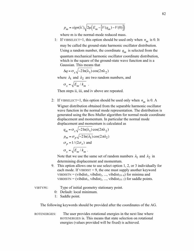
82

pm = sign( !λ ) 2µ Em − V (qm)−V (0)!" #$( )

where m is the normal-mode reduced mass. 1: If VIBSELECT=1, this option should be used only when nm is 0. It

may be called the ground-state harmonic oscillator distribution. Using a random number, the coordinate qm is selected from the quantum mechanical harmonic oscillator coordinate distribution, which is the square of the ground-state wave function and is a Gaussian. This means that

Δq = σx −2ln(λ1) cos(2πλ2)

where λ1 and λ2 are two random numbers, and

σx = Em / km .

Then steps ii, iii, and iv above are repeated.

2: If VIBSELECT=1, this option should be used only when nm is 0. A Wigner distribution obtained from the separable harmonic oscillator wave function in the normal mode representation. The distribution is generated using the Box-Muller algorithm for normal mode coordinate displacement and momentum. In particular the normal mode displacement and momentum is calculated as

qm = σx −2ln(λ1) cos(2πλ2)

pm =σ p −2 ln(λ1) cos(2πλ2) σ p =1/ (2σ x ) and

σx = Em / km . Note that we use the same set of random numbers λ1 and λ2 in determining displacement and momentum.

9. This option allows one to use select option 1, 2, or 3 individually for each mode. If VIBDIST = 9, the one must supply another keyword VIBDISTN = (vibdist1, vibdist2, ..., vibdist3N–6) for minima and

VIBDISTN = (vibdist1, vibdist2, ..., vibdist3N–7) for saddle points. VIBTYPE: Type of initial geometry stationary point. 0: Default: local minimum. 1: Saddle point.

The following keywords should be provided after the coordinates of the AG. ROTENERGIES: The user provides rotational energies in the next line where

ROTENERGIES is. This means that state selection on rotational energies (values provided will be fixed) is achieved.

83

ROTSTATES: The user provides rotational quantum numbers in the next line where

ROTSTATES is. Only linear AG can be dealt with at present. This means that state selection on rotational states is achieved. If both ROTSTATES and ROTENERGIES are not provided, by default, the program will randomly generate the rotational state or rotational energies needed according to the Boltzmann distribution for every trajectory.

VIBDISTN If VIBDIST=9, user must supply this keyword to select VIBDIST (0, 1,

or 2) individually for each vibrational mode. For example, if one wants to choose different phase space distribution method for a molecule with 6 vibrational modes (vibrational modes are in order of decreasing magnitude of their frequencies)

VIBDISTN 0 0 0 1 1 1

VIBENE Double precision: fixed energy for each vibrational mode in eV. The

default is 0.02 eV for all modes. (i) When VIBSELECT = 4 or 6, the amount of energy for each

mode is the same so only one value is needed after this keyword

(ii) When VIBSELECT = 5 or 7, user provides 3N-6 (local minimum) or 3N-7 (first order saddle point) energies for each mode individually. For example, a molecule with 5 vibrational modes has following input

VIBENE 0.02 0.02 0.02 0.01 0.01

VIBSTATES: For a local minimum, the user provides vibrational quantum numbers of each mode in the line following the keyword VIBSTATES. Using this keyword means to do a normal mode analysis to provide initial coordinates and also means VIBSELECT=1. For a saddle point, the user provides the 3N−6 (linear molecule) or 3N−7 (nonlinear molecule) vibrational quantum numbers for the bound normal modes, and a positive or negative real number meaning the translational energy along the unbound normal mode in its positive or negative direction, respectively (in eV). The vibrational quantum numbers can be fractional (e.g. 0.5). This is useful to distribute excitations equally along degenerate components of a normal mode. For example, for a doubly degenerate normal mode, a single excitation could be specified assigning 0.5 to both components in the input file. VIBSTATES 0 0 0 0 1

84

XII.L. $COMXX input deck

$COMXX: The Cartesian coordinates (in Å) of the center of mass for all the AGs. For example, the first AG is placed at the origin, while the second AG is

placed 20.0 Å away on the z axis: $COMXX 0.0 0.0 0.0 0.0 0.0 20.0 $END

XII.M. $COMPP input deck $COMPP: The three components of momenta (in atomic units) of the center of

mass for all the AGs. For example: $COMPP 0.0 0.0 0.0 0.0 0.0 20.0 $END

85

XIII. Output files Unit 6 (standard output): General output. General information and error warnings are written to the standard output (unit 6). Unit 10: Initial coordinates. The first line contains the trajectory index and potential energy in eV, followed by (one line for each atom) 1. Atomic symbol 2. Atomic mass in amu 3. The Cartesian coordinates in Å. Unit 11: Initial momenta. The first line contains the trajectory index and kinetic energy in eV, followed by (one line for each atom) 1. Atomic symbol 2. Atomic mass in amu 3. The Cartesian components of the nuclear momentum in atomic units. Unit 20: Final coordinates. The first line contains the trajectory index and potential energy in eV, followed by (one line for each atom) 1. Atomic symbol 2. Atomic mass in amu 3. The Cartesian coordinates in Å. Unit 21: Final momenta. The first line contains the trajectory index and kinetic energy in eV, followed by (one line for each atom) 1. Atomic symbol 2. Atomic mass in amu 3. The Cartesian components of the nuclear momentum in atomic units. Unit 22: Intermediate coordinates; step interval printing is controlled by NPRINT. The first line contains the number of atoms, and the second line contains trajectory index, the step index, the time (fs), and the potential energy in eV, followed by (one line for each atom) 1. Atomic symbol 2. The Cartesian coordinates in Å. This file is essentially xyz format so that it can be visualized by various visualization programs, e.g. molden. Unit 221: Adiabatic potential energies in eV. Each line contains: index of trajectory, time (fs), weight of the trajectory at the current time, mean potential energy, adiabatic

86

potential energies for electronic surface 1, 2, 3, …, NSURFT. In case of single surface trajectory, mean potential and electronic surface 1 are the same values. Unit 222: Upper triangle of density matrix elements. The representation of the density matrix is determined by REPFLAG keyword. Each line contains: index of trajectory, time (fs), weight of the trajectory at the current time, (Re(ρij ), j =1,nsurft), i =1,nsurft) . Unit 223: Upper triangle of diabatic energy matrix (in eV). Each line contains: index of trajectory, time (fs), weight of the trajectory at the current time, (Uij, j =1,nsurft), i =1,nsurft) . Unit 23: Intermediate momenta; step interval printing is controlled by NPRINT. The first line contains the trajectory index, index of this geometry for this trajectory, the step index, the time (fs), and the kinetic energy in eV, followed by (one line for each atom) 1. Atomic symbol 2. Atomic mass in amu 3. The Cartesian components of the nuclear momentum in atomic units. Unit 24 and Unit 25 are used to save the coordinates and momentum of a fragments during fragmentation analysis run (TERMFLAG=7) and are only written when a fragmentation occurs. Unit 24: fragment coordinates. The first line contains the trajectory index and fragment index for this dissociated trajectory, followed by (one line for each atom) 1. Original index 2. Atomic symbol 3. Atomic mass in amu 4. The Cartesian coordinates in Å. Unit 25: fragment momentum. The first line contains the trajectory index and fragment index for this dissociated trajectory, followed by (one line for each atom) 1. Original index 2. Atomic symbol 3. Atomic mass in amu 4. The Cartesian components of the nuclear momentum in atomic units. Unit 26: Geometry at the end of momentum rescaling/temperature changing. The first line contains the trajectory index, the times of the momentum rescalings/temperature changes, average temperature, and potential energy at this geometry, followed by (one line for each atom) 1. Atomic symbol 2. Atomic mass in amu 3. The Cartesian coordinates in Å.

87

Unit 27: Information on the dynamics. By default, some information is printed out at the beginning and at the end of the dynamics for mean-field approaches, but also at each allowed for surface-hopping methods. This file contains the trajectory index, the current step, the current surface (the adiabatic surface n which the dynamics is performed for surface-hopping methods, but the adiabatic surface to which the average surface tends to decay for the CSDM method), the current time (related to the current step, and expressed in fs), the populations on each surface, and the adiabatic or diabatic energies (depending on the representation used for the dynamics). Unit 28: Used by TFLAG1=5 only. Optimized geometry. A geometry optimization is sometimes performed to calculate some thermal properties of the system during the dynamics. The first line contains the number of iterations needed for optimization, the optimized potential energy at this geometry, the current step at which the geometry is optimized, the current time (related to the current step, and expressed in fs), the average temperature, and is followed by the optimized geometry itself (one line for each atom): 1. Atomic symbol. 2. Atomic mass in amu. 3. The Cartesian coordinates in Å. Unit 29: Information on geometries and relative translational energies between each H atom and NH2 fragment for the NH3 potential (printed out as often as Unit 27 for NH3). When LMODPOP is false, each line contains the trajectory index, the current step, the current surface index, the current number of allowed hops (0 for mean-field approaches), the current time (related to the current step, and expressed in fs), the adiabatic and diabatic energies (in eV), the three relative translational energies between H and NH2 (in eV), the three N-H distances (in Å), the three H-N-H angles (in deg), the nonplanarity angle (in deg, see Refs 13). When LMODPOP is true, we also add the mode populations at the end of each line. Remark 1: The definition of the current surface on which the dynamics is performed is not exactly the same within the framework of multi-surface simulations according to the dynamical method used. In surface hopping methods (TFS and FSTU methods), the current surface is the index of the surface on which the system has hopped. This surface may be a diabatic or adiabatic one, this depending on the chosen representation. When using mean-field methods with decay of mixing (SCDM and CSDM methods), the current surface is in fact the surface (diabatic or adiabatic) through which the system will relax to asymptotically reach a physical surface. The propagation in mean-field methods is indeed performed on an averaged surface. Remark 2: Relative energies are derived from the subroutine RELENERG that was designed to give the three meaningful relative energies of NH3 (that is, relative energies between H and NH2).

88

Unit 30: Atom-diatom scattering output (for INITX=4 only). Note: The rovibrational quantum numbers are not accurate for the semiclassical Ehrenfest method because the code assumes a single potential energy surface when the simulation terminates. 1. Trajectory index 2. Final surface label 3. Final arrangement label Note: 1 = AB + C, 2 = BC + A, 3 = CA + B 4. Total time for the trajectory in (fs) 5. Total number of integration steps 6. Final value of the electronic state density matrix for state 1 7. Final value of the electronic state density matrix for state 2 8. Final total energy (eV) 9. Potential energy of the classical minimum of the final arrangement (eV) 10. Final kinetic energy corresponding to the relative atom-diatom translational

motion (eV) 11. Final internal (rovibrational) energy of the diatomic fragment (eV) 12. Final vibrational energy of the diatomic fragment (eV) 13. Final rotational energy of the diatomic fragment (eV) 14. Final classical (unquantized) vibrational quantum number. 15. Final classical (unquantized) rotational quantum number. Unit 31: Bimolecular collision output (for TERMFLAG=3 only) 1. Trajectory index 2. Final surface label 3. Final outcome index 4. Time in fs 5. Final relative translational energy in eV for fragment 1 6. Final angular momentum of fragment 1 about the origin in atomic units 7. Final angular momentum of fragment 1 about the center of mass of fragment 1 8. Final relative translational energy in eV for fragment 2 9. Final angular momentum of fragment 2 about the origin in atomic units 10. Final angular momentum of fragment 2 about the center of mass of fragment 2. Unit 34: Geometries along tunneling paths. The starting point, maximum of potential, and ending point of each accepted tunneling path are printed in this file in xyz format. This file can be visualized using Molden. The tunneling probability and weight of each path is printed along with the starting geometry. Unit 340: Adiabatic, diabatic potential energies (in eV) and real part of density elements

along tunneling path. Density matrix depends on representation used. Every three lines contains following information 1. Length of tunneling path (Å), mean potential, adiabatic potential (V1, V2, …, Vnsurft) 2. Length of tunneling path (Å), diabatic potentials (Uij, j =1,nsurft), i =1,nsurft) 3. Length of tunneling path (Å), density elements (Re(ρij ), j =1,nsurft), i =1,nsurft)

89

For each tunneling path, the first three lines are for starting of tunneling, the second three lines are for maximum-effective-potential point, and the last three lines are for the end of tunneling path. Unit 40: Temperature ramping output. Note: This output is written only if TFLAG1= 2, 3, or 4. Data is written every time after momenta ramping or temperature changing. Each line contains: 1. Trajectory index 2. Step 3. Time in fs 4. Time average of the temperature 5. Berry parameter (the relative second moment of the bond distances, averaged over

all atom pairs)

2 22 ( ) /( 1) ij ij ij

i j iR R R

N Nδ

>

= < > − < > < >− ∑∑ ,

where N is the number of atoms and Rij is the distance between atoms i and j. 6. Time average heat capacity in eV/K 7. Time average cohesive energy in eV/atom 8. Time average kinetic energy 9. Time average total energy 10. Time average sphericity L calculated by

( ), ,

( max )

13

unique

average

unique i i i averagei A B C

average A B C

IL

I

I I i i I I I

I I I I

δ=

=

⎡ ⎤= = − −⎢ ⎥⎣ ⎦

= + +

Iunique is the principal moment of inertia deviating most from the average. IA, IB, and IC are the three principal moments of inertia

11. Standard deviation of L 12. Time average distance between the atoms and the CoM in Ǻ:

1 | |i CoMi

RCoM r rN

= −∑ v v

13. Time average square distance between the atoms and the CoM in Ǻ2: 212 | |i CoM

iRCoM r r

N= −∑ v v

14. If file unit 50 is required, time average volume (in Ǻ3) of the Atom Group (AG) calculated by an overlap sphere method (currently only pure aluminum is available)

15. If file unit 50 is required, standard deviation of the volume of the cluster calculated by the overlap sphere method

90

16. If file unit 50 is required, time average density (in g/cm3) of the AG calculated by the overlap sphere method

17. If file unit 50 is required, standard deviation of the density (in g/cm3) of the AG calculated by the overlap sphere method

18. Time average volume (in Ǻ3) of the AG estimated by the radius of gyration method (Volg):

( ) , 1 3g i iR I M i= = − , where {Ii, i = 1 – 3} are the three principal moments of inertia. The volume of the cluster is calculated by:

3/ 2

(1) (2) (3)4 53 2g g g gVol R R Rπ ⎛ ⎞≈ ⎜ ⎟⎝ ⎠

.

19. Standard deviation of the Volg 20. Time average density (in g/cm3) of the cluster calculated by the radius of gyration

method 21. Standard deviation of the density (in g/cm3) calculated by the radius of gyration

method. Note: Entries 4 - 21 are calculated between temperature rescalings/changing. Unit 41: Radial distribution function Data is written for every NPRINT steps and at the end of each trajectory. 1. Trajectory index 2. Time in fs 3. A series of numbers representing the radial distribution function binned into

equally spaced bins and averaged over the trajectory. The radial distribution function is normalized to unit area. The bin size [RBIN] is hard coded in RADIALDIST to be 1/8 the bulk Al nearest-neighbor distance (i.e., 1/8 of 4.02 Å)

91

Unit 42: Honeycutt-Andersen parameter. This output is written when the temperature is rescaled (TFLAG1=2) and when each trajectory finishes. For a definition of the Honeycutt-Andersen (HA) index see Ref. 27 in Section XV. Briefly, the HA index is a set of four indices which describes the local geometry of a bonded pair of atoms (i.e., a pair of atoms with a bond distance less than some cutoff distance RNN). Here we record the fraction of bonded pairs H(i, j, k, l) with HA indices (i, j, k, l). RNN is hard-coded in HONEY with the value 3.5 Å. 1. Trajectory index 2. Time in fs 3. The sum of H(1, 2, k, l) for all k and l 4. The sum of H(1, 3, k, l) for all k and l 5. The sum of H(1, 4, k, l) for all k and l 6. The sum of H(1, 5, k, l) for all k and l 7. The sum of H(1, 6, k, l) for all k and l 8. H(1, 4, 2, 1) 9. H(1, 4, 2, 2) Unit 43: Time average of the distance of each atom to the CoM. Data is written at the end of momentum ramping or temperature changing. Each line contains: 1. Trajectory index 2. Step 3. Time in fs 4. Time average of the temperature 5. RCoM in Ǻ. 6. RCoM(i) of all the atoms:

( ) | |i CoMRCoM i r r= −v v Unit 430: Same as unit 43 but written for every NPRINT steps. Unit 44: Time average of the square distance of each atom to the CoM. Data is written at the end of momentum ramping or temperature changing. Each line contains: 1. Trajectory index 2. Step 3. Time in fs 4. Time average of the temperature 5. RCoM2 in Ǻ. 6. RCoM2(i) of all the atoms:

22( ) | |i CoMRCoM i r r= −v v Unit 440: Same as unit 44 but written for every NPRINT steps. Unit 45: Single-atom-Berry parameter of each atom.

92

Data is written at the end of momentum ramping or temperature changing. Each line contains: 1. Trajectory index 2. Step 3. Time in fs 4. Time average of the temperature 5. Total Berry parameter 6. Single-atom-Berry parameter of all the atoms:

2 21 ( ) /1i ij ij ijj i

R R RN

δ≠

= < > − < > < >− ∑

Unit 450: Same as unit 45 but written for every NPRINT steps. Unit 46: Binned Berry parameter. Data is written at the end of momenta ramping or temperature changing. Each line contains: 1. Trajectory index 2. Step 3. Time in fs 4. Time average of the temperature 5. Total Berry parameter 6. Binned Berry parameter:

___

1bin m i

i bin mbin mNδ δ

∈

= ∑

_bin mN is the time average of the number of atoms in bin m. Unit 460: Same as unit 46 but written for every NPRINT steps. Unit 49: Radial atom number distribution. Data is written at the end of momentum ramping or temperature changing. Each line contains: 1. Trajectory index 2. Step 3. Time in fs 4. Time average of the temperature 5. Time average of number of atoms in bins ( _bin mN ) Unit 490: Same as unit 49 but written for every NPRINT steps. Unit 500: Volume and density of the AG the overlap sphere method. Data is written for every NPRINT steps. Each line contains: 1. Trajectory index 2. Step 3. Time in fs

93

4. Time average of the temperature 5. Time average volume (in Ǻ3) of the AG calculated by the overlap sphere method 6. Standard deviation of the volume calculated by the overlap sphere method 7. Time average density (in g/cm3) of the AG calculated by the overlap sphere

method 8. Standard deviation of the density (in g/cm3) of the AG calculated by the overlap

sphere method Unit 51: Binned RCoM. Data is written at the end of momentum ramping or temperature changing. Each line contains: 1. Trajectory index 2. Step 3. Time in fs 4. Time average of the temperature 5. RCoM in Ǻ. 6. Binned RCoM:

___

1 ( )bin mi bin mbin m

RCoM RCOM iN ∈

= ∑

Unit 510: Same as unit 51 but written for every NPRINT steps. Unit 60: Initial structure data saved from the equilibration run for the first AG Records (ITRAJ-1)*NATOM(1)+1 to ITRAJ*NATOM(1) is the x, y, z coordinates of the ITHAJth trajectory. Unit 61: Initial momentum data saved from the equilibration run for the first AG. Records (ITRAJ-1)*NATOM(1)+1 to ITRAJ*NATOM(1) is the x, y, z components of the momentum of the ITHAJth trajectory. Unit 62: Initial structure data saved from the equilibration run for the second AG. Records (ITRAJ-1)*NATOM(1)+1 to ITRAJ*NATOM(1) is the x, y, z coordinates of the ITHAJth trajectory. Unit 63: Initial momentum data saved from the equilibration run for the second AG. Records (ITRAJ-1)*NATOM(1)+1 to ITRAJ*NATOM(1) is the x, y, z components of the momentum of the ITHAJth trajectory. Unit 77: Used only for reactive collision simulation. Data are written every step. Each line contains: 1. Trajectory index 2. Step 3. Time in fs 4. Distance (in Ǻ) between the CoMs of the two collision AGs 5. Kinetic energy (in eV) of the CoM motion of the first AG 6. Kinetic energy (in eV) of the CoM motion of the second AG (incident AG)

94

7. Projection of the CoM motion momentum (in atomic units) of the second AG (incident AG) onto the CoM vector between the two AGs ( (2) (1)CoM CoMR R−

v v)

8. Kinetic energy (in eV) of the projected CoM motion momentum of the second AG (incident AG).

9.

95

XIV. Test suite The test suite for using analytic potential energy surfaces is in the directories tests_bimol/ and tests_unimol/ and the test suite for direct dynamics is in the directory testruns_dd/. XIV.A. Test suite for bimolecular processes using analytic potential energy surfaces The entire test suite in the directory tests_bimol/ may be compiled and run by executing

./runall from the tests_bimol/ directory. The generated outputs are placed in the tests_bimol/output/ subdirectory. The output may be compared to output obtained using previous versions of the code, stored in the subdirectory testruns/outputVN, where VN is an ANT version number. The following are brief descriptions of the runs in this test suite. Al2-Al2-rx-normod-400-1.0.in Ten trajectories simulating the collision of an Al2 molecule with another Al2 molecule using the NP-B potential. This is a single-surface calculation (METHFLAG=0). The initial conditions are prepared with normal mode analysis with randomly generated vibrational states. The initial rotational states of the two Al2 are also randomly generated. The products are monitored with the fragment merge termination condition (TERMFLAG=4) with a default TERMSTEPS (50). Al2-Al-rx-normod-400-1.0.in Ten trajectories simulating the collision of an Al2 molecule with an Al atom using the NP-B potential. This is a single-surface calculation (METHFLAG=0). The initial conditions are prepared with normal mode analysis with randomly generated vibrational states. The initial rotational states of the two Al2 are also randomly generated. Al-Al59-rx-2000.in Three trajectories simulating the collision of an Al atom with an Al59 cluster using the NP-B potential. This is a single-surface calculation (METHFLAG=0). The Al59 cluster is equilibrated for 20000 fs before saving configurations for the later bimolecular collision simulation. OH+H2-rx-normod-1000-0.5.in Two thousand trajectories simulating the bimolecular reactive collision of OH + H2 using the OH3 potential. This is a single-surface calculation (METHFLAG=0). The initial conditions are prepared with normal mode analysis with randomly generated vibrational states. The initial rotational states of OH and H2 are also randomly generated. The products are monitored with OH bond forming condition (TERMFLAG=3). The reaction rate constant at 1000 K is calculated, and it is about 3.6 times of the experimental value.

96

LiFH-SEa.in Three trajectories for adiabatic (REPFLAG=0) semiclassical Ehrenfest (METHFLAG= 2) atom-diatom scattering calculations using the LiFHJ potential. The Bulirsch-Stoer integrator with the method of Hack et al. [Ref. 4 in Section XV] of calculating hopping probabilities (BULSTOINTHACK) is employed in this and in the other LiFH calculations. This calculation involves two coupled electronic states. The initial conditions are set by INITX=4, and INITP is not used. LiFH-SEd.in Three trajectories for diabatic (REPFLAG=1) semiclassical Ehrenfest (METHFLAG=2) atom-diatom scattering calculations using the LiFHJ potential. Note: the SE method gives identical trajectories for the adiabatic and diabatic representations for two electronic surfaces. This calculation involves two coupled electronic states. The initial conditions are set by INITX=4, and INITP is not used. LiFH-u22.in Three single-surface (METHFLAG=0) diabatic (REPFLAG=1) bimolecular trajectories for the LiFHJ potential. The initial conditions are set by INITX=4, and INITP is not used. LiFH-v1.in Three single-surface (METHFLAG=0) adiabatic (REPFLAG=0) bimolecular trajectories for the LiFHJ potential. This calculation involves two coupled electronic states. The initial conditions are set by INITX=4, and INITP is not used. MCH-SCDMa.in Three adiabatic (REPFLAG=0) SCDM (METHFLAG=3) bimolecular trajectories for the MCH(SB) potential. This calculation involves two coupled electronic states. The Bulirsch-Stoer integrator with the method of Hack et al. [Ref. 4 in Section XV] of calculating hopping probabilities (BULSTOINTHACK) is employed in this and in the other MCH calculations. The initial conditions are set by INITX=4, and INITP is not used. MCH-SCDMd.in Three diabatic (REPFLAG=1) SCDM (METHFLAG=3) trajectories for the MCH(SB) potential. This calculation involves two coupled electronic states. The initial conditions are set by INITX=4, and INITP is not used. MCH-CSDMa.in Three adiabatic (REPFLAG=0) CSDM (METHFLAG=4) bimolecular trajectories for the MCH(SB) potential. This calculation involves two coupled electronic states. The initial conditions are set by INITX=4, and INITP is not used. MCH-CSDMd.in Three diabatic (REPFLAG=1) CSDM (METHFLAG=4) bimolecular trajectories for the MCH(SB) potential. This calculation involves two coupled electronic states. The initial conditions are set by INITX=4, and INITP is not used.

97

YRH-FSa.in Three adiabatic (REPFLAG=0) fewest-switches surface hopping (METHFLAG=1) trajectories for the YRH(0.2) potential. This calculation involves two coupled electronic states. The Bulirsch-Stoer integrator with the method of Hack et al. [Ref. 4 in Section XV] of calculating hopping probabilities (BULSTOINTHACK) is employed in this and in the other YRH calculations. The initial conditions are set by INITX=4, and INITP is not used. YRH-FSd.in Three diabatic (REPFLAG=1) fewest-switches surface hopping (METHFLAG=1) trajectories for the YRH(0.2) potential. This calculation involves two coupled electronic states. The initial conditions are set by INITX=4, and INITP is not used. YRH-FSTUa.in Three adiabatic (REPFLAG=0) fewest-switches with time uncertainty surface hopping (METHFLAG=5) trajectories for the YRH(0.2) potential. This calculation involves two coupled electronic states. The initial conditions are set by INITX=4, and INITP is not used. YRH-FSTUd.in Three diabatic (REPFLAG=1) fewest-switches with time uncertainty surface hopping trajectories (METHFLAG=5) for the YRH(0.2) potential. This calculation involves two coupled electronic states. The initial conditions are set by INITX=4, and INITP is not used. n2o-3pp.in This tests the atomdiatom input for the case where ECOL, B_MIN, and B_MAX are specified. XIV.B. Test suite for unimolecular processes using analytic potential energy surfaces The test suite for unimolecular processes in the directory tests_unimol/ may be compiled and run by executing

./runall from the tests_unimol/ directory. The generated outputs are placed in the tests_unimol/output/ subdirectory. The output may be compared to output obtained using previous versions of the code, stored in the subdirectory tests_unimol/outputVN, where VN is an ANT version number. The following are brief descriptions of the runs in this test suite. Al2-opt.in Steepest descent minimization of Al2 using the NP-B potential. This is a single-surface calculation (METHFLAG=0). This run tests the steepest-descent option (TFLAG1 = 1). The initial conditions are set by INITX=1 and INITP=0. The termination condition is the RMS of gradient smaller than 0.0001 eV/A (TERMFLAG= 2, T_GRADMAG=0.0001).

98

Al3-frag.in 100 trajectories of unimolecular dissociation simulation of Al3, propagated for 20000 time steps using the fourth-order Runge-Kutta integrator with a time step of 2.0 fs and the NP-B potential. This is a single-surface calculation (METHFLAG=0). The initial geometry is the global minimum. The initial conditions are prepared with an equilibration run whose initial conditions are prepared by normal mode analysis. The temperature of the system is controlled using a Nosé-Hoover two-chain thermostat with system characteristic frequency of 0.05 1/fs. Al13-melt.in One trajectory of the simulated heating of Al13, propagated using the fourth-order Runge-Kutta integrator with a time step of 2.0 fs and the NP-B potential. This is a single-surface calculation (METHFLAG=0). The initial geometry is the global minimum. The initial conditions are prepared by normal mode analysis. The temperature of the system is controlled using a Nosé-Hoover two-chain thermostat with system characteristic frequency of 0.05 1/fs. The Atom Group (AG) is heated from 1100 K to 1300 K with a temperature step of 100 K. At each temperature, the temperature is controlled by the thermostat for 11 ps, with the last 10 ps used to average various properties. Al20-ransph-dyn-nvt-400-1.0-BS.in Three trajectories of randomized Al20 clusters, propagated for 1000 time steps using the Bulirsch-Stoer integrator and the NP-B potential. This is a single-surface calculation (METHFLAG=0). The initial conditions are set by INITX=1 (in a sphere with radius 6 Å) and INITP=1. The temperature of the system is controlled using a Berendsen thermostat with a default HSTEP0/TAUT=0.0025. Al20-rancub-dyn-nvt-400-1.0-RK4.in Three trajectories for randomly generated Al20 clusters, propagated for 1000 time steps using the fourth-order Runge-Kutta integrator and the NP-B potential. This is a single-surface calculation (METHFLAG=0). The initial conditions are set by INITX=2 (in a cubic cell with length 6 Å) and INITP=1. The temperature of the system is controlled using a Berendsen thermostat with a default HSTEP0/TAUT=0.0025. Al20-ransph-dyn-nvt-400-1.0-RK4.in Three trajectories for randomly generated Al20 clusters, propagated for 1000 time steps using the fourth-order Runge-Kutta integrator and the NP-B potential. This is a single-surface calculation (METHFLAG=0). The initial conditions are set by INITX=1 (in a sphere with radius 6 Å) and INITP=1. The temperature of the system is controlled using a Berendsen thermostat with a default HSTEP0/TAUT=0.0025. Al20-ransph-dyn-nvt-400-1.0-nh-RK4.in Three trajectories for randomly generated Al20 clusters, propagated for 1000 time steps using the fourth-order Runge-Kutta integrator and the NP-B potential. This is a single-surface calculation (METHFLAG=0). The initial conditions are set by INITX=1 (in a sphere with radius 6 Å) and INITP=1. The temperature of the system is controlled using a Nosé-Hoover two-chain thermostat with a system characteristic frequency of 0.05 1/fs.

99

Al20-ransph-dyn-nvt-400-1.0-an-RK4.in Three trajectories for randomly generated Al20 clusters, propagated for 1000 time steps using the fourth-order Runge-Kutta integrator and the NP-B potential. This is a single-surface calculation (METHFLAG = 0). The initial conditions are set by INITX=1 (in a sphere with radius 6 Å) and INITP=1. The temperature of the system is controlled using an Andersen thermostat with a collision frequency of 0.01 1/fs. Al20-arb-dyn-nvt-400-1.0-RK4.in Three trajectories for randomly generated Al20 clusters, propagated for 1000 time steps using the fourth-order Runge-Kutta integrator and the NP-B potential. This is a single-surface calculation (METHFLAG=0). The initial conditions are set by INITX=3 (arbitrary shape) and INITP=1. The temperature of the system is controlled using an Andersen thermostat with a default HSTEP0/TAUT=0.0025. CH2BrClPES-CSDMd7en50ev.in Two diabatic (REPFLAG=1) CSDM (METHFLAG=4) spin-coupled photodissociation trajectories for the BrCH2Cl dissociation system. The initial conditions are prepared for v =0 vibrational state of the ground-state potential for all normal modes, using a Wigner distribution generated by using the Box-Muller algorithm [Refs. 2 and 3 in Section XV]. The Bulirsch-Stoer integrator with the method of Hack et al. [Ref. 4 in Section XV] (BULSTOINTHACK) is employed. The option for minimal printout of the selection of initial conditions step (MINPRINTICON) is defined. The dynamics starts in the n = 7 potential at constant energy (5 eV) and the trajectory dissociates in electronic state n =7 to produce Br(2P3/2 + CH2Cl(X 1A´). HBr-FSTUa.in One hundred adiabatic (REPFLAG=0) FSTU (METHFLAG=5) spin-coupled photodissociation trajectories for the HBr diatomic (see Ref. 10 in Section XV). The initial conditions are prepared for v = 0 vibrational state of the ground-state potential using a Wigner distribution generated by using the Box-Muller algorithm [Refs. 2 and 3 in Section XV] with projected Hessian for the initial normal mode (NTRAPZ=1). The Bulirsch-Stoer integrator with the method of Hack et al. [Ref. 4 in Section XV] of calculating hopping probabilities (BULSTOINTHACK) is employed. The option for minimal printout of the selection of initial conditions step (MINPRINTICON) is defined. The dynamics starts in the n = 8 potential at constant energy (7 eV) corresponding to the spin-orbit coupled 1Π1 state and dissociates in three different electronic states (n = 4 corresponding to 3Π1, n = 8 corresponding to 1Π1, and n = 11 corresponding to 3Σ1). The first two electronic states correlate with bromine in its lower fine-structure level (H(2S) + Br(2P3/2)) and the third electronic state correlates with the bromine higher fine-structure level (H(2S) + Br(2P1/2)). HBr-FSTUSDa.in One hundred adiabatic (REPFLAG=0) FSTU/SD (METHFLAG= 5, STODECOFLAG=1) spin-coupled photodissociation trajectories for the HBr diatomic (see Ref. 10 in Section XV). The initial conditions and the rest of options are the same as for the ´HBr-FSTUa.in´ job.

100

HBr-CSDMa.in One hundred adiabatic (REPFLAG=0) CSDM (METHFLAG=4) spin-coupled photodissociation trajectories for the HBr diatomic (see Ref. 10 in Section XV). The initial conditions and the rest of options are the same as for the FSTU and FSTU/SD jobs. HN2-tunneling.in Ten single-surface trajectories for H-N dissociation. Tunneling is included using the army ants tunneling algorithm. The total energy is 0.65 eV, and initial conditions are selected with INITX=0 and INITP=1. nh3-SCDMa.in One adiabatic (REPFLAG=0) SCDM (METHFLAG=3) photodissociation trajectory for the nh3potg-new potential. This calculation involves two coupled electronic states. The Bulirsch-Stoer integrator with the method of Hack et al. [Ref. 4 in Section XV] of calculating hopping/switching probabilities (BULSTOINTHACK) is employed in this and in the other NH3 calculations. The initial conditions are set by INITX=1, VIBSELECT=2, and INITP is not used. nh3-SCDMd.in One diabatic (REPFLAG=1) SCDM (METHFLAG=3) photodissociation trajectory for the nh3potg-new potential. This calculation involves two coupled electronic states. The initial conditions are set by INITX=1, VIBSELECT=2, and INITP is not used. nh3-CSDMa.in One adiabatic (REPFLAG=0) CSDM (METHFLAG=4) photodissociation trajectory for the nh3potg-new potential. This calculation involves two coupled electronic states. The initial conditions are set by INITX=1, VIBSELECT=2, and INITP is not used. nh3-CSDMd.in One diabatic (REPFLAG=1) CSDM (METHFLAG=4) photodissociation trajectory for the nh3potg-new potential. This calculation involves two coupled electronic states. The initial conditions are set by INITX=1, VIBSELECT=2, and INITP is not used. nh3-FSTUa.in Three adiabatic (REPFLAG=0) FSTU (METHFLAG=5) photodissociation trajectories for the nh3potg-new potential. The frustrated hops are ignored (FRUSMETH=0). This calculation involves two coupled electronic states starting from the vibrational ground state of the first electronic excited state minimum of NH3. The initial conditions are set by INITX=1, VIBSELECT=1, and VIBDIST=0, and INITP is not used. The projected Hessian is used to generate initial conditions, but TRAPZ-like methods are not used during the dynamics (NTRAPZ=1). nh3-FSTUd.in Three diabatic (REPFLAG=1) FSTU (METHFLAG=5) photodissociation trajectories for the nh3potg-new potential. The frustrated hops are treated using the gradV method

101

(FRUSMETH=2). This calculation involves two coupled electronic states starting from the vibrational ground state of the first electronic excited state minimum of NH3. The initial conditions are set by INITX=1, VIBSELECT=1, and VIBDIST=0, and INITP is not used. nh3-FSTUSDamTRAPZ.in One adiabatic (REPFLAG=0) FSTU/SD (METHFLAG=5) photodissociation trajectory for the nh3potg-new potential. This calculation involves two coupled electronic states starting from the vibrational ground state of the first electronic excited state minimum of NH3. The initial conditions are set by INITX=1, VIBSELECT=1, VIBDIST=0, and INITP is not used. The projected Hessian is used to generate initial conditions, and the mTRAPZ method is used in the dynamics (NTRAPZ=3, NVERS=1). The option for minimal printout of information related to TRAPZ-like methods (MINIPRINTTRAPZ) is used. nh3-FSTUSDa.in One adiabatic (REPFLAG=0) FSTU/SD (METHFLAG=5) photodissociation trajectory for the nh3potg-new potential. This calculation has most of its input options defined as in the previous calculation, but here the unprojected Hessian is used to generate initial conditions and none of the TRAPZ-like methods is used in the dynamics (NTRAPZ=0). nh3-FSTUaSaddle.in Three adiabatic (REPFLAG=0) FSTU (METHFLAG=5) photodissociation trajectory for the nh3potg-new potential. This calculation starts at the saddle point of the excited adiabatic PES (V2). The initial conditions are set by INITX=0, INITP=-1, VIBSELECT=1, VIBDIST=0, and VIBTYPE=1. The bound modes at the saddle point are at their ground state and an energy of 0.1 eV is added along the positive direction of the unbound normal mode. phohaprp-CSDMtunn.in One three-surface trajectory for phenol photodissociation using anchor-points reactive potentials. Nonadiabatic tunneling is included using the army ants tunneling algorithm. The initial conditions are selected with INITX=0, INITP=-1, VIBSELECT=5 VIBDIST=1 keywords for a state-selected initial condition with the initial population on adiabatic state 2 (using NSURFI=2 and NSURF0=2). The vibrational energies for each vibrational state are specified by keyword VIBENE. Note carefully that this test isn't actually long enough to observe a successful tunneling event. To properly test this option the integration time should be greatly increased, but then the run will be very expensive. XIV.C. Direct dynamics test suite Two test runs for direct dynamics are in the testruns_dd/ directory. In each subdirectory, a .pbs file is given to illustrate how to run the job in a system with the PBS scheduler. DH2 This test run is for the reactive collision of D with H2 in the ground electronic state. The Gaussian09 package is used for energy and gradient calculations on the fly (QCPACK=1). The potential energy surface is calculated by the MP2/6-31G(d) method.

102

HCOH Ten trajectories for the isomerization of cis-HCOH to trans-HCOH in the ground electronic state. The potential energy (PM3/PDDG) is calculated by the MOPAC-mn program. Tunneling is included using the army ants tunneling algorithm.

103

XV. Bibliography

1 F. J. Vesely, J. Comp. Phys. 47, 291 (1982).

2 E. Wigner, Phys. Rev. 40, 749 (1932).

3 W. H. Press, S. A. Teukolsky, W. T. Vetterling, and B. P. Flannery, Numerical

Recipes in FORTRAN, 2nd ed., Cambridge University Press, Cambridge, U. K., 1994.

4 M. D. Hack, A.W. Jasper, Y. L. Volobuev, D. W. Schwenke, and D. G. Truhlar, J.

Phys. Chem. A 103, 6309 (1999).

5 J. C. Tully, J. Chem. Phys. 93, 1061 (1990).

6 C. Zhu, S. Nangia, A. W. Jasper, and D. G. Truhlar, J. Chem. Phys. 121, 7658 (2004).

7 A. W. Jasper, S. N. Stechmann, and D. G. Truhlar, J. Chem. Phys. 116, 5424 (2002),

117, 10427(E) (2002).

8 A. W. Jasper and D. G. Truhlar, Chem. Phys. Lett. 369, 60 (2003).

9 A. W. Jasper and D. G. Truhlar, J. Chem. Phys. 127, 194306 (2007).

10 R. Valero, D. G. Truhlar, and A. W. Jasper, J. Phys. Chem. A 112, 5756 (2008).

11 K. F. Lim and D. A. McCormack, J. Chem. Phys. 102, 1705 (1995).

12 D. A. McCormack and K. F. Lim, Phys. Chem. Chem. Phys. 1, 1 (1999).

13 D. Bonhommeau and D. G. Truhlar, J. Chem. Phys. 129, 014302 (2008).

14 D. G. Truhlar, A. D. Isaacson, and B. C. Garrett, "Generalized Transition State

Theory," in Theory of Chemical Reaction Dynamics, edited by M. Baer, CRC Press,

Boca Raton, FL, 1985, Vol. 4, pp. 65-137.

15 D. G. Truhlar and J. T. Muckerman, "Reactive Scattering Cross Sections:

Quasiclassical and Semiclassical Methods," in Atom-Molecule Collision Theory: A

Guide for the Experimentalist, edited by R. B. Bernstein (Plenum Press, New York,

1979), pp. 505-566.

16 R. D. Levine, Molecular Reaction Dynamics (Cambridge University Press,

Cambridge, 2005).

17 L. Verlet, Phys. Rev. 159, 98 (1967); 165, 201 (1968).

18 W. C. Swope, H. C. Andersen, P. H. Berens, and K. R. Wilson, J. Chem. Phys. 76,

637 (1982).

19 D. Beeman, J. Comp. Phys. 20, 130 (1976).

104

20 M. Tuckerman, B. J. Berne, and G. J. Martyna, J. Chem. Phys. 97, 1990 (1992).

21 D. Frenkel and B. Smit, Understanding Molecular Simulation: From Algorithms to

Applications, 2nd ed., Academic Press, San Diego, 2002.

22 M. Allen and D. Tildesley, Computer Simulation of Liquids, Clarendon Press, New

York, 1987.

23 A. C. Andersen, J. Chem. Phys. 72, 2384 (1980).

24 (a) S. Nosé, J. Chem. Phys. 81, 511 (1984). (b) S. Nosé, Mol. Phys. 52, 255 (1984).

(c) W. G. Hoover, Phys. Rev. A 31, 1695 (1985).

25 G. J. Martyna, M. L. Klein, and M. Tuckerman, J. Chem. Phys. 97, 2635 (1992).

26 H. J. C. Berendsen, J. P. M. Postma, W. F. van Gunsteren, A. Di Nola, and J. R.

Haak, J. Chem. Phys. 81, 3684 (1984).

27 J. D. Honeycutt and H. C. Andersen, J. Phys. Chem. 91, 4950 (1987).

28 S. Nosé, Mol. Phys. 100, 191 (2002).

29 D. Bonhommeau and D. G. Truhlar, unpublished results (2008).

30 A. W. Jasper and D. G. Truhlar, “Non-Born-Oppenheimer Molecular Dynamics for

Conical Intersections, Avoided Crossings, and Weak Interactions,” in Conical

Intersections: Theory, Computation, and Experiment, edited by W. Domcke, D. R.

Yarkony, and H. Köppel (World Scientific, Singapore, 2011), pp. 375-412.

31 J. Zheng, X. Xu, R. Meana-Pañeda, and D. G. Truhlar, Chem. Sci. 5, 2091 (2014).

32 J. Zheng, R. Meana-Pañeda, and D. G. Truhlar, J. Phys. Chem. Lett. 5, 2039 (2014).

33 J. B. Anderson, Adv. Chem. Phys. 91, 381 (1995).

34 D. G. Truhlar and B. C. Garrett, Faraday Discuss. Chem. Soc. 84, 464 (1987).

35 M. S. Topaler, M. D. Hack, T. C. Allison, Y.-P. Liu, S. L. Mielke, D. W. Schwenke,

and D. G. Truhlar, Journal of Chemical Physics 106, 8699 (1997).

105

XVI. Parallelization

The six nested loops in the subroutine getdvec3.for are parallelized by using the OpenMP DO directive. This collapses loops and thereby speeds calculations with a large number of electronic surfaces, e.g., the CH2BrCl molecule with 24 surfaces. If the potential is parallelized with OpenMP, the program can run as a parallel computation. Two potentials in pot/ directory are parallelized with OpenMP; they are BrCH2Cl-openmp.for and NP-Bd-v3-openmp.for. To use more than one processors, one could use the shell environment variable to specify the number of threads to be used, for example export OMP_NUM_THREADS = 8 (in bash) setenv OMP_NUM_THREADS 8 (in tcsh) Note that the suffix .for is reserved for the OpenMP code in the Makefile so that all the files with .for suffix have the correct complier flags for OpenMP.

106

XVII. Platforms, operating systems, and compilers Version 2008 of the code has been compiled and tested on the following computers at the Supercomputing Institute for Digital Simulation and Advanced Computations of University of Minnesota: ________________________________________________________________________ Computer Operating System FORTRAN Compilers _______________________________________________________________________ Itasca Linux Cluster SuSE Linux Intel Fortran Compiler, v11.1

Elmo Linux Cluster SuSE Linux Intel Fortran Compiler, v12.1

_______________________________________________________________________

Version 2012-A of the code has been compiled and tested on the following computers at the Minnesota Supercomputing Institute of the University of Minnesota: ________________________________________________________________________ Computer Operating System FORTRAN Compilers (GNU core Utilities) ________________________________________________________________________ Itasca Linux Cluster SuSE Linux Intel Fortran Compiler, v11.1

(GNU coreutils 8.4) GCC Compiler, v4.6

Koronis Linux Cluster SuSE Linux Intel Fortran Compiler, v12.1

(GNU coreutils 6.12) GCC Compiler, v4.4.3

_______________________________________________________________________

Version 2013 of the code has been compiled and tested on the following computers at the Minnesota Supercomputing Institute of the University of Minnesota: ________________________________________________________________________ Computer Operating System FORTRAN Compilers (GNU core Utilities) ________________________________________________________________________ Itasca Linux Cluster SuSE Linux Intel Fortran Compiler, v11.1

(GNU coreutils 8.4) GCC Compiler, v4.6

Koronis Linux Cluster SuSE Linux Intel Fortran Compiler, v12.1

(GNU coreutils 6.12) GCC Compiler, v4.4.3

________________________________________________________________________

107

Version 2014 of the code has been compiled and tested on the following computers at the Minnesota Supercomputing Institute of the University of Minnesota: ________________________________________________________________________ Computer Operating System FORTRAN Compilers (GNU core Utilities) _______________________________________________________________________ Itasca Linux Cluster SuSE Linux Intel Fortran Compiler, v13.1.3

(GNU coreutils 8.4) GCC Compiler, v4.6.3

Koronis Linux Cluster SuSE Linux Intel Fortran Compiler, v13.1.3

(GNU coreutils 6.12) GCC Compiler, v4.4.3

_______________________________________________________________________

Version 2014-2 of the code has been compiled and tested on the following computers at the Minnesota Supercomputing Institute of the University of Minnesota: ________________________________________________________________________ Computer Operating System FORTRAN Compilers (GNU core Utilities) ________________________________________________________________________ Itasca Linux Cluster CentOS 6.6 Linux Intel Fortran Compiler, v13.1.3

(GNU coreutils 8.4) GCC Compiler, v4.6.3

________________________________________________________________________

Version 2015 of the code has been compiled and tested on the following computers at the Minnesota Supercomputing Institute of the University of Minnesota: ________________________________________________________________________ Computer Operating System FORTRAN Compilers (GNU core Utilities) ________________________________________________________________________ Itasca Linux Cluster CentOS 6.6 Linux Intel Fortran Compiler, v13.1.3

(GNU coreutils 8.4) GCC Compiler, v4.6.3

________________________________________________________________________

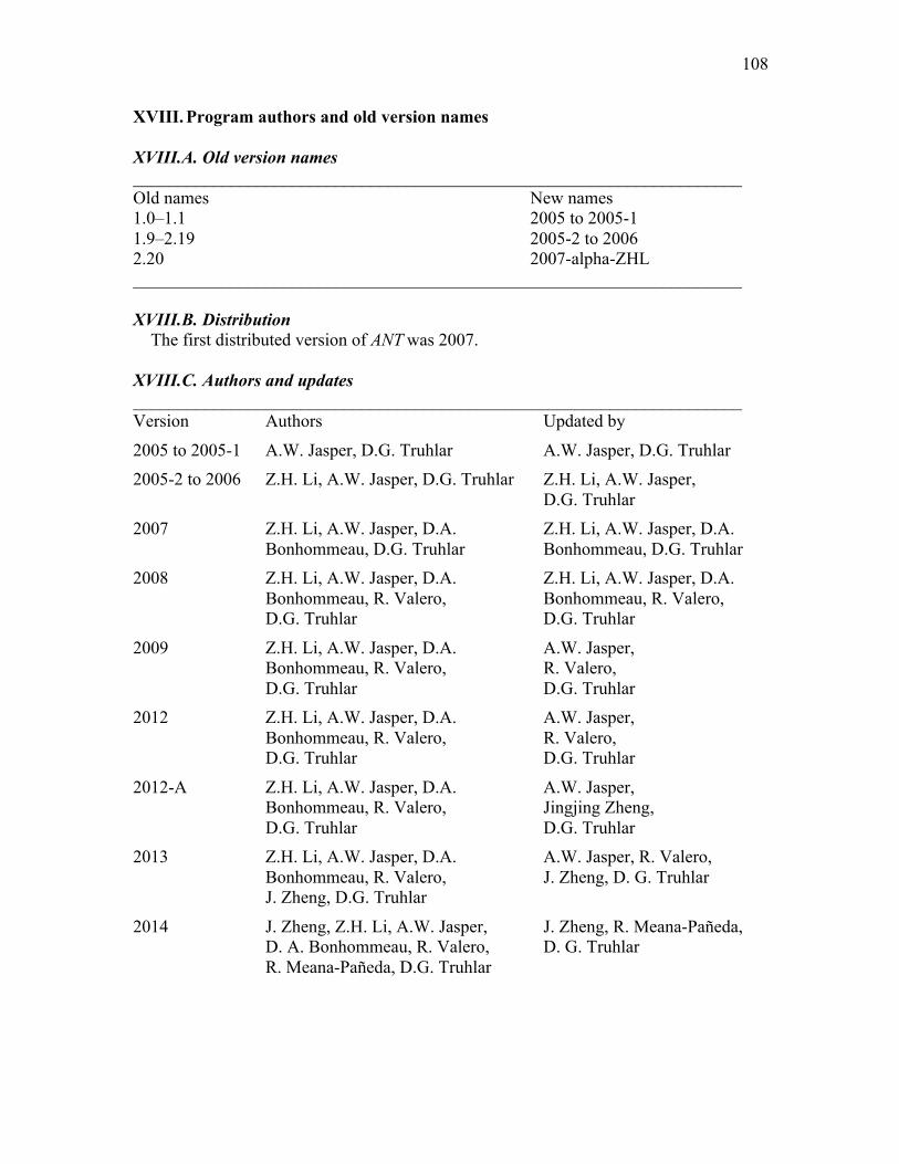
108

XVIII. Program authors and old version names XVIII.A. Old version names _____________________________________________________________________ Old names New names 1.0–1.1 2005 to 2005-1 1.9–2.19 2005-2 to 2006 2.20 2007-alpha-ZHL _____________________________________________________________________ XVIII.B. Distribution The first distributed version of ANT was 2007. XVIII.C. Authors and updates _____________________________________________________________________ Version Authors Updated by

2005 to 2005-1 A.W. Jasper, D.G. Truhlar A.W. Jasper, D.G. Truhlar 2005-2 to 2006 Z.H. Li, A.W. Jasper, D.G. Truhlar Z.H. Li, A.W. Jasper, D.G. Truhlar 2007 Z.H. Li, A.W. Jasper, D.A. Z.H. Li, A.W. Jasper, D.A. Bonhommeau, D.G. Truhlar Bonhommeau, D.G. Truhlar 2008 Z.H. Li, A.W. Jasper, D.A. Z.H. Li, A.W. Jasper, D.A. Bonhommeau, R. Valero, Bonhommeau, R. Valero, D.G. Truhlar D.G. Truhlar

2009 Z.H. Li, A.W. Jasper, D.A. A.W. Jasper, Bonhommeau, R. Valero, R. Valero, D.G. Truhlar D.G. Truhlar 2012 Z.H. Li, A.W. Jasper, D.A. A.W. Jasper, Bonhommeau, R. Valero, R. Valero, D.G. Truhlar D.G. Truhlar

2012-A Z.H. Li, A.W. Jasper, D.A. A.W. Jasper, Bonhommeau, R. Valero, Jingjing Zheng, D.G. Truhlar D.G. Truhlar 2013 Z.H. Li, A.W. Jasper, D.A. A.W. Jasper, R. Valero, Bonhommeau, R. Valero, J. Zheng, D. G. Truhlar J. Zheng, D.G. Truhlar

2014 J. Zheng, Z.H. Li, A.W. Jasper, J. Zheng, R. Meana-Pañeda, D. A. Bonhommeau, R. Valero, D. G. Truhlar R. Meana-Pañeda, D.G. Truhlar

109

2014-2 J. Zheng, Z.H. Li, A.W. Jasper, J. Zheng, R. Meana-Pañeda, D. A. Bonhommeau, R. Valero, D. G. Truhlar R. Meana-Pañeda, D.G. Truhlar 2015 J. Zheng, Z.H. Li, A.W. Jasper, R. Meana-Pañeda, J. Zheng, D. A. Bonhommeau, R. Valero, D. G. Truhlar R. Meana-Pañeda, D.G. Truhlar 2015-2 J. Zheng, Z.H. Li, A.W. Jasper, S. L. Mielke, D.G. Truhlar D. A. Bonhommeau, R. Valero, R. Meana-Pañeda, S.L. Mielke, D.G. Truhlar

2016 J. Zheng, Z.H. Li, A.W. Jasper, S. L. Mielke, D.G. Truhlar D. A. Bonhommeau, R. Valero, R. Meana-Pañeda, S.L. Mielke, D.G. Truhlar 2017 J. Zheng, Z.H. Li, A.W. Jasper, S. L. Mielke, D.G. Truhlar D. A. Bonhommeau, R. Valero, R. Meana-Pañeda, S.L. Mielke, D.G. Truhlar _____________________________________________________________________

110

XIX. Revision XX. history Version 2005

Most routines were written from scratch; some were borrowed from and/or based on NAT 8.1 by C. Zhu, S. Nangia, A. W. Jasper, Y. Volobuev, M. S. Topaler, T. C. Allison, M. D. Hack, Y.-P. Liu, A. G. Anderson, S. N. Stechmann, T. F. Miller III, N. C. Blais, and D. G. Truhlar.

Version 2005-1

Added some more analysis routines. Changed several aspects of INITx = 2. Bug fixed in the subroutine HONEY. Cleaned up output. Added the Methane.in test run.

Version 2005-2

1. Arrays in Ant1.1 to save vibrational frequencies, vibrational quantum numbers, only work for single Atom Group (AG) simulation. Corrected.

2. Temperature calculation method in Ant1.1 was improved. 3. Added more terminal conditions. The problem for the terminal condition in

Ant1.1 to monitor bond breaking was fixed. 4. Randomly generate rotational orientation of each AG. 5. Randomly generate vibrational states according to Boltzmann distribution. 6. Randomly generate rotational states according to Boltzmann distribution. 7. Added a simple temperature adjusting algorithm. 8. The calculation of moment of inertia matrix in Ant1.1 is incorrect and was fixed. 9. Reactive collision run for bimolecular reactions is added. The program can

calculate reactive cross section and reaction rate constant. Initial conditions can be specified by the user, randomly generated by the program, or to run an equilibration simulation first to provide them.

10. The program can now deal with linear AGs in a normal mode analysis. 11. Added two more methods to generate random structures: arbitrary cluster and

cuboid method. The original method for randomly generate spherical clusters was also improved.

12. Input of the program is now using a keyword input style. 13. Default values for the simulation were set.

Version 2005-2-A

Do not remove any overall motion (rotation and CoM translation) for Andersen thermostat.

Version 2005-2-B

1. Setting initial CoM translation motion for Andersen thermostat and if COMPP is not provided by the user.

2. Added a new integer variable (IEQTHERM) to control the ensemble used in the equilibration run.

111

Version 2005-2-C Change logical value NVT, NPT, NVE to integer value ITHERM: 0: NVE (default); 1: NVT; 2: NPT.

Version 2005-2-D

Added file units 22 and 23 to control writing of Cartesian coordinates and momentum every NPRINT steps.

Version 2005-3

Implement Nosé-Hoover thermostat. Version 2005-3-A

Implement Nosé-Hoover-Chain thermostat (two variables) Version 2005-3-B

Added three input parameters to control the method to choose trajectories during equilibration run: PICKTHR, DELTE0, and IPICKTRJ.

Version 2005-3-C

1. Change of rijmatr.f for termflag=7: bond forming threshold is the same as breaking threshold.

2. Modification of NP-A and NP-B for periodic conditions. Version 2005-3-D

1. Added two file units, 24 and 25, to save the fragment coordinates and momentum. 2. Modification of readin.f and c_struct.f, so that it can read in charge information

for different atoms. Added one input parameter IREADCHG to control whether or not to read in charge for each atom.

Version 2005-3-E

1. Modification of driverim.F to average total energy above and below the energy threshold (delte0).

2. Modification of Nosé-Hoover. Not require input of “mass”, but instead input characteristic vibration frequency of the system. Program automatically calculates corresponding “mass” according to the equation Nosé recommended.

3. Change of fragmentation analysis: added one subroutine FRAGCOM, to calculate the CoM coordinate and CoM motion of each fragment, and judging if a fragment is leaving CoM or not. Saving the projection of CoM motion onto CoM coordinate of this leaving fragment for later use in DRIVERIM and DRIVER.

Version 2005-3-F

1. Added one input parameter DEMAX and change DELTE0 to DEMIN, for the equilibration run, if DEMIN <= IE < DEMAX, (IE, total energy excluding overall translation energy) then save configurations.

2. An error in calculating the relative translational momentum for the reactive collision simulation was fixed: the momentum of both AGs should be Eµ2 , the

112

first AG has an initial momentum directing to –z, while that of the second AG directing to +z.

3. Added one logical variable ICFRAG to control the calculating of fragments concentration (in atomic units) in DRIVER.f (input variable: FRAGCON).

Version 2005-3-G

1. Do not remove overall rotation for equilibration runs and unimolecular fragmentation analysis (TERMFLAG = 7).

2. Modification of TERMFLAG = 4 in DRIVER: a) Use different variables to count the three termination conditions. b) For two-atom-merge condition (two-atom-reactive-collision condition), use the energy criteria in a none NVE simulation instead of TERMSTEP criteria.

Version 2006

1. Take the mean free path (λ) into account in reactive collisions: the second AG is placed at λ away from the first AG;

2. For a reactive collision run, if the distance (RCOM) between the CoMs of the two colliding AGs is less than R0COLLISION, a collision occurs. After collision, if RCOM > R0COLLISION again, terminate the simulation to save time.

3. Added a logical variable IFR0EFF to tell the program whether to use R0COLLISION or λ. R0EFFECT (the effective collision distance between two reactants) is the input variable used to calculate λ.

4. Added one logical variable (IFNOANG) to control whether to remove the CoM angular momentum before entering DRIVE (input variable, KEEPANGMOM).

5. Added IFEQWITHROT and IFREINITROT in $TRAJECT input deck to control whether equilibrate the AG with angular momenta in DRIVERIM or reinitialize the angular momentum of an AG after equilibration run.

6. Added integer variables N_RAMP and NEQUIL (input parameter NEQUILRAMP), and changed double precision variable RAMPTIME to integer variable NRAMPSTEP to control the cooling/heating.

7. Added one termination parameter (N_TURN) for reactive collisions; this parameter counts the number of the signs changed for the relative velocity of the two reactants.

8. Added one subroutine ARCOM to calculate the average distance between atoms and the CoM.

9. Average the sphericity. 10. Modification of file unit 40 to save more information during simulated annealing

simulation. 11. Added several subroutines used for calculating the volume and density of

aluminum clusters using an overlap sphere method. 12. Added several test runs for aluminum cluster simulation. 13. The program was migrated to SGI Altix with SuSE Linux operating system using

Intel FORTRAN Compiler version 8.1. 14. Added more property analysis for studying the melting of clusters. 15. Added four testing runs for NH3POTG potential.

113

Version 2007 1. Added four integrators: The simple Verlet algorithm; velocity Verlet algorithm;

Beeman algorithm; Liouville approach to velocity Verlet. 2. Improved random seed when the seed is not provided by the user. 3. Improved system time calculation. 4. Modified TFLAG1 = 4 option: Geometry optimization changed to BFGS method. 5. Added TFLAG1 = 5 option: When doing a simulated annealing simulation, at

each step, optimize the geometry with BFGS method with a probability of PICKTHR.

6. An error in the periodic boundary condition was corrected. 7. Removing overall translational momentum is an option. 8. A bug in the subroutine to remove angular momenta was fixed. 9. A bug in preparing the initial conditions for periodic systems has been fixed. 10. A bug is fixed in the adiabatic representation of the NH3 potential. 11. The parameter CPARAM used in the CSDM and SCDM algorithms is now an

input parameter. 12. For initial conditions prepared with the normal mode analysis in a single AG

simulation, the total energy can be fixed to some exact value by scaling the momenta.

13. Initial conditions on one potential energy surface can be prepared from the normal mode analysis of another potential energy surface in a multi-surface simulation.

14. Added two types of phase space distributions for the initial conditions prepared with normal mode analysis.

15. Added one output file for analyzing the relative translational energies between H atom and the NH2 fragment for the NH3 potential. A subroutine relenerg.f was added to calculating these quantities.

16. At the end of each trajectory, the program will print out the final information for surface hopping.

17. A bug introduced in ANT2.19 related to the OH3 potential surface was fixed. 18. Added two test runs for the NH3POTG potential and a test run for the collision

between an Al atom and an aluminum cluster. Version 2008

1. Three new methods for conservation of zero-point energy (called TRAPZ, mTRAPZ, and mTRAPZ*) have been implemented. The use of these methods is optional but is recommended if ZPE conservation is important in the classical or semiclassical dynamics. For non-Born-Oppenheimer calculations, the TRAPZ-like methods can only be used with trajectory surface hopping (FS, FSTU, and FSTUSD) methods, not with Ehrenfest-type (SE, SCDM or CSDM) methods. The source files normod-trapz.f and trapz.f have been added to the code.

2. The initial normal modes can now be constructed using either an unprojected Hessian or a projected Hessian. This option is normally used with the TRAPZ-like methods but can also be used independently to obtain initial normal modes where the rotational motion has been projected out and the rotational frequencies

114

are precisely zero (due to round-off and numerical noise, this is not the case for the unprojected Hessian).

3. A new scheme for the treatment of frustrated hops caused by an inaccurate treatment of decoherence, called stochastic decoherence (SD) [see Refs. 9, 10, and 13 in Section XV] has been added. The method is only meaningfully used in combination with trajectory surface hopping (FS and FSTU) methods, not with Ehrenfest-type (SE, SCDM or CSDM) methods. The method was developed in combination with FSTU (FSTU/SD), and this is the recommended combination. However, the SD scheme could also be used with FS although this combination is expected to give less accurate results. The source files elecdeco.f and stodeco.F have been added to the code.

4. Added the integration scheme of Hack et al. [Ref. 4 in Section XV] for hopping probabilities (FS, FSTU, and FSTU/SD) and switching probabilities (SCDM and CSDM). The new scheme uses the Bulirsh-Stoer integrator and is more accurate than the previous scheme using the same integrator. The source files getrhocsdm.f and integhop.f have been added to the code.

5. A bug that caused the program to give different results in different machines has been fixed adding the statement ‘SAVE hnext’ in the subroutine TAKESTEP.

6. A bug that caused trajectories reaching the time limit to be considered as dissociative has been fixed.

7. We add the possibility to perform a mode population analysis in a harmonic potential well.

8. The criterion to apply the TRAPZ-like algorithms is changed. We do not apply TRAPZ-like methods if the number of nonzero modes is above 3N -6 (resp. 3N -5) for nonlinear (resp. linear) molecules, or equivalently, if there are less than 6 (resp. 5) zero frequencies.

Version 2009

1. A new option to deal with saddle point initial geometries has been added. With this option trajectories can be started from a saddle point in a ground or excited state potential energy surface and translational energy can be added in the positive or negative direction of the unbound normal mode.

2. In the stochastic decoherence procedure, a mistake that was made before in the paper (Ref. 9) and the code has been corrected. In particular, in eq. (5) of that paper, )/exp()( τttP Δ−=Δ , Δt was defined as t − th, where th is the stochastic decoherence time, and τ is the characteristic decoherence time. The correct definition of Δt as equal to the time step of the trajectory propagation has now been implemented in the code. The literature reference for the correction is:

"Coupled-Surface Investigation of the Photodissociation of NH3(Ã): Effect of Exciting the Symmetric and Antisymmetric Stretching Modes," D. Bonhommeau, R. Valero, D. G. Truhlar, and A. Jasper, Journal of Chemical Physics 130, 234303.

3. It is now possible to define fractional initial vibrational quantum numbers. This is useful to distribute quanta of energy equally between the degenerate components

115

of normal modes. This is accomplished changing the variable qnmvib0 from an integer to a double precision variable in c_initial.f

Version 2012

1. The sum of the magnitudes of the ‘reduced’ nonadiabatic coupling vectors (see appendix 0.E) for CSDM calculations in a diabatic representation is now calculated. The subroutine getgrad.f was changed for this purpose. The sum of the magnitudes of the ‘reduced’ nonadiabatic coupling vectors is the sum of the 2x2 couplings between the current diabatic state toward which the trajectory is decohering and all the other diabatic states. (At the beginning of the subroutine there was a calculation of the magnitude of these coupling vectors that later on in the program is used to decide if there is an electronic reinitialization or not, but it was carried out with the real nonadiabatic coupling vectors, not with their equivalent in a diabatic rep. Therefore there were too many reinitializations when one ran CSDM diabatic calculations.)

2. The ‘reduced’ nonadiabatic coupling vectors for the FS and FSTU methods in diabatic representation are now calculated. The subroutine getpem.f was changed for this purpose. For all multistate systems, the same piece of code was added to getpem.f after the respective potential calls.

3. There are two new calling variables in getpem.f. One of them, named ‘icall’, allows one to call the adiabatic calculation part of the potential subroutine for a diabatic trajectory propagation that starts in the adiabatic ground state only when needed, namely, to compute the initial conditions. The other variable, named ‘nsurf’, is the current potential surface on which the trajectory is running.

Version 2012-A

1. Bugfixes: a. finalstate.f: Line 100 was changed to correctly identify and assign

arrangement 2 trajectories. b. turn.f: The unassigned parameter CAUEV was changed to AUTOEV,

which is assigned in param.f. We thank George McBane for identifying bugs a and b and their fixes.

c. LiFHJ.f: line 1448 should be commented with character “c” which was mistyped as “d” and caused a compiling problem.

2. The directory pot/ containing potential subroutines is put back into the distribution; it was missing in version 12

3. The “ –O3” flag in Makefile is replaced by an “–O” flag because aggressive optimization could lead to jobs crashing on some systems, e.g., on the Itasca machine with the ifort compiler.

4. header.f: the correct version number is updated.

116

Version 2013

1. Bugfixes: a. initelec.f: the variable nsurf is changed to nsurf0. b. driver.f: the lines in all write statements with this form:

comppm(k)*autoang/(amutoau*autofs) are changed to (comppm(k)*autoang/(amutoau*autofs),k=1,3)

c. driver.f: change natsame(mnmol,mnmol),isame(mnmol), indsame(mnat,mnmol,mnmol) to natsame(mnfrag,mnfrag), isame(mnfrag), indsame(mnat,mnfrag,mnfrag). And also change the parameters mnfrag and mnat in param.f from 1000 to 100 in order to reduce the demand for memory.

d. c_struct.f: change nattype(mnmol+1, 111) to nattype(mnmol+1,121). The numbers 112 – 121 in the second dimension are reserved for the model atoms, e.g. MCH potential.

e. normal.f: the variable nsurf is changed to either nsurf0 or nsurfi in the subroutine getpem arguments.

f. getdvec2.f: change do k = 1, nsurft do k = 1, nsurft to do k= 1, 2 do l= 1, 2

g. param.f: the parameter mnyarray=6*mnat+8*mnsurf is changed to mnyarray=6*mnat+5*mnsurf+3*mnsurf*(mnsurf-1)/2

h. In previous versions, a reactive collision may exit when distance RCOM > R0COLLISION after collision; in this case, the TERMSTEP condition does not meet even a reaction happens, so the count of reactive trajectories may be wrong. This bug is fixed.

i. decocheck.F: Add "mxtmp=0" and "mntmp=0" to initialize two variables.

j. gepol_mod.F: Add "NEJCI=0" to initialize variable NEJCI. This bug could cause segmentation fault in some cases.

k. driver.F: "itp_c_min = 0" is added to initialize the itp_c_min variable for termflag = 4 case.

2. The file getdvec3.f is changed to getdvec3.for by adding openmp derivatives. This change significantly improves the CH2BrCl dynamics by a factor of 10 speedup with one processor. Starting from this version, the suffix .for is reserved for subroutines that are parallelized with OpenMP.

3. Capability of direct dynamics is implemented. The ANT program is interfaced with the Gaussian09 and Molpro packages for direct dynamics.

Version 2014

1. The army ants tunneling algorithm is implemented for unimolecular single-

117

surface trajectories with zero total angular momentum. 2. Direct dynamics in conjunction with the MOPAC-mn program is

implemented. Version 2014-2

1. The army ants tunneling algorithm is extended to be able to treat unimolecular nonadiabatic trajectories using mean-field methods, for example, by using the SE and CSDM methods.

2. Full-dimensional anchor points-reactive potentials of phenol are added in the pot/ directory.

3. The keywords VIBENE, VERTE, BANDWD, and VIBDISTN have been implemented and VIBSELECT and VIBDIST keywords are extended so that users have more options to specify state-selected initial conditions and have vertical excitation options.

4. The keyword TINYRHO is implemented to avoid dividing by zero (or by a number that is very close to zero) in non-Born-Oppenheimer decay-of-mixing trajectories when using eq. (69) of Ref. 30. TINYRHO is used for CSDM or SCDM methods.

5. A bug in printing the final electronic state using mean-field methods (e.g. CSDM and SCDM) is fixed.

6. A bug in randomly determining the B0IMPACT parameter is fixed. 7. The calculation of time averaged decoherence time for CSDM and SCDM

methods is revised as follows:

1τ=

Δt jj∑

ρii, jτ iK, ji≠K

ρKK, j>0.98

∑

Δt jj∑

, where Δt j is time of each integration step j.

8. The input file is case insensitive now. 9. The manual has been reorganized with regard to explaining initial conditions

and input.

Version 2015

1. A new method to set the initial conditions for atom-diatom has been added. The keywords MODE, BPARAM, EMODE, and ECOL has been added to the $ATOMDIATOM input deck section.

2. All the calls to SPRNG library had been centralized in a few specialized subroutines that are located in the rng_interface.F file. Thus the extension .F is not anymore needed for any the source files of the code except for rng_interface.F.

3. The library SPRNG version 2.0 has been added. The available methods to generate random numbers in SPRNG2.0 are:

118

a. SPRNG_LFG (modified) lagged fibonacci generator b. SPRNG_LCG (48 bit) linear congruential generator (with prime addend) c. SPRNG_LCG64 64 bit linear congruential generator (with prime addend) d. SPRNG_CMRG combined multiple recursive generator e. SPRNG_MLFG multiplicative lagged fibonnaci generator When SPRNG 2.0 is used, any of these methods can be used inside the code. Currently, the ANT code uses the multiplicative lagged fibonnaci generator.

4. All the dependences in the Makefile had been updated. 5. The file gaudist.f (generation of random numbers according to a Gaussian

distribution) has been deleted. 6. The keyword FLAGDIA has been added, it defines how the diatomic potential is

computed, either with a external subroutine specific for diatoms or with the regular PES subroutine. Section III.C explains how to compile the code using the diatom potential subroutine.

Version 2015-2

1. Fixed a number of bugs related to argument mismatches or missing arguments to subroutine calls that were indicated by compiling with the "–gen interfaces –warn interfaces" flags.

2. Fixed bugs in the subroutine iteramat that allowed termination with unconverged and even diverged results and adjusted angle step sizes in actionint.f90 and actionint_nt.f90 so that calls to iteramat fell within the convergent regime. This will increase the cost of such calculations, and ideally a more-efficient scheme would be used than using fixed step sizes, but properly addressing this issue is reserved for later work. Added the correct information for linear bends to the calls generating Wilson B matrices.

3. Converted the include files containing large common blocks to modules and invoked the modules within the various routines using the "only" syntax so that all variables used from these modules are explicitly named.

4. Converted all except 4 old routines from *.f to *.f90 format. 5. Miscellaneous cleanup, grammar, and spelling corrections to fortran and make

files.

Version 2016 Changes in this version:

1. Fixed errors for the weights assigned in the army ants tunneling algorithm (changes to actionint.f90, actionint_nt.f90).

2. Removed an erroneous statement that caused all tunneling events having a probability > 0.95 to instead have a 0% tunneling probability (changes to actionint.f90, actionint_nt.f90).

3. Added the constraints necessary to ensure that the magnitudes of the atomic momenta are conserved during the determination of the momenta at the outer turning point of a tunneling event (changes to cnsvangmom.f90). Tunneling

119

calculations done prior to this correction may not exhibit proper energy conservation.

4. Removed the undebugged "HBrpotdiabfit2" potential from the potential library and rewrote the test run execution scripts so that the three HBr test runs now use the correct potential. Results for these test runs in earlier versions of the code were wrong.

5. Modified the starting guess for the iterative determination of the final momenta after a tunneling event (changes to cnsvangmom.f90) and added code to calculate the momenta at several "waypoints" along a tunneling event to ensure that the Newton–Raphson iteration at the outer tunneling point actually converges (changes to actionint.f90, actionint_nt.f90).

6. Fixed several bugs in iteramat related to the proper treatment of periodicity for angular internal coordinates.

7. Modified intcart.f90 so that when calls to iteramat do not converge the calculations are repeated with successively smaller step sizes until convergence is achieved and also increased initial step sizes.

8. Modified the routine that calculates the dihedral angle to avoid calls to atan2(0,0), which is undefined.

9. Fixed an error in takestep_nt.f90 so that after an integration step the y array is unpacked and the various components are properly updated. Previous calculations with nonadiabatic tunneling were not being properly integrated due to this error.

10. Changed the space allocated to the array tunnd in module c_traj so that memory overwrites do not occur.

11 Corrected dimensioning errors for the arrays crei and cimi. 12. Altered the code so that the variable pdoti has been calculated before the first

test to see if a turning point has been reached. In previous calculations a turning point was sometimes incorrectly indicated at the second integration step of a trajectory (the first time a test was conducted for the presence of a turning point).

13. Added a routine (brent.f90) to use Brent's algorithm for finding a zero of a 1-D function. We now use this routine to efficiently and accurately determine the location of the outer turning point during a tunneling calculation. Previously the code only calculated data on a fine grid and chose the outer turning point from the most appropriate grid point, which was slower and less accurate.

14. Replaced the use of a bisection routine with calls to brent.f90 in the routine turn.f90, which calculates vibrational turning points.

15. Added date and time stamps to the output at the beginning and the end of execution.

16. Minor formatting changes were made to the output; many minor code formatting changes were made.

120

Version 2017 Changes in this version:

1. Three related bugs (in ant.f90 and driver.f90) dating back to the ANT2014-2 revision were fixed. These problems resulted in qualitatively inaccurate results for the final printout of the reaction probability, collision probability, cross section, and rate constant in the main output file (for versions 2014-2, 2015, 2015-2, and 2016).

2. For atom-diatom calculations the code now checks for inconsistent choices among various keywords and it exits with an informative error message if any are found. The allowed input parameters have been changed; bparam, emode, and mode are no longer valid parameters and the parameters jzero, b_min, and b_max have been added. The value of emode is determined internally based on whether a collision energy or a total energy is specified. If the keyword "jzero" is specified, the code sets mode = 1 internally and sets limits on the impact parameter appropriate for J = 0 scattering; otherwise, minimum and maximum input parameters (b_min and b_max, respectively) must be specified and the code sets mode = 2 internally. Note that in previous versions of the code, the parser would, under certain conditions, overwrite the value of the input parameter "mode" with the value of "emode", and removing these parameters from the input has resolved this bug.

3. A bug in preatomdiatom.f90 that resulted in uninitialized variables being used was fixed. Previous atom-diatom calculations with mode = 2 (nonzero angular momentum) would have led to incorrect results because the sampling over the initial diatom separation would not have been done correctly.

4. A bug was fixed in the routine diamin.f90, which finds minima in diatomic potentials and diatomic effective potentials, using Brent's minimization algorithm. Previously, if the initial attempt at bracketing the minimum failed, the code would find a valid bracket but then exit without correctly optimizing the minimum. The routine produced correct results only in cases where the default bracket was appropriate.

5. Corrections were made to the routines ewkb.f90 and turn.f90 to prevent failures in the calculations of outer turning points of diatomic potentials at energies near to the dissociation limit.

6. Some seemingly contradictory output that occurred during atom-diatom calculations was modified (changes to ewkb.f90).

7. Some missing arguments were added to the call to getpem in the routine diapot.f90. This error was probably harmless, but, in any event, would only have affected atom-diatom calculations.

8. The potflag = 8 option was generalized so that a user-supplied single surface PES could be called (previously only an HN2 potential was accessible for this option). Users are expected to include code that prints a potential identifier and any desired references in the routine "prepot". See Section III.B for additional details.

9. Three corrections were made to the subroutine readin.f90; the first prevented incorrect information about possible use of the TRAPZ method from being

121

printed, the second halts the code when incorrect vibdistn related keywords are given, and the third removes a spurious error message about incorrect options for the keyword vibsel (also, when this error message is now encountered the code now stops).

10. Corrections where made to initmol.f90 to ensure that removal of initial angular momentum was not done for atom-diatom initial conditions.

11. Changes where made to finalstate.f90 to avoid a failure when the diatom energy is above the dissociation limit during the calculation of a vibrational quantum number in vwkb.f90; now we don't call the routine for such energies.

12. The code will now print out information about the highest potential energy configuration encountered during a trajectory in addition to the existing printout of information about the lowest energy configuration encountered.

13. Two new potentials, for the 3A' and 3A'' N2O surfaces, and a new test suite calculation (illustrating an atom-diatom calculation with ECOL, B_MIN, and B_MAX specified) were added.

The authors are grateful to Shaohong Li, ,Wei Lin, Rubén Meana-Pañeda, and Zoltan Varga for help in identifying some of the problems discussed above.

122

Appendices

A1. Generation of initial conditions (appendix to sections IV.A and IV.C) Rotational states

For a linear AG, if a rotational quantum state is not provided, the program will randomly generate rotational states with a Boltzmann distribution:

1. Generate a random number ξ. 2. Erot= -kBTln(1-ξ)

3. Since IJJE2

)1(rot

+= (in atomic units), where I is the inertia of rotation of the

AG, thus the quantum rotational number J can be obtained by solving

0)1ln(22 =−++ ξTIkJJ B 4. Once the rotational state J and the corresponding rotational energy

IJJE2

)1(rot

+=

are obtained, from

IE

IE

rot

2rot

221

=θ

θ=

!

!

Then

IJJ )1( +

=θ! and θ=⊥ !iii rmp

where pi⊥ is the momentum component of atom i perpendicular to the axis where the AG is on, ri is the distance between the atom and the center of mass of this AG.

5. Generate another random number ξ1 to generate the direction of θ! . 6. Add pi⊥ to original pi.

For non-linear AG, the steps to generate pi⊥ is similar to linear AG, except that Erot

generated is -0.5 kBTln(1-ξ), there is no step 3 to calculate J, and steps 1 to 5 (without 3) are repeated 3 times to produce three sets of θ! and thus three rotational momenta ( θ!I ) around each principal axis of rotation. In step 6, NOANG is called to add the rotational momenta onto the original momenta (See III.B). Vibrational states

The Boltzmann-like distribution of vibrational quantum numbers is determined as follows:

1. Frequencies are firstly calculated in subroutine NORMOD called by PREMOL. 2. Generate a random number ξ.

123

3. Vibrational energy of ith vibrational mode: Evib(i)= -kBTln(1-ξ) = nm mω , nm is the vibrational quantum number and mω is the vibrational frequency in atomic units.

4. Vibrational quantum number m

Bm

Tknω

ξ )1ln( −−=

5. Steps 2-4 are repeated until 3*N - 5 (6) (N is the atom number of this AG) vibrational quantum numbers are generated.

Once vibrational quantum numbers are generated, the following steps are used to

generate the initial momenta and position of the atoms. [Steps 1–7 are performed in NORMOD, which is called by PREMOL.]

1. The Hessian is computed numerically [ ] hXhVXhVH

jiijijjiij 2/)ˆ()ˆ( 00, ′′′′ −∇−+∇= XX

where i and i' run over atoms, j and j' run over x,y,z, h is the step size for the numerical second derivative, and the notation )ˆ( 0 ijXhV +∇ X indicates the gradient at a geometry where a small step (of magnitude h) is taken away from the initial structure in the direction of Xij. Currently, h is hard-coded to be 0.00001 a0.

2. The Hessian is mass-scaled

jjjiijjiij MM

HH′

′′′′µ→ ,, [HESS]

where m [MU] is hard-coded in PARAM and has the value 1 amu. 3. The Hessian is diagonalized using the LAPACK routine DSYEV. 4. The 6 or 5 smallest eigenvalues (7 or 6 when this is a saddle point) are

automatically ignored without any checks (to see if the system is linear, for example).

5. The remaining eigenvalues lm (force constants) are converted to harmonic frequencies

µλ=ω /mm [FREQ] where m labels the modes in order of decreasing magnitude.

6. The mass-scaled eigenvectors ijmX̂ are stored, where j labels atoms, and i labels

x,y,z. 7. The user specifies the vibrational quantum number nm [NMQN] for each mode,

and the energy for each mode is computed )( 2

1HO +ω= mmm nE ! Steps 8–13 are performed in POPNORM.

8. The turning points are computed from

µω=−±

2

HO0 2

m

mmm

ERR [RTURN]

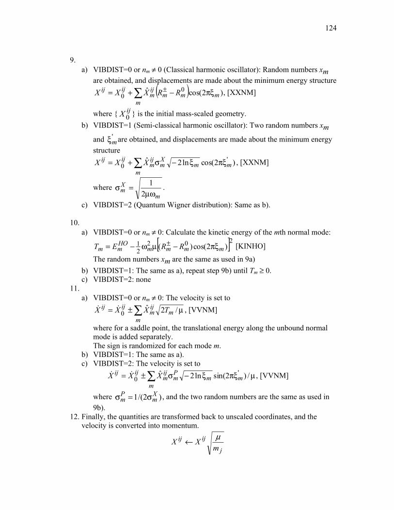
124

9.

a) VIBDIST=0 or nm ≠ 0 (Classical harmonic oscillator): Random numbers xm are obtained, and displacements are made about the minimum energy structure

( )∑ πξ−+= ±

mmmm

ijm

ijij RRXXX )2cos(ˆ 00 , [XXNM]

where { ijX 0 } is the initial mass-scaled geometry. b) VIBDIST=1 (Semi-classical harmonic oscillator): Two random numbers xm

and 'mξ are obtained, and displacements are made about the minimum energy

structure

∑ πξξ−σ+=m

mmXm

ijm

ijij XXX )2cos(ln2ˆ '0 , [XXNM]

where m

Xm µω

=σ21 .

c) VIBDIST=2 (Quantum Wigner distribution): Same as b).

10. a) VIBDIST=0 or nm ≠ 0: Calculate the kinetic energy of the mth normal mode:

[ ]20221 )2cos()( mmmm

HOmm RRET πξ−µω−= ± [KINHO]

The random numbers xm are the same as used in 9a) b) VIBDIST=1: The same as a), repeat step 9b) until Tm ≥ 0. c) VIBDIST=2: none

11. a) VIBDIST=0 or nm ≠ 0: The velocity is set to

∑ µ±=m

mijm

ijij TXXX /2ˆ0!! , [VVNM]

where for a saddle point, the translational energy along the unbound normal mode is added separately. The sign is randomized for each mode m.

b) VIBDIST=1: The same as a). c) VIBDIST=2: The velocity is set to

∑ µπξξ−σ±=m

mmPm

ijm

ijij XXX /)2sin(ln2ˆ '0!! , [VVNM]

where )2/(1 Xm

Pm σ=σ , and the two random numbers are the same as used in

9b). 12. Finally, the quantities are transformed back to unscaled coordinates, and the

velocity is converted into momentum.

j

ijijm

XX µ←

125

j

j

ijij mm

XP µ!←

Comparison of different distributions The following plots are prepared using the ammonia potential energy surface

(nh3potg.f). The distributions are always obtained for the vibrational ground state of mode 3 (asymmetric stretch) of the first electronic adiabatic excited state (V2) of ammonia.

Figure 2 Normalized distribution of mass scaled displacement (mass scaled Bohr) of

the third normal mode of the planar minimum of ammonia on the V2 adiabatic potential energy surface.

126

Figure 3 Normalized distribution of mass scaled momentum (mass scaled Bohr/atomic-unit-of-time) of the third normal mode of the planar minimum of ammonia on the V2 adiabatic potential energy surface.

Notice that for the classical and semi-classical harmonic oscillators, the

displacements fall into the range of [ 0mm RR −− , 0

mm RR −+ ].

Figure 4 Normalized distribution of total kinetic energy of the planar minimum of ammonia on the V2 adiabatic potential energy surface.

127

Figure 5 Normalized distribution of potential energy of the planar minimum of ammonia on the V2 adiabatic potential energy surface.

Figure 6 Normalized distribution of total energy of the third normal mode of the planar

minimum of ammonia on the V2 adiabatic potential energy surface. Generation of initial condition between two AGs in a reactive collision run a) Initial relative position between two AGs in a reactive collision run

1. The user provides or the program will generate a maximum distance R0 (input parameter R0COLLISION) between two AGs

2. Place the center of mass (CoM) of the first AG at the origin of the coordinate system.

3. Generate a random number ξ. 4. Calculate ξ01 Rb = , ξ−= 102 Rb . If the user provides b1 (impact parameter,

input parameter B0IMPACT), b2 is set as 21

20 bR − ; 5. Set the CoM coordinate of the second AG as:

COMXX(1,2) (x) = 0.0 COMXX(2,2) (y) = b1 COMXX(3,2) (z) = -b2 where COMXX(i,2), i = 1, 3 are the coordinates of the CoM of the second AG.

b) Initial relative translation between two AGs in a reactive collision run

1. Generate a random number ξ.

128

2. Calculate u by an iterative method, initial guess u1=1:

i

ui

ii ueu

uui)1(1

1ξ−++

+=+

3. Relative translation energy Etrans=u kBT. 4. Set all the x and y components of the CoM momentum of both the two AGs as

zero, while the z component of the first AG as - trans2 Eµ , and that of the second

AG as trans2 Eµ , where µ is the reduced mass of the two AG.

A2. Choice of thermostats

Currently, three thermostats are implemented: Andersen thermostat, Berendsen thermostat, and Nosé-Hoover thermostat with two chains.

The Berendsen thermostat is the least expensive one, but it fails for diatomic

systems if too small of a value of TAUT value is set, but even with large TAUT, it still cannot reproduce the correct canonical momentum distribution for diatomic systems.

The Andersen thermostat and the Nosé-Hoover thermostat with two chains

(hereafter called the NH thermostat) can both well reproduce the correct canonical momentum distribution for diatomic systems. However, it is well known that the Andersen thermostat does not give a continuous trajectory and its kinetic properties are greatly affected by the VFREQ value (the value determining how often the momentum of an atom is reset). Basically any result can be obtained by changing VFREQ. Nevertheless, the average static properties, such as the energies, are well predicted by the Andersen thermostat.

The NH thermostat seems to be the best of the three methods, but there are still

debates about this. Although the results are not very sensitive to the choice of the QNOSE value (the “MASS” of the two additional thermostat degrees of freedom), Nosé suggested that QNOSE should properly be chosen so that the oscillation period of the added degree of freedom is equal to the typical vibrational period of the system studied or the collision period of the system with the bath [Ref. 28 in Section XV]. The actual QNOSE value is calculated using the following equation by setting <s>2 = 1.

20

2 22

⎟⎠⎞⎜

⎝⎛=

πt

sTfkQnose B ,

where t0 is the vibrational period of collision, and f is the number of degrees of freedom of the system.

A comparison of the three thermostats for aluminum dimer: 1. Plots of momentum of one Al atom with respect to half of the Al-Al bond

distance.

129

Andersen, vfreq=0.001 and 0.05 1/fs

Berendsen, τ = 1000 fs

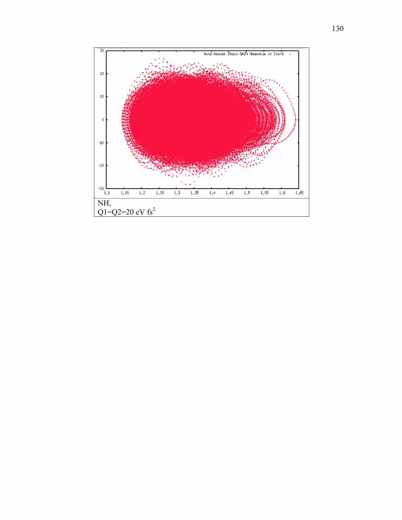
130

NH, Q1=Q2=20 eV fs2

131

2. Plot of momentum distribution (dNp/dp vs p, where Np is the number of points falling in the range from p to p+dp).

Andersen, vfreq=0.001, 0.05, 0.5 1/fs

Berendsen, τ = 1000 fs

132

NH Q1=Q2=20 eV fs2

133

A3. Description of potential interfaces (appendix to section III.B) (1) Molecular mechanics interfaces, which allow for a variable number of atoms and are labeled

T-MM-D

where T = "HO" or "HE" for a homonuclear or heteronuclear potential energy subroutine, respectively, MM stands for "molecular mechanics", and D is the number of analytic derivatives available.

The following molecular mechanics interfaces are currently standard in POTLIB-online: HO-MM-0, HO-MM-1.

More interfaces can be added as new potential energy subroutines become available. (2) Interfaces for a fixed number of atoms. These interfaces are labeled

N-DM

where N is the number of bodies, D is the number of analytic derivatives available plus one (e.g., for D = 1, only the potential energy is available, for D = 2, the potential energy and the first derivatives are available), and M is S for scalar mode (i.e., the energy for one geometry is computed per subroutine call, and the geometries, energies, and derivatives (when available) are passed using common blocks) and V for vector mode (i.e., the energies and derivatives (when available) for an array of geometries are calculated per subroutine call and are passed as arguments). Note if D = X, the potential interface is general enough to handle more than one value of D.

The following interfaces for a fixed number of atoms are currently standard in POTLIB-online: POTLIB-2001, 3-XS, 3-1V, 3-2V, 4-XS, 4-1S, 5-1S, 6-1S, and 7-1S.

(3) Interfaces for specific systems

Interfaces for the NH3, HBr, and CH2BrCl photodissociation systems.

A3.1 HO-MM-0 interface The HO-MM-0 interface is used for potential energy subprograms capable of handling an arbitrary number of identical atoms. The driver program passes the geometry as a set of Cartesian coordinates for each atom, and the potential energy is returned. Format and selected details: In general, a HO-MM-0 potential energy routine has the following format:

134

SUBROUTINE POT( X, Y, Z, E, NATOM, MAXATOM) DIMENSION X(MAXATOM), Y(MAXATOM), Z(MAXATOM) E = SOME FUNCTION OF ( X, Y, and Z ) RETURN END Required variables:

The subroutine POT takes the following arguments

POT ( X(NATOM), Y(NATOM), Z(NATOM), E, NATOM, MAXATOM ) where

NATOM input, integer The number of identical atoms.

MAXATOM input, integer Sets the dimension of the cartesian variables X, Y, and Z. MAXATOM must be greater than or equal to NATOM.

X(NATOM) Y(NATOM) Z(NATOM)

input, double precision One-dimensional arrays containing the X, Y, and Z components of all NATOM atoms, where the index labels the atoms.

E output, double precision The potential energy.

A3.2 HO-MM-1 The HO-MM-1 interface is used for potential energy subprograms capable of handling an arbitrary number of identical atoms. The driver program passes the geometry as a set of cartesian coordinates for each atom, and the potential energy and first derivatives are returned. Format and selected details: In general, a HO-MM-1 potential energy routine has the following format: SUBROUTINE POT(X, Y, Z, E, DEDX, DEDY, DEDZ, NATOM, MAXATOM) DIMENSION X(MAXATOM), Y(MAXATOM), Z(MAXATOM) DIMENSION DEDX(MAXATOM), DEDY(MAXATOM), DEDZ(MAXATOM)

135

E = SOME FUNCTION OF X, Y, and Z DEDX = SOME FUNCTION OF X, Y, and Z DEDY = SOME FUNCTION OF X, Y, and Z DEDZ = SOME FUNCTION OF X, Y, and Z RETURN END Required variables: The subroutine POT takes the following arguments

POT ( X(NATOM), Y(NATOM), Z(NATOM), E, DEDX(NATOM), DEDY(NATOM), DEDZ(NATOM), NATOM, MAXATOM ) where

NATOM input, integer The number of identical atoms.

MAXATOM input, integer Sets the dimension of the cartesian variables X, Y, and Z. MAXATOM must be greater than or equal to NATOM.

X(NATOM) Y(NATOM) Z(NATOM)

input, double precision One-dimensional arrays containing the X, Y, and Z components of all NATOM atoms, where the index labels the atoms.

E output, double precision The potential energy.

DEDX(NATOM) DEDY(NATOM) DEDZ(NATOM)

output, double precision One-dimensional arrays containing the first derivatives of the energy E with respect to the X, Y, and Z components of all NATOM atoms, where the index labels the atoms.

A3.3. POTLIB-2001 The POTLIB-2001 interface is described in detail in the Computer Physics Communications article accompanying the POTLIB-2001 program entry in the CPC program library. The reference is: R. J. Duchovic, Y. L. Volobuev, G. C. Lynch, D. G. Truhlar, T. C. Allison, A. F. Wagner, B. C. Garrett, and J. C. Corchado, "POTLIB: A Potential Energy Surface

136

Library for Chemical Systems", Computer Physics Communications 144, 169-187 (2002), 156, 319-322(E) (2004). 3-XS: The interface 3-XS is the standard interface for a 3-body system, where common blocks are used to pass data between the calling routine and the potential energy routine. The potential energy (and possibly the derivatives) are calculated for a single geometry for each call to POT. The subroutine POT requires no arguments. The common block PT1CM is required by the POT subroutine; this common block is used to pass the geometry of the triatomic system from the calling program to the potential routine and to return the electronic state energy and derivatives to the calling program. There are several other optional common blocks that may be used to further refine calls to POT. This interface may be used with or without derivatives. Format and selected details: SUBROUTINE POT COMMON /PT1CM/ R, ENERGY, DEDR DIMENSION R(3), DEDR(3) Note: The following common blocks are optional and are used to pass control variables to the potential subroutine. COMMON /PT2CM/ NSURF, NDER, NFLAG COMMON /PT3CM/ LFLAG COMMON /PT4CM/ IPTPRT, IDUM COMMON /PT5CM/ EASYAB, EASYBC, EASYAC DIMENSION NFLAG(21), LFLAG(20), IDUM(19) Note: The following common blocks are optional and are used to pass excited-state energies and derivatives if available. COMMON /PT6CM/ ENGY2, DE2DR COMMON /PT7CM/ ENGY12, DE12DR COMMON /PT8CM/ ENGY12 COMMON /PT9CM/ D2E1D, D2E2D, D2E12D DIMENSION DE2DR(3), DE12DR(3), ENGY12(9), D2E1D(3,3), D2E2D(3,3), D2E12D(3,3) ENERGY = SOME FUNCTION OF R . . . DEDR(:) = . . . RETURN END

137

Description of the common blocks: The common block PT1CM is the only common block that is always required. COMMON /PT1CM/ R, ENERGY, DEDR DIMENSION R(3), DEDR(3)

R(3) input, double precision An array of the three internuclear bond distances. Atomic units are used.

ENERGY output, double precision The computed potential energy. Atomic units are used.

DEDR(3) output, double precision The computed derivatives with respect to the three internuclear distances. This field is included even when derivatives are not available. Atomic units are used.

The common block PT2CM is optional. It is used when there is more than one electronic state and/or derivatives are computed. COMMON /PT2CM/ NSURF, NDER, NFLAG DIMENSION NFLAG(21)

NSURF input, integer For a single surface routine, NSURF is not used. For a multiple surface routine, NSURF controls which surface is computed. When NSURF is equal to 0, the ground electronic state is used. When NSURF is equal to 1, the energy for the first excited electronic surface is computed. When both the ground and first excited surfaces are to be computed, NSURF is 2. Not all potential routines support NSURF=1 or 2.

NDER input, integer NDER controls the calculation of the derivatives of the energy with respect to the internuclear coordinates. If NDER is equal to 0, the derivatives are not

138

calculated. If NDER is equal to 1, the energy and the first derivatives are calculated. If NDER is equal to 2, the energy and the first and second derivatives are calculated. Not all potential routines support NDER=1 or NDER=2. NDER controls the derivative calculations for whichever electronic surface or combination of surfaces is called for by NSURF. Therefore, if NSURF and NDER are both equal to 1, the energy and first derivatives for the first excited electronic state are computed. If NSURF is equal to 2 and NDER is equal to 1, the subprogram computes the energy and the derivatives for both the ground and the first excited electroinc states.

NFLAG(21) input, integer This is included for compatibility with existing codes. These flags may be used to control various options in the potential routine.

The common block PT3CM is optional. COMMON /PT3CM/ LFLAG DIMENSION LFLAG(20)

LFLAG(20) input, logical This is included for compatibility with existing codes. These flags may be used to control various options in the potential routine.

The common block PT4CM is optional and is used to control input/output. COMMON /PT4CM/ IPTPRT, IDUM DIMENSION IDUM(19)

IPTPRT input, integer This potential routine will write data to the file fort.IPTPRT.

IDUM(19) input, integer This potential routine will read data from zero or more of the files

139

fort.IDUM(1), fort.IDUM(2), etc...

The common block PT5CM is optional. COMMON /PT5CM/ EASYAB, EASYBC, EASYAC

EASYAB, EASYBC, EASYAC

output, double precision The asymptotic energies at the minimum of the diatomic potential well.

The common block PT6CM is optional and is used to return excited surface energies and their derivatives when they are available. COMMON /PT6CM/ ENGY2, DE2DR DIMENSION DE2DR(3)

ENGY2, DE2DR(3) output, double precision The same as ENERGY and DEDR(3) (PT1CM) except for the first excited state. This common block is used with NSURF=1 or NSURF=2, where NSURF is set in PT2CM.

The common block PT7CM is optional and is used when a two-state system is represented in the diabatic representation. COMMON /PT7CM/ ENGY12, DE12DR DIMENSION DE12DR(3)

ENGY12, DE12DR(3) output, double precision The same as ENERGY and DEDR(3) (PT1CM) except for the diabatic coupling surface. This common block is used with NSURF=1 or NSURF=2, where NSURF is set in PT2CM.

The common block PT8CM is optional and is used when a two-state system is represented in the adiabatic representation. COMMON /PT8CM/ ENGY12 DIMENSION ENGY12(8)

ENGY12(9) output, double precision The nine-dimension vector of the nonadiabatic coupling between the two electronic states.

140

The common block PT9CM is optional and is used when the potential routine is used to compute analytic Hessians. COMMON /PT9CM/ D2E1D, D2E2D, D2E12D DIMENSION D2E1D(3,3), D2E2D(3,3), D2E12D(3,3)

D2E1D(3,3) output, double precision The Hessian of the ground state.

D2E2D(3,3) output, double precision The Hessian of the first-excited state.

D2E12D(3,3) output, double precision The Hessian of the diabatic coupling surface.

3-1V: The 3-1V interface is used with potential energy subprograms for 3-body systems. The driver program obtains the energy at one or more nuclear geometries by passing them as arguments between the subprogram and the driver program. Format and selected details: The subroutine PREPOT, which takes no arguments, is called once before subsequent calls to the subroutine POT. PREPOT is usually used to initialize constant parameters of the surface, which are stored using the FORTRAN command save. Alternatively, the parameters may be stored in common blocks. Once the surface has been initialized, the subroutine POT may be called whenever the potential energy is needed. In general, a 3-1V potential energy routine has the following format: SUBROUTINE PREPOT DATA STORAGE/HERE/,ETC... SAVE RETURN ENTRY POT( R, E, NVALS, NSURF) DIMENSION R(NVALS,3), E(NVALS) DO I=1,NVALS E(I) = SOME FUNCTION OF ( R(I,1), R(I,2), R(I,3), and NSURF ) ENDDO RETURN END

141

Required variables: The subroutine POT takes the following arguments

POT( R, E, NVALS, NSURF) DIMENSION R(NVALS,3), E(NVALS) where

NVALS input, integer The energy and the derivatives are computed for NVALS different geometries.

NSURF input, integer NSURF labels the potential energy surface. For a single-surface potential, NSURF=1. For a two-state potential, NSURF=1 and 3 for the two diagonal diabatic potential energy surfaces, and NSURF=2 for the diabatic coupling surface.

R(NVALS,3) input, double precision A two dimensional array containing the internuclear bond distances. The first index labels the NVALS different geometries, and the second index labels the three internuclear distances. Atomic units are used.

E(NVALS) output, double precision An array containing the potential energies of surface NSURF at each of the NVALS geometries. Atomic units are used.

3-2V: The 3-2V interface is used with potential energy subprograms that calculate the potential energy and the analytical derivatives for a 3-body system. The driver program obtains the energy and its derivatives at one or more nuclear geometries by passing them as arguments between the subprogram and the driver program. Format and selected details: The subroutine PREPOT, which takes no arguments, is called once before subsequent calls to the subroutine POT. PREPOT is usually used to initialize constant parameters of the surface, which are stored using the FORTRAN command save. Alternatively, the parameters may be stored in common blocks. Once the surface has been initialized, the subroutine POT may be called whenever the potential energy and its derivatives are needed.

142

In general, a 3-2V potential energy routine has the following format: SUBROUTINE PREPOT DATA STORAGE/HERE/,ETC... SAVE RETURN ENTRY POT( R, E, DE, NVALS, NSURF) DIMENSION R(NVALS,3), E(NVALS), DE(3,NVALS) DO I=1,NVALS E(I) = SOME FUNCTION OF ( R(I,1), R(I,2), R(I,3), and NSURF ) DE(1,I) = . . . DE(2,I) = . . . DE(3,I) = . . . ENDDO RETURN END Required variables: The subroutine POT takes the following arguments

POT( R, E, DE, NVALS, NSURF) DIMENSION R(NVALS,3), E(NVALS), DE(3,NVALS) where

NVALS input, integer The energy and the derivatives are computed for NVALS different geometries.

NSURF input, integer NSURF labels the potential energy surface. For a single-surface potential, NSURF=1. For a two-state potential, NSURF=1 and 3 for the two diagonal diabatic potential energy surfaces, and NSURF=2 for the diabatic coupling surface.

R(NVALS,3) input, double precision A two dimensional array containing the internuclear bond distances. The first index labels the NVALS different

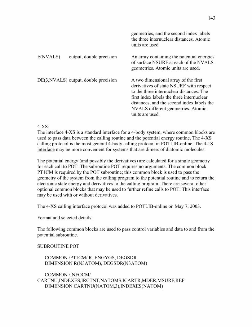
143

geometries, and the second index labels the three internuclear distances. Atomic units are used.

E(NVALS) output, double precision An array containing the potential energies of surface NSURF at each of the NVALS geometries. Atomic units are used.

DE(3,NVALS) output, double precision A two dimensional array of the first derivatives of state NSURF with respect to the three internuclear distances. The first index labels the three internuclear distances, and the second index labels the NVALS different geometries. Atomic units are used.

4-XS: The interface 4-XS is a standard interface for a 4-body system, where common blocks are used to pass data between the calling routine and the potential energy routine. The 4-XS calling protocol is the most general 4-body calling protocol in POTLIB-online. The 4-1S interface may be more convenient for systems that are dimers of diatomic molecules. The potential energy (and possibly the derivatives) are calculated for a single geometry for each call to POT. The subroutine POT requires no arguments. The common block PT1CM is required by the POT subroutine; this common block is used to pass the geometry of the system from the calling program to the potential routine and to return the electronic state energy and derivatives to the calling program. There are several other optional common blocks that may be used to further refine calls to POT. This interface may be used with or without derivatives. The 4-XS calling interface protocol was added to POTLIB-online on May 7, 2003. Format and selected details: The following common blocks are used to pass control variables and data to and from the potential subroutine. SUBROUTINE POT COMMON /PT1CM/ R, ENGYGS, DEGSDR DIMENSION R(N3ATOM), DEGSDR(N3ATOM) COMMON /INFOCM/ CARTNU,INDEXES,IRCTNT,NATOMS,ICARTR,MDER,MSURF,REF DIMENSION CARTNU(NATOM,3),INDEXES(NATOM)

144

COMMON /USRICM/ CART,ANUZERO,NULBL,NFLAG,NASURF,NDER DIMENSION CART(NATOM,3),NULBL(NATOM),NFLAG(20),NASURF(ISURF+1,ISURF+1) COMMON /USROCM/ PENGYGS,PENGYES,PENGYIJ,DGSCART,DESCART,DIJCART DIMENSION PENGYES(ISURF),PENGYIJ(JSURF),DGSCART(NATOM,3), + DESCART(NATOM,3,ISURF),DIJCART(NATOM,3,JSURF) COMMON /PT3CM/ EZERO(ISURF+1) DIMENSION EZERO(ISURF+1) COMMON /PT4CM/ ENGYES,DEESDR DIMENSION ENGYES(ISURF),DEESDR(N3ATOM,ISURF) COMMON /PT5CM/ ENGYIJ,DEIJDR DIMENSION ENGYIJ(JSURF),DEIJDR(N3ATOM,JSURF) ENGYGS = ENERGY AS SOME FUNCTION OF R . . . DEGSDR(:) = . . . RETURN END A detailed description of the common blocks is provided in: R. J. Duchovic, Y. L. Volobuev, G. C. Lynch, D. G. Truhlar, T. C. Allison, A. F. Wagner, B. C. Garrett, and J. C. Corchado, "POTLIB: A Potential Energy Surface Library for Chemical Systems", Computer Physics Communications 144, 169-187 (2002). The common block PT1CM is the only common block that is always required. COMMON /PT1CM/ R, ENGYGS, DEGSDR DIMENSION R(N3ATOM), DEGSDR(N3ATOM)

R(N3ATOM) input, real*8 An array of the N3ATOM internuclear bond distances.

ENGYGS output, real*8 The computed potential energy.

DEGSDR(N3ATOM) output, real*8 The computed derivatives with respect to the N3ATOM internuclear distances. This field is included even when derivatives are not available.

145

4-1S: The 4-1S interface is used with potential energy subprograms for 4-body systems. The coordinate system used is useful for systems that are dimers of two diatomic molecules. (The 4-XS interface is designed for more general 4-body systems.) The driver program obtains the energy at one or more nuclear geometries by passing them as arguments between the subprogram and the driver program. Format and selected details: The subroutine PREPOT, which takes no arguments, is called once before subsequent calls to the subroutine POT. PREPOT is usually used to initialize constant parameters of the surface, which are stored using the FORTRAN command save. Alternatively, the parameters may be stored in common blocks. Once the surface has been initialized, the subroutine POT may be called whenever the potential energy is needed. In general, a 4-1S potential energy routine has the following format: SUBROUTINE PREPOT DATA STORAGE/HERE/,ETC... SAVE RETURN ENTRY POT( R1, R2, R, TH1, TH2, TAU, E ) E = . . . RETURN END Required variables:

The subroutine POT takes the following arguments

POT ( R1, R2, R, TH1, TH2, TAU, E ) where

Throughout this discussion we will consider a dimer of diatomics (AB)(AB) as our four-body system, although the interface is more general. Atomic units are used throughout.

R1,R2 input, double precision Diatomic internuclear distances for each dimer.

146

R input, double precision Distance between the centers of mass of the dimers.

TH1,TH2 input, double precision The angles between the AB diatom bonds and the vector connecting the centers of mass of the two diatoms.

TAU input, double precision The dihedral angle between two planes; the first plane contains the first AB diatom bond and the vector connecting the centers of mass of the two diatoms, and the second plane contains the second AB diatom bond and the vector connecting the centers of mass of the two diatoms.

E output, double precision The potential energy. 5-1S:

The interface 5-1S (5-body system, scalar mode) provides a set of calling conventions for a subroutine that calculates single-point potential energy of a 5-body system on a ground surface. This interface follows the calling conventions imposed by POLYRATE. 6-1S: The interface 6-1S (6-body system, scalar mode) provides a set of calling conventions for a subroutine that calculates single-point potential energy of a 6-body system on a ground surface. This interface follows the calling conventions imposed by POLYRATE. 7-1S: The interface 7-1S (7-body system, scalar mode) provides a set of calling conventions for a subroutine that calculates single-point potential energy of a 7-body system on a ground surface. This interface follows the calling conventions imposed by POLYRATE. A3.4. NH3 Reference: "Improved Direct Diabatization and Fitting of Coupled Potential Energy Surfaces for the Photodissociation of Ammonia," Z. H. Li, R. Valero, and D. G. Truhlar, Theoretical Chemistry Accounts 118, 9-24 (2007). The interface NH3 calculates the potential energy and the analytical derivatives for the lowest two adiabatic states or the two equivalent diabatic states and their coupling for the

147

NH3 system. The driver program obtains the energy and its derivatives at a given nuclear geometry by passing them as arguments between the subprogram and the driver program. The subroutine PREPOT, which takes no arguments, is called once before subsequent calls to the subroutine POT. PREPOT is used to initialize constant parameters of the surface, which are stored in a common block. Once the surface has been initialized, the subroutine POT may be called whenever the potential energies and coupling their derivatives are needed. The NH3 potential energy routine has the following format: SUBROUTINE PREPOT call potcoeff RETURN END SUBROUTINE POT(Xcart, U11, U22, U12, V1, V2, gU11, gU22, gU12, gV1, gV2) DOUBLE PRECISION Xcart(12), U11,U22,U12,V1,V2,gU11(12),gU22(12),gU12(12),gV1(12),gV2(12) parameter(autoang=0.5291772108d0) parameter (EV_TO_HARTREE= 1.d0/autoev) parameter (ANG_TO_BOHR=1.0d0/autoang) parameter (gconv = EV_TO_HARTREE/ANG_TO_BOHR) do i=1,12 cart(i)= Xcart(i)*autoang end do call packpot(cart,U11,U22,U12,V1,V2,gU11,gU22,gU12,gV1,gV2) U11 = U11 * EV_TO_HARTREE U22 = U22 * EV_TO_HARTREE U12 = U12 * EV_TO_HARTREE V1 = V1 * EV_TO_HARTREE V2 = V2 * EV_TO_HARTREE do i=1,12 gU11(i) = gU11(i) * gconv gU22(i) = gU22(i) * gconv gU12(i) = gU12(i) * gconv gV1(i) = gV1(i) * gconv gV2(i) = gV2(i) * gconv enddo RETURN

148

END Required variables: The subroutine POT takes the following arguments:

POT(Xcart, U11, U22, U12, V1, V2, gU11, gU22, gU12, gV1, gV2) where

Xcart input, double precision Cartesian coordinates of input geometry in bohr.

U11, U22 output, double precision The two diagonal diabatic potential energy surfaces. Energies are given in hartrees.

U12 output, double precision The diabatic coupling surface. The coupling is given in hartrees.

V1, V2 gU11, gU22

output, double precision output, double precision

The two adiabatic potential energy surfaces. Energies are given in hartrees. Nuclear Cartesian derivatives of the two diagonal diabatic potential energies. Units are hartree/bohr.

gU12 output, double precision Nuclear Cartesian derivatives of the

diabatic coupling. Units are hartree/bohr.

gV1, gV2 output, double precision Nuclear Cartesian derivatives of the

adiabatic potential energies. Units are hartree/bohr.

A3.5. HBr Reference: "Adiabatic States Derived from a Spin-Coupled Diabatic Transformation: Semiclassical Trajectory Study of Photodissociation of HBr and the Construction of Potential Curves for LiBr+," R. Valero, D. G. Truhlar, and A. W. Jasper, Journal of Physical Chemistry A 112, 5756-5769 (2008).

149

The interface HBr calculates the potential energy and the analytical derivatives for the twelve spin-coupled adiabatic states of HBr that correlate with ground-state atoms (H(2S) + Br(2P)), or the twelve equivalent diabatic states and their couplings. The driver program obtains the energy and its derivatives at a given nuclear geometry by passing them as arguments between the subprogram and the driver program. The subroutine PREPOT, which takes no arguments, is called once before subsequent calls to the subroutine POT. PREPOT is used to initialize constant parameters of the surface, which are stored in a common block. Once the surface has been initialized, the subroutine POT may be called whenever the potential energies and their derivatives and the nonadiabatic couplings are needed. The HBr potential energy routine has the following format: SUBROUTINE PREPOT call potcoeff RETURN END SUBROUTINE POT(Xcart, UI, UIJ, VI, gUI, gUIJ, gVI, dvec) DOUBLE PRECISION Xcart(6), UI(12), UIJ(12, 12), VI(12), gUI(3,2,12), gUIJ(3,2,12,12), gVI(3,2,12) parameter(autoang=0.5291772108d0) parameter (EV_TO_HARTREE= 1.d0/autoev) parameter (ANG_TO_BOHR=1.0d0/autoang) parameter (gconv = EV_TO_HARTREE/ANG_TO_BOHR) do i=1,6 cart(i)= Xcart(i)*autoang end do call packpot(cart, UI, UIJ, VI, gUI, gUIJ, gVI, dvec) do i=1,12 UI(i) = UI(i) * EV_TO_HARTREE VI(i) = VI(i) * EV_TO_HARTREE do j=1,12 UIJ(i,j) = UIJ(i,j) * EV_TO_HARTREE enddo enddo do i=1,3 do j=1,2 do k=1,12 gUI(i,j,k) = gUI(i,j,k) * gconv gVI(i,j,k) = gVI(i,j,k) * gconv

150

do l=1,12 gUIJ(i,j,k,l) = gUIJ(i,j,k,l) *gconv enddo enddo enddo enddo do i1 = 1,3 do i2 = 1,2 do j = 1,12 do k = 1,12 dvec(i1,i2,j,k) = dvec(i1,i2,j,k) * autoang enddo enddo enddo enddo RETURN END Required variables: The subroutine POT takes the following arguments:

POT(Xcart, UI, UIJ, VI, gUI, gUIJ, gVI, dvec) where

Xcart input, double precision Cartesian coordinates of input geometry in bohr.

UI output, double precision Array with the twelve diagonal diabatic potential energy surfaces. Energies are given in hartrees.

UIJ output, double precision 12×12 matrix with the diabatic coupling surfaces. The coupling is given in hartrees.

VI

output, double precision

Array with the twelve adiabatic potential energy surfaces. Energies are given in hartrees.

151

gUI output, double precision Array with the nuclear Cartesian derivatives of the twelve diagonal diabatic potential energies. Units are hartree/bohr.

gUIJ output, double precision 12×12 matrix with nuclear Cartesian

derivatives of the diabatic couplings. Units are hartree/bohr.

gVI output, double precision Array with the nuclear Cartesian

derivatives of the twelve adiabatic potential energies. Units are hartree/bohr.

dvec output, double precision Nonadiabatic coupling vector. Units are

bohr-1. A3.6. BrCH2Cl Reference: "Photochemistry in a Dense Manifold of Electronic States: Photodissociation of CH2ClBr," R. Valero and D. G. Truhlar, Journal of Chemical Physics 137, 22A539/1-14 (2012). The interface BrCH2Cl calculates the potential energies and the analytical derivatives for the twenty-four spin-coupled adiabatic states of BrCH2Cl that correlate with ground- and excited state polyatomic fragments and ground- and spin-orbit excited atomic fragments derived from the dissociations Br + CH2Cl and Cl + CH2Br; therefore, eight asymptotic states in total (Br(2P3/2 + CH2Cl(X 1A´), Br(2P1/2 + CH2Cl(X 1A´), Br(2P3/2 + CH2Cl(A 1A´´), Br(2P1/2 + CH2Cl(A 1A´´), Cl(2P3/2 + CH2Br(X 1A´), Cl(2P1/2 + CH2Br(X 1A´), Cl(2P3/2 + CH2Br(A 1A´´), and Cl(2P1/2 + CH2Br(A 1A´´)), or the twenty-four equivalent diabatic states and their couplings. The driver program obtains the energy and its derivatives at a given nuclear geometry by passing them as arguments between the subprogram and the driver program. The subroutine PREPOT, which takes no arguments, is called once before subsequent calls to the subroutine POT. PREPOT is used to initialize constant parameters of the surface, which are stored in a common block. Once the surface has been initialized, the subroutine POT may be called whenever the potential energies and their derivatives and the nonadiabatic couplings are needed. The BrCH2Cl potential energy routine has the following format: SUBROUTINE PREPOT call potcoeff RETURN END

152

SUBROUTINE pot(Xcart,UI,UIJ,VI,gUI,gUIJ,gVI,dvec,icall) real*8 cart(15) real*8 UI(24),VI(24),gUI(3,5,24),gVI(3,5,24) real*8 UIJ(24,24),gUIJ(3,5,24,24) real*8 mat(24,24),UIJpl(24,24),UIJmin(24,24) real*8 dvec(3,5,24,24) real*8 VIpl(24),VImin(24),UIpl(24),UImin(24) real*8 cartpl(15),cartmin(15) integer icall parameter(autoang=0.5291772108d0) parameter(autoev=27.2113845d0) parameter (EV_TO_HARTREE= 1.d0/autoev) parameter (ANG_TO_BOHR=1.0d0/autoang) parameter (gconv = EV_TO_HARTREE/ANG_TO_BOHR) do i=1,15 cart(i)= Xcart(i)*autoang end do C Finite differences do i=1,15 cartpl(i)= cart(i) cartmin(i) = cart(i) end do DELTA = 0.0001d0 kk = 0 do j=1,5 do i=1,3 kk = kk + 1 cartpl(kk) = cart(kk) + DELTA call packpot(cartpl,UIpl,UIJpl,VIpl,mat,icall) cartmin(kk) = cart(kk) - DELTA call packpot(cartmin,UImin,UIJmin,VImin,mat,icall) do l=1,24 gVI(i,j,l) = (VIpl(l) - VImin(l)) / (2.d0*DELTA) gUI(i,j,l) = (UIpl(l) - UImin(l)) / (2.d0*DELTA) do m=1,24

153

gUIJ(i,j,l,m) = (UIJpl(l,m) - UIJmin(l,m)) / (2.d0*DELTA) enddo enddo cartpl(kk) = cart(kk) cartmin(kk) = cart(kk) enddo enddo call packpot(cart,UI,UIJ,VI,mat,icall) do i=1,24 UI(i) = UI(i) * EV_TO_HARTREE VI(i) = VI(i) * EV_TO_HARTREE do j=1,24 UIJ(i,j) = UIJ(i,j) * EV_TO_HARTREE enddo enddo do i=1,3 do j=1,5 do k=1,24 gUI(i,j,k) = gUI(i,j,k) * gconv gVI(i,j,k) = gVI(i,j,k) * gconv do l=1,24 gUIJ(i,j,k,l) = gUIJ(i,j,k,l) *gconv enddo enddo enddo enddo do k=1,24 do i=1,3 do j=1,5 gUIJ(i,j,k,k) = gUI(i,j,k) enddo enddo enddo C Compute the nonadiabatic coupling vectors call getdvec3(5,UI,gUIJ,VI,dvec,mat) RETURN END

154

Required variables: The subroutine POT takes the following arguments:

POT(Xcart, UI, UIJ, VI, gUI, gUIJ, gVI, dvec, icall) where

Xcart input, double precision Cartesian coordinates of input geometry in bohr.

UI output, double precision Array with the 24 diagonal diabatic potential energy surfaces. Energies are given in hartrees.

UIJ output, double precision 24×24 matrix with the diabatic coupling surfaces. The coupling is given in hartrees.

VI gUI

output, double precision output, double precision

Array with the 24 adiabatic potential energy surfaces. Energies are given in hartrees. Array with the nuclear Cartesian derivatives of the 24 diagonal diabatic potential energies. Units are hartree/bohr.

gUIJ output, double precision 24×24 matrix with nuclear Cartesian

derivatives of the diabatic couplings. Units are hartree/bohr.

gVI output, double precision Array with the nuclear Cartesian

derivatives of the 24 adiabatic potential energies. Units are hartree/bohr.

dvec output, double precision Nonadiabatic coupling vector. Units are

bohr-1. icall

input, integer

Variable controlling the calculation of adiabatic potential surfaces. Only if icall=1 will they be calculated.

155

A4. SPRNG documentation The user’s guide for the SPRNG (Scalable Parallel (Pseudo-) Random Number Generator) library can be found in the subdirectory sprng/DOCS of the ANT distribution and also at the web address http://sprng.cs.fsu.edu/ The version of SPRNG in the present version of the ANT package is version 1.0.

A5. Gaussian09 documentation The user’s guide for Gaussian09 is available at the web address http://www.gaussian.com/g_tech/g_ur/l_keywords09.htm. The version of Gaussian09 tested with the ANT program is G09 C.01. But we expect that the ANT program will also work with other versions of the Gaussian09 program and also the Gaussian03 program.

A6. Molpro documentation The user’s guide for Molpro is available at the web address http://www.molpro.net/info/2012.1/doc/manual/. The version of Molpro tested with the ANT program is version 2010.1.24. But we expect that the ANT program will also work with other versions of the Molpro program.

156

A7. Surface couplings in non-BO calculations The couplings in an adiabatic representation are called nonadiabatic couplings. These are vectors. They are the "derivative" couplings, caused by the nuclear momentum, which is a vector derivative operator (i.e., a gradient). The couplings in a diabatic representation are scalars. The vector couplings are assumed to vanish in a diabatic representation. The scalar couplings vanish in an adiabatic representation. However, in an FSTU calculation, even in the diabatic representation, we compute a special "nonadiabatic coupling" vector as described on page 389 of

“Non-Born-Oppenheimer Molecular Dynamics for Conical Intersections, Avoided Crossings, and Weak Interactions,” A. W. Jasper and D. G. Truhlar, in Conical Intersections: Theory, Computation, and Experiment, edited by W. Domcke, D. R. Yarkony, and H. Köppel (World Scientific, Singapore, 2011), pp. 375-412. (chapter 10) [Adv. Ser. Phys. Chem. 17, 375-412 (2011)]. [A PDF of this book chapter is available at http://comp.chem.umn.edu/Truhlar/bookchap.htm]

This is the nonadiabatic coupling that one would have if one temporarily switched to a special adiabatic representation. If one is considering a hop between diabatic states K and K´, this special adiabatic representation is what one gets if one temporarily drops all states except K and K´ and diagonalizes the resulting two-by-two matrix. The resulting coupling is giving by the two-by-two version of equation 13. For a two-by-two case, the sum in eq 13 just has i,j = K,K and i,j = K',K. For example, if K = a ands K´ = b, we just need Wab and Wba, where the latter equals Wab.

A8. Computation of the reduced nonadiabatic couplings

This appendix section describes the correction of a bug in the calculation of the reduced nonadiabatic couplings that has been fixed in version-2014-2 (and later versions) of the code. This bug is related to the use of unclear notation in equation (46) of the book chapter

"Non-Born-Oppenheimer Molecular Dynamics for Conical Intersections, Avoided Crossings, and Weak Interactions," A. W. Jasper and D. G. Truhlar, in Conical Intersections: Theory, Computation, and Experiment, edited by W. Domcke, D. R. Yarkony, and H. Köppel (World Scientific, Singapore, 2011), pp. 375-412. (Chapter 10) [The citation as a periodical would be A. W. Jasper and D. G. Truhlar, Adv. Ser. Phys. Chem. 17, 375-412 (2011)].

157

A clearer version of the equation is included in the present section.

A concise background summary of the relevant issues concerning nonadiabatic coupling is presented next, followed by a description of the code change.

The energy matrix in the diabatic representation is represented as W , with Wij being the ij element of the matrix; the matrix is symmetric. Adiabatic energies and couplings are calculated from these diabatic potential energy matrix elements Wij and their

gradients. The adiabatic energies are the eigenvalues of the diabatic energy matrix W , and dij are the coefficients of the linear combination of the adiabatic states (ϕi ) that represents the diabatic electronic wave functions:

ϕ jd = dijϕi

i∑

(1)

Note the d matrix, formed by the elements dij , is the matrix whose columns are the eigenvalues of W . The gradients of the adiabatic surfaces are

∇nVi = dij

*dik∇nWjkj,k∑

(2)

and the nonadiabatic couplings are

Fij =1

Vj −Vidik

* d jl∇nWkl (i ≠ j)k,l∑

0 (i = j)

%

&'

('

(3)

where the subindexes i, j denote the coupling between electronic state surfaces i and j. Thus, the element F21 is given by the equation

F21 =1

V1 −V2d2k

* dl1∇nWkl k,l∑

(4)

In the surface hopping and decay of mixing algorithms, the direction that is used for the change in momentum due to hopping or the decay of mixing is called the hopping direction. When propagation is carried out in the adiabatic representation or when propagation is carried out in a two-state diabatic representation, the hopping direction is the direction of the nonadiabatic coupling vector, as calculated from eq. (3). However, if propagation is carried out in a diabatic representation with more than two states, FKK ' (where K and K ' represent any two electronic states) cannot be used as the hopping direction because the adiabatic and diabatic state labels do not generally correlate to a

Vi

158

globally consistent pair of states. Instead of using the nonadiabatic coupling vectors, one uses the reduced nonadiabatic coupling vectors computed from the submatrix:

W r =WKK WKK 'WK 'K WK 'K '

!

"

##

$

%

&&

, (5)

The expression

FKK 'r =

dKKr,* dK 'K

r ∇nWKK + (dKKr,* dK 'K '

r + dKK 'r,* dK 'K

r )∇nWKK ' + dKK 'r dK 'K '

r ∇nWK 'K 'W+ −W− (6)

is given for the reduced nonadiabatic coupling vectors in equation (46) of the book chapter cited above; see also equation (A9) of

"Quantum Mechanical and Quasiclassical Trajectory Surface Hopping Studies of the Electronically Nonadiabatic Predissociation of the à State of NaH2," M. D. Hack, A. W. Jasper, Y. L. Volobuev, D. W. Schwenke, and D. G. Truhlar, Journal of Physical Chemistry A 103, 6309-6326 (1999).

The notation used for the eigenvalues,W+ and W− , of the submatrix Wr is incorrect (or at least confusing) in the book chapter, and this led to an error in the sign of the denominator for some of the reduced nonadiabatic coupling vectors in early versions of the code. Equation (46) can be written in a clearer way as follows:

FKK 'r =

dKKr,* dK 'K

r ∇nWKK + (dKKr,* dK 'K '

r + dKK 'r,* dK 'K

r )∇nWKK ' + dKK 'r dK 'K '

r ∇nWK 'K 'WK 'r −WK

r(6)

where WK 'r

and WKr

are the eigenvalues corresponding to statesK ' and K respectively. Thus, the reduced nonadiabatic coupling vector between surface 1 and 2 is given by

F12r =

d11r,*d21

r ∇nW11+ (d11r,*d22

r + d12r,*d21

r )∇nW12 + d12r d22

r ∇nW22W2r −W1

r (7)

Note that only some elements of the full reduced coupling vectors matrix are

computed, and in the correct code they can fall in either the upper or the lower triangular part of the matrix; e.g. for a three-state system propagating on the second surface, only

the reduced couplings F12r , and F32

r are computed. Here is the corrected code: do k=1,nsurft if(k.ne.nsurf) then

159

u2b2(1,1) = pemd(k,k) u2b2(1,2) = pemd(k,nsurf) u2b2(2,1) = pemd(nsurf,k) u2b2(2,2) = pemd(nsurf,nsurf) do i=1,3 do j=1,NCLU gu2b2(i,j,1,1) = gpemd(i,j,k,k) gu2b2(i,j,1,2) = gpemd(i,j,k,nsurf) gu2b2(i,j,2,1) = gpemd(i,j,nsurf,k) gu2b2(i,j,2,2) = gpemd(i,j,nsurf,nsurf) enddo enddo call getdvec2(NCLU,u2b2,gu2b2,dvec2b2) do i=1,3 do j=1,NCLU dvec(i,j,k,nsurf) = dvec2b2(i,j) dvec(i,j,nsurf,k) = -dvec2b2(i,j) enddo enddo endif enddo However in the subroutine getdvec2, which computes the reduced nonadiabatic coupling vectors, the numerator was originally written to compute the upper triangular matrix element of the 2×2 matrix while the denominator computed the lower matrix element. This created an inconsistency in the sign of the reduced nonadibatic couplings. This has been fixed, and here is the corrected code as of version 2014:

1. Changing the getdvec2 subroutine for computing FKK ' being K ' < K (e.g. the

element F21 for a system with two surfaces)

do i1 = 1,3 do i2 = 1,nclu dvec2b2(i1,i2) = 0.d0 do k = 1, 2 do l = 1, 2 dvec2b2(i1,i2) = dvec2b2(i1,i2) & +cc(k,2)*cc(l,1)*gu2b2(i1,i2,k,l) enddo enddo if ((v1-v2) .ne. 0.0d0) then dvec2b2(i1,i2) = dvec2b2(i1,i2)/(v1-v2) else dvec2b2(i1,i2) = 0.0d0 endif enddo

160

enddo

2. Keeping track of the indexes of the surfaces and changing the sign if necessary when the reduced nonadiabatic coupling is computed. do k=1,nsurft if(k.ne.nsurf) then u2b2(1,1) = pemd(k,k) u2b2(1,2) = pemd(k,nsurf) u2b2(2,1) = pemd(nsurf,k) u2b2(2,2) = pemd(nsurf,nsurf) do i=1,3 do j=1,NCLU gu2b2(i,j,1,1) = gpemd(i,j,k,k) gu2b2(i,j,1,2) = gpemd(i,j,k,nsurf) gu2b2(i,j,2,1) = gpemd(i,j,nsurf,k) gu2b2(i,j,2,2) = gpemd(i,j,nsurf,nsurf) enddo enddo call getdvec2(NCLU,u2b2,gu2b2,dvec2b2) do i=1,3 do j=1,NCLU if(k.gt.nsurf) then dvec(i,j,k,nsurf) = dvec2b2(i,j) else dvec(i,j,k,nsurf) = -dvec2b2(i,j) endif dvec(i,j,nsurf,k) = -dvec(i,j,k,nsurf) enddo enddo endif enddo This bug is fixed in version-2014 of the ANT code and hence in all later versions as well.

A9. Wigner distribution of a ground-state harmonic oscillator This section presents a derivation of the ground-state Wigner distribution for a vibrational mode in term of energy for a given force constant and reduced mass. The purposes of expressing the distribution in terms of energy is that it be applied even when the energy in a mode is not the zero point energy (sometimes we want it to be smaller than the zero point energy in order to minimize unphysical zero point vibrational energy leak.

161

Let the Hamiltonian H be given by p2

2m+kx2

2, where p is the momentum, m is the mass

or reduced mass, k is the force constant, and x is the displacement coordinate. The Wigner distribution for the ground state of a harmonic oscillator (HO) is

P = Ne−ax2e−bp

2

where N, a, and b are constants. If the energy of the oscillator is E, we know by the HO virial theorem that <T> = <V> = E/2. The Wigner distribution must be normalized and give these expectation values. Therefore

N dxdp∫ e−ax

2e−bp

2=1

N dxdp∫ p2

2me−ax

2e−bp

2= E / 2

N dxdp∫ kx2

2e−ax

2e−bp

2= E / 2

All integrals are (-∞,∞). These three equations can be solved for N, a, and b. Doing the integrals:

N π

aπb=1

N π

aπb14mb

=14mb

= E / 2

N π

aπbk4a

=k4a

= E / 2

So we have

N =

abπ

b = 12mE

a = k2E

This should reduce to the usual result if E = !2km

.