Embed Size (px)
Citation preview
NPS ARCHIVE1997.12HICKS, J.
NAVAL POSTGRADUATE SCHOOLMonterey, California
THESIS
A CAUSAL BASED INVENTORY FORECASTING MODELFOR AN ELECTRONICS CAPITAL EQUIPMENT
MANUFACTURER
By
John E. Hicks
December, 1997
Thesis Advisor:
Second Reader:ThesisH526952
Kevin R. GueShu S. Liao
Approved for public release; distribution is unlimited.

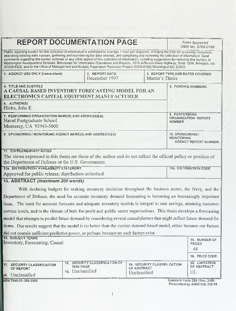
REPORT DOCUMENTATION PAGE Form ApprovedOMB No. 0704-0188
Public reporting burden for this collection of information is estimated to average 1 hour per response, including the time for reviewing instruction,
searching existing data sources, gathering and maintaining the data needed, and completing and reviewing the collection of information. Sendcomments regarding this burden estimate or any other aspect of this collection of information, including suggestions for reducing this burden, to
Washington headquarters Services, Directorate for Information Operations and Reports, 1215 Jefferson Davis Highway, Suite 1204, Arlington, VA22202-4302, and to the Office of Management and Budget, Paperwork Reduction Project (0704-0188) Washington DC 20503.
1. AGENCY USE ONLY (Leave blank) 2. REPORT DATE
December 19973. REPORT TYPE AND DATES COVEREDMaster's Thesis
4. TITLE AND SUBTITLE
A CAUSAL BASED INVENTORY FORECASTING MODEL FOR ANELECTRONICS CAPITAL EQUIPMENT MANUFACTURER6. AUTHOR(S)
Hicks, John E.
5. FUNDING NUMBERS
7. PERFORMING ORGANIZATION NAME(S) AND ADDRESS(ES)
Naval Postgraduate School
Monterey, CA 93943-5000
8. PERFORMINGORGANIZATION REPORTNUMBER
9. SPONSORING / MONITORING AGENCY NAME(S) AND ADDRESS(ES) 10. SPONSORING/MONITORING
AGENCY REPORT NUMBER
11. SUPPLEMENTARY NOTES
The views expressed in this thesis are those of the author and do not reflect the official policy or position of
the Department of Defense or the U.S. Government.
12a. DISTRIBUTION / AVAILABILITY STATEMENT
Approved for public release; distribution unlimited.
12b. DISTRIBUTION CODE
13. ABSTRACT (maximum 200 words)
With declining budgets for making inventory decisions throughout the business sector, the Navy, and the
Department of Defense, the need for accurate inventory demand forecasting is becoming an increasingly important
issue. The need for accurate forecasts and adequate inventory models is integral to cost savings, attaining customer
service levels, and to the climate of both for-profit and public sector organizations. This thesis develops a forecasting
model that attempts to predict future demand by considering several causal-factors that might reflect future demand for
items. Our results suggest that the model is no better than the current demand-based model, either because our factors
did not contain sufficient predictive power, or perhaps because no such factors exist.
14. SUBJECT TERMSInventory, Forecasting, Causal
15. NUMBER OFPAGES
46
16. PRICE CODE
17. SECURITY CLASSIFICATIONOF REPORT
18. Unclassified
18. SECURITY CLASSIFICATION OFTHIS PAGE
19. Unclassified
19. SECURITY CLASSIFI- CATIONOF ABSTRACTUnclassified
20. LIMITATIONOF ABSTRACT
UL
MSN 7540-01-280-5500 Standard Form 298 (Rev. 2-89)
Prescribed by ANSI Std. 239-18

11
Approved for public release; distribution is unlimited
A CAUSAL BASED INVENTORY FORECASTING MODEL FOR ANELECTRONICS CAPITAL EQUIPMENT MANUFACTURER
John E. Hicks
Lieutenant Commander, United States NavyB.S., Manhattan College, 1985
Submitted in partial fulfillment of the
requirements for the degree of
MASTER OF SCIENCE IN SYSTEMS MANAGEMENT
from the
NAVAL POSTGRADUATE SCHOOLDecember 1997


ABSTRACT
With declining budgets for making inventory decisions throughout the business sector,
the Navy, and the Department of Defense, the need for accurate inventory demand
forecasting is becoming an increasingly important issue. The need for accurate forecasts
and adequate inventory models is integral to cost savings, attaining customer service
levels, and to the climate of both for-profit and public sector organizations.
This thesis develops a forecasting model for a high-technology firm that attempts
to predict future demand by considering several causal-factors that might reflect future
demand for items. Our results suggest that the model is no better than the current
demand-based model, either because our factors did not contain sufficient predictive
power, or perhaps because no such factors exist.

VI
TABLE OF CONTENTS
I. INTRODUCTION 1
A. PROBLEM DESCRIPTION 2
B. WHY IS A NEW MODEL REQUIRED 8
C. FACTORS NOT ACCOUNTED FOR IN THE DEMAND BASED MODEL 9
D. INSTALLED BASE SHORTCOMINGS 11
E. EMERGENT ISSUES 12
F. DISTRIBUTION REQUIREMENTS PLANNING (DRP) FORECASTING
MODEL: THE FUTURE 13
G. RESEARCH OBJECTIVES 15
H. PREVIEW 15
II. METHODOLOGY 17
A. CAUSAL BASED MODELING 17
B. DETERMINATION OF CAUSAL FACTORS 1
8
C. CAUSAL FACTORS 19
III. ANALYSIS 23
A. INITIAL TEST RUNS OF THE REGRESSION ANALYSIS 23
B. INDIVIDUAL REGRESSION MODELS 24
C. MULTIPLE REGRESSION MODEL 27
D. CHECKING THE VALIDITY OF THE REGRESSION ASSUMPTIONS 28
IV. CONCLUSIONS AND RECOMMENDATIONS 29
A. CONCLUSIONS AND RECOMMENDATIONS 29
Vll

APPENDIX 32
BIBLIOGRAPHY 35
INITIAL DISTRIBUTION LIST 37
Vlll

I. INTRODUCTION
With declining budgets for making inventory decisions throughout much of the business
sector, the Navy, and the Department of Defense (DOD), the need for accurate inventory demand
forecasting is becoming an increasingly important issue. In order to remain competitive in
today's environment, all organizations require efficiency and effectiveness in inventory
management. The need for accurate forecasts and adequate inventory models are integral to
saving costs and attaining customer service levels for both for-profit and public sector
organizations.
Demand-based forecasting is an adequate method in a slow growth industry; however, in
a high growth industry, such as the technology sector, a demand-based model requires extensive
manipulation by individual forecasters to achieve satisfactory results. The individual forecasters'
proficiency, flexibility to make decisions, and knowledge of the product lines are key factors in
making an adequate forecast.
In the high-tech arena, a causal based inventory model using multiple regression analysis
might more adequately meet the needs of the company. At the same time, the model would
reduce the manpower required to manually manipulate the results of the computer-generated
model.
A global, multi-billion dollar electronics capital equipment manufacturer provides all the
data used in this thesis. They are referred to thoughout the thesis as the testfirm or simply the
firm.
This thesis focuses on one electronic capital equipment manufacturer that serves high-
technology customers. In a private paper, the test firm has identified the following problem
statement: "The data, tools and processes used to develop global spares inventory stocking
levels, are not robust enough to provide a level of accuracy to achieve optimal asset
performance, while delivering customer expected service levels."1
The private paper continues
with the inadequacies of the demand-based model currently installed. The paper discusses the
lack of available mean time between failure (MTBF) data and the lack of adequate data
regarding the installed base configuration in the individual customer plants.
The firm's directors are concerned about the return on inventory investment and their
efficiency in managing a quarter billion dollar inventory. In 1 996, spares revenue accounted for
1 1 percent of the test firm's total revenue. 2 The directors are interested in any resource saving
initiatives that do not detract from the customer service levels currently in place.
A. PROBLEM DESCRIPTION
One might summarize a typical business life cycle as infancy, growth, maturity, and
decline. The test firm has experienced tremendous growth during the past decade and is
currently in the growth stage of its life cycle. This stage allows for some inefficiency in
delivering the firm's products and support to its customers, because high profit margins tend to
mask high costs. The firm will eventually reach the peak of its growth and need to become more
efficient as it enters the maturity stage.
Private Paper, Director, Spares Planning and Support, Research Test Firm, August 19972Private Paper, Director, Spares Operation, Research Test Firm, March 1997
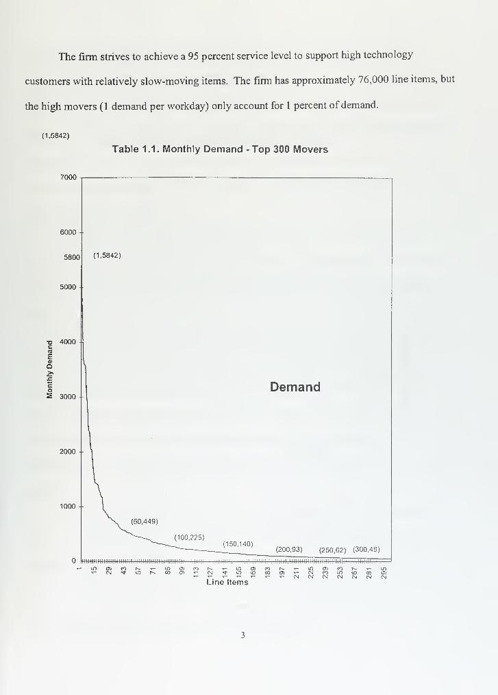
The firm strives to achieve a 95 percent service level to support high technology
customers with relatively slow-moving items. The firm has approximately 76,000 line items, but
the high movers (1 demand per workday) only account for 1 percent of demand.
(1,5842)
Table 1.1. Monthly Demand -Top 300 Movers
7000
6000
5800
5000
o 4000cnEd>
Q
3000 --
2000
1000
(1,5842)
Demand
(50,449)
(100,225)(150,140)
(200,93) (250,62) (300,48)
li i i i i ii iiiii i iiii i i i iiii iii ii i iiiiiiiiii[iiiiiii :i
i ;iiii i iii!ii! ii i! i iii ; [ii i ii i iiiiiiiii! ! i :::
.••
;: :!
: ;>!,
::— '•
•=• —'~- 'H ii
'
i'i .v
»no)roi^-'«-ino>foi^T-mo5coi^T-mo5ros..T-m<-t\iTrir)r~-oocnT-cM-^-in<Dooo>T-csjrointDoo02'-'-'-''-'-'-NNNMMMIMLine Items
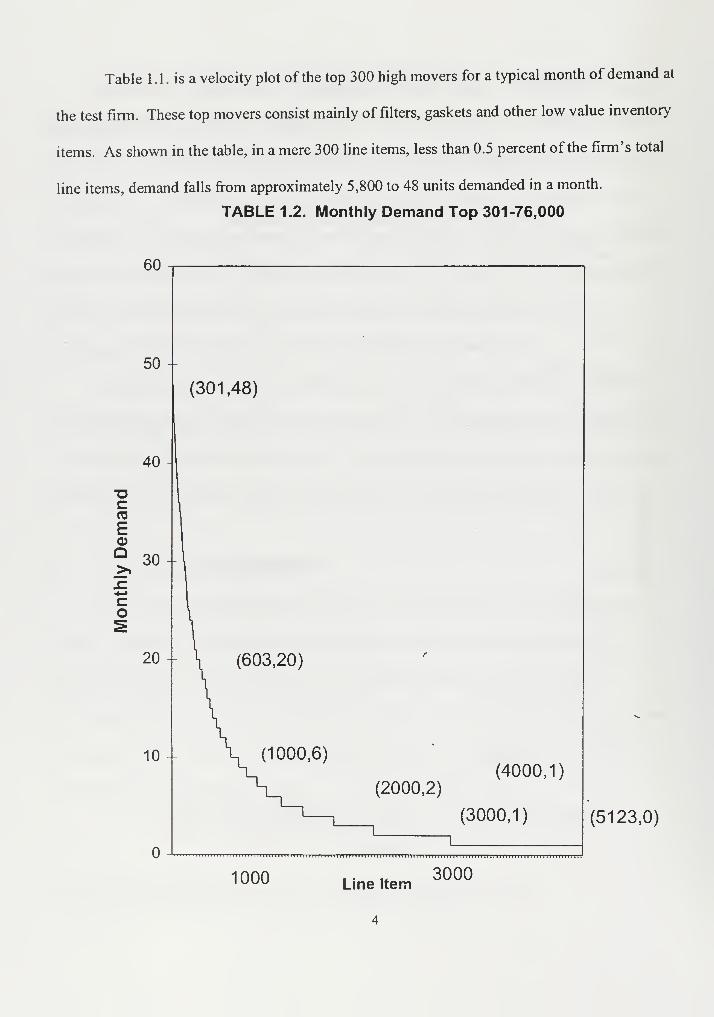
Table 1.1. is a velocity plot of the top 300 high movers for a typical month of demand at
the test firm. These top movers consist mainly of filters, gaskets and other low value inventory
items. As shown in the table, in a mere 300 line items, less than 0.5 percent of the firm's total
line items, demand falls from approximately 5,800 to 48 units demanded in a month.
TABLE 1.2. Monthly Demand Top 301-76,000
ocro
E0)
Q>»JZ*-•
co
50 -
(301,48)
40 -
30 -
20 -\ (603,20)
/
10 - \ (1000,6)
I
(4000,1)(2000,2)
(3000,1)l_ H_
-
(5123,0)
1000 Line Item3000

Table 1.2. shows a velocity plot for the remaining 76,000 line items for the month of
August 1997. These line items still include certain low valued items, but also include many high
valued items. The company may choose to stock only one of these high valued items or even
choose to manufacture on demand for the item, in an attempt to reduce holding costs. Table 1 .2.
shows that by the 700th
line item demand is below 20. The table shows that at line item 3,000,
demand drops to a single item. The bottom 71,000 line items (over 93 percent of total line items)
had no demand in this typical month.
The forecasted items (8 hits in 12 months) account for only 20 percent of the total
inventory and only 7 percent of total line items in inventory. The firm currently relies on this
demand data and the knowledge of its forecasters to establish an inventory level for specific
items.
Managers at the firm believe that the demand based forecasting model presently in place
does not adequately adjust for new installations, customer workload trends, and aging
equipment. The model was installed in October 1995 and relies on a three month moving average
to make forecasts. Three months of history is simply not enough data points to make an accurate
forecast. The model depends on the opinions of forecasters and their knowledge of the product
line, and therefore fails to give adequate forecasts based on the infrequent demand of the "high
movers".
The firm currently does not meet a 95 percent service level and routinely maintains
only a 60 or 70 percent monthly service level.3The service level rarely reaches 80 percent and
only once in the last 4 years reached 90 percent.4The service level trend is increasing as shown
3Private Paper, Director, Spares Operation, Research Test Firm, March 1997
4Private Paper, Director, Spares Operation, Research Test Firm, March 1997
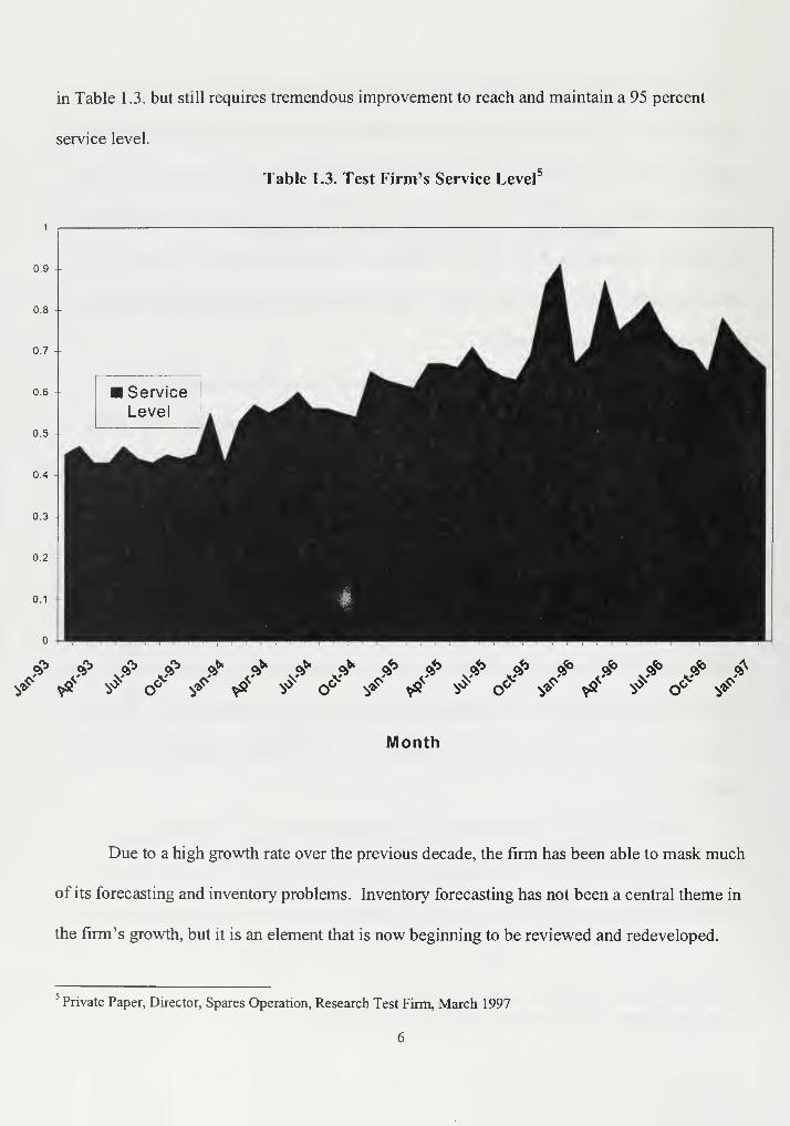
in Table 1.3. but still requires tremendous improvement to reach and maintain a 95 percent
service level.
Table 1.3. Test Firm's Service Level5
* *a o° v» *» o° & Vs
Month
Due to a high growth rate over the previous decade, the firm has been able to mask much
of its forecasting and inventory problems. Inventory forecasting has not been a central theme in
the firm's growth, but it is an element that is now beginning to be reviewed and redeveloped.
' Private Paper, Director, Spares Operation, Research Test Firm, March 1997
6

The firm's total inventory is only $270 million, which is a relatively insignificant amount for the
multi-billion dollar company, but holding costs are becoming an increasingly significant issue
and total inventory must be reduced 10 percent by the middle of the current fiscal year.6
If the
firm's forecasting methods were more accurate, holding costs might be reduced and service
levels may be met.
Further, inventory is becoming an increasingly important topic since many of the stocked
items are considered obsolete. Obsolescence occurs in the high-tech sector, not in a matter of
years as in many industries, but in a matter of weeks or months.7 Due mostly to obsolescence,
the annual holding cost rate is routinely 50% in the high tech sector.8
"The spares demand forecasting process, which drives stocking levels for direct sales and
ready to serve inventory, relies on historical data that includes non-conformance and non-
recurring demand and is not founded directly on any MTBF element and does not tie directly to
the installed base."9The firm believes that this is the time to eliminate inefficiencies and is
considering either a demand based model known as Distribution Requirements Planning (DRP)
or a causal model.
These models will eventually include demand or causal factors, mean time between
failures (MTBF), mean time between maintenance (MTBM), operating hours and the installed
base in the model's individual analysis. MTBF, MTBM, and operating hours from installed
systems is currently unavailable to the test firm but should be included at a later date.
6Private Conversation, Director, Spares Planning and Support, Research Test Firm, August 1997
7 Private Conversation, Forecaster, Research Test Firm, August 1997
Private Conversation, Director, Spares Planning and Support, Research Test Firm, August 1 997
Private Paper, Director, Spares Operations, Research Test Firm, March 1997

Information on the installed base is currently only available through an individual analyst's self-
developed database.
The installed base is the total of the various configurations of the test firm's systems,
installed at customer sites. These systems are owned and maintained by the customers, but over
60 percent of the part support is supplied by the test firm. A private paper described the installed
base performance as "the most important manifestation of our commitment to our customers, a
catalyst for future business opportunities, and a major business opportunity in itself: profitability
and market share."10
B. WHY A NEW MODEL IS REQUIRED
The firm believes that a new model is required to meet a 95 percent service level, while
reducing the costs associated with inventory and priority shipping.11
Further, a dozen full-time
forecasters are employed in an attempt to reduce the real problem of not having an adequate
estimate of future customer demand.
The customer service levels shown in Table 1 .3 describes a customer service level goal
that the firm cannot currently meet with the present forecasting system. In most instances, the
firm is routinely 20 to 35 percent below the target level. The firm currently has a demand-based
system in place that requires manual adjustment. The complexity of this problem is increasing
due to the high growth of the firm and the increased number of line items stocked in inventory.
Currently, computer-generated forecasts are changed manually by the individual
10Private Paper, Director, Spares Planning and Support, Research Test Firm, August, 1997
11Private Conversation, Director, Spares Planning and Support, Research Test Firm, August 1997
12Private Conversation, Forecaster, Research Test Firm, August 1997

forecasters, resulting in inefficiencies. These forecasters must rely on their knowledge of the
factors affecting their line items, use the results of the demand-based model as a starting point,
and manually adjust the computer-generated forecasts up or down to determine the stocking level
of the individual line items. The forecasters must account for lead time and dollar value of the
line items and must also determine if an item is being phased in or phased out, to avoid shortages
or reduce obsolescence.
C. FACTORS NOT ACCOUNTED FOR IN THE DEMAND BASED MODEL
1
.
Since different forecasting methods are based on historical information, the
director must consider how much data is currently on hand, what information it contains, and
what it would cost to gather additional data (Wheelwright and Makridakis, 1980). The firm's
current demand-based model is lacking much of the rudimentary data required to make adequate
forecasts. For example, the firm must also evaluate the recipient costs of not having the
information or data available and what this lack of information costs them in increased
production, purchasing, expediting and inventory costs. We suggest that the firm either gather or
purchase this data from both the firm's manufacturers, and the firm's customers. This will be
discussed further in the recommendation section of Chapter IV.
"Particular attention should be paid to whether one is trying to predict the continuance of
a historical pattern for a particular item or a turning point for some change in the basic pattern."13
The demand-based model does not account for these changes to the basic pattern and the
forecasters must manually adjust the model. These fluctuations are taken into account to some
13Wheelwright and Makridakis, Forecasting Methods For Management, John Wiley & Sons, Third Edition, 1980,
Page 40.

degree by the knowledge of the installations and the customers manufacturing schedule. The
individual forecasters review the computer-generated forecasts and add or subtract for the
individual line items that they determine require adjusting, when preparing a forecast.
2. The demand-based model does not take into account cyclical business patterns in
preparing a forecast. Cyclical business patterns refer to the normal business fluctuations that
occur in virtually all industries. The electronics industry reaches a point of under producing,
where the industry is selling all the products they have available at a profitable price. The market
factors that affect supply and demand are generally considered good for the industry as a whole,
during this period. They eventually reach a level due to increased production or new entrants to
the industry where they struggle to find a buyer or customer at any profitable price, due to the
glut of the item in the marketplace. The test firm is in a cyclical business, yet the current
demand-based forecasting model does not account for these patterns. These cycles are different
lengths in different industries and are affected by the local, state, national and global economies,
but inventory stock levels must be adequately adjusted to alleviate shortages and excess
inventories.
3. The current model does not take into account seasonal issues such as Christmas
and New Year's plant shut downs. It relies on the individual forecasters to manually adjust these
figures. A causal model could not automatically adjust for the fluctuations until MTBM was
included as a causal factor and the typical scheduled holiday maintenance was account for.
4. Regional and national differences are not accounted for in the demand-forecasting
model. Certain customers who desire a high degree of safety stock may order twice the required
amount to augment their individual safety stock. Other companies may choose to maintain
virtually no safety stock and rely on expedited shipments for replacement parts. Globally, the
10

current trend in Asia is to order two parts each time a single part fails, thus showing a higher
demand pattern. Additionally, in regional parts of the United States many customers choose to
rely on airborne carriers, such as FedEx, to expedite parts that they choose not to stock at the
regional depot or local stocking point. This forces the forecasters to be reactive vice proactive.
We address the differences between regional depots and local stocking points later in this
section.
The model does not separate initial or new installation demand from normal demand.
This does not adequately allow either the current model or the individual forecaster in many
instances to adequately forecast future demand patterns, because the figure is elevated by the
new installation amount. This increases the holding costs for the inventory that is carried based
on the inaccuracy of the previous period or period's demand. The additional inventory could
very likely not be required because the individual parts may have high reliability rates.
D. INSTALLED BASE SHORTCOMINGS
The company currently does not have complete information of its installed base, nor does
it have the ability to determine which parts are being ordered for periodic maintenance, ready
spares or actual failure. In not possessing this key information the forecasters are faced with
demand patterns that are skewed, which cause difficulties for the demand-based forecasting
model and individual forecasters. For example, when one line item fails, the customer orders
two parts, one for the failure and one for the ready spare. This would indicate a demand of two.
If this part fails again, it might not be ordered at all, or at most one part would be ordered to
replace the ready spare. The original two creates a higher stocking level and the second failure
11
may or may not be reported. If it is not reported a lower than required stocking level might
develop.
Consider another example: A customer orders 12 each for periodic maintenance that is
conducted every four years. The forecaster increases the forecast, believing this is a normal
demand pattern, and the inventory stocking level is increased. However this item may not be
required for another four years and may even become obsolete in that time period.
E. EMERGENT ISSUES
The firm currently maintains 55 stocking locations, ofwhich 25 are considered Depots.
The stocking locations generally maintain fewer parts than the depots and are designed to
support a single customer. Depots are designed to support more than one customer; however,
certain depots currently only support an individual customer at a single location. These single
customer depots were initially setup with plans to gain additional customers in the geographic
area.
The firm maintains computerized stock records on approximately 76,000 line items, but
only stocks approximately 28,000 of these. Demand is forecasted for 2,000 of these stocked line
items. The firm employs 1 2 full-time forecasters to validate the computer driven forecasts for
these items.
Despite this effort, more than 20 percent of current orders are emergencies a condition in
which the right part is not in the right geographic location and must be priority shipped to the
customer. Routinely, these parts must be manufactured or purchased at an increased cost to the
firm. In the electronics industry, emergencies are reacted to in a critical manner, in much the
12
same way the Navy reacts to Casualty Reporting (CASREP). Operational issues are deemed
critical and expenses are deemed secondary in filling the urgent requirement.
F. DISTRIBUTION REQUIREMENTS PLANNING (DRP) FORECASTING
MODEL: THE FUTURE
The firm is in the initial stages of a transition to DRP and is expecting to have DRP
online during the 1998 calendar year. DRP should be an improvement over the current system,
because it uses a material class ranking system to enable forecasters to key in on the most critical
items. Table 1 . 1 shows how the material class is developed.
The current system must draw on forecaster queries to develop a patterned approach to
determine which line items should be manually forecasted. The queries determine which items
are most critical and should be worked in descending order. DRP should be able to establish
quickly which are the most critical to review by simply keying in on the highest material class
and then working methodically through the various classes. An example is an "A3" which has a
high value and high demand will be forecasted first under this methodology, whereas a "CO"
would be forecasted last. The other items are worked in descending order based on their material
class. An example of this order is A3, A2, B3, B2, Al, C3, C2, Bl, CI, AO, BO, and CO.
13

Table 1.4. Development of the Material Class
Demand
Value
HIGH = 3 MED = 2 LOW=l NO =
High = A A3 A2 Al AO
Med = B B3 B2 Bl BO
Low = C C3 C2 CI CO
DRP relies on moving and weighted averages, single and double smoothing, and linear
regression, which are all based on previous demand patterns. DRP uses a 12-month period of
demand vice the current system's three-month limitation. The model clearly separates repair
from new installations. This change should provide for a more constant demand pattern and
allow for a more accurate forecast.
The system provides more flexibility to receive input from other systems, but at this time,
none are currently developed. The system will eventually receive MTBF and MTBM input. It
will also have data input either by a system or manually for the installed base populations and
various configurations. If these inputs were used they would allow for more accurate forecasts.
"As the system is currently planned, it may prove to be reliable but will probably still
entail many man-hours, days and years ofmanual forecasting; until DRP becomes a more
integrated method in the total logistics pipeline instead of a stand-alone system."14 As DRP
becomes more integrated it should provide a much more adequate forecast and may
eventually evolve to a level where manual inputs or manual changes to its computer-generated
forecasts are unnecessary.
14

G. RESEARCH OBJECTIVES
The objectives of this thesis are to identify potential inventory stocking policy
efficiencies through the development of a causal based model and to identify potential advances
that can be implemented. We address the research question: Will a causal based model Provide
better forecasts than the existing demand-based forecasting inventory model currently in use?
We analyze the firm's demand, specifically as it relates to inventory decisions, and
examine the operational or potentially causative factors that may affect repair parts and
consumable demand. We use regression analysis to determine the relationship between those
factors. A causal regression model is developed to predict future demand and to establish current
inventory stocking policies. The results of the analysis will determine if the causative model is a
better predictor ofdemand than the demand-based models.
H. PREVIEW
Chapter II identifies the causal factors and develops a causal based model. Chapter III
analyzes the individual regression model and validates its accuracy. A multiple regression model
will be developed based on the results of the individual regressions. Chapter IV provides
conclusions and makes recommendations based on the previous chapters.
14Private Conversation, Director, Spares Planning and Support, Research Test Firm, August 1997
15

16

II. METHODOLOGY
A. CAUSAL BASED MODELING
Causal based models determine the value of the relationship between the
independent variable or variables and the dependent variable. The most common way of
determining this hypothetical relationship is with the use of regression analysis.
1. Simple Regression
In the use of simple regression, the starting point is the assumption that a basic
relationship exists between two variables and can be represented by some functional
form. Mathematically the relationship can be written as:
Y=f(X)
which simply states that the value of Y is a function of the value ofX. Simple regression
is a straight-line method and the mathematical function is written as:
Y = a + bX
where a is the point at which the line intersects the T-axis. This also implies the use of
the error term u (Wheelwright and Makridakis, 1980). "Simple regression uses the least
squares method to find the equation for a straight line which most closely approximates
the historical observations."15
2. Multiple Regression
Multiple regression is generally more accurate than simple regression because it
can handle more than one independent variable. There is a limit to the number of
15 Wheelwright and Makridakis, Forecasting Methods For Management, 1980, Page 120
17

variables that can be used, because of the added complexity and higher costs
(Wheelwright and Makridakis, 1980). The costs of accumulating or purchasing data to
increase the number of variables, at some point becomes counterproductive. However,
the "noise" or residuals must be balanced when determining the number of variables. The
error term u which denotes the variations not explained by the model, should be reduced
to as small a value as possible, which is done by adding variables (Wheelwright and
Makridakis, 1980). "Thus we have to try to introduce the smallest number of variables
(the principle of parsimony) and at the same time achieve a range of values for u as small
as possible."16
The multiple regression equation is written as follows:
Yc = a + b/X, + b2X2 + ... + W„
Multiple regression also implies the error term u (Wheelwright and Makridakis,
1980). We will use both simple and multiple regression to develop the causal based
models.
B. DETERMINATION OF CAUSAL FACTORS
As discussed above, causal models are based on the value of the relationship
between the independent variables and the dependent variable. Independent variables are
selected due to their hypothesized relationship to the dependent variable and their
availability over the entire range of the proposed study. Data for the independent and
dependent variables was collected for the period September 1995 to August 1997. For
realizations of the dependent variable, demand data from the test firm was used. From
the approximately 76,000 stock records, records that had at least one demand in each of
the previous 15 months were selected; providing just over 1,600 data records. Then 25
16 Wheelwright and Makridakis, Forecasting Methods For Management, 1980, Page 120
18

data records that had demand over each of the months, in the two-year period, were
randomly selected to function as the dependent variable. A data record that did not have
a 24-month history was replaced by another randomly selected record with 24 months of
demand data.
The independent variables were determined by the availability of data and the
hypothesized relationship to the dependent variable. Five independent variables were
identified: 1) test firm's stock price, 2) leading customer's stock price, 3) installed base,
and 4) number ofnew installations completed during the month, and 5) age of installed
base.
C. CAUSAL FACTORS
1. Test Firm's Stock Price
It was suspected that the stock price might be a good indicator of the test firm's
general business direction, profitability, and both short and long term commitments.
Stock price might be a good criteria to base inventory stock levels on because it functions
as an indicator of the company's general business direction, growth projections and
earning estimates. As a company grows and earnings increase, the inventory levels
required to increase sales or revenues necessarily increase.
In infancy a company's stock price is low and there is little demand for the
companies developing product line or lines and therefore little demand for their
inventory. Demand for parts for a company in the growth or maturity levels of the
business cycle will be high. In the growth stage a company's installed base is being
implemented and there is a need for a high amount of parts and subsequent inventory. In
19

maturity when a company has many systems installed the inventory would have to be
high to support those systems.
A business in the decline stage of the business cycle would out of necessity
attempt to reduce inventory and especially inventory holding costs in an attempt to
remain a viable business entity. Therefore in infancy where the stock price is low and in
decline where the stock price trend is downward inventory levels would tend to be low.
In growth and maturity the stock price should be trending upward.
2. Leading Customer's Stock Price
As a supplier of high technology, the test firm's leading customer's stock price
might be a good indicator to base inventory stock levels on, for the same reasons stated
above. This leading customer provides over 15 percent of the firm's total sales and
revenue and therefore is an important segment of the firm's business.
This leading customer's industry is also three to six months ahead of the test
firm's industry and could function as a good indicator of market trends which will affect
inventory demand three to six months into the future. The leading customer's stock price
might indicate inventory levels in forecasting done today by the test firm and allow the
lead-time to make the necessary adjustments to inventory levels. This would reduce costs
and improve the accuracy of demand forecasting.
3. Installed Base
The installed base is an aggregate total of the test firm's units or systems installed
at customers' facilities. This is a key indicator because it identifies the parts required for
both the initial outfitting and more importantly for the long-term repair and replacement
of failed units. The installed base should eventually transform into a real time data link
20

that will take into account mean time between failure, mean time between maintenance,
and usage data at its customer plants.
This real time data is currently unavailable, but would greatly improve the
models, whether they are demand-based or causal. The data would more adequately relate
the various reasons for demand to the projected forecasts.
Currently, the installed base data is in the initial stages of development. The only
version, albeit rough, is available from an analyst who single-handedly developed a list of
the installed base, listing the location, model, and date of installation. While there are
configuration differences even among the same models, this is currently the most
accurate manner in which to identify and use the data of the installed base.
4. Number of New Installations
Number ofnew installations relates the amount ofnew installs that are completed
each month. These are systems that are installed in the firm's customer sites and then
support for by increased inventories at the test firm. The number ofnew installations
does not take into account machines that are being taken off-line due to obsolescence.
The number ofnew installations simply identifies a potential relationship between
the new installations for a given month and the parts that should be carried to support the
installation. This might give an indication of a causal relationship to assist in future
demand forecasting.
5. Age of Installed Base
Age of installed base attempts to relate the age of the various customers' installed
base to the demand for parts based on the increased need for maintenance and repair as
the systems age. This hypothesis is based on the theory that the older the installed base
21

the greater the number of parts required. This may be a key indicator of the short and
long term requirement for parts.
The age of the installed base was computed using the data available on the
installed base. Then the total number of systems that were installed in each of the
months, of the 24 month test period, were added to the existing systems, and the installed
base was aged in each incremental period, by one month.
22

III. ANALYSIS
A. INITIAL TEST RUNS OF THE REGRESSION ANALYSIS
During the initial test run of regression analysis, the least squared method, which
is shown in the Appendix, was used to perform several simple regressions. The initial
tests showed a low correlation between the independent and dependent variables.
We hypothesized that each independent variable would not have much relevance
until they were combined using multiple regression.
The five independent variables might have some effect on stocking decisions, but
taken individually an item such as stock price cannot hope to explain all the intricacies
that go into forecasting demand. The initial regressions confirmed this hypothesis.
The coefficient of determination (r2) was reviewed to determine if the
independent variables had some correlation with the dependent variable. This was
determined with the use of the F-test. The F-test is used to determine if there is
significant correlation at the 95 percent confidence level.
1. F-test
The F-observed statistic needs to be greater than the F-critical value to have a
relationship among the variables. When the number of observations is greater than 10 it
can roughly be said that the value of F must be greater than five to be significant at the 95
percent confidence level (Wheelwright and Makridakis, 1980). In this thesis the number
of observations was 24. The individual results are shown later in the chapter, but for each
of the simple regressions, the F-observed value was less than five. Therefore, in all of the
23
simple regressions any relationship between the dependent and independent variable was
determined to be the result of chance (Wheelwright and MaknJakis, 1980).
2. T-test
The T-test was subsequently run with negative results. The T-test is used to
determine the significance of each coefficient. If the sample size is greater than 15 the T-
test must have a value greater than two in order to be significant at the 95 percent
confidence level. In each of the individual regressions, the T-test observed value was less
than two.
Multiple regression analysis was performed using all five independent variables to
determine if the independent variables had a relationship with the dependent variable.
The F-Test again shows a relationship based on chance. The T-test for each of the
independent variables was also less than two and was deemed insignificant. Both the F-
and T-tests are shown in Table 3.2.
The coefficient of determination (r ) was .303 for the test sample of 25 randomly
selected data records. In one of the randomly selected records, r2was as high as .49 yet
in another it was only .08.
B. INDIVIDUAL REGRESSION MODELS
Table 3.1. summarizes the simple regression analysis for demand in relationship
to each of the independent variables. The results indicate that the various r2values are
not significant per the T-stat value of less than two. An F-Observed value of less than
five indicates that any perceived relationship between the independent and dependent
variables, occurred merely by chance.
24
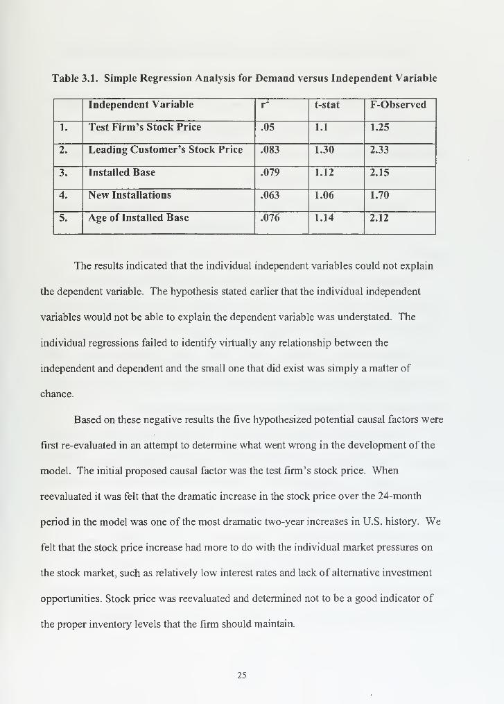
Table 3.1. Simple Regression Analysis for Demand versus Independent Variable
Independent Variable r2
t-stat F-Observed
1. Test Firm's Stock Price .05 1.1 1.25
2. Leading Customer's Stock Price .083 1.30 2.33
3. Installed Base .079 1.12 2.15
4. New Installations .063 1.06 1.70
5. Age of Installed Base .076 1.14 2.12
The results indicated that the individual independent variables could not explain
the dependent variable. The hypothesis stated earlier that the individual independent
variables would not be able to explain the dependent variable was understated. The
individual regressions failed to identify virtually any relationship between the
independent and dependent and the small one that did exist was simply a matter of
chance.
Based on these negative results the five hypothesized potential causal factors were
first re-evaluated in an attempt to determine what went wrong in the development of the
model. The initial proposed causal factor was the test firm's stock price. When
reevaluated it was felt that the dramatic increase in the stock price over the 24-month
period in the model was one of the most dramatic two-year increases in U.S. history. We
felt that the stock price increase had more to do with the individual market pressures on
the stock market, such as relatively low interest rates and lack of alternative investment
opportunities. Stock price was reevaluated and determined not to be a good indicator of
the proper inventory levels that the firm should maintain.
25

The second independent variable was the leading customer's stock price. This
was flawed for the same reasons stated above.
The third hypothesized causal factor was the installed base. This independent
variable was flawed due to the fallibility of the database that the installed base is
maintained on. The installed base database does not currently show any deletion of
systems and simply identifies the additions.
Additionally, with a lack ofMTBF, MTBM, and usage data for the installed base,
a causal based model is unlikely to forecast demand any better than a demand-based
model.
The fourth independent variable was the number ofnew installations. The
number ofnew installations may have been flawed because while the aggregate number
ofnew installs was available, the reliability data for these new systems was unavailable.
Further, no data was available to indicate if these were replacing existing machines or
simply initial outfitting. The hypothesized existing machines may have had two or three
times the demand requirements that the new installations now have.
The fifth potential causal factor was age of the installed base. This again had the
problem of adding additional units as they came online but no method for identifying
those systems that were discarded.
Additionally, the factors not accounted for in the demand-based model, discussed
in the initial chapter, were reviewed to determine if our causal model did a better job of
accounting for them. The first factor of attempting to account for a change in a basic
pattern a causal model is well suited to, however a causal based model will not solve for
the other three factors any more than demand-based model currently installed. The
26

second factor, cyclical business patterns, must be accounted for with time-series analysis
vice a causal based model. The third factor, seasonal issues is also best solved with a
time-series model vice a causal model. The fourth factor discussed regional and national
differences and the causal model developed did not account for these differences.
Further, there were no independent variables identified that could account for this fourth
factor.
C. MULTIPLE REGRESSION MODEL
A multiple regression model using all the hypothesized independent variables was
developed to test the initial hypothesis that together the independent variable may have a
relationship with the dependent variable.
The sixth and final model uses multiple regression analysis to compare all of the
independent variables to demand. Table 3.2. shows a summary of the results of the
multiple regression model. The r of .303 predicts that 30.3% of the total variation is
explained by the independent variables. However, the results additionally indicate that
the r2is not significant per the t-stat value of .97 1 , .939, . 1 .05 1 , .974, and 1 .0 1 3 for the
respective independent variables which are all less than two that is required for
significance at this level. The F-Observed of 1.74 indicates that any proposed
relationship between the independent and dependent variables, occurs merely by chance.
27
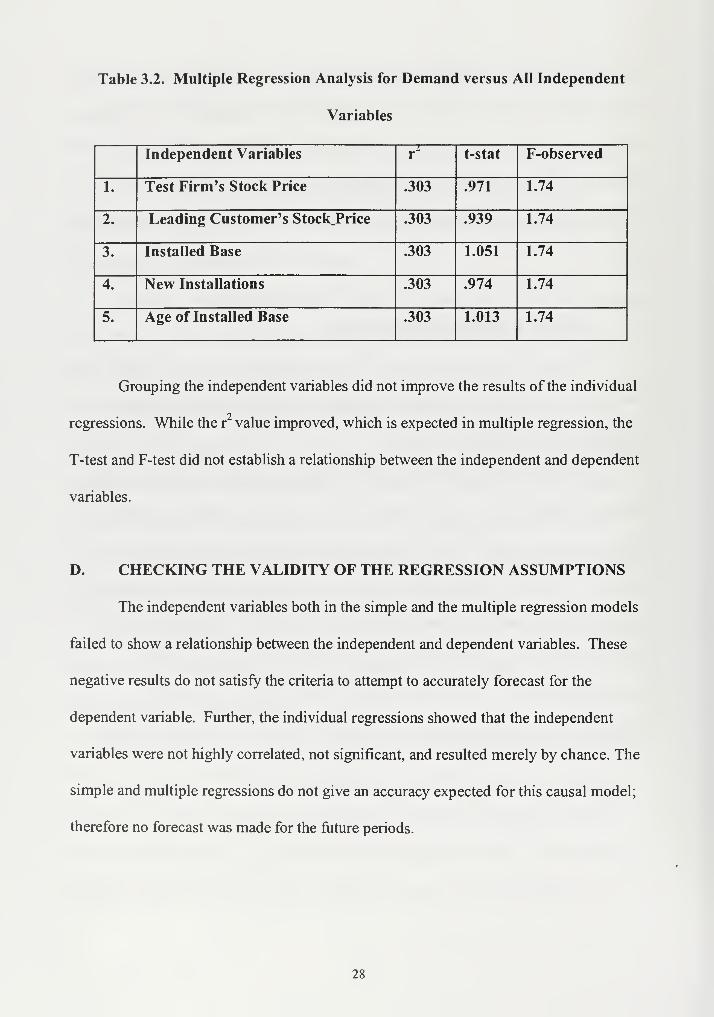
Table 3.2. Multiple Regression Analysis for Demand versus All Independent
Variables
Independent Variables r1
t-stat F-observed
1. Test Firm's Stock Price .303 .971 1.74
2. Leading Customer's StockPrice .303 .939 1.74
3. Installed Base .303 1.051 1.74
4. New Installations .303 .974 1.74
5. Age of Installed Base .303 1.013 1.74
Grouping the independent variables did not improve the results of the individual
regressions. While the r value improved, which is expected in multiple regression, the
T-test and F-test did not establish a relationship between the independent and dependent
variables.
D. CHECKING THE VALIDITY OF THE REGRESSION ASSUMPTIONS
The independent variables both in the simple and the multiple regression models
failed to show a relationship between the independent and dependent variables. These
negative results do not satisfy the criteria to attempt to accurately forecast for the
dependent variable. Further, the individual regressions showed that the independent
variables were not highly correlated, not significant, and resulted merely by chance. The
simple and multiple regressions do not give an accuracy expected for this causal model;
therefore no forecast was made for the future periods.
28
IV. CONCLUSIONS AND RECOMMENDATIONS
A. CONCLUSIONS AND RECOMMENDATIONS
This thesis addressed the need for a new forecasting method at an electronics
capital equipment manufacturer. The primary research question asked was: Can a causal
based model replace the existing demand-based forecasting inventory model currently in
use at an electronics capital equipment manufacturer supporting high technology
customers?
1. Transition to DRP
Conclusion: A causal based model was developed which yielded negative
results. The thesis research concluded that a demand-based model is a better model at this
time. The test firm should transition to DRP as soon as possible.
Recommendation: The test firm should implement the DRP demand-based
model and continue to develop accurate information on the installed base of its
customers. The firm should develop and implement a database that eventually accounts
for the MTBF, MTBM and operating hours for their entire product line. DRP can do this
with the correct inputs. The firm's customers and manufacturer must be persuaded to
share this data with the firm. If necessary, the firm should purchase this information
from its largest customers.
DRP should continue to improve the service level, but without the aforementioned
inputs a 95 percent service level is probably unattainable.
29

2. Need for Accurate Forecasts/Lack of "High Movers"
Conclusion: Due to the lack of "high movers" the firm requires an additional
level of safety stock to attain the required customer service level.
Recommendation: The infrequency of demand and an absence of "top
movers" will continue to plague the forecasting process, until the firm reaches its
maturity level. The firm should carry an extra level of safety stock to increase customer
service levels during its current growth stage until it can more adequately forecast
demand.
3. Develop and Retain Forecasters
Conclusion: The forecasters are currently an integral part of the forecasting
system and need to be developed and retained. DRP may ease the burden on them,
however until the other factors affecting the forecasting process can be identified and
inputted into the DRP model, the model will require manual adjustments.
Recommendation: The firm further needs to continue to develop and retain
their forecasters until they are able to develop or install a more capable system. The
forecasters are currently the integral part of the link in reducing inventory costs and
improving effectiveness. As more data becomes available, the forecasters should become
less critical in inventory forecasting.
4. Identify Global Trends
Conclusion: Global trends must be identified and accounted for by either by the
DRP model or through manual forecasting.
Recommendation: The firm needs to identify the causal factors that affect their
industry such as market trends or the global economy and use this data to more accurately
30

forecast future demand. Asia, Europe and several individual countries on both continents
greatly affect the demand for parts, revenue and system sales. The firm is integrated into
the various global markets and economies and is greatly affected by the market trends
that affect those economies. To quantify these effects and potential causal factors, the
firm should identify several readily available indexes that their directors determine affect
demand for their products.
5. Continue to Identify Regional and National Variances in Demand
Patterns
Conclusion: Regional and national differences in demand patterns must be
accounted for by either DRP or manually. This will allow for a more normalized demand
pattern, which will avoid increased inventory holding costs and shortages. Shortages will
result in a lower customer service level.
Recommendation: Regional and national variances in the firm's customers
demand patterns need to continue to be identified and implemented into the demand-
based model. This will help identify actual demand patterns from perceived patterns as
discussed earlier in the thesis.
6. Implement Cyclical Business Patterns and Seasonal Fluctuations into
DRP
Conclusion: DRP forecasts will become more accurate if the cyclical business
and seasonal trends are taken into account.
Recommendation: Cyclical business patterns and seasonal fluctuations are a
part of the firm's business. Therefore these factors must be accounted for as part of DRP,
whether directly in the demand based model or as an input from another system.
31
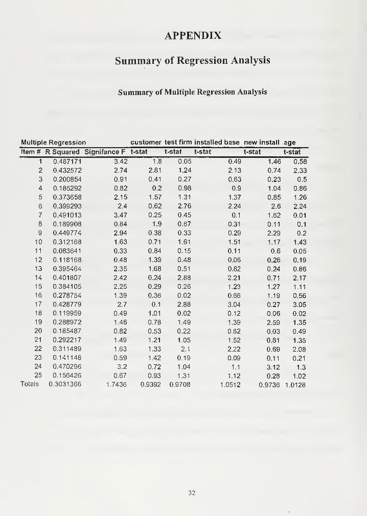
APPENDIX
Summary of Regression Analysis
Summary of Multiple Regression Analysis
Multiple Regression customer test firm installed base new install age
ltem# R Squared Signifance F t-stat t-stat t-stat t-stat t-stat
1 0.487171 3.42 1.8 0.05 0.49 1.46 0.58
2 0.432572 2.74 2.81 1.24 2.13 0.74 2.33
3 0.200854 0.91 0.41 0.27 0.63 0.23 0.5
4 0.185292 0.82 0.2 0.98 0.9 1.04 0.86
5 0.373658 2.15 1.57 1.31 1.37 0.85 1.26
6 0.399293 2.4 0.62 2.76 2.24 2.6 2.24
7 0.491013 3.47 0.25 0.45 0.1 1.62 0.01
8 0.189908 0.84 1.9 0.67 0.31 0.11 0.1
9 0.449774 2.94 0.38 0.33 0.29 2.29 0.2
10 0.312168 1.63 0.71 1.61 1.51 1.17 1.43
11 0.083641 0.33 0.84 0.15 0.11 0.6 0.05
12 0.118168 0.48 1.39 0.48 0.06 0.26 0.19
13 0.395464 2.35 1.68 0.51 0.82 0.24 0.86
14 0.401807 2.42 0.24 2.88 2.21 0.71 2.17
15 0.384105 2.25 0.29 0.26 1.23 1.27 1.11
16 0.278754 1.39 0.36 0.02 0.66 1.19 0.56
17 0.428779 2.7 0.1 2.88 3.04 0.27 3.05
18 0.119959 0.49 1.01 0.02 0.12 0.06 0.02
19 0.288972 1.46 0.78 1.49 1.39 2.59 1.35
20 0.185487 0.82 0.53 0.22 0.62 0.03 0.49
21 0.292217 1.49 1.21 1.05 1.52 0.81 1.35
22 0.311489 1.63 1.33 2.1 2.22 0.69 2.08
23 0.141148 0.59 1.42 0.19 0.09 0.11 0.21
24 0.470296 3.2 0.72 1.04 1.1 3.12 1.3
25 0.156426 0.67 0.93 1.31 1.12 0.28 1.02
Totals 0.3031366 1 .7436 0.9392 0.9708 1.0512 0.9736 1.0128
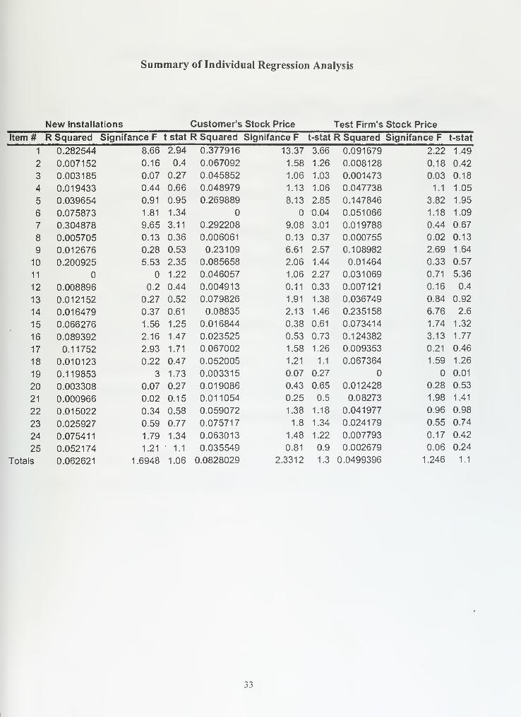
Summary of Individual Regression Analysis
New installations Customer's Stock Price Test Firm's Stock Price
ltem# R Squared Signifance F t stat R Squared Signifance F t-stat R Squared Signifance F t-stat
1 0.282544 8.66 2.94 0.377916 13.37 3.66 0.091679 2.22 1.49
2 0.007152 0.16 0.4 0.067092 1.58 1.26 0.008128 0.18 0.42
3 0.003185 0.07 0.27 0.045852 1.06 1.03 0.001473 0.03 0.18
4 0.019433 0.44 0.66 0.048979 1.13 1.06 0.047738 1.1 1.05
5 0.039654 0.91 0.95 0.269889 8.13 2.85 0.147846 3.82 1.95
6 0.075873 1.81 1.34 0.04 0.051066 1.18 1.09
7 0.304878 9.65 3.11 0.292208 9.08 3.01 0.019788 0.44 0.67
8 0.005705 0.13 0.36 0.006061 0.13 0.37 0.000755 0.02 0.13
9 0.012676 0.28 0.53 0.23109 6.61 2.57 0.108982 2.69 1.64
10 0.200925 5.53 2.35 0.085658 2.06 1.44 0.01464 0.33 0.57
11 1.22 0.046057 1.06 2.27 0.031069 0.71 5.36
12 0.008896 0.2 0.44 0.004913 0.11 0.33 0.007121 0.16 0.4
13 0.012152 0.27 0.52 0.079826 1.91 1.38 0.036749 0.84 0.92
14 0.016479 0.37 0.61 0.08835 2.13 1.46 0.235158 6.76 2.6
15 0.066276 1.56 1.25 0.016844 0.38 0.61 0.073414 1.74 1.32
16 0.089392 2.16 1.47 0.023525 0.53 0.73 0.124382 3.13 1.77
17 0.11752 2.93 1.71 0.067002 1.58 1.26 0.009353 0.21 0.46
18 0.010123 0.22 0.47 0.052005 1.21 1.1 0.067364 1.59 1.26
19 0.119853 3 1.73 0.003315 0.07 0.27 0.01
20 0.003308 0.07 0.27 0.019086 0.43 0.65 0.012428 0.28 0.53
21 0.000966 0.02 0.15 0.011054 0.25 0.5 0.08273 1.98 1.41
22 0.015022 0.34 0.58 0.059072 1.38 1.18 0.041977 0.96 0.98
23 0.025927 0.59 0.77 0.075717 1.8 1.34 0.024179 0.55 0.74
24 0.075411 1.79 1.34 0.063013 1.48 1.22 0.007793 0.17 0.42
25 0.052174 1.21 1.1 0.035549 0.81 0.9 0.002679 0.06 0.24
Totals 0.062621 1.6948 1.06 0.0828029 2.3312 1.3 0.0499396 1.246 1.1
33
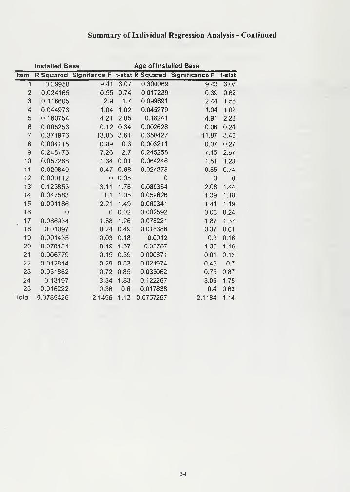
Installed Base
Summary of Individual Regression Analysis - Continued
Age of Installed Base
Item R Squared Signifance F t-stat R Squared Significance F t-stat
1 0.29958 9.41 3.07 0.300069 9.43 3.07
2 0.024165 0.55 0.74 0.017239 0.39 0.62
3 0.116605 2.9 1.7 0.099691 2.44 1.56
4 0.044973 1.04 1.02 0.045279 1.04 1.02
5 0.160754 4.21 2.05 0.18241 4.91 2.22
6 0.005253 0.12 0.34 0.002628 0.06 0.24
7 0.371976 13.03 3.61 0.350427 11.87 3.45
8 0.004115 0.09 0.3 0.003211 0.07 0.27
9 0.248175 7.26 2.7 0.245258 7.15 2.67
10 0.057268 1.34 0.01 0.064246 1.51 1.23
11 0.020849 0.47 0.68 0.024273 0.55 0.74
12 0.000112 0.05
13 0.123853 3.11 1.76 0.086364 2.08 1.44
14 0.047583 1.1 1.05 0.059626 1.39 1.18
15 0.091186 2.21 1.49 0.060341 1.41 1.19
16 0.02 0.002592 0.06 0.24
17 0.066934 1.58 1.26 0.078221 1.87 1.37
18 0.01097 0.24 0.49 0.016386 0.37 0.61
19 0.001435 0.03 0.18 0.0012 0.3 0.16
20 0.078131 0.19 1.37 0.05787 1.35 1.16
21 0.006779 0.15 0.39 0.000671 0.01 0.12
22 0.012814 0.29 0.53 0.021974 0.49 0.7
23 0.031862 0.72 0.85 0.033062 0.75 0.87
24 0.13197 3.34 1.83 0.122267 3.06 1.75
25 0.016222 0.36 0.6 0.017838 0.4 0.63
Total 0.0789426 2.1496 1.12 0.0757257 2.1184 1.14
34

BIBLIOGRAPHY
Makridakis, S., and Wheelwright, S., Interactive Forecasting . 2nd
ed., Holden-Day Inc,
1978
Thomopoulos, N., Applied Forecasting Methods . Prentice-Hall, Inc, 1980
Benton, W., Forecasting For Management . Addison-Wesley Publishing Company, 1972
Seitz, N., Business Forecasting On Your Personal Computer. Reston Publishing
Company, 1984
Makridakis, S., and Wheelwright, S., Forecasting . John Wiley & Sons, 1978
Makridakis, S., and Wheelwright, S., The Handbook Of Forecasting . 2nd
ed., John Wiley
&Sons, 1987
O'Donovan, T., Short Term Forecasting . John Wiley & Sons, 1983
Wheelwright, S., and Makridakis, S., Forecasting Methods For Management . 3rd
ed.,
John Wiley & Sons, 1980
Liao, S., The Basic Regression Model , unpublished manuscript, 1997
Liao, S., Multiple Regression , unpublished manuscript, 1997
James, L., Mulaik, S., and Brett, J., Causal Analysis Assumptions. Models And Data .
Sage Publications, 1982
Asher, H., Causal Modeling . Sage Publications, 1983
Berry, W., Nonrecursive Causal Models . Sage Publications, 1984
35

36
INITIAL DISTRIBUTION LIST
No. Copies
1
.
Defense Technical Information Center 2
8725 John J. Kingman Rd., Ste 0944
Ft. Belvoir, VA 22060-6218
2. Dudley Knox Library 2
Naval Postgraduate School
411 DyerRd.
Monterey, CA 93943-5101
3. Dr. Kevin R. Gue 1
Department of Systems Management
Naval Postgraduate School
Monterey, CA 93943-5002
4. Dr. Shu S. Liao 1
Department of Systems Management
Naval Postgraduate School
Monterey, CA 93943-5002
5. LCDR John E. Hicks 1
216 Naples Road
Seaside, CA 93955
37


DUDLEY KNOX LIBRARY
9III IIilHI
3 2768 00342141 3