Embed Size (px)
Citation preview

J. N. REDDYDepartment of Mechanical EngineeringTexas A&M UniversityCollege Station, Texas, 77843-3123, USA
An Introduction to NonlinearFinite Element Analysis
with applications to heat transfer, fluid mechanics,and solid mechanics
Second Edition
3
3
Great Clarendon Street, Oxford, OX2 6DP,United Kingdom
Oxford University Press is a department of the University of Oxford.It furthers the University’s objective of excellence in research, scholarship,and education by publishing worldwide. Oxford is a registered trade mark ofOxford University Press in the UK and in certain other countries
c© Oxford University Press 2015
The moral rights of the author have been asserted
First Edition published in 2004Second Edition published in 2015
Impression: 1
All rights reserved. No part of this publication may be reproduced, stored ina retrieval system, or transmitted, in any form or by any means, without theprior permission in writing of Oxford University Press, or as expressly permittedby law, by licence or under terms agreed with the appropriate reprographicsrights organization. Enquiries concerning reproduction outside the scope of theabove should be sent to the Rights Department, Oxford University Press, at theaddress above
You must not circulate this work in any other formand you must impose this same condition on any acquirer
Published in the United States of America by Oxford University Press198 Madison Avenue, New York, NY 10016, United States of America
British Library Cataloguing in Publication Data
Data available
Library of Congress Control Number: 2014935440
ISBN 978–0–19–964175–8
Printed in Great Britain byClays Ltd, St Ives plc
Links to third party websites are provided by Oxford in good faith andfor information only. Oxford disclaims any responsibility for the materialscontained in any third party website referenced in this work.

To my beloved teacher and mentor
Professor John Tinsley Oden

Preface to the Second Edition
The development of realistic mathematical models that govern the response ofsystems or processes is intimately connected to the ability to translate theminto meaningful discrete models that enable us to systematically evaluate vari-ous parameters of the systems and processes. Mathematical model developmentand numerical simulations are aids to designers, who are seeking to maximizethe reliability of products and minimize the cost of production, distribution,and repairs. Mathematical models are developed using laws of physics and as-sumptions concerning a system’s behavior. The most important step in arrivingat a design that is both reliably functional and cost-effective is the constructionof a suitable mathematical model of the system behavior and its translationinto a powerful numerical simulation tool. While a select number of courses oncontinuum mechanics, material science, and dynamical systems, among others,provides engineers with the background to formulate a suitable mathemati-cal model, courses on numerical methods prepare engineers and scientists toevaluate mathematical models and test material models in the context of thefunctionality and design constraints placed on the system. In cases where phys-ical experiments are prohibitively expensive, numerical simulations are the onlyalternative, especially when the phenomena is governed by nonlinear differentialequations, in evaluating various design options. It is in this context a course onnonlinear finite element analysis proves to be very useful.
Most books on nonlinear finite element analysis tend to be abstract in thepresentation of details of the finite element formulations, derivation of elementequations, and their solution by iterative methods. Such books serve as refer-ence books but not as textbooks. The present textbook is unique (i.e. thereis no parallel to this book in its class) since it actually helps the readers withdetails of finite element model development and implementation. In particular,it provides illustrative examples and problem sets that enable readers to testtheir understanding of the subject matter and utilize the tools developed in theformulation and finite element analysis of engineering problems.
The second edition of An Introduction to Nonlinear Finite Element Anal-ysis has the same objective as the first edition, namely, to facilitate an easyand thorough understanding of the details that are involved in the theoreticalformulation, finite element model development, and solutions of nonlinear prob-lems. The book offers easy-to-understand treatment of the subject of nonlinearfinite element analysis, which includes element development from mathematicalmodels and numerical evaluation of the underlying physics. The new editionis extensively reorganized and contains substantially large amount of new ma-terial. In particular, Chapter 1 in the second edition contains a section onapplied functional analysis; Chapter 2 on nonlinear continuum mechanics is en-tirely new; Chapters 3 through 8 in the new edition correspond to Chapter 2
vi PREFACE TO THE SECOND EDITION
through 8 of the first edition but with additional explanations, examples, andexercise problems (material on time dependent problems from Chapter 8 of thefirst edition is absorbed into Chapters 6 through 10 of the new edition); Chap-ter 9 is extensively revised and it contains up to date developments in the largedeformation analysis of isotropic, composite, and functionally graded shells;Chapter 10 of the first edition on material nonlinearity and coupled problems isreorganized in the second edition by moving the material on solid mechanics toChapter 12 in the new edition, and material on coupled problems to Chapter 10on weak-form Galerkin finite element models of viscous incompressible fluids;finally, Chapter 11 in the second edition is entirely new and devoted to least-squares finite element models of viscous incompressible fluids. Chapter 12 ofthe second edition (available only online) contains material on one-dimensionalformulations of nonlinear elasticity, plasticity, and viscoelasticity. In general,all of the chapters of the second edition contain additional explanations, de-tailed example problems, and additional exercise problems. Although all of theprogramming segments are in Fortran, the logic used in these Fortran programsis transparent and can be used in Matlab or C++ versions of the same. Thusthe new edition more than replaces the first edition, and it is hoped that it isacquired by the library of every institution of higher learning as well as seriousfinite element analysts.
The book may be used as a textbook for an advanced course (after a firstcourse) on the finite element method or the first course on nonlinear finiteelement analysis. A solutions manual has also been prepared for the book. Thesolution manual is available from the publisher only to instructors who adoptthe book as a textbook for a course.
Since the publication of the first edition, many users of the book communi-cated their comments and compliments as well as errors they found, for whichthe author thanks them. All of the errors known to the author have been cor-rected in the current edition. The author is grateful to the following professionalcolleagues for their friendship, encouragement, and constructive comments onthe book:
Hasan Akay, Purdue University at IndianapolisMarcilio Alves, University of Sao Paulo, BrazilMarco Amabili, McGill University, CanadaTed Belytschko, Northwestern UniversityK. Chandrashekara, Missouri University of Science and TechnologyA. Ecer, Purdue University at IndianapolisAntonio Ferreira, University of Porto, PortugalAntonio Grimaldi, University of Rome II, ItalyR. Krishna Kumar, Indian Institute of Technology, MadrasH. S. Kushwaha, Bhabha Atomic Research Centre, IndiaA. V. Krishna Murty, Indian Institute of Science, BangaloreK. Y. Lam, Nanyang Technological University, Singapore
PREFACE TO THE SECOND EDITION vii
K. M. Liew, City University of Hong KongC. W. Lim, City University of Hong KongFranco Maceri, University of Rome II, ItalyC. S. Manohar, Indian Institute of Science, BangaloreAntonio Miravete, Zaragoza University, SpainAlan Needleman, Brown UniversityJ. T. Oden, University of Texas at AustinP. C. Pandey, Indian Institute of Science, BangaloreGlaucio Paulino, University of Illinois at Urbana-ChampaignA. Rajagopal, Indian Institute of Technology, HyderabadEkkehard Ramm, University of Stuttgart, GermanyJani Romanoff, Aalto University, FinlandSamit Roy, University of Alabama, TuscaloosaSiva Prasad, Indian Institute of Technology, MadrasElio Sacco, University of Cassino, ItalyRudger Schmidt, University of Aachen, GermanyE. C. N. Silva, University of Sao Paulo, BrazilFanis Strouboulis, Texas A&M UniversityKaran Surana, University of KansasLiqun Tang, South China University of TechnologyVinu Unnikrishnan, University of Alabama, TuscaloosaC. M. Wang, National University of SingaporeJohn Whitcomb, Texas A&M UniversityY. B. Yang, National Taiwan University
Drafts of the manuscript of this book prior to its publication were read by theauthor’s doctoral students, who have made suggestions for improvements. Inparticular, the author wishes to thank the following former and current students(listed in alphabetical order): Roman Arciniega, Ronald Averill, Ever Barbero,K. Chandrashekhara, Feifei Cheng, Stephen Engelstad, Eugenio Garcao, MiguelGutierrez Rivera, Paul Heyliger, Filis Kokkinos, C. F. Liao, Goy Teck Lim,Ravisankar Mayavaram, John Mitchell, Filipa Moleiro, Felix Palmerio, GregoryPayette, Jan Pontaza, Vivek Prabhakar, Grama Praveen, N. S. Putcha, RakeshRanjan, Mahender Reddy, Govind Rengarajan, Donald Robbins, Jr., SamitRoy, Vinu Unnikrishnan, Ginu Unnikrihnan, Yetzirah Urthaler, Venkat Vallala;Archana Arbind, Parisa Khodabakhshi, Jinseok Kim, Wooram Kim, HelnazSoltani, and Mohammad Torki. The author also expresses his sincere thanksto Mr. Sonke Adlung (Senior Editor, Engineering) and Ms. Victoria Mortimer(Senior Production editor) at Oxford University Press for their encouragementand help in producing this book. The author requests readers to send theircomments and corrections to [email protected].
J. N. ReddyCollege Station, Texas

Preface to the First Edition
The objective of this book is to present the theory and computer implemen-tation of the finite element method as applied to simple nonlinear problems ofheat transfer and similar field problems, fluid mechanics, and solid mechanics.Both geometric as well as material nonlinearities are considered, and static andtransient (i.e. time-dependent) responses are studied. The guiding principle inwriting the book was to make the presentation suitable for (a) adoption as atext book for a first course on nonlinear finite element analysis (or for a secondcourse following an introductory course on the finite element method) and (b)for use by engineers and scientists from various disciplines for self-study andpractice.
There exist a number of books on nonlinear finite elements. Most of thesebooks contain a good coverage of the topics of structural mechanics, and fewaddress topics of fluid dynamics and heat transfer. While these books serveas good references to engineers or scientists who are already familiar with thesubject but wish to learn advanced topics or latest developments, they are notsuitable as textbooks for a first course or for self study on nonlinear finiteelement analysis.
The motivation and encouragement that led to the writing of the presentbook have come from the users of the author’s book, An Introduction to theFinite Element Method (McGraw-Hill, 1984; Second Edition, 1993; third editionscheduled for 2004), who have found the approach presented there to be mostsuitable for any one – irrespective of their scientific background – interestedin learning the method, and also from the fact that there does not exist abook that is suitable as a textbook for a first course on nonlinear finite elementanalysis. The author has taught a course on nonlinear finite element analysismany times during the last twenty years, and the present book is an outcomeof the lecture notes developed during this period. The same approach as thatused in the aforementioned book, namely, the differential equation approach, isadopted in the present book to introduce the theory, formulation, and computerimplementation of the finite element method as applied to nonlinear problemsof science and engineering.
Beginning with a model (i.e. typical) second-order, nonlinear differentialequation in one dimension, the book takes the reader through increasinglycomplex problems of nonlinear beam bending, nonlinear field problems in twodimensions, nonlinear plate bending, nonlinear formulations of solid continua,flows of viscous incompressible fluids in two dimensions (i.e. Navier–Stokesequations), time-approximation schemes, continuum formulations of shells, andmaterial nonlinear problems of solid mechanics.
As stated earlier, the book is suitable as a textbook for a first course onnonlinear finite elements in civil, aerospace, mechanical, and mechanics depart-
x PREFACE TO THE FIRST EDITION
ments as well as in applied sciences. It can be used as a reference by engineersand scientists working in industry, government laboratories, and academia. In-troductory courses on the finite element method, continuum mechanics, andnumerical analysis should prove to be helpful.
The author has benefited in writing the book by the encouragement andsupport of many colleagues around the world who have used his book, AnIntroduction to the Finite Element Method, and students who have challengedhim to explain and implement complicated concepts and formulations in simpleways. While it is not possible to name all of them, the author expresses hissincere appreciation. The author expresses his deep sense of gratitude to histeacher and mentor, Professor J. T. Oden (University of Texas at Austin),without whose advice and support it would not have been possible for theauthor to modestly contribute to the field of applied mechanics in general andtheory and application of the finite element method in particular, through histeaching, research, and writings.
J. N. Reddy
College Station, Texas
Contents
Preface to the Second Edition . . . . . . . . . . . . . . . . . . vPreface to the First Edition . . . . . . . . . . . . . . . . . . ixAbout the Author . . . . . . . . . . . . . . . . . . . . . . xxvList of Symbols . . . . . . . . . . . . . . . . . . . . . . . xxvii
1 General Introduction and Mathematical Preliminaries . . . 1
1.1 General Comments . . . . . . . . . . . . . . . . . . . . . . 1
1.2 Mathematical Models . . . . . . . . . . . . . . . . . . . . . 2
1.3 Numerical Simulations . . . . . . . . . . . . . . . . . . . . 4
1.4 The Finite Element Method . . . . . . . . . . . . . . . . . . 6
1.5 Nonlinear Analysis . . . . . . . . . . . . . . . . . . . . . . 8
1.5.1 Introduction . . . . . . . . . . . . . . . . . . . . . . . 8
1.5.2 Classification of Nonlinearities . . . . . . . . . . . . . . . 8
1.6 Review of Vectors and Tensors . . . . . . . . . . . . . . . . 12
1.6.1 Preliminary Comments . . . . . . . . . . . . . . . . . 12
1.6.2 Definition of a Physical Vector . . . . . . . . . . . . . . 13
1.6.2.1 Vector addition . . . . . . . . . . . . . . . . . . 13
1.6.2.2 Multiplication of a vector by a scalar . . . . . . . . . 13
1.6.3 Scalar and Vector Products . . . . . . . . . . . . . . . 14
1.6.3.1 Scalar product (or “dot” product) . . . . . . . . . . 14
1.6.3.2 Vector product . . . . . . . . . . . . . . . . . . . 14
1.6.3.3 Plane area as a vector . . . . . . . . . . . . . . . 15
1.6.3.4 Linear independence of vectors . . . . . . . . . . . . 16
1.6.3.5 Components of a vector . . . . . . . . . . . . . . . 16
1.6.4 Summation Convention and Kronecker Delta andPermutation Symbol . . . . . . . . . . . . . . . . . . 17
1.6.4.1 Summation convention . . . . . . . . . . . . . . . 17
1.6.4.2 Kronecker delta symbol . . . . . . . . . . . . . . . 17
1.6.4.3 The permutation symbol . . . . . . . . . . . . . . 18
1.6.5 Tensors and their Matrix Representation . . . . . . . . . . 19
1.6.5.1 Concept of a second-order tensor . . . . . . . . . . . 19
1.6.5.2 Transformation laws for vectors and tensors . . . . . . 20
.
xii CONTENTS
1.6.6 Calculus of Vectors and Tensors . . . . . . . . . . . . . 22
1.7 Concepts from Functional Analysis . . . . . . . . . . . . . . 27
1.7.1 Introduction . . . . . . . . . . . . . . . . . . . . . . 27
1.7.2 Linear Vector Spaces . . . . . . . . . . . . . . . . . . 28
1.7.2.1 Vector addition . . . . . . . . . . . . . . . . . . 28
1.7.2.2 Scalar multiplication . . . . . . . . . . . . . . . . 29
1.7.2.3 Linear subspaces . . . . . . . . . . . . . . . . . . 29
1.7.2.4 Linear dependence and independence of vectors . . . . 29
1.7.3 Normed Vector Spaces . . . . . . . . . . . . . . . . . 30
1.7.3.1 Holder inequality . . . . . . . . . . . . . . . . . . 30
1.7.3.2 Minkowski inequality . . . . . . . . . . . . . . . . 30
1.7.4 Inner Product Spaces . . . . . . . . . . . . . . . . . . 32
1.7.4.1 Orthogonality of vectors . . . . . . . . . . . . . . . 33
1.7.4.2 Cauchy–Schwartz inequality . . . . . . . . . . . . . 33
1.7.4.3 Hilbert spaces . . . . . . . . . . . . . . . . . . . 35
1.7.5 Linear Transformations . . . . . . . . . . . . . . . . . 36
1.7.6 Linear Functionals, Bilinear Forms, and Quadratic Forms . . 37
1.7.6.1 Linear functional . . . . . . . . . . . . . . . . . . 38
1.7.6.2 Bilinear forms . . . . . . . . . . . . . . . . . . . 38
1.7.6.3 Quadratic forms . . . . . . . . . . . . . . . . . . 38
1.8 The Big Picture . . . . . . . . . . . . . . . . . . . . . . 40
1.9 Summary . . . . . . . . . . . . . . . . . . . . . . . . . 42
Problems . . . . . . . . . . . . . . . . . . . . . . . . . 42
2 Elements of Nonlinear Continuum Mechanics . . . . . . . 47
2.1 Introduction . . . . . . . . . . . . . . . . . . . . . . . . 47
2.2 Description of Motion . . . . . . . . . . . . . . . . . . . . 48
2.2.1 Configurations of a Continuous Medium . . . . . . . . . . 48
2.2.2 Material and Spatial Descriptions . . . . . . . . . . . . . 49
2.2.3 Displacement Field . . . . . . . . . . . . . . . . . . . 53
2.3 Analysis of Deformation . . . . . . . . . . . . . . . . . . . 54
2.3.1 Deformation Gradient . . . . . . . . . . . . . . . . . . 54
2.3.2 Volume and Surface Elements in the Material andSpatial Descriptions . . . . . . . . . . . . . . . . . . 55
CONTENTS xiii
2.4 Strain Measures . . . . . . . . . . . . . . . . . . . . . . 56
2.4.1 Deformation Tensors . . . . . . . . . . . . . . . . . . 56
2.4.2 The Green–Lagrange Strain Tensor . . . . . . . . . . . . 57
2.4.3 The Cauchy and Euler Strain Tensors . . . . . . . . . . . 58
2.4.4 Infinitesimal Strain Tensor and Rotation Tensor . . . . . . 59
2.4.4.1 Infinitesimal strain tensor . . . . . . . . . . . . . . 59
2.4.4.2 Infinitesimal rotation tensor . . . . . . . . . . . . . 60
2.4.5 Time Derivatives of the Deformation Tensors . . . . . . . . 60
2.5 Measures of Stress . . . . . . . . . . . . . . . . . . . . . 62
2.5.1 Stress Vector . . . . . . . . . . . . . . . . . . . . . . 62
2.5.2 Cauchy’s Formula and Stress Tensor . . . . . . . . . . . . 63
2.5.3 Piola–Kirchhoff Stress Tensors . . . . . . . . . . . . . . 65
2.5.3.1 First Piola–Kirchhoff stress tensor . . . . . . . . . . . 65
2.5.3.2 Second Piola–Kirchhoff stress tensor . . . . . . . . . 67
2.6 Material Frame Indifference . . . . . . . . . . . . . . . . . 67
2.6.1 The Basic Idea . . . . . . . . . . . . . . . . . . . . . 67
2.6.2 Objectivity of Strains and Strain Rates . . . . . . . . . . 69
2.6.3 Objectivity of Stress Tensors . . . . . . . . . . . . . . . 69
2.6.3.1 Cauchy stress tensor . . . . . . . . . . . . . . . . . 69
2.6.3.2 First Piola–Kirchhoff stress tensor . . . . . . . . . . 70
2.6.3.3 Second Piola–Kirchhoff stress tensor . . . . . . . . . 70
2.7 Equations of Continuum Mechanics . . . . . . . . . . . . . . 70
2.7.1 Introduction . . . . . . . . . . . . . . . . . . . . . . 70
2.7.2 Conservation of Mass . . . . . . . . . . . . . . . . . . 71
2.7.2.1 Spatial form of the continuity equation . . . . . . . . 71
2.7.2.2 Material form of the continuity equation . . . . . . . 72
2.7.3 Reynolds Transport Theorem . . . . . . . . . . . . . . . 72
2.7.4 Balance of Linear Momentum . . . . . . . . . . . . . . 73
2.7.4.1 Spatial form of the equations of motion . . . . . . . . 73
2.7.4.2 Material form of the equations of motion . . . . . . . 73
2.7.5 Balance of Angular Momentum . . . . . . . . . . . . . . 74
2.7.6 Thermodynamic Principles . . . . . . . . . . . . . . . . 74
2.7.6.1 Energy equation in the spatial description . . . . . . . 75
xiv CONTENTS
2.7.6.2 Energy equation in the material description . . . . . . 76
2.7.6.3 Entropy inequality . . . . . . . . . . . . . . . . . 77
2.8 Constitutive Equations for Elastic Solids . . . . . . . . . . . . 78
2.8.1 Introduction . . . . . . . . . . . . . . . . . . . . . . 78
2.8.2 Restrictions Placed by the Entropy Inequality . . . . . . . 79
2.8.3 Elastic Materials and the Generalized Hooke’s Law . . . . . 80
2.9 Energy Principles of Solid Mechanics . . . . . . . . . . . . . 83
2.9.1 Virtual Displacements and Virtual Work . . . . . . . . . . 83
2.9.2 First Variation or Gateaux Derivative . . . . . . . . . . . 83
2.9.3 The Principle of Virtual Displacements . . . . . . . . . . 84
2.10 Summary . . . . . . . . . . . . . . . . . . . . . . . . . 88
Problems . . . . . . . . . . . . . . . . . . . . . . . . . 91
3 The Finite Element Method: A Review . . . . . . . . . . 97
3.1 Introduction . . . . . . . . . . . . . . . . . . . . . . . . 97
3.2 One-Dimensional Problems . . . . . . . . . . . . . . . . . . 98
3.2.1 Governing Differential Equation . . . . . . . . . . . . . 98
3.2.2 Finite Element Approximation . . . . . . . . . . . . . . 98
3.2.3 Derivation of the Weak Form . . . . . . . . . . . . . . . 101
3.2.4 Approximation Functions . . . . . . . . . . . . . . . . 104
3.2.5 Finite Element Model . . . . . . . . . . . . . . . . . . 107
3.2.6 Natural Coordinates . . . . . . . . . . . . . . . . . . . 114
3.3 Two-Dimensional Problems . . . . . . . . . . . . . . . . . 116
3.3.1 Governing Differential Equation . . . . . . . . . . . . . 116
3.3.2 Finite Element Approximation . . . . . . . . . . . . . . 118
3.3.3 Weak Formulation . . . . . . . . . . . . . . . . . . . 118
3.3.4 Finite Element Model . . . . . . . . . . . . . . . . . . 121
3.3.5 Approximation Functions: Element Library . . . . . . . . 122
3.3.5.1 Linear triangular element . . . . . . . . . . . . . . 122
3.3.5.2 Linear rectangular element . . . . . . . . . . . . . 125
3.3.5.3 Higher-order triangular elements . . . . . . . . . . . 126
3.3.5.4 Higher-order rectangular elements . . . . . . . . . . 128
3.3.6 Assembly of Elements . . . . . . . . . . . . . . . . . . 130
CONTENTS xv
3.4 Axisymmetric Problems . . . . . . . . . . . . . . . . . . . 136
3.4.1 Introduction . . . . . . . . . . . . . . . . . . . . . . 136
3.4.2 One-Dimensional Problems . . . . . . . . . . . . . . . . 137
3.4.3 Two-Dimensional Problems . . . . . . . . . . . . . . . 138
3.5 The Least-Squares Method . . . . . . . . . . . . . . . . . . 139
3.5.1 Background . . . . . . . . . . . . . . . . . . . . . . 139
3.5.2 The Basic Idea . . . . . . . . . . . . . . . . . . . . . 141
3.6 Numerical Integration . . . . . . . . . . . . . . . . . . . . 143
3.6.1 Preliminary Comments . . . . . . . . . . . . . . . . . 143
3.6.2 Coordinate Transformations . . . . . . . . . . . . . . . 143
3.6.3 Integration Over a Master Rectangular Element . . . . . . 147
3.6.4 Integration Over a Master Triangular Element . . . . . . . 148
3.7 Computer Implementation . . . . . . . . . . . . . . . . . . 149
3.7.1 General Comments . . . . . . . . . . . . . . . . . . . 149
3.7.2 One-Dimensional Problems . . . . . . . . . . . . . . . . 152
3.7.3 Two-Dimensional Problems . . . . . . . . . . . . . . . 157
3.8 Summary . . . . . . . . . . . . . . . . . . . . . . . . . 163
Problems . . . . . . . . . . . . . . . . . . . . . . . . . 164
4 One-Dimensional Problems Involving a Single Variable . 175
4.1 Model Differential Equation . . . . . . . . . . . . . . . . . 175
4.2 Weak Formulation . . . . . . . . . . . . . . . . . . . . . 177
4.3 Finite Element Model . . . . . . . . . . . . . . . . . . . . 177
4.4 Solution of Nonlinear Algebraic Equations . . . . . . . . . . . 180
4.4.1 General Comments . . . . . . . . . . . . . . . . . . . 180
4.4.2 Direct Iteration Procedure . . . . . . . . . . . . . . . . 180
4.4.3 Newton’s Iteration Procedure . . . . . . . . . . . . . . . 185
4.5 Computer Implementation . . . . . . . . . . . . . . . . . . 192
4.5.1 Introduction . . . . . . . . . . . . . . . . . . . . . . 192
4.5.2 Preprocessor Unit . . . . . . . . . . . . . . . . . . . . 193
4.5.3 Processor Unit . . . . . . . . . . . . . . . . . . . . . 194
4.5.3.1 Calculation of element coefficients . . . . . . . . . . . 194
xvi CONTENTS
4.5.3.2 Assembly of element coefficients . . . . . . . . . . . 198
4.5.3.3 Imposition of boundary conditions . . . . . . . . . . 200
4.6 Summary . . . . . . . . . . . . . . . . . . . . . . . . . 208
Problems . . . . . . . . . . . . . . . . . . . . . . . . . 209
5 Nonlinear Bending of Straight Beams . . . . . . . . . . 213
5.1 Introduction . . . . . . . . . . . . . . . . . . . . . . . . 213
5.2 The Euler–Bernoulli Beam Theory . . . . . . . . . . . . . . 214
5.2.1 Basic Assumptions . . . . . . . . . . . . . . . . . . . 214
5.2.2 Displacement and Strain Fields . . . . . . . . . . . . . . 214
5.2.3 The Principle of Virtual Displacements: Weak Form . . . . . 216
5.2.4 Finite Element Model . . . . . . . . . . . . . . . . . . 222
5.2.5 Iterative Solution Strategies . . . . . . . . . . . . . . . 224
5.2.5.1 Direct iteration procedure . . . . . . . . . . . . . . 225
5.2.5.2 Newton’s iteration procedure . . . . . . . . . . . . 225
5.2.6 Load Increments . . . . . . . . . . . . . . . . . . . . 228
5.2.7 Membrane Locking . . . . . . . . . . . . . . . . . . . 228
5.2.8 Computer Implementation . . . . . . . . . . . . . . . . 230
5.2.8.1 Rearrangement of equations and computation ofelement coefficients . . . . . . . . . . . . . . . . . 230
5.2.8.2 Computation of strains and stresses . . . . . . . . . 235
5.2.9 Numerical Examples . . . . . . . . . . . . . . . . . . 237
5.3 The Timoshenko Beam Theory . . . . . . . . . . . . . . . . 242
5.3.1 Displacement and Strain Fields . . . . . . . . . . . . . . 242
5.3.2 Weak Forms . . . . . . . . . . . . . . . . . . . . . . 243
5.3.3 General Finite Element Model . . . . . . . . . . . . . . 245
5.3.4 Shear and Membrane Locking . . . . . . . . . . . . . . 247
5.3.5 Tangent Stiffness Matrix . . . . . . . . . . . . . . . . . 249
5.3.6 Numerical Examples . . . . . . . . . . . . . . . . . . 251
5.3.7 Functionally Graded Material Beams . . . . . . . . . . . 256
5.3.7.1 Material variation and stiffness coefficients . . . . . . . 256
5.3.7.2 Equations of equilibrium . . . . . . . . . . . . . . 257
5.3.7.3 Finite element model . . . . . . . . . . . . . . . . 258
5.4 Summary . . . . . . . . . . . . . . . . . . . . . . . . . 261
CONTENTS xvii
Problems . . . . . . . . . . . . . . . . . . . . . . . . . 261
6 Two-Dimensional Problems Involving a Single Variable . 265
6.1 Model Equation . . . . . . . . . . . . . . . . . . . . . . 265
6.2 Weak Form . . . . . . . . . . . . . . . . . . . . . . . . 266
6.3 Finite Element Model . . . . . . . . . . . . . . . . . . . . 268
6.4 Solution of Nonlinear Equations . . . . . . . . . . . . . . . 269
6.4.1 Direct Iteration Scheme . . . . . . . . . . . . . . . . . 269
6.4.2 Newton’s Iteration Scheme . . . . . . . . . . . . . . . . 269
6.5 Axisymmetric Problems . . . . . . . . . . . . . . . . . . . 271
6.5.1 Introduction . . . . . . . . . . . . . . . . . . . . . . 271
6.5.2 Governing Equation and the Finite Element Model . . . . . 272
6.6 Computer Implementation . . . . . . . . . . . . . . . . . . 273
6.6.1 Introduction . . . . . . . . . . . . . . . . . . . . . . 273
6.6.2 Numerical Integration . . . . . . . . . . . . . . . . . . 273
6.6.3 Element Calculations . . . . . . . . . . . . . . . . . . 275
6.7 Time-Dependent Problems . . . . . . . . . . . . . . . . . . 282
6.7.1 Introduction . . . . . . . . . . . . . . . . . . . . . . 282
6.7.2 Semidiscretization . . . . . . . . . . . . . . . . . . . . 283
6.7.3 Full Discretization of Parabolic Equations . . . . . . . . . 284
6.7.3.1 Eigenvalue problem . . . . . . . . . . . . . . . . . 284
6.7.3.2 Time (α-family of) approximations . . . . . . . . . . 284
6.7.3.3 Fully discretized equations . . . . . . . . . . . . . . 286
6.7.3.4 Direct iteration scheme . . . . . . . . . . . . . . . 286
6.7.3.5 Newton’s iteration scheme . . . . . . . . . . . . . . 287
6.7.3.6 Explicit and implicit formulations and mass lumping . . 287
6.7.4 Full Discretization of Hyperbolic Equations . . . . . . . . 289
6.7.4.1 Newmark’s scheme . . . . . . . . . . . . . . . . . 289
6.7.4.2 Fully discretized equations . . . . . . . . . . . . . . 289
6.7.5 Stability and Accuracy . . . . . . . . . . . . . . . . . 292
6.7.5.1 Preliminary comments . . . . . . . . . . . . . . . . 292
6.7.5.2 Stability criteria . . . . . . . . . . . . . . . . . . 293
6.7.6 Computer Implementation . . . . . . . . . . . . . . . . 294
6.7.7 Numerical Examples . . . . . . . . . . . . . . . . . . 299
xviii CONTENTS
6.8 Summary . . . . . . . . . . . . . . . . . . . . . . . . . 306
Problems . . . . . . . . . . . . . . . . . . . . . . . . . 306
7 Nonlinear Bending of Elastic Plates . . . . . . . . . . . 311
7.1 Introduction . . . . . . . . . . . . . . . . . . . . . . . . 311
7.2 The Classical Plate Theory . . . . . . . . . . . . . . . . . 312
7.2.1 Assumptions of the Kinematics . . . . . . . . . . . . . . 312
7.2.2 Displacement and Strain Fields . . . . . . . . . . . . . . 312
7.3 Weak Formulation of the CPT . . . . . . . . . . . . . . . . 315
7.3.1 Virtual Work Statement . . . . . . . . . . . . . . . . . 315
7.3.2 Weak Forms . . . . . . . . . . . . . . . . . . . . . . 318
7.3.3 Equilibrium Equations . . . . . . . . . . . . . . . . . . 318
7.3.4 Boundary Conditions . . . . . . . . . . . . . . . . . . 319
7.3.4.1 The Kirchhoff free-edge condition . . . . . . . . . . . 320
7.3.4.2 Typical edge conditions . . . . . . . . . . . . . . . 321
7.3.5 Stress Resultant–Deflection Relations . . . . . . . . . . . 322
7.4 Finite Element Models of the CPT . . . . . . . . . . . . . . 324
7.4.1 General Formulation . . . . . . . . . . . . . . . . . . 324
7.4.2 Tangent Stiffness Coefficients . . . . . . . . . . . . . . . 327
7.4.3 Non-Conforming and Conforming Plate Elements . . . . . . 331
7.5 Computer Implementation of the CPT Elements . . . . . . . . 333
7.5.1 General Remarks . . . . . . . . . . . . . . . . . . . . 333
7.5.2 Programming Aspects . . . . . . . . . . . . . . . . . . 335
7.5.3 Post-Computation of Stresses . . . . . . . . . . . . . . . 339
7.6 Numerical Examples using the CPT Elements . . . . . . . . . 340
7.6.1 Preliminary Comments . . . . . . . . . . . . . . . . . 340
7.6.2 Results of Linear Analysis . . . . . . . . . . . . . . . . 340
7.6.3 Results of Nonlinear Analysis . . . . . . . . . . . . . . . 344
7.7 The First-Order Shear Deformation Plate Theory . . . . . . . . 348
7.7.1 Introduction . . . . . . . . . . . . . . . . . . . . . . 348
7.7.2 Displacement Field . . . . . . . . . . . . . . . . . . . 348
7.7.3 Weak Forms using the Principle of Virtual Displacements . . 349
CONTENTS xix
7.7.4 Governing Equations . . . . . . . . . . . . . . . . . . 350
7.8 Finite Element Models of the FSDT . . . . . . . . . . . . . . 352
7.8.1 Weak Forms . . . . . . . . . . . . . . . . . . . . . . 352
7.8.2 The Finite Element Model . . . . . . . . . . . . . . . . 354
7.8.3 Tangent Stiffness Coefficients . . . . . . . . . . . . . . . 356
7.8.4 Shear and Membrane Locking . . . . . . . . . . . . . . 358
7.9 Computer Implementation and Numerical Results ofthe FSDT Elements . . . . . . . . . . . . . . . . . . . . . 359
7.9.1 Computer Implementation . . . . . . . . . . . . . . . . 359
7.9.2 Results of Linear Analysis . . . . . . . . . . . . . . . . 359
7.9.3 Results of Nonlinear Analysis . . . . . . . . . . . . . . . 363
7.10 Transient Analysis of the FSDT . . . . . . . . . . . . . . . 370
7.10.1 Equations of Motion . . . . . . . . . . . . . . . . . . . 370
7.10.2 The Finite Element Model . . . . . . . . . . . . . . . . 371
7.10.3 Time Approximation . . . . . . . . . . . . . . . . . . 374
7.10.4 Numerical Examples . . . . . . . . . . . . . . . . . . 375
7.11 Summary . . . . . . . . . . . . . . . . . . . . . . . . . 378
Problems . . . . . . . . . . . . . . . . . . . . . . . . . 379
8 Nonlinear Bending of Elastic Shells . . . . . . . . . . . 385
8.1 Introduction . . . . . . . . . . . . . . . . . . . . . . . . 385
8.2 Governing Equations . . . . . . . . . . . . . . . . . . . . 387
8.2.1 Geometric Description . . . . . . . . . . . . . . . . . . 387
8.2.2 General Strain–Displacement Relations . . . . . . . . . . 392
8.2.3 Stress Resultants . . . . . . . . . . . . . . . . . . . . 394
8.2.4 Displacement and Strain Fields . . . . . . . . . . . . . . 395
8.2.5 Equations of Equilibrium . . . . . . . . . . . . . . . . 397
8.2.6 Shell Constitutive Relations . . . . . . . . . . . . . . . 399
8.3 Finite Element Formulation . . . . . . . . . . . . . . . . . 399
8.3.1 Weak Forms . . . . . . . . . . . . . . . . . . . . . . 399
8.3.2 Finite Element Model . . . . . . . . . . . . . . . . . . 400
8.3.3 Linear Analysis . . . . . . . . . . . . . . . . . . . . . 402
8.3.4 Nonlinear Analysis . . . . . . . . . . . . . . . . . . . 410
xx CONTENTS
8.4 Summary . . . . . . . . . . . . . . . . . . . . . . . . . 413
Problems . . . . . . . . . . . . . . . . . . . . . . . . . 415
9 Finite Element Formulations of Solid Continua . . . . . . 417
9.1 Introduction . . . . . . . . . . . . . . . . . . . . . . . . 417
9.1.1 Background . . . . . . . . . . . . . . . . . . . . . . 417
9.1.2 Summary of Definitions and Concepts fromContinuum Mechanics . . . . . . . . . . . . . . . . . . 418
9.1.3 Energetically-Conjugate Stresses and Strains . . . . . . . . 419
9.2 Various Strain and Stress Measures . . . . . . . . . . . . . . 421
9.2.1 Introduction . . . . . . . . . . . . . . . . . . . . . . 421
9.2.2 Notation . . . . . . . . . . . . . . . . . . . . . . . . 422
9.2.3 Conservation of Mass . . . . . . . . . . . . . . . . . . 423
9.2.4 Green–Lagrange Strain Tensors . . . . . . . . . . . . . . 423
9.2.4.1 Green–Lagrange strain increment tensor . . . . . . . . 424
9.2.4.2 Updated Green–Lagrange strain tensor . . . . . . . . 424
9.2.5 Euler–Almansi Strain Tensor . . . . . . . . . . . . . . . 425
9.2.6 Relationships Between Various Stress Tensors . . . . . . . 426
9.2.7 Constitutive Equations . . . . . . . . . . . . . . . . . 426
9.3 Total Lagrangian and Updated Lagrangian Formulations . . . . . 429
9.3.1 Principle of Virtual Displacements . . . . . . . . . . . . 429
9.3.2 Total Lagrangian Formulation . . . . . . . . . . . . . . 430
9.3.2.1 Weak form . . . . . . . . . . . . . . . . . . . . 430
9.3.2.2 Incremental decompositions . . . . . . . . . . . . . 431
9.3.2.3 Linearization . . . . . . . . . . . . . . . . . . . . 432
9.3.3 Updated Lagrangian Formulation . . . . . . . . . . . . . 433
9.3.3.1 Weak form . . . . . . . . . . . . . . . . . . . . 433
9.3.3.2 Incremental decompositions . . . . . . . . . . . . . 435
9.3.3.3 Linearization . . . . . . . . . . . . . . . . . . . . 436
9.3.4 Some Remarks on the Formulations . . . . . . . . . . . . 437
9.4 Finite Element Models of 2-D Continua . . . . . . . . . . . . 439
9.4.1 Introduction . . . . . . . . . . . . . . . . . . . . . . 439
9.4.2 Total Lagrangian Formulation . . . . . . . . . . . . . . 439
CONTENTS xxi
9.4.3 Updated Lagrangian Formulation . . . . . . . . . . . . . 444
9.4.4 Computer Implementation . . . . . . . . . . . . . . . . 445
9.4.5 A Numerical Example . . . . . . . . . . . . . . . . . . 450
9.5 Conventional Continuum Shell Finite Element . . . . . . . . . 458
9.5.1 Introduction . . . . . . . . . . . . . . . . . . . . . . 458
9.5.2 Incremental Equations of Motion . . . . . . . . . . . . . 459
9.5.3 Finite Element Model of a Continuum . . . . . . . . . . . 460
9.5.4 Shell Finite Element . . . . . . . . . . . . . . . . . . . 462
9.5.5 Numerical Examples . . . . . . . . . . . . . . . . . . 468
9.5.5.1 Simply-supported orthotropic plate under uniform load . 468
9.5.5.2 Four-layer (0/90/90/0) clamped plate underuniform load . . . . . . . . . . . . . . . . . . . . 469
9.5.5.3 Cylindrical shell roof under self-weight . . . . . . . . . 470
9.5.5.4 Simply-supported spherical shell under point load . . . . 471
9.5.5.5 Shallow cylindrical shell under point load . . . . . . . 472
9.6 A Refined Continuum Shell Finite Element . . . . . . . . . . . 473
9.6.1 Backgound . . . . . . . . . . . . . . . . . . . . . . . 473
9.6.2 Representation of Shell Mid-Surface . . . . . . . . . . . . 474
9.6.3 Displacement and Strain Fields . . . . . . . . . . . . . . 478
9.6.4 Constitutive Relations . . . . . . . . . . . . . . . . . . 480
9.6.4.1 Isotropic and functionally graded shells . . . . . . . . 481
9.6.4.2 Laminated composite shells . . . . . . . . . . . . . 483
9.6.5 The Principle of Virtual Displacements and its Discretization . 486
9.6.6 The Spectral/hp Basis Functions . . . . . . . . . . . . . 488
9.6.7 Finite Element Model and Solution of Nonlinear Equations . . 491
9.6.7.1 The Newton procedure . . . . . . . . . . . . . . . 491
9.6.7.2 The cylindrical arc-length procedure . . . . . . . . . . 493
9.6.7.3 Element-level static condensation andassembly of elements . . . . . . . . . . . . . . . . 495
9.6.8 Numerical Examples . . . . . . . . . . . . . . . . . . 497
9.6.8.1 A cantilevered plate strip under an end transverse load . 498
9.6.8.2 Post-buckling of a plate strip under axial compressive load 500
9.6.8.3 An annular plate with a slit under an end transverse load 501
9.6.8.4 A cylindrical panel subjected to a point load . . . . . . 504
9.6.8.5 Pull-out of an open-ended cylindrical shell . . . . . . . 509
xxii CONTENTS
9.6.8.6 A pinched half-cylindrical shell . . . . . . . . . . . . 512
9.6.8.7 A pinched cylinder with rigid diaphragms . . . . . . . 513
9.6.8.8 A pinched hemisphere with an 18 hole . . . . . . . . 515
9.6.8.9 A pinched composite hyperboloidal shell . . . . . . . . 517
9.7 Summary . . . . . . . . . . . . . . . . . . . . . . . . . 521
Problems . . . . . . . . . . . . . . . . . . . . . . . . . 522
10 Weak-Form Finite Element Models of Flows ofViscous Incompressible Fluids . . . . . . . . . . . . . . 523
10.1 Introduction . . . . . . . . . . . . . . . . . . . . . . . . 523
10.2 Governing Equations . . . . . . . . . . . . . . . . . . . . 524
10.2.1 Introduction . . . . . . . . . . . . . . . . . . . . . . 524
10.2.2 Equation of Mass Continuity . . . . . . . . . . . . . . . 525
10.2.3 Equations of Motion . . . . . . . . . . . . . . . . . . . 525
10.2.4 Energy Equation . . . . . . . . . . . . . . . . . . . . 526
10.2.5 Constitutive Equations . . . . . . . . . . . . . . . . . 526
10.2.6 Boundary Conditions . . . . . . . . . . . . . . . . . . 527
10.3 Summary of Governing Equations . . . . . . . . . . . . . . . 529
10.3.1 Vector Form . . . . . . . . . . . . . . . . . . . . . . 529
10.3.2 Cartesian Component Form . . . . . . . . . . . . . . . 529
10.4 Velocity–Pressure Finite Element Model . . . . . . . . . . . . 530
10.4.1 Weak Forms . . . . . . . . . . . . . . . . . . . . . . 530
10.4.2 Semidiscrete Finite Element Model . . . . . . . . . . . . 532
10.4.3 Fully Discretized Finite Element Model . . . . . . . . . . 534
10.5 Penalty Finite Element Models . . . . . . . . . . . . . . . . 535
10.5.1 Introduction . . . . . . . . . . . . . . . . . . . . . . 535
10.5.2 Penalty Function Method . . . . . . . . . . . . . . . . 536
10.5.3 Reduced Integration Penalty Model . . . . . . . . . . . . 538
10.5.4 Consistent Penalty Model . . . . . . . . . . . . . . . . 539
10.6 Computational Aspects . . . . . . . . . . . . . . . . . . . 540
10.6.1 Properties of the Finite Element Equations . . . . . . . . . 540
10.6.2 Choice of Elements . . . . . . . . . . . . . . . . . . . 541
10.6.3 Evaluation of Element Matrices in Penalty Models . . . . . 543
CONTENTS xxiii
10.6.4 Post-Computation of Pressure and Stresses . . . . . . . . . 544
10.7 Computer Implementation . . . . . . . . . . . . . . . . . . 545
10.7.1 Mixed Model . . . . . . . . . . . . . . . . . . . . . . 545
10.7.2 Penalty Model . . . . . . . . . . . . . . . . . . . . . 549
10.7.3 Transient Analysis . . . . . . . . . . . . . . . . . . . 552
10.8 Numerical Examples . . . . . . . . . . . . . . . . . . . . 552
10.8.1 Preliminary Comments . . . . . . . . . . . . . . . . . 552
10.8.2 Linear Problems . . . . . . . . . . . . . . . . . . . . 552
10.8.3 Nonlinear Problems . . . . . . . . . . . . . . . . . . . 561
10.8.4 Transient Analysis . . . . . . . . . . . . . . . . . . . 567
10.9 Non-Newtonian Fluids . . . . . . . . . . . . . . . . . . . 570
10.9.1 Introduction . . . . . . . . . . . . . . . . . . . . . . 570
10.9.2 Governing Equations in Cylindrical Coordinates . . . . . . 570
10.9.3 Power-Law Fluids . . . . . . . . . . . . . . . . . . . . 572
10.9.4 White–Metzner Fluids . . . . . . . . . . . . . . . . . . 574
10.9.5 Numerical Examples . . . . . . . . . . . . . . . . . . 578
10.10 Coupled Fluid Flow and Heat Transfer . . . . . . . . . . . . 582
10.10.1 Finite Element Models . . . . . . . . . . . . . . . . . . 582
10.10.2 Numerical Examples . . . . . . . . . . . . . . . . . . 583
10.10.2.1 Heated cavity . . . . . . . . . . . . . . . . . . . 583
10.10.2.2 Solar receiver . . . . . . . . . . . . . . . . . . . . 584
10.11 Summary . . . . . . . . . . . . . . . . . . . . . . . . . 587
Problems . . . . . . . . . . . . . . . . . . . . . . . . . 587
11 Least-Squares Finite Element Models of Flows ofViscous Incompressible Fluids . . . . . . . . . . . . . . 589
11.1 Introduction . . . . . . . . . . . . . . . . . . . . . . . . 589
11.2 Least-Squares Finite Element Formulation . . . . . . . . . . . 593
11.2.1 The Navier–Stokes Equations of Incompressible Fluids . . . . 593
11.2.2 Numerical Examples . . . . . . . . . . . . . . . . . . 595
11.2.2.1 Low Reynolds number flow past a circular cylinder . . . 595
11.2.2.2 Steady flow over a backward facing step . . . . . . . . 600
11.2.2.3 Lid-driven cavity flow . . . . . . . . . . . . . . . . 604
xxiv CONTENTS
11.3 A Least-Squares Finite Element Model with EnhancedElement-Level Mass Conservation . . . . . . . . . . . . . . . 607
11.3.1 Introduction . . . . . . . . . . . . . . . . . . . . . . 607
11.3.2 Unsteady Flows . . . . . . . . . . . . . . . . . . . . . 608
11.3.2.1 The velocity–pressure–vorticity first-order system . . . . 609
11.3.2.2 Temporal discretization . . . . . . . . . . . . . . . 609
11.3.2.3 The standard L2-norm based least-squares model . . . . 610
11.3.2.4 A modified L2-norm based least-squares model withimproved element-level mass conservation . . . . . . . 611
11.3.3 Numerical Examples: Verification Problems . . . . . . . . 613
11.3.3.1 Steady Kovasznay flow . . . . . . . . . . . . . . . 613
11.3.3.2 Steady flow in a 1× 2 rectangular cavity . . . . . . . 616
11.3.3.3 Steady flow past a large cylinder in a narrow channel . . 619
11.3.3.4 Unsteady flow past a circular cylinder . . . . . . . . . 621
11.3.3.5 Unsteady flow past a large cylinder in a narrow channel . 627
11.4 Summary and Future Direction . . . . . . . . . . . . . . . . 632
Problems . . . . . . . . . . . . . . . . . . . . . . . . . 635
Appendix 1 : Solution Procedures for Linear Equations . . . . 637
A1.1 Introduction . . . . . . . . . . . . . . . . . . . . . . . . 637
A1.2 Direct Methods . . . . . . . . . . . . . . . . . . . . . . . 639
A1.2.1 Preliminary Comments . . . . . . . . . . . . . . . . . 639
A1.2.2 Symmetric Solver . . . . . . . . . . . . . . . . . . . . 640
A1.2.3 Unsymmetric Solver . . . . . . . . . . . . . . . . . . . 642
A1.3 Iterative Methods . . . . . . . . . . . . . . . . . . . . . . 644
Appendix 2 : Solution Procedures for Nonlinear Equations . . 645
A2.1 Introduction . . . . . . . . . . . . . . . . . . . . . . . . 645
A2.2 The Picard Iteration Method . . . . . . . . . . . . . . . . . 646
A2.3 The Newton Iteration Method . . . . . . . . . . . . . . . . 650
A2.4 The Riks and Modified Riks Methods . . . . . . . . . . . . . 654
References . . . . . . . . . . . . . . . . . . . . . . . . . . 663
Index . . . . . . . . . . . . . . . . . . . . . . . . . . . . . 679
About the Author
J. N. Reddy is a University Distinguished Professor, Regents Professor, andthe Holder of Oscar S. Wyatt Endowed Chair in the Department of MechanicalEngineering at Texas A&M University. Prior to the current position, he was theClifton C. Garvin Professor in the Department of Engineering Science and Me-chanics at Virginia Tech, and Associate Professor in the School of Mechanical,Aerospace and Nuclear Engineering at the University of Oklahoma.
Dr. Reddy is internationally known for his contributions to theoretical andapplied mechanics and computational mechanics. He is the author of more than500 journal papers and 18 textbooks with multiple editions. Professor Reddy isthe recipient of numerous awards including the Worcester Reed Warner Medal,the Charles Russ Richards Memorial Award, and the Honorary Member awardfrom the American Society of Mechanical Engineers, the Nathan M. NewmarkMedal and the Raymond D. Mindlin Medal from the American Society of CivilEngineers, the Distinguished Research Award and the Excellence in the Fieldof Composites Award from the American Society of Composites, the Compu-tational Solid Mechanics Award from the U.S. Association of ComputationalMechanics, the Computational Mechanics Award from the Japanese Society ofMechanical Engineers, the IACM Award from the International Associationof Computational Mechanics, and the Archie Higdon Distinguished EducatorAward from the American Society of Engineering Education. Dr. Reddy re-ceived honorary degrees (Honoris Causa) from the Technical University of Lis-bon (Portugal), and from Odlar Yurdu University (Azerbaijan). He is a Fellowof the American Society of Mechanical Engineers, the American Institute ofAeronautics and Astronautics, the American Society of Civil Engineers , theAmerican Academy of Mechanics, the American Society of Composites, theU.S. Association of Computational Mechanics, the International Association ofComputational Mechanics, and the Aeronautical Society of India.
Professor Reddy is the Editor-in-Chief of Mechanics of Advanced Materialsand Structures and International Journal of Computational Methods in En-gineering Science and Mechanics, and co-Editor of International Journal ofStructural Stability and Dynamics; he also serves on the editorial boards ofmore than two dozen other journals, including International Journal for Nu-merical Methods in Engineering, Computer Methods in Applied Mechanics andEngineering, and International Journal of Non-Linear Mechanics.
Dr. Reddy is a selective researcher in engineering around the world who isrecognized by ISI Highly Cited Researchers with over 15,000 citations (withoutself-citations over 14,000) with h-index of over 58 as per Web of Science; as perGoogle Scholar, the current number of citations exceed 39,000, and the h-indexis 77. A more complete resume with links to journal papers can be found athttp://www.tamu.edu/acml/.

List of SymbolsThe symbols that are used throughout the book for various quantities are de-fined in the following list but the list is not exhaustive. In some cases, the samesymbol has different meaning in different parts of the book, as it would be clearin the context.
Arabic alphabetical symbols
a Acceleration vector, DvDt
B(·, ·) Bilinear formB Left Cauchy–Green deformation tensor (or Finger tensor),
B = F · FT; magnetic flux density vector
B Cauchy strain tensor, B = F−T · F−1; B−1 = Bc Specific heat, moisture concentrationcv, cp Specific heat at constant volume and pressurec Couple vectorC Right Cauchy–Green deformation tensor, C = FT · F;
fourth-order elasticity tensor [see Eq. (2.4.3)]with coefficients Cij or Cijkl
d Symmetric part of the velocity gradient tensor, l = (∇v)T,that is d = 1
2
[(∇v)T + ∇v
]; electric flux vector;
mass diffusivity tensorD Internal dissipationda Area element (vector) in spatial descriptiondA Area element (vector) in material descriptiondx Line element (vector) in current configurationdX Line element (vector) in reference configurationD/Dt, d/dt Material time derivativeds Surface element in current configurationdS Surface element in reference configurationec Internal energy per unit masse Almansi strain tensor, e = 1
2
(I− F−T · F−1
)ei A basis vector in the xi-directioneijk Components of alternating or permutation tensor, Ee A unit vectoreA A unit basis vector in the direction of vector AE,E1, E2 Young’s modulus (modulus of elasticity)E Green–Lagrange strain tensor, E = 1
2
(FT · F− I
)with components Eij
Ei Unit base vector along the Xi material coordinate directionf Body force vectorfx, fy, fz Body force components in the x, y, and z directionsf Load per unit length of a bar
LIST OF SYMBOLS
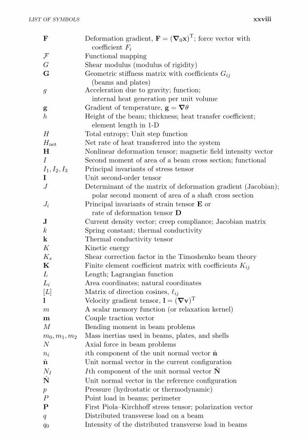
F Deformation gradient, F = (∇0x)T; force vector withcoefficient Fi
F Functional mappingG Shear modulus (modulus of rigidity)G Geometric stiffness matrix with coefficients Gij
(beams and plates)g Acceleration due to gravity; function;
internal heat generation per unit volumeg Gradient of temperature, g = ∇θh Height of the beam; thickness; heat transfer coefficient;
element length in 1-DH Total entropy; Unit step functionHnet Net rate of heat transferred into the systemH Nonlinear deformation tensor; magnetic field intensity vectorI Second moment of area of a beam cross section; functionalI1, I2, I3 Principal invariants of stress tensorI Unit second-order tensorJ Determinant of the matrix of deformation gradient (Jacobian);
polar second moment of area of a shaft cross sectionJi Principal invariants of strain tensor E or
rate of deformation tensor DJ Current density vector; creep compliance; Jacobian matrixk Spring constant; thermal conductivityk Thermal conductivity tensorK Kinetic energyKs Shear correction factor in the Timoshenko beam theoryK Finite element coefficient matrix with coefficients Kij
L Length; Lagrangian functionLi Area coordinates; natural coordinates[L] Matrix of direction cosines, `ij [see Eq. (1.6.21)]l Velocity gradient tensor, l = (∇v)T
m A scalar memory function (or relaxation kernel)m Couple traction vectorM Bending moment in beam problemsm0,m1,m2 Mass inertias used in beams, plates, and shellsN Axial force in beam problemsni ith component of the unit normal vector nn Unit normal vector in the current configuration
NI Ith component of the unit normal vector N
N Unit normal vector in the reference configurationp Pressure (hydrostatic or thermodynamic)P Point load in beams; perimeterP First Piola–Kirchhoff stress tensor; polarization vectorq Distributed transverse load on a beamq0 Intensity of the distributed transverse load in beams
xxviii
xxix LIST OF SYMBOLS
q0 Heat flux vector in the reference configurationqi Force componentsq Heat flux vector in the current configurationQ First moment of area; volume rate of flowQh Heat inputr Radial coordinate in the cylindrical polar systemrh Internal heat generation per unit mass in the
current configurationr0 Internal heat generation per unit mass in the
reference configurationR Radial coordinate in the spherical coordinate system;
universal gas constantR Position vector in the spherical coordinate system;
proper orthogonal tensor; residual vectorS A second-order tensor; second Piola–Kirchhoff stress tensorSij Elastic compliance coefficientst Timet Stress vector; traction vectorT Torque; temperatureT Tangent coefficient matrix with coefficients Tiju Displacement vectoru1, u2, u3 Displacements in the x1, x2, and x3 directionsU Internal (or strain) energyU Right Cauchy stretch tensoru, v, w Displacement components in the x, y, and z directionsux, uy, uz Displacements in the x, y, and z directionsv Velocity, v = |v|V Shear force in beam problems; potential energy due to loadsVf Scalar potential
v Velocity vector in spatial coordinates, v = DxDt
V Velocity vector in material coordinates;left Cauchy stretch tensor
vx, vy, vz Velocity components in the x, y, and z directionsw Vorticity vector, w = 1
2∇× vWnet Net rate of power inputW Skew symmetric part of the velocity gradient tensor,
L = (∇v)T; that is W = 12
[(∇v)T −∇v
],
x Spatial coordinatesX Material coordinatesx1, x2, x3 Rectangular Cartesian coordinatesx, y, z Rectangular Cartesian coordinatesY Relaxation modulusz Transverse coordinate in the beam problem;
axial coordinate in the torsion problem
qn Heat flux normal to the boundary, qn = ∇ · n
LIST OF SYMBOLS
Greek and parenthetical symbols
α Angle; coefficient of thermal expansion;a parameter in time-approximation schemes
αij Thermal coefficients of expansionβ Acceleration parameter for convergenceβij Material coefficients, βij = Cijk` αk`γ Parameter in the Newmark scheme; penalty parameterγyz, γxz, γxy Shear strains in structural problemsΓ Internal entropy production; boundary of Ωδ Variational operator used in Chapter 2; Dirac deltaδij Components of the unit tensor, I (Kronecker delta)∆ Change of (followed by another symbol)ε Infinitesimal strain tensorε Symmetric part of the displacement gradient tensor,
(∇u)T; that is ε = 12
[(∇u)T + ∇u
]ε Total stored energy per unit mass; convergence toleranceεij Rectangular components of the infinitesimal
strain tensorζ Natural coordinateη Entropy density per unit mass; dashpot constant;
natural coordinateη0 Viscosity coefficientθ Angular coordinate in the cylindrical and spherical
coordinate systems; angle; twist per unit length;absolute temperature
κ0, κ Reference and current configurationsλ Extension ratio; Lame constant; eigenvalueµ Lame constant; viscosity; principal value of strainν Poisson’s ratio; νij Poisson’s ratiosξ Natural coordinateΠ Total potential energy functionalρ Density in the current configuration; charge densityρ0 Density in the reference configurationσ Boltzman constantσ Mean stressσ Cauchy stress tensorτ Shear stress; timeτ Viscous stress tensorχ Deformation mappingϕi Approximation functions; Hermite interpolation functionsφ A typical variable; angular coordinate in the spherical
coordinate system; electric potential; relaxation function
xxx
xxxi LIST OF SYMBOLS
φf Moisture sourceΦ Viscous dissipation, Φ = τ : D; Gibb’s potential;
Airy stress functionψ Warping function; stream function; creep functionψi Finite element (Lagrange) interpolation functionsΨ Helmholtz free energy density; Prandtl stress functionω Angular velocityω Infinitesimal rotation vector, ω = 1
2 ∇× uΩ Domain of a problemΩ Skew symmetric part of the displacement gradient tensor,
(∇u)T; that is Ω = 12
[(∇u)T −∇u
]∇ Gradient operator with respect to x∇0 Gradient operator with respect to X[ ] Matrix associated with the enclosed quantity Column vector associated with the enclosed quantity| | Magnitude or determinant of the enclosed quantity˙( ) Time derivative of the enclosed quantity
( )∗ Enclosed quantity with superposed rigid-body motion
( )′
Deviatoric tensors associated with the enclosed tensor
Note:
Quotes by various people included in this book were found at various web sites,for example,
http://naturalscience.com/dsqhome.html/,http://thinkexist.com/quotes/david hilbert/, andhttp://www.yalescientific.org/2010/10/from-the-editor-imagination-in-science/.
This author is inspired to include the quotes at various places in his bookfor their wit and wisdom; the author cannot vouch for their accuracy. Trainyour mind to test every concept, definition, derivation, computation, train ofreasoning, and claim to truth.

1
1
General Introduction andMathematical Preliminaries
Mathematics is the language with which God has written the universe. ——– Galileo Galilei
1.1 General Comments
Engineers and scientists from applied sciences are involved in one or more ofthe following activities in studying engineering systems:
(1) Develop mathematical models of physical systems
(2) Carry out numerical simulations of the mathematical models
(3) Conduct experiments to determine and understand characteristics of thesystem
(4) Design the components of a system
(5) Manufacture the components and integrate them to build a system
All these activities are interdependent, and they are carried out consistent withgoals of the study.
Manufacturing of a system or its components can take place only after thecomponents are designed to meet the functionality and other requirements.On the other hand, design is an iterative process of selecting materials andconfigurations to meet the design requirements and cost-effectiveness. Duringeach stage of the design, analysis is carried out for the selected configuration(i.e. geometry), materials, and loads. Analysis is deterministic and involvesanalytically determining the response of the system or its components withthe help of a mathematical model (which may account for uncertainties inthe data) and a numerical method. A mathematical model of a system orits components is a collection of relationships – algebraic, differential, and/orintegral – among the quantities that describe the response. The present studyis concerned with the first two tasks, namely, the development of mathematicalmodels and numerical evaluation of the mathematical models using the finiteelement method. Additional discussion of these two topics is presented next.
J.N. Reddy, An Introduction to Nonlinear Finite Element Analysis, Second Edition. c©J.N.Reddy 2015. Published in 2015 by Oxford University Press.
2 GENERAL INTRODUCTION AND MATHEMATICAL PRELIMINARIES
1.2 Mathematical Models
One of the most important tasks engineers and scientists perform is to modelnatural phenomena. They develop conceptual and mathematical models tosimulate physical events, whether they are aerospace, biological, chemical, geo-logical, or mechanical. A mathematical model can be broadly defined as a set ofanalytical relationships among variables that express the essential features of aphysical system or process. The mathematical models are described in termsof algebraic, differential, and/or integral equations relating various quantitiesof interest.
Mathematical models of physical phenomena are often based on fundamen-tal scientific laws of physics, such as the principles of conservation of massand balance of linear momentum, angular momentum, and energy, and also as-sumptions concerning the geometry, loads, boundary conditions, as well as theconstitutive behavior. Mathematical models of biological and other phenomenamay be based on observations and accepted theories. Keeping the scope of thepresent study in mind, the discussion is limited to engineering systems that aregoverned by principles of continuum mechanics.
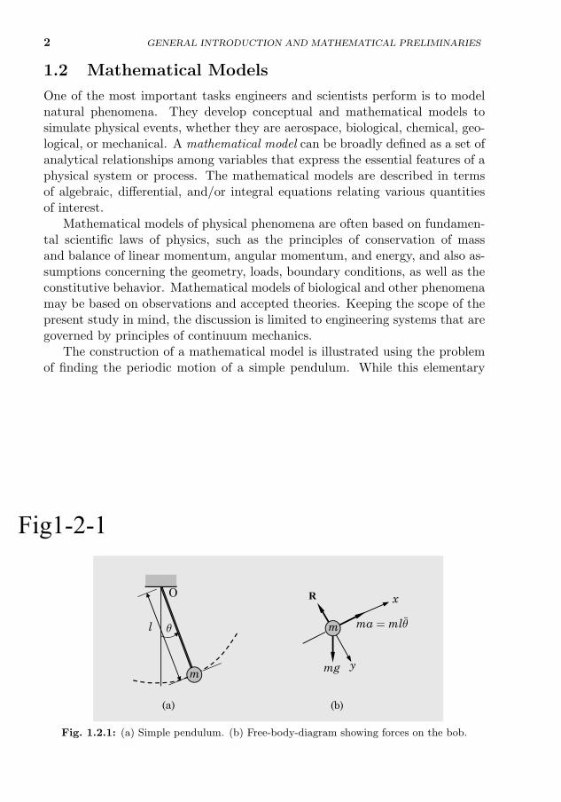
The construction of a mathematical model is illustrated using the problemof finding the periodic motion of a simple pendulum. While this elementaryexample does not bring out all aspects of formulating a complex real-worldproblem, it sheds light on some basic steps involved in the development of amathematical model.
Example 1.2.1
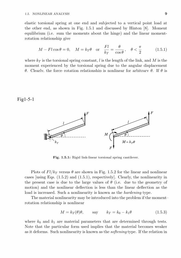
Consider the problem of a simple pendulum. The system consists of a bob of mass m attachedto one end of a rod of length l and the other end is pivoted to a fixed point O, as shown inFig. 1.2.1(a). Assume that: (1) the bob as well as the rod connecting the bob to the fixedpoint O are rigid, (2) the mass of the rod is negligible relative to the mass of the bob that isconstant, and (3) there is no friction at the pivot. Derive the differential equation governingthe periodic motion of the simple pendulum and determine the analytical solution to thesmall-amplitude motion (i.e. linear solution) of the bob.
Fig1-2-1
O R
l q
m
m
y
x
mg
ma = mlq
(a) (b)
Fig. 1.2.1: (a) Simple pendulum. (b) Free-body-diagram showing forces on the bob.
1.2. MATHEMATICAL MODELS 3
Solution: The equation governing the motion of the bob can be derived, consistent withthe stated assumptions, using the principle of balance of linear momentum, also known asNewton’s second law of motion, which can be stated as the vector sum of externally appliedforces is equal to the time rate of change of the linear momentum of the body (see Reddy [1]):
F = ma (1)
where F is the vector sum of all forces acting on a system, m is the mass of the system(assumed to be independent of time t), and a is the acceleration of the system (i.e. a = dv
dt,
where v is the velocity vector).The x-component of Eq. (1) is of interest in the present problem. We have [see Fig.
1.2.1(b)]
Fx = −mg sin θ, vx = ldθ
dt, ax = l
d2θ
dt2(2)
where θ is the angular displacement, vx is the velocity along x, g is the acceleration due togravity, and t is the time. Then, the x-component of the equation of motion becomes
−mg sin θ = mld2θ
dt2or
d2θ
dt2+g
lsin θ = 0 (3)
Thus, the problem at hand involves solving the nonlinear differential equation
d2θ
dt2+g
lsin θ = 0, 0 < t ≤ T (4)
subjected to the initial conditions (i.e. values of θ and its derivative at time t = 0)
θ(0) = θ0,dθ
dt(0) =
v0l
(5)
where θ0 and v0 are the initial values of angular displacement and velocity, respectively, andT is the final time. Mathematically, the problem is called an initial-value problem becauseit requires initial values (as opposed to boundary values) of θ and its derivative to solve theproblem.
If the amplitude θ of the periodic motion is not small, the restoring moment is proportionalto sin θ, and Eq. (3) represents a nonlinear equation. For small θ, sin θ is approximately equalto the angle θ, and the motion is described by the linear equation
d2θ
dt2+ λ2θ = 0, λ2 =
g
l(6)
whose solution represents a simple harmonic motion.The general analytical, which is exact, solution to the linear differential equation in Eq. (6)
is given by
θ(t) = c1 sinλt+ c2 cosλt, λ =
√g
l(7)
where c1 and c2 are constants to be determined using the initial conditions in Eq. (5). Forthe present case, they are
c1 =v0λl
, c2 = θ0 (8)
and the solution to the linear problem is
θ(t) =v0λl
sinλt+ θ0 cosλt (9)
For zero initial velocity and non-zero initial position θ0, the solution becomes
θ(t) = θ0 cosλt (10)
4 GENERAL INTRODUCTION AND MATHEMATICAL PRELIMINARIES
1.3 Numerical Simulations
Mathematical models of engineering systems are often characterized by verycomplex equations posed on geometrically complicated regions. Consequently,many of the mathematical models, until the advent of electronic computation,were drastically simplified in the interest of analytically solving them. Overthe last three decades, however, the computer has made it possible, with thehelp of realistic mathematical models and numerical methods, to solve manypractical problems of science and engineering. There now exists a large bodyof knowledge associated with the use of numerical methods and computers toanalyze mathematical models of physical systems, and this body of knowledgeis known as computational mechanics. Major established industries such as theautomobile, aerospace, chemical, pharmaceutical, petroleum, electronics, andcommunications, as well as emerging industries such as nano and biotechnol-ogy, rely on computational mechanics-based capabilities to simulate complexsystems for design and manufacture of high-technology products.
Numerical simulation of a process means that the solution of the governingequations (or mathematical model) of the process is obtained using a numericalmethod and a computer. While the derivation of the governing equations formost problems is not unduly difficult, their solution by exact methods of anal-ysis is a formidable task. In such cases, numerical methods of analysis providean alternative means of finding solutions. Numerical methods typically trans-form differential equations to algebraic equations that are to be solved usingcomputers. For example, the mathematical formulation of the simple pendulumresulted in a nonlinear differential equation, Eq. (4) of Example 1.2.1, whoseanalytical solution cannot be obtained. Therefore, one must consider using anumerical method to solve it. Even linear problems may not admit exact so-lutions due to geometric and material complexities, but it is relatively easy toobtain approximate solutions using numerical methods. These ideas are illus-trated below using the simple pendulum problem of Example 1.2.1. The finitedifference method is used as a numerical method of solution.
Example 1.3.1
Determine the numerical solution to Eq. (4) of Example 1.2.1 governing a simple pendulumusing a suitable finite difference method.
Solution: In the finite difference method, the derivatives are approximated by difference quo-tients (or the function is expanded in a Taylor series) that involve the unknown value of thesolution at time ti+1 and the known value of the solution at time t = ti. For example, considerthe first-order equation
du
dt= f(t, u) with u(0) = u0 (1)
The derivative at t = ti is approximated using the forward difference scheme(dudt
)∣∣∣t=ti
≈ u(ti+1)− u(ti)
ti+1 − ti(2)
1.3. NUMERICAL SIMULATIONS 5
so that the discrete form of Eq. (1) is
ui+1 = ui + ∆ti+1 f(ti, ui) (3)
ui = u(ti), ∆ti+1 = ti+1 − ti (4)
Equation (3) can be solved repeatedly for ui+1, starting from the known value u0 of u(t) att = t0 = 0. The repeated solution of Eq. (3) produces the values of u at times t1 = ∆t1,t2 = ∆t1 +∆t2, . . ., tn =
∑ni=1 ∆ti = T . This scheme is also known as Euler’s explicit method
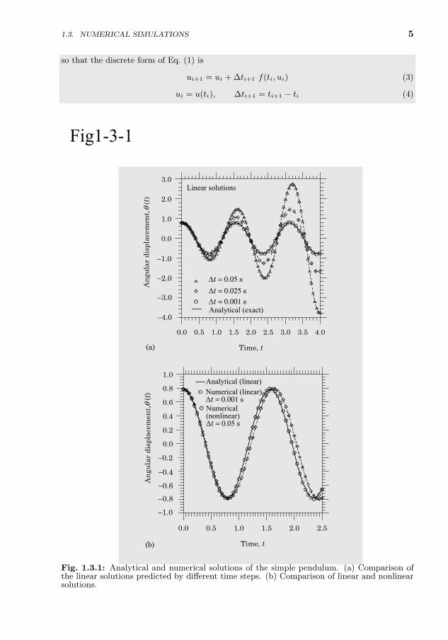
or the first-order Runge–Kutta method. Note that the ordinary differential equation in Eq. (1)is converted to an algebraic equation, Eq. (3), which is then evaluated at different times toconstruct the discrete time history of u(t), as shown in Fig. 1.3.1.
Fig1-3-1
(b)
0.0 0.5 1.0 1.5 2.0 2.5 3.0 3.5 4.0
Time, t
-4.0
-3.0
-2.0
-1.0
0.0
1.0
2.0
3.0
An
gula
r di
spla
cem
ent,
θ (t
)
(a)
θ (t
)
0.0 0.5 1.0 1.5 2.0 2.5
Time, t
-1.0
-0.8
-0.6
-0.4
-0.2
0.0
0.2
0.4
0.6
0.8
1.0
An
gula
r di
spla
cem
ent,
Δt = 0.05 sΔt = 0.025 sΔt = 0.001 sAnalytical (exact)
Analytical (linear)Numerical (linear)Δt = 0.001 sNumerical (nonlinear) Δt = 0.05 s
Linear solutions
−0.2
−0.4
−0.6
−1.0
−0.8
−4.0
−1.0
−2.0
−3.0
Fig. 1.3.1: Analytical and numerical solutions of the simple pendulum. (a) Comparison ofthe linear solutions predicted by different time steps. (b) Comparison of linear and nonlinearsolutions.
6 GENERAL INTRODUCTION AND MATHEMATICAL PRELIMINARIES
Euler’s explicit method can be applied to the nonlinear second-order differential equationin Eq. (4) of Example 1.2.1 after rewriting it as a pair of first-order differential equations:
dθ
dt=v
l≡ f1(v),
dv
dt= −g sin θ ≡ f2(θ) (5)
which are coupled (i.e. one cannot be solved without the other). Applying the Euler’s schemeof Eq. (3) to the two equations at hand, one obtains
θi+1 = θi + ∆t f1(vi); vi+1 = vi + ∆t f2(θi) (6)
where ∆t = ∆t1 = ∆t2 = . . . = ∆tn (i.e. uniform time step is used). The expressions inEq. (6) are repeatedly evaluated for θi+1 and vi+1 using the known solution (θi, vi) from theprevious time step. At time t = t0 = 0, the known initial values (θ0, v0) are used. Thus,one needs a computer and a computer language like Fortran (77 or 90) to write a program tocompute numbers.
The numerical solutions of Eq. (6) for three different time steps, ∆t = 0.05 s, ∆t = 0.025s, and ∆t = 0.001 s along with the exact linear solution in Eq. (10) of Example 1.2.1 (withθ0 = π/4, v0 = 0 m/s, l = 2 m, and g = 9.81 m/s2) are presented in Fig. 1.3.1(a). Thesmaller the time step the more accurate the solution is. This is because the approximation ofthe derivative in Eq. (2) tends to the exact derivative with ∆t → 0. In fact, the numericalsolution predicted by the Euler’s scheme for ∆t = 0.05 s is unstable; that is, error growswith time and the solution may go unbounded with time. The numerical solutions of thenonlinear problem are compared for the time step ∆t = 0.05 s with the linear solution inFig. 1.3.1(b). The nonlinear solution differs from the linear solution slightly and has longerperiod of oscillation.
1.4 The Finite Element Method
As illustrated in the previous section, numerical methods are extremely powerfultools for engineering analysis. With the advent of computers, there has beena tremendous explosion in the development and use of numerical methods inengineering analysis and design. Of these, the finite difference methods and thefinite element method and their variants are the most commonly used methodstoday in the analysis of practical engineering problems. In finite differencemethods, derivatives of various order are approximated using truncated Taylor’sseries approximations. The traditional finite difference methods suffer fromtwo major drawbacks: (1) applying gradient-type boundary conditions requiresadditional approximation of the boundary data; (2) finite difference formulasare traditionally developed for rectangular grids, making it difficult to use themfor irregular domains. Advances have been made in recent years to overcomethese drawbacks but the remedies are problem-dependent.
The finite element method is based on the idea that every physical systemis composed of different parts and, hence, its solution may also be representedin parts. In addition, the solution over each part is represented as a linearcombination of undetermined parameters and known functions of position andpossibly time, like in the traditional variational methods (e.g. the Ritz andGalerkin methods [2, 3]). The parts can differ from each other in shape, ma-
1.4. THE FINITE ELEMENT METHOD 7
terial properties, as well as physical behavior. Even when the system is of onegeometric shape and made of one material, it is simpler to represent its solutionin a piecewise manner, with certain continuity conditions between piecewisesolutions. In recent years, generalizations of the finite element method haveemerged (e.g. the generalized finite element method and element-free or mesh-less methods) but they are not considered in this book. Interested readers mayconsult the advanced titles [4–12] listed in the References at the end of thisbook.
The traditional finite element method is endowed with three basic features[2]. First, a domain of the system is represented as a collection of geometricallysimple subdomains, called finite elements. Second, over each finite element,the unknown variable(s) are approximated by a linear combination of algebraicpolynomials and undetermined parameters, and algebraic relations among theparameters are obtained by satisfying the governing equation(s), in a weighted-integral sense, over each element. The undetermined parameters represent thevalues of the unknown variables at a finite number of preselected points, callednodes, in the element. Third, the algebraic relations from all elements are puttogether (or “assembled”) using continuity and balance considerations.
There are several reasons why an engineer or scientist should study the finiteelement method. They are outlined in the following:
(1) The finite element method is a powerful numerical procedure devised forthe analysis of practical engineering problems. It is capable of handlinggeometrically complicated domains, all physically meaningful boundaryconditions, nonlinearities, and coupled phenomena that are common inpractical problems. The knowledge of how the method works greatlyenhances the analysis skill and provides a greater understanding of theproblem being solved.
(2) Commercial software packages or canned computer programs based onthe finite element method are often used in industrial, research, and aca-demic institutions for the solution of a variety of engineering and scientificproblems. The intelligent use of these programs and a correct interpreta-tion of the output are often predicated on knowledge of the basic theoryunderlying the method.
(3) It is not uncommon to find mathematical models derived in personal re-search and development that cannot be evaluated using canned programs.In such cases, an understanding of the finite element method and know-ledge of computer programming can help design “user specified” programsto evaluate the mathematical models or parts thereof.
The basic ideas underlying the finite element method are presented in Chap-ter 3 using a model linear differential equation in a single variable in one andtwo dimensions. Readers who are familiar with these steps as applied to lineardifferential equations may skip Chapter 3 and go straight to Chapter 4.
8 GENERAL INTRODUCTION AND MATHEMATICAL PRELIMINARIES
1.5 Nonlinear Analysis
1.5.1 Introduction
Recall from the simple pendulum problem of Examples 1.2.1 and 1.3.1, thatnonlinearity naturally arises in a rigorous mathematical formulation of mostphysical problems. Based on assumptions of smallness of certain quantitiesof the formulation, the problem may be reduced to a linear problem. Linearsolutions may be obtained with considerable ease and less computational costwhen compared to nonlinear solutions. Further, linear solutions due to variousboundary conditions and “load” cases may be scaled and superimposed. Inmany instances, assumptions of linearity lead to reasonable idealization of thebehavior of the system. However, in some cases assumption of linearity mayresult in an unrealistic approximation of the response or inefficient use of thematerials used. The type of analysis, linear or nonlinear, depends on the goalof the analysis and errors in the system’s response that may be tolerated. Insome cases, nonlinear analysis is the only option left for the analyst as well asthe designer (e.g. high-speed flows of inviscid fluids around solid bodies).
Nonlinear analysis is a necessity, for example, in (a) designing high-perfor-mance and efficient components of certain industries (e.g. aerospace, defense,and nuclear), (b) assessing functionality (e.g. residual strength and stiffness ofstructural elements) of existing systems that exhibit some types of damage andfailure, (c) establishing causes of system failure, (d) simulating true materialbehavior of processes, and (e) research to gain a realistic understanding ofphysical phenomena.
The following features of nonlinear analysis should be noted:
• The principle of superposition does not hold.
• Analysis can be carried out for one load case at a time.
• The history (or sequence) of loading influences the response.
• The initial state of the system (e.g. prestress) may be important.
1.5.2 Classification of Nonlinearities
There are two common sources of nonlinearity: (1) geometry and (2) mater-ial. The geometric nonlinearity arises purely from geometric consideration (e.g.nonlinear strain-displacement relations), and the material nonlinearity is due tononlinear constitutive behavior of the material of the system. A third type ofnonlinearity may arise due to changing initial or boundary conditions. Varioustypes of nonlinearities will be discussed through simple examples.
The simple pendulum problem of Example 1.2.1 is an example of geometricnonlinearity because the amplitude of angular motion is the deciding factor totreat it as the linear (sin θ ≈ θ) or nonlinear problem. Another example ofthe geometric nonlinearity is provided by a rigid link supported by a linear
1.5. NONLINEAR ANALYSIS 9
elastic torsional spring at one end and subjected to a vertical point load atthe other end, as shown in Fig. 1.5.1 and discussed by Hinton [8]. Momentequilibrium (i.e. sum the moments about the hinge) and the linear moment-rotation relationship give
M − Fl cos θ = 0, M = kT θ orFl
kT=
θ
cos θ, θ <
π
2(1.5.1)
where kT is the torsional spring constant, l is the length of the link, and M is themoment experienced by the torsional spring due to the angular displacementθ. Clearly, the force–rotation relationship is nonlinear for arbitrary θ. If θ isrestricted to small values (say, θ < 10), cos θ ≈ 1 and the governing equation,Eq. (1.5.1), is reduced to a linear equation
Fl
kT= θ (1.5.2)
Fig1-5-1
θ
l
F
•
F
Mθ
l
F
kT M = kTθ
Fig. 1.5.1: Rigid link-linear torsional spring cantilever.
Plots of Fl/kT versus θ are shown in Fig. 1.5.2 for the linear and nonlinearcases [using Eqs. (1.5.2) and (1.5.1), respectively]. Clearly, the nonlinearity inthe present case is due to the large values of θ (i.e. due to the geometry ofmotion) and the nonlinear deflection is less than the linear deflection as theload is increased. Such a nonlinearity is known as the hardening type.
The material nonlinearity may be introduced into the problem if the moment–rotation relationship is nonlinear
M = kT (θ)θ, say kT = k0 − k1θ (1.5.3)
where k0 and k1 are material parameters that are determined through tests.Note that the particular form used implies that the material becomes weakeras it deforms. Such nonlinearity is known as the softening type. If the relation in
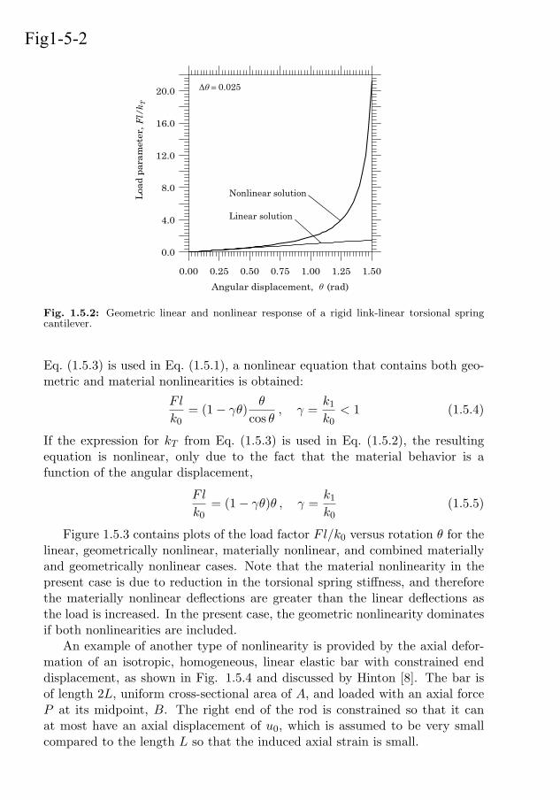
10 GENERAL INTRODUCTION AND MATHEMATICAL PRELIMINARIES
0.00 0.25 0.50 0.75 1.00 1.25 1.50
Angular displacement, (rad)
0.0
4.0
8.0
12.0
16.0
20.0
Loa
d pa
ram
eter
,
Δθ=0.025
Fl/
k T
Linear solution
Nonlinear solution
Δθ = 0.025
θ
Fig1-5-2
Fig. 1.5.2: Geometric linear and nonlinear response of a rigid link-linear torsional springcantilever.
Eq. (1.5.3) is used in Eq. (1.5.1), a nonlinear equation that contains both geo-metric and material nonlinearities is obtained:
Fl
k0= (1− γθ) θ
cos θ, γ =
k1
k0< 1 (1.5.4)
If the expression for kT from Eq. (1.5.3) is used in Eq. (1.5.2), the resultingequation is nonlinear, only due to the fact that the material behavior is afunction of the angular displacement,
Fl
k0= (1− γθ)θ , γ =
k1
k0(1.5.5)
Figure 1.5.3 contains plots of the load factor Fl/k0 versus rotation θ for thelinear, geometrically nonlinear, materially nonlinear, and combined materiallyand geometrically nonlinear cases. Note that the material nonlinearity in thepresent case is due to reduction in the torsional spring stiffness, and thereforethe materially nonlinear deflections are greater than the linear deflections asthe load is increased. In the present case, the geometric nonlinearity dominatesif both nonlinearities are included.
An example of another type of nonlinearity is provided by the axial defor-mation of an isotropic, homogeneous, linear elastic bar with constrained enddisplacement, as shown in Fig. 1.5.4 and discussed by Hinton [8]. The bar isof length 2L, uniform cross-sectional area of A, and loaded with an axial forceP at its midpoint, B. The right end of the rod is constrained so that it canat most have an axial displacement of u0, which is assumed to be very smallcompared to the length L so that the induced axial strain is small.
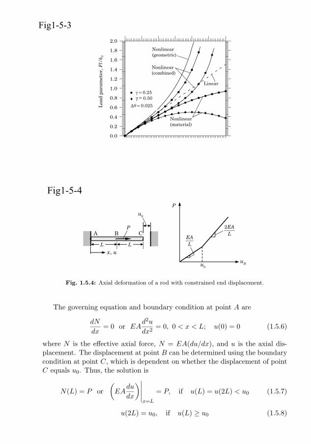
1.5. NONLINEAR ANALYSIS 11Fig1-5-3
0.00 0.25 0.50 0.75 1.00 1.25 1.50
Angular displacement, (rad)
0.0
0.2
0.4
0.6
0.8
1.0
1.2
1.4
1.6
1.8
2.0
Loa
d pa
ram
eter
,
Δθ=0.025
Fl/
k 0
q
Nonlinear(geometric)
Nonlinear(material)
Nonlinear(combined)
Linear
Δθ = 0.025
♦
γ = 0.25γ = 0.50
Fig. 1.5.3: Linear and nonlinear response of a rigid link-torsional spring cantilever.
Fig1-5-4
A B C
• ••
2EAL
EAL
Bu0u
P
0u
P
L L
,x u
Fig. 1.5.4: Axial deformation of a rod with constrained end displacement.
The governing equation and boundary condition at point A are
dN
dx= 0 or EA
d2u
dx2= 0, 0 < x < L; u(0) = 0 (1.5.6)
where N is the effective axial force, N = EA(du/dx), and u is the axial dis-placement. The displacement at point B can be determined using the boundarycondition at point C, which is dependent on whether the displacement of pointC equals u0. Thus, the solution is
N(L) = P or
(EA
du
dx
)∣∣∣∣∣x=L
= P, if u(L) = u(2L) < u0 (1.5.7)
u(2L) = u0, if u(L) ≥ u0 (1.5.8)
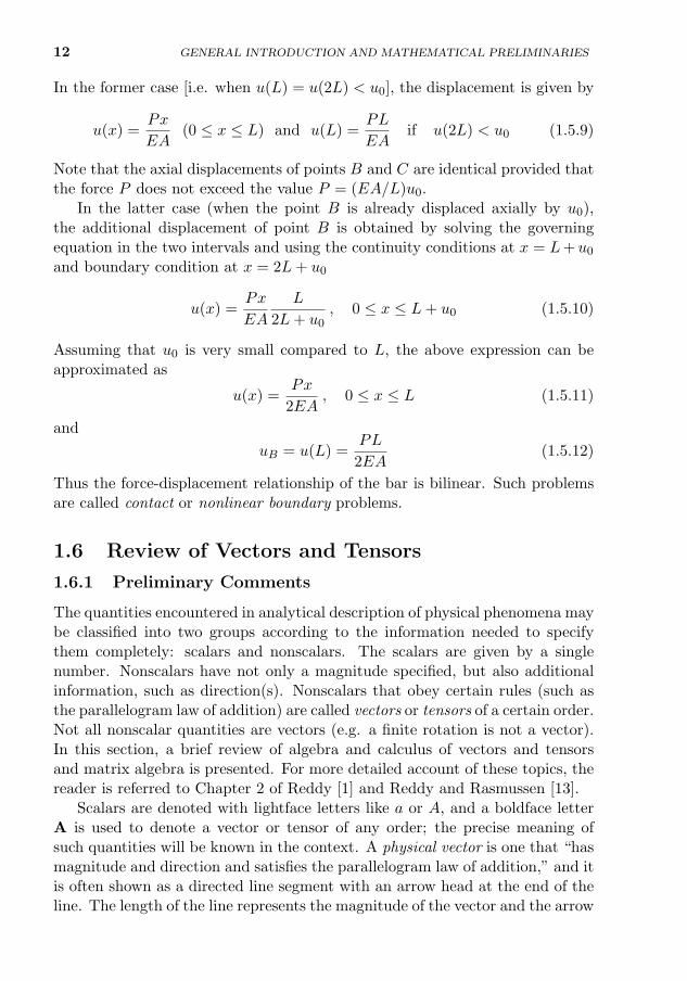
12 GENERAL INTRODUCTION AND MATHEMATICAL PRELIMINARIES
In the former case [i.e. when u(L) = u(2L) < u0], the displacement is given by
u(x) =Px
EA(0 ≤ x ≤ L) and u(L) =
PL
EAif u(2L) < u0 (1.5.9)
Note that the axial displacements of points B and C are identical provided thatthe force P does not exceed the value P = (EA/L)u0.
In the latter case (when the point B is already displaced axially by u0),the additional displacement of point B is obtained by solving the governingequation in the two intervals and using the continuity conditions at x = L+ u0
and boundary condition at x = 2L+ u0
u(x) =Px
EA
L
2L+ u0, 0 ≤ x ≤ L+ u0 (1.5.10)
Assuming that u0 is very small compared to L, the above expression can beapproximated as
u(x) =Px
2EA, 0 ≤ x ≤ L (1.5.11)
and
uB = u(L) =PL
2EA(1.5.12)
Thus the force-displacement relationship of the bar is bilinear. Such problemsare called contact or nonlinear boundary problems.
1.6 Review of Vectors and Tensors
1.6.1 Preliminary Comments
The quantities encountered in analytical description of physical phenomena maybe classified into two groups according to the information needed to specifythem completely: scalars and nonscalars. The scalars are given by a singlenumber. Nonscalars have not only a magnitude specified, but also additionalinformation, such as direction(s). Nonscalars that obey certain rules (such asthe parallelogram law of addition) are called vectors or tensors of a certain order.Not all nonscalar quantities are vectors (e.g. a finite rotation is not a vector).In this section, a brief review of algebra and calculus of vectors and tensorsand matrix algebra is presented. For more detailed account of these topics, thereader is referred to Chapter 2 of Reddy [1] and Reddy and Rasmussen [13].
Scalars are denoted with lightface letters like a or A, and a boldface letterA is used to denote a vector or tensor of any order; the precise meaning ofsuch quantities will be known in the context. A physical vector is one that “hasmagnitude and direction and satisfies the parallelogram law of addition,” and itis often shown as a directed line segment with an arrow head at the end of theline. The length of the line represents the magnitude of the vector and the arrow
1.6. REVIEW OF VECTORS AND TENSORS 13
indicates the direction. The mathematical definition of an abstract vector,which can be a function satisfying certain rules of addition and multiplicationby a scalar, is given in Section 1.7.
1.6.2 Definition of a Physical Vector
Physical vectors are entities that obey the following rules of vector addition andmultiplication by a scalar.
1.6.2.1 Vector addition
Let A, B, and C be any vectors. Then there exists a vector A+B, called sumof A and B, with the properties
(1) A + B = B + A (commutative),
(2) (A + B) + C = A + (B + C) (associative),
(3) there exists a unique vector, 0, independent of A such that
A + 0 = A (existence of the zero vector), (1.6.1)
(4) to every vector A there exists a unique vector −A(that depends on A) such that
A + (−A) = 0 (existence of the negative vector).
The negative vector −A has the same magnitude as A, but has the oppositesense. Subtraction of vectors is carried out along the same lines. To form thedifference A −B, one may write A + (−B) and subtraction is reduced to theoperation of addition.
1.6.2.2 Multiplication of a vector by a scalar
Let A and B be vectors and α and β be real numbers (scalars). To every vectorA and every real number α, there corresponds a unique vector αA such that
(1) α(βA) = (αβ)A (scalar multiplication is associative),
(2) (α+ β)A = αA + βA (scalar addition is distributive),
(3) α(A + B) = αA + αB (vector addition is distributive),
(4) 1 ·A = A · 1 = A, 0 ·A = 0.
(1.6.2)
The magnitude of the vector A is denoted by |A|, ‖A‖, or A. The actualcomputation of |A| will be presented shortly. A vector of unit length is called aunit vector. The unit vector along A may be defined as eA = A/A, and vectorA may now be expressed as
A = A eA

14 GENERAL INTRODUCTION AND MATHEMATICAL PRELIMINARIES
Thus, any vector may be represented as a product of its magnitude and a unitvector along the vector. A unit vector is used to designate direction; it doesnot have any physical dimensions. However, |A| has the physical dimensions.A “hat” (caret) above the boldface letter, e, is used to signify that it is a vectorof unit magnitude. A vector of zero magnitude is called a zero vector or a nullvector, and denoted by boldface zero, 0. Note that a lightface zero, 0, is a scalarand boldface zero, 0, is the zero vector. Also, a zero vector has no directionassociated with it. Two vectors A and B are equal if their magnitudes areequal, |A| = |B|, and if their directions are equal.
1.6.3 Scalar and Vector Products
In engineering analysis, products of one vector with another vector are en-countered. There are two such products involving vectors, one encountered inwriting the work done and another in computing the moment due to a force.
1.6.3.1 Scalar product (or “dot” product)
Work done by a force (vector) F is the product of the magnitude of the force Fand the magnitude of the displacement (vector) u in the direction of the force,that is the projection of the displacement vector in the direction of the force,d = u cos θ, where θ denotes the angle between the two vectors, F and u. Theproduct is denoted by F · u and it has the meaning
F · u = |F| |u| cos θ = F u cos θ (1.6.3)
and it is known as the scalar product (or “dot” product) to indicate the factthat the result is a scalar. If the scalar product of two non-zero vectors is zero,A ·B = 0, then vector A is perpendicular to vector B, and the vectors A and Bare said to be orthogonal to each other. In view of the definition in Eq. (1.6.3)of the scalar product of vectors, the magnitude of a vector A can be defined asthe square root of
√A ·A because
A ·A = |A| |A| cos 0 = |A|2 (1.6.4)
1.6.3.2 Vector product
Next consider the concept of the moment of a force about a point. The magni-tude of the moment about a point O of a force F acting at a point P is definedto be the magnitude of the force F multiplied by the perpendicular distance` from the point O to the line of action of the force, F ` = F r sin θ, wherer is the magnitude of the vector r from the point O to point P, as shown inFig. 1.6.1(a). A direction can be assigned to the moment. Drawing the vectorsF and r from the common point O, we note that the rotation due to F tendsto bring vector r into vector F, as can be seen from Fig. 1.6.1(b). The axis of
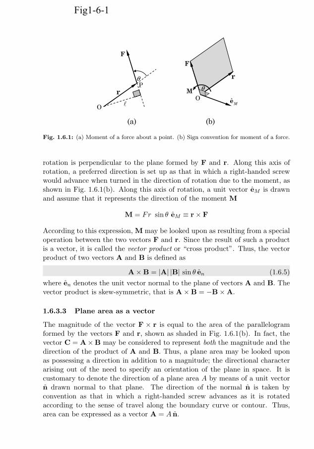
1.6. REVIEW OF VECTORS AND TENSORS 15
Fig1-6-1
P
F
O
rθ
O
rF
θ
eM
M
(a) (b)
Fig. 1.6.1: (a) Moment of a force about a point. (b) Sign convention for moment of a force.
rotation is perpendicular to the plane formed by F and r. Along this axis ofrotation, a preferred direction is set up as that in which a right-handed screwwould advance when turned in the direction of rotation due to the moment, asshown in Fig. 1.6.1(b). Along this axis of rotation, a unit vector eM is drawnand assume that it represents the direction of the moment M
M = Fr sin θ eM ≡ r× F
According to this expression, M may be looked upon as resulting from a specialoperation between the two vectors F and r. Since the result of such a productis a vector, it is called the vector product or “cross product”. Thus, the vectorproduct of two vectors A and B is defined as
A×B = |A| |B| sin θ en (1.6.5)
where en denotes the unit vector normal to the plane of vectors A and B. Thevector product is skew-symmetric, that is A×B = −B×A.
1.6.3.3 Plane area as a vector
The magnitude of the vector F × r is equal to the area of the parallelogramformed by the vectors F and r, shown as shaded in Fig. 1.6.1(b). In fact, thevector C = A×B may be considered to represent both the magnitude and thedirection of the product of A and B. Thus, a plane area may be looked uponas possessing a direction in addition to a magnitude; the directional characterarising out of the need to specify an orientation of the plane in space. It iscustomary to denote the direction of a plane area A by means of a unit vectorn drawn normal to that plane. The direction of the normal n is taken byconvention as that in which a right-handed screw advances as it is rotatedaccording to the sense of travel along the boundary curve or contour. Thus,area can be expressed as a vector A = A n.
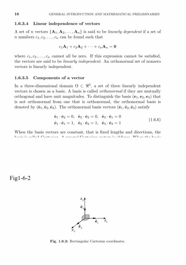
16 GENERAL INTRODUCTION AND MATHEMATICAL PRELIMINARIES
1.6.3.4 Linear independence of vectors
A set of n vectors A1,A2, . . . ,An is said to be linearly dependent if a set ofn numbers c1, c2, . . . , cn can be found such that
c1A1 + c2A2 + · · ·+ cnAn = 0
where c1, c2, . . . , cn cannot all be zero. If this expression cannot be satisfied,the vectors are said to be linearly independent. An orthonormal set of nonzerovectors is linearly independent.
1.6.3.5 Components of a vector
In a three-dimensional domain Ω ⊂ <3, a set of three linearly independentvectors is chosen as a basis. A basis is called orthonormal if they are mutuallyorthogonal and have unit magnitudes. To distinguish the basis (e1, e2, e3) thatis not orthonormal from one that is orthonormal, the orthonormal basis isdenoted by (e1, e2, e3). The orthonormal basis vectors (e1, e2, e3) satisfy
e1 · e2 = 0, e2 · e3 = 0, e3 · e1 = 0
e1 · e1 = 1, e2 · e2 = 1, e3 · e3 = 1(1.6.6)
When the basis vectors are constant, that is fixed lengths and directions, thebasis is called Cartesian. A general Cartesian system is oblique. When the basisvectors are unit and orthogonal, the basis system is called rectangular Cartesian.The familiar rectangular Cartesian coordinate system (x, y, z) = (x1, x2, x3) isshown in Fig. 1.6.2.
Any vector in three-dimensional space can be represented as a linear com-bination of the basis vectors (e1, e2, e3)
A = A1e1 +A2e2 +A3e3. (1.6.7)
The vectors A1e1, A2e2, and A3e3 are called the vector components of A, andA1, A2, and A3 are called the scalar components of A with respect to the basis
Fig1-6-2
e1ˆ
e2ˆ
e3ˆ
1x
2x
3x
Fig. 1.6.2: Rectangular Cartesian coordinates.
1.6. REVIEW OF VECTORS AND TENSORS 17
(e1, e2, e3), as indicated in Fig. 1.6.2. Note that
A · ei = Ai and therefore A =
3∑i=1
(A · ei) ei (1.6.8)
1.6.4 Summation Convention and Kronecker Deltaand Permutation Symbol
1.6.4.1 Summation convention
A typical term in Eq. (1.6.7) is of the form Aiei, where i takes the values of 1,2, and 3. Therefore, the expression can be abbreviated as
A =
3∑i=1
Aiei or A =
3∑j=1
Aj ej
The summation index i or j is arbitrary as long as the same index is usedfor both A and e. The expression can be further shortened by omitting thesummation sign and having the understanding that a repeated index meanssummation over all values of that index. Thus, the three-term expression forA can be simply written as
A = Aiei = Aj ej (1.6.9)
This notation is called the summation convention. The index that is repeatedis called a dummy index, as it can be replaced with any other index, as longas it is not already used in the expression. For example, an arbitrary vector Acan be expressed in terms of its components as
A = Aiei = (A · ei) ei = (A · ej) ej
In an expression of the form AiBjCj , j is the dummy index, while i, which isnot repeated, is known as the free index.
1.6.4.2 Kronecker delta symbol
The scalar product of vectors A and B in an orthogonal Cartesian system canbe expressed in terms of their components as
A ·B = (Aiei) · (Bj ej) = AiBj (ei · ej)
In view of the orthogonal relationships among the basis vectors (e1, e2, e3)
ei · ej = 1, whenever i and j have the same value,
ei · ej = 0, whenever i and j do not have the same value
18 GENERAL INTRODUCTION AND MATHEMATICAL PRELIMINARIES
the scalar product of two vectors can be written as
A ·B = AiBj δij
where δij denotes the Kronecker delta symbol
δij =
1, if i = j for fixed values of i and j0, if i 6= j for fixed values of i and j
(1.6.10)
The Kronecker delta constitutes the rectangular Cartesian components of theunit second-order tensor I = δij ei ej , as will be shown in the section on ten-sors. The scalar product of two vectors can now be expressed in terms of theircomponents as
A ·B = AiBj δij = AiBi = AjBj (1.6.11)
1.6.4.3 The permutation symbol
Consider the triple product
A ·B×C = AiBjCk ei · ej × ek
In view of the following vector products of the basis vectors:
e1 × e1 = 0, e1 × e2 = e3, e1 × e3 = −e2
e2 × e1 = −e3, e2 × e2 = 0, e2 × e3 = e1
e3 × e1 = e2, e3 × e2 = −e1, e3 × e3 = 0
(1.6.12)
the triple scalar product can be expressed as
A ·B×C = AiBjCk eijk
whereeijk = ei · ej × ek or ei × ej = eijk ek (1.6.13)
The symbol eijk is called the alternating symbol or permutation symbol, definedby
eijk =
1, if i, j, k are in cyclic order
and not repeated (i 6= j 6= k)−1, if i, j, k are not in cyclic order
and not repeated (i 6= j 6= k)0, if any of i, j, k are repeated
(1.6.14)
By definition, the subscripts of the permutation symbol can be permuted with-out changing its value; an interchange of any two subscripts will change thesign (hence, interchange of two subscripts twice keeps the value unchanged):eijk = ekij = ejki, eijk = −ejik = ejki = −ekji.
The rectangular Cartesian coordinates of a typical point x in Ω are denotedby (x1, x2, x3) and x is expressed as
x = x1e1 + x2e2 + x3e3 = xi ei (1.6.15)
1.6. REVIEW OF VECTORS AND TENSORS 19
1.6.5 Tensors and their Matrix Representation
1.6.5.1 Concept of a second-order tensor
As is well known, the specification of stress, which is force per unit area, notonly depends on the magnitude as well as the direction of the force but alsoon the orientation of the area on which the force acts. Thus, specification ofstress at a point requires two vectors, one perpendicular to the plane on whichthe force is acting and the other in the direction of the force. Such quantitiesare termed dyads or second-order tensors. Because of its utilization in physicalapplications, a dyad is defined as two vectors standing side by side and actingas a unit, S = AB. The transpose of a dyad is obtained by the interchange ofthe two vectors in the dyad. Similarly, one can define a triad (or a third-ordertensor) as an entity with three vectors standing next to each other, and so on.
Scalar products and cross products of vectors can be extended to tensors ofany order. For example, the dot product of a second-order tensor S = AB witha vector V is
S ·V = A(B ·V) and V · S = (V ·A)B
Thus, the dot product between a second-order tensor and a vector results in avector. In the first case the tensor acts as a prefactor and in the second caseas a postfactor. The two operations in general produce different vectors. Theexpressions in the above equation can also be written in alternative form usingthe definition of the transpose of a second-order tensor as
V · S = ST ·V, S ·V = V · ST
In general, one can show that the transpose of the product of tensors (of anyorder) follows the rule
(R · S)T = ST ·RT, (R · S ·T)T = TT · ST ·RT
Much like a vector, a tensor can be expressed in component form withrespect to a basis. For example, a second-order tensor S can be representedwith respect to the rectangular Cartesian basis (e1, e2, e3) as
S = S11e1e1 + S12e1e2 + S13e1e3
+S21e2e1 + S22e2e2 + S23e2e3
+S31e3e1 + S32e3e2 + S33e3e3
or in the index notationS = Sij eiej (1.6.16)
where Sij are termed the components of the second-order tensor S with respectto the basis (e1, e2, e3).
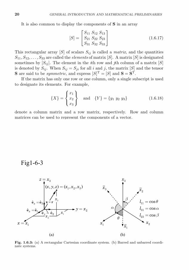
20 GENERAL INTRODUCTION AND MATHEMATICAL PRELIMINARIES
It is also common to display the components of S in an array
[S] =
S11 S12 S13
S21 S22 S23
S31 S32 S33
(1.6.17)
This rectangular array [S] of scalars Sij is called a matrix, and the quantitiesS11, S12, . . . , S33 are called the elements of matrix [S]. A matrix [S] is designatedsometimes by [Sij ]. The element in the ith row and jth column of a matrix [S]is denoted by Sij . When Sij = Sji for all i and j, the matrix [S] and the tensorS are said to be symmetric, and express [S]T = [S] and S = ST.
If the matrix has only one row or one column, only a single subscript is usedto designate its elements. For example,
X =
x1
x2
x3
and Y = y1 y2 y3 (1.6.18)
denote a column matrix and a row matrix, respectively. Row and columnmatrices can be used to represent the components of a vector.
1.6.5.2 Transformation laws for vectors and tensors
In much of the present study, only Cartesian bases are used. An orthonormalCartesian basis is denoted by
ex, ey, ez or e1, e2, e3
The Cartesian coordinates are denoted by (x, y, z) or (x1, x2, x3). The familiarrectangular Cartesian coordinate system is shown in Fig. 1.6.3(a). Only right-handed coordinate systems are used in this study.
1x 2x
3x
2x
1x
3x
q
11 cosl q=
31 cosl a=a
23 cosl b=
b
(b)(a)
.
1x2x
3x
1x x=
2y x=
3z x=
1 2 3( ) ( )x, y,z x ,x ,x=
2yˆ ˆ=e e1xˆ ˆ=e e
3zˆ ˆ=e e =x r
Fig1-6-3
Fig. 1.6.3: (a) A rectangular Cartesian coordinate system. (b) Barred and unbarred coordi-nate systems.
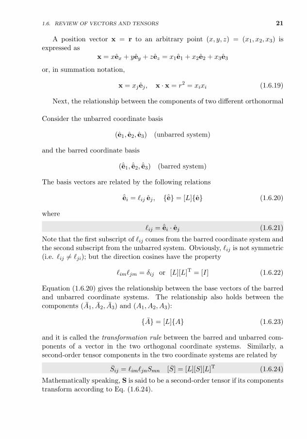
1.6. REVIEW OF VECTORS AND TENSORS 21
A position vector x = r to an arbitrary point (x, y, z) = (x1, x2, x3) isexpressed as
x = xex + yey + zez = x1e1 + x2e2 + x3e3
or, in summation notation,
x = xj ej , x · x = r2 = xixi (1.6.19)
Next, the relationship between the components of two different orthonormalcoordinate systems, say, unbarred and barred [see Fig. 1.6.3(b)] is established.Consider the unbarred coordinate basis
(e1, e2, e3) (unbarred system)
and the barred coordinate basis
(ˆe1, ˆe2, ˆe3) (barred system)
The basis vectors are related by the following relations
ˆei = `ij ej , ˆe = [L]e (1.6.20)
where
`ij = ˆei · ej (1.6.21)
Note that the first subscript of `ij comes from the barred coordinate system andthe second subscript from the unbarred system. Obviously, `ij is not symmetric(i.e. `ij 6= `ji); but the direction cosines have the property
`im`jm = δij or [L][L]T = [I] (1.6.22)
Equation (1.6.20) gives the relationship between the base vectors of the barredand unbarred coordinate systems. The relationship also holds between thecomponents (A1, A2, A3) and (A1, A2, A3):
A = [L]A (1.6.23)
and it is called the transformation rule between the barred and unbarred com-ponents of a vector in the two orthogonal coordinate systems. Similarly, asecond-order tensor components in the two coordinate systems are related by
Sij = `im`jnSmn [S] = [L][S][L]T (1.6.24)
Mathematically speaking, S is said to be a second-order tensor if its componentstransform according to Eq. (1.6.24).
22 GENERAL INTRODUCTION AND MATHEMATICAL PRELIMINARIES
1.6.6 Calculus of Vectors and Tensors
Let us denote a scalar field by φ = φ(x), x being the position vector in a rectan-gular Cartesian system (x1, x2, x3). Let us now denote a differential elementwith dx and its magnitude by ds ≡ |dx|. Then e = dx/ds is a unit vector inthe direction of dx, and it may be expressed as (by the use of the chain rule)(
dφ
ds
)e
=dx
ds· ∂φ∂x
= e ·(e1∂φ
∂x1+ e2
∂φ
∂x2+ e3
∂φ
∂x3
)The derivative (dφ/ds)e is called the directional derivative of φ. Thus, it is therate of change of φ with respect to distance and it depends on the direction ein which the distance is taken. The vector ∂φ/∂x is called the gradient vectorand is denoted by grad(φ) = ∇φ:
∇φ = gradφ = e1∂φ
∂x1+ e2
∂φ
∂x2+ e3
∂φ
∂x3(1.6.25)
The expression gradφ is interpreted as some operator operating on function φ,that is gradφ ≡∇φ. This operator is denoted by
∇ ≡ e1∂
∂x1+ e2
∂
∂x2+ e3
∂
∂x3= ex
∂
∂x+ ey
∂
∂y+ ez
∂
∂z(1.6.26)
and is called the del operator. The del operator is a vector differential operator.The gradient of a scalar function is a vector and the gradient of a vector functionis a second-order tensor.
If a surface is given by φ(x) = c, the unit normal to the surface at point xis determined by
n = ± gradφ
|gradφ|(1.6.27)
The plus or minus sign appears because the direction of n may point in eitherdirection away from the surface. If the surface is closed, the usual conventionis to take n pointing outward.
Two types of gradients are used in continuum mechanics: forward and back-ward gradients. The forward gradient is the usual gradient and backward gra-dient is the transpose of the forward gradient operator. To see the differencebetween the two types of gradients, consider a vector function A = Ai(x)ei.The forward and backward gradients of A are
−→∇A = ∇A = ej
∂
∂xj
(Aiei
)=∂Ai∂xj
ej ei = Ai,j ej ei (1.6.28)
←−∇A =
(∇A
)T=∂Ai∂xj
(ej ei
)T= Ai,j eiej (1.6.29)
where Ai,j = ∂Ai/∂xj .
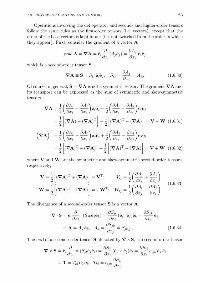
1.6. REVIEW OF VECTORS AND TENSORS 23
Operations involving the del operator and second- and higher-order tensorsfollow the same rules as the first-order tensors (i.e. vectors), except that theorder of the base vectors is kept intact (i.e. not switched from the order in whichthey appear). First, consider the gradient of a vector A
gradA = ∇A = ei∂
∂xi(Aj ej) =
∂Aj∂xi
eiej
which is a second-order tensor S
∇A ≡ S = Sij eiej , Sij =∂Aj∂xi
= Aj,i (1.6.30)
Of course, in general, S = ∇A is not a symmetric tensor. The gradient ∇A andits transpose can be expressed as the sum of symmetric and skew-symmetrictensors
∇A =1
2
(∂Aj∂xi
+∂Ai∂xj
)eiej −
1
2
(∂Ai∂xj− ∂Aj∂xi
)eiej
=1
2
[(∇A) + (∇A)T
]− 1
2
[(∇A)T − (∇A)
]= V −W (1.6.31)
(∇A
)T=
1
2
(∂Aj∂xi
+∂Ai∂xj
)ej ei +
1
2
(∂Aj∂xi− ∂Ai∂xj
)ej ei
=1
2
[(∇A)T + (∇A)
]+
1
2
[(∇A)T − (∇A)
]= V + W (1.6.32)
where V and W are the symmetric and skew-symmetric second-order tensors,respectively,
V =1
2
[(∇A)T + (∇A)
]= VT; Vij =
1
2
(∂Aj∂xi
+∂Ai∂xj
)W =
1
2
[(∇A)T − (∇A)
]= −WT; Wij =
1
2
(∂Ai∂xj− ∂Aj∂xi
) (1.6.33)
The divergence of a second-order tensor S is a vector A
∇ · S = ei∂
∂xi· (Sjkej ek) =
∂Sjk∂xi
(ei · ej)ek =∂Sjk∂xj
ek
≡ A = Ak ek, Ak =∂Sjk∂xj
= Sjk,j (1.6.34)
The curl of a second-order tensor S, denoted by ∇×S, is a second-order tensor
∇× S = ei∂
∂xi× (Sjlej el) =
∂Sjl∂xi
(ei × ej)el =∂Sjl∂xi
eijk ek el
≡ T = Tkl ek el, Tkl = eijk∂Sjl∂xi
24 GENERAL INTRODUCTION AND MATHEMATICAL PRELIMINARIES
Thus, the gradient of a tensor S of any order increases its order by one, thedivergence of S decreases its order by one, and the curl of S keeps the orderunchanged.
Two types of “double-dot products” between two second-order tensors areuseful in the sequel. The horizontal double-dot product and the vertical double-dot product between a dyad (AB) and another dyad (CD) (i.e. A, B, C, andD are vectors) are defined as the scalars
(AB) · ·(CD) ≡ (B ·C)(A ·D); (AB) : (CD) ≡ (A ·C)(B ·D)
The double-dot products, by this definition, are commutative. The two double-dot products between two dyads S and T in a rectangular Cartesian systemare
S · ·T = SijTmn(ej · em)(ei · en) = SijTmnδjmδin = Sij Tji (1.6.35)
S : T = SijTmn(ei · em)(ej · en) = SijTmnδimδjn = Sij Tij (1.6.36)
The trace of a second-order tensor (i.e. the sum of the diagonal terms of thematrix representing the tensor) is defined to be the double-dot product of thetensor with the unit tensor
trS = S : I = S · ·I (1.6.37)
Certain combinations of the components of a tensor remain the same in allcoordinate systems; that is they are invariant under coordinate transformations.Such quantities (involving sums and products of the components of a tensor)are termed invariants. For example, the determinant of a tensor is the samein all coordinate systems. Similarly, the trace of the matrix representing atensor is an invariant. Among many invariants of a tensor, the following threeinvariants, called principal invariants, are identified because of their role infinding eigenvalues of the tensor (readers should be aware of the fact that thedefinition of the second and third principal invariants may differ from otherbooks)
I1 = trS, I2 = 12
[(trS)2 − tr
(S2)], I3 = |S| (1.6.38)
In terms of the rectangular Cartesian components of S, the three principalinvariants have the form
I1 = Sii, I2 = 12 (SiiSjj − SijSji) , I3 = |S| (1.6.39)
In the general scheme that is developed so far, scalars are the zeroth-ordertensors, vectors are the first-order tensors, and dyads are the second-order ten-sors. The order of a tensor can be determined by counting the number of basisvectors in the representation of a tensor. In order to qualify as a tensor its com-ponents must obey the transformation law (in rectangular Cartesian componentform)
Tijkl··· = `ip`jq`kr`ls · · · Tpqrs··· (1.6.40)
1.6. REVIEW OF VECTORS AND TENSORS 25
In view of the matrix representation of a second-order tensor, many of thedefinitions and properties introduced for matrices can be extended to second-order tensors, S. They are summarized here.
(1) S is symmetric if and only if S = ST (Sij = Sji).
(2) S is skew-symmetric if and only if S = −ST (Sij = −Sji for i 6= j andS(i)(i) = 0 for any fixed i).
(3) S can be represented as a sum of symmetric and skew-symmetric parts:
S = 12
(S + ST
)+ 1
2
(S− ST
)≡ Ssym + Sskew (1.6.41)
(4) If S is symmetric, W is skew-symmetric, and T is an arbitrary tensor,then
S : W = W : S = 0, S : T = S : Tsym,
W : T = −W : TT = W : Tskew
Also, if S : T = 0 for any tensor S, then T = 0. If S : T = 0 for anysymmetric tensor S, then T is skew-symmetric. The converse also holds:If S : W = 0 for any skew-symmetric tensor W, then S is symmetric.
(5) The inverse T of any second-order tensor S, denoted T = S−1, is definedto be S−1 · S = S · S−1 = I. The notation (S−1)T = (ST)−1 = S−T isused, and note that (S ·T)−1 = T−1 · S−1 and (S ·T)−T = S−T ·T−T.
(6) A necessary and sufficient condition for a second-order tensor Q to beorthogonal is Q · QT = I. The determinant of an orthogonal matrix is|Q| = ±1. When |Q| = +1, Q is called a proper orthogonal matrix. Itcan be shown that an orthogonal tensor Q preserves the inner product inthe sense that (Q ·u) · (Q ·v) = u ·v. In the case of physical vectors, thisamounts to preserving the lengths of the vectors u and v as well as theangle between them.
(7) A second-order tensor S is said to be positive-definite if and only if u·S·u >0 for all nonzero vectors u.
The gradient and divergence of a tensor T in other coordinate systemscan be readily obtained by writing ∇ and T in that coordinate system andaccounting for the derivatives of the basis vectors. One of the commonly usedorthogonal curvilinear coordinate system is the cylindrical coordinate system(see Fig. 1.6.4), and Table 1.6.1 contains a summary of the basic information forthe coordinate system. The transformation equations between the orthogonalrectangular Cartesian system (x, y, z) and the cylindrical coordinate system(r, θ, z) are obvious from Table 1.6.1.
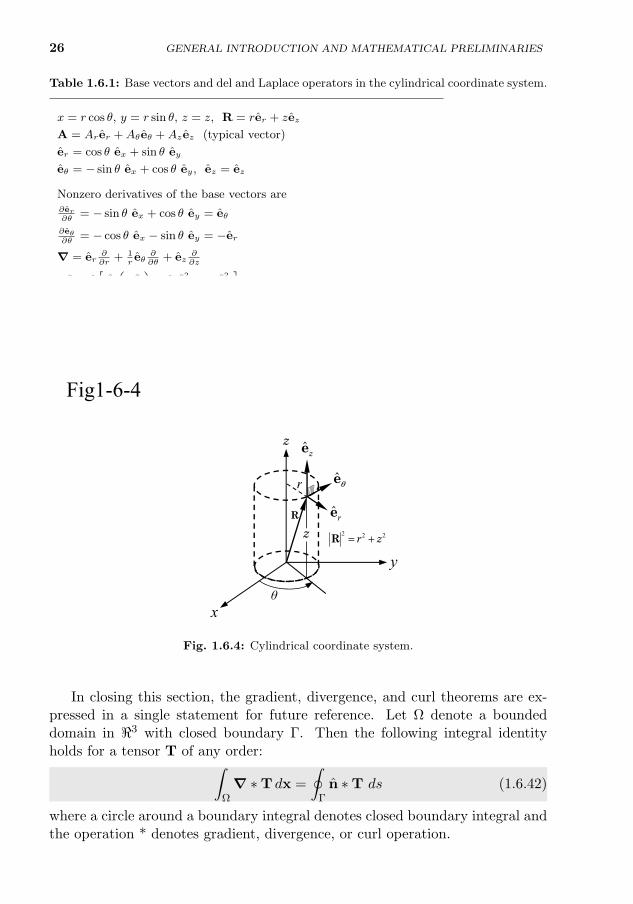
26 GENERAL INTRODUCTION AND MATHEMATICAL PRELIMINARIES
Table 1.6.1: Base vectors and del and Laplace operators in the cylindrical coordinate system.
x = r cos θ, y = r sin θ, z = z, R = rer + zez
A = Arer +Aθeθ +Az ez (typical vector)
er = cos θ ex + sin θ ey
eθ = − sin θ ex + cos θ ey, ez = ez
Nonzero derivatives of the base vectors are∂er∂θ
= − sin θ ex + cos θ ey = eθ
∂eθ∂θ
= − cos θ ex − sin θ ey = −er∇ = er
∂∂r
+ 1reθ
∂∂θ
+ ez∂∂z
∇2 = 1r
[∂∂r
(r ∂∂r
)+ 1
r∂2
∂θ2+ r ∂
2
∂z2
]∇A = erer
∂Ar∂r
+ ereθ∂Aθ∂r
+ eθer1r
(∂Ar∂θ−Aθ
)+ erez
∂Az∂r
+ ez er∂Ar∂z
+eθeθ1r
(Ar + ∂Aθ
∂θ
)+ 1
reθez
∂Az∂θ
+ ez eθ∂Aθ∂z
+ ez ez∂Az∂z
∇ ·A = 1r
[∂(rAr)∂r
+ ∂Aθ∂θ
+ r ∂Az∂z
]∇×A =
(1r∂Az∂θ− ∂Aθ
∂z
)er +
(∂Ar∂z− ∂Az
∂r
)eθ + 1
r
[∂(rAθ)∂r
− ∂Ar∂θ
]ezFig1-6-4
x
y
θ
r eθ
R2 2 2R r z= +z
z
er
ez
Fig. 1.6.4: Cylindrical coordinate system.
In closing this section, the gradient, divergence, and curl theorems are ex-pressed in a single statement for future reference. Let Ω denote a boundeddomain in <3 with closed boundary Γ. Then the following integral identityholds for a tensor T of any order:∫
Ω∇ ∗T dx =
∮Γn ∗T ds (1.6.42)
where a circle around a boundary integral denotes closed boundary integral andthe operation * denotes gradient, divergence, or curl operation.
1.7. CONCEPTS FROM FUNCTIONAL ANALYSIS 27
1.7 Concepts from Functional Analysis
1.7.1 Introduction
In the study of solutions to various physical problems that are unrelated, onemay find that they share certain common mathematical structure. For example,the approximate solution of problems by numerical methods ultimately leadsto the solution of a set of linear equations. Then it is necessary to know underwhat conditions these equations, without regard to a specific problem, have asolution (existence) and it is the only solution (uniqueness). That is, insteadof studying a particular kind of problem, the particular problem is studied inthe context of a general problem. A systematic study of the mathematicaland computational properties of a given class of problems leads to a formaltreatment that is more abstract than the treatment of a specific problem. Thisin turn leads to deeper understanding and, more importantly, provides insightsinto the essential – physical, mathematical, and computational – features of theproblem. A good example of this kind is provided by the notion of an abstractvector, which includes as a special case the geometric vector studied in Section1.6. The notion of “direction” is generalized to include a “property” that thevector should possess, among other things, in order to qualify as a vector. Thecollection of all vectors which share a common property, such as satisfying agiven differential equation, and satisfying certain rules of addition and scalarmultiplication, is termed a vector space. An abstract vector space contains pointsthat could be numbers, points in ordinary Euclidean space of functions, and soon. The study of those properties of a completely arbitrary collection of pointsin a space which hold independently of their particular nature, whether theybe numbers, points, or functions, is the subject of functional analysis.
In functional analysis the fundamental concepts and methods from elemen-tary analysis, algebra, and geometry are studied from a unified point of viewand for more general objects. For example, the definitions of a functional, its ex-tremum, and the conditions for the existence of an extremum in the calculus ofvariations are entirely analogous to the definitions of a function, its extremum,and the conditions for the existence of an extremum in the differential calcu-lus. Another example of analogy between functional analysis and geometry isgiven by the development of functions with respect to elements of an orthogonalsystem, which resemble orthogonal systems of vectors in the Euclidean space.Thus, functional analysis is an indispensable tool in approximation theoriesand numerical analysis. Therefore, a brief exposure to the subject will makethe reader comfortable when abstract variational statements are encounteredin the context of finite element formulations of physical problems. To keep thescope of this review within reasonable limits, only the concepts useful in thepresent study from linear algebra and analysis are included here. For more de-tails the reader may consult any one of the many books on functional analysis[14–16].
28 GENERAL INTRODUCTION AND MATHEMATICAL PRELIMINARIES
The following notation is used in presenting concepts from linear algebra:
⊂ means “a subset of”6⊂ means “not a subset of”∈ means “an element of”6∈ means “not an element of”3 means “such that”∀ means “for all”< = x : x is a real number, −∞ < x <∞
[a, b] = x : x is real, a ≤ x ≤ b[a, b) = x : x is real, a ≤ x < b(a, b] = x : x is real, a < x ≤ b(a, b) = x : x is real, a < x < b
The set [a, b] is called a closed interval and (a, b) is called an open interval.
1.7.2 Linear Vector Spaces
In Section 1.6, a geometric or physical vector is considered. In this section, moregeneral, abstract objects than physical vectors, which are also called vectors,are studied. A collection of vectors, u, v, w, . . . , is called a linear vector space Vover the real number field < if the following rules of vector addition and scalarmultiplication of a vector are satisfied by the elements of the vector space.
1.7.2.1 Vector addition
To every pair of vectors u, v ∈ V , there corresponds a unique vector u+ v ∈ V ,called the sum of u and v, with the following properties:
(1) u+ v = v + u (commutative)(2) (u+ v) + w = u+ (v + w) (associative)(3) there exists a unique vector, 0 ∈ V, independent of u such that
u+ 0 = u for every u ∈ V (existence of an identity or zero element)(4) to every u there exists a unique vector, −u
(that depends on u) such that u+ (−u) = 0 for every u ∈ V(existence of the additive inverse element)
All properties listed above for an abstract vector are a generalization of theproperties of a physical vector that we discussed in Section 1.6.2. We note thatthe notion of a vector in abstract analysis does not require the vector to havea magnitude. However, in nearly all cases of engineering analysis the vectoris endowed with a magnitude, in which case the vector is said to belong to anormed vector space, which is discussed in Section 1.7.3. Thus, physical vectorsof Section 1.6 belong to a special normed vector space.
1.7. CONCEPTS FROM FUNCTIONAL ANALYSIS 29
1.7.2.2 Scalar multiplication
To every vector u ∈ V and every real number α ∈ < there corresponds a uniquevector αu ∈ V such that the following properties hold:
(1) α(βu) = (αβ)u (associative)(2) (α+ β)u = αu+ βu (distributive with respect to the scalar addition)(3) α(u+ v) = αu+ αv (distributive with respect to the vector addition)(4) 1 · u = u · 1; 0 · u = 0
1.7.2.3 Linear subspaces
A linear subspace S of a given linear vector space V over < is a nonemptysubset of V which is (i.e. S) itself a linear vector space with respect to theoperations of addition and scalar multiplication defined over V . To determinewhether a given subset of a linear vector space qualifies as a subspace, one mustfirst check if it is a linear vector space by itself. In other words, a subset S ofa linear space V is a subspace if and only if αu + βv ∈ S for all u, v ∈ S andscalars α, β ∈ < (closure property), and the identity and inverse elements arethe same as those defined in V .
1.7.2.4 Linear dependence and independence of vectors
Let V be a linear vector space. If an element u ∈ V can be expressed asu =
∑αiui, αi ∈ < and ui ∈ V , then u is said to be a linear combination of
ui’s. An expression of the form∑αiui = 0 is called a linear relation among
the ui’s. A relation with all αi = 0 is called a trivial relation, and a relationwith at least one coefficient nonzero is called a nontrivial relation.
A set of vectors ui is said to be linearly dependent if there exist realnumbers αi, not all zero, such that
∑αiui = 0, that is there exists a nontrivial
relation among them. Otherwise the set is said to be linearly independent.The following observations are simple consequences of the definitions:
(1) If (u1, u2, . . . , un) are dependent, at least one vector is a linear combina-tion of the others.
(2) If the zero vector belongs to a set of vectors, the set is linearly dependent(since for α ∈ < and 0 ∈ V, α0 = 0).
(3) A set consisting of exactly one nonzero vector is linearly independent(since for α ∈ < and u ∈ V , αu = 0 implies α = 0).
(4) If (u1, u2, . . . , un) is a linearly dependent set, so is any set that includes(u1, u2, . . . , un). A set of vectors is linearly dependent if some subset of itis linearly dependent.
(5) If (u1, u2, . . . , un) is a linearly independent set, any subset of it is alsolinearly independent.
30 GENERAL INTRODUCTION AND MATHEMATICAL PRELIMINARIES
1.7.3 Normed Vector Spaces
Let V be a linear vector space over the real number field <. The notation || · ||is used to denote the norm of real-valued functions u(x), x ∈ Ω ⊂ <3. Theintegral ∫
Ωu(x) dx
denotes the Lebesgue integral1 of u. For 1 ≤ p ≤ ∞, let
||u||Lp(Ω) ≡ ||u||p =
[∫Ω|u(x)|p dx
]1/p
<∞ (1.7.1)
and for p =∞ set
||u||L∞(Ω) ≡ ||u||∞ = sup |u(x)| : x ∈ Ω (1.7.2)
For 1 ≤ p ≤ ∞, the Lebesgue spaces are defined by
Lp(Ω) = u : ‖u‖p <∞ (1.7.3)
The following inequalities are useful in establishing the continuity of linear andbilinear forms.
1.7.3.1 Holder inequality
For 1 ≤ p, q ≤ ∞ such that 1/p + 1/q = 1 and if f ∈ Lp(Ω) and g ∈ Lq(Ω),then fg ∈ L1(Ω) and
‖fg‖1 =
∫Ω|fg|dx ≤
(∫Ω|f |pdx
)1/p(∫Ω|g|qdx
)1/q
(1.7.4)
For p = q = 2, the above inequality is known as the Cauchy–Schwartz inequality.
1.7.3.2 Minkowski inequality
For 1 ≤ p ≤ ∞ and f, g ∈ Lp(Ω), the following inequality holds:
‖f + g‖p ≤ ‖f‖p + ‖g‖p (1.7.5)
A norm ‖ · ‖ can be used to define a notion of distance, or natural metric
d(u, v) ≡ ‖u− v‖ for u, v ∈ V (1.7.6)
1Formal definitions of Riemann and Lebesgue integrable functions are quite involved andrequire considerable mathematical machinery [12]. In simple terms, the Riemann integral isone in which the integrand is continuous and integrable in the usual sense, whereas piecewisecontinuous functions may have finite jump discontinuities, but they are locally Lebesgueintegrable.
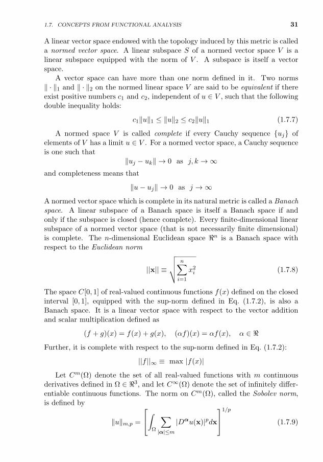
1.7. CONCEPTS FROM FUNCTIONAL ANALYSIS 31
A linear vector space endowed with the topology induced by this metric is calleda normed vector space. A linear subspace S of a normed vector space V is alinear subspace equipped with the norm of V . A subspace is itself a vectorspace.
A vector space can have more than one norm defined in it. Two norms‖ · ‖1 and ‖ · ‖2 on the normed linear space V are said to be equivalent if thereexist positive numbers c1 and c2, independent of u ∈ V , such that the followingdouble inequality holds:
c1‖u‖1 ≤ ‖u‖2 ≤ c2‖u‖1 (1.7.7)
A normed space V is called complete if every Cauchy sequence uj ofelements of V has a limit u ∈ V . For a normed vector space, a Cauchy sequenceis one such that
‖uj − uk‖ → 0 as j, k →∞and completeness means that
‖u− uj‖ → 0 as j →∞
A normed vector space which is complete in its natural metric is called a Banachspace. A linear subspace of a Banach space is itself a Banach space if andonly if the subspace is closed (hence complete). Every finite-dimensional linearsubspace of a normed vector space (that is not necessarily finite dimensional)is complete. The n-dimensional Euclidean space <n is a Banach space withrespect to the Euclidean norm
||x|| ≡
√√√√ n∑i=1
x2i (1.7.8)
The space C[0, 1] of real-valued continuous functions f(x) defined on the closedinterval [0, 1], equipped with the sup-norm defined in Eq. (1.7.2), is also aBanach space. It is a linear vector space with respect to the vector additionand scalar multiplication defined as
(f + g)(x) = f(x) + g(x), (αf)(x) = αf(x), α ∈ <
Further, it is complete with respect to the sup-norm defined in Eq. (1.7.2):
||f ||∞ ≡ max |f(x)|
Let Cm(Ω) denote the set of all real-valued functions with m continuousderivatives defined in Ω ∈ <3, and let C∞(Ω) denote the set of infinitely differ-entiable continuous functions. The norm on Cm(Ω), called the Sobolev norm,is defined by
‖u‖m,p =
∫Ω
∑|α|≤m
|Dαu(x)|pdx
1/p
(1.7.9)
32 GENERAL INTRODUCTION AND MATHEMATICAL PRELIMINARIES
for 1 ≤ p ≤ ∞ and for all u ∈ Cm(Ω). In Eq. (1.7.9), α denotes an n-tuple ofintegers
α = (α1, α2, · · · , αn), |α| =n∑i
αi, αi ≥ 0
Dα =∂|α|
∂xα11 ∂xα2
2 · · · ∂xαnn
(1.7.10)
For m = 1, n = 2, and 1 ≤ p < ∞ [α = (α1, α2), α1, α2 = 0, 1], the norm isgiven by
‖u‖1,p =
∫Ω⊂<2
[|u|p +
∣∣∣∣∂u∂x∣∣∣∣p +
∣∣∣∣∂u∂y∣∣∣∣p] dxdy1/p
(1.7.11)
The space Cm(Ω) is not complete with respect to the Sobolev norm || · ||m,p.The completion of Cm(Ω) with respect to the norm || · ||m,p is called the Sobolevspace of order (m, p), denoted by Wm,p(Ω). The completion of C(Ω) is theL2(Ω) space. Hence the Sobolev space is a Banach space. Of course, theLebesque space Lp(Ω) is a special case of the Sobolev space Wm,p for m = 0,and of L2(Ω) for p = 2, with the norms defined in Eq. (1.7.9).
If U and V are each normed linear spaces, a norm can be defined on theproduct space U × V ≡W. First, addition of vectors and scalar multiplicationof numbers from U × V must be defined so that W = U × V can qualify as alinear vector space. Let w1 = (u1, v1) and w2 = (u2, v2) be two vectors in Wwith u1, u2 ∈ U and v1, v2 ∈ V . The addition of two vectors is defined as
w1 + w2 = (u1, v1) + (u2, v2) = (u1 + u2, v1 + v2)
and multiplication by a scalar α as
αw = α(u, v) = (αu, αv)
One can verify that W = U × V is a linear vector space with respect to theseoperations.
1.7.4 Inner Product Spaces
The notion of a norm provides us with a way of measuring the length of a vector,or the difference between two vectors of a linear vector space. In order to havea means of measuring the angle between two vectors, the notion of an innerproduct (analogous to the scalar product or dot product of ordinary physicalvectors) must be introduced.
An inner product on a linear vector space V over < is a real-valued functionthat associates with each pair of vectors u, v ∈ V a scalar, denoted (u, v) ∈ <,which satisfies the following axioms:
1.7. CONCEPTS FROM FUNCTIONAL ANALYSIS 33
(1) (u, v) = (v, u) (symmetry)
(2a) (αu, v) = α(u, v) (homogeneous) (1.7.12)
(2b) (u1 + u2, v) = (u1, v) + (u2, v) (additive)
(3) (u, v) ≥ 0 and (u, u) = 0 if and only if u = 0 (positive-definite)
for every u, u1, u2, v ∈ V and α ∈ <. A linear vector space on which an innerproduct can be defined is called an inner product space. A linear subspace S ofan inner product space V is a subspace with the inner product of V .
Note that the square root of the inner product of a vector with itself satisfiesthe axioms of a norm. Consequently, one can associate with every inner producta norm by defining
||u|| =√
(u, u) (1.7.13)
The norm thus obtained is called the natural norm induced by the inner product.Since a norm can be associated with each inner product, every inner productspace is also a normed vector space. It should be obvious to the reader thatthe converse does not hold in general.
1.7.4.1 Orthogonality of vectors
The concept of orthogonality from the ordinary physical vectors can be gener-alized to the elements of linear vector spaces with the aid of an inner product.Two vectors u and v in an inner product space are said to be orthogonal if
(u, v) = 0 (1.7.14)
A set of vectors u1, u2, . . . is called an orthogonal set if each pair of the set isorthogonal: (ui, uj) = 0 for i 6= j. The set un is called orthonormal if
(ui, uj) = δij (1.7.15)
As already stated earlier, an orthonormal set of nonzero vectors is linearlyindependent.
The following lemma, known as the fundamental lemma of variational cal-culus, plays an important role in the variational theory.
Lemma 1.7.1: Let V be an inner product space. If (u, v) = 0 for all v ∈ V ,then u = 0.Proof: Since (u, v) = 0 for all v, it must also hold for v = u. Then (u, u) = 0implies that u = 0.
1.7.4.2 Cauchy–Schwartz inequality
Recall that the Holder inequality for p = q = 2 is known as the Cauchy–Schwartz inequality. The inequality is given here in terms of a norm. Let u and
34 GENERAL INTRODUCTION AND MATHEMATICAL PRELIMINARIES
v be any elements of an inner product space V . Then the Cauchy–Schwartzinequality can be stated as
|(u, v)| ≤√
(u, u)(v, v) = ||u|| ||v|| (1.7.16)
Let V be the set of ordinary (physical) vectors in <3. A typical elementa ∈ V has the form a = (a1, a2, a3). It is an inner product space with respectto the inner product,
(a,b) ≡ a · b = a1b1 + a2b2 + a3b3
|a| =√a2
1 + a22 + a2
3
The angle θ between two vectors a and b is given by
cos θ =a · b|a||b|
=a1b1 + a2b2 + a3b3√
a21 + a2
2 + a23 ·√b21 + b22 + b23
If two vectors a and b are orthogonal in V, then
a · b = 0, cos θ = 0 or θ = π/2
This means vectors a and b are perpendicular to each other. The projection ofthe vector a on the line generated by b is given by
Pa =(a · b)b
|b|2= (a · eb)eb = |a| cos θ eb, eb =
b
|b|
Note that the projection is a vector.Let V be the two-dimensional linear subspace of C[0, 1] spanned by
sin 2πx,
cos 2πx
. Define the inner product on C[0, 1] (hence on V ) by
(u, v) =
∫ 1
0u(x)v(x)dx
The inner product of u = a1 sin 2πx+a2 cos 2πx and v = b1 sin 2πx+ b2 cos 2πxis the real number
(u, v) =1
2(a1b1 + a2b2)
An element u = a1 sin 2πx + a2 cos 2πx is orthogonal to v ∈ V if and only if vis of the form
v = −a2 sin 2πx+ a1 cos 2πx
The “angle” between u and v is given by
cos θ =(u, v)
||u|| ||v||=
(a1b1 + a2b2)√a2
1 + a22
√b21 + b22
1.7. CONCEPTS FROM FUNCTIONAL ANALYSIS 35
The projection of the vector u on the line generated by v is
Pu = (a1b1 + a2b2)(b1 sin 2πx+ b2 cos 2πx)(b21 + b22)−1
The Schwartz inequality takes the form
|(a1b1 + a2b2)| ≤√a2
1 + a22 ·√b21 + b22
From previous discussions it is clear that the geometry of normed and in-ner product vector spaces is much like the familiar two- and three-dimensionalEuclidean geometry. The geometry of Hilbert spaces is even closer to the Eu-clidean geometry. For example, if two vectors u and v of an inner product spaceV are orthogonal, then the Pythagorean theorem holds even in function spaces:
||(u+ v)||2 = (u+ v, u+ v) = (u, u) + 2(u, v) + (v, v) = ||u||2 + ||v||2
1.7.4.3 Hilbert spaces
A complete (in its natural metric) inner product space is called a Hilbert space.Every inner product space (hence a normed space) has a completion.
Euclidean Space, <n. The n-dimensional Euclidean space is a Hilbert space.The inner product in <n is defined by
(x,y) =n∑i=1
xiyi, x,y ∈ <n (1.7.17)
The space <n is complete. To see this, let xk = (xk1, xk2, . . . , x
kn) be a Cauchy
sequence in <n. Then for any ε > 0 there exists an N such that
d(xm,xp) ≡ (xm − xp,xm − xp) =
[n∑i=1
(x(m)i − x(p)
i )2
]1/2
≤ ε
whenever m, p > N . This implies that
|x(m)1 − x(p)
1 | ≤ ε, |x(m)2 − x(p)
2 | ≤ ε, . . . , |x(m)n − x(p)
n | ≤ ε, for m, p > N
Thus, each of the sequences x(k)n must converge, since < is complete, as k →∞.
Let limk→∞x(k)i = xi; then limk→∞xk = (x1, x2, . . . , xn), and the space <n is
complete. Hence, it is a Hilbert space. The Schwartz inequality becomes[n∑k=1
xkyk
]≤
[n∑k=1
x2k
]1/2[ n∑k=1
y2k
]1/2
The completeness of <n implies the completeness of all finite-dimensional vectorspaces.
36 GENERAL INTRODUCTION AND MATHEMATICAL PRELIMINARIES
Hm(Ω)-inner product. Consider the Sobolev space Wm,2(Ω) ≡ Hm(Ω) withΩ ⊂ <3. For u, v ∈ Hm(Ω) define
(u, v)m =
∫Ω
∑|α|≤m
Dαu ·Dαv dx (1.7.18)
This defines an inner product on Hm(Ω). Once again, the L2(Ω) inner productis obtained as a special case of the Hm(Ω) inner product by setting m = 0:
(u, v)0 =
∫Ωu · v dx (1.7.19)
For example, let Ω ⊂ <2 (n = 2) and m = 1 in Eq. (1.7.18). Then the H1(Ω)inner product becomes
(u, v)1 =
∫Ω
(uv +
∂u
∂x
∂v
∂x+∂u
∂y
∂v
∂y
)dxdy (1.7.20)
Similarly,
(u, v)2 = (u, v)1 +
∫Ω
(∂2u
∂x∂y
∂2v
∂x∂y+∂2u
∂x2
∂2v
∂x2+∂2u
∂y2
∂2v
∂y2
)dx dy
=
∫Ω
(uv +
∂u
∂x
∂v
∂x+∂u
∂y
∂v
∂y+
∂2u
∂x∂y
∂2v
∂x∂y+∂2u
∂x2
∂2v
∂x2+∂2u
∂y2
∂2v
∂y2
)dx dy
(1.7.21)
The norm induced by the inner product gives back the Sobolev norm || · ||m,2.However, there is no inner product associated with the Sobolev norm || · ||m,p(i.e. when p 6= 2).
Hilbert spaces, Hm(Ω). Since the Sobolev space Wm,p(Ω) is a Banach space,Wm,2(Ω) is a Hilbert space with the inner product defined in Eq. (1.7.18). Itshould be noted once again that the Hilbert space Hm(Ω) is a special case ofthe Sobolev space Wm,p(Ω). For p 6= 2, Wm,p(Ω) is not a Hilbert space. TheHilbert space Hm
0 (Ω) is a linear subspace of functions from Hm(Ω) that vanish,along with their derivatives up to order m− 1, on the boundary of Ω.
1.7.5 Linear Transformations
The notion of a function or transformation from one set into another can beextended to vector spaces. A transformation T from a linear vector space Uinto another linear vector space V (both vector spaces are defined on the samefield of scalars) is a correspondence which assigns to each element u ∈ U aunique element v = Tu ∈ V . The terms transformation, mapping, and operatorare used interchangeably and the transformation is expressed as T : U → V .
A transformation T : U → V , where U and V are vector spaces that havethe same scalar field, is said to be linear if
1.7. CONCEPTS FROM FUNCTIONAL ANALYSIS 37
(1) T (αu) = αT (u), for all u ∈ U, α ∈ < (homogeneous)
(2) T (u1 + u2) = T (u1) + T (u2), for all u1, u2 ∈ U (additive) (1.7.22)
Otherwise, it is said to be a nonlinear transformation. Conditions 1 and 2 canbe combined into one: a transformation T : U → V is said to be linear if
T (αu1 + βu2) = αT (u1) + βT (u2) (1.7.23)
for all vectors u1, u2 ∈ U and scalars α, β ∈ <. A transformation T : U → Vis said to be a continuous linear transformation if it is linear and continuous.The operator T is said to be bounded if there exists a real number M ≥ 0 suchthat
||Tu||V ≤M ||u||U , for all u ∈ U (1.7.24)
where || · ||U is the norm in U and || · ||V is the norm in V . A linear trans-formation T : U → V is continuous if and only if it is bounded. In finite-dimensional normed vector spaces, all linear transformations are continuous(hence bounded).
If T1 : U → V and T2 : V → W are linear transformations, then theircomposition T2T1 is also linear:
(T2T1)(αu1 + βu2) = T2(αT1(u1) + βT1(u2))= αT2(T1(u1)) + βT2(T1(u2))= α(T2T1)(u1) + β(T2T1)(u2)
The norm ||T || of a bounded linear transformation T : U → V , where Uand V are normed spaces, is defined by
||T || = inf M : ||Tu||V ≤M ||u||U for all u ∈ U (1.7.25)
Other equivalent operator norms are
||T || = sup ||Tu||V : ||u||U ≤ 1
||T || = sup
||Tu||V||u||U
: ||u||U 6= 0
(1.7.26)
Physically, the number ||Tu||/||u|| can be viewed as the amplification of T atthe point u, and ||T || as the maximum amplification of a system.
1.7.6 Linear Functionals, Bilinear Forms, and Quadratic Forms
Linear transformations that map linear vector spaces or products of linear vectorspaces into the real numbers < are of considerable interest in the study ofvariational formulation of operator equations. Such transformations are calledfunctionals.
38 GENERAL INTRODUCTION AND MATHEMATICAL PRELIMINARIES
1.7.6.1 Linear functional
Let U be a linear vector space over the real number field <. A linear trans-formation ` : U → < is called a linear form or linear functional. Since linearfunctionals are a special case of linear transformations, the concepts and re-sults given in Section 1.7.5 still hold for linear functionals. The set of all linearfunctionals on a linear vector space is itself a vector space, called the dual orconjugate space of U .
1.7.6.2 Bilinear forms
Let U and V be two vector spaces with the same field of scalars. The mappingB : U × V → < of pairs (u, v), u ∈ U, v ∈ V , into the field of scalars < suchthat
B(αu1 + βu2, µv1 + λv2) = αµB(u1, v1) + αλB(u1, v2) + βµB(u2, v1)
+ βλB(u2, v2) (1.7.27)
is called a bilinear form. A simple example of the bilinear form is the innerproduct, in which U = V and B(u, v) = (u, v).
A bilinear form B(·, ·) : U × U → < is said to be symmetric if B(u, v) =B(v, u) for all u, v ∈ U . If B(u, u) = 0 and B(u, v) = −B(v, u) for all u, v ∈ U ,the bilinear form is said to be skew-symmetric. Every bilinear form can berepresented uniquely as a sum of a symmetric Bs(·, ·) and a skew-symmetricBss(·, ·) bilinear form,
B(u, v) =1
2[B(u, v) +B(v, u)] +
1
2[B(u, v)−B(v, u)] = Bs(u, v) +Bss(u, v)
(1.7.28)
1.7.6.3 Quadratic forms
Let U be a vector space and B(·, ·) be a bilinear form on U × U . A quadraticform is a functional Q on U defined by setting
Q(u) = B(u, u) (1.7.29)
Note that if B(·, ·) is represented as the sum of a symmetric and a skew-symmetric bilinear form. Hence,
Q(u) = B(u, u) = Bs(u, u) +Bss(u, u) = Bs(u, u) (1.7.30)
That is Q(u) is completely determined by the symmetric part of the bilinearform. Therefore, two different bilinear forms with the same symmetric partmust generate the same quadratic form.
1.7. CONCEPTS FROM FUNCTIONAL ANALYSIS 39
Linear functionals in <n are of the form,
f(x) =
n∑i=1
fixi
where xi are components of the vector x in <n, and fi are any numbers whichcan be thought of as components of a vector f. Clearly, the scalar product ofordinary vectors is a special case of the above statement. Indeed, every boundedlinear functional can be written as a scalar product,
f(x) = (f ,x)
Let V = L2(0, 1) and define a linear functional on V by
`(v) =
∫ 1
0f(x)v(x) dx
where f is an arbitrary function. The functional ` is linear because it is homo-geneous,
`(αv) =
∫ 1
0f(x)αv(x) dx = α
∫ 1
0f(x)v(x) dx = α`(v)
and additive,
`(v1 + v2) =
∫ 1
0f(x)(v1 + v2)dx = `(v1) + `(v2)
The functional is also continuous. If ||vn − v|| → 0, then
|`(vn)− `(v)| = |`(vn − v)| ≤ ||f || ||vn − v||
Since ||f || is independent of v and vn, it follows that ` is continuous.Consider the bilinear form defined by
B(u, v) =
∫Ω⊂<3
(c1 grad u · grad v + c0uv)dx, c1, c0 = constants
on H10 (Ω) × H1
0 (Ω), where Ω is a bounded domain in <3, and H10 (Ω) is the
Hilbert space. It is easy to verify that B(·, ·) is linear in its arguments. Thebilinear form B(·, ·) is also continuous. Indeed, by appealing to the Cauchy–Schwartz inequality, one has
|B(u, v)| ≤M[∫
Ω(|u|2 + | grad u|2)dx
]1/2[∫Ω
(|v|2 + | grad v|2)dx
]1/2
= M ||u||1||v||1, M = max (c1, c0)
40 GENERAL INTRODUCTION AND MATHEMATICAL PRELIMINARIES
where || · ||1 denotes the H1(Ω)-norm in Eq. (1.7.20). Further, the associatedquadratic form is bounded below (or positive-definite):
Q(u) = B(u, u) =
∫Ω
(c1| grad u|2 + c0|u|2)dx ≥ µ||u||21
where µ = min(c1, c0). The continuity and positive-definite properties play acrucial role in the existence and uniqueness of solutions to functional equations.
The functional analysis concepts introduced in this section will be used onlywhere it is appropriate in this book. In particular, importance will be given tophysical and computational aspects over functional analysis framework.
1.8 The Big Picture
Engineering design is the process of altering dimensions, shapes, and materialsto find the best (optimum) configuration of the system to carry out certainspecific function. Analysis is an aid to design, and it involves (1) mathematicalmodel development, (2) data acquisition by measurements, (3) numerical simu-lation, and (4) evaluation of the results in light of known information and correc-tions to the mathematical model. The mathematical model is developed usinglaws of physics and assumptions concerning the process behavior. The datainclude the actual system parameters such as the geometry, material proper-ties, loading, and boundary conditions. The material properties are determinedthrough laboratory experiments. The mathematical model, in most practicalcases, does not admit an analytical solution due to the geometric complexityand/or nonlinearities. Nonlinearities in a mathematical model arise from chang-ing geometry or material behavior. Thus, it is necessary to employ numericalmethods to compute an approximate solution to the mathematical model. Thefinite element method has emerged as a powerful computational procedure thatcan be used to analyze a variety of practical engineering problems.
A typical finite element analysis exercise begins with the actual physicalsystem or part thereof to be analyzed. First, a set of objectives for the analysisis identified. If the analysis objective is to help develop a preliminary design ofthe system, the analysis can be very simple. On the other hand, if the analysisobjective is to verify and certify the final design of a system, the analysis mustbe the most sophisticated one. Thus, the objective will dictate the type ofidealization of the system to be adopted; for example, should it be modeledas a two-dimensional or three-dimensional problem, analyzed as a linear ornonlinear problem and what type of nonlinearities to be considered, what typeconstitutive model be used, how the loads and boundary conditions of the actualsystem are idealized, what coupling effects, if any, to be considered, and so on.
Once the system idealization has been completed (i.e. mathematical modelis in place), one must decide on type of numerical approximation (and softwareto be used). This involves (1) choice of unknowns, which in turn dictates the
1.8. THE BIG PICTURE 41
type of finite element model, (2) type of elements, (3) type of the mesh (i.e.density of elements), and if nonlinear analysis is to be carried out, select (4)magnitude of load increments, (5) type of iterative method of solution, (6) errorcriterion, (7) error tolerance, and (8) maximum allowable number of iterationsfor the termination of the program. Of course, engineering background in thetopic area coupled with experience with the software being used are alwayshelpful in creating a suitable computational model of the problem at hand.
The final step in creating a computational model is verification of the codeand validation of the mathematical model [17–21]. Verification is the processof determining if the computational model is an accurate discrete analog of themathematical model. Thus, if the round-off errors introduced due to finite arith-metic in a computer are negligible, the computational model should give theexact solution of the mathematical model. Thus verification involves compar-ing the numerical results with known exact solutions of benchmark problems.A benchmark problem is one that has a number of features to test a computerprogram for correctness, including the following:
(1) has a set of standard reference results (analytical and numerical) that canbe used to compare the accuracy and efficiency of computation;
(2) provides a list of pitfalls and difficulties;
(3) has a means to assess the adequacy of theoretical formulations and nu-merical algorithms;
(4) allows assessing robustness of the program (i.e. the ability of the programto handle ill-defined or sensitive conditions); and
(5) illustrates the use of a computer program.
On the other hand, validation is the process of determining the degree towhich the mathematical model (hence the computer code that is verified) rep-resents the physical reality of the system from the perspective of the intendeduses of the model. For example, a mathematical model based on linear elastic-ity is adequate for determining linear elastic solutions of a solid but inadequatefor determining its nonlinear response. The validation exercise allows one tomodify the mathematical model to include the missing elements of the math-ematical model that make the computed response come closer to the physicalresponse. In fact, a mathematical model can never be validated because onedoes not know all the physics of the problem; it can only be invalidated. It isalways a good idea, when developing a new computer program (also called acode), to undertake the verification exercise. Validation is a must when study-ing new problems and/or simultaneously accounting for multiple components ofthe physics involved (also called multiphysics problems). Additional conceptsrelated to verification and validation of simulation models can be found in [17,19, 20].
42 GENERAL INTRODUCTION AND MATHEMATICAL PRELIMINARIES
1.9 Summary
In this chapter a motivation for the present study is provided and the meaningof mathematical models and numerical simulations is discussed. The mainfeatures of the finite element method and nonlinear analysis are also discussed,and some mathematical preliminaries that are useful in the coming chaptersare presented. In particular, a review of ordinary vectors and tensors, indexnotation, and linear vector spaces is presented.
Readers familiar with the material on vectors and tensors and functionalanalysis may browse through the material and skip the details of the respectivesections. However, Chapter 2, which deals with nonlinear continuum mechanics,makes use of the material on vectors and tensors. Therefore readers should, atleast, get familiar with the notation introduced here.
Problems
Vectors and Tensors
1.1 Establish the following identities:
(a) eijk =
∣∣∣∣∣∣δi1 δi2 δi3δj1 δj2 δj3δk1 δk2 δk3
∣∣∣∣∣∣ . (b) eijkepqr =
∣∣∣∣∣∣δip δiq δirδjp δjq δjrδkp δkq δkr
∣∣∣∣∣∣ .(c) eijkemnk = δimδjn − δinδjm. (d) eijk eijk = 6.
1.2 Determine the transformation matrix relating the orthonormal basis vectors (e1, e2, e3)and (e′1, e
′2, e′3), when e′i are given by
(a) e′1 is along the vector e1 − e2 + e3 and e′2 is perpendicular to the plane 2x1 +3x2 + x3 − 5 = 0.
(b) e′1 is along the line segment connecting point (1,−1, 3) to (2,−2, 4) and e′3 =(−e1 + e2 + 2e3)/
√6.
1.3 The displacement vector at a point referred to the basis (e1, e2, e3) is u = 2e1+2e2−4e3.Determine ui with respect to the basis (ˆe1, ˆe2, ˆe3), where ˆe1 = (2e1 + 2e2 + e3)/3 andˆe2 = (e1 − e2)/
√2.
1.4 Determine the rotation transformation matrix such that the new base vector ˆe1 is alonge1 − e2 + e3, and ˆe2 is along the normal to the plane 2x1 + 3x2 + x3 = 5. If S is thetensor whose components in the unbarred system are given by s11 = 1, s12 = s21 =0, s13 = s31 = −1, s22 = 3, s23 = s32 = −2, and s33 = 0, find the components in thebarred coordinates.
1.5 Let r denote a position vector r = x = xiei (r2 = xixi) and A be an arbitrary constantvector. Use index notation to show that:
(a) ∇2(rn) = n(n+ 1)rn−2. (b) ∇(r ·A) = A.
(c) ∇ · (r×A) = 0. (d) ∇× (r×A) = −2A.
(e) ∇ · (rA) =1
r(r ·A). (f) ∇× (rA) =
1
r(r×A).
1.6 Use the index notation to rewrite the vector expression as a sum or difference of twovector expressions, when A is a vector-valued function:
∇× (∇×A)
PROBLEMS 43
1.7 Establish the following identities for a second-order tensor S:
(a) |S| = eijk s1i s2j s3k. (b) |S| = 16sir sjs skt erst eijk.
(c) erst|S| = eijk sir sjs skt. (d)
∣∣∣∣∣∣sim sin sipsjm sjn sjpskm skn skp
∣∣∣∣∣∣ = eijk emnp |S|.
1.8 Express the components of the symmetric part of the gradient of a vector A
V =1
2
[(∇A)T + (∇A)
]in terms of the components of vector A and definition of the del operator ∇ in thecylindrical coordinate system (see Table 1.6.1). In particular, show that
Vrr =∂Ar∂r
, Vrθ =1
2
(1
r
∂Ar∂θ
+∂Aθ∂r− Aθ
r
), Vrz =
1
2
(∂Ar∂z
+∂Az∂r
)Vθθ =
Arr
+1
r
∂Aθ∂θ
, Vzθ =1
2
(∂Aθ∂z
+1
r
∂Az∂θ
), Vzz =
∂Az∂z
1.9 Express the components of the skew-symmetric part of the gradient of a vector A
W =1
2
[(∇A)T − (∇A)
]in terms of the components of vector A and definition of the del operator ∇ in thecylindrical coordinate system. In particular, show that
Wrθ =1
2
(1
r
∂Ar∂θ− Aθ
r− ∂Aθ
∂r
)= −Wθr
Wrz =1
2
(∂Ar∂z− ∂Az
∂r
)= −Wzr
Wzθ =1
2
(1
r
∂Az∂θ− ∂Aθ
∂z
)= −Wθz
1.10 For an arbitrary second-order tensor S show that ∇ · S in the cylindrical coordinatesystem is given by
∇ · S =
[∂Srr∂r
+1
r
∂Sθr∂θ
+∂Szr∂z
+1
r(Srr − Sθθ)
]er
+
[∂Srθ∂r
+1
r
∂Sθθ∂θ
+∂Szθ∂z
+1
r(Srθ + Sθr)
]eθ
+
[∂Srz∂r
+1
r
∂Sθz∂θ
+∂Szz∂z
+1
rSrz
]ez
1.11 For an arbitrary second-order tensor S show that ∇ · S in the spherical coordinatesystem is given by
∇ · S =
∂SRR∂R
+1
R
∂SφR∂φ
+1
R sinφ
∂SθR∂θ
+1
R[2SRR − Sφφ − Sθθ + SφR cotφ]
eR
+
∂SRφ∂R
+1
R
∂Sφφ∂φ
+1
R sinφ
∂Sθφ∂θ
+1
R[(Sφφ − Sθθ) cotφ+ SφR + 2SRφ]
eφ
+
∂SRθ∂R
+1
R
∂Sφθ∂φ
+1
R sinφ
∂Sθθ∂θ
+1
R[(Sφθ + Sθφ) cotφ+ 2SRθ + SθR]
eθ.
44 GENERAL INTRODUCTION AND MATHEMATICAL PRELIMINARIES
where
∇ = eR∂
∂R+
1
Reφ
∂
∂φ+
1
R sinφeθ
∂
∂θ
∂eR∂φ
= eφ, ∂eR∂θ
= sinφ eθ,∂eφ∂φ
= −eR,∂eφ∂θ
= cosφ eθ,∂eθ∂θ
= − sinφ eR − cosφ eφ
All other derivatives of the base vectors are zero.
1.12 For an arbitrary second-order tensor S show that ∇ × S in the cylindrical coordinatesystem is given by
∇× S = erer
(1
r
∂Szr∂θ− ∂Sθr
∂z− 1
rSzθ
)+ eθeθ
(∂Srθ∂z− ∂Szθ
∂r
)+ ez ez
(1
rSθz −
1
r
∂Srz∂θ
+∂Sθz∂r
)+ ereθ
(1
r
∂Szθ∂θ− ∂Sθθ
∂z+
1
rSzr
)+ eθer
(∂Srr∂z− ∂Szr
∂r
)+ erez
(1
r
∂Szz∂θ− ∂Sθz
∂z
)+ ez er
[∂Sθr∂r− 1
r
∂Srr∂θ
+1
r(Srθ + Sθr)
]+ eθez
(∂Srz∂z− ∂Szz
∂r
)+ ez eθ
[∂Sθθ∂r
+1
r(Sθθ − Srr)−
1
r
∂Srθ∂θ
]
Functional Analysis
1.13 Let P be the space of all polynomials with real coefficients. Determine which of thefollowing subsets of P are subspaces:
(a) S1 = p(x) : p(1) = 0(b) S2 = p(x) : degree of p(x) = 3(c) S3 = p(x) : degree of p(x) ≤ 3(d) S4 = p(x) : constant term is zero
1.14 Determine which of the following sets in <3 are linearly independent:
(a) (−1, 1, 0), (−1, 1, 1), (−2,−1, 1), (1, 1, 1)(b) (1, 0, 0), (1, 1, 0), (1, 1, 1)(c) (1, 1, 1), (1, 2, 3), (2,−1, 1)
1.15 Determine which of the following sets span <3:
(a) (2, 1, 0), (1,−1, 2), (0, 3,−4)(b) (1, 1, 1), (−2,−1, 2), (−1, 1, 1), (−1, 1, 0)(c) (−1, 1, 0), (−1, 1, 1), (−2,−1, 1), (1, 1, 1)(d) (1, 0, 0), (1, 2, 0), (1, 2, 3)
1.16 Compute the L2 norm and the sup-norm of the following functions in the intervalindicated:
(a) u(x) = sinπx− x, on 0 ≤ x ≤ 1
(b) u(x) = x1/3, on 0 ≤ x ≤ 1
(c) u(x) = cosπx+ 2x− 1, on 0 ≤ x ≤ 1
(d) u(x) =√
1 + x2, on 0 ≤ x ≤ 1
PROBLEMS 45
1.17 Prove the following relations in a real inner product space:
(a) Parallelogram law: ||u+ v||2 + ||u− v||2 = 2(||u||2 + ||v||2)
(b) (u, v) = 14[||u+ v||2 − ||u− v||2]
(c)∣∣||u|| − ||v||∣∣ ≤ ||u− v||
1.18 If two vectors u and v of an inner product space V are orthogonal, show that thePythagorean theorem holds even in function spaces: ||(u+ v)||2 = ||u||2 + ||v||2.
1.19 Compute the inner product of the following pairs of functions on the interval indicated.Use the L2 inner product and the H1(0, 1) inner product.
(a) u = (1 + x), v = 3x2 − 1, on −1 ≤ x ≤ 1
(b) u = sinπx, v = cosπx, on 0 ≤ x ≤ 1
(c) u = sinπx, v = a+ bx+ cx2, on 0 ≤ x ≤ 1
(d) u = sinπx sinπy, v = (1− x2 − y2), on 0 ≤ x, y ≤ 1
1.20 Determine a vector in the space P of polynomials of degree 2 such that the vector isorthogonal to the polynomials p1 = 1 + x− 2x2 and p2 = −2 + 4x+ x2 in L2(0, 1).
1.21 Determine the constants a and b such that w(x) = a+bx+3x2 is orthogonal in L2(0, 1)to both u(x) = 2 + 3x2 − x and v(x) = 1
3+ 3x− 5x2.
1.22 Let T1 and T2 be the linear operators defined on <3 as T1(x) = (0, x1 − x3, x2 + x3)and T2(x) = (x2 − x3, 2x1 − x2, x1). Determine (a) T1 + T2, (b) T1T2, and (c) T2T1.
1.23 Determine which of the following operators represent bilinear forms:
(a) B : <2 ×<2 → <, B(x,y) = (x1 + y1)2 − (x1 − y1)2
(b) B : <2 ×<2 → <, B(x,y) = x1y2 − x2y1

47
2
Elements of NonlinearContinuum Mechanics
Although to penetrate into the intimate mysteries of nature and thence to learn the true
causes of phenomena is not allowed to us, nevertheless it can happen that a certain fictive
hypothesis may suffice for explaining many phenomena. ——– Leonhard Euler
2.1 Introduction
The study of matter at molecular or atomistic levels is very useful for under-standing a variety of phenomena. However, studies at these scales are notuseful to solve common engineering problems. The understanding gained atthe molecular level needs to be taken to the macroscopic scale (i.e. the scalevisible to an unaided eye) to be able to study its behavior. At the macroscopicscale, it is assumed that the length scales of interest are large compared to thelength scales of the discrete molecular structure. In other words, the systemis treated as a continuum in which all physical quantities such as the density,displacements, velocities, and stresses vary continuously so that their spatialderivatives exist and are continuous. The continuum assumption allows us toshrink an arbitrary volume of material to a point, in much the same way aswe take the limit in defining a derivative, so that we can define quantities ofinterest at a point.1 A mathematical study of mechanics of such an idealizedcontinuum is called continuum mechanics.
The present chapter deals with a review of continuum mechanics conceptsas applied to an idealized matter, whether a solid or fluid, subjected to exter-nal forces. In particular, we discuss kinematics of deformation, conservationof mass, balance of momenta and energy, and constitutive relations, and thederivation of field equations resulting from the conservation and balance prin-ciples valid over a continuum. Most of the material presented here is takenfrom the author’s text book on continuum mechanics [1]; the readers may alsoconsult the books by Holzapfel [22], Bonet and Wood [23], and Malvern [24].
1The continuum assumption is not valid when one considers discontinuity in density andvelocity (e.g. shock waves). In such cases, certain jump conditions are employed to deal withthe discontinuities. We do not consider such situations in this book.
J.N. Reddy, An Introduction to Nonlinear Finite Element Analysis, Second Edition. c©J.N.Reddy 2015. Published in 2015 by Oxford University Press.
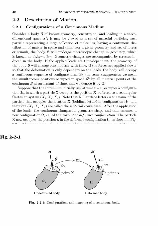
48 ELEMENTS OF NONLINEAR CONTINUUM MECHANICS
2.2 Description of Motion
2.2.1 Configurations of a Continuous Medium
Consider a body B of known geometry, constitution, and loading in a three-dimensional space <3; B may be viewed as a set of material particles, eachparticle representing a large collection of molecules, having a continuous dis-tribution of matter in space and time. For a given geometry and set of forcesor stimuli, the body B will undergo macroscopic change in geometry, whichis known as deformation. Geometric changes are accompanied by stresses in-duced in the body. If the applied loads are time-dependent, the geometry ofthe body B will change continuously with time. If the forces are applied slowlyso that the deformation is only dependent on the loads, the body will occupya continuous sequence of configurations. By the term configuration we meanthe simultaneous positions occupied in space <3 by all material points of thecontinuum B at an instant of time, and we denote it by Ω.
Suppose that the continuum initially, say at time t = 0, occupies a configura-tion Ω0, in which a particle X occupies the position X, referred to a rectangularCartesian system (X1, X2, X3). Note that X (lightface letter) is the name of theparticle that occupies the location X (boldface letter) in configuration Ω0, andtherefore (X1, X2, X3) are called the material coordinates. After the applicationof the loads, the continuum changes its geometric shape and thus assumes anew configuration Ω, called the current or deformed configuration. The particleX now occupies the position x in the deformed configuration Ω, as shown in Fig.2.2.1. The mapping χ : Ω0 → Ω is called the deformation mapping of the bodyB from Ω0 to Ω. The deformation mapping χ(X) takes the position vector Xfrom the reference configuration Ω0 and places the same point in the deformedconfiguration Ω as x = χ(X).
N
dA
dfdf
nda
X( )χ
Undeformed body Deformed body
point x• •
point X
0Ω Ω
Fig. 2-2-1
Fig. 2.2.1: Configurations and mapping of a continuous body.
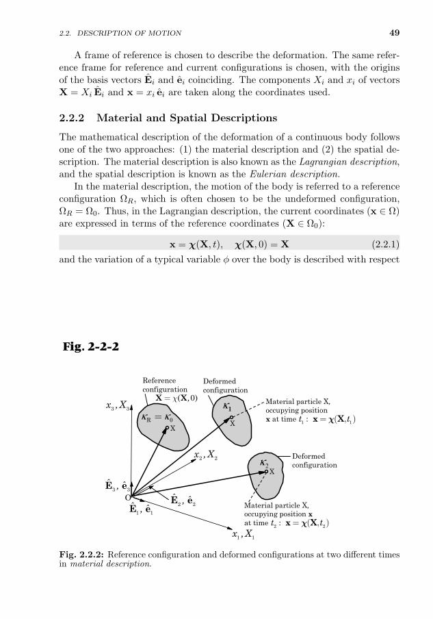
2.2. DESCRIPTION OF MOTION 49
A frame of reference is chosen to describe the deformation. The same refer-ence frame for reference and current configurations is chosen, with the originsof the basis vectors Ei and ei coinciding. The components Xi and xi of vectorsX = Xi Ei and x = xi ei are taken along the coordinates used.
2.2.2 Material and Spatial Descriptions
The mathematical description of the deformation of a continuous body followsone of the two approaches: (1) the material description and (2) the spatial de-scription. The material description is also known as the Lagrangian description,and the spatial description is known as the Eulerian description.
In the material description, the motion of the body is referred to a referenceconfiguration ΩR, which is often chosen to be the undeformed configuration,ΩR = Ω0. Thus, in the Lagrangian description, the current coordinates (x ∈ Ω)are expressed in terms of the reference coordinates (X ∈ Ω0):
x = χ(X, t), χ(X, 0) = X (2.2.1)
and the variation of a typical variable φ over the body is described with respectto the material coordinates X and time t:
φ = φ(X, t) (2.2.2)
For a fixed value of X ∈ Ω0, φ(X, t) gives the value of φ at time t associatedwith the fixed material point X whose position in the reference configurationis X, as shown in Fig. 2.2.2. Thus, a change in time t implies that the samematerial particle X, occupying position X in Ω0, has a different value φ. Thus,the attention is focused on material particles of the continuum.Fig. 2-2-2
Reference configuration
Deformed configuration
Material particle X, occupying position x at time
Deformed configuration
Material particle X, occupying position x at time
3 3x ,X0=Rκ κ
1κ( 0),c=X X
2 2t t: = ( , ) x Xc
1 1t t: = ( , ) x Xc
2 2x ,X
1 1x ,X
2κ
O1 1
ˆ ˆ,E e 2 2ˆ ˆ,E e
3 3ˆ ˆ,E e
XX
X
Fig. 2.2.2: Reference configuration and deformed configurations at two different timesin material description.
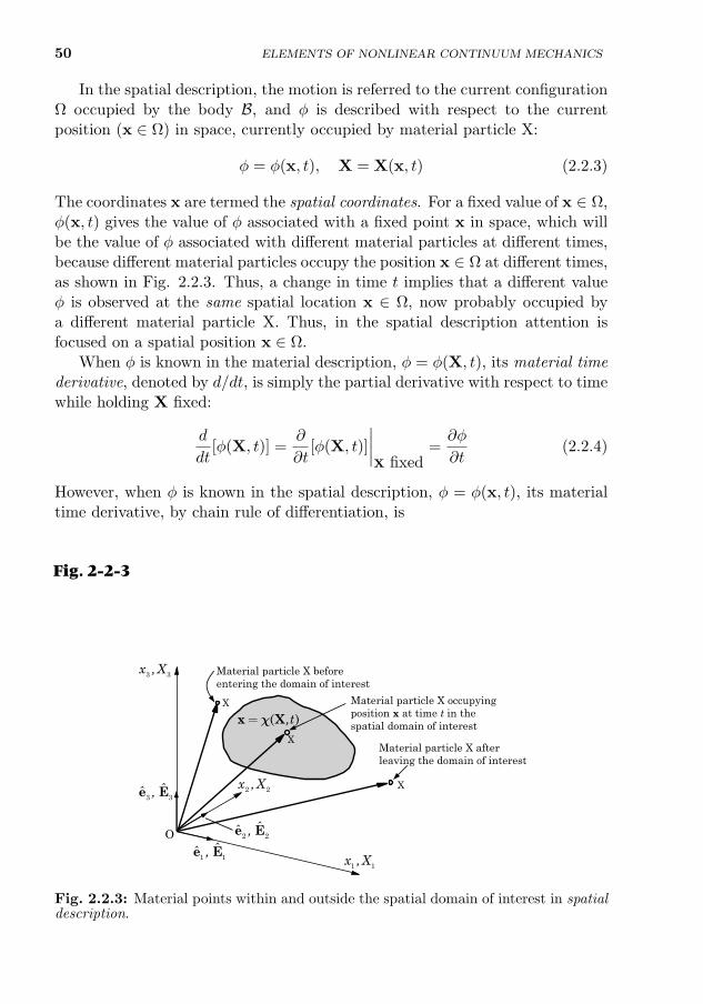
50 ELEMENTS OF NONLINEAR CONTINUUM MECHANICS
In the spatial description, the motion is referred to the current configurationΩ occupied by the body B, and φ is described with respect to the currentposition (x ∈ Ω) in space, currently occupied by material particle X:
φ = φ(x, t), X = X(x, t) (2.2.3)
The coordinates x are termed the spatial coordinates. For a fixed value of x ∈ Ω,φ(x, t) gives the value of φ associated with a fixed point x in space, which willbe the value of φ associated with different material particles at different times,because different material particles occupy the position x ∈ Ω at different times,as shown in Fig. 2.2.3. Thus, a change in time t implies that a different valueφ is observed at the same spatial location x ∈ Ω, now probably occupied bya different material particle X. Thus, in the spatial description attention isfocused on a spatial position x ∈ Ω.
When φ is known in the material description, φ = φ(X, t), its material timederivative, denoted by d/dt, is simply the partial derivative with respect to timewhile holding X fixed:
d
dt[φ(X, t)] =
∂
∂t[φ(X, t)]
∣∣∣∣X fixed
=∂φ
∂t(2.2.4)
However, when φ is known in the spatial description, φ = φ(x, t), its materialtime derivative, by chain rule of differentiation, is
d
dt[φ(x, t)] =
∂
∂t[φ(x, t)] +
∂
∂xi[φ(x, t)]
dxidt
=∂φ
∂t+ vi
∂φ
∂xi=∂φ
∂t+ v ·∇φ (2.2.5)
( ),t=x XcMaterial particle X occupying position x at time t in the spatial domain of interest
Material particle X after leaving the domain of interest
Material particle X before entering the domain of interest
1 1x ,X
2 2x ,X
3 3x ,X
3 3ˆˆ ,e E
1 1ˆˆ ,e E
2 2ˆˆ ,e EO
X
X
X
Fig. 2-2-3
Fig. 2.2.3: Material points within and outside the spatial domain of interest in spatialdescription.
2.2. DESCRIPTION OF MOTION 51
where v is the velocity vector
v =dx
dt≡ x (2.2.6)
Thus, the material time derivative of a spatial field is the operator
d
dt=
∂
∂t+ v ·∇ (2.2.7)
For example, the acceleration of a particle X occupying position x is given by
a(x, t) =dv(x, t)
dt=∂v
∂t+ v ·∇v; ai =
∂vi∂t
+ vj∂vi∂xj
(2.2.8)
Example 2.2.1 (see Reddy [1]) illustrates the determination of the inverseof a given mapping and computation of the material time derivative of a givenfunction in material and spatial descriptions.
Example 2.2.1
Suppose that the motion of a continuous medium B is described by the mapping χ : Ω0 → Ω,
χ(X, t) = x = (X1 + α tX2)e1 + (X2 − α tX1)e2 +X3 e3
where α is a constant, and suppose that the temperature T in the continuum in the spatialdescription is given by
T (x, t) = x1 + tx2
Determine (a) the inverse of the mapping, (b) the velocity components, and (c) the timederivatives of T in the two descriptions.
Solution: A known deformation mapping χ(X, t) relates the material coordinates (X1, X2, X3)to the spatial coordinates (x1, x2, x3) of a particle X. In the present case, we have
x1 = X1 + α tX2, x2 = X2 − α tX1, x3 = X3 or
x1
x2
x3
=
1 α t 0−α t 1 0
0 0 1
X1
X2
X3
(1)
Clearly, the relationships between xi and Xi are linear (i.e. the mapping is linear). Therefore,it maps polygons into polygons. In particular, a unit square is mapped into a square that isrotated in clockwise direction, as shown in Fig. 2.2.4. Note that, in general, the deformedsquare is not a unit square as the side now has a length of 1/ cos θ, where θ = tan−1(α t). Thereference configuration and deformed configurations at four different times, t = 1, 2, 3, and 4,for a value of α = 0.25, are shown in Fig. 2.2.5.
(a) The inverse mapping can be determined, when possible, by expressing (x1, x2, x3) in termsof (X1, X2, X3). In the present case, it is possible to invert the relations in Eq. (1) and obtain
X1
X2
X3
=1
(1 + α2t2)
1 −α t 0α t 1 00 0 1 + α2t2
x1
x2
x3
(2)
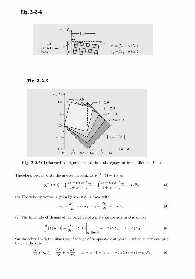
52 ELEMENTS OF NONLINEAR CONTINUUM MECHANICS
1 1,x X
x , X2 2
1 1 2
2 2 1
3 3
( )
( )
x X t X
x X t X
x X
a
a
= +
= -
=
Initial(undeformed)body
Deformed body
ta
ta
1 0.
1 0.
Fig. 2-2-4
Fig. 2.2.4: A sketch of the mapping χ as applied to a unit square.
1.0
0.5
0.0
−0.5
−1.00.0 0.4 0.8 1.2 1.6 2.0
x , X1 1
2 2x , X
0 25.a=
4 0t .=
3 0t .=
2 0t .=
1 0t .=0 0t .=
Fig. 2-2-5
Fig. 2.2.5: Deformed configurations of the unit square at four different times.
Therefore, we can write the inverse mapping as χ−1 : Ω→ Ω0 as
χ−1(x, t) =
(x1 − α t x2
1 + α2 t2
)E1 +
(x2 + α t x1
1 + α2 t2
)E2 + x3 E3 (3)
(b) The velocity vector is given by v = v1e1 + v2e2, with
v1 =dx1
dt= αX2, v2 =
dx2
dt= −αX1 (4)
(c) The time rate of change of temperature of a material particle in B is simply
d
dt[T (X, t)] =
∂
∂t[T (X, t)]
∣∣∣∣∣X fixed
= −2α tX1 + (1 + α)X2 (5)
On the other hand, the time rate of change of temperature at point x, which is now occupiedby particle X, is
d
dt[T (x, t)] =
∂T
∂t+ vi
∂T
∂xi= x2 + v1 · 1 + v2 · t = −2α tX1 + (1 + α)X2 (6)
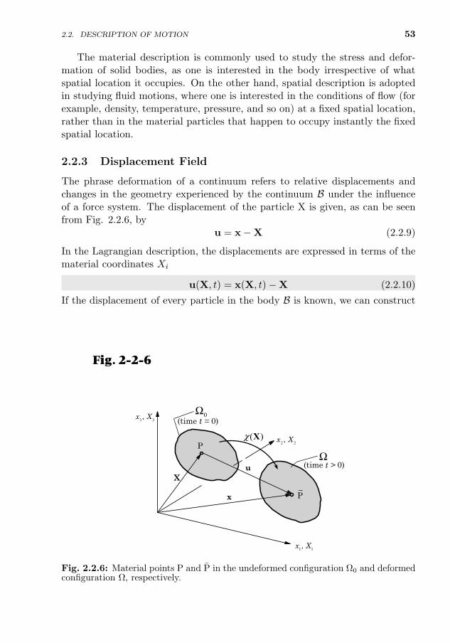
2.2. DESCRIPTION OF MOTION 53
The material description is commonly used to study the stress and defor-mation of solid bodies, as one is interested in the body irrespective of whatspatial location it occupies. On the other hand, spatial description is adoptedin studying fluid motions, where one is interested in the conditions of flow (forexample, density, temperature, pressure, and so on) at a fixed spatial location,rather than in the material particles that happen to occupy instantly the fixedspatial location.
2.2.3 Displacement Field
The phrase deformation of a continuum refers to relative displacements andchanges in the geometry experienced by the continuum B under the influenceof a force system. The displacement of the particle X is given, as can be seenfrom Fig. 2.2.6, by
u = x−X (2.2.9)
In the Lagrangian description, the displacements are expressed in terms of thematerial coordinates Xi
u(X, t) = x(X, t)−X (2.2.10)
If the displacement of every particle in the body B is known, we can constructthe current configuration Ω from the reference configuration Ω0, χ(X) = X +u(X). On the other hand, in the Eulerian description the displacements areexpressed in terms of the spatial coordinates xi
u(x, t) = x−X(x, t) (2.2.11)
P
X
P_
x
u
(time t = 0)
(time t > 0)
( )Xχ
Ω
0Ω3 3,x X
2 2,x X
1 1,x X
Fig. 2-2-6
Fig. 2.2.6: Material points P and P in the undeformed configuration Ω0 and deformedconfiguration Ω, respectively.
54 ELEMENTS OF NONLINEAR CONTINUUM MECHANICS
A rigid-body motion is one in which all material particles of the continuumB undergo the same linear and angular displacements. On the other hand, adeformable body is one in which the material particles can move relative toeach other. Then the deformation of a continuum can be determined only byconsidering the change of distance between any two arbitrary but infinitesimallyclose points of the continuum.
2.3 Analysis of Deformation
2.3.1 Deformation Gradient
One of the key quantities in deformation analysis is the deformation gradient,which gives the relationship of a material line dX before deformation to the linedx (consisting of the same material as dX) after deformation. It is defined as
dx = F · dX = dX · FT, F ≡←−∇0x = (∇0x)T =
(∂x
∂X
)T
(2.3.1)
where ∇0 is the gradient operator with respect to X. The definition of F givenin Eq. (2.3.1) may appear as the transpose of that defined in other books butthese books use backward gradient operator without explicitly stating. We notethat F ≡ (∇0x)T = FiJ ei EJ , whereas ∇0x = EJ
∂xi∂XJ
ei = FiJ EJ ei = FT,and the definition of FiJ used here and in other books is the same.
The inverse relations are given by
dX = F−1 · dx = dx · F−T, where F−1 =
(∂X
∂x
)T
≡ (∇X)T (2.3.2)
and ∇ is the gradient operator with respect to x. In indicial notation, thematrix forms of F and F−1 are
[F ] =
∂x1∂X1
∂x1∂X2
∂x1∂X3
∂x2∂X1
∂x2∂X2
∂x2∂X3
∂x3∂X1
∂x3∂X2
∂x3∂X3
, [F ]−1 =
∂X1∂x1
∂X1∂x2
∂X1∂x3
∂X2∂x1
∂X2∂x2
∂X2∂x3
∂X3∂x1
∂X3∂x2
∂X3∂x3
(2.3.3)
In Eqs. (2.3.2) and (2.3.3), the lower case indices refer to the current (spatial)Cartesian coordinates, whereas upper case indices refer to the reference (ma-terial) Cartesian coordinates. The determinant of F is called the Jacobian ofthe motion, and it is denoted by J = det F. The equation F · dX = 0 fordX 6= 0 implies that a material line in the reference configuration is reduced tozero by the deformation. Since this is physically not realistic, we conclude thatF · dX 6= 0 for dX 6= 0. That is, F is a non-singular tensor, J 6= 0. Hence, Fhas an inverse F−1. The deformation gradient can be expressed in terms of thedisplacement vector as
F = (∇0x)T = (∇0u + I)T or F−1 = (∇X)T = (I−∇u)T (2.3.4)
2.3. ANALYSIS OF DEFORMATION 55
2.3.2 Volume and Surface Elements in the Material andSpatial Descriptions
Here we discuss how deformation mapping affects surface areas and volumes ofa continuum. First, we consider three non-coplanar line elements dX(1), dX(2),and dX(3) forming the edges of a parallelepiped at a point with position vectorX in the reference configuration Ω0 of body B so that
dx(i) = F · dX(i), i = 1, 2, 3 (2.3.5)
Note that the vectors dx(i) are not necessarily parallel to or have the samelength as the vectors dX(i) due to shearing and stretching of the parallelepiped.We assume that the triad (dX(1), dX(2), dX(3)) is positively oriented in the sensethat the triple scalar product dX(1) · dX(2) × dX(3) > 0. The volume of theparallelepiped is
dV = dX(1) · dX(2) × dX(3) =(N1 · N2 × N3
)dX(1) dX(2) dX(3)
= dX(1) dX(2) dX(3) (2.3.6)
where Ni denote the unit vector along dX(i). The corresponding volume in thecurrent deformed configuration Ω is given by
dv = dx(1) · dx(2) × dx(3)
=(F · N1
)·(F · N2
)×(F · N3
)dX(1) dX(2) dX(3)
= det F dX(1) dX(2) dX(3) = J dV (2.3.7)
We assume that the volume elements are positive so that the relative orientationof the line elements is preserved under the deformation, that is, J > 0. Thus, Jhas the physical meaning of being the local ratio of current volume to referencevolume of a material volume element.
Next, we consider an infinitesimal vector element of material surface dA ina neighborhood of the point X in the undeformed configuration. The surfacevector can be expressed as dA = dA N, where N is the positive unit normalto the surface in the reference configuration. Suppose that dA becomes da inthe deformed body, where da = da n, n being the positive unit normal to thesurface in the deformed configuration. The areas of the parallelograms in thetwo configurations are related by (see Problem 2.7)
da = JF−T · dA or n da = JF−T · N dA (2.3.8)
which is known as the Nanson’s formula.The relations in Eqs. (2.3.7) and (2.3.8) are useful in expressing volume and
area integrals defined in the current configuration in terms of the integrals overthe volume and surface elements in the reference configuration.
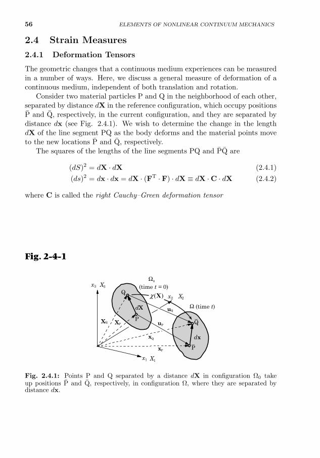
56 ELEMENTS OF NONLINEAR CONTINUUM MECHANICS
2.4 Strain Measures
2.4.1 Deformation Tensors
The geometric changes that a continuous medium experiences can be measuredin a number of ways. Here, we discuss a general measure of deformation of acontinuous medium, independent of both translation and rotation.
Consider two material particles P and Q in the neighborhood of each other,separated by distance dX in the reference configuration, which occupy positionsP and Q, respectively, in the current configuration, and they are separated bydistance dx (see Fig. 2.4.1). We wish to determine the change in the lengthdX of the line segment PQ as the body deforms and the material points moveto the new locations P and Q, respectively.
The squares of the lengths of the line segments PQ and PQ are
(dS)2 = dX · dX (2.4.1)
(ds)2 = dx · dx = dX · (FT · F) · dX ≡ dX ·C · dX (2.4.2)
where C is called the right Cauchy–Green deformation tensor
C = FT · F (2.4.3)
By definition, C is a symmetric second-order tensor. The inverse of C is denotedby B and it is called Piola deformation tensor
B = C−1 = F−1 · F−T (2.4.4)
XQ
Q
P Q_
XP
xP P_
xQ
uQ
uP
3x X3
dx
dX2x X2
1x X1
(time t = 0)
(time t)
( )Xχ
0Ω
Ω
Fig. 2-4-1
Fig. 2.4.1: Points P and Q separated by a distance dX in configuration Ω0 takeup positions P and Q, respectively, in configuration Ω, where they are separated bydistance dx.
2.4. STRAIN MEASURES 57
2.4.2 The Green–Lagrange Strain Tensor
The change in the squared lengths that occurs as a body deforms from thereference to the current configuration can be expressed relative to the originallength as
(ds)2 − (dS)2 = 2 dX ·E · dX (2.4.5)
where E is called the Green–St. Venant (Lagrangian) strain tensor or simplythe Green strain tensor2. The Green strain tensor can be expressed, in view ofEqs. (2.4.1)–(2.4.3), as
E = 12
(FT · F− I
)= 1
2 (C− I) (2.4.6)
= 12
[∇0u + (∇0u)T + (∇0u) · (∇0u)T
](2.4.7)
By definition, the Green strain tensor is a symmetric second-order tensor. Also,the change in the squared lengths is zero if and only if E = 0.
The vector form of the Green strain tensor in Eq. (2.4.7) allows us to ex-press it in terms of its components in any coordinate system. In particular,in rectangular Cartesian coordinate system (X1, X2, X3), the components of Eand C are given by
EIJ =1
2
(∂uI∂XJ
+∂uJ∂XI
+∂uK∂XI
∂uK∂XJ
)CIJ =
∂xk∂XI
∂xk∂XJ
(2.4.8)
where sum on repeated indices is implied.In expanded notation, the components of E are given by
E11 =∂u1
∂X1+
1
2
[(∂u1
∂X1
)2
+
(∂u2
∂X1
)2
+
(∂u3
∂X1
)2]E22 =
∂u2
∂X2+
1
2
[(∂u1
∂X2
)2
+
(∂u2
∂X2
)2
+
(∂u3
∂X2
)2]E33 =
∂u3
∂X3+
1
2
[(∂u1
∂X3
)2
+
(∂u2
∂X3
)2
+
(∂u3
∂X3
)2](2.4.9)
E12 =1
2
(∂u1
∂X2+∂u2
∂X1+∂u1
∂X1
∂u1
∂X2+∂u2
∂X1
∂u2
∂X2+∂u3
∂X1
∂u3
∂X2
)E13 =
1
2
(∂u1
∂X3+∂u3
∂X1+∂u1
∂X1
∂u1
∂X3+∂u2
∂X1
∂u2
∂X3+∂u3
∂X1
∂u3
∂X3
)E23 =
1
2
(∂u2
∂X3+∂u3
∂X2+∂u1
∂X2
∂u1
∂X3+∂u2
∂X2
∂u2
∂X3+∂u3
∂X2
∂u3
∂X3
)Note that both C and E are material strain tensors.2The reader should distinguish between the symbol E used for the Lagrangian strain tensorand Ei used for the basis vectors in the reference configuration.
58 ELEMENTS OF NONLINEAR CONTINUUM MECHANICS
2.4.3 The Cauchy and Euler Strain Tensors
Returning to the strain measures, the change in the squared lengths that oc-curs as the body deforms from the initial to the current configuration can beexpressed relative to the current length. First, we express dS in terms of dx as
(dS)2 = dX · dX = dx · (F−T · F−1) · dx ≡ dx · b−1 · dx (2.4.10)
where b is called the left Cauchy–Green strain tensor
b = F · FT (2.4.11)
The tensor b is sometimes referred to as the Finger deformation tensor, whichis a symmetric second-order tensor in spatial coordinates.
Now the change in the squares of the lengths can be expressed in the currentcoordinates (i.e. spatial description) as
(ds)2 − (dS)2 = 2 dx · e · dx (2.4.12)
where e, called the Euler–Almansi strain tensor or the Euler strain tensor, is
e = 12
(I− F−T · F−1
)= 1
2
(I− b−1
)(2.4.13)
= 12
[∇u + (∇u)T − (∇u) · (∇u)T
](2.4.14)
The rectangular Cartesian components of e are given by
eij = 12
(δij −
∂XK
∂xi
∂XK
∂xj
)= 1
2
(∂ui∂xj
+∂uj∂xi− ∂uk∂xi
∂uk∂xj
)(2.4.15)
Note that b and e are spatial strain tensors.The transformations between spatial and material fields are often called
push-forward operations and pull-back operations. For example, a push-forwardoperation transforms a field expressed in a reference configuration Ω0 to thecurrent configuration Ω. A pull-back is an inverse operation, where a field inthe current configuration Ω is transformed to the reference configuration Ω0.As a specific example, consider the push-forward operation between e and E:
e = 12
(I− F−T · F−1
)= 1
2F−T · FT ·(I− F−T · F−1
)· F · F−1
= 12F−T ·
(FT · F− I
)· F−1 = F−T ·E · F−1 (2.4.16)
The pull-back operation gives
E = FT · e · F (2.4.17)
2.4. STRAIN MEASURES 59
2.4.4 Infinitesimal Strain Tensor and Rotation Tensor
2.4.4.1 Infinitesimal strain tensor
When all displacements gradients are small, that is, |∇0u| << 1, we can neglectthe nonlinear terms in the definition of the Green–Lagrange strain tensor Edefined in Eq. (2.4.7). In order to derive the infinitesimal strain tensor fromE, we must linearize E by using a measure of smallness. We introduce thenonnegative function
ε(t) = ‖∇0u‖∞ = supX∈Ω|∇0u|
where “sup” stands for supremum or the least upper bound of the set of allabsolute values of ∇0u defined for all X ∈ Ω.
If E is of the order O(ε) in ∇0u, then we mean
∂uI∂XJ
= O(ε) as ε→ 0
If terms of the order O(ε2) as ε → 0 can be omitted in E, then EIJ can beapproximated as
EIJ ≈ 12
(∂uI∂XJ
+∂uJ∂XI
)= O(ε) as ε→ 0
Thus, it is immaterial whether the partial derivative of the displacement fieldu is taken with respect to xj or Xj so that ∂ui
∂xj= ∂ui
∂Xj; that is, |∇u| ≈ |∇0u| =
O(ε). In other words, in the case of infinitesimal strains, no distinction is madebetween the material coordinates X and the spatial coordinates x, and it is notnecessary to distinguish between the Green–Lagrange strain tensor E and theEulerian strain tensor e. The infinitesimal strain tensor is denoted by ε, andit is defined as
E ≈ ε = 12
[∇0u + (∇0u)T
](2.4.18)
The rectangular Cartesian components of the infinitesimal strain tensor aregiven by
εij = 12
(∂ui∂Xj
+∂uj∂Xi
)(2.4.19)
or, in expanded form:
ε11 =∂u1
∂X1, ε22 =
∂u2
∂X2, ε12 = 1
2
(∂u1
∂X2+∂u2
∂X1
)ε33 =
∂u3
∂X3, ε13 = 1
2
(∂u1
∂X3+∂u3
∂X1
), ε23 = 1
2
(∂u2
∂X3+∂u3
∂X2
) (2.4.20)
The strain components ε11, ε22, and ε33 are the infinitesimal normal strains andε12, ε13, and ε23 are the infinitesimal shear strains. The shear strains 2ε12 = γ12,2ε13 = γ13, and 2ε23 = γ23 are called the engineering shear strains.
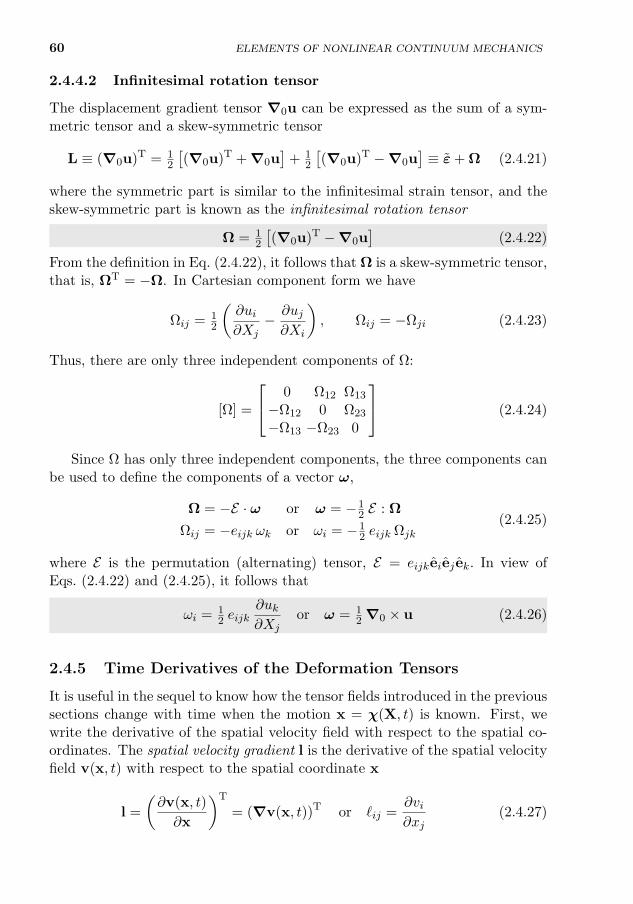
60 ELEMENTS OF NONLINEAR CONTINUUM MECHANICS
2.4.4.2 Infinitesimal rotation tensor
The displacement gradient tensor ∇0u can be expressed as the sum of a sym-metric tensor and a skew-symmetric tensor
L ≡ (∇0u)T = 12
[(∇0u)T + ∇0u
]+ 1
2
[(∇0u)T −∇0u
]≡ ε+ Ω (2.4.21)
where the symmetric part is similar to the infinitesimal strain tensor, and theskew-symmetric part is known as the infinitesimal rotation tensor
Ω = 12
[(∇0u)T −∇0u
](2.4.22)
From the definition in Eq. (2.4.22), it follows that Ω is a skew-symmetric tensor,that is, ΩT = −Ω. In Cartesian component form we have
Ωij = 12
(∂ui∂Xj
− ∂uj∂Xi
), Ωij = −Ωji (2.4.23)
Thus, there are only three independent components of Ω:
[Ω] =
0 Ω12 Ω13
−Ω12 0 Ω23
−Ω13 −Ω23 0
(2.4.24)
Since Ω has only three independent components, the three components canbe used to define the components of a vector ω,
Ω = −E · ω or ω = −12 E : Ω
Ωij = −eijk ωk or ωi = −12 eijk Ωjk
(2.4.25)
where E is the permutation (alternating) tensor, E = eijkeiej ek. In view ofEqs. (2.4.22) and (2.4.25), it follows that
ωi = 12 eijk
∂uk∂Xj
or ω = 12 ∇0 × u (2.4.26)
2.4.5 Time Derivatives of the Deformation Tensors
It is useful in the sequel to know how the tensor fields introduced in the previoussections change with time when the motion x = χ(X, t) is known. First, wewrite the derivative of the spatial velocity field with respect to the spatial co-ordinates. The spatial velocity gradient l is the derivative of the spatial velocityfield v(x, t) with respect to the spatial coordinate x
l =
(∂v(x, t)
∂x
)T
= (∇v(x, t))T or `ij =∂vi∂xj
(2.4.27)
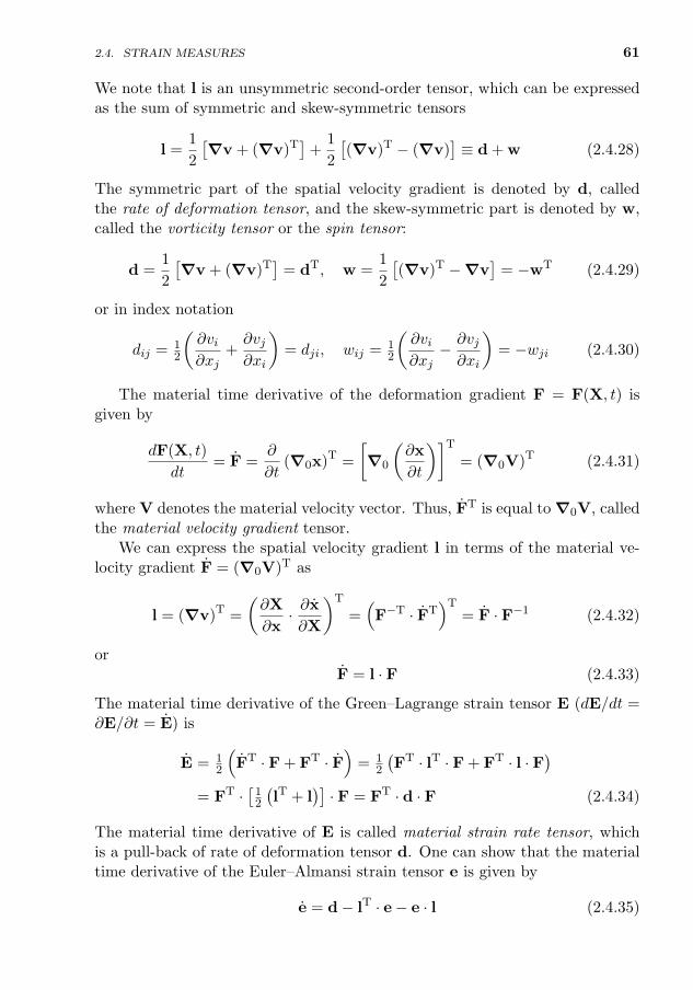
2.4. STRAIN MEASURES 61
We note that l is an unsymmetric second-order tensor, which can be expressedas the sum of symmetric and skew-symmetric tensors
l =1
2
[∇v + (∇v)T
]+
1
2
[(∇v)T − (∇v)
]≡ d + w (2.4.28)
The symmetric part of the spatial velocity gradient is denoted by d, calledthe rate of deformation tensor, and the skew-symmetric part is denoted by w,called the vorticity tensor or the spin tensor:
d =1
2
[∇v + (∇v)T
]= dT, w =
1
2
[(∇v)T −∇v
]= −wT (2.4.29)
or in index notation
dij = 12
(∂vi∂xj
+∂vj∂xi
)= dji, wij = 1
2
(∂vi∂xj− ∂vj∂xi
)= −wji (2.4.30)
The material time derivative of the deformation gradient F = F(X, t) isgiven by
dF(X, t)
dt= F =
∂
∂t(∇0x)T =
[∇0
(∂x
∂t
)]T
= (∇0V)T (2.4.31)
where V denotes the material velocity vector. Thus, FT is equal to ∇0V, calledthe material velocity gradient tensor.
We can express the spatial velocity gradient l in terms of the material ve-locity gradient F = (∇0V)T as
l = (∇v)T =
(∂X
∂x· ∂x
∂X
)T
=(F−T · FT
)T= F · F−1 (2.4.32)
orF = l · F (2.4.33)
The material time derivative of the Green–Lagrange strain tensor E (dE/dt =∂E/∂t = E) is
E = 12
(FT · F + FT · F
)= 1
2
(FT · lT · F + FT · l · F
)= FT ·
[12
(lT + l
)]· F = FT · d · F (2.4.34)
The material time derivative of E is called material strain rate tensor, whichis a pull-back of rate of deformation tensor d. One can show that the materialtime derivative of the Euler–Almansi strain tensor e is given by
e = d− lT · e− e · l (2.4.35)
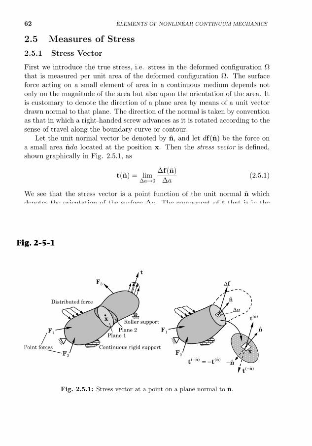
62 ELEMENTS OF NONLINEAR CONTINUUM MECHANICS
2.5 Measures of Stress
2.5.1 Stress Vector
First we introduce the true stress, i.e. stress in the deformed configuration Ωthat is measured per unit area of the deformed configuration Ω. The surfaceforce acting on a small element of area in a continuous medium depends notonly on the magnitude of the area but also upon the orientation of the area. Itis customary to denote the direction of a plane area by means of a unit vectordrawn normal to that plane. The direction of the normal is taken by conventionas that in which a right-handed screw advances as it is rotated according to thesense of travel along the boundary curve or contour.
Let the unit normal vector be denoted by n, and let df(n) be the force ona small area nda located at the position x. Then the stress vector is defined,shown graphically in Fig. 2.5.1, as
t(n) = lim∆a→0
∆f(n)
∆a(2.5.1)
We see that the stress vector is a point function of the unit normal n whichdenotes the orientation of the surface ∆a. The component of t that is in thedirection of n, (t · n)n, is called the normal stress vector. The component of tthat is normal to n, but lies in the plane of t and n, is called the shear stress.Because of Newton’s third law for action and reaction, we see that
t(−n) = −t(n)
F1
F2)ˆ()ˆ( nn tt −=−
)ˆ(nt
n
•
nt ˆ( )−n−
Roller support
Plane 1 Plane 2F1
F2
F3
Point forces
Distributed force
•
t
Δf
Δa
n
••
Continuous rigid support
x
x
Fig. 2-5-1
Fig. 2.5.1: Stress vector at a point on a plane normal to n.
2.5. MEASURES OF STRESS 63
2.5.2 Cauchy’s Formula and Stress Tensor
To establish the relationship between t and n we set up an infinitesimal tetra-hedron in Cartesian coordinates, as shown in Fig. 2.5.2. If −t1,−t2,−t3, and tdenote the stress vectors in the outward directions on the faces of the infinitesi-mal tetrahedron whose areas are ∆a1, ∆a2, ∆a3, and ∆a, respectively, we haveby Newton’s second law for the mass inside the tetrahedron,
t ∆a− t1 ∆a1 − t2 ∆a2 − t3 ∆a3 + ρ∆v f = ρ∆v a (2.5.2)
where ∆v is the volume of the tetrahedron, ρ the density, f the body force perunit mass, and a the acceleration. Since the total vector area of a closed surfaceis zero, we have
∆a n−∆a1 e1 −∆a2 e2 −∆a3 e3 = 0 (2.5.3)
It follows that
∆ai = (n · ei)∆a = (ei · n)∆a for i = 1, 2, 3 (2.5.4)
(b)
x1
x3
x21e 2e3e aΔ
2aΔ
1aΔ
3aΔ
nnt ˆ( )
t t( 3)3
− = −
t t( 1)1
− = −
t t( 2)2
− = −
3ˆ-e
e- 2
e- 1
•
F1
(a)
F2
F3 t
tt
1x
2x
3x
t2
t1
t3
nn
n
Interior of the body
On the boundary
Fig. 2-5-2
Fig. 2.5.2: Tetrahedral element in Cartesian coordinates.
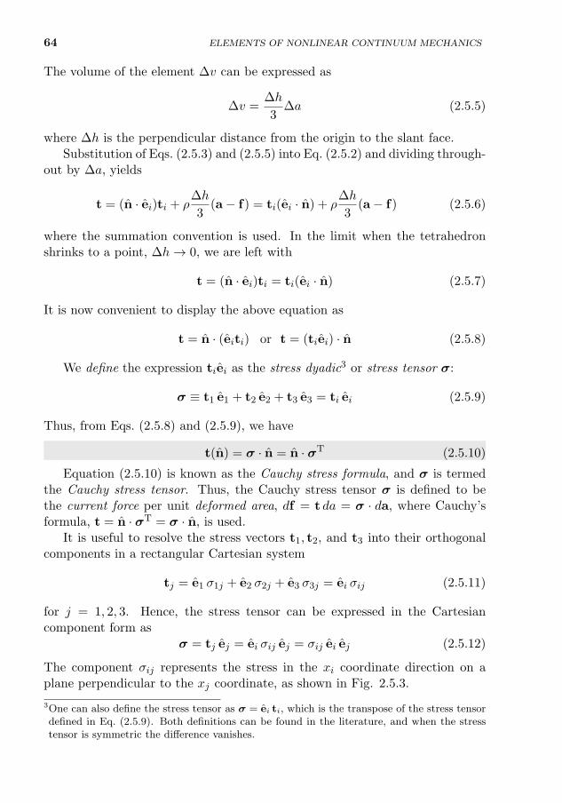
64 ELEMENTS OF NONLINEAR CONTINUUM MECHANICS
The volume of the element ∆v can be expressed as
∆v =∆h
3∆a (2.5.5)
where ∆h is the perpendicular distance from the origin to the slant face.Substitution of Eqs. (2.5.3) and (2.5.5) into Eq. (2.5.2) and dividing through-
out by ∆a, yields
t = (n · ei)ti + ρ∆h
3(a− f) = ti(ei · n) + ρ
∆h
3(a− f) (2.5.6)
where the summation convention is used. In the limit when the tetrahedronshrinks to a point, ∆h→ 0, we are left with
t = (n · ei)ti = ti(ei · n) (2.5.7)
It is now convenient to display the above equation as
t = n · (eiti) or t = (tiei) · n (2.5.8)
We define the expression tiei as the stress dyadic3 or stress tensor σ:
σ ≡ t1 e1 + t2 e2 + t3 e3 = ti ei (2.5.9)
Thus, from Eqs. (2.5.8) and (2.5.9), we have
t(n) = σ · n = n · σT (2.5.10)
Equation (2.5.10) is known as the Cauchy stress formula, and σ is termedthe Cauchy stress tensor. Thus, the Cauchy stress tensor σ is defined to bethe current force per unit deformed area, df = t da = σ · da, where Cauchy’sformula, t = n · σT = σ · n, is used.
It is useful to resolve the stress vectors t1, t2, and t3 into their orthogonalcomponents in a rectangular Cartesian system
tj = e1 σ1j + e2 σ2j + e3 σ3j = ei σij (2.5.11)
for j = 1, 2, 3. Hence, the stress tensor can be expressed in the Cartesiancomponent form as
σ = tj ej = ei σij ej = σij ei ej (2.5.12)
The component σij represents the stress in the xi coordinate direction on aplane perpendicular to the xj coordinate, as shown in Fig. 2.5.3.
3One can also define the stress tensor as σ = ei ti, which is the transpose of the stress tensordefined in Eq. (2.5.9). Both definitions can be found in the literature, and when the stresstensor is symmetric the difference vanishes.
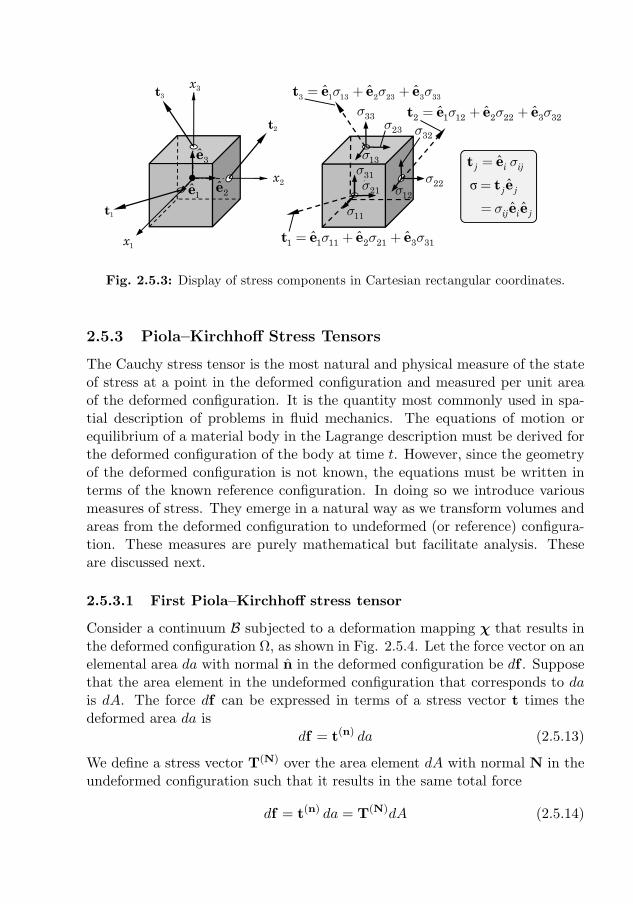
2.5. MEASURES OF STRESS 65
t3
t2
t1
1x
2x
3x
σ
ˆ
ˆ
ˆ ˆ
j i ij
j j
ij i j
s
s
=
=
=
t et e
e e12s
s22
32ss33
23s
13s
s11
21s31s
t e e e2 1 12 2 22 3 32ˆ ˆ ˆ= + +s s s
t e e e1 1 11 2 21 3 31ˆ ˆ ˆ= + +s s s
3 1 13 2 23 3 33ˆ ˆ ˆs s s= + +t e e e
1e
3e
2e
Fig. 2.5.3: Display of stress components in Cartesian rectangular coordinates.
2.5.3 Piola–Kirchhoff Stress Tensors
The Cauchy stress tensor is the most natural and physical measure of the stateof stress at a point in the deformed configuration and measured per unit areaof the deformed configuration. It is the quantity most commonly used in spa-tial description of problems in fluid mechanics. The equations of motion orequilibrium of a material body in the Lagrange description must be derived forthe deformed configuration of the body at time t. However, since the geometryof the deformed configuration is not known, the equations must be written interms of the known reference configuration. In doing so we introduce variousmeasures of stress. They emerge in a natural way as we transform volumes andareas from the deformed configuration to undeformed (or reference) configura-tion. These measures are purely mathematical but facilitate analysis. Theseare discussed next.
2.5.3.1 First Piola–Kirchhoff stress tensor
Consider a continuum B subjected to a deformation mapping χ that results inthe deformed configuration Ω, as shown in Fig. 2.5.4. Let the force vector on anelemental area da with normal n in the deformed configuration be df . Supposethat the area element in the undeformed configuration that corresponds to dais dA. The force df can be expressed in terms of a stress vector t times thedeformed area da is
df = t(n) da (2.5.13)
We define a stress vector T(N) over the area element dA with normal N in theundeformed configuration such that it results in the same total force
df = t(n) da = T(N)dA (2.5.14)
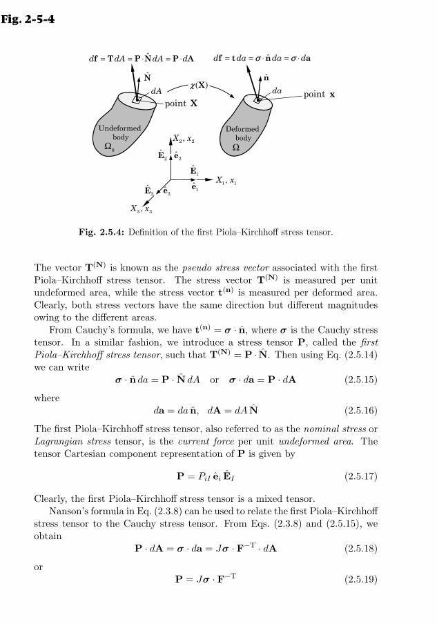
66 ELEMENTS OF NONLINEAR CONTINUUM MECHANICS
1 1,X x
2 2,X x
3 3,X x
e3ˆ e1ˆ
E1ˆ
E3ˆ
e2ˆE2ˆ
NdA
f t n aˆd da da d= = ⋅ = ⋅σ σf T P N P Aˆd dA dA d= = ⋅ = ⋅
nda
X( )χ
Undeformed body
Deformed body
point x•• point X
0Ω Ω
Fig. 2-5-4
Fig. 2.5.4: Definition of the first Piola–Kirchhoff stress tensor.
The vector T(N) is known as the pseudo stress vector associated with the firstPiola–Kirchhoff stress tensor. The stress vector T(N) is measured per unitundeformed area, while the stress vector t(n) is measured per deformed area.Clearly, both stress vectors have the same direction but different magnitudesowing to the different areas.
From Cauchy’s formula, we have t(n) = σ · n, where σ is the Cauchy stresstensor. In a similar fashion, we introduce a stress tensor P, called the firstPiola–Kirchhoff stress tensor, such that T(N) = P · N. Then using Eq. (2.5.14)we can write
σ · n da = P · N dA or σ · da = P · dA (2.5.15)
whereda = da n, dA = dA N (2.5.16)
The first Piola–Kirchhoff stress tensor, also referred to as the nominal stress orLagrangian stress tensor, is the current force per unit undeformed area. Thetensor Cartesian component representation of P is given by
P = PiI ei EI (2.5.17)
Clearly, the first Piola–Kirchhoff stress tensor is a mixed tensor.Nanson’s formula in Eq. (2.3.8) can be used to relate the first Piola–Kirchhoff
stress tensor to the Cauchy stress tensor. From Eqs. (2.3.8) and (2.5.15), weobtain
P · dA = σ · da = Jσ · F−T · dA (2.5.18)
orP = Jσ · F−T (2.5.19)
2.6. MATERIAL FRAME INDIFFERENCE 67
where J is the Jacobian. In general, the first Piola–Kirchhoff stress tensor P isunsymmetric even when the Cauchy stress tensor σ is symmetric.
2.5.3.2 Second Piola–Kirchhoff stress tensor
The second Piola–Kirchhoff stress tensor S, which is used in the study of largedeformation analysis, is introduced as the stress tensor associated with the forcedF in the undeformed elemental area dA that corresponds to the force df onthe deformed elemental area da
dF = S · dA (2.5.20)
Thus, the second Piola–Kirchhoff stress tensor gives the transformed currentforce per unit undeformed area.
Similar to the relationship between dx and dX, dX = F−1 · dx, the force dfon the deformed elemental area da is related to the force dF on the undeformedelemental area dA
dF = F−1 · df = F−1 · (P · dA) = S · dA (2.5.21)
Hence, the second Piola–Kirchhoff stress tensor is related to the first Piola–Kirchhoff stress tensor and Cauchy stress tensor according to the equations
S = F−1 ·P = JF−1 · σ · F−T (2.5.22)
Clearly, S is symmetric whenever σ is symmetric. Cartesian component repre-sentation of S is
S = SIJ EIEJ (2.5.23)
We can introduce the pseudo stress vector T associated with the second Piola–Kirchhoff stress tensor by
dF = T dA = S · N dA = S · dA (2.5.24)
2.6 Material Frame Indifference
2.6.1 The Basic Idea
In the analytical description of physical events, the following two requirementsmust be followed:
1. Invariance of the equations with respect to stationary coordinate framesof reference.
2. Invariance of the equations with respect to frames of reference that movein arbitrary relative motion.
68 ELEMENTS OF NONLINEAR CONTINUUM MECHANICS
The first requirement is readily met by expressing the equations in vector/tensorform, which is invariant. The assertion that an equation is in “invariant form”refers to the vector form that is independent of the choice of a coordinatesystem. The coordinate systems used in the present study were assumed to berelatively at rest. The second requirement is that the invariance property holdsfor reference frames (or observers) moving arbitrarily with respect to each other.This requirement is dictated by the need for forces to be the same as measuredby all observers irrespective of their relative motions. The concept of frames ofreference should not be confused with that of coordinate systems, as they arenot the same at all. A given observer is free to choose any coordinate system asmay be convenient to observe or analyze the system response. Invariance withrespect to changes of observer is termed material frame indifference or materialobjectivity. In general, if a quantity is objective, then it is independent of anobserver.
A detailed discussion of frame indifference is outside the scope of the presentstudy, and only a brief discussion is presented here. Let F denote a referenceframe with origin at O in which x is the current position of a particular particleat time t. Let F∗ be another reference frame with origin at O∗ with timedenoted with t∗. Let φ be a scalar field when described in the frame F and φ∗
is the same scalar field described with respect to the frame F∗, and let (u,u∗)and (S,S∗) be the vector and tensor fields in the two frames. Scalar, vector, andtensor fields are called frame indifferent or objective if they transform accordingto the following equations:
1. Events x∗ = c(t) + Q(t) · x, t∗ = t− a2. Scalar field φ∗(x∗, t∗) = φ(x, t)3. Displacement vector u∗(x∗, t∗) = Q(t) · u(x, t) (2.6.1)
4. General second-order tensors S∗(x∗, t∗) = Q(t) · S(x, t) ·QT(t)5. Two-point second-order tensors F∗(x∗, t∗) = Q(t) · F(x, t)
where Q(t) is a proper orthogonal tensor that rotates frame F∗ into frame F ,c(t) is a vector from O to O∗ that only depends on time t, and a is a constant.For example, x and x∗ refer to the same motion, but mathematically x∗ is themotion obtained from x by superposition of a rigid rotation and translation.The mapping x∗ = c(t) + Q(t) · x may be interpreted as one that takes (x, t)to (x∗, t∗) as a change of observer from O to O∗, so that the event which isobserved at place x at time t by observer O is the same event as that observedat place x∗ at time t∗ by observer O∗, where t∗ = t − a, and a is a constant.Thus, a change of observer merely changes the description of an event. In short,the objectivity insures that the direction(s) and magnitude are independent ofthe coordinate frame used to describe them.
2.6. MATERIAL FRAME INDIFFERENCE 69
2.6.2 Objectivity of Strains and Strain Rates
Under the following general rigid body mapping
x∗(X, t∗) = c(t) + Q(t) · x, t∗ = t− a (2.6.2)
between observer O and observer O∗ (if the reference configuration is indepen-dent of the observer) the right Cauchy–Green deformation tensor C and theGreen–Lagrange strain tensor E change as follows:
C∗ = (F∗)T · F∗ =(FT ·QT
)·(Q · F
)= FT · F = C (2.6.3)
where the property QT · Q = I of an orthogonal matrix Q is used. Hence,by definition, the Green–Lagrange strain tensor E and the right Cauchy–Greendeformation tensor C, being defined with respect to the reference configuration,are unaffected by the superposed rigid-body motion:
E = E∗, C = C∗ (2.6.4)
However, the velocities and accelerations of a material point are affected by thesuperposed rigid-body motion. For example, consider velocity after imposingthe rigid-body motion (note that dt/dt∗ = 1)
v∗(x∗, t∗) =dx∗
dt∗=
d
dt∗(c(t) + Q(t) · x) = c(t) + Q(t) · x + Q(t) · v (2.6.5)
which shows that v∗ and v are not the same, but one can be calculated fromthe other when c and Q are known for the superposed rigid-body motion.
In addition, the symmetric part of l (or lT), namely, d is also objective inthe sense
d∗ = Q · d ·QT (2.6.6)
We have noted that the two observers’ view of the velocity and acceleration ofa given motion are different, even though the rate of change at fixed X is thesame in each case. Thus, velocity and acceleration vectors are not objective.
2.6.3 Objectivity of Stress Tensors
2.6.3.1 Cauchy stress tensor
The Cauchy stress tensor is objective if we can show that σ∗ = Q · σ ·QT [seeEq. (2.6.1) for the definition of the objectivity of various order tensors]. Webegin with the relations
t = σ · n, t∗ = σ∗ · n∗; t∗ = Q · t, n∗ = Q · n (2.6.7)
Then
t∗ = σ∗ · n∗ = σ∗ · (Q · n),
70 ELEMENTS OF NONLINEAR CONTINUUM MECHANICS
t∗ = Q · t = Q · σ · n (2.6.8)
Then, we haveσ∗ ·Q = Q · σ
from which it follows thatσ∗ = Q · σ ·QT (2.6.9)
Thus, the Cauchy stress tensor is objective.
2.6.3.2 First Piola–Kirchhoff stress tensor
Since the first Piola–Kirchhoff stress tensor P is a two-point tensor, it trans-forms like the other two-point tensor F. To establish this, we begin with therelation between P and σ after superposed rigid-body motion and make use ofthe relations F∗ = Q · F and J∗ = J ,
P∗ = J∗ σ∗ · (F∗)−T = J(Q · σ ·QT) · (Q · F)−T
= J Q · σ · (QT ·Q−T) · F−T = J Q · σ · F−T = Q ·P (2.6.10)
Thus P, being a two-point tensor, transforms like vector under superposedrigid-body motion, and hence is objective.
2.6.3.3 Second Piola–Kirchhoff stress tensor
The second Piola–Kirchhoff stress tensor S is the stress tensor of choice inthe study of solid mechanics. Since it is defined with respect to the referenceconfiguration, rigid-body motion should not alter it. Using the relations F∗ =Q · F and σ∗ = Q · σ ·QT, we obtain
S∗ = J∗ (F∗)−1 · σ∗ · (F∗)−T = J (F−1 ·Q−1) · (Q · σ ·QT) · (Q−T · F−T)= J F−1 · σ · F−T = S (2.6.11)
Thus, S is not affected by the superposed rigid-body motion and, therefore, itis objective.
2.7 Equations of Continuum Mechanics
2.7.1 Introduction
This section is devoted to a review of the conservation principles and balancelaws of physics in analytical terms. The laws of physics that we consider are: (1)the principle of conservation of mass, (2) the balance of linear momentum, (3)the balance of angular momentum, and (4) the balance of energy. The equationsresulting from these principles are outlined here. For additional details, readermay consult the continuum mechanics text by the author [1].
2.7. EQUATIONS OF CONTINUUM MECHANICS 71
2.7.2 Conservation of Mass
The principle of conservation of mass can be stated as: the total mass of anypart of the body does not change in any motion. The mathematical form of thisprinciple is different in different descriptions of motion. The equation result-ing from the principle of conservation of mass is also known as the continuityequation.
2.7.2.1 Spatial form of the continuity equation
First we derive the equation resulting from the principle of conservation ofmass in the spatial description. Let each element of mass in the medium movewith the velocity v(x, t) and consider a spatial region Ω such that the boundingsurface Γ is attached to a fixed set of material elements. Then each point of thissurface moves itself with the material velocity, and the region Ω thus containsa fixed mass since no mass crosses the boundary surface Γ. The time rate ofchange of an integral of a function φ(x, t) over this material region is the sum ofthe integral of the instantaneous change of φ with time and the rate of outflowof φ through the surface:
d
dt
∫Ωφ(x, t) dv =
∫Ω
∂φ
∂tdv +
∮Γφv · n ds (2.7.1)
which holds for a material region, that is, a region of fixed total mass.Let ρ(x, t) denote the mass density of a continuous region Ω with closed
boundary Γ. Then the principle of conservation of mass for a fixed materialregion requires that
0 =d
dt
∫Ωρ dv ≡
∫Ω
∂ρ
∂tdv +
∮Γρv · n ds (2.7.2)
where Eq. (2.7.1) with φ = ρ is used in arriving at the last statement. Con-verting the surface integral in Eq. (2.7.2) to a volume integral by means of thedivergence theorem, we obtain∫
Ω
[∂ρ
∂t+ div(ρv)
]dv = 0 (2.7.3)
Since this integral vanishes, for a continuous medium, for any arbitrary region Ω,we deduce that this can be true only if the integrand itself vanishes identically,giving the following local (i.e. point-wise) form:
∂ρ
∂t+ div(ρv) = 0 (2.7.4)
This equation, called the continuity equation, expresses local conservation ofmass at any point in a continuous medium.
72 ELEMENTS OF NONLINEAR CONTINUUM MECHANICS
2.7.2.2 Material form of the continuity equation
Next, we derive the continuity equation in the material description. Considera material body B that occupies configuration Ω0 with density ρ0(X, t). Thesame material body occupies the configuration Ω under the action of externalforces, and it has a density ρ(x, t). Then the principle of conservation of massgives ∫
Ω0
ρ0 dV =
∫Ωρ dv (2.7.5)
Using the relation (2.3.7) between the volume elements of the body in the un-deformed and deformed configurations, dv = J dV , where J is the determinantof the deformation gradient F, we arrive at∫
Ω0
(ρ0 − Jρ) dV = 0 (2.7.6)
This is the global form of the continuity equation in the material description.Since the material volume Ω0 we selected is arbitrarily small, as we shrink thevolume to a point, we obtain the local form of the continuity equation
ρ0 = Jρ (2.7.7)
2.7.3 Reynolds Transport Theorem
The material derivative operator d/dt corresponds to changes with respect toa fixed mass, that is, ρ dv is constant with respect to this operator. Therefore,from Eq. (2.7.1) it follows that, for φ = ρQ(x, t), the result
d
dt
∫ΩρQdv =
∂
∂t
∫ΩρQdv +
∮ΓρQv · n ds (2.7.8)
or
d
dt
∫ΩρQdv =
∫Ω
[ρ∂Q
∂t+Q
∂ρ
∂t+ ∇ · (ρQv)
]dv
=
∫Ω
[ρ
(∂Q
∂t+ v ·∇Q
)+Q
(∂ρ
∂t+ ∇ · (ρv)
)]dv (2.7.9)
and using the continuity equation, Eq. (2.7.3), and the definition of the materialtime derivative, we arrive at the result
d
dt
∫ΩρQdv =
∫ΩρdQ
dtdv (2.7.10)
Equation (2.7.10) is known as the Reynolds transport theorem.
2.7. EQUATIONS OF CONTINUUM MECHANICS 73
2.7.4 Balance of Linear Momentum
The principle of balance of linear momentum (i.e. mass times velocity) appliedto a given mass of a medium B, instantaneously occupying a region Ω withbounding surface Γ, can be stated as: the time rate of change of linear mo-mentum be equal to sum of forces acting on the body. The principle results inequations of motion governing a continuum.
2.7.4.1 Spatial form of the equations of motion
Let f be the body force per unit volume and t be the surface force per unit area.Consider an elemental volume dv inside Ω. The body force of the elementalvolume dv is equal to dv f and the surface force on an elemental surface ds ist ds. Then the principle of balance of linear momentum requires that
d
dt
∫Ωρv dv =
∮Γ
t ds+
∫Ω
f dv =
∫Ω
(∇ · σT + f
)dv (2.7.11)
where v is the velocity vector, and the stress vector t is expressed in terms ofthe stress tensor σ by Cauchy’s formula in Eq. (2.5.10) and the divergence the-orem is used in arriving at the final expression. Using the Reynolds TransportTheorem, Eq. (2.7.10), we arrive at
0 =
∫Ω
(∇ · σT + f − ρdv
dt
)dv (2.7.12)
which is the global form of the equation of motion. The local form is given by
∇ · σT + f = ρdv
dt(2.7.13)
or
∇ · σT + f = ρ
(∂v
∂t+ v ·∇v
)(2.7.14)
In Cartesian rectangular system, we have
∂σij∂xj
+ fi = ρ
(∂vi∂t
+ vj∂vi∂xj
)(2.7.15)
Equations (2.7.13)–(2.7.15) are valid in the current configuration, Ω.
2.7.4.2 Material form of the equations of motion
To express the spatial form of the equation of motion, Eq. (2.7.13), in ma-terial description, we rewrite Eq. (2.7.12) in the reference configuration usingappropriate transformations. The following relations hold:
dv = J dV, Jρdv
dt= ρ0
∂v
∂t,
∫Ω∇ · σT dv =
∫Ω0
∇0 ·PT dV (2.7.16)
74 ELEMENTS OF NONLINEAR CONTINUUM MECHANICS
Substitution of the above relations into Eq. (2.7.12), we arrive at
0 =
∫Ω0
(∇0 ·PT + f0 − ρ0
∂V
∂t
)dV
wheref0 = J f (2.7.17)
and V(X, t) = v(x, t) is the material velocity field. Thus, the local form of theequation of motion in terms of the first Piola–Kirchhoff stress tensor P in thematerial description is given by
∇0 ·PT + f0 = ρ0∂V
∂t, X ∈ Ω0 (2.7.18)
The local form of the equation of motion in terms of the second Piola–Kirchhoffstress tensor S in the material description is given by [PT = (F·S)T = ST ·FT]
∇0 ·(ST · FT
)+ f0 = ρ0
∂V
∂t, X ∈ Ω0 (2.7.19)
2.7.5 Balance of Angular Momentum
The principle of balance of angular momentum can be stated as: the time rateof change of the total moment of momentum for a continuum is equal to vectorsum of the moments of external forces acting on the continuum. The principleyields, in the absence of body couples, symmetry of the Cauchy stress tensor.A continuum said to have no body couples (that is volume-dependent couplesM) if lim∆V→0 ∆M/∆V = 0 holds.
The principle of balance of angular momentum can be expressed analyticallyas ∮
Γx× t ds+
∫Ω
x× f dv =d
dt
∫Ω
x× ρv dv (2.7.20)
which yields, in view of the equations of motion, Eq. (2.7.13), the symmetry ofthe Cauchy stress tensor
σ = σT or σij = σji (2.7.21)
2.7.6 Thermodynamic Principles
There are two laws of thermodynamics. The first law of thermodynamics can bestated as: the time rate of the total energy is equal to the sum of the rate of workdone by the external forces and the change of heat content per unit mass. Thesecond law of thermodynamics provides a restriction on the inter-convertibilityof energies (e.g. thermal to mechanical). In this section, a simple form of theenergy equation is derived and the second law is only briefly discussed. Foradditional details, the reader may consult [1].
2.7. EQUATIONS OF CONTINUUM MECHANICS 75
2.7.6.1 Energy equation in the spatial description
The first law of thermodynamics for a system occupying the domain (controlvolume) Ω can be expressed as
d
dt
∫Ωρε dv = Wnet +Hnet (2.7.22)
where ε is the total energy stored per unit mass, Wnet is the net rate of worktransferred into the system, and Hnet is the net rate of heat transfer into thesystem. The total stored energy per unit mass ε consists of the internal energy(sum of all microscopic forms of energy) per unit mass ec and the kinetic energyper unit mass v2/2
ε = ec + 12(v · v) (2.7.23)
The power input, in the nonpolar case (i.e. for a continuum without bodycouples), consists of the rate of work done by external surface tractions t perunit area and body forces f per unit volume of the region Ω bounded by Γ:
Wnet =
∮Γ
t · v ds+
∫Ω
f · v dv
=
∫Ω
[(∇ · σ + f) · v + σ : ∇v] dv
=
∫Ω
(ρdv
dt· v + σ: ∇v
)dv (2.7.24)
where : denotes the “double-dot product” defined in Eq. (1.6.36). In arrivingat the second line and the third line of Eq. (2.7.24), we have used Cauchy’sformula, Eq. (2.5.10), the divergence theorem in Eq. (1.6.42), and the equationof motion (2.7.14). Because of the symmetry of the stress tensor σ, only thesymmetric part of σ : ∇v, namely, σ : d is nonzero. Hence, we can writeEq. (2.7.24) as
Wnet = 12
∫Ωρd
dt(v · v) dv +
∫Ωσ : d dv
= 12
d
dt
∫Ωρv · v dv +
∫Ωσ : d dv (2.7.25)
where d is the symmetric part of the velocity gradient tensor ∇v [see Eq. (2.4.29)]
d = 12
[∇v + (∇v)T
]and the Reynolds transport theorem (2.7.10) is used to write the final expres-sion.
The rate of heat input consists of conduction through the surface s and heatgeneration inside the region Ω (possibly from a radiation field or transmission
76 ELEMENTS OF NONLINEAR CONTINUUM MECHANICS
of electric current). Let q be the heat flux vector and g be the internal heatgeneration per unit volume. Then the heat inflow across the surface element dsis −q · n ds, and internal heat generation in volume element dv is g dv. Hence,the total heat input is
Hnet = −∮
Γq · n ds+
∫Ωg dv =
∫Ω
(−∇ · q + g) dv (2.7.26)
Substituting the expressions for ε, Wnet, andHnet from Eqs. (2.7.23)–(2.7.26)into Eq. (2.7.22), we obtain
d
dt
∫Ωρ(
12v · v + ec
)dv = 1
2
d
dt
∫Ωρv · v dv +
∫Ω
(σ : d−∇ · q + g
)dv
or
0 =
∫Ω
(ρdecdt− σ: d + ∇ · q− g
)dv (2.7.27)
which is the global form of the energy equation. The local form of the energyequation is given by
ρdecdt
= σ: d−∇ · q + g (2.7.28)
which is known as the thermodynamic form of the energy equation for a con-tinuum. The term σ : d is known as the stress power.
The heat flux vector q is related to the gradient of temperature by theFourier heat conduction equation (a constitutive relation for conduction of heat)
q = −k ·∇T (2.7.29)
where k is the second-order conductivity tensor and T denotes the temperature.
2.7.6.2 Energy equation in the material description
To derive the energy equation in the material description, we express all quan-tities in the material coordinates (see Reddy [1] for details):
n ds = J F−T · N dS = J N · F−1 dS, ρ dv = ρ0 dV (2.7.30)
and ∫Ωρε dv =
∫Ω0
ρ0
(12V ·V + ec
)dV (2.7.31)
Wnet =
∫Ω0
[(∇0 ·PT + f0
)·V + PT : ∇0V
]dV
=
∫Ω0
[12ρ0
∂
∂t(V ·V) + PT : ∇0V
]dV (2.7.32)
Hnet = −∮
Γn · q ds+
∫Ωg dv = −
∮Γ0
N · q0 dS +
∫Ω0
g0 dV
2.7. EQUATIONS OF CONTINUUM MECHANICS 77
=
∫Ω0
[−∇0 · q0 + g0] dV (2.7.33)
where Eqs. (2.7.16) and (2.7.18) are used to write the final expressions. Sub-stitution of expressions from Eqs. (2.7.32)–(2.7.33) into Eq. (2.7.22), we obtainthe following local form of the energy equation in the material description:
ρ0∂ec∂t
= PT : ∇0V −∇0 · q0 + g0 (2.7.34)
In terms of the second Piola–Kirchhoff stress tensor S, we have
ρ0∂ec∂t
= (S · FT) : ∇0V −∇0 · q0 + g0 (2.7.35)
2.7.6.3 Entropy inequality
The concept of entropy is a difficult one (at least for the author) to explain insimple terms. It is generally considered as a measure of the tendency of theatoms toward a disorder. Crystals with atoms closely bound in a highly or-dered array have less entropy. The second law of thermodynamics says that theinternal entropy production is always positive,4 and it is known as the entropyinequality principle or the Clausius–Duhem inequality.
To derive the Clausius–Duhem inequality, we introduce the entropy densityper unit mass, η, so that the total entropy is
E =
∫Ωρη dv (2.7.36)
We introduce θ as the absolute temperature whose greatest lower bound is zero.We also recall that in an admissible deformation, the deformation gradient Fshould be nonsingular.5 The entropy production is then defined as
Γ =dEdt−[−∮
Γ
1
θq · n ds+
∫Ω
g
θdv
]=
∫Ω
[ρdη
dt+ ∇ ·
(q
θ
)− g
θ
]dv (2.7.37)
The second law of thermodynamics requires Γ ≥ 0:∫Ωρdη
dtdv ≥
∫Ω
[gθ−∇ ·
(q
θ
)]dv (2.7.38)
which is the global form of the Clausius–Duhem inequality. The local form ofthe entropy inequality is
4That is, things can only get more disorderly than orderly from their current state.5Thus, each thermodynamic process must satisfy the conditions θ ≥ 0 and J 6= 0.
78 ELEMENTS OF NONLINEAR CONTINUUM MECHANICS
ρdη
dt≥ g
θ−∇ ·
(q
θ
)or ρθ
dη
dt− g + ∇ · q− 1
θq ·∇θ ≥ 0 (2.7.39)
The quantity q/θ is known as the entropy flux.The sum of internal energy (ec) and irreversible heat energy (−θη) is known
as Helmhotz free energy density
Ψ = ec − θη (2.7.40)
Substituting Eq. (2.7.40) into Eq. (2.7.28), we obtain
ρdΨ
dt= σ : d− ρ dθ
dtη −D (2.7.41)
where d is the symmetric part of the velocity gradient tensor and D is theinternal dissipation
D = ρ θdη
dt+ ∇ · q− g (2.7.42)
In view of Eq. (2.7.39) we can write
D − 1
θq ·∇θ ≥ 0 (2.7.43)
We have D > 0 for an irreversible process and D = 0 for a reversible process.
2.8 Constitutive Equations for Elastic Solids
2.8.1 Introduction
Constitutive equations are those relations that connect the kinematic variablesto kinetic variables. Materials for which the constitutive behavior is only afunction of the current state of deformation are known as elastic. Special cases ofthese materials are the Hookean solids. A study of these “theoretical” materialsis important because these materials provide good mathematical models for thebehavior of “real” materials. There exist other materials, for example, polymersand elastomers, whose constitutive relations cannot be adequately described bythose of a Hookean solid.
Constitutive equations are often postulated directly from experimental ob-servations. While experiments are necessary in the determination of variousparameters (e.g. elastic constants) appearing in the constitutive equations, theformulation of the constitutive equations for a given material is very difficultin nonlinear continuum mechanics, and their development is guided by certainphysical requirements [1], including invariance of the equations and materialframe indifference discussed in Section 2.6.
2.8. CONSTITUTIVE EQUATIONS FOR ELASTIC SOLIDS 79
2.8.2 Restrictions Placed by the Entropy Inequality
All constitutive equations must be consistent with the thermodynamic princi-ples; in particular, they must satisfy the conditions resulting from the entropyinequality. The stress tensor σ, the Helmholtz free energy density Ψ, specificentropy η, and heat flux vector q must be the dependent variables in the con-stitutive models for a homogeneous and isotropic material. Suppose that thefree energy potential Ψ is a function of F, θ, and g. The entropy inequality,from Eq. (2.7.41), is
−ρΨ + σ : l− ρθη − 1
θq · g ≥ 0 (2.8.1)
where g = ∇θ, and l is the velocity gradient tensor, l = (∇v)T = d + w, andd is the symmetric part and w is the skew-symmetric part of l. We can write
Ψ =∂Ψ
∂F: FT +
∂Ψ
∂θθ +
∂Ψ
∂g· g (2.8.2)
Using Eq. (2.4.33) in Eq. (2.8.2) and the result into Eq. (2.8.1), we obtain(σ − ρ∂Ψ
∂F· FT
): lT − ρ
(η +
∂Ψ
∂θ
)θ − ∂Ψ
∂g· g − 1
θq · g ≥ 0 (2.8.3)
Since l, θ, and g are linearly independent of each other, it follows that
σ − ρ∂Ψ
∂F· FT = 0 (2.8.4)
η +∂Ψ
∂θ= 0 (2.8.5)
−∂Ψ
∂g= 0 (2.8.6)
−q · g ≥ 0 (2.8.7)
Equation (2.8.6) implies that Ψ is not a function of the temperature gradientg. Also, Eq. (2.8.7) implies that
q · g ≤ 0 (2.8.8)
Therefore, q is proportional to the negative of the gradient of the temperatureg = ∇θ, as can be seen from the Fourier heat conduction law in Eq. (2.7.29).Equation (2.8.5) implies that η can be determined from Ψ and, hence, cannotbe a dependent variable in the constitutive model. Furthermore, we concludefrom Eq. (2.8.4), because Ψ is only a function of F and θ, that σ can onlydepend on F and θ.
80 ELEMENTS OF NONLINEAR CONTINUUM MECHANICS
2.8.3 Elastic Materials and the Generalized Hooke’s Law
A material is called Cauchy-elastic or elastic if the stress field at time t dependsonly on the state of deformation and temperature at that time, and not on thehistory of these variables. A hyperelastic material, also known as the Green-elastic material, is one for which there exists a Helmholtz free-energy potentialΨ (measured per unit volume), whose derivative with respect to a strain givescorresponding stress and whose derivative with respect to temperature givesheat flux vector. When Ψ is solely a function of F, C, or some strain tensor, itis called the strain energy density function, and denoted by U0 (measured perunit mass). For example, if U0 = U0(F), we have [see Eq. (2.8.4)]
P = ρ0∂U0(F)
∂F
(PiJ = ρ0
∂U0
∂FiJ
)(2.8.9)
σ =1
JP · FT = ρ
∂U0(F)
∂F· FT (2.8.10)
S = F−1 ·P = ρ0F−1 · ∂U0(F)
∂F(2.8.11)
The linear relations between the stress and strain components for the caseof infinitesimal deformation (i.e. |∇u| = O(ε) << 1) of linear elastic solidsare known as the generalized Hooke’s law. Here, we do not distinguish betweenvarious measures of stress and strain, and use S ≈ σ for the stress tensor andE ≈ ε for the strain tensor in the material description used in solid mechanics.For such materials, the Helmholtz free energy density Ψ is the same as the strainenergy density U0, and it is more meaningful to assume that the strain energydensity is a function of the strain, ε, rather than the deformation gradient,although one may also assume that U0 is a function of the strain invariants.
The constitutive relations to be discussed here for stress tensor σ do notinclude creep at constant stress and stress relaxation at constant strain. Thus,the material coefficients that specify the constitutive relationship between thestress and strain components are assumed to be constant during the deforma-tion. We account for the thermal expansion of the material, which can producestrains or stresses as large as those produced by the applied mechanical forces.
The hyperelastic constitutive equations for linearized elasticity can be de-rived using
σ = ρ0∂U0(ε)
∂ε
(σij = ρ0
∂U0
∂εij
)(2.8.12)
In developing a mathematical model of the constitutive behavior of a hypere-lastic material, ρ0U0 is expanded in Taylor’s series about ε = 0 as
ρ0U0 = C0 + Cij εij +1
2!Cijk` εij εk` +
1
3!Cijk`mn εij εk` εmn + . . . (2.8.13)
where C0, Cij , and so on are material stiffnesses. For nonlinear elastic materials,Ψ is a cubic and higher-order function of the strains. For linear elastic materials
2.8. CONSTITUTIVE EQUATIONS FOR ELASTIC SOLIDS 81
Ψ is a quadratic function of strains and we can write, assuming that the bodyis free of stress prior to the load application,
σ = C : ε (σij = Cijk` εk`) (2.8.14)
where C is a fourth-order elasticity tensor. The coefficients Cijk` are calledelastic stiffness coefficients. In general, there are 81(= 34) scalar components ofthe fourth-order tensor C. However, the components Cijk` satisfy the followingsymmetry conditions by virtue of the symmetry of stress and strain tensorcomponents:
Cijk` = Ck`ij , Cijk` = Cjik`, Cij`k = Cijk`, Cijk` = Cji`k (2.8.15)
Thus, the number of independent coefficients in Cijk` is reduced to 21.For an orthotropic material, we have the following strain–stress relations [1]
(introducing single-subscript notation, ε = [S]σ):
ε11 ≡ ε1
ε22 ≡ ε2
ε33 ≡ ε3
2ε23 ≡ ε4
2ε13 ≡ ε5
2ε12 ≡ ε6
=
1E1−ν21E2−ν31E3
0 0 0
−ν12E1
1E2−ν32E3
0 0 0
−ν13E1−ν23E2
1E3
0 0 0
0 0 0 1G23
0 0
0 0 0 0 1G13
0
0 0 0 0 0 1G12
σ11 ≡ σ1
σ22 ≡ σ2
σ33 ≡ σ3
σ23 ≡ σ4
σ13 ≡ σ5
σ12 ≡ σ6
(2.8.16)
where E1, E2, E3 are Young’s moduli in 1, 2, and 3 material directions, respec-tively, νij is Poisson’s ratio, defined as the ratio of transverse strain in the jthdirection to the axial strain in the ith direction when stressed in the i-direction,and G23, G13, G12 are the shear moduli in the 2-3, 1-3, and 1-2 planes, respec-tively. Since [S] is the inverse of [C] and the [C] is symmetric, then [S] is also asymmetric matrix. This in turn implies that the following reciprocal relationshold:
νijEi
=νjiEj
(2.8.17)
for i, j = 1, 2, 3. The nine independent material coefficients for an orthotropicmaterial are
E1, E2, E3, G23, G13, G12, ν12, ν13, ν23 (2.8.18)
Isotropic materials are those for which the material properties are indepen-dent of the direction; that is, there exist an infinite number of material symme-try planes. An isotropic fourth-order tensor, whose components are symmetricwith respect to the first two and the last two indices, can be expressed as
Cijk` = λδijδk` + 2µδikδj` (2.8.19)
82 ELEMENTS OF NONLINEAR CONTINUUM MECHANICS
where µ and λ are called the Lame constants. Then, Eq. (2.8.14) takes thesimple form
σ = 2µ ε+ λ tr(ε)I (σij = 2µ εij + λ εkk δij) (2.8.20)
where tr(·) denotes the trace (sum of the diagonal elements) of the enclosedtensor. Thus, only two material parameters, µ and λ, are needed to characterizethe mechanical response of an isotropic material. The Lame constants µ and λare related to E and ν by
µ = E2(1+ν) , λ = νE
(1+ν)(1−2ν) , 2µ+ λ = (1−ν)E(1+ν)(1−2ν) (2.8.21)
The stress–strain relations in Eq. (2.8.20) can be expressed in terms of E andν as
σ = E1+νε+ νE
(1+ν)(1−2ν) tr(ε) I[σij = E
1+ν εij + νE(1+ν)(1−2ν) εkk δij
](2.8.22)
and the inverse relations are
ε =(
1+νE
)σ − ν
E tr(σ) I [εij =(
1+νE
)σij − ν
E σkk δij ] (2.8.23)
The strain energy functional ρ0U0 for an isotropic material takes the form
ρ0U0(ε) =λ
2(tr ε)2 + µ tr(ε · ε)
[ρ0U0(εij) = µεijεij + 1
2λ(εkk)2]
(2.8.24)
Note that the strain energy density U0 is positive-definite, that is,
U0(ε) > 0 whenever ε 6= 0, and U0(ε) = 0 only when ε = 0 (2.8.25)
For the isotropic case, the stress–strain relations (2.8.22) for an isotropicmaterial can be expressed in matrix form as
σ1
σ2
σ3
σ4
σ5
σ6
=
E
(1 + ν)(1− 2ν)
1− ν ν ν 0 0 0ν 1− ν ν 0 0 0ν ν 1− ν 0 0 00 0 0 1−2ν
2 0 00 0 0 0 1−2ν
2 00 0 0 0 0 1−2ν
2
ε1
ε2
ε3
ε4
ε5
ε6
(2.8.26)
If the only nonzero normal stress component is σ11 = σ and the only nonzeroshear component is σ12 = τ , and if we denote ε11 = ε and 2ε12 = γ, thenEq. (2.8.23) gives the following uniaxial strain–stress relations:
ε =1
Eσ → σ = E ε; γ =
2(1 + ν)
Eτ → τ = Gγ (2.8.27)
2.9. ENERGY PRINCIPLES OF SOLID MECHANICS 83
2.9 Energy Principles of Solid Mechanics
2.9.1 Virtual Displacements and Virtual Work
A mechanical system can take many possible geometric configurations consis-tent with the geometric constraints placed on the system. Of all the possibleconfigurations, only one corresponds to the equilibrium configuration of thesystem under the prescribed set of forces. It is this configuration that satisfiesNewton’s second law of motion of the system. The set of configurations thatsatisfy the geometric constraints, but not necessarily Newton’s second law, iscalled the set of admissible configurations. These configurations are restrictedto a neighborhood of the true configuration so that they are obtained frominfinitesimal variations of the true configuration. During such variations, thegeometric constraints of the system are not violated and all the forces are fixedat their actual values. When a mechanical system experiences such variationsin its configuration, it is said to undergo virtual displacements from its actualconfiguration. The difference between the displacements of two neighboringconfigurations is denoted by δu, and it is called the first variation of the dis-placement field u; δu is arbitrary and infinitesimal. These displacements neednot have any relationship to the actual displacements that might occur due to achange in the applied loads. The displacements are called virtual because theyare imagined to take place while the actual loads are acting at their fixed values[3].
When a force F acts on a material point and moves it through a displacementu, the work done by the force is defined by the projection of the force in thedirection of the displacement times the magnitude of the displacement, that is,the work done is F · u. When F and u are vector functions of position in athree-dimensional domain, the work done is obtained by the volume integral ofthe product F · u:
W =
∫Ω
F · u dv
The work done by the actual forces F moving through virtual displacements δuis called the virtual work, and it is given by
δW =
∫Ω
F · δu dv (2.9.1)
where dv denotes a volume element in the region occupied by Ω.
2.9.2 First Variation or Gateaux Derivative
The virtual displacement δu is totally independent of the actual displacementu and it is taken at a fixed instant of time. It may be expressed in terms ofspatial coordinates or material coordinates
δu(x) = δu(χ(X)) = δU(X) (2.9.2)
84 ELEMENTS OF NONLINEAR CONTINUUM MECHANICS
For simplicity, we use δU(X) = δu(X) for the virtual displacement in thematerial coordinate system.
Let ϕ = ϕ(u(X)) be a smooth (i.e. differentiable) function of the vector uin the material description. The directional derivative of ϕ(u) at any fixed uin the direction of δu, denoted as Dδuϕ(u) and called the Gateaux derivative,is defined as
δϕ(u, δu) = Dδuϕ(u) ≡ d
dεϕ(u + ε δu)
∣∣∣ε=0
(2.9.3)
and say that δϕ(u, δu) is the first variation of the function ϕ(u) in the directionof the virtual displacement field δu. Thus, δ is a differential operator withrespect to the dependent variables.
The delta symbol “δ” used in conjunction with virtual displacements canbe interpreted as an operator, called the variational operator, and it is linear.Indeed, the laws of variation of sums, products, ratios, powers, and so forthare completely analogous to the corresponding laws of differentiation. In addi-tion, the variational operator can be interchanged with differential and integraloperators (commutativity):
δ(∇u) =
[d
dε∇(u + ε δu)
]ε=0
= ∇(δu) (2.9.4)
δ
(∫Ω
u dv
)=
[d
dε
∫Ω
(u + ε δu) dv
]ε=0
=
∫Ωδu dv (2.9.5)
The variational operator proves to be very useful in constructing virtualwork statements and deriving governing equations from virtual work princi-ples, as will be shown shortly. The following identities can be established (seeProblem 2.20):
∇δu = F−T ·∇0 δu; ∇δv = F−T ·∇0 δv (2.9.6)
δF = (∇0 δu)T; δF = (∇0 δv)T; δF−1 = −(∇ δu)T (2.9.7)
δε = 12
[(∇0 δu)T + ∇0 δu
](2.9.8)
δE = 12FT ·
[(∇ δu)T + ∇ δu
]· F ≈ FT · δε · F (2.9.9)
δd = 12
[(∇ δv)T + ∇ δv
]= δF · F−1 (2.9.10)
where F is the deformation gradient, E is the Green–Lagrange strain tensor,and ε is the infinitesimal strain tensor [see Eqs. (2.3.1)–(2.3.4), (2.4.6), (2.4.7),and (2.4.18) for various definitions].
2.9.3 The Principle of Virtual Displacements
Consider a rigid body acted upon by a set of applied forces F1, F2, . . . ,Fn,and suppose that the points of application of these forces are subjected to thevirtual displacements δu1, δu2, . . . , δun, respectively. The virtual displacement
2.9. ENERGY PRINCIPLES OF SOLID MECHANICS 85
δui has no relation to δuj , for i 6= j. The external virtual work done by thevirtual displacements is
δWE ≡ −[F1 · δu1 + F2 · δu2 + · · ·+ Fn · δun] = −Fi · δui (2.9.11)
where the sum on repeated indices (over the range of 1 to n) is implied. Theminus sign is used to indicate that the work is done on the body as opposedto work stored in the body. Since the body is assumed to be rigid, no internalforces are generated. In addition, the virtual displacements δu1, δu2, . . . , δunshould all be the same, say δu, for a rigid body. Thus, we have
δWE = −Fi · δui = −
(n∑i=1
Fi
)· δu (2.9.12)
But by Newton’s second law, the vector sum of the forces acting on a bodyin equilibrium is zero. Thus, for a rigid body in equilibrium, the total virtualwork done due to virtual displacements is zero. This statement is known as theprinciple of virtual displacements.
The principle of virtual displacements also holds for a deformable continuumfor which the work done by actual internal forces in moving through the virtualinternal displacements, δWI , is not zero. To establish this, we begin with thevirtual work done per unit time by body force f and surface traction t:
δWE = −(∫
Ωf · δv dv +
∫Γσ
t · δv ds)
(2.9.13)
where v is the velocity vector and Γσ is the portion of the boundary Γ of Ωon which tractions are specified. On the remaining portion, Γu = Γ − Γσ,displacements are specified.6 Virtual displacements (or velocities) are arbi-trary, continuous functions except that they satisfy the homogeneous form ofspecified geometric boundary conditions (i.e. they must belong to the set ofadmissible variations). Thus, δv is necessarily zero on Γu. Therefore, we canwrite Eq. (2.9.13) as (notice that the boundary integral is now a closed integral)
δWE ≡ −(∫
Ωf · δv dv +
∮Γ
t · δv ds)
(2.9.14)
Using Cauchy’s formula in Eq. (2.5.10) and the divergence theorem, we canwrite7∫
Ωf · δv dv +
∮Γ
t · δv ds =
∫Ω
f · δv dv +
∮Γ
n · σ · δv ds
=
∫Ω
f · δv dv +
∫Ω∇ · (σ · δv) dv
=
∫Ω
[(∇ · σ + f) · δv + σ : ∇(δv)] dv (2.9.15)
6The boundary portions Γu and Γσ are disjoint (i.e. do not overlap), and their sum is thetotal boundary Γ.
7Unless stated otherwise, hereafter we assume that the Cauchy stress tensor is symmetric.
86 ELEMENTS OF NONLINEAR CONTINUUM MECHANICS
Using the equation of equilibrium
∇ · σ + f = 0 (2.9.16)
we obtain∫Ωσ : ∇(δv) dv −
(∫Ω
f · δv dv +
∮Γ
t · δv ds)
= 0 (2.9.17)
We shall call the first expression in Eq. (2.9.17) the internal virtual work perunit time stored in the body, δWI (symmetry of σ is assumed)
δWI ≡∫
Ωσ : ∇(δv) dv =
∫Ωσ : δlT dv =
∫Ωσ : δd dv (2.9.18)
The last expression is arrived at using the following identity [see Eq. (2.4.28)]:
σ : δlT = σ : (δd− δw) = σ : δd (2.9.19)
where σ : δw is zero because w is a skew-symmetric tensor.The principle of virtual displacements can now be stated as follows: If a
continuous system is in equilibrium, the virtual work of all actual forces inmoving through a virtual displacement is zero:
δW ≡ δWI + δWE = 0 (2.9.20)
In deriving Eq. (2.9.20) no assumption is made concerning the material consti-tutive behavior. Therefore, the principle of virtual work is independent of anyconstitutive law and applies to both elastic (linear and nonlinear) and inelasticcontinua. Since δWI is the virtual work (or virtual energy) per unit currentvolume and time produced by the product, σ : d, the pair (σ, d) is said to beenergetically conjugate with respect to the current deformed volume.
For equilibrium problems of linearized elasticity, the principle of virtualwork, Eq. (2.9.20), is valid with δWE and δWI defined in terms of the virtualdisplacement δu
δWE = −[∫
Ωf · δu dv +
∫Γσ
t · δu ds]
(2.9.21)
δWI =
∫Ωσ : δε dv (2.9.22)
where σ is the Cauchy stress tensor and ε is the infinitesimal strain tensor
ε = 12
[(∇u)T + ∇u
](2.9.23)
Then the principle of virtual displacements for configuration Ω in equilibriumcan be expressed as∫
Ωσ : δε dv −
∫Ω
f · δu dv −∫
Γσ
t · δu ds = 0 (2.9.24)
2.9. ENERGY PRINCIPLES OF SOLID MECHANICS 87
Writing in terms of the Cartesian rectangular components, Eq. (2.9.24) takesthe form (sum on repeated subscripts is implied)∫
Ω(σijδεij − fiδui) dv −
∫Γσ
tiδui ds = 0 (2.9.25)
We can show that the statement in Eq. (2.9.24) is equivalent to the followingequilibrium equations of the 3-D elasticity in Ω and the traction boundaryconditions on Γσ (see Problem 2.22):
σji,j + ρfi = 0 (∇ · σ + f = 0) in Ω (2.9.26)
σjinj − ti = 0 (n · σ = t) on Γσ (2.9.27)
Equations (2.9.26) and (2.9.27) are called the Euler equations associated withthe principle of virtual displacements for a body in spatial description. Theboundary conditions in Eq. (2.9.27) are known as the natural boundary condi-tions.
The integrals in Eq. (2.9.17) can be transformed to the initial volume andarea using the relation dv = J dV (see Reddy [1])∫
Ω0
Jσ : ∇(δV) dV −(∫
Ω0
f0 · δV dV +
∮Γ0
t0 · δV dS
)= 0 (2.9.28)
where f0 = Jf is the body force vector measured per unit undeformed volumeand t0 = t(ds/dS) is the traction vector measured per unit undeformed surface.The quantity Jσ is called the Kirchhoff stress tensor.
Next, consider the internal virtual work done per unit time from Eq. (2.9.18):
δWI =
∫Ω0
J σ : (∇ δV) dV =
∫Ω0
J σ : δd dV
=
∫Ω0
J σ : (δF · F−1) dV =
∫Ω0
(J σ · F−T) : δF dV (2.9.29)
where Eq. (2.9.10) and the symmetry of σ are used in arriving at the laststatement. The expression J σ ·F−T, by Eq. (2.5.19), is equal to the first Piola–Kirchhoff stress tensor, P. Thus, the pair (P, F) is energetically conjugate withrespect to the undeformed volume. The principle of virtual displacements interms of P is∫
Ω0
P : δF dV −(∫
Ω0
f0 · δV dV +
∮Γ0
t0 · δV dS
)= 0 (2.9.30)
Finally, using the identity [see Eq. (2.4.34)]8
8Based on the Lie derivative of a tensor; d is the push forward of E, whereas e is the pushforward of E.
88 ELEMENTS OF NONLINEAR CONTINUUM MECHANICS
δE = FT · δd · F or δd = F−T · δE · F−1 (2.9.31)
in the first line of Eq. (2.9.29), we obtain
δWI =
∫Ω0
J σ : δd dV =
∫Ω0
J σ : (F−T · δE · F−1) dV
=
∫Ω0
(J F−1 · σ · F−T) : δE dV =
∫Ω0
S : δE dV (2.9.32)
where S is the second Piola–Kirchhoff stress tensor [see Eq. (2.5.22)]. Thus, thepair (S, E) is energetically conjugate with respect to the undeformed volume.The principle of virtual displacements in terms of the second Piola–Kirchhoffstress tensor S is∫
Ω0
S : δE dV −(∫
Ω0
f0 · δV dV +
∮Γ0
t0 · δV dS
)= 0 (2.9.33)
For equilibrium problems, the principle of virtual displacements takes the form(work done unit time)∫
Ω0
S : δE dV −(∫
Ω0
f0 · δu dV +
∮Γ0
t0 · δu dS)
= 0 (2.9.34)
The principles of virtual work are valid only for bounded continuum of afixed material. The concept of virtual work is not meaningful for a continuumthat instantly occupies a fixed region because the principle of conservation ofmass must also be satisfied by the virtual velocity field. In this study, we developintegral statements, called weak forms, of governing equations of a continuum,which form the basis of finite element models. For structural problems, theweak forms are the same as the statements resulting from the application of theprinciple of virtual displacements.
2.10 Summary
In this chapter, the two descriptions of motion, namely, the spatial (Eulerian)and material (Lagrangian) descriptions of motion are discussed, and the de-formation gradient, Cauchy–Green deformation tensors, and various measuresof strain and stress were introduced. The strain tensors discussed include theGreen–Lagrange strain tensor, Cauchy strain tensor, and the Euler strain ten-sor. The stress measures introduced include the Cauchy stress tensor and firstand second Piola–Kirchhoff stress tensors. Equations governing a continuum,resulting from the conservation of mass and energy and balance of momenta,are derived, and constitutive relations for an elastic body are presented. Theprinciple of conservation of angular momentum yields, in the absence of bodycouples, in the symmetry of Cauchy stress tensor. The concept of virtual workand first variation are introduced and principles of virtual displacements in the
2.10. SUMMARY 89
spatial and material descriptions are presented. The governing equations arederived in invariant (i.e. vector and tensor) form so that they can be expressedin any chosen coordinate system (e.g. rectangular, cylindrical, spherical, oreven a curvilinear system). The continuum mechanics concepts presented andequations derived in this chapter are useful in the remaining chapters of thisbook.
The main equations of the chapter are summarized here for ready reference.Generally, capital letters are used for quantities in the material description andlowercase letters are used for those in the spatial description.• Coordinates, mapping, and gradient operator:
Material coordinates: X = (X1, X2, X3)
Spatial coordinates: x = (x1, x2, x3) (2.10.1)
Motion mapping: x = χ(X, t), X = χ−1(x, t)
Material and spatial gradients: ∇0 = ∂/∂X , ∇ = ∂/∂x
• Displacement vectors:
u(x, t) = x−X(x, t) = x− χ−1(x, t)
U(X, t) = x(X, t)−X = χ(X, t)−X
U(X, t) = U(χ−1(x, t)) = u(x, t)
(2.10.2)
• Velocity vectors:
V(x, t) =dx
dt
∣∣∣∣X=fixed
=
(∂χ(X, t)
∂t
) ∣∣∣∣X=fixed
=
(∂U(X, t)
∂t
) ∣∣∣∣X=fixed
v(x, t) =dx
dt
∣∣∣∣X =fixed
=
(∂χ(X, t)
∂t
) ∣∣∣∣X=χ−1(x,t)
(2.10.3)
V(X, t) = V[χ−1(x, t)] = v(x, t)
• Acceleration vectors:
A(x, t) =dV
dt
∣∣∣∣X=fixed
=
(∂V(X, t)
∂t
) ∣∣∣∣X=fixed
a(x, t) =dv
dt=∂v(x, t)
∂t+ v ·∇v
A(X, t) = A[χ−1(x, t)] = a(x, t)
(2.10.4)
• Deformation gradient:
F =←−∇0x = (∇0x)T (2.10.5)
• Green–Lagrange strain tensor:
E = 12
(FT · F− I
)= 1
2
[∇0u + (∇0u)T + (∇0u) · (∇0u)T
](2.10.6)
90 ELEMENTS OF NONLINEAR CONTINUUM MECHANICS
• Euler–Almansi strain tensor:
e = 12
(I− F−T · F−1
)= 1
2
[∇u + (∇u)T − (∇u) · (∇u)T
](2.10.7)
• Velocity gradient tensor and its symmetric and skew-symmetric parts:
l =
(∂v(x, t)
∂x
)T
= (∇v(x, t))T = d + w (2.10.8)
d = 12
[∇v + (∇v)T
]= dT, w = 1
2
[(∇v)T −∇v
]= −wT (2.10.9)
• Nanson’s formula:n da = JF−T · N dA (2.10.10)
• Relationships:e = F−T ·E · F−1, E = FT · e · F (2.10.11)
F ≡ dF
dt= (∇0v)T , F = l · F, E ≡ dE
dt= FT · d · F (2.10.12)
e = d− lT · e− e · l (2.10.13)
• Stress measures:σ = Cauchy stress tensor; P = first Piola–Kirchhoff stress tensor;S = second Piola–Kirchhoff stress tensor
P = Jσ · F−T, S = F−1 ·P = JF−1 · σ · F−T (2.10.14)
• Conservation of mass in spatial and material descriptions:
∂ρ
∂t+ ∇ · (ρv) = 0 (2.10.15)
ρ0 = Jρ (2.10.16)
• Equations of motion in spatial and material descriptions:
∇ · σT + f = ρ
(∂v
∂t+ v ·∇v
)(2.10.17)
∇0 ·(ST · FT
)+ f0 = ρ0
∂2u
∂t2(2.10.18)
• Energy equation in spatial description:ec = internal energy per unit mass; q = heat flux vector;g = internal heat generation per unit volume;k = conductivity tensor, and T is the temperature:
ρdecdt
= σ: d−∇ · q + g (2.10.19)
q = −k ·∇T (2.10.20)
PROBLEMS 91
• Principle of virtual power in spatial and material descriptions:
0 =
∫Ωσ : δd dv −
(∫Ω
f · δv dv +
∮Γ
t · δv ds)
(2.10.21)
0 =
∫Ω0
S : δE dV −(∫
Ω0
f0 · δV dV +
∮Γ0
t0 · δV dS
)(2.10.22)
Problems
More problems can be found in the textbook by the author [1].
Kinematics and kinetics
2.1 Given the motionx = (1 + t)X
determine the velocity and acceleration fields of the motion.
2.2 Show that in the spatial description the acceleration components in the cylindricalcoordinates are
ar =∂vr∂t
+ vr∂vr∂r
+vθr
∂vr∂θ
+ vz∂vr∂z− v2
θ
r
aθ =∂vθ∂t
+ vr∂vθ∂r
+vθr
∂vθ∂θ
+ vz∂vθ∂z
+vrvθr
az =∂vz∂t
+ vr∂vz∂r
+vθr
∂vz∂θ
+ vz∂vz∂z
2.3 The motion of a body is described by the mapping
χ(X) = (X1 + t2X2) e1 + (X2 + t2X1) e2 +X3 e3
where t denotes time. Determine
(a) the components of the deformation gradient F,
(b) the components of the displacement, velocity, and acceleration vectors,and
(c) the position (X1, X2, X3) of the particle in undeformed configuration thatoccupies the position (x1, x2, x3) = (9, 6, 1) at time t = 2 s in the deformedconfiguration.
2.4 Suppose that the motion of a continuous medium is given by
x1 = X1 cosαt+X2 sinαt
x2 = −X1 sinαt+X2 cosαt
x3 = (1 + ct)X3
where α and c are constants. Determine the components of
(a) the displacement vector in the material description,
(b) the displacement vector in the spatial description, and
(c) the Green–Lagrange and Euler–Almansi strain tensors.
2.5 If the deformation mapping of a body is given by
χ(X) = (X1 + k1X2) e1 + (X2 + k2X1) e2 +X3 e3
where k1 and k2 are constants, determine
92 ELEMENTS OF NONLINEAR CONTINUUM MECHANICS
(a) the displacement components in the material description,
(b) the displacement components in the spatial description, and
(c) the components of the Green–Lagrange and Euler–Almansi strain tensors.
2.6 Consider the uniform deformation of a square of side 2 units initially centered at X =(0, 0). The deformation is given by the mapping
x1 = 14(18 + 4X1 + 6X2), x2 = 1
4(14 + 6X2)
(a) Sketch the deformed configuration of the body.
(b) Compute the components of the deformation gradient F and its inverse (displaythem in matrix form).
(c) Compute the components of the right and left Cauchy–Green deformation tensors(display them in matrix form).
(d) Compute the Green–Lagrange and Euler–Almansi strain tensor components (dis-play them in matrix form).
2.7 Nanson’s formula Let the differential area in the reference configuration be dA. Then
NdA = dX(1) × dX(2) or NIdA = eIJKdX(1)J dX
(2)K
where dX(1) and dX(2) are two nonparallel differential vectors in the reference configu-ration. The mapping from the undeformed configuration to the deformed configurationmaps dX(1) and dX(2) into dx(1) and dx(2), respectively. Then nda = dx(1) × dx(2).Show that
n da = JF−T · N dA
2.8 Show that the components of the Green–Lagrange strain tensor in cylindrical coordinatesystem are given by
Err =∂ur∂r
+1
2
[(∂ur∂r
)2
+
(∂uθ∂r
)2
+
(∂uz∂r
)2]Erθ =
1
2
(1
r
∂ur∂θ
+∂uθ∂r− uθ
r+
1
r
∂ur∂r
∂ur∂θ
+1
r
∂uθ∂r
∂uθ∂θ
+1
r
∂uz∂r
∂uz∂θ
+urr
∂uθ∂r− uθ
r
∂ur∂r
)Erz =
1
2
(∂ur∂z
+∂uz∂r
+∂ur∂r
∂ur∂z
+∂uθ∂r
∂uθ∂z
+∂uz∂r
∂uz∂z
)Eθθ =
urr
+1
r
∂uθ∂θ
+1
2
[(1
r
∂ur∂θ
)2
+
(1
r
∂uθ∂θ
)2
+
(1
r
∂uz∂θ
)2
− 2
r2uθ∂ur∂θ
+2
r2ur∂uθ∂θ
+(uθr
)2
+(urr
)2]
Eθz =1
2
(∂uθ∂z
+1
r
∂uz∂θ
+1
r
∂ur∂θ
∂ur∂z
+1
r
∂uθ∂θ
∂uθ∂z
+1
r
∂uz∂θ
∂uz∂z− uθ
r
∂ur∂z
+urr
∂uθ∂z
)Ezz =
∂uz∂z
+1
2
[(∂ur∂z
)2
+
(∂uθ∂z
)2
+
(∂uz∂z
)2]2.9 Show that
d
dt
[(ds)2] = 2dx · d · dx
PROBLEMS 93
2.10 Verify that
v =∂v
∂t+ 1
2grad (v · v) + 2w · v
=∂v
∂t+ 1
2grad (v · v) + 2ω × v
where w is the spin tensor and ω is the vorticity vector.
2.11 Show that the components of the spin tensor w in cylindrical coordinate system are
wθr =1
2
(1
r
∂vr∂θ− vθ
r− ∂vθ
∂r
)= −wrθ
wzr =1
2
(∂vr∂z− ∂vz
∂r
)= −wrz
wθz =1
2
(1
r
∂vz∂θ− ∂vθ
∂z
)= −wzθ
2.12 Establish the identity in Eq. (2.4.35): e = d− lT · e− e · l.2.13 Show that
∇0 ·PT = J∇ · σT, ∇0 =∂
∂X, ∇ =
∂
∂x
where P is the first Piola–Kirchhoff stress tensor and σ is the Cauchy stress tensor.
Conservation of Mass and Balance Principles
2.14 Let an arbitrary region in a continuous medium be denoted by Ω and the boundingclosed surface of this region be continuous and denoted by Γ. Let each point on thebounding surface move with the velocity v. It can be shown that the time derivativeof the volume integral over some continuous function Q(x, t) is given by
d
dt
∫Ω
Q(x, t) dv ≡∫
Ω
∂Q
∂tdv +
∮Γ
Qv · n ds (1)
This expression for the differentiation of a volume integral with variable limits is some-times known as the three-dimensional Leibniz rule. The material derivative operatord/dt corresponds to changes with respect to a fixed mass, that is ρ dv is constant withrespect to this operator. Show formally by means of Leibniz’s rule, the divergencetheorem, and conservation of mass that
d
dt
∫Ω
ρφ dv ≡∫
Ω
ρdφ
dtdv (2)
2.15 Use the statement in Eq. (2.7.20) to establish the symmetry of the Cauchy stress tensor,Eq. (2.7.21).
2.16 Establish the symmetry of the Cauchy stress tensor, Eq. (2.7.21), using the statement
σij =∂Ψ
∂εij(1)
2.17 Let ec denote the thermodynamic internal energy per unit mass of a material. Thenthe principle of balance of total energy of a material region can be expressed as
d
dt
∫Ω
ρ
(ec +
v2
2
)dv =
∮Γ
n · σT · v ds+
∫Ω
f · v dv −∮
Γ
q · n ds (1)
The first two terms on the right-hand side describe the rate of work done on the materialregion by the surface stresses and the body forces. The third integral describes the netoutflow of heat from the region, causing a decrease of energy inside the region. The
94 ELEMENTS OF NONLINEAR CONTINUUM MECHANICS
heat-flux vector q describes the magnitude and direction of the flow of heat energy perunit time and per unit area. By suitable operations, obtain the differential form of theenergy equation
ρd
dt
(ec +
v2
2
)= ∇ ·
(σT · v
)+ f · v −∇ · q (2)
and subsequently the relation
ρdecdt
= ∇ ·(σT · v
)−∇ · σT · v −∇ · q (3)
2.18 Specialize the equations of motion in Eq. (2.7.14) and the continuity equation inEq. (2.7.4) for two-dimensional flows of viscous, incompressible (i.e. ρ is a constant),isotropic fluids in terms of the velocity components (v1, v2) and pressure P . Assumethat the total stress tensor σ can be expressed as
σ = 2µd− P I, σij = 2µdij − Pδij
d =1
2
[(∇v)T + ∇v
], dij =
1
2
(∂vi∂xj
+∂vj∂xi
)(1)
where µ is the viscosity of the fluid.
2.19 Use the Fourier heat conduction law in Eq. (2.7.29) to express the energy equation inEq. (2.7.28) for incompressible fluids in terms of velocity components v1 and v2 andtemperature T in rectangular Cartesian coordinates (x1, x2) for an isotropic (k = kI)two-dimensional medium. Neglect stress power and assume that the internal energy ecis equal to cpT , where cp is the specific heat at constant pressure.
Variational Principles
2.20 Establish the identities in Eqs. (2.9.6)–(2.9.10).
2.21 Show that δJ = J (∇ · δu).
2.22 Show that the principle of virtual displacements, Eq. (2.9.24) or Eq. (2.9.25) yieldsEqs. (2.9.26) and (2.9.27) as the Euler equations.
2.23 Establish the equivalence ∫Ω
σ : δe dv =
∫Ω0
S : δE dV
so that the principle of virtual displacements for the static case takes the form∫Ω0
S : δE dV −(∫
Ω0
f0 · δu dV +
∮Γ0
t0 · δu dS)
= 0
Use the identity δe = F−T · δE · F−1.
2.24 Derive the Euler equations in terms of the second Piola–Kirchhoff stress tensor S usingthe principle of virtual displacements given in Problem 2.23.
2.25 A special case of the principle of virtual displacements that deals with linear as well asnonlinear elastic bodies is known as the principle of minimum total potential energy.For elastic bodies (in the absence of temperature variations), there exists a strain energydensity function Ψ (measured per unit volume) such that
σij =∂Ψ
∂εij(1)
Equation (1) represents the constitutive equation of a hyperelastic material. The strainenergy density Ψ is a single-valued function of strains at a point, and is assumed to
PROBLEMS 95
be positive-definite. The statement of the principle of virtual displacements can beexpressed in terms of the strain energy density Ψ:∫
Ω
∂Ψ
∂εijδεij dv −
[∫Ω
fi δui dv +
∫Γσ
ti δui ds
]= 0 (2)
The first integral in Eq. (2) is equal to [see Eq. (2.8.12)]∫Ω
σij δεij dv =
∫Ω
δΨ dv = δΨ (3)
where Ψ is the strain energy density
U =
∫Ω
Ψ dv =
∫Ω
(∫ εij
0
σij dεij
)dv (4)
For linear elastic material, the strain energy U can be expressed as
U =1
2
∫Ω
σij εij dv (5)
The expression in the square brackets of Eq. (2) can be identified as −δWE . We supposethat there exists a potential V = WE whose first variation is
δV = δWE = −[∫
Ω
fi δui dv +
∫Γσ
ti δui ds
](6)
Then the principle of virtual work takes the form
δU + δV = δ(U + V ) ≡ δΠ = 0 (7)
The sum U + V = Π is called the total potential energy of the elastic body. Thestatement in Eq. (7) is known as the principle of minimum total potential energy. Derivethe Euler equations for an isotropic Hookean solid using the principle of minimum totalpotential energy, Eq. (7). Assume small strains (i.e. linearized elasticity).
2.26 Hamilton’s principle is a generalization of the principle of virtual displacements to dy-namics. The dynamics version of the principle of virtual displacements, i.e. Hamilton’sprinciple, is based on the assumption that a dynamical system is characterized by twoenergy functions: a kinetic energy K and a potential energy W . Hamilton used the prin-ciple of D’Alembert, which asserts that any law of statics becomes transformed into alaw of kinetics if the forces acting on the system are augmented by inertial forces, toextend the principle of virtual displacements to kinetics. Hamilton’s principle statesthat of all possible paths that a material particle could travel from its position at timet1 to its position at time t2, its actual path will be one for which the integral∫ t2
t1
(K −W ) dt (1)
is an extremum. The difference between the kinetic and potential energies is called theLagrangian function
L = K −W = K − (WI +WE) (2)
Using D’Alembert’s principle, the virtual work done by external forces in the dynamiccase can be expressed as
δWE = −[∫
Ω
(f − ρdv
dt
)· δv dv +
∫Γσ
t · δv ds]
(3)
96 ELEMENTS OF NONLINEAR CONTINUUM MECHANICS
where v is the velocity vector of a material particle in the body. Then, Hamilton’sprinciple can be expressed as
0 =
∫ t2
t1
(δWI + δWE) dt (4)
Use Hamilton’s principle to derive the equations of motion in Eq. (2.7.13) as the Euler–Lagrange equations. See Reddy [3, 13] for more details and examples of applications ofHamilton’s principle.
97
3
The Finite Element Method:A Review
Once the whole is divided, the parts need names.There are already enough names.One must know when to stop. ——– Lao Tsu (and Taoism)
3.1 Introduction
The main ideas of the finite element method were briefly visited in Chapter 1.To summarize, the finite element method has the following basic features:
1. Divide the whole domain of the system into parts, called finite elements(because the size of each part remains finite, no matter how small thepart is).
2. Over each representative finite element, develop algebraic relations amongpairs of dual variables, called the primary and secondary variables (e.g. re-lations between pairs of dual variables; e.g. “forces” and “displacements”,“heats” and “temperatures”, and so on).
3. Assemble the elements (i.e. put together the algebraic relations of allelements), using certain physical and mathematical requirements, to ob-tain relations between the primary and secondary variables of the wholesystem.
The meaning of the phrases “primary” and “secondary” variables will be madeclear in the coming sections. The first feature, namely, dividing the wholeinto parts, of the finite element method is shared by no other method. Notall geometric shapes can be used as “elements”; only those shapes that allowunique derivation of their approximation functions qualify as elements.
In the present chapter, we review the basic steps involved in the finite el-ement model development as applied to one- and two-dimensional problemsdescribed by typical linear second-order differential equations involving a singledependent unknown. The main objective is to familiarize the reader with theterminology and specific steps involved in the finite element model developmentand applications. Readers who are familiar with the author’s approach, as pre-sented in the textbook by Reddy [2], to finite element model development froma set of differential equations may skip this chapter.
J.N. Reddy, An Introduction to Nonlinear Finite Element Analysis, Second Edition. c©J.N.Reddy 2015. Published in 2015 by Oxford University Press.
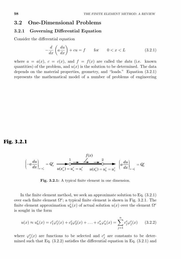
98 THE FINITE ELEMENT METHOD: A REVIEW
3.2 One-Dimensional Problems
3.2.1 Governing Differential Equation
Consider the differential equation
− d
dx
(adu
dx
)+ cu = f for 0 < x < L (3.2.1)
where a = a(x), c = c(x), and f = f(x) are called the data (i.e. knownquantities) of the problem, and u(x) is the solution to be determined. The datadepends on the material properties, geometry, and “loads.” Equation (3.2.1)represents the mathematical model of a number of problems of engineeringand applied science, and it must be solved subject to appropriate boundaryconditions. Table 3.2.1 contains a list of field problems, by no means exhaustive,in which Eq. (3.2.1) arises.
3.2.2 Finite Element Approximation
The domain Ω = (0, L) of the problem consists of all points between x = 0and x = L. The points x = 0 and x = L are the boundary points of the totaldomain. In the finite element method, the domain (0, L) is divided into a setof intervals, Ωe = (xea, x
eb), where xea and xeb denote the coordinates of the end
points of the finite element Ωe with respect to the coordinate x, as shown inFig. 3.2.1. A typical interval Ωe is called a finite element, and it is of lengthhe = xeb − xea.Fig. 3.2.1
1 2
ea
ea
x x
dua Q
dx =
æ ö÷ç- =÷ç ÷÷çè ø
( )f x
1( )e e ea au x u u= = e
b
eb
x x
dua Q
dx =
æ ö÷ç =÷ç ÷÷çè ø2( )e e e
b bu x u u= =
Fig. 3.2.1: A typical finite element in one dimension.
In the finite element method, we seek an approximate solution to Eq. (3.2.1)over each finite element Ωe; a typical finite element is shown in Fig. 3.2.1. Thefinite element approximation ueh(x) of actual solution u(x) over the element Ωe
is sought in the form
u(x) ≈ ueh(x) = ce1ϕe1(x) + ce2ϕ
e2(x) + . . .+ cenϕ
en(x) =
n∑j=1
cejϕej(x) (3.2.2)
where ϕej(x) are functions to be selected and cej are constants to be deter-mined such that Eq. (3.2.2) satisfies the differential equation in Eq. (3.2.1) and
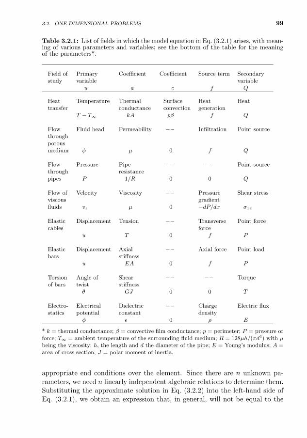
3.2. ONE-DIMENSIONAL PROBLEMS 99
Table 3.2.1: List of fields in which the model equation in Eq. (3.2.1) arises, with mean-ing of various parameters and variables; see the bottom of the table for the meaningof the parameters*.
Field of Primary Coefficient Coefficient Source term Secondarystudy variable variable
u a c f Q
Heat Temperature Thermal Surface Heat Heattransfer conductance convection generation
T − T∞ kA pβ f Q
Flow Fluid head Permeability −− Infiltration Point sourcethroughporousmedium φ µ 0 f Q
Flow Pressure Pipe −− −− Point sourcethrough resistancepipes P 1/R 0 0 Q
Flow of Velocity Viscosity −− Pressure Shear stressviscous gradientfluids vz µ 0 −dP/dx σxz
Elastic Displacement Tension −− Transverse Point forcecables force
u T 0 f P
Elastic Displacement Axial −− Axial force Point loadbars stiffness
u EA 0 f P
Torsion Angle of Shear −− −− Torqueof bars twist stiffness
θ GJ 0 0 T
Electro- Electrical Dielectric −− Charge Electric fluxstatics potential constant density
φ ε 0 ρ E
* k = thermal conductance; β = convective film conductance; p = perimeter; P = pressure orforce; T∞ = ambient temperature of the surrounding fluid medium; R = 128µh/(πd4) with µbeing the viscosity; h, the length and d the diameter of the pipe; E = Young’s modulus; A =area of cross-section; J = polar moment of inertia.
appropriate end conditions over the element. Since there are n unknown pa-rameters, we need n linearly independent algebraic relations to determine them.Substituting the approximate solution in Eq. (3.2.2) into the left-hand side ofEq. (3.2.1), we obtain an expression that, in general, will not be equal to the
100 THE FINITE ELEMENT METHOD: A REVIEW
right-hand side of the equation, f(x). The difference between the two sides ofthe equation is called the residual (i.e. error in the differential equation)
− d
dx
(aduehdx
)+ cueh(x)− f(x) ≡ Re(x, ce1, ce2, . . . , cen) 6= 0 (3.2.3)
We wish to determine cej (j = 1, 2, . . . , n) such that the residual Re is zero, insome meaningful sense, over the element.
One way of making the residual zero over the element domain is to set theweighted-integral of the residual to zero:∫ xeb
xea
wei (x)Re(x, ce1, ce2, . . . , c
en) dx = 0, i = 1, 2, . . . , n (3.2.4)
where wei (i = 1, 2, . . . , n) are weight functions. Equation (3.2.4) provides aset of n algebraic relations among the parameters cej (j = 1, 2, . . . , n). Theset wei (x)ni=1 must be linearly independent so that the algebraic equations inEq. (3.2.4) are also linearly independent and invertible. Note that if we = 1,we will have only one relation among n unknowns ce1, c
e2, . . . , c
en.
There are several choices of wei that may be used. In the present study, wetake wei (x) to be the same as the approximation functions ϕei (x). This partic-ular choice is adopted in the Galerkin method. Different choice of the weightfunctions wei ni=1 will result in a different set of algebraic relations or a dif-ferent finite element model of the same differential equation. In particular, thealgebraic relations resulting from the weighted-residual statement with wei = ϕeiis called the Galerkin finite element model. We note that Re contains the sameorder derivatives of the dependent unknown u(x) as in the differential equa-tion, Eq. (3.2.1), and hence requires at least quadratic representation of ueh(x).To reduce or weaken the differentiability of ϕei , we mathematically distributedifferentiation equally (when the given differential equation is of even order)between wei and ueh, and the resulting integral form is known as the weak form,as will be discussed in more detail shortly. The resulting finite element modelwill be termed weak form Galerkin finite element model.
In solid and structural mechanics, the governing equations are often derivedfrom the principle of virtual displacements or its special case, the principle ofminimum total potential energy. These principles are based on energy conceptsand constitute the basis of classical variational methods like the Ritz method(see Reddy [1, 2] for additional details), and most of the finite element modelsin the literature are based on an element-wise application of the Ritz method.The statement of the principle of virtual displacements is an integral state-ment, which is the same as the weak form derived directly from the governingdifferential equation. However, the derivation of the weak form of a differentialequation is independent of any variational principle and thus has a general set-ting independent of the field of study. All commercial finite element programs
3.2. ONE-DIMENSIONAL PROBLEMS 101
are based on weak forms of the differential equations arising in various physicalfields. Therefore, more importance is given in this study to the weak form de-velopment of governing equations while making connection to the principle ofvirtual displacements wherever appropriate.
3.2.3 Derivation of the Weak Form
The starting point to construct the weak form of Eq. (3.2.1) is the weighted-residual statement in Eq. (3.2.4). The next step is to weaken the differentiabilityrequired of ueh(x) [and hence ϕj of Eq. (3.2.2)]. This requires trading half ofthe differentiation from ueh to wei such that both ueh and wei are differentiatedequally, once each in the present case. The resulting integral form is termed theweak form of Eq. (3.2.1) because it allows approximation functions with less orweaker continuity than that required in the integral statement in Eq. (3.2.1). Athree-step procedure of constructing the weak form of Eq. (3.2.1) is presentednext.
Step 1. The first step is to write the weighted-residual statement as in Eq. (3.2.4)
0 =
∫ xeb
xea
wei
[− d
dx
(aduehdx
)+ cueh − f
]dx (3.2.5)
Step 2. The second step is to trade differentiation from ueh to wei , using inte-gration by parts. We obtain
0 =
∫ xeb
xea
(adweidx
duehdx
+ cweiueh − wei f
)dx−
[wei · a
duehdx
]xebxea
(3.2.6)
Consider the boundary term appearing in Eq. (3.2.6), namely, the expression[wei · a
du
dx
]xebxea
The coefficient of the weight function wei in the boundary expression, a(du/dx),is called the secondary variable, and its specification constitutes the natural orNeumann boundary condition. The primary variable is the dependent unknownof the differential equation, u, in the same form as the weight function weiin the boundary expression. The specification of a primary variable on theboundary constitutes the essential or Dirichlet boundary condition. For themodel equation at hand, the primary and secondary variables are
Primary variable: u ; Secondary variable: nx
(adu
dx
)≡ Q(x) (3.2.7)
where nx = −1 at the left end and nx = 1 at the right end of the element.
102 THE FINITE ELEMENT METHOD: A REVIEW
Step 3. In writing the final weak form, we denote the secondary variables atthe ends of the element as
Qea = Q(xea) = −(adu
dx
)xea
, Qeb = Q(xeb) =
(adu
dx
)xeb
(3.2.8)
The primary and secondary variables at the nodes are shown on the typicalelement in Fig. 3.2.1. It can be viewed as the free-body diagram of a typicalbut arbitrary portion of a bar, with Qea and Qeb denoting the axial forces; Qeais a compressive force while Qeb is a tensile force (algebraically, both are in thepositive x direction, as shown in Fig. 3.2.1). For heat conduction problems,Qea denotes the heat input at the left end and Qeb the heat output from theright end of the element. Although Q replaced a(du/dx), it is not consideredas function of u; it is a variable that is dual to u.
With the notation in Eq. (3.2.8), the final expression for the weak form isgiven by
0 =
∫ xeb
xea
(adweidx
duehdx
+ cweiueh − wei f
)dx− wei (xea)Qea − wei (xeb)Qeb (3.2.9)
This completes the three-step procedure of constructing the weak form.Some remarks on the weak form derivation are in order.
1. The integration-by-parts used in Step 2 has two implications: (i) reducesthe degree of finite element approximation used to represent ueh; and (ii)introduces secondary variables Qea and Qeb that are physically meaningfulin the sense that they can be specified at a point whenever the primaryvariable ueh is not specified there. If a secondary variable resulting fromthe integration by parts is not a physical quantity, then integration byparts should not be carried out even if it results in the weakening of thedifferentiability of ueh.
2. The weak form in Eq. (3.2.9) contains two types of expressions: thosecontaining both wei and ueh, and those containing only wei . The expressioncontaining both wei and ueh is called a bilinear functional when it is linearin wei as well as ueh (see Section 1.7.6):
B(wei , ueh) ≡
∫ xeb
xea
(adweidx
duehdx
+ cweiueh
)dx (3.2.10)
When a and/or c is a function of u, B(wei , ueh) is (always) linear in wei
but nonlinear in ueh. The expression containing only wei is called a linearfunctional because it is (always) linear in wei
`(wei ) =
∫ xeb
xea
wei f dx+ wei (xa)Qea + wei (xb)Q
eb (3.2.11)
3.2. ONE-DIMENSIONAL PROBLEMS 103
3. In view of the definitions in Eqs. (3.2.10) and (3.2.11), the weak form inEq. (3.2.9) can now be expressed as
B(wei , ueh) = `(wei )
which is called the variational problem associated with Eq. (3.2.1). In thefunctional analysis terminology, the variational problem can be stated asone of finding ue ∈ U such that
B(wei , ueh) = `(wei ) (3.2.12)
holds for all wei ∈ U , where U ⊂ H1(Ωe), the Hilbert space of order 1
H1(Ωe) =
u : u,
du
dx∈ L2(xa, xb), xa < x < xb
(3.2.13)
L2(Ωe) =
u :
∫ xeb
xea
|u| dx <∞
(3.2.14)
where Ωe = (xea, xeb). As will be seen later, the bilinear form B(wei , u
eh)
results in the left-hand side Keue and the linear form `(wei ) leads to theright-hand side column vector Fe of the finite element equations, Keue =Fe.
4. Those who have a background in solid and structural mechanics will ap-preciate the fact that the weak form in Eq. (3.2.9) or the variationalproblem in Eq. (3.2.12) is nothing but the statement of the principle ofthe minimum total potential energy Π(ueh) applied to a bar element (seeReddy [2, 3]): δΠ = B(δueh, u
eh)− `(δueh) = 0, where δ denotes the varia-
tional symbol and Π(ueh) is the quadratic functional
Π(ueh) =1
2B(ueh, u
eh)− `(ueh) (3.2.15)
=
∫ xeb
xea
[a
2
(dueidx
)2
+c
2(ueh)2 − uehf
]dx− ueh(xea)Q
ea − ueh(xeb)Q
eb
(3.2.16)
Equation (3.2.15) holds only when B(wei , ueh) is bilinear and symmetric in
ueh and wei = δueh,B(wei , u
eh) = B(ueh, w
ei ) (3.2.17)
and `(wei ) is linear in wei . The expression 12B(ueh, u
eh) represents the elastic
strain energy stored in the bar finite element and `(ueh) represents the workdone by the applied distributed force f(x) and point loads Qea and Qeb.
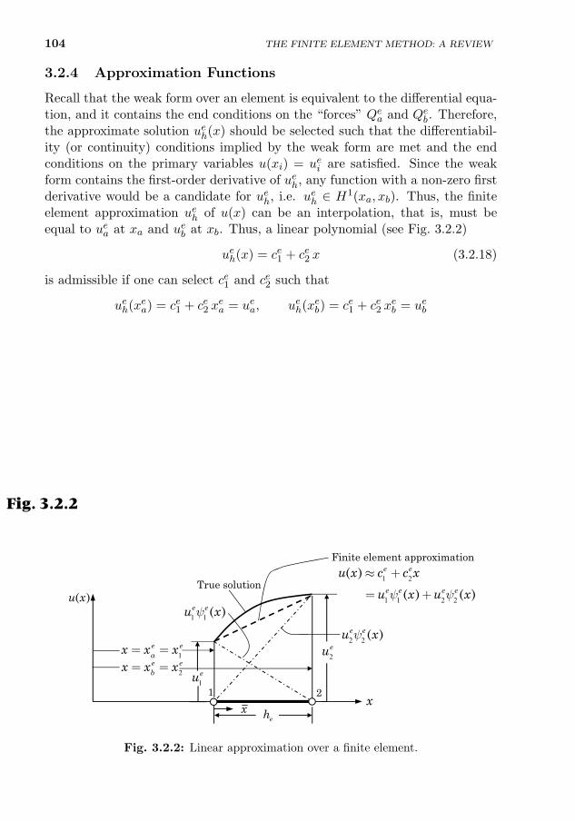
104 THE FINITE ELEMENT METHOD: A REVIEW
3.2.4 Approximation Functions
Recall that the weak form over an element is equivalent to the differential equa-tion, and it contains the end conditions on the “forces” Qea and Qeb. Therefore,the approximate solution ueh(x) should be selected such that the differentiabil-ity (or continuity) conditions implied by the weak form are met and the endconditions on the primary variables u(xi) = uei are satisfied. Since the weakform contains the first-order derivative of ueh, any function with a non-zero firstderivative would be a candidate for ueh, i.e. ueh ∈ H1(xa, xb). Thus, the finiteelement approximation ueh of u(x) can be an interpolation, that is, must beequal to uea at xa and ueb at xb. Thus, a linear polynomial (see Fig. 3.2.2)
ueh(x) = ce1 + ce2 x (3.2.18)
is admissible if one can select ce1 and ce2 such that
ueh(xea) = ce1 + ce2 xea = uea, ueh(xeb) = ce1 + ce2 x
eb = ueb
or [1 xea1 xeb
]ce1ce2
=
ueaueb
→ ce1 =
uea xeb − ueb xeaxeb − xea
, ce2 =ueb − ueaxeb − xea
(3.2.19)
Substitution of Eq. (3.2.19) for cei into Eq. (3.2.18) yields
ueh(x) = ψe1(x)ue1 + ψe2(x)ue2 =
2∑j=1
ψej (x)uej (3.2.20)
where (noting that he = xeb − xea)
ψe1(x) =xeb − xhe
, ψe2(x) =x− xeahe
(3.2.21)
1 2
True solution
1e eax x x= =
1 2
1 1 2 2
( )
( ) ( )
e e
e e e e
u x c c x
u x u xy y
» +
= +
2eu
( )u x
2 2 ( )e eu xy
ehx
2e ebx x x= =
1 1 ( )e eu xy
1eu
x
Finite element approximation
Fig. 3.2.2
Fig. 3.2.2: Linear approximation over a finite element.
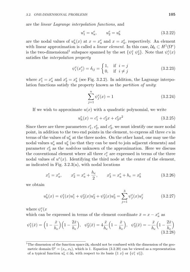
3.2. ONE-DIMENSIONAL PROBLEMS 105
are the linear Lagrange interpolation functions, and
ue1 = uea, ue2 = ueb (3.2.22)
are the nodal values of ueh(x) at x = xea and x = xeb, respectively. An elementwith linear approximation is called a linear element. In this case, Uh ⊂ H1(Ωe)is the two-dimensional1 subspace spanned by the set ψe1 ψe2. Note that ψei (x)satisfies the interpolation property
ψei (xej) = δij =
1, if i = j0, if i 6= j
(3.2.23)
where xe1 = xea and xe2 = xeb (see Fig. 3.2.2). In addition, the Lagrange interpo-lation functions satisfy the property known as the partition of unity:
n∑j=1
ψej (x) = 1 (3.2.24)
If we wish to approximate u(x) with a quadratic polynomial, we write
ueh(x) = ce1 + ce2x+ ce3x2 (3.2.25)
Since there are three parameters ce1, ce2, and ce3, we must identify one more nodalpoint, in addition to the two end points in the element, to express all three c,s interms of the values of ueh at the three nodes. On the other hand, one may use thenodal values uea and ueb (so that they can be used to join adjacent elements) andparameter ce3 as the nodeless unknown of the approximation. Here we discussthe conventional element where all three cei are expressed in terms of the threenodal values of ue(x). Identifying the third node at the center of the element,as indicated in Fig. 3.2.3(a), with nodal locations
xe1 = xea, xe2 = xea +he2, xe3 = xea + he = xeb (3.2.26)
we obtain
ueh(x) = ψe1(x)ue1 + ψe2(x)ue2 + ψe3(x)ue3 =3∑j=1
ψej (x)uej (3.2.27)
where ψei (x) are the quadratic Lagrange interpolation functions [see Fig. 3.2.3(b)],which can be expressed in terms of the element coordinate x = x− xea as
ψe1(x) =(
1− x
he
)(1− 2x
he
), ψe2(x) = 4
x
he
(1− x
he
), ψe3(x) = − x
he
(1− 2x
he
)(3.2.28)
1The dimension of the function space Uh should not be confused with the dimension of the geo-metric domain Ωe = (xa, xb), which is 1. Equation (3.2.20) can be viewed as a representationof a typical function ueh ∈ Uh with respect to its basis 1 x or ψe1 ψe2.
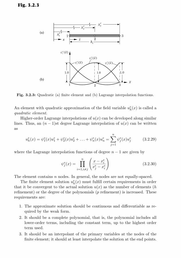
106 THE FINITE ELEMENT METHOD: A REVIEW
12
3x
(a)
ex3ex2
ex1
xeh
1.0 1.01.0
(b)
1 2 3
1 ( )e xy
( )ei xy
2 ( )e xy
3 ( )e xy
x
Fig. 3.2.3
Fig. 3.2.3: Quadratic (a) finite element and (b) Lagrange interpolation functions.
An element with quadratic approximation of the field variable ueh(x) is called aquadratic element.
Higher-order Lagrange interpolations of u(x) can be developed along similarlines. Thus, an (n− 1)st degree Lagrange interpolation of u(x) can be writtenas
ueh(x) = ψe1(x)ue1 + ψe2(x)ue2 + . . .+ ψen(x)uen =n∑j=1
ψej (x)uej (3.2.29)
where the Lagrange interpolation functions of degree n− 1 are given by
ψej (x) =
n∏i=1,i 6=j
(x− xeixej − xei
)(3.2.30)
The element contains n nodes. In general, the nodes are not equally-spaced.The finite element solution ueh(x) must fulfill certain requirements in order
that it be convergent to the actual solution u(x) as the number of elements (hrefinement) or the degree of the polynomials (p refinement) is increased. Theserequirements are:
1. The approximate solution should be continuous and differentiable as re-quired by the weak form.
2. It should be a complete polynomial, that is, the polynomial includes alllower-order terms, including the constant term, up to the highest orderterm used.
3. It should be an interpolant of the primary variables at the nodes of thefinite element; it should at least interpolate the solution at the end points.
3.2. ONE-DIMENSIONAL PROBLEMS 107
The reason for the first requirement is obvious; it ensures that every termof the governing equation has a non-zero contribution to the coefficient matrix.The second requirement is necessary in order to capture all possible states –say, constant, linear and so on – of the actual solution. For example, if a linearpolynomial without the constant term is used to represent the temperaturedistribution in a one-dimensional system, the approximate solution can neverbe able to represent a uniform state of temperature field in the element. Thethird requirement is necessary in order to enforce continuity of the primaryvariables across the elements, i.e. at the end points, where the element isconnected to other elements.
3.2.5 Finite Element Model
Substitution of Eq. (3.2.29) into Eq. (3.2.9) gives the necessary algebraic equa-tions among the nodal values uei and Qei of the element, which will be termedthe finite element model. In order to formulate the finite element model (i.e.derive a set of algebraic relations among uei and Qei ) based on the weak form inEq. (3.2.9), it is not necessary to decide the degree of approximation of ueh(x)a priori. The model can be developed using an arbitrary degree of interpo-lation. For n > 2, the weak form in Eq. (3.2.9) must be modified to includenon-zero secondary variables, if any, at interior nodes:
0 =
∫ xb
xa
(adweidx
duehdx
+ cweiueh
)dx−
∫ xb
xa
wei f dx−n∑j=1
wei (xej)Q
ej (3.2.31)
where xei is the global coordinate of the ith node of element Ωe = (xa, xb). Ifnodes 1 and n denote the end points of the element, then Qe1 = Qea and Qen = Qebrepresent the unknown point sources, and all other Qei (i = 2, 3, . . . , n− 1) arethe externally applied (hence, known) point sources at nodes 2, 3, . . . , n − 1,respectively.
Substituting Eq. (3.2.29) for ueh and we1 = ψe1, we2 = ψe2, . . . , wei = ψei , . . . ,
wen = ψen into the weak form Eq. (3.2.31), we obtain n algebraic equations. Thischoice of replacing wei with ψei amounts to using the Galerkin method; however,the original Galerkin method was based on the weighted-integral statement ofthe residual – not on the weak form. In fact, it amounts to using the Ritzmethod [1, 2]. The element equations are numbered according to the choice ofthe weight function wei . In other words, the ith algebraic equation is the onethat is obtained from Eq. (3.2.31) by replacing wei with ψei ,
0 =
∫ xb
xa
[adψeidx
(n∑j=1
uejdψejdx
)+ cψei
(n∑j=1
uejψej
)− ψei f
]dx−
n∑j=1
ψei (xej)Q
ej
=
n∑j=1
[∫ xb
xa
(adψeidx
dψejdx
+ cψeiψej
)dx
]uej −
∫ xb
xa
ψei f dx−Qei
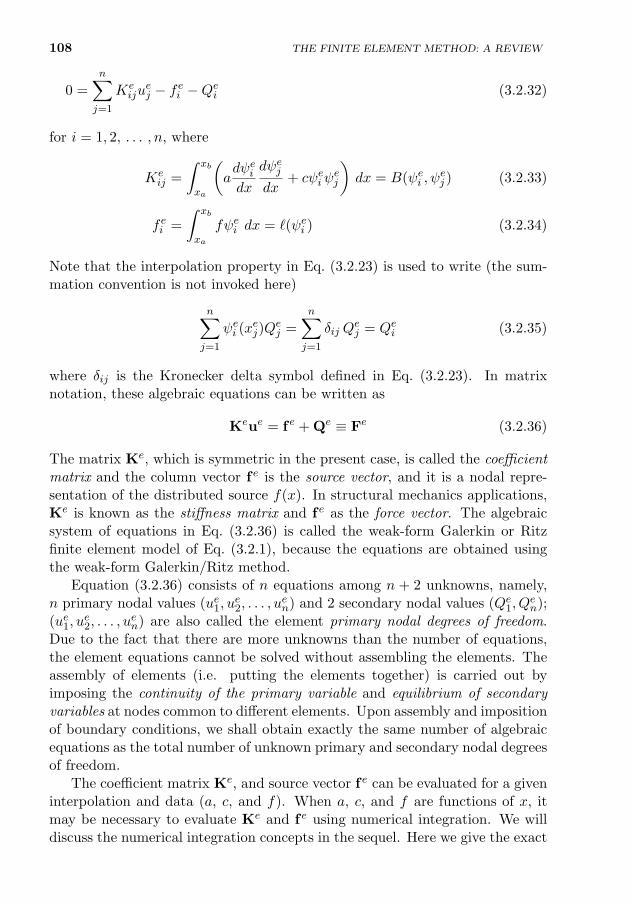
108 THE FINITE ELEMENT METHOD: A REVIEW
0 =
n∑j=1
Keiju
ej − fei −Qei (3.2.32)
for i = 1, 2, . . . , n, where
Keij =
∫ xb
xa
(adψeidx
dψejdx
+ cψeiψej
)dx = B(ψei , ψ
ej ) (3.2.33)
fei =
∫ xb
xa
fψei dx = `(ψei ) (3.2.34)
Note that the interpolation property in Eq. (3.2.23) is used to write (the sum-mation convention is not invoked here)
n∑j=1
ψei (xej)Q
ej =
n∑j=1
δij Qej = Qei (3.2.35)
where δij is the Kronecker delta symbol defined in Eq. (3.2.23). In matrixnotation, these algebraic equations can be written as
Keue = f e + Qe ≡ Fe (3.2.36)
The matrix Ke, which is symmetric in the present case, is called the coefficientmatrix and the column vector f e is the source vector, and it is a nodal repre-sentation of the distributed source f(x). In structural mechanics applications,Ke is known as the stiffness matrix and f e as the force vector. The algebraicsystem of equations in Eq. (3.2.36) is called the weak-form Galerkin or Ritzfinite element model of Eq. (3.2.1), because the equations are obtained usingthe weak-form Galerkin/Ritz method.
Equation (3.2.36) consists of n equations among n + 2 unknowns, namely,n primary nodal values (ue1, u
e2, . . . , u
en) and 2 secondary nodal values (Qe1, Q
en);
(ue1, ue2, . . . , u
en) are also called the element primary nodal degrees of freedom.
Due to the fact that there are more unknowns than the number of equations,the element equations cannot be solved without assembling the elements. Theassembly of elements (i.e. putting the elements together) is carried out byimposing the continuity of the primary variable and equilibrium of secondaryvariables at nodes common to different elements. Upon assembly and impositionof boundary conditions, we shall obtain exactly the same number of algebraicequations as the total number of unknown primary and secondary nodal degreesof freedom.
The coefficient matrix Ke, and source vector f e can be evaluated for a giveninterpolation and data (a, c, and f). When a, c, and f are functions of x, itmay be necessary to evaluate Ke and f e using numerical integration. We willdiscuss the numerical integration concepts in the sequel. Here we give the exact
3.2. ONE-DIMENSIONAL PROBLEMS 109
element equations for linear and quadratic elements for the case in which thedata (a, c, and f) is element-wise constant. Suppose that ae, ce, and fe denotethe element-wise constant values of a(x), c(x), and f(x), respectively. Then theelement (matrix) equations are obtained by analytically evaluating the integralsappearing in Ke
ij and fei . The results are summarized here for elements withlinear and quadratic approximations.
Linear element (i.e. element with linear approximation)
ψe1(x) = 1− x
he, ψe2(x) =
x
he(3.2.37)(
aehe
[1 −1−1 1
]+cehe
6
[2 11 2
])ue1ue2
=fehe
2
11
+
Qe1Qe2
(3.2.38)
Quadratic element (i.e. element with quadratic approximation)
ψe1(x) =
(1− 2x
he
)(1− x
he
), ψe2(x) =
4x
he
(1− x
he
), ψe3(x) = − x
he
(1− 2x
he
)(3.2.39) ae
3he
7 −8 1−8 16 −8
1 −8 7
+cehe30
4 2 −12 16 2−1 2 4
ue1ue2ue3
=fehe
6
141
+
Qe1Qe2Qe3
(3.2.40)
We note that the contribution of a uniform source to the nodes in a quadratic el-ement is non-uniform, that is, fei 6= fehe/3; also, the source vector of a quadraticelement of length he is not equivalent to that of two linear elements of lengthhe/2 each; it is the source vector that is consistent with the coefficient matrixof the quadratic element. We also note that there are more unknowns than thenumber of equations, independent of the degree of interpolation. Therefore, theelement equations cannot be solved without properly assembling finite elementequations associated with all elements in the mesh. When only one element isused, there will be only n unknowns because two known values are provided bythe boundary conditions. Next we consider an example to illustrate the ideaspresented here.
Example 3.2.1
Consider a homogeneous, isotropic bar of length L (m), cross-sectional area A (m2), andconductivity k [W/(m· C)], as shown in Fig. 3.2.4(a). The bar is maintained at a temperatureof T0 (C) at the left end, insulated throughout the length so that there is no heat loss fromthe surface, and the right end is exposed to air at an ambient temperature of Tinf(
C) witha uniform internal heat generation of g0 (W/m). The heat transfer coefficient associatedwith fin material and the air is β [W/(m2 · C]. Use two different cases of uniform mesh (i.e.elements of equal size), (a) four linear elements and (b) two quadratic elements, in the domainto determine the temperature distribution along the length of the bar and heat at the left end.
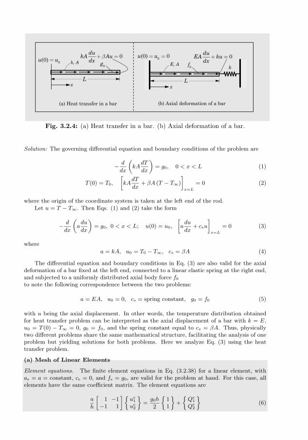
110 THE FINITE ELEMENT METHOD: A REVIEW
(a) Heat transfer in a bar
x
E, Ak
x
k, A0(0)u u= 0(0) 0u u= =0du
kA Audx
b+ = 0du
EA kudx
+ =
(b) Axial deformation of a bar
LL
0f0g
Fig. 3.2.4: (a) Heat transfer in a bar. (b) Axial deformation of a bar.
Solution: The governing differential equation and boundary conditions of the problem are
− d
dx
(kA
dT
dx
)= g0, 0 < x < L (1)
T (0) = T0,
[kA
dT
dx+ βA (T − T∞)
]x=L
= 0 (2)
where the origin of the coordinate system is taken at the left end of the rod.Let u = T − T∞. Then Eqs. (1) and (2) take the form
− d
dx
(adu
dx
)= g0, 0 < x < L; u(0) = u0,
[adu
dx+ csu
]x=L
= 0 (3)
where
a = kA, u0 = T0 − T∞, cs = βA (4)
The differential equation and boundary conditions in Eq. (3) are also valid for the axialdeformation of a bar fixed at the left end, connected to a linear elastic spring at the right end,and subjected to a uniformly distributed axial body force f0 [see Fig. 3.2.4(b)]. One only needto note the following correspondence between the two problems:
a = EA, u0 = 0, cs = spring constant, g0 = f0 (5)
with u being the axial displacement. In other words, the temperature distribution obtainedfor heat transfer problem can be interpreted as the axial displacement of a bar with k = E,u0 = T (0) − T∞ = 0, g0 = f0, and the spring constant equal to cs = βA. Thus, physicallytwo different problems share the same mathematical structure, facilitating the analysis of oneproblem but yielding solutions for both problems. Here we analyze Eq. (3) using the heattransfer problem.
(a) Mesh of Linear Elements
Element equations. The finite element equations in Eq. (3.2.38) for a linear element, withae = a = constant, ce = 0, and fe = g0, are valid for the problem at hand. For this case, allelements have the same coefficient matrix. The element equations are
a
h
[1 −1−1 1
]ue1ue2
=g0h
2
11
+
Qe1Qe2
(6)
3.2. ONE-DIMENSIONAL PROBLEMS 111
Assembled equations. Since there are no external heat inputs at the global nodes common tothe elements, we require that
Q12 +Q2
1 = 0, Q22 +Q3
1 = 0, Q32 +Q4
1 = 0
Therefore, the assembled system of equations is given by
a
h
1 −1 0 0 0−1 2 −1 0 0
0 −1 2 −1 00 0 −1 2 −10 0 0 −1 1
U1
U2
U3
U4
U5
=g0h
2
12221
+
Q1
1
Q12 +Q2
1 = 0Q2
2 +Q31 = 0
Q32 +Q4
1 = 0Q4
2
(7)
where UI denotes the temperature at the Ith global node, I = 1, 2, . . . , 5. The assembledequations presented in Eq. (7) for a mesh of four linear elements that are connected in seriesare valid for any set of boundary conditions.
Imposition of boundary conditions. The boundary conditions in Eq. (3) can be expressed interms of the global nodal variables as follows:
u(0) = u0 → U1 = u0;
[adu
dx
]x=L
+ csu(L) = 0→ Q42 + csU5 = 0 (8)
Then the assembled system of equations become
a
h
1 −1 0 0 0−1 2 −1 0 0
0 −1 2 −1 00 0 −1 2 −10 0 0 −1 1
u0
U2
U3
U4
U5
=g0h
2
12221
+
Q1
1
000
−csU5
(9)
Condensed equations. The assembled equations can be grouped into two kinds, one in terms ofthe unknown primary global nodal variables and the other in terms of the unknown secondaryvariables. They are called condensed equations. Since only one element of each pair of primaryand secondary variables, (UI , FI), at a node are known, we will always have only N unknowns,where N is the total number of global nodes. In the present case, the unknown primary globalvariables are (U2, U3, U4, U5); hence, the condensed equations for unknown primary globalvariables are
a
h
2 −1 0 0−1 2 −1 0
0 −1 2 −10 0 −1 1 + α
U2
U3
U4
U5
=goh
2
2221
+
ahu0
000
(10)
where α = csh/a. The algebraic equations in Eq. (10) can be readily solved, since thecoefficient matrix is invertible, for U2, U3, U4, and U5. The unknown heat at nodes 1 is givenby
Q11 =
a
h(u0 − U2)− goh
2(11)
(b) Mesh of Quadratic Elements
Element equations. For the uniform mesh of two quadratic elements (i.e. h1 = h2 = h = L/2),the element equations are
a
3h
7 −8 1−8 16 −8
1 −8 7
ue1ue2ue3
=g0h
6
141
+
Qe1Qe2Qe3
(12)
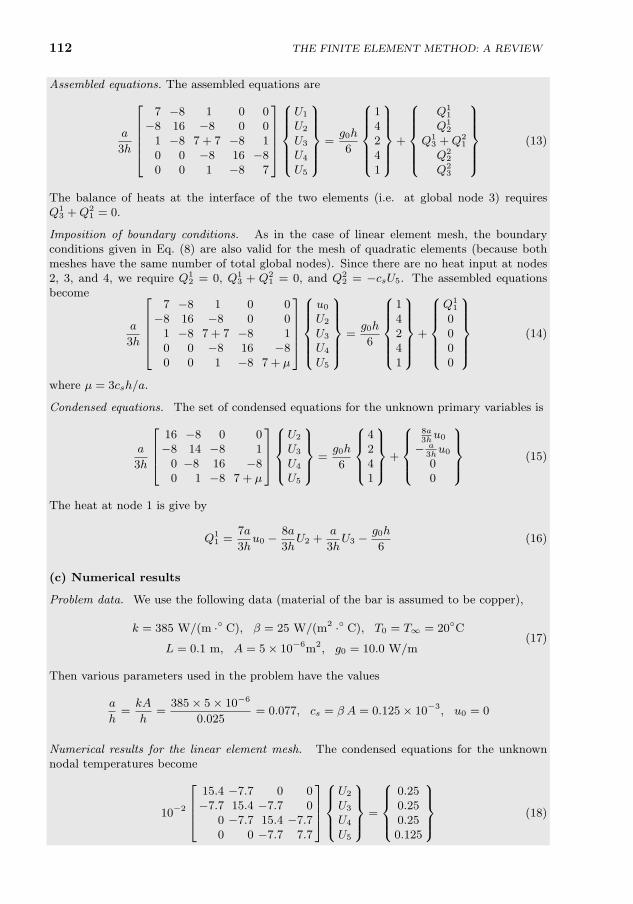
112 THE FINITE ELEMENT METHOD: A REVIEW
Assembled equations. The assembled equations are
a
3h
7 −8 1 0 0−8 16 −8 0 0
1 −8 7 + 7 −8 10 0 −8 16 −80 0 1 −8 7
U1
U2
U3
U4
U5
=g0h
6
14241
+
Q1
1
Q12
Q13 +Q2
1
Q22
Q23
(13)
The balance of heats at the interface of the two elements (i.e. at global node 3) requiresQ1
3 +Q21 = 0.
Imposition of boundary conditions. As in the case of linear element mesh, the boundaryconditions given in Eq. (8) are also valid for the mesh of quadratic elements (because bothmeshes have the same number of total global nodes). Since there are no heat input at nodes2, 3, and 4, we require Q1
2 = 0, Q13 + Q2
1 = 0, and Q22 = −csU5. The assembled equations
become
a
3h
7 −8 1 0 0−8 16 −8 0 0
1 −8 7 + 7 −8 10 0 −8 16 −80 0 1 −8 7 + µ
u0
U2
U3
U4
U5
=g0h
6
14241
+
Q1
1
0000
(14)
where µ = 3csh/a.
Condensed equations. The set of condensed equations for the unknown primary variables is
a
3h
16 −8 0 0−8 14 −8 1
0 −8 16 −80 1 −8 7 + µ
U2
U3
U4
U5
=g0h
6
4241
+
8a3hu0
− a3hu0
00
(15)
The heat at node 1 is give by
Q11 =
7a
3hu0 −
8a
3hU2 +
a
3hU3 −
g0h
6(16)
(c) Numerical results
Problem data. We use the following data (material of the bar is assumed to be copper),
k = 385 W/(m · C), β = 25 W/(m2 · C), T0 = T∞ = 20C
L = 0.1 m, A = 5× 10⁻⁶m2, g0 = 10.0 W/m(17)
Then various parameters used in the problem have the values
a
h=kA
h=
385× 5× 10−6
0.025= 0.077, cs = β A = 0.125× 10⁻³, u0 = 0
Numerical results for the linear element mesh. The condensed equations for the unknownnodal temperatures become
10−2
15.4 −7.7 0 0−7.7 15.4 −7.7 0
0 −7.7 15.4 −7.70 0 −7.7 7.7
U2
U3
U4
U5
=
0.250.250.250.125
(18)
3.2. ONE-DIMENSIONAL PROBLEMS 113
The solution of these equations (obtained with the help of an equation solver in a computer)is (note that U1 = 0.0 C)
U2 = 11.322 C, U3 = 19.397 C, U4 = 24.225 C, U5 = 25.806 C (19)
The heat input at node 1 from Eq. (11) is
Q11 =
a
h(U1 − U2)− g0h
2= 0.077(0− 11.322)− 0.125 = −0.9968 W (20)
On the other hand, from the definition
(Q11)def = −a
(du
dx
)x=0
≈ −a(duhdx
)x=0
= −a(U1dψ1
dx+ U2
dψ2
dx
)x=0
= −ah
(U2 − U1) = −0.872 W (21)
where ψi are the linear functions defined in Eq. (3.2.21). The value of heat computed fromthe definition differs from the heat computed from Eq. (11), and the difference is 0.125. Thedifference is exactly equal to g0h/2. As the mesh is refined in the neighborhood of x = 0, thepost-computed heat loss from the definition converges to that computed from Eq. (11), whichis exact.
Numerical results for the quadratic element mesh. For the mesh of two quadratic elements,the system of the condensed equations for the unknown temperatures is
10−2
20.533 −10.267 0 0−10.267 17.967 −10.267 12.883
0 −10.267 20.533 −10.2670 12.883 −10.267 8.996
U2
U3
U4
U5
= 10−2
33.33316.66733.3338.333
(22)
whose solution is
U2 = 11.322 C, U3 = 19.397 C, U4 = 24.225 C, U5 = 25.806 C
The solution is the same as that predicted by the mesh of four linear elements. The heat inputat node 1 from Eq. (16) is
Q11 =
a
3h(7U1 − 8U2 + U3)− g0h
6= −0.9968 W
and from the definition we have
(Q11)def = −a
h
(du
dx
)x=0
≈ −ah
(duhdx
)x=0
= −a(U1dψ1
dx+ U2
dψ2
dx+ U3
dψ3
dx
)x=0
= −ah
(−3U1 + 4U2 − U3) = −0.9968 W
where ψi are the quadratic functions defined in Eq. (3.2.28). Thus, for the mesh of quadraticelements, the value of heat at node 1 obtained with Eq. (16) and the definition is the same.
The exact solution of the problem described by Eq. (3) is
u(x) = −g0x2
2a+ c1x+ c2, 0 < x < L
c1 =
[g0L
(1 + 0.5
csL
a
)− csu0
](a+ csL)−1, c2 = u0
114 THE FINITE ELEMENT METHOD: A REVIEW
Evaluating the exact solution at the nodes, we obtain the same values as the finite elementsolution at the nodes. The exact value of heat at node 1 is −0.9968.
To interpret the results for the axial deformation of a bar, the conductivity k shouldbe replaced by modulus E (which is several orders of magnitude larger than k); since thedisplacement is inversely proportional to the modulus, the values of u would be approximately(not exactly because of the nonzero spring constant) of the order ku/E.
3.2.6 Natural Coordinates
From Section 3.2.4, it is clear that the approximation functions ψei in the finiteelement method are defined over an element and they do not extend to theneighboring elements. Therefore, they can be derived in terms of a coordinate,called a local coordinate, that is fixed in the element. The coordinate x used inFig. 3.2.3 is an example of a local coordinate. This facilitates easier evaluation(especially, when numerical integration is used) of the element coefficients Ke
ij
and fei . In fact, in two or three dimensions, it is not practical to derive theapproximation functions using the global coordinates. A natural coordinate isa local coordinate that is dimensionless. Here we consider two different naturalcoordinate systems in one dimension.
The first natural coordinate is x/h, with the origin at the left end of theelement. A pair of functions that measure the distance of an arbitrary pointP in the element relative to the two ends of the element are defined by [seeFig. 3.2.5(a)]:
L1(x) = 1− x
h, L2(x) = 1− L1 =
x
h(3.2.41)
The element label is omitted for brevity. We note that L1 and L2 are the samefunctions as the linear approximation functions defined in Eq. (3.2.37)
ψ1(x) = L1(x), ψ2(x) = L2(x) (3.2.42)
which satisfy the “Kronecker delta property” in Eq. (3.2.23) and “partition ofunity” in Eq. (3.2.24). Similarly, the quadratic functions in Eq. (3.2.39) can beexpressed in terms of L1 and L2 as
ψ1(x) = (2L1 − 1)L1, ψ2(x) = 4L1L2, ψ3(x) = (2L2 − 1)L2 (3.2.43)Fig. 3.2.5
1 1 ( / )L x h= -
•x P
2 ( / )L x h=
h
•x
1x =-
h
1x =+x
(a) (b)
Fig. 3.2.5: (a) Natural coordinates L1 and L2. (b) Natural coordinate ξ.
3.2. ONE-DIMENSIONAL PROBLEMS 115
In view of the relation x = x− xa and x = x(L1, L2), we have
d
dx=
d
dx=dL1
dx
∂
∂L1+dL2
dx
∂
∂L2=
1
h
(∂
∂L2− ∂
∂L1
)(3.2.44)
anddLidx
=1
h
(∂Li∂L2
− ∂Li∂L1
)=
1
h(δ2i − δ1i) (i = 1, 2) (3.2.45)
The integral of the products of various powers of Li can be evaluated using theformula ∫ h
0Lm1 Ln2 dx =
m!n!
(m+ n+ 1)!h (3.2.46)
where 0! = 1, ! is the factorial symbol.The second natural coordinate, denoted as ξ, is the one that is used more
commonly with Gauss quadrature (i.e. numerical integration; see Section 3.6)rule. The origin of ξ is taken to be at the center of the element, with ξ = −1and ξ = +1 being the left and right ends, respectively, of the element [seeFig. 3.2.5(b)]. The relationships between x and ξ and between x and ξ aregiven by
x = xa +h
2(1 + ξ),
x
h=
1
2(1 + ξ), ξ =
2
h(x− xa)− 1 =
2x
h− 1 (3.2.47)
Then the linear and quadratic interpolation functions in Eqs. (3.2.37) and(3.2.39) can be expressed in terms of ξ as
Linear: ψ1 =1
2(1− ξ), ψ2 =
1
2(1 + ξ)
Quadratic: ψ1 = −1
2ξ(1− ξ), ψ2 = (1− ξ2), ψ3 =
1
2ξ(1 + ξ)
(3.2.48)
The relationship between the derivative with respect to x and the derivativewith respect to ξ is given by
d
dx=
2
h
d
dξ,
dψidx
=2
h
dψidξ
(3.2.49)
Integrals over the element domain Ωe = (xa, xb) can be expressed as the one oninterval (−1, 1) as∫ xb
xa
ψi(x) dx =
∫ h
0ψi(x) dx =
h
2
∫ 1
−1ψi(ξ) dξ∫ xb
xa
dψidx
dx =
∫ h
0
dψidx
dx =
∫ 1
−1
dψidξ
dξ∫ xb
xa
dψidx
dψjdx
dx =2
h
∫ 1
−1
dψidξ
dψjdξ
dξ
(3.2.50)
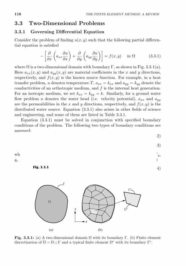
116 THE FINITE ELEMENT METHOD: A REVIEW
3.3 Two-Dimensional Problems
3.3.1 Governing Differential Equation
Consider the problem of finding u(x, y) such that the following partial differen-tial equation is satisfied
−[∂
∂x
(axx
∂u
∂x
)+
∂
∂y
(ayy
∂u
∂y
)]= f(x, y) in Ω (3.3.1)
where Ω is a two-dimensional domain with boundary Γ, as shown in Fig. 3.3.1(a).Here axx(x, y) and ayy(x, y) are material coefficients in the x and y directions,respectively, and f(x, y) is the known source function. For example, in a heattransfer problem, u denotes temperature T , axx = kxx and ayy = kyy denote theconductivities of an orthotropic medium, and f is the internal heat generation.For an isotropic medium, we set kxx = kyy = k. Similarly, for a ground waterflow problem u denotes the water head (i.e. velocity potential), axx and ayyare the permeabilities in the x and y directions, respectively, and f(x, y) is thedistributed water source. Equation (3.3.1) also arises in other fields of scienceand engineering, and some of them are listed in Table 3.3.1.
Equation (3.3.1) must be solved in conjunction with specified boundaryconditions of the problem. The following two types of boundary conditions areassumed:
u = u(s) on Γu (3.3.2)(axx
∂u
∂xnx + ayy
∂u
∂yny
)+ qc = qn(s) on Γq (3.3.3)
where Γu and Γq are disjoint portions of the boundary Γ such that Γ = Γu∪Γq,qc refers to the convective component of flux (e.g. in heat transfer problems)
qc = hc(u− uc) (3.3.4)Fig. 3.3.1
x
y eW
eG
G
W
(a) (b)
Fig. 3.3.1: (a) A two-dimensional domain Ω with its boundary Γ. (b) Finite elementdiscretization of Ω = Ω ∪ Γ and a typical finite element Ωe with its boundary Γe.
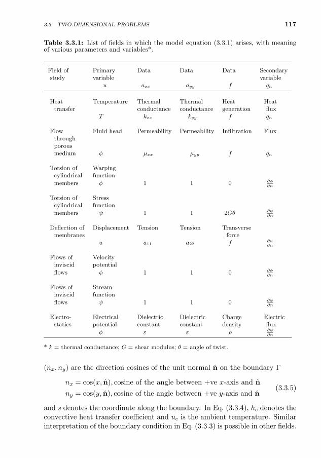
117
Table 3.3.1: List of fields in which the model equation (3.3.1) arises, with meaningof various parameters and variables*.
Field of Primary Data Data Data Secondarystudy variable variable
u axx ayy f qn
Heat Temperature Thermal Thermal Heat Heattransfer conductance conductance generation flux
T kxx kyy f qn
Flow Fluid head Permeability Permeability Infiltration Fluxthroughporousmedium φ µxx µyy f qn
Torsion of Warpingcylindrical function
members φ 1 1 0 ∂φ∂n
Torsion of Stresscylindrical function
members ψ 1 1 2Gθ ∂ψ∂n
Deflection of Displacement Tension Tension Transversemembranes force
u a11 a22 f ∂u∂n
Flows of Velocityinviscid potential
flows φ 1 1 0 ∂φ∂n
Flows of Streaminviscid function
flows ψ 1 1 0 ∂ψ∂n
Electro- Electrical Dielectric Dielectric Charge Electricstatics potential constant constant density flux
φ ε ε ρ ∂ψ∂n
* k = thermal conductance; G = shear modulus; θ = angle of twist.
(nx, ny) are the direction cosines of the unit normal n on the boundary Γ
nx = cos(x, n), cosine of the angle between +ve x-axis and n
ny = cos(y, n), cosine of the angle between +ve y-axis and n(3.3.5)
and s denotes the coordinate along the boundary. In Eq. (3.3.4), hc denotes theconvective heat transfer coefficient and uc is the ambient temperature. Similarinterpretation of the boundary condition in Eq. (3.3.3) is possible in other fields.
3.3. TWO-DIMENSIONAL PROBLEMS
118 THE FINITE ELEMENT METHOD: A REVIEW
3.3.2 Finite Element Approximation
In the finite element method, the domain Ω = Ω ∪ Γ is divided into a set ofsub-domains Ωe = Ωe ∪ Γe, called finite elements [see Fig. 3.3.1(b)]. Any geo-metric shape qualifies as an element provided that the approximation functionsψei can be derived uniquely for the shape. We shall discuss simple geometricshapes and orders of approximation shortly. To keep the formulation steps verygeneral, that is, not confine the formulation to a specific geometric shape, wehave denoted the domain of a typical element by Ωe and its boundary by Γe.The element Ωe can be a triangle or quadrilateral in shape, and the degree ofinterpolation over it can be linear, quadratic, and higher. The non-overlappingsum of all elements Ωe is denoted by Ωh, and it is called the finite elementmesh of the domain Ω. In general, Ωh may not equal Ω when the boundary Γis curved. Of course, for polygonal domains, the finite element mesh exactlyrepresents the actual domain.
Suppose that the dependent unknown u is approximated over a typical finiteelement Ωe by ueh(x) ∈ Uh
u(x) ≈ ueh(x) =
n∑j=1
uejψej (x), x = (x, y) ∈ Ωe (3.3.6)
where uej denote the values of the function ueh(x) at a selected number of points
(i.e. element nodes) in the element Ωe, and ψej are the Lagrange interpolationfunctions associated with the element. Here the symbol ‘∈’ means “an elementof” or “a point in”. As we shall see shortly, the interpolation functions dependnot only on the number of nodes in the element, but also on the shape ofthe element. The shape of the element must be such that its geometry isuniquely defined by a set of nodes and the approximated function varies amongnodes according to the adopted approximation. A triangle is the simplest two-dimensional geometric shape in two dimensions because it is uniquely defined bythree points (n = 3) in a plane and the approximated function varies betweenany two points according to ueh(x) = ce1 +ce2x+ce3y. A triangle with three nodesper side (a total of six nodes in the element) will uniquely define the geometrywhile representing the quadratic variation ueh(x) = ce1 + ce2x + ce3y + ce4xy +ce5x
2 + ce6y2 uniquely along any of the three segments. On the other hand, a
pentagon requires five points to define its geometry uniquely, but there is nofive-parameter polynomial in (x, y) that uniquely defines the linear variationalong any segment of the pentagon.
3.3.3 Weak Formulation
The n nodal values uej in Eq. (3.3.6) must be determined such that the approx-imate solution ueh(x) satisfies Eq. (3.3.1) and interpolates the nodal values ofueh(x) over the element Ωe. As described in Sections 3.2.2 and 3.2.3, we seek
3.3. TWO-DIMENSIONAL PROBLEMS 119
to satisfy the governing differential equation in a weak-form sense, with theweight functions being the same as the approximation functions. The resultingfinite element model i.e. set of algebraic equations) will be called the weak-formGalerkin finite element model or the Ritz finite element model.
We use the three-step procedure described in Section 3.2.3 to develop theweak form of Eq. (3.3.1) that accounts for the form of the natural boundarycondition in Eq. (3.3.3) over the typical element Ωe.
Step 1. The first step is to take all non-zero expressions in Eq. (3.3.1) to oneside of the equality, multiply the resulting equation with a weight function weifrom a set of linearly independent functions wei ni=1, and integrate the equationover the element domain Ωe:
0 =
∫Ωewei
[− ∂
∂x
(axx
∂ueh∂x
)− ∂
∂y
(ayy
∂ueh∂y
)− f(x, y)
]dA (3.3.7)
where dA = dx dy. The expression in the square brackets of the above equationrepresents the residual of the approximation of the differential equation (3.3.1)because ueh(x) is only an approximation of u(x). For n independent choicesof wei , we obtain a set of n linearly independent algebraic equations, calledweighted-residual finite element model.
Step 2. In the second step, we distribute the differentiation among ueh and weiequally so that both ueh and weh are required to be differentiable only once withrespect to x and y. To achieve this we use the component form of the gradient(or divergence) theorem [see Eq. (1.6.42)]∫
Ωe
∂
∂x(weiF1) dA =
∮Γe
(weiF1)nx ds∫Ωe
∂
∂y(weiF2) dA =
∮Γe
(weiF2)ny ds
(3.3.8)
where nx and ny are the components of the unit normal vector n
n = nxex + nyey = cosα ex + sinα ey (3.3.9)
on the boundary Γe, and ds is the arc length of an infinitesimal line elementalong the boundary. With
F1 = axx∂ueh∂x
, F2 = ayy∂ueh∂y
and identities
−wei∂F1
∂x= − ∂
∂x(weiF1) + F1
∂wei∂x
, −wei∂F2
∂y= − ∂
∂y(weiF2) + F2
∂wei∂y
we obtain
0 =
∫Ωe
(axx
∂wei∂x
∂ueh∂x
+ ayy∂wei∂y
∂ueh∂y− wei f
)dA
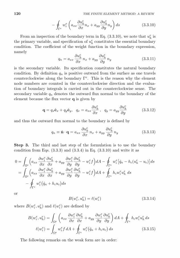
120 THE FINITE ELEMENT METHOD: A REVIEW
−∮
Γewei
(axx
∂ueh∂x
nx + ayy∂ueh∂y
ny
)ds (3.3.10)
From an inspection of the boundary term in Eq. (3.3.10), we note that ueh isthe primary variable, and specification of ueh constitutes the essential boundarycondition. The coefficient of the weight function in the boundary expression,namely
qn = axx∂ueh∂x
nx + ayy∂ueh∂y
ny (3.3.11)
is the secondary variable. Its specification constitutes the natural boundarycondition. By definition qn is positive outward from the surface as one travelscounterclockwise along the boundary Γe. This is the reason why the elementnode numbers are counted in the counterclockwise direction and the evalua-tion of boundary integrals is carried out in the counterclockwise sense. Thesecondary variable qn denotes the outward flux normal to the boundary of theelement because the flux vector q is given by
q = qxex + qyey, qx = axx∂ueh∂x
, qy = ayy∂ueh∂y
(3.3.12)
and thus the outward flux normal to the boundary is defined by
qn ≡ n · q = axx∂ueh∂x
nx + ayy∂ueh∂y
ny (3.3.13)
Step 3. The third and last step of the formulation is to use the boundarycondition from Eqs. (3.3.3) and (3.3.4) in Eq. (3.3.10) and write it as
0 =
∫Ωe
(axx
∂wei∂x
∂ueh∂x
+ ayy∂wei∂y
∂ueh∂y− wei f
)dA−
∮Γewei[qn − hc(ueh − uc)
]ds
=
∫Ωe
(axx
∂wei∂x
∂ueh∂x
+ ayy∂wei∂y
∂ueh∂y− wei f
)dA+
∮Γehcw
eiueh ds
−∮
Γewei(qn + hcuc
)ds
orB(wei , u
eh) = `(wei ) (3.3.14)
where B(wei , ueh) and `(wei ) are defined by
B(wei , ueh) =
∫Ωe
(axx
∂wei∂x
∂ueh∂x
+ ayy∂wei∂y
∂ueh∂y
)dA+
∮Γehcw
eiueh ds
`(wei ) =
∫Ωewei f dA+
∮Γewei(qn + hcuc
)ds (3.3.15)
The following remarks on the weak form are in order:
3.3. TWO-DIMENSIONAL PROBLEMS 121
1. The variational problem associated with Eqs. (3.3.1)–(3.3.3) over a finiteelement Ωe is to find ueh ∈ Uh ⊂ H1(Ωe) such that
B(wei , ueh) = `(wei ) (3.3.16)
holds for all wei ∈ Uh. In the finite element method, the subspace Uh ⊂H1(Ωe) is a finite-dimensional subspace spanned by set of polynomialbasis functions, as will be discussed shortly.
2. Note that B(wei , ueh) is bilinear and symmetric in its arguments wei and
ueh, and `(wei ) is linear in wei . Therefore, it is possible to construct theassociated quadratic functional from the formula (see Reddy [2, 3])
Ie(ueh) =1
2B(ueh, u
eh)− `(ueh) (3.3.17)
which is of considerable interest in the sense that the minimum of thefunctional I(ueh) (often dictated by some principle of mechanics) is equiv-alent to solving the variational problem in Eq. (3.3.14). Although itis possible to construct the weak form of any second- and higher-orderdifferential equations (linear or not), it is not always possible to con-struct a functional whose first variation is equivalent to the weak form[i.e. δIe = B(δueh, u
eh) − `(δueh) = 0]. However, when the variational
problem does not correspond to the necessary condition that a functionalbe a minimum, Eq. (3.3.14) merely provides a means for computing thesolution ueh, and it does not necessarily guaranty that the error in theapproximation is a minimum.
3.3.4 Finite Element Model
The weak form in Eq. (3.3.14) requires that ueh be at least linear in both x and yso that there are no terms in Eq. (3.3.14) that become identically zero. Supposethat ueh is represented over a typical finite element Ωe by expression of the formin Eq. (3.3.6). Substituting the finite element approximation, Eq. (3.3.6), intothe weak form in Eq. (3.3.14), we obtain
0 =
n∑j=1
∫Ωe
[∂wei∂x
(axx
∂ψej∂x
)+∂wei∂y
(ayy
∂ψej∂y
)]dA+
∮Γehcw
eiψ
ej ds
uej
−∫
Ωewei f dx−
∮Γewei(qn + hcuc
)ds (3.3.18)
This equation must hold for any weight function wei from the set wei ni=1. Inparticular it must hold for the case wei = ψei . This particular choice of weightfunctions is a natural one when the weight function is viewed as a virtualvariation of the dependent unknown [i.e. wei (x) = δueh(x) =
∑ni=1 δu
ei ψ
ei (x)].
122 THE FINITE ELEMENT METHOD: A REVIEW
For each choice of wei we obtain an algebraic relation among (ue1, ue2, . . . , u
en).
The ith algebraic equation is obtained by substituting wei = ψei into Eq. (3.3.14):
n∑j=1
Keiju
ej = fei + qei or Keue = f e + qe ≡ Fe (3.3.19)
where the coefficients Keij = Ke
ji (i.e. Ke is symmetric), fei , and qei are definedby
Keij =
∫Ωe
(axx
∂ψei∂x
∂ψej∂x
+ ayy∂ψei∂y
∂ψej∂y
)dA+
∮Γehcψ
eiψ
ej ds
fei =
∫Ωef ψei dA, qei =
∮Γe
(qn + hcuc
)ψei ds
(3.3.20)
3.3.5 Approximation Functions: Element Library
As before, we seek polynomial approximations of u(x). The finite elementapproximation ueh(x) of u(x, y) over an element Ωe must satisfy the followingconditions in order for the approximate solution to converge to the true solution:
1. ueh(x) must be continuous as required in the weak form of the problem;that is, all terms in the weak form are represented as non-zero values.
2. The polynomials used to represent ueh(x) must be complete and containboth x and y of the same order (i.e. equi-presence of x and y). Thismeans all terms, beginning with a constant term up to the highest orderdesired, in both x and y, should be included in the expression of ueh(x).
3. All terms in the polynomial should be linearly independent.
As already discussed, the number of linearly independent terms in the repre-sentation of ueh dictates the shape and the number of nodes in the element. Itturns out that only triangular and quadrilateral shapes meet the requirementsstated above. Here we review the interpolation functions of linear and quadratictriangular and rectangular elements.
3.3.5.1 Linear triangular element
An examination of the statement (3.3.18) and the finite element matrices inEq. (3.3.20) shows that ψei (i = 1, 2, . . . , n) should be, at least, a linear functionof x and y. The lowest-order linear polynomial that meets the requirements is
ueh(x) = ce1 + ce2 x+ ce3 y (3.3.21)
The polynomial is complete because constant and linear terms in x and y areincluded, both x and y are represented equally, and the set 1, x, y is linearly
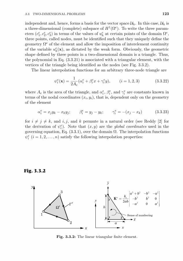
3.3. TWO-DIMENSIONAL PROBLEMS 123
independent and, hence, forms a basis for the vector space Uh. In this case, Uh isa three-dimensional (complete) subspace of H1(Ωe). To write the three param-eters (ce1, c
e2, c
e3) in terms of the values of ueh at certain points of the domain Ωe,
three points, called nodes, must be identified such that they uniquely define thegeometry Ωe of the element and allow the imposition of interelement continuityof the variable ueh(x), as dictated by the weak form. Obviously, the geometricshape defined by three points in a two-dimensional domain is a triangle. Thus,the polynomial in Eq. (3.3.21) is associated with a triangular element, with thevertices of the triangle being identified as the nodes (see Fig. 3.3.2).
The linear interpolation functions for an arbitrary three-node triangle are
ψei (x) =1
2Ae(αei + βei x+ γei y), (i = 1, 2, 3) (3.3.22)
where Ae is the area of the triangle, and αei , βei , and γei are constants known in
terms of the nodal coordinates (xi, yi), that is, dependent only on the geometryof the element
αei = xjyk − xkyj ; βei = yj − yk; γei = −(xj − xk) (3.3.23)
for i 6= j 6= k, and i, j, and k permute in a natural order (see Reddy [2] forthe derivation of ψei ). Note that (x, y) are the global coordinates used in thegoverning equation, Eq. (3.3.1), over the domain Ω. The interpolation functionsψei (i = 1, 2, . . . , n) satisfy the following interpolation properties:
(i) ψei (xj , yj) = δij , (i, j = 1, 2, 3); (ii)
3∑i=1
ψei (x, y) = 1 (3.3.24)
and they are the linear Lagrange interpolation functions associated with a tri-angle. The use of linear approximation of the actual function u(x, y), which ispossibly a surface, results in a planar shape, as shown in Fig. 3.3.3.
y
x
1
2
3
ΩΓe
e
2 2 2 2
2 2
2 2
02
0
e e
a b b ak
b bab
a a
é ù+ - -ê úê ú= -ê úê ú-ê úë û
K
1 2
3
Sense of numbering
•
•• x
y
x
y
a
b
Fig. 3.3.2
Fig. 3.3.2: The linear triangular finite element.
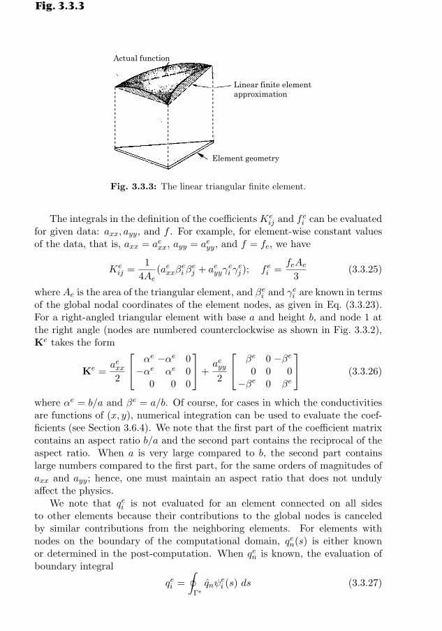
124 THE FINITE ELEMENT METHOD: A REVIEW
Fig. 3.3.3
Actual function
Element geometry
Linear finite elementapproximation
Fig. 3.3.3: The linear triangular finite element.
The integrals in the definition of the coefficients Keij and fei can be evaluated
for given data: axx, ayy, and f . For example, for element-wise constant valuesof the data, that is, axx = aexx, ayy = aeyy, and f = fe, we have
Keij =
1
4Ae(aexxβ
ei β
ej + aeyyγ
ei γ
ej ); fei =
feAe3
(3.3.25)
where Ae is the area of the triangular element, and βei and γei are known in termsof the global nodal coordinates of the element nodes, as given in Eq. (3.3.23).For a right-angled triangular element with base a and height b, and node 1 atthe right angle (nodes are numbered counterclockwise as shown in Fig. 3.3.2),Ke takes the form
Ke =aexx2
αe −αe 0−αe αe 0
0 0 0
+aeyy2
βe 0 −βe0 0 0
−βe 0 βe
(3.3.26)
where αe = b/a and βe = a/b. Of course, for cases in which the conductivitiesare functions of (x, y), numerical integration can be used to evaluate the coef-ficients (see Section 3.6.4). We note that the first part of the coefficient matrixcontains an aspect ratio b/a and the second part contains the reciprocal of theaspect ratio. When a is very large compared to b, the second part containslarge numbers compared to the first part, for the same orders of magnitudes ofaxx and ayy; hence, one must maintain an aspect ratio that does not undulyaffect the physics.
We note that qei is not evaluated for an element connected on all sidesto other elements because their contributions to the global nodes is canceledby similar contributions from the neighboring elements. For elements withnodes on the boundary of the computational domain, qen(s) is either knownor determined in the post-computation. When qen is known, the evaluation ofboundary integral
qei =
∮Γeqnψ
ei (s) ds (3.3.27)
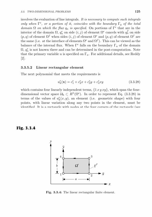
3.3. TWO-DIMENSIONAL PROBLEMS 125
involves the evaluation of line integrals. It is necessary to compute such integralsonly when Γe, or a portion of it, coincides with the boundary Γq of the totaldomain Ω on which the flux qn is specified. On portions of Γe that are in theinterior of the domain Ω, qen on side (i, j) of element Ωe cancels with qfn on side(p, q) of element Ωf when sides (i, j) of element Ωe and (p, q) of element Ωf arethe same (i.e. at the interface of elements Ωe and Ωf ). This can be viewed as thebalance of the internal flux. When Γe falls on the boundary Γu of the domainΩ, qen is not known there and can be determined in the post-computation. Notethat the primary variable u is specified on Γu. For additional details, see Reddy[2].
3.3.5.2 Linear rectangular element
The next polynomial that meets the requirements is
ueh(x) = ce1 + ce2x+ ce3y + ce4xy (3.3.28)
which contains four linearly independent terms, 1x y xy, which span the four-dimensional vector space Uh ⊂ H1(Ωe). In order to represent Eq. (3.3.28) interms of the values of ueh(x, y), an element (i.e. geometric shape) with fourpoints, with linear variation along any two points in the element, must beidentified. It is a rectangle with nodes at the four corners of the rectangle (seeFig. 3.3.4). When the element is a quadrilateral in shape, we use coordinatetransformations to represent the integrals posed on the quadrilateral elementequivalent to those over a square geometry and then use numerical integrationto evaluate the integrals over the quadrilateral domain.
For a linear rectangular element (some times called bilinear element becauseit is linear in both x and y), we have
y
x
b
1
4 3
2a
x_
y_
Ω Γe e
Fig. 3.3.4
Fig. 3.3.4: The linear rectangular finite element.
126
ueh(x) =
4∑i=1
ueiψei (x, y) (3.3.29)
where ψei are the Lagrange interpolation functions expressed in terms of theelement coordinates (x, y)
ψe1 =(
1− x
a
)(1− y
b
), ψe2 =
x
a
(1− y
b
)ψe3 =
x
a
y
b, ψe4 =
(1− x
a
) yb
(3.3.30)
and (x, y) denote the local coordinates with the origin located at node 1 ofthe element, and (a, b) denote the horizontal and vertical dimensions of therectangle, as shown in Fig. 3.3.4.
The integrals in the definition of Keij and fei can be easily evaluated over a
rectangular element of sides a and b. For example, for element-wise constantvalues of the data, that is, axx = aexx, ayy = aeyy, and f = fe, we have (seeReddy [1, p. 313; p. 387]) the following results:
Ke = aexxS11 + aeyyS
22, fei =feab
4(3.3.31)
where
S11 =1
6
2α −2α −α α−2α 2α α −α−α α 2α −2αα −α −2α 2α
, S22 =1
6
2β β −β −2ββ 2β −2β −β−β −2β 2β β−2β −β β 2β
(3.3.32)
and α = b/a and β = a/b. Once again, we note that the element aspectratio should be kept at a reasonable value so that the coefficient matrix is notill-conditioned.
3.3.5.3 Higher-order triangular elements
Higher-order triangular elements (i.e. triangular elements with interpolationfunctions of higher degree) can be systematically developed with the help of theso-called area coordinates. For triangular elements, it is possible to constructthree natural coordinates Li (i = 1, 2, 3), like in the case of one-dimensionalelements, which vary in a direction normal to the sides directly opposite toeach node, as shown in Fig. 3.3.5(a). The coordinates are defined as
ψi = Li =AiA
, A = area of the triangle (3.3.33)
where Ai is the area of the triangle formed by nodes j and k and an arbitrarypoint P in the element, and A is the total area of the element. For example, A1
THE FINITE ELEMENT METHOD: A REVIEW
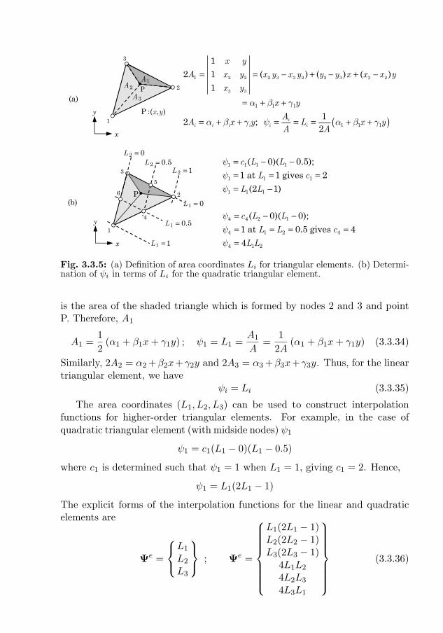
3.3. TWO-DIMENSIONAL PROBLEMS 127
(a)
x
y P :( , )x y
P
3
2
1
1A2A
3A
•
( )
2 2 2 3 3 2 2 3 3 2
3 3
1
1 1 1
1 1 1
12 1 ( ) ( ) ( )
1
12 ;
2
a b g
a b g y a b g
= = − + − + −
= + +
= + + = = = + +ii i i i i i
x y
A x y x y x y y y x x x y
x y
x y
AA x y L x y
A A
1 1 1 1
1 1 1
1 1 1
4 4 2 1
4 1 2 4
4 1 2
( 0)( 0.5);
1 at 1 gives 2
(2 1)
( 0)( 0);
1 at 0.5 gives 4
4
c L L
L c
L L
c L L
L L c
L L
yyy
yyy
= − −= = == −
= − −= = = ==x
y
P
5
3
1
•(b) 1 0L =
1 0.5L =
1 1L =
2
4
6
2 0L =
2 1L =2 0.5L =
Fig. 3.3.5: (a) Definition of area coordinates Li for triangular elements. (b) Determi-nation of ψi in terms of Li for the quadratic triangular element.
is the area of the shaded triangle which is formed by nodes 2 and 3 and pointP. Therefore, A1 is given by [see Fig. 3.3.5(a)]
A1 =1
2(α1 + β1x+ γ1y) ; ψ1 = L1 =
A1
A=
1
2A(α1 + β1x+ γ1y) (3.3.34)
Similarly, 2A2 = α2 +β2x+γ2y and 2A3 = α3 +β3x+γ3y. Thus, for the lineartriangular element, we have
ψi = Li (3.3.35)
The area coordinates (L1, L2, L3) can be used to construct interpolationfunctions for higher-order triangular elements. For example, in the case ofquadratic triangular element (with midside nodes) ψ1 is given by [see Fig. 3.3.5(b)]
ψ1 = c1(L1 − 0)(L1 − 0.5)
where c1 is determined such that ψ1 = 1 when L1 = 1, giving c1 = 2. Hence,
ψ1 = L1(2L1 − 1)
The explicit forms of the interpolation functions for the linear and quadraticelements are
Ψe =
L1
L2
L3
; Ψe =
L1(2L1 − 1)L2(2L2 − 1)L3(2L3 − 1)
4L1L2
4L2L3
4L3L1
(3.3.36)
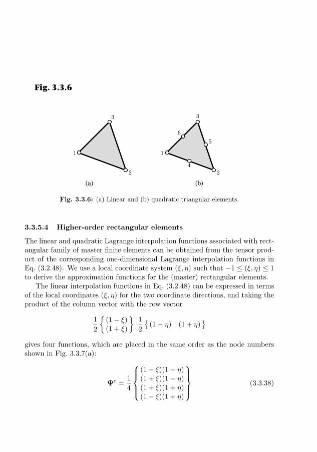
128 THE FINITE ELEMENT METHOD: A REVIEW
Note that the order of the interpolation functions in the above arrays corre-sponds to the node numbers shown in Figs. 3.3.6(a) and (b).
Integrals of the products of the area coordinates Li over an element can beevaluated using the following formula:∫
ALp1 L
q2 L
r3 dA =
p! q! r!
(p+ q + r + 1)!A (3.3.37)
1
2
3
1
4
3
2
5
6
Fig. 3.3.6
(a) (b)
Fig. 3.3.6: (a) Linear and (b) quadratic triangular elements.
3.3.5.4 Higher-order rectangular elements
The linear and quadratic Lagrange interpolation functions associated with rect-angular family of master finite elements can be obtained from the tensor prod-uct of the corresponding one-dimensional Lagrange interpolation functions inEq. (3.2.48). We use a local coordinate system (ξ, η) such that −1 ≤ (ξ, η) ≤ 1to derive the approximation functions for the (master) rectangular elements.
The linear interpolation functions in Eq. (3.2.48) can be expressed in termsof the local coordinates (ξ, η) for the two coordinate directions, and taking theproduct of the column vector with the row vector
1
2
(1− ξ)(1 + ξ)
1
2
(1− η) (1 + η)
gives four functions, which are placed in the same order as the node numbersshown in Fig. 3.3.7(a):
Ψe =1
4
(1− ξ)(1− η)(1 + ξ)(1− η)(1 + ξ)(1 + η)(1− ξ)(1 + η)
(3.3.38)
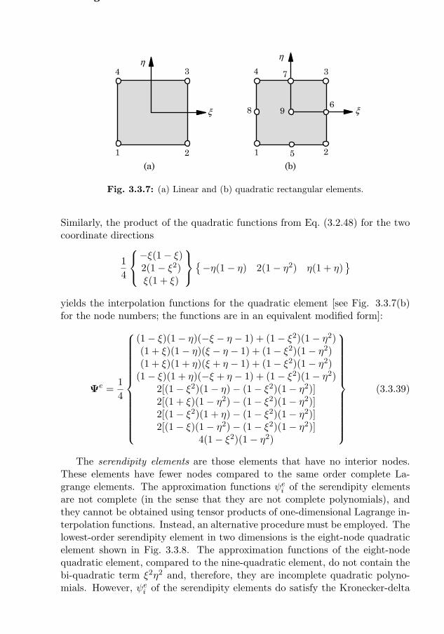
3.3. TWO-DIMENSIONAL PROBLEMS 129
Fig. 3.3.7
1 2
3
1
4 7
8
5
6ξ ξ
η η
2
34
9
(a) (b)
Fig. 3.3.7: (a) Linear and (b) quadratic rectangular elements.
Similarly, the product of the quadratic functions from Eq. (3.2.48) for the twocoordinate directions
1
4
−ξ(1− ξ)2(1− ξ2)ξ(1 + ξ)
−η(1− η) 2(1− η2) η(1 + η)
yields the interpolation functions for the quadratic element [see Fig. 3.3.7(b)for the node numbers; the functions are in an equivalent modified form]:
Ψe =1
4
(1− ξ)(1− η)(−ξ − η − 1) + (1− ξ2)(1− η2)(1 + ξ)(1− η)(ξ − η − 1) + (1− ξ2)(1− η2)(1 + ξ)(1 + η)(ξ + η − 1) + (1− ξ2)(1− η2)
(1− ξ)(1 + η)(−ξ + η − 1) + (1− ξ2)(1− η2)2[(1− ξ2)(1− η)− (1− ξ2)(1− η2)]2[(1 + ξ)(1− η2)− (1− ξ2)(1− η2)]2[(1− ξ2)(1 + η)− (1− ξ2)(1− η2)]2[(1− ξ)(1− η2)− (1− ξ2)(1− η2)]
4(1− ξ2)(1− η2)
(3.3.39)
The serendipity elements are those elements that have no interior nodes.These elements have fewer nodes compared to the same order complete La-grange elements. The approximation functions ψei of the serendipity elementsare not complete (in the sense that they are not complete polynomials), andthey cannot be obtained using tensor products of one-dimensional Lagrange in-terpolation functions. Instead, an alternative procedure must be employed. Thelowest-order serendipity element in two dimensions is the eight-node quadraticelement shown in Fig. 3.3.8. The approximation functions of the eight-nodequadratic element, compared to the nine-quadratic element, do not contain thebi-quadratic term ξ2η2 and, therefore, they are incomplete quadratic polyno-mials. However, ψei of the serendipity elements do satisfy the Kronecker-delta
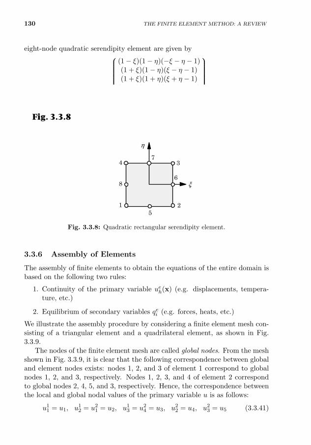
130 THE FINITE ELEMENT METHOD: A REVIEW
property [i.e. property (i) in Eq. (3.3.24)]. The interpolation functions for theeight-node quadratic serendipity element are given by
Ψe =1
4
(1− ξ)(1− η)(−ξ − η − 1)(1 + ξ)(1− η)(ξ − η − 1)(1 + ξ)(1 + η)(ξ + η − 1)
(1− ξ)(1 + η)(−ξ + η − 1)2(1− ξ2)(1− η)2(1 + ξ)(1− η2)2(1− ξ2)(1 + η)2(1− ξ)(1− η2)
(3.3.40)
ξ
η
1 2
34
5
68
7
Fig. 3.3.8
Fig. 3.3.8: Quadratic rectangular serendipity element.
3.3.6 Assembly of Elements
The assembly of finite elements to obtain the equations of the entire domain isbased on the following two rules:
1. Continuity of the primary variable ueh(x) (e.g. displacements, tempera-ture, etc.)
2. Equilibrium of secondary variables qei (e.g. forces, heats, etc.)
We illustrate the assembly procedure by considering a finite element mesh con-sisting of a triangular element and a quadrilateral element, as shown in Fig.3.3.9.
The nodes of the finite element mesh are called global nodes. From the meshshown in Fig. 3.3.9, it is clear that the following correspondence between globaland element nodes exists: nodes 1, 2, and 3 of element 1 correspond to globalnodes 1, 2, and 3, respectively. Nodes 1, 2, 3, and 4 of element 2 correspondto global nodes 2, 4, 5, and 3, respectively. Hence, the correspondence betweenthe local and global nodal values of the primary variable u is as follows:
u11 = u1, u1
2 = u21 = u2, u1
3 = u24 = u3, u2
2 = u4, u23 = u5 (3.3.41)
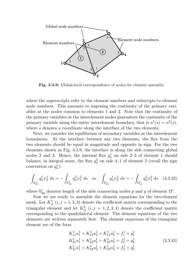
3.3. TWO-DIMENSIONAL PROBLEMS 131
Element node numbers
1
2
3
14
5
2
1
2
32
1
3
4
Global node numbers
Element numbers
Fig. 3.3.9: Global-local correspondence of nodes for element assembly.
where the superscripts refer to the element numbers and subscripts to elementnode numbers. This amounts to imposing the continuity of the primary vari-ables at the nodes common to elements 1 and 2. Note that the continuity ofthe primary variables at the interelement nodes guarantees the continuity of theprimary variable along the entire interelement boundary, that is u1(s) = u2(s),where s denotes a coordinate along the interface of the two elements.
Next, we consider the equilibrium of secondary variables at the interelementboundaries. At the interface between any two elements, the flux from thetwo elements should be equal in magnitude and opposite in sign. For the twoelements shown in Fig. 3.3.9, the interface is along the side connecting globalnodes 2 and 3. Hence, the internal flux q1
n on side 2–3 of element 1 shouldbalance, in integral sense, the flux q2
n on side 4–1 of element 2 (recall the signconvention on qen):∫
h123
q1nψ
12 ds = −
∫h2
14
q2nψ
21 ds or
∫h1
23
q1nψ
13 ds = −
∫h2
14
q2nψ
24 ds (3.3.42)
where hepq denotes length of the side connecting nodes p and q of element Ωe.Now we are ready to assemble the element equations for the two-element
mesh. Let K1ij (i, j = 1, 2, 3) denote the coefficient matrix corresponding to the
triangular element and let K2ij (i, j = 1, 2, 3, 4) denote the coefficient matrix
corresponding to the quadrilateral element. The element equations of the twoelements are written separately first. The element equations of the triangularelement are of the form
K111u
11 +K1
12u12 +K1
13u13 = f1
1 + q11
K121u
11 +K1
22u12 +K1
23u13 = f1
2 + q12
K131u
11 +K1
32u12 +K1
33u13 = f1
3 + q13
(3.3.43)
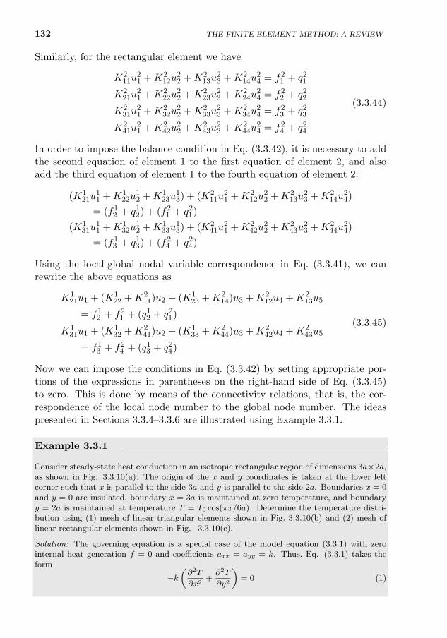
132 THE FINITE ELEMENT METHOD: A REVIEW
Similarly, for the rectangular element we have
K211u
21 +K2
12u22 +K2
13u23 +K2
14u24 = f2
1 + q21
K221u
21 +K2
22u22 +K2
23u23 +K2
24u24 = f2
2 + q22
K231u
21 +K2
32u22 +K2
33u23 +K2
34u24 = f2
3 + q23
K241u
21 +K2
42u22 +K2
43u23 +K2
44u24 = f2
4 + q24
(3.3.44)
In order to impose the balance condition in Eq. (3.3.42), it is necessary to addthe second equation of element 1 to the first equation of element 2, and alsoadd the third equation of element 1 to the fourth equation of element 2:
(K121u
11 +K1
22u12 +K1
23u13) + (K2
11u21 +K2
12u22 +K2
13u23 +K2
14u24)
= (f12 + q1
2) + (f21 + q2
1)
(K131u
11 +K1
32u12 +K1
33u13) + (K2
41u21 +K2
42u22 +K2
43u23 +K2
44u24)
= (f13 + q1
3) + (f24 + q2
4)
Using the local-global nodal variable correspondence in Eq. (3.3.41), we canrewrite the above equations as
K121u1 + (K1
22 +K211)u2 + (K1
23 +K214)u3 +K2
12u4 +K213u5
= f12 + f2
1 + (q12 + q2
1)
K131u1 + (K1
32 +K241)u2 + (K1
33 +K244)u3 +K2
42u4 +K243u5
= f13 + f2
4 + (q13 + q2
4)
(3.3.45)
Now we can impose the conditions in Eq. (3.3.42) by setting appropriate por-tions of the expressions in parentheses on the right-hand side of Eq. (3.3.45)to zero. This is done by means of the connectivity relations, that is, the cor-respondence of the local node number to the global node number. The ideaspresented in Sections 3.3.4–3.3.6 are illustrated using Example 3.3.1.
Example 3.3.1
Consider steady-state heat conduction in an isotropic rectangular region of dimensions 3a×2a,as shown in Fig. 3.3.10(a). The origin of the x and y coordinates is taken at the lower leftcorner such that x is parallel to the side 3a and y is parallel to the side 2a. Boundaries x = 0and y = 0 are insulated, boundary x = 3a is maintained at zero temperature, and boundaryy = 2a is maintained at temperature T = T0 cos(πx/6a). Determine the temperature distri-bution using (1) mesh of linear triangular elements shown in Fig. 3.3.10(b) and (2) mesh oflinear rectangular elements shown in Fig. 3.3.10(c).
Solution: The governing equation is a special case of the model equation (3.3.1) with zerointernal heat generation f = 0 and coefficients axx = ayy = k. Thus, Eq. (3.3.1) takes theform
−k(∂2T
∂x2+∂2T
∂y2
)= 0 (1)
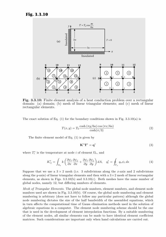
3.3. TWO-DIMENSIONAL PROBLEMS 133Fig. 3.3.10
x
y ax
TT6
cos0π=
Insu
late
d
Insulated
0=T
a3
a2(a)
(c)(b)
1 2 3 4
5 6 7 8
9 10 11 12
1
2
3
4
5
6
7
8 10 12
119
1 2
3
3
1 2
2 2 2
1 1 111
1 1
2
1 2 3 4
5 6 7 8
9 10 11 12
1
3
1 2 3
4 5 6
2
4
1 1
1 1 1
Fig. 3.3.10: Finite element analysis of a heat conduction problem over a rectangulardomain: (a) domain; (b) mesh of linear triangular elements; and (c) mesh of linearrectangular elements.
The exact solution of Eq. (1) for the boundary conditions shown in Fig. 3.3.10(a) is
T (x, y) = T0cosh (πy/6a) cos (πx/6a)
cosh(π/3)(2)
The finite element model of Eq. (1) is given by
KeTe = qe (3)
where T ei is the temperature at node i of element Ωe, and
Keij =
∫Ωe
k
(∂ψi∂x
∂ψj∂x
+∂ψi∂y
∂ψj∂y
)dA, qei =
∮Γe
qnψi ds (4)
Suppose that we use a 3 × 2 mesh (i.e. 3 subdivisions along the x-axis and 2 subdivisionsalong the y-axis) of linear triangular elements and then with a 3×2 mesh of linear rectangularelements, as shown in Figs. 3.3.10(b) and 3.3.10(c). Both meshes have the same number ofglobal nodes, namely 12, but differing numbers of elements.
Mesh of Triangular Elements. The global node numbers, element numbers, and element nodenumbers used are shown in Fig. 3.3.10(b). Of course, the global node numbering and elementnumbering is arbitrary (does not have to follow any particular pattern) although the globalnode numbering dictates the size of the half bandwidth of the assembled equations, whichin turn affects the computational time of Gauss elimination methods used in the solution ofalgebraic equations in a computer. The element node numbering scheme should be the onethat is used in the development of element interpolation functions. By a suitable numberingof the element nodes, all similar elements can be made to have identical element coefficientmatrices. Such considerations are important only when hand calculations are carried out.
134 THE FINITE ELEMENT METHOD: A REVIEW
For a typical element of the mesh of triangles in Fig. 3.3.10(b), the element coefficientmatrix is given by [see Eq. (3.3.26) and Fig. 3.3.2 for the element matrix and element geome-try],
Ke =k
2
1 −1 0−1 2 −1
0 −1 1
, fe = 0 (5)
where k is the conductivity of the medium. Note that the element matrix is independent ofthe size of the element, as long as the element is a right-angle triangle with its base equal toits height.
The assembly of the elements follows the logic discussed earlier. For example, we have
K11 = K111 +K2
33 =k
2(1 + 1), K12 = K1
12 =k
2(−1), K13 = 0
K15 = K232 =
k
2(−1), K16 = K1
13 +K231 = 0 + 0, etc.
F1 = q11 + q2
3 , F6 = q13 + q2
1 + q42 + q7
2 + q91 + q10
3 , etc.
(6)
In view of the boundary conditions, we have
U4 = U8 = U12 = 0, U9 = T0, U10 =
√3
2T0, U11 =
T0
2
F1 = F2 = F3 = F5 = 0
(7)
and the balance of internal heat flow requires that
F6 = F7 = 0 (8)
Thus, the unknown primary variables and secondary variables of the problem are:
U1, U2, U3, U5, U6, U7; F4, F8, F9, F10, F11, F12 (9)
We write the six finite element equations for the six unknown primary variables. Theseequations come from rows 1, 2, 3, 5, 6, and 7 (corresponding to the same global nodes):
K11U1 +K12U2 + · · ·+K1(12)U12 = F1 = (q11 + q2
3) = 0
K21U1 +K22U2 + · · ·+K2(12)U12 = F2 = (q12 + q3
1 + q43) = 0
...
K71U1 +K72U2 + · · ·+K7(12)U12 = F7 = (q33 + q4
1 + q62 + q9
2 + q111 + q12
3 ) = 0
(10)
Using the boundary conditions and the values of KIJ , we obtain
k(U1 −1
2U2 −
1
2U5) = 0
k(−1
2U1 + 2U2 −
1
2U3 − U6) = 0
k(−1
2U2 + 2U3 − U7) = 0
k(−1
2U1 + 2U5 − U6 −
1
2U9) = 0 (U9 = T0)
k(−U2 − U5 + 4U6 − U7 − U10) = 0 (U10 =
√3
2T0)
k(−U3 − U6 + 4U7 − U11) = 0 (U11 =1
2T0)
(11)
3.3. TWO-DIMENSIONAL PROBLEMS 135
or, in the matrix form
k
2
2 −1 0 −1 0 0−1 4 −1 0 −2 0
0 −1 4 0 0 −2−1 0 0 4 −2 0
0 −2 0 −2 8 −20 0 −2 0 −2 8
U1
U2
U3
U5
U6
U7
=k
2
000T0√3T0
T0
(12)
The solution of these equations is (in C)
U1 = 0.6362T0, U2 = 0.5510T0, U3 = 0.3181T0
U5 = 0.7214T0, U6 = 0.6248T0, U7 = 0.3607T0
(13)
Evaluating the exact solution in Eq. (2) at the nodes, we have (in C)
T1 = 0.6249T0, T2 = 0.5412T0, T3 = 0.3124T0
T5 = 0.7125T0, T6 = 0.6171T0, T7 = 0.3563T0
(14)
The heat at node 4, for example, can be computed from the 4th finite element equation
F4 = Q52 = K41U1 +K42U2 +K43U3 +K44U4 +K45U5
+K46U6 +K47U7 +K48U8 + . . . (15)
Noting that K41 = K42 = K45 = · · · = K4(12) = 0 and U4 = U8 = 0, we obtain
Q52 = −1
2kU3 = −0.1591kT0 (in W) (16)
Mesh of Rectangular Elements. For a 3 × 2 mesh of linear rectangular elements [seeFig. 3.3.10(c)], the element coefficient matrix is given by Eq. (3.3.31)
Ke =k
6
4 −1 −2 −1−1 4 −1 −2−2 −1 4 −1−1 −2 −1 4
, fe = 0 (17)
The present mesh of rectangular elements is node-wise equivalent to the triangular elementmesh considered in Fig. 3.3.10(b). Hence the boundary conditions in Eqs. (7) and (8) arevalid for the present case. The assembled global coefficients are
K11 = K111, K12 = K1
12, K15 = K114, K16 = K1
13, K22 = K122 +K2
11
K23 = K212, K25 = K1
24, K26 = K123 +K2
14, K27 = K213, etc.
F1 = q11 , F2 = q1
2 + q21 , F3 = q2
2 + q31 , F4 = q3
2 , etc.
(18)
The equations for the unknown temperatures (i.e. condensed equations for the unknownprimary variables) are
k
6
4 −1 0 −1 −2 0−1 8 −1 −2 −2 −2
0 −1 8 0 −2 −2−1 −2 0 8 −2 0−2 −2 −2 −2 16 −2
0 −2 −2 0 −2 16
U1
U2
U3
U5
U6
U7
=k
6
000
T0 +√
3T0
2T0 +√
3T0 + T0√3T0 + T0
(19)
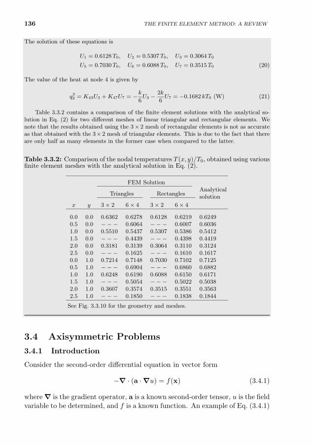
136 THE FINITE ELEMENT METHOD: A REVIEW
The solution of these equations is
U1 = 0.6128T0, U2 = 0.5307T0, U3 = 0.3064T0
U5 = 0.7030T0, U6 = 0.6088T0, U7 = 0.3515T0 (20)
The value of the heat at node 4 is given by
q32 = K43U3 +K47U7 = −k
6U3 −
2k
6U7 = −0.1682 kT0 (W) (21)
Table 3.3.2 contains a comparison of the finite element solutions with the analytical so-lution in Eq. (2) for two different meshes of linear triangular and rectangular elements. Wenote that the results obtained using the 3× 2 mesh of rectangular elements is not as accurateas that obtained with the 3×2 mesh of triangular elements. This is due to the fact that thereare only half as many elements in the former case when compared to the latter.
Table 3.3.2: Comparison of the nodal temperatures T (x, y)/T0, obtained using variousfinite element meshes with the analytical solution in Eq. (2).
FEM SolutionAnalyticalsolution
Triangles Rectangles
x y 3× 2 6× 4 3× 2 6× 4
0.0 0.0 0.6362 0.6278 0.6128 0.6219 0.62490.5 0.0 −−− 0.6064 −−− 0.6007 0.60361.0 0.0 0.5510 0.5437 0.5307 0.5386 0.54121.5 0.0 −−− 0.4439 −−− 0.4398 0.44192.0 0.0 0.3181 0.3139 0.3064 0.3110 0.31242.5 0.0 −−− 0.1625 −−− 0.1610 0.16170.0 1.0 0.7214 0.7148 0.7030 0.7102 0.71250.5 1.0 −−− 0.6904 −−− 0.6860 0.68821.0 1.0 0.6248 0.6190 0.6088 0.6150 0.61711.5 1.0 −−− 0.5054 −−− 0.5022 0.50382.0 1.0 0.3607 0.3574 0.3515 0.3551 0.35632.5 1.0 −−− 0.1850 −−− 0.1838 0.1844
See Fig. 3.3.10 for the geometry and meshes.
3.4 Axisymmetric Problems
3.4.1 Introduction
Consider the second-order differential equation in vector form
−∇ · (a ·∇u) = f(x) (3.4.1)
where ∇ is the gradient operator, a is a known second-order tensor, u is the fieldvariable to be determined, and f is a known function. An example of Eq. (3.4.1)
3.4. AXISYMMETRIC PROBLEMS 137
is provided by heat conduction equation, where u is the temperature, a is theconductivity tensor, and f is the internal heat generation.
The equations governing physical processes in cylindrical geometries aredescribed analytically in terms of cylindrical coordinates (r, θ, z). For a cylin-drically orthotropic material (i.e. when the material axes of an orthotropicmaterial coincide with the r, θ, and z axes), Eq. (3.4.1) takes the form
−1
r
∂
∂r
(rarr
∂u
∂r
)− 1
r2
∂
∂θ
(aθθ
∂u
∂θ
)− ∂
∂z
(azz
∂u
∂z
)= f(r, θ, z) (3.4.2)
When the geometry, loading, and boundary conditions are independent of thecircumferential direction (i.e. θ-coordinate direction), the problem is said to beaxisymmetric and the governing equation becomes two-dimensional in terms ofr and z:
−1
r
∂
∂r
(rarr
∂u
∂r
)− ∂
∂z
(azz
∂u
∂z
)= f(r, z) (3.4.3)
In addition, if the problem geometry and data are independent of z, for example,when the cylinder is very long, the equation is a function of only the radialcoordinate r:
−1
r
d
dr
(rarr
du
dr
)= f(r) for a < r < b (3.4.4)
In this section we develop the finite element models of one-dimensional andtwo-dimensional axisymmetric problems described by Eqs. (3.4.3) and (3.4.4),which may arise in various different fields, and the coefficients arr, aθθ, andazz may be functions of u and its derivatives. In each case, we begin with thedevelopment of the weak form, where the volume element dv is replaced bydv = rdrdθdz.
3.4.2 One-Dimensional Problems
In developing the weak form of Eq. (3.4.4), we replace u with its approximationuh, multiply the resulting residual with a weight function wi(r), and integrateover the element volume ve = (ra, rb) × (0, 2π) × (0, 1) of the cylinder of unitlength (a ≡ arr)
0 =
∫vewi
[−1
r
d
dr
(raduhdr
)− f
]dv = 2π
∫ rb
ra
wi
[−1
r
d
dr
(raduhdr
)− f
]r dr
(3.4.5)where (ra, rb) is the domain of a typical element along the radial direction.Next, we carry out the remaining two steps of the weak formulation:
0 = 2π
∫ rb
ra
(adwidr
duhdr− wif
)rdr − 2π
[wi ra
duhdr
]rbra
0 = 2π
∫ rb
ra
(adwidr
duhdr− wif
)rdr − wi(ra)Qe1 − wi(rb)Qe2 (3.4.6)
138 THE FINITE ELEMENT METHOD: A REVIEW
where
Qe1 ≡ −2π
(raduhdr
) ∣∣∣∣ra
, Qe2 ≡ 2π
(raduhdr
) ∣∣∣∣rb
(3.4.7)
The finite element model is obtained by substituting the approximation
u(r) ≈n∑j=1
uejψej (r) (3.4.8)
where ψej (r) are the Lagrange interpolation functions; the only change is thatthe axial coordinate x is replaced by the radial r. For example, the linearinterpolation functions are of the form (he = rb − ra)
ψe1(r) =rb − rhe
, ψe2(r) =r − rahe
(3.4.9)
or, in terms of the local coordinate r, we have
ψe1(r) = 1− r
he, ψe2(r) =
r
he(3.4.10)
As before, we replace wi with ψei to obtain the ith algebraic equation of theRitz (or weak-form Galerkin) finite element model
n∑j=1
Keiju
ej = fei +Qei or Keue = f e + Qe (3.4.11)
where
Keij = 2π
∫ rb
ra
adψeidr
dψejdr
rdr, fei = 2π
∫ rb
ra
ψei f r dr (3.4.12)
3.4.3 Two-Dimensional Problems
Following the three-step procedure, we obtain the weak form (the constantmultiplier 2π is omitted)
0 =
∫Ωe
(arr
∂wi∂r
∂uh∂r
+ azz∂wi∂z
∂uh∂z− wif
)r dr dz −
∮Γe
wiqn ds (3.4.13)
where wi is the ith weight function and qn is the flux normal to the boundary
qn = r
(arr
∂uh∂r
nr + azz∂uh∂z
nz
)(3.4.14)
Let us assume that u(r, z) is approximated by the finite element interpola-tion ueh over the element Ωe
u ≈ ueh(r, z) =
n∑j=1
uejψej (r, z) (3.4.15)
3.5. THE LEAST-SQUARES METHOD 139
where interpolation functions ψej (r, z) are the same as those developed for lineartriangular and rectangular elements, with x = r and y = z. Substitution ofEq. (3.4.15) for uh and ψei for wi into the weak form gives the ith equation ofthe finite element model
0 =
n∑j=1
[∫Ωe
(arr
∂ψei∂r
∂ψej∂r
+ azz∂ψei∂z
∂ψej∂z
)rdrdz
]uej
−∫
Ωe
ψei f r dr dz −∮
Γe
ψei qn ds (3.4.16)
or
0 =
n∑j=1
Keiju
ej − fei −Qei (3.4.17)
where
Keij =
∫Ωe
(arr
∂ψei∂r
∂ψej∂r
+ azz∂ψei∂z
∂ψej∂z
)r dr dz
fei =
∫Ωe
ψei f r dr dz, Qei =
∮Γe
ψei qn ds
(3.4.18)
3.5 The Least-Squares Method
3.5.1 Background
The success of weak-form Galerkin finite element models in the field of solidand structural mechanics is intimately connected with the notion of global min-imization of quadratic functionals, which often represent the total energy of thesystem. When weak forms of a set of partial differential equations can be ob-tained equivalently through the minimization of a quadratic functional, thefinite element solution becomes an orthogonal projection of the exact solutiononto the space of approximations associated with the finite element discretiza-tion. The resulting numerical solution represents the best possible approxi-mation of the exact solution in the space of approximation as measured withrespect to the norm induced by the functional, called the energy norm. Whenthe energy norm can be shown to be equivalent to a norm in an appropriateHilbert space, such as the H1, optimal convergence rates of the finite elementsolution can be established. Such a setting, often referred to as a variationalsetting, is ideal for finite element approximation.
The finite element models based on the weak-form Galerkin approach oftendepart from the ideal variational setting. For example, the weak-form formu-lation of the Stokes equations yields a constrained variational problem, whosediscrete solution must satisfy restrictive compatibility conditions on the approx-imations used for velocity components and pressure. The weak-form Galerkinfinite element model of the Navier–Stokes equations, on the other hand, is
140 THE FINITE ELEMENT METHOD: A REVIEW
completely divorced from any minimization principles and further inherits theinf-sup condition [25–27] of the Stokes problem. Numerical solutions are farfrom optimal as characterized by the need for severe mesh refinement in or-der to suppress spurious oscillations of the solution. A considerable amount ofresearch in recent years has been devoted to modifications of the weak formGalerkin approach in the hope of obtaining a more favorable setting for the nu-merical solution. These include the meshless and particle methods [28–37] andleast-squares finite element formulations [38–45], including the k-version finiteelement method advanced by Surana, Reddy, and their colleagues [40–42]. Sta-bilized finite element formulations based on the penalty, SUPG and Galerkinleast-squares methods have been proposed and extensively researched [46–48](also see [10, 49, 50] for additional references). These schemes have yet to gainwide acceptance, due in part to the associated time- and mesh-dependent adhoc parameters that must be fine tuned in each formulation.
Finite element models based on least-squares formulations offer an attrac-tive alternative to the more popular weak-form Galerkin approach. In the caseof linear problems, the least-squares formulation always admits a symmetricpositive-definite coefficient matrix, regardless of whether or not such symme-try is manifest in the governing partial differential equations. As a result,robust iterative solution algorithms such as the preconditioned conjugate gra-dient method can be employed in the solution process, and only half of thecoefficient matrix need be stored in memory. This is not the case when theweak-form Galerkin scheme is applied to nonself-adjoint systems of equations.In the context of fluid mechanics problems, the least-squares formulation doesnot suffer from the restrictive inf-sup condition. Approximations of the velocityand pressure can therefore be sought using the same bases of interpolation.
Least-squares variational formulations allow us to define a convex least-squares functional constructed in terms of the sum of the squares of the normsof the residuals of approximation of a set of differential equations. It is alsopossible to define a norm associated with the least-squares functional. If it canbe shown that the norm induced by the least-squares functional is equivalent toa Hm norm, optimal convergence rates can be established for the least-squaresfinite element approximations. Under such conditions, the least-squares finiteelement model constitutes an ideal variational setting, regardless of whetheror not such a setting is achieved by the associated weak-form Galerkin formu-lation. Unfortunately, norm equivalence (or H1-coercivity of the least squaresfunctional) cannot always be established for a given least-squares functional.However, unlike weak-form Galerkin formulations, such a departure from theideal variational setting does not typically result in disastrous consequences forleast-squares finite element models. In particular, Pontaza and Reddy [43, 44]and Prabhakar and Reddy [45] demonstrated numerically that hp least-squaresfinite element models are capable of yielding highly accurate results even whenthe least-squares functional cannot be shown to be H1-coercive a priori.
3.5. THE LEAST-SQUARES METHOD 141
Least-squares formulations are certainly not without their own shortcom-ings. Most problems in engineering physics possess, at the very minimum,second-order spatial differential operators. Least-squares formulations of suchequations typically require higher-order approximations of solution variables.This significantly affects the conditioning of the coefficient matrix and the num-ber of iterations needed for convergence of an iterative solution scheme used tosolve linear equations. To circumvent these challenges, the governing equationsare often recast as a set of first-order equations through the introduction ofauxiliary variables. This not only allows for a better conditioning of the ma-trices, but also leads to a larger global system of equations. It can be arguedthat such a formulation is at least somewhat useful, since the auxiliary vari-ables often represent important physical quantities of interest (e.g. heat fluxand components of the stress tensor). The objective of this section is to discussthe basic idea of the least-squares formulation. A more detailed discussion willbe presented in Chapter 11.
3.5.2 The Basic Idea
The least-squares method is based on the idea of minimizing the error func-tional, which is the integral of the squares of the errors introduced in the ap-proximation of a differential equation and associated boundary conditions, withrespect to the parameters (i.e. nodal values) of the approximation. To illus-trate the idea, we consider a problem described by linear operator equationsinvolving a single variable u defined over a domain Ω
A(u)− f = 0, in Ω and B(u)− g = 0 on Γ (3.5.1)
where A and B are linear differential operators and f and g are the data.Suppose that the domain Ω is decomposed into a set of finite elements Ωe
and the dependent variable u is approximated in Ωe by expression of the form
u(x) ≈ ueh(x) =
n∑j=1
∆ejϕ
ej(x) (3.5.2)
where ∆j are unknown parameters, related to the values of u and possibly itsderivatives, and ϕj(x) are suitably selected approximation functions. Then
Re1 ≡ A(ueh)− f =n∑j=1
∆ejA(ϕej(x))− f 6= 0, in Ωe
Re2 ≡ B(ueh)− g =
n∑j=1
∆ejB(ϕej(x))− g 6= 0, on Γe
are the residuals in the differential equation and the boundary conditions dueto the approximation of u by ueh.
142 THE FINITE ELEMENT METHOD: A REVIEW
To cast the problem in a suitable functional analysis setting, recall fromSection 1.7 the standard notation used for the Sobolev (or Hilbert) space oforder m ≥ 0, Hm(Ωe) and Hm(Γe) of functions defined in the domain Ωe andits boundary Γe. When m = 0, we use the notation L2(Ωe) = H0(Ωe) andL2(Γe) = H0(Γe). Therefore, one can construct the least-squares functional interms of the sum of the squares of the L2 norms of the residuals
J e(ueh; f, g) =1
2
∫Ωe
[Re1]2 dx +1
2
∫Γe
[Re2]2 ds
=1
2
(‖A(ueh)− f‖2Ωe,0 + ‖B(ueh)− g‖2Γe,0
)(3.5.3)
The least-squares (minimum) principle associated with the least-squares func-tional J e can be stated as follows: find ueh ∈ Uh ⊂ H(Ωe) such that
J (ueh; f, g) 6 J (weh; f, g) for all weh ∈ Uh (3.5.4)
where Uh is an appropriate vector space, such as H1(Ωe), spanned by the setϕeini=1. The necessary condition for the minimum of J (ueh) is that its firstvariation be zero
δJ (ueh, δueh; f, g) = (A(δueh),A(ueh)− f)Ωe,0 + (B(δueh), B(ueh)− g)Γe,0 (3.5.5)
where δueh ∈ Uh is an admissible variation of ueh, (·, ·)Ωe,0 and (·, ·)Γe,0 are theL2-inner products, and ‖ · ‖Ωe,0 and ‖ · ‖Γe,0 are the associated norms. Now thevariational problem associated with Eq. (3.5.5) can be stated as: find ueh ∈ Uhsuch that
B(weh, ueh) = F(weh) for all weh ∈ Uh (3.5.6)
where the bilinear form B and linear form F are given as
B(weh, ueh) = (A(weh), A(ueh))Ωe,0 + (B(weh), B(ueh))Γe,0
F(weh) = (A(weh), f)Ωe,0 + (B(weh), g)Γe,0
(3.5.7)
We can define a norm ‖ · ‖A associated with the least-squares functional as
‖u‖A =√J (u; 0, 0) (3.5.8)
We note that, when A and B are linear, the bilinear form B(·, ·) is symmetricregardless of whether or not operator A is self-adjoint. When the differentialoperator A is nonlinear, this is no longer the case.
Substitution of the finite element approximation, Eq. (3.5.2) into the varia-tional statement in Eq. (3.5.6), we obtain the finite element model
Ke∆e = Fe (3.5.9)
3.6. NUMERICAL INTEGRATION 143
where
Keij =
(A(ϕei ), A(ϕej)
)Ωe,0
+(B(ϕei ), B(ϕej)
)Γe,0
=
∫ΩeA(ϕei )A(ϕej) dx +
∫ΓeB(ϕei )B(ϕej) ds
F ei = (A(ϕei ), f)Ωe,0 + (B(ϕei ), g)Γe,0
=
∫ΩeA(ϕei ) f dx +
∫ΓeB(ϕei ) g ds
(3.5.10)
We note that the approximations ϕei should be selected such that A(ϕei ) ex-ists and is square-integrable, and B(ueh) is continuous across the interelementboundary. Thus, ϕei (x) must belong to the Hermite class of functions when Ais a second- or higher-order differential operator.
3.6 Numerical Integration
3.6.1 Preliminary Comments
An accurate representation of irregular domains (i.e. domains with curvedboundaries) can be accomplished by the use of refined meshes and/or irregu-larly shaped curvilinear elements. For example, a non-rectangular region cannotbe represented using rectangular elements; however, it can be represented byquadrilateral elements. Since the interpolation functions are easily derivablefor a rectangular element and it is easier to evaluate integrals over rectangulargeometries, we transform the finite element integral statements defined overquadrilaterals to a rectangle. The transformation results in complicated ex-pressions for the integrands in terms of the coordinates used for the rectangularelement. Therefore, numerical integration is used to evaluate such complicatedintegrals. The numerical integration schemes, such as the Gauss–Legendre nu-merical integration scheme, require the integral to be evaluated on a specificdomain or with respect to a specific coordinate system.
3.6.2 Coordinate Transformations
Gauss quadrature requires the integral to be expressed over a square regionΩ of dimension 2 × 2 with respect to the coordinate system, (ξ, η) such that−1 ≤ (ξ, η) ≤ 1. The transformation of the geometry and the variable coef-ficients of the differential equation from the problem coordinates (x, y) to thelocal coordinates (ξ, η) results in algebraically complex expressions, and theypreclude analytical (i.e. exact) evaluation of the integrals. Thus, the trans-formation of a given integral expression defined over an element Ωe to one onthe domain Ω facilitates the numerical integration. Each element Ωe of thefinite element mesh Ωh is transformed to Ω, only for the purpose of numerically
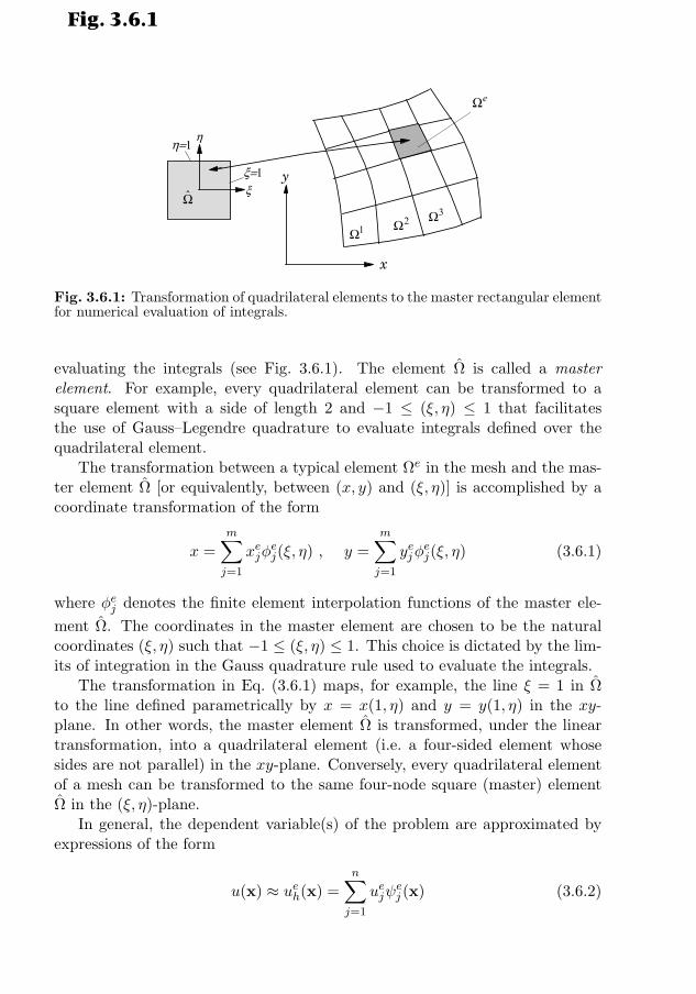
144 THE FINITE ELEMENT METHOD: A REVIEW
ξ
η
ξ=1
η=1
x
y
eΩ
1Ω2Ω
3ΩΩ
Fig. 3.6.1
Fig. 3.6.1: Transformation of quadrilateral elements to the master rectangular elementfor numerical evaluation of integrals.
evaluating the integrals (see Fig. 3.6.1). The element Ω is called a masterelement. For example, every quadrilateral element can be transformed to asquare element with a side of length 2 and −1 ≤ (ξ, η) ≤ 1 that facilitatesthe use of Gauss–Legendre quadrature to evaluate integrals defined over thequadrilateral element.
The transformation between a typical element Ωe in the mesh and the mas-ter element Ω [or equivalently, between (x, y) and (ξ, η)] is accomplished by acoordinate transformation of the form
x =
m∑j=1
xejφej(ξ, η) , y =
m∑j=1
yejφej(ξ, η) (3.6.1)
where φej denotes the finite element interpolation functions of the master ele-
ment Ω. The coordinates in the master element are chosen to be the naturalcoordinates (ξ, η) such that −1 ≤ (ξ, η) ≤ 1. This choice is dictated by the lim-its of integration in the Gauss quadrature rule used to evaluate the integrals.
The transformation in Eq. (3.6.1) maps, for example, the line ξ = 1 in Ωto the line defined parametrically by x = x(1, η) and y = y(1, η) in the xy-plane. In other words, the master element Ω is transformed, under the lineartransformation, into a quadrilateral element (i.e. a four-sided element whosesides are not parallel) in the xy-plane. Conversely, every quadrilateral elementof a mesh can be transformed to the same four-node square (master) elementΩ in the (ξ, η)-plane.
In general, the dependent variable(s) of the problem are approximated byexpressions of the form
u(x) ≈ ueh(x) =n∑j=1
uejψej (x) (3.6.2)
3.6. NUMERICAL INTEGRATION 145
The interpolation functions ψej used for the approximation of the dependentvariable, in general, are different from φej used in the approximation of thegeometry. Depending on the relative degree of approximations used for thegeometry [see Eq. (3.6.1)] and the dependent variable(s) [see Eq. (3.6.2)], thefinite element formulations are classified into three categories:
1. Superparametric (m > n). The approximation used for the geometry ishigher order than that used for the dependent variable.
2. Isoparametric (m = n). Equal degrees of approximation are used for bothgeometry and dependent variables.
3. Subparametric (m < n). Higher-order approximation of the dependentvariable is used.
It should be noted that the transformation of a quadrilateral element of amesh to the master element Ω is solely for the purpose of numerically evalu-ating the integrals (see Fig. 3.6.1). No transformation of the physical domainor elements is involved in the finite element analysis. The resulting algebraicequations of the finite element formulation are always in terms of the nodal val-ues of the physical domain. Different elements of the finite element mesh canbe generated from the same master element by assigning appropriate globalcoordinates to each of the elements. Master elements of a different order de-fine different transformations and hence different collections of finite elementswithin the mesh. For example, a quadratic rectangular master element can beused to generate a mesh of quadratic curvilinear quadrilateral elements. Thetransformations of a master element should be such that no spurious gaps existbetween elements, and no element overlaps occur. For example, consider theelement coefficients
Keij =
∫Ωe
[axx(x)
∂ψei∂x
∂ψej∂x
+ ayy(x)∂ψei∂y
∂ψej∂y
]dA (3.6.3)
The integrand (i.e. the expression in the square brackets under the integral) is afunction of the global coordinates x and y. We must rewrite it in terms of ξ andη using the transformation in Eq. (3.6.1). Note that the integrand contains notonly functions but also derivatives with respect to the global coordinates (x, y).
Therefore, we must relate(∂ψei∂x ,
∂ψei∂y
)to(∂ψei∂ξ ,
∂ψei∂η
)using the transformation
in Eq. (3.6.1).The functions ψei (x, y) can be expressed in terms of the local coordinates
(ξ, η) by means of the transformation in Eq. (3.6.1). Hence, by the chain ruleof partial differentiation, we have
∂ψei∂ξ
=∂ψei∂x
∂x
∂ξ+∂ψei∂y
∂y
∂ξ;
∂ψei∂η
=∂ψei∂x
∂x
∂η+∂ψei∂y
∂y
∂η
146 THE FINITE ELEMENT METHOD: A REVIEW
or, in matrix notation ∂ψei∂ξ∂ψei∂η
=
[∂x∂ξ
∂y∂ξ
∂x∂η
∂y∂η
]∂ψei∂x∂ψei∂y
(3.6.4)
which gives the relation between the derivatives of ψei with respect to the globaland local coordinates. The matrix in Eq. (3.6.4) is called the Jacobian matrixof the transformation in Eq. (3.6.1):
Je =
[∂x∂ξ
∂y∂ξ
∂x∂η
∂y∂η
](3.6.5)
Note from the expression given for Keij in Eq. (3.6.3) that we must relate (
∂ψei∂x ,
∂ψei∂y ) to (
∂ψei∂ξ ,
∂ψei∂η ) whereas Eq. (3.6.4) provides the inverse relations. Therefore,
Eq. (3.6.4) must be inverted. We have∂ψei∂x∂ψei∂y
= (Je)−1
∂ψei∂ξ∂ψei∂η
(3.6.6)
This requires that the Jacobian matrix Je be non-singular (i.e. Je = det Je 6= 0).In fact, to transform a right-handed coordinate system into a right-handedcoordinate system, we require Je > 0.
Using the transformation in Eq. (3.6.1), we can write
∂x
∂ξ=
m∑j=1
xej∂φej∂ξ
,∂y
∂ξ=
m∑j=1
yej∂φej∂ξ
∂x
∂η=
m∑j=1
xej∂φej∂η
,∂y
∂η=
m∑j=1
yej∂φej∂η
(3.6.7)
and by means of Eq. (3.6.5) one can compute the Jacobian matrix and then itsinverse. Thus, given the global coordinates (xej , y
ej ) of node j of element Ωe and
the interpolation functions φej used for geometry approximation, the Jacobianmatrix can be evaluated using Eq. (3.6.5). A necessary and sufficient conditionfor (Je)−1 to exist is that the determinant Je, called the Jacobian, be non-zeroat every point (ξ, η) in Ω :
Je ≡ det Je =∂x
∂ξ
∂y
∂η− ∂x
∂η
∂y
∂ξ6= 0. (3.6.8)
From Eq. (3.6.8) it is clear that the functions ξ(x, y) and η(x, y) must be con-tinuous, differentiable, and invertible. Moreover, the transformation shouldbe algebraically simple so that the Jacobian matrix can be easily evaluated.
3.6. NUMERICAL INTEGRATION 147
Transformations of the form in Eq. (3.6.1) satisfy these requirements and therequirement that no spurious gaps between elements or overlapping of elementsoccur.
Returning to numerical evaluation of integrals, we have from Eq. (3.6.6),∂ψei∂x∂ψei∂y
= (Je)−1
∂ψei∂ξ∂ψei∂η
≡ J∗
∂ψei∂ξ∂ψei∂η
(3.6.9)
where J∗ij is the element in position (i, j) of the inverse of the Jacobian matrixJe. The element area dA = dx dy in element Ωe is transformed to dξdη in themaster element Ω with the relation
dA = Je dξ dη (3.6.10)
Equations (3.6.7)–(3.6.10) provide the necessary relations to transform in-tegral expressions on any element Ωe to the master element Ωe. For instance,consider the integral expression in Eq. (3.6.3), where axx and ayy are functionsof x and y. Suppose that the finite element Ωe can be generated by the masterelement Ωe. Under transformation, Eq. (3.6.1), we can write
Keij =
∫Ωe
[axx(x)
∂ψei∂x
∂ψej∂x
+ayy(x)∂ψei∂y
∂ψej∂y
]dA ≡
∫ΩeF eij(ξ, η) dξ dη (3.6.11)
where
F eij =
[axx(ξ, η)
(J∗11
∂ψei∂ξ
+ J∗12
∂ψei∂η
)(J∗11
∂ψej∂ξ
+ J∗12
∂ψej∂η
)+ ayy(ξ, η)
(J∗21
∂ψei∂ξ
+ J∗22
∂ψei∂η
)(J∗21
∂ψej∂ξ
+ J∗22
∂ψej∂η
)]Je (3.6.12)
The discussion presented above is valid for master elements of both rectan-gular and triangular geometry. In the present study, the geometry will be ap-proximated using the same degree of Lagrange interpolation functions as thoseused for the field variable(s). When all or some of the variables are approximatedusing Hermite interpolation functions, linear approximation of the geometry isused; thus, isoparametric or subparametric formulations are adopted.
3.6.3 Integration Over a Master Rectangular Element
Integrals defined over a rectangular master element ΩeR = [−1, 1] × [−1, 1] can
be numerically evaluated using the Gauss–Legendre quadrature formulas∫ΩeR
F (ξ, η) dξ dη =
∫ 1
−1
∫ 1
−1F (ξ, η) dξ dη ≈
M∑I=1
N∑J=1
F (ξI , ηJ) WIWJ (3.6.13)
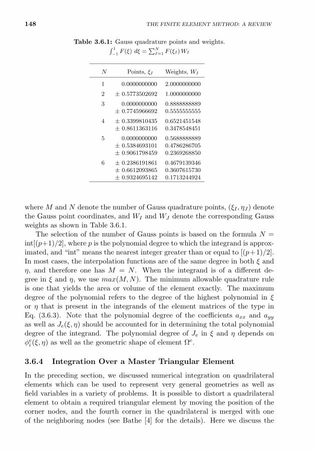
148 THE FINITE ELEMENT METHOD: A REVIEW
Table 3.6.1: Gauss quadrature points and weights.∫ 1
−1F (ξ) dξ =
∑NI=1 F (ξI)WI
N Points, ξI Weights, WI
1 0.0000000000 2.0000000000
2 ± 0.5773502692 1.0000000000
3 0.0000000000 0.8888888889± 0.7745966692 0.5555555555
4 ± 0.3399810435 0.6521451548± 0.8611363116 0.3478548451
5 0.0000000000 0.5688888889± 0.5384693101 0.4786286705± 0.9061798459 0.2369268850
6 ± 0.2386191861 0.4679139346± 0.6612093865 0.3607615730± 0.9324695142 0.1713244924
where M and N denote the number of Gauss quadrature points, (ξI , ηJ) denotethe Gauss point coordinates, and WI and WJ denote the corresponding Gaussweights as shown in Table 3.6.1.
The selection of the number of Gauss points is based on the formula N =int[(p+1)/2], where p is the polynomial degree to which the integrand is approx-imated, and “int” means the nearest integer greater than or equal to [(p+1)/2].In most cases, the interpolation functions are of the same degree in both ξ andη, and therefore one has M = N . When the integrand is of a different de-gree in ξ and η, we use max(M,N). The minimum allowable quadrature ruleis one that yields the area or volume of the element exactly. The maximumdegree of the polynomial refers to the degree of the highest polynomial in ξor η that is present in the integrands of the element matrices of the type inEq. (3.6.3). Note that the polynomial degree of the coefficients axx and ayyas well as Je(ξ, η) should be accounted for in determining the total polynomialdegree of the integrand. The polynomial degree of Je in ξ and η depends onφei (ξ, η) as well as the geometric shape of element Ωe.
3.6.4 Integration Over a Master Triangular Element
In the preceding section, we discussed numerical integration on quadrilateralelements which can be used to represent very general geometries as well asfield variables in a variety of problems. It is possible to distort a quadrilateralelement to obtain a required triangular element by moving the position of thecorner nodes, and the fourth corner in the quadrilateral is merged with oneof the neighboring nodes (see Bathe [4] for the details). Here we discuss the
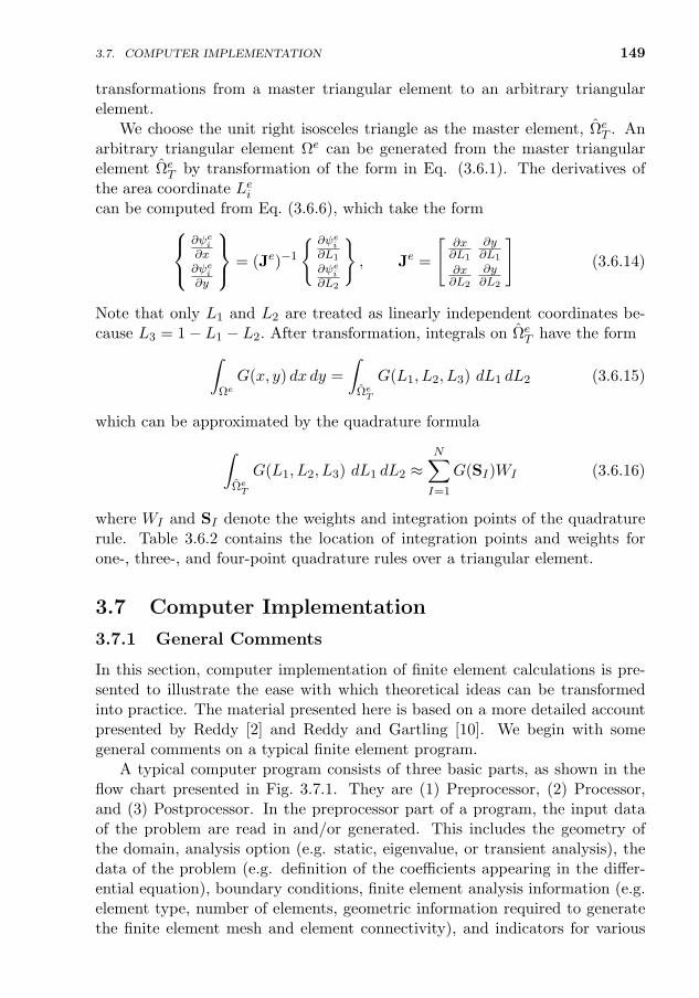
3.7. COMPUTER IMPLEMENTATION 149
transformations from a master triangular element to an arbitrary triangularelement.
We choose the unit right isosceles triangle as the master element, ΩeT . An
arbitrary triangular element Ωe can be generated from the master triangularelement Ωe
T by transformation of the form in Eq. (3.6.1). The derivatives ofthe area coordinate Lei [see Eq. (3.3.33)] with respect to the global coordinatescan be computed from Eq. (3.6.6), which take the form
∂ψei∂x∂ψei∂y
= (Je)−1
∂ψei∂L1
∂ψei∂L2
, Je =
[∂x∂L1
∂y∂L1
∂x∂L2
∂y∂L2
](3.6.14)
Note that only L1 and L2 are treated as linearly independent coordinates be-cause L3 = 1− L1 − L2. After transformation, integrals on Ωe
T have the form∫ΩeG(x, y) dx dy =
∫ΩeT
G(L1, L2, L3) dL1 dL2 (3.6.15)
which can be approximated by the quadrature formula∫ΩeT
G(L1, L2, L3) dL1 dL2 ≈N∑I=1
G(SI)WI (3.6.16)
where WI and SI denote the weights and integration points of the quadraturerule. Table 3.6.2 contains the location of integration points and weights forone-, three-, and four-point quadrature rules over a triangular element.
3.7 Computer Implementation
3.7.1 General Comments
In this section, computer implementation of finite element calculations is pre-sented to illustrate the ease with which theoretical ideas can be transformedinto practice. The material presented here is based on a more detailed accountpresented by Reddy [2] and Reddy and Gartling [10]. We begin with somegeneral comments on a typical finite element program.
A typical computer program consists of three basic parts, as shown in theflow chart presented in Fig. 3.7.1. They are (1) Preprocessor, (2) Processor,and (3) Postprocessor. In the preprocessor part of a program, the input dataof the problem are read in and/or generated. This includes the geometry ofthe domain, analysis option (e.g. static, eigenvalue, or transient analysis), thedata of the problem (e.g. definition of the coefficients appearing in the differ-ential equation), boundary conditions, finite element analysis information (e.g.element type, number of elements, geometric information required to generatethe finite element mesh and element connectivity), and indicators for various
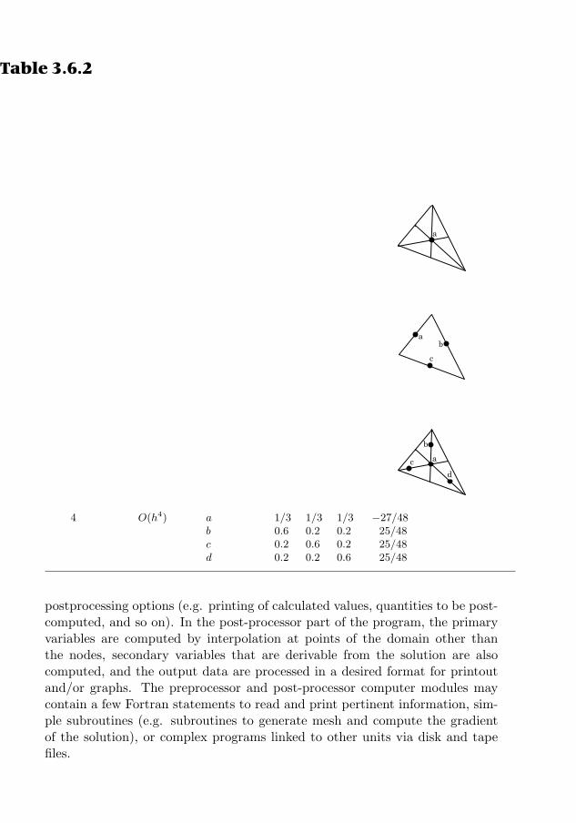
150 THE FINITE ELEMENT METHOD: A REVIEW
Table 3.6.2: Quadrature weights and points for triangular elements.
Degree ofNumber of polynomialintegration Order of Geometricpoints the residual locations S1 S2 S3 WI
1
a
ba
c
a
b
c
d
Table 3.6.2
1 O(h2) a 1/3 1/3 1/3 1
2
a
ba
c
a
b
c
d
Table 3.6.2
3 O(h3) a 1/2 0 1/2 1/3b 1/2 1/2 0 1/3c 0 1/2 1/2 1/3
3
a
ba
c
a
b
c
d
Table 3.6.2
4 O(h4) a 1/3 1/3 1/3 −27/48b 0.6 0.2 0.2 25/48c 0.2 0.6 0.2 25/48d 0.2 0.2 0.6 25/48
postprocessing options (e.g. printing of calculated values, quantities to be post-computed, and so on). In the post-processor part of the program, the primaryvariables are computed by interpolation at points of the domain other thanthe nodes, secondary variables that are derivable from the solution are alsocomputed, and the output data are processed in a desired format for printoutand/or graphs. The preprocessor and post-processor computer modules maycontain a few Fortran statements to read and print pertinent information, sim-ple subroutines (e.g. subroutines to generate mesh and compute the gradientof the solution), or complex programs linked to other units via disk and tapefiles.
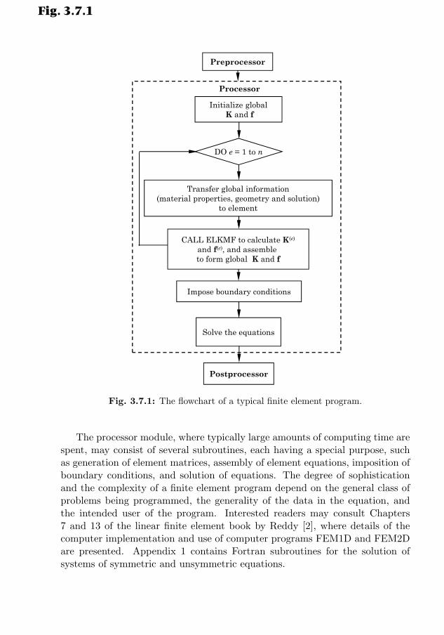
3.7. COMPUTER IMPLEMENTATION 151
Initialize globalK and f
DO e = 1 to n
Impose boundary conditions
Transfer global information(material properties, geometry and solution)
to element
Solve the equations
Postprocessor
CALL ELKMF to calculate K(e)
and f(e), and assemble to form global K and f
Processor
Preprocessor
Fig. 3.7.1
Fig. 3.7.1: The flowchart of a typical finite element program.
The processor module, where typically large amounts of computing time arespent, may consist of several subroutines, each having a special purpose, suchas generation of element matrices, assembly of element equations, imposition ofboundary conditions, and solution of equations. The degree of sophisticationand the complexity of a finite element program depend on the general class ofproblems being programmed, the generality of the data in the equation, andthe intended user of the program. Interested readers may consult Chapters7 and 13 of the linear finite element book by Reddy [2], where details of thecomputer implementation and use of computer programs FEM1D and FEM2Dare presented. Appendix 1 contains Fortran subroutines for the solution ofsystems of symmetric and unsymmetric equations.
152 THE FINITE ELEMENT METHOD: A REVIEW
3.7.2 One-Dimensional Problems
Here we discuss the main ideas behind the calculation of element coefficientmatrices, Ke and f e, for the model problem discussed in Sections 3.2 and 3.3.Recall that the coefficients of Ke and f e involve integrals of the form
Keij =
∫ xb
xa
[a(x)
dψeidx
dψejdx
+ c(x)ψeiψej
]dx, fei =
∫ xb
xa
f(x)ψei (x) dx (3.7.1)
To evaluate these integrals using the Gauss quadrature, we first transform theintegrals posed over interval (xa, xb) to the ones posed on interval (−1, 1) bythe use of the coordinate transformation [see Eq. (3.6.1)]
x =
m∑j=1
xejφej(ξ) (3.7.2)
In Eq. (3.7.2), xej denotes the global coordinate of node j of element Ωe =(xa, xb), and φej is the approximation function used to approximate the geome-try. For example, if we use linear interpolation functions to represent the geom-etry of the element, we have xe1 = xa, x
e2 = xb, φ
e1 = 0.5(1− ξ), φe2 = 0.5(1 + ξ),
and Eq. (3.7.2) becomes
x = xaφe1(ξ) + xbφ
e2(ξ) =
xa + xb2
+xb − xa
2ξ = xa +
he2ξ (3.7.3)
and the Jacobian of transformation is a constant
Je ≡dx
dξ=he2
(3.7.4)
The derivatives of ψei (x) with respect to the global coordinate x is given by
dψeidx
=dψeidξ
dξ
dx=dψeidξ
J−1e
Then the integrals in Eq. (3.7.1) become
Keij =
∫ xb
xa
[a(x)
dψeidx
dψejdx
+ c(x)ψeiψej
]dx
=
∫ 1
−1
[a(ξ)
(dψeidξ
Je−1
)(dψejdξ
J−1e
)+ c(ξ)ψeiψ
ej
]Je dξ
fei =
∫ xb
xa
f(x)ψei (x) dx =
∫ 1
−1f(ξ)ψei (ξ) Je(ξ) dξ
(3.7.5)
where a(ξ) = a(x(ξ)) and so on. Each of the integral expressions above can beevaluated using the Gauss quadrature∫ 1
−1F (ξ)Je dξ =
NGP∑I=1
F (ξI) Je(ξI)WI (3.7.6)
3.7. COMPUTER IMPLEMENTATION 153
where NGP is the number of Gauss points, and ξI is the Ith Gauss point andWI is the Ith Gauss weight from the Gauss rule with NGP points.
To implement the above development into a computer subroutine for anarbitrary degree of ψei , we must first create a subroutine of all interpolationfunctions and their derivatives with respect to ξ that we intend to use in ouranalysis. For the present discussion, we limit them to the linear and quadraticLagrange family of functions. The functions and their derivatives are givenbelow.
Linear
ψ1(ξ) =1
2(1− ξ) , dψ1
dξ= −0.5; ψ2(ξ) =
1
2(1 + ξ) ,
dψ2
dξ= 0.5 (3.7.7)
Quadratic
ψ1(ξ) = −1
2ξ (1− ξ) , ψ2(ξ) =
(1− ξ2
), ψ3(ξ) =
1
2ξ (1 + ξ)
dψ1
dξ= 0.5 (2ξ − 1) ,
dψ2
dξ= −2ξ,
dψ3
dξ= 0.5 (1 + 2ξ)
(3.7.8)Approximation functions ψi and their derivatives with respect to the globalcoordinate x at point ξ are evaluated in subroutine INTERPLN1D, which ispresented in Box 3.7.1.
The following variable names are used in the subroutine INTERPLN1D:
SFL(i) = ψei , DSFL(i) =dψeidξ
, GDSFL(i) =dψeidx
(3.7.9)
The notation should be transparent to the reader: SFL = shape functions of theLagrange family; DSFL = derivative of SFL with respect to ξ; and GDSFL =the global derivative (i.e. derivative with respect to x) of SFL. All of them aren× 1 arrays, where n is the number of nodes per element, NPE. The notationGJ is used for the Jacobian Je and XI for the normalized coordinate ξ.
Next, we implement the steps to evaluate the matrix coefficients Keij and
fei (i = 1 to NPE) into a subroutine, ELMATRCS1D (element coefficientmatrix). To this end, we assume the following polynomial representation of thedata, a(x), c(x), and f(x) for the entire domain of the problem:
a(x) = a0 + a1x, c(x) = c0 + c1x, f(x) = f0 + f1x
AX = AX0 + AX1 · x, CX = CX0 + CX1 · x, FX = FX0 + FX1 · x
The coefficients a0 = AX0, a1 = AX1, etc. of the polynomials must be read inthe preprocessor and transferred to the subroutine ELMATRCS1D through aCOMMON block (or the argument list). For this choice of data, it is sufficientto use NGP = 2 for the linear element and NGP = 3 for the quadratic elementto exactly evaluate the integrals appearing in the definition of Ke and f e.
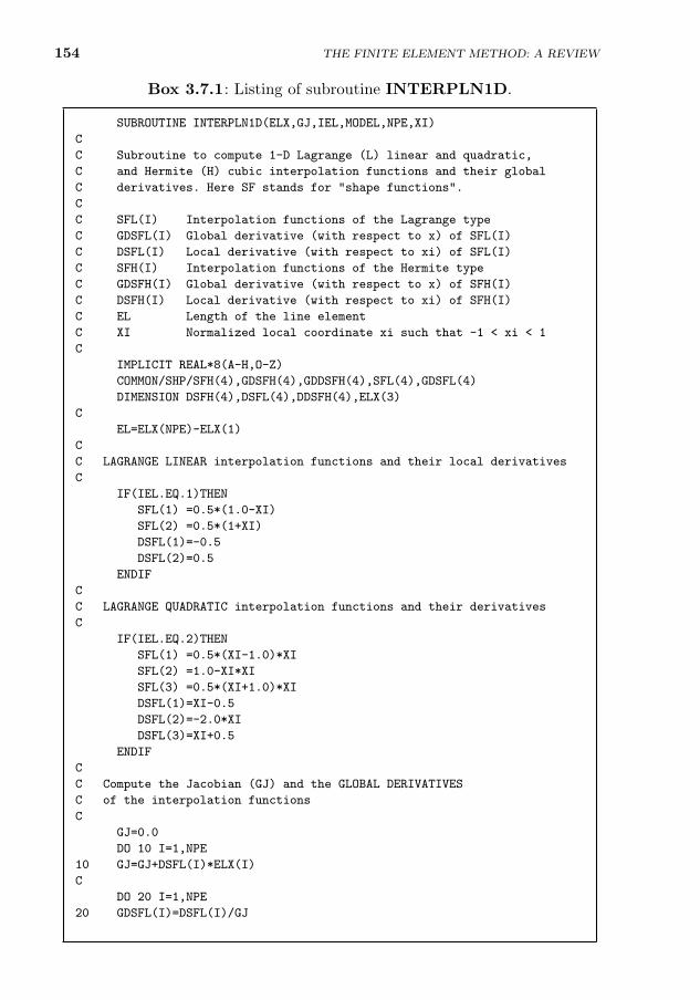
154 THE FINITE ELEMENT METHOD: A REVIEW
Box 3.7.1: Listing of subroutine INTERPLN1D.
SUBROUTINE INTERPLN1D(ELX,GJ,IEL,MODEL,NPE,XI)
C
C Subroutine to compute 1-D Lagrange (L) linear and quadratic,
C and Hermite (H) cubic interpolation functions and their global
C derivatives. Here SF stands for "shape functions".
C
C SFL(I) Interpolation functions of the Lagrange type
C GDSFL(I) Global derivative (with respect to x) of SFL(I)
C DSFL(I) Local derivative (with respect to xi) of SFL(I)
C SFH(I) Interpolation functions of the Hermite type
C GDSFH(I) Global derivative (with respect to x) of SFH(I)
C DSFH(I) Local derivative (with respect to xi) of SFH(I)
C EL Length of the line element
C XI Normalized local coordinate xi such that -1 < xi < 1
C
IMPLICIT REAL*8(A-H,O-Z)
COMMON/SHP/SFH(4),GDSFH(4),GDDSFH(4),SFL(4),GDSFL(4)
DIMENSION DSFH(4),DSFL(4),DDSFH(4),ELX(3)
C
EL=ELX(NPE)-ELX(1)
C
C LAGRANGE LINEAR interpolation functions and their local derivatives
C
IF(IEL.EQ.1)THEN
SFL(1) =0.5*(1.0-XI)
SFL(2) =0.5*(1+XI)
DSFL(1)=-0.5
DSFL(2)=0.5
ENDIF
C
C LAGRANGE QUADRATIC interpolation functions and their derivatives
C
IF(IEL.EQ.2)THEN
SFL(1) =0.5*(XI-1.0)*XI
SFL(2) =1.0-XI*XI
SFL(3) =0.5*(XI+1.0)*XI
DSFL(1)=XI-0.5
DSFL(2)=-2.0*XI
DSFL(3)=XI+0.5
ENDIF
C
C Compute the Jacobian (GJ) and the GLOBAL DERIVATIVES
C of the interpolation functions
C
GJ=0.0
DO 10 I=1,NPE
10 GJ=GJ+DSFL(I)*ELX(I)
C
DO 20 I=1,NPE
20 GDSFL(I)=DSFL(I)/GJ
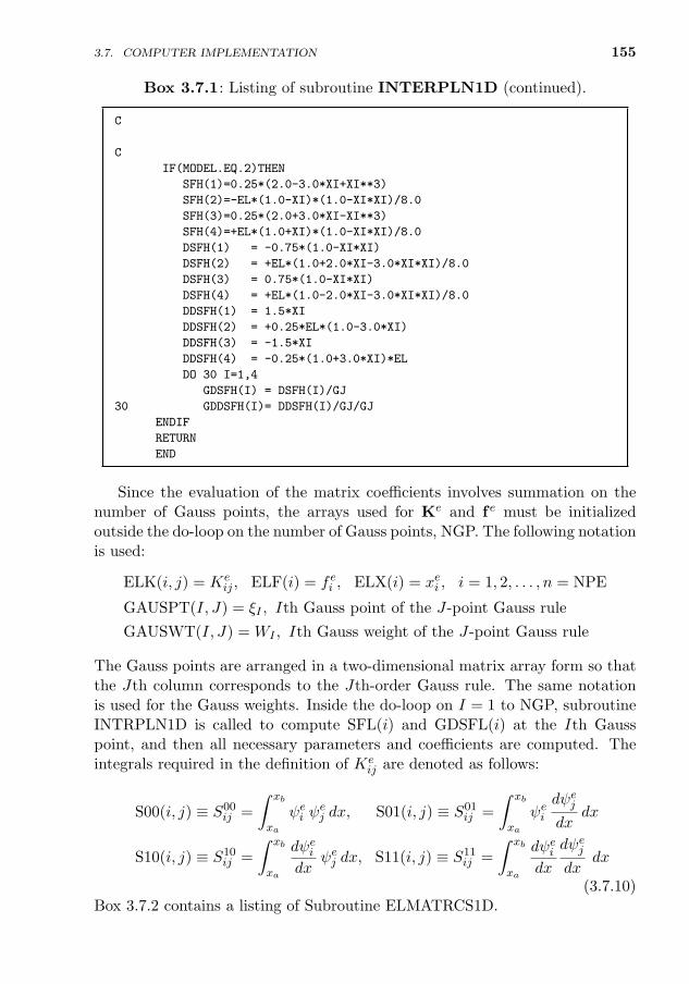
3.7. COMPUTER IMPLEMENTATION 155
Box 3.7.1: Listing of subroutine INTERPLN1D (continued).
C
C HERMITE CUBIC interpolation functions [see Eq. (5.2.28)]
C
IF(MODEL.EQ.2)THEN
SFH(1)=0.25*(2.0-3.0*XI+XI**3)
SFH(2)=-EL*(1.0-XI)*(1.0-XI*XI)/8.0
SFH(3)=0.25*(2.0+3.0*XI-XI**3)
SFH(4)=+EL*(1.0+XI)*(1.0-XI*XI)/8.0
DSFH(1) = -0.75*(1.0-XI*XI)
DSFH(2) = +EL*(1.0+2.0*XI-3.0*XI*XI)/8.0
DSFH(3) = 0.75*(1.0-XI*XI)
DSFH(4) = +EL*(1.0-2.0*XI-3.0*XI*XI)/8.0
DDSFH(1) = 1.5*XI
DDSFH(2) = +0.25*EL*(1.0-3.0*XI)
DDSFH(3) = -1.5*XI
DDSFH(4) = -0.25*(1.0+3.0*XI)*EL
DO 30 I=1,4
GDSFH(I) = DSFH(I)/GJ
30 GDDSFH(I)= DDSFH(I)/GJ/GJ
ENDIF
RETURN
END
Since the evaluation of the matrix coefficients involves summation on thenumber of Gauss points, the arrays used for Ke and f e must be initializedoutside the do-loop on the number of Gauss points, NGP. The following notationis used:
ELK(i, j) = Keij , ELF(i) = fei , ELX(i) = xei , i = 1, 2, . . . , n = NPE
GAUSPT(I, J) = ξI , Ith Gauss point of the J-point Gauss rule
GAUSWT(I, J) = WI , Ith Gauss weight of the J-point Gauss rule
The Gauss points are arranged in a two-dimensional matrix array form so thatthe Jth column corresponds to the Jth-order Gauss rule. The same notationis used for the Gauss weights. Inside the do-loop on I = 1 to NGP, subroutineINTRPLN1D is called to compute SFL(i) and GDSFL(i) at the Ith Gausspoint, and then all necessary parameters and coefficients are computed. Theintegrals required in the definition of Ke
ij are denoted as follows:
S00(i, j) ≡ S00ij =
∫ xb
xa
ψei ψej dx, S01(i, j) ≡ S01
ij =
∫ xb
xa
ψeidψejdx
dx
S10(i, j) ≡ S10ij =
∫ xb
xa
dψeidx
ψej dx, S11(i, j) ≡ S11ij =
∫ xb
xa
dψeidx
dψejdx
dx
(3.7.10)Box 3.7.2 contains a listing of Subroutine ELMATRCS1D.
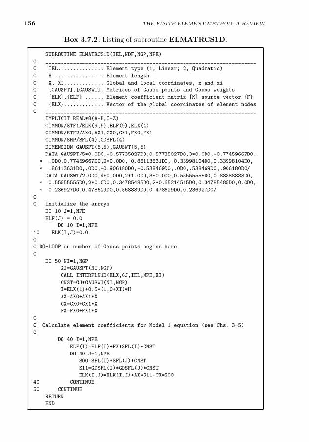
156
Box 3.7.2: Listing of subroutine ELMATRCS1D.
SUBROUTINE ELMATRCS1D(IEL,NDF,NGP,NPE)
C _____________________________________________________________________
C IEL............... Element type (1, Linear; 2, Quadratic)
C H................. Element length
C X, XI............. Global and local coordinates, x and xi
C [GAUSPT],[GAUSWT]. Matrices of Gauss points and Gauss weights
C [ELK],ELF ...... Element coefficient matrix [K] source vector F
C ELX............. Vector of the global coordinates of element nodes
C _____________________________________________________________________
IMPLICIT REAL*8(A-H,O-Z)
COMMON/STF1/ELK(9,9),ELF(9),ELX(4)
COMMON/STF2/AX0,AX1,CX0,CX1,FX0,FX1
COMMON/SHP/SFL(4),GDSFL(4)
DIMENSION GAUSPT(5,5),GAUSWT(5,5)
DATA GAUSPT/5*0.0D0,-0.57735027D0,0.57735027D0,3*0.0D0,-0.77459667D0,
* .0D0,0.77459667D0,2*0.0D0,-0.86113631D0,-0.33998104D0,0.33998104D0,
* .86113631D0,.0D0,-0.906180D0,-0.538469D0,.0D0,.538469D0,.906180D0/
DATA GAUSWT/2.0D0,4*0.0D0,2*1.0D0,3*0.0D0,0.55555555D0,0.88888888D0,
* 0.55555555D0,2*0.0D0,0.34785485D0,2*0.65214515D0,0.34785485D0,0.0D0,
* 0.236927D0,0.478629D0,0.568889D0,0.478629D0,0.236927D0/
C
C Initialize the arrays
DO 10 J=1,NPE
ELF(J) = 0.0
DO 10 I=1,NPE
10 ELK(I,J)=0.0
C
C DO-LOOP on number of Gauss points begins here
C
DO 50 NI=1,NGP
XI=GAUSPT(NI,NGP)
CALL INTERPLN1D(ELX,GJ,IEL,NPE,XI)
CNST=GJ*GAUSWT(NI,NGP)
X=ELX(1)+0.5*(1.0+XI)*H
AX=AX0+AX1*X
CX=CX0+CX1*X
FX=FX0+FX1*X
C
C Calculate element coefficients for Model 1 equation (see Chs. 3-5)
C
DO 40 I=1,NPE
ELF(I)=ELF(I)+FX*SFL(I)*CNST
DO 40 J=1,NPE
S00=SFL(I)*SFL(J)*CNST
S11=GDSFL(I)*GDSFL(J)*CNST
ELK(I,J)=ELK(I,J)+AX*S11+CX*S00
40 CONTINUE
50 CONTINUE
RETURN
END
THE FINITE ELEMENT METHOD: A REVIEW
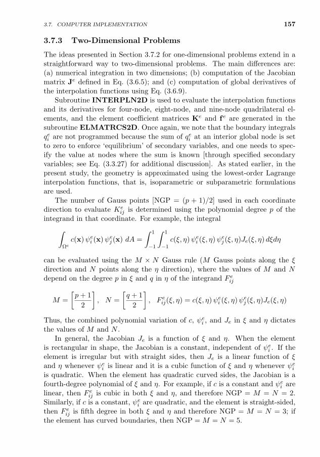
3.7. COMPUTER IMPLEMENTATION 157
3.7.3 Two-Dimensional Problems
The ideas presented in Section 3.7.2 for one-dimensional problems extend in astraightforward way to two-dimensional problems. The main differences are:(a) numerical integration in two dimensions; (b) computation of the Jacobianmatrix Je defined in Eq. (3.6.5); and (c) computation of global derivatives ofthe interpolation functions using Eq. (3.6.9).
Subroutine INTERPLN2D is used to evaluate the interpolation functionsand its derivatives for four-node, eight-node, and nine-node quadrilateral el-ements, and the element coefficient matrices Ke and f e are generated in thesubroutine ELMATRCS2D. Once again, we note that the boundary integralsqei are not programmed because the sum of qei at an interior global node is setto zero to enforce ‘equilibrium’ of secondary variables, and one needs to spec-ify the value at nodes where the sum is known [through specified secondaryvariables; see Eq. (3.3.27) for additional discussion]. As stated earlier, in thepresent study, the geometry is approximated using the lowest-order Lagrangeinterpolation functions, that is, isoparametric or subparametric formulationsare used.
The number of Gauss points [NGP = (p + 1)/2] used in each coordinatedirection to evaluate Ke
ij is determined using the polynomial degree p of theintegrand in that coordinate. For example, the integral∫
Ωec(x)ψei (x)ψej (x) dA =
∫ 1
−1
∫ 1
−1c(ξ, η)ψei (ξ, η)ψej (ξ, η)Je(ξ, η) dξdη
can be evaluated using the M × N Gauss rule (M Gauss points along the ξdirection and N points along the η direction), where the values of M and Ndepend on the degree p in ξ and q in η of the integrand F eij
M =
[p+ 1
2
], N =
[q + 1
2
], F eij(ξ, η) = c(ξ, η)ψei (ξ, η)ψej (ξ, η)Je(ξ, η)
Thus, the combined polynomial variation of c, ψei , and Je in ξ and η dictatesthe values of M and N .
In general, the Jacobian Je is a function of ξ and η. When the elementis rectangular in shape, the Jacobian is a constant, independent of ψei . If theelement is irregular but with straight sides, then Je is a linear function of ξand η whenever ψei is linear and it is a cubic function of ξ and η whenever ψeiis quadratic. When the element has quadratic curved sides, the Jacobian is afourth-degree polynomial of ξ and η. For example, if c is a constant and ψei arelinear, then F eij is cubic in both ξ and η, and therefore NGP = M = N = 2.Similarly, if c is a constant, ψei are quadratic, and the element is straight-sided,then F eij is fifth degree in both ξ and η and therefore NGP = M = N = 3; ifthe element has curved boundaries, then NGP = M = N = 5.
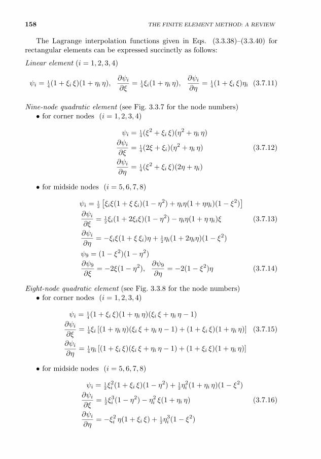
158 THE FINITE ELEMENT METHOD: A REVIEW
The Lagrange interpolation functions given in Eqs. (3.3.38)–(3.3.40) forrectangular elements can be expressed succinctly as follows:
Linear element (i = 1, 2, 3, 4)
ψi = 14(1 + ξi ξ)(1 + ηi η),
∂ψi∂ξ
= 14ξi(1 + ηi η),
∂ψi∂η
= 14(1 + ξi ξ)ηi (3.7.11)
Nine-node quadratic element (see Fig. 3.3.7 for the node numbers)• for corner nodes (i = 1, 2, 3, 4)
ψi = 14(ξ2 + ξi ξ)(η
2 + ηi η)
∂ψi∂ξ
= 14(2ξ + ξi)(η
2 + ηi η) (3.7.12)
∂ψi∂η
= 14(ξ2 + ξi ξ)(2η + ηi)
• for midside nodes (i = 5, 6, 7, 8)
ψi = 12
[ξiξ(1 + ξ ξi)(1− η2) + ηiη(1 + ηηi)(1− ξ2)
]∂ψi∂ξ
= 12ξi(1 + 2ξiξ)(1− η2)− ηiη(1 + η ηi)ξ (3.7.13)
∂ψi∂η
= −ξiξ(1 + ξ ξi)η + 12ηi(1 + 2ηiη)(1− ξ2)
ψ9 = (1− ξ2)(1− η2)
∂ψ9
∂ξ= −2ξ(1− η2),
∂ψ9
∂η= −2(1− ξ2)η (3.7.14)
Eight-node quadratic element (see Fig. 3.3.8 for the node numbers)• for corner nodes (i = 1, 2, 3, 4)
ψi = 14(1 + ξi ξ)(1 + ηi η)(ξi ξ + ηi η − 1)
∂ψi∂ξ
= 14ξi [(1 + ηi η)(ξi ξ + ηi η − 1) + (1 + ξi ξ)(1 + ηi η)] (3.7.15)
∂ψi∂η
= 14ηi [(1 + ξi ξ)(ξi ξ + ηi η − 1) + (1 + ξi ξ)(1 + ηi η)]
• for midside nodes (i = 5, 6, 7, 8)
ψi = 12ξ2i (1 + ξi ξ)(1− η2) + 1
2η2i (1 + ηi η)(1− ξ2)
∂ψi∂ξ
= 12ξ3i (1− η2)− η2
i ξ(1 + ηi η) (3.7.16)
∂ψi∂η
= −ξ2i η(1 + ξi ξ) + 1
2η3i (1− ξ2)
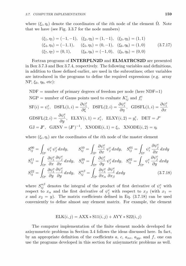
3.7. COMPUTER IMPLEMENTATION 159
where (ξi, ηi) denote the coordinates of the ith node of the element Ω. Notethat we have (see Fig. 3.3.7 for the node numbers)
(ξ1, η1) = (−1,−1), (ξ2, η2) = (1,−1), (ξ3, η3) = (1, 1)
(ξ4, η4) = (−1, 1), (ξ5, η5) = (0,−1), (ξ6, η6) = (1, 0)
(ξ7, η7) = (0, 1), (ξ8, η8) = (−1, 0), (ξ9, η9) = (0, 0)
(3.7.17)
Fortran programs of INTERPLN2D and ELMATRCS2D are presentedin Box 3.7.3 and Box 3.7.4, respectively. The following variables and definitions,in addition to those defined earlier, are used in the subroutines; other variablesare introduced in the programs to define the required expressions (e.g. arrayNP, ξ0, η0, etc):
NDF = number of primary degrees of freedom per node (here NDF=1)
NGP = number of Gauss points used to evaluate Keij and fei
SF(i) = ψei , DSFL(1, i) =∂ψei∂ξ
, DSFL(2, i) =∂ψei∂η
, GDSFL(1, i) =∂ψei∂x
GDSFL(2, i) =∂ψei∂y
, ELXY(i, 1) = xei , ELXY(i, 2) = yei , DET = Je
GJ = Je, GJINV = (Je)−1, XNODE(i, 1) = ξi, XNODE(i, 2) = ηi
where (ξi, ηi) are the coordinates of the ith node of the master element
S00ij =
∫Ωeψei ψ
ej dxdy, S10
ij =
∫Ωe
∂ψei∂x
ψej dxdy, S01ij =
∫Ωeψei
∂ψej∂x
dxdy
S11ij =
∫Ωe
∂ψei∂x
∂ψej∂x
dxdy, S20ij =
∫Ωe
∂ψei∂y
ψej dxdy, S02ij =
∫Ωeψei
∂ψej∂y
dxdy
S22ij =
∫Ωe
∂ψei∂y
∂ψej∂y
dxdy, Sαβij =
∫Ωe
∂ψei∂xα
∂ψej∂xβ
dxdy (3.7.18)
where Sαβij denotes the integral of the product of first derivative of ψei withrespect to xα and the first derivative of ψej with respect to xβ (with x1 =x and x2 = y). The matrix coefficients defined in Eq. (3.7.18) can be usedconveniently to define almost any element matrix. For example, the elementmatrix in Eq. (3.6.3) can be expressed as [see Eq. (3.3.31)]
ELK(i, j) = AXX ∗ S11(i, j) + AYY ∗ S22(i, j)
The computer implementation of the finite element models developed foraxisymmetric problems in Section 3.4 follows the ideas discussed here. In fact,by an appropriate definition of the coefficients a, c, axx, ayy, and f , one canuse the programs developed in this section for axisymmetric problems as well.
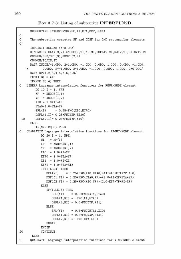
160 THE FINITE ELEMENT METHOD: A REVIEW
Box 3.7.3: Listing of subroutine INTERPLN2D.
SUBROUTINE INTERPLN2D(NPE,XI,ETA,DET,ELXY)
C
C The subroutine computes SF and GDSF for 2-D rectangular elements
C
IMPLICIT REAL*8 (A-H,O-Z)
DIMENSION ELXY(9,2),XNODE(9,2),NP(9),DSFL(2,9),GJ(2,2),GJINV(2,2)
COMMON/SHP/SFL(9),GDSFL(2,9)
COMMON/IO/IN,IT
DATA XNODE/-1.0D0, 2*1.0D0, -1.0D0, 0.0D0, 1.0D0, 0.0D0, -1.0D0,
* 0.0D0, 2*-1.0D0, 2*1.0D0, -1.0D0, 0.0D0, 1.0D0, 2*0.0D0/
DATA NP/1,2,3,4,5,7,6,8,9/
FNC(A,B) = A*B
IF(NPE.EQ.4) THEN
C LINEAR Lagrange interpolation functions for FOUR-NODE element
DO 10 I = 1, NPE
XP = XNODE(I,1)
YP = XNODE(I,2)
XI0 = 1.0+XI*XP
ETA0=1.0+ETA*YP
SFL(I) = 0.25*FNC(XI0,ETA0)
DSFL(1,I)= 0.25*FNC(XP,ETA0)
10 DSFL(2,I)= 0.25*FNC(YP,XI0)
ELSE
IF(NPE.EQ.8) THEN
C QUADRATIC Lagrange interpolation functions for EIGHT-NODE element
DO 20 I = 1, NPE
NI = NP(I)
XP = XNODE(NI,1)
YP = XNODE(NI,2)
XI0 = 1.0+XI*XP
ETA0 = 1.0+ETA*YP
XI1 = 1.0-XI*XI
ETA1 = 1.0-ETA*ETA
IF(I.LE.4) THEN
SFL(NI) = 0.25*FNC(XI0,ETA0)*(XI*XP+ETA*YP-1.0)
DSFL(1,NI) = 0.25*FNC(ETA0,XP)*(2.0*XI*XP+ETA*YP)
DSFL(2,NI) = 0.25*FNC(XI0,YP)*(2.0*ETA*YP+XI*XP)
ELSE
IF(I.LE.6) THEN
SFL(NI) = 0.5*FNC(XI1,ETA0)
DSFL(1,NI) = -FNC(XI,ETA0)
DSFL(2,NI) = 0.5*FNC(YP,XI1)
ELSE
SFL(NI) = 0.5*FNC(ETA1,XI0)
DSFL(1,NI) = 0.5*FNC(XP,ETA1)
DSFL(2,NI) = -FNC(ETA,XI0)
ENDIF
ENDIF
20 CONTINUE
ELSE
C QUADRATIC Lagrange interpolation functions for NINE-NODE element
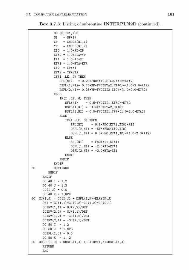
3.7. COMPUTER IMPLEMENTATION 161
Box 3.7.3: Listing of subroutine INTERPLN2D (continued).
DO 30 I=1,NPE
NI = NP(I)
XP = XNODE(NI,1)
YP = XNODE(NI,2)
XI0 = 1.0+XI*XP
ETA0 = 1.0+ETA*YP
XI1 = 1.0-XI*XI
ETA1 = 1.0-ETA*ETA
XI2 = XP*XI
ETA2 = YP*ETA
IF(I .LE. 4) THEN
SFL(NI) = 0.25*FNC(XI0,ETA0)*XI2*ETA2
DSFL(1,NI)= 0.25*XP*FNC(ETA2,ETA0)*(1.0+2.0*XI2)
DSFL(2,NI)= 0.25*YP*FNC(XI2,XI0)*(1.0+2.0*ETA2)
ELSE
IF(I .LE. 6) THEN
SFL(NI) = 0.5*FNC(XI1,ETA0)*ETA2
DSFL(1,NI) = -XI*FNC(ETA2,ETA0)
DSFL(2,NI) = 0.5*FNC(XI1,YP)*(1.0+2.0*ETA2)
ELSE
IF(I .LE. 8) THEN
SFL(NI) = 0.5*FNC(ETA1,XI0)*XI2
DSFL(2,NI) = -ETA*FNC(XI2,XI0)
DSFL(1,NI) = 0.5*FNC(ETA1,XP)*(1.0+2.0*XI2)
ELSE
SFL(NI) = FNC(XI1,ETA1)
DSFL(1,NI) = -2.0*XI*ETA1
DSFL(2,NI) = -2.0*ETA*XI1
ENDIF
ENDIF
ENDIF
30 CONTINUE
ENDIF
ENDIF
DO 40 I = 1,2
DO 40 J = 1,2
GJ(I,J) = 0.0
DO 40 K = 1,NPE
40 GJ(I,J) = GJ(I,J) + DSFL(I,K)*ELXY(K,J)
DET = GJ(1,1)*GJ(2,2)-GJ(1,2)*GJ(2,1)
GJINV(1,1) = GJ(2,2)/DET
GJINV(2,2) = GJ(1,1)/DET
GJINV(1,2) = -GJ(1,2)/DET
GJINV(2,1) = -GJ(2,1)/DET
DO 50 I = 1,2
DO 50 J = 1,NPE
GDSFL(I,J) = 0.0
DO 50 K = 1, 2
50 GDSFL(I,J) = GDSFL(I,J) + GJINV(I,K)*DSFL(K,J)
RETURN
END
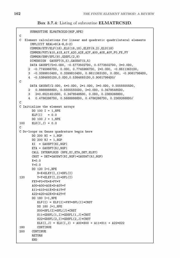
162 THE FINITE ELEMENT METHOD: A REVIEW
Box 3.7.4: Listing of subroutine ELMATRCS2D.
SUBROUTINE ELMATRCS2D(NGP,NPE)
C
C Element calculations for linear and quadratic quadrilateral elements
IMPLICIT REAL*8(A-H,O-Z)
COMMON/STF/ELF(18),ELK(18,18),ELXY(9,2),ELU(18)
COMMON/PST/A10,A1X,A1Y,A20,A2X,A2Y,A00,A0X,A0Y,F0,FX,FY
COMMON/SHP/SFL(9),GDSFL(2,9)
DIMENSION GAUSPT(5,5),GAUSWT(5,5)
DATA GAUSPT/5*0.0D0, -0.57735027D0, 0.57735027D0, 3*0.0D0,
2 -0.77459667D0, 0.0D0, 0.77459667D0, 2*0.0D0, -0.86113631D0,
3 -0.33998104D0, 0.33998104D0, 0.86113631D0, 0.0D0, -0.90617984D0,
4 -0.53846931D0,0.0D0,0.53846931D0,0.90617984D0/
C
DATA GAUSWT/2.0D0, 4*0.0D0, 2*1.0D0, 3*0.0D0, 0.55555555D0,
2 0.88888888D0, 0.55555555D0, 2*0.0D0, 0.34785485D0,
3 2*0.65214515D0, 0.34785485D0, 0.0D0, 0.23692688D0,
4 0.47862867D0, 0.56888888D0, 0.47862867D0, 0.23692688D0/
C
C Initialize the element arrays
DO 100 I = 1,NPE
ELF(I) = 0.0
DO 100 J = 1,NPE
100 ELK(I,J) = 0.0
C
C Do-loops on Gauss quadrature begin here
DO 200 NI = 1,NGP
DO 200 NJ = 1,NGP
XI = GAUSPT(NI,NGP)
ETA = GAUSPT(NJ,NGP)
CALL INTERPLN2D (NPE,XI,ETA,DET,ELXY)
CNST = DET*GAUSWT(NI,NGP)*GAUSWT(NJ,NGP)
X=0.0
Y=0.0
DO 120 I=1,NPE
X=X+ELXY(I,1)*SFL(I)
120 Y=Y+ELXY(I,2)*SFL(I)
FXY=F0+FX*X+FY*Y
A00=A00+A0X*X+A0Y*Y
A11=A10+A1X*X+A1Y*Y
A22=A20+A2X*X+A2Y*Y
DO 180 I=1,NPE
ELF(I) = ELF(I)+FXY*SFL(I)*CNST
DO 180 J=1,NPE
S00=SFL(I)*SFL(J)*CNST
S11=GDSFL(1,I)*GDSFL(1,J)*CNST
S22=GDSFL(2,I)*GDSFL(2,J)*CNST
ELK(I,J) = ELK(I,J) + A00*S00 + A11*S11 + A22*S22
180 CONTINUE
200 CONTINUE
RETURN
END
163
3.8 Summary
The present chapter was devoted to a study of: (1) the weak-form Galerkin(or Ritz) finite element models of one- and two-dimensional problems involvinggeneralized Poisson’s equation, (2) a derivation of interpolation functions forbasic one- and two-dimensional elements, (3) description of the least-squaresfinite element model of a linear operator equation, (4) numerical evaluationof integrals, (5) computer implementation ideas, and (6) finite element modelsof axisymmetric problems. An understanding of the topics presented in thischapter is a necessary prerequisite for the subsequent chapters of this book.
The advantages of the weak-form finite element models of second-orderboundary-value problems are: (1) identification of the primary and secondaryvariables – a duality that exists in all phenomena of nature, (2) weakening thedifferentiability required of approximation functions used for the primary vari-ables and leading to C0–approximations, and hence simpler finite elements, and(3) possible symmetry of the finite element coefficient matrix for most problemsof engineering physics. The weak-form formulations are the most natural insolid mechanics problems because the weak forms are the same as those result-ing from the principle of virtual displacements. In general, the derivation of theweak forms from the governing differential equations is subject to the require-ment that the resulting secondary variables be physically meaningful in thatthey can be specified on the portions of the boundary where the correspondingprimary variables are unknown.
A disadvantage of the C0–approximation is that the derivatives of the vari-ables being approximated are discontinuous across interelement boundaries.Another disadvantage of the weak-form formulations for problems without aphysical principle (that give rise to the weak forms) is that they only offer ameans for computing the solution, without the idea of minimization of the errorin the approximation. Of course, one may interpret the weak forms as thoseequivalent to forcing the weighted-integral of the error in the differential equa-tion to zero. Such statements are “weaker” than minimizing the error, as in theleast-squares method. On the other hand, least-squares formulations involvehigher-order approximations (the same as in the original differential equation)and/or lead to more unknowns in the resulting finite element model.
The strong point of methods that use global approximations (i.e. no sub-division of the domain into elements, like in the traditional Ritz and Galerkinmethods) is that they do not introduce discontinuities in the derivatives of thesolution between elements. At the moment there are no clear consensus onthe overall effectiveness and robustness of such computational procedures tobe competitive with or displace the current weak-form finite element technol-ogy. It is possible that a hybrid technology that utilizes different computationalprocedures for different problems or different parts of the same problem mayemerge in the years ahead.
3.8 SUMMARY
164 THE FINITE ELEMENT METHOD: A REVIEW
Problems
The readers may find additional examples and problems in the author’s textbook [2] to testand extend their understanding of the finite element method as applied to linear problems ofengineering and applied science.
Finite Element Models of One-Dimensional Problems
3.1 Consider the differential equation
− d
dx
(adu
dx
)+
d2
dx2
(bd2u
dx2
)+ cu = f
where a, b, c, and f are known functions of position x. (a) Develop the weak form overa typical element Ωe = (xa, xb) such that the bilinear form is symmetric, (b) identifythe bilinear and linear forms and construct the quadratic functional, (c) discuss thetype of finite element approximation of u that may be used, and (d) develop the finiteelement model of the equation.
3.2 Derive the Lagrange cubic interpolation functions for a four-node (one-dimensional)element (with equally spaced nodes) using the alternative procedure based on inter-polation properties listed in Eqs. (3.2.23) and (3.2.24). Use the local coordinate x forsimplicity.
3.3 Derive the finite element model of the differential equation
− d
dx
(a(x)
du
dx
)= f(x) for 0 < x < L (1)
over an element while accounting for the mixed boundary condition of the followingform at both ends of the element[
nx
(a(x)
du
dx
)+ β(u− uc)
]= P (2)
where nx = −1 at x = xa and nx = 1 at x = xb.
3.4 Rewrite Eq. (3.2.1) as a pair of first-order equations
−dvdx
+ cu− f = 0, v − adudx
= 0 (1)
and develop the weak-form Galerkin finite element model of the pair.
Finite Element Models of Two-Dimensional Problems
3.5 Evaluate the coefficients Keij and F ei of Eq. (3.3.20) for a linear triangular element when
axx, ayy, f , hc and uc are constants.
3.6 Repeat Problem 3.5 for a linear rectangular element.
3.7 (Plane Elasticity) The governing equations of plane (i.e. two-dimensional) elasticityproblems are summarized below.
Equilibrium of forces
∂σxx∂x
+∂σxy∂y
+ fx = 0, (1)
PROBLEMS 165
∂σxy∂x
+∂σyy∂y
+ fy = 0, (2)
where (σxx, σyy, σxy) are the stress components and fx and fy are the componentsof the body force vector (measured per unit volume) along the x- and y-directions,respectively.
Stress-displacement (or constitutive) relationsσxxσyyσxy
=
c11 c12 0c12 c22 00 0 c66
∂ux∂x
∂uy
∂y∂ux∂y
+∂uy
∂x
(3)
where cij(cji = cij) are the elasticity (material) constants for an orthotropic mediumwith the material principal directions (x1, x2, x3) coinciding with the coordinate axes(x, y, z) used to describe the problem and (ux, uy) are the displacements. The cij canbe expressed in terms of the engineering constants (E1, E2, ν12, G12) for an orthotropicmaterial. For plane stress problems the elastic constants are given by
c11 =E1
(1− ν12ν21), c22 =
E2
(1− ν12ν21), c12 = ν12c22 = ν21c11, c66 = G12 (4)
There are four independent material constants for plane stress case: E1, E2, ν12, andG12. For isotropic case we have
c11 = c22 =E
(1− ν2), c12 =
νE
(1− ν2), c66 = G (5)
For plane strain problems they are given by
c11 =(1− ν23ν32)E1
(1− ν23ν32 − ν13ν31 − ν12ν21 − 2ν12ν23ν31),
c12 =(ν12 + ν13ν32)E2
(1− ν23ν32 − ν13ν31 − ν12ν21 − 2ν12ν23ν31)
=(ν21 + ν23ν31)E1
(1− ν23ν32 − ν13ν31 − ν12ν21 − 2ν12ν23ν31),
c22 =(1− ν13ν31)E2
(1− ν23ν32 − ν13ν31 − ν12ν21 − 2ν12ν23ν31)
(6)
Thus, there are seven independent material constants for the plane strain case: E1, E2,E3 (to determine ν31 and ν32) ν12, ν13, ν23, and G12. For isotropic case, the constitutiveequations reduce to
c11 = c22 =(1− ν)E
(1 + ν)(1− 2ν), c12 =
νE
(1 + ν)(1− 2ν), c66 = G (7)
Boundary conditions
σxxnx + σxyny = tx, σxynx + σyyny = ty (8)
where (nx, ny) denote the components (or direction cosines) of the unit normal vectoron the boundary Γ; tx and ty denote the components of the specified traction vector,and ux and uy are the components of specified displacement vector. Only one elementof each pair, (ux, tx) and (uy, ty), may be specified at a boundary point. Eliminatethe stresses from Eqs. (1) and (2) by substituting the stress–displacement relations (3).Develop weak-form Galerkin finite element model of the resulting equations.
3.8 Consider the stress equilibrium equations, Eqs. (1) and (2), and inverse of the stress-displacement relations, Eq. (3), in Problem 3.7 to formulate the mixed finite elementmodel.
166 THE FINITE ELEMENT METHOD: A REVIEW
Finite Element Models of Axisymmetric Probems
3.9 Give the explicit forms of the coefficients Keij and fei in Eq. (3.4.12) for element-wise
constant values of a = ae and f = fe for linear and quadratic elements.
3.10 The principle of minimum total potential energy for axisymmetric bending of po-lar orthotropic plates according to the first-order shear deformation theory requiresδΠ(w, φr) = 0, where
δΠ =
∫ a
b
[(D11
dφrdr
+D12φrr
)dδφrdr
+1
r
(D12
dφrdr
+D22φrr
)δφr
+A55
(φr +
dw
dr
)(δφr +
dδw
dr
)− q δw
]rdr (1)
where b is the inner radius and a the outer radius. Derive the displacement finiteelement model of the equations. In particular, show that the finite element model is ofthe form [
[K11] [K12][K12]T [K22]
]wφr
=
F 1F 2
(2)
and define the matrix coefficients.
3.11 The following differential equation arises in connection with the axisymmetric deforma-tion (i.e. only the radial displacement ur is nonzero) of a thick-walled cylinder of insideradius a and outside radius b, made of an isotropic material (with Lame constants, µand λ), pressurized at r = a and/or at r = b, and rotating about its own axis at auniform angular velocity ω:
−1
r
d
dr
(rσrr
)+
1
rσθθ − ρω2r = 0, a < r < b (1)
where σrr and σθθ are radial and circumferential stresses, respectively, and they arerelated to the radial and circumferential components of the linear strains
εrr =durdr
, εθθ =urr
(2)
byσrr = (2µ+ λ)εrr + λεθθ, σθθ = (2µ+ λ)εθθ + λεrr (3)
Develop the displacement finite element model of Eq. (1).
3.12 Consider the partial differential equation governing heat transfer in an axisymmetricgeometry
−1
r
∂
∂r
(rkrr
∂T
∂r
)− ∂
∂z
(kzz
∂T
∂z
)= f(r, z) (1)
where (krr, kzz) and f are the conductivities and internal heat generation per unitvolume, respectively. In developing the weak form, we integrate over the elementalvolume of the axisymmetric geometry: r dr dθ dz. Develop the weak form and associatedfinite element model over an element.
Least-Squares Finite Element Models
3.13 Rewrite Eq. (3.2.1) as a pair of first-order equations
−dvdx
+ cu− f = 0, v − adudx
= 0 (1)
and develop the least-squares finite element model of the pair.
PROBLEMS 167
3.14 Consider the residual Re of Eq. (3.2.3). In the least-squares method, we minimize theleast-squares functional
δ
∫ xb
xa
[Re]2dx = 0 or∂
∂ci
∫ xb
xa
[Re(x, c1, c2, · · · , cn)]2dx = 0, i = 1, 2, · · · , n
(a) Identify the weight function wei if the least-squares method is to be deduced fromEq. (3.2.4), (b) develop the least-squares finite element model, and (c) discuss thetype of finite element approximation ueh (i.e. the nodal variables and approximationfunctions) that may be used.
3.15 Consider the equations
−dVdx
+ kw − q = 0, θ +dw
dx= 0,
M
EI− dθ
dx= 0, −V +
dM
dx= 0 (1)
This set of equations arise in bending of beams according to the Euler–Bernoulli beamtheory, where the first equation represents equilibrium of transverse forces on the beam,the second equation defines the slope θ in terms of the transverse deflection w, the thirdequation is a constitutive equation (moment-slope relation), and the fourth equationrepresents equilibrium of moments; here M is the bending moment, V the shear force,q the transversely distributed load, k the modulus of elastic foundation, and EI > 0 isthe product of Young’s modulus and second moment of area.Eliminating V and θ from the above set yields the pair
−d2M
dx2+ kw − q = 0,
M
EI+d2w
dx2= 0 (2)
Develop the weak-form Galerkin finite element model of the pair and discuss the natureof approximation of the variables.
3.16 Develop a least-squares finite element model of the pair of equations in Eq. (2) ofProblem 3.15.
3.17 Consider the following system of equations that arise in connection with the Timo-shenko beam theory of straight beams:
−dVdx
+ kw − q = 0,V
a−(φ+
dw
dx
)= 0, (1, 2)
M
b− dφ
dx= 0, −V +
dM
dx= 0 (3, 4)
where the first equation represents equilibrium of transverse forces on the beam, thesecond equation defines the shear force V in terms of the rotation φ, the third equation isa constitutive equation between the bending moment M and rotation φ, and the fourthequation represents equilibrium of moments; here q is the transversely distributed load,k is the modulus of elastic foundation, a > 0 is the shear stiffness (a = GAKs, G is theshear modulus, A is the area of cross section, and Ks is the shear correction factor),and b > 0 is the product of Young’s modulus E and second moment of area I (b = EI).Eliminating the shear force V and bending moment M from the above equations, wearrive at
− d
dx
[a(φ+
dw
dx
)]+ kw − q = 0, (5)
− d
dx
(bdφ
dx
)+ a(φ+
dw
dx
)= 0, (6)
Develop the weak-form Galerkin finite element model of the equations.
3.18 Develop the least-squares finite element model of Eqs. (5) and (6) of Problem 3.17.
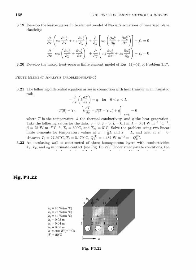
168 THE FINITE ELEMENT METHOD: A REVIEW
3.19 Develop the least-squares finite element model of Navier’s equations of linearized planeelasticity:
∂
∂x
(c11
∂uhx∂x
+ c12∂uhy∂y
)+
∂
∂y
[c66
(∂uhx∂y
+∂uhy∂x
)]+ fx = 0
∂
∂x
[c66
(∂uhx∂y
+∂uhy∂x
)]+
∂
∂y
(c12
∂uhx∂x
+ c22∂uhy∂y
)+ fy = 0
3.20 Develop the mixed least-squares finite element model of Eqs. (1)–(4) of Problem 3.17.
Finite Element Analysis (problem-solving)
3.21 The following differential equation arises in connection with heat transfer in an insulatedrod:
− d
dx
(kdT
dx
)= q for 0 < x < L
T (0) = T0,
[kdT
dx+ β(T − T∞) + q
] ∣∣∣∣x=L
= 0
where T is the temperature, k the thermal conductivity, and q the heat generation.Take the following values for the data: q = 0, q = 0, L = 0.1 m, k = 0.01 W m−1 C−1,β = 25 W m−2C−1, T0 = 50C, and T∞ = 5C. Solve the problem using two linearfinite elements for temperature values at x = 1
2L and x = L, and heat at x = 0.
Answer: T2 = 27.59C, T3 = 5.179C, Q(1)1 = 4.482 W m−2 = −Q(2)
2 .
3.22 An insulating wall is constructed of three homogeneous layers with conductivitiesk1, k2, and k3 in intimate contact (see Fig. P3.22). Under steady-state conditions, thetemperatures at the boundaries of the layers are characterized by the external surfacetemperatures T1 and T4 and the interface temperatures T2 and T3. Formulate the prob-lem to determine the temperatures Ti (i = 1, . . . , 4) when the ambient temperatures T0
and T5 and the (surface) film coefficients β0 and β5 are known for the following cases:Case 1: T0 = T5 = 20C and β0 = β5 = 500 W/m2·C; Case 2: T0 = 120C, T5 = 20C,β0 = 500 W/m2·C, and β5 = 560 W/m2·C; Case 3: T1 = 100C, T5 = 20C, andβ5 = 500W/m2·C. Assume that there is no internal heat generation and that the heatflow is one-dimensional (∂T/∂y = 0).
Fig. P3.22
x
L
1 2 321 3 4
k1 = 90 W/(m ºC) k2 = 75 W/(m ºC)k3 = 50 W/(m ºC)h1 = 0.03 mh2 = 0.04 mh3 = 0.05 mb = 500 W/(m2 ºC)T∞ = 20ºC
h1 h2 h3
Fig. P3.22
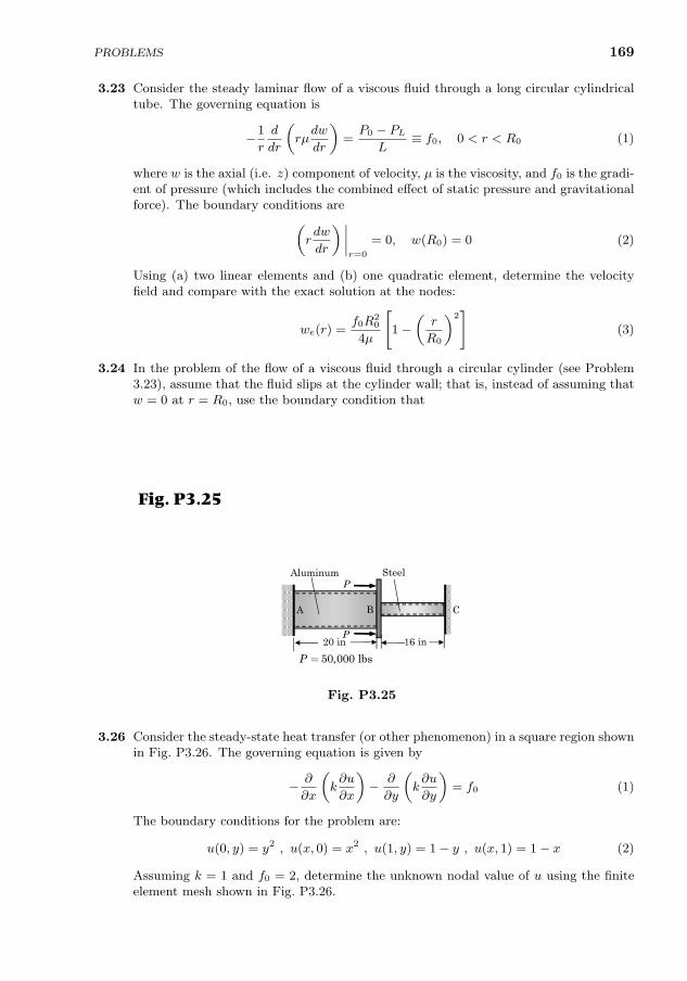
PROBLEMS 169
3.23 Consider the steady laminar flow of a viscous fluid through a long circular cylindricaltube. The governing equation is
−1
r
d
dr
(rµdw
dr
)=P0 − PL
L≡ f0, 0 < r < R0 (1)
where w is the axial (i.e. z) component of velocity, µ is the viscosity, and f0 is the gradi-ent of pressure (which includes the combined effect of static pressure and gravitationalforce). The boundary conditions are(
rdw
dr
) ∣∣∣∣r=0
= 0, w(R0) = 0 (2)
Using (a) two linear elements and (b) one quadratic element, determine the velocityfield and compare with the exact solution at the nodes:
we(r) =f0R
20
4µ
[1−
(r
R0
)2]
(3)
3.24 In the problem of the flow of a viscous fluid through a circular cylinder (see Problem3.23), assume that the fluid slips at the cylinder wall; that is, instead of assuming thatw = 0 at r = R0, use the boundary condition that
kw = −µdwdr
at r = R0 (1)
in which k is the “coefficient of sliding friction.” Solve the problem with two linearelements.
3.25 The two members in Fig. P3.25 are fastened together and to rigid walls. If the membersare stress free before they are loaded, what will be the stresses and deformations ineach after two 50,000 lbs loads are applied? Use Es = 30× 106 psi and Ea = 107 psi;the aluminum rod is of 2 in diameter and the steel rod is of 1.5 in diameter.
Fig. P3.25
20 in
AluminumP
A B C
P
Steel
16 in
50,000 lbsP =
Fig. P3.25
3.26 Consider the steady-state heat transfer (or other phenomenon) in a square region shownin Fig. P3.26. The governing equation is given by
− ∂
∂x
(k∂u
∂x
)− ∂
∂y
(k∂u
∂y
)= f0 (1)
The boundary conditions for the problem are:
u(0, y) = y2 , u(x, 0) = x2 , u(1, y) = 1− y , u(x, 1) = 1− x (2)
Assuming k = 1 and f0 = 2, determine the unknown nodal value of u using the finiteelement mesh shown in Fig. P3.26.
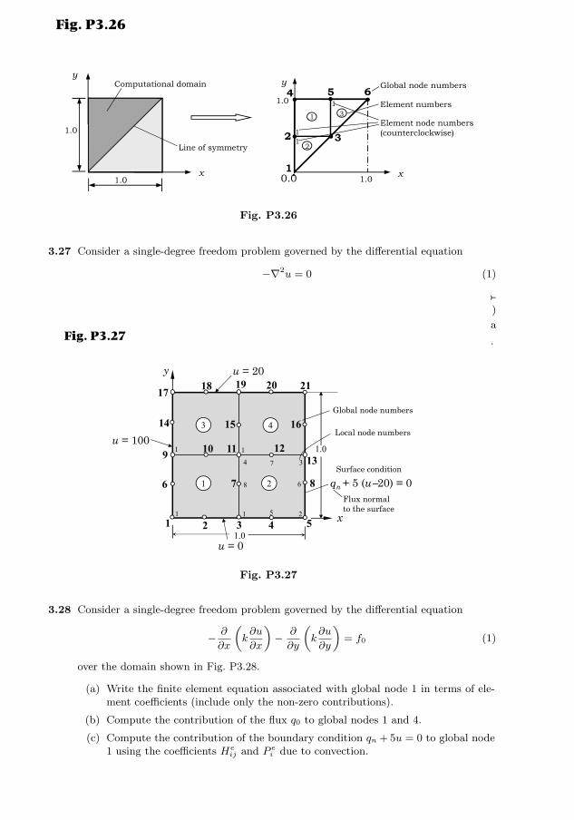
170 THE FINITE ELEMENT METHOD: A REVIEW
1.0
1.0
x
yy
x1.0
1.0
0.0
Computational domain
Line of symmetry•
• • •
•
•
11
1
1
2 3
4 5 6
Element node numbers(counterclockwise)
2
1 3
Global node numbers
Element numbers
Fig. P3.26
Fig. P3.26
3.27 Consider a single-degree freedom problem governed by the differential equation
−∇2u = 0 (1)
over the domain shown in Fig. P3.27. Write the global finite element equation asso-ciated with global node 8 and identify all of the coefficients (other than unknown UI)
in the equation in terms of the element coefficients K(e)ij (algebraic) and problem data
only (i.e. you must give the numerical values of other contributions other than K(e)ij ).
111 3
9 11
5
13
19
x
y
1.0
qn + 5 (u−20) = 0
1.0
1 2
3 4
2 4
6 7 8
10 12
14 15
17 18
u = 0
u = 100
u = 20
25
6
374
8
Global node numbers
Local node numbers16
20 21
11
Surface condition
Flux normal to the surface
Fig. P3.27
Fig. P3.27
3.28 Consider a single-degree freedom problem governed by the differential equation
− ∂
∂x
(k∂u
∂x
)− ∂
∂y
(k∂u
∂y
)= f0 (1)
over the domain shown in Fig. P3.28.
(a) Write the finite element equation associated with global node 1 in terms of ele-ment coefficients (include only the non-zero contributions).
(b) Compute the contribution of the flux q0 to global nodes 1 and 4.
(c) Compute the contribution of the boundary condition qn + 5u = 0 to global node1 using the coefficients He
ij and P ei due to convection.
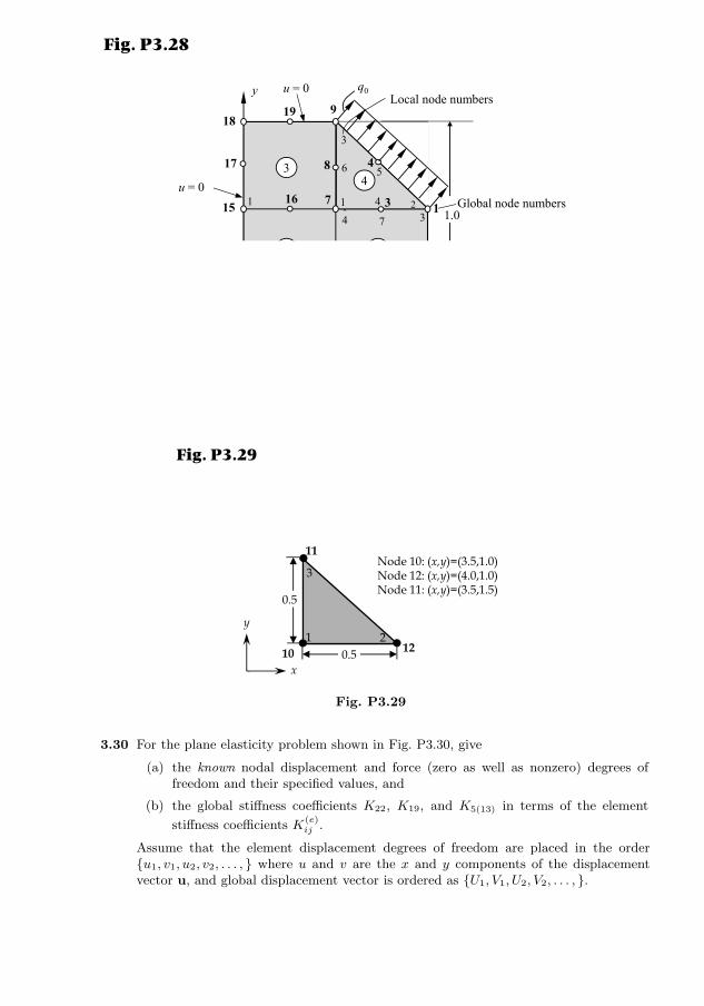
PROBLEMS 171
1
1
1
11311
15 7
5
1
9
x
y
1.0
q0
qn + 5 u = 0
1.0
1 2
34
1
12 10
14 6 2
16 3
17 8 4
1819
u = 0
u = 0
u = 0
2
3
4
56
25
6
374
8
Global node numbers
Local node numbers
Fig. P3.28
Fig. P3.28
3.29 The nodal values of a linear triangular element (see Fig. P3.29) in the finite-elementanalysis of the field problem −∇2u = f0 are ue1 = U10 = 389.79, ue2 = U12 = 337.19,and ue3 = U11 = 395.08. Find the (a) gradient of the solution
∇u ≡ ∂u
∂xex +
∂u
∂yey
in the element, and (b) the places where the u = 392 isoline intersects the boundary ofthe element.
x
y2
3
10.5
0.5
Node 10: (x,y)=(3.5,1.0)Node 12: (x,y)=(4.0,1.0)Node 11: (x,y)=(3.5,1.5)
10 12
11
Fig. P3.29
Fig. P3.29
3.30 For the plane elasticity problem shown in Fig. P3.30, give
(a) the known nodal displacement and force (zero as well as nonzero) degrees offreedom and their specified values, and
(b) the global stiffness coefficients K22, K19, and K5(13) in terms of the element
stiffness coefficients K(e)ij .
Assume that the element displacement degrees of freedom are placed in the orderu1, v1, u2, v2, . . . , where u and v are the x and y components of the displacementvector u, and global displacement vector is ordered as U1, V1, U2, V2, . . . , .
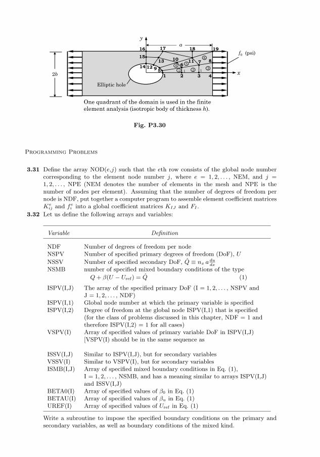
172 THE FINITE ELEMENT METHOD: A REVIEW
One quadrant of the domain is used in the finite element analysis (isotropic body of thickness h).
ya
2b
••
•••
•• •••
••• • ••
1 2 3 4
8
x
f0 (psi)•••
19
5911
17 18
136 7
1615
14 1210
1 14
1 2 35
6
Elliptic hole
Fig. P3.30
Programming Problems
3.31 Define the array NOD(e,j) such that the eth row consists of the global node numbercorresponding to the element node number j, where e = 1, 2, . . . , NEM, and j =1, 2, . . . , NPE (NEM denotes the number of elements in the mesh and NPE is thenumber of nodes per element). Assuming that the number of degrees of freedom pernode is NDF, put together a computer program to assemble element coefficient matricesKeij and fei into a global coefficient matrices KIJ and FI .
3.32 Let us define the following arrays and variables:
Variable Definition
NDF Number of degrees of freedom per nodeNSPV Number of specified primary degrees of freedom (DoF), U
NSSV Number of specified secondary DoF, Q ≡ nx a dudxNSMB number of specified mixed boundary conditions of the type
Q+ β(U − Uref) = Q (1)
ISPV(I,J) The array of the specified primary DoF (I = 1, 2, . . . , NSPV andJ = 1, 2, . . . , NDF)
ISPV(I,1) Global node number at which the primary variable is specifiedISPV(I,2) Degree of freedom at the global node ISPV(I,1) that is specified
(for the class of problems discussed in this chapter, NDF = 1 andtherefore ISPV(I,2) = 1 for all cases)
VSPV(I) Array of specified values of primary variable DoF in ISPV(I,J)[VSPV(I) should be in the same sequence asthe specified DoF in array ISPV(I,1)]
ISSV(I,J) Similar to ISPV(I,J), but for secondary variablesVSSV(I) Similar to VSPV(I), but for secondary variablesISMB(I,J) Array of specified mixed boundary conditions in Eq. (1),
I = 1, 2, . . . , NSMB, and has a meaning similar to arrays ISPV(I,J)and ISSV(I,J)
BETA0(I) Array of specified values of β0 in Eq. (1)BETAU(I) Array of specified values of βu in Eq. (1)UREF(I) Array of specified values of Uref in Eq. (1)
Write a subroutine to impose the specified boundary conditions on the primary andsecondary variables, as well as boundary conditions of the mixed kind.

PROBLEMS 173
3.33 Modify the subroutine ELMATRCS1D to evaluate the element coefficient matrix andforce vector in Eq. (3.4.12) for axisymmetric problems.
3.34 Modify the subroutine ELMATRCS2D to evaluate the element coefficient matrix andforce vector in Eq. (3.4.18) for axisymmetric problems.

175
4
One-Dimensional ProblemsInvolving a Single Variable
It is really quite amazing by what margins competent but conservative scientists and engineerscan miss the mark, when they start with the preconceived idea that what they are investigatingis impossible. When this happens, the most well-informed men become blinded by theirprejudices and are unable to see what lies directly ahead of them. ——– Arthur C. Clarke
4.1 Model Differential Equation
We shall consider a model nonlinear differential equation involving a single un-known in one-dimensional problems to illustrate its finite element model devel-opment and discuss solution methods to solve the nonlinear algebraic equations.As we shall see, the weak form and finite element model development discussedin Section 3.2 for a linear model equation are also valid for a nonlinear equation.
We consider differential operator equations of the form A(u(x)) = f(x)in the interval 0 < x < L, with boundary condition of the form B(u) = g.If the operators A and B satisfy the conditions of the type A(αu + βv) =αA(u) + βA(v) for any real numbers α and β, we say that the problem islinear; if either A or B are not linear, the problem is said to be nonlinear (seeSection 1.7.5 for a formal definition of a linear transformation or operator).
Consider the differential equation (see Table 3.2.1 for fields of study)
− d
dx
[a(x, u)
du
dx
]+ b(x, u)
du
dx+ c(x, u)u = f(x), 0 < x < L (4.1.1)
subjected to boundary conditions of the form
nx adu
dx+ β(x, u) (u− u∞) = Q, or u = u (4.1.2)
at a boundary point. Here u(x) denotes the dependent variable to be deter-mined, a, b, and c are known functions of x and u (and possibly derivatives ofu), f is a known function of x, (u∞, u, β, Q) are known (or specified) quantities,and nx is the cosine of the angle between the positive x-axis and the outwardnormal to the edge at the node (note that nx = −1 and β = β1 at x = xa andnx = 1 and β = β2 at x = xb).
J.N. Reddy, An Introduction to Nonlinear Finite Element Analysis, Second Edition. c©J.N.Reddy 2015. Published in 2015 by Oxford University Press.
176 ONE-DIMENSIONAL PROBLEMS INVOLVING A SINGLE VARIABLE
The first boundary condition in Eq. (4.1.2) is called a mixed boundary con-dition or Newton’s type boundary condition, and it is a statement of the balanceof “forces” at the boundary point. In the case of axial deformation of bars, themixed boundary condition (with u∞ = 0) represents the balance of the internalforce nxa(du/dx), with nx = 1, the external applied force Q, and the springforce −β2u, as illustrated in Fig. 4.1.1. Similarly, for one-dimensional heat flow,the mixed boundary condition is a statement of balance of energy due to theinternal heat a(du/dx), the externally applied heat Q, and the heat due to con-vection β2(u− u∞). The second boundary condition in Eq. (4.1.2) is a specialcase of the first boundary condition (with u∞ = u) in the limit β2 →∞.
Equation (4.1.1) and the first boundary condition in Eq. (4.1.2) can beexpressed in operator form as
A(u) = f in 0 < x < L; B(u) = g at x = 0 or L
where A and B are the differential operators
A ≡ − d
dx
(ad
dx
)+ b
d
dx+ c, B ≡ nx a
d
dx+ β, g ≡ βu∞ + Q
Clearly, operator A or B is not linear whenever any of the coefficients (a, b, c)are functions of u. The source of nonlinearity can be coefficients a, b, c and/or βwhich, in most engineering systems, include geometric and material parametersthat may be functions of position x and the dependent variable u. For example,in the study of heat conduction in a rod with convective heat transfer throughthe surface, a is equal to the product a = kA, b = 0, and c = Pβ, wherek denotes conductivity, β the convective heat transfer coefficient, A the cross-sectional area, and P the perimeter of the rod. Then the nonlinearity arises fromthe conductivity and heat transfer coefficients being functions of temperatureu. Such nonlinearity is known as the material nonlinearity. We wish to solvethis nonlinear differential equation using the finite element method.
L 1 2
1b 2b
Q
2 ( )u Lb
2b du
adx
Q
2
Fig. 4.1.1: Interpretation of the mixed boundary condition a(du/dx) + β2u = Q.
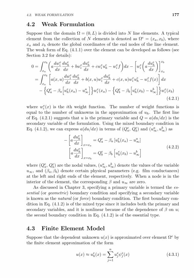
4.2. WEAK FORMULATION 177
4.2 Weak Formulation
Suppose that the domain Ω = (0, L) is divided into N line elements. A typicalelement from the collection of N elements is denoted as Ωe = (xa, xb), wherexa and xb denote the global coordinates of the end nodes of the line element.The weak form of Eq. (4.1.1) over the element can be developed as follows (seeSection 3.2 for details):
0 =
∫ xb
xa
(adwe
i
dx
duehdx
+ bwei
duehdx
+ cweiu
eh − we
i f
)dx−
[wei
(aduehdx
)]xb
xa
=
∫ xb
xa
[a(x, u)
dwei
dx
duehdx
+ b(x, u)wei
duehdx
+ c(x, u)weiu
eh − we
i f(x)
]dx
−Qe
a − βa[ueh(xa)− ua∞
]wei (xa)−
Qe
b − βb[ueh(xb)− ub∞
]wei (xb)
(4.2.1)
where wei (x) is the ith weight function. The number of weight functions is
equal to the number of unknowns in the approximation of uh. The first lineof Eq. (4.2.1) suggests that u is the primary variable and Q = a(du/dx) is thesecondary variable of the formulation. Using the mixed boundary condition inEq. (4.1.2), we can express a(du/dx) in terms of (Qe
a, Qeb) and (ua∞, u
b∞) as
−[aduehdx
]x=xa
= Qea − βa [ueh(xa)− ua∞][
aduehdx
]x=xb
= Qeb − βb
[ueh(xb)− ub∞
] (4.2.2)
where (Qea, Qe
b) are the nodal values, (ua∞, ub∞) denote the values of the variable
u∞, and (βa, βb) denote certain physical parameters (e.g. film conductances)at the left and right ends of the element, respectively. When a node is in theinterior of the element, the corresponding β and u∞ are zero.
As discussed in Chapter 3, specifying a primary variable is termed the es-sential (or geometric) boundary condition and specifying a secondary variableis known as the natural (or force) boundary condition. The first boundary con-dition in Eq. (4.1.2) is of the mixed type since it includes both the primary andsecondary variables, and it is nonlinear because of the dependence of β on u;the second boundary condition in Eq. (4.1.2) is of the essential type.
4.3 Finite Element Model
Suppose that the dependent unknown u(x) is approximated over element Ωe bythe finite element approximation of the form
u(x) ≈ ueh(x) =
n∑j=1
uejψej (x) (4.3.1)
178 ONE-DIMENSIONAL PROBLEMS INVOLVING A SINGLE VARIABLE
Substituting the approximation from Eq. (4.3.1) for u and wei = ψe
i (Galerkin’sapproach) into the weak form, Eq. (4.2.1), we obtain the following weak-formGalerkin or Ritz finite element model:
Ke(ue) ue = Fe (4.3.2)
where
Keij =
∫ xb
xa
[a(x, ueh)
dψei
dx
dψej
dx+ b(x, ueh)ψe
i
dψej
dx+ c(x, ueh)ψe
iψej
]dx
+ βaψei (xa)ψe
j (xa) + βbψei (xb)ψ
ej (xb) (4.3.3)
F ei =
∫ xb
xa
f(x)ψei dx+ βau
a∞ψ
ei (xa) + βbu
b∞ψ
ei (xb) +Qaψ
ei (xa) +Qbψ
ei (xb)
Note that the coefficient matrix Ke is a function of the unknown nodal valuesuej , and it is an unsymmetric matrix when b 6= 0; when b = 0, Ke is a symmetricmatrix. The term involving c is symmetric, independent of whether it dependson u and/or du/dx. Therefore, it is advisable to include nonlinear terms of thetype u (du/dx) in a differential equation as the c-term in the equation by writingit as u (du/dx) = cu, with c = du/dx; otherwise, it will be unsymmetric andconvergence of the solution may become a problem. The coefficients involvingβ in Ke and Fe should be included only in elements that have end nodes withthe convection type boundary condition. Example 4.3.1 provides more insightinto the make-up of the coefficient matrix Ke.
Example 4.3.1
Consider the problem described by Eqs. (4.1.1) and (4.1.2). Suppose that a(x) = a0 +au u(x)and b = c = 0, where a0 and au are functions of x only. Determine the explicit form of theelement matrices Ke and fe using linear approximation of u and element-wise constant valuesae0 and aeu of a0 and au, respectively.
Solution: For all elements except for the last one, the coefficients βa and βb are zero; for thelast element we have βa = 0 and βb 6= 0 when the end x = L is subjected to the convectionboundary condition. Thus, we have for e 6= N , where N denotes the total number of elementsin a mesh of elements connected end-to-end:
Keij =
∫ xb
xa
[ae0 + aeu
( n∑k=1
uekψ
ek
)]dψei
dx
dψej
dxdx
=
∫ xb
xa
ae0dψe
i
dx
dψej
dxdx+
n∑k=1
uek
∫ xb
xa
aeuψekdψe
i
dx
dψej
dxdx (1)
For the linear (n = 2) approximation of u(x), we have [see Eq. (3.2.21)]
ueh(x) = ue
1ψe1(x) + ue
2ψe2(x) = ue
1
(xb − xhe
)+ ue
2
(x− xahe
)(2)
and
Keij = ae0
∫ xb
xa
dψei
dx
dψej
dxdx+
2∑k=1
aeu uek
∫ xb
xa
ψekdψe
i
dx
dψej
dxdx
4.3. FINITE ELEMENT MODEL 179
= (−1)i+j 1
h2e
[ae0
∫ xb
xa
1 · dx+ aeu
2∑k=1
uek
∫ xb
xa
ψek dx
]
= (−1)i+j 1
h2e
[ae0he + aeu
he
2
( 2∑k=1
uek
)]= (−1)i+j 1
he
[ae0 +
aeu2
ue
1 + ue2
)](3)
or
Ke =ae0 + 0.5aeu(ue
1 + ue2)
he
[1 −1−1 1
], 1 < e < N (4)
The last (i.e. Nth) element coefficient matrix and source vector are given by
K(N) =ae0 + 0.5aeu(ue
1 + ue2)
he
[1 −1−1 1
]+
[0 00 βb
], f (N) =
f
(N)1
f(N)2
+
0
βbub∞
σ(5)
The assembly of element equations follows the same procedure as in linearfinite element analysis. If we denote the global nodal vector by U, the assembledsystem of equations can be written as
K(U)U = F(U) (4.3.4)
where K and F denote the global coefficient matrix and the right-hand side vec-tor, respectively. In Example 4.3.1, K is a linear function of the nodal values Ui
and it is a symmetric matrix. Consequently, the resulting finite element equa-tions are nonlinear; in the present case, the algebraic equations are quadraticin Ui. The right-hand side vector F depends on U only when the boundaryconditions are nonlinear. Example 4.3.2 illustrates these ideas.
Example 4.3.2
Consider the problem of Example 4.3.1 with the following specific boundary conditions:
u(0) = u0,
[adu
dx+ β (u− u∞)
]x=L
= Q (1)
withβ = β0 + β1u (2)
Give the assembled finite element equations after the imposition of boundary conditions for auniform mesh of two linear elements.
Solution: The assembled equations associated with a mesh of two linear elements of equallength h and with uniform data a0 and au, but without the contribution due to the convectionboundary condition (1) at x = L, are
1
h
a0 + 0.5au(U1 + U2) −a0 − 0.5au(U1 + U2) 0−a0 − 0.5au(U1 + U2) 2a0 + 0.5au(U1 + 2U2 + U3) −a0 − 0.5au(U2 + U3)
0 −a0 − 0.5au(U2 + U3) a0 + 0.5au(U2 + U3)
U1
U2
U3
=
f
(1)1
f(1)2 + f
(2)1
f(2)2
+
Q
(1)1
Q(1)2 +Q
(2)1
Q(2)2
(3)
180 ONE-DIMENSIONAL PROBLEMS INVOLVING A SINGLE VARIABLE
The boundary conditions for the present mesh of two linear elements imply
U1 = u0, Q(2)2 = Q− (β0 + β1U3) (U3 − u∞) (4)
Hence, after imposing the boundary conditions and balance of the secondary variables Q(1)2 +
Q(2)1 = 0, the assembled equations in (3) becomea0
h
1 −1 0−1 2 −1
0 −1 1
+au2h
(U1 + U2) −(U1 + U2) 0−(U1 + U2) (U1 + 2U2 + U3) −(U2 + U3)
0 −(U2 + U3) (U2 + U3)
u0
U2
U3
+
0 0 00 0 00 0 β0 + β1U3
u0
U2
U3
=
f
(1)1
f(1)2 + f
(2)1
f(2)2
+
Q(1)1
0
Q+ (β0 + β1U3)u∞
(5)
Clearly, the assembled equations in Eq. (5) are the same as the system of equations obtainedby assembling the element matrices in Eqs. (4) and (5) of Example 4.3.1. Note that in thepresent case, due to the nonlinearity in the boundary condition, F is a function of U. Onemay move the term involving the unknown U3 from the right-hand side vector to the left sideof the equality in Eq. (5).
4.4 Solution of Nonlinear Algebraic Equations
4.4.1 General Comments
Numerical procedures used to solve nonlinear algebraic equations of the type inEq. (4.3.4) are iterative in nature. All iterative methods of solution of nonlinearalgebraic equations are based on linearization of the element coefficient matrixKe (and the source vector Fe if it is dependent on ue). Then the elementequations are assembled and boundary conditions are imposed before solvingthem by an iterative procedure. Two iterative procedures are outlined herefor the problem at hand. Some general features of iterative methods used fornonlinear equations are discussed before getting into the details of each method(see Appendix 2 for additional discussion).
4.4.2 Direct Iteration Procedure
Suppose that we wish to solve the assembled system, Eq. (4.3.4), which alreadyhas the boundary conditions imposed on them. Since K(U) cannot be evaluateduntil U is known and the solution is not known until we solve the equations,one must resort to an iterative procedure in which we assume that solution atthe (r − 1)st iteration is known and seek solution at the rth iteration:
K(U(r−1))U(r) = F(U(r−1)) (4.4.1)
This procedure of solving Eq. (4.4.1) iteratively is called the direct iterationtechnique, also known as the Picard iteration or the method of successive sub-stitutions.
4.4. SOLUTION OF NONLINEAR ALGEBRAIC EQUATIONS 181
At the beginning of the iteration process, that is, when r = 1, solutionU(0) must be assumed or “guessed” consistent with the problem boundaryconditions. Using the solution from the (r− 1)st iteration, we can compute thecoefficient matrix K(r−1) ≡ K(U(r−1)) and vector F(r−1) ≡ F(U(r−1)). Thesolution at the rth iteration is determined by inverting Eq. (4.4.1):
U(r) = [K(r−1)]−1F(r−1) (4.4.2)
In writing Eq. (4.4.2), we have assumed that the coefficient matrix K(r−1) isinvertible after the imposition of boundary conditions. Thus, the initial guessvector U0 should be such that: (a) it satisfies the specified essential boundaryconditions and (b) K(0) is invertible.
Once the solution U(r) is obtained, we check to see if the residual vector
R(r) ≡ K(r)U(r) − F(r) (4.4.3)
is zero. The magnitude of this residual vector will be small enough if the solutionhas converged. In other words, we terminate the iteration if the magnitude ofthe residual vector, measured in a suitable norm, is less than some preselectedtolerance ε. If the problem data are such that KU as well as F are very small,the norm of the residual vector may also be very small even when the solutionU has not converged. Therefore, it is necessary to normalize the residual vectorwith respect to F. Using the Euclidean norm1, we can express the error criterionas √
R(r) ·R(r)
F(r) · F(r)≤ ε (4.4.4)
Alternatively, one may check to see if the normalized difference between solutionvectors from two consecutive iterations, measured with the Euclidean norm, isless than a preselected tolerance ε:√
∆U ·∆U
U(r) ·U(r)=
√√√√∑NI=1 |U
(r)I − U (r−1)
I |2∑NI=1 |U
(r)I |2
≤ ε (4.4.5)
where ∆U = U(r) − U(r−1). Thus, the iteration process is continued untilthe error criterion in Eq. (4.4.4) or Eq. (4.4.5) is satisfied or the number ofiterations exceeds a preselected maximum number of iterations, so that theprocess does not go into a loop of indefinite number of iterations in the case ofnon-convergence.
Acceleration of convergence for some types of nonlinearities may be achievedby using a weighted-average of solutions from the last two iterations rather thanthe solution from the last iteration to evaluate the coefficient matrix:1The Euclidean norm of a vector r = (r1, r2, . . . , rn), where ri are real numbers, is ‖r‖ =(r2
1 + r22 + · · ·+ r2
n)1/2, and it is a measure of the length of the vector r; see Eq. (1.7.8).
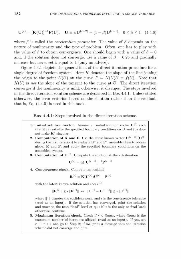
182
U(r) = [K(U)]−1F(U), U ≡ βU(r−2) + (1− β)U(r−1), 0 ≤ β ≤ 1 (4.4.6)
where is called the acceleration parameter. The value of β depends on thenature of nonlinearity and the type of problem. Often, one has to play withthe value of β to obtain convergence. One should begin with a value of β = 0and, if the solution does not converge, use a value of β = 0.25 and graduallyincrease but never set equal to 1 (only an advice).
Figure 4.4.1 depicts the general idea of the direct iteration procedure for asingle-degree-of-freedom system. Here K denotes the slope of the line joiningthe origin to the point K(U) on the curve F = K(U)U ≡ f(U). Note thatK(U) is not the slope of the tangent to the curve at U . The direct iterationconverges if the nonlinearity is mild; otherwise, it diverges. The steps involvedin the direct iteration solution scheme are described in Box 4.4.1. Unless statedotherwise, the error criterion based on the solution rather than the residual,that is, Eq. (4.4.5) is used in this book.
Box 4.4.1: Steps involved in the direct iteration scheme.
1. Initial solution vector. Assume an initial solution vector U(0) suchthat it (a) satisfies the specified boundary conditions on U and (b) doesnot make Ke singular.
2. Computation of K and F. Use the latest known vector U(r−1) (U(0)
during the first iteration) to evaluate Ke and Fe, assemble them to obtainglobal K and F, and apply the specified boundary conditions on theassembled system.
3. Computation of U(r). Compute the solution at the rth iteration
U(r) = [K(U(r−1))]−1F(r−1)
4. Convergence check. Compute the residual
R(r) = K(U(r))U(r) − F(r)
with the latest known solution and check if
‖R(r)‖ ≤ ε ‖F(r)‖ or ‖U(r) −U(r−1)‖ ≤ ε ‖U(r)‖
where ‖ · ‖ denotes the euclidean norm and ε is the convergence tolerance(read as an input). If the solution has converged, print the solutionand move to the next “load” level or quit if it is the only or final load;otherwise, continue.
5. Maximum iteration check. Check if r < itmax, where itmax is themaximum number of iterations allowed (read as an input). If yes, setr → r + 1 and go to Step 2; if no, print a message that the iterationscheme did not converge and quit.
ONE-DIMENSIONAL PROBLEMS INVOLVING A SINGLE VARIABLE
β
β
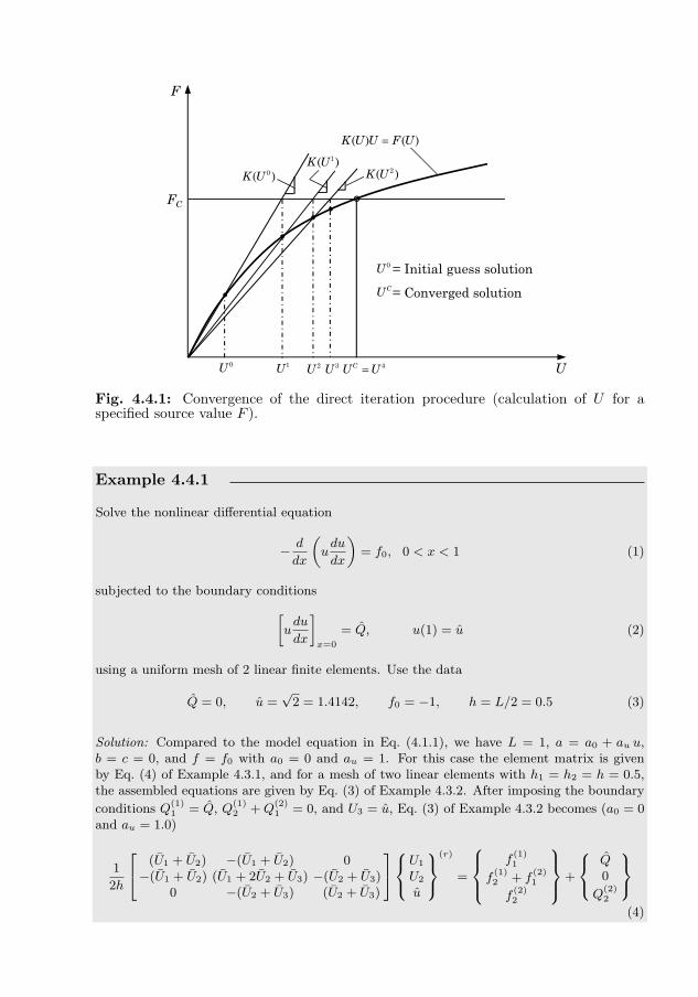
4.4. SOLUTION OF NONLINEAR ALGEBRAIC EQUATIONS 183
F
U
FC
•
•• • °
= Initial guess solution
= Converged solution
0( )K U
1( )K U2( )K U
( ) ( )K U U F U=
0U
CU
0U 1U 2U 3U 4CU U=
Fig. 4.4.1: Convergence of the direct iteration procedure (calculation of U for aspecified source value F ).
Example 4.4.1
Solve the nonlinear differential equation
− d
dx
(udu
dx
)= f0, 0 < x < 1 (1)
subjected to the boundary conditions[udu
dx
]x=0
= Q, u(1) = u (2)
using a uniform mesh of 2 linear finite elements. Use the data
Q = 0, u =√
2 = 1.4142, f0 = −1, h = L/2 = 0.5 (3)
Solution: Compared to the model equation in Eq. (4.1.1), we have L = 1, a = a0 + au u,b = c = 0, and f = f0 with a0 = 0 and au = 1. For this case the element matrix is givenby Eq. (4) of Example 4.3.1, and for a mesh of two linear elements with h1 = h2 = h = 0.5,the assembled equations are given by Eq. (3) of Example 4.3.2. After imposing the boundary
conditions Q(1)1 = Q, Q
(1)2 +Q
(2)1 = 0, and U3 = u, Eq. (3) of Example 4.3.2 becomes (a0 = 0
and au = 1.0)
1
2h
(U1 + U2) −(U1 + U2) 0−(U1 + U2) (U1 + 2U2 + U3) −(U2 + U3)
0 −(U2 + U3) (U2 + U3)
U1
U2
u
(r)
=
f
(1)1
f(1)2 + f
(2)1
f(2)2
+
Q0
Q(2)2
(4)
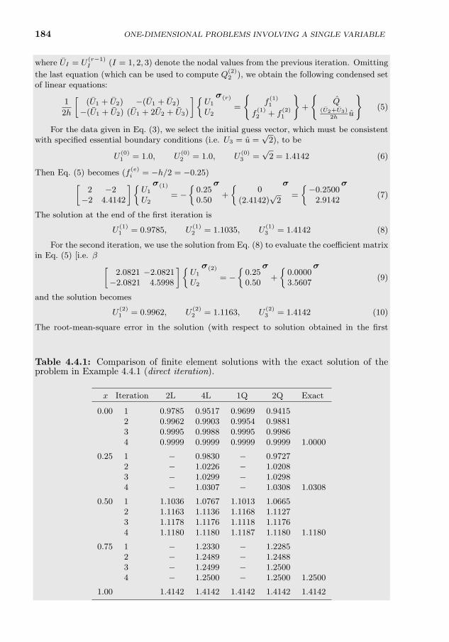
184 ONE-DIMENSIONAL PROBLEMS INVOLVING A SINGLE VARIABLE
where UI = U(r−1)I (I = 1, 2, 3) denote the nodal values from the previous iteration. Omitting
the last equation (which can be used to compute Q(2)2 ), we obtain the following condensed set
of linear equations:
1
2h
[(U1 + U2) −(U1 + U2)−(U1 + U2) (U1 + 2U2 + U3)
]U1
U2
σ(r)
=
f
(1)1
f(1)2 + f
(2)1
+
Q
(U2+U3)2h
u
(5)
For the data given in Eq. (3), we select the initial guess vector, which must be consistentwith specified essential boundary conditions (i.e. U3 = u =
√2), to be
U(0)1 = 1.0, U
(0)2 = 1.0, U
(0)3 =
√2 = 1.4142 (6)
Then Eq. (5) becomes (f(e)i = −h/2 = −0.25)[
2 −2−2 4.4142
]U1
U2
σ(1)
= −
0.250.50
σ+
0
(2.4142)√
2
σ=
−0.2500
2.9142
σ(7)
The solution at the end of the first iteration is
U(1)1 = 0.9785, U
(1)2 = 1.1035, U
(1)3 = 1.4142 (8)
For the second iteration, we use the solution from Eq. (8) to evaluate the coefficient matrixin Eq. (5) [i.e. β = 0 in Eq. (4.4.6)] and obtain[
2.0821 −2.0821−2.0821 4.5998
]U1
U2
σ(2)
= −
0.250.50
σ+
0.00003.5607
σ(9)
and the solution becomes
U(2)1 = 0.9962, U
(2)2 = 1.1163, U
(2)3 = 1.4142 (10)
The root-mean-square error in the solution (with respect to solution obtained in the firstiteration) [see Eq. (4.4.5)] is 0.0106.
Table 4.4.1: Comparison of finite element solutions with the exact solution of theproblem in Example 4.4.1 (direct iteration).
x Iteration 2L 4L 1Q 2Q Exact
0.00 1 0.9785 0.9517 0.9699 0.94152 0.9962 0.9903 0.9954 0.98813 0.9995 0.9988 0.9995 0.99864 0.9999 0.9999 0.9999 0.9999 1.0000
0.25 1 − 0.9830 − 0.97272 − 1.0226 − 1.02083 − 1.0299 − 1.02984 − 1.0307 − 1.0308 1.0308
0.50 1 1.1036 1.0767 1.1013 1.06652 1.1163 1.1136 1.1168 1.11273 1.1178 1.1176 1.1118 1.11764 1.1180 1.1180 1.1187 1.1180 1.1180
0.75 1 − 1.2330 − 1.22852 − 1.2489 − 1.24883 − 1.2499 − 1.25004 − 1.2500 − 1.2500 1.2500
1.00 1.4142 1.4142 1.4142 1.4142 1.4142
4.4. SOLUTION OF NONLINEAR ALGEBRAIC EQUATIONS 185
The exact solution to this problem, with the data given in Eq. (3), is (one can verify bydirect substitution)
u(x) =√
1 + x2
The convergence tolerance is taken to be ε = 10−3, and the maximum number of iterations isprescribed to be ten. The finite element solutions obtained with the linear (L) and quadratic(Q) elements are compared with the exact solution in Table 4.4.1. The finite element solutionconverges to the exact solution in four iterations.
4.4.3 Newton’s Iteration Procedure
In Newton’s method, we expand the residual vector R(r) of Eq. (4.4.3) in Tay-lor’s series about the known solution U(r−1):
R(r) = R(r−1) +
(∂R
∂U
)(r−1)·∆U +
1
2!
[(∂2R
∂U2
)(r−1)·∆U
]·∆U + · · · (4.4.7)
where∆U = U(r) −U(r−1) (4.4.8)
Omitting the terms of order 2 and higher in ∆U and requiring that R(r) bezero, we obtain (
∂R
∂U
)(r−1)∆U = −R(r−1) (4.4.9)
or
T(r−1) ∆U = −R(r−1) → T(r−1) U(r) = −R(r−1) + T(r−1) U(r−1) (4.4.10)
where T is called the tangent matrix, and it is defined as
T(r−1) ≡(∂R
∂U
)(r−1)(4.4.11)
The component definition of the tangent matrix is
TIJ ≡∂RI
∂UJ=
∂
∂UJ
( N∑m=1
KImUm − FI
)
=
N∑m=1
(KIm
∂Um
∂UJ+∂KIm
∂UJUm
)− ∂FI
∂UJ
= KIJ +N∑
m=1
∂KIm
∂UJUm −
∂FI
∂UJ
for I, J = 1, 2, . . . , N , where N is the total number of nodes in the mesh.All of the ideas presented above also apply to the element equation in
Eq. (4.3.2). Indeed, since element matrices are computed at the element level,
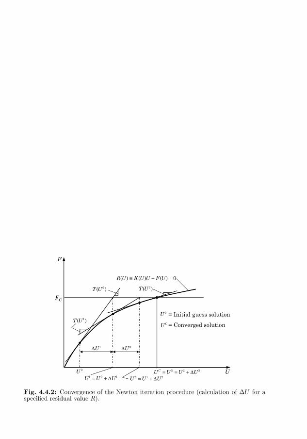
186 ONE-DIMENSIONAL PROBLEMS INVOLVING A SINGLE VARIABLE
we apply Newton’s procedure at the element level, and then assemble elementequations to form the global equations. The element equation for the Newtoniteration procedure is
Te(u(r−1)) ∆ue = −Re(u(r−1)) (4.4.12)
and the tangent coefficient matrix at the element level is
T eij ≡
∂Rei
∂uej=
∂
∂uej
(n∑
m=1
Keimu
em − F e
i
)= Ke
ij +
n∑m=1
∂Keim
∂uejuem −
∂F ei
∂uej(4.4.13)
When the vector Fe is independent of ue, we have ∂F ei /∂u
ej = 0.
The element equations in Eq. (4.4.12) are assembled and the boundary con-ditions are imposed on the increment ∆U before solving the assembled systemfor ∆U = −T−1R. The total solution at the rth iteration is then
Ur = U(r−1) + ∆U (4.4.14)
Figure 4.4.2 shows convergence of the Newton iteration procedure for asingle degree-of-freedom system. Here T (U) denotes the slope of the tangent tothe curve F = K(U)U at U . The Newton iteration converges for hardening aswell as softening type nonlinearities. For the hardening type, convergence maybe accelerated using the under-relaxation given in Eq. (4.4.6). The method maydiverge for a saddle-point behavior. The steps involved in Newton’s iterationsolution approach are described in Box 4.4.2.
F
U
FC
•
•• °
( ) ( ) ( ) 0R U K U U F U≡ − =
0( )T U 2( )T U
1( )T U
1UΔ 2UΔ
0U1 0 1U U U= + Δ 2 1 2U U U= + Δ
3 2 3CU U U U= = + Δ
CU
0U = Initial guess solution
= Converged solution
Fig. 4.4.2: Convergence of the Newton iteration procedure (calculation of ∆U for aspecified residual value R).
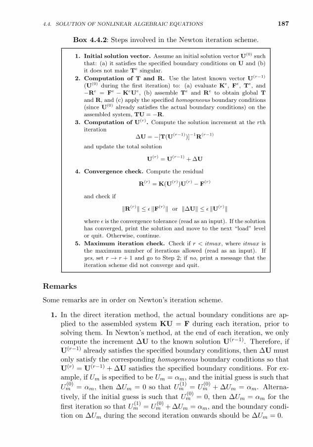
4.4. SOLUTION OF NONLINEAR ALGEBRAIC EQUATIONS 187
Box 4.4.2: Steps involved in the Newton iteration scheme.
1. Initial solution vector. Assume an initial solution vector U(0) suchthat: (a) it satisfies the specified boundary conditions on U and (b)it does not make Te singular.
2. Computation of T and R. Use the latest known vector U(r−1)
(U(0) during the first iteration) to: (a) evaluate Ke, Fe, Te, and−Re = Fe − KeUe, (b) assemble Te and Re to obtain global Tand R, and (c) apply the specified homogeneous boundary conditions(since U(0) already satisfies the actual boundary conditions) on theassembled system, TU = −R.
3. Computation of U(r). Compute the solution increment at the rthiteration
∆U = −[T(U(r−1))]−1R(r−1)
and update the total solution
U(r) = U(r−1) + ∆U
4. Convergence check. Compute the residual
R(r) = K(U(r))U(r) − F(r)
and check if
‖R(r)‖ ≤ ε ‖F(r)‖ or ‖∆U‖ ≤ ε ‖U(r)‖
where ε is the convergence tolerance (read as an input). If the solutionhas converged, print the solution and move to the next “load” levelor quit. Otherwise, continue.
5. Maximum iteration check. Check if r < itmax, where itmax isthe maximum number of iterations allowed (read as an input). Ifyes, set r → r + 1 and go to Step 2; if no, print a message that theiteration scheme did not converge and quit.
Remarks
Some remarks are in order on Newton’s iteration scheme.
1. In the direct iteration method, the actual boundary conditions are ap-plied to the assembled system KU = F during each iteration, prior tosolving them. In Newton’s method, at the end of each iteration, we onlycompute the increment ∆U to the known solution U(r−1). Therefore, ifU(r−1) already satisfies the specified boundary conditions, then ∆U mustonly satisfy the corresponding homogeneous boundary conditions so thatU(r) = U(r−1) + ∆U satisfies the specified boundary conditions. For ex-ample, if Um is specified to be Um = αm, and the initial guess is such that
U(0)m = αm, then ∆Um = 0 so that U
(1)m = U
(0)m + ∆Um = αm. Alterna-
tively, if the initial guess is such that U(0)m = 0, then ∆Um = αm for the
first iteration so that U(1)m = U
(0)m + ∆Um = αm, and the boundary condi-
tion on ∆Um during the second iteration onwards should be ∆Um = 0.
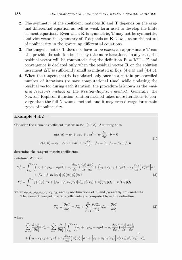
188 ONE-DIMENSIONAL PROBLEMS INVOLVING A SINGLE VARIABLE
2. The symmetry of the coefficient matrices K and T depends on the orig-inal differential equation as well as weak form used to develop the finiteelement equations. Even when K is symmetric, T may not be symmetric,and vice versa; the symmetry of T depends on K as well as on the natureof nonlinearity in the governing differential equations.
3. The tangent matrix T does not have to be exact; an approximate T canalso provide the solution but it may take more iterations. In any case, theresidual vector will be computed using the definition R = KU − F andconvergence is declared only when the residual vector R or the solutionincrement ∆U is sufficiently small as indicated in Eqs. (4.4.4) and (4.4.5).
4. When the tangent matrix is updated only once in a certain pre-specifiednumber of iterations (to save computational time) while updating theresidual vector during each iteration, the procedure is known as the mod-ified Newton’s method or the Newton–Raphson method. Generally, theNewton–Raphson iteration solution method takes more iterations to con-verge than the full Newton’s method, and it may even diverge for certaintypes of nonlinearity.
Example 4.4.2
Consider the element coefficient matrix in Eq. (4.3.3). Assuming that
a(x, u) = a0 + a1u+ a2u2 + a3
du
dx, b = 0
c(x, u) = c0 + c1u+ c2u2 + c3
du
dx, βa = 0, βb = β0 + β1u
(1)
determine the tangent matrix coefficients.
Solution: We have
Keij =
∫ xb
xa
[(a0 + a1uh + a2u
2h + a3
duh
dx
)dψei
dx
dψej
dx+(c0 + c1uh + c2u
2h + c3
duh
dx
)ψe
iψej
]dx
+ [β0 + β1uh(xb)]ψei (xb)ψ
ej (xb) (2)
F ei =
∫ xb
xa
f(x)ψei dx+
[β0 + β1uh(xb)
]ub∞ψ
ei (xb) + ψe
i (xa)Qa + ψei (xb)Qb
where a0, a1, a2, a3, c0, c1, c2, and c3 are functions of x, and β0 and β1 are constants.The element tangent matrix coefficients are computed from the definition
T eij ≡
∂Rei
∂uej
= Keij +
n∑m=1
∂Keim
∂uej
uem −
∂F ei
∂uej
(3)
where
n∑m=1
∂Keim
∂uej
uem =
n∑m=1
∂
∂uej
∫ xb
xa
[(a0 + a1uh + a2u
2h + a3
duh
dx
)dψei
dx
dψem
dx
+(c0 + c1uh + c2u
2h + c3
duh
dx
)ψe
iψem
]dx+
[β0 + β1uh(xb)
]ψe
i (xb)ψem(xb)
σuem
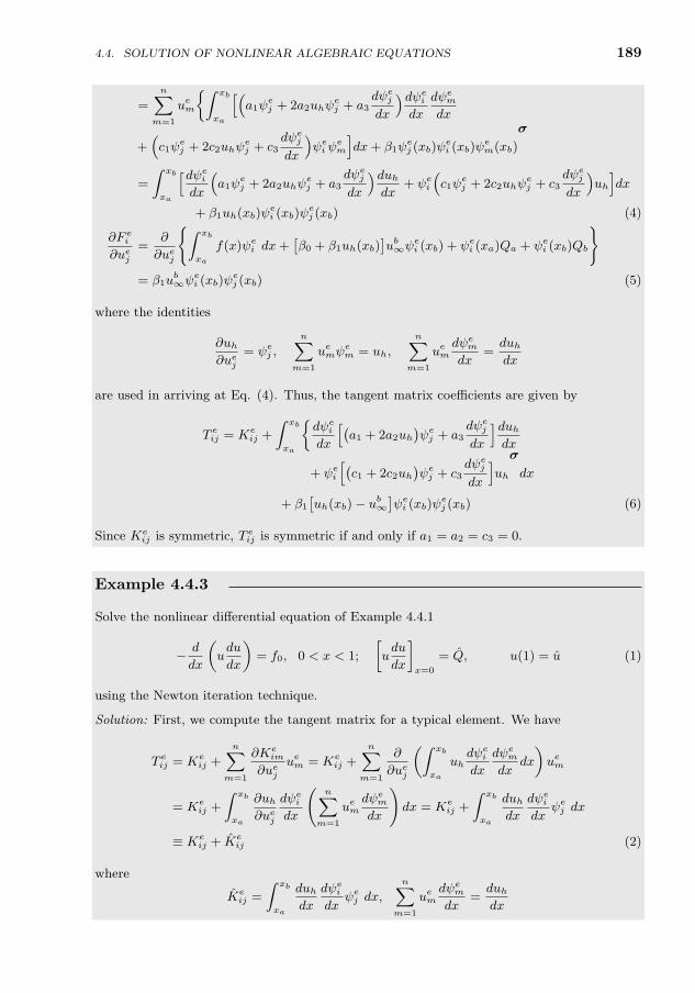
4.4. SOLUTION OF NONLINEAR ALGEBRAIC EQUATIONS 189
=
n∑m=1
uem
∫ xb
xa
[(a1ψ
ej + 2a2uhψ
ej + a3
dψej
dx
)dψei
dx
dψem
dx
+(c1ψ
ej + 2c2uhψ
ej + c3
dψej
dx
)ψe
iψem
]dx+ β1ψ
ej (xb)ψ
ei (xb)ψ
em(xb)
σ=
∫ xb
xa
[dψei
dx
(a1ψ
ej + 2a2uhψ
ej + a3
dψej
dx
)duh
dx+ ψe
i
(c1ψ
ej + 2c2uhψ
ej + c3
dψej
dx
)uh
]dx
+ β1uh(xb)ψei (xb)ψ
ej (xb) (4)
∂F ei
∂uej
=∂
∂uej
∫ xb
xa
f(x)ψei dx+
[β0 + β1uh(xb)
]ub∞ψ
ei (xb) + ψe
i (xa)Qa + ψei (xb)Qb
= β1u
b∞ψ
ei (xb)ψ
ej (xb) (5)
where the identities
∂uh
∂uej
= ψej ,
n∑m=1
uemψ
em = uh,
n∑m=1
uemdψe
m
dx=duh
dx
are used in arriving at Eq. (4). Thus, the tangent matrix coefficients are given by
T eij = Ke
ij +
∫ xb
xa
dψe
i
dx
[a1 + 2a2uh
)ψe
j + a3dψe
j
dx
]duh
dx
+ ψei
[c1 + 2c2uh
)ψe
j + c3dψe
j
dx
]uh
σdx
+ β1
[uh(xb)− ub
∞]ψe
i (xb)ψej (xb) (6)
Since Keij is symmetric, T e
ij is symmetric if and only if a1 = a2 = c3 = 0.
Example 4.4.3
Solve the nonlinear differential equation of Example 4.4.1
− d
dx
(udu
dx
)= f0, 0 < x < 1;
[udu
dx
]x=0
= Q, u(1) = u (1)
using the Newton iteration technique.
Solution: First, we compute the tangent matrix for a typical element. We have
T eij = Ke
ij +
n∑m=1
∂Keim
∂uej
uem = Ke
ij +
n∑m=1
∂
∂uej
(∫ xb
xa
uhdψe
i
dx
dψem
dxdx
)uem
= Keij +
∫ xb
xa
∂uh
∂uej
dψei
dx
(n∑
m=1
uemdψe
m
dx
)dx = Ke
ij +
∫ xb
xa
duh
dx
dψei
dxψe
j dx
≡ Keij + Ke
ij (2)
where
Keij =
∫ xb
xa
duh
dx
dψei
dxψe
j dx,n∑
m=1
uemdψe
m
dx=duh
dx
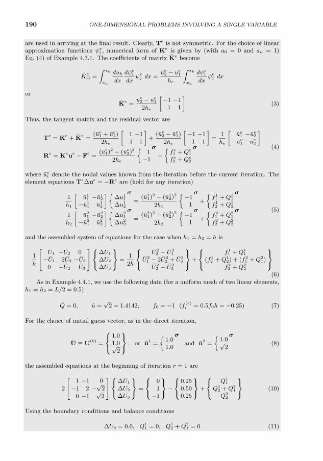
190 ONE-DIMENSIONAL PROBLEMS INVOLVING A SINGLE VARIABLE
are used in arriving at the final result. Clearly, Te is not symmetric. For the choice of linearapproximation functions ψe
i , numerical form of Ke is given by (with a0 = 0 and au = 1)Eq. (4) of Example 4.3.1. The coefficients of matrix Ke become
Keij =
∫ xb
xa
duh
dx
dψei
dxψe
j dx =ue
2 − ue1
he
∫ xb
xa
dψei
dxψe
j dx
or
Ke =ue
2 − ue1
2he
[−1 −1
1 1
](3)
Thus, the tangent matrix and the residual vector are
Te = Ke + Ke =(ue
1 + ue2)
2he
[1 −1−1 1
]+
(ue2 − ue
1)
2he
[−1 −1
1 1
]=
1
he
[ue
1 −ue2
−ue1 ue
2
]Re = Keue − Fe =
(ue1)2 − (ue
2)2
2he
1−1
σ−fe
1 +Qe1
fe2 +Qe
2
σ (4)
where uei denote the nodal values known from the iteration before the current iteration. The
element equations Te∆ue = −Re are (hold for any iteration)
1
h1
[u1
1 −u12
−u11 u1
2
]∆u1
1
∆u12
σ=
(u11)2 − (u1
2)2
2h1
−1
1
σ+
f1
1 +Q11
f12 +Q1
2
σ1
h2
[u2
1 −u22
−u21 u2
2
]∆u2
1
∆u22
σ=
(u21)2 − (u2
2)2
2h2
−1
1
σ+
f2
1 +Q21
f22 +Q2
2
σ (5)
and the assembled system of equations for the case when h1 = h2 = h is
1
h
U1 −U2 0−U1 2U2 −U3
0 −U2 U3
∆U1
∆U2
∆U3
=1
2h
U2
2 − U21
U21 − 2U2
2 + U23
U22 − U2
3
+
f1
1 +Q11
(f12 +Q1
2) + (f21 +Q2
1)f2
2 +Q22
(6)
As in Example 4.4.1, we use the following data (for a uniform mesh of two linear elements,h1 = h2 = L/2 = 0.5)
Q = 0, u =√
2 = 1.4142, f0 = −1 (f(e)i = 0.5f0h = −0.25) (7)
For the choice of initial guess vector, as in the direct iteration,
U ≡ U(0) =
1.01.0√
2
, or u1 =
1.01.0
σand u2 =
1.0√
2
σ(8)
the assembled equations at the beginning of iteration r = 1 are
2
1 −1 0
−1 2 −√
2
0 −1√
2
∆U1
∆U2
∆U3
=
01−1
−
0.250.500.25
+
Q1
1
Q12 +Q2
1
Q22
(10)
Using the boundary conditions and balance conditions
∆U3 = 0.0, Q11 = 0, Q1
2 +Q21 = 0 (11)
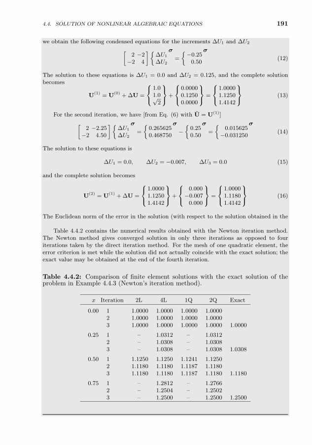
191
we obtain the following condensed equations for the increments ∆U1 and ∆U2[2 −2−2 4
]∆U1
∆U2
σ=
−0.25
0.50
σ(12)
The solution to these equations is ∆U1 = 0.0 and ∆U2 = 0.125, and the complete solutionbecomes
U(1) = U(0) + ∆U =
1.01.0√
2
+
0.00000.12500.0000
=
1.00001.12501.4142
(13)
For the second iteration, we have [from Eq. (6) with U = U(1)][2 −2.25−2 4.50
]∆U1
∆U2
σ=
0.2656250.468750
σ−
0.250.50
σ=
0.015625−0.031250
σ(14)
The solution to these equations is
∆U1 = 0.0, ∆U2 = −0.007, ∆U3 = 0.0 (15)
and the complete solution becomes
U(2) = U(1) + ∆U =
1.00001.12501.4142
+
0.000−0.007
0.000
=
1.00001.11801.4142
(16)
The Euclidean norm of the error in the solution (with respect to the solution obtained in thefirst iteration) [see Eq. (4.4.5)] is 0.0034.
Table 4.4.2 contains the numerical results obtained with the Newton iteration method.The Newton method gives converged solution in only three iterations as opposed to fouriterations taken by the direct iteration method. For the mesh of one quadratic element, theerror criterion is met while the solution did not actually coincide with the exact solution; theexact value may be obtained at the end of the fourth iteration.
Table 4.4.2: Comparison of finite element solutions with the exact solution of theproblem in Example 4.4.3 (Newton’s iteration method).
x Iteration 2L 4L 1Q 2Q Exact
0.00 1 1.0000 1.0000 1.0000 1.00002 1.0000 1.0000 1.0000 1.00003 1.0000 1.0000 1.0000 1.0000 1.0000
0.25 1 – 1.0312 – 1.03122 – 1.0308 – 1.03083 – 1.0308 – 1.0308 1.0308
0.50 1 1.1250 1.1250 1.1241 1.12502 1.1180 1.1180 1.1187 1.11803 1.1180 1.1180 1.1187 1.1180 1.1180
0.75 1 – 1.2812 – 1.27662 – 1.2504 – 1.25023 – 1.2500 – 1.2500 1.2500
4.4. SOLUTION OF NONLINEAR ALGEBRAIC EQUATIONS
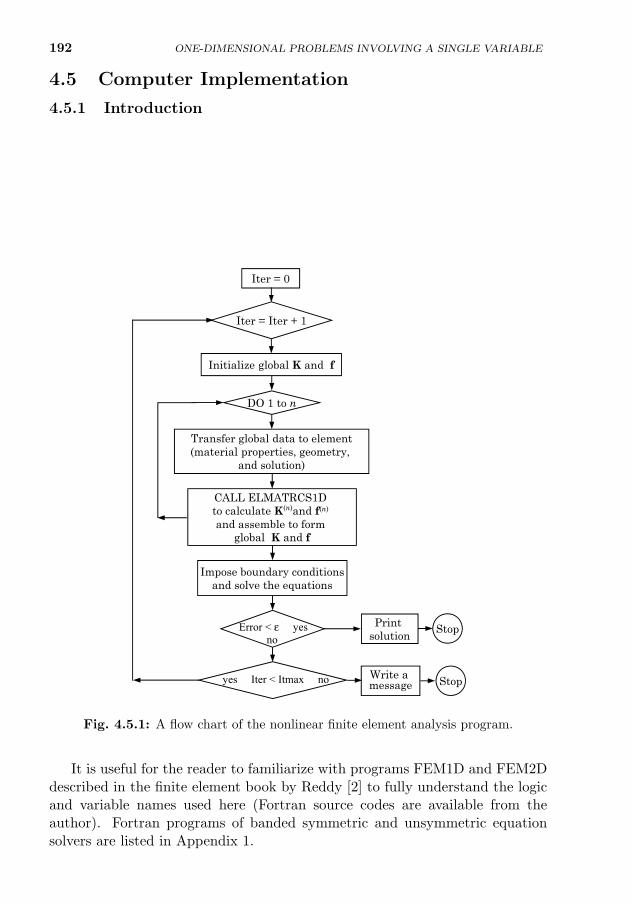
192
4.5 Computer Implementation
4.5.1 Introduction
The nonlinear formulations and solution procedures described in the precedingsections can be implemented on a computer using a programming language.Fortran is chosen here mainly because of its transparent nature compared toC++ language and the author’s own background. Of course, once the logicof implementation is understood, one may carry out the computations in anyprogramming language. A flow chart of a typical nonlinear analysis program isshown in Fig. 4.5.1.
Initialize global K and f
Iter = Iter + 1
DO 1 to n
Iter = 0
Impose boundary conditionsand solve the equations
CALL ELMATRCS1D to calculate K(n)and f(n)
and assemble to form global K and f
Transfer global data to element(material properties, geometry,
and solution)
Print solution
Write a message
StopError < ε yesno
yes Iter < Itmax no Stop
Fig. 4.5.1: A flow chart of the nonlinear finite element analysis program.
It is useful for the reader to familiarize with programs FEM1D and FEM2Ddescribed in the finite element book by Reddy [2] to fully understand the logicand variable names used here (Fortran source codes are available from theauthor). Fortran programs of banded symmetric and unsymmetric equationsolvers are listed in Appendix 1.
ONE-DIMENSIONAL PROBLEMS INVOLVING A SINGLE VARIABLE
4.5. COMPUTER IMPLEMENTATION 193
4.5.2 Preprocessor Unit
The preprocessor has the objective of reading the problem data (e.g. coefficientsof the differential equation) and analysis type, generating the mesh information(e.g. connectivity array, global coordinates of the nodes) and printing the dataand analysis information.
1. Read or define the problem and analysis data
(a) Define the coefficients a(x, u), b(x, u), and c(x, u), and f(x) thatappear in the model differential equation, Eq. (4.1.1); for example,one may assume a, b, c, and f to depend on x, u, and du/dx asfollows:
a(x, u) = ax0 + ax1x+ au1u+ au2u2 + aux1
(dudx
)+ aux2
(dudx
)2b(x, u) = bx0 + bx1x+ bu1u+ bu2u
2 + bux1
(dudx
)+ bux2
(dudx
)2c(x, u) = cx0 + cx1x+ cu1u+ cu2u
2 + cux1
(dudx
)+ cux2
(dudx
)2f(x) = fx0 + fx1x+ fx2x
2 (4.5.1)
so that a large number of nonlinear problems described by the modelequation in Eq. (4.1.1) may be solved with the same computer pro-gram. Thus, one must read all parameters appearing in the aboveexpressions; the data is assumed to be the same for the whole do-main: AX0, AX1, AU1, AU2, AUX1, AUX2; BX0, BX1, BU1, etc.
(b) Read and generate geometry, material, and FE analysis data (thedomain is assumed to be a straight line):
Variable Definition
X0 Global coordinate of the first node of the domainAL Domain lengthIEL Degree of interpolation used (1: linear; 2: quadratic)NEM Number of elements in the meshNNM Number of nodes in the meshNDF Number of degrees of freedom per node (here, NDF=1)NEQ Number of equations in the mesh, NEQ=NNM*NDFNLS Number of “load” steps (= 1 for the present case)NONLIN Parameter for the type of analysis:
= 0, linear analysis;= 1, nonlinear analysis using the direct iteration;> 1, nonlinear analysis using Newton’s iteration
EPS Allowable error tolerance ε for the convergence testITMAX Maximum allowable number of iterations for convergence
(c) Read data to specify the boundary and initial conditions. The vari-ables names and their meaning is given here.
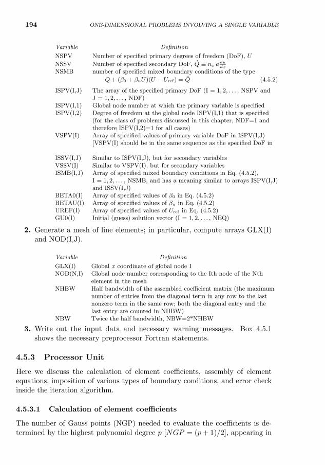
194 ONE-DIMENSIONAL PROBLEMS INVOLVING A SINGLE VARIABLE
Variable Definition
NSPV Number of specified primary degrees of freedom (DoF), U
NSSV Number of specified secondary DoF, Q ≡ nx adudx
NSMB number of specified mixed boundary conditions of the type
Q+ (β0 + βuU)(U − Uref) = Q (4.5.2)
ISPV(I,J) The array of the specified primary DoF (I = 1, 2, . . . , NSPV andJ = 1, 2, . . . , NDF)
ISPV(I,1) Global node number at which the primary variable is specifiedISPV(I,2) Degree of freedom at the global node ISPV(I,1) that is specified
(for the class of problems discussed in this chapter, NDF=1 andtherefore ISPV(I,2)=1 for all cases)
VSPV(I) Array of specified values of primary variable DoF in ISPV(I,J)[VSPV(I) should be in the same sequence as the specified DoF inarray ISPV(I,1)]
ISSV(I,J) Similar to ISPV(I,J), but for secondary variablesVSSV(I) Similar to VSPV(I), but for secondary variablesISMB(I,J) Array of specified mixed boundary conditions in Eq. (4.5.2),
I = 1, 2, . . . , NSMB, and has a meaning similar to arrays ISPV(I,J)and ISSV(I,J)
BETA0(I) Array of specified values of β0 in Eq. (4.5.2)BETAU(I) Array of specified values of βu in Eq. (4.5.2)UREF(I) Array of specified values of Uref in Eq. (4.5.2)GU0(I) Initial (guess) solution vector (I = 1, 2, . . . , NEQ)
2. Generate a mesh of line elements; in particular, compute arrays GLX(I)and NOD(I,J).
Variable Definition
GLX(I) Global x coordinate of global node INOD(N,I) Global node number corresponding to the Ith node of the Nth
element in the meshNHBW Half bandwidth of the assembled coefficient matrix (the maximum
number of entries from the diagonal term in any row to the lastnonzero term in the same row; both the diagonal entry and thelast entry are counted in NHBW)
NBW Twice the half bandwidth, NBW=2*NHBW
3. Write out the input data and necessary warning messages. Box 4.5.1shows the necessary preprocessor Fortran statements.
4.5.3 Processor Unit
Here we discuss the calculation of element coefficients, assembly of elementequations, imposition of various types of boundary conditions, and error checkinside the iteration algorithm.
4.5.3.1 Calculation of element coefficients
The number of Gauss points (NGP) needed to evaluate the coefficients is de-termined by the highest polynomial degree p [NGP = (p+ 1)/2], appearing in
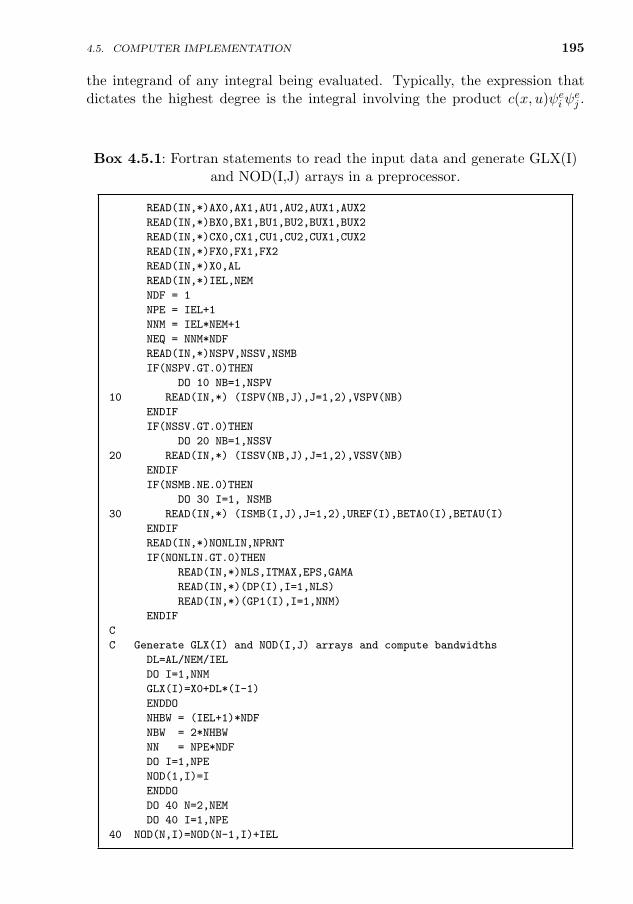
4.5. COMPUTER IMPLEMENTATION 195
the integrand of any integral being evaluated. Typically, the expression thatdictates the highest degree is the integral involving the product c(x, u)ψe
iψej .
Box 4.5.1: Fortran statements to read the input data and generate GLX(I)and NOD(I,J) arrays in a preprocessor.
READ(IN,*)AX0,AX1,AU1,AU2,AUX1,AUX2
READ(IN,*)BX0,BX1,BU1,BU2,BUX1,BUX2
READ(IN,*)CX0,CX1,CU1,CU2,CUX1,CUX2
READ(IN,*)FX0,FX1,FX2
READ(IN,*)X0,AL
READ(IN,*)IEL,NEM
NDF = 1
NPE = IEL+1
NNM = IEL*NEM+1
NEQ = NNM*NDF
READ(IN,*)NSPV,NSSV,NSMB
IF(NSPV.GT.0)THEN
DO 10 NB=1,NSPV
10 READ(IN,*) (ISPV(NB,J),J=1,2),VSPV(NB)
ENDIF
IF(NSSV.GT.0)THEN
DO 20 NB=1,NSSV
20 READ(IN,*) (ISSV(NB,J),J=1,2),VSSV(NB)
ENDIF
IF(NSMB.NE.0)THEN
DO 30 I=1, NSMB
30 READ(IN,*) (ISMB(I,J),J=1,2),UREF(I),BETA0(I),BETAU(I)
ENDIF
READ(IN,*)NONLIN,NPRNT
IF(NONLIN.GT.0)THEN
READ(IN,*)NLS,ITMAX,EPS,GAMA
READ(IN,*)(DP(I),I=1,NLS)
READ(IN,*)(GP1(I),I=1,NNM)
ENDIF
C
C Generate GLX(I) and NOD(I,J) arrays and compute bandwidths
DL=AL/NEM/IEL
DO I=1,NNM
GLX(I)=X0+DL*(I-1)
ENDDO
NHBW = (IEL+1)*NDF
NBW = 2*NHBW
NN = NPE*NDF
DO I=1,NPE
NOD(1,I)=I
ENDDO
DO 40 N=2,NEM
DO 40 I=1,NPE
40 NOD(N,I)=NOD(N-1,I)+IEL
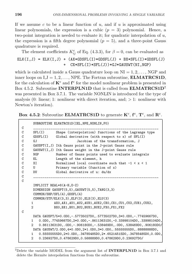
196 ONE-DIMENSIONAL PROBLEMS INVOLVING A SINGLE VARIABLE
If we assume c to be a linear function of u, and if u is approximated usinglinear polynomials, the expression is a cubic (p = 3) polynomial. Hence, atwo-point integration is needed to evaluate it; for quadratic interpolation of u,the expression is a fifth degree polynomial (p = 5), and a three-point Gaussquadrature is required.
The element coefficients Keij of Eq. (4.3.3), for β = 0, can be evaluated as
ELK(I,J) = ELK(I,J) + (AX*GDSFL(I)*GDSFL(J) + BX*SFL(I)*GDSFL(J)
+ CX*SFL(I)*SFL(J))*GJ*GAUSWT(NI,NGP)
which is calculated inside a Gauss quadrature loop on NI = 1, 2, . . . , NGP andinner loops on I,J = 1, 2, . . . , NPE. The Fortran subroutine, ELMATRCS1D,for the calculation of Ke and f e for the model nonlinear problem is presented inBox 4.5.2. Subroutine INTERPLN1D that is called from ELMATRCS1D2
was presented in Box 3.7.1. The variable NONLIN is introduced for the type ofanalysis (0: linear; 1: nonlinear with direct iteration, and; > 1: nonlinear withNewton’s iteration).
Box 4.5.2: Subroutine ELMATRCS1D to generate Ke, f e, Te, and Re.
SUBROUTINE ELMATRCS1D(IEL,NPE,NONLIN,F0)
C __________________________________________________________________
C SFL(I) Shape (interpolation) functions of the Lagrange type
C GDSFL(I) Global derivative (with respect to x) of SFL(I)
C GJ Jacobian of the transformation, J
C GAUSPT(I,J) Ith Gauss point in the J-point Gauss rule
C GAUSWT(I,J) Ith Gauss weight in the J-point Gauss rule
C NGP Number of Gauss points used to evaluate integrals
C EL Length of the element, h
C XI Normalized local coordinate such that -1 < x < 1
C U Primary variable (function of x)
C DU Global derivative of u: du/dx
C __________________________________________________________________
C
IMPLICIT REAL*8(A-H,O-Z)
DIMENSION GAUSPT(5,5),GAUSWT(5,5),TANG(3,3)
COMMON/SHP/SFL(4),GDSFL(4)
COMMON/STF/ELK(3,3),ELF(3),ELX(3),ELU(3)
1 AX0,AX1,AU1,AU2,AUX1,AUX2,CX0,CX1,CU1,CU2,CUX1,CUX2,
2 BX0,BX1,BU1,BU2,BUX1,BUX2,FX0,FX1,FX2
C
DATA GAUSPT/5*0.0D0,-.57735027D0,.57735027D0,3*0.0D0,-.77459667D0,
1 0.0D0,.77459667D0,2*0.0D0,-.86113631D0,-0.33998104D0,.33998104D0,
2 0.86113631D0,.0D0,-.906180D0,-.538469D0,.0D0,.538469D0,.906180D0/
DATA GAUSWT/2.0D0,4*0.0D0,2*1.0D0,3*0.0D0,.55555555D0,.88888888D0,
1 0.55555555D0,2*0.0D0,.34785485D0,2*.65214515D0,.34785485D0,0.0D0,
2 0.236927D0,0.478629D0,0.568889D0,0.478629D0,0.236927D0/
2Delete the variable MODEL from the argument list of INTERPLN1D in Box 3.7.1 anddelete the Hermite interpolation functions from the subroutine.
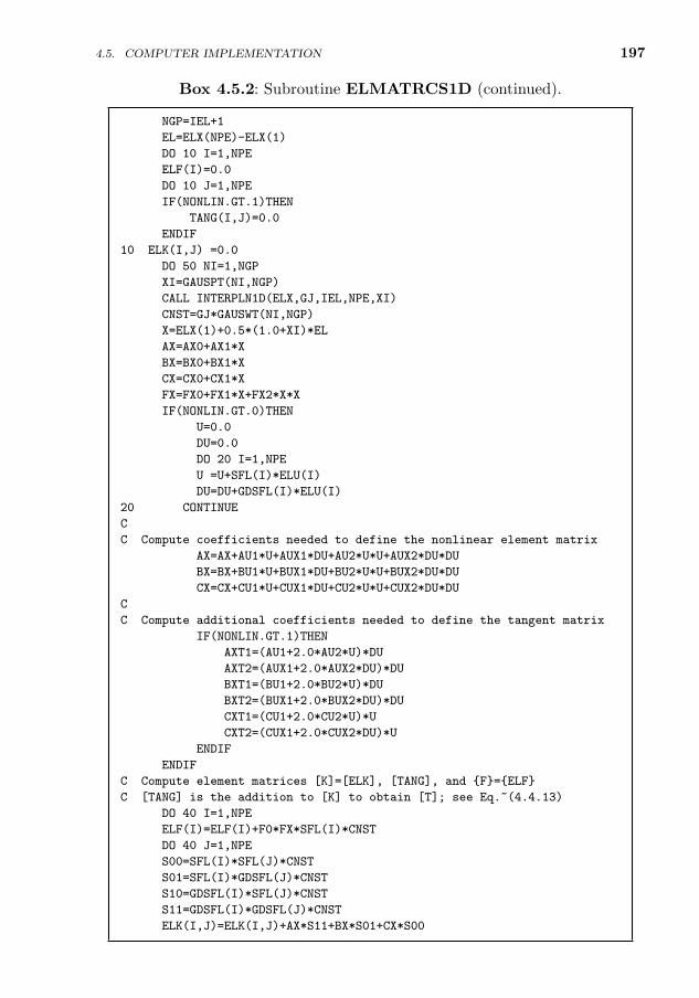
4.5. COMPUTER IMPLEMENTATION 197
Box 4.5.2: Subroutine ELMATRCS1D (continued).
NGP=IEL+1
EL=ELX(NPE)-ELX(1)
DO 10 I=1,NPE
ELF(I)=0.0
DO 10 J=1,NPE
IF(NONLIN.GT.1)THEN
TANG(I,J)=0.0
ENDIF
10 ELK(I,J) =0.0
DO 50 NI=1,NGP
XI=GAUSPT(NI,NGP)
CALL INTERPLN1D(ELX,GJ,IEL,NPE,XI)
CNST=GJ*GAUSWT(NI,NGP)
X=ELX(1)+0.5*(1.0+XI)*EL
AX=AX0+AX1*X
BX=BX0+BX1*X
CX=CX0+CX1*X
FX=FX0+FX1*X+FX2*X*X
IF(NONLIN.GT.0)THEN
U=0.0
DU=0.0
DO 20 I=1,NPE
U =U+SFL(I)*ELU(I)
DU=DU+GDSFL(I)*ELU(I)
20 CONTINUE
C
C Compute coefficients needed to define the nonlinear element matrix
AX=AX+AU1*U+AUX1*DU+AU2*U*U+AUX2*DU*DU
BX=BX+BU1*U+BUX1*DU+BU2*U*U+BUX2*DU*DU
CX=CX+CU1*U+CUX1*DU+CU2*U*U+CUX2*DU*DU
C
C Compute additional coefficients needed to define the tangent matrix
IF(NONLIN.GT.1)THEN
AXT1=(AU1+2.0*AU2*U)*DU
AXT2=(AUX1+2.0*AUX2*DU)*DU
BXT1=(BU1+2.0*BU2*U)*DU
BXT2=(BUX1+2.0*BUX2*DU)*DU
CXT1=(CU1+2.0*CU2*U)*U
CXT2=(CUX1+2.0*CUX2*DU)*U
ENDIF
ENDIF
C Compute element matrices [K]=[ELK], [TANG], and F=ELF
C [TANG] is the addition to [K] to obtain [T]; see Eq.~(4.4.13)
DO 40 I=1,NPE
ELF(I)=ELF(I)+F0*FX*SFL(I)*CNST
DO 40 J=1,NPE
S00=SFL(I)*SFL(J)*CNST
S01=SFL(I)*GDSFL(J)*CNST
S10=GDSFL(I)*SFL(J)*CNST
S11=GDSFL(I)*GDSFL(J)*CNST
ELK(I,J)=ELK(I,J)+AX*S11+BX*S01+CX*S00
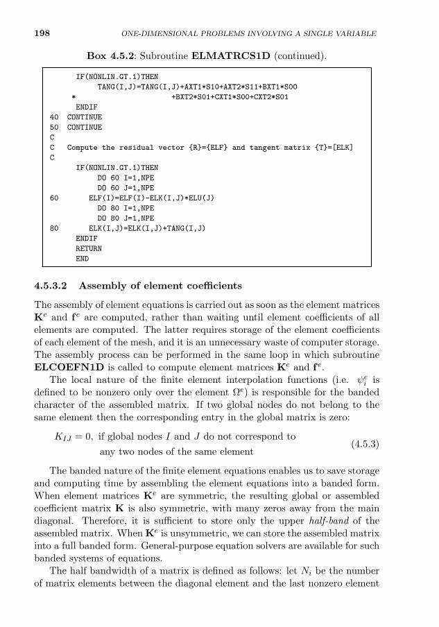
198 ONE-DIMENSIONAL PROBLEMS INVOLVING A SINGLE VARIABLE
Box 4.5.2: Subroutine ELMATRCS1D (continued).
IF(NONLIN.GT.1)THEN
TANG(I,J)=TANG(I,J)+AXT1*S10+AXT2*S11+BXT1*S00
* +BXT2*S01+CXT1*S00+CXT2*S01
ENDIF
40 CONTINUE
50 CONTINUE
C
C Compute the residual vector R=ELF and tangent matrix T=[ELK]
C
IF(NONLIN.GT.1)THEN
DO 60 I=1,NPE
DO 60 J=1,NPE
60 ELF(I)=ELF(I)-ELK(I,J)*ELU(J)
DO 80 I=1,NPE
DO 80 J=1,NPE
80 ELK(I,J)=ELK(I,J)+TANG(I,J)
ENDIF
RETURN
END
4.5.3.2 Assembly of element coefficients
The assembly of element equations is carried out as soon as the element matricesKe and f e are computed, rather than waiting until element coefficients of allelements are computed. The latter requires storage of the element coefficientsof each element of the mesh, and it is an unnecessary waste of computer storage.The assembly process can be performed in the same loop in which subroutineELCOEFN1D is called to compute element matrices Ke and f e.
The local nature of the finite element interpolation functions (i.e. ψei is
defined to be nonzero only over the element Ωe) is responsible for the bandedcharacter of the assembled matrix. If two global nodes do not belong to thesame element then the corresponding entry in the global matrix is zero:
KIJ = 0, if global nodes I and J do not correspond to
any two nodes of the same element(4.5.3)
The banded nature of the finite element equations enables us to save storageand computing time by assembling the element equations into a banded form.When element matrices Ke are symmetric, the resulting global or assembledcoefficient matrix K is also symmetric, with many zeros away from the maindiagonal. Therefore, it is sufficient to store only the upper half-band of theassembled matrix. When Ke is unsymmetric, we can store the assembled matrixinto a full banded form. General-purpose equation solvers are available for suchbanded systems of equations.
The half bandwidth of a matrix is defined as follows: let Ni be the numberof matrix elements between the diagonal element and the last nonzero element

4.5. COMPUTER IMPLEMENTATION 199
in the ith row, after which all elements in that row are zero; the half-bandwidthis the maximum of (Ni + 1)×NDF (NDF is the number of degrees of freedomper node):
max
1 ≤ i ≤ NEQ[(Ni + 1)×NDF]
where NEQ is the number of equations (or rows) in the matrix.The half-bandwidth NHBW of the assembled (i.e. global) finite element
matrix can be determined in the finite element program itself. The property inEq. (4.5.3) enables us to determine the half-bandwidth NHBW of the assembledmatrix as
NHBW =max
1≤N≤NEM1≤I,J,≤NPE
abs[NOD(N,I)−NOD(N,J)] + 1
×NDF (4.5.4)
For example, for one-dimensional problems with elements connected in series(i.e. connected in one line), the maximum difference between nodes of an ele-ment is equal to NPE−1. Hence, we have
NHBW = [(NPE− 1) + 1]×NDF = NPE×NDF (4.5.5)
The logic behind assembling the element matrices Ke into the upper-bandedform of the global coefficient matrix K is that the assembly be skipped when-ever the column number is both less than the row number and greater thanthe half bandwidth plus the row number. Similarly, the full-banded form isobtained by skipping assembly whenever the column number is both less thanthe row number minus NHBW and greater than the row number plus NHBW.In the case of the upper-banded form, the main diagonal of the actual matrixK becomes the first column of the assembled banded matrix KFB, as shownin Fig. 4.5.2 (also see Box 4.5.3). For the full-banded form the actual matrix,
K11 K12 . . . K1k 0 0 0 . K21 K22 . . . K2k K2k+1 0 0 K31 K32 . . . K3k K3k+1 . . .. . … . . . .
0 . . 0 KNk . . . KNN
K = KFB =(full-banded
form)
NHBW NBW = 2*NHBW
NEQ = N
Main diagonalLast diagonal beyond which all
coefficients are zero
NEQ = N
11 12 1* * * kK K K
21 22 23 2( 1)* * + kK K K K
31 32 33 34 3( 2)* + kK K K K K
( 1) * * *− N N NNK K
NBW-th column;used for storing F
1
2
3
.
.
.
N
FFF
F
First diagonal before which all coefficients are zero
. . … . . . .
Fig. 4.5.2: Assembled coefficient matrix storage in (upper) half-banded and full-banded forms.
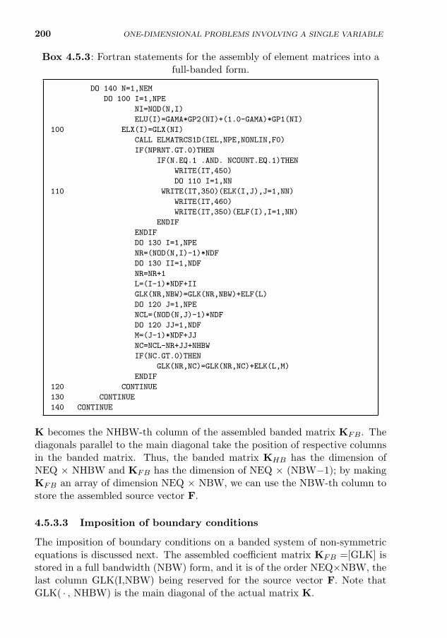
200 ONE-DIMENSIONAL PROBLEMS INVOLVING A SINGLE VARIABLE
Box 4.5.3: Fortran statements for the assembly of element matrices into afull-banded form.
DO 140 N=1,NEM
DO 100 I=1,NPE
NI=NOD(N,I)
ELU(I)=GAMA*GP2(NI)+(1.0-GAMA)*GP1(NI)
100 ELX(I)=GLX(NI)
CALL ELMATRCS1D(IEL,NPE,NONLIN,F0)
IF(NPRNT.GT.0)THEN
IF(N.EQ.1 .AND. NCOUNT.EQ.1)THEN
WRITE(IT,450)
DO 110 I=1,NN
110 WRITE(IT,350)(ELK(I,J),J=1,NN)
WRITE(IT,460)
WRITE(IT,350)(ELF(I),I=1,NN)
ENDIF
ENDIF
DO 130 I=1,NPE
NR=(NOD(N,I)-1)*NDF
DO 130 II=1,NDF
NR=NR+1
L=(I-1)*NDF+II
GLK(NR,NBW)=GLK(NR,NBW)+ELF(L)
DO 120 J=1,NPE
NCL=(NOD(N,J)-1)*NDF
DO 120 JJ=1,NDF
M=(J-1)*NDF+JJ
NC=NCL-NR+JJ+NHBW
IF(NC.GT.0)THEN
GLK(NR,NC)=GLK(NR,NC)+ELK(L,M)
ENDIF
120 CONTINUE
130 CONTINUE
140 CONTINUE
K becomes the NHBW-th column of the assembled banded matrix KFB. Thediagonals parallel to the main diagonal take the position of respective columnsin the banded matrix. Thus, the banded matrix KHB has the dimension ofNEQ × NHBW and KFB has the dimension of NEQ × (NBW−1); by makingKFB an array of dimension NEQ × NBW, we can use the NBW-th column tostore the assembled source vector F.
4.5.3.3 Imposition of boundary conditions
The imposition of boundary conditions on a banded system of non-symmetricequations is discussed next. The assembled coefficient matrix KFB =[GLK] isstored in a full bandwidth (NBW) form, and it is of the order NEQ×NBW, thelast column GLK(I,NBW) being reserved for the source vector F. Note thatGLK( · , NHBW) is the main diagonal of the actual matrix K.
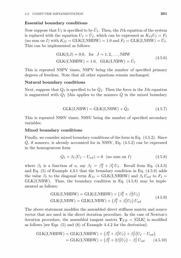
4.5. COMPUTER IMPLEMENTATION 201
Essential boundary conditions
Now suppose that UI is specified to be UI . Then, the Ith equation of the systemis replaced with the equation UI = UI , which can be expressed as KIIUI = FI
(no sum on I) with KII = GLK(I,NHBW) = 1.0 and FI = GLK(I,NBW) = UI .This can be implemented as follows:
GLK(I,J) = 0.0, for J = 1, 2, . . . ,NBW
GLK(I,NHBW) = 1.0, GLK(I,NBW) = UI
(4.5.6)
This is repeated NSPV times, NSPV being the number of specified primarydegrees of freedom. Note that all other equations remain unchanged.
Natural boundary conditions
Next, suppose that QI is specified to be QI . Then the force in the Ith equationis augmented with QI [this applies to the nonzero Q in the mixed boundarycondition in Eq. (4.5.2)]:
GLK(I,NBW) = GLK(I,NBW) + QI (4.5.7)
This is repeated NSSV times, NSSV being the number of specified secondaryvariables.
Mixed boundary conditions
Finally, we consider mixed boundary conditions of the form in Eq. (4.5.2). SinceQ, if nonzero, is already accounted for in NSSV, Eq. (4.5.2) can be expressedin the homogeneous form
QI + βI (UI − Uref) = 0 (no sum on I) (4.5.8)
where βI is a function of u, say βI = β0I + β1I UI . Recall from Eq. (4.3.3)and Eq. (5) of Example 4.3.1 that the boundary condition in Eq. (4.5.8) addsthe value βI to the diagonal term KII = GLK(I,NHBW) and βI Uref to FI =GLK(I,NBW). Thus, the boundary condition in Eq. (4.5.8) may be imple-mented as follows:
GLK(I,NHBW) = GLK(I,NHBW) +(β0I + β1IUI
)GLK(I,NBW) = GLK(I,NBW) +
(β0I + β1IUI
)Uref
(4.5.9)
The above statement modifies the assembled direct stiffness matrix and sourcevector that are used in the direct iteration procedure. In the case of Newton’siteration procedure, the assembled tangent matrix TFB = [GLK] is modifiedas follows [see Eqs. (5) and (6) of Example 4.4.2 for the derivation]:
GLK(I,NHBW) = GLK(I,NHBW) +(β0I + β1IUI
)+ β1I
(UI − Uref
)= GLK(I,NHBW) +
(β0I + 2β1IUI
)− β1I Uref (4.5.10)
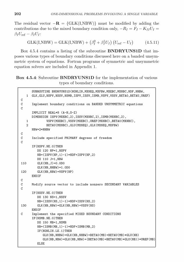
202 ONE-DIMENSIONAL PROBLEMS INVOLVING A SINGLE VARIABLE
The residual vector −R = GLK(I,NBW) must be modified by adding thecontributions due to the mixed boundary condition only, −RI = FI −KIIUI =βIUref − βIUI :
GLK(I,NBW) = GLK(I,NBW) +(β0I + β1IUI
) (Uref − UI
)(4.5.11)
Box 4.5.4 contains a listing of the subroutine BNDRYUNS1D that im-poses various types of boundary conditions discussed here on a banded unsym-metric system of equations. Fortran programs of symmetric and unsymmetricequation solvers are included in Appendix 1.
Box 4.5.4: Subroutine BNDRYUNS1D for the implementation of varioustypes of boundary conditions.
SUBROUTINE BNDRYUNS1D(NONLIN,MXNEQ,MXFBW,MXEBC,MXNBC,NDF,NHBW,
1 GLK,GLU,NSPV,NSSV,NSMB,ISPV,ISSV,ISMB,VSPV,VSSV,BETA0,BETAU,UREF)
C
C Implement boundary conditions on BANDED UNSYMMETRIC equations
C
IMPLICIT REAL*8 (A-H,O-Z)
DIMENSION ISPV(MXEBC,2),ISSV(MXNBC,2),ISMB(MXNBC,2),
1 VSPV(MXEBC),VSSV(MXEBC),UREF(MXNBC),BETA0(MXNBC),
2 BETAU(MXNBC),GLU(MXNEQ),GLK(MXNEQ,MXFBW)
NBW=2*NHBW
C
C Include specified PRIMARY degrees of freedom
C
IF(NSPV.NE.0)THEN
DO 120 NP=1,NSPV
NB=(ISPV(NP,1)-1)*NDF+ISPV(NP,2)
DO 110 J=1,NBW
110 GLK(NB,J)=0.0D0
GLK(NB,NHBW)=1.0D0
120 GLK(NB,NBW)=VSPV(NP)
ENDIF
C
C Modify source vector to include nonzero SECONDARY VARIABLES
C
IF(NSSV.NE.0)THEN
DO 130 NS=1,NSSV
NB=(ISSV(NS,1)-1)*NDF+ISSV(NS,2)
130 GLK(NB,NBW)=GLK(NB,NBW)+VSSV(NS)
ENDIF
C Implement the specified MIXED BOUNDARY CONDITIONS
IF(NSMB.NE.0)THEN
DO 150 MB=1,NSMB
NB=(ISMB(MB,1)-1)*NDF+ISMB(MB,2)
IF(NONLIN.LE.1)THEN
GLK(NB,NHBW)=GLK(NB,NHBW)+BETA0(MB)+BETAU(MB)*GLU(NB)
GLK(NB,NBW)=GLK(NB,NBW)+(BETA0(MB)+BETAU(MB)*GLU(NB))*UREF(MB)
ELSE
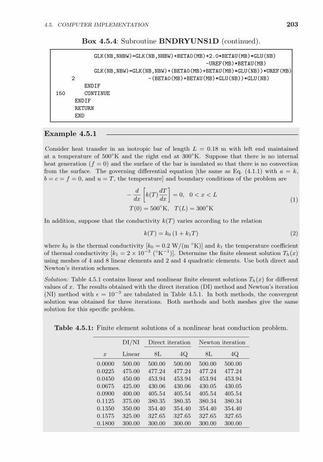
4.5. COMPUTER IMPLEMENTATION 203
Box 4.5.4: Subroutine BNDRYUNS1D (continued).
GLK(NB,NHBW)=GLK(NB,NHBW)+BETA0(MB)+2.0*BETAU(MB)*GLU(NB)
-UREF(MB)*BETAU(MB)
GLK(NB,NBW)=GLK(NB,NBW)+(BETA0(MB)+BETAU(MB)*GLU(NB))*UREF(MB)
2 -(BETA0(MB)+BETAU(MB)*GLU(NB))*GLU(NB)
ENDIF
150 CONTINUE
ENDIF
RETURN
END
Example 4.5.1
Consider heat transfer in an isotropic bar of length L = 0.18 m with left end maintainedat a temperature of 500K and the right end at 300K. Suppose that there is no internalheat generation (f = 0) and the surface of the bar is insulated so that there is no convectionfrom the surface. The governing differential equation [the same as Eq. (4.1.1) with a = k,b = c = f = 0, and u = T , the temperature] and boundary conditions of the problem are
− d
dx
[k(T )
dT
dx
]= 0, 0 < x < L
T (0) = 500K, T (L) = 300K
(1)
In addition, suppose that the conductivity k(T ) varies according to the relation
k(T ) = k0 (1 + k1T ) (2)
where k0 is the thermal conductivity [k0 = 0.2 W/(m K)] and k1 the temperature coefficientof thermal conductivity [k1 = 2× 10⁻³ (K−1)]. Determine the finite element solution Th(x)using meshes of 4 and 8 linear elements and 2 and 4 quadratic elements. Use both direct andNewton’s iteration schemes.
Solution: Table 4.5.1 contains linear and nonlinear finite element solutions Th(x) for differentvalues of x. The results obtained with the direct iteration (DI) method and Newton’s iteration(NI) method with ε = 10−3 are tabulated in Table 4.5.1. In both methods, the convergentsolution was obtained for three iterations. Both methods and both meshes give the samesolution for this specific problem.
Table 4.5.1: Finite element solutions of a nonlinear heat conduction problem.
DI/NI Direct iteration Newton iteration
x Linear 8L 4Q 8L 4Q
0.0000 500.00 500.00 500.00 500.00 500.000.0225 475.00 477.24 477.24 477.24 477.240.0450 450.00 453.94 453.94 453.94 453.940.0675 425.00 430.06 430.06 430.05 430.050.0900 400.00 405.54 405.54 405.54 405.540.1125 375.00 380.35 380.35 380.34 380.340.1350 350.00 354.40 354.40 354.40 354.400.1575 325.00 327.65 327.65 327.65 327.650.1800 300.00 300.00 300.00 300.00 300.00
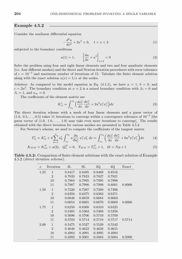
204 ONE-DIMENSIONAL PROBLEMS INVOLVING A SINGLE VARIABLE
Example 4.5.2
Consider the nonlinear differential equation
−d2u
dx2+ 2u3 = 0, 1 < x < 2 (1)
subjected to the boundary conditions
u(1) = 1,
[du
dx+ u2
]x=2
= 0 (2)
Solve the problem using four and eight linear elements and two and four quadratic elements(i.e. four different meshes) and the direct and Newton iteration procedures with error toleranceof ε = 10−3 and maximum number of iterations of 15. Tabulate the finite element solutionalong with the exact solution u(x) = 1/x at the nodes.
Solution: As compared to the model equation in Eq. (4.1.1), we have a = 1, b = 0, andc = 2u2. The boundary condition at x = 2 is a mixed boundary condition with β0 = 0 andβ1 = 1, and u∞ = 0.
The coefficients of the element matrix are
Keij =
∫ xb
xa
(dψei
dx
dψej
dx+ 2u2ψe
iψej
)dx (3)
The direct iteration scheme with a mesh of four linear elements and a guess vector of(1.0, 0.5, . . . , 0.5) takes 11 iterations to converge within a convergence tolerance of 10−3 [theguess vector of (1.0, 1.0, . . . , 1.0) may take even more iterations to converge]. The resultsobtained with the direct iteration for various meshes are presented in Table 4.5.2.
For Newton’s scheme, we need to compute the coefficients of the tangent matrix
T eij = Ke
ij + 4n∑
k=1
uek
∫ xb
xa
u∂u
∂uej
ψeiψ
ek dx =
∫ xb
xa
(dψe
i
dx
dψej
dx+ 6u2ψe
iψej
)dx (4)
KMM = KNnn + u(2), QN
n = 0, TMM = TNnn + 1, M = Np+ 1 (5)
Table 4.5.2: Comparison of finite element solutions with the exact solution of Example4.5.2 (direct iteration scheme).
x Iteration 4L 8L 2Q 4Q Exact
1.25 1 0.8417 0.8495 0.8469 0.85162 0.7833 0.7823 0.7827 0.7821
10 0.7984 0.7995 0.7995 0.799811 0.7987 0.7998 0.7999 0.8001 0.8000
1.50 1 0.7220 0.7287 0.7289 0.73062 0.6394 0.6375 0.6383 0.6371
10 0.6648 0.6659 0.6664 0.666311 0.6654 0.6665 0.6670 0.6669 0.6666
1.75 1 0.6250 0.6308 0.6310 0.63252 0.5385 0.5362 0.5369 0.5356
10 0.5696 0.5706 0.5710 0.570911 0.5703 0.5714 0.5718 0.5717 0.5714
2.00 1 0.5475 0.5527 0.5529 0.55422 0.4648 0.4622 0.4628 0.4615
10 0.4984 0.4991 0.4995 0.499411 0.4992 0.5001 0.5004 0.5004 0.5000
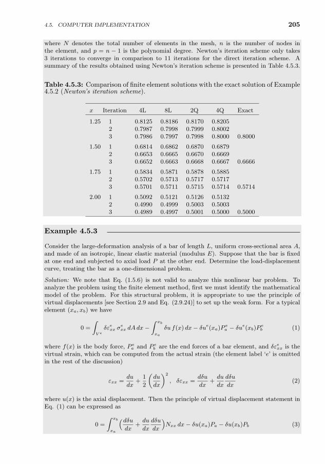
4.5. COMPUTER IMPLEMENTATION 205
where N denotes the total number of elements in the mesh, n is the number of nodes inthe element, and p = n − 1 is the polynomial degree. Newton’s iteration scheme only takes3 iterations to converge in comparison to 11 iterations for the direct iteration scheme. Asummary of the results obtained using Newton’s iteration scheme is presented in Table 4.5.3.
Table 4.5.3: Comparison of finite element solutions with the exact solution of Example4.5.2 (Newton’s iteration scheme).
x Iteration 4L 8L 2Q 4Q Exact
1.25 1 0.8125 0.8186 0.8170 0.82052 0.7987 0.7998 0.7999 0.80023 0.7986 0.7997 0.7998 0.8000 0.8000
1.50 1 0.6814 0.6862 0.6870 0.68792 0.6653 0.6665 0.6670 0.66693 0.6652 0.6663 0.6668 0.6667 0.6666
1.75 1 0.5834 0.5871 0.5878 0.58852 0.5702 0.5713 0.5717 0.57173 0.5701 0.5711 0.5715 0.5714 0.5714
2.00 1 0.5092 0.5121 0.5126 0.51322 0.4990 0.4999 0.5003 0.50033 0.4989 0.4997 0.5001 0.5000 0.5000
Example 4.5.3
Consider the large-deformation analysis of a bar of length L, uniform cross-sectional area A,and made of an isotropic, linear elastic material (modulus E). Suppose that the bar is fixedat one end and subjected to axial load P at the other end. Determine the load-displacementcurve, treating the bar as a one-dimensional problem.
Solution: We note that Eq. (1.5.6) is not valid to analyze this nonlinear bar problem. Toanalyze the problem using the finite element method, first we must identify the mathematicalmodel of the problem. For this structural problem, it is appropriate to use the principle ofvirtual displacements [see Section 2.9 and Eq. (2.9.24)] to set up the weak form. For a typicalelement (xa, xb) we have
0 =
∫V e
δεexx σexx dAdx−
∫ xb
xa
δu f(x) dx− δue(xa)P ea − δue(xb)P
eb (1)
where f(x) is the body force, P ea and P e
b are the end forces of a bar element, and δεexx is thevirtual strain, which can be computed from the actual strain (the element label ‘e’ is omittedin the rest of the discussion)
εxx =du
dx+
1
2
(du
dx
)2
, δεxx =dδu
dx+du
dx
dδu
dx(2)
where u(x) is the axial displacement. Then the principle of virtual displacement statement inEq. (1) can be expressed as
0 =
∫ xb
xa
(dδudx
+du
dx
dδu
dx
)Nxx dx− δu(xa)Pa − δu(xb)Pb (3)
206 ONE-DIMENSIONAL PROBLEMS INVOLVING A SINGLE VARIABLE
where
Nxx =
∫Ae
σxx dA = EAεxx = EA
[du
dx+
1
2
(du
dx
)2]
(4)
Equation (3) forms the basis of the finite element model. The governing differential equationof the problem can be determined from Eq. (3) as
− d
dx
[(1 +
du
dx
)Nxx
]− f = 0, xa < x < xb (5)
The boundary conditions involve specifying one element of each of the pairs (u(xa), Pa) and(u(xb), Pb), where
Pa = −[(
1 +du
dx
)Nxx
]xa
, Pb =[(
1 +du
dx
)Nxx
]xb
(6)
The finite element model Keue = Fe is obtained by assuming approximation of the form
u(x) ≈n∑
j=1
uejψ
ej (x) (7)
into the virtual work statement in Eq. (3) with
Keij =
∫ xb
xa
EeAe(
1 +du
dx
)(1 +
1
2
du
dx
)dψei
dx
dψej
dxdx
F ei =
∫ xb
xa
fψei (x) dx+ P e
aψei (xa) + P e
b ψei (xb)
(8)
A comparison of the element coefficients in Eq. (8) with those in Eq. (4.3.3) indicates thatthe present model is a special case of Eq. (4.3.3) with βa = βb = b = c = 0, and
a(x, u) = E(x)A(x)(
1 +du
dx
)(1 +
1
2
du
dx
)(9)
Hence, the finite element program developed to analyze problems described by Eq. (4.1.1) canbe used to solve the problem at hand. The tangent stiffness matrix in the present case is givenby
T eij = Ke
ij +
∫ xb
xa
EA(dudx
)(3
2+du
dx
) dψei
dx
dψej
dxdx (10)
Note that, in the present problem, both Ke and Te are symmetric matrices.Figure 4.5.3 contains the nondimensional load P = P/AE versus the dimensionless dis-
placement u = u(L)/L for a bar (with constant EA) fixed at one end and subjected to axialload P at the other end (f = 0). The exact solution is
u(x) = kx, where k is the real root of k3 + 3k2 + 2k − 2P = 0, P =P
EA>
1
27(11)
The finite element results were obtained using Newton’s iteration method with eight linearelements (a mesh of four quadratic elements also gives the same results, and both coincidewith the exact solution); a tolerance of ε = 10−3 was used with a load increment of ∆P = 0.2.Convergence was achieved for five and four iterations for the first two load steps, respectively,and only three iterations were taken during the remaining load steps. It should be noted thatthe direct iteration method takes many more iterations to converge, especially at higher loads.From the load-deflection curve, it is clear that the geometric nonlinearity is that of hardeningtype, that is, the bar becomes stiff as it deforms. Of course, we assumed that the modulusremains unchanged during the deformation, which most likely does not hold for large strains.
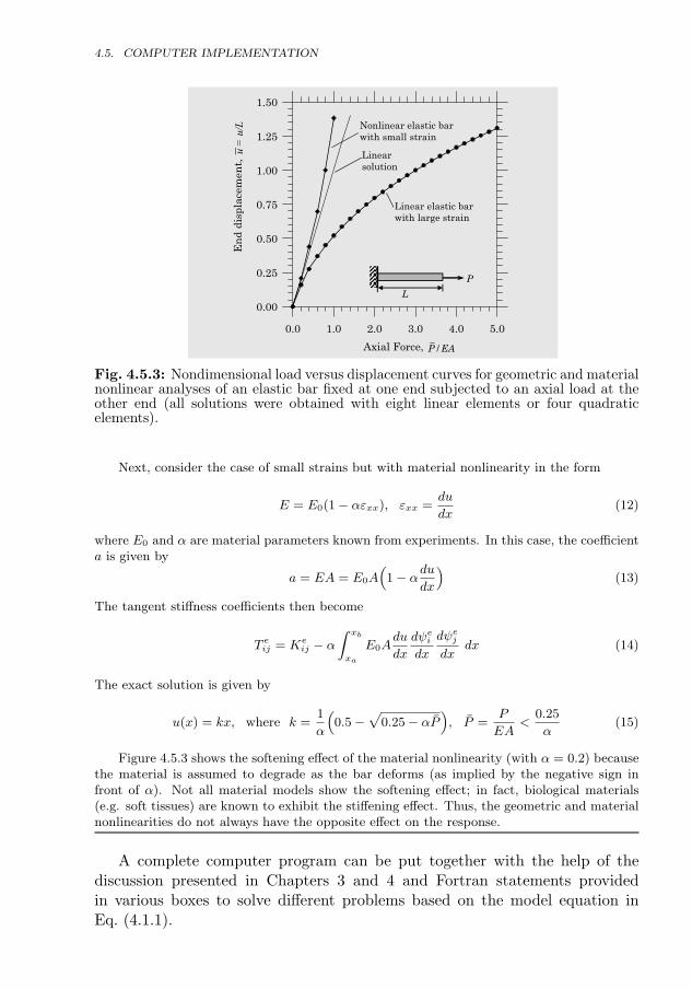
207
P
L
/P EA
Nonlinear elastic barwith small strain
Linear solution
Linear elastic barwith large strain
0.0 1.0 2.0 3.0 4.0 5.0
Axial Force,
0.00
0.25
0.50
0.75
1.00
1.25
1.50
En
d di
spla
cem
ent,
u =
u/L
Fig. 4.5.3: Nondimensional load versus displacement curves for geometric and materialnonlinear analyses of an elastic bar fixed at one end subjected to an axial load at theother end (all solutions were obtained with eight linear elements or four quadraticelements).
Next, consider the case of small strains but with material nonlinearity in the form
E = E0(1− αεxx), εxx =du
dx(12)
where E0 and α are material parameters known from experiments. In this case, the coefficienta is given by
a = EA = E0A(
1− αdudx
)(13)
The tangent stiffness coefficients then become
T eij = Ke
ij − α∫ xb
xa
E0Adu
dx
dψei
dx
dψej
dxdx (14)
The exact solution is given by
u(x) = kx, where k =1
α
(0.5−
√0.25− αP
), P =
P
EA<
0.25
α(15)
Figure 4.5.3 shows the softening effect of the material nonlinearity (with α = 0.2) becausethe material is assumed to degrade as the bar deforms (as implied by the negative sign infront of α). Not all material models show the softening effect; in fact, biological materials(e.g. soft tissues) are known to exhibit the stiffening effect. Thus, the geometric and materialnonlinearities do not always have the opposite effect on the response.
A complete computer program can be put together with the help of thediscussion presented in Chapters 3 and 4 and Fortran statements providedin various boxes to solve different problems based on the model equation inEq. (4.1.1).
4.5. COMPUTER IMPLEMENTATION
208 ONE-DIMENSIONAL PROBLEMS INVOLVING A SINGLE VARIABLE
4.6 Summary
In this chapter, the weak-form Galerkin finite element model of a typical second-order nonlinear boundary-value problem in one dimension is presented, iterativemethods of solving nonlinear finite element equations are discussed, and com-puter implementation of the nonlinear finite element analysis is outlined. Themodel equation used is such that it can account for both geometric and materialnonlinearities through the definition of the data a(x, u), b(x, u), and c(x, u).
The most difficult part of solving nonlinear equations is that they have mul-tiple solutions and convergence to a particular solution is often dictated by thechoice of the solution vector, U(0). The choice of the iterative solution schemealso makes a difference in achieving convergence. In general, the coefficientmatrix being inverted, K in the case of direct iteration and T in the case ofNewton’s iteration, is responsible for convergence. If the coefficient matrix issymmetric or diagonally dominant, the process may yield faster convergence.
Another comment relates to the coefficient b(x, u) in the model equation,Eq. (4.1.1). Even when the problem is linear, the coefficient changes the char-acter of the equation from elliptic to hyperbolic, and it is responsible for theunsymmetry of K. In general, hyperbolic equations are difficult to solve (evenfor linear problems) numerically. Therefore, when there is a choice during lin-earization of the equation, we should pick one that yields a symmetric K fordirect iteration scheme or a symmetric T for Newton’s iteration scheme, be-cause there is a greater chance of convergence with such choices. As an example,consider the equation
− d
dx
(adu
dx
)+ bu
du
dx+ cu = f, 0 < x < L
There are two choices of b and c that will produce the model equation: (1)b = bu and c = c and (2) c = c+ b(du/dx). The second choice may work betterfor the direct iteration scheme while either choice may be alright, depending onresulting T, for Newton’s iteration scheme.
In some cases, several terms of a given differential equation can be combinedto make it a special case of the model equation, Eq. (4.1.1). An example isprovided by the equation
−(c0 + c1u)d2u
dx2−(dc0dx
+dc1dx
u+ c1du
dx
)du
dx= f(x)
where c0 and c1 are functions of x only. This equation is the same as
− d
dx
[(c0 + c1u)
du
dx
]= f(x)
and a special case of Eq. (4.1.1) with a(x, u) = (c0 + c1u), b(x, u) = 0 andc(x, u) = 0.
PROBLEMS 209
With a good understanding of the contents of this chapter, one should beable to develop a nonlinear finite element analysis program to solve boundaryvalue problems described by Eq. (4.1.1) or its variation (see Problem 4.19).When faced with analyzing a physical problem, one must first determine if itcan be modeled as a one-dimensional problem, and then see if its mathematicalmodel is a special case of Eq. (4.1.1) or Eq. (1) of Problem 4.19.
Problems
See Problem 4.22 for the development of a computer program to solve the problems of thischapter. Additional nonlinear differential equations can be found in [51] and [52].
4.1 Consider the second-order differential equation
− d
dx
(µdu
dx
)= f(x), µ = µ0
(du
dx
)n−1
(1)
where u(x) is the dependent unknown, f(x) is a known function of position x, and µis a function of the dependent variable, as given in Eq. (1). Write the finite elementmodel and derive the tangent stiffness matrix coefficients.
4.2 Consider Eqs. (4.1.1) and (4.1.2) with a(x, u) = ae0(x) dudx
, b = 0, c(x, u) = 0, and β = 0.Compute the tangent matrix.
4.3 Consider the nonlinear differential equation
−(√
2 + u)d2u
dx2−(du
dx
)2
= 1, 0 < x < 1 (1)
du
dx(0) = 0, u(1) = 0 (2)
Analyze the nonlinear problem using the finite element method with direct iterationprocedure. Tabulate the nodal values of u(x) for four and eight linear elements andtwo and four quadratic elements.
4.4 Formulate Problem 4.3 with Newton’s iteration procedure, and compute the tangentcoefficient matrix. Tabulate the nodal values of u(x) for four and eight linear elementsand two and four quadratic elements. Use an error tolerance of ε = 10−3.
4.5 Develop the finite element model of the nonlinear differential equation
−d2u
dx2− 2u
du
dx= 0, 0 < x < 1 (1)
u(0) = 1, u(1) = 0.5 (2)
and solve the problem using direct iteration procedure. Tabulate the nodal values ofu(x) for four and eight linear elements and two and four quadratic elements. The exactsolution is given by u(x) = 1/(1 + x).
4.6 Compute the tangent stiffness matrix associated with Problem 4.5, and solve it withNewton’s iteration procedure. Tabulate the nodal values of u(x) for four and eight linearelements and two and four quadratic elements (use an error tolerance of ε = 10−3).
4.7 Formulate the nonlinear differential equation in Problem 4.5 subject to the boundaryconditions [
du
dx
]x=0
= −1,
[du
dx+ u2
]x=1
= 0 (1)
210 ONE-DIMENSIONAL PROBLEMS INVOLVING A SINGLE VARIABLE
and solve it with (a) direct and (b) Newton’s iteration procedures with a convergencetolerance of 10−4. Tabulate the nodal values of u(x) for four and eight linear elementsand two and four quadratic elements, along with the exact solution u(x) = 1/(1 + x).
4.8 Formulate the nonlinear differential equation in Problem 4.5 subject to the boundaryconditions
u(0) = 1,
[du
dx+ u2
]x=1
= 0 (1)
and solve the problem using direct iteration procedure (use an error tolerance of ε =10−3). Tabulate the nodal values of u(x) for four and eight linear elements and twoand four quadratic elements. The exact solution is given by u(x) = 1/(1 + x).
4.9 Compute the tangent stiffness matrix associated with Problem 4.8, and solve it withNewton’s iteration procedure (use an error tolerance of ε = 10−4). Tabulate the nodalvalues of u(x) for four and eight linear elements and two and four quadratic elements.
4.10 Develop the finite element model of the nonlinear differential equation in Problem 4.5subject to the boundary conditions[
du
dx+ 2u
]x=0
= 1,
[du
dx+ u2
]x=1
= 0 (1)
and solve the problem using direct iteration procedure (use an error tolerance of ε =10−4). Tabulate the nodal values of u(x) for four and eight linear elements and twoand four quadratic elements. The exact solution is given by u(x) = 1/(1 + x).
4.11 Compute the tangent stiffness matrix associated with Problem 4.10, and solve it withNewton’s iteration procedure (use an error tolerance of ε = 10−4). Tabulate the nodalvalues of u(x) for eight linear elements and four quadratic elements.
4.12 Develop the finite element model of the nonlinear differential equation
−d2u
dx2−(du
dx
)3
= 0, 0 < x < 1 (1)
[du
dx+ u
]x=0
=3√2,
[du
dx
]x=1
= 0.5 (2)
using the finite element method, and solve the problem using direct iteration procedure.Tabulate the nodal values of u(x) for four and eight linear elements and two and fourquadratic elements. The exact solution is given by u(x) =
√2(1 + x).
4.13 Consider simultaneous steady-state conduction and radiation in a plate. The mathe-matical formulation of the problem in non-dimensional form is given by
− d
dx
(k(θ)
dθ
dx
)= 0, 0 < x < x0 (1)
θ(0) = θ0, θ(x0) = 1.0 (2)
where x is the non-dimensional thickness coordinate, θ is the non-dimensional temper-ature, and k is the conductivity
k(θ) = k0
(1 +
4
3Nθn)
(3)
and N is called the conduction-to-radiation parameter. Develop the finite elementmodel of the problem and compute the element tangent matrix.
4.14 Analyze the nonlinear problem in Problem 4.13 using the finite element method withNewton’s iteration procedure for the following two cases:
Case 1: k(θ) = k0
(1 +
4
3Nθ2
); Case 2: k(θ) = k0
(1 +
4
3Nθ3
)(1)
PROBLEMS 211
with k0 = 1, N = 0.01, x0 = 1, θ0 = 0.5, error tolerance of ε = 10−3, and maximumallowable iterations to be ten. Tabulate the nodal values of θ(x) for eight linear elementsand four quadratic elements.
4.15 The explosion of a solid explosive material in the form of an infinite cylinder may bedescribed by
−1
r
d
dr
(rdu
dr
)= 2eu, 0 < r < 1
subject to the boundary conditions
At r = 0 :du
dr= 0; At r = 1 : u = 0
The exact solution of the nonlinear equation is
u(r) = ln4
(1 + r2)2
Analyze the nonlinear problem using the finite element method with (a) Newton’s and(b) direct iteration procedure. Tabulate and plot the nodal values of u(r) for eightlinear elements and four quadratic elements and compare with the exact solution.
4.16 Redo Problem 4.15 when the right-hand side is replaced by eu. This problem has twosolutions
ui(r) = ln8λi
(1 + λir2)2, i = 1, 2
where λi are the roots of the equation
8λ
(1 + λ)2= 1
4.17 Axial mixing in an isothermal tubular reactor where a second-order reaction occurs isdescribed by
− 1
Pe
d2u
dx2+du
dx+ Da u2 = 0, 0 < x < 1
subject to the boundary conditions
At x = 0 : u = 1 +1
Pe
du
dx; At x = 1 :
du
dx= 0
where Pe and Da are the problem parameters. Analyze the nonlinear problem usingthe finite element method with the direct iteration procedure. Take Pe = 5 and Da =1, and tabulate and plot the solution u(x) for eight linear elements.
4.18 Consider the nonlinear equation
− d
dx
(adu
dx
)+ cu− f = 0 (1)
with
a = a0(x) + a1(x)u(x) + a2(x)du
dx, c = c0(x) + c1(x)u(x) + c2(x)
du
dx(2)
Develop the least-squares finite element model and compute the coefficients of thetangent matrix.
4.19 Consider the following differential equation, which contains Eq. (4.1.1) as a special case:
− d
dx
[a(x, u)
du
dx+ b1(x, u)u
]+ b2(x, u)
du
dx+ c(x, u)u = f(x), x0 < x < xL (1)
where (x0, xL) is the problem domain and a, b1, b2, c, and f are the problem data.Develop the finite element model of the equation over a typical element.

212 ONE-DIMENSIONAL PROBLEMS INVOLVING A SINGLE VARIABLE
4.20 Show that the finite element model developed in Problem 3.11 is a special case of theone developed in Problem 4.19. Identify the coefficients a, b1, b2, c, and f in terms ofµ, λ, and the radial coordinate r.
4.21 Verify that the exact solutions presented in Eqs. (11) and (15) of Example 4.5.3 areindeed the solutions that satisfy the respective differential equation and boundary con-ditions.
4.22 Put together a complete finite element program based on the logic presented in Fig. 4.5.1and Boxes 4.5.1–4.5.4 that has the capability of solving the problems of this chapter.
213
5
Nonlinear Bending ofStraight Beams
It is not uncommon for engineers to accept the reality of phenomena that are not yet under-stood, as it is very common for physicists to disbelieve the reality of phenomena that seem tocontradict contemporary beliefs of physics. ——– Henry H. Bauer
5.1 Introduction
In this chapter, we consider a slightly more complicated one-dimensional nonlin-ear problem than that discussed in Chapter 4. We consider bending of straightbeams. A beam is a structural member whose length to cross-sectional dimen-sions is very large and it undergoes not only stretching along its length butalso bending about an axis transverse to the length. When the applied loadson the beam are large, the linear load–deflection relationship ceases to be validbecause the beam develops internal forces that resist deformation and the mag-nitude of internal forces increases with loading as well as deformation. Thisnonlinear load–deflection response of straight beams is the topic of this section.The development presented herein is limited to static problems.
In developing a general nonlinear formulation of beams, straight or curved,one must define the measures of stress and strain consistent with the defor-mations accounted for in the formulation (see Chapter 2 and [1–3]). Such aformulation, called a continuum formulation, will be discussed in Chapter 9.The present nonlinear formulation of straight beams is based on assumptions ofsmall strains and small or moderate rotations. Further, it is assumed that thegeometry does not change significantly, so that the principle of virtual displace-ments for the deformed body can be written over the undeformed body. Theseassumptions allow us to use the stress as a measure of force per unit undeformedarea and strain as a measure of change in length to the original length (andin the case of shear strain, change in the angle from π/2). The changes in thegeometry are small so that no distinction between the Cauchy stress tensor andother stress measures (e.g. the Piola–Kirchhoff tensor discussed in Chapter 2)will be made. The nonlinearity in the formulation comes solely from the inclu-sion of the in-plane forces that are proportional to the square of the rotation ofa transverse normal line in the beam (see [4–6] for details).
J.N. Reddy, An Introduction to Nonlinear Finite Element Analysis, Second Edition. c©J.N.Reddy 2015. Published in 2015 by Oxford University Press.
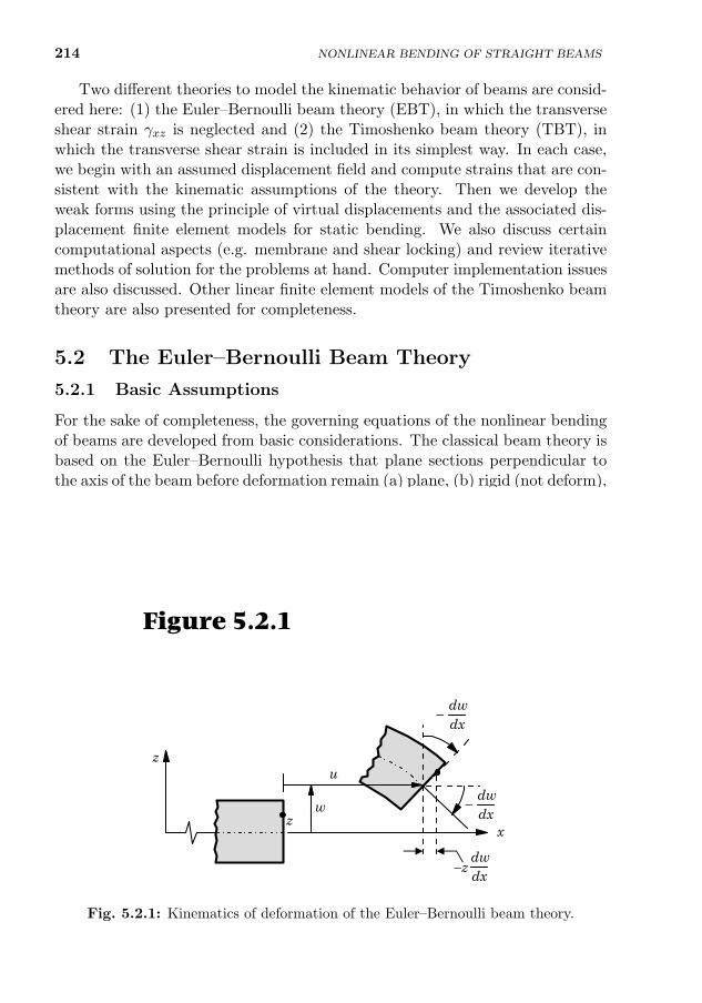
214 NONLINEAR BENDING OF STRAIGHT BEAMS
Two different theories to model the kinematic behavior of beams are consid-ered here: (1) the Euler–Bernoulli beam theory (EBT), in which the transverseshear strain γxz is neglected and (2) the Timoshenko beam theory (TBT), inwhich the transverse shear strain is included in its simplest way. In each case,we begin with an assumed displacement field and compute strains that are con-sistent with the kinematic assumptions of the theory. Then we develop theweak forms using the principle of virtual displacements and the associated dis-placement finite element models for static bending. We also discuss certaincomputational aspects (e.g. membrane and shear locking) and review iterativemethods of solution for the problems at hand. Computer implementation issuesare also discussed. Other linear finite element models of the Timoshenko beamtheory are also presented for completeness.
5.2 The Euler–Bernoulli Beam Theory
5.2.1 Basic Assumptions
For the sake of completeness, the governing equations of the nonlinear bendingof beams are developed from basic considerations. The classical beam theory isbased on the Euler–Bernoulli hypothesis that plane sections perpendicular tothe axis of the beam before deformation remain (a) plane, (b) rigid (not deform),and (c) rotate such that they remain perpendicular to the (deformed) axis afterdeformation, as shown in Fig. 5.2.1. These assumptions amount to neglectingthe Poisson effect and transverse normal and shear strains. The principle ofvirtual displacements will be used to formulate the variational problem andassociated finite element model.
5.2.2 Displacement and Strain Fields
The bending of beams with moderately large rotations but with small strainscan be derived using the displacement field
z
x
w
u
dwdx
−
z
dwdx
−
dwdx
−z
Figure 5.2.1
Fig. 5.2.1: Kinematics of deformation of the Euler–Bernoulli beam theory.
5.2. THE EULER–BERNOULLI BEAM THEORY 215
u1 = u(x)− z dwdx, u2 = 0, u3 = w(x) (5.2.1)
where (u1, u2, u3) are the total displacements of a material point occupyingthe location (x, y, z) in the undeformed body [usually denoted with capitalletters: (X,Y, Z) = (X1, X2, X3)], and u and w denote the axial and transversedisplacements of a point on the x-axis, which is taken along the geometriccentroid of the cross section of the beam. We note that once (u, 0, w) areknown, the total displacement field (u1, 0, u3) can be determined.
Using the Green strain tensor components [nonlinear strain-displacementrelations from Eqs. (2.4.8) and (2.4.9)], we can write
Eij ≈ εij =1
2
(∂ui∂xj
+∂uj∂xi
)+
1
2
∂uk∂xi
∂uk∂xj
(5.2.2)
where sum on repeated subscripts is implied. In the present case (u2 = 0), theexplicit form of ε11, for example, is
ε11 =∂u1
∂x1+
1
2
[(∂u1
∂x1
)2+
(∂u3
∂x1
)2]In the remainder of the chapter we shall use the notation x1 = x, x2 = y, andx3 = z.
In view of the small strain assumption, the first term in the square bracketsis neglected, i.e. (∂u1/∂x) = O(ε) and hence (∂u1/∂x)2 = O(ε2) ≈ 0. Thesecond term, ∂u3/∂x, denotes the rotation of a line perpendicular to the beamaxis. Even when the strains are small, because of the slenderness, beams canundergo moderate to large rotations. Hence, we retain the square of the rotation∂u3/∂x, which is assumed to be of the order O(
√ε), in the strain component
ε11. Nonlinear strains in which only squares of the rotations are included whileneglecting the squares of the in-plane stretching terms are known as the vonKarman nonlinearity in beams, plates, and shells. In view of the displacementfield in Eq. (5.2.1), the only nonzero strain (assuming that ε33 = ε13 = 0 sothat one may use uniaxial stress-strain relations) is
ε11 = εxx =du
dx− z d
2w
dx2+
1
2
(dw
dx
)2
=
[du
dx+
1
2
(dw
dx
)2]− z d
2w
dx2
≡ ε0xx + zε1
xx (5.2.3)
ε0xx =
du
dx+
1
2
(dw
dx
)2
, ε1xx = −d
2w
dx2
Such strains are known as the von Karman strains.
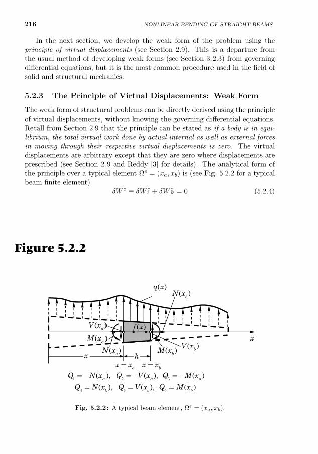
216 NONLINEAR BENDING OF STRAIGHT BEAMS
In the next section, we develop the weak form of the problem using theprinciple of virtual displacements (see Section 2.9). This is a departure fromthe usual method of developing weak forms (see Section 3.2.3) from governingdifferential equations, but it is the most common procedure used in the field ofsolid and structural mechanics.
5.2.3 The Principle of Virtual Displacements: Weak Form
The weak form of structural problems can be directly derived using the principleof virtual displacements, without knowing the governing differential equations.Recall from Section 2.9 that the principle can be stated as if a body is in equi-librium, the total virtual work done by actual internal as well as external forcesin moving through their respective virtual displacements is zero. The virtualdisplacements are arbitrary except that they are zero where displacements areprescribed (see Section 2.9 and Reddy [3] for details). The analytical form ofthe principle over a typical element Ωe = (xa, xb) is (see Fig. 5.2.2 for a typicalbeam finite element)
δW e ≡ δW eI + δW e
E = 0 (5.2.4)
where δW eI is the virtual strain energy stored in the element due to actual
stresses σij in moving through the virtual strains δεij , and δW eE is the work
done by external applied loads in moving through their respective virtual dis-placements. Here σij and εij denote the Cartesian components of the Cauchy orsecond Piola–Kirchhoff stress and the Green–Lagrange strain tensors, respec-tively. As stated earlier, no distinction is made between deformed and unde-formed configurations and various measures of stress and strain (see Chapter 2for a detailed discussion of various measures of stress and strain).
Figure 5.2.2
ax x= bx x=
( )bM x
( )aM x( )bV x
( )aV x
x
1 2 3
4 5 6
( ), ( ), ( )
( ), ( ), ( )a a a
b b b
Q N x Q V x Q M x
Q N x Q V x Q M x
=- =- =-
= = =
( )q x
( )f x
( )bN x
( )aN xhx
Fig. 5.2.2: A typical beam element, Ωe = (xa, xb).
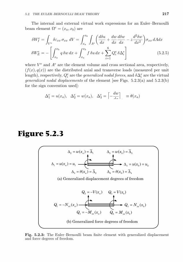
5.2. THE EULER–BERNOULLI BEAM THEORY 217
The internal and external virtual work expressions for an Euler–Bernoullibeam element Ωe = (xa, xb) are
δW eI =
∫V eδεxx σxx dV =
∫ xb
xa
∫Ae
(dδu
dx+dw
dx
dδw
dx− z d
2δw
dx2
)σxx dAdx
δW eE = −
[∫ xb
xa
q δw dx+
∫ xb
xa
f δu dx+6∑i=1
Qei δ∆ei
](5.2.5)
where V e and Ae are the element volume and cross sectional area, respectively,(f(x), q(x)) are the distributed axial and transverse loads (measured per unitlength), respectively, Qei are the generalized nodal forces, and δ∆e
i are the virtualgeneralized nodal displacements of the element [see Figs. 5.2.3(a) and 5.2.3(b)for the sign convention used]:
∆e1 = u(xa), ∆e
2 = w(xa), ∆e3 =
[−dwdx
]xa≡ θ(xa)
∆e4 = u(xb), ∆e
5 = w(xb), ∆e6 =
[−dwdx
]xb≡ θ(xb)
(5.2.6)
Qe1 = −Nxx(xa), Qe4 = Nxx(xb), Qe2 = −[dwdxNxx +
dMxx
dx
]xa≡ −Vx(xa)
Qe5 =[dwdxNxx +
dMxx
dx
]xb≡ Vx(xb), Qe3 = −Mxx(xa), Qe6 = Mxx(xb)
(5.2.7)
2 1( )aw xΔ = = Δ 5 3( )bw xΔ = = Δ
1 1( )au x uΔ = =4 2( )bu x uΔ = =
3 2( )axqΔ = = Δ 6 4( )bxqΔ = = Δ
(a) Generalized displacement degrees of freedom
2 ( )aQ V x= −
(b) Generalized force degrees of freedom
1 ( )xx aQ N x= − 4 ( )xx bQ N x=
5 ( )bQ V x=
3 ( )xx aQ M x= − 6 ( )xx bQ M x=
Figure 5.2.3
Fig. 5.2.3: The Euler–Bernoulli beam finite element with generalized displacementand force degrees of freedom.
218 NONLINEAR BENDING OF STRAIGHT BEAMS
The word generalized is used here to convey the meaning that rotations andmoments are treated as displacements and forces, respectively; because, forexample, rotation is also a displacement that is angular.
In view of the explicit nature of the assumed displacement field in Eq. (5.2.1)in the thickness coordinate z (and it is independent of coordinate y), the volumeintegral can be expressed as a product of integrals over the length and area ofthe element. Therefore, the expression for the virtual strain energy can besimplified as
δW eI =
∫ xb
xa
∫Ae
[(dδu
dx+dw
dx
dδw
dx
)− z(d2δw
dx2
)]σxx dAdx
=
∫ xb
xa
[(dδu
dx+dw
dx
dδw
dx
)Nxx −
d2δw
dx2Mxx
]dx (5.2.8)
where Nxx is the axial force (N) and Mxx is the moment (N·m)
Nxx =
∫Aeσxx dA , Mxx =
∫Aeσxxz dA (5.2.9)
The virtual work statement in Eq. (5.2.4) becomes
0 =
∫ xb
xa
[(dδu
dx+dw
dx
dδw
dx
)Nxx −
d2δw
dx2Mxx
]dx
−∫ xb
xa
δw q dx−∫ xb
xa
δu f dx−6∑i=1
δ∆ei Q
ei (5.2.10)
The virtual work statement in Eq. (5.2.10) is equivalent to the following twoweak forms, which are obtained by collecting terms involving δu and δw sepa-rately:
0 =
∫ xb
xa
(dδu
dxNxx − δuf
)dx− δ∆e
1Qe1 − δ∆e
4Qe4 (5.2.11)
0 =
∫ xb
xa
[dδw
dx
(dw
dxNxx
)− d2δw
dx2Mxx − δw q
]dx
− δ∆e2Q
e2 − δ∆e
3Qe3 − δ∆e
5Qe5 − δ∆e
6Qe6 (5.2.12)
The differential equations governing nonlinear bending of straight beams canbe obtained, although not needed for finite element model development, fromthe virtual work statement in Eq. (5.2.10), or equivalently, the weak forms inEqs. (5.2.11) and (5.2.12), as explained next.
Integration by parts of the expressions in Eqs. (5.2.11) and (5.2.12) to relieveδu and δw of any differentiation results in the following statements:
0 =
∫ xb
xa
δu
(−dNxx
dx− f
)dx+ [δuNxx]xbxa − δ∆
e1Q
e1 − δ∆e
4Qe4
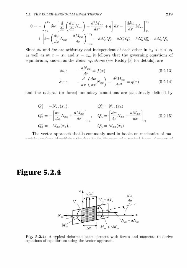
5.2. THE EULER–BERNOULLI BEAM THEORY 219
0 = −∫ xb
xa
δw
[d
dx
(dw
dxNxx
)+d2Mxx
dx2+ q
]dx−
[dδw
dxMxx
]xbxa
+
[δw
(dw
dxNxx +
dMxx
dx
)]xbxa
− δ∆e2Q
e2 − δ∆e
3Qe3 − δ∆e
5Qe5 − δ∆e
6Qe6
Since δu and δw are arbitrary and independent of each other in xa < x < xbas well as at x = xa and x = xb, it follows that the governing equations ofequilibrium, known as the Euler equations (see Reddy [3] for details), are
δu : − dNxx
dx= f(x) (5.2.13)
δw : − d
dx
(dw
dxNxx
)− d2Mxx
dx2= q(x) (5.2.14)
and the natural (or force) boundary conditions are [as already defined byEq. (5.2.7)]
Qe1 = −Nxx(xa), Qe4 = Nxx(xb)
Qe2 = −[dw
dxNxx +
dMxx
dx
]xa
, Qe5 =
[dw
dxNxx +
dMxx
dx
]xb
Qe3 = −Mxx(xa), Qe6 = Mxx(xb)
(5.2.15)
The vector approach that is commonly used in books on mechanics of ma-terials involves identifying the free-body-diagram of a typical beam element oflength ∆x from the deformed configuration (in contrast to the element takenfrom the undeformed configuration in the linear analysis), with all its forces andmoments displayed on it, setting the sums of the forces in the x and z direc-tions and moments about the y-axis to zero separately (i.e. applying Newton’ssecond law), and taking the limit ∆x → 0. However, the vector approach doesnot provide the boundary conditions. To see how this approach works, considerthe free-body-diagram of the beam element shown in Fig. 5.2.4. Summing theforces in the x- and z-directions and moments about the y-axis, we obtain
Figure 5.2.4
z
x
dwdxx xV V+ Δ
( )q x
xxM
xxN
xx xxN N+ Δ
xV
xx xxM M+ ΔxΔ
Fig. 5.2.4: A typical deformed beam element with forces and moments to deriveequations of equilibrium using the vector approach.
220 NONLINEAR BENDING OF STRAIGHT BEAMS
−Nxx + (Nxx + ∆Nxx) + f(x)∆x = 0
−Vx + (Vx + ∆Vx) + q(x)∆x = 0
−Mxx + (Mxx + ∆Mxx)− Vx∆x+Nxx∆xdw
dx− q(x)∆x(c∆x) = 0
where 0 < c < 1 is a constant that depends on the nature of the load q(x).Taking the limit ∆x → 0, we obtain the following three equations:
dNxx
dx+ f(x) = 0,
dVxdx
+ q(x) = 0,dMxx
dx− Vx +Nxx
dw
dx= 0
which are equivalent to the two equations in Eqs. (5.2.13) and (5.2.14) (whenVx is eliminated from the second equation using the third equation). Note thatVx is the shear force on a section perpendicular to the x-axis, and it is not equalto the shear force Qx ≡ dMxx/dx acting on the section perpendicular to thedeformed beam. In fact, one can show that Vx = Qx +Nxx(dw/dx).
If one begins with Eqs. (5.2.13) and (5.2.14), their weak forms can be de-veloped using the usual three-step procedure of Section 3.2.3:
0 =
∫ xb
xa
v1
(−dNxx
dx− f
)dx =
∫ xb
xa
(dv1
dxNxx − v1f
)dx− [v1Nxx]xbxa
=
∫ xb
xa
(dv1
dxNxx − v1f
)dx− v1(xa)[−Nxx(xa)]− v1(xb)Nxx(xb) (5.2.16)
0 =
∫ xb
xa
v2
[− d
dx
(dw
dxNxx
)− d2Mxx
dx2− q]dx
=
∫ xb
xa
[dv2
dx
(dw
dxNxx
)− d2v2
dx2Mxx − v2q
]dx
−[v2
(dw
dxNxx +
dMxx
dx
)]xbxa
−[(−dv2
dx
)Mxx
]xbxa
=
∫ xb
xa
[dv2
dx
(dw
dxNxx
)− d2v2
dx2Mxx − v2q
]dx
− v2(xa)
[−(dw
dxNxx +
dMxx
dx
)]xa
− v2(xb)
[dw
dxNxx +
dMxx
dx
]xb
−[−dv2
dx
]xa
[−Mxx(xa)]−[−dv2
dx
]xb
Mxx(xb) (5.2.17)
where v1 and v2 are the weight functions, whose meaning is obvious if theexpressions fv1dx and qv2dx are to represent the work done by external forces.We see that v1 ∼ δu and v2 ∼ δw. Clearly, Eqs. (5.2.16) and (5.2.17) are thesame as those in Eqs. (5.2.11) and (5.2.12) with v1 = δu and v2 = δw.
5.2. THE EULER–BERNOULLI BEAM THEORY 221
The force Nxx and moment Mxx can be expressed in terms of the displace-ments once the constitutive behavior is assumed. Suppose that the beam ismade of a linear elastic material with modulus of elasticity E, which can be, ingeneral, a function of x and possibly z, and obeys Hooke’s law
σxx = Eεxx (5.2.18)
Then we have
Nxx =
∫Aeσxx dA =
∫AeEe
[du
dx+
1
2
(dw
dx
)2
− z d2w
dx2
]dA
= Aexx
[du
dx+
1
2
(dw
dx
)2]−Be
xx
d2w
dx2(5.2.19)
Mxx =
∫Aeσxx z dA =
∫AeEe
[du
dx+
1
2
(dw
dx
)2
− z d2w
dx2
]z dA
= Bexx
[du
dx+
1
2
(dw
dx
)2]−De
xx
d2w
dx2(5.2.20)
where Aexx, Bexx, and De
xx are the extensional, extensional-bending, and bendingstiffnesses of the beam element
(Aexx, Bexx, D
exx) =
∫AeEe(x, z)
(1, z, z2
)dA (5.2.21)
For beams made of a material for which Ee is a function of only x and thex-axis is taken along the geometric centroid, then Aexx, Be
xx, and Dexx are given
by
Aexx = EeAe, Bexx = 0, De
xx = EeIe (5.2.22)
where ∫AedA = Ae,
∫Aez dA = 0,
∫Aez2 dA = Ie
Here Ae and Ie are the cross-sectional area and moment of inertia about the y-axis of the beam element. In general, Aexx and De
xx are functions of x wheneverthe modulus Ee and/or the cross-sectional area Ae is a function of x.
When Bexx = 0, Eqs. (5.2.11) and (5.2.12) can be expressed in terms of the
generalized displacements (u,w) with the help of Eqs. (5.2.19) and (5.2.20) as
0 =
∫ xb
xa
Axx
dδu
dx
[du
dx+
1
2
(dw
dx
)2]− f δu
dx
− δu(xa)Q1 − δu(xb)Q4 (5.2.23)
222 NONLINEAR BENDING OF STRAIGHT BEAMS
0 =
∫ xb
xa
dδw
dx
dw
dxAxx
[du
dx+
1
2
(dw
dx
)2]
+Dxxdδ2w
dx2
d2w
dx2− q δw
dx
− δw(xa)Q2 − δθ(xa)Q3 − δw(xb)Q5 − δθ(xb)Q6 (5.2.24)
where the element label ‘e’ is omitted on Axx, Bxx, and Dxx for simplicity.
5.2.4 Finite Element Model
Let the axial displacement u(x) and transverse deflection w(x) be approximatedas [θ = −(dw/dx)]
u(x) ≈ uh(x) =
2∑j=1
ujψj(x) , w(x) ≈ wh(x) =
4∑J=1
∆JϕJ(x) (5.2.25)
∆1 ≡ w(xa), ∆2 ≡ θ(xa), ∆3 ≡ w(xb), ∆4 ≡ θ(xb) (5.2.26)
and ψj (j = 1, 2) are the linear Lagrange interpolation functions and ϕJ (J =1, 2, 3, 4) are the Hermite cubic interpolation functions:
ψe1(ζ) = 1− ζ, ψe2(ζ) = ζ (5.2.27)
ϕe1(ζ) = 1− 3ζ2 + 2ζ3, ϕe2(ζ) = −heζ (1− ζ)2
ϕe3(ζ) = 3ζ2 − 2ζ3, ϕe4(ζ) = −heζ(ζ2 − ζ
) (5.2.28)
where
ζ =x− xahe
, 0 ≤ ζ ≤ 1 (5.2.29)
Substituting the approximations from Eq. (5.2.25) for u and w, and δu(x) =ψi(x) and δw(x) = ϕJ(x) (to obtain the ith algebraic equation of each weakform) into the weak forms in Eqs. (5.2.23) and (5.2.24), we obtain
0 =
2∑j=1
K11ij uj +
4∑J=1
K12iJ ∆J − F 1
i (i = 1, 2)
0 =
2∑j=1
K21Ij uj +
4∑J=1
K22IJ∆J − F 2
I (I = 1, 2, 3, 4)
(5.2.30)
where, for the case in which Bxx = 0, we have
K11ij =
∫ xb
xa
Axxdψidx
dψjdx
dx , K12iJ =
1
2
∫ xb
xa
(Axx
dw
dx
)dψidx
dϕJdx
dx
K21Ij =
∫ xb
xa
Axxdw
dx
dϕIdx
dψjdx
dx , K21Ij = 2K12
jI
K22IJ =
∫ xb
xa
Dxxd2ϕIdx2
d2ϕJdx2
dx+1
2
∫ xb
xa
[Axx
(dw
dx
)2]dϕIdx
dϕJdx
dx
5.2. THE EULER–BERNOULLI BEAM THEORY 223
F 1i =
∫ xb
xa
f ψi dx+ Qi , F 2I =
∫ xb
xa
q ϕI dx+ QI (5.2.31)
for (i, j = 1, 2) and (I, J = 1, 2, 3, 4), where Q1 = Q1, Q2 = Q4, Q1 = Q2,Q2 = Q3, Q3 = Q5, and Q4 = Q6, and the definition of Qi is given Eq. (5.2.15).The pair of equations in Eq. (5.2.30) can be expressed in matrix form as[
K11 K12
K21 K22
]∆1
∆2
=
F1
F2
or Ke∆e = Fe (5.2.32)
where∆1i = ui, i = 1, 2; ∆2
I = ∆I , I = 1, 2, 3, 4 (5.2.33)
We also note that (K12)T 6= K21.The coefficient matrices K12, K21, and K22 of Eq. (5.2.32) are functions of
the unknown displacement w(x). When the nonlinearity is not considered, wewill have K12 = 0 and K21 = 0, and the equations involving u (the bar problem)are uncoupled from those involving ∆ (the beam problem), and therefore, theycan be solved independent of each other:
K11u = F1, K22∆ = F2 (5.2.34)
When nonlinearity is accounted for, the equations are coupled (i.e. bendingand stretching deformations of the beam are coupled) and nonlinear. Therefore,an iterative method must be used to solve the assembled equations. Whenthese matrix coefficients are evaluated using the value of w(x) =
∑∆jϕj from
the previous iteration, we say that the equations are linearized. Hence, theelement stiffness matrix and therefore, the assembled stiffness matrix, are notsymmetric.
The definitions of the coefficients Kαβij in Eq. (5.2.31) can be different if we
had accounted for the terms differently, even though the particular choice inderiving Eqs. (5.2.23) and (5.2.24) is probably the most natural. For example,all expressions involving dδw/dx and dw/dx in Eq. (5.2.24) could have beenused to define K22, leaving no term to define K21 (making K21 = 0). Thus, itis possible to decouple the nonlinear equations (after linearization) for u and ∆and solve them iteratively, feeding the solution from one equation to the other.However, this choice of linearization for the direct iteration solution scheme isknown to slow down the convergence. It does not make any difference in thecase of Newton’s iteration scheme because the tangent matrix will be the sameindependent of how the direct stiffness coefficients Kαβ are defined.
Note that the direct stiffness matrix is unsymmetric only due to the factthat K12 contains the factor 1/2 whereas K21 does not. One way to make(K21)T = K12 is to split the linear strain du/dx in Eq. (5.2.24) into two equal
224 NONLINEAR BENDING OF STRAIGHT BEAMS
parts and take one of the two parts as known from a previous iteration:∫ xb
xa
Axx
dδw
dx
dw
dx
[du
dx+
1
2
(dw
dx
)2]
dx
=1
2
∫ xb
xa
Axx
dw
dx
dδw
dx
du
dx+
[du
dx+
(dw
dx
)2]dδw
dx
dw
dx
dx
The first term of the above equation constitutes K21 and the second one con-stitutes a part of K22. The resulting algebraic equations are now symmetric[
K11 K12
K21 K22
]u∆
=
F1
F2
or Ke∆e = Fe (5.2.35)
where (the element label e is omitted)
∆1 = u1, ∆2 = ∆1, ∆3 = ∆2, ∆4 = u2, ∆5 = ∆3 , ∆6 = ∆4
F1 = F 11 , F2 = F 2
1 , F3 = F 22 , F4 = F 1
2 , F5 = F 23 , F6 = F 2
4
K11ij = K11
ij =
∫ xb
xa
Axxdψidx
dψjdx
dx
K12iJ = K12
iJ =1
2
∫ xb
xa
(Axx
dw
dx
)dψidx
dϕJdx
dx (5.2.36)
K21Ij =
1
2
∫ xb
xa
(Axx
dw
dx
)dϕIdx
dψjdx
dx , K21Ij = K12
jI
K22IJ =
∫ xb
xa
Dxxd2ϕIdx2
d2ϕJdx2
dx+1
2
∫ xb
xa
Axx
[du
dx+
(dw
dx
)2]dϕIdx
dϕJdx
dx
Note that in the symmetrized case, we must assume that u(x) is also known,in addition to w(x), from the previous iteration. As one can show, this choiceof definition of the direct stiffness coefficients Kαβ also gives the same tangentstiffness matrix as those defined in Eqs. (5.2.49)–(5.2.51).
Readers with a structural mechanics background may have seen Ke and Fe
in Eq. (5.2.32) expressed in terms of matrices as
Ke =
∫Ωe
BTDB dv, Fe =
∫Ωe
ΨTf dv +
∮Γe
ΨTt ds (5.2.37)
It is possible to rewrite the virtual work statement in Eq. (5.2.10), finite elementapproximation in Eq. (5.2.25), and subsequently the finite element model inEq. (5.2.32) in the form of Eq. (5.2.37).
5.2.5 Iterative Solution Strategies
The direct iteration and Newton’s iteration methods introduced in Chapter4 are revisited here in connection with the nonlinear finite element equations
5.2. THE EULER–BERNOULLI BEAM THEORY 225
derived in Section 5.2.4. Consider the nonlinear equations in Eq. (5.2.32)
Ke(∆e)∆e = Fe (5.2.38)
where the sign conventions of the generalized nodal displacements and forces areshown in Fig. 5.2.3. The system of nonlinear algebraic equations in Eq. (5.2.38)can be linearized using the direct iteration method or Newton’s iteration methoddiscussed in Section 4.4. Note that the linearized equations may be symmetricor unsymmetric, depending on the formulation (i.e. weighted-residual or weakform) and the form of the original differential equations (i.e. self-adjoint ornot) and, therefore, an appropriate equation solver must be used. On the otherhand, an unsymmetric banded equation solver may be used for all finite elementequations.
5.2.5.1 Direct iteration procedure
In the direct iteration procedure, the solution at the rth iteration is determinedfrom the assembled set of equations
K(U(r−1))U(r) = F(r−1) (5.2.39)
where U is the global displacement vector and K is the global direct stiffnessmatrix, which is obtained by assembling the element stiffness matrices Ke eval-uated at the element level using the known solution vector ∆e from the (r−1)stiteration. At the end of each iteration (i.e. after assembly, imposition of bound-ary conditions, and solution of equations), we check for convergence using thenormalized global residual vector R or global solution vector U:√
R(r) ·R(r)
F(r) · F(r)≤ ε, R(r) ≡ K(U(r))U(r) − F(r)
√∆U ·∆U
U(r) ·U(r)≤ ε, ∆U ≡ U(r) −U(r−1)
(5.2.40)
where ε denotes a preselected value of the error tolerance (e.g. ε = 10−3).Figure 4.4.1 depicts the general idea of the direct iteration procedure for asingle-degree-of-freedom system, and the steps involved in the direct iterationsolution scheme remain the same as those presented in Box 4.4.1.
5.2.5.2 Newton’s iteration procedure
In Newton’s iterative procedure, the linearized element equation at the begin-ning of the rth iteration is
Te(∆(r−1))δ∆(r) = −Re(∆(r−1)) = (Fe −Ke∆e)(r−1) (5.2.41)
226 NONLINEAR BENDING OF STRAIGHT BEAMS
where the tangent stiffness matrix Te associated with the Euler–Bernoulli beamelement is calculated using the definition
Te ≡ ∂Re
∂∆eor T eij ≡
∂Rei∂∆e
j
(5.2.42)
The global incremental displacement vector ∆U at the rth iteration is obtainedby solving the assembled equations (after the imposition of the boundary con-ditions)
∆U = −[T(U(r−1))]−1R(r−1) (5.2.43)
and the total solution is computed from
U(r) = U(r−1) + ∆U (5.2.44)
The comments made in the remarks after Box 4.4.2 about the imposition ofboundary conditions in Newton’s scheme also apply here.
Although the direct stiffness matrix Ke may be unsymmetric, it can beshown that the tangent stiffness matrix Te of the Euler–Bernoulli beam isalways symmetric. That is, the tangent stiffness matrix is the same whetherone uses Ke of Eq. (5.2.32) or Ke of Eq. (5.2.35).
The coefficients of the element tangent stiffness matrix Te can be computedusing the definition in Eq. (5.2.42). It is convenient to view Te as one that hasstructure similar to Ke in Eq. (5.2.32). That is, Eq. (5.2.41) is actually has theform [
T11 T12
T21 T22
]δ∆1
δ∆2
= −
R1
R2
(5.2.45)
where symbol δ is used in place of ∆, for obvious reason, to denote the incrementof the displacements. Also, note that ∆1 = ue and ∆2 = ∆e. Then we cancompute Tαβ from the definition
Tαβij =∂Rαi
∂∆βj
, α, β = 1, 2 (5.2.46)
The components Rαi of the residual vector R can be expressed as
Rαi =
2∑γ=1
n(γ)∑p=1
Kαγip ∆γ
p − Fαi =
2∑p=1
Kα1ip ∆1
p +
4∑P=1
Kα2iP ∆2
P − Fαi
=
2∑p=1
Kα1ip up +
4∑P=1
Kα2iP ∆P − Fαi (5.2.47)
where n(γ) denotes the number of element degrees of freedom [n(1) = 2 andn(2) = 4]. We have
Tαβij =∂Rαi
∂∆βj
=∂
∂∆βj
2∑γ=1
n(γ)∑p=1
Kαγip ∆γ
p − Fαi
5.2. THE EULER–BERNOULLI BEAM THEORY 227
=
2∑γ=1
n(γ)∑p=1
(Kαγip
∂∆γp
∂∆βj
+∂Kαγ
ip
∂∆βj
∆γp
)− ∂Fαi
∂∆βj
= Kαβij +
2∑p=1
∂
∂∆βj
(Kα1ip
)up +
4∑P=1
∂
∂∆βj
(Kα2iP
)∆P −
∂Fαi
∂∆βj
(5.2.48)
Since Fαi is independent of ∆ (unless the boundary conditions are nonlinear)
and Kαβij depend, at the most, on ∆2 = ∆ and not on ∆1 = u, we have
Tα1ij = Kα1
ij for α = 1, 2 (5.2.49)
T 12iJ = K12
iJ +
4∑P=1
∂
∂∆J
(K12iP
)∆P
= K12iJ +
4∑P=1
[∫ xb
xa
1
2Aexx
∂
∂∆J
(4∑
K=1
∆KdϕKdx
)dψidx
dϕPdx
dx
]∆P
= K12iJ +
4∑P=1
[∫ xb
xa
1
2Aexx
dϕJdx
dψidx
dϕPdx
dx
]∆P
= K12iJ +
∫ xb
xa
1
2Aexx
dψidx
dϕJdx
(4∑
P=1
dϕPdx
∆P
)dx
= K12iJ +
∫ xb
xa
(1
2Aexx
dw
dx
)dψidx
dϕJdx
dx = 2K12iJ = K21
Ji (5.2.50)
T 22IJ = K22
IJ +2∑p=1
∂
∂∆J
(K21Ip
)up +
4∑P=1
∂
∂∆J
(K22IP
)∆P
= K22IJ +
2∑p=1
[∫ xb
xa
Aexx∂
∂∆J
(4∑
K=1
∆KdϕKdx
)dϕIdx
dψpdx
dx
]up
+4∑
P=1
[∫ xb
xa
1
2Aexx
∂
∂∆J
(dw
dx
)2 dϕIdx
dϕPdx
dx
]∆P
= K22IJ +
∫ xb
xa
AexxdϕIdx
dϕJdx
2∑p=1
dψpdx
up
dx
+
∫ xb
xa
Aexx
(dw
dx
)dϕIdx
dϕJdx
(4∑
P=1
∆PdϕPdx
)dx
= K22IJ +
∫ xb
xa
Aexx
(du
dx+dw
dx
dw
dx
)dϕIdx
dϕJdx
dx (5.2.51)
228 NONLINEAR BENDING OF STRAIGHT BEAMS
5.2.6 Load Increments
Examining the expression in Eq. (5.2.19) for the internal axial force Nxx, it isclear that the rotation of a transverse normal contributes to the tensile com-ponent of Nxx, irrespective of the sign of the applied bending loads. As aresult, the beam becomes increasingly stiff as it experiences bending deforma-tion. Hence, for large bending loads the nonlinearity may be too large forthe numerical scheme to yield convergent solution. Therefore, it is necessaryto divide the applied total load, say F , into several smaller load incrementsδF1, δF2, . . . , δFN such that
F =
N∑i=1
δFi (5.2.52)
For the first load step, we use the initial guess of U(0) = 0 so that we canobtain the linear solution of the problem for the first load, F1, at the end ofthe first iteration. One of the iterative procedures outlined earlier is used todetermine the solution, U(1). If the iterative scheme does not converge withina pre-specified number of iterations (ITMAX), it may be necessary to furtherreduce the size of the load increment F1 = δF1. Once the solution for the firstload increment is obtained, it is used as the initial “guess” vector for the nextload, F2 = δF1 + δF2. This is continued until the total load is reached.
Another way to accelerate the convergence is to use a weighted average ofthe solutions from the last two iterations in evaluating the stiffness matrix atthe rth iteration, as discussed in Eq. (4.4.6):
U(r−1) = βU(r−2) + (1− β)U(r−1), 0 ≤ β ≤ 1 (5.2.53)
where β is the acceleration parameter. A value of β = 0.5 is suggested, butone may experiment with the value of β when the iterative scheme experiencesnon-convergence. Otherwise, one should use β = 0.
5.2.7 Membrane Locking
For the linear case, the axial displacement u is uncoupled from the bendingdeflection w, and they can be determined independently from the finite elementequations [see Eq. (5.2.34)]
K11u = F1, K11ij =
∫ xb
xa
Aexxdψidx
dψjdx
dx (5.2.54)
K22(L)∆ = F2, K22(L)IJ =
∫ xb
xa
Dexx
d2ϕIdx2
d2ϕJdx2
dx (5.2.55)
respectively. Here the superscript L signifies the linear stiffness coefficients.Under the assumptions of linearity, if a beam is subjected to only bendingloads and no axial loads, then u(x) = 0 [when u is specified to be zero at least
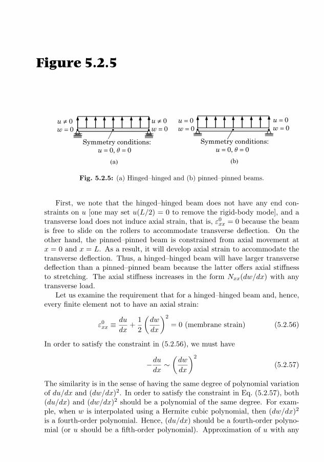
5.2. THE EULER–BERNOULLI BEAM THEORY 229
at one point]. In other words, a hinged–hinged beam and a pinned–pinned beam[see Figs. 5.2.5(a) and 5.2.5(b), respectively] will have the same deflection w(x)under the same loads and u(x) = 0 for all x. However, this is not the casewhen the von Karman nonlinearity is included. The coupling between u andw will cause the beam to undergo axial displacement even when there are noaxial forces, and the solution (u,w) will be different for the two cases shown inFigs. 5.2.5(a) and 5.2.5(b).
(a)
00
uw
≠=
00
uw
≠=
Symmetry conditions:0, 0u q= =
(b)
00
uw
==
Symmetry conditions:0, 0u q= =
00
uw
==
Figure 5.2.5
Fig. 5.2.5: (a) Hinged–hinged and (b) pinned–pinned beams.
First, we note that the hinged–hinged beam does not have any end con-straints on u [one may set u(L/2) = 0 to remove the rigid-body mode], and atransverse load does not induce axial strain, that is, ε0
xx = 0 because the beamis free to slide on the rollers to accommodate transverse deflection. On theother hand, the pinned–pinned beam is constrained from axial movement atx = 0 and x = L. As a result, it will develop axial strain to accommodate thetransverse deflection. Thus, a hinged–hinged beam will have larger transversedeflection than a pinned–pinned beam because the latter offers axial stiffnessto stretching. The axial stiffness increases in the form Nxx(dw/dx) with anytransverse load.
Let us examine the requirement that for a hinged–hinged beam and, hence,every finite element not to have an axial strain:
ε0xx ≡
du
dx+
1
2
(dw
dx
)2
= 0 (membrane strain) (5.2.56)
In order to satisfy the constraint in (5.2.56), we must have
−dudx∼(dw
dx
)2
(5.2.57)
The similarity is in the sense of having the same degree of polynomial variationof du/dx and (dw/dx)2. In order to satisfy the constraint in Eq. (5.2.57), both(du/dx) and (dw/dx)2 should be a polynomial of the same degree. For exam-ple, when w is interpolated using a Hermite cubic polynomial, then (dw/dx)2
is a fourth-order polynomial. Hence, (du/dx) should be a fourth-order polyno-mial (or u should be a fifth-order polynomial). Approximation of u with any
230 NONLINEAR BENDING OF STRAIGHT BEAMS
polynomial less than the fifth-order and w with Hermite cubic polynomials, theconstraint in Eq. (5.2.57) is clearly not satisfied and the resulting element stiff-ness matrix will be excessively stiff; hence, results in almost zero displacementfield, and the element is said to lock, and this phenomenon is known as themembrane locking.
A practical way to satisfy the constraint in Eq. (5.2.57) is to use the mini-mum interpolation of u and w (i.e. linear interpolation of u and Hermite cubicinterpolation of w) but treat ε0
xx as a constant. This may seem impossible, butit is possible from a numerical point of view. Since du/dx is constant, it isnecessary to treat (dw/dx)2 as a constant in the numerical evaluation of theelement stiffness coefficients. Thus, if Axx is a constant, all nonlinear stiffnesscoefficients should be evaluated using one-point Gauss quadrature, that is, onehas to use the reduced integration to evaluate all nonlinear terms of the stiffnesscoefficients. These coefficients include K12
iJ , K21Ij , T 12
iJ , T 21Ij , and the nonlinear
parts of K22IJ and T 22
IJ . All other terms may be evaluated exactly using two-pointquadrature for constant values of Axx and Dxx.
5.2.8 Computer Implementation
The flow chart for nonlinear bending of beams is presented in Fig. 5.2.6. Notethat there is an outer loop on load increments (NLS = number of load steps).Except for the definition of stiffness coefficients, much of the logic remains thesame as that shown in Box 4.5.2.
5.2.8.1 Rearrangement of equations and computation ofelement coefficients
While the particular form in Eq. (5.2.32) of the finite element model of multi-degree-of-freedom systems is natural, that is, the element stiffness matrix isdefined by submatrices K11, K12, K21, and K22 and the solution vector ∆ ispartitioned into vectors of extensional and bending degrees of freedom, u and∆, respectively. However, in practice, it is desirable to rearrange (e.g. to reducethe bandwidth of the assembled system of equations) the solution vector as
∆ = u1, w1 = ∆1, θ1 = ∆2, u2, w2 = ∆3, θ2 = ∆4T (5.2.58)
This, in turn, requires rearrangement of the stiffness coefficients such that theoriginal symmetry, if any, of the stiffness matrix is preserved. For linear inter-polation of u(x) and Hermite cubic interpolation of w(x), the order of varioussubmatrices of Eq. (5.2.32) is as follows: K11 is of the order 2× 2, K12 is 2× 4,K21 is 4 × 2, and K22 is 4 × 4. The total size of the stiffness matrix is 6 × 6.The vectors ∆1 and F1 are 2× 1 and ∆2 and F2 are 4× 1.
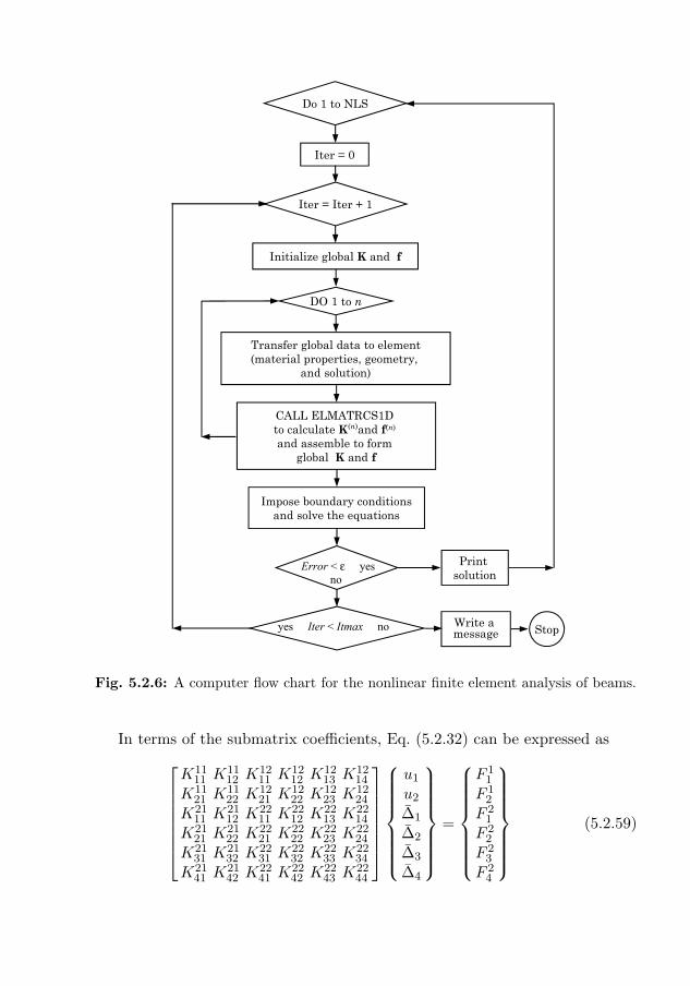
5.2. THE EULER–BERNOULLI BEAM THEORY 231
Initialize global K and f
Iter = Iter + 1
DO 1 to n
Iter = 0
Impose boundary conditionsand solve the equations
CALL ELMATRCS1D to calculate K(n)and f(n)
and assemble to form global K and f
Transfer global data to element(material properties, geometry,
and solution)
Print solution
Write a message
Error < ε yesno
yes Iter < Itmax no Stop
Do 1 to NLS
Fig. 5.2.6: A computer flow chart for the nonlinear finite element analysis of beams.
In terms of the submatrix coefficients, Eq. (5.2.32) can be expressed as
K1111 K
1112 K
1211 K
1212 K
1213 K
1214
K1121 K
1122 K
1221 K
1222 K
1223 K
1224
K2111 K
2112 K
2211 K
2212 K
2213 K
2214
K2121 K
2122 K
2221 K
2222 K
2223 K
2224
K2131 K
2132 K
2231 K
2232 K
2233 K
2234
K2141 K
2142 K
2241 K
2242 K
2243 K
2244
u1
u2
∆1
∆2
∆3
∆4
=
F 11
F 12
F 21
F 22
F 23
F 24
(5.2.59)
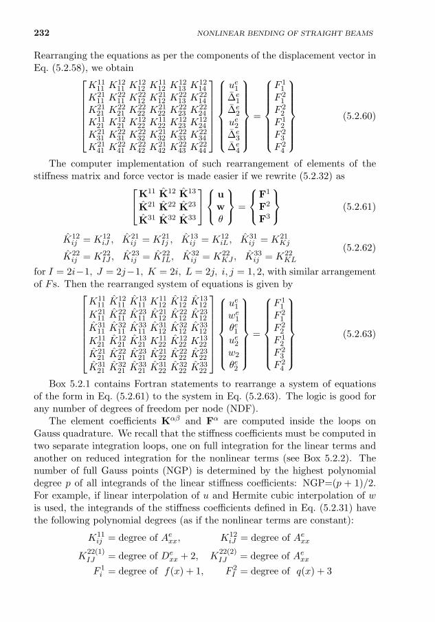
232 NONLINEAR BENDING OF STRAIGHT BEAMS
Rearranging the equations as per the components of the displacement vector inEq. (5.2.58), we obtain
K1111 K
1211 K
1212 K
1112 K
1213 K
1214
K2111 K
2211 K
2212 K
2112 K
2213 K
2214
K2121 K
2221 K
2222 K
2122 K
2223 K
2224
K1121 K
1221 K
1222 K
1122 K
1223 K
1224
K2131 K
2231 K
2232 K
2132 K
2233 K
2234
K2141 K
2241 K
2242 K
2142 K
2243 K
2244
ue1∆e
1
∆e2
ue2∆e
3
∆e4
=
F 11
F 21
F 22
F 12
F 23
F 24
(5.2.60)
The computer implementation of such rearrangement of elements of thestiffness matrix and force vector is made easier if we rewrite (5.2.32) asK11 K12 K13
K21 K22 K23
K31 K32 K33
uwθ
=
F1
F2
F3
(5.2.61)
K12ij = K12
iJ , K21ij = K21
Ij , K13ij = K12
iL , K31ij = K21
Kj
K22ij = K22
IJ , K23ij = K22
IL, K32ij = K22
KJ , K33ij = K22
KL
(5.2.62)
for I = 2i−1, J = 2j−1, K = 2i, L = 2j, i, j = 1, 2, with similar arrangementof F s. Then the rearranged system of equations is given by
K1111 K
1211 K
1311 K
1112 K
1212 K
1312
K2111 K
2211 K
2311 K
2112 K
2212 K
2312
K3111 K
3211 K
3311 K
3112 K
3212 K
3312
K1121 K
1221 K
1321 K
1122 K
1222 K
1322
K2121 K
2221 K
2321 K
2122 K
2222 K
2322
K3121 K
3221 K
3321 K
3122 K
3222 K
3322
ue1we1θe1ue2w2
θe2
=
F 11
F 21
F 22
F 12
F 23
F 24
(5.2.63)
Box 5.2.1 contains Fortran statements to rearrange a system of equationsof the form in Eq. (5.2.61) to the system in Eq. (5.2.63). The logic is good forany number of degrees of freedom per node (NDF).
The element coefficients Kαβ and Fα are computed inside the loops onGauss quadrature. We recall that the stiffness coefficients must be computed intwo separate integration loops, one on full integration for the linear terms andanother on reduced integration for the nonlinear terms (see Box 5.2.2). Thenumber of full Gauss points (NGP) is determined by the highest polynomialdegree p of all integrands of the linear stiffness coefficients: NGP=(p + 1)/2.For example, if linear interpolation of u and Hermite cubic interpolation of wis used, the integrands of the stiffness coefficients defined in Eq. (5.2.31) havethe following polynomial degrees (as if the nonlinear terms are constant):
K11ij = degree of Aexx, K12
iJ = degree of Aexx
K22(1)IJ = degree of De
xx + 2, K22(2)IJ = degree of Aexx
F 1i = degree of f(x) + 1, F 2
I = degree of q(x) + 3
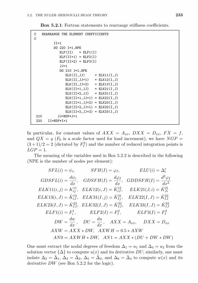
5.2. THE EULER–BERNOULLI BEAM THEORY 233
Box 5.2.1: Fortran statements to rearrange stiffness coefficients.
C REARRANGE THE ELEMENT COEFFICIENTS
C
II=1
DO 220 I=1,NPE
ELF(II) = ELF1(I)
ELF(II+1) = ELF2(I)
ELF(II+2) = ELF3(I)
JJ=1
DO 210 J=1,NPE
ELK(II,JJ) = ELK11(I,J)
ELK(II,JJ+1) = ELK12(I,J)
ELK(II,JJ+2) = ELK13(I,J)
ELK(II+1,JJ) = ELK21(I,J)
ELK(II+2,JJ) = ELK31(I,J)
ELK(II+1,JJ+1) = ELK22(I,J)
ELK(II+1,JJ+2) = ELK23(I,J)
ELK(II+2,JJ+1) = ELK32(I,J)
ELK(II+2,JJ+2) = ELK33(I,J)
210 JJ=NDF*J+1
220 II=NDF*I+1
In particular, for constant values of AXX = Axx, DXX = Dxx, FX = f ,and QX = q (F0 is a scale factor used for load increment), we have NGP =(3 + 1)/2 = 2 (dictated by F 2
I ) and the number of reduced integration points isLGP = 1.
The meaning of the variables used in Box 5.2.2 is described in the following(NPE is the number of nodes per element):
SFL(i) = ψi, SFH(I) = ϕI , ELU(i) = ∆ei
GDSFL(i) =dψidx
, GDSFH(I) =dϕIdx
, GDDSFH(I) =d2ϕIdx2
ELK11(i, j) = K11ij , ELK12(i, J) = K12
iJ , ELK21(J, i) = K21Ji
ELK13(i, J) = K13iJ , ELK31(I, j) = K31
Ij , ELK22(I, J) = K22IJ
ELK23(I, J) = K23IJ , ELK32(I, J) = K32
IJ , ELK33(I, J) = K33IJ
ELF1(i) = F 1i , ELF2(I) = F 2
I , ELF3(I) = F 3I
DW =dw
dx, DU =
du
dx, AXX = Axx, DXX = Dxx
AXW = AXX ∗DW, AXWH = 0.5 ∗AXWAN0 = AXWH ∗DW, AN1 = AXX ∗ (DU +DW ∗DW )
One must extract the nodal degrees of freedom ∆1 = u1 and ∆4 = u2 from thesolution vector ∆ to compute u(x) and its derivative DU ; similarly, one mustisolate ∆2 = ∆1, ∆3 = ∆2, ∆5 = ∆3, and ∆6 = ∆4 to compute w(x) and itsderivative DW (see Box 5.2.2 for the logic).
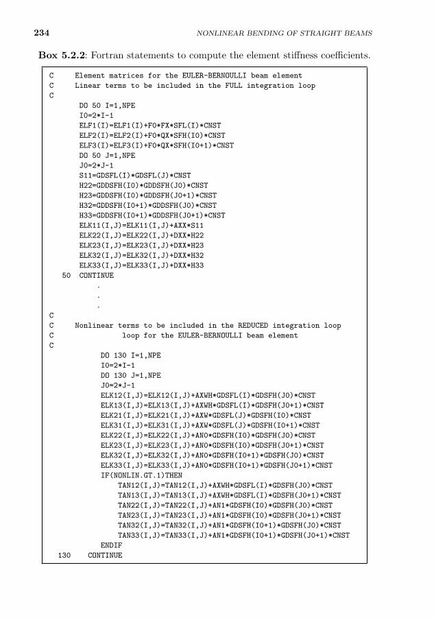
234 NONLINEAR BENDING OF STRAIGHT BEAMS
Box 5.2.2: Fortran statements to compute the element stiffness coefficients.
C Element matrices for the EULER-BERNOULLI beam element
C Linear terms to be included in the FULL integration loop
C
DO 50 I=1,NPE
I0=2*I-1
ELF1(I)=ELF1(I)+F0*FX*SFL(I)*CNST
ELF2(I)=ELF2(I)+F0*QX*SFH(I0)*CNST
ELF3(I)=ELF3(I)+F0*QX*SFH(I0+1)*CNST
DO 50 J=1,NPE
J0=2*J-1
S11=GDSFL(I)*GDSFL(J)*CNST
H22=GDDSFH(I0)*GDDSFH(J0)*CNST
H23=GDDSFH(I0)*GDDSFH(J0+1)*CNST
H32=GDDSFH(I0+1)*GDDSFH(J0)*CNST
H33=GDDSFH(I0+1)*GDDSFH(J0+1)*CNST
ELK11(I,J)=ELK11(I,J)+AXX*S11
ELK22(I,J)=ELK22(I,J)+DXX*H22
ELK23(I,J)=ELK23(I,J)+DXX*H23
ELK32(I,J)=ELK32(I,J)+DXX*H32
ELK33(I,J)=ELK33(I,J)+DXX*H33
50 CONTINUE
.
.
.
C
C Nonlinear terms to be included in the REDUCED integration loop
C loop for the EULER-BERNOULLI beam element
C
DO 130 I=1,NPE
I0=2*I-1
DO 130 J=1,NPE
J0=2*J-1
ELK12(I,J)=ELK12(I,J)+AXWH*GDSFL(I)*GDSFH(J0)*CNST
ELK13(I,J)=ELK13(I,J)+AXWH*GDSFL(I)*GDSFH(J0+1)*CNST
ELK21(I,J)=ELK21(I,J)+AXW*GDSFL(J)*GDSFH(I0)*CNST
ELK31(I,J)=ELK31(I,J)+AXW*GDSFL(J)*GDSFH(I0+1)*CNST
ELK22(I,J)=ELK22(I,J)+AN0*GDSFH(I0)*GDSFH(J0)*CNST
ELK23(I,J)=ELK23(I,J)+AN0*GDSFH(I0)*GDSFH(J0+1)*CNST
ELK32(I,J)=ELK32(I,J)+AN0*GDSFH(I0+1)*GDSFH(J0)*CNST
ELK33(I,J)=ELK33(I,J)+AN0*GDSFH(I0+1)*GDSFH(J0+1)*CNST
IF(NONLIN.GT.1)THEN
TAN12(I,J)=TAN12(I,J)+AXWH*GDSFL(I)*GDSFH(J0)*CNST
TAN13(I,J)=TAN13(I,J)+AXWH*GDSFL(I)*GDSFH(J0+1)*CNST
TAN22(I,J)=TAN22(I,J)+AN1*GDSFH(I0)*GDSFH(J0)*CNST
TAN23(I,J)=TAN23(I,J)+AN1*GDSFH(I0)*GDSFH(J0+1)*CNST
TAN32(I,J)=TAN32(I,J)+AN1*GDSFH(I0+1)*GDSFH(J0)*CNST
TAN33(I,J)=TAN33(I,J)+AN1*GDSFH(I0+1)*GDSFH(J0+1)*CNST
ENDIF
130 CONTINUE
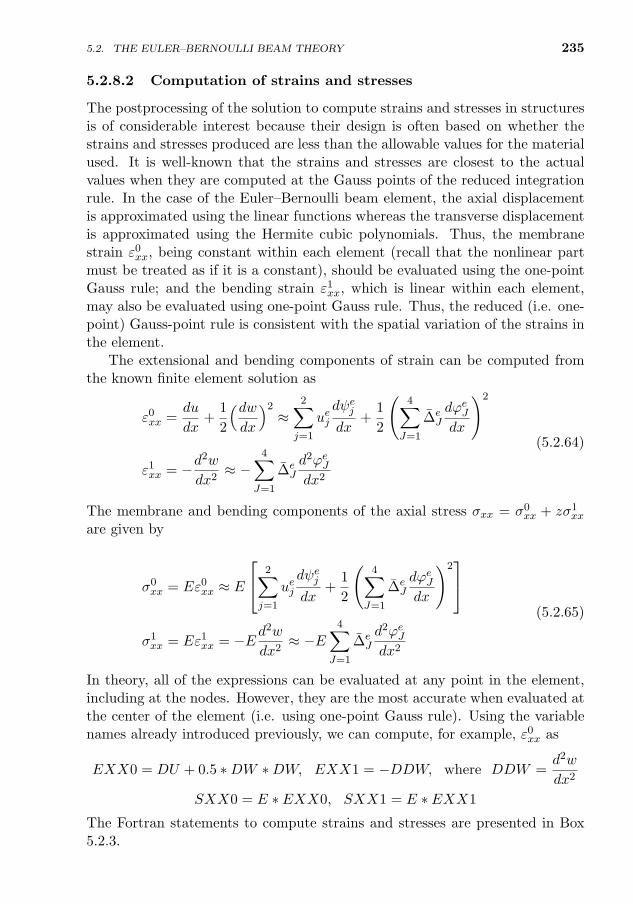
5.2. THE EULER–BERNOULLI BEAM THEORY 235
5.2.8.2 Computation of strains and stresses
The postprocessing of the solution to compute strains and stresses in structuresis of considerable interest because their design is often based on whether thestrains and stresses produced are less than the allowable values for the materialused. It is well-known that the strains and stresses are closest to the actualvalues when they are computed at the Gauss points of the reduced integrationrule. In the case of the Euler–Bernoulli beam element, the axial displacementis approximated using the linear functions whereas the transverse displacementis approximated using the Hermite cubic polynomials. Thus, the membranestrain ε0
xx, being constant within each element (recall that the nonlinear partmust be treated as if it is a constant), should be evaluated using the one-pointGauss rule; and the bending strain ε1
xx, which is linear within each element,may also be evaluated using one-point Gauss rule. Thus, the reduced (i.e. one-point) Gauss-point rule is consistent with the spatial variation of the strains inthe element.
The extensional and bending components of strain can be computed fromthe known finite element solution as
ε0xx =
du
dx+
1
2
(dwdx
)2≈
2∑j=1
uejdψejdx
+1
2
(4∑
J=1
∆eJ
dϕeJdx
)2
ε1xx = −d
2w
dx2≈ −
4∑J=1
∆eJ
d2ϕeJdx2
(5.2.64)
The membrane and bending components of the axial stress σxx = σ0xx + zσ1
xx
are given by
σ0xx = Eε0
xx ≈ E
2∑j=1
uejdψejdx
+1
2
(4∑
J=1
∆eJ
dϕeJdx
)2
σ1xx = Eε1
xx = −Ed2w
dx2≈ −E
4∑J=1
∆eJ
d2ϕeJdx2
(5.2.65)
In theory, all of the expressions can be evaluated at any point in the element,including at the nodes. However, they are the most accurate when evaluated atthe center of the element (i.e. using one-point Gauss rule). Using the variablenames already introduced previously, we can compute, for example, ε0
xx as
EXX0 = DU + 0.5 ∗DW ∗DW, EXX1 = −DDW, where DDW =d2w
dx2
SXX0 = E ∗ EXX0, SXX1 = E ∗ EXX1
The Fortran statements to compute strains and stresses are presented in Box5.2.3.
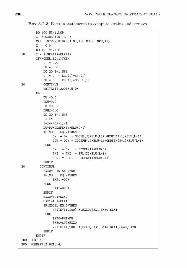
236
Box 5.2.3: Fortran statements to compute strains and stresses.
DO 100 NI=1,LGP
XI = GAUSPT(NI,LGP)
CALL INTERPLN1D(ELX,GJ,IEL,MODEL,NPE,XI)
X = 0.0
DO 10 I=1,NPE
10 X = X+SFL(I)*ELX(I)
IF(MODEL.EQ.1)THEN
U = 0.0
DU = 0.0
DO 20 I=1,NPE
U = U + ELU(I)*SFL(I)
DU = DU + ELU(I)*GDSFL(I)
20 CONTINUE
WRITE(IT,200)X,U,DX
ELSE
DW =0.0
DDW=0.0
PHI=0.0
DPHI=0.0
DO 30 I=1,NPE
L=I*NDF-1
J=I*(NDF-1)-1
DU=DU+GDSFL(I)*ELU(L-1)
IF(MODEL.EQ.2)THEN
DW = DW + GDSFH(J)*ELU(L)+ GDSFH(J+1)*ELU(L+1)
DDW = DDW + GDDSFH(J)*ELU(L)+GDDSFH(J+1)*ELU(L+1)
ELSE
DW = DW + GDSFL(I)*ELU(L)
PHI = PHI + SFL(I)*ELU(L+1)
DPHI = DPHI + GDSFL(I)*ELU(L+1)
ENDIF
30 CONTINUE
EXX0=DU+0.5*DW*DW
IF(MODEL.EQ.2)THEN
EXX1=-DDW
ELSE
EXX1=DPHI
ENDIF
SXX0=AU1*EXX0
SXX1=AU1*EXX1
IF(MODEL.EQ.2)THEN
WRITE(IT,200) X,EXX0,EXX1,SXX0,SXX1
ELSE
EXZ0=PHI+DW
SXZ0=AU2*EXZ0
WRITE(IT,200) X,EXX0,EXX1,SXX0,SXX1,EXZ0,SXZ0
ENDIF
ENDIF
100 CONTINUE
200 FORMAT(5X,8E13.4)
NONLINEAR BENDING OF STRAIGHT BEAMS
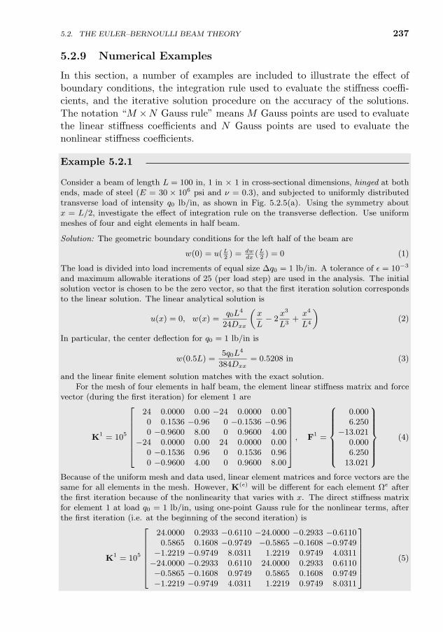
5.2. THE EULER–BERNOULLI BEAM THEORY 237
5.2.9 Numerical Examples
In this section, a number of examples are included to illustrate the effect ofboundary conditions, the integration rule used to evaluate the stiffness coeffi-cients, and the iterative solution procedure on the accuracy of the solutions.The notation “M ×N Gauss rule” means M Gauss points are used to evaluatethe linear stiffness coefficients and N Gauss points are used to evaluate thenonlinear stiffness coefficients.
Example 5.2.1
Consider a beam of length L = 100 in, 1 in × 1 in cross-sectional dimensions, hinged at bothends, made of steel (E = 30 × 106 psi and ν = 0.3), and subjected to uniformly distributedtransverse load of intensity q0 lb/in, as shown in Fig. 5.2.5(a). Using the symmetry aboutx = L/2, investigate the effect of integration rule on the transverse deflection. Use uniformmeshes of four and eight elements in half beam.
Solution: The geometric boundary conditions for the left half of the beam are
w(0) = u(L2
) = dwdx
(L2
) = 0 (1)
The load is divided into load increments of equal size ∆q0 = 1 lb/in. A tolerance of ε = 10−3
and maximum allowable iterations of 25 (per load step) are used in the analysis. The initialsolution vector is chosen to be the zero vector, so that the first iteration solution correspondsto the linear solution. The linear analytical solution is
u(x) = 0, w(x) =q0L
4
24Dxx
(x
L− 2
x3
L3+x4
L4
)(2)
In particular, the center deflection for q0 = 1 lb/in is
w(0.5L) =5q0L
4
384Dxx= 0.5208 in (3)
and the linear finite element solution matches with the exact solution.For the mesh of four elements in half beam, the element linear stiffness matrix and force
vector (during the first iteration) for element 1 are
K1 = 105
24 0.0000 0.00 −24 0.0000 0.000 0.1536 −0.96 0 −0.1536 −0.960 −0.9600 8.00 0 0.9600 4.00
−24 0.0000 0.00 24 0.0000 0.000 −0.1536 0.96 0 0.1536 0.960 −0.9600 4.00 0 0.9600 8.00
, F1 =
0.0006.250
−13.0210.0006.250
13.021
(4)
Because of the uniform mesh and data used, linear element matrices and force vectors are thesame for all elements in the mesh. However, K(e) will be different for each element Ωe afterthe first iteration because of the nonlinearity that varies with x. The direct stiffness matrixfor element 1 at load q0 = 1 lb/in, using one-point Gauss rule for the nonlinear terms, afterthe first iteration (i.e. at the beginning of the second iteration) is
K1 = 105
24.0000 0.2933 −0.6110 −24.0000 −0.2933 −0.61100.5865 0.1608 −0.9749 −0.5865 −0.1608 −0.9749−1.2219 −0.9749 8.0311 1.2219 0.9749 4.0311−24.0000 −0.2933 0.6110 24.0000 0.2933 0.6110−0.5865 −0.1608 0.9749 0.5865 0.1608 0.9749−1.2219 −0.9749 4.0311 1.2219 0.9749 8.0311
(5)
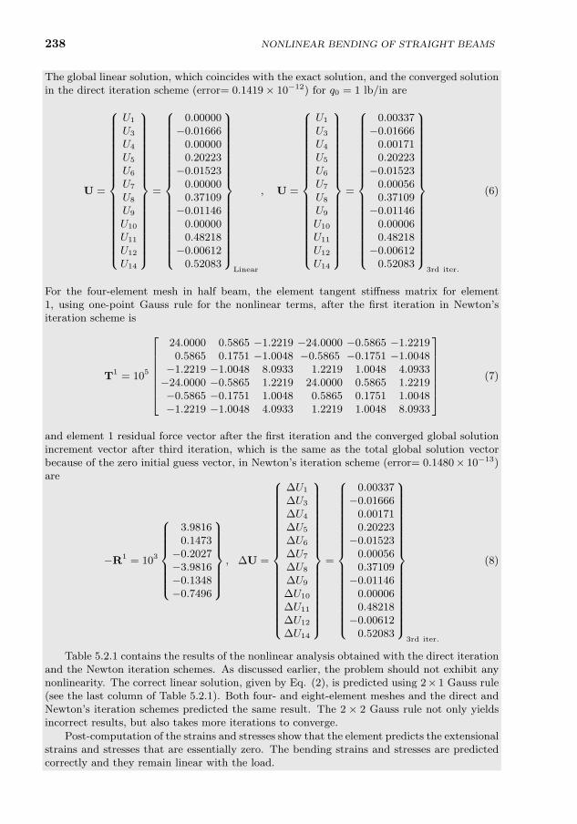
238 NONLINEAR BENDING OF STRAIGHT BEAMS
The global linear solution, which coincides with the exact solution, and the converged solutionin the direct iteration scheme (error= 0.1419× 10⁻¹²) for q0 = 1 lb/in are
U =
U1
U3
U4
U5
U6
U7
U8
U9
U10
U11
U12
U14
=
0.00000−0.01666
0.000000.20223−0.01523
0.000000.37109−0.01146
0.000000.48218−0.00612
0.52083
Linear
, U =
U1
U3
U4
U5
U6
U7
U8
U9
U10
U11
U12
U14
=
0.00337−0.01666
0.001710.20223−0.01523
0.000560.37109−0.01146
0.000060.48218−0.00612
0.52083
3rd iter.
(6)
For the four-element mesh in half beam, the element tangent stiffness matrix for element1, using one-point Gauss rule for the nonlinear terms, after the first iteration in Newton’siteration scheme is
T1 = 105
24.0000 0.5865 −1.2219 −24.0000 −0.5865 −1.22190.5865 0.1751 −1.0048 −0.5865 −0.1751 −1.0048−1.2219 −1.0048 8.0933 1.2219 1.0048 4.0933−24.0000 −0.5865 1.2219 24.0000 0.5865 1.2219−0.5865 −0.1751 1.0048 0.5865 0.1751 1.0048−1.2219 −1.0048 4.0933 1.2219 1.0048 8.0933
(7)
and element 1 residual force vector after the first iteration and the converged global solutionincrement vector after third iteration, which is the same as the total global solution vectorbecause of the zero initial guess vector, in Newton’s iteration scheme (error= 0.1480× 10⁻¹³)are
−R1 = 103
3.98160.1473−0.2027−3.9816−0.1348−0.7496
, ∆U =
∆U1
∆U3
∆U4
∆U5
∆U6
∆U7
∆U8
∆U9
∆U10
∆U11
∆U12
∆U14
=
0.00337−0.01666
0.001710.20223−0.01523
0.000560.37109−0.01146
0.000060.48218−0.00612
0.52083
3rd iter.
(8)
Table 5.2.1 contains the results of the nonlinear analysis obtained with the direct iterationand the Newton iteration schemes. As discussed earlier, the problem should not exhibit anynonlinearity. The correct linear solution, given by Eq. (2), is predicted using 2× 1 Gauss rule(see the last column of Table 5.2.1). Both four- and eight-element meshes and the direct andNewton’s iteration schemes predicted the same result. The 2 × 2 Gauss rule not only yieldsincorrect results, but also takes more iterations to converge.
Post-computation of the strains and stresses show that the element predicts the extensionalstrains and stresses that are essentially zero. The bending strains and stresses are predictedcorrectly and they remain linear with the load.
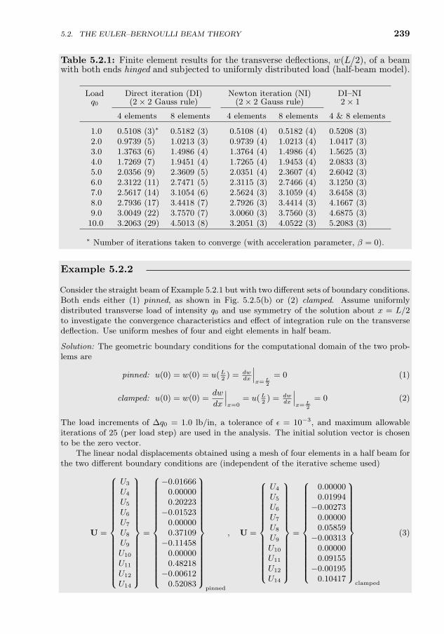
5.2. THE EULER–BERNOULLI BEAM THEORY 239
Table 5.2.1: Finite element results for the transverse deflections, w(L/2), of a beamwith both ends hinged and subjected to uniformly distributed load (half-beam model).
Load Direct iteration (DI) Newton iteration (NI) DI–NIq0 (2× 2 Gauss rule) (2× 2 Gauss rule) 2× 1
4 elements 8 elements 4 elements 8 elements 4 & 8 elements
1.0 0.5108 (3)∗ 0.5182 (3) 0.5108 (4) 0.5182 (4) 0.5208 (3)2.0 0.9739 (5) 1.0213 (3) 0.9739 (4) 1.0213 (4) 1.0417 (3)3.0 1.3763 (6) 1.4986 (4) 1.3764 (4) 1.4986 (4) 1.5625 (3)4.0 1.7269 (7) 1.9451 (4) 1.7265 (4) 1.9453 (4) 2.0833 (3)5.0 2.0356 (9) 2.3609 (5) 2.0351 (4) 2.3607 (4) 2.6042 (3)6.0 2.3122 (11) 2.7471 (5) 2.3115 (3) 2.7466 (4) 3.1250 (3)7.0 2.5617 (14) 3.1054 (6) 2.5624 (3) 3.1059 (4) 3.6458 (3)8.0 2.7936 (17) 3.4418 (7) 2.7926 (3) 3.4414 (3) 4.1667 (3)9.0 3.0049 (22) 3.7570 (7) 3.0060 (3) 3.7560 (3) 4.6875 (3)
10.0 3.2063 (29) 4.5013 (8) 3.2051 (3) 4.0522 (3) 5.2083 (3)
∗ Number of iterations taken to converge (with acceleration parameter, β = 0).
Example 5.2.2
Consider the straight beam of Example 5.2.1 but with two different sets of boundary conditions.Both ends either (1) pinned, as shown in Fig. 5.2.5(b) or (2) clamped. Assume uniformlydistributed transverse load of intensity q0 and use symmetry of the solution about x = L/2to investigate the convergence characteristics and effect of integration rule on the transversedeflection. Use uniform meshes of four and eight elements in half beam.
Solution: The geometric boundary conditions for the computational domain of the two prob-lems are
pinned: u(0) = w(0) = u(L2
) = dwdx
∣∣∣x=L
2
= 0 (1)
clamped: u(0) = w(0) =dw
dx
∣∣∣x=0
= u(L2
) = dwdx
∣∣∣x=L
2
= 0 (2)
The load increments of ∆q0 = 1.0 lb/in, a tolerance of ε = 10−3, and maximum allowableiterations of 25 (per load step) are used in the analysis. The initial solution vector is chosento be the zero vector.
The linear nodal displacements obtained using a mesh of four elements in a half beam forthe two different boundary conditions are (independent of the iterative scheme used)
U =
U3
U4
U5
U6
U7
U8
U9
U10
U11
U12
U14
=
−0.016660.000000.20223−0.01523
0.000000.37109−0.11458
0.000000.48218−0.00612
0.52083
pinned
, U =
U4
U5
U6
U7
U8
U9
U10
U11
U12
U14
=
0.000000.01994−0.00273
0.000000.05859−0.00313
0.000000.09155−0.00195
0.10417
clamped
(3)
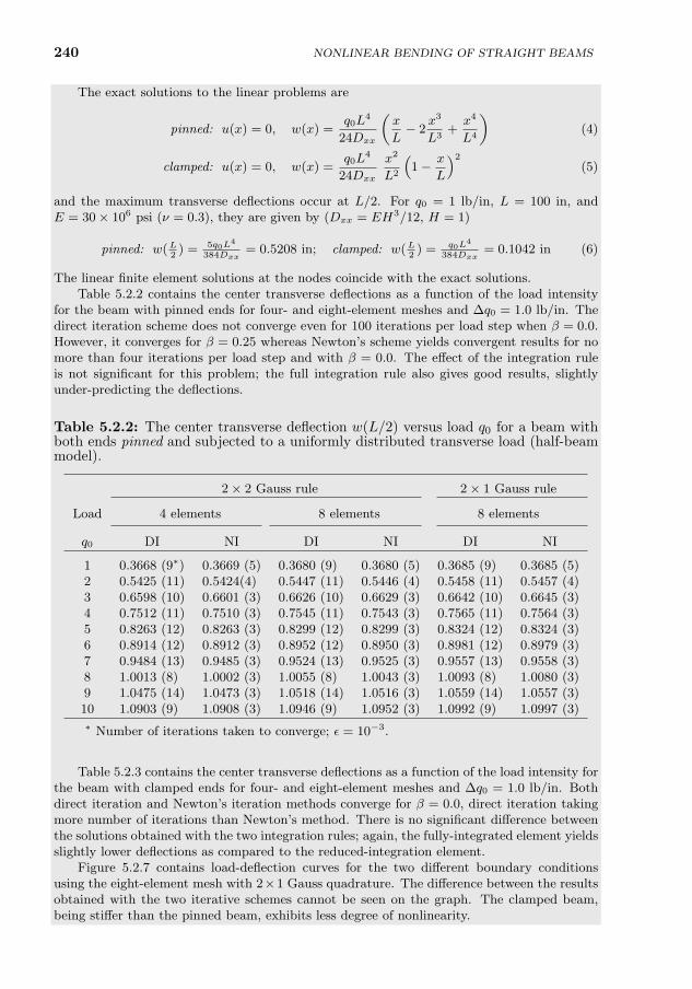
240 NONLINEAR BENDING OF STRAIGHT BEAMS
The exact solutions to the linear problems are
pinned: u(x) = 0, w(x) =q0L
4
24Dxx
(x
L− 2
x3
L3+x4
L4
)(4)
clamped: u(x) = 0, w(x) =q0L
4
24Dxx
x2
L2
(1− x
L
)2(5)
and the maximum transverse deflections occur at L/2. For q0 = 1 lb/in, L = 100 in, andE = 30× 106 psi (ν = 0.3), they are given by (Dxx = EH3/12, H = 1)
pinned: w(L2
) = 5q0L4
384Dxx= 0.5208 in; clamped: w(L
2) = q0L
4
384Dxx= 0.1042 in (6)
The linear finite element solutions at the nodes coincide with the exact solutions.Table 5.2.2 contains the center transverse deflections as a function of the load intensity
for the beam with pinned ends for four- and eight-element meshes and ∆q0 = 1.0 lb/in. Thedirect iteration scheme does not converge even for 100 iterations per load step when β = 0.0.However, it converges for β = 0.25 whereas Newton’s scheme yields convergent results for nomore than four iterations per load step and with β = 0.0. The effect of the integration ruleis not significant for this problem; the full integration rule also gives good results, slightlyunder-predicting the deflections.
Table 5.2.2: The center transverse deflection w(L/2) versus load q0 for a beam withboth ends pinned and subjected to a uniformly distributed transverse load (half-beammodel).
2× 2 Gauss rule 2× 1 Gauss rule
Load 4 elements 8 elements 8 elements
q0 DI NI DI NI DI NI
1 0.3668 (9∗) 0.3669 (5) 0.3680 (9) 0.3680 (5) 0.3685 (9) 0.3685 (5)2 0.5425 (11) 0.5424(4) 0.5447 (11) 0.5446 (4) 0.5458 (11) 0.5457 (4)3 0.6598 (10) 0.6601 (3) 0.6626 (10) 0.6629 (3) 0.6642 (10) 0.6645 (3)4 0.7512 (11) 0.7510 (3) 0.7545 (11) 0.7543 (3) 0.7565 (11) 0.7564 (3)5 0.8263 (12) 0.8263 (3) 0.8299 (12) 0.8299 (3) 0.8324 (12) 0.8324 (3)6 0.8914 (12) 0.8912 (3) 0.8952 (12) 0.8950 (3) 0.8981 (12) 0.8979 (3)7 0.9484 (13) 0.9485 (3) 0.9524 (13) 0.9525 (3) 0.9557 (13) 0.9558 (3)8 1.0013 (8) 1.0002 (3) 1.0055 (8) 1.0043 (3) 1.0093 (8) 1.0080 (3)9 1.0475 (14) 1.0473 (3) 1.0518 (14) 1.0516 (3) 1.0559 (14) 1.0557 (3)10 1.0903 (9) 1.0908 (3) 1.0946 (9) 1.0952 (3) 1.0992 (9) 1.0997 (3)
∗ Number of iterations taken to converge; ε = 10−3.
Table 5.2.3 contains the center transverse deflections as a function of the load intensity forthe beam with clamped ends for four- and eight-element meshes and ∆q0 = 1.0 lb/in. Bothdirect iteration and Newton’s iteration methods converge for β = 0.0, direct iteration takingmore number of iterations than Newton’s method. There is no significant difference betweenthe solutions obtained with the two integration rules; again, the fully-integrated element yieldsslightly lower deflections as compared to the reduced-integration element.
Figure 5.2.7 contains load-deflection curves for the two different boundary conditionsusing the eight-element mesh with 2×1 Gauss quadrature. The difference between the resultsobtained with the two iterative schemes cannot be seen on the graph. The clamped beam,being stiffer than the pinned beam, exhibits less degree of nonlinearity.
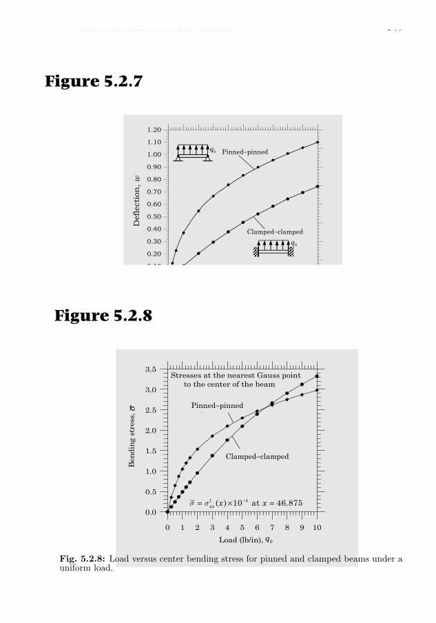
5.2. THE EULER–BERNOULLI BEAM THEORY 241
If the axial displacement degrees of freedom are suppressed (i.e. set u = 0 at everypoint of the beam) in the nonlinear analysis of beams, the beam will behave very stiff andthe deflections experienced will be less than those shown in Tables 5.2.2 and 5.2.3. Figure5.2.8 contains plots of bending stresses σ1
xx at x = 46.875 versus load for the two boundaryconditions [see Eq. (5.2.65) for the expressions used for stresses; σxx(x, z) = σ0
xx(x)+zσ1xx(x)].
For the clamped case, the maximum stress occurs at x = 0 and it is compressive.
Figure 5.2.7
0.0 1.0 2.0 3.0 4.0 5.0 6.0 7.0 8.0 9.0 10.0Load,
0.00
0.10
0.20
0.30
0.40
0.50
0.60
0.70
0.80
0.90
1.00
1.10
1.20D
efle
ctio
n,
Clamped-clamped
Pinned-pinned
q0
w
0q
• • 0q Pinned−pinned
Clamped−clamped
Fig. 5.2.7: Load versus center transverse deflection for pinned and clamped beamsunder a uniform load.
Figure 5.2.8
0 1 2 3 4 5 6 7 8 9 10
Load (lb/in),
0.0
0.5
1.0
1.5
2.0
2.5
3.0
3.5
Ben
din
g st
ress
, Pinned-pinned beam
Clamped-clamped beam
Stresses at the nearest Gauss point to the center of the beam
1 4( ) 10 at 46.875xx x xs s −= × =
σ
0q
Clamped−clamped
Pinned−pinned
Fig. 5.2.8: Load versus center bending stress for pinned and clamped beams under auniform load.
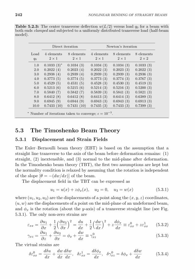
242 NONLINEAR BENDING OF STRAIGHT BEAMS
Table 5.2.3: The center transverse deflection w(L/2) versus load q0 for a beam withboth ends clamped and subjected to a uniformly distributed transverse load (half-beammodel).
Direct iteration Newton’s iteration
Load 4 elements 8 elements 4 elements 8 elements 8 elementsq0 2× 1 2× 1 2× 1 2× 1 2× 2
1.0 0.1033 (3)∗ 0.1034 (3) 0.1034 (3) 0.1034 (3) 0.1033 (3)2.0 0.2022 (4) 0.2023 (4) 0.2022 (3) 0.2023 (3) 0.2022 (3)3.0 0.2938 (4) 0.2939 (4) 0.2939 (3) 0.2939 (3) 0.2936 (3)4.0 0.3773 (5) 0.3774 (5) 0.3773 (3) 0.3774 (3) 0.3767 (3)5.0 0.4529 (5) 0.4531 (5) 0.4528 (3) 0.4530 (3) 0.4519 (3)6.0 0.5213 (6) 0.5215 (6) 0.5214 (3) 0.5216 (3) 0.5200 (3)7.0 0.5840 (7) 0.5842 (7) 0.5839 (3) 0.5841 (3) 0.5821 (3)8.0 0.6412 (8) 0.6412 (8) 0.6413 (3) 0.6414 (3) 0.6389 (3)9.0 0.6945 (9) 0.6944 (9) 0.6943 (3) 0.6943 (3) 0.6913 (3)
10.0 0.7433 (10) 0.7431 (10) 0.7435 (3) 0.7433 (3) 0.7399 (3)
∗ Number of iterations taken to converge; ε = 10−3.
5.3 The Timoshenko Beam Theory
5.3.1 Displacement and Strain Fields
The Euler–Bernoulli beam theory (EBT) is based on the assumption that astraight line transverse to the axis of the beam before deformation remains: (1)straight, (2) inextensible, and (3) normal to the mid-plane after deformation.In the Timoshenko beam theory (TBT), the first two assumptions are kept butthe normality condition is relaxed by assuming that the rotation is independentof the slope [θ = −(dw/dx)] of the beam.
The displacement field in the TBT can be expressed as
u1 = u(x) + zφx(x), u2 = 0, u3 = w(x) (5.3.1)
where (u1, u2, u3) are the displacements of a point along the (x, y, z) coordinates,(u,w) are the displacements of a point on the mid-plane of an undeformed beam,and φx is the rotation (about the y-axis) of a transverse straight line (see Fig.5.3.1). The only non-zero strains are
εxx =∂u1
∂x+
1
2
(∂u3
∂x
)2=du
dx+
1
2
(dwdx
)2+ z
dφxdx≡ ε0
xx + zε1xx (5.3.2)
γxz =∂u1
∂z+∂u3
∂x= φx +
dw
dx≡ γ0
xz (5.3.3)
The virtual strains are
δε0xx =
dδu
dx+dw
dx
dδw
dx, δε1
xx =dδφxdx
, δγ0xz = δφx +
dδw
dx(5.3.4)
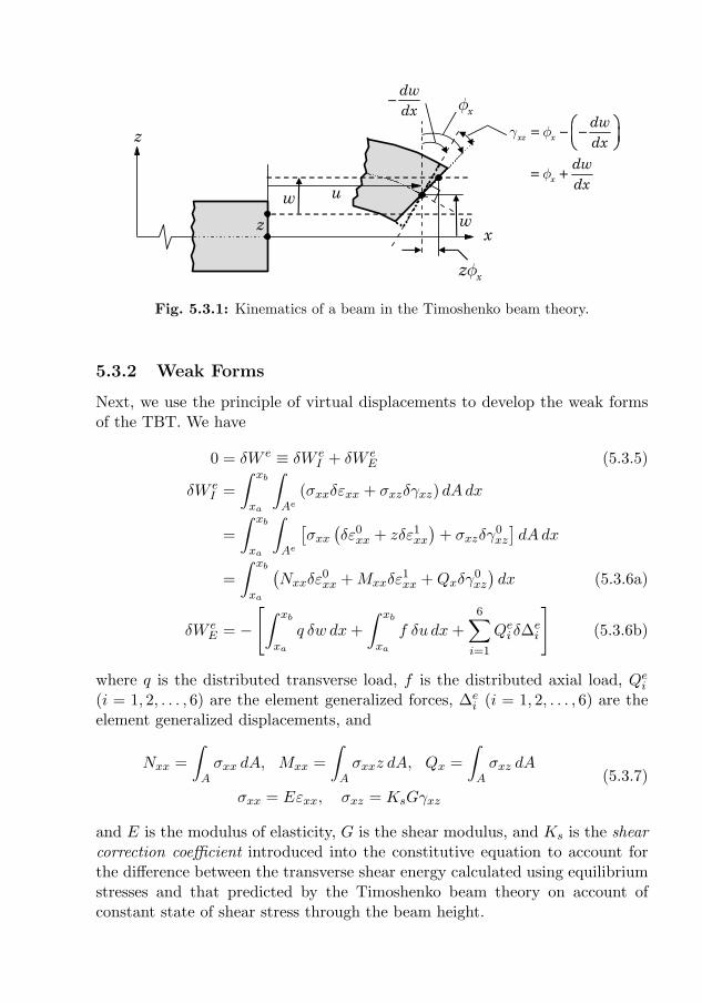
5.3. THE TIMOSHENKO BEAM THEORY 243
xz x
x
dwdx
dwdx
g f
f
= − −
= +
xzf
xfdwdx
−
z
xw
w
z
u
Fig. 5.3.1: Kinematics of a beam in the Timoshenko beam theory.
5.3.2 Weak Forms
Next, we use the principle of virtual displacements to develop the weak formsof the TBT. We have
0 = δW e ≡ δW eI + δW e
E (5.3.5)
δW eI =
∫ xb
xa
∫Ae
(σxxδεxx + σxzδγxz) dAdx
=
∫ xb
xa
∫Ae
[σxx
(δε0xx + zδε1
xx
)+ σxzδγ
0xz
]dAdx
=
∫ xb
xa
(Nxxδε
0xx +Mxxδε
1xx +Qxδγ
0xz
)dx (5.3.6a)
δW eE = −
[∫ xb
xa
q δw dx+
∫ xb
xa
f δu dx+
6∑i=1
Qei δ∆ei
](5.3.6b)
where q is the distributed transverse load, f is the distributed axial load, Qei(i = 1, 2, . . . , 6) are the element generalized forces, ∆e
i (i = 1, 2, . . . , 6) are theelement generalized displacements, and
Nxx =
∫Aσxx dA, Mxx =
∫Aσxxz dA, Qx =
∫Aσxz dA
σxx = Eεxx, σxz = KsGγxz
(5.3.7)
and E is the modulus of elasticity, G is the shear modulus, and Ks is the shearcorrection coefficient introduced into the constitutive equation to account forthe difference between the transverse shear energy calculated using equilibriumstresses and that predicted by the Timoshenko beam theory on account ofconstant state of shear stress through the beam height.
244 NONLINEAR BENDING OF STRAIGHT BEAMS
For example, consider a homogeneous beam with rectangular cross section,with width B and height H. The shear stress distribution through the thicknessof the beam according to the theory of elasticity is given by
σexz =3V
2A
[1−
(2z
H
)2], −H
2≤ z ≤ H
2
where V is the transverse force and A = BH is the cross-sectional area. Thetransverse shear stress and shear strain in the Timoshenko beam theory areindependent of z, σTxz = V/A and γTxz = V/(GAKs). Thus, the strain energiesdue to the transverse shear stress in the two theories are
U es =1
2
∫Aσexzγ
exz dA =
1
2G
∫A
(σexz)2 dA =
3V 2
5GA
UTs =1
2
∫AσTxzγ
Txz dA =
A
2σTxzγ
Txz =
V 2
2GAKs
Equating the two energies, we find that the shear correction factor is equal toKs = 5/6. The shear correction factor, in general, depends on the beam crosssection and material properties.
The statement of the principle of virtual displacements in Eq. (5.3.5) can beused to derive the governing equations, known as the Euler–Lagrange equations
δu : − dNxx
dx= f(x) (5.3.8)
δw : − dQxdx− d
dx
(Nxx
dw
dx
)= q(x) (5.3.9)
δφx : − dMxx
dx+Qx = 0 (5.3.10)
It is clear that (u,w, φx) are the primary variables and
Nxx, Qx, and Mxx (5.3.11)
are the secondary variables. Thus, the pairing of the primary and secondaryvariables is as follows:
(u,Nxx), (w,Qx), (φx,Mxx) (5.3.12)
Only one member of each pair may be specified at a point in the beam.The axial force Nxx, shear force Qx, and bending moment Mxx can be ex-
pressed in terms of the generalized displacements (u,w, φx) using the definitionsin Eq. (5.3.7). We obtain
Nxx = Axx
[du
dx+
1
2
(dw
dx
)2]
+Bxxdφxdx
5.3. THE TIMOSHENKO BEAM THEORY 245
Mxx = Bxx
[du
dx+
1
2
(dw
dx
)2]
+Dxxdφxdx
(5.3.13)
Qx = Sxx
(dw
dx+ φx
)where Axx, Bxx, and Dxx are defined in Eq. (5.2.21), and Sxx is the shearstiffness
Sxx = Ks
∫AG dA = KsGA =
KsEA
2(1 + ν)(5.3.14)
As discussed earlier, the beam stiffness coefficients Axx, Bxx, and Dxx are func-tions of x whenever the modulus E and/or cross-sectional area A is a functionof x. For homogeneous (through the thickness) beams, we have Bxx = 0.
The equations of equilibrium of the TBT for a homogeneous beam can beexpressed in terms of the generalized displacements as
− d
dx
Axx
[du
dx+
1
2
(dw
dx
)2]
= f (5.3.15)
− d
dx
[Sxx
(dw
dx+ φx
)]− d
dx
Axx
dw
dx
[du
dx+
1
2
(dw
dx
)2]
= q (5.3.16)
− d
dx
(Dxx
dφxdx
)+ Sxx
(dw
dx+ φx
)= 0 (5.3.17)
5.3.3 General Finite Element Model
The finite element model of the Timoshenko beam equations can be constructedusing the virtual work statement in Eq. (5.3.5), where the axial force Nxx, theshear force Qx, and the bending moment Mxx are known in terms of the gen-eralized displacements (u,w, φx) by Eq. (5.3.13). The virtual work statementin Eq. (5.3.5) is equivalent to the following three statements, which can also beobtained from the governing equations in Eqs. (5.3.15)–(5.3.17):
0 =
∫ xb
xa
Axx
dδu
dx
[du
dx+
1
2
(dw
dx
)2]− fδu
dx
−Qe1 δu(xa)−Qe4 δu(xb) (5.3.18)
0 =
∫ xb
xa
dδw
dx
Sxx
(dw
dx+ φx
)+Axx
dw
dx
[du
dx+
1
2
(dw
dx
)2]
dx
−∫ xb
xa
δwq dx−Qe2 δw(xa)−Qe5 δw(xb) (5.3.19)
0 =
∫ xb
xa
[Dxx
dδφxdx
dφxdx
+ Sxx δφx
(dw
dx+ φx
)]dx
−Qe3 δφx(xa)−Qe6 δφx(xb) (5.3.20)
246 NONLINEAR BENDING OF STRAIGHT BEAMS
where δu, δw, and δφx are the virtual displacements, which take the roles ofthe weight functions in the weak-form Galerkin model (or Ritz model). The Qei(i = 1, 2, . . . , 6) have the same physical meaning as in the Euler–Bernoulli beamelement, and their relationships to the horizontal displacement u, transversedeflection w, and rotation φx, are
Qe1 = −Nxx(xa), Qe4 = Nxx(xb)
Qe2 = −[Qx +Nxx
dw
dx
]x=xa
, Qe5 =
[Qx +Nxx
dw
dx
]x=xb
(5.3.21)
Qe3 = −Mxx(xa), Qe6 = Mxx(xb)
An examination of the virtual work statements in Eqs. (5.3.18)–(5.3.20) sug-gests that u(x), w(x), and φx(x) are the primary variables and, therefore, mustbe carried as nodal degrees of freedom. In general, u, w, and φx need notbe approximated by polynomials of the same degree. However, the approxi-mations should be such that possible deformation modes (i.e. kinematics) arerepresented correctly. We will return to this point shortly.
Suppose that the displacements are approximated as
u(x) =m∑j=1
uejψ(1)j , w(x) =
n∑j=1
wejψ(2)j , φx(x) =
p∑j=1
sejψ(3)j (5.3.22)
where ψ(α)j (x) (α = 1, 2, 3) are Lagrange interpolation functions of degree (m−
1), (n− 1), and (p− 1), respectively. At the moment, the values of m, n, and pare arbitrary, that is arbitrary degree of polynomial approximations of u, w, and
φx may be used. Substitution of Eq. (5.3.22) for u, w, and φx, and δu = ψ(1)i ,
δw = ψ(2)i , and δφx = ψ
(3)i into Eqs. (5.3.18)–(5.3.20) yields the finite element
model
0 =
m∑j=1
K11ij u
ej +
n∑j=1
K12ij w
ej +
p∑j=1
K13ij s
ej − F 1
i (5.3.23)
0 =m∑j=1
K21ij u
ej +
n∑j=1
K22ij w
ej +
p∑j=1
K23ij s
ej − F 2
i (5.3.24)
0 =m∑j=1
K31ij u
ej +
n∑j=1
K32ij w
ej +
p∑j=1
K33ij s
ej − F 3
i (5.3.25)
The stiffness and force coefficients are
K11ij =
∫ xb
xa
Axxdψ
(1)i
dx
dψ(1)j
dxdx, K12
ij =1
2
∫ xb
xa
Axxdw
dx
dψ(1)i
dx
dψ(2)j
dxdx
K21ij =
∫ xb
xa
Axxdw
dx
dψ(2)i
dx
dψ(1)j
dxdx, K13
ij = 0, K31ij = 0
5.3. THE TIMOSHENKO BEAM THEORY 247
K22ij =
∫ xb
xa
Sxxdψ
(2)i
dx
dψ(2)j
dxdx+
1
2
∫ xb
xa
Axx
(dw
dx
)2 dψ(2)i
dx
dψ(2)j
dxdx
K23ij =
∫ xb
xa
Sxxdψ
(2)i
dxψ
(3)j dx = K32
ji (5.3.26)
K33ij =
∫ xb
xa
(Dxx
dψ(3)i
dx
dψ(3)j
dx+ Sxxψ
(3)i ψ
(3)j
)dx
F 1i =
∫ xb
xa
ψ(1)i f dx+Qe1ψ
(1)i (xa) +Qe4ψ
(1)i (xb)
F 2i =
∫ xb
xa
ψ(2)i q dx+Qe2ψ
(2)i (xa) +Qe5ψ
(2)i (xb)
F 3i = Qe3ψ
(3)i (xa) +Qe6ψ
(3)i (xb)
The element equations, Eqs. (5.3.23)–(5.3.25), can be expressed in matrix formas K11 K12 K13
K21 K22 K23
K31 K32 K33
uws
=
F1
F2
F3
(5.3.27)
The choice of the approximation functions ψ(α)i (α = 1, 2, 3) dictates different
finite element models. For the pure bending case (i.e. linear analysis), the use
of linear polynomials to approximate both w and φx (i.e. ψ(2)i = ψ
(3)i ) is known
to yield a stiffness matrix that is nearly singular and the phenomenon is known
as shear locking. When ψ(2)i and ψ
(3)i are higher-order (than linear), with n ≥ p,
shear locking disappears.
5.3.4 Shear and Membrane Locking
A number of Timoshenko beam finite elements for the linear case (i.e. withoutvon Karman nonlinearity) have appeared in the literature. They differ fromeach other in the choice of approximation functions used for the transversedeflection w and rotation φx, or in the variational form used to develop thefinite element model. Some are based on equal interpolation and others onunequal interpolation of w and φx.
The Timoshenko beam finite element with linear interpolation of both wand φx is the simplest element. Linear interpolation of w means that the slopedw/dx is constant (see Fig. 5.3.2). In thin beam limit, that is, as the length-to-thickness ratio becomes large (say, 100), the slope should be equal to −φx,which is also represented as linear as opposed to being a constant. On theother hand, a constant representation of φx results in zero bending energywhile the transverse shear is nonzero. This inconsistency in the representationof the kinematics through linear approximation of both w and φx results in
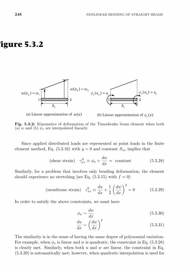
248 NONLINEAR BENDING OF STRAIGHT BEAMS
zero displacements and rotations, which trivially satisfy the Kirchhoff constraintφx = −dw/dx, and the element is said to be very stiff in the thin-beam limitand experience shear locking.
To overcome the locking, one may use equal interpolation for both w andφx but treat φx as a constant in the evaluation of the shear strain, γxz =(dw/dx)+φx. This is often realized by using selective integration, in which one-point (reduced) Gauss quadrature is used to evaluate the stiffness coefficientsassociated with the transverse shear strain, and all other coefficients of thestiffness matrix are evaluated using the exact (full) integration.
1( )aw x w=
1 2
2( )bw x w=
eh
1( )x ax sf =
1 2
eh
2( )x bx sf =
(a) Linear approximation of (b) Linear approximation of ( )w x ( )x xf
Figure 5.3.2
Fig. 5.3.2: Kinematics of deformation of the Timoshenko beam element when both(a) w and (b) φx are interpolated linearly.
Since applied distributed loads are represented as point loads in the finiteelement method, Eq. (5.3.16) with q = 0 and constant Sxx implies that
(shear strain) γ0xz ≡ φx +
dw
dx= constant (5.3.28)
Similarly, for a problem that involves only bending deformation, the elementshould experience no stretching [see Eq. (5.3.15) with f = 0]:
(membrane strain) ε0xx ≡
du
dx+
1
2
(dw
dx
)2
= 0 (5.3.29)
In order to satisfy the above constraints, we must have
φx ∼dw
dx(5.3.30)
du
dx∼(dw
dx
)2
(5.3.31)
The similarity is in the sense of having the same degree of polynomial variation.For example, when φx is linear and w is quadratic, the constraint in Eq. (5.3.28)is clearly met. Similarly, when both u and w are linear, the constraint in Eq.(5.3.29) is automatically met; however, when quadratic interpolation is used for
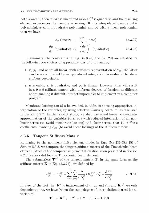
5.3. THE TIMOSHENKO BEAM THEORY 249
both u and w, then du/dx is linear and (dw/dx)2 is quadratic and the resultingelement experiences the membrane locking. If u is interpolated using a cubicpolynomial, w with a quadratic polynomial, and φx with a linear polynomial,then we have
φx (linear) ∼ dw
dx(linear) (5.3.32)
du
dx(quadratic) ∼
(dw
dx
)2
(quadratic) (5.3.33)
In summary, the constraints in Eqs. (5.3.28) and (5.3.29) are satisfied forthe following two choices of approximations of u, w, and φx:
1. u, φx, and w are all linear, with constant representation of γxz; the lattercan be accomplished by using reduced integration to evaluate the shearstiffness coefficients.
2. u is cubic, w is quadratic, and φx is linear. However, this will resultin a 9 × 9 stiffness matrix with different degrees of freedom at differentnodes, making it difficult (but not impossible) to implement in a computerprogram.
Membrane locking can also be avoided, in addition to using appropriate in-terpolation of the variables, by using selective Gauss quadrature, as discussedin Section 5.2.7. In the present study, we shall use equal linear or quadraticapproximation of the variables (u,w, φx) with reduced integration of all non-linear terms (to avoid membrane locking) and shear terms, that is, stiffnesscoefficients involving Sxx (to avoid shear locking) of the stiffness matrix.
5.3.5 Tangent Stiffness Matrix
Returning to the nonlinear finite element model in Eqs. (5.3.23)–(5.3.25) ofSection 5.3.3, we compute the tangent stiffness matrix of the Timoshenko beamelement. Much of the computer implementation discussion presented in Section5.2.8 is also valid for the Timoshenko beam element.
The submatrices Tαβ of the tangent matrix T, in the same form as thestiffness matrix K in Eq. (5.3.27), are defined by
Tαβij = Kαβij +
3∑γ=1
n∑k=1
∂
∂∆βj
(Kαγik
)∆γk −
∂Fαi
∂∆βj
(5.3.34)
In view of the fact that Fα is independent of u, w, and φx, and Kαβ are onlydependent on w, we have (when the same degree of interpolation is used for allvariables)
Tα1 = Kα1, Tα3 = Kα3 for α = 1, 2, 3
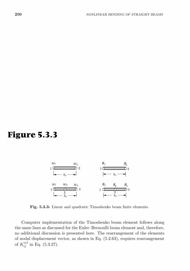
250 NONLINEAR BENDING OF STRAIGHT BEAMS
T 12ij = K12
ij +1
2
∫ xb
xa
Axxdw
dx
dψidx
dψjdx
dx = 2K12ij
T 22ij = K22
ij +
∫ xb
xa
Axx
[du
dx+
(dw
dx
)2]dψidx
dψjdx
dx
T 32ij = K32
ij + 0 = K32ij , T 33
ij = K33ij + 0 = K33
ij
(5.3.35)
where the direct stiffness coefficients Kαβij are defined in Eq. (5.3.26).
As discussed earlier, we must use reduced integration on all nonlinear stiff-ness coefficients as well as all shear stiffness coefficients, while the remainingstiffness coefficients are evaluated using full integration. For example, considerthe following integral expression:∫ xb
xa
Axx
[du
dx
dψidx
dψjdx
+3
2
(dw
dx
)2 dψidx
dψjdx
]dx (5.3.36)
If quadratic approximation of both u and w is used (see Fig. 5.3.3) and Axxis constant, then the first term in the integrand is a cubic polynomial whilethe second term is a fourth-order polynomial. Thus, exact evaluation of thefirst term requires two-point Gauss quadrature while the second term requiresthree-point Gauss quadrature. If we use two-point Gauss quadrature to evalu-ate T 22
ij (and K22ij ), the first term in the coefficient of Axx is integrated exactly
while the second term is integrated approximately. This amounts to approx-imating (dw/dx)2 as a linear polynomial while du/dx as a linear polynomial.Consequently, the constraint ε0
xx = 0 [see Eq. (5.3.29)] is satisfied.
he
1
he
1
w1
2 2
w s s2 21
he
1
he
1
w1
3 3
w w s3 s312
2 2
s2
Figure 5.3.3
Fig. 5.3.3: Linear and quadratic Timoshenko beam finite elements.
Computer implementation of the Timoshenko beam element follows alongthe same lines as discussed for the Euler–Bernoulli beam element and, therefore,no additional discussion is presented here. The rearrangement of the elementsof nodal displacement vector, as shown in Eq. (5.2.63), requires rearrangement
of Kαβij in Eq. (5.3.27).
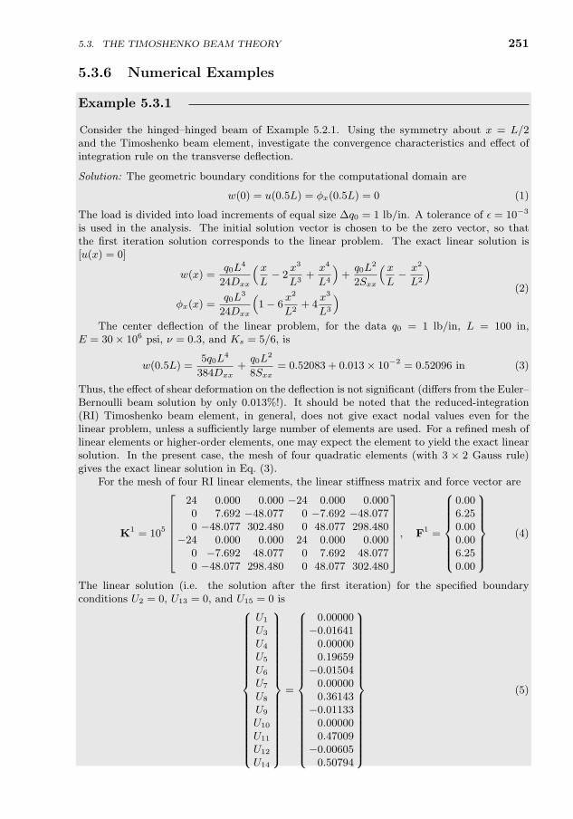
5.3. THE TIMOSHENKO BEAM THEORY 251
5.3.6 Numerical Examples
Example 5.3.1
Consider the hinged–hinged beam of Example 5.2.1. Using the symmetry about x = L/2and the Timoshenko beam element, investigate the convergence characteristics and effect ofintegration rule on the transverse deflection.
Solution: The geometric boundary conditions for the computational domain are
w(0) = u(0.5L) = φx(0.5L) = 0 (1)
The load is divided into load increments of equal size ∆q0 = 1 lb/in. A tolerance of ε = 10−3
is used in the analysis. The initial solution vector is chosen to be the zero vector, so thatthe first iteration solution corresponds to the linear problem. The exact linear solution is[u(x) = 0]
w(x) =q0L
4
24Dxx
( xL− 2
x3
L3+x4
L4
)+q0L
2
2Sxx
( xL− x2
L2
)φx(x) =
q0L3
24Dxx
(1− 6
x2
L2+ 4
x3
L3
) (2)
The center deflection of the linear problem, for the data q0 = 1 lb/in, L = 100 in,E = 30× 106 psi, ν = 0.3, and Ks = 5/6, is
w(0.5L) =5q0L
4
384Dxx+q0L
2
8Sxx= 0.52083 + 0.013× 10−2 = 0.52096 in (3)
Thus, the effect of shear deformation on the deflection is not significant (differs from the Euler–Bernoulli beam solution by only 0.013%!). It should be noted that the reduced-integration(RI) Timoshenko beam element, in general, does not give exact nodal values even for thelinear problem, unless a sufficiently large number of elements are used. For a refined mesh oflinear elements or higher-order elements, one may expect the element to yield the exact linearsolution. In the present case, the mesh of four quadratic elements (with 3 × 2 Gauss rule)gives the exact linear solution in Eq. (3).
For the mesh of four RI linear elements, the linear stiffness matrix and force vector are
K1 = 105
24 0.000 0.000 −24 0.000 0.0000 7.692 −48.077 0 −7.692 −48.0770 −48.077 302.480 0 48.077 298.480
−24 0.000 0.000 24 0.000 0.0000 −7.692 48.077 0 7.692 48.0770 −48.077 298.480 0 48.077 302.480
, F1 =
0.006.250.000.006.250.00
(4)
The linear solution (i.e. the solution after the first iteration) for the specified boundaryconditions U2 = 0, U13 = 0, and U15 = 0 is
U1
U3
U4
U5
U6
U7
U8
U9
U10
U11
U12
U14
=
0.00000−0.01641
0.000000.19659−0.01504
0.000000.36143−0.01133
0.000000.47009−0.00605
0.50794
(5)
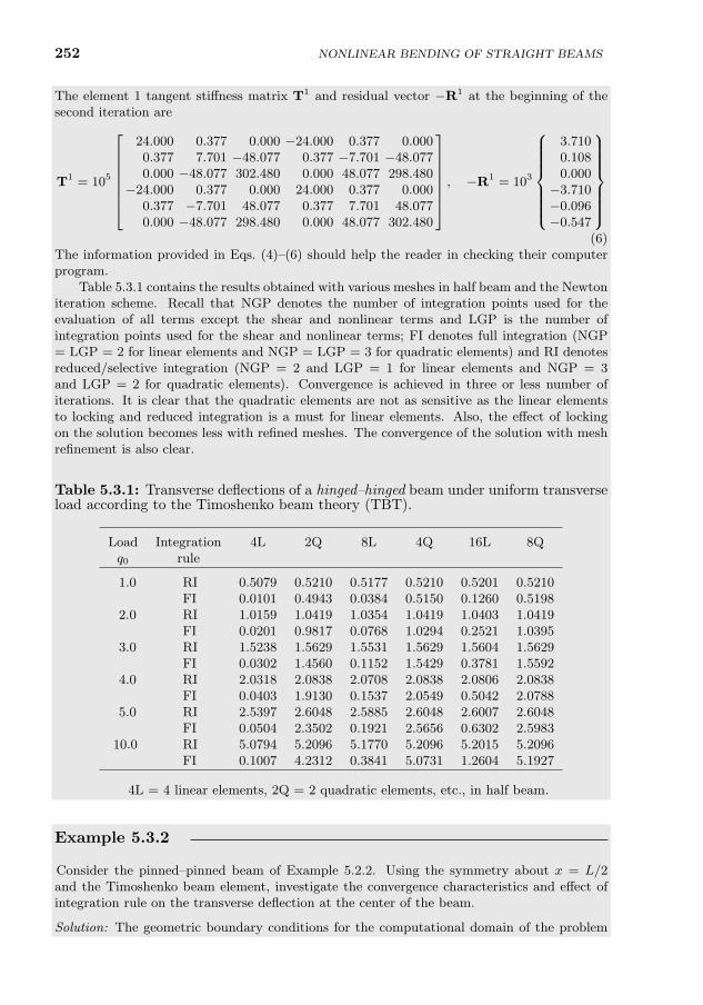
252 NONLINEAR BENDING OF STRAIGHT BEAMS
The element 1 tangent stiffness matrix T1 and residual vector −R1 at the beginning of thesecond iteration are
T1 = 105
24.000 0.377 0.000 −24.000 0.377 0.0000.377 7.701 −48.077 0.377 −7.701 −48.0770.000 −48.077 302.480 0.000 48.077 298.480
−24.000 0.377 0.000 24.000 0.377 0.0000.377 −7.701 48.077 0.377 7.701 48.0770.000 −48.077 298.480 0.000 48.077 302.480
, −R1 = 103
3.7100.1080.000−3.710−0.096−0.547
(6)
The information provided in Eqs. (4)–(6) should help the reader in checking their computerprogram.
Table 5.3.1 contains the results obtained with various meshes in half beam and the Newtoniteration scheme. Recall that NGP denotes the number of integration points used for theevaluation of all terms except the shear and nonlinear terms and LGP is the number ofintegration points used for the shear and nonlinear terms; FI denotes full integration (NGP= LGP = 2 for linear elements and NGP = LGP = 3 for quadratic elements) and RI denotesreduced/selective integration (NGP = 2 and LGP = 1 for linear elements and NGP = 3and LGP = 2 for quadratic elements). Convergence is achieved in three or less number ofiterations. It is clear that the quadratic elements are not as sensitive as the linear elementsto locking and reduced integration is a must for linear elements. Also, the effect of lockingon the solution becomes less with refined meshes. The convergence of the solution with meshrefinement is also clear.
Table 5.3.1: Transverse deflections of a hinged–hinged beam under uniform transverseload according to the Timoshenko beam theory (TBT).
Load Integration 4L 2Q 8L 4Q 16L 8Qq0 rule
1.0 RI 0.5079 0.5210 0.5177 0.5210 0.5201 0.5210FI 0.0101 0.4943 0.0384 0.5150 0.1260 0.5198
2.0 RI 1.0159 1.0419 1.0354 1.0419 1.0403 1.0419FI 0.0201 0.9817 0.0768 1.0294 0.2521 1.0395
3.0 RI 1.5238 1.5629 1.5531 1.5629 1.5604 1.5629FI 0.0302 1.4560 0.1152 1.5429 0.3781 1.5592
4.0 RI 2.0318 2.0838 2.0708 2.0838 2.0806 2.0838FI 0.0403 1.9130 0.1537 2.0549 0.5042 2.0788
5.0 RI 2.5397 2.6048 2.5885 2.6048 2.6007 2.6048FI 0.0504 2.3502 0.1921 2.5656 0.6302 2.5983
10.0 RI 5.0794 5.2096 5.1770 5.2096 5.2015 5.2096FI 0.1007 4.2312 0.3841 5.0731 1.2604 5.1927
4L = 4 linear elements, 2Q = 2 quadratic elements, etc., in half beam.
Example 5.3.2
Consider the pinned–pinned beam of Example 5.2.2. Using the symmetry about x = L/2and the Timoshenko beam element, investigate the convergence characteristics and effect ofintegration rule on the transverse deflection at the center of the beam.
Solution: The geometric boundary conditions for the computational domain of the problem
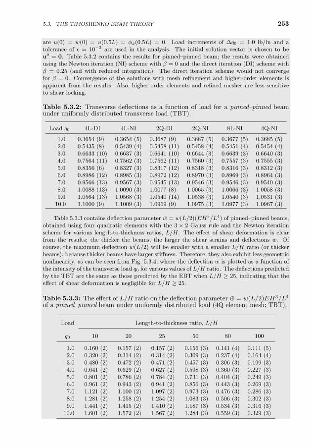
5.3. THE TIMOSHENKO BEAM THEORY 253
are u(0) = w(0) = u(0.5L) = φx(0.5L) = 0. Load increments of ∆q0 = 1.0 lb/in and atolerance of ε = 10−3 are used in the analysis. The initial solution vector is chosen to beu0 = 0. Table 5.3.2 contains the results for pinned–pinned beam; the results were obtainedusing the Newton iteration (NI) scheme with β = 0 and the direct iteration (DI) scheme withβ = 0.25 (and with reduced integration). The direct iteration scheme would not convergefor β = 0. Convergence of the solutions with mesh refinement and higher-order elements isapparent from the results. Also, higher-order elements and refined meshes are less sensitiveto shear locking.
Table 5.3.2: Transverse deflections as a function of load for a pinned–pinned beamunder uniformly distributed transverse load (TBT).
Load q0 4L-DI 4L-NI 2Q-DI 2Q-NI 8L-NI 4Q-NI
1.0 0.3654 (9) 0.3654 (5) 0.3687 (9) 0.3687 (5) 0.3677 (5) 0.3685 (5)2.0 0.5435 (8) 0.5439 (4) 0.5458 (11) 0.5458 (4) 0.5451 (4) 0.5454 (4)3.0 0.6633 (10) 0.6637 (3) 0.6641 (10) 0.6644 (3) 0.6639 (3) 0.6640 (3)4.0 0.7564 (11) 0.7562 (3) 0.7562 (11) 0.7560 (3) 0.7557 (3) 0.7555 (3)5.0 0.8356 (6) 0.8327 (3) 0.8317 (12) 0.8318 (3) 0.8316 (3) 0.8312 (3)6.0 0.8986 (12) 0.8985 (3) 0.8972 (12) 0.8970 (3) 0.8969 (3) 0.8964 (3)7.0 0.9566 (13) 0.9567 (3) 0.9545 (13) 0.9546 (3) 0.9546 (3) 0.9540 (3)8.0 1.0088 (13) 1.0090 (3) 1.0077 (8) 1.0065 (3) 1.0066 (3) 1.0058 (3)9.0 1.0564 (13) 1.0568 (3) 1.0540 (14) 1.0538 (3) 1.0540 (3) 1.0531 (3)
10.0 1.1000 (9) 1.1009 (3) 1.0969 (9) 1.0975 (3) 1.0977 (3) 1.0967 (3)
Table 5.3.3 contains deflection parameter w = w(L/2)(EH3/L4) of pinned–pinned beams,obtained using four quadratic elements with the 3 × 2 Gauss rule and the Newton iterationscheme for various length-to-thickness ratios, L/H. The effect of shear deformation is clearfrom the results; the thicker the beams, the larger the shear strains and deflections w. Ofcourse, the maximum deflection w(L/2) will be smaller with a smaller L/H ratio (or thickerbeams), because thicker beams have larger stiffness. Therefore, they also exhibit less geometricnonlinearity, as can be seen from Fig. 5.3.4, where the deflection w is plotted as a function ofthe intensity of the transverse load q0 for various values of L/H ratio. The deflections predictedby the TBT are the same as those predicted by the EBT when L/H ≥ 25, indicating that theeffect of shear deformation is negligible for L/H ≥ 25.
Table 5.3.3: The effect of L/H ratio on the deflection parameter w = w(L/2)EH3/L4
of a pinned–pinned beam under uniformly distributed load (4Q element mesh; TBT).
Load Length-to-thickness ratio, L/H
q0 10 20 25 50 80 100
1.0 0.160 (2) 0.157 (2) 0.157 (2) 0.156 (3) 0.141 (4) 0.111 (5)2.0 0.320 (2) 0.314 (2) 0.314 (2) 0.309 (3) 0.237 (4) 0.164 (4)3.0 0.480 (2) 0.472 (2) 0.471 (2) 0.457 (3) 0.306 (3) 0.199 (3)4.0 0.641 (2) 0.629 (2) 0.627 (2) 0.598 (3) 0.360 (3) 0.227 (3)5.0 0.801 (2) 0.786 (2) 0.784 (2) 0.731 (3) 0.404 (3) 0.249 (3)6.0 0.961 (2) 0.943 (2) 0.941 (2) 0.856 (3) 0.443 (3) 0.269 (3)7.0 1.121 (2) 1.100 (2) 1.097 (2) 0.973 (3) 0.476 (3) 0.286 (3)8.0 1.281 (2) 1.258 (2) 1.254 (2) 1.083 (3) 0.506 (3) 0.302 (3)9.0 1.441 (2) 1.415 (2) 1.410 (2) 1.187 (3) 0.534 (3) 0.316 (3)
10.0 1.601 (2) 1.572 (2) 1.567 (2) 1.284 (3) 0.559 (3) 0.329 (3)
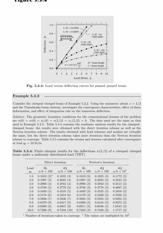
254 NONLINEAR BENDING OF STRAIGHT BEAMS
0 1 2 3 4 5 6 7 8 9 10
Load (lb/in),
0.0
0.2
0.4
0.6
0.8
1.0
Def
lect
ion
3
4(0.5 )EH
w w LL
=
0q
/ 100(TBT,EBT)L H =
/ 80(TBT,EBT)L H =
/ 50(TBT,EBT)L H =
w
/ 10(TBT)L H =
/ 10(EBT)L H =
H = beam heightL = beam length
• • 0q
Figure 5.3.4
Fig. 5.3.4: Load versus deflection curves for pinned–pinned beam.
Example 5.3.3
Consider the clamped–clamped beam of Example 5.2.2. Using the symmetry about x = L/2and the Timoshenko beam element, investigate the convergence characteristics, effect of sheardeformation, and effect of integration rule on the transverse deflection.
Solution: The geometric boundary conditions for the computational domain of the problemare u(0) = w(0) = φx(0) = u(L/2) = φx(L/2) = 0. The data used are the same as thatused in Example 5.3.2. Table 5.3.4 contains the nonlinear analysis results for the clamped–clamped beam; the results were obtained with the direct iteration scheme as well as theNewton iteration scheme. The results obtained with both schemes and meshes are virtuallythe same, but the direct iteration scheme takes more iterations than the Newton iterationscheme to converge. Table 5.3.5 contains the strains and stresses calculated after convergenceat load q0 = 10 lb/in.
Table 5.3.4: Finite element results for the deflections w(L/2) of a clamped–clampedbeam under a uniformly distributed load (TBT).
Direct iteration Newton’s iteration
Load 8L 4Q 8L 4Q 4Qq0 a/h = 100 a/h = 100 a/h = 100 a/h = 100 a/h = 10†
1.0 0.1019 (3)∗ 0.1035 (3) 0.1019 (3) 0.1035 (3) 0.1172 (2)2.0 0.1997 (4) 0.2025 (4) 0.1997 (3) 0.2025 (3) 0.2343 (2)3.0 0.2906 (4) 0.2943 (4) 0.2906 (3) 0.2943 (3) 0.3515 (2)4.0 0.3738 (5) 0.3778 (5) 0.3738 (3) 0.3778 (3) 0.4687 (2)5.0 0.4493 (5) 0.4535 (5) 0.4493 (3) 0.4535 (3) 0.5858 (2)6.0 0.5178 (6) 0.5219 (6) 0.5179 (3) 0.5220 (3) 0.7030 (2)7.0 0.5806 (7) 0.5846 (7) 0.5805 (3) 0.5845 (3) 0.8202 (2)8.0 0.6379 (8) 0.6417 (8) 0.6380 (3) 0.6418 (3) 0.9373 (2)9.0 0.6908 (8) 0.6947 (9) 0.6911 (3) 0.6946 (3) 1.0545 (2)
10.0 0.7406 (9) 0.7434 (10) 0.7403 (3) 0.7436 (3) 1.1717 (2)
∗ Number of iterations taken to converge. † The values are multiplied by 103.
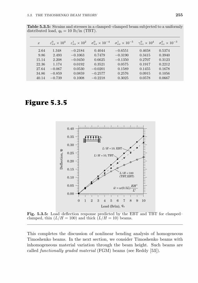
5.3. THE TIMOSHENKO BEAM THEORY 255
Table 5.3.5: Strains and stresses in a clamped–clamped beam subjected to a uniformlydistributed load, q0 = 10 lb/in (TBT).
x ε0xx × 104 ε1xx × 102 σ0xx × 10−4 σ1
xx × 10−5 γ0xz × 104 σ0
xz × 10−3
2.64 1.348 −0.2184 0.4044 −0.6551 0.4658 0.53749.86 2.493 −0.1063 0.7479 −0.3190 0.3415 0.3940
15.14 2.208 −0.0450 0.6625 −0.1350 0.2707 0.312322.36 1.174 0.0192 0.3521 0.0575 0.1917 0.221227.64 −0.067 0.0530 −0.0201 0.1589 0.1455 0.167834.86 −0.859 0.0859 −0.2577 0.2576 0.0915 0.105640.14 −0.739 0.1008 −0.2218 0.3025 0.0578 0.066747.36 0.044 0.1109 0.0133 0.3327 0.0149 0.0172
Figure 5.3.5 contains plots of the deflection parameter, w = w(L/2)EH3/L4, against q0for the EBT and TBT. The results were obtained using the direct iteration scheme, and fourquadratic TBT elements and eight EBT elements. Note that, for L/H = 10, the beam doesnot exhibit nonlinearity but the effect of shear deformation is clear; it increases the deflectioncompared to the Euler–Bernoulli beam theory. For L/H = 100, the effect of shear deformationis negligible, and both theories predict essentially the same load-deflection response.
0 1 2 3 4 5 6 7 8 9 10
Load (lb/in),
0.00
0.05
0.10
0.15
0.20
0.25
0.30
0.35
0.40
Def
lect
ion
, w
0q
3
4(0.5 )
EHw w L
L=
/ 100(TBT,EBT)L H =
/ 10, TBTL H =
/ 10, EBTL H =
0q
Figure 5.3.5
Fig. 5.3.5: Load–deflection response predicted by the EBT and TBT for clamped–clamped, thin (L/H = 100) and thick (L/H = 10) beams.
This completes the discussion of nonlinear bending analysis of homogeneousTimoshenko beams. In the next section, we consider Timoshenko beams withinhomogeneous material variation through the beam height. Such beams arecalled functionally graded material (FGM) beams (see Reddy [53]).
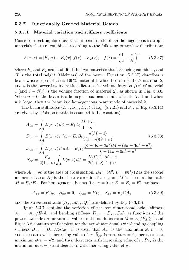
256 NONLINEAR BENDING OF STRAIGHT BEAMS
5.3.7 Functionally Graded Material Beams
5.3.7.1 Material variation and stiffness coefficients
Consider a rectangular cross-section beam made of two homogeneous isotropicmaterials that are combined according to the following power-law distribution:
E(x, z) = [E1(x)− E2(x)] f(z) + E2(x), f(z) =
(1
2+
z
H
)n(5.3.37)
where E1 and E2 are moduli of the two materials that are being combined, andH is the total height (thickness) of the beam. Equation (5.3.37) describes abeam whose top surface is 100% material 1 while bottom is 100% material 2,and n is the power-law index that dictates the volume fraction f(z) of material1 [and 1 − f(z) is the volume fraction of material 2], as shown in Fig. 5.3.6.When n = 0, the beam is a homogeneous beam made of material 1 and whenn is large, then the beam is a homogeneous beam made of material 2.
The beam stiffnesses (Axx, Bxx, Dxx) of Eq. (5.2.21) and Sxx of Eq. (5.3.14)are given by (Poisson’s ratio is assumed to be constant)
Axx =
∫AE(x, z) dA = E2A0
M + n
1 + n
Bxx =
∫AE(x, z)z dA = E2B0
n(M − 1)
2(1 + n)(2 + n)(5.3.38)
Dxx =
∫AE(x, z)z2 dA = E2I0
(6 + 3n+ 3n2)M + (8n+ 3n2 + n3)
6 + 11n+ 6n2 + n3
Sxx =Ks
2(1 + ν)
∫AE(x, z) dA =
KsE2A0
2(1 + ν)
M + n
1 + n
where A0 = bh is the area of cross section, B0 = bh2, I0 = bh3/12 is the secondmoment of area, Ks is the shear correction factor, and M is the modulus ratioM = E1/E2. For homogeneous beams (i.e. n = 0 or E1 = E2 = E), we have
Axx = EA0, Bxx = 0, Dxx = EI0 , Sxx = KsGA0 (5.3.39)
and the stress resultants (Nxx,Mxx, Qx) are defined by Eq. (5.3.13).Figure 5.3.7 contains the variation of the non-dimensional axial stiffness
Axx = Axx/E2A0 and bending stiffness Dxx = Dxx/E2I0 as functions of thepower-law index n for various values of the modulus ratio M = E1/E2 ≥ 1 andFig. 5.3.8 contains similar plots for the non-dimensional axial-bending couplingstiffness Bxx = Bxx/E2B0. It is clear that Axx is the maximum at n = 0and decreases with increasing value of n; Bxx is zero at n = 0, increases to amaximum at n =
√2, and then decreases with increasing value of n; Dxx is the
maximum at n = 0 and decreases with increasing value of n.
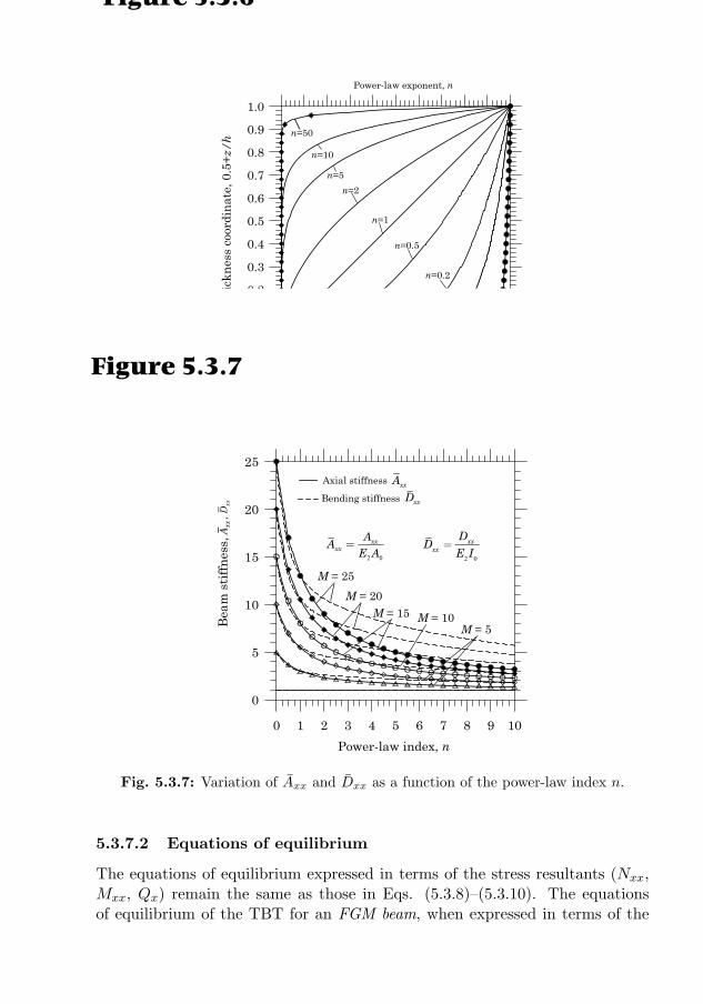
5.3. THE TIMOSHENKO BEAM THEORY 257
Figure 5.3.6
0.0 0.2 0.4 0.6 0.8 1.0
Volume fraction of material 1
0.0
0.1
0.2
0.3
0.4
0.5
0.6
0.7
0.8
0.9
1.0
Th
ick
nes
s co
ordi
nat
e, 0
.5+
z/h
Power-law exponent, n
n=5
n=10
n=0.02
n=1
n=50
n=0.5
n=0.2
n=2
n=0.1
Fig. 5.3.6: Volume fraction of material 1 as a function of the power-law index n.
Figure 5.3.7
0 1 2 3 4 5 6 7 8 9 10
Power-law index, n
0
5
10
15
20
25
Bea
m s
tiff
nes
s,
Axial stiffness
Bending stiffness
xxA
2 0
xxxx
AA
E A=
xxD
2 0
xxxx
DD
E I=
Axx
, Dxx
M = 25
M = 20M = 15 M = 10
M = 5
Fig. 5.3.7: Variation of Axx and Dxx as a function of the power-law index n.
5.3.7.2 Equations of equilibrium
The equations of equilibrium expressed in terms of the stress resultants (Nxx,Mxx, Qx) remain the same as those in Eqs. (5.3.8)–(5.3.10). The equationsof equilibrium of the TBT for an FGM beam, when expressed in terms of the
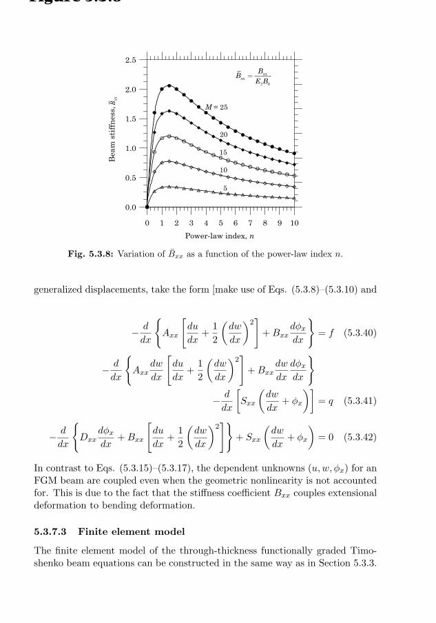
258 NONLINEAR BENDING OF STRAIGHT BEAMS
Figure 5.3.8
0 1 2 3 4 5 6 7 8 9 10
Power-law index, n
0.0
0.5
1.0
1.5
2.0
2.5
Bea
m s
tiff
nes
s, B
xx
2 0
xxxx
BB
E B=
M = 25
20
15
10
5
Fig. 5.3.8: Variation of Bxx as a function of the power-law index n.
generalized displacements, take the form [make use of Eqs. (5.3.8)–(5.3.10) and(5.3.13)]
− d
dx
Axx
[du
dx+
1
2
(dw
dx
)2]
+Bxxdφxdx
= f (5.3.40)
− d
dx
Axx
dw
dx
[du
dx+
1
2
(dw
dx
)2]
+Bxxdw
dx
dφxdx
− d
dx
[Sxx
(dw
dx+ φx
)]= q (5.3.41)
− d
dx
Dxx
dφxdx
+Bxx
[du
dx+
1
2
(dw
dx
)2]
+ Sxx
(dw
dx+ φx
)= 0 (5.3.42)
In contrast to Eqs. (5.3.15)–(5.3.17), the dependent unknowns (u,w, φx) for anFGM beam are coupled even when the geometric nonlinearity is not accountedfor. This is due to the fact that the stiffness coefficient Bxx couples extensionaldeformation to bending deformation.
5.3.7.3 Finite element model
The finite element model of the through-thickness functionally graded Timo-shenko beam equations can be constructed in the same way as in Section 5.3.3.
5.3. THE TIMOSHENKO BEAM THEORY 259
The weak forms associated with Eqs. (5.3.40)–(5.3.42) are
0 =
∫ xb
xa
Axx
dδu
dx
[du
dx+
1
2
(dw
dx
)2]
+Bxxdδu
dx
dφxdx− fδu
dx
−Qe1 δu(xa)−Qe4 δu(xb) (5.3.43)
0 =
∫ xb
xa
dδw
dx
Sxx
(dw
dx+ φx
)+Axx
dw
dx
[du
dx+
1
2
(dw
dx
)2]
+Bxxdw
dx
dφxdx
dx−
∫ xb
xa
δw q dx
−Qe2 δw(xa)−Qe5 δw(xb) (5.3.44)
0 =
∫ xb
xa
Dxx
dδφxdx
dφxdx
+Bxxdδφxdx
[du
dx+
1
2
(dw
dx
)2]
+ Sxx δφx
(dw
dx+ φx
)dx−Qe3 δφx(xa)−Qe6 δφx(xb) (5.3.45)
where Qei (i = 1, 2, . . . , 6) have the same physical meaning as before and theyare defined by Eq. (5.3.21).
Using the finite element approximations in Eq. (5.3.22), we obtain the finiteelement model in Eq. (5.3.27), and the only coefficients that are different fromthose listed in Eq. (5.3.26) are
K13ij =
∫ xb
xa
Bxxdψ
(1)i
dx
dψ(3)j
dxdx = K31
ji
K23ij =
∫ xb
xa
(Sxx
dψ(2)i
dxψ
(3)j +Bxx
dw
dx
dψ(2)i
dx
dψ(3)j
dx
)dx
K32ij =
∫ xb
xa
(Sxxψ
(3)i
dψ(2)j
dx+
1
2Bxx
dw
dx
dψ(3)i
dx
dψ(2)j
dx
)dx
(5.3.46)
The tangent stiffness coefficients also remain the same as in Eq. (5.3.35), exceptfor the following coefficients:
T 22ij = K22
ij +
∫ xb
xa
Axx
[du
dx+
(dw
dx
)2]
+Bxxdφxdx
dψ
(2)i
dx
dψ(2)j
dxdx
T 32ij = K32
ij +1
2
∫ xb
xa
Bxxdw
dx
dψ(3)i
dx
dψ(2)j
dxdx = K23
ji (5.3.47)
In the implementation of the element, we use the same degree of interpola-tion functions for all three variables. The computational aspects with regard to
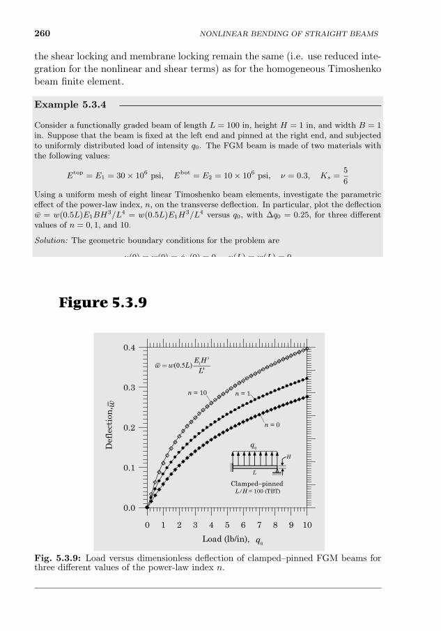
260
the shear locking and membrane locking remain the same (i.e. use reduced inte-gration for the nonlinear and shear terms) as for the homogeneous Timoshenkobeam finite element.
Example 5.3.4
Consider a functionally graded beam of length L = 100 in, height H = 1 in, and width B = 1in. Suppose that the beam is fixed at the left end and pinned at the right end, and subjectedto uniformly distributed load of intensity q0. The FGM beam is made of two materials withthe following values:
Etop = E1 = 30× 106 psi, Ebot = E2 = 10× 106 psi, ν = 0.3, Ks =5
6
Using a uniform mesh of eight linear Timoshenko beam elements, investigate the parametriceffect of the power-law index, n, on the transverse deflection. In particular, plot the deflectionw = w(0.5L)E1BH
3/L4 = w(0.5L)E1H3/L4 versus q0, with ∆q0 = 0.25, for three different
values of n = 0, 1, and 10.
Solution: The geometric boundary conditions for the problem are
u(0) = w(0) = φx(0) = 0, u(L) = w(L) = 0
The program developed earlier for homogeneous beams can be modified for two-constituentfunctionally graded beams. Figure 5.3.9 shows the load-deflection curves for three values ofthe power-law index, n = 0, 1, and 10. The results were obtained with the Newton iterationscheme with a tolerance of ε = 10−3. The value n = 0 corresponds to the homogeneous beammade of material 1. For increasing values of n the beam material approaches that of material2 (with smaller modulus) and, therefore, the beam experiences larger deflections.
0 1 2 3 4 5 6 7 8 9 10
Load (lb/in),
0.0
0.1
0.2
0.3
0.4
Def
lect
ion
,
Clamped-pinned beam
n = 10
L/H = 100 (TBT)
n = 0
n = 1
31
40 5( . )E H
w w LL
=
H
0q
L
0q
w
Figure 5.3.9
Clamped−pinned
Fig. 5.3.9: Load versus dimensionless deflection of clamped–pinned FGM beams forthree different values of the power-law index n.
NONLINEAR BENDING OF STRAIGHT BEAMS
5.4. SUMMARY 261
5.4 Summary
Two different beam theories, namely, the Euler–Bernoulli beam theory and theTimoshenko beam theory, are discussed and their finite element models aredeveloped. Geometric nonlinearity in the form of small strains and moderaterotations (i.e. the von Karman nonlinearity) is included in simplifying the Greenstrain component Exx ≈ εxx. The principle of virtual displacements is used toderive the weak forms of the two beam theories. Displacement finite elementmodels are developed using arbitrary and independent degree of approximationsof the generalized displacements.
Linear approximation of both transverse deflection w and rotation φx in theTimoshenko beam finite element make it experience shear locking. Membranelocking occurs in both theories when inconsistent interpolation of the axialand transverse displacements is used. Both types of locking are eliminated byuse of reduced integration rule in the numerical evaluation stiffness coefficientsinvolving all nonlinear terms and all shear terms.
Computer implementation of the finite element models developed herein isdiscussed and numerical examples are presented to illustrate the effects of theintegration rule, the degree of approximation, and the number of elements onthe accuracy of the results. Postcomputation of stresses is also discussed.
The ideas presented in this chapter for straight beams can be extendedto study axisymmetric bending of circular plates (see Problems 5.6 and 5.7).In fact, the computer program developed for straight beams can be readilymodified for axisymmetric bending of circular plates.
Problems
Weak Forms and Finite Element Models
5.1 Give the expressions for the stiffness coefficients Kαβ (α, β = 1, 2) for the Euler–Bernoulli beam theory for the case in which Bxx 6= 0.
5.2 Give the expressions for the tangent matrix coefficients Tαβ (α, β = 1, 2) for the Euler–Bernoulli beam theory for the case in which Bxx 6= 0.
5.3 Consider the following pair of nonlinear equations:
−dNxxdx
= f(x) (1)
d2
dx2
(Dxx
d2w
dx2
)− d
dx
(Nxx
dw
dx
)= q(x) (2)
where q(x) is the distributed transverse force (positive upward), and
Nxx = Axx
[du
dx+
1
2
(dw
dx
)2]
(3)
Rewrite the equations, by introducing the bending moment M(x) as a dependent vari-able, as a set of second-order equations
− d
dx
Axx
[du
dx+
1
2
(dw
dx
)2]− f(x) = 0 (4)
262 NONLINEAR BENDING OF STRAIGHT BEAMS
−d2w
dx2− Mxx
Dxx= 0 (5)
−d2Mxx
dx2− d
dx
dw
dxAxx
[du
dx+
1
2
(dw
dx
)2]
= q(x) (6)
Develop: (a) the weak form and (b) the finite element model using interpolation of theform
u =m∑j=1
uejψ(1)j (x), w =
n∑j=1
wejψ(2)j (x), Mxx =
r∑j=1
Mej ψ
(3)j (x) (7)
5.4 Consider the problem of bending of beams according to the Euler–Bernoulli beam the-ory. The principle of minimum total potential energy states that if the beam is inequilibrium, then the total potential energy associated with the equilibrium configu-ration is the minimum; that is, the equilibrium displacements are those which makethe total potential energy a minimum. Thus, solving the equations governing the equi-librium of the Euler–Bernoulli beam is equivalent to minimizing the total potentialenergy
Π(u,w) =
∫ xb
xa
Axx
2
[du
dx+
1
2
(dw
dx
)2]2
+Dxx
2
(d2w
dx2
)2dx
−∫ xb
xa
(fu+ qw) dx (1)
where Axx = EA and Dxx = EI are the extensional and bending stiffness coefficients,respectively. The necessary condition for the minimum of a functional is that its firstvariation be zero: δΠ = 0, which yields the governing equations of equilibrium. Asyou know, the statement δΠ = 0 is the same as the weak forms of the governingequations of the Euler–Bernoulli beam theory. The weak form requires Hermite cubicinterpolation of the transverse deflection w. Now suppose that we wish to relax thecontinuity required of the interpolation used for w(x) by introducing the relation
−dwdx
= φx(x) (2)
Then the total potential energy functional takes the form
Π(u,w, φ) =
∫ xb
xa
Axx
2
[du
dx+
1
2
(dw
dx
)2]2
+Dxx
2
(dφxdx
)2dx
−∫ xb
xa
(fu+ qw) dx−6∑i=1
∆eiQ
ei (3)
Since the functional now contains only the first derivative of u, w, and φx, linearLagrange (minimum) interpolation can be used. Thus the original problem is replacedwith the following equivalent problem: minimize Π(u,w, φx) in Eq. (3) subjected tothe constraint
dw
dx+ φx(x) = 0 (4)
In the penalty method, the constraint is included in the functional to be minimized ina least-squares sense, that is construct Πp such that
Πp = Π +γ
2
∫ xb
xa
[dw
dx+ φx(x)
]2dx (5)
where γ is known as the penalty parameter. Develop the penalty function formulationof the constrained problem by deriving (a) the weak form and (b) the finite elementmodel.
PROBLEMS 263
5.5 Develop the weak forms of the governing equations, Eqs. (5.3.15)–(5.3.17); make use ofthe definitions of Qi in Eq. (5.3.21).
5.6 Beginning with the displacement field in axisymmetric bending of a circular plate
ur = u(r)− z dwdr
, uθ = 0, uz = w(r) (1)
(a) develop the virtual work statement and (b) the finite element model for nonlinearbending of circular plates. The strain–displacement relations for small strains andmoderate rotation case are given by (see Reddy [1])
εrr =∂ur∂r
+1
2
(∂uz∂r
)2
, εθθ =urr
(2)
and the (plane–stress) stress–strain relations areσrrσθθ
=
E
1− ν2
[1 νν 1
]εrrεθθ
(3)
where E and ν are Young’s modulus and Poisson’s ratio, respectively.
5.7 The displacement field of circular plates according to the first-order shear deformationplate theory is
ur = u(r) + zφr(r) , uθ = 0, uz = w(r) (1)
Develop (a) the virtual work statement and (b) finite element model accounting forthe von Karman nonlinear strains. See the statement of Problem 5.6 for additionalinformation.
5.8 Develop the mixed finite element model of the following set of nonlinear equationsamong the variables (u,w,M) of the Euler–Bernoulli beam theory with the von Karmanstrains:
−dNdx
= f (1)
−d2M
dx2− d
dx
(Ndw
dx
)= q (2)
M
EI+d2w
dx2= 0 (3)
where f(x) and q(x) are the distributed axial and transverse forces, respectively, EAand EI are the axial and bending stiffnesses, and N is known in terms of u and w as
N = EA
[du
dx+
1
2
(dw
dx
)2]
(4)
Also, compute the tangent stiffness coefficients. Present the finite element model in thestandard format [see, for example, Eq. (5.2.32)] and define all coefficients.
5.9 Develop a mixed least-squares finite element model of the equations in Problem 5.8.
5.10 Develop a least-squares finite element model of the following set of nonlinear equationsthat arise in connection with the Timoshenko beam theory (assume that EA, EI, andGAKs are constant):
−dNdx
= f (1)
− d
dx
[GAKs
(φ+
dw
dx
)]− d
dx
(Ndw
dx
)= q (2)
− d
dx
(EI
dφ
dx
)+GAKs
(φ+
dw
dx
)= 0 (3)
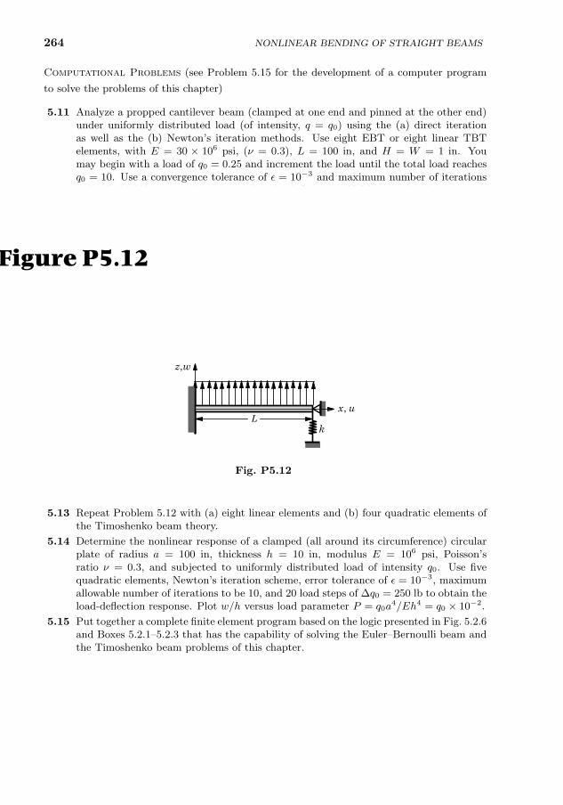
264 NONLINEAR BENDING OF STRAIGHT BEAMS
Computational Problems (see Problem 5.15 for the development of a computer program
to solve the problems of this chapter)
5.11 Analyze a propped cantilever beam (clamped at one end and pinned at the other end)under uniformly distributed load (of intensity, q = q0) using the (a) direct iterationas well as the (b) Newton’s iteration methods. Use eight EBT or eight linear TBTelements, with E = 30 × 106 psi, (ν = 0.3), L = 100 in, and H = W = 1 in. Youmay begin with a load of q0 = 0.25 and increment the load until the total load reachesq0 = 10. Use a convergence tolerance of ε = 10−3 and maximum number of iterationsto be ITMAX = 50. Tabulate and plot the deflection w(L/2) versus load q0.
5.12 Analyze a beam (EA, EI, L) with one end fixed and the other end vertically supportedby a linear elastic spring with spring constant k (lb/in), as shown in Fig. P5.12. Thebeam is subjected to uniformly distributed transverse load of intensity q0 (lb/in). Usethe Euler–Bernoulli beam element with Newton’s iteration method. Use eight elementsin the beam (1× 1 in2 cross section, E = 30× 106 psi, and L = 100 in) and k = 0, 25,and 250 (i.e. three different cases). Tabulate and plot the deflection w(L) versus theload q0, with maximum load of q0 = 10 (lb/in), for two separate cases: (a) horizontalmovement of the free end is not restricted, and (b) the horizontal movement of thefree end is restricted to zero. A load increment of ∆q0 = 0.5 (lb/in) is suggested.Use a convergence tolerance of ε = 10−3 and the maximum number of iterations to beITMAX = 25.
Figure P5.12
L,x u
,z w
k
Fig. P5.12
5.13 Repeat Problem 5.12 with (a) eight linear elements and (b) four quadratic elements ofthe Timoshenko beam theory.
5.14 Determine the nonlinear response of a clamped (all around its circumference) circularplate of radius a = 100 in, thickness h = 10 in, modulus E = 106 psi, Poisson’sratio ν = 0.3, and subjected to uniformly distributed load of intensity q0. Use fivequadratic elements, Newton’s iteration scheme, error tolerance of ε = 10−3, maximumallowable number of iterations to be 10, and 20 load steps of ∆q0 = 250 lb to obtain theload-deflection response. Plot w/h versus load parameter P = q0a
4/Eh4 = q0 × 10−2.
5.15 Put together a complete finite element program based on the logic presented in Fig. 5.2.6and Boxes 5.2.1–5.2.3 that has the capability of solving the Euler–Bernoulli beam andthe Timoshenko beam problems of this chapter.
265
6
Two-Dimensional ProblemsInvolving a Single Variable
I know that most men, including those at ease with problems of the greatest complexity, canseldom accept even the simplest and most obvious truth if it be such as would oblige them toadmit the falsity of conclusions which they have delighted in explaining to colleagues, whichthey have proudly taught to others, and which they have woven, thread by thread, into thefabric of their lives. ——– Leo Nikolayevich Tolstoy
6.1 Model Equation
The finite element analysis of nonlinear two-dimensional problems involves thesame basic steps as those described for one-dimensional problems in Chapter3. Finite element formulation of a model second-order equation was presentedin Section 3.3. Here, we extend that development to problems in which thecoefficients of the differential equation are possibly functions of the dependentvariable and its derivatives.
Consider the problem of finding the solution u(x, y) of the following second-order partial differential equation (a more general equation than the one con-sidered in Section 3.3)
− ∂
∂x
(axx
∂u
∂x+ axy
∂u
∂y
)− ∂
∂y
(ayx
∂u
∂x+ ayy
∂u
∂y
)+ a00u = f(x, y) in Ω
(6.1.1)where axx, ayy, axy, ayx, and a00 are known functions of position (x, y) as wellas the dependent unknown u and its derivatives, and f is a known function ofposition in a two-dimensional domain Ω with boundary Γ [see Fig. 6.1.1(a)]. Ingeneral, axy 6= ayx and a00, in most cases, is zero. For example, axx may beassumed to be of the form
axx = axx
(x, y, u,
∂u
∂x,∂u
∂y
)(6.1.2)
The same type of dependence of other coefficients on u, ∂u/∂x, and ∂u/∂y isassumed. The equation is subject to certain boundary conditions, whose formwill be apparent from the weak formulation.
J.N. Reddy, An Introduction to Nonlinear Finite Element Analysis, Second Edition. c©J.N.Reddy 2015. Published in 2015 by Oxford University Press.
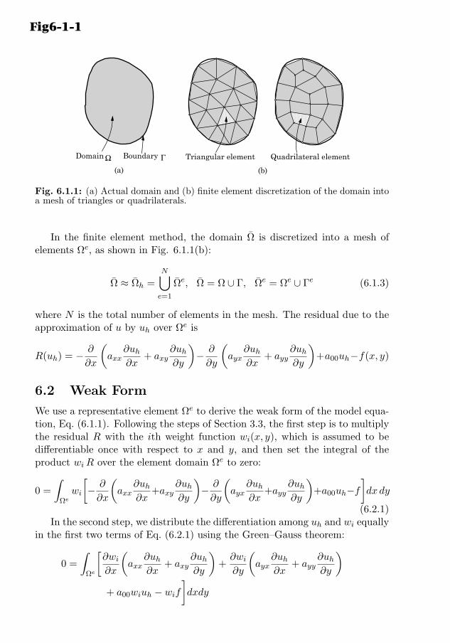
266 TWO-DIMENSIONAL PROBLEMS INVOLVING A SINGLE VARIABLE
Triangular element Quadrilateral elementDomain Boundary
(a) (b)
Ω Γ
Fig6-1-1
Fig. 6.1.1: (a) Actual domain and (b) finite element discretization of the domain intoa mesh of triangles or quadrilaterals.
In the finite element method, the domain Ω is discretized into a mesh ofelements Ωe, as shown in Fig. 6.1.1(b):
Ω ≈ Ωh =
N⋃e=1
Ωe, Ω = Ω ∪ Γ, Ωe = Ωe ∪ Γe (6.1.3)
where N is the total number of elements in the mesh. The residual due to theapproximation of u by uh over Ωe is
R(uh) = − ∂
∂x
(axx
∂uh∂x
+ axy∂uh∂y
)− ∂
∂y
(ayx
∂uh∂x
+ ayy∂uh∂y
)+a00uh−f(x, y)
6.2 Weak Form
We use a representative element Ωe to derive the weak form of the model equa-tion, Eq. (6.1.1). Following the steps of Section 3.3, the first step is to multiplythe residual R with the ith weight function wi(x, y), which is assumed to bedifferentiable once with respect to x and y, and then set the integral of theproduct wiR over the element domain Ωe to zero:
0 =
∫Ωe
wi
[− ∂
∂x
(axx
∂uh∂x
+axy∂uh∂y
)− ∂
∂y
(ayx
∂uh∂x
+ayy∂uh∂y
)+a00uh−f
]dx dy
(6.2.1)In the second step, we distribute the differentiation among uh and wi equally
in the first two terms of Eq. (6.2.1) using the Green–Gauss theorem:
0 =
∫Ωe
[∂wi∂x
(axx
∂uh∂x
+ axy∂uh∂y
)+∂wi∂y
(ayx
∂uh∂x
+ ayy∂uh∂y
)+ a00wiuh − wif
]dxdy
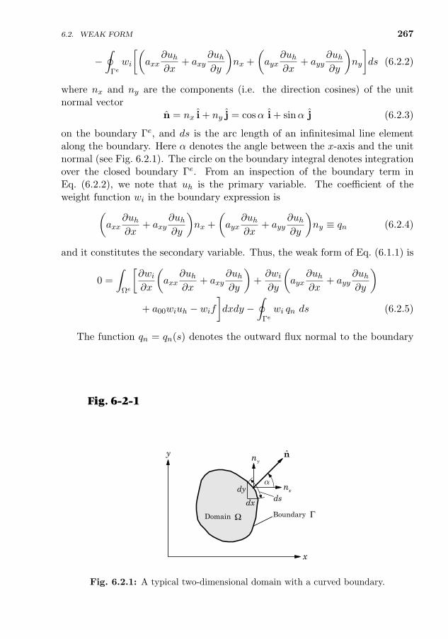
6.2. WEAK FORM 267
−∮
Γe
wi
[(axx
∂uh∂x
+ axy∂uh∂y
)nx +
(ayx
∂uh∂x
+ ayy∂uh∂y
)ny
]ds (6.2.2)
where nx and ny are the components (i.e. the direction cosines) of the unitnormal vector
n = nx i + ny j = cosα i + sinα j (6.2.3)
on the boundary Γe, and ds is the arc length of an infinitesimal line elementalong the boundary. Here α denotes the angle between the x-axis and the unitnormal (see Fig. 6.2.1). The circle on the boundary integral denotes integrationover the closed boundary Γe. From an inspection of the boundary term inEq. (6.2.2), we note that uh is the primary variable. The coefficient of theweight function wi in the boundary expression is(
axx∂uh∂x
+ axy∂uh∂y
)nx +
(ayx
∂uh∂x
+ ayy∂uh∂y
)ny ≡ qn (6.2.4)
and it constitutes the secondary variable. Thus, the weak form of Eq. (6.1.1) is
0 =
∫Ωe
[∂wi∂x
(axx
∂uh∂x
+ axy∂uh∂y
)+∂wi∂y
(ayx
∂uh∂x
+ ayy∂uh∂y
)+ a00wiuh − wif
]dxdy −
∮Γe
wi qn ds (6.2.5)
The function qn = qn(s) denotes the outward flux normal to the boundaryas we move counter-clockwise along the boundary Γe. The secondary variableqn is of physical interest in most problems. For example, in the case of the heattransfer through an anisotropic medium, aij denotes the conductivities of themedium, and qn denotes the heat flux normal to the boundary of the element.The weak form in Eq. (6.2.5) will be the basis of the weak-form Galerkin finiteelement model, in which wi will be replaced by the approximation functionsused to represent uh.
Fig. 6-2-1
x
y
ΩDomain
dy
dx dsxn
yn n
Boundary Γ
a
Fig. 6.2.1: A typical two-dimensional domain with a curved boundary.
268 TWO-DIMENSIONAL PROBLEMS INVOLVING A SINGLE VARIABLE
6.3 Finite Element Model
The weak form in Eq. (6.2.5) requires that the approximation chosen for ushould be at least linear in both x and y so that every term in Eq. (6.2.5)has a non-zero contribution to the integral. Since the primary variable is justu, which must be made continuous between elements, the Lagrange family ofinterpolation functions is admissible. Hence, u is approximated over a typicalfinite element Ωe by the expression
u(x, y) ≈ ueh(x, y) =
n∑j=1
uejψej (x, y) (6.3.1)
where uej is the value of ueh at the jth node of the element, and ψej are theLagrange interpolation functions derived in Section 3.3.5, and they have thefollowing properties:
ψei (xej , y
ej ) = δij ,
n∑j=1
ψej (x, y) = 1 (6.3.2)
where (xej , yej ) denote the global coordinates of the jth node of element Ωe.
Substituting the finite element approximation in Eq. (6.3.1) for uh into theweak form, Eq. (6.2.5), we obtain
0 =n∑j=1
uej
∫Ωe
[∂wi∂x
(axx
∂ψej∂x
+ axy∂ψej∂y
)+∂wi∂y
(ayx
∂ψej∂x
+ ayy∂ψej∂y
)
+ a00wiψej
]dxdy −
∫Ωe
wif dxdy −∮
Γe
wi qn ds (6.3.3)
For the weak-form Galerkin model, we replace the weight function with ψei andobtain
n∑j=1
Keiju
ej − fei −Qei = 0 or Keue = f e + Qe (6.3.4)
where
Keij =
∫Ωe
[∂ψei∂x
(axx
∂ψej∂x
+ axy∂ψej∂y
)+∂ψei∂y
(ayx
∂ψej∂x
+ ayy∂ψej∂y
)+ a00ψ
eiψ
ej
]dxdy (6.3.5)
fei =
∫Ωe
ψei f dx dy, Qe =
∮Γe
ψei qn ds
Note that Keij 6= Ke
ji (i.e. Ke is not symmetric) unless axy = ayx. Equation(6.3.4) represents a set of n nonlinear algebraic equations.
6.4. SOLUTION OF NONLINEAR EQUATIONS 269
Equation (6.3.4) represents the finite element model of Eq. (6.1.1). Thiscompletes the finite element model development. The usual tasks of assemblyof element equations, imposition of boundary conditions, and solution of linearalgebraic equations (after an iterative method is applied) are standard, whichwere discussed in Chapter 3. Therefore, they are not discussed here again.
6.4 Solution of Nonlinear Equations
6.4.1 Direct Iteration Scheme
The assembled form of the nonlinear equation, Eq. (6.3.4) is
K(U)U = F (6.4.1)
where K is the assembled coefficient matrix, U the vector of global nodal values,and F the assembled source vector. In the direct iteration scheme, we assumethat the solution at the (r − 1)st iteration is known and seek the solution atthe rth iteration from the equation
K(U(r−1))U(r) = F(r−1) (6.4.2)
where the direct coefficient matrix K and the right-hand side vector F, if de-pends on U, are evaluated using the known solution from the (r−1)st iteration.As applied to the element equation in Eq. (6.3.4), the direct iteration schemehas the form
Ke(u(r−1))u(r) = Fe (6.4.3)
Thus, we evaluate element matrices using the solution known from (r − 1)stiteration and assemble them to obtain Eq. (6.4.2). The assembled system ofequations is then solved after applying the boundary conditions.
6.4.2 Newton’s Iteration Scheme
In the Newton procedure, we solve the assembled system of equations for thesolution increment ∆U
T(U(r−1))∆U = −R(U(r−1)) (6.4.4)
where R is the assembled residual vector
R(U) = K(U)U− F (6.4.5)
and T is the assembled tangent matrix
T(U) ≡ ∂R
∂U(6.4.6)
270 TWO-DIMENSIONAL PROBLEMS INVOLVING A SINGLE VARIABLE
The total solution at the end of the rth iteration is given by
U(r) = U(r−1) + ∆U (6.4.7)
The element-wise computation of the tangent matrix coefficients were dis-cussed in Chapters 4 and 5. The coefficients of the element tangent matrix arecomputed using the definition
T eij ≡∂Rei∂uej
= Keij +
n∑m=1
∂Keim
∂uejuem −
∂F ei∂uej
(6.4.8)
At the element level, Eq. (6.4.4) takes the form
[Te(ue)](r−1)∆u(r) = Fe(u(r−1))− [Ke(ue)](r−1)(ue)(r−1) (6.4.9)
Example 6.4.1
Suppose that axy, ayx, and a00 are functions of x and y, and aexx and aeyy have the form
aexx = ae11 + ae1u · u+ ae1ux ·∂u
∂x+ ae1uy ·
∂u
∂y
aeyy = ae22 + ae2u · u+ ae2ux ·∂u
∂x+ ae2uy ·
∂u
∂y
(1)
where a11, a1u, and so on are functions of only x and y. Determine the tangent coefficientmatrix.
Solution: We have
T eij = Ke
ij +
n∑m=1
∂Keim
∂ujuem (2)
where
n∑m=1
∂Keim
∂uej
uem =
n∑m=1
[∫Ωe
(∂aexx∂ue
j
∂ψei
∂x
∂ψem
∂x+∂aeyy∂ue
j
∂ψei
∂y
∂ψem
∂y
)dx dy
]uem
=n∑
m=1
∫Ωe
[(ae1uψ
ej + ae1ux
∂ψej
∂x+ ae1uy
∂ψej
∂y
)∂ψei
∂x
∂ψem
∂x
+(ae2uψ
ej + ae2ux
∂ψej
∂x+ ae2uy
∂ψej
∂y
)∂ψei
∂y
∂ψem
∂y
]dx dy
uem
=
∫Ωe
[∂u
∂x
∂ψei
∂x
(ae1uψ
ej + ae1ux
∂ψej
∂x+ ae1uy
∂ψej
∂y
)+∂u
∂y
∂ψei
∂y
(ae2uψ
ej + ae2ux
∂ψej
∂x+ ae2uy
∂ψej
∂y
)]dx dy (3)
The symmetry of Te depends on the nature of the nonlinearity and Ke.
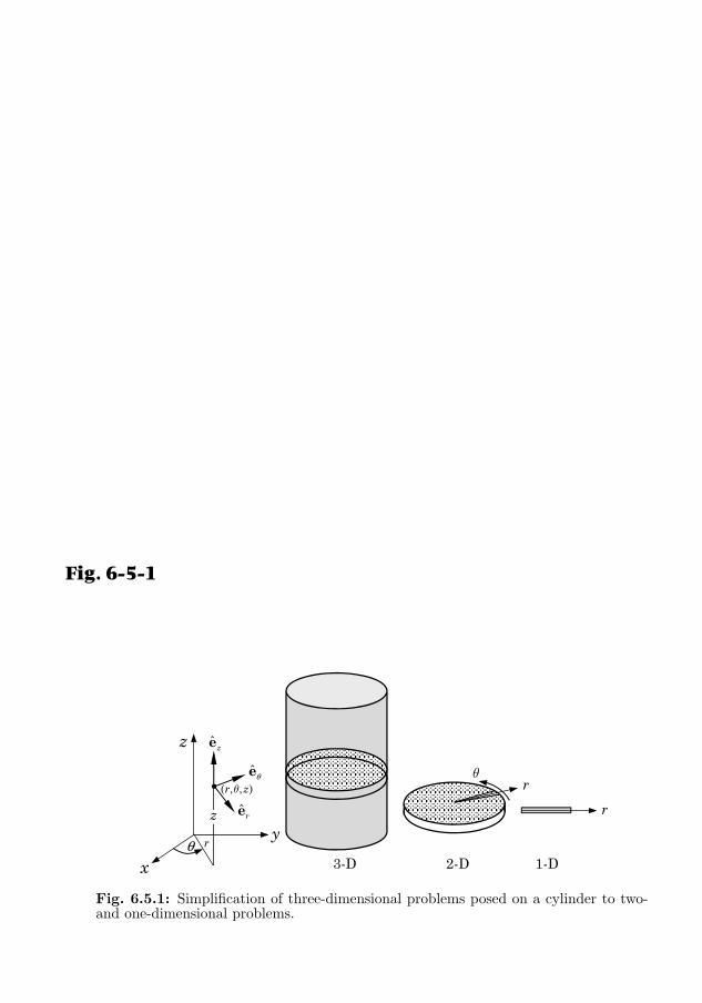
6.5. AXISYMMETRIC PROBLEMS 271
6.5 Axisymmetric Problems
6.5.1 Introduction
Consider the differential equation in the cylindrical coordinate system (r, θ, z)
−1
r
∂
∂r
(rarr
∂u
∂r
)− 1
r2
∂
∂θ
(aθθ
∂u
∂θ
)− ∂
∂z
(azz
∂u
∂z
)= f (6.5.1)
where, in general, u, f , arr, aθθ, and azz are functions of r, θ, and z. When thedomain of the phenomena is a circular cylinder, the problem may be reduced toa two-dimensional or even one-dimensional problem, depending on the materialproperties (arr, aθθ, and azz), boundary conditions, and applied load, f . Theproblems described by Eq. (6.5.1) and posed on a circular cylinder, hollow orsolid, can be simplified as follows.
When the cylinder is very long and material properties, boundary condi-tions, and applied loads do not vary along the length of the cylinder (i.e. in-dependent of the coordinate z), it can be modeled as a circular disk of arbi-trary thickness, that is, two-dimensional domain in the rθ-plane, as shown inFig. 6.5.1. In addition, if the material properties, boundary conditions, andapplied loads do not vary with the circumferential coordinate θ, the disc canbe replaced with a radial line and the problem becomes a one-dimensional one.
The governing equation for the two-dimensional case is given by
−1
r
∂
∂r
(rarr
∂u
∂r
)− 1
r2
∂
∂θ
(aθθ
∂u
∂θ
)= f(r, θ) (6.5.2)
and for the one-dimensional case, the governing equation is
−1
r
d
dr
(rarr
du
dr
)= f(r) (6.5.3)
2-D 1-D
r
r
q
3-Dx
z
yθ
z
( , , )r zq
r
ez
er
eθ
Fig. 6-5-1
Fig. 6.5.1: Simplification of three-dimensional problems posed on a cylinder to two-and one-dimensional problems.
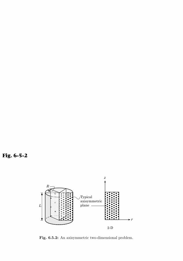
272 TWO-DIMENSIONAL PROBLEMS INVOLVING A SINGLE VARIABLE
6.5.2 Governing Equation and the Finite Element Model
When the cylinder is of finite length and material properties, boundary condi-tions, and applied loads vary along the length of the cylinder but independent ofthe circumferential coordinate θ, we can use any typical plane (a wedge) of thedomain, as shown in Fig. 6.5.2. The governing equation in this case becomes
−1
r
∂
∂r
(rarr
∂u
∂r
)− ∂
∂z
(azz
∂u
∂z
)= f(r, z) (6.5.4)
The weak form of Eq. (6.5.4) is given by
0 =
∫Ωe
wi
[−1
r
∂
∂r
(rarr
∂uh∂r
)− ∂
∂z
(azz
∂uh∂z
)− f(r, z)
]rdrdz
=
∫Ωe
[arr(r, z, uh)
∂wi∂r
∂uh∂r
+ azz(r, z, uh)∂wi∂z
∂uh∂z
]rdrdz
−∫
Ωe
wif(r, z) rdrdz −∮
Γe
wiqn ds (6.5.5)
where
qn(s) = r[arr(r, z, uh)
∂uh∂r
nr + azz(r, z, uh)∂uh∂z
nz
](6.5.6)
and (nr, nz) are the direction cosines of the unit normal n to the boundary Γe.The finite element model is given by
Keue = f e + Qe ≡ Fe (6.5.7)
where
Keij =
∫Ωe
[arr(r, z, uh)
∂ψei∂r
∂ψej∂r
+ azz(r, z, uh)∂ψei∂z
∂ψej∂z
]rdrdz
fei =
∫Ωe
f(r, z)ψei rdrdz, Qei =
∮Γe
qnψei ds
(6.5.8)
L
R
z
r
Typical axisymmetric plane
2-D
Fig. 6-5-2
Fig. 6.5.2: An axisymmetric two-dimensional problem.
6.6. COMPUTER IMPLEMENTATION 273
and ψei (r, z) are the Lagrange interpolation functions of Section 3.3.5 [with(x, y) replaced by (r, z)]. This completes the finite element formulation of axi-symmetric problems. All other aspects are the same as those discussed for planeproblems.
6.6 Computer Implementation
6.6.1 Introduction
An accurate representation of non-rectangular domains and domains with curvedboundaries can be accomplished by the use of refined meshes and/or higher-order elements (i.e. elements with higher-order interpolation functions). Thegeometry of the elements used to represent an irregular domain tend to benon-rectangular and, therefore, evaluation of the integrals involved in the com-putation of Ke
ij , fei , and T eij over the irregularly-shaped elements is difficult. A
coordinate transformation between the coordinates (x, y) used in the formula-tion of the problem, called global coordinates, and another coordinate system(ξ, η), called a local coordinate system, which is convenient in deriving the in-terpolation functions as well as evaluating the integrals is needed. The choiceof the local coordinate system is dictated by the choice of the numerical inte-gration method. As discussed in Section 3.6, we shall use, as was done in one-dimensional problems, the Gauss quadrature rule to evaluate integrals definedover two-dimensional elements. The main steps in the numerical evaluation offinite element matrices are reviewed here from a computational view point.
6.6.2 Numerical Integration
The transformation between Ωe and Ω is accomplished by a coordinate trans-formation of the form [see Eqs. (3.6.1) and (3.6.2)]
x =
m∑j=1
xejψej (ξ, η) , y =
m∑j=1
yej ψej (ξ, η) (6.6.1)
while a typical dependent variable u(x, y) is approximated by
u(x, y) =
n∑j=1
uejψej (x, y) =
n∑j=1
uejψej (x(ξ, η), y(ξ, η)) (6.6.2)
where ψej denote the interpolation functions of the master element Ω and ψej arethe interpolation functions of a typical element Ωe over which u is approximated.The transformation in Eq. (6.6.1) maps a point (x, y) in a typical element Ωe
of the mesh to a point (ξ, η) in the master element Ω and vice versa, if theJacobian Je of the transformation is positive-definite [see Eqs. (3.6.5)–(3.6.8)].
274 TWO-DIMENSIONAL PROBLEMS INVOLVING A SINGLE VARIABLE
The integral expressions involved in the calculation of Ke and f e [see Eqs.(6.3.5) and (6.5.8)] are, in general, complicated algebraically due to the geome-try of the element, spatial variation of the parameters and their dependence onthe solution and possibly its derivatives, and the coordinate transformations.Therefore, the integrals are evaluated numerically, which requires evaluation ofthe integrand at a selective number of points in the domain, multiplying theirvalues with suitable weights, and summing. Here we use the Gauss quadraturediscussed in Section 3.6.3 to evaluate integrals over quadrilateral elements.
We recall from Section 3.6.3 the essential elements of the Gauss quadratureby considering the following integral expression:
Keij =
∫Ωe
(axx
∂ψei∂x
∂ψej∂x
+ ayy∂ψei∂y
∂ψej∂y
+ a00ψeiψ
ej
)dx dy (6.6.3)
We wish to transform the integral from Ωe to the master element Ω = (ξ, η) :−1 ≤ ξ ≤ 1, −1 ≤ η ≤ 1 so that the Gauss quadrature can be used. Thederivatives of ψei with respect to the global coordinates (x, y) in Ke
ij must beexpressed in terms of the derivative with respect to (ξ, η). This relationship isgiven by Eq. (3.6.6)
∂ψei
∂x
∂ψei
∂y
= (Je)−1
∂ψe
i∂ξ
∂ψei
∂η
(6.6.4)
where Je is the Jacobian matrix defined in Eq. (3.6.5), and it is calculated from
Je =
[∂x∂ξ
∂y∂ξ
∂x∂η
∂y∂η
]=
∑mi=1 xi
∂ψi
∂ξ
∑mi=1 yi
∂ψi
∂ξ∑mi=1 xi
∂ψi
∂η
∑mi=1 yi
∂ψi
∂η
=
∂ψ1
∂ξ∂ψ2
∂ξ · · ·∂ψm
∂ξ
∂ψ1
∂η∂ψ2
∂η · · ·∂ψm
∂η
x1 y1
x2 y2...
...xm ym
(6.6.5)
Thus, given the global coordinates (xei , yei ) of element nodes and the interpo-
lation functions ψei used for geometry, the Jacobian matrix can be evaluatedusing Eq. (6.6.5). Note that ψei are different, in general, from ψei used in theapproximation of the dependent variables. Whenever ψei = ψei , we say that anisoparametric formulation is adopted. The Jacobian is given by
Je = |Je| = Je11Je22 − Je12J
e21 (6.6.6)
We have from Eq. (6.6.4)∂ψe
i∂x
∂ψei
∂y
= (Je)−1
∂ψe
i∂ξ
∂ψei
∂η
≡ J∗
∂ψe
i∂ξ
∂ψei
∂η
(6.6.7)
where
J∗11 = Je22/Je, J∗
12 = −Je12/Je, J∗22 = Je11/Je, J∗
21 = −Je21/Je (6.6.8)
6.6. COMPUTER IMPLEMENTATION 275
Returning to the coefficients Keij in Eq. (6.6.3), we can write it now in terms
of the natural coordinates (ξ, η) as
Keij =
∫Ω
axx(ξ, η)
(J∗
11
∂ψei∂ξ
+ J∗12
∂ψei∂η
)(J∗
11
∂ψej∂ξ
+ J∗12
∂ψej∂η
)+ ayy(ξ, η)
(J∗
21
∂ψei∂ξ
+ J∗22
∂ψei∂η
)(J∗
21
∂ψej∂ξ
+ J∗22
∂ψej∂η
)+ a00(ξ, η)ψeiψ
ej
Je dξ dη
≡∫
ΩF eij(ξ, η) dξ dη (6.6.9)
where the element area dA = dxdy in element Ωe is transformed to Je dξ dη inthe master element Ω, and axx = axx(x(ξ, η), y(ξ, η), u(ξ, η)), and so on.
Using the M × N Gauss quadrature to evaluate integrals defined over arectangular master element Ω, we obtain∫
ΩF eij(ξ, η) dξ dη =
∫ 1
−1
[∫ 1
−1F eij(ξ, η) dη
]dξ ≈
∫ 1
−1
[N∑J=1
F eij(ξ, ηJ)WJ
]dξ
≈M∑I=1
N∑J=1
F eij(ξI , ηJ)WIWJ (6.6.10)
where M and N denote the number of Gauss quadrature points in the ξ andη directions, respectively, (ξI , ηJ) denote the Gauss points, and WI and WJ
denote the corresponding Gauss weights, as listed in Table 3.6.1.As already discussed, if the integrand is a polynomial of degree p in a coordi-
nate direction, it is integrated exactly by employing NGP ≡ N = int[12(p+ 1)]
(the nearest equal or larger integer number) Gauss points in that direction. Inmost cases, the interpolation functions are of the same degree in both ξ andη, and we take N = M . For example, consider the expression involving a00 inKeij of Eq. (6.6.3). When a00 is a linear function of ξ and η, it requires a 2× 2
Gauss rule when ψei are linear and a 3 × 3 Gauss rule when ψei are quadraticto be evaluated exactly. When a00 is quadratic or cubic, it requires 3 × 3 and4× 4 Gauss rules for linear and quadratic rectangular elements, respectively.
6.6.3 Element Calculations
Calculation of element coefficients require evaluation of interpolation functionsand their derivatives. The statements for the calculation of the approximationfunctions ψei (ξ, η), their derivatives with respect to (ξ, η), the Jacobian matrixand its determinant, and derivatives of ψei with respect to (x, y) using Eq. (6.6.7)are included in the subroutine INTERPLN2D, which is listed in Box 3.7.3. The
276 TWO-DIMENSIONAL PROBLEMS INVOLVING A SINGLE VARIABLE
notation used in INTERPLN2D is recalled briefly here (also see Section 3.7.3for more details):
SFL(i) = ψei
DSFL(1, i) =∂ψei∂ξ
, DSFL(2, i) =∂ψei∂η
[ELXY] = array of the global coordinates of element nodes
ELXY(i, 1) = xi, ELXY(i, 2) = yi
[GJ] = the Jacobian matrix,Je; [GJ] = [DSFL][ELXY]
[GJINV] = inverse of the Jacobian matrix, [GJ]−1
DET = the determinant of the Jacobian matrix, Je = |Je|
GDSFL(1, i) =∂ψei∂x
, GDSFL(2, i) =∂ψei∂y
[GDSFL] = [GJINV][DSFL]
A Fortran listing of subroutine ELEMATRCS2D, in which matrices Ke andf e for the model problem (with axy = ayx = 0) of this chapter are calculated,is listed in Box 6.6.1. The following notation is used (n = NPE):
ELF(i) = fei , the ith component of the source vector
ELK(i, j) = Keij , the (i, j) component of the element coefficient matrix
TANG(i, j) =
n∑m=1
∂Keim
∂ujuem, addition to Ke
ij to obtain T eij
GAUSPT(I, J) = Ith Gauss point in the Jth Gauss-point rule (I ≤ J)
GAUSWT(I, J) = Ith Gauss weight in the Jth Gauss-point rule (I ≤ J)
ELU(I) = uei from the previous iteration
NGPF = number of Gauss points - full integration
NONLIN = Flag for nonlinear analysis; it is also used for type of
the iteration method: = 1, Picard; > 1, Newton
The element matrix Ke can be expressed in terms of the submatrices Sαβ
[Sαβ(i, j) = Sαβij ] defined in Eq. (3.7.10), and therefore one can use them toverify the values of Ke calculated in a computer program.
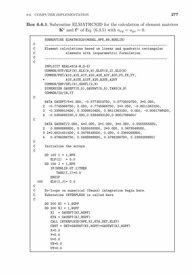
6.6. COMPUTER IMPLEMENTATION 277
Box 6.6.1: Subroutine ELMATRCS2D for the calculation of element matricesKe and f e of Eq. (6.3.5) with axy = ayx = 0.
SUBROUTINE ELMATRCS2D(MODEL,NPE,NN,NONLIN)
C ________________________________________________________________
C Element calculations based on linear and quadratic rectangular
C elements with isoparametric formulation.
C ________________________________________________________________
C
IMPLICIT REAL*8(A-H,O-Z)
COMMON/STF/ELF(9),ELK(9,9),ELXY(9,2),ELU(9)
COMMON/PST/A10,A1X,A1Y,A20,A2X,A2Y,A00,F0,FX,FY,
* A1U,A1UX,A1UY,A2U,A2UX,A2UY
COMMON/SHP/SFL(9),GDSFL(2,9)
DIMENSION GAUSPT(5,5),GAUSWT(5,5),TANG(9,9)
COMMON/IO/IN,IT
C
DATA GAUSPT/5*0.0D0, -0.57735027D0, 0.57735027D0, 3*0.0D0,
2 -0.77459667D0, 0.0D0, 0.77459667D0, 2*0.0D0, -0.86113631D0,
3 -0.33998104D0, 0.33998104D0, 0.86113631D0, 0.0D0, -0.90617984D0,
4 -0.53846931D0,0.0D0,0.53846931D0,0.90617984D0/
C
DATA GAUSWT/2.0D0, 4*0.0D0, 2*1.0D0, 3*0.0D0, 0.55555555D0,
2 0.88888888D0, 0.55555555D0, 2*0.0D0, 0.34785485D0,
3 2*0.65214515D0, 0.34785485D0, 0.0D0, 0.23692688D0,
4 0.47862867D0, 0.56888888D0, 0.47862867D0, 0.23692688D0/
C
C Initialize the arrays
C
DO 100 I = 1,NPE
ELF(I) = 0.0
DO 100 J = 1,NPE
IF(NONLIN.GT.1)THEN
TANG(I,J)=0.0
ENDIF
100 ELK(I,J)= 0.0
C
C Do-loops on numerical (Gauss) integration begin here.
C Subroutine INTERPLN2D is called here
C
DO 200 NI = 1,NGPF
DO 200 NJ = 1,NGPF
XI = GAUSPT(NI,NGPF)
ETA = GAUSPT(NJ,NGPF)
CALL INTERPLN2D(NPE,XI,ETA,DET,ELXY)
CNST = DET*GAUSWT(NI,NGPF)*GAUSWT(NJ,NGPF)
X=0.0
Y=0.0
U=0.0
UX=0.0
UY=0.0
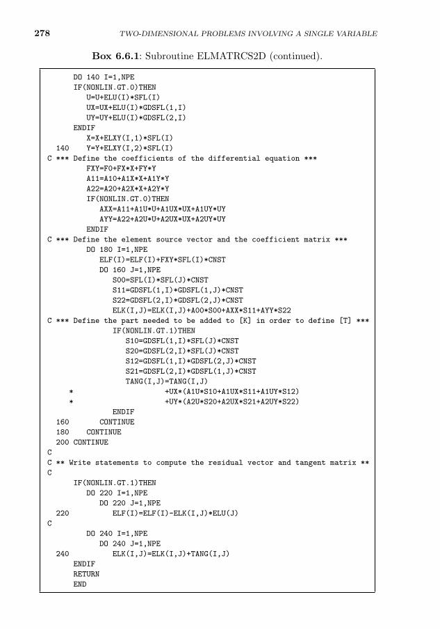
278 TWO-DIMENSIONAL PROBLEMS INVOLVING A SINGLE VARIABLE
Box 6.6.1: Subroutine ELMATRCS2D (continued).
DO 140 I=1,NPE
IF(NONLIN.GT.0)THEN
U=U+ELU(I)*SFL(I)
UX=UX+ELU(I)*GDSFL(1,I)
UY=UY+ELU(I)*GDSFL(2,I)
ENDIF
X=X+ELXY(I,1)*SFL(I)
140 Y=Y+ELXY(I,2)*SFL(I)
C *** Define the coefficients of the differential equation ***
FXY=F0+FX*X+FY*Y
A11=A10+A1X*X+A1Y*Y
A22=A20+A2X*X+A2Y*Y
IF(NONLIN.GT.0)THEN
AXX=A11+A1U*U+A1UX*UX+A1UY*UY
AYY=A22+A2U*U+A2UX*UX+A2UY*UY
ENDIF
C *** Define the element source vector and the coefficient matrix ***
DO 180 I=1,NPE
ELF(I)=ELF(I)+FXY*SFL(I)*CNST
DO 160 J=1,NPE
S00=SFL(I)*SFL(J)*CNST
S11=GDSFL(1,I)*GDSFL(1,J)*CNST
S22=GDSFL(2,I)*GDSFL(2,J)*CNST
ELK(I,J)=ELK(I,J)+A00*S00+AXX*S11+AYY*S22
C *** Define the part needed to be added to [K] in order to define [T] ***
IF(NONLIN.GT.1)THEN
S10=GDSFL(1,I)*SFL(J)*CNST
S20=GDSFL(2,I)*SFL(J)*CNST
S12=GDSFL(1,I)*GDSFL(2,J)*CNST
S21=GDSFL(2,I)*GDSFL(1,J)*CNST
TANG(I,J)=TANG(I,J)
* +UX*(A1U*S10+A1UX*S11+A1UY*S12)
* +UY*(A2U*S20+A2UX*S21+A2UY*S22)
ENDIF
160 CONTINUE
180 CONTINUE
200 CONTINUE
C
C ** Write statements to compute the residual vector and tangent matrix **
C
IF(NONLIN.GT.1)THEN
DO 220 I=1,NPE
DO 220 J=1,NPE
220 ELF(I)=ELF(I)-ELK(I,J)*ELU(J)
C
DO 240 I=1,NPE
DO 240 J=1,NPE
240 ELK(I,J)=ELK(I,J)+TANG(I,J)
ENDIF
RETURN
END
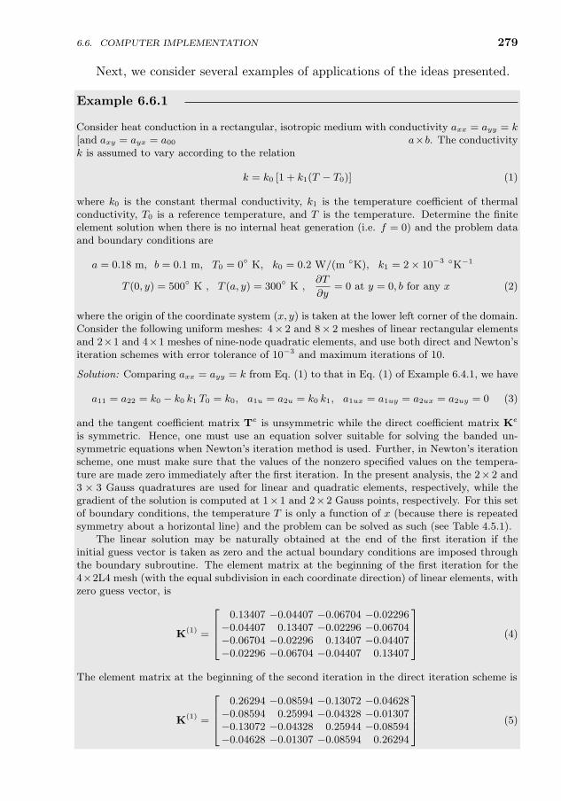
6.6. COMPUTER IMPLEMENTATION 279
Next, we consider several examples of applications of the ideas presented.
Example 6.6.1
Consider heat conduction in a rectangular, isotropic medium with conductivity axx = ayy = k[and axy = ayx = a00 = 0 in Eq. (6.1.1)]. The domain is of dimensions a×b. The conductivityk is assumed to vary according to the relation
k = k0 [1 + k1(T − T0)] (1)
where k0 is the constant thermal conductivity, k1 is the temperature coefficient of thermalconductivity, T0 is a reference temperature, and T is the temperature. Determine the finiteelement solution when there is no internal heat generation (i.e. f = 0) and the problem dataand boundary conditions are
a = 0.18 m, b = 0.1 m, T0 = 0 K, k0 = 0.2 W/(m K), k1 = 2× 10⁻³ K−1
T (0, y) = 500 K , T (a, y) = 300 K ,∂T
∂y= 0 at y = 0, b for any x (2)
where the origin of the coordinate system (x, y) is taken at the lower left corner of the domain.Consider the following uniform meshes: 4× 2 and 8× 2 meshes of linear rectangular elementsand 2×1 and 4×1 meshes of nine-node quadratic elements, and use both direct and Newton’siteration schemes with error tolerance of 10−3 and maximum iterations of 10.
Solution: Comparing axx = ayy = k from Eq. (1) to that in Eq. (1) of Example 6.4.1, we have
a11 = a22 = k0 − k0 k1 T0 = k0, a1u = a2u = k0 k1, a1ux = a1uy = a2ux = a2uy = 0 (3)
and the tangent coefficient matrix Te is unsymmetric while the direct coefficient matrix Ke
is symmetric. Hence, one must use an equation solver suitable for solving the banded un-symmetric equations when Newton’s iteration method is used. Further, in Newton’s iterationscheme, one must make sure that the values of the nonzero specified values on the tempera-ture are made zero immediately after the first iteration. In the present analysis, the 2× 2 and3 × 3 Gauss quadratures are used for linear and quadratic elements, respectively, while thegradient of the solution is computed at 1×1 and 2×2 Gauss points, respectively. For this setof boundary conditions, the temperature T is only a function of x (because there is repeatedsymmetry about a horizontal line) and the problem can be solved as such (see Table 4.5.1).
The linear solution may be naturally obtained at the end of the first iteration if theinitial guess vector is taken as zero and the actual boundary conditions are imposed throughthe boundary subroutine. The element matrix at the beginning of the first iteration for the4×2L4 mesh (with the equal subdivision in each coordinate direction) of linear elements, withzero guess vector, is
K(1) =
0.13407 −0.04407 −0.06704 −0.02296−0.04407 0.13407 −0.02296 −0.06704−0.06704 −0.02296 0.13407 −0.04407−0.02296 −0.06704 −0.04407 0.13407
(4)
The element matrix at the beginning of the second iteration in the direct iteration scheme is
K(1) =
0.26294 −0.08594 −0.13072 −0.04628−0.08594 0.25994 −0.04328 −0.01307−0.13072 −0.04328 0.25944 −0.08594−0.04628 −0.01307 −0.08594 0.26294
(5)
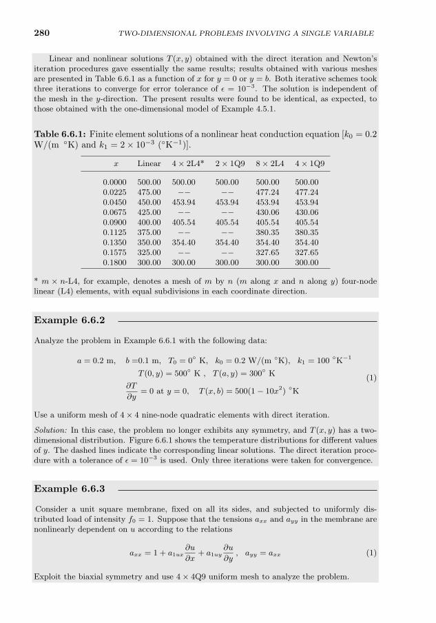
280 TWO-DIMENSIONAL PROBLEMS INVOLVING A SINGLE VARIABLE
Linear and nonlinear solutions T (x, y) obtained with the direct iteration and Newton’siteration procedures gave essentially the same results; results obtained with various meshesare presented in Table 6.6.1 as a function of x for y = 0 or y = b. Both iterative schemes tookthree iterations to converge for error tolerance of ε = 10−3. The solution is independent ofthe mesh in the y-direction. The present results were found to be identical, as expected, tothose obtained with the one-dimensional model of Example 4.5.1.
Table 6.6.1: Finite element solutions of a nonlinear heat conduction equation [k0 = 0.2W/(m K) and k1 = 2× 10⁻³ (K−1)].
x Linear 4× 2L4* 2× 1Q9 8× 2L4 4× 1Q9
0.0000 500.00 500.00 500.00 500.00 500.000.0225 475.00 −− −− 477.24 477.240.0450 450.00 453.94 453.94 453.94 453.940.0675 425.00 −− −− 430.06 430.060.0900 400.00 405.54 405.54 405.54 405.540.1125 375.00 −− −− 380.35 380.350.1350 350.00 354.40 354.40 354.40 354.400.1575 325.00 −− −− 327.65 327.650.1800 300.00 300.00 300.00 300.00 300.00
* m × n-L4, for example, denotes a mesh of m by n (m along x and n along y) four-nodelinear (L4) elements, with equal subdivisions in each coordinate direction.
Example 6.6.2
Analyze the problem in Example 6.6.1 with the following data:
a = 0.2 m, b =0.1 m, T0 = 0 K, k0 = 0.2 W/(m K), k1 = 100 K−1
T (0, y) = 500 K , T (a, y) = 300 K
∂T
∂y= 0 at y = 0, T (x, b) = 500(1− 10x2) K
(1)
Use a uniform mesh of 4× 4 nine-node quadratic elements with direct iteration.
Solution: In this case, the problem no longer exhibits any symmetry, and T (x, y) has a two-dimensional distribution. Figure 6.6.1 shows the temperature distributions for different valuesof y. The dashed lines indicate the corresponding linear solutions. The direct iteration proce-dure with a tolerance of ε = 10−3 is used. Only three iterations were taken for convergence.
Example 6.6.3
Consider a unit square membrane, fixed on all its sides, and subjected to uniformly dis-tributed load of intensity f0 = 1. Suppose that the tensions axx and ayy in the membrane arenonlinearly dependent on u according to the relations
axx = 1 + a1ux∂u
∂x+ a1uy
∂u
∂y, ayy = axx (1)
Exploit the biaxial symmetry and use 4× 4Q9 uniform mesh to analyze the problem.
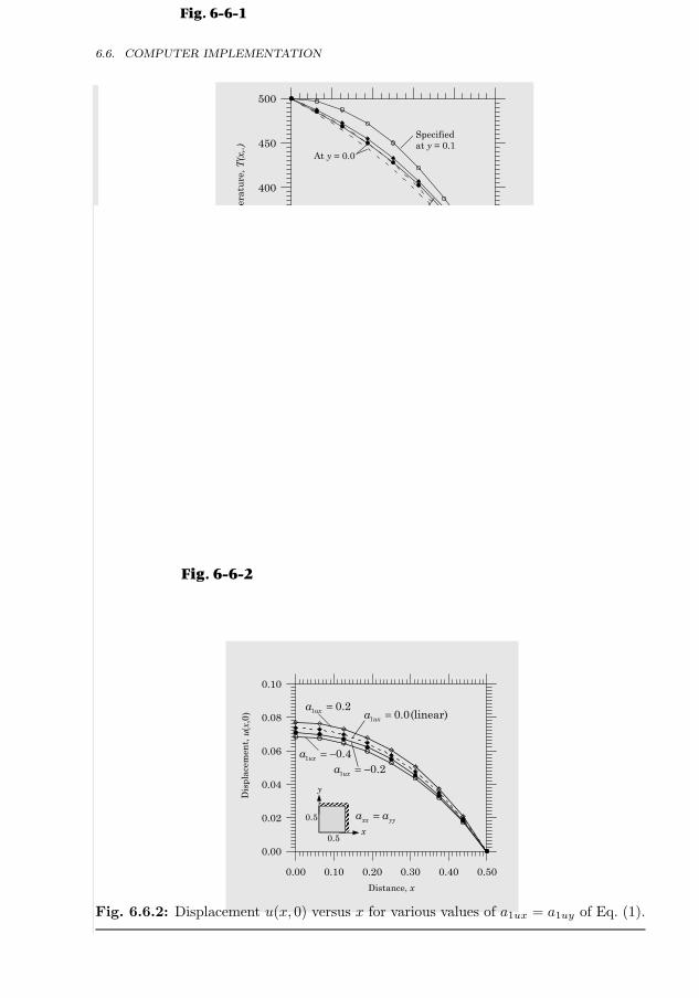
281
0.00 0.04 0.08 0.12 0.16 0.20
Distance, x
300
350
400
450
500
Tem
pera
ture
, T(x
,.)
Specifiedat y = 0.1
At y = 0.05
At y = 0.0
Fig. 6-6-1
Fig. 6.6.1: Temperature distribution in a rectangular region with temperature depen-dent conductivity.
Solution: The Newton iteration scheme with ε = 10−3 is used. The deflections u(x, 0) along thesymmetry line y = 0 are presented in Table 6.6.2 (also see Fig. 6.6.2) for a1ux = −0.4,−0.2, 0,and 0.2. The deflections increase with a1ux increasing from −0.4 to 0.2.
Table 6.6.2: Deflections of a square membrane subjected to uniform load.
x a1ux = −0.4 a1ux = −0.2 a1ux = 0.0 a1ux = 0.2
0.0000 0.068440 0.070848 0.073670 0.0770770.0625 0.067473 0.069875 0.072691 0.0760920.1250 0.064573 0.066940 0.069719 0.0730810.1875 0.059696 0.061973 0.064656 0.0679130.2500 0.052723 0.054834 0.057334 0.0603870.3125 0.043488 0.045328 0.047523 0.0502290.3750 0.031776 0.033208 0.034931 0.0370830.4375 0.017358 0.018196 0.019218 0.020515
0.00 0.10 0.20 0.30 0.40 0.50
Distance, x
0.00
0.02
0.04
0.06
0.08
0.10
Dis
plac
emen
t,
1 0.2uxa = −
u(x,
0)
1 0.4uxa = −
1 0.2uxa =1 0.0(linear)uxa =
x
y
xx yya a=
0.5
0.5
Fig. 6-6-2
Fig. 6.6.2: Displacement u(x, 0) versus x for various values of a1ux = a1uy of Eq. (1).
6.6. COMPUTER IMPLEMENTATION
282 TWO-DIMENSIONAL PROBLEMS INVOLVING A SINGLE VARIABLE
6.7 Time-Dependent Problems
6.7.1 Introduction
In this section, we develop the finite element models of 2-D time-dependentproblems with nonlinearities and describe some standard time approximationschemes. We begin with the general discussion of the finite element modeling oftime-dependent problems. Consider the time-dependent version of the modelequation, Eq. (6.1.1)
− ∂
∂x
(axx
∂u
∂x+ axy
∂u
∂y
)− ∂
∂y
(ayx
∂u
∂x+ ayy
∂u
∂y
)+a00u+ c0
∂u
∂t+ c1
∂2u
∂t2= f(x, y, t) (6.7.1)
where aij and ci are, in general, functions of position x, time t, u, ∂u/∂x,and ∂u/∂y. The equation is subjected to appropriate boundary and initialconditions.
The finite element formulation of time-dependent problems involves follow-ing two steps:
1. Spatial approximation, where the solution u(x, t) of the equation underconsideration is approximated by expressions of the form
u(x, t) ≈ ueh(x, t) =n∑j=1
uej(t)ψej (x) (6.7.2)
and the spatial finite element model of the equation is developed usingthe procedures of static or steady-state problems, while carrying all time-dependent terms in the formulation. This step results in a set of ordinarydifferential equations in time for the nodal variables uej(t) of the elementKeue+Ceue+Meue = Fe. When the solution is separable into functionsof time only and space only, that is, u(x, t) = T (t)X(x), approximationof the type in Eq. (6.7.2) is justified for the overall transient response ofa system, in contrast to wave propagation type solutions. Since this steponly addresses spatial approximation, it is termed semidiscretization.
2. Temporal approximation, where the system of ordinary differential equa-tions in time are further approximated to obtain a system of algebraicequations, called fully discretized equations. Depending on the goal ofthe study, one may reduce the ordinary differential equations to either analgebraic eigenvalue problem (K − λM)u = Q, or an algebraic systemof equations Kus+1 = Fs,s+1 that can be solved for various fixed timesby marching in time to obtain the transient response; here λ denotes aneigenvalue and us+1 ≡ u(ts+1).
283
6.7.2 Semidiscretization
The spatial approximation (i.e. semidiscretization) follows the same two stepsas in the steady-state case discussed in Sections 6.2 and 6.3, namely, the devel-opment of the weak form and approximation of the field variables to obtain thealgebraic relations. The weak form of Eq. (6.7.1) is given by
0 =
∫Ωe
[∂wi∂x
(axx
∂uh∂x
+ axy∂uh∂y
)+∂wi∂y
(ayx
∂uh∂x
+ ayy∂uh∂y
)+ a00wiuh
+ c0wi∂uh∂t
+ c1wi∂2uh∂t2
− wif]dx dy −
∮Γe
wiqn ds (6.7.3)
The finite element approximation is assumed to be of the form
u(x, t) ≈ ueh(x, t) =n∑j=1
uej(t)ψej (x) (6.7.4)
where the nodal values uej are now assumed to be functions of time. Substitutionof Eq. (6.7.4) into Eq. (6.7.3) gives rise to the finite element equations
Meue + Ceue + Keue = f e + Qe ≡ Fe (6.7.5)
where
Ceij =
∫Ωe
c0ψeiψ
ej dx dy, M e
ij =
∫Ωe
c1ψeiψ
ej dx dy
Keij =
∫Ωe
[∂ψei∂x
(axx
∂ψej∂x
+ axy∂ψej∂y
)+∂ψei∂y
(ayx
∂ψei∂x
+ ayy∂ψej∂y
)+ a00ψ
eiψ
ej
]dx dy
fei =
∫Ωe
ψei f dx dy, Qe =
∮Γe
ψei qn ds (6.7.6)
In Sections 6.7.3 and 6.7.4, we consider time-approximation schemes to re-duce Eq. (6.7.5) to a set of algebraic equations among the nodal values, com-pleting the discretization in space and time. As a matter of information, thereduction of an equation of motion to the associated eigenvalue problem is alsodiscussed. The case of M = 0 arises in heat transfer and fluid dynamics prob-lems, and the equation is known as the parabolic equation. Equation (6.7.5),in its general form is known as a hyperbolic equation, where C denotes thedamping matrix and M the mass matrix, and it arises in structural dynamicswith damping (C 6= 0) and without damping (C = 0). The time approximationof Eq. (6.7.5) for parabolic and hyperbolic equations will be derived separately.An equation of the type in Eq. (6.7.5) is also obtained by other spatial approx-imations methods like the finite difference method and the boundary elementmethod, among others. Therefore, the discussion of converting matrix equa-tions of the type in Eq. (6.7.5) is equally valid for other numerical methodsused to approximate the spatial variation of the solution.
6.7. TIME-DEPENDENT PROBLEMS
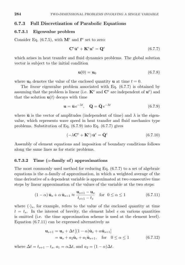
284 TWO-DIMENSIONAL PROBLEMS INVOLVING A SINGLE VARIABLE
6.7.3 Full Discretization of Parabolic Equations
6.7.3.1 Eigenvalue problem
Consider Eq. (6.7.5), with Me and f e set to zero:
Ceue + Keue = Qe (6.7.7)
which arises in heat transfer and fluid dynamics problems. The global solutionvector is subject to the initial condition
u(0) = u0 (6.7.8)
where u0 denotes the value of the enclosed quantity u at time t = 0.The linear eigenvalue problem associated with Eq. (6.7.7) is obtained by
assuming that the problem is linear (i.e. Ke and Ce are independent of ue) andthat the solution u(t) decays with time
u = u e−λt, Q = Q e−λt (6.7.9)
where u is the vector of amplitudes (independent of time) and λ is the eigen-value, which represents wave speed in heat transfer and fluid mechanics typeproblems. Substitution of Eq. (6.7.9) into Eq. (6.7.7) gives
(−λCe + Ke) ue = Qe (6.7.10)
Assembly of element equations and imposition of boundary conditions followsalong the same lines as for static problems.
6.7.3.2 Time (α-family of) approximations
The most commonly used method for reducing Eq. (6.7.7) to a set of algebraicequations is the α-family of approximation, in which a weighted average of thetime derivative of a dependent variable is approximated at two consecutive timesteps by linear approximation of the values of the variable at the two steps:
(1− α) us + α us+1 ≈us+1 − usts+1 − ts
for 0 ≤ α ≤ 1 (6.7.11)
where (·)s, for example, refers to the value of the enclosed quantity at timet = ts. In the interest of brevity, the element label e on various quantitiesis omitted (i.e. the time approximation scheme is used at the element level).Equation (6.7.11) can be expressed alternatively as
us+1 = us + ∆t [(1− α)us + αus+1]
= us + a2us + a1us+1, for 0 ≤ α ≤ 1 (6.7.12)
where ∆t = ts+1 − ts, a1 = α∆t, and a2 = (1− α)∆t.
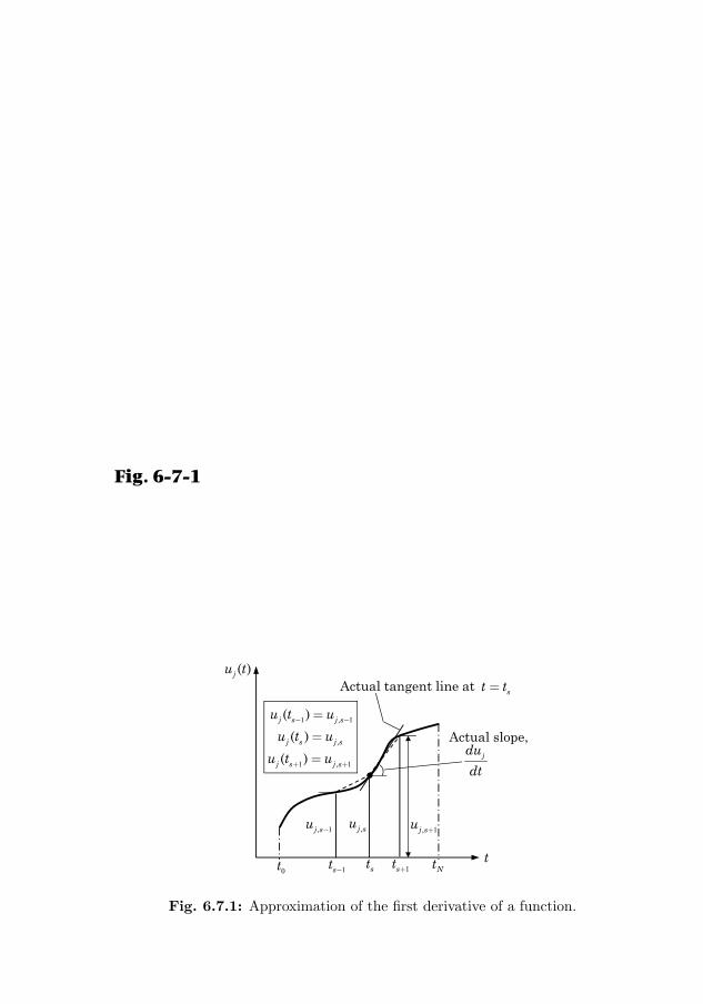
6.7. TIME-DEPENDENT PROBLEMS 285
Note that when α = 0, Eq. (6.7.11) reduces, for any vector of nodal valuesu(t), to
us =
(du
dt
)t=ts
≈ u(ts+1)− u(ts)
ts+1 − ts(6.7.13)
Clearly, it amounts to replacing the time derivative of u(t) at t = ts with thefinite difference of its values at t = ts+1 (i.e. the value from a time step ahead)and t = ts. Equation (6.7.13) is nothing but an approximation of the derivativeof a function, since ∆t = ts+1 − ts is finite (i.e. ∆t cannot approach zero).The approximation in Eq. (6.7.13) is known as the forward difference methodbecause it uses the function value ahead of the current position in computingthe slope [see Fig. 6.7.1 for the approximation of the slope of a typical nodalvalue uj(t)]. One may also use the value of the function from a time step behind(
du
dt
)t=ts
≈ u(ts)− u(ts−1)
ts − ts−1(6.7.14a)
or (du
dt
)t=ts+1
≈ u(ts+1)− u(ts)
ts+1 − ts(6.7.14b)
which is the same as that in Eq. (6.7.11) when α = 1. Equation (6.7.14b)is known as the backward difference method. If we use the values ahead andbehind in computing the slope(
du
dt
)t=ts
≈ u(ts+1)− u(ts−1)
ts+1 − ts−1(6.7.15)
it is called the centered difference method, which is not a special case of theα-family of approximation in Eq. (6.7.11).
•
Actual slope,
( )ju t
1 1
1 1
,
,
,
( )
( )
( )
j s j s
j s j s
j s j s
u t u
u t u
u t u
- -
+ +
=
=
=
Actual tangent line at st t=
jdu
dt
1,j su - ,j su 1,j su +
t0t 1st - st 1st + Nt
Fig. 6-7-1
Fig. 6.7.1: Approximation of the first derivative of a function.
286 TWO-DIMENSIONAL PROBLEMS INVOLVING A SINGLE VARIABLE
For different values of α, we obtain the following well-known numerical in-tegration schemes from Eq. (6.7.12):
α =
0, the forward difference scheme (conditionally stable);
Order of accuracy = O(∆t)12 , the Crank–Nicolson scheme (stable); O((∆t)2)23 , the Galerkin method (stable); O((∆t)2)1, the backward difference scheme (stable); O(∆t)
(6.7.16)
The meaning of the phrases “stability” and “conditional stability” will be dis-cussed in Section 6.7.5.
6.7.3.3 Fully discretized equations
Equation (6.7.12) can be used to reduce ordinary differential equations in Eq.(6.7.7) to algebraic equations among the nodal values uj at time ts+1. Assumingthat C is independent of time t (hence, independent of u), we can use theapproximation in Eq. (6.7.12) to eliminate u in Eq. (6.7.7). PremultiplyingEq. (6.7.12) with C and replacing Cus and Cus+1 with the aid of Eq. (6.7.7)evaluated at times ts and ts+1, respectively, we obtain
K(us+1)us+1 = K(us)us + Fs,s+1 ≡ F (6.7.17)
where
K(us+1) = C + a1K(us+1), K(us) = C− a2K(us)
Fs,s+1 = a1Fs+1 + a2Fs, a1 = α∆t, a2 = (1− α)∆t(6.7.18)
6.7.3.4 Direct iteration scheme
When the direct iteration is used to solve the nonlinear equations in Eq. (6.7.17),at the (r + 1)st iteration we solve the equation
K(urs+1)ur+1s+1 = F(us,Fs,Fs+1) (6.7.19)
withF =
[C− a2K(us)
]us + a1Fs+1 + a2Fs (6.7.20)
Note that F remains unchanged during the nonlinear iteration for a given timestep, whereas K changes during the iteration due to its dependence on the latestknown solution urs+1. Equation (6.7.19) provides a means to compute for ur+1
s+1
whenever us and urs+1 are known. Of course, C, K, and F are known for alltimes (parts of F may not be known at the element level, but after assemblythey are known whenever the corresponding u is unknown). Equations (6.7.19)and (6.7.20) are valid for a typical element.
6.7. TIME-DEPENDENT PROBLEMS 287
6.7.3.5 Newton’s iteration scheme
When the Newton iteration procedure is used, we solve for the incrementalsolution vector ∆u from
∆u = −[T(urs+1)]−1Rrs+1 (6.7.21)
where T is the tangent matrix associated with Eq. (6.7.17)
T(urs+1) ≡[∂Rs+1
∂us+1
]r, Rr
s+1 = K(urs+1)urs+1 − F (6.7.22)
The total solution is obtained from
ur+1s+1 = urs+1 + ∆u (6.7.23)
6.7.3.6 Explicit and implicit formulations and mass lumping
Note that for α = 0 (the forward difference scheme), Eq. (6.7.18) gives Ke = Ce.If the matrix Ce is diagonal, then Eq. (6.7.17) becomes explicit in the sensethat the solution of Eq. (6.7.17) for us+1 does not involve inverting a matrix.However, in the spatial approximation by the finite element method, matrixCe is derived using a weak form and it is never a diagonal matrix. The matrixCe derived using a weak form is called the consistent matrix. Thus, the finiteelement equations with consistent matrix Ce can never be explicit. In a finitedifference method, the matrix Ce is diagonal, and therefore a time integrationscheme like the forward difference method results in explicit set of equations,which are quite inexpensive to solve at each time step. To have the advantageof less computational time in dynamic/transient analysis by the finite elementmethod, it is desirable to have Ce diagonalized. Thus, explicit finite elementequations can be obtained only when: (a) the time approximation scheme issuch that K is equal to or a multiple of C and (b) the matrix C is diagonal.Otherwise, the formulation is called implicit.
There are two ways one may diagonalize the consistent matrix C. The di-agonalized matrices are also called lumped matrices. The row-sum lumping andproportional lumping techniques are the two ways to compute diagonal matrices.In row-sum lumping, the sum of the coefficients of each row of the consistentmatrix C is used as the diagonal element and the off-diagonal elements are setto zero (no sum on i):
Cii =
n∑j=1
∫Ωe
c0ψeiψ
ej dx =
∫Ωe
c0 ψei dx, Cij = 0 for i 6= j (6.7.24)
where the property∑n
j=1 ψej = 1 of the interpolation functions is used. In
proportional lumping the diagonal elements are computed to be proportional
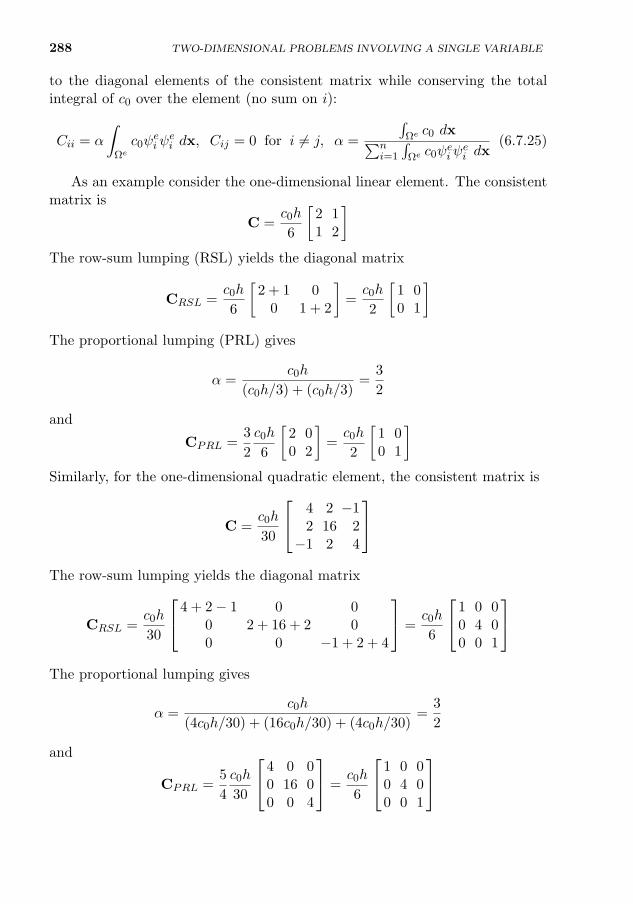
288 TWO-DIMENSIONAL PROBLEMS INVOLVING A SINGLE VARIABLE
to the diagonal elements of the consistent matrix while conserving the totalintegral of c0 over the element (no sum on i):
Cii = α
∫Ωe
c0ψeiψ
ei dx, Cij = 0 for i 6= j, α =
∫Ωe c0 dx∑n
i=1
∫Ωe c0ψeiψ
ei dx
(6.7.25)
As an example consider the one-dimensional linear element. The consistentmatrix is
C =c0h
6
[2 11 2
]The row-sum lumping (RSL) yields the diagonal matrix
CRSL =c0h
6
[2 + 1 0
0 1 + 2
]=c0h
2
[1 00 1
]The proportional lumping (PRL) gives
α =c0h
(c0h/3) + (c0h/3)=
3
2
and
CPRL =3
2
c0h
6
[2 00 2
]=c0h
2
[1 00 1
]Similarly, for the one-dimensional quadratic element, the consistent matrix is
C =c0h
30
4 2 −12 16 2−1 2 4
The row-sum lumping yields the diagonal matrix
CRSL =c0h
30
4 + 2− 1 0 00 2 + 16 + 2 00 0 −1 + 2 + 4
=c0h
6
1 0 00 4 00 0 1
The proportional lumping gives
α =c0h
(4c0h/30) + (16c0h/30) + (4c0h/30)=
3
2
and
CPRL =5
4
c0h
30
4 0 00 16 00 0 4
=c0h
6
1 0 00 4 00 0 1
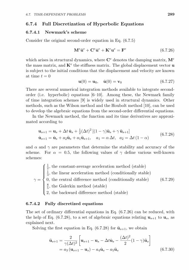
6.7. TIME-DEPENDENT PROBLEMS 289
6.7.4 Full Discretization of Hyperbolic Equations
6.7.4.1 Newmark’s scheme
Consider the original second-order equation in Eq. (6.7.5)
Meue + Ceue + Keue = Fe (6.7.26)
which arises in structural dynamics, where Ce denotes the damping matrix, Me
the mass matrix, and Ke the stiffness matrix. The global displacement vector uis subject to the initial conditions that the displacement and velocity are knownat time t = 0
u(0) = u0, u(0) = v0 (6.7.27)
There are several numerical integration methods available to integrate second-order (i.e. hyperbolic) equations [6–10]. Among these, the Newmark familyof time integration schemes [9] is widely used in structural dynamics. Othermethods, such as the Wilson method and the Houbolt method [10], can be usedto develop the algebraic equations from the second-order differential equations.
In the Newmark method, the function and its time derivatives are approxi-mated according to
us+1 = us + ∆t us + 12(∆t)2 [(1− γ)us + γ us+1]
us+1 = us + a2us + a1us+1, a1 = α∆t, a2 = ∆t (1− α)(6.7.28)
and α and γ are parameters that determine the stability and accuracy of thescheme. For α = 0.5, the following values of γ define various well-knownschemes:
γ =
12 , the constant-average acceleration method (stable)13 , the linear acceleration method (conditionally stable)
0, the central difference method (conditionally stable)85 , the Galerkin method (stable)
2, the backward difference method (stable)
(6.7.29)
6.7.4.2 Fully discretized equations
The set of ordinary differential equations in Eq. (6.7.26) can be reduced, withthe help of Eq. (6.7.28), to a set of algebraic equations relating us+1 to us, asexplained next.
Solving the first equation in Eq. (6.7.28) for us+1, we obtain
us+1 =2
γ(∆t)2
[us+1 − us −∆tus −
(∆t)2
2(1− γ)us
]= a3 (us+1 − us)− a4us − a5us (6.7.30)
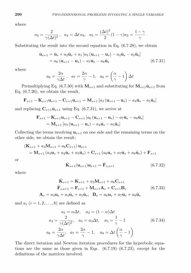
290 TWO-DIMENSIONAL PROBLEMS INVOLVING A SINGLE VARIABLE
where
a3 =2
γ(∆t)2, a4 = ∆t a3, a5 =
(∆t)2
2(1− γ)a3 =
1− γγ
Substituting the result into the second equation in Eq. (6.7.28), we obtain
us+1 = us + a2us + a1 [a3 (us+1 − us)− a4us − a5us]
= a6 (us+1 − us)− a7us − a8us (6.7.31)
where
a6 =2α
γ∆t, a7 =
2α
γ− 1, a8 =
(α
γ− 1
)∆t
Premultiplying Eq. (6.7.30) with Ms+1 and substituting for Ms+1us+1 fromEq. (6.7.26), we obtain the result,
Fs+1 −Ks+1us+1 −Cs+1us+1 = Ms+1 [a3 (us+1 − us)− a4us − a5us]
and replacing Cs+1us+1 using Eq. (6.7.31), we arrive at
Fs+1 −Ks+1us+1 −Cs+1 [a6 (us+1 − us)− a7us − a8us]
= Ms+1 [a3 (us+1 − us)− a4us − a5us]
Collecting the terms involving us+1 on one side and the remaining terms on theother side, we obtain the result:
(Ks+1 + a3Ms+1 + a6Cs+1)us+1
= Ms+1 (a3us + a4us + a5us) + Cs+1 (a6us + a7us + a8us) + Fs+1
orKs+1(us+1)us+1 = Fs,s+1 (6.7.32)
where
Ks+1 = Ks+1 + a3Ms+1 + a6Cs+1
Fs,s+1 = Fs+1 + Ms+1As + Cs+1Bs (6.7.33)
As = a3us + a4us + a5us, Bs = a6us + a7us + a8us
and ai (i = 1, 2, . . . , 8) are defined as
a1 = α∆t, a2 = (1− α)∆t
a3 =2
γ(∆t)2, a4 = a3∆t, a5 =
1
γ− 1 (6.7.34)
a6 =2α
γ∆t, a7 =
2α
γ− 1, a8 = ∆t
(α
γ− 1
)The direct iteration and Newton iteration procedures for the hyperbolic equa-tions are the same as those given in Eqs. (6.7.19)–(6.7.23), except for thedefinitions of the matrices involved.
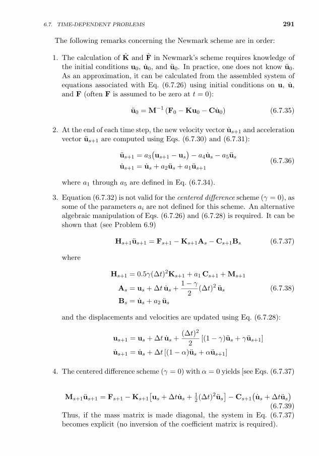
6.7. TIME-DEPENDENT PROBLEMS 291
The following remarks concerning the Newmark scheme are in order:
1. The calculation of K and F in Newmark’s scheme requires knowledge ofthe initial conditions u0, u0, and u0. In practice, one does not know u0.As an approximation, it can be calculated from the assembled system ofequations associated with Eq. (6.7.26) using initial conditions on u, u,and F (often F is assumed to be zero at t = 0):
u0 = M−1 (F0 −Ku0 −Cu0) (6.7.35)
2. At the end of each time step, the new velocity vector us+1 and accelerationvector us+1 are computed using Eqs. (6.7.30) and (6.7.31):
us+1 = a3
(us+1 − us
)− a4us − a5us
us+1 = us + a2us + a1us+1(6.7.36)
where a1 through a5 are defined in Eq. (6.7.34).
3. Equation (6.7.32) is not valid for the centered difference scheme (γ = 0), assome of the parameters ai are not defined for this scheme. An alternativealgebraic manipulation of Eqs. (6.7.26) and (6.7.28) is required. It can beshown that (see Problem 6.9)
Hs+1us+1 = Fs+1 −Ks+1As −Cs+1Bs (6.7.37)
where
Hs+1 = 0.5γ(∆t)2Ks+1 + a1 Cs+1 + Ms+1
As = us + ∆t us +1− γ
2(∆t)2 us (6.7.38)
Bs = us + a2 us
and the displacements and velocities are updated using Eq. (6.7.28):
us+1 = us + ∆t us +(∆t)2
2[(1− γ)us + γus+1]
us+1 = us + ∆t [(1− α)us + αus+1]
4. The centered difference scheme (γ = 0) with α = 0 yields [see Eqs. (6.7.37)and (6.7.38)]
Ms+1us+1 = Fs+1 −Ks+1
[us + ∆tus + 1
2(∆t)2us]−Cs+1
(us + ∆tus
)(6.7.39)
Thus, if the mass matrix is made diagonal, the system in Eq. (6.7.37)becomes explicit (no inversion of the coefficient matrix is required).
292 TWO-DIMENSIONAL PROBLEMS INVOLVING A SINGLE VARIABLE
5. For natural vibration, the forces and the solution are assumed to beperiodic (F = Q when the source term is set to zero)
u = u0 eiωt, Q = Q0 eiωt, i =√−1
where u0 is the vector of amplitudes (independent of time) and ω is thefrequency of natural vibration of the system. Substitution of the periodicmotion into Eq. (6.7.26), assuming that it is linear, yields(
−ω2M + iωC + K)u0 = Q0 (6.7.40)
where Q0 is the vector of secondary variables. Equation (6.7.40) is calledan eigenvalue problem, which may have complex eigenvalues when damp-ing C is included.
6.7.5 Stability and Accuracy
6.7.5.1 Preliminary comments
In general, the application of a time approximation scheme to an initial-valueproblem results in an equation of the type
Kus+1 = Kus or us+1 = Aus (6.7.41)
where A = K−1 K is called the amplification matrix, and K and K are ma-trix operators that depend on the problem parameters [see Eqs. (6.7.33) and(6.7.34)], for example, geometric and material properties, time step, and meshparameter, and us+1 is the solution vector at time ts+1.
Since Eq. (6.7.11), for example, represents an approximation that is usedto derive an equation of the type in Eq. (6.7.41), error is introduced into thesolution us+1 at each time step. Since the solution us+1 at time ts+1 dependson the solution us at time ts, the error can grow with time. The time ap-proximation scheme is said to be stable if the error introduced in us does notgrow unbounded as Eq. (6.7.41) is solved repeatedly for s = 0, 1, . . . , . In orderfor the error to remain bounded, it is necessary and sufficient that the largesteigenvalue of the amplification matrix A be less than or equal to unity:
|λmax| ≤ 1 (6.7.42)
where λmax is the largest value that satisfies the equation
(A− λAI)u = 0 (6.7.43)
We note that λA depends on the characteristic length of the mesh, time step,and material parameters (such as the density and modulus). Since modulusand density are fixed for a given problem, the stability criterion essentially
6.7. TIME-DEPENDENT PROBLEMS 293
provides a relation between the characteristic element size and the time stepused. Equation (6.7.43) represents a nonlinear eigenvalue problem, if one canbe formulated. If the condition in Eq. (6.7.42) is satisfied for any value of ∆t,independent of the mesh size, the scheme is said to be unconditionally stable,or simply stable. If Eq. (6.7.42) places a restriction, for a given mesh, on thesize of the time step ∆t, the scheme is said to be conditionally stable. As themesh is refined, the value of the maximum eigenvalue increases and, hence, thevalue of the critical time step decreases.
Accuracy of a numerical scheme is a measure of the closeness between theapproximate solution and the exact solution, whereas stability of a solutionis a measure of the boundedness of the approximate solution with time. Asone might expect, the size of the time step can influence both accuracy andstability. When we construct an approximate solution, we like it to converge tothe true solution when the number of elements or the degree of approximationis increased and the time step ∆t is decreased. A time approximation schemeis said to be convergent if, for fixed ts and ∆t, the numerical value us convergesto its true value u(ts) as ∆t→ 0. Accuracy is measured in terms of the rate atwhich the approximate solution converges. If a numerical scheme is stable andconsistent, it is also convergent.
6.7.5.2 Stability criteria
The discussion here is limited only to linear problems, as there are no proofsavailable for stability criteria for nonlinear problems. The α-family of approxi-mations applied to linear problems can be shown to be stable for all numericalschemes for which α ≥ 1
2 ; for α < 12 , the scheme is conditionally stable if the
time step ∆t is such that the following (stability) condition is satisfied:
∆t < ∆tcr ≡2
(1− 2α)λmax(6.7.44)
where λmax is the largest eigenvalue of the finite element equations after assem-bly and imposition of boundary conditions
(K− λC)u0 = 0 (6.7.45)
Note that the same mesh as that used for the transient analysis must be used tocalculate the eigenvalues of the assembled system; after assembly and impositionof boundary conditions, the eigenvalue problem becomes homogeneous, as givenin Eq. (6.7.45).
The stability criterion in Eq. (6.7.44) is arrived using Eq. (6.7.42). Theamplification matrix for the α-family of approximations as applied to linearproblems is given by
A = (K)−1 K =(C + a1K
)−1(C− a2K
)(6.7.46)
294 TWO-DIMENSIONAL PROBLEMS INVOLVING A SINGLE VARIABLE
Let λmax be the maximum eigenvalue of Eq. (6.7.45). Then it can be shownthat (using spectral decomposition of A) the maximum eigenvalue of A is equalto
(λA)max =
∣∣∣∣1− (1− α)∆t λmax
1 + α∆t λmax
∣∣∣∣ ≤ 1 (6.7.47)
from which it follows that the α-family of approximations is unconditionallystable if α ≥ 1
2 . In the case α < 12 , the method is stable only if the condition
in Eq. (6.7.44) is satisfied.Similarly, for all Newmark schemes in which γ < α and α ≥ 1
2 , the stabilityrequirement is (for linear problems)
∆t ≤ ∆tcr =
[1
2ω2
max(α− γ)
]−1/2
(6.7.48)
where ωmax is the maximum natural frequency of the undamped system (6.7.40)(K− ω2M
)u = 0 (6.7.49)
For all nonlinear problems, one often uses the time step restrictions imposedby linear stability criteria.
6.7.6 Computer Implementation
Computer implementation of linear or nonlinear time-dependent problems iscomplicated by the fact that one must keep track of the solution vectors atdifferent times and iterations. In general, there are three loops. The outermostone is on the load, which can be a force or source term whose influence on thesystem is investigated. While it is the load placed on the system in the case of asolid mechanics problem, it may be the Reynolds number in fluid flow problemsand heat flux in heat transfer problems. The outer loop on the number of loadsteps is followed by a loop on the number of time steps, and the inner most loopbeing on nonlinear equilibrium iterations. The flow chart shown in Fig. 6.7.2illustrates the general idea.
One must keep track of the solution vector from the previous time step usand the solution vector from the previous iteration urs+1. This is because the
formulation requires solution us to compute F [see Eqs. (6.7.18) and (6.7.20)in the case of parabolic equations and Eqs. (6.7.33) and (6.7.34) for hyper-bolic equations], and the latest known solution urs+1 is required to update the
coefficient matrix Ks+1 during the equilibrium iteration.Another point one must note is that the source vector F due to the body
force f(x, t) [see Eqs. (6.7.1) and (6.7.6)] appears in the fully discretized equa-tion of the parabolic equations [see Eq. (6.7.18)] as a vector multiplied by ∆t.Therefore, when nonzero secondary variables are read as input through the
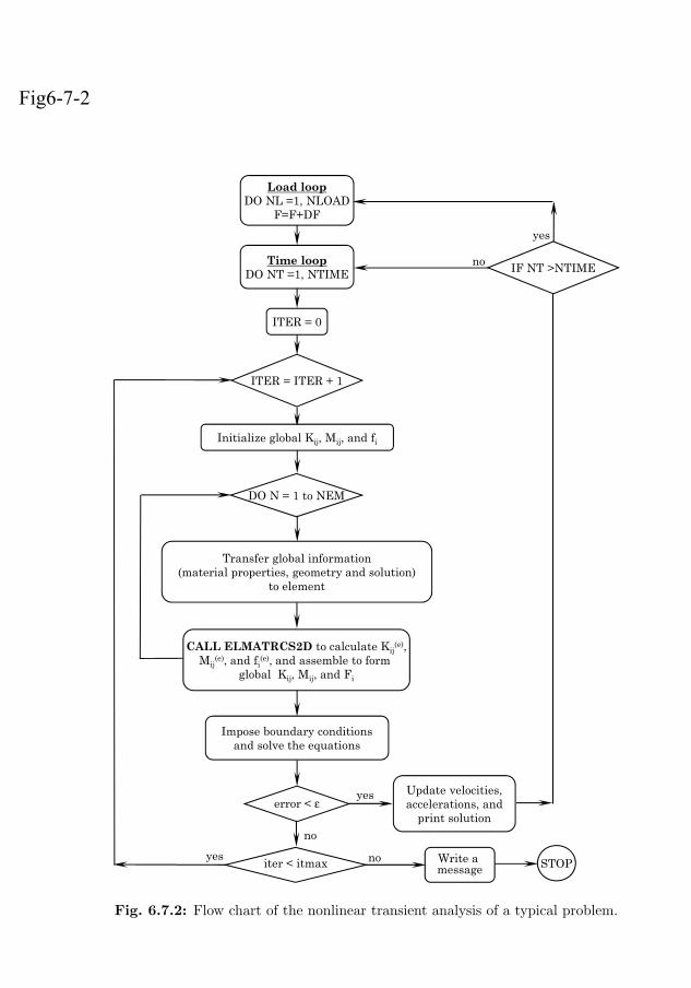
6.7. TIME-DEPENDENT PROBLEMS 295
boundary conditions, they must be multiplied by ∆t (assuming that f is in-dependent of time) inside the program. This is not required in the case ofhyperbolic equations, as can be seen from Eq. (6.7.33). Although it can bedone, we will not consider time-dependent boundary conditions here.
DO N = 1 to NEM
error < ε
STOPnoyes
no
yes
Impose boundary conditionsand solve the equations
Transfer global information(material properties, geometry and solution)
to element
Initialize global Kij, Mij, and fi
ITER = 0
CALL ELMATRCS2D to calculate Kij(e),
Mij(e), and fi
(e), and assemble to form global Kij, Mij, and Fi
Update velocities,accelerations, and
print solution
Write a message
ITER = ITER + 1
Time loopDO NT =1, NTIME
Load loopDO NL =1, NLOAD
F=F+DF
iter < itmax
IF NT >NTIME
yes
no
Fig6-7-2
Fig. 6.7.2: Flow chart of the nonlinear transient analysis of a typical problem.
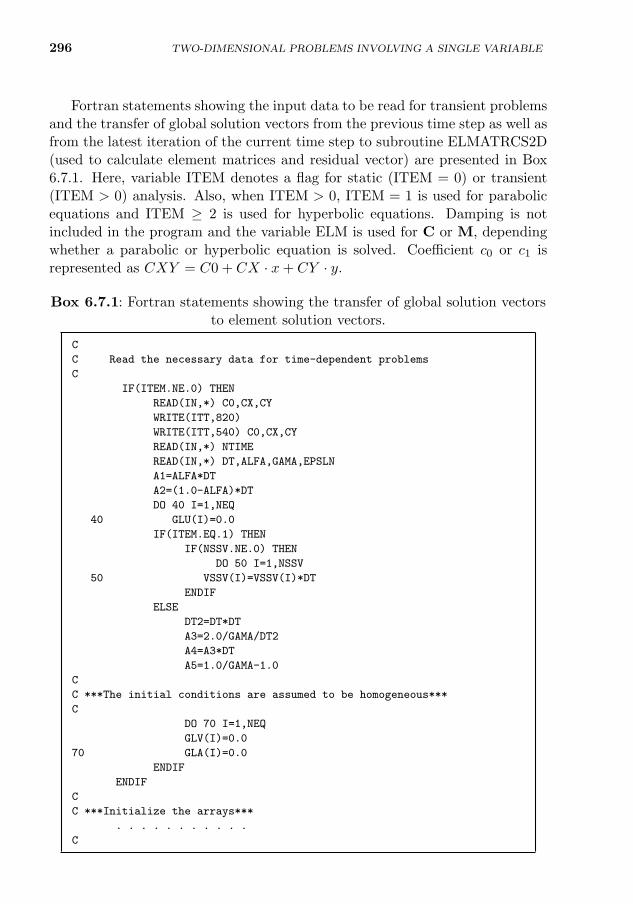
296 TWO-DIMENSIONAL PROBLEMS INVOLVING A SINGLE VARIABLE
Fortran statements showing the input data to be read for transient problemsand the transfer of global solution vectors from the previous time step as well asfrom the latest iteration of the current time step to subroutine ELMATRCS2D(used to calculate element matrices and residual vector) are presented in Box6.7.1. Here, variable ITEM denotes a flag for static (ITEM = 0) or transient(ITEM > 0) analysis. Also, when ITEM > 0, ITEM = 1 is used for parabolicequations and ITEM ≥ 2 is used for hyperbolic equations. Damping is notincluded in the program and the variable ELM is used for C or M, dependingwhether a parabolic or hyperbolic equation is solved. Coefficient c0 or c1 isrepresented as CXY = C0 + CX · x+ CY · y.
Box 6.7.1: Fortran statements showing the transfer of global solution vectorsto element solution vectors.
C
C Read the necessary data for time-dependent problems
C
IF(ITEM.NE.0) THEN
READ(IN,*) C0,CX,CY
WRITE(ITT,820)
WRITE(ITT,540) C0,CX,CY
READ(IN,*) NTIME
READ(IN,*) DT,ALFA,GAMA,EPSLN
A1=ALFA*DT
A2=(1.0-ALFA)*DT
DO 40 I=1,NEQ
40 GLU(I)=0.0
IF(ITEM.EQ.1) THEN
IF(NSSV.NE.0) THEN
DO 50 I=1,NSSV
50 VSSV(I)=VSSV(I)*DT
ENDIF
ELSE
DT2=DT*DT
A3=2.0/GAMA/DT2
A4=A3*DT
A5=1.0/GAMA-1.0
C
C ***The initial conditions are assumed to be homogeneous***
C
DO 70 I=1,NEQ
GLV(I)=0.0
70 GLA(I)=0.0
ENDIF
ENDIF
C
C ***Initialize the arrays***
. . . . . . . . . . .
C
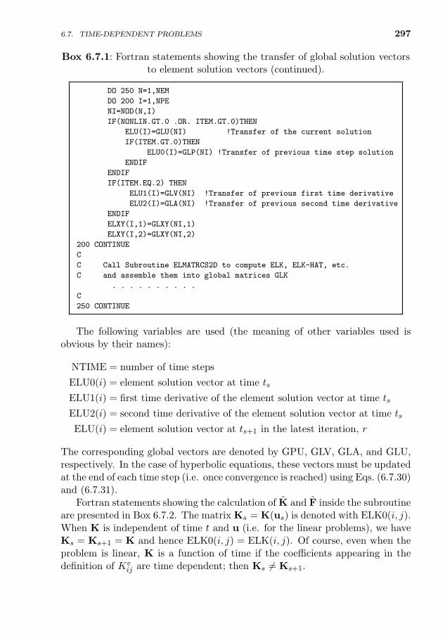
6.7. TIME-DEPENDENT PROBLEMS 297
Box 6.7.1: Fortran statements showing the transfer of global solution vectorsto element solution vectors (continued).
DO 250 N=1,NEM
DO 200 I=1,NPE
NI=NOD(N,I)
IF(NONLIN.GT.0 .OR. ITEM.GT.0)THEN
ELU(I)=GLU(NI) !Transfer of the current solution
IF(ITEM.GT.0)THEN
ELU0(I)=GLP(NI) !Transfer of previous time step solution
ENDIF
ENDIF
IF(ITEM.EQ.2) THEN
ELU1(I)=GLV(NI) !Transfer of previous first time derivative
ELU2(I)=GLA(NI) !Transfer of previous second time derivative
ENDIF
ELXY(I,1)=GLXY(NI,1)
ELXY(I,2)=GLXY(NI,2)
200 CONTINUE
C
C Call Subroutine ELMATRCS2D to compute ELK, ELK-HAT, etc.
C and assemble them into global matrices GLK
. . . . . . . . . .
C
250 CONTINUE
The following variables are used (the meaning of other variables used isobvious by their names):
NTIME = number of time steps
ELU0(i) = element solution vector at time ts
ELU1(i) = first time derivative of the element solution vector at time ts
ELU2(i) = second time derivative of the element solution vector at time ts
ELU(i) = element solution vector at ts+1 in the latest iteration, r
The corresponding global vectors are denoted by GPU, GLV, GLA, and GLU,respectively. In the case of hyperbolic equations, these vectors must be updatedat the end of each time step (i.e. once convergence is reached) using Eqs. (6.7.30)and (6.7.31).
Fortran statements showing the calculation of K and F inside the subroutineare presented in Box 6.7.2. The matrix Ks = K(us) is denoted with ELK0(i, j).When K is independent of time t and u (i.e. for the linear problems), we haveKs = Ks+1 = K and hence ELK0(i, j) = ELK(i, j). Of course, even when theproblem is linear, K is a function of time if the coefficients appearing in thedefinition of Ke
ij are time dependent; then Ks 6= Ks+1.
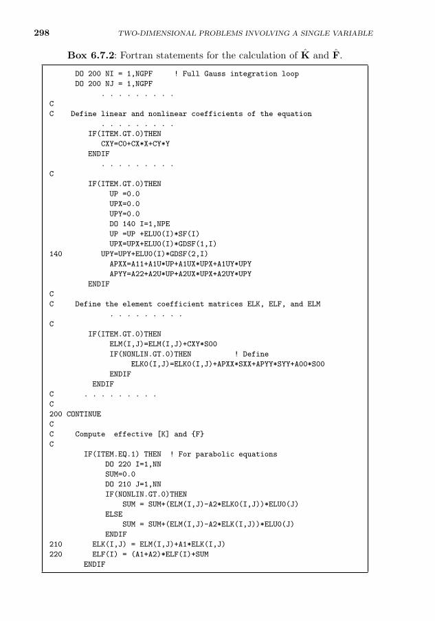
298 TWO-DIMENSIONAL PROBLEMS INVOLVING A SINGLE VARIABLE
Box 6.7.2: Fortran statements for the calculation of K and F.
DO 200 NI = 1,NGPF ! Full Gauss integration loop
DO 200 NJ = 1,NGPF
. . . . . . . . .
C
C Define linear and nonlinear coefficients of the equation
. . . . . . . . .
IF(ITEM.GT.0)THEN
CXY=C0+CX*X+CY*Y
ENDIF
. . . . . . . . .
C
IF(ITEM.GT.0)THEN
UP =0.0
UPX=0.0
UPY=0.0
DO 140 I=1,NPE
UP =UP +ELU0(I)*SF(I)
UPX=UPX+ELU0(I)*GDSF(1,I)
140 UPY=UPY+ELU0(I)*GDSF(2,I)
APXX=A11+A1U*UP+A1UX*UPX+A1UY*UPY
APYY=A22+A2U*UP+A2UX*UPX+A2UY*UPY
ENDIF
C
C Define the element coefficient matrices ELK, ELF, and ELM
. . . . . . . . .
C
IF(ITEM.GT.0)THEN
ELM(I,J)=ELM(I,J)+CXY*S00
IF(NONLIN.GT.0)THEN ! Define
ELK0(I,J)=ELK0(I,J)+APXX*SXX+APYY*SYY+A00*S00
ENDIF
ENDIF
C . . . . . . . . .
C
200 CONTINUE
C
C Compute effective [K] and F
C
IF(ITEM.EQ.1) THEN ! For parabolic equations
DO 220 I=1,NN
SUM=0.0
DO 210 J=1,NN
IF(NONLIN.GT.0)THEN
SUM = SUM+(ELM(I,J)-A2*ELK0(I,J))*ELU0(J)
ELSE
SUM = SUM+(ELM(I,J)-A2*ELK(I,J))*ELU0(J)
ENDIF
210 ELK(I,J) = ELM(I,J)+A1*ELK(I,J)
220 ELF(I) = (A1+A2)*ELF(I)+SUM
ENDIF
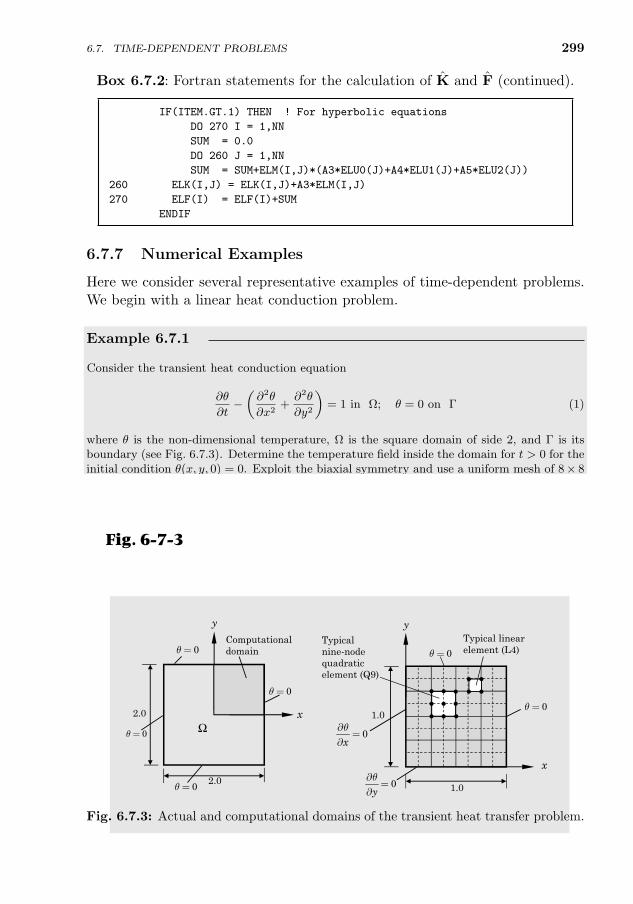
6.7. TIME-DEPENDENT PROBLEMS 299
Box 6.7.2: Fortran statements for the calculation of K and F (continued).
IF(ITEM.GT.1) THEN ! For hyperbolic equations
DO 270 I = 1,NN
SUM = 0.0
DO 260 J = 1,NN
SUM = SUM+ELM(I,J)*(A3*ELU0(J)+A4*ELU1(J)+A5*ELU2(J))
260 ELK(I,J) = ELK(I,J)+A3*ELM(I,J)
270 ELF(I) = ELF(I)+SUM
ENDIF
6.7.7 Numerical Examples
Here we consider several representative examples of time-dependent problems.We begin with a linear heat conduction problem.
Example 6.7.1
Consider the transient heat conduction equation
∂θ
∂t−(∂2θ
∂x2+∂2θ
∂y2
)= 1 in Ω; θ = 0 on Γ (1)
where θ is the non-dimensional temperature, Ω is the square domain of side 2, and Γ is itsboundary (see Fig. 6.7.3). Determine the temperature field inside the domain for t > 0 for theinitial condition θ(x, y, 0) = 0. Exploit the biaxial symmetry and use a uniform mesh of 8× 8linear rectangular elements to model the domain. Also, investigate the stability and accuracyof various schemes.
Solution: The boundary conditions along the lines of symmetry require that the heat flux bezero there. Thus, the boundary conditions of the computational domain are
∂θ
∂x(0, y, t) = 0,
∂θ
∂y(x, 0, t) = 0, θ(1, y, t) = 0, θ(x, 1, t) = 0 (2)
2.0
2.0 x
y
0q =
0q =
0q =
0q =
x
y
1.0
0xq¶=
¶
1.0
0q =
0q =
Ω
Computational domain
Typical nine-nodequadratic element (Q9) • •
• •
Typical linear element (L4)
0yq¶=
¶
Fig. 6-7-3
Fig. 6.7.3: Actual and computational domains of the transient heat transfer problem.
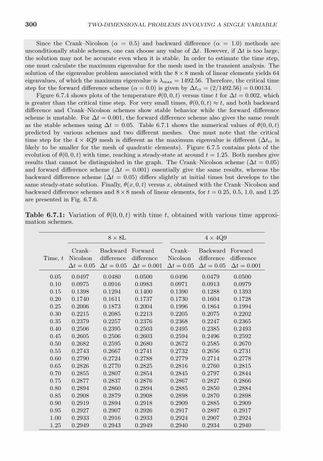
300 TWO-DIMENSIONAL PROBLEMS INVOLVING A SINGLE VARIABLE
Since the Crank–Nicolson (α = 0.5) and backward difference (α = 1.0) methods areunconditionally stable schemes, one can choose any value of ∆t. However, if ∆t is too large,the solution may not be accurate even when it is stable. In order to estimate the time step,one must calculate the maximum eigenvalue for the mesh used in the transient analysis. Thesolution of the eigenvalue problem associated with the 8× 8 mesh of linear elements yields 64eigenvalues, of which the maximum eigenvalue is λmax = 1492.56. Therefore, the critical timestep for the forward difference scheme (α = 0.0) is given by ∆tcr = (2/1492.56) = 0.00134.
Figure 6.7.4 shows plots of the temperature θ(0, 0, t) versus time t for ∆t = 0.002, whichis greater than the critical time step. For very small times, θ(0, 0, t) ≈ t, and both backwarddifference and Crank–Nicolson schemes show stable behavior while the forward differencescheme is unstable. For ∆t = 0.001, the forward difference scheme also gives the same resultas the stable schemes using ∆t = 0.05. Table 6.7.1 shows the numerical values of θ(0, 0, t)predicted by various schemes and two different meshes. One must note that the criticaltime step for the 4 × 4Q9 mesh is different as the maximum eigenvalue is different (∆tcr islikely to be smaller for the mesh of quadratic elements). Figure 6.7.5 contains plots of theevolution of θ(0, 0, t) with time, reaching a steady-state at around t = 1.25. Both meshes giveresults that cannot be distinguished in the graph. The Crank–Nicolson scheme (∆t = 0.05)and forward difference scheme (∆t = 0.001) essentially give the same results, whereas thebackward difference scheme (∆t = 0.05) differs slightly at initial times but develops to thesame steady-state solution. Finally, θ(x, 0, t) versus x, obtained with the Crank–Nicolson andbackward difference schemes and 8× 8 mesh of linear elements, for t = 0.25, 0.5, 1.0, and 1.25are presented in Fig. 6.7.6.
Table 6.7.1: Variation of θ(0, 0, t) with time t, obtained with various time approxi-mation schemes.
8× 8L 4× 4Q9
Crank– Backward Forward Crank– Backward ForwardTime, t Nicolson difference difference Nicolson difference difference
∆t = 0.05 ∆t = 0.05 ∆t = 0.001 ∆t = 0.05 ∆t = 0.05 ∆t = 0.001
0.05 0.0497 0.0480 0.0500 0.0496 0.0479 0.05000.10 0.0975 0.0916 0.0983 0.0971 0.0913 0.09790.15 0.1398 0.1294 0.1400 0.1390 0.1288 0.13930.20 0.1740 0.1611 0.1737 0.1730 0.1604 0.17280.25 0.2006 0.1873 0.2004 0.1996 0.1864 0.19940.30 0.2215 0.2085 0.2213 0.2205 0.2075 0.22020.35 0.2379 0.2257 0.2376 0.2368 0.2247 0.23650.40 0.2506 0.2395 0.2503 0.2495 0.2385 0.24930.45 0.2605 0.2506 0.2603 0.2594 0.2496 0.25920.50 0.2682 0.2595 0.2680 0.2672 0.2585 0.26700.55 0.2743 0.2667 0.2741 0.2732 0.2656 0.27310.60 0.2790 0.2724 0.2788 0.2779 0.2714 0.27780.65 0.2826 0.2770 0.2825 0.2816 0.2760 0.28150.70 0.2855 0.2807 0.2854 0.2845 0.2797 0.28440.75 0.2877 0.2837 0.2876 0.2867 0.2827 0.28660.80 0.2894 0.2860 0.2894 0.2885 0.2850 0.28840.85 0.2908 0.2879 0.2908 0.2898 0.2870 0.28980.90 0.2919 0.2894 0.2918 0.2909 0.2885 0.29090.95 0.2927 0.2907 0.2926 0.2917 0.2897 0.29171.00 0.2933 0.2916 0.2933 0.2924 0.2907 0.29241.25 0.2949 0.2943 0.2949 0.2940 0.2934 0.2940
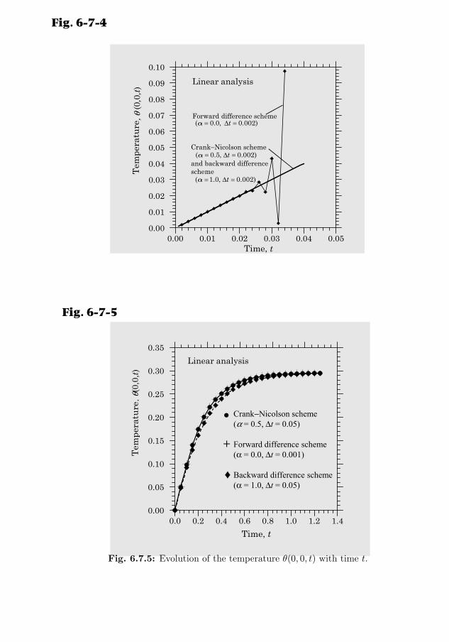
6.7. TIME-DEPENDENT PROBLEMS 301
0.00 0.01 0.02 0.03 0.04 0.05Time,
0.00
0.01
0.02
0.03
0.04
0.05
0.06
0.07
0.08
0.09
0.10
Tem
pera
ture
t
, θ (0
,0,t
)
Forward difference scheme
Crank−Nicolson scheme
and backward difference scheme
( 0.0, 0.002)ta = Δ =
( 0.5, 0.002)ta = Δ =
( 1.0, 0.002)ta = Δ =
Linear analysis
Fig. 6-7-4
Fig. 6.7.4: Transient response predicted by various schemes.
0.0 0.2 0.4 0.6 0.8 1.0 1.2 1.4
Time, t
0.00
0.05
0.10
0.15
0.20
0.25
0.30
0.35
Tem
pera
ture
, θ(0
,0,t
)
Crank−Nicolson scheme (α = 0.5, Δt = 0.05)
Forward difference scheme (α = 0.0, Δt = 0.001)
Backward difference scheme (α = 1.0, Δt = 0.05)
+
♦
Linear analysis
Fig. 6-7-5
Fig. 6.7.5: Evolution of the temperature θ(0, 0, t) with time t.
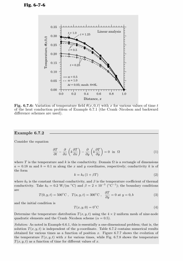
302 TWO-DIMENSIONAL PROBLEMS INVOLVING A SINGLE VARIABLE
0.0 0.2 0.4 0.6 0.8 1.0
Distance, x
0.00
0.05
0.10
0.15
0.20
0.25
0.30
0.35
Tem
pera
ture
t = 1.0
t = 0.5
t = 0.25
α = 0.5 α = 1.0
, θ(x
,0,t
)
Δt = 0.05; mesh: 8×8L
t = 1.25Linear analysis
Fig. 6-7-6
Fig. 6.7.6: Variation of temperature field θ(x, 0, t) with x for various values of time tof the heat conduction problem of Example 6.7.1 (the Crank–Nicolson and backwarddifference schemes are used).
Example 6.7.2
Consider the equation
∂T
∂t− ∂
∂x
(k∂T
∂x
)− ∂
∂y
(k∂T
∂y
)= 0 in Ω (1)
where T is the temperature and k is the conductivity. Domain Ω is a rectangle of dimensionsa = 0.18 m and b = 0.1 m along the x and y coordinates, respectively; conductivity k is ofthe form
k = k0 (1 + βT ) (2)
where k0 is the constant thermal conductivity, and β is the temperature coefficient of thermalconductivity. Take k0 = 0.2 W/(m C) and β = 2 × 10⁻³ (C−1); the boundary conditionsare
T (0, y, t) = 500C , T (a, y, t) = 300C ,∂T
∂y= 0 at y = 0, b (3)
and the initial condition isT (x, y, 0) = 0C (4)
Determine the temperature distribution T (x, y, t) using the 4× 2 uniform mesh of nine-nodequadratic elements and the Crank–Nicolson scheme (α = 0.5).
Solution: As noted in Example 6.6.1, this is essentially a one-dimensional problem; that is, thesolution T (x, y, t) is independent of the y-coordinate. Table 6.7.2 contains numerical resultsobtained for various times as a function of position x. Figure 6.7.7 shows the evolution ofthe temperature T (x, y, t) with x for various times, while Fig. 6.7.8 shows the temperatureT (x, y, t) as a function of time for different values of x.
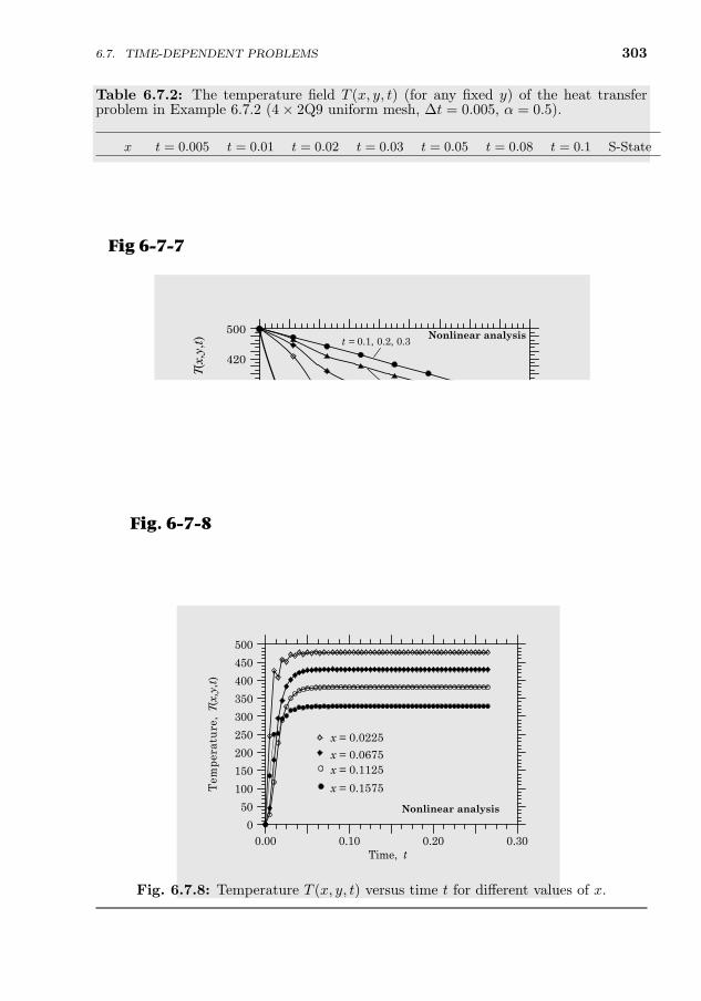
6.7. TIME-DEPENDENT PROBLEMS 303
Table 6.7.2: The temperature field T (x, y, t) (for any fixed y) of the heat transferproblem in Example 6.7.2 (4× 2Q9 uniform mesh, ∆t = 0.005, α = 0.5).
x t = 0.005 t = 0.01 t = 0.02 t = 0.03 t = 0.05 t = 0.08 t = 0.1 S-State
0.0225 245.11 426.98 456.58 471.48 477.94 477.91 477.58 477.310.0450 107.47 289.91 386.74 427.69 448.56 448.57 453.09 454.030.0675 45.03 178.65 343.35 401.46 427.61 427.63 430.44 430.120.0900 24.16 119.18 311.87 375.39 402.23 402.23 405.01 405.570.1125 26.78 118.01 289.07 350.37 377.43 377.39 380.55 380.320.1350 56.82 167.10 278.43 326.88 350.15 350.13 354.00 354.340.1575 134.67 250.20 293.20 316.45 327.11 327.12 327.79 327.58
0.00 0.02 0.04 0.06 0.08 0.10 0.12 0.14 0.16 0.18
Distance, x
20
100
180
260
340
420
500
Tem
pera
ture
, Τ(x
,y,t
) t = 0.1, 0.2, 0.3
4×2Q9 meshCrank−Nicolson(Δt = 0.005)
t = 0.01
t = 0.02
t = 0.03
t = 0.005
Nonlinear analysis
Fig 6-7-7
Fig. 6.7.7: Temperature T (x, y, t) versus x for different values of t.
0.00 0.10 0.20 0.30Time,
0
50
100
150
200
250
300
350
400
450
500
Tem
pera
ture
, Τ(
x,y,
t)
t
x = 0.0225
x = 0.0675x = 0.1125
x = 0.1575
Nonlinear analysis
Fig. 6-7-8
Fig. 6.7.8: Temperature T (x, y, t) versus time t for different values of x.
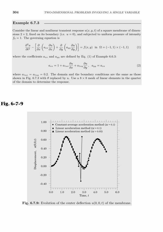
304 TWO-DIMENSIONAL PROBLEMS INVOLVING A SINGLE VARIABLE
Example 6.7.3
Consider the linear and nonlinear transient response u(x, y, t) of a square membrane of dimen-sions 2× 2, fixed on its boundary (i.e. u = 0), and subjected to uniform pressure of intensityf0 = 1. The governing equation is
∂2u
∂t2−[∂
∂x
(axx
∂u
∂x
)+
∂
∂y
(ayy
∂u
∂y
)]= f(x, y) in Ω = (−1, 1)× (−1, 1) (1)
where the coefficients axx and ayy are defined by Eq. (1) of Example 6.6.3:
axx = 1 + a1ux∂u
∂x+ a1uy
∂u
∂y, ayy = axx (2)
where a1ux = a1uy = 0.2. The domain and the boundary conditions are the same as thoseshown in Fig. 6.7.3 with θ replaced by u. Use a 8× 8 mesh of linear elements in the quarterof the domain to determine the response.
Solution: The critical time step for the linear acceleration method (α = 0.5 and γ = 1/3) is(λmax = 1492.56) ∆tcr = 0.0897. Figure 6.7.9 shows plots of the transverse deflection u(0, 0, t)versus time t for the linear case (i.e. a1ux = a1uy = 0) with ∆t = 0.1, which is greaterthan the critical time step. The linear acceleration method (α = 0.5 and γ = 1/3) givesalmost the same response as the constant-average acceleration method (α = 0.5 and γ = 0.5)when ∆t = 0.05 (see Table 6.7.3). The linear and nonlinear (with a1ux = a1uy = 0.2) centerdeflections as functions of time are shown in Fig. 6.7.10. The nonlinear deflection starts todrift away from the linear solution, both in amplitude and period with time.
0.0 1.0 2.0 3.0 4.0 5.0 6.0Time, t
-0.40
-0.20
0.00
0.20
0.40
0.60
0.80
1.00
Dis
plac
emen
t, u
(x,0
,t)
Constant-average acceleration method (Δt = 0.1)Linear acceleration method (Δt = 0.1)Linear acceleration method (Δt = 0.05)
•
Fig. 6-7-9
u(0,
0,t)
Fig. 6.7.9: Evolution of the center deflection u(0, 0, t) of the membrane.
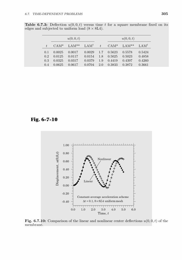
6.7. TIME-DEPENDENT PROBLEMS 305
Table 6.7.3: Deflection u(0, 0, t) versus time t for a square membrane fixed on itsedges and subjected to uniform load (8× 8L4).
u(0, 0, t) u(0, 0, t)
t CAM* LAM** LAM† t CAM* LAM** LAM†
0.1 0.0025 0.0017 0.0029 1.7 0.5623 0.5578 0.54240.2 0.0125 0.0117 0.0154 1.8 0.5025 0.5023 0.48580.3 0.0325 0.0317 0.0379 1.9 0.4419 0.4397 0.42600.4 0.0625 0.0617 0.0704 2.0 0.3833 0.3872 0.36610.5 0.1025 0.1017 0.1129 2.1 0.3243 0.3122 0.30690.6 0.1525 0.1517 0.1657 2.2 0.2655 0.2841 0.25110.7 0.2125 0.2117 0.2269 2.3 0.2105 0.1740 0.19590.8 0.2825 0.2812 0.2989 2.4 0.1601 0.2250 0.14270.9 0.3624 0.3626 0.3896 2.5 0.1131 −0.0078 0.10141.0 0.4500 0.4565 0.4876 2.6 0.0706 0.2833 0.06931.1 0.5378 0.5482 0.5701 2.7 0.0343 −0.3422 0.02891.2 0.6110 0.6161 0.6301 2.8 0.0038 0.6653 −0.01961.3 0.6550 0.6546 0.6619 2.9 −0.0204 −1.1816 −0.05531.4 0.6656 0.6658 0.6608 3.0 −0.0348 1.9454 −0.06251.5 0.6492 0.6482 0.6359 3.1 −0.0339 −3.5058 −0.03581.6 0.6133 0.6079 0.5939 3.2 −0.0102 5.9399 0.0207
* CAM = constant-average acceleration method (α = 0.5, γ = 0.5, ∆t = 0.1);** LAM = linear acceleration method (α = 0.5, γ = 1/3, ∆t = 0.1).† LAM with ∆t = 0.05.
0.0 1.0 2.0 3.0 4.0 5.0 6.0Time, t
-0.40
-0.20
0.00
0.20
0.40
0.60
0.80
1.00
Dis
plac
emen
t , u
(0,0
,t)
Constant-average acceleration scheme0.1, 8 8 4 uniformmesht LΔ = ×
Linear
Nonlinear
Fig. 6-7-10
Fig. 6.7.10: Comparison of the linear and nonlinear center deflections u(0, 0, t) of themembrane.
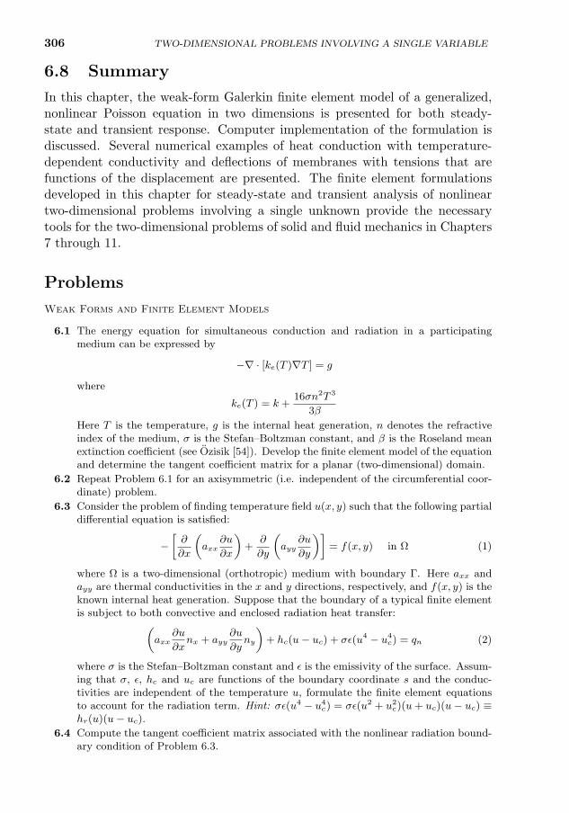
306 TWO-DIMENSIONAL PROBLEMS INVOLVING A SINGLE VARIABLE
6.8 Summary
In this chapter, the weak-form Galerkin finite element model of a generalized,nonlinear Poisson equation in two dimensions is presented for both steady-state and transient response. Computer implementation of the formulation isdiscussed. Several numerical examples of heat conduction with temperature-dependent conductivity and deflections of membranes with tensions that arefunctions of the displacement are presented. The finite element formulationsdeveloped in this chapter for steady-state and transient analysis of nonlineartwo-dimensional problems involving a single unknown provide the necessarytools for the two-dimensional problems of solid and fluid mechanics in Chapters7 through 11.
Problems
Weak Forms and Finite Element Models
6.1 The energy equation for simultaneous conduction and radiation in a participatingmedium can be expressed by
−∇ · [ke(T )∇T ] = g
where
ke(T ) = k +16σn2T 3
3β
Here T is the temperature, g is the internal heat generation, n denotes the refractiveindex of the medium, σ is the Stefan–Boltzman constant, and β is the Roseland meanextinction coefficient (see Ozisik [54]). Develop the finite element model of the equationand determine the tangent coefficient matrix for a planar (two-dimensional) domain.
6.2 Repeat Problem 6.1 for an axisymmetric (i.e. independent of the circumferential coor-dinate) problem.
6.3 Consider the problem of finding temperature field u(x, y) such that the following partialdifferential equation is satisfied:
−[∂
∂x
(axx
∂u
∂x
)+
∂
∂y
(ayy
∂u
∂y
)]= f(x, y) in Ω (1)
where Ω is a two-dimensional (orthotropic) medium with boundary Γ. Here axx andayy are thermal conductivities in the x and y directions, respectively, and f(x, y) is theknown internal heat generation. Suppose that the boundary of a typical finite elementis subject to both convective and enclosed radiation heat transfer:(
axx∂u
∂xnx + ayy
∂u
∂yny
)+ hc(u− uc) + σε(u4 − u4
c) = qn (2)
where σ is the Stefan–Boltzman constant and ε is the emissivity of the surface. Assum-ing that σ, ε, hc and uc are functions of the boundary coordinate s and the conduc-tivities are independent of the temperature u, formulate the finite element equationsto account for the radiation term. Hint: σε(u4 − u4
c) = σε(u2 + u2c)(u+ uc)(u− uc) ≡
hr(u)(u− uc).
6.4 Compute the tangent coefficient matrix associated with the nonlinear radiation bound-ary condition of Problem 6.3.
PROBLEMS 307
Computational Problems
6.5 Solve the problem of Example 6.6.1 for the following data:
a = 0.2 m, b = 0.1 m, β = 0.2 (K−1) (1)
T (0, y) = 500 K , T (a, y) = 300 K ,∂T
∂y= 0 at y = 0, T (x, b) = 500− 1000x K
(2)All other data remain the same. Use 4×4 and 8×8 linear element meshes, and 2×2 and4×4 nine-node quadratic element meshes to analyze the two problems using the directiteration and Newton’s iteration schemes. Use a convergence tolerance of ε = 10−3 andmaximum allowable iterations to be 10.
6.6 Consider the nonlinear problem of Example 6.6.1 (heat transfer in two dimensions).Use the uniform 4× 4 nine-node quadratic element mesh to analyze the problem usingthe following data and boundary conditions (see Fig. P6.6) and the direct iterationprocedure:
a = 0.18 m, b = 0.1 m, f0 = 0 W/m3 (1)
k = k0 (1 + βT ) , k0 = 25 W/(m C) (2)
T (0, y) = 100 C , T (a, y) = 50 C
k∂T
∂n+ hc(T − T∞) = 0 at y = 0, b (3)
Use β = 0.2, T∞ = 10C, and hc = 50 W/(m2 C), and ε = 10−3 and ITMAX =10. Plot linear and nonlinear solutions T (x, y) as functions of x for fixed y = 0 andy = 0.05. Hint: See Section 3.3.4 for the treatment of convection heat transfer boundaryconditions, and Chapter 8 of Reddy [2] for computational details of such problems.
100 CT = 50 CT =
210 C, 50W/(m . C)cT h∞ = =
0 0k k k Tb= +
Domain with boundary conditions
Line of symmetry
210 C, 50W/(m . C)cT h∞ = =
Fig. P6-1
Fig. P6.6
6.7 Analyze Problem 6.6 using the Newton iteration procedure.
Time-Dependent Problems
6.8 Derive Eq. (6.7.17) for parabolic equations when C is a function of time.
6.9 Show that Eq. (6.7.27) can be expressed in the alternative form
Hs+1us+1 = Fs+1
and define Hs+1 and Fs+1.
308 TWO-DIMENSIONAL PROBLEMS INVOLVING A SINGLE VARIABLE
6.10 The α-family of approximation and a general class of time-approximation schemes basedon truncated Taylor’s series can also be derived using the finite element method in timedomain. Consider a first-order differential equation of the form
Cdu
dt+Ku(t) = F (t) (1)
where, in general, C, K, and F are functions of time, t. Suppose that u(t) is approxi-mated as
u(t) ≈n∑
j=1
ujψj(t) (2)
where uj denotes the value of u(t) at time t = tj and ψj(t) is the associated approx-imation function. The weighted-integral method seeks the solution of Eq. (1) over atypical time interval (ts, ts+1) by requiring
0 =
∫ ts+1
ts
wj(t) (Cu+Ku− F ) dt (3)
where wj(t) is the jth weight function (j = 1, 2, · · · , n). Obtain the (Petrov–Galerkin)finite element model using the weighted-integral statement, Eq. (3), and then special-ize the result for the choice φj = ψj (i.e. using the Galerkin method) as the linearinterpolation functions. Assume that F (t) can also be approximated as
F (t) = F1ψ1(t) + F2ψ2(t) (4)
and derive the equation for us+1 = u2 in terms of us = u1, Fs = F1, Fs+1 = F2, and∆t = ts+1 − ts using constant values of C and K.
6.11 Use quadratic approximation of u(t) with φi = ψi (i.e. Galerkin’s method) in theweighted-integral form in Eq. (3) of Problem 6.10 and arrive at the finite elementequations (
C
6
−3 4 −1−4 0 4
1 −4 3
+K∆t
30
4 2 −12 16 2−1 2 4
)U1
U2
U3
=
∆t
30
4 2 −12 16 2−1 2 4
F1
F2
F3
(1)
whereU1 = us, U2 = us+ 1
2, U3 = us+1 (2)
and similar definition holds for Fi. Determine the values of U2 and U3 in terms of U1.
6.12 Consider the equation
c∂u
∂t− ∂
∂x
(axx
∂u
∂x
)− ∂
∂y
(ayy
∂u
∂y
)= f(x, y, t) in Ω (1)
where u is the dependent unknown and axx and ayy are known functions of position(x, y) and u and its derivatives
axx = ayy = c1(x, y) + 12c2(x, y)
[(∂u
∂x
)2
+
(∂u
∂y
)2]
(2)
Develop a fully discretized finite element model and determine the tangent coefficientmatrix of a typical element.
PROBLEMS 309
6.13 Consider the transient heat conduction equation
∂θ
∂t− k
(∂2θ
∂x2+∂2θ
∂y2
)= 1 in Ω; θ = 0 on Γ (1)
where θ is the non-dimensional temperature, Ω is the square domain of side 2, andΓ is its boundary with the boundary conditions shown in Fig. 6.7.3. Determine thetemperature field inside the domain as a function of position and time when k =k0(1+βθ) with k0 = 1.0 and β = 0.4×10⁻³. Assume zero initial condition θ(x, y, 0) = 0,exploit the biaxial symmetry, and use a uniform mesh of 4 × 4 nine-node rectangularelements in a quadrant, the Crank–Nicolson scheme (i.e. α = 0.5) with ∆t = 0.05,and error tolerance of ε = 10−3 for the direct iteration method. Plot the temperatureθ(x0, 0, t) as a function of time for x0 = 0.0, 0.5, and 0.75. The total number of timesteps are such that the temperature reaches a steady state.
6.14 Repeat Problem 6.13 with β = 0.4 and all other data being the same.
6.15 Solve the problem in Example 6.7.3 with
axx = ayy = 1 + au · u
with au = 0.1 and plot the solution u(0, 0, t) versus time.
6.16 Solve the problem in Example 6.7.3 with
axx = ayy = 1 + au · u
with au = 1.0 and plot the solution u(0, 0, t) versus time.
6.17 Put together a complete finite element program based on the logic presented in Box6.6.1 that has the capability of solving two-dimensional nonlinear problems involvinga single unknown.

311
7
Nonlinear Bending ofElastic Plates
Science is the search for the truth – it is not a game in which one tries to beat his opponent,to do harm to others. ——– Linus Pauling
7.1 Introduction
A plate is a flat structural element with planform dimensions that are large com-pared to its thickness and is subjected to loads that cause bending deformationin addition to stretching in the plane [3, 55, 56]. In most cases, the thicknessis no greater than one-tenth of the smallest in-plane dimension. Because of thesmallness of the thickness dimension, it is often not necessary to model themusing three-dimensional elasticity equations. Simple two-dimensional plate the-ories, much like the beam theories considered in Chapter 5, can be developed tostudy the deformation and stresses in plate structures undergoing small strains,small to moderate rotations, and large displacements (i.e. w/h > 1).
As in the case of beams, we consider both classical and shear deformationplate theories, which are extensions of the Euler–Bernoulli and Timoshenkobeam theories, respectively, to two dimensions. The extension of the Euler–Bernoulli beam theory to two dimensions is known as the classical or Kirchhoffplate theory, while the extension of the Timoshenko beam theory to two di-mensions is termed the first-order shear deformation plate theory. Geometricnonlinearity is considered via the von Karman strains, as in the case of beams.
In nonlinear continuum mechanics (see Reddy [1] and Chapter 2), one usesthe notation X = (X1, X2, X3) for the material coordinates and x for the spa-tial coordinates. As discussed previously in connection with beams, the presentstudy of plates is limited to small strains and moderate rotations, and thereforeno distinction is made here between the material coordinates X and spatial co-ordinates x = (x1, x2, x3). In fact, x is used to denote the material coordinates,i.e. x = x1 = X1, y = x2 = X2, and z = x3 = X3.
The weak forms of each plate theory are developed using the principle ofvirtual displacements. Then the displacement finite element models of both the-ories are developed, their computer implementation is discussed, and numericalexamples of some representative plate problems are presented.
J.N. Reddy, An Introduction to Nonlinear Finite Element Analysis, Second Edition. c©J.N.Reddy 2015. Published in 2015 by Oxford University Press.
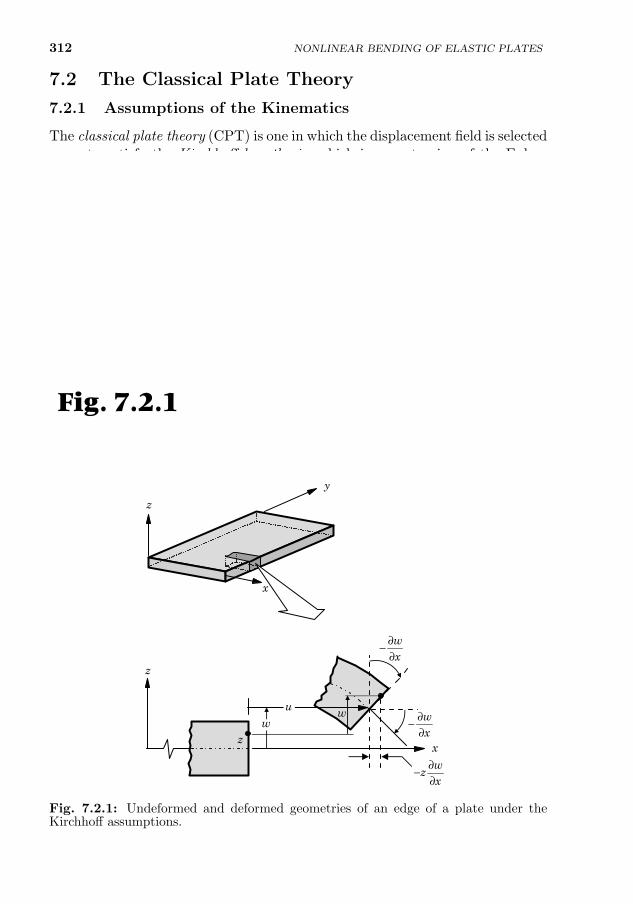
312 NONLINEAR BENDING OF ELASTIC PLATES
7.2 The Classical Plate Theory
7.2.1 Assumptions of the Kinematics
The classical plate theory (CPT) is one in which the displacement field is selectedso as to satisfy the Kirchhoff hypothesis, which is an extension of the Euler–Bernoulli hypothesis of beams to two dimensions. The Kirchhoff hypothesisconsists of the following three assumptions (see Fig. 7.2.1):
(1) Straight lines perpendicular to the mid-surface (i.e. transverse normals)before deformation, remain straight after deformation.
(2) The transverse normals do not experience elongation (i.e. inextensible).
(3) The transverse normals rotate such that they remain perpendicular to themid-surface after deformation.
7.2.2 Displacement and Strain Fields
Let us denote the undeformed mid-plane of the plate with symbol Ω0. The totaldomain of the plate is the tensor product Ω0 × (−h/2, h/2). The boundary ofthe total domain consists of surfaces St(z = h/2) and Sb(z = −h/2), and theedge Γ ≡ Γ × (−h/2, h/2). In general, Γ is a curved surface, with outwardnormal n = nxex + nyey, where nx and ny are the direction cosines of the unitnormal.
x
y
z
xz
u
wz
x∂−∂
wx
∂−∂
wx
∂−∂
ww
z
Fig. 7.2.1
Fig. 7.2.1: Undeformed and deformed geometries of an edge of a plate under theKirchhoff assumptions.
7.2. THE CLASSICAL PLATE THEORY 313
The Kirchhoff hypothesis implies the following form of the displacementfield (see Fig. 7.2.1 for the kinematics of bending)
u1(x, y, z, t) = u(x, y, t)− z ∂w∂x
u2(x, y, z, t) = v(x, y, t)− z ∂w∂y
(7.2.1)
u3(x, y, z, t) = w(x, y, t)
where (u, v, w) denote the displacements of a material point occupying the posi-tion (x, y, 0) in the undeformed configuration for any time t, whereas (u1, u2, u3)are the total displacement components of a material point located at an arbi-trary point x = (x, y, z) in the undeformed body.
The definition of the components of the Green–Lagrange strain tensor E interms of the components of the total displacement vector u = x(X, t) −X is[see Eqs. (2.4.8) and (2.4.9); shortly, Xi will be replaced with xi]
E11 =∂u1
∂X1+
1
2
[(∂u1
∂X1
)2
+
(∂u2
∂X1
)2
+
(∂u3
∂X1
)2]
E22 =∂u2
∂X2+
1
2
[(∂u1
∂X2
)2
+
(∂u2
∂X2
)2
+
(∂u3
∂X2
)2]
E33 =∂u3
∂X3+
1
2
[(∂u1
∂X3
)2
+
(∂u2
∂X3
)2
+
(∂u3
∂X3
)2]
(7.2.2)
E12 =1
2
(∂u1
∂X2+∂u2
∂X1+∂u1
∂X1
∂u1
∂X2+∂u2
∂X1
∂u2
∂X2+∂u3
∂X1
∂u3
∂X2
)E13 =
1
2
(∂u1
∂X3+∂u3
∂X1+∂u1
∂X1
∂u1
∂X3+∂u2
∂X1
∂u2
∂X3+∂u3
∂X1
∂u3
∂X3
)E23 =
1
2
(∂u2
∂X3+∂u3
∂X2+∂u1
∂X2
∂u1
∂X3+∂u2
∂X2
∂u2
∂X3+∂u3
∂X2
∂u3
∂X3
)If the components of the displacement gradients are of the order ε (a very
small parameter, ε << 1)
∂u1
∂X1,∂u1
∂X2,∂u1
∂X3,∂u2
∂X1,∂u2
∂X2,∂u2
∂X3, · · · , ∂u3
∂X3= O(ε) (7.2.3)
then the small strain assumption implies that terms of order ε2 are omitted inthe strains. If the rotations of transverse normals are moderate (say 10–15),then the following terms are small but not negligible compared to ε(
∂u3
∂X1
)2
,
(∂u3
∂X2
)2
,∂u3
∂X1
∂u3
∂X2(7.2.4)
314
Thus for small strains and moderate rotations, the strain-displacement relations(7.2.2) take the form [here we switch from Xi to xi and subsequently to (x, y, z)]
Exx ≈ εxx =∂u1
∂x+
1
2
(∂u3
∂x
)2
, Exy ≈ εxy =1
2
(∂u1
∂y+∂u2
∂x+∂u3
∂x
∂u3
∂y
)Exz ≈ εxz =
1
2
(∂u1
∂z+∂u3
∂x
), Eyy ≈ εyy =
∂u2
∂y+
1
2
(∂u3
∂y
)2
Eyz ≈ εyz =1
2
(∂u2
∂z+∂u3
∂y
), Ezz ≈ εzz =
∂u3
∂z(7.2.5)
where, for this special case of geometric nonlinearity (i.e. small strains butmoderate rotations), notation εij is used in place of Eij . The correspondingCartesian components of the second Piola–Kirchhoff stress tensor will be de-noted σij (notation σij is usually reserved for the Cauchy stress tensor; seeReddy [1] and Chapter 2).
For the displacement field in Eq. (7.2.1), we have εzz = ∂u3∂z = ∂w
∂z = 0 andthe strains in Eq. (7.2.5) reduce to
εxx =∂u
∂x+
1
2
(∂w
∂x
)2
− z ∂2w
∂x2
εyy =∂v
∂y+
1
2
(∂w
∂y
)2
− z ∂2w
∂y2
2εxy =∂u
∂y+∂v
∂x+∂w
∂x
∂w
∂y− 2z
∂2w
∂x∂y≡ γxy
2εxz = −∂w∂x
+∂w
∂x≡ γxz = 0
2εyz = −∂w∂y
+∂w
∂y≡ γyz = 0
(7.2.6)
The strains in Eq. (7.2.6) are called the von Karman strains, and the associatedplate theory is termed the classical plate theory with the von Karman strains.Note that the transverse strains (εxz, εyz, εzz) are identically zero in the classicalplate theory. In matrix notation, the total strains in Eq. (7.2.6) can be writtenas the sum of membrane strains ε(0) and bending strains ε(1)
εxxεyyγxy
=
ε0xx
ε0yy
γ0xy
+ z
ε1xx
ε1yy
γ1xy
(7.2.7)
ε0xx
ε0yy
γ0xy
=
∂u∂x + 1
2
(∂w∂x
)2∂v∂y + 1
2
(∂w∂y
)2
∂u∂y + ∂v
∂x + ∂w∂x
∂w∂y
,
ε1xx
ε1yy
γ1xy
= −
∂2w∂x2
∂2w∂y2
2 ∂2w∂x∂y
(7.2.8)
NONLINEAR BENDING OF ELASTIC PLATES
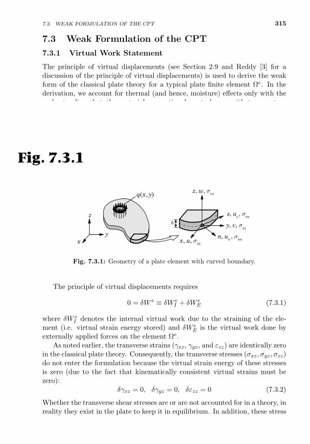
7.3. WEAK FORMULATION OF THE CPT 315
7.3 Weak Formulation of the CPT
7.3.1 Virtual Work Statement
The principle of virtual displacements (see Section 2.9 and Reddy [3] for adiscussion of the principle of virtual displacements) is used to derive the weakform of the classical plate theory for a typical plate finite element Ωe. In thederivation, we account for thermal (and hence, moisture) effects only with theunderstanding that the material properties do not change with temperatureand that temperature T is a known function of position (hence, δT = 0). Thus,temperature enters the formulation only through constitutive equations.
Suppose that the total domain (i.e. midplane) Ω of the plate is representedby a set of finite elements, and let Ωe be a typical plate element with boundaryΓe. Suppose that q(x, y) is the distributed transverse force at the top surface,z = h/2, and (σnn, σns, σnz) are the stress components on the boundary Γe =Γe× (−h
2 ,h2 ) of the plate element (see Fig. 7.3.1 for a plate element with curved
boundary).
h
, , nzz w s
, ,s nss u s
, ,n nnn u s, , xxx u s
, , xyy v s
z
yx
( , )q x y
Fig. 7.3.1
Fig. 7.3.1: Geometry of a plate element with curved boundary.
The principle of virtual displacements requires
0 = δW e ≡ δW eI + δW e
E (7.3.1)
where δW eI denotes the internal virtual work due to the straining of the ele-
ment (i.e. virtual strain energy stored) and δW eE is the virtual work done by
externally applied forces on the element Ωe.As noted earlier, the transverse strains (γxz, γyz, and εzz) are identically zero
in the classical plate theory. Consequently, the transverse stresses (σxz, σyz, σzz)do not enter the formulation because the virtual strain energy of these stressesis zero (due to the fact that kinematically consistent virtual strains must bezero):
δγxz = 0, δγyz = 0, δεzz = 0 (7.3.2)
Whether the transverse shear stresses are or are not accounted for in a theory, inreality they exist in the plate to keep it in equilibrium. In addition, these stress
316 NONLINEAR BENDING OF ELASTIC PLATES
components may be specified on the boundary. Thus, the transverse stressesdo not enter the virtual strain energy expression but must be accounted for inequilibrium equations.
The virtual strain energy in element Ωe is given by
δW eI =
∫Ωe
∫ h2
−h2
(σxxδεxx + σyyδεyy + 2σxyδεxy) dz dx dy
=
∫Ωe
(Nxxδε
0xx +Mxxδε
1xx +Nyyδε
0yy +Myyδε
1yy
+Nxyδγ0xy +Mxyδγ
1xy
)dx dy (7.3.3)
where (Nxx, Nyy, Nxy) are the forces per unit length and (Mxx,Myy,Mxy) arethe moments per unit length as defined by
Nxx
Nyy
Nxy
=
∫ h2
−h2
σxxσyyσxy
dz ,
Mxx
Myy
Mxy
=
∫ h2
−h2
σxxσyyσxy
z dz (7.3.4)
Figure 7.3.2 shows various stress resultants on a plate edge with unit normaln = nxi + ny j; an alternative sign convention for moments, based on the right-hand screw rule, is displayed in Fig. 7.3.3. We note that the subscripts on N ’sand M ’s refer to the subscripts of stresses that produce them.
The virtual work done by the distributed transverse load q(x, y), the trans-verse reaction force of an elastic foundation at z = −h/2, in-plane normal stressσnn, in-plane tangential stress σns, and transverse shear stress σnz is
δW eE = −
∫Ωeq(x, y)δw(x, y,
h
2) dx dy +
∫ΩeFs(x, y) δw(x, y,−h
2) dx dy
+
∮Γe
∫ h2
−h2
[σnn
(δun − z
∂δw
∂n
)+ σns
(δus − z
∂δw
∂s
)+ σnzδw
]dz ds
(7.3.5)
= −[∮
Γe
(Nnnδun −Mnn
∂δw
∂n+Nnsδus −Mns
∂δw
∂s+Qnδw
)ds
+
∫Ωe
(q − kw) δw dx dy
](7.3.6)
where Fs = −kw is the foundation force, k is the foundation modulus, andun, us, and w are the displacements along the normal, tangential, and transversedirections, respectively (see Fig. 7.3.1), andNnn
Nns
=
∫ h2
−h2
σnnσns
dz,
Mnn
Mns
=
∫ h2
−h2
σnnσns
z dz, Qn =
∫ h2
−h2
σnz dz
(7.3.7)
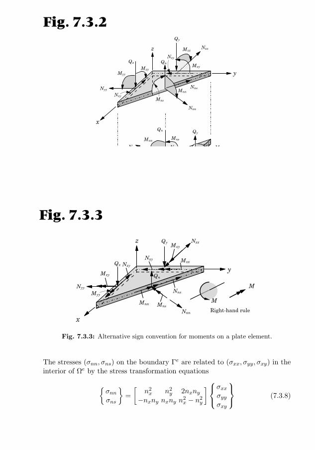
7.3. WEAK FORMULATION OF THE CPT 317
x
z
yMyy
Qx
Nxx
Nyy
Mxx
Mxy
Qy
Qn
Nnn
Nns
Mns
Mxy
Nxy
Nxy
Mnn
Myy
Qx
Nxx
Nyy
Mxx
QyQn
Nns
Mns
Mxy
Nnn
Mnn
Nxy
Nxy
Mxy
Fig. 7.3.2
Fig. 7.3.2: Forces and moments per unit length on a plate element.
x
z
y
Myy
Qx
Nxx
Nyy
Mxx
Mxy
Qy
Qn
Nnn
Nns
Mns
Mxy
Nxy
Nxy
MnnM
Right-hand rule
M
Fig. 7.3.3
Fig. 7.3.3: Alternative sign convention for moments on a plate element.
The stresses (σnn, σns) on the boundary Γe are related to (σxx, σyy, σxy) in theinterior of Ωe by the stress transformation equations
σnnσns
=
[n2x n2
y 2nxny−nxny nxny n2
x − n2y
]σxxσyyσxy
(7.3.8)
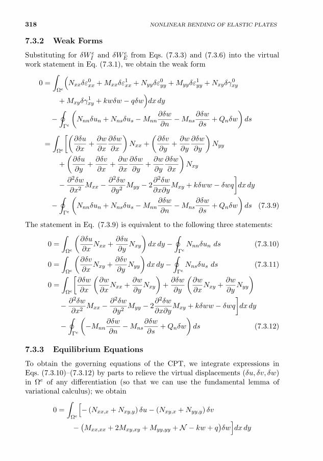
318 NONLINEAR BENDING OF ELASTIC PLATES
7.3.2 Weak Forms
Substituting for δW eI and δW e
E from Eqs. (7.3.3) and (7.3.6) into the virtualwork statement in Eq. (7.3.1), we obtain the weak form
0 =
∫Ωe
(Nxxδε
0xx +Mxxδε
1xx +Nyyδε
0yy +Myyδε
1yy +Nxyδγ
0xy
+Mxyδγ1xy + kwδw − qδw
)dx dy
−∮
Γe
(Nnnδun +Nnsδus −Mnn
∂δw
∂n−Mns
∂δw
∂s+Qnδw
)ds
=
∫Ωe
[(∂δu
∂x+∂w
∂x
∂δw
∂x
)Nxx +
(∂δv
∂y+∂w
∂y
∂δw
∂y
)Nyy
+
(∂δu
∂y+∂δv
∂x+∂w
∂x
∂δw
∂y+∂w
∂y
∂δw
∂x
)Nxy
− ∂2δw
∂x2Mxx −
∂2δw
∂y2Myy − 2
∂2δw
∂x∂yMxy + kδww − δwq
]dx dy
−∮
Γe
(Nnnδun +Nnsδus −Mnn
∂δw
∂n−Mns
∂δw
∂s+Qnδw
)ds (7.3.9)
The statement in Eq. (7.3.9) is equivalent to the following three statements:
0 =
∫Ωe
(∂δu
∂xNxx +
∂δu
∂yNxy
)dx dy −
∮ΓeNnnδun ds (7.3.10)
0 =
∫Ωe
(∂δv
∂xNxy +
∂δv
∂yNyy
)dx dy −
∮ΓeNnsδus ds (7.3.11)
0 =
∫Ωe
[∂δw
∂x
(∂w
∂xNxx +
∂w
∂yNxy
)+∂δw
∂y
(∂w
∂xNxy +
∂w
∂yNyy
)− ∂2δw
∂x2Mxx −
∂2δw
∂y2Myy − 2
∂2δw
∂x∂yMxy + kδww − δwq
]dx dy
−∮
Γe
(−Mnn
∂δw
∂n−Mns
∂δw
∂s+Qnδw
)ds (7.3.12)
7.3.3 Equilibrium Equations
To obtain the governing equations of the CPT, we integrate expressions inEqs. (7.3.10)–(7.3.12) by parts to relieve the virtual displacements (δu, δv, δw)in Ωe of any differentiation (so that we can use the fundamental lemma ofvariational calculus); we obtain
0 =
∫Ωe
[− (Nxx,x +Nxy,y) δu− (Nxy,x +Nyy,y) δv
−(Mxx,xx + 2Mxy,xy +Myy,yy +N − kw + q
)δw]dx dy
7.3. WEAK FORMULATION OF THE CPT 319
+
∮Γe
[(Nxxnx +Nxyny) δu+ (Nxynx +Nyyny) δv
+(Mxx,xnx +Mxy,ynx +Myy,yny +Mxy,xny + P
)δw
− (Mxxnx +Mxyny)∂δw
∂x− (Mxynx +Myyny)
∂δw
∂y
]ds
−∮
Γe
(Nnnδun +Nnsδus −Mnn
∂δw
∂n−Mns
∂δw
∂s+Qnδw
)ds (7.3.13)
where a comma followed by subscripts denotes differentiation with respect tothe subscripts: Nxx,x = ∂Nxx/∂x, and so on, and
N (u, v, w) =∂
∂x
(Nxx
∂w
∂x+Nxy
∂w
∂y
)+
∂
∂y
(Nxy
∂w
∂x+Nyy
∂w
∂y
)P(u, v, w) =
(Nxx
∂w
∂x+Nxy
∂w
∂y
)nx +
(Nxy
∂w
∂x+Nyy
∂w
∂y
)ny
(7.3.14)The equations of equilibrium are obtained by setting the coefficients of δu, δv,and δw in Ωe to zero:
δu :∂Nxx
∂x+∂Nxy
∂y= 0 (7.3.15)
δv :∂Nxy
∂x+∂Nyy
∂y= 0 (7.3.16)
δw :∂2Mxx
∂x2+ 2
∂2Mxy
∂y∂x+∂2Myy
∂y2+N (u, v, w)− kw + q = 0 (7.3.17)
7.3.4 Boundary Conditions
To cast the boundary conditions on an arbitrary edge whose normal is n, we ex-press all generalized displacements (u, v, w, ∂w∂x ,
∂w∂x ) from the (x, y, z) system in
terms of the corresponding generalized displacements in the normal, tangential,and transverse directions. We have
u = unnx − usny, v = unny + usnx (7.3.18a)
∂w
∂x=∂w
∂nnx −
∂w
∂sny,
∂w
∂y=∂w
∂nny +
∂w
∂snx (7.3.18b)
The boundary expression of Eq. (7.3.13) takes the form∮Γe
[(Nxxnx +Nxyny) (δunnx − δusny) + (Nxynx +Nyyny) (δunny + δusnx)
+
(Mxx,xnx +Mxy,ynx +Myy,yny +Mxy,xny + P
)δw
320 NONLINEAR BENDING OF ELASTIC PLATES
− (Mxxnx +Mxyny)
(∂δw
∂nnx −
∂δw
∂sny
)− (Mxynx +Myyny)
(∂δw
∂nny +
∂δw
∂snx
)]ds
−∮
Γe
(Nnnδun +Nnsδus −Mnn
∂δw
∂n−Mns
∂δw
∂s+Qnδw
)ds
=
∮Γe
(Nxxn
2x + 2Nxynxny +Nyyn
2y −Nnn
)δun
+[(Nyy −Nxx)nxny +Nxy(n
2x − n2
y)−Nns
]δus
+ (Mxx,xnx +Mxy,ynx +Myy,yny +Mxy,xny + P −Qn) δw
−(Mxxn
2x + 2Mxynxny +Myyn
2y −Mnn
) ∂δw∂n
−[(Myy −Mxx)nxny +Mxy(n
2x − n2
y)−Mns
] ∂δw∂s
ds (7.3.19)
The natural boundary conditions are obtained by setting the coefficients ofδun, δus, δw, ∂δw
∂n and ∂δw∂s on Γe to zero:
δun : Nnn = Nxxn2x + 2Nxynxny +Nyyn
2y
δus : Nns = (Nyy −Nxx)nxny +Nxy(n2x − n2
y) (7.3.20a)
δw : Qn = Mxx,xnx +Mxy,ynx +Myy,yny +Mxy,xny + P
∂δw
∂n: Mnn = Mxxn
2x + 2Mxynxny +Myyn
2y
∂δw
∂s: Mns = (Myy −Mxx)nxny +Mxy(n
2x − n2
y)
(7.3.20b)
From Eq. (7.3.20), it is clear that the primary variables (i.e. generalized dis-placements) and secondary variables (i.e. generalized forces) of the theory are:
Primary variables: un, us, w,∂w
∂n,
∂w
∂sSecondary variables: Nnn, Nns, Qn, Mnn, Mns
(7.3.21)
7.3.4.1 The Kirchhoff free-edge condition
We note that the equations of equilibrium in Eqs. (7.3.15)–(7.3.17) have thecombined spatial differential order of eight. In other words, if the governingequations are expressed in terms of displacements (u, v, w), they would containsecond-order spatial derivatives of u and v and fourth-order spatial derivativesof w. This implies that there should be only eight (four essential and fournatural) boundary conditions, whereas Eq. (7.3.21) shows five essential and fivenatural boundary conditions, giving a total of ten boundary conditions. To
7.3. WEAK FORMULATION OF THE CPT 321
eliminate this discrepancy, one may integrate the tangential derivative term byparts to obtain the boundary term
−∮
ΓMns
∂δw
∂sds =
∮Γ
∂Mns
∂sδw ds− [Mnsδw]Γ (7.3.22)
The term [Mnsδw]Γ is zero when the end points of a closed curve coincide orwhen Mns = 0. If Mns = 0 is not specified at corners of the boundary Γof a polygonal plate, concentrated forces of magnitude Fc = −2Mns will beproduced at the corners. The factor of 2 appears because Mns from two sidesof the corner are added there.
The remaining boundary term in Eq. (7.3.22) is added to the shear forceQn (because it is a coefficient of δw on Γe) to obtain the effective shear force
Vn ≡ Qn +∂Mns
∂s(7.3.23)
The specification of this effective shear force Vn is known as the Kirchhoff free-edge condition. Finally, the correct boundary conditions of the CPT involvespecifying the following quantities:
Generalized displacements: un, us, w,∂w
∂nGeneralized forces: Nnn, Nns, Vn, Mnn
(7.3.24)
Thus, at every boundary point one must know un or Nnn, us or Nns, w or Vn,and ∂w/∂n or Mnn. On an edge parallel to the x-axis (i.e. s = x and n = y),for example, the above boundary conditions become
un = v, us = u, w,∂w
∂n=∂w
∂y(7.3.25a)
Nnn =Nyy, Nns = Nyx, Vn = Vy, Mnn = Myy (7.3.25b)
7.3.4.2 Typical edge conditions
Next we discuss some common types of boundary conditions for the linearbending of a rectangular plate with edges parallel to the x and y coordinates.Here we use the edge with normal n (with components nx and ny) to discuss theboundary conditions (see Fig. 7.3.2). The force boundary conditions may beexpressed in terms of the generalized displacements using the plate constitutiveequations discussed in the next section.
Free edge with normal n: A free edge is one that is geometrically notrestrained in any way. Hence, we have
un 6= 0, us 6= 0, w 6= 0,∂w
∂n6= 0 (7.3.26a)
322 NONLINEAR BENDING OF ELASTIC PLATES
However, the edge may have applied forces and/or moments
Nnn = Nnn, Nns = Nns, Vn ≡ Qn +∂Mns
∂s= Vn, Mnn = Mnn (7.3.26b)
where quantities with a hat are specified forces/moments.
Fixed (or clamped) with normal n: A fixed edge is one that is geometricallyfully restrained
un = 0, us = 0, w = 0,∂w
∂n= 0 (7.3.27)
Therefore, the forces and moments on a fixed edge are not known a priori (i.e.they are reactions to be determined as part of the analysis).
Simply-supported edge with normal n: The phrase “simply-supported”does not uniquely define the boundary conditions and one must indicate whatit means, especially when both in-plane and bending deflections are coupled.Here we define two types of simply-supported boundary conditions:
SS–1: us = 0, w = 0; Nnn = Nnn, Mnn = Mnn (7.3.28)
SS–2: un = 0, w = 0; Nns = Nns, Mnn = Mnn (7.3.29)
7.3.5 Stress Resultant–Deflection Relations
To express the forces and moments (N,M) per unit length in terms of thegeneralized displacements (u, v, w), we must invoke appropriate stress–strainrelations. In the CPT, all three transverse strain components (εzz, εxz, εyz) arezero by definition. Since εzz = 0, the transverse normal stress σzz, though notzero identically, does not appear in the virtual work statement and hence inthe equations of motion. Consequently, it amounts to neglecting the transversenormal stress. Thus, in theory, we have a case of both plane strain and planestress. However, from practical considerations, a thin to moderately thick plateis in a state of plane stress because the thickness is small as compared to thein-plane dimensions. Hence, the plane stress-reduced constitutive relations areused.
For an orthotropic material with principal material axes (x1, x2, x3) coincid-ing with the plate coordinates (x, y, z), the plane stress-reduced thermoelasticconstitutive equations can be expressed as (see Reddy [55] for the discussion ofconstitutive relations for orthotropic and laminated plates)
σxxσyyσxy
=
Q11 Q12 0Q12 Q22 0
0 0 Q66
εxx − α1 ∆Tεyy − α2 ∆T
γxy
(7.3.30)
7.3. WEAK FORMULATION OF THE CPT 323
where Qij are the plane stress-reduced stiffnesses
Q11 =E1
1− ν12ν21, Q12 =
ν12E2
1− ν12ν21=
ν21E1
1− ν12ν21
Q22 =E2
1− ν12ν21, Q66 = G12
(7.3.31)
and (σi, εi) are the stress and strain components, respectively, α1 and α2 are thecoefficients of thermal expansion, and ∆T is the temperature increment from areference state, ∆T = T−T0. The moisture strains are similar to thermal strains(i.e. for moisture strains, replace ∆T and αi with the moisture concentrationincrement and coefficients of hygroscopic expansion, respectively).
The plate constitutive equations relate the forces and moments per unitlength in Eq. (7.3.4) to the strains in Eq. (7.2.8) of the plate theory. For aplate made of a single or multiple orthotropic layers, the plate constitutiverelations are obtained using the definitions in Eq. (7.3.4). For plates laminatedof multiple orthotropic layers whose material axes are arbitrarily oriented withrespect to the plate axes, the plate constitutive relations couple the in-planedisplacements to the out-of-plane displacements even for linear problems (seeReddy [55, 56] for details). For a single orthotropic layer, the plate constitutiverelations are greatly simplified. They are
Nxx
Nyy
Nxy
=
∫ h2
−h2
Q11 Q12 0Q12 Q22 0
0 0 Q66
ε0xx + zε1
xx − α1∆T
ε0yy + zε1
yy − α2∆T
γ0xy + zγ1
xy
dz
=
A11 A12 0A12 A22 00 0 A66
ε0xx
ε0yy
γ0xy
−NTxx
NTyy
0
(7.3.32)
Mxx
Myy
Mxy
=
∫ h2
−h2
Q11 Q12 0Q12 Q22 0
0 0 Q66
ε0xx + zε1
xx − α1∆T
ε0yy + zε1
yy − α2∆T
γ0xy + zγ1
xy
z dz
=
D11 D12 0D12 D22 0
0 0 D66
ε1xx
ε1yy
γ1xy
−MTxx
MTyy
0
(7.3.33)
where Aij are extensional stiffnesses and Dij are bending stiffnesses, which aredefined in terms of the elastic stiffnesses Qij as
(Aij , Dij) =
∫ h2
−h2
Qij (1, z2) dz or Aij = Qij h, Dij = Qijh3
12(7.3.34)
324 NONLINEAR BENDING OF ELASTIC PLATES
and NT and MT are thermal stress resultantsNTxx
NTyy
=
Q11α1 +Q12α2
Q12α1 +Q22α2
∫ h2
−h2
∆T (x, y, z) dz (7.3.35a)
MTxx
MTyy
=
Q11α1 +Q12α2
Q12α1 +Q22α2
∫ h2
−h2
∆T (x, y, z) z dz (7.3.35b)
where α1 and α2 are the thermal coefficients of expansion, and ∆T is the tem-perature change (above a stress-free temperature), which is a known functionof position. For isotropic plates, Eqs. (7.3.35a,b) simplify to NT
xx = NTyy = NT
and MTxx = MT
yy = MT , where
(NT ,MT ) =Eα
1− ν
∫ h2
−h2
∆T (1, z) dz (7.3.36)
7.4 Finite Element Models of the CPT
7.4.1 General Formulation
In this section, the displacement finite element model of Eqs. (7.3.15)–(7.3.17)governing plates according to the CPT is developed. The virtual work state-ments of the CPT over a typical orthotropic plate finite element Ωe are givenby [from Eqs. (7.3.10)–(7.3.12)]
0 =
∫Ωe
(∂δu
∂x
A11
[∂u
∂x+
1
2
(∂w
∂x
)2]+A12
[∂v
∂y+
1
2
(∂w
∂y
)2]+A66
∂δu
∂y
[∂u
∂y+∂v
∂x+∂w
∂x
∂w
∂y
])dx dy −
∫Ωe
∂δu
∂xNTxx dxdy
−∮
ΓeNnnδun ds (7.4.1)
0 =
∫Ωe
(∂δv
∂y
A12
[∂u
∂x+
1
2
(∂w
∂x
)2]+A22
[∂v
∂y+
1
2
(∂w
∂y
)2]+A66
∂δv
∂x
[∂u
∂y+∂v
∂x+∂w
∂x
∂w
∂y
])dx dy −
∫Ωe
∂δv
∂yNTyy dxdy
−∮
ΓeNnsδus ds (7.4.2)
0 =
∫Ωe
∂δw
∂x
[∂w
∂x
A11
[∂u
∂x+
1
2
(∂w
∂x
)2]+A12
[∂v
∂y+
1
2
(∂w
∂y
)2]+A66
∂w
∂y
(∂u
∂y+∂v
∂x+∂w
∂x
∂w
∂y
)]+∂δw
∂y
[∂w
∂y
A12
[∂u
∂x+
1
2
(∂w
∂x
)2]+A22
[∂v
∂y+
1
2
(∂w
∂y
)2]+A66
∂w
∂x
(∂u
∂y+∂v
∂x+∂w
∂x
∂w
∂y
)]
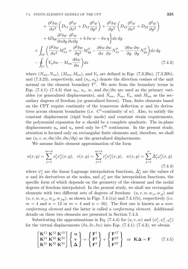
7.4. FINITE ELEMENT MODELS OF THE CPT 325
+∂2δw
∂x2
(D11
∂2w
∂x2+D12
∂2w
∂y2
)+∂2δw
∂y2
(D12
∂2w
∂x2+D22
∂2w
∂y2
)+ 4D66
∂2δw
∂x∂y
∂2w
∂x∂y+ k δww − δw q
dx dy
+
∫Ωe
(∂2δw
∂x2MTxx +
∂2δw
∂y2MTyy −
∂δw
∂x
∂w
∂xNTxx −
∂δw
∂y
∂w
∂yNTyy
)dx dy
−∮
Γe
(Vnδw −Mnn
∂δw
∂n
)ds (7.4.3)
where (Nnn, Nns), (Mnn,Mns), and Vn are defined in Eqs. (7.3.20a), (7.3.20b),and (7.3.23), respectively, and (nx, ny) denote the direction cosines of the unitnormal on the element boundary Γe. We note from the boundary terms inEqs. (7.4.1)–(7.4.3) that un, us, w, and ∂w/∂n are used as the primary vari-ables (or generalized displacements), and Nnn, Nns, Vn, and Mnn as the sec-ondary degrees of freedom (or generalized forces). Thus, finite elements basedon the CPT require continuity of the transverse deflection w and its deriva-tives across element boundaries (i.e. C1-continuity of w). Also, to satisfy theconstant displacement (rigid body mode) and constant strain requirements,the polynomial expansion for w should be a complete quadratic. The in-planedisplacements un and us need only be C0 continuous. In the present study,attention is focused only on rectangular finite elements and, therefore, we shalluse (u, v, w, ∂w/∂x, ∂w/∂y) as the generalized displacements.
We assume finite element approximation of the form
u(x, y) =
m=4∑j=1
uejψej (x, y), v(x, y) =
m=4∑j=1
vejψej (x, y), w(x, y) =
n∑j=1
∆ejϕ
ej(x, y)
(7.4.4)where ψej are the linear Lagrange interpolation functions, ∆e
j are the values ofw and its derivatives at the nodes, and ϕej are the interpolation functions, thespecific form of which depends on the geometry of the element and the nodaldegrees of freedom interpolated. In the present study, we shall use rectangularelements with two different sets of degrees of freedom: (u, v, w,w,x, w,y) and(u, v, w,w,x, w,y, w,xy), as shown in Figs. 7.4.1(a) and 7.4.1(b), respectively (i.e.m = 4 and n = 12 or m = 4 and n = 16). The first one is known as a non-conforming element and the latter is called a conforming element. Additionaldetails on these two elements are presented in Section 7.4.3.
Substituting the approximations in Eq. (7.4.4) for (u, v, w) and (ψei , ψei , ϕ
ei )
for the virtual displacements (δu, δv, δw) into Eqs. (7.4.1)–(7.4.3), we obtainK11 K12 K13
K21 K22 K23
K31 K32 K33
uv∆
=
F1
F2
F3
+
F1T
F2T
F3T
or K∆ = F (7.4.5)
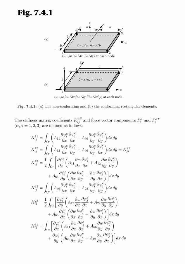
326 NONLINEAR BENDING OF ELASTIC PLATES
a
b
z
x
43
21
ya
b
ξ = x/a, η = y/b
az
x
43
21
y
b ξ = x/a, η = y/b
(b)
(a)
( , , , / , / ) at each nodeu v w w x w y∂ ∂ ∂ ∂
2( , , , / , / , / ) at each nodeu v w w x w y w x y∂ ∂ ∂ ∂ ∂ ∂ ∂
Fig. 7.4.1
Fig. 7.4.1: (a) The non-conforming and (b) the conforming rectangular elements.
The stiffness matrix coefficients Kαβij and force vector components Fαi and FαTi
(α, β = 1, 2, 3) are defined as follows:
K11ij =
∫Ωe
(A11
∂ψei∂x
∂ψej∂x
+A66∂ψei∂y
∂ψej∂y
)dx dy
K12ij =
∫Ωe
(A12
∂ψei∂x
∂ψej∂y
+A66∂ψei∂y
∂ψej∂x
)dx dy = K21
ji
K13ij =
1
2
∫Ωe
[∂ψei∂x
(A11
∂w
∂x
∂ϕej∂x
+A12∂w
∂y
∂ϕej∂y
)+A66
∂ψei∂y
(∂w
∂x
∂ϕej∂y
+∂w
∂y
∂ϕej∂x
)]dx dy
K22ij =
∫Ωe
(A66
∂ψei∂x
∂ψej∂x
+A22∂ψei∂y
∂ψej∂y
)dx dy
K23ij =
1
2
∫Ωe
[∂ψei∂y
(A12
∂w
∂x
∂ϕej∂x
+A22∂w
∂y
∂ϕej∂y
)+A66
∂ψei∂x
(∂w
∂x
∂ϕej∂y
+∂w
∂y
∂ϕej∂x
)]dx dy
K31ij =
∫Ωe
[∂ϕei∂x
(A11
∂w
∂x
∂ψej∂x
+A66∂w
∂y
∂ψej∂y
)+∂ϕei∂y
(A66
∂w
∂x
∂ψej∂y
+A12∂w
∂y
∂ψej∂x
)]dx dy
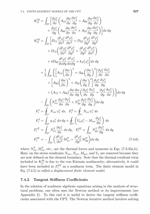
7.4. FINITE ELEMENT MODELS OF THE CPT 327
K32ij =
∫Ωe
[∂ϕei∂x
(A12
∂w
∂x
∂ψej∂y
+A66∂w
∂y
∂ψej∂x
)+∂ϕei∂y
(A66
∂w
∂x
∂ψej∂x
+A22∂w
∂y
∂ψej∂y
)]dx dy
K33ij =
∫Ωe
[D11
∂2ϕei∂x2
∂2ϕej∂x2
+D22∂2ϕei∂y2
∂2ϕej∂y2
+D12
(∂2ϕei∂x2
∂2ϕej∂y2
+∂2ϕei∂y2
∂2ϕej∂x2
)+ 4D66
∂2ϕei∂x∂y
∂2ϕej∂x∂y
+ kϕeiϕej
]dx dy
+1
2
∫Ωe
[A11
(∂w
∂x
)2
+A66
(∂w
∂y
)2]∂ϕei∂x
∂ϕej∂x
+
[A66
(∂w
∂x
)2
+A22
(∂w
∂y
)2]∂ϕei∂y
∂ϕej∂y
+(A12 +A66
)∂w∂x
∂w
∂y
(∂ϕei∂x
∂ϕej∂y
+∂ϕei∂y
∂ϕej∂x
)dx dy
−∫
Ωe
(NTxx
∂ϕei∂x
∂ϕej∂x
+NTyy
∂ϕei∂y
∂ϕej∂y
)dx dy
F 1i =
∮ΓeNnn ψ
ei ds, F 2
i =
∮ΓeNns ψ
ei ds
F 3i =
∫Ωeq ϕei dx dy +
∮Γe
(Vnϕ
ei −Mnn
∂ϕei∂n
)ds
F 1Ti =
∫ΩeNTxx
∂ψei∂x
dx dy, F 2Ti =
∫ΩeNTyy
∂ψei∂y
dx dy
F 3Ti = −
∫Ωe
(∂2ϕei∂x2
MTxx +
∂2ϕei∂y2
MTyy
)dx dy (7.4.6)
where NTxx,M
Txx, etc., are the thermal forces and moments in Eqs. (7.3.35a,b).
Hatsˆon the stress resultants Nnn, Nns, Mnn, and Vn are removed because theyare now defined on the element boundary. Note that the thermal resultant termincluded in K33
ij is due to the von Karman nonlinearity; alternatively, it could
have been included in F 3Ti as a nonlinear term. The finite element model in
Eq. (7.4.5) is called a displacement finite element model.
7.4.2 Tangent Stiffness Coefficients
In the solution of nonlinear algebraic equations arising in the analysis of struc-tural problems, one often uses the Newton method or its improvements (seeAppendix 2). To this end it is useful to derive the tangent stiffness coeffi-cients associated with the CPT. The Newton iterative method involves solving
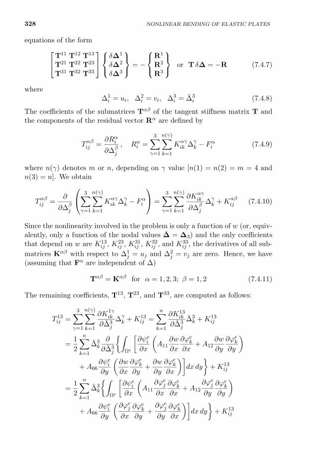
328 NONLINEAR BENDING OF ELASTIC PLATES
equations of the formT11 T12 T13
T21 T22 T23
T31 T32 T33
δ∆1
δ∆2
δ∆3
= −
R1
R2
R3
or T δ∆ = −R (7.4.7)
where∆1i = ui, ∆2
i = vi, ∆3i = ∆3
i (7.4.8)
The coefficients of the submatrices Tαβ of the tangent stiffness matrix T andthe components of the residual vector Rα are defined by
Tαβij =∂Rαi
∂∆βj
, Rαi =3∑
γ=1
n(γ)∑k=1
Kαγik ∆γ
k − Fαi (7.4.9)
where n(γ) denotes m or n, depending on γ value [n(1) = n(2) = m = 4 andn(3) = n]. We obtain
Tαβij =∂
∂∆βj
3∑γ=1
n(γ)∑k=1
Kαγik ∆γ
k − Fαi
=
3∑γ=1
n(γ)∑k=1
∂Kαγik
∂∆βj
∆γk +Kαβ
ij (7.4.10)
Since the nonlinearity involved in the problem is only a function of w (or, equiv-alently, only a function of the nodal values ∆ = ∆3) and the only coefficientsthat depend on w are K13
ij , K23ij , K31
ij , K32ij , and K33
ij , the derivatives of all sub-
matrices Kαβ with respect to ∆1j = uj and ∆2
j = vj are zero. Hence, we have(assuming that Fα are independent of ∆)
Tαβ = Kαβ for α = 1, 2, 3; β = 1, 2 (7.4.11)
The remaining coefficients, T13, T23, and T33, are computed as follows:
T 13ij =
3∑γ=1
n(γ)∑k=1
∂K1γik
∂∆3j
∆γk +K13
ij =n∑k=1
∂K13ik
∂∆3j
∆3k +K13
ij
=1
2
n∑k=1
∆3k
∂
∂∆3j
∫Ωe
[∂ψei∂x
(A11
∂w
∂x
∂ϕek∂x
+A12∂w
∂y
∂ϕek∂y
)+A66
∂ψei∂y
(∂w
∂x
∂ϕek∂y
+∂w
∂y
∂ϕek∂x
)]dx dy
+K13
ij
=1
2
n∑k=1
∆3k
∫Ωe
[∂ψei∂x
(A11
∂ϕej∂x
∂ϕek∂x
+A12
∂ϕej∂y
∂ϕek∂y
)+A66
∂ψei∂y
(∂ϕej∂x
∂ϕek∂y
+∂ϕej∂y
∂ϕek∂x
)]dx dy
+K13
ij
7.4. FINITE ELEMENT MODELS OF THE CPT 329
=1
2
∫Ωe
[∂ψei∂x
(A11
∂w
∂x
∂ϕej∂x
+A12∂w
∂y
∂ϕej∂y
)+A66
∂ψei∂y
(∂w
∂x
∂ϕej∂y
+∂w
∂y
∂ϕej∂x
)]dx dy +K13
ij
= K13ij +K13
ij = 2K13ij (= T 31
ji );(T13
)T= T31 = K31 (7.4.12)
T 23ij =
3∑γ=1
n(γ)∑k=1
∂K2γik
∂∆3j
∆γk +K23
ij =n∑k=1
∂K23ik
∂∆3j
∆3k +K23
ij
=1
2
n∑k=1
∆3k
∂
∂∆3j
∫Ωe
[∂ψei∂y
(A12
∂w
∂x
∂ϕek∂x
+A22∂w
∂y
∂ϕek∂y
)+A66
∂ψei∂x
(∂w
∂x
∂ϕek∂y
+∂w
∂y
∂ϕek∂x
)]dx dy
+K23
ij
=1
2
n∑k=1
∆3k
∫Ωe
[∂ψei∂y
(A12
∂ϕej∂x
∂ϕek∂x
+A22
∂ϕej∂y
∂ϕek∂y
)+A66
∂ψei∂x
(∂ϕej∂x
∂ϕek∂y
+∂ϕej∂y
∂ϕek∂x
)]dx dy
+K23
ij
=1
2
∫Ωe
[∂ψei∂y
(A12
∂w
∂x
∂ϕej∂x
+A22∂w
∂y
∂ϕej∂y
)+A66
∂ψei∂x
(∂w
∂y
∂ϕej∂x
+∂w
∂x
∂ϕej∂y
)]dx dy +K23
ij
= K23ij +K23
ij = 2K23ij (= T 32
ji );(T23
)T= T32 = K32 (7.4.13)
The computation of T 33ij requires the calculation of three parts:
T 33ij = K33
ij +m=4∑k=1
∂K31ik
∂∆3j
uk +m=4∑k=1
∂K32ik
∂∆3j
vk +n∑k=1
∂K33ik
∂∆3j
∆3k (7.4.14)
We shall compute these three terms first. We have
m=4∑k=1
uk∂K31
ik
∂∆3j
=
m=4∑k=1
uk∂
∂∆3j
∫Ωe
[∂ϕei∂x
(A11
∂w
∂x
∂ψek∂x
+A66∂w
∂y
∂ψek∂y
)+∂ϕei∂y
(A66
∂w
∂x
∂ψek∂y
+A12∂w
∂y
∂ψek∂x
)]dx dy
=
m=4∑k=1
uk
∫Ωe
[∂ϕei∂x
(A11
∂ϕej∂x
∂ψek∂x
+A66
∂ϕej∂y
∂ψek∂y
)+∂ϕei∂y
(A66
∂ϕej∂x
∂ψek∂y
+A12
∂ϕej∂y
∂ψek∂x
)]dx dy
330 NONLINEAR BENDING OF ELASTIC PLATES
=
∫Ωe
[∂ϕei∂x
(A11
∂u
∂x
∂ϕej∂x
+A66∂u
∂y
∂ϕej∂y
)+∂ϕei∂y
(A66
∂u
∂y
∂ϕej∂x
+A12∂u
∂x
∂ϕej∂y
)]dx dy (7.4.15)
m=4∑k=1
vk∂K32
ik
∂∆3j
=m=4∑k=1
vk∂
∂∆3j
∫Ωe
[∂ϕei∂x
(A12
∂w
∂x
∂ψek∂y
+A66∂w
∂y
∂ψek∂x
)+∂ϕei∂y
(A66
∂w
∂x
∂ψek∂x
+A22∂w
∂y
∂ψek∂y
)]dx dy
=
m∑k=1
vk
∫Ωe
[∂ϕei∂x
(A12
∂ϕej∂x
∂ψek∂y
+A66
∂ϕej∂y
∂ψek∂x
)+∂ϕei∂y
(A66
∂ϕej∂x
∂ψek∂x
+A22
∂ϕej∂y
∂ψek∂y
)]dx dy
=
∫Ωe
[∂ϕei∂x
(A12
∂v
∂y
∂ϕej∂x
+A66∂v
∂x
∂ϕej∂y
)+∂ϕei∂y
(A66
∂v
∂x
∂ϕej∂x
+A22∂v
∂y
∂ϕej∂y
)]dx dy (7.4.16)
n∑k=1
∆3k
∂K33ik
∂∆3j
=1
2
n∑k=1
∆3k
∂
∂∆3j
[∫Ωe
[A11
(∂w
∂x
)2
+A66
(∂w
∂y
)2]∂ϕei∂x
∂ϕek∂x
+
[A66
(∂w
∂x
)2
+A22
(∂w
∂y
)2]∂ϕei∂y
∂ϕek∂y
+ A12∂w
∂x
∂w
∂y
(∂ϕei∂x
∂ϕek∂y
+∂ϕei∂y
∂ϕek∂x
)dx dy
]
=1
2
n∑k=1
∆3k
∫Ωe
[(2A11
∂w
∂x
∂ϕej∂x
+ 2A66∂w
∂y
∂ϕej∂y
)∂ϕei∂x
∂ϕek∂x
+
(2A66
∂w
∂x
∂ϕej∂x
+ 2A22∂w
∂y
∂ϕej∂y
)∂ϕei∂y
∂ϕek∂y
+ A12
(∂w
∂x
∂ϕej∂y
+∂w
∂y
∂ϕej∂x
)(∂ϕei∂x
∂ϕek∂y
+∂ϕei∂y
∂ϕek∂x
)]dx dy
=
∫Ωe
[A11
(∂w
∂x
)2∂ϕei∂x
∂ϕej∂x
+A22
(∂w
∂y
)2∂ϕei∂y
∂ϕej∂y
+A66∂w
∂x
∂w
∂y
(∂ϕei∂x
∂ϕej∂y
+∂ϕei∂y
∂ϕej∂x
)+A12
2
(∂ϕei∂x
∂w
∂y+∂ϕei∂y
∂w
∂x
)(∂w
∂x
∂ϕej∂y
+∂w
∂y
∂ϕej∂x
)]dx dy
(7.4.17)
7.4. FINITE ELEMENT MODELS OF THE CPT 331
where A12 = A12 + A66. Combining the expressions in Eqs. (7.4.15)–(7.4.17),we obtain
T 33ij =
∫Ωe
[Nxx
∂ϕei∂x
∂ϕej∂x
+ Nyy∂ϕei∂y
∂ϕej∂y
+ Nxy
(∂ϕei∂x
∂ϕej∂y
+∂ϕei∂y
∂ϕej∂x
)]dx dy
(7.4.18)where
Nxx = Nxx +1
2
[A11
(∂w
∂x
)2
+A66
(∂w
∂y
)2]
Nyy = Nyy +1
2
[A66
(∂w
∂x
)2
+A22
(∂w
∂y
)2]
Nxy = Nxy +
(A12 +A66
2
)∂w
∂x
∂w
∂y
(7.4.19)
Therefore, T33 = K33 + T33 is given by
T 33ij =
∫Ωe
[D11
∂2ϕei∂x2
∂2ϕej∂x2
+D22∂2ϕei∂y2
∂2ϕej∂y2
+D12
(∂2ϕei∂x2
∂2ϕej∂y2
+∂2ϕei∂y2
∂2ϕej∂x2
)+ 4D66
∂2ϕei∂x∂y
∂2ϕej∂x∂y
+ kϕeiϕej + Nxx
∂ϕei∂x
∂ϕej∂x
+ Nyy∂ϕei∂y
∂ϕej∂y
+ Nxy
(∂ϕei∂x
∂ϕej∂y
+∂ϕei∂y
∂ϕej∂x
)]dx dy (7.4.20)
where
Nxx = Nxx +A11
(∂w
∂x
)2
+A66
(∂w
∂y
)2
Nyy = Nyy +A66
(∂w
∂x
)2
+A22
(∂w
∂y
)2
Nxy = Nxy +(A12 +A66
) ∂w∂x
∂w
∂y
(7.4.21)
and (Nxx, Nyy, Nxy) are defined by Eq. (7.3.32). Clearly, the tangent stiffnessmatrix of the CPT element is symmetric, while the original element stiffness isnot symmetric.
7.4.3 Non-Conforming and Conforming Plate Elements
A non-conforming rectangular element has w, ∂w/∂x, and ∂w/∂y as the nodalvariables, in addition to the in-plane displacement degrees of freedom (u, v),as shown in Fig. 7.4.1(a). The in-plane displacements are approximated usinglinear interpolation functions [see Eqs. (3.3.38)]
u ≈ uh =
4∑j=1
ujψj(ξ, η), v ≈ vh =
4∑j=1
vjψj(ξ, η)
332 NONLINEAR BENDING OF ELASTIC PLATES
The transverse deflection w is approximated by (see Melosh [57] and Zienkiewiczand Cheung [58])
w ≈ wh(ξ, η) = c1 + c2ξ + c3η + c4ξη + c5ξ2 + c6η
2 + c7ξ3 + c8ξ
2η + c9ξη2
+ c10η3 + c11ξ
3η + c12ξη3 =
12∑j=1
∆jϕj(ξ, η) (7.4.22)
where ϕi are the cubic interpolation functions associated with the degrees offreedom (w, ∂w/∂x, ∂w/∂y)
ϕi = gi1 (i = 1, 4, 7, 10); ϕi = gi2 (i = 2, 5, 8, 11); ϕi = gi3 (i = 3, 6, 9, 12)
gi1 =1
8(1 + ξi ξ)(1 + ηi η)(2 + ξi ξ + ηi η − ξ2 − η2)
gi2 =1
8aξi(ξ0 − 1)(1 + η0)(1 + ξ0)2, ξ =
x− xca
, η =y − ycb
(7.4.23)
gi3 =1
8bηi(η0 − 1)(1 + ξ0)(1 + η0)2, ξ0 = ξiξ, η0 = ηiη
where 2a and 2b are the sides of the rectangle, (xc, yc) are the global coordinatesof the center of the rectangle, and (ξi, ηi) are the coordinates of the nodes in the(ξ, η) coordinate system [e.g. (ξ1, η1) = (−1,−1), (ξ2, η2) = (1,−1), and so on].The variation of the normal slope ∂w/∂n is cubic along an edge, whereas thereare only two values of it available on the edge. Therefore, the cubic polynomialsfor the normal derivatives of w are not the same on an edge common to twoelements; hence, it is said to be non-conforming. The size of the non-conformingelement stiffness matrix is 20× 20.
A conforming rectangular element with w, ∂w/∂x, ∂w/∂y, and ∂2w/∂x∂yas the bending degrees of freedom was developed by Bogner et al. [59]. Thedeflection w is approximated by the 16-term complete polynomial
w ≈ wh(ξ, η) = c1 + c2ξ + c3η + c4ξη + c5ξ2 + c6η
2 + c7ξ3 + c8ξ
2η + c9ξη2
+ c10η3 + c11ξ
3η + c12ξη3 + c13ξ
2η2
+ c14ξ3η2 + c15ξ
2η3 + c16ξ3η3 =
16∑j=1
∆jϕj(ξ, η) (7.4.24)
where
ϕei = gi1 (i = 1, 5, 9, 13); ϕei = gi2 (i = 2, 6, 10, 14)
ϕei = gi3 (i = 3, 7, 11, 15); ϕei = gi4 (i = 4, 8, 12, 16)
gi1 =1
16(ξ + ξi)
2(ξi ξ − 2)(η + ηi)2(ηi η − 2)
gi2 =1
16aξi(ξ + ξi)
2(1− ξi ξ)(η + ηi)2(ηi η − 2) (7.4.25)
gi3 =1
16bηi(ξ + ξi)
2(ξi ξ − 2)(η + ηi)2(1− ηi η)
7.5. COMPUTER IMPLEMENTATION OF THE CPT ELEMENTS 333
gi4 =1
16abξiηi(ξ + ξi)
2(1− ξi ξ)(η + ηi)2(1− ηi η)
Here a and b are the sides of the rectangular element, and ξ = x/a and η = y/b.In this case the normal slope continuity between elements is satisfied, hencetermed a conforming element (also see [60,61]). The conforming element has 6degrees of freedom per node (u, v, w,w,x, w,y, w,xy), as shown in Fig. 7.4.1(b).For the conforming rectangular element, the total number of nodal degrees offreedom per element is 6× 4 = 24, and hence the size of the stiffness matrix is24× 24.
7.5 Computer Implementation of the CPT Elements
7.5.1 General Remarks
The conforming and non-conforming rectangular finite elements developed inthis chapter can be implemented into a computer program in the same wayas the Euler–Bernoulli beam element. Here we use a bilinear interpolation of(u, v) and a Hermite cubic interpolation of w, as discussed in Section 7.4.3. Theelement geometry is represented using bilinear interpolation functions. In viewof the different interpolation of the in-plane displacements and the transversedeflection, one must compute both types of interpolation functions and theirderivatives. Since the stiffness coefficients of the CPT element involve both first-and second-order derivatives of ϕi(x, y) with respect to the global coordinates(x, y), the associated formulas, similar to that for the first-order derivatives [seeEq. (3.6.6) or Eq. (6.6.4)], must be developed.
Let the transformation between the global coordinates (x, y) and local nor-malized coordinates (ξ, η) in a Lagrange element Ωe be
x =
m∑i=1
xiψi(ξ, η), y =
m∑i=1
yiψi(ξ, η) (7.5.1)
where (xei , yei ) denote the global coordinates of the element nodes. As shown in
Sections 3.6.2 and 6.6.2, the derivatives of the interpolation function ϕei withrespect to the global coordinates (x, y) are related to their derivatives withrespect to the local coordinates (ξ, η) by
∂ϕei∂x∂ϕei∂y
= J−1
∂ϕei∂ξ∂ϕei∂η
(7.5.2)
where the Jacobian matrix J is defined in Eq. (6.6.5). in terms of ψei and (xei , yei ).
The same procedure as that used to derive the result in Eq. (7.5.2) (i.e. chainrule of differentiation) can be used to develop the relationship between the
334 NONLINEAR BENDING OF ELASTIC PLATES
second-order derivatives of ϕi with respect to (x, y) and the derivatives of ϕiwith respect to (ξ, η).
We begin with
∂ϕi∂ξ
=∂ϕi∂x
∂x
∂ξ+∂ϕi∂y
∂y
∂ξ,
∂ϕi∂η
=∂ϕi∂x
∂x
∂η+∂ϕi∂y
∂y
∂η
and find the second derivative
∂2ϕi∂ξ2
=∂
∂ξ
(∂ϕi∂x
∂x
∂ξ+∂ϕi∂y
∂y
∂ξ
)=
∂
∂ξ
(∂ϕi∂x
)∂x
∂ξ+∂ϕi∂x
∂2x
∂ξ2+
∂
∂ξ
(∂ϕi∂y
)∂y
∂ξ+∂ϕi∂y
∂2y
∂ξ2
=∂2ϕi∂x2
(∂x
∂ξ
)2
+∂2ϕi∂x∂y
∂x
∂ξ
∂y
∂ξ+∂ϕi∂x
∂2x
∂ξ2
+∂2ϕi∂y2
(∂y
∂ξ
)2
+∂2ϕi∂x∂y
∂x
∂ξ
∂y
∂ξ+∂ϕi∂y
∂2y
∂ξ2(7.5.3a)
Similarly, the second derivative with respect to η and the mixed derivative canbe computed as
∂2ϕi∂η2
=∂2ϕi∂x2
(∂x
∂η
)2
+ 2∂2ϕi∂x∂y
∂x
∂η
∂y
∂η+∂ϕi∂x
∂2x
∂η2+∂ϕi∂y
∂2y
∂η2+∂2ϕi∂y2
(∂y
∂η
)2
∂2ϕi∂η∂ξ
=∂2ϕi∂x2
∂x
∂ξ
∂x
∂η+∂2ϕi∂x∂y
(∂x
∂η
∂y
∂ξ+∂x
∂ξ
∂y
∂η
)+∂2ϕi∂y2
∂y
∂ξ
∂y
∂η
+∂ϕi∂x
∂2x
∂η∂ξ+∂ϕi∂y
∂2y
∂η∂ξ(7.5.3b)
Since we need to write the global derivatives in terms of the local derivatives,we invert Eqs. (7.5.3a,b) to write the global derivatives in terms of the localderivatives and obtain
∂2ϕei∂x2
∂2ϕei∂y2
∂2ϕei∂x∂y
=
(∂xe∂ξ
)2 (∂ye∂ξ
)22∂xe∂ξ
∂ye∂ξ(
∂xe∂η
)2 (∂ye∂η
)22∂xe∂η
∂ye∂η
∂xe∂ξ
∂xe∂η
∂ye∂ξ
∂ye∂η
∂xe∂η
∂ye∂ξ + ∂xe
∂ξ∂ye∂η
−1
×
∂2ϕei∂ξ2
∂2ϕei∂η2
∂2ψei∂ξ∂η
−
∂2xe∂ξ2
∂2ye∂ξ2
∂2xe∂η2
∂2ye∂η2
∂2xe∂ξ ∂η
∂2ye∂ξ∂η
∂ϕei∂x
∂ϕei∂y
(7.5.4)
7.5. COMPUTER IMPLEMENTATION OF THE CPT ELEMENTS 335
=
(∂xe∂ξ
)2 (∂ye∂ξ
)22∂xe∂ξ
∂ye∂ξ(
∂xe∂η
)2 (∂ye∂η
)22∂xe∂η
∂ye∂η
∂xe∂ξ
∂xe∂η
∂ye∂ξ
∂ye∂η
∂xe∂η
∂ye∂ξ + ∂xe
∂ξ∂ye∂η
−1
×
∂2ϕei∂ξ2
∂2ϕei∂η2
∂2ϕei∂ξ∂η
−
∂2xe∂ξ2
∂2ye∂ξ2
∂2xe∂η2
∂2ye∂η2
∂2xe∂ξ ∂η
∂2ye∂ξ∂η
J−1
∂ϕei∂ξ
∂ϕei∂η
(7.5.5)
where the first- and second-derivatives of x and y with respect to ξ and η aredetermined from the transformation equations in Eq. (7.5.1). These opera-tions are carried out in the subroutine INTERPLN2D, which must now containthe Hermite cubic interpolation functions and their derivatives with respect toξ and η. Box 7.5.1 contains a listing of the subroutine INTERPLN2D withHermite interpolation functions. In addition, one must rearrange the stiffnesscoefficients such that the finite element nodal displacement vector of the con-forming element, for example, is of the form (to minimize the bandwidth of thestiffness matrix)
∆ = u1, v1, w1, w,x1, w,y1, w,xy1, u2, v2, w2, w,x2, w,y2, w,xy2, . . .T
where (ui, vi, wi, w,xi, w,yi, w,xyi) are the generalized displacements at node i.Box 5.2.1 contains the logic used to rearrange the element stiffness coefficients.
7.5.2 Programming Aspects
As in the case of beams, reduced integration of the nonlinear terms in the stiff-ness matrices is required to eliminate the membrane locking. Suppose that theelastic foundation term is absent (i.e. k = 0) and all the plate stiffnesses Aijand Dij are constant. For a rectangular element, the Jacobian and hence itsinverse are independent of (ξ, η). Then the exact evaluation of K11, K12, K21,and K22 requires only the 2×2 Gauss rule (2 Gauss points along the ξ-axis and2 Gauss points along the η-axis) for linear element and 3 × 3 for a quadraticelement. When the element is a quadrilateral, the Jacobian is a linear functionof ξ and η. The exact evaluation of the linear terms in K33 may require the 3×3or no more than the 4×4 Gauss rule because its integrand is a fifth-degree poly-nomial in ξ as well as η when quadrilateral elements are involved, not countingthe contribution of J∗
ij (coefficients of the inverse J−1) to the polynomial de-gree. When a mesh of rectangular elements is used, the nonlinear terms, beinglinear in ξ and η, should be evaluated using the 1× 1 Gauss rule. If quadrilat-eral elements are used, it requires the 2 × 2 Gauss rule. Thus, full integrationrequires the 4 × 4 Gauss rule and the nonlinear stiffnesses may be evaluated
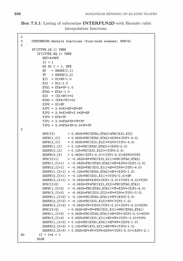
336 NONLINEAR BENDING OF ELASTIC PLATES
Box 7.5.1: Listing of subroutine INTERPLN2D with Hermite cubicinterpolation functions.
C
C CONFORMING Hermite functions (four-node element; NPE=4)
C
IF(ITYPE.LE.1) THEN
IF(ITYPE.EQ.1) THEN
NET=4*NPE
II = 1
DO 60 I = 1, NPE
XP = XNODE(I,1)
YP = XNODE(I,2)
XI1 = XI*XP-1.0
XI2 = XI1-1.0
ETA1 = ETA*YP-1.0
ETA2 = ETA1-1.0
XI0 = (XI+XP)**2
ETA0 = (ETA+YP)**2
XIP0 = XI+XP
XIP1 = 3.0*XI*XP+XP*XP
XIP2 = 3.0*XI*XP+2.0*XP*XP
YIP0 = ETA+YP
YIP1 = 3.0*ETA*YP+YP*YP
YIP2 = 3.0*ETA*YP+2.0*YP*YP
C
SFH(II) = 0.0625*FNC(ETA0,ETA2)*FNC(XI0,XI2)
DSFH(1,II) = 0.0625*FNC(ETA0,ETA2)*XIP0*(XIP1-4.0)
DSFH(2,II) = 0.0625*FNC(XI0,XI2)*YIP0*(YIP1-4.0)
DDSFH(1,II) = 0.125*FNC(ETA0,ETA2)*(XIP2-2.0)
DDSFH(2,II) = 0.125*FNC(XI0,XI2)*(YIP2-2.0)
DDSFH(3,II) = 0.0625*(XIP1-4.0)*(YIP1-4.0)*XIP0*YIP0
SFH(II+1) = -0.0625*XP*FNC(XI0,XI1)*FNC(ETA0,ETA2)
DSFH(1,II+1) = -0.0625*FNC(ETA0,ETA2)*XP*XIP0*(XIP1-2.0)
DSFH(2,II+1) = -0.0625*FNC(XI0,XI1)*XP*YIP0*(YIP1-4.0)
DDSFH(1,II+1) = -0.125*FNC(ETA0,ETA2)*XP*(XIP2-1.0)
DDSFH(2,II+1) = -0.125*FNC(XI0,XI1)*(YIP2-2.0)*XP
DDSFH(3,II+1) = -0.0625*XP*XIP0*(XIP1-2.0)*(YIP1-4.0)*YIP0
SFH(II+2) = -0.0625*YP*FNC(XI0,XI2)*FNC(ETA0,ETA1)
DSFH(1,II+2) = -0.0625*FNC(ETA0,ETA1)*YP*XIP0*(XIP1-4.0)
DSFH(2,II+2) = -0.0625*FNC(XI0,XI2)*YP*YIP0*(YIP1-2.0)
DDSFH(1,II+2) = -0.125*FNC(ETA0,ETA1)*YP*(XIP2-2.0)
DDSFH(2,II+2) = -0.125*FNC(XI0,XI2)*YP*(YIP2-1.0)
DDSFH(3,II+2) = -0.0625*YP*YIP0*(YIP1-2.0)*(XIP1-4.0)*XIP0
SFH(II+3) = 0.0625*XP*YP*FNC(XI0,XI1)*FNC(ETA0,ETA1)
DSFH(1,II+3) = 0.0625*FNC(ETA0,ETA1)*XP*YP*(XIP1-2.0)*XIP0
DSFH(2,II+3) = 0.0625*FNC(XI0,XI1)*XP*YP*(YIP1-2.0)*YIP0
DDSFH(1,II+3) = 0.125*FNC(ETA0,ETA1)*XP*YP*(XIP2-1.0)
DDSFH(2,II+3) = 0.125*FNC(XI0,XI1)*XP*YP*(YIP2-1.0)
DDSFH(3,II+3) = 0.0625*XP*YP*YIP0*XIP0*(YIP1-2.0)*(XIP1-2.)
60 II = I*4 + 1
ELSE
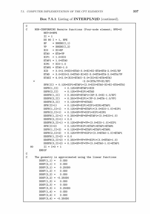
7.5. COMPUTER IMPLEMENTATION OF THE CPT ELEMENTS 337
Box 7.5.1: Listing of INTERPLN2D (continued).
C
C NON-CONFORMING Hermite functions (Four-node element; NPE=4)
NET=3*NPE
II = 1
DO 80 I = 1, NPE
XP = XNODE(I,1)
YP = XNODE(I,2)
XI0 = XI*XP
ETA0 = ETA*YP
XIP1 = 1.0+XI0
ETAP1 = 1.0+ETA0
XIM1 = XI0-1.0
ETAM1 = ETA0-1.0
XID = 3.0+2.0*XI0+ETA0-3.0*XI*XI-ETA*ETA-2.0*XI/XP
ETAD = 3.0+XI0+2.0*ETA0-XI*XI-3.0*ETA*ETA-2.0*ETA/YP
ETAXI = 4.0+2.0*(XI0+ETA0)-3.0*(XI*XI+ETA*ETA)
* -2.0*(ETA/YP+XI/XP)
SFH(II) = 0.125*XIP1*ETAP1*(2.0+XI0+ETA0-XI*XI-ETA*ETA)
DSFH(1,II) = 0.125*XP*ETAP1*XID
DSFH(2,II) = 0.125*YP*XIP1*ETAD
DDSFH(1,II) = 0.250*XP*ETAP1*(XP-3.0*XI-1.0/XP)
DDSFH(2,II) = 0.250*YP*XIP1*(YP-3.0*ETA-1.0/YP)
DDSFH(3,II) = 0.125*XP*YP*ETAXI
SFH(II+1) = 0.125*XP*XIP1*XIP1*XIM1*ETAP1
DSFH(1,II+1) = 0.125*XP*XP*ETAP1*(3.0*XI0-1.0)*XIP1
DSFH(2,II+1) = 0.125*XP*YP*XIP1*XIP1*XIM1
DDSFH(1,II+1) = 0.250*XP*XP*XP*ETAP1*(3.0*XI0+1.0)
DDSFH(2,II+1) = 0.0
DDSFH(3,II+1) = 0.125*XP*XP*YP*(3.0*XI0-1.0)*XIP1
SFH(II+2) = 0.125*YP*XIP1*ETAP1*ETAP1*ETAM1
DSFH(1,II+2) = 0.125*XP*YP*ETAP1*ETAP1*ETAM1
DSFH(2,II+2) = 0.125*YP*YP*XIP1*(3.0*ETA0-1.0)*ETAP1
DDSFH(1,II+2) = 0.0
DDSFH(2,II+2) = 0.250*YP*YP*YP*XIP1*(3.0*ETA0+1.0)
DDSFH(3,II+2) = 0.125*XP*YP*YP*(3.0*ETA0-1.0)*ETAP1
80 II = I*3 + 1
ENDIF
C
C The geometry is approximated using the linear functions
DDSF(1,1) = 0.0D0
DDSF(2,1) = 0.0D0
DDSF(3,1) = 0.250D0
DDSF(1,2) = 0.0D0
DDSF(2,2) = 0.0D0
DDSF(3,2) = -0.250D0
DDSF(1,3) = 0.0D0
DDSF(2,3) = 0.0D0
DDSF(3,3) = 0.250D0
DDSF(1,4) = 0.0D0
DDSF(2,4) = 0.0D0
DDSF(3,4) = -0.250D0
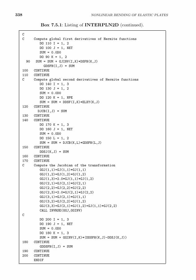
338 NONLINEAR BENDING OF ELASTIC PLATES
Box 7.5.1: Listing of INTERPLN2D (continued).
C
C Compute global first derivatives of Hermite functions
DO 110 I = 1, 2
DO 100 J = 1, NET
SUM = 0.0D0
DO 90 K = 1, 2
90 SUM = SUM + GJINV(I,K)*DSFH(K,J)
GDSFH(I,J) = SUM
100 CONTINUE
110 CONTINUE
C Compute global second derivatives of Hermite functions
DO 140 I = 1, 3
DO 130 J = 1, 2
SUM = 0.0D0
DO 120 K = 1, NPE
SUM = SUM + DDSF(I,K)*ELXY(K,J)
120 CONTINUE
DJCB(I,J) = SUM
130 CONTINUE
140 CONTINUE
DO 170 K = 1, 3
DO 160 J = 1, NET
SUM = 0.0D0
DO 150 L = 1, 2
SUM = SUM + DJCB(K,L)*GDSFH(L,J)
150 CONTINUE
DDSJ(K,J) = SUM
160 CONTINUE
170 CONTINUE
C Compute the Jacobian of the transformation
GGJ(1,1)=GJ(1,1)*GJ(1,1)
GGJ(1,2)=GJ(1,2)*GJ(1,2)
GGJ(1,3)=2.0*GJ(1,1)*GJ(1,2)
GGJ(2,1)=GJ(2,1)*GJ(2,1)
GGJ(2,2)=GJ(2,2)*GJ(2,2)
GGJ(2,3)=2.0*GJ(2,1)*GJ(2,2)
GGJ(3,1)=GJ(2,1)*GJ(1,1)
GGJ(3,2)=GJ(2,2)*GJ(1,2)
GGJ(3,3)=GJ(2,1)*GJ(1,2)+GJ(1,1)*GJ(2,2)
CALL INVRSE(GGJ,GGINV)
C
DO 200 I = 1, 3
DO 190 J = 1, NET
SUM = 0.0D0
DO 180 K = 1, 3
SUM = SUM + GGINV(I,K)*(DDSFH(K,J)-DDSJ(K,J))
180 CONTINUE
GDDSFH(I,J) = SUM
190 CONTINUE
200 CONTINUE
ENDIF
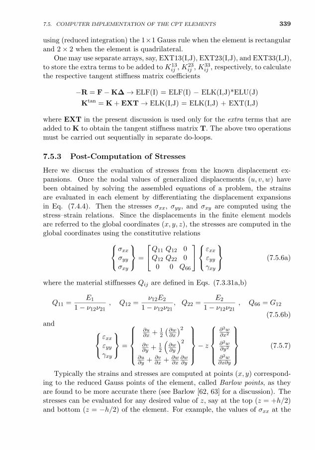
7.5. COMPUTER IMPLEMENTATION OF THE CPT ELEMENTS 339
using (reduced integration) the 1×1 Gauss rule when the element is rectangularand 2× 2 when the element is quadrilateral.
One may use separate arrays, say, EXT13(I,J), EXT23(I,J), and EXT33(I,J),to store the extra terms to be added to K13
ij , K23ij , K33
ij , respectively, to calculatethe respective tangent stiffness matrix coefficients
−R = F−K∆→ ELF(I) = ELF(I) − ELK(I,J)*ELU(J)
Ktan = K + EXT→ ELK(I,J) = ELK(I,J) + EXT(I,J)
where EXT in the present discussion is used only for the extra terms that areadded to K to obtain the tangent stiffness matrix T. The above two operationsmust be carried out sequentially in separate do-loops.
7.5.3 Post-Computation of Stresses
Here we discuss the evaluation of stresses from the known displacement ex-pansions. Once the nodal values of generalized displacements (u, v, w) havebeen obtained by solving the assembled equations of a problem, the strainsare evaluated in each element by differentiating the displacement expansionsin Eq. (7.4.4). Then the stresses σxx, σyy, and σxy are computed using thestress–strain relations. Since the displacements in the finite element modelsare referred to the global coordinates (x, y, z), the stresses are computed in theglobal coordinates using the constitutive relations
σxxσyyσxy
=
Q11 Q12 0Q12 Q22 0
0 0 Q66
εxxεyyγxy
(7.5.6a)
where the material stiffnesses Qij are defined in Eqs. (7.3.31a,b)
Q11 =E1
1− ν12ν21, Q12 =
ν12E2
1− ν12ν21, Q22 =
E2
1− ν12ν21, Q66 = G12
(7.5.6b)and
εxxεyyγxy
=
∂u∂x + 1
2
(∂w∂x
)2∂v∂y + 1
2
(∂w∂y
)2
∂u∂y + ∂v
∂x + ∂w∂x
∂w∂y
− z
∂2w∂x2
∂2w∂y2
∂2w∂x∂y
(7.5.7)
Typically the strains and stresses are computed at points (x, y) correspond-ing to the reduced Gauss points of the element, called Barlow points, as theyare found to be more accurate there (see Barlow [62, 63] for a discussion). Thestresses can be evaluated for any desired value of z, say at the top (z = +h/2)and bottom (z = −h/2) of the element. For example, the values of σxx at the
340
top and bottom of the element at a point (xc, yc) corresponding to a Gausspoint are computed using
σtopxx = σxx(xc, yc, h/2) = Q11
[∂u
∂x+
1
2
(∂w
∂x
)2]− h
2
∂2w
∂x2
(xc,yc)
+Q12
[∂v
∂y+
1
2
(∂w
∂y
)2]− h
2
∂2w
∂y2
(xc,yc)
(7.5.8)
σbottomxx = σxx(xc, yc,−h/2) = Q11
[∂u
∂x+
1
2
(∂w
∂x
)2]
+h
2
∂2w
∂x2
(xc,yc)
+Q12
[∂v
∂y+
1
2
(∂w
∂y
)2]
+h
2
∂2w
∂y2
(xc,yc)
(7.5.9)
Similar expressions hold for σyy and σxy.
7.6 Numerical Examples using the CPT Elements
7.6.1 Preliminary Comments
Solution symmetries available in a problem should be taken advantage of toidentify the computational domain because they reduce computational effort. Asolution is symmetric about a line only if (a) the geometry, including boundaryconditions, (b) the material properties, and (c) the loading are symmetric aboutthe line. The boundary conditions along the edges and the symmetry lines of asimply-supported rectangular plate are shown in Fig. 7.6.1. In the case of theconforming element, we may also set ∂2w/∂x∂y = 0 at the center of the plate.When one is not sure of the solution symmetry, it is advised that the wholeplate be modeled.
All meshes used in the examples are uniform (i.e. the same size elementsare used). At every boundary node, one is required to specify one element ineach of the four pairs (i.e. either the generalized displacement or generalizedforce) given in Eq. (7.3.24). When no displacement or force is specified at anode, then it is understood that the specified generalized force is specified to bezero at that node. The range of loads used in the examples has the sole purposeof bringing out the geometric nonlinearity exhibited in the problem, and veryseldom plate structures are loaded into the nonlinear range.
7.6.2 Results of Linear Analysis
We consider the bending of rectangular plates with various edge conditions toevaluate the non-conforming and conforming rectangular plate elements based
NONLINEAR BENDING OF ELASTIC PLATES
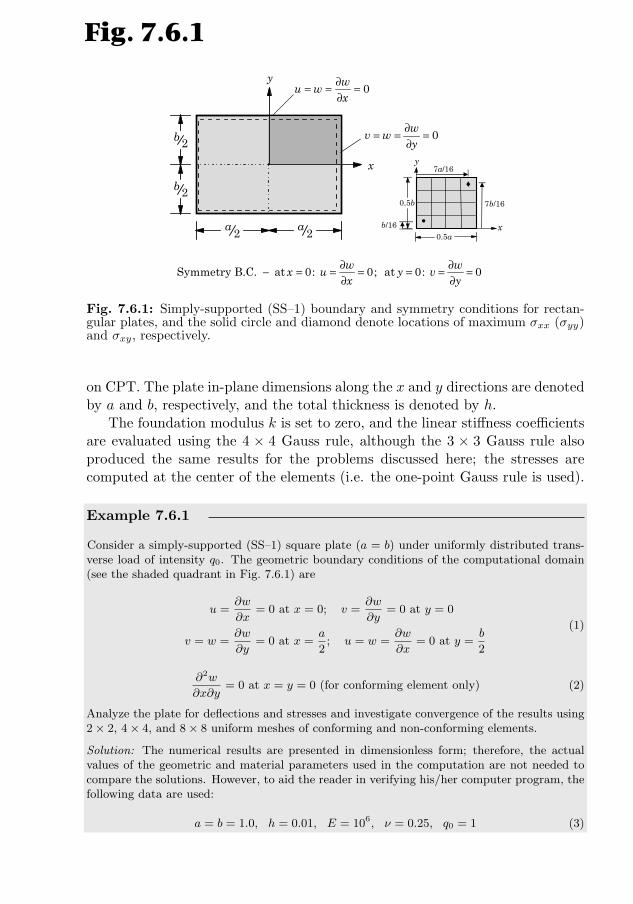
7.6. NUMERICAL EXAMPLES USING THE CPT ELEMENTS 341
x
y
a2
b 2
b 2
a2
0w
u wx
∂= = =∂
0w
v wy
∂= = =∂
∂ ∂− = = = = = =∂ ∂
Symmetry B.C. at 0: 0; at 0: 0w w
x u y vx y
x
y
•
♦
0.5b
0.5a
7b/16
b/16
7a/16
Fig. 7.6.1
Fig. 7.6.1: Simply-supported (SS–1) boundary and symmetry conditions for rectan-gular plates, and the solid circle and diamond denote locations of maximum σxx (σyy)and σxy, respectively.
on CPT. The plate in-plane dimensions along the x and y directions are denotedby a and b, respectively, and the total thickness is denoted by h.
The foundation modulus k is set to zero, and the linear stiffness coefficientsare evaluated using the 4 × 4 Gauss rule, although the 3 × 3 Gauss rule alsoproduced the same results for the problems discussed here; the stresses arecomputed at the center of the elements (i.e. the one-point Gauss rule is used).
Example 7.6.1
Consider a simply-supported (SS–1) square plate (a = b) under uniformly distributed trans-verse load of intensity q0. The geometric boundary conditions of the computational domain(see the shaded quadrant in Fig. 7.6.1) are
u =∂w
∂x= 0 at x = 0; v =
∂w
∂y= 0 at y = 0
v = w =∂w
∂y= 0 at x =
a
2; u = w =
∂w
∂x= 0 at y =
b
2
(1)
∂2w
∂x∂y= 0 at x = y = 0 (for conforming element only) (2)
Analyze the plate for deflections and stresses and investigate convergence of the results using2× 2, 4× 4, and 8× 8 uniform meshes of conforming and non-conforming elements.
Solution: The numerical results are presented in dimensionless form; therefore, the actualvalues of the geometric and material parameters used in the computation are not needed tocompare the solutions. However, to aid the reader in verifying his/her computer program, thefollowing data are used:
a = b = 1.0, h = 0.01, E = 106, ν = 0.25, q0 = 1 (3)
342 NONLINEAR BENDING OF ELASTIC PLATES
The axial and bending stiffnesses are A11 = A22 = 0.10667 × 10⁵, A12 = 0.26667 × 10⁴,A66 = 0.4× 10⁴, D11 = D22 = 0.088889, D12 = 0.022222, and D66 = 0.033333. The first fiverows and the last two rows, denoted by the subscripts, of the element stiffness matrix, andthe element force vector for the non-conforming element in the 2× 2 mesh are
K(1)1 =
0.48889× 10⁴ 0.16667× 10⁴ 0.0 0.0 0.0−0.28889× 10⁴ −0.33333× 10³ 0.0 0.0 0.0−0.24444× 10⁴ −0.16667× 10⁴ 0.0 0.0 0.0
0.44444× 10³ 0.33333× 10³ 0.0 0.0 0.0
K(1)2 =
0.16667× 10⁴ 0.48889× 10⁴ 0.0 0.0 0.00.33333× 103 0.44444× 10³ 0.0 0.0 0.0−0.16667× 10⁴ −0.24444× 10⁴ 0.0 0.0 0.0−0.33333× 10³ −0.28889× 10⁴ 0.0 0.0 0.0
K
(1)3 =
0.0 0.0 0.60302× 10² 0.27307× 10² 0.27307× 10²
0.0 0.0 −0.26169× 10² 0.24462× 10² 0.68267× 101
0.0 0.0 −0.79644× 101 0.96711× 101 0.96711× 101
0.0 0.0 −0.26169× 10² 0.68267× 101 0.24462× 10²
K(1)4 =
0.0 0.0 0.27307× 10² 0.34892× 10² 0.56889× 101
0.0 0.0 −0.24462× 10² 0.14033× 10² −0.55708× 10⁻⁸
0.0 0.0 −0.96711× 101 0.87230× 101 −0.22204× 10⁻¹⁵
0.0 0.0 0.68267× 101 0.10619× 10² 0.55708× 10⁻⁸
K(1)5 =
0.0 0.0 0.27307× 10² 0.56889× 101 0.34892× 10²
0.0 0.0 0.68267× 101 0.55708× 10⁻⁸ 0.10619× 10²
0.0 0.0 −0.96711× 101 −0.16653× 10⁻¹⁵ 0.87230× 101
0.0 0.0 −0.24462× 10² −0.55708× 10⁻⁸ 0.14033× 10²
K(1)19 =
0.0 0.0 0.68267× 101 0.10619× 10² −0.42595× 10⁻⁸
0.0 0.0 −0.96711× 101 0.87230× 101 −0.27756× 10⁻¹⁵
0.0 0.0 −0.24462× 10² 0.14033× 10² 0.42595× 10⁻⁸
0.0 0.0 0.27307× 10² 0.34892× 10² −0.56889× 101
K(1)20 =
0.0 0.0 0.24462× 10² 0.42595× 10⁻⁸ 0.14033× 10²
0.0 0.0 0.96711× 101 −0.22204× 10⁻¹⁵ 0.87230× 101
0.0 0.0 −0.68267× 101 −0.42595× 10⁻⁸ 0.10619× 10²
0.0 0.0 −0.27307× 10² −0.56889× 101 0.34892× 10²
f (1) =
0.0 0.0 0.39063× 10⁻² 0.13021× 10⁻² 0.13021× 10⁻²
0.0 0.0 0.39063× 10⁻² −0.13021× 10⁻² 0.13021× 10⁻²
0.0 0.0 0.39063× 10⁻² −0.13021× 10⁻² −0.13021× 10⁻²
0.0 0.0 0.39063× 10⁻² 0.13021× 10⁻² −0.13021× 10⁻²T (4)
The non-dimensional finite element solutions for center transverse displacement andmaximum normal and shear stresses along with the analytical solutions (see Reddy [3,55, 56]) of isotropic (ν = 0.25) and orthotropic (E1/E2 = 25, G12 = G13 = 0.5E2,ν12 = 0.25) square plates are presented in Table 7.6.1. The (x, y, z) locations in theplate where the normal stresses are computed are (a/8, a/8, h/2), (a/16, a/16, h/2), and(a/32, a/32, h/2) for 2 × 2, 4 × 4, and 8 × 8 uniform meshes, respectively, while those ofσxy are (3a/8, 3a/8,−h/2), (7a/16, 7a/16,−h/2), and (15a/32, 15a/32,−h/2) for the samethree meshes. The analytical solutions were evaluated using m,n = 1, 3, . . . , 19. The exactmaximum deflection occurs at x = y = 0, maximum stresses σxx and σyy occur at (0, 0, h/2),and the maximum shear stress σxy occurs at (a/2, a/2,−h/2). The conforming element isslightly more accurate than the non-conforming element in predicting the deflections andboth converge to the analytical solutions as the mesh is refined.
7.6. NUMERICAL EXAMPLES USING THE CPT ELEMENTS 343
Table 7.6.1: Maximum transverse deflections and stresses* of simply-supported squareplates under a uniformly distributed load q0.
Variable Non-conforming Conforming Analytical
2× 2 4× 4 8× 8 2× 2 4× 4 8× 8 solution
Isotropic platesw × 102 4.8571 4.6425 4.5883 4.7619 4.5952 4.5739 4.5698σxx 0.2405 0.2673 0.2740 0.2239 0.2637 0.2731 0.2762σxy 0.1713 0.1964 0.2050 0.1688 0.1935 0.2040 0.2085
Orthotropic plates
w × 102 0.7082 0.6635 0.6531 0.7710 0.6651 0.6522 0.6497σxx 0.7148 0.7709 0.7828 0.5560 0.7388 0.7743 0.7866σyy 0.0296 0.0253 0.0246 0.0278 0.0249 0.0245 0.0244σxy 0.0337 0.0421 0.0444 0.0375 0.0416 0.0448 0.0463
*w = wE2h3/(q0a
4), σ = σh2/(q0a2).
Example 7.6.2
Consider a clamped square plate under uniformly distributed transverse load of intensity q0.Consider both isotropic (ν = 0.25) and orthotropic (E1/E2 = 25, G12 = G13 = 0.5E2, ν12 =0.25) plates. The boundary conditions are [the origin of the coordinate system (x, y, z) istaken at the center of the plate]:
u =∂w
∂x= 0 at x = 0; v =
∂w
∂y= 0 at y = 0 (1)
u = v = w =∂w
∂x=∂w
∂y= 0 at x =
a
2; u = v = w =
∂w
∂x=∂w
∂y= 0 at y =
b
2(2)
∂2w
∂x∂y= 0 on clamped edges (for conforming element only) (3)
Analyze the plate for deflections and stresses and investigate convergence of the results using2× 2, 4× 4, and 8× 8 uniform meshes of conforming and non-conforming elements.
Solution: Table 7.6.2 contains the non-dimensional deflections and stresses. The (x, y, z)locations of the normal stresses reported for the three meshes are:
2× 2 :
(a
8,b
8,−h
2
); 4× 4 :
(a
16,b
16,−h
2
); 8× 8 :
(a
32,b
32,−h
2
)(4)
and shear stresses reported for the three meshes are
2× 2 :
(3a
8,
3b
8,−h
2
); 4× 4 :
(7a
16,
7b
16,−h
2
); 8× 8 :
(15a
32,
15b
32,−h
2
)(5)
These stresses are not necessarily the maximum ones in the plate. For example,for an 8 × 8 mesh, the maximum normal stress in the isotropic plate is found tobe 0.2300 at (0.46875a, 0.03125b,−h/2) and the maximum shear stress is 0.0226 at(0.28125a, 0.09375b,−0.5h) for the non-conforming element. The conforming element yieldsslightly different solutions than the non-conforming element for deflections but not for thestresses, and both elements show good convergence.
344 NONLINEAR BENDING OF ELASTIC PLATES
Table 7.6.2: Maximum transverse deflections and stresses* of clamped (CCCC),isotropic and orthotropic, square plates (a = b) under a uniformly distributed loadq0 (linear analysis).
Variable Non-conforming Conforming
2× 2 4× 4 8× 8 2× 2 4× 4 8× 8
Isotropic platew × 102 1.5731 1.4653 1.4342 1.4778 1.4370 1.4249σxx 0.0987 0.1238 0.1301 0.0861 0.1197 0.1288σxy 0.0497 0.0222 0.0067 0.0489 0.0224 0.0068
Orthotropic platew × 102 0.1434 0.1332 0.1314 0.1402 0.1330 0.1311σxx 0.1962 0.2491 0.2598 0.1559 0.2358 0.2576σyy 0.0085 0.0046 0.0042 0.0066 0.0047 0.0043σxy 0.0076 0.0046 0.0019 0.0083 0.0048 0.0020
*w = wE2h3/(q0a
4), σ = σh2/(q0a2).
7.6.3 Results of Nonlinear Analysis
Here we investigate geometrically nonlinear response of plates using the con-forming and non-conforming plate finite elements. The nonlinear terms areevaluated using reduced integration. Full integration (F) means 4 × 4 Gaussrule and reduced integration (R) means 1× 1 Gauss rule.
Example 7.6.3
Consider nonlinear bending of an isotropic (ν = 0.3) square plate under uniformly distributedtransverse load, q0. This problem was analyzed by Levy [64], Wang [65], and Kawai andYoshimura [66]. The following simply-supported (SS–3) geometric boundary conditions areused:
u = v = w = 0 on all four edges (1)
Since (∂w/∂x) and (∂w/∂y) are not specified in SS–3, it follows that the following forceboundary conditions are satisfied in the integral sense [see Eq. (7.4.6)]:
on y = 0, b : Mxy = Myy = 0; on x = 0, a : Mxx = Mxy = 0 (2)
Use the biaxial symmetry to model only a quadrant of the plate with uniform 4× 4 and 8× 8meshes of rectangular elements to obtain deflections and stresses as functions of the load.
Solution: The boundary conditions along the lines of symmetry are shown in Fig. 7.6.1.The following geometric and material parameters are used, although the non-dimensionaldeflections and stresses presented here are independent of them (but may depend on ν):
a = b = 10 in, h = 0.1 in, E = 30× 106 psi, ν = 0.3 (3)
A load increment of ∆q = 7.5, which is equal to the increment of load parameter, ∆P ≡a4∆q/Eh4 = 25, is used along with the convergence tolerance of ε = 10−2. Except forthe first load step, which took five iterations, the convergence was achieved for two or threeiterations.
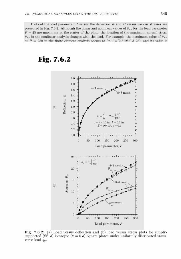
7.6. NUMERICAL EXAMPLES USING THE CPT ELEMENTS 345
Plots of the load parameter P versus the deflection w and P versus various stresses arepresented in Fig. 7.6.2. Although the linear and nonlinear values of σxx for the load parameterP = 25 are maximum at the center of the plate, the location of the maximum normal stressσxx in the nonlinear analysis changes with the load. For example, the maximum value of σxxat P = 250 in the finite element analysis occurs at (x, y)=(2.8125,0.3125), and its value isfound to be 21.177. Note that membrane stresses are a significant part of total stresses.
The center deflection, w = w/h, and total stresses (i.e. sum of membrane and flexural con-tributions), σxx = σxx(A,A, h/2)(a2/Eh2) and σxy = σxy(B,B,−h/2)(a2/Eh2), as functionsof the load parameter, P = q0a
4/Eh4 are presented in Table 7.6.3. The location (A,A, h/2)refers to the Gauss point nearest to the center (x = y = 0) but at the top of the plate, while(B,B,−h/2) refers to the Gauss point nearest to the corner x = y = a/2, at the bottom of the
0 50 100 150 200 250 300
Load parameter
0.0
0.2
0.4
0.6
0.8
1.0
1.2
1.4
1.6
1.8
2.0
Def
lect
ion
,
(a)
4×4 mesh8×8 mesh
w
, P
a = b = 10 in, h = 0.1 inE = 30×106, ν = 0.3
40
4,q aw
w Ph Eh
= =
(b)
0 50 100 150 200 250 300
Load parameter,
0
5
10
15
20
25
Str
esse
s,
4×4 mesh
8×8 mesh
xxs
xys
(membrane)xxs
σ xx
P
2
2xx xx
aEh
s sæ ö÷ç= ÷ç ÷÷çè ø
Fig. 7.6.2
Fig. 7.6.2: (a) Load versus deflection and (b) load versus stress plots for simply-supported (SS–3) isotropic (ν = 0.3) square plates under uniformly distributed trans-verse load q0.
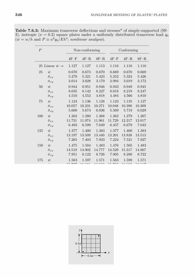
346 NONLINEAR BENDING OF ELASTIC PLATES
Table 7.6.3: Maximum transverse deflections and stresses* of simply-supported (SS–3), isotropic (ν = 0.3) square plates under a uniformly distributed transverse load q0(w = w/h and P ≡ a4q0/Eh4; nonlinear analysis).
P Non-conforming Conforming
4F–F 4F–R 8F–R 4F–F 4F–R 8F–R
25 Linear w → 1.127 1.127 1.113 1.116 1.116 1.110
25 w 0.670 0.673 0.670 0.669 0.670 0.669σxx 5.279 5.321 5.423 5.252 5.324 5.426σxy 3.014 3.028 3.179 2.994 3.019 3.172
50 w 0.944 0.951 0.946 0.943 0.949 0.945σxx 8.035 8.142 8.227 8.018 8.219 8.247σxy 4.510 4.552 4.818 4.484 4.566 4.810
75 w 1.124 1.136 1.128 1.123 1.135 1.127σxx 10.057 10.231 10.271 10.048 10.390 10.309σxy 5.600 5.674 6.036 5.569 5.719 6.029
100 w 1.262 1.280 1.268 1.262 1.279 1.267σxx 11.731 11.974 11.961 11.729 12.217 12.017σxy 6.493 6.599 7.049 6.457 6.679 7.042
125 w 1.377 1.400 1.383 1.377 1.400 1.383σxx 13.197 13.509 13.440 13.201 13.838 13.513σxy 7.265 7.403 7.933 7.224 7.521 7.927
150 w 1.475 1.504 1.483 1.476 1.505 1.483σxx 14.519 14.902 14.777 14.529 15.317 14.867σxy 7.951 8.122 8.726 7.905 8.280 8.722
175 w 1.563 1.597 1.571 1.563 1.598 1.571σxx 15.737 16.191 16.009 15.752 16.693 16.117σxy 8.573 8.778 9.451 8.524 8.979 9.449
200 w 1.641 1.681 1.651 1.642 1.683 1.651σxx 16.874 17.401 17.162 16.894 17.989 17.287σxy 9.147 9.385 10.123 9.094 9.631 10.123
225 w 1.713 1.758 1.724 1.713 1.761 1.724σxx 17.946 18.546 18.251 17.970 19.222 18.393σxy 9.681 9.952 10.751 9.625 10.244 10.754
250 w 1.779 1.830 1.791 1.779 1.834 1.791σxx 18.965 19.638 19.287 18.993 20.401 19.446σxy 10.182 10.486 11.344 10.122 10.827 11.349
*w = w/h, σ = σ(a2/Eh2).
x
y
•
♦
0.5a
0.5a
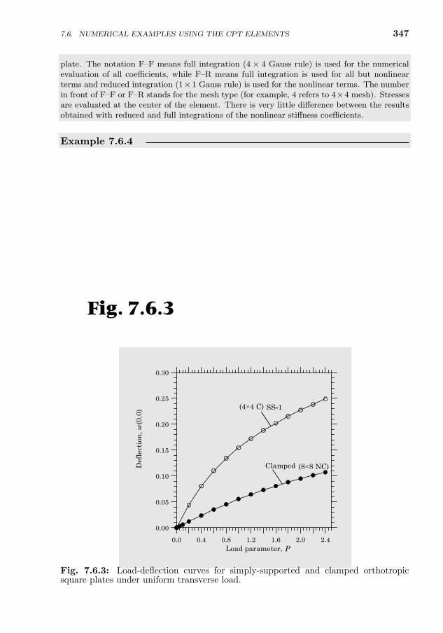
7.6. NUMERICAL EXAMPLES USING THE CPT ELEMENTS 347
plate. The notation F–F means full integration (4 × 4 Gauss rule) is used for the numericalevaluation of all coefficients, while F–R means full integration is used for all but nonlinearterms and reduced integration (1×1 Gauss rule) is used for the nonlinear terms. The numberin front of F–F or F–R stands for the mesh type (for example, 4 refers to 4×4 mesh). Stressesare evaluated at the center of the element. There is very little difference between the resultsobtained with reduced and full integrations of the nonlinear stiffness coefficients.
Example 7.6.4
Consider the bending of (a) simply-supported (SS–1) and (b) clamped orthotropic squareplates under a uniformly distributed transverse load q0. Use the following geometric andmaterial properties:
a = b = 12 in, h = 0.138 in, E1 = 3× 10⁶ psi, E2 = 1.28× 10⁶ psi
G12 = G23 = G13 = 0.37× 10⁶ psi, ν12 = ν23 = ν13 = 0.32(1)
Use a load increment of ∆q = 0.2 psi and a uniform mesh of 4×4 non-conforming elements ina quarter plate for the simply-supported plate. Assume the boundary conditions of a clamped
edge to be u = v = w = ∂w∂x
= ∂w∂y
= ∂2w∂x∂y
= 0, use a uniform mesh of 8 × 8 non-conformingelements in a quarter plate, and load increments of ∆q = 0.05, 0.05, 0.1, 0.2, 0.2, . . . , 0.2psi. Plot the center deflection versus load for the two problems.
Solution: Numerical solutions to large deflection bending of orthotropic rectangular plates bythe method of differential quadrature can be found in a paper by Bert, Jang, and Striz [67].Figure 7.6.3 shows a plot of the center deflection versus the intensity of the distributed loadfor the simply-supported (SS–1) plate.
The linear solution for the clamped plate at q0 = 0.05 is found to be w(0, 0) = 0.00302 in.Figure 7.6.3 also contains a plot of the center deflection versus the intensity of the distributedload for the clamped orthotropic plate (see [68–80]).
0.0 0.4 0.8 1.2 1.6 2.0 2.4Load parameter,
0.00
0.05
0.10
0.15
0.20
0.25
0.30
Def
lect
ion
,
SS-1
Clamped
(4×4 C)
(8×8 NC)
w(0
,0)
P
Fig. 7.6.3
Fig. 7.6.3: Load-deflection curves for simply-supported and clamped orthotropicsquare plates under uniform transverse load.
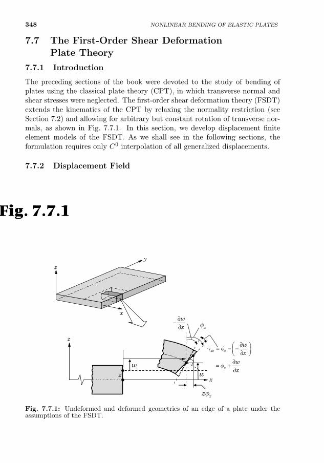
348
7.7 The First-Order Shear DeformationPlate Theory
7.7.1 Introduction
The preceding sections of the book were devoted to the study of bending ofplates using the classical plate theory (CPT), in which transverse normal andshear stresses were neglected. The first-order shear deformation theory (FSDT)extends the kinematics of the CPT by relaxing the normality restriction (seeSection 7.2) and allowing for arbitrary but constant rotation of transverse nor-mals, as shown in Fig. 7.7.1. In this section, we develop displacement finiteelement models of the FSDT. As we shall see in the following sections, theformulation requires only C0 interpolation of all generalized displacements.
7.7.2 Displacement Field
Under the same assumptions and restrictions as in the classical laminate theorybut relaxing the normality condition, the displacement field of the FSDT canbe expressed in the form
u1(x, y, z) = u(x, y) + zφx(x, y)
u2(x, y, z) = v(x, y) + zφy(x, y) (7.7.1)
u3(x, y, z) = w(x, y)
zy
x
z
x
∂ = − − ∂ ∂= +∂
xz x
x
wx
wx
g f
f
xzf
xf∂−∂wx
ww
z
Fig. 7.7.1
Fig. 7.7.1: Undeformed and deformed geometries of an edge of a plate under theassumptions of the FSDT.
NONLINEAR BENDING OF ELASTIC PLATES
349
where (u, v, w, φx, φy) are unknown functions to be determined. As before,(u, v, w) denote the displacements of a point on the plane z = 0 and φx and φyare the rotations of a transverse normal line about the y- and x-axes, respec-tively (see Fig. 7.7.1). The quantities (u, v, w, φx, φy) are called the generalizeddisplacements.
The notation that φx denotes the rotation of a transverse normal aboutthe y-axis and φy denotes the rotation about the x-axis may be confusing tosome because they do not follow the right-hand rule. However, the notationhas been used extensively in the literature and we will not depart from it. If(βx, βy) denote the rotations about the x- and y-axes, respectively, that followthe right-hand rule, then
βx = −φy , βy = φx (7.7.2)
For thin plates, that is, when the plate in-plane characteristic dimension tothickness ratio is on the order of 50 or greater, the rotation functions φx andφy should approach the respective slopes of the transverse deflection [21]:
φx = −∂w∂x
, φy = −∂w∂y
(7.7.3)
However, this equality is not achieved in the discrete model, resulting in shearlocking, as in the case of the Timoshenko beam theory, when the same lower-order approximations are used for the transverse deflection w as well as therotations (φx and φy).
The von Karman nonlinear strains associated with the displacement field inEq. (7.7.1) are (εzz = 0)
εxxεyyγyzγxzγxy
=
ε0xx
ε0yy
γ0yz
γ0xz
γ0xy
+ z
ε1xx
ε1yy
00γ1xy
=
∂u∂x + 1
2(∂w∂x )2
∂v∂y + 1
2(∂w∂y )2
∂w∂y + φy∂w∂x + φx
∂u∂y + ∂v
∂x + ∂w∂x
∂w∂y
+ z
∂φx∂x∂φy∂y
00
∂φx∂y +
∂φy∂x
(7.7.4)
Note that the strains (εxx, εyy, γxy) are linear through the plate thickness, whilethe transverse shear strains (γxz, γyz) are constant.
7.7.3 Weak Forms using the Principle of Virtual Displacements
The weak forms of the FSDT can be derived using the principle of virtualdisplacements
0 = δW e ≡ δW eI + δW e
E (7.7.5)
THE FIRST-ORDER SHEAR DEFORMATION PLATE THEORY7.7.
350
where the virtual strain energy δW eI and the virtual work done by applied forces
δW eE in an element Ωe are given by
δW eI =
∫Ωe
∫ h2
−h2
[σxx
(δε0xx + zδε1
xx
)+ σyy
(δε0yy + zδε1
yy
)+σxy
(δγ0xy + zδγ1
xy
)+Ksσxzδγ
0xz +Ksσyzδγ
0yz
]dz
dx dy (7.7.6)
δW eE = −
∮Γe
∫ h2
−h2
[σnn (δun + zδφn) + σns (δus + zδφs) + σnzδw] dz ds
+
∫Ωe
(q − kw) δw dx dy
(7.7.7)
where Ωe denotes the undeformed mid-plane of a typical plate element, h is thetotal thickness, k is the modulus of the elastic foundation (if any), (σnn, σns,σnz) are the edge stresses along the (n, s, z) coordinates, and Ks is the shearcorrection coefficient (Ks = 5/6).
Substituting for δW eI and δW e
E from Eqs. (7.7.6) and (7.7.7) into the virtualwork statement in Eq. (7.7.5) and integrating through the thickness, we obtain
0 =
∫Ωe
[Nxxδε
0xx +Mxxδε
1xx +Nyyδε
0yy +Myyδε
1yy +Nxyδγ
0xy
+Mxyδγ1xy +Qxδγ
0xz +Qyδγ
0yz + kwδw − qδw ] dx dy
−∮
Γe(Nnnδun +Nnsδus +Mnnδφn +Mnsδφs +Qnδw) ds (7.7.8)
where φn and φs are the rotations of a transverse normal about s and −n coordi-nates, respectively, (Nxx, Nyy, Nxy, Mxx, Myy, Mxy) are defined in Eq. (7.3.4),and (Nnn, Nns, Mnn, Mns, Qn) are defined in Eq. (7.3.7). The transverse shearforces per unit length (Qx, Qy) are defined by
QxQy
= Ks
∫ h2
−h2
σxzσyz
dz (7.7.9)
7.7.4 Governing Equations
Equation (7.7.8) contains five different statements associated with the five vir-tual displacements (δu, δv, δw, δφx, δφy), and they form the basis of the finiteelement model. The governing equations of equilibrium of the FSDT, althoughthey are not needed to develop the finite element model, can be derived byfirst expressing the virtual strains in Eq. (7.7.8) in terms of the virtual dis-placements and then integrating-by-parts all expressions to relieve the virtual
NONLINEAR BENDING OF ELASTIC PLATES
351
displacements (δu, δv, δw, δφx, δφy) in Ωe of any differentiation. Then the fun-damental lemma of calculus of variations is used to declare that the coefficientsof (δu, δv, δw, δφx, δφy) in Ωe must be zero, obtaining
0 =
∫Ωe
[− (Nxx,x +Nxy,y) δu− (Nxy,x +Nyy,y) δv
− (Mxx,x +Mxy,y −Qx) δφx − (Mxy,x +Myy,y −Qy) δφy− (Qx,x +Qy,y − kw +N + q) δw
]dx dy
+
∮Γe
[(Nxxnx +Nxyny) δu+ (Nxynx +Nyyny) δv
+ (Mxxnx +Mxyny) δφx + (Mxynx +Myyny) δφy
+(Qxnx +Qyny + P
)δw]ds
−∮
Γe(Nnnδun +Nnsδus +Mnnδφn +Mnsδφs +Qnδw) ds (7.7.10)
where N and P are defined by Eq. (7.3.14). The boundary terms can beexpressed in terms of the normal and tangential components un, us, φn, and φsusing Eqs. (7.3.18a) and
φx = nxφn − nyφs , φy = nyδφn + nxδφs (7.7.11)
This will yield the natural boundary conditions given in Eqs. (7.3.20a, b), whichrelate the forces and moments on an arbitrary edge to those on edges parallelto the coordinates (x, y, z).
The Euler–Lagrange equations are
δu :∂Nxx
∂x+∂Nxy
∂y= 0 (7.7.12)
δv :∂Nxy
∂x+∂Nyy
∂y= 0 (7.7.13)
δw :∂Qx∂x
+∂Qy∂y− kw +N (u, v, w, φx, φy) + q = 0 (7.7.14)
δφx :∂Mxx
∂x+∂Mxy
∂y−Qx = 0 (7.7.15)
δφy :∂Mxy
∂x+∂Myy
∂y−Qy = 0 (7.7.16)
The primary and secondary variables of the theory are
primary variables: un, us, w, φn, φs
secondary variables: Nnn, Nns, Qn, Mnn, Mns(7.7.17)
The plate constitutive equations in Eqs. (7.3.32) and (7.3.33) are valid alsofor the first-order plate theory. Since the transverse shear strains are repre-sented as constant through the plate thickness, it follows that the transverse
THE FIRST-ORDER SHEAR DEFORMATION PLATE THEORY7.7.
352
shear stresses will also be constant. It is well known from elementary theoryof homogeneous beams that the transverse shear stress variation is parabolicthrough the beam thickness, as noted in connection with the Timoshenko beamtheory. This discrepancy between the actual stress state and the constant stressstate predicted by the FSDT is often corrected in computing the transverseshear forces (Qx, Qy) by multiplying the transverse shear stiffnesses (Q44, Q55)with the shear correction factor Ks. Thus, the constitutive equations for trans-verse shear forces of an orthotropic plate are
QyQx
= Ks
∫ h2
−h2
σyzσxz
dz =
[A44 00 A55
]γyzγxz
(7.7.18)
where the transverse shear stiffnesses A44 and A55 are defined by
(A44, A55) = Ks
∫ h2
−h2
(Q44, Q55) dz, Q44 = G23, Q55 = G13 (7.7.19)
In summary, the stress resultants in an orthotropic plate are related to thegeneralized displacements (u, v, w, φx, φy) by [see Eqs. (7.3.32) and (7.3.33)]
Nxx
Nyy
Nxy
=
A11 A12 0A12 A22 00 0 A66
ε0xx
ε0yy
γ0xy
−NTxx
NTyy
0
(7.7.20)
Mxx
Myy
Mxy
=
D11 D12 0D12 D22 0
0 0 D66
ε1xx
ε1yy
γ1xy
−MTxx
MTyy
0
(7.7.21)
QyQx
=
[A44 00 A55
]γ0yz
γ0xz
(7.7.22)
where (i, j = 1, 2, 6)
Aij = Qij h, Dij = Qijh3
12; A44 = KsG23h, A55 = KsG13h (7.7.23)
Q11 =E1
1− ν12ν21, Q22 = Q11
E2
E1, Q12 = ν12Q22, Q66 = G12 (7.7.24)
7.8 Finite Element Models of the FSDT
7.8.1 Weak Forms
Using the weak forms, Eq. (7.7.8), developed in Section 7.7, we can constructthe finite element models of the equations governing the FSDT. The stress
NONLINEAR BENDING OF ELASTIC PLATES
353
resultants in Eq. (7.7.8) are understood to be known in terms of the general-ized displacements (u, v, w, φx, φy) via Eqs. (7.7.20)–(7.7.22). As stated earlier,the virtual work statement of Eq. (7.7.8) is equivalent to (collecting the termsinvolving δu, δv, δw, δφx, and δφy separately) the following five weak forms:
0 =
∫Ωe
(∂δu
∂xNxx +
∂δu
∂yNxy
)dx dy −
∮Γe
(Nxxnx +Nxyny) δu ds (7.8.1)
0 =
∫Ωe
(∂δv
∂xNxy +
∂δv
∂yNyy
)dx dy −
∮Γe
(Nxynx +Nyyny) δv ds (7.8.2)
0 =
∫Ωe
[∂δw
∂xQx +
∂δw
∂yQy +
∂δw
∂x
(Nxx
∂w
∂x+Nxy
∂w
∂y
)
+∂δw
∂y
(Nxy
∂w
∂x+Nyy
∂w
∂y
)− δwq + kwδw
]dx dy
−∮
Γe
[(Qx +Nxx
∂w
∂x+Nxy
∂w
∂y
)nx
+
(Qy +Nxy
∂w
∂x+Nyy
∂w
∂y
)ny
]δw ds (7.8.3)
0 =
∫Ωe
(∂δφx∂x
Mxx +∂δφx∂y
Mxy + δφxQx
)dx dy
−∮
Γe(Mxxnx +Mxyny) δφx ds (7.8.4)
0 =
∫Ωe
(∂δφy∂x
Mxy +∂δφy∂y
Myy + δφyQy
)dx dy
−∮
Γe(Mxynx +Myyny) δφy ds (7.8.5)
We note from the boundary terms in Eqs. (7.8.1)–(7.8.5) that (u, v, w, φx, φy)are used as the primary variables (or generalized displacements) as opposed to(un, us, w, φn, φs). We identify the secondary variables [dual to (u, v, w, φx,φy)] of the formulation as
Nnn ≡ Nxxnx +Nxyny, Nns ≡ Nxynx +Nyyny (7.8.6a)
Mnn ≡Mxxnx +Mxyny, Mns ≡Mxynx +Myyny (7.8.6b)
Qn ≡(Qx +Nxx
∂w
∂x+Nxy
∂w
∂y
)nx +
(Qy +Nxy
∂w
∂x+Nyy
∂w
∂y
)ny (7.8.7)
Recall that the rotations (φx, φy) are independent of w. Since no derivativesof (u, v, w, φx, φy) appear in the list of the primary variables, all generalized dis-placements may be interpolated using Lagrange interpolation functions. Hence,the element is called C0 element with respect to all dependent unknowns.
7.8. FINITE ELEMENT MODELS OF THE FSDT
354
7.8.2 The Finite Element Model
The virtual work statements in Eqs. (7.8.1)–(7.8.5) contain at the most only thefirst derivatives of the dependent variables (u, v, w, φx, φy). Therefore, they canall be approximated using the Lagrange interpolation functions. In principle,(u, v), w, and (φx, φy) can be approximated with differing degrees of Lagrangeinterpolation functions. Let
u(x, y) =
m∑j=1
ujψ(1)j (x, y), v(x, y) =
m∑j=1
vjψ(1)j (x, y) (7.8.8)
w(x, y) =n∑j=1
wjψ(2)j (x, y) (7.8.9)
φx(x, y) =
p∑j=1
S1jψ
(3)j (x, y), φy(x, y) =
p∑j=1
S2jψ
(3)j (x, y) (7.8.10)
where ψ(α)j (α = 1, 2, 3) are Lagrange interpolation functions. One can use
linear, quadratic, or higher-order interpolations of these variables. Althoughthe development is general, in the implementation of this element, we shall useequal interpolation of all variables (see Reddy [55, 56]).
Substituting Eqs. (7.8.8)–(7.8.10) for (u, v, w, φx, φy) into Eqs. (7.8.1)–(7.8.5),we obtain the following finite element model:
K11 K12 K13 K14 K15
K21 K22 K23 K24 K25
K31 K32 K33 K34 K35
K41 K42 K43 K44 K45
K51 K52 K53 K54 K55
ue
ve
we
S1
S2
=
F1
F2
F3
F4
F5
+
F1T
F2T
0F4T
F5T
(7.8.11)
or, in generic matrix formKe∆e = Fe (7.8.12)
where the coefficients of the submatrices Kαβ and vectors Fα and FαT aredefined, for α, β = 1, 2, 3, 4, 5, by the expressions
K11ij =
∫Ωe
(A11
∂ψ(1)i
∂x
∂ψ(1)j
∂x+A66
∂ψ(1)i
∂y
∂ψ(1)j
∂y
)dx dy
K12ij =
∫Ωe
(A12
∂ψ(1)i
∂x
∂ψ(1)j
∂y+A66
∂ψ(1)i
∂y
∂ψ(1)j
∂x
)dx dy
K13ij =
1
2
∫Ωe
[∂ψ
(1)i
∂x
(A11
∂w
∂x
∂ψ(2)j
∂x+A12
∂w
∂y
∂ψ(2)j
∂y
)+A66
∂ψ(1)i
∂y
(∂w
∂x
∂ψ(2)j
∂y+∂w
∂y
∂ψ(2)j
∂x
)]dx dy
NONLINEAR BENDING OF ELASTIC PLATES
7.8. FINITE ELEMENT MODELS OF THE FSDT 355
K22ij =
∫Ωe
(A66
∂ψ(1)i
∂x
∂ψ(1)j
∂x+A22
∂ψ(1)i
∂y
∂ψ(1)j
∂y
)dx dy
K23ij =
1
2
∫Ωe
[∂ψ
(1)i
∂y
(A12
∂w
∂x
∂ψ(2)j
∂x+A22
∂w
∂y
∂ψ(2)j
∂y
)+A66
∂ψ(1)i
∂x
(∂w
∂x
∂ψ(2)j
∂y+∂w
∂y
∂ψ(2)j
∂x
)]dx dy
K31ij =
∫Ωe
[∂ψ
(2)i
∂x
(A11
∂w
∂x
∂ψ(1)j
∂x+A66
∂w
∂y
∂ψ(1)j
∂y
)
+∂ψ
(2)i
∂y
(A66
∂w
∂x
∂ψ(1)j
∂y+A12
∂w
∂y
∂ψ(1)j
∂x
)]dx dy
K32ij =
∫Ωe
[∂ψ
(2)i
∂x
(A12
∂w
∂x
∂ψ(1)j
∂y+A66
∂w
∂y
∂ψ(1)j
∂x
)+∂ψ
(2)i
∂y
(A66
∂w
∂x
∂ψ(1)j
∂x+A22
∂w
∂y
∂ψ(1)j
∂y
)]dx dy
K33ij =
∫Ωe
(A55
∂ψ(2)i
∂x
∂ψ(2)j
∂x+A44
∂ψ(2)i
∂y
∂ψ(2)j
∂y+ kψ
(2)i ψ
(2)j
)dx dy
+1
2
∫Ωe
[A11
(∂w
∂x
)2
+A66
(∂w
∂y
)2]∂ψ(2)i
∂x
∂ψ(2)j
∂x
+
[A66
(∂w
∂x
)2
+A22
(∂w
∂y
)2]∂ψ(2)i
∂y
∂ψ(2)j
∂y
+ (A12 +A66)∂w
∂x
∂w
∂y
(∂ψ
(2)i
∂x
∂ψ(2)j
∂y+∂ψ
(2)i
∂y
∂ψ(2)j
∂x
)dx dy
−∫
Ωe
(NTxx
∂ψ(2)i
∂x
∂ψ(2)j
∂x+NT
yy
∂ψ(2)i
∂y
∂ψ(2)j
∂y
)dx dy
K34ij =
∫ΩeA55
∂ψ(2)i
∂xψ
(3)j dx dy, K35
ij =
∫ΩeA44
∂ψ(2)i
∂yψ
(3)j dx dy
K44ij =
∫Ωe
(D11
∂ψ(3)i
∂x
∂ψ(3)j
∂x+D66
∂ψ(3)i
∂y
∂ψ(3)j
∂y+A55ψ
(3)i ψ
(3)j
)dx dy
K45ij =
∫Ωe
(D12
∂ψ(3)i
∂x
∂ψ(3)j
∂y+D66
∂ψ(3)i
∂y
∂ψ(3)j
∂x
)dx dy
K55ij =
∫Ωe
(D66
∂ψ(3)i
∂x
∂ψ(3)j
∂x+D22
∂ψ(3)i
∂y
∂ψ(3)j
∂y+A44ψ
(3)i ψ
(3)j
)dx dy
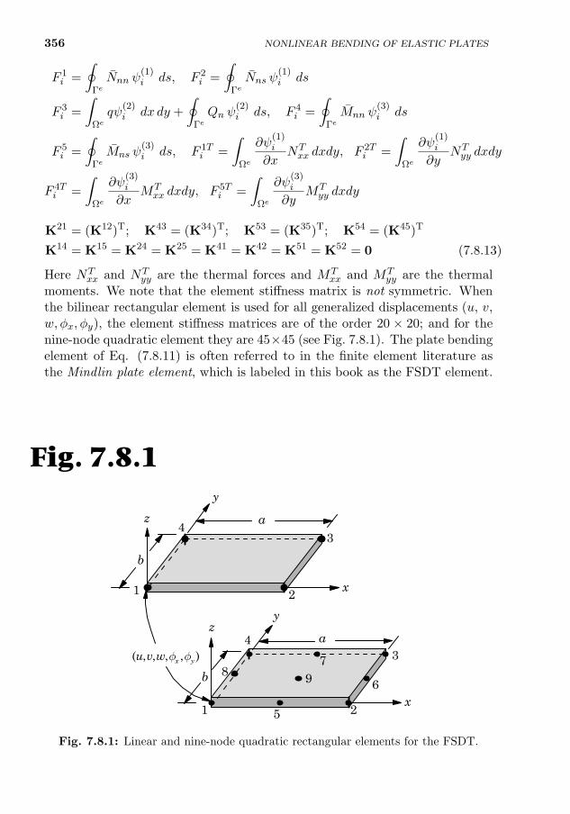
356
F 1i =
∮ΓeNnn ψ
(1)i ds, F 2
i =
∮ΓeNns ψ
(1)i ds
F 3i =
∫Ωeqψ
(2)i dx dy +
∮ΓeQn ψ
(2)i ds, F 4
i =
∮ΓeMnn ψ
(3)i ds
F 5i =
∮ΓeMns ψ
(3)i ds, F 1T
i =
∫Ωe
∂ψ(1)i
∂xNTxx dxdy, F 2T
i =
∫Ωe
∂ψ(1)i
∂yNTyy dxdy
F 4Ti =
∫Ωe
∂ψ(3)i
∂xMTxx dxdy, F 5T
i =
∫Ωe
∂ψ(3)i
∂yMTyy dxdy
K21 = (K12)T; K43 = (K34)T; K53 = (K35)T; K54 = (K45)T
K14 = K15 = K24 = K25 = K41 = K42 = K51 = K52 = 0 (7.8.13)
Here NTxx and NT
yy are the thermal forces and MTxx and MT
yy are the thermalmoments. We note that the element stiffness matrix is not symmetric. Whenthe bilinear rectangular element is used for all generalized displacements (u, v,w, φx, φy), the element stiffness matrices are of the order 20 × 20; and for thenine-node quadratic element they are 45×45 (see Fig. 7.8.1). The plate bendingelement of Eq. (7.8.11) is often referred to in the finite element literature asthe Mindlin plate element, which is labeled in this book as the FSDT element.
7.8.3 Tangent Stiffness Coefficients
The tangent stiffness matrix coefficients for the FSDT can be computed usingthe definition in Eq. (7.4.9), with γ = 1, 2, . . . , 5. Since the source of nonlinearityin the CPT and FSDT is the same, the nonlinear parts of the tangent stiffnesscoefficients derived for the CPT are also valid for the FSDT.
a
b
z
x
y
43
21
a
b
x
y
43
21
7
6
5
8 9
z
( , , , , )x yu v w f f
Fig. 7.8.1
Fig. 7.8.1: Linear and nine-node quadratic rectangular elements for the FSDT.
NONLINEAR BENDING OF ELASTIC PLATES
7.8. FINITE ELEMENT MODELS OF THE FSDT 357
Suppose that the tangent stiffness matrix is of the same form as the directstiffness matrix in Eq. (7.8.11). Then the coefficients of the submatrices Tαβ
are defined by
Tαβij =∂Rαi
∂∆βj
(7.8.14)
where the components of the residual vector Rα are given by
Rαi =5∑
γ=1
n(γ)∑k=1
Kαγik ∆γ
k − Fαi (7.8.15)
∆1i = ui, ∆2
i = vi, ∆3i = wi, ∆4
i = S1i , ∆5
i = S2i (7.8.16)
and n(γ) denotes n, m, or p, depending on the nodal degree of freedom. Thus,we have
Tαβij =∂
∂∆βj
( 5∑γ=1
n(γ)∑k=1
Kαγik ∆γ
k − Fαi
)=
5∑γ=1
n(γ)∑k=1
∂Kαγik
∂∆βj
∆γk +Kαβ
ij (7.8.17)
We note that the only coefficients that depend on the solution are K13ij , K23
ij ,
K31ij , K32
ij , and K33ij . Further, they are functions of only w (or functions of wj).
Hence, derivatives of all submatrices with respect to uj , vj , S1j , and S2
j are zero.Thus, we have (for α = 1, 2, 3, 4, 5)
Tα1 = Kα1 = (K1α)T, Tα2 = Kα2 = (K2α)T
Tα4 = Kα4 = (K4α)T, Tα5 = Kα5 = (K5α)T(7.8.18)
and Tα3, for α = 1, 2, 3, are calculated as follows:
T 13ij =
5∑γ=1
n(γ)∑k=1
∂K1γik
∂wj∆γk +K13
ij =n∑k=1
∂K13ik
∂wjwk +K13
ij
=1
2
∫Ωe
[∂ψ
(1)i
∂x
(A11
∂w
∂x
∂ψ(2)j
∂x+A12
∂w
∂y
∂ψ(2)j
∂y
)
+A66∂ψ
(1)i
∂y
(∂w
∂x
∂ψ(2)j
∂y+∂w
∂y
∂ψ(2)j
∂x
)]dx dy +K13
ij
= K13ij +K13
ij = 2K13ij = T 31
ji , (T13)T = T31 = K31 (7.8.19)
T 23ij =
5∑γ=1
n(γ)∑k=1
∂K2γik
∂wj∆γk +K23
ij =
n∑k=1
∂K23ik
∂wjwk +K23
ij
=1
2
∫Ωe
[∂ψ
(1)i
∂y
(A12
∂w
∂x
∂ψ(2)j
∂x+A22
∂w
∂y
∂ψ(2)j
∂y
)
358
+A66∂ψ
(1)i
∂x
(∂w
∂y
∂ψ(2)j
∂x+∂w
∂x
∂ψ(2)j
∂y
)]dx dy +K23
ij
= K23ij +K23
ij = 2K23ij = T 32
ji , (T23)T = T32 = K32 (7.8.20)
T 33ij =
5∑γ=1
n(γ)∑k=1
∂K3γik
∂wj∆γk +K33
ij =
n(γ)∑k=1
(∂K31
ik
∂wjuk +
∂K32ik
∂wjvk +
∂K33ik
∂wjwk
)+K33
ij
=
∫Ωe
(A55
∂ψ(2)i
∂x
∂ψ(2)j
∂x+A44
∂ψ(2)i
∂y
∂ψ(2)j
∂y+ kψ
(2)i ψ
(2)j
)dx dy
+
∫Ωe
Nxx
∂ψ(2)i
∂x
∂ψ(2)j
∂x+Nyy
∂ψ(2)i
∂y
∂ψ(2)j
∂y+Nxy
∂ψ(2)i
∂x
∂ψ(2)j
∂y
+Nxy∂ψ
(2)i
∂y
∂ψ(2)j
∂x+(A12 +A66
)∂w∂x
∂w
∂y
(∂ψ
(2)i
∂x
∂ψ(2)j
∂y+∂ψ
(2)i
∂y
∂ψ(2)j
∂x
)
+
[A11
(∂w
∂x
)2
+A66
(∂w
∂y
)2]∂ψ
(2)i
∂x
∂ψ(2)j
∂x
+
[A66
(∂w
∂x
)2
+A22
(∂w
∂y
)2]∂ψ
(2)i
∂y
∂ψ(2)j
∂y
dx dy (7.8.21)
where (Nxx, Nyy, Nxy) are given by Eq. (7.7.20). We note that the tangentstiffness matrix of the FSDT element is symmetric.
7.8.4 Shear and Membrane Locking
The C0 plate bending elements based on the FSDT are among the simplestavailable in the literature. Unfortunately, when lower order (quadratic or less)equal interpolation of the generalized displacements is used, the elements be-come excessively stiff in the thin plate limit, yielding displacements that are toosmall compared to the true solution. As discussed earlier for beams, this typeof behavior is known as shear locking. There are a number of papers on thesubject of shear locking and elements developed to alleviate the problem (see[23–30]). A commonly used technique to avoid shear locking and membranelocking is to use selective integration: use full integration to evaluate all linearstiffness coefficients and use reduced integration to evaluate the transverse shearstiffnesses, i.e. all coefficients in Kαβ
ij that contain A44 and A55 and nonlinearstiffnesses. Higher-order elements or refined meshes of lower-order elementsexperience relatively less locking, but sometimes at the expense of the rate ofconvergence. With the suggested Gauss rule, highly distorted elements tend tohave slower rates of convergence but they give sufficiently accurate results.
NONLINEAR BENDING OF ELASTIC PLATES
7.9. COMPUTER IMPLEMENTATION AND NUMERICAL RESULTS (FSDT) 359
7.9 Computer Implementation and NumericalResults of the FSDT Elements
7.9.1 Computer Implementation
The FSDT element is quite simple to implement, and the implementation fol-lows the same ideas as discussed in Chapter 6 for single-variable problems intwo dimensions and for CPT elements discussed in Section 7.5. The elementequations are rearranged using the Fortran statements included in Box 5.2.1.The element displacement vector is of the form
∆T = u1, v1, w1, φx1, φy1, u2, v2, w2, φx2, φy2, . . .
Two separate do-loops on Gauss quadrature are required to compute allthe force and stiffness coefficients. The full integration loop is used to evaluateall force components and all linear stiffnesses except for the transverse shearstiffnesses. The reduced integration loop has two parts: one for the transverseshear terms and the other for nonlinear terms. One may use separate arrays(say, EXT13(I, J), EXT23(I, J), EXT33(I, J),) to store the extra terms to
those of Kαβij to obtain the tangent stiffness coefficients.
The stresses in the FSDT are computed in the same way as discussed inSection 7.5.3, except that the strains are defined by Eq. (7.7.4). Also note thatin the FSDT the transverse shear stresses computed through the constitutiveequations are not zero.
7.9.2 Results of Linear Analysis
In this section, the effect of the integration rule and the convergence characteris-tics of the FSDT plate element based on equal interpolation (linear or quadraticelements) of all variables is illustrated through several examples. All meshesused consist of either linear or quadratic elements, and they are uniform (i.e.same size elements are used). A shear correction factor of Ks = 5/6 is used.
We note that the submatrices Kαβ appearing in Eq. (7.8.11) for the linearcase are readily available, for verification of the element stiffness matrices, fromSαβ [see Eq. (3.7.10)]. For example, we have K11 = A11 S11 + A66 S22, K12 =A12 S12 +A66 S21, K22 = A66 S11 +A22 S22, K34 = A55 S10, K35 = A44 S20, andso on. Also at every boundary node, one element of each of the following pairsshould be known [see Eq. (7.7.17)]: (un, Nnn), (us, Nns), (w,Qn), (φn,Mnn),and (φs,Mns).
Example 7.9.1
Consider a simply-supported (SS–1) isotropic (ν = 0.25 and Ks = 5/6) square plate underuniformly distributed transverse load q0. The geometric boundary conditions of the compu-tational domain (see the shaded quadrant in Fig. 7.9.1) are
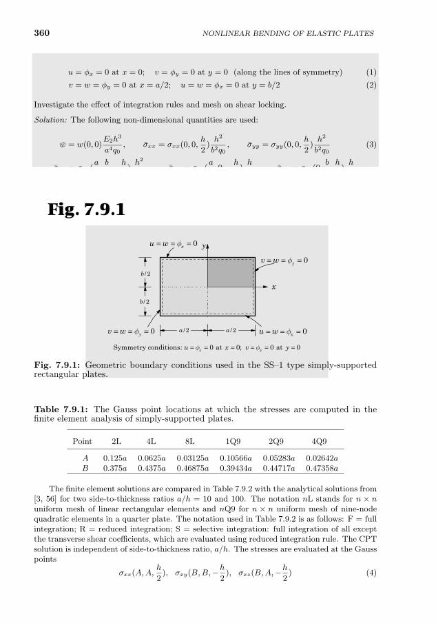
360
u = φx = 0 at x = 0; v = φy = 0 at y = 0 (along the lines of symmetry) (1)
v = w = φy = 0 at x = a/2; u = w = φx = 0 at y = b/2 (2)
Investigate the effect of integration rules and mesh on shear locking.
Solution: The following non-dimensional quantities are used:
w = w(0, 0)E2h
3
a4q0, σxx = σxx(0, 0,
h
2)h2
b2q0, σyy = σyy(0, 0,
h
2)h2
b2q0(3)
σxy = σxy(a
2,b
2,−h
2)h2
b2q0, σxz = σxz(
a
2, 0,−h
2)h
bq0, σyz = σyz(0,
b
2,h
2)h
bq0
where the origin of the coordinate system is taken at the center of the plate, 0 ≤ x ≤ a/2, 0 ≤y ≤ b/2, and −h/2 ≤ z ≤ h/2. The stresses in the finite element analysis are computed at thereduced Gauss points, irrespective of the Gauss rule used for the evaluation of the elementstiffness coefficients. The Gauss point coordinates A and B are shown in Table 7.9.1.
/ 2a / 2a
/ 2b
/ 2b
x
y0xu w f= = =
0xu w f= = =
0yv w f= = =
0yv w f= = =
Symmetry conditions: 0 at 0; 0 at 0x yu x v yf f= = = = = =
Fig. 7.9.1
Fig. 7.9.1: Geometric boundary conditions used in the SS–1 type simply-supportedrectangular plates.
Table 7.9.1: The Gauss point locations at which the stresses are computed in thefinite element analysis of simply-supported plates.
Point 2L 4L 8L 1Q9 2Q9 4Q9
A 0.125a 0.0625a 0.03125a 0.10566a 0.05283a 0.02642aB 0.375a 0.4375a 0.46875a 0.39434a 0.44717a 0.47358a
The finite element solutions are compared in Table 7.9.2 with the analytical solutions from[3, 56] for two side-to-thickness ratios a/h = 10 and 100. The notation nL stands for n × nuniform mesh of linear rectangular elements and nQ9 for n × n uniform mesh of nine-nodequadratic elements in a quarter plate. The notation used in Table 7.9.2 is as follows: F = fullintegration; R = reduced integration; S = selective integration: full integration of all exceptthe transverse shear coefficients, which are evaluated using reduced integration rule. The CPTsolution is independent of side-to-thickness ratio, a/h. The stresses are evaluated at the Gausspoints
σxx(A,A,h
2), σxy(B,B,−h
2), σxz(B,A,−
h
2) (4)
NONLINEAR BENDING OF ELASTIC PLATES
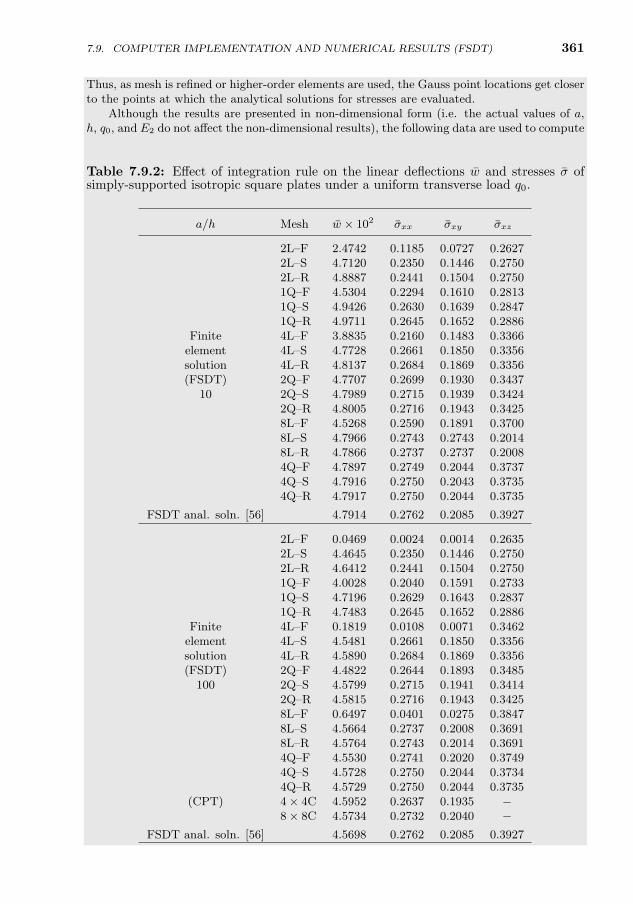
7.9. COMPUTER IMPLEMENTATION AND NUMERICAL RESULTS (FSDT) 361
Thus, as mesh is refined or higher-order elements are used, the Gauss point locations get closerto the points at which the analytical solutions for stresses are evaluated.
Although the results are presented in non-dimensional form (i.e. the actual values of a,h, q0, and E2 do not affect the non-dimensional results), the following data are used to compute
Table 7.9.2: Effect of integration rule on the linear deflections w and stresses σ ofsimply-supported isotropic square plates under a uniform transverse load q0.
a/h Mesh w × 102 σxx σxy σxz
2L–F 2.4742 0.1185 0.0727 0.26272L–S 4.7120 0.2350 0.1446 0.27502L–R 4.8887 0.2441 0.1504 0.27501Q–F 4.5304 0.2294 0.1610 0.28131Q–S 4.9426 0.2630 0.1639 0.28471Q–R 4.9711 0.2645 0.1652 0.2886
Finite 4L–F 3.8835 0.2160 0.1483 0.3366element 4L–S 4.7728 0.2661 0.1850 0.3356solution 4L–R 4.8137 0.2684 0.1869 0.3356(FSDT) 2Q–F 4.7707 0.2699 0.1930 0.3437
10 2Q–S 4.7989 0.2715 0.1939 0.34242Q–R 4.8005 0.2716 0.1943 0.34258L–F 4.5268 0.2590 0.1891 0.37008L–S 4.7966 0.2743 0.2743 0.20148L–R 4.7866 0.2737 0.2737 0.20084Q–F 4.7897 0.2749 0.2044 0.37374Q–S 4.7916 0.2750 0.2043 0.37354Q–R 4.7917 0.2750 0.2044 0.3735
FSDT anal. soln. [56] 4.7914 0.2762 0.2085 0.3927
2L–F 0.0469 0.0024 0.0014 0.26352L–S 4.4645 0.2350 0.1446 0.27502L–R 4.6412 0.2441 0.1504 0.27501Q–F 4.0028 0.2040 0.1591 0.27331Q–S 4.7196 0.2629 0.1643 0.28371Q–R 4.7483 0.2645 0.1652 0.2886
Finite 4L–F 0.1819 0.0108 0.0071 0.3462element 4L–S 4.5481 0.2661 0.1850 0.3356solution 4L–R 4.5890 0.2684 0.1869 0.3356(FSDT) 2Q–F 4.4822 0.2644 0.1893 0.3485
100 2Q–S 4.5799 0.2715 0.1941 0.34142Q–R 4.5815 0.2716 0.1943 0.34258L–F 0.6497 0.0401 0.0275 0.38478L–S 4.5664 0.2737 0.2008 0.36918L–R 4.5764 0.2743 0.2014 0.36914Q–F 4.5530 0.2741 0.2020 0.37494Q–S 4.5728 0.2750 0.2044 0.37344Q–R 4.5729 0.2750 0.2044 0.3735
(CPT) 4× 4C 4.5952 0.2637 0.1935 −8× 8C 4.5734 0.2732 0.2040 −
FSDT anal. soln. [56] 4.5698 0.2762 0.2085 0.3927
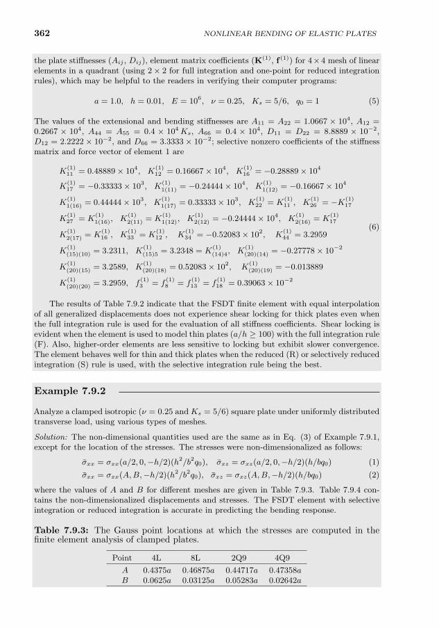
362
the plate stiffnesses (Aij , Dij), element matrix coefficients (K(1), f (1)) for 4×4 mesh of linearelements in a quadrant (using 2× 2 for full integration and one-point for reduced integrationrules), which may be helpful to the readers in verifying their computer programs:
a = 1.0, h = 0.01, E = 106, ν = 0.25, Ks = 5/6, q0 = 1 (5)
The values of the extensional and bending stiffnesses are A11 = A22 = 1.0667 × 10⁴, A12 =0.2667 × 10⁴, A44 = A55 = 0.4 × 10⁴Ks, A66 = 0.4 × 10⁴, D11 = D22 = 8.8889 × 10⁻²,D12 = 2.2222× 10⁻², and D66 = 3.3333× 10⁻²; selective nonzero coefficients of the stiffnessmatrix and force vector of element 1 are
K(1)11 = 0.48889× 10⁴, K
(1)12 = 0.16667× 10⁴, K
(1)16 = −0.28889× 10⁴
K(1)17 = −0.33333× 10³, K
(1)
1(11) = −0.24444× 10⁴, K(1)
1(12) = −0.16667× 10⁴
K(1)
1(16) = 0.44444× 10³, K(1)
1(17) = 0.33333× 10³, K(1)22 = K
(1)11 , K
(1)26 = −K(1)
17
K(1)27 = K
(1)
1(16), K(1)
2(11) = K(1)
1(12), K(1)
2(12) = −0.24444× 10⁴, K(1)
2(16) = K(1)17
K(1)
2(17) = K(1)16 , K
(1)33 = K
(1)12 , K
(1)34 = −0.52083× 10², K
(1)44 = 3.2959
K(1)
(15)(10) = 3.2311, K(1)
(15)5 = 3.2348 = K(1)
(14)4, K(1)
(20)(14) = −0.27778× 10⁻²
K(1)
(20)(15) = 3.2589, K(1)
(20)(18) = 0.52083× 10², K(1)
(20)(19) = −0.013889
K(1)
(20)(20) = 3.2959, f(1)3 = f
(1)8 = f
(1)13 = f
(1)18 = 0.39063× 10⁻²
(6)
The results of Table 7.9.2 indicate that the FSDT finite element with equal interpolationof all generalized displacements does not experience shear locking for thick plates even whenthe full integration rule is used for the evaluation of all stiffness coefficients. Shear locking isevident when the element is used to model thin plates (a/h ≥ 100) with the full integration rule(F). Also, higher-order elements are less sensitive to locking but exhibit slower convergence.The element behaves well for thin and thick plates when the reduced (R) or selectively reducedintegration (S) rule is used, with the selective integration rule being the best.
Example 7.9.2
Analyze a clamped isotropic (ν = 0.25 and Ks = 5/6) square plate under uniformly distributedtransverse load, using various types of meshes.
Solution: The non-dimensional quantities used are the same as in Eq. (3) of Example 7.9.1,except for the location of the stresses. The stresses were non-dimensionalized as follows:
σxx = σxx(a/2, 0,−h/2)(h2/b2q0), σxz = σxz(a/2, 0,−h/2)(h/bq0) (1)
σxx = σxx(A,B,−h/2)(h2/b2q0), σxz = σxz(A,B,−h/2)(h/bq0) (2)
where the values of A and B for different meshes are given in Table 7.9.3. Table 7.9.4 con-tains the non-dimensionalized displacements and stresses. The FSDT element with selectiveintegration or reduced integration is accurate in predicting the bending response.
Table 7.9.3: The Gauss point locations at which the stresses are computed in thefinite element analysis of clamped plates.
Point 4L 8L 2Q9 4Q9
A 0.4375a 0.46875a 0.44717a 0.47358aB 0.0625a 0.03125a 0.05283a 0.02642a
NONLINEAR BENDING OF ELASTIC PLATES
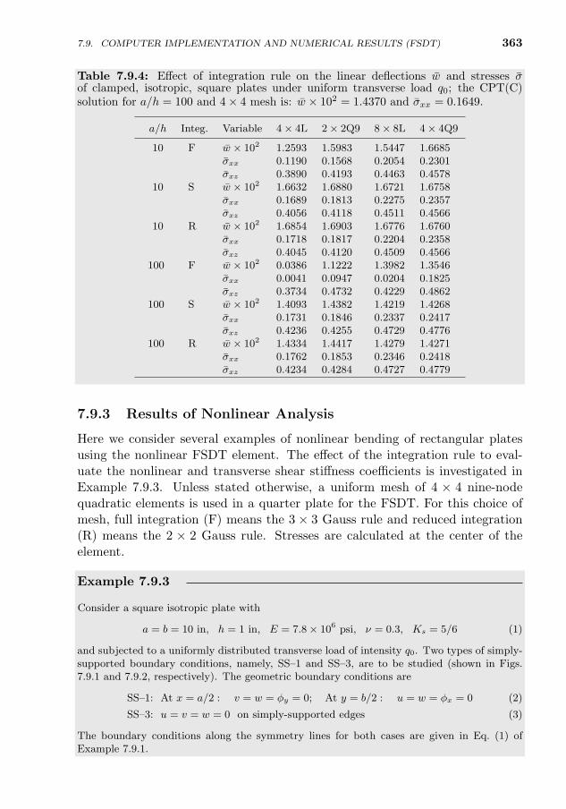
7.9. COMPUTER IMPLEMENTATION AND NUMERICAL RESULTS (FSDT) 363
Table 7.9.4: Effect of integration rule on the linear deflections w and stresses σof clamped, isotropic, square plates under uniform transverse load q0; the CPT(C)solution for a/h = 100 and 4× 4 mesh is: w × 102 = 1.4370 and σxx = 0.1649.
a/h Integ. Variable 4× 4L 2× 2Q9 8× 8L 4× 4Q9
10 F w × 102 1.2593 1.5983 1.5447 1.6685σxx 0.1190 0.1568 0.2054 0.2301σxz 0.3890 0.4193 0.4463 0.4578
10 S w × 102 1.6632 1.6880 1.6721 1.6758σxx 0.1689 0.1813 0.2275 0.2357σxz 0.4056 0.4118 0.4511 0.4566
10 R w × 102 1.6854 1.6903 1.6776 1.6760σxx 0.1718 0.1817 0.2204 0.2358σxz 0.4045 0.4120 0.4509 0.4566
100 F w × 102 0.0386 1.1222 1.3982 1.3546σxx 0.0041 0.0947 0.0204 0.1825σxz 0.3734 0.4732 0.4229 0.4862
100 S w × 102 1.4093 1.4382 1.4219 1.4268σxx 0.1731 0.1846 0.2337 0.2417σxz 0.4236 0.4255 0.4729 0.4776
100 R w × 102 1.4334 1.4417 1.4279 1.4271σxx 0.1762 0.1853 0.2346 0.2418σxz 0.4234 0.4284 0.4727 0.4779
7.9.3 Results of Nonlinear Analysis
Here we consider several examples of nonlinear bending of rectangular platesusing the nonlinear FSDT element. The effect of the integration rule to eval-uate the nonlinear and transverse shear stiffness coefficients is investigated inExample 7.9.3. Unless stated otherwise, a uniform mesh of 4 × 4 nine-nodequadratic elements is used in a quarter plate for the FSDT. For this choice ofmesh, full integration (F) means the 3× 3 Gauss rule and reduced integration(R) means the 2 × 2 Gauss rule. Stresses are calculated at the center of theelement.
Example 7.9.3
Consider a square isotropic plate with
a = b = 10 in, h = 1 in, E = 7.8× 10⁶ psi, ν = 0.3, Ks = 5/6 (1)
and subjected to a uniformly distributed transverse load of intensity q0. Two types of simply-supported boundary conditions, namely, SS–1 and SS–3, are to be studied (shown in Figs.7.9.1 and 7.9.2, respectively). The geometric boundary conditions are
SS–1: At x = a/2 : v = w = φy = 0; At y = b/2 : u = w = φx = 0 (2)
SS–3: u = v = w = 0 on simply-supported edges (3)
The boundary conditions along the symmetry lines for both cases are given in Eq. (1) ofExample 7.9.1.
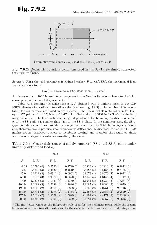
364
/ 2a / 2a
/ 2b
/ 2b
x
y0u v w= = =
Symmetry conditions: 0 at 0; 0 at 0x yu x v yf f= = = = = =
0u v w= = =
0u v w= = =0u v w= = =
Fig. 7.9.2
Fig. 7.9.2: Geometric boundary conditions used in the SS–3 type simply-supportedrectangular plates.
Solution: Using the load parameter introduced earlier, P ≡ q0a4/Eh4, the incremental load
vector is chosen to be
∆P = 6.25, 6.25, 12.5, 25.0, 25.0, . . . , 25.0
A tolerance of ε = 10−2 is used for convergence in the Newton iteration scheme to check forconvergence of the nodal displacements.
Table 7.9.5 contains the deflections w(0, 0) obtained with a uniform mesh of 4 × 4Q9FSDT elements for various integration rules (also see Fig. 7.9.3). The number of iterationstaken for convergence are listed in parentheses. The linear FSDT plate solution for loadq0 = 4875 psi (or P = 6.25) is w = 0.2917 in for SS–1 and w = 0.3151 in for SS–3 (for the R-Rintegration rule). The linear solution, being independent of the boundary conditions on u andv, of the SS–1 plate is smaller than that of the SS–3 plate. In the nonlinear case, the SS–3type boundary conditions provide more edge restraint than the SS–1 boundary conditionsand, therefore, would produce smaller transverse deflections. As discussed earlier, the 4×4Q9meshes are not sensitive to shear or membrane locking, and therefore the results obtainedwith various integration rules are essentially the same.
Table 7.9.5: Center deflection w of simply-supported (SS–1 and SS–3) plates underuniformly distributed load q0.
SS–3 SS–1
P R–R∗ F–R F–F R–R F–R F–F
6.25 0.2790 (4) 0.2790 (4) 0.2780 (3) 0.2813 (3) 0.2813 (3) 0.2812 (3)12.5 0.4630 (3) 0.4630 (3) 0.4619 (3) 0.5186 (3) 0.5186 (3) 0.5185 (3)25.0 0.6911 (3) 0.6911 (3) 0.6902 (3) 0.8673 (4) 0.8673 (4) 0.8672 (4)50.0 0.9575 (3) 0.9575 (3) 0.9570 (3) 1.3149 (4) 1.3149 (4) 1.3147 (4)75.0 1.1333 (3) 1.1333 (3) 1.1330 (3) 1.6241 (3) 1.6239 (3) 1.6237 (3)
100.0 1.2688 (3) 1.2688 (3) 1.2686 (3) 1.8687 (3) 1.8683 (3) 1.8679 (3)125.0 1.3809 (2) 1.3809 (2) 1.3808 (2) 2.0758 (2) 2.0751 (2) 2.0746 (2)150.0 1.4774 (2) 1.4774 (2) 1.4774 (2) 2.2567 (2) 2.2556 (2) 2.2549 (2)175.0 1.5628 (2) 1.5629 (2) 1.5629 (2) 2.4194 (2) 2.4177 (2) 2.4168 (2)200.0 1.6398 (2) 1.6399 (2) 1.6399 (2) 2.5681 (2) 2.5657 (2) 2.5645 (2)
* The first letter refers to the integration rule used for the nonlinear terms while the secondletter refers to the integration rule used for the shear terms; R = reduced; F = full integration.
NONLINEAR BENDING OF ELASTIC PLATES
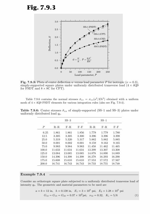
7.9. COMPUTER IMPLEMENTATION AND NUMERICAL RESULTS (FSDT) 365Fig. 7.9.3
0 50 100 150 200 250Load parameter,
0.0
0.5
1.0
1.5
2.0
2.5
3.0
Def
lect
ion
, SS-3 (CPT)
SS-1 (CPT)
SS-1 (FSDT)
SS-3 (FSDT)w
P
40
4,q aw
w Ph Eh
= =
Fig. 7.9.3: Plots of center deflection w versus load parameter P for isotropic (ν = 0.3),simply-supported square plates under uniformly distributed transverse load (4 × 4Q9for FSDT and 8× 8C for CPT).
Table 7.9.6 contains the normal stresses σxx = σxx(a2/Eh2) obtained with a uniformmesh of 4× 4Q9 FSDT elements for various integration rules (also see Fig. 7.9.4).
Table 7.9.6: Center stresses σxx of simply-supported (SS–1 and SS–3) plates underuniformly distributed load q0.
SS–3 SS–1
P R–R F–R F–F R–R F–R F–F
6.25 1.861 1.861 1.856 1.779 1.779 1.78012.5 3.305 3.305 3.300 3.396 3.396 3.39825.0 5.319 5.320 5.317 5.882 5.882 5.88550.0 8.001 8.002 8.001 9.159 9.162 9.16575.0 9.983 9.984 9.983 11.458 11.462 11.465
100.0 11.633 11.634 11.634 13.299 13.307 13.308125.0 13.084 13.085 13.085 14.878 14.890 14.889150.0 14.396 14.398 14.398 16.278 16.293 16.290175.0 15.608 15.610 15.610 17.553 17.572 17.567200.0 16.741 16.743 16.743 18.733 18.755 18.748
Example 7.9.4
Consider an orthotropic square plate subjected to a uniformly distributed transverse load ofintensity q0. The geometric and material parameters to be used are
a = b = 12 in, h = 0.138 in, E1 = 3× 10⁶ psi, E2 = 1.28× 10⁶ psi
G12 = G13 = G23 = 0.37× 10⁶psi, ν12 = 0.32, Ks = 5/6 (1)
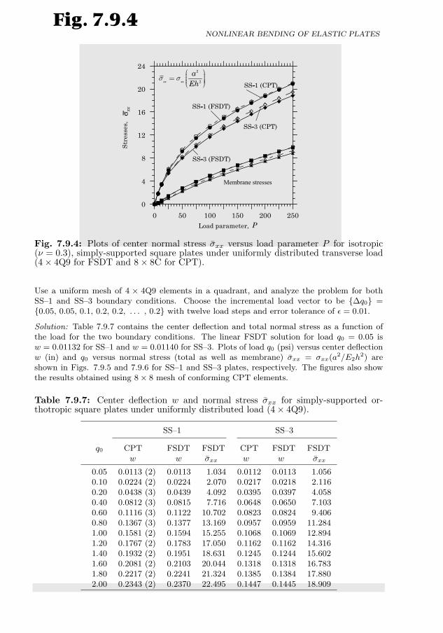
366Fig. 7.9.4
0 50 100 150 200 250Load parameter,
0
4
8
12
16
20
24
Str
esse
s, SS-3 (CPT)
SS-1 (CPT)
SS-1 (FSDT)
SS-3 (FSDT)
σ xx
P
Membrane stresses
2
2xx xx
aEh
s sæ ö÷ç= ÷ç ÷÷çè ø
Fig. 7.9.4: Plots of center normal stress σxx versus load parameter P for isotropic(ν = 0.3), simply-supported square plates under uniformly distributed transverse load(4× 4Q9 for FSDT and 8× 8C for CPT).
Use a uniform mesh of 4 × 4Q9 elements in a quadrant, and analyze the problem for bothSS–1 and SS–3 boundary conditions. Choose the incremental load vector to be ∆q0 =0.05, 0.05, 0.1, 0.2, 0.2, . . . , 0.2 with twelve load steps and error tolerance of ε = 0.01.
Solution: Table 7.9.7 contains the center deflection and total normal stress as a function ofthe load for the two boundary conditions. The linear FSDT solution for load q0 = 0.05 isw = 0.01132 for SS–1 and w = 0.01140 for SS–3. Plots of load q0 (psi) versus center deflectionw (in) and q0 versus normal stress (total as well as membrane) σxx = σxx(a2/E2h
2) areshown in Figs. 7.9.5 and 7.9.6 for SS–1 and SS–3 plates, respectively. The figures also showthe results obtained using 8× 8 mesh of conforming CPT elements.
Table 7.9.7: Center deflection w and normal stress σxx for simply-supported or-thotropic square plates under uniformly distributed load (4× 4Q9).
SS–1 SS–3
q0 CPT FSDT FSDT CPT FSDT FSDTw w σxx w w σxx
0.05 0.0113 (2) 0.0113 1.034 0.0112 0.0113 1.0560.10 0.0224 (2) 0.0224 2.070 0.0217 0.0218 2.1160.20 0.0438 (3) 0.0439 4.092 0.0395 0.0397 4.0580.40 0.0812 (3) 0.0815 7.716 0.0648 0.0650 7.1030.60 0.1116 (3) 0.1122 10.702 0.0823 0.0824 9.4060.80 0.1367 (3) 0.1377 13.169 0.0957 0.0959 11.2841.00 0.1581 (2) 0.1594 15.255 0.1068 0.1069 12.8941.20 0.1767 (2) 0.1783 17.050 0.1162 0.1162 14.3161.40 0.1932 (2) 0.1951 18.631 0.1245 0.1244 15.6021.60 0.2081 (2) 0.2103 20.044 0.1318 0.1318 16.7831.80 0.2217 (2) 0.2241 21.324 0.1385 0.1384 17.8802.00 0.2343 (2) 0.2370 22.495 0.1447 0.1445 18.909
NONLINEAR BENDING OF ELASTIC PLATES
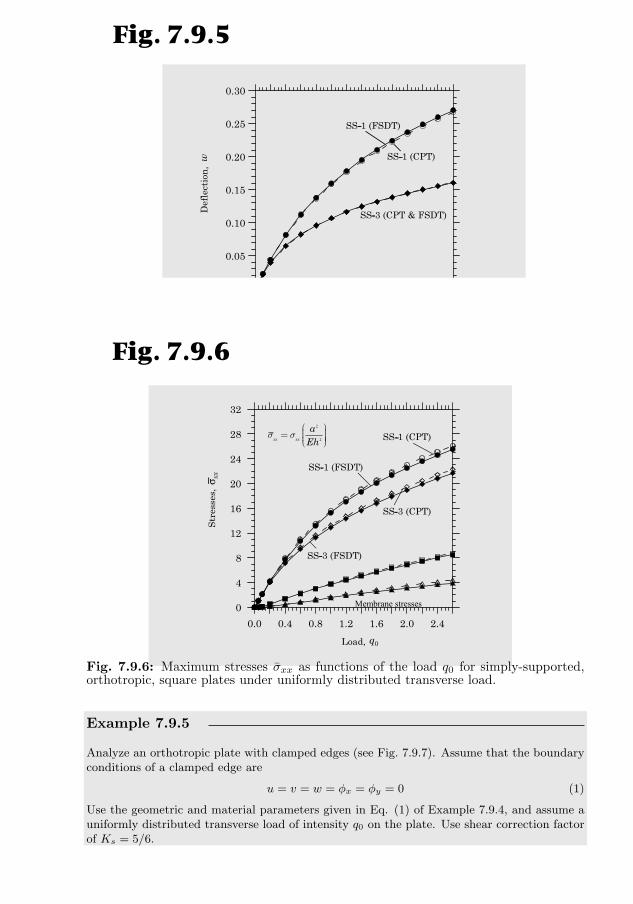
7.9. COMPUTER IMPLEMENTATION AND NUMERICAL RESULTS (FSDT) 367Fig. 7.9.5
0.0 0.4 0.8 1.2 1.6 2.0 2.4
Load,
0.00
0.05
0.10
0.15
0.20
0.25
0.30
Def
lect
ion
,
SS-1 (CPT)
SS-1 (FSDT)
SS-3 (CPT & FSDT)w
q0
Fig. 7.9.5: Center deflection w(0, 0) as a function of the load q0 for simply-supported,orthotropic, square plates under uniformly distributed transverse load.
Fig. 7.9.6
0.0 0.4 0.8 1.2 1.6 2.0 2.4
Load,
0
4
8
12
16
20
24
28
32
Str
esse
s,
SS-3 (CPT)
SS-1 (CPT)
SS-1 (FSDT)
SS-3 (FSDT)
σ xx
Membrane stresses
2
2xx xx
aEh
s sæ ö÷ç= ÷ç ÷÷çè ø
q0
Fig. 7.9.6: Maximum stresses σxx as functions of the load q0 for simply-supported,orthotropic, square plates under uniformly distributed transverse load.
Example 7.9.5
Analyze an orthotropic plate with clamped edges (see Fig. 7.9.7). Assume that the boundaryconditions of a clamped edge are
u = v = w = φx = φy = 0 (1)
Use the geometric and material parameters given in Eq. (1) of Example 7.9.4, and assume auniformly distributed transverse load of intensity q0 on the plate. Use shear correction factorof Ks = 5/6.
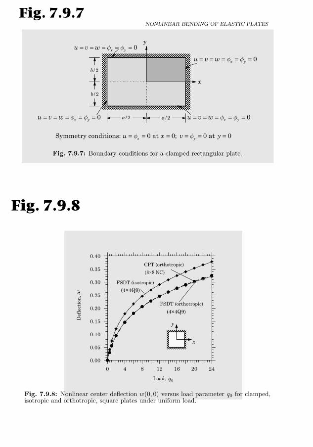
368
/ 2a / 2a
/ 2b
/ 2b
x
y0x yu v w f f= = = = =
Symmetry conditions: 0 at 0; 0 at 0x yu x v yf f= = = = = =
0x yu v w f f= = = = =
0x yu v w f f= = = = = 0x yu v w f f= = = = =
Fig. 7.9.7
Fig. 7.9.7: Boundary conditions for a clamped rectangular plate.
Solution: The linear transverse deflection at the center of the plate is w(0, 0) = 0.0301 forload q0 = 0.5. Figure 7.9.8 contains a plot of load q0 versus center deflection w(0, 0). Figure7.9.8 also contains plots of the center deflection of an isotropic square plate (h = 0.138 in,E = 1.28× 10⁶ psi, and ν = 0.3). The results are predicted by the CPT element using a 8× 8mesh of the non-conforming elements and the 4×4Q9 mesh of the FSDT element. Table 7.9.8contains numerical values of the center transverse deflection w and stress σxx as a function ofq0 for the same problem (see [18–20]).
q0
(8×8 NC)
(4×4 Q9)
(4×4 Q9)
w
x
y
0 4 8 12 16 20 24
Load,
0.00
0.05
0.10
0.15
0.20
0.25
0.30
0.35
0.40
Def
lect
ion
,
CPT (orthotropic)
FSDT (orthotropic)
FSDT (isotropic)
Fig. 7.9.8
(4×4Q9)
(4×4Q9)
Fig. 7.9.8: Nonlinear center deflection w(0, 0) versus load parameter q0 for clamped,isotropic and orthotropic, square plates under uniform load.
NONLINEAR BENDING OF ELASTIC PLATES
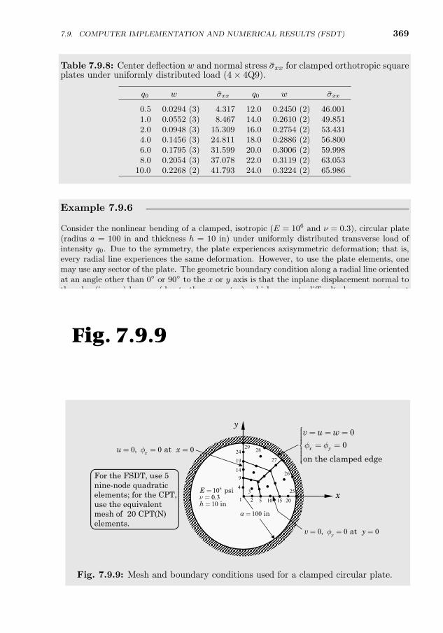
7.9. COMPUTER IMPLEMENTATION AND NUMERICAL RESULTS (FSDT) 369
Table 7.9.8: Center deflection w and normal stress σxx for clamped orthotropic squareplates under uniformly distributed load (4× 4Q9).
q0 w σxx q0 w σxx
0.5 0.0294 (3) 4.317 12.0 0.2450 (2) 46.0011.0 0.0552 (3) 8.467 14.0 0.2610 (2) 49.8512.0 0.0948 (3) 15.309 16.0 0.2754 (2) 53.4314.0 0.1456 (3) 24.811 18.0 0.2886 (2) 56.8006.0 0.1795 (3) 31.599 20.0 0.3006 (2) 59.9988.0 0.2054 (3) 37.078 22.0 0.3119 (2) 63.053
10.0 0.2268 (2) 41.793 24.0 0.3224 (2) 65.986
Example 7.9.6
Consider the nonlinear bending of a clamped, isotropic (E = 106 and ν = 0.3), circular plate(radius a = 100 in and thickness h = 10 in) under uniformly distributed transverse load ofintensity q0. Due to the symmetry, the plate experiences axisymmetric deformation; that is,every radial line experiences the same deformation. However, to use the plate elements, onemay use any sector of the plate. The geometric boundary condition along a radial line orientedat an angle other than 0 or 90 to the x or y axis is that the inplane displacement normal tothe edge (i.e. un) be zero (due to the symmetry), which presents difficulty because un is notone of the degrees of freedom of the element. Analyze the problem using the computationaldomain (a quadrant of the plate) and the finite element mesh and boundary conditions shownin Fig. 7.9.9, with a load step of ∆q0 = 2.5 lb and a total load of q0 = 120 lb. Plot the centerdeflection w and stress σxx as a function of the load.
Solution: The exact center deflection for the linear case, for the two theories, is given by (seeReddy [3,56])
wFSDT(0) =q0a
4
64D
(1 +
8
3(1− ν)Ks
h2
a2
), wCPT(0) =
q0a4
64D(1)
••
• •
••
••
••
• ••
••
•
•••
•••
• •
••
•
••
0 0 0, atyv yf= = =
0 0 0, atxu xf= = =
00
on the clamped edgex y
v u wf f
ìï = = =ïïï = =íïïïïî
1 23
4
5 10 2015
25
26
27
2829
9
24
19
14
6100 310
psi.
in
E
hn
===
x
y
100 ina =
For the FSDT, use 5 nine-node quadratic elements; for the CPT,use the equivalent mesh of 20 CPT(N) elements.
Fig. 7.9.9
Fig. 7.9.9: Mesh and boundary conditions used for a clamped circular plate.
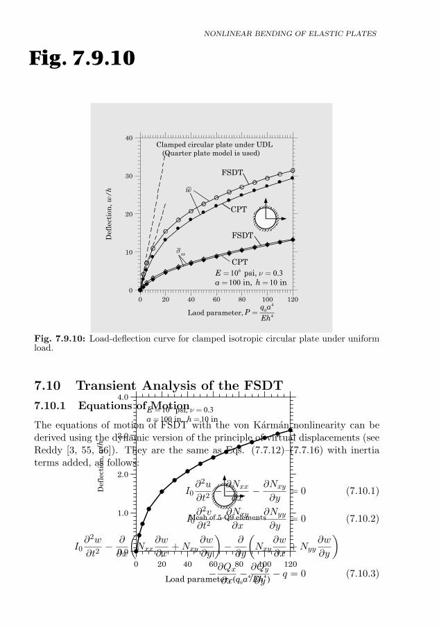
370
where a denotes the radius of the plate. For ν = 0.3, Ks = 5/6, and a/h = 10, the linearFSDT center deflection is given by w(0) = 1.0457(q0a
4/64D). The linear FSDT solutionobtained with the mesh of five nine-node quadratic elements is w(0) = 1.0659(q0a
4/64D)(< 2% error). Figure 7.9.10 shows the nonlinear load-deflection curve and load versus σxx =σxx(A,A)(a/h)2/10E curve for the problem. The same results can be obtained with anaxisymmetric one-dimensional element (see Problem 5.14).
w/h
0 20 40 60 80 100 120
Load parameter,
0.0
1.0
2.0
3.0
4.0
Def
lect
ion
,
Mesh of 5-Q9 elements
610 0 3100 10
psi, .in, in
Ea h
n= == =
4 40( )q a Eh
0 20 40 60 80 100 120
Laod parameter,
0
10
20
30
40
Def
lect
ion
, w/
h
Clamped circular plate under UDL (Quarter plate model is used)
40
4
q aP
Eh=
FSDT
CPT
CPT
FSDT
w
xxs
610 0 3100 10
psi, .in, in
Ea h
n= == =
Fig. 7.9.10
Fig. 7.9.10: Load-deflection curve for clamped isotropic circular plate under uniformload.
7.10 Transient Analysis of the FSDT
7.10.1 Equations of Motion
The equations of motion of FSDT with the von Karman nonlinearity can bederived using the dynamic version of the principle of virtual displacements (seeReddy [3, 55, 56]). They are the same as Eqs. (7.7.12)–(7.7.16) with inertiaterms added, as follows:
I0∂2u
∂t2− ∂Nxx
∂x− ∂Nxy
∂y= 0 (7.10.1)
I0∂2v
∂t2− ∂Nxy
∂x− ∂Nyy
∂y= 0 (7.10.2)
I0∂2w
∂t2− ∂
∂x
(Nxx
∂w
∂x+Nxy
∂w
∂y
)− ∂
∂y
(Nxy
∂w
∂x+Nyy
∂w
∂y
)−∂Qx∂x− ∂Qy
∂y− q = 0 (7.10.3)
NONLINEAR BENDING OF ELASTIC PLATES
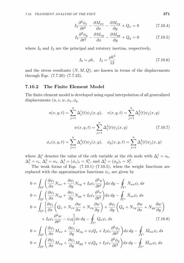
7.10. TRANSIENT ANALYSIS OF THE FSDT 371
I2∂2φx∂t2
− ∂Mxx
∂x− ∂Mxy
∂y+Qx = 0 (7.10.4)
I2∂2φy∂t2
− ∂Mxy
∂x− ∂Myy
∂y+Qy = 0 (7.10.5)
where I0 and I2 are the principal and rotatory inertias, respectively,
I0 = ρh, I2 =ρh3
12(7.10.6)
and the stress resultants (N,M,Q), are known in terms of the displacementsthrough Eqs. (7.7.20)–(7.7.22).
7.10.2 The Finite Element Model
The finite element model is developed using equal interpolation of all generalizeddisplacements (u, v, w, φx, φy) [see Eqs. (7.8.8)–(7.8.10)]
u(x, y, t) =n∑j=1
∆1j (t)ψj(x, y), v(x, y, t) =
n∑j=1
∆2j (t)ψj(x, y)
w(x, y, t) =n∑j=1
∆3j (t)ψj(x, y) (7.10.7)
φx(x, y, t) =
n∑j=1
∆4j (t)ψj(x, y), φy(x, y, t) =
n∑j=1
∆5j (t)ψj(x, y)
where ∆αi denotes the value of the αth variable at the ith node with ∆1
i = ui,∆2i = vi, ∆3
i = wi, ∆4i = (φx)i = S1
i , and ∆5i = (φy)i = S2
i .The weak forms of Eqs. (7.10.1)–(7.10.5), when the weight functions are
replaced with the approximation functions ψi, are given by
0 =
∫Ωe
(∂ψi∂x
Nxx +∂ψi∂y
Nxy + I0ψi∂2u
∂t2
)dx dy −
∮ΓeNnnψi ds
0 =
∫Ωe
(∂ψi∂x
Nxy +∂ψi∂y
Nyy + I0ψi∂2v
∂t2
)dx dy −
∮ΓeNnsψi ds
0 =
∫Ωe
[∂ψi∂x
(Qx +Nxx
∂w
∂x+Nxy
∂w
∂y
)+∂ψi∂y
(Qy +Nxy
∂w
∂x+Nyy
∂w
∂y
)+ I0ψi
∂2w
∂t2− ψiq
]dx dy −
∮ΓeQnψi ds (7.10.8)
0 =
∫Ωe
(∂ψi∂x
Mxx +∂ψi∂y
Mxy + ψiQx + I2ψi∂2φx∂t2
)dx dy −
∮ΓeMnnψi ds
0 =
∫Ωe
(∂ψi∂x
Mxy +∂ψi∂y
Myy + ψiQy + I2ψi∂2φy∂t2
)dx dy −
∮ΓeMnsψi ds
372
where (Nnn, Nns, Mnn, Mns, Qn) are the stress resultants on an edge with unitnormal n, and they are defined in Eqs. (7.8.6a,b) and (7.8.7).
Note that the nonlinearity in Eq. (7.10.8) is solely due to w, and the non-linear terms are present only in (Nxx, Nxy, Nyy). For convenience of writing thefinite element equations, the linear and nonlinear parts of the inplane forces(Nxx, Nxy, Nyy) are denoted as
N = N0 + N1 (7.10.9)
where N0 is the linear part and N1 is the nonlinear part. For an orthotropicplate (with the principal material axes coinciding with the plate axes), the forcesand moments are related to the generalized displacements (u, v, w, φx, φy) asfollows:
N0xx = A11
∂u
∂x+A12
∂v
∂y, N0
yy = A12∂u
∂x+A22
∂v
∂y
N0xy = A66
(∂u
∂y+∂v
∂x
), Mxx = D11
∂φx∂x
+D12∂φy∂y
Myy = D12∂φx∂x
+D22∂φy∂y
, Mxy = D66
(∂φx∂y
+∂φy∂x
)Qx = A55
(φx +
∂w
∂x
), Qy = A44
(φy +
∂w
∂y
)(7.10.10)
N1xx =
1
2
[A11
(∂w
∂x
)2
+A12
(∂w
∂y
)2]N1yy =
1
2
[A12
(∂w
∂x
)2
+A22
(∂w
∂y
)2]N1xy = A66
∂w
∂x
∂w
∂y
and Aij and Dij are the plate stiffnesses [see Eq. (7.7.23)]
Aij = hQij , Dij =h3
12Qij (7.10.11)
and Qij are defined in Eq. (7.7.24).By substituting the expansions in Eq. (7.10.10) into the weak forms in
Eq. (7.10.8), we obtain the finite element model
0 =5∑
β=1
n∑j=1
Mαβij ∆β
j +5∑
β=1
n∑j=1
Kαβij ∆β
j − Fαi ≡ Rαi (7.10.12)
for α = 1, 2, . . . , 5, where ∆αi denotes the value of the αth variable, in the order
(u, v, w, φx, φy), at the ith node (i = 1, 2, . . . , n) of the element. The non-zero
NONLINEAR BENDING OF ELASTIC PLATES
373
coefficients of Eq. (7.10.12) are defined by
M11ij =
∫ΩeI0ψiψj dx dy; M44
ij =
∫ΩeI2ψiψj dx dy
M22ij = M33
ij = M11ij , M55
ij = M44ij
K1αij =
∫Ωe
(∂ψi∂x
Nα1j +
∂ψi∂y
Nα6j
)dx dy
K2αij =
∫Ωe
(∂ψi∂x
Nα6j +
∂ψi∂y
Nα2j
)dx dy
K3αij =
∫Ωe
[∂ψi∂x
(Qα1j +
∂w
∂xNα
1j +∂w
∂yNα
6j
)+∂ψi∂y
(Qα2j +
∂w
∂xNα
6j +∂w
∂yNα
2j
)]dx dy (7.10.13)
K4αij =
∫Ωe
(Qα1jψi +
∂ψi∂x
Mα1j +
∂ψi∂y
Mα6j
)dx dy
K5αij =
∫Ωe
(Qα2jψi +
∂ψi∂x
Mα6j +
∂ψi∂y
Mα2j
)dx dy
F 1i =
∮ΓeNnnψi ds, F 2
i =
∮ΓeNnsψi ds, F 4
i =
∮ΓeMnnψi ds
F 3i =
∫Ωeqψi dx dy +
∮ΓeQnψi ds, F 5
i =
∮ΓeMnsψi ds
and Kαβij denotes the coefficient matrix of the αth variable in the βth equation
(α, β = 1, 2, 3, 4, 5). Thus, N Iij denotes the contribution from Ni(= N0
i + N1i )
(i = 1, 2, . . . , 6) to the Ith variable, (I = 1, 2, . . . , 5) where j denotes the node
number. The non-zero terms appearing in the definition of Kαβij are:
M41j = D11
∂ψj∂x
, M46j = D66
∂ψj∂y
, M42j = D12
∂ψj∂x
M51j = D12
∂ψj∂y
, M56j = D66
∂ψj∂x
, M52j = D22
∂ψj∂y
(7.10.14)
N11j = A11
∂ψj∂x
, N16j = A66
∂ψj∂y
, N21j = A12
∂ψj∂y
N26j = A66
∂ψj∂x
, N31j =
1
2
(A11
∂w
∂x
∂ψj∂x
+A12∂w
∂y
∂ψj∂y
)N3
6j =A66
2
(∂w
∂x
∂ψj∂y
+∂w
∂y
∂ψj∂x
), N1
2j = A12∂ψj∂x
N22j = A22
∂ψj∂y
, N32j =
1
2
(A12
∂w
∂x
∂ψj∂x
+A22∂w
∂y
∂ψj∂y
)(7.10.15)
Q31j = A55
∂ψj∂x
, Q32j = A44
∂ψj∂y
, Q41j = A55ψj , Q5
2j = A44ψj (7.10.16)
7.10. TRANSIENT ANALYSIS OF THE FSDT
374
7.10.3 Time Approximation
The finite element equations in Eq. (7.10.12) can be cast in the general matrixform
M∆ + K(∆)∆ = F (7.10.17)
which is of the same general form as one in Eq. (6.7.27) with C = 0. Therefore,the discussion presented in Section 6.7.4 is valid. The fully discretized equationsare [see Eq. (6.7.33)]
K(∆s+1)∆s+1 = Fs,s+1 (7.10.18)
where
K(∆s+1) = K(∆s+1) + a3 Ms+1
Fs,s+1 = Fs+1 + Ms+1
(a3∆s + a4∆s + a5∆s
) (7.10.19)
and ai are defined as
a1 = α∆t, a2 = (1−α)∆t, a3 =2
γ(∆t)2, a4 = a3∆t, a5 =
1
γ−1 (7.10.20)
At the end of each time step, the new velocity vector ∆s+1 and accelerationvector ∆s+1 are computed using the equations
∆s+1 = a3
(∆s+1 −∆s
)− a4 ∆− a5 ∆s
∆s+1 = ∆s + a2 ∆s + a1 ∆s+1
(7.10.21)
Solution of Eq. (7.10.18) by the Newton iteration method results in thefollowing linearized equations for the incremental solution at the (r+ 1)st iter-ation:
δ∆ = −(T(∆rs+1))−1Rr
s+1 (7.10.22)
T(∆rs+1) ≡
[∂R
∂∆
]rs+1
, Rrs+1 = K(∆r
s+1)∆rs+1 − F (7.10.23)
The total solution is obtained from
∆r+1s+1 = ∆r
s+1 + δ∆ (7.10.24)
Note that the tangent stiffness matrix Trs+1, the coefficient matrix Kr
s+1, andthe residual vector Rr
s+1 are evaluated using the latest known solution ∆rs+1.
The right-hand side vector F only depends on the known load vector (afterassembly and imposition of boundary conditions) Fs,s+1 and known solutions(∆s, ∆s, ∆s) from the previous time step. At the end of each time step (i.e.after nonlinear convergence is reached), the velocity and acceleration vectorsare updated using the formulas in Eq. (7.10.21). Computer implementationaspects were discussed in Section 6.7.6, and the flow chart in Fig. 6.7.2 andFortran statements presented in Boxes 6.7.1 and 6.7.2 are also applicable here.
NONLINEAR BENDING OF ELASTIC PLATES
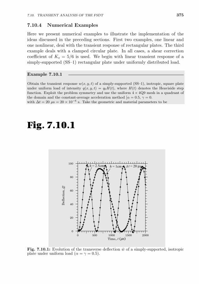
7.10. TRANSIENT ANALYSIS OF THE FSDT 375
7.10.4 Numerical Examples
Here we present numerical examples to illustrate the implementation of theideas discussed in the preceding sections. First two examples, one linear andone nonlinear, deal with the transient response of rectangular plates. The thirdexample deals with a clamped circular plate. In all cases, a shear correctioncoefficient of Ks = 5/6 is used. We begin with linear transient response of asimply-supported (SS–1) rectangular plate under uniformly distributed load.
Example 7.10.1
Obtain the transient response w(x, y, t) of a simply-supported (SS–1), isotropic, square plateunder uniform load of intensity q(x, y, t) = q0H(t), where H(t) denotes the Heaviside stepfunction. Exploit the problem symmetry and use the uniform 4× 4Q9 mesh in a quadrant ofthe domain and the constant-average acceleration method [α = 0.5, γ = 0.5; see Eq. (6.7.30)]with ∆t = 20 µs = 20× 10−6 s. Take the geometric and material parameters to be
a = b = 25 cm, h = 1 or 2.5 cm, E1 = E2 = 2.1× 10⁶ N/cm2
ν12 = 0.25, ρ = 8× 10⁻⁶ N.s2/cm4(1)
Solution: Figure 7.10.1 shows plots of the non-dimensionalized transverse deflection w =103w(0, 0, t)E2h
3/q0a4 versus time t (in µs) for thin (h = 1 cm) and thick (h = 2.5 cm),
simply-supported, isotropic (ν = 0.25) plates (4 × 4Q9 mesh; ∆t = 20µs). Comparing theresults of thin and thick plates, we conclude that the effect of shear deformation is to increasethe amplitude and reduce the period of the transverse deflection (also see Table 7.10.1 for thenumerical results).
, t (μs)
w
h = 1cmh = 2.5cm Δ t = 20 μs
0 500 1000 1500 2000Time
0
20
40
60
80
100
Def
lect
ion
,
Fig. 7.10.1
Fig. 7.10.1: Evolution of the transverse deflection w of a simply-supported, isotropicplate under uniform load (α = γ = 0.5).
376
Table 7.10.1: Non-dimensionalized center deflection w versus time t for simply-supported, isotropic, square plates (α = γ = 0.5).
t w t w
(µs) h = 1 h = 2.5 (µs) h = 1 h = 2.5
20 0.067 0.426 360 50.661 76.73940 0.334 2.193 380 54.768 68.26360 0.860 6.074 400 58.922 58.35280 1.626 12.813 420 63.078 46.337
100 2.674 22.770 440 67.238 33.574120 4.189 34.696 460 71.368 22.403140 6.405 46.408 480 75.488 13.751160 9.348 56.971 500 79.533 7.423180 12.871 66.677 520 83.218 3.213200 16.819 75.708 540 86.276 0.605220 21.044 84.185 560 88.635 −0.511240 25.459 91.721 580 90.348 0.728260 30.002 96.806 600 91.472 5.332280 34.532 98.062 620 92.084 13.441300 38.861 95.669 640 92.323 23.727320 42.878 90.826 660 92.251 34.641
Example 7.10.2
Obtain the nonlinear transient response of the plate considered in Example 7.10.1. Use thesame data as given in Eq. (1) of Example 7.10.1, except h = 2.5 cm and ∆t = 10 µs.
Solution: Table 7.10.2 contains the linear and nonlinear center deflections versus time for q0 =103, q0 = 5 × 10³, and q0 = 104 (also see Fig. 7.10.2). The deflection is non-dimensionalizedas w = 103w(0, 0, t)E2h
3/q0a4.
Table 7.10.2: Center deflections w versus time t (µs) for a simply-supported squareplate under uniform load (α = γ = 0.5).
t Linear Nonlinear
(µs) q0 = 1 q0 = 103 q0 = 5× 10³ q0 = 104
10 0.105 0.105 0.105 0.10520 0.525 0.525 0.525 0.52540 2.637 2.637 2.637 2.63780 15.119 15.119 15.116 15.108
100 26.282 26.277 26.147 25.746200 78.605 77.565 61.334 42.258300 93.457 86.558 30.263 4.352400 53.509 41.715 −2.343 7.872500 6.760 2.214 25.179 42.854600 9.727 17.908 62.625 18.889700 59.089 69.535 33.608 0.115800 95.215 90.271 0.151 36.143900 73.660 51.497 23.921 37.009
1,000 20.968 5.232 60.393 1.060
NONLINEAR BENDING OF ELASTIC PLATES
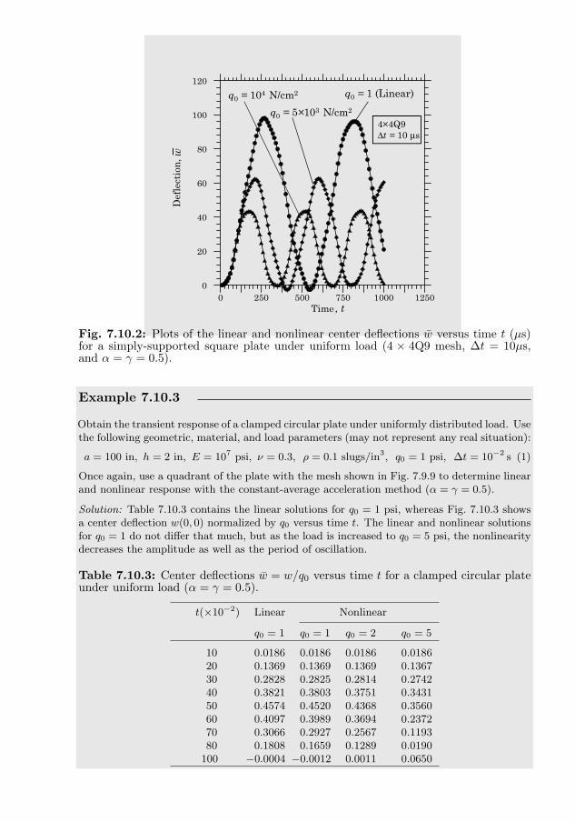
7.10. TRANSIENT ANALYSIS OF THE FSDT 377
0 250 500 750 1000 1250Time
0
20
40
60
80
100
120
Def
lect
ion
,
, t
w
q0 = 1 (Linear)
q0 = 5×10³ N/cm2
q0 = 104 N/cm2
4×4Q9Δt = 10 μs
Fig. 7.10.2: Plots of the linear and nonlinear center deflections w versus time t (µs)for a simply-supported square plate under uniform load (4 × 4Q9 mesh, ∆t = 10µs,and α = γ = 0.5).
Example 7.10.3
Obtain the transient response of a clamped circular plate under uniformly distributed load. Usethe following geometric, material, and load parameters (may not represent any real situation):
a = 100 in, h = 2 in, E = 107 psi, ν = 0.3, ρ = 0.1 slugs/in3, q0 = 1 psi, ∆t = 10−2 s (1)
Once again, use a quadrant of the plate with the mesh shown in Fig. 7.9.9 to determine linearand nonlinear response with the constant-average acceleration method (α = γ = 0.5).
Solution: Table 7.10.3 contains the linear solutions for q0 = 1 psi, whereas Fig. 7.10.3 showsa center deflection w(0, 0) normalized by q0 versus time t. The linear and nonlinear solutionsfor q0 = 1 do not differ that much, but as the load is increased to q0 = 5 psi, the nonlinearitydecreases the amplitude as well as the period of oscillation.
Table 7.10.3: Center deflections w = w/q0 versus time t for a clamped circular plateunder uniform load (α = γ = 0.5).
t(×10−2) Linear Nonlinear
q0 = 1 q0 = 1 q0 = 2 q0 = 5
10 0.0186 0.0186 0.0186 0.018620 0.1369 0.1369 0.1369 0.136730 0.2828 0.2825 0.2814 0.274240 0.3821 0.3803 0.3751 0.343150 0.4574 0.4520 0.4368 0.356060 0.4097 0.3989 0.3694 0.237270 0.3066 0.2927 0.2567 0.119380 0.1808 0.1659 0.1289 0.0190
100 −0.0004 −0.0012 0.0011 0.0650
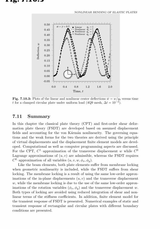
378
0 1q =0 1q =0 2q =0 5q =
0 5.α γ= =
0.0 0.4 0.8 1.2 1.6 2.0
Time, t
-0.05
0.00
0.05
0.10
0.15
0.20
0.25
0.30
0.35
0.40
0.45
0.50
Def
lect
ion
,
Linear
NonlinearNonlinear
Nonlinear
w
Fig. 7.10.3
Fig. 7.10.3: Plots of the linear and nonlinear center deflections w = w/q0 versus timet for a clamped circular plate under uniform load (4Q9 mesh, ∆t = 10−2).
7.11 Summary
In this chapter the classical plate theory (CPT) and first-order shear defor-mation plate theory (FSDT) are developed based on assumed displacementfields and accounting for the von Karman nonlinearity. The governing equa-tions and the weak forms for the two theories are derived using the principleof virtual displacements and the displacement finite element models are devel-oped. Computational as well as computer programming aspects are discussed.For the CPT, C1–approximation of the transverse displacement w while C0
Lagrange approximations of (u, v) are admissible, whereas the FSDT requiresC0–approximation of all variables (u, v, w, φx, φy).
Like the beam elements, both plate elements suffer from membrane lockingwhen geometric nonlinearity is included, while the FSDT suffers from shearlocking. The membrane locking is a result of using the same low-order approx-imations of the in-plane displacements (u, v) and the transverse displacementw, while the membrane locking is due to the use of the same low-order approx-imations of the rotation variables (φx, φy) and the transverse displacement w.Both types of locking are avoided using reduced integration of shear and non-linear terms of the stiffness coefficients. In addition, finite element model forthe transient response of FSDT is presented. Numerical examples of static andtransient response of rectangular and circular plates with different boundaryconditions are presented.
NONLINEAR BENDING OF ELASTIC PLATES
PROBLEMS 379
Problems
Weak Forms and Finite Element Models
7.1 Develop the weak forms of the following linear equations governing the classical platetheory:
−(∂2Mxx
∂x2+ 2
∂2Mxy
∂x∂y+∂2Myy
∂y2
)= q (1)
−∂2w
∂x2−D22Mxx − D12Myy
)= 0 (2)
−∂2w
∂y2−D12Mxx − D11Myy
)= 0 (3)
−2∂2w
∂x∂y− (D66)−1Mxy = 0 (4)
where
Dij =DijD0
, D0 = D11D22 −D212, Dij = Qij
h3
12, (i = 1, 2, 6) (5)
and Qij are the elastic stiffnesses defined in terms of the principal moduli (E1, E2),shear modulus G12, and Poisson’s ratio ν12 as
Q11 =E1
1− ν12ν21, Q12 =
ν12E2
1− ν12ν21, Q22 =
E2
1− ν12ν21
Q66 =1
S66= G12, ν21 = ν12
E2
E1
(6)
7.2 Develop the (mixed) finite element model associated with the equations in Problem7.1. Assume approximation of the form
w =r∑i=1
wiψ(1)i , Mxx =
s∑i=1
Mxiψ(2)i
Myy =
p∑i=1
Myiψ(3)i , Mxy =
q∑i=1
Mxyiψ(4)i
where ψ(α)i , (α = 1, 2, 3, 4) are appropriate interpolation functions. Discuss the mini-
mum requirements of the interpolation functions.
7.3 Develop the weak forms of the following nonlinear equations governing the classicalplate theory:
−(∂Nxx∂x
+∂Nxy∂y
)= 0 (1)
−(∂Nxy∂x
+∂Nyy∂y
)= 0 (2)
−(∂2Mxx
∂x2+ 2
∂2Mxy
∂x∂y+∂2Myy
∂y2
)−N (u, v, w) = q (3)
−∂2w
∂x2−D22Mxx − D12Myy
)= 0 (4)
−∂2w
∂y2−D12Mxx − D11Myy
)= 0 (5)
−2∂2w
∂x∂y− (D66)−1Mxy = 0 (6)
380
where (Nxx, Nyy, Nxy,N ) are known in terms of (u, v, w) and their derivatives byEqs. (7.3.32) and (7.3.14). Note that the dependent unknowns are u, v, w, Mxx,Myy, and Mxy.
7.4 Develop the (mixed) nonlinear finite element model of the equations in Problem 7.3.Assume interpolation of the form
u =
r∑i=1
uiψ(1)i , v =
r∑i=1
viψ(1)i , w =
r∑i=1
wiψ(2)i (1)
Mxx =
s∑i=1
Mxiψ(3)i , Myy =
p∑i=1
Myiψ(4)i , Mxy =
q∑i=1
Mxyiψ(5)i (2)
7.5 Develop the weak forms of the following nonlinear equations governing the classicalplate theory:
−(∂Nxx∂x
+∂Nxy∂y
)= 0 (1)
−(∂Nxy∂x
+∂Nyy∂y
)= 0 (2)
−∂2Mxx
∂x2+ 4D66
∂4w
∂x2∂y2− ∂2Myy
∂y2− ∂
∂x
(Nxx
∂w
∂x+Nxy
∂w
∂y
)− ∂
∂y
(Nxy
∂w
∂x+Nyy
∂w
∂y
)= q (3)
−∂2w
∂x2−D22Mxx + D12Myy
)= 0 (4)
−∂2w
∂y2−D12Mxx + D11Myy
)= 0 (5)
where (Nxx, Nyy, Nxy) are known in terms of (u, v, w) and their derivatives by Eq. (7.3.32).Note that the dependent unknowns are u, v, w, Mxx, and Myy.
7.6 Develop the (mixed) nonlinear finite element model of the equations in Problem 7.5 byassuming approximations of the form
u =
r∑i=1
uiψ(1)i , v =
r∑i=1
viψ(1)i , w =
r∑i=1
wiψ(2)i (1)
Mxx =
s∑i=1
Mxiψ(3)i , Myy =
p∑i=1
Myiψ(4)i (2)
7.7 Consider the following alternative form of nonlinear equations governing the first-ordershear deformation plate theory:
−(∂Nxx∂x
+∂Nxy∂y
)= 0 (1)
−(∂Nxy∂x
+∂Nyy∂y
)= 0, (2)
−A55∂
∂x
(∂w
∂x+ φx
)−A44
∂
∂y
(∂w
∂y+ φy
)− ∂
∂x
(Nxx
∂w
∂x+Nxy
∂w
∂y
)− ∂
∂y
(Nxy
∂w
∂x+Nyy
∂w
∂y
)= q, (3)
−∂Mxx
∂x−D66
∂
∂y
(∂φx∂y
+∂φy∂x
)+KsA55
(∂w
∂x+ φx
)= 0, (4)
NONLINEAR BENDING OF ELASTIC PLATES
PROBLEMS 381
−∂Myy
∂y−D66
∂
∂x
(∂φx∂y
+∂φy∂x
)+KsA44
(∂w
∂y+ φy
)= 0, (5)
∂φx∂x−(D11Mxx + D12Myy
)= 0, (6)
∂φy∂y−(D12Mxx + D22Myy
)= 0. (7)
where (Nxx, Nyy, Nxy) are known in terms of (u, v, w) and their derivatives by [seeEqs. (7.7.20)–(7.7.22)] and
Dij =DijD0
, D0 = D11D22 −D212 (8)
The dependent unknowns of the formulation (note the order) are (u, v, w,φx, φy, Mxx,Myy).Develop the weak forms of Eqs. (4)–(7) such that they are symmetric in (φx, φy,Mxx,Myy),and identify the primary and secondary variables.
7.8 Develop the (mixed) nonlinear finite element model of the equations in Problem 7.7 byassuming approximations of the form
u =r∑i=1
uiψ(1)i , v =
r∑i=1
viψ(1)i , w =
r∑i=1
wiψ(2)i
φx =
r∑i=1
S1i ψ
(3)i , φy =
r∑i=1
S2i ψ
(3)i , Mxx =
s∑i=1
Mxiψ(4)i , Myy =
p∑i=1
Myiψ(5)i
7.9 Consider the governing equations of equilibrium of elastic plates according to the first-order shear deformation plate theory with the von Karman nonlinearity. Assume thatthe material of the plate is isotropic and obeys the generalized Hooke’s law. However,the elastic modulus E varies nonlinearly with the displacement gradients according tothe equation
E = E0 + E1
(∂u
∂x+∂v
∂y
)(1)
Assuming that Poisson’s ratio is constant, develop (a) the finite element model of theequations and (b) compute the tangent stiffness coefficients, T 11
ij and T 33ij .
7.10 Consider the governing equations of equilibrium of elastic plates according to the first-order shear deformation plate theory with the von Karman nonlinearity. Assume thatthe plate is made of two homogeneous isotropic materials that are combined accordingto the following power-law distribution [see Eq. (5.3.37)]:
E(z) = (E1 − E2) f(z) + E2, f(z) =
(1
2+z
h
)n(1)
where E1 and E2 are moduli of the two materials that are being mixed, h is the totalthickness of the plate, and n is the power-law index that dictates the volume fractionf(z) of material 1. Develop the displacement finite element model of the functionallygraded plate and determine the tangent stiffness coefficients.
Programming Problems (Development of finite element computer programs based on Prob-lems 7.1–7.8 and Problem 7.10 can also be assigned)
7.11 Write a computer subroutine to calculate stresses for the CPT, based on the discussionof Section 7.5.3.
7.12 Write a computer subroutine to calculate stresses for FSDT, following the discussionof Section 7.5.3.
382
7.13 Write a computer subroutine to implement the time-approximation schemes of Section7.10.
Computational Problems
7.14 Analyze an orthotropic square plate using a = 10 in, h = 1 in, E1 = 7.8 × 10⁶ psi,E2 = 2.6×10⁶ psi, ν12=0.25, G12 = G13 = G23 = 1.3×10⁶ psi, and 8×8 uniform meshof conforming CPT(C) elements in a quadrant of the plate for SS–1 and SS–3 boundaryconditions. The material coordinates (x1, x2) coincide with the plate coordinates (x, y).Use load parameter P = q0a
4/(E2h4) equal to 25 for the first four steps, 50 for the
next two steps, and 100 for the last ten steps. Use a convergence tolerance of ε = 10−3
and a maximum of ten allowable iterations.
7.15 Analyze Problem 7.14 using the FSDT elements with 4× 4 mesh of Q9 elements.
7.16 Consider a clamped square plate, subjected to uniformly distributed transverse loadq = q0 = constant. The geometric and material parameters are a = 10 in, h = 1 in,E1 = 7.8×10⁶ psi, E2 = 2.6×10⁶ psi, ν12=0.25, G12 = G13 = G23 = 1.3×10⁶ psi. Use8× 8 and 4× 4 uniform meshes of linear and equivalent meshes of nine-node quadraticrectangular elements in a quadrant of the plate to analyze the problem. Use load stepssuch that the load parameter ∆P ≡ q0a
4/E2h4 is equal to 5, and use 32 load steps to
obtain the nonlinear response. Plot (a) load versus center deflection (w/h versus P ),and (b) load versus maximum stress (σxx and σxy). Use a convergence tolerance ofε = 10−3 and maximum number of iterations for convergence to be ten.
7.17 Determine the load–deflection behavior of a square plate with two opposite edgessimply-supported (SS–1) and the other two edges free, and subjected to uniformly dis-tributed transverse load. The material coordinates (x1, x2) coincide with the plate co-ordinates (x, y), and assume that the edges parallel to the x-axis are simply-supported.Use a = 10 in, h = 1 in, E1 = 7.8 × 10⁶ psi, E2 = 2.6 × 10⁶ psi, ν12=0.25,G12 = G13 = G23 = 1.3×10⁶ psi, and 8×8 uniform mesh of conforming CPT elementsin a quadrant of the plate. Use load steps such that the load parameter P ≡ q0a4/E2h
4
is equal to 20, and use 12 load steps. Tabulate results for the maximum transversedeflection w and stress σxx. Use a tolerance of ε = 10−2 and ten maximum iterations.
7.18 Repeat Problem 7.17 for a square plate with two opposite edges simply-supported (SS–1) and the other two edges clamped (CC). The material coordinates (x1, x2) coincidewith the plate coordinates (x, y), and assume that the edges parallel to the x-axis areclamped and the edges parallel to the y-axis are simply-supported. Use 8 × 8 meshof (a) conforming CPT element, and (b) non-conforming CPT element. Present theload-deflection curves in graphical form.
7.19 Determine the load–deflection behavior of a square plate with two opposite edgesclamped and the other two edges free, and subjected to uniformly distributed trans-verse load. The material coordinates (x1, x2) coincide with the plate coordinates (x, y),and assume that the edges parallel to the x-axis are clamped. Use a = 10 in, h = 1in, E1 = 7.8 × 10⁶ psi, E2 = 2.6 × 10⁶ psi, ν12=0.25, G12 = G13 = G23 = 1.3 × 10⁶
psi, and 8× 8 uniform mesh of (a) non-conforming CPT elements, and (b) conformingCPT elements. Use load steps such that the load parameter P ≡ q0a4/E2h
4 is equal to20, and use 12 load steps with ε = 10−2. Plot load versus center deflection (P versusw). Use a convergence tolerance of ε = 10−2 and ten maximum iterations.
7.20 Repeat Problem 7.17 using 4× 4Q9 mesh of the FSDT elements.
7.21 Repeat Problem 7.18 using 4× 4Q9 mesh of the FSDT elements.
7.22 Repeat Problem 7.19 using 4× 4Q9 mesh of the FSDT elements.
7.23 Analyze the circular plate problem of Example 7.9.6 using an equivalent mesh of thenonconforming plate elements. Use all other parameters as in Example 7.9.6.
NONLINEAR BENDING OF ELASTIC PLATES
PROBLEMS 383
7.24 Analyze the circular plate problem of Example 7.10.3 when the edge is simply-supported(SS–3). Use the 5Q9 mesh of FSDT elements and parameters of Example 7.10.3.
7.25 Find the nonlinear transient response of the circular plate problem in Problem 7.24 forq0 = 10, 20, and 100. Use all parameters as in Example 7.10.3.
7.26 Find the nonlinear transient response of a simply-supported (SS–1) orthotropic squareplate under uniformly distributed load of intensity q0 = 103 psi. Use the followinggeometric and material parameters:
a = b = 25 in, h = 2.5 in, E1 = 7.5× 10⁶ psi, E2 = 2× 10⁶ psi
G12 = 1.25× 10⁶ psi, G13 = G23 = 0.625× 10⁶ psi
ν12 = 0.25, ρ = 1.0× 10⁻⁶ lb-s2/in4, α = γ = 0.5
and a time step of ∆t = 10−5 to capture at least the first period of the response.
7.27 Repeat Problem 7.26 for the SS–3 boundary conditions.

385
8
Nonlinear Bending ofElastic Shells
The man who cannot occasionally imagine events and conditions of existence that are contraryto the causal principle as he knows it will never enrich his science by the addition of a newidea. ——– Max Planck
8.1 Introduction
In Chapter 7, we considered plates whose planform dimensions are large com-pared to their thicknesses and subjected to loads that cause bending deforma-tion in addition to stretching. Shells are much like plates in terms of theirthicknesses being considerably smaller than the other two dimensions, exceptthat they are curved. Shells are common in nature as well as in many engineer-ing structures, including pressure vessels, submarine and ship hulls, airplanewings and fuselages, containment structures, pipes, exteriors of rockets, mis-siles, automobile tires, concrete roofs, chimneys, cooling towers, liquid storagetanks, and many others. In nature, they can be found in the form of sea shells,eggs, inner ear, skull, and geological formations. Shell structures have beenbuilt by humans for centuries, mostly in the form of masonry and stone domes,roofs, and arches; some of which still exist around the world. They are themost efficient structures because loads applied in any direction are resisted bya combination of transverse as well as surface forces even when the deformationis small. This is primarily due to its curved geometry.
Finite element models of shells are developed using either (1) a shell theoryor (2) the 2-D equations obtained from a degenerated 3-D elasticity model.The latter is more often known as the continuum shell model, which will bediscussed in Chapter 9. The present chapter is devoted to the development ofshell theory-based finite element models.
A number of shell theories exist in the literature, and many of these theo-ries were developed originally for thin shells and are based on the Kirchhoff–Love kinematic hypothesis, similar to the Kirchhoff hypothesis for plates, thatstraight lines normal to the undeformed midsurface remain straight, inextensi-ble, and normal to the middle surface after deformation. A detailed study ofthin isotropic shells can be found in the monographs by Ambartsumyan [81–83],
J.N. Reddy, An Introduction to Nonlinear Finite Element Analysis, Second Edition. c©J.N.Reddy 2015. Published in 2015 by Oxford University Press.
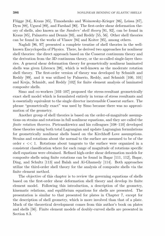
386
Flugge [84], Kraus [85], Timoshenko and Woinowsky-Krieger [86], Leissa [87],Dym [88], Ugural [89], and Farshad [90]. The first-order shear deformation the-ory of shells, also known as the Sanders’ shell theory [91, 92], can be found inKraus [85], Palazotto and Dennis [93], and Reddy [55, 56]. Other shell theoriescan be found in the works of Vlasov [94] and Koiter [95], among others.
Naghdi [96, 97] presented a complete treatise of shell theories in the well-known Encyclopedia of Physics. There, he derived two approaches for nonlinearshell theories: the direct approach based on the Cosserat continuum theory andthe derivation from the 3D continuum theory, or the so-called single-layer theo-ries. A general shear deformation theory for geometrically nonlinear laminatedshells was given Librescu [98], which is well-known as the moderate rotationshell theory. The first-order version of theory was developed by Schmidt andReddy [99], and it was utilized by Palmerio, Reddy, and Schmidt [100, 101]and Kreja, Schmidt, and Reddy [102] for finite element analysis of laminatedcomposite shells.
Simo and co-workers [103–107] proposed the stress-resultant geometricallyexact shell model which is formulated entirely in terms of stress resultants andis essentially equivalent to the single director inextensible Cosserat surface. Thephrase “geometrically exact” was used by Simo because there was no approxi-mation of the geometry.
Another group of shell theories is based on the order-of-magnitude assump-tions on strains and rotations in full nonlinear equations, and they are called thefinite rotation theories. Pietraszkiewicz and his colleagues [108–110] developedthese theories using both total Lagrangian and update Lagrangian formulationsfor geometrically nonlinear shells based on the Kirchhoff–Love assumptions.Strains and rotations about the normal to the surface are assumed to be of theorder ε << 1. Rotations about tangents to the surface were organized in aconsistent classification where for each range of magnitude of rotations specificshell equations were obtained. Refined high-order shear deformation models forcomposite shells using finite rotations can be found in Basar [111, 112], Basar,Ding, and Schultz [113] and Balah and Al-Ghamedy [114]. Both approachesutilize the third-order shell theory for the analysis of composite shells via thefinite element method.
The objective of this chapter is to review the governing equations of shellsbased on the first-order shear deformation shell theory and develop its finiteelement model. Following this introduction, a description of the geometry,kinematic relations, and equilibrium equations for shells are presented. Thepresentation is similar to that presented for plates in Chapter 7, except forthe description of shell geometry, which is more involved than that of a plate.Much of the theoretical development comes from this author’s book on platesand shells [56]. Finite element models of doubly-curved shells are presented inSection 8.3.
NONLINEAR BENDING OF ELASTIC SHELLS
8.2. GOVERNING EQUATIONS 387
8.2 Governing Equations
8.2.1 Geometric Description
Consider a curved shell element of uniform thickness, as shown in Fig. 8.2.1(a).Here (ξ1, ξ2, ζ) denote the curvilinear coordinates such that ξ1 and ξ2 curves arethe lines of curvature on the middle surface (ζ = 0). The position vector of atypical point (ξ1, ξ2, 0) on the middle surface is denoted by r, and the positionof an arbitrary point (ξ1, ξ2, ζ) is denoted by R [see Figs. 8.2.1(b) and (c)]. Adifferential line element on the middle surface can be written as
dr =∂r
∂ξαdξα = gαdξα , gα =
∂r
∂ξα(α = 1, 2) (8.2.1)
where the vectors g1 and g2 are tangent to the ξ1 and ξ2 coordinate lines,as shown in Fig. 8.2.1(b). The components of the surface metric tensor gαβ(α, β = 1, 2) are
gα · gβ ≡ gαβ, a1 =√g11, a2 =
√g22, g1 · g2 = a1a2 cosχ (8.2.2)
where χ denotes the angle between the coordinate curves. The unit vector nor-mal to the middle surface (hence, normal to both g1 and g2) can be determinedfrom
n =g1 × g2
a1a2 sinχ(8.2.3)
In general, n, a1 and a2 are functions of ξ1 and ξ2. The square of the distanceds between points (ξ1, ξ2, 0) and (ξ1 + dξ1, ξ2 + dξ2, 0) on the middle surface isdetermined by
(ds)2 = dr · dr = gαβ dξα dξβ = a21 (dξ1)2 + a2
2 (dξ2)2 + 2a1a2 cosχdξ1 dξ2
(8.2.4)The right-hand side of the above equation is known as the first quadratic formof the surface, which allows us to determine the infinitesimal lengths, the anglebetween the curves, and area of the surface. The terms a2
1, a22, and a1a2 cosχ
are called the first fundamental quantities.Let r = r(s) be the equation of a curve s on the surface. The unit vector
tangent to the curve is
t =dr
ds=
∂r
∂ξα
dξαds
= gαdξαds
(8.2.5)
According to Frenet’s formula, the derivative of this unit vector is
dt
ds=
N
ρ(8.2.6)
388 NONLINEAR BENDING OF ELASTIC SHELLS
Fig. 8.2.1: (a) Shell geometry. (b) Position vector of a point and coordinates on themiddle surface. (c) Position vectors of points on the middle surface and above themiddle surface.
where 1/ρ is the curvature of the curve, and N is the unit vector of the principalnormal to the curve. From Eqs. (8.2.5) and (8.2.6), we obtain
N
ρ=
d
ds
(dr
ds
)=∂gα∂ξβ
dξαds
dξβds
+ gαd2ξαds2
(8.2.7)
Let ϕ be the angle between the normal to the surface, n, and the principalnormal to the curve, N; i.e. cosϕ = n · N. Then, taking the dot product ofboth sides of Eq. (8.2.7), we obtain
cosϕ
ρ=L (dξ1)2 + 2M dξ1 dξ2 +N (dξ2)2
ds2(8.2.8)
8.2. GOVERNING EQUATIONS 389
where
L = n · ∂2r
∂ξ21
, M = n · ∂2r
∂ξ1∂ξ2, N = n · ∂
2r
∂ξ22
(8.2.9)
The numerator on the right-hand side of Eq. (8.2.8) is called the secondquadratic form of the surface, and the quantities L, M , and N are the co-efficients of the quadratic form.
Equation (8.2.8) can be used to compute the curvatures of the curves ob-tained by intersecting the surface with normal planes. For the curve generatedby a normal plane, n and N have opposite directions (ϕ = π) because the out-ward normal (to the right of the curve) is taken positive as we traverse alongdr. Thus, Eq. (8.2.8) yields
1
R= − L (dξ1)2 + 2M dξ1 dξ2 +N (dξ2)2
a21 (dξ1)2 + 2a1a2 cosχdξ1 dξ2 + a2
2 (dξ2)2(8.2.10)
In particular, the curvatures of the ξ1 curve (ξ2 = constant) and ξ2 curve (ξ1 =constant) are
1
R1= − L
a21
,1
R2= −N
a22
(8.2.11)
From this point onwards, we assume that ξ1 and ξ2 are orthogonal, that is,curves ξ1 = constant and ξ2 = constant are lines of principal curvatures of theundeformed middle surface; then cosχ = 0 and M = 0. The derivatives of thevectors n and eα ≡ gα/aα (no sum on α) are given by (see Kraus [85])
∂n
∂ξα=aαRα
eα =gαRα
(α = 1, 2)
∂eα∂ξβ
=1
aα
∂aβ∂ξα
eβ (α 6= β)
∂eα∂ξα
= − 1
aβ
∂aα∂ξβ
eβ −aαRα
n (α 6= β)
(8.2.12)
In Eq. (8.2.12), no sum on repeated indices is implied. The first equation inEq. (8.2.12) is known as the Theorem of Rodrigues, and the second and thirdrelations are known as the Weingarten formulas.
In addition, we have the identities
∂
∂ξ1
(1
a1
∂a2
∂ξ1
)+
∂
∂ξ2
(1
a2
∂a1
∂ξ2
)= − a1a2
R1R2= −a1a2
K(8.2.13)
∂
∂ξ2
(a1
R1
)=
1
R2
∂a1
∂ξ2,
∂
∂ξ1
(a2
R2
)=
1
R1
∂a2
∂ξ1(8.2.14)
where 1/K = 1/R1R2 is called the Gaussian curvature. Equation (8.2.13) isknown as the Gauss characteristic equation, and the formulas given in Eq. (8.2.14)are called Mainardi–Codazzi relations.
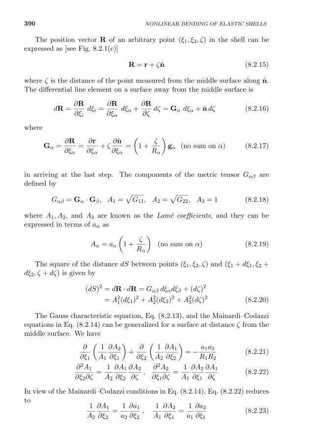
390 NONLINEAR BENDING OF ELASTIC SHELLS
The position vector R of an arbitrary point (ξ1, ξ2, ζ) in the shell can beexpressed as [see Fig. 8.2.1(c)]
R = r + ζn (8.2.15)
where ζ is the distance of the point measured from the middle surface along n.The differential line element on a surface away from the middle surface is
dR =∂R
∂ξidξi =
∂R
∂ξαdξα +
∂R
∂ζdζ = Gα dξα + n dζ (8.2.16)
where
Gα =∂R
∂ξα=
∂r
∂ξα+ ζ
∂n
∂ξα=
(1 +
ζ
Rα
)gα (no sum on α) (8.2.17)
where the Theorem of Rodrigues [i.e. the first equation in Eq. (8.2.12)] is usedin arriving at the last step. The components of the metric tensor Gαβ aredefined by
Gαβ = Gα ·Gβ, A1 =√G11, A2 =
√G22, A3 = 1 (8.2.18)
where A1, A2, and A3 are known as the Lame coefficients, and they can beexpressed in terms of aα as
Aα = aα
(1 +
ζ
Rα
)(no sum on α) (8.2.19)
The square of the distance dS between points (ξ1, ξ2, ζ) and (ξ1 + dξ1, ξ2 +dξ2, ζ + dζ) is given by
(dS)2 = dR · dR = Gαβ dξαdξβ + (dζ)2
= A21(dξ1)2 +A2
2(dξ2)2 +A23(dζ)2 (8.2.20)
The Gauss characteristic equation, Eq. (8.2.13), and the Mainardi–Codazziequations in Eq. (8.2.14) can be generalized for a surface at distance ζ from themiddle surface. We have
∂
∂ξ1
(1
A1
∂A2
∂ξ1
)+
∂
∂ξ2
(1
A2
∂A1
∂ξ2
)= − a1a2
R1R2(8.2.21)
∂2A1
∂ξ2∂ζ=
1
A2
∂A1
∂ξ2
∂A2
∂ζ,
∂2A2
∂ξ1∂ζ=
1
A1
∂A2
∂ξ1
∂A1
∂ζ(8.2.22)
In view of the Mainardi–Codazzi conditions in Eq. (8.2.14), Eq. (8.2.22) reducesto
1
A2
∂A1
∂ξ2=
1
a2
∂a1
∂ξ2,
1
A1
∂A2
∂ξ1=
1
a1
∂a2
∂ξ1(8.2.23)
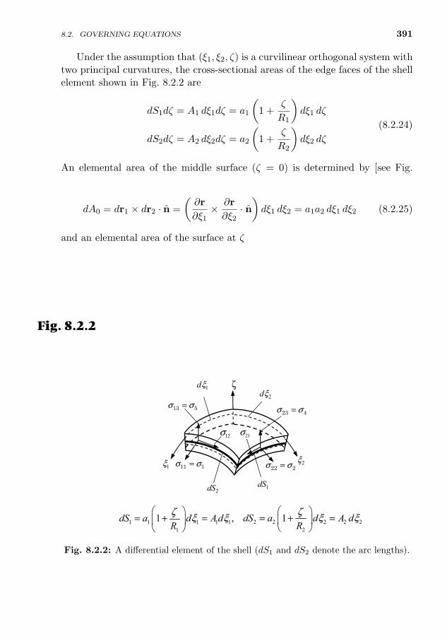
391
Under the assumption that (ξ1, ξ2, ζ) is a curvilinear orthogonal system withtwo principal curvatures, the cross-sectional areas of the edge faces of the shellelement shown in Fig. 8.2.2 are
dS1dζ = A1 dξ1dζ = a1
(1 +
ζ
R1
)dξ1 dζ
dS2dζ = A2 dξ2dζ = a2
(1 +
ζ
R2
)dξ2 dζ
(8.2.24)
An elemental area of the middle surface (ζ = 0) is determined by [see Fig.8.2.3(a)]
dA0 = dr1 × dr2 · n =
(∂r
∂ξ1× ∂r
∂ξ2· n)dξ1 dξ2 = a1a2 dξ1 dξ2 (8.2.25)
and an elemental area of the surface at ζ is given by [see Fig. 8.2.3(b)]
dAζ = dR1 × dR2 · n =
(∂R
∂ξ1× ∂R
∂ξ2· n)dξ1 dξ2 = A1A2 dξ1 dξ2 (8.2.26)
The volume of a differential shell element is given by
dV = dR1 × dR2 · n dζ = dAζ dζ = A1A2 dξ1 dξ2 dζ
=
[a1
(1 +
ζ
R1
)][a2
(1 +
ζ
R2
)]dξ1 dξ2 dζ (8.2.27)
1 1 1 1 11
1 ,ζ ξ ξ = + =
dS a d A d
R 2 2 2 2 22
1dS a d A dRζ ξ ξ
= + =
ζ
12σ 21σ
13 5σ σ=23 4σ σ=
22 2σ σ=11 1σ σ=
1dξ2dξ
1dS2dS
1ξ 2ξ
Fig. 8.2.2
Fig. 8.2.2: A differential element of the shell (dS1 and dS2 denote the arc lengths).
8.2. GOVERNING EQUATIONS
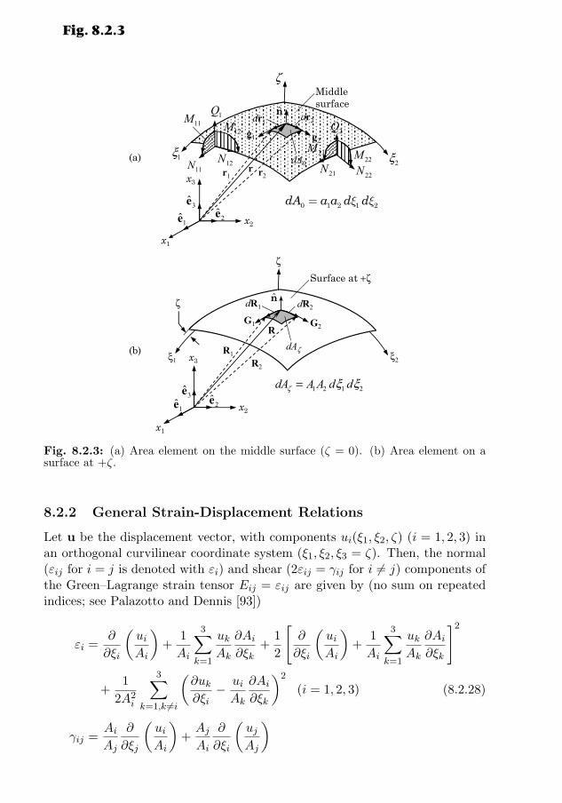
392 NONLINEAR BENDING OF ELASTIC SHELLS
(b) ξ1 ξ2
ζ
Surface at +ζ
dR1 dR2n
dAζ
x1
x2
x3 R2
R1
RG2
G1
ζ
1 2 1 2dA A A d dζ ξ ξ=
1e3e
2e
Middle surface
dr1 dr2n
dA0
x1
x2
x3r2r1
r
g2g1
(a)
ζ
1ξ2ξ
0 1 2 1 2dA a a d dx x=
1e3e
2e
11N
1Q
12N21N
2Q
22N
12M11M
21M22M
Fig. 8.2.3
Fig. 8.2.3: (a) Area element on the middle surface (ζ = 0). (b) Area element on asurface at +ζ.
8.2.2 General Strain-Displacement Relations
Let u be the displacement vector, with components ui(ξ1, ξ2, ζ) (i = 1, 2, 3) inan orthogonal curvilinear coordinate system (ξ1, ξ2, ξ3 = ζ). Then, the normal(εij for i = j is denoted with εi) and shear (2εij = γij for i 6= j) components ofthe Green–Lagrange strain tensor Eij = εij are given by (no sum on repeatedindices; see Palazotto and Dennis [93])
εi =∂
∂ξi
(uiAi
)+
1
Ai
3∑k=1
ukAk
∂Ai∂ξk
+1
2
[∂
∂ξi
(uiAi
)+
1
Ai
3∑k=1
ukAk
∂Ai∂ξk
]2
+1
2A2i
3∑k=1,k 6=i
(∂uk∂ξi− uiAk
∂Ai∂ξk
)2
(i = 1, 2, 3) (8.2.28)
γij =AiAj
∂
∂ξj
(uiAi
)+AjAi
∂
∂ξi
(ujAj
)
8.2. GOVERNING EQUATIONS 393
+
3∑k=1,k 6=i,k 6=j
1
AiAj
(∂uk∂ξi− uiAk
∂Ai∂ξk
)(∂uk∂ξj− ujAk
∂Aj∂ξk
)
+1
Aj
(∂ui∂ξj− ujAi
∂Aj∂ξi
)[∂
∂ξi
(uiAi
)+
1
Ai
3∑k=1
ukAk
∂Ai∂ξk
]
+1
Ai
(∂uj∂ξi− uiAj
∂Ai∂ξj
)[∂
∂ξj
(ujAj
)+
1
Aj
3∑k=1
ukAk
∂Aj∂ξk
](8.2.29)
where i 6= j (i, j = 1, 2, 3) in Eq. (8.2.29), and
ξ3 = ζ, A1 = a1
(1 +
ζ
R1
), A2 = a2
(1 +
ζ
R2
), A3 = a3 = 1 (8.2.30)
Substituting Eq. (8.2.30) into Eqs. (8.2.28) and (8.2.29) and making use ofconditions in Eqs. (8.2.12)–(8.2.14) and Eq. (8.2.23), one obtains
ε1 = ε11 =1
A1
(∂u1
∂ξ1+u2
a2
∂a1
∂ξ2+a1
R1u3
)+
1
2A21
[(∂u1
∂ξ1+u2
a2
∂a1
∂ξ2+a1
R1u3
)2
+
(∂u2
∂ξ1− u1
a2
∂a1
∂ξ2
)2
+
(∂u3
∂ξ1− a1
R1u1
)2]
ε2 = ε22 =1
A2
(∂u2
∂ξ2+u1
a1
∂a2
∂ξ1+a2
R2u3
)+
1
2A22
[(∂u2
∂ξ2+u1
a1
∂a2
∂ξ1+a2
R2u3
)2
+
(∂u1
∂ξ2− u2
a1
∂a2
∂ξ1
)2
+
(∂u3
∂ξ2− a2
R2u2
)2]
ε3 = ε33 =∂u3
∂ζ+
1
2
[(∂u1
∂ζ
)2
+
(∂u2
∂ζ
)2
+
(∂u3
∂ζ
)2]
ε4 = 2ε23 =1
A2
∂u3
∂ξ2+A2
∂
∂ζ
(u2
A2
)+
1
A2
[∂u2
∂ζ
(∂u2
∂ξ2+u1
a1
∂a2
∂ξ1+a2
R2u3
)
+∂u1
∂ζ
(∂u1
∂ξ2− u2
a1
∂a2
∂ξ1
)+∂u3
∂ζ
(∂u3
∂ξ2− a2
R2u2
)]
ε5 = 2ε13 =1
A1
∂u3
∂ξ1+A1
∂
∂ζ
(u1
A1
)+
1
A1
[∂u1
∂ζ
(∂u1
∂ξ1+u2
a2
∂a1
∂ξ2+a1
R1u3
)
+∂u2
∂ζ
(∂u2
∂ξ1− u1
a2
∂a1
∂ξ2
)+∂u3
∂ζ
(∂u3
∂ξ1− a1
R1u1
)]
ε6 = 2ε12 =A2
A1
∂
∂ξ1
(u2
A2
)+A1
A2
∂
∂ξ2
(u1
A1
)
394 NONLINEAR BENDING OF ELASTIC SHELLS
+1
A1A2
[(∂u1
∂ξ2− u2
a1
∂a2
∂ξ1
)(∂u1
∂ξ1+
1
a2
∂a1
∂ξ2u2 +
a1
R1u3
)+
(∂u2
∂ξ1− u1
a2
∂a1
∂ξ2
)(∂u2
∂ξ2+
1
a1
∂a2
∂ξ1u1 +
a2
R2u3
)+
(∂u3
∂ξ1− a1
R1u1
)(∂u3
∂ξ2− a2
R2u2
)](8.2.31)
The linear strain–displacement relations are obtained by setting the terms inthe square brackets of Eq. (8.2.31) to zero.
8.2.3 Stress Resultants
Next, we introduce the stress resultants acting on a shell element. The tensileforce measured per unit length along a ξ2-coordinate line on a cross sectionperpendicular to a ξ1 coordinate line [see Fig. 8.2.3(a)] is σ11 dS2. The totaltensile force on the differential element in the ξ1-direction can be computed byintegrating over the entire thickness of the shell:∫ h/2
−h/2σ11 dS2 dζ = a2
[∫ h/2
−h/2σ11
(1 +
ζ
R2
)dζ
]dξ2 ≡ N11 a2 dξ2 (8.2.32)
where h is the total thickness of the shell, ζ = −h/2 and ζ = h/2 denote thebottom and top surfaces of the shell, and N11 is the membrane force per unitlength in the ξ1-direction, acting on a surface perpendicular to the ξ1-coordinate(see Fig. 8.2.3):
N11 =
∫ h/2
−h/2σ11
(1 +
ζ
R2
)dζ
Similarly, the moment of the force σ11 dS2 about the ξ2-axis is∫ h/2
−h/2σ11 dS2 ζ dζ = a2
[∫ h/2
−h/2σ11
(1 +
ζ
R2
)ζ dζ
]dξ2 ≡M11 a2 dξ2 (8.2.33)
Thus, the stress resultants per unit length (see Fig. 8.2.3) can be defined asN11
N12
Q1
=
∫ h/2
−h/2
σ11
σ12
Ksσ13
(
1 +ζ
R2
)dζ
N22
N21
Q2
=
∫ h/2
−h/2
σ22
σ21
Ksσ23
(
1 +ζ
R1
)dζ
(8.2.34)
8.2. GOVERNING EQUATIONS 395M11
M12
=
∫ h/2
−h/2
σ11
σ12
(1 +
ζ
R2
)ζ dζ
M22
M21
=
∫ h/2
−h/2
σ22
σ21
(1 +
ζ
R1
)ζ dζ
(8.2.35)
where Ks is the shear correction factor. Note that, in general, Nαβ 6= Nβα
and Mαβ 6= Mβα for α 6= β (α, β = 1, 2). However, if we assume that thethickness of the shell is small as compared to the smallest radius of curvatureof the middle surface, one can neglect ζ/R1 and ζ/R2. Such shells are calledthin shells, and for thin shells we have Nαβ = Nβα and Mαβ = Mβα, as in aplate theory.
8.2.4 Displacement and Strain Fields
In developing a moderately thick (i.e. shear deformation) shell theory with thevon Karman nonlinear strains (i.e. small strains but moderate rotations), thefollowing assumptions (as in the case of plates) are made:
1. The transverse normal is inextensible (i.e. ε3 ≈ 0) and the transverse nor-mal stress is small as compared with the other normal stress componentsand may be neglected.
2. Normals to the undeformed middle surface of the shell before deformationremain straight, but not necessarily normal after deformation.
3. The deflections and strains are sufficiently small so that the quantities ofsecond- and higher-order magnitudes, except for second-order rotationsabout the transverse normals, may be neglected in comparison with thefirst-order terms.
4. The rotations about the ξ1 and ξ2 axes are moderate so that we retainsecond-order terms [i.e. terms that are products and squares of the terms(∂u3/∂ξα) − (aαuα/Rα)] in the strain–displacement relations (the vonKarman nonlinearity).
Love’s first approximation theory further assumes that: (1) the thickness ofthe shell is small as compared with the other dimensions, (2) the transversenormals to the undeformed middle surface remain not only straight but alsonormal to the deformed middle surface after deformation, and (3) the strainsare infinitesimal so that all nonlinear terms are neglected. The first assumptionallows us to neglect the higher powers of ζ/R and h/R in the derivation of shelltheories. The second assumption (also known as the Kirchhoff hypothesis)results in the neglect of transverse shear strains.
396 NONLINEAR BENDING OF ELASTIC SHELLS
Consistent with the assumptions (1)–(4) of a moderately thick shell theory,we assume the following form of the displacement components ui:
u1(ξ1, ξ2, ζ, t) = u(ξ1, ξ2, t) + ζϕx(ξ1, ξ2, t)
u2(ξ1, ξ2, ζ, t) = v(ξ1, ξ2, t) + ζϕy(ξ1, ξ2, t)
u3(ξ1, ξ2, ζ, t) = w(ξ1, ξ2, t)
(8.2.36)
where (u, v, w) are the displacements of a point (ξ1, ξ2, 0) on the middle surfaceof the shell in the ξi-direction, and (φx, φy) are the rotations of a normal to thereference surface about the ξ2 and ξ1 axes, respectively
φx =∂u1
∂ζ, φy =
∂u2
∂ζ(8.2.37)
The five variables (u, v, w, φx, φy) completely determine the displacements of anarbitrary point (ξ1, ξ2, ζ) in the shell.
In writing the von Karman strains, we make approximations of the typeζ2ϕ2
α ≈ 0, ζu0αϕα ≈ 0, and ζu3,αϕα ≈ 0 (no sum on α) and[
∂u3
∂ξα− aαRα
(u0α + ζϕα
)]2
≈(∂u0
3
∂ξα− aαu
0α
Rα
)2
(8.2.38)
and use the identity
Aα∂
∂ζ
(uαAα
)=∂uα∂ζ
+Aαuα∂
∂ζ
(1
Aα
)=∂uα∂ζ− uαAα
aαRα
=aαAα
(ϕα −
u0α
Rα
)(8.2.39)
The von Karman nonlinear strains can be expressed as the sum of membranestrains ε0
i and flexural strains ε1i (see [56] for details)
ε = ε0+ ζε1 (8.2.40a)
where
ε0
1
ε02
ε04
ε05
ε06
=
1A1
[∂u∂ξ1
+ va2∂a1∂ξ2
+ a1wR1
+ 12A1
(∂w∂ξ1− a1u
R1
)2]1A2
[∂v∂ξ2
+ ua1∂a2∂ξ1
+ a2wR2
+ 12A2
(∂w∂ξ2− a2v
R2
)2]a2A2
(1a2
∂w∂ξ2− v
R2+ φy
)a1A1
(1a1
∂w∂ξ1− u
R1+ φx
)1A1
[∂v∂ξ1− u
a2∂a1∂ξ2
+ 12A2
(∂w∂ξ1− a1u
R1
)(∂w∂ξ2− a2v
R2
)]+ 1A2
[∂u∂ξ2− v
a1∂a2∂ξ1
+ 12A1
(∂w∂ξ1− a1u
R1
)(∂w∂ξ2− a2v
R2
)]
(8.2.40b)
8.2. GOVERNING EQUATIONS 397
ε1
1
ε12
ε14
ε15
ε16
=
1A1
(∂φx∂ξ1
+φya2
∂a1∂ξ2
)1A2
(∂φy∂ξ2
+ φxa1
∂a2∂ξ1
)00
1A1
(∂φy∂ξ1− φx
a2∂a1∂ξ2
)+ 1
A2
(∂φx∂ξ2− φy
a1∂a2∂ξ1
)
(8.2.40c)
8.2.5 Equations of Equilibrium
The equations governing generalized Sanders shell theory can be derived us-ing the principle of virtual displacements. The generalization is to includethe von Karman strains. The displacement field in Eq. (8.2.36) and strains inEq. (8.2.40) are used to derive the governing equations. In addition, the van-ishing of the moments about the normal to the differential element (Fig. 8.2.3)yields the following additional relation among the twisting moments and surfaceshear forces:
M21
R2− M12
R1+N21 −N12 = 0 (8.2.41)
which must be accounted for in the formulation; otherwise, it will lead to incon-sistency associated with rigid body rotations (i.e. a rigid body rotation gives anon-vanishing torsion except for flat plates and spherical shells). The equationsof equilibrium thus obtained are (see [56] for details)
1
a2a1
∂
∂ξ1
(a2N11
)+
∂
∂ξ2
(a1N21
)+N12
∂a1
∂ξ2−N22
∂a2
∂ξ1+ C0a1
∂M12
∂ξ2
+
N11
a1R1
(∂w
∂ξ1− a1u
R1
)+
N12
a2R1
(∂w
∂ξ2− a2v
R2
)+Q1
R1+ f1 = 0 (8.2.42)
1
a1a2
∂
∂ξ2
(a1N22
)+
∂
∂ξ1
(a2N12
)+N21
∂a2
∂ξ1−N11
∂a1
∂ξ2− C0a2
∂M12
∂ξ1
+
N22
a2R2
(∂w
∂ξ2− a2v
R2
)+
N12
a1R2
(∂w
∂ξ1− a1u
R1
)+Q2
R2+ f2 = 0 (8.2.43)
1
a1a2
∂
∂ξ1
[a2
a1N11
(∂w
∂ξ1− a1u
R1
)+ N12
(∂w
∂ξ2− a2v
R2
)]+
∂
∂ξ2
[a1
a2N22
(∂w
∂ξ2− a2v
R2
)+ N12
(∂w
∂ξ1− a1u
R1
)]+
∂
∂ξ1
(a2Q1
)+
∂
∂ξ2
(a1Q2
)−(N11
R1+N22
R2
)+ f3 = 0 (8.2.44)
1
a1a2
[∂
∂ξ1
(a2M11
)+
∂
∂ξ2
(a1M21
)−M22
∂a2
∂ξ1+M12
∂a1
∂ξ2
]−Q1 = 0 (8.2.45)
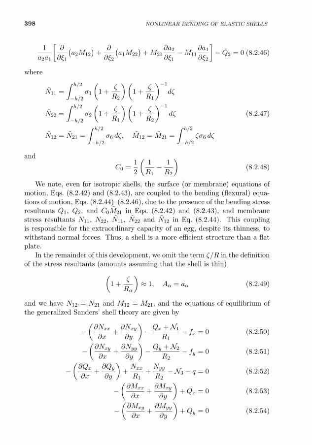
398 NONLINEAR BENDING OF ELASTIC SHELLS
1
a2a1
[∂
∂ξ1
(a2M12
)+
∂
∂ξ2
(a1M22
)+M21
∂a2
∂ξ1−M11
∂a1
∂ξ2
]−Q2 = 0 (8.2.46)
where
N11 =
∫ h/2
−h/2σ1
(1 +
ζ
R2
)(1 +
ζ
R1
)−1
dζ
N22 =
∫ h/2
−h/2σ2
(1 +
ζ
R1
)(1 +
ζ
R2
)−1
dζ
N12 = N21 =
∫ h/2
−h/2σ6 dζ, M12 = M21 =
∫ h/2
−h/2ζσ6 dζ
(8.2.47)
and
C0 =1
2
(1
R1− 1
R2
)(8.2.48)
We note, even for isotropic shells, the surface (or membrane) equations ofmotion, Eqs. (8.2.42) and (8.2.43), are coupled to the bending (flexural) equa-tions of motion, Eqs. (8.2.44)–(8.2.46), due to the presence of the bending stressresultants Q1, Q2, and C0M21 in Eqs. (8.2.42) and (8.2.43), and membranestress resultants N11, N22, N11, N22 and N12 in Eq. (8.2.44). This couplingis responsible for the extraordinary capacity of an egg, despite its thinness, towithstand normal forces. Thus, a shell is a more efficient structure than a flatplate.
In the remainder of this development, we omit the term ζ/R in the definitionof the stress resultants (amounts assuming that the shell is thin)(
1 +ζ
Rα
)≈ 1, Aα = aα (8.2.49)
and we have N12 = N21 and M12 = M21, and the equations of equilibrium ofthe generalized Sanders’ shell theory are given by
−(∂Nxx
∂x+∂Nxy
∂y
)− Qx +N1
R1− fx = 0 (8.2.50)
−(∂Nxy
∂x+∂Nyy
∂y
)− Qy +N2
R2− fy = 0 (8.2.51)
−(∂Qx∂x
+∂Qy∂y
)+Nxx
R1+Nyy
R2−N3 − q = 0 (8.2.52)
−(∂Mxx
∂x+∂Mxy
∂y
)+Qx = 0 (8.2.53)
−(∂Mxy
∂x+∂Myy
∂y
)+Qy = 0 (8.2.54)
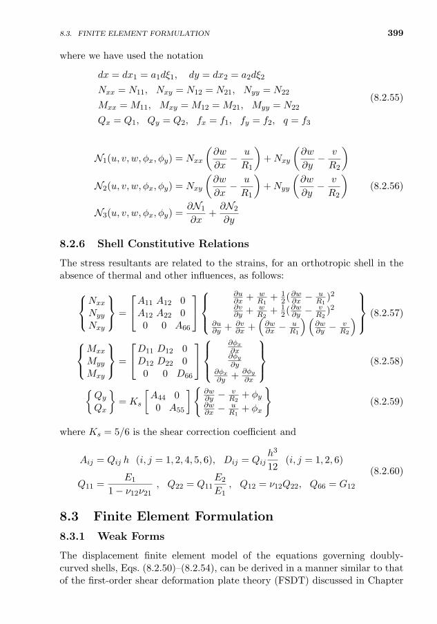
8.3. FINITE ELEMENT FORMULATION 399
where we have used the notation
dx = dx1 = a1dξ1, dy = dx2 = a2dξ2
Nxx = N11, Nxy = N12 = N21, Nyy = N22
Mxx = M11, Mxy = M12 = M21, Myy = N22
Qx = Q1, Qy = Q2, fx = f1, fy = f2, q = f3
(8.2.55)
N1(u, v, w, φx, φy) = Nxx
(∂w
∂x− u
R1
)+Nxy
(∂w
∂y− v
R2
)N2(u, v, w, φx, φy) = Nxy
(∂w
∂x− u
R1
)+Nyy
(∂w
∂y− v
R2
)(8.2.56)
N3(u, v, w, φx, φy) =∂N1
∂x+∂N2
∂y
8.2.6 Shell Constitutive Relations
The stress resultants are related to the strains, for an orthotropic shell in theabsence of thermal and other influences, as follows:
Nxx
Nyy
Nxy
=
A11 A12 0A12 A22 00 0 A66
∂u∂x + w
R1+ 1
2(∂w∂x −uR1
)2
∂v∂y + w
R2+ 1
2(∂w∂y −vR2
)2
∂u∂y + ∂v
∂x +(∂w∂x −
uR1
)(∂w∂y −
vR2
) (8.2.57)
Mxx
Myy
Mxy
=
D11 D12 0D12 D22 0
0 0 D66
∂φx∂x∂φy∂y
∂φx∂y +
∂φy∂x
(8.2.58)
QyQx
= Ks
[A44 00 A55
] ∂w∂y −
vR2
+ φy∂w∂x −
uR1
+ φx
(8.2.59)
where Ks = 5/6 is the shear correction coefficient and
Aij = Qij h (i, j = 1, 2, 4, 5, 6), Dij = Qijh3
12(i, j = 1, 2, 6)
Q11 =E1
1− ν12ν21, Q22 = Q11
E2
E1, Q12 = ν12Q22, Q66 = G12
(8.2.60)
8.3 Finite Element Formulation
8.3.1 Weak Forms
The displacement finite element model of the equations governing doubly-curved shells, Eqs. (8.2.50)–(8.2.54), can be derived in a manner similar to thatof the first-order shear deformation plate theory (FSDT) discussed in Chapter
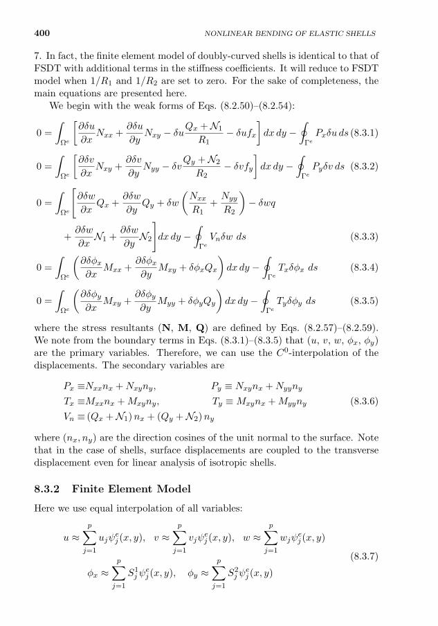
400 NONLINEAR BENDING OF ELASTIC SHELLS
7. In fact, the finite element model of doubly-curved shells is identical to that ofFSDT with additional terms in the stiffness coefficients. It will reduce to FSDTmodel when 1/R1 and 1/R2 are set to zero. For the sake of completeness, themain equations are presented here.
We begin with the weak forms of Eqs. (8.2.50)–(8.2.54):
0 =
∫Ωe
[∂δu
∂xNxx +
∂δu
∂yNxy − δu
Qx +N1
R1− δufx
]dx dy −
∮Γe
Pxδu ds (8.3.1)
0 =
∫Ωe
[∂δv
∂xNxy +
∂δv
∂yNyy − δv
Qy +N2
R2− δvfy
]dx dy −
∮Γe
Pyδv ds (8.3.2)
0 =
∫Ωe
[∂δw
∂xQx +
∂δw
∂yQy + δw
(Nxx
R1+Nyy
R2
)− δwq
+∂δw
∂xN1 +
∂δw
∂yN2
]dx dy −
∮Γe
Vnδw ds (8.3.3)
0 =
∫Ωe
(∂δφx∂x
Mxx +∂δφx∂y
Mxy + δφxQx
)dx dy −
∮Γe
Txδφx ds (8.3.4)
0 =
∫Ωe
(∂δφy∂x
Mxy +∂δφy∂y
Myy + δφyQy
)dx dy −
∮Γe
Tyδφy ds (8.3.5)
where the stress resultants (N, M, Q) are defined by Eqs. (8.2.57)–(8.2.59).We note from the boundary terms in Eqs. (8.3.1)–(8.3.5) that (u, v, w, φx, φy)are the primary variables. Therefore, we can use the C0-interpolation of thedisplacements. The secondary variables are
Px ≡Nxxnx +Nxyny, Py ≡ Nxynx +Nyyny
Tx ≡Mxxnx +Mxyny, Ty ≡Mxynx +Myyny
Vn ≡ (Qx +N1)nx + (Qy +N2)ny
(8.3.6)
where (nx, ny) are the direction cosines of the unit normal to the surface. Notethat in the case of shells, surface displacements are coupled to the transversedisplacement even for linear analysis of isotropic shells.
8.3.2 Finite Element Model
Here we use equal interpolation of all variables:
u ≈p∑j=1
ujψej (x, y), v ≈
p∑j=1
vjψej (x, y), w ≈
p∑j=1
wjψej (x, y)
φx ≈p∑j=1
S1jψ
ej (x, y), φy ≈
p∑j=1
S2jψ
ej (x, y)
(8.3.7)
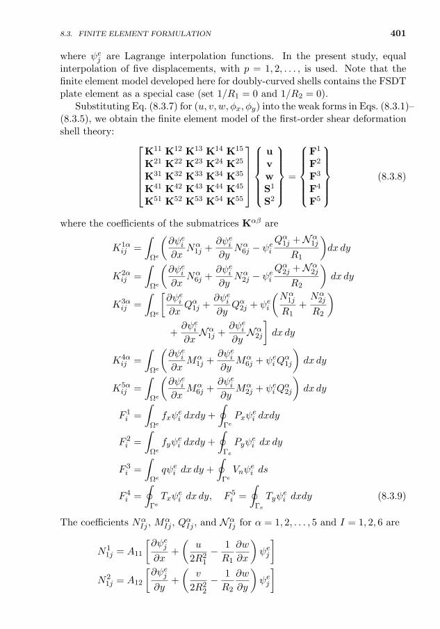
8.3. FINITE ELEMENT FORMULATION 401
where ψej are Lagrange interpolation functions. In the present study, equalinterpolation of five displacements, with p = 1, 2, . . . , is used. Note that thefinite element model developed here for doubly-curved shells contains the FSDTplate element as a special case (set 1/R1 = 0 and 1/R2 = 0).
Substituting Eq. (8.3.7) for (u, v, w, φx, φy) into the weak forms in Eqs. (8.3.1)–(8.3.5), we obtain the finite element model of the first-order shear deformationshell theory:
K11 K12 K13 K14 K15
K21 K22 K23 K24 K25
K31 K32 K33 K34 K35
K41 K42 K43 K44 K45
K51 K52 K53 K54 K55
uvwS1
S2
=
F1
F2
F3
F4
F5
(8.3.8)
where the coefficients of the submatrices Kαβ are
K1αij =
∫Ωe
(∂ψei∂x
Nα1j +
∂ψei∂y
Nα6j − ψei
Qα1j +Nα1j
R1
)dx dy
K2αij =
∫Ωe
(∂ψei∂x
Nα6j +
∂ψei∂y
Nα2j − ψei
Qα2j +Nα2j
R2
)dx dy
K3αij =
∫Ωe
[∂ψei∂x
Qα1j +∂ψei∂y
Qα2j + ψei
(Nα
1j
R1+Nα
2j
R2
)+∂ψei∂xNα
1j +∂ψei∂yNα
2j
]dx dy
K4αij =
∫Ωe
(∂ψei∂x
Mα1j +
∂ψei∂y
Mα6j + ψeiQ
α1j
)dx dy
K5αij =
∫Ωe
(∂ψei∂x
Mα6j +
∂ψei∂y
Mα2j + ψeiQ
α2j
)dx dy
F 1i =
∫Ωe
fxψei dxdy +
∮Γe
Pxψei dxdy
F 2i =
∫Ωe
fyψei dxdy +
∮Γe
Pyψei dx dy
F 3i =
∫Ωe
qψei dx dy +
∮Γe
Vnψei ds
F 4i =
∮Γe
Txψei dx dy, F 5
i =
∮Γe
Tyψei dxdy (8.3.9)
The coefficients NαIj , M
αIj , Q
αIj , and Nα
Ij for α = 1, 2, . . . , 5 and I = 1, 2, 6 are
N11j = A11
[∂ψej∂x
+
(u
2R21
− 1
R1
∂w
∂x
)ψej
]N2
1j = A12
[∂ψej∂y
+
(v
2R22
− 1
R2
∂w
∂y
)ψej
]
402 NONLINEAR BENDING OF ELASTIC SHELLS
N31j =
(A11
R1+A12
R2
)ψej +
1
2
(A11
∂w
∂x
∂ψej∂x
+A12∂w
∂y
∂ψej∂y
)N1
6j = A66
[∂ψej∂y− 1
R1
(∂w
∂y− 1
2
v
R2
)ψej
]N2
6j = A66
[∂ψej∂x− 1
R2
(∂w
∂x− 1
2
u
R1
)ψej
]N3
6j =A66
2
(∂w
∂x
∂ψej∂y
+∂w
∂y
∂ψej∂x
)N1
2j = A12
[∂ψej∂x
+
(u
2R21
− 1
R1
∂w
∂x
)ψej
]N2
2j = A22
[∂ψej∂y
+
(v
2R22
− 1
R2
∂w
∂y
)ψej
]N3
2j =
(A12
R1+A22
R2
)ψej +
1
2
(A12
∂w
∂x
∂ψej∂x
+A22∂w
∂y
∂ψej∂y
)N4
6j = 0, N56j = 0, N4
1j = 0, N51j = 0, N4
2j = 0, N52j = 0
Q11j = −KsA55
R1ψej , Q3
1j = KsA55
∂ψej∂x
, Q41j = KsA55ψ
ej
Q22j = −KsA44
R2ψej , Q3
2j = KsA44
∂ψej∂y
, Q52j = KsA44ψ
ej
Q21j = 0, Q5
1j = 0, Q12j = 0, Q4
2j = 0
N 11j = −Nxx
R1ψej , N 2
1j = −Nxy
R2ψej , N 3
1j = Nxx
∂ψej∂x
+Nxy
∂ψej∂y
N 12j = −Nxy
R1ψej , N 2
2j = −Nyy
R2ψej , N 3
2j = Nxy
∂ψej∂x
+Nyy
∂ψej∂y
N 41j = 0, N 5
1j = 0, N 42j = 0, N 5
2j = 0
M11j = M2
1j = M31j = 0, M4
1j = D11
∂ψej∂x
, M51j = D12
∂ψej∂y
M12j = M2
2j = M32j = 0, M4
2j = D12
∂ψej∂x
, M52j = D22
∂ψej∂y
M16j = M2
6j = M36j = 0, M4
6j = D66
∂ψej∂y
, M56j = D66
∂ψej∂x
(8.3.10)
8.3.3 Linear Analysis
Numerical results are presented here for linear analysis of some benchmarkproblems from the literature. Quadrilateral elements are used with selectiveintegration rule to evaluate the stiffness coefficients: full integration for bendingterms and reduced integration for bending-membrane coupling terms as well astransverse shear terms.
8.3. FINITE ELEMENT FORMULATION 403
Example 8.3.1
Consider the deformation of a cylindrical shell with internal pressure. The shell is clampedat its ends (see Fig. 8.3.1). The geometric and material parameters used are:
R1 = 1030 (or 1/R1 ≈ 0) , R2 = R = 20 in, a = 20 in, h = 1 in (1)
E1 = 7.5 × 10⁶ psi, E2 = 2 × 10⁶ psi, G12 = 1.25 × 10⁶ psi
G13 = G23 = 0.625 × 10⁶ psi, ν12 = 0.25(2)
Assume a transverse pressure of p0 = (6.41/π) ksi. Using 4× 4 mesh of four-node rectangularelements (4 × 4L4) and 2 × 2 mesh of nine-node (quadratic) rectangular elements (2 × 2Q9)in an octant (u = φx = 0 at x = 0; v = φy = 0 at y = 0, πR/2; and u = v = w = φx = φy = 0at x = a/2) of the shell, obtain the maximum transverse deflection.
Solution: The numerical results obtained are presented in Table 8.3.1. The reference solutionsby Rao [115] and Timoshenko and Woinowsky-Krieger [86] did not account for the transverseshear strains.
x1
ζ = x3
Rp0
a
ζ = x3
x2
p0
Fig. 8.3.1
Fig. 8.3.1: Clamped cylindrical shell with internal pressure.
Table 8.3.1: Maximum radial deflection (w in) of a clamped cylindrical shell withinternal pressure.
Laminate Present solution Ref. [115] Ref. [86]
4 × 4L4 2 × 2Q9
0 0.3754 0.3727 0.3666 0.367
Example 8.3.2
Consider a doubly-curved spherical shell panel (R1 = R2 = R) under a central point loadF0 = 100 lbs. The shell panel is simply supported at edges (see Fig. 8.3.2). The geometricand material parameters to be used are:
R1 = R2 = R = 96 in, a = b = 32 in, h = 0.1 in
E1 = 25E2, E2 = 106 psi, G12 = G13 = 0.5E2, G23 = 0.2E2, ν12 = 0.25(1)
404 NONLINEAR BENDING OF ELASTIC SHELLS
hξ1
ξ2
ζ
x1
x2
x3
R2 R1
b a
F0
Fig. 8.3.2: Simply supported spherical shell panel under central point load.
Analyze the problem for isotropic (E = 25 × 106 and ν = 0.25) and orthotropic materialproperties using various meshes.
Solution: The numerical results obtained using various meshes of linear and quadratic ele-ments in a quadrant of the shell are presented in Table 8.3.2. The finite element solutionconverges with refinement of the mesh to the series solution of Vlasov [94], who did notconsider transverse shear strains in his analysis.
Table 8.3.2: Maximum radial deflection (−w× 10 in) of a simply supported sphericalshell panel under central point load.
Material Present results Ref. [115] Ref. [94]
4 × 4L4 2 × 2Q9 4 × 4Q9 4 × 4Q9Uniform Uniform Uniform Nonuniform
Isotropic 0.3506 0.3726 0.3904 0.3935 0.3866 0.3956
Orthotropic 0.9373 1.0349 − 1.2644 − −
The remaining example problems of this chapter are analyzed using variousp levels [see Eq. (8.3.7)]. With five degrees of freedom at each node, the numberof degrees of freedom per element for different p values are presented in Table8.3.3.
The numerical integration rule (Gauss quadrature) used is I×J×K, whereK denotes the Gauss rule (i.e. K ×K) used to evaluate the transverse shearterms (i.e. those containing A44 and A55), J denotes the Gauss rule used toevaluate the bending-membrane coupling terms (which are zero for the linearanalysis of plates), and I denotes the Gauss rule used to evaluate all remainingterms in the stiffness matrix. One may use full integration for all terms, reduced
8.3. FINITE ELEMENT FORMULATION 405
Table 8.3.3: Number of degrees of freedom per element for different p.
Element type p level DoF per element
L4 1 20
Q9 2 45
Q25 4 125
Q49 6 245
Q81 8 405
integration for all terms, or selective integration where reduced integration fortransverse shear and coupling terms and full integration for all other terms inthe stiffness matrix. The values of I, J , and K used in the present study fordifferent p levels and integration rules are listed in Table 8.3.4.
Table 8.3.4: The Gauss quadrature rule used for various terms.
p Full Selective Reducedintegration integration integration
1 2× 2× 2 2× 1× 1 1× 1× 12 3× 3× 3 3× 2× 2 2× 2× 24 5× 5× 5 5× 4× 4 4× 4× 46 7× 7× 7 7× 6× 6 6× 6× 68 9× 9× 9 9× 8× 8 8× 8× 8
Example 8.3.3
Consider a clamped isotropic cylindrical shell panel with the following geometric and materialparameters and subjected to uniformly distributed transverse (normal to the surface) load q(see Fig. 8.3.3):
α =0.1 rad, R = 100 in, a = 20 in, h = 0.125 in
E = 0.45 × 10⁶ psi, ν = 0.3, q = 0.04 psi(1)
Use two sets of uniform meshes, one with 81 nodes (405 DoF) and the other with 289 nodes(1,445 DoF), in a quadrant of the shell with different p levels to analyze the problem.
Solution: For p = 1 the mesh is 8×8Q4, for p = 2 the mesh is 4×4Q9, and for p = 8 the meshis 1 × 1Q81 – all meshes have a total of 81 nodes. Doubling the above meshes will have 289nodes. The vertical displacement at the center of the shell obtained with various meshes andintegration rules are presented in Table 8.3.5. The results obtained with selective and reducedintegrations are in close agreement with those of Palazotto and Dennis [93] and Brebbia andConnor [116].
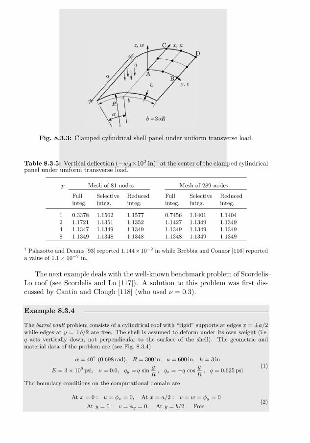
406 NONLINEAR BENDING OF ELASTIC SHELLS
AB
CD
Fig. 8.3.3: Clamped cylindrical shell panel under uniform transverse load.
Table 8.3.5: Vertical deflection (−wA×102 in)† at the center of the clamped cylindricalpanel under uniform transverse load.
p Mesh of 81 nodes Mesh of 289 nodes
Full Selective Reduced Full Selective Reducedinteg. integ. integ. integ. integ. integ.
1 0.3378 1.1562 1.1577 0.7456 1.1401 1.14042 1.1721 1.1351 1.1352 1.1427 1.1349 1.13494 1.1347 1.1349 1.1349 1.1349 1.1349 1.13498 1.1349 1.1348 1.1348 1.1348 1.1349 1.1349
† Palazotto and Dennis [93] reported 1.144×10⁻² in while Brebbia and Connor [116] reporteda value of 1.1 × 10⁻² in.
The next example deals with the well-known benchmark problem of Scordelis–Lo roof (see Scordelis and Lo [117]). A solution to this problem was first dis-cussed by Cantin and Clough [118] (who used ν = 0.3).
Example 8.3.4
The barrel vault problem consists of a cylindrical roof with “rigid” supports at edges x = ±a/2while edges at y = ±b/2 are free. The shell is assumed to deform under its own weight (i.e.q acts vertically down, not perpendicular to the surface of the shell). The geometric andmaterial data of the problem are (see Fig. 8.3.4)
α = 40 (0.698 rad), R = 300 in, a = 600 in, h = 3 in
E = 3 × 10⁶ psi, ν = 0.0, qy = q siny
R, qz = −q cos
y
R, q = 0.625 psi
(1)
The boundary conditions on the computational domain are
At x = 0 : u = φx = 0, At x = a/2 : v = w = φy = 0
At y = 0 : v = φy = 0, At y = b/2 : Free(2)
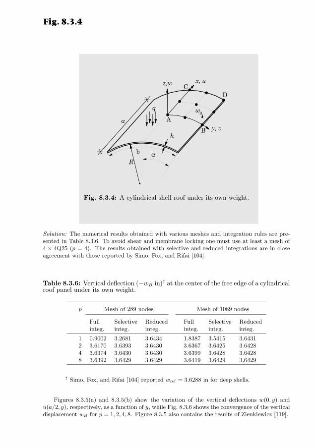
8.3. FINITE ELEMENT FORMULATION 407
Use two sets of uniform meshes, one with 289 nodes (1,445 DoF) and the other with1,089 nodes (5,445 DoF), in a quadrant of the shell with different p levels to determine thedisplacement at x = 0 and y = ±b/2 (middle of the free edge) of the shell.
y, v
x, u
a
b
z,w
R
h
q
α
A
B
wB
CD
Fig. 8.3.4
Fig. 8.3.4: A cylindrical shell roof under its own weight.
Solution: The numerical results obtained with various meshes and integration rules are pre-sented in Table 8.3.6. To avoid shear and membrane locking one must use at least a mesh of4 × 4Q25 (p = 4). The results obtained with selective and reduced integrations are in closeagreement with those reported by Simo, Fox, and Rifai [104].
Table 8.3.6: Vertical deflection (−wB in)† at the center of the free edge of a cylindricalroof panel under its own weight.
p Mesh of 289 nodes Mesh of 1089 nodes
Full Selective Reduced Full Selective Reducedinteg. integ. integ. integ. integ. integ.
1 0.9002 3.2681 3.6434 1.8387 3.5415 3.64312 3.6170 3.6393 3.6430 3.6367 3.6425 3.64284 3.6374 3.6430 3.6430 3.6399 3.6428 3.64288 3.6392 3.6429 3.6429 3.6419 3.6429 3.6429
† Simo, Fox, and Rifai [104] reported wref = 3.6288 in for deep shells.
Figures 8.3.5(a) and 8.3.5(b) show the variation of the vertical deflections w(0, y) andu(a/2, y), respectively, as a function of y, while Fig. 8.3.6 shows the convergence of the verticaldisplacement wB for p = 1, 2, 4, 8. Figure 8.3.5 also contains the results of Zienkiewicz [119].
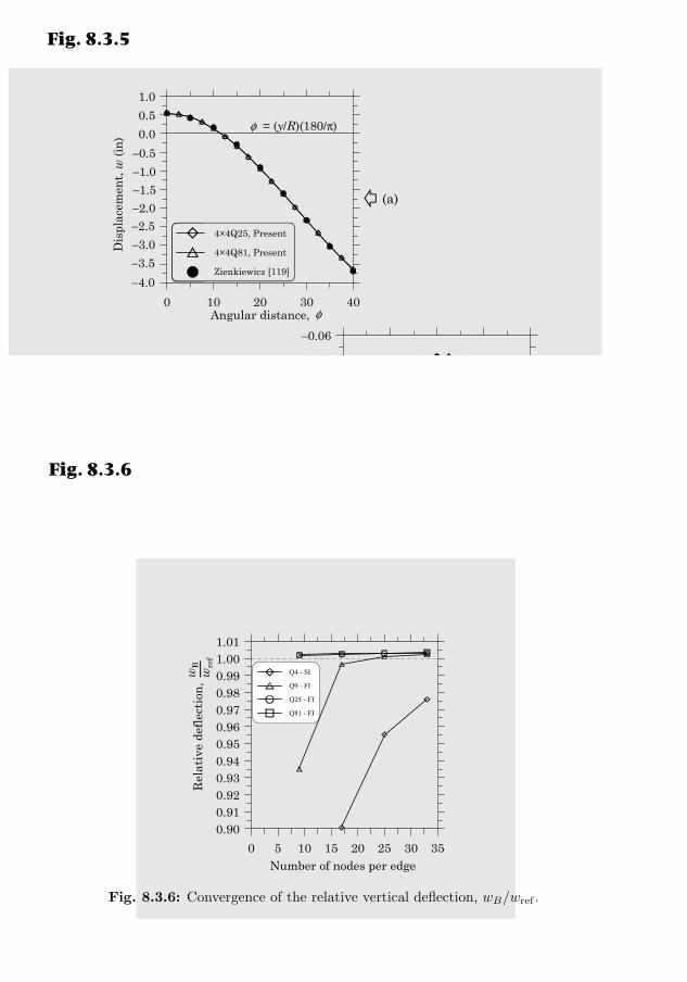
408 NONLINEAR BENDING OF ELASTIC SHELLSFig. 8.3.5
(a)
φ = (y/R)(180/π)
φ
-4.0
-3.5
-3.0
-2.5
-2.0
-1.5
-1.0
-0.5
0.0
0.5
1.0
Ver
tica
l de
flec
tion
,
4x4Q25 - Present
4x4Q81 - Present
Zienkiewicz [58]
0 10 20 30 40Angular distance,
4×4Q25, Present
4×4Q81, Present
Zienkiewicz [119]
−0.5
−1.0
−1.5
−2.0−2.5
−3.0
−3.5
−4.0
Dis
plac
emen
t, w
(in
)
(b)
u(i
n)
φ
-0.06
-0.03
0.00
0.03
0.06
0.09
0.12
0.15
0.18
Dis
plac
emen
t,
4x4Q25 - Present
4x4Q81 - Present
Zienkiewicz [58]
0 10 20 30 40Angular distance,
4×4Q25, Present
4×4Q81, Present
Zienkiewicz [119]
−0.06
−0.03
Dis
plac
emen
t, u
(in
)
Fig. 8.3.5: (a) Deflection w(0, y). (b) Displacement u(a/2, y).
wB
wre
f
0.900.910.920.930.940.950.960.970.980.991.001.01
Rel
ativ
e de
flec
tion
,
0 5 10 15 20 25 30 35Number of nodes per edge
Q4 - SI
Q9 - FI
Q25 - FI
Q81 - FI
Fig. 8.3.6
Fig. 8.3.6: Convergence of the relative vertical deflection, wB/wref .
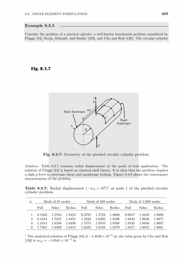
8.3. FINITE ELEMENT FORMULATION 409
Example 8.3.5
Consider the problem of a pinched cylinder, a well-known benchmark problem considered byFlugge [84], Kreja, Schmidt, and Reddy [102], and Cho and Roh [120]. The circular cylinderwith “rigid” end diaphragms is subjected to a point load at the center on opposite sides ofthe cylinder, as shown in Fig. 8.3.7. The geometric and material data are
α =π
2rad, R = 300 in, a = 600 in, h = 3 in
E = 3 × 10⁶ psi, ν12 = 0.3(1)
The boundary conditions for the computational domain are
At x = 0 : u = φx = 0, At x = a/2 : v = w = φy = 0
At y = 0, b/2 : v = φy = 0(2)
Use three different meshes with 81 nodes, 289 nodes, and 1,089 nodes (with different p values)in the octant of the cylinder to analyze the problem.
Fig. 8.3.7
Fig. 8.3.7: Geometry of the pinched circular cylinder problem.
Solution: Table 8.3.7 contains radial displacement at the point of load application. Thesolution of Flugge [84] is based on classical shell theory. It is clear that the problem requiresa high p level to overcome shear and membrane locking. Figure 8.3.8 shows the convergencecharacteristics of the problem.
Table 8.3.7: Radial displacement (−wA × 105)† at node 1 of the pinched circularcylinder problem.
p Mesh of 81 nodes Mesh of 289 nodes Mesh of 1,089 nodes
Full Selec. Reduc. Full Selec. Reduc. Full Selec. Reduc.
1 0.1282 1.5784 1.8453 0.2785 1.7724 1.8600 0.6017 1.8432 1.86902 0.4184 1.7247 1.8451 1.2238 1.8395 1.8596 1.6844 1.8636 1.86774 1.1814 1.8108 1.8438 1.7574 1.8510 1.8586 1.8335 1.8648 1.86678 1.7562 1.8309 1.8415 1.8325 1.8548 1.8579 1.8471 1.8653 1.8661
† The analytical solution of Flugge [84] is −1.8248× 10⁻⁵ in; the value given by Cho and Roh[120] is wref = −1.8541 × 10⁻⁵ in.
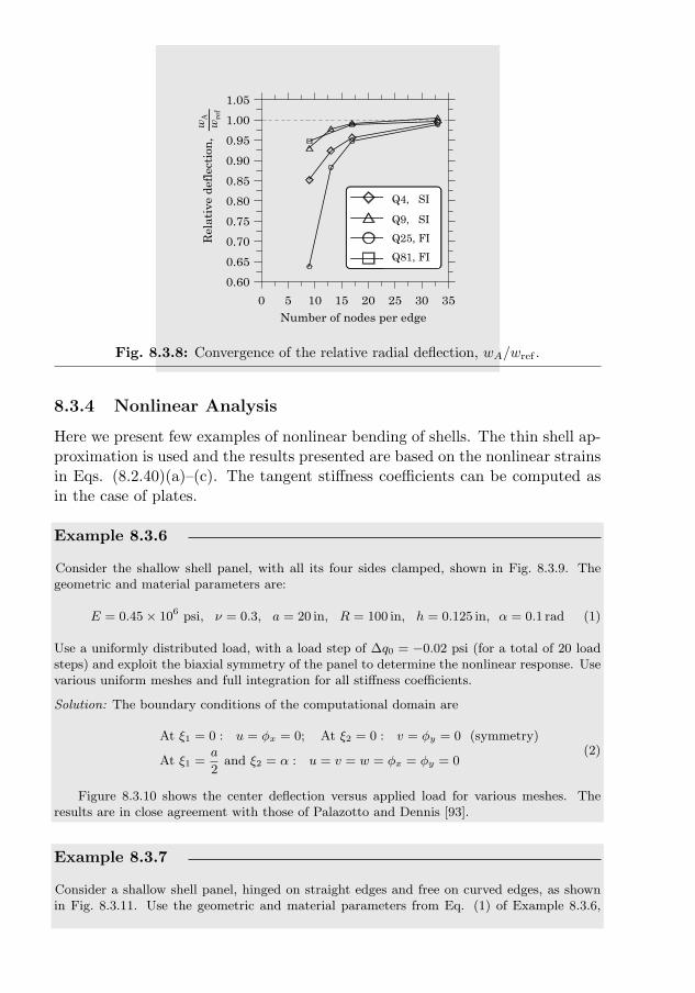
410 NONLINEAR BENDING OF ELASTIC SHELLS
0.60
0.65
0.70
0.75
0.80
0.85
0.90
0.95
1.00
1.05
Rel
ativ
e de
flec
tion
,
0 5 10 15 20 25 30 35Number of nodes per edge
Q4 - SI
Q9 - SI
Q25 - FI
Q81 - FI
wA
wre
f
Q4, SI
Q9, SI
Q25, FI
Q81, FI
Fig. 8.3.8: Convergence of the relative radial deflection, wA/wref .
8.3.4 Nonlinear Analysis
Here we present few examples of nonlinear bending of shells. The thin shell ap-proximation is used and the results presented are based on the nonlinear strainsin Eqs. (8.2.40)(a)–(c). The tangent stiffness coefficients can be computed asin the case of plates.
Example 8.3.6
Consider the shallow shell panel, with all its four sides clamped, shown in Fig. 8.3.9. Thegeometric and material parameters are:
E = 0.45 × 10⁶ psi, ν = 0.3, a = 20 in, R = 100 in, h = 0.125 in, α = 0.1 rad (1)
Use a uniformly distributed load, with a load step of ∆q0 = −0.02 psi (for a total of 20 loadsteps) and exploit the biaxial symmetry of the panel to determine the nonlinear response. Usevarious uniform meshes and full integration for all stiffness coefficients.
Solution: The boundary conditions of the computational domain are
At ξ1 = 0 : u = φx = 0; At ξ2 = 0 : v = φy = 0 (symmetry)
At ξ1 =a
2and ξ2 = α : u = v = w = φx = φy = 0
(2)
Figure 8.3.10 shows the center deflection versus applied load for various meshes. Theresults are in close agreement with those of Palazotto and Dennis [93].
Example 8.3.7
Consider a shallow shell panel, hinged on straight edges and free on curved edges, as shownin Fig. 8.3.11. Use the geometric and material parameters from Eq. (1) of Example 8.3.6,
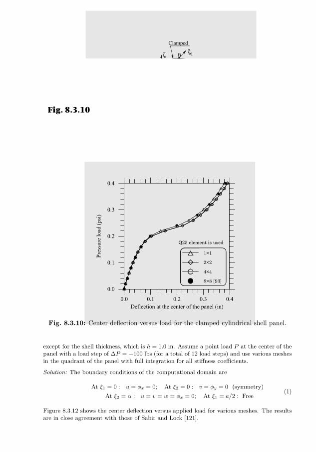
8.3. FINITE ELEMENT FORMULATION 411
ξ1
a
bR
α
A
BC
D
h
q0
Rξ2
ζ
Clamped
Clamped
Clamped
Clamped
Fig. 8.3.9: Geometry and computational domain of the cylindrical shell panel.
0.0
0.1
0.2
0.3
0.4
Pres
sure
load
(psi
)
0.0 0.1 0.2 0.3 0.4Deflection at the center of the panel (in)
1x1Q25
2x2Q25
4x4Q25
8x8Q [51]
Fig. 8.3.10
[93]
1×1
2×2
4×4
8×8 [93]
Q25 element is used
Fig. 8.3.10: Center deflection versus load for the clamped cylindrical shell panel.
except for the shell thickness, which is h = 1.0 in. Assume a point load P at the center of thepanel with a load step of ∆P = −100 lbs (for a total of 12 load steps) and use various meshesin the quadrant of the panel with full integration for all stiffness coefficients.
Solution: The boundary conditions of the computational domain are
At ξ1 = 0 : u = φx = 0; At ξ2 = 0 : v = φy = 0 (symmetry)
At ξ2 = α : u = v = w = φx = 0; At ξ1 = a/2 : Free(1)
Figure 8.3.12 shows the center deflection versus applied load for various meshes. The resultsare in close agreement with those of Sabir and Lock [121].
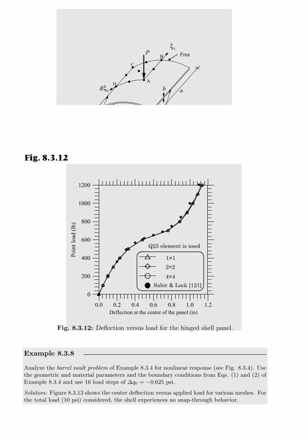
412 NONLINEAR BENDING OF ELASTIC SHELLS
ξ1
a
bR α
A
BC
DhRξ2
Hinged
Hinged
P Free
Free
Fig. 8.3.11: Geometry and computational domain of the shell panel.
0
200
400
600
800
1000
1200
Poin
t loa
d (lb
)
1x1Q25
2x2Q25
4x4Q25
Sabir and Lock [61]
0.0 0.2 0.4 0.6 0.8 1.0 1.2Deflection at the center of the panel (in)
Fig. 8.3.12
Sabir & Lock [121]
Q25 element is used
1×1
2×2
4×4
Fig. 8.3.12: Deflection versus load for the hinged shell panel.
Example 8.3.8
Analyze the barrel vault problem of Example 8.3.4 for nonlinear response (see Fig. 8.3.4). Usethe geometric and material parameters and the boundary conditions from Eqs. (1) and (2) ofExample 8.3.4 and use 16 load steps of ∆q0 = −0.625 psi.
Solution: Figure 8.3.13 shows the center deflection versus applied load for various meshes. Forthe total load (10 psi) considered, the shell experiences no snap-through behavior.
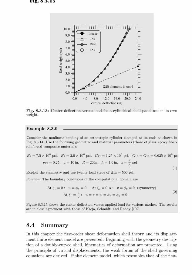
8.4. SUMMARY 413
0.0
1.0
2.0
3.0
4.0
5.0
6.0
7.0
8.0
9.0
10.0
Dea
d w
eigh
t (ps
i)
Linear
1x1Q25
2x2Q25
4x4Q25
0.0 4.0 8.0 12.0 16.0 20.0 24.0Vertical deflection (in)
Fig. 8.3.13
1×1
Q25 element is used
2×2
4×4
Linear
Fig. 8.3.13: Center deflection versus load for a cylindrical shell panel under its ownweight.
Example 8.3.9
Consider the nonlinear bending of an orthotropic cylinder clamped at its ends as shown inFig. 8.3.14. Use the following geometric and material parameters (those of glass–epoxy fiber-reinforced composite material):
E1 = 7.5 × 10⁶ psi, E2 = 2.0 × 10⁶ psi, G12 = 1.25 × 10⁶ psi, G13 = G23 = 0.625 × 10⁶ psi
ν12 = 0.25, a = 10 in, R = 20 in, h = 1.0 in, α =π
8rad
(1)Exploit the symmetry and use twenty load steps of ∆q0 = 500 psi.
Solution: The boundary conditions of the computational domain are
At ξ1 = 0 : u = φx = 0; At ξ2 = 0, α : v = φy = 0 (symmetry)
At ξ1 =a
2: u = v = w = φx = φy = 0
(2)
Figure 8.3.15 shows the center deflection versus applied load for various meshes. The resultsare in close agreement with those of Kreja, Schmidt, and Reddy [102].
8.4 Summary
In this chapter the first-order shear deformation shell theory and its displace-ment finite element model are presented. Beginning with the geometry descrip-tion of a doubly-curved shell, kinematics of deformation are presented. Usingthe principle of virtual displacements, the weak forms of the shell governingequations are derived. Finite element model, which resembles that of the first-
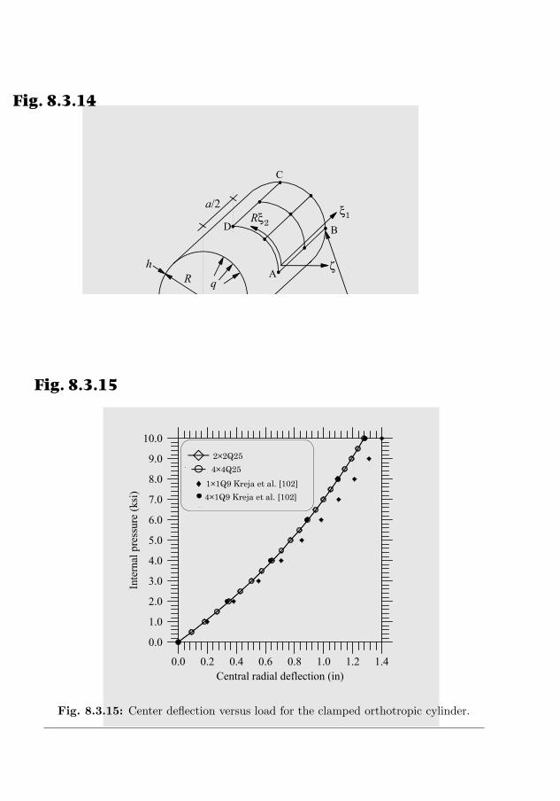
414 NONLINEAR BENDING OF ELASTIC SHELLS
order shear deformation plate theory, is developed and some numerical examplesare presented. The shell finite element developed here contains the FSDT plateelement as a special case. Therefore, it can be used to analyze plate problemsas well.
a/2
hR A
B
C
Dξ1
ζ
Rξ2
Clamped
q
Fig. 8.3.14
Fig. 8.3.14: Geometry and computational domain of a clamped circular cylinder.
0.0
1.0
2.0
3.0
4.0
5.0
6.0
7.0
8.0
9.0
10.0
Inte
rnal
pre
ssur
e (k
si)
2x2Q25
4x4Q25
1x1Q9 Kreja et al. [60]
4x1Q9 Kreja et al. [60]
0.0 0.2 0.4 0.6 0.8 1.0 1.2 1.4Central radial deflection (in)
Fig. 8.3.15
• 4×1Q9 Kreja et al. [102]
♦ 1×1Q9 Kreja et al. [102]
4×4Q25
2×2Q25
Fig. 8.3.15: Center deflection versus load for the clamped orthotropic cylinder.
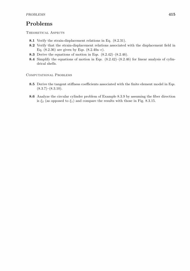
PROBLEMS 415
Problems
Theoretical Aspects
8.1 Verify the strain-displacement relations in Eq. (8.2.31).
8.2 Verify that the strain-displacement relations associated with the displacement field inEq. (8.2.36) are given by Eqs. (8.2.40a–c).
8.3 Derive the equations of motion in Eqs. (8.2.42)–(8.2.46).
8.4 Simplify the equations of motion in Eqs. (8.2.42)–(8.2.46) for linear analysis of cylin-drical shells.
Computational Problems
8.5 Derive the tangent stiffness coefficients associated with the finite element model in Eqs.(8.3.7)–(8.3.10).
8.6 Analyze the circular cylinder problem of Example 8.3.9 by assuming the fiber directionis ξ2 (as opposed to ξ1) and compare the results with those in Fig. 8.3.15.

417
9
Finite Element Formulationsof Solid Continua
The fact that an opinion has been widely held is no evidence whatever that it is not utterlyabsurd; indeed in view of the silliness of the majority of mankind a widespread belief is morelikely to be foolish than sensible. ——– Bertrand Russell
9.1 Introduction
9.1.1 Background
In chapters leading to the present one, we have assumed that the system un-der consideration was continuous in the sense that all field variables that enterthe description of the physical phenomenon, such as temperature and displace-ments, are differentiable. Central to this assumption is that the discrete natureof matter can be overlooked, provided the length scales of interest are largecompared to the length scales of discrete molecular structure. Thus, matter atsufficiently large length scales can be treated as a continuum in which all phys-ical quantities of interest, including density, are continuously differentiable.
Another assumption that was implicit in writing the equations in the previ-ous chapters was that changes in the geometry of the domain are negligible sothat the physical principles can be applied to “undeformed” configuration. Ingeometrically nonlinear analysis of beams and plates that was considered in ear-lier chapters, the assumption of small strains allowed us to ignore the changesin the geometry of the body, and no distinction between various measures ofstress and strain was made as we proceeded to determine the deformation forthe next load.
When large changes in the original configuration occur, the physical princi-ple should be stated in the deformed configuration, which is not known a pri-ori. In this chapter, we shall study geometrically nonlinear behavior in whichchanges in geometry are updated. Consequently, it becomes necessary to distin-guish between various measures of stress and strain and descriptions of motion,as discussed in Chapter 2. Intuition tells us that if the strain energy is basedon the product of stress and strain, it is not expected to change simply becauseof our choice of stress or strain measure. Thus, “energetically conjugate” pairsof stress and strain that produce the same strain energy must be used [1].
J.N. Reddy, An Introduction to Nonlinear Finite Element Analysis, Second Edition. c©J.N.Reddy 2015. Published in 2015 by Oxford University Press.
418 FINITE ELEMENT FORMULATIONS OF SOLID CONTINUA
9.1.2 Summary of Definitions and Conceptsfrom Continuum Mechanics
The main equations of Chapter 2 that are useful in the present chapter aresummarized here for ready reference (refer to Fig. 9.1.1 for the notation).
• Kinematics:
Material coordinates: X = (X1, X2, X3)
Spatial coordinates: x = (x1, x2, x3) (9.1.1)
Motion mapping: x = χ(X, t), X = χ−1(x, t)
Material and spatial gradients: ∇0 = ∂/∂X , ∇ = ∂/∂x
• Displacement vector:
u(x, t) = x−X(x, t) = x− χ−1(x, t) (9.1.2)
• Deformation gradient:F = (∇0x)T (9.1.3)
• Green–Lagrange strain tensor:
E =1
2
(FT · F− I
)=
1
2
[∇0u + (∇0u)T + (∇0u) · (∇0u)T
](9.1.4)
• Euler–Almansi strain tensor:
e =1
2
(I− F−T · F−1
)=
1
2
[∇u + (∇u)T − (∇u) · (∇u)T
](9.1.5)
• Velocity gradient tensor:
l =
(∂v(x, t)
∂x
)T
= (∇v(x, t))T = d + w (9.1.6)
• Symmetric and skew-symmetric parts of l:
d =1
2
[∇v + (∇v)T
]= dT, w =
1
2
[(∇v)T −∇v
]= −wT (9.1.7)
• Nanson’s formula:n da = JF−T · N dA (9.1.8)
• Relationships:
e = F−T ·E · F−1, E = FT · e · F
F ≡ dF
dt= (∇0v)T , l = F · F−1, d = F−T · E · F−1
(9.1.9)
• Stress measures (σ = Cauchy stress tensor; P = first Piola–Kirchhoff stresstensor; S = second Piola–Kirchhoff stress tensor):
P = Jσ · F−T, S = F−1 ·P = JF−1 · σ · F−T (9.1.10)
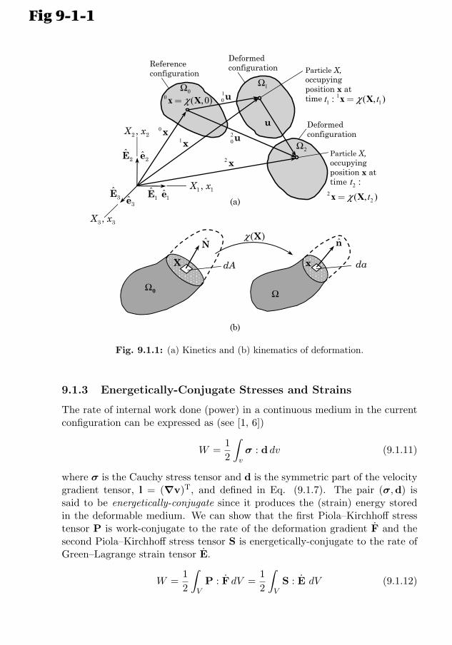
9.1. INTRODUCTION 419
n
da
N
dA
X( )χ
X x
Ω0 Ω
(b)
1 1,X x
2 2,X x
3 3,X x
e3ˆe1ˆE1
ˆE3ˆ
e2ˆE2ˆ
Reference configuration
Deformed configuration Particle X,
occupying position x at time
Deformed configuration
Particle X, occupying position x at time
1Ω0 ( ,0)=x Xχ 1
1 1: ( , )=x Xt tχ0Ω
2Ω
(a)
0 x1x
2 x
10u
20u
2 :t2
2( , )=x X tχ
u
Fig 9-1-1
Fig. 9.1.1: (a) Kinetics and (b) kinematics of deformation.
9.1.3 Energetically-Conjugate Stresses and Strains
The rate of internal work done (power) in a continuous medium in the currentconfiguration can be expressed as (see [1, 6])
W =1
2
∫vσ : d dv (9.1.11)
where σ is the Cauchy stress tensor and d is the symmetric part of the velocitygradient tensor, l = (∇v)T, and defined in Eq. (9.1.7). The pair (σ,d) issaid to be energetically-conjugate since it produces the (strain) energy storedin the deformable medium. We can show that the first Piola–Kirchhoff stresstensor P is work-conjugate to the rate of the deformation gradient F and thesecond Piola–Kirchhoff stress tensor S is energetically-conjugate to the rate ofGreen–Lagrange strain tensor E.
W =1
2
∫V
P : F dV =1
2
∫V
S : E dV (9.1.12)
420 FINITE ELEMENT FORMULATIONS OF SOLID CONTINUA
To establish the result in Eq. (9.1.12), we begin with the expression in Eq.(9.1.11):
1
2
∫vσ :d dv =
1
2
∫vσ : l dv (by symmetry of σ and d)
=1
2
∫VJ σ :
(F · F−1
)dV [using Eqs. (2.3.7) and (9.1.9)]
=1
2
∫VJ (σij eiej) :
[(FpI epEI
)·(
(F−1)Jq EJ eq
)]dV
=1
2
∫VJ (σij eiej) :
(FpI ep(F
−1)Iqeq
)dV
=1
2
∫VJ σijFiI(F
−1)Ij dV
=1
2
∫VJ σijFjI(F
−1)Ii dV (by symmetry of σij = σji)
=1
2
∫VJ[(
(F−1)IqEI eq
)· (σij eiej)
]T:(FpJ epEJ
)dV
=1
2
∫V
(J σ · F−T
): F dV
=1
2
∫V
P : F dV (9.1.13)
Similarly, we obtain
1
2
∫vσ : d dv =
1
2
∫VJ σ :
(F−T · E · F−1
)dV [using Eqs. (2.3.7) and (9.1.9)]
=1
2
∫VJ (σij eiej) :
((F−1)Ipep EIJ (F−1)Jq eq
)dV
=1
2
∫VJ((F−1)Ii σij (F−1)Jj
)EIJ dV
=1
2
∫VJ
[((F−1)IpEI ep
)· (σij eiej) ·
((F−1)JqEJ eq
)T]
:(EPQEP EQ
)dV
=1
2
∫VJ(F−1 · σ · F−T
): E dV =
1
2
∫V
S : E dV (9.1.14)
We also have the following equivalence [see Problem 2.23; follows from Problem2.22 and Eq. (2.5.22)] ∫
Ωσ : δe dv =
∫Ω0
S : δE dV (9.1.15)
which is useful in rewriting the principle of virtual displacements stated overthe deformed domain Ω as one on the reference (known) domain Ω0.
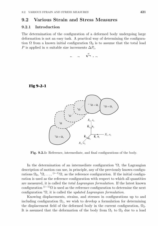
9.2. VARIOUS STRAIN AND STRESS MEASURES 421
9.2 Various Strain and Stress Measures
9.2.1 Introduction
The determination of the configuration of a deformed body undergoing largedeformation is not an easy task. A practical way of determining the configura-tion Ω from a known initial configuration Ω0 is to assume that the total loadP is applied in n suitable size increments ∆Pi,
P = Pn =n∑i=1
∆Pi
so that the body occupies n configurations, iΩ (i = 1, 2, . . . , n), prior to oc-cupying the final configuration Ω2 ≡ nΩ, as shown in Fig. 9.2.1. The magni-tude of load increments should be such that the computational method usedis capable of predicting the deformed configuration iΩ at the end of each loadPi =
∑ik=1 ∆Pk, ∆Pi being the last load increment.Fig 9-2-1
1 1,X x
2 2,X x
3 3,X x
e3ˆe1ˆE1
ˆE3ˆ
e2ˆE2ˆ
2nΩ Ω=
00Ω Ω=
11
n Ω Ω- =
1Ω
2 Ω
k Ω
Fig. 9.2.1: Reference, intermediate, and final configurations of the body.
In the determination of an intermediate configuration iΩ, the Lagrangiandescription of motion can use, in principle, any of the previously known configu-rations Ω0, 1Ω, . . . , (i−1)Ω, as the reference configuration. If the initial configu-ration is used as the reference configuration with respect to which all quantitiesare measured, it is called the total Lagrangian formulation. If the latest knownconfiguration (i−1)Ω is used as the reference configuration to determine the nextconfiguration iΩ, it is called the updated Lagrangian formulation.
Knowing displacements, strains, and stresses in configurations up to andincluding configuration Ω1, we wish to develop a formulation for determiningthe displacement field of the deformed body in the current configuration, Ω2.It is assumed that the deformation of the body from Ω1 to Ω2 due to a load
422 FINITE ELEMENT FORMULATIONS OF SOLID CONTINUA
increment is small, and the accumulated deformation of the body from Ω0
to Ω1 can be arbitrarily large but continuous (i.e. neighborhoods move intoneighborhoods).
9.2.2 Notation
We consider three equilibrium configurations of the body, namely, Ω0, n−1Ω =Ω1, and nΩ = Ω2, which correspond to the undeformed configuration and thetwo configurations corresponding to the last two load increments, respectively,as shown in Fig. 9.2.1. A notation similar to one used by Bathe [4] is adopted inthe present study. A left superscript on a quantity denotes the configuration inwhich the quantity occurs, and a left subscript denotes the configuration withrespect to which the quantity is measured. Thus ijQ indicates that the quantityQ occurs in configuration Ωi but measured in configuration Ωj . When thequantity under consideration is measured in the same configuration in whichit occurs, the left subscript may not be used. The left superscript will beomitted on incremental quantities that occur between configurations Ω1 andΩ2. Of course, right subscript(s) refer to components in rectangular Cartesiancoordinate systems, as will be clear in the context of the discussion. Althoughsomewhat cumbersome, the notation conveys the meaning more directly.
Since we are dealing with three different configurations, namely, Ω0, Ω1, andΩ2, it is necessary to introduce the following notation in the three configurations[see Fig. 9.1.1(a) for the notation]:
Configuration: Ω0 Ω1 Ω2
Position vector: 0x 1x 2x
Volume: 0V 1V 2V
Area: 0A 1A, 2A
Density: 0ρ 1ρ 2ρ
Displacement vector: 10u
20u
(9.2.1)
We use a rectangular Cartesian coordinate system to formulate the equa-tions. We rewrite the field equations presented in Chapter 2 in a form suit-able for the current objective of formulating finite element models of continua.When the body deforms under the action of external forces, a particle1 X occu-pying the position X ≡ 0x = (0x1,
0x2,0x3) = (X1, X2, X3) in configuration Ω0
moves to a new position 1x = (1x1,1x2,
1x3) in configuration Ω1 and position2x = (2x1,
2x2,2x3) in configuration Ω2. The total displacements of the particle
X in the two configurations Ω1 and Ω2 can be written as
10u = 1x− 0x or 1
0ui = 1xi − 0xi (i = 1, 2, 3) (9.2.2)
1Recall that X denotes the name of a particle whose location in Ω0 is 0x = X and its currentlocation in Ω = Ω2 is 2x.
9.2. VARIOUS STRAIN AND STRESS MEASURES 423
20u = 2x− 0x or 2
0ui = 2xi − 0xi (i = 1, 2, 3) (9.2.3)
and the displacement increment of the point from Ω1 to Ω2 is
u = 20u− 1
0u or ui = 20ui − 1
0ui (i = 1, 2, 3) (9.2.4)
9.2.3 Conservation of Mass
The relations among the mass densities 0ρ, 1ρ, and 2ρ of the materials of config-urations Ω0, Ω1, and Ω2, respectively, can be established using the principle ofconservation of mass. The principle requires that the mass of a material bodybe conserved in moving through different configurations∫
2V
2ρ d 2V =
∫1V
1ρ d 1V =
∫0V
0ρ d 0V (9.2.5)
where iV is the volume of the body when it occupies the configuration Ωi
(i = 0, 1, 2). By a change of coordinates from 2xi to 0xi, we have∫2V
2ρ d 2V =
∫0V
2ρ 20J d 0V (9.2.6)
where 20J is the determinant of the deformation gradient 2
0F (or the Jacobianof the transformation)
20J = det
(20F)
=
∣∣∣∣∂ 2xi∂ 0xj
∣∣∣∣ =
∣∣∣∣∣∣∣∂ 2x1∂ 0x1
∂ 2x1∂ 0x2
∂ 2x1∂ 0x3
∂ 2x2∂ 0x1
∂ 2x2∂ 0x2
∂ 2x2∂ 0x3
∂ 2x3∂ 0x1
∂ 2x3∂ 0x2
∂ 2x3∂ 0x3
∣∣∣∣∣∣∣ (9.2.7)
Equation (9.2.5) implies, in view of Eq. (9.2.6), that [see Eq. (2.7.7)]
0ρ = 2ρ 20J (9.2.8)
Similarly, we have1ρ = 2ρ 2
1J (9.2.9)
9.2.4 Green–Lagrange Strain Tensors
The Cartesian components of the Green–Lagrange strain tensors, 10Eij and 2
0Eij ,in the two configurations Ω1 and Ω2 are defined by
10Eij =
1
2
(∂ 1
0ui∂ 0xj
+∂ 1
0uj∂ 0xi
+∂ 1
0uk∂ 0xi
∂ 10uk
∂ 0xj
)(9.2.10)
20Eij =
1
2
(∂ 2
0ui∂ 0xj
+∂ 2
0uj∂ 0xi
+∂ 2
0uk∂ 0xi
∂ 20uk
∂ 0xj
)(9.2.11)
424 FINITE ELEMENT FORMULATIONS OF SOLID CONTINUA
9.2.4.1 Green–Lagrange strain increment tensor
It is useful to define the incremental strain components 0εij , that is, strainsinduced in moving from configuration Ω1 to configuration Ω2. The Green–Lagrange strain increment tensor is defined as
2 (0εij) d0xi d
0xj = (2ds)2 − (1ds)2
= [(2ds)2 − (0ds)2]− [(1ds)2 − (0ds)2]
= 2(
20Eij − 1
0Eij)d 0xi d
0xj (9.2.12)
≡ 2 (0eij + 0ηij) d0xi d
0xj (9.2.13)
where 0eij are linear components of strain increment tensor
0eij =1
2
(∂ui∂ 0xj
+∂uj∂ 0xi
+∂ 1
0uk∂ 0xi
∂uk∂ 0xj
+∂ 1
0uk∂ 0xj
∂uk∂ 0xi
)(9.2.14)
and 0ηij are the nonlinear components
0ηij =1
2
∂uk∂ 0xi
∂uk∂ 0xj
(9.2.15)
The linearity of 0eij and nonlinearity of 0ηij are understood to be in termsof the incremental displacement components ui. Note that the displacementcomponents 1
0uj are known, making 0eij linear in the increments ui.For geometrically linear analysis, that is when strains are infinitesimal, only
two configurations Ω1 = Ω0 and Ω2 are involved, 1ui = 0, 2ui = ui, and ui,k aresmall enough to neglect their products. Consequently, the linear componentsof strain increment tensor 0eij become the same as the components of theGreen–Lagrange strain tensor 2
0Eij , and both reduce to the infinitesimal straincomponents
0eij =1
2
(∂ui∂ 0xj
+∂uj∂ 0xi
)(9.2.16)
9.2.4.2 Updated Green–Lagrange strain tensor
The Green–Lagrange strain tensor 20Eij introduced earlier is useful in the total
Lagrangian formulation. With the updated Lagrangian formulation in mind,we define the components of Green–Lagrange strain tensor with respect to con-figuration Ω1. Such a strain tensor, denoted as 2
1εij , is called the updated Green–Lagrange strain tensor. It is defined by
2 (21εij) d
1xi d1xj =
(2ds)2 − (1ds)2 (9.2.17)
Using (note that all are first-order derivatives)
d 2xi =∂ 2xi∂ 1xj
d 1xj , (2ds)2 =∂ 2xk∂ 1xi
∂ 2xk∂ 1xj
d 1xi d1xj (9.2.18)
9.2. VARIOUS STRAIN AND STRESS MEASURES 425
ui = 2xi − 1xi,∂ 2xk∂ 1xi
=∂ uk∂ 1xi
+ δki (9.2.19)
we can write
21εij =
1
2
(∂ui∂ 1xj
+∂uj∂ 1xi
+∂uk∂ 1xi
∂uk∂ 1xj
)(9.2.20)
≡ 1eij + 1ηij (9.2.21)
where
1eij =1
2
(∂ui∂ 1xj
+∂uj∂ 1xi
), 1ηij =
1
2
(∂uk∂ 1xi
∂uk∂ 1xj
)(9.2.22)
Note that the definition of 21εij involves the components of the displacement
increment vector u. Therefore, 21εij are also called the updated Green–Lagrange
strain increment components.
9.2.5 Euler–Almansi Strain Tensor
Suppose that a body occupying the undeformed configuration Ω0 takes a num-ber of intermediate configurations before occupying the deformed configurationΩ1, as shown in Fig. 9.2.1. Then we wish to determine the next configurationΩ2 in a single incremental step. Although the accumulated displacements 1ui ofthe body from configuration Ω0 to configuration Ω1 can be large, the incremen-tal displacements ui within the incremental step from Ω1 to Ω2 are assumedto be small. Hence, we may refer the strains to configuration Ω2. The strainsoccurring in the body at configuration Ω2 and measured in the same configura-tion, i.e. the Euler–Almansi strain tensor components defined in Eq. (2.4.14),can be expressed in terms of the components of the displacement increment uias
2 22εij d
2xi d2xj =
(2ds)2 − (1ds)2
=
(δij −
∂ 1xk∂ 2xi
∂ 1xk∂ 2xj
)d 2xi d
2xj (9.2.23)
or (22εij ≡ 2εij)
2εij =1
2
(∂ui∂ 2xj
+∂uj∂ 2xi
− ∂uk∂ 2xi
∂uk∂ 2xj
)(9.2.24)
The linear part of 2εij is called the infinitesimal strain tensor and denoted 2eij
2eij =1
2
(∂ui∂ 2xj
+∂uj∂ 2xi
)(9.2.25)
which is identical in form to the infinitesimal strain tensor given in Eq. (2.4.19),except that the reference configuration is changed to Ω2.
426 FINITE ELEMENT FORMULATIONS OF SOLID CONTINUA
9.2.6 Relationships Between Various Stress Tensors
The Cauchy stress components σij in configurations Ω1 and Ω2 are denoted by
1σij = 11σij ,
2σij = 22σij (9.2.26)
We note that the second Piola–Kirchhoff stress tensor characterizes the currentforce in Ω2 but transformed to and measured per unit area in Ω0.
It is useful in the updated Lagrangian formulation to define another kind ofstress tensor called the updated Kirchhoff stress tensor. Consider the infinitesi-mal rectangular parallelepiped containing the point P in Ω1 enclosed by the sixsurfaces
1xi = constant, 1xi + d 1xi = constant (i = 1, 2, 3) (9.2.27)
The Cauchy stress components on this rectangular parallelepiped are 1σij . Asthe body deforms from configuration Ω1 to configuration Ω2, this rectangularparallelepiped will deform into, in general, a non-rectangular parallelepiped.Using Ω1 as the reference configuration, the updated Kirchhoff stress compo-nents 2
1Sij are defined as the internal forces per unit area acting along the normaland two tangential directions of each of the side surfaces of the parallelepipedin Ω2. The updated Kirchhoff stress components 2
1Sij can be decomposed as
21Sij = 1σij + 1Sij (9.2.28)
where 1σij = 11Sij are the Cauchy stress components in Ω1 and 1Sij are the
updated Kirchhoff stress increment tensor components.The second Piola–Kirchhoff stress tensor components in Ω1 and Ω2 are
denoted by 10Sij and 2
0Sij , respectively, which are related by
20Sij = 1
0Sij + 0Sij (9.2.29)
where 0Sij are the Kirchhoff stress increment tensor components.
9.2.7 Constitutive Equations
As discussed in Section 2.8, materials for which the constitutive behavior isonly a function of the current state of deformation are known as elastic. Inthe special case in which the work done by the stresses during a deformation isdependent only on the initial state and the current configuration, the materialis called hyperelastic. For hyperelastic materials we assume that there exists astored strain energy potential, Ψ, measured per unit undeformed volume, suchthat the components of the material elasticity tensor C [see Section 2.8.2 andEq. (2.8.14)] are given by
∂Ψ
∂Eij= Sij = Cijk`Ek` (9.2.30)
9.2. VARIOUS STRAIN AND STRESS MEASURES 427
where Cijk` are the components of the fourth-order elasticity tensor.In the derivation of finite element models of incremental nonlinear anal-
ysis of solid continua, it is necessary to specify the stress–strain relations inincremental form. In the total Lagrangian formulation, for example, the consti-tutive relations are expressed in terms of the Kirchhoff stress increment tensorcomponents 0Sij and Green–Lagrange strain increment tensor components 0εijas
0Sij = 0Cijk` 0εk` (9.2.31)
In the updated Lagrangian formulation, the constitutive relations are expressedin terms of the updated Kirchhoff stress increment tensor components 1Sij andupdated Green–Lagrange strain increment tensor components 1εij :
1Sij = 1Cijk` 1εk` (9.2.32)
where 0Cijkl and 1Cijkl denote the components of the elasticity tensors withrespect to the configurations Ω0 and Ω1, respectively.
Often, the incremental material laws in Eqs. (9.2.31) and (9.2.32) with iden-tical coefficients, that is, 0Cijk` = 1Cijk`, are employed in the total and updatedLagrangian finite element formulations. Of course, the error introduced by theassumption can be negligible if the strains are relatively small, but the differencecan be significant in large strain problems.
In single subscript notation for stresses and strains, analogous to those listedin Eq. (2.8.16), Eq. (9.2.31) can be expressed as
0Si = 0Cij 0εj (9.2.33)
where it is understood that the principal material coordinate system coin-cides with the coordinate system chosen to describe the motion. Otherwise,Eq. (9.2.33) has the form
0S′i = 0C
′ij 0ε
′j (9.2.34)
where all quantities are referred to the material coordinate system (X′1, X
′2, X
′3).
For orthotropic materials (with respect to the principal material coordinates),
0C′ij can be expressed in terms of the material properties as
0C′11 =
1− ν23ν23
E2E3∆, 0C
′12 =
ν21 + ν31ν23
E2E3∆=ν12 + ν32ν13
E1E3∆
0C′13 =
ν31 + ν21ν32
E2E3∆=ν13 + ν12ν23
E1E2∆
0C′22 =
1− ν13ν31
E1E3∆, 0C
′23 =
ν32 + ν12ν31
E1E3∆=ν23 + ν21ν13
E1E2∆(9.2.35)
0C′33 =
1− ν12ν21
E1E2∆, 0C
′44 = G23, 0C
′55 = G31, 0C
′66 = G12
∆ = (1− ν12ν21 − ν23ν32 − ν31ν13 − 2ν21ν32ν13)/E1E2E3
428 FINITE ELEMENT FORMULATIONS OF SOLID CONTINUA
where E1, E2, E3 are Young’s moduli in 1, 2, and 3 material directions, respec-tively, νij is Poisson’s ratio, defined as the ratio of transverse strain in the Xjthdirection to the strain in the Xith direction when stressed in the Xith direc-tion, and G23,G13, and G12 are shear moduli in the X2-X3, X1-X3, and X1-X2
planes, respectively. The following reciprocal relations hold on account of thesymmetries of the stress, strain, and elasticity tensors:
ν21
E2=ν12
E1;ν31
E3=ν13
E1;ν32
E3=ν23
E2
or, in shortνijEi
=νjiEj
(no sum on i, j) (9.2.36)
for i, j = 1, 2, 3. The nine independent material coefficients for an orthotropicmaterial are
E1, E2, E3, G23, G13, G12, ν12, ν13, ν23 (9.2.37)
When the material coordinate system (X′1, X
′2, X
′3) does not coincide with
(X1, X2, X3) used to describe the motion, one must transform Eq. (9.2.34) toEq. (9.2.33) using the direction cosines between the two coordinate systems (seeChapter 1 of Reddy [1] for detailed discussion of coordinate transformations andrelations between the components of stress, strain, and elasticity tensor in thetwo coordinate systems).
For a two-dimensional elasticity problem, when the material coordinate sys-tem is the same as that used for the description of motion, typical stress–strainrelations are given by
σ1
σ2
σ6
=
C11 C12 0C12 C22 00 0 C66
ε1
ε2
ε6
(9.2.38)
For transversely isotropic material (i.e. E3 = E2, ν23 = ν32, and ν12 = ν13) ina state of plane strain and orthotropic material in a state of plane stress thematerial stiffness Cij can be expressed in terms of the engineering constants asfollows:
Plane strain
C11 =E1(1− ν23)
(1− ν23 − 2ν12ν21), C12 =
ν21E1
(1− ν23 − 2ν12ν21)
C22 =E2(1− ν12ν21)
(1 + ν23)(1− ν23 − 2ν12ν21)(9.2.39)
C44 = G13, C55 = G23, C66 = G12
9.3. TOTAL LAGRANGIAN AND UPDATED LAGRANGIAN FORMULATIONS 429
Plane stress
C11 =E1
(1− ν12ν21), C22 =
E2
(1− ν12ν21)
C12 = ν12C22, C44 = G13, C55 = G23, C66 = G12
(9.2.40)
This completes the discussion of various strain and stress measures betweenconfigurations Ω0, Ω1, and Ω2. In the next section we study variational for-mulations based on principles of virtual displacements and total and updatedLagrangian descriptions of motion.
9.3 Total Lagrangian and Updated LagrangianFormulations
9.3.1 Principle of Virtual Displacements
The equations of the Lagrangian incremental description of motion can be de-rived from the principles of virtual work (i.e. principles of virtual displacements,virtual forces, or mixed virtual displacements and forces). Since our ultimateobjective is to develop the finite element model of the equations governing adeformable continuum, we will not actually derive the differential equationsof motion but utilize the virtual work statements, which are the weak formsneeded to develop the finite element models.
The displacement finite element models to be developed in this chapter arebased on the principle of virtual displacements (see Section 2.9). The principlerequires that the sum of the external virtual work done on and the internalvirtual work stored in the body should be equal to zero:
δW ≡ δWI + δWE = 0 (9.3.1)
where δWI is the internal virtual work and δWE is the virtual work done byexternal forces
δWI =
∫2V
2σ : δ(2ε) d2V =
∫2V
2σij δ(2εij) d2V (9.3.2)
δWE = −[∫
2V
2f · δu d 2V +
∫2S
2t · δu d 2S
]= −
[∫2V
2fiδui d2V +
∫2S
2ti δui d2S
]≡ −δ 2R (9.3.3)
and d 2S denotes surface element and 2f is the body force vector (measured perunit volume) and 2t is the boundary stress (or traction) vector (measured perunit surface area) in configuration Ω2; σ and e denote the Cauchy stress tensorand Euler–Almansi strain tensors, respectively.
430 FINITE ELEMENT FORMULATIONS OF SOLID CONTINUA
Equations (9.3.2) and (9.3.3) are not useful in large deformation analy-sis because the configuration Ω2 is unknown and hence integration cannot becarried out on an unknown geometry. This is an important difference com-pared with the linear analysis in which we assume that the displacements areinfinitesimally small and that the configuration of the body does not changeappreciably, Ω2 ≈ Ω0. In a large deformation analysis, special attention mustbe given to the fact that the configuration of the body changes continuously asload is incremented, and the configuration of the deformed body slowly driftsaway from the configuration of the undeformed body, making Ω2 to be sub-stantially different from Ω0 (although Ω1 and Ω2 may be close enough if theload increment is small). This change in configuration can be dealt with bydefining appropriate stress and strain measures, as discussed in Chapter 2. Theobjective of their introduction into the analysis is to express the virtual workexpressions in Eqs. (9.3.2) and (9.3.3) in terms of an integral over a config-uration that is known. The stress and strain measures that we shall use arethe second Piola–Kirchhoff stress tensor and the Green–Lagrange strain tensor,which are “energetically conjugate” to each other [see Eq. (9.1.15)].
9.3.2 Total Lagrangian Formulation
9.3.2.1 Weak form
In the total Lagrangian formulation, all quantities are measured with respectto the initial configuration Ω0. Hence, the virtual work statement in Eq. (9.3.1)must be expressed in terms of quantities referred to the reference configuration.We use the following identities:∫
2V
2σij δ(2εij) d2V =
∫0V
20Sij δ(
20Eij) d
0V∫2V
2fi δui d2V =
∫0V
20fi δui d
0V (9.3.4)∫2S
2ti δui d2S =
∫0S
20ti δui d
0S
where 20fi and 2
0ti are the body force and boundary traction components referredto the configuration Ω0. Substituting the equivalence from Eq. (9.3.4) intoEqs. (9.3.2) and (9.3.3) for δWI and δWE , respectively, and then using them inEq. (9.3.1), we arrive at
0 =
∫0V
20Sij δ(
20Eij) d
0V −∫
0V
20fi δui d
0V −∫
0S
20ti δui d
0S (9.3.5)
9.3. TOTAL LAGRANGIAN AND UPDATED LAGRANGIAN FORMULATIONS 431
9.3.2.2 Incremental decompositions
Next we simplify the virtual work statement in Eq. (9.3.5) further. First, wenote that [see Eqs. (9.2.12), (9.2.13), and (9.2.29)]
δ(20Eij) = δ(1
0Eij) + δ(0εij) = δ(0εij)20Sij = 1
0Sij + 0Sij(9.3.6)
where δ(10Eij) = 0 because 1
0Eij is not a function of the unknown ui [see Eq.(9.2.10)]. The virtual strains δ(0εij) are given by
δ(0εij) = δ(0eij) + δ(0ηij) (9.3.7)
where δ(0eij) and δ(0ηij) are [see Eqs. (9.2.14) and (9.2.15)]
δ(0eij) =1
2
(∂δui∂ 0xj
+∂δuj∂ 0xi
+∂δuk∂ 0xi
∂ 10uk
∂ 0xj+∂ 1
0uk∂ 0xi
∂δuk∂ 0xj
)(9.3.8)
δ(0ηij) =1
2
(∂δuk∂ 0xi
∂uk∂ 0xj
+∂uk∂ 0xi
∂δuk∂ 0xj
)(9.3.9)
Substituting Eq. (9.3.6) for δ(20Eij) and 2
0Sij into Eq. (9.3.5), we arrive at theexpression
0 =
∫0V
(10Sij + 0Sij
)δ(0εij) d
0V − δ(20R)
=
∫0V
10Sij [δ(0eij) + δ(0ηij)] + 0Sij δ(0εij)
d 0V − δ(2
0R)
=
∫0V
10Sij δ(0ηij) d
0V +
∫0V
0Sij δ(0εij) d0V
+
∫0V
10Sij δ(0eij) d
0V − δ(20R) (9.3.10)
where
δ(20R) =
∫0V
20fi δui d
0V +
∫0S
20ti δui d
0S (9.3.11)
Since the body is in equilibrium at configuration Ω1, by the principle of virtualwork applied to configuration Ω1 we have
0 =
∫0V
10Sij δ(0eij) d
0V −∫
0V
10fi δui d
0V −∫
0S
10tiδui d
0S (9.3.12)
Consequently, Eq. (9.3.10) takes the form∫0V
0Sij δ(0εij) d0V +
∫0V
10Sij δ(0ηij) d
0V = δ(20R)− δ(1
0R) (9.3.13)
432 FINITE ELEMENT FORMULATIONS OF SOLID CONTINUA
where
δ(10R) =
∫0V
10Sij δ(0eij) d
0V =
∫0V
10fi δui d
0V +
∫0S
10ti δui d
0S (9.3.14)
Equation (9.3.13) forms the basis for the finite element model of the totalLagrangian formulation. The first term of Eq. (9.3.13) represents the changein the virtual strain energy due to the virtual incremental displacements ui be-tween configurations Ω1 and Ω2. The second term represents the virtual workdone by forces due to initial stresses (i.e. stresses accumulated through configu-ration Ω1) 1
0Sij , as shown symbolically in Fig. 9.3.1. The two terms together onthe right-hand side denote the change in the virtual work done by applied bodyforces and surface tractions in moving from Ω1 to Ω2. Equation (9.3.13) rep-resents the statement of virtual work for the incremental deformation betweenthe configurations Ω1 and Ω2, and no approximations are made in arriving atit. Replacing 0Sij in terms of the strains 0εk` using the constitutive relation,Eq. (9.2.31), we obtain∫
0V0Cijk` 0εk` δ(0εij) d
0V +
∫0V
10Sij δ(0ηij) d
0V = δ(20R)− δ(1
0R) (9.3.15)
1 1,X x
2 2,X x
3 3,X x
e3ˆe1ˆE1
ˆE3ˆ
e2ˆE2ˆ
00Ω Ω=
1Ω
10S
0d V
12Ω 2
rΩ2Ω1
2rΩ +
0d S
10E
0e
Equilibrium iterations
0S
20S20E
Fig 9-3-1
Fig. 9.3.1: Reference and final configurations of the body in the total Lagrangianformulation.
9.3.2.3 Linearization
Equation (9.3.15) is nonlinear, through 0ηij , in the displacement increments ui.From a computational point of view, it is necessary to linearize the equation.Toward this end, we assume that the displacements ui are small, which is indeed
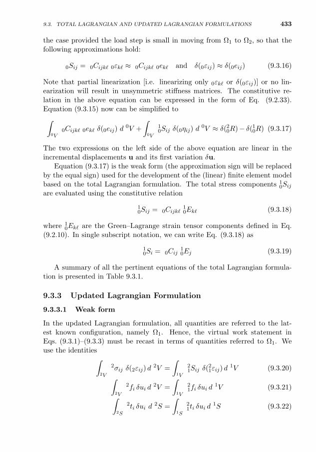
9.3. TOTAL LAGRANGIAN AND UPDATED LAGRANGIAN FORMULATIONS 433
the case provided the load step is small in moving from Ω1 to Ω2, so that thefollowing approximations hold:
0Sij = 0Cijk` 0εk` ≈ 0Cijk` 0ek` and δ(0εij) ≈ δ(0eij) (9.3.16)
Note that partial linearization [i.e. linearizing only 0εk` or δ(0εij)] or no lin-earization will result in unsymmetric stiffness matrices. The constitutive re-lation in the above equation can be expressed in the form of Eq. (9.2.33).Equation (9.3.15) now can be simplified to∫
0V0Cijk` 0ek` δ(0eij) d
0V +
∫0V
10Sij δ(0ηij) d
0V ≈ δ(20R)− δ(1
0R) (9.3.17)
The two expressions on the left side of the above equation are linear in theincremental displacements u and its first variation δu.
Equation (9.3.17) is the weak form (the approximation sign will be replacedby the equal sign) used for the development of the (linear) finite element modelbased on the total Lagrangian formulation. The total stress components 1
0Sijare evaluated using the constitutive relation
10Sij = 0Cijk`
10Ek` (9.3.18)
where 10Ek` are the Green–Lagrange strain tensor components defined in Eq.
(9.2.10). In single subscript notation, we can write Eq. (9.3.18) as
10Si = 0Cij
10Ej (9.3.19)
A summary of all the pertinent equations of the total Lagrangian formula-tion is presented in Table 9.3.1.
9.3.3 Updated Lagrangian Formulation
9.3.3.1 Weak form
In the updated Lagrangian formulation, all quantities are referred to the lat-est known configuration, namely Ω1. Hence, the virtual work statement inEqs. (9.3.1)–(9.3.3) must be recast in terms of quantities referred to Ω1. Weuse the identities∫
2V
2σij δ(2εij) d2V =
∫1V
21Sij δ(
21εij) d
1V (9.3.20)∫2V
2fi δui d2V =
∫1V
21fi δui d
1V (9.3.21)∫2S
2ti δui d2S =
∫1S
21ti δui d
1S (9.3.22)
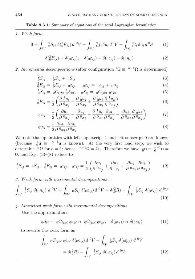
434 FINITE ELEMENT FORMULATIONS OF SOLID CONTINUA
Table 9.3.1: Summary of equations of the total Lagrangian formulation.
1. Weak form
0 =
∫0V
20Sij δ(
20Eij) d
0V −∫
0V
20fi δui d
0V −∫
0S
20ti δui d
0S (1)
δ(20Eij) = δ(0εij), δ(0εij) = δ(0eij) + δ(0ηij) (2)
2. Incremental decompositions (after configuration 1Ω ≡ n−1Ω is determined)
20Sij = 1
0Sij + 0Sij (3)20Eij = 1
0Eij + 0εij , 0εij = 0eij + 0ηij (4)10Sij = 0Cijk`
10Ek`, 0Sij = 0Cijk` 0εk` (5)
10Eij =
1
2
(∂ 1
0ui∂ 0xj
+∂ 1
0uj∂ 0xi
+∂ 1
0uk∂ 0xi
∂ 10uk
∂ 0xj
)(6)
0eij =1
2
(∂ui∂ 0xj
+∂uj∂ 0xi
+∂ 1
0uk∂ 0xi
∂uk∂ 0xj
+∂uk∂ 0xi
∂ 10uk
∂ 0xj
)(7)
0ηij =1
2
∂uk∂ 0xi
∂uk∂ 0xj
(8)
We note that quantities with left superscript 1 and left subscript 0 are known(because 1
0u ≡n−10 u is known). At the very first load step, we wish to
determine nΩ for n = 1; hence, n−1Ω = Ω0. Therefore we have 10u ≡
n−10 u =
0, and Eqs. (3)–(8) reduce to
10Sij = 0Sij ,
10Eij = 0εij , 0εij =
1
2
(∂ui∂ 0xj
+∂uj∂ 0xi
+∂uk∂ 0xi
∂uk∂ 0xj
)(9)
3. Weak form with incremental decompositions∫0V
10Sij δ(0ηij) d
0V +
∫0V
0Sij δ(0εij) d0V = δ(2
0R)−∫
0V
10Sij δ(0eij) d
0V
(10)
4. Linearized weak form with incremental decompositions
Use the approximations
0Sij = 0Cijk` 0εk` ≈ 0Cijk` 0ek`, δ(0εij) ≈ δ(0eij) (11)
to rewrite the weak form as∫0V
0Cijk` 0ek` δ(0eij) d0V +
∫0V
10Sij δ(0ηij) d
0V
= δ(20R)−
∫0V
10Sij δ(0eij) d
0V (12)

9.3. TOTAL LAGRANGIAN AND UPDATED LAGRANGIAN FORMULATIONS 435
where 21fi and 2
1ti are the body force and boundary traction components referredto the configuration Ω1, and 2
1εij are the components of the updated Green–Lagrange strain tensor components defined in Eq. (9.2.20). Using Eqs. (9.3.20)–(9.3.22), Eqs. (9.3.1)–(9.3.3) can be expressed as∫
1V
21Sij δ(
21εij) d
1V −∫
1V
21fi δui d
1V −∫
1S
21ti δui d
1S = 0 (9.3.23)
The virtual strains are given by [see Eqs. (9.2.20)–(9.2.22)]
δ(21εij) = δ(1eij) + δ(1ηij)
δ(1eij) =1
2
(∂δui∂ 1xj
+∂δuj∂ 1xi
)δ(1ηij) =
1
2
(∂δuk∂ 1xi
∂uk∂ 1xj
+∂uk∂ 1xi
∂δuk∂ 1xj
) (9.3.24)
9.3.3.2 Incremental decompositions
Now using Eqs. (9.2.28) and (9.3.24), we can express Eq. (9.3.23) as
0 =
∫1V
21Sij δ(
21εij) d
1V − δ(21R)
=
∫1V
(1σij + 1Sij
)δ(2
1εij) d1V − δ(2
1R)
=
∫1V
1Sij δ(
21εij) + 1σij [δ(1eij) + δ(1ηij)]
d 1V − δ(2
1R)
=
∫1V
1Sij δ(21εij) d
1V +
∫1V
1σij δ(1ηij) d1V + δ(1
1R)− δ(21R) (9.3.25)
where u is the displacement from Ω1 to Ω2, δu is its first variation, and
δ(21R) =
∫1V
21fi δui d
1V +
∫1S
21ti δui d
1S
δ(11R) =
∫1V
1σij δ(1eij) d1V
(9.3.26)
Note that δ(11R) is the virtual internal energy stored in the body at configuration
Ω1 (see Fig. 9.3.2). Since the body is in equilibrium at configuration Ω1, theprinciple of virtual work applied to configuration Ω1 yields
δ(11R) =
∫1V
11fi δui d
1V +
∫1S
11ti δui d
1S (9.3.27)
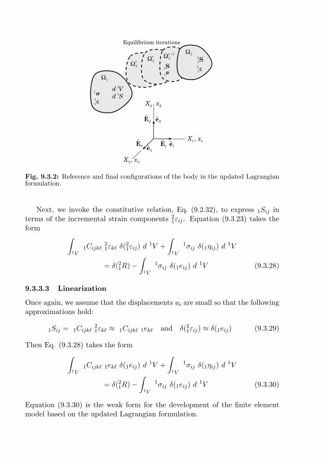
436 FINITE ELEMENT FORMULATIONS OF SOLID CONTINUA
1 1,X x
2 2,X x
3 3,X x
e3ˆe1ˆE1
ˆE3ˆ
e2ˆE2ˆ
1Ω
1s1d V
12Ω 2
rΩ2Ω1
2rΩ +
1d S
1S
11e
21e
Equilibrium iterations
21S
1e
Fig. 9.3.2: Reference and final configurations of the body in the updated Lagrangianformulation.
Next, we invoke the constitutive relation, Eq. (9.2.32), to express 1Sij interms of the incremental strain components 2
1εij . Equation (9.3.23) takes theform ∫
1V1Cijk`
21εk` δ(
21εij) d
1V +
∫1V
1σij δ(1ηij) d1V
= δ(21R)−
∫1V
1σij δ(1eij) d1V (9.3.28)
9.3.3.3 Linearization
Once again, we assume that the displacements ui are small so that the followingapproximations hold:
1Sij = 1Cijk`21εk` ≈ 1Cijk` 1ek` and δ(2
1εij) ≈ δ(1eij) (9.3.29)
Then Eq. (9.3.28) takes the form∫1V
1Cijk` 1ek` δ(1eij) d1V +
∫1V
1σij δ(1ηij) d1V
= δ(21R)−
∫1V
1σij δ(1eij) d1V (9.3.30)
Equation (9.3.30) is the weak form for the development of the finite elementmodel based on the updated Lagrangian formulation.
9.3. TOTAL LAGRANGIAN AND UPDATED LAGRANGIAN FORMULATIONS 437
The total Cauchy stress components 1σij are evaluated using the constitutiverelation
1σij = 1Cijk`11εk` (9.3.31)
where 11εk` are the Euler–Almansi strain tensor components defined by
2 11εij d
1xi d1xj =
(1ds)2 − (0ds)2
which gives
11εij =
1
2
(∂ 1
0ui∂ 1xj
+∂ 1
0uj∂ 1xi
− ∂ 10uk
∂ 1xi
∂ 10uk
∂ 1xj
)(9.3.32)
A summary of all the pertinent equations of the updated Lagrangian for-mulation is presented in Table 9.3.2.
9.3.4 Some Remarks on the Formulations
Let us examine the consequence of the linearizations used in arriving at thevirtual work statements in Eqs. (9.3.17) and (9.3.30). First, we note that thelinearization only approximated the left-hand side of the virtual work state-ments. Therefore, the errors in the two formulations are
TL Formulation: ETL = δ(20R)−
∫0V
10Sij δ(0eij) d
0V (9.3.33)
UL Formulation: EUL = δ(21R)−
∫1V
1σij δ(1eij) d1V (9.3.34)
The expressions in Eqs. (9.3.33) and (9.3.34) denote the virtual work doneby the “out-of-balance” forces in the two formulations. Therefore, iteration isnecessary to make the virtual work done by the imbalance forces approach zerowithin an assumed tolerance. Even though, in theory, the displacements 1
0uiare assumed to be known, they have to be determined by iteration. Thus, Eqs.(9.3.17) and (9.3.30) at the beginning of the rth (Newton’s) iteration are∫
0V0C
(r−1)ijk` 0e
(r)k` δ(0eij) d
0V +
∫0V
10S
(r−1)ij δ(0η
(r)ij ) d 0V
= δ(20R)−
∫0V
10S
(r−1)ij δ(0e
(r−1)ij ) d 0V (9.3.35)
∫1V
1C(r−1)ijk` 1e
(r)k` δ(1eij) d
1V +
∫1V
1σ(r−1)ij δ(1η
(r)ij ) d 1V
= δ(21R)−
∫1V
1σ(r−1)ij δ(1e
(r−1)ij ) d 1V (9.3.36)
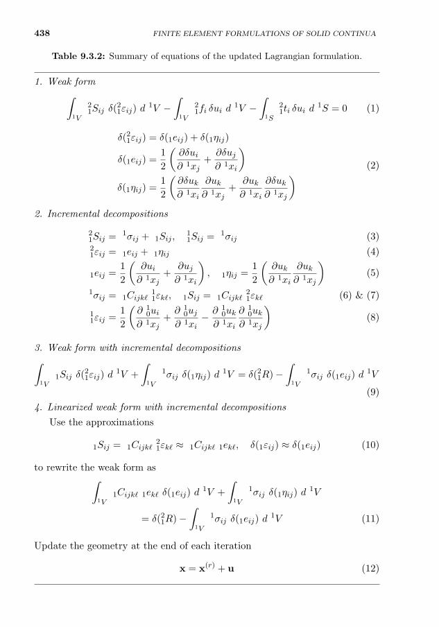
438 FINITE ELEMENT FORMULATIONS OF SOLID CONTINUA
Table 9.3.2: Summary of equations of the updated Lagrangian formulation.
1. Weak form∫1V
21Sij δ(
21εij) d
1V −∫
1V
21fi δui d
1V −∫
1S
21ti δui d
1S = 0 (1)
δ(21εij) = δ(1eij) + δ(1ηij)
δ(1eij) =1
2
(∂δui∂ 1xj
+∂δuj∂ 1xi
)δ(1ηij) =
1
2
(∂δuk∂ 1xi
∂uk∂ 1xj
+∂uk∂ 1xi
∂δuk∂ 1xj
) (2)
2. Incremental decompositions
21Sij = 1σij + 1Sij ,
11Sij = 1σij (3)
21εij = 1eij + 1ηij (4)
1eij =1
2
(∂ui∂ 1xj
+∂uj∂ 1xi
), 1ηij =
1
2
(∂uk∂ 1xi
∂uk∂ 1xj
)(5)
1σij = 1Cijk`11εk`, 1Sij = 1Cijk`
21εk` (6) & (7)
11εij =
1
2
(∂ 1
0ui∂ 1xj
+∂ 1
0uj∂ 1xi
− ∂ 10uk
∂ 1xi
∂ 10uk
∂ 1xj
)(8)
3. Weak form with incremental decompositions∫1V
1Sij δ(21εij) d
1V +
∫1V
1σij δ(1ηij) d1V = δ(2
1R)−∫
1V
1σij δ(1eij) d1V
(9)
4. Linearized weak form with incremental decompositions
Use the approximations
1Sij = 1Cijk`21εk` ≈ 1Cijk` 1ek`, δ(1εij) ≈ δ(1eij) (10)
to rewrite the weak form as∫1V
1Cijk` 1ek` δ(1eij) d1V +
∫1V
1σij δ(1ηij) d1V
= δ(21R)−
∫1V
1σij δ(1eij) d1V (11)
Update the geometry at the end of each iteration
x = x(r) + u (12)
9.4. FINITE ELEMENT MODELS OF 2-D CONTINUA 439
9.4 Finite Element Models of 2-D Continua
9.4.1 Introduction
Here we discuss finite element models based on the total and updated La-grangian formulations presented in the previous section. Attention is focusedhere on two-dimensional problems under the assumption of linear, orthotropic,elastic material behavior. The volume integral will be replaced, at the end,with dV = heA, where he denotes the thickness of the elastic body; one maytake he = 1 for plane strain problems.
9.4.2 Total Lagrangian Formulation
We introduce the notation
0x1 = x, 0x2 = y, 1u1 = u, 1u2 = v, u1 = u, u2 = v (9.4.1)
We can write the first expression of Eq. (9.3.17) in matrix form∫0V
0Cijk` 0ek` δ(0eij) d0V =
∫0V
(δ0e)T0C 0e d
0V
=
∫0V
[(D + Du)δu]T 0C (D + Du) u
d 0V (9.4.2)
where
0e =
0exx0eyy
2 0exy
=
∂u∂x∂v∂y
∂u∂y + ∂v
∂x
+
∂u∂x
∂u∂x + ∂v
∂x∂v∂x
∂u∂y
∂u∂y + ∂v
∂y∂v∂y
∂u∂x
∂u∂y + ∂v
∂x∂v∂y + ∂u
∂x∂u∂y + ∂v
∂x∂v∂y
=
∂∂x 0
0 ∂∂y
∂∂y
∂∂x
+
∂u∂x
∂∂x
∂v∂x
∂∂x
∂u∂y
∂∂y
∂v∂y
∂∂y
∂u∂y
∂∂x + ∂u
∂x∂∂y
∂v∂y
∂∂x + ∂v
∂x∂∂y
u
v
≡ (D + Du) u (9.4.3)
D =
∂∂x 0
0 ∂∂y
∂∂y
∂∂x
, Du =
∂u∂x
∂∂x
∂v∂x
∂∂x
∂u∂y
∂∂y
∂v∂y
∂∂y
∂u∂y
∂∂x + ∂u
∂x∂∂y
∂v∂y
∂∂x + ∂v
∂x∂∂y
(9.4.4)
0C =
0C11 0C12 0
0C12 0C22 00 0 0C66
, u =
uv
(9.4.5)
δ 0e = (D + Du) δu (9.4.6)
440 FINITE ELEMENT FORMULATIONS OF SOLID CONTINUA
where the coefficients 0Cij are defined in Eqs. (9.2.39) and (9.2.40) for planestrain and plane stress cases, respectively. The second expression of Eq. (9.3.17)can be written as∫
0V
10Sij δ(0ηij) d
0V
=
∫0V
[10Sxx
(∂δu
∂x
∂u
∂x+∂δv
∂x
∂v
∂x
)+ 1
0Syy
(∂δu
∂y
∂u
∂y+∂δv
∂y
∂v
∂y
)+ 1
0Sxy
(∂δu
∂x
∂u
∂y+∂δv
∂x
∂v
∂y+∂u
∂x
∂δu
∂y+∂v
∂x
∂δv
∂y
)]d 0V
=
∫0V
∂δu∂x∂δu∂y∂δv∂x∂δv∂y
T
10Sxx
10Sxy 0 0
10Sxy
10Syy 0 0
0 0 10Sxx
10Sxy
0 0 10Sxy
10Syy
∂u∂x∂u∂y∂v∂x∂v∂y
d 0V
=
∫0V
(Dδu)T 10S (Du) d 0V (9.4.7)
where
10S =
10Sxx
10Sxy 0 0
10Sxy
10Syy 0 0
0 0 10Sxx
10Sxy
0 0 10Sxy
10Syy
, D =
∂∂x 0∂∂y 0
0 ∂∂x
0 ∂∂y
(9.4.8)
Next, the total and incremental displacement fields, u and u, are interpo-lated as
u =
uv
=
∑nj=1 uj ψj(x)∑nj=1 vj ψj(x)
= Ψ ∆ (9.4.9)
u =
uv
=
∑nj=1 uj ψj(x)∑nj=1 vj ψj(x)
= Ψ ∆, δu = Ψ δ∆ (9.4.10)
where
Ψ =
[ψ1 0 ψ2 0 · · · ψn 00 ψ1 0 ψ2 · · · 0 ψn
](9.4.11)
∆T = u1, v1, u2, v2, · · · , un, vn (9.4.12)
∆T = u1, v1, u2, v2, · · · , un, vn (9.4.13)
Here ψj(x) denote the set of Lagrange family of approximation functions andn is the number of nodes per element. The size of the element stiffness matrixis 2n× 2n.
9.4. FINITE ELEMENT MODELS OF 2-D CONTINUA 441
The expressions in Eqs. (9.4.2) and (9.4.7) can now be expressed in matrixform as ∫
0V
[(D + Du)δu]T 0C (D + Du) u
d 0V
=
∫0V
(δ∆)T [(D + Du) Ψ]T 0C [(D + Du) Ψ] ∆ d 0V
≡∫
0V(δ∆)T(B1)T
0C B1∆ d 0V (9.4.14)
∫0V
(Dδu)T 10S (Du) d 0V =
∫0V
(δ∆)T(B2)T 10S B2∆ d 0V (9.4.15)
where B1 is the 3× 2n matrix and B2 is the 4× 2n matrix defined by
B1 = (D + Du) Ψ, B2 = DΨ (9.4.16)
and 10S is the 4 × 4 matrix defined in Eq. (9.4.8). The right-hand sides of Eq.
(9.3.17) can be written in terms of the finite element approximations as
δ(10R) =
∫0V
10Sij δ(0eij) d
0V =
∫0V
(δ 0e)T 10Sv d
0V
=
∫0V
(δ∆)T(B1)T 10Sv d
0V (9.4.17)
δ(20R) =
∫0V
20fiδui d
0V +
∫0S
20tiδui d
0S
=
∫0V
(δ∆)T ΨT 20f d
0V +
∫0S
(δ∆)T ΨT 20t d
0S (9.4.18)
where
10Sv =
10Sxx10Syy10Sxy
=
0C11 0C12 0
0C12 0C22 0
0 0 0C66
10Exx10Eyy
2 10Exy
≡ 0C10E (9.4.19)
10E =
10Exx10Eyy
2 10Exy
=
∂u∂x + 1
2
[(∂u∂x
)2+(∂v∂x
)2]∂v∂y + 1
2
[(∂u∂y
)2+(∂v∂y
)2]
∂u∂y + ∂v
∂x +(∂u∂x
∂u∂y + ∂v
∂x∂v∂y
) (9.4.20)
Substitution of Eqs. (9.4.14)–(9.4.20) into Eq. (9.3.17), and use of the fun-damental lemma of calculus of variations (i.e. δ∆ is a vector of arbitraryvariations), yields the following finite element model associated with the totalLagrangian formulation of two-dimensional nonlinear continua:
(K1 + K2) ∆ = 20F− 1
0F (9.4.21)
442 FINITE ELEMENT FORMULATIONS OF SOLID CONTINUA
where
K1 =
∫0V
(B1)T0C B1 d
0V, K2 =
∫0V
(B2)T 10S B2 d
0V
10F =
∫0V
(B1)T 10Sv d
0V, 20f =
20fx20fy
, 2
0t =
20tx20ty
(9.4.22)
20F =
∫0V
ΨT 20f d
0V +
∫0S
ΨT 20t d
0S
Note that the stiffness matrix K = K1 + K2 is a 2n × 2n matrix, wheren is the number of nodes in the 2-D element. It is symmetric on account ofthe symmetry of the matrices K1 and K2, and whose symmetry is due to thesymmetry of 1
0S and 0C. Also, the total and updated Lagrangian formulationsare incremental formulations, where ∆ is the incremental displacement vectorand K is the stiffness matrix. The direct stiffness matrix is implicit in the vector10F. For a linear analysis, ∆ becomes the total displacement vector, 1
0F = 0,and K2 = 0.
For two-dimensional problems, the explicit forms of matrices B1 and B2 aregiven by
B1 = B01 + Bu
1 + Bv1 (9.4.23)
B01 =
∂ψ1
∂x 0 ∂ψ2
∂x 0 · · · ∂ψn∂x 0
0 ∂ψ1
∂y 0 ∂ψ2
∂y · · · 0 ∂ψn∂y
∂ψ1
∂y∂ψ1
∂x∂ψ2
∂y∂ψ2
∂x · · ·∂ψn∂y
∂ψn∂x
(9.4.24)
Bu1 =
∂u∂x
∂ψ1
∂x 0 ∂u∂x
∂ψ2
∂x · · · ∂u∂x
∂ψn∂x 0
∂u∂y
∂ψ1
∂y 0 ∂u∂y
∂ψ2
∂y · · · ∂u∂y
∂ψn∂y 0
∂u∂x
∂ψ1
∂y + ∂u∂y
∂ψ1
∂x 0 ∂u∂x
∂ψ2
∂y + ∂u∂y
∂ψ2
∂x · · ·∂u∂x
∂ψn∂y + ∂u
∂y∂ψn∂x 0
(9.4.25)
Bv1 =
0 ∂v∂x
∂ψ1
∂x 0 ∂v∂x
∂ψ2
∂x · · · ∂v∂x
∂ψn∂x
0 ∂v∂y
∂ψ1
∂y 0 ∂v∂y
∂ψ2
∂y · · · ∂v∂y
∂ψn∂y
0 ∂v∂x
∂ψ1
∂y + ∂v∂y
∂ψ1
∂x 0 ∂v∂x
∂ψ2
∂y + ∂v∂y
∂ψ2
∂x · · ·∂v∂x
∂ψn∂y + ∂v
∂y∂ψn∂x
(9.4.26)
B2 =
∂ψ1
∂x 0 ∂ψ2
∂x 0 · · · ∂ψn∂x 0∂ψ1
∂y 0 ∂ψ2
∂y 0 · · · ∂ψn∂y 0
0 ∂ψ1
∂x 0 ∂ψ2
∂x · · · 0 ∂ψn∂x
0 ∂ψ1
∂y 0 ∂ψ2
∂y · · · 0 ∂ψn∂y
(9.4.27)
The finite element equations, Eq. (9.4.21), can be written in explicit form as[K11
1 + K112 K12
1
K211 K22
1 + K222
]uv
=
20F
1 − 10F
1
20F
2 − 10F
2
(9.4.28)
9.4. FINITE ELEMENT MODELS OF 2-D CONTINUA 443
where
K11ij(1) = he
∫Ωe
0C11
(1 +
∂u
∂x
)2 ∂ψi∂x
∂ψj∂x
+ 0C22
(∂u
∂y
)2 ∂ψi∂y
∂ψj∂y
+ 0C12
(1 +
∂u
∂x
)∂u
∂y
(∂ψi∂x
∂ψj∂y
+∂ψi∂y
∂ψj∂x
)+ 0C66
[(1 +
∂u
∂x
)∂ψi∂y
+∂u
∂y
∂ψi∂x
]×[(
1 +∂u
∂x
)∂ψj∂y
+∂u
∂y
∂ψj∂x
]dx dy
K12ij(1) = he
∫Ωe
0C11
(1 +
∂u
∂x
)∂v
∂x
∂ψi∂x
∂ψj∂x
+ 0C22
(1 +
∂v
∂y
)∂u
∂y
∂ψi∂y
∂ψj∂y
+ 0C12
[(1 +
∂u
∂x
)(1 +
∂v
∂y
)∂ψi∂x
∂ψj∂y
+∂u
∂y
∂v
∂x
∂ψi∂y
∂ψj∂x
]+ 0C66
[(1 +
∂u
∂x
)∂ψi∂y
+∂u
∂y
∂ψi∂x
]×[(
1 +∂v
∂y
)∂ψj∂x
+∂v
∂x
∂ψj∂y
]dx dy = K21
ji(1)
K22ij(1) = he
∫Ωe
0C11
(∂v
∂x
)2 ∂ψi∂x
∂ψj∂x
+ 0C22
(1 +
∂v
∂y
)2 ∂ψi∂y
∂ψj∂y
+ 0C12
(1 +
∂v
∂y
)∂v
∂x
(∂ψi∂x
∂ψj∂y
+∂ψi∂y
∂ψj∂x
)+ 0C66
[(1 +
∂v
∂y
)∂ψi∂x
+∂v
∂x
∂ψi∂y
]×[(
1 +∂v
∂y
)∂ψj∂x
+∂v
∂x
∂ψj∂y
]dx dy
K11ij(2) = he
∫Ωe
[10Sxx
∂ψi∂x
∂ψj∂x
+ 10Sxy
(∂ψi∂y
∂ψj∂x
+∂ψi∂x
∂ψj∂y
)+ 1
0Syy∂ψi∂y
∂ψj∂y
]dx dy = K22
ij(2) (9.4.29)
20F
1i = he
∫Ωe
20fxψi dx dy + he
∮Γe
20txψi ds
20F
2i = he
∫Ωe
20fyψi dx dy + he
∮Γe
20tyψi ds
10F
1i = he
∫Ωe
(1 +
∂u
∂x
)∂ψi∂x
10Sxx +
∂u
∂y
∂ψi∂y
10Syy
+
[(1 +
∂u
∂x
)∂ψi∂y
+∂u
∂y
∂ψi∂x
]10Sxy
dx dy
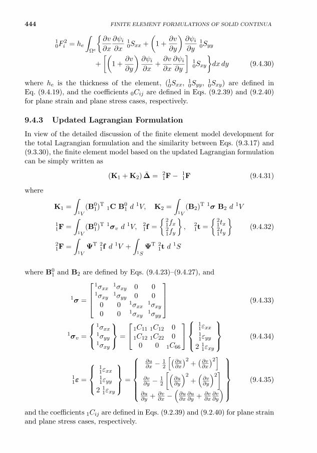
444 FINITE ELEMENT FORMULATIONS OF SOLID CONTINUA
10F
2i = he
∫Ωe
∂v
∂x
∂ψi∂x
10Sxx +
(1 +
∂v
∂y
)∂ψi∂y
10Syy
+
[(1 +
∂v
∂y
)∂ψi∂x
+∂v
∂x
∂ψi∂y
]10Sxy
dx dy (9.4.30)
where he is the thickness of the element, (10Sxx, 1
0Syy,10Sxy) are defined in
Eq. (9.4.19), and the coefficients 0Cij are defined in Eqs. (9.2.39) and (9.2.40)for plane strain and plane stress cases, respectively.
9.4.3 Updated Lagrangian Formulation
In view of the detailed discussion of the finite element model development forthe total Lagrangian formulation and the similarity between Eqs. (9.3.17) and(9.3.30), the finite element model based on the updated Lagrangian formulationcan be simply written as
(K1 + K2) ∆ = 21F− 1
1F (9.4.31)
where
K1 =
∫1V
(B01)T
1C B01 d
1V, K2 =
∫1V
(B2)T 1σ B2 d1V
11F =
∫1V
(B01)T 1σv d
1V, 21f =
21fx21fy
, 2
1t =
21tx21ty
(9.4.32)
21F =
∫1V
ΨT 21f d
1V +
∫1S
ΨT 21t d
1S
where B01 and B2 are defined by Eqs. (9.4.23)–(9.4.27), and
1σ =
1σxx
1σxy 0 01σxy
1σyy 0 00 0 1σxx
1σxy0 0 1σxy
1σyy
(9.4.33)
1σv =
1σxx1σyy1σxy
=
1C11 1C12 0
1C12 1C22 00 0 1C66
11εxx11εyy
2 11εxy
(9.4.34)
11ε =
11εxx11εyy
2 11εxy
=
∂u∂x −
12
[(∂u∂x
)2+(∂v∂x
)2]∂v∂y −
12
[(∂u∂y
)2+(∂v∂y
)2]
∂u∂y + ∂v
∂x −(∂u∂x
∂u∂y + ∂v
∂x∂v∂y
) (9.4.35)
and the coefficients 1Cij are defined in Eqs. (9.2.39) and (9.2.40) for plane strainand plane stress cases, respectively.
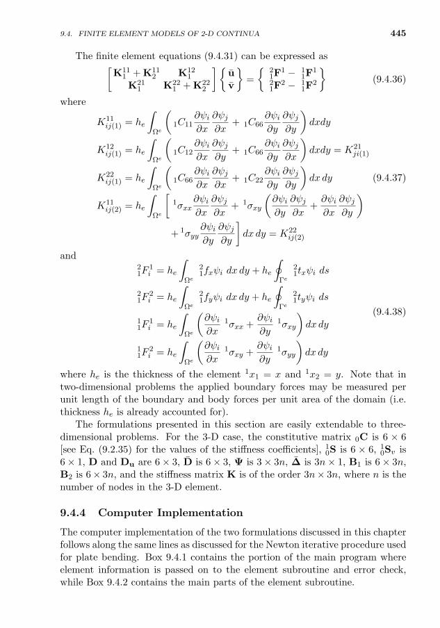
9.4. FINITE ELEMENT MODELS OF 2-D CONTINUA 445
The finite element equations (9.4.31) can be expressed as[K11
1 + K112 K12
1
K211 K22
1 + K222
]uv
=
21F
1 − 11F
1
21F
2 − 11F
2
(9.4.36)
where
K11ij(1) = he
∫Ωe
(1C11
∂ψi∂x
∂ψj∂x
+ 1C66∂ψi∂y
∂ψj∂y
)dxdy
K12ij(1) = he
∫Ωe
(1C12
∂ψi∂x
∂ψj∂y
+ 1C66∂ψi∂y
∂ψj∂x
)dxdy = K21
ji(1)
K22ij(1) = he
∫Ωe
(1C66
∂ψi∂x
∂ψj∂x
+ 1C22∂ψi∂y
∂ψj∂y
)dx dy (9.4.37)
K11ij(2) = he
∫Ωe
[1σxx
∂ψi∂x
∂ψj∂x
+ 1σxy
(∂ψi∂y
∂ψj∂x
+∂ψi∂x
∂ψj∂y
)+ 1σyy
∂ψi∂y
∂ψj∂y
]dx dy = K22
ij(2)
and21F
1i = he
∫Ωe
21fxψi dx dy + he
∮Γe
21txψi ds
21F
2i = he
∫Ωe
21fyψi dx dy + he
∮Γe
21tyψi ds
11F
1i = he
∫Ωe
(∂ψi∂x
1σxx +∂ψi∂y
1σxy
)dx dy
11F
2i = he
∫Ωe
(∂ψi∂x
1σxy +∂ψi∂y
1σyy
)dx dy
(9.4.38)
where he is the thickness of the element 1x1 = x and 1x2 = y. Note that intwo-dimensional problems the applied boundary forces may be measured perunit length of the boundary and body forces per unit area of the domain (i.e.thickness he is already accounted for).
The formulations presented in this section are easily extendable to three-dimensional problems. For the 3-D case, the constitutive matrix 0C is 6 × 6[see Eq. (9.2.35) for the values of the stiffness coefficients], 1
0S is 6 × 6, 10Sv is
6× 1, D and Du are 6× 3, D is 6× 3, Ψ is 3× 3n, ∆ is 3n× 1, B1 is 6× 3n,B2 is 6× 3n, and the stiffness matrix K is of the order 3n× 3n, where n is thenumber of nodes in the 3-D element.
9.4.4 Computer Implementation
The computer implementation of the two formulations discussed in this chapterfollows along the same lines as discussed for the Newton iterative procedure usedfor plate bending. Box 9.4.1 contains the portion of the main program whereelement information is passed on to the element subroutine and error check,while Box 9.4.2 contains the main parts of the element subroutine.
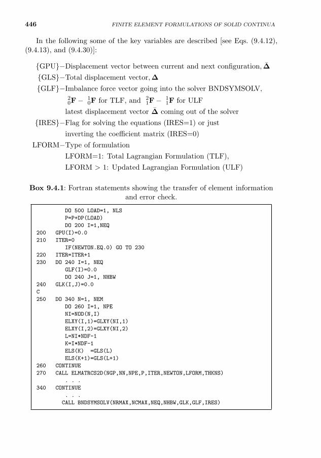
446 FINITE ELEMENT FORMULATIONS OF SOLID CONTINUA
In the following some of the key variables are described [see Eqs. (9.4.12),(9.4.13), and (9.4.30)]:
GPU−Displacement vector between current and next configuration, ∆
GLS−Total displacement vector,∆
GLF−Imbalance force vector going into the solver BNDSYMSOLV,20F− 1
0F for TLF, and 21F− 1
1F for ULF
latest displacement vector ∆ coming out of the solver
IRES−Flag for solving the equations (IRES=1) or just
inverting the coefficient matrix (IRES=0)
LFORM−Type of formulation
LFORM=1: Total Lagrangian Formulation (TLF),
LFORM > 1: Updated Lagrangian Formulation (ULF)
Box 9.4.1: Fortran statements showing the transfer of element informationand error check.
DO 500 LOAD=1, NLS
P=P+DP(LOAD)
DO 200 I=1,NEQ
200 GPU(I)=0.0
210 ITER=0
IF(NEWTON.EQ.0) GO TO 230
220 ITER=ITER+1
230 DO 240 I=1, NEQ
GLF(I)=0.0
DO 240 J=1, NHBW
240 GLK(I,J)=0.0
C
250 DO 340 N=1, NEM
DO 260 I=1, NPE
NI=NOD(N,I)
ELXY(I,1)=GLXY(NI,1)
ELXY(I,2)=GLXY(NI,2)
L=NI*NDF-1
K=I*NDF-1
ELS(K) =GLS(L)
ELS(K+1)=GLS(L+1)
260 CONTINUE
270 CALL ELMATRCS2D(NGP,NN,NPE,P,ITER,NEWTON,LFORM,THKNS)
. . .
340 CONTINUE
. . .
CALL BNDSYMSOLV(NRMAX,NCMAX,NEQ,NHBW,GLK,GLF,IRES)
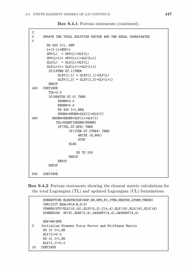
9.4. FINITE ELEMENT MODELS OF 2-D CONTINUA 447
Box 9.4.1: Fortran statements (continued).
C
C UPDATE THE TOTAL SOLUTION VECTOR AND THE NODAL COORDINATES
C
DO 420 I=1, NNM
L=(I-1)*NDF+1
GPU(L) = GPU(L)+GLF(L)
GPU(L+1)= GPU(L+1)+GLF(L+1)
GLS(L) = GLS(L)+GLF(L)
GLS(L+1)= GLS(L+1)+GLF(L+1)
IF(LFORM.GT.1)THEN
GLXY(I,1) = GLXY(I,1)+GLF(L)
GLXY(I,2) = GLXY(I,2)+GLF(L+1)
ENDIF
420 CONTINUE
TOL=0.0
IF(NEWTON.GT.0) THEN
SNORM=0.0
ENORM=0.0
DO 430 I=1,NEQ
SNORM=SNORM+GLS(I)*GLS(I)
430 ENORM=ENORM+GLF(I)*GLF(I)
TOL=DSQRT(ENORM/SNORM)
IF(TOL.GT.EPS) THEN
IF(ITER.GT.ITMAX) THEN
WRITE (6,860)
STOP
ELSE
. . .
GO TO 220
ENDIF
ENDIF
ENDIF
. . .
500 CONTINUE
Box 9.4.2: Fortran statements showing the element matrix calculations forthe total Lagrangian (TL) and updated Lagrangian (UL) formulations.
SUBROUTINE ELMATRCS2D(NGP,NN,NPE,F0,ITER,NEWTON,LFORM,THKNS)
IMPLICIT REAL*8(A-H,O-Z)
COMMON/STF/ELK(18,18),ELXY(9,2),C(4,4),ELF(18),ELS(18),ELU(18)
DIMENSION SF(9),GDSF(2,9),GAUSSPT(4,4),GAUSSWT(4,4)
. . .
NDF=NN/NPE
C Initialize Element Force Vector and Stiffness Matrix
DO 10 I=1,NN
ELF(I)=0.0
DO 10 J=1,NN
ELK(I,J)=0.0
10 CONTINUE
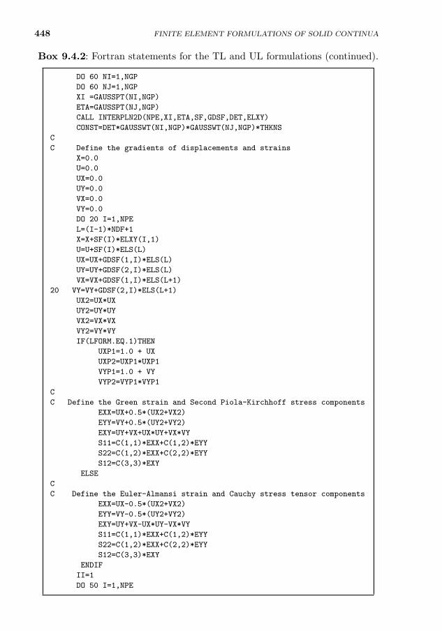
448 FINITE ELEMENT FORMULATIONS OF SOLID CONTINUA
Box 9.4.2: Fortran statements for the TL and UL formulations (continued).
DO 60 NI=1,NGP
DO 60 NJ=1,NGP
XI =GAUSSPT(NI,NGP)
ETA=GAUSSPT(NJ,NGP)
CALL INTERPLN2D(NPE,XI,ETA,SF,GDSF,DET,ELXY)
CONST=DET*GAUSSWT(NI,NGP)*GAUSSWT(NJ,NGP)*THKNS
C
C Define the gradients of displacements and strains
X=0.0
U=0.0
UX=0.0
UY=0.0
VX=0.0
VY=0.0
DO 20 I=1,NPE
L=(I-1)*NDF+1
X=X+SF(I)*ELXY(I,1)
U=U+SF(I)*ELS(L)
UX=UX+GDSF(1,I)*ELS(L)
UY=UY+GDSF(2,I)*ELS(L)
VX=VX+GDSF(1,I)*ELS(L+1)
20 VY=VY+GDSF(2,I)*ELS(L+1)
UX2=UX*UX
UY2=UY*UY
VX2=VX*VX
VY2=VY*VY
IF(LFORM.EQ.1)THEN
UXP1=1.0 + UX
UXP2=UXP1*UXP1
VYP1=1.0 + VY
VYP2=VYP1*VYP1
C
C Define the Green strain and Second Piola-Kirchhoff stress components
EXX=UX+0.5*(UX2+VX2)
EYY=VY+0.5*(UY2+VY2)
EXY=UY+VX+UX*UY+VX*VY
S11=C(1,1)*EXX+C(1,2)*EYY
S22=C(1,2)*EXX+C(2,2)*EYY
S12=C(3,3)*EXY
ELSE
C
C Define the Euler-Almansi strain and Cauchy stress tensor components
EXX=UX-0.5*(UX2+VX2)
EYY=VY-0.5*(UY2+VY2)
EXY=UY+VX-UX*UY-VX*VY
S11=C(1,1)*EXX+C(1,2)*EYY
S22=C(1,2)*EXX+C(2,2)*EYY
S12=C(3,3)*EXY
ENDIF
II=1
DO 50 I=1,NPE
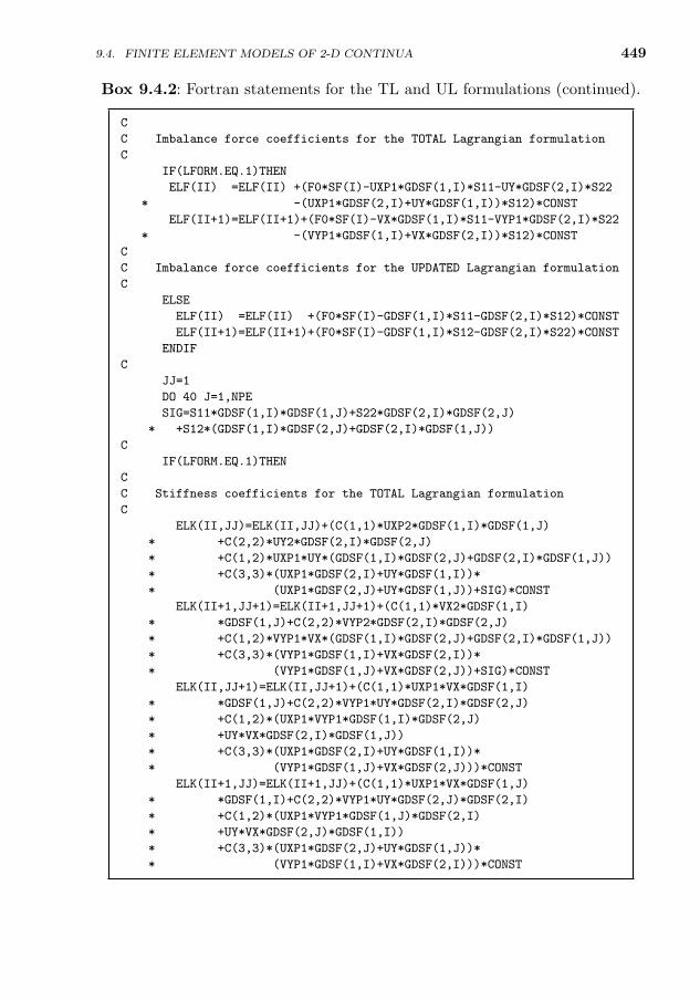
9.4. FINITE ELEMENT MODELS OF 2-D CONTINUA 449
Box 9.4.2: Fortran statements for the TL and UL formulations (continued).
C
C Imbalance force coefficients for the TOTAL Lagrangian formulation
C
IF(LFORM.EQ.1)THEN
ELF(II) =ELF(II) +(F0*SF(I)-UXP1*GDSF(1,I)*S11-UY*GDSF(2,I)*S22
* -(UXP1*GDSF(2,I)+UY*GDSF(1,I))*S12)*CONST
ELF(II+1)=ELF(II+1)+(F0*SF(I)-VX*GDSF(1,I)*S11-VYP1*GDSF(2,I)*S22
* -(VYP1*GDSF(1,I)+VX*GDSF(2,I))*S12)*CONST
C
C Imbalance force coefficients for the UPDATED Lagrangian formulation
C
ELSE
ELF(II) =ELF(II) +(F0*SF(I)-GDSF(1,I)*S11-GDSF(2,I)*S12)*CONST
ELF(II+1)=ELF(II+1)+(F0*SF(I)-GDSF(1,I)*S12-GDSF(2,I)*S22)*CONST
ENDIF
C
JJ=1
DO 40 J=1,NPE
SIG=S11*GDSF(1,I)*GDSF(1,J)+S22*GDSF(2,I)*GDSF(2,J)
* +S12*(GDSF(1,I)*GDSF(2,J)+GDSF(2,I)*GDSF(1,J))
C
IF(LFORM.EQ.1)THEN
C
C Stiffness coefficients for the TOTAL Lagrangian formulation
C
ELK(II,JJ)=ELK(II,JJ)+(C(1,1)*UXP2*GDSF(1,I)*GDSF(1,J)
* +C(2,2)*UY2*GDSF(2,I)*GDSF(2,J)
* +C(1,2)*UXP1*UY*(GDSF(1,I)*GDSF(2,J)+GDSF(2,I)*GDSF(1,J))
* +C(3,3)*(UXP1*GDSF(2,I)+UY*GDSF(1,I))*
* (UXP1*GDSF(2,J)+UY*GDSF(1,J))+SIG)*CONST
ELK(II+1,JJ+1)=ELK(II+1,JJ+1)+(C(1,1)*VX2*GDSF(1,I)
* *GDSF(1,J)+C(2,2)*VYP2*GDSF(2,I)*GDSF(2,J)
* +C(1,2)*VYP1*VX*(GDSF(1,I)*GDSF(2,J)+GDSF(2,I)*GDSF(1,J))
* +C(3,3)*(VYP1*GDSF(1,I)+VX*GDSF(2,I))*
* (VYP1*GDSF(1,J)+VX*GDSF(2,J))+SIG)*CONST
ELK(II,JJ+1)=ELK(II,JJ+1)+(C(1,1)*UXP1*VX*GDSF(1,I)
* *GDSF(1,J)+C(2,2)*VYP1*UY*GDSF(2,I)*GDSF(2,J)
* +C(1,2)*(UXP1*VYP1*GDSF(1,I)*GDSF(2,J)
* +UY*VX*GDSF(2,I)*GDSF(1,J))
* +C(3,3)*(UXP1*GDSF(2,I)+UY*GDSF(1,I))*
* (VYP1*GDSF(1,J)+VX*GDSF(2,J)))*CONST
ELK(II+1,JJ)=ELK(II+1,JJ)+(C(1,1)*UXP1*VX*GDSF(1,J)
* *GDSF(1,I)+C(2,2)*VYP1*UY*GDSF(2,J)*GDSF(2,I)
* +C(1,2)*(UXP1*VYP1*GDSF(1,J)*GDSF(2,I)
* +UY*VX*GDSF(2,J)*GDSF(1,I))
* +C(3,3)*(UXP1*GDSF(2,J)+UY*GDSF(1,J))*
* (VYP1*GDSF(1,I)+VX*GDSF(2,I)))*CONST
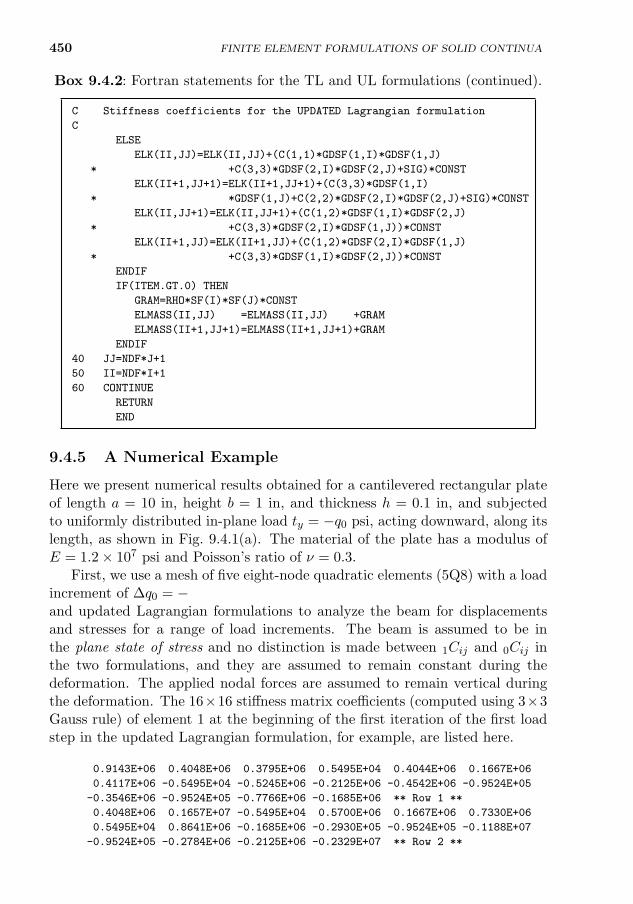
450
Box 9.4.2: Fortran statements for the TL and UL formulations (continued).
C Stiffness coefficients for the UPDATED Lagrangian formulation
C
ELSE
ELK(II,JJ)=ELK(II,JJ)+(C(1,1)*GDSF(1,I)*GDSF(1,J)
* +C(3,3)*GDSF(2,I)*GDSF(2,J)+SIG)*CONST
ELK(II+1,JJ+1)=ELK(II+1,JJ+1)+(C(3,3)*GDSF(1,I)
* *GDSF(1,J)+C(2,2)*GDSF(2,I)*GDSF(2,J)+SIG)*CONST
ELK(II,JJ+1)=ELK(II,JJ+1)+(C(1,2)*GDSF(1,I)*GDSF(2,J)
* +C(3,3)*GDSF(2,I)*GDSF(1,J))*CONST
ELK(II+1,JJ)=ELK(II+1,JJ)+(C(1,2)*GDSF(2,I)*GDSF(1,J)
* +C(3,3)*GDSF(1,I)*GDSF(2,J))*CONST
ENDIF
IF(ITEM.GT.0) THEN
GRAM=RHO*SF(I)*SF(J)*CONST
ELMASS(II,JJ) =ELMASS(II,JJ) +GRAM
ELMASS(II+1,JJ+1)=ELMASS(II+1,JJ+1)+GRAM
ENDIF
40 JJ=NDF*J+1
50 II=NDF*I+1
60 CONTINUE
RETURN
END
9.4.5 A Numerical Example
Here we present numerical results obtained for a cantilevered rectangular plateof length a = 10 in, height b = 1 in, and thickness h = 0.1 in, and subjectedto uniformly distributed in-plane load ty = −q0 psi, acting downward, along itslength, as shown in Fig. 9.4.1(a). The material of the plate has a modulus ofE = 1.2× 10⁷ psi and Poisson’s ratio of ν = 0.3.
First, we use a mesh of five eight-node quadratic elements (5Q8) with a loadincrement of ∆q0 = −500 psi [as shown in Figs. 9.4.1(b) and (c)] in both totaland updated Lagrangian formulations to analyze the beam for displacementsand stresses for a range of load increments. The beam is assumed to be inthe plane state of stress and no distinction is made between 1Cij and 0Cij inthe two formulations, and they are assumed to remain constant during thedeformation. The applied nodal forces are assumed to remain vertical duringthe deformation. The 16×16 stiffness matrix coefficients (computed using 3×3Gauss rule) of element 1 at the beginning of the first iteration of the first loadstep in the updated Lagrangian formulation, for example, are listed here.
0.9143E+06 0.4048E+06 0.3795E+06 0.5495E+04 0.4044E+06 0.1667E+06
0.4117E+06 -0.5495E+04 -0.5245E+06 -0.2125E+06 -0.4542E+06 -0.9524E+05
-0.3546E+06 -0.9524E+05 -0.7766E+06 -0.1685E+06 ** Row 1 **
0.4048E+06 0.1657E+07 -0.5495E+04 0.5700E+06 0.1667E+06 0.7330E+06
0.5495E+04 0.8641E+06 -0.1685E+06 -0.2930E+05 -0.9524E+05 -0.1188E+07
-0.9524E+05 -0.2784E+06 -0.2125E+06 -0.2329E+07 ** Row 2 **
FINITE ELEMENT FORMULATIONS OF SOLID CONTINUA
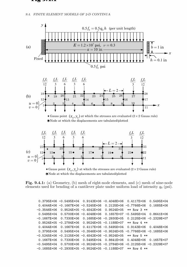
451
Fig 9.4.1
10 ina =
0 1. inh =
1 inb =71 2 10 0 3. psi, .E n= ´ =
0 00 5 0 5. .f q h= (per unit length)
00 5. psif
Fixed
x
y
•
••
•
• •
•• •
•
•
•
• •
••••
•
•••
••
•
• •
•
1 2 311
5 7 912 17
281820 22 24 26♦
♦ Gauss point at which the stresses are evaluated (2 × 2 Gauss rule)
•Node at which the displacements are tabulated/plotted
00
uv==
0
12f L 0
12f L0
6f L0
3f L
4 6 8 1013 14 15 16
19 21 23 25 27
0
3f L 0
6f L 0
3f L
2L =
x
0 0( , )x y
•
••
•
• •
•• •
•••
•
• •
•• •
•••
•
•••
••
•••
••
•
1 2 3 115 7 92112 22
33
1713 15 19
23 25 27 29 31♦
♦ Gauss point at which the stresses are evaluated (2 × 2 Gauss rule)
•Node at which the displacements are tabulated/plotted
0
12f L 0
12f L0
6f L0
3f L 0
3f L 0
6f L
0
3f L
2L =
0 0( , )x y
(a)
(b)
(c)
00
uv==
Fig. 9.4.1: (a) Geometry, (b) mesh of eight-node elements, and (c) mesh of nine-nodeelements used for bending of a cantilever plate under uniform load of intensity q0 (psi).
0.3795E+06 -0.5495E+04 0.9143E+06 -0.4048E+06 0.4117E+06 0.5495E+04
0.4044E+06 -0.1667E+06 -0.5245E+06 0.2125E+06 -0.7766E+06 0.1685E+06
-0.3546E+06 0.9524E+05 -0.4542E+06 0.9524E+05 ** Row 3 **
0.5495E+04 0.5700E+06 -0.4048E+06 0.1657E+07 -0.5495E+04 0.8641E+06
-0.1667E+06 0.7330E+06 0.1685E+06 -0.2930E+05 0.2125E+06 -0.2329E+07
0.9524E+05 -0.2784E+06 0.9524E+05 -0.1188E+07 ** Row 4 **
0.4044E+06 0.1667E+06 0.4117E+06 -0.5495E+04 0.9143E+06 0.4048E+06
0.3795E+06 0.5495E+04 -0.3546E+06 -0.9524E+05 -0.7766E+06 -0.1685E+06
-0.5245E+06 -0.2125E+06 -0.4542E+06 -0.9524E+05 ** Row 5 **
0.1667E+06 0.7330E+06 0.5495E+04 0.8641E+06 0.4048E+06 0.1657E+07
-0.5495E+04 0.5700E+06 -0.9524E+05 -0.2784E+06 -0.2125E+06 -0.2329E+07
-0.1685E+06 -0.2930E+05 -0.9524E+05 -0.1188E+07 ** Row 6 **
9.4. FINITE ELEMENT MODELS OF 2-D CONTINUA
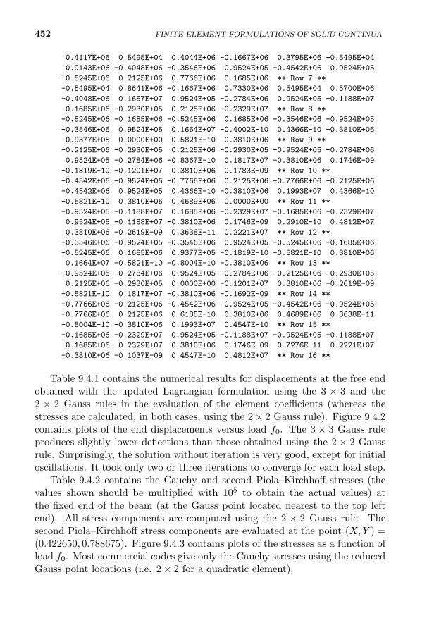
452 FINITE ELEMENT FORMULATIONS OF SOLID CONTINUA
0.4117E+06 0.5495E+04 0.4044E+06 -0.1667E+06 0.3795E+06 -0.5495E+04
0.9143E+06 -0.4048E+06 -0.3546E+06 0.9524E+05 -0.4542E+06 0.9524E+05
-0.5245E+06 0.2125E+06 -0.7766E+06 0.1685E+06 ** Row 7 **
-0.5495E+04 0.8641E+06 -0.1667E+06 0.7330E+06 0.5495E+04 0.5700E+06
-0.4048E+06 0.1657E+07 0.9524E+05 -0.2784E+06 0.9524E+05 -0.1188E+07
0.1685E+06 -0.2930E+05 0.2125E+06 -0.2329E+07 ** Row 8 **
-0.5245E+06 -0.1685E+06 -0.5245E+06 0.1685E+06 -0.3546E+06 -0.9524E+05
-0.3546E+06 0.9524E+05 0.1664E+07 -0.4002E-10 0.4366E-10 -0.3810E+06
0.9377E+05 0.0000E+00 0.5821E-10 0.3810E+06 ** Row 9 **
-0.2125E+06 -0.2930E+05 0.2125E+06 -0.2930E+05 -0.9524E+05 -0.2784E+06
0.9524E+05 -0.2784E+06 -0.8367E-10 0.1817E+07 -0.3810E+06 0.1746E-09
-0.1819E-10 -0.1201E+07 0.3810E+06 0.1783E-09 ** Row 10 **
-0.4542E+06 -0.9524E+05 -0.7766E+06 0.2125E+06 -0.7766E+06 -0.2125E+06
-0.4542E+06 0.9524E+05 0.4366E-10 -0.3810E+06 0.1993E+07 0.4366E-10
-0.5821E-10 0.3810E+06 0.4689E+06 0.0000E+00 ** Row 11 **
-0.9524E+05 -0.1188E+07 0.1685E+06 -0.2329E+07 -0.1685E+06 -0.2329E+07
0.9524E+05 -0.1188E+07 -0.3810E+06 0.1746E-09 0.2910E-10 0.4812E+07
0.3810E+06 -0.2619E-09 0.3638E-11 0.2221E+07 ** Row 12 **
-0.3546E+06 -0.9524E+05 -0.3546E+06 0.9524E+05 -0.5245E+06 -0.1685E+06
-0.5245E+06 0.1685E+06 0.9377E+05 -0.1819E-10 -0.5821E-10 0.3810E+06
0.1664E+07 -0.5821E-10 -0.8004E-10 -0.3810E+06 ** Row 13 **
-0.9524E+05 -0.2784E+06 0.9524E+05 -0.2784E+06 -0.2125E+06 -0.2930E+05
0.2125E+06 -0.2930E+05 0.0000E+00 -0.1201E+07 0.3810E+06 -0.2619E-09
-0.5821E-10 0.1817E+07 -0.3810E+06 -0.1692E-09 ** Row 14 **
-0.7766E+06 -0.2125E+06 -0.4542E+06 0.9524E+05 -0.4542E+06 -0.9524E+05
-0.7766E+06 0.2125E+06 0.6185E-10 0.3810E+06 0.4689E+06 0.3638E-11
-0.8004E-10 -0.3810E+06 0.1993E+07 0.4547E-10 ** Row 15 **
-0.1685E+06 -0.2329E+07 0.9524E+05 -0.1188E+07 -0.9524E+05 -0.1188E+07
0.1685E+06 -0.2329E+07 0.3810E+06 0.1746E-09 0.7276E-11 0.2221E+07
-0.3810E+06 -0.1037E-09 0.4547E-10 0.4812E+07 ** Row 16 **
Table 9.4.1 contains the numerical results for displacements at the free endobtained with the updated Lagrangian formulation using the 3 × 3 and the2 × 2 Gauss rules in the evaluation of the element coefficients (whereas thestresses are calculated, in both cases, using the 2× 2 Gauss rule). Figure 9.4.2contains plots of the end displacements versus load f0. The 3 × 3 Gauss ruleproduces slightly lower deflections than those obtained using the 2 × 2 Gaussrule. Surprisingly, the solution without iteration is very good, except for initialoscillations. It took only two or three iterations to converge for each load step.
Table 9.4.2 contains the Cauchy and second Piola–Kirchhoff stresses (thevalues shown should be multiplied with 105 to obtain the actual values) atthe fixed end of the beam (at the Gauss point located nearest to the top leftend). All stress components are computed using the 2 × 2 Gauss rule. Thesecond Piola–Kirchhoff stress components are evaluated at the point (X,Y ) =(0.422650, 0.788675). Figure 9.4.3 contains plots of the stresses as a function ofload f0. Most commercial codes give only the Cauchy stresses using the reducedGauss point locations (i.e. 2× 2 for a quadratic element).
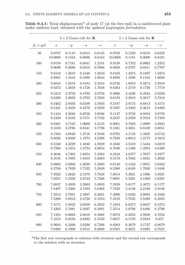
9.4. FINITE ELEMENT MODELS OF 2-D CONTINUA 453
Table 9.4.1: Total displacements* of node 17 (at the free end) in a cantilevered plateunder uniform load; obtained with the updated Lagrangian formulation.
3 × 3 Gauss rule for K 2 × 2 Gauss rule for K
f0 = q0h x −y −u −v x −y −u −v
50 9.9787 0.1145 0.0213 0.6145 9.9782 0.1229 0.0218 0.622910.0000 0.1164 0.0000 0.6164 10.0000 0.1181 0.0000 0.6181
100 9.9159 0.7181 0.0841 1.2181 9.9138 0.7352 0.0862 1.23529.9690 0.2686 0.0310 0.7686 9.9689 0.2707 0.0311 0.7707
150 9.8152 1.3010 0.1848 1.8010 9.8103 1.3274 0.1897 1.82749.8901 1.1644 0.1099 1.6644 9.8896 1.1698 0.1104 1.6698
200 9.6816 1.8554 0.3184 2.3554 9.6726 1.8919 0.3274 2.39199.8272 1.2658 0.1728 1.7658 9.8264 1.2719 0.1736 1.7719
250 9.5212 2.3758 0.4788 2.8758 9.5066 2.4230 0.4934 2.92309.6208 2.2693 0.3792 2.7693 9.6183 2.2818 0.3817 2.7818
300 9.3402 2.8593 0.6598 3.3593 9.3187 2.9174 0.6813 3.41749.5421 2.3359 0.4579 2.8359 9.5387 2.3493 0.4613 2.8493
350 9.1444 3.3046 0.8556 3.8046 9.1147 3.3738 0.8853 3.87389.2429 3.2102 0.7571 3.7102 9.2347 3.2350 0.7653 3.7350
400 8.9391 3.7125 1.0609 4.2125 8.9001 3.7923 1.0999 4.29239.1659 3.2796 0.8341 3.7796 9.1561 3.3051 0.8439 3.8051
450 8.7284 4.0846 1.2716 4.5846 8.6795 4.1743 1.3205 4.67438.8026 4.0388 1.1974 4.5388 8.7828 4.0812 1.2172 4.5812
500 8.5160 4.4229 1.4840 4.9229 8.4566 4.5219 1.5434 5.02198.7266 4.1054 1.2734 4.6054 8.7046 4.1480 1.2954 4.6480
550 8.3046 4.7302 1.6954 5.2302 8.2343 4.8377 1.7657 5.33778.3545 4.7083 1.6455 5.2083 8.3179 4.7692 1.6821 5.2692
600 8.0962 5.0093 1.9038 5.5093 8.0149 5.1242 1.9851 5.62428.2768 4.7839 1.7232 5.2839 8.2380 4.8448 1.7620 5.3448
650 7.8922 5.2628 2.1078 5.7628 7.8014 5.3821 2.1986 5.88217.9257 5.2508 2.0743 5.7508 7.8691 5.3291 2.1309 5.8291
700 7.6937 5.4933 2.3063 5.9933 7.5928 5.6177 2.4072 6.11777.8407 5.3368 2.1593 5.8368 7.7820 5.4146 2.2180 5.9146
750 7.5013 5.7031 2.4987 6.2031 7.3906 5.8320 2.6094 6.33207.5280 5.6913 2.4720 6.1913 7.4510 5.7835 2.5490 6.2835
800 7.3171 5.8922 2.6829 6.3922 7.1953 6.0272 2.8047 6.52727.4303 5.7881 2.5697 6.2881 7.3514 5.8796 2.6486 6.3796
850 7.1384 6.0668 2.8616 6.5668 7.0072 6.2052 2.9928 6.70527.1618 6.0550 2.8382 6.5550 7.0657 6.1576 2.9343 6.657
900 6.9664 6.2268 3.0336 6.7268 6.8263 6.3679 3.1737 6.86797.0488 6.1600 2.9512 6.6600 6.9505 6.2621 3.0495 6.7621
*The first row corresponds to solution with iteration and the second row correspondsto the solution with no iteration.
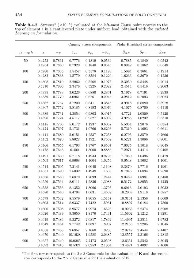
454
Table 9.4.2: Stresses* (×10−5) evaluated at the left-most Gauss point nearest to thetop of element 1 in a cantilevered plate under uniform load; obtained with the updatedLagrangian formulation.
Cauchy stress components Piola–Kirchhoff stress components
f0 = q0h x −y σxx σyy −σxy SXX SY Y SXY
50 0.4253 0.7861 0.7776 0.1819 0.0539 0.7885 0.1840 0.05420.4254 0.7860 0.7929 0.1840 0.0545 0.8042 0.1862 0.0548
100 0.4280 0.7835 1.5457 0.3578 0.1198 1.5894 0.3661 0.12140.4282 0.7833 1.5779 0.3584 0.1220 1.6236 0.3670 0.1236
150 0.4308 0.7810 2.2962 0.5268 0.1975 2.3950 0.5448 0.20140.4310 0.7806 2.3476 0.5225 0.2022 2.4514 0.5416 0.2063
200 0.4335 0.7783 3.0226 0.6880 0.2861 3.1978 0.7191 0.29380.4339 0.7779 3.0961 0.6761 0.2943 3.2812 0.7093 0.3024
250 0.4362 0.7757 3.7200 0.8411 0.3845 3.9918 0.8880 0.39780.4367 0.7752 3.8185 0.8193 0.3970 4.1075 0.8700 0.4110
300 0.4389 0.7731 4.3854 0.9863 0.4915 4.7721 1.0509 0.51200.4396 0.7724 4.5117 0.9527 0.5092 4.9255 1.0232 0.5310
350 0.4415 0.7706 5.0172 1.1237 0.6057 5.5354 1.2076 0.63540.4424 0.7697 5.1731 1.0766 0.6293 5.7310 1.1693 0.6611
400 0.4441 0.7680 5.6151 1.2537 0.7258 6.2795 1.3579 0.76660.4452 0.7670 5.8027 1.1921 0.7562 6.5221 1.3086 0.8001
450 0.4466 0.7655 6.1793 1.3767 0.8507 7.0025 1.5018 0.90450.4478 0.7643 6.400 1.3000 0.8886 7.2971 1.4414 0.9468
500 0.4491 0.7630 6.7118 1.4933 0.9793 7.7050 1.6396 1.04790.4505 0.7617 6.9668 1.4004 1.0254 8.0548 1.5682 1.1001
550 0.4514 0.7605 7.2141 1.6040 1.1108 8.3870 1.7716 1.19610.4531 0.7590 7.5032 1.4948 1.1658 8.7948 1.6894 1.2590
600 0.4536 0.7580 7.6879 1.7093 1.2444 9.0489 1.8981 1.34800.4556 0.7564 8.0111 1.5836 1.3088 9.5172 1.8055 1.4225
650 0.4558 0.7556 8.1352 1.8096 1.3795 9.6916 2.0193 1.50320.4580 0.7540 8.4794 1.6631 1.4502 10.2038 1.9118 1.5857
700 0.4579 0.7532 8.5579 1.9055 1.5157 10.3161 2.1356 1.66090.4603 0.7514 8.9337 1.7422 1.5961 10.8897 2.0184 1.7560
750 0.4600 0.7508 8.9577 1.9973 1.6525 10.9233 2.2474 1.82080.4626 0.7489 9.3650 1.8176 1.7431 11.5602 2.1212 1.9291
800 0.4619 0.7486 9.3272 2.0817 1.7862 11.4997 2.3511 1.97820.4649 0.7464 9.7742 1.8897 1.8907 12.2153 2.2205 2.1045
850 0.4638 0.7463 9.6857 2.1660 1.9230 12.0742 2.4544 2.14070.4670 0.7440 10.1628 1.9588 2.0385 12.8557 2.3166 2.2818
900 0.4657 0.7440 10.0265 2.2473 2.0598 12.6351 2.5542 2.30450.4692 0.7416 10.5321 2.0253 2.1864 13.4821 2.4097 2.4606
*The first row corresponds to the 3× 3 Gauss rule for the evaluation of K and the secondrow corresponds to the 2 × 2 Gauss rule for the evaluation of K.
FINITE ELEMENT FORMULATIONS OF SOLID CONTINUA
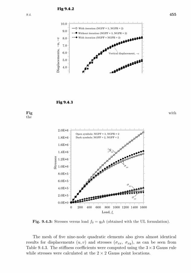
9.4. FINITE ELEMENT MODELS OF 2-D CONTINUA 455
0 200 400 600 800 1000 1200 1400 1600
Load, f
0.0
1.0
2.0
3.0
4.0
5.0
6.0
7.0
8.0
9.0
10.0
Dis
plac
emen
ts, -
u, -
v
With iteration (NGPF = 3, NGPR = 2)
Without iteration (NGPF = 3, NGPR = 2)
With iteration (NGPF = NGPR = 2)
Vertical displacement, -v
Horizontal displacement, -u
Fig 9.4.2
0f
v-
u-
−u, −
v
Fig. 9.4.2: Node 17 displacements −v and −u versus load f0 = q0h (obtained withthe UL formulation).
Fig 9.4.3
0 200 400 600 800 1000 1200 1400 1600
Load, f
0.0E+0
2.0E+5
4.0E+5
6.0E+5
8.0E+5
1.0E+6
1.2E+6
1.4E+6
1.6E+6
1.8E+6
2.0E+6
Str
esse
s
Open symbols: NGPF = 3, NGPR = 2Dark symbols: NGPF = 2, NGPF = 2
xxs
yys
xys
21 xxS
0f
Fig. 9.4.3: Stresses versus load f0 = q0h (obtained with the UL formulation).
The mesh of five nine-node quadratic elements also gives almost identicalresults for displacements (u, v) and stresses (σxx, σxy), as can be seen fromTable 9.4.3. The stiffness coefficients were computed using the 3×3 Gauss rulewhile stresses were calculated at the 2× 2 Gauss point locations.
456 FINITE ELEMENT FORMULATIONS OF SOLID CONTINUA
Table 9.4.3: Total displacements* of node 22 and stresses in a cantilevered plateunder uniform load; obtained with the updated Lagrangian formulation and the meshof 5Q9 elements.
f0 = q0h x −y −u −v x −y σxx −σxy
50 9.9782 0.1218 0.0218 0.6218 0.4254 0.7860 0.7759 0.05490.4226 0.7887 0.7877 0.0552
100 9.9142 0.7323 0.0858 1.2323 0.4282 0.7833 1.5429 0.12390.4226 0.7887 1.5904 0.1253
150 9.8115 1.3214 0.1885 1.8214 0.4311 0.7806 2.2924 0.20650.4226 0.7887 2.3997 0.2102
200 9.6754 1.8810 0.3246 2.3810 0.4340 0.7780 3.0175 0.30180.4226 0.7887 3.2081 0.3093
250 9.5123 2.4057 0.4877 2.9057 0.4368 0.7753 3.7131 0.40840.4226 0.7887 4.0087 0.4214
300 9.3286 2.8923 0.6714 3.3923 0.4396 0.7726 4.3758 0.52490.4226 0.7887 4.7966 0.5452
350 9.1301 3.3400 0.8699 3.8400 0.4424 0.7699 5.0042 0.64970.4226 0.7887 5.5681 0.6793
400 8.9224 3.7494 1.0776 4.2494 0.4450 0.7673 5.5980 0.78140.4226 0.7887 6.3207 0.8222
450 8.7095 4.1224 1.2905 4.6224 0.4476 0.7646 6.1572 0.91850.4226 0.7887 7.0524 0.9725
500 8.4953 4.4611 1.5047 4.9611 0.4501 0.7621 6.6840 1.06000.4226 0.7887 7.7638 1.1291
550 8.2823 4.7684 1.7177 5.2684 0.4525 0.7595 7.1800 1.20470.4226 0.7887 8.4548 1.2909
600 8.0725 5.0472 1.9275 5.5472 0.4549 0.7570 7.6470 1.35210.4226 0.7887 9.1257 1.4570
650 7.8675 5.3002 2.1325 5.8002 0.4572 0.7545 8.0870 1.50120.4226 0.7887 9.7774 1.6266
700 7.6681 5.5301 2.3319 6.0301 0.4594 0.7520 8.5019 1.65170.4226 0.7887 10.4110 1.7992
750 7.4750 5.7392 2.5250 6.2392 0.4615 0.7496 8.8936 1.80300.4226 0.7887 11.0270 1.9742
800 7.2886 5.9299 2.7114 6.4299 0.4635 0.7472 9.2638 1.95470.4226 0.7887 11.6270 2.1511
850 7.1114 6.1013 2.8886 6.6013 0.4655 0.7449 9.6050 2.10200.4226 0.7887 12.1960 2.3241
900 6.9392 6.2604 3.0608 6.7604 0.4674 0.7426 9.9366 2.25340.4226 0.7887 12.7650 2.5033
950 6.7738 6.4064 3.2262 6.9064 0.4693 0.7403 1.0251 2.40480.4226 0.7887 13.3220 2.6837
1,000 6.6150 6.5407 3.3850 7.0407 0.4711 0.7380 10.5510 2.55580.4226 0.7887 13.8660 2.8651
1,050 6.4627 6.6644 3.5373 7.1644 0.4728 0.7357 10.8350 2.70640.4226 0.7887 14.3990 3.0471
1,100 6.3167 6.7787 3.6833 7.2787 0.4745 0.7334 11.1060 2.85640.4226 0.7887 14.9210 3.2297
*The second row corresponds to the second Piola–Kirchhoff stress components.
9.4. FINITE ELEMENT MODELS OF 2-D CONTINUA 457
Table 9.4.4 contains the displacements and stresses obtained with the totalLagrangian formulation and the two different meshes. The results are in closeagreement with those obtained with the updated Lagrangian formulation.
Table 9.4.4: Total displacements* and stresses in a cantilevered plate under uniformload; obtained with the total Lagrangian formulation.
f0 = q0h −u −v x −y σxx −σxy Sxx −Sxy
50 0.0216 0.6144 0.4253 0.7861 0.7738 0.0508 0.7736 0.04840.0221 0.6218 0.4254 0.7860 0.7713 0.0512 0.7711 0.0482
100 0.0853 1.2177 0.4278 0.7836 1.5311 0.1073 1.5299 0.09790.0871 1.2320 0.4280 0.7834 1.5255 0.1090 1.5243 0.0971
150 0.1874 1.7997 0.4303 0.7810 2.2656 0.1692 2.2619 0.14870.1912 1.8203 0.4306 0.7807 2.2559 1.7300 2.2521 0.1470
200 0.3225 2.3524 0.4327 0.7784 2.9724 0.2361 2.9642 0.20090.3290 2.3786 0.4331 0.7780 2.9577 0.2428 2.9493 0.1980
250 0.4846 2.8706 0.4350 0.7759 3.6481 0.3074 3.6333 0.25450.4940 2.9013 0.4355 0.7754 3.6276 0.3177 3.6121 0.2502
300 0.6671 3.3510 0.4372 0.7734 4.2912 0.3825 4.2672 0.30940.6795 3.3854 0.4380 0.7727 4.2641 0.3970 4.2387 0.3036
350 0.8641 3.7927 0.4393 0.7709 4.9013 0.4605 4.8656 0.36560.8795 3.8300 0.4400 0.7702 4.8669 0.4800 4.8287 0.3581
400 1.0702 4.1965 0.4413 0.7684 5.4792 0.5411 5.4290 0.42281.0886 4.2358 0.4420 0.7676 5.4368 0.5657 5.3830 0.4136
450 1.2812 4.5640 0.4432 0.7660 6.0261 0.6235 5.9588 0.48091.3023 4.6048 0.4439 0.7651 5.9753 0.6539 5.9032 0.4701
500 1.4936 4.8977 0.4450 0.7636 6.5438 0.7073 6.4570 0.53981.5171 4.9394 0.4457 0.7626 6.4843 0.7438 6.3911 0.5274
550 1.7045 5.2003 0.4466 0.7613 7.0343 0.7922 6.9256 0.59941.7302 5.2426 0.4474 0.7602 6.9658 0.8351 6.8491 0.5853
600 1.9122 5.4746 0.4482 0.7590 7.4997 0.8778 7.3668 0.65941.9398 5.5171 0.4490 0.7578 7.4219 0.9274 7.2794 0.6438
650 2.1150 5.7234 0.4497 0.7567 7.9418 0.9638 7.7827 0.71982.1444 5.7659 0.4505 0.7555 7.8546 1.0203 7.6842 0.7027
700 2.3121 5.9493 0.4511 0.7545 8.3625 1.0501 8.1754 0.78052.343 5.9916 0.4520 0.7532 8.2660 1.1138 8.0656 0.7620
750 2.5028 6.1547 0.4524 0.7523 8.7638 1.1364 8.5467 0.84142.5350 6.1967 0.4533 0.7509 8.6578 1.2074 8.4257 0.8216
800 2.6868 6.3418 0.4536 0.7501 9.1471 1.2227 8.8985 0.90252.7201 6.3833 0.4546 0.7487 9.0316 1.3012 8.7662 0.8814
850 2.8654 6.5138 0.4548 0.7480 9.5153 1.3090 9.2337 0.96372.8997 6.5548 0.4557 0.7465 9.3904 1.3951 9.0900 0.9415
900 3.0353 6.6697 0.4559 0.7459 9.8669 1.3949 9.5508 1.02483.0704 6.7101 0.4569 0.7444 9.7325 1.4887 9.3960 1.0016
*The first row corresponds to the mesh of five 5Q8 elements and the second rowcorresponds to the mesh of 5Q9 elements.
458 FINITE ELEMENT FORMULATIONS OF SOLID CONTINUA
This completes the development of finite element models of nonlinear con-tinua. The total and updated Lagrangian formulations developed in Sections 9.3and 9.4 can be readily extended to axisymmetric problems, three-dimensionalproblems, problems with assumed displacements and/or strains [4], and com-posite plates and shells [55]. The extension of the formulations to transientproblems is straightforward in view of the discussion presented in Chapter 6.In the next section, we extend the formulation to shells by invoking the kine-matic assumptions of a shell theory in the approximation of the geometry andthe displacement field.
9.5 Conventional Continuum Shell Finite Element
9.5.1 Introduction
In previous chapters, beam, plate, and shell finite elements were developedusing beam, plate, and shell theories, respectively, that were derived from anassumed displacement field. Such theories are often limited to geometricallylinear analysis and nonlinear analysis with small strains and moderate rotations.In these elements, the geometry is not updated explicitly during the nonlinearequilibrium iterations.
The finite element model to be developed in this section is based on three-dimensional continuum equations and is known as the continuum shell element,which was first introduced by Ahmad, Irons, and Zienkiewicz [122]. The three-dimensional geometry of the continuum is approximated by imposing appro-priate kinematic assumptions on the displacement field; although no shell the-ory is explicitly invoked, the resulting formulation may be identified as a shellelement with qualities consistent with a first-order or third-order shear defor-mation shell model. Such formulations especially applicable to material andgeometrical nonlinear analysis of shell-type structures in which large displace-ments and rotations are experienced (see [55, 123–137]). Although the shelltheory-based and continuum-based shell finite elements appear quite differentfrom each other because of the way they are constructed, the formulations arequite similar when based on the same kinematic assumptions, and they “differonly in the kind of discretization” (see Buchter and Ramm [138]).
It is well known that low-order finite element implementations for shells suf-fer from various forms of locking whenever a purely displacement-based formu-lation is adopted. The locking phenomena occurs on account of inconsistenciesthat arise in the discrete finite element representation of the membrane andtransverse shear energies. In recent years, the issue of locking has been ad-dressed through the use of low-order finite technology using Hu–Washizu typemixed variational principles. Among the low-order implementations are the as-sumed strain formulation of Dvorkin and Bathe [133] and Hinton and Huang[139], and the enhanced strain formulation of Simo and Rifai [107] are notable.
459
High-order finite element implementations have also been advocated in recentyears as a means of eliminating the locking phenomena completely. Whenevera sufficient degree of p-refinement is employed, highly reliable locking free nu-merical solutions may be obtained in displacement-based models. Among theseworks are high-order interpolations by Pitkaranta and his colleagues [140–142]for linear analysis of isotropic shells, the least-squares finite element formu-lations of Pontaza and Reddy [143, 144] for the linear analysis of plates andshells, and the shell theory-based weak form Galerkin finite element models ofArciniega [145] and Arciniega and Reddy [146, 147] for the analysis of isotropic,laminated composite, and functionally graded shells.
In this section, we develop continuum shell element based on first-order sheardeformation theory kinematics with five generalized displacements per node (ina general setting, a sixth degree of freedom, namely the “drilling” degree offreedom in the form of rotation about the transverse normal is introduced).The generalized displacements are introduced through the kinematics of thesurface displacements while the transverse displacement is assumed to preservethe inextensibility of a transverse normal line. Consequently, the plane-stressassumption is invoked in writing the stress–strain relations.
9.5.2 Incremental Equations of Motion
Assuming that the body may experience large displacements and rotations, wewish to determine deformed configurations of the body for different times/loads.We assume that all configurations from time t = 0 to the current time t, bothinclusive, have been determined, and the configuration Ω2 for time t = t + ∆tis being sought next. The total Lagrangian description with the principle ofvirtual displacements, Eq. (9.3.17), is used to express the equilibrium of thebody in configuration Ω2.
For dynamic analysis, the statement of the principle of virtual displacementsbased on the total Lagrangian formulation, Eq. (9.3.17), must be modified toinclude inertial terms. Consider the motion in a fixed Cartesian coordinatesystem. In this case we have∫
2V
2ρ 2ui δ2ui d
2V =
∫0V
0ρ 2ui δ2ui d
0V (9.5.1)
and hence the mass matrix can be evaluated using the initial configuration ofthe body. Using Hamilton’s principle we obtain the equations of motion of themoving body at time t+ ∆t in the variational form as∫
0V
0ρ 2ui δ(2ui) d
0V +
∫0V
0Cijrs 0ers δ 0eij d0V +
∫0V
10Sij δ 0ηij d
0V
= δ(20R)−
∫0V
10Sij δ 0eij d
0V (9.5.2)
where δ(2ui) = δui.
9.5. CONVENTIONAL CONTINUUM SHELL FINITE ELEMENT
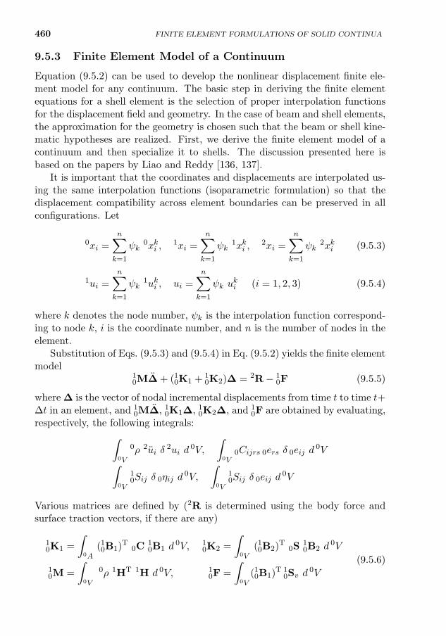
460 FINITE ELEMENT FORMULATIONS OF SOLID CONTINUA
9.5.3 Finite Element Model of a Continuum
Equation (9.5.2) can be used to develop the nonlinear displacement finite ele-ment model for any continuum. The basic step in deriving the finite elementequations for a shell element is the selection of proper interpolation functionsfor the displacement field and geometry. In the case of beam and shell elements,the approximation for the geometry is chosen such that the beam or shell kine-matic hypotheses are realized. First, we derive the finite element model of acontinuum and then specialize it to shells. The discussion presented here isbased on the papers by Liao and Reddy [136, 137].
It is important that the coordinates and displacements are interpolated us-ing the same interpolation functions (isoparametric formulation) so that thedisplacement compatibility across element boundaries can be preserved in allconfigurations. Let
0xi =
n∑k=1
ψk0xki ,
1xi =
n∑k=1
ψk1xki ,
2xi =
n∑k=1
ψk2xki (9.5.3)
1ui =
n∑k=1
ψk1uki , ui =
n∑k=1
ψk uki (i = 1, 2, 3) (9.5.4)
where k denotes the node number, ψk is the interpolation function correspond-ing to node k, i is the coordinate number, and n is the number of nodes in theelement.
Substitution of Eqs. (9.5.3) and (9.5.4) in Eq. (9.5.2) yields the finite elementmodel
10M∆ + (1
0K1 + 10K2)∆ = 2R− 1
0F (9.5.5)
where ∆ is the vector of nodal incremental displacements from time t to time t+∆t in an element, and 1
0M∆, 10K1∆, 1
0K2∆, and 10F are obtained by evaluating,
respectively, the following integrals:∫0V
0ρ 2ui δ2ui d
0V,
∫0V
0Cijrs 0ers δ 0eij d0V∫
0V
10Sij δ 0ηij d
0V,
∫0V
10Sij δ 0eij d
0V
Various matrices are defined by (2R is determined using the body force andsurface traction vectors, if there are any)
10K1 =
∫0A
(10B1)T
0C10B1 d
0V, 10K2 =
∫0V
(10B2)T
0S10B2 d
0V
10M =
∫0V
0ρ 1HT 1H d 0V, 10F =
∫0V
(10B1)T 1
0Sv d0V
(9.5.6)
461
In the above equations, 10B1 and 1
0B2 are the linear and nonlinear strain–displacement transformation matrices, 0C is the incremental stress–strain ma-terial property matrix, 1
0S is a matrix of second Piola–Kirchhoff stress compo-nents, 1
0Sv is a vector of these stresses, and 1H is the incremental displacementinterpolation matrix [see Eq. (9.5.23)]. All matrix elements correspond to theconfiguration at time t and are defined with respect to the configuration at timet = 0. It is important to note that Eq. (9.5.5) is only an approximation to theactual solution to be determined in each time step [see Eq. (9.3.15)]. Therefore,it may be necessary to iterate in each time step until Eq. (9.3.15), with inertiaterms, is satisfied to a required tolerance.
The finite element equations, Eq. (9.5.5), are second-order differential equa-tions in time. In order to obtain numerical solutions at each time step, Eq. (9.5.5)needs to be converted to algebraic equations using a time approximation scheme,as explained in Chapter 6. In the present study the Newmark scheme is used(see Section 6.7.4 for details).
In the Newmark time integration scheme, the displacements and velocitiesare approximated by [see Eq. (6.7.29)]
t+∆t∆ = t∆ + ∆t t∆ +1
2(∆t)2[(1− γ) t∆ + γ t+∆t∆]
t+∆t∆ = t∆ + ∆t[(1− α) t∆ + α t+∆t∆](9.5.7)
where α = 12 and γ = 1
2 for the constant-average acceleration method, and ∆tis the time step. Rearranging Eqs. (9.5.5) and (9.5.7), we obtain [10M ≈ 2
0M;see Eq. (6.7.33)]
10K∆ = 2R (9.5.8)
where t∆ is the vector of nodal incremental displacements at time t, ∆ =t+∆t∆− t∆, and
10K = a3
10M + 1
0K1 + 10K2
2R = 2R− 10F + 1
0M(a3
t∆ + a4t∆ + a5
t∆) (9.5.9)
a3 =1
β(∆t)2, a4 = a3∆t, a5 =
1
2β− 1 (9.5.10)
Once Eq. (9.5.8) is solved for ∆ at time t + ∆t, the acceleration and velocityvectors are obtained using [a1 = α∆t and a2 = (1− α)∆t; see Eq. (6.7.36)]
t+∆t∆ = a3(t+∆t∆− t∆)− a4t∆− a5
t∆t+∆t∆ = t∆ + a1
t+∆t∆ + a2t∆
(9.5.11)
The finite element equations, Eq. (9.5.8), are solved iteratively at each timestep (after assembly and imposition of boundary conditions) until Eq. (9.5.8)is satisfied within a required tolerance. The Newton–Raphson method withWempner–Riks algorithm (see Wempner [148], Riks [149, 150], Crisfield [151],and Kweon and Hong [152]; also, see Appendix 1) is used in the present study.
9.5. CONVENTIONAL CONTINUUM SHELL FINITE ELEMENT
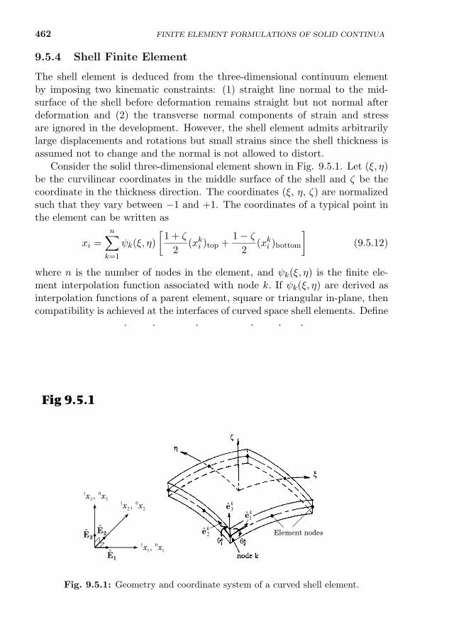
462 FINITE ELEMENT FORMULATIONS OF SOLID CONTINUA
9.5.4 Shell Finite Element
The shell element is deduced from the three-dimensional continuum elementby imposing two kinematic constraints: (1) straight line normal to the mid-surface of the shell before deformation remains straight but not normal afterdeformation and (2) the transverse normal components of strain and stressare ignored in the development. However, the shell element admits arbitrarilylarge displacements and rotations but small strains since the shell thickness isassumed not to change and the normal is not allowed to distort.
Consider the solid three-dimensional element shown in Fig. 9.5.1. Let (ξ, η)be the curvilinear coordinates in the middle surface of the shell and ζ be thecoordinate in the thickness direction. The coordinates (ξ, η, ζ) are normalizedsuch that they vary between −1 and +1. The coordinates of a typical point inthe element can be written as
xi =
n∑k=1
ψk(ξ, η)
[1 + ζ
2(xki )top +
1− ζ2
(xki )bottom
](9.5.12)
where n is the number of nodes in the element, and ψk(ξ, η) is the finite ele-ment interpolation function associated with node k. If ψk(ξ, η) are derived asinterpolation functions of a parent element, square or triangular in-plane, thencompatibility is achieved at the interfaces of curved space shell elements. Define
V k3i = (xki )top − (xki )bottom, ek3 = Vk
3/|Vk3 | (9.5.13)
where Vk3 is the vector connecting the upper and lower points of the normal at
node k. Equation (9.5.12) can be rewritten as
xi =n∑k=1
ψk(ξ, η)
[(xki )mid +
ζ
2V k
3i
]=
n∑k=1
ψk(ξ, η)
[(xki )mid +
ζ
2hke
k3i
](9.5.14)
k3e
k1e
k2e
3E
1E
2E Element nodes
1 01 1,x x
1 02 2,x x
1 03 3,x x
Fig 9.5.1
Fig. 9.5.1: Geometry and coordinate system of a curved shell element.
9.5. CONVENTIONAL CONTINUUM SHELL FINITE ELEMENT 463
where hk = |Vk3 | is the thickness of the shell element at node k. Hence, the
coordinates of any point in the element at time t are interpolated by the ex-pression
1xi =n∑k=1
ψk(ξ, η)
[1xki +
ζ
2hk
1ek3i
](9.5.15)
and the displacements and incremental displacements by
1ui = 1xi − 0x1 =n∑k=1
ψk(ξ, η)
[1uki +
ζ
2hk
(1ek3i − 0ek3i
)](9.5.16)
ui = 2ui − 1ui =n∑k=1
ψk(ξ, η)
[uki +
ζ
2hk
(2ek3i − 1ek3i
)](9.5.17)
Here 1uki and uki denote, respectively, the displacement and incremental dis-placement components in the xi-direction at the kth node and time t. Forsmall rotation dΩ at each node, we have
dΩ = θk21ek1 + θk1
1ek2 + θk31ek3 (9.5.18)
The increment of vector 1ek3 can be written as
∆1ek3 = 2ek3 − 1ek3 = dΩ× 1ek3 = θk11ek1 − θk2 1ek2 (9.5.19)
Then Eq. (9.5.17) becomes
ui =
n∑k=1
ψk(ξ, η)
[uki +
ζ
2hk
(θk1
1ek1i − θk2 1ek2i
)](i = 1, 2, 3) (9.5.20)
The unit vectors 1ek1 and 1ek2 at node k can be obtained from the relations
1ek1 =E2 × 1ek3|E2 × 1ek3|
, 1ek2 = 1ek3 × 1ek1 (9.5.21)
where Ei are the unit vectors of the stationary global coordinate system (0x1,0x2, 0x3). Equation (9.5.20) can be written in matrix form as
uT =
u1
u2
u3
= 1H∆e (9.5.22)
where ∆e = uk1 uk2 uk3 θk1 θk2T, (k = 1, 2, . . . , n, and n is the number of nodes)is the vector of nodal incremental displacements (five per node), and 1H is theincremental displacement interpolation matrix
1H3×5n =
. . . ψk 0 0 12ψkζhk
1ek11 −12ψkζhk
1ek21 . . .. . . 0 ψk 0 1
2ψkζhk1ek12 −1
2ψkζhk1ek22 . . .
. . . 0 0 ψk12ψkζhk
1ek13 −12ψkζhk
1ek23 . . .
(9.5.23)
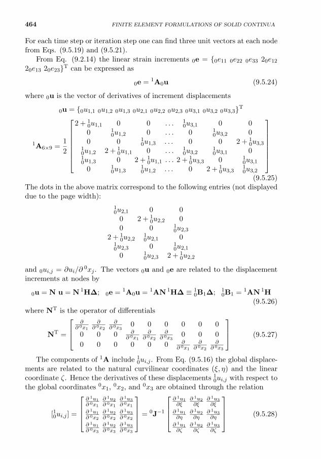
464 FINITE ELEMENT FORMULATIONS OF SOLID CONTINUA
For each time step or iteration step one can find three unit vectors at each nodefrom Eqs. (9.5.19) and (9.5.21).
From Eq. (9.2.14) the linear strain increments 0e = 0e11 0e22 0e33 20e12
20e13 20e23T can be expressed as
0e = 1A0u (9.5.24)
where 0u is the vector of derivatives of increment displacements
0u = 0u1,1 0u1,2 0u1,3 0u2,1 0u2,2 0u2,3 0u3,1 0u3,2 0u3,3T
1A6×9 =1
2
2 + 10u1,1 0 0 . . . 1
0u3,1 0 00 1
0u1,2 0 . . . 0 10u3,2 0
0 0 10u1,3 . . . 0 0 2 + 1
0u3,310u1,2 2 + 1
0u1,1 0 . . . 10u3,2
10u3,1 0
10u1,3 0 2 + 1
0u1,1 . . . 2 + 10u3,3 0 1
0u3,1
0 10u1,3
10u1,2 . . . 0 2 + 1
0u3,310u3,2
(9.5.25)
The dots in the above matrix correspond to the following entries (not displayeddue to the page width):
10u2,1 0 0
0 2 + 10u2,2 0
0 0 10u2,3
2 + 10u2,2
10u2,1 0
10u2,3 0 1
0u2,1
0 10u2,3 2 + 1
0u2,2
and 0ui,j = ∂ui/∂0xj . The vectors 0u and 0e are related to the displacement
increments at nodes by
0u = N u = N 1H∆; 0e = 1A0u = 1AN 1H∆ ≡ 10B1∆; 1
0B1 = 1AN 1H(9.5.26)
where NT is the operator of differentials
NT =
∂
∂ 0x1∂
∂ 0x2∂
∂ 0x30 0 0 0 0 0
0 0 0 ∂∂ 0x1
∂∂ 0x2
∂∂ 0x3
0 0 0
0 0 0 0 0 0 ∂∂ 0x1
∂∂ 0x2
∂∂ 0x3
(9.5.27)
The components of 1A include 10ui,j . From Eq. (9.5.16) the global displace-
ments are related to the natural curvilinear coordinates (ξ, η) and the linearcoordinate ζ. Hence the derivatives of these displacements 1
0ui,j with respect tothe global coordinates 0x1, 0x2, and 0x3 are obtained through the relation
[10ui,j ] =
∂ 1u1∂ 0x1
∂ 1u2∂ 0x1
∂ 1u3∂ 0x1
∂ 1u1∂ 0x2
∂ 1u2∂ 0x2
∂ 1u3∂ 0x2
∂ 1u1∂ 0x3
∂ 1u2∂ 0x3
∂ 1u3∂ 0x3
= 0J−1
∂ 1u1∂ξ
∂ 1u2∂ξ
∂ 1u3∂ξ
∂ 1u1∂η
∂ 1u2∂η
∂ 1u3∂η
∂ 1u1∂ζ
∂ 1u2∂ζ
∂ 1u3∂ζ
(9.5.28)
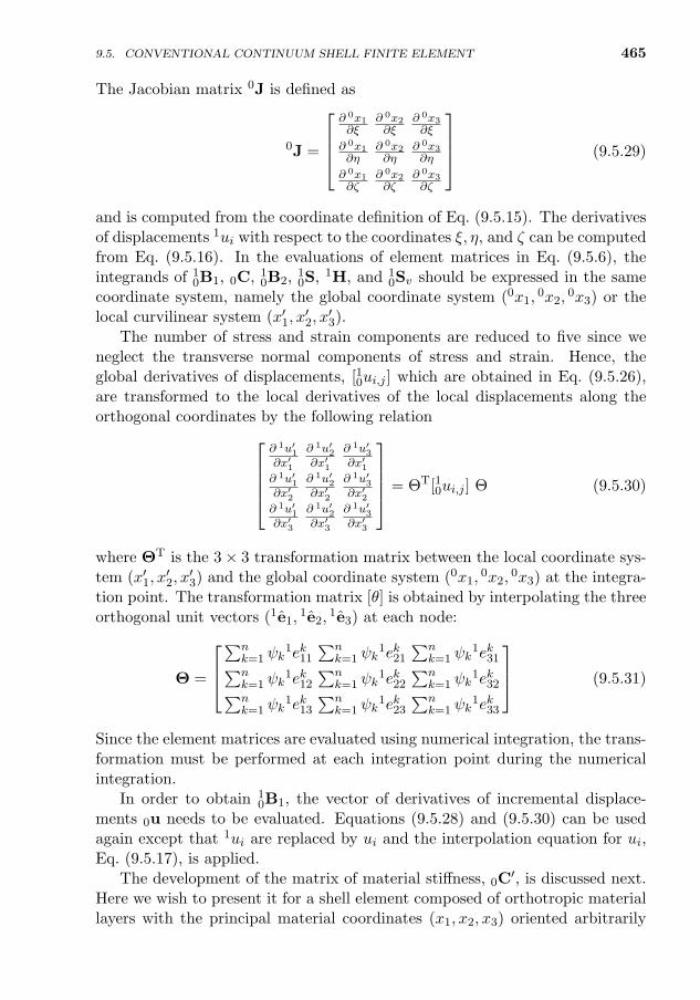
9.5. CONVENTIONAL CONTINUUM SHELL FINITE ELEMENT 465
The Jacobian matrix 0J is defined as
0J =
∂ 0x1∂ξ
∂ 0x2∂ξ
∂ 0x3∂ξ
∂ 0x1∂η
∂ 0x2∂η
∂ 0x3∂η
∂ 0x1∂ζ
∂ 0x2∂ζ
∂ 0x3∂ζ
(9.5.29)
and is computed from the coordinate definition of Eq. (9.5.15). The derivativesof displacements 1ui with respect to the coordinates ξ, η, and ζ can be computedfrom Eq. (9.5.16). In the evaluations of element matrices in Eq. (9.5.6), theintegrands of 1
0B1, 0C, 10B2, 1
0S, 1H, and 10Sv should be expressed in the same
coordinate system, namely the global coordinate system (0x1,0x2,
0x3) or thelocal curvilinear system (x′1, x
′2, x′3).
The number of stress and strain components are reduced to five since weneglect the transverse normal components of stress and strain. Hence, theglobal derivatives of displacements, [10ui,j ] which are obtained in Eq. (9.5.26),are transformed to the local derivatives of the local displacements along theorthogonal coordinates by the following relation
∂ 1u′1∂x′1
∂ 1u′2∂x′1
∂ 1u′3∂x′1
∂ 1u′1∂x′2
∂ 1u′2∂x′2
∂ 1u′3∂x′2
∂ 1u′1∂x′3
∂ 1u′2∂x′3
∂ 1u′3∂x′3
= ΘT[10ui,j ] Θ (9.5.30)
where ΘT is the 3× 3 transformation matrix between the local coordinate sys-tem (x′1, x
′2, x′3) and the global coordinate system (0x1,
0x2,0x3) at the integra-
tion point. The transformation matrix [θ] is obtained by interpolating the threeorthogonal unit vectors (1e1,
1e2,1e3) at each node:
Θ =
∑n
k=1 ψk1ek11
∑nk=1 ψk
1ek21
∑nk=1 ψk
1ek31∑nk=1 ψk
1ek12
∑nk=1 ψk
1ek22
∑nk=1 ψk
1ek32∑nk=1 ψk
1ek13
∑nk=1 ψk
1ek23
∑nk=1 ψk
1ek33
(9.5.31)
Since the element matrices are evaluated using numerical integration, the trans-formation must be performed at each integration point during the numericalintegration.
In order to obtain 10B1, the vector of derivatives of incremental displace-
ments 0u needs to be evaluated. Equations (9.5.28) and (9.5.30) can be usedagain except that 1ui are replaced by ui and the interpolation equation for ui,Eq. (9.5.17), is applied.
The development of the matrix of material stiffness, 0C′, is discussed next.
Here we wish to present it for a shell element composed of orthotropic materiallayers with the principal material coordinates (x1, x2, x3) oriented arbitrarily
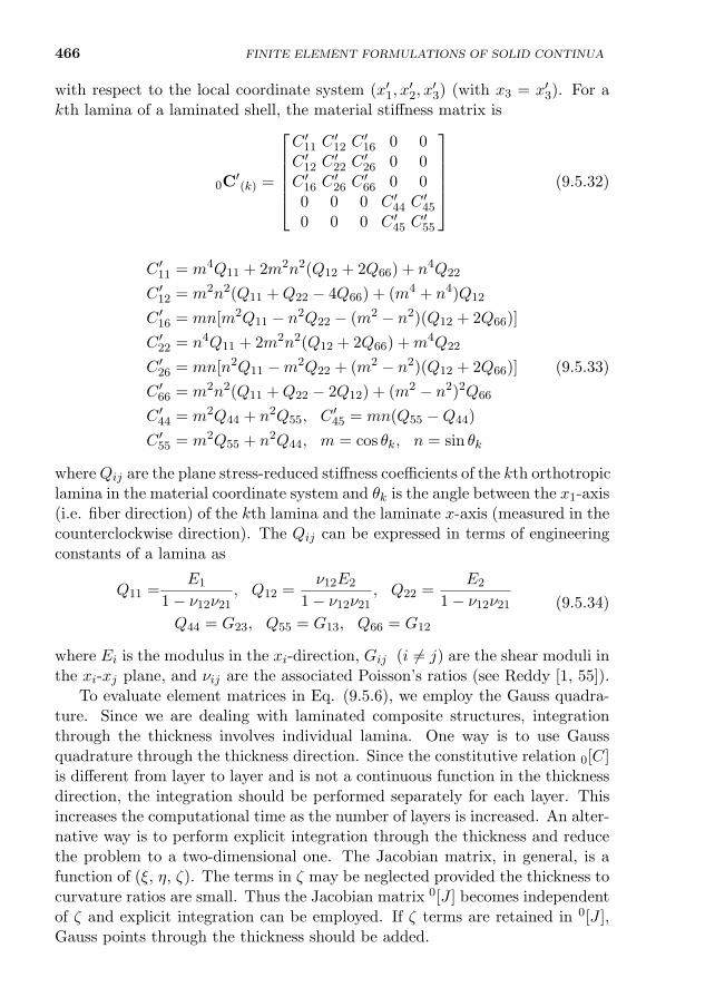
466 FINITE ELEMENT FORMULATIONS OF SOLID CONTINUA
with respect to the local coordinate system (x′1, x′2, x′3) (with x3 = x′3). For a
kth lamina of a laminated shell, the material stiffness matrix is
0C′(k) =
C ′11 C
′12 C
′16 0 0
C ′12 C′22 C
′26 0 0
C ′16 C′26 C
′66 0 0
0 0 0 C ′44 C′45
0 0 0 C ′45 C′55
(9.5.32)
C ′11 = m4Q11 + 2m2n2(Q12 + 2Q66) + n4Q22
C ′12 = m2n2(Q11 +Q22 − 4Q66) + (m4 + n4)Q12
C ′16 = mn[m2Q11 − n2Q22 − (m2 − n2)(Q12 + 2Q66)]
C ′22 = n4Q11 + 2m2n2(Q12 + 2Q66) +m4Q22
C ′26 = mn[n2Q11 −m2Q22 + (m2 − n2)(Q12 + 2Q66)] (9.5.33)
C ′66 = m2n2(Q11 +Q22 − 2Q12) + (m2 − n2)2Q66
C ′44 = m2Q44 + n2Q55, C ′45 = mn(Q55 −Q44)
C ′55 = m2Q55 + n2Q44, m = cos θk, n = sin θk
whereQij are the plane stress-reduced stiffness coefficients of the kth orthotropiclamina in the material coordinate system and θk is the angle between the x1-axis(i.e. fiber direction) of the kth lamina and the laminate x-axis (measured in thecounterclockwise direction). The Qij can be expressed in terms of engineeringconstants of a lamina as
Q11 =E1
1− ν12ν21, Q12 =
ν12E2
1− ν12ν21, Q22 =
E2
1− ν12ν21
Q44 = G23, Q55 = G13, Q66 = G12
(9.5.34)
where Ei is the modulus in the xi-direction, Gij (i 6= j) are the shear moduli inthe xi-xj plane, and νij are the associated Poisson’s ratios (see Reddy [1, 55]).
To evaluate element matrices in Eq. (9.5.6), we employ the Gauss quadra-ture. Since we are dealing with laminated composite structures, integrationthrough the thickness involves individual lamina. One way is to use Gaussquadrature through the thickness direction. Since the constitutive relation 0[C]is different from layer to layer and is not a continuous function in the thicknessdirection, the integration should be performed separately for each layer. Thisincreases the computational time as the number of layers is increased. An alter-native way is to perform explicit integration through the thickness and reducethe problem to a two-dimensional one. The Jacobian matrix, in general, is afunction of (ξ, η, ζ). The terms in ζ may be neglected provided the thickness tocurvature ratios are small. Thus the Jacobian matrix 0[J ] becomes independentof ζ and explicit integration can be employed. If ζ terms are retained in 0[J ],Gauss points through the thickness should be added.
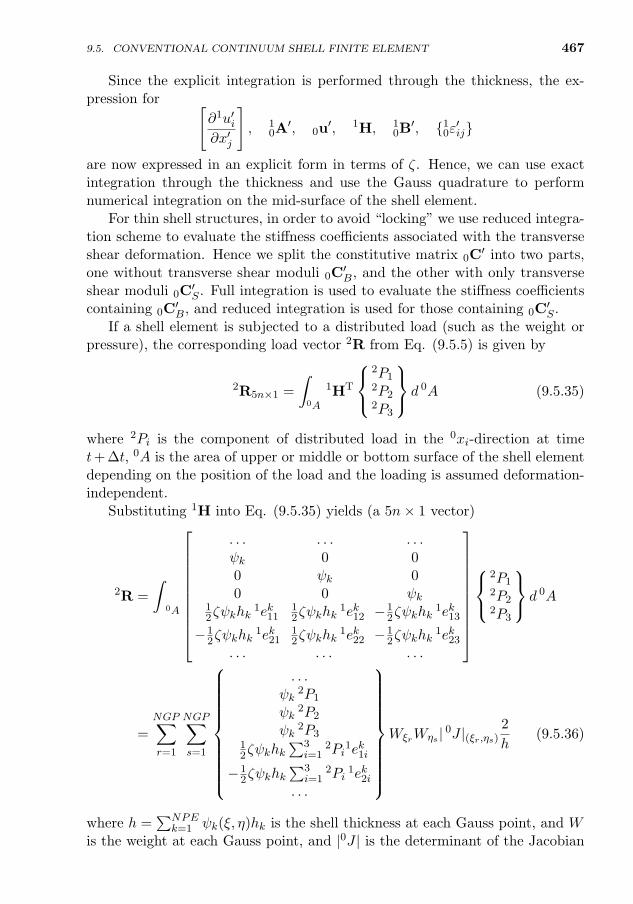
9.5. CONVENTIONAL CONTINUUM SHELL FINITE ELEMENT 467
Since the explicit integration is performed through the thickness, the ex-pression for [
∂1u′i∂x′j
], 1
0A′, 0u
′, 1H, 10B′, 10ε′ij
are now expressed in an explicit form in terms of ζ. Hence, we can use exactintegration through the thickness and use the Gauss quadrature to performnumerical integration on the mid-surface of the shell element.
For thin shell structures, in order to avoid “locking” we use reduced integra-tion scheme to evaluate the stiffness coefficients associated with the transverseshear deformation. Hence we split the constitutive matrix 0C
′ into two parts,one without transverse shear moduli 0C
′B, and the other with only transverse
shear moduli 0C′S . Full integration is used to evaluate the stiffness coefficients
containing 0C′B, and reduced integration is used for those containing 0C
′S .
If a shell element is subjected to a distributed load (such as the weight orpressure), the corresponding load vector 2R from Eq. (9.5.5) is given by
2R5n×1 =
∫0A
1HT
2P12P22P3
d 0A (9.5.35)
where 2Pi is the component of distributed load in the 0xi-direction at timet+ ∆t, 0A is the area of upper or middle or bottom surface of the shell elementdepending on the position of the load and the loading is assumed deformation-independent.
Substituting 1H into Eq. (9.5.35) yields (a 5n× 1 vector)
2R =
∫0A
. . . . . . . . .ψk 0 00 ψk 00 0 ψk
12ζψkhk
1ek1112ζψkhk
1ek12 −12ζψkhk
1ek13
−12ζψkhk
1ek2112ζψkhk
1ek22 −12ζψkhk
1ek23
. . . . . . . . .
2P12P22P3
d 0A
=
NGP∑r=1
NGP∑s=1
. . .ψk
2P1
ψk2P2
ψk2P3
12ζψkhk
∑3i=1
2Pi1ek1i
−12ζψkhk
∑3i=1
2Pi1ek2i
. . .
WξrWηs | 0J |(ξr,ηs)
2
h(9.5.36)
where h =∑NPE
k=1 ψk(ξ, η)hk is the shell thickness at each Gauss point, and Wis the weight at each Gauss point, and |0J | is the determinant of the Jacobian
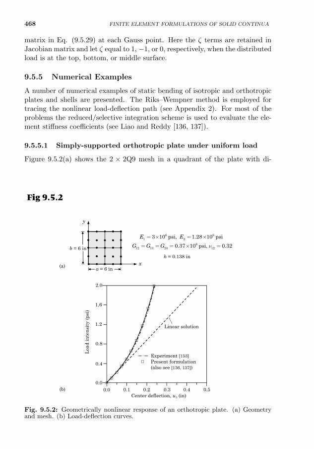
468 FINITE ELEMENT FORMULATIONS OF SOLID CONTINUA
matrix in Eq. (9.5.29) at each Gauss point. Here the ζ terms are retained inJacobian matrix and let ζ equal to 1, −1, or 0, respectively, when the distributedload is at the top, bottom, or middle surface.
9.5.5 Numerical Examples
A number of numerical examples of static bending of isotropic and orthotropicplates and shells are presented. The Riks–Wempner method is employed fortracing the nonlinear load-deflection path (see Appendix 2). For most of theproblems the reduced/selective integration scheme is used to evaluate the ele-ment stiffness coefficients (see Liao and Reddy [136, 137]).
9.5.5.1 Simply-supported orthotropic plate under uniform load
Figure 9.5.2(a) shows the 2 × 2Q9 mesh in a quadrant of the plate with di-mensions and material properties used. The boundary and symmetry condi-tions used are the same as those listed in Fig. 7.9.1. The results are shownin Fig. 9.5.2(b) along with the experimental results of Zaghloul and Kennedy[153]. For this simply-supported plate, the finite element results are in goodagreement with the experimental results of Zaghloul and Kennedy [153].
h = 0.138 in
6 61 2
612 13 23 12
3 10 psi, 1.28 10 psi
0.37 10 psi, 0.32
E E
G G G n
= ´ = ´
= = = ´ =
• • •
•••
• • •
•
•
•
•
•
•
• • • • •
• ••• •x
y
b = 6 in
a = 6 in(a)
(b)
Linear solution
Experiment [153]Present formulation(also see [136, 137])
0.1 0.2 0.3 0.4 0.5
Loa
d in
ten
sity
(ps
i)
Center deflection, u3 (in)
0.00.0
0.4
0.8
1.2
1.6
2.0
Fig 9.5.2
Fig. 9.5.2: Geometrically nonlinear response of an orthotropic plate. (a) Geometryand mesh. (b) Load-deflection curves.
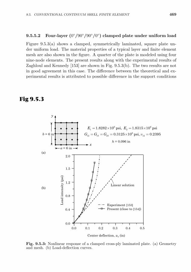
9.5. CONVENTIONAL CONTINUUM SHELL FINITE ELEMENT 469
9.5.5.2 Four-layer (0/90/90/0) clamped plate under uniform load
Figure 9.5.3(a) shows a clamped, symmetrically laminated, square plate un-der uniform load. The material properties of a typical layer and finite elementmesh are also shown in the figure. A quarter of the plate is modeled using fournine-node elements. The present results along with the experimental results ofZaghloul and Kennedy [153] are shown in Fig. 9.5.3(b). The two results are notin good agreement in this case. The difference between the theoretical and ex-perimental results is attributed to possible difference in the support conditionsused in the finite element analysis and those used in the experiment (i.e. theexact nature of clamped boundary conditions used in the test may not be theones used in the finite element analysis), because the present results are verifiedagainst independent finite element study by Putcha and Reddy [154].
(a)
(b)
2.0
1.5
1.2
0.8
0.4
0.0
Linear solution
Experiment [153]Present (close to [154])
0.0 0.1 0.2 0.3 0.4 0.5
Loa
d in
ten
sity
(ps
i)
Center deflection, u3 (in)
h = 0.096 in
6 61 2
612 13 23 12
1.8282 10 psi, 1.8315 10 psi
0.3125 10 psi, 0.2395
E E
G G G n
= ´ = ´
= = = ´ =
• • •
•••
• • •
•
•
•
•
•
•
• • • • •
• ••• •x
y
b = 6 in
a = 6 in
Fig 9.5.3
Fig. 9.5.3: Nonlinear response of a clamped cross-ply laminated plate. (a) Geometryand mesh. (b) Load-deflection curves.
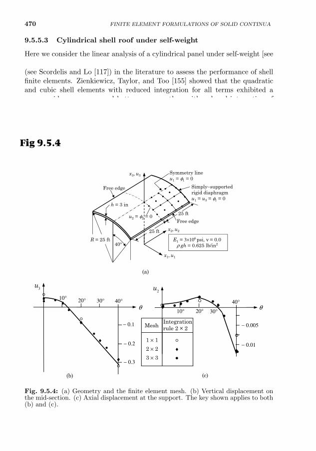
470 FINITE ELEMENT FORMULATIONS OF SOLID CONTINUA
9.5.5.3 Cylindrical shell roof under self-weight
Here we consider the linear analysis of a cylindrical panel under self-weight [seeExample 8.3.4 and Fig. 9.5.4(a)]. This is often used as a benchmark problem(see Scordelis and Lo [117]) in the literature to assess the performance of shellfinite elements. Zienkiewicz, Taylor, and Too [155] showed that the quadraticand cubic shell elements with reduced integration for all terms exhibited amore rapid convergence and better accuracy than with reduced integration oftransverse shear terms only. The linear results obtained in the present studywith the nine-node quadratic element and reduced integration are shown inFigs. 9.5.4(b) and 9.5.4(c). Even with one element, the results show goodagreement with the exact solution [117] and for further mesh refinements theresults are close to the exact one.Fig 9.5.4
-
-
-
25 ft
25 ft
R = 25 ft
x1, u1
x2, u2
x3, u3
40°
h = 3 in
Free edge
Free edge
••••
• •
••
•
••••••
••••••••••
Simply−supportedrigid diaphragmu1 = u3 = φ1 = 0
Symmetry lineu1 = φ1 = 0
u2 = φ2 = 0
(a)
E1 = 3×10⁶ psi, ν = 0.0ρ gh = 0.625 lb/in2
(c)
•
MeshIntegrationrule 2 × 2
1 × 1
2 × 2
3 × 3
♦°
(b)
•••
••
••°
°♦♦
♦
°♦
♦
− 0.1
− 0.2
− 0.3
20°10° 30° 40°θ
3u
♦•° °
°
♦♦ ♦
♦
• • • ••
•
40°
30°20°10°
− 0.005
− 0.01
θ
2u
Fig. 9.5.4: (a) Geometry and the finite element mesh. (b) Vertical displacement onthe mid-section. (c) Axial displacement at the support. The key shown applies to both(b) and (c).
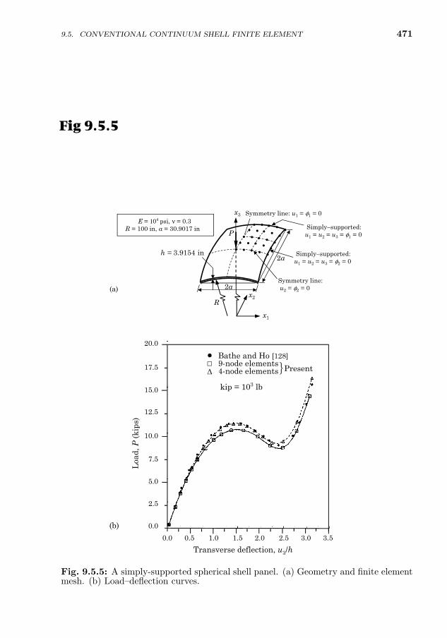
9.5. CONVENTIONAL CONTINUUM SHELL FINITE ELEMENT 471
9.5.5.4 Simply-supported spherical shell under point load
A simply-supported isotropic spherical shell panel under central point load [seeFig. 9.5.5(a)] is analyzed for its large displacement response using a meshesof sixteen four-node elements and four nine-node elements in a quarter of theshell. Figure 9.5.5(b) shows the responses calculated, including the postbucklingrange, with the modified Riks–Wempner method. The figure also includes theresults of Bathe and Ho [128], who have used a 5× 5 mesh of a three-node flattriangular shell element in a quadrant. The element has six degrees of freedomper node, and its stiffness matrix is obtained by superimposing membrane andbending stiffness matrices. They have used the updated Lagrangian formulationin their analysis.
Fig 9.5.5
2ax2-
x1
x3
R
h = 3.9154 in2a
Simply−supported:u1 = u2 = u3 = φ1 = 0
• • ••
• ••
•••••
• • ••••
• •••
•••
Symmetry line: u1 = φ1 = 0
P
Simply−supported:u1 = u2 = u3 = φ2 = 0
Symmetry line:u2 = φ2 = 0
E = 104 psi, ν = 0.3R = 100 in, a = 30.9017 in
(a)
- -- - - -
0.0 0.5 1.0 1.5 2.0 2.5 3.0 3.5
-
20.0
17.5
15.0
12.5
10.0
7.5
5.0
2.5
0.0
-
-
-
-
Bathe and Ho [128]9-node elements4-node elements Present
Loa
d, P
(kip
s)
Transverse deflection, u3/h
(b)
kip = 103 lb
•
Δ
Fig. 9.5.5: A simply-supported spherical shell panel. (a) Geometry and finite elementmesh. (b) Load–deflection curves.
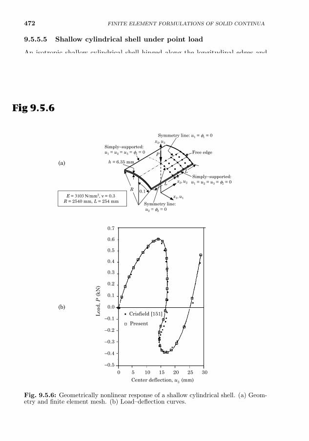
472 FINITE ELEMENT FORMULATIONS OF SOLID CONTINUA
9.5.5.5 Shallow cylindrical shell under point load
An isotropic shallow cylindrical shell hinged along the longitudinal edges andfree at the curved boundaries and subjected to a point load, as shown inFig. 9.5.6(a), is analyzed. One-quarter of the shell is modeled with four nine-node shell elements. The structure exhibits snap-through as well as snap-backphenomena, as shown in Fig. 9.5.6(b). The solution obtained by Crisfield [151]is also shown in Fig. 9.5.6(b) (also see Sabir and Lock [121]).
This completes the discussion of the use of continuum element for the largedisplacement analysis of a number of benchmark problems. The next section isdevoted to the discussion of a refined continuum shell element.
E = 3103 Ν/mm2, ν = 0.3R = 2540 mm, L = 254 mm
-
-
-
L
R
x1, u1
x2, u2
x3, u3
h = 6.35 mm
Free edge
•••••
••••
••••••
••••••
••••
Simply−supported:u1 = u2 = u3 = φ2 = 0
Symmetry line: u1 = φ1 = 0
Simply−supported:u1 = u2 = u3 = φ2 = 0
0.1
L
Symmetry line:u2 = φ2 = 0
P
(a)
0.7
0.6
0.5
0.4
0.3
0.2
0.1
0.0
−0.1
−0.2
−0.3
−0.4
−0.50 5 10 15 20 25 30
Center deflection, u3 (mm)
Loa
d, P
(kN
)
Crisfield [151]
Present
(b)•
Fig 9.5.6
Fig. 9.5.6: Geometrically nonlinear response of a shallow cylindrical shell. (a) Geom-etry and finite element mesh. (b) Load–deflection curves.
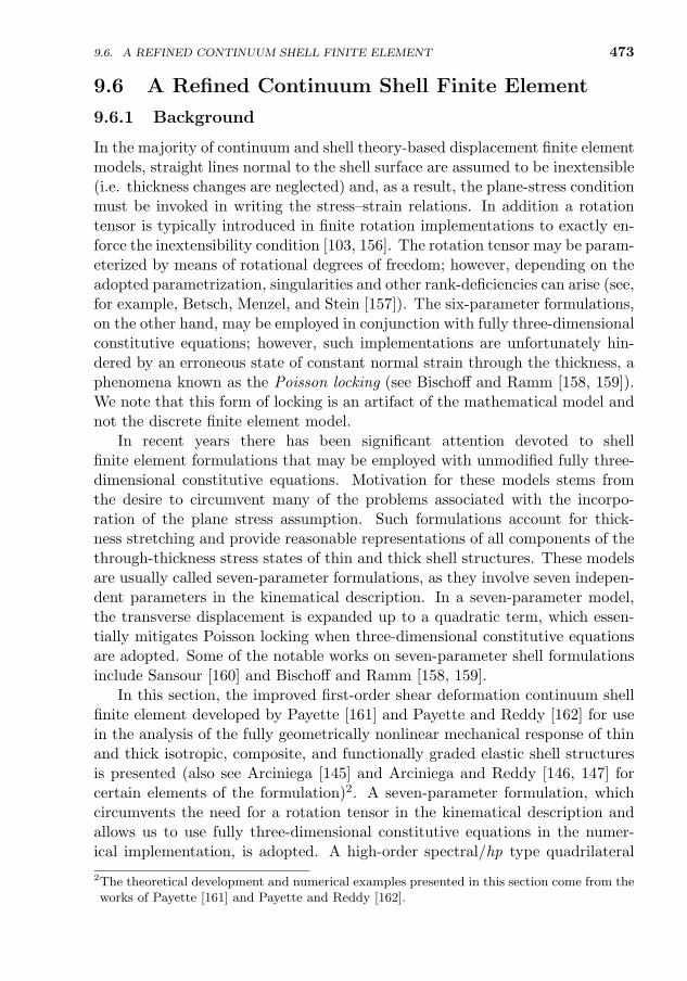
9.6. A REFINED CONTINUUM SHELL FINITE ELEMENT 473
9.6 A Refined Continuum Shell Finite Element
9.6.1 Background
In the majority of continuum and shell theory-based displacement finite elementmodels, straight lines normal to the shell surface are assumed to be inextensible(i.e. thickness changes are neglected) and, as a result, the plane-stress conditionmust be invoked in writing the stress–strain relations. In addition a rotationtensor is typically introduced in finite rotation implementations to exactly en-force the inextensibility condition [103, 156]. The rotation tensor may be param-eterized by means of rotational degrees of freedom; however, depending on theadopted parametrization, singularities and other rank-deficiencies can arise (see,for example, Betsch, Menzel, and Stein [157]). The six-parameter formulations,on the other hand, may be employed in conjunction with fully three-dimensionalconstitutive equations; however, such implementations are unfortunately hin-dered by an erroneous state of constant normal strain through the thickness, aphenomena known as the Poisson locking (see Bischoff and Ramm [158, 159]).We note that this form of locking is an artifact of the mathematical model andnot the discrete finite element model.
In recent years there has been significant attention devoted to shellfinite element formulations that may be employed with unmodified fully three-dimensional constitutive equations. Motivation for these models stems fromthe desire to circumvent many of the problems associated with the incorpo-ration of the plane stress assumption. Such formulations account for thick-ness stretching and provide reasonable representations of all components of thethrough-thickness stress states of thin and thick shell structures. These modelsare usually called seven-parameter formulations, as they involve seven indepen-dent parameters in the kinematical description. In a seven-parameter model,the transverse displacement is expanded up to a quadratic term, which essen-tially mitigates Poisson locking when three-dimensional constitutive equationsare adopted. Some of the notable works on seven-parameter shell formulationsinclude Sansour [160] and Bischoff and Ramm [158, 159].
In this section, the improved first-order shear deformation continuum shellfinite element developed by Payette [161] and Payette and Reddy [162] for usein the analysis of the fully geometrically nonlinear mechanical response of thinand thick isotropic, composite, and functionally graded elastic shell structuresis presented (also see Arciniega [145] and Arciniega and Reddy [146, 147] forcertain elements of the formulation)2. A seven-parameter formulation, whichcircumvents the need for a rotation tensor in the kinematical description andallows us to use fully three-dimensional constitutive equations in the numer-ical implementation, is adopted. A high-order spectral/hp type quadrilateral
2The theoretical development and numerical examples presented in this section come from theworks of Payette [161] and Payette and Reddy [162].
474 FINITE ELEMENT FORMULATIONS OF SOLID CONTINUA
finite element technology in a purely displacement-based finite element settingis adopted. This allows us to obtain: (1) highly accurate approximations ofarbitrary shell geometries and (2) reliable numerical results that are completelylocking-free. In the computer implementation, the Schur complement methodis adopted at the element level to statically condense out all degrees of freedominterior to each element in a given finite element discretization. This procedurevastly improves computer memory requirements in the numerical implementa-tion of the resulting shell element and allows for significant parallelization ofthe global solver (for more details see [161, 162]). This constitutes an impor-tant departure from the tensor based shell finite element formulation proposedpreviously in the work of Arciniega and Reddy [146, 147], where a chart wasemployed to ensure exact parametrization of the shell mid-surface.
The shell finite element framework presented in this study is applicable tothe fully geometrically nonlinear analysis of elastic shell structures based on theSt. Venant–Kirchhoff material model. The formulation requires the prescrip-tion of the three-dimensional coordinates of the shell mid-surface as well as twosets of directors (one set normal and the other tangent to the mid-surface) ateach node in the shell finite element model as input. Each of these quantitiesis approximated discretely using the standard spectral/hp finite element inter-polation functions within a given shell element. The prescribed tangent vectoris particularly useful, as it allows for the simple construction of the local basesassociated with the principal orthotropic material directions of each lamina in agiven composite. This allows us to use skewed and/or arbitrarily curved quadri-lateral shell elements in actual finite element simulations. Through the numeri-cal simulation of a number of non-trivial benchmark problems, it is shown thatthe developed shell element is insensitive to all forms of numerical locking andsevere geometric distortions.
9.6.2 Representation of Shell Mid-Surface
In theories of shells, the undeformed mid-surface Ω (where Ω, an open boundedset) of a shell is used as the reference along with the thickness h to constructthe three-dimensional domain of the shell. The mid-surface is characterizedusing either a single or a set of two-dimensional charts from R2 into R3. In thisstudy we dispense with this exact parametrization of Ω and instead introducean appropriate finite element approximation of the mid-surface. To this end,we assume that the closure of Ω, denoted by Ω = Ω
⋃Γ, is approximated by
a set of N high-order spectral/hp quadrilateral finite elements. We denote theresulting finite element approximation of Ω by Ωhp =
⋃Ne=1 Ωe. This description
of the mid-surface leads to the following standard finite element approximationof the geometry within a given master element Ωe:
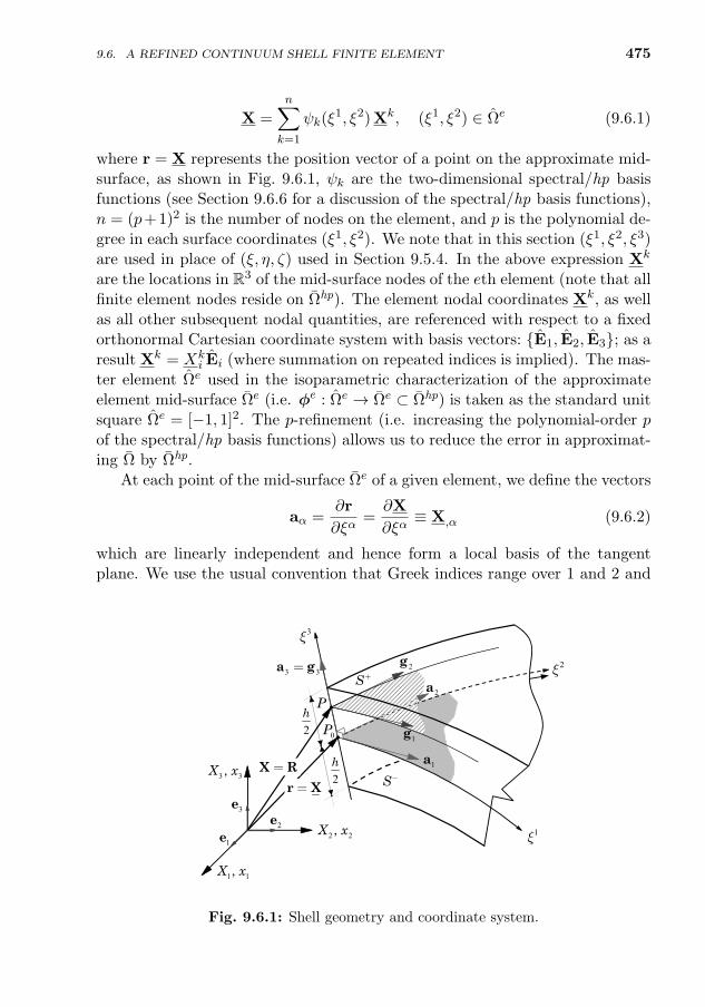
9.6. A REFINED CONTINUUM SHELL FINITE ELEMENT 475
X =
n∑k=1
ψk(ξ1, ξ2) Xk, (ξ1, ξ2) ∈ Ωe (9.6.1)
where r = X represents the position vector of a point on the approximate mid-surface, as shown in Fig. 9.6.1, ψk are the two-dimensional spectral/hp basisfunctions (see Section 9.6.6 for a discussion of the spectral/hp basis functions),n = (p+1)2 is the number of nodes on the element, and p is the polynomial de-gree in each surface coordinates (ξ1, ξ2). We note that in this section (ξ1, ξ2, ξ3)are used in place of (ξ, η, ζ) used in Section 9.5.4. In the above expression Xk
are the locations in R3 of the mid-surface nodes of the eth element (note that allfinite element nodes reside on Ωhp). The element nodal coordinates Xk, as wellas all other subsequent nodal quantities, are referenced with respect to a fixedorthonormal Cartesian coordinate system with basis vectors: E1, E2, E3; as aresult Xk = Xk
i Ei (where summation on repeated indices is implied). The mas-ter element Ωe used in the isoparametric characterization of the approximateelement mid-surface Ωe (i.e. φe : Ωe → Ωe ⊂ Ωhp) is taken as the standard unitsquare Ωe = [−1, 1]2. The p-refinement (i.e. increasing the polynomial-order pof the spectral/hp basis functions) allows us to reduce the error in approximat-ing Ω by Ωhp.
At each point of the mid-surface Ωe of a given element, we define the vectors
aα =∂r
∂ξα=∂X
∂ξα≡ X,α (9.6.2)
which are linearly independent and hence form a local basis of the tangentplane. We use the usual convention that Greek indices range over 1 and 2 and
3
2
1
1 1,X x
2 2,X x
3 3,X x
3 3a g2a
2g
1g
1a
r XX R
S
S
P
0P
3e2e
1e
2h
2h
Fig. 9.6.1: Shell geometry and coordinate system.
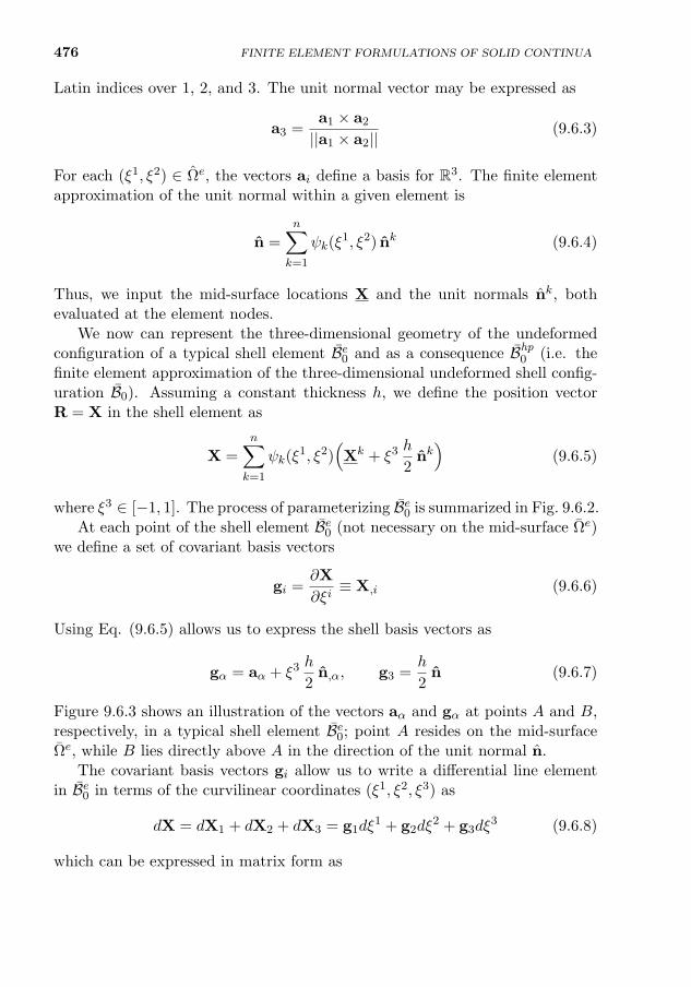
476
Latin indices over 1, 2, and 3. The unit normal vector may be expressed as
a3 =a1 × a2
||a1 × a2||(9.6.3)
For each (ξ1, ξ2) ∈ Ωe, the vectors ai define a basis for R3. The finite elementapproximation of the unit normal within a given element is
n =n∑k=1
ψk(ξ1, ξ2) nk (9.6.4)
Thus, we input the mid-surface locations X and the unit normals nk, bothevaluated at the element nodes.
We now can represent the three-dimensional geometry of the undeformedconfiguration of a typical shell element Be0 and as a consequence Bhp0 (i.e. thefinite element approximation of the three-dimensional undeformed shell config-uration B0). Assuming a constant thickness h, we define the position vectorR = X in the shell element as
X =n∑k=1
ψk(ξ1, ξ2)
(Xk + ξ3 h
2nk)
(9.6.5)
where ξ3 ∈ [−1, 1]. The process of parameterizing Be0 is summarized in Fig. 9.6.2.At each point of the shell element Be0 (not necessary on the mid-surface Ωe)
we define a set of covariant basis vectors
gi =∂X
∂ξi≡ X,i (9.6.6)
Using Eq. (9.6.5) allows us to express the shell basis vectors as
gα = aα + ξ3 h
2n,α, g3 =
h
2n (9.6.7)
Figure 9.6.3 shows an illustration of the vectors aα and gα at points A and B,respectively, in a typical shell element Be0; point A resides on the mid-surfaceΩe, while B lies directly above A in the direction of the unit normal n.
The covariant basis vectors gi allow us to write a differential line elementin Be0 in terms of the curvilinear coordinates (ξ1, ξ2, ξ3) as
dX = dX1 + dX2 + dX3 = g1dξ1 + g2dξ
2 + g3dξ3 (9.6.8)
which can be expressed in matrix form as
FINITE ELEMENT FORMULATIONS OF SOLID CONTINUA
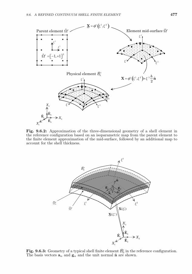
9.6. A REFINED CONTINUUM SHELL FINITE ELEMENT 477
1ξ 2ξ
3ξ
1ξ
2ξ
ˆParent element eΩ Element mid-surface eΩ
h
1ξ 2ξ
3ξ0Physical element eB
2ˆ 1, 1eΩ = − +⎡ ⎤⎣ ⎦
( )1 2 3 ˆ,2
e hX nξ ξ ξ= +φ
( )1 2,eX ξ ξ=φ
1X2X
3X
1E2E
3E
Fig. 9.6.2: Approximation of the three-dimensional geometry of a shell element inthe reference configuration based on an isoparametric map from the parent element tothe finite element approximation of the mid-surface, followed by an additional map toaccount for the shell thickness.
..................
*( )iξX
*( )αξX
1a 2a1g 2g
1ξ 2ξ
3ξ
1X2X
3X
1E2E
3E
.n
AB
0eB
*eΩ
eΩ
Fig. 9.6.3: Geometry of a typical shell finite element Be0 in the reference configuration.The basis vectors aα and gα and the unit normal n are shown.
478 FINITE ELEMENT FORMULATIONS OF SOLID CONTINUA
dX1
dX2
dX3
= dξT[J ] =
dξ1
dξ2
dξ3
T∂X1∂ξ1
∂X2∂ξ1
∂X3∂ξ1
∂X1∂ξ2
∂X2∂ξ2
∂X3∂ξ2
∂X1∂ξ3
∂X2∂ξ3
∂X3∂ξ3
(9.6.9)
Here [J ] denotes the Jacobian matrix (or the matrix of deformation gradient),and its determinant is denoted as J . The inverse (assumed to exist) of [J ] isdenoted here as [J?]. A differential volume element in Be0 is given as
dBe0 = dX1 · (dX2 × dX3) = Jdξ1dξ2dξ3 (9.6.10)
We associate with the covariant basis, a dual or contravariant basis defined by
gi · gj = δij (9.6.11)
where δij is the Kronecker delta. The contravariant basis vectors may also bedetermined from the following formulae
g1 = (g2 × g3)/J, g2 = (g3 × g1)/J, g3 = (g1 × g2)/J (9.6.12)
The covariant and contravariant basis vectors may be alternatively defined interms of the components of Jacobian matrix and its inverse
gi = JijEj , gi = J?jiEj (9.6.13)
9.6.3 Displacement and Strain Fields
We now consider the motion χ(X, t) of the shell from the reference finite element
configuration Bhp0 to the current configuration Bhpt . The displacement of amaterial point from the reference configuration to the current configuration is
u(X, t) = χ(X, t)−X = x(X, t)−X (9.6.14)
Next, we assume that at any point within a typical shell element Be0, the dis-placement vector may expanded in Taylor’s series expansion with respect to thethickness coordinate ξ3
u(X(ξi), t) ∼= u(0)(ξα, t) + ξ3u(1)(ξα, t) +(ξ3)2
2u(2)(ξα, t) + · · · (9.6.15)
where u(j)(ξα, t) = ∂ju(ξi, t)/∂(ξ3)j |ξ3=0.The Taylor series for u is truncated such that the resulting shell model is
asymptotically consistent with three-dimensional elasticity (see Chapelle and
9.6. A REFINED CONTINUUM SHELL FINITE ELEMENT 479
Bathe [156]), thereby allowing for the use of fully three-dimensional constitu-tive equations in the mathematical model and subsequent numerical implemen-tation. Therefore, the displacement field is restricted to the following seven-parameter expansion:
u(ξi) = u(ξα) + ξ3h
2ϕ(ξα) + (ξ3)2h
2ψ(ξα) (9.6.16)
where each u(j)(ξα, t) (j = 0, 1 and 2) has been renamed, and for j = 1 and2, scaled by some factor of h. For the sake of brevity, the time parametert is omitted from the above expressions and the subsequent discussion. Thegeneralized displacements u, ϕ and ψ may be expressed as
u(ξα) = ui(ξα)Ei, ϕ(ξα) = ϕi(ξ
α)Ei, ψ(ξα) = Ψ(ξα)n(ξα) (9.6.17)
The quantity u represents the mid-plane displacement and ϕ is the so-calleddifference vector (which gives the change in the mid-surface director). Theseventh parameter Ψ is included to circumvent spurious stresses in the thick-ness direction, caused in the six-parameter formulation by an artificial constantnormal strain (a phenomena referred to as Poisson locking [158]).
The position occupied by a material point belonging to Be0 at the currenttime t may be evaluated by substituting the assumed displacement field intoEq. (9.6.14) which upon rearrangement yields
x = X + u = x + ξ3h
2ˆn + (ξ3)2h
2Ψn (9.6.18)
where x = X + u (a point on the deformed mid-surface) and ˆn = n + ϕ(a pseudo-director associated with the deformed mid-surface). We note that,unlike n, the director ˆn is in general neither a unit vector nor it is normal tothe deformed mid-surface.
The finite element approximation of the displacement field given in Eq.(9.6.16) is represented as (i.e. isoparametric formulation is used)
u(ξi) =n∑k=1
ψk(ξ1, ξ2)
(uk + ξ3h
2ϕk + (ξ3)2h
2Ψkn(ξα)
)(9.6.19)
where n(ξα) is given by Eq. (9.6.4). Note that we interpolate Ψ and n sep-arately in the finite element approximation of ψ, as opposed to interpolatingthe product Ψn as a single entity. The derivative of the displacement field withrespect to the curvilinear coordinates of the element may be expressed as
u,α =n∑k=1
∂ψk∂ξα
[uk + ξ3h
2ϕk + (ξ3)2h
2
(Ψkn(ξβ) + nkΨ(ξβ)
)](9.6.20a)
480 FINITE ELEMENT FORMULATIONS OF SOLID CONTINUA
u,3 = h
n∑k=1
ψk(ξ1, ξ2)
(1
2ϕk + ξ3Ψkn(ξβ)
)(9.6.20b)
The deformation gradient F is given by [see Eq. (9.1.3)]
F = (∇0x(X, t))T = x,igi = gjg
j (9.6.21)
where gj = g,j+u,j are the covariant basis vectors associated with the deformed
finite element configuration of the three-dimensional shell Bhpt . The symbol ∇0
denotes the material gradient operator. The Green–Lagrange strain tensor Eis
E =1
2
(FTF− I
)=
1
2
(u,i · gj + gi · u,j + u,i · u,j
)gigj (9.6.22)
The covariant components of the Green–Lagrange strain tensor [i.e. the coef-ficients of the second-order tensor contravariant bases gigj appearing in Eq.(9.6.22)] may be expanded in terms of the thickness coordinate ξ3 as
Eij(ξm) = ε
(0)ij + ξ3ε
(1)ij + (ξ3)2ε
(2)ij + (ξ3)3ε
(3)ij + (ξ3)4ε
(4)ij (9.6.23)
where ε(n)ij = ε
(n)ij (ξα). In the present formulation all covariant components of
E that are of higher order than linear in ξ3 [i.e. the underlined terms in Eq.(9.6.23)] are neglected. The covariant components of the retained strain termsmay be determined from
ε(0)αβ =
1
2
(u,α · aβ + aα · u,β + u,α · u,β
)(9.6.24a)
ε(1)αβ =
h
4
[u,α ·
(n,β +ϕ,β
)+(n,α +ϕ,α
)· u,β +ϕ,α · aβ + aα ·ϕ,β
](9.6.24b)
ε(0)α3 =
h
4
[u,α ·
(n +ϕ
)+ aα ·ϕ
](9.6.24c)
ε(1)α3 =
h
2
h
4
[ϕ,α · n +
(n,α +ϕ,α
)·ϕ]
+(aα + u,α
)·ψ
(9.6.24d)
ε(0)33 =
h2
8
(2n +ϕ
)·ϕ (9.6.24e)
ε(1)33 =
h2
2
(n +ϕ
)·ψ (9.6.24f)
The six-parameter formulation is obtained as a special case by setting ψ = 0;
that is, the strain component ε(1)33 is identically zero.
9.6.4 Constitutive Relations
The underlying kinematic assumptions of the adopted shell finite element for-mulation can be applied in the context of a multitude of material models (e.g.
9.6. A REFINED CONTINUUM SHELL FINITE ELEMENT 481
Cauchy elastic, hyperelastic, viscoelastic, elasto–plastic, etc.). In this work weassume that the material response remains in the elastic regime. Furthermore,we assume that the second Piola–Kirchhoff stress tensor S is related to theGreen–Lagrange strain tensor E by the following relation
S = C : E (9.6.25)
where C = Cijklgi gj gk gl is the fourth-order elasticity tensor [with symmetriesgiven in Eq. (2.8.15)]. We assume the elasticity tensor to be independent ofthe shell deformation. However, we do allow C to be non-homogeneous (i.e.a function of X). In the numerical implementation, we rely on the followingcomponent representation of the set of constitutive equations
Sij = CijklEkl (9.6.26)
The adopted material model may also be expressed in matrix form as
S11
S22
S33
S23
S13
S12
=
C1111 C1122 C1133 C1123 C1113 C1112
C1122 C2222 C2233 C2223 C2213 C2212
C1133 C2233 C3333 C3323 C3313 C3312
C1123 C2223 C3323 C2323 C2313 C2312
C1113 C2213 C3313 C2313 C1313 C1312
C1112 C2212 C3312 C2312 C1312 C1212
E11
E22
E33
2E23
2E13
2E12
(9.6.27)
where the coefficient matrix [Cijkl] appearing in the above expression is thematrix form of the contravariant components of the elasticity tensor C. Itshould be evident that there are in general 21 unique contravariant componentsof C.
For completeness, we recall that the second Piola–Kirchhoff stress tensor Sis related to the Cauchy stress tensor σ by [see Eq. (9.1.10)]
S = JF F−1 σF−T (9.6.28)
where JF = det(F). The symmetry of S follows from the symmetry of σ.
9.6.4.1 Isotropic and functionally graded shells
We now specialize the assumed constitutive model for use in the context ofisotropic shells. We consider the homogeneous case and also the scenario wherethe material is functionally graded through the thickness of the shell. Homo-geneous shells are abundant and can be found in piping, pressure vessels, shiphulls, large roofs, and the bodies of automobiles. Functionally graded shellson the other hand have been advocated for use in high-temperature environ-ments with applications in reactor vessels, turbines, and other machine parts
482 FINITE ELEMENT FORMULATIONS OF SOLID CONTINUA
(see Reddy [55]). These materials are typically composed of metals and ceram-ics to maximize the strength and toughness properties of the former and thethermal and corrosion resistance attributes of the latter.
For isotropic materials, the fourth-order elasticity tensor C may be ex-pressed as
C = λI I + 2µΠ (9.6.29)
Here I = δijEi Ej is the second-order unit tensor and Π = 12(δik δjl+δil δjk)Ei Ej
Ek El is the fourth-order unit tensor. These tensors may also be expressed withrespect to the covariant basis vectors gi as
I = G = gijgi gj , Π =1
2(gikgjl + gilgjk)gi gj gk gl (9.6.30)
where gij = gi ·gj are the contravariant components of the Riemannian metrictensor G in the reference configuration. We can therefore express the con-travariant components of C as
Cijkl = λgijgkl + µ(gikgjl + gilgjk) (9.6.31)
Although C depends on only the Lame parameters, the 21 unique contravariantcomponents associated with the matrix [Cijkl] are, in general, distinct from oneanother. The Lame parameters λ and µ are related to Young’s modulus E andPoisson’s ratio ν by the following expressions:
λ =νE
(1 + ν)(1− 2ν), µ =
E
2(1 + ν)(9.6.32)
For the homogeneous case, Young’s modulus E and Poisson’s ratio ν areconstant throughout the shell structure. For functionally graded structures,we assume that the shell is composed of two isotropic constituents that arecombined in a prescribed fashion through the shell thickness. In such cases, weallow Young’s modulus to vary, while Poisson’s ratio is constant, with respectto the shell thickness coordinate ξ3 as follows (see Reddy [55]):
E(ξ3) = (E+ − E−)f+(ξ3) + E− (9.6.33)
where
f+(ξ3) =
(ξ3 + 1
2
)n(9.6.34)
The quantities E− and E+ constitute Young’s moduli at the bottom (ξ3 =−1) and top (ξ3 = +1) surfaces of the shell, respectively. Equation (9.6.33)constitutes a power-law variation of E through the shell thickness (where thenon-negative constant n is the power-law parameter). Note that E− and E+
are recovered throughout the thickness in the limits where n→∞ and n→ 0,respectively. As in the homogeneous case, functionally graded shells may alsobe described using Eq. (9.6.31) if the Lame parameters are taken as functionsof ξ3.
483
9.6.4.2 Laminated composite shells
In this work we are also concerned with the numerical simulation of laminatedcomposite shell structures. A composite laminae is a thin sheet (plate or shelllike) of material, typically composed of two distinct constituents, which to-gether possess desirable mechanical properties that cannot be exhibited by theindividual materials acting in bulk alone. A laminated composite shell is a col-lection of stacked laminae (where the stacking sequence is typically prescribedin a manner which maximizes the desired stiffness of the composite). In ouranalysis, we treat each laminae as an orthotropic layer of material. We furtherassume that for a given structure, perfect bonding exists between each layerand that the continuum hypothesis holds.
To simplify the discussion, we initially restrict our attention to a shell com-posed of a single orthotopic layer (i.e. one lamina). Next, we define at eachnode in Ωhp a unit vector t that is tangent to the finite element approximationof the mid-plane. The discrete tangents are utilized to define a continuous tan-gent vector field in Ωhp. Within each element, the tangent field is representedas
t =n∑k=1
ψk(ξ1, ξ2) tk (9.6.35)
The tangent vector t is prescribed in a manner that allows us to easily constructa local orthogonal Cartesian basis e1, e2, e3 associated with the principaldirections of the orthotropic laminae. Figure 9.6.4 contains the geometry, nodes,unit normals nk, and unit tangents tk for a typical high-order spectral/hp shellfinite element. Note that the direction of t need not coincide with the directionof either a1 or a2.
The elasticity tensor C can be expressed with respect to the local basise1, e2, e3 (which we will soon define) as
C = Cijkl ei ej ek el (9.6.36)
Assuming an orthotropic material model, we can express the coefficients Cijklin matrix form as follows:
[C] =
C1111 C1122 C1133 0 0 0
C1122 C2222 C2233 0 0 0
C1133 C2233 C3333 0 0 0
0 0 0 C2323 0 0
0 0 0 0 C1313 0
0 0 0 0 0 C1212
(9.6.37)
9.6. A REFINED CONTINUUM SHELL FINITE ELEMENT
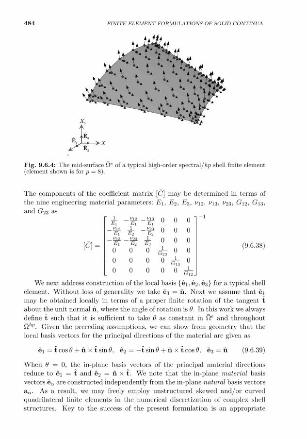
484 FINITE ELEMENT FORMULATIONS OF SOLID CONTINUA
1X2
X
3X
1E2E
3E
Fig. 9.6.4: The mid-surface Ωe of a typical high-order spectral/hp shell finite element(element shown is for p = 8).
The components of the coefficient matrix [C] may be determined in terms ofthe nine engineering material parameters: E1, E2, E3, ν12, ν13, ν23, G12, G13,and G23 as
[C] =
1E1−ν12E1−ν13E1
0 0 0
−ν12E1
1E2−ν23E2
0 0 0
−ν13E1−ν23E2
1E3
0 0 0
0 0 0 1G23
0 0
0 0 0 0 1G13
0
0 0 0 0 0 1G12
−1
(9.6.38)
We next address construction of the local basis e1, e2, e3 for a typical shellelement. Without loss of generality we take e3 = n. Next we assume that e1
may be obtained locally in terms of a proper finite rotation of the tangent tabout the unit normal n, where the angle of rotation is θ. In this work we alwaysdefine t such that it is sufficient to take θ as constant in Ωe and throughoutΩhp. Given the preceding assumptions, we can show from geometry that thelocal basis vectors for the principal directions of the material are given as
e1 = t cos θ + n× t sin θ, e2 = −t sin θ + n× t cos θ, e3 = n (9.6.39)
When θ = 0, the in-plane basis vectors of the principal material directionsreduce to e1 = t and e2 = n × t. We note that the in-plane material basisvectors eα are constructed independently from the in-plane natural basis vectorsaα. As a result, we may freely employ unstructured skewed and/or curvedquadrilateral finite elements in the numerical discretization of complex shellstructures. Key to the success of the present formulation is an appropriate
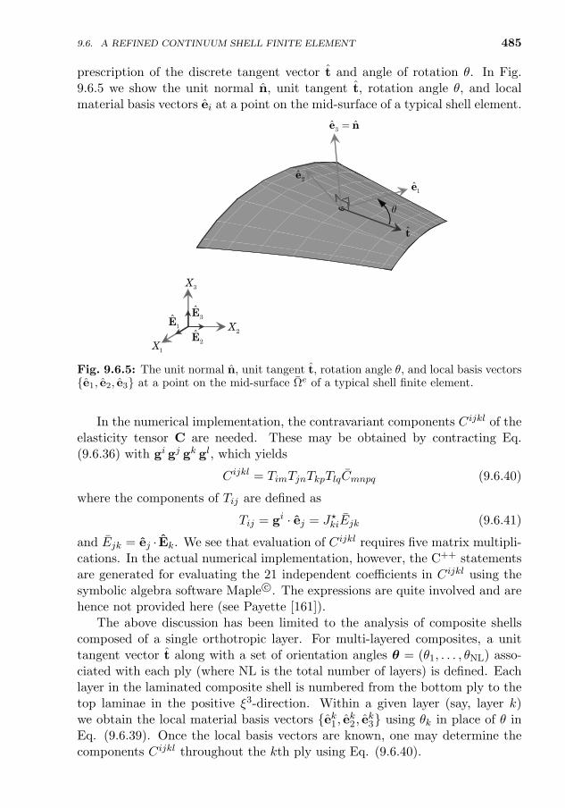
485
prescription of the discrete tangent vector t and angle of rotation θ. In Fig.9.6.5 we show the unit normal n, unit tangent t, rotation angle θ, and localmaterial basis vectors ei at a point on the mid-surface of a typical shell element.
1X2X
3X
1E2E
3E
t
1e2e
3ˆ ˆ=e n
θ
Fig. 9.6.5: The unit normal n, unit tangent t, rotation angle θ, and local basis vectorse1, e2, e3 at a point on the mid-surface Ωe of a typical shell finite element.
In the numerical implementation, the contravariant components Cijkl of theelasticity tensor C are needed. These may be obtained by contracting Eq.(9.6.36) with gi gj gk gl, which yields
Cijkl = TimTjnTkpTlqCmnpq (9.6.40)
where the components of Tij are defined as
Tij = gi · ej = J?kiEjk (9.6.41)
and Ejk = ej · Ek. We see that evaluation of Cijkl requires five matrix multipli-cations. In the actual numerical implementation, however, the C++ statementsare generated for evaluating the 21 independent coefficients in Cijkl using thesymbolic algebra software Maple c©. The expressions are quite involved and arehence not provided here (see Payette [161]).
The above discussion has been limited to the analysis of composite shellscomposed of a single orthotropic layer. For multi-layered composites, a unittangent vector t along with a set of orientation angles θ = (θ1, . . . , θNL) asso-ciated with each ply (where NL is the total number of layers) is defined. Eachlayer in the laminated composite shell is numbered from the bottom ply to thetop laminae in the positive ξ3-direction. Within a given layer (say, layer k)we obtain the local material basis vectors ek1, ek2, ek3 using θk in place of θ inEq. (9.6.39). Once the local basis vectors are known, one may determine thecomponents Cijkl throughout the kth ply using Eq. (9.6.40).
9.6. A REFINED CONTINUUM SHELL FINITE ELEMENT
486 FINITE ELEMENT FORMULATIONS OF SOLID CONTINUA
9.6.5 The Principle of Virtual Displacements andits Discretization
The finite element model is formulated using the principle of virtual displace-ments. The formulation presented here is restricted to static analysis by omit-ting the inertial terms (see Section 9.5.3 for transient analysis). The principleof virtual displacements may be stated for the continuous problem at hand asfollows: find Φ ∈ V such that for all δΦ ∈ W the following weak statementholds:
G(δΦ,Φ) = δWI(δΦ,Φ) + δWE(δΦ,Φ) ≡ 0 (9.6.42)
where Φ = (u,ϕ,Ψ) and δWI and δWE are the internal and external virtualworks, respectively, due to actual forces in moving through virtual displace-ments. These quantities may be defined with respect to the undeformed con-figuration as
δWI =
∫B0δE : S dB0 (9.6.43a)
δWE = −∫B0ρ0 δu · f0 dB0 −
∫Γσ
δu · t0 ds0 (9.6.43b)
where ρ0 is the density, f0 is the body force, and t0 is the traction vector,which are expressed with respect to the reference configuration. The space ofadmissible configurations V and the vector space of admissible variationsW aredefined for the continuous problem as
V :=
Φ = (u,ϕ,Ψ) : Φ ∈ H1(ω)×H1(ω)× L2(ω), Φ = Φp on ΓD
(9.6.44a)
W :=δΦ = (δu, δϕ, δΨ) : δΦ ∈ H1(ω)×H1(ω)× L2(ω), δΦ = 0 on ΓD
(9.6.44b)
where H1(Ω) = [H1(Ω)]2, and H1(Ω) and L2(Ω) are standard Sobolev andLebesgue spaces on Ω, respectively (see Section 1.7). Furthermore, ΓD is thepart of the boundary on which Φ is specified.
In the numerical implementation, we restrict Φ and δΦ to their appropriatespectral/hp finite element subspaces: Φhp ∈ Vhp and δΦhp ∈ Whp. This resultsin the following discrete variation problem: find Φhp ∈ Vhp such that
G(δΦhp,Φhp) = δWI(δΦhp,Φhp) + δWE(δΦhp,Φhp) ≡ 0, ∀δΦhp ∈ Whp
(9.6.45)Evaluation of the internal virtual work statement for the eth element of thediscrete problem yields
9.6. A REFINED CONTINUUM SHELL FINITE ELEMENT 487
δW eI =
∫Be0
(δε(0) + ξ3δε(1)
): C :
(ε(0) + ξ3ε(1)
)dBe0
=
∫Ωe
∫ +1
−1
(δε
(0)ij + ξ3δε
(1)ij
)Cijkl
(ε
(0)kl + ξ3ε
(1)kl
)J dξ3dΩe
=
∫Ωe
[Aijklδε
(0)ij ε
(0)kl +Bijkl
(δε
(0)ij ε
(1)kl + δε
(1)ij ε
(0)kl
)+Dijklδε
(1)ij ε
(1)kl
]dΩe
(9.6.46)
where∫
Ωe ( · ) dΩe =∫ +1−1
∫ +1−1 ( · ) dξ1dξ2. The quantities Aijkl, Bijkl, and Dijkl
are the contravariant components of the effective extensional, extensional-bendingcoupling, and bending fourth-order stiffness tensors, respectively, defined as
Aijkl, Bijkl, Dijkl
=
∫ +1
−1
1, ξ3, (ξ3)2
CijklJ dξ3 (9.6.47)
We note that the stiffness components have been defined such that they in-clude the Jacobian determinant J . In the computer implementation, we per-form the above integration numerically using the Gauss–Legendre quadraturerule (with 50 quadrature points taken along the thickness direction of each lam-inae). Therefore, no thin- or shallow-shell type approximating assumptions areimposed on either J or Cijkl in the finite element formulation.
The derivation of virtual internal energy in Eq. (9.6.46) is not a trivial task.Even for isotropic materials these expressions have an extremely complex formwhen displacements and rotations are large. Table 9.6.1, taken from Arciniega[145], gives the number of terms of the virtual strain energy for the shell modelpresented here and for different other problems.
The external virtual work consists of body forces and tractions. For eachelement, we decompose the boundary of the shell into top Γeσ,+, bottom Γeσ,−,and lateral Γeσ,S surfaces. As a result, the external virtual work for a typicalshell element may be expressed as
δW eE = −
∫Be0ρ0δu · f0 dBe0 −
∫Γeσ,+
δu · t+0 ds
+ −∫
Γeσ,−
δu · t−0 ds−
−∫
Γeσ,s
δu · ts0 dss (9.6.48)
The traction boundary conditions along the top and bottom of the shell elementmay be expressed as
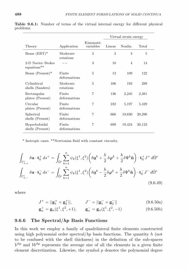
488 FINITE ELEMENT FORMULATIONS OF SOLID CONTINUA
Table 9.6.1: Number of terms of the virtual internal energy for different physicalproblems.
Virtual strain energy
KinematicTheory Application variables Linear Nonlin. Total
Beam (EBT)* Moderate 2 2 3 5rotations
2-D Navier–Stokes −− 3 10 4 14equations**
Beam (Present)* Finite 5 13 109 122deformations
Cylindrical Moderate 5 106 193 299shells (Sanders) rotations
Rectangular Finite 7 136 2,245 2,381plates (Present) deformations
Circular Finite 7 232 5,197 5,429plates (Present) deformations
Spherical Finite 7 666 19,630 20,296shells (Present) deformations
Hyperboloidal Finite 7 699 19,424 20,123shells (Present) deformations
* Isotropic cases. **Newtonian fluid with constant viscosity.
∫Γeσ,+
δu · t+0 ds
+ =
∫Ωe
n∑k=1
ψk(ξ1, ξ2)
(δuk +
h
2δϕk +
h
2δΨkn
)· t+
0 J+ dΩe
∫Γeσ,−
δu · t−0 ds− =
∫Ωe
n∑k=1
ψk(ξ1, ξ2)
(δuk − h
2δϕk +
h
2δΨkn
)· t−0 J
− dΩe
(9.6.49)
where
J+ = ||g+1 × g+
2 ||, J− = ||g−1 × g−2 || (9.6.50a)
g+α = gα(ξ1, ξ2,+1), g−α = gα(ξ1, ξ2,−1) (9.6.50b)
9.6.6 The Spectral/hp Basis Functions
In this work we employ a family of quadrilateral finite elements constructedusing high polynomial order spectral/hp basis functions. The quantity h (notto be confused with the shell thickness) in the definition of the sub-spacesVhp and Whp represents the average size of all the elements in a given finiteelement discretization. Likewise, the symbol p denotes the polynomial degree
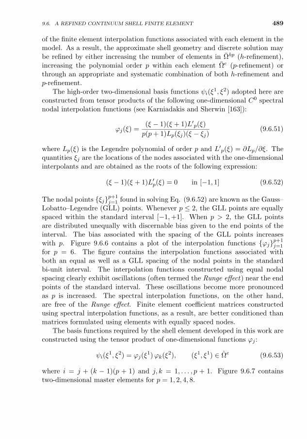
489
of the finite element interpolation functions associated with each element in themodel. As a result, the approximate shell geometry and discrete solution maybe refined by either increasing the number of elements in Ωhp (h-refinement),increasing the polynomial order p within each element Ωe (p-refinement) orthrough an appropriate and systematic combination of both h-refinement andp-refinement.
The high-order two-dimensional basis functions ψi(ξ1, ξ2) adopted here are
constructed from tensor products of the following one-dimensional C0 spectralnodal interpolation functions (see Karniadakis and Sherwin [163]):
ϕj(ξ) =(ξ − 1)(ξ + 1)L′p(ξ)
p(p+ 1)Lp(ξj)(ξ − ξj)(9.6.51)
where Lp(ξ) is the Legendre polynomial of order p and L′p(ξ) = ∂Lp/∂ξ. Thequantities ξj are the locations of the nodes associated with the one-dimensionalinterpolants and are obtained as the roots of the following expression:
(ξ − 1)(ξ + 1)L′p(ξ) = 0 in [−1, 1] (9.6.52)
The nodal points ξjp+1j=1 found in solving Eq. (9.6.52) are known as the Gauss–
Lobatto–Legendre (GLL) points. Whenever p ≤ 2, the GLL points are equallyspaced within the standard interval [−1,+1]. When p > 2, the GLL pointsare distributed unequally with discernable bias given to the end points of theinterval. The bias associated with the spacing of the GLL points increaseswith p. Figure 9.6.6 contains a plot of the interpolation functions ϕjp+1
j=1
for p = 6. The figure contains the interpolation functions associated withboth an equal as well as a GLL spacing of the nodal points in the standardbi-unit interval. The interpolation functions constructed using equal nodalspacing clearly exhibit oscillations (often termed the Runge effect) near the endpoints of the standard interval. These oscillations become more pronouncedas p is increased. The spectral interpolation functions, on the other hand,are free of the Runge effect. Finite element coefficient matrices constructedusing spectral interpolation functions, as a result, are better conditioned thanmatrices formulated using elements with equally spaced nodes.
The basis functions required by the shell element developed in this work areconstructed using the tensor product of one-dimensional functions ϕj :
ψi(ξ1, ξ2) = ϕj(ξ
1)ϕk(ξ2), (ξ1, ξ1) ∈ Ωe (9.6.53)
where i = j + (k − 1)(p + 1) and j, k = 1, . . . , p + 1. Figure 9.6.7 containstwo-dimensional master elements for p = 1, 2, 4, 8.
9.6. A REFINED CONTINUUM SHELL FINITE ELEMENT
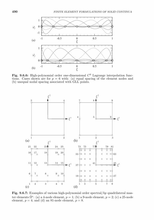
490
(a)
(b)
jϕ
ξ-1 -0.5 0 0.5 1
0
1
jϕ
ξ-1 -0.5 0 0.5 1
-1
0
1
Fig. 9.6.6: High-polynomial order one-dimensional C0 Lagrange interpolation func-tions. Cases shown are for p = 6 with: (a) equal spacing of the element nodes and(b) unequal nodal spacing associated with GLL points.
1 2
3 4
1 3
7 9
1 5 1 9
21 25
2
4 65
8
2 3 4
6 107 8 9
11 1512 13 14
16 2017 18 19
22 23 24
3 5 7
19
37
55
73 8175 77 79
27
45
63
41
(a) (b)
(c) (d)
ξ
ξ
ξ
ξ
ξ
ξ
ξ
ξ
2
22
2
1
11
1
Fig. 9.6.7: Examples of various high-polynomial order spectral/hp quadrilateral mas-
ter elements Ωe: (a) a 4-node element, p = 1; (b) a 9-node element, p = 2; (c) a 25-nodeelement, p = 4; and (d) an 81-node element, p = 8.
FINITE ELEMENT FORMULATIONS OF SOLID CONTINUA
9.6. A REFINED CONTINUUM SHELL FINITE ELEMENT 491
9.6.7 Finite Element Model and Solution of NonlinearEquations
Here we employ Newton’s method in the solution of the resulting nonlinearalgebraic equations. To facilitate a numerical solution for problems involv-ing very large deformations, we further embed the iterative Newton procedurewithin an incremental load stepping algorithm. For post-buckling analysis weemploy a cylindrical arc-length solution procedure. In an effort to improve sys-tem memory requirements in the numerical implementation, we further adoptelement-level static condensation, wherein, the interior degrees of freedom ofeach element are implicitly eliminated prior to global assembly of the sparsefinite element coefficient matrix.
9.6.7.1 The Newton procedure
The Newton iteration proceeds as follows: given a known solution state Φrhp we
seek ∆Φr+1hp satisfying the following linearized problem:
G(δΦhp,Φrhp) +DG(δΦhp,Φ
rhp)[∆Φr+1
hp ] = 0 (9.6.54)
where ∆Φr+1hp = Φr+1
hp − Φrhp. To simplify the present discussion, we introduce
the following notation for the discrete quantities: Φr = Φrhp, δΦ = δΦhp, and
∆Φr+1 = ∆Φr+1hp . The discrete tangent operator DG(δΦhp,Φ
rhp)[∆Φr+1
hp ] maybe evaluated within a typical element as
DGe(δΦ, Φr)[∆Φr+1] = DGeG(δΦ, Φr)[∆Φr+1] +DGeM (δΦ, Φr)[∆Φr+1] (9.6.55)
The geometric tangent operator DGeG(δΦ, Φr)[∆Φr+1] and material tangent op-
erator DGeM (δΦ, Φr)[∆Φr+1] are determined within the element as
DGeG(δΦ, Φr)[∆Φr+1] =
∫Be0
(Dδε
(0)ij [∆Φr+1] + ξ3Dδε
(1)ij [∆Φr+1]
)SijdBe0
(9.6.56a)
=
∫Ωe
(Dδε
(0)ij [∆Φr+1]N ij +Dδε
(1)ij [∆Φr+1]M ij
)dΩe
DGeM (δΦ, Φr)[∆Φr+1] =
∫Be0
(δε
(0)ij + ξ3δε
(1)ij
)Cijkl
(Dε
(0)kl [∆Φr+1] (9.6.56b)
+ ξ3Dε(1)kl [∆Φr+1]
)dBe0
=
∫Ωe
[(Aijklδε
(0)ij +Bijklδε
(1)ij
)Dε
(0)kl [∆Φr+1]
+(Bijklδε
(0)ij +Dijklδε
(1)ij
)Dε
(1)kl [∆Φr+1]
]dΩe
492 FINITE ELEMENT FORMULATIONS OF SOLID CONTINUA
The contravariant components of the internal stress resultants N ij and M ij
appearing in the discrete tangent operator may be evaluated as
N ij =
∫ +1
−1SijJ dξ3 =
(Aijklε
(0)kl +Bijklε
(1)kl
)∣∣∣Φhp=Φr
(9.6.57a)
M ij =
∫ +1
−1ξ3SijJ dξ3 =
(Bijklε
(0)kl +Dijklε
(1)kl
)∣∣∣Φhp=Φr
(9.6.57b)
Upon substitution of the finite element approximations into the linearizedvirtual work statement, we arrive at the finite element model (i.e. a system ofnonlinear algebraic equations) for the eth element
[Ke](r)δ∆e(r+1) = F e(r) (9.6.58)
where [Ke](r) is the element tangent coefficient matrix at the beginning of therth iteration, F e(r) is the element imbalance force vector and δ∆e(r+1) =∆e(r+1) − ∆e(r) is the incremental solution to be determined. Due to theincredible complexity of the above system of equations (there are 22,050 uniqueterms in the discrete tangent operator DGe(δΦ, Φr)[∆Φr+1]), the symbolic al-gebra software Maple c© has been utilized in the construction of [Ke](r) andF e(r). We partition Eq. (9.6.58) into the following equivalent form[eK11](r) · · · [eK17](r)
.... . .
...
[eK71](r) · · · [eK77](r)
eδ∆(1)(r+1)
...
eδ∆(7)(r+1)
=
eF (1)(r)
...
eF (7)(r)
(9.6.59)
where
eKαβ(r)ij =
∫Ωe
2∑l=0
2∑m=0
Cαβlm (X(ξ1, ξ2), r(ξ1, ξ2),Φrhp(ξ1, ξ2))S lmij (ξ1, ξ2)dΩe
(9.6.60a)
eF(α)(r)i =
∫Ωe
2∑l=0
Fαl (X(ξ1, ξ2), r(ξ1, ξ2),Φnhp(ξ1, ξ2))T li (ξ1, ξ2)dΩe (9.6.60b)
for i, j = 1, . . . , (p + 1)2 and α, β = 1, . . . , 7. The functions S lmij and T li are ofthe form
S00ij = ψiψj , S0m
ij = ψi∂ψj∂ξm
, S l0ij =∂ψi∂ξl
ψj , S lmij =∂ψi∂ξl
∂ψj∂ξm
(9.6.61a)
T 0i = ψi, T 1
i =∂ψi∂ξ1
, T 2i =
∂ψi∂ξ2
(9.6.61b)
where l and m each range from 1 to 2. The coefficients Cαβlm and Fαl (which areindependent of i and j) are quite involved; in the numerical implementation,
9.6. A REFINED CONTINUUM SHELL FINITE ELEMENT 493
these quantities are obtained symbolically using Maple c© and have then trans-lated the resulting expressions into C++ code. At this point it is worth notingthat interpolating Ψ and n separately in the finite element approximation ofψ [refer to Eq. (9.6.19)] is crucial in ensuring that Cαβlm and Fαl are indeed
independent of the i and j indices in eKαβ(r)ij and eF
(α)(r)i .
The components of the element coefficient matrix and force vector are ob-tained numerically using the Gauss–Legendre quadrature rule, where p + 1quadrature points are taken in each coordinate direction of Ωe. At a given inte-gration point (ξ1
I , ξ2J) ∈ Ωe we evaluate numerically, based on Eq. (9.6.47), the
components of Aijkl, Bijkl, and Dijkl. Once the effective stiffnesses are knownwe determine Cαβlm (ξ1
I , ξ2J) and Fαl (ξ1
I , ξ2J) and then apply the summation pro-
cedure of the Gauss–Legendre quadrature rule to the components of eKαβ(r)ij
and eF(α)(r)i . Repeating this process at each quadrature point in Ωe ensures an
efficient numerical implementation.
9.6.7.2 The cylindrical arc-length procedure
For a vast majority of nonlinear problems, the Newton iterative procedure isadequate to solve the assembled set of nonlinear finite element equations. How-ever, in the numerical simulation of the post-buckling of shell structures, sucha strategy may fail to trace the equilibrium path through the limit points (i.e.points where the tangent matrix is singular). For these problems an arc-lengthprocedure is adopted, wherein a constraint equation is proposed to control theload factor associated with a given load step. For general details on the histor-ical development of the arc-length method one may consult the works of Riks[149, 150] and Crisfield [151] (detailed explanations of the method may also befound in the textbook of Bathe [4] and Appendix 2).
In both solution schemes, we assume that the external loads are appliedin increments. Then we express the discrete weak formulation, given by Eq.(9.6.42), at the current load step as
R(r+1) = F int(r+1) − λ(r+1)F ext ≡ 0 (9.6.62)
where F int(r+1) is a column vector obtained from the internal virtual workand F ext is a constant vector (independent of the load step) constructedfrom the externally applied virtual work. The quantity λ(r+1) is the load factorassociated with the current load step. Linearizing the above expression usingNewton’s method yields
[K](r)δ∆(r+1) = −R(r) + δλ(r+1)F ext (9.6.63)
where δ∆(r+1) and δλ(r+1) are defined as
δ∆(r+1) = ∆(r+1) − ∆(r) (9.6.64a)
494 FINITE ELEMENT FORMULATIONS OF SOLID CONTINUA
δλ(r+1) = λ(r+1) − λ(r) (9.6.64b)
In the Newton solution procedure, λ(r+1) is prescribed by the user, andhence δλ(r+1) = 0. In the arc-length procedure, we solve for a sequence ofshell configurations associated with the prescribed load parameters kλNk=1.In solving for the next configuration, the coefficient matrix [K](0) and residualR(0) are constructed using the converged solution from the previous load step.
In the arc-length solution procedure, the following additive decompositionof the incremental solution is introduced:
δ∆(r+1) = δ∆(r+1) + δλ(r+1)δ∆(r+1) (9.6.65)
Using the above expression along with Eq. (9.6.63) allows us to obtain thefollowing two sets of linearized equations for δ∆(r+1) and δ∆(r+1):
[K](r)δ∆(r+1) = −R(r) (9.6.66a)
[K](r)δ∆(r+1) = F ext (9.6.66b)
Once the above equations have been solved (and assuming, of course, thatδλ(r+1) is known), we may obtain δ∆(r+1) using Eq. (9.6.65). Next we definethe solution increments ∆(r+1) and λ(r+1), between the current configurationsand the configuration being sought, as
∆(r+1) = ∆(r+1) − ∆= ∆(r) + δ∆(r+1) + δλ(r+1)δ∆(r+1) (9.6.67a)
λ(r+1) = λ(r) + δλ(r+1) (9.6.67b)
With the aid of the above formulae, we can define the standard spherical arc-length constraint equation for δλ(r+1) as
K(r+1) = ||∆(r+1)||2 + β(λ(r+1))2||F ext||2 − (∆L)2
= a1(δλ(r+1))2 + a2δλ(r+1) + a3 = 0
(9.6.68)
where ∆L is the arc-length, β is a scaling parameter, and || · || denotes theEuclidean norm. The constraint K(r+1) is a quadratic equation in δλ(r+1) withcoefficients a1, a2, and a3 defined as
a1 = ||δ∆(r+1)||2 + β||F ext||2 (9.6.69a)
a2 = 2[(∆(r) + δ∆(r+1)
)Tδ∆(r+1) + βλ(r)||F ext||2]
(9.6.69b)
a3 = ||∆(r) + δ∆(r+1)||2 + β(λ(r))2||F ext||2 − (∆L)2 (9.6.69c)
The two possible solutions for the constraint equation may be expressed as
δλ(r+1)1 =
−a2 +√a2
2 − 4a1a3
2a1, δλ
(r+1)2 =
−a2 −√a2
2 − 4a1a3
2a1(9.6.70)
9.6. A REFINED CONTINUUM SHELL FINITE ELEMENT 495
We select δλ(r+1)i such that the inner product of ∆(r+1) with ∆(r) is posi-
tive. This ensures that we do not march backwards along the previously com-
puted solution path. In the event that both δλ(r+1)1 and δλ
(r+1)2 yield positive
inner products of t+∆t∆(n+1) with t+∆t∆(r), we select δ∆(r+1) such thatt+∆t∆(r+1) is closest to t+∆t∆(r) in the Euclidean metric. For the firstiteration of a given load step, we select ∆(1) such that the inner product of∆(1) with ∆ is positive (where ∆ is the converged incremental solutionfrom the previous load step). In the numerical implementation, we take β = 0,which results in the well-known cylindrical arc-length procedure (see Crisfield[151] for a discussion on the importance of β).
To initialize the arc-length solution method (at the first load step and thebeginning of the first iteration: r = 0) we take λ(0) = 0, prescribe an ap-propriate value for δλ(1) (typically we define F ext such that it is sufficientto take δλ(1) = 1) and then solve Eq. (9.6.66b) for δ∆(1). We then takeδ∆(1) = δλ(1)δ∆(1) and define the arc-length ∆L for the subsequent non-linear iterations as
1∆L = δλ(1)||δ∆(1)|| (9.6.71)
To improve the efficiency of the arc-length method, the arc-length 2∆L isadjusted for the next load step, depending on how many iterations were requiredto achieve nonlinear solution convergence at the immediate previous load step.Here the following formula from the literature (see Kweon and Hong [152]) isadopted:
2∆L = 1∆L√
2I/1I (9.6.72)
where 1I is the actual number of iterations required for convergence at theimmediate previous load step and 2I is the desired number of iterations requiredto satisfy the convergence criterion at the current load step. Typically we maytake 4 ≤ 2I ≤ 6, which naturally reduces the arc-length in the vicinity of limitpoints and increases the arc-length whenever nonlinear convergence is quicklyachieved.
9.6.7.3 Element-level static condensation and assembly of elements
A major disadvantage of high-order finite elements is that the number of inte-rior nodes increases with the polynomial order p. As a result, the coefficientmatrix of the resulting global system of finite element equations will in generalbe more dense than a system of equations obtained using a low-order discretiza-tion (assuming of course that both discretizations possess the same number ofdegrees of freedom).
To improve the competitiveness of the shell finite elements based on higher-order spectral interpolation functions, an element-level static condensation isadopted, wherein the element-level equations are rearranged for element e [given
496
by Eq. (9.6.59)] with respect to the element boundary eδ∆(B)(r+1) and ele-ment interior eδ∆(I)(r+1) solution increments as[
[eKBB](r) [eKBI ](r)
[eKIB](r) [eKII ](r)
]eδ∆(B)(r+1)
eδ∆(I)(r+1)
=
eF (B)(r)eF (I)(r)
(9.6.73)
The interior nodal degrees of freedom for element e do not have connectivity toother elements in the mesh and therefore they may be implicitly removed fromthe above system of equations to yield (note that this is possible because theforces corresponding to internal nodal degrees of freedom are known)
[Ke](r)eδ∆(B)(r+1) = F e(r) (9.6.74)
where the effective element coefficient matrix [Ke](r) and force vector F e(r)are of the form
[Ke](r) = [eKBB](r) − [eKBI ](r)[eKII ](r)−1[eKIB](r) (9.6.75a)
F e(r) = eF (B)(r) − [eKBI ](r)[eKII ](r)−1eF (I)(r) (9.6.75b)
The effective element coefficient matrix and force vector may be constructedusing the dense matrix routines available in LAPACK.
The statically-condensed element-level equations are assembled into the fol-lowing global system of linearized algebraic equations:
[K](r)δ∆(B)(r+1) = F(r) (9.6.76)
whose solution yields the degree of freedom increments for the collection ofnodes residing on the element boundaries. The interior degree of freedom in-crements may be recovered by post computing (for each element) the solutionusing the following set of equations
[eKII ](r)eδ∆(I)(r+1) = eF (I)(r) − [eKIB](r)eδ∆(B)(r+1) (9.6.77)
We note that the present high-order spectral/hp finite element formulationis very much comparable with standard low-order shell finite element implemen-tations in terms of system memory requirements associated with constructingand storing the sparse form of [K](r). Figure 9.6.8 shows an example of a meshof p-level four elements before and after static condensation. In addition, thepresent formulation admits straightforward parallelization in the constructionof the effective element matrices and also the post-computation of the interiorsolution increments. In addition, unlike many low-order discretizations, thepresent shell finite element formulation is completely displacement-based.
FINITE ELEMENT FORMULATIONS OF SOLID CONTINUA
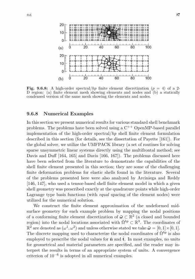
9.6. A REFINED CONTINUUM SHELL FINITE ELEMENT 497
Fig. 9.6.8: A high-order spectral/hp finite element discretization (p = 4) of a 2-D region: (a) finite element mesh showing elements and nodes and (b) a staticallycondensed version of the same mesh showing the elements and nodes.
9.6.8 Numerical Examples
In this section we present numerical results for various standard shell benchmarkproblems. The problems have been solved using a C++ OpenMP-based parallelimplementation of the high-order spectral/hp shell finite element formulationdescribed in this section (for details, see the dissertation of Payette [161]). Forthe global solver, we utilize the UMFPACK library (a set of routines for solvingsparse unsymmetric linear systems directly using the multifrontal method; seeDavis and Duff [164, 165] and Davis [166, 167]). The problems discussed herehave been selected from the literature to demonstrate the capabilities of theshell finite element presented in this section; they are some of the challengingfinite deformation problems for elastic shells found in the literature. Severalof the problems presented here were also analyzed by Arciniega and Reddy[146, 147], who used a tensor-based shell finite element model in which a givenshell geometry was prescribed exactly at the quadrature points while high-orderLagrange type basis functions (with equal spacing of the element nodes) wereutilized for the numerical solution.
We construct the finite element approximation of the undeformed mid-surface geometry for each example problem by mapping the nodal positionsof a conforming finite element discretization of ω ⊂ R2 (a closed and boundedregion) into the nodal locations associated with Ωhp ⊂ R3. The coordinates ofR2 are denoted as (ω1, ω2) and unless otherwise stated we take ω = [0, 1]×[0, 1].The discrete mapping used to characterize the nodal coordinates of Ωhp is alsoemployed to prescribe the nodal values for n and t. In most examples, no unitsfor geometrical and material parameters are specified, and the reader may in-terpret the results in terms of an appropriate system of units. A convergencecriterion of 10−6 is adopted in all numerical examples.
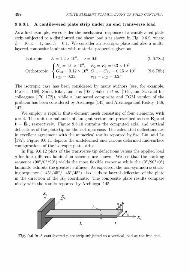
498
9.6.8.1 A cantilevered plate strip under an end transverse load
As a first example, we consider the mechanical response of a cantilevered platestrip subjected to a distributed end shear load q as shown in Fig. 9.6.9, whereL = 10, b = 1, and h = 0.1. We consider an isotropic plate and also a multi-layered composite laminate with material properties given as
Isotropic : E = 1.2× 10⁶, ν = 0.0 (9.6.78a)
Orthotropic :
E1 = 1.0× 10⁶, E2 = E3 = 0.3× 10⁶
G23 = 0.12× 10⁶, G13 = G12 = 0.15× 10⁶
ν23 = 0.25, ν13 = ν12 = 0.25(9.6.78b)
The isotropic case has been considered by many authors (see, for example,Parisch [168], Simo, Rifai, and Fox [106], Saleeb et al. [169], and Sze and hiscolleagues [170–172]), while a laminated composite and FGM version of theproblem has been considered by Arciniega [145] and Arciniega and Reddy [146,147].
We employ a regular finite element mesh consisting of four elements, withp = 4. The unit normal and unit tangent vectors are prescribed as n = E3 andt = E1, respectively. Figure 9.6.10 contains the computed axial and verticaldeflections of the plate tip for the isotropic case. The calculated deflections arein excellent agreement with the numerical results reported by Sze, Liu, and Lo[172]. Figure 9.6.11 depicts the undeformed and various deformed mid-surfaceconfigurations of the isotropic plate strip.
In Fig. 9.6.12 plots of the transverse tip deflections versus the applied loadq for four different lamination schemes are shown. We see that the stackingsequence (90/0/90) yields the most flexible response while the (0/90/0)laminate exhibits the greatest stiffness. As expected, the non-symmetric stack-ing sequence (−45/45/−45/45) also leads to lateral deflection of the platein the direction of the X2 coordinate. The composite plate results comparenicely with the results reported by Arciniega [145].
L
h
bX1
X2X3
q
Fig. 9.6.9: A cantilevered plate strip subjected to a vertical load at the free end.
FINITE ELEMENT FORMULATIONS OF SOLID CONTINUA
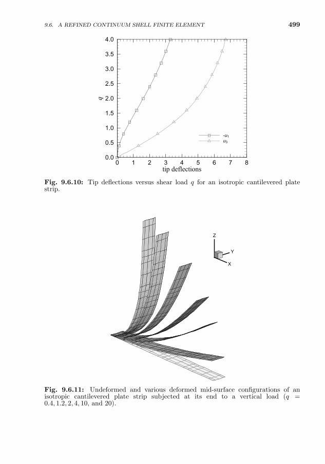
499
tip deflections
q
0 1 2 3 4 5 6 7 80.0
0.5
1.0
1.5
2.0
2.5
3.0
3.5
4.0
-u1u3
Fig. 9.6.10: Tip deflections versus shear load q for an isotropic cantilevered platestrip.
Y
Z
X
Fig. 9.6.11: Undeformed and various deformed mid-surface configurations of anisotropic cantilevered plate strip subjected at its end to a vertical load (q =0.4, 1.2, 2, 4, 10, and 20).
9.6. A REFINED CONTINUUM SHELL FINITE ELEMENT
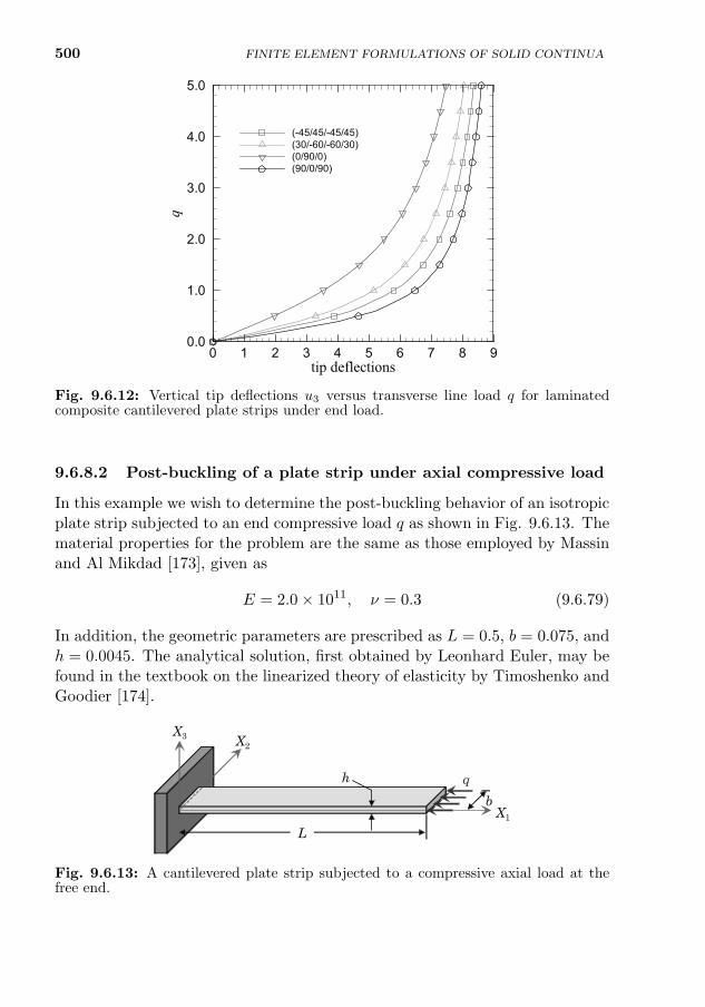
500 FINITE ELEMENT FORMULATIONS OF SOLID CONTINUA
tip deflections
q
0 1 2 3 4 5 6 7 8 90.0
1.0
2.0
3.0
4.0
5.0
(-45/45/-45/45)(30/-60/-60/30)(0/90/0)(90/0/90)
Fig. 9.6.12: Vertical tip deflections u3 versus transverse line load q for laminatedcomposite cantilevered plate strips under end load.
9.6.8.2 Post-buckling of a plate strip under axial compressive load
In this example we wish to determine the post-buckling behavior of an isotropicplate strip subjected to an end compressive load q as shown in Fig. 9.6.13. Thematerial properties for the problem are the same as those employed by Massinand Al Mikdad [173], given as
E = 2.0× 10¹¹, ν = 0.3 (9.6.79)
In addition, the geometric parameters are prescribed as L = 0.5, b = 0.075, andh = 0.0045. The analytical solution, first obtained by Leonhard Euler, may befound in the textbook on the linearized theory of elasticity by Timoshenko andGoodier [174].
L
hbX1
X2X3
q
Fig. 9.6.13: A cantilevered plate strip subjected to a compressive axial load at thefree end.
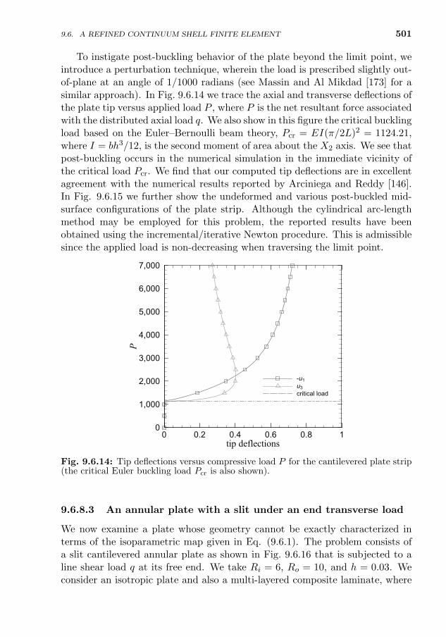
501
To instigate post-buckling behavior of the plate beyond the limit point, weintroduce a perturbation technique, wherein the load is prescribed slightly out-of-plane at an angle of 1/1000 radians (see Massin and Al Mikdad [173] for asimilar approach). In Fig. 9.6.14 we trace the axial and transverse deflections ofthe plate tip versus applied load P , where P is the net resultant force associatedwith the distributed axial load q. We also show in this figure the critical bucklingload based on the Euler–Bernoulli beam theory, Pcr = EI(π/2L)2 = 1124.21,where I = bh3/12, is the second moment of area about the X2 axis. We see thatpost-buckling occurs in the numerical simulation in the immediate vicinity ofthe critical load Pcr. We find that our computed tip deflections are in excellentagreement with the numerical results reported by Arciniega and Reddy [146].In Fig. 9.6.15 we further show the undeformed and various post-buckled mid-surface configurations of the plate strip. Although the cylindrical arc-lengthmethod may be employed for this problem, the reported results have beenobtained using the incremental/iterative Newton procedure. This is admissiblesince the applied load is non-decreasing when traversing the limit point.
tip deflections
P
0 0.2 0.4 0.6 0.8 10
1,000
2,000
3,000
4,000
5,000
6,000
7,000
-u1u3critical load
Fig. 9.6.14: Tip deflections versus compressive load P for the cantilevered plate strip(the critical Euler buckling load Pcr is also shown).
9.6.8.3 An annular plate with a slit under an end transverse load
We now examine a plate whose geometry cannot be exactly characterized interms of the isoparametric map given in Eq. (9.6.1). The problem consists ofa slit cantilevered annular plate as shown in Fig. 9.6.16 that is subjected to aline shear load q at its free end. We take Ri = 6, Ro = 10, and h = 0.03. Weconsider an isotropic plate and also a multi-layered composite laminate, where
9.6. A REFINED CONTINUUM SHELL FINITE ELEMENT
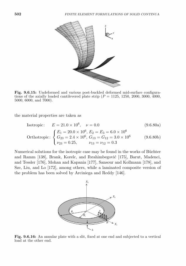
502 FINITE ELEMENT FORMULATIONS OF SOLID CONTINUA
Y
Z
X
Fig. 9.6.15: Undeformed and various post-buckled deformed mid-surface configura-tions of the axially loaded cantilevered plate strip (P = 1125, 1250, 2000, 3000, 4000,5000, 6000, and 7000).
the material properties are taken as
Isotropic : E = 21.0× 10⁶, ν = 0.0 (9.6.80a)
Orthotropic :
E1 = 20.0× 10⁶, E2 = E3 = 6.0× 10⁶
G23 = 2.4× 10⁶, G13 = G12 = 3.0× 10⁶
ν23 = 0.25, ν13 = ν12 = 0.3(9.6.80b)
Numerical solutions for the isotropic case may be found in the works of Buchterand Ramm [138], Brank, Korelc, and Ibrahimbegovic [175], Barut, Madenci,and Tessler [176], Mohan and Kapania [177], Sansour and Kollmann [178], andSze, Liu, and Lo [172], among others, while a laminated composite version ofthe problem has been solved by Arciniega and Reddy [146].
X1
X2
X3
q
h
RoRi
B
A
Fig. 9.6.16: An annular plate with a slit, fixed at one end and subjected to a verticalload at the other end.
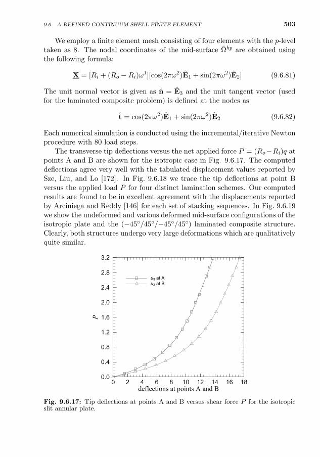
503
We employ a finite element mesh consisting of four elements with the p-leveltaken as 8. The nodal coordinates of the mid-surface Ωhp are obtained usingthe following formula:
X = [Ri + (Ro −Ri)ω1][cos(2πω2)E1 + sin(2πω2)E2] (9.6.81)
The unit normal vector is given as n = E3 and the unit tangent vector (usedfor the laminated composite problem) is defined at the nodes as
t = cos(2πω2)E1 + sin(2πω2)E2 (9.6.82)
Each numerical simulation is conducted using the incremental/iterative Newtonprocedure with 80 load steps.
The transverse tip deflections versus the net applied force P = (Ro−Ri)q atpoints A and B are shown for the isotropic case in Fig. 9.6.17. The computeddeflections agree very well with the tabulated displacement values reported bySze, Liu, and Lo [172]. In Fig. 9.6.18 we trace the tip deflections at point Bversus the applied load P for four distinct lamination schemes. Our computedresults are found to be in excellent agreement with the displacements reportedby Arciniega and Reddy [146] for each set of stacking sequences. In Fig. 9.6.19we show the undeformed and various deformed mid-surface configurations of theisotropic plate and the (−45/45/−45/45) laminated composite structure.Clearly, both structures undergo very large deformations which are qualitativelyquite similar.
deflections at points A and B
P
0 2 4 6 8 10 12 14 16 180.0
0.4
0.8
1.2
1.6
2.0
2.4
2.8
3.2
u3 at Au3 at B
Fig. 9.6.17: Tip deflections at points A and B versus shear force P for the isotropicslit annular plate.
9.6. A REFINED CONTINUUM SHELL FINITE ELEMENT
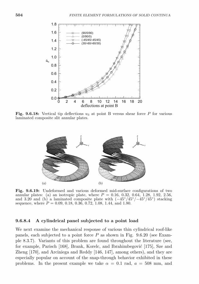
504 FINITE ELEMENT FORMULATIONS OF SOLID CONTINUA
deflections at point B
P
0 2 4 6 8 10 12 14 16 18 200.0
0.2
0.4
0.6
0.8
1.0
1.2
1.4
1.6
1.8
(90/0/90)(0/90/0)(-45/45/-45/45)(30/-60/-60/30)
Fig. 9.6.18: Vertical tip deflections u3 at point B versus shear force P for variouslaminated composite slit annular plates.
XY
Z
XY
Z
(a) (b)
Fig. 9.6.19: Undeformed and various deformed mid-surface configurations of twoannular plates: (a) an isotropic plate, where P = 0.16, 0.32, 0.64, 1.28, 1.92, 2.56,and 3.20 and (b) a laminated composite plate with (−45/45/−45/45) stackingsequence, where P = 0.09, 0.18, 0.36, 0.72, 1.08, 1.44, and 1.80.
9.6.8.4 A cylindrical panel subjected to a point load
We next examine the mechanical response of various thin cylindrical roof-likepanels, each subjected to a point force P as shown in Fig. 9.6.20 (see Exam-ple 8.3.7). Variants of this problem are found throughout the literature (see,for example, Parisch [168], Brank, Korelc, and Ibrahimbegovic [175], Sze andZheng [170], and Arciniega and Reddy [146, 147], among others), and they areespecially popular on account of the snap-through behavior exhibited in theseproblems. In the present example we take α = 0.1 rad, a = 508 mm, and
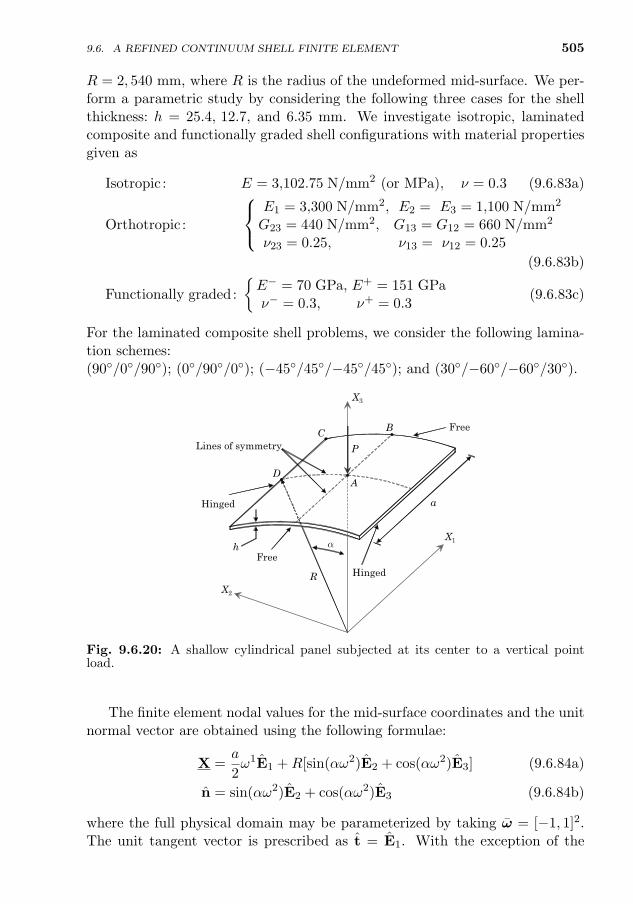
9.6. A REFINED CONTINUUM SHELL FINITE ELEMENT 505
R = 2, 540 mm, where R is the radius of the undeformed mid-surface. We per-form a parametric study by considering the following three cases for the shellthickness: h = 25.4, 12.7, and 6.35 mm. We investigate isotropic, laminatedcomposite and functionally graded shell configurations with material propertiesgiven as
Isotropic : E = 3,102.75 N/mm2 (or MPa), ν = 0.3 (9.6.83a)
Orthotropic :
E1 = 3,300 N/mm2, E2 = E3 = 1,100 N/mm2
G23 = 440 N/mm2, G13 = G12 = 660 N/mm2
ν23 = 0.25, ν13 = ν12 = 0.25
(9.6.83b)
Functionally graded:
E− = 70 GPa, E+ = 151 GPaν− = 0.3, ν+ = 0.3
(9.6.83c)
For the laminated composite shell problems, we consider the following lamina-tion schemes:(90/0/90); (0/90/0); (−45/45/−45/45); and (30/−60/−60/30).
X1
X2
X3
P
α
R
aHinged
HingedFree
Free
Lines of symmetry
h
A
BC
D
Fig. 9.6.20: A shallow cylindrical panel subjected at its center to a vertical pointload.
The finite element nodal values for the mid-surface coordinates and the unitnormal vector are obtained using the following formulae:
X =a
2ω1E1 +R[sin(αω2)E2 + cos(αω2)E3] (9.6.84a)
n = sin(αω2)E2 + cos(αω2)E3 (9.6.84b)
where the full physical domain may be parameterized by taking ω = [−1, 1]2.The unit tangent vector is prescribed as t = E1. With the exception of the
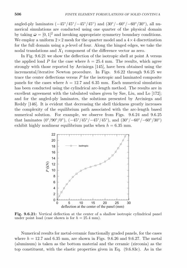
506 FINITE ELEMENT FORMULATIONS OF SOLID CONTINUA
angled-ply laminates (−45/45/−45/45) and (30/−60/−60/30), all nu-merical simulations are conducted using one quarter of the physical domainby taking ω = [0, 1]2 and invoking appropriate symmetry boundary conditions.We employ a uniform 2×2 mesh for the quarter model and a 4×4 discretizationfor the full domain using a p-level of four. Along the hinged edges, we take thenodal translations and X1 component of the difference vector as zero.
In Fig. 9.6.21 we show the deflection of the isotropic shell at point A versusthe applied load P for the case where h = 25.4 mm. The results, which agreestrongly with those reported by Arciniega [145], have been obtained using theincremental/iterative Newton procedure. In Figs. 9.6.22 through 9.6.25 wetrace the center deflections versus P for the isotropic and laminated compositepanels for the cases where h = 12.7 and 6.35 mm. Each numerical simulationhas been conducted using the cylindrical arc-length method. The results are inexcellent agreement with the tabulated values given by Sze, Liu, and Lo [172];and for the angled-ply laminates, the solutions presented by Arciniega andReddy [146]. It is evident that decreasing the shell thickness greatly increasesthe complexity of the equilibrium path associated with the arc-length basednumerical solution. For example, we observe from Figs. 9.6.24 and 9.6.25that laminates (0/90/0), (−45/45/−45/45), and (30/−60/−60/30)exhibit highly nonlinear equilibrium paths when h = 6.35 mm.
deflection at the center of the panel (mm)
P (k
N)
0 5 10 15 20 25 300
2
4
6
8
10
12
14
16
18
20
22
isotropic
Fig. 9.6.21: Vertical deflection at the center of a shallow isotropic cylindrical panelunder point load (case shown is for h = 25.4 mm).
Numerical results for metal-ceramic functionally graded panels, for the caseswhere h = 12.7 and 6.35 mm, are shown in Figs. 9.6.26 and 9.6.27. The metal(aluminum) is taken as the bottom material and the ceramic (zirconia) as thetop constituent, with the elastic properties given in Eq. (9.6.83c). As in the
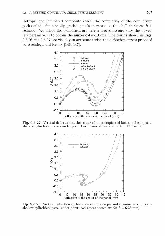
507
isotropic and laminated composite cases, the complexity of the equilibriumpaths of the functionally graded panels increases as the shell thickness h isreduced. We adopt the cylindrical arc-length procedure and vary the power-law parameter n to obtain the numerical solutions. The results shown in Figs.9.6.26 and 9.6.27 are visually in agreement with the deflection curves providedby Arciniega and Reddy [146, 147].
deflection at the center of the panel (mm)
P (k
N)
0 5 10 15 20 25 30 35-0.5
0.0
0.5
1.0
1.5
2.0
2.5
3.0
3.5
4.0
isotropic(90/0/90)(0/90/0)(-45/45/-45/45)(30/-60/-60/30)
Fig. 9.6.22: Vertical deflection at the center of an isotropic and laminated compositeshallow cylindrical panels under point load (cases shown are for h = 12.7 mm).
deflection at the center of the panel (mm)
P (k
N)
0 5 10 15 20 25 30 35 40 45-1.0
-0.5
0.0
0.5
1.0
1.5
2.0
2.5
3.0
3.5
4.0
isotropic(90/0/90)
Fig. 9.6.23: Vertical deflection at the center of an isotropic and a laminated compositeshallow cylindrical panel under point load (cases shown are for h = 6.35 mm).
9.6. A REFINED CONTINUUM SHELL FINITE ELEMENT
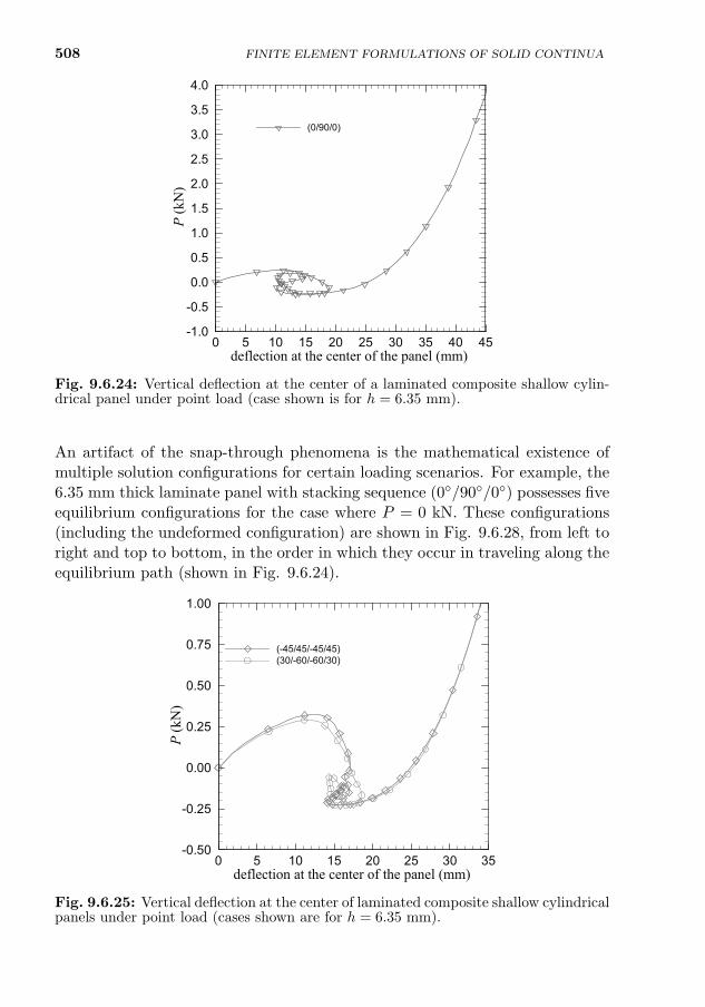
508
deflection at the center of the panel (mm)
P (k
N)
0 5 10 15 20 25 30 35 40 45-1.0
-0.5
0.0
0.5
1.0
1.5
2.0
2.5
3.0
3.5
4.0
(0/90/0)
Fig. 9.6.24: Vertical deflection at the center of a laminated composite shallow cylin-drical panel under point load (case shown is for h = 6.35 mm).
An artifact of the snap-through phenomena is the mathematical existence ofmultiple solution configurations for certain loading scenarios. For example, the6.35 mm thick laminate panel with stacking sequence (0/90/0) possesses fiveequilibrium configurations for the case where P = 0 kN. These configurations(including the undeformed configuration) are shown in Fig. 9.6.28, from left toright and top to bottom, in the order in which they occur in traveling along theequilibrium path (shown in Fig. 9.6.24).
deflection at the center of the panel (mm)
P (k
N)
0 5 10 15 20 25 30 35-0.50
-0.25
0.00
0.25
0.50
0.75
1.00
(-45/45/-45/45)(30/-60/-60/30)
Fig. 9.6.25: Vertical deflection at the center of laminated composite shallow cylindricalpanels under point load (cases shown are for h = 6.35 mm).
FINITE ELEMENT FORMULATIONS OF SOLID CONTINUA
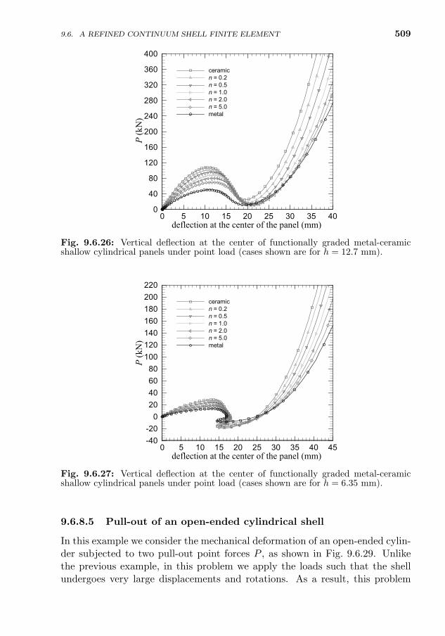
509
deflection at the center of the panel (mm)
P (k
N)
0 5 10 15 20 25 30 35 400
40
80
120
160
200
240
280
320
360
400
ceramicn = 0.2n = 0.5n = 1.0n = 2.0n = 5.0metal
Fig. 9.6.26: Vertical deflection at the center of functionally graded metal-ceramicshallow cylindrical panels under point load (cases shown are for h = 12.7 mm).
deflection at the center of the panel (mm)
P (k
N)
0 5 10 15 20 25 30 35 40 45-40-20020406080100120140160180200220
ceramicn = 0.2n = 0.5n = 1.0n = 2.0n = 5.0metal
Fig. 9.6.27: Vertical deflection at the center of functionally graded metal-ceramicshallow cylindrical panels under point load (cases shown are for h = 6.35 mm).
9.6.8.5 Pull-out of an open-ended cylindrical shell
In this example we consider the mechanical deformation of an open-ended cylin-der subjected to two pull-out point forces P , as shown in Fig. 9.6.29. Unlikethe previous example, in this problem we apply the loads such that the shellundergoes very large displacements and rotations. As a result, this problem
9.6. A REFINED CONTINUUM SHELL FINITE ELEMENT
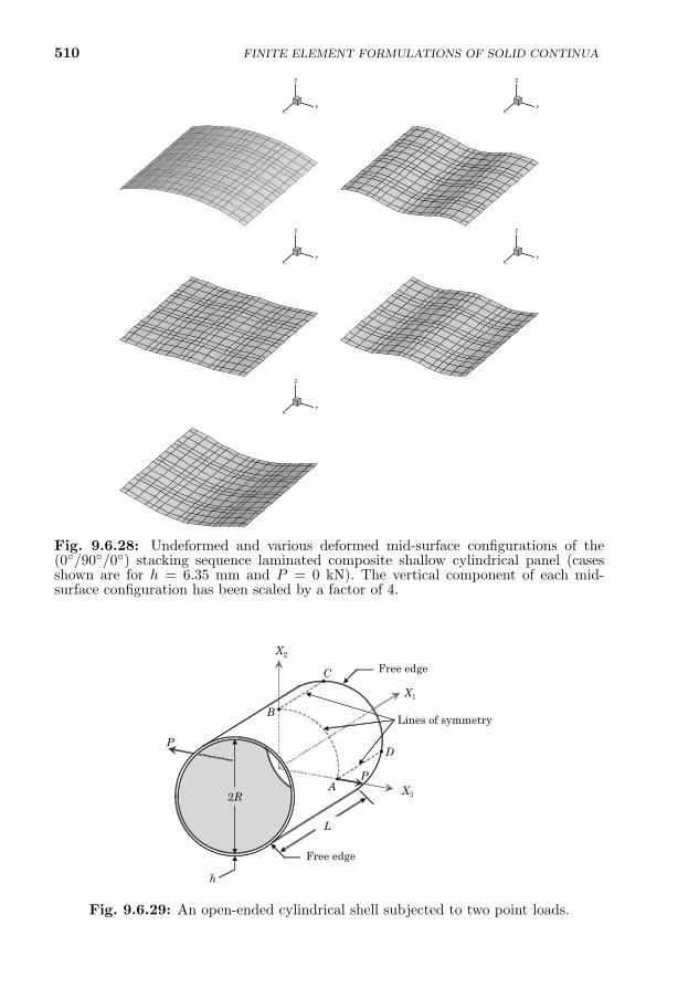
510 FINITE ELEMENT FORMULATIONS OF SOLID CONTINUA
XY
Z
XY
Z
XY
Z
XY
Z
XY
Z
Fig. 9.6.28: Undeformed and various deformed mid-surface configurations of the(0/90/0) stacking sequence laminated composite shallow cylindrical panel (casesshown are for h = 6.35 mm and P = 0 kN). The vertical component of each mid-surface configuration has been scaled by a factor of 4.
X3
X1
X2
P
P
A
B
C
D
h
2R
Lines of symmetry
Free edge
Free edge
L
Fig. 9.6.29: An open-ended cylindrical shell subjected to two point loads.
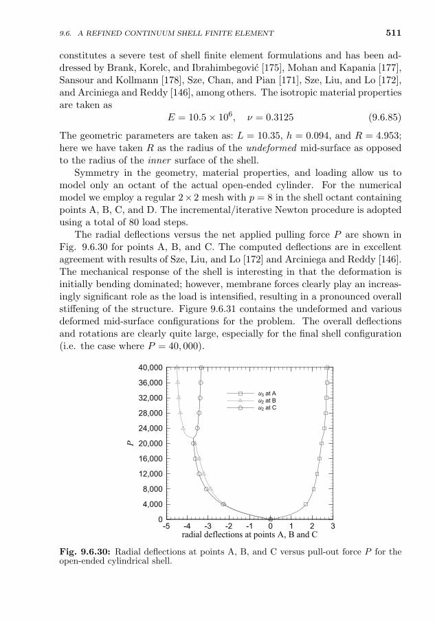
511
constitutes a severe test of shell finite element formulations and has been ad-dressed by Brank, Korelc, and Ibrahimbegovic [175], Mohan and Kapania [177],Sansour and Kollmann [178], Sze, Chan, and Pian [171], Sze, Liu, and Lo [172],and Arciniega and Reddy [146], among others. The isotropic material propertiesare taken as
E = 10.5× 10⁶, ν = 0.3125 (9.6.85)
The geometric parameters are taken as: L = 10.35, h = 0.094, and R = 4.953;here we have taken R as the radius of the undeformed mid-surface as opposedto the radius of the inner surface of the shell.
Symmetry in the geometry, material properties, and loading allow us tomodel only an octant of the actual open-ended cylinder. For the numericalmodel we employ a regular 2×2 mesh with p = 8 in the shell octant containingpoints A, B, C, and D. The incremental/iterative Newton procedure is adoptedusing a total of 80 load steps.
The radial deflections versus the net applied pulling force P are shown inFig. 9.6.30 for points A, B, and C. The computed deflections are in excellentagreement with results of Sze, Liu, and Lo [172] and Arciniega and Reddy [146].The mechanical response of the shell is interesting in that the deformation isinitially bending dominated; however, membrane forces clearly play an increas-ingly significant role as the load is intensified, resulting in a pronounced overallstiffening of the structure. Figure 9.6.31 contains the undeformed and variousdeformed mid-surface configurations for the problem. The overall deflectionsand rotations are clearly quite large, especially for the final shell configuration(i.e. the case where P = 40, 000).
radial deflections at points A, B and C
P
-5 -4 -3 -2 -1 0 1 2 30
4,000
8,000
12,000
16,000
20,000
24,000
28,000
32,000
36,000
40,000
u3 at Au2 at Bu2 at C
Fig. 9.6.30: Radial deflections at points A, B, and C versus pull-out force P for theopen-ended cylindrical shell.
9.6. A REFINED CONTINUUM SHELL FINITE ELEMENT
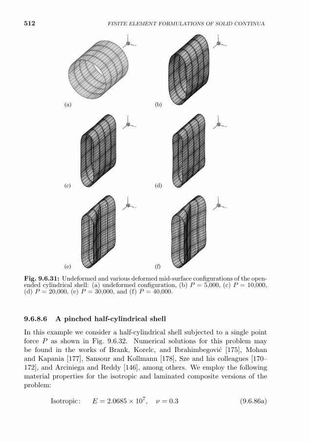
512 FINITE ELEMENT FORMULATIONS OF SOLID CONTINUA
XY
Z
XY
Z
XY
Z
XY
Z
XY
Z
XY
Z
(a) (b)
(c) (d)
(e) (f)
Fig. 9.6.31: Undeformed and various deformed mid-surface configurations of the open-ended cylindrical shell: (a) undeformed configuration, (b) P = 5,000, (c) P = 10,000,(d) P = 20,000, (e) P = 30,000, and (f) P = 40,000.
9.6.8.6 A pinched half-cylindrical shell
In this example we consider a half-cylindrical shell subjected to a single pointforce P as shown in Fig. 9.6.32. Numerical solutions for this problem maybe found in the works of Brank, Korelc, and Ibrahimbegovic [175], Mohanand Kapania [177], Sansour and Kollmann [178], Sze and his colleagues [170–172], and Arciniega and Reddy [146], among others. We employ the followingmaterial properties for the isotropic and laminated composite versions of theproblem:
Isotropic : E = 2.0685× 10⁷, ν = 0.3 (9.6.86a)
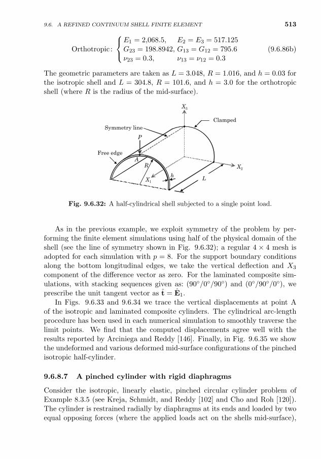
513
Orthotropic :
E1 = 2,068.5, E2 = E3 = 517.125G23 = 198.8942, G13 = G12 = 795.6ν23 = 0.3, ν13 = ν12 = 0.3
(9.6.86b)
The geometric parameters are taken as L = 3.048, R = 1.016, and h = 0.03 forthe isotropic shell and L = 304.8, R = 101.6, and h = 3.0 for the orthotropicshell (where R is the radius of the mid-surface).
X2
X1
X3
P
A
h
R
Symmetry lineClamped
L
Free edge
Fig. 9.6.32: A half-cylindrical shell subjected to a single point load.
As in the previous example, we exploit symmetry of the problem by per-forming the finite element simulations using half of the physical domain of theshell (see the line of symmetry shown in Fig. 9.6.32); a regular 4 × 4 mesh isadopted for each simulation with p = 8. For the support boundary conditionsalong the bottom longitudinal edges, we take the vertical deflection and X3
component of the difference vector as zero. For the laminated composite sim-ulations, with stacking sequences given as: (90/0/90) and (0/90/0), weprescribe the unit tangent vector as t = E1.
In Figs. 9.6.33 and 9.6.34 we trace the vertical displacements at point Aof the isotropic and laminated composite cylinders. The cylindrical arc-lengthprocedure has been used in each numerical simulation to smoothly traverse thelimit points. We find that the computed displacements agree well with theresults reported by Arciniega and Reddy [146]. Finally, in Fig. 9.6.35 we showthe undeformed and various deformed mid-surface configurations of the pinchedisotropic half-cylinder.
9.6.8.7 A pinched cylinder with rigid diaphragms
Consider the isotropic, linearly elastic, pinched circular cylinder problem ofExample 8.3.5 (see Kreja, Schmidt, and Reddy [102] and Cho and Roh [120]).The cylinder is restrained radially by diaphragms at its ends and loaded by twoequal opposing forces (where the applied loads act on the shells mid-surface),
9.6. A REFINED CONTINUUM SHELL FINITE ELEMENT
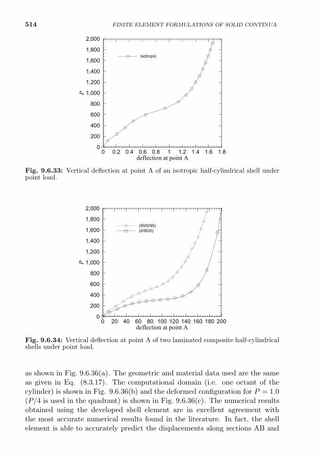
514 FINITE ELEMENT FORMULATIONS OF SOLID CONTINUA
deflection at point A
P
0 0.2 0.4 0.6 0.8 1 1.2 1.4 1.6 1.80
200
400
600
800
1,000
1,200
1,400
1,600
1,800
2,000
isotropic
Fig. 9.6.33: Vertical deflection at point A of an isotropic half-cylindrical shell underpoint load.
deflection at point A
P
0 20 40 60 80 100 120 140 160 180 2000
200
400
600
800
1,000
1,200
1,400
1,600
1,800
2,000
(90/0/90)(0/90/0)
Fig. 9.6.34: Vertical deflection at point A of two laminated composite half-cylindricalshells under point load.
as shown in Fig. 9.6.36(a). The geometric and material data used are the sameas given in Eq. (8.3.17). The computational domain (i.e. one octant of thecylinder) is shown in Fig. 9.6.36(b) and the deformed configuration for P = 1.0(P/4 is used in the quadrant) is shown in Fig. 9.6.36(c). The numerical resultsobtained using the developed shell element are in excellent agreement withthe most accurate numerical results found in the literature. In fact, the shellelement is able to accurately predict the displacements along sections AB and
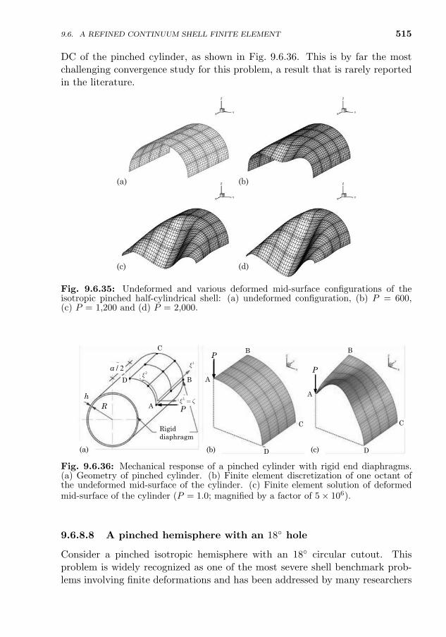
515
DC of the pinched cylinder, as shown in Fig. 9.6.36. This is by far the mostchallenging convergence study for this problem, a result that is rarely reportedin the literature.
X Y
Z
X Y
Z
X Y
Z
X Y
Z(a) (b)
(c) (d)
Fig. 9.6.35: Undeformed and various deformed mid-surface configurations of theisotropic pinched half-cylindrical shell: (a) undeformed configuration, (b) P = 600,(c) P = 1,200 and (d) P = 2,000.
P
P1
3
P
2/a
Rigid diaphragm
A
B
C
D2
B B
Rh
D
C
A
A
D
C
(a) (b) (c)
Fig. 9.6.36: Mechanical response of a pinched cylinder with rigid end diaphragms.(a) Geometry of pinched cylinder. (b) Finite element discretization of one octant ofthe undeformed mid-surface of the cylinder. (c) Finite element solution of deformedmid-surface of the cylinder (P = 1.0; magnified by a factor of 5× 10⁶).
9.6.8.8 A pinched hemisphere with an 18 hole
Consider a pinched isotropic hemisphere with an 18 circular cutout. Thisproblem is widely recognized as one of the most severe shell benchmark prob-lems involving finite deformations and has been addressed by many researchers
9.6. A REFINED CONTINUUM SHELL FINITE ELEMENT
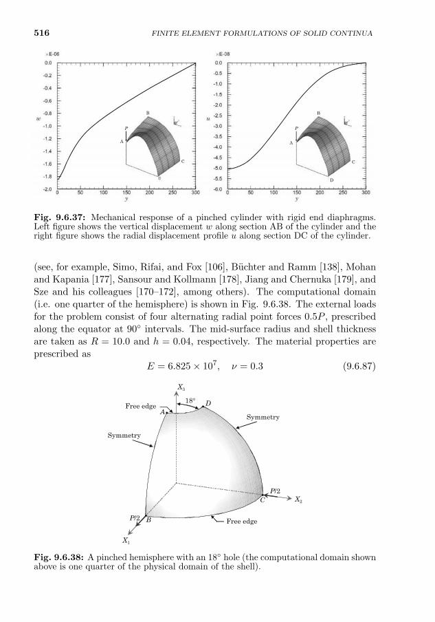
516 FINITE ELEMENT FORMULATIONS OF SOLID CONTINUA
A
B
C
D
A
B
C
P P
Fig. 9.6.37: Mechanical response of a pinched cylinder with rigid end diaphragms.Left figure shows the vertical displacement w along section AB of the cylinder and theright figure shows the radial displacement profile u along section DC of the cylinder.
(see, for example, Simo, Rifai, and Fox [106], Buchter and Ramm [138], Mohanand Kapania [177], Sansour and Kollmann [178], Jiang and Chernuka [179], andSze and his colleagues [170–172], among others). The computational domain(i.e. one quarter of the hemisphere) is shown in Fig. 9.6.38. The external loadsfor the problem consist of four alternating radial point forces 0.5P , prescribedalong the equator at 90 intervals. The mid-surface radius and shell thicknessare taken as R = 10.0 and h = 0.04, respectively. The material properties areprescribed as
E = 6.825× 10⁷, ν = 0.3 (9.6.87)
X1
X2
X3
P/2
P/2 Free edge
Symmetry
SymmetryFree edge
18°
B
C
AD
Fig. 9.6.38: A pinched hemisphere with an 18 hole (the computational domain shownabove is one quarter of the physical domain of the shell).
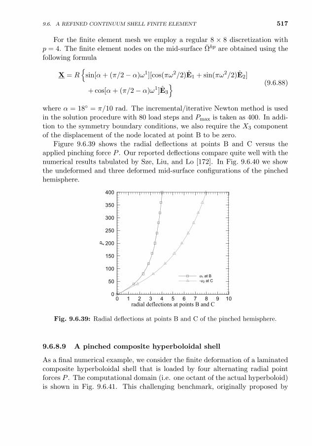
517
For the finite element mesh we employ a regular 8 × 8 discretization withp = 4. The finite element nodes on the mid-surface Ωhp are obtained using thefollowing formula
X = R
sin[α+ (π/2− α)ω1][cos(πω2/2)E1 + sin(πω2/2)E2]
+ cos[α+ (π/2− α)ω1]E3
(9.6.88)
where α = 18 = π/10 rad. The incremental/iterative Newton method is usedin the solution procedure with 80 load steps and Pmax is taken as 400. In addi-tion to the symmetry boundary conditions, we also require the X3 componentof the displacement of the node located at point B to be zero.
Figure 9.6.39 shows the radial deflections at points B and C versus theapplied pinching force P . Our reported deflections compare quite well with thenumerical results tabulated by Sze, Liu, and Lo [172]. In Fig. 9.6.40 we showthe undeformed and three deformed mid-surface configurations of the pinchedhemisphere.
radial deflections at points B and C
P
0 1 2 3 4 5 6 7 8 9 100
50
100
150
200
250
300
350
400
u1 at B-u2 at C
Fig. 9.6.39: Radial deflections at points B and C of the pinched hemisphere.
9.6.8.9 A pinched composite hyperboloidal shell
As a final numerical example, we consider the finite deformation of a laminatedcomposite hyperboloidal shell that is loaded by four alternating radial pointforces P . The computational domain (i.e. one octant of the actual hyperboloid)is shown in Fig. 9.6.41. This challenging benchmark, originally proposed by
9.6. A REFINED CONTINUUM SHELL FINITE ELEMENT
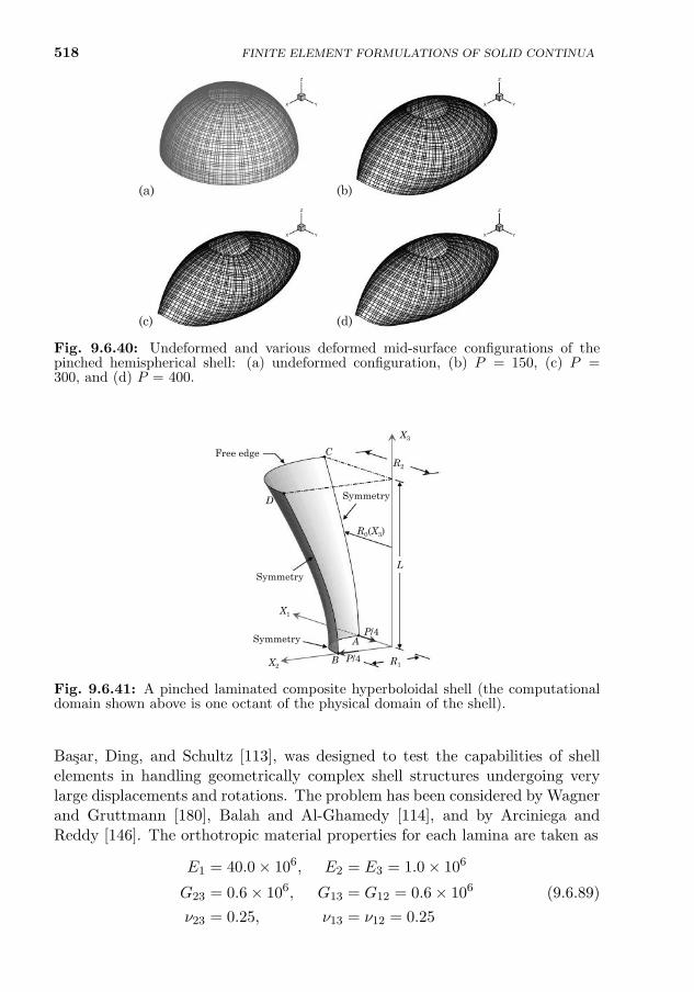
518 FINITE ELEMENT FORMULATIONS OF SOLID CONTINUA
X Y
Z
X Y
Z
X Y
Z
(b)
(c) (d)
X Y
Z
(a)
Fig. 9.6.40: Undeformed and various deformed mid-surface configurations of thepinched hemispherical shell: (a) undeformed configuration, (b) P = 150, (c) P =300, and (d) P = 400.
X3
X2
X1
P/4
P/4
R0(X3)
L
D
C
B
A
R1
R2Free edge
Symmetry
Symmetry
Symmetry
Fig. 9.6.41: A pinched laminated composite hyperboloidal shell (the computationaldomain shown above is one octant of the physical domain of the shell).
Basar, Ding, and Schultz [113], was designed to test the capabilities of shellelements in handling geometrically complex shell structures undergoing verylarge displacements and rotations. The problem has been considered by Wagnerand Gruttmann [180], Balah and Al-Ghamedy [114], and by Arciniega andReddy [146]. The orthotropic material properties for each lamina are taken as
E1 = 40.0× 10⁶, E2 = E3 = 1.0× 10⁶
G23 = 0.6× 10⁶, G13 = G12 = 0.6× 10⁶ (9.6.89)
ν23 = 0.25, ν13 = ν12 = 0.25
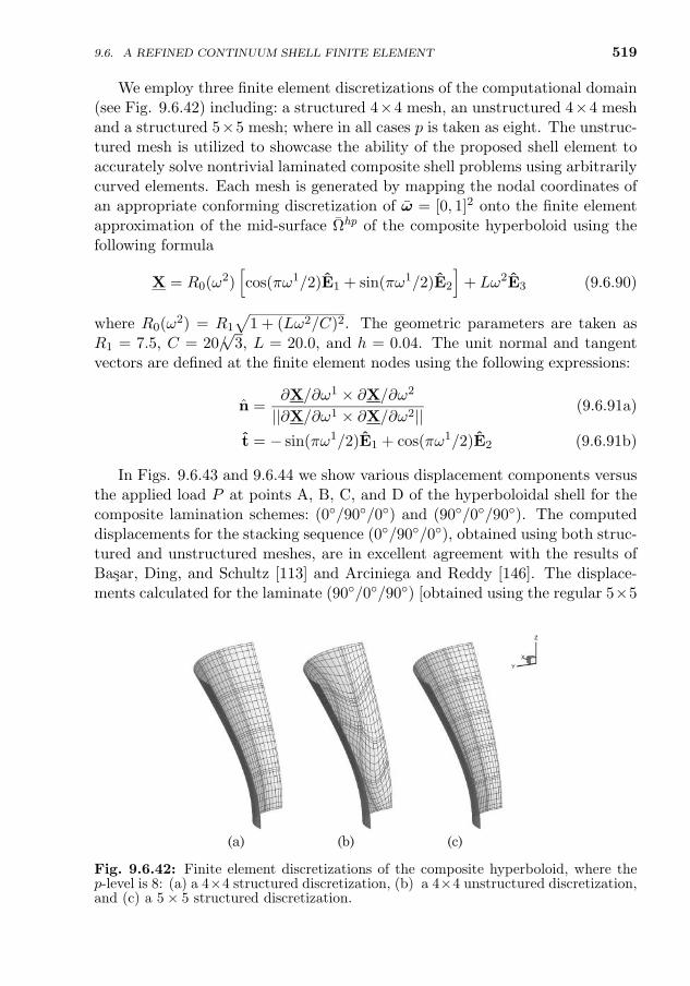
519
We employ three finite element discretizations of the computational domain(see Fig. 9.6.42) including: a structured 4×4 mesh, an unstructured 4×4 meshand a structured 5×5 mesh; where in all cases p is taken as eight. The unstruc-tured mesh is utilized to showcase the ability of the proposed shell element toaccurately solve nontrivial laminated composite shell problems using arbitrarilycurved elements. Each mesh is generated by mapping the nodal coordinates ofan appropriate conforming discretization of ω = [0, 1]2 onto the finite elementapproximation of the mid-surface Ωhp of the composite hyperboloid using thefollowing formula
X = R0(ω2)[cos(πω1/2)E1 + sin(πω1/2)E2
]+ Lω2E3 (9.6.90)
where R0(ω2) = R1
√1 + (Lω2/C)2. The geometric parameters are taken as
R1 = 7.5, C = 20/√
3, L = 20.0, and h = 0.04. The unit normal and tangentvectors are defined at the finite element nodes using the following expressions:
n =∂X/∂ω1 × ∂X/∂ω2
||∂X/∂ω1 × ∂X/∂ω2||(9.6.91a)
t = − sin(πω1/2)E1 + cos(πω1/2)E2 (9.6.91b)
In Figs. 9.6.43 and 9.6.44 we show various displacement components versusthe applied load P at points A, B, C, and D of the hyperboloidal shell for thecomposite lamination schemes: (0/90/0) and (90/0/90). The computeddisplacements for the stacking sequence (0/90/0), obtained using both struc-tured and unstructured meshes, are in excellent agreement with the results ofBasar, Ding, and Schultz [113] and Arciniega and Reddy [146]. The displace-ments calculated for the laminate (90/0/90) [obtained using the regular 5×5
(a) (b) (c)
X
Y
Z
Fig. 9.6.42: Finite element discretizations of the composite hyperboloid, where thep-level is 8: (a) a 4×4 structured discretization, (b) a 4×4 unstructured discretization,and (c) a 5× 5 structured discretization.
9.6. A REFINED CONTINUUM SHELL FINITE ELEMENT
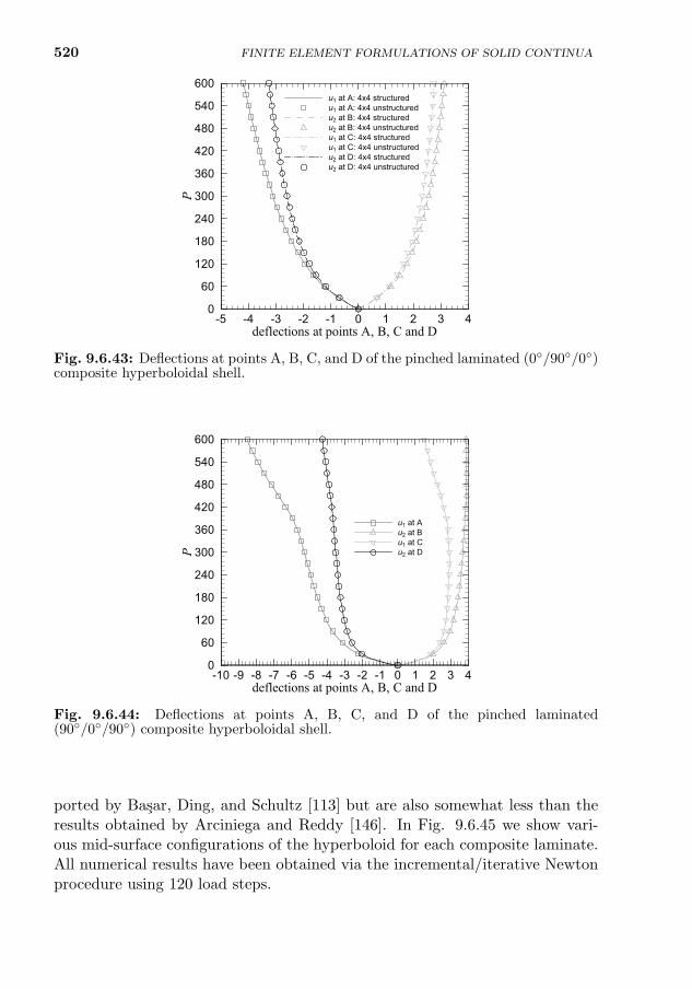
520
deflections at points A, B, C and D
P
-5 -4 -3 -2 -1 0 1 2 3 40
60
120
180
240
300
360
420
480
540
600u1 at A: 4x4 structuredu1 at A: 4x4 unstructuredu2 at B: 4x4 structuredu2 at B: 4x4 unstructuredu1 at C: 4x4 structuredu1 at C: 4x4 unstructuredu2 at D: 4x4 structuredu2 at D: 4x4 unstructured
Fig. 9.6.43: Deflections at points A, B, C, and D of the pinched laminated (0/90/0)composite hyperboloidal shell.
deflections at points A, B, C and D
P
-10 -9 -8 -7 -6 -5 -4 -3 -2 -1 0 1 2 3 40
60
120
180
240
300
360
420
480
540
600
u1 at Au2 at Bu1 at Cu2 at D
Fig. 9.6.44: Deflections at points A, B, C, and D of the pinched laminated(90/0/90) composite hyperboloidal shell.
discretization shown in Fig. 9.6.43(c)], however, are greater than the values re-ported by Basar, Ding, and Schultz [113] but are also somewhat less than theresults obtained by Arciniega and Reddy [146]. In Fig. 9.6.45 we show vari-ous mid-surface configurations of the hyperboloid for each composite laminate.All numerical results have been obtained via the incremental/iterative Newtonprocedure using 120 load steps.
FINITE ELEMENT FORMULATIONS OF SOLID CONTINUA
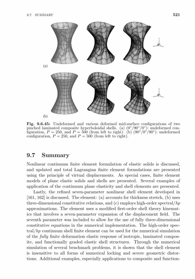
9.7. SUMMARY 521
X Y
Z
(b)
X Y
Z
(a)
Fig. 9.6.45: Undeformed and various deformed mid-surface configurations of twopinched laminated composite hyperboloidal shells. (a) (0/90/0): undeformed con-figuration, P = 250, and P = 500 (from left to right). (b) (90/0/90): undeformedconfiguration, P = 250, and P = 500 (from left to right).
9.7 Summary
Nonlinear continuum finite element formulation of elastic solids is discussed,and updated and total Lagrangian finite element formulations are presentedusing the principle of virtual displacements. As special cases, finite elementmodels of plane elastic solids and shells are presented. Several examples ofapplication of the continuum plane elasticity and shell elements are presented.
Lastly, the refined seven-parameter nonlinear shell element developed in[161, 162] is discussed. The element: (a) accounts for thickness stretch, (b) usesthree-dimensional constitutive relations, and (c) employs high-order spectral/hpapproximations. The element uses a modified first-order shell theory kinemat-ics that involves a seven-parameter expansion of the displacement field. Theseventh parameter was included to allow for the use of fully three-dimensionalconstitutive equations in the numerical implementation. The high-order spec-tral/hp continuum shell finite element can be used for the numerical simulationof the fully finite deformation elastic response of isotropic, laminated compos-ite, and functionally graded elastic shell structures. Through the numericalsimulation of several benchmark problems, it is shown that the shell elementis insensitive to all forms of numerical locking and severe geometric distor-tions. Additional examples, especially applications to composite and function-
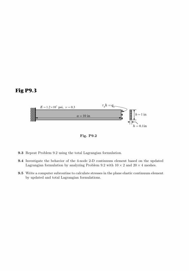
522 FINITE ELEMENT FORMULATIONS OF SOLID CONTINUA
ally graded plates and shells, can be found in [145–147, 161, 162]. Extensionsof the element to include inelastic material behavior and damage prediction areawaiting attention.
Problems
9.1 Investigate the behavior of the 4-node 2-D continuum element based on the updatedLagrangian formulation by analyzing the cantilevered plate problem in Fig. 9.4.1 with10 × 2 and 20 × 4 meshes.
9.2 Use the updated Lagrangian formulation to analyze the cantilevered plate problem inFig. 9.4.1, except that the load is replaced by an end shear load −τ0h = −q0 (lb/in),as shown in Fig. P9.2. Use 5× 1Q9 mesh, an increment of ∆q0 = 500 lb/in (or f0 = 50lb/in.), and 32 load steps with convergence tolerance of ε = 10−3. Plot the load versusvertical deflection at node 22 and load versus Cauchy stresses σxx and σxy at the Gausspoint nearest to the top left end.
1 inb =
0 1. inh =
0 0h qt =
10 ina =
71 2 10 0 3. psi, .E n= ´ =
Fig P9.3
Fig. P9.2
9.3 Repeat Problem 9.2 using the total Lagrangian formulation.
9.4 Investigate the behavior of the 4-node 2-D continuum element based on the updatedLagrangian formulation by analyzing Problem 9.2 with 10 × 2 and 20 × 4 meshes.
9.5 Write a computer subroutine to calculate stresses in the plane elastic continuum elementby updated and total Lagrangian formulations.
523
10
Weak-Form Finite ElementModels of Flows of Viscous
Incompressible Fluids
I have steadily endeavoured to keep my mind free so as to give up any hypothesis, howevermuch beloved (and I cannot resist forming one on every subject), as soon as the facts areshown to be opposed to it. ——– Charles Darwin
10.1 Introduction
Flows of viscous incompressible fluids can be classified into two major types: asmooth, orderly motion is called laminar flow, and a random fluctuating motionis called turbulent flow. Flows of viscous fluids can be characterized by a non-dimensional parameter known as the Reynolds number, Re = ρV L/µ, whichis defined as the ratio of inertial forces ρV 2 to viscous forces µV/L. Here ρdenotes the density of the fluid, µ the fluid viscosity, V the characteristic flowvelocity, and L is a characteristic dimension of the flow region. High viscosityfluids and/or small velocities produce relatively small Reynolds numbers and alaminar flow. The case of Re << 1 corresponds to the flow (called Stokes flow)in which the inertial effects are small compared to the viscous effects and aretherefore neglected. The flow of less viscous fluids and/or higher velocities leadto higher Reynolds numbers and a turbulent flow.
Tremendous progress has been achieved over the last few decades in the fieldof computational fluid dynamics. The advent of the digital computer and, inparticular, parallel processing has made it possible to numerically simulate com-plex flow patterns that could only have been investigated using experimentalprocedures and dimensional analyses. Much of the success and breakthroughsin the numerical simulation of the Navier–Stokes equations for incompressiblefluids have come in the context of low-order finite difference and finite volumetechnologies. Although the finite element method has become the dominantmethod of choice in the numerical analysis of solids, it has yet to receive suchwidespread acceptance when applied to fluid flow problems. It is well known,however, that the finite element method offers many advantages over the finitedifference and finite volume methods. In particular, the finite element method
J.N. Reddy, An Introduction to Nonlinear Finite Element Analysis, Second Edition. c©J.N.Reddy 2015. Published in 2015 by Oxford University Press.
524
can naturally deal with complex regions and complicated boundary conditions,and it possesses a rich mathematical foundation. As a result, there has beena renewed interest in recent years in developing efficient and accurate finiteelement models of the Navier–Stokes equations governing flows of viscous in-compressible fluids.
Generally, whenever any weak formulation is equivalent to the problem ofminimizing an unconstrained convex quadratic functional, the finite elementmodel inherits the following desirable mathematical and computational prop-erties:
1. The numerical solution becomes an orthogonal projection of the exactsolution onto the trial space of a given conforming finite element approx-imation. As a result, the numerical solution represents the “best approx-imation” of the exact solution in the trial space (as measured by a welldefined energy norm).
2. No restrictive compatibility requirements, such as the discrete inf-supcondition, ever arise that must be additionally satisfied by the discreteconforming function spaces of the various dependent variables.
3. The resulting linear algebraic system of global finite element equations arealways symmetric and positive-definite – a property that may be exploitedby both direct as well as iterative solvers.
The vast majority of finite element models for fluids are based on weak-form Galerkin formulations. However, weak-form Galerkin formulations of theNavier–Stokes equations are not equivalent to minimization of unconstrainedconvex quadratic functionals. Therefore, the approximations used for velocityfield and pressure must satisfy ceratin restrictive conditions, as will be discussedin the forthcoming sections.
In the present chapter we develop weak-form Galerkin finite element modelsusing basic physical variables, namely, velocities and pressure. Both Newtonianand non-Newtonian (power-law) fluids are considered here. Computer imple-mentation of the finite element models developed herein is also discussed, andsome representative examples of applications of the finite element models arepresented.
10.2 Governing Equations
10.2.1 Introduction
Here we review the governing equations of a continuous medium based on theEulerian description, as presented in Chapter 2 (also see Reddy [1]). The nota-tion used here is the same as that used in Chapter 2. The vector form as well asthe rectangular Cartesian form of the equations are presented. The summationconvention (of summing repeated indices over their ranges) is used.
WEAK FORM FINITE ELEMENT MODELS OF INCOMPRESSIBLE FLUIDS
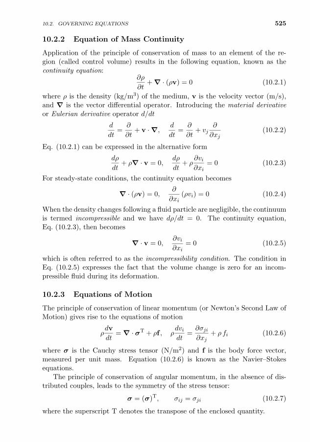
525
10.2.2 Equation of Mass Continuity
Application of the principle of conservation of mass to an element of the re-gion (called control volume) results in the following equation, known as thecontinuity equation:
∂ρ
∂t+ ∇ · (ρv) = 0 (10.2.1)
where ρ is the density (kg/m3) of the medium, v is the velocity vector (m/s),and ∇ is the vector differential operator. Introducing the material derivativeor Eulerian derivative operator d/dt
d
dt=
∂
∂t+ v ·∇,
d
dt=
∂
∂t+ vj
∂
∂xj(10.2.2)
Eq. (10.2.1) can be expressed in the alternative form
dρ
dt+ ρ∇ · v = 0,
dρ
dt+ ρ
∂vi∂xi
= 0 (10.2.3)
For steady-state conditions, the continuity equation becomes
∇ · (ρv) = 0,∂
∂xi(ρvi) = 0 (10.2.4)
When the density changes following a fluid particle are negligible, the continuumis termed incompressible and we have dρ/dt = 0. The continuity equation,Eq. (10.2.3), then becomes
∇ · v = 0,∂vi∂xi
= 0 (10.2.5)
which is often referred to as the incompressibility condition. The condition inEq. (10.2.5) expresses the fact that the volume change is zero for an incom-pressible fluid during its deformation.
10.2.3 Equations of Motion
The principle of conservation of linear momentum (or Newton’s Second Law ofMotion) gives rise to the equations of motion
ρdv
dt= ∇ · σT + ρf , ρ
dvidt
=∂σji∂xj
+ ρ fi (10.2.6)
where σ is the Cauchy stress tensor (N/m2) and f is the body force vector,measured per unit mass. Equation (10.2.6) is known as the Navier–Stokesequations.
The principle of conservation of angular momentum, in the absence of dis-tributed couples, leads to the symmetry of the stress tensor:
σ = (σ)T, σij = σji (10.2.7)
where the superscript T denotes the transpose of the enclosed quantity.
10.2. GOVERNING EQUATIONS
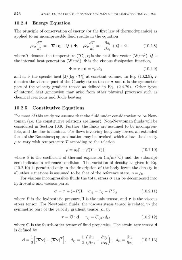
526 WEAK FORM FINITE ELEMENT MODELS OF INCOMPRESSIBLE FLUIDS
10.2.4 Energy Equation
The principle of conservation of energy (or the first law of thermodynamics) asapplied to an incompressible fluid results in the equation
ρcvdT
dt= −∇ · q +Q+ Φ, ρcv
dT
dt= − ∂qi
∂xi+Q+ Φ (10.2.8)
where T denotes the temperature (C), q is the heat flux vector (W/m2), Q isthe internal heat generation (W/m3), Φ is the viscous dissipation function,
Φ = τ : d = τij dij (10.2.9)
and cv is the specific heat [J/(kg ·C)] at constant volume. In Eq. (10.2.9), τdenotes the viscous part of the Cauchy stress tensor σ and d is the symmetricpart of the velocity gradient tensor as defined in Eq. (2.4.29). Other typesof internal heat generation may arise from other physical processes such aschemical reactions and Joule heating.
10.2.5 Constitutive Equations
For most of this study we assume that the fluid under consideration to be New-tonian (i.e. the constitutive relations are linear). Non-Newtonian fluids will beconsidered in Section 10.9. Further, the fluids are assumed to be incompress-ible, and the flow is laminar. For flows involving buoyancy forces, an extendedform of the Boussinesq approximation may be invoked, which allows the densityρ to vary with temperature T according to the relation
ρ = ρ0[1− β(T − T0)] (10.2.10)
where β is the coefficient of thermal expansion (m/m/C) and the subscriptzero indicates a reference condition. The variation of density as given in Eq.(10.2.10) is permitted only in the description of the body force; the density inall other situations is assumed to be that of the reference state, ρ = ρ0.
For viscous incompressible fluids the total stress σ can be decomposed intohydrostatic and viscous parts:
σ = τ + (−P )I, σij = τij − P δij (10.2.11)
where P is the hydrostatic pressure, I is the unit tensor, and τ is the viscousstress tensor. For Newtonian fluids, the viscous stress tensor is related to thesymmetric part of the velocity gradient tensor, d, by
τ = C : d, τij = Cijk` dk` (10.2.12)
where C is the fourth-order tensor of fluid properties. The strain rate tensor dis defined by
d =1
2
[(∇v) + (∇v)T
], dij =
1
2
(∂vi∂xj
+∂vj∂xi
); dii =
∂vi∂xi
(10.2.13)
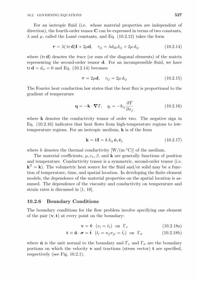
10.2. GOVERNING EQUATIONS 527
For an isotropic fluid (i.e. whose material properties are independent ofdirection), the fourth-order tensor C can be expressed in terms of two constants,λ and µ, called the Lame constants, and Eq. (10.2.12) takes the form
τ = λ( tr d)I + 2µd, τij = λdkkδij + 2µdij (10.2.14)
where (tr d) denotes the trace (or sum of the diagonal elements) of the matrixrepresenting the second-order tensor d. For an incompressible fluid, we havetr d = dii = 0 and Eq. (10.2.14) becomes
τ = 2µd, τij = 2µdij (10.2.15)
The Fourier heat conduction law states that the heat flux is proportional to thegradient of temperature
q = −k ·∇T, qi = −kij∂T
∂xj(10.2.16)
where k denotes the conductivity tensor of order two. The negative sign inEq. (10.2.16) indicates that heat flows from high-temperature regions to low-temperature regions. For an isotropic medium, k is of the form
k = kI = k δij ei ej (10.2.17)
where k denotes the thermal conductivity [W/(m·C)] of the medium.The material coefficients, µ, cv, β, and k are generally functions of position
and temperature. Conductivity tensor is a symmetric, second-order tensor (i.e.kT = k). The volumetric heat source for the fluid and/or solid may be a func-tion of temperature, time, and spatial location. In developing the finite elementmodels, the dependence of the material properties on the spatial location is as-sumed. The dependence of the viscosity and conductivity on temperature andstrain rates is discussed in [1, 10].
10.2.6 Boundary Conditions
The boundary conditions for the flow problem involve specifying one elementof the pair (v, t) at every point on the boundary:
v = v (vi = vi) on Γv (10.2.18a)
t ≡ n · σ = t (ti = njσji = ti) on Γσ (10.2.18b)
where n is the unit normal to the boundary and Γv and Γσ are the boundaryportions on which the velocity v and tractions (stress vector) t are specified,respectively (see Fig. 10.2.1).
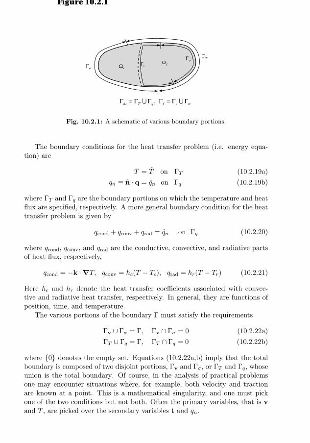
528 WEAK FORM FINITE ELEMENT MODELS OF INCOMPRESSIBLE FLUIDS
TΓ
qΓ sΩ fΩ
σΓ = Γ Γ Γ = Γ Γ ,ht T q f v
vΓΓσ
Figure 10.2.1
Fig. 10.2.1: A schematic of various boundary portions.
The boundary conditions for the heat transfer problem (i.e. energy equa-tion) are
T = T on ΓT (10.2.19a)
qn ≡ n · q = qn on Γq (10.2.19b)
where ΓT and Γq are the boundary portions on which the temperature and heatflux are specified, respectively. A more general boundary condition for the heattransfer problem is given by
qcond + qconv + qrad = qn on Γq (10.2.20)
where qcond, qconv, and qrad are the conductive, convective, and radiative partsof heat flux, respectively,
qcond = −k ·∇T, qconv = hc(T − Tc), qrad = hr(T − Tr) (10.2.21)
Here hc and hr denote the heat transfer coefficients associated with convec-tive and radiative heat transfer, respectively. In general, they are functions ofposition, time, and temperature.
The various portions of the boundary Γ must satisfy the requirements
Γv ∪ Γσ = Γ, Γv ∩ Γσ = 0 (10.2.22a)
ΓT ∪ Γq = Γ, ΓT ∩ Γq = 0 (10.2.22b)
where 0 denotes the empty set. Equations (10.2.22a,b) imply that the totalboundary is composed of two disjoint portions, Γv and Γσ, or ΓT and Γq, whoseunion is the total boundary. Of course, in the analysis of practical problemsone may encounter situations where, for example, both velocity and tractionare known at a point. This is a mathematical singularity, and one must pickone of the two conditions but not both. Often the primary variables, that is vand T , are picked over the secondary variables t and qn.
10.3. SUMMARY OF GOVERNING EQUATIONS 529
10.3 Summary of Governing Equations
10.3.1 Vector Form
Equations (10.2.3), (10.2.6), and (10.2.8) can be expressed in terms of the prim-itive variables (v, P, T ) through Eqs. (10.2.12)–(10.2.16). The results are sum-marized below for isotropic, Newtonian, viscous, incompressible fluids in thepresence of buoyancy forces:
∇ · v = 0 (10.3.1)
ρ
(∂v
∂t+ v ·∇v
)= −∇P + µ∇ ·
[(∇v) + (∇v)T
]+ ρf + ρg β(T − T0) (10.3.2)
ρcv
(∂T
∂t+ v ·∇T
)= ∇ · (k∇T ) + g + Φ (10.3.3)
where v is the velocity vector, ρ is the density, g is the gravity force vector perunit mass, T is the temperature, cv is the specific heat of the fluid at constantvolume, and g is the rate of internal heat generation per unit volume.
The above equations are valid for the fluid region Ωf . In the solid regionΩs, the fluid velocity is zero, v = 0, and the only relevant equation is (10.3.3).The energy equation, Eq. (10.3.3), for the solid region is given by
ρscs∂T
∂t= ∇ · (ks∇T ) + gs (10.3.4)
In writing Eq. (10.3.4) it is assumed that the solid is stationary with respectto the coordinate frame such that the convective transport of energy [i.e. thenonlinear part of Eq. (10.3.3)] need not be considered. The finite elementmodel of Eq. (10.3.4) was discussed in Chapter 6 when the conductivity ks isa function, in general, of x, y, and T .
10.3.2 Cartesian Component Form
The vector forms of Eqs. (10.3.1)–(10.3.3) allow us to express them in anycoordinate system by expressing the vector operator ∇ and all other vectorsin that coordinate system. In the Cartesian coordinate system (x1, x2, x3), thekinematic and constitutive relations take the form
dij =1
2
(∂vi∂xj
+∂vj∂xi
)(10.3.5)
σij = −Pδij + τij ; τij = 2µdij (10.3.6)
The conservation equations can be expressed as
∂vi∂xi
= 0 (10.3.7)
530 WEAK FORM FINITE ELEMENT MODELS OF INCOMPRESSIBLE FLUIDS
ρ
(∂vi∂t
+ vj∂vi∂xj
)=
∂
∂xj
[−Pδij + µ
(∂vi∂xj
+∂vj∂xi
)]+ ρfi − ρgiβ(T − T0) (10.3.8)
ρcv
(∂T
∂t+ vj
∂T
∂xj
)=
∂
∂xi
(k∂T
∂xi
)+ g + 2µdijdij (10.3.9)
for the fluid region Ωf and
ρscs∂T
∂t=
∂
∂xi
(ks∂T
∂xi
)+ gs (10.3.10)
for the solid region Ωs. Equations (10.3.5)–(10.3.10) are written for a Cartesiangeometry in an Eulerian reference frame, with the indices i, j = 1, 2, 3 (ori, j = 1, 2 for two-dimensional problems); the Einstein summation conventionon repeated indices is used.
In the present study, we shall consider two different finite element modelsof Eqs. (10.3.7) and (10.3.8). The first one is a natural formulation in whichthe weak forms of Eqs. (10.3.7) and (10.3.8) are used to construct the finite ele-ment model. The resulting finite element model is termed the velocity–pressuremodel or mixed model. The phrase “mixed” is used because velocity variablesare mixed with the force-like variable, pressure, and both types of variables areretained in a single formulation. The second model is based on the interpreta-tion that the continuity equation, Eq. (10.3.7), is an additional relation amongthe velocity components (i.e. a constraint among the vi), and the constraintis satisfied in a least-squares (i.e. approximate) sense. This particular methodof including the constraint in the formulation is known as the penalty functionmethod, and the model is termed the penalty–finite element model. In this case,the pressure variable is effectively eliminated from the formulation. It is infor-mative to note that the velocity–pressure (or mixed) formulation is the sameas the Lagrange multiplier formulation, wherein the constraint is included bymeans of the Lagrange multiplier method. The Lagrange multiplier turns outto be the negative of the pressure.
There exist in computational fluid dynamics literature hundreds of papers onfinite element models of incompressible flows and their applications. Interestedreaders may consult the books by Reddy and Gartling [10] and Gresho andSani [181] for many of these references. Some of these works will be cited atappropriate places of this book.
10.4 Velocity–Pressure Finite Element Model
10.4.1 Weak Forms
The starting point for the development of the finite element models of Eqs.(10.3.7) and (10.3.8) is their weak forms. Here we consider the two-dimensional
10.4. VELOCITY–PRESSURE FINITE ELEMENT MODEL 531
case, and the three-dimensional case follows in a straightforward manner. First,we write Eqs. (10.3.7) and (10.3.8) for the two-dimensional case using thenotation v1 = vx, v2 = vy, x1 = x, and x2 = y. Keeping in mind that thesequence of variables is (vx, vy, P ), we write the momentum equations followedby the continuity equation. We have
0 = ρ
(∂vx∂t
+ vx∂vx∂x
+ vy∂vx∂y
)− ∂
∂x
(2µ∂vx∂x− P
)− ∂
∂y
[µ
(∂vx∂y
+∂vy∂x
)]− ρfx (10.4.1)
0 = ρ
(∂vy∂t
+ vx∂vy∂x
+ vy∂vy∂y
)− ∂
∂y
(2µ∂vy∂y− P
)− ∂
∂x
[µ
(∂vx∂y
+∂vy∂x
)]− ρfy (10.4.2)
0 =∂vx∂x
+∂vy∂y
(10.4.3)
where (fx, fy) are the components of the body force vector f.The weighted-integral statements of these equations over a typical element
Ωe are given by
0 =
∫Ωewx
ρ
(∂vx∂t
+ vx∂vx∂x
+ vy∂vx∂y
)− ∂
∂x
(2µ∂vx∂x− P
)− ∂
∂y
[µ
(∂vx∂y
+∂vy∂x
)]− ρfx
dx dy (10.4.4)
0 =
∫Ωewy
ρ
(∂vy∂t
+ vx∂vy∂x
+ vy∂vy∂y
)− ∂
∂y
(2µ∂vy∂y− P
)− ∂
∂x
[µ
(∂vx∂y
+∂vy∂x
)]− ρfy
dx dy (10.4.5)
0 =
∫ΩeQ
(∂vx∂x
+∂vy∂y
)dx dy (10.4.6)
where (wx, wy, Q) are weight functions, which will be equated, in the Ritz orweak-form Galerkin finite element models, to the interpolation functions usedfor (vx, vy, P ), respectively.
Equation (10.4.6) will remain unaffected, as integration-by-parts does nothelp reduce differentiability on (vx, vy). In addition, the boundary terms ob-tained will be in conflict with the physical boundary conditions. The samecomment applies to the time-derivative and nonlinear terms in Eqs. (10.4.4)and (10.4.5). Note that trading of differentiability between the weight functionsand problem variables is subjected to the restriction that the resulting bound-ary expressions are physically meaningful. Otherwise, the secondary variables
532 WEAK FORM FINITE ELEMENT MODELS OF INCOMPRESSIBLE FLUIDS
of the formulation may not be the quantities the physical problem admits asboundary quantities. An examination of the boundary stress components tα inEq. (10.2.18b) shows that the pressure term appears as a part of the expression[also see Eq. (10.3.6)]. Therefore, the pressure term must also be integrated-by-parts to keep the boundary stresses intact. The integration-by-parts alsoallows the pressure variable to have lower-order approximation.
The final expressions for the weak forms are given by
0 =
∫Ωe
[wx ρ
(∂vx∂t
+ vx∂vx∂x
+ vy∂vx∂y
)+ 2µ
∂wx∂x
∂vx∂x− ∂wx
∂xP
+ µ∂wx∂y
(∂vx∂y
+∂vy∂x
)− ρwxfx
]dx dy −
∮Γewxtx ds (10.4.7)
0 =
∫Ωe
[wy ρ
(∂vy∂t
+ vx∂vy∂x
+ vy∂vy∂y
)+ 2µ
∂wy∂y
∂vy∂y− ∂wy
∂yP
+ µ∂wy∂x
(∂vx∂y
+∂vy∂x
)− ρwyfy
]dx dy −
∮Γewyty ds (10.4.8)
0 =
∫ΩeQ
(∂vx∂x
+∂vy∂y
)dx dy (10.4.9)
where (tx, ty) are the boundary stress (or traction) components
tx =(
2µ∂vx∂x− P
)nx + µ
(∂vx∂y
+∂vy∂x
)ny
ty = µ(∂vx∂y
+∂vy∂x
)nx +
(2µ∂vy∂y− P
)ny
(10.4.10)
and (nx, ny) are the direction cosines of the unit normal vector n on the bound-ary Γe.
10.4.2 Semidiscrete Finite Element Model
Since we are developing the weak-form Galerkin finite element models, thechoice of the weight functions is restricted to the spaces of approximation func-tions used for the pressure and velocity fields. Suppose that the dependentvariables (vx, vy, P ) are approximated by expansions of the form
vx(x, y, t) ≈ vhx =m∑j=1
vjx(t)ψj(x, y)
vy(x, y, t) ≈ vhy =m∑j=1
vjy(t)ψj(x, y) (10.4.11)
P (x, y, t) ≈ Ph =
n∑j=1
Pj(t)φj(x, y)
10.4. VELOCITY–PRESSURE FINITE ELEMENT MODEL 533
where ψj and φj are interpolation (or shape) functions, and (vjx, vjy, Pj) are
nodal values of (vx, vy, P ), respectively. The weight functions (wx, wy, Q) havethe following correspondence:
wx ∼ vx, wy ∼ vy, Q ∼ P (10.4.12)
Substitution of Eq. (10.4.11) into Eqs. (10.4.7)–(10.4.9) results in the followingfinite element equations:M 0 0
0 M 00 0 0
vxvyP
+
C(v) 0 00 C(v) 00 0 0
vxvyP
+
2S11 + S22 (S12)T −S10
S12 S11 + 2S22 −S20
−(S10)T −(S20)T 0
vxvyP
=
F1
F2
0
(10.4.13)
The coefficient matrices shown in Eq. (10.4.13) are defined by
Mij =
∫Ωeρψiψj dx dy, S10
ij =
∫Ωe
∂ψi∂x
φj dx dy
S20ij =
∫Ωe
∂ψi∂y
φj dx dy, S12ij =
∫Ωeµ∂ψi∂x
∂ψj∂y
dx dy
S11ij =
∫Ωeµ∂ψi∂x
∂ψj∂x
dx dy, S22ij =
∫Ωeµ∂ψi∂y
∂ψj∂y
dx dy
Cij =
∫Ωeρψi
(vx∂ψj∂x
+ vy∂ψj∂y
)dx dy
F 1i =
∫Ωeρψifx dx dy +
∮Γeψitx ds
F 2i =
∫Ωeρψify dx dy +
∮Γeψity ds
(10.4.14)
The two sets of interpolation functions used in Eq. (10.4.11) should be of theLagrange type, that is, derived by interpolating only the values of the functionsand not their derivatives. There are two different finite elements associated withthe two sets of field variables, (vx, vy) and P , and hence there are two differentfinite element meshes corresponding to the two variables over the same domain,Ω. If one of the meshes contains the other mesh as a subset, then we chooseto display the first mesh and indicate the nodal degrees of freedom associatedwith the nodes of a typical element of the mesh.
The interpolation used for the pressure variable should be different fromthat used for the velocities, because the weak forms in Eqs. (10.4.7)–(10.4.9)contain only the first derivatives of the velocities vx and vy and no derivativesof the pressure P . Also, note that the governing equations, Eqs. (10.4.1) and
534 WEAK FORM FINITE ELEMENT MODELS OF INCOMPRESSIBLE FLUIDS
(10.4.2), contain second-order derivatives of vx and vy and first-order derivativesof P . Thus, for consistency, vx and vy must be interpolated using functions thatare one order higher than those used for P , unless very high-order functionsare used for all variables (in which case the consistency will be satisfied byadjusting degrees of polynomial used for velocities and pressure). In addition,the essential boundary conditions of the formulation do not include specificationof the pressure; it enters the boundary conditions as a part of the naturalboundary conditions (i.e. in specifying tx and ty). This implies that the pressurevariable need not be carried as a variable that is continuous across inter-elementboundaries. These observations lead to the conclusion that the pressure variableshould be interpolated with functions that are one order less than those usedfor the velocity field and that the approximation may be discontinuous (i.e. notcontinuous from one element to other). Thus, quadratic interpolation of vi anddiscontinuous linear interpolation of P are admissible. Models that use equalinterpolation of the velocities and pressure with this formulation are known togive inaccurate results (see [182–189]).
10.4.3 Fully Discretized Finite Element Model
The semidiscrete finite element model developed in the previous section can beconverted to the fully discretized model using the time approximations discussedin Chapter 6. Equation (10.4.13) can be written in a compact form as
M∆ + (C + K)∆ = F (10.4.15)
where ∆ = (v, P ). In view of Eqs. (6.7.17) and (6.7.18), we obtain
K(vs+1)∆s+1 = K(vs)∆s + Fs,s+1 (10.4.16)
where
K(vs+1) = M + a1 [C(vs+1) + K(vs+1)]
K(vs) = M− a2 [C(vs) + K(vs)] (10.4.17)
Fs,s+1 = a1Fs+1 + a2Fs, a1 = α∆t, a2 = (1− α)∆t
where α is the parameter that defines the time approximation scheme as definedin Eq. (6.7.16), and ∆t is the time step. Dependence of C on the nodal valuesv is due to the convective terms, and dependence of K on v is due to viscositybeing a function of the strain rates (e.g. power-law fluids). If the viscosity isconstant, that is Newtonian fluids, then K is independent of the nodal values vof the velocity field. For direct iteration solution, Eq. (10.4.16) takes the form
K(vrs+1)∆r+1s+1 = K(vs)∆s + Fs,s+1 (10.4.18)
10.5. PENALTY FINITE ELEMENT MODELS 535
10.5 Penalty Finite Element Models
10.5.1 Introduction
The penalty function method, like the Lagrange multiplier method, allows us toreformulate a problem with constraints as one without constraints (see [2, 10,181–187]). In order to use the penalty function method for the flow of a viscousincompressible fluid, first it is reformulated as a variational problem subjectedto a constraint. For the purpose of describing the penalty function method, weconsider the steady-state Stokes flow problem (i.e. without time-dependent andnonlinear terms) in two dimensions. Then the penalty method is applied to thevariational problem with a constraint. The development will then be extendedto unsteady Navier–Stokes equations.
Consider the weak forms in Eqs. (10.4.7)–(10.4.9), and omit the time deriva-tive and nonlinear terms. These can be expressed in the form
B((w, Q), (v, P )) = `(w, Q) (10.5.1)
where (w, Q) are the weight functions used for the momentum and continuityequations, respectively, B(·, ·) is a bilinear form [i.e. an expression that is linearin (w, Q) as well as (v, P )] and `(·) is a linear form, defined by
B((w, Q), (v, P ))
=
∫Ωeµ
[2
(∂wx∂x
∂vx∂x
+∂wy∂y
∂vy∂y
)+
(∂wx∂y
+∂wy∂x
)(∂vx∂y
+∂vy∂x
)]dx dy
−∫
Ωe
[(∂wx∂x
+∂wy∂y
)P +
(∂vx∂x
+∂vy∂y
)Q
]dx dy (10.5.2a)
`(w, Q) =
∫Ωeρ (wxfx + wyfy) dx dy +
∮Γe
(wxtx + wyty) ds (10.5.2b)
and (tx, ty) are the boundary stress components defined in Eq. (10.4.10). Thestatement in Eq. (10.5.1) is known as the variational problem associated withsteady-state Stokes problem.
The finite element model based on the variational problem, Eq. (10.5.1), isa special case of the mixed finite element model in Eq. (10.4.13). Equation(10.4.13) is more general than the problem at hand in that Eq. (10.4.13) isvalid for time-dependent Navier–Stokes equations. To make it simple to un-derstand the penalty function method, only the steady-state Stokes problem isconsidered. The inertial (i.e. time-dependent) and convective (i.e. nonlinear)terms may be added to the equations of the penalty formulation as they arenot connected to the divergence-free (i.e. incompressibility) condition, which iscentral to the penalty formulation.
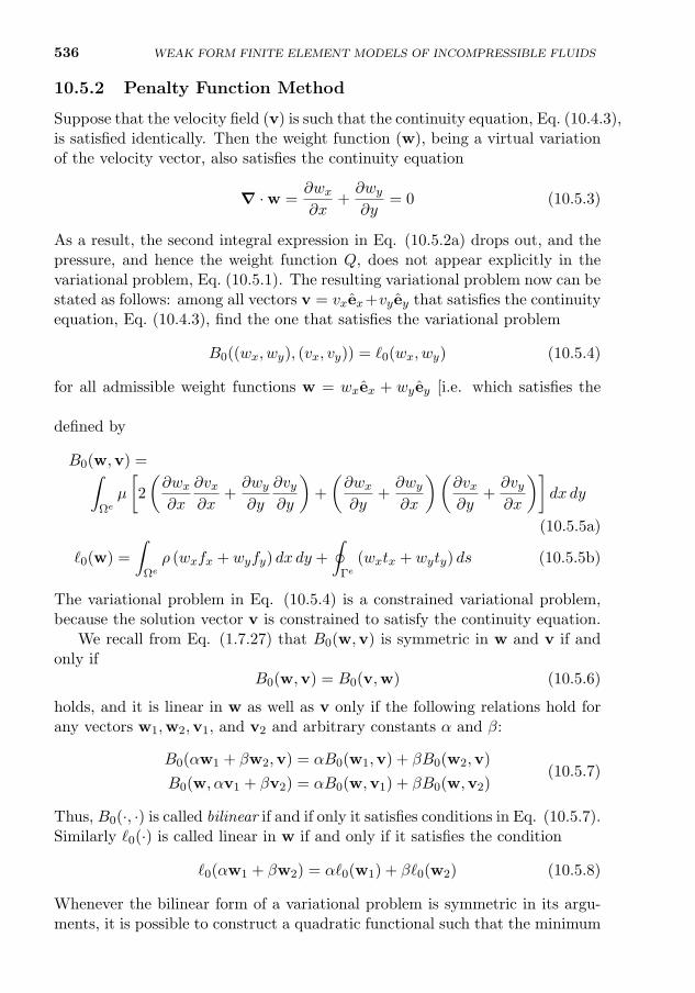
536 WEAK FORM FINITE ELEMENT MODELS OF INCOMPRESSIBLE FLUIDS
10.5.2 Penalty Function Method
Suppose that the velocity field (v) is such that the continuity equation, Eq. (10.4.3),is satisfied identically. Then the weight function (w), being a virtual variationof the velocity vector, also satisfies the continuity equation
∇ ·w =∂wx∂x
+∂wy∂y
= 0 (10.5.3)
As a result, the second integral expression in Eq. (10.5.2a) drops out, and thepressure, and hence the weight function Q, does not appear explicitly in thevariational problem, Eq. (10.5.1). The resulting variational problem now can bestated as follows: among all vectors v = vxex+vyey that satisfies the continuityequation, Eq. (10.4.3), find the one that satisfies the variational problem
B0((wx, wy), (vx, vy)) = `0(wx, wy) (10.5.4)
for all admissible weight functions w = wxex + wyey [i.e. which satisfies thecondition in Eq. (10.5.3)]. The bilinear form and linear form in Eq. (10.5.4) aredefined by
B0(w,v) =∫Ωeµ
[2
(∂wx∂x
∂vx∂x
+∂wy∂y
∂vy∂y
)+
(∂wx∂y
+∂wy∂x
)(∂vx∂y
+∂vy∂x
)]dx dy
(10.5.5a)
`0(w) =
∫Ωeρ (wxfx + wyfy) dx dy +
∮Γe
(wxtx + wyty) ds (10.5.5b)
The variational problem in Eq. (10.5.4) is a constrained variational problem,because the solution vector v is constrained to satisfy the continuity equation.
We recall from Eq. (1.7.27) that B0(w,v) is symmetric in w and v if andonly if
B0(w,v) = B0(v,w) (10.5.6)
holds, and it is linear in w as well as v only if the following relations hold forany vectors w1,w2,v1, and v2 and arbitrary constants α and β:
B0(αw1 + βw2,v) = αB0(w1,v) + βB0(w2,v)
B0(w, αv1 + βv2) = αB0(w,v1) + βB0(w,v2)(10.5.7)
Thus, B0(·, ·) is called bilinear if and if only it satisfies conditions in Eq. (10.5.7).Similarly `0(·) is called linear in w if and only if it satisfies the condition
`0(αw1 + βw2) = α`0(w1) + β`0(w2) (10.5.8)
Whenever the bilinear form of a variational problem is symmetric in its argu-ments, it is possible to construct a quadratic functional such that the minimum
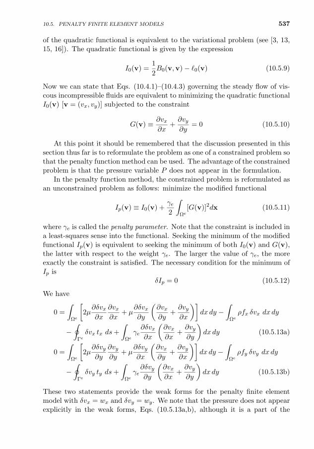
10.5. PENALTY FINITE ELEMENT MODELS 537
of the quadratic functional is equivalent to the variational problem (see [3, 13,15, 16]). The quadratic functional is given by the expression
I0(v) =1
2B0(v,v)− `0(v) (10.5.9)
Now we can state that Eqs. (10.4.1)–(10.4.3) governing the steady flow of vis-cous incompressible fluids are equivalent to minimizing the quadratic functionalI0(v) [v = (vx, vy)] subjected to the constraint
G(v) ≡ ∂vx∂x
+∂vy∂y
= 0 (10.5.10)
At this point it should be remembered that the discussion presented in thissection thus far is to reformulate the problem as one of a constrained problem sothat the penalty function method can be used. The advantage of the constrainedproblem is that the pressure variable P does not appear in the formulation.
In the penalty function method, the constrained problem is reformulated asan unconstrained problem as follows: minimize the modified functional
Ip(v) ≡ I0(v) +γe2
∫Ωe
[G(v)]2dx (10.5.11)
where γe is called the penalty parameter. Note that the constraint is included ina least-squares sense into the functional. Seeking the minimum of the modifiedfunctional Ip(v) is equivalent to seeking the minimum of both I0(v) and G(v),the latter with respect to the weight γe. The larger the value of γe, the moreexactly the constraint is satisfied. The necessary condition for the minimum ofIp is
δIp = 0 (10.5.12)
We have
0 =
∫Ωe
[2µ∂δvx∂x
∂vx∂x
+ µ∂δvx∂y
(∂vx∂y
+∂vy∂x
)]dx dy −
∫Ωeρfx δvx dx dy
−∮
Γeδvx tx ds+
∫Ωeγe∂δvx∂x
(∂vx∂x
+∂vy∂y
)dx dy (10.5.13a)
0 =
∫Ωe
[2µ∂δvy∂y
∂vy∂y
+ µ∂δvy∂x
(∂vx∂y
+∂vy∂x
)]dx dy −
∫Ωeρfy δvy dx dy
−∮
Γeδvy ty ds+
∫Ωeγe∂δvy∂y
(∂vx∂x
+∂vy∂y
)dx dy (10.5.13b)
These two statements provide the weak forms for the penalty finite elementmodel with δvx = wx and δvy = wy. We note that the pressure does not appearexplicitly in the weak forms, Eqs. (10.5.13a,b), although it is a part of the
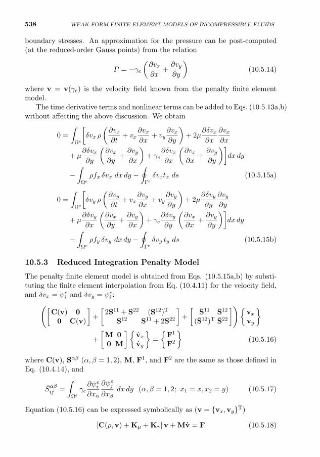
538 WEAK FORM FINITE ELEMENT MODELS OF INCOMPRESSIBLE FLUIDS
boundary stresses. An approximation for the pressure can be post-computed(at the reduced-order Gauss points) from the relation
P = −γe(∂vx∂x
+∂vy∂y
)(10.5.14)
where v = v(γe) is the velocity field known from the penalty finite elementmodel.
The time derivative terms and nonlinear terms can be added to Eqs. (10.5.13a,b)without affecting the above discussion. We obtain
0 =
∫Ωe
[δvx ρ
(∂vx∂t
+ vx∂vx∂x
+ vy∂vx∂y
)+ 2µ
∂δvx∂x
∂vx∂x
+ µ∂δvx∂y
(∂vx∂y
+∂vy∂x
)+ γe
∂δvx∂x
(∂vx∂x
+∂vy∂y
)]dx dy
−∫
Ωeρfx δvx dx dy −
∮Γeδvxtx ds (10.5.15a)
0 =
∫Ωe
[δvy ρ
(∂vy∂t
+ vx∂vy∂x
+ vy∂vy∂y
)+ 2µ
∂δvy∂y
∂vy∂y
+ µ∂δvy∂x
(∂vx∂y
+∂vy∂x
)+ γe
∂δvy∂y
(∂vx∂x
+∂vy∂y
)]dx dy
−∫
Ωeρfy δvy dx dy −
∮Γeδvy ty ds (10.5.15b)
10.5.3 Reduced Integration Penalty Model
The penalty finite element model is obtained from Eqs. (10.5.15a,b) by substi-tuting the finite element interpolation from Eq. (10.4.11) for the velocity field,and δvx = ψei and δvy = ψei :([
C(v) 00 C(v)
]+
[2S11 + S22 (S12)T
S12 S11 + 2S22
]+
[S11 S12
(S12)T S22
])vxvy
+
[M 00 M
]vxvy
=
F1
F2
(10.5.16)
where C(v), Sαβ (α, β = 1, 2), M, F1, and F2 are the same as those defined inEq. (10.4.14), and
Sαβij =
∫Ωeγe∂ψei∂xα
∂ψej∂xβ
dx dy (α, β = 1, 2; x1 = x, x2 = y) (10.5.17)
Equation (10.5.16) can be expressed symbolically as (v = vx,vyT)
[C(ρ,v) + Kµ + Kγ ] v + Mv = F (10.5.18)
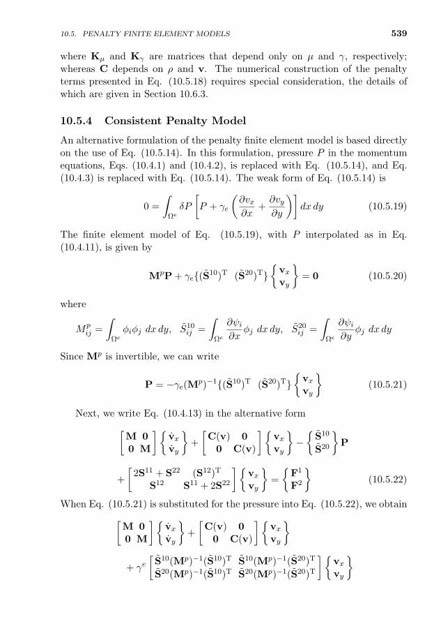
10.5. PENALTY FINITE ELEMENT MODELS 539
where Kµ and Kγ are matrices that depend only on µ and γ, respectively;whereas C depends on ρ and v. The numerical construction of the penaltyterms presented in Eq. (10.5.18) requires special consideration, the details ofwhich are given in Section 10.6.3.
10.5.4 Consistent Penalty Model
An alternative formulation of the penalty finite element model is based directlyon the use of Eq. (10.5.14). In this formulation, pressure P in the momentumequations, Eqs. (10.4.1) and (10.4.2), is replaced with Eq. (10.5.14), and Eq.(10.4.3) is replaced with Eq. (10.5.14). The weak form of Eq. (10.5.14) is
0 =
∫ΩeδP
[P + γe
(∂vx∂x
+∂vy∂y
)]dx dy (10.5.19)
The finite element model of Eq. (10.5.19), with P interpolated as in Eq.(10.4.11), is given by
MpP + γe(S10)T (S20)T
vxvy
= 0 (10.5.20)
where
Mpij =
∫Ωeφiφj dx dy, S10
ij =
∫Ωe
∂ψi∂x
φj dx dy, S20ij =
∫Ωe
∂ψi∂y
φj dx dy
Since Mp is invertible, we can write
P = −γe(Mp)−1(S10)T (S20)T
vxvy
(10.5.21)
Next, we write Eq. (10.4.13) in the alternative form[M 00 M
]vxvy
+
[C(v) 0
0 C(v)
]vxvy
−
S10
S20
P
+
[2S11 + S22 (S12)T
S12 S11 + 2S22
]vxvy
=
F1
F2
(10.5.22)
When Eq. (10.5.21) is substituted for the pressure into Eq. (10.5.22), we obtain[M 00 M
]vxvy
+
[C(v) 0
0 C(v)
]vxvy
+ γe[
S10(Mp)−1(S10)T S10(Mp)−1(S20)T
S20(Mp)−1(S10)T S20(Mp)−1(S20)T
]vxvy
540 WEAK FORM FINITE ELEMENT MODELS OF INCOMPRESSIBLE FLUIDS
+
[2S11 + S22 (S12)T
S12 S11 + 2S22
]vxvy
=
F1
F2
(10.5.23)
which can be written in compact form as
Mv + [C(v) + Kµ + Kpγ ]v = F (10.5.24)
where [see Eq. (10.4.14) for the definition of Mij and Smnij ]
M =
[M 00 M
], C =
[C(v) 0
0 C(v)
], v =
vxvy
Kpγ = γe[
S10(Mp)−1(S10)T S10(Mp)−1(S20)T
S20(Mp)−1(S10)T S20(Mp)−1(S20)T
](10.5.25)
Kµ =
[2S11 + S22 (S12)T
S12 S11 + 2S22
]The penalty finite element model described here is termed a consistent
penalty model because it is derived from the discretized form of Eq. (10.5.14).This is in contrast to the reduced penalty model described earlier, which fallsinto the category known as the reduced integration penalty (RIP) model (seeOden [188]). Equation (10.5.24) has the same general form as Eq. (10.5.18).However, while Kµ defined in Eqs. (10.5.25) and (10.5.16) are the same, Kpγ
defined in Eq. (10.5.25) and Kγ defined in Eq. (10.5.16) are not the same. Theoverall size of the penalty finite element model in Eqs. (10.5.18) and (10.5.24)is reduced in comparison to the mixed finite element model in Eq. (10.4.13)because of the elimination of the pressure variable. To recover the pressure inthe consistent penalty finite element model, the inverted form of Eq. (10.5.21)is used with the velocity field known from Eq. (10.5.24). The numerical imple-mentation of the consistent penalty method relies on the ability to invert Mp
at the element level. This restricts the choice of the basis functions used torepresent the pressure.
10.6 Computational Aspects
10.6.1 Properties of the Finite Element Equations
Some of the properties of the matrix equations in Eqs. (10.4.13), (10.5.18), and(10.5.24) are listed below because they greatly influence the choice of a solutionprocedure for the various types of problems [10].
1. The matrix equations in Eqs. (10.4.13), (10.5.18), and (10.5.24) representdiscrete analogs of the basic conservation equations with each term repre-senting a particular physical process. For example, M represents the massmatrix, C represents the velocity dependent convective transport term,
10.6. COMPUTATIONAL ASPECTS 541
Kµ represents the viscous terms, and Kγ represents the divergence-freecondition. The right-hand side F contains body forces and surface forces.
2. An inspection of the structure of the individual matrices in Eq. (10.4.14)shows that M and Kµ are symmetric, while C is unsymmetric. Thismakes the coefficient matrices of the vector v in Eqs. (10.4.13), (10.5.18),and (10.5.24) unsymmetric, and the solution procedure must deal withan unsymmetric system. When material properties are constant and flowvelocities are sufficiently small, the convective terms are negligible andthe equations are linear and symmetric.
3. An additional difficulty of the mixed finite element model is the presenceof zeroes on the matrix diagonals corresponding to the pressure variables[see Eq. (10.4.13)]. Direct equation solving methods must use some typeof pivoting strategy, while the use of iterative solvers is severely handi-capped by poor convergence behavior attributable mainly to the form ofthe constraint equation.
4. Equations (10.4.13), (10.5.18), and (10.5.24) represent a set of ordinarydifferential equations in time. The fact that the pressure does not appearexplicitly in the continuity equation [see Eq. (10.4.13)] makes the systemtime-singular in the pressure and precludes the use of purely explicit time-integration methods.
5. The choice of the penalty parameter is largely dictated by the ratio ofthe magnitude of penalty terms to the viscous and convective terms (orcompared to the Reynolds number, Re), the mesh, and the precision ofthe computer. The following range of γ is used in computations
γ = 104Re to γ = 1012Re (10.6.1)
10.6.2 Choice of Elements
As is clear from the weak statements, the finite element models of conduc-tive heat transfer as well as viscous incompressible flows require only the C0-continuous functions to approximate the field variables (i.e. temperature, ve-locities, and pressure). Thus, any of the Lagrange and serendipity family ofinterpolation functions are admissible for the interpolation of the velocity fieldin mixed and penalty finite element models.
The choice of interpolation functions used for the pressure variable in themixed finite element model is further constrained by the special role the pres-sure plays in incompressible flows. Recall that the pressure can be interpretedas a Lagrange multiplier that serves to enforce the incompressibility constrainton the velocity field. From Eq. (10.4.11) it is seen that the approximation func-tions φi used for pressure is the weighting function for the continuity equation.
542
In order to prevent an over-constrained system of discrete equations, the inter-polation used for pressure must be at least one order lower than that used forthe velocity field (i.e. unequal order interpolation). Further, pressure need notbe made continuous across elements because the pressure variable does not con-stitute a primary variable of the weak form presented in Eqs. (10.4.7)–(10.4.9).Note that the unequal order interpolation criteria can be relaxed for certain“stabilized” formulations [189], which will not be discussed here.
Convergent finite element approximations of problems with constraints aregoverned by the ellipticity requirement and the Ladyzhenskaya–Babuska–Brezzi(LBB) condition (see Reddy [15, pp. 454–461], Oden [188], and others [190–194]). It is by no means a simple task to rigorously prove whether every newelement developed for the viscous incompressible flows satisfies the LBB condi-tion. The discussion of the LBB condition is beyond the scope of the presentstudy and will not be discussed here.
Commonly used elements for two-dimensional flows of viscous incompress-ible fluids are shown in Fig. 10.6.1. In the case of linear elements, pressure istreated as discontinuous between elements; otherwise, the whole domain willhave the same pressure. Two different pressure approximations have been usedwhen the velocities are approximated by quadratic Lagrange functions. Thefirst is a continuous linear approximation, in which the pressure is defined atthe corner nodes of the element and is made continuous across element bound-aries. The second pressure approximation involves a discontinuous (betweenelements) linear variation defined on the element by
Φ =
1xy
(10.6.2)
Here the unknowns are not nodal point values of the pressure but correspondto the coefficients in P = a · 1 + b · x + c · y. In Eq. (10.6.2) the interpolationfunctions are written in terms of the global coordinates (x, y) for the problem.
When the eight-node quadratic element is used to represent the velocityfield, a continuous-linear pressure approximation may be selected. When adiscontinuous pressure variation is used with this element, the constant pressurerepresentation over each element must be used. The quadratic quadrilateralelements shown in Fig. 10.6.1 are known to satisfy the LBB condition and thusgive reliable solutions for velocity and pressure fields. Other elements may yieldacceptable solutions for the velocity field but the pressure field is often in error(e.g. pressure values may appear as in the so-called checker-board pattern).In such cases, pressure may be determined from the Poisson equation for thepressure (see Reddy and Gartling [10]).
WEAK FORM FINITE ELEMENT MODELS OF INCOMPRESSIBLE FLUIDS
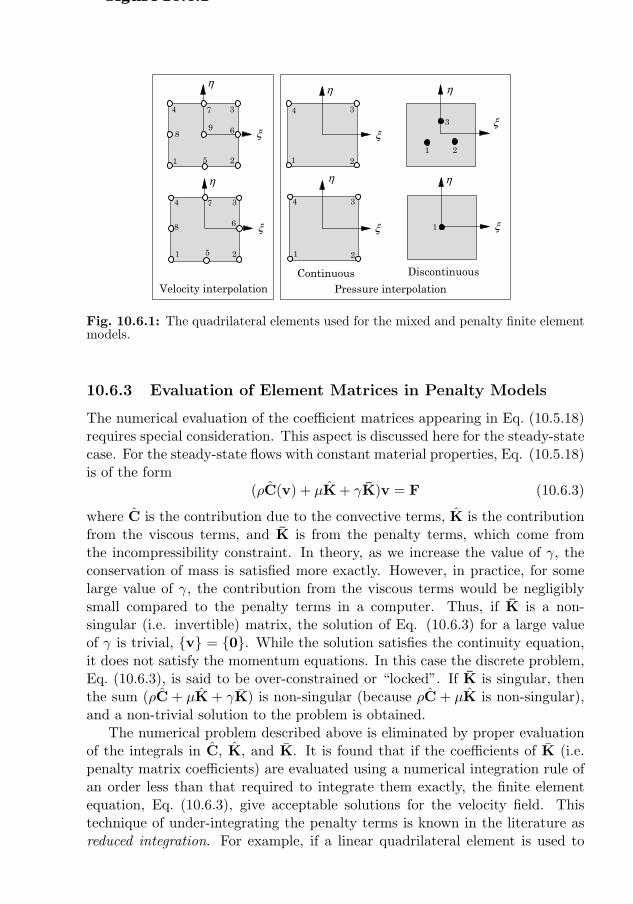
10.6. COMPUTATIONAL ASPECTS 543
ξ
η
ξ
η
ξ
η
Velocity interpolation Pressure interpolationContinuous Discontinuous
ξ
η
ξ
η
ξ
η
1 2
4 3
5
6
7
89
1 2
34
5
6
7
8
1 2
34
1 2
34
1
1 2
3
Figure 10.6.1
Fig. 10.6.1: The quadrilateral elements used for the mixed and penalty finite elementmodels.
10.6.3 Evaluation of Element Matrices in Penalty Models
The numerical evaluation of the coefficient matrices appearing in Eq. (10.5.18)requires special consideration. This aspect is discussed here for the steady-statecase. For the steady-state flows with constant material properties, Eq. (10.5.18)is of the form
(ρC(v) + µK + γK)v = F (10.6.3)
where C is the contribution due to the convective terms, K is the contributionfrom the viscous terms, and K is from the penalty terms, which come fromthe incompressibility constraint. In theory, as we increase the value of γ, theconservation of mass is satisfied more exactly. However, in practice, for somelarge value of γ, the contribution from the viscous terms would be negligiblysmall compared to the penalty terms in a computer. Thus, if K is a non-singular (i.e. invertible) matrix, the solution of Eq. (10.6.3) for a large valueof γ is trivial, v = 0. While the solution satisfies the continuity equation,it does not satisfy the momentum equations. In this case the discrete problem,Eq. (10.6.3), is said to be over-constrained or “locked”. If K is singular, thenthe sum (ρC + µK + γK) is non-singular (because ρC + µK is non-singular),and a non-trivial solution to the problem is obtained.
The numerical problem described above is eliminated by proper evaluationof the integrals in C, K, and K. It is found that if the coefficients of K (i.e.penalty matrix coefficients) are evaluated using a numerical integration rule ofan order less than that required to integrate them exactly, the finite elementequation, Eq. (10.6.3), give acceptable solutions for the velocity field. Thistechnique of under-integrating the penalty terms is known in the literature asreduced integration. For example, if a linear quadrilateral element is used to
544 WEAK FORM FINITE ELEMENT MODELS OF INCOMPRESSIBLE FLUIDS
approximate the velocity field, the matrix coefficients C and K (as well asM for unsteady problems) are evaluated using the 2 × 2 Gauss quadrature,and K is evaluated using the one-point (1 × 1) Gauss quadrature. The one-point quadrature yields a singular K. Therefore, Eq. (10.6.3) can be solvedbecause (ρC + µK + γK) is non-singular and can be inverted (after assemblyand imposition of boundary conditions) to obtain a good finite element solutionof the original problem. When a quadratic quadrilateral element is used, the3× 3 Gauss quadrature is used to evaluate C, K, and M, and the 2× 2 Gaussquadrature is used to evaluate K. Of course, as the degree of interpolationgoes up, or very refined meshes are used, the resulting equations become lesssensitive to locking.
Concerning the post-computation of pressure in the penalty model, the pres-sure should be computed by evaluating Eq. (10.5.14) at integration points cor-responding to the reduced Gauss rule. This is equivalent to using an interpola-tion for pressure that is one order less than the one used for the velocity field.The pressure computed using Eq. (10.5.14) at the reduced integration points isnot always reliable and accurate. The pressures predicted using the linear ele-ments, especially for coarse meshes, are seldom acceptable. Quadratic elementsare known to yield more reliable results. In general, triangular elements do notyield stable solutions for pressures. Various techniques have been proposed inthe literature to obtain accurate pressure fields (see [185, 195–197]).
10.6.4 Post-Computation of Pressure and Stresses
The analysis of a flow problem generally includes calculation of not only thevelocity field and pressure but also the computation of the stress field. For aplane two-dimensional flow, the stress components (σxx, σyy, σxy) are given by
σxx = 2µ∂vx∂x− P, σyy = 2µ
∂vy∂y− P, σxy = µ
(∂vx∂y
+∂vy∂x
)(10.6.4)
where µ is the viscosity of the fluid.First, pressure P is calculated in mixed finite element model from
P (x, y) =n∑j=1
φj(x, y)Pj (10.6.5)
and in reduced-integration penalty finite element model from
Pγ(x, y) = −γm∑j=1
(∂ψj∂x
vjx +∂ψj∂y
vjy
)(10.6.6)
In the latter, the expression is evaluated using reduced integration rule. Substi-tution of the finite element approximations, Eq. (10.4.11) for the velocity field
545
and pressure from Eq. (10.6.5) or Eq. (10.6.6) into Eq. (10.6.4) yields
σxx = 2µm∑j=1
∂ψj∂x
vjx − P, σyy = 2µm∑j=1
∂ψj∂y
vjy − P
σxy = µ
m∑j=1
(∂ψj∂y
vjx +∂ψj∂x
vjy
) (10.6.7)
The spatial derivatives of the interpolation functions in Eq. (10.6.7) must beevaluated using the reduced Gauss point rule. Thus, the stresses (as well as thepressure) are computed using the one-point Gauss rule for linear elements andthe 2× 2 Gauss rule for quadratic elements. The stresses computed at interiorintegration points can be extrapolated to the nodes by a simple linear extrap-olation procedure, and they may be appropriately averaged between adjacentelements to produce a continuous stress field. In the consistent penalty finiteelement model, pressure is calculated at the nodes using Eq. (10.5.21).
10.7 Computer Implementation
10.7.1 Mixed Model
The computer implementation of the mixed model is some what complicated bythe fact that the element contains variable degrees of freedom and the coefficientmatrix is not positive-definite due to the appearance of zeros on the diagonal.Here, we discuss computer implementation of mixed model with quadratic ap-proximation of the velocity field and continuous linear approximation of thepressure. A eight- or nine-node element depicting all nodal values of the for-mulation will have three degrees of freedom (vx, vy, P ) at the corner nodes andtwo degrees of freedom (vx, vy) at the mid-side and interior nodes, as shown inFig. 10.7.1. This complicates the calculation of element matrices as well theassembly of element equations to form the global system of equations.
To facilitate the assembly, we create a companion array NFD to the con-nectivity array NOD. Recall that NOD(I, J) denotes the global node numbercorresponding to the Jth node of element I in the mesh. Array NFD is similarto array NOD but it connects the degrees of freedom rather than the globalnode numbers associated with the element nodes:
NFD(I, J) = The last global degree of freedom number associated with theJth node of the Ith element.
The word ‘last’ refers to the third degree of freedom at the corner nodes andthe second degree of freedom at the mid-side and interior nodes. To see the
10.7. COMPUTER IMPLEMENTATION
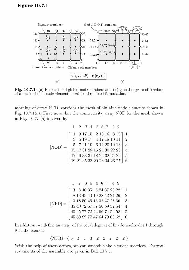
546 WEAK FORM FINITE ELEMENT MODELS OF INCOMPRESSIBLE FLUIDS
(a)
•• •
•
•
• •
•
••
•
•
•
•
•
•• •
••
• •
•
•• •
•
•
• ••
•
•
•
•
•
•
•
•• •
••
• ••
(b)
1 2 3 4 5 6 7
8 14
21
28
3529
22
15
30 31 32 33 34
1−3 4,5 6-8 11−139,10 16−1814,15
19,20 31,32
48−50
80−82
63,64
65−67 68,69 70−7273,74
75−7778,79
51,52
33-35
21,22 23,24
36,37 38−40
1
4
2 3
5 6
1 2
34
5
6
7
8 9
Global node numbers
Global D.O.F. numbersElement numbers
Element node numbers
•( ), ,x yv v P ( ),x yv v
Figure 10.7.1
Fig. 10.7.1: (a) Element and global node numbers and (b) global degrees of freedomof a mesh of nine-node elements used for the mixed formulation.
meaning of array NFD, consider the mesh of six nine-node elements shown inFig. 10.7.1(a). First note that the connectivity array NOD for the mesh shownin Fig. 10.7.1(a) is given by
1 2 3 4 5 6 7 8 9
[NOD] =
1 3 17 15 2 10 16 8 93 5 19 17 4 12 18 10 115 7 21 19 6 14 20 12 13
15 17 31 29 16 24 30 22 2317 19 33 31 18 26 32 24 2519 21 35 33 20 28 34 26 27
123456
The NFD array is [see Fig. 10.7.1(b)] as follows:
1 2 3 4 5 6 7 8 9
[NFD] =
3 8 40 35 5 24 37 20 228 13 45 40 10 28 42 24 26
13 18 50 45 15 32 47 28 3035 40 72 67 37 56 69 52 5440 45 77 72 42 60 74 56 5845 50 82 77 47 64 79 60 62
123456
In addition, we define an array of the total degrees of freedom of nodes 1 through9 of the element
NFR= 3 3 3 3 2 2 2 2 2
With the help of these arrays, we can assemble the element matrices. Fortranstatements of the assembly are given in Box 10.7.1.
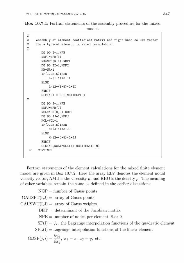
10.7. COMPUTER IMPLEMENTATION 547
Box 10.7.1: Fortran statements of the assembly procedure for the mixedmodel.
C
C Assembly of element coefficient matrix and right-hand column vector
C for a typical element in mixed formulation.
C
DO 90 I=1,NPE
NDFI=NFR(I)
NR=NFD(N,I)-NDFI
DO 90 II=1,NDFI
NR=NR+1
IF(I.LE.5)THEN
L=(I-1)*3+II
ELSE
L=12+(I-5)*2+II
ENDIF
GLF(NR) = GLF(NR)+ELF(L)
C
DO 90 J=1,NPE
NDFJ=NFR(J)
NCL=NFD(N,J)-NDFJ
DO 90 JJ=1,NDFJ
NCL=NCL+1
IF(J.LE.5)THEN
M=(J-1)*3+JJ
ELSE
M=12+(J-5)*2+JJ
ENDIF
GLK(NR,NCL)=GLK(NR,NCL)+ELK(L,M)
90 CONTINUE
Fortran statements of the element calculations for the mixed finite elementmodel are given in Box 10.7.2. Here the array ELV denotes the element nodalvelocity vector, AMU is the viscosity µ, and RHO is the density ρ. The meaningof other variables remain the same as defined in the earlier discussions:
NGP = number of Gauss points
GAUSPT(I,J) = array of Gauss points
GAUSWT(I,J) = array of Gauss weights
DET = determinant of the Jacobian matrix
NPE = number of nodes per element, 8 or 9
SF(I) = ψi, the Lagrange interpolation functions of the quadratic element
SFL(I) = Lagrange interpolation functions of the linear element
GDSF(j, i) =∂ψi∂xj
, x1 = x, x2 = y, etc.
548 WEAK FORM FINITE ELEMENT MODELS OF INCOMPRESSIBLE FLUIDS
Box 10.7.2: Fortran statements for the calculation of element matrices of themixed finite element model.
DO 100 NI=1,NGPF
DO 100 NJ=1,NGPF
XI=GAUSPT(NI,NGPF)
ETA=GAUSPT(NJ,NGPF)
CALL SHP2DPV(NPE,XI,ETA,ELXY,DET)
CONST=DET*GAUSWT(NI,NGPF)*GAUSWT(NJ,NGPF)
VX=0.0
VY=0.0
DO 60 I=1,NPE
L=2*I-1
VX=VX+SF(I)*ELV(L)
VY=VY+SF(I)*ELV(L+1)
60 CONTINUE
II=1
KI = 3
DO 80 I = 1,NPE
JJ=1
KJ = 3
DO 70 J = 1,NPE
CONV = SF(I)*(VX*GDSF(1,J)+VY*GDSF(2,J))*CONST
S11 = GDSF(1,I)*GDSF(1,J)*CONST
S22 = GDSF(2,I)*GDSF(2,J)*CONST
S12 = GDSF(1,I)*GDSF(2,J)*CONST
S21 = GDSF(2,I)*GDSF(1,J)*CONST
IF(J.LE.4)THEN
S10 = GDSF(1,I)*SFL(J)*CONST
S20 = GDSF(2,I)*SFL(J)*CONST
ENDIF
IF(I.LE.4)THEN
S01 = GDSF(1,J)*SFL(I)*CONST
S02 = GDSF(2,J)*SFL(I)*CONST
ENDIF
ELK(II,JJ) = ELK(II,JJ)+AMU*(2.0*S11+S22)+RHO*CONV
ELK(II,JJ+1) = ELK(II,JJ+1)+AMU*S21
ELK(II+1,JJ+1) = ELK(II+1,JJ+1)+AMU*(S11+2.0*S22)+RHO*CONV
ELK(II+1,JJ) = ELK(II+1,JJ) +AMU*S12
IF(J .LE. 4)THEN
ELK(II,JJ+2) = ELK(II,JJ+2) - S10
ELK(II+1,JJ+2) = ELK(II+1,JJ+2) - S20
ENDIF
IF(I .LE. 4)THEN
ELK(II+2,JJ) = ELK(II+2,JJ) - S01
ELK(II+2,JJ+1) = ELK(II+2,JJ+1) - S02
ENDIF
IF(J .GT. 4)KJ=2
70 JJ = JJ + KJ
IF(I .GT. 4)KI=2
80 II = II + KI
100 CONTINUE
10.7. COMPUTER IMPLEMENTATION 549
10.7.2 Penalty Model
Computer implementation of the penalty finite element model is quite straight-forward and is the same as any multi-degree of freedom systems (see Chapters5 and 7 and Box 10.7.3), and hence not discussed further. Only note should bemade of the fact that the element calculations involve two Gauss loops: a fullintegration loop for the evaluations of all terms except for the penalty termsand the other one is a reduced integration loop for the evaluation of the penaltyterms of the coefficient matrix K [see Eq. (10.6.3)]. Box 10.7.3 contains a For-tran listing of the subroutine to evaluate the coefficient matrix in the penaltyfinite element model of the Navier–Stokes equations (for the direct iterationonly). Box 10.7.4 contains Fortran statements for the computation of stressesand pressure in the penalty finite element model [based on Eqs. (10.6.4) and(10.6.6)].
Box 10.7.3: Fortran statements for the calculation of element matrices of thepenalty finite element model.
SUBROUTINE PNLTY2D(NGPF,NPE,NN,NONLIN,GAMMA,RHO,AMU)
C
C Calculates the coefficient matrix for penalty model
C
IMPLICIT REAL*8(A-H,O-Z)
COMMON/STF1/STIF(18,18),ELF(18),ELXY(9,2),VEL(18)
COMMON/SHP/SFL(9),GDSFL(2,9)
DIMENSION GAUSPT(4,4),GAUSWT(4,4)
DATA GAUSPT/4*.0D0,-.57735027D0,.57735027D0,2*.0D0,-.77459667D0,
* 0.0D0,.77459667D0,.0D0,-.86113631D0,-.33998104D0,.33998104D0,
* 0.86113631D0/
DATA GAUSWT/2.0D0,3*0.D0,2*1.0D0,2*.0D0,.55555555D0,.88888888D0,
* 0.55555555D0,0.0D0,0.34785485D0,2*0.65214515D0,0.34785485D0/
C
NDF=NN/NPE
NGPR=NGPF-1
DO 20 I=1,NN
ELF(I)=0.0
DO 20 J=1,NN
20 STIF(I,J)=0.0
DO 100 NI=1,NGPF
DO 100 NJ=1,NGPF
XI =GAUSPT(NI,NGPF)
ETA=GAUSPT(NJ,NGPF)
CALL INTERPLN2D(NPE,XI,ETA,DET,ELXY)
X=0.0D0
DO 30 I=1,NPE
30 X=X+ELXY(I,1)*SFL(I)
CONST=DET*GAUSWT(NI,NGPF)*GAUSWT(NJ,NGPF)
IF(NONLIN.GT.0)THEN
U=0.0D0
V=0.0D0
550 WEAK FORM FINITE ELEMENT MODELS OF INCOMPRESSIBLE FLUIDS
Box 10.7.3: Fortran statements for the penalty model (continued).
DO 40 I=1,NPE
L = (I-1)*NDF+1
U=VEL(L)*SFL(I)+U
40 V=VEL(L+1)*SFL(I)+V
ENDIF
II=1
DO 90 I=1,NPE
JJ=1
DO 80 J=1,NPE
S11=GDSFL(1,I)*GDSFL(1,J)*CONST
S22=GDSFL(2,I)*GDSFL(2,J)*CONST
S12=GDSFL(1,I)*GDSFL(2,J)*CONST
S21=GDSFL(2,I)*GDSFL(1,J)*CONST
STIF(II,JJ) =STIF(II,JJ) +AMU*(2.0*S11+S22)
STIF(II+1,JJ+1)=STIF(II+1,JJ+1)+AMU*(S11+2.0*S22)
STIF(II,JJ+1) =STIF(II,JJ+1) +AMU*S21
STIF(II+1,JJ) =STIF(II+1,JJ) +AMU*S12
IF(NONLIN.GT.0)THEN
CNV=SFL(I)*(U*GDSFL(1,J)+V*GDSFL(2,J))*CONST
STIF(II,JJ) =STIF(II,JJ) + RHO*CNV
STIF(II+1,JJ+1)=STIF(II+1,JJ+1)+ RHO*CNV
ENDIF
80 JJ=NDF*J+1
90 II=NDF*I+1
100 CONTINUE
C Evaluate the penalty terms using reduced integration
DO 150 NI=1,NGPR
DO 150 NJ=1,NGPR
XI =GAUSPT(NI,NGPR)
ETA=GAUSPT(NJ,NGPR)
CALL INTERPLN2D(NPE,XI,ETA,DET,ELXY)
DO 110 I=1,NPE
110 X=X+ELXY(I,1)*SFL(I)
CONST=DET*GAUSWT(NI,NGPR)*GAUSWT(NJ,NGPR)
II=1
DO 140 I=1,NPE
JJ=1
DO 130 J=1,NPE
S11=GDSFL(1,I)*GDSFL(1,J)*CONST
S22=GDSFL(2,I)*GDSFL(2,J)*CONST
S12=GDSFL(1,I)*GDSFL(2,J)*CONST
S21=GDSFL(2,I)*GDSFL(1,J)*CONST
STIF(II,JJ) = STIF(II,JJ) + GAMMA*S11
STIF(II+1,JJ+1) = STIF(II+1,JJ+1) + GAMMA*S22
STIF(II,JJ+1) = STIF(II,JJ+1) + GAMMA*S12
STIF(II+1,JJ) = STIF(II+1,JJ) + GAMMA*S21
130 JJ=NDF*J+1
140 II=NDF*I+1
150 CONTINUE
RETURN
END
10.7. COMPUTER IMPLEMENTATION 551
Box 10.7.4: Fortran statements for stress and pressure calculation in thepenalty finite element model.
SUBROUTINE STRS2D(GAMMA,AMU,NGPR,NPE,ELXY,VEL,NONLIN)
C
C Computes viscous stresses, pressure, and the divergence of velocity
C at the integration points of the reduced integration rule
C
IMPLICIT REAL*8 (A-H,O-Z)
COMMON/SHP/SFL(9),GDSFL(2,9)
DIMENSION ELXY(9,2),VEL(18),GAUSPT(4,4)
DATA GAUSPT/4*0.0D0,-.57735027D0,.57735027D0,2*0.0D0,-.77459667D0,
*0.0D0,0.77459667D0,0.0D0,-0.86113631D0,-0.33998104D0,.33998104D0,
*0.86113631D0/
C
C Calculation of strain-rates and stresses in the element
C
IT=6
NDF=2
DO 50 NI=1, NGPR
DO 50 NJ=1, NGPR
XI = GAUSPT(NI,NGPR)
ETA = GAUSPT(NJ,NGPR)
CALL INTERPLN2D(NPE,XI,ETA,DET,ELXY)
X = 0.0
Y = 0.0
U =0.0
UX=0.0
UY=0.0
VX=0.0
VY=0.0
DO 30 I=1,NPE
X = X + ELXY(I,1)*SFL(I)
Y = Y + ELXY(I,2)*SFL(I)
L=(I-1)*NDF+1
UX=UX+VEL(L)*GDSFL(1,I)
UY=UY+VEL(L)*GDSFL(2,I)
VX=VX+VEL(L+1)*GDSFL(1,I)
VY=VY+VEL(L+1)*GDSFL(2,I)
30 CONTINUE
DIV=UX+VY
PRS=-GAMMA*DIV
SX =2.0*AMU*UX-PRS
SY =2.0*AMU*VY-PRS
SXY=AMU*(UY+VX)
50 WRITE (IT,60) X,Y,SX,SY,SXY,PRS
60 FORMAT(6(2X,E11.4))
RETURN
END
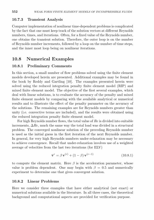
552 WEAK FORM FINITE ELEMENT MODELS OF INCOMPRESSIBLE FLUIDS
10.7.3 Transient Analysis
Computer implementation of nonlinear time-dependent problems is complicatedby the fact that one must keep track of the solution vectors at different Reynoldsnumbers, times, and iterations. Often, for a fixed value of the Reynolds number,one obtains the transient solution. Therefore, the outer loop is on the numberof Reynolds number increments, followed by a loop on the number of time steps,and the inner most loop being on nonlinear iterations.
10.8 Numerical Examples
10.8.1 Preliminary Comments
In this section, a small number of flow problems solved using the finite elementmodels developed herein are presented. Additional examples may be found inthe book by Reddy and Gartling [10]. The examples presented herein weresolved using the reduced integration penalty finite element model (RIP) andmixed finite element model. The objective of the first several examples, whichdeal with linear solutions, is to evaluate the accuracy of the penalty and mixedfinite element models by comparing with the available analytical or numericalresults and to illustrate the effect of the penalty parameter on the accuracy ofthe solutions. The remaining examples are for Reynolds numbers greater thanunity (i.e. convective terms are included), and the results were obtained usingthe reduced integration penalty finite element model.
For high Reynolds number flows, the total value of Re is divided into suitableincrements, ∆Re, much the same way the total load was divided in a structuralproblem. The converged nonlinear solution of the preceding Reynolds numberis used as the initial guess in the first iteration of the next Reynolds number.In general, for very high Reynolds numbers under-relaxation may be necessaryto achieve convergence. Recall that under-relaxation involves use of a weightedaverage of velocities from the last two iterations (for ELV)
vr = β v(r) + (1− β) v(r−1) (10.8.1)
to compute the element matrix. Here β is the acceleration parameter, whosevalue is problem dependent. One may begin with β = 0.5 and numericallyexperiment to determine one that gives convergent solution.
10.8.2 Linear Problems
Here we consider three examples that have either analytical (not exact) ornumerical solutions available in the literature. In all three cases, the theoreticalbackground and computational aspects are provided for verification purpose.
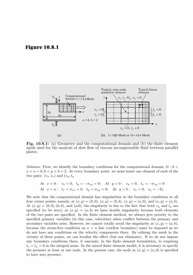
10.8. NUMERICAL EXAMPLES 553
Example 10.8.1
Fluid Squeezed Between Parallel Plates. Consider the slow flow of a viscous incompressiblematerial squeezed between two long parallel plates, as shown in Fig. 10.8.1(a). Let V0 be thevelocity with which the two plates are moving toward each other (i.e. squeezing out the fluid),and let 2b and 2a denote, respectively, the distance between and the length of the plates at afixed instant of time. Assuming that the length of the plates (into the plane of the paper) isvery large compared to both the width of and the distance between the plates, the problemcan be treated as one of a plane flow. Use the biaxial symmetry (prove it to yourself), use a5 × 3 nonuniform mesh of nine-node quadratic elements (Q9) in the mixed model, a 10 × 6mesh of the four-node linear elements (L4), and 5 × 3 mesh of nine-node quadratic elementsin the penalty model, as shown in Fig. 10.8.1(b), to analyze the problem for velocity andpressure fields.
x
(a)
V0
Computational domain
y
2b2a
V0 y
(b)
Typical linear element
Typical, nine-node, quadratic element
x
==
0
0
y
x
t
v
0,0 == xy tv
0,0 =−= xy vVv
==
0
0
y
x
t
t••• •5 3 L4 Mesh´
5 3 9 6 4Q Mesh or 10 L Mesh´ ´
a = 6, b = 2
Figure 10.8.1
Fig. 10.8.1: (a) Geometry and the computational domain and (b) the finite elementmesh used for the analysis of slow flow of viscous incompressible fluid between parallelplates.
Solution: First, we identify the boundary conditions for the computational domain, Ω : 0 <x < a = 6, 0 < y < b = 2. At every boundary point, we must know one element of each of thetwo pairs: (vx, tx) and (vy, ty). We have [see Fig. 10.8.1(b)]
At x = 0 : vx = 0, ty = −σxy = 0; At y = 0 : vy = 0, tx = −σxy = 0
At x = a : tx = σxx = 0, ty = σxy = 0; At y = b : vx = 0, vy = −V0
We note that the computational domain has singularities in the boundary conditions at allfour corner points, namely, at (x, y) = (0, 0), (x, y) = (0, b), (x, y) = (a, 0), and (x, y) = (a, b).At (x, y) = (0, 0), (0, b), and (a,0), the singularity is due to the fact that both vy and ty arespecified (to be zero); at (x, y) = (a, b) we have double singularity because both elementsof the two pairs are specified. In the finite element method, we always give priority to thespecified primary variables (in this case, velocities) when conflict between the primary andsecondary variables arise. However, we cannot totally avoid the singularity at (x, y) = (a, b),because the stress-free condition on x = a line (outflow boundary) must be imposed as wedo not have any conditions on the velocity components there. By refining the mesh in thevicinity of these points, we can localize the effect (but not eliminate). If we do not imposeany boundary conditions there, it amounts, in the finite element formulation, to requiringtx = ty = 0 in the integral sense. In the mixed finite element model, it is necessary to specifythe pressure at least at one node. In the present case, the node at (x, y) = (a, 0) is specifiedto have zero pressure.
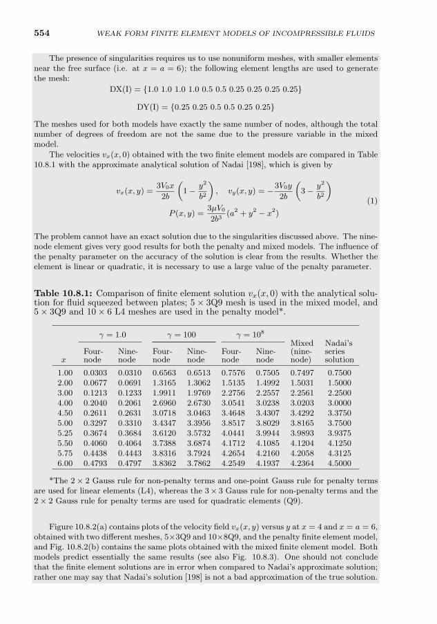
554 WEAK FORM FINITE ELEMENT MODELS OF INCOMPRESSIBLE FLUIDS
The presence of singularities requires us to use nonuniform meshes, with smaller elementsnear the free surface (i.e. at x = a = 6); the following element lengths are used to generatethe mesh:
DX(I) = 1.0 1.0 1.0 1.0 0.5 0.5 0.25 0.25 0.25 0.25
DY(I) = 0.25 0.25 0.5 0.5 0.25 0.25
The meshes used for both models have exactly the same number of nodes, although the totalnumber of degrees of freedom are not the same due to the pressure variable in the mixedmodel.
The velocities vx(x, 0) obtained with the two finite element models are compared in Table10.8.1 with the approximate analytical solution of Nadai [198], which is given by
vx(x, y) =3V0x
2b
(1− y2
b2
), vy(x, y) = −3V0y
2b
(3− y2
b2
)P (x, y) =
3µV0
2b3(a2 + y2 − x2)
(1)
The problem cannot have an exact solution due to the singularities discussed above. The nine-node element gives very good results for both the penalty and mixed models. The influence ofthe penalty parameter on the accuracy of the solution is clear from the results. Whether theelement is linear or quadratic, it is necessary to use a large value of the penalty parameter.
Table 10.8.1: Comparison of finite element solution vx(x, 0) with the analytical solu-tion for fluid squeezed between plates; 5× 3Q9 mesh is used in the mixed model, and5× 3Q9 and 10× 6 L4 meshes are used in the penalty model*.
γ = 1.0 γ = 100 γ = 108
Mixed Nadai’sFour- Nine- Four- Nine- Four- Nine- (nine- series
x node node node node node node node) solution
1.00 0.0303 0.0310 0.6563 0.6513 0.7576 0.7505 0.7497 0.75002.00 0.0677 0.0691 1.3165 1.3062 1.5135 1.4992 1.5031 1.50003.00 0.1213 0.1233 1.9911 1.9769 2.2756 2.2557 2.2561 2.25004.00 0.2040 0.2061 2.6960 2.6730 3.0541 3.0238 3.0203 3.00004.50 0.2611 0.2631 3.0718 3.0463 3.4648 3.4307 3.4292 3.37505.00 0.3297 0.3310 3.4347 3.3956 3.8517 3.8029 3.8165 3.75005.25 0.3674 0.3684 3.6120 3.5732 4.0441 3.9944 3.9893 3.93755.50 0.4060 0.4064 3.7388 3.6874 4.1712 4.1085 4.1204 4.12505.75 0.4438 0.4443 3.8316 3.7924 4.2654 4.2160 4.2058 4.31256.00 0.4793 0.4797 3.8362 3.7862 4.2549 4.1937 4.2364 4.5000
*The 2× 2 Gauss rule for non-penalty terms and one-point Gauss rule for penalty termsare used for linear elements (L4), whereas the 3× 3 Gauss rule for non-penalty terms and the2× 2 Gauss rule for penalty terms are used for quadratic elements (Q9).
Figure 10.8.2(a) contains plots of the velocity field vx(x, y) versus y at x = 4 and x = a = 6,obtained with two different meshes, 5×3Q9 and 10×8Q9, and the penalty finite element model,and Fig. 10.8.2(b) contains the same plots obtained with the mixed finite element model. Bothmodels predict essentially the same results (see also Fig. 10.8.3). One should not concludethat the finite element solutions are in error when compared to Nadai’s approximate solution;rather one may say that Nadai’s solution [198] is not a bad approximation of the true solution.
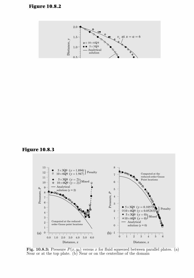
10.8. NUMERICAL EXAMPLES 555
Figure 10.8.2
0.0 0.5 1.0 1.5 2.0 2.5 3.0 3.5 4.0 4.5
Horizontal velocity,
0.0
0.5
1.0
1.5
2.0
Dis
tan
ce, y
vx at x = 4
Analytical solution
5 3 9Q´10 6 9Q´
0.0 0.5 1.0 1.5 2.0 2.5 3.0 3.5 4.0 4.5
Horizontal velocity,
0.0
0.5
1.0
1.5
2.0
Dis
tan
ce, y
vx at x = 4
Analytical solution
5 3 9Q´10 6 9Q´
(a)
(b)
( , )xv x y
( , )xv x y
vx at x = 6
6atxv x a= =
Fig. 10.8.2: Velocity fields v(x0, y) at x0 = 4 and x0 = 6 for fluid squeezed betweenparallel plates. (a) Penalty model. (b) Mixed model.
Analytical solution (y = 2)
Analytical solution (y = 0)
Mixed
0.0 1.0 2.0 3.0 4.0 5.0 6.0
Distance, x
0
1
2
3
4
5
6
7
8
9
10
11
12
13
Pre
ssu
re, P
0 1 2 3 4 5 6
Distance, x
-1
0
1
2
3
4
5
6
7
8
Pre
ssu
re, P
5 3 9 1 894Q ( . )y´ =10 6 9 1 947Q ( . )y´ =
5 3 9 2Q ( )y´ =10 6 9 2Q ( )y´ =
Penalty
Mixed
Penalty
5 3 9 0 1057Q ( . )y´ =10 6 9 0 05283Q ( . )y´ =5 3 9 0Q ( )y´ =
10 6 9 0Q ( )y´ =
Figure 10.8.3
Computed at the reduced-order Gauss point locations
Computed at the reduced-order Gauss Point locations
(a) (b)
Fig. 10.8.3: Pressure P (x, y0) versus x for fluid squeezed between parallel plates. (a)Near or at the top plate. (b) Near or on the centerline of the domain
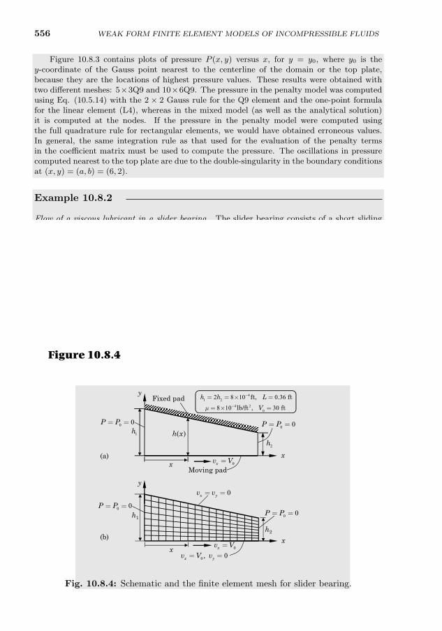
556 WEAK FORM FINITE ELEMENT MODELS OF INCOMPRESSIBLE FLUIDS
Figure 10.8.3 contains plots of pressure P (x, y) versus x, for y = y0, where y0 is they-coordinate of the Gauss point nearest to the centerline of the domain or the top plate,because they are the locations of highest pressure values. These results were obtained withtwo different meshes: 5×3Q9 and 10×6Q9. The pressure in the penalty model was computedusing Eq. (10.5.14) with the 2 × 2 Gauss rule for the Q9 element and the one-point formulafor the linear element (L4), whereas in the mixed model (as well as the analytical solution)it is computed at the nodes. If the pressure in the penalty model were computed usingthe full quadrature rule for rectangular elements, we would have obtained erroneous values.In general, the same integration rule as that used for the evaluation of the penalty termsin the coefficient matrix must be used to compute the pressure. The oscillations in pressurecomputed nearest to the top plate are due to the double-singularity in the boundary conditionsat (x, y) = (a, b) = (6, 2).
Example 10.8.2
Flow of a viscous lubricant in a slider bearing. The slider bearing consists of a short slidingpad moving at a velocity vx = V0 relative to a stationary pad inclined at a small angle withrespect to the stationary pad, as depicted in Fig. 10.8.4(a), and the small gap between thetwo pads is filled with a viscous lubricant. Since the ends of the bearing are generally open,the pressure there is atmospheric, P = P0. If the upper pad is parallel to the base plate, thepressure everywhere in the gap must be atmospheric (because dP/dx is a constant for flowbetween parallel plates), and the bearing cannot support any transverse load. If the upperpad is inclined to the base pad, pressure (in general, P is a function of x and y) develops in thegap. For large values of V0, the pressure developed can be of sufficient magnitude to supportheavy loads normal to the base pad. Determine the velocity and pressure distributions in thegap, and plot (a) horizontal velocity vx(x0, y) as a function of y for x0 = 0, 0.18 and x0 = 0.36and (b) pressure and shear stress as a function of x for y = 0.
Solution: In the finite element analysis, we solve the Stokes equations [i.e. neglect the convec-tive terms in Eqs. (10.4.1) and (10.4.2)] using a mesh of 16×8 linear quadrilateral elements toanalyze the problem. Figure 10.8.4(b) shows the mesh (graded uniformly) and the boundaryconditions.
Figure 10.8.4
y
h1
h2
x
y
x(b)
0x yv v= =
0 0P P= =
0 0,x yv V v= =0xv V=
0 0P P= =
xx(a)
0 0P P= =
2h1h
0 0P P= =
Fixed pad
Moving pad
( )h x
0xv V=
41 2
4 20
2 8 10 0 36
8 10 30
ft, . ft
lb/ft , ft
h h L
V
-
-
= = ´ =
= ´ =m
Fig. 10.8.4: Schematic and the finite element mesh for slider bearing.
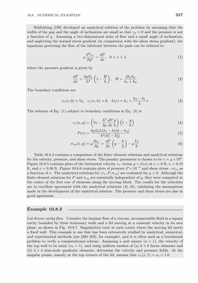
10.8. NUMERICAL EXAMPLES 557
Schlichting [199] developed an analytical solution of the problem by assuming that thewidth of the gap and the angle of inclination are small so that vy = 0 and the pressure is nota function of y. Assuming a two-dimensional state of flow and a small angle of inclination,and neglecting the normal stress gradient (in comparison with the shear stress gradient), theequations governing the flow of the lubricant between the pads can be reduced to
µ∂2vx∂y2
=dP
dx, 0 < x < L (1)
where the pressure gradient is given by
dP
dx=
6µV0
h2
(1− H
h
), H =
2h1h2
h1 + h2(2)
The boundary conditions are
vx(x, 0) = V0, vx(x, h) = 0, h(x) = h1 +h2 − h1
Lx (3)
The solution of Eq. (1) subject to boundary conditions in Eq. (3) is
vx(x, y) =
(V0 −
h2
2µ
dP
dx
y
h
)(1− y
h
)(4)
P (x) =6µV0L(h1 − h)(h− h2)
h2(h21 − h2
2)(5)
σxy(x, y) = µ∂vx∂y
=dP
dx
(y − h
2
)− µV0
h(6)
Table 10.8.2 contains a comparison of the finite element solutions and analytical solutionsfor the velocity, pressure, and shear stress. The penalty parameter is chosen to be γ = µ×108.Figure 10.8.5 contains plots of the horizontal velocity vx versus y = h(x) at x = 0 ft, x = 0.18ft, and x = 0.36 ft. Figure 10.8.6 contains plots of pressure P ×10−2 and shear stress −σxy asa function of x. The analytical solutions for (vx, P, σxy) are evaluated for y = 0. Although thefinite element solutions for P and σxy are essentially independent of y, they were computed atthe center of the first row of elements along the moving block. The results for the velocitiesare in excellent agreement with the analytical solutions (4)–(6), validating the assumptionsmade in the development of the analytical solution. The pressure and shear stress are also ingood agreement.
Example 10.8.3
Lid-driven cavity flow. Consider the laminar flow of a viscous, incompressible fluid in a squarecavity bounded by three stationary walls and a lid moving at a constant velocity in its ownplane, as shown in Fig. 10.8.7. Singularities exist at each corner where the moving lid meetsa fixed wall. This example is one that has been extensively studied by analytical, numerical,and experimental methods (see [200–202], for example), and it is often used as a benchmarkproblem to verify a computational scheme. Assuming a unit square (a = 1), the velocity ofthe top wall to be unity (v0 = 1), and using uniform meshes of (a) 8× 8 linear elements and(b) 4 × 4 nine-node quadratic elements, determine the velocity and pressure fields. At thesingular points, namely at the top corners of the lid, assume that vx(x, 1) = v0 = 1.0.
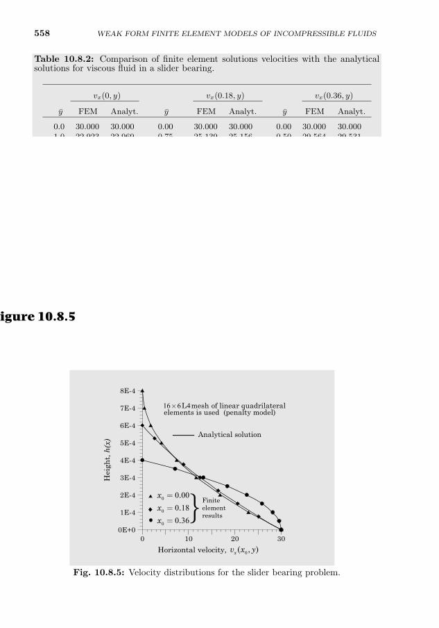
558 WEAK FORM FINITE ELEMENT MODELS OF INCOMPRESSIBLE FLUIDS
Table 10.8.2: Comparison of finite element solutions velocities with the analyticalsolutions for viscous fluid in a slider bearing.
vx(0, y) vx(0.18, y) vx(0.36, y)
y FEM Analyt. y FEM Analyt. y FEM Analyt.
0.0 30.000 30.000 0.00 30.000 30.000 0.00 30.000 30.0001.0 22.923 22.969 0.75 25.139 25.156 0.50 29.564 29.5312.0 16.799 16.875 1.50 20.596 20.625 1.00 28.182 28.1253.0 11.626 11.719 2.25 16.372 16.406 1.50 25.853 25.7814.0 7.403 7.500 3.00 12.465 12.500 2.00 22.577 22.5005.0 4.130 4.219 3.75 8.874 8.906 2.50 18.354 18.2816.0 1.805 1.875 4.50 5.600 5.625 3.00 13.184 13.1257.0 0.429 0.469 5.25 2.642 2.656 3.50 7.066 7.0318.0 0.000 0.000 6.00 0.000 0.000 4.00 0.000 0.000
Analytical FEM
x P (x, 0) −σxy(x, 0) x y P −σxy0.01 7.50 59.99 0.1125 0.4922 8.46 56.610.03 22.46 59.89 0.3375 0.4766 25.46 56.600.05 37.29 59.67 0.5625 0.4609 42.31 56.470.07 51.89 59.30 0.7875 0.4453 58.76 56.170.09 66.12 58.77 1.0125 0.4297 74.69 55.690.27 129.60 38.40 2.5875 0.3203 134.40 41.770.29 118.57 32.71 2.8125 0.3047 125.60 36.930.31 99.58 25.70 3.0375 0.2891 107.60 30.760.33 70.30 17.04 3.2625 0.2734 77.39 22.890.35 27.61 6.31 3.4875 0.2578 30.80 12.82
x = 10x, y = y × 104, P = P × 10−2.
16 6 4L mesh of linear quadrilateral elements is used (penalty model)
´
0
0
0
0 000 180 36
.
.
.
x
x
x
=
=
=
0 10 20 30
Horizontal velocity,
0E+0
1E-4
2E-4
3E-4
4E-4
5E-4
6E-4
7E-4
8E-4
Hei
ght,
h(x
)
0( , )xv x y
Analytical solution
Finite elementresults
Figure 10.8.5
Fig. 10.8.5: Velocity distributions for the slider bearing problem.
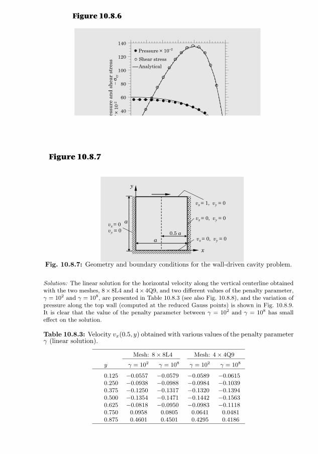
10.8. NUMERICAL EXAMPLES 559
Shear stress
Pressure × 10−2
Analytical
−σ x
yP
×10
-2
0.00 0.12 0.24 0.36
Distance, x
0
20
40
60
80
100
120
140
Pre
ssu
re a
nd
shea
r st
ress
16 6 4L mesh of linear quadrilateral elements is used (penalty model)
´
Figure 10.8.6
Fig. 10.8.6: Pressure and shear stress distributions for the slider bearing problem.
x
vx = 1, vy = 0
vx = 0, vy = 0
vx = 0, vy = 0vx = 0 vy = 0
y
a
a
0.5 a
Figure 10.8.7
Fig. 10.8.7: Geometry and boundary conditions for the wall-driven cavity problem.
Solution: The linear solution for the horizontal velocity along the vertical centerline obtainedwith the two meshes, 8× 8L4 and 4× 4Q9, and two different values of the penalty parameter,γ = 102 and γ = 108, are presented in Table 10.8.3 (see also Fig. 10.8.8), and the variation ofpressure along the top wall (computed at the reduced Gauss points) is shown in Fig. 10.8.9.It is clear that the value of the penalty parameter between γ = 102 and γ = 108 has smalleffect on the solution.
Table 10.8.3: Velocity vx(0.5, y) obtained with various values of the penalty parameterγ (linear solution).
Mesh: 8× 8L4 Mesh: 4× 4Q9
y γ = 102 γ = 108 γ = 102 γ = 108
0.125 −0.0557 −0.0579 −0.0589 −0.06150.250 −0.0938 −0.0988 −0.0984 −0.10390.375 −0.1250 −0.1317 −0.1320 −0.13940.500 −0.1354 −0.1471 −0.1442 −0.15630.625 −0.0818 −0.0950 −0.0983 −0.11180.750 0.0958 0.0805 0.0641 0.04810.875 0.4601 0.4501 0.4295 0.4186
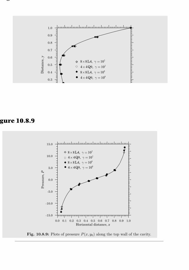
560 WEAK FORM FINITE ELEMENT MODELS OF INCOMPRESSIBLE FLUIDS
-0.2 -0.1 0.0 0.1 0.2 0.3 0.4 0.5 0.6 0.7 0.8 0.9 1.0Horizontal velocity,
0.0
0.1
0.2
0.3
0.4
0.5
0.6
0.7
0.8
0.9
1.0
Dis
tan
ce, y
0 5( . , )xv y
2
2
8
8
8 8 4 104 4 9 108 8 4 104 4 9 10
L ,
Q ,
L ,
Q ,
gggg
´ =
´ =
´ =
´ =
Figure 10.8.8
Fig. 10.8.8: Plots of horizontal velocity vx(0.5, y) along the vertical centerline of thecavity.
0.0 0.1 0.2 0.3 0.4 0.5 0.6 0.7 0.8 0.9 1.0Horizontal distance, x
-15.0
-10.0
-5.0
0.0
5.0
10.0
15.0
Pre
ssu
re, P
2
2
8
8
8 8 4 104 4 9 108 8 4 104 4 9 10
L ,Q ,L ,Q ,
gggg
´ =´ =´ =´ =
Figure 10.8.9
Fig. 10.8.9: Plots of pressure P (x, y0) along the top wall of the cavity.
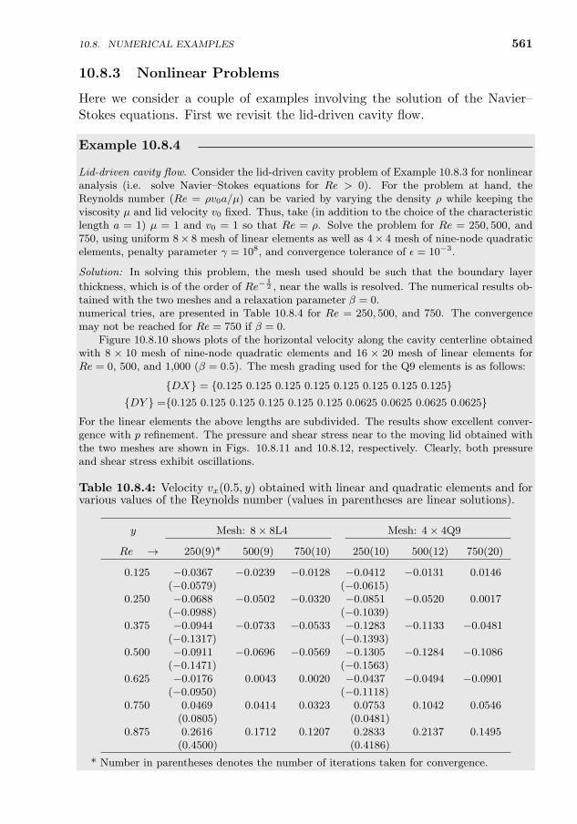
10.8. NUMERICAL EXAMPLES 561
10.8.3 Nonlinear Problems
Here we consider a couple of examples involving the solution of the Navier–Stokes equations. First we revisit the lid-driven cavity flow.
Example 10.8.4
Lid-driven cavity flow. Consider the lid-driven cavity problem of Example 10.8.3 for nonlinearanalysis (i.e. solve Navier–Stokes equations for Re > 0). For the problem at hand, theReynolds number (Re = ρv0a/µ) can be varied by varying the density ρ while keeping theviscosity µ and lid velocity v0 fixed. Thus, take (in addition to the choice of the characteristiclength a = 1) µ = 1 and v0 = 1 so that Re = ρ. Solve the problem for Re = 250, 500, and750, using uniform 8× 8 mesh of linear elements as well as 4× 4 mesh of nine-node quadraticelements, penalty parameter γ = 108, and convergence tolerance of ε = 10−3.
Solution: In solving this problem, the mesh used should be such that the boundary layer
thickness, which is of the order of Re−12 , near the walls is resolved. The numerical results ob-
tained with the two meshes and a relaxation parameter β = 0.25 [see Eq. (10.8.1)], after somenumerical tries, are presented in Table 10.8.4 for Re = 250, 500, and 750. The convergencemay not be reached for Re = 750 if β = 0.
Figure 10.8.10 shows plots of the horizontal velocity along the cavity centerline obtainedwith 8 × 10 mesh of nine-node quadratic elements and 16 × 20 mesh of linear elements forRe = 0, 500, and 1,000 (β = 0.5). The mesh grading used for the Q9 elements is as follows:
DX = 0.125 0.125 0.125 0.125 0.125 0.125 0.125 0.125DY =0.125 0.125 0.125 0.125 0.125 0.125 0.0625 0.0625 0.0625 0.0625
For the linear elements the above lengths are subdivided. The results show excellent conver-gence with p refinement. The pressure and shear stress near to the moving lid obtained withthe two meshes are shown in Figs. 10.8.11 and 10.8.12, respectively. Clearly, both pressureand shear stress exhibit oscillations.
Table 10.8.4: Velocity vx(0.5, y) obtained with linear and quadratic elements and forvarious values of the Reynolds number (values in parentheses are linear solutions).
y Mesh: 8× 8L4 Mesh: 4× 4Q9
Re → 250(9)* 500(9) 750(10) 250(10) 500(12) 750(20)
0.125 −0.0367 −0.0239 −0.0128 −0.0412 −0.0131 0.0146(−0.0579) (−0.0615)
0.250 −0.0688 −0.0502 −0.0320 −0.0851 −0.0520 0.0017(−0.0988) (−0.1039)
0.375 −0.0944 −0.0733 −0.0533 −0.1283 −0.1133 −0.0481(−0.1317) (−0.1393)
0.500 −0.0911 −0.0696 −0.0569 −0.1305 −0.1284 −0.1086(−0.1471) (−0.1563)
0.625 −0.0176 0.0043 0.0020 −0.0437 −0.0494 −0.0901(−0.0950) (−0.1118)
0.750 0.0469 0.0414 0.0323 0.0753 0.1042 0.0546(0.0805) (0.0481)
0.875 0.2616 0.1712 0.1207 0.2833 0.2137 0.1495(0.4500) (0.4186)
* Number in parentheses denotes the number of iterations taken for convergence.
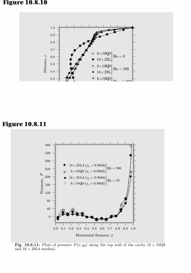
562 WEAK FORM FINITE ELEMENT MODELS OF INCOMPRESSIBLE FLUIDS
0 5( . , )xv y
8 10 90
16 20
8 10 9500
16 20
8 10 91 000
16 20
QRe
L
QRe
L
QRe ,
L
ü´ ïï =ýï´ ïþü´ ïï =ýï´ ïþü´ ïï =ýï´ ïþ
-0.4 -0.2 0.0 0.2 0.4 0.6 0.8 1.0
Horizontal velocity,
0.0
0.1
0.2
0.3
0.4
0.5
0.6
0.7
0.8
0.9
1.0
Dis
tan
ce, y
8 310 10 0 5, , .g e b-= = =
Figure 10.8.10
Fig. 10.8.10: Velocity vx(0.5, y) versus y for Reynolds numbers Re = 0, 500, and 1,000(obtained with 8× 10Q9 and 16× 20L4 meshes).
0.0 0.1 0.2 0.3 0.4 0.5 0.6 0.7 0.8 0.9 1.0
Horizontal distance, x
0
40
80
120
160
200
240
280
320
360
Pre
ssu
re,
P
0
0
0 3
0
16 20 4 0 9844500
8 10 9 0 9868
16 20 4 0 984410
8 10 9 0 9868
L ( . )Re
Q ( . )
L ( . )Re
Q ( . )
y
y
y
y
ü´ = ïï =ýï´ = ïþü´ = ïï =ýï´ = ïþ
Figure 10.8.11
Fig. 10.8.11: Plots of pressure P (x, y0) along the top wall of the cavity (8 × 10Q9and 16× 20L4 meshes).
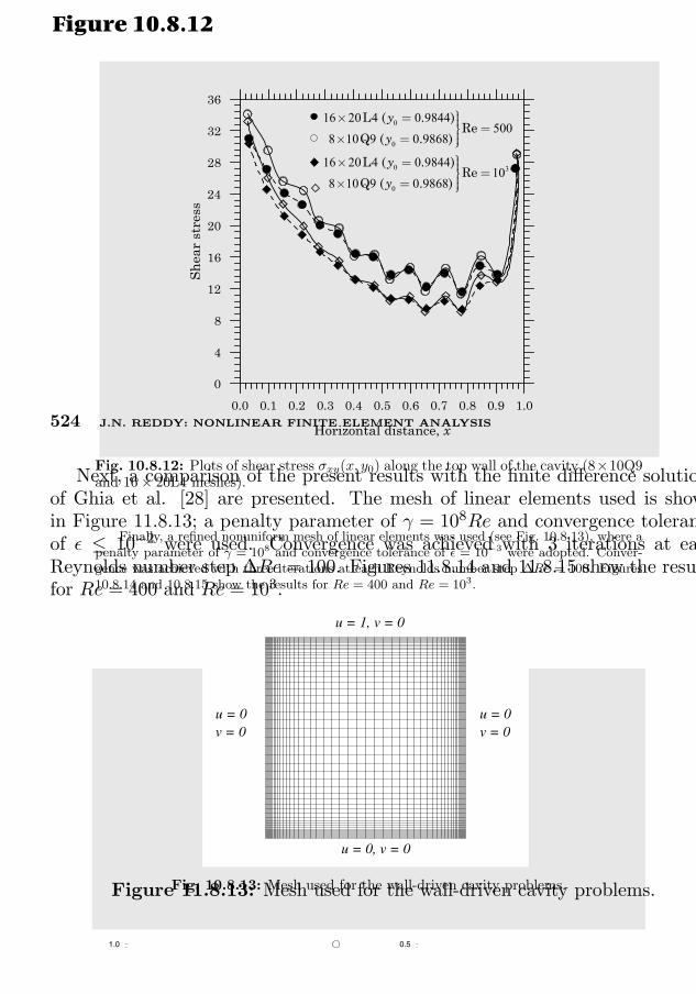
10.8. NUMERICAL EXAMPLES 563
0.0 0.1 0.2 0.3 0.4 0.5 0.6 0.7 0.8 0.9 1.0
Horizontal distance, x
0
4
8
12
16
20
24
28
32
36
Sh
ear
stre
ss
0
0
0 3
0
16 20 4 0 9844500
8 10 9 0 9868
16 20 4 0 984410
8 10 9 0 9868
L ( . )Re
Q ( . )
L ( . )Re
Q ( . )
y
y
y
y
ü´ = ïï =ýï´ = ïþü´ = ïï =ýï´ = ïþ
Figure 10.8.12
Fig. 10.8.12: Plots of shear stress σxy(x, y0) along the top wall of the cavity (8×10Q9and 16× 20L4 meshes).
Finally, a refined nonuniform mesh of linear elements was used (see Fig. 10.8.13), where apenalty parameter of γ = 108 and convergence tolerance of ε = 10−3 were adopted. Conver-gence was achieved with three iterations at each Reynolds number step ∆Re = 100. Figures10.8.14 and 10.8.15 show the results for Re = 400 and Re = 103.
u = 0v = 0
u = 0v = 0
u = 0, v = 0
u = 1, v = 0
0.51.0
524 J.N. REDDY: NONLINEAR FINITE ELEMENT ANALYSIS
Next, a comparison of the present results with the finite difference solutionsof Ghia et al. [28] are presented. The mesh of linear elements used is shownin Figure 11.8.13; a penalty parameter of γ = 108Re and convergence toleranceof ² ≤ 10−2 were used. Convergence was achieved with 3 iterations at eachReynolds number step ∆Re = 100. Figures 11.8.14 and 11.8.15 show the resultsfor Re = 400 and Re = 103.
Figure 11.8.13: Mesh used for the wall-driven cavity problems.Fig. 10.8.13: Mesh used for the wall-driven cavity problems.
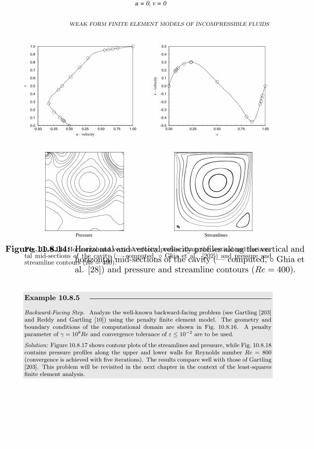
564
u = 0, v = 0
StreamlinesPressure
x
v-
velo
city
0.00 0.25 0.50 0.75 1.00-0.5
-0.4
-0.3
-0.2
-0.1
0.0
0.1
0.2
0.3
0.4
0.5
u - velocity
y
-0.50 -0.25 0.00 0.25 0.50 0.75 1.000.0
0.1
0.2
0.3
0.4
0.5
0.6
0.7
0.8
0.9
1.0
Figure 11.8.14: Horizontal and vertical velocity profiles along the vertical andhorizontal mid-sections of the cavity (– computed, Ghia etal. [28]) and pressure and streamline contours (Re = 400).
Fig. 10.8.14: Horizontal and vertical velocity profiles along the vertical and horizon-tal mid-sections of the cavity (— computed, Ghia et al. [202]) and pressure andstreamline contours (Re = 400).
Example 10.8.5
Backward-Facing Step. Analyze the well-known backward-facing problem (see Gartling [203]and Reddy and Gartling [10]) using the penalty finite element model. The geometry andboundary conditions of the computational domain are shown in Fig. 10.8.16. A penaltyparameter of γ = 108Re and convergence tolerance of ε ≤ 10−2 are to be used.
Solution: Figure 10.8.17 shows contour plots of the streamlines and pressure, while Fig. 10.8.18contains pressure profiles along the upper and lower walls for Reynolds number Re = 800(convergence is achieved with five iterations). The results compare well with those of Gartling[203]. This problem will be revisited in the next chapter in the context of the least-squaresfinite element analysis.
WEAK FORM FINITE ELEMENT MODELS OF INCOMPRESSIBLE FLUIDS
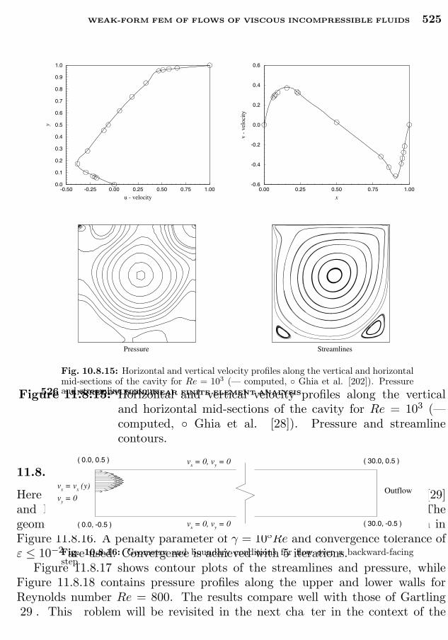
10.8. NUMERICAL EXAMPLES 565
StreamlinesPressure
x
v-
velo
city
0.00 0.25 0.50 0.75 1.00-0.6
-0.4
-0.2
0.0
0.2
0.4
0.6
u - velocity
y
-0.50 -0.25 0.00 0.25 0.50 0.75 1.000.0
0.1
0.2
0.3
0.4
0.5
0.6
0.7
0.8
0.9
1.0
WEAK-FORM FEM OF FLOWS OF VISCOUS INCOMPRESSIBLE FLUIDS 525
Figure 11.8.15: Horizontal and vertical velocity profiles along the verticaland horizontal mid-sections of the cavity for Re = 103 (–computed, Ghia et al. [28]). Pressure and streamlinecontours.
11.8.3.2 Backward-Facing Step
Here we analyze the well-known backward-facing problem (see Gartling [29]and Reddy and Gartling [3]) using the penalty finite element model. Thegeometry and boundary conditions of the computational domain are shown inFigure 11.8.16. A penalty parameter of γ = 108Re and convergence tolerance ofε ≤ 10−2 are used. Convergence is achieved with 5 iterations.Figure 11.8.17 shows contour plots of the streamlines and pressure, while
Figure 11.8.18 contains pressure profiles along the upper and lower walls forReynolds number Re = 800. The results compare well with those of Gartling29 . This roblem will be revisited in the next cha ter in the context of the
Fig. 10.8.15: Horizontal and vertical velocity profiles along the vertical and horizontalmid-sections of the cavity for Re = 103 (— computed, Ghia et al. [202]). Pressureand streamline contours.
vx = vx (y)
vy = 0
vx = 0, vy = 0
vx = 0, vy = 0
Outflow
( 0.0, 0.5 )
( 0.0, -0.5 )
( 30.0, 0.5 )
( 30.0, -0.5 )
526 J.N. REDDY: NONLINEAR FINITE ELEMENT ANALYSIS
Fig. 10.8.16: Geometry and boundary conditions for flow over a backward-facingstep.
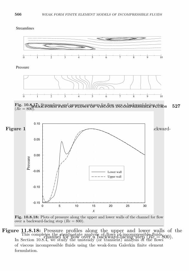
566
0 1 2 3 4 5 6 7 8 9 10
Pressure
0 1 2 3 4 5 6 7 8 9 10
Streamlines
Figure 11.8.17: Streamlines and pressure contours for flow over a backward-facing step (Re = 800).
Fig. 10.8.17: Streamlines and pressure contours for flow over a backward-facing step(Re = 800).
x
Pre
ssur
e
0 5 10 15 20 25 30-0.15
-0.10
-0.05
0.00
0.05
0.10
Lower wall
Upper wall
WEAK-FORM FEM OF FLOWS OF VISCOUS INCOMPRESSIBLE FLUIDS 527
Figure 11.8.18: Pressure profiles along the upper and lower walls of thechannel for flow over a backward-facing step (Re = 800).
Fig. 10.8.18: Plots of pressure along the upper and lower walls of the channel for flowover a backward-facing step (Re = 800).
This completes the steady-state analysis of flows of incompressible fluids.In Section 10.8.4, we study the unsteady (or transient) analysis of the flowsof viscous incompressible fluids using the weak-form Galerkin finite elementformulation.
WEAK FORM FINITE ELEMENT MODELS OF INCOMPRESSIBLE FLUIDS
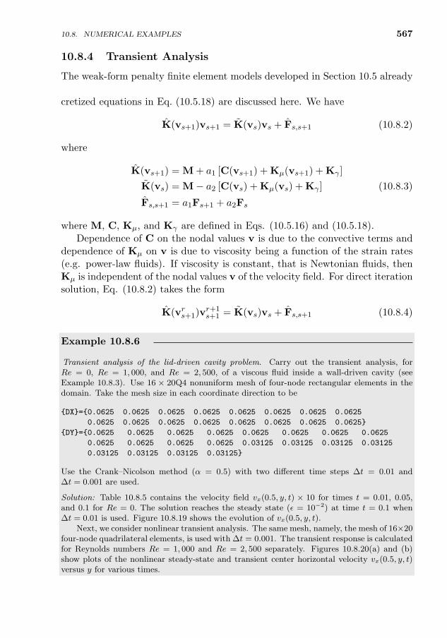
10.8. NUMERICAL EXAMPLES 567
10.8.4 Transient Analysis
The weak-form penalty finite element models developed in Section 10.5 alreadyinclude time-dependent terms [see Eq. (10.5.16) or (10.5.18)]. The fully dis-cretized equations in Eq. (10.5.18) are discussed here. We have
K(vs+1)vs+1 = K(vs)vs + Fs,s+1 (10.8.2)
where
K(vs+1) = M + a1 [C(vs+1) + Kµ(vs+1) + Kγ ]
K(vs) = M− a2 [C(vs) + Kµ(vs) + Kγ ] (10.8.3)
Fs,s+1 = a1Fs+1 + a2Fs
where M, C, Kµ, and Kγ are defined in Eqs. (10.5.16) and (10.5.18).Dependence of C on the nodal values v is due to the convective terms and
dependence of Kµ on v is due to viscosity being a function of the strain rates(e.g. power-law fluids). If viscosity is constant, that is Newtonian fluids, thenKµ is independent of the nodal values v of the velocity field. For direct iterationsolution, Eq. (10.8.2) takes the form
K(vrs+1)vr+1s+1 = K(vs)vs + Fs,s+1 (10.8.4)
Example 10.8.6
Transient analysis of the lid-driven cavity problem. Carry out the transient analysis, forRe = 0, Re = 1, 000, and Re = 2, 500, of a viscous fluid inside a wall-driven cavity (seeExample 10.8.3). Use 16 × 20Q4 nonuniform mesh of four-node rectangular elements in thedomain. Take the mesh size in each coordinate direction to be
DX=0.0625 0.0625 0.0625 0.0625 0.0625 0.0625 0.0625 0.0625
0.0625 0.0625 0.0625 0.0625 0.0625 0.0625 0.0625 0.0625
DY=0.0625 0.0625 0.0625 0.0625 0.0625 0.0625 0.0625 0.0625
0.0625 0.0625 0.0625 0.0625 0.03125 0.03125 0.03125 0.03125
0.03125 0.03125 0.03125 0.03125
Use the Crank–Nicolson method (α = 0.5) with two different time steps ∆t = 0.01 and∆t = 0.001 are used.
Solution: Table 10.8.5 contains the velocity field vx(0.5, y, t) × 10 for times t = 0.01, 0.05,and 0.1 for Re = 0. The solution reaches the steady state (ε = 10−2) at time t = 0.1 when∆t = 0.01 is used. Figure 10.8.19 shows the evolution of vx(0.5, y, t).
Next, we consider nonlinear transient analysis. The same mesh, namely, the mesh of 16×20four-node quadrilateral elements, is used with ∆t = 0.001. The transient response is calculatedfor Reynolds numbers Re = 1, 000 and Re = 2, 500 separately. Figures 10.8.20(a) and (b)show plots of the nonlinear steady-state and transient center horizontal velocity vx(0.5, y, t)versus y for various times.
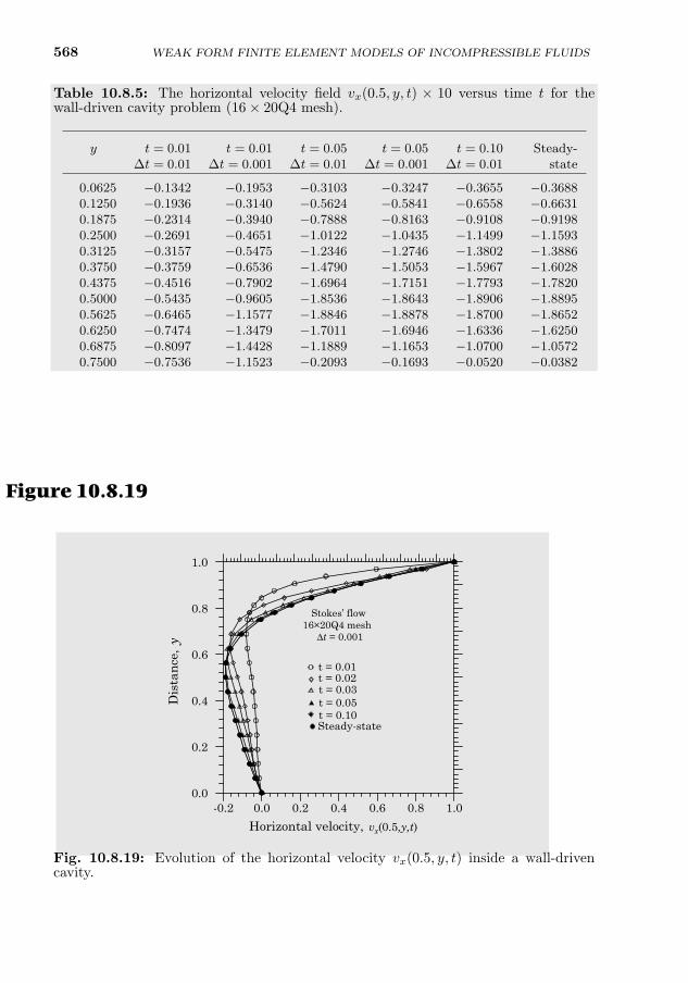
568 WEAK FORM FINITE ELEMENT MODELS OF INCOMPRESSIBLE FLUIDS
Table 10.8.5: The horizontal velocity field vx(0.5, y, t) × 10 versus time t for thewall-driven cavity problem (16× 20Q4 mesh).
y t = 0.01 t = 0.01 t = 0.05 t = 0.05 t = 0.10 Steady-∆t = 0.01 ∆t = 0.001 ∆t = 0.01 ∆t = 0.001 ∆t = 0.01 state
0.0625 −0.1342 −0.1953 −0.3103 −0.3247 −0.3655 −0.36880.1250 −0.1936 −0.3140 −0.5624 −0.5841 −0.6558 −0.66310.1875 −0.2314 −0.3940 −0.7888 −0.8163 −0.9108 −0.91980.2500 −0.2691 −0.4651 −1.0122 −1.0435 −1.1499 −1.15930.3125 −0.3157 −0.5475 −1.2346 −1.2746 −1.3802 −1.38860.3750 −0.3759 −0.6536 −1.4790 −1.5053 −1.5967 −1.60280.4375 −0.4516 −0.7902 −1.6964 −1.7151 −1.7793 −1.78200.5000 −0.5435 −0.9605 −1.8536 −1.8643 −1.8906 −1.88950.5625 −0.6465 −1.1577 −1.8846 −1.8878 −1.8700 −1.86520.6250 −0.7474 −1.3479 −1.7011 −1.6946 −1.6336 −1.62500.6875 −0.8097 −1.4428 −1.1889 −1.1653 −1.0700 −1.05720.7500 −0.7536 −1.1523 −0.2093 −0.1693 −0.0520 −0.03820.7813 −0.6325 −0.7744 0.5100 0.5471 0.6713 0.68200.8125 −0.4077 −0.1695 1.4014 1.4197 1.5467 1.55260.8438 −0.0054 0.7336 2.4885 2.4716 2.5918 2.59650.8750 0.6329 1.9318 3.7259 3.6716 3.7646 3.78240.9063 1.7000 3.5232 5.1185 5.0707 5.1198 5.16160.9375 3.3334 5.3837 6.5139 6.5756 6.6082 6.64100.9688 5.9470 7.5970 7.9975 8.2488 8.3805 8.2838
vx(0.5,y,t)
y
Stokes’ flow 16×20Q4 mesh
Δt = 0.001
-0.2 0.0 0.2 0.4 0.6 0.8 1.0
Horizontal velocity,
0.0
0.2
0.4
0.6
0.8
1.0
Dis
tan
ce,
t = 0.01t = 0.02
Steady-state
t = 0.03
t = 0.10t = 0.05
Figure 10.8.19
Fig. 10.8.19: Evolution of the horizontal velocity vx(0.5, y, t) inside a wall-drivencavity.
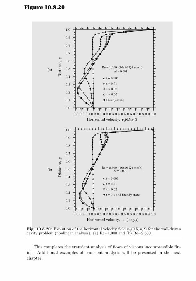
10.8. NUMERICAL EXAMPLES 569
-0.3-0.2-0.1 0.0 0.1 0.2 0.3 0.4 0.5 0.6 0.7 0.8 0.9 1.0
Horizontal velocity,
0.0
0.1
0.2
0.3
0.4
0.5
0.6
0.7
0.8
0.9
1.0
Dis
tan
ce,
t = 0.001
t = 0.01
t = 0.02
t = 0.05
Steady state
Re = 1,000 (16x20 Q4 mesh)
(b)
y
vx(0.5,y,t)
Δt = 0.001
-0.3-0.2-0.1 0.0 0.1 0.2 0.3 0.4 0.5 0.6 0.7 0.8 0.9 1.0
Horizontal velocity,
0.0
0.1
0.2
0.3
0.4
0.5
0.6
0.7
0.8
0.9
1.0
Dis
tan
ce,
t = 0.001
t = 0.01
t = 0.02
t = 0.1 and Steady state
Re = 2,500 (16x20 Q4 mesh)
(a)
y
vx(0.5,y,t)
Δt = 0.001
-
-
Figure 10.8.20
Fig. 10.8.20: Evolution of the horizontal velocity field vx(0.5, y, t) for the wall-drivencavity problem (nonlinear analysis). (a) Re=1,000 and (b) Re=2,500.
This completes the transient analysis of flows of viscous incompressible flu-ids. Additional examples of transient analysis will be presented in the nextchapter.
570 WEAK FORM FINITE ELEMENT MODELS OF INCOMPRESSIBLE FLUIDS
10.9 Non-Newtonian Fluids
10.9.1 Introduction
Some of the most challenging and important areas currently under investigationin computational fluid mechanics concern flows of non-Newtonian fluids (i.e.stresses are nonlinear functions of strain rates). Such fluids may or may nothave memory of past deformation (i.e. viscoelastic or not). Practical examplesof such fluids are multi-grade oils, liquid detergents, paints, and printing inks.Polymer solutions and polymer melts also fall within this category. All suchflows are extremely important in forming processes of various kinds applied tometals, plastics, or glass.
Numerical approaches used for analyzing flows of non-Newtonian fluids dif-fer very little from the ones used for Newtonian fluids. When the shear viscosityis a function of the rate of deformation tensor (i.e. for so-called power-law flu-ids), the equation of motion can still be written explicitly in terms of velocitycomponents. For such fluids, the same formulations as those of the Newtonianfluids can be used. For example, the pressure–velocity and penalty finite el-ement models discussed in the preceding sections can be used for power-lawfluids. The constitutive equations of a viscoelastic fluid can be described interms of the extra stress components and are given in terms of either differ-ential equations or integral equations. In a differential constitutive model, theextra stress components and their derivatives are related to the velocity compo-nents and their derivatives and, therefore, require us to treat stress componentsas independent variables along with the velocity components and pressure.
Most existing works in the finite element analysis of viscoelastic fluids haveconsidered different types of Maxwell/Oldroyd models, in which both viscosityand relaxation time are constants. The analysis was based on mixed formula-tions in which the velocities, pressure, and stresses are treated as nodal vari-ables. An important class of fluids, which are characterized by shear viscosityand elasticity require additional study from numerical simulation point of view.The viscoelastic effects along with memory effects of such fluids can be studiedusing the White–Metzner model (see [204–207]).
The objective of this section is to study penalty finite element models ofpower-law and viscoelastic White–Metzner type fluids [204–212]. As a part ofthis discussion, we present finite element models of equations governing flowsof viscous incompressible fluids through axisymmetric geometries. Therefore,first we rewrite the conservation of mass and momentum in the cylindricalcoordinate system.
10.9.2 Governing Equations in Cylindrical Coordinates
Equations (10.3.1)–(10.3.3) can be expressed in a cylindrical coordinate system,(r, θ, z), by writing all vectors and tensors, including the del operator, in terms of
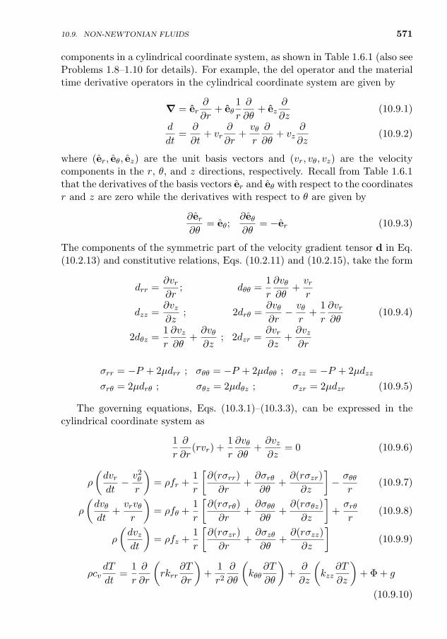
10.9. NON-NEWTONIAN FLUIDS 571
components in a cylindrical coordinate system, as shown in Table 1.6.1 (also seeProblems 1.8–1.10 for details). For example, the del operator and the materialtime derivative operators in the cylindrical coordinate system are given by
∇ = er∂
∂r+ eθ
1
r
∂
∂θ+ ez
∂
∂z(10.9.1)
d
dt=
∂
∂t+ vr
∂
∂r+vθr
∂
∂θ+ vz
∂
∂z(10.9.2)
where (er, eθ, ez) are the unit basis vectors and (vr, vθ, vz) are the velocitycomponents in the r, θ, and z directions, respectively. Recall from Table 1.6.1that the derivatives of the basis vectors er and eθ with respect to the coordinatesr and z are zero while the derivatives with respect to θ are given by
∂er∂θ
= eθ;∂eθ∂θ
= −er (10.9.3)
The components of the symmetric part of the velocity gradient tensor d in Eq.(10.2.13) and constitutive relations, Eqs. (10.2.11) and (10.2.15), take the form
drr =∂vr∂r
; dθθ =1
r
∂vθ∂θ
+vrr
dzz =∂vz∂z
; 2drθ =∂vθ∂r− vθ
r+
1
r
∂vr∂θ
(10.9.4)
2dθz =1
r
∂vz∂θ
+∂vθ∂z
; 2dzr =∂vr∂z
+∂vz∂r
σrr = −P + 2µdrr ; σθθ = −P + 2µdθθ ; σzz = −P + 2µdzz
σrθ = 2µdrθ ; σθz = 2µdθz ; σzr = 2µdzr (10.9.5)
The governing equations, Eqs. (10.3.1)–(10.3.3), can be expressed in thecylindrical coordinate system as
1
r
∂
∂r(rvr) +
1
r
∂vθ∂θ
+∂vz∂z
= 0 (10.9.6)
ρ
(dvrdt−v2θ
r
)= ρfr +
1
r
[∂(rσrr)
∂r+∂σrθ∂θ
+∂(rσzr)
∂z
]− σθθ
r(10.9.7)
ρ
(dvθdt
+vrvθr
)= ρfθ +
1
r
[∂(rσrθ)
∂r+∂σθθ∂θ
+∂(rσθz)
∂z
]+σrθr
(10.9.8)
ρ
(dvzdt
)= ρfz +
1
r
[∂(rσzr)
∂r+∂σzθ∂θ
+∂(rσzz)
∂z
](10.9.9)
ρcvdT
dt=
1
r
∂
∂r
(rkrr
∂T
∂r
)+
1
r2
∂
∂θ
(kθθ
∂T
∂θ
)+
∂
∂z
(kzz
∂T
∂z
)+ Φ + g
(10.9.10)
572 WEAK FORM FINITE ELEMENT MODELS OF INCOMPRESSIBLE FLUIDS
where the stress components are known in terms of the velocity componentsvia Eqs. (10.9.4) and (10.9.5). The viscous dissipation Φ is given by
Φ = 2µ(d2rr + d2
θθ + d2zz
)+ 4µ
(d2rθ + d2
rz + d2zθ
)(10.9.11)
Note that the time derivative of a vector (or tensor) in a rotating referenceframe is given by (see Reddy and Rasmussen [13], pp. 69–74)[
d(·)dt
]nonrot
=
[d(·)dt
]rot
+ ω × (·)
where ω = dθdt ez = vθ
r ez is the angular velocity vector of the rotating frame ofreference. Therefore, we have(
dv
dt
)nonrot
=
(dv
dt
)rot
+ (vθr
ez)× v
= er
(dvrdt− vθ
vθr
)+ eθ
(dvθdt
+ vrvθr
)+ ez
dvzdt
(10.9.12)
Equation (10.9.12) could be used in conjunction with Eqs. (10.9.6)–(10.9.11) toprovide a description of fluid motion in a rotating cylindrical coordinate system.
For axisymmetric conditions (i.e. all variables are independent of θ andfθ = vθ = 0), the governing equations are simplified to
1
r
∂
∂r(rvr) +
∂vz∂z
= 0 (10.9.13)
ρ
(∂vr∂t
+ vr∂vr∂r
+ vz∂vr∂z
)= ρfr +
1
r
∂(rσrr)
∂r+∂σzr∂z− σθθ
r(10.9.14)
ρ
(∂vz∂t
+ vr∂vz∂r
+ vz∂vz∂z
)= ρfz +
1
r
∂(rσzr)
∂r+∂σzz∂z
(10.9.15)
ρcv
(∂T
∂t+ vr
∂T
∂r+ vz
∂T
∂z
)=
1
r
∂
∂r
(rkrr
∂T
∂r
)+
∂
∂z
(kzz
∂T
∂z
)+ Φ + g
(10.9.16)
10.9.3 Power-Law Fluids
Many viscous fluids used in industrial applications are characterized by so-calledpower-law constitutive behavior. Power-law fluids exhibit nonlinear materialbehavior according to the relation (sum on i and j is implied)
σ = τ − P I, τ = 2µ(I2)D, µ = µ0 (I2)(n−1)
2
I2 =1
2
(d2rr + d2
θθ + d2zz
)+ drθdrθ + drzdrz + dθzdθz
(10.9.17)
where τ is the viscous part of the stress tensor σ, I is the unit tensor, I2
is the second invariant of d, and parameters µ0 and n characterize the fluid
10.9. NON-NEWTONIAN FLUIDS 573
(determined experimentally). For many non-Newtonian fluids, the viscosity µdecreases with increasing shear rate. These are called shear thinning fluids andhave the power law index n < 1. Fluids with power law index n > 1 are calledshear-thickening fluids. For such fluids, µ increases with increasing shear rate.For n = 1, Eq. (10.9.17) gives the Newtonian relation (µ = µ0, constant). Thepower-law constitutive relation in Eq. (10.9.17) makes the problem nonlinearfor n 6= 1, even for the case where the convective term v ·∇v is negligible.
To illustrate how the power-law constitutive equation affects the finite ele-ment equations, we consider steady, isothermal, axisymmetric flows of viscousincompressible fluids. Assuming negligible viscous dissipation and body forces,Eqs. (10.9.13)–(10.9.16) can be expressed in terms of (vr, vz) as
1
r
∂
∂r(rvr) +
∂vz∂z
= 0 (10.9.18)
ρ
(vr∂vr∂r
+ vz∂vr∂z
)=
1
r
∂
∂r
(2µr
∂vr∂r
)+
∂
∂z
[µ
(∂vr∂z
+∂vz∂r
)]− 2µ
vrr2− ∂P
∂r(10.9.19)
ρ
(vr∂vz∂r
+ vz∂vz∂z
)=
1
r
∂
∂r
[µr
(∂vr∂z
+∂vz∂r
)]+
∂
∂z
(2µ∂vz∂z
)− ∂P
∂z
(10.9.20)
The penalty-finite element model of Eqs. (10.9.18)–(10.9.20) can be ob-tained as before. After replacing P in Eqs. (10.9.19) and (10.9.20) with
P = −γp(∂vr∂r
+vrr
+∂vz∂z
)(10.9.21)
one may construct their weak forms and go on to develop the finite elementmodel [note that Eq. (10.9.18) is no longer used]. The value of the penaltyparameter γp that is most suitable for this class problems must be determinedby conducting numerical experiments with some benchmark problems. Thefinite element model has the form [see Eq. (10.5.18) or (10.5.24)]
[C(v) + Kµ + Kγ ]v = F or K(v)v = F (10.9.22)
where C, Kµ, and Kγ are the convective, diffusive, and penalty contributions,respectively, to the coefficient matrix. Because of the dependence of µ on v,both C and Kµ are functions of the unknown velocity field v, as can be seenfrom Eqs. (10.5.16) and (10.4.13).
The direct iteration scheme for this case is given by
K(v(r))vr+1 = F (10.9.23)
where K is evaluated using the viscosity µ = µ(Dij) computed according to Eq.(10.9.17) at the rth iteration. It would be more appropriate to compute µ at the
574 WEAK FORM FINITE ELEMENT MODELS OF INCOMPRESSIBLE FLUIDS
Gauss points of the element and use it in the evaluation of Kij , than to assumeµ is an element-wise constant. For example, consider the diffusion/viscousportion of the element coefficients K11
ij :
K11ij =
∫Ωeµ
(2∂ψi∂r
∂ψj∂r
+∂ψi∂z
∂ψj∂z
)r drdz (10.9.24)
For numerical evaluation of K11ij we use the Gauss quadrature rule
K11ij =
NGP∑I,J=1
AMU(I, J) ∗ [2.0 ∗GDSF (1, i) ∗GDSF (1, j)
+GDSF (2, i) ∗GDSF (2, j) ] ∗ CONST (10.9.25)
where AMU(I, J) is the value of µ at the (I, J)th Gauss point. Obviously,AMU(I, J) must be evaluated using Eq. (10.9.17) prior to using it in Eq.(10.9.25).
10.9.4 White–Metzner Fluids
The general constitutive equation for fluids dominated by shear viscosity isgiven by (see [204–206])
τ + λ
∂τ
∂t+ v ·∇τ − [(∇v)T · τ + τ · (∇v)]
= 2ηd (10.9.26)
where λ is the relaxation time, η is the shear viscosity of the fluid, and d is thesymmetric part of the velocity gradient tensor.
To characterize the White–Metzner fluid, it is necessary to know the viscos-ity curve as a function of shear rate and the first normal stress difference. Theextra stress tensor τ is separated into purely viscous part τ 2 and viscoelasticpart τ 1:
τ = τ 1 + τ 2 (10.9.27)
τ 1 + λ
∂τ 1
∂t+ v ·∇τ 1 −
[(∇v)T · τ 1 + τ 1 · (∇v)
]= 2η1d (10.9.28)
τ2 = 2η2d (10.9.29)
and η1 and η2 can be defined as the fractions of the shear viscosity η. Thefluid which obeys Eq. (10.9.27) is characterized by η1, η2, and λ, which are thefunctions of the symmetric part of the velocity gradient tensor, d.
Here, the relaxation time λ is assumed to depend on the shear rate γ ac-cording to
λ(γ) = a+ b(log γ) + c(log γ)2, γ =√
4I2 (10.9.30)
10.9. NON-NEWTONIAN FLUIDS 575
All constants in Eq. (10.9.30) are evaluated by curve fitting data of polymericmelts (see [208]). Also, η is assumed to be of the particular form
η = η(I2), I2 =1
2
(d2rr + d2
θθ + d2zz
)+ drθdrθ + drzdrz + dθzdθz (10.9.31)
Although Eq. (10.9.31) gives the general functional form for the viscosity func-tion, experimental observation and a theoretical basis must be used to providea specific model for non-Newtonian viscosities. A variety of models can beused to calculate viscosity. Here, the power law model in Eq. (10.9.17) is used(replace µ with η).
In view of Eq. (10.9.27), the equation of motion (in the absence of bodyforces) for the White–Metzner viscoelastic fluids can be written as
∇ · (τ 1 + 2η2d)−∇P = ρ
(∂v
∂t+ v ·∇v
)(10.9.32)
For simplicity, we drop the superscript 1 from τ 1 in Eq. (10.9.32) as well as inEq. (10.9.28). Equations (10.9.32) and (10.9.28), together with the continuityequation ∇ ·v = 0, represent the system of governing equations for the White–Metzner fluids. The viscosity η1 is calculated using Eq. (10.9.28) and λ fromEq. (10.9.30). Viscosity η2 is often taken as a function of η1. Note that thepower-law constitutive equation can be obtained as a special case from Eq.(10.9.28).
For axisymmetric flows of White–Metzner fluids, the governing equationsare given by (with u = vr and w = vz)
∂u
∂r+u
r+∂w
∂z= 0 (10.9.33)
∂
∂r
(τrr + 2η2
∂u
∂r
)+
1
r
(τrr + 2η2
∂u
∂r− τθθ − 2η2
u
r
)+
∂
∂z
[τrz + η2
(∂u
∂z+∂w
∂r
)]− ∂P
∂r= ρ
(∂u
∂t+ u
∂u
∂r+ w
∂u
∂z
)(10.9.34)
∂
∂r
[τrz + η2
(∂u
∂z+∂w
∂r
)]+
1
r
[τrz + η2
(∂u
∂z+∂w
∂r
)]+
∂
∂z
(τzz + 2η2
∂w
∂z
)− ∂P
∂z= ρ
(∂w
∂t+ u
∂w
∂r+ w
∂w
∂z
)(10.9.35)
τrr+λ
[∂τrr∂t
+ u∂τrr∂r
+ w∂τrr∂z− 2
(∂u
∂rτrr +
∂u
∂zτrz
)]= 2η1
∂u
∂r(10.9.36)
τzz+λ
[∂τzz∂t
+ u∂τzz∂r
+ w∂τzz∂z− 2
(∂w
∂zτzz +
∂w
∂rτrz
)]= 2η1
∂w
∂z(10.9.37)
576 WEAK FORM FINITE ELEMENT MODELS OF INCOMPRESSIBLE FLUIDS
τrz+λ
[∂τrz∂t
+ u∂τrz∂r
+ w∂τrz∂z− 2
(∂u
∂rτrz +
∂w
∂zτrz +
∂u
∂zτzz +
∂w
∂rτrr
)]= η1
(∂w
∂r+∂u
∂z
)(10.9.38)
τθθ + λ
[∂τθθ∂t
+ u∂τθθ∂r
+ w∂τθθ∂z− 2
u
rτθθ
]= 2η1
u
r(10.9.39)
where u and w denote the velocity components in the radial and axial directions,respectively.
The (mixed) penalty finite element model of the above equations can bedeveloped by constructing the weak forms of Eqs. (10.9.34)–(10.9.39) [afterreplacing the pressure with Eq. (10.9.21)] and interpolating velocities (u,w)and extra stress components (τrr, τθθ, τzz, τrz) as follows:
u(r, z, t) =
n∑j=1
uj(t)ψj(r, z), w(r, z, t) =
n∑j=1
wj(t)ψj(r, z)
τrr(r, z, t) =
L∑j=1
τ jrr(t)ψj(r, z), τzz(r, z, t) =
L∑j=1
τ jzz(t)ψj(r, z) (10.9.40)
τrz(r, z, t) =
L∑j=1
τ jrz(t)ψj(r, z), τθθ(r, z, t) =
L∑j=1
τ jθθ(t)ψj(r, z)
where, (uj , wj) are the nodal velocities, (τ jrr, τjzz, τ
jrz, τ
jθθ) are the nodal extra
stress components, and ψj are the Lagrange interpolation functions. The finiteelement model has the general form
Me∆e + Ke∆e = Fe (10.9.41)
where(∆e)T = u w τ rr τ zz τ rz τ θθ (10.9.42)
The nonzero coefficients of the matrices are listed below.
K11ij =
∫Ωe
[ρψi
(u∂ψj∂r
+ w∂ψj∂z
)+ η2
(2∂ψi∂r
∂ψj∂r
+∂ψi∂z
∂ψj∂z
+ 2ψiψjr2
)]r dr dz
+ γp
∫Ωe
1
r
∂(rψi)
∂r
∂(rψj)
∂rdr dz
K12ij =
∫Ωeη2∂ψi∂z
∂ψj∂r
r dr dz + γp
∫Ωe
∂(rψi)
∂r
∂ψj∂z
dr dz
K13ij =
∫Ωe
∂(rψi)
∂rψj dr dz, K15
ij =
∫Ωe
∂ψi∂z
ψj r dr dz, K16ij =
∫Ωeψiψj dr dz
K21ij =
∫Ωeη2
(∂ψi∂r
∂ψj∂z− 1
rψi∂ψj∂z
)r dr dz + γp
∫Ωe
∂ψi∂z
∂(rψj)
∂rdr dz
10.9. NON-NEWTONIAN FLUIDS 577
K22ij =
∫Ωe
[ρψi
(u∂ψj∂r
+ w∂ψj∂z
)+ η2
(∂ψi∂r
∂ψj∂r
+ 2∂ψi∂z
∂ψj∂z
)+ η2 ψi
∂ψj∂r
]r dr dz + γp
∫Ωe
∂ψi∂z
∂ψj∂z
r dr dz
K24ij =
∫Ωe
∂ψi∂z
ψj r dr dz, K25ij =
∫Ωe
∂(rψi)
∂rψj dr dz
K31ij = −2
∫Ωeη1ψi
∂ψj∂r
r dr dz, K35ij = −2
∫Ωeλ∂u
∂zψiψj r dr dz
K33ij =
∫Ωe
ψiψj + λ
[ψi
(u∂ψj∂r
+ w∂ψj∂z
)− 2
(∂u
∂r
)ψiψj
]r dr dz
K42ij = −2
∫Ωeη1ψi
∂ψj∂z
r dr dz
K44ij =
∫Ωe
ψiψj + λ
[ψi
(u∂ψj∂r
+ w∂ψj∂z
)− 2
∂w
∂zψiψj
]r dr dz
K45ij = −2
∫Ωeλ∂w
∂rψiψj r dr dz, K51
ij = −2
∫Ωeη1ψi
∂ψi∂z
r dr dz
K52ij = −2
∫Ωeη1ψi
∂ψj∂r
r dr dz, K53ij = −2
∫Ωeλ∂w
∂rψiψj r dr dz
K54ij = −2
∫Ωeλ∂u
∂zψiψj r dr dz, K61
ij = −2
∫Ωeη1ψiψj dr dz
K55ij =
∫Ωe
ψiψj + λ
[ψi
(u∂ψj∂r
+ w∂ψj∂z
)− 2
(∂u
∂r+∂w
∂z
)ψiψj
]r dr dz
K66ij =
∫Ωe
ψiψj + λ
[ψi
(u∂ψj∂r
+ w∂ψj∂z
)− 2
ruψiψj
]r dr dz
M11ij =
∫Ωeρψiψj r dr dz, M22
ij =
∫Ωeρψiψj r dr dz
M33ij =
∫Ωeλψiψj r dr dz, M44
ij =
∫Ωeλψiψj r dr dz
M55ij =
∫Ωeλψiψj r dr dz, M66
ij =
∫Ωeλψiψj r dr dz (10.9.43)
A bar over the velocities u and w indicate that they are calculated using thenodal values from the previous iteration.
For viscoelastic fluids, specification of velocities is insufficient on account offluid memory. If the boundary of the domain contains an entry region, then fullydeveloped flow conditions may be assumed. All extra stress components mustbe specified as essential boundary conditions along the entry region. Failing todo so may lead to the propagation of errors throughout the flow domain whenrelaxation time λ becomes large.
578 WEAK FORM FINITE ELEMENT MODELS OF INCOMPRESSIBLE FLUIDS
10.9.5 Numerical Examples
Consider the steady flow of a power-law fluid in a uniform pipe (R = 1, L = 6,w0 = 10, n = 0.2, µ0 = 1.0, and γp = 108). The geometry and boundaryconditions of the computational domain are shown in Fig. 10.9.1. Three dif-ferent meshes shown in Fig. 10.9.2 are used [208]. The finite element resultsobtained using the velocity finite element model in Eq. (10.9.22) along with theanalytical results for the axial velocities as a function of the radial distance arepresented in Table 10.9.1, where the analytical solution for the axial velocity is
w(r, L) = w0
(3n+ 1
n+ 1
)[1−
( rR
)1+ 1n
]Next, the same problem (with R = 1 and L = 5) is studied with the mixed
finite element model in Eq. (10.9.38). Both power-law (n = 0.25, η0 = 104,η2 = 0) and White–Metzner (n = 0.25, η0 = 104, η2 = 0, a = 0.435, b = −0.453,c = 0.1388) fluids are analyzed. A uniform mesh of 10×6, 4-node, quadrilateralelements is used. In addition to the velocity boundary conditions shown inFig. 10.9.1, the stresses are specified to be zero at the entrance. The penaltyparameter is taken to be γp = 108.
Figures 10.9.3 and 10.9.4 contain plots of the axial velocity profiles at z = 0,z = 2.0, and z = 5.0, for power-law and White–Metzner fluids, respectively. Wenote that the velocity profiles obtained with the velocity model (VM) in Eq.(10.9.22) and mixed model (MM) in Eq. (10.9.38) are essentially the same whenstress boundary conditions are not imposed. The stress boundary conditions(which can be imposed point-wise only in the mixed model) do have an effect:specification of the stresses at the inlet increases the centerline velocity forboth power-law fluids as well as White–Metzner fluids. If the stress boundaryconditions are not imposed, the mixed model for the White–Metzner fluid doesnot yield converged solution. Figure 10.9.5 shows the effect of the penaltyparameter on the velocity field.
z
u = w = 0
u = 0
u = 0w = w0
u = 0
r
L
Rz
r
Figure 10.9.1
Fig. 10.9.1: Geometry and boundary conditions for flow through a pipe.
10.9. NON-NEWTONIAN FLUIDS 579
Mesh 2: 6×10 (uniform)
Mesh 1: 3×5 (uniform)
Mesh 3: 12×15 (non-uniform)
Figure 10.9.2
Fig. 10.9.2: Three different meshes used for the pipe flow.
0.0
0.2
0.4
0.6
0.8
1.0
r
0.0 0.5 1.0
w(r, 0)
w(r, 2) w(r, 5)
0
0.2
0.4
0.6
0.8
1.0
0 0.5 1.0 1.5 2.0
r r
0.0 0.5 1.0 1.5 2.0
Axial velocity, w(r,z)
0.0
0.2
0.4
0.6
0.8
1.0
Nonlinear (MM) without SBCLinear (MM) with SBCNonlinear (MM) with SBC
°SBC = Stress boundary conditions
Linear (VM, MM) without SBCNonlinear (VM)
Figure 10.9.3
Fig. 10.9.3: Axial velocity profiles for the flow of power-law fluid through a pipe.
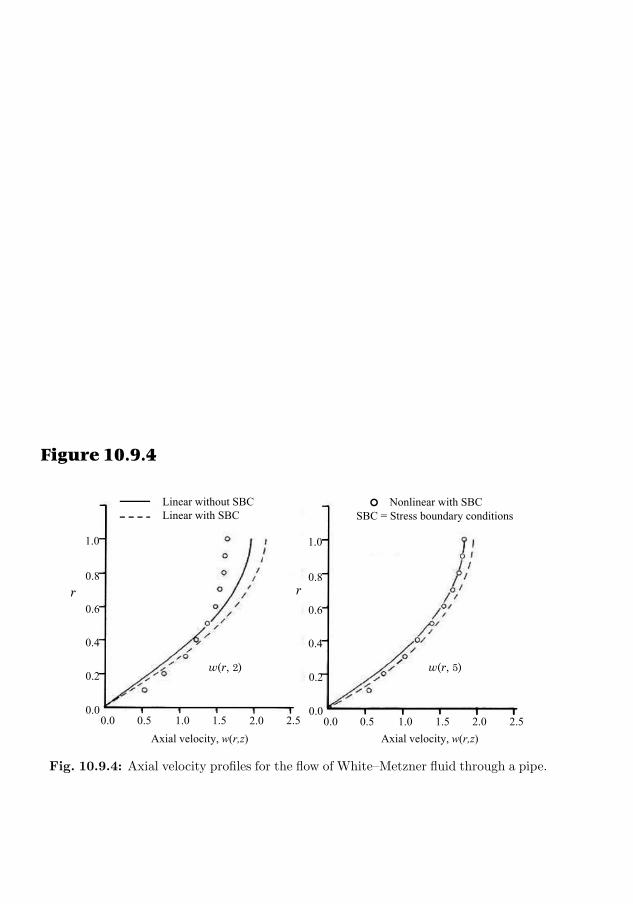
580 WEAK FORM FINITE ELEMENT MODELS OF INCOMPRESSIBLE FLUIDS
Table 10.9.1: A comparison of the velocity field w(r, 6) for the flow of a power-lawfluid in a pipe (R = 1, L = 6, w0 = 10, n = 0.2, µ0 = 1.0, and γp = 108).
r Mesh 1 Mesh2 Mesh 3 Analytical
0.00 11.894 12.833 13.402 13.3330.05 − − − 13.3330.10 − 12.832 13.401 13.3330.15 − − − 13.3330.20 11.865 12.826 13.395 13.3320.25 − − − 13.3300.30 − 12.795 13.360 13.3240.35 − − − 13.3090.40 11.721 12.686 13.243 13.2790.45 − − − 13.2230.50 − 12.401 12.940 13.1250.55 − − 12.679 12.9640.60 10.852 11.783 12.305 12.7110.65 − − 11.787 12.3280.70 − 10.610 11.086 11.7650.75 − − 10.156 10.9600.80 7.916 8.563 8.946 9.8380.85 − − 7.396 8.3050.90 − 5.133 5.451 6.2480.95 − − 2.993 3.5321.00 0.000 0.000 0.000 0.000
w(r, 2) w(r, 5)
r r
1.0
0.8
0.6
0.4
0.2
0.00.0 0.5 1.0 1.5 2.0 2.5
1.0
0.8
0.6
0.4
0.2
0.00.0 0.5 1.0 1.5 2.0 2.5
Axial velocity, w(r,z) Axial velocity, w(r,z)
Nonlinear with SBC°SBC = Stress boundary conditionsLinear without SBCLinear with SBC
Figure 10.9.4
Fig. 10.9.4: Axial velocity profiles for the flow of White–Metzner fluid through a pipe.
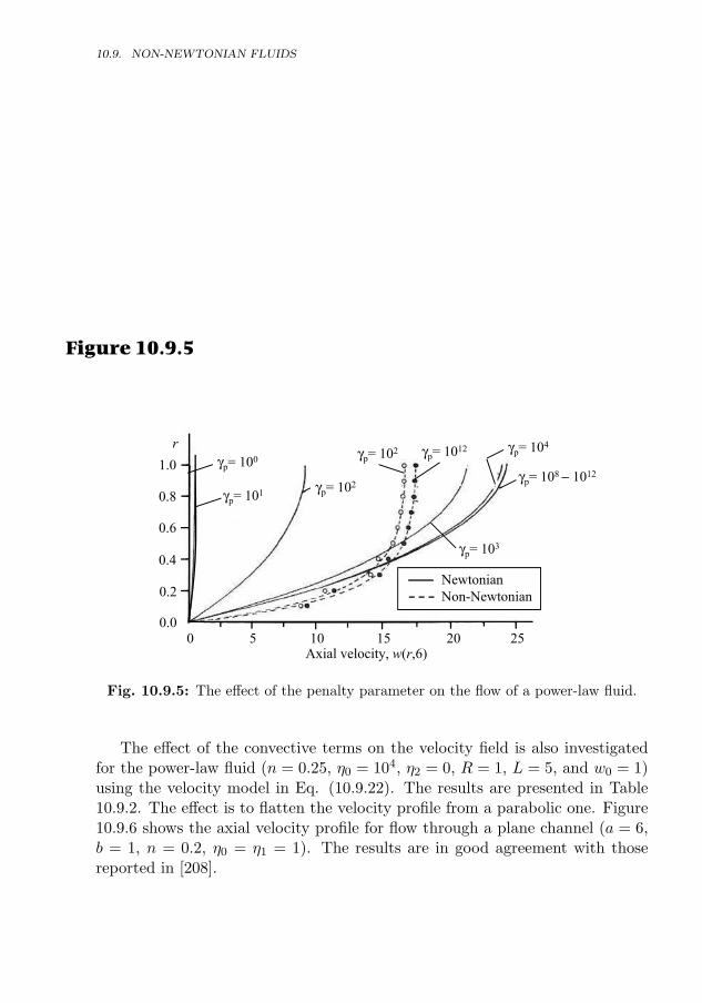
581
Table 10.9.2: Effect of the convective terms* on the velocity field w(r, 5) for the flowof a power-law fluid in a pipe (R = 1, L = 5, w0 = 10, n = 0.2, and 10× 6Q4 mesh).
r Newtonian Non-Newtonian
Re = 0 Re = 102 Re = 103
0.0 1.8358 1.3357 1.1312 1.02670.1 1.8001 1.3355 1.1302 1.02650.2 1.7398 1.3338 1.1289 1.02660.3 1.6461 1.3271 1.1270 1.02680.4 1.5186 1.3081 1.1241 1.02710.5 1.3578 1.2657 1.1197 1.02750.6 1.1651 1.1849 1.1097 1.02740.7 0.9397 1.0468 1.0799 1.02650.8 0.6712 0.8273 0.9809 1.02090.9 0.3079 0.4795 0.6709 0.89671.0 0.0000 0.0000 0.0000 0.0000
* Re = ρw0Rη0
0.0
0.2
0.4
0.6
0.8
1.0r
0 5 10 15 20 25Axial velocity, w(r,6)
γp= 100
γp= 101 γp= 102
γp= 102 γp= 1012
γp= 103
γp= 104
γp= 108 − 1012
NewtonianNon-Newtonian
Figure 10.9.5
Fig. 10.9.5: The effect of the penalty parameter on the flow of a power-law fluid.
The effect of the convective terms on the velocity field is also investigatedfor the power-law fluid (n = 0.25, η0 = 104, η2 = 0, R = 1, L = 5, and w0 = 1)using the velocity model in Eq. (10.9.22). The results are presented in Table10.9.2. The effect is to flatten the velocity profile from a parabolic one. Figure10.9.6 shows the axial velocity profile for flow through a plane channel (a = 6,b = 1, n = 0.2, η0 = η1 = 1). The results are in good agreement with thosereported in [208].
10.9. NON-NEWTONIAN FLUIDS
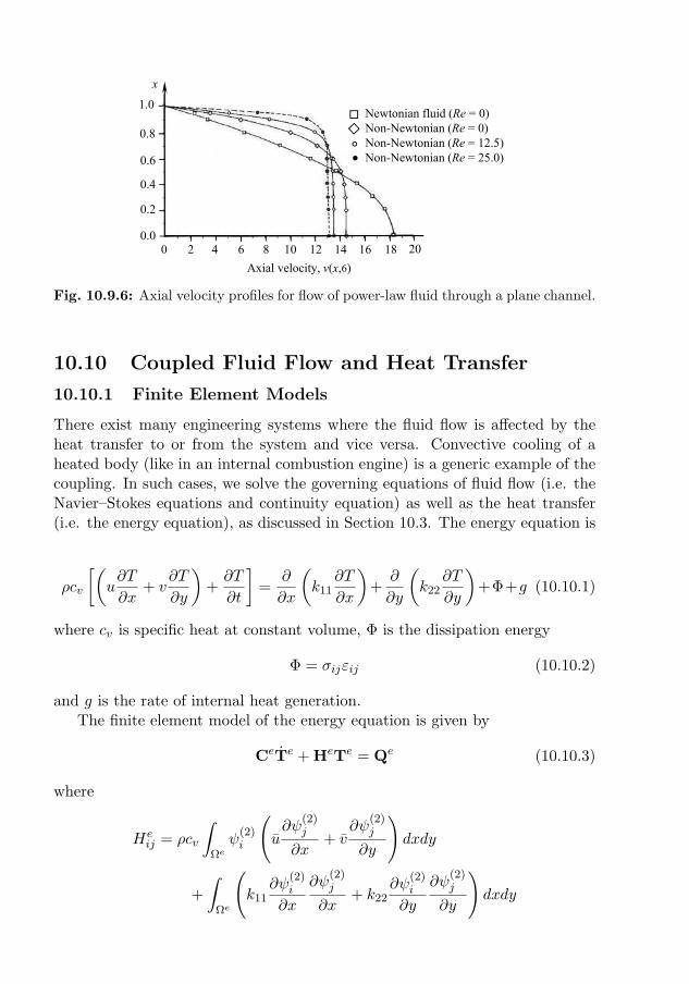
582 WEAK FORM FINITE ELEMENT MODELS OF INCOMPRESSIBLE FLUIDS
x
1.0
0.8
0.6
0.4
0.2
0.00 2 4 6 8 10 12 14 16 18 20
Axial velocity, v(x,6)
°•
Newtonian fluid (Re = 0)Non-Newtonian (Re = 0)Non-Newtonian (Re = 12.5)Non-Newtonian (Re = 25.0)
Fig. 10.9.6: Axial velocity profiles for flow of power-law fluid through a plane channel.
10.10 Coupled Fluid Flow and Heat Transfer
10.10.1 Finite Element Models
There exist many engineering systems where the fluid flow is affected by theheat transfer to or from the system and vice versa. Convective cooling of aheated body (like in an internal combustion engine) is a generic example of thecoupling. In such cases, we solve the governing equations of fluid flow (i.e. theNavier–Stokes equations and continuity equation) as well as the heat transfer(i.e. the energy equation), as discussed in Section 10.3. The energy equation isgiven by [see Eq. (10.3.3)]
ρcv
[(u∂T
∂x+ v
∂T
∂y
)+∂T
∂t
]=
∂
∂x
(k11
∂T
∂x
)+∂
∂y
(k22
∂T
∂y
)+Φ+g (10.10.1)
where cv is specific heat at constant volume, Φ is the dissipation energy
Φ = σijεij (10.10.2)
and g is the rate of internal heat generation.The finite element model of the energy equation is given by
CeTe + HeTe = Qe (10.10.3)
where
Heij = ρcv
∫Ωeψ
(2)i
(u∂ψ
(2)j
∂x+ v
∂ψ(2)j
∂y
)dxdy
+
∫Ωe
(k11
∂ψ(2)i
∂x
∂ψ(2)j
∂x+ k22
∂ψ(2)i
∂y
∂ψ(2)j
∂y
)dxdy
10.10. COUPLED FLUID FLOW AND HEAT TRANSFER 583
Ceij = ρcv
∫Ωeψ
(2)i ψ
(2)j dxdy
Qei =
∫Ωeψ
(2)i (g + Φ)dxdy +
∮Γeqnψ
(2)i ds (10.10.4)
u and v being the velocity components (that couple to the fluid flow problem),
and ψ(2)i the Lagrange interpolation functions used to interpolate the temper-
ature field.Equation (10.10.3) must be solved along with the flow equations
Me∆e + Ke∆e = Fe (10.10.5)
developed earlier. Both equations, Eqs. (10.10.3) and (10.10.5), must be solvediteratively, using the latest velocity field and temperature field to compute thecoefficient matrices. It should be noted that fluid flow equations are coupled tothe heat transfer equation through the body force terms fx and fy in the Navier–Stokes equations. For buoyancy-driven flows, the body force in the directionof the gravity is a function of the temperature, that is, fy = −ρagβ(T − T0)if the y-axis is taken vertically up, where ag is acceleration due to gravity andβ is thermal expansion coefficient. Thus, the momentum equations are fullycoupled with the energy equation.
The following strategy is found suitable for the convective heat transferproblems. Solve the energy equation, Eq. (10.10.3), with an assumed velocityfield (say, zero). Then use the assumed velocity and temperature fields in Eq.(10.10.5) and solve for the new velocity field. The initial guess of the velocityfield can be either the linear (Stokes) solution or the solution of a problemat lower Rayleigh number when solving for high Rayleigh number flows. TheRayleigh number Ra and Prandtl number Pr (characteristic numbers used inconvective heat transfer) are defined by
Ra =β ag L
3 ∆T
κ ν, ν =
µ
ρ, κ =
k
ρcp, P r =
ν
κ(10.10.6)
where L is the characteristic dimension of the flow region, ∆T is the temperaturedifference between hot and cold walls, ρ is the density, µ is the viscosity, k isthe conductivity, and cp is the specific heat at constant pressure.
10.10.2 Numerical Examples
Here we include a couple of sample problems, taken from Reddy and Gartling[10], to illustrate the ideas presented above.
10.10.2.1 Heated cavity
Consider a closed square cavity filled with a viscous incompressible fluid. Thetop and bottom faces of the cavity are assumed to be insulated while the vertical
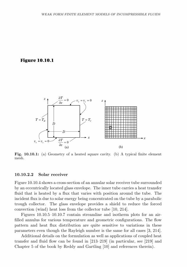
584
faces subjected to different temperatures, as shown in Fig. 10.10.1(a). A typical16× 16 mesh of eight-node quadratic elements is shown in Fig. 10.10.1(b).
This problem was solved using the earliest versions of NACHOS code [213],which is based on velocity–pressure (mixed) formulation and used the directiteration (Picard) scheme. More recent solutions have been obtained usingNewton’s method for the combined equation set equivalent to Eqs. (10.10.3)and (10.10.5). The streamline and isotherm plots are shown in Figs. 10.10.2and 10.10.3 for Rayleigh numbers of Ra = 104 and 106, respectively (Pr =ν/κ = 0.71). For the lower Rayleigh number, the flow is relatively weak andthe thermal field is only slightly perturbed from a conduction solution. At thehigher Rayleigh number, the flow field develops a considerable structure whilethe thermal field becomes vertically stratified in the core of the cavity with highheat flux regions along the vertical boundaries (see [213]).
x
z
••••••• •
D
D
HT T= CT T=
0Tz
∂ =∂
0Tz
∂ =∂
0x zv v= =
0x zv v= =z
x
(b)(a)
Figure 10.10.1
Fig. 10.10.1: (a) Geometry of a heated square cavity. (b) A typical finite elementmesh.
10.10.2.2 Solar receiver
Figure 10.10.4 shows a cross-section of an annular solar receiver tube surroundedby an eccentrically located glass envelope. The inner tube carries a heat transferfluid that is heated by a flux that varies with position around the tube. Theincident flux is due to solar energy being concentrated on the tube by a parabolictrough collector. The glass envelope provides a shield to reduce the forcedconvection (wind) heat loss from the collector tube [10, 214].
Figures 10.10.5–10.10.7 contain streamline and isotherm plots for an air-filled annulus for various temperature and geometric configurations. The flowpattern and heat flux distribution are quite sensitive to variations in theseparameters even though the Rayleigh number is the same for all cases [3, 214].
Additional details on the formulation as well as applications of coupled heattransfer and fluid flow can be found in [213–219] (in particular, see [219] andChapter 5 of the book by Reddy and Gartling [10] and references therein).
WEAK FORM FINITE ELEMENT MODELS OF INCOMPRESSIBLE FLUIDS
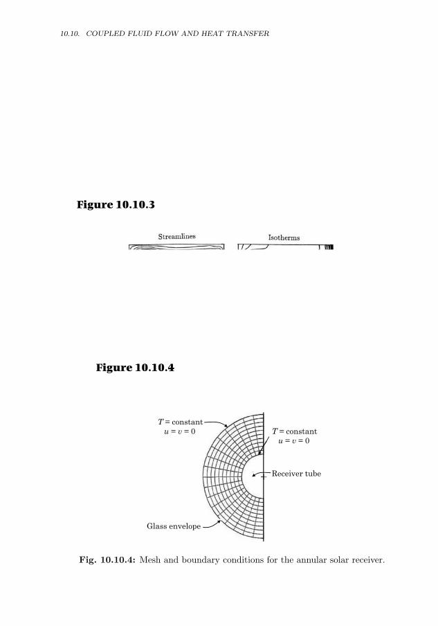
585
Figure 10.10.2
Fig. 10.10.2: Streamlines and isotherms for natural convection in a square cavityfilled with viscous fluid (Ra = 104, Pr = 0.71).
Figure 10.10.3
Fig. 10.10.3: Streamlines and isotherms for natural convection in a square cavityfilled with viscous fluid (Ra = 106, Pr = 0.71).
+
T = constantu = v = 0
Glass envelope
T = constantu = v = 0
Receiver tube
Figure 10.10.4
Fig. 10.10.4: Mesh and boundary conditions for the annular solar receiver.
10.10. COUPLED FLUID FLOW AND HEAT TRANSFER
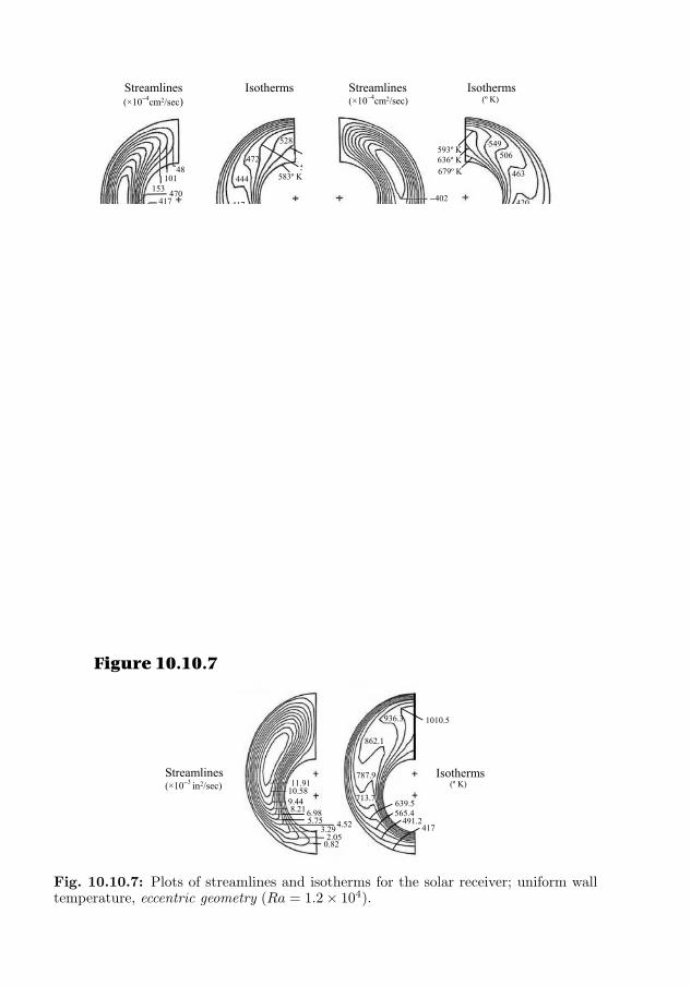
586 WEAK FORM FINITE ELEMENT MODELS OF INCOMPRESSIBLE FLUIDS
IsothermsStreamlines(×10−4cm2/sec)
(a)
48101
153 470417365
312259206
528
583º K
556º K472500º K
444
417
389
361
333
Streamlines(×10−4cm2/sec)
Isotherms
(b)
593º K
−402−357−312−266−221−176−132−86−41
636º K679º K
549506
463
420
377
(º K)
Fig. 10.10.5: Plots of streamlines and isotherms for the solar receiver: (a) uniformwall temperature, Ra = 1.2 × 10⁴ and (b) asymmetric wall temperature, hot on top(Ra = 1.2× 10⁴).
Streamlines
Figure 10.10.6
Isotherms
−2.33−1.25
−0.38−5.49×10⁻³
4.52 3.542.56
1.580.60
677.8
755.6833.2
911.1908.9
1066.7
1144.41222.2
(º K)
Fig. 10.10.6: Plots of streamlines and isotherms for the solar receiver; nonuniformwall temperature, hot on bottom (Ra = 1.2× 10⁴).
Streamlines(×10−3 in2/sec)
Isotherms
1010.5936.3
862.1
787.9
713.7 639.5565.4
491.2417
11.9110.589.448.216.98
5.75
0.82
4.522.05
3.29
Figure 10.10.7
(º K)
Fig. 10.10.7: Plots of streamlines and isotherms for the solar receiver; uniform walltemperature, eccentric geometry (Ra = 1.2× 10⁴).
10.11. SUMMARY 587
10.11 Summary
In this chapter, finite element models of flows of viscous incompressible fluids arepresented for Newtonian and non-Newtonian (power-law) fluids. Two differentfinite element models are formulated, namely, the mixed finite element modelinvolving velocities and pressure and the penalty finite element model thatinvolves only velocity degrees of freedom. A number of examples are presented.Formulation of the equations of motion for transient analysis is also discussed.Finally, finite element models of coupled fluid flow and heat transfer, using thepenalty method, accounting for buoyancy effects is presented and a number ofnumerical examples are included.
Problems
10.1 Consider the vector equations, Eqs. (10.3.1) and (10.3.2). Develop the weak statementsof the equations in vector form. Under what conditions can these equations be obtainedfrom the minimum of a quadratic functional? See Oden and Reddy [220] for details.
10.2 Consider Eqs. (10.4.1)–(10.4.3) in cylindrical coordinates (r, θ, z). For axisymmetricviscous incompressible flows (i.e. the flow field is independent of the θ coordinate), andwhen the convective (nonlinear) terms are neglected, we have
ρdvrdt
=1
r
∂
∂r(rσrr)−
σθθr
+∂σrz∂z
+ fr (1)
ρdvzdt
=1
r
∂
∂r(rσrz) +
∂σzz∂z
+ fz (2)
0 =1
r
∂
∂r(rvr) +
∂vz∂z
(3)
where
σrr = −P + 2µ∂vr∂r
, σθθ = −P + 2µvrr
σz = −P + 2µ∂vz∂z
, σrz = µ
(∂vr∂z
+∂vz∂r
) (4)
and (vr, vz) are the components of the velocity vector v = ervr + ezvz. Develop thesemidiscrete mixed finite element model of the equations.
10.3 Develop the semidiscrete penalty finite element model of the equations in Problem 10.2.
10.4 The equations governing unsteady slow flow (i.e. Stokes flow) of viscous incompressiblefluids in the x-y plane can be expressed in terms of vorticity ω and stream function ψ:
ρ∂ω
∂t− µ∇2ω = 0 (1)
−ω −∇2ψ = 0 (2)
Develop the semidiscrete finite element model of the equations. Discuss the meaningof the secondary variables. Use the α-family of approximation to reduce the ordinarydifferential equations to algebraic equations.
10.5 Compute the tangent coefficient matrix for the penalty finite element model in Eq.(10.5.16).
10.6 Verify Eqs. (10.9.7)–(10.9.9).
10.7 Carry out steady-state analysis of the lid-driven cavity problem (see Example 10.8.4)for Re=5,000 using the 16 × 20 mesh of bilinear elements. Use DX(I) and DY (I) as

588 WEAK FORM FINITE ELEMENT MODELS OF INCOMPRESSIBLE FLUIDS
given in Example 10.8.6. You may experiment with the acceleration parameter β (forconvergence) and use a convergence tolerance of 10−2. Plot the horizontal velocity vx atthe vertical centerline of the cavity versus the coordinate y for the linear and nonlinearcases. Note that you must pick ρ and µ to obtain the desired Reynolds number.
10.8 Carry out the transient analysis of the lid-driven cavity of Problem 10.7. Use the data
of Example 10.8.6.
589
11
Least-Squares Finite ElementModels of Flows of Viscous
Incompressible Fluids
Let the mind be enlarged, according to its capacity, to the grandeur of the mysteries, and notthe mysteries contracted to the narrowness of the mind. ——– Francis Bacon
11.1 Introduction
Finite element models based on least-squares method often offer an appealingalternative to the more popular weak-form Galerkin approach used for flows ofviscous incompressible fluids. Although not as popular as weak-form Galerkinformulations, least-squares models of partial differential equations have beenan active field of research since at least the early 1970’s [221–223]. In 1976,Eason [49] compiled an extensive review containing well over 200 references toleast-squares methods as applied to the solution of partial differential equations.Since the publication of this review article, least-squares finite element modelshave continued to receive substantial attention and discussion in the literature.
Least-squares variational formulations allow us to define an unconstrainedconvex least-squares functional J (u) in terms of the sum of the squares of thenorms of the partial differential equation residuals [38], where standard Sobolevnorms are employed (e.g. norms associated with L2(Ω) or Hk(Ω), where k ∈ N).If the governing equations (augmented by the appropriate boundary conditions)are well posed, it can be readily shown that the exact solution coincides withthe minimizer of the least-squares functional. As a result, in the least-squaresmethod the variational problem is obtained via direct minimization of J (u). Inthe case of linear differential equations, it is always possible to associate withthe least-squares functional a well-defined energy norm ‖u‖E . If it can be shownthat the energy norm induced by the least-squares functional is equivalent toan appropriate standard norm, such as the H1(Ω) norm, optimal convergencerates can be established for the least-squares finite element model. Under suchconditions the least-squares finite element formulation constitutes an ideal vari-ational setting, regardless of whether such a setting is achieved by the associatedweak-form Galerkin finite element formulation [39].
J.N. Reddy, An Introduction to Nonlinear Finite Element Analysis, Second Edition. c©J.N.Reddy 2015. Published in 2015 by Oxford University Press.
590 LEAST-SQUARES FE MODELS OF VISCOUS INCOMPRESSIBLE FLUIDS
To maintain practicality in the numerical implementation, it becomes com-putationally advantageous to construct the least-squares functional in termsof the sum of the squares of the L2(Ω) norms of the first-order form of thepartial differential equation residuals. Regrettably, it is not always possibleto establish a priori norm equivalence (or H1(Ω)-coercivity) of the resultingleast-squares formulation. As identified by Bochev [224] using Agmon, Douglis,and Nirenberg (ADN) elliptic theory [225], it is typically possible to constructa least-squares functional that is H1(Ω)-coercive [39, 222, 226, 227]. Unfor-tunately, the optimal choice of norms can: (a) depend on the nature of theboundary conditions of a given problem and (b) result in an unattractive com-putational implementation. It is important to note that departure from theideal variational setting (i.e. using a least-squares functional that is non-H1(Ω)-coercive) does not typically result in disastrous consequences for least-squaresfinite element models. Even when a given formulation is non-H1(Ω)-coercive,the least-squares finite element model always: (a) possesses the best approx-imation property with respect to a well-defined norm (i.e. the energy norm‖u‖E) and (b) avoids restrictive compatibility requirements on the finite ele-ment function spaces (i.e. the discrete inf-sup condition never arises). Thatthe least-squares method is always based on a minimization principle ensuresa robust setting that is often lacking in Galerkin based weak formulations.It is well known, however, that non-H1(Ω)-coercive low-order finite elementimplementations are often prone to locking whenever full numerical integrationtechniques are employed in evaluating the coefficient matrices. In the context ofthe Navier–Stokes equations, it has been shown that such issues may be largelyavoided through the use of collocation or selective reduced integration strategies(see Jiang and his colleagues [38, 179, 228–230]). On the other hand, the com-bination of high-order finite element technology with least-squares variationalprinciples has also shown great promise in recent years. In particular, buildingoff of the earlier work of Jiang and Sonnad [229], Bell and Surana [231, 232],Gerrtisma and coworkers [233–237], Pontaza and Reddy [43, 44, 238], Prab-hakar and Reddy [45, 239, 240], Prabhakar, Pontaza, and Reddy [241], andPayette and Reddy [50] have demonstrated numerically that hp-least-squaresfinite element models are capable of yielding highly accurate results even whenthe least-squares functional cannot be shown to be H1(Ω)-coercive a priori.
Least-squares finite element models offer several additional attractive fea-tures as compared with weak-form Galerkin formulations. In the case of lin-ear analysis, the least-squares formulation always admits a symmetric positive-definite (SPD) coefficient matrix, regardless of whether or not such symmetry ismanifest in the governing partial differential equations. As a result, extremelyrobust direct as well as iterative solution algorithms (such as the preconditionedconjugate gradient method) can be employed in the solution process and onlyhalf of the global coefficient matrix need be stored in memory. This is not thecase when the weak-form Galerkin scheme is applied to non-self-adjoint systems
11.1. INTRODUCTION 591
of equations. As mentioned previously, the least-squares formulation does notsuffer from the restrictive inf-sup condition [242, 243]. This is highly desirablein the numerical discretization of fluid mechanics problems, as it allows the ve-locity and pressure to be approximated using the same bases of interpolation.Finally, least-squares formulations are also free from the need for numerical dis-sipation through the use of upwind techniques. As a result, ad hoc stabilizationis not needed in the analysis of convection dominated problems [38].
Least-squares formulations are certainly not without their own deficiencies.Most problems in physics possess at the very minimum second-order spatial dif-ferential operators. Since no weakening of these operators is typically possiblethrough the employment of Green’s identities (as can be readily accomplished inweak form Galerkin formulations), least-squares models typically require higherregularity of the approximate solution within each element. Higher regularityrequirements negatively affect the condition number of the coefficient matrixand also the continuity requirement of the solution across element boundaries.High regularity requirements may be avoided by constructing the least-squaresfinite element model in terms of an equivalent lower-order system by the in-troduction of additional independent auxiliary variables [38]. The resultingmixed formulation permits the use of standard Lagrange interpolation func-tions and also improves the conditioning of the global coefficient matrix [244,245]. However, such benefits are gained at the expense of an increase in sizeof the global system of equations. It can be argued that such a formulationis at least somewhat useful, however, as the auxiliary variables often representimportant physical quantities of interest (e.g. the heat flux, vorticity, stress,etc.).
Other drawbacks to least-squares formulations, in the context of fluid me-chanics, include lack of local mass conservation and poor coupling betweenthe velocity and pressure in transient problems [246]. This is especially truewhenever low-order elements are employed in a given finite element discretiza-tion. The discrete violation of the requirement that the velocity be a solenoidalvector is often attributed to the fact that, in least-squares formulations, localsatisfaction of the governing PDEs is sacrificed in favor of global minimizationof the governing equation residuals [247]. In transient flow problems, lack ofvelocity–pressure coupling has also been identified as a source for poor localmass conservation [248]. We must emphasize that the violation is not merelynumerical noise and, depending on the nature of the domain and boundaryconditions, can actually be quite substantial [247].
Several techniques have been proposed to improve local mass conservationin least-squares finite element models. For example, Deang and Gunzburger[246] advocated weighting the continuity equation residual in the definition ofthe least-squares functional, where the chosen weight may be either uniformacross the whole problem domain or distinct for each element. Chang andNelson [247], on the other hand, combined the least-squares method with La-
592 LEAST-SQUARES FE MODELS OF VISCOUS INCOMPRESSIBLE FLUIDS
grange multipliers to exactly enforce element-level mass conservation. In thisapproach the continuity equation is treated as an additional constraint for eachelement that is enforced in the discrete setting through a set of NE Lagrangemultipliers. Although successful, this approach comes at the expense of in-creasing the system size of the finite element equations and compromising theunconstrained minimization setting that is so attractive for least-squares finiteelement models. Heys et al. [249] demonstrated improved mass balance usinga least-squares functional based on a novel first-order reformulation of the in-compressible Navier–Stokes equations. It is worth noting that increasing thep-level also tends to improves mass conservation, as demonstrated by Pontazaand Reddy [238].
For non-stationary flows, lack of strong velocity–pressure coupling can alsocompromise local mass conservation and further lead to total instability inspace-time decoupled finite element simulations [238]. Pontaza [250] showedthat the employment of a regularized form of the continuity equation in least-squares formulations can greatly enhance velocity–pressure coupling and as adirect consequence local mass conservation. Similar approaches have also beenadvocated in the iterative penalty formulations of Prabhakar and Reddy [239,240]. For a more mathematical analysis of such optimization methods as appliedto the Stokes problem, one may consult the book of Bochev and Gunzburger[39].
In this chapter1 we consider the least-squares finite element formulation ofthe Navier–Stokes equations governing viscous incompressible fluids. An L2-norm based least-squares functional is constructed as a (possibly, a weighted)sum of the norms of the residuals in the governing equations due to the approx-imation of the dependent unknowns. Weak forms are obtained by minimizingthe least-squares functional with respect to each of the dependent variable.When the governing equations are nonlinear (i.e. the least-squares functionalis cubic or higher-order function of the dependent unknowns), the weak formsare obtained via direct minimization of the least-squares functional with theaid of the Gateaux derivative. Although, in theory, the least-squares princi-ple requires that minimization ought to be performed prior to linearization,such an approach is often impractical and not necessary. We illustrate thedifferences between the various linearization schemes adopted in the abstractformulation, by numerically solving several nonlinear two-dimensional verifi-cation benchmark boundary-value problems using least-squares finite elementmodels.
1This chapter is based on the dissertation of the author’s graduate student, Dr. GregoryPayette, Spectral/hp Finite Element Models for Fluids and Structures, Texas A&M Univer-sity, College Station, May 2012; also, see [161].
11.2. LEAST-SQUARES FINITE ELEMENT FORMULATION 593
11.2 Least-Squares Finite Element Formulation
11.2.1 The Navier–Stokes Equations of Incompressible Fluids
We next turn our attention to the incompressible form of the stationary Navier–Stokes equations, which constitutes a very popular application for least-squaresvariational principles. The classical problem for the non-dimensional form ofthe incompressible Navier–Stokes equations can be stated as follows: find thevelocity vector v(x) and pressure P (x) such that
v ·∇v = −∇P +1
Re∇ · (∇v + ∇vT) + b in Ω (11.2.1a)
∇ · v = 0 in Ω (11.2.1b)
v = vp on ΓD (11.2.1c)
n · σ = tp on ΓN (11.2.1d)
where Re is the Reynolds number, b is the body force, σ is the Cauchy stresstensor, and n is the outward unit normal. The Cauchy stress is given in termsof the following constitutive equation
σ = −P I +1
Re(∇v + ∇vT) (11.2.2)
There are many first-order formulations of the Navier–Stokes equations thathave been presented in the literature that can be used to construct finite elementmodels of least-squares type. One of the most popular schemes is the velocity–pressure–vorticity (v, P,ω) formulation. In this formulation the vorticity vectorω = ∇× v is introduced, along with the vector identity
∇× (∇× v) = −∇2v + ∇(∇ · v) (11.2.3)
As a result, the original problem can be restated as one of finding the velocityv(x), pressure P (x), and vorticity ω(x) such that
v ·∇v + ∇P +1
Re∇× ω = b in Ω (11.2.4a)
ω −∇× v = 0 in Ω (11.2.4b)
∇ · v = 0 in Ω (11.2.4c)
v = vp on Γv (11.2.4d)
ω = ωp on Γω (11.2.4e)
n · σ = tp on ΓN (11.2.4f)
where ΓD has been partitioned such that ΓD = Γv⋃
Γω and Γv⋂
Γω = ∅. Wenote that the incompressibility constraint has been imposed in the construction
594 LEAST-SQUARES FE MODELS OF VISCOUS INCOMPRESSIBLE FLUIDS
of the momentum equation. The pseudo-traction boundary condition tp is givenin terms of the pseudo-stress tensor σ defined as
σ = −P I +1
Re∇v (11.2.5)
For three-dimensional analysis it is helpful to augment the above equations bythe compatibility condition ∇ · ω = 0.
We associate with the stationary first-order form of the incompressibleNavier–Stokes equations the following true least-squares functional
J (v, P,ω; b, tp) =1
2
(‖v ·∇v + ∇P +
1
Re∇× ω − b‖2Ω,0 + ‖∇ · v‖2Ω,0
+‖ω −∇× v‖2Ω,0)
(11.2.6)
The outflow boundary condition may also be directly accounted for in the def-inition of the least-squares functional. Linearized versions of the least-squaresfunctional may be obtained by replacing the nonlinear convective term withfollowing Picard or Newton approximations:
v ·∇v|Pic = v0 ·∇v (11.2.7a)
v ·∇v|New = v ·∇v0 + v0 ·∇v − v0 ·∇v0 (11.2.7b)
The linearized least-squares based weak form resulting from invoking the mini-mization principle may be stated as follows: find u ∈ V such that for all δu ∈ Wthe following expression holds:
B(δu,u) = F(δu) (11.2.8)
where u = (v, P,ω), δu = (δv, δP, δω), and V and W are appropriate functionspaces. The forms B(δu,u) and F(δu) are
B(δu,u) =
∫Ω
[(v0 ·∇δv + ∇δP +
1
Re∇× δω
)·(
v0 ·∇v + ∇P
+1
Re∇× ω
)+ (∇ · δv)(∇ · v) + (δω −∇× δv) · (ω −∇× v)
+ (δv ·∇v0) · (v ·∇v0)
]dΩ (11.2.9a)
F(δu) =
∫Ω
[(v0 ·∇δv + ∇δp+
1
Re∇× δω
)· b− (δv ·∇v0)·(
∇p0 +1
Re∇× ω0 − b
)]dΩ (11.2.9b)
when the Picard linearization scheme is employed, and
B(δu,u) =
∫Ω
[(δv ·∇v0 + v0 ·∇δv + ∇δP +
1
Re∇× δω
)·
11.2. LEAST-SQUARES FINITE ELEMENT FORMULATION 595(v ·∇v0 + v0 ·∇v + ∇P +
1
Re∇× ω
)+ (∇ · δv)(∇ · v)
+ (δω −∇× δv) · (ω −∇× v) + (δv ·∇v + v ·∇δv)·(v0 ·∇v0 + ∇p0 +
1
Re∇× ω0 − b
)]dΩ (11.2.10a)
F(δu) =
∫Ω
[(δv ·∇v0 + v0 ·∇δv + ∇δP +
1
Re∇× ω
)· (b + v0 ·∇v0)
+ (δv ·∇v0 + v0 ·∇δv) ·(
v0 ·∇v0 + ∇p0 +1
Re∇× ω0 − b
)]dΩ
(11.2.10b)
when Newton’s method is applied. The underlined terms appear when mini-mization is performed prior to linearization.
11.2.2 Numerical Examples
11.2.2.1 Low Reynolds number flow past a circular cylinder
In this example we consider flow past a circular cylinder, a problem that hasbeen studied extensively by way of experiment [251–253] and is a standardbenchmark for numerical computation [254–256]. It is well-known from bothexperimentation [253] and numerical modeling [257] that for moderately lowReynolds numbers (5 < Re < 46.1) the flow is spatially stationary and char-acterized by two symmetric regions of circulation directly downwind of thecylinder. The size of the standing vortices in the wake region is proportional tothe Reynolds number.
Ideally we would like to model the flow in a manner such that the effectsdue to the truncation of the problem’s infinite domain to a finite computationaldomain do not corrupt the numerical solution. To this end we take Ω to be theset difference between the rectangular region [−25, 25]× [−15, 15] and an opencircular region with unit diameter centered about the origin. The computationaldomain Ωhp ∼= Ω consists of 240 nonuniform finite elements, with 15 elementlayers in the radial direction and 16 along the circumference of the cylinder, asshown in Fig. 11.2.1. The smallest elements are placed in the vicinity of thecylinder to ensure adequate numerical resolution in the anticipated wake region.The mesh geometry is characterized using an isoparametric formulation which,when combined with high-order finite element technology, allows for a highlyaccurate approximation of the cylinder surface. As in the Poisson benchmarkproblem, we refine the mesh by systematically increasing the p-level of the finiteelement approximation functions. We consider the cases where p = 2, 4, 6, and8; which amounts to 3,968, 15,616, 34,944, and 61,952 total degrees of freedomfor each corresponding finite element discretization. The outflow boundarycondition is enforced weakly through the least-squares functional with tp taken
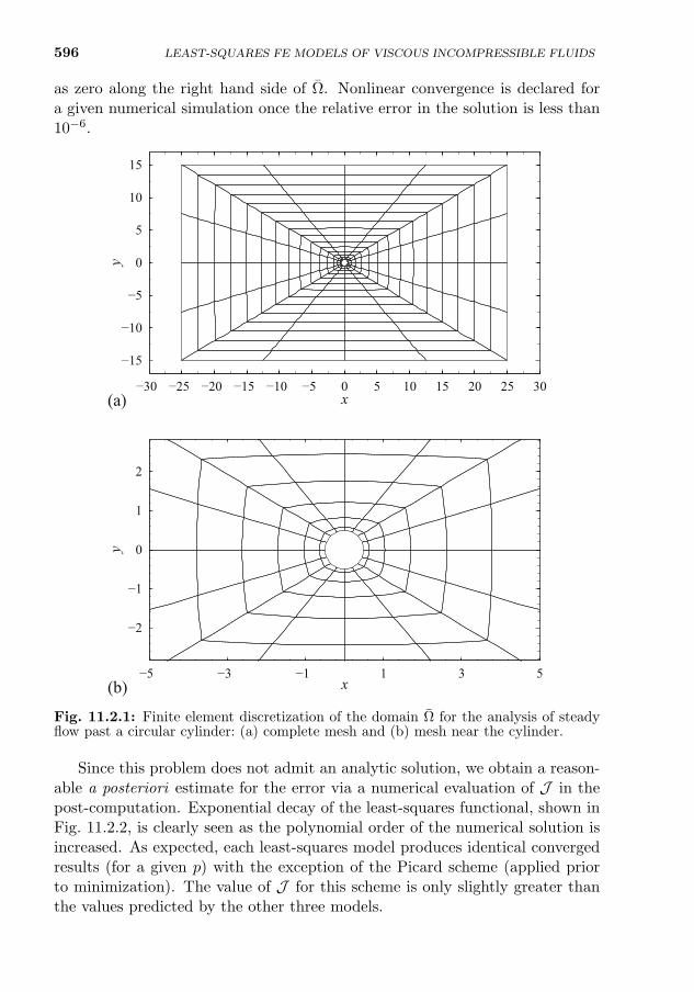
596 LEAST-SQUARES FE MODELS OF VISCOUS INCOMPRESSIBLE FLUIDS
as zero along the right hand side of Ω. Nonlinear convergence is declared fora given numerical simulation once the relative error in the solution is less than10−6.
−30 −25 −20 −15 −10 −5 0 5 10 15 20 25 30
−15
−10
−5
0
5
10
15
x
y
−5 −3 −1 1 3 5
−2
−1
0
1
2
x
y
(a)
(b)
Fig. 11.2.1: Finite element discretization of the domain Ω for the analysis of steadyflow past a circular cylinder: (a) complete mesh and (b) mesh near the cylinder.
Since this problem does not admit an analytic solution, we obtain a reason-able a posteriori estimate for the error via a numerical evaluation of J in thepost-computation. Exponential decay of the least-squares functional, shown inFig. 11.2.2, is clearly seen as the polynomial order of the numerical solution isincreased. As expected, each least-squares model produces identical convergedresults (for a given p) with the exception of the Picard scheme (applied priorto minimization). The value of J for this scheme is only slightly greater thanthe values predicted by the other three models.
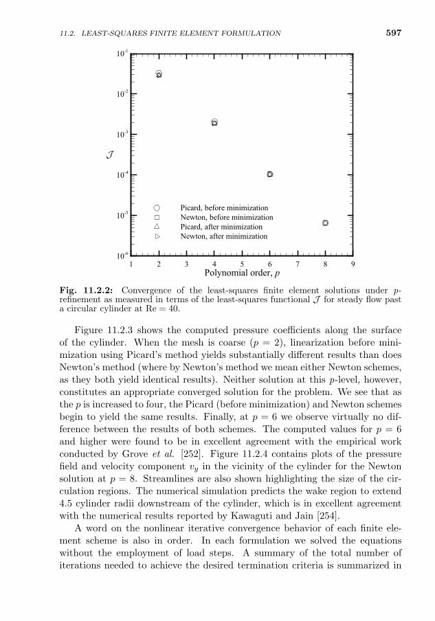
597
Polynomial order, p
J
1 2 3 4 5 6 7 8 910-6
10-5
10-4
10-3
10-2
10-1
Picard, before minimizationNewton, before minimizationPicard, after minimizationNewton, after minimization
Fig. 11.2.2: Convergence of the least-squares finite element solutions under p-refinement as measured in terms of the least-squares functional J for steady flow pasta circular cylinder at Re = 40.
Figure 11.2.3 shows the computed pressure coefficients along the surfaceof the cylinder. When the mesh is coarse (p = 2), linearization before mini-mization using Picard’s method yields substantially different results than doesNewton’s method (where by Newton’s method we mean either Newton schemes,as they both yield identical results). Neither solution at this p-level, however,constitutes an appropriate converged solution for the problem. We see that asthe p is increased to four, the Picard (before minimization) and Newton schemesbegin to yield the same results. Finally, at p = 6 we observe virtually no dif-ference between the results of both schemes. The computed values for p = 6and higher were found to be in excellent agreement with the empirical workconducted by Grove et al. [252]. Figure 11.2.4 contains plots of the pressurefield and velocity component vy in the vicinity of the cylinder for the Newtonsolution at p = 8. Streamlines are also shown highlighting the size of the cir-culation regions. The numerical simulation predicts the wake region to extend4.5 cylinder radii downstream of the cylinder, which is in excellent agreementwith the numerical results reported by Kawaguti and Jain [254].
A word on the nonlinear iterative convergence behavior of each finite ele-ment scheme is also in order. In each formulation we solved the equationswithout the employment of load steps. A summary of the total number ofiterations needed to achieve the desired termination criteria is summarized in
11.2. LEAST-SQUARES FINITE ELEMENT FORMULATION
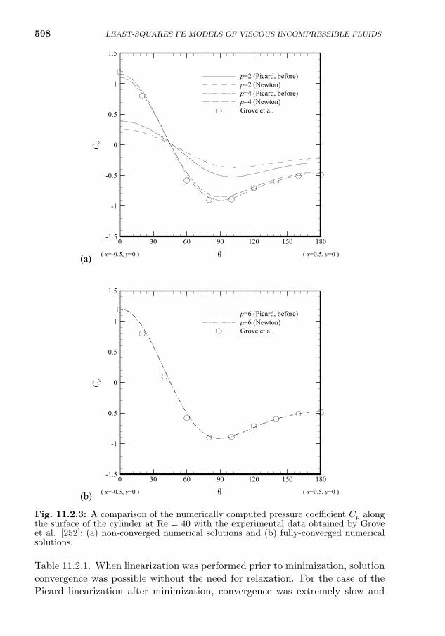
598 LEAST-SQUARES FE MODELS OF VISCOUS INCOMPRESSIBLE FLUIDS
(b) ( x=-0.5, y=0 ) ( x=0.5, y=0 )θ
Cp
0 30 60 90 120 150 180-1.5
-1
-0.5
0
0.5
1
1.5
p=6 (Picard, before)p=6 (Newton)Grove et al.
(a) ( x=-0.5, y=0 ) ( x=0.5, y=0 )θ
Cp
0 30 60 90 120 150 180-1.5
-1
-0.5
0
0.5
1
1.5
p=2 (Picard, before)p=2 (Newton)p=4 (Picard, before)p=4 (Newton)Grove et al.
Fig. 11.2.3: A comparison of the numerically computed pressure coefficient Cp alongthe surface of the cylinder at Re = 40 with the experimental data obtained by Groveet al. [252]: (a) non-converged numerical solutions and (b) fully-converged numericalsolutions.
Table 11.2.1. When linearization was performed prior to minimization, solutionconvergence was possible without the need for relaxation. For the case of thePicard linearization after minimization, convergence was extremely slow and
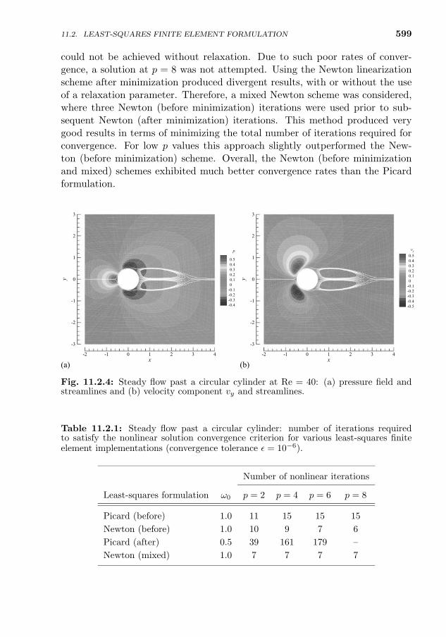
11.2. LEAST-SQUARES FINITE ELEMENT FORMULATION 599
could not be achieved without relaxation. Due to such poor rates of conver-gence, a solution at p = 8 was not attempted. Using the Newton linearizationscheme after minimization produced divergent results, with or without the useof a relaxation parameter. Therefore, a mixed Newton scheme was considered,where three Newton (before minimization) iterations were used prior to sub-sequent Newton (after minimization) iterations. This method produced verygood results in terms of minimizing the total number of iterations required forconvergence. For low p values this approach slightly outperformed the New-ton (before minimization) scheme. Overall, the Newton (before minimizationand mixed) schemes exhibited much better convergence rates than the Picardformulation.
(a)x
y
-2 -1 0 1 2 3 4
-3
-2
-1
0
1
2
3
p
0.50.40.30.20.10
-0.1-0.2-0.3-0.4
(b)x
y
-2 -1 0 1 2 3 4
-3
-2
-1
0
1
2
3
vy0.50.40.30.20.10
-0.1-0.2-0.3-0.4-0.5
Fig. 11.2.4: Steady flow past a circular cylinder at Re = 40: (a) pressure field andstreamlines and (b) velocity component vy and streamlines.
Table 11.2.1: Steady flow past a circular cylinder: number of iterations requiredto satisfy the nonlinear solution convergence criterion for various least-squares finiteelement implementations (convergence tolerance ε = 10−6).
Number of nonlinear iterations
Least-squares formulation ω0 p = 2 p = 4 p = 6 p = 8
Picard (before) 1.0 11 15 15 15
Newton (before) 1.0 10 9 7 6
Picard (after) 0.5 39 161 179 –
Newton (mixed) 1.0 7 7 7 7
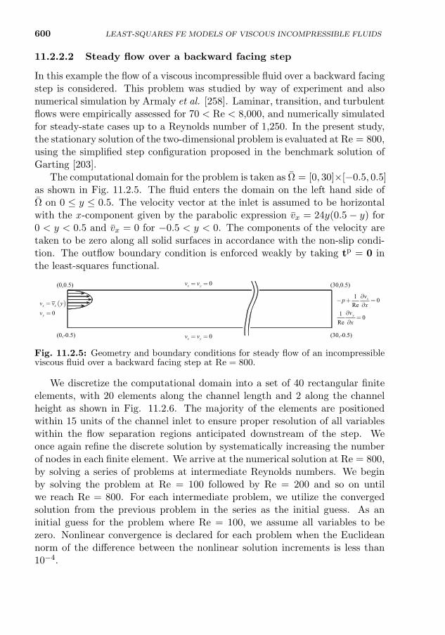
600
11.2.2.2 Steady flow over a backward facing step
In this example the flow of a viscous incompressible fluid over a backward facingstep is considered. This problem was studied by way of experiment and alsonumerical simulation by Armaly et al. [258]. Laminar, transition, and turbulentflows were empirically assessed for 70 < Re < 8,000, and numerically simulatedfor steady-state cases up to a Reynolds number of 1,250. In the present study,the stationary solution of the two-dimensional problem is evaluated at Re = 800,using the simplified step configuration proposed in the benchmark solution ofGarting [203].
The computational domain for the problem is taken as Ω = [0, 30]×[−0.5, 0.5]as shown in Fig. 11.2.5. The fluid enters the domain on the left hand side ofΩ on 0 ≤ y ≤ 0.5. The velocity vector at the inlet is assumed to be horizontalwith the x -component given by the parabolic expression vx = 24y(0.5− y) for0 < y < 0.5 and vx = 0 for −0.5 < y < 0. The components of the velocity aretaken to be zero along all solid surfaces in accordance with the non-slip condi-tion. The outflow boundary condition is enforced weakly by taking tp = 0 inthe least-squares functional.
(0,-0.5)
(0,0.5)
(30,-0.5)
(30,0.5)
1 0Re
1 0Re
x
y
vpx
vx
∂− + =
∂∂=
∂
( )0
x x
y
v v yv=
=
0x yv v= =
0x yv v= =
Fig. 11.2.5: Geometry and boundary conditions for steady flow of an incompressibleviscous fluid over a backward facing step at Re = 800.
We discretize the computational domain into a set of 40 rectangular finiteelements, with 20 elements along the channel length and 2 along the channelheight as shown in Fig. 11.2.6. The majority of the elements are positionedwithin 15 units of the channel inlet to ensure proper resolution of all variableswithin the flow separation regions anticipated downstream of the step. Weonce again refine the discrete solution by systematically increasing the numberof nodes in each finite element. We arrive at the numerical solution at Re = 800,by solving a series of problems at intermediate Reynolds numbers. We beginby solving the problem at Re = 100 followed by Re = 200 and so on untilwe reach Re = 800. For each intermediate problem, we utilize the convergedsolution from the previous problem in the series as the initial guess. As aninitial guess for the problem where Re = 100, we assume all variables to bezero. Nonlinear convergence is declared for each problem when the Euclideannorm of the difference between the nonlinear solution increments is less than10−4.
LEAST-SQUARES FE MODELS OF VISCOUS INCOMPRESSIBLE FLUIDS
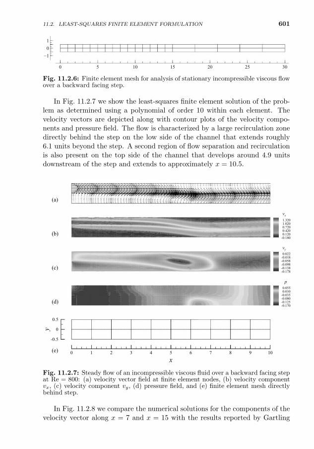
11.2. LEAST-SQUARES FINITE ELEMENT FORMULATION 601
0 5 10 15 20 25 30
−101
Fig. 11.2.6: Finite element mesh for analysis of stationary incompressible viscous flowover a backward facing step.
In Fig. 11.2.7 we show the least-squares finite element solution of the prob-lem as determined using a polynomial of order 10 within each element. Thevelocity vectors are depicted along with contour plots of the velocity compo-nents and pressure field. The flow is characterized by a large recirculation zonedirectly behind the step on the low side of the channel that extends roughly6.1 units beyond the step. A second region of flow separation and recirculationis also present on the top side of the channel that develops around 4.9 unitsdownstream of the step and extends to approximately x = 10.5.
x
y
0 1 2 3 4 5 6 7 8 9 10
-0.5
0
0.5
(a)
(b)
(c)
(d)
(e)
p0.0550.010
-0.035-0.080-0.125-0.170
vy0.022
-0.018-0.058-0.098-0.138-0.178
vx1.3201.0200.7200.4200.120
-0.180
Fig. 11.2.7: Steady flow of an incompressible viscous fluid over a backward facing stepat Re = 800: (a) velocity vector field at finite element nodes, (b) velocity componentvx, (c) velocity component vy, (d) pressure field, and (e) finite element mesh directlybehind step.
In Fig. 11.2.8 we compare the numerical solutions for the components of thevelocity vector along x = 7 and x = 15 with the results reported by Gartling
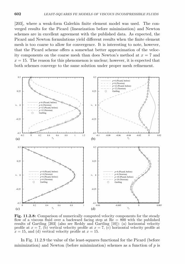
602 LEAST-SQUARES FE MODELS OF VISCOUS INCOMPRESSIBLE FLUIDS
[203], where a weak-form Galerkin finite element model was used. The con-verged results for the Picard (linearization before minimization) and Newtonschemes are in excellent agreement with the published data. As expected, thePicard and Newton formulations yield different results when the finite elementmesh is too coarse to allow for convergence. It is interesting to note, however,that the Picard scheme offers a somewhat better approximation of the veloc-ity components on the coarse mesh than does Newton’s method at x = 7 andx = 15. The reason for this phenomenon is unclear; however, it is expected thatboth schemes converge to the same solution under proper mesh refinement.
vx
y
0 0.2 0.4 0.6 0.8 1-0.5
-0.25
0
0.25
0.5
p=4 (Picard, before)p=4 (Newton)p=6 (Picard, before)p=6 (Newton)Gartling
vy
y
-0.01 -0.005 0 0.005-0.5
-0.25
0
0.25
0.5
p=4 (Picard, before)p=4 (Newton)p=10 (Picard, before)p=10 (Newton)Gartling
vx
y
-0.2 0 0.2 0.4 0.6 0.8 1 1.2-0.5
-0.25
0
0.25
0.5
p=6 (Picard, before)p=6 (Newton)p=12 (Picard, before)p=12 (Newton)Gartling
vy
y
-0.1 -0.08 -0.06 -0.04 -0.02 0 0.02-0.5
-0.25
0
0.25
0.5p=6 (Picard, before)p=6 (Newton)p=12 (Picard, before)p=12 (Newton)Gartling
(a) (b)
(c) (d)
Fig. 11.2.8: Comparison of numerically computed velocity components for the steadyflow of a viscous fluid over a backward facing step at Re = 800 with the publishedresults of Gartling [203] (also see Reddy and Gartling [10]): (a) horizontal velocityprofile at x = 7, (b) vertical velocity profile at x = 7, (c) horizontal velocity profile atx = 15, and (d) vertical velocity profile at x = 15.
In Fig. 11.2.9 the value of the least-squares functional for the Picard (beforeminimization) and Newton (before minimization) schemes as a function of p is
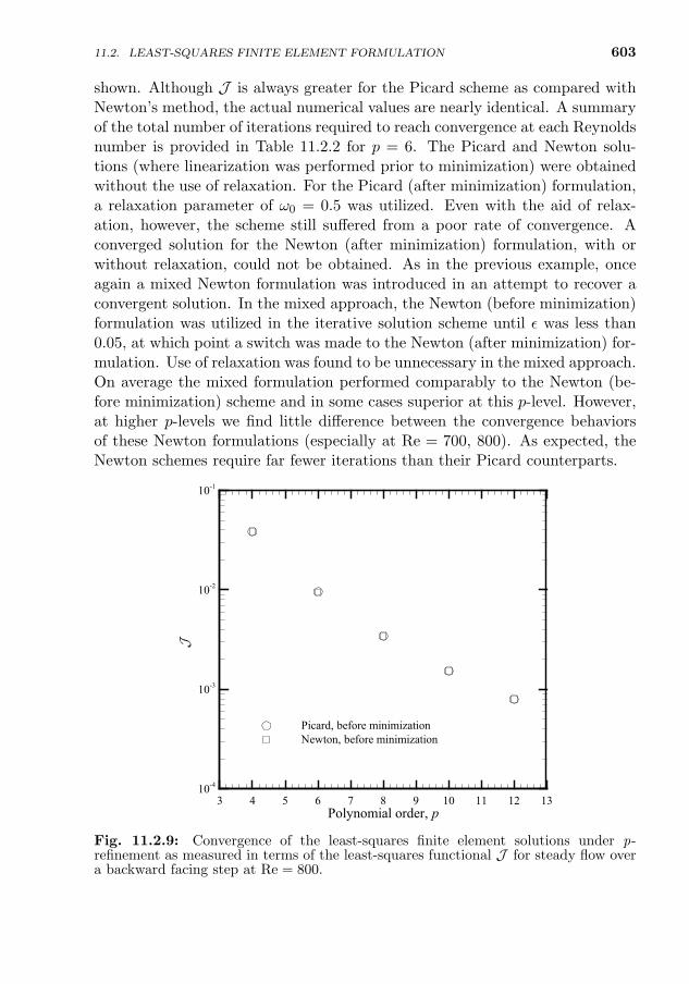
11.2. LEAST-SQUARES FINITE ELEMENT FORMULATION 603
shown. Although J is always greater for the Picard scheme as compared withNewton’s method, the actual numerical values are nearly identical. A summaryof the total number of iterations required to reach convergence at each Reynoldsnumber is provided in Table 11.2.2 for p = 6. The Picard and Newton solu-tions (where linearization was performed prior to minimization) were obtainedwithout the use of relaxation. For the Picard (after minimization) formulation,a relaxation parameter of ω0 = 0.5 was utilized. Even with the aid of relax-ation, however, the scheme still suffered from a poor rate of convergence. Aconverged solution for the Newton (after minimization) formulation, with orwithout relaxation, could not be obtained. As in the previous example, onceagain a mixed Newton formulation was introduced in an attempt to recover aconvergent solution. In the mixed approach, the Newton (before minimization)formulation was utilized in the iterative solution scheme until ε was less than0.05, at which point a switch was made to the Newton (after minimization) for-mulation. Use of relaxation was found to be unnecessary in the mixed approach.On average the mixed formulation performed comparably to the Newton (be-fore minimization) scheme and in some cases superior at this p-level. However,at higher p-levels we find little difference between the convergence behaviorsof these Newton formulations (especially at Re = 700, 800). As expected, theNewton schemes require far fewer iterations than their Picard counterparts.
Polynomial order, p
J
3 4 5 6 7 8 9 10 11 12 1310-4
10-3
10-2
10-1
Picard, before minimizationNewton, before minimization
Fig. 11.2.9: Convergence of the least-squares finite element solutions under p-refinement as measured in terms of the least-squares functional J for steady flow overa backward facing step at Re = 800.
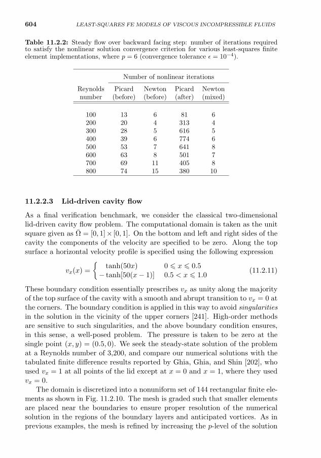
604 LEAST-SQUARES FE MODELS OF VISCOUS INCOMPRESSIBLE FLUIDS
Table 11.2.2: Steady flow over backward facing step: number of iterations requiredto satisfy the nonlinear solution convergence criterion for various least-squares finiteelement implementations, where p = 6 (convergence tolerance ε = 10−4).
Number of nonlinear iterations
Reynolds Picard Newton Picard Newtonnumber (before) (before) (after) (mixed)
100 13 6 81 6200 20 4 313 4300 28 5 616 5400 39 6 774 6500 53 7 641 8600 63 8 501 7700 69 11 405 8800 74 15 380 10
11.2.2.3 Lid-driven cavity flow
As a final verification benchmark, we consider the classical two-dimensionallid-driven cavity flow problem. The computational domain is taken as the unitsquare given as Ω = [0, 1]× [0, 1]. On the bottom and left and right sides of thecavity the components of the velocity are specified to be zero. Along the topsurface a horizontal velocity profile is specified using the following expression
vx(x) =
tanh(50x) 0 6 x 6 0.5− tanh[50(x− 1)] 0.5 < x 6 1.0
(11.2.11)
These boundary condition essentially prescribes vx as unity along the majorityof the top surface of the cavity with a smooth and abrupt transition to vx = 0 atthe corners. The boundary condition is applied in this way to avoid singularitiesin the solution in the vicinity of the upper corners [241]. High-order methodsare sensitive to such singularities, and the above boundary condition ensures,in this sense, a well-posed problem. The pressure is taken to be zero at thesingle point (x, y) = (0.5, 0). We seek the steady-state solution of the problemat a Reynolds number of 3,200, and compare our numerical solutions with thetabulated finite difference results reported by Ghia, Ghia, and Shin [202], whoused vx = 1 at all points of the lid except at x = 0 and x = 1, where they usedvx = 0.
The domain is discretized into a nonuniform set of 144 rectangular finite ele-ments as shown in Fig. 11.2.10. The mesh is graded such that smaller elementsare placed near the boundaries to ensure proper resolution of the numericalsolution in the regions of the boundary layers and anticipated vortices. As inprevious examples, the mesh is refined by increasing the p-level of the solution
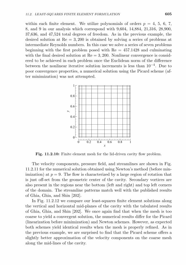
605
within each finite element. We utilize polynomials of orders p = 4, 5, 6, 7,8, and 9 in our analysis which correspond with 9,604, 14,884, 21,316, 28,900,37,636, and 47,524 total degrees of freedom. As in the previous example, thedesired solution at Re = 3, 200 is obtained by solving a series of problems atintermediate Reynolds numbers. In this case we solve a series of seven problemsbeginning with the first problem posed with Re = 457.1428 and culminatingwith the final desired solution at Re = 3, 200. Nonlinear convergence is consid-ered to be achieved in each problem once the Euclidean norm of the differencebetween the nonlinear iterative solution increments is less than 10−4. Due topoor convergence properties, a numerical solution using the Picard scheme (af-ter minimization) was not attempted.
x
y
0 0.2 0.4 0.6 0.8 10
0.2
0.4
0.6
0.8
1
Fig. 11.2.10: Finite element mesh for the lid-driven cavity flow problem.
The velocity components, pressure field, and streamlines are shown in Fig.11.2.11 for the numerical solution obtained using Newton’s method (before min-imization) at p = 9. The flow is characterized by a large region of rotation thatis just off-set from the geometric center of the cavity. Secondary vortices arealso present in the regions near the bottom (left and right) and top left cornersof the domain. The streamline patterns match well with the published resultsof Ghia, Ghia, and Shin [202].
In Fig. 11.2.12 we compare our least-squares finite element solutions alongthe vertical and horizontal mid-planes of the cavity with the tabulated resultsof Ghia, Ghia, and Shin [202]. We once again find that when the mesh is toocoarse to yield a convergent solution, the numerical results differ for the Picard(linearization before minimization) and Newton schemes. However, as expectedboth schemes yield identical results when the mesh is properly refined. As inthe previous example, we are surprised to find that the Picard scheme offers aslightly better approximation of the velocity components on the coarse meshalong the mid-lines of the cavity.
11.2. LEAST-SQUARES FINITE ELEMENT FORMULATION
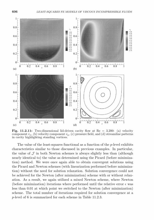
606
(a)
(c)
x0 0.2 0.4 0.6 0.8 10
0.2
0.4
0.6
0.8
1
vx
0.900.780.660.540.420.300.180.06
-0.06-0.18-0.30-0.42
x0 0.2 0.4 0.6 0.8 10
0.2
0.4
0.6
0.8
1
p0.700.620.540.460.380.300.220.140.06
-0.02-0.10
(b)
(d)
x0 0.2 0.4 0.6 0.8 10
0.2
0.4
0.6
0.8
1
vy0.400.300.200.100.00
-0.10-0.20-0.30-0.40-0.50-0.60-0.70
x0 0.2 0.4 0.6 0.8 10
0.2
0.4
0.6
0.8
1
Fig. 11.2.11: Two-dimensional lid-driven cavity flow at Re = 3,200: (a) velocitycomponent vx, (b) velocity component vy, (c) pressure field, and (d) streamline patternsin cavity highlighting standing vortices.
The value of the least-squares functional as a function of the p-level exhibitscharacteristics similar to those discussed in previous examples. In particular,the value of J in both Newton schemes is always slightly less than (althoughnearly identical to) the value as determined using the Picard (before minimiza-tion) method. We were once again able to obtain convergent solutions usingthe Picard and Newton schemes (with linearization performed before minimiza-tion) without the need for solution relaxation. Solution convergence could notbe achieved for the Newton (after minimization) scheme with or without relax-ation. As a result, we again utilized a mixed Newton scheme, where Newton(before minimization) iterations where performed until the relative error ε wasless than 0.01 at which point we switched to the Newton (after minimization)scheme. The total number of iterations required for solution convergence at ap-level of 6 is summarized for each scheme in Table 11.2.3.
LEAST-SQUARES FE MODELS OF VISCOUS INCOMPRESSIBLE FLUIDS
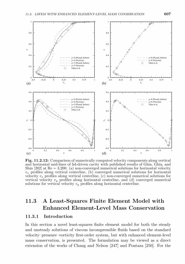
607
(a) (b)
(c) (d)
vx
y
-0.5 -0.25 0 0.25 0.5 0.75 10
0.2
0.4
0.6
0.8
1
p=4 (Picard, before)p=4 (Newton)p=5 (Picard, before)p=5 (Newton)Ghia et al.
vx
y
-0.5 -0.25 0 0.25 0.5 0.75 10
0.2
0.4
0.6
0.8
1
p=8 (Picard, before)p=8 (Newton)Ghia et at.
x
v y
0 0.2 0.4 0.6 0.8 1-0.6
-0.4
-0.2
0
0.2
0.4
0.6
p=4 (Picard, before)p=4 (Newton)p=5 (Picard, before)p=5 (Newton)Ghia et al.
x
v y
0 0.2 0.4 0.6 0.8 1-0.6
-0.4
-0.2
0
0.2
0.4
0.6
p=8 (Picard, before)p=8 (Newton)Ghia et al.
Fig. 11.2.12: Comparison of numerically computed velocity components along verticaland horizontal mid-lines of lid-driven cavity with published results of Ghia, Ghia, andShin [202] at Re = 3,200: (a) non-converged numerical solutions for horizontal velocityvx profiles along vertical centerline, (b) converged numerical solutions for horizontalvelocity vx profiles along vertical centerline, (c) non-converged numerical solutions forvertical velocity vy profiles along horizontal centerline, and (d) converged numericalsolutions for vertical velocity vy profiles along horizontal centerline.
11.3 A Least-Squares Finite Element Model withEnhanced Element-Level Mass Conservation
11.3.1 Introduction
In this section a novel least-squares finite element model for both the steadyand unsteady solutions of viscous incompressible fluids based on the standardvelocity–pressure–vorticity first-order system, but with enhanced element-levelmass conservation, is presented. The formulation may be viewed as a directextension of the works of Chang and Nelson [247] and Pontaza [250]. For the
11.3. LSFEM WITH ENHANCED ELEMENT-LEVEL MASS CONSERVATION
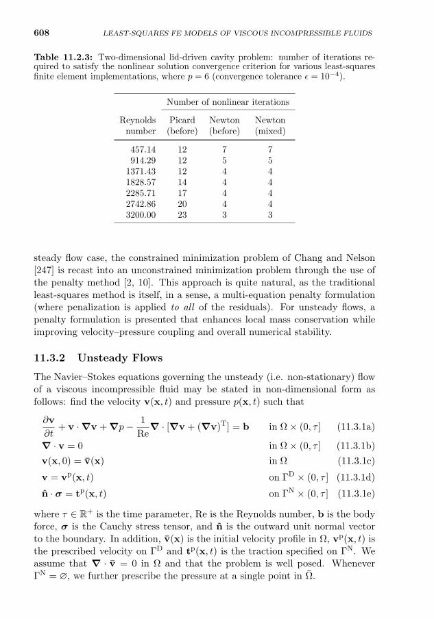
608 LEAST-SQUARES FE MODELS OF VISCOUS INCOMPRESSIBLE FLUIDS
Table 11.2.3: Two-dimensional lid-driven cavity problem: number of iterations re-quired to satisfy the nonlinear solution convergence criterion for various least-squaresfinite element implementations, where p = 6 (convergence tolerance ε = 10−4).
Number of nonlinear iterations
Reynolds Picard Newton Newtonnumber (before) (before) (mixed)
457.14 12 7 7914.29 12 5 5
1371.43 12 4 41828.57 14 4 42285.71 17 4 42742.86 20 4 43200.00 23 3 3
steady flow case, the constrained minimization problem of Chang and Nelson[247] is recast into an unconstrained minimization problem through the use ofthe penalty method [2, 10]. This approach is quite natural, as the traditionalleast-squares method is itself, in a sense, a multi-equation penalty formulation(where penalization is applied to all of the residuals). For unsteady flows, apenalty formulation is presented that enhances local mass conservation whileimproving velocity–pressure coupling and overall numerical stability.
11.3.2 Unsteady Flows
The Navier–Stokes equations governing the unsteady (i.e. non-stationary) flowof a viscous incompressible fluid may be stated in non-dimensional form asfollows: find the velocity v(x, t) and pressure p(x, t) such that
∂v
∂t+ v ·∇v + ∇p− 1
Re∇ · [∇v + (∇v)T] = b in Ω× (0, τ ] (11.3.1a)
∇ · v = 0 in Ω× (0, τ ] (11.3.1b)
v(x, 0) = v(x) in Ω (11.3.1c)
v = vp(x, t) on ΓD × (0, τ ] (11.3.1d)
n · σ = tp(x, t) on ΓN × (0, τ ] (11.3.1e)
where τ ∈ R+ is the time parameter, Re is the Reynolds number, b is the bodyforce, σ is the Cauchy stress tensor, and n is the outward unit normal vectorto the boundary. In addition, v(x) is the initial velocity profile in Ω, vp(x, t) isthe prescribed velocity on ΓD and tp(x, t) is the traction specified on ΓN. Weassume that ∇ · v = 0 in Ω and that the problem is well posed. WheneverΓN = ∅, we further prescribe the pressure at a single point in Ω.
11.3. LSFEM WITH ENHANCED ELEMENT-LEVEL MASS CONSERVATION 609
11.3.2.1 The velocity–pressure–vorticity first-order system
As discussed in Section 11.2, the Navier–Stokes equations as expressed in termsof the primitive variables v(x, t) and p(x, t) are ill-suited for direct implemen-tation in a least-squares finite element formulation. To allow for the use ofC0 basis functions in the numerical implementation we introduce the vorticityvector ω = ∇×v to allow us to recast the Navier–Stokes equations in terms ofan equivalent first-order system, which amounts to finding the velocity v(x, t),pressure p(x, t), and vorticity ω(x, t) such that
∂v
∂t+ v ·∇v + ∇p+
1
Re∇× ω = b in Ω× (0, τ ] (11.3.2a)
∇ · v = 0 in Ω× (0, τ ] (11.3.2b)
ω −∇× v = 0 in Ω× (0, τ ] (11.3.2c)
v(x, 0) = v(x) in Ω (11.3.2d)
v = vp(x, t) on Γv × (0, τ ] (11.3.2e)
ω = ωp(x, t) on Γω × (0, τ ] (11.3.2f)
n · σ = tp(x, t) on ΓN × (0, τ ] (11.3.2g)
In the above expressions ωP(x, t) is the prescribed vorticity on Γω, σ = −P I +1/Re∇v is the pseudo stress tensor and tp(x, t) is the pseudo traction vectorspecified on ΓN. The Dirichlet part of the boundary has been partitioned suchthat ΓD = Γv
⋃Γω and Γv
⋂Γω = ∅. The expression ∇(∇ · v) has been
eliminated from the momentum equation on account of the solenoidal natureof the velocity field; as a result, the outflow condition given in Eq. (11.3.2g) ispreferred over Eq. (11.3.1e) (see Sani and Gresho [259]). For three-dimensionalproblems it is helpful to augment the first-order system with the seeminglyredundant compatibility condition ∇ · ω = 0 in Ω× (0, τ ] [38].
11.3.2.2 Temporal discretization
In this work we employ a space-time decoupled finite element approximation ofthe dependent variables. At each time step we approximate the time derivativeof the velocity field using the backwards difference formula of order n (or BDFn)
∂vs+1
∂t∼=
1
∆ts+1
(γn0 vs+1 −
∑n−1
q=0βnq vs−q
)(11.3.3)
where ∆ts+1 = ts+1− ts is the time increment and γn0 and βnq are the temporalintegration parameters. It is well-known that the backward difference formu-lae are particularly useful in the numerical solutions of stiff partial differentialequations and differential-algebraic equations (DAEs). The backward differenceformulae are especially valuable in achieving numerical stability and typicallyprovide sufficient numerical dissipation of spurious high-frequency modes [260].
610 LEAST-SQUARES FE MODELS OF VISCOUS INCOMPRESSIBLE FLUIDS
In this chapter we adopt the BDF1 and BDF2 formulae. Since the BDF2 timeintegrator is non-self-starting, we employ the BDF1 formula in the first fewtime steps.
11.3.2.3 The standard L2-norm based least-squares model
The standard least-squares functional associated with the first-order vorticityform of the Navier–Stokes equations is constructed in terms of the sum ofthe squares of the L2 norms of the partial differential equation residuals. Inthe space-time decoupled formulation, we define the least-squares functionalassociated with the current time step t = ts+1 as
J∆t(v, P,ω; b, tp) =1
2
(α‖λn0v + v ·∇v0 + v0 ·∇v + ∇P +
1
Re∇× ω − b‖2Ω,0
+ ‖∇ · v‖2Ω,0 + ‖ω −∇× v‖2Ω,0 + ‖n · σ − tp‖2ΓN,0
)(11.3.4)
where the quantities λn0 and b are defined as
λn0 = γn0 /∆t, b = b + v0 ·∇v0 +1
∆t
∑n−1
q=0βnq vs−q (11.3.5)
All quantities appearing in the definition of J∆t are evaluated at the currenttime step t = ts+1 unless explicitly noted otherwise. Newton’s method hasbeen employed in linearizing the momentum equation prior to minimization (seeSection 11.2 and Payette and Reddy [50]). The weighting parameter α is takenas α = (∆t)2 to ensure the discrete minimization problem is not extraneouslydominated by the momentum equation residual in the limit as ∆t→ 0.
The least-squares based weak formulation resulting from minimization ofJ∆t may be stated as follows: find u ∈ V such that
B∆t(δu,u) = F∆t(δu) for all δu ∈ W (11.3.6)
where u = (v, P,ω), δu = (δv, δP, δω), and V and W are appropriate functionspaces. The form B∆t(δu,u) and linear functional F∆t(δu) are given as
B∆t(δu,u) =
∫Ω
[α
(λn0δv + δv ·∇v0 + v0 ·∇δv + ∇δP +
1
Re∇× δω
)·(
λn0v + v ·∇v0 + v0 ·∇v + ∇P +1
Re∇× ω
)+ (∇ · δv)(∇ · v) + (δω −∇× δv) · (ω −∇× v)
]dΩ
+
∫ΓN
(− δP n +
1
Ren ·∇δv
)·(− P n +
1
Ren ·∇v
)dΓN
(11.3.7a)
11.3. LSFEM WITH ENHANCED ELEMENT-LEVEL MASS CONSERVATION 611
F∆t(δu) =
∫Ωα
(λn0δv + δv · ∇v0 + v0 · ∇δv +∇δP +
1
Re∇× δω
)· b dΩ
+
∫ΓN
(− δP n +
1
Ren ·∇δv
)· tp dΓN (11.3.7b)
The least-squares finite element model associated with the above standard(v, P, ω)-space-time decoupled least-squares functional J∆t often suffers frompoor local mass conservation and can lead to an ill-behaved response (mostnotability in the pressure) as we march in time; this is especially true when ∆tis small and α is taken as unity.
11.3.2.4 A modified L2-norm based least-squares model withimproved element-level mass conservation
The purpose of this section is to present a modified least-squares finite ele-ment model that both enhances local mass conservation and improves velocity–pressure coupling. To this end we first recall that in the traditional weak-formGalerkin model, the pressure may be identified as the Lagrange multiplier whoserole is to enforce the divergence free constraint on the velocity field. In least-squares finite element models, however, the pressure no longer plays this well-defined role. In an effort to improve the function of the pressure in enforcingthe continuity equation, Pontaza [250] proposed a penalty least-squares finiteelement model (also see Prabhakar and his colleagues [240, 241]) based on thefollowing regularized form of the divergence free condition for the velocity:
∇ · v = −εp ∆P in Ω× (0, τ ] (11.3.8)
where εp is a small parameter, ∆P = Pk+1−Pk, and the index k ∈ N pertains tothe iterative penalization of the divergence free constraint. The incompressibil-ity constraint is recovered in either the limit as εp → 0 or k →∞ (assuming thatthe sequence ∆P∞k=0 is a Cauchy sequence). In practice the regularizationmay be adopted in conjunction with the iterative Newton solution procedure.Pontaza [250] demonstrated numerically that using Eq. (11.3.8) in place of Eq.(11.3.2b) in the construction of J∆t results in a significant improvement in theevolution of P for unsteady flows.
With the regularized continuity equation in mind, we propose a novel un-constrained least-squares formulation that both enhances element-level massconservation for steady flows and improves the temporal evolution of the pres-sure for non-stationary flows. The basic idea is to add directly to J∆t a penal-ized sum of the squares of the appropriately normalized element-level integralsof Eq. (11.3.8). To make the concept clear, we consider the integral of Eq.(11.3.8) over an arbitrary, possibly time dependent, region P(t)
QP(t) =
∮∂P(t)
n · v dΓP(t) +
∫P(t)
εp ∆P dP(t) (11.3.9)
612 LEAST-SQUARES FE MODELS OF VISCOUS INCOMPRESSIBLE FLUIDS
When the second term on the right-hand side is neglected, the quantity QP(t)may be identified in the discrete setting as the volumetric flow rate imbalanceassociated with region P(t). Replacing P(t) with Ωe in the above equationallows us to obtain the following expression for the eth element of the finiteelement discretization:
Qe(t) =
∮Γe
n · v dΓe +
∫Ωe
εp ∆P dΩe (11.3.10)
We find it useful to normalize the above expression as Qe(t) = Qe(t)/µ(Ωe)where µ(Ωe) denotes the Lebesgue measure or nd -dimensional volume of Ωe.As a result, Qe(t) represents (when εp = 0) the volumetric flow rate imbalanceper nd -dimensional volume of Ωe.
We now can define the following modified space-time decoupled least-squaresfunctional for the first-order vorticity form of the Navier–Stokes equations:
J ?∆t(v, P, ω; b, tp) = J∆t(v, P, ω; b, tp) +γ
2
NE∑e=1
(Qe)2 (11.3.11)
where γ is a global penalty parameter. The modified least-squares problemresulting from minimization of J ?∆t may be stated as follows: find u ∈ V suchthat
B?∆t(δu,u) = F?∆t(δu) for all δu ∈ W (11.3.12)
where B?∆t(δu,u) and F?∆t(δu) are
B?∆t(δu,u) = B∆t(δu,u) + γNE∑e=1
(∮Γe
n · δv dΓe +
∫Ωe
εpδP dΩe
)×(∮
Γe
n · v dΓe +
∫Ωe
εpP dΩe
)/µ(Ωe)2 (11.3.13a)
F?∆t(δu) = F∆t(δu) + γNE∑e=1
(∮Γe
n · δv dΓe +
∫Ωe
εp δP dΩe
)×∫
Ωe
εp P0 dΩe/µ(Ωe)2 (11.3.13b)
Unlike J∆t, the modified least-squares functional J ?∆t clearly includes bothelement-level mass conservation as well as velocity–pressure coupling. Workingin terms of J ?∆t leads to an unconstrained minimization problem that maybe viewed as an attractive alternative to the Lagrange multiplier based least-squares model of the Stokes equations proposed by Chang and Nelson [247].For steady flows, we find that it is sufficient to take εp = 0.
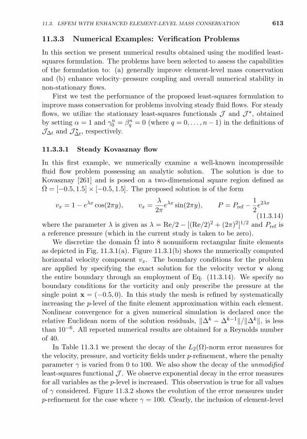
613
11.3.3 Numerical Examples: Verification Problems
In this section we present numerical results obtained using the modified least-squares formulation. The problems have been selected to assess the capabilitiesof the formulation to: (a) generally improve element-level mass conservationand (b) enhance velocity–pressure coupling and overall numerical stability innon-stationary flows.
First we test the performance of the proposed least-squares formulation toimprove mass conservation for problems involving steady fluid flows. For steadyflows, we utilize the stationary least-squares functionals J and J ?, obtainedby setting α = 1 and γn0 = βnq = 0 (where q = 0, . . . , n− 1) in the definitions ofJ∆t and J ?∆t, respectively.
11.3.3.1 Steady Kovasznay flow
In this first example, we numerically examine a well-known incompressiblefluid flow problem possessing an analytic solution. The solution is due toKovasznay [261] and is posed on a two-dimensional square region defined asΩ = [−0.5, 1.5]× [−0.5, 1.5]. The proposed solution is of the form
vx = 1− eλx cos(2πy), vx =λ
2πeλx sin(2πy), P = Pref −
1
2e2λx
(11.3.14)where the parameter λ is given as λ = Re/2 − [(Re/2)2 + (2π)2]1/2 and Pref isa reference pressure (which in the current study is taken to be zero).
We discretize the domain Ω into 8 nonuniform rectangular finite elementsas depicted in Fig. 11.3.1(a). Figure 11.3.1(b) shows the numerically computedhorizontal velocity component vx. The boundary conditions for the problemare applied by specifying the exact solution for the velocity vector v alongthe entire boundary through an employment of Eq. (11.3.14). We specify noboundary conditions for the vorticity and only prescribe the pressure at thesingle point x = (−0.5, 0). In this study the mesh is refined by systematicallyincreasing the p-level of the finite element approximation within each element.Nonlinear convergence for a given numerical simulation is declared once therelative Euclidean norm of the solution residuals, ‖∆k − ∆k−1‖/‖∆k‖, is lessthan 10−6. All reported numerical results are obtained for a Reynolds numberof 40.
In Table 11.3.1 we present the decay of the L2(Ω)-norm error measures forthe velocity, pressure, and vorticity fields under p-refinement, where the penaltyparameter γ is varied from 0 to 100. We also show the decay of the unmodifiedleast-squares functional J . We observe exponential decay in the error measuresfor all variables as the p-level is increased. This observation is true for all valuesof γ considered. Figure 11.3.2 shows the evolution of the error measures underp-refinement for the case where γ = 100. Clearly, the inclusion of element-level
11.3. LSFEM WITH ENHANCED ELEMENT-LEVEL MASS CONSERVATION
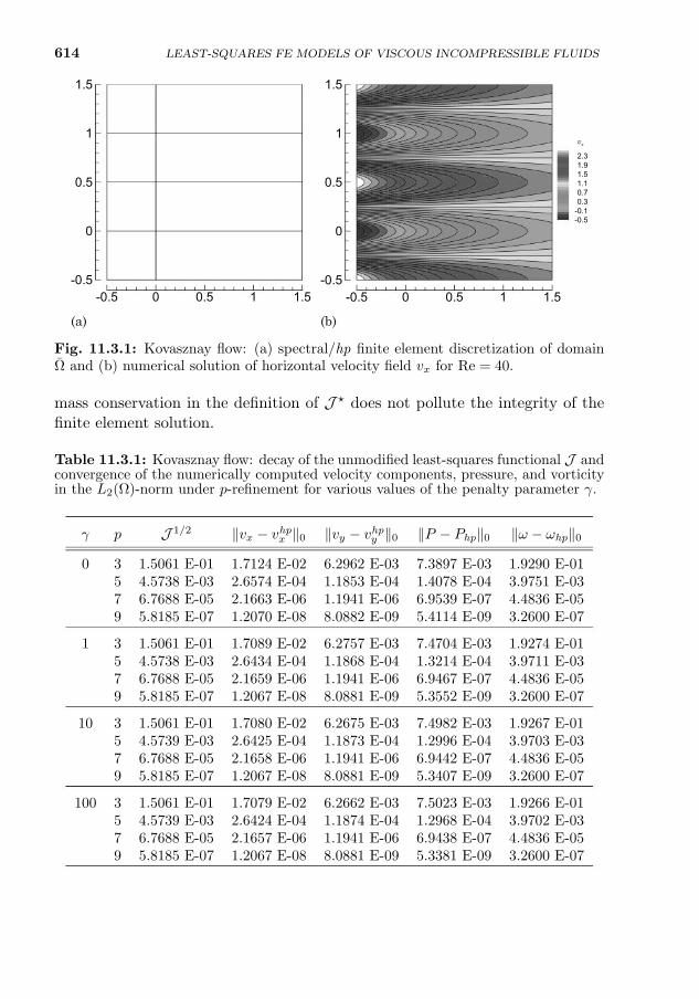
614 LEAST-SQUARES FE MODELS OF VISCOUS INCOMPRESSIBLE FLUIDS
-0.5 0 0.5 1 1.5-0.5
0
0.5
1
1.5
(a) (b)-0.5 0 0.5 1 1.5
-0.5
0
0.5
1
1.5
vx
2.31.91.51.10.70.3-0.1-0.5
Fig. 11.3.1: Kovasznay flow: (a) spectral/hp finite element discretization of domainΩ and (b) numerical solution of horizontal velocity field vx for Re = 40.
mass conservation in the definition of J ? does not pollute the integrity of thefinite element solution.
Table 11.3.1: Kovasznay flow: decay of the unmodified least-squares functional J andconvergence of the numerically computed velocity components, pressure, and vorticityin the L2(Ω)-norm under p-refinement for various values of the penalty parameter γ.
γ p J 1/2 ‖vx − vhpx ‖0 ‖vy − vhpy ‖0 ‖P − Php‖0 ‖ω − ωhp‖0
0 3 1.5061 E-01 1.7124 E-02 6.2962 E-03 7.3897 E-03 1.9290 E-015 4.5738 E-03 2.6574 E-04 1.1853 E-04 1.4078 E-04 3.9751 E-037 6.7688 E-05 2.1663 E-06 1.1941 E-06 6.9539 E-07 4.4836 E-059 5.8185 E-07 1.2070 E-08 8.0882 E-09 5.4114 E-09 3.2600 E-07
1 3 1.5061 E-01 1.7089 E-02 6.2757 E-03 7.4704 E-03 1.9274 E-015 4.5738 E-03 2.6434 E-04 1.1868 E-04 1.3214 E-04 3.9711 E-037 6.7688 E-05 2.1659 E-06 1.1941 E-06 6.9467 E-07 4.4836 E-059 5.8185 E-07 1.2067 E-08 8.0881 E-09 5.3552 E-09 3.2600 E-07
10 3 1.5061 E-01 1.7080 E-02 6.2675 E-03 7.4982 E-03 1.9267 E-015 4.5739 E-03 2.6425 E-04 1.1873 E-04 1.2996 E-04 3.9703 E-037 6.7688 E-05 2.1658 E-06 1.1941 E-06 6.9442 E-07 4.4836 E-059 5.8185 E-07 1.2067 E-08 8.0881 E-09 5.3407 E-09 3.2600 E-07
100 3 1.5061 E-01 1.7079 E-02 6.2662 E-03 7.5023 E-03 1.9266 E-015 4.5739 E-03 2.6424 E-04 1.1874 E-04 1.2968 E-04 3.9702 E-037 6.7688 E-05 2.1657 E-06 1.1941 E-06 6.9438 E-07 4.4836 E-059 5.8185 E-07 1.2067 E-08 8.0881 E-09 5.3381 E-09 3.2600 E-07
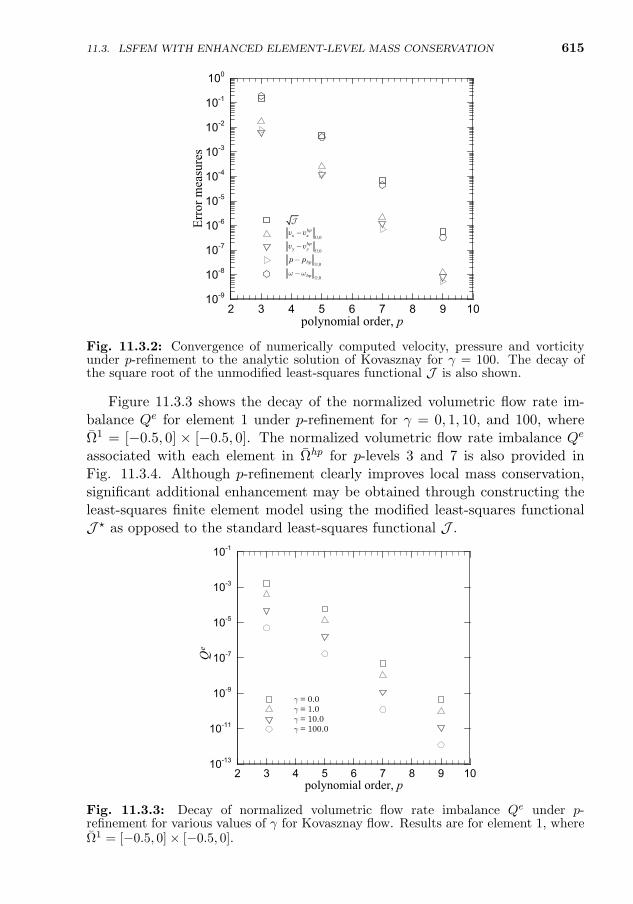
615
polynomial order, p
Erro
r mea
sure
s
2 3 4 5 6 7 8 9 1010-910-810-710-610-510-410-310-210-1100
,0
hpx xv v
Ω−
,0
hpy yv v
Ω−
,0hpp pΩ
−
,0hpω ωΩ
−
J
Fig. 11.3.2: Convergence of numerically computed velocity, pressure and vorticityunder p-refinement to the analytic solution of Kovasznay for γ = 100. The decay ofthe square root of the unmodified least-squares functional J is also shown.
Figure 11.3.3 shows the decay of the normalized volumetric flow rate im-balance Qe for element 1 under p-refinement for γ = 0, 1, 10, and 100, whereΩ1 = [−0.5, 0] × [−0.5, 0]. The normalized volumetric flow rate imbalance Qe
associated with each element in Ωhp for p-levels 3 and 7 is also provided inFig. 11.3.4. Although p-refinement clearly improves local mass conservation,significant additional enhancement may be obtained through constructing theleast-squares finite element model using the modified least-squares functionalJ ? as opposed to the standard least-squares functional J .
polynomial order, p
Q e
2 3 4 5 6 7 8 9 1010-13
10-11
10-9
10-7
10-5
10-3
10-1
γ = 0.0γ = 1.0γ = 10.0γ = 100.0
Fig. 11.3.3: Decay of normalized volumetric flow rate imbalance Qe under p-refinement for various values of γ for Kovasznay flow. Results are for element 1, whereΩ1 = [−0.5, 0]× [−0.5, 0].
11.3. LSFEM WITH ENHANCED ELEMENT-LEVEL MASS CONSERVATION

616 LEAST-SQUARES FE MODELS OF VISCOUS INCOMPRESSIBLE FLUIDS
(a) (b)
(c) (d)
-0.5 0 0.5 1 1.5-0.5
0
0.5
1
1.5
Q e
1.4E-031.3E-031.0E-038.5E-046.5E-044.5E-042.5E-045.0E-05
-0.5 0 0.5 1 1.5-0.5
0
0.5
1
1.5
Q e
5.6E-065.0E-064.4E-063.8E-063.2E-062.6E-062.0E-061.4E-068.0E-072.0E-07
-0.5 0 0.5 1 1.5-0.5
0
0.5
1
1.5
Q e
4.7E-084.4E-084.1E-083.8E-083.5E-083.2E-082.9E-082.6E-082.3E-08
-0.5 0 0.5 1 1.5-0.5
0
0.5
1
1.5
Q e
2.3E-102.1E-101.9E-101.7E-101.5E-101.3E-101.1E-109.0E-117.0E-115.0E-11
Fig. 11.3.4: Normalized volumetric flow rate imbalance Qe for each finite element inΩhp for Kovasznay flow. Results are for various polynomial orders and values of γ:(a) p-level = 3 and γ = 0, (b) p-level = 3 and γ = 100, (c) p-level = 7 and γ = 0, and(d) p-level = 7 and γ = 100.
11.3.3.2 Steady flow in a 1× 2 rectangular cavity
In this example, we test the modified least-squares finite element model witha two-dimensional lid-driven cavity flow problem consisting of a rectangulardomain, Ω = [0, 1]× [0, 2], with an aspect ratio of 2. Along the bottom and leftand right sides of the cavity, the velocity is taken to be zero in accordance withthe no slip condition. It is a common practice in the literature to prescribe aunit value for the horizontal velocity component vx along the entire top surfaceof the cavity. In the context of high-order finite elements, however, such aboundary condition produces undesirable singularities in the vicinity of thecorners of the upper cavity. In an effort to avoid an ill-posed discrete problem,the horizontal velocity profile is prescribed in terms of the following expression:
vpx(x) =
tanh(50x) 0 6 x 6 0.5− tanh[50(x− 1)] 0.5 < x 6 1.0
(11.3.15)
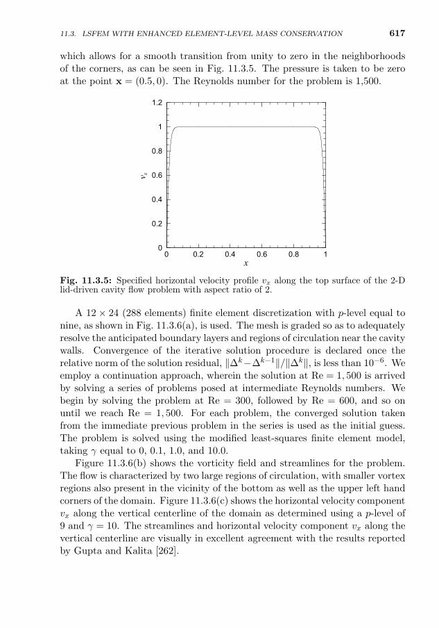
11.3. LSFEM WITH ENHANCED ELEMENT-LEVEL MASS CONSERVATION 617
which allows for a smooth transition from unity to zero in the neighborhoodsof the corners, as can be seen in Fig. 11.3.5. The pressure is taken to be zeroat the point x = (0.5, 0). The Reynolds number for the problem is 1,500.
x
v x
0 0.2 0.4 0.6 0.8 10
0.2
0.4
0.6
0.8
1
1.2
Fig. 11.3.5: Specified horizontal velocity profile vx along the top surface of the 2-Dlid-driven cavity flow problem with aspect ratio of 2.
A 12× 24 (288 elements) finite element discretization with p-level equal tonine, as shown in Fig. 11.3.6(a), is used. The mesh is graded so as to adequatelyresolve the anticipated boundary layers and regions of circulation near the cavitywalls. Convergence of the iterative solution procedure is declared once therelative norm of the solution residual, ‖∆k−∆k−1‖/‖∆k‖, is less than 10−6. Weemploy a continuation approach, wherein the solution at Re = 1, 500 is arrivedby solving a series of problems posed at intermediate Reynolds numbers. Webegin by solving the problem at Re = 300, followed by Re = 600, and so onuntil we reach Re = 1, 500. For each problem, the converged solution takenfrom the immediate previous problem in the series is used as the initial guess.The problem is solved using the modified least-squares finite element model,taking γ equal to 0, 0.1, 1.0, and 10.0.
Figure 11.3.6(b) shows the vorticity field and streamlines for the problem.The flow is characterized by two large regions of circulation, with smaller vortexregions also present in the vicinity of the bottom as well as the upper left handcorners of the domain. Figure 11.3.6(c) shows the horizontal velocity componentvx along the vertical centerline of the domain as determined using a p-level of9 and γ = 10. The streamlines and horizontal velocity component vx along thevertical centerline are visually in excellent agreement with the results reportedby Gupta and Kalita [262].
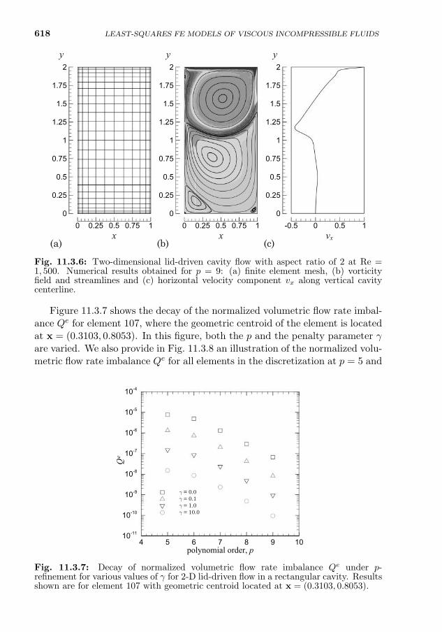
618 LEAST-SQUARES FE MODELS OF VISCOUS INCOMPRESSIBLE FLUIDS
0 0.25 0.5 0.75 10
0.25
0.5
0.75
1
1.25
1.5
1.75
2
0 0.25 0.5 0.75 10
0.25
0.5
0.75
1
1.25
1.5
1.75
2
(a) (b) (c)x x vx
y y y
-0.5 0 0.5 10
0.25
0.5
0.75
1
1.25
1.5
1.75
2
Fig. 11.3.6: Two-dimensional lid-driven cavity flow with aspect ratio of 2 at Re =1, 500. Numerical results obtained for p = 9: (a) finite element mesh, (b) vorticityfield and streamlines and (c) horizontal velocity component vx along vertical cavitycenterline.
Figure 11.3.7 shows the decay of the normalized volumetric flow rate imbal-ance Qe for element 107, where the geometric centroid of the element is locatedat x = (0.3103, 0.8053). In this figure, both the p and the penalty parameter γare varied. We also provide in Fig. 11.3.8 an illustration of the normalized volu-metric flow rate imbalance Qe for all elements in the discretization at p = 5 and
polynomial order, p
Q e
4 5 6 7 8 9 1010-11
10-10
10-9
10-8
10-7
10-6
10-5
10-4
γ = 0.0γ = 0.1γ = 1.0γ = 10.0
Fig. 11.3.7: Decay of normalized volumetric flow rate imbalance Qe under p-refinement for various values of γ for 2-D lid-driven flow in a rectangular cavity. Resultsshown are for element 107 with geometric centroid located at x = (0.3103, 0.8053).
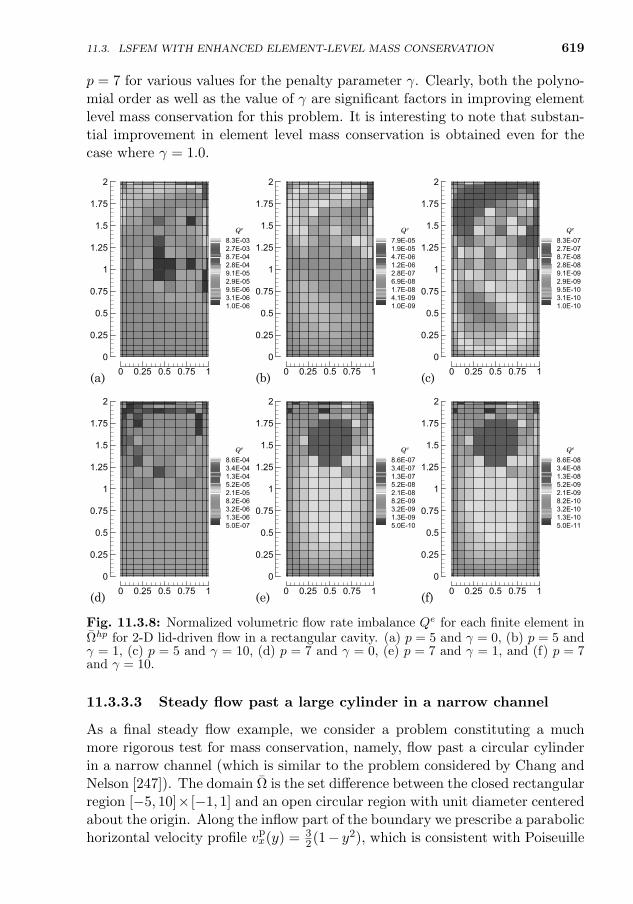
11.3. LSFEM WITH ENHANCED ELEMENT-LEVEL MASS CONSERVATION 619
p = 7 for various values for the penalty parameter γ. Clearly, both the polyno-mial order as well as the value of γ are significant factors in improving elementlevel mass conservation for this problem. It is interesting to note that substan-tial improvement in element level mass conservation is obtained even for thecase where γ = 1.0.
0 0.25 0.5 0.75 10
0.25
0.5
0.75
1
1.25
1.5
1.75
2
Q e
8.3E-032.7E-038.7E-042.8E-049.1E-052.9E-059.5E-063.1E-061.0E-06
0 0.25 0.5 0.75 10
0.25
0.5
0.75
1
1.25
1.5
1.75
2
Q e
8.6E-043.4E-041.3E-045.2E-052.1E-058.2E-063.2E-061.3E-065.0E-07
0 0.25 0.5 0.75 10
0.25
0.5
0.75
1
1.25
1.5
1.75
2
Q e
7.9E-051.9E-054.7E-061.2E-062.8E-076.9E-081.7E-084.1E-091.0E-09
0 0.25 0.5 0.75 10
0.25
0.5
0.75
1
1.25
1.5
1.75
2
Q e
8.3E-072.7E-078.7E-082.8E-089.1E-092.9E-099.5E-103.1E-101.0E-10
0 0.25 0.5 0.75 10
0.25
0.5
0.75
1
1.25
1.5
1.75
2
Q e
8.6E-073.4E-071.3E-075.2E-082.1E-088.2E-093.2E-091.3E-095.0E-10
0 0.25 0.5 0.75 10
0.25
0.5
0.75
1
1.25
1.5
1.75
2
Q e
8.6E-083.4E-081.3E-085.2E-092.1E-098.2E-103.2E-101.3E-105.0E-11
(c)(b)(a)
(d) (e) (f)
Fig. 11.3.8: Normalized volumetric flow rate imbalance Qe for each finite element inΩhp for 2-D lid-driven flow in a rectangular cavity. (a) p = 5 and γ = 0, (b) p = 5 andγ = 1, (c) p = 5 and γ = 10, (d) p = 7 and γ = 0, (e) p = 7 and γ = 1, and (f) p = 7and γ = 10.
11.3.3.3 Steady flow past a large cylinder in a narrow channel
As a final steady flow example, we consider a problem constituting a muchmore rigorous test for mass conservation, namely, flow past a circular cylinderin a narrow channel (which is similar to the problem considered by Chang andNelson [247]). The domain Ω is the set difference between the closed rectangularregion [−5, 10]× [−1, 1] and an open circular region with unit diameter centeredabout the origin. Along the inflow part of the boundary we prescribe a parabolichorizontal velocity profile vp
x(y) = 32(1− y2), which is consistent with Poiseuille
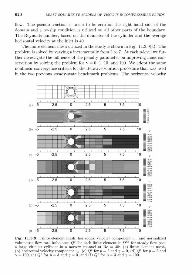
620 LEAST-SQUARES FE MODELS OF VISCOUS INCOMPRESSIBLE FLUIDS
flow. The pseudo-traction is taken to be zero on the right hand side of thedomain and a no-slip condition is utilized on all other parts of the boundary.The Reynolds number, based on the diameter of the cylinder and the averagehorizontal velocity at the inlet is 40.
The finite element mesh utilized in the study is shown in Fig. 11.3.9(a). Theproblem is solved by varying p incrementally from 2 to 7. At each p-level we fur-ther investigate the influence of the penalty parameter on improving mass con-servation by solving the problem for γ = 0, 1, 10, and 100. We adopt the samenonlinear convergence criteria for the iterative solution procedure that was usedin the two previous steady-state benchmark problems. The horizontal velocity
-5 -2.5 0 2.5 5 7.5 10
vx2.62.21.91.51.10.70.40.0
-5 -2.5 0 2.5 5 7.5 10(a)
(b)
(c)
(d)
(e)
(f)
-5 -2.5 0 2.5 5 7.5 10
Q e
7.4E-022.1E-026.1E-031.8E-035.1E-041.5E-044.2E-051.2E-053.5E-061.0E-06
-5 -2.5 0 2.5 5 7.5 10
Q e
7.4E-032.1E-036.1E-041.8E-045.1E-051.5E-054.2E-061.2E-063.5E-071.0E-07
-5 -2.5 0 2.5 5 7.5 10
Q e
3.9E-021.2E-023.7E-031.2E-033.6E-041.1E-043.4E-051.0E-053.2E-061.0E-06
-5 -2.5 0 2.5 5 7.5 10
Q e
7.4E-042.1E-046.1E-051.8E-055.1E-061.5E-064.2E-071.2E-073.5E-081.0E-08
Fig. 11.3.9: Finite element mesh, horizontal velocity component vx, and normalizedvolumetric flow rate imbalance Qe for each finite element in Ωhp for steady flow pasta large circular cylinder in a narrow channel at Re = 40: (a) finite element mesh,(b) horizontal velocity component vx, (c) Qe for p = 2 and γ = 0, (d) Qe for p = 2 andγ = 100, (e) Qe for p = 3 and γ = 0, and (f) Qe for p = 3 and γ = 100.
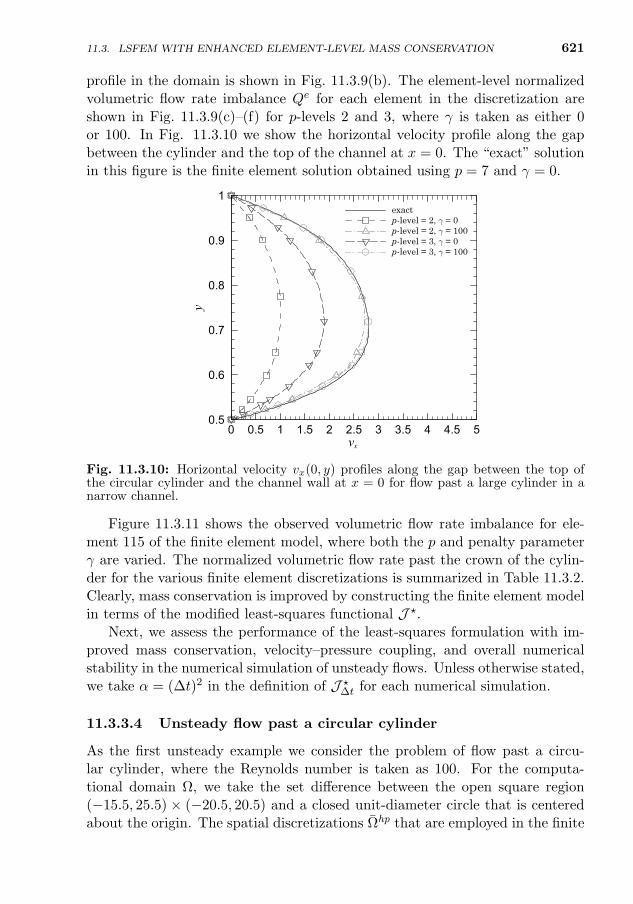
621
profile in the domain is shown in Fig. 11.3.9(b). The element-level normalizedvolumetric flow rate imbalance Qe for each element in the discretization areshown in Fig. 11.3.9(c)–(f) for p-levels 2 and 3, where γ is taken as either 0or 100. In Fig. 11.3.10 we show the horizontal velocity profile along the gapbetween the cylinder and the top of the channel at x = 0. The “exact” solutionin this figure is the finite element solution obtained using p = 7 and γ = 0.
vx
y
0 0.5 1 1.5 2 2.5 3 3.5 4 4.5 50.5
0.6
0.7
0.8
0.9
1exactp-level = 2, γ = 0p-level = 2, γ = 100p-level = 3, γ = 0p-level = 3, γ = 100
Fig. 11.3.10: Horizontal velocity vx(0, y) profiles along the gap between the top ofthe circular cylinder and the channel wall at x = 0 for flow past a large cylinder in anarrow channel.
Figure 11.3.11 shows the observed volumetric flow rate imbalance for ele-ment 115 of the finite element model, where both the p and penalty parameterγ are varied. The normalized volumetric flow rate past the crown of the cylin-der for the various finite element discretizations is summarized in Table 11.3.2.Clearly, mass conservation is improved by constructing the finite element modelin terms of the modified least-squares functional J ?.
Next, we assess the performance of the least-squares formulation with im-proved mass conservation, velocity–pressure coupling, and overall numericalstability in the numerical simulation of unsteady flows. Unless otherwise stated,we take α = (∆t)2 in the definition of J ?∆t for each numerical simulation.
11.3.3.4 Unsteady flow past a circular cylinder
As the first unsteady example we consider the problem of flow past a circu-lar cylinder, where the Reynolds number is taken as 100. For the computa-tional domain Ω, we take the set difference between the open square region(−15.5, 25.5) × (−20.5, 20.5) and a closed unit-diameter circle that is centeredabout the origin. The spatial discretizations Ωhp that are employed in the finite
11.3. LSFEM WITH ENHANCED ELEMENT-LEVEL MASS CONSERVATION
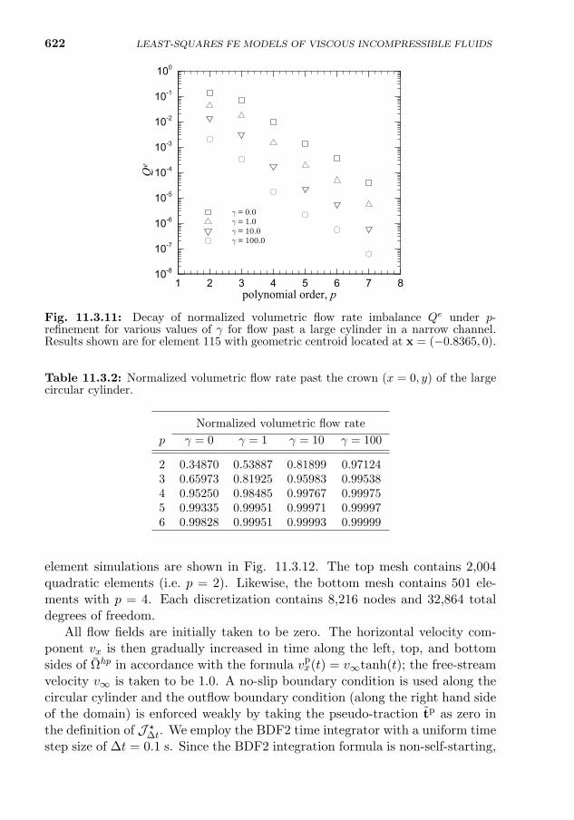
622
polynomial order, p
Q e
1 2 3 4 5 6 7 810-8
10-7
10-6
10-5
10-4
10-3
10-2
10-1
100
γ = 0.0γ = 1.0γ = 10.0γ = 100.0
Fig. 11.3.11: Decay of normalized volumetric flow rate imbalance Qe under p-refinement for various values of γ for flow past a large cylinder in a narrow channel.Results shown are for element 115 with geometric centroid located at x = (−0.8365, 0).
Table 11.3.2: Normalized volumetric flow rate past the crown (x = 0, y) of the largecircular cylinder.
Normalized volumetric flow rate
p γ = 0 γ = 1 γ = 10 γ = 100
2 0.34870 0.53887 0.81899 0.971243 0.65973 0.81925 0.95983 0.995384 0.95250 0.98485 0.99767 0.999755 0.99335 0.99951 0.99971 0.999976 0.99828 0.99951 0.99993 0.99999
element simulations are shown in Fig. 11.3.12. The top mesh contains 2,004quadratic elements (i.e. p = 2). Likewise, the bottom mesh contains 501 ele-ments with p = 4. Each discretization contains 8,216 nodes and 32,864 totaldegrees of freedom.
All flow fields are initially taken to be zero. The horizontal velocity com-ponent vx is then gradually increased in time along the left, top, and bottomsides of Ωhp in accordance with the formula vp
x(t) = v∞tanh(t); the free-streamvelocity v∞ is taken to be 1.0. A no-slip boundary condition is used along thecircular cylinder and the outflow boundary condition (along the right hand sideof the domain) is enforced weakly by taking the pseudo-traction tp as zero inthe definition of J ?∆t. We employ the BDF2 time integrator with a uniform timestep size of ∆t = 0.1 s. Since the BDF2 integration formula is non-self-starting,
LEAST-SQUARES FE MODELS OF VISCOUS INCOMPRESSIBLE FLUIDS
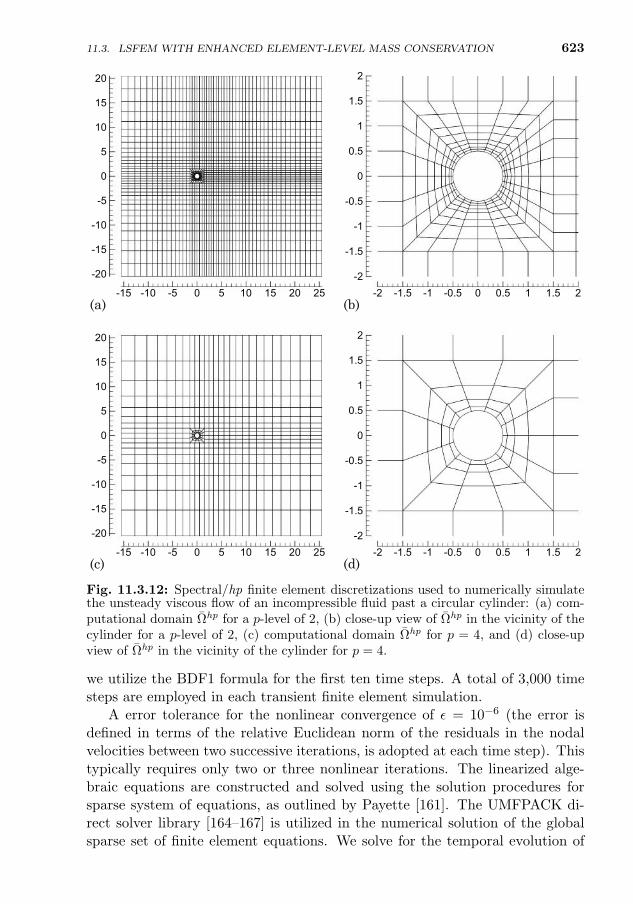
11.3. LSFEM WITH ENHANCED ELEMENT-LEVEL MASS CONSERVATION 623
(c) (d)-15 -10 -5 0 5 10 15 20 25
-20
-15
-10
-5
0
5
10
15
20
-2 -1.5 -1 -0.5 0 0.5 1 1.5 2-2
-1.5
-1
-0.5
0
0.5
1
1.5
2
-15 -10 -5 0 5 10 15 20 25
-20
-15
-10
-5
0
5
10
15
20
-2 -1.5 -1 -0.5 0 0.5 1 1.5 2-2
-1.5
-1
-0.5
0
0.5
1
1.5
2
(a) (b)
Fig. 11.3.12: Spectral/hp finite element discretizations used to numerically simulatethe unsteady viscous flow of an incompressible fluid past a circular cylinder: (a) com-putational domain Ωhp for a p-level of 2, (b) close-up view of Ωhp in the vicinity of thecylinder for a p-level of 2, (c) computational domain Ωhp for p = 4, and (d) close-upview of Ωhp in the vicinity of the cylinder for p = 4.
we utilize the BDF1 formula for the first ten time steps. A total of 3,000 timesteps are employed in each transient finite element simulation.
A error tolerance for the nonlinear convergence of ε = 10−6 (the error isdefined in terms of the relative Euclidean norm of the residuals in the nodalvelocities between two successive iterations, is adopted at each time step). Thistypically requires only two or three nonlinear iterations. The linearized alge-braic equations are constructed and solved using the solution procedures forsparse system of equations, as outlined by Payette [161]. The UMFPACK di-rect solver library [164–167] is utilized in the numerical solution of the globalsparse set of finite element equations. We solve for the temporal evolution of
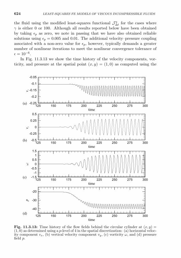
624 LEAST-SQUARES FE MODELS OF VISCOUS INCOMPRESSIBLE FLUIDS
the fluid using the modified least-squares functional J ?∆t for the cases whereγ is either 0 or 100. Although all results reported below have been obtainedby taking εp as zero, we note in passing that we have also obtained reliablesolutions using εp = 0.005 and 0.01. The additional velocity–pressure couplingassociated with a non-zero value for εp, however, typically demands a greaternumber of nonlinear iterations to meet the nonlinear convergence tolerance ofε = 10−6.
In Fig. 11.3.13 we show the time history of the velocity components, vor-ticity, and pressure at the spatial point (x, y) = (1, 0) as computed using the
(a)
time
v y
125 150 175 200 225 250 275 300-0.5
-0.25
0
0.25
0.5
time
ω
125 150 175 200 225 250 275 300-1.5-1
-0.50
0.51
1.5
time
v x
125 150 175 200 225 250 275 300-0.25
-0.2
-0.15
-0.1
-0.05
time
p
125 150 175 200 225 250 275 300
-40
-30
-20
(b)
(c)
(d)
Fig. 11.3.13: Time history of the flow fields behind the circular cylinder at (x, y) =(1, 0) as determined using a p-level of 4 in the spatial discretization: (a) horizontal veloc-ity component vx, (b) vertical velocity component vy, (c) vorticity ω, and (d) pressurefield p.
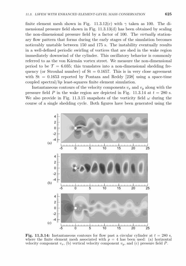
625
finite element mesh shown in Fig. 11.3.12(c) with γ taken as 100. The di-mensional pressure field shown in Fig. 11.3.13(d) has been obtained by scalingthe non-dimensional pressure field by a factor of 100. The virtually station-ary flow pattern that forms during the early stages of the simulation becomesnoticeably unstable between 150 and 175 s. The instability eventually resultsin a well-defined periodic swirling of vortices that are shed in the wake regionimmediately downwind of the cylinder. This oscillatory behavior is commonlyreferred to as the von Karman vortex street. We measure the non-dimensionalperiod to be T = 6.035; this translates into a non-dimensional shedding fre-quency (or Strouhal number) of St = 0.1657. This is in very close agreementwith St = 0.1653 reported by Pontaza and Reddy [238] using a space-timecoupled spectral/hp least-squares finite element simulation.
Instantaneous contours of the velocity components vx and vy along with thepressure field P in the wake region are depicted in Fig. 11.3.14 at t = 280 s.We also provide in Fig. 11.3.15 snapshots of the vorticity field ω during thecourse of a single shedding cycle. Both figures have been generated using the
(a)
(b)
(c)
-5 0 5 10 15 20 25
-4
-2
0
2
4
-5 0 5 10 15 20 25
-4
-2
0
2
4
-5 0 5 10 15 20 25
-4
-2
0
2
4
Fig. 11.3.14: Instantaneous contours for flow past a circular cylinder at t = 280 s,where the finite element mesh associated with p = 4 has been used: (a) horizontalvelocity component vx, (b) vertical velocity component vy, and (c) pressure field P .
11.3. LSFEM WITH ENHANCED ELEMENT-LEVEL MASS CONSERVATION
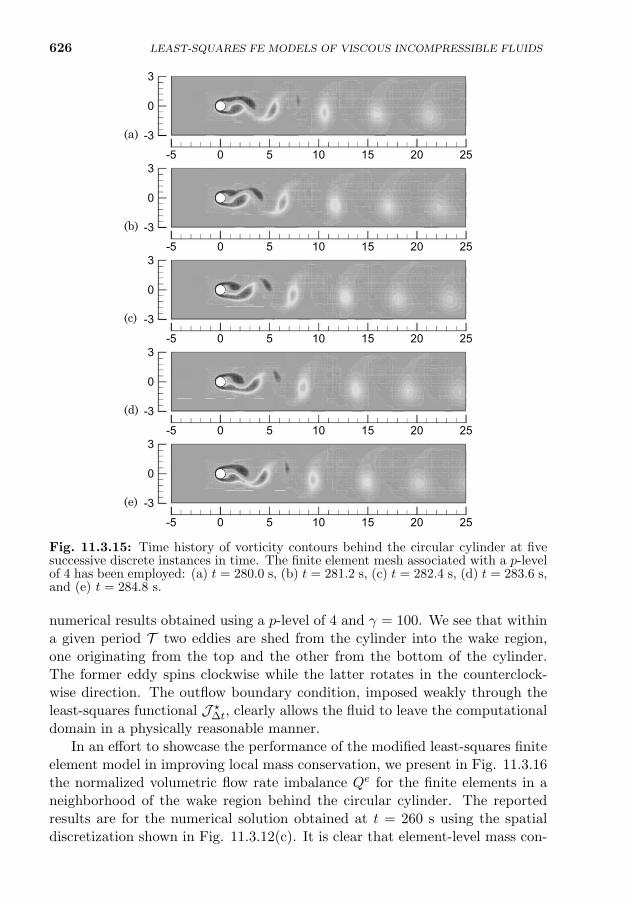
626 LEAST-SQUARES FE MODELS OF VISCOUS INCOMPRESSIBLE FLUIDS
(a)-5 0 5 10 15 20 25
-3
0
3
-5 0 5 10 15 20 25
-3
0
3
-5 0 5 10 15 20 25
-3
0
3
-5 0 5 10 15 20 25
-3
0
3
-5 0 5 10 15 20 25
-3
0
3
(b)
(e)
(d)
(c)
Fig. 11.3.15: Time history of vorticity contours behind the circular cylinder at fivesuccessive discrete instances in time. The finite element mesh associated with a p-levelof 4 has been employed: (a) t = 280.0 s, (b) t = 281.2 s, (c) t = 282.4 s, (d) t = 283.6 s,and (e) t = 284.8 s.
numerical results obtained using a p-level of 4 and γ = 100. We see that withina given period T two eddies are shed from the cylinder into the wake region,one originating from the top and the other from the bottom of the cylinder.The former eddy spins clockwise while the latter rotates in the counterclock-wise direction. The outflow boundary condition, imposed weakly through theleast-squares functional J ?∆t, clearly allows the fluid to leave the computationaldomain in a physically reasonable manner.
In an effort to showcase the performance of the modified least-squares finiteelement model in improving local mass conservation, we present in Fig. 11.3.16the normalized volumetric flow rate imbalance Qe for the finite elements in aneighborhood of the wake region behind the circular cylinder. The reportedresults are for the numerical solution obtained at t = 260 s using the spatialdiscretization shown in Fig. 11.3.12(c). It is clear that element-level mass con-
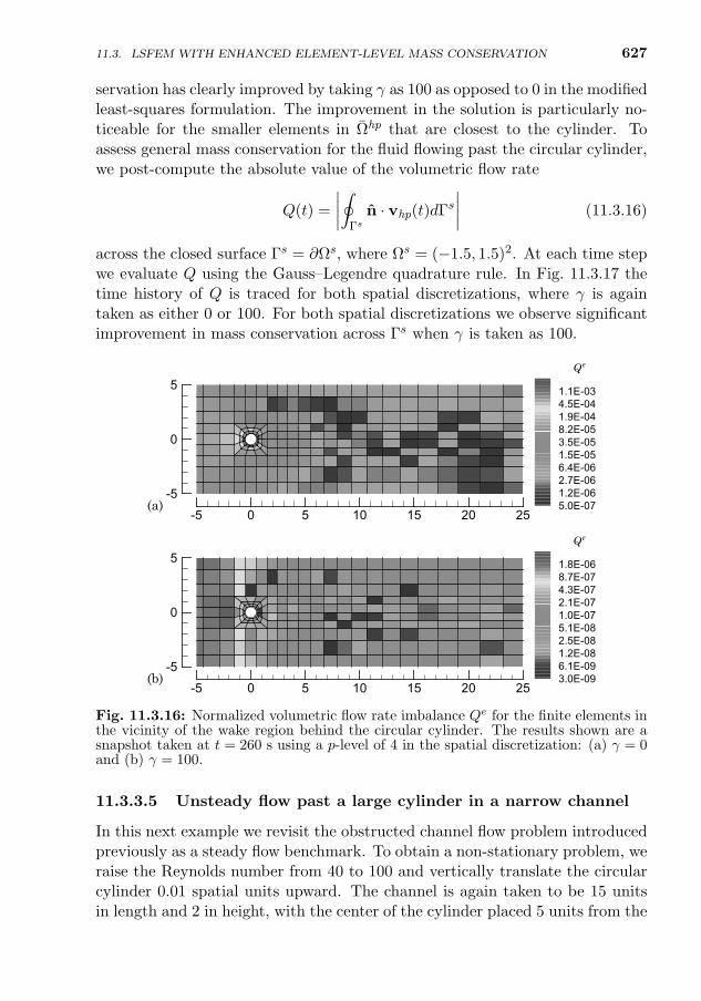
627
servation has clearly improved by taking γ as 100 as opposed to 0 in the modifiedleast-squares formulation. The improvement in the solution is particularly no-ticeable for the smaller elements in Ωhp that are closest to the cylinder. Toassess general mass conservation for the fluid flowing past the circular cylinder,we post-compute the absolute value of the volumetric flow rate
Q(t) =
∣∣∣∣∮Γs
n · vhp(t)dΓs∣∣∣∣ (11.3.16)
across the closed surface Γs = ∂Ωs, where Ωs = (−1.5, 1.5)2. At each time stepwe evaluate Q using the Gauss–Legendre quadrature rule. In Fig. 11.3.17 thetime history of Q is traced for both spatial discretizations, where γ is againtaken as either 0 or 100. For both spatial discretizations we observe significantimprovement in mass conservation across Γs when γ is taken as 100.
(a)
(b)
-5 0 5 10 15 20 25
-5
0
5Q e
1.1E-034.5E-041.9E-048.2E-053.5E-051.5E-056.4E-062.7E-061.2E-065.0E-07
-5 0 5 10 15 20 25
-5
0
5Q e
1.8E-068.7E-074.3E-072.1E-071.0E-075.1E-082.5E-081.2E-086.1E-093.0E-09
Fig. 11.3.16: Normalized volumetric flow rate imbalance Qe for the finite elements inthe vicinity of the wake region behind the circular cylinder. The results shown are asnapshot taken at t = 260 s using a p-level of 4 in the spatial discretization: (a) γ = 0and (b) γ = 100.
11.3.3.5 Unsteady flow past a large cylinder in a narrow channel
In this next example we revisit the obstructed channel flow problem introducedpreviously as a steady flow benchmark. To obtain a non-stationary problem, weraise the Reynolds number from 40 to 100 and vertically translate the circularcylinder 0.01 spatial units upward. The channel is again taken to be 15 unitsin length and 2 in height, with the center of the cylinder placed 5 units from the
11.3. LSFEM WITH ENHANCED ELEMENT-LEVEL MASS CONSERVATION
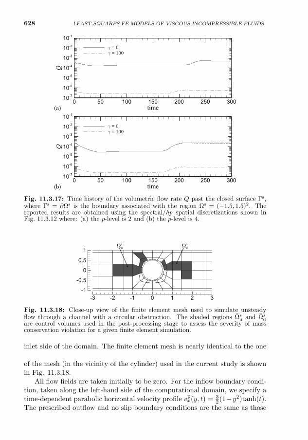
628 LEAST-SQUARES FE MODELS OF VISCOUS INCOMPRESSIBLE FLUIDS
(a)
(b) time
Q
0 50 100 150 200 250 30010-710-610-510-410-310-210-1
γ = 0γ = 100
time
Q
0 50 100 150 200 250 30010-710-610-510-410-310-210-1
γ = 0γ = 100
Fig. 11.3.17: Time history of the volumetric flow rate Q past the closed surface Γs,where Γs = ∂Ωs is the boundary associated with the region Ωs = (−1.5, 1.5)2. Thereported results are obtained using the spectral/hp spatial discretizations shown inFig. 11.3.12 where: (a) the p-level is 2 and (b) the p-level is 4.
-3 -2 -1 0 1 2 3-1
-0.5
0
0.5
1 usΩ d
sΩ
Fig. 11.3.18: Close-up view of the finite element mesh used to simulate unsteadyflow through a channel with a circular obstruction. The shaded regions Ωs
u and Ωsd
are control volumes used in the post-processing stage to assess the severity of massconservation violation for a given finite element simulation.
inlet side of the domain. The finite element mesh is nearly identical to the oneemployed in the stationary flow problem [see Fig. 11.3.9(a)]. A close-up viewof the mesh (in the vicinity of the cylinder) used in the current study is shownin Fig. 11.3.18.
All flow fields are taken initially to be zero. For the inflow boundary condi-tion, taken along the left-hand side of the computational domain, we specify atime-dependent parabolic horizontal velocity profile vp
x(y, t) = 32(1−y2)tanh(t).
The prescribed outflow and no slip boundary conditions are the same as those
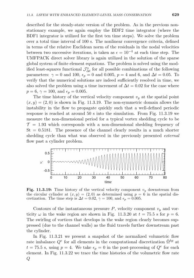
11.3. LSFEM WITH ENHANCED ELEMENT-LEVEL MASS CONSERVATION 629
described for the steady-state version of the problem. As in the previous non-stationary example, we again employ the BDF2 time integrator (where theBDF1 integrator is utilized for the first ten time steps). We solve the problemover a total time interval of 100 s. The nonlinear convergence criteria, definedin terms of the relative Euclidean norm of the residuals in the nodal velocitiesbetween two successive iterations, is taken as ε = 10−4 at each time step. TheUMFPACK direct solver library is again utilized in the solution of the sparseglobal system of finite element equations. The problem is solved using the mod-ified least-squares functional J ?∆t for all possible combinations of the followingparameters: γ = 0 and 100, εp = 0 and 0.005, p = 4 and 6, and ∆t = 0.05. Toverify that the numerical solutions are indeed sufficiently resolved in time, wealso solved the problem using a time increment of ∆t = 0.02 for the case wherep = 6, γ = 100, and εp = 0.005.
The time history of the vertical velocity component vy at the spatial point(x, y) = (2, 0) is shown in Fig. 11.3.19. The non-symmetric domain allows theinstability in the flow to propagate quickly such that a well-defined periodicresponse is reached at around 50 s into the simulation. From Fig. 11.3.19 wemeasure the non-dimensional period for a typical vortex shedding cycle to beT = 1.93 which corresponds with a non-dimensional shedding frequency ofSt = 0.5181. The presence of the channel clearly results in a much shortershedding cycle than what was observed in the previously presented externalflow past a cylinder problem.
time
v y
0 10 20 30 40 50 60 70 80
-0.5
0
0.5
Fig. 11.3.19: Time history of the vertical velocity component vy downstream fromthe circular cylinder at (x, y) = (2, 0) as determined using p = 6 in the spatial dis-cretization. The time step is ∆t = 0.02, γ = 100, and εp = 0.005.
Contours of the instantaneous pressure P , velocity component vy and vor-ticity ω in the wake region are shown in Fig. 11.3.20 at t = 75.5 s for p = 6.The swirling of vortices that develops in the wake region clearly becomes sup-pressed (due to the channel walls) as the fluid travels further downstream pastthe cylinder.
In Fig. 11.3.21 we present a snapshot of the normalized volumetric flowrate imbalance Qe for all elements in the computational discretization Ωhp att = 75.5 s, using p = 4. We take εp = 0 in the post-processing of Qe for eachelement. In Fig. 11.3.22 we trace the time histories of the volumetric flow rateQ [obtained using Eq. (11.3.16)] through the closed boundaries of the upstream
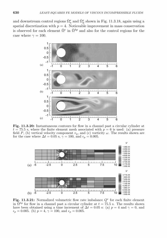
630
and downstream control regions Ωsu and Ωs
d shown in Fig. 11.3.18, again using aspatial discretization with p = 4. Noticeable improvement in mass conservationis observed for each element Ωe in Ωhp and also for the control regions for thecase where γ = 100.
(a) -1 0 1 2 3 4 5 6-1
-0.50
0.51
-1 0 1 2 3 4 5 6-1
-0.50
0.51
(c)
-1 0 1 2 3 4 5 6-1
-0.50
0.51
(b)
Fig. 11.3.20: Instantaneous contours for flow in a channel past a circular cylinder att = 75.5 s, where the finite element mesh associated with p = 6 is used: (a) pressurefield P , (b) vertical velocity component vy, and (c) vorticity ω. The results shown arefor the case where ∆t = 0.05 s, γ = 100, and εp = 0.005.
(a) -5 -2.5 0 2.5 5 7.5 10
Q e
1.08E-034.95E-042.28E-041.05E-044.83E-052.23E-051.02E-054.72E-062.17E-061.00E-06
(b) -5 -2.5 0 2.5 5 7.5 10
Q e
4.71E-051.84E-057.20E-062.81E-061.10E-064.29E-071.68E-076.55E-082.56E-081.00E-08
Fig. 11.3.21: Normalized volumetric flow rate imbalance Qe for each finite elementin Ωhp for flow in a channel past a circular cylinder at t = 75.5 s. The results shownhave been obtained using a time increment of ∆t = 0.05 s: (a) p = 4 and γ = 0, andεp = 0.005. (b) p = 4, γ = 100, and εp = 0.005.
LEAST-SQUARES FE MODELS OF VISCOUS INCOMPRESSIBLE FLUIDS
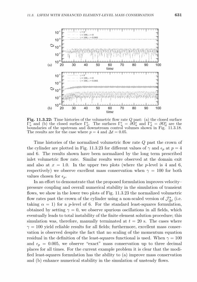
631
(a)time
Q
20 30 40 50 60 70 80 90 10010-910-710-510-310-1 γ = 0
γ = 100, ε = 0γ = 100, ε = 0.005
(b)time
Q
20 30 40 50 60 70 80 90 10010-910-710-510-310-1 γ = 0
γ = 100, ε = 0γ = 100, ε = 0.005
Fig. 11.3.22: Time histories of the volumetric flow rate Q past: (a) the closed surfaceΓsu and (b) the closed surface Γs
d. The surfaces Γsu = ∂Ωs
u and Γsd = ∂Ωs
d are theboundaries of the upstream and downstream control volumes shown in Fig. 11.3.18.The results are for the case where p = 4 and ∆t = 0.05.
Time histories of the normalized volumetric flow rate Q past the crown ofthe cylinder are plotted in Fig. 11.3.23 for different values of γ and εp at p = 4and 6. The results shown have been normalized by the long term prescribedinlet volumetric flow rate. Similar results were observed at the domain exitand also at x = 1.0. In the upper two plots (where the p-level is 4 and 6,respectively) we observe excellent mass conservation when γ = 100 for bothvalues chosen for εp.
In an effort to demonstrate that the proposed formulation improves velocity–pressure coupling and overall numerical stability in the simulation of transientflows, we show in the lower two plots of Fig. 11.3.23 the normalized volumetricflow rates past the crown of the cylinder using a non-scaled version of J ?∆t (i.e.taking α = 1) for a p-level of 6. For the standard least-squares formulation,obtained by setting γ = 0, we observe spurious oscillations in all fields, whicheventually leads to total instability of the finite element solution procedure; thissimulation was, therefore, manually terminated at t = 20 s. The cases whereγ = 100 yield reliable results for all fields; furthermore, excellent mass conser-vation is observed despite the fact that no scaling of the momentum equationresidual in the definition of the least-squares functional is used. When γ = 100and εp = 0.005, we observe “exact” mass conservation up to three decimalplaces for all times. For the current example problem it is clear that the modi-fied least-squares formulation has the ability to (a) improve mass conservationand (b) enhance numerical stability in the simulation of unsteady flows.
11.3. LSFEM WITH ENHANCED ELEMENT-LEVEL MASS CONSERVATION
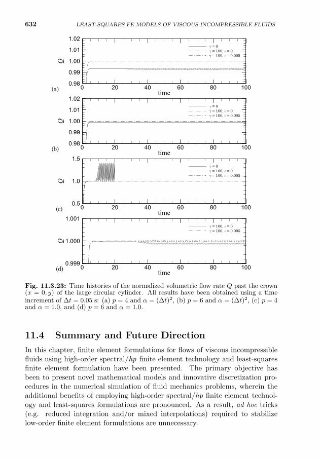
632 LEAST-SQUARES FE MODELS OF VISCOUS INCOMPRESSIBLE FLUIDS
time
Q
0 20 40 60 80 1000.98
0.99
1.00
1.01
1.02γ = 0γ = 100, ε = 0γ = 100, ε = 0.005
(a)
time
Q
0 20 40 60 80 1000.999
1.000
1.001γ = 100, ε = 0γ = 100, ε = 0.005
(d)
time
Q
0 20 40 60 80 1000.5
1.0
1.5γ = 0γ = 100, ε = 0γ = 100, ε = 0.005
(c)
time
Q
0 20 40 60 80 1000.98
0.99
1.00
1.01
1.02γ = 0γ = 100, ε = 0γ = 100, ε = 0.005
(b)
Fig. 11.3.23: Time histories of the normalized volumetric flow rate Q past the crown(x = 0, y) of the large circular cylinder. All results have been obtained using a timeincrement of ∆t = 0.05 s: (a) p = 4 and α = (∆t)2, (b) p = 6 and α = (∆t)2, (c) p = 4and α = 1.0, and (d) p = 6 and α = 1.0.
11.4 Summary and Future Direction
In this chapter, finite element formulations for flows of viscous incompressiblefluids using high-order spectral/hp finite element technology and least-squaresfinite element formulation have been presented. The primary objective hasbeen to present novel mathematical models and innovative discretization pro-cedures in the numerical simulation of fluid mechanics problems, wherein theadditional benefits of employing high-order spectral/hp finite element technol-ogy and least-squares formulations are pronounced. As a result, ad hoc tricks(e.g. reduced integration and/or mixed interpolations) required to stabilizelow-order finite element formulations are unnecessary.
11.4. SUMMARY AND FUTURE DIRECTION 633
Following the works of Payette [161] and Payette and Reddy [50], a novelleast-squares finite element model of the steady-state and non-stationary in-compressible Navier–Stokes equations with enhanced local mass conservationis also presented. The presented model is a modification of the standard L2-norm least-squares formulation of the Navier–Stokes equations based on theequivalent velocity–pressure–vorticity first-order system. In the new model, wemodified the standard least-squares functional to also include an appropriatelypenalized sum of the squares of the element-level integrals of a regularized formof the continuity equation. As a consequence, the resulting finite element modeldirectly inherited terms in the bilinear form and linear functional (which couldbe adjusted based on the penalty parameter) that tend to improve element-levelmass conservation. A notable quality of the formulation was that improved massconservation could be attained without introducing additional variables or com-promising the unconstrained minimization setting for the numerical solution.Numerical simulations confirmed that the proposed formulation could signifi-cantly improve mass conservation for both steady and non-stationary flows. Fortransient flows, the formulation was further shown to enhance velocity–pressurecoupling and overall numerical stability (most notably for cases where the mo-mentum equation residual, appearing in the least-squares functional, was notweighted by the square of the time step).
In the way of an extension of the works by Payette [161] and Payette andReddy [50], problems of fluid–structure interaction is the most promising. Herewe briefly describe an example problem that is solved by Payette [161] usinga least-squares finite element model discussed in this chapter that can handlemoving fluid boundaries (a preliminary step towards the development of a fluid–structure interaction computational methodology).
We consider the flow of a viscous incompressible fluid inside a square cavity,where the cavity under consideration is a unit square centered at the origin.A 0.28 units diameter solid circular cylinder is positioned at the origin of thecavity at t = 0 s. Immediately following t = 0 s, the cylinder begins to translatewith an instantaneous unit velocity in the x direction. We impose no-slip typeboundary conditions along all solid surfaces, including the cylinder Γcyl andcavity walls Γwalls, where Γ = Γcyl ∪ Γwalls. This amounts to specifying v = 0on Γwalls and vx = 1 on Γcyl. We prescribe the pressure to be zero at the singlenode located at (x, y) = (−1, 0). The Reynolds number for the flow is taken asRe = 100 by specifying ρ = 1, µ = 1/100 and a characteristic unit length. Theinitial boundary-value problem is posed on the time interval t = (0, 0.7] s.
The computational domain is discretized into 480 nonuniform finite ele-ments, where we place 40 element layers along the circumference of the cylinderand 12 in the radial direction. A depiction of the finite element mesh at t = 0and t = 0.70 is shown in Fig. 11.4.1. Mesh refinement is employed near thecylinder to ensure acceptable numerical resolution of all variables in the wakeregion downstream of the cylinder. We solve the problem using a p-level of 4
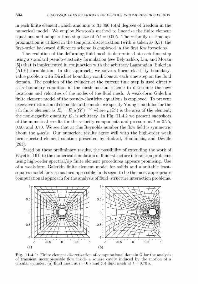
634 LEAST-SQUARES FE MODELS OF VISCOUS INCOMPRESSIBLE FLUIDS
in each finite element, which amounts to 31,360 total degrees of freedom in thenumerical model. We employ Newton’s method to linearize the finite elementequations and adopt a time step size of ∆t = 0.005. The α-family of time ap-proximation is utilized in the temporal discretization (with α taken as 0.5); thefirst-order backward difference scheme is employed in the first few iterations.
The evolution of the deforming fluid mesh is determined at each time stepusing a standard pseudo-elasticity formulation (see Belytschko, Liu, and Moran[5]) that is implemented in conjunction with the arbitrary Lagrangian–Eulerian(ALE) formulation. In this approach, we solve a linear elasticity boundary-value problem with Dirichlet boundary conditions at each time step on the fluiddomain. The position of the cylinder at the current time step is used directlyas a boundary condition in the mesh motion scheme to determine the newlocations and velocities of the nodes of the fluid mesh. A weak-form Galerkinfinite element model of the pseudo-elasticity equations is employed. To preventexcessive distortion of elements in the model we specify Young’s modulus for theeth finite element as Ee = E0µ(Ωe)−0.5 where µ(Ωe) is the area of the element;the non-negative quantity E0 is arbitrary. In Fig. 11.4.2 we present snapshotsof the numerical results for the velocity components and pressure at t = 0.25,0.50, and 0.70. We see that at this Reynolds number the flow field is symmetricabout the y-axis. Our numerical results agree well with the high-order weakform spectral element solution presented by Bodard, Bouffanais, and Deville[263].
Based on these preliminary results, the possibility of extending the work ofPayette [161] to the numerical simulation of fluid–structure interaction problemsusing high-order spectral/hp finite element procedures appears promising. Useof a weak-form Galerkin finite element model for solids and a suitable least-squares model for viscous incompressible fluids seem to be the most appropriatecomputational approach for the analysis of fluid–structure interaction problems.
(a) (b)-1 -0.5 0 0.5 1
-1
-0.5
0
0.5
1
-1 -0.5 0 0.5 1-1
-0.5
0
0.5
1
Fig. 11.4.1: Finite element discretization of computational domain Ω for the analysisof transient incompressible flow inside a square cavity induced by the motion of acircular cylinder: (a) fluid mesh at t = 0 s and (b) fluid mesh at t = 0.70 s.
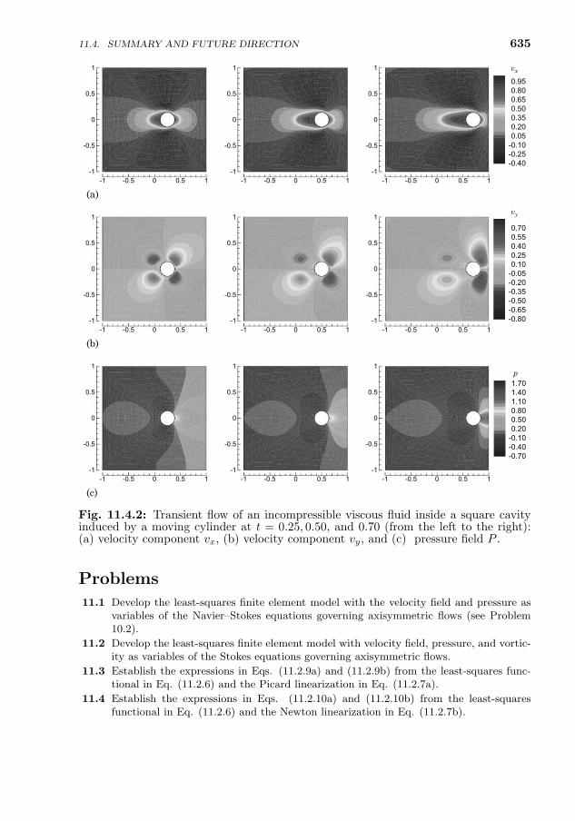
11.4. SUMMARY AND FUTURE DIRECTION 635
(a)
(b)
(c)
-1 -0.5 0 0.5 1-1
-0.5
0
0.5
1
-1 -0.5 0 0.5 1-1
-0.5
0
0.5
1
-1 -0.5 0 0.5 1-1
-0.5
0
0.5
1 vx
0.950.800.650.500.350.200.05-0.10-0.25-0.40
-1 -0.5 0 0.5 1-1
-0.5
0
0.5
1vy
0.700.550.400.250.10-0.05-0.20-0.35-0.50-0.65-0.80
-1 -0.5 0 0.5 1-1
-0.5
0
0.5
1
-1 -0.5 0 0.5 1-1
-0.5
0
0.5
1
-1 -0.5 0 0.5 1-1
-0.5
0
0.5
1p1.701.401.100.800.500.20-0.10-0.40-0.70
-1 -0.5 0 0.5 1-1
-0.5
0
0.5
1
-1 -0.5 0 0.5 1-1
-0.5
0
0.5
1
Fig. 11.4.2: Transient flow of an incompressible viscous fluid inside a square cavityinduced by a moving cylinder at t = 0.25, 0.50, and 0.70 (from the left to the right):(a) velocity component vx, (b) velocity component vy, and (c) pressure field P .
Problems
11.1 Develop the least-squares finite element model with the velocity field and pressure asvariables of the Navier–Stokes equations governing axisymmetric flows (see Problem10.2).
11.2 Develop the least-squares finite element model with velocity field, pressure, and vortic-ity as variables of the Stokes equations governing axisymmetric flows.
11.3 Establish the expressions in Eqs. (11.2.9a) and (11.2.9b) from the least-squares func-tional in Eq. (11.2.6) and the Picard linearization in Eq. (11.2.7a).
11.4 Establish the expressions in Eqs. (11.2.10a) and (11.2.10b) from the least-squaresfunctional in Eq. (11.2.6) and the Newton linearization in Eq. (11.2.7b).


637
1
Appendix:Solution Proceduresfor Linear Equations
A1.1 Introduction
All finite element equations, after assembly and imposition of boundary (andinitial) conditions, can be expressed as a set of linear algebraic equations thatmust be solved. In general, the finite element equations are of the form
[A]X = B (A1.1.1)
where [A] is the coefficient matrix resulting from the assembly of element ma-trices, X is the column of unknowns (typically nodal values), and B is theknown column vector. In the finite element method, [A] is a banded sparse ma-trix that may be either symmetric or unsymmetric depending on the character-istics of the governing differential equation(s) describing the physical problem,and possibly the nonlinear solution method used (see Appendix 2).
A banded matrix is one in which all elements beyond a diagonal parallel tothe main diagonal are zero. The maximum number of non-zero diagonals aboveor below the main diagonal plus one (to account for the main diagonal) is calledhalf bandwidth (NHBW) of the matrix [see Fig. A1.1.1(a)]. When the matrixis symmetric, it is sufficient to store elements in upper or lower half bandwidthof the matrix [A] [see Fig. A1.1.1(b)] and write solvers to take note of the factthat aij = aji for all rows i and columns j of the matrix. When the matrix isnot symmetric, one must store all elements in the full bandwidth (2*NHBW-1) of the matrix1. Here we include the Fortran subroutines of a symmetricbanded equation solver (SYMSOLVR) and unsymmetric banded equation solver(UNSYMSLV).
1In the computer program UNSYMSLV, NBW=2*NHBW is used for full bandwidth. Thisgives one extra column in the coefficient matrix, which is used to store the global sourcevector.
J.N. Reddy, An Introduction to Nonlinear Finite Element Analysis, Second Edition. c©J.N.Reddy 2015. Published in 2015 by Oxford University Press.
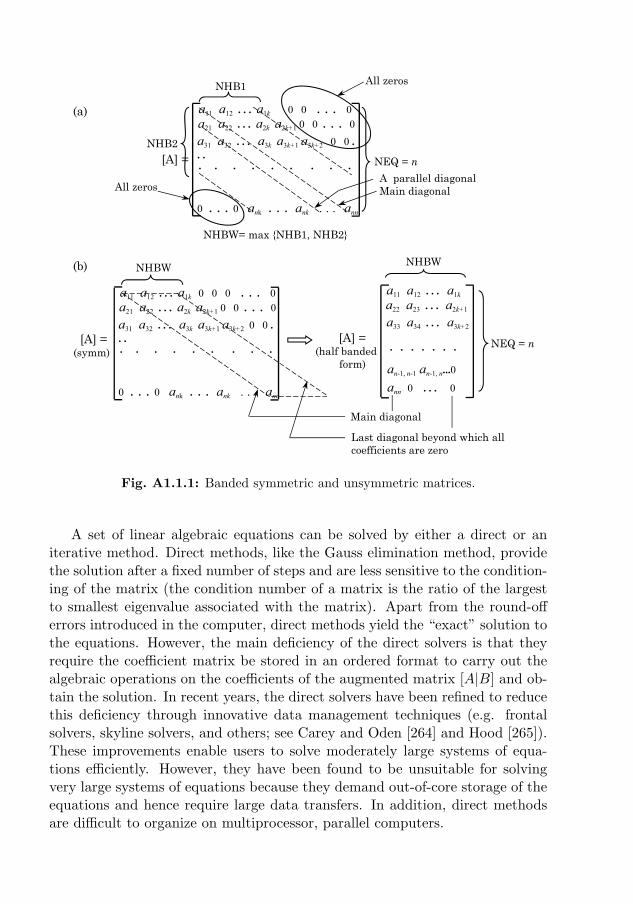
638 APPENDIX 1: SOLUTION PROCEDURES FOR LINEAR EQUATIONS
a11 a12 . . . a1k 0 0 . . . 0 a21 a22 . . . a2k a2k+1 0 0 . . . 0 a31 a32 . . . a3k a3k+1 a3k+2 0 0 . . .. . . . . . . . .
0 . . . 0 ank . . . ank . . . ann
[A] =
NHB1
NHB2
NHBW= max NHB1, NHB2
A parallel diagonalMain diagonal
All zeros
All zeros
(a)
NEQ = n
a11 a12 . . . a1k 0 0 0 . . . 0 a21 a22 . . . a2k a2k+1 0 0 . . . 0 a31 a32 . . . a3k a3k+1 a3k+2 0 0 . . .. . . . . . . . .
0 . . . 0 ank . . . ank . . . ann
[A] =(symm)
(b)
[A] =(half banded
form)
a11 a12 . . . a1k
a22 a23 . . . a2k+1
a33 a34 . . . a3k+2
. . . . . . .
NHBW
ann 0 . . . 0
an-1, n-1 an-1, n...0
NHBW
NEQ = n
Main diagonal
Last diagonal beyond which all coefficients are zero
Fig. A1.1.1: Banded symmetric and unsymmetric matrices.
A set of linear algebraic equations can be solved by either a direct or aniterative method. Direct methods, like the Gauss elimination method, providethe solution after a fixed number of steps and are less sensitive to the condition-ing of the matrix (the condition number of a matrix is the ratio of the largestto smallest eigenvalue associated with the matrix). Apart from the round-offerrors introduced in the computer, direct methods yield the “exact” solution tothe equations. However, the main deficiency of the direct solvers is that theyrequire the coefficient matrix be stored in an ordered format to carry out thealgebraic operations on the coefficients of the augmented matrix [A|B] and ob-tain the solution. In recent years, the direct solvers have been refined to reducethis deficiency through innovative data management techniques (e.g. frontalsolvers, skyline solvers, and others; see Carey and Oden [264] and Hood [265]).These improvements enable users to solve moderately large systems of equa-tions efficiently. However, they have been found to be unsuitable for solvingvery large systems of equations because they demand out-of-core storage of theequations and hence require large data transfers. In addition, direct methodsare difficult to organize on multiprocessor, parallel computers.
A1.2. DIRECT METHODS 639
The limitations on CPU time and storage requirements preclude the use ofdirect solvers for complex problems with more than a quarter million equations,and iterative methods are found to be more efficient in that they require lessstorage and CPU time. Iterative methods are approximate and only convergedsolutions will be close to the true solutions. In iterative methods, the globalmatrix formation may be avoided. The major operation in iterative methodsis the matrix-vector multiplication as compared to the matrix reduction (byelementary operations) in direct methods. A significant advantage of iterativemethods is that a given set of equations can be divided into as many subsets ofequations as there are processors and calculations can be performed in parallelon the array of processors. However, convergence characteristics of iterativemethods depend on the condition number of the system of linear equations,and a suitable preconditioner is a must to achieve convergence. For additionaldetails, the reader may consult [265–268].
A1.2 Direct Methods
A1.2.1 Preliminary Comments
Direct methods are those in which simultaneous linear algebraic equations aresolved “exactly” (within the computational round-off error) by successive elim-ination of variables and back substitution. The Gauss elimination method is afixed-step technique [266–268], and frontal [265] and skyline [4] solution meth-ods are examples of direct solution methods that use the Gauss eliminationtechnique efficiently. The direct methods are the most commonly used tech-niques when the number of equations involved is not too large. The numberof elementary operations for Gauss elimination is of the order n3/3 + O(n2),where n denotes the number of unknowns.
The frontal solution procedure [265] is faster than most direct solvers; itrequires less core space as long as active variables can be kept in the core, andit allows for partial pivoting. An additional advantage is that no specific nodenumbering scheme is needed, though a judicious element numbering helps tominimize the front width.
Due to the fact that the approximation functions are defined only within anelement, the coefficient matrix in the finite element method is banded; that is,aij = 0 for j > i + nb, where nb is the half bandwidth of the matrix [A]. Thisgreatly reduces the number of operations in solving the equations, if we makenote of the fact that elements outside the bandwidth are zero. Of course, thebandwidth size depends on the global node numbering. The skyline technique isone in which bandedness of the finite element equations is exploited by storingthe row number mj of the first nonzero element in column j. The variables mi,i = 1, 2, . . . , n, define the skyline of the matrix (see Bathe [4] for details).
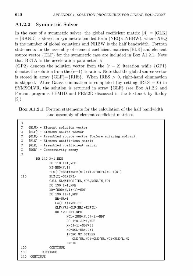
640 APPENDIX 1: SOLUTION PROCEDURES FOR LINEAR EQUATIONS
A1.2.2 Symmetric Solver
In the case of a symmetric solver, the global coefficient matrix [A] ≡ [GLK]= [BAND] is stored in symmetric banded form (NEQ× NHBW), where NEQis the number of global equations and NHBW is the half bandwidth. Fortranstatements for the assembly of element coefficient matrices [ELK] and elementsource vector ELF for the symmetric case are included in Box A1.2.1. Notethat BETA is the acceleration parameter, β [see Eq. (4.4.6)], and the arrayGP2 denotes the solution vector from the (r − 2) iteration while GP1denotes the solution from the (r−1) iteration. Note that the global source vectoris stored in array GLF=RHS. When IRES > 0, right-hand eliminationis skipped. After Gauss elimination is completed (by setting IRES = 0) inSYMSOLVR, the solution is returned in array GLF (see Box A1.2.2 andFortran programs FEM1D and FEM2D discussed in the textbook by Reddy[2]).
Box A1.2.1: Fortran statements for the calculation of the half bandwidthand assembly of element coefficient matrices.
C
C ELU - Element solution vector
C ELF - Element source vector
C GLF - Assembled source vector (before entering solver)
C [ELK] - Element coefficient matrix
C [GLK] - Assembled coefficient matrix
C [NOD] - Connectivity array
C
DO 140 N=1,NEM
DO 110 I=1,NPE
NI=NOD(N,I)
ELU(I)=BETA*GP2(NI)+(1.0-BETA)*GP1(NI)
110 ELX(I)=GLX(NI)
CALL ELMATRCS(IEL,NPE,NONLIN,F0)
DO 130 I=1,NPE
NR=(NOD(N,I)-1)*NDF
DO 130 II=1,NDF
NR=NR+1
L=(I-1)*NDF+II
GLF(NR)=GLF(NR)+ELF(L)
DO 120 J=1,NPE
NCL=(NOD(N,J)-1)*NDF
DO 120 JJ=1,NDF
M=(J-1)*NDF+JJ
NC=NCL-NR+JJ+1
IF(NC.GT.0)THEN
GLK(NR,NC)=GLK(NR,NC)+ELK(L,M)
ENDIF
120 CONTINUE
130 CONTINUE
140 CONTINUE
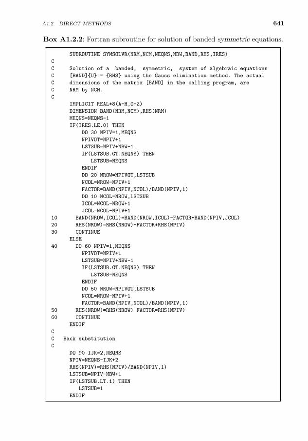
A1.2. DIRECT METHODS 641
Box A1.2.2: Fortran subroutine for solution of banded symmetric equations.
SUBROUTINE SYMSOLVR(NRM,NCM,NEQNS,NBW,BAND,RHS,IRES)
C
C Solution of a banded, symmetric, system of algebraic equations
C [BAND]U = RHS using the Gauss elimination method. The actual
C dimensions of the matrix [BAND] in the calling program, are
C NRM by NCM.
C
IMPLICIT REAL*8(A-H,O-Z)
DIMENSION BAND(NRM,NCM),RHS(NRM)
MEQNS=NEQNS-1
IF(IRES.LE.0) THEN
DO 30 NPIV=1,MEQNS
NPIVOT=NPIV+1
LSTSUB=NPIV+NBW-1
IF(LSTSUB.GT.NEQNS) THEN
LSTSUB=NEQNS
ENDIF
DO 20 NROW=NPIVOT,LSTSUB
NCOL=NROW-NPIV+1
FACTOR=BAND(NPIV,NCOL)/BAND(NPIV,1)
DO 10 NCOL=NROW,LSTSUB
ICOL=NCOL-NROW+1
JCOL=NCOL-NPIV+1
10 BAND(NROW,ICOL)=BAND(NROW,ICOL)-FACTOR*BAND(NPIV,JCOL)
20 RHS(NROW)=RHS(NROW)-FACTOR*RHS(NPIV)
30 CONTINUE
ELSE
40 DO 60 NPIV=1,MEQNS
NPIVOT=NPIV+1
LSTSUB=NPIV+NBW-1
IF(LSTSUB.GT.NEQNS) THEN
LSTSUB=NEQNS
ENDIF
DO 50 NROW=NPIVOT,LSTSUB
NCOL=NROW-NPIV+1
FACTOR=BAND(NPIV,NCOL)/BAND(NPIV,1)
50 RHS(NROW)=RHS(NROW)-FACTOR*RHS(NPIV)
60 CONTINUE
ENDIF
C
C Back substitution
C
DO 90 IJK=2,NEQNS
NPIV=NEQNS-IJK+2
RHS(NPIV)=RHS(NPIV)/BAND(NPIV,1)
LSTSUB=NPIV-NBW+1
IF(LSTSUB.LT.1) THEN
LSTSUB=1
ENDIF
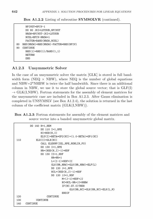
642 APPENDIX 1: SOLUTION PROCEDURES FOR LINEAR EQUATIONS
Box A1.2.2: Listing of subroutine SYMSOLVR (continued).
NPIVOT=NPIV-1
DO 80 JKI=LSTSUB,NPIVOT
NROW=NPIVOT-JKI+LSTSUB
NCOL=NPIV-NROW+1
FACTOR=BAND(NROW,NCOL)
80 RHS(NROW)=RHS(NROW)-FACTOR*RHS(NPIV)
90 CONTINUE
RHS(1)=RHS(1)/BAND(1,1)
RETURN
END
A1.2.3 Unsymmetric Solver
In the case of an unsymmetric solver the matrix [GLK] is stored in full band-width form (NEQ × NBW), where NEQ is the number of global equationsand NBW=2*NHBW is twice the half bandwidth. Since there is an additionalcolumn in NBW, we use it to store the global source vector; that is GLF(I)→ GLK(I,NBW). Fortran statements for the assembly of element matrices forthe unsymmetric case are included in Box A1.2.3. After Gauss elimination iscompleted in UNSYMSLV (see Box A1.2.4), the solution is returned in the lastcolumn of the coefficient matrix GLK(I,NBW).
Box A1.2.3: Fortran statements for assembly of the element matrices andsource vector into a banded unsymmetric global matrix.
DO 140 N=1,NEM
DO 110 I=1,NPE
NI=NOD(N,I)
ELU(I)=BETA*GP2(NI)+(1.0-BETA)*GP1(NI)
110 ELX(I)=GLX(NI)
CALL ELEKMF(IEL,NPE,NONLIN,F0)
DO 130 I=1,NPE
NR=(NOD(N,I)-1)*NDF
DO 130 II=1,NDF
NR=NR+1
L=(I-1)*NDF+II
GLK(NR,NBW)=GLK(NR,NBW)+ELF(L)
DO 120 J=1,NPE
NCL=(NOD(N,J)-1)*NDF
DO 120 JJ=1,NDF
M=(J-1)*NDF+JJ
NC=NCL-NR+JJ+NHBW
IF(NC.GT.0)THEN
GLK(NR,NC)=GLK(NR,NC)+ELK(L,M)
ENDIF
120 CONTINUE
130 CONTINUE
140 CONTINUE
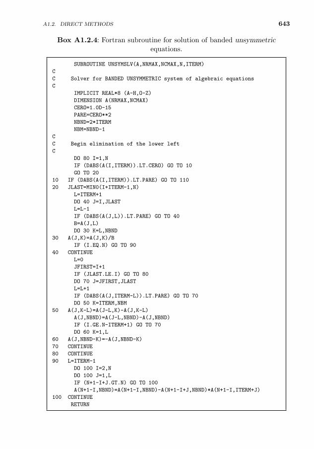
A1.2. DIRECT METHODS 643
Box A1.2.4: Fortran subroutine for solution of banded unsymmetricequations.
SUBROUTINE UNSYMSLV(A,NRMAX,NCMAX,N,ITERM)
C
C Solver for BANDED UNSYMMETRIC system of algebraic equations
C
IMPLICIT REAL*8 (A-H,O-Z)
DIMENSION A(NRMAX,NCMAX)
CERO=1.0D-15
PARE=CERO**2
NBND=2*ITERM
NBM=NBND-1
C
C Begin elimination of the lower left
C
DO 80 I=1,N
IF (DABS(A(I,ITERM)).LT.CERO) GO TO 10
GO TO 20
10 IF (DABS(A(I,ITERM)).LT.PARE) GO TO 110
20 JLAST=MIN0(I+ITERM-1,N)
L=ITERM+1
DO 40 J=I,JLAST
L=L-1
IF (DABS(A(J,L)).LT.PARE) GO TO 40
B=A(J,L)
DO 30 K=L,NBND
30 A(J,K)=A(J,K)/B
IF (I.EQ.N) GO TO 90
40 CONTINUE
L=0
JFIRST=I+1
IF (JLAST.LE.I) GO TO 80
DO 70 J=JFIRST,JLAST
L=L+1
IF (DABS(A(J,ITERM-L)).LT.PARE) GO TO 70
DO 50 K=ITERM,NBM
50 A(J,K-L)=A(J-L,K)-A(J,K-L)
A(J,NBND)=A(J-L,NBND)-A(J,NBND)
IF (I.GE.N-ITERM+1) GO TO 70
DO 60 K=1,L
60 A(J,NBND-K)=-A(J,NBND-K)
70 CONTINUE
80 CONTINUE
90 L=ITERM-1
DO 100 I=2,N
DO 100 J=1,L
IF (N+1-I+J.GT.N) GO TO 100
A(N+1-I,NBND)=A(N+1-I,NBND)-A(N+1-I+J,NBND)*A(N+1-I,ITERM+J)
100 CONTINUE
RETURN
644 APPENDIX 1: SOLUTION PROCEDURES FOR LINEAR EQUATIONS
Box A1.2.4: Listing of subroutine UNSYMSLV (continued).
110 WRITE (6,140) I,A(I,ITERM)
STOP
140 FORMAT (/,2X,’Computation stopped in UNSYMSLV because zero appears
* on the main diagonal *** Eqn no. and value:’,I5,E12.4)
END
A1.3 Iterative Methods
Among the various iterative methods that are available in the literature, theconjugate gradient (CG) method [269] is most widely used because it is a finitestep method (i.e. apart from round-off errors, the solution is achieved in a fixednumber of iterations) and it can be used to determine the inverse. However, thenumber of iterations required depends on the condition number of the coeffi-cient matrix. The convergence of the conjugate gradient method, and iterativemethods in general, can be improved by preconditioning and/or scaling theequations [270–272].
The limitations on storage can be overcome by solving the equations atthe element level, that is, use the Gauss–Seidel iteration idea for the set ofvariables associated with the element. This approach avoids assembly of elementmatrices to form the global coefficient matrix. This idea of using the element-by-element data structure of the coefficient matrix was first pointed out by Foxand Stanton [273] and Fried [274]. The phrase element-by-element refers toa particular data structure for finite element techniques wherein informationis stored and maintained at the element level rather than assembled into aglobal data structure. In this method the matrix–vector multiplications arecarried out at the element level and the assembly is carried out on the resultantvector. This idea proves to be very attractive when solving large problems,because the matrix–vector multiplication can be done in parallel on a series ofprocessors. Another advantage of this method is that the resultant savings instorage, compared to direct solvers, allows solution of large problems on smallcomputers.
The advantages of the element-by-element data structure over assemblingthe global coefficient matrix are: (1) the need for formation and storage of aglobal matrix is eliminated, and therefore the total storage and computationalcosts are low, (2) the amount of storage is independent of the node numberingand mesh topology and depends on the number and type of elements in themesh, and (3) the element-by-element solution algorithms can be vectorizedfor efficient use on supercomputers. The major disadvantage of the element-by-element data structure is the limited number of preconditioners that canbe formulated from the unassembled matrices. A review of the literature onelement-by-element algorithms can be found in [275], and the methods havebeen investigated by numerous investigators [197, 275–278].
645
2
Appendix:Solution Procedures
for Nonlinear Equations
A2.1 Introduction
Finite element formulations of nonlinear differential equations lead to nonlinearalgebraic equations for each element of the finite element mesh. The elementequation is of the form,
[Ke(ue)]ue = F e (A2.1.1)
where
[Ke] − element coefficient matrix (or “stiffness” matrix), which
depends on the solution vectorue,ue − column vector of element nodal values, and (A2.1.2)
F e − column vector of element nodal “forces”.
When [Ke] is independent of ue, the matrix coefficients can be evaluated forall elements and the assembled equations can be solved for the global nodalvalues u after imposing boundary conditions. When [Ke] depends on theunknown solution vector ue, the matrix coefficients cannot be evaluated. Ifwe can find an approximation to ue, say ue1, then [Ke(ue1)] can beevaluated and assembled. This amounts to linearizing the nonlinear equations,Eq. (A2.1.1). Then a next approximation to the solution can be obtained bysolving the assembled equations,
u2 = [K(u1)]−1F (A2.1.3)
This procedure can be repeated until the approximate solution comes close tothe actual solution in some measure. Such a procedure is called an iterativeprocedure.
J.N. Reddy, An Introduction to Nonlinear Finite Element Analysis, Second Edition. c©J.N.Reddy 2015. Published in 2015 by Oxford University Press.
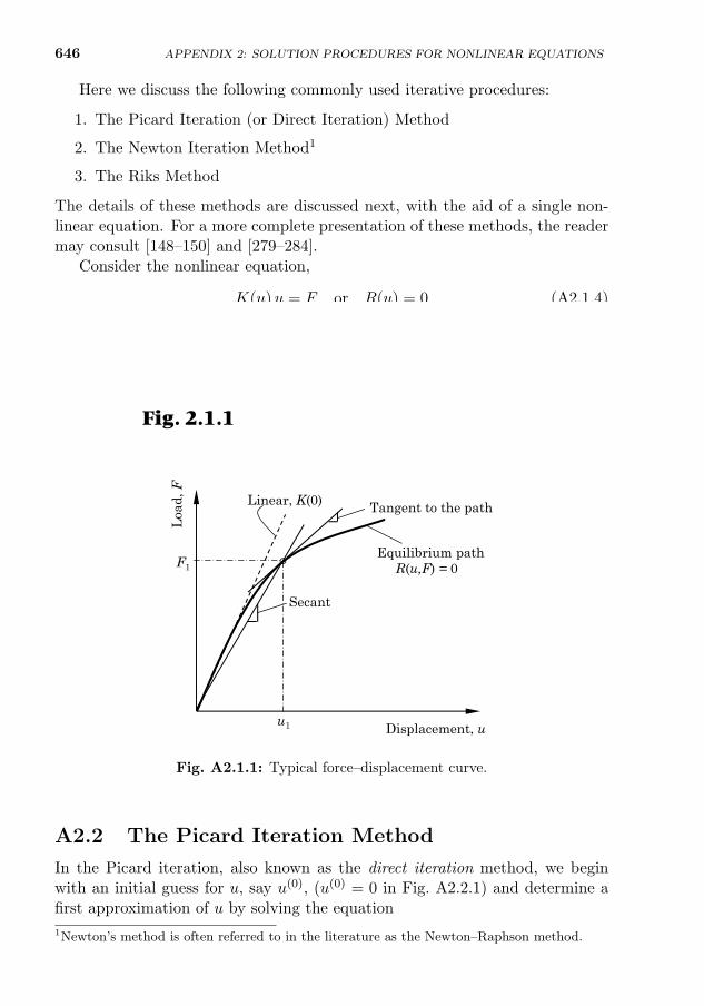
646
Here we discuss the following commonly used iterative procedures:
1. The Picard Iteration (or Direct Iteration) Method
2. The Newton Iteration Method1
3. The Riks Method
The details of these methods are discussed next, with the aid of a single non-linear equation. For a more complete presentation of these methods, the readermay consult [148–150] and [279–284].
Consider the nonlinear equation,
K(u)u = F or R(u) = 0 (A2.1.4)
where u is the solution to be determined, K(u) is a known function of u, F isthe known ‘force’, and R is the residual
R(u) = K(u)u− F (A2.1.5)
A plot of the equilibrium path, R(u, F ) = 0, is shown in Fig. A2.1.1. For anyvalue u1, K(u1) denotes the secant of the curve at u = u1, and (∂R∂u )|u1 denotesthe tangent of the curve at u = u1.
Displacement, u
Linear, K(0)
Equilibrium pathR(u,F) = 0
Tangent to the path
Secant
F1
Loa
d, F
°
u1
Fig. 2.1.1
Fig. A2.1.1: Typical force–displacement curve.
A2.2 The Picard Iteration Method
In the Picard iteration, also known as the direct iteration method, we beginwith an initial guess for u, say u(0), (u(0) = 0 in Fig. A2.2.1) and determine afirst approximation of u by solving the equation
1Newton’s method is often referred to in the literature as the Newton–Raphson method.
APPENDIX 2: SOLUTION PROCEDURES FOR NONLINEAR EQUATIONS
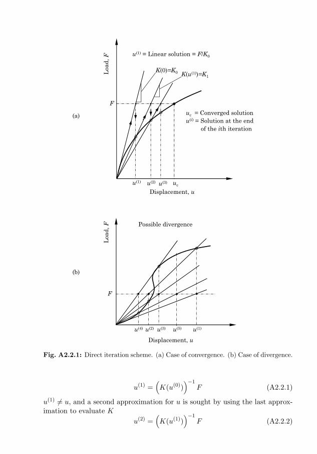
A2.2. THE PICARD ITERATION METHOD 647
Displacement, u
u(1) = Linear solution = F/K0
FL
oad,
F
u(1)
uc = Converged solutionu(i) = Solution at the end
of the ith iteration
uc
K(0)=K0
°
°
K(u(1))=K1
• • •
°•
(a)
u(2) u(3)
(b)
Displacement, u
F
Loa
d, F Possible divergence
°
°
• ••°
°
••
u(4) u(2) u(1)u(5)u(3)
Fig. A2.2.1: Direct iteration scheme. (a) Case of convergence. (b) Case of divergence.
u(1) =(K(u(0))
)−1F (A2.2.1)
u(1) 6= u, and a second approximation for u is sought by using the last approx-imation to evaluate K
u(2) =(K(u(1))
)−1F (A2.2.2)
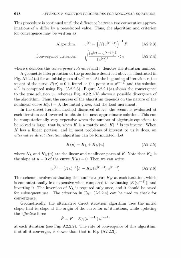
648 APPENDIX 2: SOLUTION PROCEDURES FOR NONLINEAR EQUATIONS
This procedure is continued until the difference between two consecutive approx-imations of u differ by a preselected value. Thus, the algorithm and criterionfor convergence may be written as
Algorithm: u(r) =(K(u(r−1))
)−1F (A2.2.3)
Convergence criterion:
√(u(r) − u(r−1))2
(u(r))2< ε (A2.2.4)
where ε denotes the convergence tolerance and r denotes the iteration number.A geometric interpretation of the procedure described above is illustrated in
Fig. A2.2.1(a) for an initial guess of u(0) = 0. At the beginning of iteration r, thesecant of the curve R(u) = 0 is found at the point u = u(r−1) and the solutionu(r) is computed using Eq. (A2.2.3). Figure A2.2.1(a) shows the convergenceto the true solution uc, whereas Fig. A2.2.1(b) shows a possible divergence ofthe algorithm. Thus, the success of the algorithm depends on the nature of thenonlinear curve R(u) = 0, the initial guess, and the load increment.
In the direct iteration method discussed above, the secant is evaluated ateach iteration and inverted to obtain the next approximate solution. This canbe computationally very expensive when the number of algebraic equations tobe solved is large, that is, when K is a matrix and [K]−1 is its inverse. WhenK has a linear portion, and in most problems of interest to us it does, analternative direct iteration algorithm can be formulated. Let
K(u) = KL +KN (u) (A2.2.5)
where KL and KN (u) are the linear and nonlinear parts of K. Note that KL isthe slope at u = 0 of the curve R(u) = 0. Then we can write
u(r) = (KL)−1[F −KN (u(r−1))u(r−1)] (A2.2.6)
This scheme involves evaluating the nonlinear part KN at each iteration, whichis computationally less expensive when compared to evaluating [K(ur−1))] andinverting it. The inversion of KL is required only once, and it should be savedfor subsequent use. The criterion in Eq. (A2.2.4) can be used to check forconvergence.
Geometrically, the alternative direct iteration algorithm uses the initialslope, that is, slope at the origin of the curve for all iterations, while updatingthe effective force
F ≡ F −KN (u(r−1))u(r−1)
at each iteration (see Fig. A2.2.2). The rate of convergence of this algorithm,if at all it converges, is slower than that in Eq. (A2.2.3).
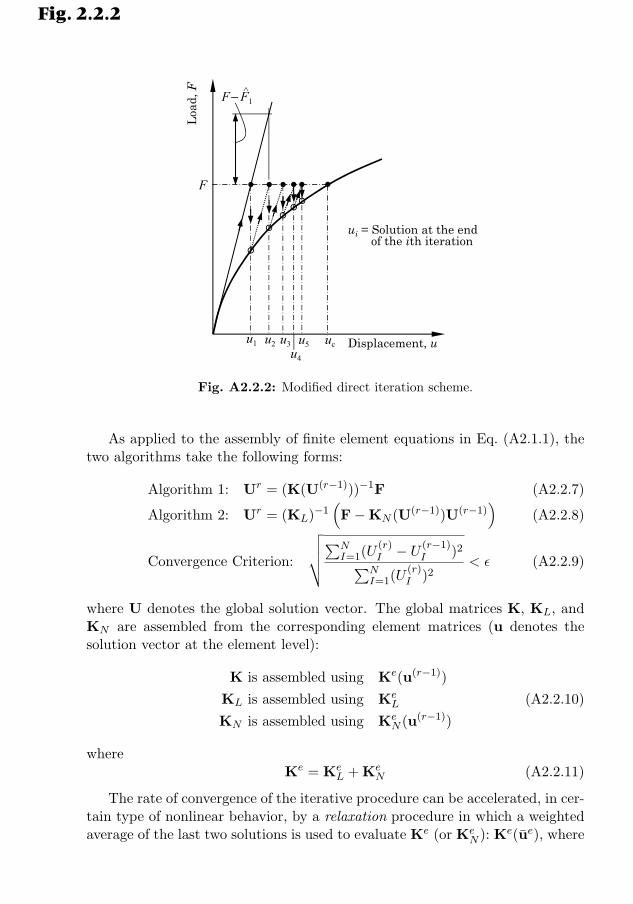
A2.2. THE PICARD ITERATION METHOD 649
F− F1^
Displacement, u
FL
oad,
F
u1 u2 u3
ui = Solution at the end of the ith iteration
uc
°
• •
u4
u5
Fig. 2.2.2
° °°°••••
Fig. A2.2.2: Modified direct iteration scheme.
As applied to the assembly of finite element equations in Eq. (A2.1.1), thetwo algorithms take the following forms:
Algorithm 1: Ur = (K(U(r−1)))−1F (A2.2.7)
Algorithm 2: Ur = (KL)−1(F−KN (U(r−1))U(r−1)
)(A2.2.8)
Convergence Criterion:
√√√√∑NI=1(U
(r)I − U
(r−1)I )2∑N
I=1(U(r)I )2
< ε (A2.2.9)
where U denotes the global solution vector. The global matrices K, KL, andKN are assembled from the corresponding element matrices (u denotes thesolution vector at the element level):
K is assembled using Ke(u(r−1))
KL is assembled using KeL (A2.2.10)
KN is assembled using KeN (u(r−1))
whereKe = Ke
L + KeN (A2.2.11)
The rate of convergence of the iterative procedure can be accelerated, in cer-tain type of nonlinear behavior, by a relaxation procedure in which a weightedaverage of the last two solutions is used to evaluate Ke (or Ke
N ): Ke(ue), where
650 APPENDIX 2: SOLUTION PROCEDURES FOR NONLINEAR EQUATIONS
ue = βu(r−2) + (1− β)u(r−1), and 0 ≤ β ≤ 1 is called the relaxation or acceler-ation parameter. In this case Eqs. (A2.2.7) and (A2.2.8) take the form,
Algorithm 1 Ur = (K(U))−1F (A2.2.12)
Algorithm 2 Ur = (KL)−1(F−KN (U)U) (A2.2.13)
U = βU(r−2) + (1− β)U(r−1) (A2.2.14)
The actual value of β varies from problem to problem.The computational algorithm of the direct iteration is summarized below.
At each load level follow the steps:
(1) Compute element matrices Ke and Fe (for transient problems, Ke andFe are to be replaced by Ke and Fe) using the solution U(r−1) from theprevious iteration (of current load and/or time). For the first iteration ofthe subsequent load steps, use Uc, the converged solution of the last loadstep. For the first load step use Uc = 0, provided K is not singular, tocompute the linear solution.
(2) Assemble the element matrices Ke and Fe (or Ke and Fe).(3) Apply the boundary conditions on the assembled set of equations.(4) Solve the assembled equations.(5) Check for convergence using Eq. (A2.2.9).
(6a) If the convergence criterion is satisfied, increase the load to next level,initialize the counter on iterations, and repeat Steps 1–5.
(6b) If the convergence criterion is not satisfied, check if the maximum numberof allowable iterations is exceeded. If yes, terminate the computationprinting a message to that effect. If the number of iterations did notexceed the maximum allowed, update U(r−1) and U(r) and repeat Steps1–5.
A2.3 The Newton Iteration Method
Suppose that we know solution u(r−1) of Eq. (A2.1.1) at (r− 1)st iteration andinterested in seeking solution at the rth iteration. We expand R(u) about theknown solution u(r−1) in Taylor’s series,
R(u) = R(u(r−1))+
(∂R
∂u
) ∣∣∣∣u(r−1)
δu+1
2
(∂2R
∂u2
) ∣∣∣∣u(r−1)
(δu)2+· · · = 0 (A2.3.1)
where δu is the increment,
δu(r) = u(r) − u(r−1) (A2.3.2)
Assuming that the second- and higher-order terms in δu are negligible, we canwrite Eq. (A2.3.1) as
δu(r) = −(KT (u(r−1))
)−1R(u(r−1))
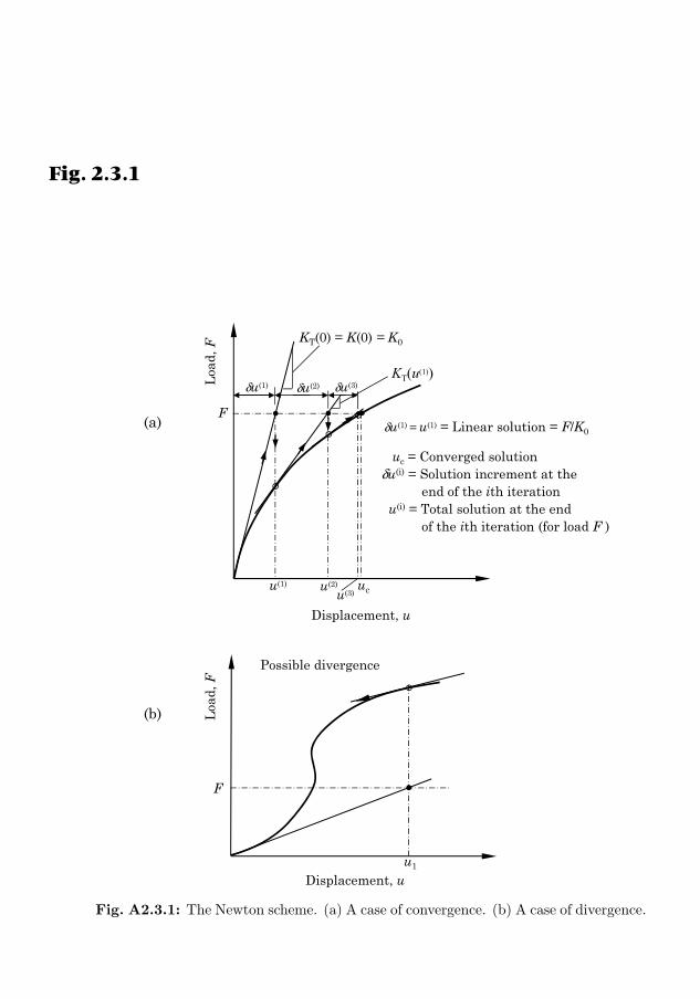
A2.3. THE NEWTON ITERATION METHOD 651
=(KT (u(r−1))
)−1 (F −K(u(r−1))u(r−1)
)(A2.3.3)
where KT is the slope (tangent) of the curve R(u) at u(r−1) (see Fig. A2.3.1):
KT =∂R
∂u
∣∣∣∣u(r−1)
(A2.3.4)
The residual or imbalance force, R(u(r−1)) is gradually reduced to zero if theprocedure converges. Equation (A2.3.3) gives the increment of u at the rthiteration so that the total solution is
u(r) = u(r−1) + δu(r) (A2.3.5)
(b)
Displacement, u
F
Loa
d, F
u1
Possible divergence
°
•
Displacement, u
δu(1) = u(1) = Linear solution = F/K0
F
Loa
d, F
uc = Converged solutionδu(i) = Solution increment at the
end of the ith iterationu(i) = Total solution at the end
of the ith iteration (for load F )
uc
KT(0) = K(0) = K0
°
°
KT(u(1))
• • •°
•(a)
u(1) u(2)
u(3)
δu(1) δu(2) δu(3)
Fig. 2.3.1
Fig. A2.3.1: The Newton scheme. (a) A case of convergence. (b) A case of divergence.
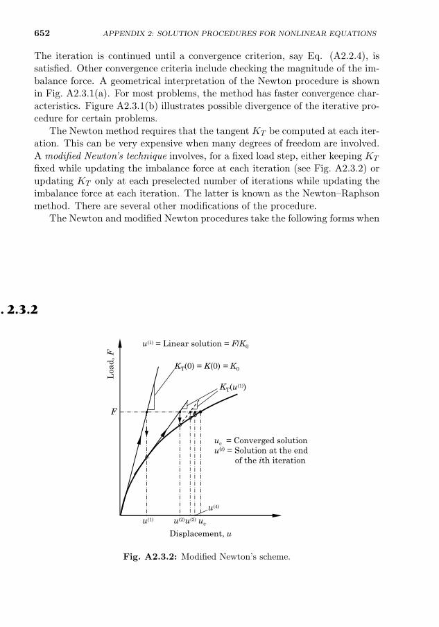
652 APPENDIX 2: SOLUTION PROCEDURES FOR NONLINEAR EQUATIONS
The iteration is continued until a convergence criterion, say Eq. (A2.2.4), issatisfied. Other convergence criteria include checking the magnitude of the im-balance force. A geometrical interpretation of the Newton procedure is shownin Fig. A2.3.1(a). For most problems, the method has faster convergence char-acteristics. Figure A2.3.1(b) illustrates possible divergence of the iterative pro-cedure for certain problems.
The Newton method requires that the tangent KT be computed at each iter-ation. This can be very expensive when many degrees of freedom are involved.A modified Newton’s technique involves, for a fixed load step, either keeping KT
fixed while updating the imbalance force at each iteration (see Fig. A2.3.2) orupdating KT only at each preselected number of iterations while updating theimbalance force at each iteration. The latter is known as the Newton–Raphsonmethod. There are several other modifications of the procedure.
The Newton and modified Newton procedures take the following forms whenapplied to the assembly of element equations (A2.3.3):
Newton’s ProcedureδU = −(KT )−1R (A2.3.6)
Modified Newton’s Procedure
δU = −(KT )−1R (A2.3.7)
Displacement, u
u(1) = Linear solution = F/K0
F
Loa
d, F
uc = Converged solutionu(i) = Solution at the end
of the ith iteration
uc
KT(0) = K(0) = K0
°
°
KT(u(1))
• • •°
••°
u(1) u(3)u(2)
u(4)
Fig. 2.3.2
Fig. A2.3.2: Modified Newton’s scheme.
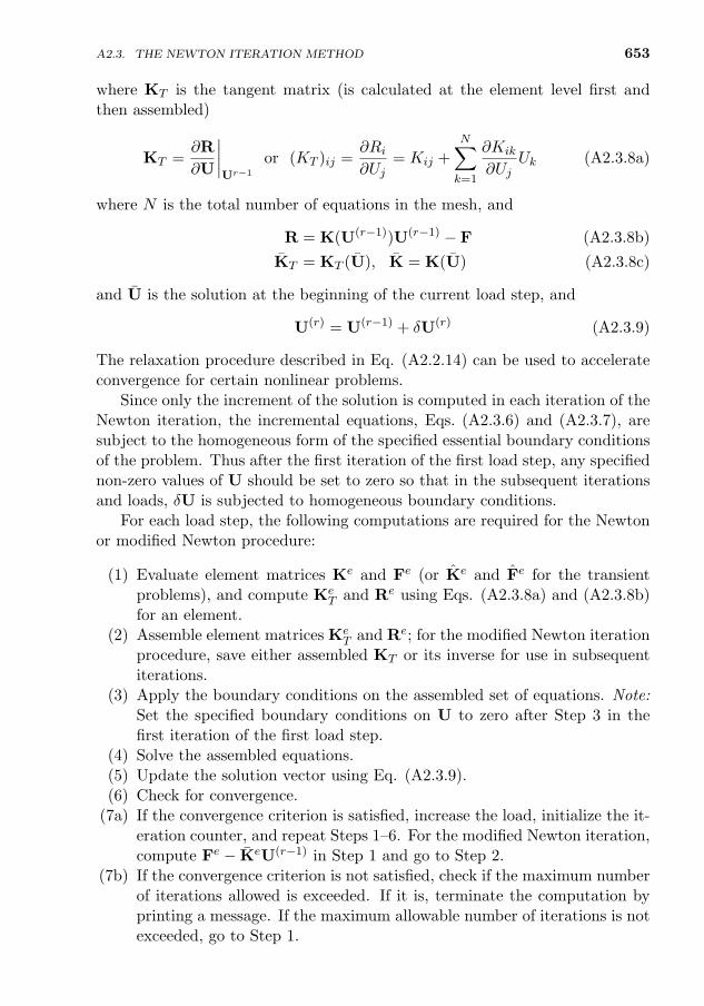
A2.3. THE NEWTON ITERATION METHOD 653
where KT is the tangent matrix (is calculated at the element level first andthen assembled)
KT =∂R
∂U
∣∣∣∣Ur−1
or (KT )ij =∂Ri∂Uj
= Kij +
N∑k=1
∂Kik
∂UjUk (A2.3.8a)
where N is the total number of equations in the mesh, and
R = K(U(r−1))U(r−1) − F (A2.3.8b)
KT = KT (U), K = K(U) (A2.3.8c)
and U is the solution at the beginning of the current load step, and
U(r) = U(r−1) + δU(r) (A2.3.9)
The relaxation procedure described in Eq. (A2.2.14) can be used to accelerateconvergence for certain nonlinear problems.
Since only the increment of the solution is computed in each iteration of theNewton iteration, the incremental equations, Eqs. (A2.3.6) and (A2.3.7), aresubject to the homogeneous form of the specified essential boundary conditionsof the problem. Thus after the first iteration of the first load step, any specifiednon-zero values of U should be set to zero so that in the subsequent iterationsand loads, δU is subjected to homogeneous boundary conditions.
For each load step, the following computations are required for the Newtonor modified Newton procedure:
(1) Evaluate element matrices Ke and Fe (or Ke and Fe for the transientproblems), and compute Ke
T and Re using Eqs. (A2.3.8a) and (A2.3.8b)for an element.
(2) Assemble element matrices KeT and Re; for the modified Newton iteration
procedure, save either assembled KT or its inverse for use in subsequentiterations.
(3) Apply the boundary conditions on the assembled set of equations. Note:Set the specified boundary conditions on U to zero after Step 3 in thefirst iteration of the first load step.
(4) Solve the assembled equations.(5) Update the solution vector using Eq. (A2.3.9).(6) Check for convergence.
(7a) If the convergence criterion is satisfied, increase the load, initialize the it-eration counter, and repeat Steps 1–6. For the modified Newton iteration,compute Fe − KeU(r−1) in Step 1 and go to Step 2.
(7b) If the convergence criterion is not satisfied, check if the maximum numberof iterations allowed is exceeded. If it is, terminate the computation byprinting a message. If the maximum allowable number of iterations is notexceeded, go to Step 1.
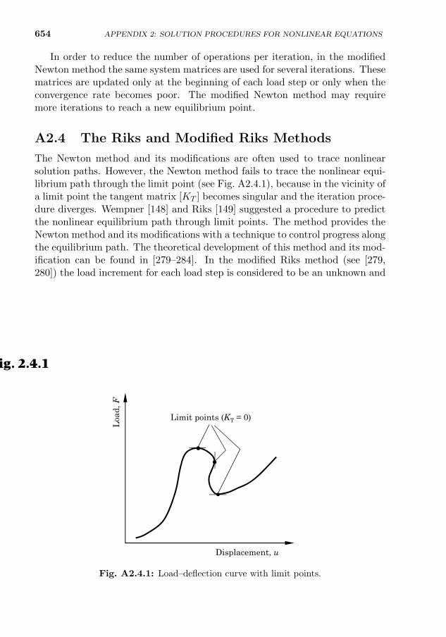
654 APPENDIX 2: SOLUTION PROCEDURES FOR NONLINEAR EQUATIONS
In order to reduce the number of operations per iteration, in the modifiedNewton method the same system matrices are used for several iterations. Thesematrices are updated only at the beginning of each load step or only when theconvergence rate becomes poor. The modified Newton method may requiremore iterations to reach a new equilibrium point.
A2.4 The Riks and Modified Riks Methods
The Newton method and its modifications are often used to trace nonlinearsolution paths. However, the Newton method fails to trace the nonlinear equi-librium path through the limit point (see Fig. A2.4.1), because in the vicinity ofa limit point the tangent matrix [KT ] becomes singular and the iteration proce-dure diverges. Wempner [148] and Riks [149] suggested a procedure to predictthe nonlinear equilibrium path through limit points. The method provides theNewton method and its modifications with a technique to control progress alongthe equilibrium path. The theoretical development of this method and its mod-ification can be found in [279–284]. In the modified Riks method (see [279,280]) the load increment for each load step is considered to be an unknown andsolved as a part of the solution.
The basic idea of the Riks technique can be described for a single nonlinearequation as follows (see Fig. A2.4.2): The length ∆s of the tangent to the cur-rent equilibrium point is prescribed, and the new point is found as the intersec-tion of the normal to the tangent with the equilibrium path [see Fig. A2.4.2(a)].Then iteration is performed along the normal toward the new equilibrium point,as illustrated in Fig. A2.4.2(a). Crisfield [151] suggested using a circular arc
Displacement, u
Loa
d, F
Limit points (KT = 0)
•
••
Fig. 2.4.1
Fig. A2.4.1: Load–deflection curve with limit points.
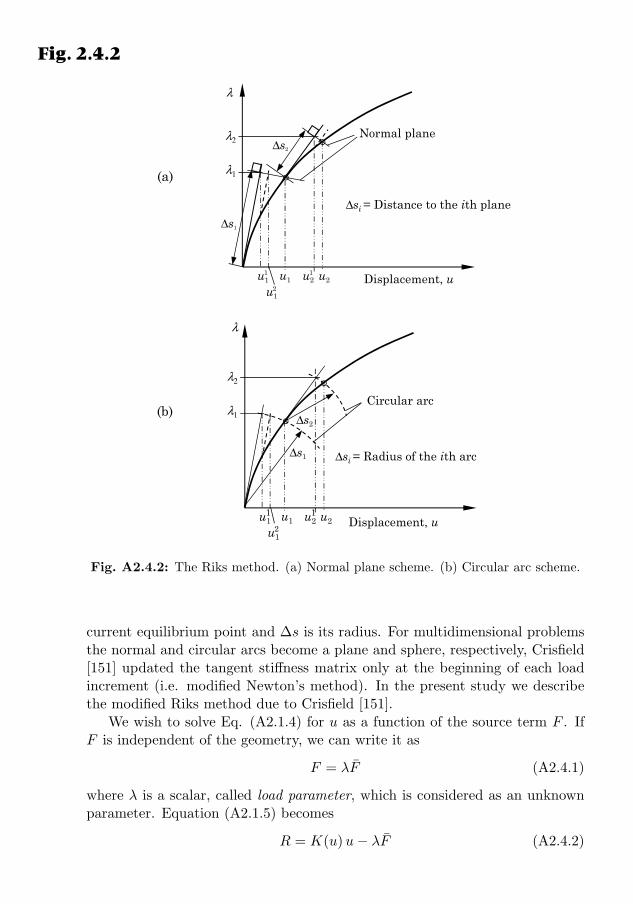
A2.4. THE RIKS AND MODIFIED RIKS METHODS 655
Displacement, uu1 u2
°
λ
λ1
Δs1
u11
Δs2
λ2 °
Δsi = Distance to the ith plane
u21
u12
Normal plane
(a)
Displacement, uu1 u2
°
λ
λ1
Δs1
u11
Δs2
λ2 °
Δsi = Radius of the ith arc
u21
u12
Circular arc (b)
Fig. 2.4.2
Fig. A2.4.2: The Riks method. (a) Normal plane scheme. (b) Circular arc scheme.
in place of the normal [see Fig. A2.4.2(b)]. The center of the circle is at thecurrent equilibrium point and ∆s is its radius. For multidimensional problemsthe normal and circular arcs become a plane and sphere, respectively, Crisfield[151] updated the tangent stiffness matrix only at the beginning of each loadincrement (i.e. modified Newton’s method). In the present study we describethe modified Riks method due to Crisfield [151].
We wish to solve Eq. (A2.1.4) for u as a function of the source term F . IfF is independent of the geometry, we can write it as
F = λF (A2.4.1)
where λ is a scalar, called load parameter, which is considered as an unknownparameter. Equation (A2.1.5) becomes
R = K(u)u− λF (A2.4.2)
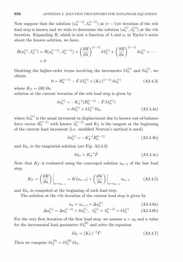
656 APPENDIX 2: SOLUTION PROCEDURES FOR NONLINEAR EQUATIONS
Now suppose that the solution (u(r−1)n , λ
(r−1)n ) at (r − 1)st iteration of the nth
load step is known and we wish to determine the solution (u(r)n , λ
(r)n ) at the rth
iteration. Expanding R, which is now a function of λ and u, in Taylor’s seriesabout the known solution, we have,
R(u(r)n , λ(r)n ) = R(u(r−1)n , λ(r−1)
n ) +
(∂R
∂λ
)(r−1)
δλ(r)n +
(∂R
∂u
)(r−1)
δu(r)n + · · ·
= 0
Omitting the higher-order terms involving the increments δλ(r)n and δu
(r)n , we
obtain0 = R(r−1)
n − F δλ(r)n + (KT )(r−1) δu(r)n (A2.4.3)
where KT = ∂R/∂u is the tangent matrix [see Eq. (A2.3.4)]. The incrementalsolution at the current iteration of the nth load step is given by
δu(r)n = −K−1T (R(r−1)
n − F δλ(r)n )
≡ δu(r)n + δλ(r)n δun (A2.4.4a)
where δu(r)n is the usual increment in displacement due to known out-of-balance
force vector R(r−1)n with known λ
(r−1)n and KT is the tangent at the beginning
of the current load increment (i.e. modified Newton’s method is used)
δu(r)n = −K−1T R(r−1)
n (A2.4.4b)
and δun is the tangential solution (see Fig. A2.4.3)
δun = K−1T F (A2.4.4c)
Note that KT is evaluated using the converged solution un−1 of the last loadstep,
KT =
(∂R
∂u
) ∣∣∣∣u=un−1
= K(un−1) +
(∂K
∂u
) ∣∣∣∣u=un−1
un−1 (A2.4.5)
and δun is computed at the beginning of each load step.The solution at the rth iteration of the current load step is given by
un = un−1 + ∆u(r)n (A2.4.6a)
∆u(r)n = ∆u(r−1)n + δu(r)n , λ(r)n = λ(r−1)
n + δλ(r)n (A2.4.6b)
For the very first iteration of the first load step, we assume u = u0 and a value
for the incremental load parameter δλ(0)1 and solve the equation
δu1 = (KT )−1F (A2.4.7)
Then we compute δu(0)1 = δλ
(0)1 δu1.
A2.4. THE RIKS AND MODIFIED RIKS METHODS 657
u0
°λ0
u1
δλ11
°
u11
Arc length
λ1
•1
Δu11
u12
u13
For N−R
Δu11 for N−R
Δu12
δu11
λ1λ10
23
••
° °
δu11
δu11∧ . δλ1
λ
1
Displacement, u
Fig. A2.4.3: Modified Riks scheme.
Select the arc length ∆s to be the length of the vector
(∆s)2 = ∆u(r)n ∆u(r)n (A2.4.8)
Substituting for ∆u(r)n from Eq. (A2.4.6b) [and δu
(r)n from Eq. (A2.4.4a)] we
obtain the following quadratic equation for the increment in the load parameter,
δλ(r)n :
a1[δλ(r)n ]2 + 2a2[δλ
(r)n ] + a3 = 0 (A2.4.9a)
a1 = δun δun
a2 = (∆u(r−1)n + δu(r)n ) δun
a3 = (∆u(r−1)n + δu(r)n ) (∆u(r−1)
n + δu(r)n )− (∆s)2 (A2.4.9b)
Let us denote the roots of this quadratic equation as δλ(r)n1 and δλ
(r)n2 . To avoid
“tracing back” the equilibrium path (i.e. going back on the known equilibriumpath), we require the angle between the incremental solution vectors at two
consecutive iterations, ∆u(r−1)n and ∆u
(r)n , be positive. Corresponding to the
two roots, δλ(r)n1 and δλ
(r)n2 , there correspond two values of ∆u
(r)n , denoted ∆u
(r)n1
and ∆u(r)n2 . The root that gives the positive angle is the one we select from
(δλ(r)n1 , δλ
(r)n2 ). The “angle” is defined to be product of the vector ∆u
(r−1)n and
∆u(r)n . Then we check to see which one of the following two products is positive:
∆u(r−1)n ∆u
(r)n1 and ∆u(r−1)
n ∆u(r)n2 (A2.4.10a)
658 APPENDIX 2: SOLUTION PROCEDURES FOR NONLINEAR EQUATIONS
If both roots are positive, then we select the ones closest to the linear solution,
δλ(r)n = − a32a2
(A2.4.10b)
The first arc length ∆s is computed using Eqs. (A2.4.7) and (A2.4.8):
∆s = δλ01√δu1 δu1 (A2.4.11)
To control the number of iterations taken to converge in the subsequent loadincrements, ∆s can be scaled,
∆sn = ∆sn−1IdI0
(A2.4.12)
where ∆sn−1 is the arc length used in the last iteration of the (n − 1)st loadstep, Id is the number of desired iterations (usually < 5) and I0 is the numberof iterations required for convergence in the previous step. Equation (A2.4.12)will automatically give small arc lengths in the areas of the most severe nonlin-earity and longer lengths when the response is linear or nearly linear. To avoidconvergence of the solution at a higher equilibrium path, maximum arc lengthsshould be specified.
For all load steps after the first, the initial incremental load parameter δλ(0)n
is calculated fromδλ(0)n = ±∆sn [δun δun]−
12 (A2.4.13)
The plus sign is for continuing the load increment in the same direction as theprevious load step and the negative sign is to reverse the load step. The signfollows that of the previous increment unless the value of determinant of thetangent matrix has changed in sign.
The modified Riks procedure described above for a single equation can beextended to the finite element equations in Eq. (A2.1.1). We introduce a loadparameter λ as an additional dependent variable,
F = λF (A2.4.14)
In writing Eq. (A2.4.14), loads are assumed to be independent of the deforma-tion. The assembled equations associated with Eq. (A2.1.1) become
R(U, λ) = KU− λF = 0 (A2.4.15)
The residual vector R is now considered as a function of both U and λ.Now suppose that the solution (U
(r−1)n , λ
(r−1)n ) at the (r−1)st iteration of the
nth load step is known. Expanding R in Taylor’s series about (U(r−1)n , λ
(r−1)n ),
we have
Ri = Ri(U(r−1)n , λ(r−1)
n )+
(∂Ri∂λ
)Ur−1,λr−1
n
δλ(r)−(∂Ri∂Uj
)U
(r−1)j ,λr−1
n
δU(r)j + · · ·
A2.4. THE RIKS AND MODIFIED RIKS METHODS 659
where the subscript ‘n’ is omitted for brevity. Omitting second- and higher-
order terms involving δλ(r) and δU(r)j , we can write
0 = R(r−1) − δλ(r)n F + KT δU(r)
or
δU(r)n = −(KT )−1R(r−1) + δλ(r)n (KT )−1F (A2.4.16a)
≡ δU(r)n + δλ(r)n δUn (A2.4.16b)
where F is the load vector, R(r−1)n the unbalanced force vector at iteration
(r − 1),δU(r)
n = −(KT )−1R(r−1)n (A2.4.17a)
and δλ(r)n the load increment [given by Eq. (A2.4.10b)], and
δUn = (KT )−1F (A2.4.17b)
For the first iteration of any load step, δλ(0)n is computed from [see Eq.
(A2.4.13)]:δλ(0)n = ±∆sn(δUT
n δUn)−1/2 (A2.4.18)
where [see Eq. (A2.4.12)]
∆sn = ∆sn−1IdI0
(A2.4.19a)
and ∆sn−1 is the arc length computed using the relation
∆sn−1 =√
∆UTn−1∆Un−1 (A2.4.19b)
∆Un−1 being the converged solution increment of the previous load step.For the first iteration of the first load step, we use:
∆s = δλ01
√δUT
1 δU1 (A2.4.20a)
δU1 = (KT )−1F, KT = KT (U0) (A2.4.20b)
where δλ01 is an assumed load increment and U0 is an assumed solution vector(often we assume δλ01 = 1 and U0 = 0).
The solution increment is updated using
∆Urn = ∆U(r−1)
n + δU(r)n (A2.4.21)
and the total solution at the current load step is given by
Un = Un−1 + ∆U(r)n (A2.4.22)
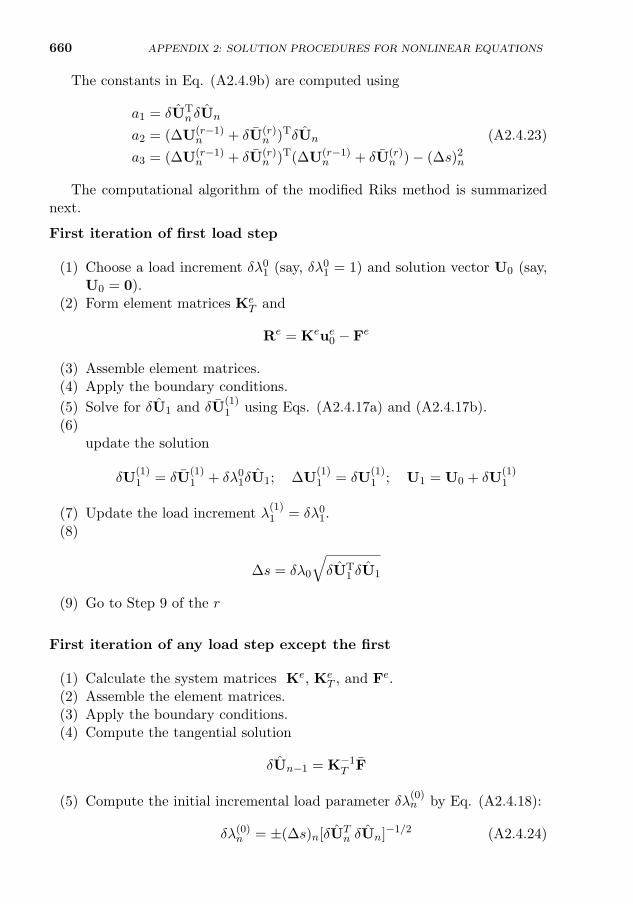
660 APPENDIX 2: SOLUTION PROCEDURES FOR NONLINEAR EQUATIONS
The constants in Eq. (A2.4.9b) are computed using
a1 = δUTn δUn
a2 = (∆U(r−1)n + δU(r)
n )TδUn (A2.4.23)
a3 = (∆U(r−1)n + δU(r)
n )T(∆U(r−1)n + δU(r)
n )− (∆s)2n
The computational algorithm of the modified Riks method is summarizednext.
First iteration of first load step
(1) Choose a load increment δλ01 (say, δλ01 = 1) and solution vector U0 (say,U0 = 0).
(2) Form element matrices KeT and
Re = Keue0 − Fe
(3) Assemble element matrices.(4) Apply the boundary conditions.
(5) Solve for δU1 and δU(1)1 using Eqs. (A2.4.17a) and (A2.4.17b).
(6) Compute the solution increment [see Eqs. (A2.4.16) and (A2.4.21)] andupdate the solution
δU(1)1 = δU
(1)1 + δλ01δU1; ∆U
(1)1 = δU
(1)1 ; U1 = U0 + δU
(1)1
(7) Update the load increment λ(1)1 = δλ01.
(8) Compute the arc length [see Eq. (A2.4.20a)]
∆s = δλ0
√δUT
1 δU1
(9) Go to Step 9 of the rth iteration of any load step [see Eq. (A2.4.26)].
First iteration of any load step except the first
(1) Calculate the system matrices Ke, KeT , and Fe.
(2) Assemble the element matrices.(3) Apply the boundary conditions.(4) Compute the tangential solution
δUn−1 = K−1T F
(5) Compute the initial incremental load parameter δλ(0)n by Eq. (A2.4.18):
δλ(0)n = ±(∆s)n[δUTn δUn]−1/2 (A2.4.24)
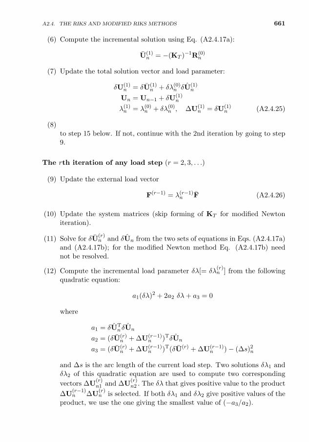
A2.4. THE RIKS AND MODIFIED RIKS METHODS 661
(6) Compute the incremental solution using Eq. (A2.4.17a):
U(1)n = −(KT )−1R(0)
n
(7) Update the total solution vector and load parameter:
δU(1)n = δU(1)
n + δλ(0)n δU(1)n
Un = Un−1 + δU(1)n
λ(1)n = λ(0)n + δλ(0)n , ∆U(1)n = δU(1)
n (A2.4.25)
(8) Check for convergence [see Eq. (A2.4.28)]. If convergence is achieved, goto step 15 below. If not, continue with the 2nd iteration by going to step9.
The rth iteration of any load step (r = 2, 3, . . .)
(9) Update the external load vector
F(r−1) = λ(r−1)n F (A2.4.26)
(10) Update the system matrices (skip forming of KT for modified Newtoniteration).
(11) Solve for δU(r)n and δUn from the two sets of equations in Eqs. (A2.4.17a)
and (A2.4.17b); for the modified Newton method Eq. (A2.4.17b) neednot be resolved.
(12) Compute the incremental load parameter δλ[= δλ(r)n ] from the following
quadratic equation:
a1(δλ)2 + 2a2 δλ+ a3 = 0
where
a1 = δUTn δUn
a2 = (δU(r)n + ∆U(r−1)
n )TδUn
a3 = (δU(r)n + ∆U(r−1)
n )T(δU(r) + ∆U(r−1)n )− (∆s)2n
and ∆s is the arc length of the current load step. Two solutions δλ1 andδλ2 of this quadratic equation are used to compute two corresponding
vectors ∆U(r)n1 and ∆U
(r)n2 . The δλ that gives positive value to the product
∆U(r−1)n ∆U
(r)n is selected. If both δλ1 and δλ2 give positive values of the
product, we use the one giving the smallest value of (−a3/a2).
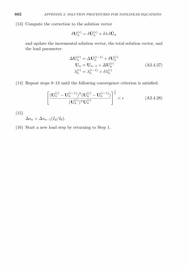
662 APPENDIX 2: SOLUTION PROCEDURES FOR NONLINEAR EQUATIONS
(13) Compute the correction to the solution vector
δU(r)n = δU(r)
n + δλ δUn
and update the incremental solution vector, the total solution vector, andthe load parameter:
∆U(r)n = ∆U(r−1)
n + δU(r)n
Un = Un−1 + ∆U(r)n (A2.4.27)
λ(r)n = λ(r−1)n + δλ(r)n
(14) Repeat steps 9–13 until the following convergence criterion is satisfied:[(U
(r)n −U
(r−1)n )T(U
(r)n −U
(r−1)n )
(U(r)n )TU
(r)n
] 12
< ε (A2.4.28)
(15) Adjust the arc length for the subsequent load steps by [see Eq. (A2.4.12)]∆sn = ∆sn−1(Id/I0).
(16) Start a new load step by returning to Step 1.
663
References
The references cited in the book are listed here by chapter. Some references are cited inmultiple chapters but they are not listed again under those chapters.
Chapter 1
1. J. N. Reddy, An Introduction to Continuum Mechanics, 2nd ed., Cambridge UniversityPress, New York (2013).
2. J. N. Reddy, An Introduction to the Finite Element Method, 3rd ed., McGraw–Hill,New York (2006).
3. J. N. Reddy, Energy Principles and Variational Methods in Applied Mechanics, 2nded., John Wiley & Sons, New York (2002).
4. K. J. Bathe, Finite Element Procedures, Prentice–Hall, Englewood Cliffs, NJ (2006).
5. T. Belytschko, W. K. Liu, B. Moran, and K. I. Elkhodary, Nonlinear Finite Elementsfor Continua and Structures, 2nd ed., John Wiley, Chichester, UK (2014).
6. C. A. Crisfield, Non-Linear Finite Element Analysis of Solids and Structures, Vol. 1:Essentials, John Wiley, Chichester, UK (1991).
7. C. A. Crisfield, Non-Linear Finite Element Analysis of Solids and Structures, Vol. 2:Advanced Topics, John Wiley, Chichester, UK (1997).
8. E. Hinton (Ed.), NAFEMS Introduction to Nonlinear Finite Element Analysis, NAFEMS,Glasgow, UK (1992).
9. D. R. J. Owen and E. Hinton, Finite Elements in Plasticity: Theory and Practice,Pineridge Press, Swansea, UK (1991).
10. J. N. Reddy and D. K. Gartling, The Finite Element Method in Heat Transfer andFluid Dynamics, 3rd ed., CRC Press, Boca Raton, FL (2010).
11. P. Wriggers, Nonlinear Finite Element Methods, Springer–Verlag, Berlin (2008).
12. O. C. Zienkiewicz and R. L. Taylor, The Finite Element Method, 4th ed., Vol. 1:Basic Formulation and Linear Problems, Vol. 2: Solid and Fluid Mechanics, Dynamicsand Non-linearity, McGraw–Hill, London, UK (1989); other editions and versions haveappeared since 1989.
13. J. N. Reddy and M. L. Rasmussen, Advanced Engineering Analysis, John Wiley &Sons, New York (1982); reprinted by Krieger, Malabar, FL (1991).
14. A. W. Naylor and G. R. Sell, Linear Operator Theory in Engineering and Science, Holt,Rinehart, and Winston, New York (1971).
15. J. N. Reddy, Applied Functional Analysis and Variational Methods in Engineering,McGraw–Hill, New York (1984); reprinted by Krieger Publishing, Malabar, Florida(1991).
16. J. N. Reddy, Lecture Notes on Applied Mathematical Analysis Methods for Engineers,Department of Mechanical Engineering, Texas A&M University, College Station, Texas(2008).
17. R. G. Sargent, “An overview of verification and validation of simulation models,” Pro-ceedings of the 1987 Winter Simulation Conference, Society of Computer Simulation(1987).
18. I. Babuska and T. Strouboulis, The Finite Element Method and its Reliability, OxfordUniversity Press, Oxford, UK (2001).
J.N. Reddy, An Introduction to Nonlinear Finite Element Analysis, Second Edition.c©J.N. Reddy 2015. Published in 2015 by Oxford University Press.
664 REFERENCES
19. I. Babuska and J. T. Oden, “Verification and validation in computational engineeringand science: basic concepts,” Computer Methods in Applied Mechanics and Engineer-ing, 193, 4057–4066 (2004).
20. Guide for Verification and Validation in Computational Solid Mechanics, ASME V&V10-2006, American Society of Mechanical Engineers, New York (2006).
21. B. Szabo and I. Babuska, Introduction to Finite Element Analysis: Formulation, Veri-fication and Validation, John Wiley & Sons, New York (2011).
Chapter 2
22. G. A. Holzapfel, Nonlinear Solid Mechanics, John Wiley & Sons, New York (2000).
23. J. Bonet and R. D. Wood, Nonlinear Continuum Mechanics for Finite Element Anal-ysis, 2nd ed., Cambridge University Press, New York (2008).
24. L. E. Malvern, Introduction to the Mechanics of a Continuous Medium, Prentice–Hall,Englewood Cliffs, NJ (1969).
Chapter 3
25. J. T. Oden and G. F. Carey, Finite Elements, Mathematical Aspects, Vol. IV, Prentice–Hall, Englewood Cliffs, NJ (1983).
26. F. Brezzi and M. Fortin, Mixed and Hybrid Finite Element Methods, Springer–Verlag,Berlin (1991).
27. F. Brezzi and K. J. Bathe, “The inf-sup condition, equivalent forms and applications,”in Reliability of Methods for Engineering Analysis, K. J. Bathe and D. R. J. Owen(Eds.), Pineridge Press, Swansea, U.K. (1986).
28. T. Belytschko, Y. Krongauz, D. Organ, M. Fleming, and P. Krysl, “Meshless Methods:An overview and recent developments,” Computer Methods in Applied Mechanics andEngineering, 139, 3–47 (1996).
29. C. A. Duarte and J. T. Oden, “H-p clouds – an h-p meshless method,” NumericalMethods for Partial Differential Equations, 12, 673–705 (1996).
30. I. Babuska and M. Melenk, “The partition of unity method,” International Journal forNumerical Methods in Engineering, 40, 727–758 (1997).
31. S. N. Atluri and S. Shen, The Meshless Local Petrov–Galerkin (MLPG) Method, TechScience Press, Encino, CA (2002).
32. S. N. Atluri, The Meshless Method (MLPG) for Domain & BIE Discretization, TechScience Press, Encino, CA (2004).
33. T. Belytschko and J. S. Chen, Meshfree and Particle Methods, John Wiley & Sons,New York (2007).
34. A. Huerta, T. Belytschko, S. Fernandez-Mendez, and T. Rabczuk, “Meshfree methods”,Encyclopedia of Computational Mechanics, 1(10), 279–309 (2004).
35. S. Li and W. K. Liu, Meshfree Particle Methods, Springer–Verlag, Berlin (2004).
36. G. R. Liu and Y. T. Gu, An Introduction to Meshfree Methods and Their Programming,Springer–Verlag, AA Dordrecht, The Netherlands (2005).
37. G. R. Liu, Meshfree Methods. Moving Beyond the Finite Element Method, 2nd ed.,CRC Press, Boca Raton, FL (2010).
38. B.-N. Jiang, The Least-Squares Finite Element Method. Theory and Applicationsin Computational Fluid Dynamics and Electromagnetics, Springer–Verlag, New York(1998).
39. P. B. Bochev and M. D. Gunzburger, Least-Squares Finite Element Methods, Springer–Verlag, New York (2009).
REFERENCES 665
40. K. S. Surana, A. R. Ahmadi, and J. N. Reddy, “The k-version of finite element methodfor non-self-adjoint operators in bvp,” International Journal of Computational Engi-neering Science, 4(4), 737–812 (2003).
41. K. S. Surana, A. R. Ahmadi, and J. N. Reddy, “The k-version of finite element methodfor nonlinear operators in BVP,” International Journal of Computational EngineeringScience, 5(1), 133–207 (2004).
42. K. S. Surana, S. Allu, P. W. TenPas, and J. N. Reddy, “k-Version finite element methodin gas dynamics: higher order global differentiability numerical solutions,” InternationalJournal for Numerical Methods in Engineering, 69(6), 1109–1157 (2007).
43. J. P. Pontaza and J. N. Reddy, “Spectral/hp least-squares finite element formulationfor the Navier–Stokes equations,” Journal of Computational Physics, 190(2), 523–549(2003).
44. J. P. Pontaza and J. N. Reddy, “Least-squares finite element formulations for viscouscompressible and incompressible fluid flows,” Computer Methods in Applied Mechanicsand Engineering, 195, 2454–2494 (2006).
45. V. Prabhakar and J. N. Reddy, “Spectral/hp penalty least-squares finite element for-mulation for the steady incompressible Navier–Stokes equations,” Journal of Compu-tational Physics, 215(1), 274–297 (2006).
46. T. J. R. Hughes and A. N. Brooks, “A multidimensional upwind scheme with no cross-wind diffusion,” in Finite Element Methods for Convection Dominated Flows, T. J. R.Hughes (Ed.), ASME, AMD 34, NY, 19–35 (1979).
47. A. N. Brooks and T. J. R. Hughes, “Streamline-upwind/Petrov–Galerkin formulationsfor convection dominated flows with particular emphasis on incompressible Navier–Stokes equation,” Computer Methods in Applied Mechanics and Engineering, 32, 199–259 (1982).
48. T. J. R. Hughes, “Multiscale phenomena: Green’s functions, the Dirichlet-to-Neumannformulation, subgrid scale models, bubbles and the origin of stabilized methods,” Com-puter Methods in Applied Mechanics and Engineering, 127, 387–401 (1995).
49. E. D. Eason, “A Review of Least-Squares Methods for Solving Partial DifferentialEquations”, International Journal for Numerical Methods in Engineering, 10(5), 1021–1046 (1976).
50. G. S. Payette and J. N. Reddy, “On the roles of minimization and linearization inleast squares finite element models of nonlinear boundary-value problems,” Journal ofComputational Physics, 230(9), 3589–3613 (2011).
Chapter 4
51. P. L. Sachdev, A Compendium on Nonlinear Ordinary Differential Equations, JohnWiley, New York (1997).
52. M. Kubicek and V. Hlavacek, Numerical Solution of Nonlinear Boundary Value Prob-lems with Applications, Prentice–Hall, Englewood Cliffs, NJ (1983).
Chapter 5
53. J. N. Reddy, “Microstructure-dependent couple stress theories of functionally graded
beams,” Journal of the Mechanics and Physics of Solids, 59, 2382–2399 (2011).
Chapter 6
54. M. N. Ozisik, Finite Difference Methods in Heat Transfer, CRC Press, Boca Raton, FL(1994).
666 REFERENCES
Chapter 7
55. J. N. Reddy, Mechanics of Laminated Plates and Shells, Theory and Analysis, 2nd ed.,CRC Press, Boca Raton, FL (2004).
56. J. N. Reddy, Theory and Analysis of Elastic Plates and Shells, 2nd ed., CRC Press,Boca Raton, FL (2007).
57. R. J. Melosh, “Basis of derivation of matrices for the direct stiffness method,” AIAAJournal, 1, 1631–1637 (1963).
58. O. C. Zienkiewicz and Y. K. Cheung, “The finite element method for analysis of elasticisotropic and orthotropic slabs,” Proceedings of the Institute of Civil Engineers, London,28, 471–488 (1964).
59. F. K. Bogner, R. L. Fox, and L. A. Schmidt, Jr., “The generation of interelement-compatible stiffness and mass matrices by the use of interpolation formulas,” Proceed-ings of the Conference on Matrix Methods in Structural Mechanics, Air Force Instituteof Technology, Wright–Patterson Air Force Base, OH, 397–443 (1965).
60. J. M. Gere and W. Weaver, Jr., Analysis of Framed Structures, D. von Nostrand, NewYork (1965).
61. B. Fraeijis de Veubeke, “A conforming finite element for plate bending,” InternationalJournal of Solids and Structures, 4(1), 95–108 (1968).
62. J. Barlow, “Optimal stress location in finite element models,” International Journalfor Numerical Methods in Engineering, 10, 243–251 (1976).
63. J. Barlow, “More on optimal stress points – reduced integration element distortionsand error estimation,” International Journal for Numerical Methods in Engineering,28, 1486–1504 (1989).
64. S. Levy, “Bending of rectangular plates with large deflections,” Report No. 737, NACA(1942).
65. C. T. Wang, “Bending of rectangular plates with large deflections,” Report No. 1462,NACA (1948).
66. T. Kawai and N. Yoshimura, “Analysis of large deflection of plates by the finite elementmethod,” International Journal for Numerical Methods in Engineering, 1, 123–133(1969).
67. C. W. Bert, S. K. Jang, and A. G. Striz, “Nonlinear bending analysis of orthotropicrectangular plates by the method of differential quadrature,” Computational Mechanics,5, 217–226 (1989).
68. S. Levy, “Square Plate with Clamped Edges Under Pressure Producing Large Deflec-tions,” Tech. Note 847, NACA (1942).
69. A. Pica, R. D. Wood, and E. Hinton, “Finite element analysis of geometrically nonlinearplate behaviour using a Mindlin formulation,” Computers and Structures, 11, 203–215(1980).
70. J. N. Reddy, “Analysis of layered composite plates accounting for large deflections andtransverse shear strains,” in Recent Advances in Non-Linear Computational Mechanics,E. Hinton, D. R. J. Owen, and C. Taylor (Eds.), Ch. 6, pp. 155–202, Pineridge Press,Swansea, UK (1982).
71. J. N. Reddy, “Simple finite elements with relaxed continuity for non-linear analysisof plates,” Proceedings of the Third International Conference in Australia on FiniteElement Methods, A. P. Kabaila and V. A. Pulmano (Eds.), University of New SouthWales, Kensington, New South Wales, Australia (1979).
72. J. N. Reddy, “A penalty plate-bending element for the analysis of laminated anisotropiccomposite plates,” International Journal for Numerical Methods in Engineering, 15(8),1187–1206 (1980).
REFERENCES 667
73. H. C. Huang and E. Hinton, “A nine node Lagrangian Mindlin plate element withenhanced shear interpolation,” Engineering Computations, 1(4), 369–379 (1984).
74. R. C. Averill and J. N. Reddy, “Behavior of plate elements based on the first-ordershear deformation theory,” Engineering Computations, 7, 57–74 (1990).
75. O. C. Zienkiewicz, J. J. M. Too, and R. L. Taylor, “Reduced integration technique ingeneral analysis of plates and shells,” International Journal for Numerical Methods inEngineering, 3, 275–290 (1971).
76. T. J. R. Hughes, M. Cohen, and M. Haroun, “Reduced and selective integration tech-niques in the finite element analysis of plates,” Nuclear Engineering and Design, 46,203–222 (1981).
77. T. Belytschko, C. S. Tsay, and W. K. Liu, “Stabilization matrix for the bilinear Mindlinplate element,” Computer Methods in Applied Mechanics and Engineering, 29, 313–327(1981).
78. K. J. Bathe and E. N. Dvorkin, “A four-node plate bending element based on Mindlin/Reissner plate theory and mixed interpolation,” International Journal for NumericalMethods in Engineering, 21, 367–383 (1985).
79. J. N. Reddy and W. C. Chao, “A comparison of closed-form and finite element solutionsof thick laminated anisotropic rectangular plates,” Nuclear Engineering and Design, 64,153–167 (1981).
80. J. N. Reddy, “On mixed finite-element formulations of a higher-order theory of compos-ite laminates,” Finite Element Methods for Plate and Shell Structures, T. J. R. Hughesand E. Hinton (Eds.), pp. 31–57, Pineridge Press, Swnasea, UK (1986).
Chapter 8
81. S. A. Ambartsumyan, “Calculation of laminated anisotropic shells,” Izvestiia AkademiiaNauk Armenskoi SSR, Ser. Fiz. Mat. Est. Tekh. Nauk., 6(3), p. 15 (1953).
82. S. A. Ambartsumyan, Theory of Anisotropic Shells, NASA Report TT F-118 (1964).
83. S. A. Ambartsumyan, Theory of Anisotropic Shells, Moscow, 1961; English translation,NASA-TT-F-118 (1964).
84. W. Flugge, Stresses in Shells, Springer, Berlin (1960).
85. H. Kraus, Thin Elastic Shells, John Wiley, New York (1967).
86. S. Timoshenko and S. Woinowsky-Krieger, Theory of Plates and Shells, McGraw–Hill,New York (1959).
87. A. W. Leissa, Vibration of Shells, NASA SP–288, Washington, D.C. (1973).
88. C. L. Dym, Introduction to the Theory of Shells, Pergamon, New York (1974).
89. A. C. Ugural, Stresses in Beams, Plates, and Shells, 3rd ed., CRC Press, Boca Raton,FL (2009).
90. M. Farshad, Design and Analysis of Shell Structures, Kluwer Academic Publishers,Dordrecht, The Netherlands (1992).
91. J. L. Sanders, Jr., “Nonlinear theories for thin shells,” Quarterly Journal of AppliedMathematics, 21(1), 21–36 (1963).
92. B. Budiansky and J. L. Sanders, “On the ‘best’ first order linear shell theory,” Progressin Applied Mechanics, The Prager Anniversary Volume, Macmillan, New York, pp.129–140 (1963).
93. A. N. Palazotto and S. T. Dennis, Nonlinear Analysis of Shell Structures, AIAA Edu-cation Series, Washington, DC (1992).
94. V. Z. Vlasov, General Theory of Shells and Its Applications in Engineering, (Transla-tion of Obshchaya teoriya obolocheck i yeye prilozheniya v tekhnike), NASA TT F-99,National Aeronautics and Space Administration, Washington, DC (1964).
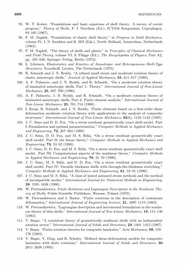
668 REFERENCES
95. W. T. Koiter, “Foundations and basic equations of shell theory. A survey of recentprogress,” Theory of Shells, F. I. Niordson (Ed.), IUTAM Symposium, Copenhagen,93–105 (1967).
96. P. M. Naghdi, “Foundations of elastic shell theory,” in Progress in Solid Mechanics,volume IV, I. N. Sneddon and R. Hill (Eds.), North–Holland, Amsterdam, Netherlands(1963).
97. P. M. Naghdi, “The theory of shells and plates,” in Principles of Classical Mechanicsand Field Theory, volume VI, S. Flugge (Ed.), The Encyclopedia of Physics, Part A2,pp. 425–640, Springer–Verlag, Berlin (1972).
98. L. Librescu, Elastostatics and Kinetics of Anisotropic and Heterogeneous Shell-TypeStructures, Noordhoff, Leyden, The Netherlands (1975).
99. R. Schmidt and J. N. Reddy, “A refined small strain and moderate rotation theory ofelastic anisotropic shells,” Journal of Applied Mechanics, 55, 611–617 (1988).
100. A. F. Palmerio, and J. N. Reddy, and R. Schmidt, “On a moderate rotation theoryof laminated anisotropic shells, Part 1: Theory,” International Journal of Non-LinearMechanics, 25, 687–700 (1990).
101. A. F. Palmerio, J. N. Reddy, and R. Schmidt, “On a moderate rotation theory oflaminated anisotropic shells, Part 2: Finite element analysis,” International Journal ofNon-Linear Mechanics, 25, 701–714 (1990).
102. I. Kreja, R. Schmidt, and J. N. Reddy, “Finite elements based on a first-order sheardeformation moderate rotation theory with applications to the analysis of compositestructures,” International Journal of Non-Linear Mechanics, 32(6), 1123–1142 (1997).
103. J. C. Simo and D. D. Fox, “On a stress resultant geometrically exact shell model. PartI: Formulation and optimal parametrization,” Computer Methods in Applied Mechanicsand Engineering, 72, 267–304 (1989).
104. J. C. Simo, D. D. Fox, and M. S. Rifai, “On a stress resultant geometrically exactshell model. Part II: the linear theory,” Computer Methods in Applied Mechanics andEngineering, 73, 53–92 (1989).
105. J. C. Simo, D. D. Fox, and M. S. Rifai, “On a stress resultant geometrically exact shellmodel. Part III: Computational aspects of the nonlinear theory,” Computer Methodsin Applied Mechanics and Engineering, 79, 21–70 (1990).
106. J. C. Simo, M. S. Rifai, and D. D. Fox, “On a stress resultant geometrically exactshell model. Part IV: Variable thickness shells with through-the-thickness stretching,”Computer Methods in Applied Mechanics and Engineering, 81, 53–91 (1990).
107. J. C. Simo and M. S. Rifai, “A class of mixed assumed strain methods and the methodof incompatible modes,” International Journal for Numerical Methods in Engineering,29, 1595–1638 (1990).
108. W. Pietraszkiewicz, Finite Rotations and Lagrangian Description in the Nonlinear The-ory of Shells, Polish Scientific Publishers, Warsaw, Poland (1979).
109. W. Pietraszkiewicz and J. Badur, “Finite rotations in the description of continuumdeformation,” International Journal of Engineering Science, 21, 1097–1115 (1983).
110. W. Pietraszkiewicz, “Lagrangian description and incremental formulation in the nonlin-ear theory of thin shells,” International Journal of Non-Linear Mechanics, 19, 115–140(1984).
111. Y. Basar, “A consistent theory of geometrically nonlinear shells with an independentrotation vector,” International Journal of Solids and Structures, 23, 1401–1415 (1987).
112. Y. Basar, “Finite-rotation theories for composite laminates,” Acta Mechanica, 98, 159–176 (1983).
113. Y. Basar, Y. Ding, and R. Schultz, “Refined shear-deformation models for compositelaminates with finite rotations,” International Journal of Solids and Structures, 302611–2638 (1993).
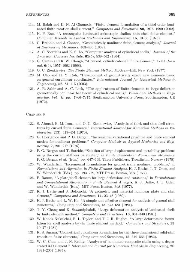
REFERENCES 669
114. M. Balah and H. N. Al-Ghamedy, “Finite element formulation of a third-order lami-nated finite rotation shell element,” Computers and Structures, 80, 1975–1990 (2002).
115. K. P. Rao, “A rectangular laminated anisotropic shallow thin shell finite element,”Computer Methods in Applied Mechanics and Engineering, 15, 13–33 (1978).
116. C. Brebbia and J. Connor, “Geometrically nonlinear finite element analysis,” Journalof Engineering Mechanics, 463–483 (1969).
117. A. C. Scordelis and K. S. Lo, “Computer analysis of cylindrical shells,” Journal of theAmerican Concrete Institute, 61(5), 539–562 (1964).
118. G. Cantin and R. W. Clough, “A curved, cylindrical-shell, finite element,” AIAA Jour-nal, 6(6), 1057–1062 (1968).
119. O. C. Zienkiewicz, The Finite Element Method, McGraw–Hill, New York (1977).
120. M. Cho and H. Y. Roh, “Development of geometrically exact new elements basedon general curvilinear coordinates,” International Journal for Numerical Methods inEngineering, 56, 81–115 (2003).
121. A. B. Sabir and A. C. Lock, “The applications of finite elements to large deflectiongeometrically nonlinear behaviour of cylindrical shells,” Variational Methods in Engi-neering, Vol. II, pp. 7/66–7/75, Southampton University Press, Southampton, UK(1972).
Chapter 9
122. S. Ahmad, B. M. Irons, and O. C. Zienkiewicz, “Analysis of thick and thin shell struc-tures by curved finite elements,” International Journal for Numerical Methods in En-gineering, 2(3), 419–451 (1970).
123. G. Horrigmoe and P. G. Bergan, “Incremental variational principle and finite elementmodels for nonlinear problems,” Computer Methods in Applied Mechanics and Engi-neering, 7, 201–217 (1976).
124. P. G. Bergan and T. Soreide, “Solution of large displacement and instability problemsusing the current stiffness parameter,” in Finite Elements in Non-Linear Mechanics,P. G. Bergan et al. (Eds.), pp. 647–669, Tapir Publishers, Trondheim, Norway (1978).
125. W. Wunderlich, “Incremental formulations for geometrically nonlinear problems,” inFormulations and Algorithm in Finite Element Analysis, K. J. Bathe, J. T. Oden, andW. Wunderlich (Eds.), pp. 193–239, MIT Press, Boston, MA (1977).
126. E. Ramm, “A plate/shell element for large deflections and rotations,” in Formulationsand Computational Algorithms in Finite Element Analysis, K. J. Bathe, J. T. Oden,and W. Wunderlich (Eds.), MIT Press, Boston, MA (1977).
127. K. J. Bathe and S. Bolourchi, “A geometric and material nonlinear plate and shellelement,” Computers and Structures, 11, 23–48 (1980).
128. K. J. Bathe and L. W. Ho, “A simple and effective element for analysis of general shellstructures,” Computers and Structures, 13, 673–681 (1981).
129. T. Y. Chang and K. Sawamiphakdi, “Large deformation analysis of laminated shellsby finite element method,” Computers and Structures, 13, 331–340 (1981).
130. W. Kanok-Nukulchai, R. L. Taylor, and T. J. R. Hughes, “A large deformation formu-lation for shell analysis by the finite element method,” Computers and Structures, 13,19–27 (1981).
131. K. S. Surana,“Geometrically nonlinear formulation for the three dimensional solid-shelltransition finite elements,” Computers and Structures, 15, 549–566 (1982).
132. W. C. Chao and J. N. Reddy, “Analysis of laminated composite shells using a degen-erated 3-D element,” International Journal for Numerical Methods in Engineering, 20,1991–2007 (1984).
670 REFERENCES
133. E. Dvorkin and K. J. Bathe, “A continuum mechanics based four-node shell elementfor general nonlinear analysis,” Engineering Computations, 1, 77–88 (1984).
134. G. M. Stanley and C. A. Felippa, “Computational procedures for postbuckling forcomposite shells,” in Finite Element Methods for Nonlinear Problems, P. G. Bergan,K. J. Bathe, and W. Wunderlich (Eds.), pp. 359–385, Springer–Verlag, Berlin (1986).
135. C. L. Liao, J. N. Reddy, and S. P. Engelstad, “A solid-shell transition element for geo-metrically nonlinear analysis of laminated composite structures,” International Journalfor Numerical Methods in Engineering, 26, 1843–1854 (1988).
136. C. L. Liao and J. N. Reddy, “A continuum-based stiffened composite shell element forgeometrically nonlinear analysis,” AIAA Journal, 27(1), 95–101 (1989).
137. C. L. Liao and J. N. Reddy, “Analysis of anisotropic, stiffened composite laminatesusing a continuum shell element,” Computers and Structures, 34(6), 805–815 (1990).
138. N. Buchter and E. Ramm,“Shell theory versus degeneration – a comparison in largerotation finite element analysis,” International Journal for Numerical Methods in En-gineering, 34(1), 39–59 (1992).
139. E. Hinton and H. C. Huang, “A family of quadrilateral Mindlin plate elements withsubstitute shear strain fields,” Computers and Structures, 23(3), 409–431 (1986).
140. L. Leino and J. Pitkaranta, “On the membrane locking of h-p finite elements in a cylin-drical shell problem,” International Journal for Numerical Methods in Engineering, 37,1053–1070 (1994).
141. J. Pitkaranta, Y. Leino, O. Ovaskainen, and J. Piila, “Shell deformation states and thefinite element method: A benchmark study of cylindrical shells,” Computer Methodsin Applied Mechanics and Engineering, 128, 81–121 (1995).
142. H. Hakula, Y. Leino, and J. Pitkaranta, “Scale resolution, locking, and high-order finiteelement modelling shells,” Computer Methods in Applied Mechanics and Engineering,133, 157–182 (1996).
143. J. P. Pontaza and J. N. Reddy, “Mixed plate bending elements based on least-squaresformulation,” International Journal for Numerical Methods in Engineering, 60(5), 891–922 (2004).
144. J. P. Pontaza and J. N. Reddy, “Least-square finite element formulation for sheardeformable shells,” Computer Methods in Applied Mechanics and Engineering, 194,2464–2493 (2005).
145. R. A. Arciniega, On a tensor-based finite element model for the analysis of shell struc-tures, Ph.D. Dissertation, Department of Mechanical Engineering, Texas A&M Univer-sity, College Station, Texas, USA, December 2005.
146. R. A. Arciniega and J. N. Reddy, “Tensor-based finite element formulation for geomet-rically nonlinear analysis of shell structures,” Computer Methods in Applied Mechanicsand Engineering, 196(4-6), 1048–1073 (2007).
147. R. A. Arciniega and J. N. Reddy, “Large deformation analysis of functionally gradedshells,” International Journal of Solids and Structures, 44(6), 2036–2052 (2007).
148. G. A. Wempner, “Discrete approximations related to nonlinear theories of solids,”International Journal of Solids and Structures, 7, 1581–1599 (1971).
149. E. Riks, “The application of Newton’s method to the problem of elastic stability,”Journal of Applied Mechanics, 39, 1060–1066 (1972).
150. E. Riks, “An incremental approach to the solution of snapping and buckling problems,”International Journal for Numerical Methods in Engineering, 15, 524–551 (1979).
151. M. A. Crisfield, “A fast incremental/iterative solution procedure that handles ‘snap-through’, ” Computers and Structures, 13(1–3), 55–62 (1981).
REFERENCES 671
152. J. H. Kweon and C. S. Hong, “An improved arc-length method for postbuckling analysisof composite cylindrical panels,” Computers and Structures, 53(3), 541–549 (1994).
153. S. A. Zaghloul and J. B. Kennedy, “Nonlinear behavior of symmetrically laminatedplates,” Journal of Applied Mechanics, 42(1), 234–236 (1975).
154. N. S. Putcha and J. N. Reddy, “A Refined Mixed Shear Flexible Finite Element forthe Nonlinear Analysis of Laminated Plates,” Computers and Structures, 22, 529–538(1986).
155. O. C. Zienkiewicz, R. L. Taylor, and J. M. Too, “Reduced integration techniques ingeneral analysis of plates and shells,” International Journal for Numerical Methods inEngineering, 3, 275–290 (1971).
156. D. Chapelle and K. J. Bathe, The Finite Element Analysis of Shells – Fundamentals,Springer–Verlag, New York (2003).
157. P. Betsch, A. Menzel, and E. Stein, “On the parametrization of finite rotations in com-putational mechanics: A classification of concepts with application to smooth shells,”Computational Methods in Applied Mechanics and Engineering, 155, 273–305 (1998).
158. M. Bischoff and E. Ramm, “Shear deformable shell elements for large strains androtations,” International Journal for Numerical Methods in Engineering, 40, 4427–4449 (1997).
159. M. Bischoff and E. Ramm, “On the physical significance of higher order kinematicand static variables in a three-dimensional shell formulation,” International Journal ofSolids and Structures, 37, 6933–6960 (2000).
160. C. Sansour, “A theory and finite element formulation of shells at finite deformationsinvolving thickness change: Circumventing the use of a rotation tensor,” Archives ofApplied Mechanics, 65, 194–216 (1995).
161. G. S. Payette, “Spectral/hp finite element models for fluids and structures,” Ph.D.Dissertation, Department of Mechanical Engineering, Texas A&M University, CollegeStation, Texas, USA, May 2012.
162. G. S. Payette and J. N. Reddy, “A seven-parameter spectral/hp finite element for-mulation for isotropic, laminated composite and functionally graded shell structures,”Computer Methods in Applied Mechanics and Engineering, 278, 664–704 (2014).
163. G. E. Karniadakis and S. J. Sherwin, Spectral/hp Element Methods for CFD, OxfordUniversity Press, New York (1999).
164. T. A. Davis and I. S. Duff, “An unsymmetric-pattern multifrontal method for sparseLU factorization,” SIAM Journal of Matrix Analysis and Applications, 18(1), 140–158(1997).
165. T. A. Davis and I. S. Duff, “A combined unifrontal/multifrontal method for unsym-metric sparse matrices,” ACM Transactions on Mathematical Software, 25(1), 1–20(1999).
166. T. A. Davis, “A column pre-ordering strategy for the unsymmetric-pattern multifrontalmethod,” ACM Transactions on Mathematical Software, 30(2), 165–195 (2004).
167. T. A. Davis, “Algorithm 832: UMFPACK V4.3 – an unsymmetric-pattern multifrontalmethod,” ACM Transactions on Mathematical Software, 30(2), 196–199 (2004).
168. H. Parisch, “Large displacements of shells including material nonlinearities,” ComputerMethods in Applied Mechanics and Engineering, 27(2), 183–214 (1981).
169. A. F. Saleeb, T. Y. Chang, W. Graf, and S. Yingyeunyong, “Hybrid/mixed model fornon-linear shell analysis and its applications to large-rotation problems,” InternationalJournal for Numerical Methods in Engineering, 29(2), 407–446 (1990).
170. K. Y. Sze and S.-J. Zheng, “A stabilized hybrid-stress solid element for geometricallynonlinear homogeneous and laminated shell analyses,” Computer Methods in AppliedMechanics and Engineering, 191, 1945–1966 (2002).
171. K. Y. Sze, W. K. Chan, and T. H. H. Pian, “An eight-node hybrid-stress solid-shell
672 REFERENCES
element for geometric non-linear analysis of elastic shells,” International Journal forNumerical Methods in Engineering, 55(7), 853–878 (2002).
172. K. Y. Sze, X. H. Liu, and S. H. Lo, “Popular benchmark problems for geometricnonlinear analysis of shells,” Finite Elements in Analysis in Design, 40(11), 1551–1569(2004).
173. P. Massin and M. Al Mikdad, “Nine node and seven node thick shell elements with largedisplacements and rotations,” Computers and Structures, 80(9-10), 835–847 (2002).
174. S. Timoshenko and J. N. Goodier, Theory of Elasticity, 3rd ed., McGraw–Hill, NewYork (1970, 1987).
175. B. Brank, J. Korelc, and A. Ibrahimbegovic, “Nonlinear shell problem formulationaccounting for through-the-thickness stretching and its finite element implementation,”Computers and Structures, 80, 699–717 (2002).
176. A. Barut, E. Madenci, and A. Tessler, “Nonlinear analysis of laminates through aMindlin-type shear deformable shallow shell element,” Computer Methods in AppliedMechanics and Engineering, 143(1-2), 155–173 (1997).
177. P. Mohan and R. K. Kapania, “Updated Lagrangian formulation of a flat triangularelement for thin laminated shells,” AIAA Journal, 36(2), 273–281 (1998).
178. C. Sansour and F. G. Kollmann, “Families of 4-node and 9-node finite elements fora finite deformation shell theory. An assessment of hybrid stress, hybrid strain andenhanced strain elements,” Computational Mechanics, 24, 435–447 (2000).
179. L. Jiang and M. W. Chernuka, “A simple four-noded corotational shell element forarbitrarily large rotations,” Computers and Structures, 53(5), 1123–1132 (1994).
180. W. Wagner and F. Gruttmann, “A simple finite rotation formulation for compositeshell elements,” Engineering Computations, 11(2), 145–176 (1994).
Chapter 10
181. P. M. Gresho and R. L. Sani, Incompressible Flow and the Finite Element Method.Advection-Diffusion and Isothermal Laminar Flow, John Wiley & Sons, Chichester,UK (1999).
182. J. N. Reddy, “On the accuracy and existence of solutions to primitive variable modelsof viscous incompressible fluids,” International Journal of Engineering Science, 16,921–929 (1978).
183. J. N. Reddy, “On the finite element method with penalty for incompressible fluidflow problems,” in The Mathematics of Finite Elements and Applications III, J. R.Whiteman (Ed.), Academic Press, New York (1979).
184. J. N. Reddy, “On penalty function methods in the finite element analysis of flow prob-lems,” International Journal of Numerical Methods in Fluids, 2, 151–171 (1982).
185. M. P. Reddy and J. N. Reddy, “Finite-element analysis of flows of non-Newtonian fluidsin three-dimensional enclosures,” International Journal of Non-Linear Mechanics, 27,9–26 (1992).
186. R. S. Marshall, J. C. Heinrich, and O. C. Zienkiewicz, “Natural convection in a squareenclosure by a finite element, penalty function method, using primitive fluid variables,”Numerical Heat Transfer, 1, 315–330 (1978).
187. T. J. R. Hughes, W. K. Liu, and A. Brooks, “Review of finite element analysis of in-compressible viscous flows by penalty function formulation,” Journal of ComputationalPhysics, 30, 1–60 (1979).
188. J. T. Oden, “RIP methods for Stokesian flows,” in R. H. Gallagher, O. C. Zienkiewicz,J. T. Oden, and D. Norrie (Eds.), Finite Element Method in Flow Problems, Vol. IV,John Wiley, London, UK (1982).
REFERENCES 673
189. T. J. R. Hughes, L. P. Franca, and M. Balestra, “A new finite element formulationfor computational fluid dynamics. V. Circumventing the Babuska–Brezzi condition: Astable Petrov–Galerkin formulation for the Stokes problem accommodating equal-orderinterpolations,” Computer Methods in Applied Mechanics and Engineering, 59, 85–99(1986).
190. F. Brezzi and M. Fortin, Mixed and Hybrid Finite Element Methods, Springer–Verlag,Berlin, Germany (1991).
191. P. Le Tallac and V. Ruas, “On the convergence of the bilinear-velocity constant-pressurefinite element method in viscous flow,” Computer Methods in Applied Mechanics andEngineering, 54, 235–243 (1986).
192. R. Temam, Theory and Numerical Analysis of the Navier–Stokes Equations, North–Holland, Amsterdam, The Netherlands (1977).
193. M. Bercovier and M. Engelman, “A finite element for the numerical solution of viscousincompressible flows,” Journal of Computational Physics, 30, 181–201 (1979).
194. M. Engelman, R. L. Sani, P. M. Gresho, and M. Bercovier, “Consistent vs. reducedintegration penalty methods for incompressible media using several old and new ele-ments,” International Journal of Numerical Methods in Fluids, 2, 25–42 (1982).
195. E. M. Salonen and J. Aalto, “A pressure determination scheme,” Proceedings of theFifth International Conference on Numerical Methods in Laminar and Turbulent Flow,C. Taylor, M. D. Olson, P. M. Gresho, and W. G. Habashi (Eds.), Pineridge Press,Swansea, UK (1985).
196. T. Shiojima and Y. Shimazaki, “A pressure-smoothing scheme for incompressible flowproblems,” International Journal of Numerical Methods in Fluids, 9, 557–567 (1989).
197. M. P. Reddy, J. N. Reddy, and H. U. Akay, “Penalty finite element analysis of incom-pressible flows using element by element solution algorithms,” Computer Methods inApplied Mechanics and Engineering, 100, 169–205 (1992).
198. A. Nadai, Theory of Flow and Fracture of Solids, McGraw–Hill, New York (1963).
199. H. Schlichting, Boundary-Layer Theory (translated by J. Kestin), 7th ed., McGraw–Hill, New York (1979).
200. O. R. Burggraf, “Analytical and numerical studies of the structure of steady separatedflows,” Journal of Fluid Mechanics, 24(1), 113–151 (1966).
201. F. Pan and A. Acrivos, “Steady flow in rectangular cavities,” Journal of Fluid Mechan-ics, 28(4), 643–655 (1967).
202. U. Ghia, K. N. Ghia, and C. T. Shin, “High-resolution for incompressible flow usingthe Navier–Stokes equations and the multigrid method,” Journal of ComputationalPhysics, 48, 387–411 (1982).
203. D. K. Gartling, “A test problem for outflow boundary conditions – flow over a back-ward facing step,” International Journal for Numerical Methods in Fluids, 11, 953–967(1990).
204. J. L. White and A. B. Metzner, “Development of constitutive equations for polymericmelts and solutions,” Journal of Applied Polymer Science, 7, 1867–1889 (1963).
205. M. J. Crochet and K. Walters, “Numerical methods in non-Newtonian fluid mechanics,”Annual Review of Fluid Mechanics, 15, 241–260 (1983).
206. M. J. Crochet, A. R. Davies, and K. Walters, Numerical Simulation of Non-NewtonianFlow, Elsevier, Amsterdam, The Netherlands (1984).
207. D. K. Gartling and N. Phan Thien, “A numerical simulation of a plastic fluid in aparallel-plate plastometer,” Journal of Non-Newtonian Fluid Mechanics, 14, 347–360(1984).
208. J. N. Reddy and V. A. Padhye,“A penalty finite element model for axisymmetric flowsof non-Newtonian fluids,” Numerical Methods for Partial Differential Equations, 4,33–56 (1988).
674 REFERENCES
209. M. Iga and J. N. Reddy, “Penalty finite element analysis of free surface flows of power-law fluids,” International Journal of Non-Linear Mechanics, 24(5), 383–399 (1989).
210. M. P. Reddy and J. N. Reddy, “Finite element analysis of flows of non-Newtonian flu-ids in three-dimensional enclosures,” International Journal of Non-Linear Mechanics,27(1), 9–26 (1992).
211. M. P. Reddy and J. N. Reddy, “Numerical simulation of forming processes using a cou-pled fluid flow and heat transfer model,” International Journal for Numerical Methodsin Engineering, 35, 807–833 (1992).
212. C. J. Coleman, “A finite element routine for analyzing non-Newtonian fluids, Part 1,”Journal of Non-Newtonian Fluid Mechanics, 7, 289–301 (1980).
213. D. K. Gartling, “Convective heat transfer analysis by the finite element method,” Com-puter Methods in Applied Mechanics and Engineering, 12, 365–382 (1977).
214. R. S. Marshall, J. C. Heinrich, and O. C. Zienkiewicz, “Natural convection in a squareenclosure by a finite element, penalty function method, using primitive fluid variables,”Numerical Heat Transfer, 1, 315–330 (1978).
215. J. N. Reddy and A. Satake,“A comparison of various finite element models of naturalconvection in enclosures,” Journal of Heat Transfer, 102, 659–666 (1980).
216. J. N. Reddy, “Penalty-finite-element analysis of 3-D Navier–Stokes equations,” Com-puter Methods in Applied Mechanics and Engineering, 35, 87–106 (1982).
217. G. de Vahl Davis and I. P. Jones, “Natural convection in a square cavity: a comparisonexercise,” International Journal for Numerical Methods in Fluids, 3, 227–248 (1983).
218. M. Dhaubhadel, D. Telionis, and J. N. Reddy, “Finite element analysis of fluid flow andheat transfer for staggered bundles of cylinders in cross flow,” International Journalfor Numerical Methods in Fluids, 7, 1325–1342 (1987).
219. D. H. Pelletier, J. N. Reddy, and J. A. Schetz, “Some recent developments and trends infinite element computational natural convection,” in Annual Review of Numerical FluidMechanics and Heat Transfer, Vol. 2, C. L. Tien and T. C. Chawla (Eds.), Hemisphere,New York, pp. 39–85 (1987).
220. J. T. Oden and J. N. Reddy, Variational Methods in Theoretical Mechanics, 2nd ed.,Springer–Verlag, New York (1983).
Chapter 11
221. J. H. Bramble and A. H. Schatz, “Least squares methods for 2mth order ellipticboundary-value problems,” Mathematics of Computation, 25(113), 1–32 (1971).
222. J. H. Bramble and J. E. Pasciak, “Least-squares methods for Stokes equations basedon a discrete minus one inner product,” Journal of Computational and Applied Math-ematics, 74(1,2), 155–173 (1996).
223. J. H. Bramble, R. D. Lazarov, and J. E. Pasciak, “Least-squares for second-order ellipticproblems,” Computer Methods in Applied Mechanics and Engineering, 152(1,2), 195–210 (1998).
224. P. B. Bochev, “Analysis of least-squares finite element methods for the Navier–Stokesequations,” SIAM Journal of Numerical Analysis, 34, 1817–1844 (1997).
225. S. Agmon, A. Douglis, and L. Nirenberg, “Estimates near the boundary for solutions ofelliptic partial differential equations satisfying general boundary conditions II,” Com-munications in Pure and Applied Mathematuics, 17(1), 35–92 (1964).
226. P. B. Bochev, Z. Cai, T. A. Manteuffel, and S. F. McCormick, “Analysis of velocity-flux first-order system least-squares principles for the Navier–Stokes equations, Part I,”SIAM Journal of Numerical Analysis, 35, 990–1009 (1998).
REFERENCES 675
227. P. B. Bochev, Z. Cai, T. A. Manteuffel, and S. F. McCormick, “Analysis of velocity-flux first-order system least-squares principles for the Navier–Stokes equations, PartII,” SIAM Journal of Numerical Analysis, 36(4), 1125–1144 (1999).
228. B.-N. Jiang, “A least-squares finite element method for incompressible Navier–Stokesproblems,” International Journal for Numerical Methods in Fluids, 14, 843–859 (1992).
229. B.-N. Jiang and V. Sonnad, “Least-squares solution of incompressible Navier–Stokesequations with the p-version of finite elements,” Computational Mechanics 15, 129–136(1994).
230. B.-N. Jiang, T. L. Lin, and L. A. Povinelli, “Large-scale computation of incompressibleviscous flow by the least-squares finite element method,” Computer Methods in AppliedMechanics and Engineering, 114, 213–231 (1994).
231. B. C. Bell and K. S. Surana, “A space-time coupled p-version least-squares finite el-ement formulation for unsteady fluid dynamics problems,” International Journal forNumerical Methods in Engineering, 37, 3545–3569 (1994).
232. B. C. Bell and K. S. Surana,“A space-time coupled p-version least-squares finite el-ement formulation for unsteady two-dimensional Navier–Stokes equations,” Interna-tional Journal for Numerical Methods in Engineering, 39, 2593–2618 (1996).
233. M. M. J. Proot and M. I. Gerritsma, “A least-squares spectral element formulation forthe Stokes problem,” Journal of Scientific Computing, 17(1-4), 285–296 (2002).
234. M. I. Gerritsma and M. M. J. Proot, “Analysis of a discontinuous least squares spectralelement method,” Journal of Scientific Computing, 17(1-4), 297–306 (2002).
235. M. M. J. Proot and M. I. Gerritsma, “Least-squares spectral elements applied to theStokes problem,” Journal of Computational Physics, 181, 454–477 (2002).
236. M. I. Gerritsma, “Direct minimization of the discontinuous least-squares spectral ele-ment method for viscoelastic fluids,” Journal of Scientific Computing, 27 (1-3), 245–256(2006).
237. B. De Maerschalck and M. I. Gerritsma, “Least-squares spectral element method fornon-linear hyperbolic differential equations,” Journal of Computational and AppliedMathematics, 215(2), 357–367 (2008).
238. J. P. Pontaza and J. N. Reddy, “Space-time coupled spectral/hp least-squares finiteelement formulation for the incompressible Navier–Stokes equations,” Journal of Com-putational Physics, 197(2), 418–459 (2004).
239. V. Prabhakar and J. N. Reddy, “A stress-based least-squares finite-element model forincompressible Navier–Stokes equations,” International Journal for Numerical Methodsin Fluids, 54(11), 1369–1385 (2007).
240. V. Prabhakar and J. N. Reddy, “Spectral/hp penalty least-squares finite element formu-lation for unsteady incompressible flows,” International Journal of Numerical Methodsfor Fluids, 58(3), 287–306 (2008).
241. V. Prabhakar, J. P. Pontaza, and J. N. Reddy, “A collocation penalty least-squaresfinite element formulation for incompressible flows,” Computer Methods in Applied Me-chanics and Engineering, 197, 449–463 (2008).
242. I. Babuska, “The finite element method with Lagrange multipliers,” Numerische Math-ematik, 20, 179–192 (1973).
243. F. Brezzi, “On the existence, uniqueness and approximation saddle-point problemsarising from Lagrangian multipliers,” Revue Francaise d’Automatique InformatiqueRecherche Operationelle, Analyse Numerique, 8, 129–151 (1974).
244. G. F. Carey and B.-N. Jiang, “Least-squares finite element method and preconditionedconjugate gradient solution,” International Journal for Numerical Methods in Fluids,24(7), 1283–1296 (1987).
676 REFERENCES
245. G. F. Carey and B.-N. Jiang, “Nonlinear preconditioned conjugate gradient and least-squares finite elements,” Computer Methods in Applied Mechanics and Engineering,62(2), 145–154 (1987).
246. J. M. Deang and M. D. Gunzburger, “Issues related to least-squares finite elementmethods for the Stokes equations,” SIAM Journal of Scientific Computing, 20(3), 878–906 (1998).
247. C. L. Chang and J. J. Nelson, “Least-squares finite element method for the Stokesproblem with zero residual of mass conservation,” SIAM Journal of Numerical Analysis,34(2), 480–489 (1997).
248. J. P. Pontaza, “Least-squares variational principles and the finite element method:theory, formulations, and models for solid and fluid mechanics,” Finite Elements inAnalysis and Design, 41(7-8), 703–728 (2005).
249. J. J. Heys, E. Lee, T. A. Manteuffel, and S. F. McCormick, “An alternative least-squares formulation of the Navier–Stokes equations with improved mass conservation,”Journal of Computational Physics, 226(1), 994–1006 (2007).
250. J. P. Pontaza, “A least-squares finite element formulation for unsteady incompressibleflows with improved velocity-pressure coupling,” Journal of Computational Physics,217(2), 563–588 (2006).
251. D. J. Tritton, “Experiments on the flow past a circular cylinder at low Reynolds num-bers,” Journal of Fluid Mechanics, 6, 547–567 (1959).
252. A. S. Grove, F. H. Shair, E. E. Petersen, and A. Acrivos, “An experimental investigationof the steady separated flow past a circular cylinder,” Journal of Fluid Mechanics, 19,60–80 (1964).
253. M. Provansal, C. Mathis, and L. Boyer, “Benard-von Karman instability: Transientand forced regimes,” Journal of Fluid Mechanics, 182, 1–22 (1987).
254. M. Kawaguti and P. Jain, “Numerical study of a viscous fluid past a circular cylinder,”Journal of Physical Society of Japan, 21, 2055–2062 (1966).
255. S. C. R. Dennis and G. Z. Chang, “Numerical solutions for steady flow past a circularcylinder at Reynolds numbers up to 100,” Journal of Fluid Mechanics, 42, 471–489(1970).
256. B. Fornberg, “A numerical study of steady viscous flow past a circular cylinder,” Journalof Fluid Mechanics, 98(4), 819–855 (1980).
257. C. P. Jackson, “A finite-element study of the onset of vortex shedding in flow pastvariously shaped bodies,” Journal of Fluid Mechanics, 182, 23–45 (1987).
258. B. F. Armaly, F. Durst, J. C. F. Pereira, and B. Schonung, “Experimental and theo-retical investigation of backward-facing step flow,” Journal of Fluid Mechanics, 127,473–496 (1983).
259. R. L. Sani and P. M. Gresho, “Resume and remarks on the open boundary conditionminisymposium,” International Journal for Numerical Methods in Fluids, 18(10), 983–1008 (1994).
260. R. W. Johnson, The Handbook of Fluid Dynamics, CRC Press, Boca Raton, FL (1988).
261. L. I. G. Kovasznay, “Laminar flow behind a two-dimensional grid,” Proceedings of theCambridge Philosophical Society, 44, 58–62 (1948).
262. M. M. Gupta and J. C. Kalita, “A new paradigm for solving Navier–Stokes equations:streamfunction–velocity formulation,” Journal of Computational Physics, 207(1), 52–68 (2005).
263. N. Bodard, R. Bouffanais, and M. O. Deville, “Solution of moving-boundary problemsby the spectral element method,” Applied Numerical Methods, 58, 968–984 (2008).
REFERENCES 677
Appendix 1
264. G. F. Carey and J. T. Oden, Finite Elements: Computational Aspects, Prentice–Hall,Englewood Cliffs, NJ (1984).
265. P. Hood, “Frontal solution program for unsymmetric matrices,” International Journalfor Numerical Methods in Engineering, 10, 379–399 (1976); also see 10, 1055 (1976)for a correction.
266. K. E. Atkinson, An Introduction to Numerical Analysis, John Wiley, New York (1978).
267. B. Carnahan, H. A. Luther, and J. O. Wilkes, Applied Numerical Methods, John Wiley,New York (1969).
268. D. K. Faddeev, V. N. Faddeeva, and C. Robert, Computational Methods of LinearAlgebra, W. H. Freeman & Co., San Francisco, CA (1963).
269. M. R. Hestenes and E. L. Stiefel, “Methods of conjugate gradients for solving linearsystems,” National Bureau of Standards Journal of Research, 49, 409–436 (1952).
270. G. H. Golub and C. F. Van Loan, Matrix Computations, 2nd ed., The Johns HopkinsUniversity Press, Baltimore, MD (1989).
271. K. C. Jea and D. M. Young, “On the simplification of generalized conjugate–gradientmethods for nonsymmetrizable linear systems,” Linear Algebra Applications, 52, 399–417 (1983).
272. D. J. Evans, “Use of preconditioning in iterative methods for solving linear equationswith symmetric positive definite matrices,” Computer Journal, 4, 73–78 (1961).
273. R. L. Fox and E. L. Stanton, “Developments in structural analysis by direct energyminimization,” AIAA Journal, 6, 1036–1042 (1968).
274. I. Fried, “A gradient computational procedure for the solution of large problems arisingfrom the finite element discretization method,” International Journal for NumericalMethods in Engineering, 2, 477–494 (1970).
275. A. J. Wathen, “An analysis of some element-by-element techniques,” Computer Methodsin Applied Mechanics and Engineering, 74, 271–287 (1989).
276. J. L. Hayes and P. Devloo, “An element-by-element block iterative method for largenon-linear problems,” in Proceedings of the International Conference on InnovativeMethods for Nonlinear Problems, W. K. Liu, T. Belytschko, and K.C. Park (Eds.),Pineridge Press, Swansea, UK, pp. 51–62 (1984).
277. Y. Saad and M. H. Schultz, “GMRES: A generalized minimal residual algorithm forsolving nonsymmetric linear systems,” SIAM Journal of Scientific and Statistical Com-putations, 7(3), 856–869 (1986).
278. J. A. Mitchell and J. N. Reddy, “A multilevel hierarchical preconditioner for thin elasticsolids,” International Journal for Numerical Methods in Engineering, 43, 1383–1400(1998).
Appendix 2
279. J. L. Batoz and G. Dhatt, “Incremental displacement algorithms for non-linear prob-lems,” International Journal for Numerical Methods in Engineering, 14, 1262–1267(1979).
280. P. G. Bergan, G. Horrigmoe, B. Krakeland, and T. H. Soreide, “Solution techniquesfor non-linear finite element problems,” International Journal for Numerical Methodsin Engineering, 12, 1677–1696 (1978).
281. I. Newton, “De analysis per aequationes infinitas (1690),” in The Mathematical Papersof Isaac Newton, Vol. 11 (1667–1670), D. T. Whiteside (Ed.), Cambridge UniversityPress, Cambridge, UK, 207–247 (1968).

678 REFERENCES
282. J. Raphson, “Analysis aequationum universalis seu ad aequationes algebraicas resolven-das methodus generalis, & expedita, ex nova infinitarum serierum methodo, deductaac demonstrata,” London (1690) (original in British Library, London); published inEnglish by RareBooksClub.com (2012).
283. F. Cajori, “Historical note on the Newton–Raphson method of approximation,” Amer-ican Mathematical Monthly, 18(2), 29–32 (1911).
284. N. Bicanic and K. H. Johnson, “Who was ‘-Raphson’?,” International Journal forNumerical Methods in Engineering, 14(1), 148–152 (1979).
Index
A
Acceleration parameter, 182, 228, 239,552, 587, 640, 650
Admissible variation, 85, 142, 486α-family of approximation, 284, 294, 294,
587, 634Alternating symbol, 18Alternative direct iteration algorithm,
648Analytical solution, 2–4, 40, 136, 237,
342, 360, 500, 537, 538, 554–558, 578
Angular:displacement, 2–5, 8–11, 54, 218momentum, 2, 70, 74, 88, 525motion, 8velocity, 166, 571
Anisotropic, 267Approximation:
finite element, 98, 102, 104, 118functions, 97, 100, 104, 114, 118,
122, 129, 141, 152, 190, 247,267, 275, 371, 440, 532, 595,639
linear, 104, 109of the boundary data, 6of the derivative, 6quadratic, 105, 109Taylor’s series, 6time,
Area coordinates, 126Assembly of:
coefficients, 198, 547, 640elements, 108, 130, 194, 495equations, 154, 179, 194, 269, 284,
545, 652matrices, 200, 637, 642, 644
Associative law, 13, 28, 29
Axisymmetric:bending, 166, 261, 263deformation, 166, 369flows, 572–574geometry, 570problems, 136–139, 271–273
B
Backward difference method, 285, 289,300
Backward gradient, 22, 54Balance of:
angular momentum, 2, 70, 74energy, 70, 176linear momentum, 2, 3, 70, 72
Banach space, 31, 36Basis vectors, 16–18, 21, 42, 49, 57, 475–
480, 484, 571Beams:
Euler–Bernoulli, 167, 213–242, 311,501
finite element models of, 222, 245functionally graded, 256–260nonlinear bending of, 213–261stiffness coefficients of, 222–227, 246–
250Timoshenko, 167, 242–255
Benchmark problem, 41, 406, 470, 474,521, 573, 595, 620
Bending deformation, 248, 258, 311Bilinear:
form, 37–39, 103, 142, 535, 633functional, 102
Body force, 63, 73, 85, 110, 165, 205,429, 435, 445, 460, 486, 525,531, 541, 583, 593
679
680
Boundary conditions, 2, 8, 11, 40, 98,101, 108, 116, 141, 151, 200,319
Dirichlet, 101essential, 101, 120, 181, 184, 201,
534, 577, 653mixed, 164, 171, 172, 176, 177, 194,
201, 202, 204natural, 87, 101, 119, 201, 320, 351,
534Neumann, 101
Boussinesq approximation, 526
C
C1-continuity, 325Cartesian:
basis, 16, 19, 483coordinate, 16, 18, 20, 54, 57, 63,
94, 422, 459, 475, 529system, 16, 17, 22, 24, 48, 64
Cauchy–Green deformation tensor, 56,69, 88
Cauchy strain tensor, 88Cauchy stress tensor, 64–67, 69, 74, 86,
90, 213, 314, 418, 426, 429,436, 452, 481
Cauchy’s formula, 64Cauchy–Green strain tensor, 58Cauchy–Schwartz inequality, 30, 33, 39Central difference method, 289Clamped, 322, 375, 469Classical beam theory, 214Classical plate theory, 312
assumptions, 312boundary conditions, 312, 319displacement field, 312, 348finite element model of, 324strains, 312, 314weak formulation, 315
Clausius–Duhem inequality, 77Closed boundary integral, 26Closed interval, 28, 31Coefficients of thermal expansion, 324,
526, 583Commutative, 13, 24, 28Conditionally stable, 286, 289, 293Configuration, 49, 419Conforming element, 366, 497, 524
Conjugate gradient method, 140, 590,644
Conjugate space, 38Continuum, see: Continuous mediumConservation of:
angular momentum, 88, 525energy, 526linear momentum, 525, 570mass, 2, 47, 70, 88, 90, 93, 423,
525, 543, 570Conservation principles, 70Consistent
matrix, 287penalty model, 539, 545
Constant-average-acceleration method,289, 304, 375, 461
Constitutive behavior, 2, 8, 78, 80, 221,426, 572
Constitutive equations, 47, 76, 78–81,167, 243, 315, 322, 339, 351,399, 426, 432, 436, 466, 473,480, 521, 526, 529, 570, 572,593
Contact, 12, 168Continuity:
conditions, 7, 12, 40, 104, 123, 325equation, 71, 525, 530, 531, 536,
541, 582, 611, 633Continuous medium, 48, 56, 62, 71, 419,
524Convergence:
criterion, 495tolerance, 181, 185, 187, 204, 264,
307, 344, 381, 522, 561, 599,604, 608, 624, 648
Coordinate transformations, 24, 143, 273,428
CPT see: Classical plate theoryCrank–Nicolson scheme, 286, 300, 566Cross product, 14, 19Curl operation, 26Curvilinear:
coordinates, 387, 464, 476, 479orthogonal system, 391
Cylindrical:coordinate system, 25, 43, 93, 271,
569–571shell, 403, 470, 472, 509–515
INDEX
INDEX 681
D
Deformation, 48, 53, 66, 77, 80, 166,214, 246, 312, 413, 421, 450,481, 491, 503, 510
Deformation gradient, 48, 54–56, 61, 65,72, 77, 80, 84, 89, 91, 418, 423,478, 480
Differentialequations, 4, 96, 100, 140, 164, 189,
216, 225, 282, 286, 289, 429,461, 541, 589
operators, 84, 141, 175, 525, 591Direct iteration, 180–184, 190–193, 201–
208, 225, 253, 269, 286, 290,307, 534, 549, 573, 639, 646–650
Direct stiffness coefficients, 224, 250Directional derivative, 22, 83Displacement field of:
classical (Kirchhoff) plate theory,313
Euler–Bernoulli beam theory, 215,263
First-order shear deformation platetheory, 348
seven-parameter shell theory, 479thick (Sanders) shell theory, 396Timoshenko beam theory, 242, 263
Distributive, 13, 29Dot product, 14, 19, 32, 75, 388Double-dot product, 24, 75Doubly-curved shell, 386, 400Dual space, 38Dummy index, 17Dyads, 19, 24
E
EBT see: Euler–Bernoulli beam theoryEigenvalues, 24, 149, 282–284, 292–294,
300, 638Elasticity tensor, 80, 426, 481–485Energetically-conjugate, 86–88, 417–419,
430Engineering constants, 428Engineering shear strains, 59Entropy:
flux, 77
inequality, 77, 78production, 77
Equations of equilibrium:CPT, 318, 319EBT, 219FSDT, 350Sanders’ shell theory, 397TBT, 245, 257
Error tolerance, 41, 193, 204, 209, 225,279, 309, 366, 623
Essential boundary conditions, 181, 201,577, 653
Euclidean:norm, 31, 182, 191, 494, 605, 613,
623space, 27, 31, 35
Euler strain tensor, 58Euler–Almansi strain tensor, 58, 61, 89,
418, 425, 429, 437Euler–Bernoulli beam:
element, 217, 226, 235, 246theory, 167, 214–242, 262, 311, 501
Euler–Bernoulli hypotheses, 312Eulerian description, 49, 53, 524Euler–Lagrange equations, 95, 244, 351Euler’s explicit method, 5Existence of a solution, 27, 40Existence of an extremum, 27Explicit formulation, 287Extensional:
deformation, 258stiffness, 221, 323, 362, 487strain, 235, 238
Extensional–bending stiffness, 221, 487Extra stress tensor, 574
F
FGM beam, 254, 256, 258, 260Finger deformation tensor, 58Finite element model:
axisymmetric, 271least-squares, 6072-D continua, 439continuum, 460coupled fluid flow, 582CPT, 324EBT, 222FSDT, 352, 371
682
Galerkin, 100, 119heat transfer, 582incompressible fluids, 524–530one-dimensional problems, 100, 177refined continuum shell, 491Ritz, 119shells, 385, 400TBT, 245, 258two-dimensional problems, 268weighted-residual, 119
First law of thermodynamics, 74, 526First Piola–Kirchhoff stress tensor, 65,
70First variation, 83First-order Runge–Kutta method, 5First-order theory of:
plates, 166, 348–378, 459shells, 386–413
Force boundary condition, 321Force vector, 65, 87, 108, 232, 326, 446,
493, 496, 525, 529, 531, 656,659
Forward difference scheme, 4, 285–287,301
Fourier’s heat conduction, 76, 79, 527Frame indifference, 67Free edge, 321, 407, 470, 472, 510Free index, 17Free-body diagram, 2, 102, 219Frontal solution, 639Full integration, 232, 240, 250, 252, 276,
335, 344, 358, 363, 402, 405,410, 467
Functional analysis, 27–40, 103, 142Fundamental lemma, 32, 318, 351, 441
G
Gateaux derivative, 83Galerkin finite element model, 100, 107,
119, 138, 139, 178, 246, 267,459, 531, 634
Galerkin method, 6, 100, 107, 286, 289,308
Gauss:elimination, 133, 638–642Gauss points, 148, 155–159, 194,
232, 235, 276, 279, 335, 345,
361, 451, 455, 466, 538, 545,547, 556, 559, 574
quadrature, 115, 143, 148, 152, 163,196, 230, 232, 248, 273–275,359, 405, 467, 544, 574
weights, 153, 156, 196, 275, 276,547
Gauss–Legendre quadrature, 144, 147,487, 493, 627
Generalized displacements, 217, 221, 245,258, 319, 321, 325, 339, 348,352, 356, 372, 459, 479
Generalized forces, 243, 321, 325Generalized Hooke’s law, 79Geometric nonlinearity, 8, 10, 206, 258,
261, 314, 340, 378Global:
coordinates, 107, 114, 123, 145, 152,177, 193, 268, 273, 332, 339,463, 542
form, 72, 76–77nodes, 131
Governing equations, 100, 116, 163, 188,216
of CPT, 317of curved shell, 387of EBT, 219of FSDT, 350of Newtonian fluids, 524of non-Newtonian fluids, 569of solid mechanics, 84of TBT, 245
Green–Lagrange strain, 57, 61, 84, 91,216, 313, 392, 418, 423, 433,480
Green–St. Venant strain tensor, 57
H
Half bandwidth, 133, 194, 198, 637, 639,642
Hamilton’s principle, 95, 459Hardening type nonlinearity, 9, 186Heat energy, 77Heat flux, 75, 78, 90, 118Heat transfer, 75, 110, 117, 166, 283,
294, 528, 582–586Hermite interpolation functions, 147, 196,
222, 229, 235, 333–338
INDEX
INDEX 683
Hilbert space, 35, 39, 103, 139Holder inequality, 30, 33Homogeneous boundary conditions, 187,
653Hydrostatic pressure, 526Hyperelastic material, 79, 94, 426
I
Imbalance force, 437, 446, 492, 651Implicit formulation, 287Imposition of boundary conditions, 111,
179, 181, 200, 225, 269, 284,293, 374, 544
Incompressibility:condition, 525, 535constraint, 541, 543, 593
Index:dummy, 17free, 17
Infinitesimal:rotation tensor, 60strain tensor, 59, 84, 88, 425
Initial conditions, 3, 193, 289, 291Inner product, 25, 32–38, 142, 495Internal dissipation, 78Interpolation functions, 105, 118, 123,
129, 138, 144, 152, 164, 198,222, 246, 268, 273, 325, 332,353, 401, 460, 489, 531, 541,545, 547, 576, 583
Interpolation property, 105, 108, 123Invariants, 24, 80, 88, 571Invariant form, 66Isoparametric formulation, 145, 147, 157,
274, 277, 460, 475, 479, 501,595
Iterative method, 41, 180, 223, 269, 327,638, 644
J
Jacobian, 54, 66, 147, 153, 158, 274,335, 424, 487
Jacobian matrix, 146, 274, 333, 466,478, 547
Jacobian of the motion, 54Jacobian of transformation, 152, 196,
274, 423
K
Kinetic energy, 75, 95Kinetics, 78, 91, 419Kirchhoff:
constraint, 248free-edge condition, 320hypothesis, 312, 395plate theory, 311stress increment tensor, 427stress tensor, 87, 426
Kovasznay flow, 613–616Kronecker delta, 17, 18, 108, 478
L
Ladyzhenskaya–Babuska–Brezzi (LBB)condition, 542
Lagrange:function, 118, 126, 130, 138, 148,
158, 542interpolation, 105, 118, 124, 128,
148, 158, 268, 401quadratic, 106, 129multiplier, 530, 535, 541, 611
Lagrangian:description, 49, 53, 421, 429, 459functional, 95strain tensor, 57stress tensor, 66
Lame constants, 81Laminar flow, 170, 523, 526, 600Least-squares, 139–143, 166–168, 211,
262, 530, 537, 589–635functional, 141, 167finite element model, 589–635
Lebesgue integral, 30Lebesgue measure, 612Lebesgue spaces, 30, 486Left Cauchy–Green strain tensor, 58, 92Linear:
acceleration method, 289, 304dependence, 29element, 105, 109, 111, 112, 156,
158, 179, 183, 190, 207, 251,279, 288, 335, 542, 545
functional, 37–39, 610, 633independence, 16, 29, 79, 100, 119,
122, 123, 125, 149, 475
684
momentum, 2, 3, 70–73, 525relation, 29, 80subspaces, 29transformation, 36–38, 145, 175vector space, 28–32, 37
Local coordinates, 114, 126, 129, 143,146, 156, 333
Locking, 248, 252, 458, 467, 544, 590
M
Mainardi–Codazzi conditions, 389Master element, 144–159, 274, 474, 489Material:
coordinates, 48, 51, 53, 59, 76, 83,89, 311, 418, 427, 465
description, 49, 71, 76, 80, 83, 89,91
frame indifference, 67–70, 78nonlinearity, 8–10, 176, 207stiffness, 80, 339, 428, 465strain rate tensor, 61time derivative, 51, 61velocity gradient tensor, 61
Membrane locking, 228, 230, 247, 249,260, 261, 335, 358, 364, 378,407
Meshless method, 7, 140Mindlin plate element, 356Minkowski inequality, 30Modified:
L2-norm, 611least-squares model, 612, 617, 621,
624, 627, 631Newton’s technique, 652, 656, 661Riks method, 471, 654–660
N
Nanson’s formula, 55, 66, 90, 92, 418Natural:
boundary condition, 201, 320, 351metric, 30, 31, 35norm, 33
Navier’s equations, 168Navier–Stokes equations, 140, 488, 523–
535, 549, 561, 582, 590, 593,608–612, 633
Neumann boundary condition, 101
Newmark scheme, 289, 291, 294, 46Newtonian fluid, 488, 524, 526, 529, 534,
567, 582Newton–Raphson method, 188, 461, 646Newton’s iteration procedure, 185, 201,
204, 225, 280, 287, 290, 307Newton’s second law, 3, 63, 82, 85, 525Nodeless unknown, 105Non-Newtonian fluids, 524, 526, 570–
582Nonpolar, 75Nontrivial relation, 29Norm, 30Normal stress, 62, 82, 316, 395Normed vector space, 28, 30–33, 37Null vector, 14Numerical:
integration, 108, 115, 124, 143–157,273, 289, 405
locking, 474, 521simulations, 4, 506
O
Oldroyd models, 570Open interval, 28Orthogonal, 14, 16, 25, 33, 64, 68, 389
Cartesian system, 17coordinates, 21, 465matrix, 69projection, 524tensor, 25, 68
Orthogonality of vectors, 33Orthonormal, 16, 20, 33, 475Orthotropic, 116, 322–324, 485, 498, 505,
513, 518laminae, 483material, 81, 137, 165, 322, 404,
427, 465, 483, 518plate, 166, 324, 343, 352, 367, 468shell, 399
P
Parabolic equations, 284, 294, 296, 307Partition of unity, 105Penalty finite element model, 535–540Penalty parameter, 262, 537, 541, 552–
565, 612, 618–621
INDEX
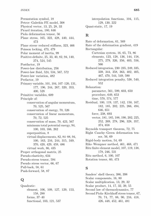
INDEX 685
Permutation symbol, 18Petrov–Galerkin FE model, 308Physical vector, 13, 25, 28, 33Picard iteration, 180, 646Piola deformation tensor, 56Plane stress, 165, 322, 428, 440, 444,
473Plane stress–reduced stiffness, 323, 466Poisson locking, 473, 479Polar moment of inertia, 99Positive-definite, 25, 33, 40, 82, 94, 140,
274, 524, 545Postfactor, 19Power-law distribution, 256Power-law fluid, 524, 534, 567, 572Power-law variation, 482Prefactor, 19Primary variable, 101, 104, 107–120, 131,
177, 196, 244, 267, 320, 353,400, 528
Primitive variables, 609Principle of:
conservation of angular momentum,70, 525, 567
conservation of energy, 70, 526conservation of linear momentum,
70, 72, 525conservation of mass, 70, 423, 567minimum total potential energy, 94,
100, 103, 166, 262superposition, 8virtual displacements, 82, 84–88, 94,
100, 163, 216, 244, 315, 349,370, 420, 429, 459, 486
virtual work, 86, 435Proper orthogonal matrix, 25Pseudo-elasticity, 634Pseudo-stress tensor, 594Pseudo stress vector, 66, 67Pull-back, 58, 61Push-forward, 58, 87
Q
Quadratic:element, 106, 109, 127, 129, 153,
158, 288forms, 37–40functional, 103, 121, 537
interpolation functions, 104, 115,129, 130, 222
Quasi-static, 17, 19
R
Rate of deformation, 61, 569Rate of the deformation gradient, 419Rectangular:
Cartesian system, 16, 65, 73, 86elements, 123, 128, 136, 144, 158,
275, 279, 326, 356, 403, 556,566
Reduced integration, 230–235, 249, 335,339, 344, 358, 363, 402, 405,467, 470, 544, 549, 590
Reduced integration penalty, 538, 540,552
Relaxation:parameter, 561, 599, 603, 650procedure, 649, 653time, 570, 574, 577
Residual, 100, 119, 137, 142, 150, 167,182, 185, 202, 225, 266, 494,646, 651
force, 238, 693vector, 181, 185, 188, 190, 202, 225,
252, 269, 278, 296, 328, 357,374, 658
Reynolds transport theorem, 72, 75Right Cauchy–Green deformation ten-
sor, 56, 69Rigid-body motion, 54, 69Riks–Wempner method, 461, 468, 471Ritz finite element model, 107, 119, 138,
178, 246, 531Ritz method, 6, 100, 107Rotation tensor, 60, 473
S
Sanders’ shell theory, 386, 398Scalar components, 16, 80Scalar multiplication, 13, 29, 32Scalar product, 14, 17, 32, 39, 55Second law of thermodynamics, 77Second Piola–Kirchhoff stress tensor, 67,
70, 74, 77, 88, 90, 216, 418,426, 448, 452, 461, 481
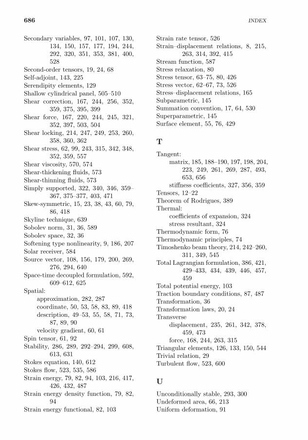
686
Secondary variables, 97, 101, 107, 130,134, 150, 157, 177, 194, 244,292, 320, 351, 353, 381, 400,528
Second-order tensors, 19, 24, 68Self-adjoint, 143, 225Serendipity elements, 129Shallow cylindrical panel, 505–510Shear correction, 167, 244, 256, 352,
359, 375, 395, 399Shear force, 167, 220, 244, 245, 321,
352, 397, 503, 504Shear locking, 214, 247, 249, 253, 260,
358, 360, 362Shear stress, 62, 99, 243, 315, 342, 348,
352, 359, 557Shear viscosity, 570, 574Shear-thickening fluids, 573Shear-thinning fluids, 573Simply supported, 322, 340, 346, 359–
367, 375–377, 403, 471Skew-symmetric, 15, 23, 38, 43, 60, 79,
86, 418Skyline technique, 639Sobolev norm, 31, 36, 589Sobolev space, 32, 36Softening type nonlinearity, 9, 186, 207Solar receiver, 584Source vector, 108, 156, 179, 200, 269,
276, 294, 640Space-time decoupled formulation, 592,
609–612, 625Spatial:
approximation, 282, 287coordinate, 50, 53, 58, 83, 89, 418description, 49–53, 55, 58, 71, 73,
87, 89, 90velocity gradient, 60, 61
Spin tensor, 61, 92Stability, 286, 289, 292–294, 299, 608,
613, 631Stokes equation, 140, 612Stokes flow, 523, 535, 586Strain energy, 79, 82, 94, 103, 216, 417,
426, 432, 487Strain energy density function, 79, 82,
94Strain energy functional, 82, 103
Strain rate tensor, 526Strain–displacement relations, 8, 215,
263, 314, 392, 415Stream function, 587Stress relaxation, 80Stress tensor, 63–75, 80, 426Stress vector, 62–67, 73, 526Stress–displacement relations, 165Subparametric, 145Summation convention, 17, 64, 530Superparametric, 145Surface element, 55, 76, 429
T
Tangent:matrix, 185, 188–190, 197, 198, 204,
223, 249, 261, 269, 287, 493,653, 656
stiffness coefficients, 327, 356, 359Tensors, 12–22Theorem of Rodrigues, 389Thermal:
coefficients of expansion, 324stress resultant, 324
Thermodynamic form, 76Thermodynamic principles, 74Timoshenko beam theory, 214, 242–260,
311, 349, 545Total Lagrangian formulation, 386, 421,
429–433, 434, 439, 446, 457,459
Total potential energy, 103Traction boundary conditions, 87, 487Transformation, 36Transformation laws, 20, 24Transverse
displacement, 235, 261, 342, 378,459, 473
force, 168, 244, 263, 315Triangular elements, 126, 133, 150, 544Trivial relation, 29Turbulent flow, 523, 600
U
Unconditionally stable, 293, 300Undeformed area, 66, 213Uniform deformation, 91
INDEX
INDEX 687
Uniqueness of solution, 27, 40Unit vector, 13–15, 22, 55, 62, 387, 463–
465, 479, 483Unsteady:
flows, 608, 611, 621, 627, 631Navier–Stokes equations, 535problems, 544
Updated Green–Lagrange strain tensor,424
Updated Green–Lagrange strain, 424–426
Updated Kirchhoff stress, 426Updated Lagrangian formulation, 386,
421, 424, 427, 429, 433, 438,444–450, 522
V
Validation, 41Variational:
calculus, 33, 318, 351, 441formulation, 37, 140methods, 6, 100operator, 84principle, 94, 100, 458, 593problem, 103, 121, 139, 142, 214,
535, 589Vectors, 12–22Velocity gradient tensor, 61, 75, 78, 89,
418, 526, 570, 573Velocity–pressure coupling, 608, 612, 621,
624Velocity–pressure FEM, 530–533Velocity–pressure–vorticity model, 607,
609Verification, 41Virtual displacements, 83–88, 205, 214,
216, 243, 246, 311, 349, 370,378, 397, 420, 429, 459, 486
Virtual strain energy, 216, 218, 315, 350,432
Viscoelastic fluid, 570, 577Viscosity, 94, 99, 169, 527, 534, 544,
572–574Viscous:
coefficients, 573dissipation, 526, 573fluid, 523, 570, 589–635stress tensor, 572
Volume element, 55, 72, 75, 83, 137von Karman, 215, 229, 247, 263, 311,
314, 327, 349, 370, 395, 625vortex, 625
Vorticity, 587, 593, 609, 612field, 613, 625tensor, 61, 93vector, 92, 593, 609
W
Weak forms, 88, 100–107, 121, 137, 188,216, 283, 287
axisymmetric problems, 138CPT, 318EBT, 216FSDT, 352least-squares, 594shell, 399Timoshenko beam (TBT), 243total Lagrangian formulation, 430two-dimensional problem, 266updated Lagrangian formulation, 433velocity–pressure FEM, 530viscous fluids, 523–587
Weak formulation, 118, 177, 265, 315Weak-form Galerkin, 108, 139, 178, 246,
267, 524, 531, 566, 590, 602,634
Weight functions, 100, 119, 177, 220,246, 371, 531
Weighted-integral, 7, 107, 100, 164, 308,531
Weighted-residual, 100, 119, 225Weingarten formulas, 389White–Metzner:
model, 570fluid, 574, 578
Work-conjugate, 419
Y
Young’s moduli, 81, 99, 167, 263, 428,482, 634
Z
Zero vector, 13, 25, 29, 33, 237, 251Zeroth-order tensors, 24