Embed Size (px)
Citation preview

Digital Object Identifier (DOI):10.1007/s00285-005-0336-4
J. Math. Biol. 51, 661–694 (2005) Mathematical Biology
O.E. Akman� · D.S. Broomhead · R.V. Abadi · R.A. Clement
Eye movement instabilities and nystagmus can bepredicted by a nonlinear dynamics model of thesaccadic system
Received: 12 March 2004 / Revised version: 20 December 2004 /Published online: 6 June 2005 – c© Springer-Verlag 2005
Abstract. The study of eye movements and oculomotor disorders has, for four decades,greatly benefitted from the application of control theoretic concepts. This paper is an exam-ple of a complementary approach based on the theory of nonlinear dynamical systems.Recently, a nonlinear dynamics model of the saccadic system was developed, comprisinga symmetric piecewise-smooth system of six first-order autonomous ordinary differentialequations. A preliminary numerical investigation of the model revealed that in addition togenerating normal saccades, it could also simulate inaccurate saccades, and the oscillatoryinstability known as congenital nystagmus (CN). By varying the parameters of the model,several types of CN oscillations were produced, including jerk, bidirectional jerk and pen-dular nystagmus.
The aim of this study was to investigate the bifurcations and attractors of the model,in order to obtain a classification of the simulated oculomotor behaviours. The applicationof standard stability analysis techniques, together with numerical work, revealed that theequations have a rich bifurcation structure. In addition to Hopf, homoclinic and saddlenodebifurcations organised by a Takens-Bogdanov point, the equations can undergo nonsmoothpitchfork bifurcations and nonsmooth gluing bifurcations. Evidence was also found for theexistence of Hopf-initiated canards.
The simulated jerk CN waveforms were found to correspond to a pair of post-canardsymmetry-related limit cycles, which exist in regions of parameter space where the equationsare a slow-fast system. The slow and fast phases of the simulated oscillations were attributedto the geometry of the corresponding slow manifold. The simulated bidirectional jerk and
�Corresponding author
O.E. Akman: The School of Mathematics, The University of Manchester, P.O. Box 88,Manchester M60 1QD, UK.
Present address: Mathematics Institute, University of Warwick, Coventry CV4 7AL, UK.e-mail: [email protected]
D.S. Broomhead: The School of Mathematics, The University of Manchester, P.O. Box 88,Manchester M60 1QD, UK. e-mail: [email protected]
R.V. Abadi: Faculty of Life Sciences, Moffat Building, The University of Manchester,Sackville St, Manchester M60 1QD, UK.e-mail: [email protected]
R.A. Clement: Visual Sciences Unit, Institute of Child Health, U.C.L., London WC1N 1EH,UK. e-mail: [email protected]
Mathematics Subject Classification (2000): 37N25
Key words or phrases: Nonlinear dynamics – Saccadic system – Congenital nystagmus –Bifurcation – Braking signal

662 O.E. Akman et al.
pendular waveforms were attributed to a symmetry invariant limit cycle produced by thegluing of the asymmetric cycles.
In contrast to control models of the oculomotor system, the bifurcation analysis placesclear restrictions on which kinds of behaviour are likely to be associated with each otherin parameter space, enabling predictions to be made regarding the possible changes in theoscillation type that may be observed upon changing the model parameters. The analysissuggests that CN is one of a range of oculomotor disorders associated with a pathologicalsaccadic braking signal, and that jerk and pendular nystagmus are the most probable oscilla-tory instabilities. Additionally, the transition from jerk CN to bidirectional jerk and pendularnystagmus observed experimentally when the gaze angle or attention level is changed isattributed to a gluing bifurcation. This suggests the possibility of manipulating the wave-forms of subjects with jerk CN experimentally to produce waveforms with an extendedfoveation period, thereby improving visual resolution.
1. Introduction
Traditionally, the study of eye movement control and oculomotor disorders hasbeen dominated by control theory [35], [42], [33], [41], [30], [21]. In the last fewyears, however, there has been increasing interest in the use of nonlinear dynamicstechniques to model oculomotor control, and to analyse eye movement time series[3], [37], [25] , [18], [7], [20]. The oculomotor control subsystem that is responsiblefor the generation of fast eye movements (saccades) has been the focus of muchtheoretical and experimental work [14], [42], [36], [18], [24]. A recent nonlineardynamics model of the saccadic system proposed in [18] was found to be able tosimulate normal saccades, abnormal saccades and normal saccades with a dynamicovershoot. In that work, numerical evidence was presented to show that a saccad-ic system model alone can generate both slow and fast eye movements. Indeed,the model was found to generate waveforms resembling those associated with thepathological oculomotor instability known as congenital nystagmus (CN), whichis currently believed to be a disorder of one or more of the oculomotor subsystemsresponsible for the generation of non-saccadic eye movements [1].
This paper describes the results of a bifurcation analysis of the model, andpresents a number of implications of the analysis for understanding saccadic abnor-malities and the aetiology of CN. In section 2, a brief overview of the relevantbiology is given. The derivation of the model equations is described in section 3,where it is also argued that the analysis of the model can effectively be reduced tothat of the equations representing the dynamics of the neurons which generate thesaccadic control signal. Section 4 presents the main results of the bifurcation anal-ysis, enabling the simulated waveforms to be organised around the correspondingbifurcation curves, and the morphology of each waveform to be interpreted in termsof the corresponding fixed point or limit cycle attractor. The results of section 4 aresummarised in Fig. 15.
Lastly, the biological implications of the analysis are discussed in section 5.Chief amongst these is the suggestion that CN may be a disorder of the saccadicsystem. This view conflicts with the characterisation of CN as an abnormality of oneof the oculomotor control subsystems responsible for slow eye movement controland fixation, based on the findings of many of the control models [33], [30], [21].

A nonlinear dynamics model of the saccadic system 663
In these models, it is implicitly assumed that the saccadic system is functioningwithin its normal parameter range. By contrast, the analysis presented here impliesthat CN may be part of a range of disorders produced by an abnormal saccadicbraking signal. Moreover, this work challenges the control theory explanation forthe morphology of jerk CN as a slow drift from the target generated by a sloweye movement disorder, followed by a corrective saccade to refixate the target. Thecharacteristic slow-fast form of jerk CN is instead attributed to the geometry of anunderlying slow manifold in the saccadic system phase space.
Several implications of this work are in agreement with previous psychophys-ical investigations. The existence of a canard implies that once the system hasdeveloped a sustained oscillatory instability, the oscillation is likely to be a jerk,bidirectional jerk or pendular CN. This is consistent with the results of a recentstudy of oscillatory eye movement disorders [2]. Additionally, the mechanism bywhich dynamic overshoots are generated by the model suggest that the movementsare caused by reversals of the saccadic control signal, as predicted by a previousstudy of the metrics of dynamic overshoots [12].
Finally, an outcome of this work which may have clinical implications is thesuggestion that the transition from a jerk nystagmus to a bidirectional jerk nystag-mus, which is often observed experimentally, may be a consequence of a gluingbifurcation. This implies the possibility of periodically forcing a target viewed by ajerk CN subject so as to bring the system close to homoclinicity, producing wave-forms that give rise to lower retinal slip velocities, and hence to improved visualperformance.
2. Oculomotor control, saccades and congenital nystagmus
2.1. Oculomotor control and saccades
In broad terms, the oculomotor system controls the movement of the eyes so as toensure that the image of the object of interest falls on the region of the retina knownas the fovea (a process referred to as foveation) [23]. Resolution of detail decreasessharply away from the fovea and is also degraded if images slip over the foveaat velocities greater than a few degrees per second. Consequently, optimal visualperformance is only attained when images are held steady on this region [44].
Saccades are fast movements of the eye which bring about foveation of newtargets [43]. The oculomotor subsystem responsible for the generation of horizon-tal saccades behaves in a very machine-like way. Experimental investigations ofthe dynamic characteristics of saccades have revealed that the peak velocity andduration of a saccade are related to its amplitude [43], [17]. This relationship isoften referred to as the main sequence, and is used to classify an eye movement asa saccade [13].
A recording of a simple accurate (normometric) saccade is shown in Fig. 1-A.Normometric saccades often have a post-saccadic component referred to as a dy-namic overshoot [34], [7]. A recorded dynamic overshoot is shown in Fig. 1-B.Inaccurate or dysmetric saccades can take the form of an initial undershoot (hyp-ometric saccade) or overshoot (hypermetric saccade) of the desired eye position,resulting in a secondary corrective saccade [14].

664 O.E. Akman et al.
0 0.1 0.2 0.3−2
0
2
4
6
8
10
12
14A
g(t)
(de
gs)
0 0.1 0.2 0.3 0.4 0.5−2
0
2
4
6
8
10
12
14B
0 0.2 0.4 0.6 0.8 1−2
−1.5
−1
−0.5
0
0.5C
0 0.2 0.4 0.6 0.8−4
−3
−2
−1
0
1
2
3D
0 0.2 0.4 0.6 0.8 1−8
−6
−4
−2
0
2
4E
0 0.2 0.4 0.6 0.8 10.6
0.8
1
1.2
1.4
1.6
1.8F
t (secs)
Fig. 1. Recorded eye movements. t=time, g(t)=horizontal eye position, with g(t) > 0 corre-sponding to rightward gaze. A: normometric saccade. B: dynamic overshoot. C: left-beatingjerk CN. D: jerk with extended foveation. E: bidirectional jerk. F: pendular CN. In A and B,the dotted line indicates the target position.
Neurophysiological studies have shown that the saccadic control signal for hor-izontal saccades is generated by excitatory burst neurons in the brainstem. Theseare normally inhibited by omnipause neurons, except during a saccade, when theomnipause neurons cease firing. The firing rate of a burst neuron is a saturatingnonlinear function of the dynamic motor error m, which is the difference betweenthe required and current eye positions [42]. The burst neurons are divided into two

A nonlinear dynamics model of the saccadic system 665
types: right burst neurons which fire maximally for rightward saccades and leftburst neurons which fire maximally for leftward saccades. The overall burst signalb can be expressed as the difference between the signals r and l from the right andleft burst neurons respectively.
In addition to the response in the direction of maximal firing (the on-response),the burst neurons also have a small response in the opposite direction (theoff-response). The off-response is believed to correspond to a small centripetaltug at the end of a small-amplitude movement that prevents the inertia of the eyecausing overshoot of the target [42]. This will be referred to here as a brakingsignal. The effectiveness of the braking signal in slowing the eye at the end ofthe movement increases with the magnitude of the off-response. Evidence has alsobeen found suggesting that burst neurons exhibit mutual inhibition, with the fir-ing of right burst neurons suppressing that of left burst neurons, and vice versa[39].
According to the displacement feedback model of saccade generation illustratedin Fig. 2, saccades are produced in response to a desired gaze displacement signal�g generated by higher brain centres [36]. In this scheme, the motor error m isobtained by subtracting an estimate s of current eye displacement from �g . Theburst signal b is sent to a complex of neurons in the brain stem, the neural integra-tor, which integrate it. The integrated signal n is then added to b, and the summedsignal is relayed to the relevant ocular motoneurons. These send the final motorcommand to the eye muscles, which produce a shift in the eye position g. A copyof b is sent to a separate resettable integrator to generate the estimate s. The epithet‘resettable’ refers to the fact that s is required to be set to 0 at the beginning ofeach saccade. This feedback model should act so as to drivem to 0, moving the eyeto the required position g (0) + �g. In control models of the oculomotor system,the ocular motoneurons and eye muscles are referred to collectively as the muscleplant.
BURST NEURONS
NEURAL INTEGRATOR
MUSCLE PLANT
RESETTABLE INTEGRATOR
∆g
s
m b-+
n g
Fig. 2. The displacement feedback model of saccade generation. A copy of the burst signal bis integrated to obtain an estimate of current eye displacement s which is fed back to generatethe motor error m. g and n denote the gaze angle and integrated burst signal respectively.�g denotes the required gaze displacement signal generated by higher brain centres, whichinitiates the saccade.

666 O.E. Akman et al.
2.2. Congenital nystagmus
CN is an involuntary, bilateral oscillation of the eyes that is present in approxi-mately 1 in 4000 of the population [4]. The oscillations in each eye are stronglycorrelated, and occur primarily in the horizontal plane. In general, the retinal imageis held on the fovea for a short time before a slow phase takes the target off thefovea. The slow phase is then interrupted by a fast or slow phase which movesthe image directly onto the fovea [22], [4], [5]. As a consequence of the reducedfoveation time, CN subjects tend to have poor visual acuity [6], [9], [16]. Somerecordings of common CN waveforms are shown in Fig. 1. Jerk CN consists ofan increasing exponential slow phase followed by a saccadic fast phase (fig. 1-C).The direction of the fast phase is referred to as the beat direction. Two variationson jerk are jerk with extended foveation, in which the eye spends a greater timein the vicinity of the foveation position (fig. 1-D), and bidirectional jerk, in whichthe eye beats alternately in both directions (Fig. 1-E). The less common pendularnystagmus consists of sinusoidal slow phase movements (Fig. 1-F).
Most CN subjects exhibit a range of different oscillations over a single record-ing period, with the particular waveform observed depending on factors such asgaze angle, attention and stress. In particular, it has been found that some sub-jects who exhibit a jerk nystagmus during a fixation task can switch to a pendularnystagmus upon entering a state of low attention, such as when closing their eyesor daydreaming [4], [5]. Many CN subjects have a gaze angle referred to as theneutral zone, in which the beat direction changes. Bidirectional oscillations can beobserved close to the neutral zone [4].
3. A nonlinear dynamics model of the saccadic system
3.1. The model
The displacement feedback model of Fig. 2 can be described using the set of coupledODEs below [18]:
g = v (1)
v = −(
1
T1+ 1
T2
)v − 1
T1T2g + 1
T1T2n+
(1
T1+ 1
T2
)(r − l) (2)
n = − 1
TNn+ (r − l) (3)
r = 1
ε
(−r − γ rl2 + F(m)
)(4)
l = 1
ε
(−l − γ lr2 + F(−m)
)(5)
m = − (r − l) . (6)
Equations (1) and (2) model the response of the muscle plant to the signals gener-ated by the burst neurons. Here, g represents the eye position and v the eye velocity.These equations are based on quantitative investigations of physical eye movementswhich show that the muscle plant can be modelled as a second-order linear system

A nonlinear dynamics model of the saccadic system 667
with a slow time constant T1 = 0.15s and a fast time constant T2 = 0.012s [33].(3) is the equation for n, the signal from the neural integrator. The slow time con-stant TN = 25s corresponds to the slow post-saccadic drift back to zero degreesobserved experimentally [15].
(4) and (5) are the equations for the activities r and l of the right and left burstneurons. The function F (m) defined by
F(m) ={α′
(1 − e−m/β ′)
if m ≥ 0
−αβmem/β if m < 0
(7)
models the response of the burst neurons to the motor error signal m. The form ofF (m) is based on the results of single-cell recordings from alert monkeys [42]. Aschematic plot of F (m) is shown in Fig. 3.
The function has four positive parameters, α′, β ′, α and β which govern theforms of the modelled on- and off- responses. Form ≥ 0, F (m) is increasing, withF (m) → α′ asm → ∞. Also, F
(β ′) = α′ (1 − e−1
). α′ therefore determines the
value at which the modelled on-response saturates as m → ∞, and β ′ determineshow quickly the saturation occurs. Form < 0, F (m) has a single global maximumat
(−β, αe
), and converges monotonically to 0 as m → −∞ from −β. α thus
determines the magnitude of the modelled off-response, and hence the strength ofthe corresponding braking signal. β determines the motor error range over which asignificant off-response occurs, and therefore the range for which there is effectivebraking.
The terms γ rl2 and γ lr2 represent the mutual inhibition between the left andright burst neurons, with the parameter γ determining the strength of the inhibi-tion. ε is a parameter which determines how quickly the neurons respond to themotor error signalm with the response time decreasing as ε is decreased. (6) is theequation for the resettable integrator, obtained by substituting m = �g − s into
F(m
)
α′
β′−β
αe−1
m
α′(1−e−1)
Fig. 3. Schematic of the function F (m) used to model the response curve for a saccadicburst neuron. The parameters α′ and β ′ determine the modelled on-response while α and βdetermine the modelled off-response.

668 O.E. Akman et al.
s = b. Note that it is assumed that the resettable integrator is a perfect integrator,in contrast to the neural integrator which is leaky.
The parameters α′, β ′ and γ are fixed at α′ = 600, β ′ = 9 and γ = 0.05, onthe basis that these values give simulated saccades which lie on the main sequence[18]. The variable parameters of the model are thus α, β and ε, representing theoff-response magnitude, off-response range and burst neuron response time respec-tively.
It should be noted that although the omnipause neurons are not explicitlyincluded in the model, the burst neuron response function F (m) implicitly incor-porates the effects of both the burst neurons and the omnipause neurons. The omni-pause neurons are active during the end of a saccade when they fire in order to bringthe saccade to a stop, and therefore contribute to the form of F (m) about m = 0.
3.2. Characterisation of the model as a skew-product
By setting x = (g, v, n)T and y = (r, l, m)T , the system can be written in theskew-product form
x = Ax + By
y = G (y) ,
where A and B are the constant matrices
A =
0 1 0
− 1T1T2
−(
1T1
+ 1T2
)1
T1T2
0 0 − 1TN
, B =
0 0 01T1
+ 1T2
−(
1T1
+ 1T2
)0
1 −1 0
,
and G (y) represents the vector field of equations (4)–(6). Sometimes, for conve-nience, this notation will be condensed further by writing z = (x, y) and z = F (z),where F (z) = (Ax + By,G (y)). Here, the fibre equations x = Ax + By rep-resent the muscle plant and neural integrator dynamics, while the base equationsy = G (y) represent the dynamics of the burst neurons and resettable integrator. Thebase equations will be referred to collectively from now on as the burst equations.The skew-product form essentially enables the analysis of the full 6-dimensionalsystem to be reduced to that of the 3-dimensional burst equations, as will now bediscussed.
F (m) is piecewise smooth about m = 0, from which it follows that G (y)is piecewise smooth about the set
{y ∈ R
3 : m = 0}. Also, it is easy to see that
F (m) is locally Lipschitz on R, and therefore that F (z) is locally Lipschitz on R6.
Solutions of z = F (z) are therefore unique with respect to initial conditions [31].Writing ϕt for the time t map of y = G (y) and ψt for the time t map of z = F (z),integration of the fibre equations implies that
ψt (z) =(eAtx+ ∫ t
0 eA(t−s)Bϕs (y) dsϕt (y)
).
The eigenvalues of eAt are{e− tT1 , e
− tT2 , e
− tTN
}, all of which lie inside the unit cir-
cle for t > 0. Under the reasonable assumption that there is an invariant compact
A nonlinear dynamics model of the saccadic system 669
subsetC of R3 such that all trajectories of y = G (y) are forward asymptotic toC, it
follows from the form ofψt (z) that there is a continuous function h : R3 → R
3 thathas two important properties. First, the graph ofh,
{(h (y) , y) : y ∈ R
3}, is invariant
and attracting in z = F (z). Secondly, the homeomorphism H : y �−→ (h (y) , y)conjugates the time t maps ϕt and ψt on C (i.e. (H ◦ ϕt ) (y) = (ψt ◦H) (y) fory ∈ C, t ≥ 0 ) [40]. This implies that, asymptotically, the burst system y = G (y)and the full system z = F (z) are topologically equivalent. The asymptotic qual-itative behaviour of the full system is therefore determined by that of the burstsystem. In particular, stable fixed points and stable limit cycles of the burst systemcorrespond to stable fixed points and stable limit cycles respectively of the fullsystem.
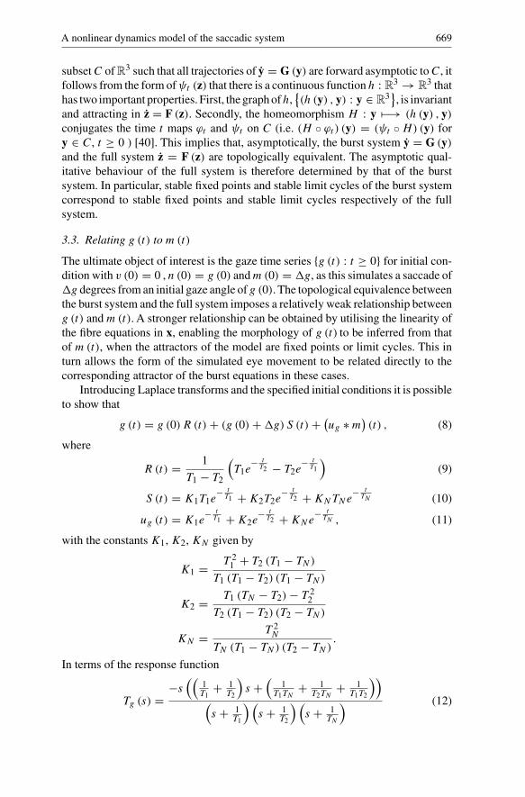
3.3. Relating g (t) to m(t)
The ultimate object of interest is the gaze time series {g (t) : t ≥ 0} for initial con-dition with v (0) = 0 , n (0) = g (0) andm(0) = �g, as this simulates a saccade of�g degrees from an initial gaze angle of g (0). The topological equivalence betweenthe burst system and the full system imposes a relatively weak relationship betweeng (t) andm(t). A stronger relationship can be obtained by utilising the linearity ofthe fibre equations in x, enabling the morphology of g (t) to be inferred from thatof m(t), when the attractors of the model are fixed points or limit cycles. This inturn allows the form of the simulated eye movement to be related directly to thecorresponding attractor of the burst equations in these cases.
Introducing Laplace transforms and the specified initial conditions it is possibleto show that
g (t) = g (0) R (t)+ (g (0)+�g) S (t)+ (ug ∗m)
(t) , (8)
where
R (t) = 1
T1 − T2
(T1e
− tT2 − T2e
− tT1
)(9)
S (t) = K1T1e− tT1 +K2T2e
− tT2 +KNTNe
− tTN (10)
ug (t) = K1e− tT1 +K2e
− tT2 +KNe
− tTN , (11)
with the constants K1, K2, KN given by
K1 = T 21 + T2 (T1 − TN)
T1 (T1 − T2) (T1 − TN)
K2 = T1 (TN − T2)− T 22
T2 (T1 − T2) (T2 − TN)
KN = T 2N
TN (T1 − TN) (T2 − TN).
In terms of the response function
Tg (s) =−s
((1T1
+ 1T2
)s +
(1
T1TN+ 1
T2TN+ 1
T1T2
))(s + 1
T1
) (s + 1
T2
) (s + 1
TN
) (12)

670 O.E. Akman et al.
of the linear system (8), S (t) and ug (t) can be written succinctly as:
S (t) = L−1[−Tg (s)
s
](13)
ug (t) = L−1 [Tg (s)
]. (14)
(In the above expressions, ∗ represents Laplace convolution while L−1 denotes theinverse Laplace transform).
In practise, there are simple approximations to these quantities which are validfor physiologically realistic values of the parameters. Using the known values ofT1, T2 and TN gives
|T2 (T1 − TN)| T 21
|T1 (TN − T2)| T 22
TN T1, T2,
from which it follows that K1T1 ≈ T2T1−T2
, K2T2 ≈ − T1T1−T2
and KNTN ≈ 1. ( 9)and (10) therefore give the following approximation for R (t):
R (t) ≈ −S (t)+ e− tTN .
Substituting this into (8) implies
g (t) ≈ g (0) e− tTN + (�g) S (t)+ (
ug ∗m)(t) . (15)
Thus, to a good approximation, the simulated eye movement decomposes into twoparts. The first two terms of (15) are independent of the error signalm(t). Figure 4is a plot of S (t) for t ≥ 0. It can be seen that S (t) tends quickly to 1 before
converging to 0 like e− tTN . Taken together, the first two terms of (15) therefore
0 0.2 0.4 0.6 0.8 10
0.2
0.4
0.6
0.8
1
1.2
t
S(t
)
Fig. 4. Plot of the function S (t) defined in (10). The function e− tTN is also shown (dotted
line).

A nonlinear dynamics model of the saccadic system 671
approximate a saccade of �g degrees from g (0). The remaining term shows howthe form of the error term m(t) modifies this basic saccade.
In the case where the attractor of the burst equations is a fixed point, then themotor error m(t) → m∗ for some m∗ ∈ R as t → ∞. Introducing the transientmotor error mT (t) = m(t)−m∗ and using (13)–(14) leads to
g (t) ≈ g (0) e− tTN + (�g −m∗) S (t)+ (
ug ∗mT)(t) . (16)
(16) and the form of S (t) suggest that if |�g| is large compared to |m∗| andm(t) → m∗ sufficiently fast as t → ∞, then g (t) will have the form of an accu-
rate saccade to g (0) +�g which drifts back to 0 like (g (0)+�g) e− tTN . In this
case, the equations model a normal saccadic control system. Clearly, if either ofthese conditions is violated, inaccurate or abnormal saccades will result. In partic-ular, oscillations in m(t) may induce oscillations in g (t).
In the case where the attractor of the burst equations is a limit cycle of period T ,the motor errorm(t)will converge to a periodic functionmS (t). Similarly the gazeangle g (t) will converge to a periodic function gS (t) which (because of the lin-earity of the fibre dynamics) also has period T . Moreover, writing mS (t) as theFourier series
mS (t) =∞∑
k=−∞mSk e
ikωT t
where ωT = 2πT
, ignoring transients and using the linearity of the convolutionimplies that gS (t) has the Fourier series
gS (t) =∞∑
k=−∞Tg (ikωT )m
Sk eikωT t
[32]. This is, in effect, a linear filtering of the time series {mS (t) : t ≥ 0}, whereTg (iω) is the response function of the filter.
It is useful to write Tg (iω) in terms of amplitude and phase variables, Tg (iω) =A (ω) eφ(ω)i . Explicit expressions forA (ω) and φ (ω) in terms of the time constantsT1, T2 and TN can be obtained, but these are rather uninformative. Figure 5 showsplots of numerical evaluations of A (ω) and φ (ω) for 0 < ω < 100. It is clear thatA (ω) depends rather weakly on frequency in this range. Indeed, if ω is restricted tothe interval 0.08 < ω < 55, then |A (ω)− 1| < 0.1. In the same frequency range,the phase varies approximately linearly. A linear regression of φ(ω) over this rangeimplies that φ (ω) ≈ −tgω+ π , where tg = 0.0115. Taken together, these expres-sions for the amplitude and phase suggest the approximation Tg (iω) ≈ −e−tgωifor 0.08 < ω < 55.
If it is assumed that the periodic function mS (t)− 〈mS (t)〉 (where 〈mS (t)〉 =1T
∫ T0 mS (t) dt) does not have significant energy outside the frequency range 0.08 <
ω < 55, then setting WS = {k ∈ Z : 0.08 < |kωT | < 55} gives the approximation
mS (t)− 〈mS (t)〉 ≈∑k∈WS
mSk eikωT t . (17)

672 O.E. Akman et al.
0 20 40 60 80 1000
0.2
0.4
0.6
0.8
1
1.2
1.4
ω
A(ω
)
0 20 40 60 80 1002
2.5
3
3.5
ω
φ(ω
)
Fig. 5. Plots of the amplitude variable A (ω) and phase variable φ (ω) of the linear filterTg (iω) defined in (12) on the range (0, 100).
As∣∣Tg (iω)∣∣ ≈ 1 for ω ∈ (0.08, 55) and
∣∣Tg (iω)∣∣ < 1 for ω /∈ (0.08, 55) withTg (0) = 0, it follows that gS (t) will also not have significant energy outside thefrequency range 0.08 < ω < 55. This leads to the approximation
gS (t) ≈∑k∈WS
Tg (ikωT )mSk eikωT t .
Substituting Tg (iω) ≈ −e−tgωi into the above then gives
gS (t) ≈ −∑k∈WS
mSk eikωT (t−tg).
Using (17) leads to the final approximation
gS (t) ≈ −mS(t − tg
) + 〈mS (t)〉 . (18)
Given this final approximation, g (t) has the form of a saccade which decays tothe periodic oscillation gS (t) as t → ∞, where the morphology of gS (t) is deter-mined by that of mS (t). The equations therefore model a pathological saccadicsystem with an asymptotically periodic oscillatory instability, the form of which isdetermined by that of the corresponding periodic motor error time series.
4. Analysis of the burst equations
It has been established in the previous sections that the asymptotic qualitativedynamics - and even quantitative dynamics - of the full model are determined bythat of the burst equations y = G (y) given explicitly by
r = 1
ε
(−r − γ rl2 + F (m)
)(19)
l = 1
ε
(−l − γ lr2 + F (−m)
)(20)
m = − (r − l) , (21)

A nonlinear dynamics model of the saccadic system 673
where F (m) = F (m;α, β) is defined in (7). Before the bifurcation analysis of theburst equations is presented in 4.2, some general properties of the equations whichaid their analysis - such as the existence of a symmetry - are discussed
4.1. General properties of the burst equations
4.1.1. SymmetryThe vector field G (y) is equivariant under the action of the group Z2 = {id, σ },where σ acts linearly on R
3 according to σ : (r, l, m) �−→ (l, r,−m). If followsthat σ maps trajectories of y = G (y) into each other, and that the set L0 definedby L0 = {
y ∈ R3 : σy = y
}is invariant under the dynamics [27]. L0 is given
explicitly by
L0 ={(x, x, 0)T : x ∈ R
}.
Restricting the vector field to L0 gives the following first order system:
x = −(
1 + γ x2)x. (22)
The point x = 0, the unique attracting fixed point of (22), corresponds to a fixedpoint at the origin 0 = (0, 0, 0)T of the full system. The invariance of L0 thereforeimplies that it is a 1-dimensional stable manifold of the origin. Since this propertyis a consequence of the symmetry, the existence and form of this stable manifolddo not depend on the model parameters α, β and ε.
4.1.2. Fixed pointsThe existence of the symmetry σ implies that invariant sets of the equations areeither symmetry invariant, or form pairs related by the action of σ . In particular,fixed points of (19)–(21) have the form (r∗, r∗,±m∗)T , where m∗ - which will betaken to be nonnegative - solves F (m) = F (−m), and r∗ ≥ 0 is the unique realsolution to γ r3 + r − F (m∗) = 0. Consideration of the form of F (m) shows that0 is always a solution of F (m) = F (−m) which gives rise to the fixed point atthe origin. Nontrivial solutions of F (m) = F (−m) on R
+ can occur genericallyin one of two ways depending on the shape of the function F (m), as illustrated inFig. 6.
Much of this can be understood in terms of the right and left derivatives ofF (m)at m = 0. Write + for limm→0+DF (m) = α′
β ′ and − for limm→0−DF (m) =−αβ
. Then as suggested by Fig. 6-A, for α > +β (that is for − − > +), there
is a single nontrivial solution m1 of F (m) = F (−m) on R+. For α < +β (that
is for − − < +), there are two possibilities. For some values of β, F (m) canintersect F (−m) tangentially as α is increased from 0 in this range. For such βvalues, there is a critical value of α at which the tangency occurs; this will be writtenas T (β). It then follows that there are no nontrivial solutions of F (m) = F (−m)on R
+ for α < T (β), a single solution m1 for α = T (β), and a pair of nontrivialsolutions {m1,m2} for T (β) < α < +β (see Fig. 6-B). The convention will be

674 O.E. Akman et al.
m m
F(m)
F(−m)
m2 m
1 0
F(m)
F(−m)
m1 0
A B
Fig. 6. Schematic of the possible intersections of the functions F (m) and F (−m) on thepositive real line.
that m1 and m2 are labelled so that m2 < m1. For β values such that no tangen-tial intersection of F (m) and F (−m) can occur when α < +β, there are nonontrivial solutions of F (m) = F (−m) on R
+ in this range.T (β) is defined parametrically in terms of m1 as below:
β =β ′m1
(1 − em1/β
′)β ′ (1 − em1/β ′) +m1
T (β) = α′β (m1) em1/β(m1)
β ′ +m1
(1 − β ′
β(m1)
) .
By considering the limitm1 → 0 in this parametric representation, it can be shownthat tangential intersections can only occur forβ > 2β ′; that is T (β) is only definedin this range. Moreover, in the (β, α) plane, the curve α = T (β) converges tangen-tially to the line α = +β as β → 2β ′+. By considering the limitm1 → ∞, it canbe deduced that the curve α = T (β) asymptotes to the line α = α′e as β → ∞,with T (β) strictly increasing on
(2β ′,∞)
.This discussion is summarised in Fig. 7 which shows a schematic of the curves
α = T (β) and α = +β in the (β, α) plane. Also shown are the fixed pointsof y = G (y), where for a given nontrivial solution mi of F (m) = F (−m) onR
+, the corresponding fixed points are written as y+i = (ri, ri , mi)
T and y−i =
(ri, ri ,−mi)T . Figure 7 suggests that(2β ′, 2α′) is a codimension 2 point at which
a line of nonsmooth pitchfork-type bifurcations at the origin intersects a line ofsymmetry-related saddlenode bifurcations.1
4.1.3. Slow manifoldFor small ε, the burst equations are a slow-fast system [46]. The associated slowmanifold, which will be written SM , is the union of curves given by the intersection
1 The bifurcation at the origin which occurs as α increases through +β is not a standardpitchfork bifurcation as the vector field G is not smooth at 0.

A nonlinear dynamics model of the saccadic system 675
α′e
α=Λ+β
2β′
2α′α=T(β)
0
β
α
0, y1+, y
1− 0, y
1+, y
1−, y
2+, y
2−
Fig. 7. Schematic plots of the curves α = +β and α = T (β) in the (β, α) plane. Thefixed points of the burst equations in each region of the (β, α) plane are also indicated.0 represents the fixed point at the origin, (0, 0, 0)T . y+
i and y−i have the forms (ri , ri , mi)
T
and (ri , ri ,−mi)T respectively, where mi > 0 solves F (m) = F (−m) and ri > 0 solves
γ r3i + ri − F (mi) = 0.
of the r- and l- nullclines. Trajectories contract onto SM parallel to the (r, l) planeand then evolve on SM according to the equation m = − (r − l). Trajectories onSM therefore move along it in the positivem direction for r < l and in the negativem direction for r > l.As ε is decreased, trajectories contract onto the slow manifoldmore quickly and follow it more closely. It can be seen from (19)–(20) that SM isindependent of ε, and is invariant under σ .
A more detailed understanding of the geometric form of SM can be obtainedby considering its parameterised form
{(F (m)
1 + γ lM (m)2 , lM (m) ,m
)T: m ∈ R
}, (23)
where lM (m) solves GM (l;m) = 0, with GM (l;m) given by
GM (l;m)= l5 − F (−m) l4 + 2
γl3 − 2F (−m)
γl2 + 1
γ
(F (m)2 + 1
γ
)l − F (−m)
γ 2 .
Consider foliating the phase space with planes of constantm. For a given valuem′ofm, sinceGM (l;m) is a quintic polynomial in l, SM intersects the planem = m′generically at 1, 3 or 5 points. Moreover, there is always at least one point of inter-section. It follows that in (r, l, m) space, SM always contains at least one curve,which will be written as S1. Asm is varied, new points of intersection are generatedthrough the quintic GM (l;m) developing pairs of additional roots.

676 O.E. Akman et al.
Something of the structure of SM can be understood by considering various
limits of m. As m → 0, F (m) → 0 , and so GM (l;m) → l(l2 + 1
γ
)2. This
function has only one real root at l = 0, and (23) implies that this root correspondsto the origin 0, which always lies on SM . It follows that for small |m|, SM = S1with S1 → 0 as m → 0.
Considering the limit as m → ∞, F (m) → α′ and F (−m) → 0, from which
it follows that GM (l;m) → l(l4 + 2
γl2 + 1
γ
((α′)2 + 1
γ
)). Again, l = 0 is the
only real root of this function implying that SM = S1 for m > 0 with m large.Moreover, (23) implies that S1 converges to the curve
{(F (m) , 0,m)T : m > 0
}asm → ∞. By symmetry, SM = S1 form < 0 with |m| large. Indeed, S1 convergesto the curve
{(0, F (−m) ,m)T : m < 0
}as m → −∞, .
For intermediate values of |m|, S1 may have turning points with respect to them-axis, while SM may contain other curves in addition to S1. As roots ofGM (l;m)are created in pairs, any such additional curves will be closed loops. Examples ofthe form of SM appear in Figs. 9, 12 and 14.
The existence of SM restricts the behaviour of the burst equations for small ε.Firstly, since all attractors must have portions lying onSM , andSM is a 1-dimensionalset, it is reasonable to assume that the only possible attractors are stable fixed pointsand stable limit cycles. Secondly, trajectories cannot cross the m = 0 plane. Thiscan be seen by noting that SM = S1 for |m| small; any trajectory which crosses theplane must therefore do so on S1, which cannot happen as S1 contains a fixed pointat the origin.
4.1.4. Smooth vector fieldsIn interpreting the bifurcations and local dynamics of the burst equations at theorigin 0 where the vector field G is not smooth, it will be useful to consider thesmooth vector fields G+ and G− defined as follows:
G+ (r, l, m) =
1ε
(−r − γ rl2 + α′
(1 − e−m/β ′))
1ε
(−l − γ lr2 + α
βme−m/β
)−(r − l)
(24)
G− (r, l, m) =
1ε
(−r − γ rl2 − α
βmem/β
)1ε
(−l − γ lr2 + α′
(1 − em/β
′))−(r − l)
. (25)
These vector fields have been chosen so as to agree with G on the appropriatehalf-spaces: G+|m≥0 = G|m≥0 and G−|m≤0 = G|m≤0. Consequently, each tra-jectory of y = G (y) can be expressed as a union of sections of trajectories ofy = G+(y) and y = G−(y). Also,σ ◦G+ = G−◦σ , and so solutions of y = G+(y)and y = G−(y) map into each other under σ . As G±|m=0 = G|m=0, 0 is a fixedpoint of both smooth systems and L0 is a stable manifold of 0, for all parametervalues.

A nonlinear dynamics model of the saccadic system 677
4.2. Bifurcations, attractors and simulated eye movements
The bifurcation analysis presented in this section is divided into two main parts. In4.2.1, the bifurcations of the burst equations which occur as α and β are varied fora fixed small ε are described. These results provide the basis for 4.2.2, in which therestriction to small ε is lifted, and the bifurcations which occur in the reduced range1.5 < β < 6, α < α′ are considered. This reduced range contains the parametervalues for which biologically realistic simulated eye movements were found duringthe initial numerical investigation of the full model presented in [18]. In 4.2.2, themorphology of each of these simulated eye movements is interpreted in terms ofthe corresponding attractor of the burst equations. The results of the section aresummarised in Fig. 15.
4.2.1. Bifurcations and attractors for small εFigure 8 is a schematic diagram of the bifurcations and attractors of the burst equa-tions for small ε. The figure was obtained by combining standard linear stabilityanalysis with numerical work and the assumption that the equations have only fixedpoint and limit cycle attractors for small ε.2 The bifurcations are organised by apair of codimension-two points. The first of these is the point
(2β ′, 2α′) identified
in section 4.1.2. The second codimension-two point, labelled (βT , αT ), is of theTakens-Bogdanov type. Each is discussed in turn below.
The codimension-two point(2β ′, 2α′): At this point, a line α = T (β) of sym-
metry-related saddlenode bifurcations intersects a line α = +β of nonsmooth,pitchfork-type bifurcations involving the origin 0. For β > βT , all fixed points{y+
1 , y−1 , y+
2 , y−2
}created by the saddlenode bifurcations are unstable, while for
β < βT ,{y+
1 , y−1
}are created stable and
{y+
2 , y−2
}are created unstable (cf. Fig. 7).
The pitchfork-type bifurcation can occur in two ways, depending on the sign ofβ−2β ′. For β < 2β ′, the bifurcation is supercritical: as α increases through +β,0 loses stability and a pair of stable fixed points
{y+
1 , y−1
}is created. For β > 2β ′,
the bifurcation is subcritical: as α increases through +β, 0 loses stability and apair of unstable fixed points
{y+
2 , y−2
}is destroyed (cf. Fig. 7 again).
The pitchfork-type bifurcation can be understood in terms of standard trans-critical and pitchfork bifurcations which occur in the smooth system y = G+(y)defined in (24). It can be shown that given a fixed β and ε, for α with |α − +β|sufficiently small, the origin has a smooth, 1-dimensional, attracting local centremanifoldW+
C , which is tangential to the vector ( +, +, 1)T at 0 when α = +β.Moreover, the dynamics on W+
C is given by
z = P (z, α) = (α − +β) z− +az2 − +(
2ε +a2 + b)z3 + O (3) , (26)
2 Many of the bifurcation curves lie very close to each other in the (β, α) plane, and so aschematic plot has been given to aid visualisation.

678 O.E. Akman et al.
2β′
α=T(β)
βT
α=αH(β)
β
α
α=Λ+β
αT
0
α=H(β,∈)
0
y1+, y
1−
0, y
1+, y
1−
0
C+, C
−
0, C+, C
−
α=αC(β,∈)
2α′
βC(∈)
Fig. 8. Bifurcations and attractors of the burst equations (4)–(6) for small ε. α = +β isa line of nonsmooth pitchfork bifurcations at the origin 0 = (0, 0, 0)T . The bifurcation issupercritical for β < 2β ′, producing a pair of stable fixed points
{y+
1 , y−1
}, and subcritical
for β > 2β ′, destroying a pair of unstable fixed points{y+
2 , y−2
}. α = T (β) is a line of
symmetry-related saddlenode bifurcations. All fixed points{y+
1 , y−1 , y+
2 , y−2
}produced by
the bifurcations are unstable for β > βT , while for β < βT ,{y+
1 , y−1
}are created stable
and{y+
2 , y−2
}are created unstable. α = αH (β) is a line of symmetry-related supercritical
Hopf bifurcations at y+1 and y−
1 at which a pair of stable limit cycles {C+, C−} are produced.α = H (β, ε) is a curve of symmetry-related saddlenode homoclinic bifurcations at y+
2 andy−
2 which destroy C+ and C−. α = αC (β, ε) is a line of symmetry-related Hopf-initiatedcanards at which C+ and C− undergo a sudden increase in amplitude.
where
z = −εr + εl +m (27)
a = 1
β− 1
2β ′ (28)
b = 1
6 (β ′)2− 1
2β2 , (29)
and O (3) represents all terms of the form{zi (α − +β)j : i + j ≥ 3
}, excluding
z3 [10]. It then follows from the symmetry that for small ε, the set WC definedby WC = (
W+C ∩ {y : m ≥ 0}) ∪ ((
σW+C
) ∩ {y : m ≤ 0}) is a 1-dimensional,

A nonlinear dynamics model of the saccadic system 679
attracting local set of the piecewise smooth system y = G (y) containing 0, onwhich the dynamics is given by
z = Q(z, α) ={
P (z, α) if z ≥ 0−P (−z, α) if z ≤ 0
. (30)
A fixed point z∗ ≥ 0 of the W+C dynamics z = P (z, α) gives rise to a pair of
fixed points {z∗,−z∗} of theWC dynamics z = Q(z, α). These in turn correspondto a pair of fixed points y∗ = (r∗, r∗, z∗)T and σy∗ = (r∗, r∗,−z∗)T of y = G (y).3
In particular, 0 is a fixed point of both theW+C andWC dynamics, corresponding to
the fixed point of y = G (y) at 0. The stability of a fixed point z∗ ≥ 0 of z = P (z, α)
determines that of both z∗ and −z∗ (as fixed points of z = Q(z, α)), and hence ofy∗ and σy∗.
Equation (26) can be thought of as an unfolding of the dynamics near a degener-ate fixed point at z = 0. In the case where β �= 2β ′ (that is when a �= 0), P (z, α) isequivalent to the normal form PN (z, α) = (α − +β) z − sign (a) z2. This fam-ily is well known to have a transcritical bifurcation at α = +β [11]. For the fullsystem, z = Q(z, α), there are correspondingly two cases depending on the signof a. When sign (a) > 0 (β < 2β ′), 0 loses stability as α is increased through +β. This is a kind of supercritical bifurcation which involves only the nonneg-ative fixed points (and their images under z �−→ −z) of the transcritical normalform. The bifurcation creates two new stable fixed points {m1,−m1}. Superficially,this resembles a standard supercritical pitchfork bifurcation; however, m1 scaleslike α − +β rather than
√α − +β. The case sign (a) < 0 (β > 2β ′) gives
the corresponding subcritical bifurcation. As α is increased through +β, 0 losesstability and a pair of unstable fixed points {m2,−m2} is destroyed. Again, m2scales like α − +β.
When β = 2β ′ (that is, when a = 0), the quadratic normal form is no longervalid.P (z, α) is instead equivalent to the normal formPN (z, α)= (α− +β) z−z3.In contrast to the case β �= 2β ′, −PN (−z, α) = PN (z, α), and so the full vectorfield Q(z, α) is also equivalent to this normal form. This family of smooth vec-tor fields is well known to have a supercritical pitchfork bifurcation at α = +β[11]. At this bifurcation, 0 loses stability creating the stable pair of fixed points{m1,−m1}.
The codimension-2 point (βT , αT ): At this point, the Jacobian matricesDG(y+
1
)and DG
(y−
1
)both have the normal form
− 4ε
0 00 0 10 0 0
,
identifying (βT , αT ) as a Takens-Bogdanov point [29]. (βT , αT ) lies at the inter-section of three curves: a curve α = αH (β) of symmetry-related supercritical Hopfbifurcations at y+
1 and y−1 ; a curve α = H (β, ε) of symmetry-related saddlenode
3 (27) implies that if (r∗, r∗,m∗)T is a fixed point of y = G (y) corresponding to z∗, thenm∗ = z∗.

680 O.E. Akman et al.
homoclinic bifurcations at y+2 and y−
2 ; and the curve α = T (β) representing thecreation of
{y+
1 , y+2
}and, by symmetry,
{y−
1 , y−2
}through saddlenode bifurcations.
The limit cycles produced by the Hopf bifurcations at y+1 and y−
1 will be referredto as C+ and C− respectively. It was pointed out in 4.1.3 that for small ε, trajectoriescannot cross the m = 0 plane. It therefore follows that C+ lies in m > 0 and C−lies inm < 0. Moreover, since σ maps trajectories of the burst equations into eachother, C− = σC+. As can be seen in Fig. 8, C+ and C− exist in the region of the(β, α) plane lying between the curves α = αH (β) and α = H (β, ε). Crossing thecurve α = H (β, ε) from left to right in the (β, α) plane causes the limit cycle C+to be destroyed in a homoclinic bifurcation at y+
2 . Similarly, by symmetry, C− isdestroyed at y−
2 .The values βT , αT and the function αH (β) are given explicitly by
βT = 2β ′mH2β ′ −mH
(α′√γ − 2
) (31)
αT = 2βT emH/βT
mH√γ
(32)
αH (β) = 2
mH√γβemH/β, (33)
where
mH = ln
(α′√γ
α′√γ − 2
)β ′
(34)
is the value ofm1 at α = αH (β). αT , βT andmH have the approximate numericalvalues αT = 1203, βT = 18.05 and mH = 0.135. Viewed as a graph in the (β, α)plane, the function αH (β) has a global minimum at mH , and increases withoutbound as β → 0.
Numerical work indicates that for a given small ε, there is a value βC (ε) ofβ such that C+ and C− undergo a sudden increase in amplitude as α is increasedfrom αH (β) for a fixed β in the range (βC (ε) , βT ). This amplitude increase ischaracterised by a local maximum of the derivative Dαρ (α, β, ε) of the function
ρ (α, β, ε) = max(r,l,m)T ∈C+
{m} − min(r,l,m)T ∈C+
{m} ,
which measures the extent of C+ (and by symmetry C−) in them direction [10]. Thevalue of α corresponding to the maximum of Dαρ (α, β, ε) for a given β and ε iswritten as αC (β, ε). The amplitude increase at this value appears to be attributableto symmetry-related Hopf-initiated canards ([28]), in which C+ and C− developsegments that lie on the slow manifold SM (α, β) as α is increased [10].
The mechanism by which the canards occur is illustrated with an example inFig. 9, which shows the evolution of C+ and SM in the region m > 0 as α isincreased for β = 0.75, ε = 0.001 (the corresponding evolution of C− and SMin the region m < 0 can be inferred from the symmetry). For α > αH (β) with|α − αH (β)| sufficiently small, SM ∩{y : m > 0} consists of the curve S1 together

A nonlinear dynamics model of the saccadic system 681
−20 10 0 10 20 30 40
0.1
0.2
0.3
0.4
0.5
0.6
0.7
r−l
m
−20 −10 0 10 20 30 40
0.1
0.2
0.3
0.4
0.5
0.6
0.7
r−l
m
−20 −10 0 10 20 30 40
0.1
0.2
0.3
0.4
0.5
0.6
0.7
r−l
m
C+
C+
C+
A
B
C
S1 S
+
S1
S1
Fig. 9. Projection into the (r − l, m) plane of the Hopf-initiated canard involving C+ whichoccurs in the burst equations for β = 0.75, ε = 0.001. A: αH (β) < α = 59.5328 < αC (β).B: αC (β) < α = 59.8486 < αC (β, ε). C: α = 59.9539 > αC (β, ε) . The dotted lineindicates the slow manifold SM .

682 O.E. Akman et al.
with a closed curve S+. The limit cycle C+ is restricted to S1, and does not interactwith S+ (see fig. 9-A). As α is increased from αH (β) through some critical valueαC (β), S+ and S1 merge, forming a single curve. For α > αC (β), C+ has portionslying on the region of S1 formed by the merging with S+. The rapid increase inthe amplitude of C+ as α increases through αC (β, ε) corresponds to the subset ofthis region lying between the origin and the point with largest m value becomingattracting (see Figs. 9-B and 9-C). The post-canard limit cycles {C+, C−} have theform of a relaxation oscillation.
Numerical computations indicate that the canard line α = αC (β, ε) and theline α = αC (β) both intersect the Takens-Bogdanov point (βT , αT ). Moreover, asε → 0, α = αC (β, ε) converges to α = αC (β).
4.2.2. Bifurcations, attractors and simulated waveforms for 1.5 < β < 6, α < α′Recall that the actual object of interest is the gaze time series {g (t) : t ≥ 0} ofthe full model (1)-(6) for initial condition with v (0) = 0, n (0) = g (0) andm(0) = �g, as this simulates a saccade of �g degrees from an initial gaze angleof g (0). In this section, the various forms of g (t) that the model can produce willbe discussed for the limited parameter range 1.5 < β < 6, α < α′, for which bio-logically realistic time series were previously found. Figure 10 is a plot of the burstsystem bifurcations and attractors for ε small and (β, α) restricted to this region(compare with Fig. 8). A range of the gaze time series that can arise for parametersfrom this region is shown in Fig. 11. Each of these will now be discussed in termsof the corresponding attractor, and the bifurcation giving rise to the attractor.
Normometric saccades, hypometric saccades and dynamic overshoots: For α < +β with ε small, the origin 0 = (0, 0, 0)T is the unique attractor of the burstequations. 0 is a stable node of y = G (y) in this range, in the sense that it is a sta-ble node of the smooth systems y = G+(y) and y = G−(y) introduced in section4.1.4. For α < +β, SM consists of the single curve S1. Since ε is small, y (t)contracts rapidly to S1 parallel to the (r, l) plane, and then converges along S1 tothe origin (see trajectory #1 of Fig. 12). The corresponding motor error variablem(t) converges quickly to 0. Hence, as suggested by approximation (16), the gazetime series has the form of a normometric (accurate) saccade to g (0)+�g degrees
which drifts back to zero like (g (0)+�g) e− tTN . Figure 11-A shows a simulated
normometric saccade (cf. Fig. 1-A)Increasing ε causes trajectories of y = G (y) to follow S1 less closely as they
converge to 0. Indeed, for ε > 1
4( +− α
β
) , DG+ (0) has a pair of complex con-
jugate eigenvalues {µ, µ} with Re {µ} < 0. Trajectories of the smooth systemsy = G+(y) and y = G−(y) spiral around the stable manifold L0 = {(
x, x, 0)T :
x ∈ R}
as they converge to the origin. Since trajectories of the piecewise smoothsystem y = G (y) can be constructed by concatenating sections of trajectories ofy = G+(y) and y = G−(y), it follows that y (t) also spirals around L0 as it con-verges to the origin (see trajectory #2 of Fig. 12). The motor error m(t) convergesto 0 by executing damped oscillations about 0. Thus, as suggested by (16), thecorresponding gaze time series g (t) has the form of a normometric saccade with

A nonlinear dynamics model of the saccadic system 683
6
α=αC
(β)
α=αH
(β)
α=Λ+β
α′
α=αC
(β,∈)
1.5
0
y1+, y
1−
C+, C
− (large−amplitude
relaxation oscillations)
0
C+, C
− (small−amplitude oscillations)
β
α
Fig. 10. Bifurcations and attractors of the burst equations for 1.5 < β < 6, α < α′ andε small. α = +β is a line of supercritical nonsmooth pitchfork bifurcations at the origin0 = (0, 0, 0)T which creates the stable fixed points
{y+
1 , y−1
}. α = αH (β) is a line of symme-
try-related supercritical Hopf bifurcations at{y+
1 , y−1
}which creates the stable limit cycles
{C+, C−}. α = αC (β, ε) is a line of symmetry-related Hopf-initiated canards involving C+and C−. α = αC (β) is the limiting curve of α = αC (β, ε) as ε → 0 (dotted line).
a post-saccadic damped oscillation about (g (0)+�g) e− tTN , which resembles a
dynamic overshoot. A numerical example is shown in Fig. 11-B (cf. Fig. 1-B).For +β < α < αH (β) with ε small, the attractors are the symmetry-related
pair of fixed points{y+
1 , y−1
}, which are stable nodes in this range. As trajectories
cannot cross the plane m = 0, y (t) → y+1 as t → ∞ if �g > 0 and y (t) → y−
1as t → ∞ if �g < 0. Thus, m(t) → sign(�g)m1 as t → ∞. If |�g| is largecompared tom1, g (t) has the form of a normometric saccade, while if |�g| is of thesame order as m1, g (t) has the form of a hypometric (under-shooting) saccade, assuggested again by approximation (16). Figure 11-C shows a simulated hypometricsaccade.
Small-amplitude nystagmus and jerk CN: In the range α > αH (β) with ε small,the attractors of the burst equations are the symmetry-related pair of stable limitcycles {C+, C−}. Moreover, since trajectories cannot cross the plane m = 0, if�g > 0, y (t) converges to C+, while if �g < 0, y (t) converges to C−. Thissituation was discussed in section 3.3 where it was stated that ifm(t) converges to

684 O.E. Akman et al.
0 0.1 0.2 0.30
2
4
6
8
10
12
14
0 0.1 0.2 0.30
2
4
6
8
10
12
14
0 0.1 0.2 0.30
0.1
0.2
0.3
0.4
0.5
0.6
0 1 2 3 40
0.1
0.2
0.3
0.4
0.5
0.6
0 0.2 0.4 0.6 0.8 1−12
−10
−8
−6
−4
−2
0
0 0.4 0.8 1.2 1.6−12
−10
−8
−6
−4
−2
0
0 0.2 0.4 0.6 0.8 1−20
−15
−10
−5
0
0 0.2 0.4 0.6 0.8 1−30
−20
−10
0
10
g(t)
t
A B
C D
E F
G H
Fig. 11. Gaze time series {g (t) : t ≥ 0} generated by the full model (1)–(6) for initial con-ditions with g (0) = v (0) = n (0) = 0 and m(0) = �g. A: α = 20, β = 3 , ε = 0.001,�g = 10. Normometric saccade. B: α = 20, β = 3, ε = 0.015, �g = 10. Dynamic over-shoot. C: α = 206, β = 3, ε = 0.001, �g = 0.5. Hypometric saccade. D: α = 207.656,β = 3, ε = 0.006, �g = 0.5. Small-amplitude nystagmus. E: α = 240, β = 3, ε = 0.004,�g = −10. Jerk CN. F: α = 240, β = 3, ε = 0.0048, �g = −10. Jerk with extendedfoveation. G: α = 240, β = 3, ε = 0.006, �g = −10. Bidirectional jerk CN. H: α = 240,β = 3, ε = 0.06, �g = −10. Pendular CN.

A nonlinear dynamics model of the saccadic system 685
−200 −100 0 100 200 300 400 500−4
−2
0
2
4
6
8
10
12
r−l
m
1
2
S1
Fig. 12. Burst system trajectories corresponding to simulated normometric saccades. Tra-jectory #1: α = 20, β = 3, ε = 0.001, �g = 10. Trajectory #2: α = 20, β = 3, ε = 0.015,�g = 10. The dotted line denotes the slow manifold SM . The stable manifold L0 is orthog-onal to this projection and passes through (0, 0). The gaze time series corresponding totrajectories #1 and #2 are shown in Figs. 11-A and 11-B respectively.
a periodic functionmS (t), then g (t) converges to a periodic function gS (t) whichis the result of applying a linear filter to mS (t) (and consequently has the sameperiod). Indeed, it was argued that if mS (t) has no significant energy outside theangular frequency range (0.08, 55), then gS (t) ≈ −mS
(t − tg
) + 〈mS (t)〉, wheretg = 0.0115.
For αH (β) < α < αC (β, ε), C+ and C− are small-amplitude limit cycles.mS (t), and hence gS (t), is therefore a small-amplitude periodic oscillation. Thecorresponding gaze time series g (t) has the form of a normometric saccade witha post-saccadic small-amplitude nystagmus. An example of such a waveform isshown in Fig. 11-D.
For α > αC (β, ε), C+ and C− are large-amplitude relaxation oscillations.Numerical work suggests that for α > αC (β), the intersection of the slow mani-fold SM with the plane m = m′ has greater extent in the positive r − l directionthan in the negative r − l direction, form′ such that there is more than one point ofintersection (cf. Figs. 9-B and 9-C). Since m = − (r − l), this configuration of SMmeans that for α > αC (β, ε), the contraction of C+ onto SM parallel to the (r, l)plane results in m changing rapidly from small and positive to large and negative(cf. Fig. 9-C). (By symmetry, the contraction of C− onto SM results in m changingrapidly from small and negative to large and positive). Accordingly, mS (t) has theform of a slow drift away from m = 0 followed by a sudden switch to a fasterreturn towardsm = 0 that resembles a jerk nystagmus. For�g > 0,mS (t) resem-bles a left-beating jerk CN and for �g < 0, mS (t) resembles a right-beating jerkCN. The approximation gS (t) ≈ −mS
(t − tg
) + 〈mS (t)〉 therefore implies that

686 O.E. Akman et al.
αC
(β) αC
(β) −
^
∈
αH
(β) αC
(β,∈′)
∈′
α
∈=∈C(α,β)
∈=∈G
(α,β)
α′
Fig. 13. Schematic of the canard surface ε = εC (α, β) and the gluing-type bifurcation sur-face ε = εG (α, β) in the (α, ε) plane for a fixed β with 1.5 < β < 6. The curve α = αC(β)represents the projection onto the (β, α) plane of the intersection of ε = εC (α, β) withε = εG (α, β).
gS (t) resembles a jerk nystagmus with a beat direction opposite to that of mS (t).For a given �g, the gaze time series g (t) has the form of a normometric saccadewith a post-saccadic oscillation which decays to a periodic jerk CN. The periodicoscillation is right-beating for�g > 0 and left-beating for�g < 0. Figure 11-E isan example of a simulated left-beating jerk CN (cf. Fig. 1-C).
Jerk with extended foveation, bidirectional jerk and pendular CN: As ε is increasedin the range α > αC (β), the canards describe a surface ε = εC (α, β) in (α, β, ε)space such that: i) the curve α = αC (β) is the intersection of ε = εC (α, β) withthe (β, α) plane, and ii) for a given value ε′ of ε, the curve α = αC
(β, ε′
)is
the projection onto the (β, α) plane of the intersection of ε = εC (α, β) with theplane ε = ε′. Numerical work suggests that as ε is increased in (α, β, ε) space,the canard surface terminates by intersecting a surface of gluing-type bifurcations,which will be written ε = εG (α, β) . A schematic of the curves ε = εC (α, β)
and ε = εG (α, β) in the (α, ε) plane for a fixed β is shown in Fig. 13 to aid theirvisualisation.
At ε = εG (α, β), C+ and C− merge, forming a single symmetry-invariantlimit cycle written as C. This bifurcation is qualitatively equivalent to a symmetric,smooth gluing bifurcation of the saddlenode type ([26]), and is a result of C+ andC− undergoing simultaneous saddlenode homoclinic bifurcations at the origin inthe smooth systems y = G+(y) and y = G−(y) respectively. Figure 14 shows thegluing of the limit cycles as ε increases through ε = εG (α, β) for α = 240 andβ = 3.

A nonlinear dynamics model of the saccadic system 687
−400 −200 0 200 400−8
−6
−4
−2
0
2
4
6
8
r−l
m
−400 −200 0 200 400−8
−6
−4
−2
0
2
4
6
8
r−l
m
−400 −200 0 200 400−8
−6
−4
−2
0
2
4
6
8
r−l
m
C+
C−
C
A
B
C
S1
S1
S1
Fig. 14. Projection into the (r − l, m) plane of the nonsmooth gluing bifurcation whichoccurs in the burst equations for α = 240, β = 3. A: ε = 0.0005. B. ε = εG (α, β) ≈0.00490167. C. ε = 0.008. The dotted lines denote the slow manifold SM .

688 O.E. Akman et al.
Letα = αC (β) denote the curve corresponding to the projection onto the (β, α)plane of the intersection of ε = εC (α, β) with ε = εG (α, β) (see Fig. 13). As εis increased from 0 for α ∈ (
αC (β) , αC (β)), the large-amplitude limit cycles C+
and C− undergo canards becoming small-amplitude limit cycles. Increasing ε from0 for α ∈ (
αC (β) , α′) causes C+ and C− to undergo the gluing bifurcation. As
ε → εG (α, β)− in this range, the limit cycles C+ and C− approach homoclinicity,resulting in mS (t) developing increasingly long periods where it is approximatelyequal to 0. For ε < εG (α, β) with |ε − εG (α, β)| small, mS (t), and hence gS (t),resembles a jerk nystagmus with an extended foveation period. The gaze time seriesg (t) has the form of a normometric saccade with a post-saccadic oscillation whichdecays to a periodic jerk nystagmus with an extended foveation period. Figure 11-Fis an example of such a simulated waveform (cf. Fig. 1-D).
For ε > εG (α, β), provided that ε− εG (α, β) is not too large, C is a relaxationoscillation with portions lying on SM (see Fig. 14-C). mS (t) is composed of slowdrifts away from 0 followed by fast returns towards 0 in alternating directions,and resembles a bidirectional jerk nystagmus. The approximation relating gS (t)and mS (t) implies that gS (t) also resembles a bidirectional jerk nystagmus. g (t)has the form of a normometric saccade which decays to a periodic bidirectionaljerk oscillation, as can be seen in Fig. 11-G (cf. Fig. 1-E). As ε → εG (α, β)+,C approaches homoclinicity, and gS (t) resembles a bidirectional jerk nystagmuswith an extended foveation period.
Increasing ε from εG (α, β) causes the limit cycle C to be successively lessconfined to the slow manifold, and to lose the form of a relaxation oscillation.mS (t) loses its slow-fast form, developing increasingly shorter foveation periods.For sufficiently large ε, mS (t) is sinusoidal with no discernible foveation period,and resembles a pendular nystagmus oscillation. gS (t) inherits this morphology,and g (t) has the form of a hypermetric (over-shooting) saccade which decays to aperiodic pendular nystagmus. Figure 11-H is an example of a pendular nystagmussimulated by the model (cf. Fig. 1-F).
Other global bifurcations are observed numerically as ε is increased for (β, α)in the range 1.5 < β < 6, α < αC (β), but these do not have any obvious bio-logical interpretation. In (α, β, ε) space, one of these bifurcation surfaces appearsto intersect the canard surface ε = εC (α, β) along the line where it intersects thesurface of nonsmooth gluing bifurcations ε = εG (α, β) [10].
The simulated eye movements generated in the parameter ranges discussedabove are summarised in Fig. 15. Numerical work indicates that αC (β)− αH (β)
is a decreasing function of β on (1.5, 6). SincemH < 1.5, αH (β) is increasing on(1.5, 6), from which it follows that
αC (β)− αH (β)
αH (β)<αC (1.5)− αH (1.5)
αH (1.5)
in this range. EvaluatingαH (1.5) and estimating αC (1.5) implies αC(1.5)−αH (1.5)αH (1.5)
<
0.0055. Hence, αC (β) ≈ αH (β) on (1.5, 6): the curves α = αH (β) and α =αC (β) lie very close to each other in the (β, α) plane.

A nonlinear dynamics model of the saccadic system 689
α (o
ff−re
spon
se m
agni
tude
)
6
α=αH
(β)
α=Λ+β
α′
α=αC
(β,∈)
1.5
[0]
[y1+, y
1−]
0
β (off−response range)
α=αC
(β) ^
Small ∈: normometric saccadeLarge ∈: dynamic overshoot
Small ∈: normometric saccade if |∆g|>>m1,
hypometric saccade if |∆g| is of the same order as m
1
Small−amplitude nystagmus [C+, C
−]
Jerk CN [C+, C
−]
∈<∈G
(α,β): jerk CN (extended foveation as ∈→∈G
(α,β)) [C+, C
−]
∈>∈G
(α,β): bilateral jerk (extended foveation as ∈→∈G
(α,β)) [C]
∈>>∈G
(α,β): pendular nystagmus [C]
Fig. 15. Schematic plot showing the range of eye movements simulated by the saccadicsystem model (1)–(6). The corresponding attractors of the burst equations (4)-(6) are shownin square brackets. α = +β is a line of nonsmooth pitchfork bifurcations at which theorigin 0 = (0, 0, 0)T goes unstable producing a pair of symmetry-related stable fixed points{y+
1 , y−1
}. α = αH (β) is a line of symmetry-related supercritical Hopf bifurcations at which
y+1 and y−
1 go unstable producing a pair of symmetry-related stable limit cycles {C+, C−}.α = αC (β, ε) is a line of symmetry-related Hopf-initiated canards at which C+ and C−undergo a sudden increase in amplitude, becoming relaxation oscillations. α = αC (β) isthe projection onto the (β, α) plane of the intersection of the canard surface ε = εC (α, β)with the surface of nonsmooth gluing bifurcations ε = εG (α, β) (see Fig. 13). As ε increasesthrough εG (α, β) for α > αC (β), C+ and C− become homoclinic to the origin and merge,producing a symmetry-invariant limit cycle C. α, β and ε represent respectively the off-response magnitude, off-response range and response time of the saccadic burst neurons.
5. Implications of the model
5.1. CN may be caused by an abnormal saccadic braking signal
The current control systems view is that CN either results from an instability ofthe oculomotor control subsystem responsible for gaze-holding, or an instabilityof the system responsible for tracking slowly moving targets (the smooth pursuitsystem) [33], [30], [21]. The saccadic system is invariably assumed to be func-tioning normally in the control models, presumably as a consequence of the factthat CN subjects produce predominately accurate saccades [45]. Possibly the most
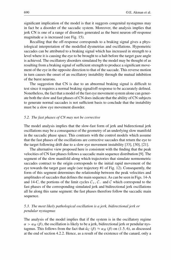
690 O.E. Akman et al.
significant implication of the model is that it suggests congenital nystagmus mayin fact be a disorder of the saccadic system. Moreover, the analysis implies thatjerk CN is one of a range of disorders generated as the burst neuron off-responsemagnitude α is increased (see Fig. 15).
Recalling that the off-response corresponds to a braking signal gives a phys-iological interpretation of the modelled dysmetrias and oscillations. Hypometricsaccades can be attributed to a braking signal which has increased in strength to alevel where it is causing the eye to be brought to a halt before the target gaze angleis achieved. The oscillatory disorders simulated by the model may be thought of asresulting from a braking signal of sufficient strength to produce a significant move-ment of the eye in the opposite direction to that of the saccade. This reverse motionin turn causes the onset of an oscillatory instability through the mutual inhibitionof the burst neurons.
The suggestion that CN is due to an abnormal braking signal is difficult totest since it requires a normal braking signal/off-response to be accurately defined.Nonetheless, the fact that a model of the fast eye movement system alone can gener-ate both the slow and fast phases of CN does indicate that the ability of CN subjectsto generate normal saccades is not sufficient basis to conclude that the instabilitymust be a slow eye movement disorder.
5.2. The fast phases of CN may not be corrective
The model analysis implies that the slow-fast form of jerk and bidirectional jerkoscillations may be a consequence of the geometry of an underlying slow manifoldin the saccadic phase space. This contrasts with the control models which assumethat the fast phases of the oscillations are corrective saccades that return the eye tothe target following drift due to a slow eye movement instability [33], [30], [21].
The alternative view proposed here is consistent with the finding that the peakvelocities of CN fast phases follows a saccadic main sequence distribution [9]. Thesegment of the slow manifold along which trajectories that simulate normometricsaccades contract to the origin corresponds to the initial rapid movement of theeye towards the target gaze angle (see trajectory #1 of Fig. 12). Consequently, theform of this segment determines the relationship between the peak velocities andamplitudes of saccades that defines the main sequence. As can be seen in Figs. 14-Aand 14-C, the portions of the limit cycles C+, C− and C which correspond to thefast phases of the corresponding simulated jerk and bidirectional jerk oscillationsall lie along this same segment: the fast phases therefore follow the saccadic mainsequence.
5.3. The most likely pathological oscillation is a jerk, bidirectional jerk orpendular nystagmus
The analysis of the model implies that if the system is in the oscillatory regimeα > αH (β), the oscillation is likely to be a jerk, bidirectional jerk or pendular nys-tagmus. This follows from the fact that αC (β) ≈ αH (β) on (1.5, 6), as discussedat the end of section 4.2.2. Hence, as a result of the existence of the canard, only a

A nonlinear dynamics model of the saccadic system 691
small increase in the braking signal strength α is required to push the system intothe range α > αC (β) in which the possible waveform types are those mentionedabove. The intermediate small-amplitude oscillation is unlikely to be observed (seeFig. 15).
This prediction is consistent with the findings of a recent major clinical eyemovement study [2]. Of the 161 CN subjects with a dominant waveform type usedin the study, all had oscillations with amplitude greater than 0.3 degrees: no sub-jects with sustained small-amplitude oscillations were reported. Moreover, 73% ofthe subjects exhibited jerk, bidirectional jerk, or pendular nystagmus oscillations,while 22% had oscillations which were variations on these basic waveforms, suchas pseudocycloid or pendular with foveating saccades.
5.4. Dynamic overshoot is caused by reversals of the saccadic control signal
It was argued in section 4.2.2 that increasing the burst neuron response time εcauses burst system trajectories to follow the slow manifold SM less closely as theyconverge to the origin. This results in oscillations of both the motor error signal mand the saccadic control signal b = r − l as they converge to 0 (see Fig. 12). Theseoscillations are converted by the muscle plant into a gaze signal g which oscillatesabout the desired gaze angle g (0)+�g, and thus simulates a dynamic overshoot(see Fig. 11-B).
The ability of the model to generate dynamic overshoots in the range α < +βis consistent with the observation that normal subjects can exhibit dynamic over-shoots in addition to normometric saccades. Moreover, the suggestion that theovershoots are attributable to oscillations of the saccadic control signal agrees withthe predictions of a psychophysical study of dynamic overshoots carried out byBahill et al [12]. Bahill et al proposed that the characterisation of the muscle plantas an overdamped harmonic oscillator implies that the reversals in eye directionobserved during dynamic overshoot are likely to be caused by reversals of the sacc-adic control signal. Furthermore, they suggested that a possible physiological causeof the reversals was post-inhibitory rebound firing of the burst neurons, possiblyaccentuated by movements of the centre of rotation of the eye during saccades [12].
The work presented here provides a simpler explanation for the reversals,namely the spiralling of trajectories around the origin in the burst neuron firing rateversus motor error phase plane, resulting from an increased burst neuron responsetime. The spiralling of trajectories is independent of the inhibition between the rightand left burst neurons, and can be reproduced by a simplified model which doesnot incorporate mutual inhibition terms in the equations for the burst neurons [7].
5.5. The evolution from jerk CN to bidirectional jerk CN is caused by a gluingbifurcation
If ε is increased in the (β, α) range 1.5 < β < 6, α > αC (β), the model simulatesthe transition from jerk nystagmus to bidirectional jerk and then pendular nystag-mus observed in some subjects as the initial gaze angle g (0) is varied, or their levelof attention is reduced [4], [5]. As ε corresponds to the speed at which the burst

692 O.E. Akman et al.
neurons respond to the motor error signal m, an increase in ε might be interpretedas a decrease in the attention level of the subject, and so the modelled waveformevolution is consistent with that observed experimentally when the attention levelis reduced. The evolution from jerk to bidirectional jerk that is seen in some sub-jects as the gaze angle passes close to the neutral zone ([8]) cannot, however, beaccounted for by the model in its current form, since g (0) is not a parameter of themodel. Additionally, the beat direction of the simulated jerk waveforms is depen-dent on the required gaze displacement �g instead of g (0). These observationssuggest incorporating g (0) explicitly in the equations. The analysis of the basicmodel presented here would provide the platform for a quantitative assessment ofthe effect of such a modification.
Despite these limitations, the model does propose a specific underlying mech-anism for the jerk to bidirectional jerk transition, namely the merging of a pair oflimit cycle attractors in a gluing bifurcation. This is a novel explanation for thequalitative change in the underlying neurobiological oscillator which could formthe basis of a new technique to control CN oscillations. A recent experimental studydemonstrated that a transient change from a unidirectional to a bidirectional jerkoscillation could be induced in a CN subject by forcing the target with a periodicwaveform [19]. The waveform used in this study was an unstable periodic orbitextracted from a previous recording of the subject’s eye movements using the tech-nique of So et al [38]. The gluing bifurcation mechanism suggested here impliesthe possibility of establishing more sophisticated control over the jerk oscillationby using periodic forcing so as to bring the system close to homoclinicity. Such atechnique could have clinical applications, as the increased foveation times shouldlead to the development of improved visual resolution.
Acknowledgements. The authors would like to thank Jerry Huke, Paul Glendinning andMark Muldoon for useful discussions. O. E. Akman was supported by a grant from theEngineering and Physical Sciences Research Council.
References
1. Abadi, R.V.: Mechanisms underlying nystagmus. J. R. Soc. Med. 95, 1–4 (2002)2. Abadi, R.V., Bjerre, A.: Motor and sensory characterisitics of infantile nystagmus.
Br. J. Ophthalmol. 86, 1152–1160 (2002)3. Abadi, R.V., Broomhead, D.S., Clement, R.A., Whittle, J.P., Worfolk, R.: Dynamical
systems analysis: A new method of analysing congenital nystagmus waveforms. Exp.Brain Res. 117, 355–361 (1997)
4. Abadi, R.V., Dickinson, C.M.: Waveform characteristics in congenital nystagmus. Doc.Ophthalmol. 64, 153–167 (1986)
5. Abadi, R.V., Dickinson, C.M., Pascal, E., Whittle, J., Worfolk, R.: Sensory and motoraspects of congenital nystagmus. In: Schmid, R., Zambarbieri, D. (eds.) OculomotorControl and Cognitive Processes, Elsevier Science Publishers B.V. (North-Holland),1991, pp. 249–262
6. Abadi, R.V., Sandikcioglu, M.: Visual resolution in congenital pendular nystagmus.Am. J. Optom. Phys. Opt. 52, 573–581 (1975)

A nonlinear dynamics model of the saccadic system 693
7. Abadi, R.V., Scallan, C.J., Clement, R.A.: The characteristics of dynamic overshootsin square-wave-jerks and in congenital and manifest latent nystagmus. Vision Res. 40,2813–2829 (2000)
8. Abadi, R.V., Whittle, J.: The nature of head postures in congenital nystagmus. Arch.Ophthalmol. 109, 216–220 (1991)
9. Abadi, R.V., Worfolk, R.: Retinal slip velocities in congenital nystagmus. Vision Res.29 (2), 195–205 (1989)
10. Akman, O.E.: Analysis of a nonlinear dynamics model of the saccadic system. Ph.D.thesis, Department of Mathematics, University of Manchester Institute of Science andTechnology, 2003
11. Arrowsmith, D.K., Place, C.M.: An Introduction to Dynamical Systems. CUP, 199012. Bahill, A.T., Clark, M.R., Stark, L.: Dynamic overshoot in saccadic eye movements is
caused by neurological control signal reversals. Exp. Neurol. 38, 107–122 (1975)13. Bahill, A.T., Clark, M.R., Stark, L.: The main sequence, a tool for studying human eye
movements. Math. Biosci. 24, 191–204 (1975)14. Becker, W., Jurgens, R.: An analysis of the saccadic system by means of double step
stimuli. Vision Res. 19, 967–983 (1979)15. Becker, W., Klein, H.M.: Accuracy of saccadic eye movements and maintenance of
eccentric eye positions in the dark. Vision Res. 13, 1021–1034 (1973)16. Bedell, H.E., Loshin, D.S.: Interrelations between measures of visul acuity and param-
eters of eye movement in congenital nystagmus. Invest. Ophth. Vis. Sci. 32, 416–421(1991)
17. Boghen, D., Troost, B.T., Daroff, R.B., Dell’Osso, L.F., Birkett, J.E.: Velocity charac-teristics of human saccades. Invest. Ophth. Vis. Sci. 13 (8), 619–623 (1974)
18. Broomhead, D.S., Clement, R.A., Muldoon, M.R., Whittle, J.P., Scallan, C.,Abadi, R.V.:Modelling of congenital nystagmus waveforms produced by saccadic system abnormal-ities. Biol. Cybern. 82, 391–399 (2000)
19. Clement, R.A., Abadi, R.V., Broomhead, D.S., Whittle, J.P.: Periodic forcing of congen-ital nystagmus. In: Boccaletti, S., Gluckman, B.J., Kurths, J., Pecora, L.M., Spano M.L.(eds.) Experimental Chaos (Proceedings of the 6th Experimental Chaos Conference,Potsdam, Germany, 2001). AIP, 2002
20. Clement, R.A., Whittle, J.P., Muldoon, M.R., Abadi, R.V., Broomhead, D.S., Akman,O.: Characterisation of congenital nystagmus waveforms in terms of periodic orbits.Vision Res. 42, 2123–2130 (2002)
21. Dell’Osso, L.F.: Nystagmus basics: Normal models that simulate dysfunction. In: Hung,G.K., Ciuffreda, K.J. (eds.) Models of the Visual System. Kluwer Academic, 2002,pp. 711–739
22. Dell’Osso, L.F., Daroff, M.D.: Congenital nystagmus waveforms and foveation strategy.Doc. Ophthalmol. 39, 155–182 (1975)
23. Ditchburn, R.W.: Eye Movements andVisual Perception. Clarendon Press, Oxford, 197324. Enderle, J.D.: Neural control of saccades. In: Hyona, J., Munoz, D.P., Heide, W., Rad-
ach, R. (eds.), The Brain’s Eye: Neurobiological and Clinical Aspects of OculomotorResearch, vol. 140, Elsevier, Amsterdam, 2002, pp. 21–49
25. Gancarz, G., Grossberg, G.: A neural model of the saccade generator in the reticularformation. Neural Networks 11, 1159–1174 (1998)
26. Glendinning, P.: Global bifurcations in flows. In: Bedford, T., Swift, J. (eds.), NewDirections in Dynamical Systems. CUP, 1988, pp. 120–149
27. Golubitsky, M.: Singularities and Groups in Bifurcation Theory. Springer Verlag, 198528. Guckenheimer, J., Hoffman, K., Weckesser, W.: Numerical computation of canards. Int.
J. Bifurcat. Chaos 10 (12), 2669–2687 (2000)

694 O.E. Akman et al.
29. Guckenheimer, J., Holmes, P.: Nonlinear Oscillations, Dynamical Systems and Bifur-cations of Vector Fields. Springer Verlag, 1983
30. Harris, C.M.: Problems in modelling congenital nystagmus: Towards a new model.In: Findlay, J.M., Walker, R., Kentridge, R.W. (eds.) Eye Movement Research: Mecha-nisms, Processes and Applications, Elsevier, Amsterdam 1995, pp. 239–253
31. Hirsch, M.W., Smale, S.: Differential Equations, Dynamical Systems and Linear Alge-bra. Academic Press, 1974
32. Kreyszig, E.: Advanced Engineering Mathematics, 7th edn. John Wiley, 199333. Optican, L.M., Zee, D.S.: A hypothetical explanation of congenital nystagmus. Biol.
Cybern. 50, 119–134 (1984)34. Robinson, D.A.: The mechanics of human saccadic eye movements. J. Physiol. 174,
245–264 (1964)35. Robinson, D.A.: Models of the saccadic eye movement control system. Kybernetik 14,
71–83 (1973)36. Scudder, C.A.: A new local feedback model of the saccadic burst generator. J. Neuro-
physiol. 59, 1455–1475 (1988)37. Shelhamer, M.: On the correlation dimension of optokinetic nystagmus eye movements:
Computational parameters, filtering, nonstationarity and surrogate data. Biol. Cybern.76, 237–250 (1997)
38. So, P., Ott, E., Sauer, T., Gluckman, B.J., Grebogi, C., Schiff, S.: Extracting unstableperiodic orbits from chaotic time series data. Phys. Rev. E 55, 5398–5417 (1997)
39. Sparks, D.L.: The brainstem control of saccadic eye movements. Nature Rev. Neurosci.3, 952–964 (2002)
40. Stark, J.: Invariant graphs for forced systems. Physica D 109, 163–179 (1997)41. Tusa, R.J., Zee, D.S., Hain, T.C., Simonsz, H.J.: Voluntary control of congenital nys-
tagmus. Clin. Vision Sci. 7, 195–210 (1992)42. Van Gisbergen, J.A.M., Robinson, D.A., Gielen, S.:A quantitative analysis of generation
of saccadic eye movements by burst neurons. J. Neurophysiol. 45, 417–442 (1981)43. Westheimer, G.: Mechanism of saccadic eye movements. Arch. Ophthalmol. 52, 710–
724 (1954)44. Westheimer, G., McKee, S.P.: Visual acuity in the presence of retinal image motion.
J. Opt. Soc. Am. 65, 847–850 (1975)45. Worfolk, R., Abadi, R.V.: Quick phase programming and saccadic re-orientation in
congenital nystagmus. Vision Res. 31 (10), 1819–1830 (1991)46. Zeeman, E.C.: Differential equations for the heartbeat and nerve impulse. In: Wadd-
ington, C.H. (ed.), Towards a Theoretical Biology, University Press, Edinburgh, 1972,pp. 8–67