Embed Size (px)
Citation preview

Simulation of electronic states in ananowire field-effect transistor
A PhD thesis
by
José María Castelo Ares
directed by
Prof. Dr. Klaus Michael Indlekofer
and tutored by
Dr. Alberto García Cristóbal
Departamento de Física Aplicada
Universidad de Valencia
2015


This thesis took place at the Hochschule RheinMain (University of
Applied Sciences) in Rüsselsheim (Germany) during the period
2011–2014
within the framework of Nanowiring:
European Marie Curie Initial Training Network


Abstract
Nanowires are emerging as promising candidates to form the basis of field-effect
transistors, among other devices. Nanowire-based field-effect transistors are fore-
seen to be industrially standardized in the near future. Simulations are important
in order to assess their performance. The multi-configurational self-consistent
Green’s function simulation method is able to correctly describe non-equilibrium
electronic transport while at the same time accounts for few-electron Coulomb
charging effects in such devices. Based on the non-equilibrium Green’s function
formalism, this method is augmented and implemented in a software package
named NWFET-Lab. This package forms the basis of the calculations performed
in this dissertation.
An adaptive numerical method to determine the non-equilibrium many-body
statistical operator for quasi-isolated electronic states within the channel of a
realistic nanowire field-effect transistor is presented. The statistical operator
must satisfy a set of constraints related to the single-particle density matrix.
Since the problem is under-determined in general, a form for its eigenvalues or
weights that maximizes the entropy is required. Two eigenbases for the statistical
operator are considered: (A) the set of all relevant Slater determinants of natural
orbitals and (B) the eigenstates of the many-body Hamiltonian projected to the
relevant Fock subspace. As an application, the onset of formation of Wigner
molecules is addressed with the help of the density–density covariance.
A new numerical determination of the correlation of the system of electrons
within the nanowire channel of the device, for pure as well as for mixed states,
is presented. In contrast to the single-particle-reduced entropy, this so-called
“modified correlation entropy” accounts for the correlation independently of the
mixture degree, as measured by the von Neumann entropy, of the many-body
state. For its determination a genetic algorithm optimization method is employed.
An analysis of these three concepts of entropy is performed.
v


Resumen
De acuerdo con la ley empírica de Moore, el número de transistores en un circuito
integrado se ve duplicado aproximadamente cada dos años. Una vez traspasada
la frontera hacia la escala nanométrica, estos dispositivos comienzan a padecer
efectos adversos al funcionamiento deseable de un transistor, como la pérdida
de integridad eléctrica, efectos debidos a la corta longitud del canal o la falta
de reproducibilidad. Las nanoestructuras cristalinas semiconductoras conocidas
como nanohilos están emergiendo como candidatos prometedores para formar una
nueva base alternativa de los transistores de efecto campo y continuar la minia-
turización tecnológica en la escala nanométrica. Esto es debido al gran control
electrostático de la puerta sobre el canal, constituido en estos dispositivos por un
nanohilo, que los transistores de efecto campo basados en nanohilos demuestran
a esta escala. Como beneficios adicionales del empleo de nanohilos para la con-
strucción de estos dispositivos cabe mencionar la posibilidad de ser producidos en
grandes cantidades en un solo proceso usando técnicas de crecimiento asequibles.
Estas nanoestructuras presentan propiedades electrónicas reproducibles debido al
control preciso del proceso de crecimiento, así como una alta movilidad de los
portadores de carga consecuencia de su estructura monocristalina y su reducción
de la dispersión. Junto a significativos avances experimentales, su estudio teórico
está resultando de importancia para evaluar sus características y rendimiento.
Los dispositivos nanométricos están gobernados por las leyes de la mecánica
cuántica, por lo que un método de simulación apropiado para su estudio debería
ser capaz de describir efectos cuánticos como el confinamiento, las resonancias,
la dispersión o el efecto tunel de los electrones en su interior. El número de
electrones involucrados en el funcionamiento de transistores con canales de una
longitud tan grande como 100 nm es del orden de 1 − 10. Por tanto, efectos
debidos a la presencia individual de electrones son relevantes en estos dispositivos,
de modo que una descripción de muchos cuerpos (basada en el espacio de Fock)
de la interacción de Coulomb es necesaria para una simulación realista. Por un
vii

viii Resumen
lado, un enfoque que considere el espacio de Fock completo del sistema es capaz
de describir correctamente estos efectos, pero ve limitada su aplicación efectiva a
dispositivos pequeños, debido a que la dimensión del espacio de Fock aumenta ex-
ponencialmente con el número de estados de una partícula (por ejemplo orbitales
localizados). Por otro lado, una descripción de campo medio para modelizar la
interacción de Coulomb es viable computacionalmente pero incapaz de describir
efectos debidos a la presencia individual de electrones, a causa de la aproximación
que esta descripción realiza de tal interacción como efecto promediado que tiene
sobre un electron el resto de electrones.
La base teórica del trabajo presentado en esta tesis doctoral está fundamen-
tada en el método multiconfiguracional autoconsistente basado en funciones de
Green, originalmente presentado por Indlekofer et al. Este método está basado
en el formalismo de funciones de Green fuera del equilibrio y como es habitual en
este formalismo, se hace uso de una descripción de campo medio para modelizar
la interacción de Coulomb. Sin embargo, el método limita este tipo de descrip-
ción para aquellos estados que no son relevantes para el transporte electrónico,
haciendo uso de una descripción de muchos cuerpos (basada en un subespacio
de Fock relevante) para los que sí son relevantes. Estados de una partícula rel-
evantes son identificados como aquellos orbitales naturales (autoestados de la
matriz densidad de una partícula ρ1) que presentan fluctuación en su número de
ocupación (autovalores de ρ1) y que no se encuentran fuertemente acoplados a
los contactos del transistor, centrándose en estados atrapados resonantemente
en el interior del nanohilo. El número de estados relevantes Nrel es habitualmente
muy inferior al número total de estados del sistema, la dimensión del subespacio
de Fock generado por los estados relevantes no es muy alta y una descripción de
muchos cuerpos dentro de este subespacio resulta ser asequible.
Uno de los objetivos de la presente tesis doctoral es el desarrollo de una her-
ramienta informática de simulación para el estudio de las propiedades de trans-
porte electrónico en transistores de efecto campo basados en nanohilos. El pa-
quete de programas se conoce como NWFET-Lab e incluye tres módulos inter-
relacionados. El primero de ellos tiene la función de preparar los parámetros del
sistema. El segundo consiste en el módulo de cálculo, fundamentado en el método
multiconfiguracional autoconsistente basado en las funciones de Green, sucinta-
mente descrito en el párrafo anterior. Este algoritmo original ha sido extendido

Resumen ix
para incluir una mayor variedad de observables físicos y magnitudes relevantes
para entender el comportamiento y características de un transistor basado en un
nanohilo, así como los cálculos que a continuación se describen. El tercero y úl-
timo de los módulos permite la visualización de los resultados obtenidos mediante
el módulo de cálculo.
También se ha desarrollado un método numérico para la determinación del op-
erador estadístico de muchos cuerpos fuera del equilibrio ρrel para el sistema de
electrones atrapados resonantemente en el interior del nanohilo del transistor.
La importancia de conocer el operador estadístico radica en que permite obtener
valores esperados de observables de muchos cuerpos del sistema, así como la en-
tropía de von Neumann. Este operador debe satisfacer ciertas restricciones dadas
por la matriz densidad de una partícula ρ1. Estas condiciones no son suficientes en
general para su determinación unívoca, por lo que se ha escogido una forma fun-
cional de los autovalores de ρrel que maximice la entropía, conocida como forma
gran-canónica o de Boltzmann. En esta forma funcional aparecen los potenciales
electroquímicos asociados a los orbitales naturales relevantes, que se convierten
en cantidades independientes si el sistema se encuentra fuera del equilibrio y se
consideran como variables de optimizacion libres que ajustar para que los auto-
valores cumplan las restricciones impuestas por ρ1. Como autoestados de ρrel se
consideran dos bases alternativas: (A) determinantes de Slater de orbitales nat-
urales relevantes y (B) la base del Hamiltoniano de muchos cuerpos proyectado
al subespacio de Fock relevante. A modo de aplicación, se ilustra la transición
desde un régimen del sistema de electrones en el canal del transistor denominado
“atómico” en el que la energía de Coulomb es relativamente pequeña, hasta un
régimen denominado “Wigner” en el que esta energía es mayor, favoreciendo la
separacion entre electrones y la consiguiente formación de moléculas de Wigner.
Finalmente se presenta una medida numérica de la correlación del sistema de
electrones, que cuantifica únicamente su correlación tanto si la preparación del
sistema es pura como si es una mezcla, en contraste con la entropía reducida de
una partícula S1 que también depende del grado de mezcla y por tanto sólo puede
cuantificar la correlación de estados puros. Esta medida numérica, denominada
entropía de correlación modificada ∆S ≡ S − S se basa en la entropía de von
Neumann S, cuyo cálculo depende del operador estadístico de muchos cuerpos
fuera del equilibrio ρrel del sistema. Asimismo, S es la entropía de von Neumann

x Resumen
obtenida mediante de un operador estadístico ρrel que se asemeja óptimamente
a ρrel pero cuya base de estados de muchos cuerpos consiste únicamente en de-
terminantes de Slater construidos a partir de una base ortonormal optimizada de
estados de una partícula, obtenida de tal manera que S sea minimizada. Esta
base se encuentra relacionada con la base de orbitales naturales mediante una
transformación unitaria U con Nrel ×Nrel elementos. El proceso de minimizacion
se lleva a cabo mediante un algoritmo genético cuyas variables de optimización
son los Nrel × Nrel ángulos mediante los cuales es posible parametrizar U. Como
resultado, se presenta un análisis de estos tres tipos de entropía (S1, S y ∆S) y
se muestra que efectivamente ∆S cuantifica la correlación electrónica independi-
entemente del grado de mezcla.

Acknowledgement
I am grateful to my supervisor Klaus Michael Indlekofer, who treated me from
the beginning with friendliness and helped me whenever I needed it. I would also
like to thank my tutor Alberto García Cristóbal as well as all the people I got to
know during these three years both in Rüsselsheim and in Valencia. Special thanks
go to all the organizers of the Nanowiring network for giving all its members a
valuable framework within which our careers, scientific skills and knowledge had
the opportunity to develop. Thanks to all the fellows of the network for the good
moments we shared and to the European Comission for financial support.
xi


Contents
Abstract v
Resumen vii
Acknowledgement xi
1. Introduction 11.1. The nanowire field-effect transistor . . . . . . . . . . . . . . . . . 1
1.2. Ultimately scaled device simulation . . . . . . . . . . . . . . . . . 5
1.3. Structure of the dissertation . . . . . . . . . . . . . . . . . . . . 6
2. Introduction to the non-equilibrium Green’s function formalism 92.1. Quantum field operators . . . . . . . . . . . . . . . . . . . . . . 9
2.2. Hamiltonian in second quantization . . . . . . . . . . . . . . . . . 10
2.3. Green’s functions . . . . . . . . . . . . . . . . . . . . . . . . . . 11
2.4. Contour-ordered Green’s function . . . . . . . . . . . . . . . . . 15
2.5. Equations of motion for the Green’s functions . . . . . . . . . . . 18
2.6. Non-equilibrium perturbation theory . . . . . . . . . . . . . . . . 19
2.7. Dyson equation . . . . . . . . . . . . . . . . . . . . . . . . . . . 20
2.8. Hartree-Fock approximation of the self-energy . . . . . . . . . . . 21
2.9. NEGF schemes . . . . . . . . . . . . . . . . . . . . . . . . . . . 23
3. Multi-configurational self-consistent Green’s function method 273.1. Introduction . . . . . . . . . . . . . . . . . . . . . . . . . . . . . 27
3.2. The system . . . . . . . . . . . . . . . . . . . . . . . . . . . . . 28
3.3. Theoretical elements of the method . . . . . . . . . . . . . . . . 28
3.3.1. Coulomb Green’s function . . . . . . . . . . . . . . . . . 29
3.3.2. Localized single-particle basis . . . . . . . . . . . . . . . . 30
3.3.3. Hamiltonian . . . . . . . . . . . . . . . . . . . . . . . . . 30
xiii

xiv Contents
3.3.4. Single-particle density matrix and natural orbital basis . . 31
3.3.5. NEGF description . . . . . . . . . . . . . . . . . . . . . . 32
3.4. The MCSCG method: fundamental features . . . . . . . . . . . . 33
3.4.1. Relevant states and relevant Fock subspace . . . . . . . . 33
3.4.2. Statistical operator . . . . . . . . . . . . . . . . . . . . . 35
3.4.3. Mean-field interaction . . . . . . . . . . . . . . . . . . . 36
3.4.4. Determination of the weigths . . . . . . . . . . . . . . . 36
3.4.5. Self-consistency algorithm . . . . . . . . . . . . . . . . . 37
3.5. Software implementation . . . . . . . . . . . . . . . . . . . . . . 37
3.6. Limit of the 1D approximation . . . . . . . . . . . . . . . . . . . 38
3.7. Results: Coulomb blockade regime . . . . . . . . . . . . . . . . . 41
4. Numerical determination of the non-equilibrium many-body statisti-cal operator 554.1. Introduction . . . . . . . . . . . . . . . . . . . . . . . . . . . . . 55
4.2. Preliminary theoretical considerations . . . . . . . . . . . . . . . 56
4.2.1. Relevant Fock space revisited . . . . . . . . . . . . . . . 56
4.2.2. Mean-field interaction revisited . . . . . . . . . . . . . . . 57
4.2.3. Change to natural orbital basis . . . . . . . . . . . . . . . 58
4.2.4. Projected many-body Hamiltonian . . . . . . . . . . . . . 59
4.2.5. Diagonalization of the projected many-body Hamiltonian . 59
4.3. Many-body statistical operator . . . . . . . . . . . . . . . . . . . 60
4.3.1. On the statistical preparation of the system . . . . . . . . 60
4.3.2. Single-particle density matrix constraint . . . . . . . . . . 61
4.3.3. Average energy constraint . . . . . . . . . . . . . . . . . 63
4.3.4. Case A: Slater determinant basis of natural orbitals . . . . 63
4.3.5. Case B: eigenbasis of the projected many-body Hamiltonian 64
4.4. Maximum entropy . . . . . . . . . . . . . . . . . . . . . . . . . . 65
4.4.1. Entropy maximization with Lagrange multipliers . . . . . . 65
4.4.2. Infinite temperature limit . . . . . . . . . . . . . . . . . . 67
4.5. Numerical determination of the weights . . . . . . . . . . . . . . 69
4.5.1. Newton-Raphson method . . . . . . . . . . . . . . . . . . 69
4.5.2. Optimization by genetic algorithm . . . . . . . . . . . . . 71
4.6. Expectation values . . . . . . . . . . . . . . . . . . . . . . . . . 71

Contents xv
4.7. Electron density and covariance . . . . . . . . . . . . . . . . . . 72
4.7.1. Physical meaning . . . . . . . . . . . . . . . . . . . . . . 72
4.7.2. Case A: diagonal elements . . . . . . . . . . . . . . . . . 74
4.7.3. Case B: full matrix . . . . . . . . . . . . . . . . . . . . . 75
4.8. Results: onset of formation of Wigner molecules . . . . . . . . . 76
4.8.1. Energy estimations . . . . . . . . . . . . . . . . . . . . . 76
4.8.2. System parameters and approach . . . . . . . . . . . . . 78
4.8.3. Resulting statistical operator . . . . . . . . . . . . . . . . 79
4.8.4. Natural orbitals . . . . . . . . . . . . . . . . . . . . . . . 79
4.8.5. Total electron density . . . . . . . . . . . . . . . . . . . . 81
4.8.6. Density–density correlation . . . . . . . . . . . . . . . . . 83
5. Correlation entropy 895.1. Introduction . . . . . . . . . . . . . . . . . . . . . . . . . . . . . 89
5.2. Single-particle-reduced entropy . . . . . . . . . . . . . . . . . . . 90
5.3. von Neumann entropy . . . . . . . . . . . . . . . . . . . . . . . . 94
5.4. Modified correlation entropy . . . . . . . . . . . . . . . . . . . . 94
5.5. Single-particle basis unitary transformation . . . . . . . . . . . . . 96
5.6. Determination of the many-body basis unitary transformation . . 96
5.6.1. Method 1 . . . . . . . . . . . . . . . . . . . . . . . . . . 97
5.6.2. Method 2 . . . . . . . . . . . . . . . . . . . . . . . . . . 98
5.6.3. Numerical performance of both methods . . . . . . . . . 101
5.7. Determination of unitary transformation of single-particle basis . . 103
5.8. Identification of a truly correlated state . . . . . . . . . . . . . . 104
5.9. Results . . . . . . . . . . . . . . . . . . . . . . . . . . . . . . . . 105
6. Summary 111
Appendices 113
A. NWFET-Lab: Simulation package 115A.1. Overview . . . . . . . . . . . . . . . . . . . . . . . . . . . . . . . 115
A.2. Structure . . . . . . . . . . . . . . . . . . . . . . . . . . . . . . 116
A.2.1. Task manager . . . . . . . . . . . . . . . . . . . . . . . . 116
A.2.2. Setup module . . . . . . . . . . . . . . . . . . . . . . . . 117
A.2.3. Calculation module . . . . . . . . . . . . . . . . . . . . . 117

xvi Contents
A.2.4. Graphical module . . . . . . . . . . . . . . . . . . . . . . 120
A.3. Technical details . . . . . . . . . . . . . . . . . . . . . . . . . . . 122
A.3.1. Libraries and APIs . . . . . . . . . . . . . . . . . . . . . 122
A.3.2. Parameters . . . . . . . . . . . . . . . . . . . . . . . . . 123
B. Genetic algorithm 127B.1. Overview . . . . . . . . . . . . . . . . . . . . . . . . . . . . . . . 127
B.2. Chang’s genetic algorithm . . . . . . . . . . . . . . . . . . . . . 129
C. Parametrization of unitary matrices 131
References 135

1. Introduction
1.1. The nanowire field-effect transistor
In this introductory chapter, we briefly address the problem of the downscaling
of field-effect transistors (FETs), point out a candidate solution for this problem,
see why this solution is promising and outline an overview of the devices this
solution has enabled so far.
Since the invention of the integrated circuit (IC) in 1958 and the creation
of the metal-oxide-semiconductor field-effect transistor (MOSFET) [1] in 1959,
technology has followed a miniaturization trend expressed by Moore’s law: the
number of transistors on ICs doubles approximately every two years [2, 3]. This
law, initially considered as a forecast, was later adopted as a target that has
driven the industry up until the present.
The answer to the question of whether nanotechnology will be able to con-
tinue fulfilling Moore’s law, despite the several difficulties [4, 5] that emerge as
the channel length of MOSFETs gets smaller, depends on whether electrical in-
tegrity, no short-channel effects, low power consumption, low leakage currents
and reproducibility can be maintained in ever downscaled devices. In this sense,
replacement of old materials with new nanostructures may give an affirmative
answer to that question.
The International Technology Roadmap for Semiconductors (ITRS) is a ref-
erence for the near and far future of semiconductor technology. As stated in
the 2013 edition report [6], one of the main goals of the ITRS is identifying key
technical requirements critical to sustain the historical scaling of semiconductor
technology (Moore’s law). In the same report one finds reference to major tech-
nological innovations, including new structures such as gate-all-around nanowires
as next natural evolution for digital logic applications for the near term (2013-
2020) and nanowire MOSFETs to below 10 nm gate length for the long term
1
2 Chapter 1. Introduction
(2021-2028). The report emphasizes the importance of understanding, modeling
and implementation into manufacturing of these innovations.
Therefore, promising candidates for new electronics building blocks are semi-
conductor nanowires [7, 8, 9, 10]. Employing either a top-down or a bottom-up
approach [11], these nanostructures are nowadays synthesized in a rational and
controllable way, enabling the possibility to create axial and radial heterostruc-
tures and select the doping by addition of impurities. Due to their unique physical,
chemical and electronic properties, nanowires find application in electronics [12,
13, 14, 15], optoelectronics [16], photovoltaics [17, 18], sensing [19] and biology
[20, 21, 22].
Key to this dissertation is the nanowire field-effect transistor (NWFET) [23].
Similarly to a planar MOSFET, a NWFET is an active unipolar electronic device
consisting of a channel, an insulator and gate, source and drain contacts. A
basic difference between these types of devices, though, is that the channel of a
NWFET is made of a single semiconductor nanowire, through which the electric
carriers flow. On the other hand, the principles of operation do not differ between
NWFETs and planar MOSFETs. Current is due to a bias voltage VDS between
the drain contact and the source contact, both contacts located at the extremes
of the nanowire. The gate is a metallic electrode that modulates the electrostatic
potential inside the channel and therefore influences the current via a gate–source
voltage VGS. There are two main gate geometries: planar and coaxial. A planar
gate consists of a two-dimensional (2D) electrode positioned at the back, top
or one side of the nanowire, while a coaxial or wrap gate is built all around the
nanowire. It is isolated from the channel by an oxide insulator so that electrons
are unable to flow out of the channel towards the gate.
The source and drain contacts can be ohmic or Schottky. Ohmic contacts
consist of the two extremes of the intrinsic nanowire being heavily doped. Schot-
tky contacts on the other hand, are made by metal deposited on the extremes
of the nanowire, forming Schottky-barriers [24, 25] that the electrons in the
source have to surpass or tunnel in order to contribute to the current. The de-
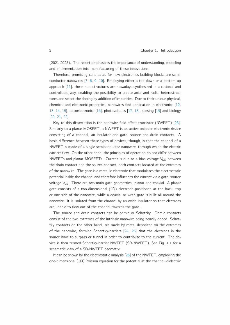
vice is then termed Schottky-barrier NWFET (SB-NWFET). See Fig. 1.1 for a
schematic view of a SB-NWFET geometry.
It can be shown by the electrostatic analysis [26] of the NWFET, employing the
one-dimensional (1D) Poisson equation for the potential at the channel–dielectric
1.1. The nanowire field-effect transistor 3
Figure 1.1.: Schematic view of a SB-NWFET.
interface Φ(x), that the relevant length scale for potential variations is given by
the screening length λ, which appears both in the 1D Poisson equation and in its
solution for point charge density Φ(x) ∝ exp(−|x |/λ).
For a coaxial gate geometry as shown in Fig. 1.1 the screening length λ is given
by [27]
λ2 =εch
εox
d2ch
8ln
(1 + 2
dox
dch
)(1.1)
where dch is the nanowire diameter, dox is the oxide thickness, εch and εox are the
channel and oxide relative dielectric constants respectively.
In order to avoid the appearance of short-channel effects [5] when scaling
down the channel length, λ has to be scaled accordingly in order to maintain
the relation L λ, which implies that the nanowire diameter dch and the oxide
thickness dox must be scaled down. In this respect, nanowires are ideally suited
for ultimately scaled FET devices, because of their one dimensional shape with a
scalable diameter into the few nanometer range.
As additional benefits of employing nanowires for FET construction it is worth
mentioning the possibility to be produced in large quantities in a single process,
using bottom-up growth techniques that are cost-effective. They present repro-
ducible electronic properties due to the precise control of the growth process.
They also display high carrier mobility due to reduction of scattering because
of their monocrystalline structure. Moreover, vertical integration of NWFETs
in densely packed ICs is now possible, which is a necessity for their large-scale
manufacturability.

4 Chapter 1. Introduction
Figure 1.2.: Number of publications per year which include the keywords “nanowiretransistor” or “nanowire field effect transistor” or “NWFET” in their contents, as obtainedfrom Elsevier’s database Scopus (http://www.scopus.com/). Note that the latest yearsdo not include all the publications, only those available to the database at the moment.
Starting from the year 2000, the number of publications related to NWFET
fabrication is growing, a fact that shows the interest and impact this subject is
having since then. One can see this tendency in Fig. 1.2. In the year 2000,
vanadium pentoxide V2O5 nanofiber-based FETs were reported [28]. The fol-
lowing year, NWFETs were demonstrated based on single-crystal InP nanowires,
up to tens of micrometers long [29]. Radial nanowire heterostructures have also
been employed as NWFETs, such as Ge/Si core/shell nanowires with a top-gate
geometry, which showed improved p-type FET behavior [30]. Motivated by the
consideration that current flowing in the on-state of NWFETs may be low due
to the small diameter of the nanowire channel, a recent work proposes a massive
parallel dense vertical nanowire array architecture for high performance FET [14].
Vertical integration [31, 32] is able to achieve a much higher density of nanowires
than horizontal integration [33] and allows three-dimensional (3D) integration
for complex structures. It is worth mentioning that programmable nanowire cir-
cuit modules have also been designed that use arrays of non-volatile multi-gate

1.2. Ultimately scaled device simulation 5
NWFETs to operate as scalable nanoprocessors that perform simple logic func-
tions [13]. As a step forward, a nanowire-based 2-bit 4-state finite-state machine
has been implemented which is able to maintain its internal state, modify this
state in response to external signals and output commands on that basis [15].
To summarize, as MOSFETs size enters into the nanometer scale, these de-
vices begin to be prone to several effects that impede their proper functioning
and a classical description of their physics begins to be inadequate. Promising
candidates to become new building blocks for electronic devices are nanowires,
which find application beyond the field of electronics. The NWFET in particular
is expected to play an important role in the future, due to its superior electro-
static control of the channel by the gate in the nanoscale. Many advances in the
experimental realization of nanowire-based devices have been reported, as well as
important progresses in their simulation, where quantum and Coulomb effects in
the nanoscale play a relevant role.
1.2. Ultimately scaled device simulation
Some of the challenges semiconductor technology will face in the near future
in relation to nanowire-based devices, according to the ITRS 2013 [6], are the
stochastic variation of dopants and thickness from device to device, the effects of
the channel surface roughness on carrier transport and reliability, and controlling
the source/drain series resistance within tolerable limits, since due to the increase
of current density, lower resistance with smaller device dimensions is a challenging
necessity. Simulation of NWFETs is therefore necessary to accurately predict the
device performance and to understand its physics.
Nanoscale devices are governed by the laws of quantum mechanics, due to their
small size in the nanometer scale. Therefore, a successful simulation method
should be able to describe quantum effects, such as carrier confinement, reso-
nances, scattering or tunneling. Furthermore, few-electron charging effects are of
relevance in such devices, so a many-body description of the Coulomb interaction
between electrons is necessary for a realistic simulation of NWFETs.
Present work on the simulation of these challenges usually focuses on a par-
ticular aspect of the problem and excludes the rest, whenever this restriction is
justified by the features of the considered problem. So one can find in the lit-

6 Chapter 1. Introduction
erature simulations of the electronic transport characteristics for non-interacting
electrons, in the presence of electron–electron or electron–phonon interaction.
Quantum mechanical formalisms employed for the modeling of electronic trans-
port in nanodevices, based on Schrödinger equation [34, 35], Wigner function [36],
Liouville [37] and Pauli [38] master equations or Green’s functions [39] have been
reported.
Key to this dissertation is the non-equilibrium Green’s function (NEGF) formal-
ism [40, 41, 42, 43, 44], which allows for a quantum mechanical description of
non-equilibrium electronic transport in ultimately scaled devices. This formalism
may include the effects of the device contacts (reservoirs) and the relevant inter-
actions (electron–electron and electron–phonon). Coulomb interaction, whenever
it is considered, is usually modeled in a mean-field way, which has the advantage
of being computationally light-weight and the disadvantage of being unable to
describe few-electron charging effects. On the other hand, a full many-body de-
scription of this interaction is able to account for these effects at the expense of
considering only small devices, as described by a suitable basis of single-particle
states (localized spin/site orbitals, for example), since the corresponding Fock
space dimension grows exponentially with the number of single-particle states,
making simulation of realistic devices unfeasible.
As an hybrid approach that shares both the benefits of the mean-field and
many-body descriptions, the multi-configurational self-consistent Green’s func-
tion (MCSCG) method [45, 46] can correctly describe few-electron charging ef-
fects in a non-equilibrium NWFET. This method is the theoretical basis for the
calculations and results obtained in this dissertation.
1.3. Structure of the dissertation
The basic formalism employed in this dissertation for the description of non-
equilibrium NWFETs is the NEGF method. A theoretical introduction to NEGF is
given in Chapter 2, where recent work concerning the simulation and understand-
ing of the important challenges NWFETs face today is also described. Chapter 3
presents a description of the NEGF-based MCSCG method, which is the algo-
rithm employed in the following calculations. The implementation of the MCSCG
method in a software package is highlighted and several results (in the Coulomb

1.3. Structure of the dissertation 7
blockade regime) obtained by means of this implementation are presented. In
Chapter 4 a numerical method to determine the non-equilibrium many-body sta-
tistical operator that describes the statistical preparation of the electrons within
the NWFET channel is presented. The statistical operator is required to satisfy
a set of constraints and its expression is furthermore determined by assuming
its probability distribution maximizes the entropy. Once obtained, expectation
values of many-body observables can be calculated. As an application, the onset
of formation of Wigner molecules by the electrons within the nanowire channel
is addressed. In Chapter 5 we study the correlation entropy of the electronic
system. Three different definitions of entropy are analyzed and their significance
(whether they account for mixture, correlation or both) is investigated. To con-
clude, a summary about the presented work and possible future ways to extend
it is outlined in Chapter 6.
The appendices provide additional information. Appendix A, in particular, con-
tains a description of NWFET-Lab, the open-source software package devel-
oped as a tool to simulate non-equilibrium electronic transport in NWFETs. It
implements and extends the MCSCG algorithm, and provides all the calculations
included in this dissertation.


2. Introduction to thenon-equilibrium Green’s functionformalism
2.1. Quantum field operators
The many-body quantum description of a system of Fermions known as second
quantization, relies on some mathematical objects known as the creation and
annihilation operators [47, 44], expressed as c†k and ck , corresponding to a state
k of a discrete orthonormal single-particle basis. Operators in the Fock space can
be represented in terms of them, in their so-called second quantized form. c†k and
ck act on a many-body state by creating or annihilating, respectively, a particle on
a given single-particle state k . In the occupation number representation, where
the state of the system is described by a vector |b0b1 . . . bk . . .〉 with bk ∈ 0, 1,this can be expressed as [48]
ck |. . . bk . . .〉 = (−1)Sk δbk ,1 |. . . bk − 1 . . .〉 (2.1a)
c†k |. . . bk . . .〉 = (−1)Sk δbk ,0 |. . . bk + 1 . . .〉 (2.1b)
where Sk = b0 + b1 + · · · bk−1 counts how many occupied states are on the left
of single-particle state k .
As a consequence of the indistinguishability of Fermions, their many-body quan-
tum state is antisymmetric under the interchange of two particles. This implies
that these operators satisfy the following anti-commutation relations [42, 43, 44]
ck , c†k ′ = δkk ′ (2.2a)
ck , ck ′ = c†k , c†k ′ = 0 (2.2b)
9

10 Chapter 2. Introduction to the NEGF formalism
where we denote A,B = AB + BA. The Fermionic quantum statistics is
respected by working with these operators satisfying these anti-commutation re-
lations. In particular, the Pauli exclusion principle is seen to hold by noting that
c†kc†k = 0, by virtue of Eqs. (2.2b), so no two particles can be in the same state.
Analogous operators and commutation relations exist for Bosonic systems.
In the position basis, the creation and annihilation operators are known as
quantum field operators, ψ†(x, σ) and ψ(x, σ), which create and annihilate, re-
spectively, a particle at position x with spin σ. They can be expressed in terms
of the creation and annihilation operators, c†k and ck , associated to a discrete
single-particle orthonormal basis φk(x, σ) as follows [42, 44]
ψ†(x, σ) =∑k
φ∗k(x, σ)c†k (2.3a)
ψ(x, σ) =∑k
φk(x, σ)ck . (2.3b)
As an example, the basis states φk(x, σ) can be localized atomic sites of a tight-
binding model, where c†k and ck create and remove an electron at site k . It can be
shown [42, 43] that given Eqs. (2.2) and Eqs. (2.3), the quantum field operators
satisfy the following anti-commutation relations
ψ(x, σ), ψ†(x′, σ′) = δ(x− x′)δσσ′ (2.4a)
ψ(x, σ), ψ(x′, σ′) = ψ†(x, σ), ψ†(x′, σ′) = 0 . (2.4b)
2.2. Hamiltonian in second quantization
We consider the Hamiltonian H = H0 + Hee of a system of electrons which has
a single-particle term H0 that includes the influence of external fields and a two-
particle term Hee that accounts for the electron–electron interaction. In terms
of quantum field operators it may be written as follows [47, 42, 43]
H =∑σ
∫dx ψ†(x, σ)
(p2
2m+ V0(x)
)ψ(x, σ) +
+1
2
∑σ,σ′
∫dx
∫dx′ ψ†(x, σ)ψ†(x′, σ′)VCoul(x, x
′)ψ(x′, σ′)ψ(x, σ) (2.5)

2.3. Green’s functions 11
where the momentum operator reads as p = −i ~∇, V0(x) is an external potential
and VCoul(x, x′) accounts for the Coulomb interaction. Here and in the rest of
the Chapter we make h = 1.
Employing a discrete orthonormal single-particle basis, the single-particle term
of the Hamiltonian can be written as
H0 =∑jk
hjkc†j ck (2.6a)
hjk =∑σ
∫dx φ†j (x, σ)φk(x, σ)V0(x) (2.6b)
and the two-particle term Hee as
Hee =1
2
∑mjkl
Vmjklc†mc†j ckcl (2.7a)
Vmjkl =∑σσ′
∫dx
∫dx′ VCoul(x, x
′)φ∗m(x, σ)φ∗j (x′, σ′)φk(x′, σ′)φl(x, σ) (2.7b)
where use of Eqs. (2.3) has been made.
The Hamiltonian governs the dynamics of the system. In particular, the equa-
tion of motion for the quantum field operator ψ(x, σ, t) reads as [42, 49](i∂
∂t− h0(x)
)ψ(x, σ, t) =
∑σ′
∫dx′ VCoul(x, x
′)n(x′, σ′, t)ψ(x, σ, t) (2.8)
which is used in Sec. 2.5. We have defined h0(x) ≡ p2/2m+V0(x) and the density
operator n(x′, σ′, t) ≡ ψ†(x′, σ′, t)ψ(x′, σ′, t). Here, ψ†(x, σ, t) and ψ(x, σ, t)
are the time-dependent quantum field operators in the Heisenberg picture with
respect to H [42]. Note that the equal-time anti-commutation relations given
by Eqs. 2.4 do not apply in general to these operators for unequal times. A
corresponding equation of motion exists for ψ†(x, σ, t).
2.3. Green’s functions
Green’s functions [40, 41, 42, 43, 44] are mathematical objects which are useful
for evaluating physical properties of a many-body system, either in thermal equi-
librium or under non-equilibrium conditions. They are quantum field correlation

12 Chapter 2. Introduction to the NEGF formalism
functions expressed in terms of the expectation value of products of quantum
field operators. One may define one-particle (two-point) Green’s functions or in
general, n-particle (2n-point) Green’s functions.
To describe a non-equilibrium system, we focus on four different (but inter-
related) one-particle Green’s functions, which we term G<, G>, GR and GA.
We consider also GT , which is useful in equilibrium. Out of these Green’s func-
tions, which are defined in the following, only two are required in a stationary
non-equilibrium situation and only one for equilibrium. Only Fermionic Green’s
functions are considered, since we are interested in describing electronic transport.
Equivalent definitions exist for Bosonic systems. We abbreviate the spatial x, spin
σ and time t coordinates of the quantum field operators ψ(x, σ, t) and ψ†(x, σ, t),
expressed in the Heisenberg picture [42], as 1 ≡ (x1, σ1, t1) and 2 ≡ (x2, σ2, t2).
The “lesser” Green’s function is defined as
G<(1, 2) ≡ i⟨ψ†(2)ψ(1)
⟩(2.9)
and provides information about the electron kinetics. The expectation value of
any string S of operators is given by means of the statistical operator of the
system ρ as⟨S⟩
= Tr(ρS). If the system’s preparation is pure (ρ = |Φ〉 〈Φ|)as given by a single state |Φ〉, we see that G<(1, 2) is the probability amplitude
for the many-body system to remain in the state |Φ〉 after removing at time t1a particle with spin σ1 at position x1 and restoring at time t2 a particle with
spin σ2 at position x2. Equivalently, it may be interpreted as the amplitude for
the process of removing a particle with coordinates 2 from state |Φ〉 given a
particle is removed at coordinates 1 from state |Φ〉. For the case of a mixture, an
additional statistical averaging over the distribution of initial states takes place.
The “greater” Green’s function is defined as
G>(1, 2) ≡ −i⟨ψ(1)ψ†(2)
⟩(2.10)
which provides information about the hole kinetics.
Other two combinations of field correlations are of importance, namely, the

2.3. Green’s functions 13
retarded Green’s function
GR(1, 2) ≡ −iθ(t1 − t2)⟨ψ(1), ψ†(2)
⟩= θ(t1 − t2)
(G>(1, 2)− G<(1, 2)
)(2.11)
and the advanced Green’s function
GA(1, 2) ≡ iθ(t2 − t1)⟨ψ(1), ψ†(2)
⟩= −θ(t2 − t1)
(G>(1, 2)− G<(1, 2)
)(2.12)
which contain information about the dynamics and spectral properties of the
system. Here θ(t) is the Heaviside step function, which takes the following two
values, θ(t < 0) = 0 and θ(t ≥ 0) = 1.
As a Green’s function that allows the construction of a systematic perturbation
theory in equilibrium, the time-ordered or causal Green’s function is defined as
GT (1, 2) ≡ −i⟨T(ψ(1)ψ†(2)
)⟩= θ(t1 − t2)G>(1, 2) + θ(t2 − t1)G<(1, 2)
(2.13)
where T is the time-ordering operator, which orders the operators in its argument
according to the criterion that the operator with the earlier time is placed on the
right
T (A(t1)B(t2)) = θ(t1 − t2)A(t1)B(t2)− θ(t2 − t1)B(t2)A(t1) . (2.14)
The anti-time-ordering operator T can also be defined, which orders oppositely
to T .
These Green’s functions satisfy the following relation
GR(1, 2)− GA(1, 2) = G>(1, 2)− G<(1, 2) (2.15)
which is a combination that results in the spectral weight function
A(1, 2) ≡ i(GR(1, 2)− GA(1, 2)) =⟨ψ(1), ψ†(2)
⟩= i(G>(1, 2)− G<(1, 2)).
(2.16)
A(1, 2) is essentially the imaginary part of the retarded Green’s function, it deter-
mines the decay of the correlations in time domain and hence also the dissipation.
It is important for obtaining the local density of states (LDOS) ρ(x, E) by Fourier
transforming it from the time domain to the energy domain (t1 − t2 → E) as

14 Chapter 2. Introduction to the NEGF formalism
follows
ρ(x, E) =1
2πA(x, x, E) . (2.17)
Furthermore, the following relations are satisfied
GA(1, 2) =(GR(2, 1)
)∗(2.18)
G<(1, 2) = −(G<(2, 1)
)∗(2.19)
G>(1, 2) = −(G>(2, 1)
)∗(2.20)
A(1, 2) = (A(2, 1))∗ . (2.21)
Expressing the field operators in terms of a discrete single-particle orthonormal
basis, as shown in Eqs. (2.3), the Green’s functions become matrices
G<jk(t1, t2) = i⟨c†k(t2)cj(t1)
⟩(2.22a)
G>jk(t1, t2) = −i⟨cj(t1)c†k(t2)
⟩(2.22b)
GRjk(t1, t2) = −iθ(t1 − t2)⟨cj(t1), c†k(t2)
⟩(2.22c)
GAjk(t1, t2) = iθ(t2 − t1)⟨cj(t1), c†k(t2)
⟩. (2.22d)
It can be shown [43] that for thermal equilibrium, the lesser Green’s function
G<, which carries information about fluctuations, is proportional to the dissipative
part as given by the spectral weight function A. This constitutes the fluctuation-
dissipation theorem which, expressing these quantities in the energy domain, reads
as
G<(E) = i f (E)A(E) (2.23)
where the proportionality factor is the probability of finding a particle (an occupied
state) as given by the Fermi-Dirac distribution function
f (E) =
(exp
(E − µkBT
)+ 1
)−1
. (2.24)
Here µ is the electrochemical potential of the system, kB is Boltzmann’s constant
and T is the temperature. Similarly, for thermal equilibrium the following relation
holds
G>(E) = −i(1− f (E))A(E) (2.25)

2.4. Contour-ordered Green’s function 15
where the proportionality factor is the probability of finding a hole (an empty
state).
A device with an applied bias voltage between the drain and source contacts is
not in equilibrium, since the electrochemical potentials of the contacts, µS and
µD, may be different. But the equilibrium expression for G< can be employed to
describe the contacts themselves, which may be assumed to be in local equilibrium.
2.4. Contour-ordered Green’s function
We may express the total Hamiltonian of the system as H(t) = H0 + H1(t),
where H0 is a time-independent term that describes the isolated and/or non-
interacting system and H1(t) is a perturbation, that we consider time-dependent
in general but which need not necessarily be so, as in the case of the electron–
electron interaction. For an arbitrary observable O, the connection between the
Heisenberg picture with respect to H(t) and the Heisenberg picture with respect
to H0 is given by [40, 42, 43]
OH(t) = U†I (t, t0)OH0 (t)UI(t, t0) (2.26)
where the evolution operator UI(t, t0) for t > t0 reads as
UI(t, t0) = T
(exp
(−i∫ t
t0
dt ′ H1H0 (t ′)
))(2.27)
and for t < t0 reads as
UI(t, t0) = T
(exp
(−i∫ t
t0
dt ′ H1H0 (t ′)
)). (2.28)
The time-ordering operator T and the anti-time-ordering operator T were intro-
duced in Sec. 2.3. The interaction Hamiltonian term in the Heisenberg picture
with respect to H0 reads as
H1H0 (t) = U†H0(t, t0)H1(t)UH0 (t, t0) (2.29)
where
UH0 (t, t0) = exp(−i H0(t − t0)
). (2.30)

16 Chapter 2. Introduction to the NEGF formalism
For a system in its ground state (ρ = |Φ〉 〈Φ|), one can obtain an expression
for the time-ordered Green’s function GT (1, 2) ready for perturbation expansion.
This is done by expressing the quantum field operators ψ†(x, σ, t) and ψ(x, σ, t)
that appear in GT (1, 2) by means of Eq. (2.26). By allowing the interaction
to be switched on and off adiabatically and using the Gell-Mann and Low the-
orem, which relates the asymptotic state in the far future |Φ(∞)〉 with that in
the far past |Φ(−∞)〉, GT (1, 2) may be written in a form amenable to Wick’s
decomposition [50, 42].
But Gell-Mann and Low theorem does not hold in non-equilibrium situations,
since then the states |Φ(∞)〉 and |Φ(−∞)〉 are not simply related and the time
evolution as given by the general Hamiltonian H(t) is not adiabatic. Equilibrium
theory cannot account for systems out of equilibrium [50].
Nevertheless, for OH(t) as given by Eq. (2.26)
OH(t) = T
(exp
(i
∫ t
t0
dt ′ H1H0 (t ′)
))OH0 (t)T
(exp
(−i∫ t
t0
dt ′ H1H0 (t ′)
))(2.31)
one can also perform a perturbative evaluation, by joining the exponential func-
tions from the left and right of OH0 (t) and introducing a time-ordering operator
that recognizes whether the field operators belong to the time-ordered or anti-
time-ordered parts of the product. This can be done by introducing a contour c
running along the time axis, as shown in Fig. 2.1, and a contour ordering operator
Tc . The time arguments t(s) of the field operators are assigned to the contour,
via a contour parameter s. We term the parts of the contour that run forward
and backward in time as the −→c -branch and the ←−c -branch, respectively, so that
c = −→c +←−c . The Tc operator orders products of operators according to the po-
sition of their contour time argument on the closed contour, earlier contour time
places an operator to the right. Reduced to the −→c -branch or the ←−c -branch, Tcbecomes the time-ordering T or the anti-time-ordering T operator respectively.
It can be shown [40, 42] that the two Heisenberg pictures, with respect to the
total Hamiltonian H(t) and with respect to the Hamiltonian H0 of the isolated
system, are connected in the following way
OH(t) = Tc
(exp
(−i∫c
ds H1H0 (t(s))
)OH0 (t)
)(2.32)

2.4. Contour-ordered Green’s function 17
Figure 2.1.: The closed time path contour c = −→c +←−c . The branches are displacedfrom the time axis only for graphical purposes.
which follows from the fact that T−→c = T and T←−c = T , so
T−→c
(exp
(−i∫−→cds H1H0 (t(s))
))= UI(t, t0) (2.33a)
T←−c
(exp
(−i∫←−cds H1H0 (t(s))
))= U†I (t, t0) . (2.33b)
The right hand side of Eq. (2.32) is in a form ready for a perturbative analysis,
by a series expansion of the exponential.
The contour-ordered one-particle Green’s function is defined as
G(x1, σ1, s1, x2, σ2, s2) ≡ −i⟨Tc(ψ(x1, σ1, t(s1))ψ†(x2, σ2, t(s2))
)⟩(2.34)
where the field operators are expressed in the Heisenberg picture with respect
to the total Hamiltonian H(t) of the system. Making the abbreviations 1 ≡(x1, σ1, t(s1)) and 2 ≡ (x2, σ2, t(s2)) and by virtue of Eq. (2.32) it reads as
G(1, 2) = −i⟨Tc
(exp
(−i∫c
ds H1H0 (t(s))
)ψH0 (1)ψ†H0
(2)
)⟩(2.35)
where the field operators are now expressed in the Heisenberg picture with respect
to the Hamiltonian H0 of the isolated system. The contour runs up to the time
tmax > t1, t2 above the largest time argument of the Green’s function.
One of the advantages of contour ordering compared to time ordering is that
depending on the position of the times t1 and t2 on the contour, four possible
combinations of Green’s functions can be distinguished. Denoting a time t+ as
belonging to the −→c -branch and a time t− as belonging to the ←−c -branch of the
contour, we have [51]
G++(1, 2) = G(x1, σ1, t+1 , x2, σ2, t
+2 ) = −i
⟨T(ψ(1)ψ†(2)
)⟩(2.36a)

18 Chapter 2. Introduction to the NEGF formalism
G−−(1, 2) = G(x1, σ1, t−1 , x2, σ2, t
−2 ) = −i
⟨T(ψ(1)ψ†(2)
)⟩(2.36b)
G+−(1, 2) = G(x1, σ1, t+1 , x2, σ2, t
−2 ) = i
⟨ψ†(2)ψ(1)
⟩(2.36c)
G−+(1, 2) = G(x1, σ1, t−1 , x2, σ2, t
+2 ) = −i
⟨ψ(1)ψ†(2)
⟩(2.36d)
It can be shown [51] that these Green’s functions are related to those introduced
in Sec. 2.3, which are the ones employed for numerical implementations, as follows
G<(1, 2) = G+−(1, 2) (2.37a)
G>(1, 2) = G−+(1, 2) (2.37b)
GR(1, 2) = G++(1, 2)− G+−(1, 2) (2.37c)
GA(1, 2) = G++(1, 2)− G−+(1, 2) . (2.37d)
2.5. Equations of motion for the Green’s functions
In general, the contour-ordered n-particle Green’s function is defined as
Gn(1, . . . , n, 1′, . . . , n′) ≡1
in⟨Tc(ψ(1) · · ·ψ(n)ψ†(n′) · · ·ψ†(1′)
)⟩. (2.38)
It can be shown [49] that these Green’s functions satisfy the following equations
of motion(id
dsk− h0(k)
)Gn(1, . . . , n, 1′, . . . , n′) =
= −i∫d 1 VCoul(k ; 1)Gn+1(1, . . . , n, 1, 1′, . . . , n′, 1+)+
+
n∑j=1
(−1)k+jδ(k ; j ′)Gn−1(1, . . . , k , . . . , n, 1′, . . . , j ′, . . . , n′) (2.39)
where, among other considerations, use of the equation of motion for the field
operator, Eq. (2.8), has been made. An analogous equation exists for the primed
variables. Here, the arguments with a ring on top are absent from the argument
list. Also, 1+ ≡ (x1, σ1, t(s+1 )) indicates a contour argument infinitesimally larger
than t(s1). As an example, only Coulomb interaction is considered. One could
also take into account scattering or contact coupling.

2.6. Non-equilibrium perturbation theory 19
This infinite set of coupled equations is known as the Martin-Schwinger hier-
archy and shows that due to the interactions as given by the Coulomb term, the
time dependence of a general n-particle Green’s function is described in terms of
lower-order and higher-order correlation functions. This makes the determination
of the Green’s functions problematic.
In the particular case of the contour-ordered one-particle Green’s function, the
equation of motion reads as(id
ds1− h0(1)
)G(1, 1′) = δ(1, 1′)− i
∫d2 VCoul(1, 2)G2(1, 2, 1′, 2+) (2.40)
where the zero-particle Green’s function is defined as the identity. Furthermore,
this equation can be rewritten in a convenient form by implicitly defining the
self-energy Σ as [49]∫d2 Σ(1, 2)G(2, 1′) = −i
∫d2 VCoul(1, 2)G2(1, 2, 1′, 2+) . (2.41)
Note that the right hand side of this definition is the second term on the right of
Eq. (2.40). With this definition at hand, the equation of motion can be recast
into a more useful form, known as Dyson equation [40, 42, 49]
G(1, 1′) = G0(1, 1′) +
∫d2
∫d3 G0(1, 2)Σ(2, 3)G(3, 1′) (2.42)
where G0(1, 1′) is the free (without VCoul) contour-ordered Green’s function.
Dyson equation provides a way to obtain G once Σ is known. Therefore the
focus of the problem is shifted towards obtaining the self-energy, which can be a
functional of the Green’s function and contains everything that is not contained in
G0 (the “perturbation”, like Coulomb interaction, scattering or contact coupling).
2.6. Non-equilibrium perturbation theory
The exponential appearing in Eq. (2.35) can be decomposed in a series expansion.
This produces a sum of terms with an ever increasing number of products of
interaction Hamiltonians under contour ordering. Under certain conditions on H0
and ρ, Wick’s theorem [42] provides the way for decomposing such averages over
strings of field operators into products involving the free or equilibrium contour-

20 Chapter 2. Introduction to the NEGF formalism
ordered Green’s function
G0(1, 2) = −i⟨Tc
(ψH0 (1)ψ†H0
(2))⟩
. (2.43)
The results of employing Wick’s theorem to decompose the contributions from
the expansion of the exponential containing the interaction are expressions with
ever increasing complexity. However, by means of the diagrams invented by Feyn-
man, it is possible to graphically depict and interpret the perturbative expressions,
as well as to construct approximations and exact equations that may hold true
beyond perturbation theory. One can argue in terms of Feynman diagrams to
define the concept of self-energy and as a result, to arrive at Dyson equation [42,
44], alternatively to what was done in the previous Sec. 2.5.
2.7. Dyson equation
Defining the operator product C = A ∗ B as [51]
C(1, 1′) =
∫dx2
∫c
dt2 A(1, 2)B(2, 1′) (2.44)
that is, integration over space and contour, Dyson equation can be rewritten as
G = G0 + G0 ∗Σ ∗ G . (2.45)
The following identities are obtained from the “∗”-product definition [51]
C++ = A++ · B++ − A+− · B−+ (2.46a)
C−− = A−+ · B+− − A−− · B−− (2.46b)
C+− = A++ · B+− − A+− · B−− (2.46c)
C−+ = A−+ · B++ − A−− · B−+ (2.46d)
where, for example, C+− = C(x1, σ1, t+1 , x2, σ2, t
−2 ) is a function with the first
time argument in the forward branch and the second one in the backward branch
of the contour. Here, we define the operator product C = A · B as
C(1, 1′) =
∫dx2
∫ ∞−∞
dt2 A(1, 2)B(2, 1′) (2.47)

2.8. Hartree-Fock approximation of the self-energy 21
that is, integration over space and time. These identities are useful in order towrite the Dyson equations for all the Green’s functions, as made explicitly in thefollowing [51]
G++ = G++0 + G++
0 Σ++G++ − G++0 Σ+−G−+ − G+−
0 Σ−+G++ + G+−0 Σ−−G−+ (2.48a)
G−− = G−−0 + G−+0 Σ++G+− − G−+
0 Σ+−G−− − G−−0 Σ−+G+− + G−−0 Σ−−G−− (2.48b)
G+− = G+−0 + G++
0 Σ++G+− − G++0 Σ+−G−− − G+−
0 Σ−+G+− + G+−0 Σ−−G−− (2.48c)
G−+ = G−+0 + G−+
0 Σ++G++ − G−+0 Σ+−G−+ − G−−0 Σ−+G++ + G−−0 Σ−−G−+ (2.48d)
where we have suppressed the “ ·”-product symbol between operators for brevity.
For a time-invariant system for which G depends only on the time difference
∆t = t1−t2, it is possible to perform a Fourier transformation from time variables
to the energy variable (∆t → E). By means of it, the “ ·”-product between time-
dependent functions becomes a simple multiplication between energy-dependent
functions, or matrices if the field operators are expressed using a discrete or-
thonormal single-particle basis, as Eqs. (2.22) show. We assume this in the
following and explicitly write the Dyson equations for the retarded and lesser
Green’s functions, according to the expressions given by Eqs. (2.48)
GR = GR0 + GR0 ΣRGR (2.49a)
G< = GRΣ<GA +(
1 + GRΣR)G<0(
1 + ΣAGA)
(2.49b)
with GA = GR†. These energy-dependent matrix equations are the foundation of
the non-equilibrium Green’s function formalism (NEGF) for the non-equilibrium
quantum kinetic simulation of nanoelectronic devices.
2.8. Hartree-Fock approximation of the self-energy
As Eq. (2.40) indicates, the determination of the contour-ordered one-particle
Green’s function G(1, 1′) depends explicitly on the contour-ordered two-particle
Green’s function G2(1, 2, 1′, 2′). It can be shown [49] that the approximation
G2(1, 2, 1′, 2′) = G(1, 1′)G(2, 2′)− G(1, 2′)G(2, 1′) (2.50)
satisfies the equations of motion for G2(1, 2, 1′, 2′) for the non-interacting case
(with VCoul(1, 2) = 0, so that the explicit dependence of G2 on G3 is absent).

22 Chapter 2. Introduction to the NEGF formalism
This is the so-called Hartree-Fock approximation [49] to G2, which indicates that,
whenever the interaction between particles is weak, G2 can be approximately ex-
pressed as the product of functions that describe how a single particle propagates
when added to the system. Due to their indistinguishability, the anti-symmetrized
version of the products appears in this approximation.
Substituting the Hartree-Fock approximation to G2 in the implicit definition of
the self-energy, Eq. (2.41), it follows that
Σ(1, 2) = δ(1, 2)VH(1) + iVCoul(1, 2)G(1, 2+) . (2.51)
Here, the Hartree potential VH is identified with
VH(1) = −i∫d3 VCoul(1, 3)G(3, 3+) =
∫dx3VCoul(x1, x3)n(x3, t(s1)) (2.52)
where n(x3, t(s1)) = −iG(x3, σ3, t(s1), x3, σ3, t(s+1 )) is the particle density. The
Hartree potential can be understood as the classical potential that a particle
experiences from a density distribution of all the particles of the system. The
second term in Σ(1, 2) is called the Fock or exchange potential, which is local in
time but non-local in space and cannot be interpreted as a classical potential.
The Hartree-Fock approximation neglects the direct interaction between two
particles, a single particle moves like a free particle under the influence of an
effective potential dependent on the position of the rest of the particles. This is
the idea of a mean-field approximation.
Written in terms of the single-particle density matrix (in the position basis)
ρ1(x1, σ1, x2, σ2, t(s)) ≡⟨ψ†(x2, σ2, t(s))ψ(x1, σ1, t(s))
⟩=
= −iG(x1, σ1, t(s), x2, σ2, t(s+)) (2.53)
the self-energy reads as
Σ(1, 2) = δ(1, 2)
∫d3 VCoul(1, 3)ρ1(3, 3)− VCoul(1, 2)ρ1(1, 2) . (2.54)
Changing the representation from the continuous position basis to a discrete
single-particle basis φk(x) (of localized spin/site orbitals, for example), the
quantum field operators change according to Eqs. (2.3). Therefore, the quantities

2.9. NEGF schemes 23
that depend directly on these operators change according to
Σ(1, 2) =∑kl
φk(x1)φ∗l (x2)Σkl (2.55)
ρ1(1, 2) =∑kl
φk(x1)φ∗l (x2)ρ1kl (2.56)
which appear in the expression for the self-energy. Substituting these quanti-
ties into Eq. (2.54), multiplying both sides of this expression with φ∗i (x1)φj(x2),
integrating with respect to x1 and x2 and taking into account the form of the
tensor elements for the interaction Hamiltonian as expressed by Eq. (2.7b), it is
straightforward to prove that the self-energy can be written in the discrete basis
as [45]
Σi j =∑kl
(Vi lkj − Vl ikj)ρ1kl . (2.57)
Here, the first term represents the Hartree potential, whereas the second term
represents the Fock or exchange potential.
2.9. NEGF schemes
Several NEGF schemes can be distinguished depending on the treatment given to
the Hamiltonian and to the Green’s function. Usually, in the following approaches
a suitable coordinate system adapted to the symmetry of the device is employed.
One of the coordinate axis coincides with the longitudinal propagation direction,
while the rest of the axes are perpendicular to it, defining adjacent “slices”. The
Hamiltonian is discretized in space and together with the considered self-energy
matrices can be used to obtain the Green’s functions, from which the charge den-
sity can be obtained. This charge density determines the electrostatic potential
in the device by means of solving Poisson’s equation. The potential is input to
the Hamiltonian and a self-consistent algorithm is thus defined. This algorithm
is known as Schrödinger-Poisson solver and employs a Hartree mean-field ap-
proximation to electronic interaction, thus being unable to describe few-electron
charging effects.
In the real space NEGF simulation scheme [52], the Hamiltonian, usually in the
effective mass approximation, is discretized in real space. Its matrix representation
in a suitable chosen basis is given by a block diagonal matrix, composed in turn

24 Chapter 2. Introduction to the NEGF formalism
of block diagonal submatrices. One can distinguish two kinds of submatrices,
namely, those which couple space points within each slice and depend both on
site coupling energies and on the potential within the slice, and those which
couple adjacent slices and depend only on site coupling energies. To obtain the
retarded Green’s function, the effective Hamiltonian matrix for each energy has
to be inverted. Since there is no restriction on the solution domain, this approach
is computationally expensive.
Within the real space representation, several methods exist which reduce the
computational cost of the NEGF calculations. The recursive Green’s function
method [53, 54, 55] performs well for two-terminal devices that can be discretized
into cross-sectional slices with nearest neighbor interaction. On the other hand,
it finds difficulties dealing with additional contacts that imply more neighbors to
be considered. The contact block reduction method [56, 57, 58] decomposes the
retarded Green’s functions into four blocks. One of the blocks concerns the con-
tacts, a second one concerns the decoupled device and the last two the coupling
between contacts and device. Focus lies on solving only for the contact and the
contact-device submatrices, those blocks necessary to obtain various electronic
observables such as the transmission coefficient. Only the contact self-energies
are considered. The corresponding reduced Dyson equation’s size is given by the
size of the contact regions only, implying calculations are reduced in number.
This method produces good results in the ballistic regime for multiterminal de-
vices with an arbitrary geometry, potential profile and number of contacts. On
the other hand, it does not describe incoherent scattering.
The mode space NEGF simulation scheme [59, 60] separates the confine-
ment in the transversal directions form the longitudinal propagation direction.
Schrödinger’s equation is solved within each transversal slice for all points along
the longitudinal direction. The resulting wave functions, together with those cor-
responding to the longitudinal direction, form a basis with which to represent the
Hamiltonian. The resulting transversal energies form subbands that depend on
the position along the transport direction and enter into the Hamiltonian matrix,
which is in this case a 1D quantity. Knowing the Hamiltonian for each subband,
the retarded Green’s function can be readily obtained. Note that in mode space
representation, the transport is reduced to 1D, in contrast to the real space
representation. In the case of a thin channel FET, strong electron quantum con-

2.9. NEGF schemes 25
finement produces a large energy separation between modes, so only the lowest
modes are populated. This, together with the reduced size of the mode space
Hamiltonian, implies that calculations in this scheme are lighter without loss in
accuracy as compared to a real space scheme, which implicitly treats all modes.
Two approaches can be employed within the mode space NEGF simulation
scheme. The uncoupled mode space representation [52, 59, 61, 62] neglects
subband coupling, which produces good results as long as the transverse poten-
tial profile along the longitudinal axis remains uniform. The mode coupling occurs
where the transversal energy does not change gradually along the transport direc-
tion. One then has to consider subband coupling and employ the coupled mode
space representation [59, 60, 63, 64].
These NEGF simulation schemes have been successfully applied to simulate
electronic transport in NWFETs. Recently there has been a great interest in
studying the variability of these devices due to discrete dopants and surface
roughness. With channel lengths and diameter below the micrometer scale, the
characteristics of a nanoscale FET become sensitive to minute variations in the
distribution of individual doping atoms [65, 66, 67, 68, 69, 70, 71] or deviation
from perfectly smooth surfaces [72, 73, 74, 75]. Therefore, simulation of these
effects has been useful to understand the impact they have on the performance
and variability of these devices. Usually a 3D real space NEGF scheme is needed
to account for these inhomogeneities. Furthermore, few-electron charging is not
considered within the mean-field Hartree-Fock approximation described above. A
many-body treatment is needed which will be addressed in the next chapter.


3. Multi-configurationalself-consistent Green’s functionmethod
3.1. Introduction
The number of electrons involved in the operation of NWFETs with channel
lengths as large as ∼ 100 nm is on the order of 1–10. Therefore single-electron
charging effects are important and an electronic transport model at these scales
must be able to describe them. This implies that such a model must take into
account the Coulomb interaction between electrons in a many-body description.
On the one hand, a NEGF approach to electronic transport in a NWFET
describes non-equilibrium states very well but the Coulomb interaction is typically
modeled in terms of a self-consistent mean-field Hartree potential, which does
not account for single-electron charging effects. On the other hand, a full many-
body formulation of the Coulomb interaction correctly predicts these effects at
the expense of considering only a small number of single-particle states, since the
dimension of the many-body Fock space increases exponentially with this number.
The multi-configurational self-consistent Green’s function (MCSCG) method
[45, 46] is an hybrid approach to the simulation of ultimately scaled NWFETs
that benefits both from the NEGF formalism to describe non-equilibrium elec-
tronic transport and from the many-body Coulomb interaction formulation for a
special small set of adaptively chosen relevant states. For the rest of the states the
interaction is treated in a conventional mean-field way. The Fock space descrip-
tion allows for the calculation of few-electron Coulomb charging effects beyond
mean-field. With the MCSCG method, Coulomb blockade effects are correctly
described for low enough temperatures, while under strong non-equilibrium and
27

28 Chapter 3. MCSCG method
Figure 3.1.: Schematic view of a 1D NWFET geometry.
high temperatures the method retains a mean-field Hartree-Fock approximation
which produces an adequate description of Coulomb interaction.
3.2. The system
A NWFET features a nanowire channel that can be considered almost 1D, since
for diameters ∼ 10 nm only a few or even a single radial mode participate in the
current. Therefore, the model describes the channel as a 1D nanowire of length
L, diameter dch and relative dielectric constant εch. In the following we consider
a coaxially gated NWFET, as illustrated in Fig. 3.1. Channel (orange color) and
gate electrode (purple color) are isolated by the presence of an oxide (gray color)
with thickness dox and relative dielectric constant εox. The two extremes of the
channel are contacted by source and drain, which can be considered to be either
Ohmic contacts or deposited metallic electrodes forming two Schottky barriers.
The system is at a temperature T .
3.3. Theoretical elements of the method
What distinguishes the MCSCG approach is its ability to describe few-electron
charging effects for realistic NWFETs out of equilibrium, based on an hybrid ap-
proach that combines both many-body Fock space and mean-field descriptions of
electron–electron Coulomb interaction. Details of its fundamental characteristic
features are given in Sec. 3.4 but first we present in the following sections the
theoretical elements the MCSCG method makes use of, which may be common
to other non-equilibrium electronic transport simulation approaches.

3.3. Theoretical elements of the method 29
3.3.1. Coulomb Green’s function
The electrostatic potential V (x) inside the 1D nanowire channel obeys a modified
Poisson equation [27, 76]
∂2V (x)
∂x2−
1
λ2V (x) = −
ρ(x)
ε0εchS−
1
λ2VG (3.1)
where ρ(x) is the 1D charge density, VG is the gate potential and S = πd2ch/4
is the effective cross-sectional area. The screening length λ, which should be
λ L to avoid short-channel effects [26], is given by Eq. (1.1) for a coaxial
transistor geometry.
Given ρ(x), Eq. (3.1) can be solved by means of a Green’s function which we
term Coulomb Green’s function and constitutes an important ingredient in the
formalism. It describes the charge interaction within the channel and enables
the formulation of classical electrostatics and the many-body interaction between
electrons on equal footing. It can be obtained as [45]
v(x, x ′) =λ
2
(e−
|x−x ′ |λ − e−
x+x ′λ
)+λ
2e−
Lλ
cosh(x−x ′λ
)sinh
(Lλ
) −cosh
(x+x ′
λ
)sinh
(Lλ
) (3.2)
with 0 ≤ x, x ′ ≤ L and vanishing potential at the boundaries V (0) = V (L) = 0.
The potential for a given charge density ρ(x) inside the channel thus reads as [77]
V (x) =1
ε0εchS
∫dx ′ v(x, x ′)ρ(x ′) + Vext(x) (3.3)
with the external potential contribution
Vext(x) =sinh
(L−xλ
)sinh
(Lλ
) VS +sinh
(xλ
)sinh
(Lλ
)VD +1
λ2
∫dx ′ v(x, x ′)(VG(x ′) + Vdop(x ′))
(3.4)
which stems from external charges due to the applied drain–source voltage, the
gate and doping influences. Here VS and VD denote the source and drain contact
potentials respectively, VG(x) is a position dependent gate potential and Vdop(x)
denotes the potential resulting from fixed charges due to ionized doping atoms.

30 Chapter 3. MCSCG method
3.3.2. Localized single-particle basis
According to Ref. [78], InP has a molecular density ρm = 1.979× 1022 cm−3 or
expressed in nanometers, an atomic density ρa = 39.58 nm−3. Considering an InP
cylindrical nanowire channel with diameter dch = 20 nm and length L = 100 nm
it is easy to verify, just by multiplying its volume by ρa, that the number of
atoms that make this nanowire is around Na ' 1.24 × 10⁶. To feasibly address
the mathematical description of such a large number of elements one needs a
simplification.
In this model, this simplification consists of considering a one-band tight-binding
description of the NWFET channel in the effective mass approximation. It is
represented by a localized 1D single-particle basis φi(x, σ) with Nmax = 2×Nsites
spin orbitals, where the factor 2 stems from considering spin and Nsites is the
number of spatial sites.
Taking again the previous InP example, whose lattice constant is a0 = 5.87 Å,
this model would need a number of localized orbitals or sites Nsites = L/a0 ' 170.
This number is much smaller than the number of atoms Na in a realistic InP
nanowire. Nevertheless, the model produces results that agree with experimental
observations.
3.3.3. Hamiltonian
The total system Hamitonian H = H0 + Hee + HS + HD in the localized orbital
basis can be split into four parts. H0 contains all single-particle terms of the
transistor channel, with matrix elements hi j which read as
H0 =
Nmax−1∑i ,j=0
hi j c†i cj (3.5a)
hi j = −e∑σ
∫dx φ∗i (x, σ)φj(x, σ)Vext(x) + δi jdi + ti j (3.5b)
where c†i and cj are Fermionic creation and annihilation operators respectively,
expressed in the single-particle localized spin/site basis, di and ti j are the diagonal
and the hopping matrix elements respectively, arising from tight-binding [41].
The many-body Coulomb interaction between electrons within the channel re-
gion is described by a two-particle term Hee with Coulomb tensor elements Vi jkl
3.3. Theoretical elements of the method 31
as follows
Hee =1
2
Nmax−1∑i ,j,k,l=0
Vi jkl c†i c†j ck cl (3.6a)
Vi jkl =e2
ε0εchS
∑σ,σ′
∫dx
∫dx ′ v(x, x ′)φ∗i (x, σ)φ∗j (x ′, σ′)φk(x ′, σ′)φl(x, σ).
(3.6b)
That the Coulomb tensor elements can be expressed by means of the Coulomb
Green’s function given by Eq. (3.2) can be seen by considering the classical ex-
pression for the Coulomb interaction energy of a charge distribution ρ(x) and its
potential V (x)
Eee =1
2
∫dx ρ(x)V (x) (3.7)
where the potential is given through the Coulomb Green’s function as follows
V (x) =1
ε0εchS
∫dx ′ v(x, x ′)ρ(x ′) (3.8)
resulting in an equation
Eee =1
2ε0εchS
∫dx
∫dx ′ ρ(x)v(x, x ′)ρ(x ′) (3.9)
which has Eqs. (3.6a) and (3.6b) associated as quantum operator and tensor
elements, respectively, in the multi-particle space.
3.3.4. Single-particle density matrix and natural orbital basis
The single-particle density matrix [79] ρ1 of the system in the localized orbital
basis can be obtained from the lesser Green’s function as follows
ρ1jk =1
2πi
∫dE G<kj(E) . (3.10)
Its dimensions are Nmax × Nmax. The eigenvectors of ρ1 are known as natural
orbitals and its eigenvalues ξi can be interpreted as average occupation numbers
of the natural orbitals [79, 80]. They satisfy 0 ≤ ξi ≤ 1. Υ is the unitary
transformation matrix that diagonalizes ρ1, such that ρdiag1 = Υ†ρ1Υ is the single-
particle density matrix in diagonal form, and gives the transformation between

32 Chapter 3. MCSCG method
natural orbital basis and spin/site basis. The natural orbitals are represented by
the columns of Υ.
Note that the index ordering criterion in Eq. (3.10) influences the expression of
the Coulomb self-energy as given by Eq. (3.16), to be compared to Eq. (2.57).
3.3.5. NEGF description
A quantum dynamical description of the many-body non-equilibrium state of the
NWFET is obtained by means of the real-time NEGF formalism, as introduced
in Chapter 2. The two-point retarded and lesser Green’s functions in the time
domain are given by
GRjk(t) = −iθ(t)⟨cj(t), c
†k(0)
⟩G<jk(t) = i
⟨c†k(0)cj(t)
⟩ (3.11)
for steady-state conditions, where the Green’s functions depend only on the time
difference ∆t = t − t ′ and we have chosen t ′ = 0. We consider the Fourier
transformed functions defined as
G(E) =1
h
∫dt e
ihEtG(t) (3.12)
and work in the energy domain. The Green’s functions satisfy the following Dyson
equations for the channel
GR = GR0 + GR0 ΣRGR
G< = GRΣ<GA + (1 + GRΣR)G<0 (ΣAGA + 1)(3.13)
where the Green’s functions G and self-energies Σ are matrices in the localized
spin/site representation, GR0 ≡ (E − h + iε)−1 with ε → 0+ is the equilibrium
retarded Green’s function and GA = GR† is the advanced Green’s function. We
assume G<0 ≡ 0, which means that the channel remains empty without contacts.
For temperatures T well above the Kondo temperature of the system, the
Coulomb interaction can be treated independently of the contact coupling. Within
this approximation, the total self-energy Σ = Σee + ΣS + ΣD can be written as a
sum of a Coulomb interaction term Σee and two contact terms ΣS and ΣD of a
non-interacting form, due to the coupling of the channel to the source and drain

3.4. The MCSCG method: fundamental features 33
regions (c = S,D), which in matrix form read as [45]
ΣRcjk
(E) =∑p,q∈c
tcjpGR0cpq (E)tcqk (3.14)
with the isolated contact Green’s function GR0c and contact-channel hopping terms
tc . The corresponding lesser self-energy is given by [45]
Σ<c = i fcΓc (3.15)
where Γc ≡ i(ΣRc −ΣA
c ). The local source and drain Fermi distribution functions
are represented by fS and fD respectively, assuming local equilibrium within the
reservoirs.
The Coulomb self-energy is obtained as a first-order expansion, represented
by the Hartree-Fock diagrams, where the four-point Green’s functions are fac-
torized into linear combinations of products of two-point functions. Using this
approximation, it reads as [45]
ΣReeml
=
Nmax−1∑j,k=0
(Vmjkl − Vjmkl) ρ1jk . (3.16)
3.4. The MCSCG method: fundamental features
So far we have described a NEGF approach to electronic transport with a mean-
field approximation to Coulomb interaction. On the one hand, for integer-number
electron filling conditions such an approximation can be employed to obtain a
good description of the system for application relevant temperatures. On the
other hand, under non-equilibrium conditions, implying non-integer average filling
situations, a first-order mean-field self-energy does not produce a good description
in general. In this section we describe the fundamental characteristic features that
define the MCSCG approach [45, 46], which is able to cope with such particle
number fluctuations.
3.4.1. Relevant states and relevant Fock subspace
In the following, the natural orbital basis is used as single-particle basis and we
express all the relevant quantities using this basis.

34 Chapter 3. MCSCG method
Given that the natural orbital basis has Nmax states, the resulting many-body
Fock space F has dimension dim(F) = 2Nmax . The set of all Slater determinants
of natural orbitals constitute a basis of the whole Fock space, corresponding
to states with well defined occupation (0 or 1) of single-particle basis states
for the chosen basis of natural orbitals. Thus, a Slater determinant |DK〉 ∈ Fcan be uniquely identified in the occupation number representation by a vector
of Nmax bits bi ∈ 0, 1 of the form |DK〉 = |b0b1 · · · bNmax−1〉 and an index
K = 0, . . . , 2Nmax − 1, which is the corresponding integer representation of the
binary sequence.
To make calculations of realistic nanowire devices numerically feasible, instead
of considering the full Fock space, we restrict ourselves to a relevant subspace
Frel as spanned by a relevant many-body basis Brel. The Slater determinants
(also known as configurations) |DK〉 ∈ Brel are constructed as follows. There
are as many Slater determinants as possible bit combinations of zeros and ones
(empty and occupied single-particle states) of the Nrel relevant natural orbitals.
Here “relevant” means fluctuating (0 < ξi < 1, with given thresholds) and weakly
coupled to the contacts, that is, resonantly trapped, quasibound electrons (the
magnitude of the imaginary part of the contact coupling self-energy is below
a given threshold), thus being responsible for few electron Coulomb charging
effects. Thus the dimension of the relevant Fock subspace is dim(Frel) = 2Nrel .
The main idea of the method is to treat the electron–electron Coulomb interac-
tion of the Nrel relevant states and their contribution to the Coulomb self-energy
ΣRee in a many body multi-configurational manner within the relevant Fock sub-
space Frel. The Nrest rest of the natural orbitals (those occupied with ξi ' 1,
those empty with ξi ' 0 or those fluctuating but strongly coupled) are kept empty
in every |DK〉 and treated in a mean-field way.
As an example, for Nmax = 100 the dimension of the full Fock space is
dim(F) ' 1.27 × 1030, making a full many-body approach to electron–electron
interaction unfeasible for typical lengths of the NWFET. On the other hand if
only Nrel = 6 natural orbitals are relevant then the dimension of the relevant Fock
subspace is dim(Frel) = 64 and the many-body approach is rendered feasible.

3.4. The MCSCG method: fundamental features 35
3.4.2. Statistical operator
Once the relevant single-particle states have been identified and the relevant
Fock subspace accordingly constructed, the state of the system is described by a
projected many-body statistical operator
ρrel =
2Nrel−1∑K=0
wK |DK〉 〈DK | (3.17)
whose eigenbasis is given by the set of relevant Slater determinants of natural
orbitals. The eigenvalue or weight wK ∈ [0, 1] can be interpreted as the proba-
bility associated with the Slater determinant or configuration |DK〉 ∈ Brel. The
statistical operator is Hermitian and satisfies Tr(ρrel) =∑K
wK = 1.
For each configuration |DK〉 = |b0b1 · · · bNrel−1〉 with bn ∈ 0, 1, a correspond-ing single-particle density matrix ρ1K can be derived from ρ1 as follows
ρ1K =∑n∈Rel
bn |φn〉 〈φn|+∑n/∈Rel
ξn |φn〉 〈φn| (3.18)
where |φn〉 and ξn are respectively the single-particle eigenstates and eigenvalues
of ρ1. The matrix expression of ρ1K in the localized orbital basis has elements
ρ1Ki j =∑n∈Rel
bnΥ∗jnΥin +∑n/∈Rel
ξnΥ∗jnΥin (3.19)
with Υ the unitary transformation matrix that diagonalizes ρ1.
These individual single-particle density matrices define, through Eq. (3.16), a
set of Coulomb self-energies Σree [ρ1K ] that we assume become adequate for each
configuration. Since the Green’s functions are calculated as expectation values
and these are given by the statistical operator, one can write the Green’s function
as a configuration average
G =
2Nrel−1∑K=0
wKG[ρ1K ] (3.20)
where G[ρ1K ] is the corresponding Green’s function (retarded and lesser) that is
obtained by using Eq. (3.13) with an individual Σree [ρ1K ].
In Chapter 4 we describe a method to numerically determine the relevant sta-

36 Chapter 3. MCSCG method
tistical operator of the NWFET system employing both the eigenbasis of Slater
determinants of natural orbitals and an alternative eigenbasis. These results
are used to extend the MCSCG algorithm, as a new implementation known as
NWFET-Lab (see Appendix A).
3.4.3. Mean-field interaction
We can include in the total system Hamiltonian H a single-particle term which
describes the mean-field interaction of relevant single-particle states with the
non-relevant. In the localized orbital basis it reads as
Hextee =
Nmax−1∑i ,j=0
ΣReei j
[ρ1vac]c†i cj (3.21)
where the Coulomb self-energy ΣRee [ρ1vac] is given Eq. (3.16) with a particular
ρ1vac, which is the single-particle density matrix for the vacuum state within Frel.
This state is the Slater determinant with all relevant single-particle states empty
(bits set to 0). ρ1vac can be obtained from its diagonal form ρdiag1vaci j = δi jξ
vaci by
assuming all relevant single-particle states have an average occupation number
ξvaci = 0 (vacuum state within Frel) and the non-relevant have their actual values
ξvaci = ξi . Performing an inverse transformation we obtain a non-diagonal single-
particle density matrix for the vacuum state ρ1vac = Υρdiag1vacΥ†.
3.4.4. Determination of the weigths
We consider a vector w of weights that describes a probability distribution that
maximizes the entropy under the subsidiary condition that ρ1 =∑K
wKρ1K . With
this approximation we obtain
wK =1
Zexp
(−
1
kBT
(EK −
Nrel−1∑i=0
µiNi(|DK〉)
))(3.22)
where Z is a normalization constant, kB is Boltzmann’s constant and T is the
temperature. Ni(|DK〉) denotes the occupation number (0 or 1) of the relevant
single-particle state i for the configuration |DK〉 and µi represents an individual
electrochemical potential, that is a Lagrange parameter for the subsidiary condi-
tion above and can be obtained with the help of a Newton iteration scheme.

3.5. Software implementation 37
0. Start with a given ρ1
1. Diagonalize ρ1 and select relevant single-particle states
2. Obtain matrices ρ1K from ρ1 for all configurations K of relevant states
3. Obtain GR[ρ1K ] from Dyson equation with Hartree-Fock ΣRee [ρ1K ], ∀K
4. Obtain G<[ρ1K ] from Dyson equation with GR[ρ1K ], ∀K5. Determine configuration weight vector w
6. Calculate averages GR =∑K
wKGR[ρ1K ] and G< =
∑K
wKG<[ρ1K ]
7. Obtain new ρ1 via numerical integration of G<(E) over E
8. Loop back to step 1 until convergence
9. Calculate observables
Table 3.1.: The MCSCG algorithm
The energy EK of the relevant Slater determinant |DK〉 is given by the diagonalmatrix elements of the projected many-body Hamiltonian Hrel within the relevant
Fock subspace Frel, which is obtained from H via projection to the relevant Fock
subspace Frel and whose components read as HrelIJ = 〈DI | H0 + Hee + Hextee |DJ〉
so that EK = HrelKK . Note that the configurations, as Slater determinants, might
not be exact eigenstates of Hrel. Later on (Chapter 4) we generalize the concept
of configuration as general many-body state.
3.4.5. Self-consistency algorithm
A self-consistency algorithm, the so-called MCSCG algorithm, can be defined
by taking the average G<
from Eq. (3.20) for the obtained set of weights w
as new G<, for a whole new iteration step of the calculation scheme defined in
the previous sections. Convergence is achieved when the mean change in the
occupation numbers ξi of the natural orbitals (eigenvalues of ρ1) between two
consecutive iterations is below a chosen threshold. We provide a view of the
implementation of the MCSCG algorithm in Table 3.1.
3.5. Software implementation
The MCSCG algorithm has been implemented in two consecutive software ver-
sions. The earliest version, named whiskersim [81], implements the algorithm
described in the previous sections and summarized in Table 3.1. As a main ob-

38 Chapter 3. MCSCG method
jective of this dissertation, a second version, named NWFET-Lab [82], has been
implemented, which includes and extends the previous version. In contrast to the
earliest version, which is console-based, the second version has a graphical user
interface. It can additionally perform calculations in a parallel, multi-threading
way, computes a larger variety of observables and includes the possibility of us-
ing an alternative eigenbasis for the relevant statistical operator ρrel as described
in Chapter 4. Also with this second implementation, the natural orbitals with
occupation numbers, associated currents and spin are calculated. Additionally,
the density–density covariance, single-particle-reduced entropy, von Neumann en-
tropy, correlation entropy, energy or spin can be obtained. For more information
about NWFET-Lab, its structure, features and technical details, see Appendix A.
3.6. Limit of the 1D approximation
Even if their aspect ratio (length-to-width ratio) is very high, semiconductor
nanowires are 3D crystals, with more than one type of atom in its unit cell in
general. Their cross-sectional geometry can be cylindrical, hexagonal, square or
triangular. And their constituent material can be a direct or indirect band gap
semiconductor. Nevertheless, the MCSCG method models the nanowire chan-
nel as a 1D nanostructure and considers only direct band gap semiconductors.
Also, instead of considering realistically the crystal lattice of the semiconduc-
tor, it makes use of a 1D single-band tight-binding description, represented by a
spatially localized 1D single-particle basis. Despite this drastic simplification, the
model yields results consistent with experimental observations. We provide in this
Section an analysis of the limit of this 1D approximation.
The single-particle Hamiltonian H0 = Hcrystal(x) − eVdop(x) − eVext(x) term
can be divided into one “crystal” contribution Hcrystal(x), a potential arising from
possible doping of the nanowire Vdop(x) and an external potential due to gate
and contacts Vext(x). The crystal Hamiltonian contains the dynamics of a single
electron under the influence of a potential Vcrystal(x) periodic with the same period
of the lattice and arising from the fixed localized ions. This term reads as
Hcrystal(x) = −h2
2m∗d2
dx2+ Vcrystal(x) . (3.23)
Written in terms of creation and annihilation operators, the single-particle Hamil-

3.6. Limit of the 1D approximation 39
tonian has the form
H0 =∑jk
hjk c†j ck (3.24a)
hjk = −e∫dx φ∗j (x)(Vdop(x) + Vext(x))φk(x) +
∫dx φ∗j (x)Hcrystal(x)φk(x).
(3.24b)
The MCSCG limits the 1D tight-binding model to nearest-neighbors and so [83]∫dx φ∗j (x)Hcrystal(x)φk(x) = δjkd − δjk−1t − δjk+1t (3.25)
where t = h2
2m∗a20are the nearest neighbors hopping terms for a single energy band
and d = 2t is the diagonal term. Here, a0 is the lattice constant of the nanowire
semiconductor. The corresponding energy band is of cosine nature and has the
expression [83]
E(k) = d − 2t cos(ka0) =h2
m∗a20
(1− cos(ka0)) (3.26)
which can be approximated by a parabola at the vicinity of the minimum k = 0
E(k) =h2k2
2m∗(3.27)
with an effective mass m∗, determined from the curvature of the band at k = 0.
Figure 3.2 shows both energy bands. For energies E(k) > t the effective mass
approximation begins to fail.
On the other hand, it can be shown [84] that a nanowire of radius R = dch/2
with the following radial potential
V (r) =
0 if 0 < r < R
∞ if r ≥ R(3.28)
is characterized by radial energies
Emnr =h2
2m∗
(xmnR
)2
(3.29)
with m = 0,±1,±2, . . . and n = 1, 2, 3, . . . being the angular and radial quantum

40 Chapter 3. MCSCG method
Figure 3.2.: Cosine and parabolic energy bands.
numbers respectively and xmn the nth root of the mth Bessel function of the first
kind Jm. We see that the radial energies depend on the nanowire diameter dch
and the electron effective mass m∗.
As long as the typical energy of the electrons within the channel does not
surpass the difference between the first and the second radial energies ∆Er =
E02r − E01
r , only the first radial mode is populated and the electronic transport
can be considered as 1D. Electrons may have energies below t = h2
2m∗a20before the
effective mass approximation begins to fail, so we compare ∆Er with the whole
range of energies Etyp(z) = zt for 0.1 ≤ z ≤ 1, to find an expression for the
maximum nanowire channel diameter d∗ch which limits the 1D approximation, as
a function of the parameter z . By equating these two energies we arrive at
d∗ch = 2a0
√x2
02 − x201
z. (3.30)
For a nanowire with diameter above the estimated limit, the first and following
excited radial modes begin to be populated and electronic transport begins to
deviate from being purely 1D. Note that ∆Er and t must also be larger than any
relevant scale in transport direction (for example, the maximum |eVDS| or thebarrier height).
Figure 3.3 shows d∗ch as a function of the typical energy Etyp(z) = zt for two
different nanowire materials: InP and ZnO. At the highest energy (z = 1), if the

3.7. Results: Coulomb blockade regime 41
Figure 3.3.:Maximum diameter for the 1D approximation to be valid as a function of theelectron energy Etyp(z) = zt for 0.1 ≤ z ≤ 1, for two different nanowire semiconductors.
chosen material is InP (a0 = 5.9 Å, m∗/me = 0.079) [78] or ZnO (a0 = 3.25 Å,
m∗/me = 0.29) [85], limit diameters d∗ch = 5.86 nm and d∗ch = 3.23 nm result,
respectively.
3.7. Results: Coulomb blockade regime
In this section, we show some results obtained by means of the MCSCG method,
for a NWFET in the Coulomb blockade regime. At low enough temperature and
drain–source voltage VDS (compared to the channel’s Coulomb charging energy
and single-particle energy level spacing), the energy which is necessary to add
an extra electron to the channel can exceed the thermal energy, and the current
through the NWFET is blocked. Within this Coulomb blockade regime, the
NWFET behaves as a single-electron transistor (SET) [86, 87, 88, 89].
We have chosen the following parameters for the system. The channel consists
of an InP nanowire, which has a lattice constant a0 = 5.9 Å, an electron effective
mass m∗/me = 0.079 and a relative dielectric constant εch = 12.5, as found in
Ref. [78]. We considered a basis with a number of sites Nsites = 30 giving a
length L = 17.7 nm. Its diameter is dch = 5 nm. The channel and the gate are
separated by a SiO2 oxide layer of thickness dox = 10 nm and relative dielectric
constant εox = 3.9. The device has a temperature of T = 77 K.

42 Chapter 3. MCSCG method
The source and drain are contacted with a metal to form Schottky barriers of
height ΦSB = 0.2 eV with respect to the electrochemical potential of the contacts
(µS and µD), which act as double tunnel barriers to confine the electrons in the
nanowire. Figure 3.4 shows four potential profiles Vext(x) (see Eq. (3.4)) along
the channel for different applied VGS and VDS for the considered system. No
doping is present (Vdop(x) = 0) and the gate influence spans the whole nanowire
(VG(0 ≤ x ≤ L) = VG). The Schottky barrier height ΦSB is highlighted in
the graphs with a two-way arrow and the electrochemical potential in the metal
contacts is located 0.5 eV above their (artificial) band minima EMBS(min) and
EMBD(min).
In the simulations, Coulomb diamonds emerge in the current–voltage character-
istics, as shown in the black areas of Fig. 3.5. In these regions, the drain current
ID reduces to almost zero by Coulomb blockade and the channel is occupied by an
integer number of electrons Ne . Along the VDS ' 0 axis, drain current can flow
where the electron number within the channel fluctuates between Ne and Ne + 1,
that is, in the regions between the vertices of consecutive diamonds. By varying
the gate–source voltage VGS along this axis, Coulomb oscillations in the drain
current or in the conductance such as those in Fig. 3.7 can be observed. The
simulations correctly resemble the features that are observed in experiments [90,
91, 92, 93], which shows that the MCSCG method is able to capture few-electron
charging effects in those situations where they play an important role.
A comparison between the current–voltage characteristics and the electron
number, as shown in Figs. 3.5 and 3.6, reveals that ID is not a smoothly changing
function of the voltages, but presents plateaus with the shape of diamonds, whose
low-left to up-right diagonals are aligned and approximately coincide with the
contour lines where Ne takes an integer number (depicted in Fig. 3.6 by numbered
black lines). These boundaries define diagonal “strips” where the current increases
in steps for a fixed non-integer Ne between integer values. In comparison, a
pure mean-field approach to the Coulomb interaction produces no plateaus, but
smooth variations in the current with the voltage [46]. Figure 3.6 reveals that
for fixed VDS, the effect of increasing VGS is to increase the electron number in
the nanowire channel. As VGS gets larger, a lower VDS is required to maintain the
same ID in the device. This is clearly shown in Fig. 3.5, where the regions with
equal drain current tend to approach the VDS = 0 axis as VGS is increased. This

3.7. Results: Coulomb blockade regime 43
Figu
re3.4.:Potentialprofi
lealongthenanowire
channelfor
differentappliedvoltages.

44 Chapter 3. MCSCG method
Figure 3.5.: Absolute value of the drain current |ID| (nA).
Figure 3.6.: Electron number Ne .

3.7. Results: Coulomb blockade regime 45
Figure 3.7.: Conductance oscillations GDS/G0 for VDS = 5 mV, where G0 = 2e2/h is theconductance quantum, and electron number Ne . Note that current flows for non-integerNe , corresponding to the regions between Coulomb diamonds.
is to be expected, since for fixed VDS the drain current increases with the number
of electric carriers Ne involved in the transport, a quantity that gets larger with
higher VGS. Indeed, the effect of the gate is to vary the number of electrons that
pass through the channel and therefore to change ID.
Figure 3.8 shows the local density of states (LDOS) for an empty channel
(Ne = 0), corresponding to the case VDS = 0 and VGS = 0. Sharp energy
resonances can be seen, which correspond to resonantly trapped states.
Additionally, we have selected two non-equilibrium voltage points to analyze
their natural orbital decomposition. Table 3.2 contains the relevant information
describing these two situations, which we term as point X and point Y. Both
Point X Point Y
VGS (V) 0.48 0.79
VDS (V) 0.38 0.31
ID (nA) 42.09 57.85
Ne 0.33 3.13
Nocc 0 2
Nrel 8 6
Table 3.2.: Characteristics of two selected voltage points.

46 Chapter 3. MCSCG method
Figure 3.8.: LDOS (1/eV) in logarithmic scale for an empty channel.
points are characterized by having an appreciable drain current, whereas their
electron numbers are quite different. As was shown in Sec. 3.3.4, the natural
orbitals correspond to the columns of the unitary transformation matrix Υ that
diagonalizes the density matrix ρ1. We present plots of the highest occupied
natural orbitals, together with their occupation numbers ξi and associated drain
currents ID, for point X in Fig. 3.9 and for point Y in Fig. 3.10. In these figures,
the modulus squared of the even-numbered natural orbital wave functions cor-
responding to spin up (dashed red lines), spin down (dotted blue lines) and the
total sum of these (solid black lines) are displayed. The odd-numbered natural
orbitals are identical to the even-numbered, except for the fact that the wave
functions for both spins are swapped, leaving the total unchanged, so they are
not displayed.
Point X features 8 relevant natural orbitals which correspond to the four first
panels in Fig. 3.9 with highest occupation number. The two lower panels corre-
spond to the 4 following non-relevant natural orbitals, which describe electrons
strongly coupled to the contacts, as is clear by the probability density distribution

3.7. Results: Coulomb blockade regime 47
being only appreciable in the extremes of the channel. These states are associ-
ated with a negative current but since their occupation number is very low, they
do not affect the total current in a sensible way. Figure 3.11 shows the electron
density for point X.
Point Y features 2 fully occupied natural orbitals (ξ0 ∼ ξ1 ∼ 1) which do not
contribute to the current, contrarily to the next 6 relevant natural orbitals, as
can be seen in Fig. 3.10. The probability densities are very similar to those of
point X, only they are indexed in a different order. The natural orbitals with the
highest contribution to the current are the same in both cases (0 and 1 for point
X, 4 and 5 for point Y). Figure 3.12 shows the electron density for point Y.
We extend the analysis of the occupation number and current of each natural
orbital to the whole VGS–VDS voltage plane. The natural orbitals are ordered
by decreasing occupation number, not by identifying their wave functions, which
may swap between voltage points. We can see by comparing Fig. 3.13a with
Fig. 3.6 that the first two natural orbitals (0 and 1) have nonzero occupation
number in the voltage regions where the electron number is Ne < 1 and present a
significant increase in occupation number in the diagonal strip with 1 < Ne < 2.
They become fully occupied roughly for those voltages where the electron number
Ne > 2. This is reasonable, since each natural orbital can be occupied by an
electron or a fraction of an electron and the first two natural orbitals are the
first to be populated. This can be better understood by analyzing the occupation
number of the natural orbitals in the Coulomb diamonds. The “zeroth” diamond
corresponds to Ne = 0 and we see that here the natural orbitals 0 and 1 are
completely empty. The electronic state is characterized by the state |00〉. The
first diamond corresponds to Ne = 1 and the electronic state is given by a mixture
of the equally probable two configurations |10〉 and |01〉. The natural orbitals 0
and 1 are relevant and their occupation number takes a value around 0.5 in this
diamond. From the second diamond on, they are fully occupied.
The same observation applies to Fig. 3.14a, where the occupation number of
the two following natural orbitals (2 and 3) gradually increases with increasing
electron number. In the voltage regions with 3 < Ne < 4 the change is larger
and for Ne > 4 they become fully occupied. The electronic state in the third
Coulomb diamond is a mixture of |1110〉 and |1101〉. The occupation number of
these natural orbitals takes a value of 0.5 in this diamond, in analogy with the

48 Chapter 3. MCSCG method
Figure 3.9.: Plots of the highest occupied natural orbitals with their occupation numbersξ and associated drain currents ID (nA) for point X. Spin up: dashed red lines. Spindown: dotted blue lines. Total: solid black lines.

3.7. Results: Coulomb blockade regime 49
Figure 3.10.: Plots of the highest occupied natural orbitals with their occupation num-bers ξ and associated drain currents ID (nA) for point Y. Spin up: dashed red lines. Spindown: dotted blue lines. Total: solid black lines.

50 Chapter 3. MCSCG method
Figure 3.11.: Electron density for point X.
Figure 3.12.: Electron density for point Y.

3.7. Results: Coulomb blockade regime 51
first two natural orbitals and the first diamond. From the fourth diamond on,
they are fully occupied. An analogous analysis applies to the natural orbitals 4
and 5 as shown in Fig. 3.15a.
Figure 3.13b shows the contribution of the first two natural orbitals (0 and 1)
to the drain current, to be compared to their occupation number as shown in
Fig. 3.13a. It is clear that the current takes nonzero values only in those voltage
regions with Ne < 1, while it drops to zero outside these areas, where Ne > 1
and these natural orbitals begin to be largely populated. Fully occupied natural
orbitals do not contribute to the total current. The same observations can be
made of Figs. 3.14 and 3.15.

52 Chapter 3. MCSCG method
(a) Occupation number for natural orbitals 0 and 1
(b) Drain current ID (nA) for natural orbitals 0 and 1
Figure 3.13.: Occupation number and drain current of natural orbitals 0 and 1 on theVGS–VDS plane.
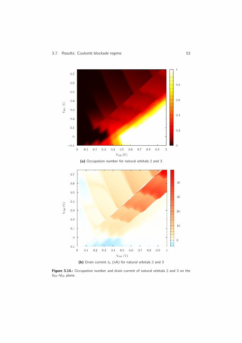
3.7. Results: Coulomb blockade regime 53
(a) Occupation number for natural orbitals 2 and 3
(b) Drain current ID (nA) for natural orbitals 2 and 3
Figure 3.14.: Occupation number and drain current of natural orbitals 2 and 3 on theVGS–VDS plane.

54 Chapter 3. MCSCG method
(a) Occupation number for natural orbitals 4 and 5
(b) Drain current ID (nA) for natural orbitals 4 and 5
Figure 3.15.: Occupation number and drain current of natural orbitals 4 and 5 on theVGS–VDS plane.

4. Numerical determination of thenon-equilibrium many-bodystatistical operator
4.1. Introduction
Various authors [94, 95, 96, 97] have considered the general mathematical con-
struction of a non-equilibrium many-body statistical operator of interacting elec-
trons for given external constraints or bias conditions. In this Chapter, we present
an adaptive numerical approach to determine a reduced non-equilibrium many-
body statistical operator ρrel for quasi-isolated electronic states within the channel
of a realistic NWFET system [98, 99, 100].
The underlying physical model assumes the knowledge of the (self-consistent)
single-particle density matrix [79] ρ1 of the whole channel system for the given
gate and bias voltage condition, resulting from a non-equilibrium Green’s function
(NEGF) calculation for the NWFET for a given set of applied voltages (see
Sec. 3.3.4). In turn, the single-particle Hilbert space of the whole channel system
is divided into a small, adaptively chosen relevant subspace and an orthogonal rest,
following the idea of the MCSCG approach, from which a relevant Fock subspace
is constructed (see Sec. 3.4.1). From the given matrix ρ1, a reduced many-body
statistical operator ρrel within the relevant subspace can be constructed. Here,
the given matrix elements of ρ1 impose constraints on ρrel. In comparison, the
approach described in Ref. [95] is based on direct constraints on single-particle
observables (such as the electronic current), whereas the approach described in
this Chapter is based on a general ρ1 with an adaptive relevant Fock subspace.
In general, the Fock subspace operator ρrel is not uniquely defined by the con-
straint of a given single-particle density matrix ρ1. Further physical assumptions
55

56 Chapter 4. Non-equilibrium many-body statistical operator
are therefore required. We assume that the eigenvalues wN of ρrel are of a gener-
alized grand-canonical Boltzmann form (to maximize entropy), parametrized by a
set of effective electrochemical potentials and an effective temperature. Further-
more, for the assumed many-body eigenbasis of ρrel, two alternatives are consid-
ered: (A) Slater determinants of relevant natural orbitals and (B) the eigenbasis
of the projected many-body Hamiltonian within the relevant subspace. In order
to determine an optimum ρrel that satisfies the given constraints on ρ1 numeri-
cally, a genetic algorithm is employed that searches for the optimum solution that
minimizes a suitably defined deviation measure.
From the determined ρrel, one can calculate expectation values for any observ-
able of the system. As an example, we describe the onset of formation of Wigner
molecules by means of the electron density (a single-particle observable obtain-
able simply by means of ρ1) and the density-density covariance (a many-body
observable which can only be obtained by means of ρrel).
The original implementation of the MCSCG algorithm (see Chapter 3) makes
use of a ρrel expressed as a mixture of relevant Slater determinants of natural
orbitals, as in case A above (see Sec. 3.4.2). NWFET-Lab, a new augmented
version of the original implementation, has the possibility to choose between
cases A and B, so it is able to alternatively employ a ρrel expressed as a mixture of
eigenstates of the projected many-body Hamiltonian within the relevant subspace.
For more details on NWFET-Lab see Appendix A.
4.2. Preliminary theoretical considerations
4.2.1. Relevant Fock space revisited
Following the lines of thought of Sec. 3.4.1, to make calculations of realistic
nanowire devices numerically feasible, instead of considering the full Fock space,
we restrict ourselves to a relevant subspace Frel. We still maintain the classi-
fication of single-particle states into relevant and non-relevant and construct a
many-body basis Brel of Frel with Slater determinants |DK〉 accordingly, so that
to each |DK〉 ∈ Brel corresponds a different combination of the bits (0 or 1) of
the Nrel relevant natural orbitals. So again we have dim(Frel) = 2Nrel .
Nevertheless, we introduce a difference here. The natural orbitals whose av-
erage occupation numbers are close to unity (ξi ' 1) can be treated in two

4.2. Preliminary theoretical considerations 57
Frel = |11000000〉, |11100000〉, |11010000〉, |11110000〉,|11001000〉, |11101000〉, |11011000〉, |11111000〉
Table 4.1.: An example of many-body relevant basis Brel.
alternative ways: (i) they may be treated as being fully occupied (bit set to 1 for
Nocc bits) in every |DK〉 and thus being incorporated statically within the many-
body Fock subspace, or (ii) they may be set as empty (bit set to 0) in every
|DK〉 and being incorporated in a mean-field way (in the single-particle part of
the Hamiltonian), which is the approach followed in Sec. 3.4.1. The rest of the
natural orbitals (i.e., those which are empty with ξi ' 0 or which are fluctu-
ating but being strongly coupled to the contacts) are kept empty (bit set to 0
for Nrest bits) in every |DK〉 and being incorporated in a mean-field way (in the
single-particle part of the Hamiltonian).
Thus, when fixing the occupied states in all Slater determinants, |DK〉 is com-
posed of Nocc to Nocc + Nrel electrons, whereas if using a mean-field description
for these single-particle states |DK〉 is composed of 0 to Nrel electrons. This can
be found in a modified version of coul.c [101].
As an example, we show the relevant many-body basis Brel of the relevant Fock
subspace Frel in Table 4.1 with Nmax = 8, Nocc = 2 and Nrel = 3, implying that
its dimension is dim(Frel) = 23 = 8.
In the special situation where Nrel = 0, all single-particle states are either
empty or occupied and the state of the system is described by a single Slater
determinant. On the other hand, whenever Nrel > 0 this is no longer the case.
The many-body state cannot then be described by just a single Slater determinant
and therefore we construct Brel which serves as a basis in order to express it.
4.2.2. Mean-field interaction revisited
As presented in the previous Sec. 4.2.1, we have the choice to treat the fully
occupied single-particle states in a many-body way, by fixing their corresponding
bits to one in every |DK〉, or set them to zero and treat them in a mean-field
way. We consider optionally also the possibility of treating the non-relevant rest
of single-particle states with a mean-field approach or not at all.
As in Sec. 3.4.3, the Coulomb self-energy given by Eq. (3.16) is used for

58 Chapter 4. Non-equilibrium many-body statistical operator
the mean-field description of Coulomb interaction, with a single-particle density
matrix ρ1vac for the vacuum state within the relevant Fock subspace Frel. ρ1vac
can be obtained from its diagonal form ρdiag1vaci j = δi jξ
vaci by ρ1vac = Υρdiag
1vacՆ,
where Υ is the unitary transformation that diagonalizes the single-particle density
matrix ρ1. We have now two options for the terms ξvaci corresponding to non-
relevant single-particle states, either to consider mean-field interaction and set
them to their actual values ξvaci = ξi or not to consider mean-field interaction
and set their values to zero ξvaci = 0. As before, all relevant single-particle states
have an average occupation number ξvaci = 0 (vacuum state within Frel).
4.2.3. Change to natural orbital basis
Since Frel is constructed in terms of Slater determinants of a subset of natu-
ral orbitals, the best would be to get the matrix elements and Coulomb tensor
elements in the natural orbital basis, whose transformation is given by Υ, the
unitary matrix that diagonalizes ρ1. Also, this is done because in case we want
to truncate the calculations using this basis, the impact on the results would be
smaller than in the case of the localized orbital basis (it would be equivalent to
cut the nanowire).
The creation and annihilation operators c†i and ci (with hat) in the spin/site
basis are related to those in the natural orbital basis c†i and ci (without hat) as
follows [42]
c†i =
Nmax−1∑k=0
Υ∗ikc†k , ci =
Nmax−1∑k=0
Υikck . (4.1)
From these expressions we can verify that the single-particle matrix given by
Eq. (3.5b) and the two-particle tensor given by Eq. (3.6b) of the Hamiltonian
transform as follows
h′i j + Σr ′eei j
[ρ1vac] =
Nmax−1∑p,q=0
Υ∗ipΥjq(hpq + Σreepq [ρ1vac]) (4.2a)
V ′i jkl =
Nmax−1∑p,q,r,s=0
Υ∗ipΥ∗jqΥkrΥlsVpqrs . (4.2b)
See implementation in coul.c [101].

4.2. Preliminary theoretical considerations 59
4.2.4. Projected many-body Hamiltonian
The projected many-body Hamiltonian Hrel within the relevant Fock subspace Frel
is obtained from H (see Sec. 3.3.3) via projection to the relevant Fock subspace
Frel. It has dimensions dim(Frel)×dim(Frel). For every pair of Slater determinants
of natural orbitals |DI〉 , |DJ〉 ∈ Brel we obtain the matrix element 〈DI | Hrel |DJ〉as follows
〈DI | (H0 + Hextee ) |DJ〉 =
Nmax−1∑i ,j=0
(h′i j + Σr ′eei j
[ρ1vac]) 〈DI | c†i cj |DJ〉 (4.3a)
〈DI | Hee |DJ〉 =
Nmax−1∑i ,j,k,l=0
V ′i jkl 〈DI | c†i c†j ckcl |DJ〉 (4.3b)
where the elements of the matrix h′i j , the Coulomb self-energy Σr ′eei j
[ρ1vac] and
the Coulomb tensor V ′i jkl in the natural orbital basis are already known.
Two kinds of operator products need to be evaluated: single-particle terms
〈DI | c†i cj |DJ〉 and two-particle terms 〈DI | c†i c†j ckcl |DJ〉. These terms are eval-
uated according to the Fermionic anti-commutation rules [42] obeyed by the
creation and annihilation operators for the natural orbital basis states c†i and ci ,
as given by Eqs. (2.2). The action of these operators is as described in Eqs. (2.1).
See implementation in functions twoop and fourop from coul.c [101].
4.2.5. Diagonalization of the projected many-bodyHamiltonian
Once the matrix representation of Hrel has been obtained it can be diagonal-
ized, yielding dim(Frel) eigenstates |ψN〉 and eigenenergies EN that satisfy the
eigenvalue equation
Hrel |ψN〉 = EN |ψN〉 . (4.4)
Every energy eigenstate expressed in the basis |DK〉 of Frel has the form
|ψN〉 =
dim(Frel)−1∑K=0
ΛKN |DK〉 (4.5)
where ΛKN = 〈DK |ψN〉, which defines a unitary transformation matrix Λ that
diagonalizes the projected many-body Hamiltonian matrix: Λ†HrelΛ = Hdiagrel .

60 Chapter 4. Non-equilibrium many-body statistical operator
In order to check the validity of the method so far, we can compare the
many-body eigenenergies EN(1) corresponding to a particle number Ne = 1
with the single-particle eigenenergies resulting from diagonalizing the Nrel × Nrel
sub-matrix of the single-particle Hamiltonian H0 expressed in the natural or-
bital basis. They should coincide. We can also compare the energy differences
EM1 (N + 1) − EM2 (N), corresponding to Ne = N + 1 and Ne = N respectively,
with the resonances in the LDOS obtained with the MCSCG method [82].
Another way of verifying the results is to treat in mean-field the non-relevant
fixed occupied and empty single-particle states but setting their respective ξvaci
to 1 and 0, not to their actual values. Forcing this situation is equivalent to
consider no mean-field and setting these states fixed in the Slater determinants.
The eigenvector components of Hrel given by Λ should coincide in both situations
and the energies should just be shifted by a constant amount.
4.3. Many-body statistical operator
4.3.1. On the statistical preparation of the system
The statistical preparation of the relevant subsystem is given by the reduced
many-body statistical operator
ρrel =
dim(Frel)−1∑N=0
wN |ρN〉 〈ρN | . (4.6)
It is Hermitian and satisfies Tr(ρrel) =∑N
wN = 1, with wN ∈ [0, 1]. The eigen-
value wN can be interpreted as the probability associated with the eigenstate
|ρN〉. The eigenvectors of ρrel can be expressed in terms of the basis of Slater
determinants of natural orbitals via the unitary transformation X as follows
|ρJ〉 =
dim(Frel)−1∑K=0
XKJ |DK〉 (4.7)
whose components read as XKJ = 〈DK | ρJ〉.There is no beforehand prescription on how to determine ρrel. It should de-
scribe in the best of the possible ways our state of knowledge about the physical
situation, without drawing any conclusions not warranted by the available data.

4.3. Many-body statistical operator 61
In this sense the probability distribution given by ρrel which is most conservative
is the one that is as smooth and spread out as possible, subject to the available
information of the system, since then no special cases or states are over or under
estimated without motivation. This measure of amount of uncertainty is given by
the entropy. In order to determine ρrel, we require that its probability distribution
maximizes the entropy subject to certain constraints. This determines the func-
tional form of the eigenvalues wN of ρrel, known as grand canonical or Boltzmann
form. Entropy maximization is covered in Sec. 4.4.
So far, no assumption has been made about the eigenvectors |ρN〉 that formthe orthonormal eigenbasis of ρrel within the relevant Fock subspace Frel. In the
following, we consider two cases: (A) the Slater determinant basis of natural
orbitals and (B) the eigenbasis of Hrel within the relevant subspace. One has
to note that for a stationary relevant subsystem, where the time evolution of
ρrel is assumed to be driven solely by the projected Hrel, both operators need
to commute, leading to the basis choice (case B) where |ρN〉 are chosen as
eigenstates of Hrel.
4.3.2. Single-particle density matrix constraint
The constraint that ρrel must satisfy is given by the following expression
ρ1i j!
= Tr(ρrelc†j ci) (∀i , j ∈ relevant) (4.8)
which links ρrel with the given ρ1 within the Nrel dimensional subspace of rele-
vant natural orbitals. It results from the fact that the expectation value of any
single-particle observable A =Nmax−1∑i ,j=0
ai jc†i cj can be obtained in the following two
equivalent ways
⟨A⟩
= Tr(ρrelA) =
Nmax−1∑i ,j=0
ai jTr(ρrelc†i cj) (4.9)
⟨A⟩
= Tr(ρ1a) =
Nmax−1∑i ,j=0
ai jρ1j i . (4.10)
Within the relevant single-particle subspace (Nrel dimensional), equation (4.8)
provides a set of Nrel × Nrel complex conditions. Noting that both sides of the
62 Chapter 4. Non-equilibrium many-body statistical operator
equation are Hermitian, we can see that the number of unique real constraints is
reduced to Nrel × Nrel.
Since we are using the natural orbital basis in which the given ρ1 is diagonal with
eigenvalues ξi and according to the expression of ρrel determined by Eq. (4.6),
the constraints imposed by Eq. (4.8) can be rewritten as
ξiδi j!
=∑n
wn 〈ρn| c†j ci |ρn〉 (∀i , j ∈ relevant). (4.11)
Here, the indices i and j are restricted to the relevant subspace in the natural
orbital basis.
One has to note that the diagonal constraints (i = j) are equivalent to con-
strained average particle numbers 〈ni 〉 for the corresponding natural orbitals. For
the following subsections, we denote the resulting coefficients as
Ni(|ρN〉) ≡ 〈ρN | c†i ci |ρN〉 = 〈ρN | ni |ρN〉 (4.12)
so that this subset of ρ1-diagonal constraints read as
ξi!
=∑N
wNNi(|ρN〉) (∀i ∈ relevant). (4.13)
It can be shown that Eqs. (4.8) are restricted to the subset of relevant single-
particle states, so the number of relevant constraints is Nrel × Nrel instead of
Nmax × Nmax. This follows from the analysis of the quantity 〈DK′ | c†j ci |DK〉,which appears in Eqs. (4.11) once we express |ρN〉 in terms of the basis of Slater
determinants of natural orbitals via the unitary transformation X (see Eq. (4.7)).
If any of the indices i or j correspond to any of the Nrest unoccupied single-
particle states of |DK〉 or |DK′〉 then 〈DK′ | c†j ci |DK〉 = 0, ∀ K,K′. Therefore
〈ρN | c†j ci |ρN〉 = 0, ∀ N and Eqs. (4.11) reduce to ξiδi j = 0. These are not a set
of constraints for w. If i = j they imply ξi = 0, which is what we assumed for
the non-relevant almost empty natural orbitals. If i 6= j they are trivial equalities
0 = 0. Similarly, if any of the indices i or j correspond to any of the Nocc
occupied single-particle states of |DK〉 or |DK′〉 then 〈DK′ | c†j ci |DK〉 = δi jδKK′ .
Therefore 〈ρN | c†j ci |ρN〉 = δi j∑K
X∗KNXKN = δi j , ∀ N and Eqs. (4.11) reduce to
ξiδi j = δi j∑N
wN = δi j . These are not a set of constraints for w. If i = j they
imply ξi = 1, which is what we assumed for the non-relevant almost occupied

4.3. Many-body statistical operator 63
natural orbitals. If i 6= j they are trivial equalities 0 = 0.
4.3.3. Average energy constraint
Assuming the average energy 〈E〉 of the system, or equivalently the tempera-
ture T , is a well-defined constant quantity, there exists a relation between the
statistical operator ρrel and 〈E〉, namely
〈E〉 = Tr(ρrelHrel) =∑N
wN 〈ρN | Hrel |ρN〉 =∑N
wNεN (4.14)
where we have defined
εN ≡ 〈ρN | Hrel |ρN〉 . (4.15)
This constraint is taken into account by fixing the temperature, which appears in
the grand canonical form of wN .
4.3.4. Case A: Slater determinant basis of natural orbitals
In this case, the statistical operator corresponds to a mixture of Slater determi-
nants of relevant natural orbitals, that is |ρN〉 = |DN〉. This is the same
situation as described in Sec. 3.4.2. Thus, we obtain
ρrel =
dim(Frel)−1∑N=0
wN |DN〉 〈DN | . (4.16)
In this case X = I and its matrix representation is diagonal in the Slater deter-
minant basis of natural orbitals |DN〉. The off-diagonal constraints given by
Eqs. (4.11) vanish. The remaining equations for the diagonal terms, Eqs. (4.13),
read as
ξi!
=
dim(Frel)−1∑N=0
wNNi(|DN〉) (∀i ∈ relevant), (4.17)
where we defined Ni(|DN〉) ≡ 〈Dn| ni |Dn〉 as the occupation number of the rele-
vant natural orbital i for the Slater determinant |Dn〉. The energies in Eq. (4.15)
associated with each eigenvector |Dn〉 of ρrel are given by the diagonal elements
of Hrel and read as εN = 〈DN | Hrel |DN〉 = HrelNN . Both quantities, Ni(|DN〉) and
εN are required in Eqs. (4.28) and (4.29) below.

64 Chapter 4. Non-equilibrium many-body statistical operator
One has to note that the vector w of eigenvalues of ρrel with dim(Frel) =
2Nrel components has to satisfy a set of Nrel conditions given by Eqs. (4.17),
so the number of unknowns is greater than the number of constraints and the
problem is under-determined in general, thus requiring further assumptions about
the function form of wN , such as a Boltzmann form (see Sec. 4.4).
4.3.5. Case B: eigenbasis of the projected many-bodyHamiltonian
In this case, we assume a stationary state of a relevant subsystem that is solely
driven by the projected Hrel. Thus, we have [ρrel, Hrel] = 0 and, consequently,
we choose |ρN〉 to be identical to the orthonormal eigenbasis |ψN〉 of the
projected Hrel. Hence, we obtain
ρrel =
dim(Frel)−1∑N=0
wN |ψN〉 〈ψN | (4.18)
which in the Slater determinant basis of natural orbitals |DN〉 reads as
ρrelKK′ = 〈DK | ρrel |DK′〉 =
dim(Frel)−1∑N=0
wNΛ∗K′NΛKN (4.19)
since in this case X = Λ. The ρ1 constraints have the form
ξiδi j!
=
dim(Frel)−1∑N=0
wN 〈ψN | c†j ci |ψN〉
=
dim(Frel)−1∑N=0
wN
dim(Frel)−1∑K,K′=0
Λ∗K′NΛKN 〈DK′ | c†j ci |DK〉 (4.20)
∀ i , j ∈ relevant. For the diagonal coefficients of Eq. (4.12) we have
Ni(|ψN〉) = 〈ψN | ni |ψN〉 =
dim(Frel)−1∑K=0
|ΛKN |2Ni(|DK〉) . (4.21)
The energies EN associated with each eigenvector |ψN〉 of ρrel are given by the
eigenvalues of Hrel, that is, εN = EN here. Both Ni(|ψN〉) and εN are required in
Eqs. (4.28) and (4.29) below.

4.4. Maximum entropy 65
The vector w of eigenvalues of ρrel with dim(Frel) = 2Nrel components has
to satisfy a set of Nrel × Nrel conditions given by Eqs. (4.20). If Nrel = 3, the
number of constraints is larger than the number of unknowns and the problem is
over-determined. If Nrel = 2 or 4, the number of constraints coincides with the
number of unknowns. For Nrel > 4 the relation 2Nrel > N2rel holds, the problem is
under-determined, thus requiring further assumptions about the function form of
wn, such as a Boltzmann form (see Sec. 4.4).
A way to check the consistency of the method is to artificially set Hrel to a
diagonal form by forcing ΛIJ = δIJ , which makes case B identical with case A and
so should yield the same results.
4.4. Maximum entropy
4.4.1. Entropy maximization with Lagrange multipliers
The chosen ansatz of a grand canonical form for the eigenvalues wN of ρrel results
from the assumption of maximum entropy under a number of constraints. This
means they must be such that the von Neumann entropy (within the relevant
subspace)
S = −kBTr(ρrel ln ρrel) = −kBdim(Frel)−1∑
N=0
wN lnwN (4.22)
is maximized. kB is Boltzmann’s constant and S has units J/K. Alternatively
we can express S in bit units. A bit is defined as kB ln 2 and S/(kB ln 2) =
−∑N
wN log2 wN is the expression of the entropy in bits.
The entropy maximization subject to several constraints can be performed by
the use of Lagrange multipliers. The constraints are given by the normalization
condition, the average energy given by Eq. (4.14) and the average particle number
(in natural orbitals) given by Eqs. (4.13). The respective Lagrange multipliers are
α, β and the set of Nrel multipliers γi . We require that the Lagrangian function
L = S − (α− kB)
dim(Frel)−1∑N=0
wN − 1
− βdim(Frel)−1∑
N=0
εNwN − 〈E〉
−−Nrel−1∑i=0
γi
dim(Frel)−1∑N=0
Ni(|ρN〉)wN − ξi
(4.23)
66 Chapter 4. Non-equilibrium many-body statistical operator
is maximized, which in essence is equal to maximizing the entropy S, since the
Lagrange multipliers multiply null expressions if the constraints are satisfied.
By requiring ∂L∂wN
= 0 we arrive at the following relation that gives the weights
once all the Lagrange multipliers are known
wN = exp
(−
1
kB
(α+ βεN +
Nrel−1∑i=0
γiNi(|ρN〉)
)). (4.24)
From this form for the weights and the normalization constraint we get an ex-
pression which determines the Lagrange multiplier α once β and γ are known
α = kB ln(Z (β, γ)) (4.25)
where we have defined the so called partition function
Z(β, γ) =
dim(Frel)−1∑N=0
exp
(−
1
kB
(βεN +
Nrel−1∑i=0
γiNi(|ρN〉)
)). (4.26)
The meaning of the Lagrange multipliers β and γi is as usual in thermodynam-
ics [102], namely
β =1
T, γi = −βµi = −
µiT
(4.27)
where T is the temperature and µi is the electrochemical potential associated
with the single particle state i . Note that if the electrochemical potentials are
different, the system is in non-equilibrium.
With these results at hand, the form of the statistical weights as functions of
the temperature T and the chemical potentials µi reads as
wN =1
Z(T, µ)exp
(−
1
kBT
(εN −
Nrel−1∑i=0
µiNi(|ρN〉)
))(4.28)
with the following expression for the partition function
Z(T, µ) =
dim(Frel)−1∑N=0
exp
(−
1
kBT
(εN −
Nrel−1∑i=0
µiNi(|ρN〉)
)). (4.29)
4.4. Maximum entropy 67
4.4.2. Infinite temperature limit
We consider here the limit in which the electrons behave like independent particles,
the maximum entropy infinite temperature limit. The consequence of making this
limit is that the form of the weights is modified. Analyzing the quantities that
appear in their exponents we have
limT→∞
(εnkBT
)= 0 , lim
T→∞
(µikBT
)= µ′i (4.30)
resulting in an expression for the weights
wN =1
Z(µ′)exp
N ′µ∑i=1
µ′iNi(|DN〉)
(4.31)
with the partition function
Z(µ′) =∑n
exp
N ′µ∑i=1
µ′iNi(|DN〉)
. (4.32)
Considering this, the present calculation of the newly defined Lagrange parameters
µ′ is analogous to the one in section 4.4. Only in this case the form of the weights
is different, the quantities εn being absent.
Furthermore, in the limit of independent particles the weights have the following
analytical form,
wn =
Nmax∏i=1
ξNi (|DN〉)i (1− ξi)1−Ni (|DN〉) (4.33)
where ξi ∈ [0, 1] is the average occupation number of fluctuating single-particle
state i (eigenvalue i of ρ1) and Ni(|DN〉) ∈ 0, 1 is the particle number in Slater
determinant |DN〉 in state i . Its implementation can be found in [81]. We expect
these solutions to reflect some of the characteristics of the Slater determinants.
It is possible to prove [103] that Eq. (4.33) implies the form of the weights
given by Eq. (4.31). For this task we first write the weights as
wN =
Nmax∏i=1
ui(Ni(|DN〉)) , ui(mi) ≡ Ki exp(µ′imi) (4.34)

68 Chapter 4. Non-equilibrium many-body statistical operator
where the expression for ui is motivated by Eq. (4.31). Then we can show that
Ki and µ′i exist which are independent of mi and only dependent on ξi . Let us
study the two possible cases
mi = 0 ⇒ ui(mi) = Ki ≡ 1− ξi (4.35a)
mi = 1 ⇒ ui(mi) = Ki exp(µ′i) ≡ ξi (4.35b)
from where we get a form for Ki and µ′i
Ki = 1− ξi , µ′i = ln
(ξi
1− ξi
). (4.36)
As one can see Ki and µ′i exist and are independent of mi and only depend on ξi .
To obtain an expression for Z we compare both forms for wn given by Eq. (4.31)
and Eq. (4.34)
wN =1
Z
Nmax∏i=1
ui(Ni(|DN〉))
Ki=
Nmax∏i=1
ui(Ni(|DN〉)) ⇒ Z =1
Nmax∏i=1
(1− ξi). (4.37)
These results prove the validity of the analytical expression Eq. (4.33) for the
weights in the case of independent particles. One can check this by substituting
the formulas for Z and µ′i in Eq. (4.31) to arrive at Eq. (4.33).
As an alternative to the derivation of the form for µ′i we consider the case of
independent particles (Fermions) with the Fermi-Dirac occupation probability
ξi = f (Ei) =1
exp(Ei−µikBT
)+ 1
. (4.38)
In the limit kBT →∞ Eqs. (4.30) hold. We have then
ξi =1
exp(−µ′i) + 1⇒ µ′i = ln
(ξi
1− ξi
)(4.39)
and we arrive at the same form for µ′i .

4.5. Numerical determination of the weights 69
4.5. Numerical determination of the weights
In order to find a solution for the vector w of 2Nrel eigenvalues of ρrel, the Nrel
electrochemical potentials µi must be adjusted in such a way that the resulting w
satisfies the ρ1 constraints. The partition function ensures normalization and the
condition that T is given is equivalent to fix the average energy of the system.
One has to note that under non-equilibrium conditions (due to an applied voltage
VDS between the source and drain contacts at the outer ends of the channel), the
effective electrochemical potentials µi become independent quantities in general.
Since the problem is under-determined in general, it is possible that more than
a single solution exists. On the other hand, there might exist no exact solution
for the constraints at all for the assumed functional form of wN and eigenbasis of
ρrel. In the latter case, one has to search for an optimum set of µi that minimizes
a measure of deviation from the constraint condition.
In Sec. 4.5.1 it is shown that in case A, the Newton-Raphson method is capable
of obtaining solutions that fulfill condition (4.13) numerically. Nevertheless, the
method cannot be applied to case B, where the number of constraints Nrel×Nrel
is larger than the number Nrel of electrochemical potentials in general.
So for case B, as well as for case A if desired, a single-objective genetic al-
gorithm [104] (GA) optimization method is used in the following. Its goal is to
minimize an objective function given by the absolute value of the deviation from
exact constraint satisfaction with the µi as optimization variables. There are
several benefits in using a GA: It operates in parallel with a population of can-
didate solutions, instead of just a single one. It always yields a solution which
improves after every iteration, in contrast to other methods that simply do not
give a solution if convergence is not achieved. It can leave local optimum points
in the search space behind, even if the objective function is not smooth. We
have chosen to implement the GA using the multi-crossover formula described in
Ref. [105]. For an overview about GAs, see Appendix B.
4.5.1. Newton-Raphson method
To obtain expressions for the chemical potentials we substitute the weights in the
form given by Eq. (4.28) in each of the constraints. By virtue of the normalization

70 Chapter 4. Non-equilibrium many-body statistical operator
constraint, we can write the constraints given by Eqs. (4.13) as
dim(Frel)−1∑N=0
(Ni(|ρN〉)− ξi)wN = 0 . (4.40)
Then substituting wN we arrive at the following Nrel relations
Fk(µ) =
dim(Frel)−1∑N=0
(Nk(|ρN〉)− ξk)E(µ) = 0 (4.41)
where we define
E(µ) ≡ exp
(−
1
kBT
(εN −
Nrel−1∑i=0
µiNi(|ρN〉)
)). (4.42)
This set of equations relate the chemical potentials µi and depend only on the
known quantities ξi , T , εN and Ni(|ρN〉). The zeros or roots of Eqs. (4.41) are
the chemical potentials we are looking for. We make use of the multidimensional
Newton-Raphson method for this task. This method starts by assigning initial
values to µi . At each iteration they are updated µi → µi + δµi by addition of a
correction δµi such that
Nrel−1∑i=0
∂Fk(µ)
∂µiδµi = −Fk(µ) , k = 0, 1, . . . , Nrel − 1 (4.43)
where from Eqs. (4.41) we have
∂Fk(µ)
∂µi=
1
kBT
dim(Frel)−1∑N=0
Ni(|ρN〉)(Nk(|ρN〉)− ξk)E(µ) . (4.44)
These equations can be written in matrix form as
Jδµ = −F → δµ = −J−1F (4.45)

4.6. Expectation values 71
where J is a Nrel × Nrel square matrix known as Jacobian with the following
structure
J =
∂F0
∂µ0· · · ∂F0
∂µNrel−1
......
∂FNrel−1
∂µ0· · · ∂FNrel−1
∂µNrel−1
. (4.46)
With the new vector µ+δµ we update the relations F , obtain a new Jacobian and
repeat the algorithm until convergence is achieved. Convergence criterion is given
by the magnitude of the corrections δµi being smaller than a given threshold.
4.5.2. Optimization by genetic algorithm
As we have seen, the free optimization variables to be adjusted in order to obtain
the eigenvalues w of ρrel are the chemical potentials µi . Assuming VDS > 0 they
are restricted to the interval −e VDS ≤ µi ≤ 0. If VDS < 0 we have 0 ≤ µi ≤−e VDS. We employ a GA as optimization method (see Appendix B for details),
where the chemical potentials are encoded in the genes of the chromosomes of
the GA and there are as many genes in a chromosome as chemical potentials.
The objective function η to be minimized is the averaged sum of the absolute
value of the deviation from the exact constraints satisfaction. It has the following
expression
η =1
Nrel × Nrel
Nrel−1∑j≤i=0
∣∣∣∣∣∣2Nrel−1∑N=0
wN 〈ρN | c†j ci |ρN〉 − δi jξi
∣∣∣∣∣∣ . (4.47)
4.6. Expectation values
Once the relevant statistical operator ρrel has been calculated, the expectation or
average value of any observable A can be obtained, as follows
⟨A⟩
= Tr(ρrelA
)=
dim(Frel)−1∑N=0
wN 〈ρN | A |ρN〉 . (4.48)
A mixture of states as given by ρrel adds an additional statistical averaging. The
expectation value, like the trace of a matrix, is independent of the representation.
So the same results are expected to be obtained in any many-body orthonormal

72 Chapter 4. Non-equilibrium many-body statistical operator
basis. Nevertheless,⟨A⟩is dependent on the actual expression of ρrel as given
by its eigenbasis and weights. So beforehand we might expect differences in the
calculated expectation values depending on the case under consideration, cases
A and B.
We analyze these two cases for a general physical observable A. The following
equations describe how to obtain⟨A⟩
⟨A⟩
=
dim(Frel)−1∑N=0
wN 〈DN | A |DN〉 (4.49a)
⟨A⟩
=
dim(Frel)−1∑N=0
wN 〈ψN | A |ψN〉 =
dim(Frel)−1∑N=0
wN
dim(Frel)−1∑I,J=0
Λ∗INΛJN 〈DI | A |DJ〉
(4.49b)
in case A and B respectively. As these two expressions show, the work-flow to
calculate the expectation value of an observable is as follows: compute the matrix
elements of the observable in the Slater determinant basis of natural orbitals,
then for case B transform to the eigenbasis of Hrel according to the unitary
transformation Λ. Finally sum all weighted contributions. So we only need one
many-body quantum mechanical calculation for each matrix element and the rest
are just matrix multiplications. We obtain ultimately the matrix elements in the
Slater determinant basis of natural orbitals since we assume A to be expressed in
terms of creation and annihilation operators acting on natural orbitals. If this is
not the case they have to be transformed to the natural orbital basis.
4.7. Electron density and covariance
4.7.1. Physical meaning
The electron number at spin/site i is given by the expectation value of the number
operator 〈ni 〉 =⟨c†i ci
⟩in the localized single-particle basis. It describes the
number of electrons that are located in each site with spin up or down. Here and
in the following we omit the spin index, which is assumed to be absorbed into a
collective spin/site index. Each electron inside the NWFET channel occupies in
general more than one site, its wave function is spread along the nanowire and so
is the electron density. Note that the expectation value of the electron number

4.7. Electron density and covariance 73
operator may be non-integer in general.
The density–density covariance is defined as
σi j ≡ 〈(ni − 〈ni 〉) (nj − 〈nj 〉)〉 = 〈ni nj〉 − 〈ni 〉 〈nj〉 (4.50)
and describes the reciprocal linear relationship between the electron densities at
two spin/sites i and j of the nanowire channel. Whenever the probability for both
densities to have deviations from the mean value which are both positive or both
negative (they “vary together”) is relatively high, the covariance takes a positive
value. On the other hand, the covariance is negative if the probability that one
deviation is positive and the other negative (they “vary oppositely”), is relatively
high. The covariance is constrained within the following limits
− σiσj ≤ σi j ≤ σiσj (4.51)
where σi ≡√σi i is the square root of the variance or standard deviation. It
can attain one of these limits only in the case that ni and nj satisfy a linear
relationship.
It can be seen that the density–density covariance is symmetric (σi j = σj i) by
noting that
ni nj = c†i ci c†j cj = δi j c
†i cj − c
†i c†j ci cj = δi j c
†i cj − c
†j c†i cj ci =
= δi j c†i cj − δi j c
†j ci + c†j cj c
†i ci = nj ni (4.52)
and we can verify that the diagonal elements, which can be identified with the
variance, have the form
σi i = 〈ni 〉 − 〈ni 〉2 (4.53)
by realizing that the number operator is idempotent
ni ni = c†i ci c†i ci = c†i ci − c
†i c†i ci ci = ni (4.54)
where we have used the fact that c†i c†i = ci ci = 0 by the Fermionic anti-
commutation relations.
Linear independence of ni and nj implies σi j = 0. On the other hand, the
density–density covariance may be zero even if there is an interdependence of a

74 Chapter 4. Non-equilibrium many-body statistical operator
nonlinear kind between these quantities. Moreover, the covariance depends on
the units of measurement. For this reason, the correlation is defined as
κi j ≡⟨(
ni − 〈ni 〉σi
)(nj − 〈nj〉σj
)⟩=
σi jσiσj
. (4.55)
This measure of interdependence does not change with a rescaling of the variables
and its limits are
− 1 ≤ κi j ≤ 1 . (4.56)
4.7.2. Case A: diagonal elements
In case A we need only the diagonal elements of the observables, as Eq. (4.49a)
shows. It is possible to transform the general expressions of the diagonal elements
into specific and simplified forms which link the quantities together.
The electron density is defined in the localized single-particle basis. Since
the Slater determinants express many-body states of natural orbitals we have to
transform ni to the natural orbital basis by means of Eqs. (4.1). Doing so leads
to the following expression
〈DN | ni |DN〉 = 〈DN | c†i ci |DN〉 =∑jk
Υ∗i jΥik 〈DN | c†j ck |DN〉︸ ︷︷ ︸Nk (|DN〉)δjk
=
=∑k
|Υik |2 Nk(|DN〉) (4.57)
and so the electron density reads
〈ni 〉 =∑N
wN∑k
|Υik |2 Nk(|DN〉) . (4.58)
More cumbersome is the calculation of the density–density covariance. Accord-
ing to Eq. (4.50), the expectation value of the product of number operators at
two spin/sites 〈ni nj〉 has to be computed. Its normal-ordered form, with all cre-
ation operators at the left and annihilation operators at the right, can be obtained
by anti-commutation as follows
ni nj = c†i ci c†j cj = c†i c
†j cj ci + δi j c
†i ci (4.59)

4.7. Electron density and covariance 75
from which we deduce that
〈DN | ni nj |DN〉 = δi j 〈DN | ni |DN〉+ 〈DN | c†i c†j cj ci |DN〉 . (4.60)
We focus on the non-diagonal term and transform it into the natural orbital basis
to obtain
〈DN | c†i c†j cj ci |DN〉 =
∑p,q,r,s
Υ∗ipΥ∗jqΥjrΥis 〈DN | c†pc†qcrcs |DN〉 . (4.61)
Since it is evaluated with respect to the same Slater determinant, the term be-
tween brackets is nonzero only if p = s and q = r or if p = r and q = s, so the
only strings of operators that have to be considered are c†pc†qcqcp = −c†pc†qcpcq
and c†pc†qcpcq.
4.7.3. Case B: full matrix
Case B according to Eq. (4.49b), makes use of all the matrix elements of ni and
ni nj in the Slater determinant basis and not only the diagonal. Their form is
more general and we give it here, noting that once obtained it is straightforward
to translate from the Slater determinant basis to the basis of the projected many-
body Hamiltonian Hrel. Transforming the operators to the natural orbital basis,
the electron density matrix elements in the Slater determinant basis of natural
orbitals read as
〈DM | ni |DN〉 = 〈DM | c†i ci |DN〉 =∑j,k
Υ∗i jΥik 〈DM | c†j ck |DN〉 (4.62)
and we can verify that 〈DN | ni |DM〉∗ = 〈DM | ni |DN〉. The remaining term to
obtain the covariance reads as
〈DM | ni nj |DN〉 = δi j 〈DM | ni |DN〉+∑p,q,r,s
Υ∗ipΥ∗jqΥjrΥis 〈DM | c†pc†qcrcs |DN〉 .
(4.63)

76 Chapter 4. Non-equilibrium many-body statistical operator
4.8. Results: onset of formation of Wignermolecules
As a result of the method to obtain the relevant many-body statistical operator
of the NWFET, we calculate the density–density correlation κi j for successive
steps in the transition between two different regimes of the electrons inside the
nanowire channel. These two regimes are termed “atomic” and “Wigner” regimes
and are characterized both by the ratio of Coulomb to single-particle energies per
electron (γE = ECoul/∆E) and channel length to screening length (γL = L/λ).
In the Wigner regime, the Coulomb energy is relatively greater than the single-
particle energy (γE 1) and the screening length is small enough (γL 1) to
favor the spatial separation of the electrons in the nanowire, forming so-called
Wigner molecules. This localization is lacking in the atomic regime, where the
Coulomb energy is not large enough. Additionally, we present graphs of the
electron density and the natural orbitals. Both cases A and B for the choice of
eigenbasis of the statistical operator are studied, case B being specially interesting
since it introduces a variation with respect to the original MCSCG method, which
employs case A.
4.8.1. Energy estimations
Obtaining the energy ratio γE implies knowledge of the Coulomb and single-
particle energies for a system of electrons in a nanowire channel, which cannot be
supplied before the simulation is performed. Therefore, we employ auxiliary energy
expressions, which have a simple analytical form and depend straightforwardly on
the parameters of the system, to estimate the actual energies.
The difference ∆E between the first two energy levels resulting from considering
the nanowire as a 1D infinite potential well is taken as an estimation of the single-
particle energy, which reads as [106]
∆E =3
8
N2e h
2
m∗L2(4.64)
where Le = L/Ne and Ne is the number of electrons in the channel. The single-
electron Coulomb charging energy as given by its classical expression ECoul =
e2/Cox serves as an estimation for the Coulomb energy per electron, where Cox

4.8. Results: onset of formation of Wigner molecules 77
is the capacitance per electron for a coaxially gated NWFET and reads as [46]
Cox =πε0εchd
2chLe
4λ2(4.65)
and the screening length λ is given by Eq. (1.1). Substituting the capacitance in
the expression of the energy we get
ECoul =4Nee
2λ2
πε0εchd2chL
. (4.66)
For a given nanowire channel and insulator material composition, the γE and
γL ratios are determined by the length L and diameter dch of the channel, the
oxide thickness dox and the electron number Ne , as these estimations show. Nev-
ertheless, to study the transition from atomic to Wigner regimes, we choose Ne ,
dch and the ratios γE and γL as free variables, determining from them the pa-
rameters L, λ and dox by means of scaling equations. Forming the ratio γE with
the quantities given by Eqs. (4.64) and (4.66) it is straightforward to express the
nanowire channel length as
L =
(3π2
32NeaBd
2chγEγ
2L
) 13
(4.67)
where the Bohr radius is defined as
aB =4πε0εchh
2
m∗e2. (4.68)
Once the nanowire length is determined, the screening length is obtained simply
as
λ =L
γL(4.69)
which can be used to determine the oxide thickness from Eq. (1.1) as
dox =dch
2
(exp
(8εox
εch
(λ
dch
)2)− 1
). (4.70)
Note that dox increases exponentially with λ2, so one must be careful with the
choice of parameters so that the produced oxide thickness is kept within realistic
limits.

78 Chapter 4. Non-equilibrium many-body statistical operator
γE Nsites L(nm) dox(nm)
0.5 34 11.05 0.926
1 42 13.65 1.717
1.5 49 15.925 2.577
3 61 19.825 5.836
5 73 23.725 12.467
10 92 29.9 50.299
Table 4.2.: Parameters of the simulated systems.
4.8.2. System parameters and approach
We have chosen the following device parameters common to both regimes. The
channel consists of a ZnO nanowire of diameter dch = 3 nm and lattice constant
a0 = 3.25 Å, electron effective mass m∗/me = 0.29 and a relative dielectric con-
stant εch = 8.66, as found in Ref. [85]. The channel and the gate are separated
by a SiO2 oxide layer of relative dielectric constant εox = 3.9. The source and
drain are contacted with a metal (Pt for example) to form Schottky barriers [24]
of height ΦSB = 0.7 eV, which act as double tunnel barriers to confine the elec-
trons in the nanowire. The temperature of the system is T = 4.2 K. Table 4.2
gathers the parameters particular to each simulation.
The choice of ZnO as nanowire material is motivated by its relatively large
effective mass, which makes possible to select a relatively high γE corresponding
to a relatively short L. Even if the lattice constant a0 is not very large, the
number Nsites = L/a0 of localized orbitals (sites) can be kept low enough, so that
the calculation time and memory are within reasonable limits.
The ratio of nanowire length L to screening length λ has been selected as
γL = 10 for all the cases we have studied. In this way, λ is small enough to guar-
antee Wigner molecule formation, provided the ratio γE of estimated Coulomb
to single-particle energy is large enough. The transition from one regime to the
other has been performed by varying γE only, for six different values. This quan-
tity determines L by application of Eq. (4.67), which in turn determines λ by
Eq. (4.69) and as a result dox by Eq. (4.70). We have selected a voltage point
with VDS = 0 and VGS = 0.15 V , which corresponds to the center of the second
Coulomb diamond, an equilibrium situation with the channel occupied by Ne = 2
electrons. The Coulomb diamond’s scale and location depend on the parameters

4.8. Results: onset of formation of Wigner molecules 79
of the system, therefore in principle one should adjust VGS (with chosen VDS = 0)
in such a way that the voltage point belongs to the diamond in all the studied
simulations. Nevertheless, the chosen value of VGS corresponds in all cases to the
second diamond.
4.8.3. Resulting statistical operator
The statistical operator with eigenbasis of Slater determinants of natural orbitals
(case A), has the form of a pure state ρrel = |D3〉 〈D3| in five of the six performed
simulations. Only the case with γE = 3 deviates from a pure state, with ρrel =
w3 |D3〉 〈D3|+w12 |D12〉 〈D12| being a mixture of the states |D3〉 = |110000 · · · 〉and |D12〉 = |001100 · · · 〉, with weights w3 = 5.276 × 10⁻¹ and w12 = 4.724 ×10⁻¹.
The statistical operator whose eigenbasis is chosen to be that of the eigenvec-
tors of the projected many-body Hamiltonian (case B), has in all simulations the
form of a pure state ρrel = |ψ〉 〈ψ| corresponding to a single many-body state
|ψ〉. Table 4.3 displays the components | 〈DK |ψ〉 |2 of the many-body state |ψ〉in the basis of Slater determinants of natural orbitals for the six studied cases.
Most of the components follow a similar pattern. There is a single component
with a value very near unity, corresponding to the same Slater determinant as
in case A, while the remaining are relatively small. Therefore, the many-body
state of the system for these simulations in case B, is almost a single Slater
determinant. This indicates that employing an eigenbasis of Slater determinants
of natural orbitals (case A) in these situations is a good choice of representation.
On the other hand, the results corresponding to γE = 3 deviate from this pattern,
since the highest valued component is not so near unity. Nevertheless, for this
simulation there is a resemblance between cases B and A, in the sense that the
highest components in case B correspond to the same Slater determinants in case
A.
4.8.4. Natural orbitals
We have carefully chosen the thresholds that determine the classification of nat-
ural orbitals into occupied, fluctuating and empty, in such a way that the Fock
subspace dimension is not drastically reduced. Even if the contribution of those

80 Chapter 4. Non-equilibrium many-body statistical operator
γE = 0.5 γE = 1
|DK〉 | 〈DK |ψ〉 |2 |DK〉 | 〈DK |ψ〉 |2
|1100000000〉 9.901087× 10⁻¹ |1100000000〉 9.287014× 10⁻¹
|0000001100〉 9.881239× 10⁻³ |0000001100〉 7.040752× 10⁻²
|0000000011〉 8.651753× 10⁻⁶ |0000000011〉 4.487365× 10⁻⁴
γE = 1.5 |0100000010〉 3.075678× 10⁻⁴
|DK〉 | 〈DK |ψ〉 |2 |1000000001〉 1.321041× 10⁻⁴
|1100000000〉 8.351109× 10⁻¹ |1000000010〉 1.842873× 10⁻⁶
|0000001100〉 1.446486× 10⁻¹ γE = 3
|0000000011〉 8.474243× 10⁻³ |DK〉 | 〈DK |ψ〉 |2
|0100000010〉 5.877250× 10⁻³ |1100000000〉 7.319653× 10⁻¹
|1000000001〉 5.877197× 10⁻³ |0011000000〉 2.232429× 10⁻¹
|0000000110〉 3.323030× 10⁻⁶ |0100000010〉 1.503594× 10⁻²
|0000001010〉 2.881298× 10⁻⁶ |1000000001〉 1.501137× 10⁻²
|0000001001〉 2.873206× 10⁻⁶ |0000000011〉 1.461581× 10⁻²
|0000000101〉 2.470142× 10⁻⁶ |0010000001〉 6.859462× 10⁻⁵
γE = 5 |0001000010〉 5.973664× 10⁻⁵
|DK〉 | 〈DK |ψ〉 |2 γE = 10
|1100000000〉 9.884781× 10⁻¹ |DK〉 | 〈DK |ψ〉 |2
|0000001100〉 1.120697× 10⁻² |1100000000〉 9.856718× 10⁻¹
|1000000100〉 2.797392× 10⁻⁴ |0000001100〉 1.350063× 10⁻²
|0100001000〉 3.521542× 10⁻⁵ |0100001000〉 3.964802× 10⁻⁴
|0000000110〉 3.498175× 10⁻⁴
|0000001010〉 6.034784× 10⁻⁵
|0100000010〉 1.953227× 10⁻⁵
|1000001000〉 1.159658× 10⁻⁶
Table 4.3.: Components | 〈DK |ψ〉 |2 > 10−6 of the many-body state |ψ〉 that charac-terizes the system for the six simulations in case B. Relevant natural orbitals are shownin boldface.

4.8. Results: onset of formation of Wigner molecules 81
natural orbitals with very low occupation number is small, we preferred to include
them so that the impact of the reduction of the Fock space is minimized within
some limits.
In all the simulations the number of relevant natural orbitals is 6, so the Fock
subspace dimension is 64. Figure 4.1 gathers them for case B. The first two (in-
dices 0 and 1) have the highest occupation number (ξi ∼ 1) and are of the highest
relevance in determining the general features of the observables, as compared to
the following four, with very small occupation numbers. This can be verified by
comparing their shape (one peak or two peaks) with that of the electron density,
as shown in Fig. 4.2.
Note that there is an index gap in all six situations. The missing natural orbitals
correspond to fluctuating states but strongly coupled to the contacts, thus not
being considered as relevant. For example, for γE = 10 these missing states have
indices 2,3,4 and 5.
4.8.5. Total electron density
Figure 4.2 displays the total electron density for the system in equilibrium and
the channel occupied by Ne = 2 electrons, as γE is increased. Examining the
tendency of the density to develop two peaks from a single one, the transition
from atomic to Wigner regime can be seen. Indeed, the two electrons in the
channel separate as a consequence of the increased Coulomb interaction and a
Wigner molecule emerges.
In any simulation, the densities corresponding to spin up and down are equal to
each other, so they are not shown separately. Specifically in the Wigner regime,
the two-peaked density associated with spin up coincides with that with spin down,
spin symmetry is preserved. This is in accordance to Pauli’s exclusion principle but
may be counterintuitive, since one might expect both electrons to have definite
and opposed spins, whereas there is no spin separation.
Note that if we had chosen to plot the densities against the absolute position x
and not against the relative position x/L, the areas below the curves would have
been the same and equal to the electron number. Cases A and B produce the
same density profiles and therefore only case B is shown.

82 Chapter 4. Non-equilibrium many-body statistical operator
Figure 4.1.: The six relevant natural orbitals for all case B simulations (varying γE).Here we make the identification of Υn(x) with Υxn, the unitary matrix that diagonalizesρ1, where the column n corresponds to the nth natural orbital and the row to site x .
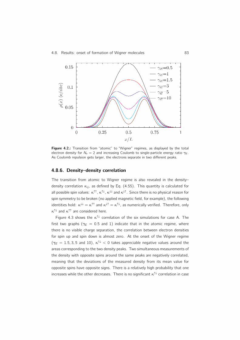
4.8. Results: onset of formation of Wigner molecules 83
Figure 4.2.: Transition from “atomic” to “Wigner” regimes, as displayed by the totalelectron density for Ne = 2 and increasing Coulomb to single-particle energy ratio γE .As Coulomb repulsion gets larger, the electrons separate in two different peaks.
4.8.6. Density–density correlation
The transition from atomic to Wigner regime is also revealed in the density–
density correlation κi j , as defined by Eq. (4.55). This quantity is calculated for
all possible spin values: κ↑↑, κ↑↓, κ↓↓ and κ↓↑. Since there is no physical reason for
spin symmetry to be broken (no applied magnetic field, for example), the following
identities hold: κ↓↓ = κ↑↑ and κ↓↑ = κ↑↓, as numerically verified. Therefore, only
κ↑↓ and κ↑↑ are considered here.
Figure 4.3 shows the κ↑↓ correlation of the six simulations for case A. The
first two graphs (γE = 0.5 and 1) indicate that in the atomic regime, where
there is no visible charge separation, the correlation between electron densities
for spin up and spin down is almost zero. At the onset of the Wigner regime
(γE = 1.5, 3, 5 and 10), κ↑↓ < 0 takes appreciable negative values around the
areas corresponding to the two density peaks. Two simultaneous measurements of
the density with opposite spins around the same peaks are negatively correlated,
meaning that the deviations of the measured density from its mean value for
opposite spins have opposite signs. There is a relatively high probability that one
increases while the other decreases. There is no significant κ↑↓ correlation in case

84 Chapter 4. Non-equilibrium many-body statistical operator
A outside these regions.
A comparison between the κ↑↓ correlation as displayed in Fig. 4.3 for case A
and Fig. 4.4 for case B, clearly shows that case B is able to capture more features
and differences exist between the two cases. Most noticeable is the appearance
of regions with positive correlation. In the atomic regime (γE = 0.5 and 1),
these regions correspond to sites positioned in different halves of the nanowire
channel. For two simultaneous density measurements of opposite spin, positive
correlation implies a relatively high probability of either an increase or a decrease
with respect to the mean value in both observables. For sites located in the
same half of the channel the correlation is negative. As γE increases, the shape
of the correlation changes continually, from a “quadrupole-like” to a “dipole-like”
geometry, where the negative areas concentrate around two peaks and the positive
areas get smaller.
Figure 4.5 shows the κ↑↑ correlations for case A. The diagonal elements are
omitted, since their value is unity and they are not relevant. In this case, κ↑↑ is
significantly nonzero in all simulations. As the Wigner regime sets on, there is a
transition from a single area with negative correlation to two separated localized
regions. Outside these areas κ↑↑ ∼ 0 is not appreciable. Except for the simula-
tions corresponding to γE = 0.5 and 1, a comparison with Fig. 4.3 shows that
κ↑↑ ∝ κ↑↓ for case A.
Figure 4.6 shows the κ↑↑ correlations for case B. The first two graphs (γE =
0.5 and 1) corresponding to the atomic regime, coincide with those for case A.
The following two graphs (γE = 1.5 and 3) feature four rounded regions in a
square arrangement with negative correlation. Finally, the κ↑↑ correlation for
γE = 5 and 10 coincides with the κ↑↓ correlation (both for case B).
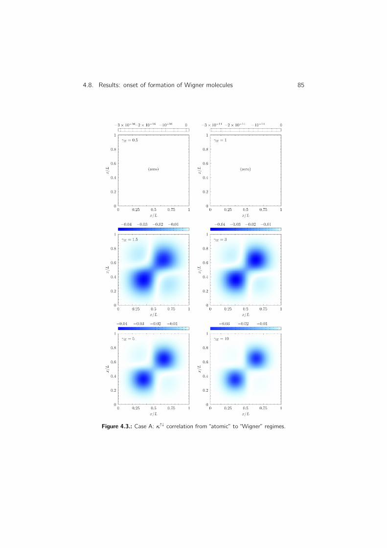
4.8. Results: onset of formation of Wigner molecules 85
Figure 4.3.: Case A: κ↑↓ correlation from “atomic” to “Wigner” regimes.

86 Chapter 4. Non-equilibrium many-body statistical operator
Figure 4.4.: Case B: κ↑↓ correlation from “atomic” to “Wigner” regimes.
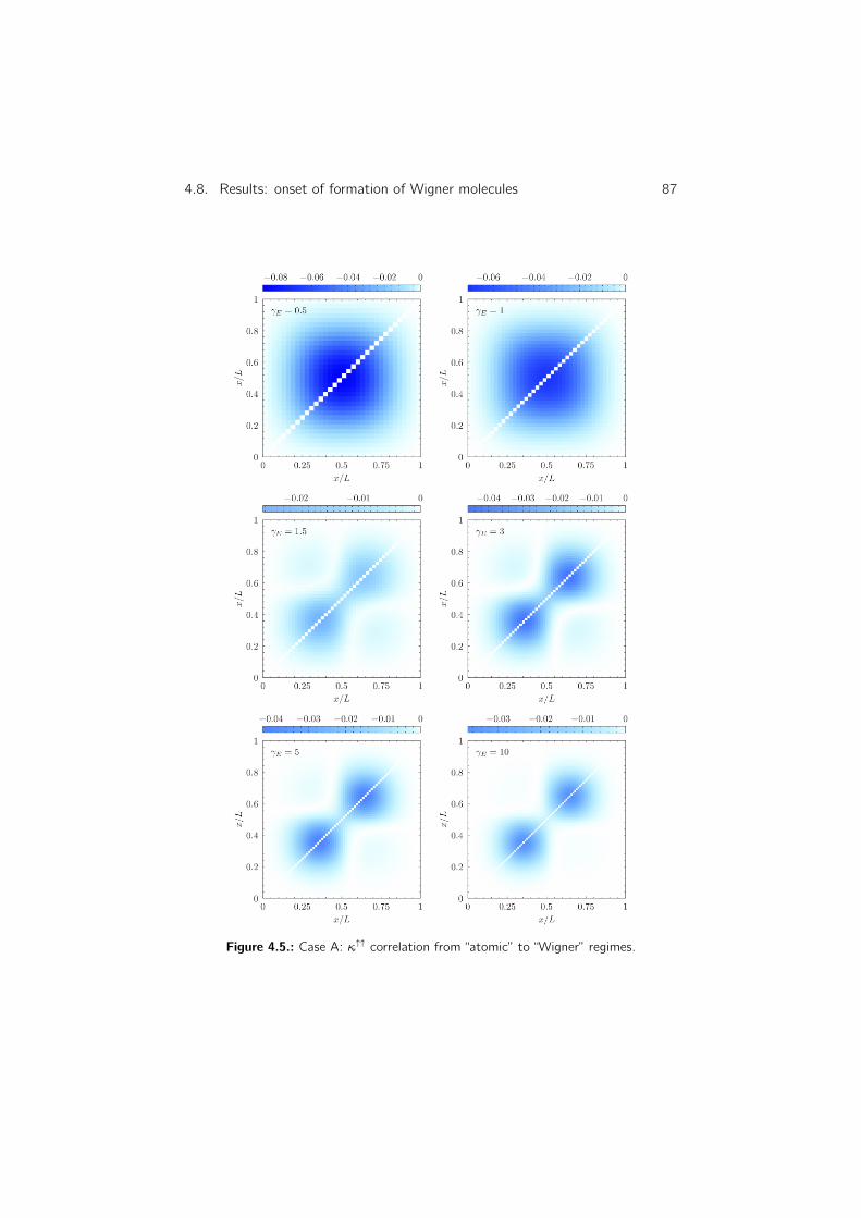
4.8. Results: onset of formation of Wigner molecules 87
Figure 4.5.: Case A: κ↑↑ correlation from “atomic” to “Wigner” regimes.

88 Chapter 4. Non-equilibrium many-body statistical operator
Figure 4.6.: Case B: κ↑↑ correlation from “atomic” to “Wigner” regimes.

5. Correlation entropy
5.1. Introduction
As an application of the method for numerically determining the non-equilibrium
many-body statistical operator described in Chapter 4 and as an interesting topic
in itself, we study in the following Sections the issue of quantifying the correlation
of interacting electrons in the channel of a NWFET. A Fock space state that
cannot be written as a Slater determinant with respect to any single-particle
basis is called a “correlated” many-body state. Note that a Slater determinant
with respect to a given basis may be written in terms of a superposition of multiple
Slater determinants with respect to a different single-particle basis. Therefore,
more than one Slater determinant in an expansion does not imply that the state
is correlated.
The topic of correlation in many-electron systems for the case where the prepa-
ration of the system is given by a pure state has been studied by several authors.
It has been shown [107, 108, 109, 110] that the single-particle-reduced entropy
S1 as given by the single-particle density matrix [79] ρ1 can be interpreted as a
measure of correlation for such pure states. If the preparation of the system is
given by a mixture of states, S1 also depends on the degree of mixture [111, 112]
and so this quantity is no longer suitable as a measure of correlation alone.
Several relative measures of correlation have been reported [113, 114], that
quantify correlation of a many-electron state by comparing it to that of an un-
correlated state. In this Chapter, for a system whose preparation is described by
a given many-body statistical operator (see Chapter 4), we consider a modified
correlation entropy ∆S ≡ S − S [111, 100] as a measure of correlation, which
is the difference between two entropies. Here, S is the von Neumann entropy as
calculated from the statistical operator ρrel of the system, providing a measure
of mixture. S is the von Neumann entropy as calculated from a statistical op-
89

90 Chapter 5. Correlation entropy
erator ρrel that resembles ρrel optimally, but whose eigenbasis consists of Slater
determinants built from an optimized single-particle orthonormal basis, obtained
in such a way that S is minimized.
In Sec. 5.2, an overview on the single-particle-reduced entropy is given and in
Sec. 5.3 the von Neumann entropy is described, before the modified correlation
entropy is introduced in Sec. 5.4. In the following sections the determination
of the modified correlation entropy is addressed, to end up with some results
illustrating its features in Sec. 5.9.
5.2. Single-particle-reduced entropy
The single-particle-reduced entropy (in bit) is defined as [108, 111]
S1 ≡ −Tr(ρ1 log2 ρ1) (5.1)
where ρ1 is the single-particle density matrix [79] of the system. In quantum
chemistry, S1 is referred to as the correlation entropy [108, 110] for pure many-
body states. Expanded in terms of the natural orbital basis, S1 can be written
as S1 = −∑i
ξi log2 ξi , where ξi denote the eigenvalues of ρ1. In general, S1
indicates the deviation from a single Slater determinant of the preparation of
the system, due to correlation, mixture or both. For the case of a single Slater
determinant, ρ1 would have only eigenvalues 0 and 1, therefore S1 = 0 in this
case. Note that we interpret 0 log2 0 = 0. As considered in previous chapters as
case A, the NWFET channel is described by a mixture of a few relevant Slater
determinants of natural orbitals with detailed Coulomb interaction and a non-
relevant rest which is treated on a mean-field level. Then, S1 measures the
degree of mixture of the system’s preparation. This feature provides additional
information about the many-body state of the channel beyond its current–voltage
characteristics.
We have simulated electronic transport in the Coulomb blockade regime by
means of the MCSCG approach [112] for case A (chosen eigenbasis of relevant
Slater determinants of natural orbitals for the statistical operator, see Sec. 4.3.4)
and the same system as in Sec. 3.7, with Schottky barriers of height ΦSB =
0.2 eV with respect to the Fermi energy of the contacts. Figure 5.1 shows
the simulated characteristics which clearly exhibit a correspodence between the

5.2. Single-particle-reduced entropy 91
Point Ne Shell (VGS, VDS) S1 Slater dets. wN
A: Empty channel 0 Empty (0.034, 0) 0.074 |000000〉 1
B: 1st Diamond 1 Open (0.15, 0) 1.07|100000〉 0.502
|010000〉 0.498
C: Non-equilibrium state (0.23, 0.026) 0.908|100000〉 0.363
|010000〉 0.361
|110000〉 0.276
D: 2nd Diamond 2 Closed (0.285, 0) 0.079 |110000〉 1
E: 3rd Diamond 3 Open (0.405, 0) 1.102|110000〉 0.024
|111000〉 0.489
|110100〉 0.487
Table 5.1.: Data from selected points in the diagrams. The table shows the electronnumber Ne , shell filling, voltage coordinates (VGS, VDS), single-particle-reduced entropyS1, the dominant Slater determinants and their associated weights wN.
Coulomb diamonds in the current–voltage characteristics and certain diamond-like
shaped structures in the entropy diagram.
Table 5.1 gathers information obtained by means of the MCSCG formalism,
corresponding to different voltage points in Fig. 5.1. Point A is associated with
an empty channel (Ne = 0), whose state is given by the vacuum state with
unity weight. S1 ' 0 in this case, indicating that the degree of mixture of the
preparation is minimum.
Point B corresponds to the first diamond (Ne = 1). Here, the single electron
in the channel has the chance to occupy one of the two states in the first single-
particle energy level: with spin up or with spin down (open shell configuration).
This is reflected in the two Slater determinants with almost equal weights w1 'w2 ' 0.5 that describe the state of the system. S1 ' 1 and therefore the degree
of mixture is higher than in the empty channel case.
A non-equilibrium state is described in point C by three Slater determinants
with similar weights w1 ' w2 ' w3 ' 0.3. This situation shows that it is equally
probable in this state to find an electron in the first single-particle energy level
with spin up or down, or two electrons with both spin directions.
Point D corresponds to the second diamond (Ne = 2). Each electron occupies
the first single-particle energy level with spin up and down respectively. Therefore,
there is only one Slater determinant to describe this situation and so its weight is
unity. S1 ' 0 as in the case of an empty channel. Again, the degree of mixture

92 Chapter 5. Correlation entropy
(a) Absolute value of the drain current |ID| (nA).
(b) Single-particle-reduced entropy S1 (bit).
Figure 5.1.: Simulated current–voltage characteristics (a) and single-particle-reducedentropy (b).

5.2. Single-particle-reduced entropy 93
Figure 5.2.: Electron number Ne and single-particle-reduced entropy S1 (bit) as a func-tion of VGS for fixed VDS = 0.
is minimum.
Finally, point E shows the case of the third diamond (Ne = 3), very similar
to that of the first diamond. Here, two electrons occupy the first single-particle
energy level, and a third one has both possibilities of spin occupation in the second
single-particle energy level. Although there is a small contribution from a doubly
occupied Slater determinant, the last two determinants are the main contributors
(w1 ' 0, w2 ' w3 ' 0.5). The fact that S1 is slightly higher than one reflects
that the first determinant also plays a minor role.
All of the near-equilibrium cases corresponding to Coulomb diamonds that we
have analyzed can be summarized in Fig. 5.2, in which Ne and S1 are plotted
against VGS for fixed VDS = 0. The Ne curve exhibits integer charging steps. On
the other hand, S1 oscillates approximately between zero and one. It can be seen
here that S1 ' 0 for Ne ' 0 and 2, corresponding to an empty channel and the
second Coulomb diamond (closed shell configuration) respectively, described by
only one Slater determinant, as shown in Table 5.1. Whereas S1 ' 1 for Ne '1 and 3, corresponding to the first and third diamonds (open shell configurations)
with more than one Slater determinant. One has to note that the rest of the
system (outside the relevant Fock subspace) also contributes to S1, leading to
slightly increased values.

94 Chapter 5. Correlation entropy
5.3. von Neumann entropy
The many-body statistical operator in its general form reads as
ρrel =
dim(Frel)−1∑J=0
wJ |ρJ〉 〈ρJ | (5.2)
and its eigenstates |ρJ〉 can be expressed in the many-body basis of Slater de-
terminants of relevant natural orbitals Brel = |DI〉 of the relevant many-body
Fock subspace Frel through the unitary transformation Λ as
|ρJ〉 =
dim(Frel)−1∑K=0
ΛKJ |DK〉 . (5.3)
Once ρrel of the system is known, by means of the numerical method described in
Chapter 4 for example, the von Neumann entropy [115] (in bit) can be obtained
as follows
S = −Tr(ρrel log2 ρrel) = −dim(Frel)−1∑
J=0
wJ log2(wJ) (5.4)
which is a measure of the mixture degree of the system’s preparation. If a state
is pure (only one weight is unity wJ = 1 and the rest are zero wK 6=J = 0) the von
Neumann entropy vanishes, otherwise S > 0.
5.4. Modified correlation entropy
For pure states (S = 0) a measure of correlation is obtained by the single-particle-
reduced entropy S1 [107, 108, 109, 110], which has the disadvantage of depending
also on the mixture degree [111, 112]. In order to avoid this contribution due
to mixture, we consider the so called “modified correlation entropy” [111, 100]
which is defined as
∆S ≡ S − S (5.5)
where S is the von Neumann entropy as a function of ρrel and
S ≡ −Tr(ρrel log2 ρrel) = −dim(Frel)−1∑
I=0
wI log2(wI) (5.6)

5.4. Modified correlation entropy 95
is the entropy for a modified many-body statistical operator
ρrel =
dim(Frel)−1∑I=0
wI
∣∣∣DI⟩⟨DI∣∣∣ (5.7)
which is diagonal in the many-body orthonormal basis Brel =∣∣∣DI⟩ of the
relevant many-body Fock subspace Frel. Here,∣∣∣DI⟩ are Slater determinants built
from an optimized single-particle orthonormal basis, chosen in such a way that S
is minimized.
The connection between the many-body basis Brel and the many-body basis
Brel = |DI〉 of relevant Slater determinants of natural orbitals, is given by the
Fock-space unitary transformation Λ, with dim(Frel) × dim(Frel) = 2Nrel × 2Nrel
components ΛJI =⟨DJ
∣∣∣ DI⟩ that depend directly on the unitary transformation
U between the optimized single-particle basis and the natural orbital basis. This
implies that ∣∣∣DI⟩ =
dim(Frel)−1∑J=0
ΛJI |DJ〉 . (5.8)
The projection weights wI are defined as
wI ≡⟨PI⟩
= Tr(ρrel
∣∣∣DI⟩⟨DI∣∣∣) =⟨DI
∣∣∣ ρrel
∣∣∣DI⟩ (5.9)
where the projectors read as PI ≡∣∣∣DI⟩⟨DI∣∣∣. The last equation shows that the
projection weights are the diagonal elements of ρrel in the basis Brel. Inserting
Parseval’s identity (within the relevant Fock subspace) in the appropriate places,
they can be expressed as
wI =∑N
wN |ΞIN |2 (5.10)
where ΞIN =dim(Frel)−1∑
K=0
ΛKIΛ∗KN and ΛKN = 〈DK | ρN〉. We see that in order
to determine the projection weights we need to obtain the amplitudes ΛKI =⟨DK
∣∣∣ DI⟩ between Slater determinants in both bases Brel and Brel, assuming the
unitary transformation Λ is known.

96 Chapter 5. Correlation entropy
5.5. Single-particle basis unitary transformation
If we denote c†i and ci (without tilde) as the creation and annihilation operators
in the natural orbital basis and c†i and ci (with tilde) as those in the optimized
single-particle basis, their relation is given by [42]
c†i =
Nmax−1∑j=0
Uj ic†j (5.11a)
ci =
Nmax−1∑j=0
U∗j icj . (5.11b)
In the case that the relevant natural orbitals are contiguous in index range, without
loss of generality, the unitary transformation U between the optimized single-
particle basis and the natural orbital basis has the following structure
U =
INocc×Nocc 0 0
0 UNrel×Nrel0
0 0 INrest×Nrest
(5.12)
and differs from the identity matrix I just for a square block U of dimensions
Nrel × Nrel which operates within the relevant single-particle space.
5.6. Determination of the many-body basis unitarytransformation
Λ is obtained by individually calculating its components ΛJI =⟨DJ
∣∣∣ DI⟩. It canbe seen that they are nonzero only if the number of occupied states in the left
and right Slater determinants is the same. The number Ωc(Nrel) of nonzero
components ΛJI as a function of the relevant states can be obtained with the
following formula
Ωc(Nrel) =
Nrel∑Ne=0
(Nrel
Ne
)2
(5.13)
where(NM
)≡ N!/(M!(N−M)!) and
(Nrel
Ne
)counts the number of many-body states
with Ne occupied relevant single-particle states.

5.6. Determination of the many-body basis unitary transformation 97
Two equivalent methods to obtain Λ and therefore the projection weights wIare described in the following, together with their respective performances.
5.6.1. Method 1
In the first approach, the Slater determinant∣∣∣DI⟩ ∈ Brel is expressed in terms
of creation operators in the single-particle optimized basis acting on the vacuum
state. Then these operators are expressed as linear combinations of those in the
natural orbital basis, according to Eq. (5.11a). 〈DJ | is written also in terms of
annihilation operators in the natural orbital basis acting on the vacuum state. As
a result ΛJI is obtained as a linear combination of expectation values of strings
of annihilation and creation operators in the natural orbital basis with respect to
the vacuum state. By considering that an annihilation operator acting on the
vacuum state yields zero and by employing the anti-commutation relations valid
for Fermions given by Eqs. (2.2) to move the annihilation operators to the right,
the strings of operators is decomposed, finally producing a sum of products of
Kronecker deltas which select specific combinations of elements of U that can be
expressed as determinants.
As an example, we consider the case of Nrel = 2 relevant single-particle states
and no fixed fully occupied states (Nocc = 0). A many-body basis Brel =
|00〉 , |10〉 , |01〉 , |11〉 of the relevant Fock-subspace of dimension dim(Frel) = 4
results. This implies that the total number of components ΛJI is 16, out of which
Ωc(2) = 6 are nonzero. We obtain them by direct calculation.⟨00∣∣∣ 00⟩
= 〈vac | vac〉 = 1 (5.14a)⟨10∣∣∣ 10⟩
=
1∑i=0
Ui0 〈vac| c0c†i︸︷︷︸
δ0i−c†i c0
|vac〉 = U00 (5.14b)
⟨01∣∣∣ 10⟩
=
1∑i=0
Ui0 〈vac| c1c†i︸︷︷︸
δ1i−c†i c1
|vac〉 = U10 (5.14c)
⟨10∣∣∣ 01⟩
=
1∑j=0
Uj1 〈vac| c0c†j︸︷︷︸
δ0j−c†j c0
|vac〉 = U01 (5.14d)

98 Chapter 5. Correlation entropy
⟨01∣∣∣ 01⟩
=
1∑j=0
Uj1 〈vac| c1c†j︸︷︷︸
δ1j−c†j c1
|vac〉 = U11 (5.14e)
⟨11∣∣∣ 11⟩
=
1∑i ,j=0
Ui0Uj1 〈vac| c0c1c†j c†i︸ ︷︷ ︸
δ0iδ1j−δ0jδ1i
|vac〉 = U00U11 − U01U10 =
∣∣∣∣∣∣U00 U01
U10 U11
∣∣∣∣∣∣(5.14f)
The vacuum state is assumed to be the same in both representations. Also note
that the amplitude Λ33 (see Eq. (5.14f)) can be expressed as a 2×2 determinant.
The resulting matrix Λ reads as
Λ =
1 0 0 0
0 U00 U01 0
0 U10 U11 0
0 0 0 U00U11 − U01U10
. (5.15)
The amplitudes corresponding to the cases with Nocc = 0 and Nocc > 0 are
equal, for the same number Nrel of relevant states. This can be seen by realizing
that the creation operator for a fixed fully occupied state i is invariant c†i =
c†i , since U is the identity outside the Nrel × Nrel subspace. The corresponding
annihilation operator ci appearing in the expression for the amplitude can be
moved by anti-commutation an even number of times to the right up to the
position of c†i , without generating extra terms. This is because the creation
operators on the right of ci , resulting from the transformation U, have indices
outside the [0, Nocc − 1] interval. Since ci , c†i = 1, moving ci one more time
generates a term which does not involve the state i and a term which is zero, since
ci anti-commutes with the rest of the creation operators and can be moved to
the last position, where ci |vac〉 = 0. When this is done for all Nocc annihilation
operators, we see that the amplitude for the case of having Nocc > 0 fix fully
occupied states reduces to that for Nocc = 0.
5.6.2. Method 2
In the second approach the Slater determinant∣∣∣DI⟩ ∈ Brel is written in terms
of creation operators in the optimized single-particle basis, similarly to the first

5.6. Determination of the many-body basis unitary transformation 99
approach. But this time the many-body matrix representations of operators in
the relevant Fock-subspace Frel, as spanned by the basis Brel, are employed. First
the matrix representation of the creation operators c†i in this basis is constructed.
Then using U they are transformed and the matrices associated with the operators
c†i are obtained. Finally, these matrices are applied to the vacuum state as ordered
products to produce the components of all Slater determinants∣∣∣DI⟩ of single-
particle states belonging to the optimized basis. Each of their components is
directly an amplitude⟨DJ
∣∣∣ DI⟩ and therefore an element of the matrix Λ.
To illustrate the method, and to compare with the previous results, we consider
again the case of Nrel = 2 relevant states and no fixed fully occupied states
(Nocc = 0). As a result dim(Frel) = 4 and Brel = |00〉 , |10〉 , |01〉 , |11〉. Each
Slater determinant is characterized by a different pattern of two bits, which is
the binary representation of its corresponding unique integer index I = 0, 1, 2, 3.
Using this index convention, the matrix elements of the two creation operators
in the natural orbital basis are given by(c†i
)IJ
= 〈DI | c†i |DJ〉 (5.16)
where i = 0, 1 and I, J = 0, 1, 2, 3. By direct calculation involving the anti-
commutation relations for Fermions, it can be seen that these are the following
integer 4× 4 matrices
c†0 =
0 0 0 0
1 0 0 0
0 0 0 0
0 0 −1 0
, c†1 =
0 0 0 0
0 0 0 0
1 0 0 0
0 1 0 0
. (5.17)
Applying Eq. (5.11a), the operators are related as follows
c†0 = U00c†0 + U10c
†1 (5.18a)
c†1 = U01c†0 + U11c
†1 (5.18b)

100 Chapter 5. Correlation entropy
which in matrix representation read as
c†0 =
0 0 0 0
U00 0 0 0
U10 0 0 0
0 U10 −U00 0
, c†1 =
0 0 0 0
U01 0 0 0
U11 0 0 0
0 U11 −U01 0
.
(5.19)
Finally, in order to obtain the Slater determinants∣∣∣DI⟩ in terms of the |DJ〉, the
matrices corresponding to c†0 and c†1 are applied to the vacuum state |vac〉 =
(1, 0, 0, 0), which is assumed to be the same in both representations. The result-
ing transformed relevant many-body states read as
∣∣∣00⟩
= |vac〉 =
1
0
0
0
= |00〉 (5.20a)
∣∣∣10⟩
= c†0 |vac〉 =
0
U00
U10
0
= U00 |10〉+ U10 |01〉 (5.20b)
∣∣∣01⟩
= c†1 |vac〉 =
0
U01
U11
0
= U01 |10〉+ U11 |01〉 (5.20c)
∣∣∣11⟩
= c†1 c†0 |vac〉 =
0
0
0
U00U11 − U01U10
= (U00U11 − U01U10) |11〉 (5.20d)
which form an orthonormal basis of the Fock-subspace Frel, as can be seen by

5.6. Determination of the many-body basis unitary transformation 101
considering that⟨
00∣∣∣ 00⟩
= 〈vac | vac〉 = 1,
⟨10∣∣∣ 10⟩ ⟨
10∣∣∣ 01⟩
⟨01∣∣∣ 10⟩ ⟨
01∣∣∣ 01⟩ =
|U00|2 + |U10|2 U∗00U01 + U∗10U11
U∗01U00 + U∗11U10 |U01|2 + |U11|2
=
= U†U = I
(5.21)
and ⟨11∣∣∣ 11⟩
= det(U†U) = det(I) = 1 (5.22)
which follows from the unitary character of the transformation U. Since the
rest of amplitudes involve Slater determinants with different number of occupied
states, they are zero. In agreement with the first method, the matrix Λ reads as
Λ =
1 0 0 0
0 U00 U01 0
0 U10 U11 0
0 0 0 U00U11 − U01U10
. (5.23)
We can verify again that the amplitudes corresponding to the cases Nocc = 0
and Nocc > 0 are equal, for the same number Nrel of relevant states. We only have
to replace the role of the vacuum state |vac〉 as a reference state by that of the
Slater determinant with all the relevant states empty∣∣∣∣ Nocc
1 · · · 1Nrel
0 · · · 0⟩. Assuming
this Slater determinant is normalized, we have
∣∣∣∣∣ Nocc
1 · · · 1Nrel
0 · · · 0
⟩=
1
0
...
0
=
∣∣∣∣ Nocc
1 · · · 1Nrel
0 · · · 0⟩
. (5.24)
5.6.3. Numerical performance of both methods
The performance of both methods is estimated by considering the most com-
plex case where ρ is composed of the maximum number of relevant many-body
states, that is wJ > 0, ∀J = 0, . . . , 2Nrel−1. The number of elemental operations

102 Chapter 5. Correlation entropy
Ωop(Nrel) needed to obtain all the amplitudes for each method is evaluated. Ele-
mental operations are defined as the real products that arise in the lowest level of
computation as a consequence of multiplying the complex elements of U. Note
that the product of two complex numbers involves four products of real numbers.
For the first method the following formula is obtained
Ωop1(Nrel) = 4
Nrel∑Ne=2
(Ne − 1)Ne!
(Nrel
Ne
)2
(5.25)
which can be understood by counting as follows
• Number of Slater determinants with Ne occupied relevant single-particle
states:(Nrel
Ne
)• Number of determinants from these Slater determinants:
(Nrel
Ne
)2
• Number of sums in a Ne × Ne determinant: Ne!
• Number of real products in a single complex term of the sums: 4×(Ne−1)
The formula for the second method has two main contributions and reads as
Ωop2(Nrel) = N2rel2
2Nrel+1 + 22(Nrel+1)
Nrel∑Ne=2
Ne
(Nrel
Ne
)(5.26)
The first contribution takes into account the number of elemental products in-
volved in the matrix representation calculations as given by Eq. (5.11a). Specifi-
cally we have:
• Number of creation operators c†i in natural orbital basis: Nrel
• Number of products of a complex Ui j and the integer matrix elements of
c†i : 2× 2Nrel × 2Nrel
• Number of creation operators c†i in optimized basis: Nrel
The second contribution counts the number of elemental products involved in the
construction of the Slater determinants∣∣∣DI⟩ ∈ B once all matrix representations
have been performed. The counting is as follows:
• Number of combinations of Ne matrices of a total of Nrel:(Nrel
Ne
)
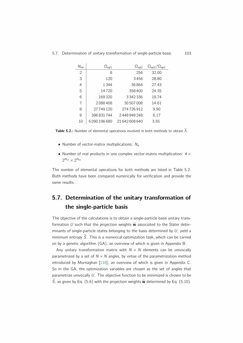
5.7. Determination of unitary transformation of single-particle basis 103
Nrel Ωop1 Ωop2 Ωop2/Ωop1
2 8 256 32.00
3 120 3 456 28.80
4 1 344 36 864 27.43
5 14 720 358 400 24.35
6 169 320 3 342 336 19.74
7 2 088 408 30 507 008 14.61
8 27 749 120 274 726 912 9.90
9 396 831 744 2 448 949 248 6.17
10 6 090 196 680 21 642 608 640 3.55
Table 5.2.: Number of elemental operations involved in both methods to obtain Λ.
• Number of vector-matrix multiplications: Ne
• Number of real products in one complex vector-matrix multiplication: 4 ×2Nrel × 2Nrel
The number of elemental operations for both methods are listed in Table 5.2.
Both methods have been compared numerically for verification and provide the
same results.
5.7. Determination of the unitary transformation ofthe single-particle basis
The objective of the calculations is to obtain a single-particle basis unitary trans-
formation U such that the projection weights w associated to the Slater deter-
minants of single-particle states belonging to the basis determined by U, yield a
minimum entropy S. This is a numerical optimization task, which can be carried
on by a genetic algorithm (GA), an overview of which is given in Appendix B.
Any unitary transformation matrix with N × N elements can be univocally
parametrized by a set of N × N angles, by virtue of the parametrization method
introduced by Murnaghan [116], an overview of which is given in Appendix C.
So in the GA, the optimization variables are chosen as the set of angles that
parametrize univocally U. The objective function to be minimized is chosen to be
S, as given by Eq. (5.6) with the projection weights w determined by Eq. (5.10).

104 Chapter 5. Correlation entropy
5.8. Identification of a truly correlated state
At first sight, a particular many-body state |ρK〉 of ρrel may appear to deviate
from being a Slater determinant, if it displays several components in the basis
Brel above a threshold of relevance, and not just one with a value close to unity.
Nonetheless, that may not be the case in the basis Brel, where this state may have
the character of a Slater determinant, and therefore is actually not a correlated
state.
In order to identify such a situation, we propose to calculate the expectation
value of the number operator ni = c†i ci in the optimized single-particle basis, with
respect to each many-body state |ρK〉 of ρrel. We find two alternative ways to
perform this calculation, which produce the same results. First, we can transform
the operators into the natural orbital basis and the state into the basis Brel, to
produce
〈ρK | ni |ρK〉 =
dim(Frel)−1∑J,L=0
Λ∗LKΛJK
Nmax−1∑j,l=0
U∗l i Uj i 〈DL| c†j cl |DJ〉 . (5.27)
As a second approach, we choose to express the state in the basis Brel, resulting
in the following expression
〈ρK | ni |ρK〉 =
dim(Frel)−1∑J,L=0
Λ∗LKΛJK 〈DL| ni |DJ〉 =
=
dim(Frel)−1∑J,L=0
Λ∗LKΛJK
dim(Frel)−1∑P,Q=0
Λ∗JP ΛLQ
⟨DP
∣∣∣ ni ∣∣∣DQ⟩ =
=
dim(Frel)−1∑J,L=0
Λ∗LKΛJK
dim(Frel)−1∑P=0
Λ∗JP ΛLP Ni
(∣∣∣DP⟩) (5.28)
where Ni(∣∣∣DP⟩) denotes the occupation number (0 or 1) of the single-particle
state i of the optimized basis with respect to the Slater determinant∣∣∣DP⟩ ∈ Brel.
Furthermore, we propose a suitable measure to check if all the expectation
values 〈ρK | ni |ρK〉 ≡ ni [K], for a given K and varying i , are close to zero or
one (Slater determinant) or if the deviate from these extreme values (correlated
state). It reads as S1[K] = −∑i
ni [K] log2 ni [K] and has an equivalent nature as

5.9. Results 105
Equilibrium Non-equilibrium
VGS (V) 0.15 0.4
VDS (V) 0 0.1
ID (nA) 0 0.167
Ne 2 ∼ 4
Nocc 0 0
Nrel 6 6
Table 5.3.: Characteristics of the equilibrium and non-equilibrium voltage points.
the single-particle-reduced entropy S1 (which is evaluated from the natural orbital
occupation numbers ξi). If all ni [K] ∈ 0, 1, a value of S1[K] = 0 follows.
5.9. Results
In case A, the statistical operator describes the state of the system as a mixture
of Slater determinants of natural orbitals. As such, the von Neumann entropy
reflects its degree of mixture. We have verified that the modified correlation
entropy ∆S is zero in this case, as expected since a mixture of Slater determinants
presents no correlation.
More interesting is case B, where the statistical operator is expressed in the
eigenbasis of the many-body Hamiltonian projected to the relevant Fock subspace.
We have analyzed two conditions, equilibrium (VDS = 0) and non-equilibrium
(VDS > 0), intermediate between atomic and Wigner regimes, corresponding to
γE = 3 and γL = 10, as specified in Sec. 4.8.2 and Table 4.2. The same system
is chosen for both cases, only varying the voltage points, as Table 5.3 shows.
The equilibrium many-body state results in a pure state (von Neumann entropy
S = 0) due to very low T , as described by the statistical operator ρrel = |ψ〉 〈ψ|,whose components are given in Table 5.4. A first look at the components indicates
that this state |ψ〉 deviates from a Slater determinant in the basis Brel of Slater
determinants of relevant natural orbitals, since there is not a single component
with a value close to unity and the rest zero. The calculation of the single-particle-
reduced entropy produces S1 = 9.126 × 10⁻², whereas the modified correlation
entropy reads as ∆S = 9.760× 10⁻¹.
On the other hand, the non-equilibrium many-body state results in a mixture of

106 Chapter 5. Correlation entropy
|DK〉 | 〈DK |ψ〉 |2
|1100000000〉 7.319546× 10⁻¹
|0011000000〉 2.232534× 10⁻¹
|1000000010〉 1.503611× 10⁻²
|0100000001〉 1.501195× 10⁻²
|0000000011〉 1.461471× 10⁻²
|0010000001〉 6.865919× 10⁻⁵
|0001000010〉 5.997900× 10⁻⁵
Table 5.4.: Pure many-body state components | 〈DK |ψ〉 |2 > 10−6 for equilibrium point.Relevant natural orbitals are shown in boldface.
four states, as reflected by the statistical operator ρrel =3∑
N=0
wN |ψN〉 〈ψN |. The
corresponding weights and the components of the eigenstates |ψN〉 are shown in
Table 5.5. One can verify that their components are closer to those corresponding
to a Slater determinant than in the equilibrium case. Nevertheless, this is a mixed
many-body state and this fact is reflected by the von Neumann entropy S = 1.173,
a value significantly larger than zero. Also, the single-particle-reduced entropy
S1 = 1.271, exhibits a higher value as compared to the equilibrium case. Indeed,
S1 accounts not only for correlation but also for mixture degree. In contrast, the
modified correlation entropy ∆S = 1.452× 10⁻² is much smaller, resembling the
fact that the eigenstates of the many-body statistical operator are very close to
Slater determinants.
The resulting ∆S for the discussed non-equilibrium case is lower than for the
discussed equilibrium case, even though in the non-equilibrium case the mixture
degree of the system’s preparation is higher than in the equilibrium case. This
stands in agreement with the idea that ∆S is indeed a measure of correlation
alone, independently of the mixture degree, in contrast to S1.
In order to analyze the degree of deviation of the many-body states |ψN〉 of ρrel
from single Slater determinants, the expectation values of the occupation numbers
ni (corresponding to optimized single-particle states, see Sec. 5.8), are shown for
the equilibrium and non-equilibrium points, in Tables 5.6 and 5.7 respectively.
Inspection of these tables shows that for the equilibrium point, 〈ψ| ni |ψ〉 deviatesfrom the extreme values 0 and 1 significantly for all six single-particle states,
indicating that the many-body state deviates from being a Slater determinant.

5.9. Results 107
w0 = 7.347524× 10⁻¹ w1 = 1.403755× 10⁻¹
|DK〉 | 〈DK |ψ0〉 |2 |DK〉 | 〈DK |ψ1〉 |2
|111100〉 9.836548× 10⁻¹ |111010〉 9.807315× 10⁻¹
|110101〉 1.231713× 10⁻² |110011〉 1.253150× 10⁻²
|111010〉 2.672775× 10⁻³ |110110〉 2.502412× 10⁻³
|001111〉 7.726548× 10⁻⁴ |111100〉 2.274014× 10⁻³
|110011〉 2.818157× 10⁻⁴ |110101〉 1.678201× 10⁻³
|100111〉 1.144070× 10⁻⁴ |111001〉 1.608453× 10⁻⁴
|011011〉 1.064737× 10⁻⁴ |101011〉 7.775216× 10⁻⁵
|111001〉 4.882806× 10⁻⁵ |011011〉 2.301173× 10⁻⁵
|101011〉 1.045020× 10⁻⁵ |011110〉 1.424845× 10⁻⁵
|010111〉 9.505482× 10⁻⁶ |101110〉 4.803740× 10⁻⁶
|110110〉 5.660192× 10⁻⁶ |010111〉 1.086428× 10⁻⁶
|011110〉 1.916602× 10⁻⁶ w3 = 1.801348× 10⁻²
|101101〉 1.571994× 10⁻⁶ |DK〉 | 〈DK |ψ3〉 |2
|011101〉 1.353062× 10⁻⁶ |110011〉 9.695261× 10⁻¹
w2 = 1.068586× 10⁻¹ |111010〉 1.377540× 10⁻²
|DK〉 | 〈DK |ψ2〉 |2 |111001〉 7.337772× 10⁻³
|110101〉 9.807050× 10⁻¹ |110110〉 6.102984× 10⁻³
|111100〉 1.265844× 10⁻² |110101〉 2.525311× 10⁻³
|110011〉 3.235242× 10⁻³ |111100〉 4.151672× 10⁻⁴
|111001〉 2.203150× 10⁻³ |101101〉 7.754029× 10⁻⁵
|111010〉 9.769919× 10⁻⁴ |011110〉 7.197020× 10⁻⁵
|010111〉 1.178670× 10⁻⁴ |101011〉 5.581797× 10⁻⁵
|101101〉 7.633732× 10⁻⁵ |011011〉 3.832239× 10⁻⁵
|110110〉 1.657535× 10⁻⁵ |100111〉 2.104038× 10⁻⁵
|011101〉 6.856518× 10⁻⁶ |001111〉 1.931576× 10⁻⁵
|100111〉 2.307765× 10⁻⁶ |010111〉 1.462401× 10⁻⁵
|011110〉 1.038164× 10⁻⁶ |101110〉 1.066728× 10⁻⁵
Table 5.5.:Mixed many-body state components | 〈DK |ψJ〉 |2 > 10−6 for non-equilibriumpoint.

108 Chapter 5. Correlation entropy
On the other hand, for the non-equilibrium point, these values are much closer
to 0 and 1. This shows that these many-body states are much closer to single
Slater determinants. These facts are reflected in the measure S1 of deviation
from single Slater determinant (see Sec. 5.8), which has a higher value in the
equilibrium case compared to the non-equilibrium case.

5.9. Results 109
S1 = 1.842036
n0 = 2.233573× 10⁻¹
n1 = 7.469910× 10⁻¹
n2 = 1.883295× 10⁻²
n3 = 7.578098× 10⁻¹
n8 = 2.233578× 10⁻¹
n9 = 2.965127× 10⁻²
Table 5.6.: 〈ψ| ni |ψ〉 and S1 for the equilibrium case. Note that for this many-bodystate, the quantities ni are neither near zero nor one, but in between. Therefore themeasure S1 is relatively high, and so is the degree of correlation.
S1[0] = 3.403052× 10⁻² S1[1] = 3.670238× 10⁻²
n0[0] = 9.995616× 10⁻¹ n0[1] = 9.986425× 10⁻¹
n1[0] = 9.991081× 10⁻¹ n1[1] = 9.999616× 10⁻¹
n2[0] = 1.849549× 10⁻³ n2[1] = 9.980165× 10⁻¹
n3[0] = 9.991022× 10⁻¹ n3[1] = 9.999206× 10⁻¹
n4[0] = 9.990541× 10⁻¹ n4[1] = 1.884835× 10⁻³
n5[0] = 1.324423× 10⁻³ n5[1] = 1.574017× 10⁻³
S1[2] = 3.789003× 10⁻² S1[3] = 1.332848× 10⁻¹
n0[2] = 1.431692× 10⁻³ n0[3] = 7.628653× 10⁻³
n1[2] = 9.998741× 10⁻¹ n1[3] = 9.998478× 10⁻¹
n2[2] = 2.166739× 10⁻³ n2[3] = 9.919029× 10⁻¹
n3[2] = 9.999182× 10⁻¹ n3[3] = 9.998045× 10⁻¹
n4[2] = 9.979671× 10⁻¹ n4[3] = 8.206616× 10⁻³
n5[2] = 9.986422× 10⁻¹ n5[3] = 9.926095× 10⁻¹
Table 5.7.: ni [K] = 〈ψK | ni |ψK〉 and S1[K] for the non-equilibrium case. Note thatthe values of the different quantities ni [K] are either very near one or very near zero,therefore the measure S1[K] is quite low for all many-body states |ψK〉. This is indicativeof low correlation.


6. Summary
In this dissertation, the multi-configurational self-consistent Green’s function
method for the simulation of non-equilibrium electronic transport in a nanowire
field-effect transistor has been augmented with new features, resulting in a new
open-source simulation package named NWFET-Lab. This package has been
the basis of the calculations performed in this work.
An adaptive numerical approach to determine a reduced non-equilibrium many-
body statistical operator for quasi-isolated electronic states within the channel of
a realistic nanowire field-effect transistor has been presented. In this approach,
the statistical operator must satisfy a set of constraints related to the single-
particle density matrix, as obtained from a non-equilibrium Green’s function self-
consistent calculation. Furthermore, since the number of constraints is in general
smaller than the number of unknowns, a form for its eigenvalues or weights that
maximizes the entropy has been chosen. As an alternative to the Slater deter-
minants of relevant natural orbitals employed in the original multi-configurational
self-consistent Green’s function implementation, the eigenstates of the projected
many-body Hamiltonian have also been used as eigenbasis of the statistical op-
erator. As an application, the onset of formation of Wigner molecules has been
discussed by means of the calculation of the electronic density–density correlation.
A new numerical determination of the correlation of the system of electrons
within the nanowire channel of the device, for pure as well as for mixed states,
has been presented. In contrast to the single-particle-reduced entropy, this so-
called “modified correlation entropy” accounts for the correlation independently
of the mixture degree of the many-body state, as given by the statistical operator
and measured by the von Neumann entropy. An analysis of these three concepts
of entropy has been performed. We compared an equilibrium pure state with
a non-equilibrium mixed state and showed that in the considered example the
modified correlation entropy was lower in the mixed state, a fact that indicates
the capability of this new entropy determination method to capture correlation
111

112 Chapter 6. Summary
beyond mixture.
The present work can be further extended in several directions. Electron–
phonon interaction can be modeled by suitable self-energies within the non-
equilibrium Green’s function formalism. Also within this formalism, the possibility
exists to describe the Coulomb interaction with a higher order approximation. The
single-band tight-binding description of the nanowire channel can be extended to
include multiple bands and inter-valley scattering by the inclusion of additional
states in the 1D single-particle localized basis. Furthermore, a better approxima-
tion than nearest neighbor hopping can be considered, as well as an alternative
derivation of the tight-binding description which takes into account more realistic
single-particle orbitals, like localized Wannier functions, and more realistic energy
bands by means, for example, of the k · p method.
As further investigations within the framework of the method employed in this
dissertation, the impact of single dopants in the channel on the performance of the
nanowire transistor can be addressed. This is a topic being actively researched
in the present by means of methods that usually do not take into account a
detailed many-body description of Coulomb interaction beyond mean-field. New
light could be thrown to such a topic, specially in regimes where few-electron
charging effects play an important role, like the Coulomb blockade regime.

Appendices
113

A. NWFET-Lab: Simulationpackage
A.1. Overview
NWFET-Lab [82] is a new simulation package with the aim to provide nanoelec-
tronics researchers with a tool by means of which to setup a NWFET system,
calculate and display its electronic transport properties. Set as one of the main
objectives of this dissertation, it spans over 30000 lines of code. Its elaboration
has been carried out with the help of a group of libraries and application program-
ming interfaces (APIs) [117, 118, 119, 120, 121, 122] in the C++ language [123]
and benefits from multithread parallel computation and 3D accelerated graph-
ics capabilities. It is an open-source, multiplatform software package that has
been shown to run under Linux and Windows operating systems. It can be re-
distributed and/or modified under the terms of the GNU General Public License
version 2 [124].
NWFET-Lab is structured in three different and interdependent modules, each
of which serves a specific purpose in the workflow of simulating electronic trans-
port in a NWFET. It is based on a jobfile which contains the list of parameters
that define the system. In order for the user to find easy configuration of these
parameters a setup module has been implemented. It provides both an interface
to edit the jobfile and also graphs to get a better idea of the characteristics of
the system.
Once the jobfile is saved to disk, it can be opened by the calculation module.
This is the module that implements the MCSCG method and took its machinery
from whiskersim [81], only to be adapted from the C programming language [125]
to C++ and augmented with new features. Quantities like the electron current
and density or the single-particle-reduced entropy are calculated by this mod-
115

116 Appendix A. NWFET-Lab: Simulation package
Figure A.1.: Screenshot of the task manager.
ule, either for a single or for a whole array of voltage points, optionally doing
the calculations in parallel if the computer provides several CPUs or a multicore
architecture. The results are output in data files.
The data files with the results of the simulation are displayed with the graphical
module. 2D graphs, 3D graphs and colormaps allow the user to easily analyze the
quantities obtained with the calculation module. Selectable axes can be used to
plot different variables against each other. If the computer provides a 3D graphics
acceleration card with a graphics processing unit (GPU), use is made of it thanks
to the OpenGL API [120].
A.2. Structure
A.2.1. Task manager
The three modules may be launched from a task manager. It is a simple interface
with a button associated to each module. Once a button is pressed the corre-
sponding module opens and the task manager is minimized. The use of the task
manager is optional, each module may be opened independently by running its
executable file.

A.2. Structure 117
A.2.2. Setup module
Running the setup module is the first step in order for the user to be able to start
a simulation. Not only does it provide access to the parameters that define the
system, but also to those that are related to the calculation algorithm itself.
The user has the option to create a new jobfile with standard parameters
given by default or to open an existing jobfile for editing it. Reading a jobfile
is accomplished by means of a parser, a tool that allows the efficient detection
of parameter tags and their corresponding values. Once this is done, the list of
parameters opens in a new window by pressing the button labeled “Edit jobfile”.
For a description of the meaning of the parameters the reader is referred to
section A.3 in this Appendix.
Another option of the setup module is the displaying of useful graphs to give a
better image of the system being setup. This can be done by pressing the button
labeled “Show graphs”. A window opens then, with four tabs on it. With the
first tab a customizable 3D view of the NWFET is displayed, with the possibility
to enable or disable drawing its various parts. The second and third tabs are
associated to 2D graphs for setting up the doping and the background potential.
These graphs are editable, the user can modify the values of each point with the
mouse. The fourth tab shows a 2D graph with the total potential profile along
the NWFET channel and selectable gate–source and drain–source voltages.
The last option is to save the jobfile, an action performed by pressing the
button labeled “Save jobfile”. Once the jobfile is saved it can be opened with the
calculation module.
A.2.3. Calculation module
The calculation module is the physical core of NWFET-Lab since it imple-
ments the MCSCG method for non-equilibrium electronic transport simulation
in NWFETs. A C++ adapted and augmented version of whiskersim [81] is used
as main calculation algorithm that depends as an input on the parameters listed
in the jobfile edited with the setup module. The user is able to load the jobfile
by pressing a button and once this is done several options can be adjusted that
affect the calculation.
The functionality of a NWFET relies on the tunning of two voltages, VGS

118 Appendix A. NWFET-Lab: Simulation package
Figure A.2.: Screenshot of the setup module.
and VDS which determine its operational regime and yield different values of its
characteristics. The calculation module can run an array of different voltage
pairs. If the number of voltage points is larger than one, the user can select
the option of performing the calculations in parallel. This is possible because
this module is programmed with parallel computing capabilities, thanks to the
OpenMP API [122]. The user can choose whether to run simultaneously several
voltage points along the VGS or the VDS axis, using for this task a selectable
number of calculation threads. Optionally, the single-particle density matrix may
be reset between points, although the algorithm performs more efficiently if the
resulting single-particle density matrix of the previous calculation point is reused
for different, close enough points. These options are available by pressing the
“Threads options” button.
Once the calculation has been started after pressing the “Start” button, the
textual output of the algorithm is displayed in the tabbed text windows that the
calculation module features. Each tab with its associated output text window
corresponds to each calculation thread. At the same time, this output is saved to
as many logfiles as threads are running for later review. The user can select which
tab to display and their text windows can be made auto-scrollable by checking
the “Autoscroll” check button.
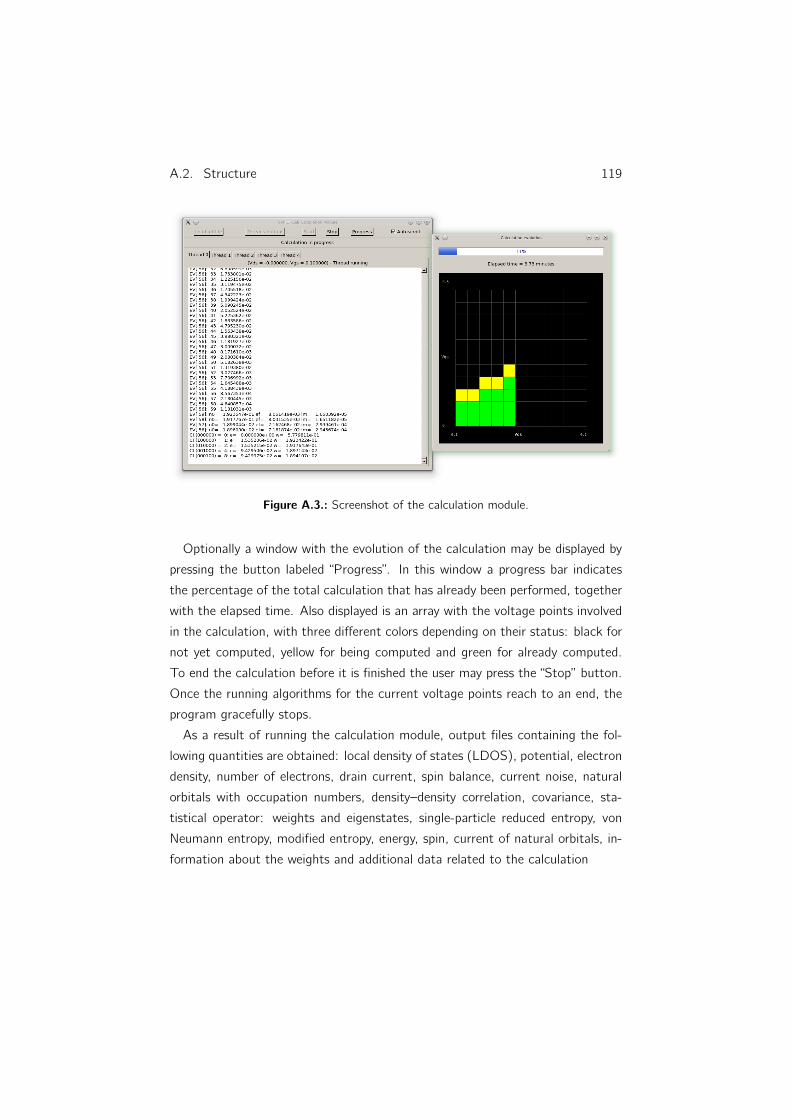
A.2. Structure 119
Figure A.3.: Screenshot of the calculation module.
Optionally a window with the evolution of the calculation may be displayed by
pressing the button labeled “Progress”. In this window a progress bar indicates
the percentage of the total calculation that has already been performed, together
with the elapsed time. Also displayed is an array with the voltage points involved
in the calculation, with three different colors depending on their status: black for
not yet computed, yellow for being computed and green for already computed.
To end the calculation before it is finished the user may press the “Stop” button.
Once the running algorithms for the current voltage points reach to an end, the
program gracefully stops.
As a result of running the calculation module, output files containing the fol-
lowing quantities are obtained: local density of states (LDOS), potential, electron
density, number of electrons, drain current, spin balance, current noise, natural
orbitals with occupation numbers, density–density correlation, covariance, sta-
tistical operator: weights and eigenstates, single-particle reduced entropy, von
Neumann entropy, modified entropy, energy, spin, current of natural orbitals, in-
formation about the weights and additional data related to the calculation

120 Appendix A. NWFET-Lab: Simulation package
A.2.4. Graphical module
The graphical module is designed with the purpose of displaying graphical views
of the several quantities obtained by the calculation module. In terms of the
number of available options it is the most complex of the four modules. The
OpenGL API is employed as the basis for the graphics and so GPUs may be used
to process them more efficiently. No external graphical representation libraries
were used, but all the details concerning graphics were programmed from scratch
by means of OpenGL.
The first thing a user can do is to open a jobfile by pressing the “Load jobfile”
button. Not only the relevant parameters for this module are read from the
jobfile, but also the output files produced by the calculation module are read.
This may take more or less time depending on the number of voltage points for
which the calculation has been performed. Immediately after the data is loaded a
floating window is opened with as many tabs available as output files were read.
If a particular data file is missing, its associated tab is disabled.
The contents of all the tabs are similar. Starting from the top, a user can find
the following groups of elements on a tab. First the “Graphs” group provides three
choice buttons to select one out of three different types of graphs: 2D graph, 3D
graph or colormap. Of these three types, the 2D graph and the colormap allow
the user to read the coordinates of every point by clicking the mouse left button.
Additionally, whenever the drain current or the single-particle-reduced entropy are
being displayed as a function of VGS and VDS in a colormap, a new window may
be opened with the electronic configurations and their weights corresponding to
the voltage point selected by clicking the mouse right button.
Next the “Axis” group comprises up to three subgroups associated to each of
the axis of the plot: X, Y and Z. The user can select which quantity to link with
each axis, given the available quantities present in the data files of each particular
tab. Some of these subgroups may be disabled if there is not enough number
of independent variables to be represented in a given type of graph. Besides, if
a 2D graph is selected the Z axis is disabled. The type of graph is restricted
according to the same criterion. The independent variables that are not linked to
an axis may be varied with the sliders present in the “Variables” group while the
plot displayed on screen is immediately updated.
The fourth group is the “Scaling” group and is associated to the scaling of the

A.2. Structure 121
Figure A.4.: Screenshot of the graphical module.
graphs. Here, minimum and maximum limit values for each of the available axis
can be entered, with the possibility to override these values and autoscale the
graph. The “Axis options” group follows which contains choice buttons to select
which transformations are performed on each of the available axis. These are:
absolute value, linear scale, logarithmic scale and arctangent scale. Whenever the
last option is chosen the user may enter the value of a factor by which to scale
the argument of the arctangent axis scaling.
Finally, the “Options” group provides several choices related to the appearance
of the graphs and its contents vary depending on the selected graph type. Com-
mon to all graph types, the user may choose between two color schemes: black
lines on a white background or white lines on a black background. For a 3D
graph the user may also choose the style of the plot: surface or mesh. For a
colormap, the color gradient used in the representation may be selected from:
thermal, rainbow, grayscale, Gaussian or positive/negative.
There is also the possibility to export the data currently being displayed to an
external data file and to export the graphs to image files, by pressing the “Export”
button. To conclude, the layout of the graphical module, consisting of the state
of all its controls, may be saved to a layout file, similar to a jobfile but concerning
only the appearance of this module. Later this file may be loaded so that the

122 Appendix A. NWFET-Lab: Simulation package
saved layout is restored.
A.3. Technical details
A.3.1. Libraries and APIs
The way NWFET-Lab presents itself to the user is not as a text-based command-
line interface but as a graphical user interface (GUI). The benefits of using a GUI
are several. It enables easy change of the parameters by making them accessible
to the user through controls of the interface. It enables also the interaction
between the external user and the internal mechanisms of the program without
the need of learning a complex command language. It makes faster and unifies
the workflow of setting up a system, calculating its characteristics and displaying
the results.
The choice of a GUI library for NWFET-Lab was guided by several consid-
erations. First of all it should be easy to learn and use. In this sense poorly
documented GUIs were discarded. The second important condition was its intru-
siveness, whether to use it would require the code to be adapted to its canons or
gave structural liberty to the programmer. This is connected to its programming
style, either procedural or object-oriented. Since the selected language to write
the software was C++ an object-oriented approach would be the best. Other
considerations included platform dependence, variety of controls, OpenGL inte-
gration, inclusion of an own window manager and 64-bit compatibility.
According to these considerations, the GUI library of choice was FOX-Toolkit
[117], a multiplatform, well-enough documented, open-source library released un-
der the GNU Lesser General Public License. There are both a FOX forum and
mailing list that were helpful whenever a question arose.
NWFET-Lab was designed from the beginning to be able to run calculations
in parallel. Two different approaches to parallel computation were assessed:
OpenMP [122] and MPI [126]. The benefits and drawbacks of each one are
summarized in the following. On the one hand, OpenMP is easier to program
and debug, its directives can be added incrementally which allows for gradual
parallelization, if desired the code can be still run serially, serial code statements
usually do not need modification and the code is easier to understand and main-
tain. On the other hand, it can be run only in shared memory computers and

A.3. Technical details 123
requires a compiler that supports it. As for MPI, although it is able to run on both
shared and distributed memory architectures and can be used on a wider range of
problems, nevertheless requires more programming changes to go from serial to
parallel version and can be harder to debug. Since shared memory computers are
more common than computing grids and our code did not need more than what
OpenMP could offer, this was the choice, which has proved to be a reliable and
efficient option.
The details concerning the graphics were implemented starting from zero, in-
stead of relying on external libraries. This allowed much control over the display
options and features. For this purpose use was made of the OpenGL API [120],
one of the most widely adopted graphics standards that produces high quality and
high performance 2D and 3D graphics regardless of operating system or window-
ing system. It is a very well documented, easy to learn API. Since by itself OpenGL
does not have the possibility to render text, the FTGL library [118] was employed
for all text-based graphics, such as labels, titles and numbers along the plot axis.
The DevIL image library [119] enabled the capturing of the plots displayed by the
graphical module and saving them into image files. Finally, the calculation and
many-body modules make use of LAPACK numerical routine libraries [121].
Links to the aforementioned libraries and APIs are presented in the following
list:
FOX-Toolkit http://www.fox-toolkit.org/
OpenMP http://openmp.org/wp/
OpenGL http://www.opengl.org/
FTGL http://sourceforge.net/apps/mediawiki/ftgl/
DevIL http://openil.sourceforge.net/
LAPACK http://www.netlib.org/lapack/
A.3.2. Parameters
To itemize and clarify the meaning of the parameters used by NWFET-Lab a list
with of all of them, together with short descriptions follows.
XXX_out Filename of the output datafile containing quantity XXX

124 Appendix A. NWFET-Lab: Simulation package
obs_XXX Indicates whether to calculate or not the observable XXX
epsilon_ch Relative dielectric constant of the nanowire channel
epsilon_ox Relative dielectric constant of the oxide
d_ch Diameter of the nanowire channel
d_ox Thickness of the oxide
l_const Screening length λ
evar_min Minimum energy for LDOS calculation
evar_max Maximum energy for LDOS calculation
devar Energy step
nevar_min Minimum energy for current noise calculation
nevar_max Maximum energy for current noise calculation
dnevar Energy step
nmax Number of orbitals in 1D nanowire channel
dom_nmax0 Maximum number of relevant single-particle states
density_dom_thres1 Minimum absolute threshold for an occupied state
density_dom_thres2 Maximum absolute threshold for an empty state
density_dom_thres3 Relative threshold for a fluctuating state
coul_empty_thres Minimum threshold for state to be included in calculations (case B)
dom_slater_dets 0 for case B, 1 for case A, 2 for case A+B
dom_wmin Minimum value for a weight below which it is considered zero
dom_imlim Maximum dissipation energy due to contacts
dom_indep_w Switches on/off the independent electron regime
a_const Lattice constant of the nanowire channel
eff_mass Effective electron mass
t_const Tight-binding hopping matrix element h2/(2m∗a2)
tc_const Contact hopping matrix element
charge_const e2/(2ε0εchA)
current_const e/h
temperature Temperature T
kt_const Thermal energy kBT
imin_vgate Site index of gate minimum limit
imax_vgate Site index of gate maximum limit
vgate0 Minimum gate–source voltage

A.3. Technical details 125
vgate1 Maximum gate–source voltage
dvgate Gate–source voltage step
vdrain0 Minimum drain–source voltage
vdrain1 Maximum drain–source voltage
dvdrain Drain–source voltage step
neq_nmin Non-equilibrium region minimum limit
neq_nmax Non-equilibrium region maximum limit
imin_npar Minimum site index for electron number count
imax_npar Maximum site index for electron number count
damp1 Self-consistency parameter
scount_min Self-consistency parameter
scount_max Self-consistency parameter
sdev_min Self-consistency parameter
dither_amp1 Self-consistency parameter
int_demin Related to the Runge-Kutta integration function.
int_demax Related to the Runge-Kutta integration function.
int_rezeps Related to the Runge-Kutta integration function.
doping Doping 1D charge density
pot0 Potential offset to band minimum
pot0_l Potential offset to band minimum within left contact
poth_l0 Potential height of left contact
pot0_r Potential offset to band minimum within right contact
poth_r0 Potential height of right contact
parallel_mode Set the voltage axis to be computed in parallel: 0 for VDS, 1 for VGS
nthreads Number of parallel threads for voltage loops
nthreads1 Number of parallel threads for case B
meanfield_rest Include mean-field interaction of the non-relevant states (case B)
meanfield_occ Include mean-field interaction of fixed occupied states (case B)
epsilon_const Optical potential
i_cur Layer of current
enable_cself Enable Coulomb self-energy
spinsplit Zeeman term
density_reset Switch on/off reset of single-particle density matrix between calculation points
hamop_diag Make many-body Hamiltonian diagonal (case B = case A)


B. Genetic algorithm
B.1. Overview
A general optimization problem consists of searching for the global optimum
solution that optimizes a specific set of objective functions in a given search
space. When considering a minimization or maximization problem, the goal is to
find the best solution that minimizes or maximizes one or more objective functions.
If the number of objective functions is greater than one, the problem is termed
multi-objective optimization. We focus here in single-objective optimization and
denote the single objective function as fitness function. These two terms are
used in the following interchangeably.
The search space is defined by the number of variables that model the sys-
tem and their limits. The fitness function has different values in each point of
the search space and in general there may exist many local minima or maxima.
These regions of the search space may constitute possible trap points of a given
numerical optimization method such as a local search technique, which for ex-
ample looks for the optimum solution using the gradient of the fitness function.
Genetic algorithms on the contrary are able to leave these local optimum points
behind, since they search in multiple directions, even if the fitness function is not
differentiable.
A genetic algorithm (GA) [104] is an optimization method inspired by Darwin’s
theory of evolution. Its ingredients are a population of chromosomes, each of
which encodes a possible solution to the problem, a set of operations performed
on the chromosomes and a fitness function. A chromosome is composed of genes
each of which encodes a variable of the problem and are defined within the limits
of the search space. Its rules are such that after every iteration the population
is expected to improve, based on the criterion defined by the fitness function for
each chromosome. Each implementation of a GA has its own peculiarities. We
127

128 Appendix B. Genetic algorithm
0. Init population: produce set of chromosomes and evaluate fitness.
1. Selection: population → mating pool.
2. Reproduction (crossover): mating pool → offspring.
3. Mutation: population → offspring.
4. Evaluate fitness of the offspring.
5. Select best chromosomes → new generation.
6. Check convergence: if converged then end, else go to 1.
Table B.1.: A typical GA.
describe a single-objective standard version and note that a specific version may
deviate in some details from it.
At the beginning the method constructs a population of chromosomes, ran-
domly or otherwise, taking care that each gene is within its domain of definition.
Then it enters into an iterative process, first selecting for reproduction a fraction
of the population that has the best fitness and constitute the mating pool. Note
that by choosing the fittest individuals the next generation should in principle be
better than the previous. Secondly comes the reproduction phase, a crossover
operation is applied between two or more randomly picked chromosomes from
the mating pool, generating new offspring. The characteristics of the parent
chromosomes are inherited by the offspring. And thirdly several randomly cho-
sen chromosomes are mutated by altering the values of their genes by a small
random amount. This adds variety to the population and avoids the algorithm
to get stuck in a local minimum or maximum. These three steps, selection, re-
production and mutation, produce a new generation which replaces the previous
population. Such algorithm is repeated until a termination criterion is satisfied.
Convergence is achieved if the fitness of the best chromosome in the population is
smaller or greater than a certain threshold value, in the case of a minimization or
maximization problem respectively, and/or if the fitness of the best chromosome
does not change appreciably between subsequent iterations. See Table B.1 for a
schematic view of a typical GA.

B.2. Chang’s genetic algorithm 129
B.2. Chang’s genetic algorithm
The GA by Chang [105] is novel because it introduces a multi-crossover formula
which makes use of three instead of the traditional two chromosomes to generate
three new ones. Let Θi represent a vector of genes or chromosome. Suppose
that three chromosomes Θ1, Θ2 and Θ3 are randomly chosen from the mating
pool to crossover and that Θ1 is the fittest of them. They define a new adjusting
direction
ΘD ≡ (Θ1 −Θ2) + (Θ1 −Θ3) = 2Θ1 −Θ2 −Θ3 (B.1)
along which all three chromosomes are changed simultaneously. If r ∈ [0, 1] is a
random number determining the crossover grade, the following multiple crossover
formulas are performedΘ1 + rΘD → Θ′1
Θ2 + rΘD → Θ′2
Θ3 + rΘD → Θ′3
(B.2)
which mean that the offspring Θ′i will be translated copies of the parents along
the direction that points to the fittest of the three.
Similarly to other GAs, the mating pool is generated by tournament selection,
but as an alternative to Chang’s original implementation this can be done by
randomly selecting in Npop rounds, t chromosomes from the total of Npop that
constitute the population and choosing the single best fit of those t for inclusion
in the mating pool, which ends up containing Npop chromosomes. The multi-
crossover operation and mutation are performed with a probability pc and pmrespectively, so that the (3 × pc)% of the mating pool undergoes reproduction
and a pm% of the population is mutated to a certain degree.


C. Parametrization of unitarymatrices
In this section we describe how to factorize any given unitary matrix as a product
of several unimodular unitary matrices which depend on a set of angles or param-
eters. This parametrization method was introduced by Murnaghan and except
for the compact expression at the end of the section, we have followed his steps
as given in Ref. [116].
An n-dimensional unitary matrix U satisfies the equation U†U = I, which implies
U−1 = U†. Because det U† = (det U)∗ it follows that det U = e iφ is a complex
number of unit modulus. Whenever det U = 1 we term U unimodular unitary
matrix.
Before describing how to parametrize an n-dimensional unitary matrix we in-
troduce the so called plane n-dimensional unimodular unitary matrices Upq(φ, σ),
which operate in the pq-plane, where q > p. They are constructed in such a way
that the diagonal terms are 1 except for (Upq)pp = (Upq)qq = cosφ and the non-
diagonal terms are 0 except for (Upq)qp = sinφ e iσ and (Upq)pq = − sinφ e−iσ.
For example, when n=3
U13(φ, σ) =
cosφ 0 − sinφ e−iσ
0 1 0
sinφ e iσ 0 cosφ
. (C.1)
Let us also define an n-dimensional diagonal matrix
D(δ1, δ2, . . . , δn) = Diag(e iδ1 , e iδ2 , . . . , e iδn) . (C.2)
We are now in a position to describe the parametrization method. We will give
only the final result, for a detailed explanation on how to arrive at it see Ref. [116].
131
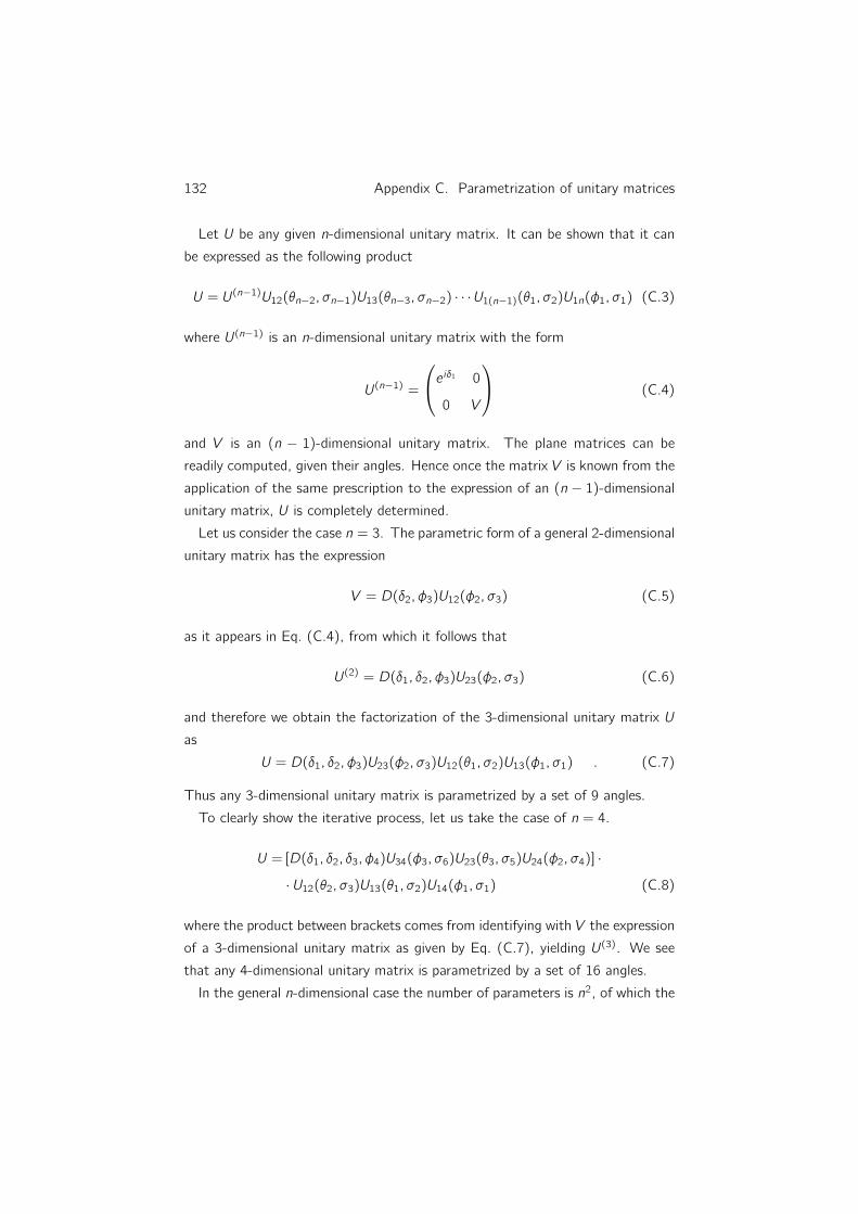
132 Appendix C. Parametrization of unitary matrices
Let U be any given n-dimensional unitary matrix. It can be shown that it can
be expressed as the following product
U = U(n−1)U12(θn−2, σn−1)U13(θn−3, σn−2) · · ·U1(n−1)(θ1, σ2)U1n(φ1, σ1) (C.3)
where U(n−1) is an n-dimensional unitary matrix with the form
U(n−1) =
e iδ1 0
0 V
(C.4)
and V is an (n − 1)-dimensional unitary matrix. The plane matrices can be
readily computed, given their angles. Hence once the matrix V is known from the
application of the same prescription to the expression of an (n − 1)-dimensional
unitary matrix, U is completely determined.
Let us consider the case n = 3. The parametric form of a general 2-dimensional
unitary matrix has the expression
V = D(δ2, φ3)U12(φ2, σ3) (C.5)
as it appears in Eq. (C.4), from which it follows that
U(2) = D(δ1, δ2, φ3)U23(φ2, σ3) (C.6)
and therefore we obtain the factorization of the 3-dimensional unitary matrix U
as
U = D(δ1, δ2, φ3)U23(φ2, σ3)U12(θ1, σ2)U13(φ1, σ1) . (C.7)
Thus any 3-dimensional unitary matrix is parametrized by a set of 9 angles.
To clearly show the iterative process, let us take the case of n = 4.
U = [D(δ1, δ2, δ3, φ4)U34(φ3, σ6)U23(θ3, σ5)U24(φ2, σ4)] ·
· U12(θ2, σ3)U13(θ1, σ2)U14(φ1, σ1) (C.8)
where the product between brackets comes from identifying with V the expression
of a 3-dimensional unitary matrix as given by Eq. (C.7), yielding U(3). We see
that any 4-dimensional unitary matrix is parametrized by a set of 16 angles.
In the general n-dimensional case the number of parameters is n2, of which the

133
n angles φ are longitude angles ∈ [−π, π[ and the n− 1 angles δ, the n(n− 1)/2
angles σ and the (n − 1)(n − 2)/2 angles θ are latitude angles ∈ [−π/2, π/2] .
The number of plane matrices Upq that appear in the factorization is n(n− 1)/2.
Any given n-dimensional unitary matrix U may be expressed in compact form
as
U = D(δ1, . . . , δn−1, φn)
1∏p=n−1
(n−1∏q=p+1
Upq(θx−p, σx)
)Upn(φp, σx) (C.9)
where the index of σ obeys the rule x = 1 + np − q − p(p − 1)/2 so that the
ordering of the angles is adequate. The first sequence product runs backwards
from higher to lower values of p, the second may not be evaluated if q > n − 1.


References
[1] M. S. Lundstrom and J. Guo. Nanoscale Transistors: Device Physics, Mod-
eling and Simulation. United States of America: Springer, 2006.
[2] G. E. Moore. “Cramming more components onto integrated circuits”. In:
Electronics 38.8 (1965).
[3] G. E. Moore. “Progress in digital integrated electronics”. In: Electron De-
vices Meeting, 1975 International 21 (1975), pp. 11–13.
[4] R. H. Dennard et al. “Design of Ion-Implanted MOSFET’s with Very Small
Physical Dimensions”. In: IEEE Journal Of Solid-State Circuits 9.5 (1974).
[5] A. Chaudhry. Fundamentals of Nanoscaled Field Effect Transistors. Springer,
2013.
[6] Process Integration, Devices, and Structures. Tech. rep. International
Technology Roadmap for Semiconductors, 2013. URL: http://www.
itrs.net/.
[7] Y. Xia et al. “One-Dimensional Nanostructures: Synthesis, Characteriza-
tion, and Applications”. In: Advanced Materials 15.5 (2003).
[8] W. Lu and C. M. Lieber. “Semiconductor nanowires”. In: Journal of Physics
D: Applied Physics 39 (2006), R387–R406.
[9] V. Schmidt et al. “Silicon Nanowires: A Review on Aspects of their Growth
and their Electrical Properties”. In: Advanced Materials 21 (2009), pp. 2681–
2702.
[10] C. M. Lieber. “Semiconductor nanowires: A platform for nanoscience and
nanotechnology”. In: MRS Bulletin 36 (2011), pp. 1052–1063.
[11] R. G. Hobbs, N. Petkov, and J. D. Holmes. “Semiconductor Nanowire
Fabrication by Bottom-Up and Top-Down Paradigms”. In: Chemistry of
Materials 24 (2012), pp. 1975–1991.
135

136 References
[12] Y. Cui et al. “High Performance Silicon Nanowire Field Effect Transistors”.
In: Nano Letters 3.2 (2003).
[13] H. Yan et al. “Programmable nanowire circuits for nanoprocessors”. In:
Nature 470 (2011), pp. 240–244.
[14] G. Larrieu and X.-L. Han. “Vertical nanowire array-based field effect tran-
sistors for ultimate scaling”. In: Nanoscale 5.2437 (2013).
[15] J. Yao et al. “Nanowire nanocomputer as a finite-state machine”. In: PNAS
111.7 (2014), pp. 2431–2435.
[16] M. S. Gudiksen et al. “Growth of nanowire superlattice structures for
nanoscale photonics and electronics”. In: Nature 415 (2002), pp. 617–
620.
[17] B. Tian, T. J. Kempa, and C. M. Lieber. “Single nanowire photovoltaics”.
In: Chemical Society Reviews 38 (2009), pp. 16–24.
[18] P. Krogstrup et al. “Single-nanowire solar cells beyond the Shockley–
Queisser limit”. In: Nature Photonics 7 (2013), pp. 306–310.
[19] F. Patolsky and C. M. Lieber. “Nanowire nanosensors”. In:Materials Today
8.4 (2005).
[20] F. Patolsky et al. “Detection, Stimulation, and Inhibition of Neuronal
Signals with High-Density Nanowire Transistor Arrays”. In: Science 313
(2006), pp. 1100–1104.
[21] F. Patolsky et al. “Nanowire-Based Nanoelectronic Devices in the Life
Sciences”. In: MRS Bulletin 32 (2007), pp. 142–149.
[22] Q. Qing et al. “Free-standing kinked nanowire transistor probes for tar-
geted intracellular recording in three dimensions”. In: Nature Nanotech-
nology 9 (2014), pp. 142–147.
[23] P.-C. Chang and J. G. Lu. “ZnO Nanowire Field-Effect Transistors”. In:
IEEE Transactions On Electron Devices 55.11 (2008), pp. 2977–2987.
[24] L. J. Brillson and Y. Lu. “ZnO Schottky barriers and Ohmic contacts”. In:
Journal of Applied Physics 109.121301 (2011).
[25] D. S. Reddy et al. “Schottky Barrier Parameters of Pd/Ti Contacts on
N-Type InP Revealed from I-V-T And C-V-T Measurements”. In: Journal
of Modern Physics 2 (2011), pp. 113–123.

References 137
[26] J. Appenzeller et al. “Toward Nanowire Electronics”. In: IEEE Transactions
On Electron Devices 55.11 (2008).
[27] C. P. Auth and J. D. Plummer. “Scaling Theory for Cylindrical, Fully-
Depleted, Surrounding-Gate MOSFET’s”. In: IEEE Electron Device Let-
ters 18.2 (1997).
[28] G. T. Kim et al. “Field-effect transistor made of individual V2O5 nanofibers”.
In: Applied Physics Letters 76.14 (2000).
[29] X. Duan et al. “ Indium phosphide nanowires as building blocks for nanoscale
electronic and optoelectronic devices”. In: Nature 409 (2001), pp. 66–69.
[30] J. Xiang et al. “Ge/Si nanowire heterostructures as high-performance
field-effect transistors”. In: Nature 441 (2006), pp. 489–493.
[31] A. I. Hochbaum et al. “Controlled Growth of Si Nanowire Arrays for Device
Integration”. In: Nano Letters 5.3 (2005).
[32] E. Latu-Romain et al. “A generic approach for vertical integration of
nanowires”. In: Nanotechnology 19.345304 (2008).
[33] Y. Huang et al. “Directed Assembly of One-Dimensional Nanostructures
into Functional Networks”. In: Science 291.5504 (2001).
[34] S. E. Laux, A. Kumar, and M. V. Fischetti. “Analysis of quantum ballistic
electron transport in ultrasmall silicon devices including space-charge and
geometric effects”. In: Journal of Applied Physics 95.10 (2004), pp. 5545–
5582.
[35] T. J. Walls and K. K. Likharev. “Two-dimensional quantum effects in
"ultimate" nanoscale metal-oxide-semiconductor field-effect transistors”.
In: Journal of Applied Physics 104.124307 (2008).
[36] M. Nedjalkov et al. “A Wigner equation with quantum electron-phonon
interaction”. In: Microelectronic Engineering 63 (2002), pp. 199–203.
[37] R. Gebauer and R. Car. “Kinetic theory of quantum transport at the
nanoscale”. In: Physical Review B 70.125324 (2004).
[38] M. V. Fischetti. “Master-equation approach to the study of electronic
transport in small semiconductor devices”. In: Physical Review B 59.7
(1999).
138 References
[39] S. Datta. “Nanoscale device modeling: the Green’s function method”. In:
Superlattices and Microstructures 28.4 (2000).
[40] P. Danielewicz. “Quantum Theory of Nonequilibrium Processes, I”. In:
Annals of Physics 152 (1984), pp. 239–304.
[41] S. Datta. Electronic Transport in Mesoscopic Systems. Cambridge Uni-
versity Press, 1999.
[42] J. Rammer. Quantum Field Theory of Non-Equilibrium States. Cambridge
University Press, 2007.
[43] H. Haug and A.-P. Jauho. Quantum Kinetics in Transport and Optics of
Semiconductors. Springer, 2008.
[44] R. A. Jishi. Feynman Diagram Techniques in Condensed Matter Physics.
Cambridge University Press, 2013.
[45] K. M. Indlekofer, J. Knoch, and J. Appenzeller. “Quantum kinetic de-
scription of Coulomb effects in one-dimensional nanoscale transistors”. In:
Physical Review B 72.125308 (2005).
[46] K. M. Indlekofer, J. Knoch, and J. Appenzeller. “Understanding Coulomb
Effects in Nanoscale Schottky-barrier-FETs”. In: IEEE Transactions On
Electron Devices 54.6 (2007).
[47] H. Haken.Quantum Field Theory of Solids: an Introduction. North-Holland,
1983.
[48] W. Schäfer and M. Wegener. Semiconductor Optics and Transport Phe-
nomena. Springer, 2002.
[49] G. Stefanucci and R. van Leeuwen. Nonequilibrium Many-Body Theory of
Quantum Systems. Cambridge University Press, 2013.
[50] J. Maciejko. An Introduction to NonequilibriumMany-Body Theory. Springer,
2007.
[51] K. M. Indlekofer. Introduction to the Non-Equilibrium Green’s Function
Formalism for the Simulation of Nanoelectronic Devices. Tech. rep. IMtech,
Hochschule RheinMain - University of Applied Sciences, Germany, 2013.
[52] R. Venugopal et al. “Simulating quantum transport in nanoscale transis-
tors: Real versus mode-space approaches”. In: Journal of Applied Physics
92.7 (2002).
References 139
[53] R. Lake et al. “Single and multiband modeling of quantum electron trans-
port through layered semiconductor devices”. In: Journal of Applied Physics
81.12 (1997), pp. 7845–7869.
[54] A. Svizhenko et al. “Two-dimensional quantum mechanical modeling of
nanotransistors”. In: Journal of Applied Physics 91.4 (2002), pp. 2343–
2354.
[55] C. Rivas and R. Lake. “Non-equilibrium Green function implementation
of boundary conditions for full band simulations of substrate-nanowire
structures”. In: Physica Status Solidi (B) 239.1 (2003), pp. 94–102.
[56] D. Mamaluy, M. Sabathil, and P. Vogl. “Efficient method for the calcula-
tion of ballistic quantum transport”. In: Journal of Applied Physics 93.8
(2003), pp. 4628–4633.
[57] D. Mamaluy et al. “Contact block reduction method for ballistic trans-
port and carrier densities of open nanostructures”. In: Physical Review B
71.245321 (2005).
[58] S. Birner et al. “Ballistic quantum transport using the contact block reduc-
tion (CBR) method”. In: Journal of Computational Electronics 8 (2009),
pp. 267–286.
[59] J. Wang, E. Polizzi, and M. Lundstrom. “A three-dimensional quantum
simulation of silicon nanowire transistors with the effective-mass aproxi-
mation”. In: Journal of Applied Physics 96.4 (2004), pp. 2192–2203.
[60] E. Polizzi and N. Ben Abdallah. “Subband decomposition approach for the
simulation of quantum electron transport in nanostructures”. In: Journal
of Computational Physics 202 (2005), pp. 150–180.
[61] Y. M. Sabry, T. M. Abdolkader, and W. F. Farouk. “Uncoupled mode-
space simulation validity for double gate MOSFETs”. In: International
Conference on Microelectronics. 2007, pp. 351–354.
[62] D. Selim et al. “Rapid and Efficient Method for Numerical Quantum Me-
chanical Simulation of Gate-All-Around Nanowire Transistors”. In: Inter-
national Conference on Microelectronics. 2012, pp. 229–232.
[63] H. Takeda and N. Mori. “Mode-Coupling Effects in Non-Equilibrium Green’s
Function Device Simulation”. In: Japanese Journal of Applied Physics
44.4B (2005), pp. 2664–2668.

140 References
[64] M. Luisier, A. Schenk, and W. Fichtner. “Quantum transport in two-
and three-dimensional nanoscale transistors: Coupled mode effects in the
nonequilibrium Green’s function formalism”. In: Journal of Applied Physics
100.043713 (2006).
[65] A. Martinez et al. “3-D Nonequilibrium Green’s Function Simulation of
Nonperturbative Scattering From Discrete Dopants in the Source and
Drain of a Silicon Nanowire Transistor”. In: IEEE Transactions On Nan-
otechnology 8.5 (2009), pp. 603–610.
[66] B. C. Johnson et al. “Darin current modulation in an nanoscale field-effect-
transistor channel by single dopant implantation”. In: Applied Physics Let-
ters 96.264102 (2010).
[67] A. Martinez et al. “NEGF simulations of a junctionless Si gate-all-around
nanowire transistor with discrete dopants”. In: Solid-State Electronics 71
(2012), pp. 101–105.
[68] M. Aldegunde, A. Martinez, and J. R. Barker. “Study of Discrete Doping-
Induced Variability in Junctionless Nanowire MOSFETs Using Dissipative
Quantum Transport Simulations”. In: IEEE Electron Device Letters 33.2
(2012), pp. 194–196.
[69] N. D. Akhavan et al. “ Influence of discrete dopant on quantum trans-
port in silicon nanowire transistors”. In: Solid-State Electronics 70 (2012),
pp. 92–100.
[70] V. P. Georgiev, E. A. Towie, and A. Asenov. “Impact of Precisely Po-
sitioned Dopants on the Performance of an Ultimate Silicon Nanowire
Transistor: A Full Three-Dimensional NEGF Simulation Study”. In: IEEE
Transactions On Electron Devices 60.3 (2013).
[71] N. D. Akhavan et al. “Discrete Dopant Impurity Scattering in p-Channel
Silicon Nanowire Transistors: A k ·p Approach”. In: IEEE Transactions On
Electron Devices 61.2 (2014), pp. 386–393.
[72] C. Buran et al. “Three-Dimensional Real-Space Simulation of Surface
Roughness in Silicon Nanowire FETs”. In: IEEE Transactions On Electron
Devices 56.10 (2009).

References 141
[73] A. Martinez et al. “Variability in Si Nanowire MOSFETs Due to the Com-
bined Effect of Interface Roughness and Random Dopants: A Fully Three-
Dimensional NEGF Simulation Study”. In: IEEE Transactions On Electron
Devices 57.7 (2010).
[74] A. Cresti et al. “A Comparative Study of Surface-Roughness-Induced Vari-
ability in Silicon Nanowire and Double-Gate FETs”. In: IEEE Transactions
On Electron Devices 58.8 (2011), pp. 2274–2281.
[75] V. P. Georgiev, E. A. Towie, and A. Asenov. “Interactions Between Pre-
cisely Placed Dopants and Interface Roughness in Silicon Nanowire Tran-
sistors: Full 3-D NEGF Simulation Study”. In: SISPAD 2013. 2013.
[76] F. G. Pikus and K. K. Likharev. “Nanoscale field-effect transistors: An
ultimate size analysis”. In: Applied Physics Letters 71.25 (1997).
[77] E. N. Economou. Green’s Functions in Quantum Physics. Springer, 2006.
[78] S. Adachi. Physical Properties of III-V Semiconductor Compounds: InP,
InAs, GaAs, GaP, InGaAs, and InGaAsP. New York: John Wiley & Sons,
1992.
[79] P.-O. Löwdin. “Quantum Theory of Many-Particle Systems. I. Physical
Interpretations by Means of Density Matrices, Natural Spin-Orbitals, and
Convergence Problems in the Method of Configuration Interaction”. In:
Physical Review 97.6 (1955).
[80] E. R. Davidson. “Properties and Uses of Natural Orbitals”. In: Reviews of
Modern Physics 44.3 (1972).
[81] K. M. Indlekofer. whiskersim. 2011. URL: http://sourceforge.net/
projects/whiskersim/.
[82] J. M. Castelo and K. M. Indlekofer. NWFET-Lab. 2014. URL: http:
//sourceforge.net/projects/nwfetlab/.
[83] K. M. Indlekofer. Diploma Thesis. RWTH Aachen, 1996.
[84] P. N. Racec, E. R. Racec, and H. Neidhardt. “Evanescent channels and
scattering in cylindrical nanowire heterostructures”. In: Physical Review B
79.155305 (2009).

142 References
[85] Z. Fan and J. G. Lu. “Zinc Oxide Nanostructures: Synthesis and Prop-
erties”. In: Journal of Nanoscience and Nanotechnology 5.10 (2005),
pp. 1561–1573.
[86] M. A. Kastner. “The single-electron transistor”. In: Reviews of Modern
Physics 64.3 (1992).
[87] H. van Houten et al. “Single Charge Tunneling”. In: NATO ASI Series
B294, New York: Plenum 167 (1992).
[88] K. K. Likharev. “Single-Electron Devices and Their Applications”. In: Pro-
ceedings of the IEEE 87.4 (1999).
[89] L. P. Kouwenhoven, D. G. Austing, and S. Tarucha. “Few-electron quan-
tum dots”. In: Reports on Progress in Physics 64 (2001), pp. 701–736.
[90] W. Tai-hong, L. Hong-wei, and Z. Jun-ming. “Coulomb blockade oscilla-
tions of Si single-electron transistors”. In: Chinese Physics 10.9 (2001),
pp. 844–846.
[91] S. De Franceschi et al. “Single-electron tunneling in InP nanowires”. In:
Applied Physics Letters 83.2 (2003).
[92] M. T. Björk et al. “Few-Electron Quantum Dots in Nanowires”. In: Nano
Letters 4.9 (2004), pp. 1621–1625.
[93] K. H. Cho et al. “Observation of Single Electron Tunneling and Ballistic
Transport in Twin Silicon Nanowire MOSFETs (TSNWFETs) Fabricated
by Top-Down CMOS Process”. In: Electron Devices Meeting, 2006. IEDM
’06. International. Dec. 2006, pp. 1–4.
[94] S. Hershfield. “Reformulation of Steady State Nonequilibrium Quantum
Statistical Mechanics”. In: Physical Review Letters 70.14 (1993).
[95] P. Bokes and R. W. Godby. “Maximum-entropy theory of steady-state
quantum transport”. In: Physical Review B 68.125414 (2003).
[96] A. Dhar, K. Saito, and P. Hänggi. “Nonequilibrium density-matrix descrip-
tion of steady-state quantum transport”. In: Physical Review E 85.011126
(2012).
[97] H. Ness. “Nonequilibrium density matrix for quantum transport: Hershfield
approach as a McLennan-Zubarev form of the statistical operator”. In:
Physical Review E 88.022121 (2013).

References 143
[98] J. M. Castelo and K. M. Indlekofer. “Numerical determination of the
non-equilibrium many-body statistical operator for a nanowire-based field-
effect transistor”. In: Deutsche Physikalische Gesellschaft. Poster presen-
tation. Dresden, 2014.
[99] J. M. Castelo and K. M. Indlekofer. “Numerical determination of a non-
equilibrium many-body statistical operator for quasi-bound electrons in a
gated nanowire system”. In: arXiv:1406.4312v1 [cond-mat.mes-hall] (2014).
[100] J. M. Castelo and K. M. Indlekofer. “Modified correlation entropy of
a gated nanowire system described by a numerically determined non-
equilibrium many-body statistical operator”. In: Physica Status Solidi (B)
(2015). DOI: 10.1002/pssb.201552174.
[101] K. M. Indlekofer. newbpotcoul. 2011. URL: http://sourceforge.net/
projects/newbpotcoul/.
[102] A. Berera. Notes for Senior Honours/Integrated Masters: Statistical Physics,
Section 2. School of Physics and Astronomy, University of Edinburgh.
2012.
[103] K. M. Indlekofer. Private communication. 2013.
[104] R. L. Haupt and S. E. Haupt. Practical Genetic Algorithms. John Wiley
& Sons, Inc., 2004.
[105] W.-D. Chang. “An improved real-coded genetic algorithm for parameters
estimation of nonlinear systems”. In: Mechanical Systems and Signal Pro-
cessing 20 (2006), pp. 236–246.
[106] J. J. Sakurai. Modern Quantum Mechanics. Addison-Wesley, 2011.
[107] P. Ziesche. “Correlation Strength and Information Entropy”. In: Interna-
tional Journal of Quantum Chemistry 56 (1995), pp. 363–369.
[108] R. O. Esquivel et al. “Physical interpretation of information entropy: Nu-
merical evidence of the Collins conjecture”. In: Physical Review A 54.1
(1996).
[109] P. Ziesche et al. “Two-site Hubbard model, the Bardeen-Cooper-Schrieffer
model, and the concept of correlation entropy”. In: Physical Review B
55.16 (1997).

144 References
[110] P. Gersdorf et al. “Correlation Entropy of the H2 Molecule”. In: Interna-
tional Journal of Quantum Chemistry 61 (1997), pp. 935–941.
[111] K. M. Indlekofer and J. M. Castelo. “On The Correlation Entropy of
Discrete Nanoelectronic Systems”. In: Annales Universitatis Scientiarum
Budapestinensis de Rolando Eötvös Nominatae, Sectio Computatorica 39
(2013), pp. 149–159.
[112] J. M. Castelo, K. M. Indlekofer, and J. Malindretos. “On the single-
particle-reduced entropy of a gated nanowire system in the Coulomb block-
ade regime”. In: Physica Status Solidi RRL 7.10 (2013), pp. 907–910.
[113] A. D. Gottlieb and N. J. Mauser. “New Measure of Electron Correlation”.
In: Physical Review Letters 96.123003 (2005).
[114] K. Byczuk et al. “Quantification of Correlations in QuantumMany-Particle
Systems”. In: Physical Review Letters 108.087004 (2012).
[115] A. Wehrl. “General properties of entropy”. In: Reviews of Modern Physics
50.2 (1978), pp. 221–260.
[116] F. D. Murnaghan. The Unitary And Rotation Groups. Washington, D. C.:
Spartan books, 1962.
[117] FOX Toolkit. 2014. URL: http://www.fox-toolkit.org/.
[118] FTGL. 2013. URL: http://sourceforge.net/projects/ftgl/.
[119] DevIL. 2014. URL: http://openil.sourceforge.net/.
[120] R. S. Wright Jr., B. Lipchak, and N. Haemel. OpenGL superbible: com-
prehensive tutorial and reference. Addison-Wesley, 2007.
[121] E. Anderson et al. LAPACK User’s Guide. SIAM, 1999.
[122] R. Chandra et al. Parallel Programming in OpenMP. Morgan Kaufmann
Publishers, 2001.
[123] B. Eckel. Thinking in C++: Introduction to Standard C++. Prentice Hall,
2000.
[124] GNU General Public License, version 2. 1991. URL: http://www.gnu.
org/licenses/gpl-2.0.html.
[125] K. N. King. C Programming: A Modern Approach. W. W. Norton &
Company, 2008.

References 145
[126] W. Gropp, E. Lusk, and A. Skjellum. Using MPI: Portable Parallel Pro-
gramming with the Message Passing Interface. The MIT Press, 1999.