Telescope optics

Jim BurgeCollege of Optical Sciences

University of Arizona

• History of telescopes• Types of telescopes• Astronomical telescope instrumentation• Modern telescopes

Telescope optical configuration

Early refractors:Galileo (Lippershey) 1609Kepler 1645

Early reflector designs:Mersenne 1636Gregory 1663Cassegrain 1672

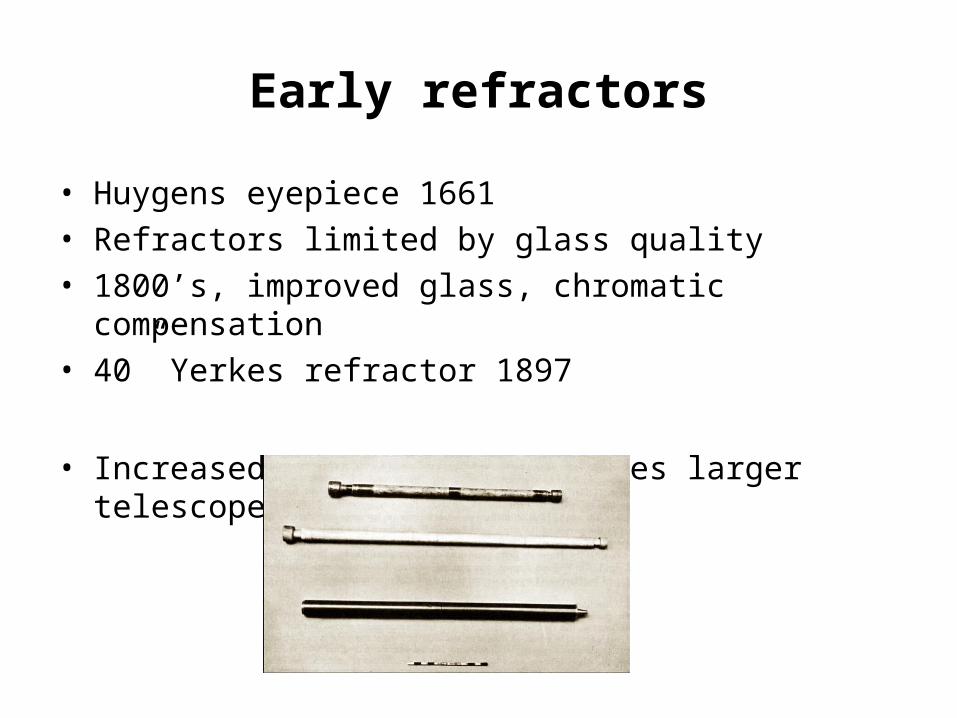
Early refractors

• Huygens eyepiece 1661• Refractors limited by glass quality• 1800’s, improved glass, chromatic compensation• 40” Yerkes refractor 1897

• Increased sensitivity requires larger telescopes

• King Fig 125

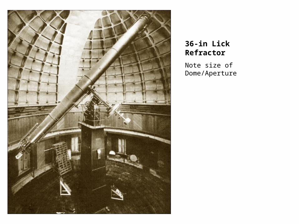
36-in Lick Refractor

Note size of Dome/Aperture

40” Yerkes refractor (1897)

Newtonian Telescope 1668

Optical design does not satisfy the sine condition – aberration of coma limits the field of view

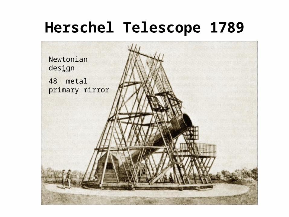
Herschel Telescope 1789

• Wilson Fig 1.11Newtonian design

48” metal primary mirror

Rosse Telescope 1845

• Wilson Fig 5.3Newtonian design

72” metal primary mirror

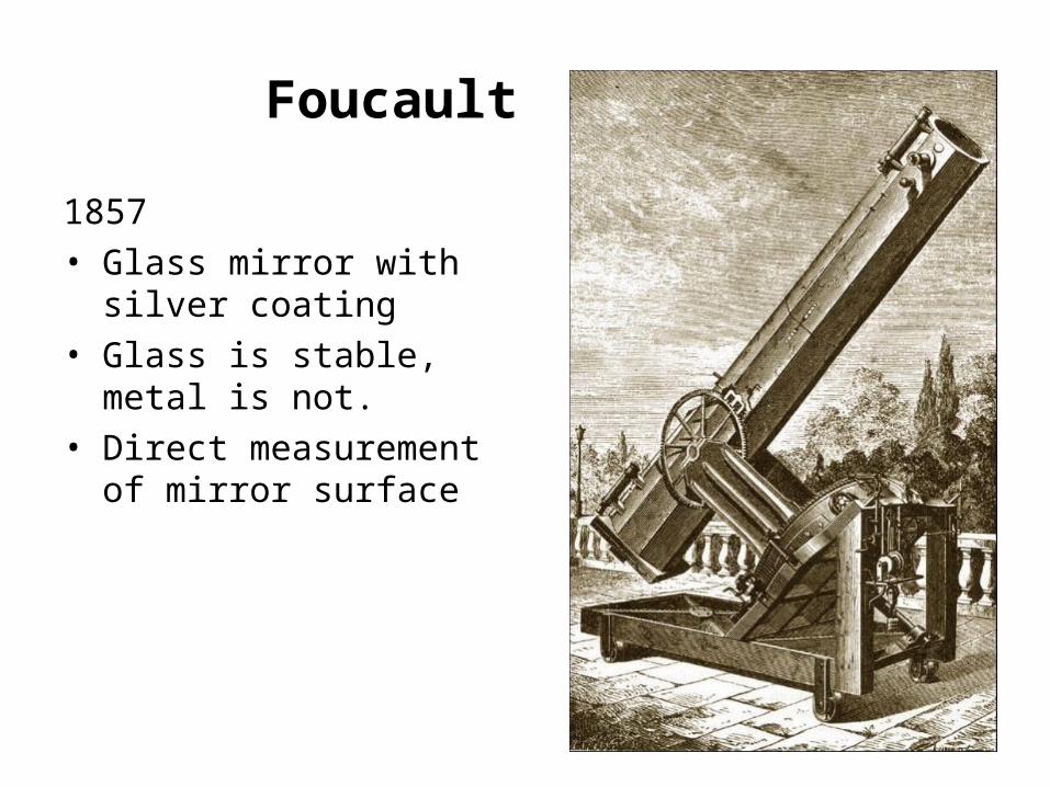
Foucault

1857• Glass mirror with

silver coating• Glass is stable,

metal is not.• Direct measurement

of mirror surface

Wilson 5.8

Mt. Wilson100” Hooker telescope (1917)

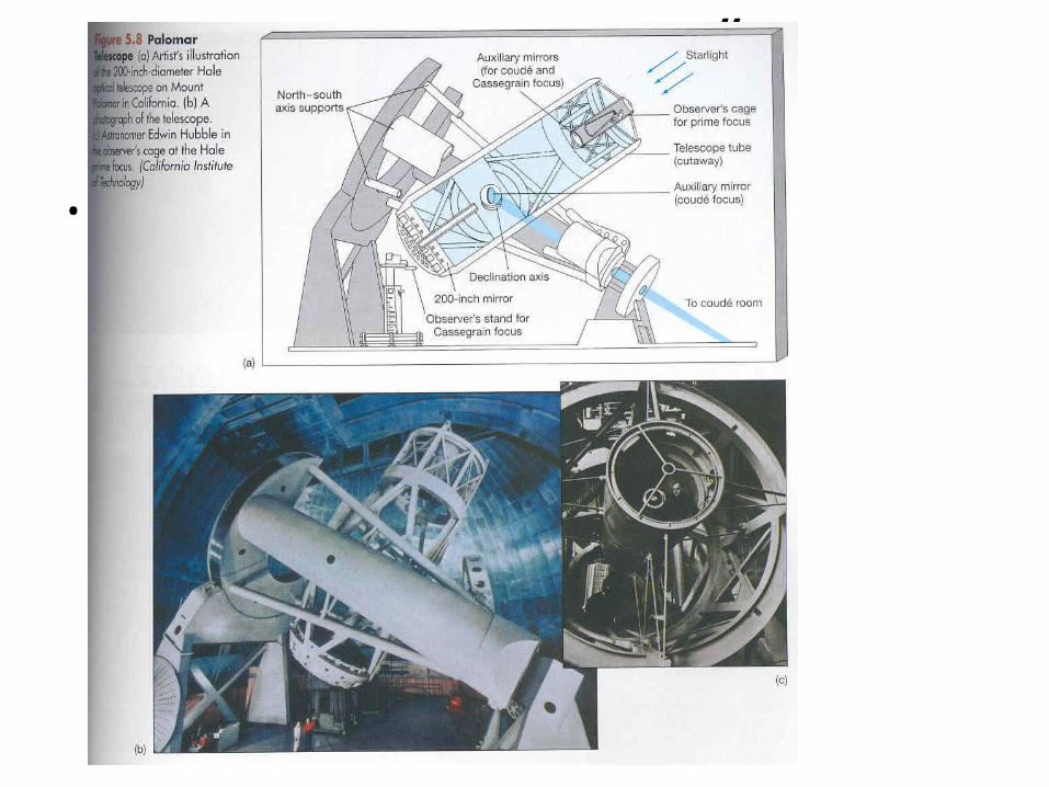
Palomar 200”

• Wilson, Fig 5.16, 5.17

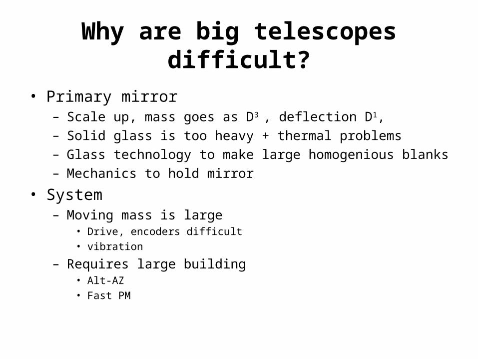
Why are big telescopes difficult?

• Primary mirror – Scale up, mass goes as D3 , deflection D1, – Solid glass is too heavy + thermal problems– Glass technology to make large homogenious blanks– Mechanics to hold mirror

• System– Moving mass is large

• Drive, encoders difficult• vibration

– Requires large building• Alt-AZ• Fast PM

Reflective telescope designs

• Cassegrain and Gregorian (add field correcting lenses)• Parabola with prime focus corrector• Dall Kirkham (Coma city)• Ritchey-Chretien – fixes coma• Couder – aplanat, ,anastigmat, diffiicult geometry• Bouwers – limited to slow telescopes by 5th order SA• Schmidt – limited by spherochromatism• Maksutov – • Solid Schmidt• Schmidt Cassegrain• Maksutov Cassegrain• Three mirror anastigmats

Equatorial mount

Polar axis

Declination axis(Note the Coude path)

Polar axis is aligned to the Earth’s axis of rotation

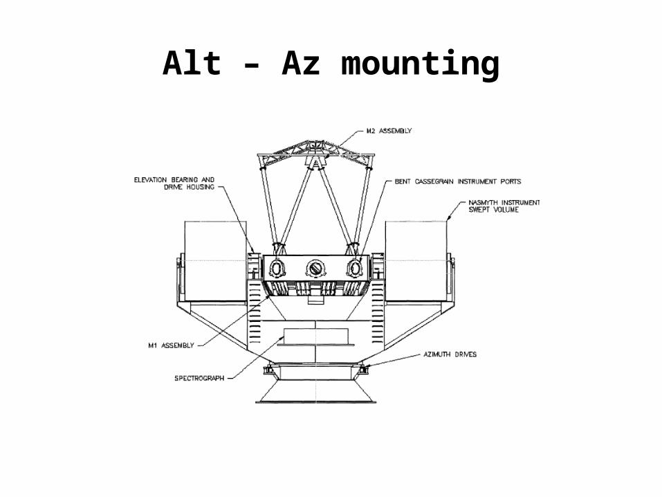
Alt – Az mounting

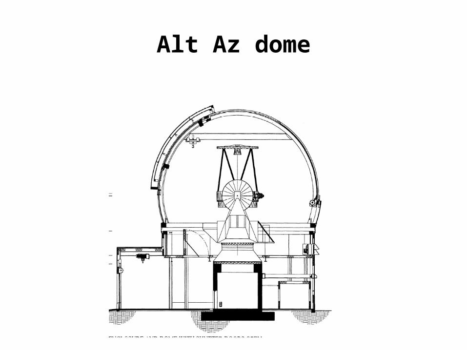
Alt Az dome

Prime focus

Wide field (>1°)

Lenses correct field aberrations from primary

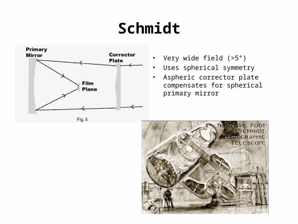
Schmidt

• Very wide field (>5°)• Uses spherical symmetry• Aspheric corrector plate compensates

for spherical primary mirror

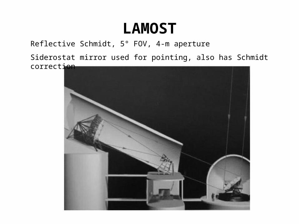
LAMOSTReflective Schmidt, 5° FOV, 4-m aperture

Siderostat mirror used for pointing, also has Schmidt correction

Solid Schmidt

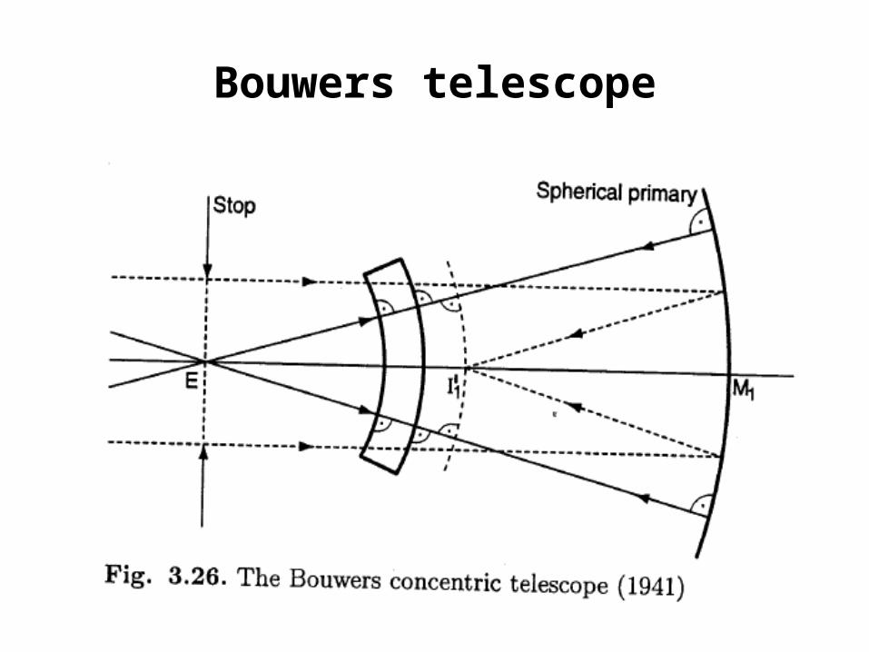
Bouwers telescope

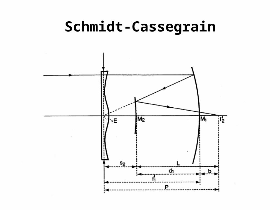
Schmidt-Cassegrain

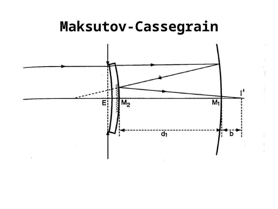
Maksutov-Cassegrain

HET, SALT

Arecibo300 m fixed spherical dish

Receiver and correction optics and moved

Couder aplanatic anastigmat

• Aplanatic – coma is corrected by satisfying the sine condition• Anastigmatic – astigmatism is balanced by the two mirrors

Hubble Space Telescope• Ritchey-Chretien design• Aplanatic – coma is corrected by

satisfying the sine condition– Primary mirror is not quite paraboloidal– Secondary is hyperboloid

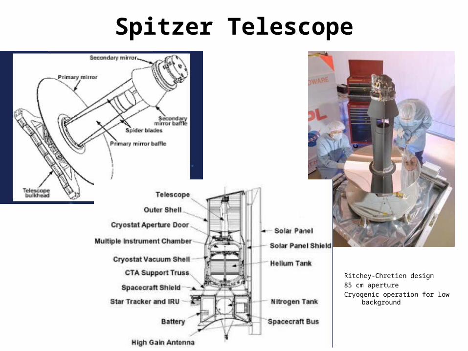
Spitzer Telescope

Ritchey-Chretien design

85 cm aperture

Cryogenic operation for low background

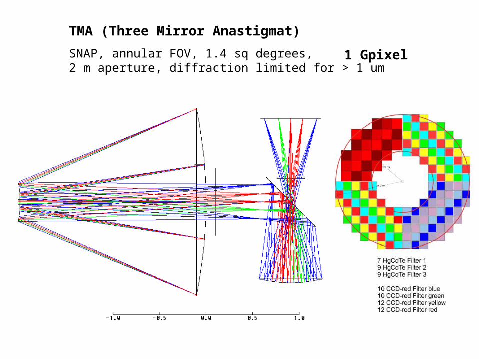
TMA (Three Mirror Anastigmat)

SNAP, annular FOV, 1.4 sq degrees, 2 m aperture, diffraction limited for > 1 um

1 Gpixel

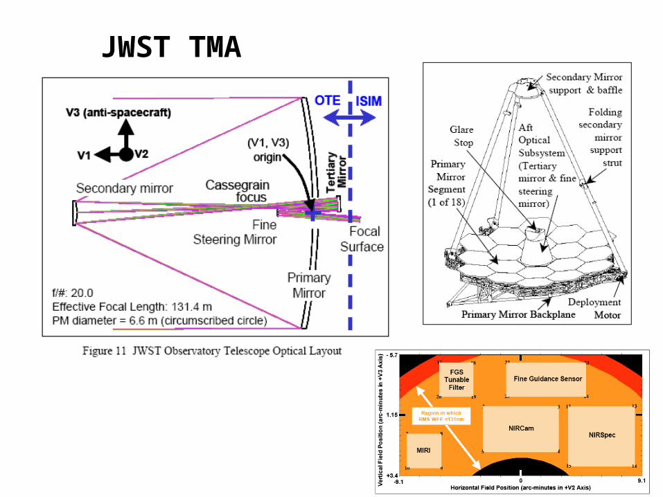
JWST TMA

James Webb Space Telescope

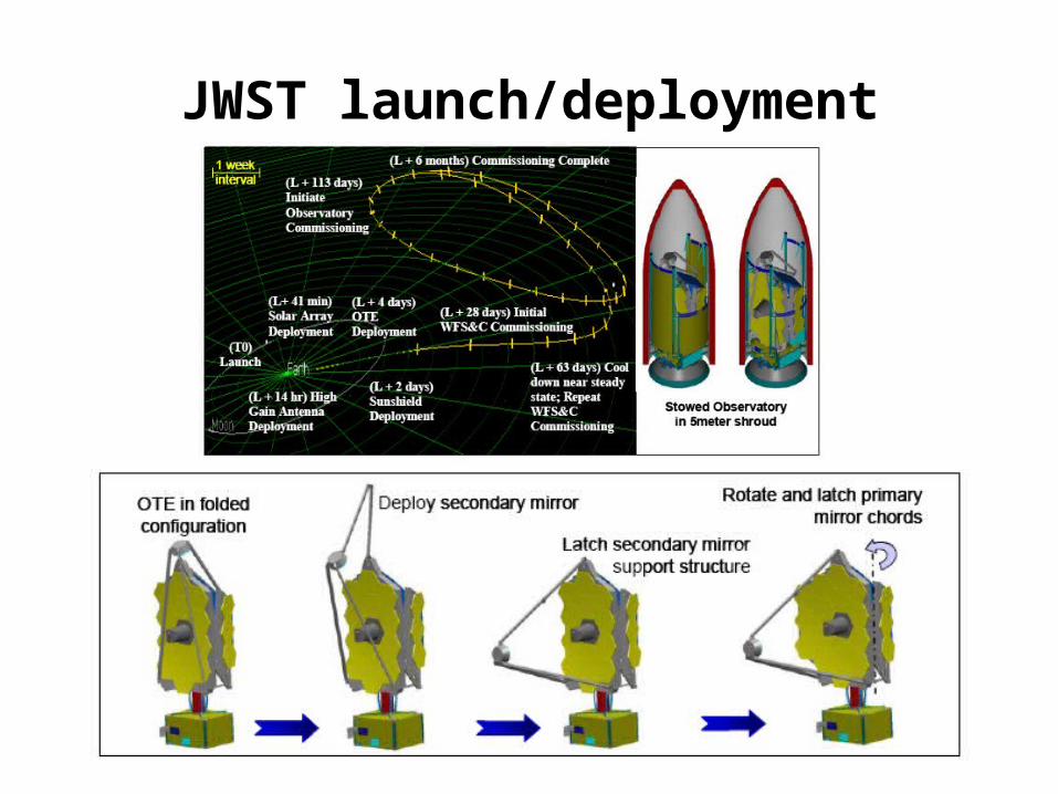
JWST launch/deployment

Historical use of telescopes

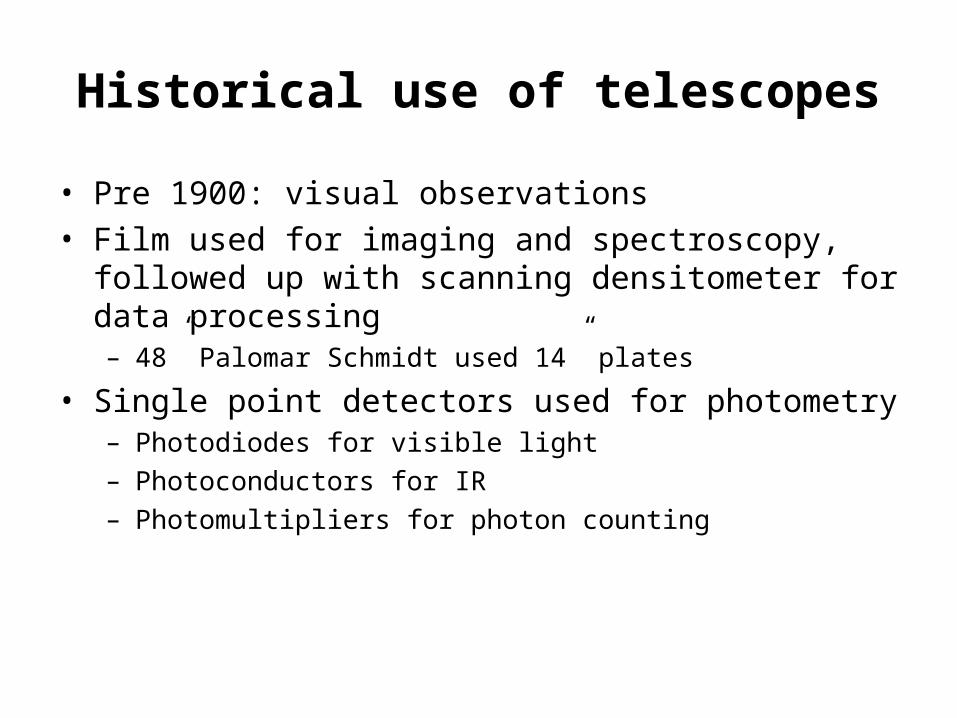
• Pre 1900: visual observations• Film used for imaging and spectroscopy, followed up

with scanning densitometer for data processing– 48” Palomar Schmidt used 14” plates

• Single point detectors used for photometry– Photodiodes for visible light– Photoconductors for IR – Photomultipliers for photon counting

Instrumentation

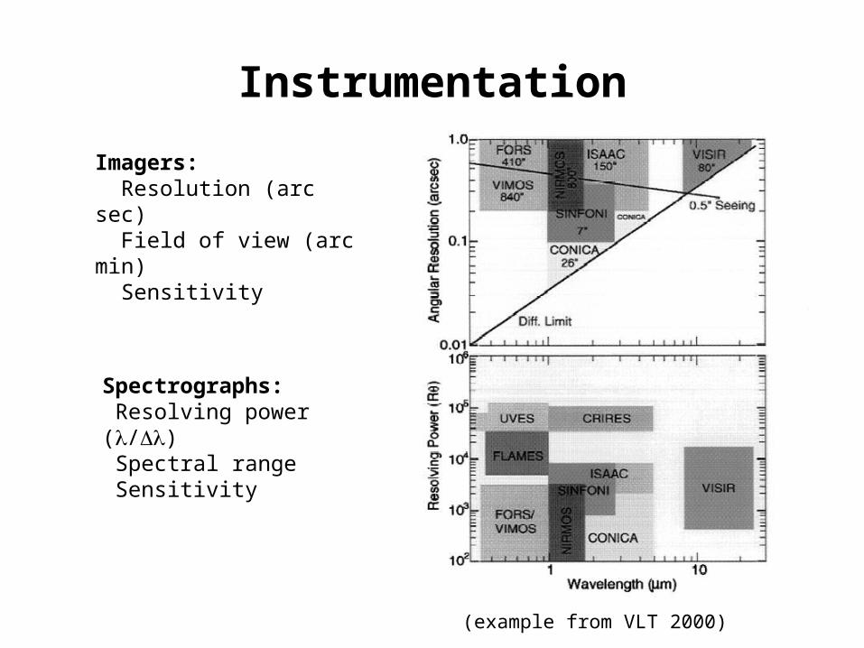
Imagers: Resolution (arc sec) Field of view (arc min) Sensitivity

Spectrographs: Resolving power (/) Spectral range Sensitivity

(example from VLT 2000)

Imaging

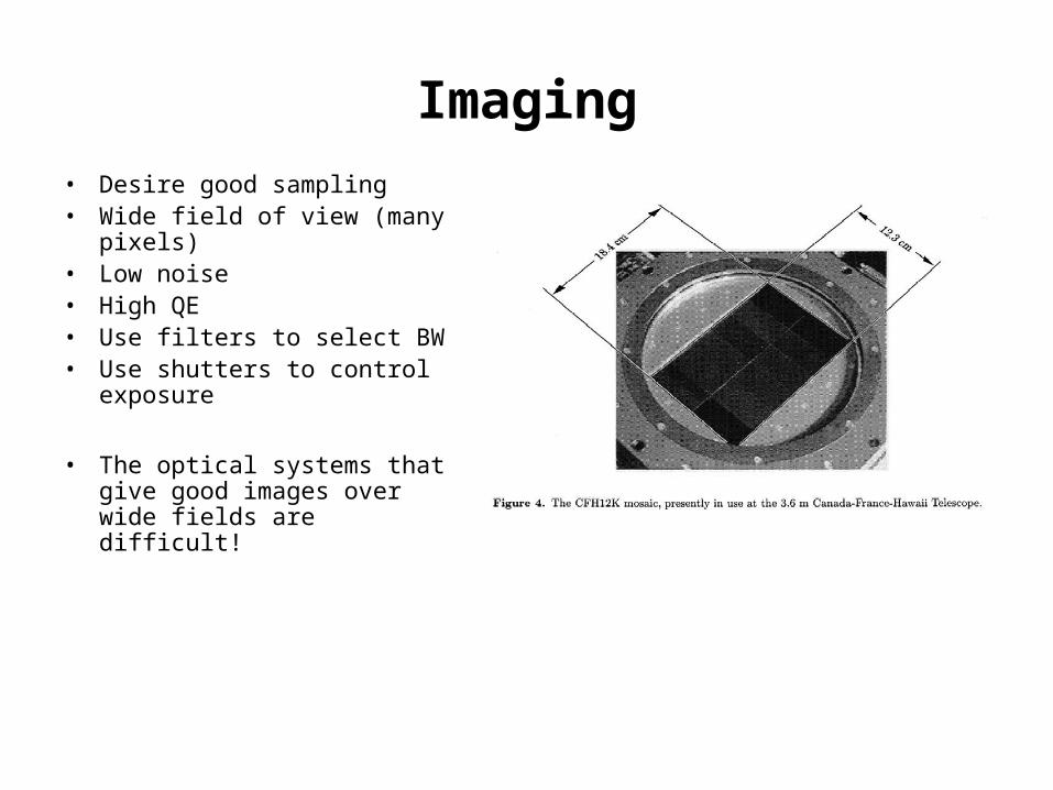
• Desire good sampling• Wide field of view (many

pixels)• Low noise• High QE• Use filters to select BW• Use shutters to control

exposure

• The optical systems that give good images over wide fields are difficult!

Revolution in data collection

CCD detectors

Many pixels (7k x 9k at Steward)

Data goes straight into the computer

QE > 90%

Read noise ~ 1 electron

Used in imagers and spectrographs

Arrays of arraysMMT f/5 focus gives 24'x24' field

36 CCDs with 2048x4608 pixels

SDSS

LSST

LSST Optical Layout

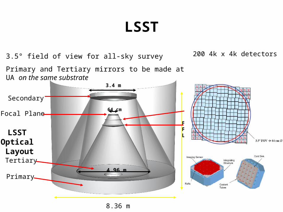
8.36 m

6.28 m

4.96 m

3.4 m

64 cm

Primary

Secondary

Tertiary

Focal Plane Filters

Field FlatteningLens

3.5° field of view for all-sky survey

Primary and Tertiary mirrors to be made at UA on the same substrate

200 4k x 4k detectors

Spectrographs

Echelle spectrograph

Cross-dispersed Echelle spectrographs

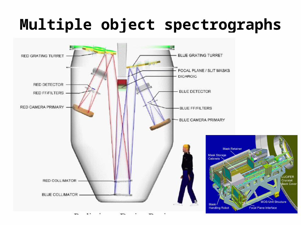
Multiple object spectrographs

Fiber coupled spectrographs

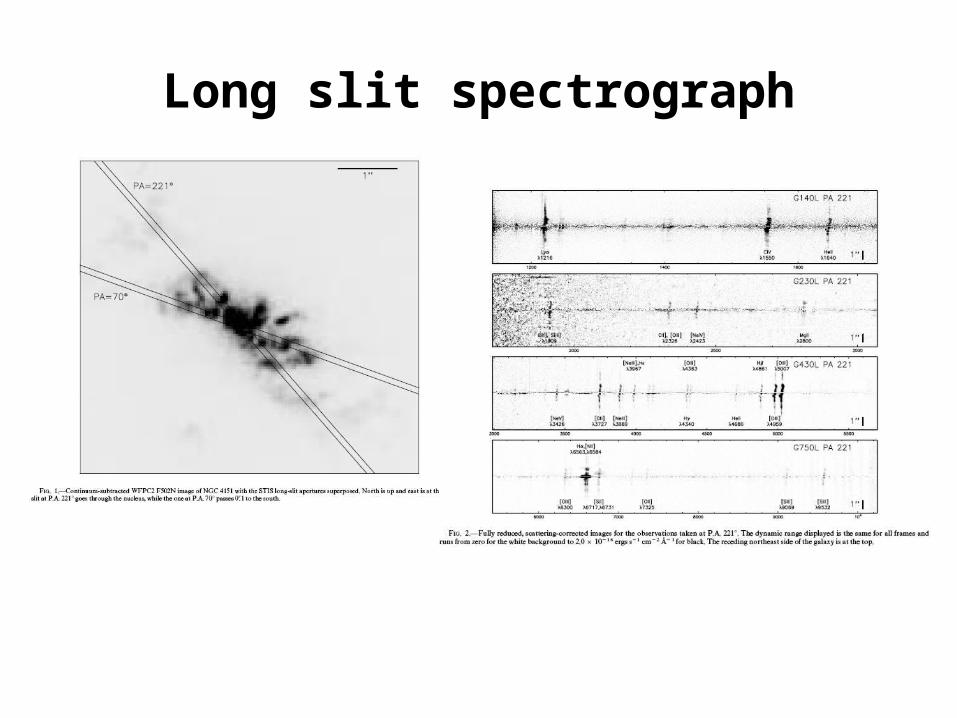
Long slit spectrograph

Integral field spectroscopy

Gives spatial variation of spectrum

Usually uses some “image slicer” to feed a spectrograph, multiplexing spatial and spectral information

(2 x 2.4 arcmin field from HDF)

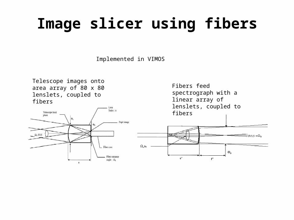
Image slicer using fibers

Telescope images onto area array of 80 x 80 lenslets, coupled to fibers

Fibers feed spectrograph with a linear array of lenslets, coupled to fibers

Implemented in VIMOS

Image slicer using mirrors

Optical telescopes

0

2

4

6

8

10

12

1900 1920 1940 1960 1980 2000

year completed

dia

me

ter

(m)

Palomar 200 inch

MMT, Magellan (2)

VLT (4), Gemini (2), Subaru

Keck

LBT

Mt. Wilson 100 inch

Multiple Mirror Telescope

MMT

MMT at the top of Mt Hopkins

The road to the top

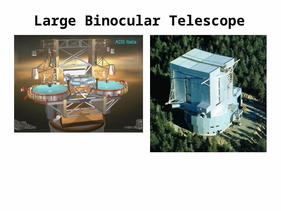
Large Binocular Telescope

Drawing of the LBT showing the two 8.4 meter mirrors on a common mount. It will be the world’s most powerful telescope with collecting area equivalent to a 12 meter telescope and the angular resolution of a 23 meter telescope (4 milli-arcsecond).

LBT enclosure on Mt. Graham in December 1999. Telescope scheduled to open with first mirror in 2002, both mirrors in 2004.

Honeycomb sandwich mirrors

Maximize stiffness:weight — 2D version of I-beam.

Optimum thermal response — ventilation reduces time constant to 40 min.

Used in MMT, Magellan (2), LBT.

8.4 meter LBT mirrors are world’s largest.

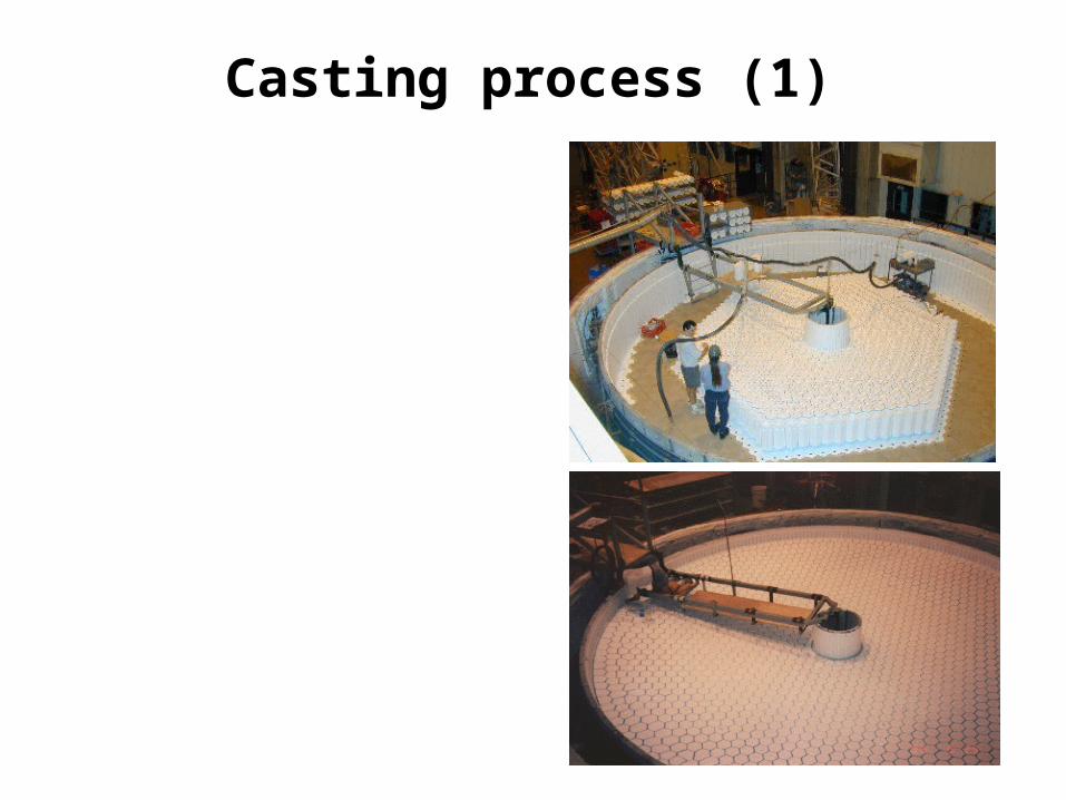
Casting process (1)

Complex manufacturing process produces world’s largest mirrors with almost ideal properties.

Mold consists of ceramic fiber boxes inside silicon carbide tub — 1600 hexagonal boxes will form cavities in mirror.

Ceramic fiber maintains strength at 1200ºC, does not react chemically with glass, and can be removed without applying high stress to glass.

Each box is machined to precise dimensions and bolted in place.

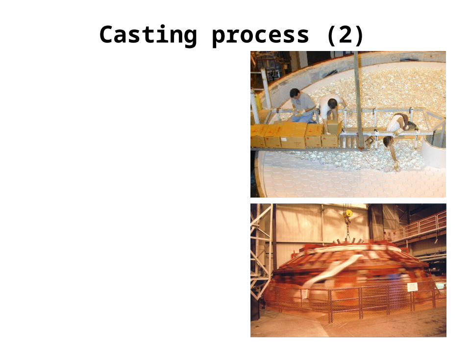
Casting process (2)

Borosilicate glass is purchased as irregular ~10 pound blocks with pristine fracture surfaces. Melts together seamlessly.

20 tons of glass are placed on top of mold.

Furnace is closed, heated to 1200ºC while spinning at 7 rpm to form paraboloid.

After melting, mirror cools for 3 months to minimize stress.

Mirror is lifted from furnace and ceramic fiber boxes are removed with high-pressure water.

Keck Telescopes

Primary mirror

36 hexagonal segments, 1.8 meter diameter

Each segment positioned by 3 actuators to form continuous paraboloid.

Edge sensors (capacitors), interferometer and image analyzer provide feedback.

Twin 10 meter telescopes on Hawaii’s Mauna Kea.

Built by U California and Cal Tech.

Commissioned 1992, 1996.

1.8-m segments

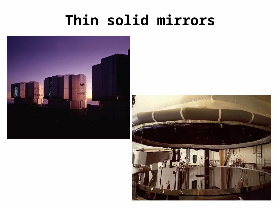
Thin solid mirrors

ESO’s Very Large Telescope (4x8 m in Chile)

Gemini Telescopes (8 m in Hawaii and Chile)

Subaru Telescope (8 m in Hawaii)

Mirrors 175-200 mm thick; require active optics to hold shape.

Wavefront sensor monitors shape; ~150 active supports bend mirror.

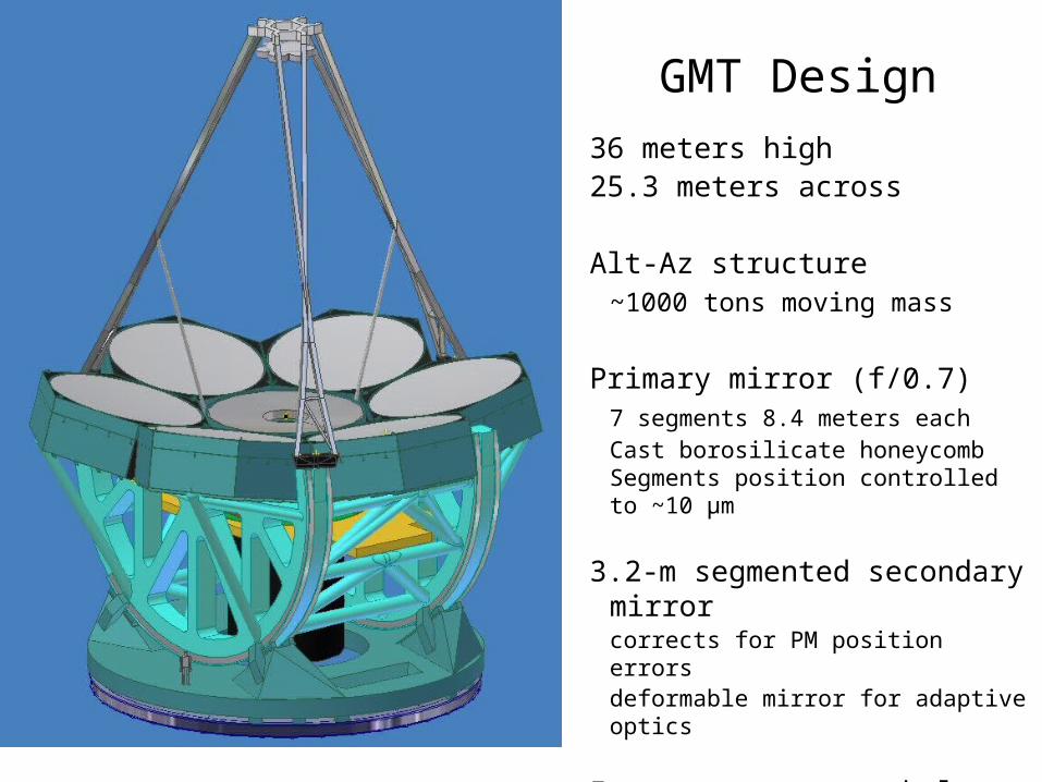
GMT Design

36 meters high25.3 meters across

Alt-Az structure~1000 tons moving mass

Primary mirror (f/0.7)7 segments 8.4 meters eachCast borosilicate honeycombSegments position controlled to ~10 µm

3.2-m segmented secondary mirrorcorrects for PM position errorsdeformable mirror for adaptive optics

Instruments mount below primary at the Gregorian focus