J. Fluid Mech. (2013), . 723, pp. … · †Email address for correspondence:[email protected] ‡Present address: Mechanical and Systems Engineering, Doshisha University,

J. Fluid Mech. (2013), vol. 723, pp. 429–455. c© Cambridge University Press 2013 429doi:10.1017/jfm.2013.137

Wall turbulence without walls

Yoshinori Mizuno1,‡ and Javier Jiménez1,2,†1School of Aeronautics, Universidad Politecnica de Madrid, 28040 Madrid, Spain2Centre for Turbulence Research, Stanford University, Stanford, CA 94305, USA

(Received 22 August 2012; revised 9 January 2013; accepted 1 March 2013)

We perform direct numerical simulations of turbulent channels whose inner layer isreplaced by an off-wall boundary condition synthesized from a rescaled interior flowplane. The boundary condition is applied within the logarithmic layer, and mimicsthe linear dependence of the length scales of the velocity fluctuations with respectto the distance to the wall. The logarithmic profile of the mean streamwise velocityis recovered, but only if the virtual wall is shifted to a position different from thelocation assumed by the boundary condition. In those shifted coordinates, most flowproperties are within 5–10 % of full simulations, including the Karman constant, thefluctuation intensities, the energy budgets and the velocity spectra and correlations.On the other hand, buffer-layer structures do not form, including the near-wall energymaximum, and the velocity fluctuation profiles are logarithmic, strongly suggestingthat the logarithmic layer is essentially independent of the near-wall dynamics. Thesame agreement holds when the technique is applied to large-eddy simulations. Thedifferent errors are analysed, especially the reasons for the shifted origin, and remediesare proposed. It is also shown that the length rescaling is required for a stationarylogarithmic-like layer. Otherwise, the flow evolves into a state resembling uniformlysheared turbulence.

Key words: turbulence simulation, turbulent boundary layers, turbulent flows

1. IntroductionWall-bounded turbulence is a problem with two separate length scales (Townsend

1976). The core flow scales with the flow thickness, which will be denoted by h, andthe near-wall layer scales in wall units, which are defined in terms of the frictionvelocity uτ and of the kinematic viscosity ν, and will be denoted by a ‘+’ superscript.The scale separation is measured by the friction Reynolds number h+. The interactionof the two scale ranges is believed to take place across an overlap layer, usually called‘logarithmic’, in which the eddy sizes are approximately proportional to the distance tothe wall, y.

The logarithmic layer is interesting for several reasons. At high Reynolds numbers,it supports the transfer of momentum, and drag, from the wall to the core flow, acrossa wide range of scales, but how the transfer is organized and how much interaction is

† Email address for correspondence: [email protected]‡ Present address: Mechanical and Systems Engineering, Doshisha University, 1-3 Tatara

Miyakodani, Kyotanabe City, 610-0394, Japan.

mailto:[email protected]

430 Y. Mizuno and J. Jiménez

there between the inner and outer layers remain open questions. Theories range fromthose in which the logarithmic eddies are created at the wall and migrate away fromit (Adrian, Mainhart & Tomkins 2000), to those in which the opposite it true (Hunt &Morrison 2000). Almost the only tentative consensus is that most of the energy- andmomentum-carrying eddies of the logarithmic layer are ‘attached’, in the sense thatthey span the full distance from the wall to their maximum height (Townsend 1961).Recent surveys have been given by Adrian (2007), Smits, McKeon & Marusic (2011)and Jimenez (2012).

The first question addressed in this paper is how independent is the logarithmic layerfrom the wall and, in particular, whether a logarithmic layer can be maintained withno wall at all. Indications that it can be done come from rough- and smooth-wallboundary layers, in which the wall dynamics are very different, but the logarithmiclayers are not (Townsend 1976; Perry & Abell 1977; Jimenez 2004; Bakken et al.2005; Flores & Jimenez 2006; Flores, Jimenez & del Alamo 2007).

Our strategy will be to substitute the wall by an off-wall boundary condition thatimposes on an interior wall-parallel plane a synthetic velocity field that mimics theflow at that wall distance. Our lowest-order assumption will be that it is enough toimpose on the flow the right length scale, which we will assume to be proportionalto y.

That proportionality was originally hypothesized as an asymptotic limit at very highReynolds numbers, and used in the classical derivation of the logarithmic velocityprofile (Millikan 1938), but it has been observed experimentally and numerically inspectra and correlations at relatively modest Reynolds numbers in pipes (Morrison& Kronauer 1969; Perry & Abell 1975, 1977; Bullock, Cooper & Abernathy 1978;Kim & Adrian 1999; Guala, Hommema & Adrian 2006; Bailey et al. 2008), andin channels and boundary layers (Tomkins & Adrian 2003; del Alamo et al. 2004;Hoyas & Jimenez 2006; Monty et al. 2007; Jimenez & Hoyas 2008). Families of flowstructures representing the coarse-grained dissipation (del Alamo et al. 2006; Floreset al. 2007) and the momentum transfer (Lozano-Duran, Flores & Jimenez 2012) havealso been isolated in channels, and shown to be geometrically self-similar, in the senseof being attached to the wall with dimensions that scale linearly with their heights.

Interestingly, the linear scaling of the eddy sizes extends beyond the traditionalrange of validity of the logarithmic mean velocity profile (y/h < 0.15; see Osterlundet al. 2000), and holds approximately to at least y/h ≈ 0.4 in many flows (Zanoun,Durst & Nagib 2003; del Alamo et al. 2004; Monty et al. 2007; Jimenez 2012). Minorcorrections, such as the use of a virtual origin for the linear law, extend its validityeven further (Mizuno & Jimenez 2011). Part of the reason why that similarity isnot easily recognized in the mean velocity profile is that it is not complete. Eddiesmuch smaller than the distance to the wall are essentially isotropic and form a localKolmogorov cascade (Saddoughi & Veeravali 1994), and structures much longer orwider than the flow thickness span the whole boundary layer and do not change sizeas they approach the wall (Perry & Abell 1977; Jimenez 1998; Kim & Adrian 1999;del Alamo et al. 2004; Jimenez 2012). On the other hand, the wall-normal velocity,the tangential Reynolds stresses and the strongest spectral cores of the other velocitycomponents can be readily recognized as scaling linearly with the wall distance (Perry& Abell 1977; Hoyas & Jimenez 2006; Jimenez & Hoyas 2008). We will definethe logarithmic layer as the region in which the eddy sizes scale linearly with y,irrespective of the mean velocity profile, and it is that linear dependence that we willtry to reproduce in our numerical experiments. The hope is that it will lead, by itself,to the establishment of a natural logarithmic layer.

Wall turbulence without walls 431

The second goal of this paper is more practical. Direct numerical simulations(DNSs) are at present too expensive to deal with most flows of industrial interest.If we accept that the integral length of the energy-containing eddies in the logarithmiclayer is proportional to y, while the smallest eddies are of the order of the Kolmogorovviscous scale, η+ ∼ y+1/4 (see Tennekes & Lumley 1972, p. 159), the number ofdegrees of freedom in a cube of side h is proportional to

NDNS ∼∫ h+

0(h+/η+)2 dy+ ∼ h+5/2

, (1.1)

which is slightly larger than the usual estimation, h+9/4, because the inhomogeneity ofthe flow concentrates eddies near the wall. In fact, the number of degrees of freedomper unit of y is proportional to (y+)−1/2, which justifies the use of logarithmic-layerestimates for the length scales, instead of outer ones. Equation (1.1) is the lowestpossible limit for the number of points required in a numerical DNS grid.

The usual strategy to avoid the Reynolds number dependence of the number of gridpoints is large-eddy simulation (LES), in which all eddies smaller than a given fractionof the integral length are modelled, and which, therefore, only requires a fixed numberof degrees of freedom. It can be argued that any computational problem requiring afixed number of points, even if it is large, will eventually be solved by the growth ofcomputer power, while potentially unbounded problems require a theory. Unfortunately,the LES strategy fails in wall-bounded flows. Repeating the estimate in (1.1), usinglengths of O(y) for the smallest eddies to be computed, we get

NLES ∼∫ h

y0

(h/y)2 dy∼ (h/y0)2, (1.2)

where the integral is dominated by the lower limit y0. In general, the integral in(1.2) should extend to the point at which the lengths stop being proportional to y,which is y+0 = O(1), so that NLES = O(h+2

). Although lower than (1.1), that estimatestill prevents the practical application of LES to most practical wall-bounded flows(Jimenez & Moser 2000). Our second reason to study the logarithmic layer is toexplore how to construct off-wall boundary conditions which could be applied at afixed y0/h, independently of the Reynolds number, thus reducing the LES estimate in(1.2) to O(1).

The search for off-wall boundary conditions for LES is not new. A commonapproach is to combine the solution of the unsteady Reynolds-averaged Navier–Stokes(RANS) equations for the near-wall layer with a LES solver for the core flow andmany variations exist. The simplest ones assume equilibrium in the near-wall layerand apply the logarithmic law locally (Deardorff 1970) or include partial contributionsfrom the acceleration terms and other improvements (Wang & Moin 2002; Catalanoet al. 2003). Recent reviews can be found in Piomelli & Balaras (2002) and Piomelli(2008). A common problem with those approaches is that, while they do a good jobof simulating the near-wall layer, they tend to provide poor boundary conditions forthe outer flow, because RANS does not simulate fluctuations. Although several cureshave been proposed for the discontinuities that appear (Nikitin et al. 2000; Hamba2003; Piomelli et al. 2003; Keating & Piomelli 2006), the problem remains unsolved.On the other hand, note that any off-wall boundary condition, however perfect, wouldeventually have to be coupled to some sort of two-layer model to approximate themean velocity of the missing inner region.


A physical approach closer to the spirit of this paper is due to Podvin & Fraigneau(2011), who used a wall model based on proper orthogonal decomposition (POD)modes to predict the flow at the off-wall boundary. It works well in relatively low-Reynolds-number channels, but the POD modes must be known in advance.

Two other papers should be cited. Even if not exactly an off-wall strategy, Pascarelli,Piomelli & Candler (2000) suggested a multi-block technique in which small DNSblocks are created in the inner layer and used to tile the wall with identical copiesto provide a boundary condition for the outer flow. Although our technique is verydifferent, we also find spurious periodicities in the boundary conditions, and ourresults will be compared with theirs.

The final interesting experiment is that by Orlandi et al. (2003), who fed velocitiesfrom an independent rough-walled channel DNS into the wall of a smooth one, in anattempt to reproduce roughness effects. Although their technique is also completelydifferent from ours, and their boundary conditions are applied at the physical wall, theuse of artificial velocities in a wall-parallel plane is conceptually similar to ours.

This paper is organized as follows. The numerical method is described in § 2,with emphasis on the off-wall boundary condition. The resulting statistics, includingthe behaviour of the spectra and correlation functions is presented in § 3. The newboundary condition is applied to LES in § 4, which also tests the effects of somevariations of the off-wall boundary conditions. Finally, the results are discussed andconclusions offered.

2. Numerical simulationsWe consider an incompressible turbulent channel driven by a streamwise pressure

gradient between two parallel planes located at y = 0 and y = 2h. The streamwise,wall-normal and spanwise coordinates and velocity components are, respectively,(x, y, z) and (U,V,W), P is the kinematic pressure and the density is fixed to unityand dropped from the equations. Lowercase letters denote fluctuations with respectto the average ( ), defined over wall-parallel planes and time, and primed quantitiesdenote root-mean-squared intensities, such as in u′2 ≡ u2. Occasionally, the notation(x1, x2, x3)= (x, y, z) and (u1, u2, u3)= (u, v,w) will be used for convenience.

The flow is assumed to be spatially periodic in the two wall-parallel directions,with wavelengths Lx and Lz, and the simulation only considers the layer betweentwo interior numerical boundaries at y = yb and y = 2h − yb, with 0 < yb < h. TheNavier–Stokes equations are solved for the primitive variables, U, V , W and P, usinga fractional-step method similar to that of Simens et al. (2009) for boundary layers,although, in this case, the streamwise periodicity makes the generation of inflowand outflow conditions unnecessary. The spatial discretization is de-aliased collocatedFourier in the two wall-parallel directions, and fourth-order compact finite differenceson a non-uniform staggered grid along y. The temporal integration is third-orderRunge–Kutta with implicit marching for all of the viscous terms (Spalart, Moser &Rogers 1991). The Fourier modes of a generic variable ψ are ψ(kx, y, kz; t), wherekx and kz are wavenumbers in the streamwise and spanwise directions. We will alsouse wavelengths, defined as λi = 2π/ki. The time t will generally be omitted, unlessexplicitly required by the argument at hand.

The definition of the simulations requires a velocity scale and a frame of reference.In traditional simulations, the latter is usually linked to the wall, while the velocityscale is either given as a fixed friction velocity or as a mass flux. In our case, the


absence of the wall makes the problem invariant to arbitrary Galilean transformations,

Ui 7→ Ui + Ai(t), (2.1)

including arbitrary accelerations, and there is no obvious preferred frame of reference.Neither can the mass flux, which depends on the frame velocity, be used to definethe velocity scale. Our choice is to define: (i) the frame velocities Ai so that theinstantaneous volumetric flux vanishes along the three directions; and (ii) the velocityscale by the fixed difference 1U between the instantaneous velocities averaged overthe wall-parallel planes at the centre and at the two numerical boundaries. In terms ofthe Fourier coefficients,

U(0, yb, 0; t)= U(0, 2h− yb, 0; t)= U(0, h, 0; t)−1U, (2.2)

with a similar condition for W (with 1W = 0). Continuity implies that the meanwall-normal velocity, V(0, y, 0), is independent of y.

Fixing the fluxes requires uniform, but temporally fluctuating, pressure gradients thatcompensate the frame accelerations in the three directions, and which are computedby the pressure-correction substep at every time step. The two wall-parallel gradientsare common to all simulations in which notionally infinite channels are approximatedby spatially periodic domains. They are not usually included in the pressure statistics,because there is no well-defined spatial average for a secular pressure trend, andthey are left out of the statistics below. The wall-normal pressure gradient is requiredto compensate the fluctuating normal Reynolds stress v2(0, y, 0) and the mean wall-normal acceleration. It is included in our pressure fluctuations, but is equivalent tothat in standard channels, because the condition of zero wall-normal volumetric fluxensures that the mean wall-normal acceleration vanishes. The implementation of (2.2)is discussed in the next section, together with the rest of the off-wall boundaryconditions.

2.1. The off-wall boundary conditionsThe boundary conditions for the higher Fourier modes are constructed from thevelocities in interior ‘reference’ planes y = yr and y = 2h − yr, where 0 < yb < yr < h,following a procedure conceptually similar to the method of Lund, Wu & Squires(1998) for creating inflow conditions for boundary layers using a downstream flowplane. Although the necessarily limited Reynolds numbers of our simulations make theexistence of a true logarithmic layer questionable, the assumption will be that both yb

and yr are in the self-similar range in which the flow length scales are proportionalto the distance to the wall. As we noted in the introduction, that is approximatelytrue over a reasonably wide range of wall distances, specially for the higher-Reynolds-number simulations. Only the operations on the lower boundary are described; thoseon the upper boundary are similar.

For each time step, the flow at yr is first shrunk by a factor α = yb/yr to mimicthe statistical proportionality of the length scales to the wall distance. Note that α−1

should be an integer to preserve the streamwise and spanwise periodicities of the flow.Next, to take into account the different advection velocities of the structures in thetwo planes, the rescaled velocity field is shifted in the two wall-parallel directions byamounts δj(t) determined by integrating the respective spatially averaged velocities,

dδj

dt= Uj(0, yb, 0)− Uj(0, yr, 0), (2.3)


where j = 1 or j = 3, and the initial δj(0) are chosen arbitrarily. In Fourier space,the shifting is done by multiplying each harmonic by the rotational factor exp(ikjδj),as used, for example, in the simulations of uniformly sheared turbulent flows bySchumann (1985) and Jimenez (2007). The integration of (2.3) is performed in parallelto the Navier–Stokes equations, using an explicit Runge–Kutta. By combining thetwo manipulations, the mapping of the velocities from the reference plane to theboundary is

U(kx, yb, kz)= U(αkx, yr, αkz) exp[iα(kxδx + kzδz)], (2.4)

which is applied explicitly, with the boundary at time tn synthesized from thereference information at time tn−1. Special cases are the boundary conditions for the(0, 0) Fourier modes, which represent the spatially averaged velocities and thereforerequire no phase shifting. They are also applied explicitly, using (2.2) to computeU(0, yb, 0; tn) from U(0, h, 0; tn−1).

Note that the delay by one time step is irrelevant because the two planes areeffectively uncorrelated. The reason is two-fold. In the first place, two harmonicfunctions of different wavenumbers are orthogonal, and in the second place, thearbitrarily large phase shifts that develop over time mean that the information atthe boundary is obtained from horizontally distant points of the reference plane. Theintegration times of our simulations are long enough for the two planes to movewith respect to each other by several box lengths. As a consequence, the only roleof the reference plane is to provide a physically realistic turbulent velocity to beused to synthesize the boundary condition. In addition, the length scale in the wall-normal direction can only be rescaled indirectly through the y-derivative of V , becausecontinuity implies that,

∂V

∂y(kx, yb, kz)= α−1 ∂V

∂y(αkx, yr, αkz). (2.5)

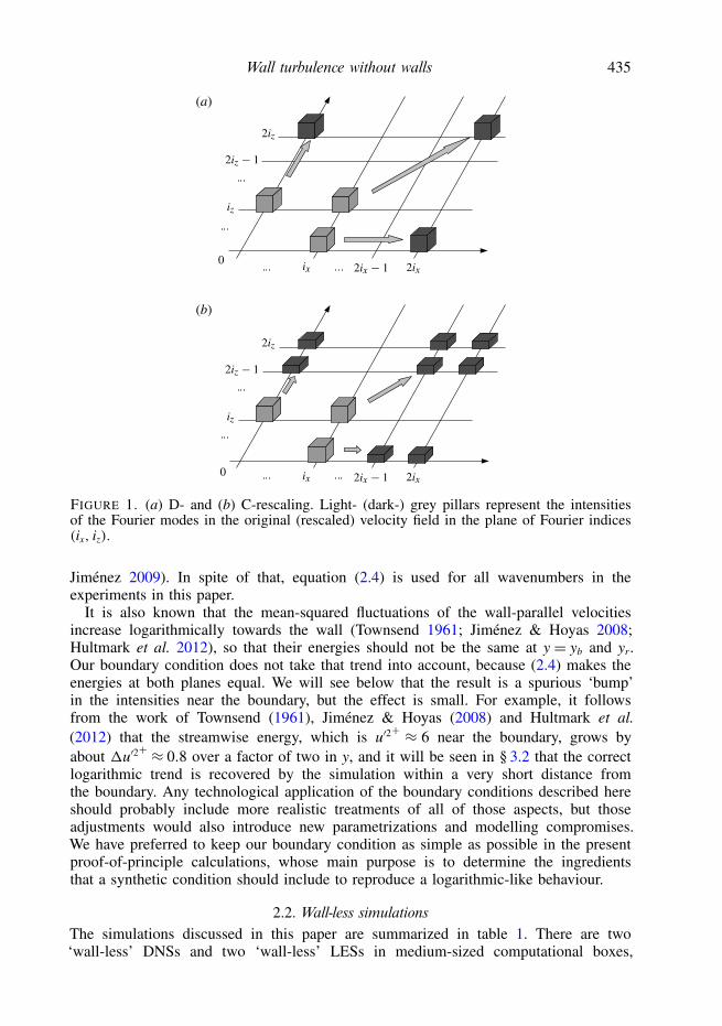
We will come back to those two points later. In our simulations the boundary and thereference planes are chosen so that α = 1/2, which would imply that the synthesizedboundary only has energy in the even-indexed Fourier modes; i.e. that the boundaryplane is covered by a tiling of four identical sub-boxes. This is reminiscent of thesimulations by Pascarelli et al. (2000), who used tiled minimal channels at the wall asboundary conditions for larger simulations above and found that the tiling periodicitywas quickly lost in the flow interior. We will call that method D-scaling (from‘discrete’, see figure 1a). To mitigate possible discreteness effects, a second methodwas implemented in which the energy of the Fourier wavenumber with indices (ix, iz)

in y= yr is equally distributed in y= yb among the four neighbouring modes, (2ix, 2iz),(2ix − 1, 2iz), (2ix, 2iz− 1) and (2ix − 1, 2iz− 1). That method is called C-scaling (from‘continuous’, see figure 1b), and is used in most simulations. The differences betweenthe two schemes will be discussed in § 4, in the context of the application to LES.

We already noted in the introduction that, even at the relatively high Reynoldsnumbers of our simulations, the proportionality of the flow scales with the walldistance only applies to structures of intermediate sizes. Fluctuations of order h,which are especially strong for the streamwise velocity component, span the fullchannel without changing their wall-parallel dimensions (Perry & Abell 1977; Jimenez1998; Kim & Adrian 1999; del Alamo et al. 2004). Those larger motions are notwell-represented near the boundary by the linear rescaling in (2.4), and neither cantheir advection velocities be approximated by the local mean velocity (del Alamo &


0

0

(a)

(b)

FIGURE 1. (a) D- and (b) C-rescaling. Light- (dark-) grey pillars represent the intensitiesof the Fourier modes in the original (rescaled) velocity field in the plane of Fourier indices(ix, iz).

Jimenez 2009). In spite of that, equation (2.4) is used for all wavenumbers in theexperiments in this paper.

It is also known that the mean-squared fluctuations of the wall-parallel velocitiesincrease logarithmically towards the wall (Townsend 1961; Jimenez & Hoyas 2008;Hultmark et al. 2012), so that their energies should not be the same at y = yb and yr.Our boundary condition does not take that trend into account, because (2.4) makes theenergies at both planes equal. We will see below that the result is a spurious ‘bump’in the intensities near the boundary, but the effect is small. For example, it followsfrom the work of Townsend (1961), Jimenez & Hoyas (2008) and Hultmark et al.(2012) that the streamwise energy, which is u′2+ ≈ 6 near the boundary, grows byabout 1u′2+ ≈ 0.8 over a factor of two in y, and it will be seen in § 3.2 that the correctlogarithmic trend is recovered by the simulation within a very short distance fromthe boundary. Any technological application of the boundary conditions described hereshould probably include more realistic treatments of all of those aspects, but thoseadjustments would also introduce new parametrizations and modelling compromises.We have preferred to keep our boundary condition as simple as possible in the presentproof-of-principle calculations, whose main purpose is to determine the ingredientsthat a synthetic condition should include to reproduce a logarithmic-like behaviour.

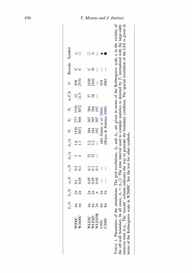
2.2. Wall-less simulationsThe simulations discussed in this paper are summarized in table 1. There are two‘wall-less’ DNSs and two ‘wall-less’ LESs in medium-sized computational boxes,


L x/h

L z/h

y b/h

y r/h

1x/η

1y/η

Nx

Ny

Nz

u τT/h

h+R

esca

leSy

mbo

l

W90

0C4π

2π0.

10.

23

1.6

1536

277

1536

1285

8C

4W

2600

C4π

2π0.

050.

14

1.7

3072

569

3072

11.5

2570

C©

WL

ESC

4π2π

0.05

0.1

323.

238

430

738

437

2430

C�

WL

ESD

4π2π

0.05

0.1

323.

238

430

738

438

2420

D�

WL

ESN

R2π

π0.

050.

1—

—19

230

719

2—

——

—C

950

8π3π

——

(del

Ala

moet

al.

2004

)93

4—

NC

2000

8π3π

——

(Hoy

as&

Jim

enez

2006

)20

03—

•T

AB

LE

1.Pa

ram

eter

sof

the

sim

ulat

ions

.T

hegr

idre

solu

tions

,1

xan

d1

y,ar

egi

ven

inte

rms

ofth

eK

olm

ogor

ovsc

aleη

inth

evi

cini

tyof

the

off-

wal

lbo

unda

ry.

Inal

lca

ses,1

z≈1

x/2.

The

time

inte

rval

used

toco

mpi

lest

atis

tics

isde

note

dby

T,

norm

aliz

edw

ithth

ela

rge-

eddy

turn

over

time

h/u τ

.T

he‘r

esca

le’

colu

mn

indi

cate

sth

ew

ayto

gene

rate

the

boun

dary

cond

ition

.T

hesp

acia

lre

solu

tion

ofth

eL

ES

isgi

ven

inte

rms

ofth

eK

olm

ogor

ovsc

ale

inW

2600

C.

See

the

text

for

othe

rsy

mbo

ls.


using the off-wall boundary technique just described. They are compared with standard‘full-channel’ simulations at similar Reynolds numbers, C950 (del Alamo et al. 2004)and C2000 (Hoyas & Jimenez 2006). The two wall-less DNSs, W900C and W2600C,use C-rescaling, while the two wall-less LESs, WLESC and WLESD, in addition toassessing the applicability of the method to LES, test the differences between thecontinuous and discrete rescaling methods.

In addition, we performed simulations in smaller boxes to investigate specific points.They will be briefly discussed when dealing with the particular issues for which theywere intended, but are not included in table 1.

More interestingly, we tested the off-wall boundary condition (2.4) without therescaling step, i.e. using α = 1. The results were similar to a uniformly sheared flow,with both the length scales and the intensities growing monotonically in time, stronglysuggesting that the spatial stratification of the length scales is a necessary ingredientfor the existence of a logarithmic region in wall-bounded flows. A LES illustrating thatpoint will be discussed in § 4.

3. Statistics3.1. The mean velocity profile

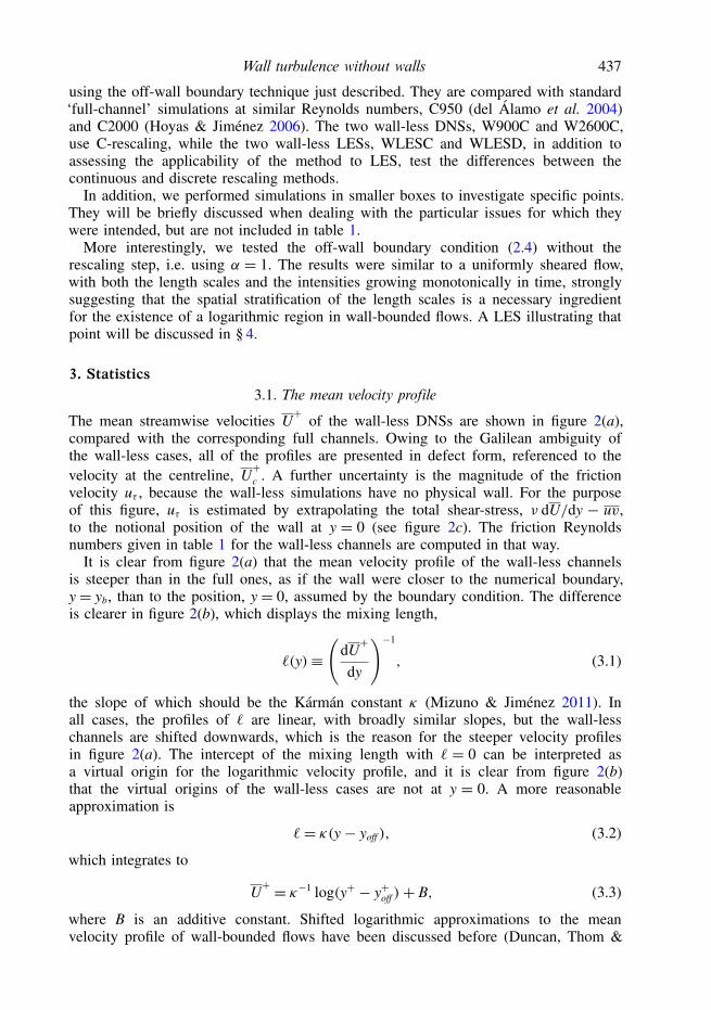
The mean streamwise velocities U+

of the wall-less DNSs are shown in figure 2(a),compared with the corresponding full channels. Owing to the Galilean ambiguity ofthe wall-less cases, all of the profiles are presented in defect form, referenced to thevelocity at the centreline, U

+c . A further uncertainty is the magnitude of the friction

velocity uτ , because the wall-less simulations have no physical wall. For the purposeof this figure, uτ is estimated by extrapolating the total shear-stress, ν dU/dy − uv,to the notional position of the wall at y = 0 (see figure 2c). The friction Reynoldsnumbers given in table 1 for the wall-less channels are computed in that way.

It is clear from figure 2(a) that the mean velocity profile of the wall-less channelsis steeper than in the full ones, as if the wall were closer to the numerical boundary,y= yb, than to the position, y= 0, assumed by the boundary condition. The differenceis clearer in figure 2(b), which displays the mixing length,

`(y)≡(

dU+

dy

)−1

, (3.1)

the slope of which should be the Karman constant κ (Mizuno & Jimenez 2011). Inall cases, the profiles of ` are linear, with broadly similar slopes, but the wall-lesschannels are shifted downwards, which is the reason for the steeper velocity profilesin figure 2(a). The intercept of the mixing length with ` = 0 can be interpreted asa virtual origin for the logarithmic velocity profile, and it is clear from figure 2(b)that the virtual origins of the wall-less cases are not at y = 0. A more reasonableapproximation is

`= κ(y− yoff ), (3.2)

which integrates to

U+ = κ−1 log(y+ − y+off )+ B, (3.3)

where B is an additive constant. Shifted logarithmic approximations to the meanvelocity profile of wall-bounded flows have been discussed before (Duncan, Thom &


–15

–10

–5

0(a) (b)

(c) (d)

10–110–2 100 0

0.3

0.2

0.1

0 0.80.60.40.2

–15

–10

–5

0

10–110–2 1000

FIGURE 2. (a) Mean streamwise velocity U for W900C, W2600C, C950 and C2000.(b) Mixing lengths corresponding to the profiles in (a). (c) Sketch of the computation of therescaled friction velocity and channel width, (d) as in (a), in rescaled coordinates. Symbols asin table 1.

Young 1970; Wosnik, Castillo & George 2000; Oberlack 2001; Buschmann & Gad-el-Hak 2005; Spalart, Coleman & Johnstone 2008). The offset represents the effect ofthe near-wall viscous layer on the logarithmic law, which cannot be extended to y= 0.Mizuno & Jimenez (2011) developed a systematic procedure to estimate the optimumparameters for (3.3). They applied it to several canonical data sets, both numerical andexperimental, and found that the Karman constant and the virtual origin depend on thetype of flow and on the Reynolds number, although their results suggest that y+off → 0at large h+.

The parameters estimated for the flows in this paper are given in table 2, where it isclear that the wall-less cases differ from the full channels and that their virtual originsfall between the notional wall and the boundary plane. The most obvious interpretationis again that they represent the effect of the artificial boundary conditions on thelogarithmic law, which cannot be expected to hold below yb. They suggest that arescaled shifted coordinate might give a better agreement between the two types ofsimulations. If we interpret the non-zero virtual origins of the full channels as aReynolds number effect, we can define a ‘baseline’ shift, yf = yoff (DNS), which isonly a function of h+ (see figure 5 of Mizuno & Jimenez 2011), and define rescaled


W900C W2600C WLESC WLESD C950 C2000

y+b 86 128 122 124 0 0y+off 32 76 76 81 −29 −13κ 0.28 0.33 0.31 0.32 0.35 0.36y+o 51 87 86 90 0 0y+b − y+o 27 34 29 26 0 0uτ/uτ 0.97 0.98 0.98 0.98 1 1

TABLE 2. Offsets, virtual origins and Karman constants for the fitted mean streamwisevelocity profiles. See the text for details.

coordinates for the wall-less cases designed to make them comparable to the full ones.Considering for this purpose that the wall-less and full simulations in table 1 havesimilar h+, we define

y= y− yo, h= h− yo, uτ = uτ (h/h)1/2, (3.4)

with

yo = (yoff − yf )/(1− yf /h), (3.5)

where yf is the virtual origin of the corresponding full flow with a similar Reynoldsnumber. Those definitions are chosen so that y = h when y = h, and yoff /h = yf /h.Note that the new virtual wall, y = 0 corresponds to y = yo and that y ≡ y in fullchannels. The modified friction velocity uτ is obtained by interpolating the linearshear-stress profile to y = yo (see figure 2c). The velocity profiles of the two wall-lessDNSs are plotted in term of the rescaled coordinates in figure 2(d) and agree with thefull channels much better than in the original coordinates. The physical reason for thisoffset will be discussed in detail in § 3.3.

The values of yo from (3.5) have been added to table 2, as well as the rescaledfriction velocities, which differ very little from the uncorrected ones. The table showsthat, while yo changes among cases, the offset relative to the numerical boundary,yb − yo, is always approximately 30 wall units. Although not included in the table, weconducted several tests in smaller computational boxes, (Lx,Lz) = (π,π/2), to explorehow yo depends on the choice of yb and yr, or on the C- or D-rescaling methods. In allcases, y+b − y+o ≈ 30.

The reason will be discussed extensively later, but a simple interpretation could bethat the flow reacts to the artificial boundary condition by creating a spurious ‘buffer’layer, the role of which is to let the flow adapt to an inconsistent boundary. However,there are no signs of viscous effects near the boundary. The linear behaviour of themixing length in figure 2(b) and the logarithmic profile of the velocity in figure 2(d)extend all of the way to the boundary, and we will see in the next section that thefluctuations are also inconsistent with a spurious layer in which viscosity becomesdominant.

A more likely explanation is that imposing a Dirichlet boundary condition that isessentially uncorrelated with the flow interior is felt by the equations as a virtual wall,although the turbulent character of the applied velocities prevents the formation of aregular buffer layer. In fact, none of the rescaled figures in this paper change too muchif they are replotted with the virtual wall exactly at the boundary plane, yo = yb.


(a) 8

4

010–110–2 100

(b) 8

4

010–110–2 100

(c) 8

4

010–110–2 100

(d) 20

10

010–110–2 100

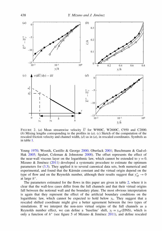
FIGURE 3. (a) Velocity fluctuation intensities for W2600C and C2000: u′+2, w′+2 and v′+2

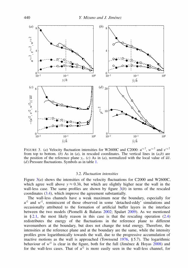
from top to bottom. (b) As in (a), in rescaled coordinates. The vertical lines in (a,b) arethe position of the reference plane yr. (c) As in (a), normalized with the local value of uv.(d) Pressure fluctuations. Symbols as in table 1.

3.2. Fluctuation intensitiesFigure 3(a) shows the intensities of the velocity fluctuations for C2000 and W2600C,which agree well above y ≈ 0.3h, but which are slightly higher near the wall in thewall-less case. The same profiles are shown by figure 3(b) in terms of the rescaledcoordinates (3.4), which improve the agreement substantially.

The wall-less channels have a weak maximum near the boundary, especially foru′2 and w′2, reminiscent of those observed in some ‘detached-eddy’ simulations andoccasionally attributed to the formation of artificial buffer layers in the interfacebetween the two models (Piomelli & Balaras 2002; Spalart 2009). As we mentionedin § 2.1, the most likely reason in this case is that the rescaling operation (2.4)redistributes the energy of the fluctuations in the reference plane to differentwavenumbers at the boundary, but does not change the total energy. Therefore, theintensities at the reference plane and at the boundary are the same, while the intensityprofiles grow logarithmically towards the wall, due to the progressive accumulation ofinactive motions as the wall is approached (Townsend 1976, § 5.7). The logarithmicbehaviour of w′2 is clear in the figure, both for the full (Jimenez & Hoyas 2008) andfor the wall-less cases. That of u′2 is more easily seen in the wall-less channel, for


which the buffer-layer peak of the natural cases is missing. Its slope is intermediatebetween that found by Jimenez & Hoyas (2008) for channels when the largest scalesare removed, u′+2 ∼ −1.15 log(y), and that found by Hultmark et al. (2012) for pipesat much higher Reynolds numbers, u′+2 ∼ −1.2 log(y). The spurious peak near theboundary can therefore be interpreted as the result of the recovery of the artificiallylow energy of the boundary to match the natural logarithmic trend in the interior of theflow, and it is interesting that it takes place within a very thin layer, of the order of1y+ = 20. The behaviour of the lower-Reynolds-number case W900C is similar to thatjust described.

Figure 3(c) tests that the amplitude differences in figure 3(b) are not due to therescaling of the friction velocity in (3.4). Even when the intensities are normalizedwith the local Reynolds stress −uv, removing the need for a velocity scale, thedifferences stay essentially the same as in figure 3(b). On the other hand, although notshown in the figure, the shifting of the wall distance is important. When figure 3(c) isplotted in terms of y/h, instead of y/h, the behaviour is closer to that in figure 3(a).

Note that, although figures 3(a)–3(c) show that the intensities of the wall-lesschannels are somewhat higher near the boundary than in the real case, their almostperfect agreement above y/h & 0.3 suggests that this is a local consequence of theimperfectly synthesized boundary velocities. The reason can be traced to the pressure,whose fluctuation intensities are plotted in figure 3(d) for the four DNS channels. Theyare much stronger near the boundary in the wall-less cases than in the full ones, andstay strong at least for y/h< 0.4. Inspection of the pressure spectra (not shown) provesthat all wavelengths get more intense, but that the effect is strongest for the smallerones. For a given Fourier component, pressure satisfies a Poisson equation of the type

∂2pk

∂y2− k2pk = RHS, (3.6)

where k2 = k2x + k2

z and the right-hand side (RHS) is a quadratic combination ofbasically all of the velocity derivatives (see, for example, Jimenez & Hoyas 2008). Ithas homogeneous solutions of the form pk ∼ exp(−ky), so that, if there is a sourceof strong velocity gradients near the boundary, its effect is only felt in a layerof order 1y ∼ λ/π = 2/k. It follows from the way that our boundary condition isconstructed that all of the wall-parallel velocity gradients are bounded, as well as∂yv from continuity. The only two possible sources of high gradients are the wall-normal derivatives of the two wall-parallel velocities, which can be written in termsof the two wall-parallel vorticities. It can indeed be shown that both are too highat the boundary, where they share the lengths scales of the vorticity in general, ofthe order of |λ+| ≈ 30η+ ≈ 70 (Jimenez 2012). Therefore, their effect decays overa distance 1y+ ≈ 20 (1y/h ≈ 0.01) in W2600C, and they correspond to the verysteep decay of the pressure fluctuations at the top left of figure 3(d). Those shortfluctuations affect little the flow above yr, but the somewhat larger ones that areseen in figure 3(d) decaying below y/h ≈ 0.4 have a stronger effect. They can betraced to the mismatched v component at the boundary, which centres at wavelengths|λ|/yr ≈ 1–5 (see figure 5 below). That spurious pressure is unlikely to be avoidedunless a ‘softer’ boundary condition can be formulated for the wall-normal velocity.

The energy budgets for the different velocity components are good indicators of howturbulence is maintained, and have been studied often from DNS data (Kim, Moin &Moser 1987; Mansour, Kim & Moin 1988; Hoyas & Jimenez 2008). The budgets for


0

0

0.03

–0.03

10–1 100 10–1 100

0

0.04

–0.04

0.03

–0.03

0

0.07

–0.07

(a) (b)

(c) (d)

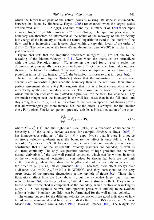
FIGURE 4. Budgets of the three diagonal components of the Reynolds stress tensor, (a) u′2,(b) v′2 and (c) w′2, and (d) the kinetic energy density K = (u′2 + v′2 + w′2)/2, as a function ofy/h, for W2600C (—–) and C2000 (– –). Symbols: ©, Pii; 4, Tii; �, Πii; ∗, εii. The horizontaldotted lines indicate zero. All of the terms are normalized in wall units.

the Reynolds stress tensor can be written as

Duiuj

Dt≡ Bij = Pij + εij + Tij +Πij + Vij, (3.7)

where the terms in the right-hand side of the equation are referred to as production,dissipation, turbulent diffusion, velocity-pressure gradient and viscous diffusion,respectively. They are defined by

Pij =−uiuk Uj,k − ujuk Ui,k, (3.8)

εij =−2ν ui,kuj,k, (3.9)Tij = uiujuk,k, (3.10)

Πij =−uip,j − ujp,i, (3.11)Vij = ν uiuj,kk, (3.12)

where subscripts after a comma (),j represent differentiation with respect to xj.Repeated subscripts imply summation over 1–3. Figure 4 presents the comparisonof the budgets of the three diagonal stresses and of the total kinetic energy in W2600Cand C2000, as functions of y/h, normalized as B+ij = νBij/u4

τ . The viscous diffusion Vii

is omitted because it is negligible compared with the other terms. All of the budgetsagree very well above y/h≈ 0.05 (y+ ≈ 100), but differ near the boundary.


101

100

10–1102100

(a)

102100

(b)

101

102

100

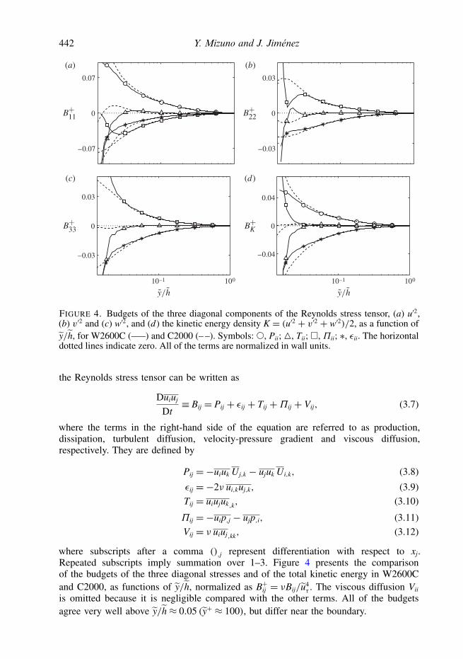
FIGURE 5. Premultiplied two-dimensional spectra, kxkzφuu (with no symbols) and kxkzφvv(with symbols), for W2600C at: —–, y/h = 0.1; – –, 0.2; − · −, 0.4. (a) As functions ofλx/y and λz/y. (b) As functions of λx/˜ and λz/˜. Each spectrum is normalized by themean-squared intensity of each component at each height and the contour level is 0.05.

The main differences are in the pressure and turbulent-diffusion terms, which aremuch stronger near the boundary of the wall-less channel than near the wall of the fullsimulation. In particular, note that the pressure term of the kinetic-energy balance infigure 4(d) is very strong near the boundary, while it essentially vanishes in the fullsimulation. The only pressure term in that equation is the pressure transport ∂(pv)/∂y,which is small near walls because, even if the flow is very inhomogeneous there,the wall-normal velocity vanishes. That is not the case near the wall-less boundary,where the transpiration is high, and we have seen that the lack of coherence betweenthe boundary and the overlying flow creates high pressures. Note also that this termtransfers energy to the two transverse velocity components, but is not very importantfor the streamwise velocity, which is mostly inactive near the boundary. The extraenergy created in this way is compensated by the turbulent diffusion of the extraneouseddies away from the wall.

3.3. Length scalesAs we mentioned in the introduction, the length scales of the velocity fluctuations havebeen observed to depend linearly on y in attached turbulent flows, even beyond theclassical range of the logarithmic velocity profile. Mizuno & Jimenez (2011) showedthat the scaling range of moderately sized attached fluctuations can be extendedeven further by the use of the mixing length `(y), to the point that it holds iny+ > 70, y/h < 0.5 for Reynolds numbers as low as h+ ' 500. The off-wall boundarycondition (2.4) is intended to mimic that dependence, and it is interesting to inquireinto whether `, or its surrogate y, represent well the length scales of the wall-lessstructures. A separate question is whether y can be used to improve the comparisonbetween the two-point statistics of wall-less and full channels, even when a linearlength scaling is not strictly satisfied.

The wall-parallel scales of the velocity fluctuations can be characterized by theirtwo-dimensional spectra,

φij(kx, y, kz)≡ ui(kx, y, kz)u∗j (kx, y, kz), (3.13)


0.20

0.10

(a)

0.05

0.50

10–2 10–1 100

0.20

0.10

(b)

0.05

0.50

10–2 10–1 100

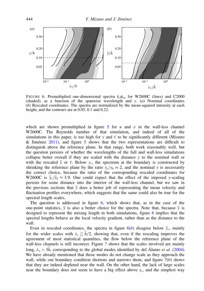
FIGURE 6. Premultiplied one-dimensional spectra kzφuu for W2600C (lines) and C2000(shaded), as a function of the spanwise wavelength and y. (a) Nominal coordinates.(b) Rescaled coordinates. The spectra are normalized by the mean-squared intensity at eachheight, and the contours are at 0.05, 0.1 and 0.22.

which are shown premultiplied in figure 5 for u and v in the wall-less channelW2600C. The Reynolds number of that simulation, and indeed of all of thesimulations in this paper, is too high for y and ` to be significantly different (Mizuno& Jimenez 2011), and figure 5 shows that the two representations are difficult todistinguish above the reference plane. In that range, both work reasonably well, butthe question persists of whether the wavelengths of the full and wall-less simulationscollapse better overall if they are scaled with the distance y to the nominal wall orwith the rescaled y or `. Below yr, the spectrum at the boundary is constructed byshrinking the reference plane by the ratio yr/yb = 2, and the nominal y is necessarilythe correct choice, because the ratio of the corresponding rescaled coordinates forW2600C is yr/yb ≈ 3.9. One could expect that the effect of the imposed y-scalingpersists for some distance into the interior of the wall-less channel, but we saw inthe previous sections that y does a better job of representing the mean velocity andfluctuation profiles everywhere, which suggests that the same could also be true for thespectral length scales.

The question is addressed in figure 6, which shows that, as in the case of theone-point statistics, y is also a better choice for the spectra. Note that, because y isdesigned to represent the mixing length in both simulations, figure 6 implies that thespectral lengths behave as the local velocity gradient, rather than as the distance to thewall.

Even in rescaled coordinates, the spectra in figure 6(b) disagree below yr, mainlyfor the wider scales with λz & h/2, showing that, even if the rescaling improves theagreement of most statistical quantities, the flow below the reference plane of thewall-less channels is still incorrect. Figure 7 shows that the scales involved are mainlylong, λx > 3h, corresponding to the global modes identified by del Alamo et al. (2004).We have already mentioned that those modes do not change scale as they approach thewall, while our boundary condition shortens and narrows them, and figure 7(b) showsthat they are indeed depleted near the wall. On the other hand, the lack of large scalesnear the boundary does not seem to have a big effect above yr, and the simplest way


(a)

10–2 10–1 100

0.20

0.10

(b)

0.05

0.50

10–2 10–1 100

0.20

0.10

0.05

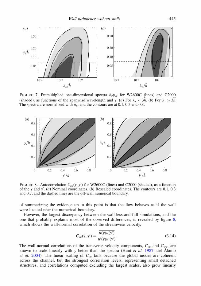
0.50

FIGURE 7. Premultiplied one-dimensional spectra kzφuu for W2600C (lines) and C2000(shaded), as functions of the spanwise wavelength and y. (a) For λx < 3h. (b) For λx > 3h.The spectra are normalized with uτ , and the contours are at 0.1, 0.3 and 0.8.

(a) (b)0.8

0.6

0.4

0.2

0 0.80.60.40.2

0.8

0.6

0.4

0.2

0 0.80.60.40.2

FIGURE 8. Autocorrelation Cuu(y, y′) for W2600C (lines) and C2000 (shaded), as a functionof the y and y′. (a) Nominal coordinates. (b) Rescaled coordinates. The contours are 0.1, 0.3and 0.7, and the dashed lines are the off-wall numerical boundary.

of summarizing the evidence up to this point is that the flow behaves as if the wallwere located near the numerical boundary.

However, the largest discrepancy between the wall-less and full simulations, and theone that probably explains most of the observed differences, is revealed by figure 8,which shows the wall-normal correlation of the streamwise velocity,

Cuu(y, y′)= u(y)u(y′)u′(y)u′(y′)

. (3.14)

The wall-normal correlations of the transverse velocity components, Cvv and Cww, areknown to scale linearly with y better than the spectra (Hunt et al. 1987; del Alamoet al. 2004). The linear scaling of Cuu fails because the global modes are coherentacross the channel, but the strongest correlation levels, representing small detachedstructures, and correlations computed excluding the largest scales, also grow linearly


with y (Bullock et al. 1978). The failure of the global scaling of Cuu and the linearscaling of its stronger contours are clear in figure 8(a) for the full channel belowy ≈ 0.3h. The wall-less simulation behaves similarly to the full simulation far fromthe wall, but it separates from it near the boundary. Its correlation length drops almostto zero at y = yb, whereas that only happens for the full channel in the immediatevicinity of the wall. The reason is almost surely that, as we have already mentioned,the phase shift and the rescaling introduced by the synthesizing step (2.4) destroys thecoherence of the boundary plane with the flow above it. Figure 8(b) shows that theeffect of the rescaled y is to restore the correct behaviour of the correlation length. Thespanwise components Cww (not shown) has weaker large-scale structures, but the effectof the boundary condition is the same as for Cuu; its correlation length at the boundaryplane is closer to what it should be at the wall than to its correct value y = yb. Thewall-normal component Cvv behaves better, because its scales are controlled at theboundary by ∂yv.

Note that this behaviour is different from those reported by Orlandi et al. (2003),who found that the most dangerous forcing was that by v, but their experimentsinvolved imposing a single velocity component at a wall in which the other twocomponents were set to zero. They therefore imposed no scale constraints differentfrom those in a smooth wall, and the effect of their forcing was controlled by differentmechanisms.

It is interesting to consider at this point what those observations imply for thequestion of which is the cause and which the effect of the similar behaviours of thecorrelation length and of the velocity profile. Mizuno & Jimenez (2011) showed thatthe spectral and correlation lengths scale better with ` ∼ (dU/dy)

−1than with the

distance to the wall, which they interpreted as implying that the mean shear determinesthe scale. However, figures 6 and 8 show that their proportionality persists even whenboth, the length scale and the velocity gradient, are incorrect and, since it is clearthat the shorter correlation lengths are caused in this case by the boundary condition(2.4), the strong implication is that the short correlation causes the steeper profile,instead of the other way around. A corollary would be that a better boundary conditionshould not only attempt to represent the wall-parallel spectral length scales, but thewall-normal ones as well.

4. Large-eddy simulations

We saw in the introduction that modelling of the inner layer is a central issue inreducing the computational requirements of the LES of wall-bounded turbulent flows,and one of the goals of this section is to investigate whether the boundary conditionsdeveloped above for DNSs can also be used for that purpose. Second, since the high-Reynolds-number direct simulations of the previous section are too expensive to allowextensive experimentation, we will use the cheaper LESs to investigate the questionof C- versus D-scaling of the boundary spectra, and to demonstrate the importance ofrescaling in maintaining an equilibrium flow.

Since our interest is in testing the boundary condition, rather than in optimizingLESs, we use a simple Smagorinsky (1963) subgrid model, in which the eddyviscosity νT is expressed in term of the filtered velocities Ui, as

νT = (CS1)2 |S|, (4.1)


102

101

103

1001.00.5 1.50 2.0

–10

0

5

0 1.0 2.00.5 1.5

(a) (b)

–5

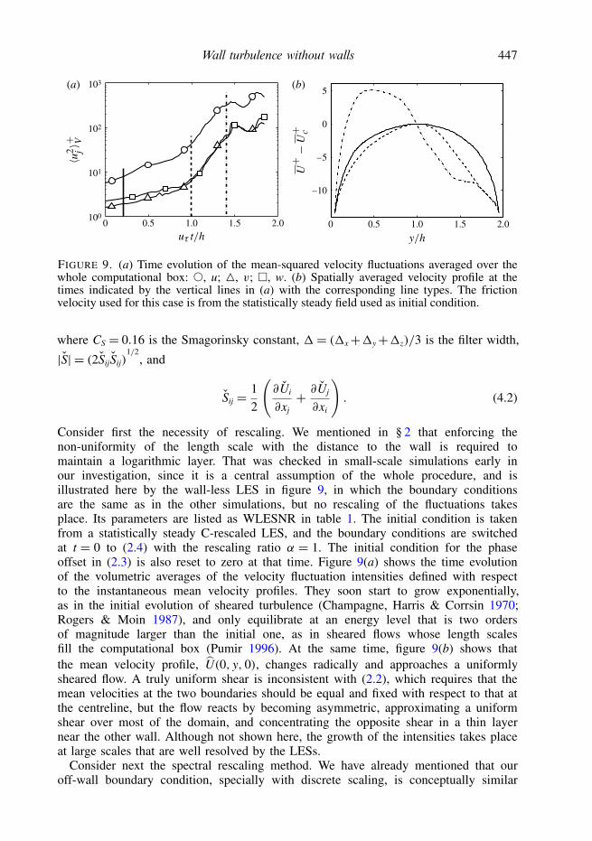
FIGURE 9. (a) Time evolution of the mean-squared velocity fluctuations averaged over thewhole computational box: ©, u; 4, v; �, w. (b) Spatially averaged velocity profile at thetimes indicated by the vertical lines in (a) with the corresponding line types. The frictionvelocity used for this case is from the statistically steady field used as initial condition.

where CS = 0.16 is the Smagorinsky constant, 1= (1x+1y+1z)/3 is the filter width,

|S| = (2SijSij)1/2

, and

Sij = 12

(∂Ui

∂xj+ ∂Uj

∂xi

). (4.2)

Consider first the necessity of rescaling. We mentioned in § 2 that enforcing thenon-uniformity of the length scale with the distance to the wall is required tomaintain a logarithmic layer. That was checked in small-scale simulations early inour investigation, since it is a central assumption of the whole procedure, and isillustrated here by the wall-less LES in figure 9, in which the boundary conditionsare the same as in the other simulations, but no rescaling of the fluctuations takesplace. Its parameters are listed as WLESNR in table 1. The initial condition is takenfrom a statistically steady C-rescaled LES, and the boundary conditions are switchedat t = 0 to (2.4) with the rescaling ratio α = 1. The initial condition for the phaseoffset in (2.3) is also reset to zero at that time. Figure 9(a) shows the time evolutionof the volumetric averages of the velocity fluctuation intensities defined with respectto the instantaneous mean velocity profiles. They soon start to grow exponentially,as in the initial evolution of sheared turbulence (Champagne, Harris & Corrsin 1970;Rogers & Moin 1987), and only equilibrate at an energy level that is two ordersof magnitude larger than the initial one, as in sheared flows whose length scalesfill the computational box (Pumir 1996). At the same time, figure 9(b) shows thatthe mean velocity profile, U(0, y, 0), changes radically and approaches a uniformlysheared flow. A truly uniform shear is inconsistent with (2.2), which requires that themean velocities at the two boundaries should be equal and fixed with respect to that atthe centreline, but the flow reacts by becoming asymmetric, approximating a uniformshear over most of the domain, and concentrating the opposite shear in a thin layernear the other wall. Although not shown here, the growth of the intensities takes placeat large scales that are well resolved by the LESs.

Consider next the spectral rescaling method. We have already mentioned that ouroff-wall boundary condition, specially with discrete scaling, is conceptually similar


(a) (b)

0.3

0.2

0.1

0.60.40.20 0.8

1.0

2.0

2.5

1.5

0.5

0.60.40.2 0.80 1.0

3.00.4

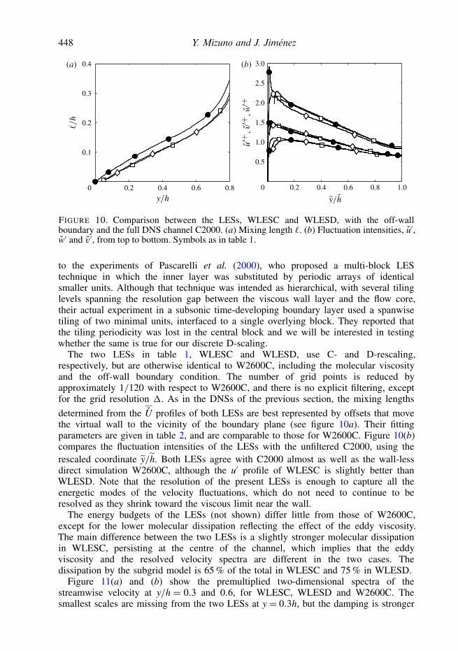
FIGURE 10. Comparison between the LESs, WLESC and WLESD, with the off-wallboundary and the full DNS channel C2000. (a) Mixing length `. (b) Fluctuation intensities, u′,w′ and v′, from top to bottom. Symbols as in table 1.

to the experiments of Pascarelli et al. (2000), who proposed a multi-block LEStechnique in which the inner layer was substituted by periodic arrays of identicalsmaller units. Although that technique was intended as hierarchical, with several tilinglevels spanning the resolution gap between the viscous wall layer and the flow core,their actual experiment in a subsonic time-developing boundary layer used a spanwisetiling of two minimal units, interfaced to a single overlying block. They reported thatthe tiling periodicity was lost in the central block and we will be interested in testingwhether the same is true for our discrete D-scaling.

The two LESs in table 1, WLESC and WLESD, use C- and D-rescaling,respectively, but are otherwise identical to W2600C, including the molecular viscosityand the off-wall boundary condition. The number of grid points is reduced byapproximately 1/120 with respect to W2600C, and there is no explicit filtering, exceptfor the grid resolution 1. As in the DNSs of the previous section, the mixing lengths

determined from the U profiles of both LESs are best represented by offsets that movethe virtual wall to the vicinity of the boundary plane (see figure 10a). Their fittingparameters are given in table 2, and are comparable to those for W2600C. Figure 10(b)compares the fluctuation intensities of the LESs with the unfiltered C2000, using therescaled coordinate y/h. Both LESs agree with C2000 almost as well as the wall-lessdirect simulation W2600C, although the u′ profile of WLESC is slightly better thanWLESD. Note that the resolution of the present LESs is enough to capture all theenergetic modes of the velocity fluctuations, which do not need to continue to beresolved as they shrink toward the viscous limit near the wall.

The energy budgets of the LESs (not shown) differ little from those of W2600C,except for the lower molecular dissipation reflecting the effect of the eddy viscosity.The main difference between the two LESs is a slightly stronger molecular dissipationin WLESC, persisting at the centre of the channel, which implies that the eddyviscosity and the resolved velocity spectra are different in the two cases. Thedissipation by the subgrid model is 65 % of the total in WLESC and 75 % in WLESD.

Figure 11(a) and (b) show the premultiplied two-dimensional spectra of thestreamwise velocity at y/h = 0.3 and 0.6, for WLESC, WLESD and W2600C. Thesmallest scales are missing from the two LESs at y= 0.3h, but the damping is stronger


0.20

0.10

0.05

0.50

10–1 100 101

(c)

10–1 100 101

10–1

100

(a)

(d)

(b)

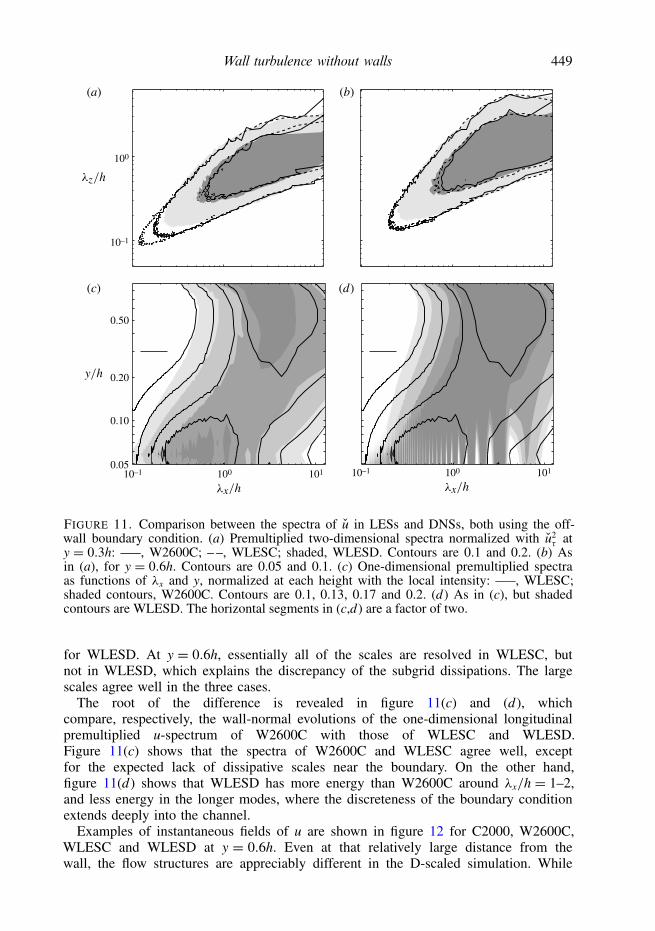
FIGURE 11. Comparison between the spectra of u in LESs and DNSs, both using the off-wall boundary condition. (a) Premultiplied two-dimensional spectra normalized with u2

τ aty = 0.3h: —–, W2600C; – –, WLESC; shaded, WLESD. Contours are 0.1 and 0.2. (b) Asin (a), for y = 0.6h. Contours are 0.05 and 0.1. (c) One-dimensional premultiplied spectraas functions of λx and y, normalized at each height with the local intensity: —–, WLESC;shaded contours, W2600C. Contours are 0.1, 0.13, 0.17 and 0.2. (d) As in (c), but shadedcontours are WLESD. The horizontal segments in (c,d) are a factor of two.

for WLESD. At y = 0.6h, essentially all of the scales are resolved in WLESC, butnot in WLESD, which explains the discrepancy of the subgrid dissipations. The largescales agree well in the three cases.

The root of the difference is revealed in figure 11(c) and (d), whichcompare, respectively, the wall-normal evolutions of the one-dimensional longitudinalpremultiplied u-spectrum of W2600C with those of WLESC and WLESD.Figure 11(c) shows that the spectra of W2600C and WLESC agree well, exceptfor the expected lack of dissipative scales near the boundary. On the other hand,figure 11(d) shows that WLESD has more energy than W2600C around λx/h = 1–2,and less energy in the longer modes, where the discreteness of the boundary conditionextends deeply into the channel.

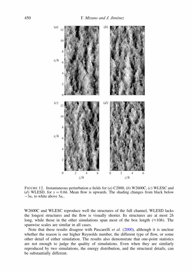
Examples of instantaneous fields of u are shown in figure 12 for C2000, W2600C,WLESC and WLESD at y = 0.6h. Even at that relatively large distance from thewall, the flow structures are appreciably different in the D-scaled simulation. While


12

10

8

6

4

2

0 2 4 6 0 2 4 6

(c)

12

10

8

6

4

2

0

(a)

(d)

(b)

FIGURE 12. Instantaneous perturbation u fields for (a) C2000, (b) W2600C, (c) WLESC and(d) WLESD, for y = 0.6h. Mean flow is upwards. The shading changes from black below−3uτ to white above 3uτ .

W2600C and WLESC reproduce well the structures of the full channel, WLESD lacksthe longest structures and the flow is visually shorter. Its structures are at most 2hlong, while those in the other simulations span most of the box length (≈10h). Thespanwise scales are similar in all cases.

Note that these results disagree with Pascarelli et al. (2000), although it is unclearwhether the reason is our higher Reynolds number, the different type of flow, or someother detail of either simulation. The results also demonstrate that one-point statisticsare not enough to judge the quality of simulations. Even when they are similarlyreproduced by two simulations, the energy distribution, and the structural details, canbe substantially different.


5. Discussion and conclusionsWe have performed DNSs of turbulent channels in which the inner layer is replaced

by an off-wall boundary condition where the velocities are substituted by a rescaledand shifted copy of an interior reference plane. The idea is to mimic the linearvariation of the length scales of the flow with the wall distance, and it is remarkablethat such a simple expedient results in a flow with a well-developed logarithmiclayer. Tests in which the rescaling was not applied resulted in a flow much closerto homogeneous shear turbulence, showing that the scale variation is a necessaryingredient of wall-bounded turbulence. That has been illustrated above by a LES.

Since the off-wall condition is applied at wall distances usually associated with thelower logarithmic layer (y/h = 0.05, y+ = 130), the flow lacks all of the structuresusually present in the near-wall buffer layer, including the kinetic energy maximum.The mean velocity profile remains approximately logarithmic all of the way to theboundary, and so do the profiles of the velocity fluctuation intensities (Townsend1976). Even the statistical properties of the structures defined by a strong Reynoldsstress (Lozano-Duran et al. 2012) are essentially identical to those in full channels (A.Lozano-Duran, Personal communication). That is consistent with the results of Flores& Jimenez (2006) who found that the properties of vorticity clusters (del Alamo et al.2006) change little when the buffer layer is manipulated to mimic rough flows. Thepresent experiments modify the buffer layer even more profoundly (indeed, suppressit), and the Reynolds number (h+ = 2600) is higher. They reinforce the conclusion thatthe logarithmic structures do not depend on seeding from the wall.

Because the present simulations lack a viscous sublayer, the resolution requirementsare relaxed with respect to full DNSs. The resolution can be set in terms of theKolmogorov viscous scale at the boundary, and does not need to resolve the wall. Inour highest-Reynolds-number simulation, the savings in the y-grid are ∼40 %. In fact,we have shown that LESs at the same Reynolds number, using ∼100 times less points,give results essentially identical to the DNS.

On the other hand, the agreement with full-domain simulations is not complete.Most errors are local to the neighbourhood of the boundary, as can be expectedfrom the accommodation region of any artificial boundary condition, but some ofthem extend deeper into the flow (y/h ≈ 0.3–0.4). Of those, some can be easilyavoided, such as the persistence of spurious periodicities introduced by the rescalingof the boundary velocity (D-scaling), which disappears after spectral smoothing of theboundary plane (C-scaling). Others are relatively mild, such as the 15 % overshoot ofthe velocity fluctuation intensities near the numerical boundary, or the depletion of thelargest scales in the same region.

Two are more serious. The first is a strong increase of the pressure fluctuationsnear the boundary, which can be traced to the ‘hard’ Dirichlet boundary conditionsimposed on the velocities. The extra pressure has two components. One is dueto the small-scale wall-parallel vorticity created by the difference between the wall-parallel boundary velocities and the flow above. That component is very strong, but isrestricted to the immediate vicinity of the boundary and can probably be taken intoaccount by sacrificing the first few grid points of the simulation. A weaker componenthas wall-parallel scales of the order of the wall-normal velocity and extends deeperinto the channel. The wall-normal velocity is copied into the boundary from theinterior reference plane without any effort to guarantee continuity and it is left to thepressure to resolve any inconsistency between the boundary transpiration velocity andthose induced by the overlying structures. The extra pressure fluctuations thus inducedmodify some of the terms of the energy budgets near the boundary and account for


the modest increase of the velocity fluctuations in that region. Any improvement of thepresent procedure should include a ‘softer’ boundary condition for the pressure.

The second problem is that the mean velocity profile, and most other flow properties,behave as if the wall were located at an intermediate point between the boundaryand the nominal position assumed by the scaling of the boundary condition. In fact,the optimal virtual origin obtained by fitting the results of the wall-less simulationsis not very far from the boundary plane itself. The reason for the offset was foundto be the lack of correlation between the synthetic boundary and the overlying flow.In part because it is impossible to shrink a plane without also moving it and alsobecause the boundary field has to be translated with respect to the reference one, toaccount for the mean shear, the reference and boundary planes quickly slide very farfrom each other. The reference plane only acts as a turbulence-like source from whichto synthesize the boundary, and the results in this paper could probably have beenobtained by using a reference plane from an unrelated simulation (Orlandi et al. 2003).That neglects the attached nature of the logarithmic-layer eddies (Townsend 1961),whose base is continually eroded. The wall-normal correlation length becomes veryshort at the numerical boundary, instead of remaining proportional to y, and the flowcreates spurious small eddies whose sizes are closer to what should happen at the wallthan to the interior of the logarithmic layer. The shear of the mean profile becomesteeper as the correlation length becomes smaller.

The last observation is significant, because most arguments for the logarithmicvelocity profile rely on the correspondence between the length scale of the flowstructures and the mean velocity gradient (Millikan 1938), which has often beeninterpreted to mean that the latter determines the former. The present result, where it isclear that the correlation length is artificially shortened by the procedure of generatingthe boundary condition, with the result of steepening the mean profile, proves that theopposite it true. It is the length scale of the structures that determines the profile.

Unfortunately, the previous remarks also imply that any off-wall boundary conditionthat attempts to reproduce the correct mean velocity profile must mimic the wall-normal correlation lengths, in addition to the in-plane ones scaled in the present study.How that can be achieved is not immediately obvious and is beyond the scope thepresent paper. This, as well as other extensions to enhance the applicability of thepresent boundary condition to practical cases, are currently under investigation.

AcknowledgementsThis work was supported by the CYCIT grants TRA2006-08226, TRA2009-11498,

the ERC advanced grant ERC-2010.AdG-20100224, and by allocations of computertime at the Barcelona Supercomputing Center. Y.M. was supported by the SpanishMinistry of Education and Science, under the Juan de la Cierva program, and by theSyeC Consolider Program CSD2007–00050. He was also partially supported by theAustralian Research Council Discovery Projects funding scheme DP1095620. We aregrateful to J. A. Sillero for the velocity correlations of the full-channel simulation infigure 8.

R E F E R E N C E S

ADRIAN, R. J. 2007 Hairpin vortex organization in wall turbulence. Phys. Fluids 19, 041301.ADRIAN, R. J., MAINHART, C. D. & TOMKINS, C. D. 2000 Vortex organization in the outer region

of the turbulent boundary layer. J. Fluid Mech. 422, 1–54.


DEL ALAMO, J. C. & JIMENEZ, J. 2009 Estimation of turbulent convection velocities andcorrections to Taylor’s approximation. J. Fluid Mech. 640, 5–26.

DEL ALAMO, J. C., JIMENEZ, J., ZANDONADE, P. & MOSER, R. D. 2004 Scaling of the energyspectra of turbulent channels. J. Fluid Mech. 500, 135–144.

DEL ALAMO, J. C., JIMENEZ, J., ZANDONADE, P. & MOSER, R. D. 2006 Self-similar vortexclusters in the turbulent logarithmic region. J. Fluid Mech. 561, 329–358.

BAILEY, S. C. C., HULTMARK, M., SMITS, A. J. & SCHULTZ, M. P. 2008 Azimuthal structure ofturbulence in high Reynolds number pipe flow. J. Fluid Mech. 615, 121–138.

BAKKEN, O. M., KROGSTAD, P. A., ASHRAFIAN, A & ANDERSSON, H. I. 2005 Reynolds numbereffects in the outer layer of the turbulent flow in a channel with rough walls. Phys. Fluids 17,065101.

BULLOCK, K. J., COOPER, R. E. & ABERNATHY, F. H. 1978 Structural similarity in radialcorrelations and spectra of longitudinal velocity fluctuations in pipe flow. J. Fluid Mech. 88,585–608.

BUSCHMANN, M. H. & GAD-EL-HAK, M. 2005 New mixing-length approach for the mean velocityprofile of turbulent boundary layers. Trans. ASME: J. Fluids Engng 127, 393–396.

CATALANO, P., WANG, M., IACCARINO, G. & MOIN, P. 2003 Numerical simulation of the flowaround a circular cylinder at high Reynolds numbers. Intl J. Heat Fluid Flow 24, 453–469.

CHAMPAGNE, F. H., HARRIS, V. G. & CORRSIN, S. 1970 Experiments on nearly homogeneousturbulent shear flow. J. Fluid Mech. 41, 81–139.

DEARDORFF, J. W. 1970 A numerical study of three-dimensional turbulent channel flow at largeReynolds numbers. J. Fluid Mech. 41, 453–480.

DUNCAN, W. J., THOM, A. S. & YOUNG, A. D. 1970 Mechanics of Fluids, 2nd edn. Arnold.FLORES, O. & JIMENEZ, J. 2006 Effect of wall-boundary disturbances on turbulent channel flows.

J. Fluid Mech. 566, 357–376.FLORES, O., JIMENEZ, J. & DEL ALAMO, J. C. 2007 Vorticity organization in the outer layer of

turbulent channels with disturbed walls. J. Fluid Mech. 591, 145–154.GUALA, M., HOMMEMA, S. E. & ADRIAN, R. J. 2006 Large-scale and very-large-scale motions in

turbulent pipe flow. J. Fluid Mech. 554, 521–542.HAMBA, F. 2003 A hybrid RANS/LES simulation of turbulent channel flow. Theor. Comput. Fluid

Dyn. 16, 387–403.HOYAS, S. & JIMENEZ, J. 2006 Scaling of velocity fluctuations in turbulent channels up to

Reτ = 2003. Phys. Fluids 18, 011702.HOYAS, S. & JIMENEZ, J. 2008 Reynolds number effects on the Reynolds-stress budgets in turbulent

channels. Phys. Fluids 20, 101511.HULTMARK, M., VALLIKIVI, M., BAILEY, S. C. C. & SMITS, A. J. 2012 Turbulent pipe flow at

extreme Reynolds numbers. Phys. Rev. Lett. 108, 094501.HUNT, J. C. R., MOIN, P., MOSER, R. D. & SPALART, P. R. 1987 Self similarity of two point

correlations in wall bounded turbulent flows. CTR Annu. Res. Briefs, 25–36.HUNT, J. C. R. & MORRISON, J. F. 2000 Eddy structure in turbulent boundary layers. Eur. J.

Mech. (B-Fluids) 19, 673–694.JIMENEZ, J. 1998 The largest scales of turbulent wall flows. CTR Annu. Res. Briefs, 137–154.JIMENEZ, J. 2004 Turbulent flows over rough walls. Annu. Rev. Fluid Mech. 36, 173–196.JIMENEZ, J. 2007 Simulation of homogeneous and inhomogeneous shear turbulence. CTR Annu. Res.

Briefs, 367–378.JIMENEZ, J. 2012 Cascades in wall-bounded turbul.. Annu. Rev. Fluid Mech. 44, 27–45.JIMENEZ, J. & HOYAS, S. 2008 Turbulent fluctuations above the buffer layer of wall-bounded flows.

J. Fluid Mech. 611, 215–236.JIMENEZ, J. & MOSER, R. D. 2000 LES: where are we and what can we expect?. AIAA J. 38,

605–612.KEATING, A. & PIOMELLI, U. 2006 A dynamic stochastic forcing method as a wall-layer model for

large-eddy simulation. J. Turbul. 7, N12.KIM, K. C. & ADRIAN, R. J. 1999 Very large-scale motions in the outer layer. Phys. Fluids 11,

417–422.


KIM, J., MOIN, P & MOSER, R. D. 1987 Turbulence statistics in fully developed channel flow atlow Reynolds number. J. Fluid Mech. 177, 133–166.

LOZANO-DURAN, A., FLORES, O. & JIMENEZ, J. 2012 The three-dimensional structure ofmomentum transfer in turbulent channels. J. Fluid Mech. 694, 100–130.

LUND, T. S., WU, X. & SQUIRES, K. D. 1998 Generation of turbulent inflow data forspatially-developing boundary layer simulations. J. Computat. Phys. 140, 233–258.

MANSOUR, N. N., KIM, J. & MOIN, P. 1988 Reynolds-stress and dissipation-rate budgets in aturbulent channel flow. J. Fluid Mech. 194, 15–44.

MILLIKAN, C. B. 1938 A critical discussion of turbulent flows in channels and circular tubes. InProceedings of 5th International Conference on Applied Mechanics, pp. 386–392. Wiley.

MIZUNO, Y. & JIMENEZ, J. 2011 Mean velocity and length scales in the overlap region ofwall-bounded turbulent flows. Phys. Fluids 23, 085112.

MONTY, J. P., STEWART, J. A., WILLIAMS, R. C. & CHONG, M. S. 2007 Large-scale features inturbulent pipe and channel flows. J. Fluid Mech. 589, 147–156.

MORRISON, W. R. B. & KRONAUER, R. E. 1969 Structure similarity for fully developed turbulencein smooth tubes. J. Fluid Mech. 39, 117–141.

NIKITIN, N. V., NICOUD, F., EASISTHO, B., SQUIRES, K. D. & SPALART, P. R. 2000 Anapproach to wall modeling in large-eddy simulations. Phys. Fluids 12, 1629–1632.

OBERLACK, M. 2001 Unified approach for symmetries in plane parallel shear flows. J. Fluid Mech.427, 299–328.

ORLANDI, P., LEONARDI, S., TUZI, R. & ANTONIA, R. A. 2003 Direct numerical simulations ofturbulent channel flow with wall velocity disturbances. Phys. Fluids 15, 3587–3601.

OSTERLUND, J. M., JOHANSSON, A. V., NAGIB, H. M. & HITES, M. 2000 A note on the overlapregion in turbulent boundary layers. Phys. Fluids 12, 1–4.

PASCARELLI, A., PIOMELLI, U. & CANDLER, G. V. 2000 Multi-block large-eddy simulations ofturbulent boundary layers. J. Comput. Phys. 157, 256–279.

PERRY, A. E. & ABELL, C. J. 1975 Scaling laws for pipe-flow turbulence. J. Fluid Mech. 67,257–271.

PERRY, A. E. & ABELL, C. J. 1977 Asymptotic similarity of turbulence structures in smooth- andrough-walled pipes. J. Fluid Mech. 79, 785–799.

PIOMELLI, U. 2008 Wall-layer models for large-eddy simulations. Prog. Aerosp. Sci. 44, 437–446.PIOMELLI, U. & BALARAS, E. 2002 Wall-layer models for large-eddy simulations. Annu. Rev. Fluid

Mech. 34, 349–374.PIOMELLI, U., BALARAS, E., PASINATO, H., SQUIRES, K. D. & SPALART, P. R. 2003 The

inner/outer layer interface in large-eddy simulations with wall-layer models. Intl J. Heat FluidFlow 24, 538–550.

PODVIN, B. & FRAIGNEAU, Y. 2011 Synthetic wall boundary conditions for the direct numericalsimulation of wall-bounded turbulence. J. Turbul. 12, 1–26.

PUMIR, A. 1996 Turbulence in homogeneous shear flows. Phys. Fluids 8, 3112–3127.ROGERS, M. M. & MOIN, P. 1987 The structure of the vorticity field in homogeneous turbulent

flows. J. Fluid Mech. 176, 33–66.SADDOUGHI, S. G. & VEERAVALI, S. V. 1994 Local isotropy in turbulent boundary layers at high

Reynolds numbers. J. Fluid Mech. 268, 333–372.SCHUMANN, U. 1985 Algorithms for direct numerical simulation of shear-periodic turbulence. In

Ninth International Conference on Numerical Methods in Fluid Dynamics, 218. Lecture Notesin Physics, pp. 492–496 Springer.

SIMENS, M. P., JIMENEZ, J., HOYAS, S. & MIZUNO, Y. 2009 A high-resolution code for turbulentboundary layers. J. Comput. Phys. 228, 4218–4231.

SMAGORINSKY, J. 1963 General circulation experiments with the primitive equations I. The basicexperiment. Mon. Weath. Rev. 91, 99–164.

SMITS, A. J., MCKEON, B. J. & MARUSIC, I. 2011 High-Reynolds number wall turbulence. Annu.Rev. Fluid Mech. 43, 353–375.

SPALART, P. R. 2009 Detached-eddy simulation. Annu. Rev. Fluid Mech. 41, 181–202.


SPALART, P. R., COLEMAN, G. N. & JOHNSTONE, R. 2008 Direct numerical simulation of theEkman layer: a step in Reynolds number, and cautious support for a log law with a shiftedorigin. Phys. Fluids 20, 101507.

SPALART, P. R., MOSER, R. D. & ROGERS, M. M. 1991 Spectral methods for the Navier–Stokesequations with one infinite and two periodic directions. J. Comput. Phys. 96, 297–324.

TENNEKES, H. & LUMLEY, J. L. 1972 A First Course in Turbulence. MIT.TOMKINS, C. D. & ADRIAN, R. J. 2003 Spanwise structure and scale growth in turbulent boundary

layers. J. Fluid Mech. 490, 37–74.TOWNSEND, A. A. 1961 Equilibrium layers and wall turbulence. J. Fluid Mech. 11, 97–120.TOWNSEND, A. A. 1976 The Structure of Turbulent Shear Flow, 2nd edn. Cambridge University

Press.WANG, M. & MOIN, P. 2002 Dynamic wall modeling for large-eddy simulation of complex

turbulent flows. Phys. Fluids 14, 2043–2051.WOSNIK, M., CASTILLO, L. & GEORGE, W. K. 2000 A theory for turbulent pipe and channel

flows. J. Fluid Mech. 421, 115–145.ZANOUN, E. S., DURST, F. & NAGIB, H. 2003 Evaluating the law of the wall in two-dimensional

fully developed turbulent channel flows. Phys. Fluids 15, 3079–3088.

Documents

J. Fluid Mech. (2013), . 723, pp. … · †Email address for correspondence:[email protected] ‡Present address: Mechanical and Systems Engineering, Doshisha University,