J. Fluid Mech. (2013), . 718, pp. doi:10.1017/jfm.2012.589 ... · 90 D. O. Hubble, P. P. Vlachos and T. E. Diller and Dullenkopf & Mayle (1995) identiﬁed a dominant frequency band

J. Fluid Mech. (2013), vol. 718, pp. 89–115. c© Cambridge University Press 2013 89doi:10.1017/jfm.2012.589

The role of large-scale vortical structures intransient convective heat transfer augmentation

David O. Hubble, Pavlos P. Vlachos† and Tom E. Diller

Department of Mechanical Engineering, Virginia Tech, Blacksburg, VA 24061, USA

(Received 6 November 2011; revised 24 November 2012; accepted 26 November 2012;first published online 8 February 2013)

The physical mechanism by which large-scale vortical structures augment convectiveheat transfer is a fundamental problem of turbulent flows. To investigate thisphenomenon, two separate experiments were performed using simultaneous heattransfer and flow field measurements to study the vortex–wall interaction. Individualvortices were identified and studied both as part of a turbulent stagnation flowand as isolated vortex rings impacting on a surface. By examining the temporalevolution of both the flow field and the resulting heat transfer, it was observedthat the surface thermal transport was governed by the transient interaction of thevortical structure with the wall. The magnitude of the heat transfer augmentation wasdependent on the instantaneous strength, size and position of the vortex relative to theboundary layer. Based on these observations, an analytical model was developed fromfirst principles that predicts the time-resolved surface convection using the transientproperties of the vortical structure during its interaction with the wall. The analyticalmodel was then applied, first to the simplified vortex ring model and then to themore complex stagnation region experiments. In both cases, the model was able toaccurately predict the time-resolved convection resulting from the vortex interactionswith the wall. These results reveal the central role of large-scale turbulent structuresin the augmentation of thermal transport and establish a simple model for quantitativepredictions of transient heat transfer.

Key words: turbulent convection, vortex flows, vortex interactions

1. IntroductionPredicting convective heat transfer in the presence of free-stream turbulence is

difficult, even for simple geometries, because of the complex and random interactionsof flow structures with the wall surface. Traditionally, methods for analysing theconvective heat transfer in the presence of free-stream turbulence rely on averageand statistical properties of the flow field. Such approaches result in empiricalcorrelations and models that often are not based on the governing physics. Forexample, empirical correlations for the augmentation of time-average heat transferby free-stream turbulence have been developed (Kestin 1966; Lowery & Vachon 1975)based on statistical turbulence properties such as the turbulence intensity (Tu) andintegral length scale (Λ) (Vanfossen, Simoneau & Ching 1995; Ames 1997). Mayle,Dullenkopf & Schulz (1998) emphasized the importance of the turbulent spectrum

† Email address for correspondence: [email protected]

mailto:[email protected]

borrego

Typewritten Text

Copyright by the Cambridge University Press. Hubble, D. O.; Vlachos, P. P.; Diller, T. E., "The role of large-scale vortical structures in transient convective heat transfer augmentation," J. Fluid Mech. (2013), vol. 718, pp. 89-115. DOI: 10.1017/jfm.2012.589

90 D. O. Hubble, P. P. Vlachos and T. E. Diller

and Dullenkopf & Mayle (1995) identified a dominant frequency band correspondingto an eddy size that is about 16 times the laminar boundary layer thickness. Asurface renewal model was used to estimate the effect of the turbulent structures fromthe free stream (Kataoka 1990; Yuan & Liburdy 1992). Time-resolved experimentalmeasurements of the fluctuating transport at the surface have shown direct correlationwith the velocity fluctuations in the free stream (Moss & Oldfield 1996; Holmberg &Diller 2005), but the impact on the overall transport was not established. All of thesemodels are valid only within the narrow range of the experimental data that yieldedthese correlations and do not offer a general predictive ability.

Adrian, Christensen & Liu (2000) describe the role of proper decomposition ofturbulent velocity fields depending on what is being studied. Although the statisticsof the fluctuating fields may be useful for Reynolds-averaged models, visualizationof the structured, coherent elements requires methods that show an entire sectionof the flow field as a function of time. For example, Hutchins & Marusic (2007)showed that the inner boundary layer small-scale structure was directly influencedby the large-scale outer flow structures and in a later work they proposed a modelcapturing these interactions (Marusic, Mathis & Hutchins 2010). The elegance of theirmodel stems from its ability to predict the near-wall flow structure, which is verychallenging to measure or accurately model, using large-scale information from theexternal flow. Although they focused on the turbulent statistics of the inner-regionvelocity and not the vortical flow structure, the connection they showed between theinner and outer regions as a function of time is most interesting and qualitativelysupports the physical processes described here in the sense that the large-scale externalflow governs the near-wall processes. The effect of turbulent spots on surface heattransfer was also studied by Sabatino & Smith (2008) using a combination of particleimage velocimetry (PIV) and liquid-crystal temperature measurements. By identifyingthe vortical structures within the boundary layer they demonstrated the importance ofthe temperature of the fluid that is brought to the surface for augmenting heat transfer.

Vortical structures are particularly important in stagnating flows where free-streamstructures are aligned with the wall and amplified through vortex stretching by themean flow strain rate (Sutera 1965). Gifford, Diller & Vlachos (2011) used time-resolved digital particle image velocimetry (TRDPIV) and a thin-film heat flux sensorto study heat transfer augmentation in the stagnation region of a flow containinglarge-scale free-stream turbulence. Subsequent tracking of the vortices present showedthat the rate of heat transfer at the wall was directly influenced by the strengthand proximity of the vortex. It appeared that the largest transport occurred when thestructures swept free-stream fluid through the boundary layer to the surface. Thisconcept is supported by two numerical studies (Romero-Mendez et al. 1998; Martin &Zenit 2008) of individual vortices near a surface and experimental measurements withsynthetic jets (Pavlova & Amitay 2006).

Other researchers have examined the time-average influence of vortices on surfacetransport. Vanfossen & Simoneau (1987) used wires to create vortices perpendicularto a downstream cylinder and studied the resulting fluid flow and heat transfer nearthe surface using a combination of smoke visualization and liquid crystals. It wasobserved that regions where vortices forced fluid towards the surface corresponded toregions of increased heat transfer. Xiong & Lele (2007) used large-eddy simulation(LES) to model isotropic turbulence impinging on a stagnation region. Vorticeswere observed to form near the stagnation boundary layer. These vortices had astronger influence on the thermal transfer compared to the momentum transfer. Directnumerical simulation (DNS) was used to model the effect of turbulent structures on

Large-scale vortical structures and heat transfer augmentation 91

surface transport in channel flow (Araya, Leonardi & Castillo 2008). Even whenthe structures are modelled directly, however, a turbulence model is still required tocalculate the transport near the surface.

Finally, for investigating vortex-induced heat transfer augmentation, the vortexring–wall interaction (Doligalski, Smith & Walker 1994) provides an attractive systemdue to the inherent ability to control the flow characteristics with simplicity andreproducibility. Vortex rings have been extensively investigated and are very wellunderstood from a fluid mechanics standpoint (Shariff & Leonard 1992) but not muchwork is available considering vortex-ring flows in combination with heat transfer. Ina recent experimental investigation (Arevalo et al. 2007) a vortex ring was createdin air and allowed to impact on a heated vertical plate. The spatially averaged heattransfer from the surface was found to increase by up to 15 % over natural convectionlevels while the vortex was in contact with the surface. In a subsequent study (Arevaloet al. 2010) they expanded their analysis by incorporating PIV measurements andquantifying the near-wall interaction and shear stresses. However, neither of thesestudies was concerned with the mechanism of the heat transfer augmentation drivenby the vortex ring, and they did not attempt to resolve the spatiotemporal correlationsbetween heat flux and the flow field.

In the present work we hypothesize that we can predict the near-wall transientheat transfer in a turbulent flow merely from the characteristics of the outer large-scale vortical structures. To help clarify this approach we first apply our model toindividual vortex rings striking the surface. This allows us to control the propertiesof the vortex and eliminates the complexity of multiple interacting vortices. Theresults with the vortex ring are then used in the more complex case of large-scalefree-stream turbulence interacting with the surface. In both experiments, the time-resolved convective heat transfer is measured while TRDPIV is used to simultaneouslymeasure the two-dimensional flow field. Analysing these measurements in combinationreveals the mechanism by which the vortex structure augments the induced heattransfer. These observations then enable the development of an analytical model whichpredicts the transient convection based only on the properties of the large-scale vorticalstructure interacting with the heated wall. The predictive ability of the model issubsequently tested and validated, first with the simplified vortex ring and then withthe stagnating turbulence data.

2. Experimental measurementsIn this study two separate experiments were performed. In the first, the convection

along the stagnation line of a bluff body in a flow which contains large-scale free-stream turbulence is examined. In the second, a pneumatically actuated vortex ringgenerator is used to produce vortex rings which were allowed to collide normally withan instrumented heated surface. The two experiments share much of the experimentalmethodology as described in this section. In both experiments, measurements weremade to resolve the flow field near the surface while simultaneously measuringthe convection from the surface. Planar TRDPIV (Raffel et al. 2007) was used tomeasure the spatiotemporal characteristics of the flow field as it interacts with thesurface. A vortex identification scheme (Zhou et al. 1999) was then used to identifyand track the vortices present in the TRDPIV data. Measurements of the convectiveheat transfer coefficient at the surface were made using the newly developed Time-Resolved Heat and Temperature Array (THeTA) (Hubble & Diller 2010b). Convectionmeasurements were performed at 10 equidistant points along the stagnation line in


Vortex ringgenerator

Flat plate model withinstrumented plate

Opticaltrain

Flowdirection

Turbulencegenerating grid Xs-5 digital camera

Pegasus laserzy

x

FIGURE 1. (Colour online) Water tunnel facility and experimental setup. During thestagnation tests the vortex ring generator was replaced with turbulence-generating grids.

the first experiment and a line that bisected the impinging vortex ring in the secondexperiment.

The experiments were conducted in the AEThER laboratory at Virginia Tech.The equipment used in the experiment includes: the water tunnel facility, avortex ring generator, an instrumented heated plate, the TRDPIV system, and theaccompanying data acquisition systems which also synchronized the heat flux andvelocity measurements. A schematic of the overall setup is shown in figure 1. Notethat the vortex ring generator is positioned normal to the flat plate and the height ofthe TRDPIV laser plane is such that it bisects the vortex ring generator’s nozzle andaligns with the heat flux sensors on the heated plate. For the stagnation experiments,the vortex ring generator is replaced with turbulence-generating grids.

2.1. Water tunnel facility and turbulence generationThe water tunnel used in the current experiment is a closed loop, variable speedfacility which was operated at 10 cm s−1 for all of the stagnation tests and was used assimply a water tank for the vortex ring tests. The test section measures 0.61 m squareby 1.77 m long and is constructed from clear acrylic. Without turbulence grids andat the tunnel speed used in the stagnation tests the free-stream turbulence intensity isapproximately 1 % throughout the test section.

Free-stream turbulence was generated using simple bi-plane grids. Grid bar sizing(b), spacing (M) and positioning was based on correlations by Baines & Peterson(1951). Three grids were constructed with solidity ratios of S = 0.7 to give integrallength scales (Λ) of approximately 1, 2, and 3 cm at a turbulence intensity (Tu) ofapproximately 7 %. In all cases, the test region was located at a distance downstreamof the grid equal to 17.5M. Properties of the generated turbulence were calculatedfrom the measured flow field with no stagnation model present at downstreamdistances 617.5M and the results compared well with the published correlations


Tank

Solenoidvalve

Master pistonPneumatic cylinder

Vortexring

NozzleSlavepiston

Hydraulic hose

FIGURE 2. (Colour online) Schematic of the vortex ring generator.

Grid b (cm) M (cm) Tu (%) Λ (cm)

1 0.66 1.46 7.4 0.812 1.60 3.54 7.2 1.933 2.16 4.77 6.9 3.24

TABLE 1. Details of grids and turbulence statistics.

(Baines & Peterson 1951). These calculations were performed using the methodsdescribed by Gifford et al. (2011). Details of the grid geometry and turbulenceproperties are given in table 1. The turbulence intensity was kept almost constant(7 %) for all three length scales in order to focus on the effect of the turbulent lengthscale and the underlying heat transfer augmentation mechanisms.

2.2. Vortex ring generatorVortex rings were produced in a conventional way (Shariff & Leonard 1992) byejecting a slug of fluid through a circular constant-diameter nozzle. The vortex ringgenerator is shown schematically in figure 2. A pneumatic cylinder is attached to aregulated air supply via a solenoid valve (MAC 224B). Prior to a test, the pistonis withdrawn a prescribed distance corresponding to the desired piston stroke length.When the valve opens, air forces the piston to move the set distance to a stop and indoing so displaces a known volume of water. The displaced water travels through thehydraulic hose where it displaces the slave piston located inside the nozzle. Movementof the slave piston displaces the fluid in the nozzle which forms the vortex ring. Thenozzle was manufactured from a clear acrylic tube with an inside diameter of 2.54 cm.The transparency of the tube allowed the velocity history as well as the stroke lengthof the slave piston to be measured optically using a high-speed digital camera andstandard shadowgraph techniques. Varying these parameters allowed the properties ofthe generated ring to be varied as shown in table 2.

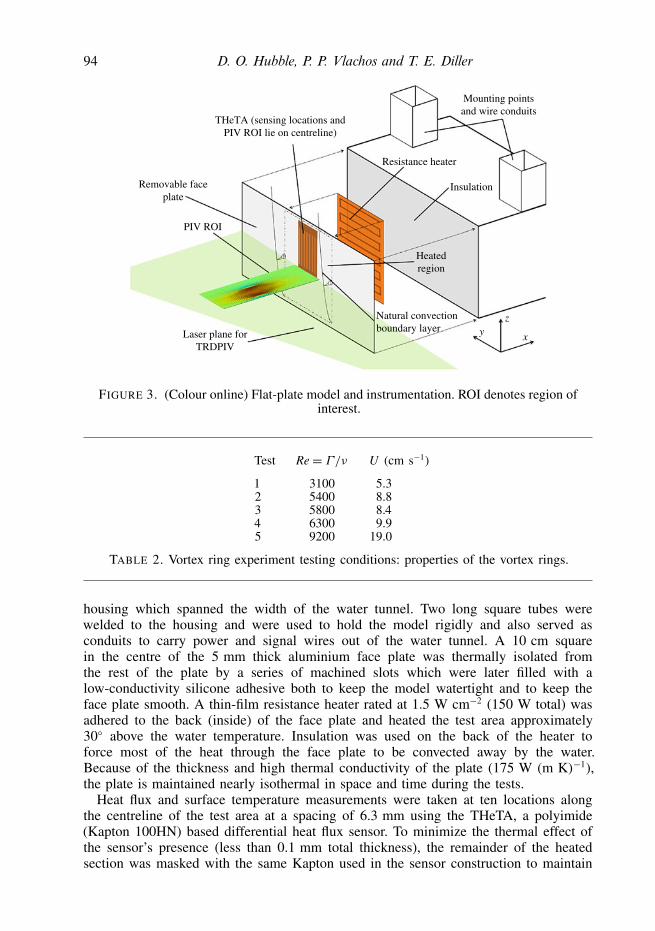
2.3. Instrumented flat plateA basic flat-plate model was constructed as shown in figures 1 and 3. The modelcomprised a smooth, removable face plate mounted onto a watertight rectangular


Removable faceplate

PIV ROI

THeTA (sensing locations andPIV ROI lie on centreline)

Mounting pointsand wire conduits

Resistance heater

Insulation

Heatedregion

Laser plane forTRDPIV

Natural convectionboundary layer

z

xy

FIGURE 3. (Colour online) Flat-plate model and instrumentation. ROI denotes region ofinterest.

Test Re= Γ/ν U (cm s−1)

1 3100 5.32 5400 8.83 5800 8.44 6300 9.95 9200 19.0

TABLE 2. Vortex ring experiment testing conditions: properties of the vortex rings.

housing which spanned the width of the water tunnel. Two long square tubes werewelded to the housing and were used to hold the model rigidly and also served asconduits to carry power and signal wires out of the water tunnel. A 10 cm squarein the centre of the 5 mm thick aluminium face plate was thermally isolated fromthe rest of the plate by a series of machined slots which were later filled with alow-conductivity silicone adhesive both to keep the model watertight and to keep theface plate smooth. A thin-film resistance heater rated at 1.5 W cm−2 (150 W total) wasadhered to the back (inside) of the face plate and heated the test area approximately30◦ above the water temperature. Insulation was used on the back of the heater toforce most of the heat through the face plate to be convected away by the water.Because of the thickness and high thermal conductivity of the plate (175 W (m K)−1),the plate is maintained nearly isothermal in space and time during the tests.

Heat flux and surface temperature measurements were taken at ten locations alongthe centreline of the test area at a spacing of 6.3 mm using the THeTA, a polyimide(Kapton 100HN) based differential heat flux sensor. To minimize the thermal effect ofthe sensor’s presence (less than 0.1 mm total thickness), the remainder of the heatedsection was masked with the same Kapton used in the sensor construction to maintain


21 signal wiressoldered onto foils

CompletedTHeTA with 10sensing locations

Each junctionresults in a sensinglocation (10 total)

Thermal barrier

Upper thermocouple junctionat T1

Lower thermocouple junction at T2

FIGURE 4. (Colour online) Schematic of the Time-resolved Heat and Temperature Array(THeTA).

uniform smooth surface conditions. Details of the development and calibration of theTHeTA are given in Hubble & Diller (2010b) and a depiction of the sensor is givenin figure 4. Heat flux through the sensor is proportional to the temperature dropacross the thermal barrier as directly measured by two type-T (copper–constantan)thermocouples connected in series (1V1). The surface area of the thermocouplecontact determines the effective measurement width, which was 1.6 mm or 25 % of thesensor spacing. Surface temperature measurements are obtained from the thermocouplelocated on the top of the THeTA (1V2). Each of the ten sensors on the THeTAwas individually directly calibrated by conduction and radiation for the steady-stateheat flux sensitivity and by radiation for the transient response, as described byHubble & Diller (2010b). Because of variations in the thickness during construction,the calibrated sensitivities of each sensor used are somewhat different. The averagesensitivity of the ten heat flux sensors on the THeTA is 223 µV (W cm−2)

−1 with a95 % time response of 509 ms. The Hybrid Heat Flux (HHF) (Hubble & Diller 2010a)technique was used to improve the initial time response of the THeTA. The HHF is anumerical signal processing technique which increases the performance of differentialheat flux sensors by accounting for the thermal energy stored within the sensor inconjunction with the heat flowing through the sensor. Differential sensors effectivelylow-pass filter the heat flux input due to the time required for heat to diffuseacross their thickness. Utilizing the HHF method enables obtaining higher frequencyinformation from the temporal derivative of the surface temperature signal, whichis then added to the low-frequency information obtained from the temperature dropacross the sensor. This method has been validated both numerically and experimentallyand has been shown to improve the 95 % time response of the THeTA to 36 ms(Hubble & Diller 2010b).

The 20 signals from the THeTA (10 heat flux, 10 surface temperature) weresampled at a rate of 1 kHz using a National Instruments 6225 16bit DAQ whichalso synchronized the TRDPIV camera and laser to the heat flux measurements


and controlled the vortex ring generator when needed. The microvolt signals fromthe THeTA were first amplified using custom-fabricated amplifier boards (Ewing2006) with a fixed gain of 1000 and 480 Hz anti-aliasing filters. Post-processing ofthe signals from the THeTA was accomplished in MATLAB which included downsampling the data to 250 Hz to match the sampling rate of the flow measurements(discussed in § 2.4). The heat flux measurements were then divided by the time-resolved temperature difference between the sensor surface and the water to obtain thetime-resolved heat transfer coefficient with an estimated uncertainty of ±7 %:

h(t)= q′′(t)Ts(t)− T∞

. (2.1)

2.4. Flow measurements: time-resolved particle image velocimetryThe present study examines the full two-dimensional velocity field in front of the flatplate using TRDPIV which delivers non-invasive flow field measurements with highspatiotemporal resolution. Details on the general method are provided by Westerweel(1997) and Raffel et al. (2007).

As shown in figure 1 the TRDPIV system used employs a New Wave ResearchPegasus dual head laser. An optical train is used to focus the laser light intoa thin (≈1 mm) sheet which illuminates the fluid plane containing the region ofinterest (ROI), located directly in front of the ten sensors. Neutrally buoyant glassmicrospheres with a mean diameter of 11 µm were used as tracer particles in the flow.Motion of the particles was tracked from underneath with an IDT XS-5 high-speedcamera using its maximum resolution of 1280 × 1024 pixels. With a magnificationof 51 um pixel−1, the camera interrogated an ROI 6.5 cm wide (along the plate) by5.2 cm long (normal to the plate).

For the stagnation tests, the TRDPIV measurements were taken in a single-pulsedfashion for approximately 13 s at a sampling rate of 250 Hz. For the vortex ring tests,the TRDPIV measurements were taken in a double-pulsed fashion for approximately6.5 s at a sampling rate of 250 Hz. Due to the large velocity dynamic rangeencountered across the different vortex ring conditions, no single pulse separationcould be used across the entire set of experiments. Therefore, for each differentvortex ring produced, preliminary testing was performed to determine the optimalpulse separation needed to obtain the desired particle displacements. This ranged from2 ms for the slowest rings to 0.5 ms for the fastest. In both experiments, the imageswere processed using in-house-developed TRDPIV software (Eckstein, Charonko &Vlachos 2008; Eckstein & Vlachos 2009a,b). Images were processed using cross-correlation with a 64 × 64 pixel window followed by a 32 × 32 window using therobust phase correlation after a discrete window offset. Using 8 by 8 pixel vectorspacing, the ROI contained 19 625 vectors with 416 µm between vectors. The totalerror in TRDPIV velocity measurements using the aforementioned experimental setupand image-processing techniques was estimated to be ±0.05–0.1 pixels (Eckstein &Vlachos 2009b).

2.5. Vortex identification and circulation calculationStarting with the velocity vector fields obtained from the TRDPIV analysis, a vortexidentification scheme was employed to dynamically identify the vortices present inthe ROI. In this study, the swirling strength (or λci) method of Zhou et al. (1999)was employed. Similar to the Delta criterion (Chong, Perry & Cantwell 1990), theλci method identifies vortices as regions where the velocity gradient tensor (∇u) has


complex eigenvalues, indicating swirling flow. In the λci method, the imaginary part ofthe complex eigenvalue of ∇u is used to identify vortices as it is a measure of theswirling strength of the vortex. To obtain the eigenvalues, the velocity-gradient-tensorcharacteristic equation is solved.

The imaginary part of the complex eigenvalue then gives the swirling strength atthe location in the flow for which ∇u is calculated. While in theory any non-zerovalue for λci indicates the presence of a vortex, Zhou et al. (1999) suggest settingsome positive threshold at a few per cent of the maximum value. By doing so, theidentification of extraordinarily weak structures is minimized. Therefore, in the presentwork, any location where λci is greater than 2 % of the maximum value for the flowfield is identified as a point within a vortex.

After identifying the vortical structures, the circulation of the vortex was calculated.Circulation is defined as the line integral around a closed curve of the velocity (Panton2005):

Γ =∮

CV ·d l (2.2)

Equation (2.2) is applied to the TRDPIV measured velocity field around the regionswhich are identified as vortices. The circulation is calculated through the line integralof the velocity along the closed path enclosing the identified vortical structure. The λci

iso-contour line defining the vortex region is segmented based on the TRDPIV spatialsampling resolution and the dot product of each segment with the measured velocity iscomputed. The sum of all the dot products then gives the measured circulation for thatparticular vortex.

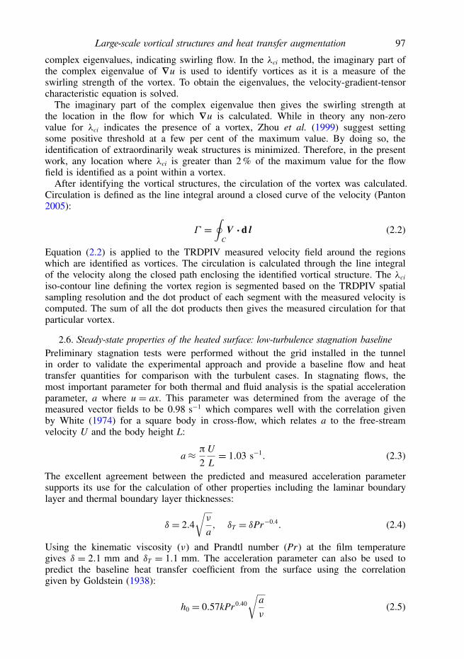
2.6. Steady-state properties of the heated surface: low-turbulence stagnation baselinePreliminary stagnation tests were performed without the grid installed in the tunnelin order to validate the experimental approach and provide a baseline flow and heattransfer quantities for comparison with the turbulent cases. In stagnating flows, themost important parameter for both thermal and fluid analysis is the spatial accelerationparameter, a where u = ax. This parameter was determined from the average of themeasured vector fields to be 0.98 s−1 which compares well with the correlation givenby White (1974) for a square body in cross-flow, which relates a to the free-streamvelocity U and the body height L:

a≈ π2

U

L= 1.03 s−1. (2.3)

The excellent agreement between the predicted and measured acceleration parametersupports its use for the calculation of other properties including the laminar boundarylayer and thermal boundary layer thicknesses:

δ = 2.4

√ν

a, δT = δPr−0.4. (2.4)

Using the kinematic viscosity (ν) and Prandtl number (Pr) at the film temperaturegives δ = 2.1 mm and δT = 1.1 mm. The acceleration parameter can also be used topredict the baseline heat transfer coefficient from the surface using the correlationgiven by Goldstein (1938):

h0 = 0.57kPr0.40

√a

ν(2.5)


where k is the thermal conductivity of the fluid. Equation (2.5) predicts a baselineheat transfer coefficient of h0 = 740 W (m2 K)−1 which matches the value ofh0 = 755 W (m2 K)−1 measured by the THeTA to within the experimental uncertainty.In the results shown throughout the paper, the measured convective heat transfercoefficients are expressed in dimensionless form by the Stanton number using theproduct of the free-stream velocity, specific heat, and density (U∞Cρ):

St = h

ρCpU∞. (2.6)

2.7. Steady-state properties of the heated surface: natural convectionFor the vortex ring tests, the properties of the natural convection boundary layer weredetermined prior to the ring interaction. Both the fluid and thermal properties of thesteady-state boundary layer were measured.

TRDPIV was used to measure the profile of the natural convection boundary layer.This test was performed using the TRDPIV setup described above except the laserplane was aligned vertically from below the tunnel and the camera was mountedhorizontally. Also, the magnification was increased to 30 µm pixel−1 to resolve thenear-wall flow field within the boundary layer. To check self-similarity, dimensionlessvelocity was plotted versus a dimensionless coordinate η involving the Grashof numberGy. The dimensionless velocity is defined as:

f ′ (η)= vy

2νG−1/2

y (2.7)

and the dimensionless coordinate and Grashof number are defined as

η = x

y

(Gy

4

)1/4

, Gy = gβy3 (Ts − T∞)ν2

(2.8)

where ν and β are the kinematic viscosity and thermal expansion coefficient of waterand g is the gravitational constant. The variables y and x are the coordinates paralleland normal to the plate respectively and v is the velocity parallel to the plate. Figure 5shows the wall jet profiles for multiple locations along the plate. A good collapse isobserved and is in good agreement with the classic work by Ostrach (1953).

The thermal state of the natural convection boundary layer was also examined usingthe heat flux and surface temperature measurements. The heat transfer coefficient at apoint on the plate a distance y from the bottom can be predicted using the equation(Incropera & DeWitt 2002)

h= k

y

Gy

4

1/4 0.75Pr1/2(0.609+ 1.221Pr1/2 + 1.238Pr

)1/4 (2.9)

where k and Pr are the thermal conductivity and Prandtl number of water evaluated atthe film temperature. Plugging in the appropriate values, (2.9) predicts the heat transfercoefficient at the sensor location to be 543 W (m2 K)−1. The average value measuredby the THeTA was 520 W (m2 K)−1 which is about 5 % below the value predicted by(2.9), but within the experimental uncertainty.

While the thermal boundary layer thickness was not directly measured in thepresent study, the match between the predicted and measured properties of the naturalconvection momentum boundary layer allows the thermal boundary layer thickness to


0.16

0.12

0.08

0.04

0 1 2 3 4 5

Ostrach (1953)

TRDPIV

6

FIGURE 5. (Colour online) Non-dimensional boundary layer profile and standard scaling.

be calculated. For water, Ostrach (1953) gives the following relation:

δT = 2.5y

(Gry

4

)−1/4

. (2.10)

This gives a value of δT = 2.1 mm at the position of the heat flux sensors for theconditions of the vortex ring experiments, which matches quite well the value forthe stagnation experiments. Both the natural convection and stagnation region thermalboundary layer thickness values will be used extensively throughout this paper.

3. Experimental observations of vortex-induced heat transfer3.1. Vortex–wall interaction in turbulent stagnation flow and resulting heat transfer

In stagnating flows, free-stream structures are amplified into strong vortices in the near-wall region. A sequence of movies was produced for each turbulence grid showingthe measured vortex interactions and resulting surface heat transfer as a function oftime. A qualitative analysis of these results is most instructive to understand the basicmechanism of heat transfer augmentation.

First, figure 6 shows a representative zoomed-in view of the near-wall flow andconvection at one instant of time when several vortices are in close proximity tothe surface. The contour of the vector plot indicates vorticity normalized by theratio of the turbulence-grid blockage-adjusted velocity (Vb = V∞/(1 − S)) to thebars spacing (Db = M − b) so that ω∗ = ω/ (Vb/Db). The bar plot in figure 6(b)represents the instantaneous convection (plotted as the Stanton number normalizedby the low-turbulence baseline) at the five sensing locations shown relative to thelaminar baseline. By measuring the heat transfer at the multiple sensing locations ofthe THeTA, the mechanism by which the vortices increase the convection is revealed.Three strong vortices with alternating rotations are observed near the surface. Thisarrangement of vortices produces alternating areas of downwash and upwash at the


30

0–25 0

3

–3

(a) (b)

0 1 2 3

FIGURE 6. (Colour online) (a) Instantaneous snapshot of the flow field and (b) normalizedStanton number. Sensor locations are indicated by the black dots in (a) and convectionmeasurements are given by the bars in (b). The contour of the vector field in (a) shows thenormalized vorticity ω∗ = ω/(Vb/Db). Convection increases are localized to areas of vortexdownwash. See supplementary movie 1 available at http://dx.doi.org/10.1017/jfm.2012.589.

surface between the individual vortices. These results, in combination with the heattransfer measurements, show that the downwash regions correspond to high levels ofconvection since cool fluid from the free stream is being forced towards the surfacein these regions. Alternatively, regions of upwash correspond to smaller increasesin convection since the fluid reaching the wall has been pulled along the heatedsurface prior to reaching these locations. This previously warmed fluid is less effectiveat removing heat from the surface in these upwash regions and is similar to theobservations of Sabatino & Smith (2008) where it was observed that the highest heattransfer in turbulent spots was near the perimeter where the vortices had the nearestaccess to cool free-stream fluid.

A second approach to view the interaction is shown in figure 7. Here, a singlevortex trajectory is shown along with the convection time histories from three nearbysensors. In figure 7(a), the identified vortex (with clockwise rotation) is shown overa time period of 5.3 s. The size of the overlapping circular markers is proportionalto the measured circulation of the vortex while its colour corresponds to the time atwhich it was identified as indicated by the colour bar in figure 7(b). The measuredconvection is shown in figure 7(b) for the three sensors whose positions are indicatedby the markers in figure 7(a). At first, the vortex is both weak and far from the surfaceand has little impact on the convection over the first 2 s. Then, the vortex movestowards the surface and its circulation is amplified. At this point, the top sensor (◦)is positioned directly in the downwash region and experiences more than double thelaminar baseline convection. As the vortex approaches the surface, the convection fromthe middle sensor (+) also increases slightly. Once the vortex is close to the surface,its mirror-image on the wall (from potential flow theory) induces a downward velocitybringing the middle sensor into the vortex downwash region. Note, however, that bythe time that the middle sensor is in a true downwash region, the vortex has movedfarther from the surface and weakened slightly. The middle sensor does experience anincrease in convection but not to the extent of the top sensor. Finally, as the vortex

http://dx.doi.org/10.1017/jfm.2012.589







































2.5

1.5

0.5

2.0

1.0

01 5

t (s)0–200

25(a) (b)

FIGURE 7. Transient interaction of a single vortex with the surface and resulting convection.Vortex location and strength are indicated by the overlapping circular markers in (a) while thecolour corresponds to the time in (b), where the convection history for the three nearby sensorlocations (marked in a) is shown.

continues to move from the surface and lose strength, the convection decays to thebaseline level. Since the bottom sensor (4) remained in the upwash region of thevortex, its convection remained below the baseline level for nearly the entire time ofthe interaction.

Over 200 heat transfer events similar to the one shown in figure 7 (events in whichthe heat transfer coefficient increased by more than 20 %) were examined from thestagnation flow data. These ranged from short duration events lasting less than aquarter of a second to individual events lasting up to five seconds. In some cases avortex would remain nearly stationary for a long period of time while in others thevortex would traverse the entire width of the instrumented region in under a second.Even though the nature of the thermal events was very diverse, in over 70 % of thecases, the sensor measuring the thermal event was located in a region identified as thedownwash region of the most dominant (largest induced velocity) local vortex.

These observations provide initial qualitative insight into the complex processescontrolling the vortex-induced heat transfer. However, the complexity of a fullydeveloped turbulent flow, with its three-dimensionality and the dynamic interactionsof numerous coherent structures with each other and with the wall, does not enablededucing the role of an individual vortex in a controlled and repeatable fashion. Withthis in mind, a second experiment was performed which examined the simpler caseof a vortex-ring–wall interaction and the ensuing heat transfer. The results of thisexperiment are discussed next.

3.2. Vortex-ring–wall interaction and resulting heat transferRepresentative results from the planar TRDPIV measurements are shown along withthe corresponding heat flux measurements during the vortex-ring–wall interaction infigure 8. This is used to gain a qualitative understanding of the effect of a singlevortex interaction on the surface heat flux. In figure 8(a), velocity fields are shownat six evenly spaced time steps over half a second with the contour representingthe vorticity normalized by the ratio of the maximum piston velocity to orifice


t (s)

0

15

0–20 0

0.4 0.6 0.8

2

0

2

0

2

0

2

0

2

0

y

x

(a) (b)

–10

10

FIGURE 8. (Colour online) Illustration of ring impingement and heat transfer. (a) Velocityfield sequence represent one half of the vortex ring over a half-second period. As thering approaches the heated plate the measured convection increases as illustrated in (b).Markers on the right of the velocity fields correspond to five of the individual heat flux sensorlocations, and the time sequence for each of these five sensors is shown in (b).

diameter, ω∗ = ω/ (Upmax/D). The velocity fields show one half of the vortex ring(the bottom axis coincides with the ring’s axis of symmetry). The five markers onthe right-hand side of the vector fields indicate the location of five heat flux sensors.In figure 8(b) measured transient Stanton numbers at these five sensor locations areshown normalized by the free convection value, St0. For all results from the vortexring experiments, the measured initial propagation velocity of the vortex ring (U)is used in place of U∞ to non-dimensionalize the heat transfer coefficient (equation(2.6)). Note that only the last velocity plot is after the vortex has rebounded fromthe surface. This present work is primarily focused on the time preceding the vortexrebound from the surface.

As the vortex ring approaches the heated plate its propagation velocity decreases andits radius increases as it stretches (Walker et al. 1987). In figure 8, this is observedas the vortex moving in the positive y-direction in the ROI, away from its axis ofsymmetry (the other half of the ring travels in the negative y-direction, not shown). Asthe vortex reaches the plate, vorticity of opposite sign is generated at the surface. Atapproximately t = 0.55 s, an eruption (Doligalski et al. 1994) occurs and a secondaryvortex forms outboard of the primary. The formation of the secondary vortex causesa rapid decrease in the radial growth of the primary ring. Consequently, the primaryvortex never moves further up the plate and never passes the top sensor. The observedbehaviour of the vortex ring is in qualitative agreement with the work of Walker et al.(1987).

As the vortex ring interacts with the heated plate, the convective heat transferincreases dramatically compared to the unperturbed natural convection level.


15

0

0

10

–10–12 0 0 1 2 43

FIGURE 9. (Colour online) Mechanism of heat removal. Close-up of interaction process andmeasured rate of convection at one time instant. The contour of the vector field shows thenormalized vorticity ω∗ = ω/(Upmax/D). The sensors in the downwash region of the vortexexperience more convection than the sensor directly beneath the vortex and much moreconvection compared to sensors in the upwash region.

To highlight the heat-transfer augmentation caused by the vortex interaction, thegrey-shaded area in figure 8(b) represents the increase between the measured Stantonnumber and the levels corresponding to natural convection. Note that when the vortexis in close proximity to the sensor, in some instances the convective transport increasesby more than a factor of four over the free convection levels. Many tests wereperformed where only thermal data were recorded and it was found that these highlevels of localized heat transfer were consistently present and always at least doublethe free convection level. This is in stark contrast to the value of 15 % reported fromspatially averaged measurements (Arevalo et al. 2007) and illustrates that the vortexhas a very localized but dominant impact on the convection.

To further demonstrate the impact that a near-surface vortex has on the local heattransfer, figure 9 illustrates the spatial convection distribution caused by a singlevortex. Here, the flow field in the vicinity of the single vortex is shown with theinstantaneous convection from five nearby sensors. Since the vortex is rotating counter-clockwise, the two sensors above the vortex are in the upwash region where thevortex is pulling fluid away from the surface. These two sensors indicate that theconvection at this point in time is essentially the natural convection level. The twosensors below the vortex are in a strong downwash region and experience a significantincrease in convection. Notably, these sensors in the downwash region are experiencingsignificantly more convection compared to the sensor nearest to the vortex even thoughit is in a region of maximum shear stress (Arevalo et al. 2010). These results indicatethat the outer fluid which is entrained towards the sensor has a much larger effectcompared to fluid sweeping along the sensor parallel to the surface. Again, sinceheat has been transferred to this fluid while traversing the surface, it is ineffective atremoving heat from the surface in the upwash region.


1

0

–1

0 0.2 0.4 0.6 0.8 1.0

O

C C

A A

By

dBA

dBC

L

2

–2

(a) (b)

FIGURE 10. (Colour online) (a) Schematic used in model development, along with (b) theaugmentation prediction (equation (4.5)) as a function of non-dimensional vortex locationy/L. Model predicts much larger convection in the downwash region compared to the upwashregion due to the smaller value of dBA compared to dBC.

4. Physical model for vortex-induced transient heat transfer augmentationThe current effort to develop a physically based model to predict the convective

transport due to a vortex is based on the surface renewal model of Nix, Diller& Ng (2007). In their work, it was hypothesized that when a flow structurepenetrates through the boundary layer, interaction with the surface causes an increase(augmentation) in the rate of heat transfer over that due to transport through thelaminar boundary layer. This process was modelled as a purely conductive eventtreating the flow structure as a semi-infinite medium. Heat is conducted to the structurefor a characteristic time τ :

1h= 1q

T∞ − TS= k√πατ

(4.1)

where α is the thermal diffusivity of the fluid. By defining the time scale as the ratioof the mean streamwise integral length scale to streamwise r.m.s. fluctuating velocity,this model successfully predicted experimentally measured values of increases in thetime-averaged heat transfer coefficient (Nix et al. 2007).

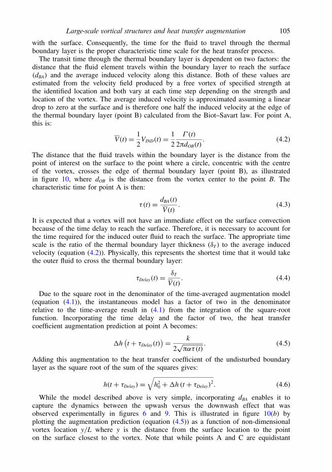
Using the surface renewal model based on the semi-infinite conduction assumptionas described above, an extension is developed which captures the time-dependentphysics of the vortex–surface interaction. Consider the case of a single vortex locatedat distance L from a heated surface with a thermal boundary layer of thicknessδT as illustrated in figure 10. The vortex induces a velocity field according to theBiot–Savart law (Panton 2005) which forces outer fluid through the boundary layer.This process can be thought of as individual fluid elements which start at the outerfluid temperature (T∞), move through the thermal boundary layer, and interact withthe surface. As soon as the fluid element reaches the thermal boundary layer, it beginsexchanging thermal energy with the warmer fluid within the boundary layer whichcauses the temperature of the fluid element to increase. The longer the fluid elementremains within the thermal boundary layer, the more heat is transferred to it and themore its temperature rises which decreases its capacity for exchanging thermal energy


with the surface. Consequently, the time for the fluid to travel through the thermalboundary layer is the proper characteristic time scale for the heat transfer process.

The transit time through the thermal boundary layer is dependent on two factors: thedistance that the fluid element travels within the boundary layer to reach the surface(dBA) and the average induced velocity along this distance. Both of these values areestimated from the velocity field produced by a free vortex of specified strength atthe identified location and both vary at each time step depending on the strength andlocation of the vortex. The average induced velocity is approximated assuming a lineardrop to zero at the surface and is therefore one half the induced velocity at the edge ofthe thermal boundary layer (point B) calculated from the Biot–Savart law. For point A,this is:

V(t)= 12

VIND(t)= 12

Γ (t)

2πdOB(t). (4.2)

The distance that the fluid travels within the boundary layer is the distance from thepoint of interest on the surface to the point where a circle, concentric with the centreof the vortex, crosses the edge of thermal boundary layer (point B), as illustratedin figure 10, where dOB is the distance from the vortex center to the point B. Thecharacteristic time for point A is then:

τ(t)= dBA(t)

V(t). (4.3)

It is expected that a vortex will not have an immediate effect on the surface convectionbecause of the time delay to reach the surface. Therefore, it is necessary to account forthe time required for the induced outer fluid to reach the surface. The appropriate timescale is the ratio of the thermal boundary layer thickness (δT) to the average inducedvelocity (equation (4.2)). Physically, this represents the shortest time that it would takethe outer fluid to cross the thermal boundary layer:

τDelay(t)= δT

V(t). (4.4)

Due to the square root in the denominator of the time-averaged augmentation model(equation (4.1)), the instantaneous model has a factor of two in the denominatorrelative to the time-average result in (4.1) from the integration of the square-rootfunction. Incorporating the time delay and the factor of two, the heat transfercoefficient augmentation prediction at point A becomes:

1h(t + τDelay(t)

)= k

2√πατ(t)

. (4.5)

Adding this augmentation to the heat transfer coefficient of the undisturbed boundarylayer as the square root of the sum of the squares gives:

h(t + τDelay)=√

h20 +1h (t + τDelay)

2. (4.6)

While the model described above is very simple, incorporating dBA enables it tocapture the dynamics between the upwash versus the downwash effect that wasobserved experimentally in figures 6 and 9. This is illustrated in figure 10(b) byplotting the augmentation prediction (equation (4.5)) as a function of non-dimensionalvortex location y/L where y is the distance from the surface location to the pointon the surface closest to the vortex. Note that while points A and C are equidistant


80

60

40

20

00.5 1.0 0 0.5 1.0 1.5

8

6

4

2

0

8

6

4

2

00.2 0.4 0.6

(a) (b) (c)

0 1.5

t (s) t (s)0 0.8

t (s)

FIGURE 11. (a) The measured circulation of the vortex as it approaches the plate for threetests. (b) The circulation is used to calculate the induced velocity at the sensor location onthe plate using the Biot–Savart law. (c) The distance that fluid must travel within the thermalboundary layer (dBA, +) is calculated from the measured vortex location. Combining this valuewith the induced velocity from above yields the characteristic time (τ , ◦) used in the model.ReΓ = 5800.

from the vortex centre, point A experiences much more convection because dBA < dBC.This curve is similar in shape to the experimentally obtained values shown in figure 9.The basic premise of the present model is the same as the one used by Nix et al.(2007) that as cold fluid is brought to the surface by a fluid disturbance it exchangesadditional thermal energy, augmenting the heat transfer. Nix et al.however, used anaverage characteristic time based on the integral length scale of the turbulence fortheir surface renewal model to give the time-average added heat transfer. Our modelanalyses each individual event as a function of time, calculating the transit timethrough the boundary layer for each packet of fluid. The shorter the time, the higherthe resulting heat transfer and the shorter the delay before the effect occurs at thesurface. This gives the time-resolved heat flux at each location on the surface. In bothmodels the increase is combined with the laminar or undisturbed heat transfer value.

5. Model validation5.1. Model comparison to the vortex-ring-induced heat transfer measurements

In each vortex ring experiment, the vortex ring interacted with a number of sensors,which can all be used for comparison with the model. In all, comparisons wereperformed for 33 time records of velocity and heat flux spanning five differentvalues of Reδ at five different heat flux sensor positions. This section alongwith figures 11–13 give a detailed description of the interaction process for onerepresentative sensor for tests corresponding to vortex ring Reynolds numbers ofReΓ = 3100, 5800, and 9200. The ReΓ = 5800 case is the same as shown in figure 8for the fourth heat flux sensor from the top. Figure 13 then summarizes the results forall the tests.

The measured transient circulation and the induced velocity at a single sensorlocation are shown in figures 11(a) and 11(b) respectively for three vortex strengthsspanning the range of test conditions. As the vortex ring propagates towards the plate,the circulation remains nearly constant. Then, upon reaching the plate, vorticity ofopposite sign is generated at the wall and the vortex strength quickly diminishes. Thisis seen as the abrupt drop in circulation at t = 0.275 s, t = 0.655 s, and t = 1.39 sfor the three tests shown. In all cases, t = 0 corresponds to the time when the vortexring first enters the ROI. The different times are due to the smaller propagation


4

3

2

1

00 0.5 1.0 1.5 0 0.5 1.0 1.5 0 0.5 1.0 1.5

t (s) t (s) t (s)

MeasuredModel

MeasuredModel

MeasuredModel

(a) (b) (c)

FIGURE 12. Comparison of model prediction to measured convection during vortexinteraction. Results shown from three representative tests spanning the range of vortexstrengths: (a) ReΓ = 3100, (b) ReΓ = 5800, (c) ReΓ = 9200.

velocity for the weaker vortex rings. Incorporating these measured vortex circulationswith the measured vortex position, the transient induced velocity at a sensor onthe plate surface is calculated for each test using the Biot–Savart law as shown infigure 11(b). Since in each test the vortex follows approximately the same trajectory,the two main differences are the speed at which the vortex passes the sensor and theinduced velocity at the sensor, both of which are affected by the circulation value.Consequently, the strongest vortex with the largest ReΓ causes the largest inducedvelocity for a short period of time while the weakest vortex causes a smaller inducedvelocity for a longer period of time.

The characteristic time used in the model is a function of the induced velocity andthe distance that the fluid travels within the thermal boundary layer (dBA). Figure 11(c)shows dBA as a function of time for the ReΓ = 5800 test. Curves for the other testsare not shown due to their similarity to those shown in figure 11(c). Specifically,the curves for dBA are essentially identical in magnitude and are only contractedor expanded in time. The characteristic time curve is smaller in magnitude for thestronger vortices and larger for the weaker vortices. It is helpful to again examinefigure 8 as dBA is calculated for the fourth sensor from the top for this test. Atthe beginning of the test, the vortex is slightly above the sensor. Therefore, theBiot–Savart law predicts that fluid interacting with the sensor travels through thethermal boundary layer at a shallow angle from beneath. Therefore, the predicteddistance is more than three times the thermal boundary layer thickness. As the vortexmoves closer and above, relative to the sensor, the sensor transitions to being ina downwash region and the distance approaches the minimum possible value of δT

which implies that the fluid is essentially passing straight through the boundary layer,normal to the surface.

The characteristic time (τ ) is then calculated by combining the curve for dBA withthe induced velocity to produce the curve shown in figure 11(c). The time decreasesas dBA decreases but then begins to increase at the end as the induced velocity (andcirculation) decrease. The characteristic time (τ ) and the time delay (τDelay) werecalculated for each sensor location for each test. Plugging these values into (4.5)and (4.6) yields a prediction of the convection as a function of time at that point.Figure 12 shows a comparison of the measured and predicted convection at a singlesensor location for the same data as presented in figure 11. For t < 0, the vortexhas not yet entered the TRDPIV region of interest and the prediction is thereforethe natural convection (undisturbed) Stanton number, St0. The gap in the prediction


6

5

4

3

2

1

654321

1.0

0.5

1.00.5Neg

ative

pred

iction

lag

Positi

ve pr

edict

ion la

g

7

0

1.5

07 1.5

Linear regression±1 STD

(a) (b)

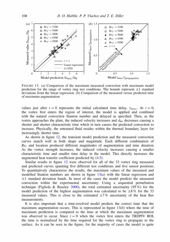
FIGURE 13. (a) Comparison of the maximum measured convection with maximum modelprediction for the range of vortex ring test conditions. The bounds represent ±1 standarddeviations from the linear regression. (b) Comparison of the measured versus predicted timeof maximum augmentation.

values just after t = 0 represents the initial calculated time delay, τDelay. At t = 0,the vortex first enters the region of interest, the model is applied and combinedwith the natural convection Stanton number and delayed as specified. Then, as thevortex approaches the plate, the induced velocity increases and dBA decreases causing ashorter and shorter characteristic time which in turn causes the predicted convection toincrease. Physically, the entrained fluid resides within the thermal boundary layer forincreasingly shorter time.

As shown in figure 12, the transient model prediction and the measured convectioncurves match well in both shape and magnitude. Each different combination ofReδ and location produced different magnitudes of augmentation and time duration.As the vortex strength increases, the induced velocity increases causing a smallercharacteristic time and smaller time delay in the model. This directly increases theaugmented heat transfer coefficient predicted by (4.5).

Similar results to figure 12 were observed for all of the 33 vortex ring measuredand predicted curves spanning five different test conditions and five sensor positions.To quantitatively characterize the results, the maximum values of the measured andmodelled Stanton numbers are shown in figure 13(a) with the linear regression and±1 standard deviation bands. In most of the cases the model predicts the measuredconvection within the experimental uncertainty. Using a sequential perturbationtechnique (Figliola & Beasley 2000), the total estimated uncertainty (95 %) for themodel prediction of the highest augmentation was calculated to be ±8 % for the 33measured values. This is close to the estimated ±7 % uncertainty of the heat fluxmeasurements.

It is also important that a time-resolved model predicts the correct time that themaximum augmentation occurs. This is represented in figure 13(b) where the time ofmaximum prediction is compared to the time at which the maximum augmentationwas observed to occur. Since t = 0 when the vortex first enters the TRDPIV ROI,the time is normalized by the time required for the vortex ring to propagate to thesurface. As it can be seen in the figure, for the majority of cases the model is quite


11 1210 13

40

35

30

25

20

15

10

5

0–20 –15 –10 –5 0

Track 1

Track 3

Track 2

Tra

ck 1

Tra

ck 3

Tra

ck 2

1.8

1.6

1.4

1.2

1.0

0.8

0.6

0.4

0.2

t (s)

2.0

0

(a) (b)

FIGURE 14. (a) Three vortex trajectories and (b) resulting measured convection. Marker sizein (a) indicates relative strength (circulation) of vortex while the fill colour corresponds to thetime as indicated in (b) where the measured convection from the sensor (black dot) is shown.(b) Comparison of the measured versus predicted time of maximum augmentation.

accurate with only a small bias towards a positive time lag, namely predicting the timeof maximum augmentation early. This implies that the choice for the model time delay(equation (4.4)) is appropriate.

5.2. Model comparison to turbulent stagnation flow heat transfer measurementsAs in the previous section, the analytical model was tested by using it to predictthe transient convective heat transfer coefficient at the heat flux sensor locationsusing the properties of the vortices identified in the measured velocity fields. Foreach of the turbulent cases, comparisons were made for the centre six sensors (3–8)to prevent unidentified vortices from outside the TRDPIV ROI from influencing theresults. In all, 36 complete tests were used (3 grids × 2 trials × 6 sensors) for theentire 13 s duration of the TRDPIV measurements (for a total of 117 000 individualcomparisons). This section along with figures 14–16 give a detailed description ofthe measured convection and the fluid structure during a particularly interesting set ofvortex interactions from one of the tests. Table 3 then summarizes the findings fromthe remaining tests.

Figure 14 shows the three vortices that influence one particular sensor over thefinal 3.5 s of test number 1 of grid 2. As in figure 7, the marker size indicates thecirculation of the vortex while its colour corresponds to the time. Figure 14(b) showsthe normalized Stanton number measured by the sensor and the vertical dotted linesdelineate the three tracks. The vortices shown are the ones that within the durationof the interaction dominated the near-wall region, causing the smallest calculatedcharacteristic time, thus the largest estimated augmentation, at the sensor location atthat point in time.

Examining figure 14 along with figure 15(a) gives a clear picture of the interactionprocess. Figure 15(a) shows the measured vortex properties over the same 3.5 s


16

12

8

4

11 12

8

6

4

2

6

5

4

3

2

1

010 13

t (s)11 1210 13

t (s)

1

2

(a) (b)2 3 1 2 3

VIND

20

0

10

0

3

0

1

FIGURE 15. (a) Transient measured properties of the three vortices shown in figure 14 duringthe interaction. The measured properties are used to determine the transient model inputs asshown in (b).

Free-streamturbulence

Identifiedstructures

Measuredconvection

Modelledconvection

Std deviationdifference of St

Grid Λ (cm) # |ReΓ | St(×1000) Aug (%) St(×1000) Aug (%) St(×1000)

1 0.81 15.8 585 2.51 38 2.50 37 0.602 1.93 8.1 463 2.35 29 2.37 30 0.543 3.24 4.4 218 2.34 29 2.08 14 0.43

TABLE 3. Summary of time-averaged results for the model applied to the stagnation data.# denotes average number of structures and Aug heat transfer augmentation.

as figure 14 and again the vertical lines delineate the three separate trajectories.Specifically, the non-dimensional distance from the vortex to the sensor (+) andthe measured circulation (�) are shown. At the beginning of the time shown, thereis no strong vortex in the vicinity of the sensor and the convection is at nearly thebaseline level. At this time, the vortex which most strongly influences the convectionat the sensor location is approximately 13 boundary layer thicknesses away and has acirculation of less than 1 cm2 s−1. This vortex then grows in strength as it approachesthe stagnation region (and the sensor) with a corresponding increase in measuredconvection. Then, at t = 10.25 s, a more dominant vortex emerges. Although vortexnumber 2 starts at approximately the same distance from the sensor as vortex number1, it is significantly stronger with a circulation of 5 cm2 s−1 compared to 3.5 cm2 s−1.This clockwise rotating vortex forces fluid straight through the thermal boundary layertowards the sensor, increasing the convection to almost 60 % above baseline levels.Then, as the vortex begins to move away and weaken, the convection returns to thebaseline level. At t = 11.7 s, the third structure appears and quickly grows into adominant vortex. The counter-clockwise vortex forms above the sensor then movesdownward along the surface. As the vortex approaches and eventually passes thesensor, its circulation grows to a maximum of 9 cm2 s−1. This causes the convection


to spike at a value nearly 75 % higher than the baseline just as the vortex reachesthe sensor. Then, as the sensor begins to enter the upwash region of the vortex, adrastic decrease in convection is observed even though the vortex is still quite closeto the sensor. Fluid elements that reach the surface in upwash regions have residedfor considerable time within the thermal boundary layer since they must now flowalong the surface first. These fluid elements have therefore warmed significantly andare much less effective at convecting heat from the surface, as indicated by the sensorfor t > 12.9 s.

From the measured vortex properties, the transient model inputs were calculated asshown in figure 15(b). The calculated induced velocity is shown (�) along with thenon-dimensional distance that the fluid must travel within the thermal boundary layer(+). When the fluid travels a short distance within the thermal boundary layer (valuesof dBA near one), the sensor is in the downwash region and the fluid is travelling nearlyperpendicular to the surface. Larger values indicate that the fluid is sweeping along thesurface prior to reaching the sensor location. Again, it is assumed that the time that thefluid remains within the thermal boundary layer (τ ) is simply the distance that fluidtravels within the thermal boundary layer (dBA) divided by the average velocity that thefluid maintains along this distance (VIND/2) which is a measure of both the strengthand proximity of the vortex (equation (4.2)). At t = 10.6 s, the induced velocity is at alocal maximum and dBA is at a local minimum which means that τ is a local minimum.Fluid, therefore, is quickly travelling a short distance to reach the surface and littleheat is transferred to the fluid prior to reaching the surface. Note that in figure 14,t = 10.6 s corresponds to a local maximum in the measured convection. Then, as thevortex decays, VIND falls to essentially zero prior to the arrival of the third vortex. Inthe third vortex trajectory, the effect of upwash versus downwash is most visible. Formost of the interaction with the wall, the vortex is above the sensor and, since thevortex has counter-clockwise rotation, the sensor remains in a region of downwash.Once the vortex passes the sensor however, the sensor enters the upwash region. Afterthis occurs, fluid enters the thermal boundary layer far below the sensor and musttravel upwards along the surface prior to reaching the sensor as indicated by the largevalue for dBA (and a correspondingly large value of τ ). This fluid has ample time towarm as it slides along the surface and the heat transfer upon its arrival to the surfaceis reduced.

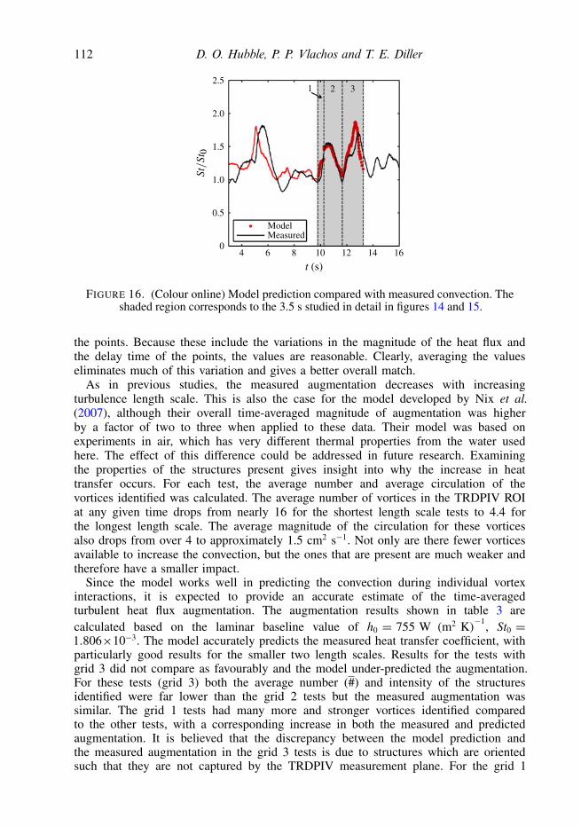
In figure 16, the final model prediction is shown compared to the measuredconvection. The shaded region indicates the 3.5 s discussed in the previous twofigures and the vertical dotted lines again delineate the different trajectories. Thedominant vortex at the sensor location is used at each instant of time with thecorresponding time delay of the model included. As in the vortex ring tests, thetransient model prediction matches the measured convection well in terms of bothshape and magnitude. The two distinct spikes in the measured convection bothcorrespond to times when fluid is quickly reaching the sensor from outside the thermalboundary layer. Times of low convection occur either when fluid is passing veryslowly through the thermal boundary layer (weak and/or distant vortex) or when fluidmust travel a great distance within the thermal boundary layer (upwash region ofvortex).

Time-averaged results were obtained by integrating all of the model predictions (asillustrated in figure 16) over the time of each test. The results for all the tests areshown in table 3. The value for each grid represents the average of 19 000 individualpoints during the experimental tests. In addition, the standard deviation between themeasured heat flux values and those calculated from the model is listed for all of


2.0

1.5

1.0

0.5ModelMeasured

1 2 3

6 8 10 12 14

2.5

04 16

t (s)

FIGURE 16. (Colour online) Model prediction compared with measured convection. Theshaded region corresponds to the 3.5 s studied in detail in figures 14 and 15.

the points. Because these include the variations in the magnitude of the heat flux andthe delay time of the points, the values are reasonable. Clearly, averaging the valueseliminates much of this variation and gives a better overall match.

As in previous studies, the measured augmentation decreases with increasingturbulence length scale. This is also the case for the model developed by Nix et al.(2007), although their overall time-averaged magnitude of augmentation was higherby a factor of two to three when applied to these data. Their model was based onexperiments in air, which has very different thermal properties from the water usedhere. The effect of this difference could be addressed in future research. Examiningthe properties of the structures present gives insight into why the increase in heattransfer occurs. For each test, the average number and average circulation of thevortices identified was calculated. The average number of vortices in the TRDPIV ROIat any given time drops from nearly 16 for the shortest length scale tests to 4.4 forthe longest length scale. The average magnitude of the circulation for these vorticesalso drops from over 4 to approximately 1.5 cm2 s−1. Not only are there fewer vorticesavailable to increase the convection, but the ones that are present are much weaker andtherefore have a smaller impact.

Since the model works well in predicting the convection during individual vortexinteractions, it is expected to provide an accurate estimate of the time-averagedturbulent heat flux augmentation. The augmentation results shown in table 3 arecalculated based on the laminar baseline value of h0 = 755 W (m2 K)−1, St0 =1.806×10−3. The model accurately predicts the measured heat transfer coefficient, withparticularly good results for the smaller two length scales. Results for the tests withgrid 3 did not compare as favourably and the model under-predicted the augmentation.For these tests (grid 3) both the average number (#) and intensity of the structuresidentified were far lower than the grid 2 tests but the measured augmentation wassimilar. The grid 1 tests had many more and stronger vortices identified comparedto the other tests, with a corresponding increase in both the measured and predictedaugmentation. It is believed that the discrepancy between the model prediction andthe measured augmentation in the grid 3 tests is due to structures which are orientedsuch that they are not captured by the TRDPIV measurement plane. For the grid 1


and 2 tests, the in-plane structures are so strong that any out-of-plane motions do notsignificantly influence the surface convection. This is not the case for the grid 3 testswhere the in-plane structures are not nearly so dominant.

6. ConclusionsThe results presented in this work clearly demonstrate that the interaction of vortices

with a surface is the primary mechanism by which heat transfer is augmented inturbulent stagnation flows. Observations of the simultaneous flow field and surfaceheat flux have allowed the physical mechanism of this interaction to be understood. Inregions where vortices force fluid directly through the boundary layer, the convectionis high because the fluid quickly reaches the surface. Conversely, regions where fluidis swept along the surface experience less convection because the fluid has alreadybeen heated within the boundary layer prior to reaching the surface. Incorporationof these observations into a first-principles-based analytical model allows accurateprediction of the time-resolved heat transfer augmentation from a single vortex asit impacts on the surface. For this simplified case, a vortex ring serves as a goodmodel for the interaction of a single vortical structure in turbulence. For the case offree-stream turbulence in the stagnation region, the heat transfer is the combinationof the heat transfer resulting from the vortex interaction and the laminar level whenno free-stream turbulence is present. The results show that this method works quitewell, with particularly good results obtained for the smaller length scales where thevortices are most dominant. However, more experimentation is needed to determinethe true range of applicability. Specifically the experiments should be done in differentfluids (most importantly air) to determine how the Prandtl number affects the results.The success of the model indicates that it is a good physical interpretation of themechanism of heat transfer augmentation by vortices in turbulent flows. Its simplicityand the ease with which it can be implemented make the model results all the moreencouraging. By looking at turbulent heat transfer as the combination of many simplevortex–wall interactions, the inherent complexity of the problem is reduced. Therefore,if the formation and motion of these large-scale structures can be accurately predicted(using LES for instance) then the resulting surface convection can be modelled withouttrying to solve for the fine-scale motions in the near-wall region.

AcknowledgementsThe authors would like to thank Dr A. Gifford for his work developing and

characterizing the turbulence grids and stagnation model. This material is based uponwork supported by the National Science Foundation under grant no. CTS-0423013.Any opinions, findings, and conclusions or recommendations expressed in this materialare those of the authors and do not necessarily reflect the views of the NationalScience Foundation.

Supplementary movieSupplementary movie are available at http://dx.doi.org/10.1017/jfm.2012.589.

R E F E R E N C E S

ADRIAN, R. J., CHRISTENSEN, K. T. & LIU, Z.-C. 2000 Analysis and interpretation ofinstantaneous turbulent velocity fields. Exp. Fluids 29 (3), 275–290.

AMES, F. E. 1997 The influence of large-scale high-intensity turbulence on vane heat transfer.Trans. ASME: J. Turbomach. 119 (1), 23–30.








































ARAYA, G., LEONARDI, S. & CASTILLO, L. 2008 Numerical assessment of local forcing on theheat transfer in a turbulent channel flow. Phys. Fluids 20, 085105.

AREVALO, G., HERNANDEZ, R. H., NICOT, C. & PLAZA, F. 2007 Vortex ring head-on collisionwith a heated vertical plate. Phys. Fluids 19, 083603.

AREVALO, G., HERNANDEZ, R. H., NICOT, C. & PLAZA, F. 2010 Particle image velocimetrymeasurements of vortex rings head-on collision with a heated vertical plate. Phys. Fluids 22,053604.

BAINES, W. D. & PETERSON, E. G. 1951 An investigation of flow through screens. Trans. ASME:J. Heat Transfer 73, 467–480.

CHONG, M. S., PERRY, A. E. & CANTWELL, B. J. 1990 A general classification of 3-dimensionalflow-fields. Phys. Fluids A 2 (5), 765–777.

DOLIGALSKI, T. L., SMITH, C. R. & WALKER, J. D. A. 1994 Vortex interactions with walls. Annu.Rev. Fluid Mech. 26 (1), 573–616.

DULLENKOPF, K. & MAYLE, R. E. 1995 An account of free-stream-turbulence length scale onlaminar heat-transfer. Trans. ASME: J. Turbomach. 117 (3), 401–406.

ECKSTEIN, A. C., CHARONKO, J. & VLACHOS, P. 2008 Phase correlation processing for DPIVmeasurements. Exp. Fluids 45 (3), 485–500.

ECKSTEIN, A. & VLACHOS, P. P. 2009a Assessment of advanced windowing techniques for digitalparticle image velocimetry (DPIV). Meas. Sci. Technol. 20 (7), 075402.

ECKSTEIN, A. C. & VLACHOS, P. 2009b Digital particle image velocimetry (DPIV) robust phasecorrelation. Meas. Sci. Technol. 20, 14.

EWING, J. A. 2006 Development of a direct-measurement thin-film heat flux array. PhD thesis,Blacksburg.

FIGLIOLA, R. S. & BEASLEY, D .E. 2000 Theory and Design for Mechanical Measurements, 3rdedn. John Wiley & Sons.

GIFFORD, A. R., DILLER, T. E. & VLACHOS, P. P. 2011 The physical mechanism of heat transferaugmentation in stagnating flows subject to freestream turbulence. J. Heat Transfer 133 (2),021901.

GOLDSTEIN, S. 1938 Modern Devlopments in Fluid Dynamics, vol. 2. Dover, 632.HOLMBERG, D. G. & DILLER, T. E. 2005 Simultaneous heat flux and velocity measurements in a

transonic turbine cascade. Trans. ASME: J. Turbomach. 127 (3), 502.HUBBLE, D. O. & DILLER, T. E. 2010a A hybrid method for measuring heat flux. Trans. ASME: J.

Heat Transfer 132 (3), 031602.HUBBLE, D. O. & DILLER, T. E. 2010b Development and evaluation of the time-resolved heat and

temperature array. ASME J. Therm. Sci. Engng Appl. 2.HUTCHINS, N. & MARUSIC, I. 2007 Evidence of very long meandering features in the logarithmic

region of turbulent boundary layers. J. Fluid Mech. 579, 1–28.INCROPERA, F. & DEWITT, D. 2002 Introduction to Heat Transfer, 5th edn John Willey & Sons.KATAOKA, K. 1990 Impingement heat-transfer augmentation due to large-scale eddies, In

Proceedings of the 9th International Heat Transfer Conference, vol. l, KN-l5, pp. 255–273.KESTIN, J. 1966 The effect of free stream turbulence on heat transfer rates. Adv. Heat Transfer 3,

1–32.LOWERY, G. W. & VACHON, R. I. 1975 Effect of turbulence on heat-transfer from heated cylinders.

Intl J. Heat Mass Transfer 18 (11), 1229–1242.MARTIN, R. & ZENIT, R. 2008 Heat transfer resulting from the interaction of a vortex pair with a

heated wall. Trans. ASME: J. Heat Transfer 130 (5), 051701.MARUSIC, I., MATHIS, R. & HUTCHINS, N. 2010 Predictive model for wall-bounded turbulent flow.

Science 329 (5988), 193–196.MAYLE, R. E., DULLENKOPF, K. & SCHULZ, A. 1998 The turbulence that matters. Trans. ASME:

J. Turbomach. 120 (3), 402–409.MOSS, R. W. & OLDFIELD, M. L. G. 1996 Effect of free stream turbulence on flat-plate heat

flux signals: Spectra and eddy transport velocities. Trans. ASME: J. Turbomach. 118 (3),461–467.

NIX, A. C., DILLER, T. E. & NG, W. F. 2007 Experimental measurements and modelling of theeffects of large-scale free stream turbulence on heat transfer. J. Trans. ASME: Turbomach.129 (3), 542–550.


OSTRACH, S. 1953 An analysis of laminar free-convection flow and heat transfer about a flatplate parallel tot he direction of the generating body force. Report 1111. National AdvisoryCommittee for Aeronautics.

PANTON, R. 2005 Incompressible Flow, 3rd edn. Wiley.PAVLOVA, A. & AMITAY, M. 2006 Electronic cooling using synthetic jet impingement. Trans ASME:

J. Heat Transfer 128, 897–907.RAFFEL, M., WILLERT, C., WERELEY, S. & KOMPENHANS, J. 2007 Particle Image Velocimetry.

Springer.ROMERO-MENDEZ, R., SEN, M., YANG, K. T. & MCCLAIN, R. L. 1998 Enhancement of heat

transfer in an inviscid-flow thermal boundary layer due to a Rankine vortex. Intl J. Heat MassTransfer 41 (23), 3829–3840.

SABATINO, D. R. & SMITH, C. R. 2008 Turbulent spot flow topology and mechanisms for surfaceheat transfer. J. Fluid Mech. 612, 81–105.

SHARIFF, K. & LEONARD, A. 1992 Vortex rings. Annu. Rev. Fluid Mech. 24, U235–U279.SUTERA, S. 1965 Vorticity amplification in stagnation-point flow and its effect on heat transfer.

J. Fluid Mech. 21, 513–534.VANFOSSEN, G. J. & SIMONEAU, R. J. 1987 A study of the relationship between free-stream

turbulence and stagnation region heat-transfer. Trans. ASME: J. Heat Transfer 109 (1),10–15.

VANFOSSEN, G. J., SIMONEAU, R. J. & CHING, C. Y. 1995 Influence of turbulence parameters,Reynolds-number, and body shape on stagnation-region heat-transfer. Trans. ASME: J. HeatTransfer 117 (3), 597–603.

WALKER, J. D. A., SMITH, C. R., CERRA, A. W. & DOLIGALSKI, T. L. 1987 The impact of avortex ring on a wall. J. Fluid Mech. 181, 99–140.

WESTERWEEL, J. 1997 Fundamentals of digital particle image velocimetry. Meas. Sci. Technol. 8(12), 1379–1392.

WHITE, F. M. 1974 Viscous Fluid Flow, 3rd edn. pp. 598–599 McGraw-HillScience/Engineering/Math.

XIONG, Z. M. & LELE, S. K. 2007 Stagnation-point flow under free stream turbulence. J. FluidMech. 590, 1–33.

YUAN, T. D. & LIBURDY, J. A. 1992 Application of a surface renewal model to the prediction ofheat-transfer in an impinging jet. Intl J. Heat Mass Transfer 35 (8), 1905–1912.

ZHOU, J., ADRIAN, R. J., BALACHANDAR, S. & KENDALL, T. M. 1999 Mechanisms forgenerating coherent packets of hairpin vortices in channel flow. J. Fluid Mech. 387, 353–396.

Documents

J. Fluid Mech. (2013), . 718, pp. doi:10.1017/jfm.2012.589 ... · 90 D. O. Hubble, P. P. Vlachos and T. E. Diller and Dullenkopf & Mayle (1995) identiﬁed a dominant frequency band