Embed Size (px)
Citation preview
J. Eisert University of Potsdam, Germany
Entanglement and transfer of quantum informationCambridge, September 2004
Optimizing linear optics quantum gates
Quantum computation withlinear optics
Effective non-linearities
OutputOpticalnetwork
Input
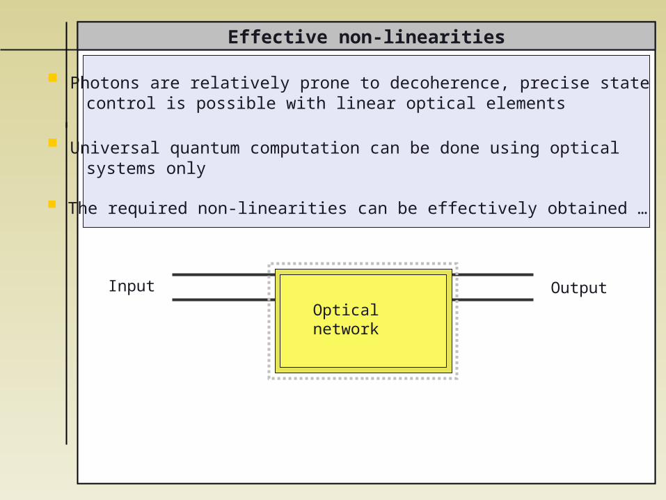
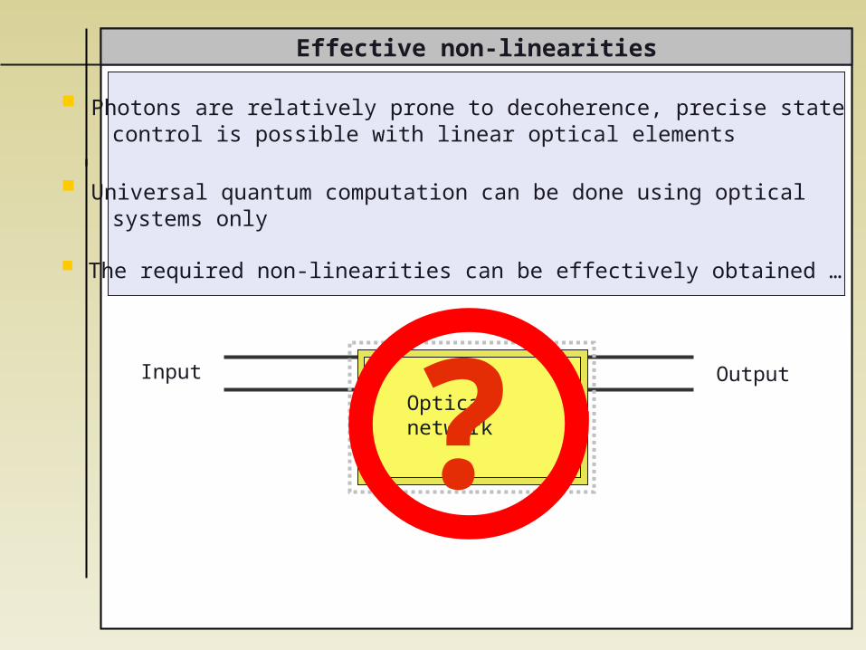
Photons are relatively prone to decoherence, precise state control is possible with linear optical elements
Universal quantum computation can be done using optical systems only
The required non-linearities can be effectively obtained …
Effective non-linearities
OutputOpticalnetwork
Input
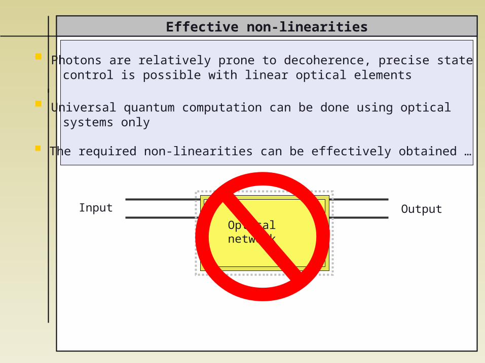
Photons are relatively prone to decoherence, precise state control is possible with linear optical elements
Universal quantum computation can be done using optical systems only
The required non-linearities can be effectively obtained …
Effective non-linearities
OutputOpticalnetwork
Input
?
Photons are relatively prone to decoherence, precise state control is possible with linear optical elements
Universal quantum computation can be done using optical systems only
The required non-linearities can be effectively obtained …
Effective non-linearities
Output
Auxiliary modes, Auxiliary photons
Linear opticsnetwork
Input
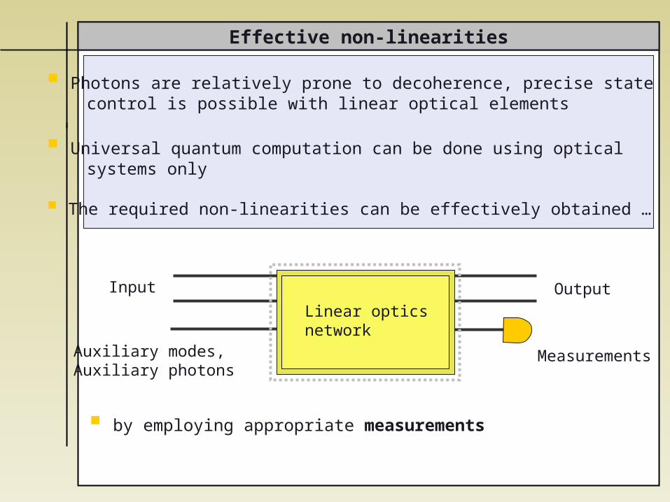
by employing appropriate measurements
Measurements
Photons are relatively prone to decoherence, precise state control is possible with linear optical elements
Universal quantum computation can be done using optical systems only
The required non-linearities can be effectively obtained …
KLM scheme
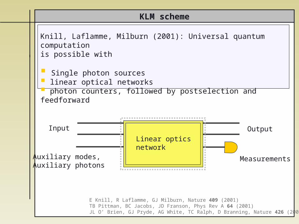
Knill, Laflamme, Milburn (2001): Universal quantum computation is possible with
Single photon sources linear optical networks photon counters, followed by postselection and feedforward
E Knill, R Laflamme, GJ Milburn, Nature 409 (2001) TB Pittman, BC Jacobs, JD Franson, Phys Rev A 64 (2001)JL O’ Brien, GJ Pryde, AG White, TC Ralph, D Branning, Nature 426 (2003)
Output
Auxiliary modes, Auxiliary photons
Linear opticsnetwork
Input
Measurements
Non-linear sign shifts
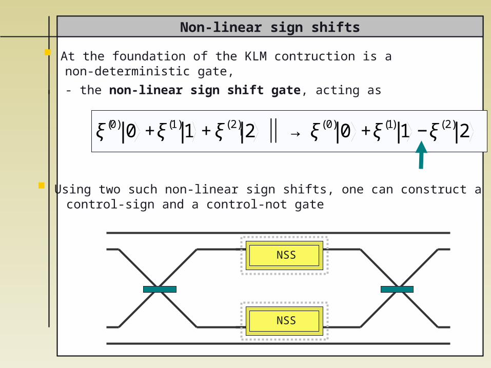
At the foundation of the KLM contruction is a non-deterministic gate,
- the non-linear sign shift gate, acting as
€
ξ(0) 0 +ξ(1)1 +ξ(2) 2 ⏐ → ⏐ ξ(0) 0 +ξ(1) 1 −ξ(2) 2
NSS
NSS
Using two such non-linear sign shifts, one can construct a control-sign and a control-not gate
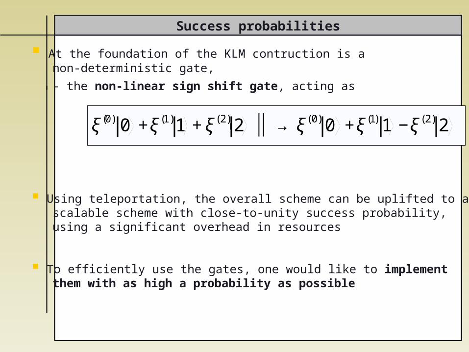
Success probabilities
At the foundation of the KLM contruction is a non-deterministic gate,
- the non-linear sign shift gate, acting as
Using teleportation, the overall scheme can be uplifted to a scalable scheme with close-to-unity success probability, using a significant overhead in resources
To efficiently use the gates, one would like to implement them with as high a probability as possible
€
ξ(0) 0 +ξ(1)1 +ξ(2) 2 ⏐ → ⏐ ξ(0) 0 +ξ(1) 1 −ξ(2) 2
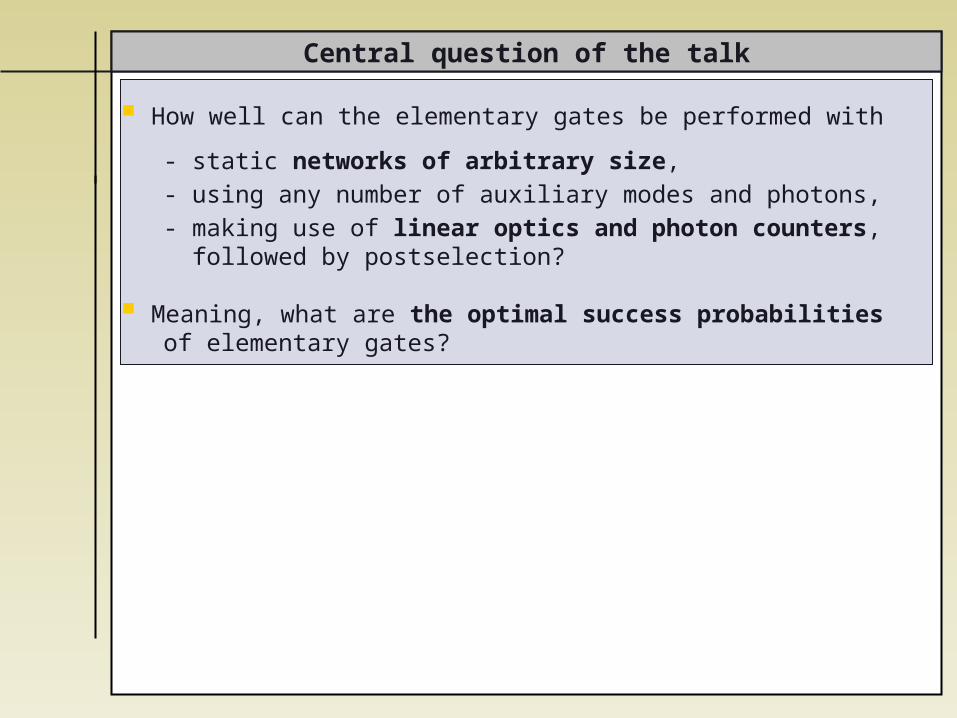
Central question of the talk
How well can the elementary gates be performed with
- static networks of arbitrary size, - using any number of auxiliary modes and photons, - making use of linear optics and photon counters, followed by postselection?
Meaning, what are the optimal success probabilities of elementary gates?
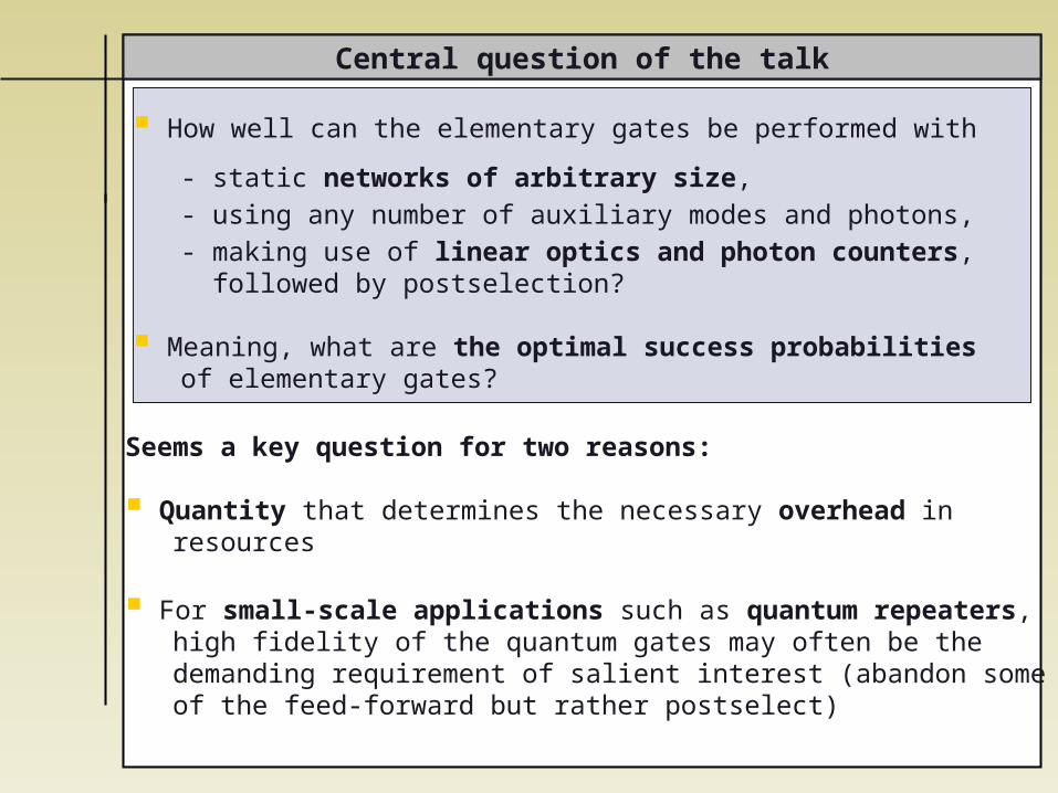
Central question of the talk
Seems a key question for two reasons:
Quantity that determines the necessary overhead in resources
For small-scale applications such as quantum repeaters, high fidelity of the quantum gates may often be the demanding requirement of salient interest (abandon some of the feed-forward but rather postselect)
How well can the elementary gates be performed with
- static networks of arbitrary size, - using any number of auxiliary modes and photons, - making use of linear optics and photon counters, followed by postselection?
Meaning, what are the optimal success probabilities of elementary gates?
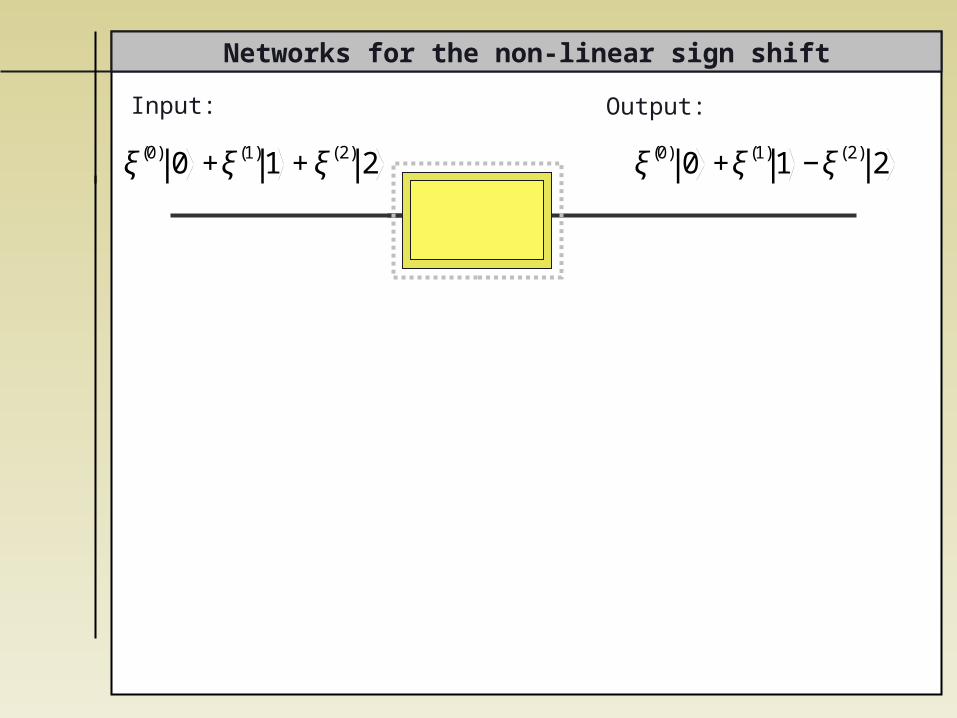
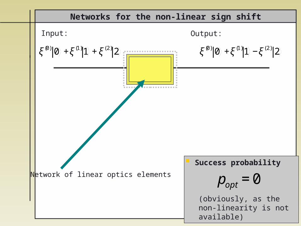
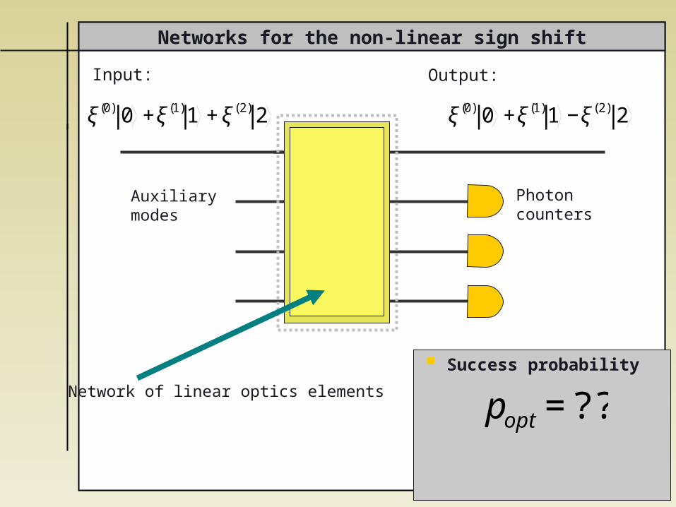
Networks for the non-linear sign shift
Input: Output:
€
ξ(0) 0 +ξ(1)1 +ξ(2) 2
€
ξ(0) 0 +ξ(1)1 −ξ(2) 2
Networks for the non-linear sign shift
Input: Output:
Network of linear optics elements
€
ξ(0) 0 +ξ(1)1 +ξ(2) 2
Success probability
(obviously, as the non-linearity is not available)
€
popt =0
€
ξ(0) 0 +ξ(1)1 −ξ(2) 2
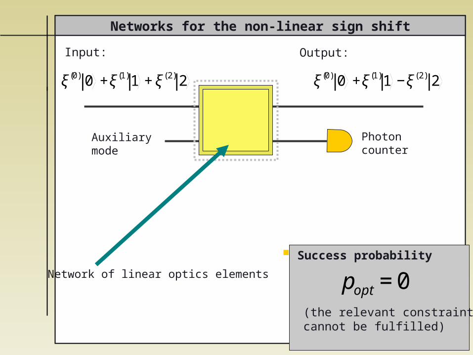
Networks for the non-linear sign shift
Input: Output:
Auxiliary mode
Success probability
(the relevant constraints cannot be fulfilled)
€
popt =0
Photoncounter
Network of linear optics elements
€
ξ(0) 0 +ξ(1)1 +ξ(2) 2
€
ξ(0) 0 +ξ(1)1 −ξ(2) 2
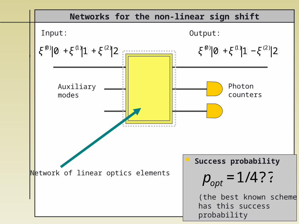
Networks for the non-linear sign shift
Input: Output:
Auxiliary modes
Success probability
(the best known scheme has this success probability
€
popt =1/4??
Photoncounters
Network of linear optics elements
€
ξ(0) 0 +ξ(1)1 +ξ(2) 2
€
ξ(0) 0 +ξ(1)1 −ξ(2) 2
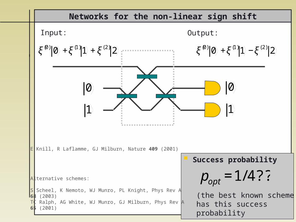
Networks for the non-linear sign shift
Input: Output:
Success probability
(the best known scheme has this success probability
€
popt =1/4??
€
0
€
1
€
0
€
1
E Knill, R Laflamme, GJ Milburn, Nature 409 (2001)
Alternative schemes:
S Scheel, K Nemoto, WJ Munro, PL Knight, Phys Rev A68 (2003)TC Ralph, AG White, WJ Munro, GJ Milburn, Phys Rev A65 (2001)
€
ξ(0) 0 +ξ(1)1 +ξ(2) 2
€
ξ(0) 0 +ξ(1)1 −ξ(2) 2
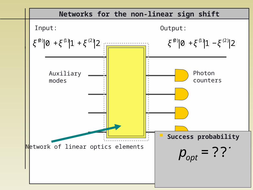
Networks for the non-linear sign shift
Input: Output:
Auxiliary modes
Success probability
€
popt =??
Photoncounters
Network of linear optics elements
€
ξ(0) 0 +ξ(1)1 +ξ(2) 2
€
ξ(0) 0 +ξ(1)1 −ξ(2) 2
Networks for the non-linear sign shift
Input: Output:
Auxiliary modes
Success probability
€
popt =???
Photoncounters
Network of linear optics elements
€
ξ(0) 0 +ξ(1)1 +ξ(2) 2
€
ξ(0) 0 +ξ(1)1 −ξ(2) 2
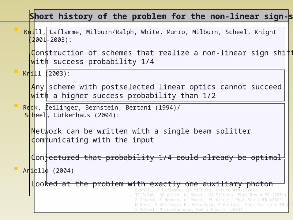
Short history of the problem for the non-linear sign-s
Knill, Laflamme, Milburn/Ralph, White, Munro, Milburn, Scheel, Knight (2001-2003):
Construction of schemes that realize a non-linear sign shift with success probability 1/4
Knill (2003):
Any scheme with postselected linear optics cannot succeed with a higher success probability than 1/2
Reck, Zeilinger, Bernstein, Bertani (1994)/ Scheel, Lütkenhaus (2004):
Network can be written with a single beam splitter communicating with the input
Conjectured that probability 1/4 could already be optimal
Aniello (2004)
Looked at the problem with exactly one auxiliary photonE Knill, R Laflamme, GJ Milburn, Nature 409 (2001)TC Ralph, AG White, WJ Munro, GJ Milburn, Phys Rev A 65 (2001)S Scheel, K Nemoto, WJ Munro, PL Knight, Phys Rev A 68 (2003)M Reck, A Zeilinger HJ Bernstein, P Bartani, Phys Rev Lett 73 (1994)S Scheel, N Luetkenhaus, New J Phys 3 (2004)

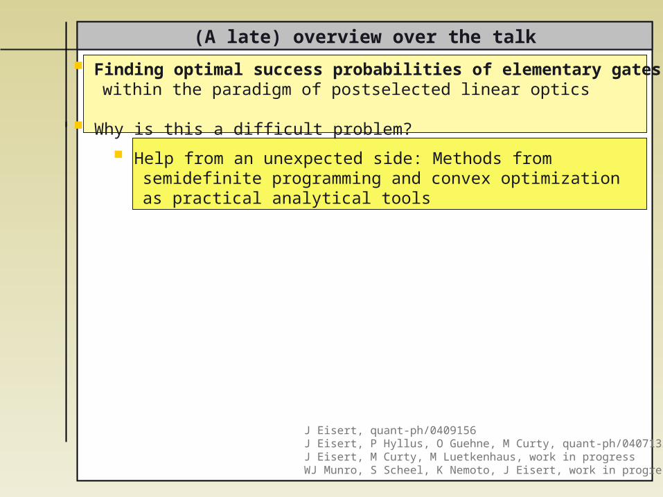
(A late) overview over the talk
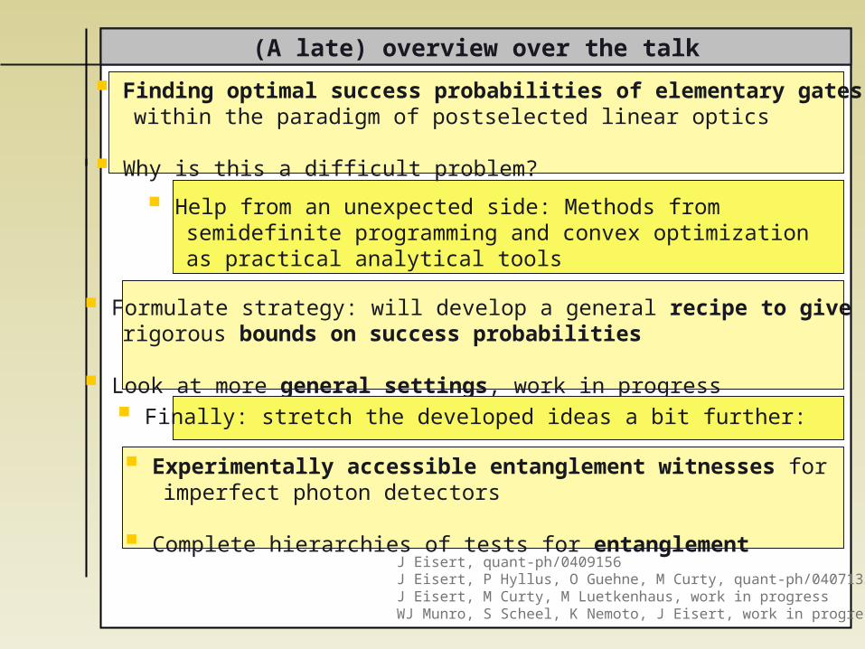
Finding optimal success probabilities of elementary gates within the paradigm of postselected linear optics
Why is this a difficult problem?
J Eisert, quant-ph/0409156J Eisert, P Hyllus, O Guehne, M Curty, quant-ph/0407135J Eisert, M Curty, M Luetkenhaus, work in progressWJ Munro, S Scheel, K Nemoto, J Eisert, work in progress
(A late) overview over the talk
Finding optimal success probabilities of elementary gates within the paradigm of postselected linear optics
Why is this a difficult problem?
Help from an unexpected side: Methods from semidefinite programming and convex optimization as practical analytical tools
J Eisert, quant-ph/0409156J Eisert, P Hyllus, O Guehne, M Curty, quant-ph/0407135J Eisert, M Curty, M Luetkenhaus, work in progressWJ Munro, S Scheel, K Nemoto, J Eisert, work in progress

(A late) overview over the talk
Finding optimal success probabilities of elementary gates within the paradigm of postselected linear optics
Why is this a difficult problem?
Help from an unexpected side: Methods from semidefinite programming and convex optimization as practical analytical tools
Formulate strategy: will develop a general recipe to give rigorous bounds on success probabilities
Look at more general settings, work in progress
J Eisert, quant-ph/0409156J Eisert, P Hyllus, O Guehne, M Curty, quant-ph/0407135J Eisert, M Curty, M Luetkenhaus, work in progressWJ Munro, S Scheel, K Nemoto, J Eisert, work in progress
(A late) overview over the talk
Finding optimal success probabilities of elementary gates within the paradigm of postselected linear optics
Why is this a difficult problem?
Help from an unexpected side: Methods from semidefinite programming and convex optimization as practical analytical tools
Formulate strategy: will develop a general recipe to give rigorous bounds on success probabilities
Look at more general settings, work in progress Finally: stretch the developed ideas a bit further:
Experimentally accessible entanglement witnesses for imperfect photon detectors
Complete hierarchies of tests for entanglementJ Eisert, quant-ph/0409156J Eisert, P Hyllus, O Guehne, M Curty, quant-ph/0407135J Eisert, M Curty, M Luetkenhaus, work in progressWJ Munro, S Scheel, K Nemoto, J Eisert, work in progress
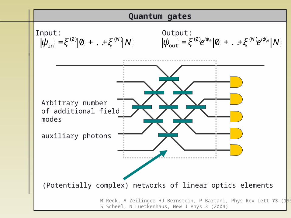
Quantum gates
€
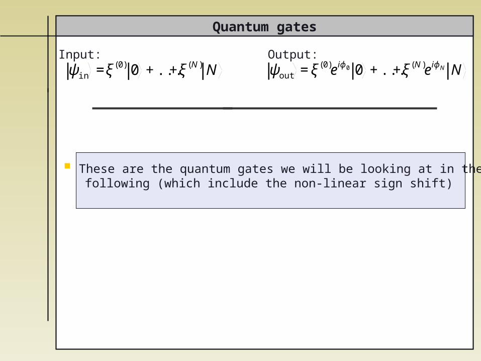
ψin =ξ(0) 0 +...+ξ(N) NInput:
€
ψout =ξ(0)eiϕ0 0 +...+ξ(N)eiϕN NOutput:
These are the quantum gates we will be looking at in the following (which include the non-linear sign shift)
Quantum gates
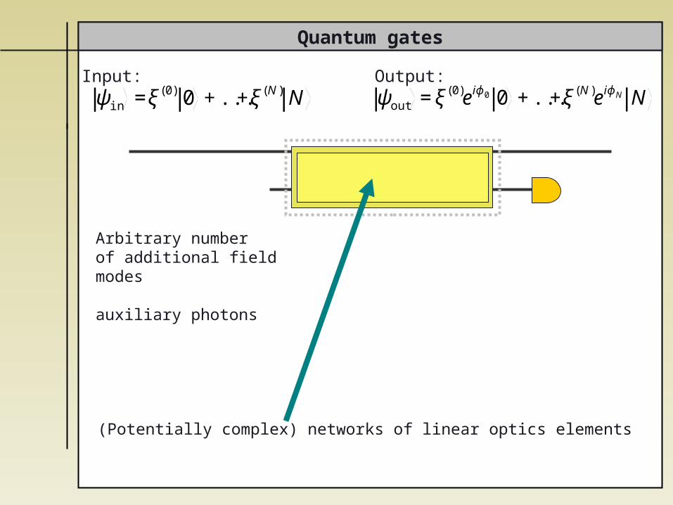
Arbitrary number of additional fieldmodes
auxiliary photons
(Potentially complex) networks of linear optics elements
Input: Output:
€
ψin =ξ(0) 0 +...+ξ(N) N
€
ψout =ξ(0)eiϕ0 0 +...+ξ(N)eiϕN N
Quantum gates
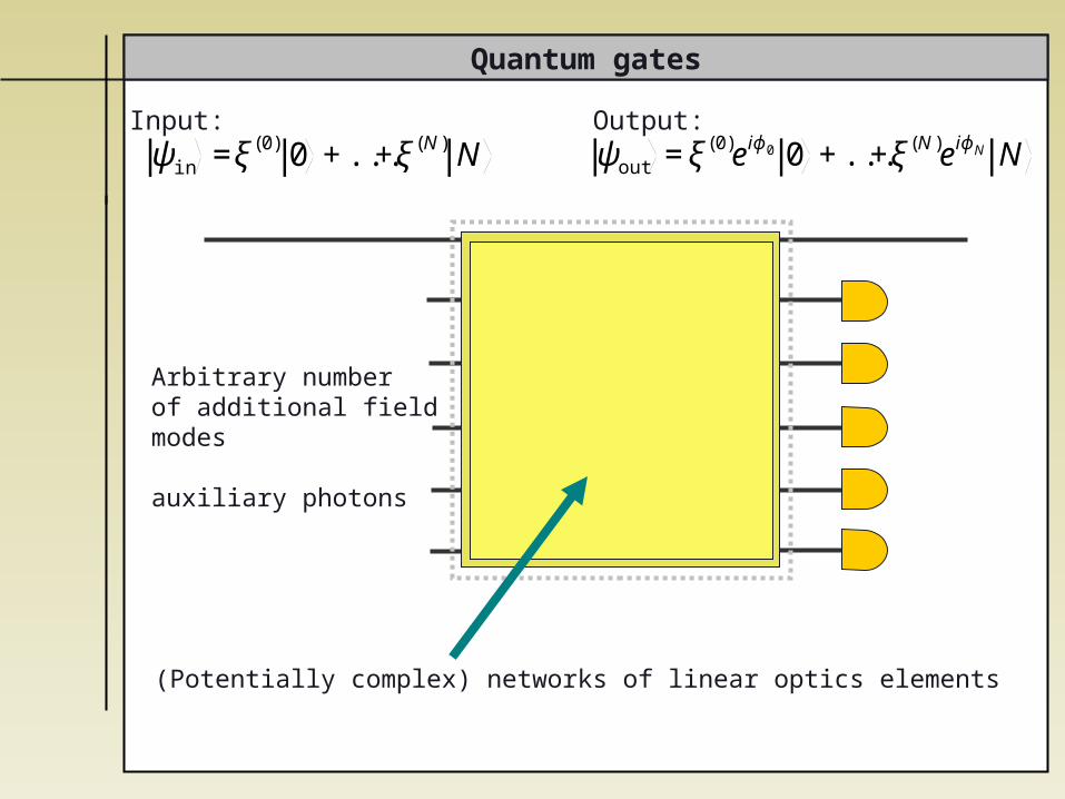
Arbitrary number of additional fieldmodes
auxiliary photons
Input: Output:
€
ψin =ξ(0) 0 +...+ξ(N) N
€
ψout =ξ(0)eiϕ0 0 +...+ξ(N)eiϕN N
(Potentially complex) networks of linear optics elements
Quantum gates
Arbitrary number of additional fieldmodes
auxiliary photons
Input: Output:
€
ψin =ξ(0) 0 +...+ξ(N) N
€
ψout =ξ(0)eiϕ0 0 +...+ξ(N)eiϕN N
(Potentially complex) networks of linear optics elements
M Reck, A Zeilinger HJ Bernstein, P Bartani, Phys Rev Lett 73 (1994)S Scheel, N Luetkenhaus, New J Phys 3 (2004)
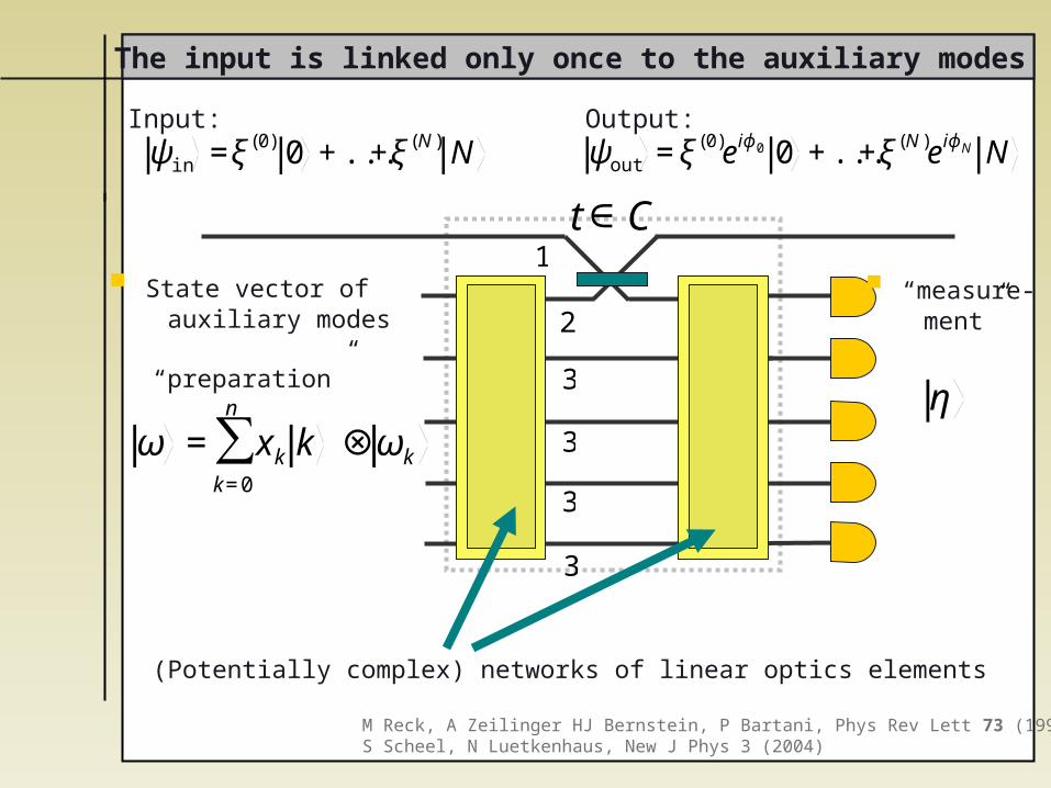
The input is linked only once to the auxiliary modes
€
t∈C
€
ω = xk kk=0
n
∑ ⊗ ωk
€
η
State vector of auxiliary modes
“preparation”
€
2
€
3
€
3
€
3
€
3
€
1
Input: Output:
“measure- ment”
€
ψin =ξ(0) 0 +...+ξ(N) N
€
ψout =ξ(0)eiϕ0 0 +...+ξ(N)eiϕN N
(Potentially complex) networks of linear optics elements
M Reck, A Zeilinger HJ Bernstein, P Bartani, Phys Rev Lett 73 (1994)S Scheel, N Luetkenhaus, New J Phys 3 (2004)
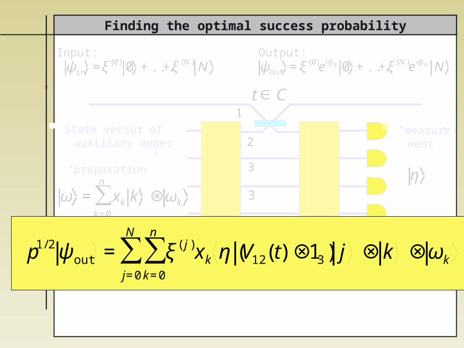
Finding the optimal success probability
€
η =U 1⊗n
€
3
State vector of auxiliary modes
“preparation”
“measure- ment”
€
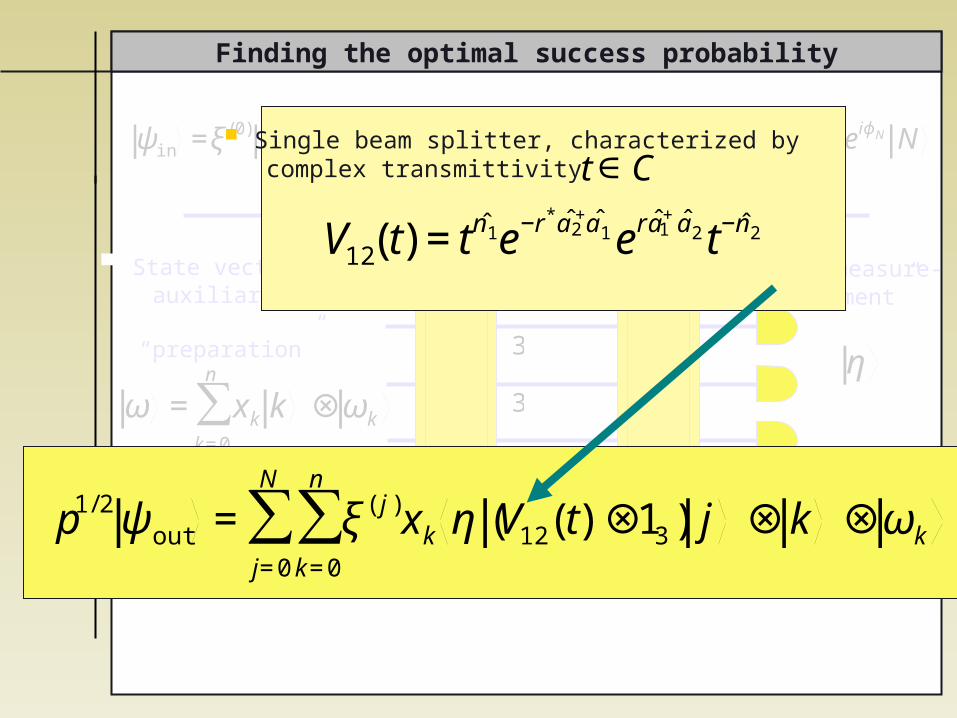
p1/2 ψout = ξ( j )xk η (V12(t)⊗13) j ⊗ kk=0
n
∑ ⊗ ωkj=0
N
∑
Input: Output:
€
ψin =ξ(0) 0 +...+ξ(N) N
€
ψout =ξ(0)eiϕ0 0 +...+ξ(N)eiϕN N
Finding the optimal success probability
€
η =U 1⊗n
€
t∈C
€
ω = xk kk=0
n
∑ ⊗ ωk
€
2
€
3
€
3
€
1
€
p1/2 ψout = ξ( j )xk η (V12(t)⊗13) j ⊗ kk=0
n
∑ ⊗ ωkj=0
N
∑
€
η
State vector of auxiliary modes
“preparation”
“measure- ment”
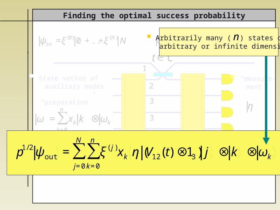
Single beam splitter, characterized by complex transmittivity
€
V12(t) =t ˆ n 1e−r* ˆ a 2+ˆ a 1er ˆ a 1+ˆ a 2t−ˆ n 2
€
t∈C
€
ψin =ξ(0) 0 +...+ξ(N) N
€
ψout =ξ(0)eiϕ0 0 +...+ξ(N)eiϕN N
Finding the optimal success probability
€
η =U 1⊗n
€
t∈C
€
ω = xk kk=0
n
∑ ⊗ ωk
€
2
€
3
€
3
€
1
Arbitrarily many ( ) states of arbitrary or infinite dimension
€
n
€
η
State vector of auxiliary modes
“preparation”
“measure- ment”
€
p1/2 ψout = ξ( j )xk η (V12(t)⊗13) j ⊗ kk=0
n
∑ ⊗ ωkj=0
N
∑
€
ψin =ξ(0) 0 +...+ξ(N) N
€
ψout =ξ(0)eiϕ0 0 +...+ξ(N)eiϕN N
Finding the optimal success probability
€
η =U 1⊗n
€
t∈C
€
ω = xk kk=0
n
∑ ⊗ ωk
€
2
€
3
€
3
€
1
€
ψout =ξ0eiϕ0 0 +...+ξNeiϕN N
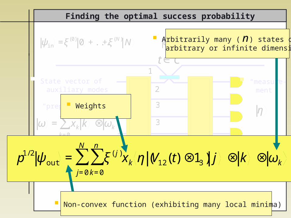
Arbitrarily many ( ) states of arbitrary or infinite dimension
Non-convex function (exhibiting many local minima)
€
n
€
η
State vector of auxiliary modes
“preparation”
“measure- ment”
€
p1/2 ψout = ξ( j )xk η (V12(t)⊗13) j ⊗ kk=0
n
∑ ⊗ ωkj=0
N
∑
Weights
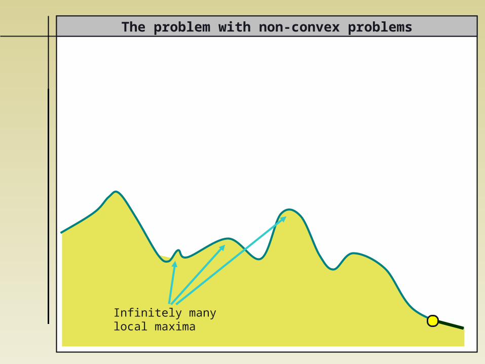
The problem with non-convex problems
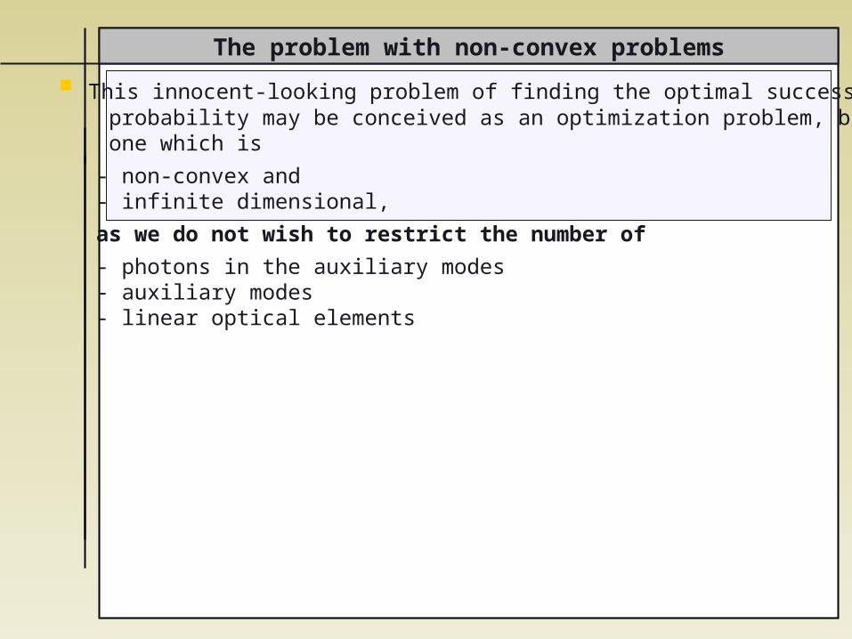
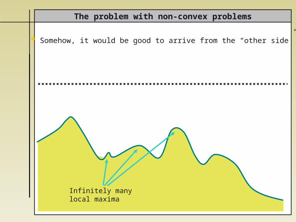
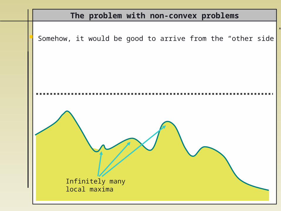
This innocent-looking problem of finding the optimal success probability may be conceived as an optimization problem, but one which is
- non-convex and - infinite dimensional,
as we do not wish to restrict the number of
- photons in the auxiliary modes - auxiliary modes - linear optical elements
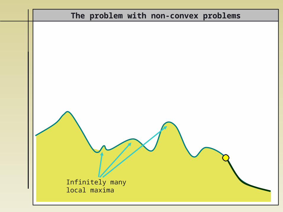
The problem with non-convex problems
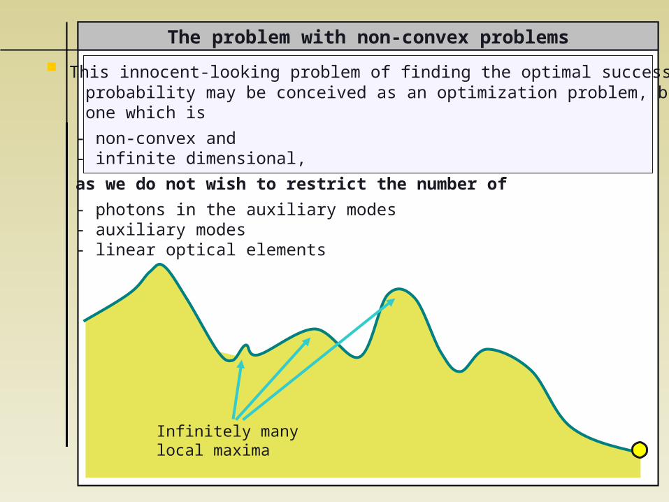
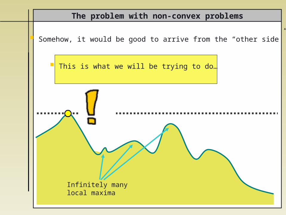
Infinitely manylocal maxima
This innocent-looking problem of finding the optimal success probability may be conceived as an optimization problem, but one which is
- non-convex and - infinite dimensional,
as we do not wish to restrict the number of
- photons in the auxiliary modes - auxiliary modes - linear optical elements
The problem with non-convex problems
Infinitely manylocal maxima
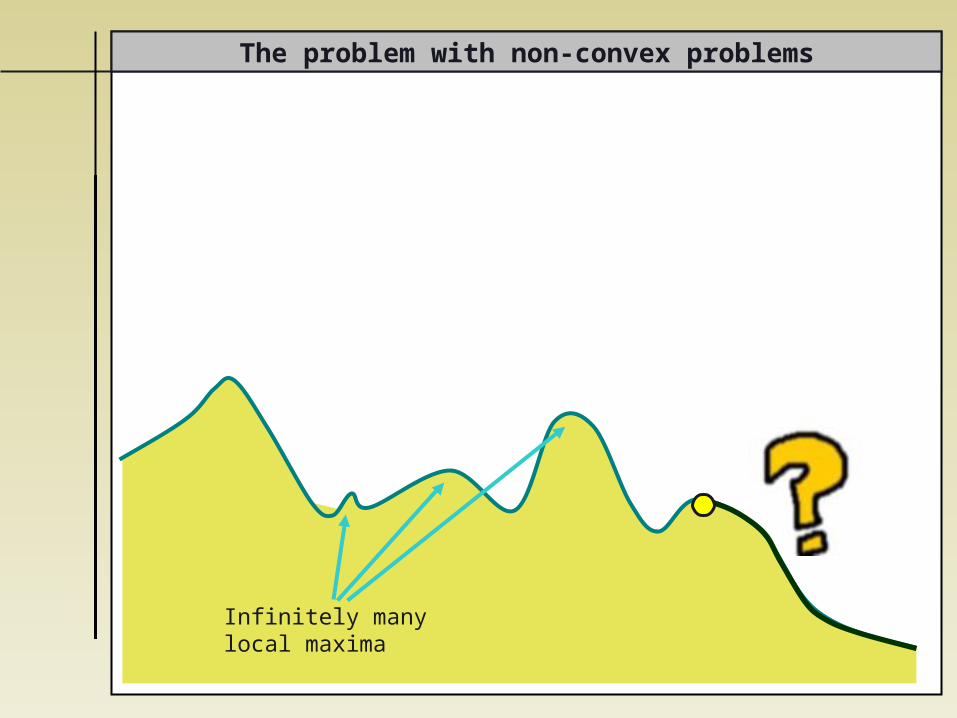
The problem with non-convex problems
Infinitely manylocal maxima
The problem with non-convex problems
Infinitely manylocal maxima
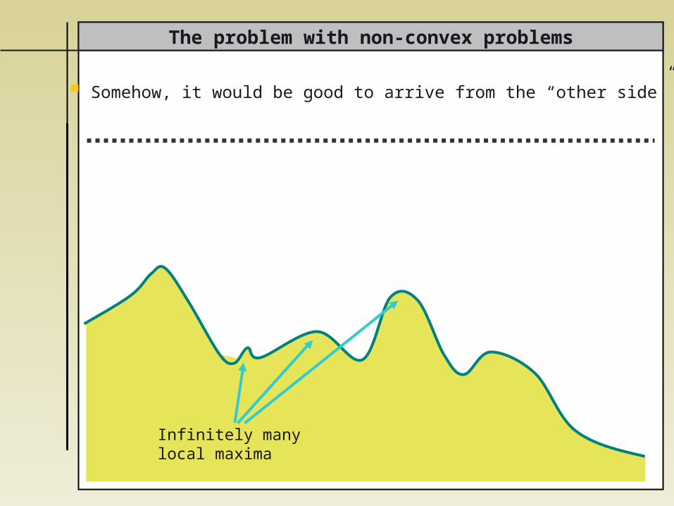
The problem with non-convex problems
Infinitely manylocal maxima
Somehow, it would be good to arrive from the “other side”
The problem with non-convex problems
Infinitely manylocal maxima
Somehow, it would be good to arrive from the “other side”
The problem with non-convex problems
Infinitely manylocal maxima
Somehow, it would be good to arrive from the “other side”
The problem with non-convex problems
Infinitely manylocal maxima
Somehow, it would be good to arrive from the “other side”
This is what we will be trying to do…

Convex optimization? Can it help?

Convex optimization problems
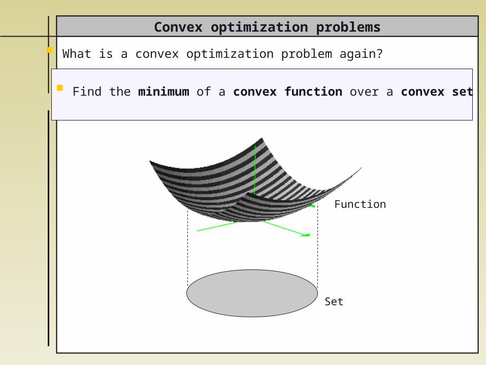
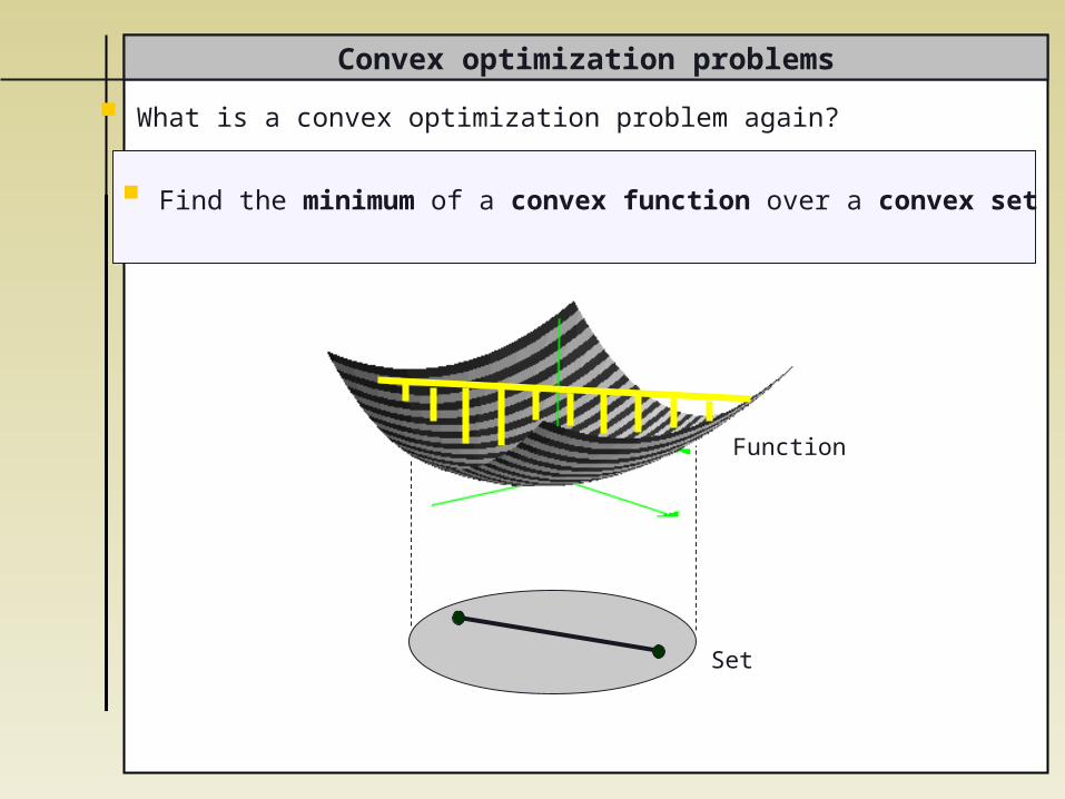
Find the minimum of a convex function over a convex set
What is a convex optimization problem again?
Convex optimization problems
Find the minimum of a convex function over a convex set
What is a convex optimization problem again?
Function
Set
Convex optimization problems
Function
Set
Find the minimum of a convex function over a convex set
What is a convex optimization problem again?
Semidefinite programs
Function
Set
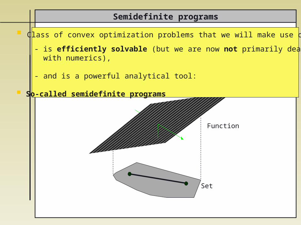
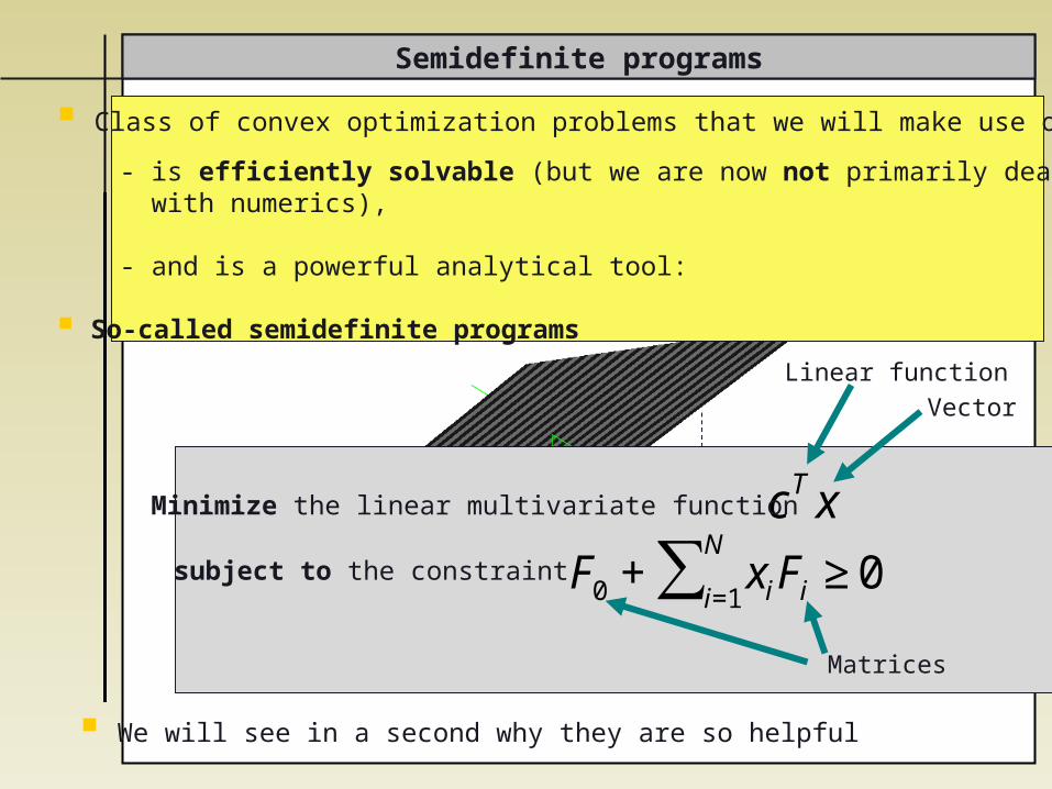
Class of convex optimization problems that we will make use of
- is efficiently solvable (but we are now not primarily dealing with numerics),
- and is a powerful analytical tool:
So-called semidefinite programs
Semidefinite programs
Set
Class of convex optimization problems that we will make use of
- is efficiently solvable (but we are now not primarily dealing with numerics),
- and is a powerful analytical tool:
So-called semidefinite programs
€
cT xMinimize the linear multivariate function
subject to the constraint
€
F0 + xiFi ≥0i=1
N∑
Linear function
Matrices
Vector
We will see in a second why they are so helpful
Yes, ok, …
… but why should this help us to assess the performance of quantum gates in the context of linear optics?
1. Recasting the problem
€
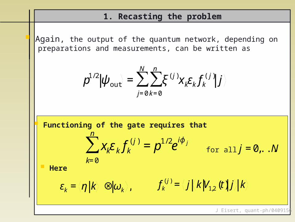
εk = η k ⊗ ωk ,
€
p1/2 ψout = ξ( j )xkεk fk( j )
k=0
n
∑j=0
N
∑ j
€
xkεk fk( j )
k=0
n
∑ =p1/2eiϕ j
€
fk( j ) = j kV1,2(t) j k
Again, the output of the quantum network, depending on preparations and measurements, can be written as
for all
€
j =0,...,N
Here
J Eisert, quant-ph/0409156
Functioning of the gate requires that
1. Recasting the problem
€
εk = η k ⊗ ωk ,
€
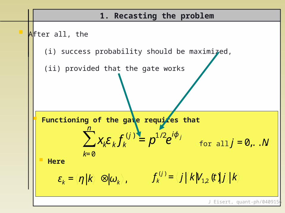
xkεk fk( j )
k=0
n
∑ =p1/2eiϕ j
€
fk( j ) = j kV1,2(t) j k
for all
€
j =0,...,N
Here
J Eisert, quant-ph/0409156
Functioning of the gate requires that
After all, the
(i) success probability should be maximized, (ii) provided that the gate works
1. Recasting the problem
€
εk = η k ⊗ ωk ,
€
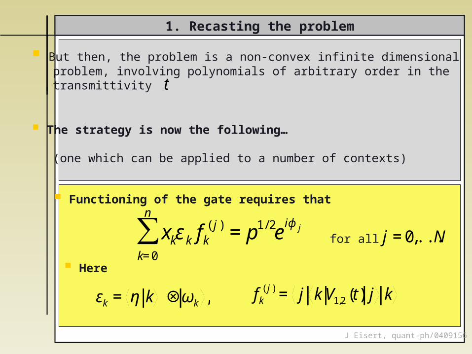
xkεk fk( j )
k=0
n
∑ =p1/2eiϕ j
€
fk( j ) = j kV1,2(t) j k
for all
€
j =0,...,N
Here
J Eisert, quant-ph/0409156
Functioning of the gate requires that
But then, the problem is a non-convex infinite dimensional problem, involving polynomials of arbitrary order in the transmittivity
The strategy is now the following…
(one which can be applied to a number of contexts)
€
t
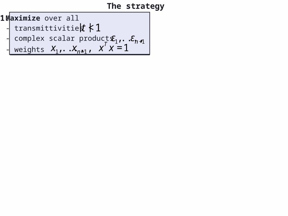
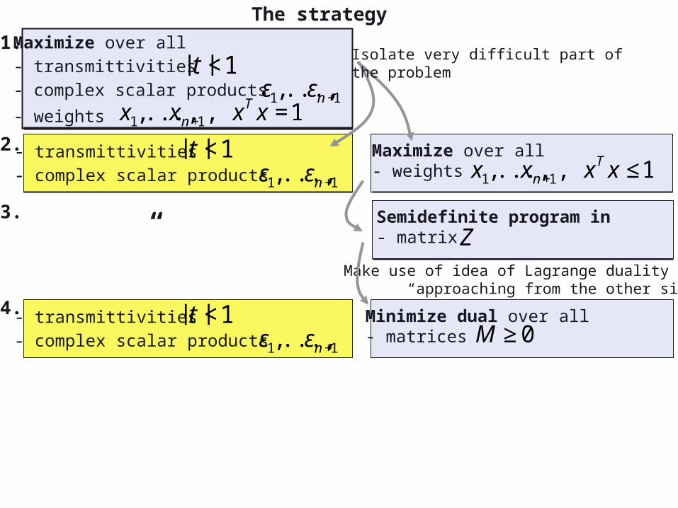
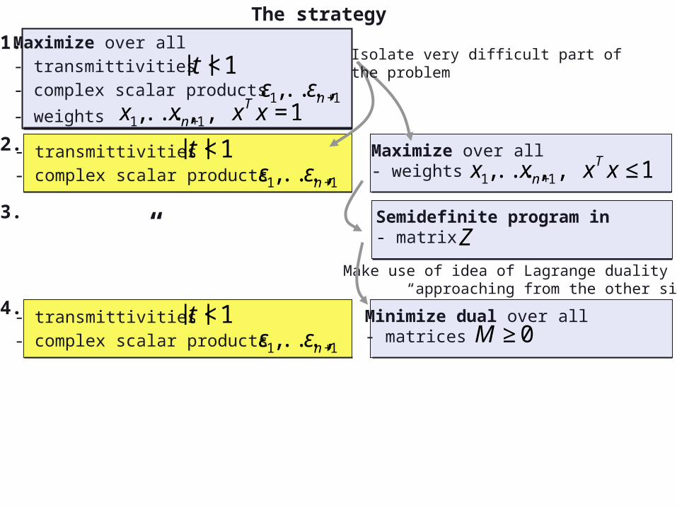
The strategy
Maximize over all- transmittivities- complex scalar products
- weights
€
|t |<1
€
ε1,...,εn+1
€
x1,...,xn+1, xT x =1
1.
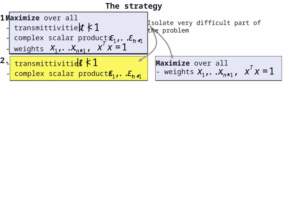
The strategy
Maximize over all- transmittivities- complex scalar products
- weights
€
|t |<1
€
ε1,...,εn+1
€
x1,...,xn+1, xT x =1
- transmittivities- complex scalar products
€
|t |<1
€
ε1,...,εn+1
Maximize over all- weights
€
x1,...,xn+1, xT x =1
Isolate very difficult part of the problem
1.
2.
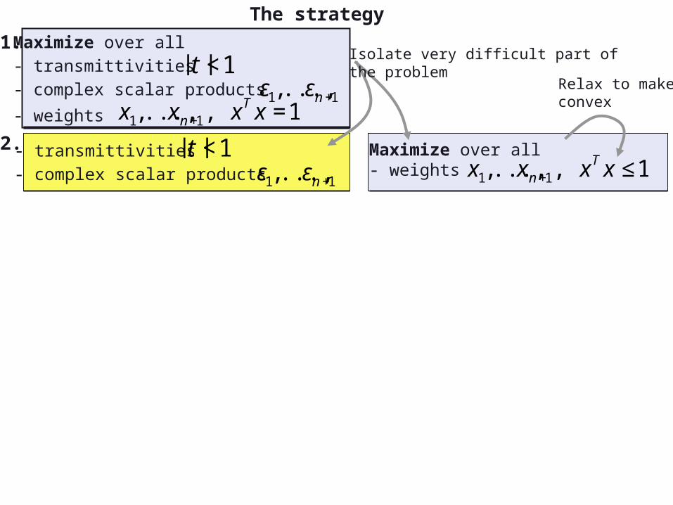
The strategy
Maximize over all- transmittivities- complex scalar products
- weights
€
|t |<1
€
ε1,...,εn+1
€
x1,...,xn+1, xT x =1
- transmittivities- complex scalar products
€
|t |<1
€
ε1,...,εn+1
Maximize over all- weights
€
x1,...,xn+1, xT x ≤1
Isolate very difficult part of the problem
Relax to makeconvex
1.
2.

3. Writing it as a semidefinite problem
Then for each the problem is found to be one with matrix constraints the elements of which are polynomials of arbitrary degree in
The resulting problem may look strange, but it is actually a semidefinite program
Why does this help us?
€
(t, εk{ })
€
t
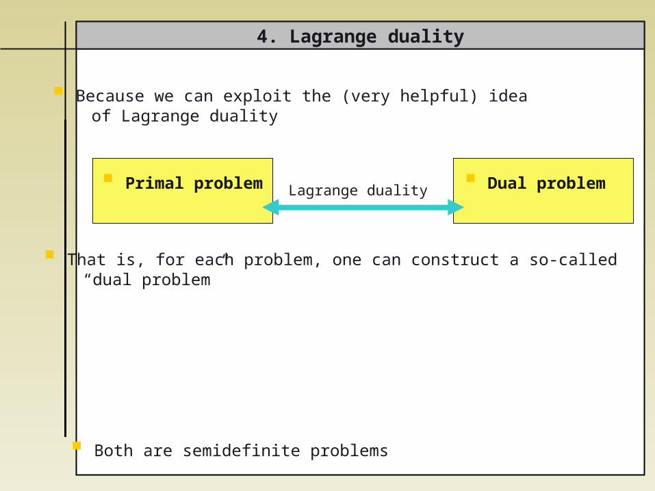
4. Lagrange duality
Primal problem Dual problem
That is, for each problem, one can construct a so-called “dual problem”
Because we can exploit the (very helpful) idea of Lagrange duality
Lagrange duality
Both are semidefinite problems
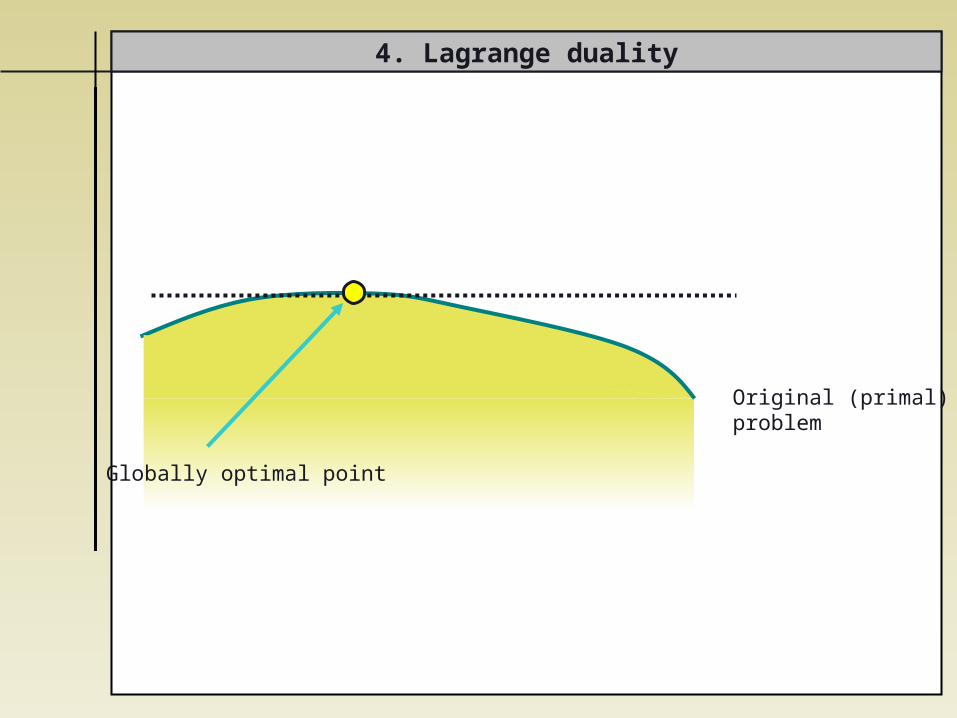
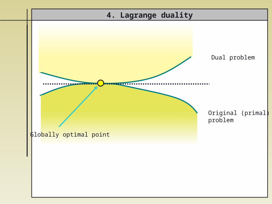
4. Lagrange duality
Globally optimal point
Original (primal) problem
4. Lagrange duality
Globally optimal point
Original (primal) problem
Dual problem
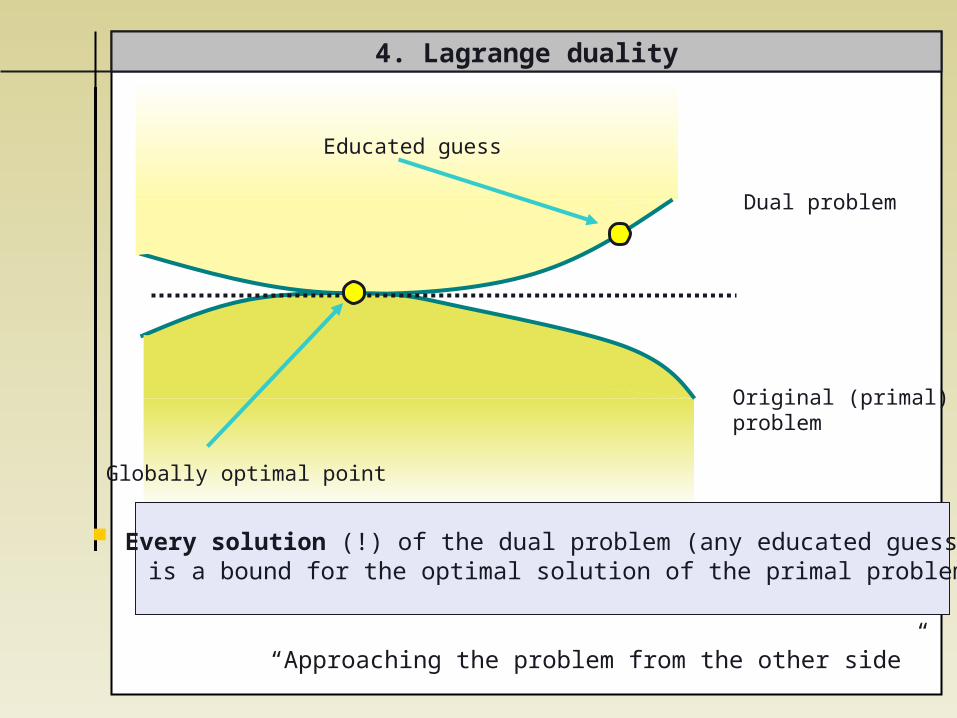
4. Lagrange duality
Globally optimal point
Original (primal) problem
Dual problem
Every solution (!) of the dual problem (any educated guess) is a bound for the optimal solution of the primal problem
Educated guess
“Approaching the problem from the other side”
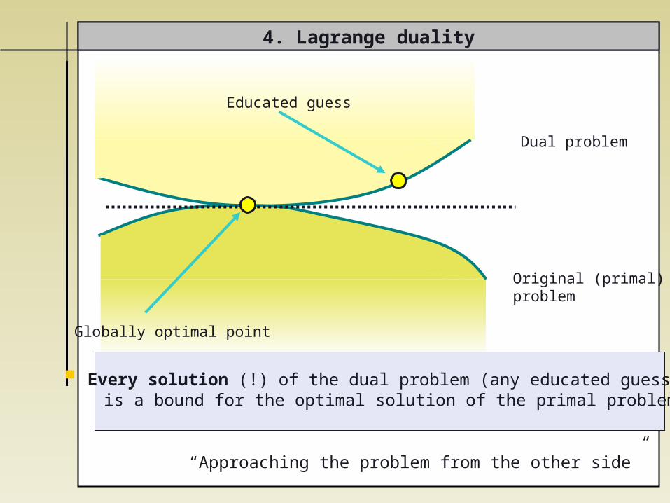
4. Lagrange duality
Globally optimal point
Original (primal) problem
Dual problem
Every solution (!) of the dual problem (any educated guess) is a bound for the optimal solution of the primal problem
“Approaching the problem from the other side”
Educated guess
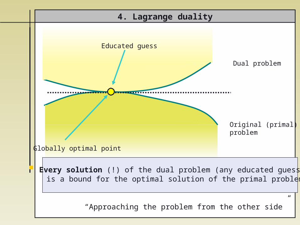
4. Lagrange duality
Globally optimal point
Original (primal) problem
Dual problem
Every solution (!) of the dual problem (any educated guess) is a bound for the optimal solution of the primal problem
“Approaching the problem from the other side”
Educated guess
The strategy
Maximize over all- transmittivities- complex scalar products
- weights
€
|t |<1
€
ε1,...,εn+1
€
x1,...,xn+1, xT x =1
- transmittivities- complex scalar products
€
|t |<1
€
ε1,...,εn+1
Maximize over all- weights
€
x1,...,xn+1, xT x ≤1
Isolate very difficult part of the problem
- transmittivities- complex scalar products
€
|t |<1
€
ε1,...,εn+1
Minimize dual over all - matrices
€
M ≥0
Make use of idea of Lagrange duality “approaching from the other side”
“ Semidefinite program in - matrix
€
Z
1.
2.
3.
4.
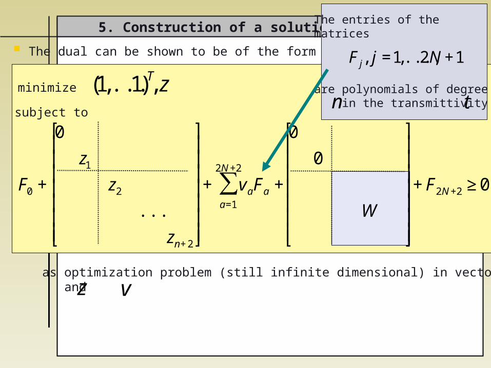
The dual can be shown to be of the form
as optimization problem (still infinite dimensional) in vectors and
5. Construction of a solution for the dual
€
(1,...,1)T z
€
F0 +
0
z1
z2
...
zn+2
⎡
⎣
⎢ ⎢ ⎢ ⎢ ⎢ ⎢ ⎢
⎤
⎦
⎥ ⎥ ⎥ ⎥ ⎥ ⎥ ⎥
+ vaFa +a=1
2N+2
∑
0
0
W
⎡
⎣
⎢ ⎢ ⎢ ⎢ ⎢ ⎢ ⎢
⎤
⎦
⎥ ⎥ ⎥ ⎥ ⎥ ⎥ ⎥
+F2N+2 ≥0
minimize
subject to
€
z
€
v
The entries of the matrices
are polynomials of degree in the transmittivity
€
F j, j =1,...,2N +1
€
n
€
t

The dual can be shown to be of the form
5. Construction of a solution for the dual
€
(1,...,1)T z
€
F0 +
0
z1
z2
...
zn+2
⎡
⎣
⎢ ⎢ ⎢ ⎢ ⎢ ⎢ ⎢
⎤
⎦
⎥ ⎥ ⎥ ⎥ ⎥ ⎥ ⎥
+ vaFa +a=1
2N+2
∑
0
0
W
⎡
⎣
⎢ ⎢ ⎢ ⎢ ⎢ ⎢ ⎢
⎤
⎦
⎥ ⎥ ⎥ ⎥ ⎥ ⎥ ⎥
+F2N+2 ≥0
minimize
subject to
Finding a solution now means “guessing” a matrix
Can be done, even in a way such that the unwanted dependence on preparation and measurement can be eliminated
Instance of a problem that can explicitly solved
€
W
€
εk{ }
The strategy
Maximize over all- transmittivities- complex scalar products
- weights
€
|t |<1
€
ε1,...,εn+1
€
x1,...,xn+1, xT x =1
- transmittivities- complex scalar products
€
|t |<1
€
ε1,...,εn+1
Maximize over all- weights
€
x1,...,xn+1, xT x ≤1
Isolate very difficult part of the problem
- transmittivities- complex scalar products
€
|t |<1
€
ε1,...,εn+1
Minimize dual over all - matrices
€
M ≥0
Make use of idea of Lagrange duality “approaching from the other side”
“ Semidefinite program in - matrix
€
Z
1.
2.
3.
4.
The strategy
Maximize over all- transmittivities- complex scalar products
- weights
€
|t |<1
€
ε1,...,εn+1
€
x1,...,xn+1, xT x =1
- transmittivities- complex scalar products
€
|t |<1
€
ε1,...,εn+1
Maximize over all- weights
€
x1,...,xn+1, xT x ≤1
Isolate very difficult part of the problem
- transmittivities- complex scalar products
€
|t |<1
€
ε1,...,εn+1
Minimize dual over all - matrices
€
M ≥0
Make use of idea of Lagrange duality “approaching from the other side”
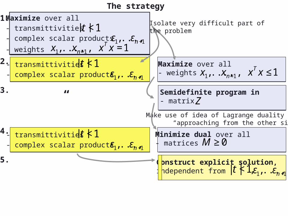
Construct explicit solution, independent from
€
|t |<1,
€
ε1,...,εn+1
“ Semidefinite program in - matrix
€
Z
1.
2.
3.
4.
5.
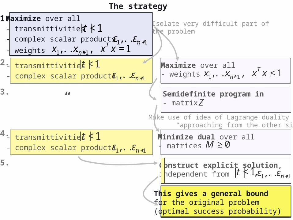
The strategy
Maximize over all- transmittivities- complex scalar products
- weights
€
|t |<1
€
ε1,...,εn+1
€
x1,...,xn+1, xT x =1
- transmittivities- complex scalar products
Maximize over all- weights
Isolate very difficult part of the problem
- transmittivities- complex scalar products
€
|t |<1
€
ε1,...,εn+1
Minimize dual over all - matrices
Make use of idea of Lagrange duality “approaching from the other side”
Construct explicit solution, independent from
This gives a general boundfor the original problem(optimal success probability)
“ Semidefinite program in - matrix
1.
2.
3.
4.
5.
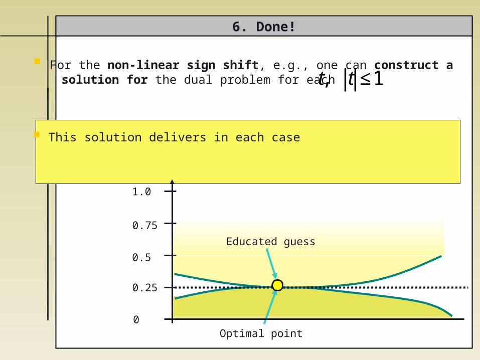
For the non-linear sign shift, e.g., one can construct a solution for the dual problem for each
This solution delivers in each case
6. Done!
€
t, t ≤1
Educated guess
Optimal point
0.25
0
0.5
0.75
1.0
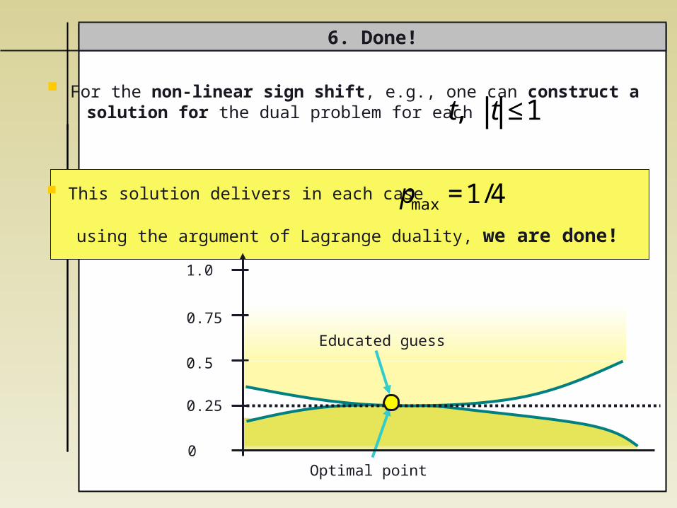
For the non-linear sign shift, e.g., one can construct a solution for the dual problem for each
This solution delivers in each case
using the argument of Lagrange duality, we are done!
6. Done!
€
pmax=1/4
€
t, t ≤1
Educated guess
Optimal point
0.25
0
0.5
0.75
1.0
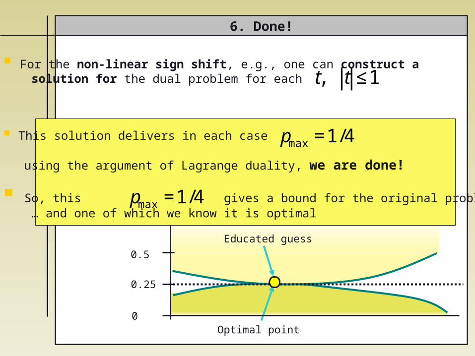
6. Done!
€
pmax=1/4
€
t, t ≤1
Educated guess
Optimal point
0.25
0
0.5
For the non-linear sign shift, e.g., one can construct a solution for the dual problem for each
This solution delivers in each case
using the argument of Lagrange duality, we are done!
So, this gives a bound for the original problem … … and one of which we know it is optimal
€
pmax=1/4
€
pmax=1/4
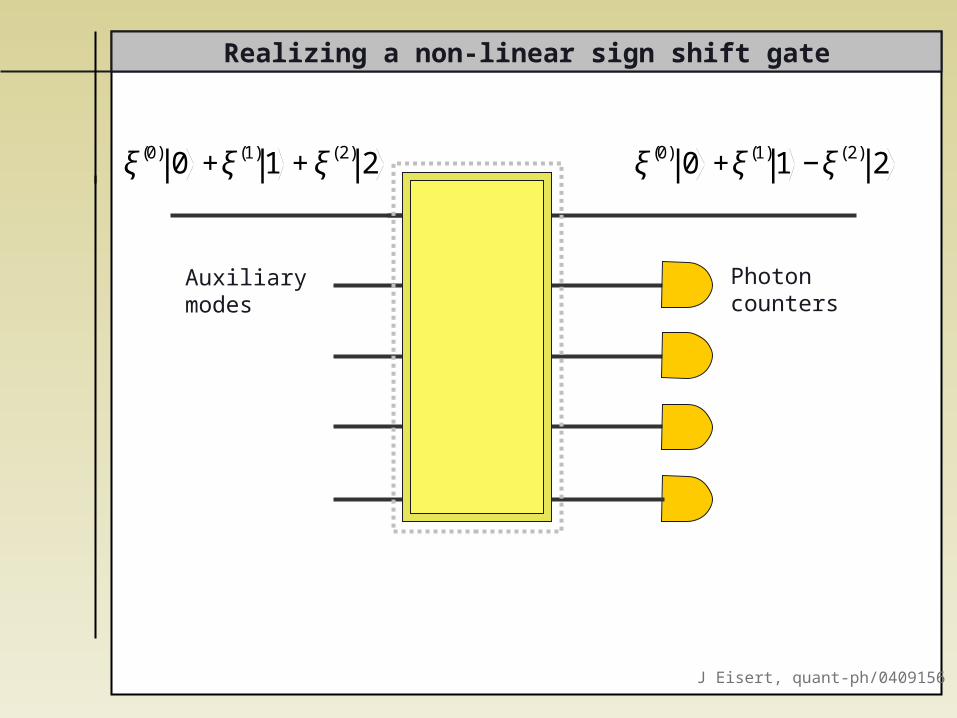
Realizing a non-linear sign shift gate
Auxiliary modes
Photoncounters
€
ξ(0) 0 +ξ(1)1 +ξ(2) 2
€
ξ(0) 0 +ξ(1)1 −ξ(2) 2
J Eisert, quant-ph/0409156
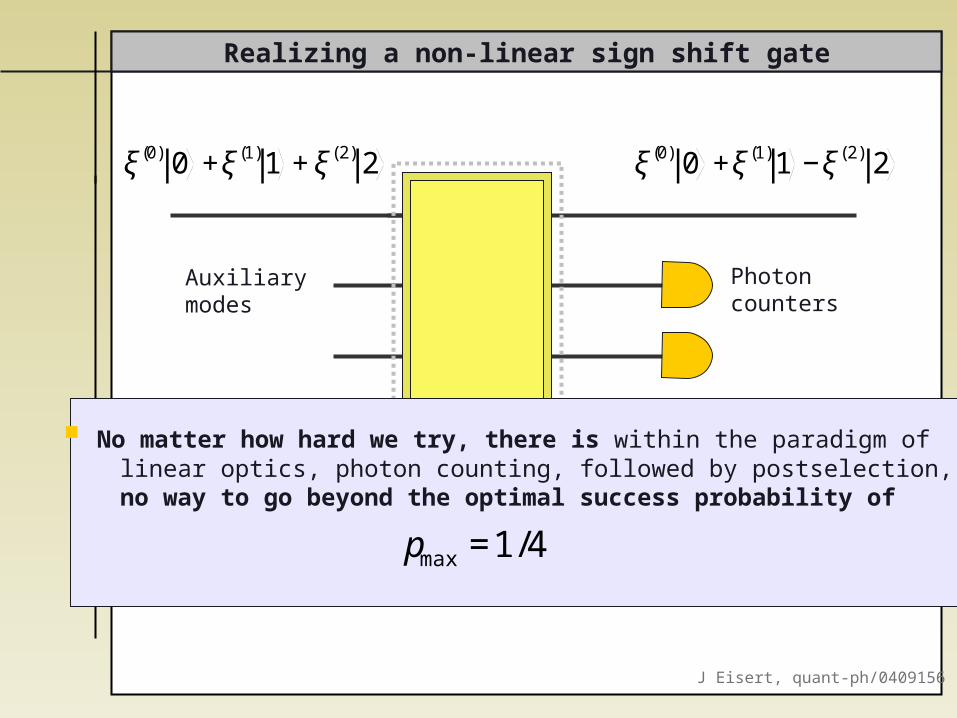
Realizing a non-linear sign shift gate
Auxiliary modes
Photoncounters
€
ξ(0) 0 +ξ(1)1 +ξ(2) 2
€
ξ(0) 0 +ξ(1)1 −ξ(2) 2
No matter how hard we try, there is within the paradigm of linear optics, photon counting, followed by postselection, no way to go beyond the optimal success probability of
€
pmax=1/4
J Eisert, quant-ph/0409156
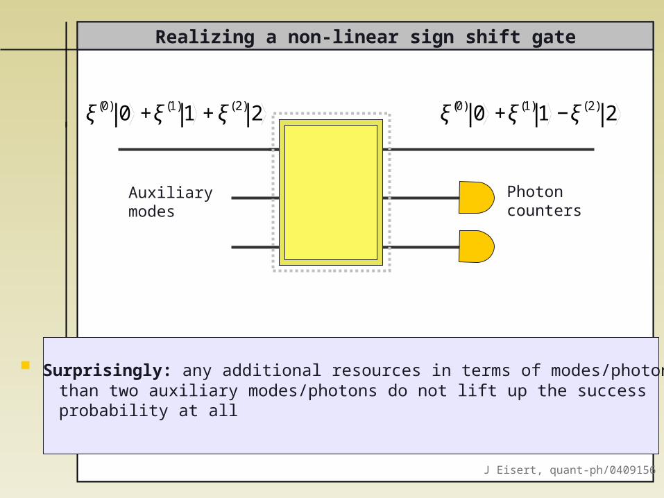
Realizing a non-linear sign shift gate
Auxiliary modes
Photoncounters
€
ξ(0) 0 +ξ(1)1 +ξ(2) 2
€
ξ(0) 0 +ξ(1)1 −ξ(2) 2
Surprisingly: any additional resources in terms of modes/photons than two auxiliary modes/photons do not lift up the success probability at all
J Eisert, quant-ph/0409156
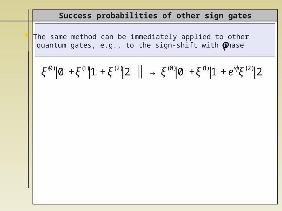
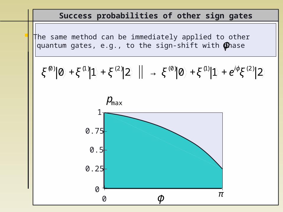
The same method can be immediately applied to other quantum gates, e.g., to the sign-shift with phase
Success probabilities of other sign gates
€
ϕ
€
ξ(0) 0 +ξ(1)1 +ξ(2) 2 ⏐ → ⏐ ξ(0) 0 +ξ(1) 1 +eiϕξ(2) 2
The same method can be immediately applied to other quantum gates, e.g., to the sign-shift with phase
Success probabilities of other sign gates
€
ϕ0
0.25
0.5
0.75
1
0
€
π
€
pmax
€
ϕ
€
ξ(0) 0 +ξ(1)1 +ξ(2) 2 ⏐ → ⏐ ξ(0) 0 +ξ(1) 1 +eiϕξ(2) 2
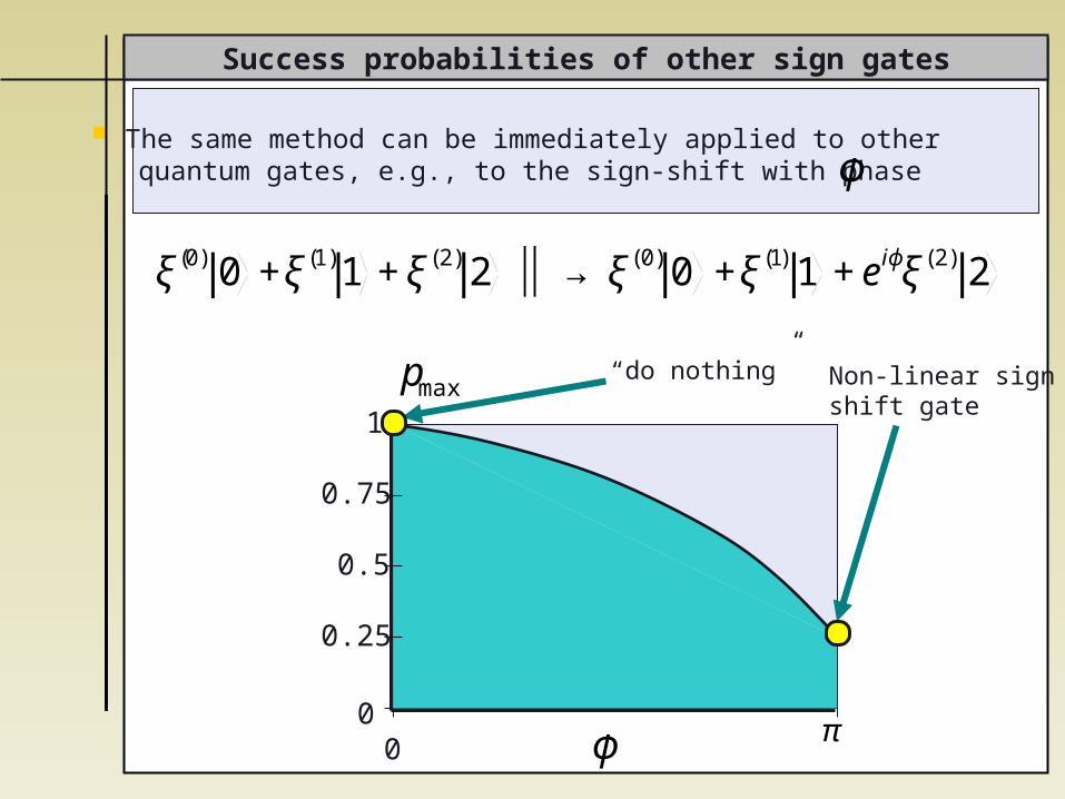
The same method can be immediately applied to other quantum gates, e.g., to the sign-shift with phase
Success probabilities of other sign gates
€
ϕ0
0.25
0.5
0.75
1
0
€
π
€
pmax
€
ϕ
“do nothing” Non-linear signshift gate
€
ξ(0) 0 +ξ(1)1 +ξ(2) 2 ⏐ → ⏐ ξ(0) 0 +ξ(1) 1 +eiϕξ(2) 2
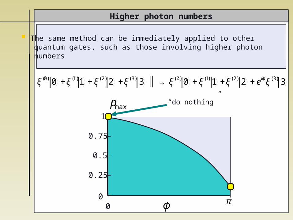
The same method can be immediately applied to other quantum gates, such as those involving higher photon numbers
Higher photon numbers
€
ξ(0) 0 +ξ(1)1 +ξ(2) 2 +ξ(3) 3 ⏐ → ⏐ ξ(0) 0 +ξ(1) 1 +ξ(2) 2 +eiϕξ(3) 3
€
ϕ0
0.25
0.5
0.75
1
0
€
π
€
pmax“do nothing”
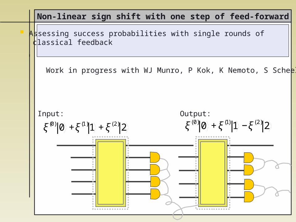
Non-linear sign shift with one step of feed-forward
Input: Output:
€
ξ(0) 0 +ξ(1)1 +ξ(2) 2
€
ξ(0) 0 +ξ(1) 1 −ξ(2) 2
Assessing success probabilities with single rounds of classical feedback
Work in progress with WJ Munro, P Kok, K Nemoto, S Scheel
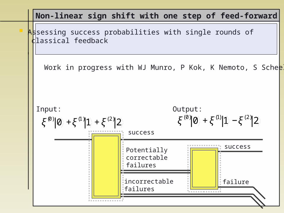
incorrectablefailures
Non-linear sign shift with one step of feed-forward
Input: Output:
€
ξ(0) 0 +ξ(1)1 +ξ(2) 2
Assessing success probabilities with single rounds of classical feedback
Work in progress with WJ Munro, P Kok, K Nemoto, S Scheel
success
failure
success
€
ξ(0) 0 +ξ(1) 1 −ξ(2) 2
Potentiallycorrectablefailures
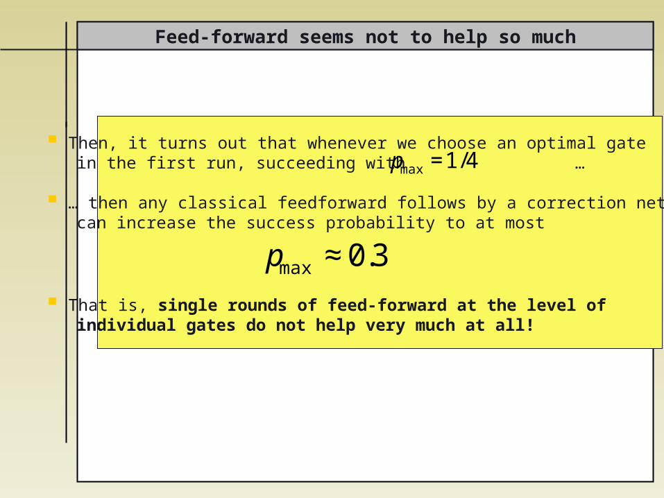
Feed-forward seems not to help so much
Then, it turns out that whenever we choose an optimal gate in the first run, succeeding with …
… then any classical feedforward follows by a correction network can increase the success probability to at most
That is, single rounds of feed-forward at the level of individual gates do not help very much at all!
€
pmax=1/4
€
pmax ≈0.3


Finally,
… extending these ideas to find other tools relevant to optical settings
Joint work with P Hyllus, O Gühne, M Curty, N Lütkenhaus

Stretch these ideas further to get practical tools
What was the point of the method before?
We developed a strategy to make methods from convex optimization applicable to solve a - non-convex and - infinite-dimensional problem to assess linear optical schemes

Stretch these ideas further to get practical tools
What was the point of the method before?
We developed a strategy to make methods from convex optimization applicable to solve a - non-convex and - infinite-dimensional problem to assess linear optical schemes
Can such strategies also formulated to find
good experimentally accessible witnesses to detect entanglement, which work for
- weak pulses and - finite detection efficiencies?
Practical tools to construct complete hierarchies of criteria for multi-particle entanglement?
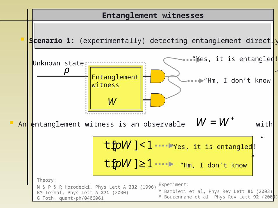
Entanglement witnesses
€
ρ
Scenario 1: (experimentally) detecting entanglement directly
Unknown state“Yes, it is entangled!”
“Hm, I don’t know”
€
tr[ρW]<1
€
W
€
tr[ρW]≥1
“Yes, it is entangled!”
“Hm, I don’t know”
Entanglement witness
An entanglement witness is an observable with
€
W =W+
Experiment:
M Barbieri et al, Phys Rev Lett 91 (2003)M Bourennane et al, Phys Rev Lett 92 (2004)
Theory:
M & P & R Horodecki, Phys Lett A 232 (1996)BM Terhal, Phys Lett A 271 (2000)G Toth, quant-ph/0406061
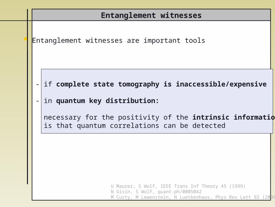
Entanglement witnesses
Entanglement witnesses are important tools
- if complete state tomography is inaccessible/expensive
- in quantum key distribution:
necessary for the positivity of the intrinsic information is that quantum correlations can be detected
U Maurer, S Wolf, IEEE Trans Inf Theory 45 (1999)N Gisin, S Wolf, quant-ph/0005042M Curty, M Lewenstein, N Luetkenhaus, Phys Rev Lett 92 (2004)
Entanglement witnesses
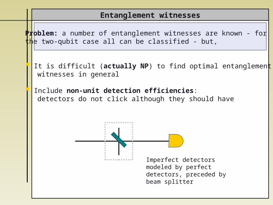
Problem: a number of entanglement witnesses are known - for the two-qubit case all can be classified - but,
It is difficult (actually NP) to find optimal entanglement witnesses in general
Include non-unit detection efficiencies: detectors do not click although they should have
Imperfect detectors modeled by perfect detectors, preceded by beam splitter
Entanglement witnesses
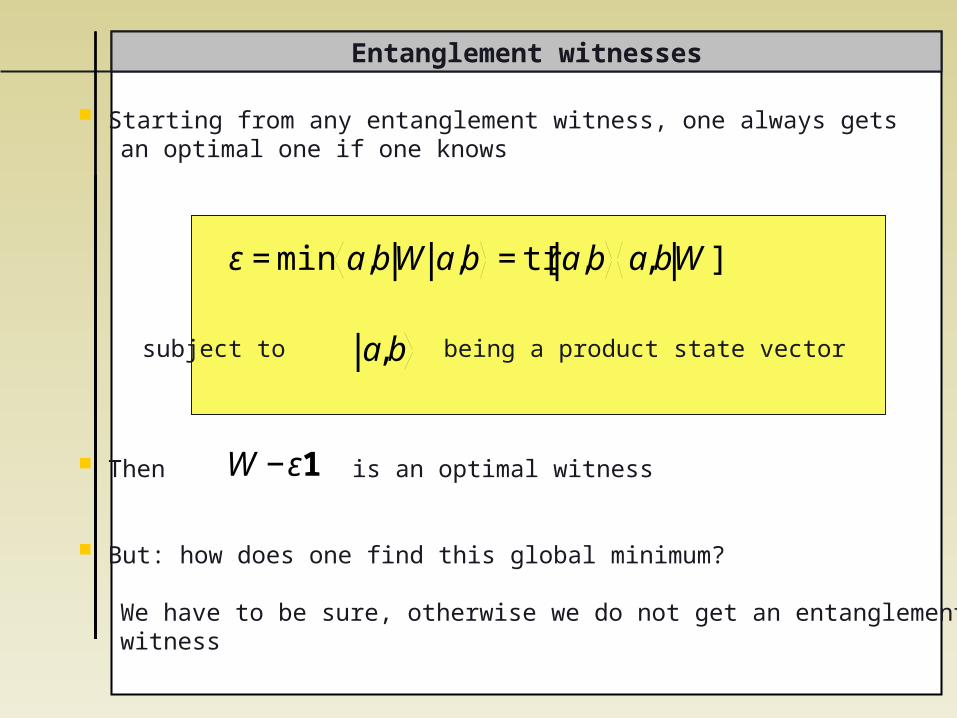
Starting from any entanglement witness, one always gets an optimal one if one knows
Then is an optimal witness
But: how does one find this global minimum?
We have to be sure, otherwise we do not get an entanglement witness
€
ε=min a,bW a,b =tr[ a,b a,bW]
€
a,bsubject to being a product state vector
€
W −ε1
The strategy
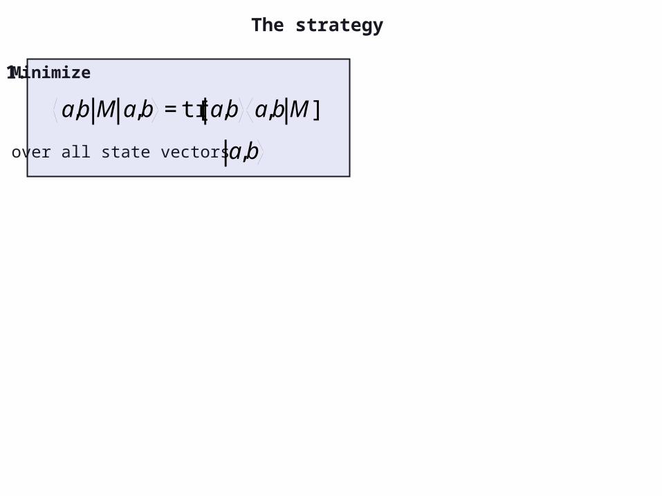
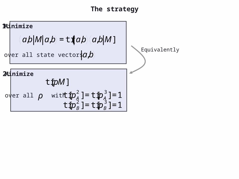
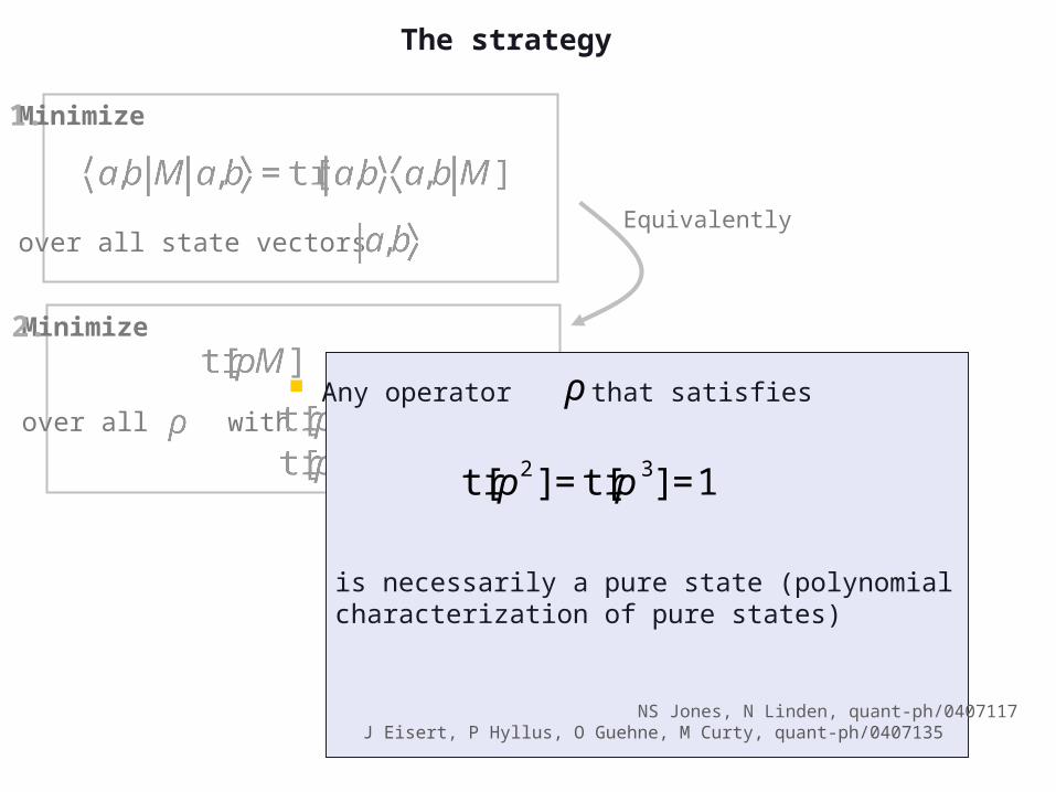
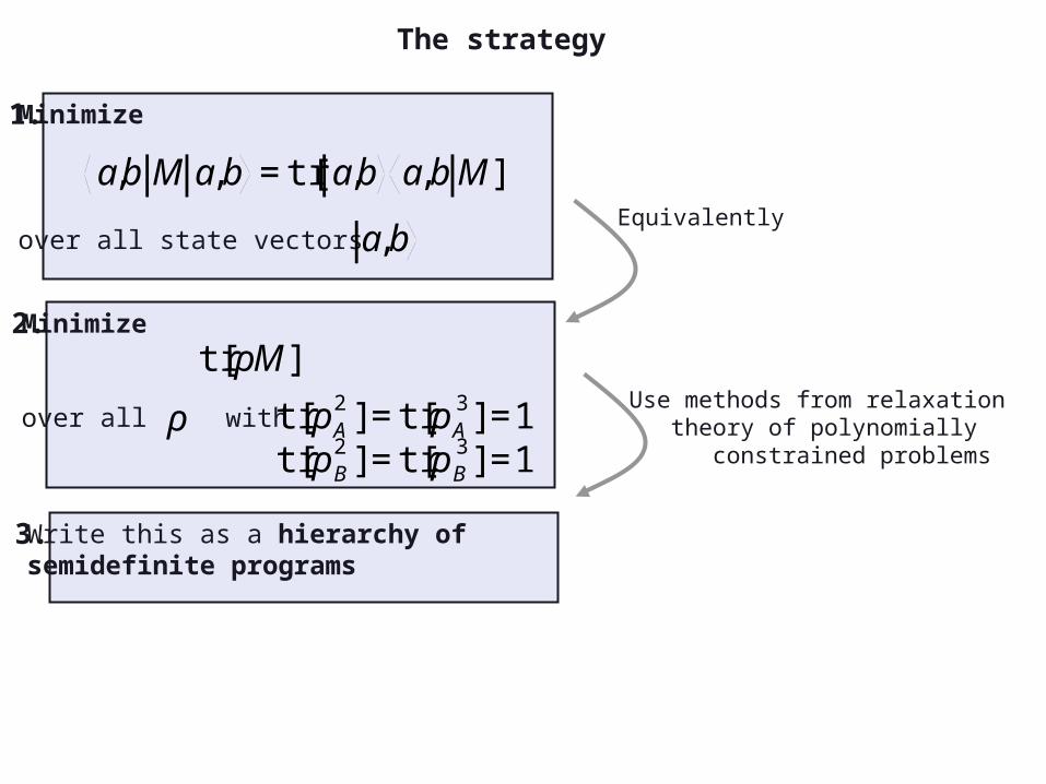
Minimize
over all state vectors
€
a,b M a,b =tr[ a,b a,bM]
1.
€
a,b
The strategy
Minimize
over all state vectors
€
a,b M a,b =tr[ a,b a,bM]Equivalently
1.
€
a,b
Minimize
over all with
€
ρ
2.
€
tr[ρM]
€
tr[ρA2 ]=tr[ρA
3]=1
€
tr[ρB2 ]=tr[ρB
3]=1
The strategy
Minimize
over all state vectors Equivalently
1.
Minimize
over all with
2.
Any operator that satisfies
is necessarily a pure state (polynomial characterization of pure states)
€
ρ
€
tr[ρ2]=tr[ρ3]=1
NS Jones, N Linden, quant-ph/0407117J Eisert, P Hyllus, O Guehne, M Curty, quant-ph/0407135
The strategy
Minimize
over all state vectors
€
a,b M a,b =tr[ a,b a,bM]Equivalently
1.
€
a,b
Minimize
over all with
€
ρ
2.
€
tr[ρM]
€
tr[ρA2 ]=tr[ρA
3]=1
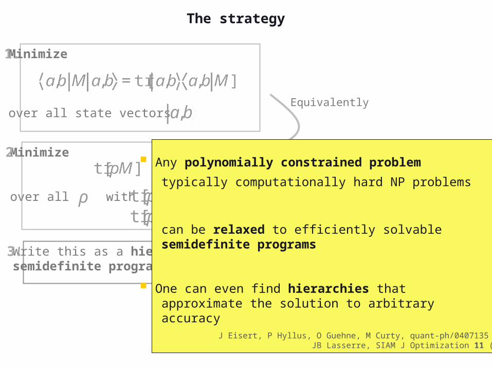
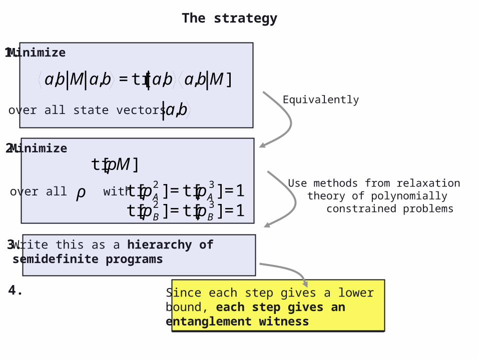
Write this as a hierarchy of semidefinite programs
3.
Use methods from relaxation theory of polynomially constrained problems
€
tr[ρB2 ]=tr[ρB
3]=1
The strategy
Write this as a hierarchy of semidefinite programs
3.
Minimize
over all state vectors Equivalently
1.
€
a,b
Minimize
over all with
€
ρ
2.
€
tr[ρA2 ]=tr[ρA
3]=1
€
tr[ρB2 ]=tr[ρB
3]=1
Any polynomially constrained problem
typically computationally hard NP problems
can be relaxed to efficiently solvable semidefinite programs
One can even find hierarchies that approximate the solution to arbitrary accuracy
J Eisert, P Hyllus, O Guehne, M Curty, quant-ph/0407135 JB Lasserre, SIAM J Optimization 11 (2001)
The strategy
Minimize
over all state vectors
€
a,b M a,b =tr[ a,b a,bM]Equivalently
1.
€
a,b
Minimize
over all with
€
ρ
2.
€
tr[ρM]
€
tr[ρA2 ]=tr[ρA
3]=1
Write this as a hierarchy of semidefinite programs
3.
Since each step gives a lowerbound, each step gives anentanglement witness
4.
Use methods from relaxation theory of polynomially constrained problems
€
tr[ρB2 ]=tr[ρB
3]=1
Entanglement witnesses for finite detection efficiencies
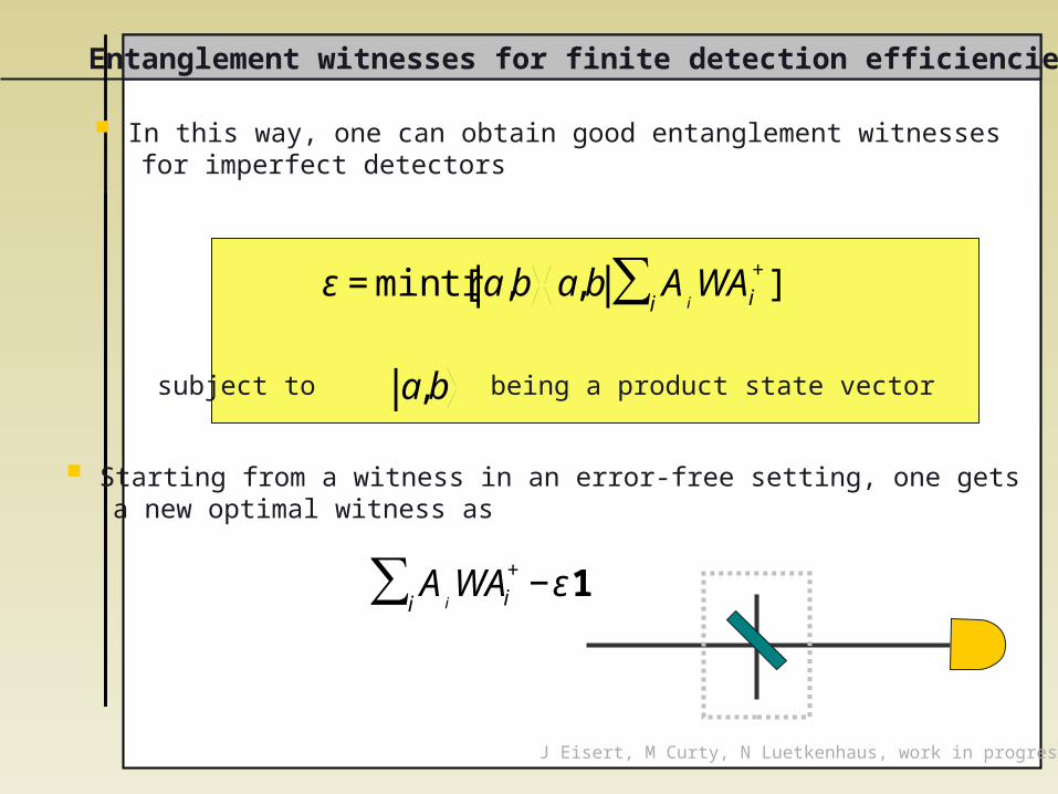
In this way, one can obtain good entanglement witnesses for imperfect detectors
€
ε=mintr[ a,b a,b Aii∑ WAi
+]
€
a,bsubject to being a product state vector
Starting from a witness in an error-free setting, one gets a new optimal witness as
€
Aii∑ WAi
+−ε1
J Eisert, M Curty, N Luetkenhaus, work in progress
Hierarchies of criteria for multi-particle entanglement
€
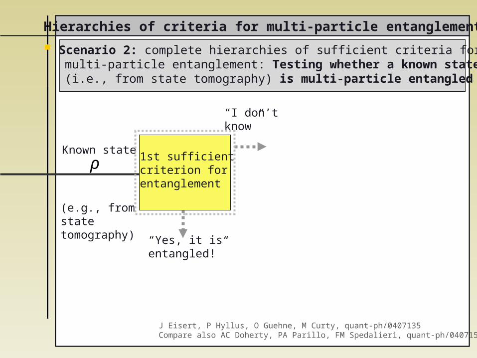
ρ
(e.g., from state tomography)
1st sufficientcriterion forentanglement
“Yes, it is entangled!”
“I don’t know”
Known state
J Eisert, P Hyllus, O Guehne, M Curty, quant-ph/0407135Compare also AC Doherty, PA Parillo, FM Spedalieri, quant-ph/0407156
Scenario 2: complete hierarchies of sufficient criteria for multi-particle entanglement: Testing whether a known state (i.e., from state tomography) is multi-particle entangled
Hierarchies of criteria for multi-particle entanglement
€
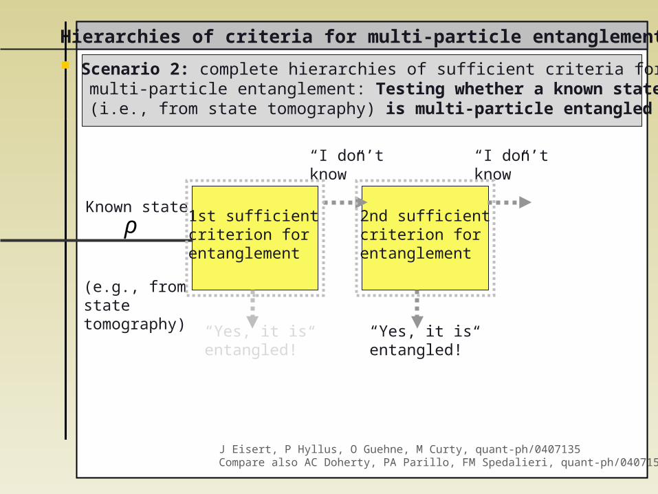
ρ
(e.g., from state tomography)
1st sufficient criterion forentanglement
“Yes, it is entangled!”
“I don’t know”
Known state2nd sufficient criterion forentanglement
“Yes, it is entangled!”
“I don’t know”
J Eisert, P Hyllus, O Guehne, M Curty, quant-ph/0407135Compare also AC Doherty, PA Parillo, FM Spedalieri, quant-ph/0407156
Scenario 2: complete hierarchies of sufficient criteria for multi-particle entanglement: Testing whether a known state (i.e., from state tomography) is multi-particle entangled
Hierarchies of criteria for multi-particle entanglement
€
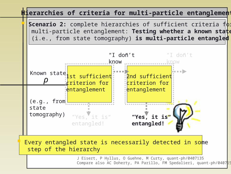
ρ
(e.g., from state tomography)
1st sufficient criterion forentanglement
“Yes, it is entangled!”
“I don’t know”
Known state2nd sufficient criterion forentanglement
“Yes, it is entangled!”
“I don’t know”
Every entangled state is necessarily detected in some step of the hierarchy
J Eisert, P Hyllus, O Guehne, M Curty, quant-ph/0407135Compare also AC Doherty, PA Parillo, FM Spedalieri, quant-ph/0407156
Scenario 2: complete hierarchies of sufficient criteria for multi-particle entanglement: Testing whether a known state (i.e., from state tomography) is multi-particle entangled
The lessons to learn
Physically: We have developed a strategy which is applicable to assess/find optimal linear optical schemes
Non-linear sign shift with linear optics, photon counting followed by postselection cannot be implemented with higher success probability than 1/4
First tight general upper bound for success probability
- Good news: the most feasible protocol is already the optimal one
- Single rounds of feedforward do not help very much
- But: also motivates the search for hybrid methods, leaving the strict framework of linear optics (see following talk by Bill Munro)
The lessons to learn
Formally:
the methods of convex optimization
are powerful when one intends to assess the maximum performance of linear optics schemes without restricting the allowed resources
in a situation where it is hard to conceive that one can find an direct solution to the original problem
And finally, we had a look at where very much related ideas can be useful to detect entanglement in optical settings