Embed Size (px)
Citation preview

J. Baker on R&D Competition Searle Antitrust Economics Conference Draft
1
Exclusionary Conduct When R&D Investment in New Products is Strategic
Jonathan B. Baker
September 9, 2014
Abstract
This paper evaluates conditions under which competition policy interventions to limit
exclusionary conduct by dominant firms increase the likelihood that an industry will develop a
new or next-generation product. The paper identifies a relationship between the nature of the
oligopoly interaction in a model of research and development (R&D) competition between a
dominant firm and a fringe rival and the payoffs to innovation in various states of the world: the
sign of the slope of a firm’s best response function turns on whether its incremental benefit of
increased R&D investment is greater if its rival succeeds in innovating or fails to innovate. In
consequence, the best response functions of the dominant firm and its fringe rival may plausibly
have differently-signed slopes: one firm may regard its rival’s R&D investment as a strategic
complement while the other regards its rival’s R&D investment as a strategic substitute.
Moreover, two of the competition policy instruments studied – challenging pre-innovation
exclusion or challenging post-innovation exclusion – will tend to be effective in different
strategic settings. For example, an upward sloping best response function for the dominant firm
and a downward sloping best response function for the fringe firm favor the success of a policy-
intervention increasing post-innovation competition in increasing the overall likelihood of
industry innovation, but work against the success of an intervention that increases pre-innovation
product market competition. In addition, a third competition policy instrument – challenging
dominant firm conduct that has the effect of increasing the marginal cost of fringe firm R&D –
necessarily benefits the overall likelihood of industry innovation if the dominant firm regards
fringe R&D investment as a strategic complement.

J. Baker on R&D Competition Searle Antitrust Economics Conference Draft
2
Exclusionary Conduct When R&D Investment in New Products is Strategic
Jonathan B. Baker*
September 9, 2014
I. Introduction
When antitrust enforcers challenge exclusionary conduct by dominant firms, the agencies
often expect to foster innovation along with price competition. Yet the connection between
antitrust enforcement and improved innovation incentives may be complex.1 A firm’s incentive
to innovate depends on economic forces that may be affected differentially by competition
policy: its incentive to innovate in order to escape pre-innovation competition, and its incentive
to innovate in order to obtain post-innovation profits.2 Moreover, a specific competition policy
intervention may affect the competitive ability and future prospects of dominant firms and their
fringe rivals in different ways. Hence the consequences of antitrust enforcement for innovation
may depend on the timing of the intervention (whether it takes place before or after innovation),
the way different market participants balance the consequences of the enforcement action for
their incentives to escape competition and obtain future profits, and the extent to which the
intervention affects on the conduct of different market participants in different ways (as when
enforcement boosts innovation prospects for one firm but reduces them for a rival).
* Professor of Law, Washington College of Law, American University. The author is particularly indebted to Paolo
Ramezzana. The author is also grateful to Yair Eilat, Joe Farrell, Rich Gilbert, Steve Salop, and Bobby Willig.
1 Several authors have surveyed the economic literature on the significance of competition and antitrust enforcement
for innovation during the past decade, including Matteo Gomellini (2013), Carl Shapiro (2012), Armin Schmutzler
(2009), Jonathan B. Baker (2007), and Richard Gilbert (2006). Other authors have applied that literature to the
antitrust review of mergers, including Benjamin Ren Kern & Juan Manuel Mantilla Contreras (2014), Michael L.
Katz & Howard A. Shelanski (2007), and Norbert Schulz (2007).
2 In Schumpeterian growth theory, the value of innovation to a firm increases as its post-innovation profits rise and
as its pre-innovation profits fall. (Phillipe Aghion, Ufuk Akcigit & Peter Howitt (2013), §3.4, Prediction 3). The
Schumpeterian growth theory perspective also emphasizes two issues not explicitly treated here: the influence of
the discrepancy between the technology of a laggard and the leader on each firm’s incentives to invest in R&D
(Philippe Aghion, Stefan Bechtold, Lea Cassar & Holger Herz (2014); Susan Athey & Armin Schumtzler (2011)),
and the potential erosion of the distinction emphasized in this paper between policies that foster pre-innovation
competition and policies that foster post-innovation competition when firms engage in successive rounds of
innovation (Ilya Segal & Michael D. Whinston (2007)). The latter issue is discussed further in a companion paper
(Jonathan B. Baker (2014)).

J. Baker on R&D Competition Searle Antitrust Economics Conference Draft
3
This paper evaluates tradeoffs facing antitrust enforcers concerned with innovation
through the lens of a Nash equilibrium model of R&D competition between a dominant firm and
its fringe rival to create new products, in which competition is constrained by antitrust rules. The
paper is concerned solely with incentives to innovate; it puts aside the potential benefits of
antitrust enforcement in lowering (quality-adjusted) prices and increasing output in static
markets. In the model, R&D investment increases the prospects of innovation success but does
not influence post-investment price competition in the event both firms succeed.
The analysis of R&D competition in this simple setting yields three insights not
previously noted in the literatures on strategic R&D competition3 or exclusionary conduct,
4
although the second has been recognized in the related literature on innovation races.5 First, the
payoffs to innovation in various states of the world influence whether a firm regards its rival’s
R&D investments as strategic substitutes or strategic complements (Jeremy I. Bulow, John D.
Geanakoplos & Paul D. Klemperer (1985)). More specifically, in the primary model, the sign of
the slope of a firm’s best response function (reaction function) depends only on whether the
3 That literature is mainly concerned with issues not treated here: the influence of R&D investment on later (second
period) price and output competition, particularly when innovation is cost-reducing (i.e. marginal costs are
decreasing in R&D) and when R&D creates externalities benefitting rival firms (Armin Schmutlzer (2013); Rabah
Amir & John Wooders (1998); Dermot Leahy & J. Peter Neary (1997)). In other related work, John Scott (2009)
finds that if R&D investment is strategic, lessened R&D competition resulting from a reduction in the number of
firms tends to dampen R&D investment by increasing the threat of post-innovation competition and reducing the
benefits of escaping pre-innovation competition; Daniel Spulber (2013) shows that when intellectual property
policies increase an inventor’s expected post-innovation profits, those policies can encourage R&D competition
among innovators, thereby enhancing aggregate incentives to innovate; Susan Athey & Armin Schmutzler (2011)
analyze firm incentives to undertake cost-reducing and demand-enhancing R&D investments in a common
framework; and Drew Fudenberg & Jean Tirole (1984) specify a model of technological interaction that is a special
case of the model studied here. Suzanne Scotchmer (2004) provides a broad survey of the economic learning on
innovation and innovation policy highlighting, among other things, the cumulative nature of innovation, which is not
studied here. Joseph Stiglitz (2014) models the possibility that intellectual property rights slow the rate of
innovation by reducing the pool of knowledge effectively available for a successive innovator.
4 The legal and economic literature on exclusionary conduct is surveyed in Jonathan B. Baker (2013). David M.
Mandy, John W. Mayo & David E. M. Sappington (2014) relate the nature of product market competition to the
vertically integrated firm’s choice of whether to foreclose an industry leader or industry follower from access to an
essential input, and identify settings in which exclusionary conduct complements process innovation by the
integrated firm.
5 The relevant literature, surveyed by Jennifer Reinganum (1989, pp. 868-884), studies patent races between
asymmetric firms (e.g. incumbent and entrant, or low-cost and high-cost). In the models, greater R&D investment
accelerates the expected timing of innovation success, and a firm’s incentives to invest depend on both its reward for
winning the race and its foregone profit in the event its rival innovates first. The model analyzed here relaxes the
assumption in the patent race literature that only one firm can succeed by allowing for the possibility, typically more
relevant for antitrust, that both firms may succeed and then compete.

J. Baker on R&D Competition Searle Antitrust Economics Conference Draft
4
firm’s marginal benefit of increased R&D investment is greater when its rival succeeds in
innovating or when its rival fails, without regard to the probability of innovation success for any
firm. This result relates the nature of the oligopoly interaction in R&D investment to aspects of
market structure potentially subject to evaluation by informed observers.
Second, the best response functions for the R&D investment interaction between a
dominant firm and its fringe rival may slope in the same direction, but they may also plausibly
have different slopes. The dominant firm may regard its rival’s investment as a strategic
complement while the fringe firm regards the dominant firm’s investment as a strategic
substitute, or vice versa. Although it is well known that reaction functions need not slope in the
same direction, most theoretical and empirical analyses of oligopoly conduct assume that they
do.6 The results in this paper suggest that greater agnosticism would be appropriate with respect
to R&D rivalry.
Third, two of the instruments for antitrust intervention to benefit new product innovation
analyzed here – challenges to pre-innovation product market exclusion and challenges to post-
innovation product market exclusion – are most likely to increase the aggregate probability of
R&D success in different strategic settings. Enforcement against pre-innovation exclusion
favors innovation success when the dominant firm regards its fringe rival’s R&D investment as a
strategic substitute or the fringe firm regards the dominant firm’s R&D investment as a strategic
complement. Enforcement against post-innovation exclusion favors innovation success when
reaction functions have the opposite slopes: when the dominant firm regards its fringe rival’s
R&D investment as a strategic complement or the fringe firm regards the dominant firm’s R&D
investment as a strategic substitute.
Section II sets forth a model of the R&D investment interaction between a dominant firm
and a fringe rival. Section III describes the policymaker’s perspective and goal. Section IV
analyzes the consequences of two policy interventions in a baseline setting in which firms are
unable to make informed judgments about the way their rivals’ investments will respond to those
interventions. Section V derives the primary results in the paper, under the assumption that firms
are informed and behave strategically. Section VI discusses the possibility that firm payoffs for
innovation success may depend on their R&D investments. Section VII uses the framework
previously developed to identify conditions under which a third policy instrument – challenging
6 Mihkel Tombak (2006) applies the term “strategic asymmetry” to describe oligopoly interactions in which one
firm regards its rival’s strategic variable as a strategic complement while the other regards its rival’s strategic
variable as a strategic substitute. Tombak’s mathematical examples involve price and quantity competition, not
R&D competition, although he also suggests that the investment decisions of Boeing and Airbus during the late
1980s were characterized by strategic asymmetry. John Beath, Yannis Katsoulacos & David Upph (1989, pp. 166-
70) note the possibility of differently-sloped reaction functions for R&D investment in the innovation race model
they study.

J. Baker on R&D Competition Searle Antitrust Economics Conference Draft
5
dominant firm conduct that raises the R&D costs of rivals – will increase the aggregate
likelihood of innovation success.
A companion paper (Jonathan B. Baker, 2014) relies on these results to evaluate
dominant firm “appropriability” defenses for alleged exclusionary conduct: claims that the
practices will benefit the prospects for innovation by increasing the dominant firm’s reward for
innovation success. That paper explains why an appropriability defense is less persuasive when
dominant firms regard rival R&D investment as a strategic complement, identifies characteristics
of firms and markets to potentially subject to evaluation by informed observers suggesting that
this would be the case, and illustrates the application of the framework using the facts of three
classic antitrust monopolization cases: the Microsoft case involving Netscape and Java, the IBM
plug compatibility cases (which are treated as a single case), and the FTC’s patent portfolio case
against Xerox.
II. Model of an R&D Investment Game
In the model, two firms, a dominant firm and its fringe rival, compete to develop similar new
or upgraded (next-generation) products by investing in R&D. 7
The model posits that strategic
interaction is limited to R&D. R&D investments need not succeed, but greater investments make
innovation success more likely. The dominant firm is designated firm 1; its fringe rival is
designated firm 2. In the model, the dominant firm may employ exclusionary practices that limit
pre-innovation competition or create impediments to post-innovation competition,8 but the
fringe firm may not do so.
Although the exclusionary practices employed are not specifically identified and the
mechanisms by which they exclude are not described, the model is consistent with a wide range
of such practices. The model distinguishes conduct excluding rivals from product market
competition before the firms innovate and conduct that excludes rivals after innovation. Before
innovation, for example, a dominant firm may raise rivals’ costs (input foreclosure) or inhibit
rival access to the market (customer foreclosure).9 In addition, dominant firms can create
impediments to post-innovation competition by their rivals in the event both firms succeed in
innovating, as through technological investments in product incompatibility; loyalty discounts;
7 The market is assumed to have potential for product innovation: the technological frontier is thought to be moving
out rapidly or susceptible to doing so, and new or better products would be valued highly by buyers.
8 The relationship between this ability and more common indicia of dominance – such as a large installed base,
strong brand reputation, and high market share – is not specifically modeled.
9 Jonathan B. Baker (2013) surveys a range of exclusionary practices identified in antitrust cases and the economics
literature.

J. Baker on R&D Competition Searle Antitrust Economics Conference Draft
6
tying; locking-in customers through the sale of complementary products, investments that raise
buyer switching or search costs;10
or the creation of impediments to rival challenges to a firm’s
misuse of intellectual property. It is useful conceptually to treat impediments to pre-innovation
competition and impediments to post-innovation competition as distinct, although many such
practices will exclude rivals both before and after the dominant firm innovates. Competition
policy interventions addressing a third class of exclusionary practices – dominant firm conduct
that raises fringe rival costs of R&D – are analyzed separately below, in Section VII.
The model implicitly presumes that the firms make decisions during two periods, but that
their interaction reduces to a one-stage game. In first period, both firms invest in R&D aimed at
developing a new or next-generation product. Each firm’s investments affect its likelihood of
successful innovation, which in turn affects its profits. There are no spillovers from one firm’s
R&D to its rival. In the second period, uncertainty about each firm’s innovation success is
resolved and the firms receive payoffs.
The dominant firm chooses an R&D investment level I. Its costs are K(I), where K(I) is
the cost of the R&D investment, with KI > 0 and KII > 0. Any costs of creating impediments to
post-innovation competition are included in K(I) and do not vary with I. The fringe firm chooses
an R&D investment level J, at a cost C(J), with CJ > 0 and CJJ > 0.
Each firm’s probability of successfully innovating depends solely on the level of its R&D
investment.11
The dominant firm’s probability of success is q(I), where 0 < q < 1, q’ > 0, and q”
< 0, and the fringe firm’s probability of success is r(J), with 0 < r < 1, r’ > 0, and r” < 0.12
One
concern of the Schumpeterian growth literature – the possibility that a firm’s likelihood of
successful innovation depends on the extent to which its current technology lags that of its rival –
could lie behind differences in the functions q(I) and r(J), but that relationship is not specifically
modeled.
The second period is characterized by four possible states of the world: both firms may
succeed in innovating, neither may succeed in doing so, only the dominant firm may succeed, or
only the fringe firm may succeed. The payoffs to the firms may be interpreted as the discounted
present value of a future profit stream, and the terms profit and payoff are used interchangeably.
10
Joseph Farrell & Paul Klemperer (2007, pp. 2001-06) discuss strategies that dominant firms may employ to inhibit
post-innovation competition by creating switching costs.
11 Hence, for example, neither firm’s prospects of innovation success depend on whether the dominant firm has
created impediments to post-innovation competition except insofar as those impediments affect I or J.
12 The assumptions that q” < 0 and r” < 0 rule out logistic functions (S-shaped) for q(I) and r(J), unless the range of q
and r is limited to q > ½ and r > ½.

J. Baker on R&D Competition Searle Antitrust Economics Conference Draft
7
The payoffs in each state and the ex ante probability of achieving it, discussed below, are
summarized in Tables 1 and 2. In the notation, Πij and Ω
ij represent payoffs to the dominant firm
and its rival, respectively, in state of the world (i,j),where i indicates whether the dominant firm
succeeded (s) or failed (f) in its innovation efforts and j similarly indicates whether or not the
fringe rival succeeded.
The payoffs to the firms in the event one firm’s innovation efforts succeed while the
other firm’s efforts do not succeed do not vary with the amount firms invest in R&D. If the
successful innovator is the dominant firm, its payoff is Πsf and its fringe rival’s payoff is
sf.
If
the successful innovator is the rival, the payoffs are Πfs and
fs for the dominant firm and its
rival, respectively. By assumption, Πsf
> Πfs ≥ 0 and
fs >
sf ≥ 0.
If both firms successfully innovate, and bring new or next-generation products to the
market, they compete on price. Their payoffs in this state of the world depend on the extent of
post-innovation product market competition, so are influenced by impediments to post-
innovation competition adopted by the dominant firm. The extent of those impediments is
indexed by δ, which increases as post-innovation competition grows (that is, as impediments are
removed). The dominant firm’s profits when both firms innovate are Πss
(δ) and the fringe firm’s
profits are ss
(δ), with Πss
(δ) > Πfs and
ss(δ) >
sf for all δ.
Impediments to post-innovation competition are assumed to benefit the dominant firm by
excluding its fringe rival, so a lessening of impediments reduces dominant firm profits (Πss
δ(δ) <
0) and increases fringe firm profits (ss
δ(δ) > 0). These assumptions rule out one class of
dominant firm strategies for discouraging fringe investment in R&D: those that involve a
commitment to aggressive competition between the two if both firms successfully innovate.
When both firms succeed, competition between them is assumed to reduce industry profits
relative to the outcome in which only one firm succeeds in innovating, so (Πsf +
sf) > (Π
ss +
ss
) > 0 and (Πfs +
fs) > (Π
ss +
ss) > 0, for all δ.
The assumption that the payoffs Πss
(δ) and ss
(δ) do not vary with the level of R&D
investments (I and J) puts aside the possibility that the magnitude of each firm’s investment
affects post-innovation competition, as would likely be the case, for example, if R&D investment
led to cost-reductions. Section VI addresses some of the additional considerations that arise
when post-innovation product market competition is affected by competition in R&D.
Finally, if neither firm succeeds, the firms compete on price with existing products. Each
earns profits that depend on the extent of pre-innovation product market competition θ, where
higher θ represents greater competition. Firm 1’s profits are Πff(θ), with Π
ffθ(θ) < 0, and firm 2’s

J. Baker on R&D Competition Searle Antitrust Economics Conference Draft
8
profits are ff(θ). Pre-innovation product market competition depends on the extent to which the
dominant firm excludes its rival, so ff
θ(θ) > 0. This assumption rules out the possibility that
competition was lessened through coordination between the firms or through greater
differentiation, either of which would imply that ff
θ < 0. By assumption, the dominant firm
earns more in the pre-innovation state of the world than does its fringe rival (Πff(θ) >
ff(θ) for
all θ); this assumption builds in the Arrow effect, by which the dominant firm has a greater
opportunity cost of innovation than the fringe firm because innovation cannibalizes the dominant
firm’s greater pre-innovation profits. Greater competition is assumed to reduce aggregate
industry profits, so Πff
θ(θ) + ff
θ(θ) < 0, for all θ. The dominant firm’s adoption of
impediments to post-innovation competition does not influence either firm’s payoffs in the event
neither achieves innovation success. By assumption, aggregate industry profits are greater if
either firm successfully innovates than if neither does so, so (Πsf
+ sf) > (Π
ff(θ) +
ff(θ)) > 0
and (Πfs + Ω
fs)
> Π
ff(θ) +
ff(θ) > 0, for all θ.
In this setup, the dominant firm (firm 1) and its fringe rival (firm 2) are not in symmetric
positions. They differ in four ways, one that captures the intuitive idea that the dominant firm is
more successful in the pre-innovation product market setting, and three that arise directly from
the dominant firm’s potential ability to exclude its fringe rival. First, the dominant firm has a
higher payoff in the pre-innovation setting in which neither firm’s R&D investments succeed
(Πff(θ) >
ff(θ) for all θ). Second, the dominant firm can make exclusionary investments that
inhibit post-innovation competition. Third, greater post-innovation competition reduces
dominant firm profits but increases fringe firm profits (Πss
δ < 0, ss
δ > 0). Finally, greater pre-
innovation competition lessens dominant firm profits but increases fringe firm profits (Πff
θ < 0,
ff
θ > 0).
Table 1
Payoffs in Each State of the World
(Firm 1, Firm 2) Firm 2 succeeds Firm 2 does not succeed
Firm 1 succeeds Πss
(δ), ss
(δ) Πsf,
sf
Firm 1 does not succeed Πfs,
fs Π
ff(θ),
ff(θ)
Table 2
Probability that Each State of the World Arises
(Firm 1, Firm 2) Firm 2 succeeds Firm 2 does not succeed
Firm 1 succeeds q(I), r(J) q(I), (1-r(J))
Firm 1 does not succeed (1-q(I)), r(J) (1-q(I)), (1-r(J))

J. Baker on R&D Competition Searle Antitrust Economics Conference Draft
9
These payoffs allow each firm’s R&D investment decision to reflect a mixture of the two
motives highlighted in the introduction. One is the incentive to escape competition. Investment
in R&D frees each firm from competition with probability: if a firm succeeds in innovating, it
will avoid the state of the world in which neither firm succeeds (in which the firms compete on
price using existing products), and it has a chance of avoiding the state of the world in which
both firms succeed (in which the firms compete on price with new products). Firm investment
decisions also reflect an incentive to innovate in order to capture profits arising from the increase
in demand associated with bringing a new or next-generation product to market. The expected
payoff for successful innovation is a probability-weighted sum of the prize in the event that the
rival firm does not also succeed and the smaller payoff in the event that both firms succeed.
During the first period, firm 1 chooses an investment level (I) in order to maximize V1,
the expected value of the dominant firm:
V1 = q(I)(1-r(J))Π
sf + q(I)r(J)Π
ss(δ) + (1-q(I))(1-r(J))Π
ff(θ) + (1-q(I))r(J)Π
fs – K(I).
Simultaneously, firm 2 chooses an investment level (J) to maximize V2, the expected value of the
fringe firm:
V2 = r(J)(1-q(I))
fs + r(J)q(I)
ss(δ) + (1-r(J))(1-q(I))
ff(θ) + (1-r(J))q(I)
sf – C(J).
The equilibrium values of I and J are determined by the simultaneous solution of the two first
order conditions, as set forth in Proposition 1.
PROPOSITION 1 (Equilibrium and First Order Conditions): If firm 1 chooses I to
maximize V1, firm 2 chooses J to maximize V
2, and the equilibrium is characterized by
an interior solution (second order conditions for a maximum hold), then I and J will
satisfy:
(1) V1
I = 0 = q’(1-r)Πsf + q’rΠ
ss – q’(1-r)Π
ff – q’rΠ
fs – KI, and
(2) V2
J = 0 = r’(1-q)fs + r’q
ss – r’(1-q)
ff – r’q
sf – CJ = 0.
Section IV uses these first order conditions to derive the equilibrium for a benchmark case in
which firms are uninformed about their rival’s R&D investments. Section V analyzes the
primary model, in which firms are informed and behave strategically. Before examining those
results, it is useful to describe how the policy-maker evaluates alternative competition policy
interventions.
J. Baker on R&D Competition Searle Antitrust Economics Conference Draft
10
III. Policymaker’s Perspective
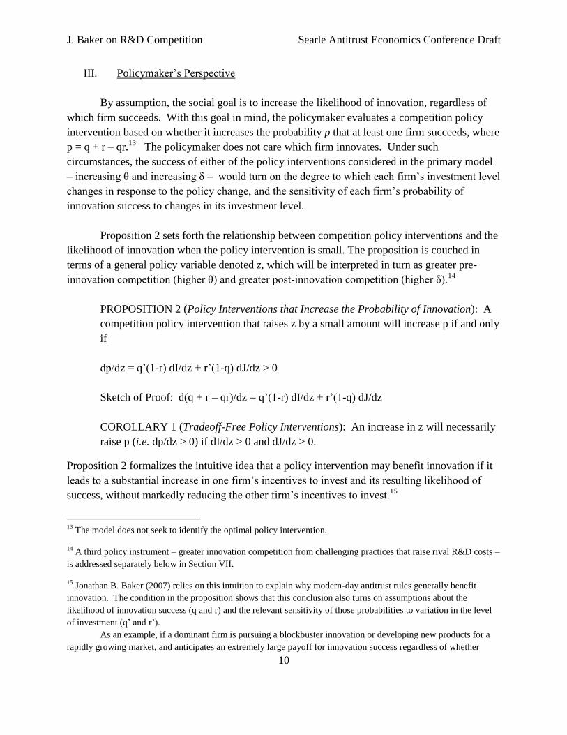
By assumption, the social goal is to increase the likelihood of innovation, regardless of
which firm succeeds. With this goal in mind, the policymaker evaluates a competition policy
intervention based on whether it increases the probability p that at least one firm succeeds, where
p = q + r – qr.13
The policymaker does not care which firm innovates. Under such
circumstances, the success of either of the policy interventions considered in the primary model
– increasing θ and increasing δ – would turn on the degree to which each firm’s investment level
changes in response to the policy change, and the sensitivity of each firm’s probability of
innovation success to changes in its investment level.
Proposition 2 sets forth the relationship between competition policy interventions and the
likelihood of innovation when the policy intervention is small. The proposition is couched in
terms of a general policy variable denoted z, which will be interpreted in turn as greater pre-
innovation competition (higher θ) and greater post-innovation competition (higher δ).14
PROPOSITION 2 (Policy Interventions that Increase the Probability of Innovation): A
competition policy intervention that raises z by a small amount will increase p if and only
if
dp/dz = q’(1-r) dI/dz + r’(1-q) dJ/dz > 0
Sketch of Proof: d(q + r – qr)/dz = q’(1-r) dI/dz + r’(1-q) dJ/dz
COROLLARY 1 (Tradeoff-Free Policy Interventions): An increase in z will necessarily
raise p (i.e. dp/dz > 0) if dI/dz > 0 and dJ/dz > 0.
Proposition 2 formalizes the intuitive idea that a policy intervention may benefit innovation if it
leads to a substantial increase in one firm’s incentives to invest and its resulting likelihood of
success, without markedly reducing the other firm’s incentives to invest.15
13
The model does not seek to identify the optimal policy intervention.
14 A third policy instrument – greater innovation competition from challenging practices that raise rival R&D costs –
is addressed separately below in Section VII.
15 Jonathan B. Baker (2007) relies on this intuition to explain why modern-day antitrust rules generally benefit
innovation. The condition in the proposition shows that this conclusion also turns on assumptions about the
likelihood of innovation success (q and r) and the relevant sensitivity of those probabilities to variation in the level
of investment (q’ and r’).
As an example, if a dominant firm is pursuing a blockbuster innovation or developing new products for a
rapidly growing market, and anticipates an extremely large payoff for innovation success regardless of whether

J. Baker on R&D Competition Searle Antitrust Economics Conference Draft
11
IV. Uninformed Firms
In some settings, firms may be unaware of the level and nature of R&D investments of
their rivals,16
and, in consequence, unable to make informed judgments about the way their
rivals’ investment levels depend on the policy variables θ and δ. Under such circumstances, a
firm may be understood as conditioning its own investment decisions on some exogenously-
determined assumption as to rival investment levels, and thus as to the probability of their rival’s
innovation success. In terms of the model, the dominant firm assumes its fringe rival will
succeed with probability r(J) = rm
, and the fringe firm assumes that the dominant firm will
succeed with probability q(I) = qm
, where rm
and qm
are constants. Given this assumption, the
firms cannot be assumed to reach a Nash equilibrium: as with a Nash equilibrium, firms will
choose their best response to their beliefs about the actions of their rival, but unlike a Nash
equilibrium, those beliefs will not be correct (except by accident). With uninformed firms,
moreover, strategic interactions between the firms’ investment decisions are not possible; the
firms act as though V1
IJm
= V2
JIm
= 0.
other firms innovate as well, it may view its expected return on R&D investment as far greater than the return on its
next best investment opportunity. Even if a competition policy intervention against post-innovation exclusion would
reduce the dominant firm’s expected payoff substantially, the expected payoff for success to the dominant firm may
remain in excess of the return on its next best opportunity – so it would not respond to antitrust enforcement by
reducing its R&D investment effort (dI/dz = 0). (One could think of the dominant has having found a corner
solution to its R&D investment optimization problem, and that the solution was unaffected by the hypothesized
change in conditions.) If the policy intervention enhances the rival’s innovation incentives, and the rival, unlike the
dominant firm, is able to improve its prospects for innovation success by investing more (r’ > 0), then the overall
probability of innovation success will increase (dp/dz = r’(1-q) dJ/dz > 0).
A second example in which only one firm’s incentives matter in practice is suggested by the emphasis on
technological leadership in the Schumpeterian growth literature. This example assumes that the rival firm lags the
dominant firm technologically, and in consequence has both a low probability of innovation success and little
expectation that incremental R&D investment will increase that probability markedly (i.e. r and r’ are both small).
Under such circumstances, the consequences of a competition policy intervention for the aggregate likelihood of
innovation would be dominated by the effects of that intervention on the innovation incentives of the dominant firm.
(In the limit as r and r’ go to zero, dp/dz = q’dI/dz).
The assumptions employed in the second example are not the only way to think about the implications of
technological leadership for R&D investment, however. As a third example, one might instead suppose that the
dominant firm, given its leadership position, would expect its payoff for innovation success to be determined
primarily by exogenous factors like customer acceptance of a new product rather than by its level of investment (i.e.
q’ is small), while its rival, starting well behind in technology, might expect that greater investment would increase
its likelihood of innovation success (r’ > 0). Then, as with the first example, the consequences of a competition
policy intervention for the aggregate likelihood of innovation would be dominated by the effects of that intervention
on the innovation incentives of the rival. (In the limit as q’ goes to zero, dp/dz = r’(1-q) dJ/dz).
16 To similar effect, firms may have so many innovation rivals that they treat the extent of R&D competition as
exogenous.

J. Baker on R&D Competition Searle Antitrust Economics Conference Draft
12
The impact of policy interventions in this setting is analyzed using a comparative statics
approach, which presumes that interventions are small. Two interventions are considered:
greater pre-innovation competition (higher θ) and greater post-innovation competition (higher δ).
The notation V1
Im
and V2
Jm
(with superscript m) is employed for the first order conditions, along
with analogous notation for second derivatives, in order to distinguish these conditions from
those that arise in the informed firm case. Arguments of the functions are suppressed. The
second order conditions, V1
IIm
< 0 and V2
JJm
< 0, are assumed to hold.17
With uninformed firms, the level of firm investments I and J will increase as the
competition policy instruments θ and δ rise if the following conditions hold:18
dI/dθ = q’(1-rm
) Πff
θ / V1
IIm
> 0,
dJ/dθ = (1–qm
)r’Ωff
θ/ V2
JJm
< 0,
dI/dδ = –q’rm
Πss
δ / V1
IIm
< 0, and
dJ/dδ = –qm
r’ Ωss
δ / V2
JJm
> 0.
The first of these conditions shows that a competition policy intervention increasing pre-
innovation competition leads to greater dominant firm investment in R&D (dI/dθ > 0), reflecting
the dominant firm’s increased incentive to escape competition. The same policy intervention
leads to less fringe firm investment in R&D (dJ/dθ < 0), as that firm’s greater freedom from pre-
innovation exclusion raises its pre-innovation profits, lessening its incentive to escape
competition through new product development. Increased post-innovation competition reduces
dominant firm investment in R&D (dI/dδ < 0), reflecting that firm’s smaller expected benefit
from innovating as its payoff shrinks in the future state of the world in which both firms’ R&D
efforts succeed. Increased post-innovation competition raises fringe firm investment in R&D
(dJ/dδ > 0), reflecting that firm’s higher payoff in the event both firms succeed and,
consequently, its greater expected benefit from innovating.
These results highlight the two economic forces influencing incentives to innovate in the
model: an incentive to escape competition, and an incentive to obtain post-innovation profits.
These forces remain central to the results obtained in the next section, in which firms are
informed and, in consequence, can behave strategically.
17
These conditions require, respectively, that V1
IIm = q”(1-r
m)Π
sf + q”r
mΠ
ss – q”(1-r
m)Π
ff – q”r
mΠ
fs – K
II < 0 and
V2JJ
m = r”(1-q
m)Ω
fs + r”q
mΩ
ss – r”(1-q
m)
ff – r”q
m
sf – CJJ < 0.
18 Total differentiation of the first order conditions yields two equations, V
1II
m dI + V
1Iδ
m dδ + V
1Iθ
m dθ = 0 and V
2JJ
m
dJ + V2Jδ
m dδ + V
2Jθ
m dθ = 0, from which these results are derived.

J. Baker on R&D Competition Searle Antitrust Economics Conference Draft
13
V. Strategic Firm Behavior With Informed Firms
When firms are informed about each other’s decision variables, and able to behave
strategically, they will account for rival responses in choosing investment levels and responding
to competition policy interventions. The latter responses will depend on the partial derivatives of
the first order conditions, set forth in Table 3. The table indicates the signs of those derivatives,
to the extent they are determined by prior assumptions.
In the table, the expressions for the cross-partial derivatives V1
IJ and V2
JI are simplified
by defining two new variables, Δ and Ψ, related to the relative size of the payoffs in various
states of the world:
Δ = [(Πss
– Πfs) – (Π
sf – Π
ff)], and
Ψ = [(ss
– sf) – (
fs –
ff)].
To interpret Δ, note that (Πss
– Πfs) is the incremental benefit of innovation success to firm 1,
conditional on firm 2 succeeding, while (Πsf – Π
ff) is the incremental benefit of innovation
success to firm 1, conditional on firm 2 not succeeding. Hence Δ is positive if and only if firm 1
gains more from innovation success conditional on firm 2 succeeding than it gains conditional on
firm 2 not succeeding. Similarly, Ψ is positive if and only if firm 2 gains more from its
innovation success in the event firm 1 also succeeds than it gains in the event firm 1 does not
succeed. In the model analyzed below, Δ and Ψ determine the slopes of firm reaction functions
and, consequently, whether each firm regards its rival’s investment as a strategic substitute or
strategic complement.
Table 3
Partial Derivatives of the First Order Conditions
Sign
V1
II q”(1-r)Πsf + q”rΠ
ss – q”(1-r)Π
ff – q”rΠ
fs – KII < 0 (SOC)
V2
JJ r”(1-q)fs + r”q
ss – r”(1-q)
ff – r”q
sf – CJJ < 0 (SOC)
V1
IJ q’r’[(Πss
– Πfs) – (Π
sf – Π
ff)] = q’r’Δ sign(Δ)
V2
JI q’r’[(ss
– sf) – (
fs –
ff)] = q’r’Ψ sign(Ψ)
V1
I δ q’r Πss
δ < 0
V2
Jδ qr’ss
δ > 0
V1
Iθ – q’(1-r)Πff
θ > 0
V2
Jθ – (1-q)r’ff
θ < 0

J. Baker on R&D Competition Searle Antitrust Economics Conference Draft
14
The first order conditions (1) and (2) imply best response functions (reaction functions)
for the two firms: I = ρ1(J) for the dominant firm, and J = ρ2(I) for the fringe firm. These
functions are assumed invertible, allowing the dominant firm’s reaction function to be written J =
ρ1-1
(I). Reaction function slopes are defined by differentiating functions of the form J(I) with
respect to I: R1 = dρ1
-1/dI and R
2 = dρ2/dI. As is usual in simultaneous-move oligopoly models,
firm conduct turns on the sign of these slopes.
PROPOSITION 3 (Slopes of Best Response Functions): The first order conditions (1)
and (2) imply best response functions with slopes:
(3) R1 = – V
1II/ V
1IJ = –V
1II/(q’r’Δ), and
(4) R2
= – V2
JI/V2
JJ = – (r’q’Ψ)/V2
JJ.
It is evident from Proposition 3 that the signs of the reaction function slopes are the same
as the signs of Δ and Ψ, respectively. If Δ and Ψ are both positive, the two best response
functions are upward sloping (strategic complements); if Δ and Ψ are both negative, the two best
response functions are downward sloping (strategic substitutes). If Δ and Ψ take on opposite
signs, the best response functions will differ in their slopes.
Equation (3) implies that the dominant firm regards its fringe rival’s R&D investment as
a strategic substitute (firm 1’s reaction function slopes downward), if and only if firm 1’s
incremental gains from innovating are greater when firm 2 does not succeed. Intuitively, a less
aggressive R&D investment strategy by firm 2 – a reduction in the second firm’s R&D
investment – lessens that firm’s likelihood of innovation success. If the incremental benefit of
R&D investment by firm 1 increases as a result – if Δ is negative – then the first firm will have
an incentive to invest more in R&D. Accordingly, when Δ is negative, firm 1 regards its rival’s
investment as a strategic substitute. By similar logic, Δ is positive if and only if firm 1 regards
its rival’s investment as a strategic complement, Ψ is negative if and only if firm 2 regards the
dominant firm’s R&D investment as a strategic substitute, and Ψ is positive if and only if firm 2
regards the dominant firm’s R&D investment as a strategic complement.19
19
When V1
IJ ≥ 0 and V2
JI ≥ 0, the game is supermodular and the functions maximized (the expected values of the
firms (V1 and V
2)) have increasing differences in the decision variables (the investment levels (I and J)). (When
games are supermodular, among other things, pure strategy Nash equilibria exist, and comparative statics results
extend to non-local changes in complementary decision variables. “Increasing differences” arise when a firm’s
benefit from increasing its decision variable is greater when the other firm’s decision variable is higher. In
supermodular games, increasing differences imply strategic complementarity of the decision variables.) The
conditions Δ ≥ 0 and Ψ ≥ 0 represent the increasing differences conditions for a different R&D investment game
than the one studied here: a game in which each firm chooses whether or not to innovate, and thus where the
probability of success is certain if the investment is made. In the R&D investment game studied here, the increasing
J. Baker on R&D Competition Searle Antitrust Economics Conference Draft
15
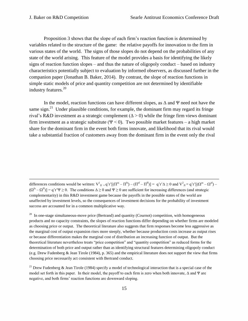
Proposition 3 shows that the slope of each firm’s reaction function is determined by
variables related to the structure of the game: the relative payoffs for innovation to the firm in
various states of the world. The signs of those slopes do not depend on the probabilities of any
state of the world arising. This feature of the model provides a basis for identifying the likely
signs of reaction function slopes – and thus the nature of oligopoly conduct – based on industry
characteristics potentially subject to evaluation by informed observers, as discussed further in the
companion paper (Jonathan B. Baker, 2014). By contrast, the slope of reaction functions in
simple static models of price and quantity competition are not determined by identifiable
industry features.20
In the model, reaction functions can have different slopes, as Δ and Ψ need not have the
same sign.21
Under plausible conditions, for example, the dominant firm may regard its fringe
rival’s R&D investment as a strategic complement (Δ > 0) while the fringe firm views dominant
firm investment as a strategic substitute (Ψ < 0). Two possible market features – a high market
share for the dominant firm in the event both firms innovate, and likelihood that its rival would
take a substantial fraction of customers away from the dominant firm in the event only the rival
differences conditions would be written: V
1IJ = q’r’[(Π
ss – Π
fs) – (Π
sf – Π
ff)] = q’r’Δ ≥ 0 and V
2JI = q’r’[(
ss –
sf) –
(fs –
ff)] = q’r’Ψ ≥ 0. The conditions Δ ≥ 0 and Ψ ≥ 0 are sufficient for increasing differences (and strategic
complementarity) in this R&D investment game because the payoffs in the possible states of the world are
unaffected by investment levels, so the consequences of investment decisions for the probability of investment
success are accounted for in a common multiplicative way.
20 In one-stage simultaneous-move price (Bertrand) and quantity (Cournot) competition, with homogeneous
products and no capacity constraints, the slopes of reaction functions differ depending on whether firms are modeled
as choosing price or output. The theoretical literature also suggests that firm responses become less aggressive as
the marginal cost of output expansion rises more steeply, whether because production costs increase as output rises
or because differentiation makes the marginal cost of distribution an increasing function of output. But the
theoretical literature nevertheless treats “price competition” and “quantity competition” as reduced forms for the
determination of both price and output rather than as identifying structural features determining oligopoly conduct
(e.g. Drew Fudenberg & Jean Tirole (1984), p. 365) and the empirical literature does not support the view that firms
choosing price necessarily act consistent with Bertrand conduct.
21 Drew Fudenberg & Jean Tirole (1984) specify a model of technological interaction that is a special case of the
model set forth in this paper. In their model, the payoff to each firm is zero when both innovate, Δ and Ψ are
negative, and both firms’ reaction functions are downward sloping.

J. Baker on R&D Competition Searle Antitrust Economics Conference Draft
16
innovates – would each tend to increase Δ while reducing Ψ.22
On the other hand, if the new
product represents a drastic innovation, both firms’ reaction functions may slope downward.23
The conditions for stability of the model’s Nash equilibria vary depending on whether
reaction functions slope in the same or opposite directions.
PROPOSITION 4 (Stability of Nash Equilibrium):
(5) If R1 and R
2 have the same sign, then the Nash equilibrium is stable if and only if
D = V1
I I V2
JJ – V1
IJ V2
JI > 0, and
(6) if R1 and R
2 have opposite signs, then the Nash equilibrium is stable if and only if
V1
I I V2
JJ + V1
IJ V2
JI > 0.
Sketch of Proof: Local stability of the Nash equilibrium of this two-player game with
one-dimensional strategy spaces requires that │R2│/│R
1│ < 1, or equivalently, that
│R1│ > │R
2│. (See Xavier Vives (1999), p. 51.)
As the proof makes clear, each stability condition in Proposition 4 requires that firm 1 have the
steeper reaction function. The expression denoted D is the determinant of the matrix of own and
cross partial derivatives of the first order conditions. D > 0 assures stability when the reaction
functions slope in the same direction. If reaction functions slope in opposite directions, D > 0
necessarily holds, but, as condition (6) shows, D > 0 is no longer sufficient for stability.
The stability requirement does not preclude the possibility that the reaction functions
would slope in opposite directions. Condition (6), which applies when R1 and R
2 have opposite
22
A high share for the dominant firm when both succeed would suggest that Πss
is large while ss
is small, and the
rival’s substantial ability to shift share from the dominant firm if it is the sole innovator would suggest that Πfs is
small while fs is large. For further analysis and applications, see Jonathan B. Baker (2014).
23 Drastic innovations can be modeled as those for which firm payoffs are high in states of the world in which the
firm successfully innovates. If the payoffs in those states of the world dwarf the payoffs in states in which the firm
does not succeed, then, in the limit, Δ = Πss
– Π
sf < 0 and Ψ =
ss –
fs < 0, so both firms’ reaction functions would
be downward sloping. But if the dominant firm’s payoff in the event neither firm innovates is of the same order of
magnitude as its payoffs from innovation success, then, again in the limit, Δ = [Πss
– (Πsf – Π
ff)]. The latter
expression could take on either sign, thus allowing the dominant firm’s reaction function to slope in either direction
(while its rival’s reaction function would still slope downward).
The distinction between drastic and incremental innovation is important in the literature on patent races.
That literature concludes that if the anticipated innovations are drastic, dominant firms have less incentive to invest
in R&D than fringe rivals, while if the innovations are small, dominant firms have greater incentive to invest in
R&D than their rivals (Reinganum, 1989, p. 873-76; Tirole 1988, pp. 395-95).

J. Baker on R&D Competition Searle Antitrust Economics Conference Draft
17
signs, will be satisfied if the product V1
I I V2
JJ is sufficiently large in absolute value. Given that
V2
JJ < 0, stability can be guaranteed by a sufficiently large absolute value of V1
I I, which, in turn,
can be guaranteed by decreasing returns to scale in dominant firm investments in R&D that are
sufficiently strong (KII sufficiently large). The remainder of this paper will presume that D > 0
and that when reaction functions have different signs, V1
I I is sufficiently large in absolute value
such that V1
I I V2
JJ > – (q’r’)2ΔΨ > 0, and thus that both stability conditions in Proposition 4
hold.24
The policy interventions are again analyzed using a comparative statics approach, which
presumes that those interventions are small.25
Propositions 5 and 6 show how increases in a
policy variable denoted z shift in the two firms’ reaction functions. The policy variable will be
interpreted in turn as greater pre-innovation competition (higher θ) and greater post-innovation
competition (higher δ). Proposition 7 provides a general comparative statics result for shifts in z.
PROPOSTION 5 (Direction of Shift of the Dominant Firm’s Reaction Function): An
increase in z shifts ρ1 in the direction of higher I if and only if –V1
Iz/ V1
II > 0.
Sketch of Proof: Total differentiation of first order condition (1) yields V1
II dI + V1
IJ dJ +
V1
Iz dz = 0. This equation is solved for dI/dz, holding dI constant.
COROLLARY 1: For ρ1, dI/dz > 0 if and only if V1
Iz > 0.
PROPOSTION 6 (Direction of Shift of the Fringe Firm’s Reaction Function): An
increase in z shifts ρ2 in the direction of higher J if and only if –V2
Jz/ V2
JJ > 0.
Sketch of Proof: Total differentiation of first order condition (2) yields V2
JI dI + V2
JJ dJ +
V2
Jz dz = 0. This equation is solved for dJ/dz, holding dI constant.
COROLLARY 1: For ρ2, dJ/dz > 0 if and only if V2
Jz > 0.
Propositions 5 and 6 imply that when the policy intervention increases pre-innovation
competition (greater θ), the dominant firm’s reaction function shifts in the direction of greater I
(as V1
Iθ > 0), reflecting that firm’s increased incentive to escape pre-innovation competition.
24
If the stability condition (6) binds, it could limit the absolute values of Δ and Ψ that would satisfy the condition
for a policy intervention to increase the probability of innovation set forth in Proposition 8.
25 This approach may mislead if the interventions alter payoffs so substantially as to change the sign of Δ or Ψ, and
thereby alter the sign of the slope of one or both reaction functions.

J. Baker on R&D Competition Searle Antitrust Economics Conference Draft
18
The fringe firm’s reaction function shifts in the direction of lower J (as V2
Jθ < 0), reflecting its
reduced incentive to escape pre-innovation competition.
If the policy intervention instead involves an increase in post-innovation competition
(greater δ), each reaction function shifts in a direction opposite to the way it shifts in response to
greater pre-innovation competition. With V1
Iδ < 0, the dominant firm’s reaction function shifts
in the direction of lower I, reflecting that firm’s lessened incentive to invest in R&D resulting
from the lower payoff it will receive in the event both firms innovate. With V2
Jδ > 0, the fringe
firm’s reaction function shifts in the direction of greater J, reflecting its increased incentive to
invest in R&D resulting from the greater payoff it will receive in the event both firms innovate.
The possibility that each reaction function may slope upward or downward generates four
cases. Figure 1 depicts the consequences for innovation of an increase in post-innovation
competition in one of these cases, in which the dominant firm’s reaction function is upward
sloping and its rival’s reaction function slopes downward. In the figure, the original reaction
functions are depicted as thick solid lines, the reactions after the policy intervention are depicted
as thin lines, and the equilibrium outcome shifts upward (toward higher J). As is evident from
the figure, an increase in post-innovation competition necessarily increases rival R&D
investment, and its consequences for dominant firm R&D investment are indeterminate. An
increase in pre-innovation competition operates in reverse, as though reaction functions shifted
from the thin lines to the thick ones in the figure. Accordingly, that policy intervention leads to a
reduction in fringe rival R&D investment and an indeterminate change in dominant firm
investment when the dominant firm’s reaction function is upward sloping and the rival’s reaction
function slopes downward.

J. Baker on R&D Competition Searle Antitrust Economics Conference Draft
19
Rival R&D Investment
J
IDominant Firm R&D Investment
Rival reaction functions (ρ2) (strategic substitutes)
Dominant firm reaction functions (ρ1)(strategic complements)
Newequilibrium
Initialequilibrium
A policy intervention increasing post-innovation competition shifts reaction functions from the thick lines to the corresponding thin lines
Figure 1Comparative statics of increased post-innovation competition
When ρ1 is upward sloping and ρ2 is downward sloping
Table 4 summarizes what Figure 1 and similar figures for the other three cases show
about the consequences of greater pre-innovation competition for each firm’s equilibrium
investment. 26
In the case evaluated in the final column, in which both best response functions
slope upward, each firms’ investment level may either increase or decrease but they cannot both
simultaneously increase unless the policy intervention has relatively little influence on the fringe
firm’s reaction function (in which case the new equilibrium would be approximately determined
by shifting the dominant firm’s reaction function along the fringe firm’s upward sloping reaction
function).
Table 4
Comparative Statics of Greater Pre-Innovation Competition
R1 > 0 & R
2 < 0 R
1 < 0 & R
2 < 0 R
1 < 0 & R
2 > 0 R
1 > 0 & R
2 > 0
I Indeterminate Increases Increases Indeterminate
J Decreases Decreases Indeterminate Indeterminate Note: R
1 is the slope of the dominant firm’s reaction function (ρ1), and R
2 is the slope of the fringe firm’s reaction
function (ρ2).
26
In drawing and interpreting such figures, it may be useful to recall that the stability condition (Proposition 4)
requires that firm 1 have the steeper reaction function (in absolute value) in every case.

J. Baker on R&D Competition Searle Antitrust Economics Conference Draft
20
Table 5 provides a similar summary of the consequences of an increase in post-
innovation competition. That policy intervention shifts each reaction function in the opposite
direction from an increase in pre-innovation competition, so it operates like a shift of the
equilibrium outcome in the reverse direction from the way the outcome moved in the cases
described in Table 4 (as evident, in the first column, for the case illustrated in Figure 1).
Accordingly, the sign of each determinate entry in Table 5 switches from the sign of the
corresponding entry in Table 4.
Table 5
Comparative Statics of Greater Post-Innovation Competition
R1 > 0 & R
2 < 0 R
1 < 0 & R
2 < 0 R
1 < 0 & R
2 > 0 R
1 > 0 & R
2 > 0
I Indeterminate Decreases Decreases Indeterminate
J Increases Increases Indeterminate Indeterminate Note: R
1 is the slope of the dominant firm’s reaction function (ρ1), and R
2 is the slope of the fringe firm’s reaction
function (ρ2).
Tables 4 and 5 suggest a relationship between the direction that reaction functions slope
and the innovation consequences of the two competition policy interventions.27
In particular,
Table 4 indicates that greater pre-innovation competition stimulates dominant firm investment
when the dominant firm’s reaction function is downward sloping, and that rival investment
cannot increase unless the rival’s reaction function is upward sloping. Table 5 indicates that
greater post-innovation competition stimulates fringe rival investment when the rival’s reaction
function is downward sloping, and that the dominant firm’s R&D investment cannot increase
unless the dominant firm’s reaction function is upward sloping.
The consequences of the two policy interventions for R&D investment are analyzed
analytically in Propositions 7 through 9. Proposition 7 derives the consequences of a small
competition policy intervention for investment by the two firms through a comparative statics
analysis.
PROPOSITION 7 (Comparative Statics): The equilibrium levels of I and J are increasing
with marginal increases in z if the following conditions hold:
27
To ensure conceptual clarity, the theoretical analysis of policy alternatives is couched in terms of the policy-maker
selecting the better intervention, ignoring the possibility that the policy-maker may not need to choose. If one
intervention mainly operates by shifting one firm’s reaction functions, while the other intervention mainly targets
the other firm’s reaction function, it is possible that a fully-informed policy-maker would do better by combining the
two interventions than by choosing between them. The theoretical analysis of policy alternatives also ignores the
possibility that the policy-maker may not have a choice, for example if the available intervention will limit exclusion
in both the pre-innovation and post-innovation product market.

J. Baker on R&D Competition Searle Antitrust Economics Conference Draft
21
(7) dI/dz = [–V1
Iz V2
JJ + V1
IJ V2
Jz] / [V1
II V2
JJ – V1
IJ V2
JI ]
= [–V1
Iz V2
JJ + V1
IJ V2
Jz] / D > 0, and
(8) dJ/dz = [–V2
Jz V1
II + V2
JI V1
Iz] / [V1
II V2
JJ – V1
IJ V2
JI ]
= [–V2
Jz V1
II + V2
JI V1
Iz] / D > 0.
Sketch of Proof: The expressions for dI/dz and dJ/dz are derived by solving
simultaneously the two equations derived through total differentiation of first order
conditions (1) and (2): V1
II dI + V1
IJ dJ + V1
Iz dz = 0 and V2
JI dI + V2
JJ dJ + V2
Jz dz = 0.
The denominator, D, is necessarily positive if the reaction functions have opposite signs.
If reaction functions have the same sign, D is positive by virtue of the assumption that the
equilibrium is stable (see equation (5)).
Each policy intervention could simultaneously increase both firms’ R&D investment, in
which case the overall probability of innovation success necessarily rises. Then intervention
would be tradeoff-free in the sense of Corollary 1 to Proposition 2. But in other cases, each
intervention may increase one firm’s R&D investment, boosting its probability of innovation
success, while reducing the other firm’s R&D investment, lessening its probability of innovation
success. Proposition 8 derives conditions under which a policy intervention will increase the
overall probability of innovation success, and Proposition 9 does so adding the additional
restriction that the intervention is tradeoff-free. These Propositions confirm what is evident from
Tables 4 and 5: that restrictions on the signs of the slopes of the reaction functions are not
sufficient to guarantee that policy interventions will benefit innovation; the steepness of those
slopes and the extent to which the intervention shifts reaction functions also matter.
PROPOSITION 8 (Conditions for Policy Interventions to Increase the Probability of
Innovation): With informed firms that behave strategically, a policy intervention that
raises z by a small amount will increase p if and only if
dp/dz = q’(1-r) [–V1
Iz V2
JJ + V1
IJ V2
Jz] / D + r’(1-q) [–V2
Jz V1
II + V2
JI V1
Iz] / D > 0
Sketch of Proof: Follows from Proposition 2.
COROLLARY 1: An increase in pre-innovation competition (greater θ) will increase p if
and only if
q’(1-r) [q’(1-r) Πff
θV2
JJ ] + r’(1-q) [(1-q)r’ff
θ V1
II] >
q’(1-r) [(q’r’Δ) ((1-q)r’ff
θ)] + r’(1-q) [(q’r’Ψ)(q’(1-r) Πff
θ)]

J. Baker on R&D Competition Searle Antitrust Economics Conference Draft
22
Sketch of Proof: Applying Proposition 8, dp/dθ = q’(1-r) [q’(1-r) Πff
θV2
JJ – (q’r’Δ)
((1-q)r’ff
θ)] /D + r’(1-q) [(1-q)r’ff
θ V1
II – (q’r’Ψ)(q’(1-r) Πff
θ)] / D > 0. With D > 0,
the condition in the corollary follows.
COROLLARY 2: An increase in post-innovation competition (greater δ) will increase p
if and only if
q(q’)2(1-r)( r’)
2
ssδΔ + (q’r’)
2(1-q)r Π
ssδΨ > (q’)
2r(1-r) Π
ssδV
2JJ + q(1-q)(r’)
2
ssδV
1II
Sketch of Proof: Applying Proposition 8, dp/dδ = q’(1-r) [–V1
Iδ V2
JJ + V1IJ V
2Jδ] / D +
r’(1-q) [–V2
Jδ V1
II + V2
JI V1
Iδ] / D > 0. The condition in the corollary follows.
From Corollary 1, two sufficient conditions for a policy intervention to increase pre-
innovation competition to raise the likelihood of innovation can be identified: 28
that the
dominant firm’s reaction function has a sufficiently downward slope (Δ is sufficiently negative)
or fringe firm’s reaction function has a sufficiently upward slope (Ψ is sufficiently positive).29
Corollary 2 similarly implies two sufficient conditions for a policy intervention that increases
post-innovation competition to raise the likelihood of innovation: that the dominant firm’s
reaction function has a sufficiently upward slope (Δ is sufficiently positive) or the fringe firm’s
reaction function has a sufficiently downward slope (Ψ is sufficiently negative).30
Proposition 9 and its corollaries identify necessary conditions for each policy intervention
to be tradeoff-free (that is, to increase both firms’ investments).
PROPOSTION 9 (Conditions for a Tradeoff-free Policy Intervention): With informed
firms that behave strategically, a policy intervention z is tradeoff-free if and only if [–V1
Iz
V2
JJ + V1
IJ V2
Jz] > 0 and [–V2
Jz V1
II + V2
JI V1
Iz] > 0.
Sketch of Proof: Follows from Corollary 2 to Proposition 2, Proposition 7, and D > 0.
COROLLARY 1: An increase in pre-innovation competition (greater θ) is tradeoff-free
if and only if 0 > –[(1-r)Πff
θV2
JJ]/[(1-q)(r’)2
ffθ > Δ , and Ψ > [(1-q)
ffθ V
1II] / [(q’)
2(1-r)
Πff
θ] > 0.
28
The condition in the corollary will also be satisfied in the limit (regardless of the signs of Δ and Ψ) as q’ grows
small, that is, as the dominant firm’s likelihood of innovation success becomes insensitive to its level of investment.
It would also be satisfied if V2
JJ is sufficiently large in absolute value and V1
II is sufficiently small in absolute value,
but this possibility is inconsistent with the stability condition (which will fail as V1
II approaches zero).
29 These are not necessary conditions because the left hand side of the inequality can take on either sign.
30 These are not necessary conditions because the right hand side of the inequality can take on either sign.

J. Baker on R&D Competition Searle Antitrust Economics Conference Draft
23
COROLLARY 2: An increase in post-innovation competition (greater δ) is tradeoff-free
if and only if Δ > (r Πss
δV2
JJ )/[q(r’)2
ssδ] > 0 , and Ψ < (q
ssδ V
1II) /[(q’)
2r Π
ssδ] < 0.
Corollary 1 shows that a policy intervention to increase pre-innovation competition necessarily
increases the likelihood of innovation if Δ is sufficiently negative and Ψ is sufficiently positive.
This cannot occur unless the dominant firm’s reaction function slopes downward and the fringe
firm’s reaction function slopes upward.31
Corollary 1 also places conditions on the reaction
functions that go beyond whether they are upward or downward sloping: it requires that the
slope of the dominant firm’s reaction function not be too steep and the slope of the fringe firm’s
reaction function be sufficiently steep.32
Corollary 2 shows that a policy intervention to increase post-innovation competition
necessarily increases the likelihood of innovation if Δ is sufficiently positive, and if Ψ is
sufficiently negative. This can only occur if the dominant firm’s reaction function slopes upward
and the fringe firm’s reaction function slopes downward.33
Corollary 2 could also be described
as identifying conditions under which the dominant firm views impediments to post-innovation
competition and R&D investment as substitute instruments for maximizing firm value, in the
sense that a reduction in such impediments leads to an increase in the dominant firm’s
investment.
The necessary conditions for policy interventions to be tradeoff-free (from Proposition
9)), the sufficient conditions for those interventions to increase the likelihood of innovation
(from Proposition 8), and the informal implications of Tables 4 and 5, all suggest that a
downward sloping best response function for the dominant firm and an upward sloping best
response function for the fringe firm favor the success of a policy-intervention increasing pre-
31
Consistent with this conclusion, Table 4 indicates that a downward sloping reaction function for the dominant
firm guarantees that the dominant firm will increase investment when pre-innovation competition increases, and that
it is necessary for the fringe firm’s reaction function to slope upward in order for that policy intervention to increase
the rival’s investment in R&D.
32 All else equal, an increase in the absolute value of Δ will reduce the absolute value of R
1 (the slope of the first
firm’s reaction function), so the dominant firm’s reaction function will become less steep, and an increase in the
absolute value of Ψ will increase the absolute value of R2, so the fringe firm’s reaction function will grow steeper.
(See equations (3) and (4)). Hence, the sufficient conditions in Corollary 1 to Proposition 9 require that the
dominant firm have a sufficiently shallow reaction function and the fringe firm have a sufficiently steep reaction
function. The dominant firm must have the steeper reaction function in equilibrium, however, in order to satisfy the
stability condition (Proposition 4).
33 Consistent with this conclusion, Table 5 indicates that a downward sloping reaction function for the fringe firm
guarantees that the fringe rival will increase investment when post-innovation competition increases, and that it is
necessary for the dominant firm’s reaction function to slope upward in order for that policy intervention to increase
the dominant firm’s investment in R&D.

J. Baker on R&D Competition Searle Antitrust Economics Conference Draft
24
innovation competition in increasing the aggregate likelihood of innovation. They also suggest
that an upward sloping reaction function for the dominant firm and a downward sloping best
response function for the fringe rival favor the success of a policy-intervention increasing post-
innovation competition.
Intuitively, a policy intervention limiting pre-innovation product market exclusion will, in
the first instance (before accounting for strategic responses), encourage the dominant firm to
invest more in R&D in order to escape competition and encourage its fringe rival to invest less
by increasing its pre-innovation profits and reducing its incentive to escape competition.34
The
dominant firm will be encouraged to invest even more in response to the investment decision of
its fringe rival, if the dominant firm regards fringe firm R&D as a strategic substitute. Assuming
that the dominant firm does invest more, 35
the rival’s non-strategic incentive to cut back on
R&D will be dampened or countered if it views the dominant firm’s R&D investment as a
strategic complement, and amplified if it views the dominant firm’s R&D investment as a
strategic substitute. If the dominant firm invests more, and its fringe rival’s R&D investment
increases or does not decline much, the aggregate probability of R&D success may increase. In
this way, the dominant firm’s downward sloping reaction function and its rival’s upward sloping
reaction function may work together to support an increase in the overall likelihood of
innovation.
A similar intuition explains how strategic responses affect whether the likelihood of
innovation will be enhanced by a policy intervention limiting post-innovation competition. The
results set forth in section IV show that before accounting for strategic effects, the fringe firm
will invest more in R&D, as its expected payoff from innovation success rises, and the dominant
firm will invest less, as its expected payoff is reduced. The rival will be encouraged to invest
even more in response to the investment decision of the dominant firm, if the rival regards
dominant firm R&D as a strategic substitute. Assuming that the fringe rival does invest more,36
34
These responses are non-strategic because they arise when firms are uninformed, as discussed above in section IV.
35 In principle, aggregate incentives to innovate may also increase even if the dominant firm invests less. This
outcome may arise if the fringe rival regards the dominant firm’s R&D investment as a strong strategic complement,
so long as the rival’s strategic response is so substantial as to lead the fringe firm to invest more and so long as the
aggregate probability of innovation is more heavily influenced by greater rival investment than by reduced dominant
firm investment. The dynamic set forth in the text emphasizes one of the sufficient conditions derived from
Corollary 1 to Proposition 8: that the dominant firm’s reaction function slopes downward. The dynamic set forth in
this note emphasizes the other sufficient condition: that the rival’s reaction function slopes upward.
36 In principle, aggregate incentives to innovate may also increase even if the fringe firm invests less. This outcome
may arise if the dominant firm regards its rival’s R&D investment as a strong strategic substitute, so long as the
rival’s strategic response is so substantial as to lead the dominant firm to invest more and so long as the aggregate
probability of innovation is more heavily influenced by greater dominant firm investment than by reduced fringe
firm investment. The dynamic set forth in the text emphasizes one of the sufficient conditions derived from

J. Baker on R&D Competition Searle Antitrust Economics Conference Draft
25
the dominant firm’s non-strategic incentive to increase R&D will be amplified if it views the
dominant firm’s R&D investment as a strategic complement, and dampened or countered if it
views the dominant firm’s R&D investment as a strategic substitute. If the fringe firm invests
more, and the dominant firm’s R&D investment increases or does not decline much, the
aggregate probability of R&D success may increase. In this way, the dominant firm’s downward
sloping reaction function and its rival’s upward sloping reaction function (the case depicted in
Figure 1) may work together to support an increase in the overall likelihood of innovation.
VI. Payoffs that Depend on R&D Investments
In the model analyzed in the previous section, the payoffs to successful innovation do not
vary with the level of R&D investment. This assumption may be implausible in some settings.
The possibility that payoffs depend upon the level of R&D investment is a central consideration
in the literature evaluating the consequences of greater product market competition for cost-
reducing innovation. It also could also arise in some settings with demand-enhancing (new
product) innovation, for example if the level of investment affects the magnitude of the quality
improvement (in a vertical differentiation model) or the proximity of new goods in product space
(in a horizontal differentiation model). The Appendix demonstrates that when payoffs to
innovation success are allowed to depend on R&D investments, the slopes of reaction functions
continue to be influenced by the payoffs in various states of the world, although additional
factors also matter.37
Corollary 2 to Proposition 8: that the fringe firm’s reaction function slopes downward. The dynamic set forth in this
note emphasizes the other sufficient condition: that the dominant firm’s reaction function slopes upward.
37 Schmuzler (2013, pp. 482, 483; 2010, p. 386) contends that when innovation is cost-reducing, R&D investments
are likely strategic substitutes for both firms in a duopoly, absent spillovers. In the present framework, this is
tantamount to asserting that V1
IJ and V2
JI – the partial derivatives that determine the direction that best response
functions slope (see Proposition 2) – are likely to be negative when innovation is cost-reducing. In the model
analyzed in the Appendix, in which payoffs to innovation success depend on the level of R&D investment, these
partial derivatives are functions of Δ and Ψ, respectively, and Δ and Ψ can take on either sign. In that context,
Schmultzer’s claim is tantamount to supposing that in the event Δ and Ψ is positive, the additional terms in the
expressions for V1
IJ and V2
JI that appear when the payoffs to innovation success depend on the level of R&D
investment are both positive and larger in absolute value than the Δ and Ψ term that is positive.
This supposition is difficult to assess within the present framework because the analytical approach taken
by Schmutzler (2013, pp. 480-82) does not map neatly to the additional terms in V1
IJ and V2
JI (the terms related to
the way the payoffs when both firms succeed change with levels of R&D investment). Schmutzler analyzes the
differential effect of increased post-innovation competition on various components of firm profits, including output,
margins and cost pass-through rates. The functions Πss
(I,J,δ) and ss
(I,J,δ) are reduced form aggregations of these
components.
One interesting case illustrates the difficulty. Assume that an industry is characterized by what Athey &
Schmutzler (2011) term “weak increasing dominance” (a firm with low marginal cost invests more than its rival)
and view the dominant firm in the present model as a technological leader. In this setting one might suppose,
consistent with the argument in Schmutzler (2010, p. 385), that Πss
I > 0 (higher investment increases the marginal

J. Baker on R&D Competition Searle Antitrust Economics Conference Draft
26
VII. Raising Rival R&D Costs
The previous sections have addressed the innovation consequences of competition policy
interventions to challenge exclusionary conduct by dominant firms in product markets,
distinguishing pre-innovation product market exclusion and post-innovation product market
exclusion. In these settings, exclusionary conduct and competition policy influence innovation
incentives indirectly, by altering the payoffs firms expect to receive in various states of the
world.
Dominant firms may also exclude innovation rivals directly by raising their R&D costs,
as by raising the cost of key inputs such as intellectual property rights. To incorporate
competition policy interventions addressing this possibility into the model, assume that antitrust
enforcers have a third policy instrument, σ, that has the effect of lowering the fringe firm’s cost
of R&D investment J. A higher σ represents reduced exclusion (consistent with the way that the
other policy interventions have been signed). To incorporate this possibility, the fringe firm’s
R&D cost function is assumed to take the form C(J,σ), where CJ > 0 and CJJ < 0 (as before), and
where CJσ < 0. This modification to the model does not alter the expression for the expected
value of the dominant firm V1, but the expected value of the fringe firm becomes:
V2 = r(J)(1-q(I))
fs + r(J)q(I)
ss(δ) + (1-r(J))(1-q(I))
ff(θ) + (1-r(J))q(I)
sf – C(J,σ).
The assumption that CJσ < 0 incorporates the idea that a competition policy intervention
limiting the ability of the dominant firm to raising its rival’s R&D costs will lower the fringe
firm’s marginal cost of R&D investments. The new policy intervention operates solely through
the fringe firm’s cost function, so σ will appear in the fringe firm’s first order condition (2) but
not in the dominant firm’s first order condition (1). Hence V1
Iσ = 0, while V2
Jσ = – CJσ > 0.
benefit of investment for the technological leader more than it increases the marginal cost of investment) and
ssJ <
0 (the technological laggard obtains very little marginal benefit from investment and has a high marginal cost). If
these terms dominate in signingV1
IJ and V2JI – that is, if the technological leader’s conduct is dominated by a desire
to extend its lead and the laggard’s conduct is dominated by a desire not to take on the leader, notwithstanding the
possibility that other terms (including those related to Δ and Ψ) may have other signs – then V1
IJ > 0 and V2JI < 0. If
so, the dominant firm’s reaction function would be upward sloping and its fringe rival’s reaction function would be
downward sloping. In this setting, a policy intervention increasing post-innovation competition by limiting
impediments imposed by the dominant firm may benefit innovation, consistent with the implications of Propositions
8 and 9, but a full analysis would also need to account for the influence of innovation success on payoffs in the state
of the world in which only one firm succeeds (which would affect the magnitude of Δ and Ψ), and account for the
consequences of an increase in post-merger competition for the marginal value of investment (which could affect the
sign and magnitude of V1
Iδ and V2
Jδ).
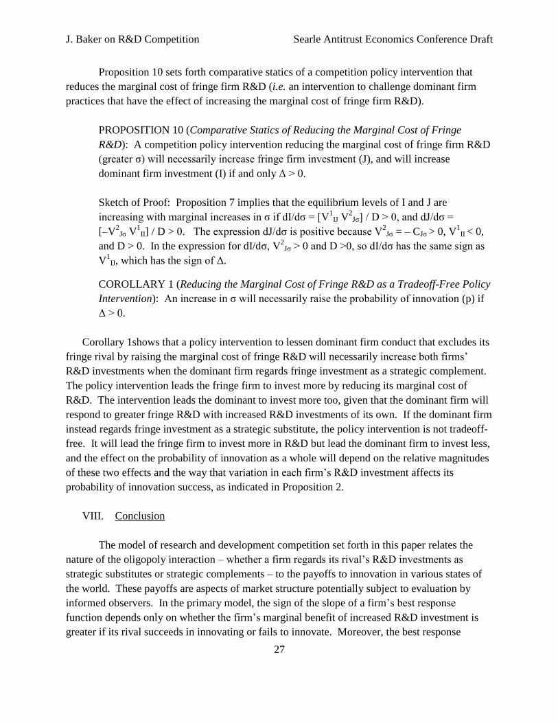
J. Baker on R&D Competition Searle Antitrust Economics Conference Draft
27
Proposition 10 sets forth comparative statics of a competition policy intervention that
reduces the marginal cost of fringe firm R&D (i.e. an intervention to challenge dominant firm
practices that have the effect of increasing the marginal cost of fringe firm R&D).
PROPOSITION 10 (Comparative Statics of Reducing the Marginal Cost of Fringe
R&D): A competition policy intervention reducing the marginal cost of fringe firm R&D
(greater σ) will necessarily increase fringe firm investment (J), and will increase
dominant firm investment (I) if and only Δ > 0.
Sketch of Proof: Proposition 7 implies that the equilibrium levels of I and J are
increasing with marginal increases in σ if dI/dσ = [V1
IJ V2
Jσ] / D > 0, and dJ/dσ =
[–V2
Jσ V1
II] / D > 0. The expression dJ/dσ is positive because V2
Jσ = – CJσ > 0, V1
II < 0,
and D > 0. In the expression for dI/dσ, V2
Jσ > 0 and D >0, so dI/dσ has the same sign as
V1
IJ, which has the sign of Δ.
COROLLARY 1 (Reducing the Marginal Cost of Fringe R&D as a Tradeoff-Free Policy
Intervention): An increase in σ will necessarily raise the probability of innovation (p) if
Δ > 0.
Corollary 1shows that a policy intervention to lessen dominant firm conduct that excludes its
fringe rival by raising the marginal cost of fringe R&D will necessarily increase both firms’
R&D investments when the dominant firm regards fringe investment as a strategic complement.
The policy intervention leads the fringe firm to invest more by reducing its marginal cost of
R&D. The intervention leads the dominant to invest more too, given that the dominant firm will
respond to greater fringe R&D with increased R&D investments of its own. If the dominant firm
instead regards fringe investment as a strategic substitute, the policy intervention is not tradeoff-
free. It will lead the fringe firm to invest more in R&D but lead the dominant firm to invest less,
and the effect on the probability of innovation as a whole will depend on the relative magnitudes
of these two effects and the way that variation in each firm’s R&D investment affects its
probability of innovation success, as indicated in Proposition 2.
VIII. Conclusion
The model of research and development competition set forth in this paper relates the
nature of the oligopoly interaction – whether a firm regards its rival’s R&D investments as
strategic substitutes or strategic complements – to the payoffs to innovation in various states of
the world. These payoffs are aspects of market structure potentially subject to evaluation by
informed observers. In the primary model, the sign of the slope of a firm’s best response
function depends only on whether the firm’s marginal benefit of increased R&D investment is
greater if its rival succeeds in innovating or fails to innovate. Moreover, the best response

J. Baker on R&D Competition Searle Antitrust Economics Conference Draft
28
functions of the dominant firm and its fringe rival may plausibly have differently-signed slopes,
with one firm regarding its rival’s investment as a strategic complement while the other regards
its rival’s investment as a strategic substitute. For this reason, two of the competition policy
instruments studied – challenging pre-innovation exclusion or challenging post-innovation
exclusion – will tend to be effective in different strategic settings. In addition, a third
competition policy instrument – challenging dominant firm conduct that has the effect of
increasing the marginal cost of fringe firm R&D – will necessarily benefit innovation if the
dominant firm regards fringe R&D investment as a strategic complement. A companion paper
(Jonathan B. Baker, 2014) relies on these results to show how to evaluate dominant firm
“appropriability” justifications – claims that the dominant firm’s practices will benefit innovation
by increasing its dominant firm’s reward for innovation success – for a range of exclusionary
practices, and illustrates its approach using the facts of three classic antitrust cases.
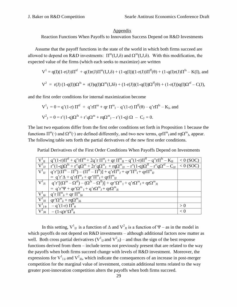
J. Baker on R&D Competition Searle Antitrust Economics Conference Draft
29
Appendix
Reaction Functions When Payoffs to Innovation Success Depend on R&D Investments
Assume that the payoff functions in the state of the world in which both firms succeed are
allowed to depend on R&D investments: Πss
(I,J,δ) and ss
(I,J,δ). With this modification, the
expected value of the firms (which each seeks to maximize) are written
V1 = q(I)(1-r(J))Π
sf + q(I)r(J)Π
ss(I,J,δ) + (1-q(I))(1-r(J))Π
ff(θ) + (1-q(I)r(J)Π
fs – K(I), and
V2 = r(J) (1-q(I))
fs + r(J)q(I)
ss(I,Jδ) + (1-r(J))(1-q(I))
ff(θ) + (1-r(J))q(I)
sf – C(J),
and the first order conditions for internal maximization become
V1
I = 0 = q’(1-r) Πsf + q’rΠ
ss + qr Π
ssI – q’(1-r) Π
ff(θ) – q’rΠ
fs – KI, and
V2
J = 0 = r’(1-q)fs + r’q
ss + rq
ssJ – r’(1-q) – CJ = 0.
The last two equations differ from the first order conditions set forth in Proposition 1 because the
functions Πss
(∙) and ss
(∙) are defined differently, and two new terms, qrΠss
I and rqss
J, appear.
The following table sets forth the partial derivatives of the new first order conditions.
Partial Derivatives of the First Order Conditions When Payoffs Depend on Investments
V1
II q”(1-r)Πsf + q”rΠ
ss + 2q’r Π
ssI + qr Π
ssII – q”(1-r)Π
ff – q”rΠ
fs – KII < 0 (SOC)
V2
JJ r”(1-q)fs + r”q
ss + 2r’q
ssJ + rq
ssJJ – r”(1-q)
ff – r”q
sf – CJJ < 0 (SOC)
V1
IJ q’r’[(Πss
– Πfs) – (Π
sf – Π
ff)] + q’rΠ
ssJ + qr’Π
ssI + qrΠ
ssIJ
= q’r’Δ + q’rΠss
J + qr’Πss
I + qrΠss
IJ
V2
JI q’r’[(ss
– sf) – (
fs –
ff)] + qr’
ss I + q’r
ssJ + qr
ssJI
= q’r’Ψ + qr’ss
I + q’rss
J + qrss
JI
V1
Iδ q’r Πss
δ + qr Πss
Iδ
V2
Jδ qr’ss
δ + rqss
Jδ
V1
I θ – q’(1-r) Πff
θ > 0
V2
Jθ – (1-q)r’ff
θ < 0
In this setting, V1
IJ is a function of Δ and V2
JI is a function of Ψ – as in the model in
which payoffs do not depend on R&D investments – although additional factors now matter as
well. Both cross partial derivatives (V1
IJ and V2
JI) – and thus the sign of the best response
functions derived from them – include terms not previously present that are related to the way
the payoffs when both firms succeed change with levels of R&D investment. Moreover, the
expressions for V1
I δ and V2
Jδ, which indicate the consequences of an increase in post-merger
competition for the marginal value of investment, contain additional terms related to the way
greater post-innovation competition alters the payoffs when both firms succeed.
J. Baker on R&D Competition Searle Antitrust Economics Conference Draft
30
References
Philippe Aghion, Ufuk Akcigit & Peter Howitt (2013). What Do We Learn From Schumpeterian
Growth Theory? NBER Working Paper No. 18824.
Philippe Aghion, Stefan Bechtold, Lea Cassar & Holger Herz (2014). The Causal Effects of
Competition on Innovation: Experimental Evidence. NBER Working Paper No. 19987.
Rabah Amir & John Wooders (1998). Cooperation vs. Competition in R&D: The Role of
Stability of Equilibrium. JOURNAL OF ECONOMETRICS, vol. 67, pp. 63-73.
Susan Athey & Armin Schmutzler (2011). Investment and Market Dominance, RAND JOURNAL
OF ECONONOMICS vol. 32, pp. 1-26.
Jonathan B. Baker (2014). Evaluating Appropriability Defenses for the Exclusionary Conduct
of Dominant Firms in Innovative Industries. Working Paper.
Jonathan B. Baker (2013). Exclusion as a Core Competition Concern. ANTITRUST LAW
JOURNAL, vol. 78, pp. 527-89.
Jonathan B. Baker (2007). Beyond Schumpeter vs. Arrow: How Antitrust Fosters Innovation,
ANTITRUST LAW JOURNAL, vol. 74, pp. 575-602.
John Beath, Yannis Katsoulacos & David Upph (1989). The Game-Theoretic Analysis of
Innovation: A Survey, BULLETIN OF ECONOMIC RESEARCH, vol. 41, pp. 163-84.
Jeremy I. Bulow, John D. Geanakoplos & Paul D. Klemperer (1985). Multimarket Oligopoly:
Strategic Substitutes and Complements. JOURNAL OF POLITICAL ECONOMY, vol. 93, pp. 488-511.
Joseph Farrell & Paul Klemperer (2007). Coordination and Lock-in: Competition with
Switching Costs and Network Effects. HANDBOOK OF INDUSTRIAL ORGANIZATION (Mark
Armstrong & Robert Porter, eds.),vol. 3, pp. 1967-2072.
Drew Fudenberg & Jean Tirole (1984). The Fat-Cat Effect, the Puppy-Dog Ploy, and the Lean
and Hungry Look. AMERICAN ECONOMIC REVIEW, vol. 74, pp. 361-66.
Richard Gilbert (2006). Looking for Mr. Schumpeter: Where Are We in the Competition-
Innovation Debate? INNOVATION POLICY AND THE ECONOMY (Adam B. Jaffe, Josh Lerner &
Scott Stern, eds.), vol. 6, pp. 159-215.
Matteo Gomellini (2013). Innovation and Competition: A Survey. Working Paper (Dec.),
http://www.bancaditalia.it/studiricerche/convegni/atti/innovation-in-Italy/Gomellini.pdf.

J. Baker on R&D Competition Searle Antitrust Economics Conference Draft
31
Michael L. Katz & Howard A. Shelanski (2007). Mergers and Innovation. ANTITRUST LAW
JOURNAL, vol. 74, pp. 1-85.
Benjamin Ren Kern & Juan Manuel Mantilla Contreras (2014). Mergers and the Incentives to
Undertake Product Innovation Oriented R&D: First Steps Towards an Assessment Approach.
MAGKS Working Paper No. 17-2014, http://ssrn.com/abstract=2403259.
Dermot Leahy & J. Peter Neary (1997). Public Policy Towards R&D in Oligopolistic Industries,
AMERICAN ECONOMIC REVIEW, vol. 87, pp. 642-62.
David M. Mandy, John W. Mayo & David E. M. Sappington (2014). Targeting Rivals: Moving
from “Whether” to Whom”. Working Paper (Feb.),
http://bear.warrington.ufl.edu/sappington/working_papers.htm.
Jennifer F. Reinganum (1989). The Timing of Innovation: Research, Development, and
Diffusion. HANDBOOK OF INDUSTRIAL ORGANIZATION (Richard Schmalensee & Robert D. Willig,
eds.), vol. 1, pp. 849-908.
Armin Schmutzler (2013). Competition and Investment – A Unified Approach. INTERNATIONAL
JOURNAL OF INDUSTRIAL ORGANIZATION, vol. 31, pp. 477-87.
Armin Schmutzler (2009). Is Competition Good for Innovation? A Simple Approach to an
Unresolved Question. FOUNDATIONS AND TRENDS IN MIROECONOMICS , vol. 5, pp. 355-428.
Norbert Schulz, Review of the Literature of the Impact of Mergers on Innovation. ZEW
Discussion Paper 07-061, ftp://ftp.zew.de/pub/zew-docs/dp/dp07061.pdf.
John T. Scott (2009). Competition in Research and Development: A Theory for Contradictory
Predictions. REVIEW OF INDUSTRIAL ORGANIZATION, vol. 34, pp.153-171.
Suzanne Scotchmer (2004). INNOVATION AND INCENTIVES.
Ilya Segal & Michael D. Whinston (2007). Antitrust in Innovative Industries. AMERICAN
ECONOMIC REVIEW, vol. 97, pp. 1703-1730.
Carl Shapiro (2012). Competition and Innovation: Did Arrow Hit the Bull's Eye?, THE RATE AND
DIRECTION OF INVENTIVE ACTIVITY REVISITED (Josh Lerner & Scott Stern eds.), pp. 361-410.
Daniel Spulber (2013). How Do Competitive Pressures Affect Incentives to Innovate When
There Is a Market for Inventions? JOURNAL OF POLITICAL ECONOMY, vol. 121, pp. 1007-1054.
Joseph E. Stiglitz (2014). Intellectual Property Rights, the Pool of Knowledge, and Innovation.
NBER Working Paper 20014.

J. Baker on R&D Competition Searle Antitrust Economics Conference Draft
32
Jean Tirole (1988). THE THEORY OF INDUSTRIAL ORGANIZATION.
Mihkel M. Tombak (2006). Strategic Asymmetry. JOURNAL OF ECONOMIC BEHAVIOR &
ORGANIZATION, vol. 61, pp. 339-350.
Xavier Vives (1999). OLIGOPOLY PRICING: OLD IDEAS AND NEW TOOLS.