Embed Size (px)
Citation preview
Erasmus University RotterdamErasmus School of EconomicsMaster Thesis Financial Economics
Risk attitude in pension plansThe effect of homeownership
Name: Jochem JanssenStudent number: 281815Supervisor: Dr. L.A.P. SwinkelsDate: December 2012

Preface
Countless people told me how marvelous it would feel to finish your thesis. The moment
has finally arrived. I am proud to present to you my master thesis, which implies the
accomplishment of the master Financial Economics at the Erasmus University in
Rotterdam.
I would like to thank the following people for helping me through my studies and my
thesis. First of all, I would like to thank my supervisor, Laurens Swinkels for his advice and
effort in guiding me through my research. Furthermore, I would like to thank my parents
for their patience and confidence in my capabilities. Above all, I would like to thank
Renske for her love and support.
Rotterdam, December 2012
Jochem Janssen
2

Table of content
Preface 2
Table of content 3
1. Introduction 4
2. Literature review 6
2.1. Risk attitude 6
2.1.1. Expected utility theory 6
2.1.2. Paradoxes 9
2.1.3. Prospect Theory 11
2.1.4. Holt and Laury (2002) 12
2.2. Pension schemes 14
2.2.1. Hybrid DB-DC plans 15
2.2.2. Life cycle theory 16
2.2.3. Collective pension funds 18
2.2.4. Behavioral finance 19
2.3. Risk attitude in pension plans 22
2.3.1. Questionnaires 24
2.3.2. Homeownership 25
3. Data and methodology 27
3.1. Questionnaire 27
3.2. Data and summary statistics 28
4. Results 34
4.1. Homeownership 38
4.2. Type of mortgages 42
4.3. Maturity of interest rates 44
5. Conclusion 48
References 50
Appendix Questionnaire 55
3

1. Introduction
Pension funds in the Netherlands have the obligation to act in the best interest of their
participants. Most pension funds have a very large group of participants and it is difficult
for the pension to know if they invest in a way that the participants would like. An
important aspect of the preferences of the participants is the risk involved with the
investments of the pension fund. Do participants want that the pension fund takes a lot of
risk with the investments? This can result in higher or lower pension payments than
expected. It is also possible that the participants prefer less risk, with the result that the
future payments can be lower than the investments with a lot of risk, however the payments
are more certain. Therefore the risk attitude of the participants of the different pension
funds in the Netherlands would be very helpful information for the board of trustees. This
way they can determine the most optimal mix of investments for their participants.
The risk attitude in pension plans can be influenced by a number of factors and a lot of
these factors have been studied. There is however is very little research on the effect of
homeownership on the risk attitude in pension plans.
A house is a very large asset and it is possible to look at a house as a long-term investment.
At some point the house is completely paid off and it is possible to sell it. A pension has the
same characteristics, also a large investment that will generate payments in the future. If
you are participating in a pension plan, owning a house might influence decisions regarding
your pension plan, for example the risk attitude. People can think of a house as an risky
assets because of the housing market and therefore they do not want to take a lot of risk in
their pension. Or they believe that if their house is paid off it will give a guaranteed amount
that they can use for their pension and therefore they want to take a bit more risk with their
pension plan. To find out if there is a relationship and how homeownership influence risk
attitude in pension plan, the main question that will be answered in this thesis is:
Is there a relationship between homeownership and the risk attitude in pension plans?
4
In order to see if other aspects of homeownership like the choice of a mortgage type and the
choice in maturities of interest rates might have an effect on the risk attitude in pension
plans, these factors will also be part of this study.
The structure of this thesis will be as follows. Chapter 2 will introduce the theoretical
foundation for the research in this thesis. Theory of risk attitude will be discussed in the
beginning of the chapter, followed by a closer look on different aspects of pension schemes
with special attention for the Dutch pension market. The last part will discuss the theory
about risk attitude in pension plans, other studies and possible ways to research this topic.
Chapter 3 will focus of the data and methodology. The chapter captures the use of the
questionnaire and the different kind of questions. Chapter 4 will show the results of the
different parts of the research. This thesis ends with chapter 5 where the conclusion of this
thesis will be discussed as well as some recommendations for further research.
5

2. Literature review
2.1 Risk attitude
The basis for research in risk attitude is theory that describes utility. Bernouilli (1738) was
the first one to introduce the concept of utility in his research on the St Petersburg Paradox.
Utility is a description of how much satisfaction a person get from a certain good and if you
know the combination of goods for which a person gets the same satisfaction, you can draw
an indifference curve. With cardinal utility it would be possible to compare the indifference
curves, for example that a combination of goods gives twice the satisfaction of another
combination of goods. In the case of ordinal utility, it says something about the way a
combination is ranked, for example that combination A gives more satisfaction than
combination B.
2.1.1. Expected utility framework
In the expected utility framework the combination of goods is replaced by a combination of
choices with a certain possibility, for example a chance of 50% on outcome A and chance
of 50% on outcome B. With these possible outcomes there is an expected utility. Neumann
and Morgenstern (1944) used the assumption that a person will try to maximize their utility
in order to derive a utility function for an individual. This way the risky choices can be
ranked on their expected utility value. Savage (1954) combines a personal utility function
with a personal probability distribution in subjective expected utility. In the expected utility
framework the shape of the utility functions can be a way to describe a person’s risk
attitude. If the utility function is concave between certain points, you can say that a person
is risk averse, a convex function would mean a person is risk seeking and a straight line
indicates that a person is risk neutral.
The most common way to write an utility function is u(x), where x can be income, wealth
or any kind of commodity. The shape of an utility function u(x) is in most cases obvious,
but comparing different concave or convex functions to see if a person is more risk seeking
or risk averse is more difficult. The most simple method to measure the amount of curve of
a function is to take the second derivative of u(x), u”(x). The second derivative for a linear
function is zero, a concave function has a negative second derivative and the second
6
derivative for a convex function is positive. These basics were used in the Arrow-Pratt
measure of risk aversion (Pratt, 1964 and Arrow, 1965), a very common measure for risk
aversion.
The second derivative might be a good starting point for measuring risk aversion, however
it is not sufficient. The second derivative is not invariant if there are positive linear
transformations. An example of such a positive linear transformations is if the formula u1
(x) is changed into u2(x) = au1(x) + b. The risk attitude of an individual did not change
because of this transformation, but u2(x) = a u2¿(x) > u1
¿(x). This indicates that the individual
is more risk averse in u2(x) than in u1(x). The second derivative is therefore not the right
measure for risk aversion. To keep the measure of risk aversion the same after a positive
linear transformation Arrow and Pratt normalized the second derivative. To do this they
divided the second derivative by the first derivative. This is almost the formula of the
Arrow-Pratt measure. The second derivative of an concave function is negative and to make
sure that the utility function of a risk averse person gives a non-negative number, the
fraction is multiplied by -1. With this formula a larger number of the Arrow-Pratt measure
indicates a more risk averse individual. The definition of the Arrow-Pratt measure of
absolute risk aversion is given by
ARA (x)=−u} (x)} over {{u} ^ {'} (x) ¿¿
In the Arrow-Pratt measure of absolute risk aversion x stands for an actual amount invested
in risky assets or put in some kind of lotteries. The actual amount can change if the wealth
of an individual changes. This leads to three different types of absolute risk aversion;
increasing, constant and decreasing. With increasing absolute risk aversion the amount put
in risky assets decreases if the amount of wealth increases, constant absolute risk aversion
indicates that the amount will be the same if wealth stays the same and that leaves
decreasing risk aversion with a higher amount in risky assets if wealth increases.
In the case that somebody is more interested in the percentage of wealth held in risky assets
of put in lotteries, for given amount of wealth, the relative risk aversion is a more
appropriate measure. To obtain this measure the formula for absolute risk aversion had to
be multiplied with the wealth w. This gives the following definition for the Arrow-Pratt
measure of relative risk aversion.
7

RRA (w)=−w u} (w)} over {{u} ^ {'} (w)¿¿
Like the situation with absolute risk aversion, this measure also has three different types.
Increasing relative risk aversion indicates that the percentage of risky assets decreases as
wealth increases, decreasing relative risk aversion indicates a higher percentage as wealth
increases, but constant relative risk aversion is most used in academic literature. This means
that the percentage held in risky assets stays the same if wealth increases. The best way to
show this is with a utility function of constant relative risk aversion (CRRA)
u(w)=w1−β−11−β
with β > 0
u'=w−β
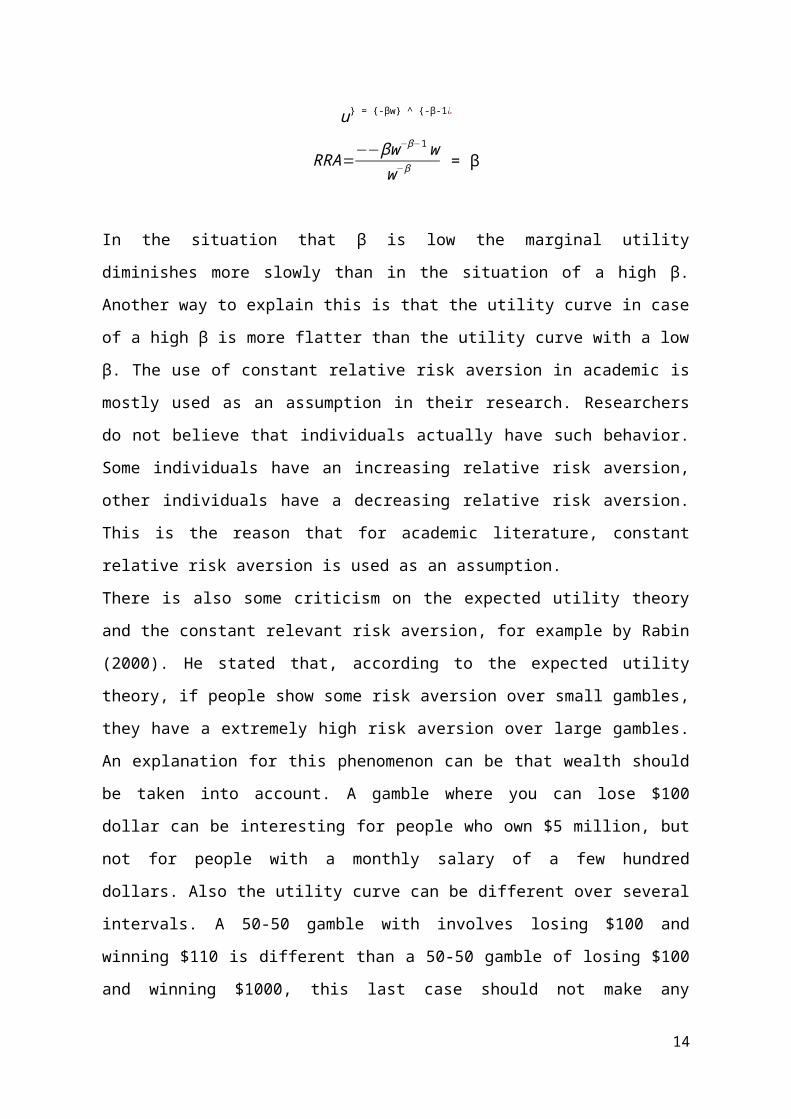
u} = {-βw} ^ {-β-1 ¿
RRA=−−βw−β−1 ww−β = β
In the situation that β is low the marginal utility diminishes more slowly than in the
situation of a high β. Another way to explain this is that the utility curve in case of a high β
is more flatter than the utility curve with a low β. The use of constant relative risk aversion
in academic is mostly used as an assumption in their research. Researchers do not believe
that individuals actually have such behavior. Some individuals have an increasing relative
risk aversion, other individuals have a decreasing relative risk aversion. This is the reason
that for academic literature, constant relative risk aversion is used as an assumption.
There is also some criticism on the expected utility theory and the constant relevant risk
aversion, for example by Rabin (2000). He stated that, according to the expected utility
theory, if people show some risk aversion over small gambles, they have a extremely high
risk aversion over large gambles. An explanation for this phenomenon can be that wealth
should be taken into account. A gamble where you can lose $100 dollar can be interesting
for people who own $5 million, but not for people with a monthly salary of a few hundred
dollars. Also the utility curve can be different over several intervals. A 50-50 gamble with
involves losing $100 and winning $110 is different than a 50-50 gamble of losing $100 and
8

winning $1000, this last case should not make any difference for individuals according to
the expected utility theory.
2.1.2. Paradoxes
Since the research of Neumann and Morgenstern and the use of lotteries, a few things were
not consistent with the theory. Experiments showed that people were not consistent in their
choices and with subjective expected utility theory. One example is the Ellsberg paradox.
This was an experiment were a ball was taken from an urn with 90 balls, 30 were red and
60 were yellow or black. People first had to choose between option A, the persons receives
$100 if a red ball was taken, and option B where the persons receives $100 if a black ball
was taken from the urn. After these choices they were given a second gamble. In this
second gamble the number of balls and the colour of these balls stay the same as in the first
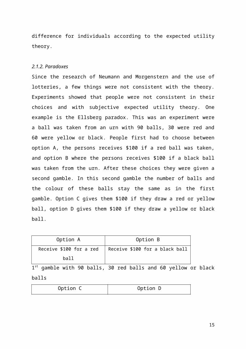
gamble. Option C gives them $100 if they draw a red or yellow ball, option D gives them
$100 if they draw a yellow or black ball.
Option A Option B
Receive $100 for a red ball Receive $100 for a black ball
1st gamble with 90 balls, 30 red balls and 60 yellow or black balls
Option C Option D
Receive $100 for a red or yellow ball Receive $100 for a black or yellow ball
2nd gamble with 90 balls, 30 red balls and 60 yellow or black balls
In the expected utility framework you would expect that a person who chooses option A
over B in the first part would choose option C over D in the second part. And if a person
chooses B over A, one would expect that option D is chosen over C. Ellsberg (1961) found
that people strictly prefer A over B, but also preferred D over C and that is not consistent
with the expected utility theory (Ellsberg, 1961). A possible explanation for this is that
people tend to decline a possibility if they do not know the exact chances of that possibility.
In the situation above the chances of a black ball are in the 0/90-60/90 range, the average
person tend to see this probability in the lower part of this range since it would in the favor
of the experimenter to put fewer black balls in the urn. In the second gamble people may
assume that there are fewer yellow balls in the urn and forget that the experimenter has no
opportunity to change the balls in the urn between the two gambles.
9
Another phenomenon is the Allais paradox (Allais, 1953). This paradox differs from the
Ellsberg paradox in a way that the probabilities of the outcomes are more known. An
individual is facing two gambles and in each gamble this person has to choose between two
options. The two gambles and the corresponding outcomes of the two options are shown
below.
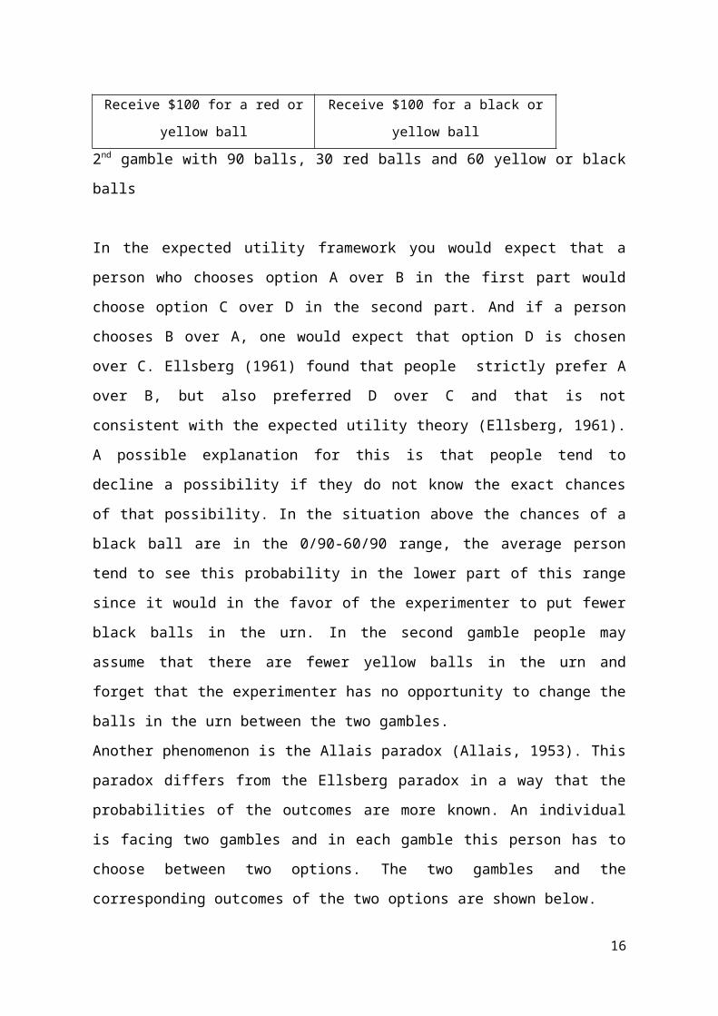
Option A Option B Option C Option D
Reward Chance Reward Chance Reward Chance Reward Chance
$1 million 100% $1 million 89% Nothing 89% Nothing 90%
Nothing 1% $1 million 11% $5 million
10%
$5 million 10%
1st Gamble 2nd Gamble
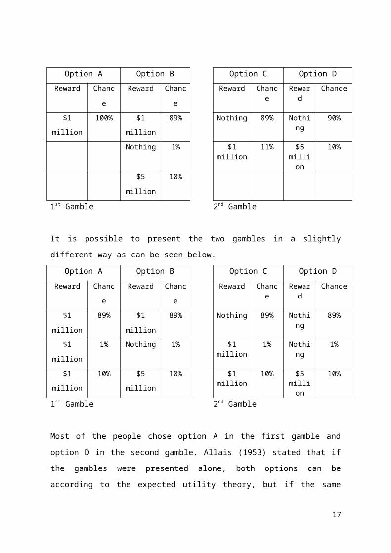
It is possible to present the two gambles in a slightly different way as can be seen below.
Option A Option B Option C Option D
Reward Chance Reward Chance Reward Chance Reward Chance
$1 million 89% $1 million 89% Nothing 89% Nothing 89%
$1 million 1% Nothing 1% $1 million 1% Nothing 1%
$1 million 10% $5 million 10% $1 million 10% $5 million
10%
1st Gamble 2nd Gamble
Most of the people chose option A in the first gamble and option D in the second gamble.
Allais (1953) stated that if the gambles were presented alone, both options can be according
to the expected utility theory, but if the same person is facing these gambles you would
expect that people would chose either option A and C or option B and D. People that chose
option A preferred the certainty of the outcome instead of the higher expected value of
option B. The outcome of option C is more certain than D, but still most people chose
option D. This research also shows that people do not always act in real life according to
the theory. Certainty and probabilities seems to influence the behavior of people.
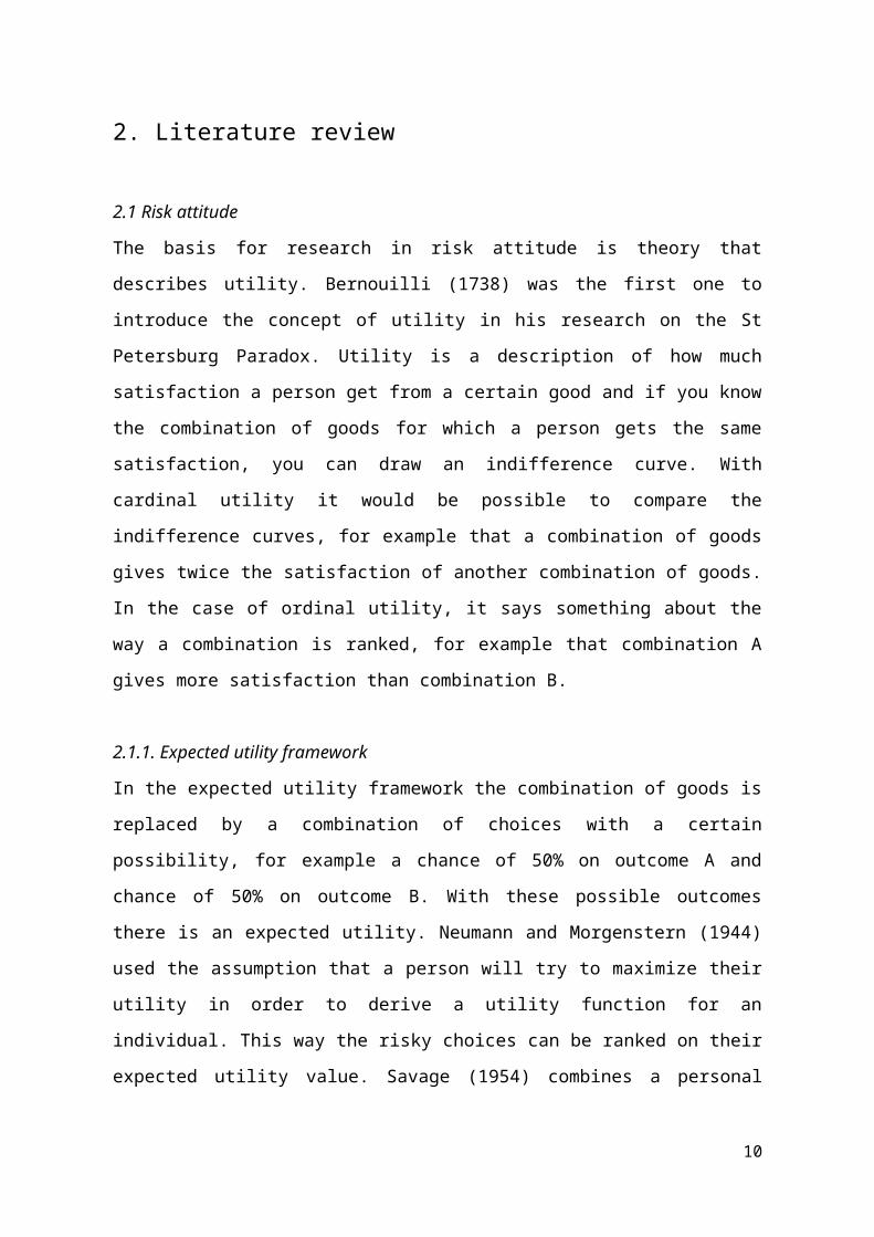
2.1.3. Prospect Theory
A reaction to the paradoxes and inconsistencies came from Kahneman and Tversky (1979)
in their paper which describes the Prospect Theory. This alternative model on the expected
10
utility framework answers some of the anomalies in lottery-choice decisions of people. It is
based on real-life decisions instead of optimal decisions. The starting point in their paper is
the definition of a person’s reference point. This point is often the current wealth of an
individual. Important to mention is that in the prospect theory the conclusions focus on
gains and losses instead of final assets. The reference point is therefore the point for which
people see the outcomes of a lottery as the same. If you look at larger outcomes than the
reference point, the value function has a concave shape. This means that people are risk
averse over gains. Outcomes that are less than the reference point has a convex shape,
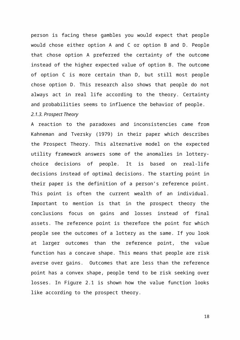
people tend to be risk seeking over losses. In Figure 2.1 is shown how the value function
looks like according to the prospect theory.
Figure 2.1. Value function according to the prospect theory
An example (Kahneman and Tversky, 1979) of this ‘reflection effect’ is that if people had
to choose between a sure gain of 3000 or an 80 percent chance of 4000, a majority choose
the sure gain. If the same choice is given in terms of losses, a certain loss of 3000 or an 80
percent chance on loosing 4000, people tend to choose the chance of losing 4000. This
effect is not what you would expect according to the expected utility framework, where a
value function is a straight line through the reference point. The behavior that people
experience an certain loss more undesirable than that the like certain gain is known as ‘loss
aversion’.
An important application of this theory is that researchers have to take the framing effect in
mind. This means that it is important how certain questions or lottery-choices are presented,
because people can give different answers for losses and gains. Benartzi and Thaler (1999)
researched the way questions were asked and they found that people also had some
11
different preferences if you look at different timelines in which people are confronted with
gains or losses. Myopic loss aversion refers to the behavior that when people could choose
between gambles that are identical in the long run, but have different results in the short
run, people are likely to choose the gamble that has the smallest loss in the short run.
In their research on prospect theory all the payoffs are hypothetical. They made the
assumption that people would know they would act in actual situations, and that people
would also have no reason to act differently from their true preferences (Kahneman and
Tversky, 1979). In their paper on cumulative prospect theory (Tversky and Kahneman,
1992) they still used hypothetical payoffs. The problem of hypothetical payoffs was known,
but they found in the later paper that there was little evidence for a difference in the
behavior on hypothetical and real payoffs.
2.1.4. Holt and Laury (2002)
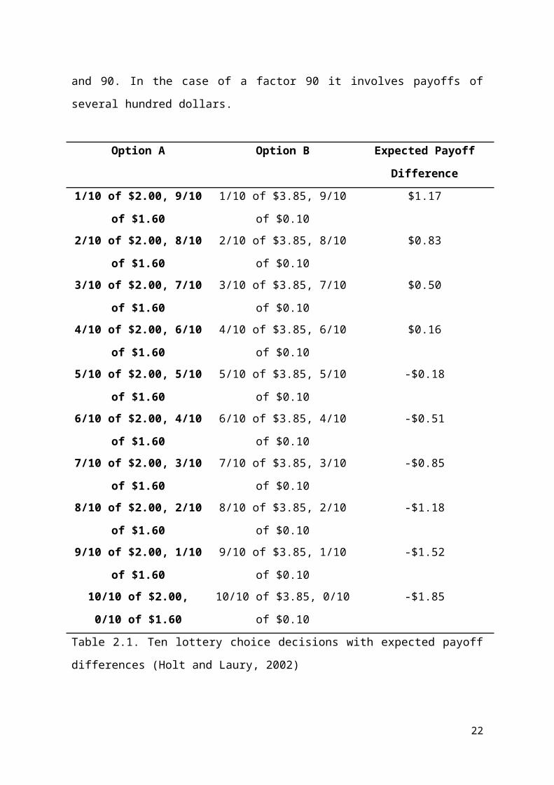
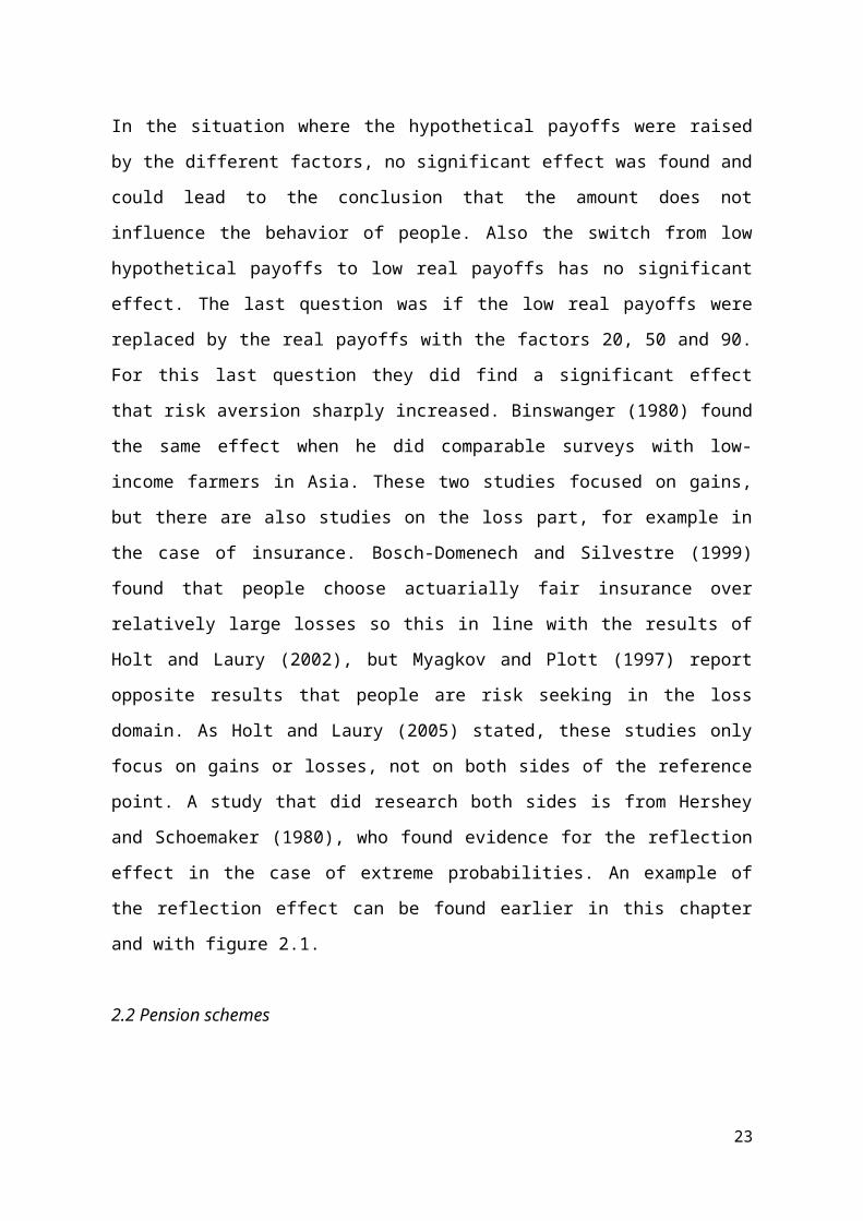
Several differences in payoffs are researched by Holt and Laury (2002). The research of
Holt and Laury consists of a set of simple choices to measure a person’s risk aversion. The
participants had to choose ten times between option A and B. In each option there are a
high and a low payoff. For option A these payoffs are $2 and $1.60, for option B $3.85 and
$0.10. The payoffs differ in amount and variability. In the ten decisions the probability
moves from 10% for the high payoff and 90% for the low payoff to 100% and 0% in ten
steps. The expected payoff is higher for option A in the first four options and risk neutral
person will choose those four options before switching to option B. In Table 2.1 the
different options and the corresponding expected payoffs are shown.
The payoffs and the number of safe choices were carefully chosen by Holt and Laury
(2002). They point on the fact that most literature assumes constant relative risk aversion
and with this the utility function for money is u(x )=x1−β for x > 0. The β in the formula
stands for the risk attitude of an individual and will not change through the experiment. If
the β is negative this implies a risk seeking person, in case the r is zero this means the
individual is risk neutral and a positive β means a risk averse person. The payouts were
selected so that between the fourth and the fifth decision the interval lies around zero
($0.16, -$0.18). These numbers are chosen because now the line between decision point
12
four and five is almost a straight line through zero and this is in line with constant relative
risk aversion.
The moment a person will switch to option B tells something about the risk aversion of that
person. To investigate if differences in payoffs have an effect on the behavior of people,
Holt and Laury also gave real payoffs instead of hypothetical. They also investigated what
changes if the hypothetical and real payoffs changes with a factor 20, 50 and 90. In the case
of a factor 90 it involves payoffs of several hundred dollars.
Option A Option B Expected Payoff
Difference
1/10 of $2.00, 9/10 of $1.60 1/10 of $3.85, 9/10 of $0.10 $1.17
2/10 of $2.00, 8/10 of $1.60 2/10 of $3.85, 8/10 of $0.10 $0.83
3/10 of $2.00, 7/10 of $1.60 3/10 of $3.85, 7/10 of $0.10 $0.50
4/10 of $2.00, 6/10 of $1.60 4/10 of $3.85, 6/10 of $0.10 $0.16
5/10 of $2.00, 5/10 of $1.60 5/10 of $3.85, 5/10 of $0.10 -$0.18
6/10 of $2.00, 4/10 of $1.60 6/10 of $3.85, 4/10 of $0.10 -$0.51
7/10 of $2.00, 3/10 of $1.60 7/10 of $3.85, 3/10 of $0.10 -$0.85
8/10 of $2.00, 2/10 of $1.60 8/10 of $3.85, 2/10 of $0.10 -$1.18
9/10 of $2.00, 1/10 of $1.60 9/10 of $3.85, 1/10 of $0.10 -$1.52
10/10 of $2.00, 0/10 of $1.60 10/10 of $3.85, 0/10 of $0.10 -$1.85
Table 2.1. Ten lottery choice decisions with expected payoff differences (Holt and Laury,
2002)
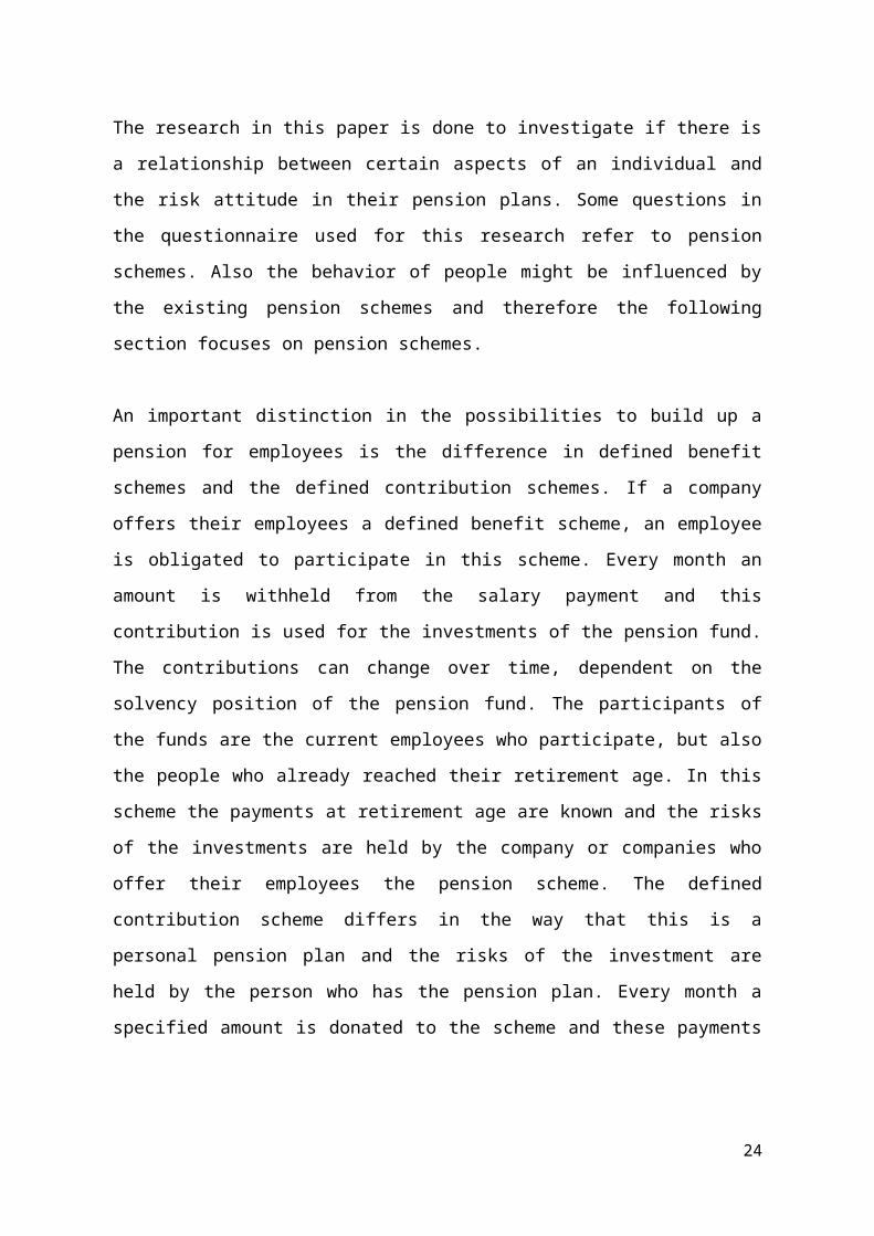
In the situation where the hypothetical payoffs were raised by the different factors, no
significant effect was found and could lead to the conclusion that the amount does not
influence the behavior of people. Also the switch from low hypothetical payoffs to low real
payoffs has no significant effect. The last question was if the low real payoffs were
replaced by the real payoffs with the factors 20, 50 and 90. For this last question they did
find a significant effect that risk aversion sharply increased. Binswanger (1980) found the
same effect when he did comparable surveys with low-income farmers in Asia. These two
studies focused on gains, but there are also studies on the loss part, for example in the case
of insurance. Bosch-Domenech and Silvestre (1999) found that people choose actuarially
fair insurance over relatively large losses so this in line with the results of Holt and Laury
13
(2002), but Myagkov and Plott (1997) report opposite results that people are risk seeking in
the loss domain. As Holt and Laury (2005) stated, these studies only focus on gains or
losses, not on both sides of the reference point. A study that did research both sides is from
Hershey and Schoemaker (1980), who found evidence for the reflection effect in the case of
extreme probabilities. An example of the reflection effect can be found earlier in this
chapter and with figure 2.1.
2.2 Pension schemes
The research in this paper is done to investigate if there is a relationship between certain
aspects of an individual and the risk attitude in their pension plans. Some questions in the
questionnaire used for this research refer to pension schemes. Also the behavior of people
might be influenced by the existing pension schemes and therefore the following section
focuses on pension schemes.
An important distinction in the possibilities to build up a pension for employees is the
difference in defined benefit schemes and the defined contribution schemes. If a company
offers their employees a defined benefit scheme, an employee is obligated to participate in
this scheme. Every month an amount is withheld from the salary payment and this
contribution is used for the investments of the pension fund. The contributions can change
over time, dependent on the solvency position of the pension fund. The participants of the
funds are the current employees who participate, but also the people who already reached
their retirement age. In this scheme the payments at retirement age are known and the risks
of the investments are held by the company or companies who offer their employees the
pension scheme. The defined contribution scheme differs in the way that this is a personal
pension plan and the risks of the investment are held by the person who has the pension
plan. Every month a specified amount is donated to the scheme and these payments are
used for investments. At retirement age the total amount of investments at that time can be
converted in an annuity.
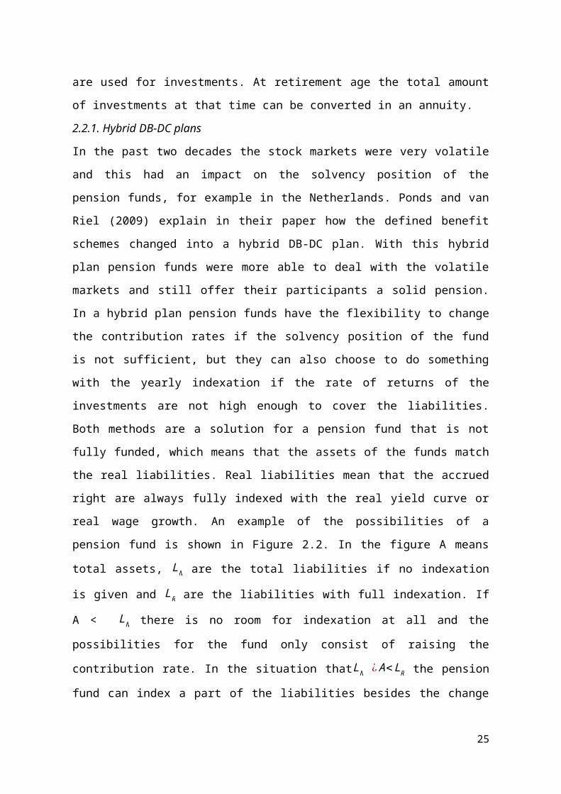
2.2.1. Hybrid DB-DC plans
In the past two decades the stock markets were very volatile and this had an impact on the
solvency position of the pension funds, for example in the Netherlands. Ponds and van Riel
(2009) explain in their paper how the defined benefit schemes changed into a hybrid DB-
14
DC plan. With this hybrid plan pension funds were more able to deal with the volatile
markets and still offer their participants a solid pension. In a hybrid plan pension funds
have the flexibility to change the contribution rates if the solvency position of the fund is
not sufficient, but they can also choose to do something with the yearly indexation if the
rate of returns of the investments are not high enough to cover the liabilities. Both methods
are a solution for a pension fund that is not fully funded, which means that the assets of the
funds match the real liabilities. Real liabilities mean that the accrued right are always fully
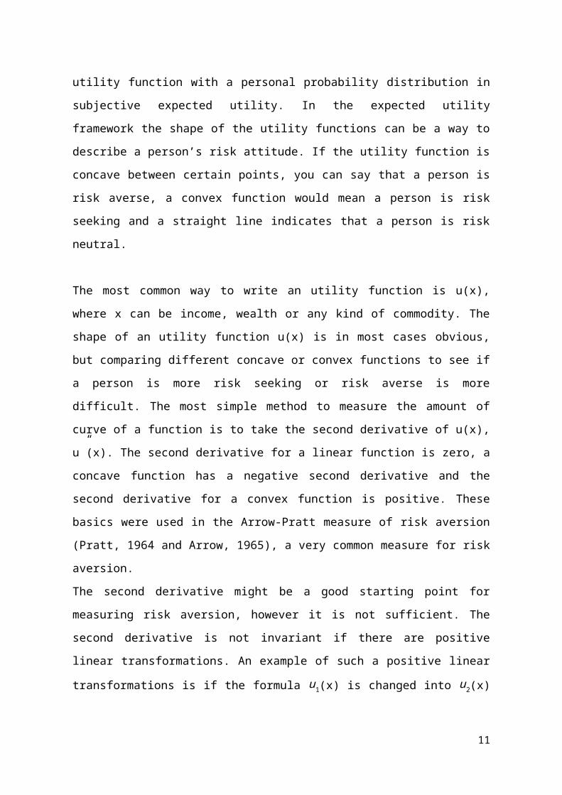
indexed with the real yield curve or real wage growth. An example of the possibilities of a
pension fund is shown in Figure 2.2. In the figure A means total assets, LN are the total
liabilities if no indexation is given and LR are the liabilities with full indexation. If A < LN
there is no room for indexation at all and the possibilities for the fund only consist of
raising the contribution rate. In the situation thatLN ¿ A<LR the pension fund can index a
part of the liabilities besides the change in contribution rates. If A > LR there is room for
full indexation and even the possibility to make up for indexation cuts in the past.
Figure 2.2. Hybrid DB-DC plan (Pond and van Riel, 2009)
Hoevenaars and Ponds (2007) investigated the performances of the three different schemes
and they found that with the same investment portfolio a defined benefit scheme comes
with the cost of a higher risk of underfunding and a higher volatility of contribution rates. A
defined contribution scheme comes with the risk of low indexation. The hybrid DB-DC
15
scheme has risks for volatile contribution rates and low indexation somewhere in the
middle of the other two schemes, but the probability of underfunding is lower than in the
both schemes.
2.2.2. Life cycle theory
The situation regarding retirement plans is different for younger people who just started
with their careers and older people who are almost at their retirement age. This difference
and a more optimal way of investing for pensions is described in the life cycle theory
(Campbell & Viceira 2002, Viceira 2007, Bodie et al. 2007).
Molenaar and Ponds (2009) describe the life cycle theory with the personal wealth of an
individual. Personal wealth consists of two components; human capital and financial
capital. Human capital is the present value of the all the income payments that a person
will receive in the future. Although the path of future income payment is not exactly
known, the certainty of future incomes is high. This certainty comes from all kind of
disability and unemployment insurances (Bovenberg et al. 2007). The human capital can be
seen as a bond with wage indexation. The income payments are coupons in the comparison
and the bond ends at the retirement age. The income payments are used for consumption
and saving. These savings are added up in the financial capital, the second component of
personal wealth. This financial capital can consist of money on a savings account, but also
the part of a house that is paid off.
In the beginning of a career, the human capital is almost the entire part of the personal
wealth. Over time, the human capital will decrease until the retirement age. This is the point
where people no longer are going to work and therefore the income payments will stop.
From the start of the career until the retirement age, the financial capital will increase over
time. The reason for this is that people will pay off their mortgage or save some money.
Their financial capital will also make a small profit, for example the house they own will
increase in value, their savings account guarantees some interest and their investments
make a profit. At retirement age the personal wealth will completely consist of financial
capital and this likely to decrease because of consumption.
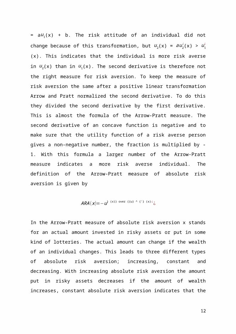
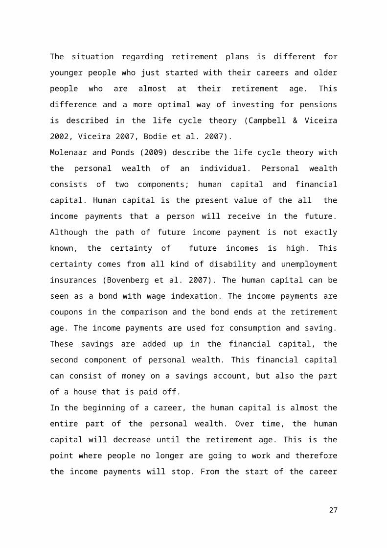
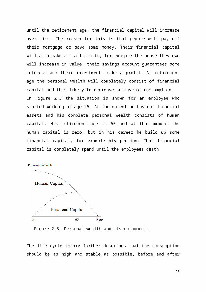
In Figure 2.3 the situation is shown for an employee who started working at age 25. At the
moment he has not financial assets and his complete personal wealth consists of human
capital. His retirement age is 65 and at that moment the human capital is zero, but in his
16
career he build up some financial capital, for example his pension. That financial capital is
completely spend until the employees death.
Figure 2.3. Personal wealth and its components
The life cycle theory further describes that the consumption should be as high and stable as
possible, before and after the retirement age. To achieve this, the financial capital should be
invested in a proper way. Several factors will influence the decisions that are made
regarding the investments, for example the risk aversion and time left to retirement of a
person. This leads to the theory that the investments of a person should bear more risk in
the beginning of a career, for example by investing in stocks. The closer the retirement age
gets, more and more should be invested in less risky assets, for example bonds. The ratio of
riskier and less risky assets depends on the consumption behavior of a person. The idea
behind this is that younger people are able to bear losses from risky assets like stocks.
Younger people can save more money in a later stadium of their career, because of the large
human capital left, to make up for these losses. Older people at the end of their working life
do not have much human capital left and have less time to save. The portfolio of these
people should therefore consist more of investments that can guarantee the value at
retirement age (Molenaar and Ponds, 2009).
Research shows that households do not invest and save according to the life cycle theory.
Lucardi (1999) did research and finds that some households have more wealth at retirement
age, but the majority of the households have too little wealth for a stable consumption path.
Another part of the theory that is not done in real life is adjusting the investments in their
17
portfolio with time. The theory describes that the ratio of risky assets like stocks should
gradually decline. Ameriks and Zeldes (2001) used surveys to find out that for a period of
ten years, fifty percent of investors did not change their portfolio and fourteen percent
changed it one time. The same result is found for European households’ portfolios in
research of Guiso, Haliassos and Jappali (2003). The theory further describes that
consumption is stable, but research of Banks, Blundell and Tanner (1998) shows that for
British households, consumption decreases more after the retirement of the supporter of the
family than you would expect according to the theory.
Pension funds in the Netherlands seem to invest somehow according to the life cycle theory
(Bikker et al., 2009) and do keep the average age of their participants into account. In their
research they found that the average age of the active participants is taken more in
consideration than the average age of the retired participants. This means that the
percentage of risky assets is higher that the theory would recommend. The relation between
average age and the ratio of investments like stocks is even stronger if you only look at the
average age of participants (Bikker et al., 2009). Although the average age is taken into
account, one could imagine that the investment policy of a pension fund is not in the best
interest of every individual, because of different risks appetites and consumption behavior.
Despite the differences, Bovenberg et al. (2007) and Teulings and de Vries (2006) showed
that the collective pension funds are still a better way to build up a pension than an
individual arrangement.
2.2.3. Collective pension funds
One important aspect of the pension schemes and the life cycle theory that are described
above is that these schemes involve a large group of participants. The risks of investments
are spread out over all the members and this has the advantage that the participants are
protected against heavy losses. The large group of participants also comes with an
disadvantage and that is that the pension fund has to keep the interests of all participants in
mind. An individual is likely to have different preferences, for example a person would like
to choose the contributions that have to be paid or maybe vary them every month. Another
example is that a person could like to choose the investment mix for his retirement plan.
Mitchell, Gordon and Twinney (1997) found that an employee could benefit from an
18
individual retirement plan, but the positive effects of an individual plan may not outweigh
the downsides of this change in pension system. In their paper van Rooij, Kool and Prast
(2007) mentions some of the downsides of a change in the involvement of an person in an
individual pension plan.
One of the most simple examples why an individual pension plan may not be the best way
to save for pension is the one of scale economies and therefore also risk sharing (Mitchell,
Gordon and Twinney 1997). Pension funds can trade on a much larger scale and because
they have a large group of participants, it is possible to have a well diversified investment
mix. With their portfolio it is much easier to reduce risk involved with their investments.
According to the portfolio theory the diversification can lead to an optimal profit while the
risks are kept relatively low. In contrary to a pension fund, an individual is likely to divide
their investments only over a couple of assets or funds (Huberman and Jiang, 2004).
Another reason for an inefficient pension plan if individuals have a say in the decisions
regarding their plan is that pension funds are likely to have a greater knowledge and
expertise. This can lead to sub-optimal investment decisions by individuals. Benartzi and
Thaler (2001) found that pension funds in the US have doubts in the investments decisions
of households, for example in the 401(k) plans. Besides the investments, also the saving
behavior can be different from the optimal saving plan (Thaler and Benartzi, 2004).
2.2.4. Behavioral finance
Other reasons why an individual can be inefficient lies in the behavioral finance theory.
Earlier in this chapter the prospect theory of Kahneman and Tversky (1979) is described.
One of the findings was that people are risk averse over gains and risk seeking over losses.
This can relate to the pension plan if you consider several periods. If a person experienced a
loss in the first period, he or she is less likely to take risk in the second period. A gain in the
first period will decrease the risk aversion in period two. This behavior can lead to sub-
optimal investments for their pension plan. Another example of behavioral finance theory is
that people tend to see investments as separate parts of their portfolio instead of a complete
investments portfolio like the portfolio theory suggests (Statman, 1999). This leads to the
behavior that the different parts of the portfolio, for example bonds and stocks, have a
different purpose in the minds of people. Bonds are used for covering downside risks and
19
stocks are used for growth of their investments. This domain dependent behavior is less
optimal than to see all the assets as a whole (Loewenstein, 2000). The behavior where
people split up their assets in several parts is also known as mental accounting. The division
in current assets and future assets, but also the way money is spent falls under this behavior.
An example is that people are likely to experience a purchase with a credit card different
from a purchase in cash.
Mental accounting can be a problem for people who have to save for themselves in their
personal pension plan. They must have some sort of self-control to make sure that the
savings rate is sufficient for their pension. Thaler and Shefrin (1981) argue that researchers
should keep in mind that individuals may not have the necessary self-control to save for
their pension. This is investigated by Thaler and Benartzi (2004) and they concluded that
individuals save less if they have the possibility to choose the saving rate themselves. In a
hybrid DB-DC scheme an employee does not have a choice and is obligated to participate
with a certain rate. To make sure that an employee has a reasonable pension the obligated
scheme seems more applicable.
The problem with retirement savings for individuals may lie in the fact that it seems that a
lot of people are myopic (Aaron, 1999). Myopic behavior means that people have trouble
with long-term planning. This long-term planning can have something to do with interest
rates. People tend to judge interest or discount rates on investments in the short future much
higher than the rates that are on the long-term investments. People should consider discount
rates as a constant, the value of a certain amount in the future decreases with the same rate
every day. Instead of a constant rate, people judge the rates much higher in short term. This
has the effect that on a short term the value of amount decreases with a higher rate than it
decreases on the long term.
According to the expected utility theory there should be no difference in how people look at
the discount rates and discounting should be exponential, this means that several periods
are taken into account. In the expected utility theory a discount rate of 10 percent over one
year means a discount rate of 21 percent over two years (1,102 = 1,21). Loevenstein (2004)
gives an example of myopic behavior where people are given a choice between 10 euro
today and 11 tomorrow. In this case they chose for the 10 euro, but when a choice of 10
euro in one year or 11 euro in a one year and one day is given they chose the 11 euro. This
20
is inconsistent and the explanation for this is that when choices with immediate rewards are
involved, the emotional part of the brain takes the decisions instead of the rational part of
the brain. This behavior is known as hyperbolic discounting and is also a self-control issue,
people are not acting rationally. Choi et al. (2004) found that people are aware of the fact
that their behavior is not optimal, two out of three individuals who participate in a defined
contribution scheme have the idea that they do not save enough for their pension plan.
To see how the different behavioral finance issues that are mentioned above affect the
actual retirement savings of individuals, it is also useful to look at studies with results from
empirical studies. A study from 1992 (the Health and Retirement Study) by Gustman and
Steinmeier (1999) showed that most of the households in the study have sufficient
retirement savings. This may not be a good study to see if people behave as they should be
to save enough for a good pension plan, because most households in this study are
participating in a defined benefit pension scheme (Thaler and Benartzi, 2004). This means
that these households did not have much choice in the important decisions involved in
pension plans, the amount of contributions they have to pay, the investments of their
retirement plan and the benefits they receive after retirement.
There are also studies that investigated the investment behavior in defined contributions
systems, for example Benartzi and Thaler (2002). They found that the individuals in their
study were very influenced by the choices that were offered to them. One example of this is
that the extremes were avoided. Their contributions were divided over the different options
or a middle portfolio is picked. In a later stage, when the same individuals were offered
several portfolios including the portfolio they first picked, they chose a different portfolio if
their first portfolio was not one of the middle choices. The fact that participants in defined
contributions schemes have some preference in choices is stated by Huberman and Jiang
(2004), participants do not divide their contributions over all the choices offered to them,
only 3 or 4 funds were selected.
Other inefficient behavior of participants in defined contribution schemes is the fact that
they do not change their portfolio frequently (Samuelson and Zeckhauser, 1988). This
status-quo bias, also known as the endowment effect, is described by Kahneman, Knetsch
and Thaler (1991). If individuals do not change the portfolio for their retirement plan this
21
may lead to a portfolio that is not optimal, for example because the investment mix is no
longer according to the life cycle theory or the investment horizon has changed.
2.3 Risk attitude in pension plans
The financial markets are very volatile and the last decade the markets declined. Pension
funds are not able to give full indexation to their participants and the contributions are no
longer declining. A large group of Dutch pension funds are under-funded and new IAS
rules state that companies with a defined benefit scheme are obligated to report the pension
fund on their balance sheet. These movements and regulations had the effect that pension
funds are slowly shifting the risks of retirement plans to the participants and that the
number of defined contribution scheme is growing. This is the reason why individuals are
more involved in their pension plan and they have to make more decisions about saving
rates and the investment mix.
Risk attitude of individuals regarding their pension becomes more important. In a study of
Donkers and van Soest (1999) Dutch household were asked about preferences in financial
decisions for example ownership of risky assets and decisions regarding home ownership
like mortgages. They found that if people show a high degree of risk aversion, it is likely
that they do not invest in risky assets. Also the houses they live in are less expensive,
because this also means that they should have a high mortgage and monthly payments. If
people show a low degree of risk aversion the opposite is found, they have more expensive
houses and more risky assets. The interest in financial matters seems to have an effect on
the risk aversion of people, if they are more interested in financial matters, the degree of
risk aversion is lower. The conclusion from this is that people who believe they are better
informed about financial matters are more willing to accept risks.
In the paper written by van Rooij, Kool and Prast (2007) the risk-return preferences of
individuals are studied. They used a survey answered by a representative sample of the
Dutch population. The risk attitude of people in their survey is dependent of individual
characteristics. They concluded that risk aversion is highest in the pension domain and that
a large part of their respondents prefer a pension scheme with compulsory saving. About
investments the individuals have a conservative investment strategy which is consistent
with their risk attitude about retirements plans. The respondents do not prefer to have
complete control about their pensions plans, but when they have to choose the choices
22
depend on several issues like their financial situation and expectations about the financial
markets. The preferences of individuals should be noticed carefully, because the
respondents are not very consistent in their preferences. An example of this inconsistency is
the fact that people expect a larger income stream from their portfolio than the income
payments that corresponds with the income stream that belongs to their preferred portfolio.
When individuals are more involved in their retirement plan it is important that the
preferences of a person are measured in such a way that the preferences are clear for the
provider of the retirement plan. This communication, but also the communication about the
nuances and difficulties about measuring risks as well as the possible consequences of the
decisions that are made, is becoming more important (Peters et al., 2007). Merton (2006)
stated that retirement decisions and risks involved with those decisions are very difficult for
individuals to understand. Mullainathan et al (2009) finds it the responsibility of the
pension provider or financial advisor to help the individual in measuring the their risk
attitude and determine the correct preferences of individuals (Bluethgen et al., 2008).
The measurement of risk attitudes is divided in two categories by Donkers, Lourenço and
Dellaert (2012). The first category is a method where the respondents have to answer direct
questions about their behavior. The second category consist of questions where the
respondents are asked to make choices in arbitrary lotteries. The method with the direct
questions is a very general method to measure risk attitude. Zuckerman et al. (1978) used
questions which are very simple statements about the behavior of people or actions they
might want to do or absolute not. The answers that can be given are on a Likert scale which
consists of five or seven answer that for example vary from strongly disagree to strongly
agree. The topics in the questionnaire are mostly about everyday situations. These questions
have the problem that it is possible that respondents do not know what they prefer or find it
difficult to answer a questions. This shortcoming, but also the problem that it is difficult to
translate the answers to an actual risk attitude in a personal retirement plan. Questions
related to financial decisions can be this translation to a retirement plan a little bit easier,
but the problem of emotional answering will still be there.
The method with choice-based approaches may be a little less flexible, but the risk attitude
can measured in a better way. The relation between risk attitude, the preferences of an
individual and a retirement plan is easier to see (Hartog et al., 2003). A common way of
23
this method is to link the choices of the respondent to a shape of an utility function, for
example by the trade-off method of Wakker and Deneffe (1996). Another example of this
method is the one of Holt and Laury (2002) which is described earlier in this chapter. The
point where a person switches from one option to another determines the risk attitude of
this person. A disadvantage of this method is that the conclusions of the risk attitude
depends on the switching moment. Switching back can lead to strange conclusions. Also
the fact that people tend to overstate the outcome of a first value or outcome is an
disadvantage of this method. Therefore individuals overstate the value they need to be
indifferent between the first two gambles. This has the result that later choices need a
higher pay-off to make the individual switch from A to B (Harrison and Rutstrom, 2008).
2.3.1. Questionnaires
In a study of the current situation in the measurement of risk attitude for pension plans,
Dellaert and Turlings (2011) found that the use of questionnaires is most common way to
measure risk attitude. The number of questions and the type of questions differ very much
from each other. Beside the general questions like age, gender and partnership, they could
divide the questions into five categories:
1. Knowledge and experience. These questions examine if the respondent is familiar with
financial products and already has some experience with investing.
2. Investment horizon. The most important part of these questions is to find out how long it
takes before the respondent has until their retirement. This horizon influences the amount of
risks an individual might want to take and therefore also the type of investments the
portfolio of this respondent should have.
3. Willingness to take risks. The questions in this category mainly focus on the different
scenarios that could happen. An example is that is asked how much money an individual is
willing to risk in return of a certain pension. The questions aim to investigate how an
individual experiences a decline or increase in wealth instead of income variations at
retirement age.
4. Dependence of pension. If the individual has a lot of financial reserves besides their
future pension this could influence the behavior of these individuals and that is why there is
a separate category for these questions.
24
5. Financial position. Questions about the financial position mainly focus on the current
situation, for example the monthly salary and existing investments.
2.3.2. Homeownership
Questions about homeownership are not very common in questionnaires yet, but can have a
large influence on the risk attitude of individuals. A house is a very large asset and
comparable with pensions. Bovenberg, Koelewijn and Kortleve (2011) describe that a
house is a good way to build up a pension as well. A house with the mortgage completely
paid off is also a good way for people to live in after their retirement age, something a lot of
people prefer. Another advantage is that they can live with a little lower pension since they
do not have any cost for rent or mortgages. At the moment they would like to cash some of
the value of their house they can move to a house with a lower price or simply rent a house
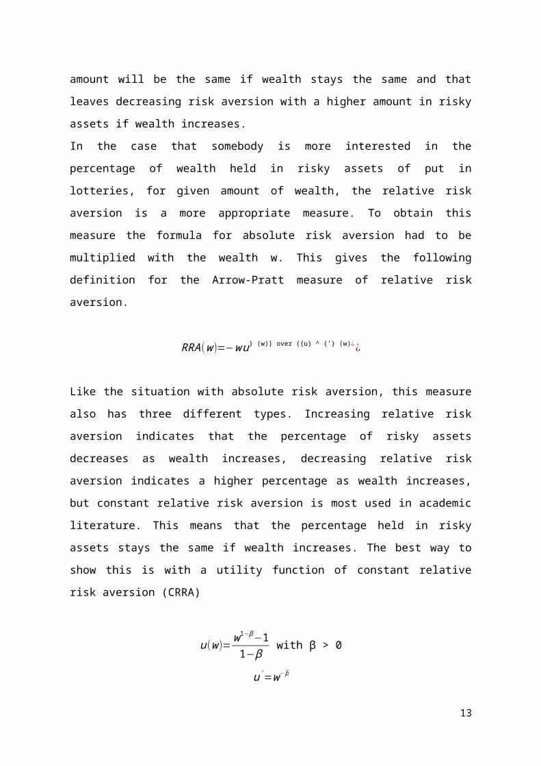
after they sold their house. Spoor (2008) describes some possibilities where people can live
in their house after retirement. An example of this is the reverse mortgage. In this
construction people keep the ownership of the house, but they receive a monthly payment
from the bank like an annuity. The individual keeps the right to live in the house for the rest
of his life which is also some sort of pension and the monthly payments look very much
like regular pension payments. Important to mention is that in this construction the bank or
other financial institutions takes over the risk that a person lives longer than expected, but
also the risk that the house prices decline. To make sure that individuals can continue to
live in their houses, it might be possible to offer these people extra help in for example
cleaning or service. These things can be paid with future pension payments. This reduces
future income streams, but guarantees an individual to live in their house. An example of
such a situation is shown in Figure 2.4.
25
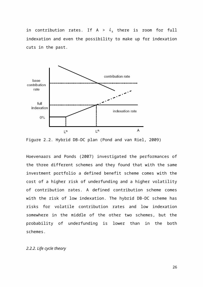
Figure 2.4 Personal wealth and its components including a house
Donkers, Lourenço and Dellaert (2012) have some recommendations for future research
with questionnaires. One of these recommendations is that the measurement of risk attitude
should always focus on the goal, in this case pension plans. This means that questions
should relate to this topic and not to general situations. With this in mind the choice-based
approaches seems more appropriate for pension plans, it gives a good insight in the
connection between risks and different outcomes in pension plans. The different outcomes
should always relate to the situation at retirement age. Another recommendation is that the
risk attitude is measured periodically, because the risk attitude of individuals can change
over time. Examples why the risk attitude can change is for example that people bought a
home, but also changes in income levels can influence the risk attitude. If the risk attitude is
measured periodically, the pension plan or investment mix can be changed on time to make
sure the pension plan is sufficient.
26
3. Data and methodology
All the data that is used in this thesis is collected from an questionnaire published on the
internet. The questions were asked in the Dutch language and the respondents filled in the
questionnaires in June or July 2012. The respondents received a link by email or social
media and they could fill in the questionnaire at a time that was most convenient for them
and the time needed to complete the questionnaire was not limited. This gives people the
time to read the questions carefully so they could understand them correctly, but also the
time to think about the answers they give. They did not receive any compensation for their
response.
3.1 Questionnaire
The research in this thesis is part of a larger study that investigates the risk attitude in
pension plans. The questions that are relevant for this research can be found in the
Appendix. Several aspects of risk attitude are investigated and in order to increase the
number of responses for each study the questionnaires of some of these studies are
combined in two separate questionnaires. Each questionnaire consists of a general set of
questions, these questions are the same for both questionnaires. Besides the general part
there is also a part that has all the questions of half of the students plus one selected
question of the other half of the group. This method is chosen so each student has the
largest number of respondents for their most important question, however the questionnaire
is not that long as when all the questions of all students were included. The longer the
questionnaire the larger the chance that people would not finish the entire set of questions.
The general set of questions includes questions that could explain the risk attitude of an
individual. Some of these questions are about facts, for example the questions about age,
gender and experience with investments. There are also questions included about a person’s
opinion, for example how the respondents think others would describe them. In the last type
of questions people are asked to choose between two options or to give a certain percentage
to outcomes. These questions are included to find out what the preferences of the
respondents are. The best example is the question that is a different version of the question
in Holt and Laury (2002). More information about this method can be found in chapter 2.1.
27
In this questionnaire there are also ten choices, but the respondents have to make the choice
between two options that describe different outcomes at the moment of retirement.
To make the questionnaire as uniform as possible all the questions where the respondents
can give several answers, there are seven possible answers. This also makes the analyses of
the data more convenient. The risk attitude that people show is very dependent of the
context in which the risk attitude is measured (Weber, Blais and Betz, 2002). This is the
reason why all the questions in the questionnaire relate to the topic of this research, the risk
attitude in pension plans. To be even more specific the focus lies on the risk attitude of
people at the moment of retirement. In the questions where people have to choose between
the two pension schemes this is shown by different amounts of pension an individual will
receive at retirement.
In total 247 respondents visited the website with the questionnaire. 184 filled in the
questionnaire with all the questions selected for this research, 63 filled in the questionnaire
that consists of all the general questions plus the question selected for this questionnaire. In
this question the respondents were asked in what kind of house they live in.
Several questionnaires were not completed or questions were not filled in correctly so for
analyses purposes these responses were left out the analyses. This leaves a total of 161
questionnaires that can be used for the research in this thesis. All of them can be used in the
analysis in the relationship between homeownership and risk attitude. 116 of the 161
questionnaires can also be used for the analysis between risk attitude and mortgage type or
maturities in interest rates.
3.2 Data and summary statistics
In this section an overview will be given of the answers that the respondents filled in on the
questionnaire. The questions included in the questionnaire are chosen because the answers
might tell something about the behavior of people regarding the risk in their pension plan.
The first type of questions requires an objective answer on the following topics:
Age Varying from 18 years to 70 yearsGender Male/femalePartner Having a partner and if that partner has its own pensionIncome 7 classes (from net monthly income less than 1225 euro to more than
3000 euro)
28
Living situation 3 choices (owning an own house, not owning a house or living with somebody)
Experience with Yes or no, also some form of investments are given (stock, mutual Investing funds and options)
The average age of the respondents is 40 years, 72% is male and 28% female. On the
question if they have a partner, 23% answered that they do not have a partner. The other
77% was asked if their partner has their own pension scheme, this was the case for 75% of
the respondents. Regarding the question about net monthly income, approximately half of
the respondents answered that they receive a net monthly income of more than 2.550 euro a
month. On the question about the living situation, a large majority of the respondents (70%)
answered that they live in their own house, 24% lives in a house they rent and the rest is
living in by somebody else. Two thirds of all the people that filled in the questionnaire has
experience with investing, mostly in stocks and mutual funds.
The second type of question is where respondents have to fill in what they think best
describes their knowledge and preferences:
Financial expertise 7 classes (from very low to very high)Carefulness 7 classes (from entirely disagree to entirely agree)(described by friends)10 gambling decisions Choice between pension scheme A and pension scheme BRisk tolerance 7 classes (from very low to very high)(pension payments)Feeling about having 7 classes (from very bad to very good)a job during pension Feeling if pension is 7 classes (from very bad to very good)50% of current income Risk tolerance 7 classes (from avoiding every risk to take a lot of risks)(pension investments) % of contributions Value from 0 to 100invested for pension
The respondents think their financial expertise is rather high. 67% filled in one of the three
highest categories and only 9 respondents of the 161 filled in the two lowest categories. The
answers on the second questions of the list above are well divided over the different
possibilities, only the first possibility has a few answers. This means that the respondents
think other people have the feeling they are pretty cautious in general. On the question with
the ten gambling decisions, the average switching point is 6.9. This means that on average
the respondents would take some risks with their monthly contributions to their pension
29
plan. Only 35 of the 161 respondents preferred pension scheme B in the first five gambles.
One other remarkable finding is that twice as much people switched to B on gamble 10 than
on gamble 9. Another question on pension payments is where respondents were asked what
their willingness for risks is with their pension payments. In contrary to the prior questions,
68% rate their willingness in the first three categories (very low, low and fairly low). The
average scores on the questions where was asked for feelings on having a job and 50% of
their current income were respectively 3.26 and 3.33. This means that on average the
feelings lie between a little bad feeling and neutral. The answers on the risk tolerance for
pension investments are very well distributed over the first six categories. This is in line
with the last question in this part, how much of your contribution should be used for
investments with risk. The answers varied from 0% to 100%, but the respondents indicated
that on average 40% of their contributions should be used for investments with risk.
The correlations for the different variables overall are not very high, however there are a
few numbers worth to mention. The correlation for the variables risk tolerance for pension
payments and pension investment is 0.71, which makes sense because the questions are
almost the same. The variable risk tolerance with pension investments is correlated for 0.53
with the % of contributions invested for pension. The living situation seems to correlate
with age and income at some level, respectively -0.62 and -0.44. This may indicate that
older a person is and the higher his net monthly income is, it is more likely that this person
owns his own house. The next paragraph shows a little more information about the living
situation and three other static variables.
The most relevant variable for this research is the question if people have their own house
or not. To get a good view of the sample and perhaps on the results of this research, we take
a closer look at the answer of the question on living situation. For example, how many
males are living in their own house and how many females is shown in Table 3.1. The
tables 3.2 and 3.3 below are showing the distribution per income group and age group.
30

Gender Owns a house Rents a
house
Lives in with somebody Total
Male 83 25 8 116
Female 29 13 3 45
Total 112 38 11 161
Table 3.1 Distribution of homeownership per gender
Income Owns a house Rents a
house
Lives in with somebody Total
< €1.225 8 8 6 22
€ 1.225-€1.500 5 3 0 8
€1.500- €1.850 2 6 2 10
€1.850- €2.150 13 7 1 21
€2.150- €2.550 14 4 0 18
€ 2.550-€3.000 18 4 2 24
>€3.000 52 6 0 58
Total 112 38 11 161
Table 3.2 Distribution of homeownership per income group
Age Owns a house Rents a
house
Lives in with somebody Total
<25 1 9 5 15
25-35 21 23 6 50
35-45 32 3 0 35
45-55 40 3 0 43
>55 18 0 0 18
Total 112 38 11 161
Table 3.3 Distribution of homeownership per age group
A few things can be seen in the tables above. All the tables show us that in total 112 of the
161 respondents own a house, 38 respondents rent a house and 11 are living in with
somebody. Table 3.1 shows the distribution per gender. The percentage of women that lives
in her own house is a little bit lower than men, respectively 64% and 71%. The most
31
interesting fact from Table 3.2 is that the number of respondents that own their own house
increases if they have a higher net monthly income, with a large group of respondents in the
highest income group, 52 respondents. The number of respondents that rent a house stays
more or less the same. Table 3.3 is showing us that the ratio of homeowners is larger in a
higher age group. In the group of respondents under the age of 25 the ratio is 7% and grows
to 100% in the last age group where people are older than 55 years.
Since there are is a group of respondents that filled in the questions that are only included in
the second set of questions, these questions are stated below. The topic of these questions
are related to homeownership and decisions about maturities of two different interest rates.
Maturity of mortgage 5 choices (from a variable rate to a >20 years fixed rate)rateMortgage type 4 different mortgage types (investment account mortgage, guaranteed
savings account mortgage, investment-savings account mortgage and an interest only mortgage)
Maturity of deposit 5 choices (from a variable rate to a >5 years fixed rate)rate
In total 116 respondents filled in the three questions above. The question on the maturity of
mortgage rate is included, because it relates to homeownership and also to risk attitude. The
longer the mortgage rate is fixed, the longer you have the certainty that you have to pay a
certain rate. The answers of the responded were well distributed over the five possible
answers. All the maturities had at least 12% and at most 33% of all the respondents
preference.
The distribution for the different mortgage type is not so equal. The type of mortgage can
also say something about the risk attitude of the respondents. Several aspects of a mortgage
are related to risk, for example if you want to start to pay back the mortgage immediately
and if you want to do some investments with your mortgage. None of the respondents chose
for the most risky mortgage, the investment account mortgage. 69 of the 116 respondents
will pick the savings account mortgage. This might indicate that people do not want to take
a lot of risks with their mortgage in general.
The last question is about the maturity of deposit rates. In contrast to the mortgage rate this
is not a rate that you have to pay, however you will receive this rate for the amount
deposited. Most of the respondents would pick a variable interest rate or only a fixed rate
32
that they will get if they choose a maturity of 1 year, respectively 27% and 36%. Only 9
respondents picked the maturity of more than 5 years.
33
4. Results
In this section, the results of the research are shown. The focus of this thesis is
homeownership and some aspects around this topic and how these factors might influence
the risk attitude of people regarding their pension plans. It is possible to see a house as an
investment that can be used for pension, by selling the house or a reversed mortgage.
Therefore the risk attitude in their pension plan can be influenced by homeownership, for
example that they consider their house as a risky asset and therefore they do not want to
take a lot of risk with their pension. Or the exact opposite, a house can generate an amount
of cash that is more or less fixed and therefore they want to take a bit more risk.
The risk attitude in pension plans is measured with two questions in the questionnaire. The
first question is the one where people had ten choices between two pension plans. The
moment they switch from pension plan A to pension plan B tells something about the risk
attitude of a person regarding their pension plan. If the switching point is high a person is
more risk averse than the person with a low switching point. This is question five in the
questionnaire.
The second question that is used for measuring risk attitude is the self-assessment question
where respondents had to fill in their risk tolerance with their pension payments. They had
seven choices from very low to very high. This is question six in the questionnaire.
The switching point is chosen as a proxy for risk attitude in pension plans for this research,
because the questions that determine this point focuses especially on the situation at
retirement date, as the literature recommends (Donkers, Lourenço and Dellaert, 2012). The
questions are also very clear, each question has only two choices. The data further showed
that almost none of the respondents were switching back from B to A again and the answers
are well distributed over the switching points 3 to 10.
The risk tolerance with pension payments is chosen as a proxy, because this is how
respondents would see their risk attitude themselves. The regressions in this chapter might
explain how factors like age, income or homeownership influences the way individuals see
their own risk attitude in pension payments. Just like the switching point it also focuses on
the situation at retirement date.
34
An advantage of all the variables, dependent and independent, used for the regressions in
this research is that with the exception of age, there are only a few answers possible. This
has the result that the possibilities of outliers in the dataset is very small. The chance that
the regressions are influenced by outliers is therefore very limited.
All the regressions in this chapter were also done with different dependent variables while
keeping the two independent variables the same. The other possible proxies for risk attitude
in pension plans are risk tolerance in pension investments, feeling of having a job during
the respondents pension and % of contributions invested for pension. These answers are all
coming from questions from the questionnaire. Almost none of the variables were
statistically significant and the p-values were much higher than in the regressions with the
switching point and risk tolerance with pension payments as the dependent variable, with
the exception of one variable. Respondents who think they have a high financial expertise
have a higher risk attitude, with the dependent variables risk tolerance in pension
investments and % of contributions invested for pension as a proxy for risk attitude.
The first and most important question is of course whether owning a house influences the
risk attitude regarding pension plans. The second question looks at the type of mortgage
people would prefer if they have to get a mortgage at the moment they filled in the
questionnaire. The third question focuses on interest rates and on the possible relationship
between the choices that people make in picking maturities for their mortgage rate or
deposit rate and the risk they want to take in their pension.
Not all the answers that the respondents gave on the questions in the questionnaire are used
in this research. Personal characteristics are included in the regressions as well as the
answer that people gave on the question how they would rate their financial expertise. One
reason why some questions of the questionnaire are not included in the regressions is
because the topic of these questions are comparable to other questions. For these
regressions only one question is chosen. An example of such a variable that is not included
is the experience with investments. In this research the financial expertise is chosen. Other
variables that are not chosen relate to the questions where respondents had to fill in how
they would feel in a certain situation, for example the question on the job they have to do
35
because if their pension is not sufficient. The answers did not deviate a lot from the average
and were not adding a lot of information to this research.
Most of the questions have only a limited number of possible answers, only the question
about age the respondents did not have a restricted number of answers. To be able to use
them in the regressions, dummy variables are added. Dummy variables make it possible to
separate the risk aversion in pension plan for example gender or the fact that the
respondents have a partner or not.
Some questions had seven possible answers and sometimes an answer was not chosen or
only a few times. In order to get a least ten answers for every variable, in some cases the
answers for categories are combined. For income the first two answers are combined and
the last two answers. This way there is a group of low income respondents (<1.500 euro), a
group of high income respondents (>2.550 euro) and a group of respondents with an
income between 1.500 en 2.550 euro. For financial expertise the same separation is made,
low expertise (very low and low), high expertise (high and very high) and average
expertise. The answers on the question if the respondents have a partner and if so a partner
with an own pension plan, is split in partner or no partner.
Table 4.1 shows the result from the regression with the switch moment as the dependent
variable and all the personal characteristics and self-assessment variable as the independent
variables. The regression has very little explanatory power, only 3.3 percent.
We see from Table 4.1 that the intercept value of 7 is significant at a level of 0.05. The age
variable has a coefficient of almost zero and the conclusion from this regression is that age
is not a factor that determines the risk aversion in pension plans. Although all the
independent variables are not statistically significant at a level of 0.05, there are a few
things that can be seen from Table 4.1, for example that men have a slightly lower
switching point than women. Regarding the income groups of the respondents, the
coefficient of the low income group and the high income group are both negative. This
means that the switching point for both these groups is lower than for the income group
with incomes between 1.500 and 2.550 euro. Having a partner might indicate that the risk
attitude is a little bit higher than the respondents without a partner. With p-values of 0.21
coefficient of the low income group and the high income group are both negative. This
36
Variable Coefficient P-value
Intercept 7.00 0.000
Age 0.01 0.536
Male -0.44 0.199
Low income -0.37 0.377
High income -0.13 0.711
Having a partner -0.27 0.469
Low financial expertise 0.75 0.214
High financial expertise 0.45 0.156
R-squared
Number of observations
0.033
161
Table 4.1 Impact of personal characteristics and self-assessment on the switching point.
means that the switching point for both these groups is lower than for the income group
with incomes between 1.500 and 2.550 euro. Having a partner might indicate that the risk
attitude is a little bit higher than the respondents without a partner. With p-values of 0.21
and 0.16, financial expertise comes closest to explaining risk attitude in this regression.
Remarkable is that both people who think they do not have a lot of expertise and people
who have the opposite opinion are more risk averse compared with people who find their
knowledge on financial matters neutral, although this finding is not statistically significant.
A possible explanation for this remarkable fact is that people with low financial expertise
are more reluctant to take risky decisions about financial matters because they do not know
what the consequences might be or they like the certainty. People who rate themselves as
someone with high expertise probably know what the downside is with a lot of risks and
therefore they want to take less risk.
Table 4.2 shows us the results from the regression with the same independent variables,
however the dependent variable is now the risk tolerance in pension payments. The
explanatory power of this regression is higher with 11.7 percent. The intercept is of course
much lower than with the switching point, because the question on risk tolerance only had
seven options. The p-value for this intercept is statistically significant at a level of 0.05. The
value of the intercept is 2.99 and this equals the answer under neutral in the questionnaire.
The coefficient of 0.38 for men indicates that men see themselves to take a little bit less risk
37
averse with pension payments than women. This is in line with the previous regression.
Although the p-values for gender and low income are lower than with the switching point
as dependent variable, with respectively 0.098 and 0.081 they are not low enough to be
statistically significant. Other variables have much higher p-values. An interesting fact from
Table 4.2 is that the conclusion for respondents in the groups that rate themselves as
someone with low expertise or high expertise, is different from the previous regression. In
this table the respondents who rate themselves as someone with high expertise, are less risk
averse than the other two groups. The coefficient for this group is positive while the
coefficient for the group who see themselves as someone with low expertise is negative. A
positive coefficient indicates a less risk averse individual. The reason for this can be that
these respondents would like to think they are taking more risks while in fact they do not.
Variable Coefficient P-value
Intercept 2.99 0.000
Age -0.01 0.570
Male 0.38 0.098
Low income -0.49 0.081
High income 0.19 0.410
Having a partner -0.16 0.515
Low financial expertise -0.47 0.237
High financial expertise 0.25 0.242
R-squared
Number of observations
0.117
161
Table 4.2 Impact of personal characteristics and self-assessment on the risk tolerance with
pension payments.
4.1 Homeownership
In this section the null hypothesis that homeownership has no effect on the risk attitude of
people regarding their pension plan is tested. The reason why this is the main question in
research is because owning a house is very similar to participating in a pension plan. A
house is a very large asset just like a pension. Another similarity is the fact that decisions
regarding a house have to be made for a long period, most mortgage that are necessary to
buy a house have a maturity of approximately thirty years. The last reason why a house is a
38
good reason to investigate the relationship is that a house can be some sort of pension as
well.
In the questionnaire people were asked to answer the question what their living situation is.
They could give the answer that they live in their own house, they rent a house or they are
living in with somebody. For the first regression the last two answers are combined and has
an explanatory power of 3.5 percent. The results are shown in Table 4.3.
Table 4.3 shows us that the values and p-values of the coefficients for personal
characteristics and self-assessment do not change a lot from the regression without
homeownership. The coefficient for homeownership is 0.28 with a p-value of 0.51. This
means that it is not possible to reject the null hypothesis and draw the conclusion that
homeownership has no effect on risk attitude in pension plans.
Variable Coefficient P-value
Intercept 7.09 0.000
Age 0.00 0.846
Male -0.44 0.198
Low income -0.35 0.403
High income -0.14 0.689
Having a partner -0.34 0.376
Low financial expertise 0.78 0.199
High financial expertise 0.45 0.158
Homeownership 0.28 0.512
R-squared 0.035
161Number of observations
Table 4.3 Impact of personal characteristics, self-assessment and homeownership on the
switching point.
Variable Coefficient P-value
Intercept 2.92 0.000
39
Age -0.00 0.951
Male 0.38 0.097
Low income -0.51 0.073
High income 0.20 0.390
Having a partner -0.10 0.711
Low financial expertise -0.50 0.215
High financial expertise 0.25 0.241
Homeownership -0.23 0.405
R-squared 0.121
161Number of observations
Table 4.4 Impact of personal characteristics, self-assessment and homeownership on the
risk tolerance with pension payments.
We can draw the same conclusion from Table 4.4. The p-value for homeownership is a
little bit lower with 0.405, however far from the level of 0.05 to be statistically significant.
The coefficient for personal characteristics and self-assessment questionnaire not very
different from Table 4.2. So with risk tolerance as a dependent variable the impact of
homeownership on risk attitude in pension plans, the conclusion must be that there is no
relationship.
To see if the it makes a differences if we take the three different living situations into
account, another regression is made and also a dummy variable for respondents who rent a
house is included. This regression has an explanatory power of 4 percent and the results are
shown in Table 4.5.
The intercept for this regression drops to 6.64 compared to the previous table and is still
significant at a level of 0.05. Noteworthy is the fact that although the p-value of the variable
of homeownership is still a lot higher than 0.05, the p-value is much smaller than the
previous regression. Both coefficients for the homeownership and renting a house are
positive, respectively 0.77 and 0.58, which means that they have a higher switching point
than people who are living in with somebody. This might be an interesting topic for further
research.
40
Variable Coefficient P-value
Intercept 6.64 0.000
Age 0.00 0.898
Male -0.42 0.225
Low income -0.29 0.501
High income -0.13 0.725
Having a partner -0.36 0.350
Low financial expertise 0.75 0.217
High financial expertise 0.41 0.120
Homeownership 0.77 0.255
Renting a house 0.59 0.350
R-squared 0.041
161Number of observations
Table 4.5 Impact of personal characteristics, self-assessment and living situation on the
switching point.
Of course the same splitting up is done for the other dependent variable and the results can
be found in Table 4.6. Except for the intercept there are still no variables statistically
significant. The explanatory power is with 12.2 percent still larger than the regression with
the switching point as the independent variable. The coefficients for the two dummy
variables are very low, 0.894 for homeownership and 0.615 for people who rent a house.
The p-values are much higher than in the previous regression. All the other coefficient are
more or less the same so with this dependent variable, therefore adding a dummy for people
who rent a house does not a difference.
Variable Coefficient P-value
Intercept 2.76 0.000
Age -0.00 0.923
Male 0.39 0.091
41
Low income -0.48 0.092
High income 0.21 0.378
Having a partner -0.10 0.691
Low financial expertise -0.51 0.207
High financial expertise 0.23 0.272
Homeownership -0.06 0.894
Renting a house 0.21 0.615
R-squared 0.122
161Number of observations
Table 4.6 Impact of personal characteristics, self-assessment and living situation on the risk
tolerance with pension payments.
4.2 Type of mortgage
To investigate if there is a relationship between risk attitude of people regarding their
pension plans and the type of mortgage people prefer, respondents had to fill in their
preferences on the topic mortgages. As explained in the chapter Data and Methodology, the
complete dataset is a combination of questionnaires and all the respondents filled in the
general questions and the question about homeownership. The question on mortgage type
and interest rates are filled in by a part of the group respondents, 116 of the 161 in total.
These upcoming regressions are therefore generated with a smaller set of data.
The respondents had the possibility to choose between a investment account mortgage, a
guaranteed savings account mortgage, a combination of the previous two mortgages and a
interest only mortgage. None of the respondents chose the investment account mortgage
and therefore only two dummy variables are included in the regression, the one for the
guaranteed savings account mortgage and for interest only mortgage. The regression has an
explanatory power of 12.9 percent and the results are shown in Table 4.7.
In Table 4.7 we see that there are a few changes compared to the tables above. The
intercept is lower than before, 6.39 and still statistically significant at a level of 0.05. The
coefficient for gender increased a bit in this regression and is now statistically significant
because of the p-value of 0.043. This means that men have a switching point that is 0.76
lower than women. Financial expertise is still not statistically significant, but the p-values
remain around 0.20 for low expertise and 0.10 for high expertise. The coefficients for the
42
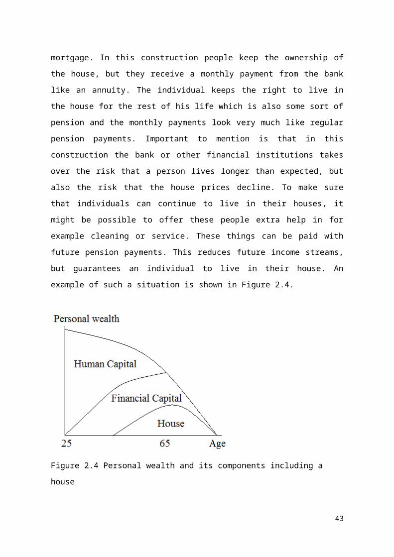
variables of a guaranteed savings account mortgage and an interest only mortgage are
respectively 0.94 and 1.25 with p-values of 0.020 and 0.026. This means that the switching
point of people who chose for such a mortgage is statistically significantly higher is than
people who chose a combined savings-investment account mortgage. The mortgage type
that has some investments in his characteristics is more risky than the other two types. The
conclusion from these numbers is that people seem to have the same attitude in their
pension as they have in picking a mortgage type. Therefore a mortgage might be
comparable with investments for a pension plan. This makes sense because it involves a
long-term decision and it is an large investment.
Variable Coefficient P-value
Intercept 6.40 0.000
Age 0.01 0.746
Male -0.76 0.043
Low income -0.16 0.743
High income 0.08 0.836
Having a partner -0.27 0.517
Low financial expertise 0.84 0.199
High financial expertise 0.62 0.110
Guaranteed savings
account mortgage
0.94 0.020
Interest only mortgage 1.25 0.026
R-squared 0.129
116Number of observations
Table 4.7 Impact of personal characteristics, self-assessment and mortgage type on the
switching point.
In the regression with the other dependent variable in this research the results show a
similar picture and has a much higher explanatory power than previous regressions. Table
4.8 reveals that besides the intercept, the two dummies for the mortgage types are
statistically significant. Just like the previous table, the conclusion must be that the chosen
mortgage type is related to the risk attitude in pension plans.
In this table, the male dummy is high and close to zero. This indicates that men are
statistically significantly less risk averse in pension plans than women. This is in line with
43
the research of Jianakoplos and Bernasek (1998) who also find evidence that women are
more risk averse than men regarding their pension plan.
Variable Coefficient P-value
Intercept 3.35 0.000
Age -0.00 0.740
Male 0.81 0.002
Low income -0.39 0.238
High income 0.11 0.673
Having a partner -0.25 0.385
Low financial expertise -0.87 0.051
High financial expertise 0.04 0.873
Guaranteed savings
account mortgage
-0.78 0.004
Interest only mortgage -0.97 0.010
R-squared 0.222
116Number of observations
Table 4.8 Impact of personal characteristics, self-assessment and mortgage type on the risk
tolerance with pension payments.
4.3 Maturity of interest rates
The last regressions have maturity of rates as independent variables. The first interest rate is
the one you have to pay for your mortgage. There is a possibility to fix this rates for a
number of years to avoid fluctuations in the interest rate you have to pay. The dummy
variables are chosen for an interest period of 5 to 10 years and for more than 10 years. The
results can be seen in Table 4.9.
The second interest rate is the one you can get on a deposit account. If you are willing to
put your money aside for a while, you can fix the interest rate you get on that account. The
dummy variables are the one for a period of 1 year and for periods longer than 1 year.
These results are shown in Table 4.10.
Variable Coefficient P-value
44

Intercept 6.98 0.000
Age 0.01 0.408
Male -0.77 0.049
Low income -0.41 0.405
High income 0.05 0.896
Having a partner -0.38 0.379
Low financial expertise 0.54 0.420
High financial expertise 0.76 0.055
Period 5-10 years 0.02 0.965
Period >10 years -0.06 0.889
R-squared 0.073
116Number of observations
Table 4.9 Impact of personal characteristics, self-assessment and mortgage rates on the
switching point.
The results are more or less the same for both regressions. Intercept and gender are both
statistically significant for a level of 0.05, for the deposit interest regression also the high
expertise variable is statistically significant for that same level. The coefficients for the
maturities of interest rates have small coefficients for all the dummies in both of the
regressions. Therefore the maturities seems to have no relationship with the switching
point. To see if there is a relationship with the risk tolerance, the regressions are also done
below with that dependent variable.
Variable Coefficient P-value
Intercept 6.85 0.000
Age 0.01 0.415
Male -0.79 0.041
Low income -0.41 0.396
High income 0.04 0.921
Having a partner -0.41 0.345
Low financial expertise 0.52 0.442
High financial expertise 0.79 0.048
45
Period 1 year 0.24 0.568
Period >1 year 0.19 0.650
R-squared 0.076
116Number of observations
Table 4.10 Impact of personal characteristics, self-assessment and deposit rates on the
switching point.
In the last two tables, Table 4.11 and Table 4.12, the results are shown for the impact of the
maturities of interest rates on the risk tolerance with pension payments. It is clear that the
maturity of mortgage rate does say a lot more than the maturities of deposit rates. Although
the p-values of the dummy for maturities in Table 4.11 are not low enough to be
statistically significant, they are much higher than the p-values for maturities of deposit
rates. This is a different conclusion than we can draw from the regressions with the
switching point. In the results from those regressions, no p-value for maturities was close to
level of 0.05.
The maturities of mortgage rates have to be chosen for a much longer period than the
maturities of deposit rates. Decision regarding pension plans, for example the risk attitude,
also have to be made for a longer period. This might explain the reason why the maturities
for mortgage rate seems to have more impact on the risk attitude of individuals than
maturities of deposit rates. Another explanation can be that the risks involved with
mortgage rates are more comparable with pension risks than deposit rates.
Variable Coefficient P-value
Intercept 3.14 0.000
Age -0.01 0.384
Male 0.88 0.001
Low income -0.26 0.425
High income 0.11 0.683
Having a partner -0.07 0.809
Low financial expertise -0.56 0.217
High financial expertise 0.00 0.990
Period 5-10 years -0.56 0.055
46
Period >10 years -0.49 0.082
R-squared 0.183
116Number of observations
Table 4.11 Impact of personal characteristics, self-assessment and mortgage rates on the
risk tolerance with pension payments.
Variable Coefficient P-value
Intercept 2.94 0.000
Age -0.01 0.374
Male 0.84 0.002
Low income -0.21 0.531
High income 0.10 0.716
Having a partner -0.17 0.568
Low financial expertise -0.54 0.241
High financial expertise -0.09 0.735
Period 1 year 0.09 0.747
Period >1 year -0.24 0.411
R-squared 0.162
116Number of observations
Table 4.12 Impact of personal characteristics, self-assessment and deposit rates on the risk
tolerance with pension payments.
47

5. Conclusion
The main purpose of the research in this thesis was to find out if there is relationship
between homeownership and the risk attitude in pension plans. Besides homeownership,
also mortgage type and maturities for two different rates are investigated to see if there is a
relationship with risk attitude. These topics are studied by using data collected from
questionnaires that were filled in on the internet. This questionnaire consists of questions
about personal characteristic as well as self-assessment questions. Also included were
questions to find out what preferences the respondents have regarding topics as pension
plans and mortgages. In line with Holt and Laury (2002), a switching point has been chosen
as the proxy for risk attitude in pension plans.
The conclusion from this research is that homeownership has no relationship with the risk
attitude in pension plans. Although a house is a large asset that has some of the
characteristics of a pension plan, it seems that it does not change the risk attitude regarding
pension plans if people own a house. Also the maturities that people would pick for their
mortgage rate and the rate they receive on a deposit account seems no factor in predicting
the risk attitude.
This research did find evidence that the choice in mortgage type can be used to predict the
risk attitude in pension plans. Respondents who would choose an investment-savings
account mortgage had a significantly lower switching point and lower risk tolerance with
pension payments. Therefore they are less risk averse than the respondents who would
choose a different type of mortgage, for example a savings account mortgage.
Another finding in this research is that men are significantly more risk seeking than women,
their switching point and risk tolerance was significantly lower in most of the regressions.
The group of respondents that believe they have a high expertise in financial matters had a
significantly higher switching point in a lot of regressions. This indicates that they are more
risk averse than people who do not believe they know a lot about financial matters.
However with the risk tolerance as dependent variable, high expertise was not statistically
significant.
48

The last finding is that age does not seem to have any influence on the risk attitude in
pension plans at all. The coefficients were very close to zero in all the results and were
never close to significant levels used in this research.
A recommendation for further research on this topic is to test the hypotheses with a larger
group of respondents. This research used a pool of 161 respondents for the main question
and 116 for the other topics. A larger group of respondents could be more reliable to draw
conclusions.
An improvement to this research can be made if the questionnaire is constructed in a better
way. Some respondents replied that they did not completely understood a question or that
the questionnaire was too long. This became clear when some questions were not filled in
correctly and a lot of questionnaires were not finished.
The last recommendation is that this topic will be investigated further in the future. The
Dutch housing market is continuously changing. The reason for this can be the economy,
but also the politics in the Netherlands. An example for this is the plan to restrict the
possibility to get an interest only mortgage. Also the pension market is changing,
participants are likely to bear more risk in their pension and defined contributions schemes
are more common every day. The effect of homeownership on risk attitude in pension plans
might become larger in the future.
49
References
Aaron, H.J. (1999), Retirement, research, and policy, in H.J. Aaron (ed), Behavioral
dimensions of retirement economics, Brookings Institutions Press Washington
DC/Russel Sage Foundation Newark, New York.
Allais, M. (1953), Le Comportement de l'Homme Rationnel devant le Risque: Critique des
Postulats et Axiomes de l'Ecole Americaine," Econometrica, 1953, 21 (4), 503-546.
Ameriks, J. and S. Zeldes (2001), How do household portfolio shares vary with age?,
mimeo, Columbia Graduate School of Business.
Arrow, K.J., “Liquidity Preference”, Lecture VI in “Lecture Note For Economics 285, The
Economics of Uncertainty”, pp.33-53, undated, Stanford University.
Arrow, K.J. (1965), The theory of risk aversion. Reprinted in Essays in the Theory of Risk
Bearing (1971) 90-109. Markham Publ., Chicago.
Banks, J., R. Blundell and S. Tanner (1998), Is there a Retirement Savings Puzzle?,
American Economic Review 88 (4), 769-788.
Benartzi, S. and Thaler, R. (1999), Risk Aversion or Myopia? Choices in Repeated
Gambles and Retirements Investments, Management Science 45(3), pp.364-381.
Benartzi, S. and R. Thaler (2001), Naïve diversification strategies in defined contribution
saving plans, American Economic Review 91(1), pp. 79-98.
Bernouilli, D., “Specimen Theoriae Novae de Mensura Sortis.” Comentarii Academia
Scientiarum Imperalis Petropolitanae, 1738, 5, pp. 175-192, translated by L.Sommer
in Econometrica, 1954, 22, pp. 23-36
Bikker, J.A., Broeders, D.W.G.A., Hollanders, D.A., & Ponds, E.H.M. (2009), Pension
Funds' Asset Allocation and Participant Age: A Test of the Life-Cycle Model.
(Netspar Discussion Paper, 09/2009-032) pp. 1-20
Bikker, J.A., Broeders, D.W.G.A., Hollanders, D.A., & Ponds, E.H.M. (2009), De invloed
van leeftijd op het beleggingsbeleid van pensioenfondsen, Economisch Statistische
Berichten, 94 (4573), 27 november, 710-713.
Binswanger, H. P. (1980). Attitudes Toward Risk: Experimental Measurement in Rural
India. American Journal of Agricultural Economics, 62(3), 395-407.
50
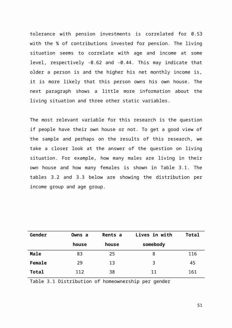
Bluethgen, Ralph, Andreas Gintschel, Andreas Hackethal and Armin Muller (2008),
Financial Advice and Individual Investors' Portfolios, working paper, available at
SSRN: http://ssrn.com/abstract=968197.
Bodie Z., McLeavy D. and Siegel L.B. (2007): The Future of Life-Cycle Saving and
Investing, The Research Foundation of CFA Institute.
Bovenberg, L., Koelewijn, W. and Kortleve, N. (2011), ‘Naar een dynamische
toekomstvoorziening. Integratie van werk, pensioen, zorg en wonen over de
levensloop’, NEA-paper 40, mei 2011.
Bovenberg. A.L. , Koijen R., Nijman Th. And Teulings C. (2007): Saving and investing
over the life cycle and the role of collective pension funds, in: De Economist vol.
155: pp. 347-415.
Campbell, J.Y., and L.M. Viceira (2002): Strategic Asset Allocation, Oxford University
Press. Choi, J., D. Laibson, B. Madrian and A. Metrick (2004), For better or for
worse: default effects and 401(k) savings behaviour, in Bodie, Z., J.B. Shoven and
D. Wise (eds), Perspectives on the Economics of Aging, University of Chicago
Press, Chicago.
Dellaert, B.G.C. and Turlings, M. (2011), Measuring Risk Profiles for Pension
Investments, Netspar NEA discussion paper (in Dutch), Tilburg: Netspar.
Donkers, B, and A. van Soest (1999), Subjective measures of household preferences and
Financial decisions, Journal of Economic Psychology 20, pp.613-642.
Donkers, B., Lourenço, C. and Dellaert, B.G.C. (2012), “Measuring and Debiasing
Consumer Pension Risk Attitudes,” Netspar Panel paper, forthcoming.
Ellsberg, D. (1961), “Risk, Ambiguity, and the Savage Axioms,” The Quarterly Journal of
Economics, vol. 75, no. 4 (Nov 1961)
Guiso, L., M. Haliassos and T. Jappelli (2003), Household stockholding in Europe: where
do we stand and where do we go?, Economic Policy 36, April 2003, pp. 125-170.
Gustman, A.L. and T.L. Steinmeier (1999), Effects of Pensions on Savings: Analysis with
Data from the Health and Retirement Study, Carnegie Rochester Conference Series
on Public Policy 50, pp. 271-324.
Harrison, Glenn W. and Elisabet E. Rutström (2008), Risk Aversion in the Laboratory, In
J.C. Cox & G.W. Harrison (eds), Risk Aversion in Experiments (vol. 12, pp. 42-
196). Bingley, UK: Emerald (Research in Experimental Economics).
51
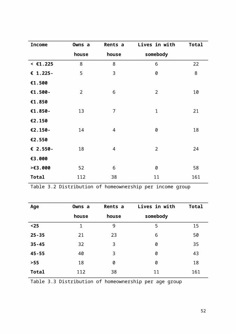
Hartog, J., Ferrer-I-Carbonell A. and Jonker, N. (2003), Linking Measured Risk
Aversion to Individual Characteristics, Kyklos, 55(1), 3-26.
Hershey, J. C., and Schoemaker, P. J. H. (1980). Risk Taking and Problem Context in the
Domain of Losses: An Expected Utility Analysis. Journal of Risk and Insurance,
47(1), 111-32.
Hoevenaars, R. M. and E. H. M. Ponds (2007) Valuation of intergenerational transfers in
funded collective pension schemes. Netspar working paper, forthcoming in
Insurance: Mathematics and Economics.
Holt, C. A., and Laury, S. K. (2002). Risk Aversion and Incentive Effects. American
Economic Review 92(5), 1644-1655.
Huberman, G. and W. Jiang (2004), The 1/N Heuristic in 401(k) Plans, Columbia Business
School Working paper, March 2004.
Jianakoplos, N.A. and A. Bernasek (1998), Are Women More Risk Averse? Economic
Inquiry 36(4) pp. 620-630.
Kahneman, D. and Tversky, A. (1979). Prospect Theory: An Analysis of Choice Under
Risk. Econometrica, 47(2), 263-291.
Kahneman, D., J. Knetsch and R. Thaler (1991), Anomalies: The Endowment Effect, Loss
Aversion and Status Quo Bias, Journal of Economic Perspectives 1, pp.193-206.
Laury, S.K. and Holt, C.A. (2005). Further Reflections on Prospect Theory, Experimental
Economics Center Working Paper Series 2006-23, Experimental Economics Center,
Andrew Young School of Policy Studies, Georgia State University.
Loewenstein, G. (2000), Emotions in Economic Theory and Economic Behaviour,
American Economic Review 90(2), pp. 426-432.
Loewenstein, G. (2004), Interview in Financial Times, October 15, p. 8.
Lusardi, A. (1999), Information, Expectations, and Savings for Retirement, in: H.J. Aaron
Behavioral dimensions of retirement economics, Brookings Institutions Press,
Washington DC/Russel Sage foundation Newark, New York.
Merton, Robert C. (2006), Allocating Shareholder Capital to Pension Plans, Journal of
Applied Corporate Finance, vol. 18, no. 1, 15-24.
Mitchell, O.S., M.S. Gordon and M.M. Twinney (1997), Assessing the Challenges to the
Pension system, in Gordon, Mitchell and Twinney, Positioning Pensions for the
Twenty-First Century, Pension Research Council and University of Pennsylvania
52
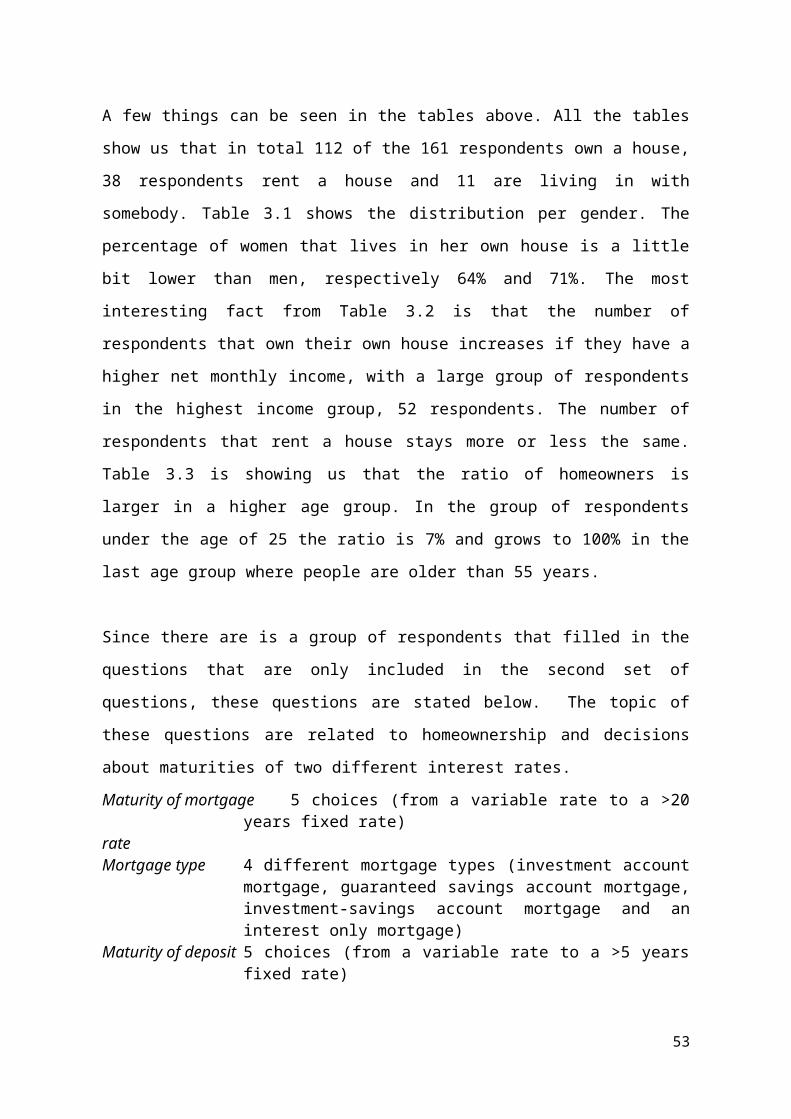
press Publishers, Philadelphia, 1997.
Molenaar, R., & Ponds, E.H.M. (2009). Differentiatie Naar Leeftijd in de Financiering van
Collectieve Pensioenen. (NEA Netspar Paper, NEA 7) pp. 1-44.
Mullainathan, S., Markus, N. and Schoar, A. (2009), The Market for Financial Advice: An
Audit Study, paper presented at AFA Denver meetings.
Myagkov, M., & Plott, C. (1997). Exchange Economies and Loss Exposure: Experiments
Exploring Prospect Theory and Competitive Equilibria in Market Environments.
American Economic Review, 87(5), 801-828.
Peters, E., Hibbard J., Slovic, P. and Dieckmann, N. (2007), Numeracy Skill and the
Communication, Comprehension and Use of Risk-Benefit Information, Health
Affairs, 26 (3), 741-748.
Ponds, E.H.M. and Riel, B. van (2009). Sharing risk: The Netherlands' new approach to
pensions. Journal of Pension Economics and Finance, 8(1), 91-105.
Pratt, J.W. (1964), “Risk Aversion in the Small and in the Large”, Econometrica, Vol.32,
No. ½, pp. 122-136.
Rabin, M. (2000). Risk Aversion and Expected-Utility Theory: A Calibration Theorem.
Econometrica 68, 1281-1292.
Samuelson, W. and R. Zeckhauser (1988), Status Quo Bias in Decision Making, Journal of
Risk and Uncertainty 1, pp. 7-59.
Savage, L.J. (1954), The Foundations of Statistics. New York: John Wiley
Spoor, L. (2008), Je huis of je leven? Eigen betalingen voor woon- en
Welzijnsvoorzieningen voor ouderen en optimalisatie van de pensioenportfolio,
NEA-paper 9, Tilburg: Netspar
Statman, M. (1999), Behavioural Finance: Past Battles and Future Engagements, Financial
Analysts Journal, pp. 18-27.
Teulings, C., and C. de Vries (2006), ‘General Accounting, Solidarity and Pension Losses’,
De Economist, vol. 154, no. 1, (March 2006), pp. 347-415.
Thaler, R.H. and S. Benartzi (2004), Save More Tomorrow: Using Behavioural Economics
to Increase Employee Saving, Journal of Political Economy 112 (1), pp.164-187.
Thaler, R. and H. Shefrin (1981), An economic theory of self-control, Journal of Political
Economy 89 (April), pp.392-406.
53
Tversky, A. and Kahneman, D. (1992). Advances in Prospect Theory: Cumulative
Representation of Uncertainty. Journal of Risk and Uncertainty, 5(4), 297-323.
van Rooij, M.C.J., Kool, C.J.M. and Prast, H.M. (2007). "Risk-return preferences in the
pension domain: are people able to choose?," Working Papers 05-04, Utrecht
School of Economics.
Viceira, L.M. (2007): Life-Cycle Funds, working paper Harvard Business School.
von Neumann, J. and Morgenstern, O. 1944. Theory of games and economic behavior.
Princeton, NJ: Princeton University Press.
Wakker, P. P. and D. Deneffe (1996), Eliciting von Neumann-Morgenstern Utilities
When Probabilities Are Distorted or Unknown, Management Science, 42(8), 1131-
1150.
Weber, E.U., Blais, A.R., Betz, E. (2002). A Domain specific risk-attitude scale: Measuring
risk perceptions and risk behaviors. Journal of Behavioral Decision Making, 15,
263–290.
Zuckerman, Marvin, Sybil B. Eysenck and Hans J. Eysenck (1978), Sensation Seeking in
England and America: Cross-Cultural, Age and Sex comparisons, Journal of
Consulting and Clinical Psychology, 46(1), 139-149
54

Appendix
Questionnaire
Dank u wel voor uw bereidheid om deze vragenlijst in te vullen. Daarmee draagt u bij aan
wetenschappelijk onderzoek en aan inzicht van uw pensioenuitvoerder in uw voorkeuren.
Dit onderzoek gaat over risico’s en hoe het pensioenfonds van uw werkgever daarmee
omgaat. Wie meer risico loopt, kan meer verdienen, maar ook meer verliezen. Wie minder
risico loopt, weet zekerder wat het resultaat zal zijn, maar dat is dan waarschijnlijk wel een
lager bedrag. Daarom zijn het belangrijke keuzes waar deze enquête over gaat. We zijn
benieuwd naar uw mening!
De antwoorden die u geeft in deze vragenlijst zijn volledig anoniem.
Vraag 1Hoe beoordeelt u uw eigen kennis en kunde met betrekking tot financiële beslissingen?
o Zeer laago Laago Redelijk laago Neutraalo Redelijk hoogo Hoogo Zeer hoog
Vraag 2Heeft u ervaring met beleggen?
o Neeo Ja
Vraag 3Hieronder staan een aantal beleggingsvormen. Kunt u aangeven of u daarin momenteel belegt? (Meerdere antwoorden mogelijk)
o Aandelen en/of obligatieso Opties, futures en/of turbo’s, speeders of sprinterso Beleggingsfondseno Ik beleg niet in bovenstaande beleggingsvormeno Niet van toepassing
55
Vraag 4Uw vrienden omschrijven u als een voorzichtig persoon.
o Helemaal mee oneenso Oneenso Beetje oneenso Neutraalo Beetje eenso Eenso Helemaal mee eens
Vraag 5Stelt u zich voor dat u 1.670 euro per maand verdient.Uw pensioenfonds vernieuwt. Pensioenopbrengsten worden minder zeker en u wordt gevraagd een nieuwe regeling te kiezen. Hieronder ziet u steeds twee mogelijke regelingen die verschillen in hoeveel pensioen u krijgt met welke waarschijnlijkheid. U krijgt een aantal keuzes voorgelegd waarbij steeds de kans op de verschillende pensioenuitkomsten anders zijn.Kiest u per vraag welke pensioenregeling voor u het meest aantrekkelijk is (alle bedragen zijn netto.
Keuze 1Bij pensioenregeling A krijgt u 1002 euro per maand of 1169 per maand als totaal pensioen (inclusief AOW). De kans dat u 1002 euro per maand krijgt is 9/10 en de kans dat u 1169 euro per maand krijgt is 1/10.Bij pensioenregeling B krijgt u 668 euro per maand of 1503 per maand als totaal pensioen (inclusief AOW). De kans dat u 668 euro per maand krijgt is 9/10 en de kans dat u 1503 euro per maand krijgt is 1/10.
Onderstaand ziet u beide regelingen in een grafiek.Welke pensioenregeling kiest u?
o Pensioenregeling Ao Pensioenregeling B
56
Keuze 2Bij pensioenregeling A krijgt u 1002 euro per maand of 1169 per maand als totaal pensioen (inclusief AOW). De kans dat u 1002 euro per maand krijgt is 8/10 en de kans dat u 1169 euro per maand krijgt is 2/10.Bij pensioenregeling B krijgt u 668 euro per maand of 1503 per maand als totaal pensioen (inclusief AOW). De kans dat u 668 euro per maand krijgt is 8/10 en de kans dat u 1503 euro per maand krijgt is 2/10.
Onderstaand ziet u beide regelingen in een grafiek.Welke pensioenregeling kiest u?
o Pensioenregeling Ao Pensioenregeling B
Keuze 3Bij pensioenregeling A krijgt u 1002 euro per maand of 1169 per maand als totaal pensioen (inclusief AOW). De kans dat u 1002 euro per maand krijgt is 7/10 en de kans dat u 1169 euro per maand krijgt is 3/10.Bij pensioenregeling B krijgt u 668 euro per maand of 1503 per maand als totaal pensioen (inclusief AOW). De kans dat u 668 euro per maand krijgt is 7/10 en de kans dat u 1503 euro per maand krijgt is 3/10.
Onderstaand ziet u beide regelingen in een grafiek.Welke pensioenregeling kiest u?
o Pensioenregeling Ao Pensioenregeling B
57
Keuze 2Bij pensioenregeling A krijgt u 1002 euro per maand of 1169 per maand als totaal pensioen (inclusief AOW). De kans dat u 1002 euro per maand krijgt is 8/10 en de kans dat u 1169 euro per maand krijgt is 2/10.Bij pensioenregeling B krijgt u 668 euro per maand of 1503 per maand als totaal pensioen (inclusief AOW). De kans dat u 668 euro per maand krijgt is 8/10 en de kans dat u 1503 euro per maand krijgt is 2/10.
Onderstaand ziet u beide regelingen in een grafiek.Welke pensioenregeling kiest u?
o Pensioenregeling Ao Pensioenregeling B
Keuze 3Bij pensioenregeling A krijgt u 1002 euro per maand of 1169 per maand als totaal pensioen (inclusief AOW). De kans dat u 1002 euro per maand krijgt is 7/10 en de kans dat u 1169 euro per maand krijgt is 3/10.Bij pensioenregeling B krijgt u 668 euro per maand of 1503 per maand als totaal pensioen (inclusief AOW). De kans dat u 668 euro per maand krijgt is 7/10 en de kans dat u 1503 euro per maand krijgt is 3/10.
Onderstaand ziet u beide regelingen in een grafiek.Welke pensioenregeling kiest u?
o Pensioenregeling Ao Pensioenregeling B
58
Keuze 4Bij pensioenregeling A krijgt u 1002 euro per maand of 1169 per maand als totaal pensioen (inclusief AOW). De kans dat u 1002 euro per maand krijgt is 6/10 en de kans dat u 1169 euro per maand krijgt is 4/10.Bij pensioenregeling B krijgt u 668 euro per maand of 1503 per maand als totaal pensioen (inclusief AOW). De kans dat u 668 euro per maand krijgt is 6/10 en de kans dat u 1503 euro per maand krijgt is 4/10.
Onderstaand ziet u beide regelingen in een grafiek.Welke pensioenregeling kiest u?
o Pensioenregeling Ao Pensioenregeling B
Keuze 5Bij pensioenregeling A krijgt u 1002 euro per maand of 1169 per maand als totaal pensioen (inclusief AOW). De kans dat u 1002 euro per maand krijgt is 5/10 en de kans dat u 1169 euro per maand krijgt is 5/10.Bij pensioenregeling B krijgt u 668 euro per maand of 1503 per maand als totaal pensioen (inclusief AOW). De kans dat u 668 euro per maand krijgt is 5/10 en de kans dat u 1503 euro per maand krijgt is 5/10.
Onderstaand ziet u beide regelingen in een grafiek.Welke pensioenregeling kiest u?
o Pensioenregeling A
59
o Pensioenregeling B
Keuze 6Bij pensioenregeling A krijgt u 1002 euro per maand of 1169 per maand als totaal pensioen (inclusief AOW). De kans dat u 1002 euro per maand krijgt is 4/10 en de kans dat u 1169 euro per maand krijgt is 6/10.Bij pensioenregeling B krijgt u 668 euro per maand of 1503 per maand als totaal pensioen (inclusief AOW). De kans dat u 668 euro per maand krijgt is 4/10 en de kans dat u 1503 euro per maand krijgt is 6/10.
Onderstaand ziet u beide regelingen in een grafiek.Welke pensioenregeling kiest u?
o Pensioenregeling Ao Pensioenregeling B
Keuze 7Bij pensioenregeling A krijgt u 1002 euro per maand of 1169 per maand als totaal pensioen (inclusief AOW). De kans dat u 1002 euro per maand krijgt is 3/10 en de kans dat u 1169 euro per maand krijgt is 7/10.Bij pensioenregeling B krijgt u 668 euro per maand of 1503 per maand als totaal pensioen (inclusief AOW). De kans dat u 668 euro per maand krijgt is 3/10 en de kans dat u 1503 euro per maand krijgt is 7/10.
Onderstaand ziet u beide regelingen in een grafiek.Welke pensioenregeling kiest u?
o Pensioenregeling A
60
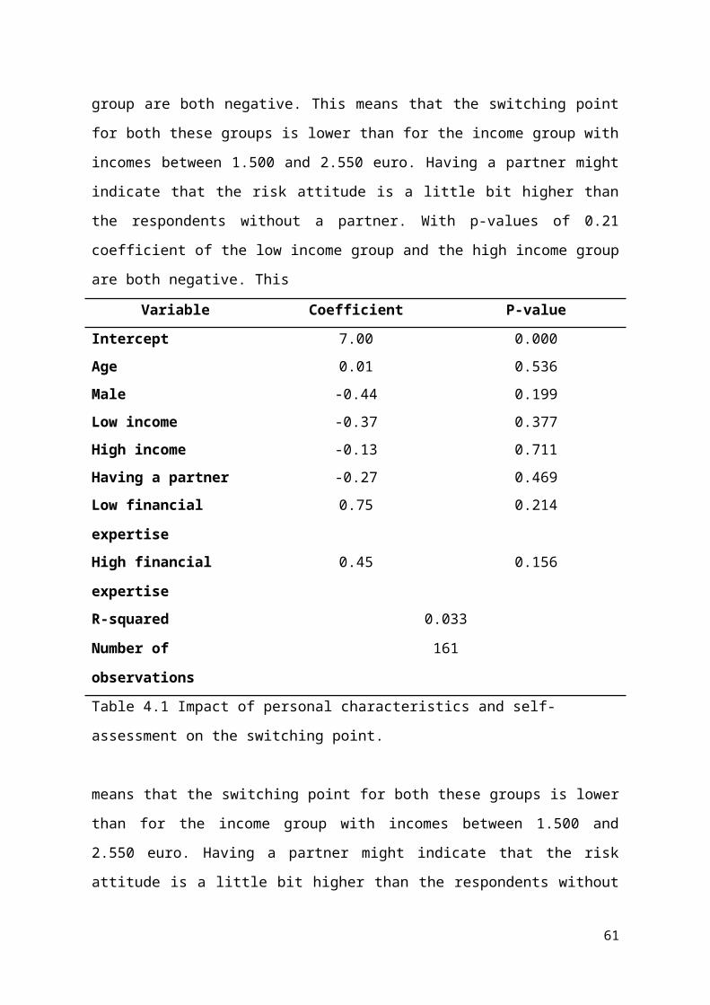
o Pensioenregeling B
Keuze 8Bij pensioenregeling A krijgt u 1002 euro per maand of 1169 per maand als totaal pensioen (inclusief AOW). De kans dat u 1002 euro per maand krijgt is 2/10 en de kans dat u 1169 euro per maand krijgt is 8/10.Bij pensioenregeling B krijgt u 668 euro per maand of 1503 per maand als totaal pensioen (inclusief AOW). De kans dat u 668 euro per maand krijgt is 2/10 en de kans dat u 1503 euro per maand krijgt is 8/10.
Onderstaand ziet u beide regelingen in een grafiek.Welke pensioenregeling kiest u?
o Pensioenregeling Ao Pensioenregeling B
Keuze 9Bij pensioenregeling A krijgt u 1002 euro per maand of 1169 per maand als totaal pensioen (inclusief AOW). De kans dat u 1002 euro per maand krijgt is 1/10 en de kans dat u 1169 euro per maand krijgt is 9/10.Bij pensioenregeling B krijgt u 668 euro per maand of 1503 per maand als totaal pensioen (inclusief AOW). De kans dat u 668 euro per maand krijgt is 1/10 en de kans dat u 1503 euro per maand krijgt is 9/10.
Onderstaand ziet u beide regelingen in een grafiek.Welke pensioenregeling kiest u?
o Pensioenregeling A
61
o Pensioenregeling B
Keuze 10Bij pensioenregeling A krijgt u 1002 euro per maand of 1169 per maand als totaal pensioen (inclusief AOW). De kans dat u 1002 euro per maand krijgt is 0/10 en de kans dat u 1169 euro per maand krijgt is 10/10.Bij pensioenregeling B krijgt u 668 euro per maand of 1503 per maand als totaal pensioen (inclusief AOW). De kans dat u 668 euro per maand krijgt is 0/10 en de kans dat u 1503 euro per maand krijgt is 10/10.
Onderstaand ziet u beide regelingen in een grafiek.Welke pensioenregeling kiest u?
o Pensioenregeling Ao Pensioenregeling B
Vraag 6Hoe groot is uw bereidheid om risico te lopen met uw pensioenuitkering?
o Zeer laago Laago Redelijk laago Neutraalo Redelijk hoogo Hoogo Zeer hoog
62
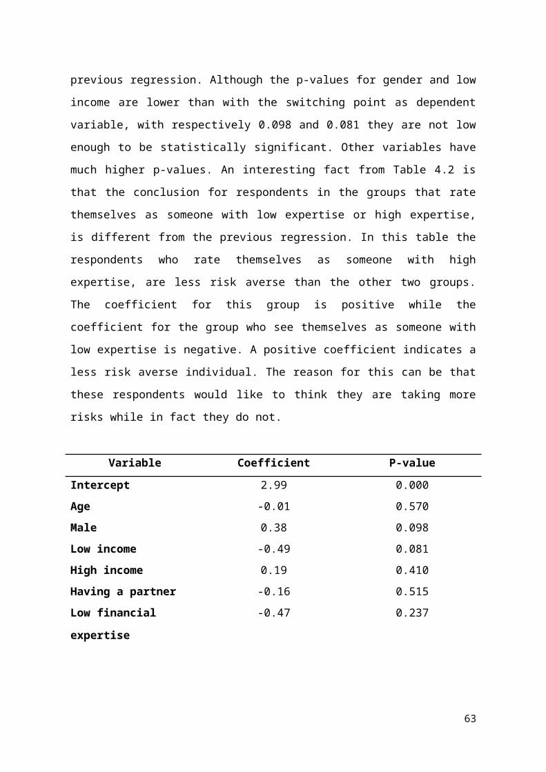
Vraag 7aHoe denkt u dat u zich voelt als u tijdens uw pensionering een bijbaantje heeft omdat uw pensioen niet toereikeind is voor uw uitgavenpatroon?
o Zeer slechto Slechto Redelijk slechto Neutraalo Redelijk goedo Goedo Zeer goed
Vraag 7bHoe denkt u dat u zich voelt als u op uw geplande pensioenleeftijd 50% van uw laatste nettoloon ontvangt als pensioen (inclusief AOW)?
o Zeer slechto Slechto Redelijk slechto Neutraalo Redelijk goedo Goedo Zeer goed
Vraag 7cHoe karakteriseert u zichzelf als het gaat om beleggen voor uw pensioen?
o Ik vermijd elk risicoo Ik vermijd de meeste risico’so Ik vermijd sommige risico’so Neutraalo Ik neem een beetje risicoo Ik accepteer diverse risico’so Ik neem veel risico
Vraag 8Pensioenregeling worden in de toekomst misschien flexibeler. In sommige nieuwe pensioenregelingen krijgt u zelf meer te zeggen over de hoeveelheid risico die u met uw pensioengeld loopt.Stelt u zich voor dat u een keuze kunt maken over hoe uw ingelegde pensioenpremies worden belegd.U moet kiezen hoeveel van uw pensioenpremie zonder risico wordt belegd (sparen) en hoeveel beleggingen met risico worden belegd (bijvoorbeeld in aandelen). De verwachte opbrengst van beleggingen zonder risico is 3% en van beleggingen in een pakket van wereldwijde aandelen met risico is 7% per jaar.Geeft u op de onderstaande schaal van 0 tot 100 aan hoeveel van uw pensioenpremie u met risico zou willen beleggen (met een verwachte – maar niet zekere – opbrengst van 7%) en
63
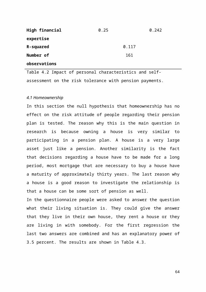
hoeveel zonder risico (met een gegarandeerde opbrengst van 3%).Een waarde van 0 geeft aan dat u wilt dat uw hele pensioenpremie zonder risico zal worden belegd en een waarde van 100 geeft aan dat u wilt dat uw hele pensioenpremie met risico zal worden belegd.Waardes daar tussenin geven aan welk deel u van uw pensioenpremie u wilt beleggen met risico.
Vraag 9In deze vraag willen we graag weten wat uw verwachtingen zijn voor beleggingen met risico. We laten u daarom eerst hieronder de gemiddelde opbrengst zien van alle wereldwijde aandelen voor de afgelopen 16 jaar.
Vraag 9aHoe schat u het risico van de onderstaande belegging in?
o Zeer laago Laago Redelijk laago Neutraalo Redelijk hoogo Hoogo Zeer hoog
64
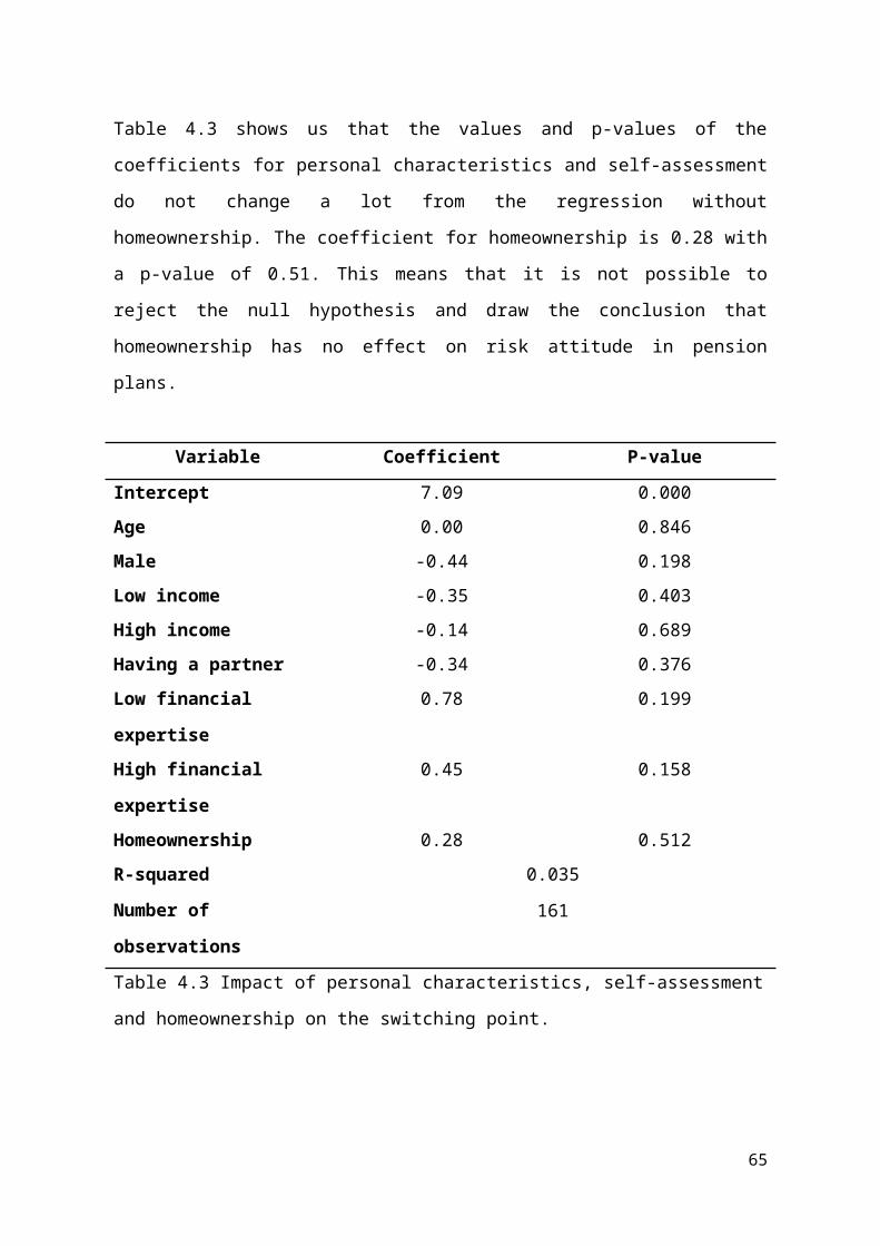
Vraag 9bStel dat u 100 euro in dit fonds kunt beleggen.Wat verwacht u dat de waarde van dit fonds volgend jaar gemiddeld zal zijn?Mijn verwachting voor de waarde van volgend jaar = ……. Euro
Vraag 9cWat denkt u dat de minimale waarde volgend jaar zal zijn (waarvoor er maar een hele kleine kans is dat de werkelijke opbrengst lager is)?De minimale waarde van volgend jaar = ……. Euro
Vraag 9dWat denkt u dat de maximale waarde volgend jaar zal zijn (waarvoor er maar een hele kleine kans is dat de werkelijke opbrengst hoger is)?De maximale waarde van volgend jaar = ……. Euro
Vraag 10Stelt u voor dat u morgen al met pensioen zou gaan.Bij welk bedrag vindt u uw pensioen dan hoog en bij welk bedrag vindt u het laag?
Heel hoog als het tenminste ….% van mijn netto loon is
65
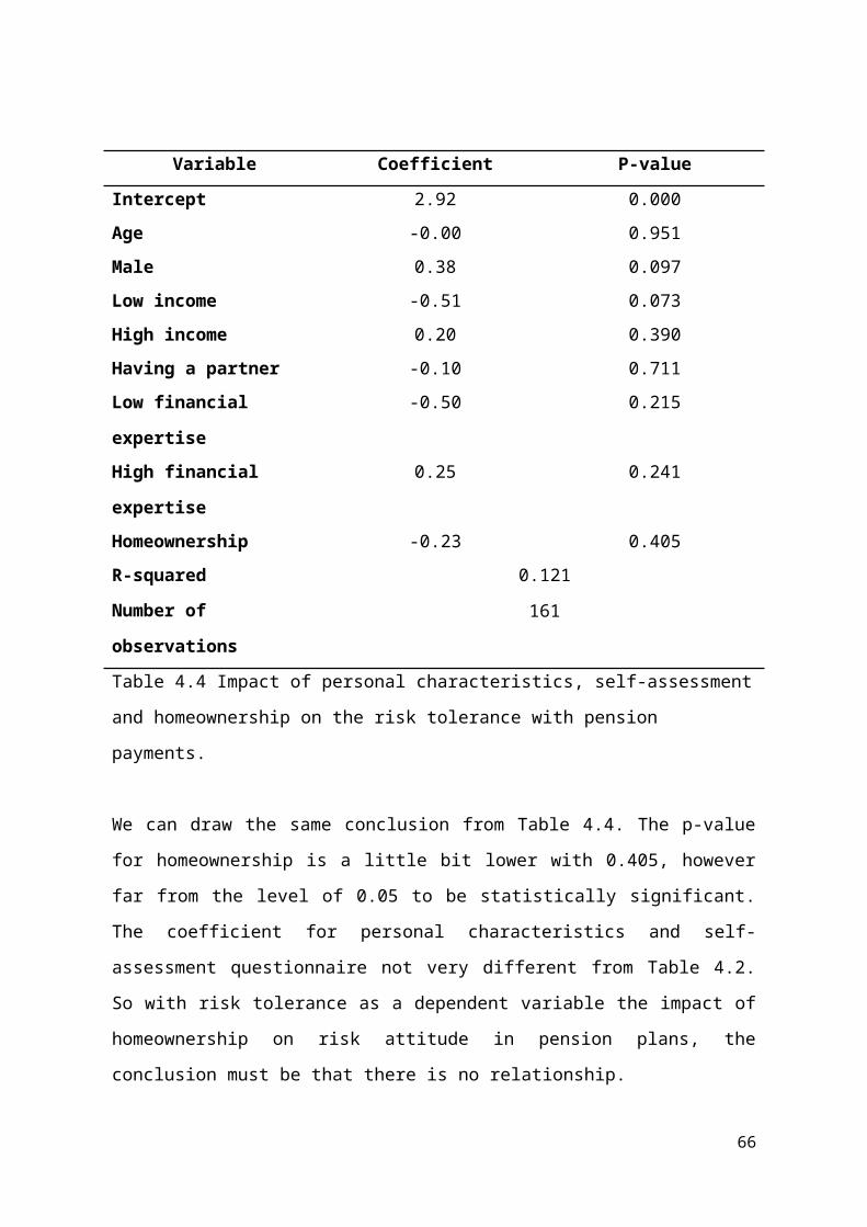
Hoog als het tenminste ….% van mijn netto loon isNiet hoog/niet laag als het ….% van mijn netto loon isLaag als het tenminste ….% van mijn netto loon isHeel laag als het tenminste ….% van mijn netto loon is
Vraag 11Wat is uw huidige woonsituatie? (Welke woonsituatie is het meest op u van toepassing?)
o Ik woon in een eigen koophuiso Ik woon in een eigen huurhuiso Ik woon bij iemand in huis
Vraag 12Bij het afsluiten van een nieuwe hypotheek heeft u vaak de keuze om de rente voor een bepaalde keuze vast te zetten of om een variabele rente te betalen. In de rentevaste periode blijft de hypotheekrente die u moet betalen hetzelfde. U bent dan in deze periode beschermd tegen een rentestijging, maar u profiteert ook niet van een rentedaling. Na afloop van de rentevaste periode kunt u opnieuw kiezen voor een rentevaste periode of voor een variabele rente, maar dan met de rentestanden van dat moment. Als u op dit moment een nieuwe hypotheek zou afsluiten, voor welke periode zou u dan kiezen?
o Een variabele renteo Een rentevaste periode van <5 jaaro Een rentevaste periode van 5-10 jaaro Een rentevaste periode van 10-20 jaaro Een rentevaste periode van >20 jaar
Vraag 13Bij het afsluiten van een nieuwe hypotheek kunt u kiezen uit veel verschillende hypotheekvormen. Stel dat u een hypotheekvorm zou moeten kiezen, welke van de vier onderstaande vormen zou het liefste kiezen?
o Een spaarhypotheek : Bij een spaarhypotheek lost u tijdens de looptijd niet af. U betaalt rente en legt maandelijks een bedrag in. Met deze inleg bouwt u een spaartegoed op. Dit spaartegoed gebruikt u aan het einde van de looptijd om de lening af te lossen.
o Een beleggingshypotheek : Met de beleggingshypotheek lost u tijdens de looptijd niet af. U bouwt vermogen op via beleggingen. Met dit vermogen lost u aan het einde van de looptijd uw hypotheekschuld helemaal of voor een deel af. Met een beleggingshypotheek is het mogelijk dat u met een restschuld blijft zitten. Beleggingen kunnen namelijk minder rendement opleveren dan verwacht. Ook de maandelijkse inleg kunt u (deels) verliezen. Omdat u niet tussendoor aflost, blijft uw rente gelijk zo lang uw rente vast staat.
66
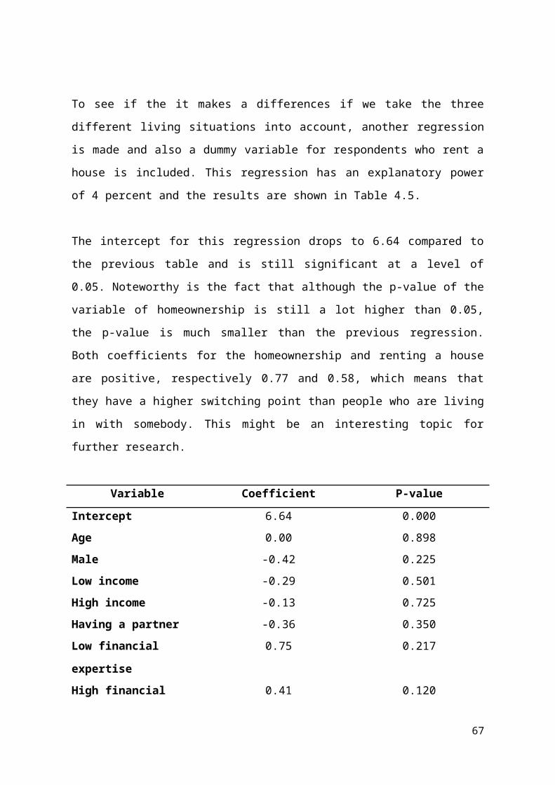
o Een spaar- en beleggingshypotheek : Met een spaar- en beleggingshypotheek bouwt u vermogen op door te sparen en te beleggen. De keuze is aan u. En wilt u uw keuze na verloop van tijd veranderen? Dan is dat mogelijk. Hieraan zijn kosten verbonden. Om uw tegoed op te bouwen legt u maandelijks een bedrag in. Met dit spaar- en beleggingstegoed lost u aan het einde van de looptijd uw hypotheekschuld helemaal of voor een deel af. Het is mogelijk dat u een restschuld overhoudt, omdat beleggingen minder rendement kunnen opleveren dan verwacht. Ook de maandelijkse inleg kunt u (deels) verliezen. Uw spaartegoed houdt u wel zeker.
o Een aflossingsvrije hypotheek : De naam zegt het al: op deze hypotheek lost u niet af. U betaalt alleen rente. Deze kunt u vaak van uw inkomen aftrekken voor de inkomstenbelasting. Gedurende de looptijd lost u niet af op deze hypotheek. Hierdoor blijft het bedrag dat u elke maand aan rente betaalt gelijk. Dit geldt uiteraard alleen als u de rente heeft vastgezet voor een bepaalde periode en niet als u voor een variabele rente heeft gekozen. Omdat u gedurende de looptijd niet aflost, heeft u na afloop een hypotheekschuld. Deze schuld moet u terugbetalen. U kunt bijvoorbeeld terugbetalen met spaargeld of met de opbrengst uit de verkoop van uw woning. In de Gedragscode Hypothecaire Financieringen staat dat u maximaal 50% van de waarde van de woning met een aflossingsvrije hypotheek mag financieren
Vraag 14Stel u heeft een huis dat volledig is afbetaald op het moment dat u met pensioen gaat. U had verwacht dat het pensioenfonds 70% van uw laatstverdiende loon zou uitkeren als pensioen, maar achteraf blijkt dat dit lager is dan verwacht. Bij welke situatie bent u bereid om uw huis te verkopen om uw pensioen aan te vullen tot 70% van uw laatstverdiende loon?
o Een variabele renteo Een periode van 1 jaaro Een periode van 2 jaaro Een periode van 2 tot 5 jaaro Een periode van >5 jaar
Vraag 29Wat is uw leeftijd?
Vraag 30Wat is uw netto maandinkomen?
o Minder dan €1.225o Tussen de €1.225 en €1.500o Tussen de €1.500 en €1.850o Tussen de €1.850 en €2.150o Tussen de €2.150 en €2.550o Tussen de €2.550 en €3.000o Meer dan €3.000
67
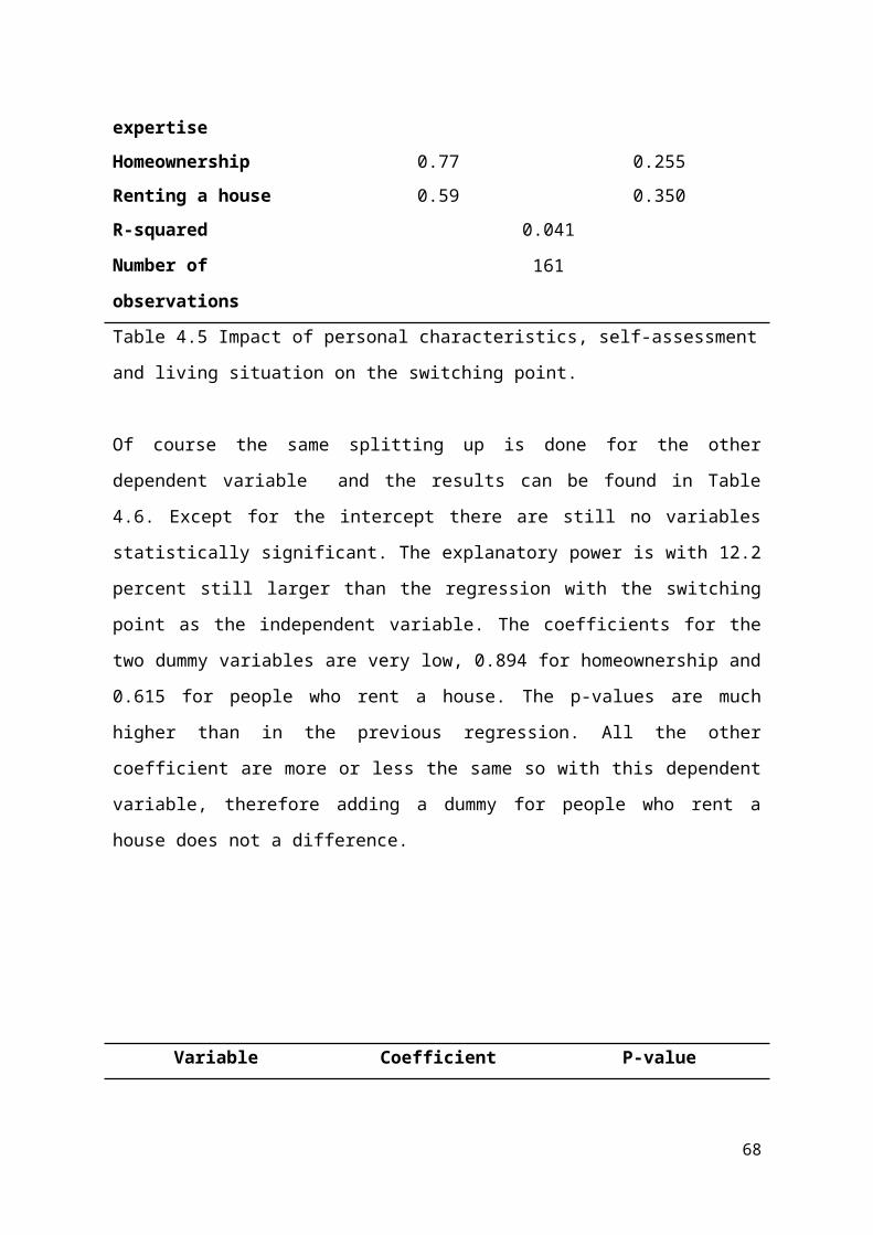
Vraag 31Wat is uw geslacht?
o Mano Vrouw
Vraag 32Heeft u een partner en zo ja, heeft uw partner een eigen pensioen?
o Nee, ik heb geen partnero Ja, ik heb een partner, maar hij/zij heeft geen eigen pensioeno Ja, ik heb een partner en hij/zij heeft een eigen pensioen
Dit is het einde van de vragenlijst, wij bedanken u dat u de tijd hiervoor genomen heeft. Mocht u nog opmerkingen hebben over de vragenlijst dan willen wij vragen om deze hieronder in te vullen.U kunt hier uw opmerking(en) (bijv. problemen of onduidelijkheden) kwijt.
68