Embed Size (px)
Citation preview
Chapter IX The Integral Transform Methods IX.3 Finite Fourier Transform November 26, 2018 755
IX.3 Finite Fourier Transform
IX.3.1 Introduction - Finite Integral Transform 756
Table “Finite Fourier Transform” 760
IX.3.2 Heat Equation in the Finite Layer 762 IX.3.3 Conduction and Advection 768
IX.3.4 Heat Equation in the Sphere 774
IX.3.5 Examples – plug flow over heating ribs 781
Chapter IX The Integral Transform Methods IX.3 Finite Fourier Transform November 26, 2018 756
IX.3.1 INRODUCTION The integral transforms we studied before (Fourier and Laplace) can be symbolically denoted as a pair of operators
:T u u→ 1 :T − u u→
defined with the help of the integral transform kernel ( ),K xλ
( ) ( ) ( ),D
u u x K x dxλ λ= ∫
( ) ( ) ( )D
u x u K ,x dλ λ λ= ∫
These transforms can be applied for solution of IBVP of classical PDE’s. In general, the procedure consisted of the following steps: 1) application of the appropriate integral transform eliminates the
corresponding derivative from the equation; 2) the transformed equation is solved for the transformed unknown
function; 3) the solution of IBVP is obtained by the inverse integral transform.
Integral Transform over Finite Interval The integral transforms were applied in the infinite and semi-infinite
domains. Now, we want to discover how to solve IBVP for PDE’s in the finite domain [ ]21 L,L∈ξ with the help of the integral transform. To do this we want integral transforms to posses the same property – the ability to eliminate the corresponding derivative from the PDE. Let us investigate this problem. The general form of an integral transform in the Cartesian coordinate system over the finite domain [ ]1 2,x L L∈ can be written as
( ) ( ) ( )2
1
L
L
u u x K ,x dxλ λ= ∫
where ( ),K xλ is the kernel of the integral transform. Apply this transform to the second derivative with respect to x and see how to choose ( ),K xλ (apply integration by parts twice):
( ) ( )2
1
2
2 ,L
L
u xK x dx
xλ
∂
∂ ∫ ( ) ( )2
1
L
L
u xK ,x d
xλ
∂ = ∂
∫
( ) ( ) ( ) ( )2 2
11
, ,L L
LL
u x u xK x K x dx
x x xλ λ
∂ ∂ ∂= − ∂ ∂ ∂
∫
( ) ( ) ( )2 2
11
, ,L L
LL
u xK x K x du
x xλ λ
∂ ∂= − ∂ ∂
∫
( ) ( ) ( ) ( ) ( )2 2 2
1 11
2
2, , ,L L L
L LL
u xK x K x u x u K x dx
x x xλ λ λ
∂ ∂ ∂ = − + ∂ ∂ ∂ ∫
( ) ( ) ( ) ( ) ( ) ( ) ( ) ( ) ( )2
1
L 22 1
2 1 2 2 1 1 2L
u L u LK ,L K ,L K ,L u L K ,L u L u K ,x dx
x x x x xλ λ λ λ λ
∂ ∂ ∂ ∂ ∂ = − − + + ∂ ∂ ∂ ∂ ∂ ∫ ( )◊
x
Chapter IX The Integral Transform Methods IX.3 Finite Fourier Transform November 26, 2018 757
Obviously, the integral term turns into the transformed function if, in general, the kernel of transform has the property
( ) ( ) ( )2
2 , ,K x c K xx
λ λ λ∂=
∂
This condition reminds the eigenvalue problem.
Auxiliary Sturm-Liouville Problem Let us consider the corresponding auxiliary Sturm-Liouville Problem (SLP) with the parameter λ in the Cartesian coordinate system: ( ) ( )2 0X x X xλ′′ + = ( ) ( ) 0LXhLXk 1111 =+′− (SLP) ( ) ( )2 2 2 2 k X L h X L 0′ + = which according to the Sturm-Liouville Theorem possesses infinitely many values of the parameter nλ , ,...2,1n = (eigenvalues) for which SLP has non-trivial solutions ( )nX x (eigenfunctions). Therefore,
eigenfunctions ( )nX x satisfy boundary conditions: ( ) ( ) 0LXhLXk 1n11n1 =+′− ( ) ( )2 n 2 2 n 2 k X L h X L 0 ′ + =
for all ,...2,1n = . In particular, the general solution of the given equation of SLP is given by
Solution of the SLP ( ) 1 2cos sinnX c x c xξ λ λ= +
In addition, the set of all eigenfunctions ( ){ }nX x , ,...2,1n = is a complete set of orthogonal functions, for which we can introduce the norm by
( )2
1
1 2
2 L
n nL
X X x dx
= ∫
Let the kernel of the integral transform be
Kernel ( ) ( ) ( ), n
n nn
X xK x K x
Xλ= = ( )∗
Differention of the kernel ( )∗ with respect to ξ twice yields
( )nK x′′ ( )n
n
X xX′′
= ( )
n
nn
XX ξλ ′′−
=2
( )2n nK xλ= −
The property which is wanted. From this follows that the last term in the equation ( )◊ becomes
( ) ( ) ( )2 2
1 1
22 2 2
2 , ,L L
n n n n nL L
u K x dx uK x dx u ux
λ λ λ λ λ λ∂= − = − = −
∂∫ ∫
Now, consider homogeneous boundary conditions, which are obviously satisfied by the kernel ( )nK x because it is constructed from the solution of SLP: if 0k,k 21 ≠ then
( ) ( ) 01111 =+′− LKhLKk nn ⇒ ( ) ( )11
11 LK
khLK nn =′
( ) ( ) 02222 =+′ LKhLKk nn ⇒ ( ) ( )22
22 LK
khLK nn
−=′
Chapter IX The Integral Transform Methods IX.3 Finite Fourier Transform November 26, 2018 758
Substitute the kernel and the derivative of the kernel into the first terms of equation ( )◊ , then
( ) ( ) ( ) ( ) ( ) ( ) ( ) ( ) ( )2
1
L 22 1
2 1 2 2 1 1 2L
u L u LK ,L K ,L K ,L u L K ,L u L u K ,x dx
x x x x xλ λ λ λ λ
∂ ∂ ∂ ∂ ∂ − − + + ∂ ∂ ∂ ∂ ∂ ∫
( ) ( ) ( ) ( ) ( ) ( ) ( ) ( )2 1 22 1 2 2 1 1n n n n n n
u L u LK L K L K L u L K L u L u
x x x xλ
∂ ∂ ∂ ∂= − − + −
∂ ∂ ∂ ∂
( ) ( ) ( ) ( ) ( ) ( ) ( ) ( )2 1 22 12 1 2 2 1 1
2 1n n n n n n
u L u L h hK L K L K L u L K L u L ux x k k
λ∂ ∂ −
= − − + −∂ ∂
0k,k 21 ≠ ( ) ( ) ( ) ( ) ( ) ( )1 2 21 2n 1 1 n 2 2 n n
1 2
u L u Lh hK L u L K L u L ux k x k
λ∂ ∂
= − + + + − ∂ ∂
Therefore, if we choose eigenfunctions ( )nX x (and the corresponding
kernel of the integral transform ( ) ( )nn
n
X xK x
X= ) such that they satisfy
the same homogeneous boundary conditions as of the function ( )u x in the BVP for PDE’s, then both the first two terms in the previous expression become zero. So, we can make the conclusion that in this case, application of the integral transform to the second derivative yields
( )2
1
L 22
n n n2L
u K x dx ux
λ∂= −
∂∫
if the kernel ( )nK x is constructed from the solution of the corresponding SLP with the same homogeneous boundary conditions as for the function
( )u x in BVP for PDE. If conditions for ( )u x are not homogeneous and both are of Robin type, then
( ) ( )1 1 11
1 1
u L h fu Lx k k
∂− + =
∂
( ) ( )2 2 22
2 2
u L h fu L
x k k∂
+ =∂
and the derivative is transformed to
( ) ( ) ( )2
1
L 221 2
n n 1 n 2 n n21 2L
f fu K x du K L K L uk kx
λ∂= + −
∂∫
If 0h,h 21 ≠ then
( ) ( ) 01111 =+′− LKhLKk nn ⇒ ( ) ( )1n1
11n LK
hk
LK ′=
( ) ( ) 02222 =+′ LKhLKk nn ⇒ ( ) ( )2n2
22n LK
hkLK ′−
=
( ) ( ) 21 2n 1 n 2 n n
1 2
f f... K L K L uk k
λ= + − ( ) ( ) ( ) ( ) ( ) ( )1 2 21 2n 1 1 n 2 2 n n
1 2
u L u Lk kK L u L K L u L uh x h x
λ∂ ∂
′ ′= − + − + − ∂ ∂
Chapter IX The Integral Transform Methods IX.3 Finite Fourier Transform November 26, 2018 759
Finite Fourier Transform over [ ]1 2,L L The integral transform with the desired operational property
nu ( ) ( )2
1
L
nL
u x K x dx= ∫ ( ) ( )2
1
Ln
nL
X xu x dx
X= ∫
( ) ( )2
1
1 L
nn L
u x X x dxX
= ∫
The orthogonal set of eigenfunctions ( ){ }nX x , ,...2,1n = can be applied
for the generalized Fourier series expansion of the function ( )u x
( ) ( )1
n nn
u x a X x∞
=
= ∑
where the Fourier coefficients are
( ) ( )2
1
2
1 L
n nLn
a u x X x dxX
= ∫
Then expansion can be written as
( )u x ( )1
n nn
a X x∞
=
= ∑ ( ) ( ) ( )2
1
21
1 L
n nn Ln
u x X x dx X xX
∞
=
=
∑ ∫
( ) ( ) ( )2
11
Ln n
n n nL
X x X xu x dx
X X
∞
=
=
∑ ∫
( ) ( ) ( )2
11
L
n nn L
u x K x dx K x∞
=
=
∑ ∫
( )1
n nn
u K x∞
=
= ∑
which can be treated as the inverse transform in the form of the series with
the same kernel ( ) ( )nn
n
X xK x
X= .
Therefore, we have the following integral transform pairs:
Finite Fourier Transform over [ ]1 2,L L nu ( ) ( )2
1
L
nL
u K dξ ξ ξ= ∫ integral transform
( )u x ( )n nn 1
u K x∞
=
= ∑ inverse transform
Finite Fourier Transform over [ ]0,L nu ( ) ( )L
n0
u K dξ ξ ξ= ∫ integral transform
( )u x ( )n nn 1
u K x∞
=
= ∑ inverse transform
Application of the Finite Fourier Transform over [ ]0,L to 2nd derivative:
( ) ( )2
20
L
n
u xK x dx
x ∂ ∂
∫ ( ) ( ) ( ) ( ) ( ) ( ) ( ) ( ) ( )L 2
n n n n n20
u L u 0K L K 0 K L u L K 0 u 0 u K x dx
x x x x x∂ ∂ ∂ ∂ ∂ = − − + + ∂ ∂ ∂ ∂ ∂
∫
( ) ( ) ( ) ( ) ( ) ( ) ( ) ( ) 2n n n n n n
u L u 0K L K 0 K L u L K 0 u 0 u
x x x xλ
∂ ∂ ∂ ∂ = − − + − ∂ ∂ ∂ ∂ ( )◊◊
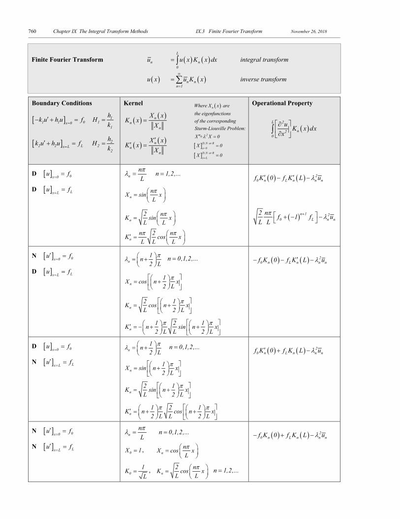
Chapter IX The Integral Transform Methods IX.3 Finite Fourier Transform November 26, 2018 760
Finite Fourier Transform nu ( ) ( )L
n0
u x K x dx= ∫ integral transform
( )u x ( )n nn 1
u K x∞
=
= ∑ inverse transform
Boundary Conditions
[ ]1 1 0x 0k u h u f=
′− + = 11
1
hHk
=
[ ]2 2 Lx Lk u h u f=
′ + = 22
2
hHk
=
Kernel
( ) ( )nn
n
X xK x
X=
( ) ( )nn
n
X xK x
X′
′ =
Operational Property
( )L 2
n20
u K x dxx
∂ ∂
∫
D [ ] 0x 0u f=
=
D [ ] Lx Lu f=
=
nnLπλ = n 1,2,...=
nnX sin xLπ =
n2 nK sin xL L
π =
nn 2 nK cos xL L Lπ π ′ =
( ) ( ) 2
0 n L n n nf K 0 f K L uλ′ ′− −
( )n 1 20 L n n
2 n f 1 f uL L
π λ+ + − −
N [ ] 0x 0u f=
′ =
D [ ] Lx Lu f=
=
n1n2 L
πλ = +
n 0,1,2,...=
n1X cos n x2 L
π = +
n2 1K cos n xL 2 L
π = +
n1 2 1K n sin n x2 L L 2 L
π π ′ = − + +
( ) ( ) 2
0 n L n n nf K 0 f K L uλ′− − −
D [ ] 0x 0u f=
=
N [ ] Lx Lu f=
′ =
n1n2 L
πλ = +
n 0,1,2,...=
n1X sin n x2 L
π = +
n2 1K sin n xL 2 L
π = +
n1 2 1K n cos n x2 L L 2 L
π π ′ = + +
( ) ( ) 2
0 n L n n nf K 0 f K L uλ′ + −
N [ ] 0x 0u f=
′ =
N [ ] Lx Lu f=
′ =
nnLπλ = n 0,1,2,...=
0X 1= , nnX cos xLπ =
01KL
= , n2 nK cos xL L
π =
n 1,2,...=
( ) ( ) 2
0 n L n n nf K 0 f K L uλ− + −
( )
[ ][ ]
n
2
D,N or R
x=0D,N or R
x L
Where X x are the eigenfunctions of the corresponding Sturm-Liouville Problem:X + X 0
X 0
X 0
λ
=
′′ =
=
=
Chapter IX The Integral Transform Methods IX.3 Finite Fourier Transform November 26, 2018 761
D [ ] 0x 0u f=
=
R [ ]2 2 Lx Lk u h u f=
′ + =
nλ are positive roots of the equation:
( ) ( )2cos L H sin L 0λ λ λ+ =
( )n nX sin xλ=
( )( )n
nn
n
sin xK
sin 2 LL2 4
λ
λλ
=
−
( )( )
n nn
n
n
cos xK
sin 2 LL2 4
λ λ
λλ
′ =
−
( ) ( ) 2L0 n n n n
2
ff K 0 K L uk
λ′ + −
N [ ] 0x 0u f=
′ =
R [ ]2 2 Lx Lk u h u f=
′ + =
nλ are positive roots of the equation:
( ) ( )2sin L H cos L 0λ λ λ− =
( )n nK cos xλ=
( )( )n
nn
n
cos xK
sin 2 LL2 4
λ
λλ
=
+
( ) ( ) 2L0 n n n n
2
ff K 0 K L uk
λ− + −
R [ ]1 1 0x 0k u h u f=
′− + =
D [ ] Lx Lu f=
=
nλ are positive roots of the equation:
( ) ( )1cos L H sin L 0λ λ λ+ =
( )n nX sin x Lλ= −
( )( )
nn
n
n
sin x LK
sin 2 LL2 4
λ
λλ
− =
−
( ) ( )nn
n
sin LK 0
Xλ−
=
( )( )
n nn
n
n
cos x LK
sin 2 LL2 4
λ λ
λλ
− ′ =
−
( ) nn
n
K LXλ′ =
( ) ( ) 20n L n n n
1
fK 0 f K L u
kλ′− −
or
( ) ( ) 20n L n n n
1
fK 0 f K L u
kλ′ ′− −
R [ ]1 1 0x 0k u h u f=
′− + =
N [ ] Lx Lu f=
′ =
nλ are positive roots of the equation:
1sin L H cos L 0λ λ λ− =
( )n nX cos x Lλ= −
( )( )
nn
n
n
cos x LK
sin 2 LL2 4
λ
λλ
− =
+
( ) ( ) 2
0 n L n n nf K 0 f K L uλ+ −
R [ ]1 1 0x 0k u h u f=
′− + =
R [ ]2 2 Lx Lk u h u f=
′ + =
nλ are positive roots of the equation:
( ) ( ) ( ) ( )21 2 1 2H H sin L H H cos L 0λ λ λ λ− + + =
( ) ( )n n n 1 nX cos x H sin xλ λ λ= +
( ) ( )( )
n n 1 nn
2 2n 1 2 1
2 2n 2
cos x H sin xK
H H HL2 2H
λ λ λ
λ
λ
+=
+ + + +
( ) ( ) 20 Ln n n n
1 2
f fK 0 K L uk k
λ+ −
Chapter IX The Integral Transform Methods IX.3 Finite Fourier Transform November 26, 2018 762
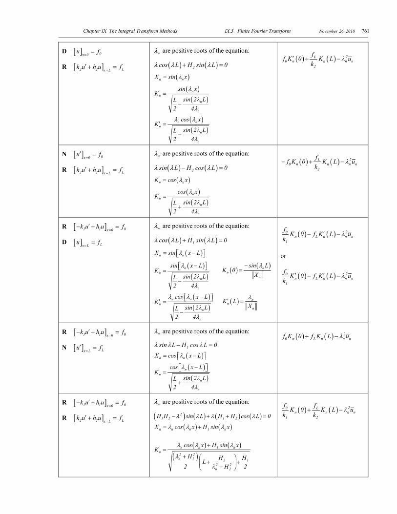
IX.3.2 Heat Equation in the Finite Layer Consider heat conduction in the 1-dimensional slab with heat generation
Equation: ( ),2
2
1 u u S x tt xα
∂ ∂= +
∂ ∂ [ ]L,0x ∈ 0t >
Initial condition: ( ) ( )xu0,xu 0=
Boundary conditions: ( )1 1 1 1,x 0
uk h u h u tx ∞
=
∂ − + = ∂ ( )0f t= Robin
[ ] ( )Lx Lu u t=
= ( )Lf t= Dirichlet 1) Integral transform According to the table FFT, the kernel of the integral transform
corresponding to Robin-Dirichlet boundary conditions is:
( ) ( )n
nn X
LxsinxK −=
λ , where ( )n
nn 4
L2sin2LX
λλ
−=
and eigenvalues nλ are the positive roots of the equation 0LsinHLcos =+ λλλ
2) Transformed equation According to the table FFT (R-D), the second derivative of ( )t,xu w.r.t. x is transformed to
( )L 2
n20
u K x dxx
∂ ∂
∫( ) ( ) ( ) ( )0 2
n L n n n1
f tK 0 f t K u t
kλ′= − −
( ) ( ) ( ) ( )0 2nn L n n
1 n
f tK 0 f t u t
k Xλ
λ= − −
Transform the source function and initial condition:
( )[ ] ( ) ( )tSdxxKt,xS nn
L
0
=∫
( )[ ] ( ) n,0n
L
00 udxxKxu =∫
Then the transformed equation has the form ( ) ( ) ( ) ( ) ( ) ( )n 0 2n
n L n n n1 n
u t f t1 K 0 f t u t S tt k X
λ λα
∂= − − + ∂
( ) ( ) ( )n 2n n n
u tu t Q t
tαλ
∂= − +
∂
left end is exposed to aconvective enviromentwith time dependenttemperature
( )L
right end is following the prescribed time-dependent temperature f t
( )0u x
( )u x,t
0 Lx
[ ] ( )Lx Lu u t=
=( )1 1 1 1,
x 0
uk h u h u tx ∞
=
∂ − + = ∂
Chapter IX The Integral Transform Methods IX.3 Finite Fourier Transform November 26, 2018 763
( ) ( ) ( )n 2n n n
u tu t Q t
tαλ
∂+ =
∂
where ( ) ( ) ( ) ( ) ( )0 nn n L n
1 n
f tQ t K 0 f t S t
k Xλα α
= − +
The transformed solution is determined by variation of parameter:
( ) ( ),
2 2 2n n n
tt t
n 0 n n0
u t u e e e Q dαλ αλ αλ τ τ τ− −= + ∫
4) If ( ) nn QtQ ≡ does not depend on time, then the solution reduces to
( ) 2 2na tn n
n 0 ,n2 2 2 2n n
Q Qu t u e
a aλ
λ λ−
= + −
If in addition, the initial condition is zero, ( ) ( ), 0u x 0 u x 0= = , then
( ) ( )2n tn
n 2n
Qu t 1 e αλ
αλ−= −
3) Solution of IBVP The solution can be obtained by the inverse transform
( ) ( ) ( )∑∞
=
=1n
nn xKtut,xu
( ) ( ) ( )2 2 2n n n
tt t
0 ,n n nn 1 0
u x,t u e e e Q d K xαλ αλ αλ τ τ τ∞
− −
=
= +
∑ ∫
4) Steady state solution In the case of constant boundary conditions and with a uniform volumetric heat generation, ( ),S x t q k= , the steady state solution is [Jonathan Stoddard, Section ]: FIT-04.mws
Without heat generation:
( ) ( ) L11
0L1s fLx
Lhkffhxu +−
+−
=
5) Example (FIT-01.mws) ( )S x,t 0=
0u 0=
0f const= Lf const=
( ) 0 nn n L
1 n
fQ K 0 fk X
λα
= −
Chapter IX The Integral Transform Methods IX.3 Finite Fourier Transform November 26, 2018 764
( )u x,t ( ) ( )2nn t
n2n 1 n
K x1 1 e Qαλ
α λ
∞−
=
= −∑
( ) ( ) 2n t
n nn n2 2
n 1 n 1n n
K x K x e1 1Q Qαλ
α λ α λ
−∞ ∞
= =
= −∑ ∑
Obviously, the steady state solution ( ) ( )s tu x limu x,t
→∞ =
exists only
when the function nQ is time independent. Then, provided that t → ∞ , from the solution for transformed function in 3), we have
( ) ns ,n 2 2
n
Qu t
a λ=
And then by inverse transform
( ) ( )ns n2
n 1 n
K x1u x Qα λ
∞
=
= ∑
This is the Fourier series representation of the steady state solution (4). FIT-01 .mws Heat Equation in the finite layer, Robin - Dirichlet boundary conditions
> restart;with(plots): > Digits:=50;
:= Digits 50
> L:=3;k1:=2;h1:=3;H1:=h1/k1;a:=1; := L 3
:= k1 2
:= h1 3
:= H1 32
:= a 1
> f0:=1;fL:=2; := f0 1
:= fL 2
> u0:=0; := u0 0
> S:=0; := S 0
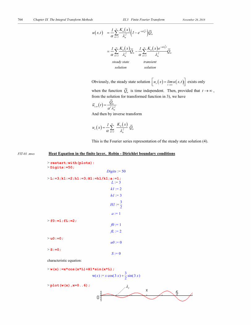
characteristic equation: > w(x):=x*cos(x*L)+H1*sin(x*L);
:= ( )w x + x ( )cos 3 x 32 ( )sin 3 x
> plot(w(x),x=0..6);
1λ
steady state transient
solution solution
Chapter IX The Integral Transform Methods IX.3 Finite Fourier Transform November 26, 2018 765
Eigenvalues: > lambda:=array(1..200);
:= λ ( )array , .. 1 200 [ ]
> n:=1: for m from 1 to 50 do y:=fsolve(w(x)=0,x=m/2..(m+1)/2): if type(y,float) then lambda[n]:=y: n:=n+1 fi od: > for i to 3 do lambda[i] od;
0.87171750182652512021379384729076722823460402426027
1.8021775720308982288404308033660197498395520355731
2.7827873192762392106009190946661202624265539349707
> N:=n-1; := N 24
> n:='n':i:='i':m:='m':y:='y':x:='x': Eigenfunctions: > X[n]:=sin(lambda[n]*(x-L));
:= Xn ( )sin λn ( ) − x 3
> NX[n]:=sqrt(L/2-sin(2*lambda[n]*L)/4/lambda[n]);
:= NXn12 − 6
( )sin 6 λn
λn
Kernel: > K[n](x):=X[n]/NX[n];
:= ( )Kn x2 ( )sin λn ( ) − x 3
− 6( )sin 6 λn
λn
> K[n](0):=subs(x=0,K[n](x));
:= ( )Kn 02 ( )sin −3 λn
− 6( )sin 6 λn
λn
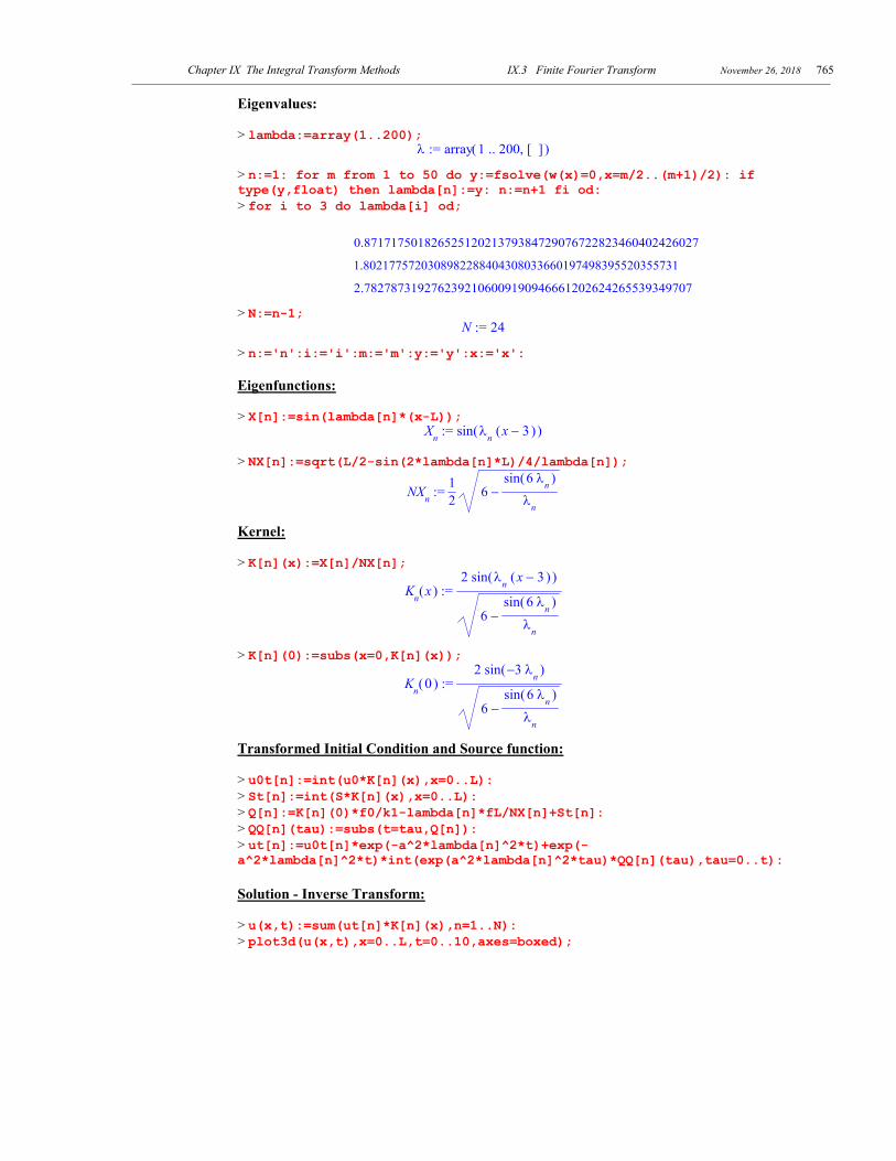
Transformed Initial Condition and Source function: > u0t[n]:=int(u0*K[n](x),x=0..L): > St[n]:=int(S*K[n](x),x=0..L): > Q[n]:=K[n](0)*f0/k1-lambda[n]*fL/NX[n]+St[n]: > QQ[n](tau):=subs(t=tau,Q[n]): > ut[n]:=u0t[n]*exp(-a^2*lambda[n]^2*t)+exp(-a^2*lambda[n]^2*t)*int(exp(a^2*lambda[n]^2*tau)*QQ[n](tau),tau=0..t): Solution - Inverse Transform: > u(x,t):=sum(ut[n]*K[n](x),n=1..N): > plot3d(u(x,t),x=0..L,t=0..10,axes=boxed);
Chapter IX The Integral Transform Methods IX.3 Finite Fourier Transform November 26, 2018 766
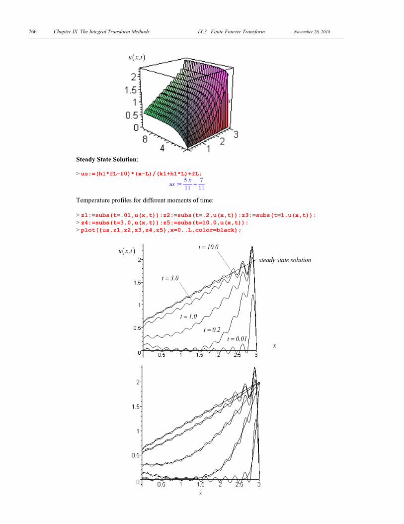
Steady State Solution: > us:=(h1*fL-f0)*(x-L)/(k1+h1*L)+fL;
:= us + 5 x11
711
Temperature profiles for different moments of time: > z1:=subs(t=.01,u(x,t)):z2:=subs(t=.2,u(x,t)):z3:=subs(t=1,u(x,t)): > z4:=subs(t=3.0,u(x,t)):z5:=subs(t=10.0,u(x,t)): > plot({us,z1,z2,z3,z4,z5},x=0..L,color=black);
t
x
( )u x,t
( )u x,t
xt 0.01=
t 0.2=
t 1.0=
t 10.0=
t 3.0=
steady state solution
Chapter IX The Integral Transform Methods IX.3 Finite Fourier Transform November 26, 2018 767
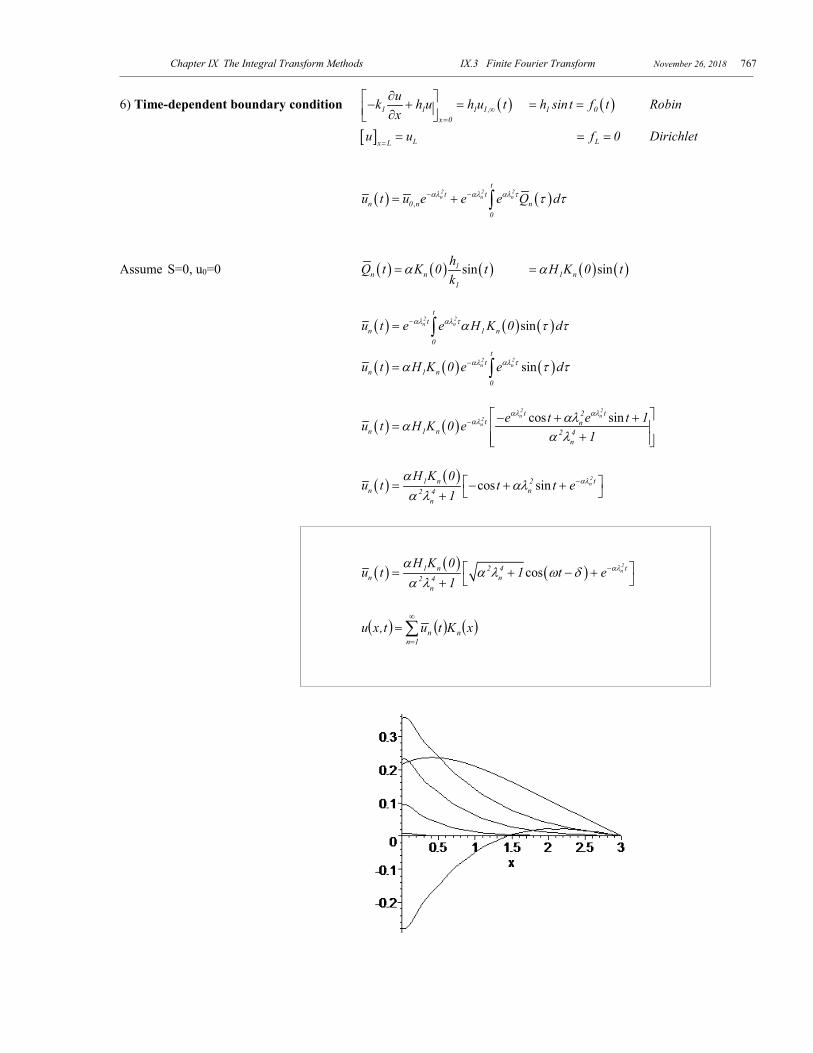
6) Time-dependent boundary condition ( )1 1 1 1,x 0
uk h u h u tx ∞
=
∂ − + = ∂ ( )1 0h sin t f t= = Robin
[ ] Lx Lu u=
= Lf 0= = Dirichlet
( ) ( ),
2 2 2n n n
tt t
n 0 n n0
u t u e e e Q dαλ αλ αλ τ τ τ− −= + ∫
Assume S=0, u0=0 ( ) ( ) ( )sin1n n
1
hQ t K 0 tk
α= ( ) ( )sin1 nH K 0 tα=
( ) ( ) ( )sin2 2n n
tt
n 1 n0
u t e e H K 0 dαλ αλ τα τ τ−= ∫
( ) ( ) ( )sin2 2n n
tt
n 1 n0
u t H K 0 e e dαλ αλ τα τ τ−= ∫
( ) ( ) cos sin2 2n n2
n
t t2t n
n 1 n 2 4n
e t e t 1u t H K 0 e1
αλ αλαλ αλα
α λ−
− + +=
+
( ) ( ) cos sin2n t1 n 2
n n2 4n
H K 0u t t t e
1αλα
αλα λ
− = − + + +
( ) ( ) ( )cos2n t1 n 2 4
n n2 4n
H K 0u t 1 t e
1αλα
α λ ω δα λ
− = + − + +
( ) ( ) ( )∑∞
=
=1n
nn xKtut,xu
Chapter IX The Integral Transform Methods IX.3 Finite Fourier Transform November 26, 2018 768
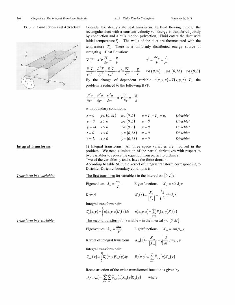
IX.3.3. Conduction and Advection Consider the steady state heat transfer in the fluid flowing through the rectangular duct with a constant velocity v. Energy is transferred jointly by conduction and a bulk motion (advection). Fluid enters the duct with initial temperature eT . The walls of the duct are thermostated with the temperature wT . There is a uniformly distributed energy source of strength g. Heat Equation:
kg
xTvaT 22 −=
∂∂
−∇ p2 c 1ak
ρα
= =
kg
xTva
zT
yT
xT 2
2
2
2
2
2
2
−=∂∂
−∂∂
+∂∂
+∂∂ ( )x 0,∈ ∞ ( )y 0,M∈ ( )z 0,L∈
By the change of dependent variable ( ) ( ) wTz,y,xTz,y,xu −= the problem is reduced to the following BVP:
kg
xuva
zu
yu
xu 2
2
2
2
2
2
2
−=∂∂
−∂∂
+∂∂
+∂∂
with boundary conditions:
0x = ( )M,0y ∈ ( )L,0z ∈ 0we uTTu =−= Dirichlet 0y = 0x > ( )L,0z ∈ 0u = Dirichlet My = 0x > ( )L,0z ∈ 0u = Dirichlet 0z = 0x > ( )M,0y ∈ 0u = Dirichlet Lz = 0x > ( )M,0y ∈ 0u = Dirichlet
Integral Transforms: 1) Integral transforms All three space variables are involved in the problem. We need elimination of the partial derivatives with respect to two variables to reduce the equation from partial to ordinary. Two of the variables, y and z, have the finite domain. According to table SLP, the kernel of integral transform corresponding to Dirichlet-Dirichlet boundary conditions is:
Transform in z-variable: The first transform for variable z in the interval [ ]L,0z ∈ :
Eigenvalues L
nn
πλ = Eigenfunctions zsinX nn λ=
Kernel ( ) zsinL2
XXzK n
n
nn λ==
Integral transform pair:
( ) ( ) ( )dzzKz,y,xuy,xu n
L
0n ∫= ( ) ( ) ( )∑
∞
=
=1n
nn zKy,xuz,y,xu
Transform in y-variable: The second transform for variable y in the interval [ ]M,0y ∈ :
Eigenvalues Mm
mπλ = Eigenfunctions ysinX mm µ=
Kernel of integral transform ( ) ysinM2
XX
zK mm
mm µ==
Integral transform pair:
( ) ( ) ( )dyyKy,xuxu m
M
0nm,n ∫= ( ) ( ) ( )∑
∞
=
=1m
mm,nn yKxuy,xu
Reconstruction of the twice transformed function is given by
( ) ( ) ( ) ( )yKyKxuz,y,xu n1m 1n
mm,n∑∑∞
=
∞
=
= where
L
M
Chapter IX The Integral Transform Methods IX.3 Finite Fourier Transform November 26, 2018 769
( ) ( ) ( ) ( ) ( ) ( ) ( ), , , , ,M L L M
n m n m m n0 0 0 0
u x u x y z K z dz K y dy u x y z K y dy K z dz
= ==
∫ ∫ ∫ ∫
Transformed source and initial conditions:
( )xg m,n ( ) ( ) ( )∫ ∫=M
0nm
L
0
dzdyzKyKk
z,y,xg
( ) ( )∫ ∫=M
0
L
0nm dzdyzKyK
kg
( ) ( )n 1 m 12
g 2 LM 1 1 1 1k nmπ
+ + = + − + − (assume
g cons t= )
m,n,0u ( ) ( )∫ ∫=M
0nm
L
00 dzdyzKyKu
( ) ( ) ( )n 1 m 1e w 2
2 LMT T 1 1 1 1nmπ
+ + = − + − + −
Transformed equation: 2) Transformed equation All boundary conditions in the transformed
domain are homogeneous, therefore, the equation is transformed to
( )2
n,m n,m2 2 2n m n,m n,m2
u ua v u g
xxλ µ
∂ ∂− − + = −
∂∂ m,n,00xm,n uu =
=
General solution of the equation consists of the general solution of the homogeneous part plus a particular solution of the non-homogeneous equation:
( )( ) ( ) ( ) ( )2 22 2 2 2 2 2 2 2
n n n n1 1a v a v 4 x a v a v 4 x2 2 n,m
n,m 1 2 2 2n m
gu x c e c e
λ µ λ µ
λ µ
− + + + + +
= + ++
For the solution to be bounded we have to choose 0c2 = , then with notation
( ) ( )22 2 2 2n,m n n
1 a v a v 42
β λ µ = − + +
The solution becomes
( ) n ,m x n,mn,m 1 2 2
n m
gu x c eβ
λ µ= +
+
The coefficient 1c can be found from the boundary condition, that yields a solution of the transformed equation
solution of transformed equation ( ) 2m
2n
m,nx2m
2n
m,nm,n,0m,n
ge
guxu m,n
µλµλβ
++
+
−=
3) Solution of BVP now can found by the double inverse transform
( )z,y,xu ( ) ( ) ( )n,m m nm 1 n 1
u x K y K z∞ ∞
= =
= ∑ ∑
( ) ( )n ,m xn,m n,m0,n,m m n2 2 2 2
m 1 n 1 n m n m
g gu e K y K zβ
λ µ λ µ
∞ ∞
= =
= − +
+ + ∑ ∑
Then change of the variable yields
Solution: ( ) ( )z,y,xuTz,y,xT w +=
( ) ( )zKyKg
eg
uT n1m 1n
m2m
2n
m,nx2m
2n
m,nm,n,0w
m,n∑∑∞
=
∞
=
++
+−+=
µλµλβ
Chapter IX The Integral Transform Methods IX.3 Finite Fourier Transform November 26, 2018 770
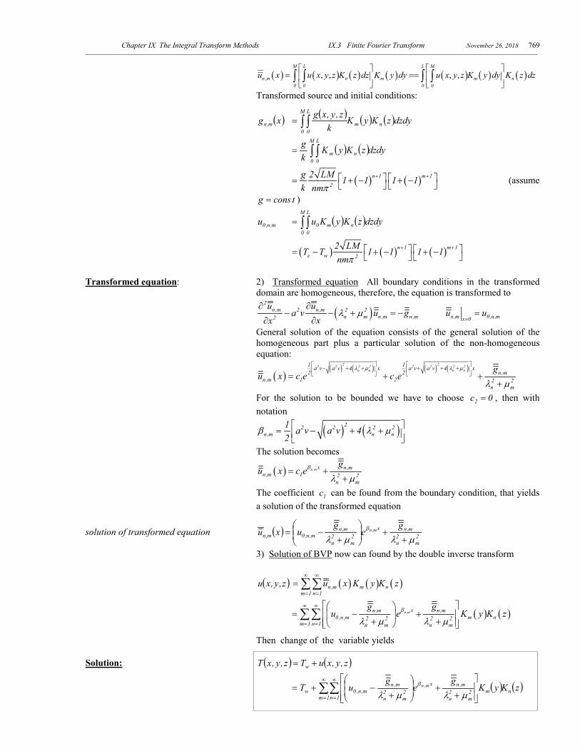
duct-03.mws Heat Transfer in the 3-D rectangular duct with advection
> restart;with(plots): > Tw:=40;Te:=20;g:=0;k:=0.1;M:=1;L:=2;v:=1;a:=5;dT:=Te-Tw;
:= Tw 40
:= Te 20
:= g 0
:= k 0.1
:= M 1 := L 2
:= v 1
:= a 5
:= dT -20 Eigenvalues: > lambda[n]:=n*Pi/L;mu[m]:=m*Pi/M;
:= λnn π2
:= µm m π
Kernel: > K[m](y):=sin(mu[m]*y)*sqrt(2/M);K[n](z):=sin(lambda[n]*z)*sqrt(2/L);
:= ( )Km y ( )sin m π y 2
:= ( )Kn z
sin n π z
2
> u0[n,m]:=dT*int(int(K[m](y),y=0..M)*K[n](z),z=0..L);
:= u0 ,n m −40 2 ( ) − ( )cos m π 1 ( ) − ( )cos n π 1
m π2 n
> u0[n,m]:=subs({cos(m*Pi)=(-1)^m,cos(n*Pi)=(-1)^n},u0[n,m]);
:= u0 ,n m −40 2 ( ) − ( )-1 m 1 ( ) − ( )-1 n 1
m π2 n
> g[n,m]:=g/k*int(int(K[n](y),y=0..L)*K[m](z),z=0..M); := g ,n m 0.
> beta[n,m]:=(a^2*v-sqrt((a^2*v)^2+4*(lambda[n]^2+mu[m]^2)))/2;
:= β ,n m − 252
+ + 625 n2 π2 4 m2 π2
2
> u[n,m]:=((u0[n,m]-g[n,m]/k/(lambda[n]^2+mu[m]^2))*exp(beta[n,m]*x) +g[n,m]/k/(lambda[n]^2+mu[m]^2))*K[m](y)*K[n](z);
:= u ,n m −80 ( ) − ( )-1 m 1 ( ) − ( )-1 n 1 e
− /25 2
+ + 625 n2 π2 4 m2 π2
2x
( )sin m π y
sin n π z
2m π2 n
Chapter IX The Integral Transform Methods IX.3 Finite Fourier Transform November 26, 2018 771
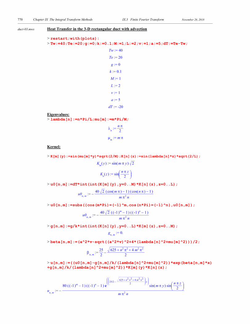
SOLUTION:
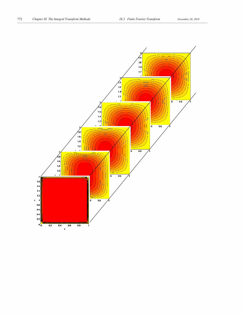
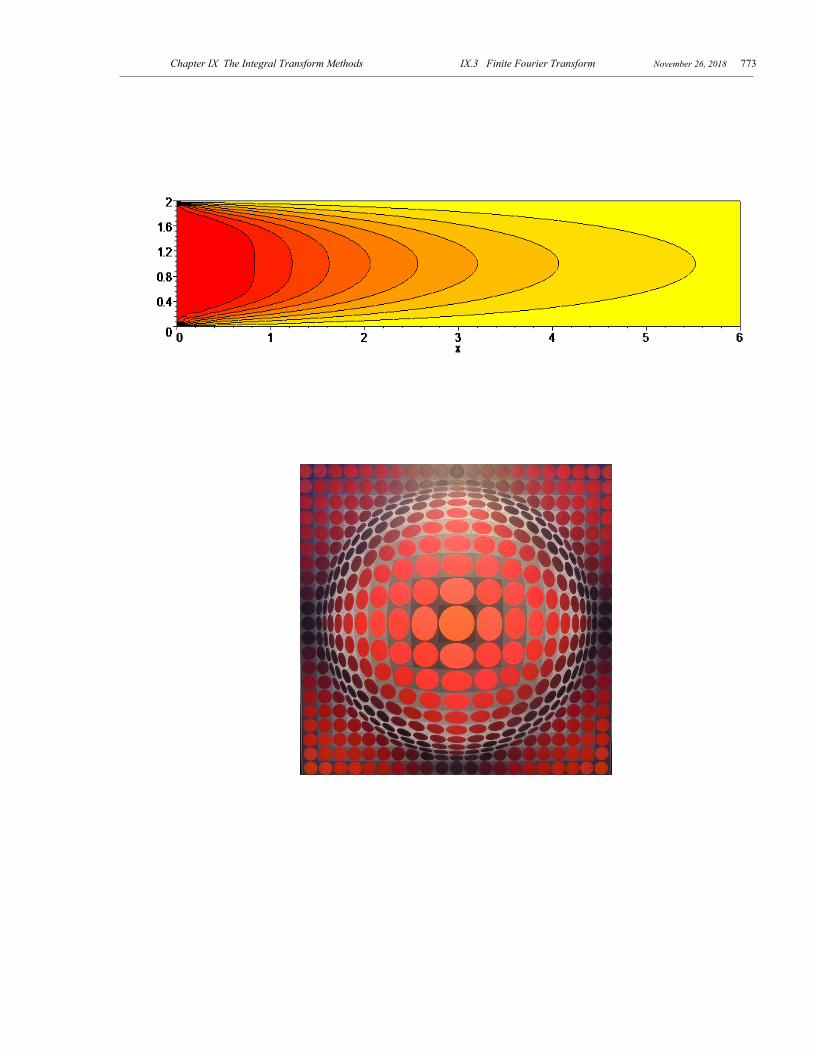
> T(x,y,z):=Tw+sum(sum(u[n,m],n=1..50),m=1..50): > ux(x):=subs({z=L/2,y=M/2},T(x,y,z)): > plot(ux(x),x=0..10);
> uxy(x,y):=subs({z=L/5},T(x,y,z)): > plot3d(uxy(x,y),x=0..5,y=0..M,axes=boxed);
> uyz0(y,z):=subs({x=0},T(x,y,z)): > uyz1(y,z):=subs({x=1},T(x,y,z)): > uyz2(y,z):=subs({x=2},T(x,y,z)): > plot3d({uyz0(y,z),uyz1(y,z)+15,uyz2(y,z)+30},y=0..M,z=0..L);
> animate3d(T(x,y,z),y=0..M,z=0..L,x=0..4,frames=200);
temperature profile along the central line
eT
eT
eT
eT
temperature profile in the plane z L 5=
wT
wT
x 2=
x 1=
x 0=
for animationsee web site
temperature distributionwith the change of x
temperature distributionwith the change of x
Chapter IX The Integral Transform Methods IX.3 Finite Fourier Transform November 26, 2018 772
Chapter IX The Integral Transform Methods IX.3 Finite Fourier Transform November 26, 2018 773
Chapter IX The Integral Transform Methods IX.3 Finite Fourier Transform November 26, 2018 774
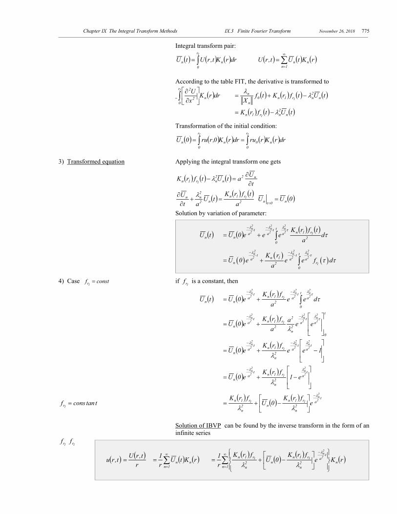
IX.3.4. Heat Equation in the Sphere Consider heat conduction in the solid sphere with angular symmetry. The spatially, non-stationary temperature field ( )t,ru depends only on the radial variable r. The Heat Equation:
( )2
2 22 2
1 ur u atr r
∂ ∂=
∂∂ [ ]1r,0r ∈ 0t >
with initial condition: ( ) ( )ru0,ru 0= and convective boundary condition:
( )1
1
r rr r
uk h u ur ∞ =
=
∂= −
∂
where ∞u is a temperature of the surroundings (generally, a function of time). We can rewrite the boundary condition in the standard form
1r r
huu h ur k k
∞
=
∂ + = ∂
1) Introduce the new dependent variable ( ) ( )t,rrut,rU = , then the HE becomes
t
UarU 22
2
∂∂
=∂∂ [ ]1r,0r ∈ 0t >
which now formally is the 1-d Heat Equation in r in the finite interval [ ]1r,0r ∈ , which requires two boundary conditions. The first condition at 0r = is obtained directly from the equation used for a change of
variable: 0ruU
0r0r==
== Dirichlet
Consider the second boundary condition at 1rr = :
k
huukh
ru
1rr
∞
=
=
+
∂∂
k
hur
Ukh
rU
r1rr
∞
=
=
+∂∂
k
hur
Ukh
rU
rU
r1
1rr2
∞
=
=
+−
∂∂
k
huUr1
kh
r1
rU
r1
1rr
∞
=
=
−+
∂∂
k
rhuUr1
kh
rU 1
rr11
∞
=
=
−+
∂∂
1
h 1Hk r
= − , ( )1
1r
hu rf tk∞=
( )tfHUrU
11
rrr
=
+
∂∂
=
Robin
2) Integral transform Consider the finite Fourier transform corresponding to the case of Dirichlet-Robin boundary conditions:
Eigenvalues nλ are positive roots of the equation: 0rsinHrcos 11 =+ λλλ
Eigenfunctions rsinX nn λ= , ( )n
1n1n 4
r2sin2rX
λλ
−=
The kernel ( )( )
n
1n1
n
n
nn
4r2sin
2r
rsinXXrK
λλ
λ
−==
( ) ( )
reduction to1-d Cartesianformulation by change of variableU r,t ru r,t=
( )U r,t
r 0U 0=
= ( )1
1
rr r
U HU f tr =
∂ + = ∂
1r r
huu h ur k k
∞
=
∂ + = ∂ h,u∞
conveciveenviroment
boundary condition
two boundary conditions
Chapter IX The Integral Transform Methods IX.3 Finite Fourier Transform November 26, 2018 775
Integral transform pair:
( ) ( ) ( )drrKt,rUtU n
r
0n
1
∫= ( ) ( ) ( )∑∞
=
=1n
nn rKtUt,rU
According to the table FIT, the derivative is transformed to
( )drrKxU
n
r
02
21
∫
∂∂ ( ) ( ) ( ) ( )tUtfrKtf
X n2nr1n0
n
n1
λλ−+=
( ) ( ) ( )tUtfrK n2nr1n 1
λ−=
Transformation of the initial condition:
( ) ( ) ( ) ( ) ( )drrKrrudrrK0,rru0U n
r
00n
r
0n
11
∫∫ ==
3) Transformed equation Applying the integral transform one gets
( ) ( ) ( )t
UatUtfrK n2n
2nr1n 1 ∂
∂=− λ
( ) ( ) ( )2
r1nn2
2nn
atfrK
tUat
U 1=+∂
∂ λ ( )0UU n0tn ==
Solution by variation of parameter:
( )tUn ( ) ( ) ( )∫
−−
+=t
02
r1nat
at
an d
atfrK
eee0U 12
2n
2
2n
2
2n
ττλλλ
( ) ( ) ( )2 2 2n n n
2 2 2
1
tt tn 1a a a
n r20
K rU 0 e e e f d
a
λ λ λτ
τ τ− −
= + ∫
4) Case 1rf const= if
1rf is a constant, then
( )tUn ( ) ( )∫
−−
+=t
0
at
a2
r1nta
n deea
frKe0U 2
2n
2
2n
12
2n
ττλλλ
( ) ( )t
0
at
a2n
2
2r1nt
an
2
2n
2
2n
12
2n
eeaa
frKe0U
+=
−− τλλλ
λ
( ) ( )
−+=
−−
1eefrK
e0Ut
at
a2n
r1nta
n2
2n
2
2n
12
2n λλλ
λ
( ) ( )
−+=
− ta
2n
r1nta
n2
2n
12
2n
e1frK
e0Uλλ
λ
ttanconsf1r
= ( ) ( ) ( ) t
a2n
r1nn2
n
r1n 2
2n
11 efrK
0UfrK λ
λλ
−
−+=
Solution of IBVP can be found by the inverse transform in the form of an
infinite series 1r
f1r
f
( )t,ru ( )r
t,rU= ( ) ( )∑
∞
=
=1n
nn rKtUr1
( ) ( ) ( ) ( )∑∞
=
−
−+=
1nn
ta
2n
r1nn2
n
r1n rKefrK
0UfrK
r1 2
2n
11
λ
λλ
Chapter IX The Integral Transform Methods IX.3 Finite Fourier Transform November 26, 2018 776
5) Example (turkey-2.mws) Roasting of a turkey (turkey-3.mws smooth solution)
The turkey is assumed to be a sphere of radius 1r 0.1 m= with the uniform initial temperature o
0u 20 C= . It is exposed to the convective environment at ou 150 C∞ = with the convective
coefficient 2
Wh 5 m K
= . The turkey is considered to be done when its minimum temperature reaches
odoneu 75 C= . Thermophysical properties of turkey meat used for calculation are from the table
(Section VIII.1.15 p.580). > restart;with(plots): > r1:=0.1;k:=0.6;h:=5;u0:=20;uinf:=150;a:=2774;
:= r1 0.1
:= k 0.6
:= h 5
:= u0 20
:= uinf 150
:= a 2774
> H[2]:=h/k-1/r1; := H2 -1.666666667
> fL:=h*uinf*r1/k; := fL 125.0000000
Characteristic equation: > w(x):=x*cos(x*r1)+H[2]*sin(x*r1);
:= ( )w x − x ( )cos 0.1 x 1.666666667 ( )sin 0.1 x
> plot(w(x),x=0..50);
Eigenvalues: > lambda:=array(1..200);
:= λ ( )array , .. 1 200 [ ]
> n:=1: for m from 1 to 50 do y:=fsolve(w(x)=0,x=10*m..10*(m+1)): if type(y,float) then lambda[n]:=y: n:=n+1 fi od: > for i to 4 do lambda[i] od;
14.56892774
46.76766900
78.32706546
> N:=n-1; := N 16
> n:='n':i:='i':m:='m':y:='y':x:='x': Eigenfunctions and kernel (See table (5) Dirichlet-Robin): > X[n]:=sin(lambda[n]*r);
:= Xn ( )sin λn r
1λ
Chapter IX The Integral Transform Methods IX.3 Finite Fourier Transform November 26, 2018 777
> XN[n]:=sqrt(r1/2-sin(2*lambda[n]*r1)/4/lambda[n]);
:= XNn − 0.05000000000 14
( )sin 0.2 λn
λn
> K[n](r):=X[n]/XN[n];
:= ( )Kn r( )sin λn r
− 0.05000000000 14
( )sin 0.2 λn
λn
> K[n](L):=subs(r=r1,K[n](r)): > U0[n]:=u0*int(r*K[n](r),r=0..r1);
:= U0n −200. ( )− + 1. ( )sin 0.1 λn 0.1 λn ( )cos 0.1 λn
−1. ( )− + 5. λn 25. ( )sin 0.2000000000 λn
λnλn
2
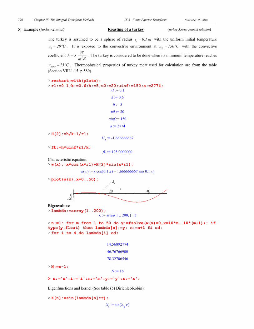
> U[n]:=fL*K[n](L)/lambda[n]^2+(U0[n]-fL*K[n](L)/lambda[n]^2)*exp(-lambda[n]^2*t/a^2): Solution: > u(r,t):=sum(U[n]*K[n](r),n=1..N)/r: > u2(r,t):=subs(r=-r,u(r,t)): > t1:=1*60*10:t2:=1*60*60:t2:=3*60*60:t3:=5*60*60:t4:=7*60*60: z1:=subs(t=t1,u2(r,t)):z2:=subs(t=t2,u2(r,t)):z3:=subs(t=t3,u2(r,t)):z4:=subs(t=t4,u2(r,t)): > plot({z1,z2,z3,z4,z5},r=-r1..r1,color=black,axes=boxed);
> with(plots): > animate(u(r,t),r=0..r1,t=0..36000,frames=150);
t 10 min=
t 1 hour=
t 7 hours=
t 5 hours=
( )u r,t
Chapter IX The Integral Transform Methods IX.3 Finite Fourier Transform November 26, 2018 778

Chapter IX The Integral Transform Methods IX.3 Finite Fourier Transform November 26, 2018 779
Chapter IX The Integral Transform Methods IX.3 Finite Fourier Transform November 26, 2018 780
Examples 1. Consider heat conduction in the 2-dimensional cross-section of the long column:
Equation: 2 2
2 2
1 u u ut x yα
∂ ∂ ∂= +
∂ ∂ ∂ ( ) ( ) ( ), , ),x y 0 L M∈ × 0t >
Initial condition: ( ) ( ), 0u x 0 u x 0= =
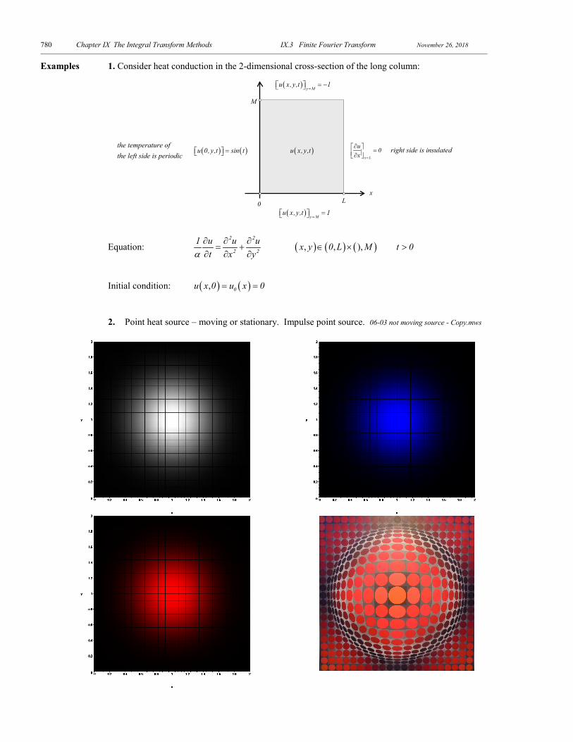
2. Point heat source – moving or stationary. Impulse point source. 06-03 not moving source - Copy.mws
the temperature of the left side is periodic
right side is insulated( )u x,y,t
0 Lx
x L
u 0x =
∂ = ∂ ( ) ( )u 0,y,t sin t=
( )y M
u x,y,t 1=
= −
( )y M
u x,y,t 1=
=
M
Chapter IX The Integral Transform Methods IX.3 Finite Fourier Transform November 26, 2018 781
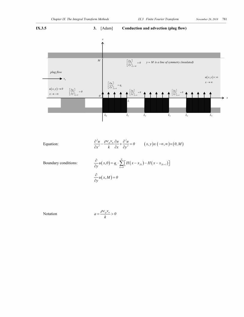
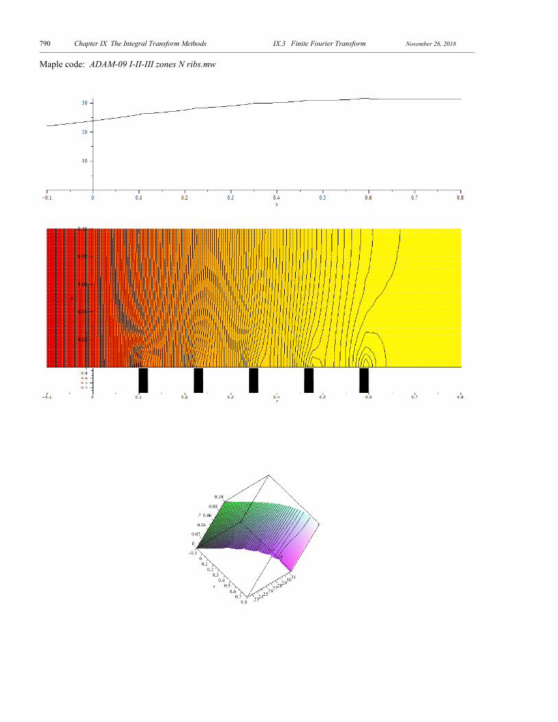
IX.3.5 3. [Adam] Conduction and advection (plug flow)
Equation: 2 2
p n2 2
c vu u u 0x k x y
ρ∂ ∂ ∂− + =
∂ ∂ ∂ ( ) ( ) ( ), , ,x y 0 M∈ −∞ ∞ ×
Boundary conditions: ( ) ( ) ( ),N
s 2k 2k 1k 0
u x 0 q H x x H x xy +
=
∂= ⋅ − − − ∂ ∑
( ),u x M 0y
∂=
∂
Notation p nc va 0
kρ
= >
plug flow
y M is a line of symmetry (insulated)=
( )u x,y 0→
0 x
y M
u 0y =
∂= ∂
nv
L
M
sy 0
u qy =
∂= ∂
y 0
u 0y =
∂= ∂
2L
y 0
u 0y =
∂= ∂
0L 1L 2L 3L 4L 5L
x → −∞
( )u x,y < ∞
x → ∞
x
y 0
u 0y =
∂= ∂
Chapter IX The Integral Transform Methods IX.3 Finite Fourier Transform November 26, 2018 782
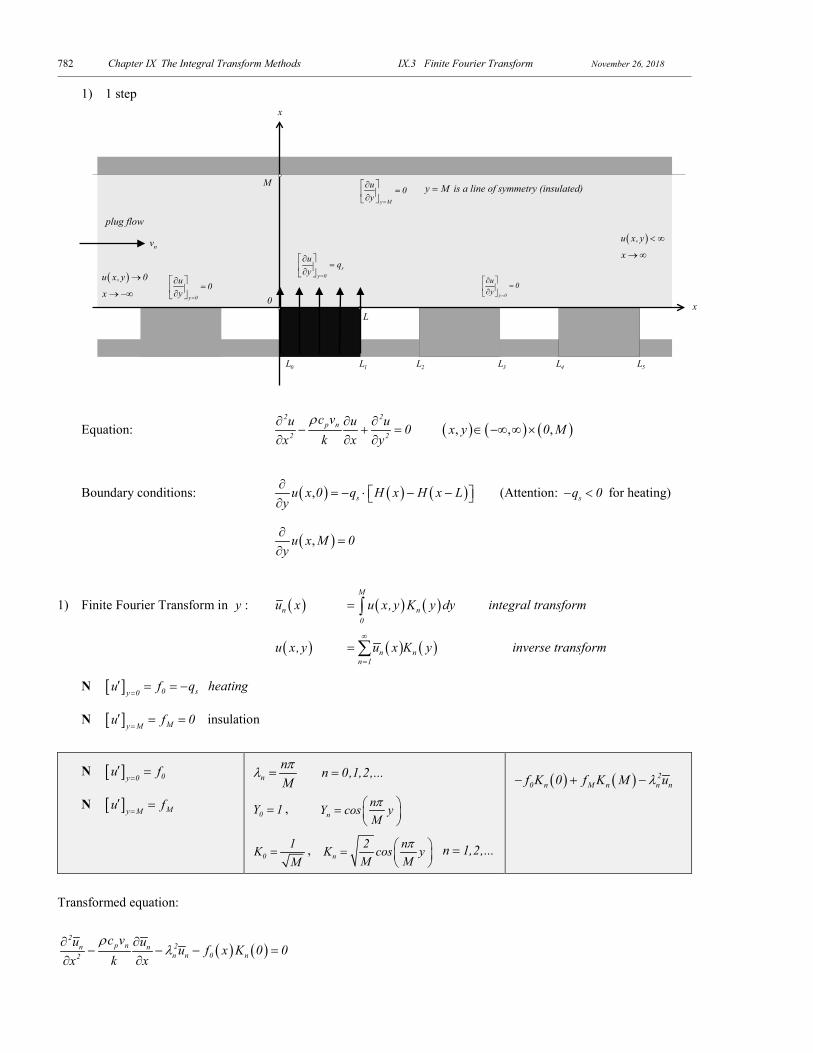
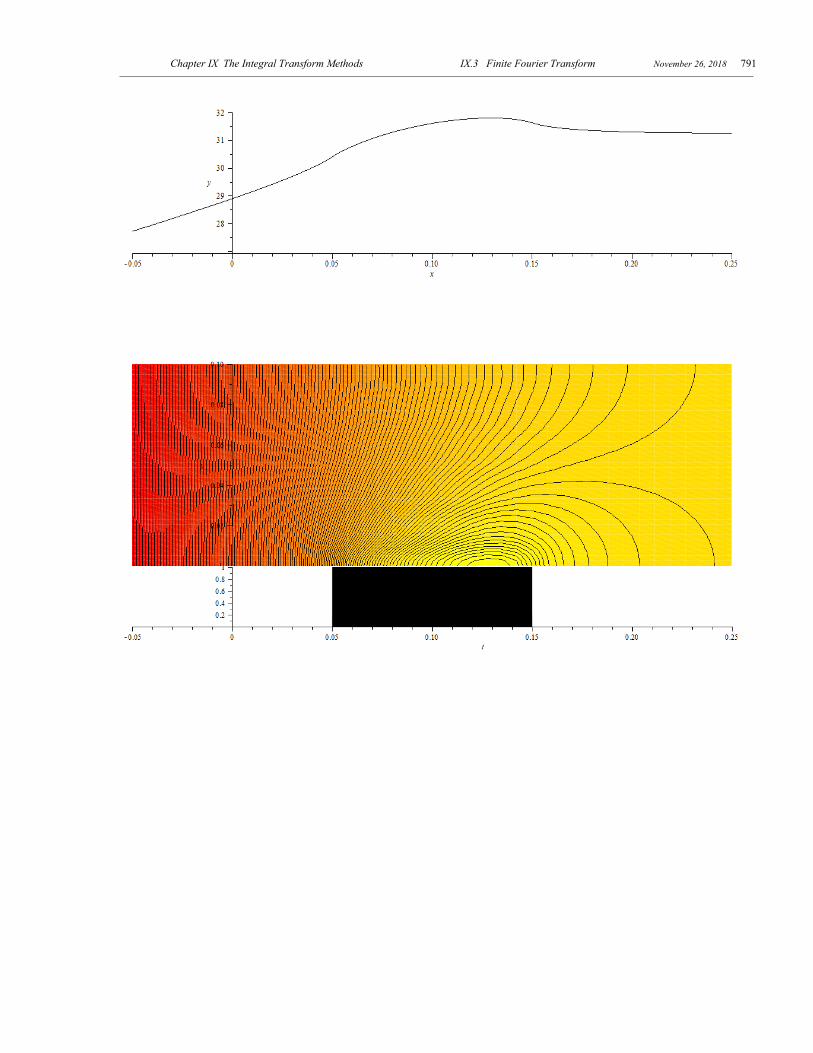
1) 1 step
Equation: 2 2
p n2 2
c vu u u 0x k x y
ρ∂ ∂ ∂− + =
∂ ∂ ∂ ( ) ( ) ( ), , ,x y 0 M∈ −∞ ∞ ×
Boundary conditions: ( ) ( ) ( ), su x 0 q H x H x Ly
∂= − ⋅ − − ∂
(Attention: sq 0− < for heating)
( ),u x M 0y
∂=
∂
1) Finite Fourier Transform in y : ( )nu x ( ) ( )M
n0
u x,y K y dy= ∫ integral transform
( )u x,y ( ) ( )n nn 1
u x K y∞
=
= ∑ inverse transform
N [ ] 0 sy 0u f q=
′ = = − heating
N [ ] My Mu f 0=
′ = = insulation
N [ ] 0y 0u f=
′ =
N [ ] My Mu f=
′ =
nnMπλ = n 0,1,2,...=
0Y 1= , nnY cos yMπ =
01KM
= , n2 nK cos yM M
π =
n 1,2,...=
( ) ( ) 2
0 n M n n nf K 0 f K M uλ− + −
Transformed equation:
( ) ( )2
p n 2n nn n 0 n2
c vu u u f x K 0 0x k x
ρλ∂ ∂
− − − =∂ ∂
plug flow
y M is a line of symmetry (insulated)=
( )u x,y 0→
0 x
y M
u 0y =
∂= ∂
nv
L
M
sy 0
u qy =
∂= ∂
y 0
u 0y =
∂= ∂
0L 1L 2L 3L 4L 5L
x → −∞
( )u x,y < ∞
x → ∞
x
y 0
u 0y =
∂= ∂
Chapter IX The Integral Transform Methods IX.3 Finite Fourier Transform November 26, 2018 783
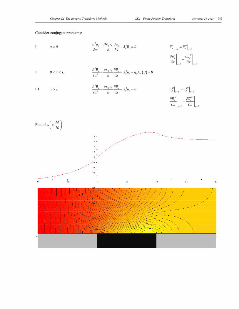
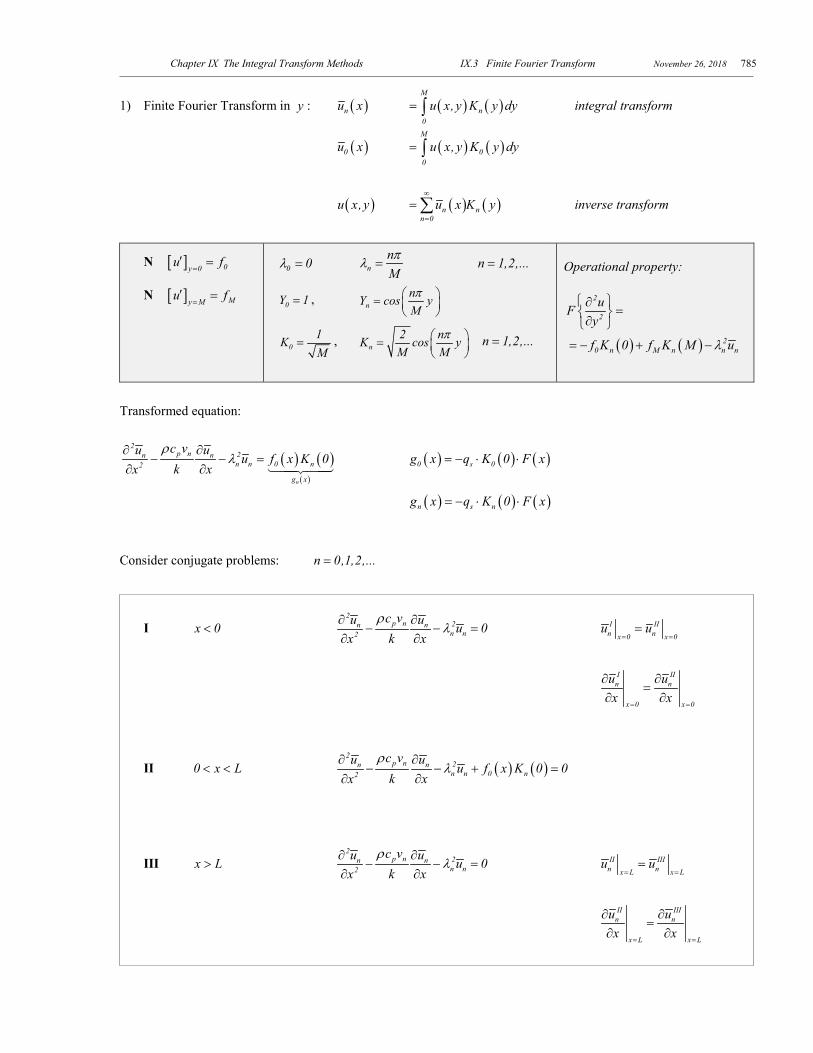
Consider conjugate problems:
I x 0< 2
p n 2n nn n2
c vu u u 0x k x
ρλ∂ ∂
− − =∂ ∂
I IIn nx 0 x 0
u u= =
=
I II
n n
x 0 x 0
u ux x
= =
∂ ∂=
∂ ∂
II 0 x L< < ( )2
p n 2n nn n s n2
c vu u u q K 0 0x k x
ρλ∂ ∂
− − + =∂ ∂
III x L> 2
p n 2n nn n2
c vu u u 0x k x
ρλ∂ ∂
− − =∂ ∂
II IIIn nx L x L
u u= =
=
II IIIn n
x L x L
u ux x
= =
∂ ∂=
∂ ∂
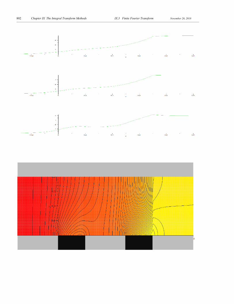
Plot of Mu x,10
Chapter IX The Integral Transform Methods IX.3 Finite Fourier Transform November 26, 2018 784
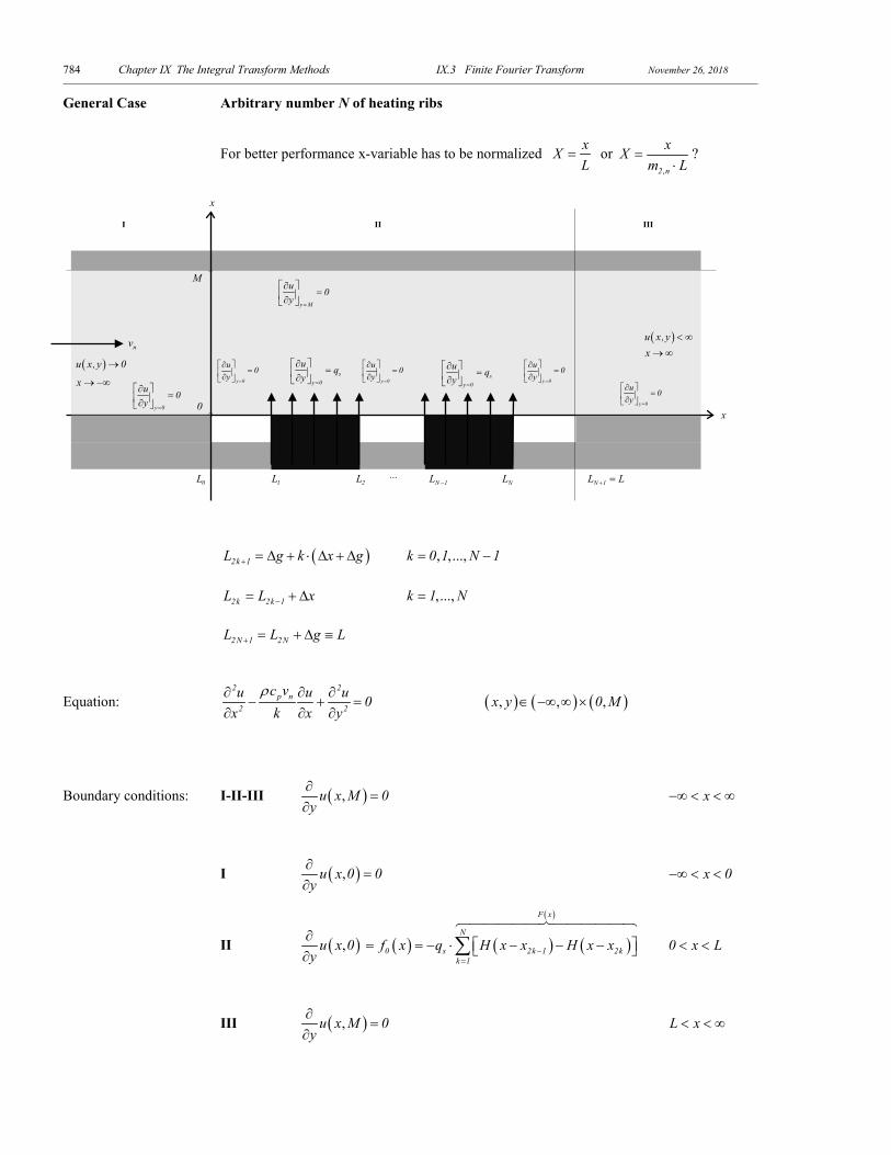
General Case Arbitrary number N of heating ribs
For better performance x-variable has to be normalized xXL
= or ,2 n
xXm L
=⋅
?
( )2k 1L g k x g+ = ∆ + ⋅ ∆ + ∆ , ,...,k 0 1 N 1= −
2k 2k 1L L x−= + ∆ ,...,k 1 N=
2 N 1 2 NL L g L+ = + ∆ ≡
Equation: 2 2
p n2 2
c vu u u 0x k x y
ρ∂ ∂ ∂− + =
∂ ∂ ∂ ( ) ( ) ( ), , ,x y 0 M∈ −∞ ∞ ×
Boundary conditions: I-II-III ( ),u x M 0y
∂=
∂ x−∞ < < ∞
I ( ),u x 0 0y
∂=
∂ x 0−∞ < <
II ( ),u x 0y
∂∂
( ) ( ) ( )
( )F x
N
0 s 2k 1 2kk 1
f x q H x x H x x−=
= = − ⋅ − − − ∑
0 x L< <
III ( ),u x M 0y
∂=
∂ L x< < ∞
plug flow
y M is a line of symmetry (insulated)=
( )u x,y 0→
0x
y M
u 0y =
∂= ∂
nv
M
sy 0
u qy =
∂= ∂
y 0
u 0y =
∂= ∂
0L 1L 2L N 1L −
x → −∞
( )u x,y < ∞x → ∞
x
y 0
u 0y =
∂= ∂
III
y 0
u 0y =
∂= ∂
III
...NL N 1L L+ =
y 0
u 0y =
∂= ∂ y 0
u 0y =
∂= ∂ s
y 0
u qy =
∂= ∂
Chapter IX The Integral Transform Methods IX.3 Finite Fourier Transform November 26, 2018 785
1) Finite Fourier Transform in y : ( )nu x ( ) ( )M
n0
u x,y K y dy= ∫ integral transform
( )0u x ( ) ( )M
00
u x, y K y dy= ∫
( )u x,y ( ) ( )n nn 0
u x K y∞
=
= ∑ inverse transform
N [ ] 0y 0u f=
′ =
N [ ] My Mu f=
′ =
0 0λ = nnMπλ = n 1,2,...=
0Y 1= , nnY cos yMπ =
01KM
= , n2 nK cos yM M
π =
n 1,2,...=
Operational property:
2
2
uFy
∂=
∂
( ) ( ) 20 n M n n nf K 0 f K M uλ= − + −
Transformed equation:
( ) ( )( )n
2p n 2n n
n n 0 n2
g x
c vu uu f x K 0
k xxρ
λ∂ ∂
− − =∂∂
( ) ( ) ( )0 s 0g x q K 0 F x= − ⋅ ⋅
( ) ( ) ( )n s ng x q K 0 F x= − ⋅ ⋅
Consider conjugate problems: n 0,1,2,...=
I x 0< 2
p n 2n nn n2
c vu u u 0x k x
ρλ∂ ∂
− − =∂ ∂
I IIn nx 0 x 0
u u= =
=
I II
n n
x 0 x 0
u ux x
= =
∂ ∂=
∂ ∂
II 0 x L< < ( ) ( )2
p n 2n nn n 0 n2
c vu uu f x K 0 0
k xxρ
λ∂ ∂
− − + =∂∂
III x L> 2
p n 2n nn n2
c vu u u 0x k x
ρλ∂ ∂
− − =∂ ∂
II IIIn nx L x L
u u= =
=
II III
n n
x L x L
u ux x
= =
∂ ∂=
∂ ∂
Chapter IX The Integral Transform Methods IX.3 Finite Fourier Transform November 26, 2018 786
,
22
1 n na am 02 2
λ = − + <
, ,
22
2 n na am 02 2
λ = + + >
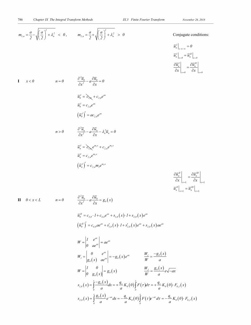
Conjugate conditions:
In x
u 0→−∞
=
I IIn nx 0 x 0
u u= =
=
I II
n n
x 0 x 0
u ux x
= =
∂ ∂=
∂ ∂
I x 0< n 0= 2
0 02
u ua 0x x
∂ ∂− =
∂ ∂
,
I0 1 0u c= ,
ax2 0c e+
,I ax
0 2 0u c e=
( ) ,I ax
0 2 0u ac e′ =
n 0> 2
2n nn n2
u ua u 0x x
λ∂ ∂− − =
∂ ∂
,
In 1 nu c= ,
1 2m x m x2 ne c e+
,2m xI
n 2 nu c e=
( ) ,2m xI
n 2 n 2u c m e′ =
II III
n n
x L x L
u ux x
= =
∂ ∂=
∂ ∂
II IIIn nx L x L
u u= =
=
II 0 x L< < n 0= ( )2
0 002
u ua g x
xx∂ ∂
− =∂∂
( ) ( ), , , ,
II ax ax0 3 0 4 0 1 0 2 0u c 1 c e s x 1 s x e= ⋅ + + ⋅ +
( ) ( ) ( ) ( ), , , ,II ax ax ax
0 4 0 1 0 2 0 2 0u c ae s x 1 s x e s x ae′ ′ ′= + ⋅ + +
ax
axax
1 eW ae
0 ae= =
( ) ( )
axax
1 0ax0
0 eW g x e
g x ae= = − ( )01 g xW
W a−
=
( ) ( )00
1 0W g x
0 g x= = ( )02 g xW e ax
W a= −
( ) ( ) ( ) ( ) ( ) ( ), ,
x x0 s s
1 0 0 0 0 10 0
g x q qs x dx K 0 F d K 0 F x
a a aτ τ
−= = + = + ⋅∫ ∫
( ) ( ) ( ) ( ) ( ) ( ), ,
x x0 ax as s
2 0 0 0 0 20 0
g x q qs x e dx K 0 F e d K 0 F x
a a aττ τ− −= = − = − ⋅∫ ∫
Chapter IX The Integral Transform Methods IX.3 Finite Fourier Transform November 26, 2018 787
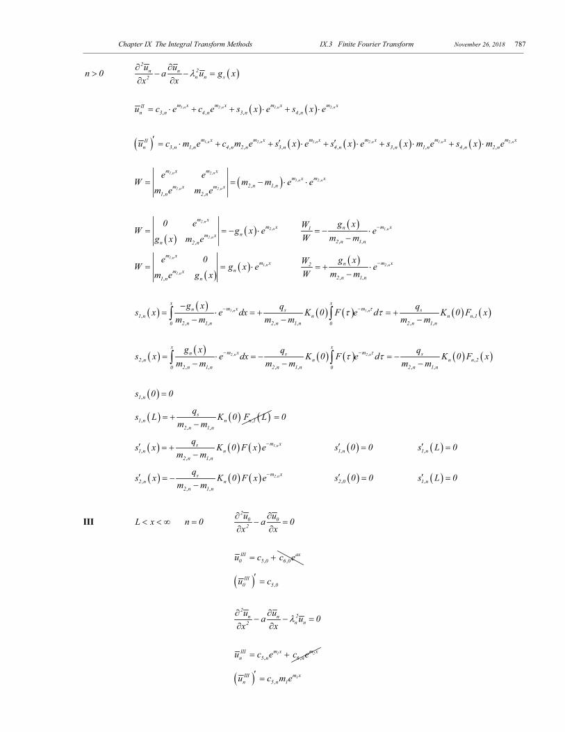
n 0> ( )2
2n nn n s2
u ua u g x
xxλ
∂ ∂− − =
∂∂
( ) ( ), , , ,
, , , ,1 n 2 n 1 n 2 nm x m x m x m xII
n 3 n 4 n 3 n 4 nu c e c e s x e s x e= ⋅ + + ⋅ + ⋅
( ) ( ) ( ) ( ) ( ), , , , , ,, , , , , , , , , ,
1 n 2 n 1 n 2 n 1 n 2 nm x m x m x m x m x m xIIn 3 n 1 n 4 n 2 n 3 n 4 n 3 n 1 n 4 n 2 nu c m e c m e s x e s x e s x m e s x m e′ ′ ′= ⋅ + + ⋅ + ⋅ + ⋅ + ⋅
( ), ,
, ,
, , , ,, ,
1 n 2 n
1 n 2 n
1 n 2 n
m x m xm x m x
2 n 1 nm x m x1 n 2 n
e eW m m e e
m e m e= = − ⋅ ⋅
( )
( ),
,
,,
2 n
2 n
2 n
m xm x
nm xn 2 n
0 eW g x e
g x m e= = − ⋅ ( )
,
, ,
1 nm xn1
2 n 1 n
g xW eW m m
−= − ⋅−
( )
( ),
,
,,
1 n
1 n
1 n
m xm x
nm x1 n n
e 0W g x e
m e g x= = ⋅ ( )
,
, ,
2 nm xn2
2 n 1 n
g xW eW m m
−= + ⋅−
( ) ( ) ( ) ( ) ( ) ( ), ,, ,
, , , , , ,
1 n 1 n
x xm x mn s s
1 n n n n 12 n 1 n 2 n 1 n 2 n 1 n0 0
g x q qs x e dx K 0 F e d K 0 F x
m m m m m mττ τ− −−
= ⋅ = + = +− − −∫ ∫
( ) ( ) ( ) ( ) ( ) ( ), ,, ,
, , , , , ,
2 n 2 n
x xm x mn s s
2 n n n n 22 n 1 n 2 n 1 n 2 n 1 n0 0
g x q qs x e dx K 0 F e d K 0 F x
m m m m m mττ τ− −= ⋅ = − = −
− − −∫ ∫
( ),1 ns 0 0=
( ) ( ) ( ), ,, ,
s1 n n n 1
2 n 1 n
qs L K 0 F L
m m= +
−0=
( ) ( ) ( ) ,,
, ,
1 nm xs1 n n
2 n 1 n
qs x K 0 F x e
m m−′ = +
− ( ),1 ns 0 0′ = ( ),1 ns L 0′ =
( ) ( ) ( ) ,,
, ,
2 nm xs2 n n
2 n 1 n
qs x K 0 F x e
m m−′ = −
− ( ),2 0s 0 0′ = ( ),1 ns L 0′ =
III L x< < ∞ n 0= 2
0 02
u ua 0x x
∂ ∂− =
∂ ∂
, ,III ax
0 5 0 6 0u c c e= +
( ) ,III
0 5 0u c′ =
2
2n nn n2
u ua u 0x x
λ∂ ∂− − =
∂ ∂
, ,1 2m x m xIII
n 5 n 6 nu c e c e= +
( ) ,1m xIII
n 5 n 1u c m e′ =
Chapter IX The Integral Transform Methods IX.3 Finite Fourier Transform November 26, 2018 788
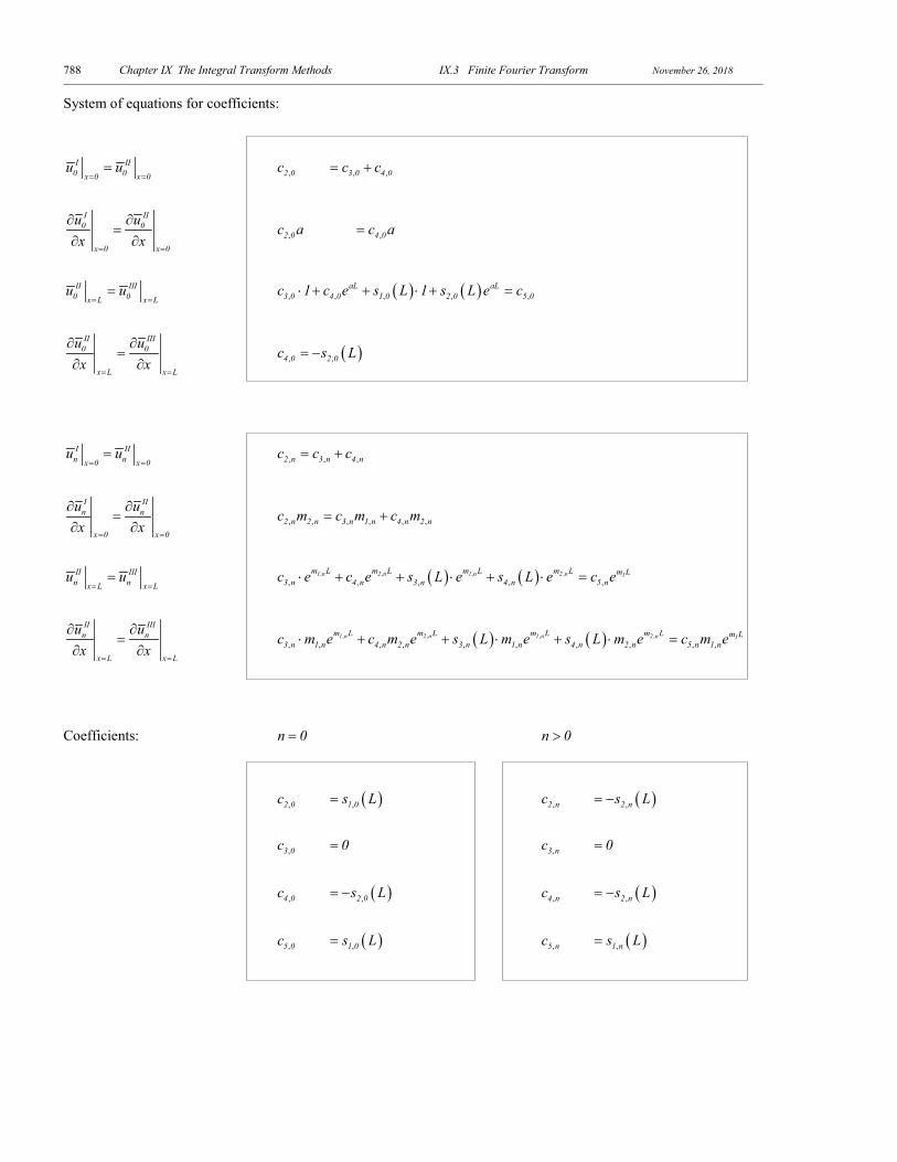
System of equations for coefficients:
I II0 0x 0 x 0
u u= =
= ,2 0c , ,3 0 4 0c c= +
I II
0 0
x 0 x 0
u ux x
= =
∂ ∂=
∂ ∂ ,2 0c a ,4 0c a=
II III
0 0x L x Lu u
= == ( ) ( ), , , , ,
aL aL3 0 4 0 1 0 2 0 5 0c 1 c e s L 1 s L e c⋅ + + ⋅ + =
II III
0 0
x L x L
u ux x
= =
∂ ∂=
∂ ∂ ( ), ,4 0 2 0c s L= −
I IIn nx 0 x 0
u u= =
= , , ,2 n 3 n 4 nc c c= +
I II
n n
x 0 x 0
u ux x
= =
∂ ∂=
∂ ∂ , , , , , ,2 n 2 n 3 n 1 n 4 n 2 nc m c m c m= +
II III
n nx L x Lu u
= == ( ) ( ), , , ,
, , , , ,1 n 2 n 1 n 2 n 1m L m L m L m L m L
3 n 4 n 3 n 4 n 5 nc e c e s L e s L e c e⋅ + + ⋅ + ⋅ =
II III
n n
x L x L
u ux x
= =
∂ ∂=
∂ ∂ ( ) ( ), , , ,
, , , , , , , , , ,1 n 2 n 1 n 2 n 1m L m L m L m L m L
3 n 1 n 4 n 2 n 3 n 1 n 4 n 2 n 5 n 1 nc m e c m e s L m e s L m e c m e⋅ + + ⋅ + ⋅ =
Coefficients: n 0= n 0>
,2 0c ( ),1 0s L= ,2 nc ( ),2 ns L= −
,3 0c 0= ,3 nc 0=
,4 0c ( ),2 0s L= − ,4 nc ( ),2 ns L= −
,5 0c ( ),1 0s L= ,5 nc ( ),1 ns L=
Chapter IX The Integral Transform Methods IX.3 Finite Fourier Transform November 26, 2018 789
Solution of the transformed equation:
I x 0< n 0= ,I ax
0 2 0u c e=
n 0> ,
2m xIn 2 nu c e=
II 0 x L< < n 0= ( ) ( ), , , ,II ax ax
0 3 0 4 0 1 0 2 0u c 1 c e s x 1 s x e= ⋅ + + ⋅ +
n 0> ( ) ( ), , , ,, , , ,
1 n 2 n 1 n 2 nm x m x m x m xIIn 3 n 4 n 3 n 4 nu c e c e s x e s x e= ⋅ + + ⋅ + ⋅
III L x< < ∞ n 0= ,III
0 5 0u c=
n 0> ,
1m xIIIn 5 nu c e=
Solution:
I x 0< ( )Iu x, y ( ) ( )In n
n 0u x K y
∞
=
= ∑
II 0 x L< < ( )IIu x, y ( ) ( )IIn n
n 0u x K y
∞
=
= ∑
III L x< < ∞ ( )IIIu x, y ( ) ( )IIIn n
n 0u x K y
∞
=
= ∑
Chapter IX The Integral Transform Methods IX.3 Finite Fourier Transform November 26, 2018 790
Maple code: ADAM-09 I-II-III zones N ribs.mw
Chapter IX The Integral Transform Methods IX.3 Finite Fourier Transform November 26, 2018 791
Chapter IX The Integral Transform Methods IX.3 Finite Fourier Transform November 26, 2018 792
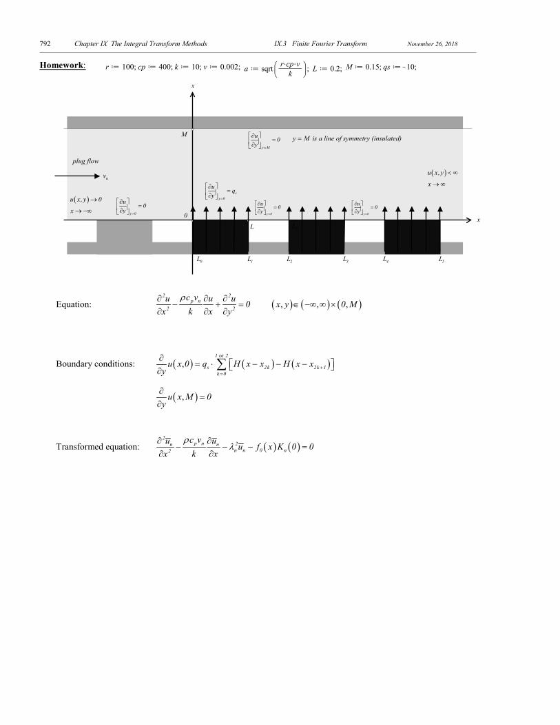
Homework:
Equation: 2 2
p n2 2
c vu u u 0x k x y
ρ∂ ∂ ∂− + =
∂ ∂ ∂ ( ) ( ) ( ), , ,x y 0 M∈ −∞ ∞ ×
Boundary conditions: ( ) ( ) ( ) or
,1 2
s 2k 2k 1k 0
u x 0 q H x x H x xy +
=
∂= ⋅ − − − ∂ ∑
( ),u x M 0y
∂=
∂
Transformed equation: ( ) ( )2
p n 2n nn n 0 n2
c vu u u f x K 0 0x k x
ρλ∂ ∂
− − − =∂ ∂
plug flow
y M is a line of symmetry (insulated)=
( )u x,y 0→
0 x
y M
u 0y =
∂= ∂
nv
L
M
sy 0
u qy =
∂= ∂
y 0
u 0y =
∂= ∂
2L
y 0
u 0y =
∂= ∂
0L 1L 2L 3L 4L 5L
x → −∞
( )u x,y < ∞
x → ∞
x
y 0
u 0y =
∂= ∂
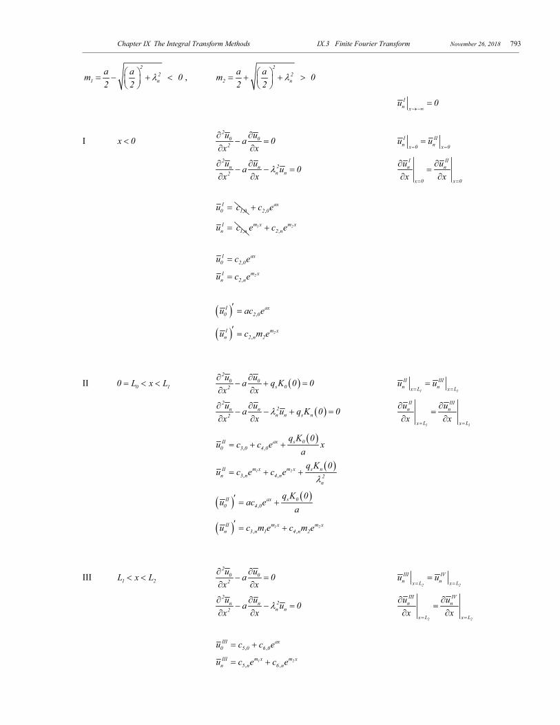
Chapter IX The Integral Transform Methods IX.3 Finite Fourier Transform November 26, 2018 793
22
1 na am 02 2
λ = − + <
, 2
22 n
a am 02 2
λ = + + >
In x
u 0→−∞
=
I x 0< 2
0 02
u ua 0x x
∂ ∂− =
∂ ∂ I II
n nx 0 x 0u u
= ==
2
2n nn n2
u ua u 0x x
λ∂ ∂− − =
∂ ∂
I IIn n
x 0 x 0
u ux x
= =
∂ ∂=
∂ ∂
,
I0 1 0u c= ,
ax2 0c e+
,I
n 1 nu c= ,1 2m x m x
2 ne c e+
,
I ax0 2 0u c e=
,2m xI
n 2 nu c e=
( ) ,I ax
0 2 0u ac e′ =
( ) ,2m xI
n 2 n 2u c m e′ =
II 0 10 L x L= < < ( )2
0 0s 02
u ua q K 0 0x x
∂ ∂− + =
∂ ∂
1 1
II IIIn nx L x L
u u= =
=
( )2
2n nn n s n2
u ua u q K 0 0x x
λ∂ ∂− − + =
∂ ∂
1 1
II IIIn n
x L x L
u ux x
= =
∂ ∂=
∂ ∂
( ), ,
s 0II ax0 3 0 4 0
q K 0u c c e x
a= + +
( ), ,
1 2m x m x s nIIn 3 n 4 n 2
n
q K 0u c e c e
λ= + +
( ) ( ),
s 0II ax0 4 0
q K 0u ac e
a′ = +
( ) , ,1 2m x m xII
n 3 n 1 4 n 2u c m e c m e′ = +
III 1 2L x L< < 2
0 02
u ua 0x x
∂ ∂− =
∂ ∂
2 2
III IVn nx L x L
u u= =
=
22n nn n2
u ua u 0x x
λ∂ ∂− − =
∂ ∂
2 2
III IVn n
x L x L
u ux x
= =
∂ ∂=
∂ ∂
, ,III ax
0 5 0 6 0u c c e= +
, ,1 2m x m xIII
n 5 n 6 nu c e c e= +
Chapter IX The Integral Transform Methods IX.3 Finite Fourier Transform November 26, 2018 794
( ) ,III ax
0 6 0u c ae′ =
( ) , ,1 2m x m xIII
n 5 n 1 6 n 2u c m e c m e′ = +
IV 2 3L x L< < ( )2
0 0s 02
u ua q K 0 0x x
∂ ∂− + =
∂ ∂
3 3
IV Vn nx L x L
u u= =
=
( )2
2n nn n s n2
u ua u q K 0 0x x
λ∂ ∂− − + =
∂ ∂
3 3
IV Vn n
x L x L
u ux x
= =
∂ ∂=
∂ ∂
( ), ,
s 0IV ax0 7 0 8 0
q K 0u c c e x
a= + +
( ), ,
1 2m x m x s nIVn 7 n 8 n 2
n
q K 0u c e c e
λ= + +
( ) ( ),
s 0IV ax0 8 0
q K 0u c ae
a′ = +
( ) , ,1 2m x m xIV
n 7 n 1 8 n 2u c m e c m e′ = +
V x L> 2
0 02
u ua 0x x
∂ ∂− =
∂ ∂
4 4
V VIn nx L x L
u u= =
=
22n nn n2
u ua u 0x x
λ∂ ∂− − =
∂ ∂
4 4
V VIn n
x L x L
u ux x
= =
∂ ∂=
∂ ∂
, ,V ax0 9 0 10 0u c c e= +
, ,1 2m x m xV
n 9 n 10 nu c e c e= +
( ) ,V ax0 10 0u c ae′ =
( ) , ,1 2m x m xV
n 9 n 1 10 n 2u c m e c m e′ = +
VI 0 10 L x L= < < ( )2
0 0s 02
u ua q K 0 0x x
∂ ∂− + =
∂ ∂
5 5
VI VIIn nx L x L
u u= =
=
( )2
2n nn n s n2
u ua u q K 0 0x x
λ∂ ∂− − + =
∂ ∂
5 5
VI VIIn n
x L x L
u ux x
= =
∂ ∂=
∂ ∂
( ), ,
s 0VI ax0 11 0 12 0
q K 0u c c e x
a= + +
( ), ,
1 2m x m x s nVIn 11 n 12 n 2
n
q K 0u c e c e
λ= + +
( ) ( ),
s 0VI ax0 12 0
q K 0u c ae
a′ = +
( ) , ,1 2m x m xVI
n 11 n 1 12 n 2u c m e c m e′ = +
Chapter IX The Integral Transform Methods IX.3 Finite Fourier Transform November 26, 2018 795
VII x L> 2
0 02
u ua 0x x
∂ ∂− =
∂ ∂
5
VIIn x L
u>
< ∞
2
2n nn n2
u ua u 0x x
λ∂ ∂− − =
∂ ∂
, ,
VII ax0 13 0 14 0u c c e= +
, ,1 2m x m xVII
n 13 n 14 nu c e c e= +
, ,
VII0 13 0 14 0u c c= + axe
, ,1m xVII
n 13 n 14 nu c e c= + 2m xe
,
VII0 13 0u c=
,1m xVII
n 13 nu c e=
( )VII0u 0′ =
( ) ,1m xVII
n 13 n 1u c m e′ =
n=0
L0 ,I ax
0 2 0u c e= ( ), ,
s 0II ax0 3 0 4 0
q K 0u c c e x
a= + +
( ) ,I ax
0 2 0u ac e′ = ( ) ( ),
s 0II ax0 4 0
q K 0u ac e
a′ = +
L1 ( ), ,
s 0II ax0 3 0 4 0
q K 0u c c e x
a= + + , ,
III ax0 5 0 6 0u c c e= +
( ) ( ),
s 0II ax0 4 0
q K 0u ac e
a′ = + ( ) ,
III ax0 6 0u c ae′ =
L2 , ,III ax
0 5 0 6 0u c c e= + ( ), ,
s 0IV ax0 7 0 8 0
q K 0u c c e x
a= + +
( ) ,III ax
0 6 0u c ae′ = ( ) ( ),
s 0IV ax0 8 0
q K 0u c ae
a′ = +
L3 ( ), ,
s 0IV ax0 7 0 8 0
q K 0u c c e x
a= + + , ,
V ax0 9 0 10 0u c c e= +
( ) ( ),
s 0IV ax0 8 0
q K 0u c ae
a′ = + ( ) ,
V ax0 10 0u c ae′ =
L4 , ,V ax0 9 0 10 0u c c e= + ( )
, ,s 0VI ax
0 11 0 12 0
q K 0u c c e x
a= + +
( ) ,V ax0 10 0u c ae′ = ( ) ( )
,s 0VI ax
0 12 0
q K 0u c ae
a′ = +
L5 ( ), ,
s 0VI ax0 11 0 12 0
q K 0u c c e x
a= + + ,
VII0 13 0u c=
Chapter IX The Integral Transform Methods IX.3 Finite Fourier Transform November 26, 2018 796
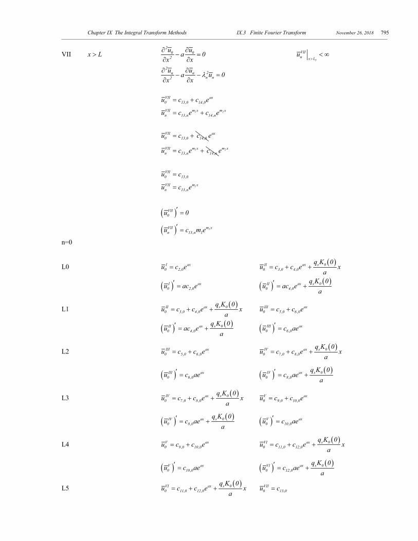
( ) ( ),
s 0VI ax0 12 0
q K 0u c ae
a′ = + ( )VII
0u 0′ =
n=0 L0 ,2 0c , ,3 0 4 0c c= +
,2 0ac ( ),
s 04 0
q K 0ac
a= +
L1 ( ), ,
1aL s 03 0 4 0 1
q K 0c c e L
a+ + , ,
1aL5 0 6 0c c e= +
( ),
1aL s 04 0
q K 0ac e
a+ ,
1aL6 0c ae=
L2 , ,2aL
5 0 6 0c c e+ ( ), ,
2aL s 07 0 8 0 2
q K 0c c e L
a= + +
,2aL
6 0c ae ( ),
2aL s 08 0
q K 0c ae
a= +
L3 ( ), ,
3aL s 07 0 8 0 3
q K 0c c e L
a+ + , ,
3aL9 0 10 0c c e= +
( ),
3aL s 08 0
q K 0c ae
a+ ,
3aL10 0c ae=
L4 , ,4aL
9 0 10 0c c e+ ( ), ,
4aL s 011 0 12 0 4
q K 0c c e L
a= + +
,4aL
10 0c ae ( ),
4aL s 012 0
q K 0c ae
a= +
L5 ( ), ,
5aL s 011 0 12 0 5
q K 0c c e L
a+ + ,13 0c=
( ),
5aL s 012 0
q K 0c ae
a+ 0=
Chapter IX The Integral Transform Methods IX.3 Finite Fourier Transform November 26, 2018 797
n>0
L0 ,2m xI
n 2 nu c e= ( ), ,
1 2m x m x s nIIn 1 n 2 n 2
n
q K 0u c e c e
λ= + +
( ) ,2m xI
n 2 n 2u c m e′ =
L1 ( ), ,
1 2m x m x s nIIn 1 n 2 n 2
n
q K 0u c e c e
λ= + + , ,
1 2m x m xIIIn 5 n 6 nu c e c e= +
( ) , ,1 2m x m xII
n 1 n 1 2 n 2u c m e c m e′ = + ( ) , ,1 2m x m xIII
n 5 n 1 6 n 2u c m e c m e′ = +
L2 , ,1 2m x m xIII
n 5 n 6 nu c e c e= + ( ), ,
1 2m x m x s nIVn 7 n 8 n 2
n
q K 0u c e c e
λ= + +
( ) , ,1 2m x m xIII
n 5 n 1 6 n 2u c m e c m e′ = + ( ) , ,1 2m x m xIV
n 7 n 1 8 n 2u c m e c m e′ = +
L3 ( ), ,
1 2m x m x s nIVn 7 n 8 n 2
n
q K 0u c e c e
λ= + + , ,
1 2m x m xVn 9 n 10 nu c e c e= +
( ) , ,1 2m x m xIV
n 7 n 1 8 n 2u c m e c m e′ = + ( ) , ,1 2m x m xV
n 9 n 1 10 n 2u c m e c m e′ = +
L4 , ,1 2m x m xV
n 9 n 10 nu c e c e= + ( ), ,
1 2m x m x s nVIn 11 n 12 n 2
n
q K 0u c e c e
λ= + +
( ) , ,1 2m x m xV
n 9 n 1 10 n 2u c m e c m e′ = + ( ) , ,1 2m x m xVI
n 11 n 1 12 n 2u c m e c m e′ = +
L5 ( ), ,
1 2m x m x s nVIn 11 n 12 n 2
n
q K 0u c e c e
λ= + + ,
1m xVIIn 13 nu c e=
( ) , ,1 2m x m xVI
n 11 n 1 12 n 2u c m e c m e′ = + ( ) ,1m xVII
n 13 n 1u c m e′ =
Chapter IX The Integral Transform Methods IX.3 Finite Fourier Transform November 26, 2018 798
n>0
L0 ,2 nc ( ), ,
s n3 n 4 n 2
n
q K 0c c
λ= + +
,2 n 2c m , ,3 n 1 4 n 2c m c m= +
L1 ( ), ,
1 1 2 1m L m L s n3 n 4 n 2
n
q K 0c e c e
λ+ + , ,
1 1 2 1m L m L5 n 6 nc e c e= +
, ,1 1 2 1m L m L
3 n 1 4 n 2c m e c m e+ , ,1 1 2 1m L m L
5 n 1 6 n 2c m e c m e= +
L2 , ,1 2 2 2m L m LIII
n 5 n 6 nu c e c e= + ( ), ,
1 2 2 2m L m L s n7 n 8 n 2
n
q K 0c e c e
λ= + +
, ,1 2 2 2m L m L
5 n 1 6 n 2c m e c m e+ , ,1 2 2 2m L m L
7 n 1 8 n 2c m e c m e= +
L3 ( ), ,
1 3 2 3m L m L s n7 n 8 n 2
n
q K 0c e c e
λ+ + , ,
1 3 2 3m L m L9 n 10 nc e c e= +
, ,1 3 2 3m L m L
7 n 1 8 n 2c m e c m e+ , ,1 3 2 3m L m L
9 n 1 10 n 2c m e c m e= +
L4 , ,1 4 2 4m L m L
9 n 10 nc e c e+ ( ), ,
1 4 2 4m L m L s n11 n 12 n 2
n
q K 0c e c e
λ= + +
, ,
1 4 2 4m L m L9 n 1 10 n 2c m e c m e+ , ,
1 4 2 4m L m L11 n 1 12 n 2c m e c m e= +
L5 ( ), ,
1 5 2 5m L m L s nVIn 11 n 12 n 2
n
q K 0u c e c e
λ= + + ,
1 5m L13 nc e=
, ,1 5 2 5m L m L
11 n 1 12 n 2c m e c m e+ ,1 5m L
13 n 1c m e=

Chapter IX The Integral Transform Methods IX.3 Finite Fourier Transform November 26, 2018 799
22
1 na am 02 2
λ = − + <
, 2
22 n
a am 02 2
λ = + + >
In x
u 0→−∞
=
I x 0< 2
0 02
u ua 0x x
∂ ∂− =
∂ ∂ I II
n nx 0 x 0u u
= ==
2
2n nn n2
u ua u 0x x
λ∂ ∂− − =
∂ ∂
I IIn n
x 0 x 0
u ux x
= =
∂ ∂=
∂ ∂
,
I0 1 0u c= ,
ax2 0c e+
,I
n 1 nu c= ,1 2m x m x
2 ne c e+
,
I ax0 2 0u c e=
,2m xI
n 2 nu c e=
( ) ,I ax
0 2 0u ac e′ =
( ) ,2m xI
n 2 n 2u c m e′ =
II 0 10 L x L= < < ( )2
0 0s 02
u ua q K 0 0x x
∂ ∂− + =
∂ ∂
1 1
II IIIn nx L x L
u u= =
=
( )2
2n nn n s n2
u ua u q K 0 0x x
λ∂ ∂− − + =
∂ ∂
1 1
II IIIn n
x L x L
u ux x
= =
∂ ∂=
∂ ∂
( ), ,
s 0II ax0 3 0 4 0
q K 0u c c e x
a= + +
( ), ,
1 2m x m x s nIIn 3 n 4 n 2
n
q K 0u c e c e
λ= + +
( ) ( ),
s 0II ax0 4 0
q K 0u ac e
a′ = +
( ) , ,1 2m x m xII
n 3 n 1 4 n 2u c m e c m e′ = +
III 1 2L x L< < 2
0 02
u ua 0x x
∂ ∂− =
∂ ∂
2 2
III IVn nx L x L
u u= =
=
22n nn n2
u ua u 0x x
λ∂ ∂− − =
∂ ∂
2 2
III IVn n
x L x L
u ux x
= =
∂ ∂=
∂ ∂
, ,III ax
0 5 0 6 0u c c e= +
, ,1 2m x m xIII
n 5 n 6 nu c e c e= +

Chapter IX The Integral Transform Methods IX.3 Finite Fourier Transform November 26, 2018 800
( ) ,III ax
0 6 0u c ae′ =
( ) , ,1 2m x m xIII
n 5 n 1 6 n 2u c m e c m e′ = +
IV 2 3L x L< < ( )2
0 0s 02
u ua q K 0 0x x
∂ ∂− + =
∂ ∂
3 3
IV Vn nx L x L
u u= =
=
( )2
2n nn n s n2
u ua u q K 0 0x x
λ∂ ∂− − + =
∂ ∂
3 3
IV Vn n
x L x L
u ux x
= =
∂ ∂=
∂ ∂
( ), ,
s 0IV ax0 7 0 8 0
q K 0u c c e x
a= + +
( ), ,
1 2m x m x s nIVn 7 n 8 n 2
n
q K 0u c e c e
λ= + +
( ) ( ),
s 0IV ax0 8 0
q K 0u c ae
a′ = +
( ) , ,1 2m x m xIV
n 7 n 1 8 n 2u c m e c m e′ = +
V x L> 2
0 02
u ua 0x x
∂ ∂− =
∂ ∂
4 4
V VIn nx L x L
u u= =
=
22n nn n2
u ua u 0x x
λ∂ ∂− − =
∂ ∂
4 4
V VIn n
x L x L
u ux x
= =
∂ ∂=
∂ ∂
, ,V ax0 9 0 10 0u c c e= +
, ,1 2m x m xV
n 9 n 10 nu c e c e= +
( ) ,V ax0 10 0u c ae′ =
( ) , ,1 2m x m xV
n 9 n 1 10 n 2u c m e c m e′ = +
VI 0 10 L x L= < < ( )2
0 0s 02
u ua q K 0 0x x
∂ ∂− + =
∂ ∂
5 5
VI VIIn nx L x L
u u= =
=
( )2
2n nn n s n2
u ua u q K 0 0x x
λ∂ ∂− − + =
∂ ∂
5 5
VI VIIn n
x L x L
u ux x
= =
∂ ∂=
∂ ∂
( ), ,
s 0VI ax0 11 0 12 0
q K 0u c c e x
a= + +
( ), ,
1 2m x m x s nVIn 11 n 12 n 2
n
q K 0u c e c e
λ= + +
( ) ( ),
s 0VI ax0 12 0
q K 0u c ae
a′ = +
( ) , ,1 2m x m xVI
n 11 n 1 12 n 2u c m e c m e′ = +
Chapter IX The Integral Transform Methods IX.3 Finite Fourier Transform November 26, 2018 801
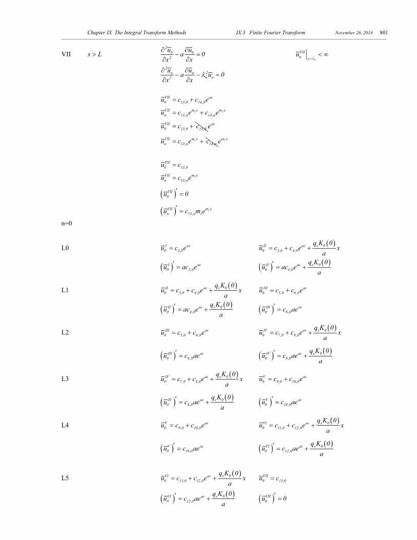
VII x L> 2
0 02
u ua 0x x
∂ ∂− =
∂ ∂
5
VIIn x L
u>
< ∞
2
2n nn n2
u ua u 0x x
λ∂ ∂− − =
∂ ∂
, ,
VII ax0 13 0 14 0u c c e= +
, ,1 2m x m xVII
n 13 n 14 nu c e c e= +
, ,VII0 13 0 14 0u c c= + axe
, ,1m xVII
n 13 n 14 nu c e c= + 2m xe
,
VII0 13 0u c=
,1m xVII
n 13 nu c e=
( )VII0u 0′ =
( ) ,1m xVII
n 13 n 1u c m e′ =
n=0
L0 ,I ax
0 2 0u c e= ( ), ,
s 0II ax0 3 0 4 0
q K 0u c c e x
a= + +
( ) ,I ax
0 2 0u ac e′ = ( ) ( ),
s 0II ax0 4 0
q K 0u ac e
a′ = +
L1 ( ), ,
s 0II ax0 3 0 4 0
q K 0u c c e x
a= + + , ,
III ax0 5 0 6 0u c c e= +
( ) ( ),
s 0II ax0 4 0
q K 0u ac e
a′ = + ( ) ,
III ax0 6 0u c ae′ =
L2 , ,III ax
0 5 0 6 0u c c e= + ( ), ,
s 0IV ax0 7 0 8 0
q K 0u c c e x
a= + +
( ) ,III ax
0 6 0u c ae′ = ( ) ( ),
s 0IV ax0 8 0
q K 0u c ae
a′ = +
L3 ( ), ,
s 0IV ax0 7 0 8 0
q K 0u c c e x
a= + + , ,
V ax0 9 0 10 0u c c e= +
( ) ( ),
s 0IV ax0 8 0
q K 0u c ae
a′ = + ( ) ,
V ax0 10 0u c ae′ =
L4 , ,V ax0 9 0 10 0u c c e= + ( )
, ,s 0VI ax
0 11 0 12 0
q K 0u c c e x
a= + +
( ) ,V ax0 10 0u c ae′ = ( ) ( )
,s 0VI ax
0 12 0
q K 0u c ae
a′ = +
L5 ( ), ,
s 0VI ax0 11 0 12 0
q K 0u c c e x
a= + + ,
VII0 13 0u c=
( ) ( ),
s 0VI ax0 12 0
q K 0u c ae
a′ = + ( )VII
0u 0′ =
Chapter IX The Integral Transform Methods IX.3 Finite Fourier Transform November 26, 2018 802


![GENERALIZED DISCRETE FINITE HALF RANGE FOURIER ......However, the treatment by Tolstov [7] is classical. Jerri [4] provides an excellent overview on convergence of the Fourier series](https://img.pdfslide.us/doc/110x75/612ed9141ecc515869431274/generalized-discrete-finite-half-range-fourier-however-the-treatment-by.jpg)