IX. Inferences from living taxa - UChicago GeoScigeosci.uchicago.edu/~foote/MODEL/2007/notes2007.9.pdf · IX. Inferences from living taxa 1 Some background on taxon-age distributions

GEOS 33001/EVOL 33001 23 October 2007 Page 1 of 22

IX. Inferences from living taxa

1 Some background on taxon-age distributions

1.1 Kinds of curves

1.1.1 Taxon-age distribution

Frequency distribution of times between origination and extinction; between originationand last time of census; or between first time of census and extinction.

1.1.2 Survivorship curves in the strict sense: survivorship (forward orbackward) in real time, with respect to some time of census.

1.2 To what are taxon-age distributions sensitive?

• origination rate

• extinction rate

• maximum time window over which durations can be observed





1.2.1 Note symmtery in effects of origination and extinction:

• If p 6= q, same taxon-age distribution results if p and q are switched.

• Distribution of ages of all taxa that become extinct within some window ofobservation is the same as that of all taxa that originate during this time window.

• Unless we know whether p > q, p = q, or p < q, we cannot independently estimate pand q from dynamic survivorship data.

• Approach we have taken—assuming dx is a function of extinction rate and time sinceorigin—works if p = q and window of observation is long compared with mean taxonduration (1/q)

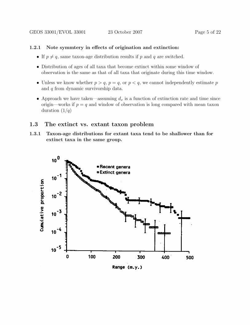
1.3 The extinct vs. extant taxon problem

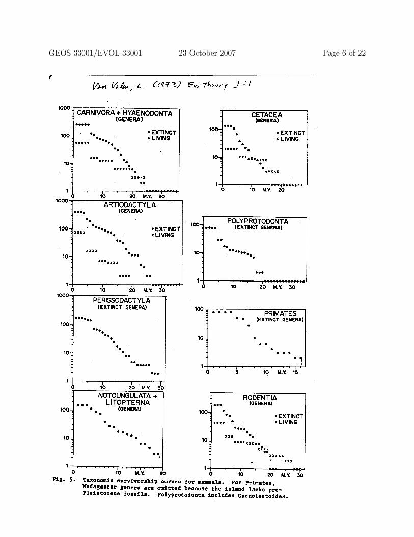
1.3.1 Taxon-age distributions for extant taxa tend to be shallower than forextinct taxa in the same group.



1.3.2 This extinct-versus-extant difference is also seen if other referenceplanes are used as the “Recent.”


1.3.3 Factors that contribute to this (assuming homogeneous origination andextinction) include the following (see Figures 9.4 and 9.5 from Foote2001a, above):

• “Reverse survivorship” of living taxa depends only on origination; age distribution ofextinct taxa depends on origination, extinction, and time window over whichobservations can be made.

• Longer-lived taxa more likely to survive to the Recent; therefore the extinct taxarepresent a biased subset, with longer-lived taxa excluded. (See Gilinsky, 1988,Paleobiology 14:370-386).

• Thus extinction rate is too high for the extinct subset of data, but origination ratefor the extant subset should not be biased.

• Extinct taxa truncated at two ends of range, extant taxa at only one end (nearlycomplete sampling in Recent).

1.4 Birth cohorts, death cohorts, boundary cohorts

1.4.1 Empirically (at least for marine animal genera), forward survivorship ofboundary cohorts is shallower than forward survivorship of immediatelysubsequent birth cohort.



1.4.2 Likewise, reverse survivorship of boundary cohorts is shallower thanreverse survivorship of immediately previous death cohort.


1.4.3 These differences are consistent with a model in which:

• the instantaneous rate at which a taxon becomes extinct declines with the age of thetaxon and

• the instantaneous rate at which a taxon gives rise to a new taxon increases with theage of the taxon

1.4.4 Why might we expect these rates to be age-dependent?

• We have already seen that, for taxa above the species level, instantaneous extinctionprobability decreases over time. This is because expected species richness within aparaclade, conditioned on survival of the paraclade, increases over time.

• Similar reasoning holds for origination, if the probability that a genus will give rise toa new genus depends on the number of species in the genus (as in Patzkowky’s [1995]model).

1.4.5 Alternatives to age-dependency of rates

• See Van Valen, Ev. Theory 4:129 (1979), and Pp. 200-16 in W. Glen, ed. The massextinction debates, Stanford (1994).

• Mixture of taxa with different rates (rates constant within each taxon).

• Special case of this: effect of a subset of taxa that are effectively “immortal” (“theLingula effect).





2 “The reconstructed evolutionary process”

2.1 Four kinds of birth-death processes

Time goes from t = 0 at clade origin to t = T at present day.

2.1.1 Unconditional

2.1.2 Conditioned on survival at least until time t

2.1.3 Conditioned on survival to time T (present day): all lineages tabulated.

2.1.4 Conditioned on survival to time T (present day): lineages tabulatedonly if they have at least one living descendant.

306 S. Nee and others The reconstructed evolutionary proc

time Figure 1. (a) A birth-death process which goes extinct before time t; (6) survives to t , but goes extinct before the present time T; the process (c) survives to the present. The bold lines are those lineages in (c) which have some descendants at the present. In (d) we have simply redrawn the bold lines in (c), removing the kinks, to construct an ideal reconstructed phylogeny.

For a birth-death process that is not extinct at time t, we have immediately, from distribution (3), the conditional probability Prz{i,t) :

Prz{i,t) = (1 - u,)uj-', i > 0. (4) I t is straightforward to derive from this the further conditional probability, Pr3{i,t; T ) , for a birth-death process that survives to T . To do this, we compound distribution (4) with the probability that a t least one of the i lineages existing at time t has some descendants at time T , and normalize appropriately: Pr3{i,t; T) =

This ugly expression disguises a simple underlying structure. The generating function of the probabilities (5) is:

1 - ut(l -{e}P(t,T)){ 1 - u,(l - P(t, T) ) s

We recognize the generating function (6) as the product of the generating functions of two random variables, say X and Y, where the distribution of X is given by (4) and the distribution of Y is given by: Pr{i,t; T ) =

that is, Y has a geometric distribution with parameter ut ( 1 - P(t, T ) ) . Hence, the number of lineages existing at time t for a birth-death process which will survive to the later time T can be treated as the sum of two independent random variables, each with a geometric distribution, but with different parameters. This distribution is, of course, not itself geometric. But we will now see that the distribution of the process reconstructed from this one, by pruning all those lineages from the tree that do not have contemporary descendants is, once again, characterized by a geometric distribution for the Pr{i,t). There are two ways to derive this distribution. The first continues our onward march and compounds distribution (5) with a modified binomial distribution. The second way ignores the underlying birth-death process and identifies a generalized birth process which generates the reconstructed process. We will do both, as each technique can be more useful than the other for addressing different questions.

Denote the probabilities (5) by 2 , . Of the k lineages existing at time t, i will have some progeny at the present time T , where i has a binomial distribution with parameter P ( t , T ) and no zero term (since at least one will survive to the present). So, for the reconstructed process: Pr4{i,t; T ) =

This simplifies to: Pr4{i,t; T ) =

that is, a geometric distribution with parameter u,P(O,T)/P(O,t). This simplification is most readily achieved by calculating the generating function of distribution (8). Notice that P(O,T)/P(O,t) is the overall probability that a birth-death process will survive to time T given that it has survived to time t.

We now identify a generalized birth process which generates distribution (9). Letting n(t) be the number of lineages at time t, we grow a reconstructed phylogenetic tree from time 0, with n(0)= 1, as follows. Each lineage gives rise to daughter lineages at a rate XP(t, T ), so after the small time interval dt, n(t + dt) = n(t) + 1 with probability n(t)hP(t, T)dt, n(t + dt) =

n(t) with probability 1 - n(t)P(t , T)dt. (10) This is a generalized birth process, with birth rate hP(t, T ) , and the formulae in Kendall (19483) give us:

where

Phil. Trans. R. Sac. Lond. B (1994)


2.2 Reconstructed process: expected no. of lineages at time t

2.2.1 Let p and q be per-capita rates of origination and extinction, and let nt

denote the number of reconstructed lineages at time t, i.e. the numberof lineages extant at time t that have at least one living descendant.

2.2.2 Let P (t1, t2) be the probability that a single lineage extant at time t1 hasat least one descendant still extant at t2:

P (t1, t2) =p− q

p− q exp[−(p− q)(t2 − t1)]

(Verify that this is correct using Raup 1985 eq. A13.)

2.2.3 Then E(nt) = exp[(p− q)t]P (t, T )/P (T )

In this expression:

• exp[(p− q)t] is the unconditional expectation

• P (t, T ) gives the probability that a lineage extant at time t will have at least onedescendant at time T

• P (T ) normalizes for the overall probability that the clade is extant at time T .

• See Harvey et al. 1994, Fig. 3.

2.2.4 Dependence of curve shape on q/p

• The larger the ratio q/p, the larger the separation between the actual andreconstructed curves, and the steeper the final rise near the recent.

• This makes sense given that age distribution of living taxa is exponential withparameter p.

2.2.5 Difficulty with visual interpretation of reconstructed curves

• Because curves must increase monotonically, many different combinations of (p, q)can lead to apparently similar curves.

• Therefore explicit parameter estimation is essential.

2.2.6 Maximum likelihood estimates of (p− q) and q/p

• Likelihood expression based on ages of lineages that have extant descendants. SeeNee et al. 1994 eq. 20

• Solution generally more sensitive to (p− q) than to q/p.


PAUL H. HARVEY ET AL.

1000: slope 0 025

1 0 0 -

Number o f

FIG.3. Log-linear plot of the average number of actual lineages through time (top line) and the average number of reconstructed lineages through time for a birth-death process with X = 0.1 and p = 0.075, as for figure 2B. The average actual number of progeny of a birth-death process at time t is exp[(X - p)t]. However, we are interested only in birth-death processes that have not gone extinct at time T, when we attempt the reconstruction, and, thus, we are interested in the average number of progeny of a birth-death process at time t, conditional upon nonextinction at time T. A routine calculation gives us the following formula for the top line: exp[(X - p)t]/P(T) - [P(t) - P(T)]/P(t)P(T - t). The early curvature in the line of actual numbers reflects the fact that those processes which survive to time Tare more likely to have got off to a flying start. The reconstructed numbers are given by equation (2) in the main text. In the middle time range [when t B 1/(X - p) and also t << T - 1/(X - p)], the reconstructed curve lies a distance a = - ln(1 - p/X) below the line of actual numbers. Starting off with a slope of X - p, at later times [roughly, t > T -1/(X - p)], the curve of reconstructed numbers steepens, ending with slope X (on a log-linear plot).

alytic approximations indicated in figure 3, and given more fully by (i) For (X - p)(T - t) smaller than unity,

ln[&(t, T)] o (constant) + Xt + . . . . (4a)

Here the constant term is -pT - ln(1 - p/X). (ii) For (X - p)(T - t) larger than unity,

Also note the early upward curvature of the line of actual numbers in figure 3, which results from the fact that not all original single lineages will have left descendants at time T. For ex- ample, if lineage death occurs before the original lineage has split into two daughter lineages, then the original lineage will leave no descendant lineages. Similarly, if the original lineage splits but then two successive lineage deaths occur, the original lineage will leave no descendants at time T. The early curvature is also evident in the sim-

ulation results given in figure 2A,B, reflecting the fact that some simulation runs result in extir- pation of all lineages early in time, whereas those that result in 1000 extant lineages are a nonran- dom sample of all runs; they are ones that got off to a flying start. This apparently higher rate of early cladogenesis would be expected in the fossil record of successful radiations, which may represent a sample of those starting with constant lineage birth and death rates. If these statistical effects are not fully appreciated, it could be tempting to misinterpret such a higher early slope as evidence for lineage birth rates being higher, and/or lineage death rates being lower, at early times.

In summary, the slope of a ln(N versus t curve that is constructed from empirical data for lineages whose birth and death rates are assumed constant can be used to make inferences about both birth and death rates. The "near-present" part of the curve provides an estimate of X, whereas the "far-distant" part gives an estimate of (X - p) [as also does the time taken to attain the asymptotic part, with its constant slope of (A - d l .

As a point of departure, the previous section used a null model in which the rates at which lineages split and become extinct do not vary either among lineages or over time. Notorious exceptions to those two assumptions occur during major radiations and mass extinctions. The identification of radiations in reconstructed phylogenies has been discussed elsewhere (Harvey et al. 1991; Nee et al. 1992, 1994). Here we ask what mass extinctions would look like on a reconstructed phylogeny. The answer depends both on the number of species becoming extinct and on the phylogenetic relationships among those species (Harvey and Nee 1993).

Consider two extreme cases. One extreme is "clade extinction," in which all members of a clade become extinct. After such an event, no descendant is left from (and therefore no record is left of) the entire clade. The other extreme is "uniform extinction," in which one representa- tive species of every lowest-level taxon becomes extinct- say one species from each genus. In between those extremes we have "random extinction," in which the species that become extinct are a phylogenetically random selection of those available.


Molecular phy1ogenie.r S. Nee and others 79

time Figure 3. The theoretically expected growth in the numbers of lineages through time for an actual (top line) and reconstructed phylogeny growing according to a constant rate birth-death process. The slopes of both curves are b-d, the speciation rate minus the extinction rate, over most of the history of the clade, and the slope of the reconstructed phylogeny asymptotically approaches the speciation rate towards the present day. 'The two curves pull apart further the greater the ratio of the extinction rate to the speciation rate.

origin and the present day. The slopes of the lines are the same (b-d) most of the time. Each line has a period of curvature. 'The push of the past', the apparently higher rate of cladogenesis a t the begin- ning of the growth of the actual phylogeny, results from the fact that we are only considering those clades which survived to the present day, and these are the ones which on average got off to a flying start. 'The pull of'the present', the apparent increase in the rate ofcladogenesis in the recent past in the reconstructed phylogeny, results from the fact that lineages which arose in the more recent past have had less time to go extinct and, so, are more likely to be represented in our reconstructed phylogeny. The slope of the reconstructed curve asymptotically approaches the birth rate as we get closer to the present (Harvey et al. 19946). Both the pull of the present and the push of the past become larger as dlb increases towards unity.

In fact, the parameters of most interest fbr phylogenies which grow according to this model are not b and

0 2 4 6 8 10 time

Figure 4. The lineages-through-time plot for species of the L)rosophila melanogaster subgroup.

Phzl. Trans. R. Soc. Lond. B (1994)

1 dlb

Figure 5. Contour plot of the likelihood surface for the Drosophila data. The maximum likelihood estimate, the peak of the surface, is marked by an X.

d separately, but functions of b and d; specifically, (b-d) and dlb. The first, (6-d), controls the rate of growth of the phylogeny and the second, dlb, controls both the magnitude of the pull of the present and the vulnerability of small clades to extinction through 'demographic stochasticity' (renru May 1973; see MacArthur & Wilson 1967).

Consider, now, figure 4, which shows the increase through time in the number of lineages in a molecular phylogeny of the Drosophzla melanogarter species subgroup (after Caccone et al. 1988). The graph starts when there are two lineages, because we have no information about the time of origin of the first lineage, and the time axis is in arbitrary units. The curve appears to be a straight line, with stochastic wobbling, and simple inspection suggests that a constant rate birth-death model is a reasonable assumption for the data, and that the extinction rate fbr this group is zero, as there is no upward curve towards the present. Using the underlying probability model, we can construct a log likelihood surfice fbr the parameters (figure 5), from which we may make inferences about which parameter values are sup-ported by the data. The peak of this surface, marked by an X, is the maximum likelihood estimate. The maximum likelihood estimate of'dlb is zero (i.e. a zero rate of extinction). The contour lines in the figure correspond to one, two and three units of 'support'. The maximum likelihood estimate of the parameters is about seven times more likely to produce the observed data than any point on the second contour line, and about twenty times more likely to produce the data than any point on the third contour line.

The shallowness of the likelihood surface in the dlb direction tells us quite clearly that we cannot exclude the possibility that, in fact, Drosophila has a substantial value of dlb. Although Drosophila give the appearance of having a zero extinction rate, this analysis shows us that we cannot have any great degree of confidence in that conclusion on the basis of these data alone. Such uncertainty about the parameters for small clades is not entirely a weakness of the evidence provided by reconstructed phylogenies as opposed to actual phylo-

Molecular phy1ogenie.r S. Nee and others 79

time Figure 3. The theoretically expected growth in the numbers of lineages through time for an actual (top line) and reconstructed phylogeny growing according to a constant rate birth-death process. The slopes of both curves are b-d, the speciation rate minus the extinction rate, over most of the history of the clade, and the slope of the reconstructed phylogeny asymptotically approaches the speciation rate towards the present day. 'The two curves pull apart further the greater the ratio of the extinction rate to the speciation rate.

origin and the present day. The slopes of the lines are the same (b-d) most of the time. Each line has a period of curvature. 'The push of the past', the apparently higher rate of cladogenesis a t the begin- ning of the growth of the actual phylogeny, results from the fact that we are only considering those clades which survived to the present day, and these are the ones which on average got off to a flying start. 'The pull of'the present', the apparent increase in the rate ofcladogenesis in the recent past in the reconstructed phylogeny, results from the fact that lineages which arose in the more recent past have had less time to go extinct and, so, are more likely to be represented in our reconstructed phylogeny. The slope of the reconstructed curve asymptotically approaches the birth rate as we get closer to the present (Harvey et al. 19946). Both the pull of the present and the push of the past become larger as dlb increases towards unity.

In fact, the parameters of most interest fbr phylogenies which grow according to this model are not b and

0 2 4 6 8 10 time

Figure 4. The lineages-through-time plot for species of the L)rosophila melanogaster subgroup.

Phzl. Trans. R. Soc. Lond. B (1994)

1 dlb

Figure 5. Contour plot of the likelihood surface for the Drosophila data. The maximum likelihood estimate, the peak of the surface, is marked by an X.

d separately, but functions of b and d; specifically, (b-d) and dlb. The first, (6-d), controls the rate of growth of the phylogeny and the second, dlb, controls both the magnitude of the pull of the present and the vulnerability of small clades to extinction through 'demographic stochasticity' (renru May 1973; see MacArthur & Wilson 1967).

Consider, now, figure 4, which shows the increase through time in the number of lineages in a molecular phylogeny of the Drosophzla melanogarter species subgroup (after Caccone et al. 1988). The graph starts when there are two lineages, because we have no information about the time of origin of the first lineage, and the time axis is in arbitrary units. The curve appears to be a straight line, with stochastic wobbling, and simple inspection suggests that a constant rate birth-death model is a reasonable assumption for the data, and that the extinction rate fbr this group is zero, as there is no upward curve towards the present. Using the underlying probability model, we can construct a log likelihood surfice fbr the parameters (figure 5), from which we may make inferences about which parameter values are sup-ported by the data. The peak of this surface, marked by an X, is the maximum likelihood estimate. The maximum likelihood estimate of'dlb is zero (i.e. a zero rate of extinction). The contour lines in the figure correspond to one, two and three units of 'support'. The maximum likelihood estimate of the parameters is about seven times more likely to produce the observed data than any point on the second contour line, and about twenty times more likely to produce the data than any point on the third contour line.

The shallowness of the likelihood surface in the dlb direction tells us quite clearly that we cannot exclude the possibility that, in fact, Drosophila has a substantial value of dlb. Although Drosophila give the appearance of having a zero extinction rate, this analysis shows us that we cannot have any great degree of confidence in that conclusion on the basis of these data alone. Such uncertainty about the parameters for small clades is not entirely a weakness of the evidence provided by reconstructed phylogenies as opposed to actual phylo-


2.2.7 Time-specific rates

• General form: p. 528 from Harvey et al. 1994

• Mass extinction (with nonselective extinction) [Harvey et al. Fig. 7]

• Mass extinction (with clade specificity vs. complete uniformity) [Harvey et al. Fig. 4]


PAUL H. HARVEY ET AL.

1000 j

100 Here P(T, t) is defined as Number Of Lineages

l 0 I I' FIG.6 . A simulated phylogeny produced according to a birth-death process, but with a density-dependent per-lineage death rate. A logistic density-dependent function was used (see text) with X = 0.05, K = 1000, and the simulation was stopped the first time that 1000 lineages were in existence. A lower value of X was used than in previous simulations, 0.05 rather than 0.1; thus, the total time taken for the simulation to reach 1000 lineages would be comparable with figure 5. The net birth rate (X - p) early on in the simulation (about 0.05 because p is near 0) is as in figure 2A. The upper light line gives the actual number of lineages at each time period, whereas the lower bold line gives the reconstructed number traced back from present-day species as in figure I.

lineages (fig. 6) is similar to that produced by a mass extinction accompanied by background mortality of lineages (fig. 5). The essential difference is that under density-dependent cladogenesis (as defined above), the slope of the curve at the start of the process is steeper than towards the end, whereas the opposite is the case for the mass extinction process. Although these distinc- tions have been recognized above in the context of particular simulations, they are likely to be generally true: whether density-dependent processes enter via lower birth rates or via higher death rates at later times, they will always tend to produce curves that are steeper in the earlier stages than in the later stages; mass extinctions (provided they lie relatively far in the past) will produce modest steepening in the earlier, pre- mass-extinction part of the curve, but the pri- mary effect will be the late upswing seen and discussed in figures 2 and 3.

The formulae for P (T - t) and k(t, T)given in equations (1) and (2), respectively, are easily generalized to the case when birth and death rates are not constant but instead vary over time. In this event, we denote the birth and death rates as X(t) and p(t), respectively. The resulting generalization of equation (1) for the probability that a lineage present at time t still has descendents at a later time T, P(t, T),is now (Kendall 1948b):

Equations (5) and (6) clearly reduce back to equation (1) when X and p are constant. Equation (2) remains valid, still giving the reconstructed number of lineages, ~ ( t , T),in this more general case {except, of course, that exp[(X - p)t] is replaced by exp[-p(t, O)] and P(T - t) by the P(t, T) of equation (91.

Now consider a catastrophe at a time T in which each of the lineages alive at time T survives with probabilityj For t > T, P(t, T)is as before given by equation (1). For t < T, P(t, T)is given by

Here z,(t, T) is the probability that a lineage that arises at time t has i progeny at time T, conditional upon its nonextinction by time 7. Equation (7) is essentially the product of the probability that the lineage has not disappeared by time T, multiplied by the probability that it has some surviving progeny by time T. The z, are known for both a constant birth-death process (Kendall 1948a) and a process in which birth and death rates vary through time (Kendall1948b), the for- mer being a special case of the latter, of course. In the case when birth and death rates are constant, both having the same values before and after the catastrophe at time 7, P(t, T) for t < T

is given by

The reconstructed number of lineages, fi(t, T), is now given by the appropriately generalized form of equation (2), exp[-p(t, O)]P(t, T)/P(O, T),with P(0, T)given by equation (8) with t = 0, P(t, T )by equation (1) if t > T and by equation (8) if t < T, and exp[-p(t, O)] by exp[(X -p)t] if t < T and f exp[(X - p)t] if t > T. More general situations, in which birth and death rates vary over time (apart from the catastrophe at t = 7) can be treated by inserting the appropriate z,(t, T) in equation (7).

foote

Rectangle

GEOS 33001/EVOL 33001 23 October 2007 Page 21 of 22529 PHYLOGENIES WITHOUT FOSSILS

Time

FIG. 7. A log-linear plot of the average actual and reconstructed numbers of lineages through time. As in figure 5, birth and death rates are 0.1 and 0.075, and a mass extinction event removes 80% of species on the first occasion that 500 lineages are in existence. The actual numbers grow as in figure 3, up to the time of the mass extinction when the number is reduced by 89%. As discussed in the text, the reconstructed curve, N, is calculated from the appropriately generalized form of equation (2), N(t, T ) = exp[-p(t, O)]P(t, T)/P(O, T), with P(t, T ) given by equation (1) for t > r and by equation (8) for t < r. Similarly, the actual number of lineages, N, is computed from the generalization of the formula given in the caption to figure 3: N(t, T ) = exp[-p(t, 0)1/P(O, T ) - [P(O, t) - P(O, T)I/P(O, t)P(t, T).

The actual a?d reconstructed numbers of lineages, Nand N, respectively, for this case when birth and death rates are everywhere constant except for a catastrophe at t = T , which extin- guishes all but a fractionf; are illustrated in figure 7. This is to be compared directly with the simulation result (for random extinction) in figure 5. These general, analytic results bear out our comments, made above on the basis of the simulation results, about the shapes of the curves.

Models of evolutionary processes can be used to reveal how the number of lineages that gave rise to present day descendants might be ex-pected to have increased through time. It is pos-

sible to separate the effects of lineage birth rates from lineage death rates in phylogenies that have been reconstructed without reference to a fossil record. It may even be possible to detect whether mass extinctions or density-dependent cladogenesis have occurred.

This research was supported by Science and Engineering Research Council grant GRIH53655 (P.H.H.), by the Royal Society (R.M.M.), and the Agriculture and Food Research Council (S.N.). We thank A. Purvis for valuable input into his project, and A. 0.Mooers for comments on the manuscript.

LITERATURECITED Harvey, P. H., and S. Nee. 1993. New uses for new

phylogenies. European Review 1: 1 1-1 9. Harvey, P. H., S. Nee, A. 0.Mooers, and L. Partridge.

199 1. These hierarchical views of life: phylogenies and metapopulations. Pp. 123-1 37 in R. J. Beny and T. J. Crawford, eds. Genes in ecology. British Ecological Society Special Publication. Blackwell, Oxford.

Kendall, D. G. 1948a. On some modes of population growth leading to R. A. Fisher's logarithmic series distribution. Biometrika 35:6-15.

. 1948b. On the generalized birth-and-death process. Annals of Mathematical Statistics 19: 1-1 5.

Nee, S., A. 0.Mooers, and P. H. Harvey. 1992. The tempo and mode of evolution revealed from molecular phylogenies. Proceedings of the National Academy of Sciences, USA 893322-8326.

Nee, S., R. M. May, and P. H. Harvey. 1994. The reconstructed evolutionary process. Philosophical Transactions of the Royal Society of London B, Biological Sciences 344:305-3 1 1.

Nitecki, M. H., and A. Hoffman. 1987. Neutral models in biology. Oxford, UK.

Raup, D. M., S. J. Gould, T. J. M. Schopf, and D. S. Simberloff. 1973. Stochastic models of phylogeny and the evolution of diversity. Journal of Geology 8 1525-542.

Corresponding Editor: D. Maddison

527 PHYLOGENIES W 'ITHOUT FOSSILS

Number Of Lineages

0 Apparent numbers uniform sxllnclian 0 Apparent "YmberS random en8nctlon

FIG.4. Here, as discussed in the text, each branch of a phylogeny splits into two at each time unit but, at time 5, 24 of the 32 extant lineages go extinct. The actual number of lineages at any time is given by the bold line. According to whether the extinct lineages form a complete clade (clade extinction), are one of each pair of most closely related sister taxa (uniform extinction), or are a random selection of lineages (random extinction), the reconstructed phylogeny produced from relationships among extant species shows different patterns.

The effects of these various types of mass extinction are shown in figure 4, which is based on a model phylogeny in which every lineage bi- furcates at each time interval. At time 0 there is 1 species, at time 1 there are 2 species, and by time 5 there are 32 species. At this time 5, a mass extinction event occurs that gets rid of 24 species; subsequently, the numbers double again each time unit. The actual total number of species at each time is shown by the bold line in figure 4, and the effects of clade, uniform, and random extinction are shown by the separate curves for the reconstructed phylogenies. Clade extinction is difficult or impossible to detect because each clade had its origin in a single branching event. When all the taxa in a clade are extirpated, evidence for that single original branching event is lost. In contrast, uniform extinction leaves a clear record because single members of many different clades are removed simultaneously. Accordingly, the phylogenetic tree reveals a time interval when far fewer lineages than expected seem to have appeared. Random extinction lies between the two extremes of clade and uniform extinction.

Figure 4 suggests that it is possible to detect the effects of some types of mass extinction in phylogenies produced by a pure birth process, that is when p = 0. To show the effect of intro- ducing background extinction into the process, we summarize the results of one typical simulation study in figure 5. In this simulation, X = 0.1, and p = 0.075, as in the simulation for figure 2B, except that when 500 extant lineages were

FIG. 5. A simulated phylogeny produced according to a birth-death process, but with a mass extinction event removing 400 lineages when 500 lineages first appeared. For this simulation birth and death rates were 0.1 and 0.075, as in figure 2B, and again the present was defined as the time when 1000 lineages were first extant. The upper light line gives the real number of lineages at each time period, and the lower bold line gives the estimated number traced back from present day species as in figure 1.

first reached a mass extinction event removed 400 species at random with respect to their phylogenetic relationships, leaving 100 species. The simulation then continued until the number of extant lineages reached 1000. The reconstructed curve starts off steeply, becomes shallower, and then after the date of the mass extinction, steepens towards the present. This latter phase is as studied in figures 2 and 3; it would be linear and coincident with the plot of actual number of species if p = 0.

The results in the reconstructed curve in figure 5 are very similar, except in one important respect, to those produced by density-dependent cladogenesis, such as was postulated for the slow- down in the rates of cladogenesis early in the radiation of the birds (Nee et al. 1992). Consider a simple model of density-dependent extinction of lineages, where p increases with the number of lineages present until an equilibrium number of lineages is reached, at which point p = X; the birth rate, A, is constant throughout. With a linear dependence of the death rate on the number of lineages, N, we have p = XN/K. Figure 6 shows the result of a typical computer simulation, for such a logistic model. The reconstructed curve starts off with a slope near to X (p is low such that X - p = A), flattens off as p increases, and the steepens again towards X in the final stages (for the reasons given earlier; see figures 2 and 3).

Note that the general shape of the reconstructed curve with density-dependent death rates of


2.2.8 Further complications

• Secular trend in rates can lead to enormous difference between true andreconstructed diversity [see Nee et al. 1994, Fig. 3].

• Incomplete sampling of living lineages leads to curve resembling that for seculardecrease in origination or secular increase in extinction [see Nee et al. 1994, Fig. 4].

310 S. Nee and others The reconstructed evolutionary process

results of this analysis are depicted in figure 3. The contrast between what actually occurred and what we see in the reconstructed phylogeny is quite stark in this case. A smooth deceleration in birth rate manifests itself as a quick radiation followed by a long period of stasis, with another burst of cladogenesis in the recent past.

So far, our models have assumed that the reconstructed phylogeny is based on all the extant members of the clade. There is a large number of ways that this assumption may be violated. One way is that the species chosen for study are a random set with respect to their phylogenetic relationships. Even with this restriction there is still a variety of ways in which this random set may be constructed. We will now consider the simplest. Suppose that each species has a probability, f , of being included in our analysis. We can pretend that a mass extinction happened a moment before the analysis and all surviving species are included in the analysis. Because the mass extinction is an entirely notional event, we will use model (10) which deals directly with the recon-structed phylogeny. We will suppose that birth and death rates are constant.

Kendall's derivations are in continuous time and, so, do not allow for simultaneous extinction or, to put it another way, a finite probability of death at any particular instant in time. We can circumvent this problem by exploiting the reasoning that leads to Dirac delta functions. Let the death rate be the following function of time:

P(t1T = P -g(t, T) lnf . (31) Here y is a constant, f is the probability of surviving the mass extinction, and g(t, T ) is essentially the Dirac delta function: a continuous function of time which is very close to zero everywhere except at t = T, the

time Figure 3. The top line is the average actual number of lineages through time, from equation (28b), and the bottom line is the average number of lineages at each time in the reconstructed phylogeny, from equation (29b). As described in the text, P ( t , T ) is found by numerical integration. p ( ~ , t )= p ( ~- t ) + (ln(1 + at) - ln(1 + a~) )pk /a . For this figure we chose T = 300, p = 0.075, k = 4, a = 0.2.

present, where it is very sharply peaked. Thus,

By using such functions we can validly exploit continuous time models and then, when we have our results, pass to the limit representing an instantaneous force of mortality at time T which is survived with probability f . Proceeding in this way we find the following expression for <n(t) > , the average number of lineages at time t for the reconstructed process (compare equation (29b)) :

where

f (A - P) f h + -f - P) exp(-(h - P ) ( T - t)) . (34)

P,(t, T ) has the same meaning as P(t , T ), and we have subscripted it solely to denote that it is the appropriate function for the postulated sampling rtgime. Figure 4 shows that the effect of this sampling is to create a spurious impression of a decline in birth rate and/or increase in death rate through time. This sampling theory has numerous biological interpreta- tions and applications (Nee et al. 1994). We thank the AFRC (SN), the Royal Society (RMM), the SERC (PHH: GR/H53655) and The Wellcome Trust (PHH: 38468) for supporting this work. We thank Professor Sir David Cox for helpful discussions.

0 100 200 300

time

Figure 4. The top curve shows the increase through time for the average number of lineages that actually existed. This curve is generated by equation (28b) with h = 0.139 and p = 0.114. Of the 10 000 species alive today, a fraction f is randomly chosen to construct the reconstructed phylogeny. Counting from the top, the second, third and fourth curves are generated by equation (33) with f = 0.1, 0.01 and 0.001, respectively, with h and p as for the top curve.

Phil. Trans. R. Soc. Land. B (1994)

310 S. Nee and others The reconstructed evolutionary process

results of this analysis are depicted in figure 3. The contrast between what actually occurred and what we see in the reconstructed phylogeny is quite stark in this case. A smooth deceleration in birth rate manifests itself as a quick radiation followed by a long period of stasis, with another burst of cladogenesis in the recent past.

So far, our models have assumed that the reconstructed phylogeny is based on all the extant members of the clade. There is a large number of ways that this assumption may be violated. One way is that the species chosen for study are a random set with respect to their phylogenetic relationships. Even with this restriction there is still a variety of ways in which this random set may be constructed. We will now consider the simplest. Suppose that each species has a probability, f , of being included in our analysis. We can pretend that a mass extinction happened a moment before the analysis and all surviving species are included in the analysis. Because the mass extinction is an entirely notional event, we will use model (10) which deals directly with the recon-structed phylogeny. We will suppose that birth and death rates are constant.

Kendall's derivations are in continuous time and, so, do not allow for simultaneous extinction or, to put it another way, a finite probability of death at any particular instant in time. We can circumvent this problem by exploiting the reasoning that leads to Dirac delta functions. Let the death rate be the following function of time:

P(t1T = P -g(t, T) lnf . (31) Here y is a constant, f is the probability of surviving the mass extinction, and g(t, T ) is essentially the Dirac delta function: a continuous function of time which is very close to zero everywhere except at t = T, the

time Figure 3. The top line is the average actual number of lineages through time, from equation (28b), and the bottom line is the average number of lineages at each time in the reconstructed phylogeny, from equation (29b). As described in the text, P ( t , T ) is found by numerical integration. p ( ~ , t )= p ( ~- t ) + (ln(1 + at) - ln(1 + a~) )pk /a . For this figure we chose T = 300, p = 0.075, k = 4, a = 0.2.

present, where it is very sharply peaked. Thus,

By using such functions we can validly exploit continuous time models and then, when we have our results, pass to the limit representing an instantaneous force of mortality at time T which is survived with probability f . Proceeding in this way we find the following expression for <n(t) > , the average number of lineages at time t for the reconstructed process (compare equation (29b)) :

where

f (A - P) f h + -f - P) exp(-(h - P ) ( T - t)) . (34)

P,(t, T ) has the same meaning as P(t , T ), and we have subscripted it solely to denote that it is the appropriate function for the postulated sampling rtgime. Figure 4 shows that the effect of this sampling is to create a spurious impression of a decline in birth rate and/or increase in death rate through time. This sampling theory has numerous biological interpreta- tions and applications (Nee et al. 1994). We thank the AFRC (SN), the Royal Society (RMM), the SERC (PHH: GR/H53655) and The Wellcome Trust (PHH: 38468) for supporting this work. We thank Professor Sir David Cox for helpful discussions.

0 100 200 300

time

Figure 4. The top curve shows the increase through time for the average number of lineages that actually existed. This curve is generated by equation (28b) with h = 0.139 and p = 0.114. Of the 10 000 species alive today, a fraction f is randomly chosen to construct the reconstructed phylogeny. Counting from the top, the second, third and fourth curves are generated by equation (33) with f = 0.1, 0.01 and 0.001, respectively, with h and p as for the top curve.

Phil. Trans. R. Soc. Land. B (1994)

Documents

IX. Inferences from living taxa - UChicago GeoScigeosci.uchicago.edu/~foote/MODEL/2007/notes2007.9.pdf · IX. Inferences from living taxa 1 Some background on taxon-age distributions