Contents

IV ELASTICITY ii

11 Elastostatics 1

11.1 Overview . . . . . . . . . . . . . . . . . . . . . . . . . . . . . . . . . . . . . . 111.2 Displacement and Strain . . . . . . . . . . . . . . . . . . . . . . . . . . . . . 4

11.2.1 Displacement Vector and its Gradient . . . . . . . . . . . . . . . . . . 411.2.2 Expansion, Rotation, Shear and Strain . . . . . . . . . . . . . . . . . 5

11.3 Stress, Elastic Moduli, and Elastostatic Equilibrium . . . . . . . . . . . . . . 1111.3.1 Stress Tensor . . . . . . . . . . . . . . . . . . . . . . . . . . . . . . . 1111.3.2 Realm of Validity for Hooke’s Law . . . . . . . . . . . . . . . . . . . 1311.3.3 Elastic Moduli and Elastostatic Stress Tensor . . . . . . . . . . . . . 1411.3.4 Energy of Deformation . . . . . . . . . . . . . . . . . . . . . . . . . . 1511.3.5 Thermoelasticity . . . . . . . . . . . . . . . . . . . . . . . . . . . . . 1711.3.6 Molecular Origin of Elastic Stress; Estimate of Moduli . . . . . . . . 1811.3.7 Elastostatic Equilibrium: Navier-Cauchy Equation . . . . . . . . . . . 20

11.4 Young’s Modulus and Poisson’s Ratio for an Isotropic Material: A SimpleElastostatics Problem . . . . . . . . . . . . . . . . . . . . . . . . . . . . . . . 23

11.5 Reducing the Elastostatic Equations to One Dimension for a Bent Beam:Cantilever Bridges, Foucault Pendulum, DNA Molecule, Elastica . . . . . . . 25

11.6 Buckling and Bifurcation of Equilibria . . . . . . . . . . . . . . . . . . . . . 3411.6.1 Elementary Theory of Buckling and Bifurcation . . . . . . . . . . . . 3411.6.2 Collapse of the World Trade Center Buildings . . . . . . . . . . . . . 3711.6.3 Buckling with Lateral Force; Connection to Catastrophe Theory . . . 3811.6.4 Other Bifurcations: Venus Fly Trap, Whirling Shaft, Triaxial Stars,

Onset of Turbulence . . . . . . . . . . . . . . . . . . . . . . . . . . . 3911.7 Reducing the Elastostatic Equations to Two Dimensions for a Deformed Thin

Plate: Stress-Polishing a Telescope Mirror . . . . . . . . . . . . . . . . . . . 4111.8 T2 Cylindrical and Spherical Coordinates: Connection Coefficients and

Components of the Gradient of the Displacement Vector . . . . . . . . . . . 4511.9 T2 Solving the 3-Dimensional Navier-Cauchy Equation in Cylindrical Co-

ordinates . . . . . . . . . . . . . . . . . . . . . . . . . . . . . . . . . . . . . . 5111.9.1 T2 Simple Methods: Pipe Fracture and Torsion Pendulum . . . . . 5111.9.2 T2 Separation of Variables and Green’s Functions: Thermoelastic

Noise in Mirrors . . . . . . . . . . . . . . . . . . . . . . . . . . . . . . 54

i

Part IV

ELASTICITY

ii

Elasticity

Version 1211.2.K, 19 Feb 2013

Although ancient civilizations built magnificent pyramids, palaces and cathedrals, andpresumably developed insights into how to avoid their collapse, mathematical models forthis (the theory of elasticity) were not developed until the 17th century and later.

The 17th-century focus was on a beam (e.g. a vertical building support) under com-pression or tension. Galileo initiated this study in 1632, followed most notably by RobertHooke in 1660. Bent beams became the focus with the work of Edme Mariotte in 1680.Bending and compression came together with Leonhard Euler’s 1744 theory of the bucklingof a compressed beam and his derivation of the complex shapes of very thin wires, whoseends are pushed toward each other (elastica). These ideas were extended to two-dimensionalthin plates by Marie-Sophie Germain and Joseph-Louis Lagrange in 1811-16, in a studythat was brought to full fruition by Augustus Edward Hugh Love in 1888. The full the-ory of 3-dimensional, stressed, elastic objects was developed by Claude-Louis Navier andby Augustin-Louis Cauchy in 1821-22; and a number of great mathematicians and naturalphilosophers then developed techniques for solving the Navier-Cauchy equations, particu-larly for phenomena relevant to railroads and construction. In 1956, with the advent ofmodern digital computers, M.J. Turner, R.W. Cough, H.C. Martin and L.J. Topp pioneeredfinite-element methods for numerically modeling stressed bodies. Finite-element numericalsimulations are now a standard tool for designing mechanical structures and devices, and,more generally, for solving difficult elasticity problems.

These historical highlights cannot begin to do justice to the history of elasticity research.For much more detail see, e.g., the (out of date) long introduction in Love (1927); and forfar more detail than most anyone wants, see the (even more out of date) two-volume workby Todhunter and Pearson (1886).

Despite its centuries-old foundations, elasticity remains of great importance today, and itsmodern applications include some truly interesting phenomena. Among those applications,most of which we shall touch on in this book, are these: (i) the design and collapse ofbridges, skyscrapers, automobiles, and other structures and mechanical devices; (ii) thedevelopment and applications of new materials such as carbon nanotubes, which are so lightand strong that one could aspire to use them to build a tether connecting a geostationarysatellite to the earth’s surface; (iii) high-precision physics experiments with torsion pendulaand microcantilevers, including brane-worlds-motivated searches for gravitational evidenceof macroscopic higher dimensions of space; (iv) nano-scale cantilever probes in scanningelectron microscopes and atomic force microscopes; (v) studies of biophysical systems such

iii

iv

as DNA molecules, cell walls, and the Venus fly trap plant; and (vi) plate tectonics, quakes,seismic waves, and seismic tomography in the earth and other planets. Indeed, elastic solidsare so central to everyday life and to modern science, that a basic understanding of theirbehavior should be part of the the repertoire of every physicist. That is the goal of this PartIV of our book.

We shall devote just two chapters to elasticity. The first (Chap. 11) will focus on elasto-statics: the properties of materials and solid objects that are in static equilibrium, with allforces and torques balancing out. The second (Chap. 12) will focus on elastodynamics: thedynamical behavior of materials and solid objects that are perturbed away from equilibrium.

Chapter 11

Elastostatics

Version 1211.2.K, 19 Feb 2013Please send comments, suggestions, and errata via email to kip@caltech.edu or on paper toKip Thorne, 350-17 Caltech, Pasadena CA 91125

Box 11.1

Reader’s Guide

• This chapter relies heavily on the geometric view of Newtonian physics (includingvector and tensor analysis) laid out in Chap. 1.

• Chapter 12 (Elastodynamics) is an extension of this chapter; to understand it, thischapter must be mastered.

• The idea of the irreducible tensorial parts of a tensor, and its most importantexample, decomposition of the gradient of a displacement vector into expansion,rotation, and shear (Sec. 11.2.2 and Box 11.2) will be encountered again in Part V(Fluid Mechanics) and Part VI (Plasma Physics).

• Differentiation of vectors and tensors with the help of connection coefficients (Sec.11.8; Track Two), will be used occasionally in Part V (Fluid Mechanics) and PartVI (Plasma Physics), and will be generalized to non-orthonormal bases in Part VII(General Relativity), where it will become Track One and will be used extensively.

• No other portions of this chapter are important for subsequent Parts of this book.

11.1 Overview

In this chapter, we consider static equilibria of elastic solids — for example, the equilibriumshape and internal strains of a steel column in the World Trade Center’s Twin Towers, afteran airliner crashed into it, and the weight of sagging floors deformed the column (Sec. 11.6).

1

2

From the viewpoint of continuum mechanics, a solid (e.g. the column’s steel) is a sub-stance that recovers its original shape after the application and removal of any small stress.Note the requirement that this be true for any small stress. Many fluids (e.g. water) satisfyour definition as long as the applied stress is isotropic, but they will deform permanentlyunder a shear stress. Other materials (for example, the earth’s crust) are only elastic forlimited times, but undergo plastic flow when a small stress is applied for a long time.

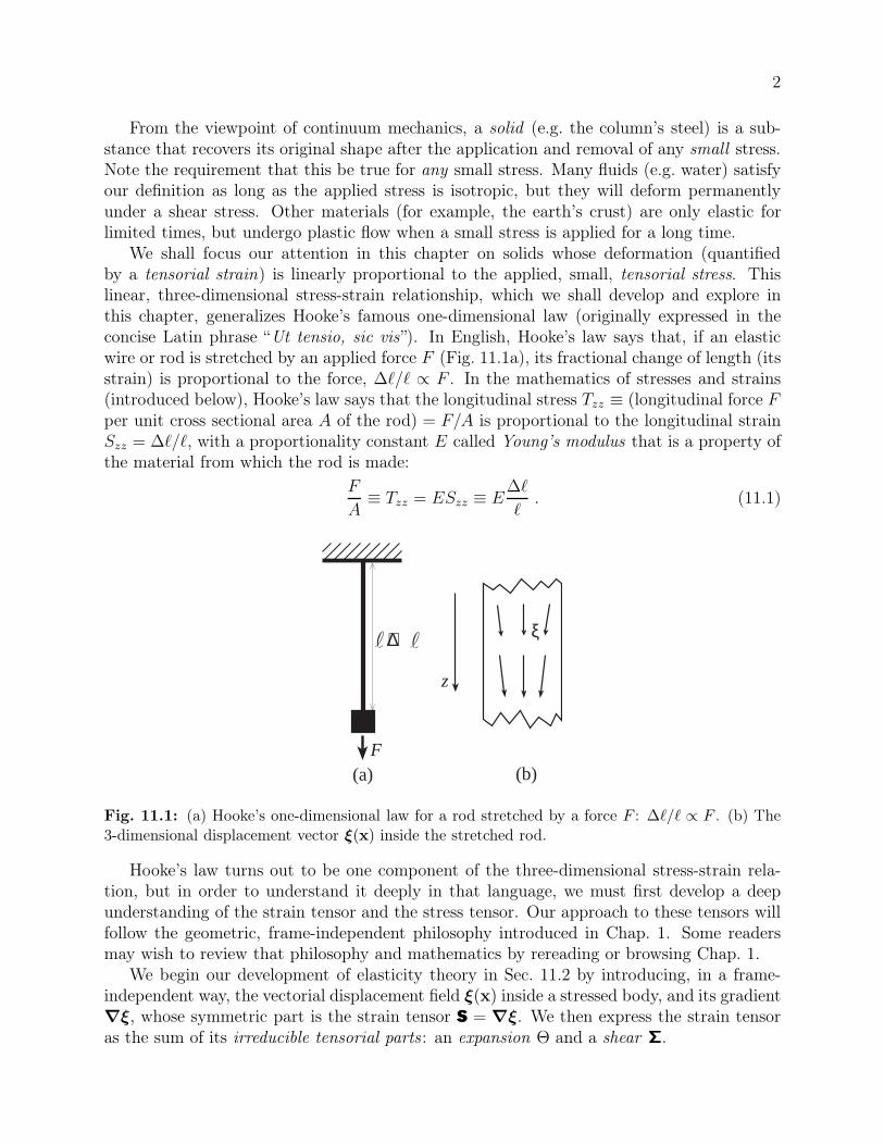
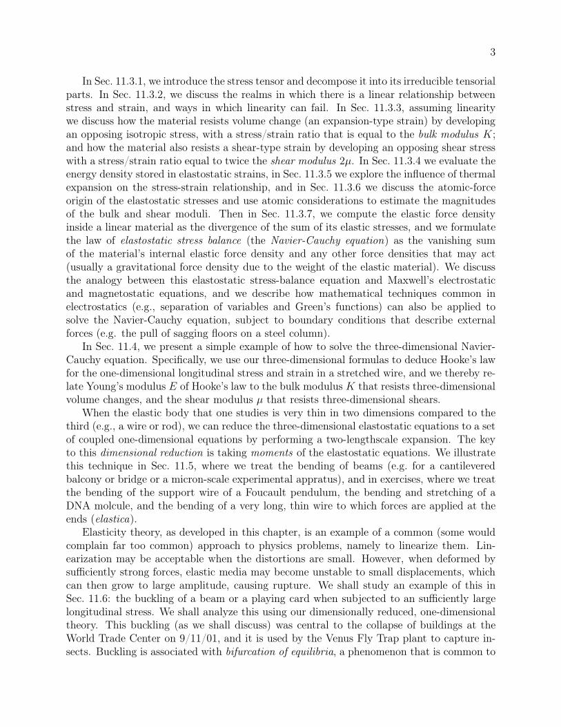
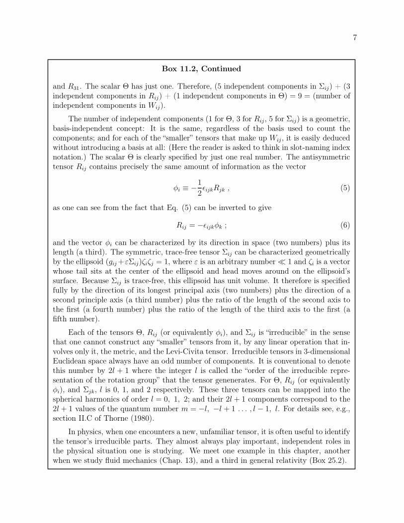
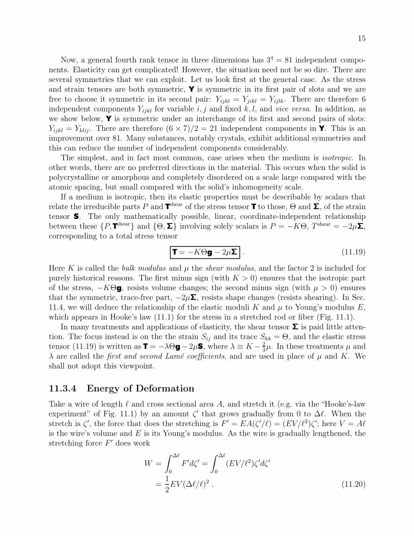
We shall focus our attention in this chapter on solids whose deformation (quantifiedby a tensorial strain) is linearly proportional to the applied, small, tensorial stress. Thislinear, three-dimensional stress-strain relationship, which we shall develop and explore inthis chapter, generalizes Hooke’s famous one-dimensional law (originally expressed in theconcise Latin phrase “Ut tensio, sic vis”). In English, Hooke’s law says that, if an elasticwire or rod is stretched by an applied force F (Fig. 11.1a), its fractional change of length (itsstrain) is proportional to the force, ∆ℓ/ℓ ∝ F . In the mathematics of stresses and strains(introduced below), Hooke’s law says that the longitudinal stress Tzz ≡ (longitudinal force Fper unit cross sectional area A of the rod) = F/A is proportional to the longitudinal strainSzz = ∆ℓ/ℓ, with a proportionality constant E called Young’s modulus that is a property ofthe material from which the rod is made:

F

A≡ Tzz = ESzz ≡ E

∆ℓ

ℓ. (11.1)

z

F

+∆

(a)

ξ

(b)

Fig. 11.1: (a) Hooke’s one-dimensional law for a rod stretched by a force F : ∆ℓ/ℓ ∝ F . (b) The3-dimensional displacement vector ξ(x) inside the stretched rod.

Hooke’s law turns out to be one component of the three-dimensional stress-strain rela-tion, but in order to understand it deeply in that language, we must first develop a deepunderstanding of the strain tensor and the stress tensor. Our approach to these tensors willfollow the geometric, frame-independent philosophy introduced in Chap. 1. Some readersmay wish to review that philosophy and mathematics by rereading or browsing Chap. 1.

We begin our development of elasticity theory in Sec. 11.2 by introducing, in a frame-independent way, the vectorial displacement field ξ(x) inside a stressed body, and its gradient∇ξ, whose symmetric part is the strain tensor S = ∇ξ. We then express the strain tensoras the sum of its irreducible tensorial parts: an expansion Θ and a shear Σ.

3

In Sec. 11.3.1, we introduce the stress tensor and decompose it into its irreducible tensorialparts. In Sec. 11.3.2, we discuss the realms in which there is a linear relationship betweenstress and strain, and ways in which linearity can fail. In Sec. 11.3.3, assuming linearitywe discuss how the material resists volume change (an expansion-type strain) by developingan opposing isotropic stress, with a stress/strain ratio that is equal to the bulk modulus K;and how the material also resists a shear-type strain by developing an opposing shear stresswith a stress/strain ratio equal to twice the shear modulus 2µ. In Sec. 11.3.4 we evaluate theenergy density stored in elastostatic strains, in Sec. 11.3.5 we explore the influence of thermalexpansion on the stress-strain relationship, and in Sec. 11.3.6 we discuss the atomic-forceorigin of the elastostatic stresses and use atomic considerations to estimate the magnitudesof the bulk and shear moduli. Then in Sec. 11.3.7, we compute the elastic force densityinside a linear material as the divergence of the sum of its elastic stresses, and we formulatethe law of elastostatic stress balance (the Navier-Cauchy equation) as the vanishing sumof the material’s internal elastic force density and any other force densities that may act(usually a gravitational force density due to the weight of the elastic material). We discussthe analogy between this elastostatic stress-balance equation and Maxwell’s electrostaticand magnetostatic equations, and we describe how mathematical techniques common inelectrostatics (e.g., separation of variables and Green’s functions) can also be applied tosolve the Navier-Cauchy equation, subject to boundary conditions that describe externalforces (e.g. the pull of sagging floors on a steel column).

In Sec. 11.4, we present a simple example of how to solve the three-dimensional Navier-Cauchy equation. Specifically, we use our three-dimensional formulas to deduce Hooke’s lawfor the one-dimensional longitudinal stress and strain in a stretched wire, and we thereby re-late Young’s modulus E of Hooke’s law to the bulk modulus K that resists three-dimensionalvolume changes, and the shear modulus µ that resists three-dimensional shears.

When the elastic body that one studies is very thin in two dimensions compared to thethird (e.g., a wire or rod), we can reduce the three-dimensional elastostatic equations to a setof coupled one-dimensional equations by performing a two-lengthscale expansion. The keyto this dimensional reduction is taking moments of the elastostatic equations. We illustratethis technique in Sec. 11.5, where we treat the bending of beams (e.g. for a cantileveredbalcony or bridge or a micron-scale experimental appratus), and in exercises, where we treatthe bending of the support wire of a Foucault pendulum, the bending and stretching of aDNA molcule, and the bending of a very long, thin wire to which forces are applied at theends (elastica).

Elasticity theory, as developed in this chapter, is an example of a common (some wouldcomplain far too common) approach to physics problems, namely to linearize them. Lin-earization may be acceptable when the distortions are small. However, when deformed bysufficiently strong forces, elastic media may become unstable to small displacements, whichcan then grow to large amplitude, causing rupture. We shall study an example of this inSec. 11.6: the buckling of a beam or a playing card when subjected to an sufficiently largelongitudinal stress. We shall analyze this using our dimensionally reduced, one-dimensionaltheory. This buckling (as we shall discuss) was central to the collapse of buildings at theWorld Trade Center on 9/11/01, and it is used by the Venus Fly Trap plant to capture in-sects. Buckling is associated with bifurcation of equilibria, a phenomenon that is common to

4

many physical systems, not just elastostatic ones. We illustrate bifurcation in Sec. 11.6 usingour beam under a compressive load, and we explore its connection to catastrophe theory.

In Sec. 11.7, we discuss dimensional reduction by the method of moments for bodies thatare thin in only one dimension, not two; e.g. plates, thin mirrors, and a Venus-fly-trap leaf.In such bodies, the three-dimensional elastostatic equations are reduced to two dimensions.We illustrate our two-dimensional formalism by the stress polishing of telescope mirrors.

Because elasticity theory entails computing gradients of vectors and tensors, and practi-cal calculations are often best performed in cylindrical or spherical coordinate systems, wepresent a mathematical digression in our Track-two Sec. 11.8 — an introduction to how onecan perform practical calculations of gradients of vectors and tensors in the orthonormalbases associated with curvilinear coordinate systems, using the concept of a connection coef-ficient (the directional derivative of one basis vector field along another). In Sec. 11.8 we alsouse these connection coefficients to derive some useful differentiation formulae in cylindricaland spherical coordinate systems and bases.

As illustrative examples of both connection coefficients and elastostatic force balance,in our Track-Two Sec 11.9 and various exercises, we give practical examples of solutions ofthe elastostatic force-balance equation in cylindrical coordinates: for a pipe that containsa fluid under pressure (Sec. 11.9.1 and Ex. 11.23); for the wire of a torsion pendulum (Ex.11.24); and for a cylinder that is subjected to a Gaussian-shaped pressure on one face (Sec.11.9.2) — a problem central to computing thermal noise in mirrors. We shall sketch how tosolve this cylinder-pressure problem using the two common techniques of elastostatics andelectrostatics: separation of variables (text of Sec. 11.9.2) and a Green’s function (Ex. 11.26).

11.2 Displacement and Strain

We begin our study of elastostatics by introducing the elastic displacement vector, its gra-dient, and the irreducible tensorial parts of its gradient. We then identify the strain as thesymmetric part of the displacement’s gradient.

11.2.1 Displacement Vector and its Gradient

We label the position of a point (a tiny bit of solid) in an unstressed body, relative to someconvenient origin in the body, by its position vector x. Let a force be applied so the bodydeforms and the point moves from x to x+ξ(x); we call ξ the point’s displacement vector. Ifξ were constant (i.e., if its components in a Cartesian coordinate system were independentof location in the body), then the body would simply be translated and would undergo nodeformation. To produce a deformation, we must make the displacement ξ change from onelocation to another. The most simple, coordinate-independent way to quantify those changesis by the gradient of ξ, ∇ξ. This gradient is a second-rank tensor field;1 we shall denote itW:

W ≡ ∇ξ . (11.2a)

1In our treatment of elasticity theory, we shall make extensive use of the tensorial concepts introduced inChap. 1.

5

This tensor is a geometric object, defined independent of any coordinate system in themanner described in Sec. 1.7. In slot-naming index notation (Sec. 1.5), it is denoted

Wij = ξi;j , (11.2b)

where the index j after the semicolon is the name of the gradient slot.In a Cartesian coordinate system the components of the gradient are always just partial

derivatives [Eq. (1.15c)], and therefore the Cartesian components of W are

Wij =∂ξi∂xj

= ξi,j . (11.2c)

(Recall that indices following a comma represent partial derivatives.) In Sec. 11.8, we shalllearn how to compute the components of the gradient in cylindrical and spherical coordinates.

In any small neighborhood of any point xo in a deformed body, we can reconstructthe displacement vector ξ from its gradient W up to an additive constant. Specifically, inCartesian coordinates, by virtue of a Taylor-series expansion, ξ is given by

ξi(x) = ξi(xo) + (xj − xo j)(∂ξi/∂xj) + . . .

= ξi(xo) + (xj − xo j)Wij + . . . . (11.3)

If we place our origin of Cartesian coordinates at xo and let the origin move with the pointthere as the body deforms [so ξ(xo) = 0], then Eq. (11.3) becomes

ξi = Wijxj when |x| is sufficiently small. (11.4)

We have derived this as a relationship between components of ξ, x, and W in a Cartesiancoordinate system. However, the indices can also be thought of as the names of slots (Sec.1.5) and correspondingly Eq. (11.4) can be regarded as a geometric, coordinate-independentrelationship between the vectors and tensor ξ, x, and W.

In Ex. 11.2 below, we shall use Eq. (11.4) to gain insight into the displacements associatedwith various parts of the gradient W.

11.2.2 Expansion, Rotation, Shear and Strain

In Box 11.2, we introduce the concept of the irreducible tensorial parts of a tensor, and westate that in physics, when one encounters a new, unfamiliar tensor, it is often useful toidentify the tensor’s irreducible parts. The gradient of the displacement vector, W = ∇ξ

is an important example. It is a second-rank tensor. Therefore, as we discuss in Box 11.2,its irreducible tensorial parts are its trace Θ ≡ Tr(W) = Wii = ∇ · ξ, which is called thedeformed body’s expansion for reasons we shall explore below; its symmetric, trace-free partΣ, which is called the body’s shear ; and its antisymmetric part R, which is called the body’srotation:

Θ = Wii = ∇ · ξ , (11.5a)

Σij =1

2(Wij +Wji)−

1

3Θgij =

1

2(ξi;j + ξj;i)−

1

3ξk;k gij , (11.5b)

6

Box 11.2

Irreducible Tensorial Parts of a Second-Rank Tensor

in 3-Dimensional Euclidean Space

In quantum mechanics, an important role is played by the rotation group, i.e.,the set of all rotation matrices, viewed as a mathematical entity called a group; see,e.g., Chap. XIII of Messiah (1962) or Chap. 16 of Mathews and Walker (1965). Eachtensor in 3-dimensional Euclidean space, when rotated, is said to generate a specificrepresentation of the rotation group. Tensors that are “big”, in a sense to be discussedbelow, can be broken down into a sum of several tensors that are “as small as possible.”These smallest tensors are said to generate irreducible representations of the rotationgroup. All this mumbo-jumbo is really very simple, when one thinks about tensors asgeometric, frame-independent objects.

As an example, consider an arbitrary second-rank tensor Wij in three-dimensional,Euclidean space. In the text Wij is the gradient of the displacement vector. From thistensor we can construct the following “smaller” tensors by linear operations that involveonly Wij and the metric gij . (As these smaller tensors are enumerated, the reader shouldthink of the notation used as the basis-independent, frame-independent, slot-namingindex notation of Sec. 1.5.1.) The smaller tensors are the contraction (i.e., trace) of Wij ,

Θ ≡ Wijgij = Wii ; (1)

the antisymmetric part of Wij

Rij ≡1

2(Wij −Wji) ; (2)

and the symmetric, trace-free part of Wij

Σij ≡1

2(Wij +Wji)−

1

3gijWkk . (3)

It is straightforward to verify that the original tensor Wij can be reconstructed fromthese three “smaller” tensors, plus the metric gij as follows:

Wij =1

3Θgij + Σij +Rij . (4)

One way to see the sense in which Θ, Rij, and Σij are “smaller” than Wij is bycounting the number of independent real numbers required to specify their componentsin an arbitrary basis. (In this counting the reader is asked to think of the index notationas components on a chosen basis.) The original tensor Wij has 3 × 3 = 9 components(W11,W12,W13,W21 , . . .), all of which are independent. By contrast, the 9 componentsof Σij are not independent; symmetry requires that Σij ≡ Σji, which reduces the numberof independent components from 9 to 6; trace-freeness, Σii = 0, reduces it further from6 to 5. The antisymmetric tensor Rij has just three independent components, R12, R23,

7

Box 11.2, Continued

and R31. The scalar Θ has just one. Therefore, (5 independent components in Σij) + (3independent components in Rij) + (1 independent components in Θ) = 9 = (number ofindependent components in Wij).

The number of independent components (1 for Θ, 3 for Rij , 5 for Σij) is a geometric,basis-independent concept: It is the same, regardless of the basis used to count thecomponents; and for each of the “smaller” tensors that make up Wij , it is easily deducedwithout introducing a basis at all: (Here the reader is asked to think in slot-naming indexnotation.) The scalar Θ is clearly specified by just one real number. The antisymmetrictensor Rij contains precisely the same amount of information as the vector

φi ≡ −1

2ǫijkRjk , (5)

as one can see from the fact that Eq. (5) can be inverted to give

Rij = −ǫijkφk ; (6)

and the vector φi can be characterized by its direction in space (two numbers) plus itslength (a third). The symmetric, trace-free tensor Σij can be characterized geometricallyby the ellipsoid (gij+εΣij)ζiζj = 1, where ε is an arbitrary number ≪ 1 and ζi is a vectorwhose tail sits at the center of the ellipsoid and head moves around on the ellipsoid’ssurface. Because Σij is trace-free, this ellipsoid has unit volume. It therefore is specifiedfully by the direction of its longest principal axis (two numbers) plus the direction of asecond principle axis (a third number) plus the ratio of the length of the second axis tothe first (a fourth number) plus the ratio of the length of the third axis to the first (afifth number).

Each of the tensors Θ, Rij (or equivalently φi), and Σij is “irreducible” in the sensethat one cannot construct any “smaller” tensors from it, by any linear operation that in-volves only it, the metric, and the Levi-Civita tensor. Irreducible tensors in 3-dimensionalEuclidean space always have an odd number of components. It is conventional to denotethis number by 2l + 1 where the integer l is called the “order of the irreducible repre-sentation of the rotation group” that the tensor genenerates. For Θ, Rij (or equivalentlyφi), and Σjk, l is 0, 1, and 2 respectively. These three tensors can be mapped into thespherical harmonics of order l = 0, 1, 2; and their 2l + 1 components correspond to the2l + 1 values of the quantum number m = −l, −l + 1 . . . , l − 1, l. For details see, e.g.,section II.C of Thorne (1980).

In physics, when one encounters a new, unfamiliar tensor, it is often useful to identifythe tensor’s irreducible parts. They almost always play important, independent roles inthe physical situation one is studying. We meet one example in this chapter, anotherwhen we study fluid mechanics (Chap. 13), and a third in general relativity (Box 25.2).

8

Rij =1

2(Wij −Wji) =

1

2(ξi;j − ξj;i) . (11.5c)

Here gij is the metric, which has components gij = δij (Kronecker delta) in Cartesiancoordinates.

We can reconstruct W = ∇ξ from these irreducible tensorial parts in the followingmanner [Eq. (4) of Box 11.2, rewritten in abstract notation]:

∇ξ = W =1

3Θg +Σ+ R . (11.6)

Let us explore the physical effects of the three separate parts of W in turn. To understandexpansion, consider a small 3-dimensional piece V of a deformed body (a volume element).When the deformation x → x+ξ occurs, a much smaller element of area2 dΣ on the surface∂V of V gets displaced through the vectorial distance ξ and in the process sweeps out avolume ξ · dΣ. Therefore, the change in the volume element’s volume, produced by ξ, is

δV =

∫

∂V

dΣ · ξ =

∫

V

dV∇ · ξ = ∇ · ξ∫

V

dV = (∇ · ξ)V . (11.7)

Here we have invoked Gauss’ theorem in the second equality, and in the third we have usedthe smallness of V to infer that ∇ · ξ is essentially constant throughout V and so can bepulled out of the integral. Therefore, the fractional change in volume is equal to the traceof the stress tensor, i.e. the expansion:

δV

V= ∇ · ξ = Θ . (11.8)

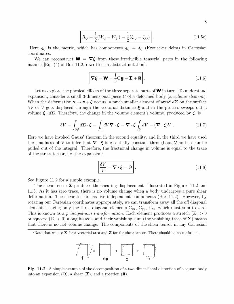
See Figure 11.2 for a simple example.The shear tensor Σ produces the shearing displacements illustrated in Figures 11.2 and

11.3. As it has zero trace, there is no volume change when a body undergoes a pure sheardeformation. The shear tensor has five independent components (Box 11.2). However, byrotating our Cartesian coordinates appropriately, we can transform away all the off diagonalelements, leaving only the three diagonal elements Σxx, Σyy, Σzz, which must sum to zero.This is known as a principal-axis transformation. Each element produces a stretch (Σ.. > 0or squeeze (Σ.. < 0) along its axis, and their vanishing sum (the vanishing trace of Σ) meansthat there is no net volume change. The components of the shear tensor in any Cartesian

2Note that we use Σ for a vectorial area and Σ for the shear tensor. There should be no confusion.

RgS

= + +

Fig. 11.2: A simple example of the decomposition of a two dimensional distortion of a square bodyinto an expansion (Θ), a shear (Σ), and a rotation (R).

9

x2

x1

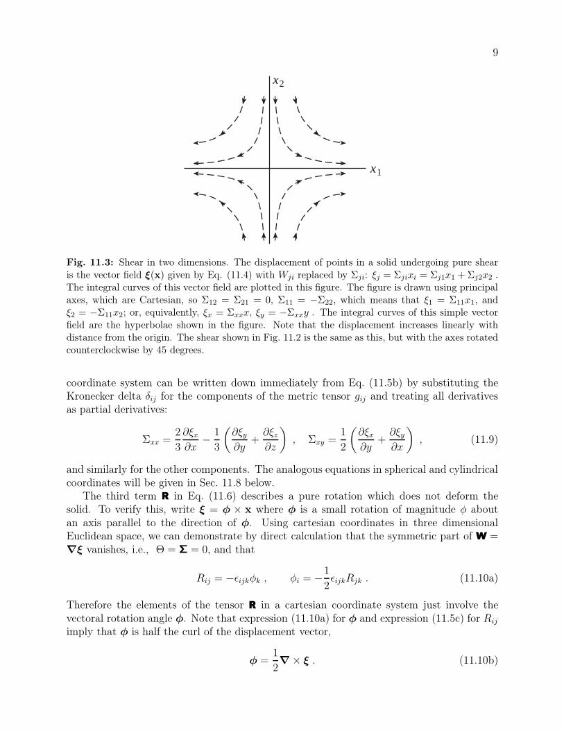
Fig. 11.3: Shear in two dimensions. The displacement of points in a solid undergoing pure shearis the vector field ξ(x) given by Eq. (11.4) with Wji replaced by Σji: ξj = Σjixi = Σj1x1 +Σj2x2 .The integral curves of this vector field are plotted in this figure. The figure is drawn using principalaxes, which are Cartesian, so Σ12 = Σ21 = 0, Σ11 = −Σ22, which means that ξ1 = Σ11x1, andξ2 = −Σ11x2; or, equivalently, ξx = Σxxx, ξy = −Σxxy . The integral curves of this simple vectorfield are the hyperbolae shown in the figure. Note that the displacement increases linearly withdistance from the origin. The shear shown in Fig. 11.2 is the same as this, but with the axes rotatedcounterclockwise by 45 degrees.

coordinate system can be written down immediately from Eq. (11.5b) by substituting theKronecker delta δij for the components of the metric tensor gij and treating all derivativesas partial derivatives:

Σxx =2

3

∂ξx∂x

− 1

3

(

∂ξy∂y

+∂ξz∂z

)

, Σxy =1

2

(

∂ξx∂y

+∂ξy∂x

)

, (11.9)

and similarly for the other components. The analogous equations in spherical and cylindricalcoordinates will be given in Sec. 11.8 below.

The third term R in Eq. (11.6) describes a pure rotation which does not deform thesolid. To verify this, write ξ = φ × x where φ is a small rotation of magnitude φ aboutan axis parallel to the direction of φ. Using cartesian coordinates in three dimensionalEuclidean space, we can demonstrate by direct calculation that the symmetric part of W =∇ξ vanishes, i.e., Θ = Σ = 0, and that

Rij = −ǫijkφk , φi = −1

2ǫijkRjk . (11.10a)

Therefore the elements of the tensor R in a cartesian coordinate system just involve thevectoral rotation angle φ. Note that expression (11.10a) for φ and expression (11.5c) for Rij

imply that φ is half the curl of the displacement vector,

φ =1

2∇× ξ . (11.10b)

10

A simple example of rotation is shown in the last picture in Figure 11.2.Elastic materials resist expansion Θ and shear Σ, but they don’t mind at all having

their orientation in space changed; i.e., they do not resist rotations R. Correspondingly, inelasticity theory, a central focus is on expansion and shear. For this reason, the symmetricpart of the gradient of ξ,

Sij ≡1

2(ξi;j + ξj;i) = Σij +

1

3Θgij , (11.11)

which includes the expansion and shear but omits the rotation, is given a special name, thestrain, and is paid great attention.

Let us consider some examples of strains that arise in physical systems.

(i) Understanding how materials deform under various loads (externally applied forces) iscentral to mechanical, civil and structural engineering. As we shall learn in Sec. 11.3.2below, all Hookean materials (materials with strain proportional to stress) rupturewhen the load is so great that any component of their strain exceeds ∼ 0.1, and almostall rupture at strains ∼ 0.001. For this reason, in our treatment of elasticity theory(this chapter and the next), we shall focus on strains that are small compared to unity.

(ii) Continental drift can be measured on the surface of the earth using Very Long BaselineInterferometry, a technique in which two or more radio telescopes are used to detectinterferometric fringes using radio waves from an astronomical point source. (A sim-ilar technique uses the Global Positioning System to achieve comparable accuracy.)By observing the fringes, it is possible to detect changes in the spacing between thetelescopes as small as a fraction of a wavelength (∼ 1 cm). As the telescopes are typ-ically 1000km apart, this means that dimensionless strains ∼ 10−8 can be measured.Now, the continents drift apart on a timescale . 108yr, so it takes roughly a year forthese changes to grow large enough to be measured. Such techniques are also usefulfor monitoring earthquake faults.

(iii) The smallest time-varying strains that have been measured so far involve laser inter-ferometer gravitational wave detectors such as LIGO. In each arm of a LIGO interfer-ometer, two mirrors hang freely, separated by 4 km. In 2010 their separations weremonitored, at frequencies ∼ 100 Hz, to ∼ 10−18 m, a thousandth the radius of a nu-cleon3 (Fig. 6.7 with ξrms =

√

f SF (f)). The associated strain is 3× 10−22. Althoughthis strain is not associated with an elastic solid, it does indicate the high accuracy ofoptical measurement techniques.

****************************

EXERCISES

3And Advanced LIGO will monitor them with ten times higher accuracy.

11

Exercise 11.1 Derivation and Practice: Reconstruction of a Tensor from its IrreducibleTensorial Parts.Using Eqs. (1), (2), and (3) of Box 11.2, show that 1

3Θgij + Σij +Rij is equal to Wij .

Exercise 11.2 Example: The Displacement Vectors Associated with Expansion, Rotationand Shear

(a) Consider a W = ∇ξ that is pure expansion, Wij =13Θgij. Using Eq. (11.4) show that,

in the vicinity of a chosen point, the displacement vector is ξi = 13Θxi. Draw this

displacement vector field.

(b) Similarly, draw ξ(x) for a W that is pure rotation. [Hint: express ξ in terms of thevectorial angle φ with the aid of Eq. (11.10a).]

(c) Draw ξ(x) for a W that is pure shear. To simplify the drawing, assume that the shearis confined to the x-y plane, and make your drawing for a shear whose only nonzerocomponents are Σxx = −Σyy. Compare your drawing with Fig. 11.3, where the nonzerocomponents are Σxx = −Σyy.

****************************

11.3 Stress, Elastic Moduli, and Elastostatic Equilibrium

11.3.1 Stress Tensor

The forces acting within an elastic solid are measured by a second rank tensor, the stresstensor introduced in Sec. 1.9. Let us recall the definition of this stress tensor:

Consider two small, contiguous regions in a solid. If we take a small element of areadΣ in the contact surface with its positive sense4 (same as the direction of dΣ viewed as avector) pointing from the first region toward the second, then the first region exerts a forcedF (not necessarily normal to the surface) on the second through this area. The force thesecond region exerts on the first (through the area −dΣ) will, by Newton’s third law, beequal and opposite to that force. The force and the area of contact are both vectors andthere is a linear relationship between them. (If we double the area, we double the force.)The two vectors therefore will be related by a second rank tensor, the stress tensor T:

dF = T · dΣ = T(. . . , dΣ) ; i.e., dFi = TijdΣj . (11.12)

Thus, the tensor T is the net (vectorial) force per unit (vectorial) area that a body exertsupon its surroundings. Be aware that many books on elasticity (e.g. Landau and Lifshitz1986) define the stress tensor with the opposite sign to (11.12). Also be careful not to confusethe shear tensor Σjk with the vectorial infinitesimal surface area dΣj.

4For a discussion of area elements including their positive sense, see Sec. 1.8.

12

We often need to compute the total elastic force acting on some finite volume V. To aidin this, we make an important assumption, which we discuss in Sec. 11.3.6, namely that thestress is determined by local conditions and can be computed from the local arrangement ofatoms. If this assumption is valid, then (as we shall see in Sec. 11.3.6), we can compute thetotal force acting on the volume element by integrating the stress over its surface ∂V:

F = −∫

∂V

T · dΣ = −∫

V

∇ · TdV , (11.13)

where we have invoked Gauss’ theorem, and the minus sign is because, for a closed surface∂V (by convention), dΣ points out of V instead of into it.

Equation (11.13) must be true for arbitrary volumes and so we can identify the elasticforce density f acting on an elastic solid as

f = −∇ · T . (11.14)

In elastostatic equilibrium, this force density must balance all other volume forces acting onthe material, most commonly the gravitational force density, so

f + ρg = 0 , (11.15)

where g is the gravitational acceleration. (Again, there should be no confusion between thevector g and the metric tensor g.) There are other possible external forces, some of whichwe shall encounter later in a fluid context, e.g. an electromagnetic force density. These canbe added to Eq. (11.15).

Just as for the strain, the stress tensor T can be decomposed into its irreducible tensorialparts, a pure trace (the pressure P ) plus a symmetric trace-free part (the shear stress):

T = Pg + Tshear ; P =1

3Tr(T) =

1

3Tii . (11.16)

There is no antisymmetric part because the stress tensor is symmetric, as we saw in Sec.1.9. Fluids at rest exert isotropic stresses, i.e. T = Pg. They cannot exert shear stress whenat rest, though when moving and shearing they can exert a viscous shear stress, as we shalldiscuss extensively in Part V (initially Sec. 13.7.2).

In SI units, stress is measured in units of Pascals, denoted Pa

1Pa = 1N/m2 = 1kgm/s2

m2, (11.17)

or sometimes in GPa = 109 Pa. In cgs units, stress is measured in dyne/cm2. Note that 1Pa = 10 dyne/cm2.

Now let us consider some examples of stresses:

(i) Atmospheric pressure is equal to the weight of the air in a column of unit area extendingabove the earth, and thus is roughly P ∼ ρgH ∼ 105Pa, where ρ ≃ 1 kg m−3 is thedensity of air, g ≃ 10m s−2 is the acceleration of gravity at the earth’s surface, andH ≃ 10 km is the atmospheric scale height [H ≡ (d lnP/dz)−1, with z the verticaldistance]. Thus 1 atmosphere is ∼ 105 Pa (or, more precisely, 1.01325× 105 Pa). Thestress tensor is isotropic.

13

(ii) Suppose we hammer a nail into a block of wood. The hammer might weigh m ∼ 0.3kgand be brought to rest from a speed of v ∼ 10m s−1 in a distance of, say, d ∼ 3mm.Then the average force exerted on the wood by the nail, as it is driven, is F ∼ mv2/d ∼104N. If this is applied over an effective area A ∼ 1mm2, then the magnitude of thetypical stress in the wood is ∼ F/A ∼ 1010Pa ∼ 105atmosphere. There is a large shearcomponent to the stress tensor, which is responsible for separating the fibers in thewood as the nail is hammered.

(iii) Neutron stars are as massive as the sun, M ∼ 2 × 1030 kg, but have far smaller radii,R ∼ 10km. Their surface gravities are therefore g ∼ GM/R2 ∼ 1012m s−2, ten billiontimes that encountered on earth. They have solid crusts of density ρ ∼ 1017kg m−3

that are about 1km thick. The magnitude of the stress at the base of a neutron-starcrust will then be P ∼ ρgH ∼ 1031Pa! This stress will be mainly hydrostatic, thoughas the material is solid, a modest portion will be in the form of a shear stress.

(iv) As we shall discuss in Chap. 28, a popular cosmological theory called inflation postu-lates that the universe underwent a period of rapid, exponential expansion during itsearliest epochs. This expansion was driven by the stress associated with a false vacuum.The action of this stress on the universe can be described quite adequately using a clas-sical stress tensor. If the interaction energy is E ∼ 1015GeV, the supposed scale of grandunification, and the associated length scale is the Compton wavelength associated withthat energy l ∼ ~c/E, then the magnitude of the stress is ∼ E/l3 ∼ 1097(E/1015GeV)4

Pa.

(v) Elementary particles interact through forces. Although it makes no sense to describethis interaction using classical elasticity, it does make sense to make order of magnitudeestimates of the associated stress. One promising model of these interactions involvesfundamental strings with mass per unit length µ = g2sc

2/8πG ∼ 0.1 Megaton/Fermi(where Megaton is not the TNT equivalent!), and cross section of order the Plancklength squared, LP

2 = ~G/c3 ∼ 10−70 m2, and tension (negative pressure) Tzz ∼µc2/LP

2 ∼ 10110 Pa. Here ~, G and c are Planck’s (reduced) constant, Newton’sgravitation constant, and the speed of light, and g2s ∼ 0.025 is the string couplingconstant.

(vi) The highest possible stress is presumably associated with spacetime singularities, forexample at the birth of the universe or inside a black hole. Here the characteristicenergy is the Planck energy EP = (~c5/G)1/2 ∼ 1019 GeV, the lengthscale is thePlanck length LP = (~G/c3)1/2 ∼ 10−35 m, and the associated ultimate stress is∼ EP/L

3P ∼ 10114 Pa.

11.3.2 Realm of Validity for Hooke’s Law

In elasticity theory, motivated by Hooke’s Law (Fig. 11.1), we shall assume a linear rela-tionship between a material’s stress and strain tensors. Before doing so, however, we shalldiscuss the realm in which this linearity is true and some ways in which it can fail.

14

Tzz=

F/A

Szz=Δ /

Proportionality Limit

Elastic Limit

Yield Limit

Rupture Point

Hooke’s

Law

F

+∆

(a) (b)

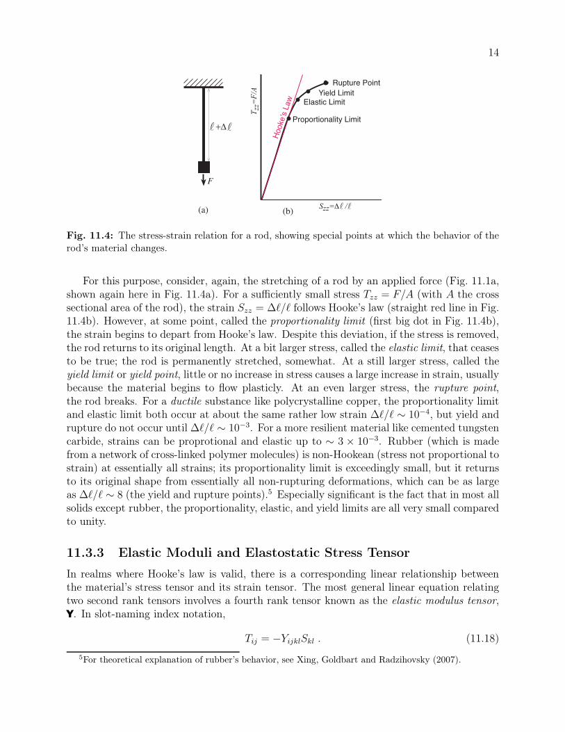
Fig. 11.4: The stress-strain relation for a rod, showing special points at which the behavior of therod’s material changes.

For this purpose, consider, again, the stretching of a rod by an applied force (Fig. 11.1a,shown again here in Fig. 11.4a). For a sufficiently small stress Tzz = F/A (with A the crosssectional area of the rod), the strain Szz = ∆ℓ/ℓ follows Hooke’s law (straight red line in Fig.11.4b). However, at some point, called the proportionality limit (first big dot in Fig. 11.4b),the strain begins to depart from Hooke’s law. Despite this deviation, if the stress is removed,the rod returns to its original length. At a bit larger stress, called the elastic limit, that ceasesto be true; the rod is permanently stretched, somewhat. At a still larger stress, called theyield limit or yield point, little or no increase in stress causes a large increase in strain, usuallybecause the material begins to flow plasticly. At an even larger stress, the rupture point,the rod breaks. For a ductile substance like polycrystalline copper, the proportionality limitand elastic limit both occur at about the same rather low strain ∆ℓ/ℓ ∼ 10−4, but yield andrupture do not occur until ∆ℓ/ℓ ∼ 10−3. For a more resilient material like cemented tungstencarbide, strains can be proprotional and elastic up to ∼ 3 × 10−3. Rubber (which is madefrom a network of cross-linked polymer molecules) is non-Hookean (stress not proportional tostrain) at essentially all strains; its proportionality limit is exceedingly small, but it returnsto its original shape from essentially all non-rupturing deformations, which can be as largeas ∆ℓ/ℓ ∼ 8 (the yield and rupture points).5 Especially significant is the fact that in most allsolids except rubber, the proportionality, elastic, and yield limits are all very small comparedto unity.

11.3.3 Elastic Moduli and Elastostatic Stress Tensor

In realms where Hooke’s law is valid, there is a corresponding linear relationship betweenthe material’s stress tensor and its strain tensor. The most general linear equation relatingtwo second rank tensors involves a fourth rank tensor known as the elastic modulus tensor,Y. In slot-naming index notation,

Tij = −YijklSkl . (11.18)

5For theoretical explanation of rubber’s behavior, see Xing, Goldbart and Radzihovsky (2007).

15

Now, a general fourth rank tensor in three dimensions has 34 = 81 independent compo-nents. Elasticity can get complicated! However, the situation need not be so dire. There areseveral symmetries that we can exploit. Let us look first at the general case. As the stressand strain tensors are both symmetric, Y is symmetric in its first pair of slots and we arefree to choose it symmetric in its second pair: Yijkl = Yjikl = Yijlk. There are therefore 6independent components Yijkl for variable i, j and fixed k, l, and vice versa. In addition, aswe show below, Y is symmetric under an interchange of its first and second pairs of slots:Yijkl = Yklij. There are therefore (6 × 7)/2 = 21 independent components in Y. This is animprovement over 81. Many substances, notably crystals, exhibit additional symmetries andthis can reduce the number of independent components considerably.

The simplest, and in fact most common, case arises when the medium is isotropic. Inother words, there are no preferred directions in the material. This occurs when the solid ispolycrystalline or amorphous and completely disordered on a scale large compared with theatomic spacing, but small compared with the solid’s inhomogeneity scale.

If a medium is isotropic, then its elastic properties must be describable by scalars thatrelate the irreducible parts P and Tshear of the stress tensor T to those, Θ and Σ, of the straintensor S. The only mathematically possible, linear, coordinate-independent relationshipbetween these {P, Tshear} and {Θ,Σ} involving solely scalars is P = −KΘ, T shear = −2µΣ,corresponding to a total stress tensor

T = −KΘg − 2µΣ . (11.19)

Here K is called the bulk modulus and µ the shear modulus, and the factor 2 is included forpurely historical reasons. The first minus sign (with K > 0) ensures that the isotropic partof the stress, −KΘg, resists volume changes; the second minus sign (with µ > 0) ensuresthat the symmetric, trace-free part, −2µΣ, resists shape changes (resists shearing). In Sec.11.4, we will deduce the relationship of the elastic moduli K and µ to Young’s modulus E,which appears in Hooke’s law (11.1) for the stress in a stretched rod or fiber (Fig. 11.1).

In many treatments and applications of elasticity, the shear tensor Σ is paid little atten-tion. The focus instead is on the the strain Sij and its trace Skk = Θ, and the elastic stresstensor (11.19) is written as T = −λΘg−2µS, where λ ≡ K− 2

3µ. In these treatments µ and

λ are called the first and second Lamé coefficients, and are used in place of µ and K. Weshall not adopt this viewpoint.

11.3.4 Energy of Deformation

Take a wire of length ℓ and cross sectional area A, and stretch it (e.g. via the “Hooke’s-lawexperiment” of Fig. 11.1) by an amount ζ ′ that grows gradually from 0 to ∆ℓ. When thestretch is ζ ′, the force that does the stretching is F ′ = EA(ζ ′/ℓ) = (EV/ℓ2)ζ ′; here V = Aℓis the wire’s volume and E is its Young’s modulus. As the wire is gradually lengthened, thestretching force F ′ does work

W =

∫ ∆ℓ

0

F ′dζ ′ =

∫ ∆ℓ

0

(EV/ℓ2)ζ ′dζ ′

=1

2EV (∆ℓ/ℓ)2 . (11.20)

16

This tells us that the stored elastic energy per unit volume is

U =1

2E(∆ℓ/ℓ)2 . (11.21)

To generalize this formula to a strained, isotropic, 3-dimensional medium, consider anarbitrary but very small region V inside a body that has already been strained by a displace-ment vector field ξi and is thus already experiencing an elastic stress Tij = −KΘδij − 2µΣij

[Eq. (11.19)]. Imagine building up this displacement gradually from zero at the same rateeverywhere in and around V, so at some moment during the buildup the displacement fieldis ξ′i = ξiǫ (with the parameter ǫ gradually growing from 0 to 1). At that moment, the stresstensor (by virtue of the linearity of the stress-strain relation) is T ′

ij = Tijǫ. On the boundary∂V of the region V, this stress exerts a force ∆F ′

i = −T ′ij∆Σj across any surface element

∆Σj , from the exterior of ∂V to its interior. As the displacement grows, this surface forcedoes the following amount of work on V:

∆Wsurf =

∫

∆F ′

idξ′

i =

∫

(−T ′

ij∆Σj)dξ′

i = −∫ 1

0

Tijǫ∆Σjξ′

idǫ = −1

2Tij∆Σjξi . (11.22)

The total amount of work done can be computed by adding up the contributions from allthe surface elements of ∂V:

Wsurf = −1

2

∫

∂V

TijξidΣj = −1

2

∫

V

(Tijξi);jdV = −1

2(Tijξi);jV . (11.23)

In the second step we have used Gauss’s theorem, and in the third step we have used thesmallness of the region V to infer that the integrand is very nearly constant and the integralis the integrand times the total volume V of V.

Does this equal the elastic energy stored in V? The answer is “no”, because we must alsotake account of the work done in the interior of V by gravity or any other non-elastic forcethat may be acting. Now, although it is not easy in practice to turn gravity off and thenon, we must do so in this thought experiment: In the volume’s final deformed state, thedivergence of its elastic stress tensor is equal to the gravitational force density, ∇ · T = ρg[Eqs. (11.14) and (11.15)]; and in the initial, undeformed and unstressed state, ∇ · T mustbe zero, whence so must be g. Therefore, we must imagine growing the gravitational forceproportional to ǫ just like we grow the displacement, strain and stress. During this growth,the gravitational force ρg′V = ρgV ǫ does the following amount of work on our tiny regionV:

Wgrav =

∫

ρV g′ · dξ′ =

∫ 1

0

ρV gǫ · ξdǫ = 1

2ρV g · ξ =

1

2(∇ · T) · ξV =

1

2Tij;jξiV . (11.24)

The total work done to deform V is the sum of the work done by the elastic force(11.23) on its surface and the gravitational force (11.24) in its interior, Wsurf + Wgrav =−1

2(ξiTij);jV + 1

2Tij;jξiV = −1

2Tijξi;jV . This work gets stored in V as elastic energy, so the

energy density is U = −12Tijξi;j. Inserting Tij = −KΘgij−2µΣij and ξi;j =

13Θgij+Σij+Rij

17

and performing some simple algebra that relies on the symmetry properties of the expansion,shear, and rotation (Ex. 11.3), we obtain

U =1

2KΘ2 + µΣijΣij . (11.25)

Note that this elastic energy density is always positive if the elastic moduli are positive —as they must be in order that matter be stable to small perturbations.

For the more general, anisotropic case, expression (11.25) becomes [by virtue of thestress-strain relation Tij = −Yijklξk;l, Eq. (11.18)]

U =1

2ξi;jYijklξk;l . (11.26)

The volume integral of the elastic energy density (11.25) or (11.26) can be used as anaction from which to compute the stress, by varying the displacement (Ex. 11.4). Sinceonly the part of Y that is symmetric under interchange of the first and second pairs of slotscontributes to U , only that part can affect the action-principle-derived stress. Therefore, itmust be that Yijkl = Yklij. This is the symmetry we asserted earlier.

****************************

EXERCISES

Exercise 11.3 Derivation and Practice: Elastic EnergyBeginning with U = −1

2Tijξi;j [text following Eq. (11.24)], derive U = 1

2KΘ2 + µΣijΣij for

the elastic energy density inside a body.

Exercise 11.4 Derivation and Practice: Action Principle for Elastic StressFor an anisotropic, elastic medium with elastic energy density U = 1

2ξi;jYijklξk;l, integrate

this energy density over a three-dimensional region V (not necessarily small) to get the totalelastic energy E. Now, consider a small variation δξi in the displacement field. Evaluate theresulting change δE in the elastic energy without using the relation Tij = −Yijklξk;l. Convertto a surface integral over ∂V and therefrom infer the stress-strain relation Tij = −Yijklξk;l.

****************************

11.3.5 Thermoelasticity

In our discussion, above, of deformation energy, we tacitly assumed that the temperature ofthe elastic medium was held fixed during the deformation; i.e., we ignored the possibility ofany thermal expansion. Correspondingly, the energy density U that we computed is actuallythe physical free energy per unit volume F , at some chosen temperature T0 of a heat bath. Ifwe increase the bath’s and material’s temperature from T0 to T = T0+δT , then the materialwants to expand by Θ = δV/V = 3αδT ; i.e., it will have vanishing expansional elastic energy

18

if Θ has this value. Here α is its coefficient of linear thermal expansion. (The factor 3 isbecause there are three directions into which it can expand: x, y and z.) Correspondingly,the physical free energy density at temperature T = T0 + δT is

F = F0(T ) +1

2K(Θ− 3αδT )2 + µΣijΣij . (11.27)

The stress tensor in this heated and strained state can be computed from Tij = −∂F/∂Sij

[a formula most easily inferred from Eq. (11.26) with U reinterpreted as F and ξi;j replacedby its symmetrization, Sij ]. Reexpressing Eq. (11.27) in terms of Sij and computing thederivative, we obtain (not surprisingly!)

Tij = − ∂F∂Sij

= −K(Θ− 3αδT )δij − 2µΣij . (11.28)

Now, what happens if we allow our material to expand adiabatically rather than atfixed temperature? Adiabatic expansion means expansion at fixed entropy S. Consider asmall sample of material that contains mass M and has volume V = M/ρ. Its entropy isS = −[∂(FV )/∂T ]V [cf. Eq. (5.33)], which, using Eq. (11.27), becomes

S = S0(T ) + 3αKΘV . (11.29)

Here we have neglected the term −9α2KδT , which can be shown to be negligible comparedto the temperature dependence of the elasticity-independent term S0(T ). If our sampleexpands adiabatically by an amount ∆V = V∆Θ, then its temperature must go down bythat amount ∆T < 0 which keeps S fixed, i.e. which makes ∆S0 = −3αKV∆Θ. Noting thatT∆S0 is the change of the sample’s thermal energy, which is ρcV ∆T with cV the specificheat per unit mass, we see that the temperature change is

∆T

T=

−3αK∆Θ

ρcVfor adiabatic expansion . (11.30)

This temperature change, accompanying an adiabatic expansion, alters slightly the elasticstress (11.28) and thence the bulk modulus K; i.e., it gives rise to an adiabatic bulk modulusthat differs slightly from the isothermal bulk modulus K introduced in previous sections.However, the differences are so small that they are generally ignored. For further detail seeSec. 6 of Landau and Lifshitz (1986).

11.3.6 Molecular Origin of Elastic Stress; Estimate of Moduli

It is important to understand the microscopic origin of the elastic stress. Consider an ionicsolid in which singly ionized ions (e.g. positively charged sodium and negatively chargedchlorine) attract their nearest (opposite-species) neighbors through their mutual Coulombattraction and repel their next nearest (same-species) neighbors, and so on. Overall, there isa net electrostatic attraction on each ion, which is balanced by the short range repulsion of itsbound electrons against its neighbors’ bound electrons. Now consider a thin slice of materialof thickness intermediate between the inter-atomic spacing and the solid’s inhomogeneity

19

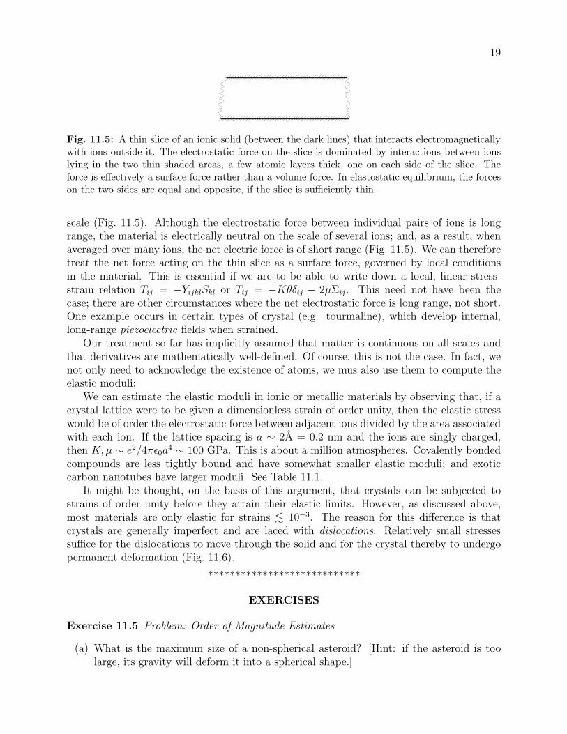
Fig. 11.5: A thin slice of an ionic solid (between the dark lines) that interacts electromagneticallywith ions outside it. The electrostatic force on the slice is dominated by interactions between ionslying in the two thin shaded areas, a few atomic layers thick, one on each side of the slice. Theforce is effectively a surface force rather than a volume force. In elastostatic equilibrium, the forceson the two sides are equal and opposite, if the slice is sufficiently thin.

scale (Fig. 11.5). Although the electrostatic force between individual pairs of ions is longrange, the material is electrically neutral on the scale of several ions; and, as a result, whenaveraged over many ions, the net electric force is of short range (Fig. 11.5). We can thereforetreat the net force acting on the thin slice as a surface force, governed by local conditionsin the material. This is essential if we are to be able to write down a local, linear stress-strain relation Tij = −YijklSkl or Tij = −Kθδij − 2µΣij. This need not have been thecase; there are other circumstances where the net electrostatic force is long range, not short.One example occurs in certain types of crystal (e.g. tourmaline), which develop internal,long-range piezoelectric fields when strained.

Our treatment so far has implicitly assumed that matter is continuous on all scales andthat derivatives are mathematically well-defined. Of course, this is not the case. In fact, wenot only need to acknowledge the existence of atoms, we mus also use them to compute theelastic moduli:

We can estimate the elastic moduli in ionic or metallic materials by observing that, if acrystal lattice were to be given a dimensionless strain of order unity, then the elastic stresswould be of order the electrostatic force between adjacent ions divided by the area associatedwith each ion. If the lattice spacing is a ∼ 2Å = 0.2 nm and the ions are singly charged,then K,µ ∼ e2/4πǫ0a

4 ∼ 100 GPa. This is about a million atmospheres. Covalently bondedcompounds are less tightly bound and have somewhat smaller elastic moduli; and exoticcarbon nanotubes have larger moduli. See Table 11.1.

It might be thought, on the basis of this argument, that crystals can be subjected tostrains of order unity before they attain their elastic limits. However, as discussed above,most materials are only elastic for strains . 10−3. The reason for this difference is thatcrystals are generally imperfect and are laced with dislocations. Relatively small stressessuffice for the dislocations to move through the solid and for the crystal thereby to undergopermanent deformation (Fig. 11.6).

****************************

EXERCISES

Exercise 11.5 Problem: Order of Magnitude Estimates

(a) What is the maximum size of a non-spherical asteroid? [Hint: if the asteroid is toolarge, its gravity will deform it into a spherical shape.]

20

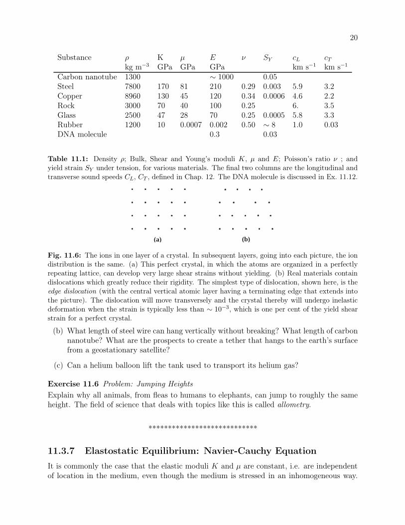
Substance ρ K µ E ν SY cL cTkg m−3 GPa GPa GPa km s−1 km s−1

Carbon nanotube 1300 ∼ 1000 0.05Steel 7800 170 81 210 0.29 0.003 5.9 3.2Copper 8960 130 45 120 0.34 0.0006 4.6 2.2Rock 3000 70 40 100 0.25 6. 3.5Glass 2500 47 28 70 0.25 0.0005 5.8 3.3Rubber 1200 10 0.0007 0.002 0.50 ∼ 8 1.0 0.03DNA molecule 0.3 0.03

Table 11.1: Density ρ; Bulk, Shear and Young’s moduli K, µ and E; Poisson’s ratio ν ; andyield strain SY under tension, for various materials. The final two columns are the longitudinal andtransverse sound speeds CL, CT , defined in Chap. 12. The DNA molecule is discussed in Ex. 11.12.

(b)(a)

Fig. 11.6: The ions in one layer of a crystal. In subsequent layers, going into each picture, the iondistribution is the same. (a) This perfect crystal, in which the atoms are organized in a perfectlyrepeating lattice, can develop very large shear strains without yielding. (b) Real materials containdislocations which greatly reduce their rigidity. The simplest type of dislocation, shown here, is theedge dislocation (with the central vertical atomic layer having a terminating edge that extends intothe picture). The dislocation will move transversely and the crystal thereby will undergo inelasticdeformation when the strain is typically less than ∼ 10−3, which is one per cent of the yield shearstrain for a perfect crystal.

(b) What length of steel wire can hang vertically without breaking? What length of carbonnanotube? What are the prospects to create a tether that hangs to the earth’s surfacefrom a geostationary satellite?

(c) Can a helium balloon lift the tank used to transport its helium gas?

Exercise 11.6 Problem: Jumping Heights

Explain why all animals, from fleas to humans to elephants, can jump to roughly the sameheight. The field of science that deals with topics like this is called allometry.

****************************

11.3.7 Elastostatic Equilibrium: Navier-Cauchy Equation

It is commonly the case that the elastic moduli K and µ are constant, i.e. are independentof location in the medium, even though the medium is stressed in an inhomogeneous way.

21

(This is because the strains are small and thus perturb the material properties by only smallamounts.) If so, then from the elastic stress tensor T = −KΘg−2µΣ and expressions (11.5a)and (11.5b) for the expansion and shear in terms of the displacement vector, we can deducethe following expression for the elastic force density f [Eq. (11.14)] inside the body:

f = −∇ · T = K∇Θ+ 2µ∇ ·Σ =

(

K +1

3µ

)

∇(∇ · ξ) + µ∇2ξ ; (11.31)

see Ex. 11.7. Here ∇ ·Σ in index notation is Σij;j = Σji;j. Extra terms must be added if weare dealing with anisotropic materials. However, in this book Eq. (11.31) will be sufficientfor our needs.

If no other countervailing forces act in the interior of the material (e.g., if there is nogravitational force), and if, as in this chapter, the material is in a static, equilibrium staterather than vibrating dynamically, then this force density will have to vanish throughoutthe material’s interior. This vanishing of f ≡ −∇ · T is just a fancy version of Newton’slaw for static situations, F = ma = 0. If the material has density ρ and is pulled on bya gravitational acceleration g, then the sum of the elastostatic force per unit volume andgravitational force per unit volume must vanish, f + ρg = 0; i.e.,

f + ρg =

(

K +1

3µ

)

∇(∇ · ξ) + µ∇2ξ + ρg = 0 . (11.32)

This is often called the Navier-Cauchy equation, since it was first written down by Claude-Louis Navier (in 1821) and in a more general form by Augustin-Louis Cauchy (in 1822).

When external forces are applied to the surface of an elastic body (for example, whenone pushes on the face of a cylinder) and gravity acts on the interior, the distribution of thestrain ξ(x) inside the body can be computed by solving the Navier-Cauchy equation (11.32)subject to boundary conditions provided by the applied forces.

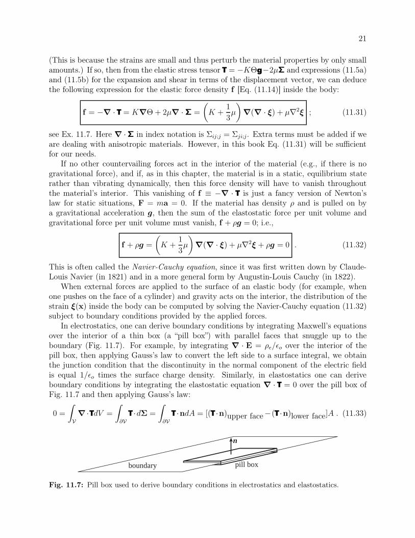
In electrostatics, one can derive boundary conditions by integrating Maxwell’s equationsover the interior of a thin box (a “pill box”) with parallel faces that snuggle up to theboundary (Fig. 11.7). For example, by integrating ∇ · E = ρe/ǫo over the interior of thepill box, then applying Gauss’s law to convert the left side to a surface integral, we obtainthe junction condition that the discontinuity in the normal component of the electric fieldis equal 1/ǫo times the surface charge density. Similarly, in elastostatics one can deriveboundary conditions by integrating the elastostatic equation ∇ · T = 0 over the pill box ofFig. 11.7 and then applying Gauss’s law:

0 =

∫

V

∇ ·TdV =

∫

∂V

T ·dΣ =

∫

∂V

T ·ndA = [(T ·n)upper face−(T ·n)lower face]A . (11.33)

n

boundary pill box

Fig. 11.7: Pill box used to derive boundary conditions in electrostatics and elastostatics.

22

Here in the next-to-last expression we have used dΣ = ndA where dA is the scalar areaelement and n is the unit normal to the pill-box face, and in the last term we have assumedthe pill box has a small face so T · n can be treated as constant and be pulled outside theintegral. The result is the boundary condition that

T · n must be continuous across any boundary; (11.34)

i.e., in index notation, Tijnj is continuous.Physically this is nothing but the law of force balance across the boundary: The force

per unit area acting from the lower side to the upper side must be equal and opposite to thatacting from upper to lower. As an example, if the upper face is bounded by vacuum then thesolid’s stress tensor must satisfy Tijnj = 0 at the surface. If a normal pressure P is appliedby some external agent at the upper face, then the solid must respond with a normal forceequal to P : niTijnj = P . If a vectorial force per unit area Fi is applied at the upper face bysome external agent, then it must be balanced: Tijnj = −Fi.

Solving the Navier-Cauchy equation (11.33) for the displacement field ξ(x), subject tospecified boundary conditions, is a problem in elastostatics analogous to solving Maxwell’sequations for an electric field subject to boundary conditions in electrostatics, or for a mag-netic field subject to boundary conditions in magnetostatics; and the types of solution tech-niques used in electrostatics and magnetostatics can also be used here. See Box 11.3.

****************************

EXERCISES

Exercise 11.7 Derivation and Practice: Elastic Force DensityFrom Eq. (11.19) derive expression (11.31) for the elastostatic force density inside an elasticbody.

Exercise 11.8 *** Practice: Biharmonic EquationA homogeneous, isotropic, elastic solid is in equilibrium under (uniform) gravity and appliedsurface stresses. Use Eq. (11.31) to show that the displacement inside it ξ(x) is biharmonic,i.e. it satisfies the differential equation

∇2∇2ξ = 0 . (11.35a)

Show also that the expansion Θ satisfies the Lapace equation

∇2Θ = 0 . (11.35b)

****************************

23

Box 11.3

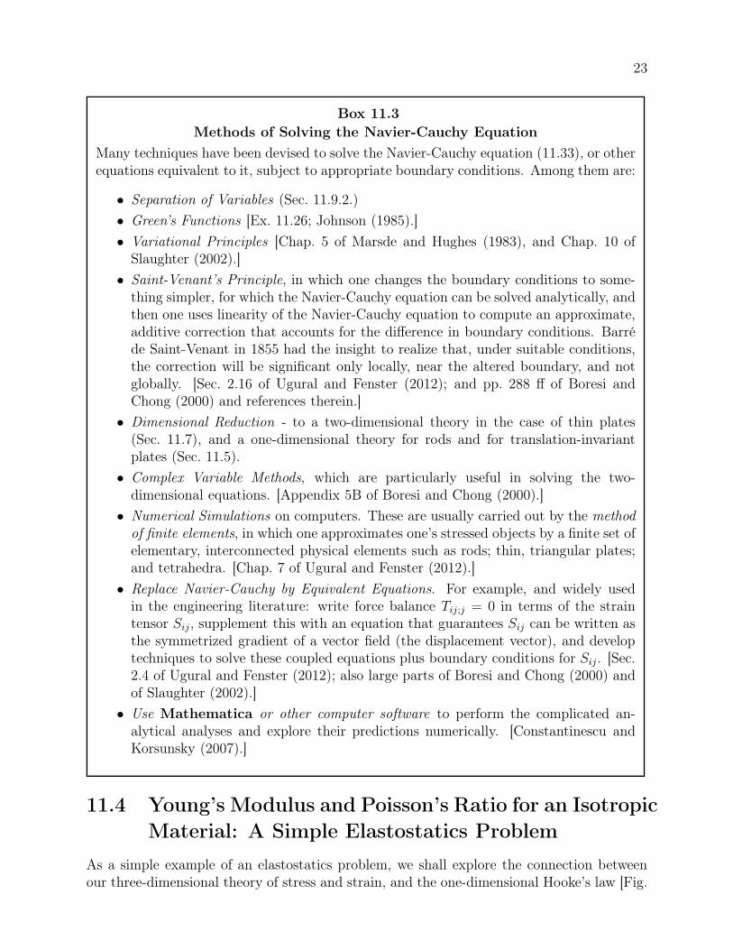
Methods of Solving the Navier-Cauchy Equation

Many techniques have been devised to solve the Navier-Cauchy equation (11.33), or otherequations equivalent to it, subject to appropriate boundary conditions. Among them are:

• Separation of Variables (Sec. 11.9.2.)

• Green’s Functions [Ex. 11.26; Johnson (1985).]

• Variational Principles [Chap. 5 of Marsde and Hughes (1983), and Chap. 10 ofSlaughter (2002).]

• Saint-Venant’s Principle, in which one changes the boundary conditions to some-thing simpler, for which the Navier-Cauchy equation can be solved analytically, andthen one uses linearity of the Navier-Cauchy equation to compute an approximate,additive correction that accounts for the difference in boundary conditions. Barréde Saint-Venant in 1855 had the insight to realize that, under suitable conditions,the correction will be significant only locally, near the altered boundary, and notglobally. [Sec. 2.16 of Ugural and Fenster (2012); and pp. 288 ff of Boresi andChong (2000) and references therein.]

• Dimensional Reduction - to a two-dimensional theory in the case of thin plates(Sec. 11.7), and a one-dimensional theory for rods and for translation-invariantplates (Sec. 11.5).

• Complex Variable Methods, which are particularly useful in solving the two-dimensional equations. [Appendix 5B of Boresi and Chong (2000).]

• Numerical Simulations on computers. These are usually carried out by the methodof finite elements, in which one approximates one’s stressed objects by a finite set ofelementary, interconnected physical elements such as rods; thin, triangular plates;and tetrahedra. [Chap. 7 of Ugural and Fenster (2012).]

• Replace Navier-Cauchy by Equivalent Equations. For example, and widely usedin the engineering literature: write force balance Tij;j = 0 in terms of the straintensor Sij , supplement this with an equation that guarantees Sij can be written asthe symmetrized gradient of a vector field (the displacement vector), and developtechniques to solve these coupled equations plus boundary conditions for Sij . [Sec.2.4 of Ugural and Fenster (2012); also large parts of Boresi and Chong (2000) andof Slaughter (2002).]

• Use Mathematica or other computer software to perform the complicated an-alytical analyses and explore their predictions numerically. [Constantinescu andKorsunsky (2007).]

11.4 Young’s Modulus and Poisson’s Ratio for an Isotropic

Material: A Simple Elastostatics Problem

As a simple example of an elastostatics problem, we shall explore the connection betweenour three-dimensional theory of stress and strain, and the one-dimensional Hooke’s law [Fig.

24

11.1 and Eq. (11.1)].Consider a thin rod of square cross section hanging along the ez direction of a Cartesian

coordinate system (Fig. 11.1). Subject the rod to a stretching force applied normally anduniformly at its ends. (It could just as easily be a rod under compression.) Its sides are freeto expand or contract transversely, since no force acts on them, dFi = TijdΣj = 0. As therod is slender, vanishing of dFi at its x and y sides implies to high accuracy that the stresscomponents Tix and Tiy will vanish throughout the interior; otherwise there would be a verylarge force density Tij;j inside the rod. Using Tij = −KΘgij − 2µΣij , we then obtain

Txx = −KΘ− 2µΣxx = 0 , (11.36a)

Tyy = −KΘ− 2µΣyy = 0 , (11.36b)

Tyz = −2µΣyz = 0 , (11.36c)

Txz = −2µΣxz = 0 , (11.36d)

Txy = −2µΣxy = 0 , (11.36e)

Tzz = −KΘ− 2µΣzz . (11.36f)

From the first two of these equations and Σxx + Σyy + Σzz = 0, we obtain a relationshipbetween the expansion and the nonzero components of the shear,

KΘ = µΣzz = −2µΣxx = −2µΣyy ; (11.37)

and from this and Eq. (11.36f), we obtain Tzz = −3KΘ. The decomposition of Sij into itsirreducible tensorial parts tells us that Szz = ξz;z = Σzz +

13Θ, which becomes, upon using

Eq. (11.37), ξz;z = [(3K + µ)/3µ]Θ. Combining with Tzz = −3KΘ we obtain Hooke’s lawand an expression for Young’s modulus E in terms of the bulk and shear moduli:

−Tzz

ξz;z=

9µK

3K + µ= E . (11.38)

It is conventional to introduce Poisson’s ratio, ν, which is minus the ratio of the lateralstrain to the longitudinal strain during a deformation of this type, where the transversemotion is unconstrained. It can be expressed as a ratio of elastic moduli as follows:

ν ≡ −ξx,xξz,z

= −ξy,yξz,z

= −Σxx +13Θ

Σzz +13Θ

=3K − 2µ

2(3K + µ), (11.39)

where we have used Eq. (11.37). We tabulate these and their inverses for future use:

E =9µK

3K + µ, ν =

3K − 2µ

2(3K + µ); K =

E

3(1− 2ν), µ =

E

2(1 + ν). (11.40)

We have already remarked that mechanical stability of a solid requires that K,µ > 0.Using Eq. (11.40), we observe that this imposes a restriction on Poisson’s ratio, namely that−1 < ν < 1/2. For metals, Poisson’s ratio is typically about 1/3 and the shear modulusis roughly half the bulk modulus. For a substance that is easily sheared but not easily

25

compressed, like rubber, the bulk modulus is relatively high and ν ≃ 1/2 (cf. Table 11.1.)For some exotic materials, Poison’s ratio can be negative (cf. Yeganeh-Haeri et al 1992).

Although we derived them for a square strut under compression, our expressions forYoung’s modulus and Poisson’s ratio are quite general. To see this, observe that the deriva-tion would be unaffected if we combined many parallel, square fibers together. All that isnecessary is that the transverse motion be free so that the only applied force is uniform andnormal to a pair of parallel faces.

11.5 Reducing the Elastostatic Equations to One Dimen-

sion for a Bent Beam: Cantilever Bridges, Foucault

Pendulum, DNA Molecule, Elastica

When dealing with bodies that are much thinner in two dimensions than the third (e.g. rods,wires, and beams), one can use the method of moments to reduce the three-dimensionalelastostatic equations to ordinary differential equations in one dimension (a process calleddimensional reduction). We have already met an almost trivial example of this in our discus-sion of Hooke’s law and Young’s modulus (Sec. 11.4 and Fig. 11.1). In this section, we shalldiscuss a more complicated example, the bending of a beam through a small displacementangle; and in Ex. 11.13 we shall analyze a more complicated example: the bending of a verylong, elastic wire into a complicated shape called an elastica.

Our beam-bending example is motivated by a common method of bridge construction,which uses cantilevers. (A famous historical example is the old bridge over the Firth of Forthin Scotland that was completed in 1890 with a main span of half a km.) The principle isto attach two independent beams to the two shores as cantilevers, and allow them to meetin the middle. (In practice the beams are usually supported at the shores on piers andstrengthened along their lengths with trusses.) Similar cantilevers, with lengths of order amicron or less, are used in in scanning electron microscopes, atomic force microscopes, andother nanotechnology applications, including quantum information experiments.

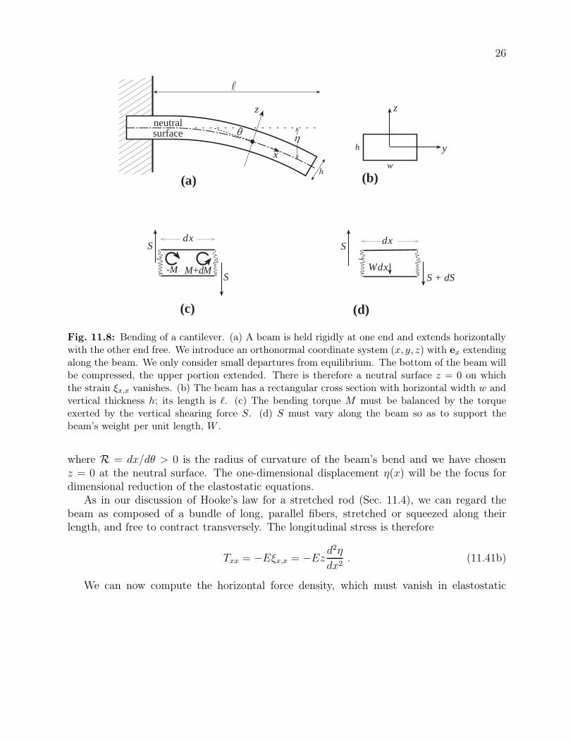
Let us make a simple model of a cantilever (Figure 11.8). Consider a beam clampedrigidly at one end, with length ℓ, horizontal width w and vertical thickness h. Introduce localcartesian coordinates with ex pointing along the beam and ez pointing vertically upward.Imagine the beam extending horizontally in the absence of gravity. Now let it sag underits own weight so that each element is displaced through a small distance ξ(x). The upperpart of the beam is stretched while the lower part is compressed, so there must be a neutralsurface where the horizontal strain ξx,x vanishes. This neutral surface must itself be curveddownward. Let its downward displacement from the horizontal plane that it occupied beforesagging be η(x)(> 0), let a plane tangent to the neutral surface make an angle θ(x) (also> 0) with the horizontal, and adjust the x and z coordinates so x runs along the slightlycurved neutral plane and z is orthogonal to it (Fig. 11.8). The longitudinal strain is thengiven to first order in small quantities by

ξx,x =z

R = zdθ

dx≃ z

d2η

dx2, (11.41a)

26

(a) (b)

(c) (d)

z

x

z

y

dx

Wdx

dxS

S + dSS

S

-M M+dM

neutralsurface

h

h

w

Fig. 11.8: Bending of a cantilever. (a) A beam is held rigidly at one end and extends horizontallywith the other end free. We introduce an orthonormal coordinate system (x, y, z) with ex extendingalong the beam. We only consider small departures from equilibrium. The bottom of the beam willbe compressed, the upper portion extended. There is therefore a neutral surface z = 0 on whichthe strain ξx,x vanishes. (b) The beam has a rectangular cross section with horizontal width w andvertical thickness h; its length is ℓ. (c) The bending torque M must be balanced by the torqueexerted by the vertical shearing force S. (d) S must vary along the beam so as to support thebeam’s weight per unit length, W .

where R = dx/dθ > 0 is the radius of curvature of the beam’s bend and we have chosenz = 0 at the neutral surface. The one-dimensional displacement η(x) will be the focus fordimensional reduction of the elastostatic equations.

As in our discussion of Hooke’s law for a stretched rod (Sec. 11.4), we can regard thebeam as composed of a bundle of long, parallel fibers, stretched or squeezed along theirlength, and free to contract transversely. The longitudinal stress is therefore

Txx = −Eξx,x = −Ezd2η

dx2. (11.41b)

We can now compute the horizontal force density, which must vanish in elastostatic

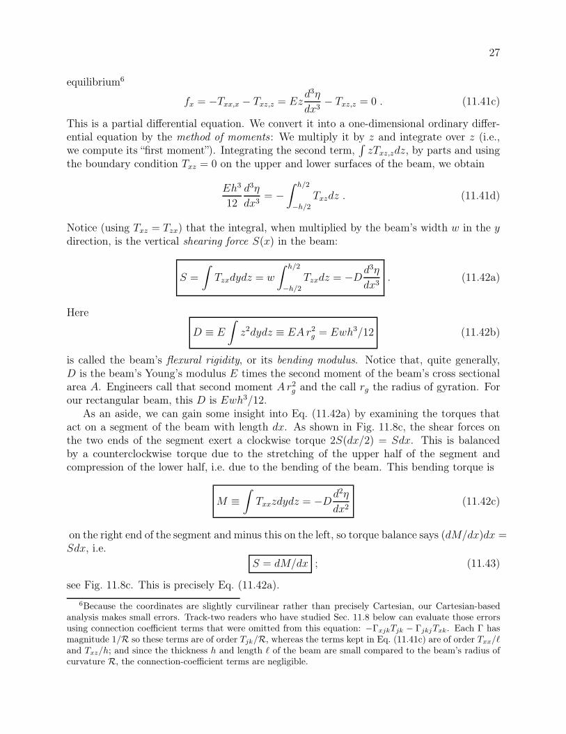
27

equilibrium6

fx = −Txx,x − Txz,z = Ezd3η

dx3− Txz,z = 0 . (11.41c)

This is a partial differential equation. We convert it into a one-dimensional ordinary differ-ential equation by the method of moments: We multiply it by z and integrate over z (i.e.,we compute its “first moment”). Integrating the second term,

∫

zTxz,zdz, by parts and usingthe boundary condition Txz = 0 on the upper and lower surfaces of the beam, we obtain

Eh3

12

d3η

dx3= −

∫ h/2

−h/2

Txzdz . (11.41d)

Notice (using Txz = Tzx) that the integral, when multiplied by the beam’s width w in the ydirection, is the vertical shearing force S(x) in the beam:

S =

∫

Tzxdydz = w

∫ h/2

−h/2

Tzxdz = −Dd3η

dx3. (11.42a)

Here

D ≡ E

∫

z2dydz ≡ EAr2g = Ewh3/12 (11.42b)

is called the beam’s flexural rigidity, or its bending modulus. Notice that, quite generally,D is the beam’s Young’s modulus E times the second moment of the beam’s cross sectionalarea A. Engineers call that second moment Ar2g and the call rg the radius of gyration. Forour rectangular beam, this D is Ewh3/12.

As an aside, we can gain some insight into Eq. (11.42a) by examining the torques thatact on a segment of the beam with length dx. As shown in Fig. 11.8c, the shear forces onthe two ends of the segment exert a clockwise torque 2S(dx/2) = Sdx. This is balancedby a counterclockwise torque due to the stretching of the upper half of the segment andcompression of the lower half, i.e. due to the bending of the beam. This bending torque is

M ≡∫

Txxzdydz = −Dd2η

dx2(11.42c)

on the right end of the segment and minus this on the left, so torque balance says (dM/dx)dx =Sdx, i.e.

S = dM/dx ; (11.43)

see Fig. 11.8c. This is precisely Eq. (11.42a).

6Because the coordinates are slightly curvilinear rather than precisely Cartesian, our Cartesian-basedanalysis makes small errors. Track-two readers who have studied Sec. 11.8 below can evaluate those errorsusing connection coefficient terms that were omitted from this equation: −ΓxjkTjk − ΓjkjTxk. Each Γ hasmagnitude 1/R so these terms are of order Tjk/R, whereas the terms kept in Eq. (11.41c) are of order Txx/ℓand Txz/h; and since the thickness h and length ℓ of the beam are small compared to the beam’s radius ofcurvature R, the connection-coefficient terms are negligible.

28

Equation (11.42a) [or equivalently (11.43)] embodies half of the elastostatic equations. Itis the x component of force balance fx = 0, converted to an ordinary differential equation byevaluating its lowest non-vanishing moment: its first moment,

∫

zfxdydz = 0 [Eq. (11.41d)].The other half is the z component of stress balance, which we can write as

Tzx,x + Tzz,z + ρg = 0 (11.44)

(vertical elastic force balanced by gravitational pull on the beam). We can convert this toa one-dimensional ordinary differential equation by taking its lowest nonvanishing moment,its zero’th moment, i.e. by integrating over y and z. The result is

dS

dx= −W , (11.45)

where W = gρwh is the beam’s weight per unit length (Fig. 11.8d).Combining our two dimensionally reduced components of force balance, Eqs. (11.42a) and

(11.45), we obtain a fourth order differential equation for our one-dimensional displacementη(x):

d4η

dx4=

W

D. (11.46)

(Fourth order differential equations are characteristic of elasticity.)Equation (11.46) can be solved subject to four appropriate boundary conditions. How-

ever, before we solve it, notice that for a beam of a fixed length ℓ, the deflection η is inverselyproportional to the flexural rigidity. Let us give a simple example of this scaling. Floors inAmerican homes are conventionally supported by wooden joists of 2” (inch) by 6” lumberwith the 6” side vertical. Suppose an inept carpenter installed the joists with the 6” sidehorizontal. The flexural rigidity of the joist would be reduced by a factor 9 and the centerof the floor would be expected to sag 9 times as much as if the joists had been properlyinstalled – a potentially catastrophic error.

Also, before solving Eq. (11.46), let us examine the approximations that we have made.First, we have assumed that the sag is small compared with the length of the beam, whenmaking the small-angle approximation in Eq. (11.41a); and we have assumed the beam’sradius of curvature is large compared to its length, when treating our slightly curved coordi-nates as Cartesian.7 These assumptions will usually be valid, but are not so for the elasticastudied in Ex. 11.13. Second, by using the method of moments rather than solving for thecomplete local stress tensor field, we have ignored the effects of some components of thestress tensor. In particular, in evaluating the bending torque [Eq. (11.42c)] we have ignoredthe effect of the Tzx component of the stress tensor. This is O(h/ℓ)Txx and so our equationscan only be accurate for fairly slender beams. Third, the extension above the neutral surfaceand the compression below the neutral surface lead to changes in the cross sectional shapeof the beam. The fractional error here is of order the longitudinal shear, which is small forreal materials.

7i.e., in more technical language, when neglecting the connection coefficient terms discussed in footnote6.

29

The solution to Eq. (11.46) is a fourth order polynomial with four unknown constants,to be set by boundary conditions. In this problem, the beam is held horizontal at the fixedend so that η(0) = η′(0) = 0, where ′ = d/dx. At the free end, Tzx and Txx must vanish, sothe shearing force S must vanish, whence η′′′(ℓ) = 0 [Eq. (11.42a)]; and the bending torqueM [Eq. (11.42c)] must also vanish, whence [by Eq. (11.43)]

∫

Sdx ∝ η′′(ℓ) = 0. By imposingthese four boundary conditions η(0) = η′(0) = η′′(ℓ) = η′′′(ℓ) on the solution of Eq. (11.46),we obtain for the beam shape

η(x) =W

D

(

1

4ℓ2x2 − 1

6ℓx3 +

1

24x4

)

. (11.47a)

Therefore the end of the beam sags by

η(ℓ) =Wℓ4

8D. (11.47b)

Problems in which the beam rests on supports rather than being clamped can be solvedin a similar manner. The boundary conditions will be altered, but the differential equation(11.46) will be unchanged.

Now suppose that we have a cantilever bridge of constant vertical thickness h and totalspan 2ℓ ∼100m made of material with density ρ ∼ 8× 103kg m−3 (e.g. reinforced concrete)and Young’s modulus E ∼ 100GPa. Suppose further that we want the center of the bridgeto sag by no more than η ∼ 1m. According to Eq. (11.47b), the thickness of the beam mustsatisfy

h &

(

3ρgℓ4

2Eη

)1/2

∼ 2.7m . (11.48)

This estimate makes no allowance for all the extra strengthening and support present in realstructures (e.g. via trusses and cables) and so it is an overestimate.

****************************

EXERCISES

Exercise 11.9 Derivation: Sag in a cantilever

(a) Verify Eqs. (11.47) for the sag in a horizontal beam clamped at one end and allowedto hang freely at the other end.

(b) Now consider a similar beam with constant cross section and loaded with weights sothat the total weight per unit length is W (x). What is the sag of the free end, expressedas an integral over W (x), weighted by an appropriate Green’s function?

Exercise 11.10 Example: Microcantilever

A microcantilever, fabricated from a single crystal of silicon, is being used to test the inversesquare law of gravity on micron scales (Weld et. al. 2008). It is clamped horizontally at

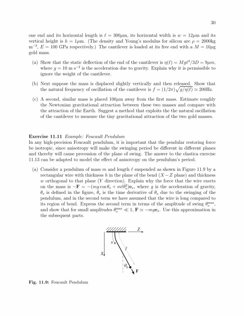
30

one end and its horizontal length is ℓ = 300µm, its horizontal width is w = 12µm and itsvertical height is h = 1µm. (The density and Young’s modulus for silicon are ρ = 2000kgm−3, E = 100 GPa respectively.) The cantilever is loaded at its free end with a M = 10µggold mass.

(a) Show that the static deflection of the end of the cantilever is η(ℓ) = Mgℓ3/3D = 9µm,where g = 10 m s−2 is the acceleration due to gravity. Explain why it is permissible toignore the weight of the cantilever.

(b) Next suppose the mass is displaced slightly vertically and then released. Show thatthe natural frequency of oscillation of the cantilever is f = (1/2π)

√

g/η(ℓ) ≃ 200Hz.

(c) A second, similar mass is placed 100µm away from the first mass. Estimate roughlythe Newtonian gravitational attraction between these two masses and compare withthe attraction of the Earth. Suggest a method that exploits the the natural oscillationof the cantilever to measure the tiny gravitational attraction of the two gold masses.

Exercise 11.11 Example: Foucault PendulumIn any high-precision Foucault pendulum, it is important that the pendular restoring forcebe isotropic, since anisotropy will make the swinging period be different in different planesand thereby will cause precession of the plane of swing. The answer to the elastica exercise11.13 can be adapted to model the effect of anisotropy on the pendulum’s period.

(a) Consider a pendulum of mass m and length ℓ suspended as shown in Figure 11.9 by arectangular wire with thickness h in the plane of the bend (X−Z plane) and thicknessw orthogonal to that plane (Y direction). Explain why the force that the wire exertson the mass is −F = −(mg cos θo + mℓθ2o)ex, where g is the acceleration of gravity,θo is defined in the figure, θo is the time derivative of θo due to the swinging of thependulum, and in the second term we have assumed that the wire is long compared toits region of bend. Express the second term in terms of the amplitude of swing θmax

o ,and show that for small amplitudes θmax

o ≪ 1, F ≃ −mgex. Use this approximation inthe subsequent parts.

X

x

F0

Z

Fig. 11.9: Foucault Pendulum

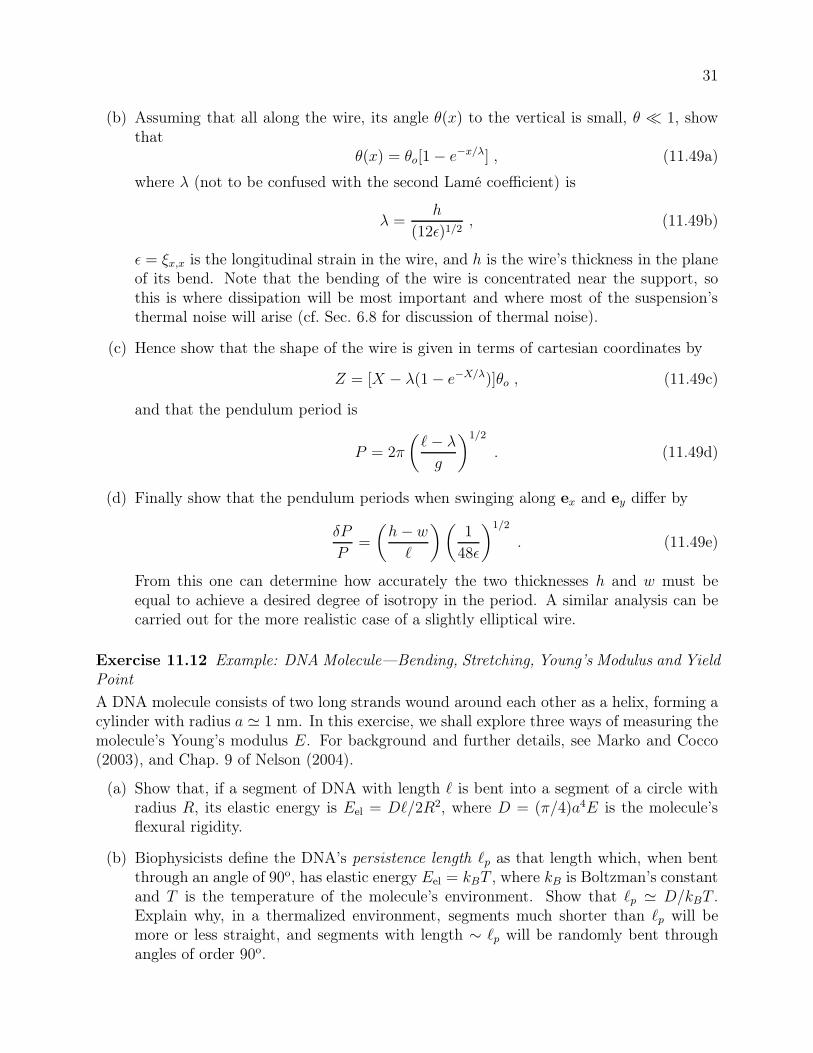
31

(b) Assuming that all along the wire, its angle θ(x) to the vertical is small, θ ≪ 1, showthat

θ(x) = θo[1− e−x/λ] , (11.49a)

where λ (not to be confused with the second Lamé coefficient) is

λ =h

(12ǫ)1/2, (11.49b)

ǫ = ξx,x is the longitudinal strain in the wire, and h is the wire’s thickness in the planeof its bend. Note that the bending of the wire is concentrated near the support, sothis is where dissipation will be most important and where most of the suspension’sthermal noise will arise (cf. Sec. 6.8 for discussion of thermal noise).

(c) Hence show that the shape of the wire is given in terms of cartesian coordinates by

Z = [X − λ(1− e−X/λ)]θo , (11.49c)

and that the pendulum period is

P = 2π

(

ℓ− λ

g

)1/2

. (11.49d)

(d) Finally show that the pendulum periods when swinging along ex and ey differ by

δP

P=

(

h− w

ℓ

)(

1

48ǫ

)1/2

. (11.49e)

From this one can determine how accurately the two thicknesses h and w must beequal to achieve a desired degree of isotropy in the period. A similar analysis can becarried out for the more realistic case of a slightly elliptical wire.

Exercise 11.12 Example: DNA Molecule—Bending, Stretching, Young’s Modulus and YieldPoint

A DNA molecule consists of two long strands wound around each other as a helix, forming acylinder with radius a ≃ 1 nm. In this exercise, we shall explore three ways of measuring themolecule’s Young’s modulus E. For background and further details, see Marko and Cocco(2003), and Chap. 9 of Nelson (2004).

(a) Show that, if a segment of DNA with length ℓ is bent into a segment of a circle withradius R, its elastic energy is Eel = Dℓ/2R2, where D = (π/4)a4E is the molecule’sflexural rigidity.

(b) Biophysicists define the DNA’s persistence length ℓp as that length which, when bentthrough an angle of 90o, has elastic energy Eel = kBT , where kB is Boltzman’s constantand T is the temperature of the molecule’s environment. Show that ℓp ≃ D/kBT .Explain why, in a thermalized environment, segments much shorter than ℓp will bemore or less straight, and segments with length ∼ ℓp will be randomly bent throughangles of order 90o.

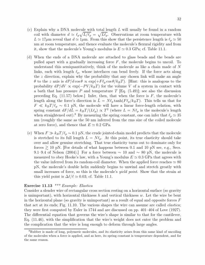
32

(c) Explain why a DNA molecule with total length L will usually be found in a randomcoil with diameter d ≃ ℓp

√

L/ℓp =√

Lℓp. Observations at room temperature withL ≃ 17µm reveal that d ≃ 1µm. From this show that the persistence length is ℓp ≃ 50nm at room temperature, and thence evaluate the molecule’s flexural rigidity and fromit, show that the molecule’s Young’s modulus is E ≃ 0.3 GPa; cf. Table 11.1.

(d) When the ends of a DNA molecule are attached to glass beads and the beads arepulled apart with a gradually increasing force F , the molecule begins to uncoil. Tounderstand this semiquantitatively, think of the molecule as like a chain made of Nlinks, each with length ℓp, whose interfaces can bend freely. If the force acts alongthe z direction, explain why the probability that any chosen link will make an angleθ to the z axis is dP/d cos θ ∝ exp(+Fℓp cos θ/kBT ). [Hint: this is analogous to theprobability dP/dV ∝ exp(−PV/kBT ) for the volume V of a system in contact witha bath that has pressure P and temperature T [Eq. (5.49)]; see also the discussionpreceding Eq. (11.57) below.] Infer, then, that when the force is F , the molecule’slength along the force’s direction is L = Nℓp tanh(Fℓp/kBT ). This tells us that forF ≪ kBT/ℓp ∼ 0.1 pN, the molecule will have a linear force-length relation, withspring constant dF/dL = kBT/(Lℓp) ∝ T 2 (where L = Nℓp is the molecule’s lengthwhen straightened out).8 By measuring the spring constant, one can infer that ℓp ≃ 35nm (roughly the same as the 50 nm inferred from the rms size of the coiled moleculeat zero force), and thence that E ≃ 0.2 GPa.

(e) When F ≫ kBT/ℓp ∼ 0.1 pN, the crude jointed-chain model predicts that the moleculeis stretched to its full length L = Nℓp. At this point, its true elasticity should takeover and allow genuine stretching. That true elasticity turns out to dominate only forforces & 10 pN. [For details of what happens between 0.1 and 10 pN see, e.g., Secs.9.1–9.4 of Nelson (2004).] For a force between ∼ 10 and ∼ 80 pN, the molecule ismeasured to obey Hooke’s law, with a Young’s modulus E ≃ 0.3 GPa that agrees withthe value inferred from its random-coil diameter. When the applied force reaches ≃ 80pN, the molecule’s double helix suddenly begins to unwind and stretch greatly withsmall increases of force, so this is the molecule’s yield point. Show that the strain atthis yield point is ∆ℓ/ℓ ≃ 0.03; cf. Table 11.1.

Exercise 11.13 *** Example: ElasticaConsider a slender wire of rectangular cross section resting on a horizontal surface (so gravityis unimportant), with horizontal thickness h and vertical thickness w. Let the wire be bentin the horizontal plane (so gravity is unimportant) as a result of equal and opposite forces Fthat act at its ends; Fig. 11.10. The various shapes the wire can assume are called elastica;they were first computed by Euler in 1744 and are discussed on pp. 401–404 of Love (1927).The differential equation that governs the wire’s shape is similar to that for the cantilever,Eq. (11.46), with the simplification that the wire’s weight does not enter the problem andthe complication that the wire is long enough to deform through large angles.

8Rubber is made of long, polymeric molecules, and its elasticity arises from this same kind of uncoilingof the molecules when a force is applied, and as here, its spring constant is temperature dependent, and forthe same reason.

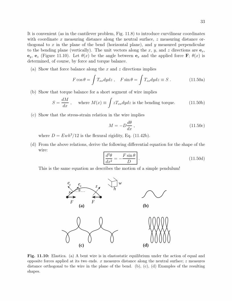
33

It is convenient (as in the cantilever problem, Fig. 11.8) to introduce curvilinear coordinateswith coordinate x measuring distance along the neutral surface, z measuring distance or-thogonal to x in the plane of the bend (horizontal plane), and y measured perpendicularto the bending plane (vertically). The unit vectors along the x, y, and z directions are ex,ey, ez (Figure 11.10). Let θ(x) be the angle between ex and the applied force F; θ(x) isdetermined, of course, by force and torque balance.

(a) Show that force balance along the x and z directions implies

F cos θ =

∫

Txxdydz , F sin θ =

∫

Tzxdydz ≡ S . (11.50a)

(b) Show that torque balance for a short segment of wire implies

S =dM

dx, where M(x) ≡

∫

zTxxdydz is the bending torque. (11.50b)

(c) Show that the stress-strain relation in the wire implies

M = −Ddθ

dx, (11.50c)

where D = Ewh3/12 is the flexural rigidity, Eq. (11.42b).

(d) From the above relations, derive the following differential equation for the shape of thewire:

d2θ

dx2= −F sin θ

D. (11.50d)

This is the same equation as describes the motion of a simple pendulum!

(a) (b)

(c) (d)

F F

xz

ez exw

h

θ

Fig. 11.10: Elastica. (a) A bent wire is in elastostatic equilibrium under the action of equal andopposite forces applied at its two ends. x measures distance along the neutral surface; z measuresdistance orthogonal to the wire in the plane of the bend. (b), (c), (d) Examples of the resultingshapes.

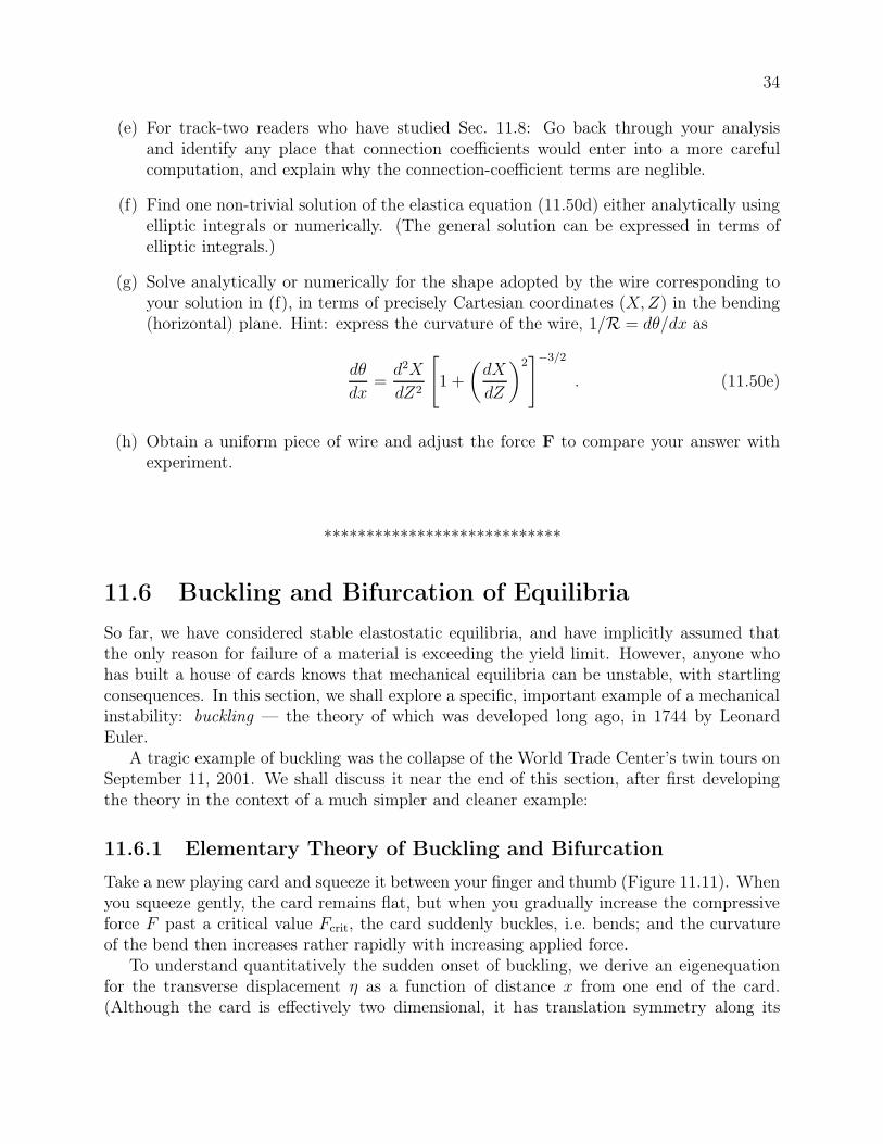
34

(e) For track-two readers who have studied Sec. 11.8: Go back through your analysisand identify any place that connection coefficients would enter into a more carefulcomputation, and explain why the connection-coefficient terms are neglible.

(f) Find one non-trivial solution of the elastica equation (11.50d) either analytically usingelliptic integrals or numerically. (The general solution can be expressed in terms ofelliptic integrals.)

(g) Solve analytically or numerically for the shape adopted by the wire corresponding toyour solution in (f), in terms of precisely Cartesian coordinates (X,Z) in the bending(horizontal) plane. Hint: express the curvature of the wire, 1/R = dθ/dx as

dθ

dx=

d2X

dZ2

[

1 +

(

dX

dZ

)2]−3/2

. (11.50e)

(h) Obtain a uniform piece of wire and adjust the force F to compare your answer withexperiment.

****************************

11.6 Buckling and Bifurcation of Equilibria

So far, we have considered stable elastostatic equilibria, and have implicitly assumed thatthe only reason for failure of a material is exceeding the yield limit. However, anyone whohas built a house of cards knows that mechanical equilibria can be unstable, with startlingconsequences. In this section, we shall explore a specific, important example of a mechanicalinstability: buckling — the theory of which was developed long ago, in 1744 by LeonardEuler.

A tragic example of buckling was the collapse of the World Trade Center’s twin tours onSeptember 11, 2001. We shall discuss it near the end of this section, after first developingthe theory in the context of a much simpler and cleaner example:

11.6.1 Elementary Theory of Buckling and Bifurcation

Take a new playing card and squeeze it between your finger and thumb (Figure 11.11). Whenyou squeeze gently, the card remains flat, but when you gradually increase the compressiveforce F past a critical value Fcrit, the card suddenly buckles, i.e. bends; and the curvatureof the bend then increases rather rapidly with increasing applied force.

To understand quantitatively the sudden onset of buckling, we derive an eigenequationfor the transverse displacement η as a function of distance x from one end of the card.(Although the card is effectively two dimensional, it has translation symmetry along its

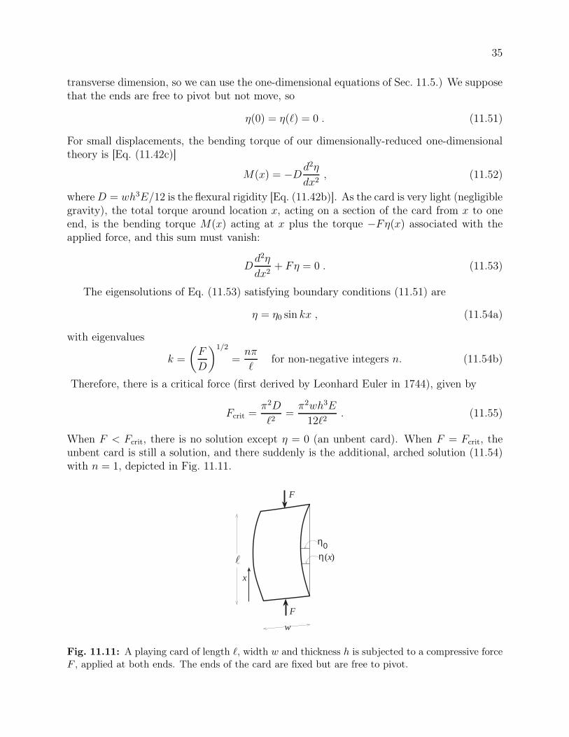
35

transverse dimension, so we can use the one-dimensional equations of Sec. 11.5.) We supposethat the ends are free to pivot but not move, so

η(0) = η(ℓ) = 0 . (11.51)

For small displacements, the bending torque of our dimensionally-reduced one-dimensionaltheory is [Eq. (11.42c)]

M(x) = −Dd2η

dx2, (11.52)

where D = wh3E/12 is the flexural rigidity [Eq. (11.42b)]. As the card is very light (negligiblegravity), the total torque around location x, acting on a section of the card from x to oneend, is the bending torque M(x) acting at x plus the torque −Fη(x) associated with theapplied force, and this sum must vanish:

Dd2η

dx2+ Fη = 0 . (11.53)

The eigensolutions of Eq. (11.53) satisfying boundary conditions (11.51) are

η = η0 sin kx , (11.54a)

with eigenvalues

k =

(

F

D

)1/2

=nπ

ℓfor non-negative integers n. (11.54b)

Therefore, there is a critical force (first derived by Leonhard Euler in 1744), given by

Fcrit =π2D

ℓ2=

π2wh3E

12ℓ2. (11.55)

When F < Fcrit, there is no solution except η = 0 (an unbent card). When F = Fcrit, theunbent card is still a solution, and there suddenly is the additional, arched solution (11.54)with n = 1, depicted in Fig. 11.11.

x

(x)

F

w

F

ηη0

Fig. 11.11: A playing card of length ℓ, width w and thickness h is subjected to a compressive forceF , applied at both ends. The ends of the card are fixed but are free to pivot.

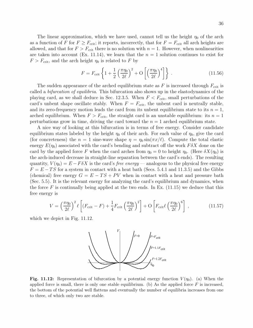
36

The linear approximation, which we have used, cannot tell us the height η0 of the archas a function of F for F ≥ Fcrit; it reports, incorrectly, that for F = Fcrit all arch heights areallowed, and that for F > Fcrit there is no solution with n = 1. However, when nonlinearitiesare taken into account (Ex. 11.14), we learn that the n = 1 solution continues to exist forF > Fcrit, and the arch height η0 is related to F by

F = Fcrit

{

1 +1

2

(πη02ℓ

)2

+O

[

(πη02ℓ

)4]}

. (11.56)

The sudden appearance of the arched equilibrium state as F is increased through Fcrit iscalled a bifurcation of equilibria. This bifurcation also shows up in the elastodynamics of theplaying card, as we shall deduce in Sec. 12.3.5. When F < Fcrit, small perturbations of thecard’s unbent shape oscillate stably. When F = Fcrit, the unbent card is neutrally stable,and its zero-frequency motion leads the card from its unbent equilibrium state to its n = 1,arched equilibrium. When F > Fcrit, the straight card is an unstable equilibrium: its n = 1perturbations grow in time, driving the card toward the n = 1 arched equilibrium state.

A nice way of looking at this bifurcation is in terms of free energy. Consider candidateequilibrium states labeled by the height η0 of their arch. For each value of η0, give the card(for concreteness) the n = 1 sine-wave shape η = η0 sin(πx/ℓ). Compute the total elasticenergy E(η0) associated with the card’s bending and subtract off the work FδX done on thecard by the applied force F when the card arches from η0 = 0 to height η0. (Here δX(η0) isthe arch-induced decrease in straight-line separation between the card’s ends). The resultingquantity, V (η0) = E−FδX is the card’s free energy — analogous to the physical free energyF = E−TS for a system in contact with a heat bath (Secs. 5.4.1 and 11.3.5) and the Gibbs(chemical) free energy G = E − TS + PV when in contact with a heat and pressure bath(Sec. 5.5). It is the relevant energy for analyzing the card’s equilibrium and dynamics, whenthe force F is continually being applied at the two ends. In Ex. (11.15) we deduce that thisfree energy is

V =(πη02ℓ

)2

ℓ

[

(Fcrit − F ) +1

4Fcrit

(πη02ℓ

)2]

+O

[

Fcritℓ(πη02ℓ

)6]

, (11.57)

which we depict in Fig. 11.12.

- η0

F=0 F=Fcrit

F=1.1Fcrit

F=1.2Fcrit

V

Fig. 11.12: Representation of bifurcation by a potential energy function V (η0). (a) When theapplied force is small, there is only one stable equilibrium. (b) As the applied force F is increased,the bottom of the potential well flattens and eventually the number of equilibria increases from oneto three, of which only two are stable.

37

At small values of the compressive force F [curve (a)], the free energy has only oneminimum η0 = 0 corresponding to a single stable equilibrium, the straight card. However,as the force is increased through Fcrit, the potential minimum flattens out and then becomesa maximum flanked by two new minima [curve (b)]. The maximum for F > Fcrit is theunstable, zero-displacement (straight-card) equilibrium and the two minima are the twostable, finite-amplitude equilibria with positive and negative η0 given by Eq. (11.56).

This procedure of representing a continuous system with an infinite number of degrees offreedom by just one or a few coordinates and finding the equilibrium by minimizing a freeenergy is quite common and powerful.

Thus far, we have discussed only two of the card’s equilibrium shapes (11.54): the straightshape n = 0 and the single-arch shape n = 1. If the card were constrained, by gentle,lateral stabilizing forces, to remain straight beyond F = Fcrit, then at F = n2Fcrit for eachn = 2, 3, 4, ..., the n’th order perturbative mode, with η = η0 sin(nπx/ℓ), would becomeunstable, and a new, stable equilibrium with this shape would bifurcate from the straightequilibrium. You can easily explore this for n = 2 using a playing card.

These higher-order modes are rarely of practical importance. In the case of a beam withno lateral constraints, as F increases above Fcrit, it will buckle into its single-arched shape,and then, for beam dimensions commonly used in construction, a fairly modest furtherincrease of F will bend it enough that its yield point and then rupture point are reached. Toexperience this yourself, take a thin meter stick, compress its ends between your two hands,and see what happens.

11.6.2 Collapse of the World Trade Center Buildings

We return, now, to the example with which we began this section. On September 11, 2001,al-Qaeda operatives hijacked two Boeing 767 passenger airplanes and crashed them into the110-story twin towers of the World Trade Center in New York City, triggering the towers’collapse a few hours later, with horrendous loss of life.

The weight of a tall building such as the towers is supported by vertical steel beams, calledcolumns. The longer the column, the lower the weight it can support without buckling, sinceFcrit = π2D/ℓ2 = π2EA(rg/ℓ)

2 with A the beam’s cross sectional area, rg its radius ofgyration, and ℓ its length [Eqs. (11.55) and (11.42b)]. The column lengths are typicallychosen such that the critical stress for buckling, Fcrit/A = E(πrg/ℓ)

2, is roughly the same asthe yield stress, Fyield ≃ 0.003E (cf. Table 11.1), which means that the columns’ slendernessratio is ℓ/rg ∼ 50. The columns are physically far longer than 50rg, but they are anchored toeach other laterally every ∼ 50rg by beams and girders in the floors, so their effective lengthfor buckling is ℓ ∼ 50rg. The columns’ radii of gyration rg are generally made large, withoutusing more steel than needed to support the overhead weight, by making the columns hollow,or giving them H shapes. In the twin towers, the thinnest beams had rg ∼ 13 cm and theywere anchored in every floor, with floor separations ℓ ≃ 3.8 m, so their slenderness ratio wasactually ℓ/rg ≃ 30.

According to a detailed investigation [NIST (2005); especially Secs. 6.14.2 and 6.14.3],the crashing airplanes ignited fires in and near floors 93–99 of the North Tower and 78–83of the South Tower, where the airplanes hit. The fires were most intense in the floors and

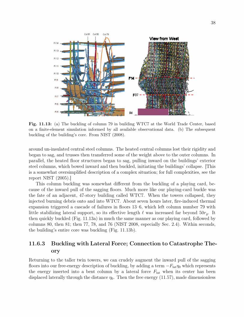
38

Fig. 11.13: (a) The buckling of column 79 in building WTC7 at the World Trade Center, basedon a finite-element simulation informed by all available observational data. (b) The subsequentbuckling of the building’s core. From NIST (2008).

around un-insulated central steel columns. The heated central columns lost their rigidity andbegan to sag, and trusses then transferred some of the weight above to the outer columns. Inparallel, the heated floor structures began to sag, pulling inward on the buildings’ exteriorsteel columns, which bowed inward and then buckled, initiating the buildings’ collapse. [Thisis a somewhat oversimplified description of a complex situation; for full complexities, see thereport NIST (2005).]

This column buckling was somewhat different from the buckling of a playing card, be-cause of the inward pull of the sagging floors. Much more like our playing-card buckle wasthe fate of an adjacent, 47-story building called WTC7. When the towers collapsed, theyinjected burning debris onto and into WTC7. About seven hours later, fire-induced thermalexpansion triggered a cascade of failures in floors 13–6, which left column number 79 withlittle stabilizing lateral support, so its effective length ℓ was increased far beyond 50rg. Itthen quickly buckled (Fig. 11.13a) in much the same manner as our playing card, followed bycolumns 80, then 81; then 77, 78, and 76 (NIST 2008, especially Sec. 2.4). Within seconds,the building’s entire core was buckling (Fig. 11.13b).

11.6.3 Buckling with Lateral Force; Connection to Catastrophe The-

ory

Returning to the taller twin towers, we can crudely augment the inward pull of the saggingfloors into our free-energy description of buckling, by adding a term −Flatη0 which representsthe energy inserted into a bent column by a lateral force Flat when its center has beendisplaced laterally through the distance η0. Then the free energy (11.57), made dimensionless

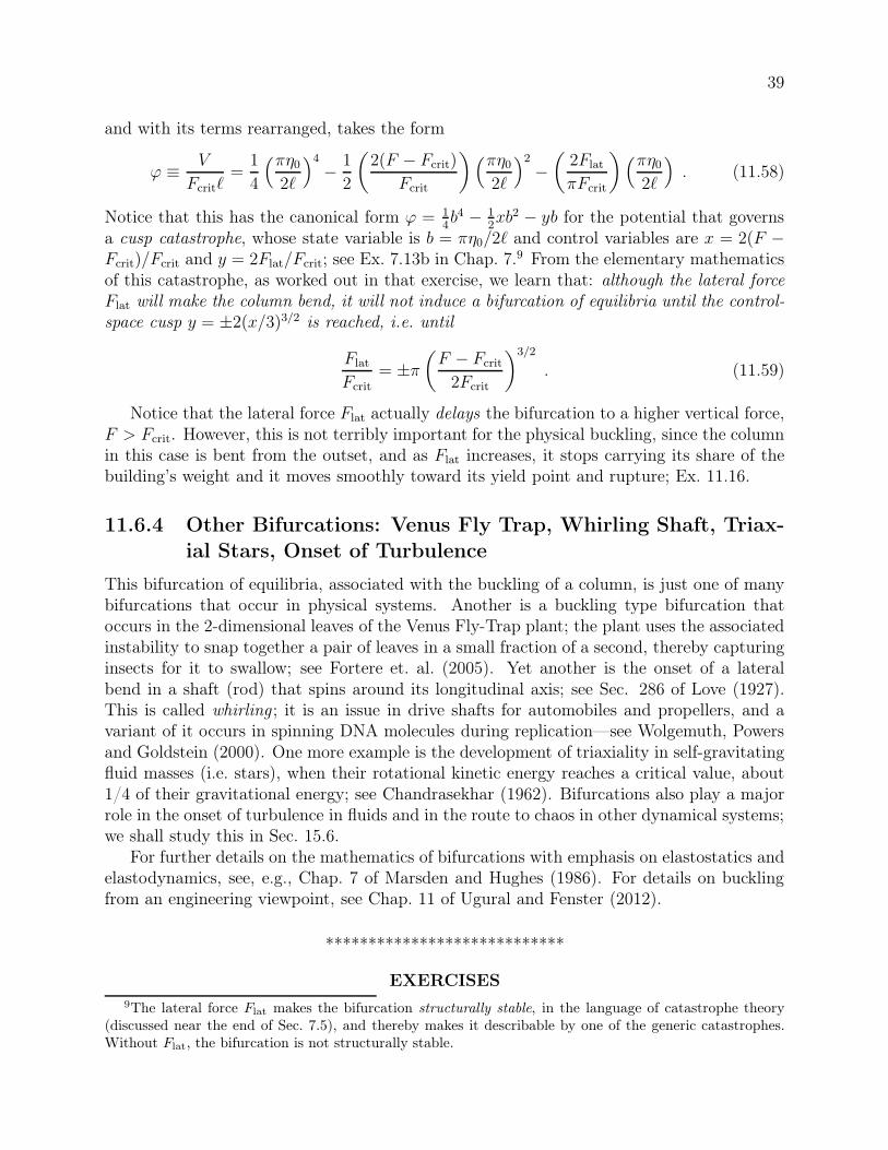
39

and with its terms rearranged, takes the form

ϕ ≡ V

Fcritℓ=

1

4

(πη02ℓ

)4

− 1

2

(

2(F − Fcrit)

Fcrit

)

(πη02ℓ

)2

−(

2Flat

πFcrit

)

(πη02ℓ

)

. (11.58)

Notice that this has the canonical form ϕ = 14b4 − 1

2xb2 − yb for the potential that governs

a cusp catastrophe, whose state variable is b = πη0/2ℓ and control variables are x = 2(F −Fcrit)/Fcrit and y = 2Flat/Fcrit; see Ex. 7.13b in Chap. 7.9 From the elementary mathematicsof this catastrophe, as worked out in that exercise, we learn that: although the lateral forceFlat will make the column bend, it will not induce a bifurcation of equilibria until the control-space cusp y = ±2(x/3)3/2 is reached, i.e. until

Flat

Fcrit

= ±π

(

F − Fcrit

2Fcrit

)3/2

. (11.59)

Notice that the lateral force Flat actually delays the bifurcation to a higher vertical force,F > Fcrit. However, this is not terribly important for the physical buckling, since the columnin this case is bent from the outset, and as Flat increases, it stops carrying its share of thebuilding’s weight and it moves smoothly toward its yield point and rupture; Ex. 11.16.

11.6.4 Other Bifurcations: Venus Fly Trap, Whirling Shaft, Triax-

ial Stars, Onset of Turbulence

This bifurcation of equilibria, associated with the buckling of a column, is just one of manybifurcations that occur in physical systems. Another is a buckling type bifurcation thatoccurs in the 2-dimensional leaves of the Venus Fly-Trap plant; the plant uses the associatedinstability to snap together a pair of leaves in a small fraction of a second, thereby capturinginsects for it to swallow; see Fortere et. al. (2005). Yet another is the onset of a lateralbend in a shaft (rod) that spins around its longitudinal axis; see Sec. 286 of Love (1927).This is called whirling ; it is an issue in drive shafts for automobiles and propellers, and avariant of it occurs in spinning DNA molecules during replication—see Wolgemuth, Powersand Goldstein (2000). One more example is the development of triaxiality in self-gravitatingfluid masses (i.e. stars), when their rotational kinetic energy reaches a critical value, about1/4 of their gravitational energy; see Chandrasekhar (1962). Bifurcations also play a majorrole in the onset of turbulence in fluids and in the route to chaos in other dynamical systems;we shall study this in Sec. 15.6.

For further details on the mathematics of bifurcations with emphasis on elastostatics andelastodynamics, see, e.g., Chap. 7 of Marsden and Hughes (1986). For details on bucklingfrom an engineering viewpoint, see Chap. 11 of Ugural and Fenster (2012).

****************************

EXERCISES

9The lateral force Flat makes the bifurcation structurally stable, in the language of catastrophe theory(discussed near the end of Sec. 7.5), and thereby makes it describable by one of the generic catastrophes.Without Flat, the bifurcation is not structurally stable.

40

Exercise 11.14 Derivation and Example: Bend as a Function of Applied ForceDerive Eq. (11.56) relating the angle θo = (dη/dx)x=0 = kηo = πηo/ℓ to the applied forceF when the card has an n = 1, arched shape. Hint: Use the elastica differential equationd2θ/dx2 = −(F/D) sin θ [Eq. (11.50d)] for the angle between the card and the applied forceat distance x from the card’s end. The sin θ becomes θ in the linear approximation usedin the text; the nonlinearities embodied in the sine give rise to the desired relation. Thefollowing steps along the way toward a solution are mathematically the same as used whencomputing the period of a pendulum as a function of its amplitude of swing.

(a) Derive the first integral of the elastica equation

(dθ/dx)2 = 2(F/D)(cos θ − cos θo) , (11.60)

where θo is an integration constant. Show that the boundary condition of no bendingtorque (no inflexion of the card’s shape) at the card ends implies θ = θo at x = 0 andx = ℓ; whence θ = 0 at the card’s center, x = ℓ/2.

(b) Integrate the differential equation (11.60) to obtain

ℓ

2=

√

D

2F

∫ θo

0

dθ√cos θ − cos θo

. (11.61)

(c) Perform the change of variable sin(θ/2) = sin(θo/2) sinφ and thereby bring Eq. (11.61)into the form

ℓ = 2

√

D

F

∫ π/2

0

dφ√

1− sin2(θo/2) sin2 φ

= 2

√

D

FK[sin2(θo/2)] . (11.62)

Here K(y) is the complete elliptic integral of the first type, with the parametrizationused by Mathematica (which differs from many books).

(d) Expand Eq. (11.62) in powers of sin2(θo/2) to obtain

F = Fcrit

4

π2K2[sin2(θo/2)] = Fcrit

[

1 +1

2sin2(θo/2) +

11

32sin4(θo/2) + . . .

]

. (11.63)

Then expand this in powers of θo/2 to obtain our desired result, Eq. (11.56).

Exercise 11.15 Problem: Free Energy of a Bent, Compressed Beam

Derive Eq. (11.57) for the free energy V of a beam that is compressed with a force F and hasa critical compression Fcrit = π2D/ℓ2, where D is its flexural rigidity. [Hint: It must be that∂V/∂η0 = 0 gives Eq. (11.56) for the beam’s equilibrium bend amplitude η0 as a function ofF −Fcrit. Use this to reduce to reduce the number of terms in V (η0) in Eq. (11.57) that youneed to derive.

41

Exercise 11.16 Problem: Bent Beam with Lateral Force

Explore, numerically, the free energy (11.58) of a bent beam with a compressive force Fand lateral force Flat. Examine how the extrema (equilibrium states) evolve as F and Flat

change, and deduce the physical consequences.

Exercise 11.17 **Problem: Applications of Buckling — Mountains and Pipes

Buckling plays a role in many natural and man-made phenomena. Explore the followingexamples:

(a) Mountain building. When two continental plates are in (very slow) collision, thecompressional force near their interface drives their crustal rock to buckle upward, pro-ducing mountains. Estimate how high such mountains can be on Earth and on Mars,and compare your estimates with their actual heights. Read about such mountainbuilding in books or on the web.

(b) Thermal expansion of pipes. When a segment of pipe is heated, e.g. by the risingsun in the morning, it will expand. If its ends are held fixed, this can easily produce alarge enough longitudinal stress to buckle the pipe. How would you deal with this inan oil pipeline on the earth’s surface? In a long vacuum tube? Compare your answerswith standard engineering solutions, which you will find in books or on the web.

****************************

11.7 Reducing the Elastostatic Equations to Two Dimen-

sions for a Deformed Thin Plate: Stress-Polishing a

Telescope Mirror

The world’s largest optical telescopes (as of 2013), the two ten meter Keck telescopes, arelocated on Mauna Kea in Hawaii. It is very difficult to support traditional, monolithicmirrors so that the mirror surfaces maintain their shape (their “figure”) as the telescopeslews, because they are so heavy; so for Keck a new method of fabrication was sought. Thesolution devised by Jerry Nelson and his colleagues was to construct the telescope out of 36separate hexagons, each 0.9m on a side. However, this posed a second problem, grinding eachhexagon’s reflecting surface to the required hyperboloidal shape. For this, a novel techniquecalled stressed mirror polishing was developed. This technique relies on the fact that it isrelatively easy to grind a surface to a spherical shape, but technically highly challenging tocreate a non-axisymmetric shape. So, during the grinding, stresses are applied around theboundary of the mirror to deform it, and a spherical surface is produced. The stresses arethen removed and the mirror springs into the desired nonspherical shape. Computing thenecessary stresses is a problem in classical elasticity theory and, in fact, is a good exampleof a large number of applications where the elastic body can be approximated as a thin

42

plate and its shape can be analyzed using elasticity equations that are reduced from threedimensions to two by the method of moments.

For stress polishing of mirrors, the applied stresses are so large that we can ignore gravi-tational forces (at least in our simplified treatment). We suppose that the hexagonal mirrorhas a uniform thickness h and idealize it as a circle of radius R, and we introduce Cartesiancoordinates with (x, y) in the horizontal plane (the plane of the mirror before deformationand polishing begin), and z vertical. The mirror is deformed as a result of a net vertical forceper unit area (pressure) P (x, y). This force is applied at the lower surface when positive andthe upper surface when negative. In addition, there are shear forces and bending momentsapplied around the rim of the mirror.

As in our analysis of a cantilever in Sec. 11.5, we assume the existence of a neutral surfacein the deformed mirror, where the horizontal strain vanishes, Tab = 0. (Here and below we useletters from the early part of the Latin alphabet for horizontal x = x1, y = x2 components.)We denote the vertical displacement of the neutral surface by η(x, y). By applying themethod of moments to the three-dimensional equation stress balance equation Tjk,k = 0 in amanner similar to our cantilever analysis, we obtain the following two-dimensional equationfor the mirror’s shape:

∇2(∇2η) = P (x, y)/D . (11.64a)

Here ∇2 is the horizontal Laplacian, i.e. ∇2η ≡ η,aa = η,xx + η,yy. Equation (11.64a) is thetwo-dimensional analog of the equation d4η/dx4 = W (x)/D for the shape of a cantileveron which a downward force per unit length W (x) acts [Eq. (11.46)]. The two-dimensionalflexural rigidity that appears in Eq. (11.64a) is

D =Eh3

12(1− ν2), (11.64b)

where E is the mirror’s Young’s modulus, h is its thickness and ν is its Poisson’s ratio. Thequantity ∇2∇2 that operates on η in the shape equation (11.64a) is called the biharmonicoperator ; it also appears in 3-dimensional form in the biharmonic equation (11.35a) for thedisplacement inside a homogeneous, isotropic body to which surface stresses are applied.

The shape equation (11.64a) must be solved subject to boundary conditions around themirror’s rim: the applied shear forces and bending torques.

The individual Keck mirror segments were constructed out of a ceramic material withYoung’s modulus E = 89GPa and Poisson’s ratio ν = 0.24 (cf. Table 11.1). A mechanicaljig was constructed to apply the shear forces and bending torques at 24 uniformly spacedpoints around the rim of the mirror (Figure 11.14). The maximum stress was applied for thesix outermost mirrors and was 2.4× 106N m−2, 12 per cent of the breaking tensile strength(2× 107N m−2).

This stress-polishing worked beautifully and the Keck telescopes have become highlysuccessful tools for astronomical research.

****************************

EXERCISES

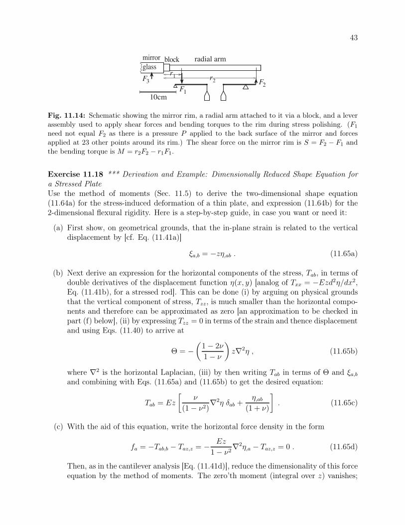
43

mirror

glassblock radial arm

F3

10cm

F2F1

r1 r2

Fig. 11.14: Schematic showing the mirror rim, a radial arm attached to it via a block, and a leverassembly used to apply shear forces and bending torques to the rim during stress polishing. (F1

need not equal F2 as there is a pressure P applied to the back surface of the mirror and forcesapplied at 23 other points around its rim.) The shear force on the mirror rim is S = F2 − F1 andthe bending torque is M = r2F2 − r1F1.

Exercise 11.18 *** Derivation and Example: Dimensionally Reduced Shape Equation fora Stressed PlateUse the method of moments (Sec. 11.5) to derive the two-dimensional shape equation(11.64a) for the stress-induced deformation of a thin plate, and expression (11.64b) for the2-dimensional flexural rigidity. Here is a step-by-step guide, in case you want or need it:

(a) First show, on geometrical grounds, that the in-plane strain is related to the verticaldisplacement by [cf. Eq. (11.41a)]

ξa,b = −zη,ab . (11.65a)

(b) Next derive an expression for the horizontal components of the stress, Tab, in terms ofdouble derivatives of the displacement function η(x, y) [analog of Txx = −Ezd2η/dx2,Eq. (11.41b), for a stressed rod]. This can be done (i) by arguing on physical groundsthat the vertical component of stress, Tzz, is much smaller than the horizontal compo-nents and therefore can be approximated as zero [an approximation to be checked inpart (f) below], (ii) by expressing Tzz = 0 in terms of the strain and thence displacementand using Eqs. (11.40) to arrive at

Θ = −(

1− 2ν

1− ν

)

z∇2η , (11.65b)

where ∇2 is the horizontal Laplacian, (iii) by then writing Tab in terms of Θ and ξa,band combining with Eqs. (11.65a) and (11.65b) to get the desired equation:

Tab = Ez

[

ν

(1− ν2)∇2η δab +

η,ab(1 + ν)

]

. (11.65c)

(c) With the aid of this equation, write the horizontal force density in the form

fa = −Tab,b − Taz,z = − Ez

1− ν2∇2η,a − Taz,z = 0 . (11.65d)

Then, as in the cantilever analysis [Eq. (11.41d)], reduce the dimensionality of this forceequation by the method of moments. The zero’th moment (integral over z) vanishes;

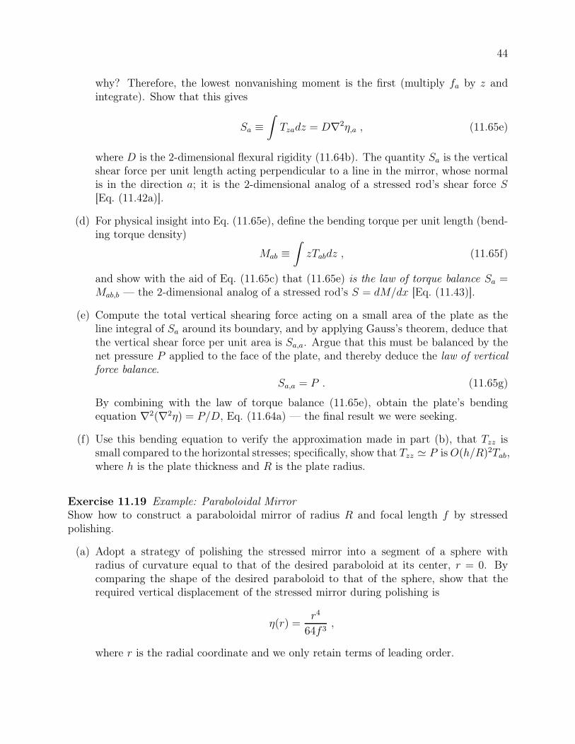
44

why? Therefore, the lowest nonvanishing moment is the first (multiply fa by z andintegrate). Show that this gives

Sa ≡∫

Tzadz = D∇2η,a , (11.65e)

where D is the 2-dimensional flexural rigidity (11.64b). The quantity Sa is the verticalshear force per unit length acting perpendicular to a line in the mirror, whose normalis in the direction a; it is the 2-dimensional analog of a stressed rod’s shear force S[Eq. (11.42a)].

(d) For physical insight into Eq. (11.65e), define the bending torque per unit length (bend-ing torque density)

Mab ≡∫

zTabdz , (11.65f)

and show with the aid of Eq. (11.65c) that (11.65e) is the law of torque balance Sa =Mab,b — the 2-dimensional analog of a stressed rod’s S = dM/dx [Eq. (11.43)].

(e) Compute the total vertical shearing force acting on a small area of the plate as theline integral of Sa around its boundary, and by applying Gauss’s theorem, deduce thatthe vertical shear force per unit area is Sa,a. Argue that this must be balanced by thenet pressure P applied to the face of the plate, and thereby deduce the law of verticalforce balance.

Sa,a = P . (11.65g)

By combining with the law of torque balance (11.65e), obtain the plate’s bendingequation ∇2(∇2η) = P/D, Eq. (11.64a) — the final result we were seeking.

(f) Use this bending equation to verify the approximation made in part (b), that Tzz issmall compared to the horizontal stresses; specifically, show that Tzz ≃ P is O(h/R)2Tab,where h is the plate thickness and R is the plate radius.

Exercise 11.19 Example: Paraboloidal MirrorShow how to construct a paraboloidal mirror of radius R and focal length f by stressedpolishing.

(a) Adopt a strategy of polishing the stressed mirror into a segment of a sphere withradius of curvature equal to that of the desired paraboloid at its center, r = 0. Bycomparing the shape of the desired paraboloid to that of the sphere, show that therequired vertical displacement of the stressed mirror during polishing is

η(r) =r4

64f 3,

where r is the radial coordinate and we only retain terms of leading order.

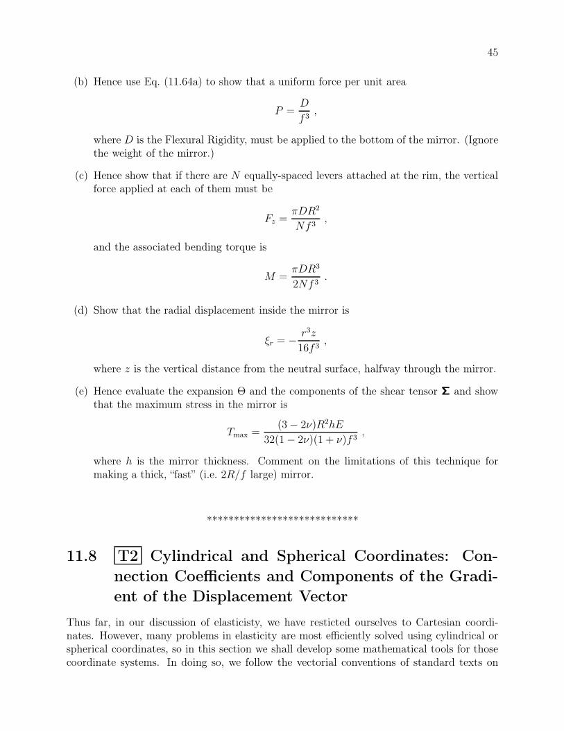
45

(b) Hence use Eq. (11.64a) to show that a uniform force per unit area

P =D

f 3,

where D is the Flexural Rigidity, must be applied to the bottom of the mirror. (Ignorethe weight of the mirror.)

(c) Hence show that if there are N equally-spaced levers attached at the rim, the verticalforce applied at each of them must be

Fz =πDR2

Nf 3,

and the associated bending torque is

M =πDR3

2Nf 3.

(d) Show that the radial displacement inside the mirror is

ξr = − r3z

16f 3,

where z is the vertical distance from the neutral surface, halfway through the mirror.

(e) Hence evaluate the expansion Θ and the components of the shear tensor Σ and showthat the maximum stress in the mirror is

Tmax =(3− 2ν)R2hE

32(1− 2ν)(1 + ν)f 3,

where h is the mirror thickness. Comment on the limitations of this technique formaking a thick, “fast” (i.e. 2R/f large) mirror.

****************************

11.8 T2 Cylindrical and Spherical Coordinates: Con-

nection Coefficients and Components of the Gradi-

ent of the Displacement Vector

Thus far, in our discussion of elasticisty, we have resticted ourselves to Cartesian coordi-nates. However, many problems in elasticity are most efficiently solved using cylindrical orspherical coordinates, so in this section we shall develop some mathematical tools for thosecoordinate systems. In doing so, we follow the vectorial conventions of standard texts on

46

electrodynamics and quantum mechanics (e.g., Jackson 1999, and Messiah 1962): We intro-duce an orthonormal set of basis vectors associated with each of our curvilinear coordinatesystems; the coordinate lines are orthogonal to each other, and the basis vectors have unitlengths and point along the coordinate lines. In our study of continuum mechanics (Part IV– Elasticity, Part V – Fluid Mechanics, and Part VI – Plasma Physics), we shall follow thispractice. Then in studying General Relativity and Cosmology (Part VII), we shall introduceand use basis vectors that are not orthonormal.

Our notation for cylindrical coordinates is (, φ, z); (pronounced “pomega”) is distancefrom the z axis, and φ is angle around the z axis, so

=√

x2 + y2 , φ = arctan(y/x) . (11.66a)

The unit basis vectors that point along the coordinate axes are denoted e, eφ, ez, and arerelated to the Cartesian basis vectors by

e = (x/)ex + (y/)ey , eφ = −(y/)ex + (x/)ey , ez = Cartesian ez . (11.66b)

Our notation for spherical coordinates is (r, θ, φ), with (as should be very familiar)

r =√

x2 + y2 + z2 , θ = arccos(z/r) , φ = arctan(y/x) . (11.67a)

The unit basis vectors associated with these coordinates are

er =x

rex +

y

rey +

z

rez , eθ =

z

re −

rez , eφ = − y

ex +

x

ey . (11.67b)

Because our bases are orthonormal, the components of the metric of 3-dimensional spaceretain the Kronecker-delta values

gjk ≡ ej · ek = δjk , (11.68)

which permits us to keep all vector and tensor indices down, by contrast with spacetimewhere we must distinguish between up and down; cf. Sec. 2.5.10

In Jackson (1999), Messiah (1962) and other standard texts, formulas are written downfor the gradient and Laplacian of a scalar field, and the divergence and curl of a vector field,in cylindrical and spherical coordinates; and one uses these formulas over and over again.In elasticity theory, we deal largely with second rank tensors, and will need formulae fortheir various derivatives in cylindrical and spherical coordinates. In this book we introducea mathematical tool, connection coefficients Γijk, by which those formulae can be derivedwhen needed.

The connection coefficients quantify the turning of the orthonormal basis vectors as onemoves from point to point in Euclidean 3-space; i.e., they tell us how the basis vectors atone point in space are connected to (related to) those at another point. More specifically, wedefine Γijk by the two equivalent relations

∇kej = Γijkei ; Γijk = ei · (∇kej) . (11.69)

10Occasionally, e.g. in the useful equation ǫijmǫklm = δijkl ≡ δikδjl − δilδ

jk [Eq. (1.23)], it is convenient to

put some indices up. In our orthonormal basis, any component with an index up is equal to that samecomponent with an index down; e.g., δik ≡ δik.

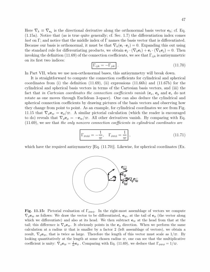
47

Here ∇k ≡ ∇ekis the directional derivative along the orthonormal basis vector ek; cf. Eq.

(1.15a). Notice that (as is true quite generally; cf. Sec. 1.7) the differentiation index comeslast on Γ; and notice that the middle index of Γ names the basis vector that is differentiated.Because our basis is orthonormal, it must be that ∇k(ei · ej) = 0. Expanding this out usingthe standard rule for differentiating products, we obtain ej · (∇kei) + ei · (∇kej) = 0. Theninvoking the definition (11.69) of the connection coefficients, we see that Γijk is antisymmetricon its first two indices:

Γijk = −Γjik . (11.70)

In Part VII, when we use non-orthonormal bases, this antisymmetry will break down.It is straightforward to compute the connection coefficients for cylindrical and spherical

coordinates from (i) the definition (11.69), (ii) expressions (11.66b) and (11.67b) for thecylindrical and spherical basis vectors in terms of the Cartesian basis vectors, and (iii) thefact that in Cartesian coordinates the connection coefficients vanish (ex, ey and ez do notrotate as one moves through Euclidean 3-space). One can also deduce the cylindrical andspherical connection coefficients by drawing pictures of the basis vectors and observing howthey change from point to point. As an example, for cylindrical coordinates we see from Fig.11.15 that ∇φe = eφ/. A similar pictorial calculation (which the reader is encouragedto do) reveals that ∇φeφ = −e/. All other derivatives vanish. By comparing with Eq.(11.69), we see that the only nonzero connection coefficients in cylindrical coordinates are

Γφφ = − 1

, Γφφ =

1

, (11.71)

which have the required antisymmetry [Eq. (11.70)]. Likewise, for spherical coordinates (Ex.

eφ

eω∼

eω∼

φ∆ eω∼

Fig. 11.15: Pictorial evaluation of Γφφ. In the right-most assemblage of vectors we compute∇φe as follows: We draw the vector to be differentiated, e, at the tail of eφ (the vector alongwhich we differentiate) and also at its head. We then subtract e at the head from that at thetail; this difference is ∇φe. It obviously points in the eφ direction. When we perform the samecalculation at a radius that is smaller by a factor 2 (left assemblage of vectors), we obtain aresult, ∇φe, that is twice as large. Therefore the length of this vector must scale as 1/. Bylooking quantitatively at the length at some chosen radius , one can see that the multiplicativecoefficient is unity: ∇φe = 1

eφ . Comparing with Eq. (11.69), we deduce that Γφφ = 1/.

48

11.21)

Γθrθ = Γφrφ = −Γrθθ = −Γrφφ =1

r, Γφθφ = −Γθφφ =

cot θ

r; (11.72)

These connection coefficients are the keys to differentiating vectors and tensors. Considerthe gradient of the displacement, W = ∇ξ. Applying the product rule for differentiation,we obtain

∇k(ξjej) = (∇kξj)ej + ξj(∇kej) = ξj,kej + ξjΓljkel . (11.73)

Here the comma denotes the directional derivative, along a basis vector, of the componentstreated as scalar fields. For example, in cylindrical coordinates we have

ξi, =∂ξi∂

, ξi,φ =1

∂ξi∂φ

, ξi,z =∂ξi∂z

; (11.74)

and in spherical coordinates we have

ξi,r =∂ξi∂r

, ξi,θ =1

r

∂ξi∂θ

, ξi,φ =1

r sin θ

∂ξi∂φ

. (11.75)

Taking the i’th component of Eq. (11.73) we obtain

Wik = ξi;k = ξi,k + Γijkξj . (11.76)

Here ξi;k are the nine components of the gradient of the vector field ξ(x).We can use Eq. (11.76) to evaluate the expansion Θ = TrW = ∇ · ξ. Using Eqs. (11.71)

and (11.72), we obtain

Θ = ∇ · ξ =∂ξ∂

+1

∂ξφ∂φ

+∂ξz∂z

+ξ

=1

∂

∂(ξ) +

1

∂ξφ∂φ

+∂ξz∂z

(11.77)

in cylindrical coordinates, and

Θ = ∇ · ξ =∂ξr∂r

+1

r

∂ξθ∂θ

+1

r sin θ

∂ξφ∂φ

+2ξrr

+cot θξθ

r

=1

r2∂

∂r(r2ξr) +

1

r sin θ

∂

∂θ(sin θξθ) +

1

r sin θ

∂ξφ∂φ

(11.78)

in spherical coordinates, in agreement with formulae in standard textbooks such as the flyleafof Jackson (1999).

The components of the rotation are most easily deduced using Rij = −ǫijkφk with φ =12∇ × ξ, and the standard expressions for the curl in cylindrical and spherical coordinates

(e.g., Jackson 1999). Since the rotation does not enter into elasticity theory in a significantway, we shall refrain from writing down the results. The components of the shear arecomputed in Box 11.4.

49

Box 11.4

T2 Shear Tensor in Spherical and Cylindrical Coordinates

Using our rules (11.76) for forming the gradient of a vector we can derive a generalexpression for the shear tensor

Σij =1

2(ξi;j + ξj;i)−

1

3δijξk;k

=1

2(ξi,j + ξj,i + Γiljξl + Γjliξl)−

1

3δij(ξk,k + Γklkξl) . (1)

Evaluating this in cylindrical coordinates using the connection coefficients (11.71), we

obtain

Σ =2

3

∂ξ∂

− 1

3

ξ

− 1

3

∂ξφ∂φ

− 1

3

∂ξz∂z

,

Σφφ =2

3

∂ξφ∂φ

+2

3

ξ

− 1

3

∂ξ∂

− 1

3

∂ξz∂z

,

Σzz =2

3

∂ξz∂z

− 1

3

∂ξ∂

− 1

3

ξ

− 1

3

∂ξφ∂φ

,

Σφz = Σzφ =1

2

∂ξz∂φ

+1

2

∂ξφ∂z

,

Σz = Σz =1

2

∂ξ∂z

+1

2

∂ξz∂

,

Σφ = Σφ =1

2

∂ξφ∂

− ξφ2

+1

2

∂ξ∂φ

. (2)

Likewise, in spherical coordinates using the connection coefficients (11.72), we obtain

Σrr =2

3

∂ξr∂r

− 2

3rξr −

cotθ

3rξθ −

1

3r

∂ξθ∂θ

− 1

3r sin θ

∂ξφ

∂φ,

Σθθ =2

3r

∂ξθ∂φ

+ξr3r

− 1

3

∂ξr∂r

− cotθξθ3r

− 1

3r sin θ

∂ξφ∂φ

,

Σφφ =2

3r sin θ

∂ξφ∂φ

+2cotθξθ

3r+

ξr3r

− 1

3

∂ξr∂r

− 1

3r

∂ξθ∂θ

,

Σθφ = Σφθ =1

2r

∂ξφ∂θ

− cotθξφ2r

+1

2r sin θ

∂ξθ∂φ

,

Σφr = Σrφ =1

2r sin θ

∂ξr∂φ

+1

2

∂ξφ∂r

− ξφ2r

,

Σrθ = Σθr =1

2

∂ξθ∂r

− ξθ2r

+1

2r

∂ξr∂θ

. (3)

50

By a computation analogous to Eq. (11.73), we can construct an expression for thegradient of a tensor of any rank. For a second rank tensor T = Tijei ⊗ ej we obtain (Ex.11.20)

Tij;k = Tij,k + ΓilkTlj + ΓjlkTil . (11.79)

Equation (11.79) for the components of the gradient can be understood as follows: In cylin-drical or spherical coordinates, the components Tij can change from point to point as a resultof two things: a change of the tensor T, or the turning of the basis vectors. The two connec-tion coefficient terms in Eq. (11.79) remove the effects of the basis turning, leaving in Tij;k

only the influence of the change of T itself. There are two correction terms corresponding tothe two slots (indices) of T; the effects of basis turning on each slot get corrected one afteranother. If T had had n slots, then there would have been n correction terms, each with theform of the two in Eq. (11.79).

These expressions for derivatives of tensors are not required to deal with the vectorfields of introductory electromagnetic theory or quantum theory, but they are essential tomanipulate the tensor fields encountered in elasticity. As we shall see in Sec. 24.3, withone further generalization, we can go on to differentiate tensors in any basis (orthonormalor non-orthonormal) in a curved spacetime, as is needed to perform calculations in generalrelativity.

Although the algebra of evaluating the components of derivatives such as (11.79) inexplicit form (e.g., in terms of {r, θ, φ}) can be long and tedious when done by hand, inthe modern era of symbolic manipulation via computers (e.g. Mathematica or Maple), thealgebra can be done quickly and accurately to obtain expressions such as Eqs. (3) of Box11.4.

****************************

EXERCISES

Exercise 11.20 Derivation and Practice: Gradient of a Second Rank TensorBy a computation analogous to Eq. (11.73), derive Eq. (11.79) for the components of thegradient of a second rank tensor in any orthonormal basis

Exercise 11.21 Derivation and Practice: Connection in Spherical Coordinates

(a) By drawing pictures analogous to Fig. 11.15, show that

∇φer =1

reφ , ∇θer =

1

reθ , ∇φeθ =

cot θ

reφ . (11.80)

(b) From these relations and antisymmetry on the first two indices [Eq. (11.70)], deducethe connection coefficients (11.72).

Exercise 11.22 Derivation and Practice: Expansion in Cylindrical and Spherical Coordi-natesDerive Eqs. (11.77) and (11.78) for the divergence of the vector field ξ in cylindrical andspherical coordinates using the connection coefficients (11.71) and (11.72).

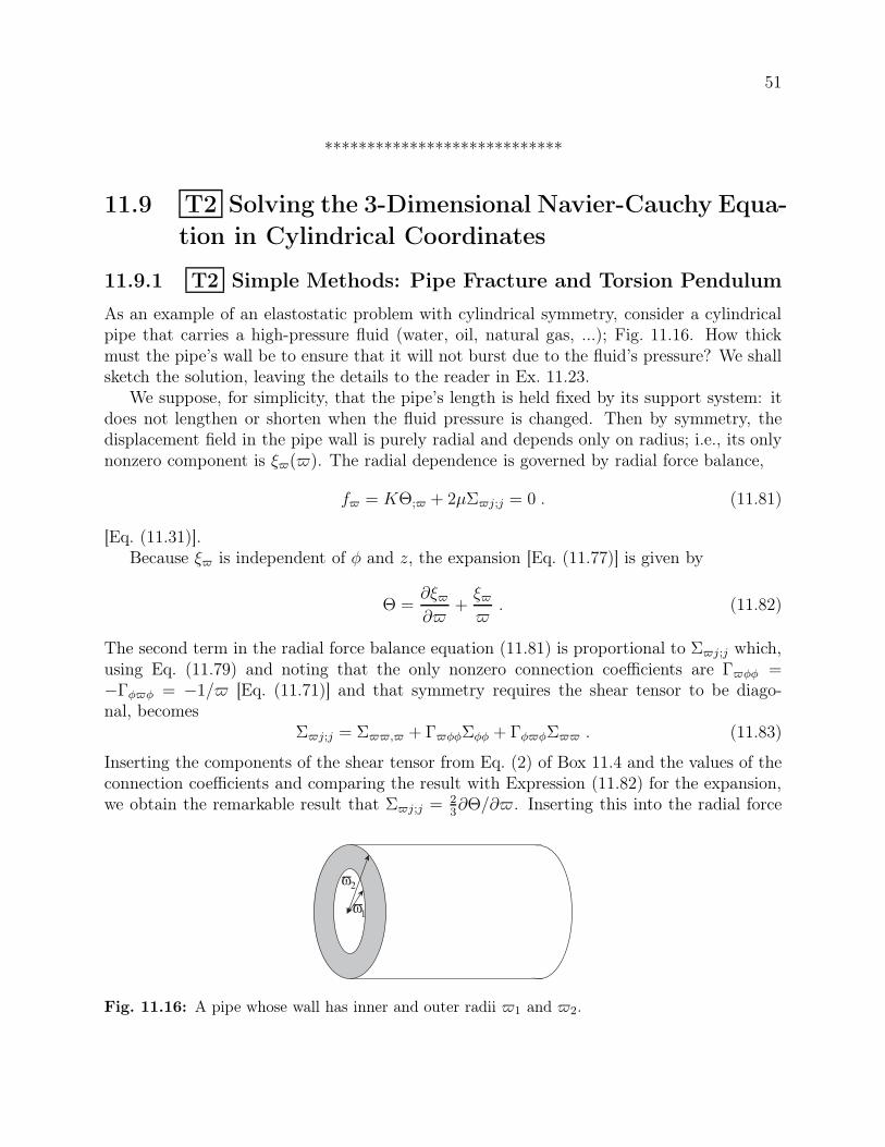
51

****************************

11.9 T2 Solving the 3-Dimensional Navier-Cauchy Equa-

tion in Cylindrical Coordinates

11.9.1 T2 Simple Methods: Pipe Fracture and Torsion Pendulum

As an example of an elastostatic problem with cylindrical symmetry, consider a cylindricalpipe that carries a high-pressure fluid (water, oil, natural gas, ...); Fig. 11.16. How thickmust the pipe’s wall be to ensure that it will not burst due to the fluid’s pressure? We shallsketch the solution, leaving the details to the reader in Ex. 11.23.

We suppose, for simplicity, that the pipe’s length is held fixed by its support system: itdoes not lengthen or shorten when the fluid pressure is changed. Then by symmetry, thedisplacement field in the pipe wall is purely radial and depends only on radius; i.e., its onlynonzero component is ξ(). The radial dependence is governed by radial force balance,

f = KΘ; + 2µΣj;j = 0 . (11.81)

[Eq. (11.31)].Because ξ is independent of φ and z, the expansion [Eq. (11.77)] is given by

Θ =∂ξ∂

+ξ

. (11.82)

The second term in the radial force balance equation (11.81) is proportional to Σj;j which,using Eq. (11.79) and noting that the only nonzero connection coefficients are Γφφ =−Γφφ = −1/ [Eq. (11.71)] and that symmetry requires the shear tensor to be diago-nal, becomes

Σj;j = Σ, + ΓφφΣφφ + ΓφφΣ . (11.83)

Inserting the components of the shear tensor from Eq. (2) of Box 11.4 and the values of theconnection coefficients and comparing the result with Expression (11.82) for the expansion,we obtain the remarkable result that Σj;j =

23∂Θ/∂. Inserting this into the radial force

ϖ1

ϖ2

Fig. 11.16: A pipe whose wall has inner and outer radii 1 and 2.

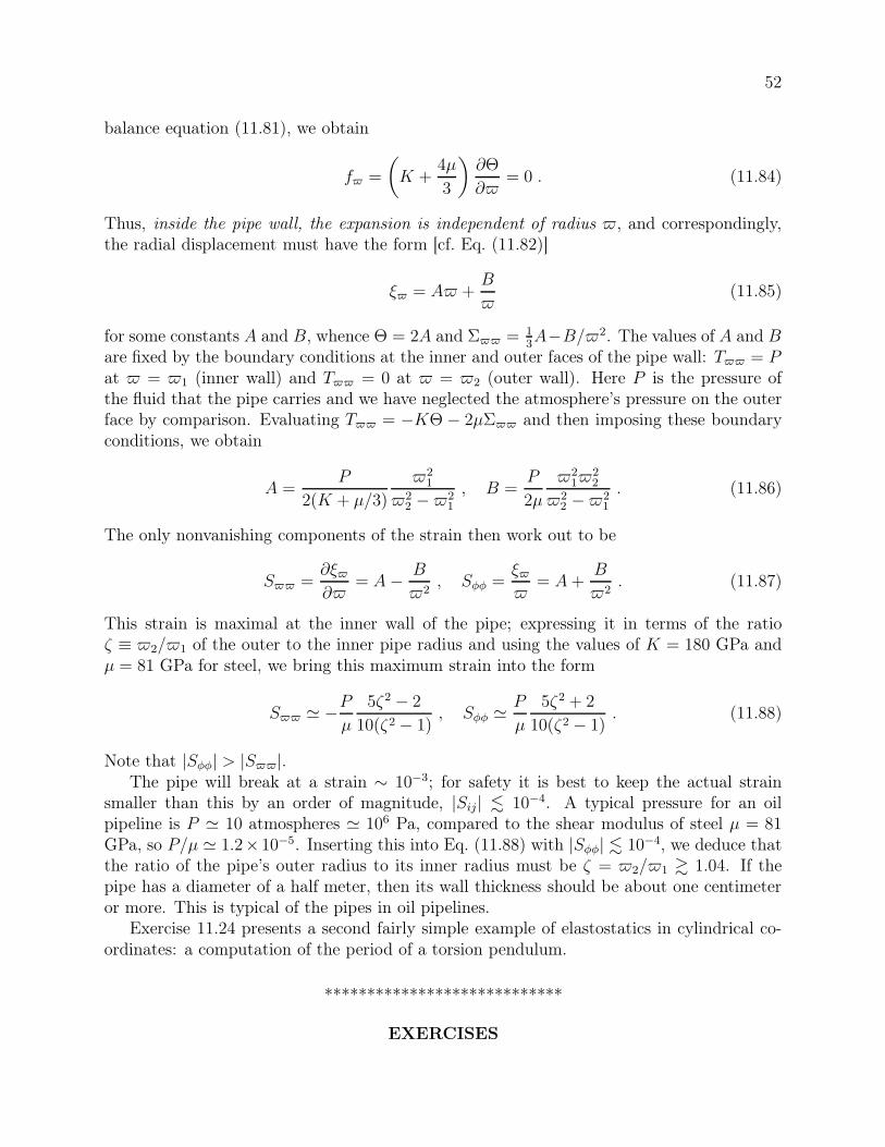
52

balance equation (11.81), we obtain

f =

(

K +4µ

3

)

∂Θ

∂= 0 . (11.84)

Thus, inside the pipe wall, the expansion is independent of radius , and correspondingly,the radial displacement must have the form [cf. Eq. (11.82)]

ξ = A +B

(11.85)

for some constants A and B, whence Θ = 2A and Σ = 13A−B/2. The values of A and B

are fixed by the boundary conditions at the inner and outer faces of the pipe wall: T = Pat = 1 (inner wall) and T = 0 at = 2 (outer wall). Here P is the pressure ofthe fluid that the pipe carries and we have neglected the atmosphere’s pressure on the outerface by comparison. Evaluating T = −KΘ − 2µΣ and then imposing these boundaryconditions, we obtain

A =P

2(K + µ/3)

21

22 −2

1

, B =P

2µ

21

22

22 −2

1

. (11.86)

The only nonvanishing components of the strain then work out to be

S =∂ξ∂

= A− B

2, Sφφ =

ξ

= A+B

2. (11.87)

This strain is maximal at the inner wall of the pipe; expressing it in terms of the ratioζ ≡ 2/1 of the outer to the inner pipe radius and using the values of K = 180 GPa andµ = 81 GPa for steel, we bring this maximum strain into the form

S ≃ −P

µ

5ζ2 − 2

10(ζ2 − 1), Sφφ ≃ P

µ

5ζ2 + 2

10(ζ2 − 1). (11.88)

Note that |Sφφ| > |S|.The pipe will break at a strain ∼ 10−3; for safety it is best to keep the actual strain

smaller than this by an order of magnitude, |Sij| . 10−4. A typical pressure for an oilpipeline is P ≃ 10 atmospheres ≃ 106 Pa, compared to the shear modulus of steel µ = 81GPa, so P/µ ≃ 1.2×10−5. Inserting this into Eq. (11.88) with |Sφφ| . 10−4, we deduce thatthe ratio of the pipe’s outer radius to its inner radius must be ζ = 2/1 & 1.04. If thepipe has a diameter of a half meter, then its wall thickness should be about one centimeteror more. This is typical of the pipes in oil pipelines.

Exercise 11.24 presents a second fairly simple example of elastostatics in cylindrical co-ordinates: a computation of the period of a torsion pendulum.

****************************

EXERCISES

53

Exercise 11.23 Derivation and Practice: Fracture of a PipeFill in the details of the text’s analysis of the deformation of a pipe carrying a high-pressurefluid, and the wall thickness required to protect the pipe against fracture, Sec. 11.9.1.

Exercise 11.24 Practice: Torsion pendulumA torsion pendulum is a very useful tool for testing the equivalence principle, for seekingevidence for hypothetical fifth (not to mention sixth) forces, and for searching for deviationsfrom gravity’s inverse square law on submillimeter scales, which could arise from gravityfeeling macroscopic higher spatial dimensions. (See, e.g., Kapner et. al. 2008, and Wagneret. al. 2013). It would be advantageous to design a torsion pendulum with a one day period(Figure 11.17). In this exercise we shall estimate whether this is possible. The pendulumconsists of a thin cylindrical wire of length l and radius a. At the bottom of the wire aresuspended three masses at the corners of an equilateral triangle at a distance b from thewire.

(a) Show that the longitudinal strain is

ξz;z =3mg

πa2E. (11.89a)

(b) What component of shear is responsible for the restoring force in the wire, which causestorsion pendulum to oscillate?

(c) Show that the pendulum undergoes torsional oscillations with period

P = 2π

(

ℓ

g

)1/2 (2b2Eξz;za2µ

)1/2

. (11.89b)

(d) Do you think you could design a pendulum that attains the goal of a one day period?

2a

m

bm

m

Fig. 11.17: Torsion Pendulum in Ex. 11.24.

****************************

54

11.9.2 T2 Separation of Variables and Green’s Functions: Ther-

moelastic Noise in Mirrors

In more complicated situations that have moderate amounts of symmetry, the elastostaticequations can be solved by the same kinds of sophisticated mathematical techniques asone uses in electrostatics: separation of variables, Green’s functions, complex potentials,or integral transform methods; see, e.g. Gladwell (1980). We provide an example in thissection, focusing on separation of variables and Green’s functions.

Motivation

Our example is motivated by an important issue in high-precision measurements with light,including, among others, gravitational-wave detectors and quantum optics experiments inwhich photons and atoms are put into entangled nonclassical states by coupling them toeach other inside Fabry Perot cavities.

In these situations, noise due to thermal motions of the mirror faces, is a serious issue.It can hide a gravitational wave, and it can cause decoherence of the atom/photon quantumstates. In Sec. 6.8.2, we formulated a generalized fluctuation-dissipation theorem by whichthis mirror thermal noise can be computed (Levin 1998):

In a thought experiment, one applies to the mirror face a force Fo that oscillates atsome frequency f at which one wants to evaluate the thermal noise, and that has the sametransverse pressure distribution as the light beam — say, for concreteness, a Gaussian dis-tribution:

T appliedzz =

e−2/2o

π2o

Fo cos(2πft) . (11.90)

This applied pressure induces a strain distribution S inside the mirror, and that oscillatingstrain interacts with imperfections to dissipate energy at some rate Wdiss(f). The fluctuation-dissipation theorem says that in the real experiment, where the light beam bounces off themirror, the reflected light will encode a noisy transverse-averaged position q for the mirrorface, and the noise spectral density for q will be

Sq(f) =8Wdiss(f)kBT

F 2o

(11.91)

[Eq. (6.88b)].Now, even if one could make the mirror perfect (no dislocations or impurities), so there is

no dissipation due to imperfections, there will remain one other source of dissipation in thisthought experiment: The applied pressure (11.90) will produce a spatially inhomogeneousexpansion Θ(x, t) inside the mirror, which in turn will produce the thermoelastic temperaturechange ∆T/T = −(3αK/ρcV )Θ [Eq. (11.30)]. The gradient of this temperature will induceheat to flow, with a thermal energy flux Fth = −κ∇∆T , where κ is the thermal conductivity.When an amount Q of this thermal energy flows from a region with temperature T to a regionof lower temperature T − dT , it produces an entropy increase dS = Q/(T − dT )− Q/T =QdT/T 2; and correspondingly, there is a rate of entropy increase per unit volume given bydS/dV dt = −Fth ·∇∆T/T 2 = κ(∇∆T )2/T 2. This entropy increase has an accompanying

55

energy dissipation rate Wdiss =∫

T (dS/dtdV )dv =∫

κ(∇∆T )2TdV . Expressing ∆T interms of the expansion that drives it via ∆T/T = −(3αK/ρcV )Θ, and inserting that into Eq.(11.91), we obtain the thermal noise spectral density that the experimenters must contendwith:

Sq(f) =2κE2α2kT 2

(1− 2ν)2c2V ρ2F 2

o (2πf)2

⟨∫

(∇Θ)2dφddz

⟩

. (11.92)

Because the dissipation producing this noise is due to heat flowing down a thermoelastictemperature gradient, it is called thermoelastic noise.

This is the motivation for our elasticity problem: To evaluate this thermoelastic noise,we must compute the expansion Θ(x, t) inside a mirror, produced by the oscillating pressure(11.90) on the mirror face; and we must then perform the integral (11.92).

Solution for Θ via separation of variables

The frequencies f at which we wish to evaluate the thermal noise are very low comparedto the sound travel time across the mirror, so in computing Θ we can regard the force asoscillating very slowly; i.e., we can use our elastostatic equations rather than dynamicalequations of the next chapter. Also, the size of the light spot on the mirror is usually smallcompared to the mirror’s transverse size and thickness, so we shall idealize the mirror asbeing infinitely large and thick—a homogeneous “half space” of isotropic, elastic material.

Because the applied stress is axially symmetric, the induced strain and expansion will alsobe axially symmetric, and are thus computed most easily using cylindrical coordinates. Ourchallenge, then, is to solve the Navier-Cauchy equation f = (K + 1

3µ)∇(∇ · ξ) + µ∇2ξ = 0

for the cylindrical components ξ(z,) and ξz(z,) of the displacement, and then evaluatethe divergence Θ = ∇ · ξ. (The component ξφ vanishes by symmetry.)

Equations of elasticity in cylindrical coordinates, and their homogeneous solution

It is straightforward, using the techniques of Sec. 11.8, to compute the cylindrical com-ponents of f . Reexpressing the bulk and shear moduli K and µ in terms of Young’s modulusE and Poisson’s ratio ν [Eq. (11.40)] and setting the internal forces to zero, we obtain

f =E

2(1 + ν)(1− 2ν)

[

2(1− ν)

(

∂2ξ∂2

+1

∂ξ∂

− ξ2

)

+ (1− 2ν)∂2ξ∂z2

+∂2ξz∂z∂

]

= 0 , (11.93a)

fz =E

2(1 + ν)(1− 2ν)

[

(1− 2ν)

(

∂2ξz∂2

+1

∂ξz∂

)

+ 2(1− ν)∂2ξz∂z2

+∂2ξ∂z∂

+1

∂ξ∂z

]

= 0 . (11.93b)

These are two coupled, linear, second-order differential equations for the two unknowncomponents of the displacement vector. As with the analogous equations of electrostaticsand magnetostatics, these can be solved by separation of variables, i.e. by setting ξ =R()Z(z) and ξz = Rz()Zz(z), and inserting into Eq. (11.93a). We seek the general

56

solution that dies out at large and z. The general solution of this sort, to the complicatedlooking Eqs. (11.93), turns out to be (really!!)

ξ =

∫

∞

0

[α(k)− (2− 2ν − kz)β(k)] e−kzJ1(k)kdk ,

ξz =

∫

∞

0

[α(k) + (1− 2ν + kz)β(k)] e−kzJ0(k)dk . (11.94)

Here J0 and J1 are Bessel functions of order 0 and 1, and α(k) and β(k) are arbitraryfunctions.

Boundary Conditions

The functions α(k) and β(k) are determined by boundary conditions on the face of thetest mass: The force per unit area exerted across the face by the strained test-mass material,Tzj at z = 0 with j = {, φ, z}, must be balanced by the applied force per unit area,T appliedzj [Eq. (11.90)]. The (shear) forces in the φ direction, Tzφ and T applied

zφ , vanish becauseof cylindrical symmetry and thus provide no useful boundary condition. The (shear) forcein the direction, which must vanish since T applied

z = 0, is given by [cf. Eq. (2) in Box 11.4]

Tz(z = 0) = −2µΣz = −µ

(

∂ξz∂

+∂ξ∂z

)

= −µ

∫

∞

0

[β(k)− α(k)] J1(kz)kdk = 0 ,

(11.95)which implies that β(k) = α(k). The (normal) force in the z direction, which must balancethe applied pressure (11.90), is Tzz = −KΘ − 2µΣzz; using Eq. (2) in Box 11.4 and Eqs.(11.94) and (11.90), this reduces to

Tzz(z = 0) = −2µ

∫

∞

0

α(k)J0(k)kdk = T appliedzz =

e−2/2o

π2o

Fo cos(2πft) , (11.96)

which can be inverted11 to give

α(k) = β(k) = − 1

4πµe−k22

o/4Fo cos(2πft) . (11.97)

Inserting this into the Eqs. (11.94) for the displacement, and then evaluating the expansionΘ = ∇ · ξ = ξz,z +−1(ξ),, we obtain

Θ = −4ν

∫

∞

0

α(k)e−kzJ0(k)kdk . (11.98)

Side Remark: As in electrostatics and magnetostatics, so also in elasticity theory, onecan solve an elastostatics problem using Green’s functions instead of separation of variables.We explore this, for our applied Gaussian force, in Ex. 11.26 below. For greater detail onGreen’s functions in elastostatics and their applications, from an engineer’s viewpoint, seeJohnson (1985). For other commonly used solution techniques see Box 11.3.

11The inversion and the subsequent evaluation of the integral of (∇Θ)2 are aided by the following expres-sions for the Dirac delta function: δ(k − k′) = k

∫

∞

0J0(k)J0(k

′)d = k∫

∞

0J1(k)J1(k

′)d.

57

Thermoelastic Noise Spectral Density

Returning to the mirror-noise problem that motivated our calculation: It is straightforwardto compute the gradient of the expansion (11.98), square and integrate to get the spectraldensity Sq(f) [Eq. (11.92)]. The result is

Sq(f) =8(1 + ν)2κα2kBT

2

√2πc2V ρ

23o(2πf)

2. (11.99)

Early plans for advanced LIGO gravitational wave detectors called for mirrors madeof high-reflectivity dielectric coatings on sapphire crystal substrates. Sapphire was chosenbecause it can be grown in giant crystals with very low impurities and disclocations andresulting low thermal noise. However, the thermoelastic noise (11.99) in sapphire turns outto be uncomfortably high. With sapphire’s ν = 0.29, κ = 40 W m−1 K−1, α = 5.0×10−6 K−1,cV = 790 J kg−1 K−1, ρ = 4000 kg m−3, and a light-beam radius o = 4 cm and roomtemperature T = 300 K, Eq. (11.99) gives for the noise in a bandwidth equal to frequency:

√

fSq(f) = 5× 10−20m

√

100Hz

f. (11.100)

While this looks like a small number, it would have been mildly unpleasant at the lowestfrequencies of interest. For that reason, and because of the birefringence of sapphire, whichcould cause technical problems, a decision was made to switch to fused silica for the advancedLIGO mirrors.

****************************

EXERCISES

Exercise 11.25 Derivation and Practice: Evaluation of Elastostatic Force in CylindricalCoordinatesDerive Eqs. (11.93) for the cylindrical components of the internal elastostatic force per unitvolume f = (K + 1

3µ)∇(∇ · ξ) + µ∇2ξ in a cylindrically symmetric situation.

Exercise 11.26 *** Example: Green’s Function for Normal Force on Half-Infinite BodySuppose that a stress T applied

zj (xo) is applied on the face z = 0 of a half-infinite elasticbody (one that fills the region z > 0). Then by virtue of the linearity of the elastostaticsequation f = (K + 1

3µ)∇(∇ · ξ) + µ∇2ξ = 0 and the linearity of its boundary conditions,

T internalzj = T applied

zj , there must be a Green’s function Gjk(x−xo) such that the body’s internaldisplacement ξ(x) is given by

ξj(x) =

∫

Gjk(x− x0)Tappliedzk (xo)d

2xo . (11.101)

Here the integral is over all points xo on the face of the body (z = 0), and x can be anywhereinside the body, z ≥ 0.

58

(a) Show that, if a force Fj is applied on the body’s surface at a single point, the origin ofcoordinates, then the displacement inside the body is

ξj(x) = Gjk(x)Fk . (11.102)

Thus, the Green’s function can be thought of as the body’s response to a point forceon its surface.

(b) As a special case, consider a point force Fz directed perpendicularly into the body.The resulting displacement turns out to have cylindrical components12

ξz = Gzz(, z)Fz =(1 + ν)

2πE

[

2(1− ν)

+

z2

3

]

Fz ,

ξ = Gz(, z)Fz = −(1 + ν)

2πE

[

1− 2ν

+ z− z

2

]

Fz . (11.103)

It is straightforward to show that this displacement does satisfy the elastostatics equa-tions (11.93). Show that it also satisfies the required boundary condition Tz(z = 0) =−2µΣz = 0.

(c) Show that for this displacement, Tzz = −KΘ − 2µΣzz vanishes everywhere on thebody’s surface z = 0 except at the origin = 0 and is infinite there. Show that theintegral of this normal stress over the surface is Fz, and therefore Tzz(z = 0) = Fzδ2(x)where δ2 is the two-dimensional Dirac delta function in the surface. This is the secondrequired boundary condition.

(d) Plot the integral curves of the displacement vector ξ (i.e. the curves to which ξ isparallel) for a reasonable choice of Poisson’s ratio ν. Explain physically why the curveshave the form you find.

(e) One can use the Green’s function (11.103) to compute the displacement ξ induced bythe Gaussian-shaped pressure (11.90) applied to the body’s face, and to then evaluatethe induced expansion and thence the thermoelastic noise; see Braginsky, Gorodetskyand Vyatchanin (1999), or Liu and Thorne (2000). The results agree with those (11.98)and (11.99) deduced using separation of variables.

****************************

Bibliographic Note

Elasticity Theory was developed in the 18th, 19th and early 20th centuries. The classic,culminating advanced textbook from that era is Love (1927), which is available as a Dover

12For the other components of the Green’s function, written in Cartesian coordinates (since a non-normalapplied force breaks the cylindrical symmetry), see Eqs. (8.18) of Landau and Lifshitz (1986).

59

Box 11.5

Important Concepts in Chapter 11

• Foundational Concepts

– Displacement vector field ξ, Sec. 11.2.1– Irreducible tensorial parts of a tensor, Box 11.2– Irreducible tensorial parts of W ≡ ∇ξ: expansion Θ, rotation R and shear Σ,

Sec. 11.2.2 and Box 11.2– Strain tensor, S = (symmetric part of ∇ξ) = Σ+ 1

3Θg, Sec. 11.2.2

– Hooke’s law and Young’s modulus E, Secs. 11.1, 11.3.2 and 11.4– Failure of Hooke’s law: Proportionality limit, elastic limit, yield point, rupture

point, 11.3.2– Dislocations in a crystal and their movement causing inelastic deformation,

Fig. 11.6– Stress tensor and its divergence as force density, Sec. 11.3.1– The Pascal as a unit of stress, Sec. 11.3.1– Bulk and shear moduli K, µ; elastic stress tensor T = −KΘg − 2µΣ, Sec.

11.3.3– Elastic energy (energy of deformation), Sec. 11.3.4– Thermal expansion and thermoelastic stress, Sec. 11.3.5– Molecular origin of elastic moduli and orders of magnitude, Sec. 11.3.6– Elastic force on a unit volume, f = −∇ · T = (K + µ/3)∇(∇ · ξ) + µ∇2ξ ,

Sec. 11.3.3– Connection Coefficients and their use in cylindrical and spherical coordinate

systems, Sec. 11.8

• Elastostatic Equilibrium

– Navier-Cauchy equation for stress balance, Sec. 11.3.7– Boundary condition Tijnj continuous, Sec. 11.3.7– Methods of solving Navier-Cauchy equation: Box 11.3– Dimensional reduction via method of moments, and application to rods, beams

and fibers, and to plates: Secs. 11.5, 11.7– The flexural rigidity D of a rod, beam, or fiber, and its relationship to the

shear and torque associated with bending Eqs. (11.42)– Buckling and bifurcation of equilibria: Sec. 11.6

reprint. An outstanding, somewhat more modern advanced text is Landau and Lifshitz(1986) — originally written in the 1950s and revised in a third edition in 1986, shortly beforeLifshitz’s death. This is among the most readable textbooks that Landau and Lifshitz wrote,

60

and is still widely used by physicists in the early 21st century.Some significant new insights, both mathematical and physical, have been developed

in recent decades; for example, catastrophe theory and its applications to bifurcations andstability, practical insights from numerical simulations, and practical applications based onnew materials such as carbon nanotubes. For a modern treatment that deals with these andmuch else from an engineering viewpoint, we strongly recommed Ugural and Fenster (2012).For a fairly brief and elementary modern treatment, we recommend Part III of Lautrup(2005). Other good texts that focus particularly on solving the equations for elastostaticequilibrium include Southwell (1941), Timoshenko and Goodier (1970), Gladwell (1980),Johnson (1985), Boresi and Chong (2000), and Slaughter (2002); see also the discussion andreferences in Box 11.3.

Bibliography

Braginsky, V. B., Gorodetsky, M. L., and Vyatchanin, S. P. 1999. “Thermodynamicalfluctuations and photo-thermal shot noise in gravitational wave antennae” PhysicsLetters A, 264,1.

Chandrasekhar, S. 1962. Ellipsoidal Figures of Equilibrium, New Haven: Yale Univer-sity Press.

Boresi, Arthur R. and Chong, Ken P. 2000. Elasticity in Engineering Mechanics, NewYork: Wiley.

Gladwell, G. M. L. 1980. Contact Problems in the Classical Theory of Elasticity,Alphen aan den Rijn: Sijthoff and Noordhoff.

Fortere, Yo el, Skothelm, Jan M., Dumals, Jacques, and Mahadevan, L. 2005. “Howthe Venus Flytrap Snaps”, Nature, 433, 421.

Jackson, J. D. 1999. Classical Electrodynamics, New York: Wiley.

Johnson, K. L. 1985. Contact Mechanics, Cambridge: Cambridge University Press.

Constantinescu, Andrei and Korsunsky, Alexander. 2007. Elasticity with Mathematica,CUP.

Kapner, D.J., Cook, T.S., Adelberger, E.G., Gundlach, J.H., Heckel, B.R., Hoyle,C.D., and Swanson, H.E. 2008, “Tests of the Gravitational Inverse-Square Law Belowthe Dark-Energy Length Scale”, Phys. Rev. Lett, 100, 041101.

Landau, L. D., and Lifshitz, E. M. 1986. Elasticity, Third Edition, Oxford: Pergamon.

Levin, Yu. 1998. “Internal thermal noise in the LIGO test masses: a direct approach”Physical Review D, 57,659–663.

61

Liu, Y. T., and Thorne, K. S. 2000. “Thermoelastic noise and thermal noise in finite-sized gravitational-wave test masses” Physical Review D, in preparation.

Lautrup B. 2005. Physics of Continuous Matter, Bristol and Philadelphia: Instituteof Physics Publishing.

Love, A.E.H. 1927. A Treatise on the Mathematical Theory of Elasticity, Cambridge:Cambridge University Press; Reprinted – New York: Dover Publications (1944).

Marko, John F. and Cocco, Simona 2003. “The Micromechanics of DNA”, PhysicsWorld, March 2003, pp. 37–41.

Marsden, Jerold E. and Hughes, Thomas J.R. 1986. Mathematical Foundations ofElasticity, Upper Saddle River NJ: Prentice-Hall; Reprinted – New York: Dover Pub-lications(1994).

Mathews, J. and Walker, R. L. 1965. Mathematical Methods of Physics, New York:Benjamin.

Messiah, A. 1962. Quantum Mechanics, Vol. II, Amsterdam: North-Holland.

Nelson, Philip 2004. Biological Physics, San Francisco: W.H. Freeman.

NIST 2005. National Institute of Standards and Technology, Final Report on the Col-lapse of the Word Trade Center Towers, U.S. Government Printing Office, WashingtonDC; available at http://www.nist.gov/el/disasterstudies/wtc/ .

NIST 2008. National Institute of Standards and Technology, Final Report on the Col-lapse of the Word Trade Center Building 7, U.S. Government Printing Office, Wash-ington DC; available at http://www.nist.gov/el/disasterstudies/wtc/ .

Southwell, R.V. 1941. An Introduction to the Theory of Elasticity for Engineers andPhysicists, Second Edition, Oxford: Clarendon Press; Reprinted – New York: DoverPublications.

Slaughter, William S. 2002. The Linearized Theory of Elasticity, Boston: Birkäuser.

Todhunter, Isaac and Pearson, Karl. 1886. A History of the Theory of Elasticity andof the Strength of Materials, from Gelilei to the Present Time (1886), Cambridge:Cambridge University Press.

Thorne, K.S. 1980. “Multipole Moments in General Relativity” Rev. Mod. Phys., 52,299.

Timoshenko, S. and Goodier, J. N. 1970. Theory of Elasticity, Third Edition, NewYork: McGraw-Hill.

Ugural, Ansel C. and Fenster, Saul, K. 2012. Advanced Mechanics of Materials andApplied Elasticity, Fifth Edition, Upper Saddle River NJ: Prentice-Hall.

62

Xing, Xiangjun, Goldbart, Paul M. and Radzihovsky, Leo 2007. “Thermal Fluctuationsand Rubber Elasticity”, Phys. Rev. Lett. 98, 075502.

Yeganeh-Haeri, A., Weidner, D. J. & Parise, J. B. 1992. Science, 257, 650.

Wagner, T.A., Schlamminger, S., Gundlach, J.H., and Adelberger, E.G. 2013. “Torsion-Balance Tests of the Weak Equivalence Principle”, Class. Quant. Grav., in press.

Weld, David M., Xia, Jing, Cabrera, Blas, and Kapitulnik, Aharon. 2008. “A NewApparatus for Detecting Micron-Scale Deviations from Newtonian Gravity”, Phys. Rev.D 77, 062006.

Wolgemuth, Charles W., Powers, Thomas R., and Goldstein, Raymond E. 2000. “Twirlingand Whirling: Viscous Dynamics of Rotating Elastic Filaments”, Phys. Rev. Lett. 84,1623–1626.