Last Modified 06/18/2015

IV-1-1

IV-1 Erosion of Rock and Soil

Introduction

Erosion of rock and soil (earth) are major areas of concern when dealing with earthen

embankments, unlined spillways, and other features of a water control or flood risk

mitigation project. Many embankment projects were not designed to be overtopped by a

storm event, so any amount of overtopping flow becomes a concern. Unlined spillways

are designed to experience flow and are usually expected to suffer some erosion damage;

erosion becomes a dam and levee safety issue if it so extensive that it destabilizes

structures or if it enlarges or breaches through the hydraulic control section, thereby

allowing an uncontrolled release of the reservoir.

When considering the many potential failure modes that include erosion of soil or rock as

a necessary component, it is important to estimate not only the likelihood of erosion, but

also the likelihood for various extents of erosion. Some potential failure modes that

could include erosion of rock and soil as a component are:

Overtopping erosion of an embankment

Overtopping erosion of a concrete dam abutment or foundation

Erosion of an unlined tunnel or spillway

Erosion of a channel downstream of a stilling basin due to flow in excess of

capacity

Erosion of the spillway foundation where floor slabs have been damaged or lost

Erosion of the water side slope of a levee due to riverine current or wave loading.

This chapter provides background on evaluating and estimating the erosion component of

the above mentioned potential failure modes. Rather than repeat this information in a

number of chapters it is provided here. The above mentioned potential failure modes

have other specific considerations, such as determining the frequency and magnitude of

overtopping and spillway flows and the performance of concrete linings. These elements

are discussed in the individual chapters on the potential failure modes.

Key Concepts and Factors

Erosion of Embankments and Spillways

The embankments to be studied are constructed of soil, rock, or some composite of the

two. This section is going to provide basic information of erosion of soil and rock for

IV-1-2

flood overtopping and spillway flows. For details on flood overtopping and how it is

handled refer to the chapter that addresses Flood Overtopping contained in this manual

Once the dam or levee has begun to overtop, or the spillway has started to flow, in

general, the most erosive flow occurs on the downstream slope, as indicated in Figure IV-

1-1. Velocities are normally highest on the downstream slope, and the slope itself can

make it easier to dislodge and transport particles. On dams and levees that have been

overtopped by floods, severe erosion has often been observed to begin where sheet flow

becomes turbulent flow. Erosion can also initiate where flow encounters an obstacle or

discontinuity, such as a structure, trees, shrubs, groins, bare patches of earth; or a change

in embankment slope.

Figure IV-1-1 – Downstream Slope Locations for Embankment Overtopping and

Spillway Flows

Rock Erosion

The analysis of rock erosion is a complex topic, requiring a comparison of the hydraulic

attack produced by the flow and the resisting physical properties of the rock. Both can be

difficult to characterize, leading to significant uncertainty. The most common

approaches to the problem today rely upon technologies that were originally created for

the mining and excavation of rock. Barton’s Q-System (Barton 1974) was developed for

IV-1-3

the characterization of rock for tunneling activities in mines. Kirsten (1983) adapted

this approach to establish a ripability index that helped the excavation industry determine

the appropriate equipment needed to rip a specified rock. The primary rock properties

determining the index are the joint alteration, joint roughness, joint orientation,

compressive strength, and size of individual rock blocks.

The ripability index was adapted for the analysis of soil erosion and described as a

headcut index by Moore et al. (1994) and Temple and Moore (1997). The index was

used to establish both thresholds and rates for headcut advancement in soils. Wibowo

(2005) used logical regression to develop threshold lines approximating Annandale’s, but

at varying probability levels.

Soil Erosion

Erosion of soil in embankments and spillways also requires a comparison of hydraulic

attack and erosion resistance to determine whether erosion damage will occur and the rate

at which it will progress. Multiple variables must be considered, including flow depth,

shear stress, flow velocity, soil material type, geometry, armoring, and vegetation.

A dense cover of turf-type grass, as seen on many dams in the eastern U.S., can provide

excellent protection against high-velocity sheet flow until the cover is removed, assuming

the growth is even, and well established. When the cover is removed, or sheet flow is

disrupted, concentrated flow can form initiating the headcut formation process, and all

benefits of cover are lost. This is something that can be analyzed using WinDAM which

is discussed later in this chapter.

Generally, the most erosion-resistant soils are plastic clays. The most erodible soils are

non-plastic silts and sands. Removal of particle size is dependent on specific velocities

required for transportation of various sized coarse material. For a given particle size, the

slope has a major effect on the flow required to initiate erosion for cohesionless

materials.

If it is necessary for the risk analysis to account for the ability of an embankment or

spillway to sustain some level of erosion without failure, the analysis should begin with a

consideration of whether the embankment slope protection will fail. If the downstream

slope protection is cohesionless and has d50 larger than 4 inches, the chart from Frizell et

al. (1998), Figure IV-1-2, can be used for guidance on the flow at which erosion would

initiate. In the chart, S is the embankment slope (V/H), and Cu is the coefficient of

uniformity (d60/d10), which can be taken as about 1.8 for typical clean uniform cobbles or

boulders, as an initial estimate if actual values are unavailable. Note that the units are

metric; one foot of overtopping corresponds to a unit discharge of roughly 2 ft3/s/ft or 0.2

m3/s/m. Points plotting on the lines represent about a 20 percent probability of erosion

beginning (not the probability of the dam breaching). Points plotting further below each

line would indicate increasing likelihood of erosion. It is critical, however, to understand

that this chart was developed from experiments on carefully placed, uniformly sized

angular riprap in the ideal conditions of a straight-sided flume, not on a dam embankment

with irregular groins, protruding structures, etc. that would cause local disturbance of the

sheet flow. Furthermore, slope protection with an infilling of finer material may behave

IV-1-4

differently, because much of the flow in the experiments occurred within the riprap,

rather than over it, which may not be possible if infilling has occurred.

Figure IV-1-2 – Erosion Initiation Chart

Given that erosion will initiate at a specific flow depth for a system, duration should be

considered as the next important variable in determining progression to the dam crest or

spillway control. Once a headcut has initiated, the material properties comprising the

embankment or spillway floor become important in determining the rate and extent of

erosion. Erosion models presented in later sections simulate the processes of headcut

formation and headcut advance that can occur after failure of the slope protection

material.

When working with soil, many of the same variables are used, but they are defined

differently than they are for rock. The interparticle bond shear strength (Kd) is equal to

the tangent of the residual friction angle. The relative ground structure number (Js) is

always equal to one (Js=1) since the material would be homogenous. The unconfined

compressive shear strength (Ms) and particle size (Kb) are values that are obtained from

lab data.

S=0.50

S=0.40

S=0.20

S=0.10

S=0.02

0.001

0.01

0.1

1

0.001 0.01 0.1 1

D5

0c

u0

.25

Unit Discharge, q (m3/s/m)

f′ = 42

IV-1-5

Shear Stress Shear stress can be used to determine if a spillway or embankment will erode due to the

water flowing across it. This calculation is also important when it is desirable to

determine if flow along the toe of an embankment or in some cases levees would be

events of concern. Shear stress in an open channel can be calculated using:

τb = γRbSe

Where Se = energy slope, Rb = hydraulic radius of the bed, and γ is the unit weight of water

(Chow 1964). Once the shear stress for flow in a system is known, then it is possible to

compare it with the critical shear stress for a material, and a determiniation can be made

for the erodibility of a material. This is a method that can be used for both cohesive and

non-cohesive materials.

Stream Power Although detailed hydraulic studies should be performed to estimate stream power if

erosion becomes a critical issue, some simplifying conservative assumptions can be made

to determine stream power for initial screening evaluations. For flow down a slope, the

rate of energy dissipation per unit of surface area (P) is a function of the flow depth, flow

velocity and the energy slope:

UhSP

where = unit weight of water, U = flow velocity, h = water depth, and S = hydraulic

energy grade line slope. The rate of energy dissipation is small as the flow just comes

over the crest and increases as the water velocity increases. The analysis of erosion

stability is performed at the location where the value of energy dissipation is the highest.

The energy slope is assumed to be approximately equal to the bed slope and flow depths

are taken to be equal to the normal depth computed for steady-state flow conditions (see

Section on Overtopping of Spillway Walls).

Erodibility Index

The concept of using a rock mass index to correlate with the power it would take to

remove the rock was original developed by Kirsten (1983) to characterize the ripability of

earth materials using mechanical equipment. This was extended to examine the removal

of soil and rock by flowing water, and at that time the term “erodibility index” was

coined. This index was correlated empirically to the erosive power of flowing water, or

the energy rate of change, termed “stream power”. Data from the performance of unlined

spillways in both soil and rock were used to calibrate the method for erosion potential.

Thus, this method can also be used for either soil or rock, but this section focuses on its

use for estimating rock erosion.

The stream power-erodibility index method can be used to estimate the likelihood of

initiating rock erosion. The erodibility index (and its possible variability) represents how

IV-1-6

erodible the foundation material is. It is relatively simple to calculate, and can be used

for an initial evaluation. The stream power represents the erosive power of the

overtopping flows, and is much more complicated to rigorously compute. This method

will provide an indication as to the likelihood that erosion will initiate, but if so,

additional judgment is needed to evaluate how quickly erosion will occur and whether it

will progress to the point of initiating a failure mode (spillway breach, dam instability,

dam breach). This requires evaluating the likelihood of erodibility at various depths and

locations. The duration of overtopping flows should also factor into the judgment on the

potential for reservoir breach.

The erodibility index, Kh, is calculated as follows:

sdbsh JKKMK

Ms is the mass strength, usually defined as the unconfined compressive strength (UCS)

for rock (expressed in MPa) when the strength is greater than 10 MPa, and

(0.78)(UCS)1.05

when the strength is less than 10 MPa.

Kb defines the particle or fragment size of rock blocks that form the mass, which can be

determined from joint spacing or rock mass classification parameters. The simplest and

most straight forward relationship is Kb = RQD/Jn, where Jn is a modified joint set

number, shown in Table IV-1-1.

Kd is the interparticle bond shear strength, and is usually taken as Jr/Ja, where Jr and Ja are

the joint roughness and joint alteration numbers, based on joint surface characteristics

defined by Barton's Q-system shown in Tables 15-2 and 15-3. Plucking and cyclic

loading introduced by turbulence, most probably the dominant processes in scour of earth

materials (Briaud, et al. 1999), act in addition to shear stress to scour earth material.

Materials mainly held together by gravity bonds scour principally because of fluctuating

forces developing over individual particles, as would be the case for cohesionless

granular soil. The fluctuating forces pluck the soil particles out of their positions of rest.

In the case of uniform cohesive soil, the cyclic loading introduced by the plucking forces

weakens the soil, resulting in scour as the soil gradually yields (Colorado Department of

Transportation Report No. CDOT-DTD-R-2000-9).

The relative shape and orientation of the blocks is accounted for by the Js parameter.

This represents the ease with which the water can penetrate the discontinuities and

dislodge the blocks. Table IV-1-4 can be used to determine Js.

Examples of orientation and discontinuities are shown below in Figures 15-3 and 15-4.

IV-1-7

Figure IV-1-3 – Discontinuity Orientation

Figure IV-1-4 – Conceptual Joint Set Illustration

IV-1-8

Table IV-1-1 – Modified Joint Set Number Values (adapted from Annandale, 2006)

Jointing Description Modified Joint Set

Number

(Jn)

Intact, no or few joints 1.00

One joint set 1.22

One joint set plus random joints 1.50

Two joint sets 1.83

Two joint sets plus random joints 2.24

Three joint sets 2.73

Three joint sets plus random joints 3.34

Four joint sets 4.09

More than four joint sets 5.00

Table IV-1-2 – Joint Roughness Number (adapted from Barton, 1977)

Joint Separation Joint Condition Joint Roughness

Number

(Jr)

Tight – rock wall contact (or

rock wall contact before 10 cm

shear)

Discontinuous 4

Rough or irregular, undulating 3

Smooth, undulating 2

Slickensided, undulating 1.5

Rough or irregular, planar 1.5

Smooth, planar 1.0

Slickensided, planar 0.5

Open – no rock wall contact

(even when sheared)

Clay mineral filling 1.0

Sand, gravel, or crushed zone 1.0

IV-1-9

Table IV-1-3 – Joint Alteration Number (adapted from Barton, 1977)

Joint Separation Joint Condition Joint

Alteration

Number

(Ja)

Tight, rock wall

contact

Tightly healed, hard, non-softening filling (quarts

or epidote)

0.75

Unaltered joint walls, surface staining only 1.0

Slightly altered joint walls, non-softening mineral

coatings (sandy particles)

2.0

Silty or sandy-clay coatings (non-softening) 3.0

Softening or low friction clay mineral coatings (<

1-2 mm thick)

4.0

Rock wall contact

before 10 cm

shear

Sandy particles (clay-free disintegrated rock) 4.0

Strongly over-consolidated non-softening clay

mineral fillings (< 5 mm thick)

6.0

Clay mineral fillings, not strongly over-

consolidated (<5 mm thick)

8.0

Swelling clay fillings (< 5 mm thick, Ja increases

with increasing percent of swelling clay)

8.0 – 12.0

No rock wall

contact (even

when sheared)

Zones or bands of silty or sandy clay (non-

softening)

5.0

Zones or bands of crushed rock and strongly over-

consolidated clay

6.0

Zones or bands of crushed rock and clay, not

strongly over-consolidated

8.0

Zones or bands of crushed rock and swelling clay

fillings (Ja increases with increasing percent of

swelling clay)

8.0 – 12.0

Thick continuous zones or bands of strongly over-

consolidated clay

10.0

Thick continuous zones or bands of clay, not

strongly over-consolidated

13.0

Thick continuous zones or bands of swelling clay

(Ja increases with increasing percent of swelling

clay)

13.0 – 20.0

IV-1-10

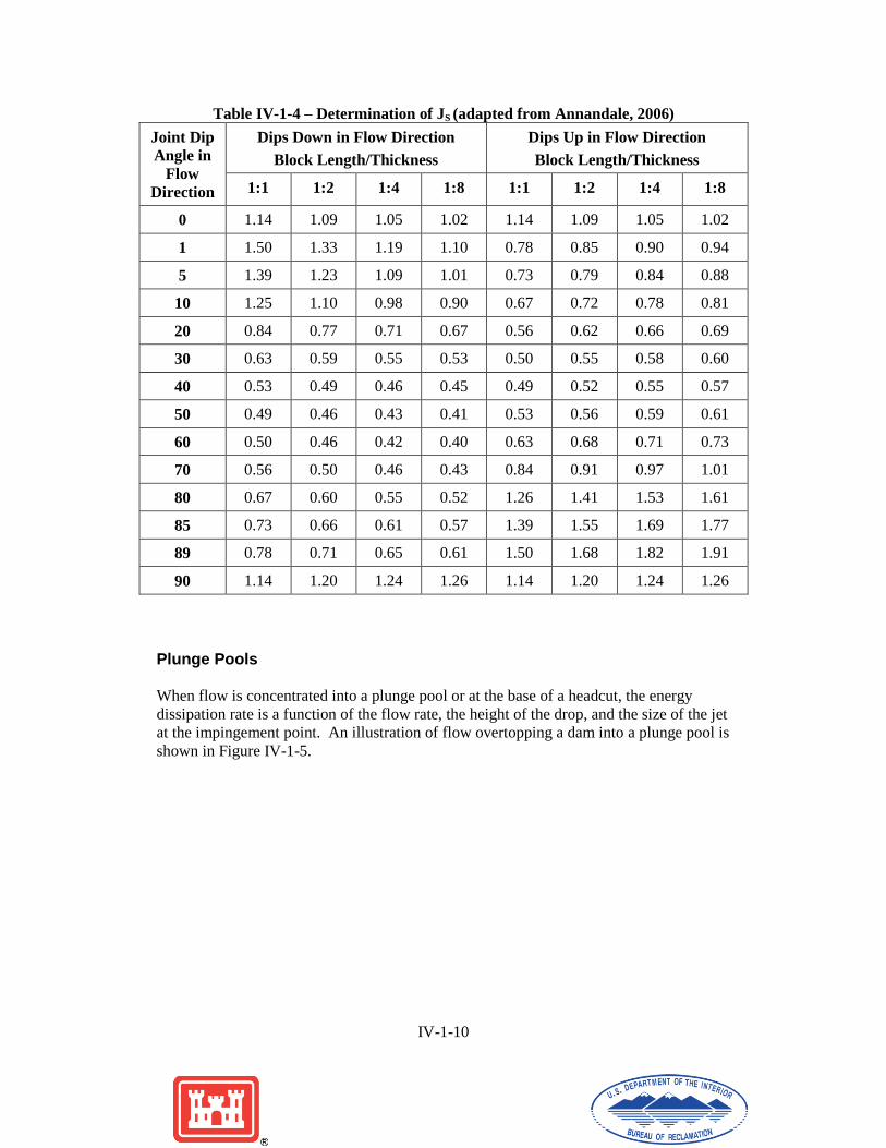
Table IV-1-4 – Determination of JS (adapted from Annandale, 2006)

Joint Dip

Angle in

Flow

Direction

Dips Down in Flow Direction

Block Length/Thickness

Dips Up in Flow Direction

Block Length/Thickness

1:1 1:2 1:4 1:8 1:1 1:2 1:4 1:8

0 1.14 1.09 1.05 1.02 1.14 1.09 1.05 1.02

1 1.50 1.33 1.19 1.10 0.78 0.85 0.90 0.94

5 1.39 1.23 1.09 1.01 0.73 0.79 0.84 0.88

10 1.25 1.10 0.98 0.90 0.67 0.72 0.78 0.81

20 0.84 0.77 0.71 0.67 0.56 0.62 0.66 0.69

30 0.63 0.59 0.55 0.53 0.50 0.55 0.58 0.60

40 0.53 0.49 0.46 0.45 0.49 0.52 0.55 0.57

50 0.49 0.46 0.43 0.41 0.53 0.56 0.59 0.61

60 0.50 0.46 0.42 0.40 0.63 0.68 0.71 0.73

70 0.56 0.50 0.46 0.43 0.84 0.91 0.97 1.01

80 0.67 0.60 0.55 0.52 1.26 1.41 1.53 1.61

85 0.73 0.66 0.61 0.57 1.39 1.55 1.69 1.77

89 0.78 0.71 0.65 0.61 1.50 1.68 1.82 1.91

90 1.14 1.20 1.24 1.26 1.14 1.20 1.24 1.26

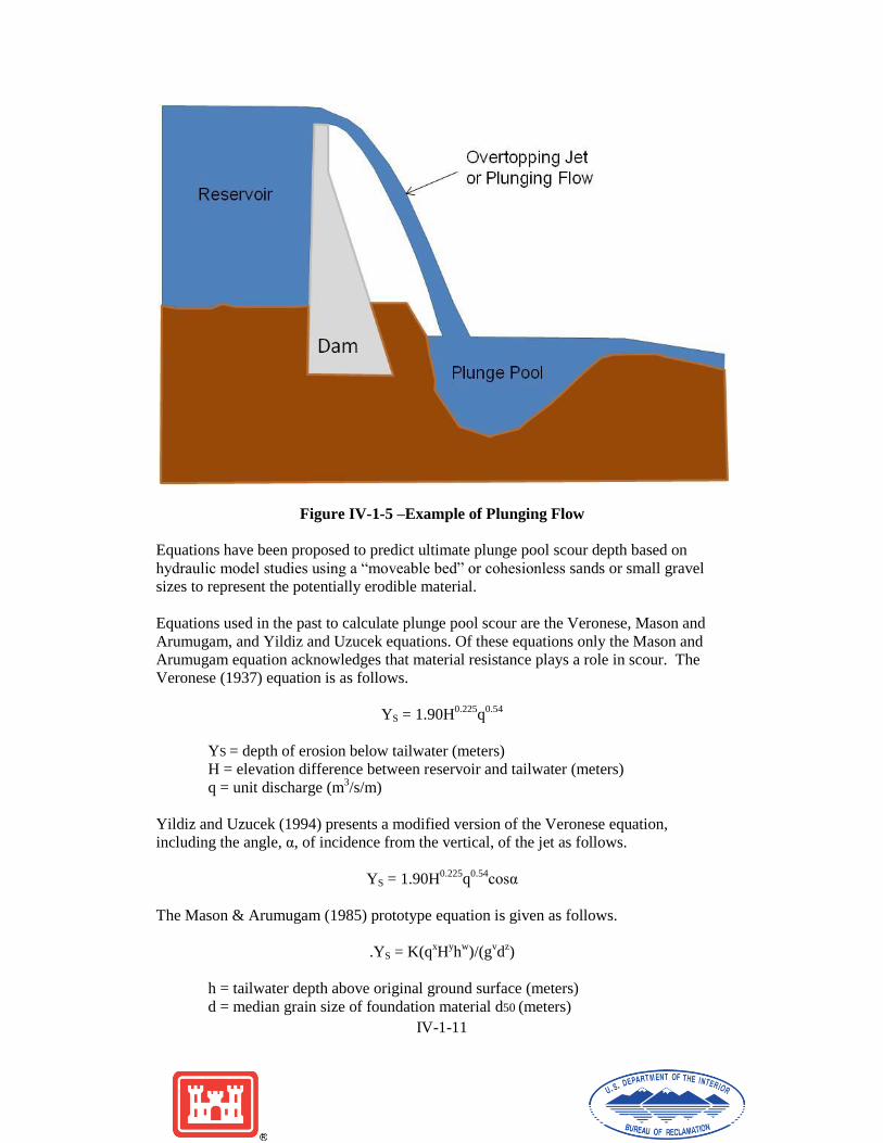
Plunge Pools

When flow is concentrated into a plunge pool or at the base of a headcut, the energy

dissipation rate is a function of the flow rate, the height of the drop, and the size of the jet

at the impingement point. An illustration of flow overtopping a dam into a plunge pool is

shown in Figure IV-1-5.

IV-1-11

Figure IV-1-5 –Example of Plunging Flow

Equations have been proposed to predict ultimate plunge pool scour depth based on

hydraulic model studies using a “moveable bed” or cohesionless sands or small gravel

sizes to represent the potentially erodible material.

Equations used in the past to calculate plunge pool scour are the Veronese, Mason and

Arumugam, and Yildiz and Uzucek equations. Of these equations only the Mason and

Arumugam equation acknowledges that material resistance plays a role in scour. The

Veronese (1937) equation is as follows.

YS = 1.90H0.225

q0.54

YS = depth of erosion below tailwater (meters)

H = elevation difference between reservoir and tailwater (meters)

q = unit discharge (m3/s/m)

Yildiz and Uzucek (1994) presents a modified version of the Veronese equation,

including the angle, α, of incidence from the vertical, of the jet as follows.

YS = 1.90H0.225

q0.54

cosα

The Mason & Arumugam (1985) prototype equation is given as follows.

.YS = K(qxH

yh

w)/(g

vd

z)

h = tailwater depth above original ground surface (meters)

d = median grain size of foundation material d50 (meters)

IV-1-12

g = acceleration of gravity (m/s2)

K = 6.42-3.1H0.10

d = 0.25m

v = 0.3

w = 0.15

x = 0.6-H/300

y = 0.15+H/200

z = 0.10.

Unlike the Veronese and the Yildiz and Uzucek equations, the Mason and Arumugam

equation includes a material factor, d. Although it is an attempt to acknowledge the role

that material properties play in resisting scour, it is unlikely that this factor adequately

represents the variety of material properties found in foundation materials. In addition,

the materials in the movable beds of the hydraulic model studies may not scale very well

to the rock material at a particular site. In most cases these equations are likely to result

in a conservative estimate of maximum plunge pool scour depth, but not in all cases,

particularly if the rock is likely to break into platy slabs or smaller blocks. Progression of

erosion upstream also may not be realistically predicted for some rock geometries.

A jet falling any significant distance will break up to some extent while falling through

the air, reducing its energy and potential for producing erosion. However, as a

conservative first simplification, it can be assumed that all of the kinetic energy from an

intact falling jet is dissipated on direct impact to the rock surface without any break-up of

the jet, and the stream power can be estimated (in KW/m2) as

P = γqH/d

where γ is the unit weight of water (9.82 KN/m3), q is the unit discharge at the location

being examined (m3/s/m), H is the head or height through which the jet falls (m), and d is

the thickness of the jet as it impacts the rock (m). This equation also does not account for

the cushioning effects of tailwater which occurs when the jet must penetrate through the

tailwater to reach the potential eroding surface (more cushioning with deeper tailwater).

Thus, this produces the maximum theoretical value of streampower. In reality, the jet

will begin to break up and spread out as it falls through the air. The fall height at which

the jet is completely broken up can be estimated by the following equation for a circular

jet (Ervine et al, 1997):

64.182.0

2

11.105.1

riu

riib

FT

FDL

where Di is the thickness of the jet where it issues from the dam (typically the

overtopping depth), Fri is the initial Froude Number, and Tu is the Turbulence Intensity

Factor from Table IV-1-5 (Bollaert, 2002).

IV-1-13

Table IV-1-5 – Turbulence Intensity Factor (Tu) (adapted from Bollaert, 2002)

Structure Type Turbulence Intensity Factor

Free overfall 0.00 – 0.03

Ski jump 0.03 – 0.05

Valve 0.03 – 0.08

However, the jet spread above this point can also be taken into account by the following

equation (Ervine et al, 1997):

jui LTDD 38.0*2

where D is the jet thickness at length Lj along the jet trajectory (which can be estimated

roughly or determined from a trajectory calculation). D can then be substituted for d in

the stream power equation, and the stream power calculated at this point is generally

assumed to remain constant for points below that level.

The above plunge pool equations can be used as a conservative first estimate of rock

erosion. A more detailed stream power estimate may be appropriate if such evaluations

produce a high likelihood of erosion that could lead to failure.

Erosion potential Combining erodibility index and the stream power estimate, we can use Figure IV-1-6 to

estimate the erosion potential. The green line is the initial erosion threshold proposed by

Annandale (1995). Annandale (1995) reviewed about 150 field observations from

spillway channels and plunge pools to develop a curve defining the threshold for erosion

as a function of applied stream power and the headcut erodibility index. Based on

stream power (y-axis) and headcut erodibility (x-axis) a line of best fit for the line

separating cases of erosion and no erosion was determined with the reviewed datasets.

IV-1-14

Figure IV-1-6 – Erodibility Threshold Graph (Annandale, 1995)

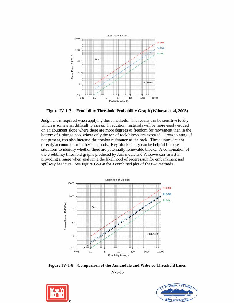
Figure IV-1-7 shows the logistic regression results obtained by Wibowo et al. (2005),

using the same data analyzed by Annandale (1995). The upper (blue line) represents a

99 percent chance of erosion initiating. The bottom (black line) represents a 1 percent

chance of erosion initiating, and the middle (red line) represents a 50 percent chance of

erosion initiating. The likelihood of erosion initiation can be interpolated between these

lines. If erosion is predicted, but the character of the rock or hydraulic characteristics

change with depth, then an iterative procedure can be employed whereby the rock is

assumed to erode to a certain depth, and then the stream power and erodibility index are

recalculated for the new geometry and geologic conditions, and re-plotted on the

empirical chart. Due to uncertainties in obtaining input parameters, it is often necessary

to look at a range of conditions. For the analysis of a jet plunging from the crest of a

concrete arch dam onto downstream canyon abutment walls, the jet will have different

stream powers levels at different elevations at which it impacts the abutment.

0.1

1

10

100

1000

10000

0.01 0.1 1 10 100 1000 10000

Str

eam

Po

wer,

P (kW

/m2)

Erodibility Index, K

Likelihood of Erosion

Scour

No Scour

IV-1-15

Figure IV-1-7 – Erodibility Threshold Probability Graph (Wibowo et al, 2005)

Judgment is required when applying these methods. The results can be sensitive to Kb,

which is somewhat difficult to assess. In addition, materials will be more easily eroded

on an abutment slope where there are more degrees of freedom for movement than in the

bottom of a plunge pool where only the top of rock blocks are exposed. Cross jointing, if

not present, can also increase the erosion resistance of the rock. These issues are not

directly accounted for in these methods. Key block theory can be helpful in these

situations to identify whether there are potentially removable blocks. A combination of

the erodibility threshold graphs produced by Annandale and Wibowo can assist in

providing a range when analyzing the likelihood of progression for embankment and

spillway headcuts. See Figure IV-1-8 for a combined plot of the two methods.

Figure IV-1-8 – Comparison of the Annandale and Wibowo Threshold Lines

P=0.01

P=0.50

P=0.99

0.1

1

10

100

1000

10000

0.01 0.1 1 10 100 1000 10000

Str

eam

Po

wer,

P (kW

/m2)

Erodibility Index, K

Likelihood of Erosion

Scour

No Scour

P=0.01

P=0.50

P=0.99

0.1

1

10

100

1000

10000

0.01 0.1 1 10 100 1000 10000

Str

eam

Po

wer,

P (kW

/m2)

Erodibility Index, K

Likelihood of Erosion

Scour

No Scour

IV-1-16

Soils Parameters for Evaluating Overtopping

Erosion Leading to Breach of Earthen Levees and

Dams

When the hydraulic loading from overtopping, typically characterized by the hydraulic

shear stress, exceeds the critical shear stress of any armoring and the underlying

embankment materials, the erosion process potentially leading to breach begins. The

erosion process occurs in two distinct phases, Breach Initiation and Breach Formation

(Wahl 1998):

In the breach initiation phase, the dam [or levee] has not yet failed, and outflow

from the dam [or levee] is slight; outflow may consist of a slight overtopping of

the dam [or levee] or a small flow through a developing pipe or seepage channel.

During the breach initiation phase, it may be possible for the dam [or levee] to

survive if the overtopping or seepage flow is stopped.

During the breach formation phase, outflow and erosion are rapidly increasing,

and it is unlikely that the outflow and the failure can be stopped.

For materials with some unconfined strength (sometimes loosely referred to as cohesive

strength) Hanson et al (2003) has further differentiated these phases into four stages:

1. Flow over the embankment initiates at t = t0. Initial overtopping flow results in

sheet and rill erosion with one or more master rills developing into a series of

cascading overfalls (Figure IV-1-9a). Cascading overfalls develop into a large

headcut (Figure IV-1-9b and 15-9c). This stage ends with the formation of a large

headcut at the downstream crest and the width of erosion approximately equal to

the width of flow at the downstream crest at t = t1,

2. The headcut migrates from the downstream to the upstream edge of the

embankment crest. The erosion widening occurs due to mass wasting of material

from the banks of the gully. This stage ends when the headcut reaches the

upstream crest at t = t2 (Figure IV-1-9d),

3. The headcut migrates into the reservoir lowering of the crest occurs during this

stage and ends when downward erosion has virtually stopped at t = t3 (Figure IV-

1-9e). Because of the small reservoir size, the peak discharge and primary water

surface lowering occurred during this stage, and

4. During this stage breach widening occurs and the reservoir drains through the

breach area (Figure IV-1-9f). In larger reservoirs, the peak discharge and primary

water surface lowering would occur during this stage (t3 < t < t4) rather than

during stage III. This stage may be broken into two stages for larger reservoirs

depending on the upstream head through the breach.

IV-1-17

Figure IV-1-9 – Generalized description of observed erosion processes during ARS

overtopping tests: a) rills and cascade of small overfalls during Stage I, b)

consolidation of small overfalls during Stage I, c) headcut at downstream crest,

transition from Stage I to Stage II, d) headcut at upstream crest, and f) transition

from Stage III to Stage IV at breach formation (Hanson et al 2003).

During each of these stages, hydraulic loading exceeds the erosion resistance of the

embankment soils, causing erosion. Generally it is believed that the rate of erosion is

proportional to the magnitude of the applied hydraulic shear stress and the erodibility of

the embankment or foundation material. For embankments and spillways comprised of

highly erodible materials, relatively minor overtopping flows (say on the order of 6

inches to 1 or 2 feet) can result in high erosion rates and rapid progression of breach

initiation and formation to complete breach. For these conditions, advanced erosion rate

models may not be warranted and typical simplified breach formation regression

relationships can be used to estimate breach formation time and peak outflow (e.g.,

IV-1-18

MacDonald Langridge-Monopolis, 1984). For embankments comprised of moderate to

high erosion resistant materials, while erosion will likely occur, the rate of erosion may

be slow enough that the breach process may not progress beyond the breach initiation

phase; A full breach may not develop (Briaud, 2008), significantly reducing breach

outflow, inundation areas, depths and associated consequences. Thus the erodibility of

the material is a primary factor impacting both the likelihood of breach and associated

consequences and can affect estimates of average annual life loss (i.e., risk) by several

orders of magnitude.

Empirical Correlations For Estimating Soil Erosion Rate Parameters

Several erosion studies have been performed that focus on identifying the erosion

parameters and correlating those parameters to formulate an expression for erosion rates

as functions of the hydraulic stress and soil erosion resistance (Hanson et al, 2011):

= kd )

where

= the erosion rate,

kd = a detachment rate/erodibility coefficient (typically expressed in US units of

ft3/lb-hr),

= the hydraulically applied boundary stress (typically in US units of lb/ft2), and

= the critical stress required to initiate erosion (typically in US units of lb/ft2).

This equation has been used in algorithms relating key processes of embankment erosion

including headcut jet impingement, headcut migration, and embankment breach

widening. The detachment rate coefficient kd and critical stress are properties of the

soil material and are affected by various factors including soil composition, compaction

characteristics, degree of cementation, etc.... This same empirical relationship is also used

in concentrated leak internal erosion analyses, where the factor of safety for initiation of

pipe enlargement is related to and rate of pipe enlargement is related to kd.

In the United States, efforts by research hydraulic and geotechnical engineers have been

progressing somewhat independently and for this guidance document will be

characterized in an oversimplified manner as the work by the US Department of

Agriculture (USDA) Natural Resources and Conservation Service and the Agricultural

Research Service (“Hanson”) and the work at Texas A&M University (“Briaud”).

In Hanson and Simon (2001), results from a study to measure the erosion resistance of

streambed materials in the loess areas of the midwestern USA were presented in a

summary chart which included a five level characterization scheme for describing the

erosion resistance of a material based on associated values of kd and (Figure IV-1-10).

kd and were found to be loosely correlated and inversely proportional. In breach

analysis, the parameter kd is found to be the dominant parameter affecting erosion rate,

thus from Figure IV-1-10, erodibility of the material is loosely characterized as follows:

Table IV-1-6 Erodibility kd (cm

3/N-s) kd (ft

3/lb-hr)

Very Erodible 1 to 5 (or more) 0.5 to 2 (or more)

Erodible 0.05 to 2 0.02 to 1

Moderately Resistant 0.01 to 0.5 0.005 to 0.2

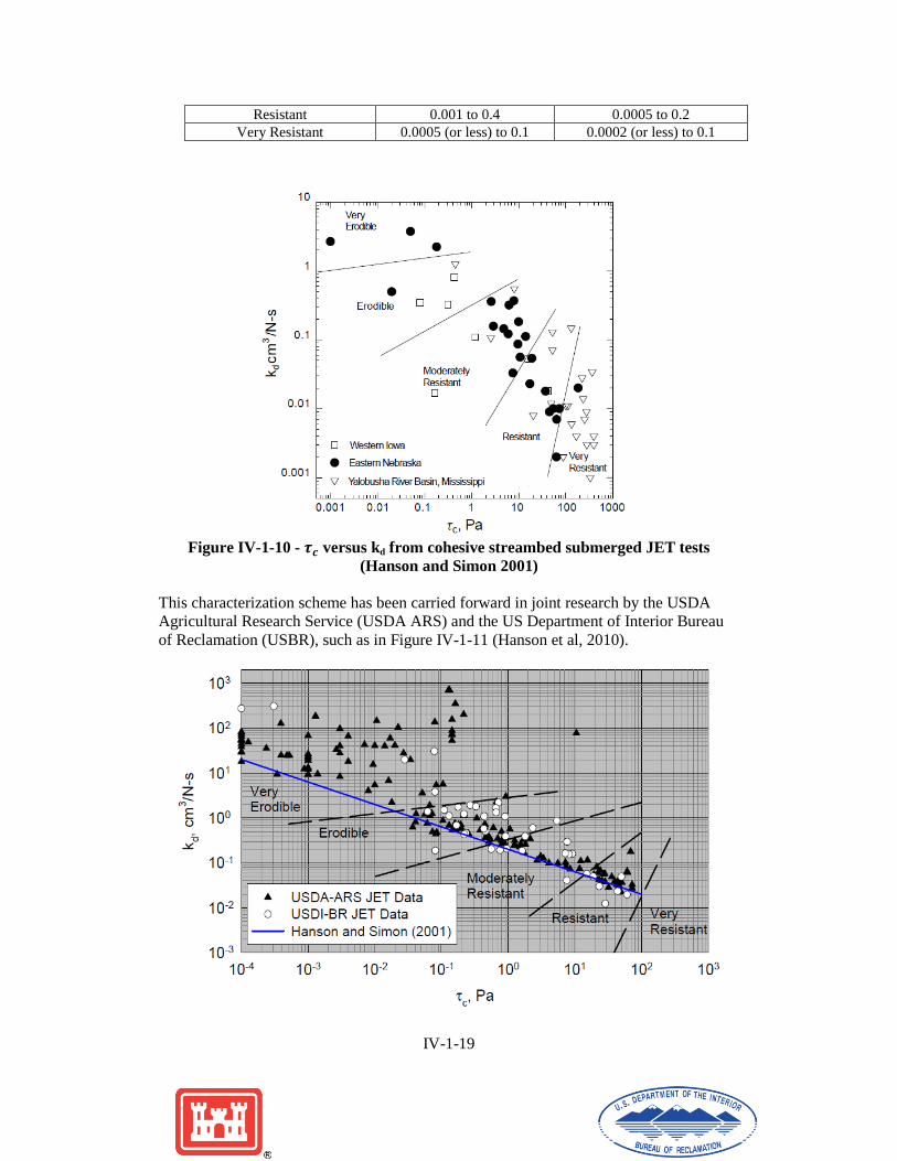
IV-1-19

Resistant 0.001 to 0.4 0.0005 to 0.2

Very Resistant 0.0005 (or less) to 0.1 0.0002 (or less) to 0.1

Figure IV-1-10 - versus kd from cohesive streambed submerged JET tests

(Hanson and Simon 2001)

This characterization scheme has been carried forward in joint research by the USDA

Agricultural Research Service (USDA ARS) and the US Department of Interior Bureau

of Reclamation (USBR), such as in Figure IV-1-11 (Hanson et al, 2010).

IV-1-20

Figure IV-1-11 - Relationship of kd and τc from JET tests on soil at the USDA-ARS

Hydraulic Engineering Research Unit and USBR Hydraulic Laboratory (Hanson et

al, 2010)

In Simon et al (2010), data from erosion tests on stream deposits suggested a similar

relationship between kd and with the relationship being influenced by test device and

generally shifted up and to the right for the presumably uncompacted and less erosion

resistant natural sediments (Figure IV-1-12).

Figure IV-1-12 - Relationship of kd and τc from 775 JET and Mini-Jet tests on

natural sediments (Simon et al, 2010)

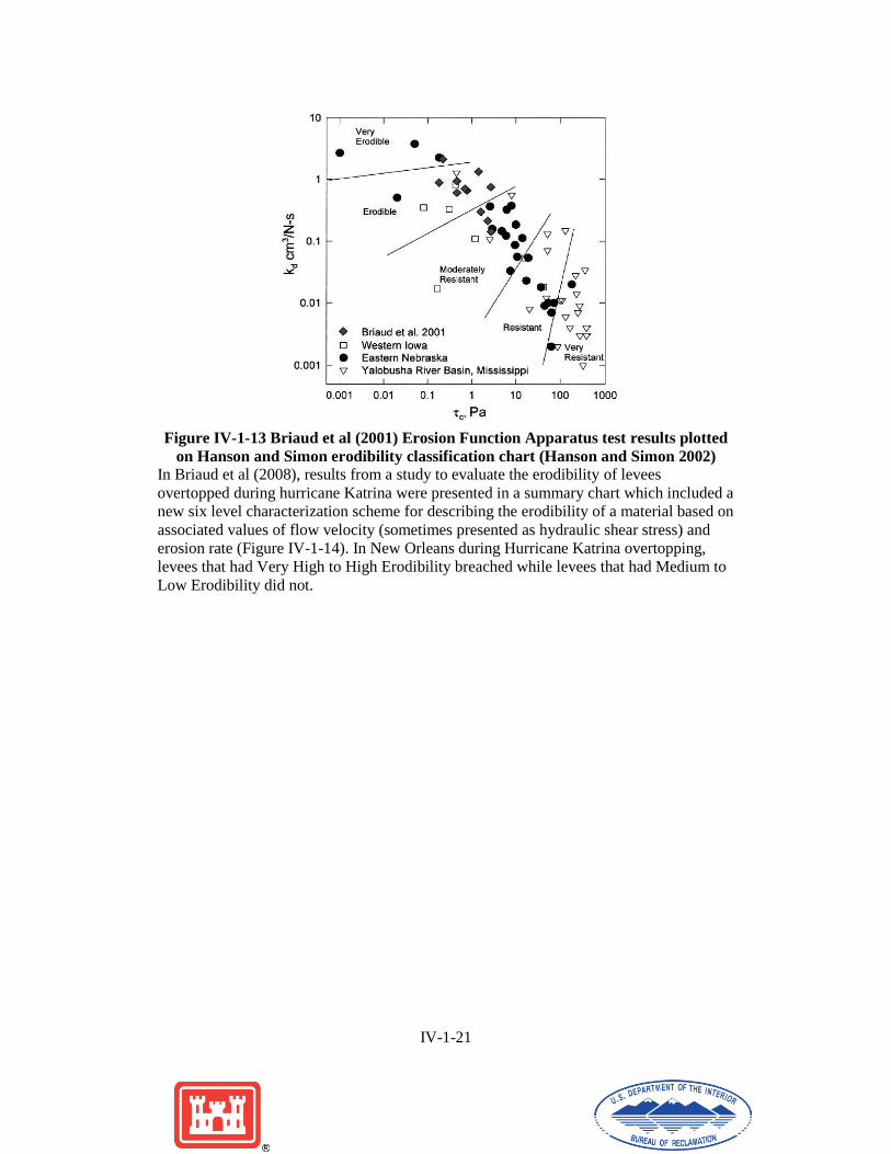
In Briaud et al (2001), a new test device, the Erosion Function Apparatus (EFA) is

described and results from tests on various soils are presented. In a companion

discussion, Hanson and Simon (2002) plot the Briaud et al (2001) data on the Hanson and

Simon (2001) erodibility classification scheme (Figure IV-1-13), again showing a

similarly correlated relationship between kd and .

IV-1-21

Figure IV-1-13 Briaud et al (2001) Erosion Function Apparatus test results plotted

on Hanson and Simon erodibility classification chart (Hanson and Simon 2002)

In Briaud et al (2008), results from a study to evaluate the erodibility of levees

overtopped during hurricane Katrina were presented in a summary chart which included a

new six level characterization scheme for describing the erodibility of a material based on

associated values of flow velocity (sometimes presented as hydraulic shear stress) and

erosion rate (Figure IV-1-14). In New Orleans during Hurricane Katrina overtopping,

levees that had Very High to High Erodibility breached while levees that had Medium to

Low Erodibility did not.

IV-1-22

Figure IV-1-14 Erosion Function Apparatus test results and overtopping levee

failure/no failure chart. Solid circles are for levees that failed and empty circles are

for levees with no damage (Briaud et al 2008)

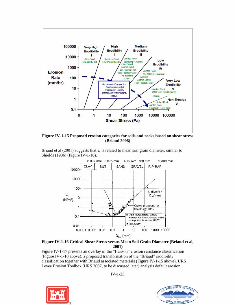
In Briaud (2008), the above erodibility characterization scheme was expanded to

encompass a wider variety of materials described in general engineering terms (Unified

Soil Classification System (USCS) based on % and type of coarse versus fines and the

plasticity of the fines for soils and jointing characteristics for rock) rather than the

agricultural “textural” terms (% sand, silt, and clay based on grain size definitions) often

used in the USDA work (Figure IV-1-15).

IV-1-23

Figure IV-1-15 Proposed erosion categories for soils and rocks based on shear stress

(Briaud 2008)

Briaud et al (2001) suggests that τc is related to mean soil grain diameter, similar to

Shields (1936) (Figure IV-1-16).

Figure IV-1-16 Critical Shear Stress versus Mean Soil Grain Diameter (Briaud et al,

2001)

Figure IV-1-17 presents an overlay of the “Hanson” erosion resistance classification

(Figure IV-1-10 above), a proposed transformation of the “Briaud” erodibility

classification together with Briaud associated materials (Figure IV-1-15 above), URS

Levee Erosion Toolbox (URS 2007, to be discussed later) analysis default erosion

IV-1-24

parameters and τc based on mean grain size, D50, from Briaud 2001 (Figure IV-1-25

above). The “Hanson” and “Briaud” classification schemes appear to be complimentary,

with each erosion class having similar ranges of values for kd and associated τc. At this

time, risk analysts are encouraged to continue using the classification scheme and

nomenclature of Hanson and Simon (Figure IV-1-10 and Table IV-1-6) when describing

the erosion resistance of materials.

Figure IV-1-17 “Hanson” erosion resistance, “Briaud” erodibility, Levee Erosion

Toolbox (URS 2007) default values for kd and associated τc for the various

“Hanson” erosion resistance classifications and Sheild’s Diagram τc from Briaud

2001.

Physical Tests For Estimating Soil Erosion Rate Parameters

Several test methods have been developed for evaluating detachment rate coefficient kd

and critical stress , including: flume tests, jet erosion test (JET), rotating cylinder test

(RCT), small samples inserted in the bottom of flumes (aka Erosion Function Apparatus

EFA), and hole erosion test (HET) are representative examples from the literature

(Hanson et al, 2011). At this time, the JET test is considered the best understood with the

most confirmation of coherence between small scale test results and the larger scale

erosion processes modeled in overtopping analyses. HET tests have gained some

popularity for evaluating internal erosion potential (scour/crack erosion), but have been

found to generally yield estimates of Kd on the order of 1 to 2 orders of magnitude too

low compared to JET tests and small scale models (Wahl et al 2008). Unfortunately,

available JET devices are too small to test samples of rockfill materials (e.g., coarse

IV-1-25

sands, gravels and cobbles), which are typical materials for many dam embankment

shells.

Factors Affecting Soil Erosion Rate Parameters

Hanson et al (2011) presents JET erosion test results from low plasticity clayey materials

compacted at different compactive efforts and moisture contents, showing that

compaction moisture content can have a significant impact on both kd (Figure IV-1-18)

and .

Figure15-18 Change in kd versus compaction water content for seven low plasticity

soils compacted at Standard Proctor (ASTM D698). Lowest values of Kd are

generally achieved just below or near optimum water content. (Hanson et al, 2011)

Figure IV-1-19 presents the measured values of kd from Hanson et al (2011), indicating

that for the low plasticity CL soil tested, kd decreases with increasing compactive effort.

Figure IV-1-19 Kd versus Compaction Water Content for Different Compactive

Efforts (low, “Standard”, and “Modified” Proctor, based on energy level in Kg-

cm/cm3) (Hanson et al, 2011)

IV-1-26

Figure IV-1-20 presents results from Hanson and Hunt (2007) indicating a slightly

different relationship for the SM and slightly dispersive CL material tested in this study,

with these materials showing less immediate increase in Kd when compacted dry of

optimum. Similar results were found in Wahl et al (2009).

Figure IV-1-20 Variation of Kd with variation in compaction moisture content

(Hanson and Hunt 2007)

Figure IV-1-21 presents the measured values of kd from Hanson et al (2010 and 2011),

Wahl et al (2009) and Shewbridge et al (2010, to be discussed later), suggesting that kd

may also vary with plastic index, decreasing with increasing plasticity, consistent with

the erosion classification chart of Briaud (2008). Unfortunately “paired” samples for

“dry” and “wet” comparisons of higher plasticity materials are not available to confirm

higher erodibility if compacted and tested with water content dry of optimum.

IV-1-27

Figure IV-1-21 Kd versus Plastic Index from tests by Hanson et al (2010 and 2011) ,

Wahl et al (2009) and Shewbridge et al (2010).

While Briaud (2008) suggests that gravels have medium to low erodibility and thus lower

expected values of kd and τc, unfortunately there is no test data available at this time to

confirm this supposition. Nevertheless, it seems reasonable to presume that both

parameters are sensitive to the amount and type of finer grained materials comprising the

gravel, as well as the inclination of the eroding surface. Steep erosion surfaces (i.e.,

inclined near the friction angle of the gravels), comprised of poorly graded gravels with

little sand and little to no fines, might have high erodibility until the eroding surface

flattens below the angle of repose as breach initiation advances. In contrast, relatively flat

erosion surfaces (i.e., inclined at say 70% of the friction angle of the soil), with

appreciable sand and fines (e.g., GW-GC or GC) may have very low erodibility,

approaching that of jointed rock. In a review of the regression breach formation equations

of Xu and Zhang (2009), Wahl (2014a) suggests that medium erodibility may be an

appropriate designation for rockfill dams. Unfortunately there is little empirical evidence

to support the above speculations and until more research data becomes available, the risk

analyst will have to apply judgment when selecting values for kd and τc to model breaches

in embankments comprised of these types of materials.

IV-1-28

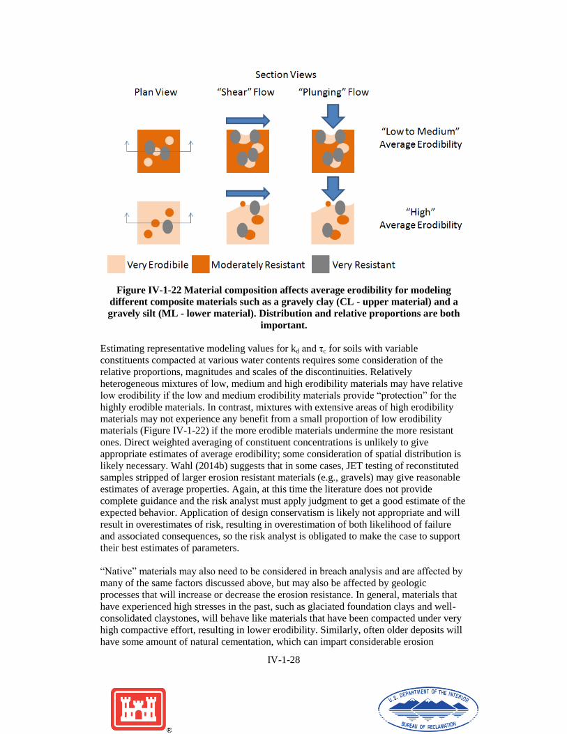
Figure IV-1-22 Material composition affects average erodibility for modeling

different composite materials such as a gravely clay (CL - upper material) and a

gravely silt (ML - lower material). Distribution and relative proportions are both

important.

Estimating representative modeling values for kd and τc for soils with variable

constituents compacted at various water contents requires some consideration of the

relative proportions, magnitudes and scales of the discontinuities. Relatively

heterogeneous mixtures of low, medium and high erodibility materials may have relative

low erodibility if the low and medium erodibility materials provide “protection” for the

highly erodible materials. In contrast, mixtures with extensive areas of high erodibility

materials may not experience any benefit from a small proportion of low erodibility

materials (Figure IV-1-22) if the more erodible materials undermine the more resistant

ones. Direct weighted averaging of constituent concentrations is unlikely to give

appropriate estimates of average erodibility; some consideration of spatial distribution is

likely necessary. Wahl (2014b) suggests that in some cases, JET testing of reconstituted

samples stripped of larger erosion resistant materials (e.g., gravels) may give reasonable

estimates of average properties. Again, at this time the literature does not provide

complete guidance and the risk analyst must apply judgment to get a good estimate of the

expected behavior. Application of design conservatism is likely not appropriate and will

result in overestimates of risk, resulting in overestimation of both likelihood of failure

and associated consequences, so the risk analyst is obligated to make the case to support

their best estimates of parameters.

“Native” materials may also need to be considered in breach analysis and are affected by

many of the same factors discussed above, but may also be affected by geologic

processes that will increase or decrease the erosion resistance. In general, materials that

have experienced high stresses in the past, such as glaciated foundation clays and well-

consolidated claystones, will behave like materials that have been compacted under very

high compactive effort, resulting in lower erodibility. Similarly, often older deposits will

have some amount of natural cementation, which can impart considerable erosion

IV-1-29

resistance, but which may also be vulnerable to degradation through solutioning water

flows and/or through slaking or other wet/dry phenomena. Further, both native and

engineered fill materials are subject to various processes, such as shrinking and swelling

with seasonal variations in moisture; this may result in cumulative change in erosion

characteristics over time, with deeper material being less and shallower material being

more susceptible to those changes. Finally most erosion tests are conducted on

compacted samples at the compaction water contents immediately after compaction,

which may not reflect in-situ conditions. Based on limited anecdotal evidence, in some

situations, it is possible that moisture conditioning over time and at relatively high

confining stresses in–situ could diminish the flocculated clay structure that may form in

plastic clays compacted dry of optimum, resulting in an increase in erosion resistance

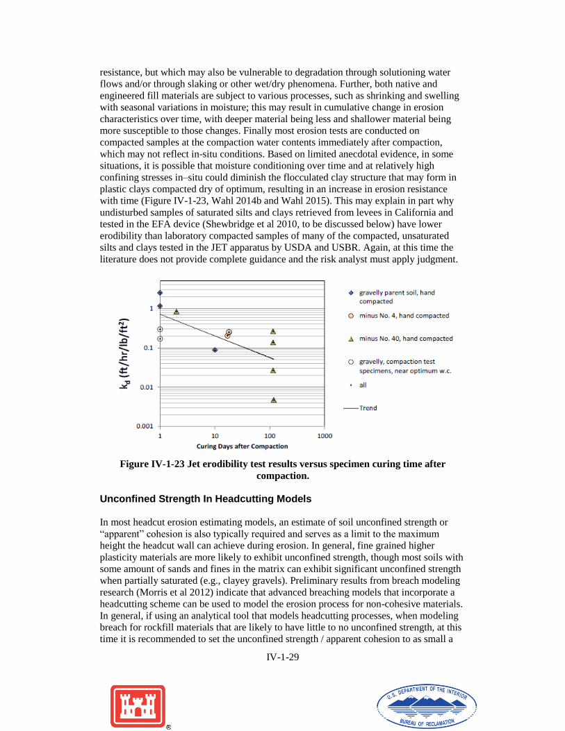
with time (Figure IV-1-23, Wahl 2014b and Wahl 2015). This may explain in part why

undisturbed samples of saturated silts and clays retrieved from levees in California and

tested in the EFA device (Shewbridge et al 2010, to be discussed below) have lower

erodibility than laboratory compacted samples of many of the compacted, unsaturated

silts and clays tested in the JET apparatus by USDA and USBR. Again, at this time the

literature does not provide complete guidance and the risk analyst must apply judgment.

Figure IV-1-23 Jet erodibility test results versus specimen curing time after

compaction.

Unconfined Strength In Headcutting Models

In most headcut erosion estimating models, an estimate of soil unconfined strength or

“apparent” cohesion is also typically required and serves as a limit to the maximum

height the headcut wall can achieve during erosion. In general, fine grained higher

plasticity materials are more likely to exhibit unconfined strength, though most soils with

some amount of sands and fines in the matrix can exhibit significant unconfined strength

when partially saturated (e.g., clayey gravels). Preliminary results from breach modeling

research (Morris et al 2012) indicate that advanced breaching models that incorporate a

headcutting scheme can be used to model the erosion process for non-cohesive materials.

In general, if using an analytical tool that models headcutting processes, when modeling

breach for rockfill materials that are likely to have little to no unconfined strength, at this

time it is recommended to set the unconfined strength / apparent cohesion to as small a

IV-1-30

value as allowed and conduct sensitivity analyses to confirm the impact on final results.

WinDAMB allows a minimum of 100 psf of apparent cohesion, which is a very small

value leading to very short headwall heights.

Soils Parameters for Evaluating Riverine Erosion

Leading to Breach of Earthen Levees

In URS 2007, a levee erosion toolbox developed for the U.S. Army Corps of Engineers

(USACE) as part of the Nationwide Levee Risk Assessment Methodology project is

described. The purpose of the erosion toolbox is to estimate the conditional probability of

levee failure due to surface erosion on the waterside of a levee. It is a risk analysis tool

for use during screening level assessments of levee risk; it is not a design tool and may

reflect less conservatism than some of the design work described above. Representative

“default” values for kd and τc associated with the “Hanson” erosion resistance categories

for use in the risk analysis computational tool were also proposed, but could be modified

by the analyst, as appropriate based on site-specific material characteristics. This toolbox

also suggested that typical USCS soil types could be associated with ranges of critical

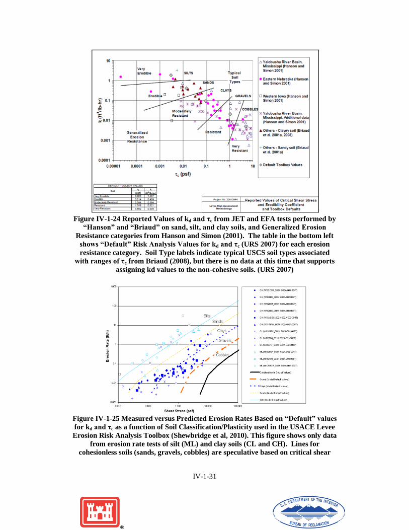
shear stress based on the work of Briaud (2008) (Figure IV-1-24). It must be emphasized

that kd values for large non-cohesive materials (coarse sands, gravels and cobbles) have

never been measured; although the USCS soil type labels are overlaid on Figure IV-1-24

in a way that follows the relation between kd and τc for cohesive materials, there is no

assurance that non-cohesive materials will have similar kd values.

In Shewbridge et al (2010), test results from a study for the California Department of

Water Resources to apply the USACE erosion toolbox methodology to levees in

California are presented. Undisturbed samples of actual levee materials from various

locations throughout the California Central Valley were retrieved, classified per the

USCS and tested in the Erosion Function Apparatus (Briaud et al, 2001). These test

results suggest that the default values for kd and τc as functions of “typical” soil type

proposed in URS 2007 were appropriate for levee screening-level risk analyses. Low

plasticity materials (silts and low plasticity clays) had higher values and higher plasticity

materials (higher plasticity clays) had lower values of kd resulting in higher and lower

predicted and measured erosion rates, respectively (Figure IV-1-25). Unfortunately, as

discussed above, at this time there are no reliable test measurements of kd for gravel and

cobble materials. In a riverine setting, current velocities are generally low enough that the

hydraulic shear stress at the levee does not exceed τc for gravels and cobbles, so estimates

of erosion rate are often not necessary to rule out erosion breach, avoiding the challenges

estimating kd.

IV-1-31

Figure IV-1-24 Reported Values of kd and τc from JET and EFA tests performed by

“Hanson” and “Briaud” on sand, silt, and clay soils, and Generalized Erosion

Resistance categories from Hanson and Simon (2001). The table in the bottom left

shows “Default” Risk Analysis Values for kd and τc (URS 2007) for each erosion

resistance category. Soil Type labels indicate typical USCS soil types associated

with ranges of τc from Briaud (2008), but there is no data at this time that supports

assigning kd values to the non-cohesive soils. (URS 2007)

Figure IV-1-25 Measured versus Predicted Erosion Rates Based on “Default” values

for kd and τc as a function of Soil Classification/Plasticity used in the USACE Levee

Erosion Risk Analysis Toolbox (Shewbridge et al, 2010). This figure shows only data

from erosion rate tests of silt (ML) and clay soils (CL and CH). Lines for

cohesionless soils (sands, gravels, cobbles) are speculative based on critical shear

IV-1-32

stress values for those particle sizes (Briaud, 2008), but at this time there are no

measurements of erosion rates for these materials.

Numerical Modeling Methods for the Erosion Process

There are multiple methods and tools that can be used to model and analyze the erosion

process in rock and soils found in embankments and spillways. In many of these cases

the methods were developed with a specific types of spillways and embankments, and

then they have been adapted for use studying other types of embankments or spillways.

User judgment will be required when applying these models to situations that vary from

their original intent.

Spillway headcut erosion – SITES Model

The SITES model (http://go.usa.gov/83z) was developed by the U.S. Department of

Agriculture (USDA) to simulate headcut erosion in earthen spillways. The model is

based on laboratory studies and field observations of headcutting in soil and grass lined

spillways. The computer program carries out a one-dimensional hydraulic simulation of

flow through the spillway channel and evaluates the stability and integrity of the channel

using a three-phase simulation of the headcutting erosion processes. Headcut erosion

occurs in a variety of natural materials, especially when cohesion or other internal bonds

hold the material together, or when there is a somewhat more erosion-resistant surface

layer. Although the model was developed with a focus on soils, it has also been applied

to rock channels.

The scope of the SITES model simulation is limited; the objective is to determine

whether a headcut will form and whether the flow duration will be sufficient to deepen

the headcut and cause it to advance upstream. If the erosion reaches the control sill of

the spillway, the model concludes that the spillway has failed, and the run terminates.

The simulation does not continue into the breach calculation phase since the spillway

hydrograph was determined outside of the spillway erosion algorithm.

The three phases of the erosion process in a SITES simulation are as follows (Temple and

Moore 1997):

1. Failure of vegetal cover and development of concentrated flow – Failure of

vegetation can take place due to instantaneous total hydraulic stresses exceeding

a threshold, or due to the time integral of erosionally effective stress exceeding a

second threshold related to the plasticity index of the soil.

2. Downward erosion in the area of concentrated flow, leading to headcut formation

– This phase is modeled using an excess stress equation with the soil

characterized by a critical shear stress needed to initiate erosion and a detachment

rate coefficient expressing the rate of erosion per unit of applied excess stress.

For soil materials, the detachment rate coefficient, kd, can be measured using

laboratory or field submerged jet tests (Hanson and Cook 2004). Experience has

shown that this is a crucial parameter affecting the performance of the SITES

model. For rock materials, this parameter cannot be directly measured, and the

SITES documentation suggests that a large detachment rate coefficient should be

used.

IV-1-33

3. Continued downward erosion (which increases the headcut height) and upstream

advance of the headcut – The advance rate is driven by the energy dissipation

(stream power) at the headcut drop, and resistance is related to the headcut

erodibility index, Kh. The index is used to establish the threshold for headcut

movement and the rate of headcut advance.

Experience with the SITES model on rock spillway erosion problems (Wahl 2008a,

2008b) has shown that the detachment rate coefficient, kd, is a crucial parameter affecting

erosion predictions. Since this parameter cannot actually be measured for rock, a great

deal of judgment is required to apply SITES to these situations.

Embankment breaching – WinDAM B model

WinDAM B is a dam breach simulation model that has been developed by the USDA,

based on research conducted at the Agricultural Research Service hydraulics laboratory

in Stillwater, Oklahoma. This software incorporates the SITES spillway erosion

technology, and also allows the user to simulate breaching of homogeneous

embankments from overtopping. WinDAM B is the second in a series of planned model

developments.

WinDAM A analyzed embankment overtopping only up to the point of

imminent breach (breach initiation), and its output consisted only of a

determination of whether breach occurred.

WinDAM B analyzed breach development, with the breach caused only by

overtopping flow

WinDAM C will analyze breach development due to internal erosion (i.e.,

piping)

Subsequent model versions are planned to incorporate capability for modeling

zoned embankments.

For embankment overtopping, WinDAM B uses a similar phased erosion process as that

employed in the SITES software, but emphasizes the breach development phase by

separately considering headcut advance through different parts of the embankment. The

four stages used by WinDAM B for embankment overtopping are:

1. Vegetal cover failure and headcut development

2. Headcut advance through the dam crest

3. Headcut advance into the reservoir (breach development)

4. Breach widening

The end of stage 2 marks the threshold for imminent breach or the end of the breach

initiation process. Up to this point, intervention to save the dam may be possible (e.g.,

sandbags on crest, opening up additional spillway capability, etc.). Once stage 3 is

entered, the flow rate increases dramatically; erosion causes the hydraulic control section

to be enlarged, which allows an uncontrolled release of the reservoir storage.

IV-1-34

WinDAM B includes practical features and capabilities that facilitate the dam breach

simulation process. These include:

routing of flows through the reservoir

variable dam crest elevations (camber)

multiple spillways

flexible specification of inflow flood hydrograph

Although WinDAM B includes the spillway erosion modeling technology described for

the SITES model, the level of output detail is not as great as SITES, so there may be

situations in which users may still prefer the SITES model, which continues to be

maintained by USDA. WinDAM B does have the capability to simulate embankment

erosion and spillway erosion simultaneously, which permits it to be used to answer the

question of which would occur first, a dam breach or spillway breach.

Differences between approaches to spillway erosion and embankment erosion in the

WinDAM B and SITES models should be emphasized again. Both SITES and WinDAM

B will simulate spillway headcut erosion only up to the point at which the most upstream

headcut advances through the crest of the spillway (the high point of the spillway

profile). For a spillway, they will not simulate the process of breach enlargement. For an

embankment overtopping scenario, WinDAM B will simulate both breach initiation and

breach development/enlargement. If a WinDAM B simulation includes both a spillway

and an overtopped embankment and the spillway breaches first, you will not be able to

draw any conclusions about what subsequently happens to the embankment. It is

possible that the breach of the spillway could save the embankment, or if the breach

process is slow, the embankment may continue to overtop and eventually fail. However,

WinDAM B can only indicate which structure breaches first.

It should also be emphasized that the spillway erosion modeling performed by SITES and

WinDAM B are intentionally conservative. The intent of these modeling tools was that

they would be used for design, with the modeler adjusting a spillway design until no

breach occurs. For this reason, the spillway erosion simulation conservatively estimates

more erosion than is likely to occur in reality. In contrast, the embankment breach

modeling capability in WinDAM was intended from the outset to be an analysis tool that

would give an analyst the most accurate possible prediction of the outflow hydrograph

produced by a potential breach.

Potential Failure Mode Event Tree for Spillway Erosion When developing event trees during a potential failure mode analysis (PFMA) all of the

steps previously mentioned in the erosion process may need to be included. In an event

tree, each step would need to occur in order to fail a system by breaching the

embankment from overtopping or failing the spillway due to headcutting. A possible

sequence of events that can be used in a spillway erosion event tree is:

IV-1-35

Hydrologic event occurs and reservoir stage reaches the spillway crest.

Spillway begins to flow.

Vegetation is removed (if it is present).

Concentrated flow erosion begins (downcutting forms headcut).

Headcut advancement begins (Headcut deepens and advances towards

spillway crest/control section).

Intervention is unsuccessful.

Headcut advances through crest of spillway and/or headcut undermines

control structure/section and flow control is lost.

Headcut advances into reservoir pool and breaching begins.

This possible event tree would be similar to one that would apply to embankment

overtopping leading to a breach. A sample event tree for embankment overtopping is

provided in the chapter on Flood Overtopping.

Relevant Case Histories

Gibson Dam: 1964 This case is described in the section on Dam Overtopping. Based on a detailed

evaluation, the erodibility index of the dolomite abutment rock was estimated to be

between 5,100 and 12,000 and the stream power was estimated to be between 43 kW/m2

on the upper abutments and 258 kW/m2 on the lower abutments. With these values,

Figure 6 would predict about a probability of erosion of at most a few percent. In fact,

very little erosion was observed.

Ricobayo Dam Ricobayo Dam is a 320-foot high double-curvature arch dam constructed from 1929 to

1933 in Spain. The spillway at Ricobayo Dam is located on the left abutment of the dam

and originally consisted of a 1300-foot long unlined channel at a slope of 0.0045

discharging over a rock cliff at the downstream end of the spillway. The design capacity

of the spillway is 164,000 ft3/s. Flows through the spillway are regulated by four 68-foot

by 35-foot gates. The rock in the spillway chute consisted of open-jointed granite.

Five separate scour events occurred along the spillway chute, with the first event

occurring shortly after the dam was commissioned. Each of the flood events lasted over a

period of several months, usually from December to June. From the initial major spill in

January 1934, scour initiated and began progressing upstream. Attempts were made to

stabilize the spillway chute after the flood events in 1934 and 1935. The vertical face of

the drop at the downstream end of the chute and the right hand slope of the plunge pool

were protected with concrete after the 1934 floods. Additional scour, about 80 feet

downwards, occurred in the base of the plunge pool during the 1935 flood. After the

1935 flood, a concrete lip was added to the end of the spillway chute to direct flows

further away from the face of the plunge pool drop. The concrete lip failed during the

1936 flood, as the plunge pool deepened another 100 feet, and the vertical face of the

plunge pool experienced additional scour. During the 1939 flood event, the plunge pool

did not deepen, but damage occurred at the vertical face of the plunge pool.

IV-1-36

Even though the plunge pool did not deepen during the 1939 flood, measures were taken

in the early 1940s to further stabilize the plunge pool. The plunge pool was lined with

concrete, and concrete protection was added to the spillway channel and the drop at the

end of the spillway channel. During 1962, the flood event reached a peak discharge of

170,000 ft3/s which caused failure of the plunge pool concrete lining that had been added

in the 1940s. After the 1962 event, hydraulic splitters were added to the end of the

spillway channel to break up the jet before it plunged into the pool. Since those

modifications the spillway has passed floods with discharges ranging from 106,000 to

124,000 ft3/s without experiencing additional damage.

The Ricobayo spillway is located within a granite massif known as the Ricobayo

Batholith. There are two prominent joint sets in the spillway foundation rock (joint sets

A & B). Joint set A is generally vertically dipping. Joint set B is more horizontally

dipping about 10-20 degrees. An anticline intersects the middle of the spillway at an

angle of approximately 40º. Both joint set A and joint set B are relatively planar, but

joint set B appears to be more continuous. Original speculation was that joints in the

spillway foundation were clay filled and that this contributed to the scour during flood

events. A site visit during 2005 indicated that the gouge was more likely rock flour and

no clay was observed. Joint separation was generally less than 5 mm, with a maximum

separation of 10 mm at some locations near the original surface. One additional feature

in the spillway foundation is a near vertical fault that trends perpendicular to the spillway.

The foundation rock adjacent to the fault has experienced intense shearing.

An evaluation of the scour that occurred over the years concluded that the geology in the

spillway chute greatly contributed to the scour. To the right of the anticline axis, the

scour progression was in the horizontal direction, while to the left of the anticline axis the

scour progression was primarily in the vertical direction. The likely cause of the change

in scour direction is the joint orientations on either side of the anticline axis. It was also

believed that the fault in the channel played a role in the progression of the scour. The

poorer quality of the rock along the fault allowed it to be easily eroded in a vertical

direction. This is reflected in the erosion that occurred in 1935 (vertical scour of about

80 feet) and in 1936 (vertical scour of about 100 feet).

The plunge pool did not deepen during the flood event of 1939, indicating that the rock in

the floor of the plunge pool was stronger than the rock that was eroded above it. This

was also confirmed during the flood event in 1962. That flood event led to the

destruction of the concrete lining in the plunge pool but no significant damage to the

underlying rock. This led to the conclusion that the rock was stronger than the concrete

lining provided to protect it.

A quantitative analysis of the plunge pool scour that occurred historically at Ricobayo

Dam was performed, using the erodibility index method. The maximum scour depth is

reached when the erosive power of the jet is less than the ability of the rock at the bottom

of the plunge pool to resist it. Calculated and observed scour depths were compared

(Annandale 2006). The calculated and observed scour depths from the 1935, 1936, and

1962 flood events generally were in good agreement. The analysis indicated that the

calculations overestimated the scour that actually occurred in 1939, but that this was

likely a function of much stronger erosion resistant rock at the base of the plunge pool

after the 1936 flood.

IV-1-37

Examples

Headcut Erodibility Index Calculation for Rock You are at a site where there is a granite formation located immediately downstream of

your spillway. Due to the weathered condition of the rock, there is concern that erosion

could occur during a high discharge. You refer to the construction documents and the

team geologist and have obtained the following information:

The material of concern is granite with a uniaxial compressive strength of

20,000 psi.

The rock quality designation is 50 percent.

The material appears to be jointed in a four joint set.

The joints are planar and smooth, with a tight joint separation, and the

walls are slightly altered with sandy particles.

The blocks appear to have a length to thickness ratio of 1:2 and the blocks

dip downward into flow at 80 degrees.

Using this information and the tables in this chapter, what is the headcut erodibility index

for the material?

IV-1-38

References

Annandale, G.W. 1995. Erodibility, Journal Hydraulic Research, IAHR, Vol. 33(4):

471-494.

Annandale, George W. Scour Technology – Mechanics and Engineering Practice,

McGraw-Hill Civil Engineering Series, First Edition, 2006, 430 pages.

Barton, N., “Estimating the Shear Strength of Complex Discontinuities,” International

Symposium on the Geotechnics of Structurally Complex Formations, vol. II, pp. 226-232,

Capri, 1977.

Briaud, J.-L., Ting F., Chen, H.C., Cao Y., Han S. -W., Kwak K. 2001. Erosion Function

Apparatus for Scour Rate Predictions. Journal of Geotechnical and Geoenvironmental

Engineering. ASCE, Vol. 127, N. 2, pp. 105-113.

Briaud, J.-L., Chen, H.C., A.V. Govindasamy, and R. Storesund 2008 “Levee Erosion by

Overtopping in New Orleans During the Katrina Hurricane” J. Geotech. Geoenviron.

Eng. 2008.134:618-632.

Briaud, J.-L., 2008, “Case Histories in Soil and Rock Erosion: Woodrow Wilson Bridge,

Brazos River Meander, Normandy Cliffs, and New Orleans Levees”, The 9th Ralph B.

Peck Lecture, Journal of Geotechnical and Geoenvironmental Engineering, Vol. 134,

ASCE, Reston Virginia, USA.

Bureau of Reclamation, Erosion and Sedimentation Manual, U.S. Department of the

Interior, Bureau of Reclamation, Technical Service Center, Denver, Colorado, November

2006.

Bollaert, E., “Transient Water Pressures in Joints and Formation Rock Scour due to High-

Velocity Jet Impact,” Communication 13, Laboratoire de Constructions Hydrauliques

Ecole Polytechnique Federale de Lausanne, Switzerland, 2002.

Chow, V.T., Handbook of Applied Hydrology, McGraw-Hill Book Company. New York.

1964.

Colorado Department of Transportation, Calculation of Bridge Scour Using the

Erodibility Index Method, Annandale, G.; Smith, S.; March 2001.

Ervine, D.A., et al, “Pressure Fluctuations on Plunge Pool Floors,” Journal of Hydraulic

Research, Vol. 35, No. 2, pp. 257-279, 1997.

Frizell, K.H, J.F. Ruff, and S. Mishra, “Simplified Design Guidelines for Riprap

Subjected to Overtopping Flow,” Proceedings, ASDSO Annual Meeting, Las Vegas,

Nevada, October 1998.

Hanson, G. J., and A. Simon, 2001, “Erodibility of cohesive streambeds in the loess area

of the midwestern USA” Hydrol. Process. 15, 23–38 (2001)

IV-1-39

Hanson, G. J., and A. Simon, 2002, “Discussion of ‘‘Erosion Function Apparatus for

Scour Rate Predictions’’ by J. L. Briaud, F. C. K. Ting, H. C. Chen, Y. Cao, S. W. Han,

and K. W. Kwak” J. Geotech. Geoenviron. Eng. 2002.128:627-628.

Hanson, G. J., K.R. Cook, W. Hahn, and S. L. Britton, 2003, “Observed erosion

processes during embankment overtopping tests.” ASAE Paper No. 032066. ASAE St.

Joseph, MI.

Hanson, G.G. and S. Hunt, 2007 “Lessons Learned Using Laboratory JET Method to

Measure Soil Erodibility of Compacted Soils” ” Applied Engineering in Agriculture Vol.

23(3): 305-312

Hanson, G.J., and D. Temple, 2007, “Final Report on Coordination and Cooperation with

the European Union on Embankment Failure Analysis” FEMA 602, 168p.

Hanson, G.J., T. Wahl, D. Temple, S. Hunt, and R. Tejral, 2010, “Erodibility

Characteristics of Embankment Materials” Proceedings Association of State Dam Safety

Officials Annual Conference

Hanson, G.J., D.M. Temple, S.L. Hunt, and R.D. Tejral, 2011, “Development and

Characterization of Soil Material Parameters for Embankment Breach” Applied

Engineering in Agriculture Vol. 27(4): 587-595

Kirsten, H.A.D., “A Classification System for Excavation in Natural Materials,” the Civil

Engineer in South Africa, pp. 292-308, July (Discussion in Vol. 25, No. 5, May 1983).

Mason, P.J., Arumugam, K., “Free Jet Scour below Dams and Flip Buckets.” ASCE

Journal of Hydraulic Engineering, Vol. 111, No. 2, 1985.

MacDonald, T.C., and Langridge-Monopolis, J., (1984). Breaching Characteristics of

Dam Failures, Journal of Hydraulic Engineering, Vol. 110, No. 5, May, pgs 567-586

Moore, John S., Darrel M. Temple, and H.A.D. Kirsten, 1994, “Headcut Advance

Threshold in Earth Spillways,” Bulletin of the Association of Engineering

Geologists, vol. XXXI, no. 2, June 1994, p. 277-280.

Morris, M.W., M.A.A.M. Hassan, T.L. Wahl , R.D. Tejral, G.J. Hanson, and D.M.

Temple, 2012. Evaluation and development of physically-based embankment breach

models. 2nd European Conference on Flood Risk Management, Nov. 20-22, 2012.

Rotterdam, The Netherlands.

Scott, G.A., “Guidelines for Geotechnical Studies for Existing Concrete Dams,” Bureau

of Reclamation, Denver, Colorado, September 1999.

Shewbridge, S.E., Perri, J., Millet, R., Huang, W., Vargas, J., Inamine, M., Mahnke, S.,

(2010) “Levee Erosion Prediction Equations Calibrated with Laboratory Testing”, Proc,

V International Conference on Scour and Erosion, San Francisco, CA

Shields, A. (1936). ‘‘Anwendung der Aenlichkeitsmechanik und der Turbulenzforschung

auf die Geschiebebewegung (Application of “similarity” mechanics and turbulence

IV-1-40

research on the glacial movement.’’ Mittleilungen der Preussischen Versuchsanstalt fur

Wasserbau und Schiffbau, W. P. Ott and J. C. Van Uchelen, translators, California

Institute of Technology, Pasadena, Calif

Simon, A, R.E. Thomas, L. Klimetz, (2010) “Comparison and Experiences with Field

Techniques to Measure Critical Sehar Stress and Erodibility of Cohesive Deposits”

Second Joint Federal interagency Conference, Las Vegas, NV

Temple, D., and Moore, J., 1997. Headcut advance prediction for earth spillways.

Transactions of the ASAE, vol. 40, no. 3, p. 557-562.

URS. 2007. Erosion Toolbox: Levee Risk Assessment Methodology: Users Manual.

Report prepared for the United States Army Corps of Engineers. 113p.

Veronese, A., “Erosioni de Fondo a Valle di uno Scarico.” Annali dei avori

Publicci, Vol. 75, No. 9, pp. 717-726, Italy, 1937.

Wahl, T.L. 1998, “Prediction of embankment dam breach parameters: A literature

review and needs assessment” DSO-98-004. Dam Safety Office, Water Resources

Research Laboratory, U.S. Bureau of Reclamation. Denver, CO.

Wahl, T.L., 2008b. Modeling headcut erosion in a proposed fuse plug auxiliary

spillway channel at Glendo Dam , Hydraulic Laboratory Report HL-2008-05, U.S.

Dept. of the Interior, Bureau of Reclamation, Denver, Colorado, 14 pp.

Wahl, T.L., 2008b. Stability analysis of proposed unlined spillway channel for

Upper San Joaquin River Basin RM 274 embankment dam alternative ,

Hydraulic Laboratory Report HL-2008-06, U.S. Dept. of the Interior, Bureau of

Reclamation, Denver, Colorado, 28 pp.

Wahl, T.L. 2009 “Quantifying Erodibility of Embankment Materials for the Modeling of

Dam Breach Processes” ASDSO Conference Proceedings

Wahl, T.L., 2014a, “Evaluation of Erodibility-Based Embankment Dam Breach

Equations,” Hydraulic Laboratory Report HL-2014-02, U.S. Bureau of Reclamation

Wahl, T.L., 2014b “Measuring Erodibility of Gravelly Fine-Grained Soils” Hydraulic

Laboratory Report HL-2014-05, U.S. Bureau of Reclamation

Wahl, T.L., 2015 Personal Communication

Wibowo, J.L., D.E. Yule, and E. Villanueva, “Earth and Rock Surface Spillway Erosion

Risk Assessment,” Proceedings, 40th U.S. Symposium on Rock Mechanics, Anchorage

Alaska, 2005.

Yildiz, D., Üzücek, E., “Prediction of Scour Depth from Free Falling Flip Bucket Jets”,

Intl. Water Power and Dam Construction, November, 1994.

IV-1-41

Xu, Y. and L.M. Zhang, 2009. Breaching parameters for earth and rockfill dams. Journal

of Geotechnical and Geoenvironmental Engineering, 135(12):1957-1970.

IV-1-42

This Page Left Blank Intentionally