.. :;-3

.. ;:,::J

,~~::Itt. ,~

~

~

~

~

~

~

~

~

:z::::t .:::=:t

.. ~

--:.:=)

.~"

~

. ;::::)

~:::::)

.=:,)

:::::)

:::::::)

.=::.:)

:::::l

::::::l

~

::::')

FLO OF FLUIDS THROUGH

VALVES, FITTINGS, AND PIPE

By the Engineering Division

Copyright, 1969-Crane Co;

All rights reserved: This publication is fully protected by copyright and nothing that appears in it may be re­printed, either wholly or in part. without special permission .

CRANE CO. Executive Office

300 Park Avenue New York, N.Y. 10022

Direct inquiries to 4100 S. Kechi. Aven'ue Chicago, Illinois 60632

Technical Paper No. 410 Price $2.50

PR1~TED IN U. S. A. ~"" (rw~lfth Print.ing-1972)

;f"~".

10

.. -" '-~""-:l . I

TablE~ of Contents ----- CHAPTER

Theory of Flow in Pipe page

Introduction ............... _ .. _ ................................. _ .... _ ....... _ .. 1-1

Physical Properties of Fluids_ ....... _ ... _ ... __ .... __ ..... _. __ ..... 1-2 Viscosity .. '" ...... _ .............................. _. __ .. _._ ... _ .. _ .......... 1-2 VV' eigh t density ..................................... _ ........ _......... 1-3 Specific volume .................. _ ..................................... 1-3 Sped fic gra \' ity ......................... _ ............. __ ............... 1-3

Nature of Flow in Pipe-Laminar and TurbulenL ................. _ .... _ .... _ ... ___ ._ ..... _ .. _. 1-4

IIIean velocity of flow ..................... _ .. _ ......... _ ........... 1-4 Reynolds number ............. _ .......... _ ........ ___ ..... _ ........ _... 1-4 Hydraulic radius ................................ _ ..................... 1-4

General Energy Equation-Bernoulli's Theorem ......................................... _._ ........ 1-5

Measurement of Pressure .......... _ ................................... 1-5

Darcy's Formula-General Equation for Flow of Fluids ..................... _ .. 1-6

Friction factor _ ............... _ ......................................... 1-6 Effect of age and use on pipe friction .................. 1-7

Principles of Co:npressible Flow in Pipe .. _ ............... 1-7 Complete isothermal equation .. _ ............................. 1-8 Simplifiedcornpressible flow-

gas pipe line formula .. _._ ..................... _ ..... _ ......... 1-8 Other commonly used formulas for

compressib:.e flow in long pipe lines ........ _ ....... 1-8 Comparison of formulas for

compressible flow in pipe lines ............ _ ... _._ ....... 1-8 Limiting flow of gases and vapors ....... _ ................ 1-9

Steam-General Discussion ._ .......................... _ ...... _ .... 1-10

------ CHAPTER 3

Formulas cmd Nomographs for Flow Through Valves, Fittings, and Pipe

page

Introduction ........... _ ............ _ .............. _ ................. _ ....... _ 3-1

Summary of Formulas .. _ ...................... _ ............ 3-2 to 3-5

Formulas and Nomographs for Liquid Flow

V e10ci ty ...................................................... _ ......... _ ..... 3-6 Reynolds number; friction factor for

clean steel and wrought iron pipe .................... 3-8 Pressure drop for turbulent flow ..... _.: .................... 3-10 Pressure drop for laminar flow .......... _ ................... 3-12 Flow through nozzles and orifices ................ _ ....... 3-14

Formulas and Nomographs for Compressible Flow

Velocity ............................................. _ ....................... 3-16 Reynolds number; friction factor for

clean steel and wrought iron pipe .................... 3-18 Pressure drop .......................................................... _. 3-20 Simplified flow f.ormula ............................................ 3-22 Flow through nozzles and orifices ........................ 3-24

CHAPTER 2 _ • ..... --__ .

flow of fluid:$ Through Valves and Fittings

Introduction ........... __ .............................. _ ....................... .

Types of Valves and Fittings Used in Pipe Systems ......... _ ... _ ......... __ .................... _ ...... 2-2

Pressure Drop Chargeable to Val ves and Fittings ........... _ ................................... '" 2-2

Crane Flow Tests ............................ _ .................. _ ........ ; 2-3

Relationship of Pressure Drop to Velocity of Flow .. _ .... _ ............. _ ............................ _ ... 2-7 Resistance Coefficient K, EquivalentLength LID, and Flow.Coefficient Cv •••••• -••••••••••••••••••••••••••••••• 2-8

Relationship of Equivalent Length LID and Resistance Coefficient K to the . Inside Diameter of Connecting Pipe ............. _ ............ Z-lC

Valves with Gradually Increased Ports ..... _ .. : ........ _ .. 2.:..iD

Effect of End Connections ....... _ .... _ ..................... _ ... _ ... 2-1C

Laminar Flow Conditions .. __ ........ _ .... _ ... _ ......... _ ............ 2'-11

Basis for Design of Charts for Determining Equivalent Length, Resistance CoeffiCient, and Flow Coefficient_ ............................ _ .. _ ........ _ ............ 2_11

Resistance of Bends ............ _ ... _ ..... _ ............................ ,., 2-12

Other Resistances to Flow .... _ .............. ~ ...... :_ ................ 2-13

Flow Through Nozzles and Orifices_ ........... ____ .......... 2 .. lJ Liquids, gases, and vapors ........................... _ ......... _Z-1:l Maximum flow of compressible:,

fluids in a nozzle ......................... _ ..... _ ... _ .............. 22..15 Flow through short tubes .............. _ ............ _._ ......... 2-15

Discharge of Fluids Through Valves, Fittings, and Pipe

Liquid flow ... _ ..... _ .......... _ ........... _._._ ..... _ .... _ ... _ ... _ ...... 2-15' Compressible' flow ._ ................ _ ............. __ ...... _~ ........ _. 2~15

1------- CHAPTER 4

Examples of Flow Problems I9';ge

Introduction ._ .................................. _ ........... _ .................. _ 4'-1 Reynolds Number. and' Friction Factor for Pipe Other than Steel or Wrought Iron .................... 4-1

Determination of Valve Resistance in L, . LID, K, and Flow Coefficient C •........ _ ....................... 4-:2

Check Valves-Determination of'Size ...................... 4--3 Laminar Flow in' Valves, Fittings, and Pipe, ......... _ .. 4-4 Pressure Drop and Velocity in Piping Systems .............. __ ......................................... ~

Pipe Line Flow Problems ..... _...................................... 4-10

Discharge of Fluids from Piping Systems ................ 4-:1'2

Flow Through Orifice MeterL .. _ ............................... 4-15

Application of Hydraulic'Radius to Flow Problems .......................................................... 4-:11

Determination of Boiler ~.apacity ..... - ... -... -............ ··· 4-:18

APPENDIX A ------------~----------- APPENDIX B

Physical Properties of Fluids and Flow Characteri'stics of Valves, Fitfings, and Pipe

page

Introduction ............................................... ~ .................. A-I

Physical Properties of Fluids Viscosity of steam .................................. A-2 Viscosity of \vater ................................................ A-3 Viscosity of liquid petroleum products .............. A-3 Viscosity of various liquids ............................... A-4 Viscosity of gases and hydrocarbon vapors ...... A-5 Viscosity of refrigerant vapors .......................... A-5 Physical properties of water.. .................................. A-6

Specific gravity-temperature relationship for petroleum oils ....................... A-7

Weight density and specific gravity of various liquids ................................. A-7

Physical properties of gases ................................... A-8 Volumetric composition and

specific gravity of gaseous fuels ........................ A-8 Steam-values of k .................................................. A-9 Weight density and specific

volume of gases and vapors ............................... A-lO Properties; saturated steam, saturated water _________ A-12 Properties; superheated steam ............................... A-16

Properties; superheated steam, compre,osed water ..... A-19

Vlow Characteristics of )zzles and Orifices Flow coefficient C for nozzles ................................. A-20' Flow coefficient C for

square edged orifices ........................................ A-20 Net expansion factor Y

for compressible flow ........................................ A-21 Critical pressure ratio, r c

for compressible flow ........................................ A-21

Flow Characteristics of Pipe, Valves, and Fittings

Net expansion factor Y for compressible flow through pipe to a larger flow area ........ A-22

Relative roughness of pipe materials and friction factor for complete turbulence ............ A-23

Friction factors for any type of commercial pipe ............................ A-24

Friction factors for clean commercial steel and wrought iron pipe ........ A-25

Resistance in pipe due to sudden enlargements and contractions............ A-26

Resistance in pipe due to pipe entrance and exit.. ........................ A-26

Resistance of 90 degree bends .............................. A-27 Resistance of miter bends .................... : ................. A-27

Types of valves (sectional ilJustrations) ............ A-28

Schedule (thickness) of steel pipe used in obtaining resistance of valves and tittings of various pressure classes ................ A-30

Representative equivalent length ( LID) in pipe diameters of valves and tittings .............. A-30

Equivalent lengths L and LID and resistance coefficient K .............................. A-31

Equivalents of resistance coefficient K and flow coefficient C, ...................................... A-32

Engineering Data page

Introduction E-I

Equivalent Volume and 'Weight Flow Rates of Compressible Fluids .......................... B.,..2

Equivalents of Viscosity Absolute ............................................................ ; ....... B-3 Kinematic ................................................ ; ................ B-3 Kinematic and Saybolt UniversaL ......... : ............ B-4 Kinematic and' Saybolt FuroL. ............................. B'-4 Kinematic, Saybolt Universal, .

Saybolt Furol, and Absolute ............................ B-5

Saybolt Universal Viscosity CharL ......................... B-6

Equivalents of Degrees API, Degrees Baume, Specific Gravity, Weight Density, and Pounds per Gallon ................ B-1

Steam Data Boiler capacity ..................................................... : ... B-8 Horsepower of an engine.......................................... B-8 Ranges in steam consumption

by prime movers ................................................. B-8

Power Required for Pumping ..................................... B-9

Equivalents (General) Measure ........................................................... :........... B-J 0 vVeight ............................................................... :....... B::..! () Velocity ...................................................................... B-IO Density ........................................................................ B-IO

Physical constants ................................................... 13-10 Temperature ............................................................... B-IO Pretixes ........................................................................ B-IO

Liquid measures and weigh t3................................... B-11 Pressure and head ....................................................... B-II

Four-Place Logarithms to Base 10 ............................ B-12

Flow Through Schedule 40 Steel Pipe Water .......................................................................... B-14 Air ................................................................................. B-15

Commercial Wrought Steel Pipe. Data Schedules 10 to 160 ................................................. B-16 Standard, extra strong,

and double extra strong ...................................... B-18

Stainless Steel Pipe Data Schedules 55, lOS, 40S, and 80S ............................ B-19

APPENDIX C

page

Bibliography C-l

Nomenclature ........................................... 5ee next page

! I ,

1

I 1

\

, t ! , , , t f f r

Nomendature---------·--~----

A

a

B C

Cd Cv

D d e / g

H h

h, hL

h", K

k

L L/D

Lm M

MR n

P P'

p' Q q

q'

q'.

q' •

q ..

, q ..

Unless otherwise stated, all symbols used in this book are defined os follows:

cross sectional area of pipe or orifice, in square feet

cross sectional area of pipe or orifice, in square inches

rate of flow in barrels (42 gallons) per hour flow coefficient for orifices and nozzles

= discharge coefficient corrected for vel­ocity of approach = Cd / " I-(do/d.)'

discharge coefficient for orifices and nozzles flow coefficient for valves: expresses flow

rate in gallons per minute of 60 F water with 1.0 psi pressure drop across valve = Q v pi (6q!:::.P)

internal diameter of pipe, in feet internal diameter of pipe, in inches base of natural logarithm = 2.718 frictio:::! factor in formula hL =/Lv'/D2g acceleration of gravity = 32.2 feet per

second per second total head, in feet of fluid static pressure head existing at a point, in

feet of fluid total heat of steam, in Btu per pound loss of static pressure head due to fluid

flow, in feet of fluid static pressure head, in inches of water resista:.'lce coefficient or velocity head loss

in the formula, hL = KV'/2g' ratio of specific heat at constant pressure

to specific heat at constant volume = cJ)/c~

length of pipe, in feet equ;\'a:ent length of a resistance to flow,

in pipe diameters length of pipe, in miles molecular weight univer~al gas constant = 1;44 exponent in equation for polytropic change

. (p' \! ~ = constant) pressure. in pounds per square inch gauge pressure, pounds per square inch absolute

(see page 1-5 for diagram showing relation-ship betu:een gauge and absolute pressure)

pressure, in pounds per square foot absolute rate of flow. in gallons per minute rate of flow, in cubic feet per second at

flowing conditions rate of flow. in cubic feet per second at

standard conditions (14.7 psia and 60F) rate of flow. in millions of standard cubic

feet per day, MMsefd rate of flow. in cubic feet per hour at stand­

ard conditions ('4.7 psia and oaF), scfh rate of flo\\', in cubic feet per minute at

flowing conditions rate of flow, in cubic feet per minute at

std. conditions (14.7 pSia and 6oF), sefm

R

s

s.

T

v Va v v,

Wi W

Wa

x

individual gas constant AfR.'1 I 544/M

Reynolds number hydraulic radius, in feet critical pressure ra[;o for compressible flo'.' specific gravity of liquids relative to wate:-

both at standard temperature (60 F) specific gravity of a gas relative to air =

the ratio of the molecular weight of ct." gas to that of air

absolute temperature. in degrees Rankine (460 + t)

temperature, in degrees Fahrenheit

specific volume of fluid, in cubic feet pc:-. pound

mean velocity of flow, in feet per minute volume. in cubic feet mean velocity of flow, in feet per second sonic (or critical) velOCity of flow of a gas.

in feet per second rate of flow, in pounds per hour rate of !low, in pounds per second weight, in pounds percent quality of steam = 100 minus pe,

cent of moisture Y net expansion factor for compressible flow

through orifices, nozzles, or pipe Z potential head or elevation above reference

level, in feet

Subscripts (0) indicates orifice or nozzle conditions unless

otherwise specified (I) indicates inlet or upstream conditions

unless otherwise specified (2) . indicates outlet or downstream conditions

unless otherwise specified (100) . refers to 100 feet of pipe

Greek LeHers L.lta

f:" differential between two points Epsilon

• Rho

P p'

Mu

, J1. ,

v , v

absol ute roughness or effective height ot pipe wall irregularities, in feet

weight density of fluid, pounds per cubic ft. density of fluid, grams per cubic centimeter

absolute (dynamic) viscosity, in centipoise absolute viscosity in pound mass per foot

second or pou~dal seconds per sq foot absolute viscosity. in slugs per foot sec~mc:

or pound force seconds per square 100!

kinematic viscosity, in centistokes kinematic visc9sity, square feet per secon<.i

~

=» :;::;t

~

.~

.::1

:::t

=:I

:::::t

=:t '=3

.=:3

:::.'.)

=» ==i

'=::)

Thec,ry of Flow

lin Pipe

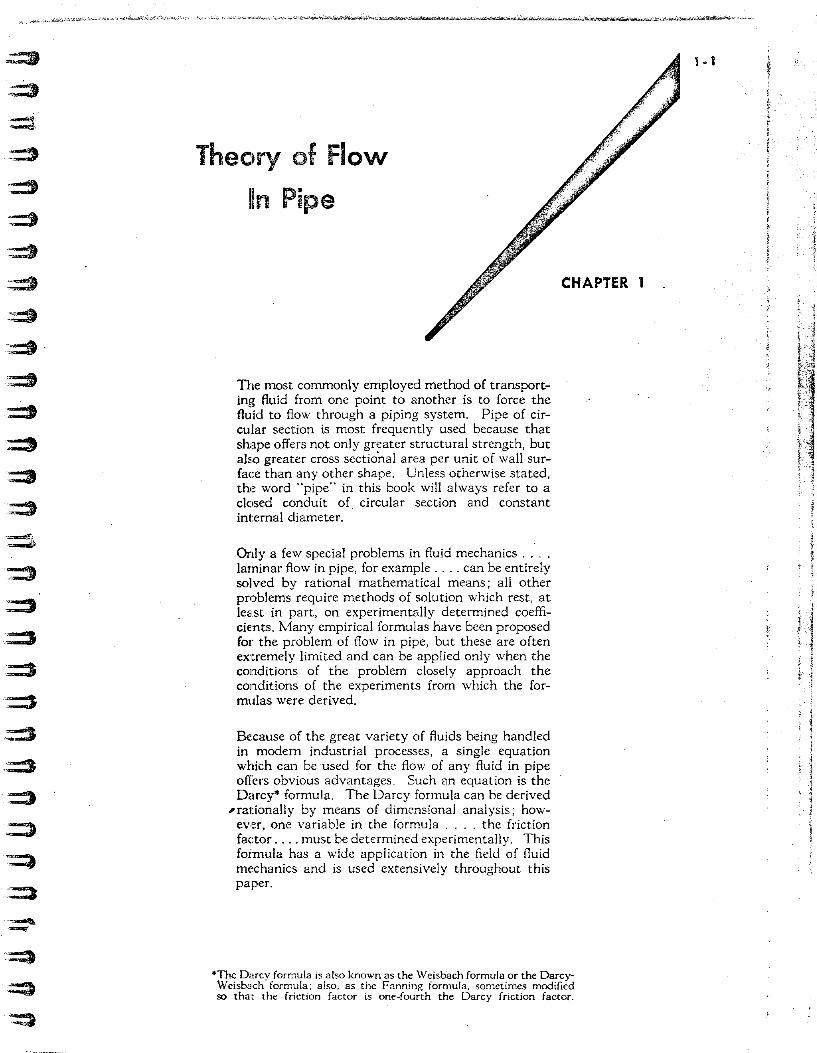
The most commonly employed method of transport­ing fluid from one point to another is to force the fluid to flow through a piping system. Pipe of cir­cular section is most frequently used because that shape offers not only greater structural strength, but also greater cross sectional area per unit of wall sur­face than any other shape. Unless otherwise stated, the word "pipe" in this book will always refer to a closed conduit of circular section and constant internal diameter.

Only a few special problems in fluid mechanics .... laminar flow in pipe, for example .... can be entirely solved by rational mathematical means; all other problems require methods of solution which rest, at least in part, on experimentally determined coeffi­cients. },,1any empirical formulas have been proposed for the problem of flow in pipe, but these are often extremely limited and can be applied only when the conditions of the problem closely approach the conditions of the experiments from which the for­mulas were derived.

Because of the great variety of fluids being handled in modern industrial processes, a single equation which can be used for the flow of any fluid in pipe offers obvious advantages. Such an equation is the Darcy* formula. The Darcy formula can be derived

'rationally by means of dimensional analysis; how­evrer, one variable in the formula .... the friction factor .... must be determined experimentally. This foimula has a wide application in the field of fluid mechanics and is used extensively throughout this paper.

CHAPTER 1

·Thc Darcy formula is also known as the \Veisbach formula or the Darcy­Wcisbach formula; also, as the Fanning formula, sometimes modified so thal~ the friction factor is one-fourth the Darcy friction factor.

1 .1

, 1 1 .~ \

1-2 CHAPTER 1 - THEORY OF flOW IN PIPE CRANE

Physical Properties of Fluids

The solution of any flow problem requires a knowl­edge of the physical properties of the fluid being handled. Accurate values for the properties affecting the flow of fluids ... namely, viscosity and weight density ... have been established by many authori­ties for all commonly used fluids and many of these data are presented in the various tables and charts in Appendix A.

Viscosity: Viscosity expresses the readiness with which a fluid flows when it is acted upon by an ex­ternal force. The coefficient of absolute viscosity or, simply, the absolute viscosity of a fluid, is a measure of its resistance to internal deformation or shear. Molasses is a highly viscous fluid; water is comparatively much less viscous; and the viscosity of gases is quite slY.all compared to that of water.

Although most fluids are predictable in their vis­cosity, in some, the viscosity depends upon the previous working of the fluid. Printer's ink, wood pulp slurries, and catsup are examples of fluids possessing such thixotropic properties of viscosity.

Considerable confusion exists concerning the units used to express viscosity; therefore, proper units must be employed whenever substituting values of viscosity into formulas. In the e.G.S. (centimeter, gram, second) or metric system, the unit of absolute viscosity is the poise which is equal to 100 centi­poise. The poise has the dimensions of dyne seconds per square centimeter or of grams per centimeter second. I t is believed that less confusion concerning units will prevail if the centipoise is used exclUSively as the unit of viscosity. For this reason, and since most handbooks and tables follow the same pro­cedure, all viscosity data in this paper are expressed in centipoise.

The English units commonly employed are "slugs per foot second" or "pound force seconds per square foot"; however, "pound mass per foot second" or "poundal seconds per square foot" may also be en­countered. The viscosity of water at a temperature of 68 F is:

fo.ol poise'

I centipoise* = 0.01 gram per cm second lo.ol dyne second per sq cm

(0.000 672 pound mass per foot second lO.OOO 6j2 poundal second per square foot

I _ {o.ooo 0209 slug per foot second p., - 0.000 0209 pound force second per square ft

Kinematic viscosity is the ratio of the absolute vis­cosity to the mass density. In the metric system, the unit of kinematic viscosity is the stoke. The stoke has dimensions of square centimeters per

second and is equivalent to 100 centistokes.

• • _ J.< (centipoise) v (centlstokes) - '( b')

p grams per cu IC cm

By definition, the specific gravity, S, in the fore­going formula is based upon water at a temperature

.of 4 C (39.2. F), whereas specific gravity used throughout this paper is based upon water at 60 F. In the English system, kinematic viscosity has dimensions of square feet per second.

Factors for conversion between metric and English system units of absolute and kinematic viscosity are given on page B-3 of Appendix B.

The measurement of the absolute viscosity of fluids (especially gases and vapors) requires elaborate equipment and considerable experimental skill. On the other hand, a rather simple instrument can be used for measuring the kinematic viscosity of oils and other viscous liquids. The instrument adopted as a standard in this country is the Saybolt Universal Viscosimeter. In measuring kinematic viscosity with this instrument, the time required for a small volume of liquid to flow through an orifice is deter­mined; consequently, the "Saybolt viscosity" of the liquid is given in seconds. For very viscous liqUids, the Saybolt Furol instrument is used.

Other viscosimeters, somewhat similar to the Saybolt but not used to any extent in this country, are the Engler, the Redwood Admiralty, and the Redwood. The relationship between Saybolt viscosity and kinematic viscosity is shown on page B-4; equiva­lents of kinematic, Saybolt Universal, Saybolt Furol, and absolute viscosity can be obtained from the chart on page B-5.

The ASTM standard viscosity temperature chart for liquid petroleum products, reproduced on page B-6, is used to determine the Saybolt Universal viscosity of a petroleum product at any temperature when the viscosities at two different temperatures are kno\\TI. The viscosities of some of the most common fluids are given on pages A-2 to A-5. It will be noted that. with a rise in temperature, the viscosity of liquids decreases, whereas the viscosity of gases increases. The effect of pressure on the viscosity of liquids and perfect gases is so small that it is of no practical interest in most flow problems. Conversely, the viscosity of saturated, or only slightly superheated. vapors is appreciably altered by pressure changes, as indicated on page A-2 showing the viscosity of steam. Unfortunately, the data on vapors are incomplete and, in some cases, contradictory. Therefore, it is expedient when dealing with vapors other than steam to neglect the effect of pressure because of [he lack of adequate data.

• Actually the viscosity of water at 68 F is 1.005 centipoise.

. .:;;='3 "'J~

,;;:::3

.:::::J

.. ~

":::=3

~

~

.~

~

:==»~

'=::.t

::;:::::)

=:3

=:)

~

::::;)

:::::» ~::::)

":::::.')

::.:::::)

.::::)

. ::::)

:.::::» ,~

"~

:=}

CRANE CHAPTER I - THEORY Of flOW IN PIPE

Physical Properties of Fluids - continued

Weight density, specific volume, and specific gravity: The weight density or specific weight of a substance is its weight per unit volume. In the English system of units, this is expressed in pounds per cubic foot and the symbol designation used in this paper is p (Rho). In the metric system, the unit is grams per cubic centimeter and the symbol designation used is p'

(Rho prime).

The specific volume V, being the reciprocal of the weight density, is expressed in the English system as the number of cubic feet of space occupied by one pound of the substance, thus;

V = .~ p

Computations in the metric system are not com­monly referred to in terms of specific volume; how­ever, the number of cubic centimeters per gram of a substance can readily be expressed as the reciprocal of the weight density, that is;

I

p'

The variations in weight density as well as other properties of water with changes in temperature are shown on page A-6. The weight densities of other common liquids are shown on page A-i. Unless very high pressures are being considered, the effect of pressure on the weight of liquids is of no practical importance in flow problems.

The weight densities of gases and vapors, however, are greatly altered by pressure changes. For the so­called "perfect" gases, the weight density can be computed from the formula;

144 P' p = f[T'

The individual gas constant R is equal to the univer­sal gas constant, AiR = 1544, divided by the molecu­lar weight of the gas,

R = 1544 M

Values of R, as well as other useful gas constants, are given on page A-8. The weight density of air for various conditions of temperature and pressure can be found on page A-ID.

In steam flow computations. the reciprocal of the weight density, which is the speCific volume, is com­monly used; these values are listed in the steam tables shown on pages A-12 to A-19. A chart for de~ termining the weight density and specific volume of gases is given on page A-II.

Specific gravity is a relative measure of weight den­sity. Since pressure has an insignificant effect upon the weight density of liquids, temperature is the only condition that must be considered in designat­ing the basis for specific gravity. The specific grav­ity of a liquid is its weight density at 60 F (unless otherwise specified) to that of water at standard temperature, 60 F.

{any liquid at 60 F, l

S = p unless otherwise specified! p (water at 60 F)

A hydrometer can be used to measure the specific gravity of liquids directly. Three hydrometer scales are common in this country .... the API scale which is used for oils .... and the two Baume scales, one for liquids heavier than water and one for liquids lighter than water. The relationship between the hydrometer scales and specific gravity are:

For oils.

S(60F/60F)

For liquids lighter than water,

S (60 F/60 F)

For liquids heavier than water.

S (60 F/60 F)

I)!.; +deg.API

140 1)0 + deg. Baume

145 145 - deg. Baume

For convenience in converting hydrometer readings to more useful units, refer to the table shown on page B-7 .

The specific gravity of gases is defined as the ratio of the molecular weight of the gas to that of air, and as the ratio of the individual gas constant of air to that of the gas.

S = R (air) _ M (gas) • R (gas) - M (air)

, !

" I !

i j

i

I i ,

,1

1 I "

1·4 CHAPTER 1 - THEORY Of flOW IN PIPE CRANE

Nature of Flow in Pipe - Laminar and Turbulent.

-"'-'--.--.-~---- ..... , .

~------ ..... ,--" .~./ ,--..; ' ... - -~ '\~- ;-'< -:. .... :.. ... -

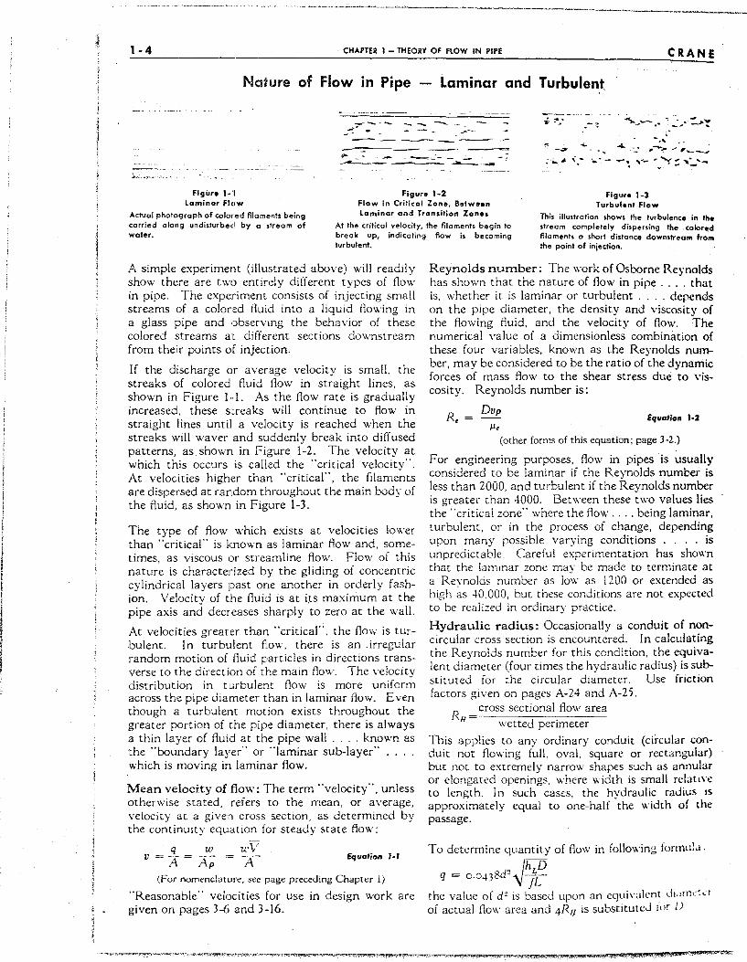
Flgu .... 1~11 Figure 1 ~2 Figur. 1.3 Laminor Flclw

Actual photograph of colored Alamenfs being carried along undisturbed by a !.treom of water.

Flow in Critical Zone, 8otw •• n Laminar and Transition Zones.

Turbulent Flow

This illustrotion shows the turbulence in th" stream completely dispersing the, colored filaments 0 short distance downstream fro", the point of injection.

At the critical velocity, the filaments begin to break up, indicating flow is becoming turbulent.

A simple experiment (illustrated above) will readily show there are two entirely different types of flow in pipe. The experiment consists of injecting small streams of a colored fluid into a liquid flowing in a glass pipe and obsel-ving the behavior of these colored streams at different sections downstream from their points of injection.

If the discharge or average velocity is small, the streaks of colored fluid flow in straight lines, as shown in Figure 1··1. As the flow rate is gradually increased, these streaks will continue to flow in straight lines until a velocity is reached when the streaks will waver and suddenly break into diffused patterns, as shown in Figure 1-2. The velocity at which this occurs is called the "critical velocity". At velocities higher than "critical"' , the filaments are dispersed at random throughout the main body of the fluid, as shown in Figure 1-3.

The type of flow which exists at velocities lower than "critical"' is known as laminar flow and, some­times, as viscous or streamline flow. Flow of this nature is characterized by the gliding of concentric cylindrical layers past one another in orderly fash­ion. Velocity of the fluid is at its maximum at the pipe axis and decreases sharply to zero at the walL

At velocities greater than "critical", the flow is tur­bulent. In turbulent flow, there is an .irregular random motion of fluid particies in directions trans­verse to the direction of the main flow. The \'elocity distribution in turbulent flow is more uniform across the pipe diameter than in laminar flow. Even though a turbulent motion exists throughout the greater portion of the pipe diameter, there is always a thin layer of fluid at the pipe wall .... known as the "boundary layer" or "laminar sub-layer" which is moving in laminar flow.

Mean velocity of flow: The term "velocity", unless otherwise stated, refers to the mean, or average, velocity at a given cross section, as determined by the continuity eq~;ation for steady state Row:

v =3.. = ~ ,= wV A Ap A Eq Clation J .. '

(For nomenclature, sec page preceding Chapter i)

"Reasonable" veiocities for use in design work are given on pages 3-6 and 3-16.

Reynolds number: The work of Osborne Reynolds has shown that the nature of Row in pipe .... that is, whether it is laminar or turbulent .... depends on the pipe diameter. the density and viscosity of the flowing fluid, and the velocity of flow. The numerical value of a dimensionless combination of these four variables, known as the Reynolds num­ber, may be considered to be the ratio of the dynamic forces of mass flow to the shear stress due to Vis­cosity. Reynolds number is:

Dvp Re = Equation 1 .. 2

(other forms of this equation; page 3-2.)

For engineering purposes, flow in pipes is usually considered to be laminar if the Reynolds number is less than 2000, and turbulent if the Reynolds number is greater than 4000. Between these two values lies the "critical zone" where the flow .... being laminar, turbulent, or in the process of change, depending upon many possible varying conditions . . . . is unpredictable. Careful experimentation has shown that the lammar zone may be made to terminate at a Reynolds number as low as 1200 or extended as high ~s 40.000, but these conditions are not expected to be realized in ordinary practice.

Hydraulic radius: Occasionally a conduit of non· circular cross section is encountered. In calculating the Reynolds number for this condition, the equiva­lent diameter (four times the hydraulic radius) is sub· stituted for the circular diameter. Use friction factors given on pages A-24 and A-25.

RH = cross sectional flow area wctted perimeter

This applies to any ordinary conduit (circular con­duit not flowing full, oval, square or rectangular) but not to extremely narrow shapes such as annular or elongated openings, where width is small relatlvc to length. In such cases, the hydraulic radius IS

approximately equal to one-half the width of the passage.

To determine quantity of flow in following forll1ui,L

/hLD q = o.o.n 8d'\j-jL

the value of d' is based upon an equivalent ,li.Hl1<·:" of actual flow area and 4RI/ is substitute,! lor I)

-:t:I

:::a :::3

.:=:1

.=­:3

-:::8

:::J

-=3

~

~

.:::1

.::::1

:::I

:::::2'

•. :::3

::::I ;:::]I

-=:I

-::;3

::::3

-:.::I

::::» ::::::I .. ::.:3

::::a ~

CRANE CHAPTER 1 - THEORY OF FLOW IN PIPE '·5

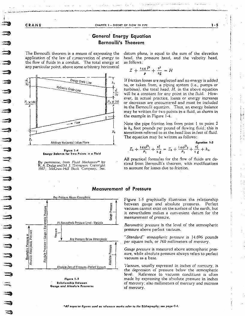
General Energy Equation Bernoulli's Theorem

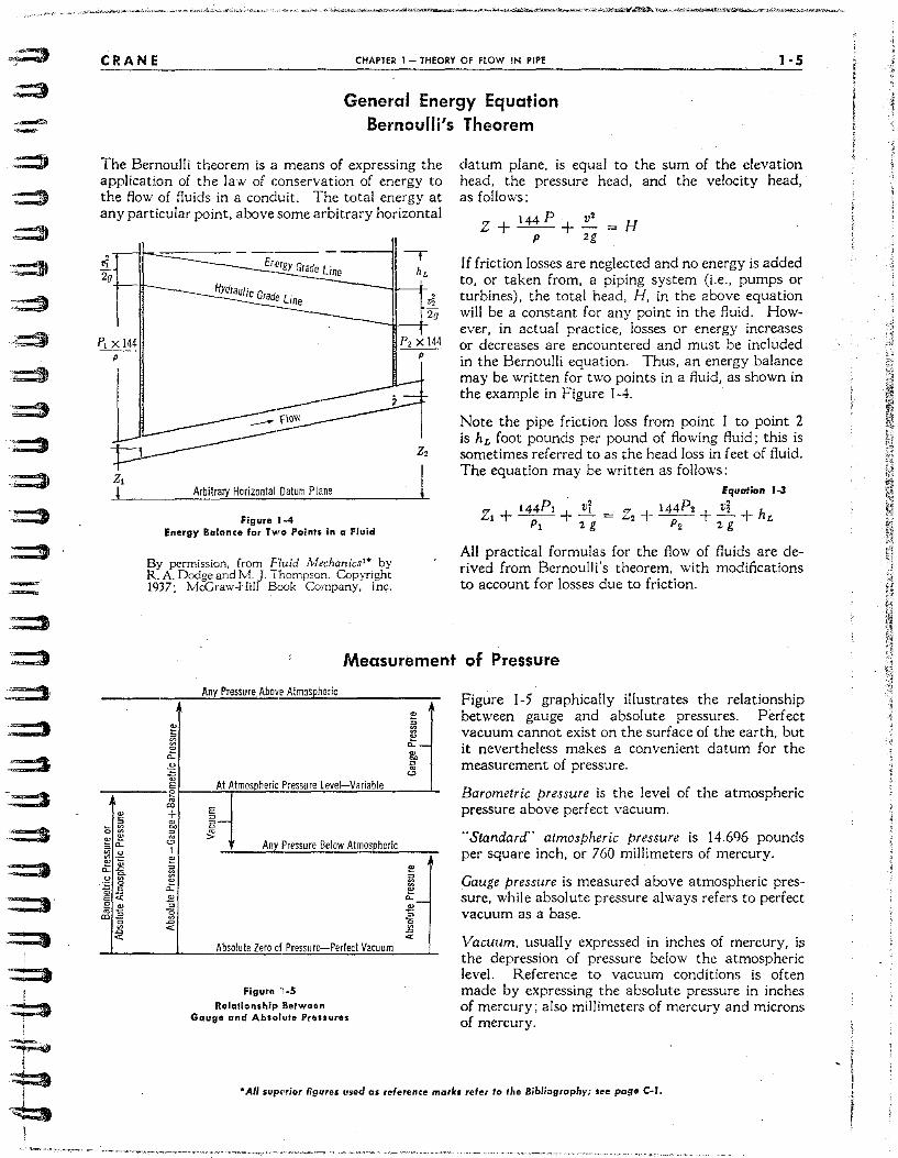
The Bernoulli theorem is a means of expressing the application of the law of conservation of energy to the flow of fluids in a conduit. The total energy at any particular point, above some arbitrary horizontal

----ll -,­Energy G fade Line hL

r~ 2g

--11--1-

Arbitrary Horizontal Datum Place

Figure 1 ~4 Energy Balance for TWI) Points ~n a Fluid

By permission. from Fll1id Mechanics'> by R. A. Dodge and M.). Thompson. Copyright 1937; McGraw-Hili Book Company, Inc.

z,

datum plane, is equal to the sum of the elevation head, the pressure head, and the velocity head, as follows:

Z + 144P + ~ = H

P 2g

If friction losses are neglected and no energy is added to, or taken from, a piping system (i.e., pumps or turbines), the total head, H, in the above equation will be a constant for any point in the fluid. How­ever, in actual practice, losses or energy increases or decreases are encountered and must be included in the Bernoulli equation. Thus, an energy balance may be written for two points in a fluid, as shown in the example in Figure 1-4.

Note the pipe friction loss from point 1 to point 2 is hL foot pounds per pound of flowing fluid; this is sometimes referred to as the head loss in feet of fluid. The equation may be written as foHows:

Equation ' .. 3

ZI + 144P , + 2i = Zz + I 44P, + ~ + hL . PI 2 g P, 2 g

All practical formulas for the flow of fluids are de­rived from Bernoulli's theorem, with modifications to account for losses due to friction .

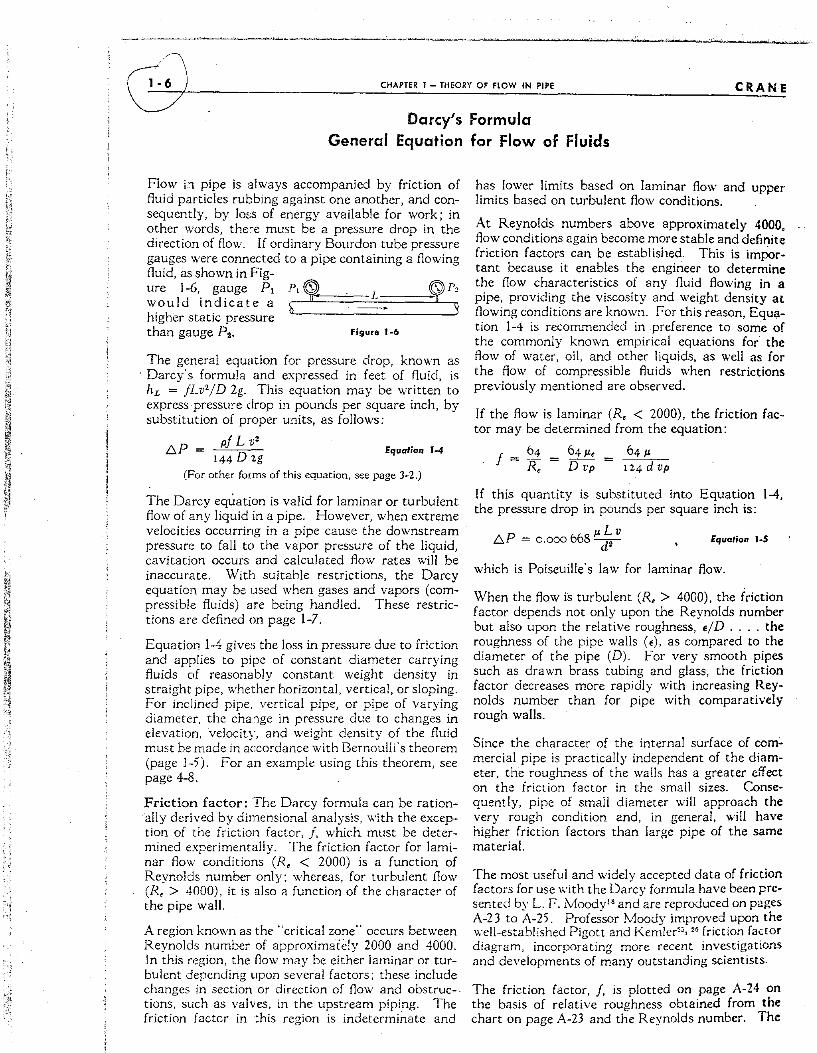
Measurement of Pressure

Any Pressure Above Atmospheric

:E v E At Atmospheric Pressure Level-Variable

~------~~--~~~~~~~~~~~~----"-OJ

+ ~ ,. "" II e tl ~

ct -~ ~

~ ~

"'"

E a-ro >

Any Pressure Below Atmospheric

I~ Absolute Zero of Pressure-Perfect Vacuum I

figure 1 ~5 Relationship B,atween

Gauge and Absolul'e Pressures

Figure 1-5 graphically illustrates the relationship between gauge and absolute pressures. Perfect vacuum cannot exist on the surface of the earth, but it nevertheless makes a convenient datum for the measurement of pressure.

Barometric pressure is the level of the atmospheric pressure above perfect vacuum.

"Standard" atmospheric pressure is 14.696 pounds per square inch, or 760 millimeters of mercury.

Gauge pressure is measured above atmospheric pres­sure, while absolute pressure always refers to perfect vacuum as a base.

Vacuum, usually expressed in inches of mercury, is the depression of pressure below the atmospheric level. Reference to vacuum conditions is often made by expressing the absolute pressure in inches of mercury; also millimeters of mercury and microns of mercury.

*Ail sl/perlor ligures used as reference morle, reler to 'he Bibliography; see page C-f.

-­.~.

>;~

.. ~

-.-

CRANE CHAPTER I - THEORY OF FLOW IN PIPE 1 ·5

General Energy Equation Bernoulli's Theorem

The Bernoulli theorem is a means of expressing the application of the law of conservation of energy to the flow of fluids in a conduit. The total energy at any particular point, above some arbitrary horizontal

.---il-'"=~-- - --- - ---11 -,-~ EC~Line hL

z, 4

HYdraulic Graoe L· ----~~-+, Ine 1."'2

Arbitrary Horizontal Datum Plane

Figure 1 .. 4

2g -_!f.--J-

Energy Balance for Two Points in a Fluid

By permission, from Fluid Nfecnanics 1* by R. A. Dodge and M. J. Thompson. Copyright 1937; McGraw-Hili B:)()k Company, Inc .

datum plane, is equal to the sum of the elevation head, the pressure head, and the velocity head, as follows:

Z + 144 P + ~ = H P ;zg

If friction losses are neglected and no energy is added to, or taken from, a piping system (Le., pumps or turbines), the total head, H, in the above equation will be a constant for any point in the fluid. How­ever, in actual practice, losses or energy increases or decreases are encountered and must be included in the Bernoulli equation. Thus, an energy balance may be written for two points in a fluid, as shown in the example in Figure 1-4.

Note the pipe friction loss from point to point 2 is hL foot pounds per pound of flowing fluid; this is sometimes referred to as the head loss in feet of fluid. The equation may be written as follows:

Equation 1-3

Z, + 144P, + .EL = z. + 144P. + vi + hL P, 2 g p. 2 g

All practical formulas for the flow of fluids are de­rived from Bernoulli's theorem, with modifications to account for losses due to friction.

~easurement of Pressure

Any Pressure Above Atmospheric Figure 1-5 graphically illustrates the relationship between gauge and absolute pressures. Perfect vacuum cannot exist on the surface of the earth, but it nevertheless makes a convenient datum for the measurement of pressure . . g .,

~ _______ §r-__ ~At~Aft~mo~s~Dh~e~ric~P~r~es~su~r~e~Le~ve~I-~va~r~iab~le~ ____ ~ Barometric pressure is the level of the atmospheric pressure above perfect vacuum.

~ co + ~ ~ ~ ~

'" II

E

B­~

Any Pressure Below Atmospheric

Absolute Zero of Pressure-Perfed Vacuum

Figure 11-5

Relationship Berween Gauge and Absolute Pressures

"Standard'· atmospheric pressure is 14.696 pounds per square inch, or 760 millimeters of mercury.

Gauge pressure is measured above atmospheric pres­sure, while absolute pressure always refers to perfect vacuum as a base.

Vacuum, usually expressed in inches of mercury, is the depression of pressure below the atmospheric level. Reference to vacuum conditions is often made by expressing the absolute pressure in inches of mercury; also millimeters of mercury and microns of mercury.

"'All supElrior figu,'es used as reference maries refer'o the Bibliography; see page C.J.

I , - I

I I

, '1

~~ __________________________ C~H~A~PT~E~R~l ___ T~H~E~O~RY~O~F~Fl~O~W~IN~P~IP~E ________________________ ~C~R~A~N~E Darcy's Formula

General Equation for Flow of Fluids

Flow in pipe is always accompanied by friction of fluid particles rubbing against one another, and con­sequently, by loss of energy available for work; in other words, there must be a pressure drop in the direction of flow. If ordinary Bourdon tube pressure gauges were connected to a pipe containing a flowing fluid, as shown in Fig-ure 1-6, gauge PI would indicate a higher static pressure than gauge p •.

L

Figure 1 .. 6

The general equlltion for pressure drop, known as , Darcy's formula and expressed in feet of fluid, is hL = fLv 2/D 2g. This equation may be written to express pressure drop in pounds per square inch, by substitution of proper units, as follows:

pf L ;~. l::.P = ---- Equation 1-4

144 D 2g

(For other forms of this equation, see page 3-2.)

The Darcy equation is valid for laminar or turbulent flow of any liquid in a pipe. However, when extreme velocities occurring in a pipe cause the downstream pressure to fall to the vapor pressure of the liquid, cavitation occurs and calculated flow rates will be inaccurate. With suitable restrictions, the Darcy equation may be used when gases and vapors (com­pressible fluids) are being handled. These restric­tions are defined on page 1-7.

Equation 1-4 gives the loss in pressure due to friction and applies to pipe of constant diameter carrying fluids of reasonably constant weight density in straight pipe, whether horizontal, vertical, or sloping. For inclined pipe, vertical pipe, or pipe of varying diameter, the change in pressure due to changes in elevation, velocity, and weight density of the fluid must be made in accordance with Bernoulli's theorem (page 1-5). For an example using this theorem, see page 4-8.

Friction factor: The Darcy formula can be ration­'ally derived by dimensional analysis, with the excep­tion of the friction factor, f, which must be deter­mined experimentally. The friction factor for lami­nar flow conditions (R, < 2000) is a function of Reynolds number only; whereas, for turbulent flow CR, > 4000), it is also a function of the character of the pipe wall.

A region known as the "critical zone" occurs between Reynolds number of approximately 2000 and 4000. In this region, the flow may be either laminar or tur­bulent depending upon several factors; these include changes in section or direction of flow and obstruc-. tions, such as valves, in the upstream piping. The friction factor in this region is indeterminate and

has lower limits based on laminar Rowand upper limits based on turbulent flow conditions. .

At Reynolds numbers above approximately 4000, flow conditions again become more stable and definite friction factors can be established. This is imPor­tant because it enables the engineer to determine the flow characteristics of any fluid Rowing in a pipe, providing the viscosity and weight density at flowing conditions are known. For this reason, Equa­tion 1-4 is recommended in preference to some of the commonly known empirical equations for the flow of water, oil, and other liquids, as well as for the flow of compl'essible fluids when restrictions previously mentioned are observed.

If the flow is laminar (R, < 2000), the friction fac­tor may be determined from the equation:

f = 64 = 64 Il, = 64 Il R, D vp 124 d vp

If this quantity is substituted into Equation 1-4, the pressure drop in pounds per square inch is:

. IlLv l::.P = 0.000668 (j'l Equation 1-5

which is Poiseuille's law for laminar flow.

When the flow is turbulent (R, > 4000), the friction factor depends not only upon the Reynolds number but also upon the relative roughness, E/D .... the roughness of the pipe walls (E), as compared to the diameter of the pipe (D). For very smooth pipes such as drawn brass tubing and glass, the friction factor decreases more rapidly with increasing Rey­nolds number than for pipe with comparatively rough walls.

Sinc€' the character of the internal surface of com­mercial pipe is practicai!y independent of the diam­eter, the roughness of the walls has a greater effect on the friction factor in the small sizes. Conse­quently, pipe of smail diameter will approach the very rough condition and, in general, will have higher friction factors than large pipe of the same material.

The most useful and widely accepted data of friction factors for use with the Darcy formula have been pre­sented by L. F. Moody" and are reproduced on pages A-23 to A-25. Professor Moody improved upon the well-established Pigott and Kemler", 26 friction factor diagram, incorporating more recent investigations and developments of many outstanding scientists.

The friction factor, j, is plotted on page A-24 on the basis of relative roughness obtained from the chart on page A-23 and the Reynolds number. The

~~

:::::;

::3 =:)

,:::,)

-;:)

~

.~

~

.~

':)

-:)

-::)

,~:j

CRANE CHAPTER I - THEORY OF flOW IN PIPE

Darcy's Formula General Equation for Flow of Fluids - continued

value of f is determined by horizonta I projection from the intersection of the d D curve under considera­tion with the calculated Reynolds number to the left hand vertical scale of the chart on page A-23. Since most calculations involve commercial steel or wrought iron pipe, the chart on page A-25 is furnished for a more direct solution. I t should be kept in mind that these figures apply to clean new pipe.

Effect of age and use on pipe friction: Friction loss in pipe is sensitive to changes in diameter and roughness of pipe. For a given rate of flow and a fixed friction factor, the pressur.e drop per foot of. pipe varies inversely with the fifth po\\-er of the diameter. Therefore, a 2% reduction of diameter

causes a 10o/c increase in pressure drop; a 59c reduc­tion of diameter increases pressure drop 23 S~. In many services. the interior of pipe becomes encrusted with scale. dirt, tubercules or other foreign matter; thus, it is often prudent to make allowance for ex­pected diameter changes.

Authorities' point out that roughness may be ex­pected to increase with use (due to corrosion or incrustation) at a rate determined by the pipe material and nature of the fluid. Ippen'B, in discuss­ing the effect of aging, cites a 4-inch galvanized steel pipe which had its roughness doubled and its friction factor increased 20'70 after three years of moderate use.

Principles of Compressible Flow in Pipe

An accurate determination of the pressure drop of a compressible fluid flowing through a pipe reqUires a knowledge of the relationship between pressure and specific volume; this is not easily determined in each particular problem. The usual extremes con­sidered are adiabatic flow (p'V:~ = constant) and iso­thermal flow (p'Va = constant). Adiabatic flow is usually assumed in short, perfectly insulated pipe. This would be consistent since no heat is transferred to or from the pipe, except for the fact that the minute amount of heat generated by friction is

.added to the flow.

Isothermal flow or flow at constant temperature is often assumed, partly for convenience but more often because it is closer to fact in piping practice. The most outstanding case of isothermal flow occurs in natural gas pipe lines. Dodge and Thompson! show that gas flow in insulated pipe is closely approximated by isothermal flow for reasonably high pressures.

Since the relationship bet\\'een pressure and volume may follow some other relationship (p'V: = con­stant) called polytropic flow, specific information in each individual case is almost a::1 impossibility.

The density of gases and vapors changes considerably

with changes in pressure; therefore, if the pressure drop between PI and p, in Figure 1-6 is great, the density and velocity will change appreciably.

When dealing with compressible fluids, such as air, steam, etc., the following restrictions should be observed in applying the Darcy formula:

1. If the calculated pressure drop (PI - P,) is less than about 10% of the inlet pressure PI, reason­able accuracy will be obtained if the specific volume used in the formula is based upon either the upstream or downstream conditions, which­ever are known.

2. If the calculated pressure drop (PI - P,) is greater than about 10%, but less than about 40% of inlet pressure PI, the Darcy equation may be used with reasonable accuracy by using a specific volume based upon the average of upstream and dO\\'nstream conditions: otherwise, the method given on page l-q may be used.

3. For greater pressure drops, such as are often encountered in long pipe lines. the methods given on the next two pages should be used. '

(cont;nued on the next page)

, ,

1-8 CHAPTER I - THEORY OF flOW IN PIPE CRANE

Principles of Compressible Flow in Pipe (continued)

Complete isothermal equation: The flow of gases in long pipe lines closely approximates isothermal con­ditions. The pressure drop in such lines is often large relative to the inlet pressure, and solution of this problem falls outside the limitations of the Darcy equation. An accurate determination of the flow characteristics falling within this category can be made by using the complete isothermal equation:

Equation J·6

] [(P;)' ;;; (P~)']

The formula is developed on the basis of these assumptions:

I. Isothermal flow. 2. No mechanical work is done on or by the system. 3. Steady flow or discharge unchanged with time. 4. Tne gas obeys the perfect gas laws. 5. The velocity may be represented by the average

velocity at a c.ross section. 6. l1t1e friction fa.ctor is constant along the pipe. 7. The pipe line is straight and horizontal between

end points.

Simplified Compressible Flow-Gas Pipe Line Formula: In the practice of gas pipe line engineer­ing, another assumption is added to the foregoing:

8. Acceleration can be neglected because the pipe line is long.

Then, the formula for discharge in a horizontal pipe may be written:

w2 = 1 2 Equation 1-1 [

144 g DN] [(P')' - (P')'] hfl. Pi

This is equivalent to the complete isothermal equa­tion if the pipe line is long and also for shorter lines if the ratio of pressure drop to initial pressure is small.

Since gas flow problems are usualiy expressed in terms of cubic feet per hour at standard conditions, it is convenient to rewrite Equation 1-7 as follows:

~i[(p't)' - (P")'] d.' q' h = 1 14.2 - Equafion J-7a . f l.m T S,

Other commonly used formulas for compress­ible flow in long pipe lines:

Weymouth formula": Equation l-a

I _ 8 d,.m '[(PII)' - (PI,),] 520 q • - 2 .0 " S. l... T

Panhandle formula' for natural gas pipe lines 6 to 2-!-inch diameter, Reynolds numbers 5 x 10' to 14 x 10', and S, = 0.6:

Equation ,'O,

[(P\l' - (PI,),] 0.5394 q'. = ,6.8 E ,p."" l.rn-

The flow efficiency factor E is defined as an expe­rience factor and is usually assumed to be 0.92 or 92% for average operating conditions. Suggested values for E for other operating conditions are given on page 3-3.

Comparison of formulas for compressible flow in pipe lines: Equations 1-7, 1-8, and 1-9 are de­rived from the same basic formula, but differ in the selection of data used for the determination of the friction factors.

Friction factors in accordance with the t-..loodv" dia­gram are normally used with the Simplified Com­pressible Flow formula (Equation 1-7). However, if the same friction factors employed in the IVeymouth or Panhandle formulas are used in the Simplified formula, identical answers will be obtained.

The Weymouth friction factor" is defined as:

f = 0.03 2

d1/'

This is identical to the Moody friction factor in the fully turbulent flow range for 20-inch 1.D. pipe only. Weymouth friction factors are greater than Moody factors for sizes less than 20-inch, and smaller for sizes larger than 20-inch.

The Panhandle friction factor' is defined as:

( d )0.,451

f= 0.1225 ----s q h 9

In the flowTange to which the Panhandle formula is limited, this results in friction factors that are lower than those obtained from either the Moody data or the Weymouth friction formula. As a result, flow rates obtained bv solution of the Panhandle formula are usuaily great~r than those obtained by employing either the Simplified Compressible Flow formula with Moody friction factors, or the Weymouth formula.

An example of the variation in flow rates which may be obtained for a specific condition by employing these formulas is given on page 4-11 ..

·.~

.• ::;:::::J

~

.,:t

.=t .=3

~

::=J

::J

.::::J

.:=J

=:.1

==» .=.::t

.::::)

::::!)

:::::::::»

:::"J

~

.:=2

-, .-.

CRANE CHAPTER 1 - THEORY OF flOW IN PIPE 1 - 9

Principles of Compressible Flow ill Pipe (continued)

Limiting flow of gases and vapors: The feature not evident in the preceding formulas (Equations 1-4 and 1-6 to 1-9 inclusive) is that the weight rate of flow (e.g., Ibs/sec) of a compressible fluid in a pipe, with a given upstream pressure, will approach a cer­tain maximum rate which it cannot exceed, no mat­ter how much the dowmtream pressure is further reduced.

The maximum velocity of a compressible fluid in pipe is limited by the velocity of propagation of a pres­sure wave which travels at the speed of sound in the fluid. Since pressure falls off and velocity in­creases as fluid proceeds downstream in pipe of uni­form cross section, the mc:ximum velocity occurs in the downstream end of the pipe. If the pressure drop is sufficiently high, the exit velocity will reach the velocity of sound. Further decrease in the out­let pressure will not be fdt upstream because the pressure wave can only travel at sonic velocity, and the "signal" will never translate upstream. The "surplus" pressure drop obtained by lowering the outlet pressure after the maximum discharge has already been reached takes place beyond the end of the pipe. This pressure is lost in shock waves and turbulence of the jetting fluid.

The maximum possible velDcity in the pipe is sonic velocity, which is expressed as:

Equation r -1 0

v, = .,JkgRT = .,Jkgl44P'V

The value of k, the ratio of specific heats at con­stant pressure to constant volume, is 1.4 for most diatomic gases; see pages A-8 and A-9 for values of k for gases and steam respectively. This velocity will occur at the outlet end or in a constricted area, when the pressure drop is sufficiently high. The pressure, temperature, and ;;pecific volume are those occurring at the point in question. When com­pressible fluids discharge from the end of a reasonably short pipe of uniform cross section into an area of larger cross section, the flow is usually considered to be adiabatic. This assumption is supported by ex­perimental data on pipe having lengths of 220 and 130 pipe diameters discharging air to atmosphere. Investigation of the complete theoretical analysis of adiabatic flow!' has led to a basis for establishing correction factors, which may be applied to the Darcy equiltion for this condition of flow. Since these correction factors compensate for the changes in fluid properties due to expansion of the fluid, they are identified as Y net expansion factors; see page A-22.

The Darcy formula, including the Y factor, is:

Equation l .. JJ

(Resistance coefficient K is defined on page 2·8)

It should be noted that the value of K in this equa­tion is the total resistance coefficient of the pipe line, including entrance and exit losses when they exist, and losses due to valves and fittings.

The pressure drop, i'c,p. in the ratio i'c,P/P', which is used for the determination of Y from the charts on page A-22, is the measured difference between the inlet pressure and the pressure in the area of larger cross section. In a system discharging compressible fluids to atmosphere, this i'c,P is equal to the inlet gauge pressure, or the difference between absolute' inlet pressure and atmospheric pressure. This value of i'c,P is also used in Equation I -11, whenever the Y factor falls within the limits defined by the re­sistance factor K curves in the charts on page A-n. When the ratio of i'c,P / P' 1, using i'c,P as defined above, falls beyond the limits of the K curves in the charts, sonic velocity occurs at the point of discharge Of at some restriction within the pipe, and the limit­ing values for Y and i'c,P, as determined from the tabulations to the right of the charts on page A-22, must be used in Equation 1-1 I.

Application of Equation 1-11 and the determination of values for K, Y, and i'c,P in the formula is demon­strated in examples on pages 4-13 and 4-14.

The charts on page A-22 are based upon the general gas laws for perfect gases and, at sonic velocity conditions at the outlet end, will yield accurate results for all gases which approximately follow the perfect gas laws. Steam and vapors deviate from the perfect gas laws, and application of the Y factor obtained from the charts to these flows, will there­fore yield flow rates slightly greater (up to about 5 %) than those calculated on the basis of sonic velocity at the outlet. However, greater accuracy will be obtained if the charts are used to establish the downstream pressure when sonic velocity occurs, and the fluid properties at this pressure condition are used in the sonic velocity and continuity equa­tions (Equations 3 -8 and 3-2 respectively) to de­termine the flow rate. An example of this type of {Jow problem is presented on page 4-13.

This condition of flow is comparable to the flow through nozzles and venturi tubes, covered on page 2-15, and the solutions of such problems are similar.

-1

. ,

I , ! i

I I I ~ ~:

~ ~ ! ~.

1 1

! 1 -

1 !

1 • 10 CHAPTER 1 - THEORY OF FlOW IN PIPE CRANE

Steam

General Discussion

Substances exist in anyone of three phases .... solid, liquid, or gas. \Vhen outside conditions are varied, they may change from one phase to another.

Water under normal atmospheric conditions exists in the form of a liquid. When a body of water is heated by means of some external medium, the tem­perature 'of the water rises and soon small bubbles, which break and form continuously, are noted on the surface. Th:s phenomenon is described as "boiling".

The amount of heat necessary to cause the tempera­ture of the water to rise is expressed in British Ther­mal Units (Btu), where, I Btu is the quantity of heat required to raise the temperature of one pound of water from 60 to 61 F. The amount of heat neces­sary to raise the temperature of a pound of water from 32 F (freezing point) to 212 F (boiling point) is ISO.I Btu. When the pressure does not exceed 50 pounds per square inch absolute, it is usually per­missible to assurr.e that each temperature increase of 1 F represents a heat content increase of one Btu per pound, regardless of the temperature of the water.

Assuming the generally accepted reference plane for zero heat content at 32 F, one pound of water at 212 F contains ISO.17 Btu. This quantity of heat is called heat of the liquid or sensible heat. In order to

change the liquid into a \'apor at atmospheric pres­sure (14.7 psia), 970.3 Btu must be added to each pound of \\'ater after the temperature of 212 F is reached. During this transition period. the tem­perature remains constant. The added quantity of heat is called the latent heat of erapuralioll. Conse­quently, the total heat of the \'apor, formed when water boils at atmospheric pressure, is the sum of the two quantities .... ISO. I Btu and 970.3 Btu, or, 1150.5 Btu per pound.

If water is heated in a closed vessel not completely filled, the pressure will rise after steam begins to form accompanied by an increase in temperature.

Saturated steam is steam in contact with liquid water from which it was generated, at a tempera­ture which is the boiling point of the water and the condensing point of the steam. It may be either "dry" or "wet", depending on the generating can· ditions. "Dry" saturated steam is steam free from mechanically mixed water particles. "Wet" satu­rated steam, on the other hand, contains \\'ater Darticles in suspension. Saturated steam at any pressure has a definite temperature.

Superheated steam is steam at any given pressure which is heated to a temperature higher than the temperature of saturated steam at that pressure.

r­r-3

C=:J

-=3

tr-:3

~~~

.d

~

8:::J

~

a:::)

~

-=::J ~~-~

.::::')

~ i 1

It.."":l

t:::)

.:::;)

L-:;)

II:::::.:)

e=:,)

a::::) e::=l

~

I!'.~

.~

//"'~"-------~ // Flow of Fluids

(Through Valves and Fittings)

'~---------

The preceding chapter has been devoted to the theory and formulas used in the study of fluid flow in pipes. Since industrial installations usually con­tain a considerable number of valves and fittings, a knowledge of their resistance to the flow of fluids is necessary to determine the flow characteristics of a complete piping system.

Many texts on hydraulics contain no information on the resistance of valves and fittings to flow, while others present only a limited discussion of the sub­ject. In realization of the need for more complete detailed information on the resistance of valves and fittings to flow, Crane Co. has conducted extensive tests in their Engineering Laboratories and has also sponsored investigations in other laboratories. These tests have been supplemented by a thorough study of all published data on this subject. Appendix A contains data from these many separate tests and the findings have been combined to furnish a basis for calculating the pressure drop through valves and fittings.

Representative resistances to flow of various types of piping components are given on pages A-26. A-27, and A-30. For conversion of "equivalent length in pipe diameters", as obtained from page A-27 or A-30, to "equivalent length in feet of pipe" for any size of valve or fitting, see page A-31. The chart on page A-31 also illustrates the correlation of equivalent length, resistance coefficient K, and pipe size. A chart is presented on page A-32 which may be used to readily determine the C" flow coefficient of any valve for which the resistance coeffIcient is known or can be determined from page A-30 and page A-31.

A discussion of the eqUivalent length and resistance coefficient K, as well as the flow coefficient Cv meth­ods of calculating pressure drop through valves and fittings is presented on pages 2-8 and 2-9.

2·1

CHAPTER 2

2-2 CHAPTER 2 - FLOW OF flUIDS THROUGH VALVES AND FITTINGS CRANE

Types of Valves and Fittings Used in Pipe Systems

Valves: Although the great variety of valve designs precludes any t'lorough classification, most of the designs may be considered as modifications of the two basic types:

I. the gate type 2. the globe type

If valves were classified according to the resistance which they offer to flow, the gate type valves would be put in the low resistance class and the globe type valves in the high resistance class. The classi­fIcation is not all-inclusive, however, because a large number of modified valve types fall between the two extremes. :lome of the most commonly used valve designs are illustrated on pages A-28 and A-29.

Fittings: Fittings may be classified as branching, reducing, eXf'anding, or deflect ing. Such litt in.!.;, as tees, crosses, side outlet elbows, etc., may be called branching fittings.

Reducing or expanding fittings are those which change the area of the fluid passageway. In this class are reducers and bushings. Deflecting fittings ..... bends, elbo\\'s, return bends, etc ... , . are those which change the direction of flow.

Some fittings, of course, may be combinations of any of the foregoing general ~lassifications. In addi­tion, there are types such as couplings and unions which offer no appreciable resistance to flow and, therefore, need not be considered here.

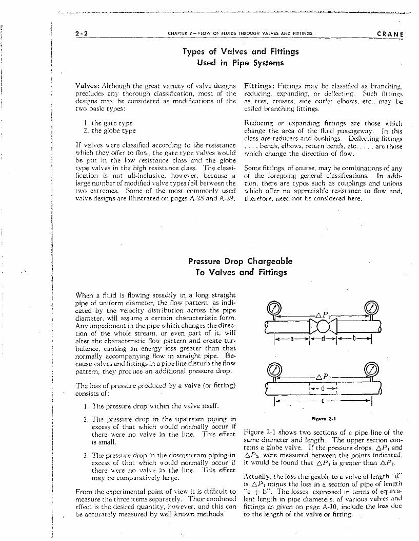
Pressure Drop Chargeable To Valves and Fittings

When a fluid is flowing steadily in a long straight pipe of uniform diameter, the flow pattern, as indi­cated by the velocity distribution across the pipe diameter, will assume a certain characteristic form. Any impediment in the pipe which changes the direc­tion of the whole stream, or even part of it, will alter the characteristic flow pattern and create tur­bulence, causing an energy loss greater than that normally accomp;mying flow in straight pipe. Be­cause valves and fir:tings in a pipe line disturb the flow pattern, they produce an additional pressure drop.

The loss of pressure produced by a val ve (or fitting) consists of:

I. The pressure drop within the valve itself.

2. The pressure drop in the upstream piping in excess of that which would normally occur if there were no valve in the line. This effect is small.

3. The pressure drop in the downstream piping in excess of tha'~ which would normally occur if there were no valve in the line. This effect may be comparatively large.

From the experimental point of view it is difficult to measure the three il:ems separately. Their combined effect is thc desired quantity, howe vcr, and this can be accurateiy measured by well known methods.

4---------C--------~

Figure 2-1 shows two sections of a pipe line of the same diameter and length. The upper section con­tains a globe valve. If the pressure drops, D.P. and D.P" were measured between the points indicated. it would be found that D.P, is greater than D.P,.

Actually, the loss chargeable to a valve of length "d" is D.P. minus the loss in a section of pipe of length "a + b". The losses, expressed in terms of equi\'a lent length in pipe diameters, of various val\'es and fittings as given on page A-30, include the loss due to the iength of the valve or fitting.

i •.. t::J

.. ~

±::)

b ~I I

,:::;) i

,:=) ,

,~

;~

:r ::::.1 -II> iiti' ..g

~-)

~

!i' )

.~

~ ~:)

CRANE CHAPTER 2 - flOW QF flUIDS THROUGH VALVES AND FITIINGS 2-3

Crane Flow Tests

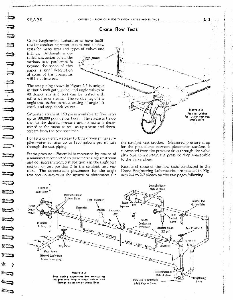
Crane Engineering Laboratories have facili­ties for conducting water, steam, and air flow tests for many sizes and types of valves and fittings. Although a de­tailed discussion of all the various tests performed is beyond the scope of this paper, a brief description of some of the apparatus will be of interest.

The test piping shown in Figure 2-3 is unique in that 6-inch gate. globe. and angle valves or 90 degree ells and tees can be tested with either water or steam. The vertical leg of the angle test section permits testing of angle lift check and stop check valves.

Saturated steam at 150 psi is available at flow rates up to 100,000 pounds pe~ rour. The steam is throt­tled to the desired pressure and its state is deter­mined at the meter as well as upstream and down­stream from the test specimen.

For tests on water, a steam turbine driven pump sup­plies water at rates up to 1200 gallons per minute through the test piping.

Static pressure differential is measured by means of a manometer connected to piezometer rings upstream and downstream from test position 1 in the angle test section, or test position 2 in the straight test sec­tion. The downstream piezometer for the angle test section serves as the upstream piezometer for

Exhaust to Atmosphele

\ Water Header

(Meteled Supply flam tumine dliven pump)

Figura 2-3 Test piping apparatus for measuring the pressure drop thrQugh valves and

nnlngs on sfoam or water lines.

-'-~,~"'-"C"'''-'

Figure 2-2 Flow test piping

for 12-inch cast steel angle valve

the straight test section. Measured pressure drop for the pipe alone between piezometer stations is subtracted from the pressure drop through the valve plus pipe to ascertain the pressure drop chargeable to the valve alone.

Results of some of the flow tests conducted in the Crane Engineering Laboratories are plotted in Fig­ures 2-4 to 2-7 shown on the two pages following.

Elbow Can Be Rotated to ________ " " Admit Water Of Steam

r ~ ~~

} .;;.

" F I i ,

f;

r ;;" r: E

2-4

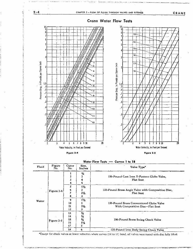
Fluid

Water

CHAPTER 2 - flOW OF flUIDS THROUGH VALVES AND FITTINGS

Crane Water Flow Tests

1~ r:~:=ll::::~:r I:;" =l1::If==l::;:=l=;:::::7.I'M IrL~-:;~ 8~4-~~4-+-~ji+--r-r+-r+--~/~//'~~~

I ; I I II//!/illl ! IIII VIJLJ,

I I ~ i IJIL /1/1111

! I I NIl 1///111 3~~-+i+l+i+-~~H&VW,~~~~~-;

3 IXII V;{riv/ I '" "I'

fhVl 1 (;)

2 3 4 5678910 20

Water Velocity, in Feet per Second

Figure 2 ... 4

Woter Flow Tests FigurE'

No. Curve

No.

I 2 3 4

S

Size, I Inches

% 2 4 6 111.

1 I 1/ II II I 1/ 'II I I I I I

2 V VI II V

2 3 678910

Water Velocity, in Feet per Second

Figure 2 .. 5

Curves 1 to 18

Valve Tl:'pe*

ISO-Pound Cast Iron Y-Pattern Globe Valve, Flat Seat

Figure 2-4 6 2 ISO-Pound Brass Angle Valve with Composition Disc, 7 2% Flat Seat 8 3

9 Ill.

I 10 2 ISO-Pound Brass Conventional Globe Valve 11 2% With Composition Disc-Flat Seat 12 I 3 I

I 13 % 14 II.

figure 2··5 15 3,4 2oo-Pound Brass Swing Check Valve 16 11,4 17 2 18 I 6 ! US-Pound Iron Body Swing Check Valve I

CRANE

*Exccpt for check valves at lower velocities where curves (l4 to 17) bend, all valves were .tested with disc fully lifted.

-~

:::::t

·~I

.=:11

~

:.:3

~

•.. :::J

.==.)

-==:.::)

-=:)

=::)

-;:::)

::::::l)

.. -:::::;)

::::)

.. :=)

,.:.::::)

:::::)

.~

::::.)

~

-~

::::::)

CRANE CHAPTER 2 - flOW OF FLUIDS THROUGH VALVES AND FITTINGS

Crane Steam Flow Tests

3 i /, V tJ ",f

1"24

!Ii /1 V " '" 4 I I il II. !"

-5 .:;

LO 9 8 7 6

5

4

3

2! gl .2 = ~ ~

'" " ~ o "­.: ~ .0 c .0

~ .0 ~ a: .0

I 9 8 7 6

.0 5

.04

.0 3

.0 2V

,

L

IL

V I

V L 1/

1/1/

il Vv

.L

If

j

V

V

,

I I

.1 /

.L L i/~

!J ~ .1

V

Ii v / .L

I. i/ L

1L':::::::' V II

.L "-V / '" 1/

I l.'f-L~V--LI ~~,L.-"-i --:'::--'---:: 3 4 6 7 8 S 10 20 30

I .0 3 45678910

.1.1

.1 I

I / 'I

.L .L 1.

.L .L L

k' L ' 27

1

~ t-2sl

.:':::, 29

"', 30

~ 1 ....... 31

20 30 Steam Velocity, in·ThoLisands of Feet per Minute Steam Velocity, ifl Thousands of Feet per Minute

Fluid Figure No.

Figurn 2 .. 6

CUrvl~ No.

Stearn Flow T esfs

Size, I' Inches

Figure 2-7

Curves 19 to 31

Valve' or Fitting Type

2-5

19 2 loo-Pound Brass Conventional Globe Valve ............. Plug Type Seat

20 6 300-Pound Steel Conventional Globe Valve ............. Plug Type Seat

21 6 lOO-Pound Steel Angle Valve ........................... Plug Type Seat

21 6 [ lOO-Pound Steel Angle Valve ......................... Ball to Cone Seat Figure 2-6

23 I 6 GOO-Pound Steel Angle Stop-Check Valve Saturated 24 G GOO-Pound Steel Y-Pattern Globe Stop-Check Valve Steam

I 25 G GOO-Pound Steel Angle Valve

50 psi 26 I) 600-Pound Steel Y-Pattern Globe Valve gauge

27 2 90° Short Radius Elbow for Use with Schedule 40 Pipe

18 (; 250-Pound Cast Iron Flanged Conventional 90° Elbow

Figure 2-7 29 I) GOO-Pound Steel Gate Valve

30 6 125-Pound Cast Iron Gate Valve

31 6 ISO-Pound Steel Gate Valve

'Except for check valves at lower velocities where curves (23 and 24) bend, all valves were tested with disc fully lifted.

..

J

I 1 j

j i

2-6 CHAPTER 2 - flOW OF flUIDS THROUGH VALVES AND FITTINGS

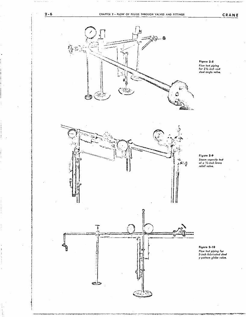
Figure 2.8 Flow test piping for 2 V:z -inch corl steel ongle valve.

Figure 2 ... 9

CRANE

Steam capacity feft of a V:z-inch bra" relief yalve.

Figure 2-10 Flow fest piping lor 2-inch fabricaled steel y-pattern globe valve.

...• » ,. ,.

;;:::j

'~

. ::::::)

.~

. ~

:=3

==:3

"":::)

'=::t .=:)

:.=)

.=)

.:::::;)

.=:)

==» :::::'»

::::3

:::::::)

-:::::)

~

--

CRANE CHAPTER 2 -- flOW OF flUIDS THROUGH VALVES AND FlTIlNGS 2-7

Relatiionship of Pressure Drop to Velocity of Flow

Many experiments have shown that the head loss due to valves and fittings is proportional to a constant power of the velocity. When pressure drop or head loss is plotted against velocity on logarithmic co­ordinates, the resulting curve is therefore a straight line. In the turbulent flow range, the value of the exponent of v has been fm;nd to vary from about 1.8 to 2.1 for different designs of valves and fittings. However, for all practical purposes, it can be as­sumed that the pressure drop or head loss due to the flow of fluids in the turbulent range through valves and fittings varies as the square of the velocity .

This relationship of pressure drop to velocity of flow is valid for check valves, only if there is suffi­cient flow to hold the disc in a wide open position . The point of deviation of the test curves from a straight line, as illustrated in Figures 2-5 and 2-6, defines the flow conditions necessary to support a check valve disc in the wide open position.

Most of the difficulties encountered with check valves, both lift and swing types, have been found to be due to oversizing which results in noisy operation and premature wear of the moving parts. Referring again to Figure 2-6, it will be noted :hat the pressure drop, at the point where the two curves representing check valves deviate from a straight line, is about 1 Yz to 2 pounds per square inch. This value will vary somewhat for different valve designs depending upon the relative weight and size of the disc; however, it has been found to be a good "rule of thumb" to size check valves so that the pressure drop in the fully open position is about 2 psi in lift checks and about Yz psi in swing checks. This rule applies only to check valves designed on the basis of estab­lished fundamental considerations which assure a

Figure 2-12

full disc lift at low flow rates. On some poorly designed lift check valves, tests have shown that the disc will not lift fully even at extremely high flow rates. In many cases, application of this rule will result in check valves smaller in size than the pipe line; however, the actual pressure drop will be little, if any, higher than that of a full size valve which is used in other than a wide open position.

The losses due to sudden contraction and enlarge­ment which will occur in such an installation with bushings or reducing flanges can be readily calculated from the data given on page A-26. if tapered reduc­ers are used, the loss due to gradual contraction at the inlet to the smaller size valve is partially com­pensated for by the corresponding gradual enlarge­ment on the outlet side, so that the added pressure drop due to these effects is minor.

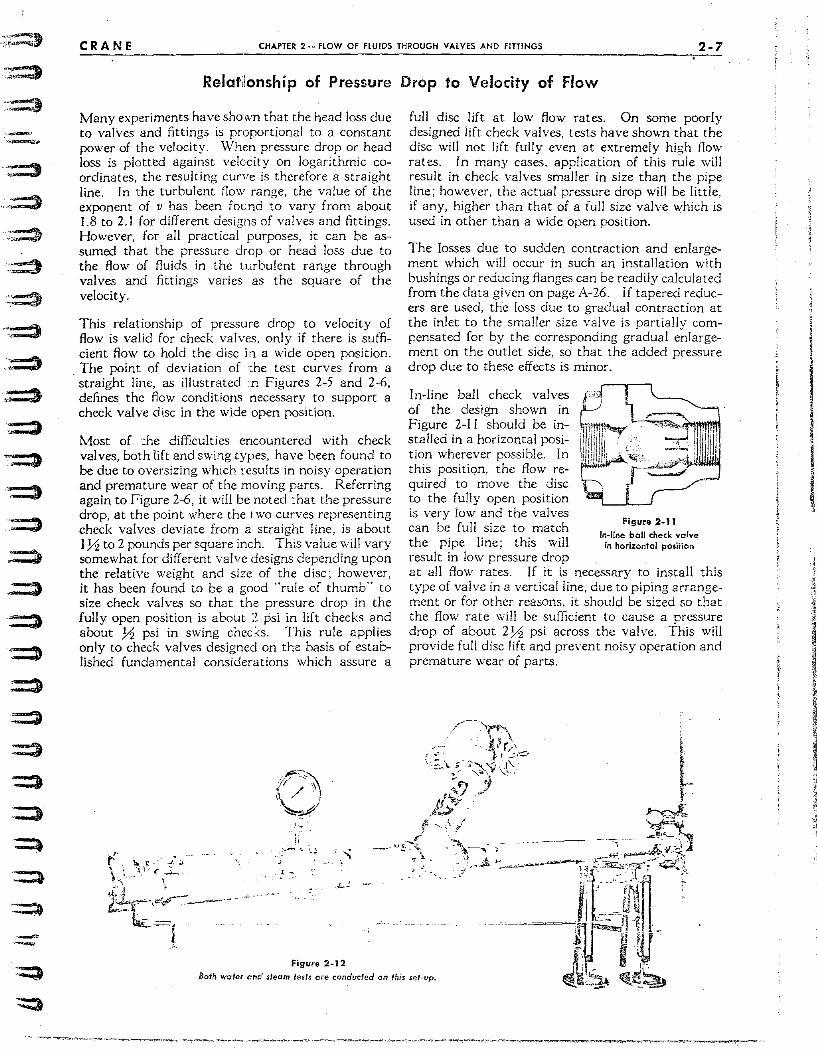
In-line ball check valves of the design shown in Figure 2-11 should be in­stalled in a horizontal posi­tion wherever possible. In this position, the flow re­quired to move the disc to the fully open position is very low and the valves can be full size to match the pipe line; this will result in low pressure drop

Figure 2.11 In· line ball check valve

in horizontal position

at all flow rates. If it is necessary to install this type of valve in a vertical line, due to piping arrange­ment or for other reasons, it should be sized so that the flow rate will be sufficient to cause a pressure drop of about 2Yz psi across the valve. This will provide full disc lift and prevent noisy operation and premature wear of parts.

, '

Both woter and steam fests ore conducted on this set-up.

2-8 CHAPTER 2 - FLOW OF FLUIDS THROUGH VALVES AND FITTINGS CRANE

Resistance Coefficient K, Equivalent length L/D, And Flow Coefficient Cv

The numerous types of valves and fittings and the great variety of service conditions make it virtually impossible to obtain test data on every size and type of valve and fitting used today. For this reason, it is desirable to find a means for utilizing the limited test data which are available. Several methods of accomplishing this have been devised; the most commonly used are the "equivalent length", .. resistance coefficient", and' 'flow coefficient".

Velocity in a pipe is obtained at the expense of static head, and decrease in static head due to velocity is:

v' h =-, 2g

which is defined as the "velocity head". Flow through a valve or fitting in a pipe line also causes a reduction in stati.C head which may be expressed in terms of velocity head. The resistance coefficient K in the equation

v' hL = K - , Equation 2-2 2g

therefore, is defined as the number of velocity heads lost due to the valve or fitting. Also, the same head loss in straight pipe is expressed by the Darcy equation

hL=(ii;)~ Equation 2 .. 3

I t follows that,

K = (it) Equation 2-4

The ratio LID is the equivalent length in pipe diam­eters of straight pipe which will cause the same pressure drop as the valve under the same flow

12-IHCH SIZE 1/6 SCALE (>'

conditions.

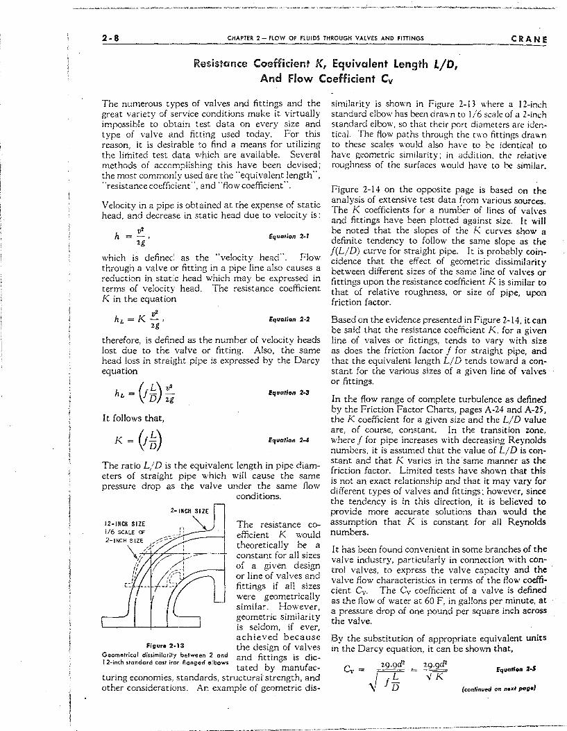
The resistance co­efficient K would theoretically be a constant for all sizes of a given design or line of valves and fittings if all sizes were geometrically similar. However, geometric simiiarity is seldom, if ever, achieved because

Figure 2-13 the design of valves Geometrical dis.similarity between 2 and and fittings is dic-12-inch standard cast iror:, flanged elbows

tated by manufac-turing economies, standards. structural strength, and other considerations. An example of geometric dis-

similarity is shown in Figure 2-13 where a 12-inch standard elbow has been drawn to 1/6 scale of a 2-inch standard elbow. so that their port diameters are iden­tical. The flow paths through the two fittings drawn to these scales would also have to be identical to have geometric similarity; in addition. the relative roughness of the surfaces would have to be similar.

Figure 2-14 on the opposite page is based on the analysis of extensive test data from various sources. The K coefficients for a number of lines of valves and fittings have been plotted against size. I t will be noted that the slopes of the K curves show a definite tendency to follow the same slope as the I(LID) curve for straight pipe. It is probably coin­cidence that the effect of geometric dissimilarity between different sizes of the same line of valves or fittings upon the resistance coefficient K is similar to that of relative roughness, or size of pipe, upon friction factor.

Based on the evidence presented in Figure 2-14, it can be said that the resistance coefficient K, for a given line of valves or fittings, tends to vary with size as does the friction factor I for straight pipe, and that the equivalent length LID tends toward a con­stant for the various sizes of a given line of valves or fittings.

In the flow range of complete turbulence as defined by the Friction Factor Charts, pages A-24 and A-25, the K coefficient for a given size and the LID value are, of course, constant. In the transition zone, where I for pipe increases with decreasing Reynolds numbers, it is assumed that the value of LID is con­stant and that K varies in the same manner as the friction factor. Limited tests have shown that this is not an exact relationship and that it may vary for different types of valves and fittings: however, since the tendency is in this direction, it is believed to provide more accurate solutions than would the assumption that K is constant for all Reynolds numbers.

It has been found convenient in some branches of the valve industry, particularly in connection with con­trol valves, to express the valve capacity and the valve flow characteristics in terms of the flow coeffi­cient Cy . The Cy coefficient of a valve is defined as the flow of water at 60 F, in gallons per minute, at a pressure drop of one pound per square inch across the valve.

By the substitution of appropriate equivalent units in the Darcy equation, it can be shown that,

C _ 29·9cl' _ 29·9cl'

y - ~ It - -vI< Equallo. 2-5

' .. ~

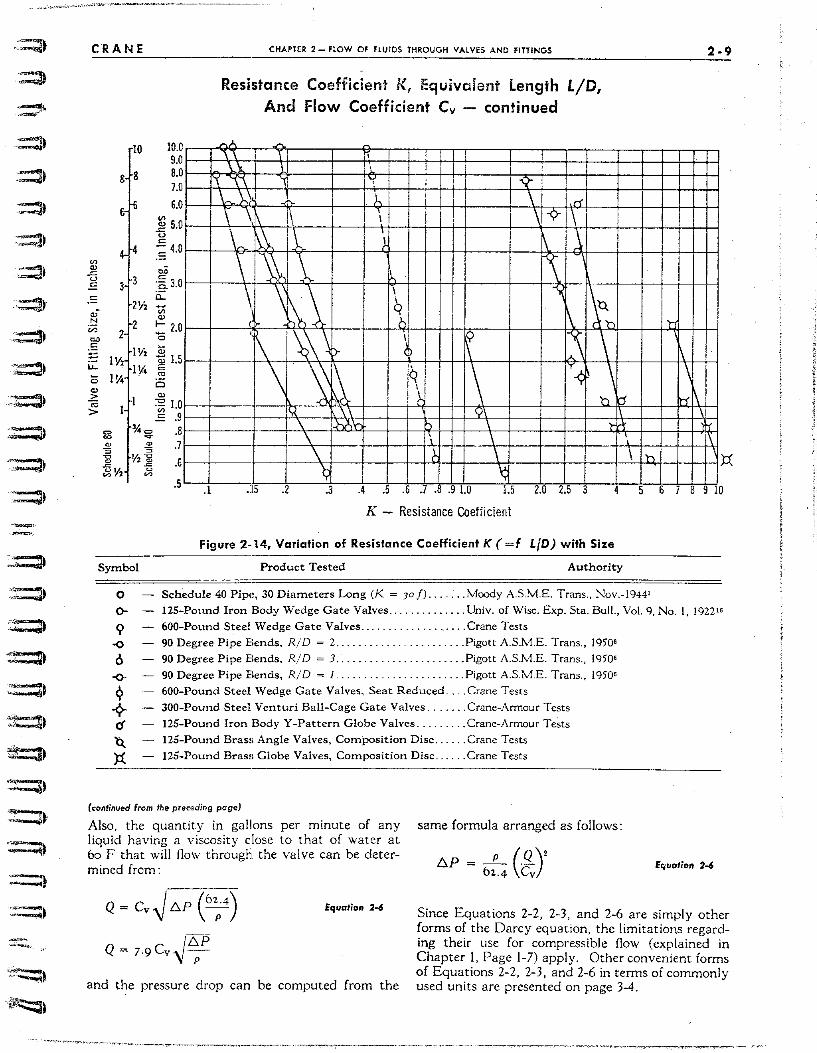
.:=J~

.~.

;;::)

';:dI

::::::)

--

CRANE

Symbol

o 0-

9 -0

6 -0-

9 -¢­cf Q. )::(

CHAPTER 2 - fLOW OF fLUIDS THROUGH VALVES AND FITTINGS

Resistance Coefficient f{, Equivalent length l./D, And Flow Coefficient Cy - continued

K - Resistance Coefficient

Figure 2-14, Variation of Resistance Coefficient K (=f L{D) with Size

Product Tested Authority

Schedule 40 Pipe, 30 Diameters Long (K = 30 f) .... : . . Moody AS.M.E. Trans., Nov.-1944'

2·9

125-Pound Iron Body Wedge Gate Valves .............. Univ. of Wise. Exp. Sta. Bull., Vol. 9, No. I, 1922"

600-Pound Steel Wedge Gate Valves ................... Crane Tests

90 Degree Pipe Bends, RID = 2 ....................... Pigott AS.M.E. Trans., 1950'

90 Degree Pipe Bends, R/D = 3 ....................... Pigott AS.M.E. Trans., 1950'

90 Degree Pipe Bends, R/D = 1 ....................... Pigott A.S.ME. Trans., 1950'

600-Pound Steel Wedge Gate Valves, Seat Reduced .... Crane Tests

JOO-Pound Steel Venturi Ball-Cage Gate Valves ....... Crane-Armour Tests

125-Pound Iron Body Y-Pattern Globe Valves ......... Crane-Armour Tests

125-Pound Brass Angle V a1 yes, Composition Disc ...... Crane Tests

125-Pound Bras!: Globe Valves, Composition Disc .... .. Crane Tests

(toflfinued from the preceding page)

Also, the quantity in gallons per minute of any liquid having a viscosity close to that of water at 60 F that will flow through the valve can be deter­mined from:

Equation 2-6

and the pressure drop can be computed from the

same formula arranged as follows:

/::,.p=- -P (Q)' 62-4 Cv

Equatjon 2-6

Since Equations 2-2, 2-3, and 2-6 are simply other forms of the Darcy equation, the limitations regard­ing their use for compressible flow (explained in Chapter I, Page 1-7) apply. Other convenient forms of Equations 2-2, 2-3, and 2-6 in terms of commonly used units are presented on page 3-4.

2 - 10 CHAPTER 2 - flOW OF flUIDS THROUGH VALVES AND fITTINGS CRANE -----

Relath)t1Ship of Equivalent length 1./D and Resistance Coefficient K To Inside Diameter of Connecting Pipe

Tests have shown that the pressure drop due to a given va!\'e or titting does not change when the product is installed with pipe of the same nominal size but of differem thickness, Small variations in entrance and exit losses caused by mating the valve ends to \'ariable pipe thicknesses, within reasonable limits, are insignitlcant. Since the pressure drop is a function of the square of the velocity, and velocity is a function of the square of the internal diameter, it follows that the equivalent length of a given valve or fItting, expressed in terms of the pipe to which it is connected, varies as the fourth power of the in­ternal diameter (If the pipe, For example, if the equivalent length of a ! i-inch valve is determined by test to be 100 pipe diameters of Schedule 80 pipe, its equi\'alent length will be 169 diameters of Sched­ule 40 pipe, since the ratio of the inside diameters of the twO pipes to the fourth power is 1.69, This ratio, of course, varies with the different sizes and thicknesses of pipes.

In vie\\' of this condition, the Crane Engineering Laboratories have established the practice of making all flow tests with pipe having internal diameters normally used with the particular valve or fitting. For this purpose, pipe normally used with the various pressure classes of valves and fittings has been arbi­trarily established in accordance with the table shown at the top of page A-30.

Computation of pressure drop using equivalent length data established on the ba;;is of this tai'k should be made USing pipe dimensions specified on pages B-IO to B-19; for installation conditions not in agreement with the table. the eLJui"aknt length In pipe diameters. should be multiplied by the ratIo of diameters to the fourth power.

( L ) ( L) (da)' - - - Equatiolt 2 .. 7

DaD • ,db Subscript "a" dcfmes the eLJuivalcnt lengths \\'ith reference to the internal diameter of the plpC in which the \'alve \\'i11 be installed.

Subscript "b" defines the known equi\'alent fengths and internal diameters of the pipe for which these equivalent lengths were established.

This procedure of obtaining equl\'alent length data with respect to pipe of various internal diameters corrects a signifIcant variable that has often been neglected in translating tcst data and makes pos­~ible a more accurate prediction of the 110w charac­teristics of untested valves and fittings by comparison of detail dimensions and shapes with tested items.

Resistance coefficient K can be calculated for the pipe in \\'hich the valve will be installed byemploy-

ing the formula Ka = fa (~ ) .. or expressed in termS of .

resistance coefficients, the formula may be written: Ka= K. (X) (~:)'

Valves with Gradually Increased Ports

Various types of valves are often made with reduced seats and have uniformly tapered ports, Straight­through \'alves such as gate, ball, plug, and conduit types when so designed are sometimes referred to as venturi or reduced seat valves, The added resistance in these valves, due to the tapered sections from port size to seat size to port size, exceeds that of the straight-through port" valve with correction for flow resistance based on Equation 2-7, for included venturi angles of 20 degrees or less with seat to port ratio of

diameters less than 0.8, Equation 2-7 yields reason­ably accurate results for included venturi angles of 7 degrees or less and \\'ith a ratio of seat to port diam­eters greater than 0.8, In globe and angle type valves where the loss through the seat section is high with respeer to the loss through the venturi ends, Equation 2-7 may be used with reasonable accuracy for included venturi angles up to 20 degrees and for seat to port ratios of diameters greater than 0.7.

Effect of End Connections

Before the advent of full port straight-through ball, plug, and conduit type \'alves, the losses due to end connections \\'ere inSignificant with respect to the over-all loss through the valve, This is still true for higher resistance val Yes, Where the flo\\' resistance of a valve in pipe diameters is equal to its end-to-end

dimension, small additional losses should be computed since they may add Significantly to the over-all valve's loss, I n screwed end val ves, the losses due to sudden enlargements and contractions (page A-26) may be a signifIcant part of the total loss, especially in the small er sizes.

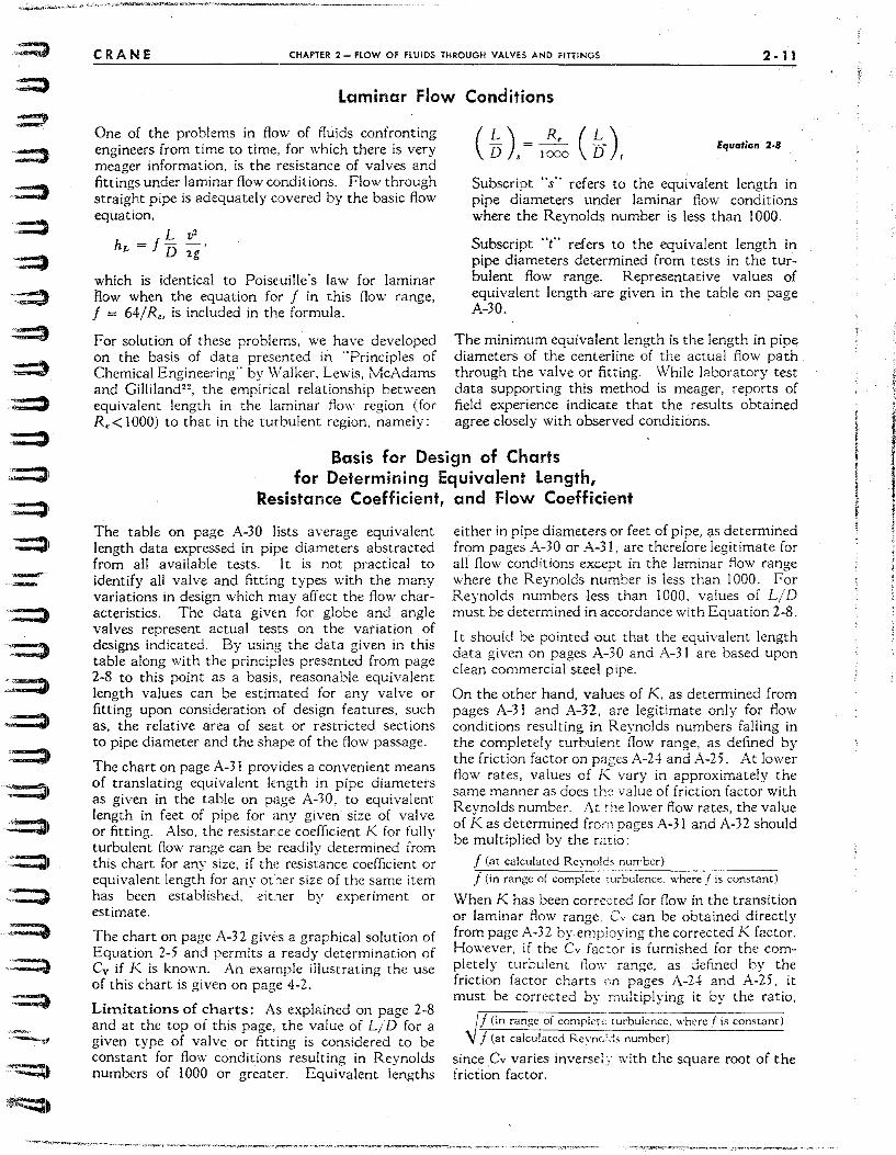
:::::::3 .==:)

.. ::::)

. :=

.-. . ::=.:)

':::::)

.~

. .=:::)

=:)

:::::II

':: :II

=1 ::::)

~I

CRANE CHAPTER 2 - FLOW OF flUIDS THROUGH VALVES AND FITTINGS 2 - 11

Laminar Flow Conditions

One of the problems in flow of fluids confronting engineers from time to time .. for which there is very meager information, is the resistance of valves and fittings under laminar flow conditions. Flow through straight pipe is adequately c~vered by the basic flow equation,

L v' hL = I D zg'

which is identical to Poiseuille's law for laminar Row when the equation for I in this flow range, I = 64/ R" is included in the formula.

For solution of these problems, we have developed on the basis of data presented in "Principles of Chemical Engineering" by Walker, Lewis, McAdams and Gilliland", the empirical relationship between equivalent length in the laminar flo\\' region (for R, < 1000) to that in the turbulent region. namely:

Subscript "s" refers to the equivalent length in pipe diameters under laminar flow conditions where the Reynolds number is less than 1000.

Subscript .. t'. refers to the equivalent length in pipe diameters determined from tests in the tur­bulent flow range. Representative values of equivalent length are given in the table on page A-30.

The minimum equivalent length is the length in pipe diameters of the centerline of the actual flow path through the valve or fitting. \Vhile laboratory test data supporting this method is meager, reports of field experience indicate that the results obtained agree closely with observed conditions .

Basis for Design of Charts for Determining Equivalent Length,

Resistance Coefficient, and Flow Coefficient

The table on page A-30 lists average equivalent length data expressed in pipe diameters abstracted from all available tests. It is not practical to identify all valve and fitting types with the many variations in design which may affect the flow char­actenstlCS. The data given for globe and angle valves represent actual tests on the variation of designs indicated. By using the data given in this table along with the principles presented from page 2-8 to this point as a basis, reasonable equivalent length values can be estimated for any valve or fitting upon consideration of design features, such as, the relative area of sea.t or restricted sections to pipe diameter and the shape of the flow passage.

The chart on page A-3! provides a convenient means of translating equivalent length in pipe diameters as given in the table on page A-30, to equivalent length in feet of pipe for any given size of valve or fitting. Also, the resistar:.ce coefficient K for fully turbulent flow range can be readily determined from this chart for any size, if the resistance coefficient or equivalent length for any other size of the same item has been established, eit~er by experiment or estimate.

The chart on page A-32 givi:s a graphical solution of Equation 2-5 and permits a readv determination of Cy if K is known. An example i-i1ustrating the use of this chart is given on page 4-2.

Limitations of charts: As explained on page 2-8 and at the top of this page, the value of L;D for a given type of valve or fitting is considered to be constant for flow conditions resulting in Reynolds numbers of 1000 or greater. Equivalent lengths

either in pipe diameters or feet of pipe, <;is determined from pages A-30 or A-3J, are therefore legitimate for all flow conditions except in the laminar flow range where the Reynolds number is less than 1000. For Reynolds numbers .Jess than 1000, values of L/ D must be determined in accordance with Equation 2-8 .

[t should be pointed out that the equivalent length data given on pages A-30 and A-31 are based upon clean commercial steel pipe.

On the other hand, values of K, as determined from pages A-31 and A-32, are legitimate only for flow conditions resulting in Reynolds numbers falling in the completely turbulent flow range, as defined by the friction factor on pages A-24 and A-25. At lower flow rates, values of K vary in approximately the same manner as does tlo;, value of friction factor with Reynolds number. At the lower flow rates, the value of K as determined from pages A-31 and A-32 should be multiplied by the raja:

I (at calculated Rcynoks number)

----------------f (in range of complete turbulence, where f is constant)

When K has been corre~t.ed for flow in the transition or laminar flow range, Cv can be obtained directly from page A-32 by employing the corrected K factor. However, if the Cv factor is furnished for the com­pletely turbulent flow range, as defined by the friction factor charts on pages A-24 and A-25, it must be corrected by multiplying it by the ratio,

I f (in range of complct~ turbulence. where f is constant)

'\J I (at calculated Rc\'nG'~ls number)

since Cv varies inverse1:; with the square root of the friction factor.

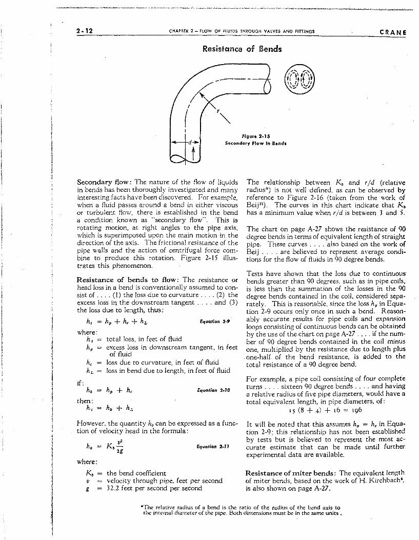
I !

I

2" 12 CHAPTER 2 - flOW OF FlUIDS THROUGH VALVES AND FITTINGS CRANE

Resistance of Bends

Figure 2-15

5Qcondory Flow In Bands

Secondary flow: The nature of the flow of liquids in bends has been thoroughly investigated and many interesting facts have been discovered. For example, when a fluid passes around a bend in either viscous or turbulent flow, there is established in the bend a condition known as ··secondary flow'·. This is rotating motion, at right angles to the pipe axis, which is superimposed upon the main motion in the direction of the axis. The frictional resistance of the pipe walls and the action of centrifugal force com­bine to produce this rotation. Figure 2-15 illus­trates this phenomenon.

Resistance of bends to flow: The resistance or head loss in a bend is conventionally assumed to con-sist of .... (I) the loss due to curvature .... (2) the excess loss in the downstream tangent .... and (3) the loss due to length, thus:

h, = h. + h, + hL Equation 2-9

where: h, h.

if: h.

then:

total loss, in feet of fluid excess loss in downstream tangent, in feet of fluid

loss due to curvature, in feet of fluid loss in bend due to length, in feet of fluid

Equation 2-JO

h, = h. + h"

However, the quantity h. can be expressed as a func­tion of velocity head in the formula:

v' h. = K.-2g

where:

the bend coefficient

Equation 2-J J

K. v g

velocity through pipe, feet per second 32.2 feet per second per second

The relationship between K, and rid (relative radius*) is not well defined, as can be observed by reference to Figure 2-16 (taken from the work of Beij2I). The curves in this chart indicate that K. has a minimum value when rid is between 3 and 5.

The chart on page A-27 shows the resistance of 90 degree bends in terms of equivalent length of straight pipe. These curves .... also based on the work of Beij .... are believed to represent a\·erage condi­tions for the flow of fluids in 90 degree bends.

Tests have shown that the loss due to continuous· bends greater than 90 degrees. such as in pipe coils, is less than the summation of the losses in the 90 degree bends contained in the coil, considered sepa­rately. This is reasonable. since the loss hp in Equa­tion 2-9 occurs only once in such a bend. Reason­ably accurate results for pipe coils and expansion loops consisting of continuous bends can be obtained by the use of the chart on page A-27 .... if the num­ber of 90 degree bends contained in the coil minus one, multiplied by the resistance due to length plus one-half of the bend resistance, is added to the total resistance of a 90 degree bend.

For example, a pipe coil consisting of four complete turns .... sixteen 90 degree bends .... and having a relative radius of five pipe diameters, would have a total equivalent length, in pipe diameters, of:

15 (8 + 4) + 16 = 196

I t will be noted that this assumes hp = he in Equa­tion 2-9; this relationship has not been established by tests but is believed to represent the most ac­curate estimate that can be made until further experimental data are available.

Resistance of miter bends: The equivalent length of miter bends, based on the work of H. Kirchbach', is also shown on page A-27.

"The relative radius of a bend is the ·ratio of the radius of the bend axis to the intemal diameter of the pipe. Both dimensions must be in the same units ..

~

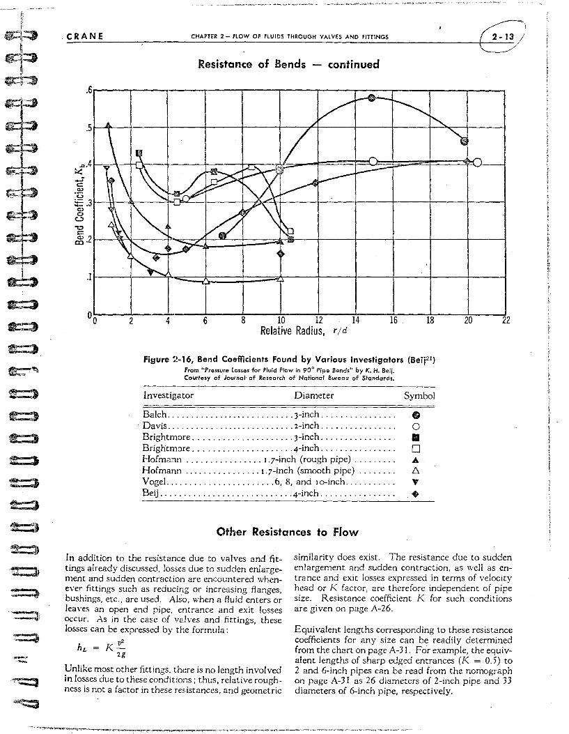
.b ~3

t=:)

c:=:;,

t=:t

c,:- ~I

CRANE CHAPTER 2 - FLOW OF flUIDS THROUGH VALVES AND FITTINGS

Resistance of Bends - continued

.6r----,----,-----r----,----.-----r----.--~---r----,----.----~

I A /V -

°O~--~2----~4-----6~--~8----~1~O----~12~--~14~--~1~6----~18~--~2~O--~22

Relative Radius, rjd

Figure ~!-16, Bend Coefficients Found by Various Investigators (BeW') From "Pressu.re Losses for Fluid Flow in 90° Pipe Bends" by K. H. Ber;. Courtesy of Journal' of Research of National Bureau of Standards.

Investigator Diameter

Balch ... , ....................... 3-inch ............... . . Davis ........................... 2-inch ............... .

Brightmore ..................... 3-inch ............... . Brightmore ..................... 4-inch ............... . Hofmann ................. 1.7-inch (rough pipe) ........ . Hofmann ............... , 1.7-inch (smooth pipe) ....... . VogeL ...................... 6, 8, and lO-inch .......... . Beij ............................ 4-inch ............... .

Other Resistances to Flow

Symbol

• o II o it.. 6. T

+

In addition to the resistance due to valves and fit­tings already discussed, losses due to sudden enlarge­ment and sudden contraction are encountered when­ever fittings such as reducing or increasing flanges, bushings, etc., are used. Also, when a fluid enters or leaves an open end pipe, entrance and exit losses occur. As in the case of VE:lves and fittings, these losses can be expressed by the formula:

similarity does exist. The resistance due to sudden enlargement and sudden contraction, as well as en­trance and exit losses expressed in terms of velocity head or K factor, are therefore independent of pipe size. Resistance coefficient K for such conditions are given on page A-26.

EqUivalent lengths corresponding to these resistance coefficients for any size can be readily determined from the chart on page A-31. For example, the equiv­alent lengths of sharp edged entrances (K = 0.5) to 2 and 6-inch pipes can be read from the nomograph on page A-3J as 26 diameters of 2-inch pipe and 33 diameters of 6-inch pipe, respectively.

hL = K!!... 2g

Unlike most other fittings. there is no length involved in losses due to these conditions; thus, relative rough­ness is not a factor in these resistances, and geometric

2 -14 CHAPTER: 2 - FLOW OF flUIDS THROUGH VALVES AND FITIINGS CRANE

Flow Through Nozzles and Orifices

The discharge of fluids through nozzles and orifices has been subject to continued investigation and, as a result, well-established data are still being supplemented. A portion of the subject is co\'ered on these faCing pages but more complete references will be found in the Bib­liography" " lO, or from the data supplied by meter manufacturers.

The rate of flow of any fluid through an orifice or nozzle, neglecting the velocity of approach, may be expressed by:

Equation 2-J2

Velocity of approach may have considerable effect on the quantity discharged through a nozzle or orifice. The factor correcting for velocity of approach,

may be incorporated in Equation 2-12 as follows:

CdA .,--q = -;====; 'V 2g hL Equation 2.13

~I-(~:y The quantity

is defined as the flow coefficient C. Values of C for nozzles and orifices are shown on page A-20. Use of the flow coefficient C eliminates the necessity for calculating the velocity of approach, and Equation 2-13 may now be written:

Orifices and nozzles are normally used in piping sys­tems as metering devices and are installed with flange taps or pipe taps in accordance with ASME specifications. The values of hL and D.P in Equation 2-14 are the measured differential static head or pressure across flange taps when values of Care taken from page A-20. The flow coefficient C is plotted for Reynolds numbers based on the internal diameter of the upstream pipe.

Flow of liquids: For nozzles and orifIces discharg­ing incompressible fluids to atmosphere, C values may be taken from page A-20 if hL or !';P in Equa­tion 2- I 4 is taken as the upstream head or gauge pressure. f'or most conditions of flow of fluids hav-

ing a low viscosity, i.e., water, gasoline. etc., the Reynolds number need not be calculated since it will fall in the range of the values on page A-20, where the flow coefficient C is a constant.

Flow of gases and vapors: The flow of compres­sible fluids through nozzles and orifices can be ex­pressed by the same equation used for liquids except the net expansion factor Y must be included.

Equa/;on 2-15

The expansion factor Y is a function of:

I. The specific heat ratio, k. 2. The ratio of orifice ot throat diameter to inlet

diameter.

3. Ratio of downstream to upstr.eam absolute pressures.

This factor"lO has been experimentally determined on the basis of air, which has a specific heat ratio of 1.4, and steam having specific heat ratios of approx­imately 1.3. The data is plotted on page A-21 and values of other specific heat ratios have been included to extend the use of the data. Values of k for some of the common vapors and gases are given on pages A-8 and A-9. The specific heat ratio, k, may vary slightly for different pressures and temperatures, but for most practical problems the values given will provide reasonably accurate results.

Equation 2-15 may be used for orifices discharging com;xessible fluids to atmosphere by using:

I. Flow coefficient C given on page A-20 in the Reynolds number range where C is a constant for the given diameter ratio.

2. Expansion factor Y per page A-21.

3 . Differential pressure !,;P, equal to the inlet gauge pressure.

This also applies to nozzles discharging compressible fluids to atmosphere only if the absolute inlet pres­sure is less than the absolute atmospheric pressure divided by the critical pressure ratio r,; this is discussed on the next page. When the absolute inlet pressure is greater than this amount, flow through nozzles should be calculated as outlined on the following page.

---c:='lll

":;::3

.~

:.:=:11

~.

. ~

.::::J

=::3

::=::J

=:t

-:::::'J

:::::)

::::::)

=.t

=:a ::::=)

=l . '=:)

~'~

:::)

CRANE CHAPTER 2 - flOW OF flUiDS THROUGH VALVES AND FITIINGS 2 -15

Flow Through Nozzles and Orifices - continued

Maximum flow of compressible fluids in a noz­zle: A smoothly convergent nozzle has the property of being able to deliver a compressible fluid up to the velocity of sound in its minimum cross section or throat, providing the available pressure drop is sufficiently high. Sonic velocity is the maximum velocity that may be attained in the throat of a nozzle (supersonic vel.ocity is attained in a gradually

, divergent section fo.llowin,c; the convergent nozzle, when sonic velocity exists In the throat),

The critical pressure ratio is the largest ratio of downstream pressure to upstream pressure capable of producing sonic velOCity. Values of critical pres­sure ratio r" which depend upon the ratio of nozzle diameter to upstream diameter as well as the specific heat ratio k, are given on page A-21 .

Flow through nozzles and venturi meters is limited by critical pressure ratio, aCId minimum values of Y to be used in Equation 2-15 for this condition, are indicated on page A-21 by the termination of the curves ar p'.IP', = f,.

Equation 2-15 may be used for discharge of com­pressible fluids through a nozzle to atmosphere, or to a downstream pressure lower than indicated by the critical pressure ratio r" by using vaiues of:

Y .. , . minimum per page A-21 C .. , , page A-20

;::,p , , , . P', (l - r,); T, per page A-21 p , .. , weight density at upstream condition

Flow through short tubes: Since complete experi­mental data for the discharge of fluids to atmos­phere through short tubes (LID is less than, or equal to, 2.5 pipe diameters)' are not available, it is sug­gested that reasonably accurate approximations may be obtained by using Equations 2-14 and 2-15, with values of C somewhere between those for orifices and nozzles, depending upon entrance conditions.

If the entrance is weil rounded, C values would tend to approach those for nozzles, whereas short tubes with square entrance would have characteristics similar to those for square edged orifices.

Dischar!3e of Fluids Through Valves, Fittings, and Pipe

Liquid flow: To determine the flow of liquid through pipe, the Darcy formula is used. Equation 1-4 (page 1-6) has been converted to more convenient terms in Chapter 3 and has been rewritten as Equation 3-14. The form of Equation 3-14 which is most applicable to liquid flow is written in terms of flow rate in gallons per minute.

h _ 0.002 59 KQ2 L - d'

Loss of head in terms of resistance coefficient K has been selected sin(;e entrance and exit losses are usually given in terms of velocity head loss, K (see page A-26). Solving for Q, the equation can be rewritten,

Q

Q

6 d' . i'"il; 19· 5 "'J K

Equation :2.76

Equation 2-16 can be employed for valves, fittings, and pipe where K would be the sum of all the resist­ances in the piping system, including entrance and exit losses when they exist. Examples of problems of this type are shown on page 4-12 .

Compressible flow: When a compressible fluid flows from a piping system into an area of larger cross sec­tion than that of the pipe, as in the case of discharge to atmosphere, a modified form of the Darcy formula, Equation I-II developed on page 1-9, is used.

The determination of values of K, Y, and 6.P in this equation is described on page 1-9 and is illustrated in the examples on pages 4-13 and 4-14,

,

.~

-1110 ~"

.. -.... ,!!l .~.

~i

~

:t::::D

~

~ !

<:~::j. I

formulas ~ond Nomographs

For Flow Through

Valves, F:ittings, and Pipe

Only basic formulas needed for the presentation of I:he theory of fluid flow through valves, fittings, and pipe were presented in the first two chapters of this paper. In the summary of formulas given in this chapter, the basic formulas are rewritten in terms of units which are most commonly used in this country. This summary provides the user with an equation which will enable him to arrive at a solution to his problem with a minimum conversion of units.

Nomographs presented in this chapter are graphical solutions of the flow formulas applying to pipe. Valve and fitting flow problems may also be solved by means of these nomographs by determining their equivalent length in terms of feet of straight pipe.

Due to the wide variety of terms and the variation in the physical properties of liquids and gases, it was necessary to divide the nomographs into two parts: the first part (pages 3-6 to }-15) pertains to liquid flow, and the second part (pages }-16 to }-25), pertains to (;ompressible flow.

All nomographs for the solution of pressure drop prob­lems are based upon Darcy's formula, since it is a general formula which is applicable to all fluids and Clan be applied to all types of pipe through the use of the Moody Friction Factor Diagram. Darcy's form­ula also provides a means of solving problems of flow through valves and fittings on the basis of equivalent length or resistance coefficient. Nomographs proVide simple, rapid, practical, and reasonably accurate solu­tions to flow formulas and the decimal point is accu­rately located.

Accuracy of a nomograph is limited by the available page space, length of scales, number of units provided on each scale, and the angle at which the connecting liine crosses the scale. Whenever the solution of a problem falls beyond the range of a nomograph, the slide rule or arithmetical solution of the formula must be employed.

3·1

CHAPTER 3

-! , I 1 1 I 1

\ !

1

I ]

I i

1

I I 1 ~ j i ! ,

3-2 CHAPTER 3 - FORMULAS AND NOMOGRAPHS fOR flOW THROUGH VALVES, FITTINGS, AND PIPE CRANE

Summary of Formulas

To eliminate needLess duplication, formulas ha\'e been written in terns of either srecific \olume '\ or \\'elf:!ht density p. but not in terms of both. since one is the reciprocal of the other.

I P = ~ \.

These equations may be substituted in any of the formulas shown in this rarer whene\'er necessary.

• Bernoulli's Iheo,<!m:

Z + 144 P + ...:=.... H p 2g

CD Mean velocity of flow in pipe: (Continuity Equolionj

q t' =A

B lI'V V = 0.286 -rrz = 18n T

Equation 3 ... 1

Equation 3 ... 2

q'.T 0.003 8 9

q'.S, l' 0.001 4. P'd'- ----;;F

\YlV 'X'V qm V A 2·40 -a- 3.06 d'

V 0.0865 q'.T P'Ql

G Reynold. number of flow in pip,!:

R, =

R, = 22

0.233 q'.S, ---;;J.2

Equation 3-3

R, \X' q'.S, Bp 6·31 dJl' 0482 ~d;- 35·4 dp,

R, Dr dl' dl' -.~ -~, 7740 -

" 12v V

R, = I 4 I 9 000 -!cr 3lbOv~ W'V 394 vd

o Viscosity equh,alents: Equation 3-4

I" v = ,

P

• Head lOiS and pressure drop in straight pipe:

Pressure loss due to tlow is t he same In a ,jorlng, \'ertical, or horizontal rir£. Ilo\\C\'el', the ,lif· ference in pressure due to the ,1I((crence In head must be considered in rressure ,irop calculations: see rage I';:

Darcy', formula: Equol;olt 3-5 '

6.P

6.P

6.P

6.P

6.P

jLB' 0.01;24 -r

fUr 0.0311 ~~

fL \\",V' d'

fLpl" 0.001 294 ~d

fLp'v" 0.000 000 J 59 d-

jLpq' 43·; --cJ.5

fLpQ' = 0.000 11b ~

fLpR' jL \PV 0.000 10;8--r = 0.000001 16-~

IL T(q'.)'S, 0.000 000 007 26

d'P'

jUq'.)'S; 0.000 000 01959 d'p

For simplified compressible fluid formvJa, see page 3-22.

CD Head loss and pressure drop with laminar flow in straight pipe:

For laminar flo\\' conditions (R- < lOcal. the friction factor is a direct mathematical function of the Reynolds number only, and can he exrressed h~ the formula:/ = b4R,. Substituting this \'alueof r i.1 the Darcy formula, it can be rewritten:

hr.

6.P

6.P

6.P

IlU3 0. 02 75 -.~,-

d P

ilL!' 0.000 668 --;]2

0.000 273

Equation 3-6

p,LQ 00393 dOP

J1.L \\" 0.00 .. 9 0 d' p'

--<

CRANE CHAPTER 3 - fORMULAS AND NOMOGRAPHS fOR flOW THROUGH VALVES, FITTINGS, AND PIPE 3·3

Summary of Formulas - continued

9 Limitations of Darcy formlu!a

Non_compressible fh,w; liquids:

The Darcy formula may be used without restriction for the flow of water. oil, and other liquids in pipe. However, when extreme \-elclCities occurring in pipe cause the downstream pressure to fail to the vapor pressure of the liquid, cavitation occurs and cal­culated flow rates are inaccurate.

CompreuibJe flow; gellse!: end vapors:

When pressure drop is less than 10'/C of PI. use p or V based on either inlet or outlet conditions. When pressure drop is greater than 10% of p, but less than 40% of P" use the average of p or \7-based on inlet and outlet conditions, or use Equa­tion 3-20_

When pressure drop is greater than 40% of P" use the rational or empirical formulas given on this page for compressible flow, or use Equation 3-20 (for theory, see page I-g)_

9 Isothermal flow of gas Equation 3-1

in pipe lines

W = 0.371 J d'

- . L P', V, V D + log, F";)

• Simplifled compressible fl,)w for long pipe lines Equation 3-7 a

w = J( ~,4/;) (P',)2;, (P'2)2)

w 0.1072 I(~ d' ') (P,,)2 ~ (P'2)') '\l V,/L, P,

, _ '( (P',)2 - (P' ,)2) 5 q. - n 14-2 'If f Lm T So d

• Maximum (sonic) velocifY of compressible fluids in pip.!

The maximum possible velocity of a compressible fluid in a pipe is equi,-alent to the speed of sound in the fluid; this is expressed as:

v, "jkgRT Equation 3-8

v, ,I k g 144P' V

V, 68_1 -.j k P' V

• Empirical formulas for the flow of water, steam, and gas

Although the rational method (using Darcy's for­mula) for solving flow problems has been recom­mended in this paper, some engineers prefer to use empirical formulas.

Hazen and Williams formultl far flow of water: Eqllof;on 3-9

- (P, -L P2)O-" Q = 0.442 d'.6' C

where: c 140 for new steel pipe C 130 for new cast iron pipe c ! 10 for riveted pipe

Babcock formula for steam flow:

Spifzglass formula for low pressure gas: (pressure less than one pound gouge)

Equation 3-10

Equation 3-ll

q'. = 3550 3 "'6 J l:.h d'

S. L (I + -j- + 0.03 d) Flowing temperature is 60 F.

Weymouth formula for high pressure gas: Equation 3-12

, _ 8 -"_667 ,(P,,)2 - (P' 2)') (520) q h - 2 .0 U- \j S. Lm T

Panhandle formula' for natural gas pipe lines 6 to 24-inch diameter and R, = (5 x 10') to (14 x 10'): Equation 3-13

q' h = 36.8E U"'·6'82 ( (P',)' Zm (P' 2)2 Y_5'94

where: gas temperature = 60 F S, 0.6 E flow efficiency E 1.00 (100%) for brand new pipe without

any bends, elbows, valves. and change of pipe diameter or elevation

E 0-95 for \'cry good operating conditions E 0-92 for 8\'erage operating conditions E 0.85 for unusually unfavorable

operating conditions

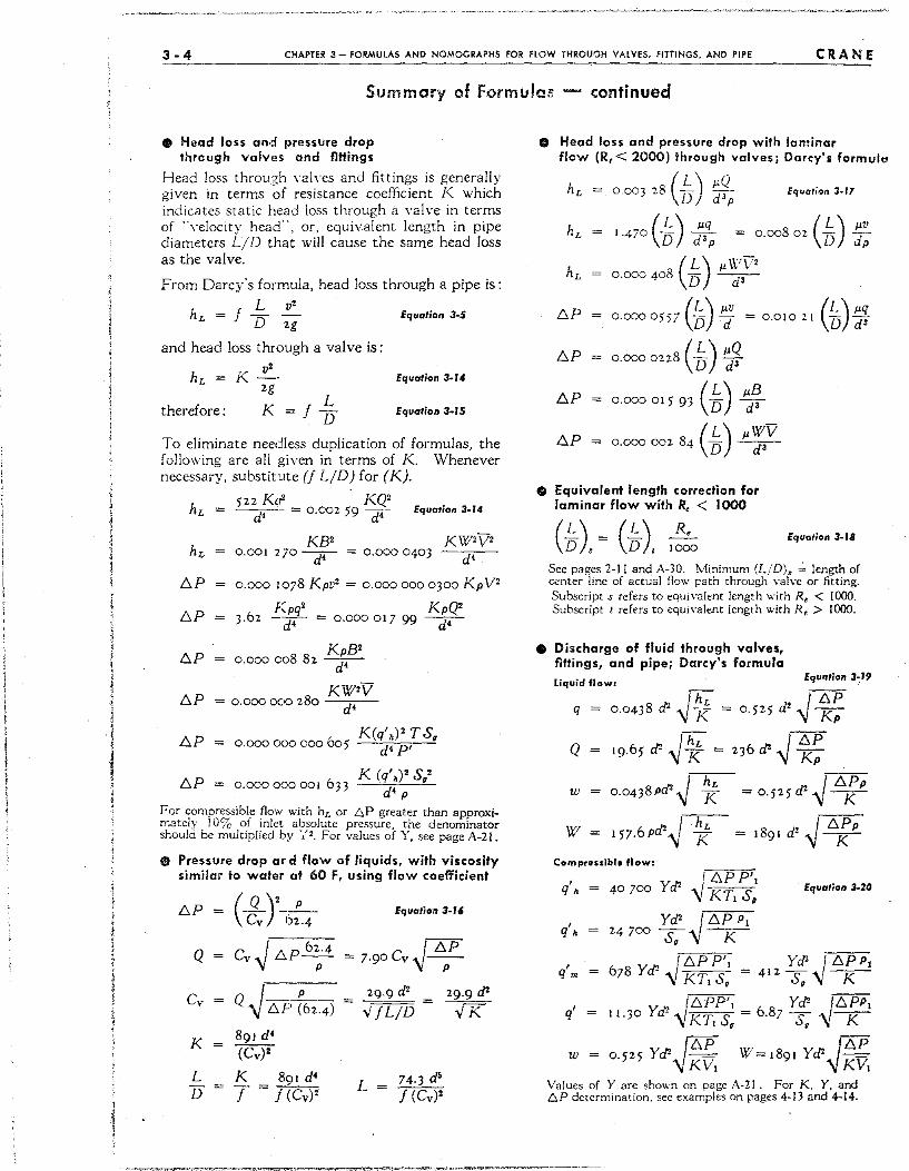
3-4 CHAPTER 3 - FORMULAS AND NOMOGRAPHS FOR flOW THROUGH VALVES. FITTINGS. AND PIPE CRANE

Summary of Formulcs - continued

• Head 1055 and pressure drop through valves and flttings

Head loss through vah'es and fittings is generally given in terms of resistance coefficient K which indicates static head loss through a vah'e in terms of "\'elocity head", or, equivalent length in pipe diameters Lj D that will cause the same head loss as the valve.

From Darcy's formula, head loss through a pipe is:

L v' hL = f - - Equation 3·5

D 2g

and head loss through a valve is:

hL K v' Equation 3.14 =

2g

therefore: K = j.l::.. D

Equarion 3.15

To eliminate needless duplication of formulas, the following are all given in terms of K. Whenever necessary, substitute (f LID) for (K).

tJ.P

fJ,P

tJ.P

522 Kq' KQ' --d-' -- = 0.002 59 (II Equation 3·14

KB' 0.001 270~ 0.000 0403

0.000 1078 Kpv' = 0.000 000 0300 Kp V'

Kpq' KpQ' 3·62 -F = 0.000 017 99 ~

KpB' 0.000 008 82 ~

KW'V tJ.P = 0.000 000280 d'

tJ.P K(q'h)' T S.

0.000000000 60 5 d' P'

K (q'.)' S; tJ.P = 0.000000001 633

d' p

For compressible flow with hL or .6P greater than approxi­mately 10% of inlet absolute pressure, the denominator should be multiplied by',". For values of Y, see page A-21 .

• Pressure drop aMid flow of liquids, with viscosity similar to waler al 60 F, using flow coefficient

tJ.P =

Q

Cv

K

L D

(Q Y p Cv 1)2.4

Cv ~ tJ.P 6:.4

Q ~ tJ.P ~62-4) 891 d' (Cv)'

K 891 d' T = j (Cv)'

Equation 3-1'

/tJ.P = 7.90 Cv -Y-p-

29.9 d'

oJ jLjD

L 74.3 d' j (Cv )'

29.9 d' oJK

.. Head loss and pressure drop with laminar flow (R,< 2000) through valves; Darcy's formult!

( L \ I'Q 0003 28 D) d'p Equotion 3·11

hL ( L) I'q 0.008 02 (fJ) JJ'I}

1-470 D d'p dp

hL ( L) I' \VV' 0.000408 D ~

fJ,P (L) I'V 0.000 0557 l5 d = 0.010 21 (L) I'~ D d'

tJ.P (L) pQ 0.0000228 I5 d3

tJ.P (L) 1'8 0.000 015 93 D (j3

tJ.P (L) I'WV 0.000 002 84 D ------cJ3

.. Equivalent length correction for laminar flow with R, < 1000

R, 1000

Equation 3-18

See pages 2-1 I and A-30. Minimum (LID), ,;, length of center line of actual ftow path through valve or fitting. Subscript s refers to equivalent length with R, < 1000. Subscript t refers to equivalent length with R, > 1000.

.. Discharge of fluid through valves, fittings, and pipe; Darcy's formula

q

Q

W 0.043 8pd' ~ !Jt W = 157.6Pd'~ ~

Compressible flow:

, / 6P PII q. 40700 Yd' \ KTIS,

, q. Yd' ~ tJ.P PI

24700 -- ---S. K

Equation 3-:"

Equation 3-20

, qm

I 6P P'. Y d' I 6P PI 678 Yd' ~ KTI S. = 412 Tv -y--pc-

q' /6PP'1 Yd' I tJ. ?PI

11.30 Yd' \j KTI S, = 6.87 Tv \j-r

~ 16P W = 0·525 Yd' '\jK'V; W= 1891 Yd' '\j KV

I

Values of Yare shown on page A-21. For K, Y. and .6P determination, sec examples on pages 4-13 and 4-14.

.~

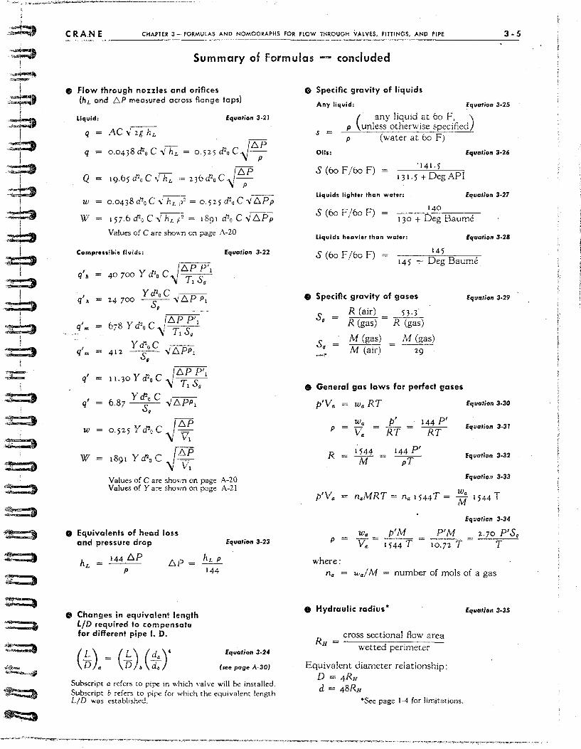
.. ==t !

C R A.N E CHAPTER J - fORMULAS AND NOMOGRAPHS FOR flOW THROUGH VALVES, FITTINGS, AND PIPE ----~--------------

3-5

Summary of Formulas - concluded

• Flow through nozzles Clnd orifices (h L and [o.P measured acrass flange taps)

Liquid: Equation 3-21

q AC ..; 2g hL

q

Q

w 0.0438d"oC"~:;Z = 0·P5d'oC;/[o.Pp

W' 157.6d"oCYhLf~ = 1891 d'oC.,f[o.Pp

Values of C are shown on page A-20

Cornprnsible ffuid~:

q'm

q'

q'

w

w

Values of C are shown on page A-20 Values of Yare shown on page A-21

• Equivalents of head lots and pressure drop

144 [o.P p

[0.1'"

• Changes in equivalent le'ngth LID required 10 compensate for different pipe I. D.

Equation 3·24

(see page A-3D)

Subscript a refers to pipe in which valve will be installed. Subscript b refers to pipe for ,I,'hich the equival~nt length L/ D was established.

• Specific gravity of liquids

CD

•

Any liquid: Equo,ion 3·25

s = (

any liquid at 60 F, ) p unless otherwise specified p (water at 60 F)

Equation 3-26

S (60 F/60 F) 131.5 +DegAPl

Liquids lighter than water: Equa/ion 3-27

140 S (60 F/60 F) = 130 + Deg Baume

liquids heavier than water: Equation 3-28

145 S (60 F /60 F) = 145 Deg Baume

Speciflc gravity of gases Equation 3·29

S, R (air) 53· 3 ---= R (gas) R (gas)

S. M (gas) M (gas)

~. M (air) 29

General gas laws for perfect gases

P'V. w. RT Equation 3·30

w. p' 144 P' Equation 3-37 p V. RT Efr

R 1544 AT

Equation 3-33

P'V. M w. T n. RT = n. 1544T = M 1544

Eq:.raticn 3·34

w. p'M p = V. = 1544 T

P'M 10.72 T

2.70 P'S, T

where: number of mols of a gas

• Hydraulic radius' Equation 3-35

cross sectional flow area wetted perimeter

Equivalent diameter relationship: D = 4RH d = 48RH

'See page 1-4 for limitations.

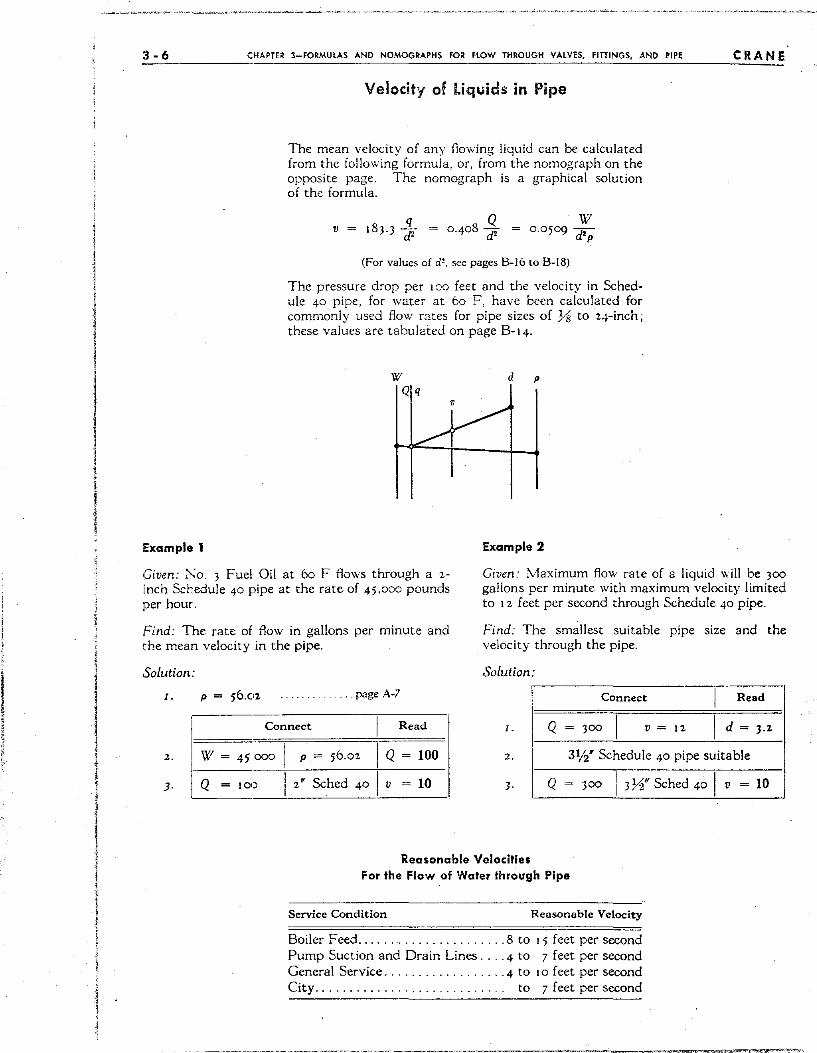
, l

1

3-6

Example 1

CHAPTER 3-FORMUlAS AND NOMOGRAPHS FOR FLOW THROUGH VAlves, FITTINGS, AND PIPE

Velocity of Liquids in Pipe

The mean velocity of any flowing liquid can be calculated from the following formula, or, from the nomograph on the opposite page. The nomograph is a graphical solution of the formula.

(For values of d', see pages B-16 to B-18)

The pressure drop per 100 feet and the velocity in Sched­ule 40 pipe, for water at 60 F, have been calculated for commonly used flow rates for pipe sizes of Ys to 24-inch; these values are tabulated on page B-14.

w Qq

v

d p

Example 2

CRANE

Given: No. J Fuel Oil at 60 F flows through a 2-inch Schedule 40 pipe at the rate of 45,000 pounds per hour.

Given: Maximum flow rate of a liquid will be )00

gallons per minute with maximum velocity limited to 12 feet per second through Schedule 40 pipe.

Find: The rate of flow in gallons per minute and the mean velocity in the pipe.

Find: The smallest suitable pipe size and the velocity through the pipe.

Solution: Solution:

1. p .............. page A-7 Connect Read

1. Q 300 I V = 12 d = 3.2

2. 31/2' Schedule 40 pipe suitable

3· Q =300 I 372' Sched 40 I v = 10

2.

1 Connect I Read I

I W= 45 000 I P = 56 .02 I Q = 100

IQ = 100 I 2' Sched 40 I V = 10 L--

3·

Reasonable Velocities For the Flow of Water through Pipe

Service Condition Reasonable Velocity

Boiler Feed ....................... 8 to 15 feet per second Pump Suction and Drain Lines .... 4 to 7 feet per second General Service .................. 4 to 10 feet per second City.. . . . . . . . . . . . . . . . . . . . . . . . . .. to 7 feet per second

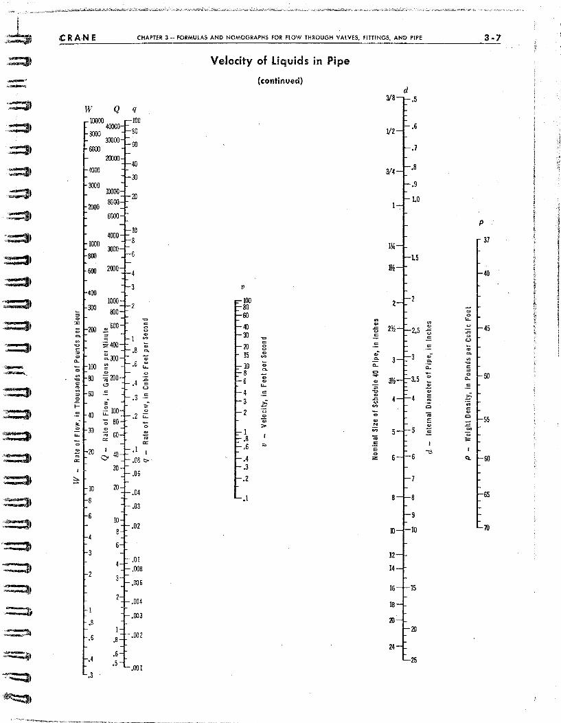
::::::I~

=~ :::::II

:::3' ;:::::::11

:=::11

:::='II

::=1'

=::::J

4"::::.':31

:::J

:::JI

==t :::3

==t

:.::::1

.~

~

... ~

'::=JJ

~

r:<J

<~

'~I

CRANE

tv Q 10000

40000 3IlOO

30000 GOoo

4000

3000

1000

:; Q

:.: ~'600 ~

c ~ ,,400 = c ~

'" ~3J0 "-~

~ 100 c

'" ~ 'iii 200 = c <!J ~ ~ c ~

'" = >-c

",' ~ 2- ~ "- ~

~ '" ~ 20 I

40 ~ 0-or

;:,.. - 10

3

.8

.S .8

.6 .S

.3

CHAPTER 3·- FORMULAS AND NOMOGRAPHS FOR FLOW THROUGH VALVES, FITIINGS, AND PIPE 3·7

Velocity of Liquids in Pipe

(continued) d

q

l P ! ,

1\4 I L5 112 ! I v i

I 100 2 2

D 1

80 ~ I 60 '" ~. ~ "-

c '" ~

~ F,

'" 4J = 2\2 '" ~ ~ 2.S = .0

'" II .:: ~ ~

~ .= (.)

0; c c Zl '" c :;; a, ~

IS '" ,; "-0; ~ c. 3

",. ~

'" :;; c. = "- 10 "- "- c

C. 8 = =

~ 0; ~ ~ Q

6 '" '" 3.5 "-~ "- :; ~ .= u

4 c ." '" c '" E ,:: 3 't5 = ~

~. ~ 0 ~ co c

'" 2 ~ ~ 0; '" "- '" 0

~ Q; '" ~ :::; > N

~ '" 5 =

~ 1 c

'" ~ .8 0;

'" or .6

., c I E I

I '" '":;l

.4 z 6 Q, .08 ""

.3 .06

.2

.04 .1 8

.03 9

.02 10 10

.• 01 12

.008 14

16

.004 18

.003 Zl

20 .002

24

25

~"~"J,\::';::\ ::-;;"'!',i·7t~Y::'"i.:t". • ,-.,.:<:;.",,~ltWI'_J,.("""'-<';'''''':-' ~"-'=""" ,--""", -~"~"'"~---'''-''""--~---

-' --.. ~ •• ,.~ .... -"~" __ -"" ... ____ ~I.-~ •. , ",<._"","",,,",,,,,.,,-,",,~", "''''.'''''''''-<'''' __ "",,"~_"'<J."""""''''''''''''''_~ ____ '' ___ ' __ ~~

Reynolds number may be calculated from the formula below, or, from the nomograph on the opposite page. The nomograph is a graphical solution of the formula.

R, = 22 700 ~: 50.6 -~ = 6.31 ! (For values of d. see p"gcs B-16 to B-18)

The friction factor for clean steel and wrought iron pipe can be obtained from the chart in the center of the nomo­graph. Friction factors for other types of pipe can be determined by using the calculated Reynolds number and referring to pages A-23 and A-24.

q.Q

\\7

J

I' d

p

Example 1 Example 2

Given: Water at 200 F flows through 4-inch Schedule 40 steel pipe at a rate of 415 gallons per minute.

Find: The /low rate in pounds per hour, the Reynolds number, and the friction factor.

Solution:

r.

2.

J.

4·

5·

6.

p

}.t

60. 107

0.3 0

.. page A-6

. page A-3

Cooo'" I R.;"~ Q = 41 5 I p = 60. 107 I W' = 200 000

W = 200 000 I 4" Schcd 40 I Index

Index I }.t = 0·30 I R, = 1 000 000

R, = 1 000 000 I ~or~~tally I j = 0.017 0, - 4.03

Given: Fuel Oil No. 3 at 60 F flows through 2-inch Schedule 40 steel pipe at a rate of 100 gallons per minute.

Find: The flow rate in pounds per hour, the Reynolds number, and the friction factor.

Solution:

1.

2.

3·

4· ).

6.

p

}.t

56.02

9·4

Q = 100

Connect

.... page A-7

........... page A-3

I Read

I p = 5602 I W = 45000

W = 45 000 I 2" Schcd 40 I Index

Index I }.t = 9·4 I R, = 14600

R, = I 600 I horizontally I 4 to d = 2.07

f = 0.03

'_'f'

Co)

co

.." !i

... > -. ~ n ...

.... m -. '" o .. :J I "Y1 0 Il ..,.., ~ ... "'" c - ('I) ~ o -< e; ":J > 0' 2- 6 ... Q.. Z

(") '" g ti" z g Q c ~ :J 3 ~ VI 0'" '" -po to 0 ('I).. '" C1i ...... ~

o 0 Cl'" :::: :J r- ... ... _. :r ..... .a 0 < c: C <; -. Q ... Q.. :r o < c: .." ~

CO - < o m ::r ~ !" - <; ~ ::; ... ~ o Z :J ~ "0 >

Z

"0 " ('I) :!

~ m

n ".

> Z m

( b n n 0 U II U II II II U U tl U 0 II U U nun n tl u u u u u

"C <= :3 ID V)

;;; Co

., ., "-

.0 ~

'-'

~ o

"- .1

'I r;

';; .08 -., ;;; .06 --'"

I .04 "" .03

.02

.01 .008

.006

.004

.003

.002

W

10 000 Index 8000 6000

4000 3000

2000

1 0110 800

600

400 ;; 0

300 :: ID Co

'" "C <= ~

0 a.. ';;

'" "C <=

'" OJ> ~

0 = f-

:: ~.

0

"-';; 2 '" ~

~

Re

200

'" 100 "0

~ 60 ~ 40

~ 200 <= 10 ., 60 ~ 40 ~

z 20 '" "C

o <= >­., ~

~

10 6 4

2

.6

.4

.2

.!

-

Internal Pipe Diameter, Inches

_74

1111r-- -~

~~~P'~-i-=-= _ il$ .0(, =-

_\ -<! I :--- . 3/4

- 1/2 -. -

-\1 \"

A\·, --

'\'\\ ,

f-"

~" f= c:::::, -.

f-- f- , ,- "'t\. '--

,--.01 .02 .03 .04 .O~

f . Friction Factor for Clean Steel and Vlrought I ron Pipe

J.l

.21

',-1

., '" 0

~ <= ., '-'

300

d

3/8~.5

.6

.7

.8 "" L .9

1.0

1.5

"f" a> a> = 2.c: ~ 2 ~ - -<= c

.:. 211 2.5 ':-Co Co

a:: a: ., ;; "C ., = ... V>

';; ., N

0;;

n; <= E 0 z

12 14

18

20

';; ;;; ro E

'" 0

n; EO ., <=

I

7 ~

500-::1 24 600

.. -." ... ~--.."",>"......,..,"""".,..."""'-... "..,.,".--.• '~--..• -", .. ~~-.-",-.• -.-.---., ... ,~,. ..,"",~.,.,--"""!"",~,,

..• ~ .. -.'" ... ~""--"'''''.'''''''''''"'.-"''''-.."

P

65

... .c ~

u -;0 n 0 Co

::I '" :::'; 'C

::I <= ~ 0 c a.. ... <= a.. ,- -.::-';;; <= .,

50 0

~ bQ

';;;

'" I Q.

, ~,".,

HH H-~~,. 'I 'iia W

"1"1 .. ;:;. :::-. 0 ::J

-n 0 ::tI n - (D 0 '< ... ::J - 0 0 .. D.. (") en

(D Z C C ::J 3

0-VI - (D !I) .., CI) -0 0 ... :J ,.. D.. -. ..c :.E c: -. .... D.. 0 c: -n to 0 ::J" ~ -... 0 ::J

3!

" CI)

n '" :Ii-z m

I~ ... I c; ~ c );

'" ,. Z 0

z 0 3: 0 Q

~ .." :l: 0>

~

0 '" ~ 5 ~ ~

:l:

'" 0 c Q :l:

< ,. < m

.'" ~

~ Z Q !" ,. z c :!! .." m

Co)

• -0

- ..... ,··,~.....--...~ ........ ___ ~""~_,,~""··_"'-"" .. C"'""'~'~A~.~,~ ~_,,_,'"-'-',".(~""'_k'"".'_'_~""",' • .-. -<"~"'"'-'~~~.""'~."~·'-"'';''''''''''''''''_.''''''''''''-.C''''''-'''''''''''''''~_~'''''--''''''''''",b_,~ ..• ,,,,;,,,,,, .. , .... ,~~_,,~ ... ~ ..... ,~ __ .......... "".~~ .... -'.,.,_.,,-"'W._, .... ,~ . .....,.,..~,.., .......... ~, .,,~.'"~''''''''' ,

The pressure drop of flowing liquids can be calculated from the Darcy formula that fol­lows, or, from the nomograph on the opposite page. The nomograph is a graphical solution of the formula.

6. P 100 f pv'

0. 129"; -d 4350 fpq~ de,

fpQ' f W' 6.P100 0.0216 ~- 0.000 336 ~

(For values of d and d', see pages 8-16 to 8-18)

q Q P

12 I d c.P,O<l

When flow rate is given in pounds per hour (W), use the following equation to convert to gallons per minute (Q), or use the nomograph on the preceding page.

W Q = 8,02;;

For Reynolds number less than 2000, flow is considered laminar and the nomograph on page )-1) should be used.

The pressure drop per 100 feet and the vc!ocity in Schedule 40 pipe, for water at 60 F, have been calculated for commonly use,J flow rates for pipc sizes of Ys to 24-inch; these values are tafJulated on page B-14.

Example 1

Given: Water at 200 F flows through 4-inch Schedule 40 new steel pipe at a rate of 200,000 pounds per hour.

Find: The pressure drop per 100 feet of pipe.

Solution:

1; p 60.10 7 · ............... , .. ,page A-6

2. P, 0.)0 · ................... page A-3

J. f 0.017 · ...... , .. Example I, page 3-8

4· Q 415 · ...... , .. Exarnple I. page 3,8

Connect ---,_ .. _---

Read

5· 6.

-T::-~-I-~--60.I07 Index I

I ndex I I Q = 4 I 5 Index 2

7· Index 2 1 4" Sched 4~ 6.P1oo = 3.6

Example 2

Given: No. 3 Fuel Oil at 60 F flows through a 2-inch Schedule 40 pipe at a velocity of 10 feet per second.

Find:· The pressure drop per 100 feet of pipe.

Solution:

1. P 56.02 · ..... , ..... , .. , .... page A-7

2. Q 100 · . ,Example I. Step 3; page 3-6

J. f 0.0)0 · ....... , . Example 2. page 3-H

4· ).

6. E - <:onneet I R~Il~

p = 56.02 1 f 0.030 'I I ;;-(l:~ I

Index I 1 Q = 100 1 --Index- 2

Index 2 1 2" Sched 40 i 6.P:o--: :--10 .-- ---------- ----- -- - - - --- ~

"til ... III III .. c: ... III

C .. 0

"tl _. ::J V-

n" c: -. a... r--. ::lI CD .. -0 .. -I c: ... C-c: iD ::J --." 0 :Ii

Co>

-o

w I (5 !< c ;: '" > z 0

z 0 3: 0 0 ,., ". .. '" '"

:l! .. m

n :IV

:to Z m

ft n '1 H If n It U···· ff rt n rt n n n " rt ft U· n ftJt-R--n-----u' ---11ft -lU' n n" tt~1 D • ~ • ~ w. ~ U ~ U ~ v. u U • ~ u • u w U U

q Q

~r" p

Index 2 30

r" /:"[>10.

20 10000

·"1 --a 000 .06

6000 d .OB-.1

---00 .." .... f- -I fI)

Index 1 ---\ 2000 20 -=

en en C

16 u .:: J

, +''' 12 w

12 ;; ~ " .05 10 1O~ 55 ~ 0-

S 800 <n 9 -'= u :;; w u

~ 600 B .= = Q.

" .04 w 7 .:: u ~ ~ Q. ,

6 .,; :;; c 400 " Q. C>- o

300 5 a:: ~ "-~

-:; c

.03 ~ " = 0

" 200 ~ 0- w '" ~ .4 '" u.. '" 50 .= Le-

E c ~ •• 3 '" "" 0 b :=: :;:;

2f) e u 0 100 ~ :;; w:: .2 ro c

.02 u.. 2 c '" Q. -:; 80 ",.

e Q. I

~ If) c :;;; e '-. 60 "" e

'" '" '" B" w

~ :; "'" ~

.... m 0 ... 0

'U

::lI ..... ..a ..... c " 0

~ a.. ::I ,.... c tD :::I .e:: m

III -0 ... -I C ..,

I ~

'" '- Q. a. ~ " .8 I

.04~ 2O~ .7 8 (( .01 .03 ~ .6 <J

3/8 .5

.4 40

IT c m ::I -." 0 :E

50

.01t4 ,,' 1181" ~40 60

.ooa .;: _ '" ao

.006 3 _ 0."- 0 100

.004 -=!- '" .• 0031 I

1 0' "':<''-.1

•• _.~_.~ .".'. ..-".",..,~'" .• "a~~""_>r;:JI"-,...,.J<,~'"""...."..._.-.'_"',',"'_' :,.',,....,~ •• , • ,,"w,._~~.,*~ .• ,_.~ •.. ~~.~~, -~.,.'''''~.".~'.."_,,.,~¥ .. _.' __ ~,,_''''''~~,,~~

n :>:I » Z m

I~ '" r

0 ~

3: c:: ); V>

> z 0

z 0 3: 0 C> ~

> " ::I: V>

0 '" ~ 0 ~ -0 :c '" 0 c: C> 0:

< > < m

'" ~ ~ z C>

'" > z 0

:!! " m

Co) -

\ ! i

l f ! I I i~ I. e

k I:

I I , f f I , L

t ! I ! i· t f i: t. 1.

t ~ ,~

[' ! I ! ~. i

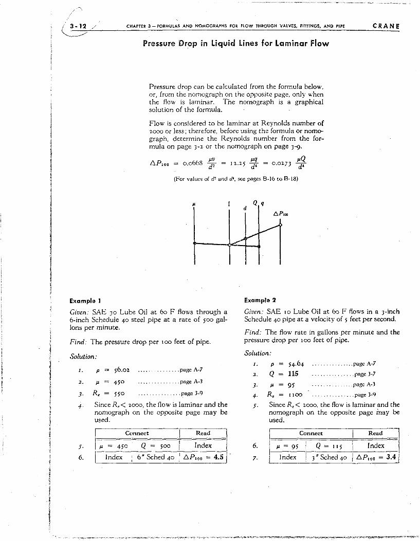
! I

I i

/ 3-12 / CHAPTER 3-fORMUlAS AND NOMOGRAPHS fOR flOW THROUGH VALVES, FITTINGS, AND PIPE CRANE ~~-------~----------------------~~~~~--~~~

Pressure Drop in liquid lines for Laminar Flow

Pressure drop can be calculated from the formula below, or, from the nomograph on the opposite page, only when the flow is laminar. The nomograph is a graphical solution of the formula_

Flow is considered to be laminar at Reynolds number of 2000 or less; therefore, before using the formula or nomo­graph, determine the Reynolds number from the for­mula on page 3-2 or the nomograph on page 3-9.

_ )LV _ )Lq _ ~ )LQ 6.PIOO - 0.0668 d2 - 12.25 d' - 0.02,3 d'

(For values of d' and d" see pages 8-16 to 8-18)

Q q d

Example 1 Example 2

Given: SAE )0 Lube Oil at 60 F flows through a 6-inch Schedule 40 steel pipe at a rate of 500 gal­lons per minute.

Find: The pressure drop per 100 feet of pipe.

Solution:

1.

2.

J.

4·

5·

6.

P 56.02 ......... page A-7

)L 450 ..... . page A-3

R, 550 .. ' . page 3-9

Since R,< 2000, the flow is laminar and the nomograph on the opposite page may be used.

Read

Q = 500 Index

r= Connect

I )L = 450

Index 6' Sched 40 I 6.P100 = 4.5

Given: SAE 10 Lube Oil at 60 F flows in a 3-inch Schedule 40 pipe at a velocity of 5 feet per second.

Find: The flow rate in gallons per minute and the pressure drop per 100 feet of pipe.

Solution:

l.

2 .

J.

4·

5·

6.

7·

p 54.64 ............. page A-7

Q 115 ... page 3-7

)L 95 .... page A-3

R, 1100 ............ page 3-9

Since R, < 2000, the flow is laminar and the nomograph on the opposite page may be used.

Connect Read

p. = 95 Q = 1 15 I Index

Index 3' Sched 40 ! 6.P100 = 3.41

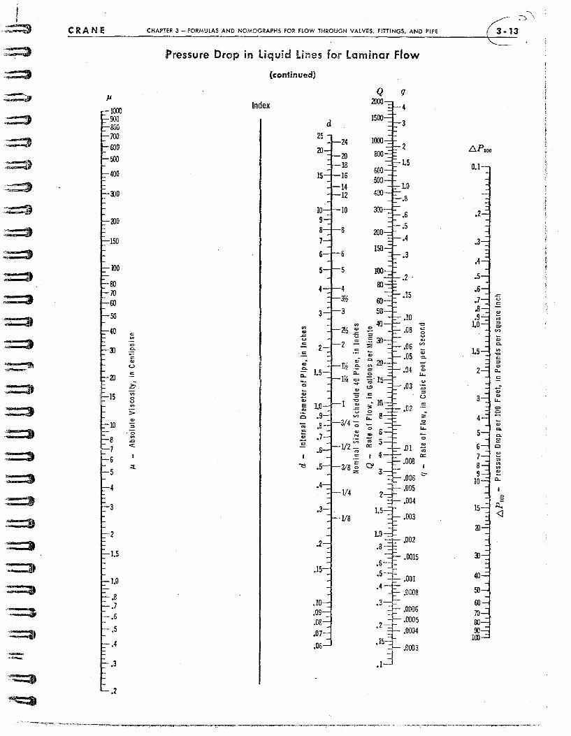
,;::::3

~~

::=:D

::::=1_

::::::3

::::=3

:=:t

=::::t ==:B

:::::3

~.

~.

CRANE

2

1.5

1.0

.B

.7

.6

.5

.4

.3

.2

'" "' '" c.

'" '" <.>

'" :?:

'" 0 u

"' ::-., ~

·0

"' ~ «

::t

"' CHAPTER 3 - ~ORMULAS AND NOMOGRAPHS FO~ flOW THROUGH VALVES, FITTINGS. AND PIPE

~ ... ;-:' ,

{ 3·13

Pressure Drop in Liquid lines for laminar Flow

(continued)

q

Index 4

d 3

2 L:::.P,oo

1.5

1.0

.8

.6

.5

.4

.3

5 .2 .

4 3ll .15 .r:

u

-= .10 ~

'" 3

-c ~ c-.08 c '" 0

u ;;; ~

.06 '" c. ;;; '" .05 -c c. c -:;; ~

.04 0

~ 0-u.. '"

.03 u

~ ~ ~

c..:> .,

"' '" ~ ~ '" = = u '"' -= -= 2

. '" '" ,;

",'

Il1 c. c. 0- 0-

';; III = ~

'" ., '" :; -= u..

.02 '" = ",' ~

-= ;;; U- c. ';; c.

e .oJ ~ 0

'" '" ~

'" I = E '" '"

.r: u 0

0 '" "-3/4 ';; 0; ~ '" ~ ., ~ N

'" '" m

1/2 - a:

'" '" .OOB ~

'" "' ~ ~

~ 3/8 ;; z

0-

I g 1/4

r:t; <J

.002

.0015

.5-

1.001

.4 .0008

3-. j:.. .0006

2!·000S • _ .0004 .IS} .= .0003

.1-J

, ,

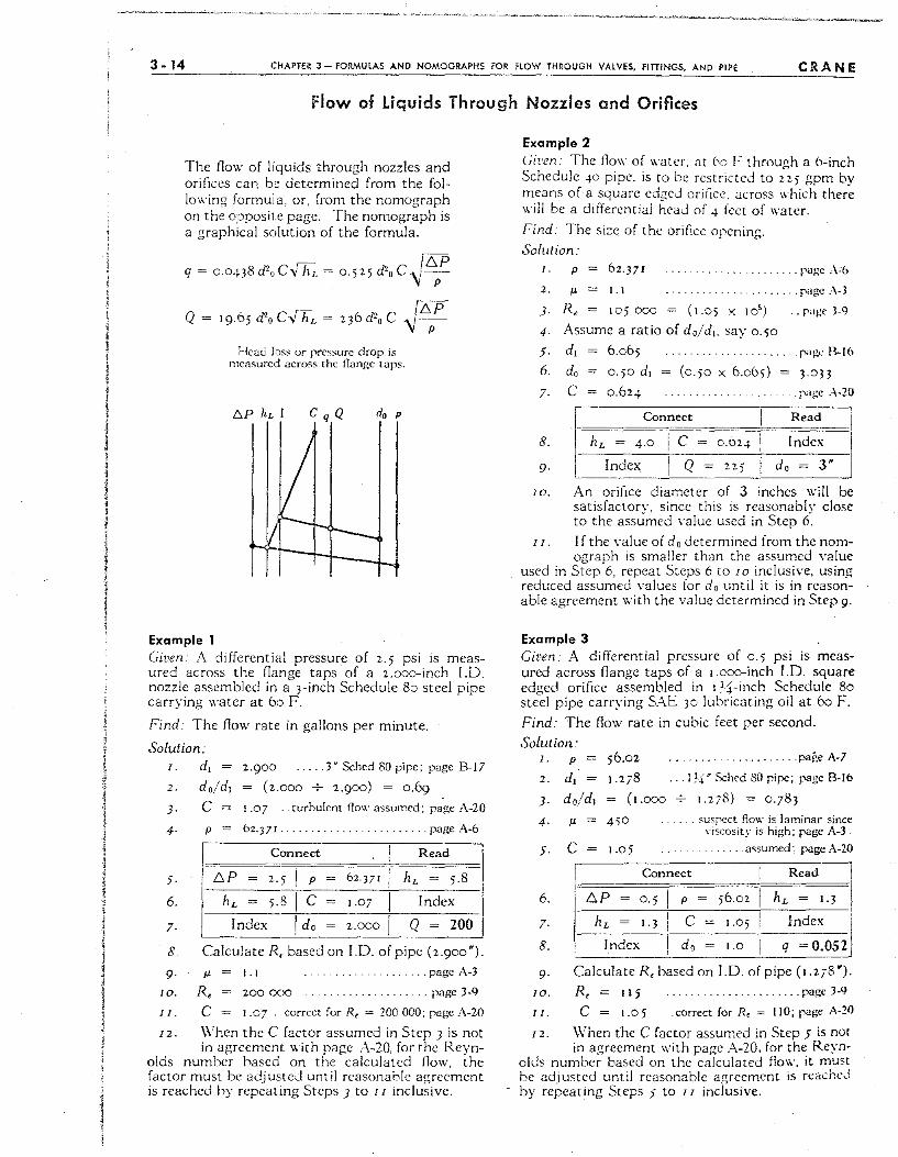
1 l j

I

I ~

3 -14 CHAPT€R 3 - fORMULAS AND NOMOGRAPHS fOR FLOW THROUGH VALVES, fITTINGS, AND PIPE CRANE

Flow of Liquids Through Nozzles and Orifices

The flow of liquids through nozzles and orifices can be determined from the fol­lowing formula, or, from the nomograph on the opposite page. The nomograph is a graphical solution of the formula.

8 '2 e .... } d" e if':,p q = 0.043 do Y II. = 0.)25 '0 '\jp

Q

}-Icad loss or pressure drop is measured across the flange taps.

CqQ do p

Example 1 Given' A differential pressure of 2.5 psi is meas­ured across the flange taps of a 2.000-inch LO. nozzle assembled in a 3-inch Schedule 80 steel pipe carrying water at 60 F.

Find. The flow rate in gallons per minute.

Solution: I.

2.

3·

4·

5·

6.

7·

2.900 .... 3" Sched 80 pipe; page B-17

= (2.000 -7- 2.900) = 0.69 1 .07 .. turbulent flow assumed; page A-20

......... page 1\-6

onnect I Read

5 I p = 62,371 I hL = 5.8

g Ie = 1.07 I Index

I do , = 2.000 I Q = 200

8, Calculate R" based on I.O. of pipe (2.900").

9· 10.

Jl

R, 1.1 200000

. ... page 1\-3

". page 3-9

I I. e 1.07 correct for R, = 200 000; page 1\-20

12. When the e factor assumed in Step 3 is not in agreement with page A-20, for the Reyn­

olds number hased on the calculated flow, the factor must be adjusteJ until reasonable agreement is reached by repeating Steps 3 to 11 inclusive.

Example 2

Cil'cn,' The flow of water, at 60 F through a 6-inch Schedule 40 pipe. is to be restricted to 225 gpm by means of a square edged orillce, across which there will be a differential heaJ of 4 feet of water.

Find: The size of the orifice opening. Solution:

I. P

2. J.L

62·371

1.1

... . page :\..:6

. . rage :\-3

J. Re 105000 (1.05 X 10') .. page J-C)

4· Assume a ratio of do/d" say 0.50

5· d, 6.06; rage B·16

6. do 0.50 d, (0.;0 X 6.065) ).033

7. e 0.624 ' ,page A·20

8.

I Connect

Index

Read

9· I Index I Q = 22; do = 3"

10. An orifice diameter of 3 inches will be satisfactorv, since this is reasonably close to the assumed value used in Step 6~

1 I. If the value of do determined from the nom-ograph is smaller than the assumed value

used in Step 6, repeat Steps 6 to 10 inclusive, using reduced assumed values for do until it is in reason­able agreement with the value determined in Step 9.

Example 3 Given,' A differential pressure of 0.; psi is meas· ured across flange taps of a I.ooo-inch 1.0. square edged orince assembled in I !:l'-inch Schedule 80 steel pipe carrying S:'\E 30 lubricating oil at 60 F. Find: The flow rate in cubic feet per second.

Solution: I.

2.

3·

4·

5·

6.

7·

8.

P 56.02 ............. page 1\-7

d, 1.278 . I !,~' Sched 80 pipe; rage 8-16

do/d, = (1.000 1.278) = 0.78 3

J.L 450 .... susrect fiow is laminar since \'iscosity is high; rage A-3

e 1.05 , ... assumed; page A·20

Connect I Read i f':,P = 0·5 ! p = 56.02 I hL = I.) I

! hL = 1.3 I e = 1.0 5 I Index i , ,

Index I do = 1.0 I q = 0.052' , 9. Calculate R, based on 1.0. of pipe (1.278") .

10. R, = 115 ......... '" . page 3-9

1 I. e = 1.0') .correct for R, = 110; page A-20

12. When the e factor assumed in Step 5 is not in agreement with page A-20, for the Reyn·

olds number based on the calculated flow, it must be adjusted until reasonable agreement is reachd by repeating Steps 5 to 11 inclusive.

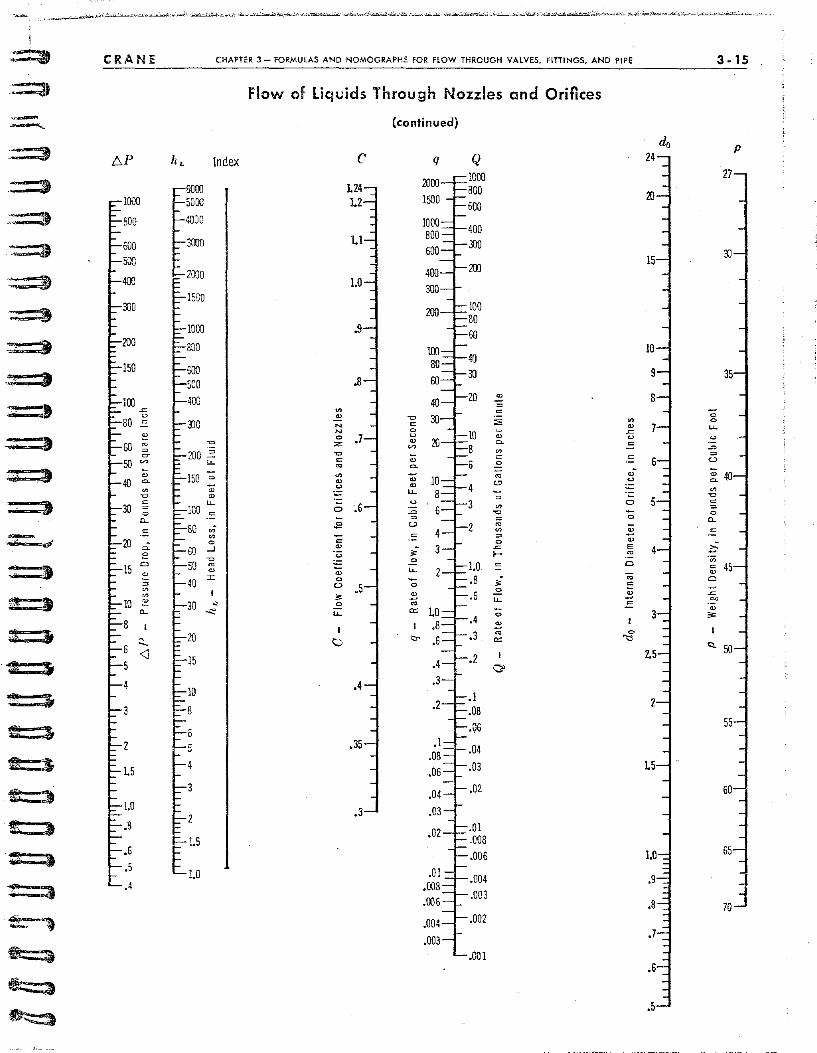
~i

Ii $

CRANE C:HAPTER 3 - fORMULAS AND NOMOGRAPHS FOR HOW THROUGH VALVES, fITTINGS, AND PIPE -------

b.P

.6

.5

.4

hL

"" u

.= := ro ~

= '" ;;;

'" "C 0= ~

0 c... c

~ ~ Cl

e.>

~

'" "' ::: "-

.:.., <J

Index

200 ~

..... 150 -;;

a; ~ .....

100 ~

80 .,; "' 0

60 -' "C

50 ro e.>

40 :c

-, "'"

20

15

10

8

6

4

3

Flow of liquids Through Nozzles and Orifices

(continued)

C q Q

alOO

lOOO 800 600

400 300

200

~

~

'" ~

::;; ~

~

~ '" N ~

10 ;;:; "" u = .= 8 ~ ~ ~ 0

ro .;

'" u --;; -

N 0 0 u

~ Z

'" '" ;;; 0= ro = '" a; ~ u ~ - .....

0 ~

'" -;; ~

- u 0 .0 - ~

ro ~ .e ~

~ 0

"" E I- ro

.E '-' ~

0= ~ ,; U

1.0 ==

Cl .= ~

..... .8 ,; ro

E .6 .= ~ .....

~

0

'-' 0

.e '" 0 ro -;;

.4 .e

.3 ro 0

"" ~

"- "" I

Co) "" .2

0>

.1

.08 .06

.04

.03

.02

.01

.008

.006

.004

.003

.002

.001

3-15

do p 24

LIl

10

'0 0 ..... u

.0 ~

'-'

~

'" ~ ~

0

"-~

?:;-

Cl

~ CD

~

'" Q,

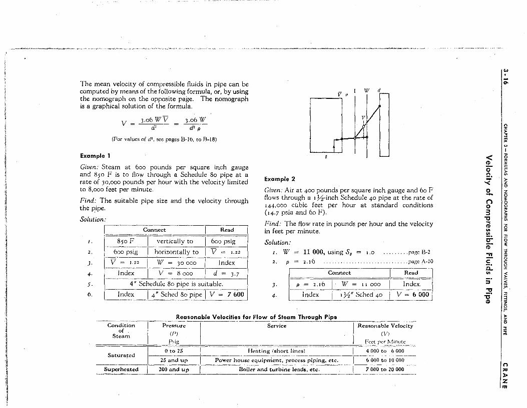
j i I

I 1 '1 1 I I I 1 l ,j

I 1 I

, -~

I I

1 4

><.,.."."k-'",-'·""'>'.' "

The mean velocity of compressible fluids in pipe can be computed by means of the following formula, or, by using the nomograph on the opposite page. The nomograph is a graphical solution of the formula.

V = 3.0 6.'!1 V 1.:06 W a' d' p

(For values of d', see pages 8-16, to 8-18)

Example 1

Given: Steam at 600 pounds per square inch gauge and 850 F is to flow through a Schedule 80 pipe at a rate of 30,000 pounds per hour with the velocity limited to 8,000 feet per minute.

Find: The suitable pipe size and the velocity through the pipe.

Solulion:

Connect Read

I. 850 F vertically to 600 psig

2. 600 psig horizontally to V = I. 22

V = I.2Z W = 30000 Index

Index V = 8000 d = 3.7 ---_ ..

J.

4·

5·

6.

4" Schedule 80 pipe is suitable.

Index 14" Sched 80 pipe 1 V = 7600 ___ 0_._.

n'I~Ul u

Example 2

Given: Air at 400 pounds per square inch gauge and 60 F flows through a I Y2-inch Schedule 40 pipe at the rate of 144,000 cubic feet per hour at standard conditions (14.7 psia and 60 F).

Find: The flow rate in pounds per hour and the velocity in feet per minute.

Solution:

I. W 2. P

11 000, using So 1.0 ......... page 8-2

2.16 ............. . .... page A-IO

p = 2.16 W = 11000 Index. J.

4·

Connect Re~d

,--_I n_d_cx I Y2" Sched 40 V = 6 000

. ___ ._______ __. ___ ~ .. ~lSonable V~ .. ~~it~~s for."!0w._oL~!eam Throu{jh Pip_e _____ . _____ ... __ ... Condition

of Steam

Saturated

Superheated

Pressure

({')

P,ig

o to 25

25 and up

200 and UD

I I

Service Reasonable Velocity

(V)

==~=~~<:<:t-J:-~-~':~~~~t-(~-~ Heating (short lines) I 4000 t;;""6-00()---

p~;:h,;;;.-;;-;;~.;iP;:,;cnt, pro~~~pi~~-~;,---r--6 .. 0()0 to 10000

T .~-------~-~--.

Boiler and turbine leads, etc. ---[--7000t; 20 000-"-

< !2.. 0 !:!. -'< 0 -n 0 3 "0 ... CD ... !a. 0-CI> "lI'I

c c.. In

::J

.." -ij'

CI>

... -0.

n :1: ,. ... ... m ,. (.>

I

0 ,. 3:: c: ;;: '" ,. z 0

z 0 3:: 0

" ,. ,. ... x '" 0 ,. ~

0 ~ ... :x ,. 0 c

" :x < ,. :;: m yo ~

~ z " yo ,. z 0 ... :;; "'

n

'" » z m

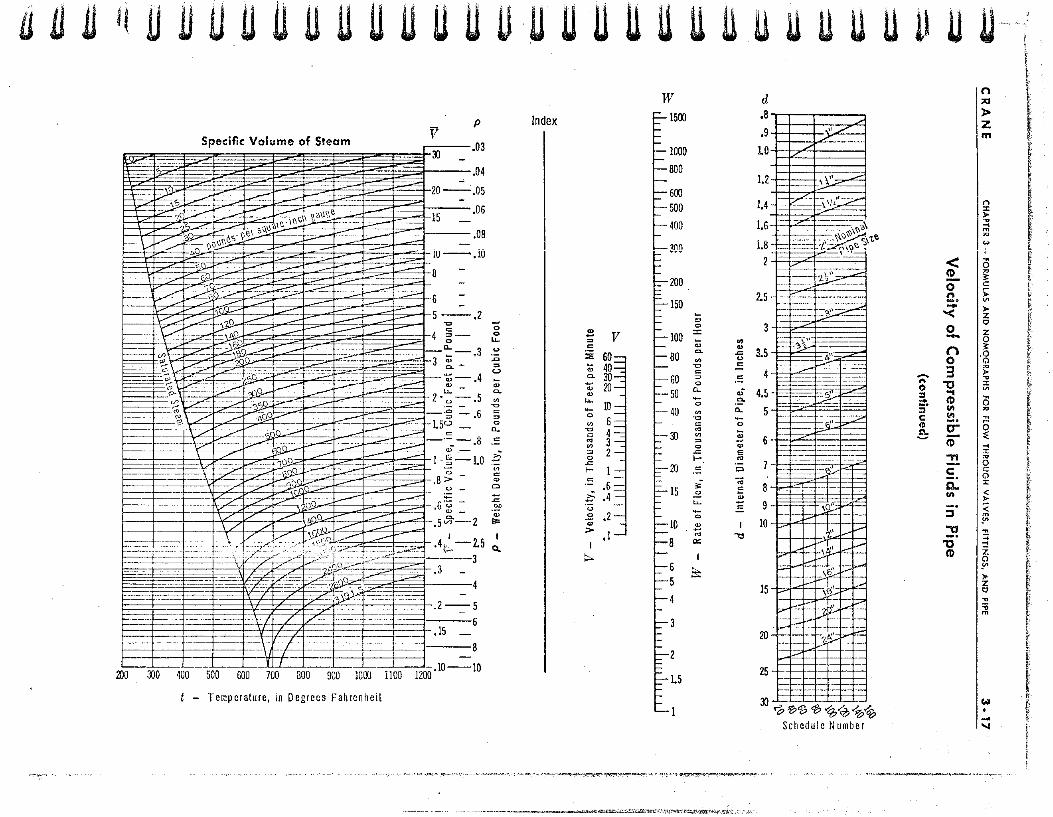
a ~ n I ( D n U U II U II U U U U U II U II U U U II U U U U U U U U~' \

Specific Volume of Steam v =r=~;;- .03

~~

p

~~~ct~~~~ I-~-r--=---.,.-''''-~-;;o~ ---~~-------~ ~\\-I'"U?,e:

-1"-r~ =:p~o: \16u~os-~~_ -- ---~ __ ==-,.. _-=~ ____ ' ___ ._- _ ~ ____ ~ __ ~ lU

~120

15

.05

.06

.OS

• 10 --,7""'- ~- - ~ ~ -- :::<~=----{ --'::::::~"'j;9f-" - 1---"' __ 0__ ____- . _== 8

-----7·~r ,;.--f<'=----:.o~~ -- ... --=-- -~-'" ~6 -- v---: .,.-::~ _ :;;:=--= ~ 5 --- 2

.....-",C ~r-,?,cl_k:::::::-~ _ --- -- -c.

t==I='''F/C::::;;-C ~~ ;;::. -;;:.~ -.:::7'. = _-=;H ~ ~ -=-~ --\- ----r~~g;· --~--=-- ... - .-:--- --- -~ "-~-;:~t:-"L~~()"'~--~------- -"~--- 3 :;;-:::-.3 ~='4.v~;::tc"~~ ;'~T';;c~ :-~~~~~ i -.4

~~-~:~J-- ~ ,,;00.--.--" p..-=-~ "--t= u> -;.,..0 l--""?'t=:"sQ;:~~ I--~ - 2· u -.5 =----;;; - - -fLO ~o=~ -- ---"'r-= :;; =- 6 =-: =:9~- 09-~--- - L5~ • =------=:----... -- - - ~-:..,...-- - ,o::;?,-" - :.,.;-___ =f.-=- E-__ ____ ___ t"' __ C-:.:.>'t ",_ ~ - _ -.S

==t=:::--t - -::;:7'~f;9.. ° =-~ -'" 1 ;;; -=± ---. -t··· -v-- 1~ - ~·t-= -~~1.0

r===!=- ----\/- ~~?: --=- '0 --'(1--/ .~. ~5:;=-- ::=:-,8:; _

~- ~~~-~~o =;::::0- ,6i:=

__ _ __ 1/ ./ c ~ ___ .5 v ,-2

b:+:~~-~t=:~~{~:/~7!:::;~~~':P'~;::' -1--= ___ .4_1~~ -2.5 ----\;; 7Lj-7.0::C'~' 0=-- .3

'0 0 LL u ,;; ~

'-' :;; 0"

'" -c c ~

0

"-

== 1::' ';;; c ., Cl

:;;; .!:." ., ,.., I

Q,

f=,:t~~"!: ~~;t =::- .. ;L=-~~~= ::=

~:::;:z::':--::'::: 1=--=--~= .2 5 i== F~

4

I---T/- --r--:.L-- --- i-- --1---- 15 ----_. -==f::,'-+-f--+-=:1---S

/ 2)0 300 400 500 600 700 aDO 900 1000 II 00 1200 .10 --10

t - Temperature, in Degrees Fahrenheit

Index

.e V ~

c

:s 60 40

~ 30 Q; 20 ., LL

10 -0 6 '" -c

~ ~

'" '" 2 ~

0 = f- 1 c

.6 £, .4 '03 .=! .2 ., > .1 I

"'"

w

200

150

100

80

60 50

40

20

15

2

1.5

;; 0

:<:

:;; 0"

'" -c c ~

0

"-':;

'" -0 c

'" '" ~ 0 = f-c

",-

.=! I.e.

':; .e '" '" i±

.. ., = u .= c

.,-0"

"-'0 .e ., E

'" Cl .. EO ., c

I ~

d .8

.9 ",/

LO

1.2 ,\;~

I-'~~~~ 1.4

1.6 --- ~--~-=---=

I.B . . - --- \'1>"\

l - =+:::-=t-·=::'-' 0S-1, =t=--~--. . i~\le ~ - -- ,,~=

.1.e

2

2.5

- F--~-;:::: t=~~·t\~_ . I=:~"l-_--__ ~",j

~;--=;,:~ 3

3.5 1-=;]:'1= - =.= f-- A~

= -i=

4.5 i -EEc 2i'.:t;Z; EI __ L:3-o-E ""-=:====

6

8

9

10

15

20

25

__ _ ;.g:::t-:= ,-- --. --r:::: ---=EJcc=

.- - :::;;'

1"-: ---=--a". -f--' "''- -*"'..=1=

¢p~

it'vJ...­I- ~k ~I-­

~i-- k:- t-::[., !;; I--c-f- --I~~ 1-

-t--".f-'1I--+-r-. k-p.-I-e:: ':l--ok j...-

~_ .X ~- ,-\-::

?o" p-F-

~F'" . 1--

1--1- _+=(::::

30 'i> 'b0 <2> '<2"~b ~~ Schedule Number

'·· .. "-..,...."...., .. ~""':"'-"""'''~-''-''r .. -'''~..,...'"''''''''' .. _.,.,....''·_~' .

-_______ . , ...... ~;:L:::..!-~::>I7.;;:';'l:"':!2/:.w.w'm'1..c:;:u:~"'_""_.~.:J,;;;_.:

< !-0 ~. -"< 0 -n 0

~ 3 " "C 0 ... ::I (!) ::-.

til ::I til C -. flI C'"

~ (!)

.."

!:. a.. til

::J

." _. "C (!)

o '" > Z m

n x ". :!l m

'" '"

~

::; ::! z Cl !" ,. Z 0 ~

:;; m

w

-'I

t I f !

I I f • Ii [ ~ Ii ~; p [ t !f:

i ~ i } " , J

! i:

I I t t } I:

t I' ¥

! ! I

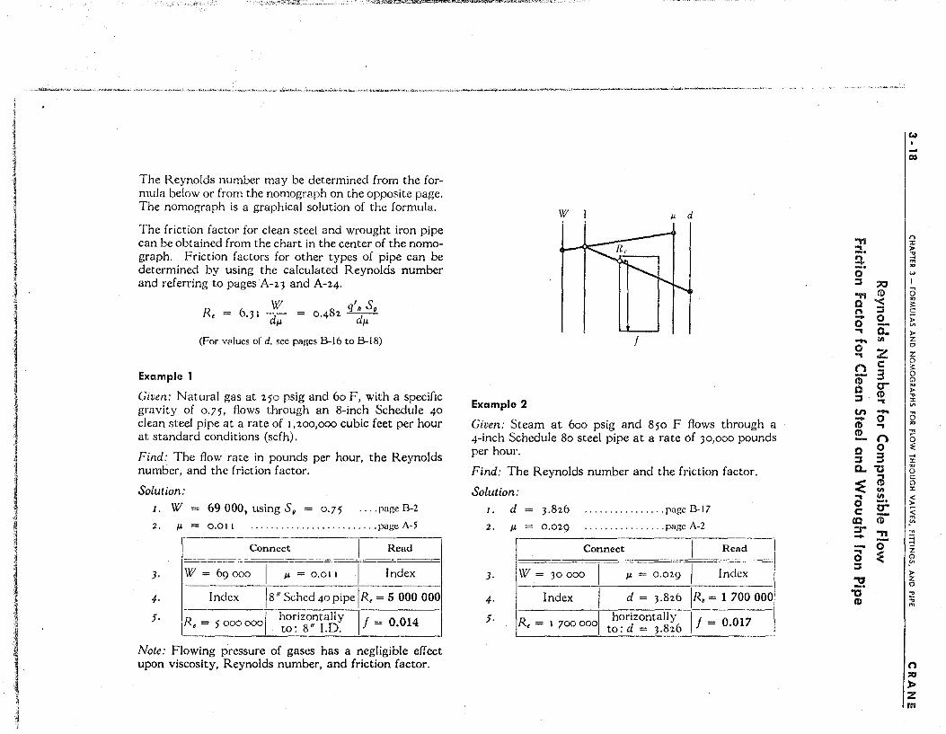
j j

I !

I t ; ,I

1

.~ 'l ~

I

1

<"..;~~.~. ____ ~o:

··::::,:',;r.7:_..,,::>·;:;-,~g,[ "-'.l':m'.$~Tt-"t4~-.:.;Wt"i.~{I'l'it1."~~$'.mcV$"""ITW'~~:f:l~''fJ,":,'··

._<_".~" .~ .• ,,,,_,""£--~'., '"~"" "'.~''''''''"'''~'.,,,u __ I-., .. ,.~.->. '" __ ""."-' """~.:...:.,~ __ ..... ,-"'~'";~ .... "' .... _, "',"H."'""""'''''''''----'''''''' ,"""~_~_ ....... ~., __ ................. , ......... ..,_~_,~-_o ........ __ '"' ........... ~ ..... __ •. __ ..... __ ._ .... __ " .... _·_·~ ...... -.----- -.-~. ~---"

The Reynolds number may be determined from the for­mula below or from the nomograph on the opposite page. The nomograph is a graphical solution of the formula.

The friction factor ior ciean steel and wrought iron pipe can be obtained from the chart in the center of the nomo­graph. Friction factors for other types of pipe can be determined by using the calculated Reynolds number and referring to pages A-2 3 and A-24.

W R, 6.31 dp. 0.482 q'. So

dp.

(For v,>lues of d. see pages B-16 to 8-18)

Example 1

Given: Natural gas at 250 psig and 60 F, with a specific gravity of 0.75, flows through an 8-inch Schedule 40 clean steel pipe at a rate of 1,200,000 cubic feet per hour at standard conditions (scfh).

Find: The flow rate in pounds per hour, the Reynolds number, and the friction factor.

Solution:

1. W = 69000, using So = 0.75 .... page B-2 2.

),

4,

$.

jJ. 0.011 .... ".""" .... ,." .. ,.pageA-5 ------

Connect l~ead

W = 69000 p. 0,011 Indcx

Index 18" Schcd 40 pipe IR, = 5 000 000

-R I horizontal! y I f 0 ,= 5000000 to: 8" I.D. = 0.14

Note: Flowing pressure of gases has a negligible effect upon viscosity, Reynolds number, and friction factor.

w p. d

f

Example 2

Given: Steam at 600 psig and 850 F flows through a 4-inch Schedule 80 steel pipe at a rate of 30,000 pounds per hour.

Find: The Reynolds number and the friction factor.

Solution:

1. d 3,826 .. ", .. ,.""" ,page B-17 2. jJ. 0.029 ., .. ,.", ,. .. page A-2

Connect Read---I 1. ____ -I Index

FZ' = 1 7000il0 L •.. '_ ... __ " .. I

f = 0.017

"TI ... _. 1"1 -o· ::J :;.c "Tl CO Q '< n :s - 0 0 .. 0-- III

0 ... Z C 0 3 tll

0 IT ::J ro ... VI -- 0 tll .. (!)

()

Q 0 ::I 3 0.."0 .. ~ tll

<It .. III 0 -. C IT

CO (!)

::r "TI - 0 .... ~ 0

::I

:9-"D (!)

w

D:I

r. ::c > ." ... m

'"

0 '" '" c ;;: '" > Z

" z 0

'" 0 Cl

> ." :x: '" 0 '" ~ 0 :;: ... '" '" 0 c Cl :c < > < m !" ~

~ z Cl !" > z 0

~ ." m

n ~

~ Z m

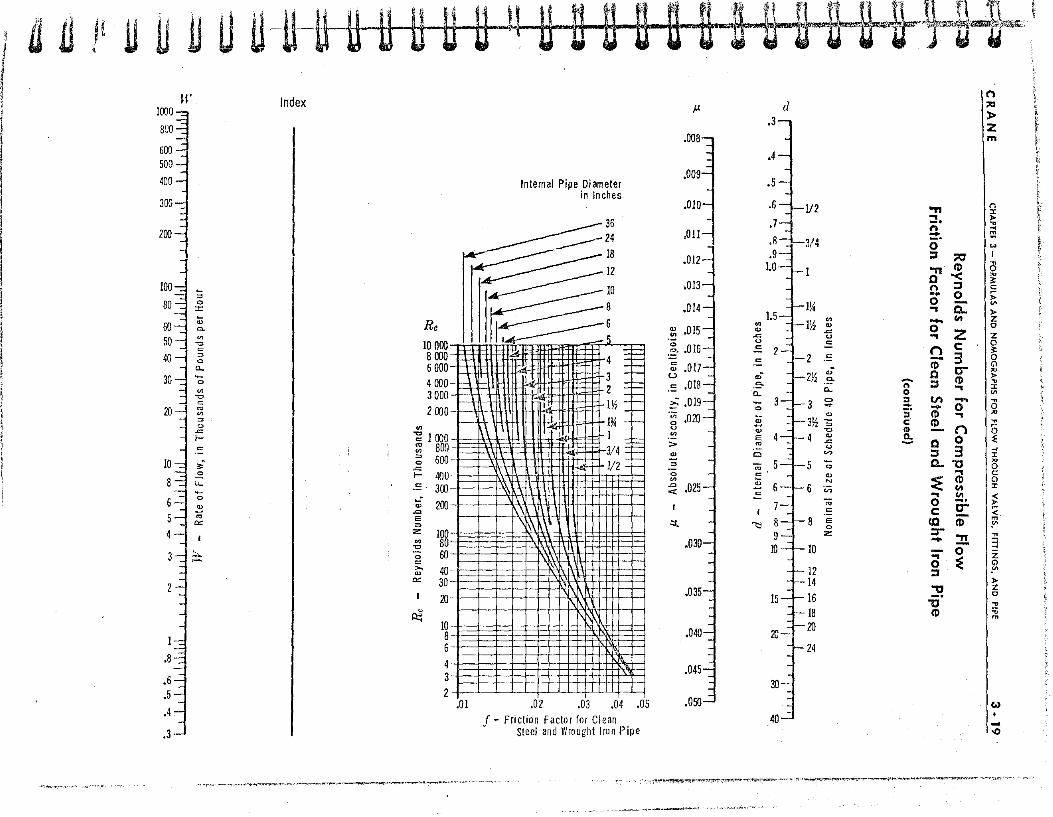
I j

I

I, I

n n ,! ~ D V U li--il--U U HUH H l' II H II· U · I+~*-

w Index

:; e

::t:

Q; Co

V> -0 <= => e "-"0 V> -0 <= N V> => 0 .c f-

'<I' e

u..

"0 '" '" '" 4

.8

'6~-.5

.4

.3·

'"

Re 10000 8000 6000 4000 3000 2000

Internal Pipe Diameter in Inches

_____ ---36 ____ _----- 24

~ _______ l~

~ _____ 12 :=::=-::: 10

III~; 1=1 =1=1 4 =+=I

(IlHf 3 :t=l __ _ ~ 2 =~ __ ril IV, :::~

\ I~ -H I, 1

1_ \' --r4 -3/4 ~§l :\-1-_ --l

~r==J=j~~~\~~ - V2-H

2: I 000 '::J BOO => 600 ,0

f:. 400 .:: 300

i" 200 -'" E

" :z

'" -0

o <= >,

'" '"

~

100 80 60

40 30 20

10 8 6

4 3 2

I' ~\\

.- •. 1-- - . _.--- i~t:~_~kd=

_ ~\' H - .'

- J.--H

1- ~ L~ _ -Ll --1-

.01 .02 .03 .04 .05 f - Friction Factor for Clean

Steel and Wrought Iron Pipe

J.I.

LJ "I. -1

.045~

'" '" .c u .: =: ",'

"'-c:: -0

'" '" E

'" Cl

ro <= Q; <=

I

~

n d I~ .3..,

Z m

.44

'1 .6 -1/2 "TI " :I:

.7 .. » -. " n ...

.R j 3/4 :::!'. ~ 0 w

.9 :J ;;ra I

1.0 _, ." CD 0 o "< '" 3: n :J c: - 0 ;;:

I~ 0 '" 1.5

... 0.. » IV, ::; - en z

0 0 .c Z u .. Z <= 0

2 - n c: 3: <= 3 0

CD Q

2V, .; 0 IT '" > - :J CD .. "-

1'1 ., :I: 0 '" -3 0 ::I VI - ~

.". - ... 0 0

'" :i" CD ... '" 3V, ""5 c CD ~

-0 CD - n 5 -4 '" .& 0 1: .c Q u 3 ...

V> ::J :I:

5 "0 0.." '" 0

'" .... c

N :E CD Q 6 V> III :I: ... !!!. <

'" 0 IT > <= c: ~ E to CD 0 !" z :r

." ~ - ~ 10 0 ... ~

z 0 Q

12 :J .V>

14 » ." z

15--1-16 -. 0

"C ~ CD ..

"' ::I- '" 20

30

40J I~ --0

"""...,...-.,-'.,., .. ..".""""'.""~".~.,.,..,."""-"'-.,-............... ----' ......... "' ... ~". .,., .. "",~'...,~,"?~~""'-i"_~~""''''''''',-'''' ,."<...--"'",.....'t"'"!'~"" .... .....,..,...,, ...... _ .... ,.....,..........,... ___ ~- •. n·¥,."",«?""' .. ·,

_~_., ___ .-."., _, ",,.~,~.u~~, ...... ,~,'

'~ , I !

t , , ,

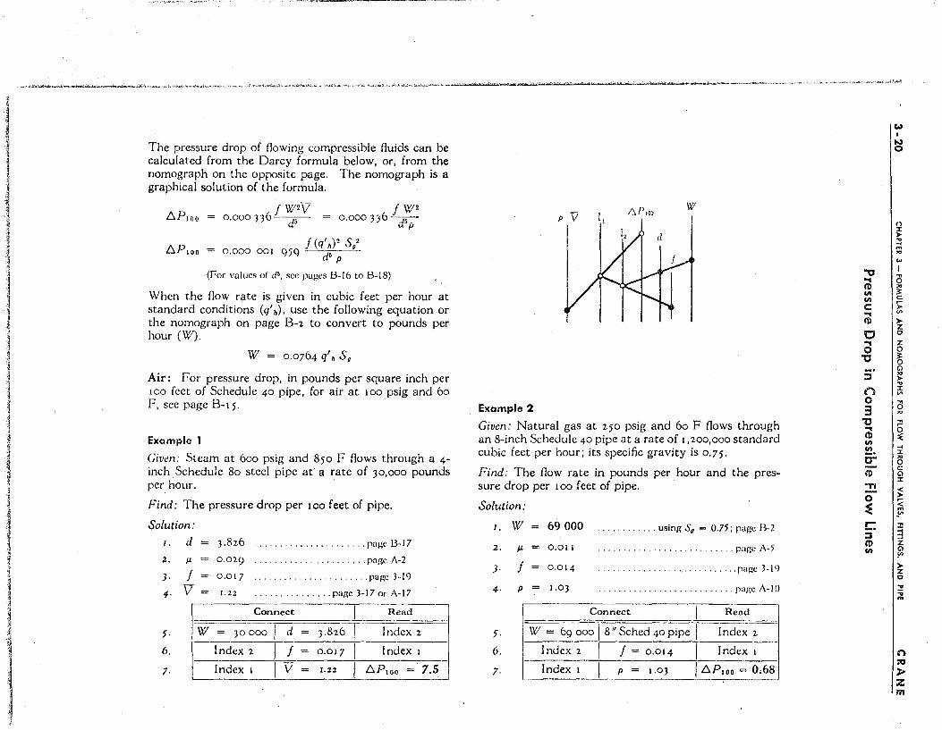
j )

I ~

I ~

1

i!

I I ,

I 1

I $

l I ,I

1

1 I ~ 1

I 1

,_~"""~""'''-'''''''''''''''''''''''~~_A''''~'''''''''"'''''''''H"""""",,;,,,,,,,,>.,,,,,'_r~ ~ .• ~" ~"d,"'~~~""'~'~;';'_""'-"''';_'''''~''_"'--'''-', .... ,, __ ,<, ,,-,.-. "" .. ""l/,,_, ",l> .'",'",b.~;".L.",,,,,".'w._ ~"""""""-'. ~~ _'_M'~.~._~_ .. "~-

The pressure drop of flowing compressible fluids can be calculated from the Darcy formula below, or, from the nomograph on the opposite page. The nomograph is a graphical solution of the formula.

/::"PIOO

/::"P 'OO

0.0003361 W'V d'

0.0003)6 f W' drIp

f (q' .)' S,' 0.000 001 959 •. -

(For values of d', sec pages 13-16 to 13-18)

When the flow rate is given in cubic feet per hour at standard conditions (q'.) , use the following equation or the nomograph on page B-2 to convert to pounds per hour (W).

W = 0.0764 q'. S,

Air: For pressure drop, in pounds per square inch per 100 feet of Schedule 40 pipe, for air at 100 psig and 60

F, see page B-15.

Example 1

Given: Steam at 600 psig and 850 F flows through a 4-

inch Schedule 80 steel pipe at' a rate of 30,000 pounds per hour.

Find: The pressure drop per 100 feet of pipe.

Solution: /,

2.

J.

4·

5·

6.

7·

d

J1.

f V

3.826

0.029

0.017

J. 22

........ page 13-17

. page A-2

. page 3-19

.. page 3-17 or A-17

Connect Read ---,

W = 30 ~-fd-~6 Index 2 ----

Index 2 1 f = 0,017 Index 1

Index ~ __ I_V 1,22 /::"P 'OO 7.5

p V /:>.r iOO w

I,

Example 2

Given: Natural gas at 250 psig and 60 F flows through an 8-inch Schedule 40 pipe at a rate of 1,200,000 standard cubic feet per hour; its specific gravity is 0.75.

Find: The flow rate in pounds per hour and the pres­sure drop per 100 feet of pipe.

Solution:

/, W

2, J1.

J. f 4· P

69000

0.011

0.014

1.0 3

Connect

.. using S, = 0.75; page 13-2

. , pai:e A-5

" .page 3-1'1

.. paile A-IO

Rend

5, W = 69 00018-;; S~ 40 pi~ i Index 2

6, Index 2 1 f = 0,014 1 Index I

7, Index _1 __ I_~_~~_J /::"P'OO = 0.68

"'tJ ... II> .. .. c: ... II>

0 ... 0

"0

::I

n 0 3

"0 .. II> .. !!!. 0-II> 'TI

0 ~ C ::I II> ..

Co> , I-) o

n ::l: > ... ~ m

'" .., I ~

0 ~ c >= V>

> z 0

Z 0 ~ 0 Cl

'" > ... ::l:

'" ~ 0 " ~

0 :E ~ ::l:

" 0 c: Cl ::l:

< > :;: m

.'" ~

~ z Cl .'" > Z 0

~ ... m

n .., > Z m

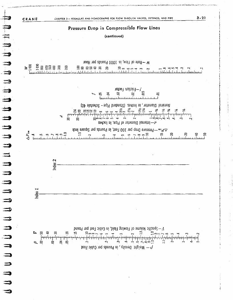
.~;::J

~

CRANE CHAPTER 3 - fORMULAS AND NOMOGRAPHS fOR HOW THROUGH VALVES, fITIINGS, AND PIPE 3 -21

Pressure Drop in Compressible Flow Lines

{continued)

JOOH Jad spunod 0001 U! 'MOlj )0 8jBIl-"11 ~ g g g gg g g g 80 000 0 0 0 ;::.; __ eo~a.noo:::t"M C'oJ ...-fooc.oL..n~('Y) N _oo(,O'"'"'~~ ('oJ _~~I.C?~C'"t':? C'! ~

!'I!!IIr1dd!l,1 II! II!!!!!!!!!!!!"'!,! I,I[!,! I I!!!,i!!!!illtddddd,t! i! :'tj,I!!1!I!!!!!,1r1d.!r!' I! jll!t!!!!!!!!!!!

..... ><

JOpe:l UO!P!J:l-J ........ Ln~ (Y:J N ~ .-...,,~~ ~ <::::> ~ ~ ,:,! I I!! ! ! ![!!!!)!!! I",! ! ,I! i I ! I

(op alnpa4JS - ad!d pJBpURlSJ S84JUI U! 'Jaj8WB!O IBU!WON qo 0 (,Oq-N 0 ~ ~ ~ "'$. ~ ~ ~ _:-;!: s_" N ('oJ ___ _ 00 (,0 U"'> ""::I'" C"')~ C'J N ............ _ to:) ..... ~

I I J ! !! I I 1 I ) J! I! I [ ! I I -f I I r'IIFIfI I!(iijilljil'( i Ililililii\iitljilii\QQ'lllil!ilii(liil\

~ ~ ~oor-(,O 1.0....... cry......... -~oql':~ u: ~ sa4JUI U! 'ad!d )0 Jajawe!o leUJajul--1'

ijJUI aJRnbs Jad sPunod U! 'jaa.::l 00 I Jad dOJO aJnssaJd -- oo'cl'i7 L.t1 0 U"'> 0000 N C"') ....... Ln(,Or-OOC':l __ N ~ "<:t' U"'>

!! ,I"!I!,!!!!,,!!!!!!!!!!!!I!! J Ifl,I,!,!! ,i"!!!!!ld!I!!I!!!!!!!!!!

~----------------.----------------------------------------------------------------.=

punod Jad laa.:l J!qn3 U! 'P!nl:l ZU!MOI:l )0 awnlol\ 3!)padS -,1 ~ ~ ~ g ~ ~ ~CJ")CX) r- <D \,.l'") ...,.. ('") c-.... 5 50;':'>':; r-.:"=! LO '¢ ("I") N

I'I'I!' I! J 1!"II'I"j!!! I I! ! I I I'I!! !! ! I t I'" ,I,!!! 1III'I!!!!]! /'!! , ! I t I'!';' I ! j ! ,:\, ,1",1 I! !'-"I!!!! '," I i I r 1 I ! r I I j I I II rill I I I I I 1111111l I 1, j .... ~1111 r (I j I I ct. ~ q ~ q """"!. ~ ~ ~ U? ~ ":CC!~~ ,-; C"-I ("I") oo::t- \,.l'")

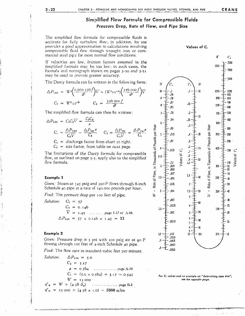
3 -22 CHAPTER 3- FORMULAS AND NOMOGRAPHS FOR flOW THROUGH VALVES. FITTINGS. AND PIPE CRANE

Simplified Flow Formula for Compressible Fluids Pressure Drop, Rate of Flow, and Pipe Size

The simplified flow formula for compressible fluids is aCCllrate for fullv turbulent flow; in addition. its use provides a good ~pproximation in calculations involving compressible flt;.id now through wrought iron or com­mercial steel pipe for most normal flow conditions.

If velocities are low. friction factors assumed in the simplified formula may be too low; in such cases, the formula and nomograph shown on pages 3-20 and 3-21 may be used to provide greater accuracy.

The Darcy formula can be written in the following form:

W·2(O.OO~/36f)v = (W'210-9)(336~00f)v

c. =

The simplified t90w formula can then be written:

C -- = C,C, f':"P1oo CJ 211 P

f':"P IOO P

C2

C1 = discharge factor from chart at right. C2 = size factor, from table on next page.

f':"PlOo P

C1

The limitations of the Darcy formula for compressible flow, as outl.ined on page 3-3, apply also to the Simplified flow formula.

Example 1

Given: Steam at H5 psig and 500 F flows through 8-inch Schedule 40 pipe at a rate of 240,000 pounds per hour.

Find: The pressure drop per 100 feet of pipe.

Solution: 0 1 57

0.146

1.45 .page 3-17 cr A-16

57 x 0.146 x 1.45 = 12

Example 2

Given: Pressure drop is 5 psi with 100 psig air at 90 F flowing through I ()O feet of 4-inch Schedule 40 pipe.

Find: The flow rate in standard cubic feet per minute.

Solution: f':"P1oo = 5.0

C2 5.17

P 0.564 ....... pageA-1O

C1 (5.0 x 0.564) + 5.17 = 0.545 W 2)000

q'm W +- (4-58 Sf!) ................ pageB-2

q'm 2) 000 + (4.58 x 1.0) = 5000scfm

:; 0

::t:

Q; c-

'" '0 § 0 a.. '0 '" '0

'" '" '" '" 0 .c f-

.= ,,-0

li: '0 '" ro a::

:=

Values of C,

II" (\ 2500

2000

1500

lOoo 900 BOO 700 EOO

500

400

DJ

2SO

100'

ISO

100 90 80 70

ill

50

40

3l

2S

20

15

LO 10

.9

.8

For C~ va/vel cnd on example on "determining pipe size"~ see the opposite page.

C '0 '" '" '" -,;; >

-

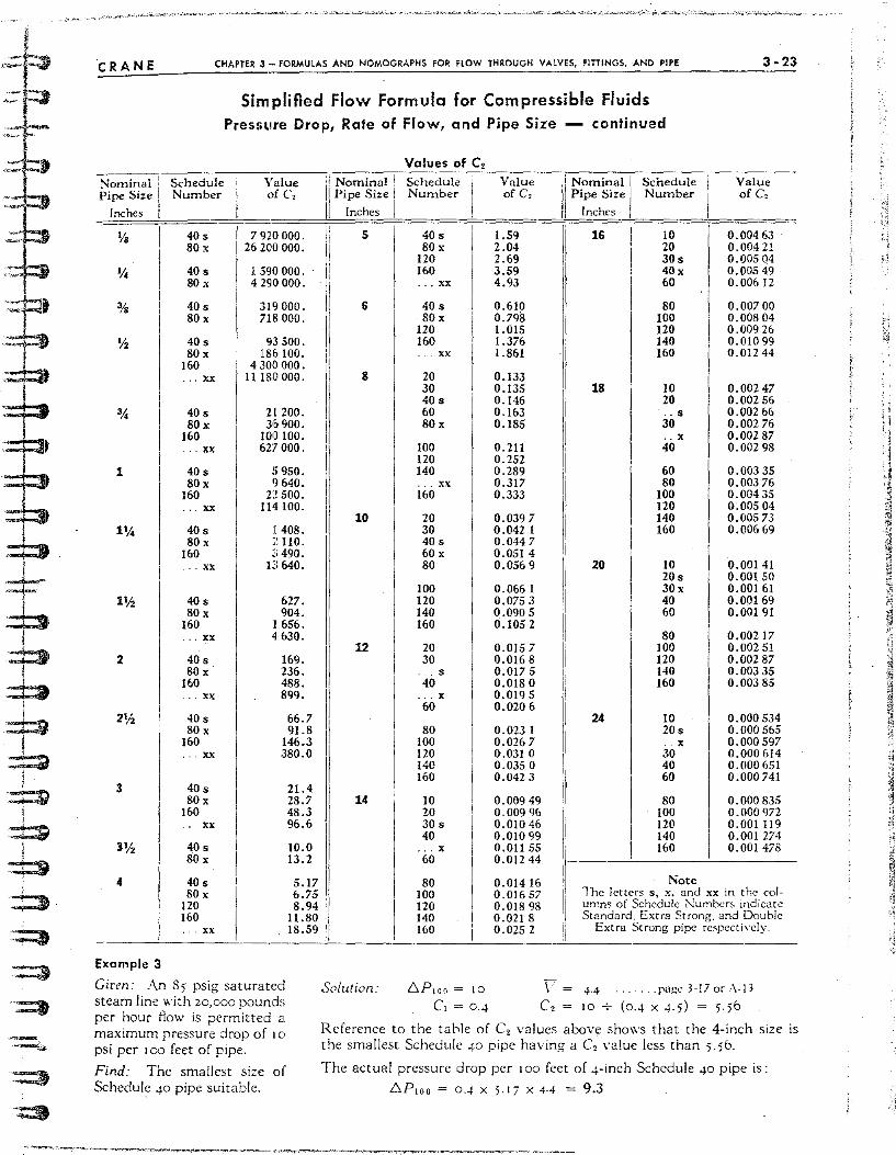
CRANE

~ominal j Pipe Size I

Inches I

1

IV:!

2

2 V:!

3

4

Example 3

CHAPTE~ 3 - FORMULAS AND NOMOGRAPHS FOR flOW THROUGH VALVES, FITTINGS, AND PIPE 3·23

Schedule Number

40 s 80 x

40 s 80 x

40 s SOx

405 SO x

160 ." xx

405 80x

160 ... xx

40. 80x

160 ." xx

40. 80 x

160 .. xx

40. 80x

160 ... xx

40. 80 x

160 .. xx

40. SO x

160 .. xx

40 s 80x

160 .' xx

40. 80 x

40. 80 x

120 160

. xx

Simplified Flow Formula for Compressible Fluids Pressure Drop, Rate of Flow, and Pipe Size - continued

Values of C, Value of C,

:1 Nomina1 I Ii Pipe Size i

Schedule Number

Value of C,

Ii Nominal i

II Pipe Size I

Schedule Number

Value of C,

II Inches I I Inches !

'

I 2~ i~,g ggg: II 1590 000. II 4290000. . ,II

I 319000.

I,

71S 000. Ii

93500. !I 186100. "

4300000. II,

11180000. II 21 200. 3& 900.

100100. 62? 000.

i; 950. Ij 640.

22500. 114100.

I. 40S. 2110. "490.

B640.

627. 904.

1656. 4630.

169. 236. 488. 899.

66.7 91.8

146.3

!I

I

I

3S0.0 I 21.4

2S.7 II 48.3 96.6

5

G

8

10

12

14

40. 80 x

120 160 ... xx

40. 80x

120 160 ... xx

20 30 40 s 60 80x

100 120 140 ... :xx 160

20 30 40. 60 x SO

100 120 140 160

20 30

' .. s 40

_ .. x 60

80 100 120 140 160

1.59 2.04 2.69 3.59 4.93

0.610 0.798 1.015 1.376 1.861

0.133 0.135 0.146 0.163 0.185

0.211 0.252 0.289 0.317 0.333

0.0397 0.042 1 0.0447 0.051 4 0.0569

0.0661 0.0753 0.0905 0.1052

0.0157 0.0168 0.0175 i 0.0180 \' 0.0195

0.0206 1'1

0.023 I 0.0267 (}.031 0 0.0350 0.0423 I

10 0.00949 III 20 0.00996 30. 0.01046

10.0 " . x O.Oll 55 40 0,01099 I

13.2 60 0.01244

5.17 80 0.01416 I 6.75 100 0.01657 ,:1

8.94 I 120 0.01898 I1.S0 I, 140 0.021 S

16

18

20

24

10 20 30. 40x 60

80 100 120 140 160

10 20 .. s 30 .. x 40

60 80

100 120 140 160

10 lOs 30x 40 60

0.00463 0.00421 0.00504 0.00549 0.00612

0.007 00 0.00804 0.00926 0.01099 0.012 44

0.00247 0.00256 0.00266 0.00276 0.00287 0.00298

0.00335 0.00376 0.00435 0.00504 0.00573 0.00669

0.00141 0.00150 0.00161 0.00169 0.00191

80 0.00217 100 0.00251 120 0.00287 140 0.00335 160 0.00385

10 20. ., x 30 40 60

0.000534 0.000565 0.000597 0.000614 0.000651 0.000741

80 0.000835 100 0.000972 120 0.001 119 140 0.001274 160 0.001478

Note The letters s, x, and xx in the col­umns of Schedule Numbers indicate Standard, Extra Strong, and Double

Extra Strong pipe respectively. IS.59 II 160 0.0252 II .~----~------~------~----------------------

Chen: /I.n 85 psig saturated steam line with 20,000 pounds per hour flow is permitted a maximum pressure drop of 10 psi per 100 feet of pipe.

Solution: 6.P"o = 10 C, = 0·4

v = 4.4 ,.pagc3-17or,\-13

C, = 10';- (0.4 X 4·5) = 5.56

Reference to the table of C2 values above shows that the 4-inch size is the smallest Schedule 40 pipe having a C, value less than 5.56.

Find: The smallest size of Schedule 40 pipe suitable.

The actual pressure drop per 100 feet of 4-inch Schedule 40 pipe is:

6.P100 = 0.4 x 5·17 x 4·4 = 9.3

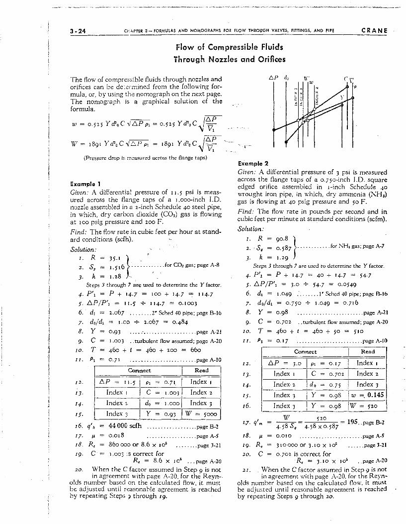
, ! j

3 _ 24 CHAPTER 3 - FORMULAS AND NOMOGRAPHS FOR HOW THROUGH VALVES, FITTINGS, AND PIPE CRANE ----Flow of Compressible Fluids

Through Nozzles and Orifices

The flow of compressible fluids through nozzles and orifices can be determined from the following for­mula, or, by using the nomograph on the next page. The nomograph is a graphical solution of the formula.

.- /I:;.p W = 0.525 Y d'o C.y I:;.p PI = 0.525 Y cPo C",,! =­

~ VI

W = 1891 Yd'OC-,jUPPI = 1891 YcPoC I~P '-.. 'V V,

(Pressure drop i~: measured across the flange taps)

Example 1 Given: A differential pressure of I 1. 5 pSI IS meas­ured across the flange taps of a I.ooo-inch I.D. nozzle assembled in a z-inch Schedule 40 steel pipe, in which, dry carbon dioxide (C02) gas is flowing at 100 psig pressure and 200 F. Find: The flow rate in cubic feet per hour at stand­ard conditions (scfh).

Solution: I. R 35. I

} .'

2. S,

3. k

1. 5 16 ........ ,' ... for CO, gas; page A-8

1.28 -. . Steps 3 through 7 are used to determine the Y factor.

4· P't = P + 14·7 = 100 + 14·7 = 114·7

5· I:;.P/P't = 11.5 + 114.7 = 0.1003

6. dl = 2.067 ....... . Z' Sched 40 pipe; page B-I6

7·

8.

9· 10.

II.

12.

13·

14·

15·

16.

17·

18.

19·

do/d. = I.CO + 2.067 = 0.484

Y 0·93 ........................ page A-21

C T

I .003 .. turbulent flow assumed; page A-ZO

460 + t = 460 + 200 = 660

0·71 .... _ ................... page A-IO

m Connect I Read

I:;.P = 11.5 PI 0·71 I Index I ·---+----------~--------I

I Index 1. __ -;--,.C ___ I_.00 __ 3+I--::-In_d_e_x __ 2 __

I Index 1C do 1.000 I Index 3 I Index J: Y 0·93 I W = 5000

q'h 44 000 scfh .................. page B-Z

I" 0.018 .................. page A-5

R, 860000 or 8.6 x 10' ........ page 3-21

C 1.003 I,S correct for R, = 8.6 X 10' ... page A-20

20. When the C factor assumed in Step 9 is not in agreement with page A-20, for the Reyn­

olds number based on the calculated flow, it must be adjusted until reasonable agreement is reached by repeating Steps 9 through 19.

6P do \\"' w

Example 2

Given: A differential pressure of 3 psi is measured across the flange taps of a 0.75o-inch I.D. square edged orifice assembled in I-inch Schedule ~o wrought iron pipe, in which, dry ammonia (NH3) gas is flowing at 40 psig pressure and 50 F. Find: The flow rate in pounds per second and in cubic feet per minute at standard conditions (scfm).

Solution:

I. R = 90.8 } 2. S. = 0.58 7 ........... for NH, gas; page A-7

3· k 1. 2 9 Steps 3 through 7 are used to determine the Y factor.

4· P', = P + 14-7 = 40 + 14·7 = 54·7

5· I:;.P /P\ = 3·0 + 54·7 = 0.0549

6. d, = 1.049 ........ 1' Schcd 40 pipe; page B-I6

7. do/d. = 0.750 + 1.0~9 = 0.716

8. Y 0.98 ........................ page A-21

9. C 10. T I I. PI

12.

13·

14·

15·

16. I 1·7- q'm

0·702 .. turbulent flow assumed; page A-ZO

460 + t = 460 + 50 = 510

0.17 ........................ page A-IO

Connect I Read

I:;.P = 3.0 I PI = 0.17 I Index I

Index 1 IC = 0·702 I Index 2

Index· 2 I do = 0·75 I Index 3

Index 3 I Y = 0.98 I W =.0.145

Index 3 1 Y = 0.98 IW = 520 I

18. I" 0.010 ....................... page A-S

19· R, 310000 or 3.10 x 10' ...... pageJ-ZI

20. C 0.702 is correct for R, = 3.10 X 10' .. page A-ZO

21. When the C factor assumed in Step 9 is not in agreement with page A-20. for the Reyn­

olds number based on the calculated flow, it must be adjusted until reasonable agreement is reached by repeating Steps 9 through 20.

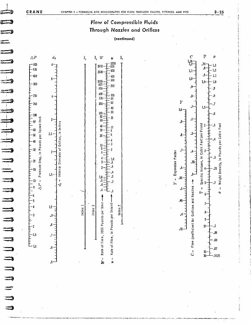
;;:::1

;::::t

" -it -.~~

~. I ~ =;::J~

,

=:::::'j

-:::=II

,":::=)

'::=8

;::p

::::::3

=3

'=:&

::=.l

:::::)

=l

=3

--

CRANE CHAPTER :1- FORMULAS AND HOMOGRAPHS FOR flOW THROUGH VALVES, FITIINGS, AND PIPE --------

6.P do I,

600 500

400

3J0

200

150

100 = Q 3

80 .:: ~

'" '" ~

60 ~

= '" 50 :u '-5

o· "- u

40 ~

" ~ ~ 0

" 30 "-~

Q: ZO e

c ~ ~ 15 ~ ~

~

'" ~ 1.5 "-

10 I

~ <J

6

5

1.0 X

'" "C ~

.8

1.5

1.0

Flow of Compressible Fluids

Through Nozzles and Orifices

(continued)

1, TV w 1, lOOO

3)00 800

<DOD 600

-400 1000 300 800 ZOO 600

400 100 300 80

<DO 60

40

100 30 80 60

<D

40 10 3) 8

<D 6

10 8 2 6

4 1.0 3 .8

2 .6

.4 1.0 .3 .8 .2 • 6

.4 .1

t i '" " "

~ N

X 0:: '" x u

'" ;;; '" '" " '" " .:: "- ;;; .:: '" "C "-= '" ~

" " = "- ~

<=> " <=> "-~ = ",. ,; '" " "- "--;; -;; ~ ~ ~ ~

'" '" I I

:: '"

Y

1.0

.9

.8

.2 " ~ "-= " .;;;

.6 = ~

"'-><

UJ

I .55

::..

3·25

V P

:; " "-Q

:u = "'- ~

~ '-' ;;;

'" "- "'-~

" ~ ~

" "-= = ,:: ~ .25 = '" Cl

:;;

t "" '"

I ..

'" '" N N Q.

" 2:

= ~

'" '" ~ " -= ! , 0

j .g

= .1 '" ! " .09 j

'" l " , u

.08 I '" ! .2 "- .07 ! I " j

u .0625 t~

:.:=:JI

~

::::)

:=;)

=.)

::=:3~

::=i~

:=:i~

::::j.

>:=:1.

:::3

::=:I. .==1t

:=D

:=:I~

~

==t . ~

:::::::n i ~

I

:b~ ~

Physical Properties of Fluids

and Flovv Characteristics of

Valves, fittings, and Pipe

The physical properties of many commonly used fluids are required for the solution of flow problems. These properties, compiled from many varied refer­ence sources, are presented in this appendix. The convenience of a condensed presentation of these data will be readily apparent.

Most texts on the subject of fluid mechanics cover in detail the flow through pipe, but the flow character­istics of valves and fittings are given little, if any, attention, probably because the information has not been available. A means of estimating the re­sistance coefficients for valves, deviating in minor detail from the standard forms for which the coeffi­cients are known, is presented in Chapter 2 .

The Y net expansion factors for discharge of compres­sible fluids from piping systems, which are presented here for the first time, provide means for a greatly simplified solution of a heretofore complex problem.

A -1

APPENDIX A ! i

i i I I I ~

I t

! I I

I I i

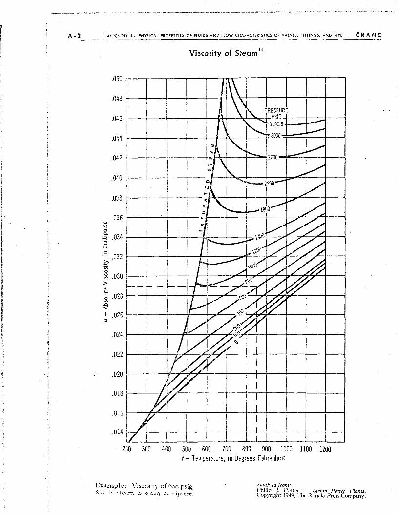
, I

! I l I

I I i ~ ~ I,

~ Vl Ie ';1 ,

A _ 2 APPENOIX ,,- PHYSICAL PROPERTIES OF flUIDS AND flOW CHARACTERISTICS OF VALVES, FITTINGS, AND PIPE

V· . f S 14 ISCOSlty 0 team

.050

.048

.046

.044

.042

.040

.038

.036 Cl.> (/l

a 0.

.034 ~

<:: Cll

U c: .-: .032 >. ~

(/l a u .030 on :> '" ~ ~ .028 (/l = « I .026 :t

.024

.022

.020

.018

.016

.014

1\\ \\ '- ~RESSURE

PSIG

\ ... '-.....""1 3191.5 -----3000

~ :::; " V « \ '-- --: \ 2600

~ V '" --Q ...... -2200-....

.,V UJ

1 1-,\ « "- 1860 ...........

V / '" 10.. =>

l-

V % « / VI

\ ~",(J ....... -,. ~ ~ % L,. \1-"'''''''

I ~ ",,,,,,,/ 0 ~ ~ I 1/ 'I ./

ll~~~ % ~ 7 -- I-- 1--

"./" V'o\)\)~ ~ 'V /" '>.\)\) .~

/' V' ?f/ L / / /~~~ I

/ //%V~/ I ~v I

I 0 0 ~ I I

~ /'1 I

I , ;; V I

I

) V' I I

l/ I I 200 300 400 500 600 700 800 900 1000 1100 1200

t - Temperature, in Degrees Fahrenheit

Adapted from:

CRANE

Example: Viscosity of 600 psig, 8;0 F steam is 0.02Q centipoise. Philip ). Potter - Steam Pou'er Planls,

Copyright 1949, The Ronald Press C'..ompany.

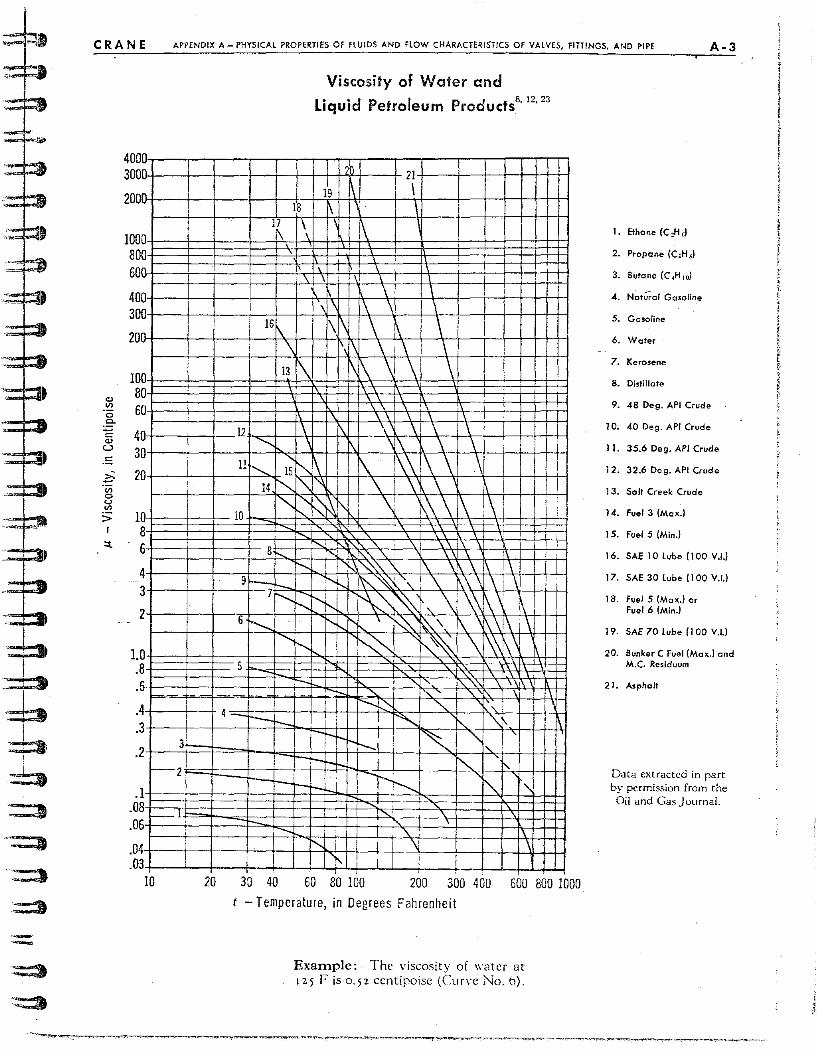
<:i •

-- I; b :6, :=3,

,--

CRANE APPENDIX A - PHYSICAL PROPERTIES Of flUIDS AND flOW CHARACTERISTICS OF VALVES, fITiiNGS, AND PIPE A-3

'" Vl

o Cl. ~

c: '" '-' c:

;:;. Vl o u <f)

> I

::t

0 400 300 Ill..

Ill.. 200

0 0

100 80 60 10-

0 40 30 0

20 0

10 8 6

0 0 0

4 3 0 0

2 0

1 0 8 6

4 3

2

1 .0 8 .6

.4

.3

I I

i ,

i 1 I

.2 3L

~2

1 .0 .0

8 6 ,..-1.

4 3

.0

.0 lD

1

,

I

4

20

18 17 \ 1\ \

_l ~

I

i 161\ I

\ 13 ~

,

12 \ -.......,

" 111-....... 15~ 14 b-I"

"'-., "-10 b,

8t--i'

9r- b 7 r----i' 6 r .........

......... i'

5

I:::: ,

Viscosity of Wafer and Liquid Petroleum Products8

,12,23

~ 21 I 119 I II \

l~ \ 1\

, , 1\ \ 1 \

....\ , _Ll \ -.1 1 \ I

\1 \ I 1\ ~ I \ I

\1\1 I \ i\ I \ 1\1\ \ \ \

1\[\ \ \ \ I ,

1 ~ 1\ , _\ \ \ 1 \ i\

\ \ \1 \ \ 1 ~ \:\ \ \ I

\ I r\ 1\\ 1\ \ \ I~ 1 ~l \' , \ I ~ ~}. ~ ~\ \ \\ \\ ,

D' ~ " ,\ \ \ I' ,,\ '\ '( \ \ II

I"'-.,"'\. 1- 1\ \ \ 1\ 11 li ~~\! \ 1\\ \ \ \

1" I t'-l, ~J, \' \\ ~~ \ '\ ' 1 N...,I' \

~ ~', 1\ \ l\\11 \ I ~ f0'\, \ \\\\\ 1\

J. ~ i,\ '\ \ ' \ \\1\ ,-::::::: ~ '\' '\. ~! 1\

~ I ~ "'-., :\ !

I I I

,

,

I

1

- -

t-t- ' , I I, l'\. ,\l-- 1\ r-t-

I r--r--r--: ~I~ \, I I T-N- ~ f"\.-

i 1')"-....... l"\. N I 1'\ ,

I -.... ~ '\.1 \ I' -1 \J \

I ~ J _L I . 30 40 60 80 100 200 300 400 600 800 1000

t - Temperature, in Degrees Fahrenheit

Example: The viscosity of ,,'ater at 125 F is 0.)2 centipoise (Cur\"c No. b).

I. Ethene (C ,H,)

2. Propene (C,H s)

4. NQtu~a' Gasoline

5. Gasoline

6. Water

7. Kerosene

8. Distillate

9. 48 Oeg. API Crude

10. 40 Oeg. API Crude

11. 35.6 Oeg. API Crude

12. 32.6 Oeg. API Crude

13. Solt Creek Crude

14. fuel 3 (Mex.)

15. fuel 5 (M;n.)

16. SAE 10 lube (100 V.I.)

17. SAE 30 lube (100 V.I.)

18. fuel 5 (Max.) or Fuel 6 (M;n.)

19. SAE 70 lube (100 V.I.l

20. Bunker C Fuel (Max..) and M.e. Residuum

21. Asphelt

Data extracted in part by' permission from the

Oil and Cas Journal.

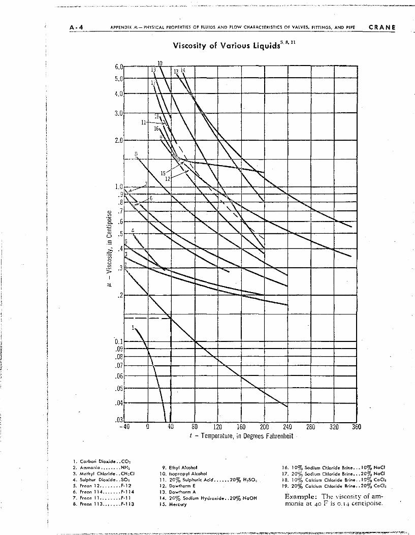
A - 4 APPENDIX fti,- PHYSICAL PROPERTIES OF flUIDS AND flOW CHARACTERISTICS OF VALVES. FITTINGS. AND PIPE ~-'----

CRANE

Viscosity of Various LiquidsS,8. II

6.0 10 1\ \ 1\ i(

5.0 1,\ \ \\ 4.0

\\ \ ,

3.0 r\ 11

18\~ \.\ \ 16~ 2.0 l\.

~

~ ,

1\ 1\'" i

ZJ ~\ r--i '\ ~ ~\

-, ~ II

~5/ r\""'" 12

" 1.0 Ii 7 - '\. ' "", -.\. .9 ~S= '\. '\. .........

.8 6 " '\. " \. ..........

.7 ,.~ "- '\. " ..... I'-... .........

Q.)

"-l'.. ...., ~. I'\.. " ............. ~ '" 0 .6 0.

"'-" '" "- '" ............ '" ~

c: &

'" .5 C,)

~,'" " " "" ~\ -............. c: I"-...... ..:::- .4

;~ .......

~ ~ "-'" ~ 0 u "-'" .3 >

'''''~ ~ "' "" ~ I p::::::: ::t. r:::::-.2 I--

I~ ---------~

'" 0.1 1\

\. I'.. .09 "-.08 .07 11 "-.06 \ " \ I~ .05

\ i .....

""-.04 \ .....

.03 \ -40 a 40 80 120 160 200 240 280 320 360

1. Carbon Dioxide •• CC~2 2. Ammonia ••• " •••• NH::;. 3. Methyl Chloride •• CH;>Ci 4. Sulphur Dioxide •. SOI~ 5. Freon 12 ...• 0 ••• F-12 6. Freon 114 ....•.. F-114 7. Freon 11 ..•....• F-l 1 8. Freon 113 ....... f·113

t - Temperature, in Degrees Fahrenheit .

9. Ethyl Akohol 10. Isopropyl Alcohol 11. 20% Sulphuric Acid ••.••• 20% H tS04

12. Dowtherm E 1 3. Dowtherm A 14. 20% Sodium Hydroxide .. 20% NoOH 15. Mercury

16. 10% Sodium Chloride Brine ••. 10% Noel 17. 20% Sodium Chloride Brine ••• 20% Noel j 8. 10% Calcium Chloride Brine .. 1 0% Coel: 19. 20% Colcivm Chloride Brine •• 20% CaCt:

Example: The viscosity of am­monia at 40 F is 0.14 centipoise.

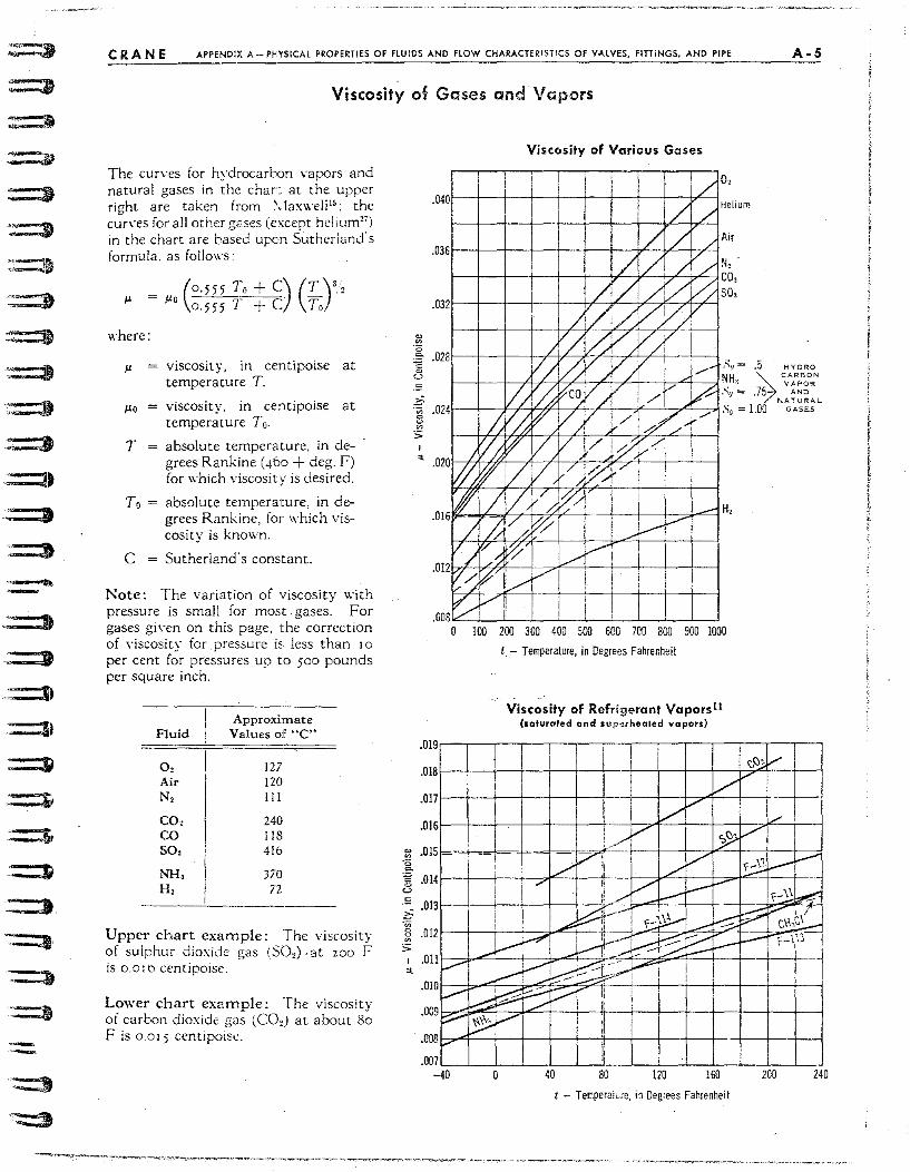
=D

=t <:=1t

::=3_ ==l. ==:I. . :=9 -:=1~

::=1.

~

.==11

==:S~

:=:I,

eRA N E APPEND I)( A-PrYSICAl PROPERTIES OF FLUIDS AND flOW CHARACTERISTICS OF VAlVES< FlnINGS< AND PIPE -'-'-:.-.-----

Viscosity of Gases and Vc;pors

The curves for hydrocarbon vapors and natural gases in the chart at the upper right are taken from \lax\\·cll 15 ; the cun·es for all other gases (except helium27) in the chart are based uJXln Sutherlamfs formula. as follows:

/1- = /1-0 (0<555 7:0 + C;) (~)3:, 0.555 7 + C To

where:

/1- viscosity, in centipoise at temperature T.

/1-0 = viscosity, in ce:1tipoise at temperature To.

T = absolute temperature, in de- . grees Rankine (460 + deg. F) for which viscosity is desired.

To = absolute temperature, in de­grees Rankine, for which vis­cosity is known .

C = Sutherland's constant.

Note: The variation of viscosity with pressure is small for most gases. For gases given on this page, the correction of viscosity for pressure is less than 10

per cent for pressures up to 500 pounds per square inch.

Approxi:mate Fluid Values of ~4C"

0, 127 Air 120 N, III

CO, 240 CO JIB SO, 41b

NH, 370 H, 72

Upper chart example: The viscosity of sulphur dioxide gas (SO,) ,at 200 l­is o.olb centipoise.

Lower chart example: The viscosity of carbon dioxide gas (CO,) at about 80 l- is 0.015 centipoise.

.04

,03

.03

::;. .;;; ,02 8 ~

:;;:

:::I.. .02

.01

.01

.00

0

6

2

8

4

/ o~

6'.#' /

/7 2

~~

Viscosity of Various Gases .

I ! I i i i / : ! 0,

I I / I / Helium

/ / / Air

I I / / / //. N, ' CO, SO, I /:/!/ V0

/i//VY~ / V/V/Y~

Y/V'XY,,{ I J----t

VA'hc<;Y /' i/r i~' ~ Vh [t' V Y .! /1 ~;

i ;.- 'a 1/

~/

V~ VV V 1/10-1 ,.¥ ;,,/.;/ I i ~ VV ~/~/, I

~ I , ,

/iv'~/)ffi I

I 1--i H,

~j//.~ i ! ).---V

~~ ~ ~ . , , ~. IV V, ! I i I I ~

8~ i ! o 100 200 300 400 500 GOO 700 800 900 1000

t - Temperature, in Degrees Fahrenheit

Viscosity of Refrigerant Vaporsll (saturated and sup·arhealed vapors)

t - Temperature, in Degrees Fahrenheit

A-5

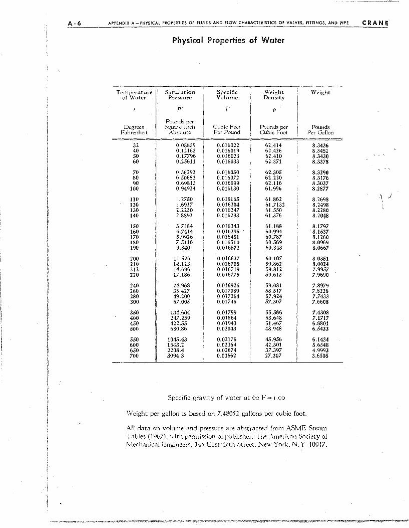
A-6 APPENDIX A-PHYSICAL PROPERTIES OF flUIDS AND flOW CHARACTERISTICS OF VALVES. FITTINGS. AND PIPE CRANE

Physical Properties of Water

Temperature 11 Saturation Specific Weight \Veight

"f\~ater I Pressure Volunlc Density

P' \' P

I Pounds per

Degrees Square Inch Cubic Feet Pounds per Pounds Fahrenheit I Absolute Per Pound Cubic Foot Per Gallon

--32 0.08859 0.016022 62.414 8.3436 40 0.12163 0.016019 62.426 8.3451 50 0.17796 0.016023 62.410 8.3430 60 0.25611 0.016033 62.371 8.3378

70 0.36292 0.016050 62.305 8.3290 , . ,

80 I 0,50683 0,016072 62.220 8.3176 90 I 0.69813 0.016099 62.116 8.3037

100 0.94924 0.016130 61.996 8.2877

110 I 1.2750 0.016165 61.862 8.2698 \ J 120 'I L6927 0.016204 61.7132 8.2498 130 II 2.2230 0.016247 61.550 8.2280 140 Ii 2,8892 0.016293 61.376 8.2048

150 Ii 3.7184 0.016343 61.188 8.1797 Ii 160 II 4.7414 0.016395 60.994 . 8.1537 170 5.9926 0.016451 60.787 8.1260 180 I' 7.5JlO 0.016510 60.569 8.0969 190 II 9.340 0.016572 60.343 8.0667

200 II 11.526 0.016637 60.107 8.0351 210 II 14.123 0.016705 59.862 8.0024 212

1\

14.696 0.016719 59.812 7.9957 220 17.186 0.016775 59.613 7.9690

240

i 24.968 0.016926 59.081 7.8979

260 35.427 0.017089 58.517 7.8226 280

II 49.200 0.017264 57.924 7.7433

300 67.005 0.01745 57.307 7.6608

350 Ii 134.604 0.01799 55.586 7.4308 400

I' 247.259 0.01864 53.648 7.1717

450

II 422.55 0.01943 51.467 6.8801

500 680.86 0.02043 48.948 6.5433

550 II 1045.43 0.02176 45.956 6.1434 600 II 1543.2 0.02364 42.301 5.6548 650 I 2208.4 0.02674 37.397 4.9993 700

I, 3094.3 0.03662 27.307 3.6505

1 1 I

I Specific gravity of water at 60 F = 1,00 I

1 Weight per gallon is based on 7.48052 gal!ons per cubic foot. j j ;

All data on volume and pressure are abstracted from ASME Steam Tables (1967), with permiSSion of publisher, The American Society of Mechanical Engineers, 345 East 47th Street, New York, N.Y. 10017.

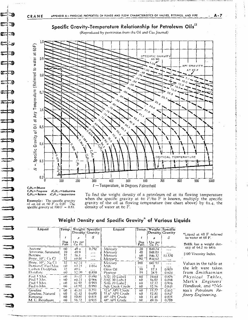
± ~I l' I

i

=::.:3

~

,-

CRANE APPENDIX A-I'HYSICAL PROPERTIES OF flUIDS AND flOW CHARACTERISTiCS OF VALVES, FITTINGS, AND PIPE A·7

-ro

o o

Specific Gravity-Temperature Relationship for Petroleum OilSl2

(Reproduced by permission from the Oil and Cas Journal)

0.2 !;--'----,~--L-:':_:_--'.-~-L--:L:-L---::L--L.._:l~-L___::!_:_--'.-~---.JL-_:l:_:-.l.--~ o 300 400 500 600 700 800 900 1000

C:Hs=Ethone t - Temperature, in Degrees Fahrenheit

C1Ha=Propane iC 4H1(l=lsobutane C.H]o=·Butane ;C;;.H 12 =Jsopentone

Example: The specific gravity of an oil at 60 F is 0,85 The specific gravity at 100 F = 0,83,

To find the weight density of a petroleum oil at its flowing temperature when the specific gravity at 60 F/60 F is known, multiply the specific gravity of the oil at flowing temperature (see chart above) by 62.4, the density of water at 60 F.

-

Weight IDensity and Specific Gravity* of Various Liquids

Liquid Temp ./ Weight Specific : Density Gravity I

IpS .

Deg. t Ll';, ~cc I Fahr. I Cu. for.

:\Ct."tone I 60 , 494

I 0]92

I I :\mmonia, Saturated! 10 40,9 .,. B,'nccnc ' 32 I 5b,1 .,. I Brme, 10'; Ca CI 32 I

6B.05 I I ! ... I B~ iric, 10'; :--:a CI

, 32 I 67.24 I ...

[It:nkns c: Furl \ lax I'D b3.25 I 1014 ! l .... nt .... pn D:-..ulphIJc J2 ~O_·~") 1),,, !111M ,,0 52,99! 0,850 l-.:~~~:rf!\-1dX---- - ~(f--5W)2~Q8 Fuel 5 \Im, bO ,,0_~3 O,9(m Fuel 5 \Ia, l'(l 61,92 0,993 Fuell' \Iin, bO , 61,<12 0,993 Ca'<)line 60 4b);J 0751 Casoline, Natural 60 42 A2 0,6S0 Kerosene 60 50)!5 0,815 M, C Residuum 60 58),2 0,935

Liquid Temp.' Weight Specific Density Gravity

I p S Des· Fahr.

Lbs. fer Cu. "t. I

Mercury

I 20 849]4 I ...

I\1ercufV 40 848m

I . ..

Mercury 60 846,32 13,570 1v1c rcury I (3Tr~ 844,62 I . .. l\/fcrcury I 100 I 842.93 I . .. !\lilk I t ! ... I - . .. Oltw 0,1 59 ,7,3 0,919 Pentane 59 38,9 0.624 S,,\E 1 O"L-uLbe-'!~---:--"7bOC;-+--;5~4-;,6-;4--';--"0;-;.8"7;;b-SAE )0 Lube! 60 5b,02 0,898 SAE70 Lubct. 60 57,12 0.916 Salt Creck Crude 60 525b 0,84J ) 2,,," A P I Crude --i--76"7C0-i---;5"'3""]"'7;--CC-CO"",8"'6'c2=-35,6" API Crude 60 52,81 0.847 40" API Crude 60 5145 0.825 48" API Crude 60 49.16 0]88

'Liquid at 60 F referred to water at bO F·

tMilk has a weight den­sity of 64,2 to 64,6,

t 100 Viscosity Index,

Values in the table at the left were taken from Smithsonian Physical Tables, Mark's' Engi~eers' Handbook, and "Nel­son's Petroleum Re­finery Engineering.

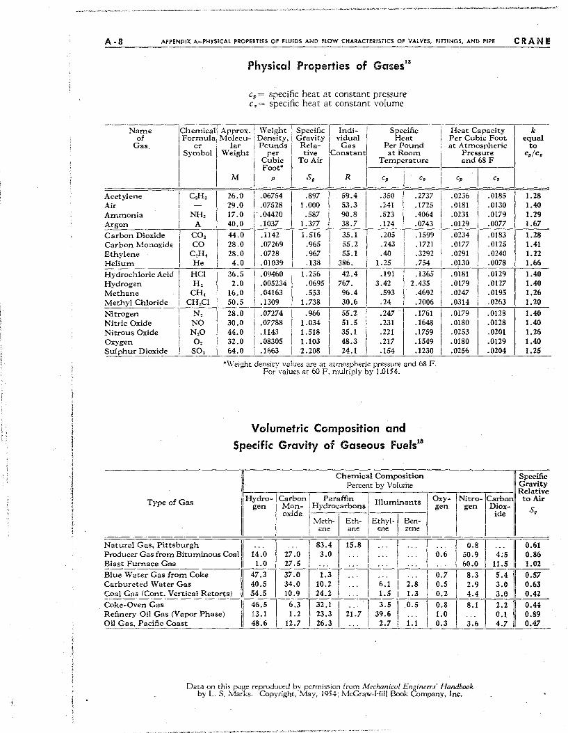
A - 8 MPENDIX A-PHYSICAL PROPERTIES OF FLUIDS AND HOW CHARACTERISTICS OF VALVES. FITTINGS. AND PIPE eRA N E ~~------------------------------------------------------------

Name of

Gas.

Physical Properties of Gases l!

Cp = specific heat at constant pressure c, = specific heat at constant volume

,CheITlicall· Approx. , Weight

Formula Moleeu-II Density,

Symbol Weight 1 per

Specific 1 lndi- Specific Gravity I vidual I Heat Rela- I Gas Per Pound tive Constant! at Room

I Heat Capacity I Per Cubic Foot

at Atmospheric Pressure and 68 F

or lIar Pounds

I

I Cubic I M FO:t>

To Air I Temperature

1

--,--;-, --1--------,-1 -I cp j Cf) Cp C" R

Acetylene Air Ammonia Argon

Carbon Dioxide I Carbon MonoxidE' ,i

Ethylene Helium

Hydrochloric Acid I

Hydrogen III

Methane Methyl Chloride

Nitrogen Nitric Oxide Nitrous Oxide Oxygen Sulphur Dioxide

C,H,

NH, A

CO2 I

C~~. II

He

HCI I H,

CH, l CH,CI

N, NO N,O 0,

SO,

26.0 I .06754 29.0 .07528 17.0 I' .04420 40.0 I .1037 44.0 28.0 28.0 4.0

36.5 2.0

16.0 50.5 28.0 30.0 44.0 32.0 64.0

.1142 I'

.07269 I' .0728

.01039

.09460

.005234

.04163 I .1309

I .07274 II .07788

.1143 I'

.08305

.1663 I

.897 1.000

.587 1.377 1. 516

.965

.967

.138 1. 256 I

.0695

1

1

.553 1.738

.966 1.034 1.518 1.103 2.208

59.4 I' 53.3 I 90.8 38.7

35.1 I 55.2 I 55.1

386. 42.4

767. 96.4 30.6 55.2 I 51.5 I 35.1 I 48.3 24.1

.350 I

.241 II, .523

.124 .205 .243 .40

1.25 .191

3.42 .593 .24 .247 .231 .221 .217 .154 I

.2737 i

.1725

.4064

.0743 .1599 .1721 .3292 .754

.1365 2.435

.4692

.2006

I

.1761 i

.1648

.1759

.1549

.1230 ,

*\\'eight density values are at atmospheric pressure and 68 F. For yalues at 60 F, multiply by 1.0154.

Volumetric Composition and

Specific Gravity of Gaseous Fuels13

, Chemical Composition I Percent by Volume

.0236

.0181

.0231

.0129

.0234

.0177

.0291

.0130

.0185

.0130

.0179

.0077

I .0183

I

.0125

.0240

.0078 .0181 .0129 .0179 .0127 .0247 .0195 .0314 I .0263 .0179 .0128 .0180 .0128 .0253 .0201 .0180 .0129 .0256 .0204

HYdrO-I Carbon i • Paraffin I IlluITlinants I Oxy- ! Nitro- Carbon Type of Gas I gen Mon- I Hydrocarbons gen

I

gen ,

oxide I I I

I I Meth- Eth- EthYl-I Ben-

I I ane ane ene zene

Natural Gas, Pittsburgh r 83.4 15.8 0.8 Producer Gas from Bituminous Coal I 14.0 27.0 3.0 0.6 50.9 Blast Furnace Gas I 1.0 27.5 60.0 Blue Water Gas from Coke

II

47.3 37.0 1.3 0.7 8.3 Carbureted Water Gas 40.5 34.0 10.2 6.1 2.8 0.5 2.9 Coal Gas (Cont. Vertical Retorts) 54.5 10.9 24.2 1.5 1.3 0.2 4.4

Coke-Oven Gas

il 46.5 6.3 32.1 3.5 0.5 0.8 8.1

Refinery Oil Gas (Vapor Phase) 13.1 1.2 23.3 21.7 39.6 1.0 Oil Gas, Pacific Coast 48.& 12.7 26.3 2.7 1.1 0.3 3.6

Data on this page reproduced by permission from Mechanical En[!,ineers' Handbook by L. S. Marks. Copyright. May. 1954; McGraw-Hili Book Company. Inc.

Diox-ide

II

4:5 11.5 5.4

II 3.0 3.0 2.2

II 0.1 4.7

k equal

to cplc,

1.28 1.40 1.29 1.67 1.28 1.41 1.22 1.66 1.40 1.40 1.26 1.20 1.40 1.40 1.26 1.40 1.25

Specific Gravity Relative to Air

S.

0.61 0.86 1.02 0.57 0.63 0.42 0.44 0.89 0.47

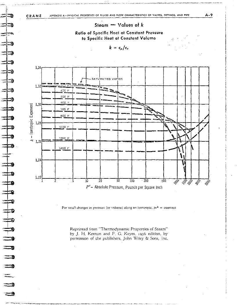
j

::::II

::::=3

::::::'1

.. ==:1

.==8

CRANE APeENDly. A-PHYSICAl PROPERTIES Of flUIDS AND flOW CHARACTERISTICS OF VALVES, FITIINGS. AND PIPE

1.34

1.3 2

§ 1.30 c 8. x

L.LJ

.0.. 12 g . c a:> (/)

8

~ ...... ""'-

"- -

-----

Steam - Values of k

Ratio of Specific Heat at Constant Pressure to Specific Heat at Constant Volume

k = epIc.

__ £H",!e",o,J r- 300 F !>;os> .. - !o-_"i"'_

400 F I ;-;::. ~ -r-::t -r- ·h ~OO-L..ro ,_~ -I __ ~ ~ 500 F I -......

~o~~ --~-- :: ~ - --~- -~o~ ~ --~--I

IOOO~ .... - ~---~- - - ~ I

""'" 1.2 ~ __ ~o~ .-6

I"- J...l40...ru;., --I------~- '"" - --- ........... 1.2 4

1.22 I 2 5 10 20 50 100 200 500

pi _ Absolute Pressure, Pounds per Square Incil

For sma'] changes in pressure (or volume) along an isentropic, pvk = constant

Reprinted from "Thermodynamic Properties of Ste2.m" by J. H. Keenan and F. G. Keyes, 1936 edition, by permission of the publishers, John Wiley &1 Sons, Inc.

~

~ R \~

I'

\\ \~ t

A-9

.// .J~ ~/ l/' ~

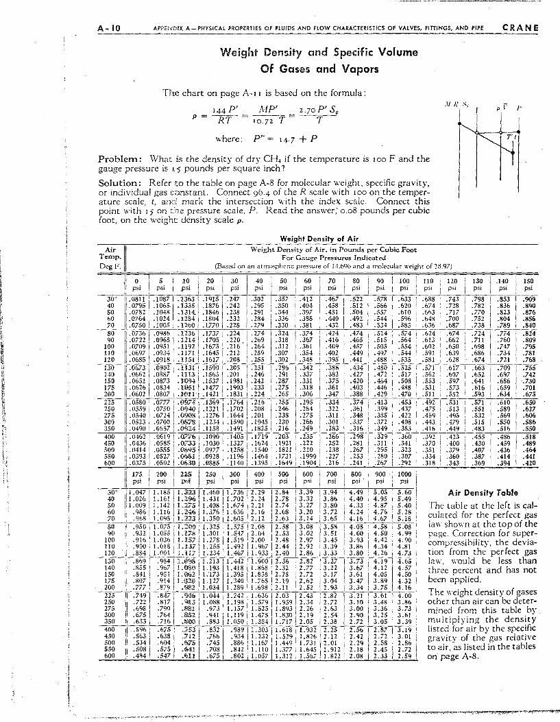
A - 10 APf'<!'<PIX A - PHYSICAL PROPERTIES OF FLUIDS AND flOW CHARACTERISTiCS OF VALVES, FITIINGS, AND PIPE '-'--'-=----

CRANE

Weight Density and Specific Volume

Of Gases and Vapors

The chart on page A-I I is based on the formula:

144 P' MP' p = ~ = 10.72 T

2.70 P' S. T

where: P" = 14.7 + P

.11 It "..;

I p p p

Problem: What is the density of dry CH, if the temperature is 100 F and the gauge pressure is 1.5 pounds per square inch?

Solution: Refer to the table on page A-8 for molecular weight, specific gravity, or individual gas constant, Connect 96.4 of the R scale with 100 on the temper­ature scale, t, ana' mark the intersection \vith the index scale. Connect this point with 15 on the pressure scale, P. Read the answer; 0.08 pounds per cubic foot, on the weigh: density scale p.

Temp,

Weight Density of Air \Veight Density of Air. in Pounds per Cubic Foot

For Gauge Pressures Indicated Air II DegF. (Based on an atmospheric pressure of 14.696 and a molecular weight of 28.(7)

o psi

5 i 10 psi I psi

20 '1 30 't 40 i 50 psi psi I psi I PSI

60 psi

70 psi

80 psi

90 i 100 psi psi

110 pSI

120 psi

130 psi

.140 psi

150 psi

30" II ,0811 I', ,10871.1363 .1915 .247 1 ,30~ I ,3~7 .412 .467 .522 .578 .633 .688 .743 .798 .853 .909 40 11.0795 " .1065 1 .133,5 .1876 .242 .29, 1.3,0 .404 .458 ,512 .566 I .620 .674 .782 .836 .890 50 I' .0782 .1048

1

.>314. .1846 .238 .291 .. 344 .397 .451 .504 .557 .610 .663 .770 ,823 ,876 60 .0764" .1024 .1284 .1804 .232 1,.284 i .336 .388 .440 .492 .544 .596 .752 .804 .856 70 ,1.0750 i .1005 .. 1260 .1770 .228 .279 I .330 .381 .432 .483 .534 .585 .738 .789 .S40

-""8"'0 ~I! .. 0736 I .09861"--;, i, C;;2~36~':". 1~7~3~7 +1-'."'22::-C4;'--;lcc.C;;27"'4~'.:;;3"'247-.-'-:. 3i:7c;.4-'---'.-;4~24;-':-' -.'-'47"'47-'---'C. 50:;2-;4-'c-~~.--'~c--'7;;:.-"-.:;. 7"'2:O-4-+-"':."'77"'4~---'C. 8"'2~4 90 1.0722' .0968 .1.214 .17051.220.! .269 .318 .367 .416 .465 .515 .711 .760 .809

100 I .07091.0951 .un .1675

1

.216 ,.264 .312 .361 0409 .457 .505 .698 .747 .795 lIO I'j ,069: .0934 I ... n:1 .1645 .212 '.259 .307 .354 .402 .449 .. 497 ,686 .734 .781

~1~20~~I.~0~68~'~~.0~9~18~c'2.~'I~~~I~.,~1~61~7rl-.~2~08?-~I~.2~5=.5-+~.3~0~2~...:.~34;8:~~.3~9~5~~.44~I~!_...:.~48~8~:~~_~~~~~~-,...:.~67i4~~.7~2~1-+-~.768 130 Ii .0673 1 .0902 'I .H31 .1590! .205 I' .251 I .296 .342 .388 .434 .480 .663 .709 .755 1401.06621.0887 .11U .1563'1.201 .246 1.291 .337 .382 .427 Ail .652 .697 .742 150 I, .0651 .0873 .n094 .1537 .1981 i .242 I' .287 .331 .375 .420 .464 .641 .686 '.730 175 1'[.06261.0834 .H151 .1477 i .1903 i .233 .275 .318 .361 i ,403 .446 .616 .659 .701 200 !. 0602 .0807,. IOn .1421 i .1831 1 .224 ,. 265;'--;"':'c;.30",6o--'---'C' 3",4",7-'..-,,3.:,.8:,c8;-,-' ...:.-;4",29.-+--,-::~_~~---'C' 50:;5:0'2-,' ..::.~59;c3;.--;---'C.6C;3.4;;'~"::'767~5 225 I' .0580' .0777 i .0974 .13691.1764 i .216 .255 .295 .334 .374 .413 .492 .531 .571 .610 .650 250 1.0559 .0750' .0940 .1321 .17021.208 .246 .284 .322 ,361 .399 .'44~95 ".513 .551 .589 .627 275 II' .0540, .07241 .()'JiOS .1276 .1644 i .201 .238 .275 .311 .348 .385 ".495 .532 .569 ,606 300 ,.0523, .0700 ',.0078 .1234, .15901.1945 .230 .266 .301 .337 .372 .443 .479, .515 .550 .586 350 if .0490, .0657 i .0824 .lI58 1 .1491 .182:-o5c+":.;:2~16:c--~.2c4,~9-+..:.~28;:c3~''':':.;:3~16~.....:.:.3",4",9-+-~:.::o-'--'-'4~16 .449' .483 .516 .550 400 1,.0462! .O?I~: .O:,§6 .1090 1.14051 .1719' .203 .235 .266 .298 .329' .392 0423 .455 .486 .51S 450 I, .0436 1.0080 i .(),,33 .1030 !.1327 : .1624 ',' .1921 .222 .252 .281 .311 .370 ADO i .430 .459 .489 500 1.0414 'I .0555 : .()695 .0977 .1258

1' .1540 ! .1821 .210 .238 .267 .295 .323 .351 .379 ,407 .436 .464

550 1'.0393 .0527' .Ol>f>l .0928 .1196, .1464 i .1731 .1999 .227 .253 .280 .307 .334 .360 .387 .414 .441 600 ii.0375! .05021 .06.3!l .0885 i .1140 i .1395' .1649 .1904 .216 .241 .267 .292 .318 .343 .369 .394 ,420

psi' psi iii 175 1 200 I 225 250 I' 300 i 400 1 500 600 l~I~I~ ~ ~I~I~ ~ ~ ~

30 0 1'1' 1. 047 1 1.185 i l. 3Z3~"'1C'."'46"0"'1c-,1'-.-7"'36;-7-1 '2 .-'2"'9--+co2"'. 8"4'--:''''3C'. 3"'9--''''3'''.'OC94~~4-.4'"9C-:-'''5~. 0;;-;5~"'5'-.760OC-

40 1.026 1.161,1.1.% 1.431',1.70212.24 2.78 3.32 3.86 4.40 4.95, 5.49 50 11.00911.142 '11.V5 1.408: 1.674 2.21 2.74 3.27 3.80 4.33 4.87 5.40 60 ii .986 i 1.116 1.2:-*6 1.376' 1.636 2.16 2.68 3.20 3.72 4.24 4.76 70 ii .968,11.09511.213 1.350 i 1.605 r 2.12 ,2.63 3.14 3.65 4.16 I 4.67

700 800, 900 1000

~g li:m: J:g~~ l::i~ U6f i i:~~; I U~ I ~:~~ tg~ n~ !:g~ ::~~ 100 Ii .916: 1.036 ! 1.157 1.2781,1.51912.00 12.48 2.97 3.45 3.93 4.42 lID .1: .900: 1.0181 LU7 1.255,1.492 1.967 2.44 2.92 3.39 3.86 4.34 120 ".884 I 1.001 ! 1.1.;;:17;.-'-01 '0' 2'73i-4-c1~1:.. 4o-:6",7-:-;1c:..",93,"3,-1c:2""-o4;:-0c-:-2~'c;:8~6-"_~3.:;.3:;;3--+..:3c:.,,,80~_40'c;2",6-i-7-7' 130 .869 I .984' Li.lI>8 1.213 \1.442 1 1.900 1 2.36 2.82 3.27 3.73 4.19 140 .855'.967 I 1..05'j 1.193 11.41811.868 1 2.32 2.77 3.22 3.67 4.12 150 .8411 .951! l,.1l!(,2 1.'17311.395,1.83812.28 2.72 3.17 3.61 4.05 175 .807, ,9!411.ll'.l1l 1.127 1.340 i 1.765 I 2.19 2.62 3.04 3.47 3.89 200 .777 I .879 I .982 1.08411.289 I 1.698 (2.11 2.52 2.93 3.34 3.75 225 .7491 .847: .'146 1.044 i 1.242 , 1.636 i 2.03 2.43 2.82 3.21, 3.61 i 4.00 250 .722 .817

1

', ""13,' 1.08811.198 i 1.5791' 1.959 2.34 2.72 3.10' 3.48 3.86 275 .698 .790 .!!lSi .973 i 1.157 11.525 1.893 2.26 2.63 3.00 i 3.36 3.73 i 300 .675

1 .764 .852 .941 '11.11911.475.1.830 2.19 2.54 2.9013.25 3.61 i

~3",50 __ ~_.~63~3~1~.,7~16~_ .. ",.m~OO","~:..8~8~3~1c:.''OC05~0~1~1~.~3~84~1_",I.~7~1~7772~'0i:5~~2:..3",8o--'~2.~7~2-+-c;.3~'0i:5~~J~.39 , 400 .596' .6751 .;;'53 .8321 .98911.30311.618 1.932 2.25 i 2.56 I 2.87 3.19-450 .5631 .6381 .712 .786 .93411.232,1.529 1.826 2.12 '2.42

1

2.72 3.01 500 .534

1 .~£~ i .675 .745 .886 1.16711.449 1.73J 2.01 2.29 2.58 2.86

550 .508 "n I ,M1 .708, .84211.110 I 1.377 1.645 1.912 i 2.18 2.45 2.72 600 .484 i .547 i .611 .675 i .802 I 1.057 1.312 1.567 1.822, 2.08 2.33 2.59

Air Density Table

The table at the left is cal­culated for the perfect gas la\\' shown at the top of the page. Correction for super­compressibility, the devia­tion from the perfect gas law, \\'Quld be less than three percent and has not been applied.

The weight density of gases other than air can be deter­mined from this table by multiplying the density listed for air by the specific gravity of the gas relative to air, as listed in the tables on page A-8,

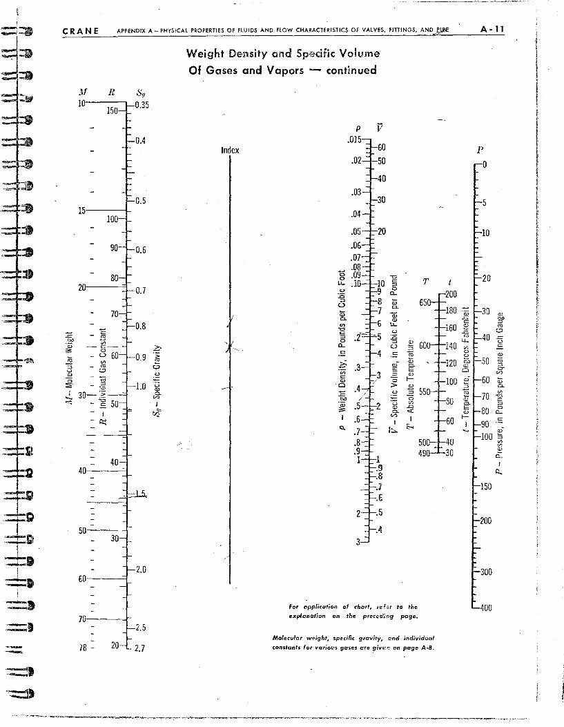
D

-

CRANE APPENDIX A - PHYSICAL PROPERTIES OF flUIDS AND flOW CHARACTERISTICS OF VALVES. FITTINGS. AND ~

R

15,----1-

~

c:: -~ OJ

:;; '" - c::-

== 0

'-' OJ V> => - '" u C-'> '" 0

::E I ..... ~

I - ~

50,---

€Ol---=I

701--~r

78 -

8g

0.35

0.4

0.5

0.6

0.7

0.8

0.9

1.0

Z;> > ~

C-'> <..)

u <1> c.

'" I

'" CQ

Weight Density and Specific Volume

Of Gases and Vapors - continued

Index

~ 0 0

LL. u .0 =>

u Q:; Cl.

'" "0 c:: => 0 a.. c

.?5 '" c

'" Cl

0;,

'" :0: I

Cl.. .6 .7 .8 .9 1

2

3

V

60

50

40

30

20

"0 c:: => 0 a.. Q:; Cl.

Q; OJ u. U

:.0 => '" u :0; c ro 0;>-

Q:; c.

E E => '" 0 I-> 2 U ::l

0 u V>

'" .0 a. <C

"" I I

I;;;. &..

for application of cho,." Fe:'!er to the

explanation on the prece#.~ng poge.

T

Molecular weight, specific gravity,. r:mo individual

constants for various gases are give;; on page A~8.

t 200

180

160

140

120

100

SO

60

A-ll

p

<1> 00 => '" C-'>

= u E :': "" => = "" Q:; "'-

'" "0 co => 0 a.. c

",-

100 :0; V>

'" '" i'.L I

0..

150

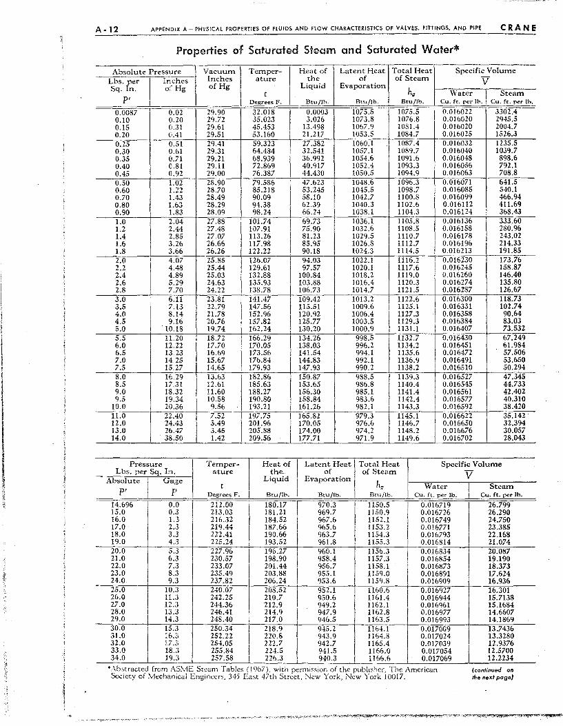
A-12 APpENDIX A - PHYSICAL PROPERTIES OF flUIDS AND flOW CHARACTERISTICS OF VALVES, FITTINGS, AND PIPE CRANE

Properties of Saturated Steam and Saturated Water*

Absolute Pressure Lbs. per Sq. In.

pi

--I-i~Ches of Hg

I

Vacuunl Inches of Hg

Temper­ature

t Degrees F.

I Heat of

the Latent Heat Total Heat

of of Steam Evaporation

Specific Volume

V Water Steam

I Liquid

Btu/lb. Btu/lb. Btu/lb. Cu. ft. per Ih. Cu. {t. per lb.

0.0087 0.02 29.90 32.018 I 0.0003 1075.5 1075.5 I 0.016022 3302.4 0.10 0.20 29.72 35.023 3.026 1073.8 1076.8 0.016020 2945.5 0.15 (1.31 29.61 45.453 13.498 1067.9 1081.4 0.016020 2004.7 0.20 0041 29.51 53.160 21.217 1053.5 1084.7 0.016025 1526.3 0.25 0.51 29.41 59.323 27.382 1060.1 1087.4 0.016032 1235.5 0.30 0.61 29.31 64.484 32.541 1057.1 1089.7 0.016040 1039.7 0.35 (i.7l 29.21 68.939 36.992 1054.6 1091.6 0.016048 898.6 0.40 0.81 29.11 72.869 40.917 1052.4 1093.3 0.016056 792.1 0.45 0'.92 29.00 76.387 44.430 1050.5 1094.9 0.016063 708.8 0.50 1.02 28.90 79.586 47.623 1048.6 1096.3 0.016071 641.5 0.60 1.22 28.70 85.218 53.245 1045.5 1098.7 Ii 0.016085 540.1 0.70 1.43 28.49 90.09 58.10 1042.7 1100.8 0.016099 466.94 0.80 1.63 28.29 94.38 62.39 1040.3 1102.6 0.016112 411.69 0.90 1.83 28.09 98.24 66.24 1038.1 1104.3 0.016124 368.43

-~I~.O~--+-~2".~04T-~~27~.i88~-f~IOil~.7~4~-r-~6~9~.7~3-+--~10~3i6~.I--r'I~lo05i.~8-i-Aor.0·'16~1~36~-r~3~33'.7.60~-1.2 'U.44 27.48 107.91 75.90 1032.6 1108.5 0.016158 280.96 1.4 2.85 27.07 113.26 81.23 1029.5 1110.7 0.016178 243.02 1.6 3.26 26.66 117.98 11 85.95 1026.8 1112.7 0.016196 214.33

__ ~1~.8~ ___ , 3.~.6~6 __ +-~2~6~.2~6 __ ~_~1~272.~2;2 __ -+~9~0~.1~8~~ __ ~1~02~4~.3~-+~11~174~.5~-r~0~.Oi1~6~2~13~~~1~9~1.~8~5 __ 2.0 I' 4.07 25.85 126.07 i 94.03 1022.1 1116.2 0.016230 173.76 2.2 4.48 25.44 129.61 I 97.57 1020.1 1117.6 0.016245 158.87 2.4 I 4.89 25.03 132.88 100.84 1018.2 1119.0 0.016260 146.40 2.6 5.29 24.63 135.93 103.88 1016.4 1120.3 0.016274 135.80

_---;2"'.800-___ L--Z.."o7-=-0-+--,;2-o;-4."'2-=-2--+---:o1-,-38;-:.-';-78i;--+-0-;1O"'6:".7"'3---t--71O;c;1",4 __ .7.--+_1~lco;2-o;-1.-;"5_-+---;0,-;.0~176",18;-;;7:----t---.1726;;-,"",67.-_ 3.0 ! 6.11 23.81 141.47 109.42 1013.2 1122.6 0.016300 118.73 3.5 , 7.13 22.79 147.56 115.51 1009.6 1125.1 0.016331 102.74 4.0 I 8.14 21.78 152.96 120.92 1006.4 1127.3 0.016358 90.64 4.5 I, 9,16 20.76 157.82 125.77 1003.5 Il29.3 0.016384 83.03

____ ~5.~0 __ --~---=-10~.,~1~8--+-~1~9~.7~4~-+--=-16~2~.~24~--+'-713~0~.~20~-+ __ ~10~0~0~.9~-+-71~13~1~.1i;-~~0-,;-.0~1-=-64-=-0;-;;7:--_~ __ ~7~3~.5~3~2 __ 5.5 11.20 18.72 166.29 'I 134.26 998.5 1132.7 0.016430 67.249 6.0 12..22 17.70 1170_05 138.03 996.2 1134.2 0.016451 61.984 6.5 13,,23 16.69 173.56 141.54 994.1 1135.6 0.016472 57.506 7.0 14,,25 15.67 170.84 144.83 992.1 1136.9 0.016491 53.650 7.5 15.27 14.65 ,179.93 147.93 990.2 1138.2 i 0.016510 50.294 8.0 16,29 13_63 182.86 150.87 988.5 1139.3 0.016527 47.345 8.5 17.31 12.61 185.63 153.65 986.8 1140.4 0.016545 44.733 9.0 18.32 11.60 188.27 156.30 985.1 1141.4 0.016561 42.402 9.5 19.34 10.58 190.80 158.84 983.6 1142.4 0.016577 40.310

10.0 20.36 9.56 193.21 I 161.26 982.1 1143.3 0.016592 38.420 11.0 22.40 7.52 197.75 II 165.82 979.3 1145.1 0.016622 35.142 12.0 24.43 5.49 201.96 170.05 976.6 1146.7 0.016650 32.394 13.0 I 26.47 3.45 205.88 I 174.00 974.2 1148.2 I 0.016676 30.057 14.0 I· 38.50 1.42 209.56 177.71 971.9 1149.6 J 0.016702 28.043

Pressure I Temper-

I Heat of I Latent Heat Total Heat Specific Volume

Lbs. per Sq. In. ature the. of of Steam Absolute

I Gage Liquid Evaporation

t I ho Water pi p Degrees F. Btu/lb. Btu/lb. Btu/lb. Cu. ft. per lb.

14.696 I 0.0

I

212.00 180.17 970.3 1150.5

I 0.016719

15.0 0.3 213.03 181.21 969.7 J150.9 0.016726 16.0 1..3 216.32 184.52 967.6 !l52.l I 0.016749 17.0 2..3 219.44 187.66 965.6 J153.2

I 0.016771

18.0 3.3 222.41 190.66 963.7 1154.3 0.016793 19.0 4.3 225.24 193.52 961.8 1155.3 0.016814 20.0 5.3 227.96 196.27 I 960.1 1156.3

I 0.016834

21.0 6.:l 230.57 198.90 , 958.4 1157.3 0.016854 22.0 7.3 233.07 201.44 I 956.7 1158.1 0.016873 23.0 8.:l 235.49 203.88

I 955.1 1159.0 0.016891

24.0 9.3 237.82 206.24 953.6 1159.8 0.016909 25.0

I 10.;; 240.07 208.52

I 952.1 1160.6 0.016927

26.0 ILl 242.25 210.7 950.6 I

1161.4 0.016944 27.0 12.J 244.36 212.9 949.2 1162.1 0.016961 28.0 13.a 246.41 214.9 947.9 1162.8 0.016977 29.0 I

I,Ll 248.40 i 217.0 I 946.5 1163.5 0.016993 30.0 15.:> 250.34 218.9 I 945.2 1164.1 0.0170G9 31.0 16.~. , 252.22 220.8 943.9 1164.8 0.017024 32.0 17.,1

I 254.05 222.7 I 942.7 1165.4 0.017039

33.0 18.3 255.84 , 224.5 ! 941.5 1166.0 0.017054 34.0 19.:> 257.58 I 226.3 , 940.3 I 1166.6 0.017069

- , --*/\bstracted from AS\1E Steam fables (1967), With perm,:O:Slon of the pubH~hcr, Ihe American Society of Mechanical Engineers, 345 East 47th Street. New York. New York 10017.

V I I

I

I

Steam Cu. ft. per lb.

26.799 26.290 24.750 23.385 22.168 21.074 20:087 19.190 18.373 17.624 16.936 16.301 15.7138 15.1684 14.6607 14.1869 13.7436 13.3280 12.9376 12.5700 12.2234

{confinued on the next page)

(;

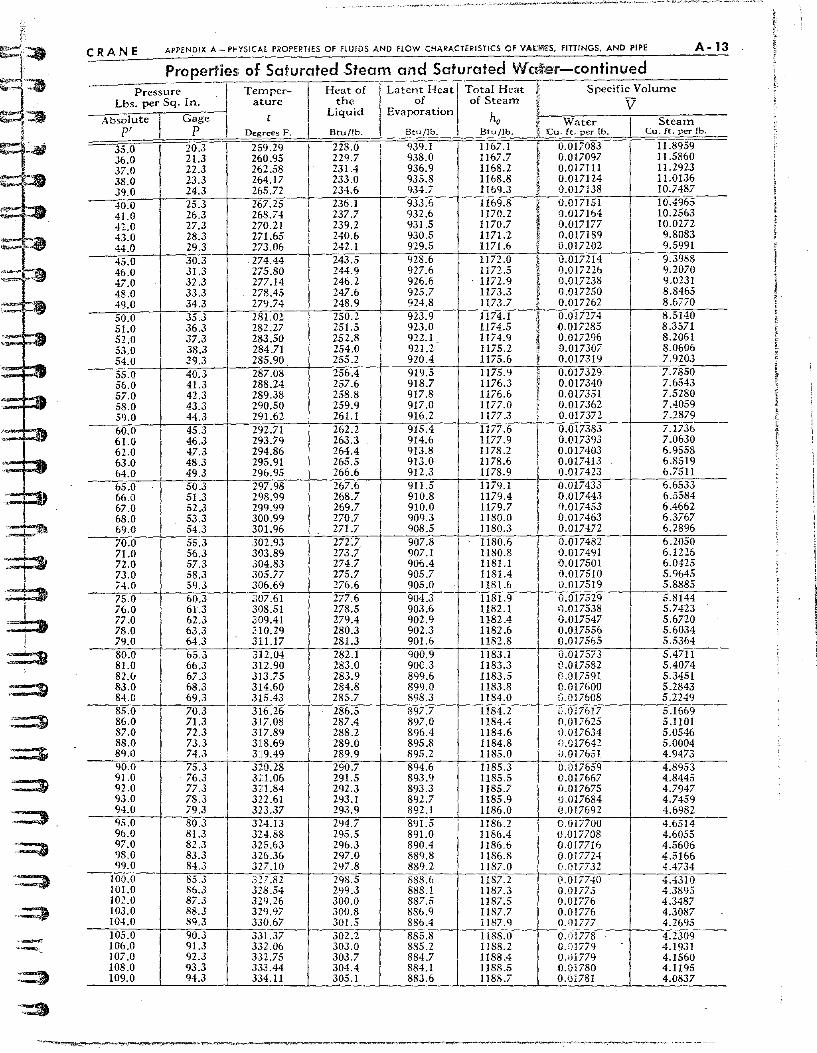
C=f-:I~ e::r=-

i ~i

9~~

=::bt

:::::::::s ::=:9

~

=:$

CRANE APPENDIX A - PI-YSICAl PROPERTIES Of flUIDS AND flOW CHARACTERISTICS OF VAItfft£S, FITTINGS. AND PIPE A-13

Properties of Saturated Steam and Saturated Wafer-continued Pressure Temper- I Heat of Latent Heat Total Heat I Specific Volume

Lbs. per Sq. In. ature the of of Steam i V Absolute I Gage t I

Liquid Evaporation h. ~ Water I Steam P' P I Degrees F. Btu/lb. Btu/lb. Btu/lb. ~ Cu. ft. per lb. Cu. ft. per lb.

35.0 20.3 259.29

I 228.0 I 939.1

I 1167.1 I O.Oi7083 I 11.8959

36.0 21.3 260.95 229.7 I 938.0 1167.7 0.017097 11.5860 37.0 22.3 262.58 231.4

I 936.9 1168.2 0.017111 I 11.2923

38.0 23.3 264.17 233.0 935.8 I 1168.8 I 0.017124 11.0136 39.0 24.3 265.72 234.6 934.7 1169.3

, 0.017138 10.7487 i

40.0 25.3 I 267.25 236.1 933.6 1169.8 I 0.017151 10.4965

41.0 26.3 , 268.74 237.7 932.6 1170.2

I 0.017164 10.2563

42.0 "., + m." 239.2 931.5 1170.7 0.017177 10.0272

43.0 28.3 271.65 240.6 930.5 I!71.1 0.017189 9.8083 44.0 29.3 273.06 242.1 929.5 1171.6 ! 0.017202 9.5991

45.0 30.3 274.44 243.5 928.6 1172.0 I 0.017214 I 9.3988 46.0 31.3 275.80 244.9 927.6 !l72.5 0.017226 9.2070 47.0 32.3 ~ 277.14 246.2 926.6 1172.9 i 0.017238 I 9.0231 48.0 33.3 278.45 247.6 925.7 1173.3

r 0.017250 8.8465

49.0 34.3 279.74 248.9 924.8 1173.7 0.017262 8.6770

50.0 I 35.3 I 281.02 250.2

I

923.9 1174.1 ,

0.017274 8.5140 51.0 I 36.3

I 282.27 251.5 923.0 1174.5 \j 0.017285 8.3571 ,

52.0 37.3 283.50 252.8 922.1 1174.9 I 0.017296 8.2061 53.0 38.3 284.71 254.0 921.2 1175.2 0.017307 8.0606 54.0 39.3 285.90 255.2 920.4 1175.6 ! 0.017319 7.9203

55.0 40.3 287.08 256.4 919.5 1175.9 , 0.017329 7.7850 56.0 41.3 I 288.24 257.6 918.7 1176.3 I 0.017340 7.6543 57.0

'U +'''." 258.8 917.8 1176.6 r 0.017351 7.5280 58.0 43.3 290.50 259.9 917.0 1177.0

r 0.017362 7.4059

59.0 44.3 291.62 26 I.! 916.2 1177.3 0.017372 7.2879

60.0 45.3 292.71 262.2 915.4 1177.6 I 0.017383 7.1736 61.0 46.3 293.79 263.3 914.6 1177.9 0.017393 7.0630 62.0 47.3 294.86 264.4 913.8 1178.2 0.017403 6.9558

295.91 265.5 913.0 1178.6 ,

0.017413 6.8519 63.0 48.3 I 64.0 49.3 296.95 266.6 912.3 1178.9 0.017423 6.7511

65.0 50.3 297.98 267.6 911.5 1179.1 0.017433 6.6533 66.0 51.3 298.99 268.7 910.8 1179.4 0.017443 6.5584 67.0 52.3 299.99 269.7 910.0 1179.7 0.017453 6.4662 68.0 53.3 300.99 270.7 909.3 1180.0 0.017463 6.3767 69.0 54.3 301.96 271.7 908.5 1180.3 0.017472 6.2896 70.0 55.3 302.93 272.7 907.8 1180.6 0.017482 6.2050 71.0 56.3 ;303.89 273.7 907.1 1180.8

I 0.017491 6.1226

72.0 57.3 304.83 274.7 906.4 118 I.! 0.017501 6.0425 73.0 58.3 ,105.77 275.7 905.7 1181.4 0.017510 5.9645 74.0 59.3 ,106.69 276.6 905.0 1181.6 0.017519 5.8885 75.0 60.3 ,107.61 I 277.6 904.3 1181.9 0.017529 5.8144 76.0 61.3 ;;08.51 278.5 903.6 1182.1 ().017538 I 5.7423 77.0 62.3 ;;;09.41 I 279.4 902.9 1182.4 0.017547 5.6720 78.0 63.3 310.29 280.3 902.3 1182.6 0.017556 5.6034 79.0 64.3 311.17 281.3 901.6 1182.8 0.017565 5.5364 80.0 65.3 312.04 282.1 900.9 1183.1 ;).017573 5.4711 81.0 66.3 312.90 283.0 900.3 1183.3 (1.017582 5.4074 82.v 67.3 313.75 283.9 899.6 1183.5 0.017591 5.3451 83.0 68.3 314.60 284.8 899.0 I 1183.8 i).017600

I 5.2843

84.0 69.3 315.43 285.7 898.3 1184.0 v.017608 5.2249 85.0 70.3 316.26 286.5 897.7 1184.2 (}.017617 5.1669 86.0 71.3 317.08 287.4 897.0 1I84.4 fI.017625 5.1101 87.0 72.3 3.17.89 288.2 896.4 !l84.6 0.017634 5.0546 88.0 73.3 3.18.69 289.0 895.8 1184.8 i).017642 5.0004 89.0 74.3 3:!9.49 289.9 895.2 1185.0 ').017651 4.947" 90.0 I 75.3 3:!D.28 290.7 894.6 1185.3 0.017659 4.8953 91.0 76.3 321.06 291.5 893.9 lI85.5 0.017667 4.8445 92.0 77.3 321.84 292.3 893.3 !l85.7 /).017675 4.7947 9.3.0 78.3 322.61 293,1 892.7 l!85.9 0.017684 4.7459 94.0 79.3 323.37 293.9 892.1 1186.0 (;.017692 4.6982 %.0 80.3 324.13 294.7 891.5 I 1186.2 0.017700 4.6514 96.0 81.3 314.88 295.5 891.0 1186.4 0.017708

I 4.6055

97.0 82.3 325.63 296.3

I 890.4 1186.6 0.017716 4.5606

98.0 83.3 32&.36 297.0 889.8 1186.8 0.017724 4.5166 99.0 84.3 327.10 297.8 889.2 1187.0 0.017732 4.4734

100.0 85.3 I

327.82 298.5 888.6 1187.2 (>.017740 4.4310 101.0 86.3 328.54 299.3 888.1 1187.3 0.01775 4.3895 102.0 87.3 329.26 300.0 887.5 1187.5 0.01776 4.3487 103.0 88.3 329.97 300.8 886.9 1187.7 0.01776 4.3087 104.0 89.3 330.67 301.5 886.4 1187.9 0.01777 4.2695 105.0 90.3 331.37 302.2 885.8 !lS8.0 0.'1l778 4.2309 106.0 91.3 33,'.06 303.0 885.2 1188.2 0.D1779 4.1931 107.0 92.3 332.75 303.7 884.7 1188.4 0.01779 4.1560 108.0 93.3 333.44 304.4 884.1 1188.5 0.01780 4.!l95 109.0 94.3 334.!l 305.1 883.6 1188.7 0.01781 4.0837

.

I I I , i I

I I ~

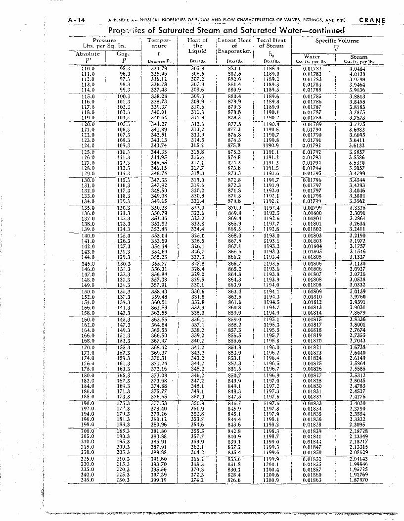
A .. 14 APPENDIX A - PHYSICAL PROPERYIES OF flUIDS AND flOW CHARACTERISTICS OF VALVES, FITTINGS, AND PIPE C-'-.'--'-___ _ CRANE

Prop'2Y iies of Saturated Steam and Saturated Water-continued -------'-

Pressure I Tcmpcr- I Heat of . Latent Heat Total Heat Specific Volume Lbs. per Sq. In. ___ i ature Ii the of; of Steam v-

1 --I Liquid Evaporation! h

AbSOpl,utc I Gap!;c I I g Water I Steam---==c~=;:==*.===i.. : Degrees F. _~~~!b_ Btu/lb. Btui!!'. Cu~~per I~. I ~~~~~

110.0 I 95.3 ! 334.79 I 305.8 883.1 1188.9 -0"])1782 Tl4-:-048.f--111.0 96.3 I 335.46 306.5 882.5 1189.0 0.01782 4.0138 112.0 97.3 336.12 I 307.2 882.0 il89.2 0.01783 3.9798 113.0 98.~ I 336.78 i 307.9 881.4 1189.3 0.01784 I 3.9464 114.0 99.c, 337.43 308.6 880.9 1189.5 0.01785 3.<)136 11- 0 100' 33808 3093 8804 11'96 001-8- I 38813 ~.

i .0 I

I ;; . I ~

116.0 101.3 I 338.73 309.9 879.9 1189.8 0.01786 I

3.8495 117.0 102.3

I 339.37 310.6 879.3 1189.9 0.01787 3.8183

118.0 I

103.3 340.01 311.3 I

878.8 1190.1 0.01787 I 3.7875 119.0 104.3 340.64 311.9 878.3 1190.2 0.01788 I 3.7573 120.0 I 105:3 341.27 312.6 I 877.8 1190.4 0.01789 3.7275 121.0 i 106.3 341.89 313.2

I

877.3 ,

1190.5 0.01790 3.6983 122.0 107.3 342.51 313.9 876.8 ! 1190.7 0.01790 3.6695 123.0 108.3 343.13 314.5 876.3 1190.8

I 0.01791 3.6411

124.0 109.3 343.74 315.2 875.8 I 1190.9 0.01792 3.6132 125.0

I 110.3 I 344.35 315.8 875.3 I 1191.1 0.01792 3.5857

126.0 111.3 I 344.95 I 316.4 874.8 ! 1191.2 0.01793 3.5586 127.0 112.3

I 345.55

I 317.1 874.3

1 1191.3 0.01794 3.5320

128.0 113.3 346.15 317.7 873.8 I 1191.5 0.01794 3.5057 129.0 114.3 346.74 318.3 873.3 I 1191.6 I 0.01795 3.4799 I ! , 130.0 115.3 I 347.33

I 319.0 ! 872.8 i 1191.7 0.01796 3.4544 I I

131.0 116.3 347.92 319.6 ,

872.3 1191.9 0.01797 3.4293 132.0 117.3 l 348.50

I 320.2 I 871.8 I 1192.0 0.01797 3.4046

133.0 118.3 , 349.08 320.8 871.3 I 1192.1 0.01798 3.3802 134.0 119.3 I 349.65 321.4 870.8 1192.2 0.01799 3.3562 135.0 I 120..3 I 350.23 322.0 870.4 1192.4 0.01799 3.3325 136.0 121.3 350.79 322.6 869.9 1192.5 0.01800 3.3091 137.0 122.3 351.36 323.2 869.4 1192.6 0.01801 3.2861 138.0 122,.3 351.92 323.8 868.9 1192.7 0.01801 3.2634 139.0 124,.3 , 352.48 324.4 868.5 1192.8 0.01802 3.2411 140.0

I 12S.3 353.04 325.0 i 868.0 1193.0 0.01803 3.2190

141.0 126.3 353.59 325.5 867.5 1193.1 0.01803 3.1972 , -, -. I I 143.0 128.3. 354.69 326.7 866.6 I 1193.3 I 0.01805 3.1546

144.0 i 129.3 355.23 I 327.3 866.2 I 1193.4 0.01805 3.1337 145.0 130.3 355.77 327.8 865.7 1193.5

I 0.01806 3.1130

146.0

I 131.3 356.31 328.4 865.2 1193.6 0.01806 3.0927

147.0 132.3 356.84 329.0

I 864.8 1193.8 0.01807 3.0726

148.0 13,1.3 357.38 329.5 864.3 1193.9 I

0.01808 3.0528 149.0 13'1.3 357.91 330.1 863.9 1194.0 0.01808 3.0332

14' 0 3~4 14 .>26 1 8671 11932 001804

150.0 13S.3 358.43 330.6 863.4 1194.1 0.01809 3.0139 152.0 137.3 359.48 331.8 862.5 1194.3 0.01810 2.9760 154.0 139.3 360.51 332.8 861.6 1194.5 0.01812 2.9391 156.0 I 141.3 361.53 333.9 860.8 1194.7 0.01813 2.9031 158.0 14,1.3 362.55 335.0 859.9 1194.9 0.01814 2.8679 160.0 145.3 363.55 , 336.1 , 859.0 1195.1 I 0.01815 2.8336 162.0 147.3 364.54 I 337.1 I 858.2 1195.3 0.01817 2.8001 I I 164.0 149.3 365.53 338.2 857.3 1195.5 0.01818 2.7674 166.0 151.3 366.50 339.2 856.5 1195.7 0.01819 2.7355 168.0 I 15:1.3 367.47 340.2 855.6 1195.8 0.01820 2.7043 I 170.0 i 15';.3 368.42 341.2 854.8 I

1196.0 0.01821 2.6738 172.0 ! 15;i.3 369.37 342.2 I 853.9 1196.2 0.01823 2.6440 174.0 159.3 . 370.31 343.2 I 853.1 I 1196.4 0.01824 2.6149 i

I 176.0 I 161.3 371.24 344.2

I 852.3 1196.5 0.01825 2.5864

178.0 ! 16:;.3 372.16 345.2 851.5 1196.7 0.01826 2.5585 180.0 I 16;;.3 373.08 ! 346.2 850.7 I 1196.9 i 0.01827 2.5312 182.0

I 167.3 373.98 . I 347.2 849.9 1197.0 0.01828 2.5045

184.0 169.3 374.88

I 348.1 849.1 1197.2 i 0.01830 2.4783

186.0 I 171.3 375.77 349.1 848.3 1197.3 I 0.01831 2.4527 188.0 ~U 376.65 350.0 847.5 1197.5 0.01832 2.4276 190.0 i 17".3

I 377.53 i 350.9 846.7 I 1197.6 0.01833 2.4030 ,

I 192.0

I 177.3 378.40 351.9

I

845.9

I

1197.8 0.01834 2.3790 194.0 179.3 379.26

I 352.8 845.1 1197.9 0.01835 2.3554

196.0 181.3 I 380.12 353.7 844.4 1198.1 I 0.01836 2.3322 198.0 I 18:3.3 I 380.96 354.6 843.6 1198.2 0.01838 2.3095 200.0

, 183.3 381.80 355.5 842.8 1198.3 I 0.01839 2_28728

205.0 I 190.3 383.88 357.7 840.9 1198.7

I 0.01841

I 2.23349

210.0 19.1.3 385.91 359.9 839.1 1199.0 0.01844 2.18217 215.0 200.3 387.91 362.1 I 837.2 1199.3 0.01847 2.13315 220.0 20:;.3 389.88 I 364.2 L 835.4 1199.6 t 0.01850 2.08629 225.0 210.3 391.80 366.2 I 833.6

, 1199.9

I 0.01852 2.01143

230.0 215.3 393.70 368.3

I

831.8 1200.1 0.01855 1.9984& 235.0 220.3 395.56 370.3 830.1 1200.4 I 0.01857 1.95725 240.0

! nu 397.39 372.3 828.4 1200.6 0.01860 1.91769

245.0 130.3 399.19 I 374.2 826.6 1200.9 I 0.01863 1.87970

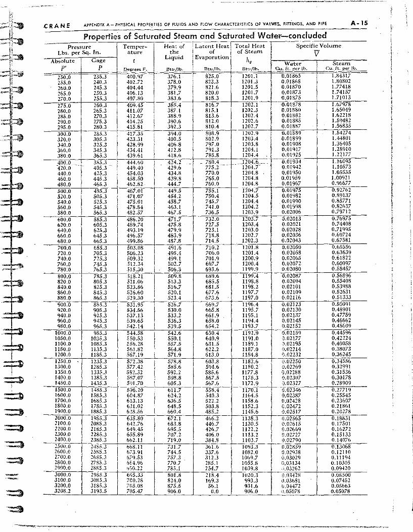
I

'9=-'--"J-1lilI .~. ,~lji

.. .,jilt

~ ~

":=:t.

~

CRANE APPENDIX A - PHYSICAL PROPERTIES OF FLUlDS AND flOW CHARACTERISTICS Of VAlVES~ FlnINGS, AND PIPE A-IS

Properties of Saturated Steam and Saturated Water-concluded Temper- Heat of . Latent Heat Total Heat

, Specific Volume Pressure

Lbs. per Sq. In. ature the of of Steam V Absolute I Gage t

Liquid Evaporation ho Water Steam P' I p Degrees F. Btu/lb. Btu/lb. Btu/lb. Ou. ft. per lb. Cu. ft. per lb.

250.0 I

235.3 400.97 376.1 I 825.0 1201.1 0.01865 1.84317 255.0 240.3 402.72 378.0 ; 823.3 1201.3 0.01868 1.80802 260.0

I 245.3 404.44 379.9

I 821.6 1201.5 0.01870 1.77418

265.0 250.3 406.13 381.7 820.0 1201.7 0.01873 1.74157 270.0 255.3 407.80 383.6 818.3 1201.9 {l.01875 1.71013

275.0

I 260.3 409.45 385.4 1 816.7 1202.1 0.01878 I 1.67978

280.0 265.3 411.07 387.1 815.1 1202.3 0.01880 1.65049 285.0 270.3 412.67 388.9 I 813.6 1202.4 0.01882 1.62218 290.0 275.3 414.25 390.6 I 812.0 1202.6 0.01885 1.59482 295.0 280.3 415.81 392.3 810.4 1202.7 0.01887 1.56835

300.0 I

285.3 417.35 394.0

I 808.9 1202.9 0.01889 1.5427-<

320.0 305.3 423.31 I 400.5 802.9 1203.4 lJ.01899 1.44801 340.0 325.3 428.99 I 406.8 797.0 . 1203.8 I 0.01908 1.36405 I 360.0 345.3 434.41 I 412.8 791.3 1204.1 0.01917 1.28910 380.0 365.3 439.61 I 418.6 785.8 1204.4 0.01925 1.22177

JOO.O -

I 385.3 I

444.60 424.2 _ 780.4 ~--- - _.t204.6_ .0.01934 1.1&095

420.0 405.3 449.40 429.6 775.2 1204.7' 11.01942 1.10573 440.0 425.3 454.03 434.8 770.0 1204.8 0.01950 1.05535 460.0

, 445.3 458.50 439'.8 765.0 1204.8 0.01959 1.00921

480.0 465.3 462.82· 444.7 760.0 1204.8 0.01967 0.96677

500.0 485.3 467.01 449.5 755.1 1204.7 0.01975 0.92762 520.0 505.3 471.07 454.2 750.4 1204.5 0.01982 0.89137 540.0 525.3 475.01 I 458.7 745.7 1204.4 0.01990 0.85771 560.0 545.3 478.84 463.1 741.0 1204.2 .0.01998 I 0.82637 580.0 565.3 482.57 I 467.5 736.5 1203.9 0.02006 0.79712

600.0 585.3 486.20 471.7 732.0 1203.7 0.02013 0.76975 620.0 605.3 489.74 475.8 727.5 1203.4 0.02021 0.74408 &40.0 &25.3 493.19 479.9 723.1 1203.0 0.02028 0.71 995 &60.0 645.3 496.57 483.9 718.8 1202.7 0.02036 0.69724 680.0 , 665.3 499.8& 487.8 714.5 1202.3 0.02043 0.67581

700.0 685.3 503.08 491.6 710.2 1201.8 0.02050 0.6555& 720.0 705.3 506.23 495.4 706.0 1201.4

I 0.02058 0.63639

740.0 725.3 509.32 499.1 701.9 1200.9 0.02065 0.61822 760.0 745.3 512.34

i 502.7 697.7 1200.4 0.02072 0.60097

780.0 765.3 515.30 50&.3 693.& 1199.9 0.02080 0.58457

800.0 I 785.3 518.21 I 509.8 689.6 1199.4 0.02087 0.5&896 820.0 I 805.3 521.06

I 513.3 685.5 1198.8 0.02094 0.55408

840.0 825.3 ;;23.86 516.7 681.5 1198.2 0.02101 0.53988 8&0.0

I 845.3 ;;26.60 520.1 677.6 1197.7 0.02109 0.52631

880.0 .865.3 ;;29.30 : 523.4 673.6 1197.0 0.02116 0.51333 900.0 I 885.3 S31.95 I 526.7 669.7 1196.4 0.02123 0.50091 920.0 905.3 534.56

I 530.0 665.8 1195.7 0.02130 0.48901

940.0 925.3 ii37.13 533.2 661.9 1195.1 0.02137 0.47759 960.0 945.3 539.&5 536.3 658.0 1194.4 0.02145 0.46662 980.0 965.3 542.14 I 539.5 654.2 1193.7 (j.02152 0.45609

1000.0 985.3 E;44.58

I 542.6 650.4 1192.9 0.02159 0.4459&

1050.0 1035.3 0,50.53 550.1 640.9 1191.0 0.02177 0.42224 1100.0 1085.3 556.28 557.5 631.5 1189.1 il.02195 0.40058 1I50.0 1135.3 I 561.82 564.8 622.2 1187.0 0.01214 0.38073 1200.0 1185.3 I 567.19 571.9 613.0 1184.8 0.02232 0.36245 1250.0 . I 1235.3 nn.38 578.8 603.8 1182.6 0.02250 0.34556 1300.0 I 1285.3 577.42 585.6 594.6 1180.2 I 0.02269 0.32991 1350.0 I 1335.3 582.32 592.2 585.6 1177.8 0.02288 0.31536 1400.0 1385.3 587.07 598.8 567.5 1175.3 0.02307 0.30178 1450.0 I 1435.3 591.70 605.3 567.6 1172.9 l)'O2327 0.28909 1500.0 1485.3 596.20 I 611.7 558.4 fi70.1 0.0234& 0.27719 1600.0 1585.3 &04.87 , 624.2 540.3 1164.5 0.02387 0.25545 1700.0 1685.3 613.13

, 636.5 522.2 1158.6 0.02428 0.23607

1800.0 1785.3 621.02 &48.5 503.8 1152.3 0.02472 0.21861 1900.0 1885.3 628.56 660.4 485.2. 1145.6 0.02517 0.20278 2000.0 1985.3 635.80 672.1 4&6.2 1138.3 0.02565 0.18831 2100.0 2085.3 642.76 683.8

I 446.7 1I30.5 0.02615 0.17501

2200.0 2185.3 649.45 695.5 426.7 1122.2 0.02669 0.16272 2300.0 2285.3

I &55.89 707.2 406.0 1113.2 0.02727 0.15133

2400.0 , 2385.3 6b2.1I I 719.0 I 384.8 1103.7 0.02790 0.14076 , 2500.0 2485.3 668.11 731.7 361.6 1093.3

, 0.02859 0.13068

2&00.0 2585.3 I &i'3.91 744.5 337.6 1082.0 0.02938 0.1211 0 2700.0 2685.3

I 679.53 757.3 312.3 1069.7 0.03029 0.11194

2800.0 2785.3 684.96 770.7 285.1 1055.8 0.03134 0.10.l05 2900.0 2885.3 690.22 785.1 'Itt"'" ;).03262 0.09420 3000.0 2985.3 M5.33 801.8 218.4 1020.3 -6-.03428 0.08500 3100.0 3085.3 700.28 824.0 1&9.3 993.3 0.03681 0.07452 3200.0 3185.3 705.08 875.5 5&.1 931.6 0.04472 0.05663 3208.2 3193.5 705.47 906.0 0.0 906.0 -'.05078 0.05078

1 !

A - 16 APPEN:0IX A - PHYSICAL PROPERTIES OF flUIDS AND flOW CHARACTERISTICS OF VALVES, fITTINGS, AND PIPE

Pressure SflI,tt-. Lbs. per Ten'>p. Sq. In.

Abs. Gage

P' P t

15.0 0.3 213.«13 \' h,

5.31 20.0 227.% V I hg

30.0 15.3 250.34 V h,

40.0 25.3 267.25 V hg

50.0 i 35.31 281.02 V hg

60.0 45.3 292.71 V h,

55.31 302.93 70.0 V h,

V 80.0 65.3 312.04 hg

90.0 75.3 ;)20.28 17 hg

100.0 85.3 327.82 V

105.31 34l'..27

h,

120.0 V hg

140.0 125.3 35J:.04 V h.

160.0 145.3 363.55 V h,

180.0 165.3 373.08 V hg

200.0 185.3 381.80 V h,

220.0 205.3 389 .. 88 V

225.31397.39

h,

240.0 V hg

260.0 245,3 404.44 V h,

280.0 265.3 411.07 V I I h,

I I

300.0 285.3 417,35 V

! h,

320.0 305.3 423.:11 V hg

340.0 325.3 428.99 V h,

360.0 I 345.3 434.41 V h,

I

Properties of Superheated Steam*

v = specific volume, cubic feet per pound

h, = total heot of steam, Btu per pound

Total Temperature-Degrees Fahrenheit (t)

500,1 600' --: 1 3500 400' 700' 800' 900' I 1000' 11 00' I , I

31. 939 33.963 37.985l41.986. 45.978 49.964 53.946157~9Z6 61.905 1216.2 1239.9 1287.3 I 1335.211383.811433.211483.4: 1534.5 1586.5

25.428 I ! I" 23.900 28.457 i 31.466, 34.465 37.458! 40.447! 43.435 46.420 1215.4 1239.2 1286.9' 1334.9 1383.5 1432.911483.2 1534.3 1586.3

15.859 16.892 18.929 20.945 22.951 24.952 26.949 28.943 30.936 1213.6 I 1237.8 1286.0 1334.2 1383.0 1432.5

1

1482.8 1534.0 1586.1

11.838 12.624 14.165 15.685. 17.195 18.699 20.199 21.697 23.194 121 1.7 1236.41 1285.0 1333.61 1382.5 I 1432.1 1482.5 1533.7 1585.8

9.424 10.0621 11.306 12.529 13.741 14.947116.150 17.350 18.549 1209.9 1234.9 I 1284.1 1332.9 1382.0 1431.7

1

1482.2 1533.4 1585.6

7.815 8.354 9.400 10.425 11.438 12.446 I 13.450 14.452 15.452 1208.0 1233.5 1283.2 1332.3 1381.5 1431.3 1481.8 1533.2 1585.3

I 6.664 7.133 8.039 8.922 9.793 10.659 11.522 12.382 13.240

1206.0 1232.0 1282.2 1331.6 1381.0 I 1430.9 1481.5 1532.9 1585.1

7.018 7.794 I 8.560 1 5.801 6.218 9.319 10.075 10.829 11.581 1204.0 1230.5 1281.3 1330.9

1

1380.5 1430.5 1481.1 1532.6 1584.9

5.128 5.505 6.2231 6.917 7.600 8.277 8.950 9.621 10.290 1202.0 1228,9 1280.3 1330.211380.0 I 1430.1 1480.8 1532.3 1584.6

4.590 4.935 5.588 6.216 6.833 7.443 8.050 8.655 9.258 1199.9 1227.4 1279.3 1329.6 I 1379.5 1429.7 1480.4 1532.0 1584.4

3.7815 4.0786 4.6341 5.163715.6813 6.1928 6.7006 7.2060 7.7096 1195.6 i 1224.1 1277.1

1

1328.2 1378.4! 1428.8 1479.8 1531.4 1583.9

3.4661 3.9526 4.411914.858815.2995 5.7364 6.1709 6.6036 1220.811275.3 1326.8 1377.4 1428.0 1479.1 1530.8 1583.4

3.0060 3.441313.8480 4.2420 I 4.6295 5.0132 5.3945 5.7741 ... 1217.4 1273,3 1325.4 1376.411427.2 1478.4 1530.3 1582.9

... 2.6474 3.0433 3.4093 3.7621 4.1084 4.4508 4.7907 5.1289

... 1213.8 1271.2 1324.0 1375.311426.3 1477.7 1529.7 1582.4

2.3598 2.i247 3.0583 3.3783 I 3.6915 4.0008 4.3077 4.6128 1210.1 1269.0 1322.6 1374.3 I 1425.5 1477.0 1529.1 1581.9

2.1240 2.4638 2.7710 3.06421 3.3504 3.6327 3.9125 4.1905 1206.3 1266.9 I 1321.2. 1373.211424.7 1476.3 1528.5 1581.4

.. 1.926812.246212.531612.80241 3.0661 3.3259 3.5831 3.8385 1202.11 1264.6 I 1319.7. 1372.1 11423.8 1475.6 1527.9 1580.9

... 12.061912.3289! 2.58081 2.8256 3.0663 3.3044 3.5408

...

I 1262.4 1318.2 1371.1 i 1423.0 1474.9 1527.3 1580.4

I 1.90371 2.1551 2.3909 i 2.6194 2.8437 3.0655 3.2855 1260.0 1316.8 1370.0 i 1422.1 1474.2 1526.8 1579.9

1.7665 2.0044 2.2263 i 2.4407 2.6509 2.8585 3.0643 1257.7 1315.2 1368.91 142 1.3 1473.6 1526.2 1579.4

1.6462 1.8725 2.08231 2.2843 2.4821 2.6774 2.8708 1255.2

1

1313.7 1367.8

1

1420.5 1472.9 1525.6 1578.9

1.5399 1.7561 1.9552 2.1463 2.3333 2.5175 2.7000 .. 1252.8 1312.2 1366.7 I 1419.6 1472.2 1525.0 1578.4

1.445411.6525 1.8421 12.0237 2.2009 2.3755 2.5482 ... 1250.3 11310.6 1365.61 1418 .7 1471.5 1542.4 1577.9 , -'Abstracted from ASME Steam rables (1967) with permission of the publisher. the

American Society 01 Mechanical Engineers. 345 East 47th Street, "ow York. ~. Y. 10017.

CRANE

1300' 1500'

69.858 77.807 1693.2 1803.4

52.388 58.352 1693.1 1803,3

34.918 38.896 1692.9 1803.2

26.183 29.168 1692.7 1803.0

20.942 23.332 1692.5 1802.9

17.448 19.441 1692.4 1802.8

14.952 16.661 1692.2 1802.6

13.081 14.577 1692.0 1802.5

11.625 12.956 1691.8 1802.4

10.460 11.659 1691.6 1802.2

8.7130 9.7130 1691.3 1802.0

7.4652 8.3233 1690.9 1801.7

6.5293 7.2811 1690.5 1801.4

5.8014 6.4704 1690.2 1801.2

5.2191 5.8219 1689.8 1800.9

4.7426 5.2913 1689.4 1800.6

4.3456 4.8492 1689.1 1800.4

4.0097 4.4750 1688.7 1800.1

3.7217 4.1543 1688.4' 1799.8

3.4721 3.8764 1688.0 1799.6

3.2538 3.6332 1687.6 1799.3

3.0611 3.4186 1687.3 1799.0

2.8898 3.2279 1686.9 1798.8

(continued oil

'he ~.l{' pog.)

: : .,

'~

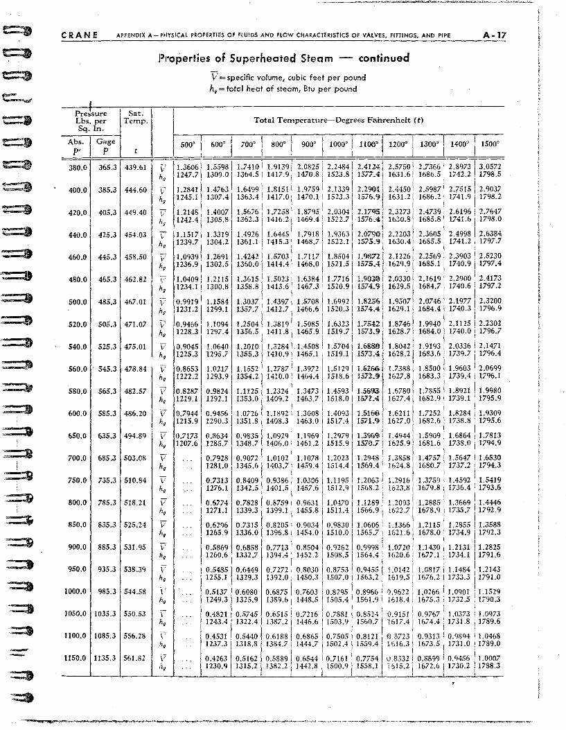
==-3 1

'~. i

~~

~

:=:$

==t#

:::=t :::::a '=::J

=---

CRANE APPENDIX A - PHYSICAL PROPERTIES OF FLUIDS AND FLOW CHARACTERISTICS Of VALVES, flnINGS. AND PIPE A.17

Pressure Sat. Lbs. per Temp. Sq. In.

AbS'1 Gage

P' P t

380.0 365.3 439.61

400.0 385.3 444.60

420.0 405.3 449.40

440.0 425.3 454.03

460.0 445.3 458.50

480.0 465.3 462.82

500.0 485.3 467.01

520.0 505.3 471.07

540.0 525.3 475.01

i

560.0 545.3 478.84

580.0 565.3 482.57

600.0 585.3 486.20

650.0 635.3 494.89

700.0 685.3 503.08

750.0 735.3 510.84

800.0 785.3 518.21

850.0 835.3 525.24

900.0 885.3 531.95

950.0 935.3 538.39

1000.0 985.3 544.58

1050.0 1035.3 550.53

1100.0 1085.3 556.28

1I50.0 1135.3 561.82

Plroperties of Superheated Steam - continued

~ h,

V hg

-V ng

V h.

V hg

V hg -V hg

V h.

V hg -'v' h,

V h.

V h. -II h.

V h.

\' hg -\I h.

V hg

V h.

V-hg

\ hg -\ hg -\ h.

V h.

v = specific volume, cubic feet per pound hg = total heat of steam, Btu per pound

1 I Total Temperature-Degrees Fahrenheit (t)

500' 6000 I 700

0 I 800' 9000 1000' I 1100" i 1200' I 13000 I

, i , , 1.3606 1.559811.7410 I 1.9139! 2.0825 1 I 1 2.2484, 2~'!.U4i 2.5750 I 2.7366 ' 1247.7 1309.011364.5 1417.91 1470.8 1523.811017.4: 1631.6, 1686.5

1 . j I 1.2841

. 1 1.9759 2.1339 I 2.2901 i 2,4450 I 2.5987 1.4763, 1.649911.8151 I 1245.1

1

1307.411363.4 I 1417.0 I 1470.1 1523.3 i 1576.9 J 1631.21 1686.2 1 j

1.2148 1.4007 1.567611.72581 1.8795 2.0304 i 2.1795) 2.32731 2.4739 1242.4 1305.8 i 1362.31 1416.21 1469.4 1522.711570.411630.8 1685.8

, 1 ,1.1517 1.3319 1.492611.6445 1 1.7918 1.936312.0790 1 2. 2203 1 2.3605 ' 1239.7 1304.2 1361.1 I 1415.31 1468.7 1522.1 1575.'1 1630.4. 1685.5

1.0939 1.2691 1.424211.57031 1.7117 1.85041 1.9872 2.12261 2.2569 1236.9 1302.5 1360.0 1414.41 1468.0 1521.5 1 1575.4 1629.9 1685.1

1 1.0409 i 1.2115 1.3615 1.5023 1.6384 1.7716 i 1.9030 2.0330 2.1619 1234.1 1300.8 1 1358.8 1413.6 I 1467.3 1520.91 1574.9 1629.5 1684.7

1.4397 1

, I

1.69921 1.8256 0.9919 1.1584 1.3037 1.5708 1.

95071

2.0746 1231.2 1299.1 1357.7 1412.7 1466.6 1520.3 1 1574.4 1629.1 1684.4

1 , 1.87461 .; 0.9466 1.1094 1.2504 1.3819 1.5085 1.6323 11.7542 1.9940

1228.3 1297.4 1356.5 1411.8 1465.9 1519.7 1573.9 1628.7 1684.0

0.9045 1.0640 1.2010 1.3284 1.4508 1.570411.6880 1.8042 1.9193 1225.3 1295.7 1355.3 1410.9 1465.1 1519.111573.4 1628;2 1683.6

0.8653 1.0217 1.155211. 2787 1.3972 1.5129 11.6266 1.7388 1.8500 1222.2 1293.9 1354.2 1410.0 1464.4 1518.6 I 1572.9 1627.8 1683.3

0.8287 f 0 .. 9824 1.1125 I 1.2324 1.3473 1.4593 i 1.5693 1.6780 1.7855 1219.1 I 1292.1 1353.0 1409.2 1463.7 1518.0 1512.4 1627.4 I 1682.9

I 0.7944 0.9456 1.0726 1.1892 1.3008 1.4093 1.511iO 1.6211 1.7252 1215.9 1290.3 1351.8 1408.3 1463.0 1517.4 1571.9 1627.0 1682.6

0.7173 0.8634 0.9835 1.0929 1.1969 1.2979 1.3%<); 1.4944 1.5909 1207.6 1285.7 1348.7 1406.0 1461.2 1515.9 1570.7 1625.9 1681.6

.. 0.7928 0.9072 1.0102 1.1078 1.2023 1.2948 1.3858 1.4757 ... 1281.0 1345.6 1403.7 1459.4 1514.4 1569.4 1624.8 1680.7

.. 0.7313 0.8409 0.9386 1.0306 1.1195 1.2063 1.2916 1.3759 1276.1 1342.5 1401.5 1457.6 1512.9 1568.2 1623.8 1679.8

... , 0.6774 0.7828 0.8759 0.9631 1.0470 1.1289 1.2093 1.2885 I 1271.1 1339.3 1399.1 1455.8 1511.4 1566.9 1622.7 1678.9

0.6296 0.7315 0.8205 0.9034 0.9830 1.0606 U366 1.2115 ... 1265.9 1336.0 1396.8 1454.0 1510.0 1565.7 1&21.6 1678.0

0.5869 0.6858 0.7713 0.8504 0.9262 0.9998 1.0720 1.1430 1260.6

1

1332.7 1394.4 1452.2 1508.5 1';64.4 1620.6 1677.1

0.54851 0.6449 0.7272 0.8030 0.8753 0.9455 1.0142 1.0817 ... 1255.1 1329.3 1392.0 1450.3 1507.0 1563.2 1619.5 1676.2

I 0.5137 0'.6080 0.6875 0.7603 0.8295 0.8966 0.9622 1.0266 1249.3 1325.911389.6 1448.5 1505.4 1561.9 1618.4 1675.3 .

0.4821 0.5745 0.6515 0.7216 0.7881 0.8524 0.9151 i 0.9767 ... 1243.411322.4 1387.2 1446.6 1503.9 1560.7 1617.41 1674.4 ;

I 0.4531 0.5440 0.6188 0.6865 0.7505 0.8121 fJ.8723 i 0.9313 : 1237.3 ,1318.8 1384.7 1444.7 1502.4 1559.4 1616.3 i 1673.5

... 0.4263 0.5162 0.5889 0.6544 0.7161 0.7754 U.8332 f 0.8899

. .. 1230.9 1315.2 1382.2 1442.8 1500.9 1558.1 ,615.21 1672.6 I

1400' I 1500' I

2.897313.0572 1742.2 I 1798.5

2.7515! 2.9037 1741.9 1798.2

2.6196 2.7647 1741.6 1798.0

2.4998 2.6384 1741.2 , 1797.7

I 2.3903 i 2.5230 1740.9 1797.4

2.2900 2.4173 1740.6 1797.2

2.1977 2.3200 1740.3 1796.9

2.1125 2.2302 1740.0 1796.7

2.0336 2.1471 1739.7 1796.4

1.9603 2.0699 1739.4 1796.1

1.8921 1.9980 1739.1 1795.9

1.8284 1.9309 1738.8 1795.6

1.6864 1.7813 1738.0 1794.9

1.5647 1.6530 1737.2 1794.3

1.4592 1.5419 1736.4 1793.6

1.3669 1.4446 1735.7 1792.9

1.2855 1.3588 1734.9 1792.3

1.2131 1.2825 1734.1 1791.6

1.1484 1.2143 1733.3 1791.0

1.0901 1.1529 1732.5 1790.3

1.0373 1.0973 1731.8 1789.6

0.9894 1.0468 1731.0 1789.0

0.9456 1.0007 1730.2 1788.3

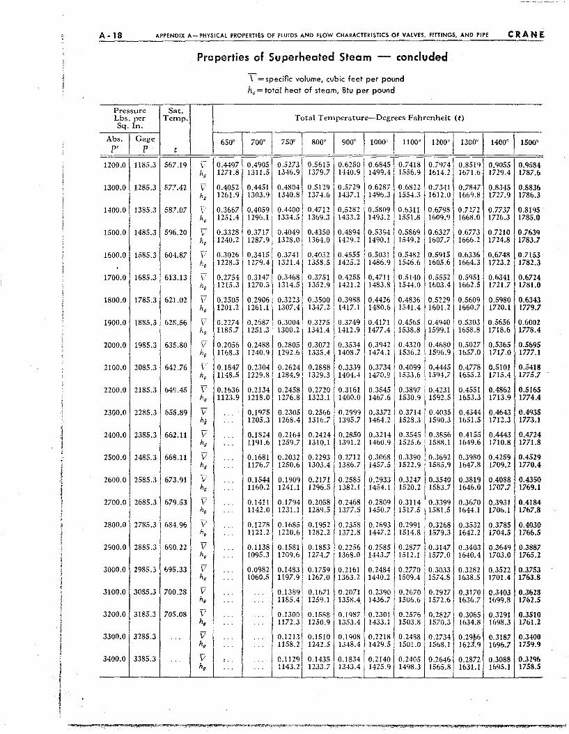
1 I I !

A -18 APPENDIX A- PHYSICAL PROPERTIES OF FLUIDS AND flOW CHARACTERISTICS OF VALVES, FITTINGS, AND PIPE CRANE

p",""" ~ So< Lbs. per Temp, Sq. In.

Abs. I Gage P' P t

1200.0 1185.3 567.19

1300.0 1285.3 577.42

1 1400.0 I 1385.3 587.07

I 1500.0 11485.3 596.20

I 1600.0 1585.3 604.87 . 1700.0 1685.3 61:1.13

1800.0 1785.3 621.02

1900.0 1885.3 628.56

2000.0 1985.3 636.80

2100.0 2085.3 642.76

2200.0 2185.3 649.45

2300.0 2285.3 655.89

2400.0 2385.3 662.11

2500.0 2485.3 668.11

2600.0 2585.3 673.91

2700.0 I 2685.3 679.53

2800.0 2785.3 684 .. 96

2900.0 2885.3 690 . .22

3000.0 2985.3 695.33

3100.0 3085.3 700.28

3200.0 3185.3 705.08

3300.0 3285.3 ...

3400.0 3385.3 . .

Properties of Superheated Steam - concluded

-\' n, i? h,

V ii,

V n, -i/ n, V h, -Ii h,

V n, -V ii,

V h,

V h,

V nJ -V h,

V n, V h,

V h, -V h,

V h,

V hg

V h.

V h.

V , h,

V h.

T' = speciflc volume, cubic feet per pound h, = totcil heat of steam, Btu per pound

Total Temperature-Degrees Fahrenheit (t)

,

I 1000' I 1100' I 1200' I 650' 700' 750' I 800' 900' 1300' 1

0.4497 0,4905 0.5273 0.5615 0.6250 1 0.68451 0.7418 0.7974 0.8519 1271.8 1311.5 1346.9 1379.7 1440,911499.4 ! 1556.9 1614.2 1671.6

0.4052 0.4451 0.4804 0.5129 0.57291 0.6287 0.6822 0.7341 0.7847 1261.9 1303.9 1340.8 1374.6 1437.1 1496.3 1554.3 1612.0 1669.8 . ,

0.3667 0.4059 0.4

4001

0.4712 0.528210.5809 0.6311 0.6798 0.7272 1251.411296.1 1334.5 1369.3 1433.2 1493.2 1551.8 1609.9 1668.0

0.3328 I 0.3717 0.40491

0.4350 0.4894 0.5394 0.5869 0.6327 0.6773 1240.2 1287.9 1328.0 1364.0 1429.2 1490.1 1549.2 1607.7 1666.2

1 0.3026 0.3415 0.37411 0.4032 0.4555 0.5031 0.5482 0.5915 0.6336 1228.3 1279.4 1321.4 1358.5 1425.2 1486.9 1546.6 1605.6 1664.3

0.2754 0.3147 0.3468 0.3751 0.4255 0.4711 0.5140 0.5552 0.5951 1215 .. 1 1270.5 1314.5 1352.9 1421.2 1483.8 1544.0 1603.4 1662.5

0.2505 0.2906 0.3213 0.3500 0.3988 0.4426 0.4836 0.5229 0.5609 1201.2 1261.1 1307.4 1347.2 1417.1 1480.6 1541.4 1601.2 1660.7

0.2274 0.2687 0.3004 0.32751 0.3749 0.4171 0.4565 0.4940 0.5303 1185.7 1251.3 1300.21 1341.4 . 1412.9 1477.4 i, 1538.8 1599.1 1658.8

I I

0.2056 0.2488 0.2805 0.3072 0.3534 0.39421 0.4320 0,4680 0.5027

1168.31 1240.9 1292.6 1335.4 1408.7 1474.1 1536.2', 1596.9 1657.0

0.1847 0.2304 0.2624 0.2888 0.3339 0.3734 0.4099 0.4445 0.4778 1148.5 . 1229.8 1284.9 1329.3 1404.4 1470.9 1533.6 1594.7 1655.2

0.16361 0.2134 0.2458 0.2720 0.3161 0.3545 0.3897 0.4231 0.4551 1123.9 1218.0 1276.8 1323.1 1400.0 1467.6 1530.9 1592.5 1653.3

.. .. 0.1975 0.2305 0.2566 0.2999 0.3372 0.3714 0.4035 0.4344 · . 1205.3 1268.4 1316.7 1395.7 1464.2 1528.3 1590.3 1651.5

1 ... 0.1824 0.2164 0.2424 0.2850 0.3214 0.3545 0.3856 0.4155 · . 1191.6 1259.71 1310.1 1391.2 1460.9 1525.6 1588.1 1649.6

· . 0.1681 0.20321 0.2293 0.2712 0.3068 0.3390 I 0.3692 0.3980 · . 1176.7 1250.6 1303.4 1386.7 I 1457.5 1522.9 1585.9 1647.8

... 0.1544 0.1909 0.2171 . 0.2585/ 0.2933 ,0.3247 0.3540 0.3819 1160.2 1241.1 1296.5 ' 1382.1 , 1454.1 11520.2 1583.7 1646.0

0.1411 0.1794 0.2058 0.2468 0.2809 0.3114 0.3399 0.3670 1142.0 1231.I 1289.5 1377.5 1450.711517.511581.5 1644.1

· . 0.1278 0.1685 0.1952 0.2358 0.26931 0.2991 0.3268 0.3532 · . 1121.2 1220.6 1282.2 1372.8 1447.2 1514.8 1579.3 IM2.2

· . 0.1l38 0.1581 0.1853 0.2256 0.2585 I 0.2877 0.3147 0.3403 ... 1095.3 1209.6 1274.7 1368.0 1443.7 I 1512.1 1577.0 1640.4

... 0.09821 0.1483 0.1759 0.2161 0.2484 0.2770 0.3033 0.3282

... 1060.5 1197.9 1267.0 1363.2 1440.2 1509.4 1574.8 1638.5

.. . · . I 0.1389 0.1671 0.2071 1 0.2390 0.2670 0.2927 0.3170

... · . 1185.4 1259.1 1358.4. 1436.71 1506.6 1572.6 1636.7

· . I 0.1300 0.1588 0.198710.2301 I 0.2576 0.28271

0.3065 .. . ... 1172.3 1250.9 1353.4 1433.1 1503.8 1570.3 1634.8

· .. 1 0.1213 1 0.1510 0.1908 0.2218 0.248810.2734 0.2:f.6 ... .. 11158.2/1242.5 1348.4 1429.511501.011568.1 162.9

... ." 1 0.1129 0.1435 0.1834 0.21401 0.2405 0.2646 0.2872

... .. 11143.21 1233.7 1343.4 1425.911498.3 1565.8 1631.1

1400' 1500'

0.9055 0.9584 1729.4 1787.6

0.8345 0.8836 1727.9 1786,3

0.7737 0.8195 1726.3 1785,0

0.7210 0.7639 1724.8 1783.7

0.6748 0.7153 1723.2 1782.3

0.6341 0.6724 1721.7 1781.0

0.5980 0.6343 1720.1 1779,7

0.5656 0.6002 1718.6 1778.4

0.5365 0.5695 1717.0 1777.1

0.5101 0.5418 1715.4 1775.7

0.4862 0.5165 1713.9 1774.4

0.4643 0.4935 1712.3 1773.1

0.4443 0.4724 1710.8 1771,8

0.4259 0.4529 1709.2 1770.4

10.4088 0.4350 1707.7 1769,1

0.3931 0.4184 1706.1 1767.8

0.3785 0.4030 1704.5 1766.5

0.3649 0.3887 1703.0 1765.2

0.3522 0.3753 1701.4 1763.8

0.3403 0.3628 1699.8 1762.5

0.3291 0.3510 1698.3 1761.2

0.3187 0.3400 1696.7 1759.9

0.3088 0.3296 1695.1 1758.5

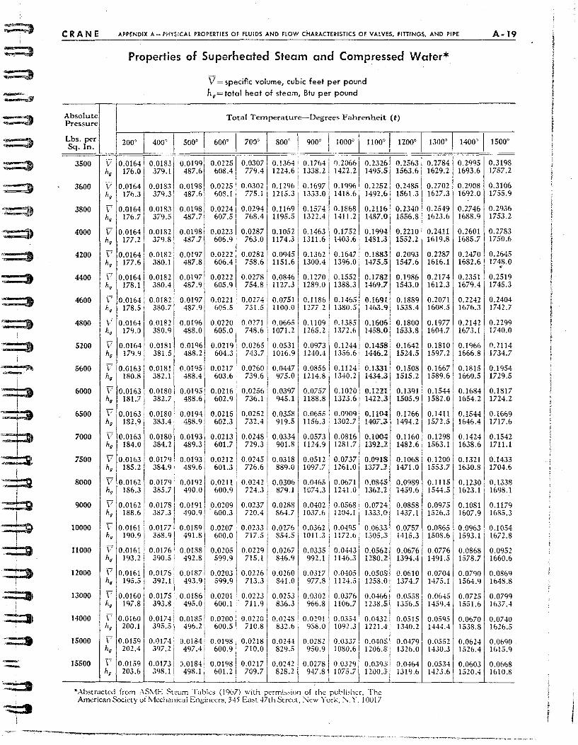
· .. ::f3 ~=::::. ,

1

-

CRANE

Absolute Pressure

APPENDIX II - PHY,ICAL PROPERTIES OF FLUIDS AND FLOW CHARACnRISTICS OF VALVES. FITTINGS. AND PIPE

Properties of Superheated Steam and Compressed Water*

v = specific volume, cubic feel per pound

h.= 10101 heal of sleam, Btu per pound

Total Temperature-Degrees Fahrenheit (t)

A-19

1400' 115000 .- --=L=~~S.=. l=p;=.r=l==*=2=0=O'=io

1 =40=0~o~I==5=0=O'=*=60=0=' ~1=7=OO='=4=80=0=' =-,\=9=0°='=41 ,=l=O=OO='=*I=l1=O=O'=*,1 =1=200' I 1300'

3500 i7 0.0164 0.018310.0199 0.0225-10.030710.1364 0.176410.206610.232610.256310.2784 0.2'195 0.3198 h. 176.0 379.11 487.6 608.4 i 779.4 1224.6 1338.21 1422.21 1495.51 1563.61 1629.2 1693.6 1757.2

I I ! I 3600 V 0.0164 0.0183 0.0198, 0.0225 0.0302 I 0.12% 0.16971 0.1996 1 0.22521 0.2485 0.2702 0.2908 0.3106

h. 176.3 379.3 Ii 487.6 608.1 775.11 1215.3 1333.011418.6 1492.6: 1561.31 1627.3 1692.0 1755.9

3800

4000

4200

4400

4600

4800

5200

5600

6000

6500

7000

7500

8000

9000

10000

11000

12000

13000

14000 1

15000

15500

"\ 0.0164 0.018.11 0.0198 0.0224 0.029410.1169 0.157410.1868 0.21161 0.2340 10.2549 0.2746 0.2936 h. 176.7 379.51' 487.7 607.5, 768.4 1195.5 1322.411411.2 1487.01 1556.8 1623.611688.9 1753.2

V 0.0164 0.0182 0.0198 0.02231 0.0287 0.1052 0.1463 'I 0.1752 0.19941 0.2210 1 0.2411 0.2601 0.2783 h. 177.2 379.8 1 487.7 606.91 763.0 1174.3 1311.6 1403.6 1481.311552.2 1619.8 1685.7 1750.6

V 0.0164 0.01821 0.0197 0.0222 0.0282 0.0945 0.1362 0.1647 0.1883 'I 0.2093 0.2287 0.2470 0.2645 487.8 606.4 758.6 1151.6 1300.4 1396.0 1475.5 1547.6 1616.1 1682.& 1748.0 • h. 177.6 380.1

V 0.0164 0.0182 h. 178.1 380.4

V 0.0164 0.0182 h, 178.5 380.7

\" 0.0164 0.0182 h. 179.0 380.9

V 0.0164 0.0181 h. 179.9 381.5

\' 0.0163 0.0181 h. 180.8 382.1

V 0.0163 0.0180 h. 181.7 382.7 -V 0.0163 0.0180 h. 182.9 383.4

V 0.0163 0.0180 h. 184.0 384.2

V 0.0163 0.0179 h. 185.2 384.9

V 0.0162 0.0179 h, 186.3 385.7

V 0.0162 0.0178 h. 188.6 3·87.3

\' 0.0161 0.0177 h, 190.9 388.9

V 0.0161 0.0176 h. 193.2 390.5

Ii 0.0161 0.0176 h, 195.5 392.1

V 10.0160 0 .. 0175 h. 197.8 393.8

"\ 0.0160 0.0174 h. 200.1 395.5

\' 0.0159 0.0174 h, 202,4 397.2

-;;c 0.0159 0.0173 h. 203.& 398.1

0.0197 0.0222 0.0278 0.0846 0.1270 0.1552 0.17821 487.9 605.9 754.8 1127.3 1289.011388.3 1469.7

! 0.0197 0.0221 0.0274, 0.0751 0.11861 0.1465 0.1691 i 487.9 605.5 751.511100.0 1277.2 1380.5 1453.'l!

0.0196 0.0220 488.0 605.0

0.0271 I 0.0665 0.1109 0.1385 0.1&061 748.6' 1071.2 1255.2 1372.6 1458.0 i

0.01% 0.0219 0.0265 0.0531 0.0973

1

0.1244 0.14581 488.2 604.3 743.7 1016.9· 1240.4 1356.6 1446.21

0.0195 0.0217 0.0260 10.0447 0.0856 0.1l241 0.1331! 488.4 603.6 739.6

1

975.0 1214.8 1340.21 1434.3! I . !

0.0195 0.0216 0.0256 0.0397 0.0757 0.1020 o.l2n

j

. 488.6 602.9 736.1' 945.1 1188.8 1323.6 1422.3

0.0194 0.0215 0.0252 0.0358 0.0655 0.0909 O.llM 488.9 602.3 732.4 919.5 1156.3 1302.7 1407.3

0.1986 1543.0

0.1889 1538.4

0.1800 1533.8

0.1642 1524.5

0.1508 1515.2

0.1391 1505.91

0.1266 1494.2

0.2174 0.2351 0.2519 1612.311679.411745.3

0.2071 0.2242 0.2404 160R.5!1670.3 1742.7

0.1977 0.2142 0.2299 1604.711673.1 1740.0

0.1810 0.1966 0.2114 1597.2 I 1666.8 1734.7

0.16671 0.1815 0.1954 1589.6

1

1660.5 1729.5

0.1544 0.1684 0.1817 1582.0! 1654.2 1724.2

0.1411 0.1544 0.1669 1572.5 1646.4 1717.6

0.0193 0.0213 0.0248 0.0334 0.05731 0.0816 O.lOM 0.1160 0.1298 0.1424 0.1542 489.3 601.7 729.3 901.8 1124.9 1281.7 1392.2 1482.6 1563.1 1638.6 1711.1

0.0193 0.0212 0.0245 0.0318 0.0512 0.0737 489.6 601.3 726.6 889.0 1097.7 1261.0

0.0192 0.0211 0.0242 0.0306 0.0465 0.0671 490.0 600.9 724.3 879.1 1074.3 1241.0

0.0191 0.0209 0.0237 0.0288 0.0402 0.0568 490.9 600.3 720.4 864.7 1037.6 1204.1

0.0189 0.0207 0.0233 0.0276 491.8 600.0 717.5 854.5

0.0188 0.0205 0.0229 0.0267 492.8 599.9 715.1 846.9

0.0362 0.0495 1011.3 1 1172.6

0.0335 0.0443 992.1 1146.3

0.0918, 0.1068 0.1200 0.13211 0.1433 1377.1':1 1471.0 1553.7 1630.8 1704.6

0.0845! 0.0989 0.1115 0.1230 0.1338 1361.2:1 1459.6 1544.5 1623.1 1698.1

i!

0.07241 0.0858 0.0975 0.1081 0.1l79 1333'()i! 1437.1 1526.3 1607.9 1685.3

J O.0633~,: 0.0757 0.0865 0.0963 0.1054 1305.3 Ii 1415.3 1508.6 1593.1 1672.8

:: 0.0562:1 0.0676 0.0776 0.0868 0.0952 1280.2:i 1394.4 1491.5 1578.7 1660.6

] 0.0187 0.0203 0.0226 0.0260 0.0,317 0.0405 0.0508': 0.0610 0.0704 0.0790 0.086'1

493.9 599.9 713.3 841.0 977.8 1124.5 1258.0 1374.7 1475.1 1564.9 1648.8 i

0.0186 0.0201 495.0 600.1

0.0213 711.9

0.0253 836.3

0.0185 0.0200 0.0220 0.0248 496.2 600.5 710.8 832.6

0.0.,02 0.0376 966.81 1106.7

0.0291 0.0354 958.0 1092.3

, 0.0466! 0.0558 0.0645 0.0725 0.0799 In8.5 i, 1356.5 1459.4 1551.6 1637.4

0.0432 1221 ...

0.0515 1340.2

0.05% 0.0670 0.07-10 1444.4 1538.8 1626.5

0.0184 0.0198 0.0218 0.OH4 0.0282 0.0337 0.0405:'. 497.4 600.9 710.0 829.5 950.9 1080.6 1206.8:

0.0479 1 1326.0

0.0552 1430.3

0.0624 0.0690 1526.4 1615.9

0.0184 0.0198 0.0217 0.0242 0.02781 0.0329 0.0393 i {).0464 0.0534 0.0603 0.0668 498.1 601.2 709.7 828.2 947.81 1075.7 1200.J 1319.6 1423.6 1520.4 1610.8

i *Abstracted from :\?~'1E Stl"am Tubles (lc}{)7) with pcrmj~.:-i()n of [he puhlbhcr. The American Society 01 ~lcchanicai Engineers, 3-15 East 47th Street. :\ew York, :\. Y. 10017

A.20

I

API'ENDIX A - PHYSICAL PROPERTIES OF flUIDS ANO flOW CHARACTERISTICS OF VALVES, FITTINGS, ANO PIPE

Fiow -~

Flow ---:r

Flow Coefficient C for Nozzles7

Data from Regelnfuet die Durch­flussmessung mit genormten Due­sen und Blenden. VDI-Verlag G. m.b H., Berlin, SN\V, 7, 1937. Published as Technical Memo­randum 952 by the NACA.

ExalTlple: The flow coeffi­cient C for a diameter ratio do/d , of 0.60 at a Reynolds number of 20,000

(2 X t04) equals 1.01.

('

1.1 8 I I] 'III " I i 6 '

! Ii! f i Illi' , 4' ! ,I ,

" '

1 11 I -,

I 1 I "

1.1

1.1

1.1

1.1

1.0

1.0

1.0

1.0

'I : ':

0' I, I !

I ", !! I'! i iii

0.l+!, , f

8, ,I , J{f' J ;, f 6 I,' i "

.1 " i i"'1 ' " I : 4 ' ' '" --'"" ').11',. VI.)': 2 " I 'I I 'i

l-i--i+-' :;?Vf......-: . 0" , , 1.0

0.9

0.9

\;,.~~

: III fY ~V.n 1

Illrvl II 0.94 4 810'

I i I rr I i rnrr

Ii II I f 'I I f

,

,

i

46810'

R, - Reynolds Number based on d l

Flow Coefficient C for Square Edged Orifices 7•

17

C

2 t I I I

I i I /' ,/ 1 I \ %;80 I

L

1.3

l.

1. I I

I t- '=751~ i 1.0 v --- I

"""" \

I \\ , '-..., I I" "~vr v I ,Itt :.65! r, .---t"

:' 1111 i n- :50i--\Y~ i T . " '" r- :---... 1"-...

0,

IIIIII/i !L~~ f , I I t-~ I' I, i'rl i -..;. 1 7 . "I', I - ,

o.

o.

0.6 I!I~ ~ I i~:;:::;:,r....L:

,4 ~ f\\\ 11Wl , - *=1#]1 /

~ ~ \':: - 3OI'V - : 0",2)

W

0.,

0,'

6 8 10 , 4tJ 60 80 102 4 6 8 103

R,. - Reynolds Number based on d1 -

c = ;==~C~d=F' ~ 1 - (~)'

Lower chart data from Regeln ruer die Durchflussmessung mit -gt?normtem Duesen und Blenden. VDI-Verlag G mb.H.. Berlin, SNW, 7, 1937, Published as Technical Memorandum 952 by the NACA.

i-

,t--

:::: --~ - F=::

4 6 810' 2 4 6 810'

11, - Reynolds Number based on d,

CRANE

,80

,77

.7

.72 s .s

.70

..

.60

.S

.SO

.40

'''0-.30 0.2

.30

().().2

:i:-r­,=~ .•

! , ; .­

i : ! II

, ::: -a

CRANE APPENDIX A- PHYSICAL PROPERTIES OF flUIDS AND FLOW CHARACTERISTICS OF VALVES, FITTINGS, AND PIPE

Net Expansion Factor, Y

c: o .. E--L-=-::t~~~-2~~"""":","+-~~~':::""H-+-+-i--I Vl

~ ;'F--i--::-C7"b-...4~...o.,:~-r--+--...;'>,~-+-~~""':~l-1:";"..l-' x

UJ

:...... .55 b--r----j--+--+--+--+--+---l---";....-->-ii-l-+~ i j I !

~~-r--__j---~.---t--+-~-~-+-~~+-~~

."I---ir---+-+-+--t---+--+---l--.f-----l-+~_+_W

.<eE:--t---j--+--+-+--+--+---l--l----I--I-i*..l-1

I l.2~!'! I , J , .

a.. ........ "" a..

.58

~"

.56

! r '! ! ,';'-)

" J ,.~ \, ,I, !li,!,!!,·,,!.!tI'

to ~ :.C ! ! I , ! ' !; )'! I ) . ! , 1 ' ! lin

, I 1, ! l ,! ,t ! '., •• t, II II [, I LO

Pressure Ratio -

Critical Pressure Ratio, rc

u 1.35

k=cp,cv

.75

For Compressible Flow through Nozzles and Orifices9,10

Data extracted from, Fluid l\1eters, Their Theory and Application, Fourth EJi­tion, 1937, and Orifice Meters wilh Supercritical Flow by R. G Cunningham, with permission of the pub­lisher, The American Soci­ety of Mechanical Engi­neers, 345 East 47th Street, New York, N,Y. 10017.

For Compressible Flow through

Nozzles and Venturi Tubes9

I I

I

A·22

1.0

0.95

0.90

0.85

0.80 y

0.75 . 0.70

0.65

0.60

0.55

0.95

0.90

0.85

0.80 Y

0.75

0.70

0.65

f 0.60 , ,f ; 0.55 I j

I

APPENDIX A-PHYSICAL PROPERTIES OF FLUIDS AND flOW CHARACTERISTICS OF VALVES, FITTINGS, AND PIPE CRANE .

Net Expansion Factor Y for Compressible Flow Through Pipe to a Larger Flow Area

k = 1.3 rk ~"rrr"xlm"tch' 1.3 for CO,. SO,. 11,0. II,S. ~i Is. ~,O, 0,. CIl,. C,II,. anJ C,II,I

~

o

0

'-.. '-.. I I

I

'\ .~ ~i

~~~ ~ ~~

l~ ~ ~ ~ ~ ~ I I~ ~,~ ~~ ~ ~ ~~ t--...

1,\

I ~ ~ ~I ~ ~ 8:: ~ ~~

I ." ""-~ ~ "R: '~8~ I "\ i'\. ~j ""~ ~t'o f:o~ '01'1'0. I '\ t'

f f-,\_\.\_,\._T"l_

~ '" "'~~ '0_ 11' " {$. "'0 "0 -0

I

0.1

0.1

I I

0.2 0.3

~ f ,\ 1-0 0 f- \.' <9 _\\_~ .. ':..0

0.4

" "'\,1' f'":" 1"0 '0 f\, l' t '0

" '" 1'F",Y'OI

0.5 t::,p p'

1

0.6 0.7

k = 1.4

0.3 0.9

r:k ~approximatcly J.4 for Air. H,. 0" "'" CO. NO. and HCl)

0.2 0.3 0.4 0.5 0.8 0.9 t::,p P' I

1.0

1.0

Limiting Factors For Sonic Velocity

k = 1.3

K I ~~I y

1.2 .525 .612 1.5 .550 .631 2.0 .593 .635

3 .642 .658 4 .678 .670 6 .722 .685

8 .750 .698 10 .773 .705 15 .807 .718

20 .831 .718 40 .877 .718

100 .920 .718

Limiting Factors For Sonic Velocity

k = 1.4

K I~~I Y

1.2 .552 .588 1.5 .57& .&0& 2.0 .&12 .&22

3 .&&2 .&39 4 .. 697 .649 & .737 .&71

8 .7&2 .&85 10 .784 .&95 15 .818 .702

20 .839 .710 40 .8831.710

100 .92& .710

=­::::::t

:::::3

~

'::=:t

~

t::I

=::I

::=:I

==­==­~ -:::=2

~

~

:::::2

=:D

:::::» .~­... ~~

::::::s

"==­."~

.".=-~

"~

,~ -'~

CRANE APPENDIX A - F'H'rS1CA1. PROiftERTIES Of HUlDS AND flOW CHARACTERISTICS Of VAtVES~ fmINGS. AND PIPE

Relative Roughness of Pipe Materials and Friction Fadors

For Complete Turbulence18

Pipe Diameter, in Feet - D

'E~.J~~I~'3t2~~I}§j.~4i~.~5t·~~1~.~8~'1~~§t'§2§~,3~S4~5~~~11~~~r'~§O'~~'~~EO~2L5 .05 ' 1 '07 04 '..:=t, '.1 I Ii·

. I 1 ' -,: Ii' h' \ I Iii i

03"' I I : ! " ! 1 I I': I I , II! 06 • "' ,I 1"'- I "' Iii I i .021---+'~'+! -Hr--+-i(-+~~'+++--+-l'-! ~-+-' -H-++-i, f-t--t-t-H---i1--..t-+--!-.05

~... I I i,\~ i '- I i I " 1 '" i I'l, I II I ~, "I iN

Pipe Diameter, in Inches - d

-.04 035

01

A-23

i ),J{,I (.'\tr;lc{CJ ironl Fflt-lltm I ';.{~I'.~ .!t)f PIPr: F!tlll' bv L F \~, ""'I •. h. \l, nh pt:rml~~10n 'of the f'uhll··-t-k:'. The .\I1'.crtcan Soci­.t't \ 01 ~ 1r,;"h;:~mci.l1 Engineer--:. 2'J \) e>( N,h l-!rcct. :\cw York.

Problem: Determine absolute and relatiye roughness. and friction fac­tor, for fully turbulent flow in Io-inch cast iron pipe (I.D. = 10.16").

Solution: Absolute roughness (.) = 0.0008; ..... Relative roughness (E. D) = 0.001 ..... Friction factor at fully turbulent flo\\" (j) = O.OlgO.

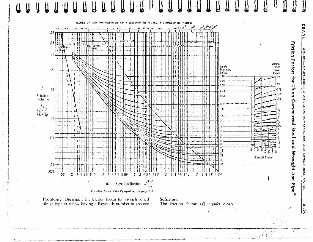
I U U ij U UU lU Uu-u U U U II U U U U U U U U U U U u n

I VALUES OF (I'd) FOR WATER AT 60' F (VELOCITY IN FT,/SEC, X OIAMETER IN INCHES)

0.1 0.2 0.4 0.6 0,8 I 6 8 10 20 40 60 80 100 200 400 600 800 \.~() 'l,~ "'~\~~~~~

'07Tf.li ~'l!Pl'!'!Ill 06 1 I 1 ' +.. TIJJ1JLIEIJf Zo'NE

, ~MIN:r. T ; TR~N~~I~.N 1.' ~"'1 .i.' T'Or'm'llhEE1'E'r rtllRT'BTUllCNctlII I r I t I t+l4-1

Irtl ,~. I I I I 1 i ' { . 'i II ,05 i t \ tN.· . . i i' II I 11111 I I I II+++-t+!-H

) '1.: 1 ~:;l', I I ' 'f I I t • t • "'},' i i

'.' , 1, ! "~i <~. > .... ~.' ..... .... 1 1 , , T •. ·,' I "ll I' " ; . IV':! f·'··~" "t .... I i. I ,04 i" i- ·'I.~r 1~" ",.J i i .. r ~·H.jl I I I H-l

I r:! !~\. tfh~t~:~rrft?::f~ + ~,I... .'., .' .

~ i: ~.' ! ft ',. ~~~ ~ -\1' l 1U11 I I UUnll11l I! H-ffiH+l:: f .! . " ill \,f'..l"}. ~ . ,,,

.03! . i •. ~ ~ , . ~;" ".,~ ., rr I ' ,,,,.r I' "1""'" ,t Friction 'f]' i '\': ~~tt ' ,;... ,I..l-l-W II Ilt41 +-1

Faclor ~ _ .. t I i~~Ht-I ..... Ii·· ' , ! I INN I ~r-N. :

. "J:, ttl·] 1\ . - I ~~, '. I-r---U 'i 1"'--1----(I) ,.' , t ". i- I ,

/)'211 r .. . ... - > ~~f:::~t! + ,,'-1--11 . 02 I J ,:~" "'" '1 'I', ',: T T "

-'T" -_... "",~ •.. , rt-. H4f- I t I fl "1 I --'- . ~;'<;;~''j.li - . J"I 1 __ " ,'\. I. ,.~ "" . I .' .. .. . -- .. ~0 .. 'i<!.tH ' c. " C" I· I : 1 .. ~t~t't~.l ... : •. :, "~ _ - .. ' _-- -i' II i 1M n· '+ 1 '''' ••. ,''. ""f' -.. . ] I 1 I~~-rl ;.... c. '

"," \:.1') , " ~-;t , '1 -,'1.'';<'1..) l' """".

Ij~1 Iff-I··t.·j·!.·.I··j· ... ,·[· .. [·-11.···1 ... I·I-~~···'<I~t':'~~~r:: .. '" ~~.·"r·~:·.I·.;~ . . H _. - ..... ... - .. ~~ ~. ",' . ~~ -l·1 . ....... . f-.. '-1-- ... +- 1+

; tID tilt lnli i liittllfll j f .. =>1J ~~J~r·:: 103 2 3 4 5 C B 104 2 3 4 5 6 8105 2 3 4 56 8106 2 3 4 56 8107 2 3 4 56 8 108

./

He - Reynolds Number ihP

}i'e

For other lormJ 01 the Re equation, see page 3·2.

Problem: Determine the friction factor for 12-inch Sched­ule 40 pipe at a flow haVing a Reynolds number of 300,000.

Solution: The friction factor (f) equals 0.016,

Nominal Pipe Sjl~,

inches ~1/8

.t==',;.f~

1/2 F~j;; __ ~1 3/4

=1 ..... '...-....., i',

BE::t:~~~ 2~i +-\:.....;..,p.-,,=:;13 Ii ..ct:~~:~~

6 8

I~ .t;;;;l~.=::t:, ::1,=, a

1 14

o 0 2 4 6 o 0 0 Q

Scnutllliu Numlier

n II IJ . . .. n ;to

» z m

t

::r 1\' ,. - ~ O· ~

m

::I z 0

." )(

Q ,.

Q. I

0 ~ -< .. '" III n - ~

0 .. .. '" 0 n ..

m

iD '" ::;

fl m

'" ::I ~

.~ ~ c

3 0 V>

3 ,. z

(I) 0 ... ~

D. 0 0 :0:

n til

:r ,. iii '" ,. (I)

n ~ m

'" Q 'a ::I n 0.. V>

0

:e ~

g ;:

ffi 10 ::r" 3 - Z ::;- G'I

0 1"

::I ,. z

." 0 -. ..

'tJ :;; m

CD i»

» I..:) UI

.. M,."'''.,~.'''"' .. ,~,'_.~~.'!'''".,,'':'' ...... :",-'',,.,~T· ... ~,''~,.t' .... ,_"'"." .... ,....,.... .... "..,."~,.,..-'""-"I'''I"I~*~_~. __ ~~_· _____ • ___ _ " '-'~..,"""' ... _"' •. c,,""_,~,.'...,.,.-

~~~k,:.'· ~._,~~N'I~.~'!i.Iif ....... ~,,~ ........... ~.-,~ ... ·~· -,~,-----... - .... --.~ .... --.---........ ---> .... ~~--.,.- .. -.. -,-~-~.~-."---------...... ~~-,~-~,,",,"--

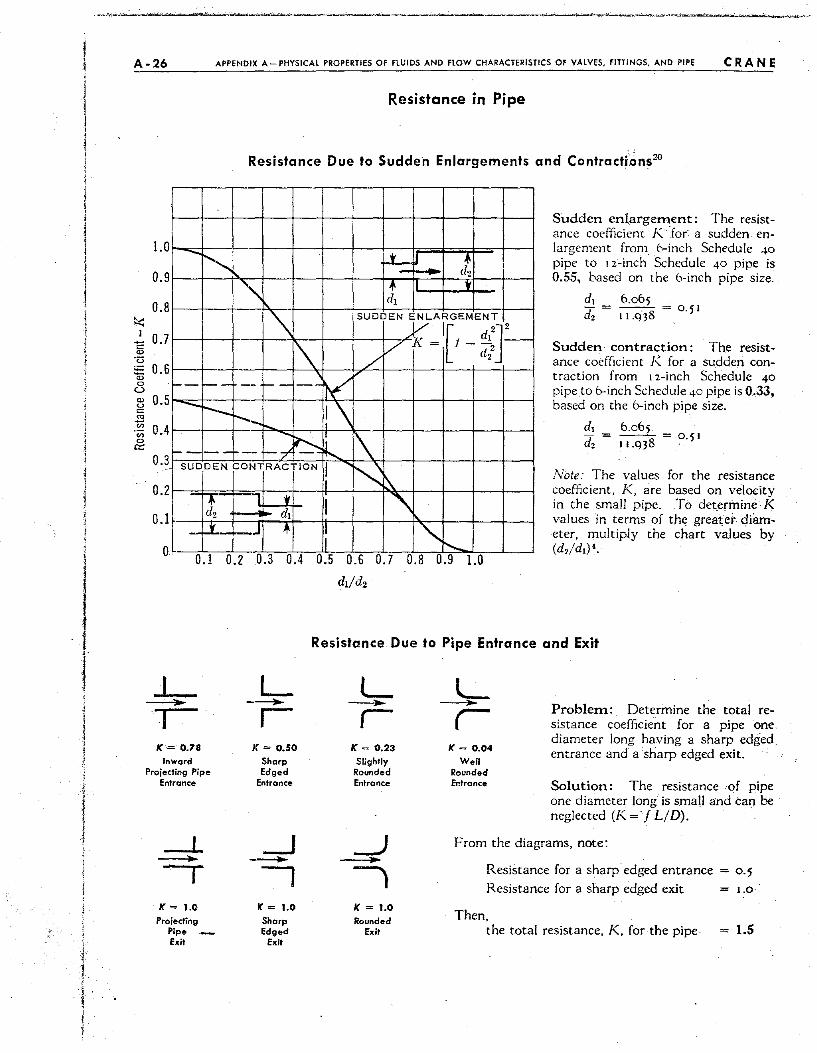
A-26 APPEN[)IX A-PHYSICAL PROPERTIES Of flUIDS AND flOW CHARACTERISTICS OF VALVES, flnINGS, AND PIPE CRANE

~ I ~

<= <l> 'u -'ii; 0 u

CD u <= .l3 '" '" CD

0:::

LO

0,9 --'" 0,8

0.7

0.6 'r-----

0.5 ---0.4

----

Resistance in Pipe

Resistance Due to Sudden Enlargements and Contractions20

''\

~ 1"'-

-- /-- -.-V ............. 1\

" K II -- -7' -~ ~

y d~

l t'

SUDDEN ENLARGEMENT

I '[ 2J /'

V f = 1- ~~21-

1\

Sudden enlargement: The resist­ance coefficient K'for a sudden en­largement from 6-inch Schedule 40 pipe to 12cinch Schedule 40 pipe is 0.55, based on the 6-inch pipe size.

6.065 11·q38

0.5 1

Sudden contraction: The resist­ance coefficient 1<. for a sudden con­traction from 12-inch Schedule 40 pipe to 6-inch Schedule 40 pipe is 0.33, based on the 6-inch pipe size.

d, 6.065 - ---. = 0,5 1 d, II.Q38

0.3 SUDDEN CONTRACTION I ~ Note: The values for the resistance

coefficient, K, are based on velocity in the small pipe. To det.erinineK values in terms of the greater diam­eter, multiply the chart values by (ddd,)'.

0.2

0.1

~

~ f I ~ dl

Y' ~ ""-r--..... 0 0.1 0.2 0.3 0.4 0.5 0.6 0.7 0.8 0.9 1.0

dIld2

I L - -~

I r K'= 0.78 Jr = 0.50

Inward Sharp Projecting Pipe Edged

Entrance Entrance

---L -.J -- -~ --r -, K = 1.0 IC = 1.0

Projecting Sharp Pipe Edged EJtit Exit

Resistance Due to Pipe Entrance and Exit

L ---r K = 0.23

Slightly Rounded Entrance

~ -I K = 1.0 Rounded

exit

L -r K = 0.04

Well Rounded Entrance

Problem: Determine the total re­sistance coefficient for a pipe one diameter long having a sharp edged entrance and a sharp edged exit.

Solution: The resistance of pipe one diameter long is small and tal1 be neglected (K = I L/ D).

From the diagrams, note:

Resistance for a sharp edged entrance = 0·5 Resistance for a sharp edged exit = 1.0'

Then, the total resistance, K, for the pipe. 1.5

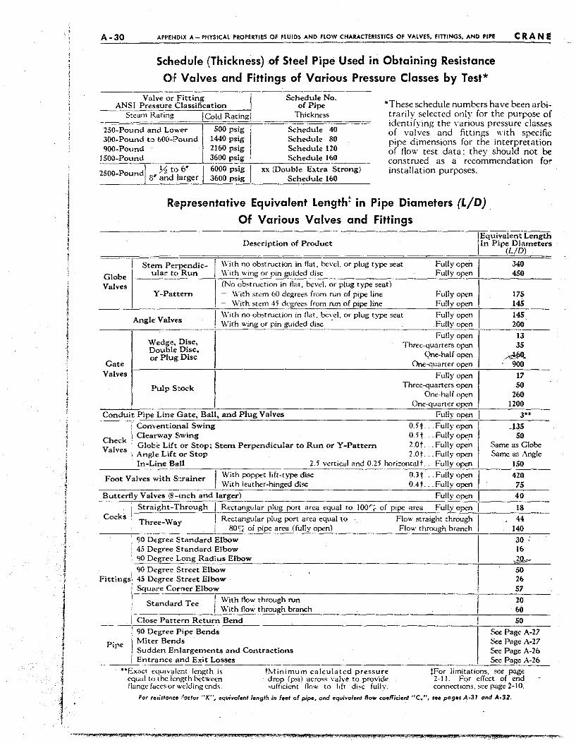
1 j I , i

f f ~

I I

j I

A-30 APPENDIX A - PHYSICAL PROPERTIES OF FLUIDS AND FlOW CHARACTERISTICS OF VALVES. fITTINGS. AND PIPE

Schedule (Thickness) of Steel Pipe Used in Obtaining Resistance

O:F Valves and Fittings of Various Pressure Classes by Test*

CRANE

Valve or Fitting ANSI Pressure Classification

Schedule No. of Pipe

Thickness *These schedule numbers have been arbi­trarily selected only for the purpose of identifying the various pressure classes of valves and fittings with specific pipe dimensions for the interpretation of flow test data; they should not be construed as a recommendation for installation purposes.

Steam Rating I Cold Rating!

l50-Pound and L0::JJer 500 psig I 300-Pound to 600-Pound 1440 psig I 900-Pound 2160 psig i

1500-Pound 3600 psig

Schedule 40 Schedule 80 Schedule 120 Schedule 160'---__

2500-Pound Yz to 6' I 6000 psig 8' and larger 3600 psig

xx (Double Extra Strong) Schedule 160

Globe Valves

Gate Valves

,

R,epresentative Equivalent Length! in Pipe Diameters (L/D)

Of Various Valves and Fittings

I Equivalent Length

Description of Product In Pipe Diameters (LID)

Stem Perpendic- With no obstruction in flat. be\'c!, or plug type seat Fully open 340 ular to Run \\'ith wing or pin guided disc Fully open 450

---------~~~~~~~~~-~~---~-----~~~--------­

Y-Pattern

Angle Valv.",

Vl edge, Disc, Double Disc, or Plug Disc

Pulp Stock

(No obstruction in flat, bevel. or plug type seat) - With stem 60 degrees from run of pipe line - With stem 45 degrees from run of pipe line

\\'ith no obstruction in flat, bc\·cl, or plug type scat With wing or pin guided disc .

Fully open Fully open

Fully open Fully open

Fully open Threc-quarters open

Qne-hal f open One-quarter open

Fully open Thrcc-quarters open

One-half open One-quartcr open

175 145

145 200

13 35

;d§Q. 900

17 50

260 1200

~ Conduit Pipe Lme bate, Ball, and Plug Valves Fully open 3" Conventional Swing Clearway Swing

O.5t .. Fully open O.5t .. _ Fully ope,n

Globe Lift or Stop; SteIll Perpendicular to Run or Y -Pattern 2.0t ... Fully open Angle Lift or Stop In-Line Ball

Foot Vatves with Strainer

2.0t ... Fully open 2.5 vertical and 0.25 hori=ontalt .. Fully open

With poppet lift-type disc 0.3t .. Fully open With leather-hinged disc OAt. _. Fully open

Butterfly Valves (8-ineh and larger) Fully open

Straight-Through I Rectangular plug port area equal to 100r~ of pipe area Fully open

Cocks Three-Way I Rectangular plug port area equal to Flow straight through 80S; of pipe area (fully open) Flow through branch

J35 50

Same as Globe Same as Angle

150

420 75

40

18

44 140

90 Degree Standard Elbow 30 45 Degree Standard Elbow 16 90 Degree Long Ra.:d.:i.cuc-s_E __ lc-bo'-'-w _________________________ --:-_---,_--"k==--__

, 90 Degree Street Elbow 50 Fittingsl, 45 Degree Street Elbow 26

II~Sq~u_a_re_c~o~r.n __ e_r~E_l_bo_W~~-~-~-~--------------_________ +-_______ 5.:7 ___ ___

Standard Tee I With flow through run 20

11~~~~--~--~I~~~·i--t--h~fl-o-w-t--h-r--Ou~g~h~b-ra=n~c-h--__________________________ ~-------60~-----Close Pattern Return Bend 50

---190 Degree Pipe Bends See Page A-27 Miter Bends See Page A-27

Pipe Sudden Enlargements and Contractions See Page A-26 i Entrance and Exit Losses See Page A~26

-----'--"Exact equivalent length is t!\.,tinimum calculated pressure tFor limitations. see page

equal to the length between drop (psi) acro<;;s valve to provide 2-1 I. For effect of end flange faces or wclding ends. sufficient flow to lift dISC fuBy. connections, see page 2-10.

For resistance :rador "K", equivalent length in Feet of pipe, end equivalent Row coefficient .. e ..... , see pages A-31 and A-32.

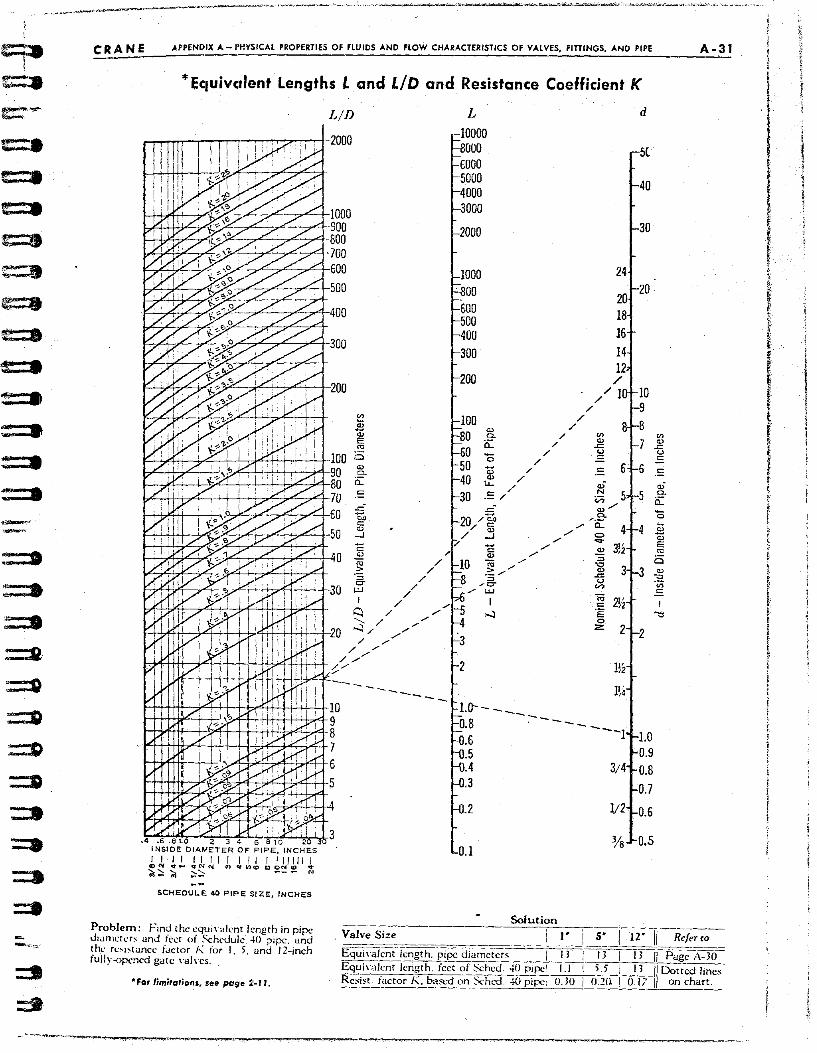
eRA N E APPEND'IX A -I'HYSICAl PROPEHIES OF FlUIDS AND FlOW CHARACTERISTICS OF YAl YES, FITTINGS, AND PIPE ~~.::.-~=---'-- A·31

*ECIUivcJlent Lengths L and LID and Resistance Coefficient K

SCHEOUL.E 40 PIPE S(ZE:. INCHES

Problem: Find the cqui"alent length in pipe Jldn1Cft.'rs and ket of Sch('duJc 40 pipe. and thl' rc.:"'I~tancc factor" for J, 5, and 12-inch fully-opened gate \·a"·cs.

·For limita,ions. see page ~!-11.

LID L

~ ..'!l '" '" Q. E 0: <'0 -Cl 0

'" Q) Q.

0: '" l.L. e .: /

.t= c;, e '" -' - -c:

/ <: 0 ..'!l

/ ..'!l CO <'0 :> / .:::/ '" / '" 0-

/ ~O-L.U / L.U / I / I ~ " ...., "- / ...;:"

" ./

/,- ./

/,-// ./

------

.2

" <I)

" '" .t=

" u / .E

" <: /

/ w-N

C;;

"'.--..... ~ /' 0-.-- 0 ,- .... .--,- ..'!l

/ '" ./ " <U .<:: <.>

'" 0; <: 'E 0 2:

---

d

S(

40

30

20

10 9 8 7

6

5

3

2

1.0 0,9

0.8

0.7

0.6

0.5

'" '" .t= u .E .£ w-Q.

0: '5 ~

..'!l <U E '" 6 '" -0 'iii .E , "<:l

Solution Valve Size

Equi\'alcnt length. pipe di;Hncters : Equi\'alcnt length. fcct of Schcd. ~U pipe! Resist. factor K, based on Schoo. 40 pipe;

I'_L~:~I ~1~:J-R~~Tto I J I I J I (J /I PagC::\-JO-

1.1 I 5. 5 i I J II Dotted lines 0,30 I O.2()' I 0.17 on chart,

, j

I !