Embed Size (px)
Citation preview

Automation, Collaboration,& E-Services
Itshak TkachYael Edan
Distributed Heterogeneous Multi Sensor Task Allocation Systems

Automation, Collaboration, & E-Services
Volume 7
Series Editor
Shimon Y. Nof, PRISM Center, Grissom, Purdue University,West Lafayette Indiana, IN, USA

The Automation, Collaboration, & E-Services series (ACES) publishes new devel-opments and advances in the fields of Automation, collaboration and e-services;rapidly and informally but with a high quality. It captures the scientific and engineer-ing theories and techniques addressing challenges of the megatrends of automation,and collaboration. These trends, defining the scope of the ACES Series, are evi-dent with wireless communication, Internetworking, multi-agent systems, sensornetworks, cyber-physical collaborative systems, interactive-collaborative devices,and social robotics – all enabled by collaborative e-Services. Within the scopeof the series are monographs, lecture notes, selected contributions from specializedconferences and workshops.
More information about this series at http://www.springer.com/series/8393

Itshak Tkach • Yael Edan
Distributed HeterogeneousMulti Sensor Task AllocationSystems
123

Itshak TkachRishon LeZion, Israel
Yael EdanDepartment of Industrial Engineeringand ManagementBen-Gurion University of the NegevBe’er Sheva, Israel
ISSN 2193-472X ISSN 2193-4738 (electronic)Automation, Collaboration, & E-ServicesISBN 978-3-030-34734-5 ISBN 978-3-030-34735-2 (eBook)https://doi.org/10.1007/978-3-030-34735-2
© Springer Nature Switzerland AG 2020This work is subject to copyright. All rights are reserved by the Publisher, whether the whole or partof the material is concerned, specifically the rights of translation, reprinting, reuse of illustrations,recitation, broadcasting, reproduction on microfilms or in any other physical way, and transmissionor information storage and retrieval, electronic adaptation, computer software, or by similar or dissimilarmethodology now known or hereafter developed.The use of general descriptive names, registered names, trademarks, service marks, etc. in thispublication does not imply, even in the absence of a specific statement, that such names are exempt fromthe relevant protective laws and regulations and therefore free for general use.The publisher, the authors and the editors are safe to assume that the advice and information in thisbook are believed to be true and accurate at the date of publication. Neither the publisher nor theauthors or the editors give a warranty, expressed or implied, with respect to the material containedherein or for any errors or omissions that may have been made. The publisher remains neutral with regardto jurisdictional claims in published maps and institutional affiliations.
This Springer imprint is published by the registered company Springer Nature Switzerland AGThe registered company address is: Gewerbestrasse 11, 6330 Cham, Switzerland

I wish to dedicate this book to my parents,Alexander and Irina Tkach.Itshak

Foreword
Integration and collaboration of sensors, communications, and tasks are critical yetnot well investigated in today’s widespread Internet of things (IoT) applications.This book provides a clear pathway for the readers to understand the sophisticatedsystems which include two functions: (1) allocating sensors to tasks and (2) taskadministration to maintain the functionality of the sensor networks.
Although building an abundant number of sensors in a system and trusting thesensors can guarantee the health of the system become a norm today, not manystudies have been done to realize the robustness of the system and the associationof the sensor network with the dynamic task requirements of the uncertain system.The pioneering study was initiated in Production, Robotics, and IntegrationSoftware for Manufacturing and Management (PRISM) Center at PurdueUniversity in the 1990s. At that time, there was neither IoT nor cloud technology.After so many years, I am pleased that Itshak Tkach and Yael Edan wrote this bookto demonstrate a full set of theories and applications. The theories and applicationsare especially meaningful and important for today’s IoT world.
The authors successfully constructed and proved the necessary theories of themulti-sensor network. With the demonstrations in this book, the readers can findsolid reasons for deploying and managing the sensors with a certain specification intheir domain applications. When I congratulate the extraordinary achievements theauthors had done, in the meantime I thank them for giving us a solid step stone tofurther investigate the world of multi-sensors.
Chin-Yin HuangTunghai University, Taiwan
PRISM Center, Purdue University, USA
International Foundation for Production ResearchTaichung, Taiwan
vii

Preface
Heterogeneous sensor system research can gain from exploring approaches com-monly found in swarm intelligence and task administration protocols. This bookincludes the description of a distributed algorithm for efficient and scalableheterogeneous multi-sensor task allocation and task administration protocols(TAPs) to handle problems in the process layer of the system.
This book presents a double-layer heterogeneous multi-sensor system for tar-get allocation (DL-TDS), which includes a process layer that allocates sensors totasks and a monitoring layer that is dedicated to handle special cases of problemswithin the sensory system of very long attendance times, priority conflicts, andfailure. The two-layer system deals with heterogeneous sensors with differentperformances that are distributed a priori in the area of interest (=the area in whichtasks occur). It was used to allocate multiple tasks, with unknown a priori prioritiesthat arrive at unknown locations at unknown times. The process layer—PL—uses abio-inspired swarm intelligence heterogeneous distributed bees algorithm (HDBA)that was developed for heterogeneous sensor allocation yielding efficient andscalable performance. It uses a dynamic temporal and spatial allocation of sensorsto tasks with different priorities appearing at different times and locations anddecides which sensor to allocate to which tasks, when, and where. For the moni-toring layer—ML, four task administration protocols (TAPs) were implemented toovercome uncertainties in task arrival and sensory performance and disturbances(i.e., high time-consuming tasks, conflicts in task priorities, and sensor failure, alldefined as overloading, deception, and tampering of sensors, respectively) in themulti-sensor system in the process layer. The developed protocols also ensureoptimal sensor availability related to their monetary cost in the system. “TRAP”manages task priorities to allow better allocation of sensors to the most importanttasks and to detect tasks when they occur. “ASAP” ensures that tasks will be treatedas soon as possible and will not be unnecessarily delayed. “SRAP” allocates thebest match of sensors to treat tasks, and “STOP” was designed to ensure optimalsensor availability in the system by time-out policy. Employing TAPs with HDBAallows dynamic, real-time allocation of distributed sensors to tasks when theyoccur. The system reacts to dynamic task occurance and applies protocols along
ix

execution and according to internal sensors’ performance using an objective systemfunction developed to predict system performance given the sensor, environmental,and task parameters.
In the extended example chapters, HDBA was evaluated in simulation incomparison with four other state-of-the-art algorithms (DBA, bees system,market-based, and greedy). Three different deployments were analyzed, griddeployment, uniformly distributed random deployment, and normally distributedrandom deployment. The algorithm efficiently assigns a heterogeneous swarm ofsensors to upcoming tasks by providing scalability, in terms of the number of tasksand sensors. The HDBA resulted in significantly better system performance interms of both allocation times and the number of unallocated tasks in comparisonwith other algorithms.
Additional evaluations of HDBA were conducted on a benchmark travelingsalesman problem (TSP) for two different cities and five algorithms, and on a lawenforcement problem (LEP) in comparison with the FMC_TAH+ algorithm andsimulated annealing algorithm. Results indicated HDBA’s fitness to solve the TSPand ability to allocate heterogeneous police officers in LEP.
The performance of the dual-layer system was simulated for a wide range ofdifferent scenarios, and the results indicated statistically significant improvement inperformance of up to 72% of the number of allocated tasks compared to a solelyoperating allocation algorithm.
System reliability was evaluated using Monte Carlo simulations for theheterogeneous sensor network. Simulation analyses indicate that overall systems’availability was improved with statistical significance of 95%, ensuringfault-tolerant system operation. Simulation results of TAP operation indicated astatistically significant increased number of processed tasks (by 13.1%, p < 0.05%)when reliability analysis recommendations were applied.
Rishon LeZion, Israel Itshak TkachBe’er Sheva, Israel Yael Edan
x Preface

About This Book
Today’s real-world problems and applications in target detection require an effi-cient, comprehensive, and fault-tolerant multi-sensor allocation system. This bookprovides theory and applications of novel methods developed for multi-sensorsystems. Advances in multi-agent systems and AI along with collaborative controltheory and tools are used within this book. A dual-layer task allocation system thatuses a new swarm intelligence algorithm for heterogeneous sensors and protocols toovercome problems of overloading, deception, and tampering is described andexplained. It presents the formulation and development of an allocation frameworkfor a heterogeneous multi-sensor system for different real-world problems thatrequire sensors with different performances to allocate multiple tasks, withunknown a priori priorities that arrive at unknown locations at unknown time. Itexplains how to decide which sensor to allocate to which tasks, when, and where.Reliability and availability issues of task allocation systems are also explained, andmethods for their optimization are given.
The following features are enabled by the decentralized architecture describedwithin this book:
1. Robustness to sensor failure (fault tolerance)—an ability to continue operationdespite partial failure in system components,
2. Quick response to dynamic conditions,3. Efficient allocation of system members (sensors)—the efficiency is defined by
performing allocation in minimal possible time,4. Allocation of sensors to tasks in real time when information is not known a
priori—allocation is an amount or portion of a resource assigned to a particulartask,
5. Ability to deal with limited range coverage of sensors,6. Ability to allocate a limited number of sensors to treat dynamic tasks,7. Ability to dynamically handle new tasks,8. Ability to dynamically reallocate sensors to tasks,
xi

9. Ability to accommodate addition/subtraction of sensors during operation(scalability),
10. Ability to accommodate heterogeneous sensors, and11. Ability to allocate large numbers of sensors.
These features are explained, measured, and evaluated by extensive simulations,and the results of these simulations are presented in this book.
This book will appeal to academics, researchers, and graduate students as well asengineers and professionals, and is relevant to various applications such asmulti-agent systems, task allocation, optimization, target allocation, team forma-tion, sensor network design, facility monitoring in industry, cyber security, firemonitoring, surveillance, and homeland security among others.
xii About This Book

Contents
1 Introduction . . . . . . . . . . . . . . . . . . . . . . . . . . . . . . . . . . . . . . . . . . 11.1 Sensory Task Attendance and Allocation . . . . . . . . . . . . . . . . . 11.2 Basic Definitions . . . . . . . . . . . . . . . . . . . . . . . . . . . . . . . . . . 21.3 The Need for Efficient Multi-sensor Task Allocation . . . . . . . . . 21.4 Main Aims of This Book . . . . . . . . . . . . . . . . . . . . . . . . . . . . 31.5 Book Summary . . . . . . . . . . . . . . . . . . . . . . . . . . . . . . . . . . . . 4References . . . . . . . . . . . . . . . . . . . . . . . . . . . . . . . . . . . . . . . . . . . . 6
2 Multi-agent Task Allocation . . . . . . . . . . . . . . . . . . . . . . . . . . . . . . 92.1 Centralized Multi-agent Task Allocation . . . . . . . . . . . . . . . . . . 92.2 Decentralized Multi-agent Task Allocation . . . . . . . . . . . . . . . . 102.3 Hybrid Multi-agent Task Allocation . . . . . . . . . . . . . . . . . . . . . 112.4 Summary . . . . . . . . . . . . . . . . . . . . . . . . . . . . . . . . . . . . . . . . 11References . . . . . . . . . . . . . . . . . . . . . . . . . . . . . . . . . . . . . . . . . . . . 12
3 Multi-sensor Task Allocation Systems . . . . . . . . . . . . . . . . . . . . . . . 153.1 Framework . . . . . . . . . . . . . . . . . . . . . . . . . . . . . . . . . . . . . . . 163.2 Assumptions . . . . . . . . . . . . . . . . . . . . . . . . . . . . . . . . . . . . . . 16
4 Evaluation Methodology . . . . . . . . . . . . . . . . . . . . . . . . . . . . . . . . . 194.1 Analyses . . . . . . . . . . . . . . . . . . . . . . . . . . . . . . . . . . . . . . . . 194.2 Performance Measures . . . . . . . . . . . . . . . . . . . . . . . . . . . . . . 20
5 Single-Layer Multi-sensor Task Allocation System . . . . . . . . . . . . . 235.1 Definitions . . . . . . . . . . . . . . . . . . . . . . . . . . . . . . . . . . . . . . . 245.2 Algorithms for Multi-agent Task Allocation . . . . . . . . . . . . . . . 28
5.2.1 Meta Heuristics . . . . . . . . . . . . . . . . . . . . . . . . . . . . . . 285.2.2 Swarm Intelligence . . . . . . . . . . . . . . . . . . . . . . . . . . . . 295.2.3 Market-Based Approaches . . . . . . . . . . . . . . . . . . . . . . 31
5.3 Specific Algorithms for Multi-sensor Task Allocation . . . . . . . . 335.3.1 Distributed Bees Algorithm . . . . . . . . . . . . . . . . . . . . . 335.3.2 Heterogeneous Distributed Bees Algorithm . . . . . . . . . . 34
xiii

5.3.3 Market-Based Algorithm . . . . . . . . . . . . . . . . . . . . . . . 375.3.4 Greedy Algorithm . . . . . . . . . . . . . . . . . . . . . . . . . . . . 385.3.5 Bee System . . . . . . . . . . . . . . . . . . . . . . . . . . . . . . . . . 395.3.6 Fisher Market Clearing Task Allocation . . . . . . . . . . . . 395.3.7 Ant Colony Optimization . . . . . . . . . . . . . . . . . . . . . . . 405.3.8 Genetic Algorithm . . . . . . . . . . . . . . . . . . . . . . . . . . . . 425.3.9 Simulated Annealing . . . . . . . . . . . . . . . . . . . . . . . . . . 42
References . . . . . . . . . . . . . . . . . . . . . . . . . . . . . . . . . . . . . . . . . . . . 43
6 Extended Examples of Single-Layer Multi-sensor Systems . . . . . . . 496.1 Security of Supply Networks . . . . . . . . . . . . . . . . . . . . . . . . . . 49
6.1.1 The Use of Algorithms to Enable Supply NetworkSecurity . . . . . . . . . . . . . . . . . . . . . . . . . . . . . . . . . . . . 52
6.1.2 Performance Measures . . . . . . . . . . . . . . . . . . . . . . . . . 536.1.3 Evaluation Scenarios . . . . . . . . . . . . . . . . . . . . . . . . . . 546.1.4 Results and Discussion . . . . . . . . . . . . . . . . . . . . . . . . . 546.1.5 Scalability Evaluation of HDBA . . . . . . . . . . . . . . . . . . 596.1.6 Influence of Bias Parameters on HDBA Behavior . . . . . 60
6.2 The Traveling Salesman Problem . . . . . . . . . . . . . . . . . . . . . . . 606.3 The Law Enforcement Problem . . . . . . . . . . . . . . . . . . . . . . . . 68References . . . . . . . . . . . . . . . . . . . . . . . . . . . . . . . . . . . . . . . . . . . . 77
7 Dual-Layer Multi-sensor Task Allocation System . . . . . . . . . . . . . . 817.1 Definitions . . . . . . . . . . . . . . . . . . . . . . . . . . . . . . . . . . . . . . . 827.2 Task Administration Protocols . . . . . . . . . . . . . . . . . . . . . . . . . 837.3 Framework Design . . . . . . . . . . . . . . . . . . . . . . . . . . . . . . . . . 867.4 Task Administration Protocols . . . . . . . . . . . . . . . . . . . . . . . . . 877.5 TAPs Implementation . . . . . . . . . . . . . . . . . . . . . . . . . . . . . . . 88References . . . . . . . . . . . . . . . . . . . . . . . . . . . . . . . . . . . . . . . . . . . . 91
8 Extended Example of Dual-Layer Multi-sensor Task AllocationSystems . . . . . . . . . . . . . . . . . . . . . . . . . . . . . . . . . . . . . . . . . . . . . . 938.1 Dual-Layer System Evaluation . . . . . . . . . . . . . . . . . . . . . . . . . 938.2 Results and Discussion . . . . . . . . . . . . . . . . . . . . . . . . . . . . . . 96References . . . . . . . . . . . . . . . . . . . . . . . . . . . . . . . . . . . . . . . . . . . . 103
9 Fault Tolerant Multi Sensor System with High Availability . . . . . . 1059.1 System Availability . . . . . . . . . . . . . . . . . . . . . . . . . . . . . . . . . 1069.2 Availability Definition . . . . . . . . . . . . . . . . . . . . . . . . . . . . . . . 107
9.2.1 Overview—Availability-Based Analysis . . . . . . . . . . . . 1079.3 Monte Carlo Simulation . . . . . . . . . . . . . . . . . . . . . . . . . . . . . 109
9.3.1 Simulation Assumptions/Parameters . . . . . . . . . . . . . . . 1109.4 Results and Discussion . . . . . . . . . . . . . . . . . . . . . . . . . . . . . . 111References . . . . . . . . . . . . . . . . . . . . . . . . . . . . . . . . . . . . . . . . . . . . 114
xiv Contents

10 Analytical Analysis of a Simplified Scenario of Two Sensorsand Two Tasks . . . . . . . . . . . . . . . . . . . . . . . . . . . . . . . . . . . . . . . . 11710.1 Single-Layer Performance Analysis . . . . . . . . . . . . . . . . . . . . . 11810.2 Dual-Layer Performance Analysis . . . . . . . . . . . . . . . . . . . . . . 122
11 An Outlook of Multi-sensor Task Allocation . . . . . . . . . . . . . . . . . . 12511.1 Summary . . . . . . . . . . . . . . . . . . . . . . . . . . . . . . . . . . . . . . . . 12511.2 Final Remarks . . . . . . . . . . . . . . . . . . . . . . . . . . . . . . . . . . . . 12811.3 Future Research Directions . . . . . . . . . . . . . . . . . . . . . . . . . . . 129Reference . . . . . . . . . . . . . . . . . . . . . . . . . . . . . . . . . . . . . . . . . . . . . 131
Appendix: Notation . . . . . . . . . . . . . . . . . . . . . . . . . . . . . . . . . . . . . . . . . . . 133
Index . . . . . . . . . . . . . . . . . . . . . . . . . . . . . . . . . . . . . . . . . . . . . . . . . . . . . . 137
Contents xv

Chapter 1Introduction
This chapter presents the fundamentals of distributed heterogeneous multi-sensortask allocation systems with several examples and illustrations. The purpose is topresent the basic definitions of these complex systems in the context of multi-agent,scalable, and reliable systems, highlight its impact on the competitive performanceof such systems, and outline the structure and objectives of this book.
1.1 Sensory Task Attendance and Allocation
Real-time allocation of dynamic tasks with unknown a priori locations, priorities,and time of occurrence, are a common problem in different applications [7, 24,36]. Multi-sensor systems can provide a robust solution for attending different tasks,overcoming the limitations inherent to a single sensor [18, 22] and yielding improvedperformance [21, 23, 36].
Task attendance by sensors is defined by Robin and Lacroix [23] as finding a taskin a given environment. Tasks may be attended by single or multiple sensors, whichcan be either mobile or fixed static sensors [23]. The assumption is that correct taskallocation requires a certain amount of attendance time and hence is not instanta-neous. Multi-sensor systems include distributed and centralized systems [35] withhomogenous or heterogeneous sensors with different features (e.g., response time,resolution, field of view).
Recent progress in sensor technologies, especially for small scale sensors, pro-vides the ability to form swarms with advanced capabilities [4]. Research in multi-sensor systems [14] deals with sensor selection, allocation [12], disturbances [26],and scheduling [12, 31]. The selection problem refers to the decision ofwhich sensorswill be used to attend the tasks. The allocation problem deals with the assignment ofavailable sensors to tasks to maximize the total utility of the system [12]. Schedulingdeals with the order in which the task requests will be executed, aiming to improvethe overall mean response time to tasks [12]. Multi-sensor task allocation can be
© Springer Nature Switzerland AG 2020I. Tkach and Y. Edan, Distributed Heterogeneous Multi Sensor Task Allocation Systems,Automation, Collaboration, & E-Services 7,https://doi.org/10.1007/978-3-030-34735-2_1
1

2 1 Introduction
defined as a variation of a multi-robot task allocation problem (MRTA) as definedby Gerkey and Mataric [9].
This book focuses on developing robust scalable methods for sensor allocationwith the ability to accommodate addition/subtraction of sensors during operation andhandle problems existing in allocation methods for task attendance with distributedheterogeneous sensors. The tasks (which can also be defined as targets) arrive atunknown times and locations and have different priorities, which are related to thetask’s importance. Tasks with higher importance must be attended faster than othertasks and obtain a greater benefit when they are detected. The aim is to attend alltasks as soon as possible. The system considers each task as a task that requiresattendance by a sensor for predefined time durations. The attendance time dependson the task type and the sensors allocated to it. A task is considered as attended whenthe corresponding time has been performed by the sensor at the task. Each sensorhas different performance features (e.g., allocation distance, resolution), which aredefined a priori according to the sensor type. The aim is to ensure continuous allo-cation despite sensory malfunctions. This system is adaptive to dynamic changes intask occurrences (i.e., able to allocate and reallocate sensors to new tasks, which aredynamic in place and time), and is scalable (i.e., easy to add or remove sensors) tocope with the increasing number of tasks.
1.2 Basic Definitions
Oxford dictionaries define sensor as “A device which detects or measures a physicalproperty and records, indicates, or otherwise responds to it”. In other words, a sensoris a device that detects and responds to some type of input from the environment.The specific input could be light, heat, motion, moisture, pressure, or any one of agreat number of other environmental phenomena. The output is generally a signalthat is converted to a human-readable display at the sensor location or transmittedelectronically over a network for reading or further processing.
According to the Merriam-Webster dictionary, a task is “a usually assigned pieceof work often to be finished within a certain time”. A single task can representa security event, a crime incident, fire, a leak in a pipeline and any other assignmentthat must be detected, monitored or carried out within a defined time slot.
Scalability is a characteristic of a system that allows it to cope with the increasedor decreased quantity of agents or tasks. This ability is also defined as scaling-up orscaling-down.
1.3 The Need for Efficient Multi-sensor Task Allocation
In applications that require constant detecting of targets (tasks), distributed multi-sensor systems can play an important role due to their capability to cover the entire

1.3 The Need for Efficient Multi-sensor Task Allocation 3
area and ensure a robust response to dynamic situations [2]. Most task allocationmulti-sensor systems rely on a very large number of sensors, usually swarms, to coverthe entire area and to be able to allocate tasks [1, 33, 36], whichmakes the problem ofthe efficient allocation of sensors to tasks NP-hard [32, 36]. Each sensor has differentcapabilities (such as allocation distance, resolution). When there are several tasksthat require the same sensors for allocation, a decisionmust bemade regarding whichsensors should be allocated to which task. The allocation depends on the sensors’availability and performance, and the priorities of individual tasks. This problembecomes more complicated when tasks arrive at unknown locations and unknowntimes, and sensors are heterogeneous. The problem of sensor disturbances deals withexternal and internal factors that can affect system performance (i.e., reliability ofthe hardware, weather conditions, jamming; [29]). This system requires solutionsthat can offer a rising level of robustness and efficiency [39].
There are different types of algorithms for sensor allocation including centralized,decentralized, and hybrid allocation algorithms ([35], Chap. 2). However, in situa-tions that include problemswithin the sensory system such as deception, overloading,and tampering (described in detail inChap. 7), algorithms for sensor allocation cannotcope solely with these problems to effectively allocate tasks.
In this book, a dual-layer task allocation system (DL-TDS) is presented to over-come these problems by developing an efficient allocation algorithm and coordina-tion protocols. It includes (1) a process layer—PL (multiple sensors and allocationalgorithm HDBA for allocating them to efficiently complete tasks); (2) a monitoringlayer—ML (task administration protocols for handling problems in the sensory sys-tem in the process layer). The DL-TDS is relevant for various applications such asfacility monitoring in industry (e.g., detecting and preventing errors, security threats,and thefts, [13, 30, 41, 42]), cyber security (e.g., protecting systems from cyber-attacks and providing near real-time response, [6, 8, 10]), fire monitoring (i.e., 24 hforest fire protection to react fast enough to suppress fire occurrence or to minimizedamage made by forest fires, [5, 16, 17, 38, 40]), surveillance [20, 27], transportationsecurity [11, 37], military (i.e., detecting moving enemy targets, monitoring soldiercamps, [3]), and homeland security (airports, railroads, and highways as well aswater, power, and energy sources security monitoring, [15, 19, 25, 28, 34]) amongothers.
1.4 Main Aims of This Book
The objective of this book is to present a framework for allocating heterogeneoussensors to multiple tasks, that arrive at unknown locations at unknown times withunknown a priori priorities. The book will illustrate how to:
1. Compute the expected value of system performance given the sensor, environ-mental, and task parameters.

4 1 Introduction
2. Decide in real time which sensor addresses which task without knowing a prioriwhen, where, and which task will enter or leave the environment.
3. Handle risks and problems within the sensory system such as sensor availability,conflicts in tasks priorities, and high-time consuming tasks.
4. Ensure fault tolerant sensor operation that is robust enough to sensor failure.
Figure 1.1 illustrates the workflow process of multi-sensor task allocation thatwill be described and explained throughout this book.
1.5 Book Summary
This book presents a heterogeneous multi-sensor system for task allocation applica-tions. It provides a framework to enable efficient allocation of heterogeneous sensorstomultiple tasks arriving at unknowndifferent times and locations and to handle prob-lems within the sensory system. An objective function of sensor performances basedon the tasks’ priorities and the distances of the sensors from tasks to quantify systemperformance is presented. A Heterogeneous Distributed Bees Algorithm (HDBA)that uses the principles of swarm intelligence is applied for efficient heterogeneoussensor allocation. It uses a dynamic temporal and spatial allocation of sensors totasks with different priorities appearing at different times and locations and decideswhich sensor to allocate to which tasks when and where. Four task administrationprotocols are used to handle problems arising in the multi-sensor system. “TRAP”manages task priorities to allow better allocation of sensors to the most importanttasks and to detect tasks when they occur. “ASAP” ensures that tasks will be treatedas soon as possible and will not be unnecessarily delayed. “SRAP” allocates the bestmatch of sensors to treat tasks and “STOP” was designed to ensure optimal sensorsavailability in the system by time-out policy. These protocols are part of DL-TDSwhich is implemented for several case studies in order to simulate and validate itsperformance. It is based on a dual-layer architecture, including a process layer anda monitoring layer. The process layer consists of multiple sensors and is responsi-ble for allocating them to complete tasks. The monitoring layer is used to monitorproblems in the process layer and applies task administration protocols for handlingthem. This architecture uses a decentralized approach for task allocation.
This book is divided into 11 chapters. Chapter 2 presents the different approachestomulti-agent task allocation. Chapter 3 describes themulti-agent task allocation sys-tems and their framework. Chapter 4 illustrates the evaluation methodology appliedin this book. Chapter 5 describes the single-layer multi-sensor task allocation systemand algorithms for multi-sensor task allocation. Chapter 6 deals with extended exam-ples of the single-layer multi-sensor task allocation system. The examples includeimplementation of the single-layer multi-sensor task allocation system to the secu-rity of supply networks, the traveling salesman problem and the law enforcementproblem. Chapter 7 describes the dual-layer multi-sensor task allocation system. It

1.5 Book Summary 5
Fig. 1.1 Sensors allocationworkflow scheme. Sensorsare represented as agents,either homogeneous orheterogeneous. Agents areallocated to tasks byallocation algorithms. Ifthere are disturbances—taskadministration protocols areassigned
Sensors
Agents
Homogeneous Heterogeneous
Tasks
Disturbances
Allocation algorithm
Task Administration
Protocols

6 1 Introduction
presents the framework design and the formulation of task administration proto-cols. Chapter 8 presents extended examples of the dual-layer system and evaluationsthrough numerical analyses. Chapter 9 presents the development of a fault toler-ant multi-sensor system with high availability. It defines the system’s availability,presents the reliability design, and evaluations through Monte Carlo simulations.Chapter 10 presents an analytical analysis of a simplified scenario of two sensors andtwo tasks for single-layer and double layer systems. The book concludes in Chap. 11,with a summary, final remarks, and discussion of future research directions to extendthe concepts and framework presented in this book.
References
1. Akyildiz IF, Su W, Sankarasubramaniam Y, Cayirci E (2002) Wireless sensor networks: asurvey. Comput Netw 38(4):393–422
2. Anastasi G, Conti M, Di Francesco M, Passarella A (2009) Energy conservation in wirelesssensor networks: a survey. Ad Hoc Netw 7(3):537–568
3. Ball MG, Qela B, Wesolkowski S (2016) A review of the use of computational intelligence inthe design of military surveillance networks. In: Recent advances in computational intelligencein defense and security. Springer International Publishing, pp 663–693
4. Bayındır L (2016) A review of swarm robotics tasks. Neurocomputing 172:292–3215. BernardoL,OliveiraR, TiagoR, Pinto P (2007)Afiremonitoring application for scatteredwire-
less sensor networks. In: Proceedings of the international conference on wireless informationnetworks and systems, Barcelona, Spain, vol 2831
6. BöhmeR, SchwartzG (2010)Modeling cyber-insurance: towards a unifying framework.WEIS,Harvard, USA
7. Civelek M, Yazici A (2016) Automated moving object classification in wireless multimediasensor networks. IEEE Sens J 17(4):1116–1131
8. Fan Y, Zhang L, Du Y (2019) A new type building fire protection facility monitoring system.In: International conference on applications and techniques in cyber security and intelligence,June. Springer, Cham, pp 78–87
9. GerkeyBP,MataricMJ (2004)A formal analysis and taxonomyof task allocation inmulti-robotsystems. Int J Robot Res 23(9):939–954
10. Haack JN, Fink GA, Maiden WM, McKinnon D, Fulp EW (2009) Mixed-initiative cybersecurity: putting humans in the right loop. In: The first international workshop on mixed-initiative multiagent systems (MIMS) at AAMAS
11. John A, Yang Z, Riahi R, Wang J (2018) A decision support system for the assessmentof seaports’ security under fuzzy environment. In: Modeling, computing and data handlingmethodologies for maritime transportation. Springer, Cham, pp 145–177
12. Kapoor KN, Majumdar S, Nandy B (2015) Techniques for allocation of sensors in sharedwireless sensor networks. J Netw 10(01):15–28
13. Lee CKH, Ho GTS, Choy KL, Pang GKH (2014) A RFID-based recursive process miningsystem for quality assurance in the garment industry. Int J Prod Res 52(14):4216–4238
14. Lekidis A, Stachtiari E, Katsaros P, Bozga M, Georgiadis CK (2018) Model-based design ofIoT systems with the BIP component framework. Softw Pract Exp 48(6):1167–1194
15. LewisTG (2006)Critical infrastructure protection in homeland security: defending a networkednation. Wiley
16. Li Y,Wang Z, Song Y (2006)Wireless sensor network design for wildfire monitoring. In: 20066th IEEE world congress on intelligent control and automation, June, vol 1, pp 109–113

References 7
17. Liu Y, Liu Y, Xu H, Teo KL (2018) Forest fire monitoring, detection and decision makingsystems bywireless sensor network. In: 2018Chinese control and decision conference (CCDC),June. IEEE, pp 5482–5486
18. Mercuri M, Rajabi M, Karsmakers P, Soh PJ, Vanrumste B, Leroux P, Schreurs D (2015) Dual-mode wireless sensor network for real-time contactless in-door health monitoring. In: IEEEMTT-S international microwave symposium (IMS), pp 1–4
19. Ostfeld A, Uber JG, Salomons E, Berry JW, Hart WE, Phillips CA, di Pierro F (2008) Thebattle of the water sensor networks (BWSN): a design challenge for engineers and algorithms.J Water Resour Plan Manag 134(6):556–568
20. Paramanandham N, Rajendiran K (2018) Multi sensor image fusion for surveillance applica-tions using hybrid image fusion algorithm. Multimed Tools Appl 77(10):12405–12436
21. Pennisi A, Previtali F, Gennari C, Bloisi DD, Iocchi L, Ficarola F, Vitaletti A, Nardi D (2015)Multi-robot surveillance through a distributed sensor network. In: Cooperative robots andsensor networks. Springer International Publishing, pp 77–98
22. Rak MB, Wozniak A, Mayer JRR (2016) The use of low density high accuracy (LDHA) datafor correction of high density low accuracy (HDLA) point cloud. Opt Lasers Eng 81:140–150
23. Robin C, Lacroix S (2015) Multi-robot target detection and tracking: taxonomy and survey.Auton Robots 1–32
24. Schneider E, Sklar EI, Parsons S, Özgelen AT (2015) Auction-based task allocation for multi-robot teams in dynamic environments. In: Towards autonomous robotic systems, pp 246–257
25. Shrivastava S, Adepu S, Mathur A (2018) Design and assessment of an orthogonal defensemechanism for a water treatment facility. Robot Auton Syst 101:114–125
26. TangY (2016) Coordination ofmulti-agent systems under switching topologies via disturbanceobserver-based approach. Int J Syst Sci 1–8
27. Tang Z, Ozguner U (2005) Motion planning for multitarget surveillance with mobile sensoragents. IEEE Robot 21:898–908
28. TuroffM,ChumerM,Hiltz SR,KlashnerRM,AllesM,VasarhelyiM,KoganA (2004)Assuringhomeland security: continuous monitoring, control and assurance of emergency preparedness.J Inf Technol Theory Appl (JITTA) 6(3):3
29. Walters JP, Liang Z, Shi W, Chaudhary V (2007) Wireless sensor network security: a survey.In: Security in distributed, grid, mobile, and pervasive computing, vol 1, pp 367
30. Wang H, Chen S, Xie Y (2010) An RFID-based digital warehouse management system in thetobacco industry: a case study. Int J Prod Res 48(9):2513–2548
31. Wang J, Qin J,MaQ,KangY, FuX (2018a)Optimal sensor scheduling for two linear dynamicalsystems under limited resources in sensor networks. Neurocomputing 273:101–110
32. Wang J, Wang Y, Zhang D, Wang F, Xiong H, Chen C, Qiu Z (2018b) Multi-task allocationin mobile crowd sensing with individual task quality assurance. IEEE Trans Mob Comput17(9):2101–2113
33. Wang P, Yang F, Zhang Y, Zhang L (2018c) Multi-sensor and multi-target task allocationmethod based on improved firefly algorithm. In: Global intelligence industry conference, vol10835. International Society for Optics and Photonics
34. Wise CR (2006) Organizing for homeland security after Katrina: is adaptive managementwhat’s missing? Public Adm Rev 66(3):302–318
35. Yan WQ (2016) Introduction to intelligent surveillance. Springer36. Yick J, Mukherjee B, Ghosal D (2008) Wireless sensor network survey. Comput Netw
52(12):2292–233037. Yoon SW,Velasquez JD, PartridgeBK,Nof SY (2008) Transportation security decision support
system for emergency response: a training prototype. Decis Support Syst 46(1):139–14838. Yu L, Wang N, Meng X (2005) Real-time forest fire detection with wireless sensor networks.
In: IEEE proceedings of international conference onwireless communications, networking andmobile computing, vol 2, pp 1214–1217
39. Yuan Q, Guan Y, Hong B, Meng X (2013) Multi-robot task allocation using CNP combineswith neural network. Neural Comput Appl 23(7–8):1909–1914

8 1 Introduction
40. Zhang J, Li W, Han N, Kan J (2008) Forest fire detection system based on a ZigBee wirelesssensor network. Front For China 3(3):369–374
41. Zhang Y, Qu T, Ho OK, Huang GQ (2011) Agent-based smart gateway for RFID-enabledreal-time wireless manufacturing. Int J Prod Res 49(5):1337–1352
42. Zhou F, Lin X, Luo X, Zhao Y, Chen Y, Chen N, Gui W (2018) Visually enhanced situationawareness for complexmanufacturing facilitymonitoring in smart factories. JVis LangComput44:58–69

Chapter 2Multi-agent Task Allocation
Multi-agent allocation has become a popular area of research and has advancedsignificantly in recent years in many applications such as multi-robot task alloca-tion, path planning, control of unmanned aerial vehicles, communication networks,conflict and error prevention, and formation of mobile robots [1, 12, 51, 55, 61].Multi-agent task allocation problems consist of a set of agents and a set of tasks thatthe agents must execute [31, 57]. According to Gerkey and Mataric [20] and Robinand Lacroix [44], tasks can be divisible, i.e., each task can be performed by an indi-vidual or by a group of agents, and may also require collaboration between agents.The problems of task allocation considered in the literature are mainly multi-agentproblems, hence the question of centralized and decentralized systems arises [44].There are diverse algorithms that are intended to solve task allocation [38, 42, 48,53, 56]. In general, the multi-agent task allocation approaches can be divided intothree categories: centralized, decentralized, and hybrid approaches [60]. The objec-tive function of these approaches is to maximize the overall utility or to minimizethe cost of performing the tasks by the agents under a variety of constraints.
2.1 Centralized Multi-agent Task Allocation
Centralized approaches are usually based on a central agent that coordinates theallocation of other agents [36]. These approaches are best suited for applicationswhere teams are small and global information about the tasks is easily available [15].The primary advantage of centralized systems is that in some problems, the obtainedsolutions can be optimal or very close to the optimal [36, 44]. However, this is underthe assumption that the information from the different agents is accurate enough.But, centralized systems are less robust since they rely on a central element thatcalculates the optimal allocation and in case of failure of this element, the wholesystem fails [9, 10]. Other problems related to this approach include limitationswith communication coverage (i.e., broadcasting messages long distances from a
© Springer Nature Switzerland AG 2020I. Tkach and Y. Edan, Distributed Heterogeneous Multi Sensor Task Allocation Systems,Automation, Collaboration, & E-Services 7,https://doi.org/10.1007/978-3-030-34735-2_2
9
10 2 Multi-agent Task Allocation
centralized agent, where large teams of agents cover a large space) and scalability(i.e., requires altering algorithms for addition/subtraction of sensors during operation,[3, 36]).
This book deals with the problem of designing a robust and scalable systemwith alarge number of agents and tasks. These agents are considered to operate in unknownenvironments without knowing a priori when, where, and which task will enter orleave the environment. This problem cannot be handled by a centralized approach.
2.2 Decentralized Multi-agent Task Allocation
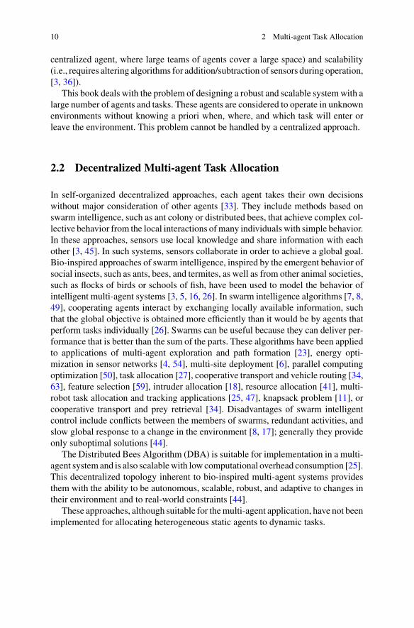
In self-organized decentralized approaches, each agent takes their own decisionswithout major consideration of other agents [33]. They include methods based onswarm intelligence, such as ant colony or distributed bees, that achieve complex col-lective behavior from the local interactions ofmany individuals with simple behavior.In these approaches, sensors use local knowledge and share information with eachother [3, 45]. In such systems, sensors collaborate in order to achieve a global goal.Bio-inspired approaches of swarm intelligence, inspired by the emergent behavior ofsocial insects, such as ants, bees, and termites, as well as from other animal societies,such as flocks of birds or schools of fish, have been used to model the behavior ofintelligent multi-agent systems [3, 5, 16, 26]. In swarm intelligence algorithms [7, 8,49], cooperating agents interact by exchanging locally available information, suchthat the global objective is obtained more efficiently than it would be by agents thatperform tasks individually [26]. Swarms can be useful because they can deliver per-formance that is better than the sum of the parts. These algorithms have been appliedto applications of multi-agent exploration and path formation [23], energy opti-mization in sensor networks [4, 54], multi-site deployment [6], parallel computingoptimization [50], task allocation [27], cooperative transport and vehicle routing [34,63], feature selection [59], intruder allocation [18], resource allocation [41], multi-robot task allocation and tracking applications [25, 47], knapsack problem [11], orcooperative transport and prey retrieval [34]. Disadvantages of swarm intelligentcontrol include conflicts between the members of swarms, redundant activities, andslow global response to a change in the environment [8, 17]; generally they provideonly suboptimal solutions [44].
The Distributed Bees Algorithm (DBA) is suitable for implementation in a multi-agent system and is also scalablewith low computational overhead consumption [25].This decentralized topology inherent to bio-inspired multi-agent systems providesthem with the ability to be autonomous, scalable, robust, and adaptive to changes intheir environment and to real-world constraints [44].
These approaches, although suitable for themulti-agent application, have not beenimplemented for allocating heterogeneous static agents to dynamic tasks.

2.3 Hybrid Multi-agent Task Allocation 11
2.3 Hybrid Multi-agent Task Allocation
Hybrid approaches use decentralized agents to control and exploit points of cen-tralization in the form of auctions to produce allocations [24, 29]. They includeintentional methods such as market-based algorithms and contract net protocols.In such systems, self-interested agents participate in a virtual market economy andallocate tasks by bidding procedures.
2.4 Summary
Various domains and applications of the multi-agent task allocation problem arediscussed in the literature. These include agents as robots [21, 22, 39, 40, 58],wirelesssensors [46, 62], computers or processors [2, 13, 32, 37], or human agents [28, 42].For each domain, there is a different objective function, a different set of variables,and a different set of constraints. The task allocation problem can be distributedand dynamic, i.e., new tasks are added to the system over time ([13, 14, 28, 42, 56,43]). Task allocation problems with a linear objective function and linear constraintscan be reduced to an instance of the optimal assignment problem [30]. This is awell-known operations research problem, which can be solved in polynomial time[19]. However, other problem domains, like the problem solved in this book, arenonlinear and complex and have been proven to be NP-hard [21, 35, 52]. Thesetypes of problems require incomplete optimization methods like meta heuristics.
Table 2.1 summarizes the advantages and disadvantages of centralized, decentral-ized and hybrid approaches.
Although previous approaches did not address reallocation for incomplete tasksthe approach described in this book considers reallocation of tasks, even if theywere already assigned to agents in previous rounds. This reallocation increases theproblem’s complexity.
Table 2.1 Summary of task allocation approaches and their features
Feature/approach Centralized Decentralized Hybrid
Handle unknown and dynamic situations No Yes Partially
Communication and computation resources demand Many Few Many
Scalability No Yes Yes
Robustness No Yes Yes
Flexibility No Yes Yes
Agents team size Small Large Medium
Need for a priori global information Yes No No

12 2 Multi-agent Task Allocation
References
1. AgmonN, Kaminka GA, Kraus S, TraubM (2010) Task reallocation in multi-robot formations.J Phys Agents 4(2):1–10
2. Attiya G, Hamam Y (2006) Task allocation for maximizing reliability of distributed systems:a simulated annealing approach. J Parallel Distrib Comput 66(10):1259–1266
3. Ball MG, Qela B, Wesolkowski S (2016) A review of the use of computational intelligence inthe design of military surveillance networks. In: Recent advances in computational intelligencein defense and security. Springer International Publishing, pp 663–693
4. Barbagallo D, Di Nitto E, Dubois DJ, Mirandola R (2010) A bio-inspired algorithm forenergy optimization in a self-organizing data center. In: Self-organizing architectures. SpringerBerlin/Heidelberg, pp 127–151
5. Bayındır L (2016) A review of swarm robotics tasks. Neurocomputing 172:292–3216. Berman S, Halász A, Kumar V, Pratt S (2007) Bio-inspired group behaviors for the deployment
of a swarm of robots to multiple destinations. In: IEEE international conference on roboticsand automation, pp 2318–2323
7. BlumC,GroßR (2015) Swarm intelligence in optimization and robotics. In: Springer handbookof computational intelligence, pp 1291–1309
8. Bonabeau E, Dorigo M, Theraulaz G (1999) Swarm intelligence: from natural to artificialsystems. Oxford University Press Inc., New York, NY, USA
9. Brumitt B, Stentz A (1998) GRAMMPS: a generalized mission planner for multiple mobilerobots. In: Proceedings of the IEEE international conference robotics and automation, Leuven,Belgium, vol 2, pp 1564–1571
10. Caloud P, Choi W, Latombe J, Le Pape C, YimM (1990) Indoor automation with many mobilerobots. In: Proceedings of the IEEE international workshop on intelligent robotics and systems(IROS), Ibaraki, Japan, vol 1, pp 67–72
11. Cao J, Yin B, Lu X, Kang Y, Chen X (2017) A modified artificial bee colony approach for the0-1 knapsack problem. Appl Intell 1–14
12. Chen XW, Nof SY (2012) Conflict and error prevention and detection in complex networks.Automatica 48(5):770–778
13. Chu WW, Holloway LJ, Lan MT, Efe K (1980) Task allocation in distributed data processing.Computer 13(11):57–69
14. De Weerdt M, Zhang Y, Klos T (2007) Distributed task allocation in social networks. In:Proceedings of the 6th international joint conference on autonomous agents and multiagentsystems, p 76
15. Dias MB, Zlot R, Kalra N, Stentz A (2006) Market-based multirobot coordination: a surveyand analysis. Proc IEEE 94(7):1257–1270
16. Duan H, Li P (2014) Bio-inspired computation in unmanned aerial vehicles. SpringerBerlin/Heidelberg, Berlin, Germany
17. Eberhart RC, Shi Y, Kennedy J (2001) Swarm intelligence. Elsevier18. Fu B, Liang Y, Chen C (2015) Bio-inspired group modeling and analysis for intruder detection
in mobile sensor/robotic networks. IEEE Trans Cybern 45:103–11519. Gale D (1960) The theory of linear economic models. McGraw-Hill20. GerkeyBP,MataricMJ (2004)A formal analysis and taxonomyof task allocation inmulti-robot
systems. Int J Robot Res 23(9):939–95421. Gerkey BP, Mataric MJ (2003) Multi-robot task allocation: analyzing the complexity and
optimality of key architectures. In: IEEE international conference on robotics and automation,pp 3862–3868
22. Giordani S, Lujak M, Martinelli F (2010) A distributed algorithm for the multirobot task allo-cation problem. In: International conference on industrial, engineering and other applicationsof applied intelligent systems, pp 721–730
23. GroβR, Nouyan S, BonaniM,Mondada F, DorigoM (2008) Division of labor in self-organizedgroups. In: Proceedings of the 10th international conference on simulation of adaptive behavior:from animals to animats. Springer-Verlag, Berlin, pp 426–436

References 13
24. Hussein A,Marín-Plaza P, García F, Armingol JM (2018) Hybrid optimization-based approachfor multiple intelligent vehicles requests allocation. J Adv Transp
25. Jevtic A, Gutiérrez A, Andina D, Jamshidi M (2012) Distributed bees algorithm for taskallocation in swarm of robots. IEEE Syst J 6(2):296–304
26. Jevtic A (2011) Swarm intelligence: novel tools for optimization, feature extraction, and multi-agent system modeling. PhD thesis
27. Jevtic A, Andina D, Jamshidi M (2014) Distributed task allocation in swarms of robots. In:Robotics: concepts, methodologies, tools, and applications. Information Science Reference,Hershey, PA, pp 450–473. https://doi.org/10.4018/978-1-4666-4607-0.ch023
28. Jones EG, DiasMB, Stentz A (2007) Learning-enhancedmarket-based task allocation for over-subscribed domains. In: Proceedings of the IEEE/RSJ international conference on intelligentrobots and systems, San Diego, CA
29. Kalra N, Stentz A, Ferguson D (2005) Hoplites: a market framework for complex tight coor-dination in multi-agent teams. In: Proceedings of the international conference on robotics andautomation (ICRA), New Orleans, USA, pp 1170–1177
30. Kao YH, Krishnamachari B, Ra MR, Bai F (2017) Hermes: latency optimal task assignmentfor resource-constrained mobile computing. IEEE Trans Mob Comput 16(11):3056–3069
31. Kapoor KN, Majumdar S, Nandy B (2015) Techniques for allocation of sensors in sharedwireless sensor networks. J Netw 10(01):15–28
32. Kartik S, Murthy CSR (1997) Task allocation algorithms for maximizing reliability ofdistributed computing systems. IEEE Trans Comput 46(6):719–724
33. Khamis A, Hussein A, Elmogy A (2015) Multi-robot task allocation: a review of the state-of-the-art. In: Cooperative robots and sensor networks. Springer International Publishing, pp31–51
34. Labella TH, Dorigo M, Deneubourg JL (2006) Division of labor in a group of robots inspiredby ants’ foraging behavior. ACM Trans Auton Adapt Syst (TAAS) 1(1):4–25
35. Lau HC, Zhang L (2003) Task allocation via multi-agent coalition formation: taxonomy, algo-rithms and complexity. In: Proceedings of the 15th IEEE international conference on tools withartificial intelligence, Sacramento, CA, USA, pp 346–350
36. Liu L, Michael N, Shell DA (2015) Communication constrained task allocation with optimizedlocal task swaps. Auton Robots 39(3):429–444
37. Ma PR, Lee EY, TsuchiyaM (1982) A task allocationmodel for distributed computing systems.IEEE Trans Comput 31(1):41–47
38. Macarthur KS, Stranders R, Ramchurn SD, Jennings NR (2011) A distributed anytime algo-rithm for dynamic task allocation inmulti-agent systems. In: Proceedings of the 25th conferenceon artificial intelligence, pp 701–706
39. Mataric MJ, Sukhatme GS, Østergård EH (2003) Multi-robot task allocation in uncertainenvironments. Auton Robots 14(2):255–263
40. Nanjanath M, Gini M (2010) Repeated auctions for robust task execution by a robot team.Robot Auton Syst 58(7):900–909
41. Quijano N, Passino KM (2010) Honey bee social foraging algorithms for resource allocation:theory and application. Eng Appl Artif Intell 23(6):845–861
42. Ramchurn SD, Polukarov M, Farinelli A, Truong C, Jennings NR (2010a) Coalition formationwith spatial and temporal constraints. In: Proceedings of the 9th international conference onautonomous agents and multiagent systems (AAMAS-10), Toronto, Canada, pp 1181–1188
43. Ramchurn SD, Farinelli A, Macarthur KS, Jennings, NR (2010b). Decentralized coordinationin robocup rescue. Comput J 53(9):1447–1461
44. Robin C, Lacroix S (2015) Multi-robot target detection and tracking: taxonomy and survey.Auton Robots 1–32
45. Rowaihy H, Eswaran S, JohnsonM, Verma D, Bar-Noy A, Brown T, Porta TL (2007) A surveyof sensor selection schemes in wireless sensor networks. In: Proceedings of SPIE, vol 6562
46. Sankary N, Ostfeld A (2018) Multiobjective optimization of inline mobile and fixed wire-less sensor networks under conditions of demand uncertainty. J Water Resour Plan Manag144(8):04018043

14 2 Multi-agent Task Allocation
47. Senanayake M, Senthooran I, Barca JC, Chung H, Kamruzzaman J, Murshed M (2016) Searchand tracking algorithms for swarms of robots: a survey. Robot Auton Syst 75:422–434
48. Shehory O, Kraus S (1998) Methods for task allocation via agent coalition formation. ArtifIntell 101(1):165–200
49. Sun Z, Liu Y, Tao L (2018) Attack localization task allocation in wireless sensor networksbased on multi-objective binary particle swarm optimization. J Netw Comput Appl 112:29–40
50. Tan Y, Ding K (2016) Survey of GPU-based implementation of swarm intelligence algorithms.IEEE Trans Cybern 46:2028–2041
51. TangY (2016) Coordination ofmulti-agent systems under switching topologies via disturbanceobserver-based approach. Int J Syst Sci 1–8
52. Tindell KW, Burns A,Wellings AJ (1992) Allocating hard real-time tasks: an NP-hard problemmade easy. Real-Time Syst 4(2):145–165
53. Turner J (2018) Distributed task allocation optimisation techniques. In: Proceedings of the 17thinternational conference on autonomous agents and multiagent systems, pp 1786–1787
54. Upadhyay D, Banerjee P (2016) An energy efficient proposed framework for time synchro-nization problem of wireless sensor network. In: Information systems design and intelligentapplications. Springer India, pp 377–385
55. Vachtsevanos G, Tang L, Reinmann J (2004) An intelligent approach to coordinated controlof multiple unmanned aerial vehicles. In: American helicopter society 60th annual forum,Baltimore
56. Walsh WE, Wellman MP (1998) A market protocol for decentralized task allocation. In:Proceedings of the international conference on multi-agent systems, pp 325–332
57. Wang J, Wang Y, Zhang D, Wang F, Xiong H, Chen C, Qiu Z (2018) Multi-task allocationin mobile crowd sensing with individual task quality assurance. IEEE Trans Mob Comput17(9):2101–2113
58. Wichmann A, Korkmaz T, Tosun AS (2018) Robot control strategies for task allocation withconnectivity constraints in wireless sensor and robot networks. IEEE Trans Mob Comput17(6):1429–1441
59. Xue B, Zhang M, Browne W (2013) Particle swarm optimization for feature selection inclassification: a multiobjective approach. IEEE Trans Cybern 43:1656–1671
60. Yan WQ (2016) Introduction to intelligent surveillance. Springer61. Yuan Q, Guan Y, Hong B, Meng X (2013) Multi-robot task allocation using CNP combines
with neural network. Neural Comput Appl 23(7–8):1909–191462. Zhan F, Wan X, Cheng Y, Ran B (2018) Methods for multi-type sensor allocations along a
freeway corridor. IEEE Intell Transp Syst Mag 10(2):134–14963. Zhang SZ, Lee CKM (2015) An improved artificial bee colony algorithm for the capacitated
vehicle routing problem. In: Proceedings of the IEEE international conference on systems,man, and cybernetics (SMC), Kowloon, China, pp 2124–2128

Chapter 3Multi-sensor Task Allocation Systems
The task allocation of a distributed heterogeneous multi-sensor system in dynamicand decentralized environments that have multiple tasks, with unknown a prioripriorities that arrive at unknown locations at unknown times is a major challenge.
Inmost cases of distributed, dynamic, and decentralized environments it is reason-able to assume that each entity has only local or limited information and its own goals,whichmay or may not conflict with other entities’ goals. In order to accomplish over-all goals with such limited information and possibly conflicting local entity goals, itis inevitable that an effective control mechanism must be provided to coordinate andallocate tasks by exchanging information and decisions among participants.
This book focuses on robust scalable methods for sensor allocation with the abil-ity to accommodate addition/subtraction of sensors during operation and handlingproblems existing in allocation methods, due to their inherent limitations, for taskallocation with distributed heterogeneous sensors. In order to overcome such limita-tions, protocols need to be able to repeatedly identify the current state of the systemand take proper actions to deal with allocation problems. Such protocols, whichassume the responsibility of making decisions actively and triggering timely actionsso that the overall system performance can be further improved, are defined as TaskAdministration Protocols (TAPs). The allocation problems handled with TAPs are:
1. Tasks that may have much higher priority over other tasks. This will occupy thesensors without the ability to perform other tasks that are close to their deadlineand must be handled quickly before less urgent tasks.
2. Many tasks have the same priorities. The system may need to reprioritize themto avoid conflicts in sensor allocation.
3. Tasks with a low priority that require long execution times. These tasks mayoccupy the sensors.
4. Failure of a portion of sensors in the system thatmay affect the allocation process.
© Springer Nature Switzerland AG 2020I. Tkach and Y. Edan, Distributed Heterogeneous Multi Sensor Task Allocation Systems,Automation, Collaboration, & E-Services 7,https://doi.org/10.1007/978-3-030-34735-2_3
15

16 3 Multi-sensor Task Allocation Systems
3.1 Framework
A framework to enable efficient allocation of heterogeneous sensors tomultiple tasksarriving at unknown different times and locations and to handle problems within thesensory system is described in this chapter. A dual-layer multi-sensor system wasdeveloped including: (1) a process layer—PL (in this research, multiple sensors andallocation algorithm HDBA for allocating them to efficiently complete tasks); (2) amonitoring layer—ML (in this research, task administration protocols for handlingproblems in the sensory system in the process layer). “TRAP”manages task prioritiesto allow better allocation of sensors to the most important tasks and to detect taskswhen they occur. “ASAP” ensures that tasks will be treated as soon as possible andwill not be unnecessarily delayed. “SRAP” allocates the best match of sensors totreat tasks and “STOP” was designed to ensure optimal availability of sensors in thesystem by time-out policy.
The book consists of three interrelated and independent parts that address multi-sensor task allocation:
1. Single-layer multi-sensor task allocation system—described in Chap. 5.2. Dual-layer multi-sensor task allocation system—described in Chap. 7.3. Fault tolerant multi sensor system with high availability—described in Chap. 9.
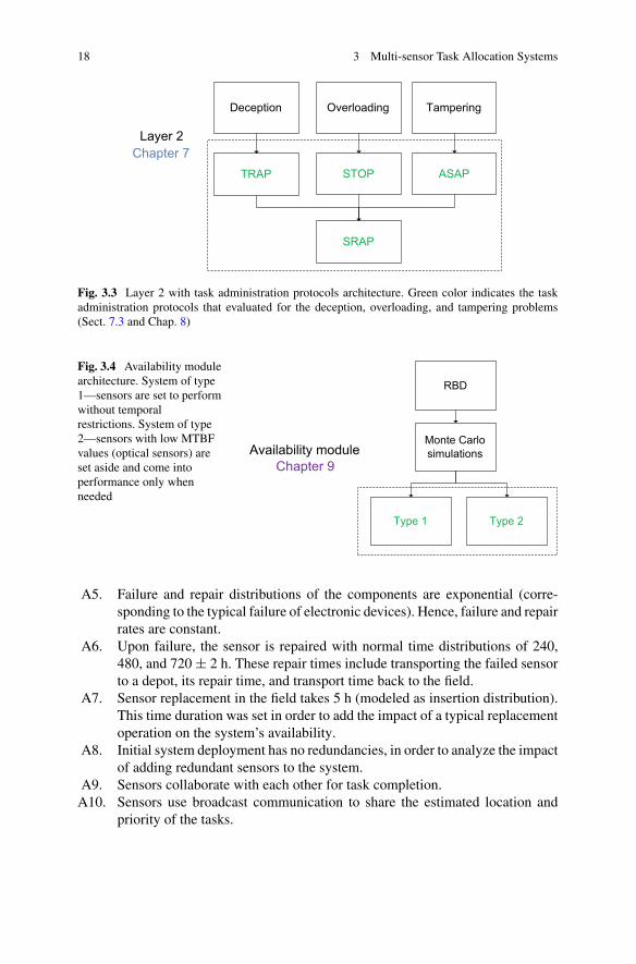
These interrelated parts are divided into specific modules necessary for efficient,scalable and robust task allocation. Figures 3.1, 3.2, 3.3 and 3.4 illustrate the overallarchitecture, the modules and the relevant book chapters where they defined.
Figure 3.2 illustrates comparison of state-of-the-art algorithms for several casestudies.
Figure 3.3 illustrates a dual-layer system with TAPs, which can handle overload-ing, deception, and tampering.
Figure 3.4 illustrates the availability optimization of the sensor’s operation toapply fault tolerance to the sensor network operation to make it robust enough to lossof sensors and/or the addition of new sensors.
3.2 Assumptions
The following assumptions were considered in the presented framework:
A1. Tasks are assigned to sensors, but their occurrence is unknown a priori.A2. All of the tasks that are within a sensor’s range can be allocated to that sensor.A3. Decision-making about the allocation for each sensor takes place as soon as
a new task is introduced.A4. Sensors can be reallocated to another task during execution. An abandoned
task keeps its remaining execution time, until a new sensor is allocated to it.

3.2 Assumptions 17
Tasks Sensors
Allocation algorithms
Allocation
Deception TamperingOverloading
Availability
Task administration
protocols
Layer 1Chapter 5
Layer 2Chapter 7
Availability moduleChapter 9
DL-TDS
Fig. 3.1 System architecture for multi-sensor task allocation. The system consists of two layersand one availability module. The color corresponds to the book chapters
Tasks Sensors
Security of SN
Layer 1Chapter 5 HDBA
DBAMarket based BSGreedy
ACO FMC_TAH+GASA
TSP LEPHChapter 6
Fig. 3.2 Layer 1 with allocation algorithms architecture. The dashed boxes contain 9 allocationalgorithms evaluated and compared for allocation (Sect. 5.3) and 3 evaluation scenarios for whichthe allocation algorithms were evaluated (Sects. 6.1, 6.2 and 6.3)
18 3 Multi-sensor Task Allocation Systems
Deception TamperingOverloading
TRAP ASAPSTOP
SRAP
Layer 2Chapter 7
Fig. 3.3 Layer 2 with task administration protocols architecture. Green color indicates the taskadministration protocols that evaluated for the deception, overloading, and tampering problems(Sect. 7.3 and Chap. 8)
Fig. 3.4 Availability modulearchitecture. System of type1—sensors are set to performwithout temporalrestrictions. System of type2—sensors with low MTBFvalues (optical sensors) areset aside and come intoperformance only whenneeded
Availability moduleChapter 9
Monte Carlo simulations
Type 1
RBD
Type 2
A5. Failure and repair distributions of the components are exponential (corre-sponding to the typical failure of electronic devices). Hence, failure and repairrates are constant.
A6. Upon failure, the sensor is repaired with normal time distributions of 240,480, and 720 ± 2 h. These repair times include transporting the failed sensorto a depot, its repair time, and transport time back to the field.
A7. Sensor replacement in the field takes 5 h (modeled as insertion distribution).This time duration was set in order to add the impact of a typical replacementoperation on the system’s availability.
A8. Initial system deployment has no redundancies, in order to analyze the impactof adding redundant sensors to the system.
A9. Sensors collaborate with each other for task completion.A10. Sensors use broadcast communication to share the estimated location and
priority of the tasks.

Chapter 4Evaluation Methodology
This chapter presents the analysis methods and the performance measures appliedin this book. The described methods are evaluated by the use of extended examplesin Chaps. 6 and 8. The evaluations include task attendance analyses that are con-ducted for both a single-layer and a dual-layer system to examine the effect and theperformance of the described framework and algorithms.
4.1 Analyses
The aim of the analyses is to reveal the ability of the described methods to copewith the problems presented in Chap. 1 and specifically to: (a) analyze effectiveallocation and scalability in terms of number of tasks and sensors to be able to easilyadd or remove sensors to cope with an increasing number of tasks; (b) examine theperformance of a dual-layer system, and its effect on optimizing task allocation incases of sensor failure, conflicts in tasks priorities, and high time consuming tasks;and (c) optimize fault tolerance of the dual-layer task allocation system by MonteCarlo simulations.
The following analysis methods are applied in this book:
1. Algorithms for sensor allocation in a single-layer system—comparison of thestate-of-the-art algorithms in terms of tasks completion times and the number ofunallocated tasks.
2. Dual-layer system performance—comparison of the performance of a dual-layersystem with task administration protocols (TAPs) and HDBA to a single-layersystem with HDBA.
3. Availability optimization of the sensors’ operation and comparison of the dual-layer system performance with optimized sensors’ availability to a regular dual-layer system.
The system performance is evaluated by:
© Springer Nature Switzerland AG 2020I. Tkach and Y. Edan, Distributed Heterogeneous Multi Sensor Task Allocation Systems,Automation, Collaboration, & E-Services 7,https://doi.org/10.1007/978-3-030-34735-2_4
19

20 4 Evaluation Methodology
1. Comparing to results of state-of-the-art algorithms and protocols using multi-agent simulation for the case studies of:
(a) Security of supply networks.(b) A benchmark for result validation based on traveling sales man problem
(TSP).(c) A Law Enforcement Problem (LEP).
2. Availability analysis (fault tolerance) of the multi sensor system using MonteCarlo simulation.
The numerical computations were implemented on a personal computer with2.90 GHz CPU, and 12 GB of RAM, usingMatlab R2015a, and JAVA SE8 programsto: (i) examine the performance of the algorithms for task allocation in a single-layer system by applying HDBA, DBA, BS, market-based, and greedy algorithmsthrough multi-agent simulations; (ii) examine the scalability of HDBA in terms ofnumber of tasks and sensors to be able to easily add or remove sensors to copewith increasing number of tasks; (iii) determine the influence of the bias parame-ters on HDBAs’ performance adjusting the sensor swarm behavior; (iv) perform amulti-agent simulation analysis for result validation of HDBA based on a benchmarktraveling salesman problem (TSP) in comparison to DBA, BS, ACO, GA, and greedyalgorithms; (v) examine the performance of HDBA for police officers task alloca-tion in a Law Enforcement Problem (LEP) in comparison to FMC_TAH+ and SAalgorithms—all in Chap. 6; (vi) examine the performance of TAPs—TRAP, ASAP,SRAP, STOP in a dual-layer system, and their effect on optimizing task allocation incases of sensor failure, conflicts in tasks priorities, and high time-consuming tasks;in Chap. 8; (vii) optimize fault tolerance of the dual-layer task allocation system byMonte Carlo simulations—in Chap. 9; and (viii) examine the performance of singleand dual-layer systems through an analytical analysis—in Chap. 10.
4.2 Performance Measures
The following performancemeasures were analyzed, harnessing different algorithmsand evaluations:
1. For the process layer, 100 independent runs of HDBA, DBA, BS, market-based, and greedy algorithms with 100 agents, were compared at the statisti-cal confidence level of 95% for task allocation using the following performancemeasures:
PM1. System performance.PM2. Tasks completion time.PM3. Number of unallocated tasks.PM4. Number of tasks allocated to sensors.
and, three sensor distributions:

4.2 Performance Measures 21
1. Deterministic deployment—grid distribution.2. Random deployment—uniform distribution.3. Random and biased deployment—normal distribution.
2. In the TSP scenario evaluation, HDBA, DBA, BS, ACO, GA, SA, and greedyalgorithms were compared for the performance measure of total distance inBerlin52 and A280 instances.
3. In the LEP scenario evaluation, 100 independent runs of HDBA, FMC_TAH+,and SA algorithms were compared at the statistical confidence level of 95% fortwo case studies:
CS1. Standard LEP with 25 agents to enable comparison with LEP benchmark.CS2. Extended LEP with 100 agents to evaluate swarm and to conduct a fair
comparison with task allocation benchmark.
The following performance measures were used:PM1. Team utility.PM2. Average execution delay.PM3. Percentage of abandoned tasks.PM4. Percentage of shared tasks.PM5. Average arrival time of agents to tasks.
4. For the monitoring layer, 100 independent runs of a dual-layer system usingTAPs—TRAP, ASAP, SRAP, STOPwas compared to a single-layer system usingHDBA at the statistical confidence level of 95% for task allocation using thefollowing performance measures:
PM1. Number of treated tasks by each sensor for a different number of falsetasks.
PM2. Number of treated tasks by each sensor for a different number of hightime-consuming tasks.
PM3. Number of treated tasks by each sensor for a different number of failedsensors.
PM4. Number of unallocated tasks for a different number of false tasks.PM5. Number of unallocated tasks for a different number of high time-
consuming tasks.PM6. Number of unallocated tasks for a different number of failed sensors.PM7. Number of important tasks treated for a different number of false tasks.PM8. Number of important tasks treated for a different number of high time-
consuming tasks.PM9. Number of important tasks treated for a different number of failed sensors.
5. For the fault tolerance analysis, 100 independent runs of a dual-layer systemwere analyzed at the statistical confidence level of 95% using the followingperformance measures:
PM1. Percentage of availability for a type 1 system—sensors are set to performwithout temporal restrictions.

22 4 Evaluation Methodology
PM2. Percentage of availability for a type 2 system—sensors with low MTBFvalues (optical sensors) are set aside and come into performance onlywhen needed.
PM3. Number of processed tasks for a type 1 system.PM4. Number of processed tasks for a type 2 system.PM5. Influence of the number of redundant optical sensors on type 1 systems’
availability with different repair times of 240, 480, and 720 h.

Chapter 5Single-Layer Multi-sensor TaskAllocation System
This chapter defines the multi–sensor task allocation in a single-layer system. Theallocation problem is described and algorithms for multi-agent and multi-sensor taskallocation are presented. Figure 5.1 illustrates the Layer 1 architecture of the system.
Tasks Sensors
Allocation algorithms
Detection
Deception TamperingOverloading
Availability
Task administration
protocols
Layer 1Chapter 5
Layer 2Chapter 7
Availability moduleChapter 9
DL-TDS
Fig. 5.1 Layer 1 in system architecture
© Springer Nature Switzerland AG 2020I. Tkach and Y. Edan, Distributed Heterogeneous Multi Sensor Task Allocation Systems,Automation, Collaboration, & E-Services 7,https://doi.org/10.1007/978-3-030-34735-2_5
23

24 5 Single-Layer Multi-sensor Task Allocation System
5.1 Definitions
The problem deals with real-time allocation of unpredictable, unknown tasks arrivingat unknown times and locations. The task occurrence is dynamic and unpredictablewith different levels of importance of each task and must be detected as fast aspossible. Examples of such tasks include surveillance (gathering information ondesired objects, [2, 72]), security monitoring (preventing theft of goods and threats,[50], fire monitoring (forest fire allocation and protection, [35, 84]), among manyothers. The sensors must be allocated to the tasks as fast as possible. The goal is toallocate to each sensor an appropriate task at an appropriate time (Fig. 5.2) and toensure all tasks are completed in minimum time.
The system includes multiple sensors that are capable of performing each taskwith different performances (Fig. 5.3). Sensory performance is defined a priori basedon the sensor’s features, namely allocation distance, resolution, and response time.Each sensor can only be allocated to one task at any given time and can be reallocatedto another task at any moment. The priority of a task is an application-specific scalarvalue, where a higher priority value represents a task that has higher importance and
S1
S2
Sm
S2
S1
Sp
S2
Sn
S1
Allocation
T1
T2
Tk
Tasks
Sensors
Fig. 5.2 Distributed multi-sensor system allocation scheme

5.1 Definitions 25
Sensors DB
Opera ng Sta on
Human Operator
Sensor
Task
Task
Task
Fig. 5.3 A monitoring sensor network with sensors, tasks, and sensors DB that informs operatorsabout the completed tasks, but does not contribute to the task allocation algorithm (after Tkachet al. [77])
must be attended to faster than other tasks. Higher priority tasks also have a higherbenefit for completing them.
In this book, there is no limitation in the number of sensors that can be allocatedto a single task. This eliminates the conflict of demanding the same task by multiplesensors. Once a sensor finds a task, it informs the neighboring sensors about thefound task and its parameters, using broadcast communication (as in [23, 34, 38,80]). This message is then forwarded by these sensors over the entire network, asin Ducatelle et al. [23]. From that moment, the sensors are aware of the detectedtask. Even though the sensors use broadcast communication to share the estimatedlocation and priority of the tasks, task allocation is performed in a decentralizedmanner. Each sensor makes an autonomous decision that is based on the informationthat it has received [77].
When there are several tasks that require the same sensors, the allocation dependson the sensors’ availability and performance, the physical distance of sensors fromthe tasks, and the priorities of individual tasks. The following assumptions wereconsidered in the proposed scenario, similar to research performed in Jevtic et al.[39]:
A1. Tasks are assigned to sensors, but their occurrence is unknown a priori.A2. All of the tasks that are within a sensor’s range can be allocated to that sensor.

26 5 Single-Layer Multi-sensor Task Allocation System
A3. Decision-making about the allocation for each sensor takes place as soon as anew task is introduced.
A4. Sensors can be reallocated to another task during execution. An abandonedtask keeps its remaining execution time, until a new sensor is allocated to it.
A5. Sensors collaborate with each other for task completion.A6. Sensors use broadcast communication to share the estimated location and
priority of the tasks.
Following Tang and Ozguner [72], the system is defined with the followingcharacteristics:
1. Sensors are stationary; and2. Tasks remain stationary after their occurrence.
Based on the taxonomy proposed by Robin and Lacroix [67], the problem ofallocating sensors to tasks corresponds to a localization and observation problem.Thetask localization involves several sensors and it is most often a multi-sensor problemto improve knowledge about the task involving selection of different viewpoints tomaximize the information gain. The observation problem involves several sensorsand several tasks in order to maximize the number of observed tasks and to minimizethe time during which any task is not observed by at least one of the sensors.
A system objective function is developed to compute the expected value of sys-tem performance given parameters of the sensors and tasks. System performance isdefined as the collective performance of sensors, task priorities values, and distancesof sensors from tasks. Consider a population of N sensors to be allocated amongM tasks. We denote the collective performance of the system by VI , a nonnegativeinteger, calculated as:
VI = max{S + φH}, 0 < φ < 1 (5.1)
S =M∑
i=1
N∑
k=1
Vik · 1
Dik(5.2)
H =M∑
j=1
Fj , j ∈ completed tasks (5.3)
Vik = 0 if k − th sensor is not assigned to task i (5.4)
where S is the collective performance of the sensors, Vik is the k-th sensor’s perfor-mance on the i-th task, and N is the number of sensors in the system.H is the sum ofthe priorities of tasks in the system that were successfully completed, and ϕ is a biasparameter for the importance of H relative to S. Fj is the priority of j-th task and Mis the total number of tasks. These values are pre-defined based on Neapolitan andNaimipour [57].

5.1 Definitions 27
It is assumed that each sensor has a different performance based on the treatedtask. This value represents the heterogeneity of agents, by assigning each agent adifferent performance value based on its skills.
In example, for tasks occurring at night time, a night vision sensor will performbetter than a regular CCD camera, but in daylight the CCD camera will have betterperformance. In a law enforcement problem, a traffic policeman will treat a trafficviolation better than amurder detective, but will be incompetent to deal with amurdercase.
Sensors are distributed in the arena with a particular distribution strategy and canbe allocated to tasks within their allocation range. The sensors are stationary. One ofthe parameters that affects system performance is the distance of the sensors fromtasks. The performance degrades as the distance increases, due to the degradationof sensors’ recognition capabilities. The Euclidean distance between the sensor andthe task in a two-dimensional arena is given by:
Dik =√
(xi − xk)2 + (yi − yk)
2 (5.5)
where (xi, yi) and (xk, yk) represent task and sensor coordinates in the arena,respectively.
Let F ε {F1, …, FM} denote the set of normalized priorities of the available tasksin the queue. Normalized priorities are calculated as fractions of the sum of prioritiesof all available tasks:
Fi = fi∑Mj=1 f j
(5.6)
where f i is a priority of task i.In real-world scenarios, the priority is an estimated value that results from sen-
sor readings or previously acquired knowledge. In a law enforcement problem, forexample, the type of the task determines its priority. A noise complaint will havea lower priority than a robbery. A murder will have a higher priority than a robbery.In a supply network security problem, an unlocked door will have lower prioritythan missing cargo, but missing cargo will have lower priority than a fire in a centrallogistics center.
Each task has a time limit, or a deadline:
�i = 1
Fi> 0, Fi > 0 (5.7)
The deadline is a function of the priority, where �i decreases with time until itreaches a value of 0, which indicates that the task i is not relevant anymore.
Once a sensor is allocated to a task, it monitors this particular task (with a per-formance Vik). A task is considered to be detected once sensors are allocated toit.

28 5 Single-Layer Multi-sensor Task Allocation System
Each task is assumed to have an initial completion time value tinit . Collaborationis achieved by sharing a task with multiple sensors. The task execution time valueis modeled as a function of the initial completion time that is required for the taskand the performances of coordinating sensors that are allocated to it. This dynamicvalue is continuously updated Eq. (5.8). The higher the cumulative performance ofthe coordinating sensors, the lower the execution time needed for the shared task.
texi ={tini t
1∑Mk=1 Vik
− tpi if∑M
k=1 Vik > 0,�i > 0
tini t if∑M
k=1 Vik = 0,�i > 0(5.8)
where texi is the remaining execution time of task i and tpi is the elapsed time of taski execution. When texi reaches 0 value, the task is completed, and it is removed fromthe arena by the broadcast communication.
When new tasks are announced, steps (1–8) are updated respectively. The overalltask completion time T is defined as a sum of the individual tasks completion timestci:
T =M∑
i=1
tci (5.9)
tci = ti f _completion − tiarrival , if �i > 0 (5.10)
The task completion time is derived by the amount of time elapsed from its arrivaltiarrival to the full completion tif_completion.
5.2 Algorithms for Multi-agent Task Allocation
5.2.1 Meta Heuristics
Meta heuristics usually have an iterative behavior and have emerged in recent yearsas successful alternatives to classical approaches in solving complex optimizationproblems in a reasonable time [8, 12, 71]. Meta heuristic algorithms include swarmintelligence, evolutionary computation, simulated annealing, tabu search, and hillclimbing among others [14, 58]. Evolutionary computation includes optimizationalgorithms that are inspired byDarwinian evolution. In these algorithms, a set of solu-tions is called a population. Each iteration is used to create a new generation from thecurrent population. This approach typically has two operators, called recombinationor crossover, which recombines two or more individuals and mutations, which mod-ifies a single individual [29]. Based on the objective function, individuals from thecurrent generation are selected for recombination and mutation, or to be repeated forthe next generation without any change, while individuals with higher fitness have

5.2 Algorithms for Multi-agent Task Allocation 29
a higher probability to be selected. Evolutionary computation algorithms includeevolutionary programming [26], evolutionary strategies [66], and genetic algorithms[36].
Tabu Search, introduced by Glover [32], uses search history in order to explorethe solution space. This algorithm applies the best improvement local search withmemory to avoid local optima. The memory is implemented as a tabu list that keepstrack of the most recently visited solutions and forbids moves toward them. At eachiteration, the best solution is chosen from the allowed set as the new current solution.
Hill climbing is a local search optimization algorithm [60, 63, 69]. It is an iterativealgorithm that attempts to find a better solution by making changes to the currentsolution. If the change produces a better solution it is selected to be further modifieduntil the best solution is obtained [69]. Hill climbing can often produce a better resultwhen the amount of time available to perform a search is limited. It is good for findinglocal optima, but it is not necessarily guaranteed to find the optimal solution.
Simulated annealing introduced in the area of combinatorial optimization byKirk-patrick et al. [47], is a state-of-the-art meta heuristic for approximating global opti-mization in a large domain [69] and one of the first having a strategy for escapinglocal optima. It simulates a physical annealing process in metallurgy, where parti-cles of a solid arrange themselves into a thermal equilibrium, a technique involvingheating and controlled cooling of a material to increase the size of its crystals andreduce their defects. Simulated annealing interprets slow cooling as low decrease inthe probability of accepting worse solutions as it explores the solution space. Accept-ing worse solutions is a fundamental property of metaheuristics because it allowsfor a more extensive search for the optimal solution (explores the solution space),reducing the chances of being converged to local optima.
Heuristic methods combine intelligently different concepts for exploring thesearch space in order to find near-optimal solutions [59] and to enable escapingfrom local optima. However, they do not always guarantee to find a globally optimalsolution [14].
5.2.2 Swarm Intelligence
Swarm-based systems are typically made of a population of simple agents (sys-tem entities that make decisions about their local environment) interacting locallywith one another and with their environment to achieve a common goal [40]. Theseapproaches simulate the behaviors of insects and animals to assign tasks to agents(Fig. 5.4). Swarm intelligence methods [21] are mainly used for agent systems inunknown environments and optimization for task allocation, clustering, navigation,and path formation [11, 68]. Since the group collaboration among individuals is dis-tributed, an individual fault does not affect the global solution [37, 46].ComputationalSwarm Intelligence represents the group of Computational Intelligence algorithmsthat model swarming behaviors in nature. Computational Intelligence belongs to thebroader field of Artificial Intelligence, and of the paradigms that relate to some kind

30 5 Single-Layer Multi-sensor Task Allocation System
Fig. 5.4 Swarm intelligence in nature. School of fish and swarms of bees and ants. Photos by KarenKayser, Topcools Tee and Mikhail Vasilyev on Unsplash
of biological or naturally occurring system [5]. Swarm intelligence methods havehigh robustness, scalability, and are suitable for distributed multi-agent systems [9].The benefits of collaboration can be significant in situations where global knowledgeof the environment does not exist. Agents within the group interact by exchanginglocally available information such that the global objective can be obtained moreefficiently than it would be done by a single agent. The group of agents acting insuch a manner can be referred to as a swarm. The problem-solving behavior thatemerges from the interactions of such agents is called Swarm Intelligence. Algorith-mic models of such behavior are referred to as Computational Swarm Intelligence[25].
Examples of collective behavior in nature are numerous. They are based on adirect or indirect exchange of information about the environment between the mem-bers of the swarm [24]. Although the rules governing the interactions at the locallevel are usually easy to describe, the result of such behavior is difficult to predict[53]. However, through collaboration, the swarms in nature are able to solve com-plex problems that are crucial for survival in a dynamically changing environment[15, 74].
There are many examples of swarming behavior in the literature as it hasalways intrigued scientists for its better understanding. Ants communicate by layingpheromone on their route in order to find the shortest path to a food source by usingforaging behavior [11, 21, 28]. Termites cooperate by stigmergy to build complexnest structures without having any global knowledge of the environment [28, 40].Bees use dancing to recruit othermembers in the swarm to follow them to the locationin the field that is rich with nectar [13]. Birds gather in flocks and fish form schoolsto have better chances of survival against predators [62]. Bacteria locally exchangeinformation about their environment, and so forth.
Pham et al. [61] developed the Bees Algorithm (BA), which in its basic versionperforms a random search combined with a neighborhood search and can be used foroptimization. The algorithm exploits the concept of the central dance floor in orderto select the fittest sites, but no direct communication between the swarm membersexists. The recruitment of the bees can be done in a deterministic way accordingto the fitness values associated with the sites, or these fitness values can be used todetermine the probability of the bees being selected. Together with scouting, thisdifferential recruitment is a key operation of the BA. The algorithm is performed

5.2 Algorithms for Multi-agent Task Allocation 31
in iterations, and it is stopped when the solution is found within the provided errormargin or when the maximal number of iterations is reached. Bailis et al. [7] pro-posed a model of the bee colony foraging to investigate the value of sharing foodsource position information in different environments. The authors show throughsimulations that in environments of highly-scattered food, relying solely on privateinformation about previously encountered food sources is more efficient than sharinginformation. However, in the nectar-rich environments, it leads to decreased foragingefficiency.
Karaboga and Akay [45] proposed a bee colony-based optimization algorithmcalled Artificial Bee Colony (ABC). The concept of the central dance floor is appliedthrough different roles that bees have in the swarm, namely scout, onlooker, andemployed bees. The algorithm uses recruitment based on the fitness values of thefood sources and applies neighborhood search for solution improvements. A scoutbee is randomly sent to search for a new food source when a previously found sourceis abandoned. Jevtic [40] proposed a distributed bees algorithm for task allocation ina swarm of robots. This algorithm assigns the robots in a swarm to the found tasksin such a way that the final distribution is proportional to the tasks’ qualities. Therobots were designed to use broadcast communication to inform other robots in therange about the estimated location and the quality of the found task.
Few other algorithms inspired by bees’ behavior appeared in literature, such asBeeHive [79], BCO [75], Virtual Bee Algorithm [82], HBMO [1], etc., and they havemostly been applied to solving combinatorial optimization problems.
This book will show how to extend the use of swarm intelligence algorithms to theproblem of allocating heterogeneous static agents to dynamic tasks with a dynamicreallocation of agents to ensure scalability and robustness.
5.2.3 Market-Based Approaches
Market-based approaches have gainedpopularity in recent years,mainly because theyoffer a good compromise between finding a good allocation and the communicationspeed [46]. Economic problems have involved humans throughout history to pursueindividual profit. This pursuit led to the formalism of the principles of the marketeconomy. These principles have inspired computational market-based approachesthat are applied to multi-agent allocation [41]. The first method of applying market-based principleswasContractNet Protocol orCNP [70]. It allocates tasks to resourcesthrough the negotiation of contracts. It establishes a virtual economy with agents asbuyers, tasks as products, and virtual money as currency.
Market-based approaches have been applied to resource allocation on computers[10, 48, 81], multi-agent [6, 42], and multi-robot coordination [18, 49, 55, 85].
In market-based systems, agents act to maximize their individual profit and simul-taneously improve the efficiency of the team. They are paid based on their bid fortasks they complete and must pay the value of the resources they consume. The bidsare managed by the auctioneer. The auctioneer can be a centralized supervisor agent
32 5 Single-Layer Multi-sensor Task Allocation System
or one of the agents. In each auction, agents compete by bidding to be allocated totasks and to maximize their profit. The new allocation achieved by bidding can resultin better solutions. One of the first distributed market-based algorithms wasM+ [17],proposed for the cooperation among multiple robots [16]. In this algorithm, robotsemploy a two-step principle to calculate the cost of a task considering the next onein order to increase the efficiency of the solution. In MURDOCH [31, 30] robots donot participate in auctions during task execution, and tasks are only allocated to idlerobots. It was reported to result in less efficient solutions thanM+ because it does notconsider future tasks and uses a purely greedy approach. However, the advantage ofMURDOCH is that it uses less communication. TraderBots [19] is a market-basedsystem designed to work in dynamic environments. This system applies schedulingto allocate multiple tasks to each robot and allows bidding on several tasks simulta-neously. It was reported to make efficient allocations despite partial failures of therobots and communications (Dias et al. [20]).
Ramchurn et al. [65] present a coalition formation with spatial and temporalconstraints problem (CFSTP). Agents form coalitions to jointly work on tasks withspatial constraints and deadlines. Agents have hard deadlines and are sharing tasksat non-additive rates to maximize the number of tasks completed. CFSTP was orig-inally solved using Coalition Formation with Look-Ahead (CFLA) [65] that appliestwo heuristics: allocating the smallest possible coalition and maximizing the numberof other tasks that can be completed before the deadline in the next time step. A dis-tributed Max-sum DCOP algorithm was used to solve CFLA [52, 64, 83]. Walsh andWellman [78] presented a mechanism to accomplish a similar goal via a distributedmarket protocol for allocating tasks to agents that contend for scarce resources.Agents trade tasks at prices determined by an auction protocol. In Jones et al. [42],a market-based mechanism was applied to a real-world firefighting problem. In thatwork, fire incidents defined as tasks were assigned to firefighting units according tothe order in which the fires were discovered; each fire had an auctioneer, and agentscomputed the change in utility for being allocated a task, using either an optimal ornear-optimal ordering, and submitted this change as a bid. The auctioneer greedilyand irrevocably allocated the task to the agent with the highest bid. Once a fire wasassigned to an agent, the agent was responsible for it until it was extinguished.
Several market-basedworks focused on task allocation problems that have restric-tions between tasks. Hoplites [43, 44] is a market-based system that applies bothpassive and active coordination. Tasks are completed faster with passive coordina-tion, resulting in less communication usage. Active coordination is used to enableagents to actively affect the bidding of other agents. Market-based algorithms forrobot routing in open spaces are presented in Mosteo et al. [54]. Guerrero and Oliver[33] presented market approaches to find an optimal number of robots needed tosolve specific tasks. Nanjanath and Gini [56] presented a variation of CNP for solv-ing task allocation problems. Their system allowed reallocation of tasks to cope withdynamic environments. Zlot and Stentz [85] addressed the market-based allocationof complex tasks with task decomposition and allocation phases considered togetherinstead of separated as usual.

5.2 Algorithms for Multi-agent Task Allocation 33
Market-based approaches capture the respective strengths of both distributed andcentralized approaches [46]. They can distribute much of the planning and executionover the team and thereby retain the benefits of distributed approaches, includingrobustness, flexibility, and speed. They also have elements of centralized systemsto produce better solutions: auctions concisely gather information about the teamand distribute resources in a team-aware context. However, if the communicationcosts are too high in the task allocation process, once there are failures in agent’scommunication, the performance will degrade noticeably [73], so these methods fitfor small and medium-scale task allocation.
The task allocation problem can be solved by various algorithms and meta heuris-tics. In this book, several of themwere implemented and compared, includingHDBAalgorithm, simulated annealing, ant colony optimization, bees system, Fisher-market,and genetic algorithm.
5.3 Specific Algorithms for Multi-sensor Task Allocation
This section describes nine algorithms suitable for multi-sensor task allocation:HDBA, DBA, Greedy algorithm, Market-based algorithm, Bee System (BS), FisherMarket Clearing for Task Allocation with Heterogeneous Agent (FMC_TAH+), AntColony Optimization (ACO), Genetic algorithm (GA), Simulated Annealing (SA).
5.3.1 Distributed Bees Algorithm
In this algorithm, each sensor is represented as a ‘bee’, and sensor utility, pik , isdefined as a probability that the sensor k is allocated to the task i and depends onboth priority and the distance of the task/task from the sensor:
pik =Fαi
(1Dik
)β
∑Mj=1 F
αj
(1Djk
)βif �i > 0 (5.11)
whereα andβ are control parameters that bias importance of the priority and distance,respectively (α, β > 0; α, β ε R). The probabilities pik are normalized, and it is easyto show that:
M∑
i=1
pik = 1 (5.12)
The DBA decision-making mechanism uses a wheel-selection rule, where eachsensor has a probability with which it is allocated to the task from a set of available

34 5 Single-Layer Multi-sensor Task Allocation System
Fig. 5.5 The waggle dance of a bee. The bee performs a waggle dance to indicate the direction,quality and distance of the food source. Photo by Damien Tupinier on Unsplash
tasks. Once all the sensors’ utilities are calculated, each of them selects a task by“spinning the wheel”.
The information is then exchanged by the sensors using broadcast communication,inspired by the waggle dance of bees in nature [27] which is used to share with otherbees the direction, quality and distance of the found source food (Fig. 5.5).
5.3.2 Heterogeneous Distributed Bees Algorithm
Researchers have proposed a distributed bees algorithm that is suitable for imple-mentation in a multi-agent system where cooperating agents interact by exchanginglocally available information, such that the global objective is obtained more effi-ciently than it would be done by agents that perform tasks individually. This swarmintelligence algorithm was enhanced to control a heterogeneous sensor networkallocation.
The DBA function of sensors’ utility (HDBA) was modified for the case of het-erogeneous sensors with different performances. This modification is assumed toimprove system performance as it can correlate the sensors’ utility function with thevalue of their performances.
In order to define HDBA for heterogeneous sensors, a new task’s utility value(Vik) is defined as a function of the sensor’s performance on that task. When a sensorreceives information about the available tasks it calculates its performance for thattask. The sensor’s utility function is updated accordingly, and depends on the task’spriority, the distance from the task, and the sensor’s performance on that task:

5.3 Specific Algorithms for Multi-sensor Task Allocation 35
pik =Fαi
(1Dik
)β
V γ
ik
∑Mj=1 F
αj
(1Djk
)β
V γ
jk
if �i > 0 (5.13)
where γ is a control parameter that biases the importance of the sensor’s performanceand Vik is the performance of sensor k on task i.
The HDBA decision-making mechanism applies the same wheel-selection ruleused in DBA to choose from a set of available tasks.
Tasks arriving at different times trigger a new decision-making iteration of thealgorithm.
Figures 5.6 and 5.7 illustrate the allocation process.
First task is received. Sensors are selected and allocated to the task.
Another task of higher priority is received.
Sensors are now reallocated to execute the two tasks. Some sensors that were allocated to the first task are now allocated to the new task with higher priority.
Fig. 5.6 Sensors to tasks allocation process. The sensors’ range coverage was set to equal valuesfor illustration purposes (after Tkach et al. [76])

36 5 Single-Layer Multi-sensor Task Allocation System
Fig. 5.7 Allocationprobabilities for each task(after Tkach et al. [76])
pi1pi2
In Fig. 5.7 two different tasks arrived at different times. The normalized priorityof task 1 is given by F1 and of task 2 by F2. The Euclidian distance of the sensorsfrom task 1 and task 2 is D1k and D2k , respectively. The performance of the sensorson task 1 and task 2 is V 1k and V 2k , respectively. The probabilities of the i’th sensorto be allocated to task 1 and task 2 are pi1 and pi2, respectively. Upon the arrival ofthe first task, HDBA is executed to calculate the probabilities of sensors allocation.Since there are no other tasks, sensors are allocated to the task that is within theirallocation range, and they cooperate to complete this task. Upon the arrival of thesecond task, another decision-making iteration of HDBA is triggered to calculate thenew probabilities of sensors allocation. Based on the calculated probabilities, HDBAconverges to a new allocation. In this allocation, additional sensors are allocated tothe second task and some sensors that were allocated to the first task are reallocatedto the second task, such that the overall task completion time is minimized. HDBAis executed until the termination condition is met.
A numerical example of HDBA’s allocation process for a simplified problem isdescribed in Chap. 10.
The DBA/HDBA, similar to other swarm intelligence algorithms, include a pop-ulation of simple agents interacting locally with one another and with their envi-ronment. Agents make an iterative construction of solutions to search the solutionspace considering previous solutions to optimize their search. This is a probabilis-tic multi-agent algorithm that uses a probability distribution to make the transitionbetween each iteration. The probabilistic nature of this algorithm allows it to avoidlocal optimum by choosing sometimes worse solutions using the wheel-selectionrule. Accepting worse solutions is a fundamental property of metaheuristics becauseit allows for a more extensive search for the global optimal solution.

5.3 Specific Algorithms for Multi-sensor Task Allocation 37
Pseudocode of the HDBA algorithm:
1. Initialize:Set t=0Place N bees on sensors
2. If termination condition met then go to step 5 else
Upon task arrival calculate the new task priority FiCalculate distances of sensors from task DikCalculate performances of sensors on tasks Vik Go to step 3
3. If new task arrived then go to step 2 For i=1 to M do
For k=1 to N do Calculate probabilities for each sensor pik
Apply wheel-selection ruleAllocate sensors according to the selection
4. If (texi=0) then set Δi=0 and go to step 2 else
Go to step 3 5. Finalize:
Calculate VICalculate TStop
5.3.3 Market-Based Algorithm
A market-based algorithm that uses bids from agents in auctions for distributedsensing tasks is presented. Agents compete to win tasks by placing bids in auctions toproduce efficient allocations. Each distributed agent computes a cost for completinga task and broadcasts the bid for that task. The auctioneer agent decides the bestavailable bid, and the winning bidder attempts to perform the task (Fig. 5.8). In thisalgorithm, the bid of sensor k to the task i is defined as (5.14).
Bidik = Fik + δ
(Vik
1
Dik− Fik
)if �i > 0 (5.14)
where Fik serves as the reservation price of task i, and δ is a control parameter withvalues between 0 and 1. Sensor k is allocated to a task if it maximizes Eq. (5.15).
Select = max(Bidik) (5.15)

38 5 Single-Layer Multi-sensor Task Allocation System
start
finish
Receive task
Announce task
Recive task
Evaluate task
Bid for task
Evaluate bids
Send bids results
Receive bid results
Assign task/Rest
Recive task
Evaluate task
Bid for task
Receive bids
Receive bid results
Assign task/Rest
Sensor1 SensornTaski
Time Time Time
Fig. 5.8 Workflow diagram for the Market-based algorithm (after Tkach et al. [76])
5.3.4 Greedy Algorithm
A greedy algorithm for a multi-task observation problem with broadcast messagingis presented. This algorithm is set to perform sensor allocation based on the bestpossible allocation of each individual sensor to a task that maximizes Vik/Dik , whereVik is the k-th sensor’s performance on the i-th task andDik is the Euclidean distancebetween the sensor and the task.
taski = maxi∈Z
(Vik
Dik
)if �i > 0 (5.16)
where taski is the chosen task of the k-th sensor out of all the possible tasks forallocation, and Z is the group of tasks in k-th sensor range out of M available tasks.

5.3 Specific Algorithms for Multi-sensor Task Allocation 39
5.3.5 Bee System
ABee System (BS) used in Lucic and Teodorovic [51] for a traveling salesman prob-lem is described. This algorithm is based on the foraging behavior of an artificialcolony of bees to optimally allocate sensors to tasks. When a new task is intro-duced, the algorithm is able to replace the obtained allocation with a new improvedallocation.
pik = eαFi−βDik
∑Mj=1 e
αFj−βDjkif �i > 0 (5.17)
whereα andβ are control parameters that bias importance of the priority and distance,respectively (α, β > 0; α, β ε R).
5.3.6 Fisher Market Clearing Task Allocation
A Fisher Market Clearing for Task Allocation with Heterogeneous Agent algorithm(FMC_TAH+) computes an allocation by modeling agents as buyers, tasks as goods,and utilities as preferences [3]. Individual tasks, especially important ones, may bedivided between multiple agents who share the workload. FMC_TAH+ schedulesthe allocation under inter-task and inter-agent constraints. The tasks allocated toeach agent are ordered by importance. Task sequences are then modified based oninter-agent constraints. Specifically, because shared tasks cannot be started until allassigned agents have arrived, agents do not benefit from arriving earlier than thelatest agent. For each agent scheduled to arrive early to a shared task, the next taskis scheduled before the shared task if this move does not delay the execution of theshared task. The stages of the FMC_TAH+ algorithm are:
1. Generate a Fisher market instance;2. Find a Fishermarket clearing solution and acquire an allocation of tasks to agents;3. Order the tasks allocated to each agent.
Each taskΨ i in FMC_TAH+ is represented as k subtasksΨ is, where k is the numberof agents with different skills in LEP. The matrixU is a 3-dimensional matrix of sizen × m × k to be used as an input for the Fisher Market Clearing mechanism. Theutility function is:
uik(xik) = (hik xik)Γi (5.18)
where u ∈ U, Γ i ∈ (0, 1) and hik = r1/Γi
iks . xik is the amount of task i that is allocatedto agent k.
Each entry riks at time t represents the personal utility of agent kwhen immediatelymoving to handle subtask Ψ is. If agent k does not possess skill s or task Ψ i does not

40 5 Single-Layer Multi-sensor Task Allocation System
require it, the value of entry riks is zero. The utility for performing taskΨ is depends onthe number of agents that work simultaneously on that task and is denoted by the non-negative capability function Cap(Ψ is, q). This can represent the minimum requiredor maximum allowed number of agents by setting capability to 0 for fewer agents orby not increasing the value of Cap(Ψ is, q) when more than the maximum numberof required agents cooperate on a task. The utility is constructed by optimisticallyignoring the inter-task ordering constraints and assuming the maximum value for thecapability function. A market clearing solution is a price vector Φ specifying a priceΦ ik for each good (task) i that allows each buyer (agent) k to spend all his money ongoods that maximize bang-per-buck (riks/Φ ik) while all goods in the market are sold(Amador et al. [4]).
riks = �(Ψis, t)max�q
{Cap(Ψis, �q)} − π(CTk,�w) (5.19)
where Δ(Ψ , t) is the soft deadline function, �q is the number of agents performinga task, π is the penalty for task interruption, Δw is the amount of work completedwhen the task is interrupted, Cap is the capability function, and CTk is the currenttask being performed by agent k.
5.3.7 Ant Colony Optimization
An ant colony swarm algorithm called Ant Colony Optimization (ACO) was devel-oped by Dorigo et al. [22]. In this method, each ant is an agent that chooses sensorswith a probability that is a function of the sensor’s performance and the amount oftrail laid. To force the ant to make legal selections, transitions to already visited sen-sors are disallowed until a cycle is completed (this is controlled by a tabu list); whenit completes a cycle, it lays a substance called trail on each sensor visited (Eq. 5.20).
υi (t + n) = ρ × υi (t) + �υi , if υi ≥ υ0 (5.20)
where υ i is the intensity of ant’s i trail at time t. n is the number of sensors (every niterations – cycle, each ant completed a cycle). ρ is a coefficient such that (1 − ρ)represents the evaporation of trail between time t and t + n, υo is a threshold.
�υi =m∑
k=1
�υki (5.21)
where Δυ i is the quantity per unit of trail laid on sensor i by the k-th ant betweentime t and t + n; it is given by:

5.3 Specific Algorithms for Multi-sensor Task Allocation 41
�υki =
{QLk
if k-th ant uses path i in its cycle
0 otherwise(5.22)
where Q is a constant and Lk is the tour length of the k-th ant. Tabu list saves thesensors already visited up to time t and forbids the ant from visiting them again.When a tour is completed, the tabu list is used to compute the ant’s current solution(i.e., the set of sensors being reached).
The probability of going to sensor i for the k-th ant is given by:
pki (t) =⎧⎨
⎩
υψ
i (t)×ξωi∑
k∈allowedk υψ
i (t)×ξωi
if i ∈ allowedk
0 otherwise(5.23)
where visibility ξ i is the collective performance of the selected sensors S, allowedkis the set of sensors not in tabu list, ψ and ω are parameters that control the relativeimportance of trail versus visibility.
The stop criterion is given by a threshold that quantifies the desired performanceof the sensors for a given task. The optimal sensor allocation is given by:
VOS =∑
k ∈ tabu list
Sj ≥ threshold (5.24)
where j is the index of sensors in the tabu list.Pseudocode of the ACO algorithm
1. Initialize:Set t=0Δυi
k=0Place N ants on sensors
2. If end of mission then go to step 5 else
Clear tabu listUpon task arrival calculate the new task priority fiUpdate queue of tasks based on their priorities Go to step 3
3. While Δi>0: If new task arrived then go to step 2
For k=1 to N do Choose the sensor i with probability pi
k(t)Insert sensor i to tabu list
4. If (texi=0) then set Δi=0 and go to step 2 else
Go to step 4 5. Finalize:
Calculate VICalculate TStop

42 5 Single-Layer Multi-sensor Task Allocation System
5.3.8 Genetic Algorithm
A genetic algorithm (GA) is an evolutionary algorithm that is used to solve optimiza-tion problems with non-polynomial complexity. The evolution usually starts froma population of randomly generated individuals consisting of legitimate candidatesolutions, and is an iterative process, with the population in each iteration called ageneration. In each generation, the fitness of every individual in the population isevaluated; the fitness is usually the value of the objective function in the optimiza-tion problem being solved. The more fit individuals are stochastically selected fromthe current population, and each individual’s genome is modified by crossover andmutation to form a new generation. The new generation of candidate solutions isthen used in the next iteration of the algorithm. Commonly, the algorithm terminateswhen either a maximum number of generations has been produced, or a satisfactorylevel of the objective function has been reached.
Pseudocode of GA
Initialize populationGenerate random genotypes representing legitimate solutions of sensor to tasks
allocationWhile not terminated do
For each chromosome from population Compute fitness functions VI
Make next population Select parentsApply crossover by recombining pairs of parents Apply mutation to offspring by changing an allocation in a
genotype Evaluate new solutions by computing fitness functions VI
Store the chromosome that obtains the best fitness function End while
Take the stored chromosome
5.3.9 Simulated Annealing
Simulated Annealing (SA) is a metaheuristic inspired by the physical annealing inmetallurgy. It uses the objective function that implicitly maximizes the team utility.SA explores the solution space using random transitions to generate new solutions,

5.3 Specific Algorithms for Multi-sensor Task Allocation 43
and redusing the temperature value to converge. SA allows occasional transitionsleading to worse solutions, but it helps keep the search from getting stuck in localoptima.
Pseudocode of SA
Create initial solution SolInitialize temperature trepeat
for i = 1 to iteration-length do Generate a random transition from Sol to Soliif Cost(Sol) ≥ Cost(Soli) then
Sol = Soli
else if > random [0,1) then Sol = Soli
end if end for Reduce temperature t
until no change in Cost(Sol)return Sol
References
1. Afshar AB, Haddad O, Marino MA, Adams BJ (2007) Honey-bee mating optimization(HBMO) algorithm for optimal reservoir operation. J Franklin Inst 344(5):452–462
2. Altahir AA, Asirvadam VS, Hamid NHB, Sebastian P, Saad NB, Ibrahim RB, Dass SC (2018)Optimizing visual sensor coverage overlaps for multiview surveillance systems. IEEE Sens J18(11):4544–4552
3. Amador S, ZivanR (2017) Incentivizing cooperation between heterogeneous agents in dynamictask allocation. In: Proceedings of 16th international conference on autonomous agents andmultiagent systems (AAMAS), Sao Paulo, Brazil, pp 1082–1090
4. Amador S, Okamoto S, Zivan R (2014) Dynamic multi-agent task allocation with spatial andtemporal constraints. Proceedings of the 2014 international conference on Autonomous agentsand multi-agent systems,1495–1496
5. Andina D, Pham DT (2007) Computational intelligence: for engineering and manufacturing.Springer-Verlag, New York Inc
6. Baert Q, Caron AC, Morge M, Routier JC (2018) Fair multi-agent task allocation for largedatasets analysis. Knowl Inf Syst 54(3):591–615
7. Bailis P, Nagpal R, Werfel J (2010) Positional communication and private information inhoneybee foraging models. In: Dorigo M, Birattari M, Di Caro G, Doursat R, Engelbrecht A,Floreano D, Gambardella L, Grob R, Sahin E, Sayama H, StÄutzle T (eds) Swarm intelligence,volume 6234 of lecture notes in computer science, Springer Berlin, Heidelberg, pp 263–274
8. Balamurugan R, Natarajan AM, Premalatha K (2015) Stellar-mass black hole optimization forbiclustering microarray gene expression data. Appl Artif Intell 29(4):353–381
9. Ball MG, Qela B, Wesolkowski S (2016) A review of the use of computational intelligence inthe design of military surveillance networks. In: Recent advances in computational intelligencein defense and security, Springer, pp 663–693

44 5 Single-Layer Multi-sensor Task Allocation System
10. Banerjee S, Hecker JP (2017) A multi-agent system approach to load-balancing andresource allocation for distributed computing. In: First complex systems digital campus worldE-conference, Springer, pp 41–54
11. Bayındır L (2016) A review of swarm robotics tasks. Neurocomputing 172:292–32112. Bianchi L, Dorigo M, Gambardella LM, Gutjahr WJ (2009) A survey on metaheuristics for
stochastic combinatorial optimization. Nat Comput 8(2):239–28713. Blum C, Li X (2008) Swarm intelligence in optimization. Springer, Berlin, pp 43–8514. BlumC, Roli A (2003)Metaheuristics in combinatorial optimization: overview and conceptual
comparison. ACM Comput Surv (CSUR) 35(3):268–30815. Bonabeau E, Dorigo M, Theraulaz G (1999) Swarm intelligence: from natural to artificial
systems. Oxford University Press Inc, New York16. Botelho S,AlamiR (2001)Multi-robot cooperation through the common use of “Mechanisms”.
In: Proceedings of IEEE/RSJ international conference on intelligent robots and systems (IROS),Maui, USA, pp 375–380
17. Botelho SC, Alami R (1999) M+: A scheme for multi-robot cooperation through negotiatedtask allocation and achievement. IEEE international conference on robotics and automation,Detroit, USA, vol 2, pp 1234–1239
18. Dias MB, Zlot R, Kalra N, Stentz A (2006) Market-based multirobot coordination: a surveyand analysis. Proc IEEE 94(7):1257–1270
19. Dias M (2004) TraderBots: a new paradigm for robust and efficient multirobot coordination indynamic environments. Ph.D. thesis, Carnegie Mellon University
20. Dias MB, Zinck M, Zlot R, Stentz A (2004) Robust multirobot coordination in dynamicenvironments. IEEE Proceedings of International Conference on Robotics and Automation,3435–3442
21. Dorigo M, Birattari M, Stützle T (2006) Ant colony optimization. IEEE Comput Intell Mag1(4):28–39
22. DorigoM,Maniezzo V, Colorni A (1996) Ant system: optimization by a colony of cooperatingagents. IEEE Trans Syst Man, Cybern Part B (Cybernetics) 26(1):29–41
23. Ducatelle F, Di Caro GA, Pinciroli C, Mondada F, Gambardella L (2011) Communica-tion assisted navigation in robotic swarms: self-organization and cooperation. In: IEEE/RSJinternational conference on intelligent robots and systems (IROS), pp 4981–4988
24. Dudek G, Jenkin M, Milios E, Wilkes D (1993) A taxonomy for swarm robots. IEEE/RSJ IntConf Intell Robots Syst 1:441–447
25. Engelbrecht AP (2005) Fundamentals of computational swarm intelligence. Wiley and SonsLtd, Chichester
26. Fogel LJ, Owens AJ, Walsh MJ (1966) Artificial intelligence through simulated evolution.Wiley & Sons, New York
27. Von Frisch K (1967) The dance language and orientation of bees. Harvard University Press,Cambridge
28. Garnier S, Gautrais J, Theraulaz G (2007) The biological principles of swarm intelligence.Swarm Intell 1(1):3–31
29. Ge Q, Yang Q, Zhuo P, Liu G, Tang S (2019) Genetic algorithm-based sensor allocation withnonlinear centralized fusion observable degree. IEEE Trans Neural Netw Learn Syst
30. Gerkey BP, Mataric MJ (2002) Sold!: auction methods for multi-robot coordination. IEEETrans Robot Autom, Spec Issue Multi-Robot Syst 18(5):758–768
31. Gerkey BP, Mataric MJ (2000) MURDOCH: publish/subscribe task allocation for heteroge-neous agents. In: Proceedings of the fourth international conference on autonomous agents,Barcelona, Spain, pp 203–204
32. Glover F (1986) Future paths for integer programming and links to artificial intelligence.Comput Oper Res 13(5):533–549
33. Guerrero J, Oliver G (2004) Multi-robot task allocation method for heterogeneous tasks withpriorities. In: Proceedings of the 7th international symposium on distributed autonomousrobotic systems (DARS), Toulouse, France

References 45
34. Gutiérrez A, Campo A, Monasterio-Huelin F, Magdalena L, Dorigo M (2010) Collectivedecision-making based on social odometry. Neural Comput Appl 19(6):807–823
35. Hefeeda M, Bagheri M (2009) Forest fire modeling and early allocation using wireless sensornetworks. Ad Hoc Sensor Wireless Netw 7(3–4):169–224
36. Holland J (1975) Adaptation in natural and artificial systems: an introductory analysis withapplication to biology. Control and artificial intelligence. MIT Press
37. HüttenrauchM, Adrian S, NeumannG (2019) Deep reinforcement learning for swarm systems.J Mach Learn Res 20(54):1–31
38. Jevtic A, Gutiérrez A (2011) Distributed bees algorithm parameters optimization for a costefficient task allocation in swarms of robots. Sensors 11(11):10880–10893
39. Jevtic A, Gutiérrez A, Andina D, Jamshidi M (2012) Distributed bees algorithm for taskallocation in swarm of robots. IEEE Syst J 6(2):296–304
40. Jevtic A (2011) Swarm intelligence: novel tools for optimization, feature extraction, and multi-agent system modeling. Ph.D. thesis
41. Jones C, Shell D, Mataric MJ, Gerkey B (2004) Principled approaches to the design of multi-robot systems. In: Proceedings of the workshop on networked robotics, IEEE/RSJ internationalconference on intelligent robots and systems (IROS 2004)
42. Jones EG, DiasMB, Stentz A (2007) Learning-enhancedmarket-based task allocation for over-subscribed domains. In: Proceedings of the IEEE/RSJ international conference on intelligentrobots and systems. San Diego, CA
43. Kalra N, Stentz A, Ferguson D (2005) Hoplites: a market framework for complex tight coor-dination in multi-agent teams. In: Proceedings of the international conference on robotics andautomation (ICRA), New Orleans, USA, pp 1170–1177
44. Kalra N, Stentz A, Ferguson D (2007) A generalized framework for solving tightly-coupledmultirobot planning problems. In: Proceedings of the international conference on robotics andautomation (ICRA), Rome, Italy, pp 1050–4729
45. Karaboga D, Akay B (2009) A comparative study of artificial bee colony algorithm. ApplMathComput 214(1):108–132
46. Khamis A, Hussein A, Elmogy A (2015) Multi-robot task allocation: a review of the state-of-the-art. in cooperative robots and sensor networks, Springer, pp 31–51
47. Kirkpatrick S, Gelatt CD, Vecchi MP (1983) Optimization by simulated annealing. Science220(4598):671–680
48. Lai K, Rasmusson L, Adar E, Zhang L, Huberman BA (2005) Tycoon: an implementation ofa distributed, market-based resource allocation system. Multiagent Grid Syst 1(3):169–182
49. Lee DH (2018) Resource-based task allocation for multi-robot systems. Robot Auton Syst103:151–161
50. Lee CKH, Ho GTS, Choy KL, Pang GKH (2014) A RFID-based recursive process miningsystem for quality assurance in the garment industry. Int J Prod Res 52(14):4216–4238
51. Lucic P, Teodorovic D (2002) Transportation modeling: an artificial life approach. In: 14thIEEE international conference on tools with artificial intelligence, pp 216–223
52. Macarthur KS, Stranders R, Ramchurn SD, Jennings NR (2011) A distributed anytime algo-rithm for dynamic task allocation inmulti-agent systems. In: Proceedings of the 25th conferenceon artificial intelligence, pp 701–706
53. Mataric MJ (1994) Interaction and intelligent behavior (No. AI-TR-1495). MassachusettsInstitute of Tech. Cambridge Artificial Intelligence Lab
54. Mosteo AR, Montano L, Lagoudakis MG (2008) Multi-robot routing under limited communi-cation range. In: Proceedings of the IEEE international conference on robotics and automation(ICRA), Pasadena, USA, pp 1531–1536
55. Nanjanath M, Gini M (2010) Repeated auctions for robust task execution by a robot team.Robot Auton Syst 58(7):900–909
56. Nanjanath M, Gini M (2006) Dynamic task allocation for robots via auctions. In: Proceedingsof the IEEE international conference on robotics and automation (ICRA), Orlando, USA, pp2781–2786

46 5 Single-Layer Multi-sensor Task Allocation System
57. Neapolitan RE, Naimipour K (1996) Foundations of algorithms, D. C. Heath and Company,Lexington, MA, USA
58. Ng KKH, Lee CKM, Chan FT, Lv Y (2018) Review on meta-heuristics approaches for airsideoperation research. Appl Soft Comput 66:104–133
59. Osman IH, Laporte G (1996) Metaheuristics: a bibliography. Ann Oper Res 63:513–62360. Ou TC, Su WF, Liu XZ, Huang SJ, Tai TY (2016) A modified bird-mating optimization with
hill-climbing for connection decisions of transformers. Energies 9(9):67161. Pham DT, Ghanbarzadeh A, Koc E, Otri S, Rahim S, Zaidi M (2011) The bees algorithm–
a novel tool for complex optimisation. Intelligent production machines and systems-2nd I*PROMS virtual international conference, Elsevier, p 454
62. Poli R, Kennedy J, Blackwell T (2007) Particle swarm optimization. Swarm Intell 1(1):33–5763. Poole D, Mackworth AK (2010) Artificial intelligence—foundations of computational agents.
Cambridge University Press64. Ramchurn SD, Farinelli A, Macarthur KS, Jennings NR (2010) Decentralized coordination in
robocup rescue. Comput J 53(9):1447–146165. Ramchurn SD, Polukarov M, Farinelli A, Truong C, Jennings NR (2010a) Coalition formation
with spatial and temporal constraints. In: Proceedings of the 9th international conference onautonomous agents and multiagent systems (AAMAS-10), Toronto, Canada, pp 1181–1188
66. Rechenberg I (1973) Evolutions strategie: optimierung technischer Systeme nach Prinzipiender biologischen Evolution. frommann-holzbog, Stuttgart, Germany
67. Robin C, Lacroix S (2015) Multi-robot task allocation and tracking: taxonomy and survey.Auton Robots, pp 1–32
68. Schwarzrock J, Zacarias I, Bazzan AL, de Araujo Fernandes RQ, Moreira LH, de Freitas EP(2018) Solving task allocation problem in multi Unmanned Aerial Vehicles systems usingSwarm intelligence. Eng Appl Artif Intell 72:10–20
69. Skiena SS (1998) The algorithm design manual: text. 1. Springer Science & Business Media70. Smith RG (1980) The contract net protocol: high-level communication and control in a
distributed problem solver. IEEE Trans Comput 12:1104–111371. Sörensen K, Sevaux M, Glover F (2018) A history of metaheuristics. Handbook of heuristics,
pp 1–1872. Tang Z, Ozguner U (2005) Motion planning for multitask surveillance with mobile sensor
agents. IEEE Robot 21:898–90873. Tang F, Parker LE (2005) Asymtre: automated synthesis of multi-robot task solutions through
software reconfiguration. In: Proceedings of the IEEE international conference on robotics andautomation, ICRA, pp 1501–1508
74. Tao Y (2018) Swarm intelligence in humans: a perspective of emergent evolution. Physica A502:436–446
75. Teodorovic D, Dell’OrcoM (2005) Bee colony optimization—a cooperative learning approachto complex transportation problems. Advanced OR and AI methods in transportation. In:Proceedings of 10th meeting of the EURO working group on transportation, p 5160
76. Tkach I, JevticA,NofSY,EdanY (2013)Automaticmulti-sensor task allocation usingmodifieddistributed bees algorithm. In: IEEE international conference on systems, man, and cybernetics(SMC), Manchester, England, pp 1401–1406
77. Tkach I, Jevtic A, Nof S, Edan Y (2018) Amodified distributed bees algorithm for multi-sensortask allocation. Sensors 18(3):759
78. Walsh WE, Wellman MP (1998) A market protocol for decentralized task allocation. In:Proceedings of the international conference on multi-agent systems, pp 325–332
79. Wedde HF, Farooq M, Zhang Y (2004) Beehive: an efficient fault-tolerant routing algorithminspired by honey bee behavior. Ant Colony, optimization and swarm intelligence, Lecturenotes in computer science, vol 3172. Springer-Verlag, pp 83–94
80. Werger B, Mataric MJ (2000) Broadcast of local eligibility for multi-task observation. In:Parker LE, Bekey G, Barhen J (eds) Distributed autonomous robotic system, Springer, Berlin,Germany, vol 4, pp 347–356

References 47
81. Wolski R, Plank JS, Brevik J, Bryan T (2001) Analyzing market-based resource allocationstrategies for the computational grid. Int J High Perform Comput Appl 15(3):258–281
82. Yang XS (2005) Engineering optimizations via nature-inspired virtual bee algorithms. ArtifIntell Knowl Eng Appl Bioinsp Appr 3562:317–323
83. YedidsionH, ZivanR, Farinelli A (2018) Applyingmax-sum to teams ofmobile sensing agents.Eng Appl Artif Intell 71:87–99
84. Zhang J, Li W, Han N, Kan J (2008) Forest fire allocation system based on a ZigBee wirelesssensor network. Front For China 3(3):369–374
85. Zlot R, Stentz A (2006) Market-based multirobot coordination for complex tasks. Int J RobotRes. Special issue on the 4th international conference on field and service robotics, 25(1):73–101

Chapter 6Extended Examples of Single-LayerMulti-sensor Systems
This chapter describes three examples of multi-agent systems: a multi-sensory secu-rity system for supply networks, a multi-agent approach to solve the travelling sales-man problem andmultiple police officers allocated to crime incidents in law enforce-ment problem. These examples are evaluated by task allocation algorithms to demon-strate the methods described in Chap. 5. The comparison of the performances of ninestate-of-the-art algorithms for these case studies is conducted in terms of tasks com-pletion times and the number of unallocated tasks. Scalability and the influence ofbias parameters of HDBA were analyzed for different numbers of sensors and tasks.
6.1 Security of Supply Networks
Supply networks are systems responsible for moving products or services and repre-sent a complex network of interrelated entities, including suppliers, manufacturers,retailers, and customers [34]. As supply networks have become more global, theybecome more vulnerable to security risks [33, 30, 48]. The security spans over theentire supply network and includes facility security, information security, and cargosecurity among others [33]. Moreover, with the growth of security threats and cargotheft in the world, monitoring and protecting the supply network became a priorityconcern in most countries [9] and especially in South America [10, 50].
While security has been the primary focus of several organizations involved insupply network operations (firms, governments, carriers, and consumers), it has beentraditionally treated by policies and regulations [9, 33, 40, 45, 55]. Firms and busi-nesses have primarily focused on theft issues and asset security; governments havefocused on restricting the flow of illegal items and preventing terrorism [9, 33, 45].To effectively meet the demands of a secure supply network in today’s environment,a more comprehensive, technological, and integrated security focus is required forrisks allocation and prevention, extending beyond procedural and organizationalapproaches [9, 33].
© Springer Nature Switzerland AG 2020I. Tkach and Y. Edan, Distributed Heterogeneous Multi Sensor Task Allocation Systems,Automation, Collaboration, & E-Services 7,https://doi.org/10.1007/978-3-030-34735-2_6
49

50 6 Extended Examples of Single-Layer Multi-sensor Systems
The common technological approach for dealing with supply chain security andmanagement includes radio frequency identification (RFID) technology, which pro-vides a common way to obtain information on individual items (e.g., cars and trucks,containers, pallets; [39, 41, 58]; Sidorov et al. [46]) and is typically used for supplychain management [12] and manufacturing [7, 26, 36]. RFID is an auto-ID tech-nology that harnesses electromagnetic fields for using radio waves to assist in dataexchange between tags and readers. Other auto-ID technologies include barcodes,biometrics, and smart cards [2].
RFID has been applied in different logistics areas improving shipping, distribu-tion, and manufacturing processes and in industries such as automotive, military,retailing, agriculture, healthcare, pharmaceutical, and security [3, 4, 37]. In sup-ply chain management, RFID tags are used to track products throughout the sup-ply network—from supplier delivery to warehouse stock, and point of sale ([22];Fig. 6.1). A central database records product movement, which manufacturers orretailers can later query for location, delivery confirmation, or theft prevention [54].RFID can improve supply chain management efficiency and ease of use. However,the RFID-based supply network is exposed to security and privacy challenges. Anorganization that implements RFID in its supply network does not want competitorsto track its shipments and inventory [54]. Therefore, a secure RFID system mustavoid eavesdropping, traffic analysis, spoofing, and denial of service [15].
RFID tags on Packages
Tracking Packages in Storage
Tracking Packages in Transport
Central DB Server Central DB
Monitoring Sta on
Receiver
RFID Reader
Receiver
Local DB server
Tracking Packages in Loading
RFID
RFID
RFID
RFID
Fig. 6.1 RFID-based supply network management system scheme (after Tkach et al. [50])

6.1 Security of Supply Networks 51
The existing gap in the technological approach for dealing with supply networksecurity is that there is no methodology or framework established for the design ofa system to detect threats with dynamic and unpredictable nature.
AsRFIDs have known limitations such as limited communication bandwidth, reli-ability issues, tag memory, range coverage, and preprogrammed information usage[13, 49], monitoring the supply network security via distributed sensors and sen-sor networks additional to RFIDs can contribute to improved performance [14] andcope with unpredictable security tasks. Combining additional multiple and differenttypes of sensors (e.g., visible, infrared, and night vision among others) can furtherincrease performance and reliability [5]. Moreover, collaboration among differentsensors through information sharing can significantly enhance the overall perfor-mance of supply networks [27]. Computer-supported assignment, allocation, andpriority logic and negotiation procedures can automatically resolve collaborationconflicts arising from competition for a limited number of sensors [56].
The major limitation is that there is no technological approach for real-timethreat monitoring in supply networks. This book shows how to use a distributed het-erogeneous multi-sensor task allocation system to enable supply network security(Fig. 6.2).
Sensor
RFID tags on Packages
Tracking Packages in Storage
Tracking Packages in Transport
Central DB Server Central DB
Monitoring Sta on
Receiver
RFID Reader
Receiver
Local DB server
Tracking Packages in Loading
Controller
Sensors DB
Opera ng Sta on
Human Operator
RFID
RFID
RFID
RFID
Fig. 6.2 Sensor based supply network management system scheme (after Tkach et al. [50])

52 6 Extended Examples of Single-Layer Multi-sensor Systems
6.1.1 The Use of Algorithms to Enable Supply NetworkSecurity
Three types of sensors are considered with different allocation ranges and perfor-mances. Experiments were performed for a square-shaped simulation arena, butit can be easily extended to relatively complicated geometries. In addition, threedeployment strategies have been considered based on Jeong and Nof [23] as shownin Fig. 6.3: (a) deterministic deployment, i.e., grid deployment; (b) random deploy-ment, i.e., uniformly distributed random deployment; and (c) random and biaseddeployment, i.e., normally distributed random deployment. Deployed sensors aremarked as blue circles and tasks are marked by dots (black dots represent tasks thatwere completed, and red dots represent non-completed tasks). In these figures, thereare 200 tasks (final distribution of tasks is described on the map) and 100 sensorsdistributed over the map. The effects of various sensor densities were examined.The choice of algorithms was made to include different approaches; specifically, we
(a) (b)
(c)
Fig. 6.3 Simulation map of the arena with three sensors distributions—a grid distribution, b uni-formly distributed random deployment, c normally distributed random deployment; deployed sen-sors are marked as blue circles, incomplete tasks are marked by red dots, and completed tasks aremarked by black dots (after Tkach et al. [52])

6.1 Security of Supply Networks 53
Table 6.1 Summary of parameter values for simulation analysis
Parameter Values
Area dimensions 100 × 100 m
Number of sensors (‘bees’) 20, 40, 60, 80, 100
Number of tasks 200
Task completion time Randomly distributed from 0 to 10 min
Simulation duration 200 steps
Tasks location Uniformly distributed at random
Control parameters α = β = γ = 1, α = 2β = 2γ , α = 2β = γ , α = 2β = 0.5γ
Sensor location Uniformly distributed random
Normally distributed random
Grid deployment
Task arrival time Every 1 step
Sensor range coverage Predefined from 15 to 45 m
compared greedy versus heuristic and swarm-based versusmarket-based approaches.Accordingly, the algorithms compared were DBA, market-based algorithm, greedyalgorithm, and Bee System. Due to the complexity of the problem a comparisonwas made with decentralized versions of market-based and greedy algorithms. Thecentralized version of these algorithms was implemented before in Tkach et al. [51]but yielded poor results.
The parameters that were used for the simulation are presented in Table 6.1.Tasks were uniformly distributed in the arena based on Rowaihy et al. [44] andByers and Nasser [8]. The sensors’ range values were predefined to cover 15–45 mrelative to the size of the arena (100 × 100 m). An inherent noise in each sensor wasintroduced according to typical operational distance ranges of known commercialsensors [59] relative to the arena size: acoustic sensor, seismic sensor, and forwardlooking infrared radar (FLIR). The allocation range of these sensors is given by:
Rseismic = 0.8 × Racoustic = 1.25 × RFL I R (6.1)
The numerical computations were performed on a PC with 2.90 GHz CPU, and12 GB of RAM, using Matlab R2015a software.
6.1.2 Performance Measures
The following performancemeasures are analyzed to compare the different allocationalgorithms:
1. System performance as defined in (5.1).2. Tasks completion time as defined in (5.9).

54 6 Extended Examples of Single-Layer Multi-sensor Systems
3. Number of unallocated tasks is defined by:
ε =M∑
i=1
taski ; taski= 1 ifN∑
k=1Vik = 0
else taski = 0(6.2)
where ε is the number of unallocated tasks, M is the total number of tasks in thesystem, N is the total number of sensors in the system, i is the index of the currenttask, and Vik is the kth sensor’s performance on the ith task.
4. Number of tasks allocated to a sensor k is defined by:
χk =M∑
i=1
taski ; taski= 1 if Vik > 0else taski = 0
(6.3)
where χ k is the number of treated tasks by the kth sensor, M is the total numberof tasks in the system, i is the index of the current task, and Vik is the kth sensor’sperformance on the ith task.
The mean values that were obtained from 100 independent runs of HDBA, DBA,BS,market-based, and greedy algorithms,were compared at the statistical confidencelevel of 95%.
6.1.3 Evaluation Scenarios
The algorithm’s performance is evaluated for the scenarios of:
1. Task allocation (Sect. 6.1).2. Traveling salesman problem (Sect. 6.2).3. Law enforcement problem (Sect. 6.3).
6.1.4 Results and Discussion
Results revealed, as expected, that as the number of sensors increased, the meannumber of unallocated tasks decreased for all of the algorithms (from 72.53 to 4.74,from 78.25 to 5.88, from 81.14 to 6.07, from 83.13 to 5.98, and from 87.65 to 8.61 inHDBA, DBA, market-based, BS, and greedy algorithms, respectively; Fig. 6.4). Byadding more sensors, the impact of their relative contribution decreases due to theoverlapping range coverage (e.g., the difference in the mean number of unallocated

6.1 Security of Supply Networks 55
Number of sensors20 40 60 80 100
Num
ber o
f una
lloca
ted
task
s
0
10
20
30
40
50
60
70
80
90
HDBADBAMarketBSGreedy
Fig. 6.4 Number of unallocated tasks for a different number of deployed sensors for each algorithmwith uniformly distributed random sensors deployment. The dots represent mean values of 100independent runs and the bars represent 95% confidence intervals
tasks between 20 sensors and 40 sensors and between 80 and 100 sensors is 36 and6, respectively). Therefore, optimal sensor density can be changed with the desiredgeometry of the arena and must be obtained through simulations. The bio-inspiredalgorithms HDBA and DBA resulted in a lower number of unallocated tasks than themarket-based and greedy algorithms by 45.9% on average (from 29.31, CI = 0.41to 42.76, CI = 0.56, p < 0.05) and with maximum of 81.7% difference (from 4.74,CI = 0.097 to 8.61, CI = 0.11, p < 0.05). The high number of unallocated tasks (72)when using 20 sensors was due to the limited coverage range of the sensors.
The best performance of HDBA was obtained for sensors with a uniform distri-bution (Fig. 6.5), resulting in the shortest task completion time with 17.1 and 26.3%improvement from the grid and normal distributions, respectively (p < 0.05). Thenormally distributed random sensor deployment achieved lower performance due tothe fact that most of the sensors were deployed in the center of the arena. Thus, tasksthat were generated in the edges of the arena were treated with lower performance.The performance changed as time advanced since sensors were allocated to the highpriority tasks that were generated in a particular simulation cycle.
The task completion times of 100 sensors using HDBA, DBA, market-based, BS,and greedy algorithms are shown in Fig. 6.6. The HDBA algorithm resulted in thelowest task completion time (291.21 min, CI = 3.42, which is 6.6% lower than the

56 6 Extended Examples of Single-Layer Multi-sensor Systems
Fig. 6.5 Heterogeneous distributed bees algorithm (HDBA) performance based on different sensordistributions (after Tkach et al. [52])
second–best algorithm, 310.12 min, CI = 3.47, and 18.3% when compared to thegreedy algorithm, 344.41 min, CI = 3.52, all with p < 0.05).
The greedy algorithm resulted in the longest completion time, due to its intrinsicgreedy logic,which resulted in the constant occupation of the best performing sensorswithout attempts to create allocation combinations that optimize the overall perfor-mance. Also, it must be noted that despite the shorter completion time (291.21 min),HDBA resulted in a higher average number of tasks (43.22, CI = 0.34) that weretreated by each sensor when compared to the market-based algorithm (38.62, CI= 0.32, with 336.71 min run time) and greedy algorithm (31.17, CI = 0.31, with344.41 min run time). In this sense, HDBA has a slight disadvantage in excessivesensor occupation (Fig. 6.7), which can result in a higher failure rate and eventuallyreduce the overall system availability; however, these risks could be reduced by amore redundant sensor design. For example, if the system is designed with severalredundant sensors in addition to the operational sensors, then the system’s availabilitywill increase.
The simulation results are summarized in Table 6.2.Collaboration was preferred for task completion. Since sensors collaborate to
complete tasks, each task was performed by many sensors. As a result, each sensortreated a high number of tasks through collaboration.

6.1 Security of Supply Networks 57
HDBA DBA Market BS Greedy
Task
com
plet
ion
time
(min
utes
)
0
50
100
150
200
250
300
350
Fig. 6.6 Average performance comparison of four sensor allocation algorithms. Black dotsrepresent mean values of 100 independent runs and red bars represent 95% confidence intervals
HDBA DBA Market BS Greedy
Num
ber o
f tre
ated
task
s by
eac
h se
nsor
0
5
10
15
20
25
30
35
40
Fig. 6.7 The average number of treated tasks by each sensor in four algorithms.Black dots representmean values of 100 independent runs and red bars represent 95% confidence intervals

58 6 Extended Examples of Single-Layer Multi-sensor Systems
Table6.2
Summaryof
results
fordifferentalgorith
msevaluatio
nwith
100independentruns
Measured
value
HDBA
Standard
deviation
DBA
Standard
deviation
BS
Standard
deviation
Market
Standard
deviation
Greedy
Standard
deviation
Num
berof
treatedtasks
byeach
sensor
43.22*
3.37
39.99*
3.42
37.48*
4.12
38.62*
3.25
31.17*
3.12
Num
berof
unallocated
tasks
29.31*
4.07
31.85*
3.96
33.79*
5.16
34.76*
4.23
42.76*
8.99
Task
completion
time
291.21
*34.23
310.12
*34.79
339.22
*41.88
336.71
*31.30
344.41
*35.21
*Statistic
ally
sign
ificant
results

6.1 Security of Supply Networks 59
6.1.5 Scalability Evaluation of HDBA
Scalability was defined by Rana and Stout [42] and Ito et al. [21] as an ability tocope with the changes in the number of agents. Following this definition, in orderto evaluate the system’s scalability, simulation analysis was conducted for differentnumbers of both sensors and tasks. In the initial setup, 80 sensors were uniformlydistributed in the arena. Twenty additional sensors were introduced into the systemin two phases. In the last phase, 10 sensors were removed. The number of tasks hasincreased throughout the simulation from 0 to 200.
The system was able to scale-up with different numbers of sensors and tasks, andto maintain the ability to allocate sensors to the upcoming tasks (Fig. 6.8). In allthree phases that were simulated by the addition and subtraction of sensors duringthe simulation, the system continued to allocate sensors and achieved an averagevalue of tasks completion time of 312.55 min, CI = 3.53, which is 7.3% higher thana system initially with 100 distributed sensors [52].
Fig. 6.8 Simulation map of the arena with subsequently introduced sensors—initially deployedsensors aremarked as blue circles, deployed sensors at phase 1 aremarked as green circles, deployedsensors at phase 2 aremarked as yellow circles, removed sensors at phase 3 aremarked by red circles,incomplete tasks are marked by red dots, and completed tasks are marked by black dots (after Tkachet al. [52])

60 6 Extended Examples of Single-Layer Multi-sensor Systems
Fig. 6.9 Average performance comparison of HDBA algorithm with different α, β, and γ values.α = β = γ = 1; α = 2β = 2γ; α = 2β = γ; α = 2β = 0.5γ. Black dots represent mean values of 100independent runs and red bars represent 95% confidence intervals
6.1.6 Influence of Bias Parameters on HDBA Behavior
The control parameters, α, β, and γ , provide amechanism to adjust the sensor swarmbehavior. The values of α, β, and γ were changed in order to bias the resultingsensors’ allocation and to test the system’s performance for different values of theseparameters: α = β = γ = 1, α = 2β = 2γ , α = 2β = γ , α = 2β = 0.5γ .
The range for these parameters was set according to Jevtic and Gutiérrez [24] andDorigo et al. [11]. The algorithm was able to converge in all of the scenarios.
A simulation with different values of α, β, and γ was conducted and revealed thatthe setup of α = β = γ = 1 achieved the best results (291.21 min) in terms of taskcompletion time (Fig. 6.9), outperforming systems with α = 2β = 2γ , α = 2β = γ
and α = 2β = 0.5γ by 5.2, 1.8, and 0.7%, respectively (p < 0.05). These parametersplay an important role in defining the system’s overall behavior. For example, theycan be set to prioritize closer tasks and reduce traveled distances at the expense ofthe execution time (a useful feature for mobile multi-sensor systems). Allocating thetasks according to their priorities would decrease the execution time of crucial tasksat the expense of longer execution of less important tasks [52].
6.2 The Traveling Salesman Problem
The Traveling Salesman Problem (TSP) is an NP-hard problem that is defined asfinding the shortest possible route between cities in a closed network, visiting eachcity exactly once, and returning to the origin city [20, 53]. The TSP is also defined

6.2 The Traveling Salesman Problem 61
as the problem of finding the shortest route to visit a set of customers by a singlesalesman and to return. It is the most known distributed constraint optimizationproblem, and due to its simple representation, it is used as a benchmark for numerousoptimization methods [17, 18] (Fig. 6.10).
Following previous chapters, we test HDBA for two TSP benchmark instancesBerlin52 and A280 using TSPLIB as a reference. TSPLIB is an online library devel-oped by the University of Heidelberg in Germany that contains several samples ofTSP and similar related problems ranged on a list of different files. It has becomea standard reference in modern research and the documentation can be obtained inReinelt [43], found in TSPLIB: http://www.iwr.uni-heidelberg.de/iwr/comopt/soft/TSPLIB95/TSPLIB.html.
The coordinates of cities are decimal numbers including negative values and thedistances between the cities are computed according to the Pythagorean Theorem.
In this evaluation, TSP is symmetric, with the distance between two neighboringcities a and b equal to the distance between b and a. The optimal solution can bederived by calculating all possible paths and then choosing the shortest one. Thisrequires an unlimited amount of calculation power for a large number of cities. Dueto the symmetrical nature of the problem, the total number of possible tours in TSPis given by the expression (n − 1)!/2 (where the tour will consist of n cities).
If we assume that we can calculate one tour per nanosecond (10−9 s) [47], thetime consumption will be as seen in Table 6.3. We can see that for 20 cities the exactcomputation of the solution is almost impractical and the time for calculation of allpossible tours will be more than a year [20].
Seller
Fig. 6.10 The traveling salesman problem illustration. The goal is to visit each city once with theshortest possible route

62 6 Extended Examples of Single-Layer Multi-sensor Systems
Table 6.3 The number of possible tours and processing time in years for different numbers of cities
n Number of possible tours [(n − 1)!/2] Time in years
3 1 ≈3.17058E−17
4 3 ≈9.51173E−17
5 12 ≈3.80469E−16
6 60 ≈1.90235E−15
7 360 ≈1.14141E−14
8 2520 ≈7.98985E−14
9 20,160 ≈6.39188E−13
10 181,440 ≈5.75269E−12
15 43,589,145,600 ≈1.38203E−06
20 60,822,550,204,416,000 ≈1.928425815
25 310,224,200,866,620,000,000,000 ≈9,835,897.301
30 4,420,880,996,869,850,000,000,000,000,000 ≈ 1.40167E +14
35 147,616,399,519,802,000,000,000,000,000,000,000,000 ≈ 4.68029E +21
40 10,198,941,040,598,700,000,000,000,000,000,000,000,000,000,000 ≈ 3.23365E +29
45 1,329,135,787,394,220,000,000,000,000,000,000,000,000,000,000,000,000,000 ≈ 4.21413E +37
50 304,140,932,017,134,000,000,000,000,000,000,000,000,000,000,000,000,000,000,000,000 ≈ 9.64302E +45
Two evaluations were conducted, the first instance is Berlin52 with 52 locations inBerlin and the second and largest instance has 280 cities [43]. Due to its complexity,this instance requires more computational time. The compared algorithms yield good

6.2 The Traveling Salesman Problem 63
Table 6.4 Summary of the results for each algorithm
Optimal HDBA DBA BS ACO GA SA Greedy
Berlin 52 7542 7577 7885 7634 7575 7542 9269 8356
A280 2579 2936 2950 2784 3092 3218 5743 4109
results in handling this NP-hard optimization problem. Table 6.4 shows the compu-tational results. HDBA provides good results for the two instances; it shows adequateperformance over the small instance of Berlin52 and robustness over the large A280.HDBA managed to solve TSP without any prior knowledge of the solution space orthe help of any local search routine. The algorithm is robust and maintains a steadyimprovement in behavior, it always gives solutions and solutions get better over time.HDBA resulted in a second-best algorithm for the large instance of A280 after BS.It is prone to falling into a local optima due to its probabilistically which updates thesolution according to the current best path.
InHDBAevery partial traveling salesman tour has twomain attributes: (a) the totallength, and (b) the number of ‘bees’ that are using the partial route. Both normalizedvalues of these attributes are defined in the followingway: (a) both normalized valuescan take any value between 0 and 1; (b) the smaller the total length normalized value,the better the partial tour; (c) the bigger the number of ‘bees’ normalized value, thebetter the partial tour. After each iteration of complete tour generation, the best ‘bee’is selected and its tour is given a better performance. The probability that the partialroute will be chosen by any agent deciding to choose the new route is based onEq. (5.13):
pik =Fαi
(1Dik
)β
V χ
ik
∑Mj=1 F
αj
(1Djk
)β
V χ
jk
where Fi is the number of agents selecting the tour i; Dik is the distance from city ito city k; Vik is the updated performance of the tour from city i to city k.

64 6 Extended Examples of Single-Layer Multi-sensor Systems
Pseudocode of the HDBA algorithm for TSP
1. Initialize:Set F=1Set V=1Randomly place N ‘bees’ on cities (Figure 6.11).
2. Until termination condition not metFor i=1 to M do
For k=1 to N doCalculate distances of agents from nearest cities: DiCalculate probabilities for each sensor pikApply wheel-selection ruleMove ‘bees’ to the selected citiesCalculate the number of agents selecting the tour i: FiSelect the best ‘bee’ and update its tour performances: Vik
3. Finalize:Select the shortest tourStop
See Fig. 6.11.Figures 6.12, 6.13, 6.14, 6.15, 6.16 and 6.17 illustrate the convergence of HDBA
to the solution in Berlin52 and A280 instances. Figure 6.12 represents the initial stateof theBerlin52 instance,where blue dots represent the cities and the scales on the axesrepresent the distances. Figure 6.13 represents the intermediate state of the Berlin52simulation process using HDBA. Lines of different colors represent different tours
Fig. 6.11 ‘Bees’ placement in random cities in the initial state of TSP

6.2 The Traveling Salesman Problem 65
0 200 400 600 800 1000 1200 1400 1600 18000
200
400
600
800
1000
1200
Fig. 6.12 Initial state of Berlin52 simulation
0 200 400 600 800 1000 1200 1400 1600 18000
200
400
600
800
1000
1200
Fig. 6.13 Intermediate state of Berlin52 simulation. HDBA generated many possible paths

66 6 Extended Examples of Single-Layer Multi-sensor Systems
0 200 400 600 800 1000 1200 1400 1600 18000
200
400
600
800
1000
1200
Fig. 6.14 Convergence to a single path of Berlin52
0 50 100 150 200 250 3000
20
40
60
80
100
120
140
160
180
Fig. 6.15 Initial state of A280 simulation

6.2 The Traveling Salesman Problem 67
Fig. 6.16 Intermediate state of A280 simulation. HDBA generated many possible paths
Fig. 6.17 Convergence to a single path of A280
generated by HDBA. Figure 6.14 represents the final state of the simulation. In thisstate, HDBA converged to the final solution that was the best during the simulation.
Figure 6.15 represents the initial state of A280 instance, where blue dots representthe cities and the scales in the axes represent the distances. Figure 6.16 represents theintermediate state of Berlin52 simulation process using HDBA. Lines of different

68 6 Extended Examples of Single-Layer Multi-sensor Systems
colors represent different tours generated by HDBA. Figure 6.17 represents the finalstate of the simulation. In this state, HDBA converged to the final solution that wasthe best during the simulation.
Table 6.4 summarizes the results of the six algorithms for the two simulatedinstances for 100 simulation cycles. Heuristics that serve as benchmarks for TSP (i.e.,GA and ACO) were chosen. The results of BS, ACO, GA, and Greedy algorithmswere obtained from Haroun and Jamal [19], Lucic and Teodorovic [32, 31], andKongkaew and Pichitlamken [28]. In the Berlin52 instance, GA achieved the bestresult of 7542. HDBA was able to solve this instance with the result of 7577. In theA280 instance, HDBA achieved the second-best result of 2936, indicating its fitnessto solve a large and complex TSP instance.
6.3 The Law Enforcement Problem
The law enforcement problem (LEP) is an NP-hard assignment problem where ateam of cooperative heterogeneous agents, each with a possibly different set of skills,has a common goal [16, 29, 57]. In LEP police officers with heterogeneous skillsconduct routine patrols and perform tasks in response to reported incidents. Thelaw enforcement tasks associated with LEP require specific combinations of agentskills. LEP was extensively analyzed by Nelke [38], who employed and comparedtwo algorithms FMC_TAH+ and SA, including optimization of the values of pricesand penalties. Therefore, in the current book we used these optimized algorithms forcomparison with HDBA.
The goal of this chapter is to meet the challenge of solving the realistic LEPproblem based on real police logs by applying and comparing HDBA to FMC_TAH+
and SA, which were found by Amador et al. [1] to be most successful in solvingLEP.
Greedy algorithm was analyzed both analytically and numerically by Nelke [38].These analyses revealed the disadvantage of the greedy algorithm, which allocatedevents to the closest agents that were on patrol when they appeared, thus resultingin worse allocation.
In such realistic applications as LEP, avoiding dependence on a central dispatchfor coordinating task allocation is preferred. In a disaster scenario, for instance,communication lines to a central location may break down and a single-point-of-failure is preferably avoided, especially in malicious scenarios (e.g., a terror attack).
The importance of each task varies from low (e.g., noise complaint) to high (e.g.,murder). Theworkload associatedwith each task, indicating the amount ofwork to becompleted for the incident to be processed, may vary as well. Multiple officers withheterogeneous skills may work together on important tasks to share the workloadand improve response time. To deal with LEP, one must allocate police officers todynamic tasks whose locations, arrival times, and importance levels are unknown apriori. The threemethodswere compared in this section for five different performancemeasures that are commonly used by law enforcement authorities.

6.3 The Law Enforcement Problem 69
Tasks may differ in complexity, importance, and urgency. In some cases, the taskis too large or complex to be handled by a single agent, while in other cases thetask may require multiple skills or fields of expertise that no single agent possesses.Furthermore, by combining the capabilities and joint effort of multiple agents, thetime required to complete a task may be significantly reduced, even if the task doesnot strictly require such collaboration. An example of LEPwith four agents allocatedto two tasks is illustrated in Fig. 6.18.
Consider the example presented above that includes an artificial city patrolled byfour police units (agents), a1, a2, a3 and a4, respectively.
Agents derive utility when they perform a task in a time unit. For a task � i thatarrives at time tΨi , we denote byw(� i) the workload for task� i in time units (i.e., thenumber of units required to handle the task). In a real-world domain, it symbolizesthe amount of time it takes a traffic officer or a detective to write down a report orto conduct an investigation of a crime scene respectively. The utility for handlingthe task is U(� i). The utility derived from patrolling is U(p). The time that it takesagent ak to reach task � i is denoted by ρ(ai, � i). Obviously, an agent will decide tohandle a task only if Ui,t(� i) > Ui,t(p).
For a single task � i, if Uk,t(� i) ≤ Uk,t(p) when for each k ∈ {1, 2, 3, 4}, then theoptimal allocation for the team is to avoid handling the events and keep patrolling.For any other case, where there is a single task � i, and for at least one of the agentsUk,t(� i) ≥ Uk,t(p) then U = Uk .
1Ψ
Ψ2Police unit
Task
a3
a2a1
a4
Fig. 6.18 LEP example with 4 police units and 2 tasks

70 6 Extended Examples of Single-Layer Multi-sensor Systems
Following example illustrated in Fig. 6.18, upon the appearance of the two tasks�1 and �2, agents a1 and a4 will be allocated to task �1, agent a2 and agent a3 willbe allocated to task �2. The total utility derived in this case will be U = U1,t(�1)+ U4,t(�1) + U2,t(�2) + U3,t(�2). This example, while very simple, illustrates apossible allocation of agents to tasks and the total utility derived.
The utility an agent derives from performing a task is affected by many factors,including the severity and urgency of the task, travel distance to the task’s location,current agent occupation, consequences of abandoning the current task, and agentskills.
In solving LEP, agents to be allocated have together a set of j unique skills S, witheach agent k having a subset Sk ∈ S of skills.
The combined effort required for completing each LEP task � i is a workloadset Wi, where ws(� i) ∈ Wi (ws(� i) ∈ R) specifies the workload of a specific skills that should be applied to � i. Thus, � i is completed only if all the work specifiedby members in Wi has been performed by agents who possess the required skills.Formally, the total workload for completing a task � i is:
Wi =∑
s
ws(Ψi ) (6.4)
The allocation specifies not only what tasks an agent has to perform but alsowhat skills they have to use in the process. If the agent is required to use more thanone skill in performing the task, they must do so sequentially. If multiple agents areperforming different skills, they can do so concurrently. Formally, allocation of tasksto agents in LEP is denoted by an n × m × k matrix X where entry xiks is the fractionof task � i assigned to agent k, utilizing the relevant skills. The schedule of eachagent must include, besides the task being performed as well as the start and endtimes, the skill the agent is utilizing. Thus, each member of the schedule σ k of agentk includes (� i, s, t, t′), specifying, respectively, the task, the skill being utilized,and the start and end times for applying skill s on task � i by agent k. In addition,there are inter-skill constraints that require concurrence between police officers withdifferent skills. The performance of task � i depends on the number of agents thatwork simultaneously on that task. Thus, capability function is defined for a vector �q ∈N that specifies the number of agents with each skill working concurrently on a task,i.e., the l’th entry in �q represents the number of agentswith skill sl working on the taskconcurrently. Each agent can be counted only once, i.e., they cannot utilize multipleskills simultaneously. The result of the function Cap(� i, �q) is a vector �g specifyingfor each skill the utility derived by an agent performing it, taking under considerationthe number of agents performing this skill and the inter-skill constraints. Let d(Ψi , �q)
be the time duration that �q represents the set of agents working simultaneously ontask � i. Thus,
d(Ψi ,�q)
w(Ψi )is the relative portion of time that the set of agents specified
by �q are working on � i. Denote by �Q the set of all possible vectors �q . The utilityderived by the agents for completing � i is:

6.3 The Law Enforcement Problem 71
U ′ =∑
→q∈→
Q
d(Ψi ,−→q )
w(Ψi )
i∑
l=1
q[l]g[l] (6.5)
where q[l] and g[l] are the l’th entry in vectors �q and �g, respectively, a workloadw(� i) indicates how much work (in time units) must be performed to complete thetask � i.
The utility derived for completing task � i starting at time tΨi depends on thecapability of the agents performing the task and the soft deadline function �(�, t)= βγ (tΨi −tiarrival ). The discounted utility for performing task � i with arrival time attime t i ar r ival and which is initially handled at time ti is:
U ′(Ψi ) = βγ (tΨi −tiarrival )∑
→q∈→
Q
d(Ψi ,−→q )
w(Ψi )
i∑
l=1
q[l]g[l] (6.6)
where β ∈ (0, 1) and γ ≥ 0 are constants.When a new task arrives, the current task (if any) being performed by agent k
is denoted CTk and the current skill that is used by agent k for CTk is denotedCSk . Agents can interrupt the performance of their current task. The penalty for taskinterruption is:
π(Ψi ,�wCSk
i
), (6.7)
which depends on the task � i and the amount of work for skill CSk completed whenthe task is interrupted. The adjusted penalty for task� i decreases exponentially withto a minimum value:
π(Ψi ,�wCSk
i
)=
⎧⎨
⎩max
{I (Ψi )cw
CSki −�w
CSki , Ξ I (Ψi )
}i f wCSk
i − �wCSki > 0 andCSk ∈ Sk
0 otherwise(6.8)
where c ∈ (0, 1) and Ξ > 0 are constants and Ξ I(vi) is the minimum penalty.The total utility derived for performing � j is thus:
U (Ψi ) = U ′(Ψi ) −∑
ai :Ψ i1 =CTi
π(CTk,�wCSki ) (6.9)
Table 6.5 illustrates the different LEP elements as a task allocation problem,market clearing problem, and swarm intelligence problem.
The experimental design resembles a realistic LEP in the city of Beer-Sheva inIsrael. To be able to compare HDBA with the best performing algorithms of thisbenchmark and to make a fair comparative analysis, two simulation settings were

72 6 Extended Examples of Single-Layer Multi-sensor Systems
Table 6.5 Modeling law enforcement as task allocation and market clearing problems
LEP Task allocation Market clearing Swarm intelligence
Police units Agents Buyers Agents ‘bees’
Missions Tasks Goods Tasks
Utility (of a policeunit performing atask)
Utility (of assigningan agent to a task)
Preference (value ofa goods to a buyer)
Probability (ofallocating an agent toa task)
conducted. In the first set, the values of the swarm size and the maximum numberof cycles of HDBA were set according to the values analyzed in LEP by Nelke [38],where the highest number of agents was 25. In the second set, the swarm size was setaccording to the task allocation benchmark analyzed in Sect. 6.1 where the numberof agents was 100. The city was represented by a rectangular region of the Euclideanplane of size 10 × 10 km, divided into 25 neighborhoods of size 2 × 2 km, and 100neighborhoods of size 1 × 1 km in settings 1 and 2, respectively. The setup includes8-h shifts (as in real police departments), with 25 and 100 agents patrolling (one ineach neighborhood) at the beginning of each shift in settings 1 and 2, respectively.The number of tasks arriving (i.e., the load) in a shift varied between 56, 111, 167,222, and 278. Tasks arrived at a fixed rate and were uniformly distributed in randomlocations in the city.
The key differences between LEP benchmark and the task allocation benchmarkare summarized in Table 6.6.
The parameters used for the simulation are presented in Table 6.7. These includedfour types of tasks of decreasing importance I(�)= 2400, 1600, 1200, 800 from type1 to type 4, respectively. Patrols had I(�) = 500. Task types were selected randomlyaccording to the distribution of real event types provided by the law enforcementauthorities: 30, 40, 15, 15% of tasks were of types 1–4, respectively. The workloadswere drawn from exponential distributions with mean values of 58, 55, 45, 37 fortasks of types 1–4, respectively [1]. The workloads are described using vectors ofsize two that represent the required workload for each skill. Theworkload for tasks oftype 1 was �w(Ψi ) = (2wi/3,wi/3), for tasks of type 2 was �w(Ψi ) = (wi/2,wi/2),and for tasks of types 3 and 4 was �w(Ψi ) = (wi ). The Cap function varied fordifferent types of tasks. The execution quality was monotonically non-decreasing as
Table 6.6 Key differencesbetween law enforcement andtask allocation problems
LEP Task allocation
Dynamic agents Static agents
Requires multiple differentskills to perform a task
Requires specific skill toperform a task
Each agent possesses severalunique skills
Each agent possesses oneskill
Limited number of agentsthat can be allocated to a task
Unlimited number of agentsthat can be allocated to a task

6.3 The Law Enforcement Problem 73
Table 6.7 Summary ofparameter values forsimulation analysis
Parameter Values
Area dimensions 10 × 10 km
Number of police officers(agents)
25, 100
Algorithms FMC_TAH+, HDBA, SA
Number of tasks 56, 111, 167, 222, 278
Number of shifts 100
Duration of shift 8 h
Importance of tasks 2400, 1600, 1200, 800
Importance of patrol 500
Distribution of tasks 30, 40, 15, 15%
Tasks location Uniformly distributed atrandom
Control parameters α = β = γ = 1
Agents location Initially 1 in eachneighborhood
more agents perform the task concurrently, up to a specific number of agents for eachof the skills.
When this specific number of agents for some skill is reached, adding additionalagents with this skill can no longer improve execution quality. For tasks of types 3and 4 the Cap function was:
Cap(Ψi , �q) ={I (Ψ ) if q1 ≥ 1, q2 ∈ N0 otherwise
(6.10)
For tasks of type 2 the Cap function was:
Cap(Ψi , �q) =⎧⎨
⎩
I (Ψ ) if q1 ≥ 1, q2 ≥ 1I (Ψ )/2 if q1 ≥ 1, q2 = 0 ∨ q1 = 0, q2 ≥ 10 if q1 = 0, q2 = 0
(6.11)
For tasks of type 1 the Cap function was:
Cap(Ψi , �q) =
⎧⎪⎪⎨
⎪⎪⎩
I (Ψ ) if q1 ≥ 2, q2 ≥ 1I (Ψ )/2 if q1 ≥ 2, q2 = 0 ∨ q1 = 1, q2 ≥ 1I (Ψ )/4 if q1 = 1, q2 = 0 ∨ q1 = 0, q2 = 10 if q1 = 0, q2 = 0
(6.12)
The numerical computations were performed on a PC with 2.00 GHz CPU and8 GB of RAM, using JAVA.

74 6 Extended Examples of Single-Layer Multi-sensor Systems
The algorithm’s performance was compared for the measures of team utility, anaverage execution delay, percentage of abandoned tasks, percentage of shared tasks,and the average arrival time of agents to tasks.
For five different performance measures, Figs. 6.19, 6.20, 6.21, 6.22 and 6.23graphically depict representative results of the simulations conducted to comparethe studied algorithms as a function of shift load. Figure 6.19 shows, as expected,that at the lower shift loads of 55, 111, and 167 tasks, the team utility increases withthe load for all three algorithms. However, in Fig. 6.19a at the higher loads of 222and 278 tasks, the team utility continues to increase for FMC_TAH+ but decreases forHDBA and SA. For the high loads of 222 and 278 tasks, the difference in team utilitybetween FMC_TAH+ and two other algorithms is significant (p < 0.05), with averageteam utility values for FMC_TAH+, HDBA, and SA being 198,713.6, 129,849.1,and 134,892.9, respectively. In Fig. 6.19b at the higher loads of 222 and 278 tasks,the team utility continues to increase for HDBA and FMC_TAH+ but decreases forSA. For the high loads of 222 and 278 tasks, the difference in team utility betweenHDBA, FMC_TAH+, and SA is significant (p < 0.05), with average team utilityvalues for FMC_TAH+, HDBA, and SA being 217,934.5, 230,713.5, and 136,719.3,respectively. Figure 6.19 shows that the average execution delay increases with shiftloads for all three algorithms. In addition, in shifts with the highest load of 278
Fig. 6.19 Team utility as a function of shift load. a Set with 25 agents, b set with 100 agents
Fig. 6.20 Average arrival time to tasks as a function of shift load. a Set with 25 agents, b set with100 agents

6.3 The Law Enforcement Problem 75
Fig. 6.21 Abandonment rate as a function of shift load. a Set with 25 agents, b set with 100 agents
Fig. 6.22 Cooperation rate as a function of shift load. a Set with 25 agents, b set with 100 agents
Fig. 6.23 Execution delay of tasks of different types for varying algorithms. a Set with 25 agents,b se with 100 agents
tasks, in Fig. 6.20a FMC_TAH+ has a lower average arrival time in minutes (28.29)compared to HDBA (72.74) and SA (65.31), and these differences are significant(p < 0.05); but in Fig. 6.20b HDBA has a lower average arrival time in minutes(21.81) compared to FMC_TAH+ (23.48) and SA (57.52), and these differences aresignificant (p < 0.05).
The measure depicted in Fig. 6.21 is the percentage of abandoned tasks, i.e.,tasks where agents stopped execution before completion. According to Fig. 6.21, the

76 6 Extended Examples of Single-Layer Multi-sensor Systems
percentage of abandoned tasks increases with the shift load for all three algorithms.At all shifts loads, FMC_TAH+ and HDBA have significantly lower percentagesof abandoned tasks compared to SA (p < 0.05), indicating that FMC_TAH+ andHDBA finish significantly more tasks in comparison to SA. Figure 6.22 presents thepercentage of shared tasks as a function of the shift load, showing above 95% tasksharing at the lower shift loads of 55, 111, and 167 tasks for all three algorithms.However, for shifts with higher loads, the percentage of shared tasks decreases for allalgorithms. At the highest shift load of 278, the statistically different percentages (p< 0.05) of shared tasks were 91.2, 88.9, and 87.3% for SA, FMC_TAH+, and HDBA,respectively, in Fig. 6.22a and 90.3, 88.6, and 89.8% for SA, FMC_TAH+, andHDBA,respectively, in Fig. 6.22b, indicating that all algorithms had a high collaboration rateduring their execution.
Figure 6.23a shows that FMC_TAH+ successfully prioritizes important tasks, min-imizing the execution delay in minutes to 17.6 and 19.1 for tasks of types 1 and 2,respectively (p < 0.05). However, the delays for tasks of types 3 (36.2) and 4 (28.5)were slightly smaller for SA with roughly the same execution delay for all task typesregardless of the task importance. HDBA had the second-best execution delay (37.9)for tasks of type 1. The inherent preference of the high importance tasks by HDBAresulted in the worst execution delay of 57.7 min for the lowest importance tasksof type 4. Figure 6.23b illustrates that HDBA prioritizes important tasks more thanFMC_TAH+ does, with execution delay of 14.9 and 15.5 min for tasks of types 1and 2, respectively (p < 0.05). However, the delays for tasks of types 3 (36.2) and4 (28.5) were slightly smaller for SA with roughly the same execution delay for alltask types regardless of the task importance.
The described evaluation is shown to be effective in allocating dynamic tasks toheterogeneous police agents using simulation analyses. All algorithms are shown tosolve the dynamic task allocation problem. For 100 agents, HDBA generated morecollaboration among agents and resulted in better performance in terms of teamutilityand execution delay than both FMC_TAH+ and SA, with statistically significant 6and 41% higher team utility in the highest shift load compared to FMC_TAH+ andSA, respectively.
One of the limitations of HDBA’s performance in the first set was the low numberof agents. Although small size swarms are able to cope with combinatorial opti-mization problems, a swarm in the order of 50 agents and above is usually neededto perform effectively on standard benchmarks [6]. An increase of the number ofagents in the swarm from 50 to 100 can significantly increase the task allocation[35] and convergence to high quality solutions [25]. HDBA resulted in improvedperformance, achieving the best team utility in the second setup with 100 agents.
HDBA was shown to solve this dynamic task allocation benchmark, illustratingits ability to be applied for a different problemwithout any adaptations and parameteroptimizations.
HDBA can be further improved by optimizing its parameters for this benchmark,which is one of the interesting future research directions. This must include theoptimization of the control parameters α, β, and γ that provide a mechanism toadjust the swarm behavior and bias the importance of the urgency, distance, and

6.3 The Law Enforcement Problem 77
skills, respectively. The optimization of these parameters can result in the reductionof the execution delay of important tasks of types 1 and 2, improving the overallutility.
References
1. Amador S, Okamoto S, Zivan R (2014) Dynamic multi-agent task allocation with spatial andtemporal constraints. In: Proceedings of the 2014 international conference on autonomousagents and multi-agent systems, pp 1495–1496
2. Angeles R (2005) RFID technologies: supply-chain applications and implementation issues.Inf Syst Manage 22(1):51
3. Attaran M (2007) RFID: an enabler of supply chain operations. Supply Chain Manag Int J12(4):249–257
4. Banks J, Hanny M, Pachano A, Thompson G (2007) RFID applied. Wiley, New Jersey5. Bian F, Kempe D, Govindan R (2006) Utility based sensor selection. In: Proceedings of the
5th international conference on information processing in sensor networks, pp 11–186. Bratton D, Kennedy J (2007) Defining a standard for particle swarm optimization. In: IEEE
swarm intelligence symposium, April, pp 120–1277. Brintrup A, Ranasinghe D, McFarlane D (2010) RFID opportunity for leaner manufacturing.
Int J Prod Res 48(9):2745–27648. Byers J, Nasser G (2000) Utility-based decision-making in wireless sensor networks. In: Pro-
ceedings of the 1st ACM international symposium on mobile ad hoc networking & computing.IEEE Press, Boston, MA, USA, pp 143–144
9. Closs DJ, McGarrell EF (2004) Enhancing security throughout the supply chain. IBM Centerfor the Business of Government, Washington, DC, pp 10–12
10. Dias EM, Fontana CF, Mori FH, Facioli LP, Zancul PJ (2008) Security supply chain. In:Mastorakis NE, Mladenov V, Bojkovic Z, Simian D, Kartalopoulos S, Varonides A (eds)WSEAS international conference on mathematics and computers in science and engineering,p 12
11. DorigoM,Maniezzo V, Colorni A (1996) Ant system: optimization by a colony of cooperatingagents. IEEE Trans Syst Man Cybern B Cybern 26(1):29–41
12. Eyers DR, Potter AT, Wang Y (2011) Supply chain implications of e-commerce channels foradditivemanufacturing. In: International conference of production research, Stuttgart,Germany
13. FloerkemeierC,LampeM(2005)RFIDmiddleware design—addressingboth applicationneedsand RFID constraints. GI Jahrestagung 1:277–281
14. Fokum DT, Frost VS, DePardo D (2009) Experiences from a transportation security sensornetwork field trial. Technical report ITTC-FY2009-TR-41420-11. The University of Kansas
15. Gao X, Xiang Z, Wang H, Shen J, Huang J, Song S (2004) An approach to security and privacyof RFID system for supply chain. In: IEEE international conference on e-commerce technologyfor dynamic e-business, pp 164–168
16. Gerkey BP, Mataric MJ (2003) Multi-robot task allocation: analyzing the complexity andoptimality of key architectures. In: IEEE international conference on robotics and automation,pp 3862–3868
17. Gutin G, Punnen AP (eds) (2006) The traveling salesman problem and its variations, vol 12.Springer Science & Business Media
18. Halim AH, Ismail I (2019) Combinatorial optimization: comparison of heuristic algorithms intravelling salesman problem. Arch Comput Methods Eng 26(2):367–380
19. Haroun SA, Jamal B (2015) A performance comparison of GA and ACO applied to TSP. Int JComput Appl 117(20)
20. Hore S, Chatterjee A, Dewanji A (2018) Improving variable neighborhood search to solve thetraveling salesman problem. Appl Soft Comput 68:83–91

78 6 Extended Examples of Single-Layer Multi-sensor Systems
21. ItoT,HattoriH,KleinM(2007)Multi-issue negotiation protocol for agents: exploring nonlinearutility spaces. IJCAI 7:1347–1352
22. Ivanov D, Dolgui A, Sokolov B (2013) Multi-disciplinary analysis of interfaces “supply chainevent management—RFID—control theory”. Int J Integr Supply Manag 8(1/2/3):52–66
23. JeongW, Nof SY (2009) A collaborative sensor network middleware for automated productionsystems. Int J Comput Ind Eng 57:106–113
24. Jevtic A, Gutiérrez A (2011) Distributed bees algorithm parameters optimization for a costefficient task allocation in swarms of robots. Sensors 11(11):10880–10893
25. Karaboga D, Basturk B (2008) On the performance of artificial bee colony (ABC) algorithm.Appl Soft Comput 8(1):687–697
26. Ko HS, Azambuja M, Lee HF (2016) Cloud-based materials tracking system prototypeintegrated with radio frequency identification tagging technology. Autom Constr 63:144–154
27. Ko HS, Yoon S, Nof SY (2011) Intelligent alert systems for error and conflict allocation insupply networks. In: 18th IFAC world congress, Milano, Italy
28. Kongkaew W, Pichitlamken J (2012) A Gaussian process regression model for the travelingsalesman problem. J Comput Sci 8(10):1749–1758
29. Lau HC, Zhang L (2003) Task allocation via multi-agent coalition formation: taxonomy, algo-rithms and complexity. In: Proceedings of the 15th IEEE international conference on tools withartificial intelligence, Sacramento, CA, USA, pp 346–350
30. Lawson B, Potter A, Pil FK, Holweg M (2019) Supply chain disruptions: the influence ofindustry and geography on firm reaction speed. Int J Oper Prod Manag
31. Lucic P, Teodorovic D (2003) Computing with bees: attacking complex transportationengineering problems. Int J Artif Intell Tools 12(03):375–394
32. Lucic P, Teodorovic D (2002) Transportation modeling: an artificial life approach. In: 14thIEEE international conference on tools with artificial intelligence, pp 216–223
33. Lánská M (2012) Supply chain security. In: Proceedings of the 9th international conferenceon logistics and sustainable transport, University of Maribor, Faculty of Logistics, Celje, pp191–195
34. Mari SI, Lee YH, Memon MS, Park YS, Kim M (2015) Adaptivity of complex networktopologies for designing resilient supply chain networks. Int J Ind Eng 22(1):102–116
35. Meng Y, Kazeem O, Muller JC (2007) A hybrid ACO/PSO control algorithm for distributedswarm robots. In: IEEE swarm intelligence symposium, April, pp 273–280
36. ModrákV,Moskvich V (2012) Impacts of RFID implementation on cost structure in networkedmanufacturing. Int J Prod Res 50(14):3847–3859
37. Naskar S, Basu P, Sen AK (2019) A literature review of the emerging field of IoT using RFIDand its applications in supply chain management. In: Securing the internet of things: concepts,methodologies, tools, and applications. IGI Global, pp 1664–1689
38. Nelke SA (2016) Market equilibrium-based mechanism for dynamic task allocation. Doctoralbook, Ben-Gurion University of the Negev, Faculty of Engineering Sciences, Department ofIndustrial Engineering and Management
39. Ngai EWT, To CK, Moon KK, Chan LK, Yeung PK, Lee MC (2010) RFID systemsimplementation: a comprehensive framework and a case study. Int J Prod Res 48(9):2583–2612
40. Park K, Min H, Min S (2016) Inter-relationship among risk taking propensity, supply chainsecurity practices, and supply chain disruption occurrence. J Purch Supply Manag 22(2):120–130
41. Qiu RG (2007) RFID-enabled automation in support of factory integration. Int J Robot ComputIntegr Manuf 23:677–683
42. Rana OF, Stout K (2000) What is scalability in multi-agent systems? In: Proceedings of thefourth international conference on autonomous agents. ACM, pp 56–63
43. Reinelt G (1991) TSPLIB—a traveling salesman problem library. ORSA J Comput 3:376–38444. Rowaihy H, Eswaran S, JohnsonM, Verma D, Bar-Noy A, Brown T, Porta TL (2007) A survey
of sensor selection schemes in wireless sensor networks. In: Proceedings of SPIE, vol 656245. Sharma SK, Vasant BS (2015) Developing a framework for analyzing global supply chain
security. IUP J Supply Chain Manag 12(3):7

References 79
46. SidorovM, OngMT, Sridharan RV, Nakamura J, Ohmura R, Khor JH (2019) "Ultralightweightmutual authentication RFID protocol for blockchain enabled supply chains." IEEE Access 7,7273–7285
47. Spector L (2004) Automatic quantum computer programming: a genetic programmingapproach, vol 7. Springer Science & Business Media
48. Subashini S, Kavitha V (2011) A survey on security issues in service delivery models of cloudcomputing. J Netw Comput Appl 34(1):1–11
49. Tkach I, Edan Y, Nof SY (2012) Security of supply chains by automatic multi-agentscollaboration. Inf Control Probl Manuf 14(1):475–480
50. Tkach I, Edan Y, Nof SY (2017) Multi-sensor task allocation framework for supply networkssecurity using task administration protocols. Int J Prod Res 55:5202–5224
51. Tkach I, JevticA,NofSY,EdanY (2013)Automaticmulti-sensor task allocation usingmodifieddistributed bees algorithm. In: IEEE international conference on systems, man, and cybernetics(SMC), Manchester, England, pp 1401–1406
52. Tkach I, JevticA,EdanY,NofSY (2018)Amodifieddistributed bees algorithm formulti-sensortask allocation. Sensors 18(3):759. https://doi.org/10.3390/s18030759
53. Vu DM, Hewitt M, Boland N, Savelsbergh M (2019) Dynamic discretization discovery forsolving the time-dependent traveling salesman problem with time windows. Transp Sci
54. Weinstein R (2005) RFID: a technical overview and its application to the enterprise. IT Prof7(3):27–33
55. Whipple JM,VossMD,ClossDJ (2009) Supply chain security practices in the food industry: dofirms operating globally and domestically differ? Int J Phys Distrib Logist Manag 39(7):574–594
56. Williams NP, Liu Y, Nof SY (2002) TestLAN approach and protocols for the integration ofdistributed assembly and test networks. Int J Prod Res 40(17):4505–4522
57. Wolski R, Plank JS, Brevik J, Bryan T (2001) Analyzing market-based resource allocationstrategies for the computational grid. Int J High Perform Comput Appl 15(3):258–281
58. Xiao F, Wang Z, Ye N, Wang R, Li XY (2018) One more tag enables fine-grained RFIDlocalization and tracking. IEEE/ACM Trans Netw 26(1):161–174
59. Yoon Y, Kim YH (2013) An efficient genetic algorithm for maximum coverage deployment inwireless sensor networks. IEEE Trans Cybern 43(5):1473–1483
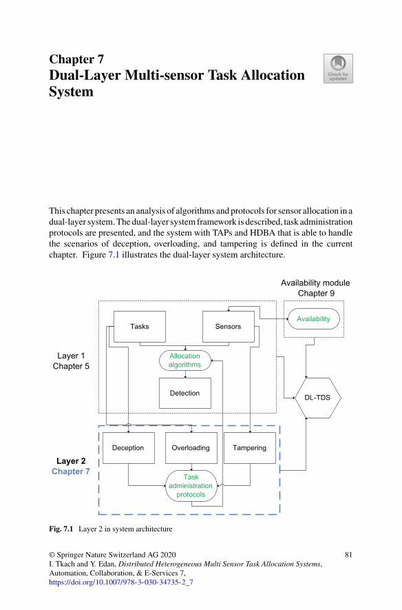
Chapter 7Dual-Layer Multi-sensor Task AllocationSystem
This chapter presents an analysis of algorithms and protocols for sensor allocation in adual-layer system.The dual-layer system framework is described, task administrationprotocols are presented, and the system with TAPs and HDBA that is able to handlethe scenarios of deception, overloading, and tampering is defined in the currentchapter. Figure 7.1 illustrates the dual-layer system architecture.
Tasks Sensors
Allocation algorithms
Detection
Deception TamperingOverloading
Availability
Task administration
protocols
Layer 1Chapter 5
Layer 2Chapter 7
Availability moduleChapter 9
DL-TDS
Fig. 7.1 Layer 2 in system architecture
© Springer Nature Switzerland AG 2020I. Tkach and Y. Edan, Distributed Heterogeneous Multi Sensor Task Allocation Systems,Automation, Collaboration, & E-Services 7,https://doi.org/10.1007/978-3-030-34735-2_7
81

82 7 Dual-Layer Multi-sensor Task Allocation System
Despite the extensive ground covered by researchers thus far regarding multi-agent task allocation algorithms, several serious shortcomings in the literature havebeen found and must be addressed. Various authors have outlined frameworks basedon design principles derived from observing real systems; however, no frameworkhas been proposed to deal with heterogeneous sensors to multiple tasks withoutknowing a priori when, where, and which task will enter or leave the environmentand handle problems within the sensory system.
Recent research in multi-agent task allocation methods and meta heuristics hasprovided a plethora of different algorithms; nevertheless, there is a lack of understand-ing on how the problems in sensors and in the allocation process such as very longattendance times and many tasks with same priorities can be handled and optimallyaddressed. Furthermore, studies have addressed agent-level and administration-levelallocation in isolation, neglecting their interrelation and the benefits of combiningthem into a dual-layer system. Not only these levels have been addressed in isolation,but they also cannot fully handle problems in the sensory system. Previous researchproposed task administration protocols to deal with three elements in task adminis-tration: task, resource, and process. This book extends and modifies these protocolsto deal with a dual-layer multi-sensor task allocation system and to analyze the statusof sensors to modify the allocation if necessary.
7.1 Definitions
In order to overcome uncertainties in task arrival and sensory performance and dis-turbances, a dual-layer approach is required. The dual-layer system is responsiblefor actively making decisions and triggering timely actions so that the overall systemperformance can be further improved. It can handle problems existing in allocationmethods and algorithms due to their inherent limitations. In order to overcome suchlimitations, protocols within this dual-layer system must repeatedly identify the cur-rent state of the system and take proper actions to deal with allocation problems.These problems include:
1. Tasks that may have much higher priority over other tasks; this will occupy thesensors without the ability to perform other tasks that are close to their deadlineand must be handled quickly before less urgent tasks.
2. Many tasks have the same priorities; the system may need to reprioritize them toavoid conflicts in sensor allocation.
3. Tasks that require long execution times but have low priority may occupy thesensors.
4. A failure of a portion of sensors in the system, which may affect the allocationprocess.
These problems are mapped in relation to the allocation and sensors limitations:

7.1 Definitions 83
1. Overloading: Tasks that require very long attendance times. These tasks mayoccupy the sensors that are allocated to them for long periods of time therebydelaying sensors from handling other tasks. The sensors are overloaded with aportion of tasks that delay them. A time out policy that recognizes if a sensor isexperiencing a delay while other tasks are waiting for execution, can overcomethis problem.
2. Deception: Sensors are occupied by some tasks that may be neither urgent norimportant and be delayed by them. This can be caused by tasks that may havehigher priority over other tasks or many tasks with similar priorities. Due tomalfunction or recognition problems, tasks may be perceived by the system witha higher priority than they should. These tasks may unnecessarily occupy thesensors. Thus reducing sensors’ ability to detect other tasks that are close totheir deadline and must be handled quickly before less urgent tasks. These casesrequire the system to reprioritize tasks.
3. Tampering: Failure of a portion of sensors in the system. Sensors may fail dueto internal properties (i.e., reliability of the hardware) and external reactions (i.e.,weather conditions, jamming). The system should be able to monitor this andensure that system performance will not be decreased.
Definition 1 Task’s deadline (�), task’s initial completion time value tinit , time outvalue to, current time tc, set of tasks in the system (M), task processing time and aqueue of tasks;
Overloading (OVL) occurs when
OVL = {M : tini t � 0&� � 0|(tc − tst > to)&(queue(M) > 0)}
Definition 2 Perceived task’s priority (F), calculated task’s priority (T ), and set oftasks in the system (M);
Deception (DCP)occurswhenDCP1 = {∀a, b ∈ M : F(a) = F(b)|T (a) < T (b)}
DCP2 = {∀a, b ∈ M : F(a) >> F(b)|T (a) < T (b)}
Definition 3 Performance of a sensor (V ), set of sensors in the system (N), and setof tasks in the system (M);
Tampering (TMP) occurs when T MP = {∀k ∈ N : Vik = 0|Vik allocated to M}for all i
7.2 Task Administration Protocols
TaskAdministration Protocols (TAPs) are defined as a set of protocols responsible formaking decisions actively and triggering timely actions so that these decisions andtriggers can improve performance [1–3, 5]. Previous research regarding TAPs dealtwith three elements in task administration: task, resource, and process. Accordingto Ko and Nof [5], TAPs were designed as a combination of three sub-protocols

84 7 Dual-Layer Multi-sensor Task Allocation System
in order to handle three administration elements: task requirement analysis protocol(TRAP), shared resource allocation protocol (SRAP), and synchronization and time-out protocol (STOP). Each of the protocols is activated by the TAP mechanism upona certain trigger and acts according to the appropriate administration element.
TAPs were used in the literature for task initialization, resource allocation, andprocess monitoring. TRAPwas used to analyze and assign priorities to tasks insertedinto a task queue. Considering the current status of resources, SRAP decides whichresource a task must be assigned. STOP was used to control procedures in which aresource may be occupied excessively by a task, preventing other tasks from beingprocessed by this resource. Beyond a certain threshold of resource occupation, thetask needs to be returned to the queue so that other tasks can be processed at theresource.
According to Ko and Nof [5], different TAP schemes must be applied dependingon the system structure and the type of resources and tasks at hand.
The design of TAPs for task administration in a collaborative production/servicesystem was investigated by Ko and Nof [5]. In this application, TAPs were designedas a control mechanism that can manage complicated situations in the collaborativetask workflow environment. A case study of applying TAPs for TestLAN, as anexample of collaborative production systems, was developed by Williams et al. [9]and enhancedbyKoandNof [5] to analyze thedesignofTAPs and show the advantageof TAPs over non-TAP coordination protocols. The simulation analysis indicatedthat TAPs performed significantly better than other non-TAPs, particularly undermedium or high load conditions. The second case study analyzed by Ko and Nof [6]included the application of TAPs to FSN (Facility Sensor Network) as an example ofcollaborative service systems. FSN is a wireless sensor network to monitor processesin collaborative production facilities. In FSN the data are transmitted under a routingprotocol, which tries to maximize the lifetime of the wireless sensor network [4],and then processed with a data processing protocol to obtain meaningful informationfrom the data. Their simulation results indicated that the performance under TAPswas significantly better than under simple coordination protocols.
These studies have addressed agent-level and administration-level allocation inisolation, neglecting their interrelation and the benefits of combining them into adual-layer system. This chapter combines an agent-level task allocation algorithmwith task administration protocols with an addition of a new protocol for analyzingthe status of agents to modify the allocation if necessary.
Task administration protocols (TAPs) are used to overcome uncertainties in taskarrival and sensory performance and disturbances (i.e., sensor failure, conflicts in taskpriorities, high time-consuming tasks) in the multi-sensor system (Fig. 7.2). TAPsconsist of four protocols, one of the protocols applies a bio-inspired HeterogeneousDistributed Bees Algorithm (HDBA) for sensors allocation and real time allocationof tasks. This algorithm efficiently allocates a high number of sensors to upcomingtasks in order to handle as many tasks as fast as possible.
Optimal sensor’s availability is related to their monetary cost in the systemachieved by deployment of redundant sensors (see Chap. 10). Employing TAPs thatuse HDBA allows dynamic, real time allocation of distributed sensors to tasks whenthey occur.

7.2 Task Administration Protocols 85
Sensor i
TRAP
Deception
ASAP
Tampering
SRAP
HDBA
STOP
Overloading
Task arrival
Yes
Yes
Yes
No
No
No
System
TAPs
Fig. 7.2 System procedure scheme (after Tkach et al. [7])
In the following situations, another layer may be required to handle problemsin the allocation process. These situations are mapped in relation to the allocationfunction and sensors limitations:
1. Tasks that require very long execution time (7.1) may occupy the sensors thatare allocated to them for long periods of time and decrease system performancedramatically by delaying these sensors without the ability to handle other tasks.
OVL = {M : tini t � 0&� � 0|(tc − tst > to)&(queue(M) > 0)} (7.1)
A time out policy that recognizes if a sensor is experiencing a delay while othertasks are waiting for execution, can overcome this problem.
2. A batch of tasks that may have much higher priority over other tasks or manytasks that have the same priority (7.2, 7.3)
DCP1 = {∀a, b ∈ M : F(a) = F(b)|T (a) < T (b)} (7.2)

86 7 Dual-Layer Multi-sensor Task Allocation System
DCP2 = {∀a, b ∈ M : F(a) >> F(b)|T (a) < T (b)} (7.3)
A similar problem may arise in cases where tasks are perceived by the sys-tem with a higher priority than it should be, due to malfunction or recognitionproblems.
Those tasks may unnecessarily occupy the sensors without the ability to per-form other tasks that are close to their deadline and need to be handled quicklybefore less urgent tasks; in these cases, the systemmay need to reprioritize them.
3. A failure of a portion of sensors in the system defined as tampering (7.4)
T MP = {∀k ∈ N : Vik = 0|Vik allocated to M} for all i (7.4)
7.3 Framework Design
The system is designed as a dual-layer network; a process layer and a monitoringlayer (Fig. 7.3). The process layer consists of multiple sensors and is responsiblefor allocating them to complete tasks. As multi-sensor systems are vulnerable tosome risks and problems [8], the monitoring layer functions at a higher level than theprocess layer and is used to monitor those problems in the process layer, applyingTAPs to handle them. The problems in the process layer are defined as overloading,deception, and tampering sensors.
The system executes task administration protocols to ensure efficient operationby the system executing the following four activities [7] (Fig. 7.4):
Dual-layer system
Sensor agents
Process layer
Monitoring layer
Protocols
Fig. 7.3 Dual-layer system scheme (after Tkach et al. [7])

7.3 Framework Design 87
Sensor
Agent1
Agent2
Agentn
Agent5
Agent4
Agent3
Sensor allocation
Queue management
Task management
Synchronization
Characteristics
Sensor
Sensor
Sensor
Sensor
Sensor
Fig. 7.4 Multi-sensor collaboration model (after Tkach et al. [7])
A1. Task managing: decides how to reassign the priorities of the required tasksbased on characteristics of each task.
A2. Queue managing: manages tasks queue such that no task will ever be delayed.This activity is important since delaying a task can cause it to lose its relevance.
A3. Sensor allocation: executes sensor allocation algorithm for the sensor to taskallocation. The sensor selection determines which sensors are appropriate toperform the task in order to optimize the performance of the overall system.This activity is responsible for executing the process layer, which uses HDBAfor sensors to task allocation.
A4. Synchronization: sets up a timeline of commands for every sensor to carryout tasks based on their availability and performances, given task requests.It ensures that tasks are not unnecessarily delayed while a current task isexperiencing delays, given that there are other tasks waiting in the queue.
7.4 Task Administration Protocols
Four task administration protocols (TAPs) are implemented for PL andML followingKo and Nof [5, 6] and based on the four activities above [7] (Table 7.1):
“TRAP” (task requirement analysis protocol):Reassigns priority levels to monitoring and allocation tasks so that they may be
sequenced in the queue.“ASAP” (assignment analysis protocol):It decides if the task should wait for the backup sensors to become active or be
processed with a set of available functional sensors.In “ASAP” there are two options:
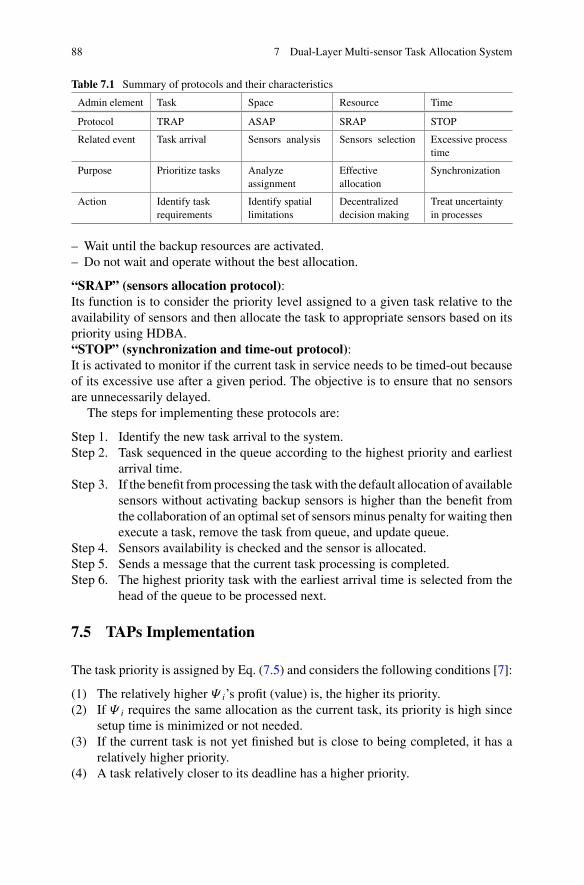
88 7 Dual-Layer Multi-sensor Task Allocation System
Table 7.1 Summary of protocols and their characteristics
Admin element Task Space Resource Time
Protocol TRAP ASAP SRAP STOP
Related event Task arrival Sensors analysis Sensors selection Excessive processtime
Purpose Prioritize tasks Analyzeassignment
Effectiveallocation
Synchronization
Action Identify taskrequirements
Identify spatiallimitations
Decentralizeddecision making
Treat uncertaintyin processes
– Wait until the backup resources are activated.– Do not wait and operate without the best allocation.
“SRAP” (sensors allocation protocol):Its function is to consider the priority level assigned to a given task relative to theavailability of sensors and then allocate the task to appropriate sensors based on itspriority using HDBA.“STOP” (synchronization and time-out protocol):It is activated to monitor if the current task in service needs to be timed-out becauseof its excessive use after a given period. The objective is to ensure that no sensorsare unnecessarily delayed.
The steps for implementing these protocols are:
Step 1. Identify the new task arrival to the system.Step 2. Task sequenced in the queue according to the highest priority and earliest
arrival time.Step 3. If the benefit fromprocessing the taskwith the default allocation of available
sensors without activating backup sensors is higher than the benefit fromthe collaboration of an optimal set of sensors minus penalty for waiting thenexecute a task, remove the task from queue, and update queue.
Step 4. Sensors availability is checked and the sensor is allocated.Step 5. Sends a message that the current task processing is completed.Step 6. The highest priority task with the earliest arrival time is selected from the
head of the queue to be processed next.
7.5 TAPs Implementation
The task priority is assigned by Eq. (7.5) and considers the following conditions [7]:
(1) The relatively higher Ψ i’s profit (value) is, the higher its priority.(2) If Ψ i requires the same allocation as the current task, its priority is high since
setup time is minimized or not needed.(3) If the current task is not yet finished but is close to being completed, it has a
relatively higher priority.(4) A task relatively closer to its deadline has a higher priority.
7.5 TAPs Implementation 89
(5) The earlier the task’s arrival time the higher its priority.
Ti = ηi ×(fi + 1
(tcti − tcurrent )+ 1
tarrival i
)(7.5)
where Ti is a calculated value of the new priority of a task according to protocolTRAP, i is the task index, f i is the initial priority value of task i, η is the assignmenttype request, tct is the task completion time, tcurrent is the current time, and tarrival isthe task arrival time.
η ={
1 i f same requested assignment0.5 otherwise
(7.6)
The decision regarding wait for backup sensors or proceed with the taskautonomously is performed by calculating the difference between the performanceof the system in default allocation and the optimal set of sensors, and the penalty forthe waiting times (7.7).
QS = VI Sdef ault − VOS + Vt × τ (7.7)
where,QS is the assignment analysis function, VISdefault is the performance of defaultallocated sensors without activating backup sensors, VOS is the performance of theoptimal set of sensors with backup sensors, Vt is waiting time penalty value, and τ
is the waiting time in seconds.A possible solution for sensor selection and allocation can be derived using
the HDBA. The stop criterion is given by a threshold that quantifies the desiredperformance of the sensors for a given task.
Time-out value is given by (7.8).
to = μct + 2σct (7.8)
whereμ is task mean completion time, σ is the standard deviation of task completiontime.
Once a job is timed-out, its arrival time is modified to reflect the time when itre-enters the system, and all the service and waiting times must be updated.
For the “STOP” implementation it is necessary to monitor the time a task hasbeen in process. If a task’s service time is greater than its time-out period and thereare tasks in the queue, the current job is timed-out and returns to the queue with anidentifier indicating its priority level and remaining process time. The exceptions for“STOP” are:
1. Task processing time has not exceeded the time-out value to.2. No other task is waiting in the queue. If queue= 0 then continue task processing.3. The task is close to completion. If tct-tcurrent≤ θ then continue task processing.

90 7 Dual-Layer Multi-sensor Task Allocation System
STOP =
⎧⎨⎩
f alseif(tcurrent tsti ≤ to) or (queue = 0) or
or (tcti − tcurrent ≤ θ)
true otherwise(7.9)
where, θ is a threshold, tsti is task start time.Pseudocode of the dual-layer system
1. Initialize: Set t=0Place N agents ‘bees’ on sensors
2. If termination condition met then go to step 6 else
Upon task arrival calculate the task priority fiActivate TRAP Calculate the new task priority function Ti
Update queue of tasks based on their new priorities Go to step 3
3. If new task arrived then go to step 2 If there are failed sensors
Activate ASAP Calculate QSIf QS>0 then make a default assignment and go to step 4 else
Activate backup sensors and go to step 44. For i=1 to M do
For k=1 to N doCalculate probabilities for each sensor pik
Apply wheel-selection rule Allocate sensors according to the selection and go to step 5
5. If (texi=0) then set Δi=0 and go to step 2 else
Calculate toIf STOP is true then set Δi=0 and go to step 2 else
Go to step 4 6. Finalize:
Calculate VICalculate TStop

References 91
References
1. Anussornnitisarn P, Peralta J, Nof SY (2002) Time-out protocol for task allocation inmulti-agentsystems. J Intell Manuf 13(6):511–522
2. HuangCY,Nof SY (2000) Formation of autonomous agent networks formanufacturing systems.Int J Prod Res 38(3):607–624
3. Huang CY, Nof SY (2002) Evaluation of agent-based manufacturing systems based on a parallelsimulator. Comput Ind Eng 43(3):529–552
4. Jeong W, Nof SY (2008) Performance evaluation of wireless sensor network protocols forindustrial applications. J Intell Manuf 19(3):335–345
5. Ko HS, Nof SY (2010) Design of protocols for task administration in collaborative productionsystems. Int J Comput Commun Control 5(1):91–105
6. Ko HS, Nof SY (2012) Design and application of task administration protocols for collaborativeproduction and service systems. Int J Prod Econ 135(1):177–189
7. Tkach I, Edan Y, Nof SY (2017) Multi-sensor task allocation framework for supply networkssecurity using task administration protocols. Int J Prod Res 55:5202–5224
8. Walters JP, Liang Z, Shi W, Chaudhary V (2007) Wireless sensor network security: a survey.Secur Distrib, Grid, Mob, Pervasive Comput 1:367
9. Williams NP, Liu Y, Nof SY (2002) TestLAN approach and protocols for the integration ofdistributed assembly and test networks. Int J Prod Res 40(17):4505–4522

Chapter 8Extended Example of Dual-LayerMulti-sensor Task Allocation Systems
This chapter describes an example of a multi-sensory security system for supplynetworks with disturbances. This example is evaluated by the use of a dual-layersystem to illustrate the methods described in Chap. 7.
The purpose of adding a second layer is to handle problems of deception, over-loading, and tampering in the allocation process. The dual-layer system employs theadvantages of HDBA with TAPs. Due to its decentralized heuristic nature, HDBAcannot guarantee an optimal solution, but it can provide sub-optimal solutions toNP-hard problems. By using TAPs these solutionswere found to be further improved.
The dual-layer system can be applied to many different types of applicationsincluding LEP. Once the problems of deception, overloading, and tampering areintroduced to LEP, adding a second layer will increase the performance (similar tothe task allocation benchmark presented in this chapter). This can be studied as partof future research.
8.1 Dual-Layer System Evaluation
A dual-layer sensory system is illustrated in Fig. 8.1. Such a sensory system mustbe able to overcome several problems. The first problem has to do with tasks thatrequire very long attendance times. These tasks may occupy the sensors allocatedto them for long time durations, thus delaying the handling of other tasks by thosesensors. In this overloading problem, the sensors are overloaded with a portion oftasks that delay them. A time-out policy, which recognizes if a sensor is experiencinga delay while other tasks are waiting for execution, can overcome this problem. Thesecond problem that the sensory system must overcome relates to tasks that mayhave much higher priority over other tasks or the same priority as other tasks. Asimilar problem may arise when, due to malfunction or recognition problems, tasksare perceived by the system to be of a higher priority than they should be. Suchtasks may unnecessarily occupy some sensors. The system may need to reprioritizethose sensors, which are unable to perform other tasks that must be handled quickly,
© Springer Nature Switzerland AG 2020I. Tkach and Y. Edan, Distributed Heterogeneous Multi Sensor Task Allocation Systems,Automation, Collaboration, & E-Services 7,https://doi.org/10.1007/978-3-030-34735-2_8
93

94 8 Extended Example of Dual-Layer Multi-sensor …
Sens
or
RFID
tags
on
Pack
ages
Trac
king
Pac
kage
s in
Stor
age
Trac
king
Pac
kage
s in
Tran
spor
t
Cent
ral D
B Se
rver
Cent
ral D
B
Mon
itorin
g St
aon
Rece
iver
RFID
Rea
der
Rece
iver
Loca
l DB
serv
er
Trac
king
Pac
kage
s in
Load
ing
Cont
rolle
r
Sens
ors D
B
Ope
rang
Sta
on
Hum
an
Ope
rato
r
RFID
RFID
RFID
RFID
Dece
pon
task
s
Ove
rload
ing
task
s
Stric
t dea
dlin
e ta
sks
Ope
rang
sens
or
Faile
d se
nsor
Fig.8
.1Anillustrationof
adu
al-layer
logistic
system
with
distributedsensorsto
mon
itorsecurity.D
eceptio
nismarkedby
redcircles,overloadingby
blue
circles,andim
portanttasks
bypu
rplecircles

8.1 Dual-Layer System Evaluation 95
ahead of less urgent tasks, due to being close to their deadline. In this deceptionproblem, sensors are occupied and delayed by some tasks that may be neither urgentnor important. The third problem that the sensory system must overcome is relatedto a failure of a portion of sensors in the system. In this tampering problem, sensorsmay fail due to internal properties (e.g., hardware reliability) and external factors(e.g., weather conditions). The system should be able to monitor these problems toensure that system performance is unharmed.
The simulation compares the performance of a dual-layer system incorporatingTAPs to a single-layer task allocation system without TAPs. The parameters used forthe simulation are presented in Table 8.1.
Tasks were uniformly distributed in the arena based on Rowaihy et al. [2] andByers and Nasser [1]. The sensors’ range values were predefined to cover 15 to 45meters relative to the size of the arena (100 × 100 m). An inherent noise in eachsensor was introduced according to typical operational distance ranges of knowncommercial sensors [3] relative to the arena size: acoustic sensor, seismic sensor,and forward-looking infrared radar (FLIR). The allocation range of these sensors isgiven by:
Rseismic = 0.8× Racoustic = 1.25× RFL I R
The numerical computations were performed on a PC with 2.90 GHz CPU and12GBofRAM,usingMatlabR2015a software.The followingperformancemeasureswere analyzed:
Table 8.1 Summary ofparameter values forsimulation analysis
Parameter Values
Area dimensions 100 × 100 m
Number of sensors (‘bees’) 100
Number of tasks 200
Task completion time Randomly distributed from 0to 10 min
Simulation duration 200 steps
Tasks’ locations Uniformly distributed atrandom
Control parameters α = β=γ = 1
Sensors’ locations Uniformly distributed random
Task’s arrival time Every 1 step
Sensor’s range coverage Predefined from 15 to 45 m
Number of false tasks 10, 20, 50
Number of failed sensors 10, 20, 30
Number of high-timeconsuming tasks
10, 20, 50
TAPs TRAP, ASAP, SRAP, STOP

96 8 Extended Example of Dual-Layer Multi-sensor …
Table 8.2 Values of deception, tampering, and overloading for simulation analysis
Deception (numberof false tasks)
Faulttolerant/tampering(number of failedsensors)
Overloading (numberof hightime-consumingtasks)
10 10 10
20 20 20
50 30 50
Responsibleprotocols
TRAP ASAP STOP
1. Number of treated tasks by each sensor is defined by: χk =M∑
i=1taski ; taski = 1 if Vik > 0
else taski = 0,
where χ k is the number of treated tasks of k-th sensor,M is the total numberof tasks in the system, i is the index of the current task, and Vik is the k-th sensor’sperformance on the i-th task.
2. Number of important tasks treated.3. Number of unallocated tasks is defined by: ε =
∑Mi=1 taski ; taski = 1 if
∑Nk=1 Vik = 0
else taski = 0,
where ε is the number of unallocated tasks, N is the total number of sensors inthe system.
The simulation values for situations of overloading, deception, and tampering aresummarized in Table 8.2. For each situation, an appropriate protocol was assigned.
The mean values obtained from 100 independent runs were compared at thestatistical confidence level of 95%.
8.2 Results and Discussion
Graphs of the simulated results are presented in Figs. 8.2, 8.3, 8.4, 8.5, 8.6, 8.7, 8.8,8.9 and 8.10 for scenarios of overloading, deception, and tampering. Each scenariowas compared for three performance measures: the number of treated tasks by eachsensor, the number of unallocated tasks, and the number of important tasks treated.
Figures 8.2, 8.3 and 8.4 illustrate the mean number of treated tasks by each sensoras a function of the number of false tasks, high time-consuming tasks, and failedsensors in single-layer and dual-layer systems. Results revealed that, as expected, asthe number of false tasks increased (Fig. 8.2), the mean number of treated tasks byeach sensor decreased (from 43.22 to 16.47 and from 43.21 to 34.78, in a single-layersystemwithHDBA, and dual-layer systemusingTAPs, respectively).Moreover,withthe increase in the number of false tasks, the difference in the number of treated tasks

8.2 Results and Discussion 97
15
20
25
30
35
40
45
TAPs
Num
ber
of tr
eate
d ta
sks
by e
ach
sens
or
as
a nu
mbe
r of
fals
e ta
sks
Deception performance
HDBA
Fig. 8.2 Number of treated tasks by each sensor for a different number of false tasks. The barsrepresentmean values of 100 independent runs, the edges of the box are the 25th and 75th percentiles,the whiskers are the most extreme data points
15
20
25
30
35
40
45
TAPs
Num
ber
of tr
eate
d ta
sks
by e
ach
sens
or a
s a
n
umbe
r of
hig
h tim
e co
nsum
ing
task
s
Overloading performance
HDBA
Fig. 8.3 Number of treated tasks by each sensor for a different number of high time-consumingtasks. The bars represent mean values of 100 independent runs, the edges of the box are the 25thand 75th percentiles, the whiskers are the most extreme data points

98 8 Extended Example of Dual-Layer Multi-sensor …
32
34
36
38
40
42
TAPs
Num
ber
of tr
eate
d ta
sks
by e
ach
sens
or
as
a nu
mbe
r of
faile
d se
nsor
s
Tampering performance
HDBA
Fig. 8.4 Number of treated tasks by each sensor for a different number of failed sensors. Thebars represent mean values of 100 independent runs, the edges of the box are the 25th and 75thpercentiles, the whiskers are the most extreme data points
-5
0
5
10
15
20
25
30
35
TAPs
Num
ber
of u
nallo
cate
d ta
sks
as a
n
umbe
r of
fals
e ta
sks
Deception performance
HDBA
Fig. 8.5 Number of unallocated tasks for a different number of false tasks. The bars represent meanvalues of 100 independent runs, the edges of the box are the 25th and 75th percentiles, the whiskersare the most extreme data points

8.2 Results and Discussion 99
-20
-10
0
10
20
30
40
50
60
70
80
TAPs
Num
ber o
f una
lloca
ted
task
s as
a n
umbe
r
of h
igh
time
cons
umin
g ta
sks
Overloading performance
HDBA
Fig. 8.6 Number of unallocated tasks for a different number of high time-consuming tasks. Thebars represent mean values of 100 independent runs, the edges of the box are the 25th and 75thpercentiles, the whiskers are the most extreme data points
0
10
20
30
40
50
60
TAPs
Num
ber o
f una
lloca
ted
task
s as
a
num
ber o
f fai
led
sens
ors
Tampering performance
HDBA
Fig. 8.7 Number of unallocated tasks for a different number of failed sensors. The central mark isthe median value of 100 independent runs, the edges of the box are the 25th and 75th percentiles,the whiskers are the most extreme data points

100 8 Extended Example of Dual-Layer Multi-sensor …
5
6
7
8
9
10
11
12
TAPs
Num
ber
of im
port
ant t
asks
trea
ted
as
a
num
ber
of fa
lse
task
s
Deception performance
HDBA
Fig. 8.8 Number of important tasks treated for a different number of false tasks. The bars representmean values of 100 independent runs, the edges of the box are the 25th and 75th percentiles, thewhiskers are the most extreme data points
3
4
5
6
7
8
9
10
11
TAPs
Num
ber o
f im
porta
nt ta
sks
treat
ed a
s a
num
ber
of h
igh
time
cons
umin
g ta
sks
Overloading performance
HDBA
Fig. 8.9 Number of important tasks treated for a different number of high time-consuming tasks.The bars represent mean values of 100 independent runs, the edges of the box are the 25th and 75thpercentiles, the whiskers are the most extreme data points

8.2 Results and Discussion 101
4
5
6
7
8
9
10
11
TAPs
Num
ber
of im
port
ant t
asks
trea
ted
as a
nu
mbe
r of
faile
d se
nsor
s
Tampering performance
HDBA
Fig. 8.10 Number of important tasks treated for a different number of failed sensors. The barsrepresentmean values of 100 independent runs, the edges of the box are the 25th and 75th percentiles,the whiskers are the most extreme data points
between TAPs and HDBA was also increased. This indicates that the monitoringlayer performed effectively by minimizing the decrease in the number of treatedtasks. Similarly, as the number of high time-consuming tasks (Fig. 8.3) and numberof failed sensors (Fig. 8.4) increased, themean number of treated tasks by each sensoralso decreased and the difference in the number of treated tasks between TAPs andHDBA increased, respectively.
Figures 8.5, 8.6 and 8.7 illustrate the mean number of unallocated tasks as afunction of the number of false tasks, high time-consuming tasks, and failed sensorsin single-layer and dual-layer systems. The difference in the number of unallocatedtasks between TAPs and HDBA was greatly increased in all scenarios. Thus, thedual-layer system managed to greatly reduce the number of unallocated tasks bymore than 72% (from 31.07 to 8.58, 72.76 to 13.78, and 65.2 to 19.72 in deception,overloading, and tampering scenarios, respectively).
Figures 8.8, 8.9 and 8.10 illustrate the mean number of important tasks that weresuccessfully treated by the system, as a function of the number of false tasks, hightime-consuming tasks, and failed sensors in single-layer and dual-layer systems. Inthese scenarios, the number of treated important tasks was increased by more than80% in the dual-layer system in comparison to the single-layer system (from 5.06to 9.01, 3.03 to 8.07, and 4.02 to 7.01 in deception, overloading, and tamperingscenarios, respectively). The simulation results are summarized in Table 8.3.

102 8 Extended Example of Dual-Layer Multi-sensor …
Table8.3
Summaryof
results
forscenariosof
overloading,
deception,
andtampering
with
100independentruns
Measured
value
Num
ber
offalse
tasks
Deceptio
nNum
berof
high
time
consum
ing
tasks
Overloading
Num
ber
offailed
sensors
Tampering
HDBA
Standard
deviation
TAPs
Standard
deviation
HDBA
Standard
deviation
TAPs
Standard
deviation
HDBA
Standard
deviation
TAPs
Standard
deviation
Num
berof
treated
tasksby
each
sensor
043.22a
8.09
43.21a
11.62
043.14a
10.59
43.47a
11.54
043.78a
4.55
43.74a
9.76
1038.47a
13.31
40.50a
8.14
1033.58a
4.22
42.95a
4.26
1038.38a
1.61
41.52a
5.33
2031.37a
2.12
39.44a
9.62
2027.32a
8.36
40.62*
4.79
2036.10a
7.93
40.13a
6.63
5016.47a
0.15
34.78a
5.59
5013.65a
9.06
37.26a
2.23
3031.45a
8.23
39.35a
2.79
Num
berof
unallocated
tasks
03.57
5.52
3.29
1.16
03.44
0.30
3.80
2.48
03.78
9.71
3.92
2.32
105.84
3.52
3.26
3.87
109.99
6.45
5.90
4.74
1018.35a
2.53
4.19
a0.62
2010.64
8.78
4.63
7.78
2019.62a
12.20
8.55
a10.53
2032.93a
3.22
8.09
a3.66
5031.07a
6.01
8.58
a2.04
5072.76a
9.63
13.78a
7.36
3065.20a
5.44
19.72a
10.65
Num
berof
important
tasks
treated
010.71a
4.47
10.51a
13.42
010.66a
5.14
10.28a
3.30
010.23a
13.13
10.31a
3.22
1010.57a
10.17
10.08a
7.65
109.73
a4.19
10.26a
13.15
108.39
a2.08
10.61a
11.18
208.81
a5.54
10.10a
10.91
207.04
a1.88
10.12a
5.32
206.98
11.38
9.83
5.27
505.06
5.09
9.01
9.53
503.03
3.90
8.07
5.03
304.02
3.78
7.01
6.77
The
firstsub-columnof
each
problem
representstheresultforeach
tested
scenario
usingHDBA,the
second
sub-columnrepresentstheresultforeach
tested
scenario
usingTA
Psa S
tatistically
significant
results

References 103
References
1. Byers J, Nasser G (2000) Utility-based decision-making in wireless sensor networks. In: Pro-ceedings of the 1st ACM international symposium onMobile ad hoc networking and computing,IEEE Press, Boston, MA, USA, pp 143–144
2. Rowaihy H, Eswaran S, Johnson M, Verma D, Bar-Noy A, Brown T, Porta TL (2007) A surveyof sensor selection schemes in wireless sensor networks. In: Proceedings of SPIE, vol 6562
3. Yoon Y, Kim YH (2013) An efficient genetic algorithm for maximum coverage deployment inwireless sensor networks. IEEE Trans Cybernetics 43(5):1473–1483

Chapter 9Fault Tolerant Multi Sensor Systemwith High Availability
This chapter describes and analyzes the ‘Availability module’ of the task allocationsystem (Fig. 9.1). This chapter presents the reliability design and availability analysisof the system to further optimize system performance in case of sensor failure andto ensure fault tolerant allocation system performance. Availability optimization ofthe sensors’ operation and comparison of the dual-layer system performance with
Tasks Sensors
Allocation algorithms
Detection
Deception TamperingOverloading
Availability
Task administration
protocols
Layer 1Chapter 5
Layer 2Chapter 7
Availability moduleChapter 9
DL-TDS
Fig. 9.1 Availability module in system architecture
© Springer Nature Switzerland AG 2020I. Tkach and Y. Edan, Distributed Heterogeneous Multi Sensor Task Allocation Systems,Automation, Collaboration, & E-Services 7,https://doi.org/10.1007/978-3-030-34735-2_9
105

106 9 Fault Tolerant Multi Sensor System with High Availability
optimized sensors’ availability to a regular non-optimized dual-layer system wasconducted for two system types using Monte Carlo simulations.
9.1 System Availability
One of the important issues in systems design is improving the fault tolerance andresilience [8] of system operation. Amulti-sensory system can bemade fault-tolerantby designing redundancy into the system [6]. Some researchers suggest that the faulttolerance of the sensory system can be increased by putting redundant sensors tosleep and awakening these sleeping sensors when they are needed to restore taskcoverage [18]. This is an important characteristic since most applications in dynamicenvironments rely on continuous progress even if some system components fail (see[5]). For example, in [7] some monitoring sensors in automated production systemmiddleware expected failures during task-execution, but it was still required that theoverall mission be completed in the best way possible given the remaining resources.Therefore, real world applications in monitoring require a novel system in whichsome sensors are redundantly distributed with different sensing capabilities (i.e.,heterogeneous sensors).
The availability of a system defines the percentage of time in which the sys-tem is operational out of the total system employment time. This is a critical valuethat influences the system uptime and its fault tolerance. In general, there are twonumerical techniques for estimating and optimizing system availability:Monte Carlosimulation and numerical solution of the underlying Markov chain, in addition toan analytical solution that mainly focuses on non-shortage probability (NSP). Sim-ulation is often the preferred solution technique for modeling real-world systems,since it is capable of solving large, complex systems with parallel components andgeneral distribution functions. DuringMonte Carlo simulation, the systems’model isrepeatedly executed, and a new random number sequence is used for each executionto compute a different failure value with each execution [1].
Reliability Block Diagram (RBD) is the most common method for expressing thereliability of systems [4]. RBD represents the reliability of a system by composing aset of blocks that are arranged in series, parallel, or combination, where each blockrepresents the reliability of the component (=sensor) of the system at time t, Rk(t).
This chapter illustrates how to incorporate availability based fault tolerancefor heterogeneous sensor network collaboration to improve allocation systemperformance.

9.2 Availability Definition 107
9.2 Availability Definition
9.2.1 Overview—Availability-Based Analysis
System availability and resilience have been studied extensively in the context ofreliability engineering and manufacturing problems, but the fault tolerance approachfor sensor network operation making it robust enough to loss of sensors and/oraddition of new sensors ismissing. In this book, reliability and availabilitymodels areused for heterogeneous sensor network collaboration to provide practical solutionsfor a fault tolerant allocation system performance.
In order to model TAPs’ performance and ensure that it is robust to sensor fail-ure, an availability-based analysis was conducted. The impact of each sensor on thesystem’s availability was analyzed and optimized according to the results by reli-ability software optimization module [14, 16]. The reliability-based modeling andanalysis approach was applied for the heterogeneous sensor collaboration for TAPswith three types of sensors (Fig. 9.2). The aim was to provide practical solutions forfault-tolerant system performance.
Monitoring Sta on
Op cal sensor
IR sensor
Night vision sensor
OS
OS
OS
OS
OS
OS
IR
IR
IR
NS
NS
NS
NS
OS
IR
NS
Fig. 9.2 Heterogeneous sensors supply network monitoring system with three different types ofsensors: optical, infra-red, and night vision sensors (after Tkach et al. [14])

108 9 Fault Tolerant Multi Sensor System with High Availability
Fig. 9.3 RBD of a serialsystem
In this simulation, the aim is to analyze the performance of different algorithmsaiming to develop an algorithm to improve the overall system availability to operatefault tolerantly up to 98% of the time.
To model the reliability structure of the system, a Reliability Block Diagram(RBD) is used. For a system to correctly function, every one of its componentsshould properly operate, the respective system RBD should be represented as aseries of its system components. Figure 9.3 illustrates a series structure of a systemcomposed of n independent components, where Rk(t) is the reliability function ofeach component [14].
A systemwith n components in series has reliability (at time t) equal to the productof the reliability of the components that compose it, as shown in Eq. (1):
R(t) =n∏
k=1
Rk(t) (9.1)
In a case where each component has an exponential failure distribution (which isthe commonway to represent the failure rate of electronic components), the reliabilitymay be represented as:
R(t) = e−λt (9.2)
where λ is the failure rate of the system, and is given by the fraction of sums of thefailure rate of each system component:
λ(t) = 1n∑
k=1
1λk (t)
(9.3)
The system availability (4) is defined as the ratio between system uptime anddowntime:
A = E[Uptime]E[Uptime] + E[Downtime] = MT BF
MT BF + MTT R(9.4)
where A is the system availability, MTBF is the mean time between failures, andMTTR is the mean time to repair. MTBF is inversely proportional to the failure rate(5):
MT BF = 1
λ(t)(9.5)

9.2 Availability Definition 109
Table 9.1 MTBF and costvalues summary
Type of sensor MTBF Cost Number ofsensors
Optical sensor ≈28,000 h $40 34
IR sensor ≈163,000 h $90 33
Night visionsensor
≈212,000 h $130 33
Consider the following MTBF values for three non-complementary sensors(optical, IR, and night vision) based on NPRD-2011 [9] and presented in Table 9.1.
We derive the analytical solution of system availability which is given by:
MT BF = 1∑n
i=11
MT BFI
= 1
34 · 127862 + 33 · 1
163132 + 33 · 1212765
= 633.84 (9.6)
A = E[Uptime]E[Uptime] + E[Downtime] = MT BF
MT BF + MTT R
= 633.84
633.84 + (720 + 5)= 0.46 (9.7)
The system’s availability value A is 46%, which means that 54% of the time thesystem will not be able to cover the entire area.
9.3 Monte Carlo Simulation
Monte Carlo simulation is a statistical analysis technique that was first used at LosAlamos National Laboratory in the 1940 s by scientists working on the developmentof an atomic bomb. It is widely used for optimization in engineering, finance, relia-bility and manufacturing among other fields [13]. Monte Carlo simulation refers tothe Monte Carlo casino in Monaco [10]. The simulation process involves generatingvariables from a statistical distribution that exhibits random behaviors. Monte Carlois also suitable for solving complex engineering problems because it can deal with alarge number of random variables, various distribution types, and highly nonlinearengineering models.
Monte Carlo simulation performs a random sampling of possible values from theinput probability distributions [11]. Each set of samples is called an iteration or his-tory, and the resulting output from that sample is calculated. Monte Carlo simulationperforms thousands of such histories, and the result is a probability distribution ofpossible outcomes that are available for statistical analysis.

110 9 Fault Tolerant Multi Sensor System with High Availability
9.3.1 Simulation Assumptions/Parameters
Simulation assumptions:
1. Failure and repair distributions of the components are exponential (correspondingto the typical failure of electronic devices). Hence, failure and repair rates areconstant.
2. Upon failure, the sensor is repaired with normal time distributions of 240, 480,and 720± 2 h. This repair time includes transporting the failed sensor to a depot,its repair time, and transporting time back to the field.
3. Sensor replacement in the field takes 5 h (modeled as insertion distribution).This time duration was set in order to add the impact of a typical replacementoperation on the system’s availability.
4. Initial system deployment has no redundancies, in order to analyze the impactof adding redundant sensors to the system.
The experimental parameters used in this analysis are stated in Table 9.2. Tasklocations were randomly distributed with uniform distributions in the arena basedon [12] and [2]. The sensor network was simulated in [15] for three sensor distribu-tions: grid distribution uniformly distributed at random and normally distributed atrandom. Best performance was obtained for the uniform distribution; therefore, thisdistribution was considered in the current analysis. The sensor’s operating distancevalues were set relative to the size of the arena (100 × 100 m). An inherent noisein each sensor was introduced according to typical operational distance ranges ofknown commercial sensors [17] relative to the arena size [14].
The simulation was performed for a period of 5 years of system operation(43,800 h) for a distributed sensor network with 100 sensors combined from threesensor types. Two types of sensor networks were considered to compare the influenceof temporal restrictions on availability values.
1. Type 1—sensors are set to perform without temporal restrictions.
Table 9.2 Experimentalparameters summary
Parameter Values
Area dimensions 100 × 100 m
Total number of sensors 100
Types of sensors Optical, IR, night vision
Sensors range coverage Predefined from 15 to 45 m
Number of tasks 200
Simulation duration 200 steps
Tasks location Uniformly distributed at random
Protocols TRAP, ASAP, SRAP, STOP
Sensor’s location Uniformly distributed random
Tasks arrival time Every 1 step

9.3 Monte Carlo Simulation 111
2. Type 2—sensors with lowMTBF values (optical sensors) are set aside and comeinto performance only when needed.
9.4 Results and Discussion
Independent Monte Carlo runs with 100 repetitions were executed. Availability anal-ysis was conducted using a Monte Carlo simulation in 1-min intervals. Results arecalculated with the statistical significance of 95%.
Results (Figs. 9.4 and 9.5) indicated that the average availability increased from38to 86% when low MTBF sensors came into action only when necessary. The systemaverage availability was increased to 98% when 6 spare sensors were used. As bothsystems start with the same initial values, they start from 100% availability. Sensorsin a system of type 1 operate based on a regular algorithm and therefore sensors withlow MTBF values start to malfunction and decrease system availability much fasterthan in a system of type 2. In Fig. 9.4, after a period of time, the availability starts toincrease as a result of sensors that have been repaired. Also, in a system of type 1,
Duration [hr] 1040 0.5 1 1.5 2 2.5 3 3.5 4 4.5
Avai
labi
lity
[%]
30
40
50
60
70
80
90
100System availability over time
Type 1 system, avg. avail. 38%Type 2 system, avg. avail. 86%
Fig. 9.4 System’s average availability over time based on different network types—same rest timefor all sensors and sensors with low MTBF values operate only when necessary. The dots representthe time interval at which sensors were repaired (after Tkach et al. [14])
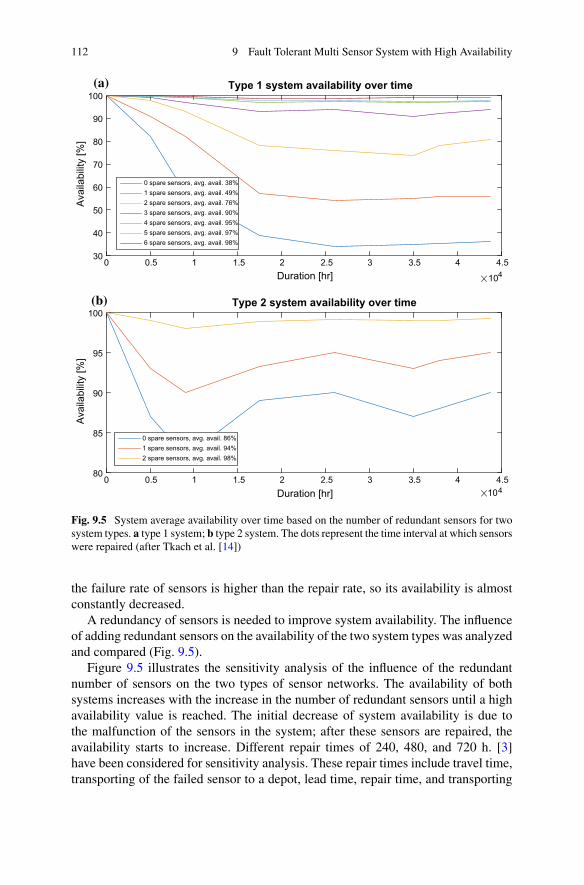
112 9 Fault Tolerant Multi Sensor System with High Availability
Duration [hr] 1040 0.5 1 1.5 2 2.5 3 3.5 4 4.5
Avai
labi
lity
[%]
30
40
50
60
70
80
90
100(a)
(b)
Type 1 system availability over time
0 spare sensors, avg. avail. 38%1 spare sensors, avg. avail. 49%2 spare sensors, avg. avail. 76%3 spare sensors, avg. avail. 90%4 spare sensors, avg. avail. 95%5 spare sensors, avg. avail. 97%6 spare sensors, avg. avail. 98%
Duration [hr] 1040 0.5 1 1.5 2 2.5 3 3.5 4 4.5
Avai
labi
lity
[%]
80
85
90
95
100Type 2 system availability over time
0 spare sensors, avg. avail. 86%1 spare sensors, avg. avail. 94%2 spare sensors, avg. avail. 98%
Fig. 9.5 System average availability over time based on the number of redundant sensors for twosystem types. a type 1 system; b type 2 system. The dots represent the time interval at which sensorswere repaired (after Tkach et al. [14])
the failure rate of sensors is higher than the repair rate, so its availability is almostconstantly decreased.
A redundancy of sensors is needed to improve system availability. The influenceof adding redundant sensors on the availability of the two system types was analyzedand compared (Fig. 9.5).
Figure 9.5 illustrates the sensitivity analysis of the influence of the redundantnumber of sensors on the two types of sensor networks. The availability of bothsystems increases with the increase in the number of redundant sensors until a highavailability value is reached. The initial decrease of system availability is due tothe malfunction of the sensors in the system; after these sensors are repaired, theavailability starts to increase. Different repair times of 240, 480, and 720 h. [3]have been considered for sensitivity analysis. These repair times include travel time,transporting of the failed sensor to a depot, lead time, repair time, and transporting

9.4 Results and Discussion 113
Table 9.3 The influence ofthe number of redundantoptical sensors on type 1systems’ availability withdifferent repair times (240,480, and 720 h)
Quantity of redundantsensors
Availability as a function of repairtime
240 h (%) 480 h (%) 720 h (%)
0 72 51 38
1 89 64 49
2 96 82 76
3 98 93 90
4 99 96 95
5 99 98 97
6 99 99 98
Table 9.4 Optimizationresults for systems’availability of 98% with720 h repair time
Type of system Quantity of redundant sensors
Type 1 system 6 optical sensors
Type 2 system 2 optical sensors
time back to the field. As in the system of type 1, the sensors malfunction morefrequently, and initial availability decreases for a longer time duration. Tables 9.3 and9.4 summarize the redundancy recommendation for the system and the availabilityachieved:
Based on the results, in order to achieve system availability above 98% over a5-year period, the systems should include 106 and 102 sensors, respectively, for type1 and type 2 systems.
After redundant sensors are introduced, the system becomes parallel. The respec-tive system RBD is updated according to the new system components. Figure 9.6illustrates the updated structure of a system composed of n independent components,where Rk(t) is the reliability function of each component. The new product of thereliability of the components that compose the system is shown in Eq. (8):
R(t) =n−m∏
k=1
Rk(t) ×⎧⎨
⎩1 −m∏
p=1
[1 − Rp(t)]⎫⎬
⎭ (9.8)
Fig. 9.6 RBD of the parallelsystem

114 9 Fault Tolerant Multi Sensor System with High Availability
Type 1 system Type 2 system
Num
ber o
f una
lloca
ted
task
s
0
10
20
30
40
50
60
70
80System performance analysis
Unoptimized systemOptimized system
Fig. 9.7 Average number of unallocated tasks based on system configuration and system type
Results of the dual-layer system applying the new approach indicate that forboth system types the optimized systems processed on average more tasks than thecorresponding un-optimized systems (Fig. 9.7). Optimized type 1 systems resulted in165.4% more processed tasks, and type 2 systems resulted in 13.1% more processedtasks when availability analysis results were implemented to the system (F = 9.34,p = 0.02). These findings indicate that the fault tolerance of the multi-sensor systemwas improved, contributing to system performance improvement.
References
1. Beaudet S, Courtney T, Sanders W (2006) A behavior-based process for evaluating availabilityachievement risk using stochastic activity networks. In: Proceedings ofRAMS,Newport Beach,California, pp 23–26
2. Byers J, Nasser G (2000) Utility-based decision-making in wireless sensor networks. In: Pro-ceedings of the 1st ACM international symposium on mobile ad hoc networking & computing.IEEE Press, Boston, MA, USA, pp 143–144
3. Cadwallader LC (2012) Review of maintenance and repair times for components in techno-logical facilities. INL/EXT-12–27734, Idaho National Laboratory
4. Dâmaso A, Rosa N, Maciel P (2014) Reliability of wireless sensor networks. Sensors14(9):15760–15785

References 115
5. Dias MB, Zinck M, Zlot R, Stentz A (2004) Robust multirobot coordination in dynamic envi-ronments. In: IEEE proceedings of international conference on robotics and automation, pp3435–3442
6. Edan Y, Nof SY (2000) Sensor economy principles and selection procedures. IIE Trans DesEng 32(3):195–203
7. JeongW, Nof SY (2009) A collaborative sensor network middleware for automated productionsystems. Int J Comput Ind Eng 57:106–113
8. Levalle RR (2018) Resilience by teaming framework. Resilience by teaming in supply chainsand networks. Springer, Cham, pp 59–64
9. Mahar D, Fields W, Reade J, Zarubin P, McCombie S (2011) Nonelectronic parts reliabilitydata. Reliability Information Analysis Center
10. Metropolis N (1987) The beginning of the Monte Carlo method. Los Alamos Sci 125–13011. Morin RL (2019) Monte Carlo simulation in the radiological sciences. CRC Press12. Rowaihy H, Eswaran S, JohnsonM, Verma D, Bar-Noy A, Brown T, Porta TL (2007) A survey
of sensor selection schemes in wireless sensor networks. Proc SPIE 656213. Sobol IM (2018) A primer for the Monte Carlo method. CRC Press14. Tkach I, Edan Y, Nof SY (2017) Multi-sensor task allocation framework for supply networks
security using task administration protocols. Int J Prod Res 55:5202–522415. Tkach I, JevticA,EdanY,NofSY (2018)Amodifieddistributed bees algorithm formulti-sensor
task allocation. Sensors 18(3):759. https://doi.org/10.3390/s1803075916. Tkach I, Nof SY, Edan Y (2013) Fault tolerant task allocation in a multisensory supply chain
monitoring system. In: International Conference of Production Research, Iguacu, Brazil17. Yoon Y, Kim YH (2013) An efficient genetic algorithm for maximum coverage deployment in
wireless sensor networks. IEEE Trans Cybern 43(5):1473–148318. Zhang S, Liu Y, Pu J, Zeng X, Xiong Z (2009) An enhanced coverage control protocol for
wireless sensor networks. In: IEEE International Conference on System Sciences, pp 1–7

Chapter 10Analytical Analysis of a SimplifiedScenario of Two Sensors and Two Tasks
This chapter describes and analyzes analytically the performance of HDBA in ‘Layer1’ and the performances of TAPs in ‘Layer 2’ of the task allocation system (Fig. 10.1).An analysis of a simplified system consisting of two sensors and two tasks is pre-sented. This analysis was conducted to reveal the basic operating mechanism ofHDBA and to analyze the benefit of the collaboration of agents in the allocation
Tasks Sensors
Allocation algorithms
Detection
Deception TamperingOverloading
Availability
Task administration
protocols
Layer 1Chapter 5
Layer 2Chapter 7
Availability moduleChapter 9
DL-TDS
Fig. 10.1 Layers 1 and 2 in system architecture
© Springer Nature Switzerland AG 2020I. Tkach and Y. Edan, Distributed Heterogeneous Multi Sensor Task Allocation Systems,Automation, Collaboration, & E-Services 7,https://doi.org/10.1007/978-3-030-34735-2_10
117

118 10 Analytical Analysis of a Simplified Scenario …
process in ‘Layer 1’ and the performance of a monitoring layer that is dedicated tohandling special cases by applying TAPs in ‘Layer 2’.
10.1 Single-Layer Performance Analysis
Analytical analysis of a small scenario that includes two sensors and two tasks ispresented. Consider the example presented in Fig. 10.2 that includes an arena withtwo sensors with different performances, and two tasks with different priorities anddistances from the sensors. For simplicity of the example,we set the initial completiontime value tinit of the tasks to 1.
The normalized priority of task 1 is F1 and task 2 is F2. The Euclidian distance ofsensor 1 from task 1 and task 2 is D11 and D21, respectively. The Euclidian distanceof sensor 2 from task 1 and task 2 is D12 and D22, respectively. The performance ofsensor 1 on task 1 and task 2 is V11 and V21, respectively. The performance of sensor2 on task 1 and task 2 is V12 and V22, respectively.
Since the penalty for synchronization and setup times are strongly influenced bythe hardware and the environment, they can vary significantly in different systems.Due to this fact, they were disregarded in this simplified analysis that represents ageneral case of two sensors and two tasks.
The derived probabilities of the sensors to be allocated to tasks in HDBA are (forsimplicity, we assume that α, β, γ = 1):
The probability of sensor 1 to be allocated to task 1 is defined by
p11 =F1
(1D11
)V11
F1
(1D11
)V11 + F2
(1D21
)V21
(10.1)
The probability of sensor 1 to be allocated to task 2 is defined by
Fig. 10.2 Two sensors andtwo tasks problem
p11 p21
sensor1
sensor2p12
p22

10.1 Single-Layer Performance Analysis 119
p21 =F2
(1D21
)V21
F1
(1D11
)V11 + F2
(1D21
)V21
(10.2)
The probability of sensor 2 to be allocated to task 1 is defined by
p12 =F1
(1D12
)V12
F1
(1D12
)V12 + F2
(1D22
)V22
(10.3)
The probability of sensor 2 to be allocated to task 2 is defined by:
p22 =F2
(1D22
)V22
F1
(1D12
)V12 + F2
(1D22
)V22
(10.4)
If we disregard the wheel-selection rule, the completion times of the tasks arederived for 4 following cases:
1. p11 > p21 and p12 > p22
2. p11 < p21 and p12 < p22
3. p11 > p21 and p12 < p22
4. p11 < p21 and p12 > p22
The solution for each case is given by:
1. At first, sensors 1 and 2 will be allocated to task 1, therefore the task completiontimes tc and the overall completion time T are given as:
tc1 = 1
V11 + V12; tc2 = 1
V11 + V12+ 1
V21 + V22
T = 2
V11 + V12+ 1
V21 + V22
2. At first, sensors 1 and 2 will be allocated to task 2, therefore the task completiontimes tc and the overall completion time T are given as:
tc1 = 1
V11 + V12+ 1
V21 + V22; tc2 = 1
V21 + V22

120 10 Analytical Analysis of a Simplified Scenario …
T = 1
V11 + V12+ 2
V21 + V22
3. At first, sensors 1 and 2 will be allocated to task 1 and task 2, respectively.Therefore, the task completion times tc and the overall completion time T aregiven as:
a. if the sensor performance values derive V11 < V22 then sensor 2 willcomplete task 2 before sensor 1 completes task 1, therefore:
tc1 = 1
V11 + V12+ 1
V22; tc2 = 1
V22
T = 1
V11 + V12+ 2
V22
b. if the sensor performance values derive V11 > V22 then sensor 1 will completetask 1 before sensor 2 completes task 2, therefore:
tc1 = 1
V11; tc2 = 1
V11+ 1
V21 + V22
T = 2
V11+ 1
V21 + V22
c. if the sensor performance values derive V11 = V22 then sensor 1 will completetask 1 at the same time sensor 2 will complete task 2, therefore:
tc1 = 1
V11; tc2 = 1
V22
T = 1
V11+ 1
V22
4. a. if the sensor performance values derive V12 < V21 then sensor 1 will completetask 2 before sensor 2 completes task 1, therefore:
tc1 = 1
V11 + V12+ 1
V21; tc2 = 1
V21
T = 1
V11 + V12+ 2
V21
b. if the sensor performance values derive V12 > V21 then sensor 2 will completetask 1 before sensor 1 completes task 2, therefore:
tc1 = 1
V12; tc2 = 1
V12+ 1
V21 + V22

10.1 Single-Layer Performance Analysis 121
T = 2
V12+ 1
V21 + V22
c. if the sensor performance values derive V12 = V21 then sensor 1 will completetask 2 at the same time sensor 2 will complete task 1, therefore:
tc1 = 1
V12; tc2 = 1
V21
T = 1
V12+ 1
V21
Considering these cases, a collaboration of sensors to complete tasks while bothsensors are allocated to the first task and afterwards to the second taskwill yield betterresults except in cases where V11 = V22 and V12 = V21. The overall completion timesin cases of collaboration are shorter than in cases without it, as can be seen in thefollowing inequalities:
2
V11 + V12+ 1
V21 + V22<
2
V11+ 1
V21 + V22(10.5)
1
V11 + V12+ 2
V21 + V22<
1
V11 + V12+ 2
V21(10.6)
2
V11 + V12+ 1
V21 + V22<
2
V12+ 1
V21 + V22(10.7)
1
V11 + V12+ 2
V21 + V22<
1
V11 + V12+ 2
V22(10.8)
A quantitative example of this collaboration is as follows:Considering example case #4 and given the performance valuesV12=V11=V22=
1 and V21= 2, full collaboration T = 2V11+V12
+ 1V21+V22
and T = 1V11+V12
+ 2V21+V22
result in overall completion times of T= 1.33 and T= 1.16, respectively, while in thepartial collaboration or non-collaboration case T = 1
V11+V12+ 2
V21, T = 2
V12+ 1
V21+V22
and T = 1V12
+ 1V21
result in T = 1.5.The example above, while very simple, indicates that there are cases where coop-
eration between sensors is beneficial. This is true especially in cases where multipletasks need to be handled concurrently.
In contrast to a greedy algorithm, the inherent statistical property of HDBA,whichis using the wheel-selection rule, enables it to search the solution space and to finda near-optimal solution that considers cooperation.

122 10 Analytical Analysis of a Simplified Scenario …
10.2 Dual-Layer Performance Analysis
A dual-layer heterogeneous multi-sensor framework includes a process layer thatexecutes HDBA and a monitoring layer that is dedicated to handling special casesof problems in sensors and in the allocation process by applying TAPs. The specialcases are defined in this book as:
(1) Overloading.(2) Deception.(3) Tampering.
To analyze the benefits of applying TAPs, these three special cases were appliedto the simplified scenario:
1. OverloadingIf p11 > p21 and p12 > p22 and task 1 is overloaded then both sensors are allo-cated to task 1 and are doomed to this allocation without the ability to completeit. The completion times of the tasks for this case are:
tc1 = ∞; tc2 = ∞
By applying STOP, the allocation of both sensors will be interrupted by theprotocol, and the new task completion times are:
tc1 = μ1 + 2σ1; tc2 = μ1 + 2σ1 + 1
V21 + V22
2. DeceptionIf p11 > p21 and p12 > p22 and task 2 needs to be handled urgently, then bothsensors will be allocated to task 1 until its completion, despite the urgency of task2, due to the inherent properties of the allocation algorithms. The task completiontimes for this case are:
tc1 = 1
V11 + V12; tc2 = 1
V11 + V12+ 1
V21 + V22
By applying TRAP, the urgency of task 2 will be considered and the allocationof both sensors will be directed to it. The new task completion times for this caseare:
tc1 = 1
V11 + V12+ 1
V21 + V22; tc2 = 1
V21 + V22
It is evident that task 2 has been completed more quickly.3. Tampering
If p11 > p21 and p12 > p22 and sensor 1 has failed, then both tasks will becompleted by sensor 2 solely. The task completion times for this case are:

10.2 Dual-Layer Performance Analysis 123
tc1 = 1
V12; tc2 = 1
V12+ 1
V22
By applying ASAP, a back-up sensor will come into action. The new taskcompletion times for this case are:
tc1 = 1
V11 + V12; tc2 = 1
V11 + V12+ 1
V21 + V22
It is evident that both tasks have been completed more quickly.
This simple analytical analysis of the dual-layer indicates that applying TAPs tospecial cases can considerably improve systems’ performance.

Chapter 11An Outlook of Multi-sensor TaskAllocation
There are plentiful applications of multi-sensor task allocation in practice. The previ-ous chapters of this book specified, formulated, described and illustrated the impactsof optimal multi-sensor task allocation on the quality and performance of supply net-works and law enforcement systems. Emerging applications and technologies of thefuture will include sensors with different abilities that need to be dynamically allo-cated to various andmultiple tasks. Someof these emerging technologies include: col-laborative telepresence combining Augmented Reality (AR), Virtual Reality (VR),5G networks and advanced sensors to enable remote work, remote healthcare andremote communication; advanced food tracking by sensors to monitor every step ofa food item’s progress through the supply network; advanced packaging and ordermonitoringof the quality of goods via sensors; safetymonitoring in nuclear and chem-ical reactors by distributed sensors to detect abnormal activities; smart cities will beenabled by sensors exploitation for safety, efficiency, traffic and lighting control;water and wastewater monitoring; fire detection; smart logistics; smart manufactur-ing and Industry 4.0; robotic navigation; conflict and error prevention; autonomousdriving with sensor embedded vehicles and future combat systems. These technolo-gies will be significantly influenced by the efficient allocation of sensors and tasksand will benefit by applying the dual-layer system architecture as described in thisbook.
11.1 Summary
A dual-layer system framework aimed at providing high quality allocations of sen-sors for task allocation that includes a process layer that allocates sensors to tasksand a monitoring layer that is dedicated to handling special cases has been described,implemented, and analyzed extensively. The framework enables allocating tasks inall locations of the area of interest independent of the sensor network distribution.A collection of activities to control such system performance is discussed and a
© Springer Nature Switzerland AG 2020I. Tkach and Y. Edan, Distributed Heterogeneous Multi Sensor Task Allocation Systems,Automation, Collaboration, & E-Services 7,https://doi.org/10.1007/978-3-030-34735-2_11
125
126 11 An Outlook of Multi-sensor Task Allocation
system objective function is presented. The correct way to implement task adminis-tration protocols to optimize the objective functionwithin the framework is presented.“TRAP”manages task priorities to deal with the deception of sensors and allows bet-ter allocation of sensors to the most important tasks. “ASAP” ensures that tasks willbe treated as soon as possible and will not be unnecessarily delayed due to tamperingof sensors. “SRAP” allocates the best match of sensors to handle tasks based on theHDBA algorithm, and “STOP” was designed to deal with attempts of overloading ofagents, and ensuring optimal sensors availability in the system by time-out policy.The framework enables dynamic task management and synchronization to optimallyallocate and manage the a priori distributed sensors to minimize handling times andmaximize the number of correctly allocated tasks.
It was shown that the HDBA algorithm efficiently allocated a large group ofheterogeneous sensors to upcoming tasks, which are unknown in their spatial andtemporal distributions; it provides scalability in terms of the number of tasks andsensors. It resulted in a statistically significant 6.6% better performance in terms oftask completion time using 100 sensors in a uniform distribution, with respect tothe second-best algorithm, and 18.3% better with respect to the Greedy algorithm,which performed the worst. The control parameters, α, β, and γ provide a mechanismto adjust the sensor swarm behavior and bias importance of the priority, distance,and sensors’ performance, respectively. Simulation results revealed that the best taskcompletion time was achieved by using α = β = γ = 1. Uniform distribution of thesensors resulted in better system performance with the shortest task completion time,with 5.1 and 26.3% improvement from the grid and normal distributions, respectively(p < 0.05).
HDBA was tested for two TSP benchmark instances: Berlin52 with 52 locationsand A280 with 280 locations, using TSPLIB as a reference. HDBA resulted in near-optimal results in handling thisNP-hard optimization problemand provided solutionsfor the two instances. HDBAmanaged to find solutions without any prior knowledgeof the solution space or the help of any local search routine. Through the instances, thealgorithm maintained a steadily improved behavior, and it resulted as a second-bestalgorithm for the large instance of A280 after BS, indicating its fitness for solvingTSP optimization efficiently.
HDBA was applied for solving the LEP problem inspired by real police logs byallocating heterogeneous police officers to dynamic tasks whose locations, arrivaltimes, and importance levels are unknown a priori. Realistic measurements wereobtained by Amador and Zivan [1] by consulting police officers about specific eval-uation metrics that are of interest to them. Three algorithms for solving the LEPproblem were compared according to five metrics: team utility, an average executiondelay, percentage of abandoned tasks, percentage of shared tasks, and the averagearrival time of agents to tasks. The application was shown to be effective in allocat-ing dynamic tasks to heterogeneous police agents using simulation analyses. HDBAgenerated more collaboration among agents and resulted in better performance interms of team utility and execution delay than both FMC_TAH+ and SA, with statis-tically significant 6 and 41% better team utility in the highest shift load compared toFMC_TAH+ and SA, respectively.

11.1 Summary 127
The dual-layer system analyses revealed that TAPs increase the system perfor-mance in the scenarios of deception, tampering, and overloading by more than 80%of the number of successful treatments for the most important tasks and decreasesby more than 72% the number of unallocated tasks in comparison to a single-layersystem.
Reliability analysis performed using Monte Carlo simulation for the heteroge-neous sensor network indicates that overall system availability was statistically sig-nificantly improved, ensuring fault tolerant system operation. Simulation results ofTAPs operation indicated a statistically significant increased number of handled tasks(by 13.1%, p = 0.02) when reliability analysis recommendations were applied.
Table 11.1 presents the relation between problems in multi-sensor task allocation,book chapters, and applications.
Table 11.1 The relation between problems in multi-sensor task allocation and book chapters andapplications
Problem Concepts and methods Application
An optimal way to control aheterogeneous sensornetwork to work adaptively inreal time without knowing apriori when, where, andwhich task will enter or leavethe environment and dealwith the difficulties ofcollaboration that arise whensimultaneously treatingseveral tasks in a crowdeddynamic environment
5. Single-layer multi-sensortask allocation system5.3 Algorithms formulti-sensor task allocation
6.2 Multi-sensor taskallocation6.3 Traveling salesmanproblem6.4 Law enforcementproblem
Disturbances in sensors andin the allocation process suchas very long attendance timesand many tasks with the samepriorities
7. Dual-layer multi-sensortask allocation system7.3 Task Administrationprotocols
8. Multi-sensor taskallocation in the supplynetworkDeceptionTamperingOverloading
Fault tolerant sensoroperation to make it robustenough to loss of sensorsand/or addition of newsensors
9. Fault tolerant multi-sensorsystem with high availability9.3 Availability
9.4 Multi-sensor taskallocation in the supplynetworkType 1 systemType 2 system

128 11 An Outlook of Multi-sensor Task Allocation
11.2 Final Remarks
The system developed in this book provides several advantages. It provides the abilityto allocate large numbers/swarms of heterogeneous sensors to tasks in real timewheninformation is not known a priori. It allows dynamic reallocation of sensors to tasksand to handle new tasks with quick response and adaptation to dynamic conditions.It allows accommodation of addition/subtraction of sensors during operation andallocation of a limited number of sensorswith limited range coverage to treat dynamictasks. The system was shown to be robust to sensor failures and able to deal withcases of priority reassignment and time-outing of tasks in real time that traditionalallocation algorithms are incapable of.
The analytical analysis revealed that there are cases where cooperation betweensensors is beneficial, especially in cases wheremultiple tasks need to be handled con-currently and that applying TAPs to special cases can considerably improve systemperformance.
The limitation of the proposed HDBA algorithm is its probabilistic nature. Dueto its decentralized nature, HDBA cannot guarantee an optimal solution, but it canprovide sub-optimal solutions to NP-hard problems; it yielded better results in com-parison to other algorithms analyzed in this book. The decentralized decision-makingprocess of the agents ensures system robustness and reliability in case of single sen-sor failure. Another limitation is that the communication regarding the estimatedlocation and priority of the tasks is done by broadcasting, which is a centralizedform of communication.
The logic and control parameters of TAPs are designed to fit the specific casestudies used in this book. The structure of these protocols can be used for differentscenarios, but the parameters should be adjusted for a specific case study and beoptimized based on the objective of the specific system for optimal results.
With this new framework, system designers can adjust and test the system fordesired or required availability, yielding a quantitative tool for controlling the num-ber of processed tasks and controlling the system’s fault tolerance level. It enablesdesigners to determine how many sensors are necessary for a decentralized systemto achieve desired system performance. This framework is essential for systems thatrequire continuous operation, e.g., monitoring systems, lifesaving systems, complexsystems with different types of agents and complex formations, and systems thatrequire high availability or demand for specific fault tolerance values. In case verylow-cost agents are applied,where quantity is not an issue, andwhen lowperformanceand availability are acceptable this framework would not be essential.
The main contributions of DL-TDS are the development of:
1. An adaptable framework, applicable to physical and digital systems that computethe expected value of system performance given the sensor, environmental, andtask parameters.
2. A swarm intelligence heterogeneous agent algorithm to decide in real time whichsensor addresses which task without knowing a priori when, where, and whichtask will enter or leave the environment.

11.2 Final Remarks 129
3. A suite of task administration protocols to handle risks and problems within thesensory system such as sensor availability, conflicts in tasks’ priorities, and hightime-consuming tasks.
4. A dual-layer system to ensure fault tolerant sensor operation that is robust enoughto sensor failure, deception, overloading, and tampering.
11.3 Future Research Directions
Multi-sensor systems and task allocation is a rapidly growing area. Future multi-sensor systems will become more complex with a high number of low-cost sensorsand the need for coordination and allocation will grow. Some research directions canbe implemented and expanded in the future:
1. Implement the multi-sensor task allocation framework on an operational moni-toring system based on a swarm of robots to allocate upcoming tasks or tasks withunknown a priori locations, priorities, and arrival times for the robots. The robotsshould possess proper hardware to be able to execute basic decisions regardingthe allocation. The formation must be distributed and tested for various deploy-ment structures of robots. The robots must have sensors of different types to beable to recognize tasks.
The experimental setup should include allocation in different environmentalconditions, i.e., daylight, night time, heat inflating tasks, etc.
All should be tested for the performance measures of tasks completion time,number of unallocated tasks, number of tasks allocated to sensors and comparedto the simulation results of this book.
This experiment can include scalability evaluation, which can be achievedby physically removing several robots during the experiment, and adding newrobots at different times.
Additional evaluations can include problemswithin the systemof overloading,deception, and tampering. These should be introduced as high time-consumingtasks, dynamic change in priorities of some tasks during execution, and failureof some robots.
The control parameters of the HDBA should be adjusted during the exper-iment in order to calibrate the performance of the robotic swarm to the actualexperimental settings.
2. Analyze the effect of communication delay between sensors, which can increasetask completion time.
A communication delay parameter can be introduced to the simulation ofthe system. The value of this communication delay should be derived from thecurrent hardware limitations. This parameter should be added to the allocationtime value of the system, and can affect the performance by increasing the taskcompletion times:

130 11 An Outlook of Multi-sensor Task Allocation
T =M∑
i=1
tci + tdi
where tdi is the communication delay of sensors involved in the allocation.3. Analyze the effect of different stopping criteria of the HDBA on the task com-
pletion time. Different stopping criteria can result in different termination timesand therefore affect the completion times.
An experimental setup of different stopping criteria should be built. It shouldinclude different numbers of simulation cycles allowed for HDBA execution.Each stopping criterion should be evaluated for 100 independent simulation runs,and themean performance value should be presented. Then, a sensitivity analysisof the stopping criteria should be conducted, analyzing the effect of increasing theallowed number of simulation cycles on the system performance for performancemeasures indicated above.
4. Apply different sensor topologies and analyze their influence on allocationperformance.
Different topologies can affect situation awareness, latency, and communica-tion, and therefore can have an impact on the performance of the system.
Different topologies of sensors can be introduced and evaluated. These caninclude topologies with different numbers of sensors and different communi-cation routing or broadcasting schemes. Examples of such topologies includestar topology, cluster-based topology, tree-based topology, to name a few. Eachtopology has its own communication pattern and can affect the performance interms of time delay and sensory awareness of the environment and tasks. Eachtopology should be implemented to the sensory system and simulated for theperformance measures indicated above.
5. Finding the threshold (in time units/cycle numbers) in HDBA required forminimal accepted allocation performance.
First, theminimal accepted allocation performance of the system can be evalu-ated. Then, sensitivity analysis of a threshold can be conducted based on the timeunits and the number of simulation cycles allowed for the algorithm to run. Thethreshold may be affected by the hardware and the software used for simulation;therefore these values are platform dependent.
6. Design of autonomous learning systems to dynamically adjust control parame-ters for HDBA and TAPs, and anticipate possible changes in the system struc-ture/function. This minimizes human intervention and system calibration andenables smart scenario-analysis to fine-tune control protocols, even in the faceof system changes.
This can be done by experiments for investigating the effect of the controlparameters on system performance for different system structures and differentgoals (minimizing allocation times, maximizing the allocation of most importanttasks, minimizing failures of best performing sensors, etc.).

11.3 Future Research Directions 131
7. A penalty can be introduced for reallocating a sensor from a task during taskexecution. This can influence the execution times and the allocation strategy,since sensors will be constrained in their reallocation.
8. Optimization of HDBA parameters for solving LEP. This must include the opti-mization of the control parameters α, β, and γ that provide a mechanism to adjustthe swarm behavior and bias the importance of the urgency, distance, and skills,respectively. The optimization of these parameters can result in the reduction ofthe execution delay of important tasks of types 1 and 2 in LEP, improving theoverall utility.
9. Adding a second layer of TAPs to LEP to improve performance and handleproblems in the allocation process.
Reference
1. Amador S, Zivan R (2017). Incentivizing cooperation between heterogeneous agents in dynamictask allocation. In: Proceedings of 16th international conference on autonomous agents andmultiagent systems (AAMAS), Sao Paulo, Brazil, pp 1082–1090

AppendixNotation
Acronyms
ACO Ant Colony OptimizationASAP Assignment Analysis ProtocolBS Bees SystemCI Confidence intervalDBA Distributed Bees AlgorithmDCP DeceptionDL-TDS Dual-layer task allocation systemFLIR Forward Looking Infrared RadarFMC_TAH+ FisherMarket Clearing for TaskAllocation with Heterogeneous AgentGA Genetic AlgorithmHDBA Heterogeneous Distributed Bees AlgorithmLEP Law Enforcement Problem with Heterogeneous AgentsML Monitoring LayerMTBF Mean Time Between FailuresMTTR Mean time to repairOVL OverloadingPL Process LayerRBD Reliability Block DiagramSA Simulated AnnealingSRAP Sensors Allocation ProtocolSTOP Synchronization and Time-Out ProtocolTAPs Task Administration ProtocolsTMP TamperingTRAP Task requirement ProtocolTSP Traveling salesman problem
© Springer Nature Switzerland AG 2020I. Tkach and Y. Edan, Distributed Heterogeneous Multi Sensor Task Allocation Systems,Automation, Collaboration, & E-Services 7,https://doi.org/10.1007/978-3-030-34735-2
133

134 Appendix: Notation
Variables
A AvailabilityCap Capability functionCTk Current task being performed by agent kDik Euclidean distance between the kth sensor and the ith taskFi Normalized priority of task i in the queuef i Priority of task iH Sum of the priorities of tasks that were successfully completedI(�) Importance of taski Index of tasksk Index of sensors/agentsLk Tour length of the kth antM Set of tasksN Set of sensorspki Probability of agent k to be allocated to task iQs Assignment analysis function�q Number of agents performing a taskR Allocation rangeRk(t) Reliability at time tS Collective performance of the sensors allocated to taskss Skill of agentT Sum of tasks completion timet Temperature in SAtci Task i completion timetcti Required completion time for task itcurrent Current timetexi Remaining execution time of task itiarrival Arrival time of task iti f _completion Full completion time of task itini ti Initial time value of task i required for its allocationto Time-out valuetpi Elapsed time of task i executiontst Task start timeuik Fisher Market utility functionVI Collective performance of the systemVI Sdef ault Default allocation performanceVik kth sensor’s performance on the ith taskVos Optimal set of sensors performanceVt Waiting time penalty valueWj Workload setws Workload of specific skillxik Amount of task that i is allocated to agent kα Parameter that control the relative importance of priority
Appendix: Notation 135
β Parameter that control the relative importance of distance�i Control parameter in Fisher Marketγ Parameter that control the relative importance of sensor performance�i Deadline value of task i�υk
i Quantity per unit of trail laid on sensor i by the kth ant�w Amount of completed workδ Control parameter in Market based algorithmε Number of unallocated tasksη Assignment type requestθ Threshold valueλ(t) Failure rate of the systemμct Task mean completion time� Constantξ i Visibility of ith antπ Penalty for task interruptionρ Evaporation of trail between time t and t + nσ ct Standard deviation of task completion timeσ k Schedule of agentτ Waiting timeυ i Intensity of ant’s i trail at time tυo Intensity threshold� Price in Fisher Marketϕ Bias parameter for the importance of H relative to Sχ k Number of treated tasks by the kth sensor� i Taskψ Parameter that control the relative importance of trailω Parameter that control the relative importance of visibilityR Real numbers

Index
AAcoustic sensor, 53, 95Agent, xi, xii, 1, 5, 9–11, 20, 21, 27–34, 36,
39, 40, 63, 68–71, 82, 84, 128Allocation, ix–xii, 1–5, 9–11, 15–17, 19–21,
24–27, 29, 32–36, 38, 39, 41, 49, 52–54, 56, 57, 60, 68–72, 76, 82, 84, 85,87–89, 93, 95, 105–107, 117, 122,125, 127–131, 133, 134
Ant colony optimization, 33, 40Artificial intelligence, 29Assignment, 1, 2, 51, 68, 87–89Augmented reality, 125Availability, x, xi, 3, 4, 6, 16–22, 25, 56, 84,
87, 88, 105–114, 127–129, 134
BBees algorithm, 10, 30, 31, 33, 133Bee system, 33, 39, 53Benchmark, x, 20, 21, 61, 71, 72, 76, 93, 126Bio-inspired approaches, 10Broadcast communication, 18, 25, 26, 28,
31, 34
CCentralized, 9, 11Collaboration, vii, 9, 29, 30, 51, 56, 69, 76,
87, 88, 106, 107, 117, 121, 126, 127Collective behavior, 10, 30Communication, 11, 26, 30–34, 51, 68, 125,
128–130Complex systems, 1, 106, 128Contract net protocol, 11Control parameters, 33, 35, 39, 53, 76, 126,
128–130
Coordination, 3, 31, 32, 84, 129Cyber security, 3
DDecentralized, xi, 4, 9–11, 25, 53, 93, 128Deception, 83, 94, 122, 127Distributed sensors, ix, 51, 59, 84, 94, 125Disturbances, ix, 1, 3, 5, 82, 84, 93Dual-layer, x, xi, 16, 20, 86, 93, 94, 122, 127,
133Dual-layer task allocation system, 3, 19, 20
EEfficiency, xi, 3, 31, 50, 125Evolutionary computation, 28Execution delay, 21, 76, 126, 131
FFacility monitoring, xii, 3Fault tolerant, x, xi, 4, 6, 105, 107, 127, 129Fire monitoring, xii, 3, 24Fisher market clearing, 33, 39, 133Forward-Looking Infrared Radar (FLIR), 95Framework, xi, 3, 4, 6, 16, 19, 51, 81, 82,
122, 125, 128, 129
GGenetic algorithm, 33, 42Greedy algorithm, 38, 53, 55, 68, 121
HHeterogeneous Distributed Bees Algorithm
(HDBA), x, 4, 34, 84
© Springer Nature Switzerland AG 2020I. Tkach and Y. Edan, Distributed Heterogeneous Multi Sensor Task Allocation Systems,Automation, Collaboration, & E-Services 7,https://doi.org/10.1007/978-3-030-34735-2
137
138 Index
Heterogeneous sensors, x–xii, 1, 3–5, 16, 34,82, 106, 126–128
Heuristic, 29Hill climbing, 28Homeland security, xii, 3
IIndustry, 3Information, xi, 9, 11, 24–26, 30, 34
LLaw Enforcement Problem (LEP), x, 20, 68,
133
MManufacturing, 50, 107, 109, 125Market-based approaches, 31, 33Market clearing, 39, 40, 71Meta heuristics, 28Monitoring layer, ix, 3, 4, 16, 21, 86, 101,
118, 122, 125Monte carlo simulations, x, 6, 19, 20, 106Multi-agent systems, 10, 11, 30, 49Multi-robot task allocation, 2, 9, 10
NNp-hard, 3, 11, 60, 63, 68, 93, 126, 128
OOptimal assignment problem, 11Optimization, xi, xii, 10, 11, 16, 19, 28–31,
33, 40, 42, 61, 63, 68, 76, 105, 107,109, 126, 131
Overloading, 83, 122, 127, 133
PPriority, ix, 15, 18, 20, 24–27, 33, 34, 39, 41,
49, 51, 55, 76, 82, 83, 87–90, 93, 118,126, 134
Probability, 29, 30, 33, 36, 40, 63, 106, 109,118, 119
Process layer, ix, 4, 16, 20, 86, 87, 122, 125Production, 84, 106Protocol, 15, 32, 83, 87, 89, 96, 126
QQueue, 27, 83, 84, 87, 89, 134
RRadio Frequency Identification (RFID), 50Reallocation, 11, 31, 32, 128, 131Real-time, 3, 51Reliability Block Diagram (RBD), 106, 108,
133Resilience, 106, 107Resource, xi, 10, 31, 82–84Robot, 2, 9–11, 31, 32Robustness, vii, 3, 30, 31, 33, 63, 128
SScalability, 2, 11, 23, 59Scheduling, 1Security, xii, 2–4, 24, 27, 49–52, 93, 94Seismic sensor, 53, 95Sensor, vii, ix–xii, 1, 4–6, 10, 11, 15, 16, 18–
22, 24–28, 33–41, 51–57, 59, 60, 81–89, 93–96, 101, 105–107, 109–113,117–123, 125–131, 133–135
Sensory system, ix, 4, 16, 82, 93, 95, 106,129, 130
Simulated annealing, 29, 33, 42, 133Simulation, x, xii, 19, 20, 31, 52, 53, 55, 56,
59, 60, 64, 65, 67, 68, 76, 84, 95, 96,101, 106, 108, 109
Single-layer, 19, 23, 118, 127Skill, 39, 70–73, 77, 134Supply networks, 4, 20, 49, 51, 93, 125Surveillance, xii, 3, 24Swarm intelligence, ix, 4, 10, 29, 30, 34, 36,
71, 128
TTabu search, 29Tampering, 83, 122, 127, 129, 133Task, vii, ix–xii, 1–6, 9–11, 15–22, 24–29,
31–41, 49, 51–57, 59, 60, 68–77, 82–87, 89, 90, 93–96, 101, 105, 106, 110,114, 117–123, 125–131, 133–135
Task administration protocols, ix, 4, 5, 15–19, 81–84, 87, 117, 118, 126, 129,133
Time-out, 4, 16, 84, 88, 89, 93, 128Transportation security, 3Traveling SalesmanProblem (TSP), The, 20,
60
UUnknown environments, 10, 29

Index 139
Utility, 1, 9, 21, 32–34, 39, 40, 42, 69–71,74, 76, 126, 131, 134
WWaiting times, 89Wheel-selection rule, 33, 35, 36, 119, 121Workload, 39, 68–72