Department of Applied Environmental Science

Institutionen för tillämpad miljövetenskap

ITM Report 185

Evaluation of air quality dispersion model

calculations of concentrations due to

emissions from wood burning in

residential areas of Gävle, Sweden

This study is part of SRIMPART – an NMR-funded research project

Christer Johansson ITM, Stockholm university

SE-106 91 Stockholm, Sweden

September 2007

Contents

Background ................................................................................................................................ 1

Objectives ................................................................................................................................... 1

Methodology .............................................................................................................................. 1

Models .................................................................................................................................... 1

The multiple source Gaussian model .................................................................................. 2

The grid model .................................................................................................................... 3

Emission data .......................................................................................................................... 3

Point sources ....................................................................................................................... 3

Area sources ........................................................................................................................ 4

Emissions in Gävle ............................................................................................................. 4

Meteorological data ................................................................................................................ 6

Calculation domain and resolutions ....................................................................................... 7

Results ........................................................................................................................................ 9

Assessment based on real time meteorology for one winter month ....................................... 9

Assessment based on climatology ........................................................................................ 10

Wind speed ............................................................................................................................... 12

Discussion ................................................................................................................................ 12

Conclusions .............................................................................................................................. 13

Acknowledgement .................................................................................................................... 13

References ................................................................................................................................ 13

Appendix 1. Description of the domestic wood burning emission data base for Gävle .......... 16

Types of installations ............................................................................................................ 16

Energy supply of each appliance .......................................................................................... 16

Supporting information in Airviro ........................................................................................ 17

Chimney ................................................................................................................................ 19

Search keys ........................................................................................................................... 19

Time dependence in emissions ............................................................................................. 19

Substance groups .................................................................................................................. 20

Emission factors ................................................................................................................... 22

1

Background

Emission due to wood burning in residential areas is the most important source of particles in many urban areas in Scandinavia during winter. One way commonly used to estimate the impact on particle concentrations is to apply air quality dispersion models. But the results of such calculations may be very uncertain. Often the main uncertainty is the estimate of the emissions. This is due to uncertainties in emission factors for different appliances and different burning conditions and also due to assumptions regarding the total amount of fuel burnt and its quality.

But there are also large uncertainties in the way the calculations of concentrations are being performed. Different types of models may give different results. The resolution and the way that the emissions are described in the calculations may also be important.

In this study a very detailed emission database that has been implemented for Gävle (Sweden) is used to assess some of the uncertainties in the air quality dispersion calculations of concentrations due to wood burning emissions.

Objectives

The objectives of this study is to assess some of the uncertainties involved in air quality dispersion calculations of the contribution of emissions from wood burning to the concentrations of air pollutants.

There may be many different factors that contribute to uncertainties and in this study the following are assessed:

- Type of dispersion model (Lagrangean Gaussian or Eulerian gridmodel)

- Horisontal resolution of the calculations

- If emissions are input as area sources without plume lift or as point sources with plume lift

Methodology

Models

A Lagrangean Gaussian and an Eulerian grid model, which are part of the Airviro-system are used (http://www.airviro.smhi.se). The Airviro software is a GIS-based Air Quality Management system. It includes modules for dispersion calculations, emission data administration and measurement data storing and presentation. Air quality modeling studies using the Airviro system have been published in scientific journals (Johansson et al., 2007; Murkherjee et al., 2000; Murkherjee and Viswanathan, 2001; Namdeo et al., 2002; Nyberg et

2

al., 2000; Bellander et al., 2001; Rosenlund et al., 2006). The Gaussian model has been used in a number of projects in the Stockholm region, mainly with the objective of describing the exposure of the population (Johansson et al., 1999; Nyberg et al., 2000; Bellander et al., 2001; Rosenlund et al., 2006; Eneroth and Johansson, 2006; Johansson and Eneroth, 2007; Lövenheim et al., 2007). Using the Lagrangean Gauss model the simulation area should be relatively flat and not too large since stationary conditions are assumed. The Eulerian grid model allows dispersion in complex topography and over large areas.

Chemical and physical transformation processes of particles as well as dry and wet deposition were neglected in these model calculations. In both models, the buildings in the city are parameterized as surface roughness, individual buildings are thus not resolved. Brief descriptions of the models are given below.

The multiple source Gaussian model

In the Gaussian model the advection of the polluted air follows trajectories in the wind field. For each emission point source, such a trajectory will constitute the plume centre line, i.e. a transformation to a Lagrangean coordinate system is made. The Gaussian plume equation is solved along the trajectories (the standard plume model may be found in any textbook on atmospheric dispersion, e.g. Hanna et al., 1982):

where the second and third exponential term within the brackets are due to reflection at the ground and top of mixed layer, respectively. For low inversions, there will be repeated reflections between the ground and the top mixed layer. The desired ground concentrations are found by setting z = 2m. The contribution of each individual (trajectory) plume is summed up on a calculation grid, where the grid concentrations are the true contributions over each grid area according to the curvature of the plume concentration distribution as a function of the distance from the plume centerline. The calculation is fast and involves no iterations.

All sources are treated as one or several point emissions, to be dispersed at a certain plume height. Depending on the emission characteristics, an initial distribution of the pollutant is defined by the initial (at X = 0) values of σy

and σz:

1) For point sources introduced either as individual point sources or through the EDB, σy and

σz at X = 0 are set equal to external stack radius.

2) For area sources introduced individually the initial σy is set to 2dxy where dxy=(width2+length2)0.5 is defined with an empirical formula for neutral conditions,

σz=0.22dxy0.78

. Area sources enter the model in the form of an emission grid with grid size ∆xyem. The corresponding values of σy will be 0.5 x ∆xyem and 0.5 x ∆xyem σz is set to max[(3.57 - 0.53U), (0.667*building height)].

3

The grid model

The grid model is based on the three-dimensional advection-diffusion equation. The model equation is:

where

c = concentration, mass of substance per unit volume/mass of air per unit volume

ρ = density of air, a function of height

u,v,w = wind velocity components

x,y,z = cartesian coordinates

wz = particle settling velocity

Q = sources

Kz= vertical turbulent diffusion coefficient

The equation is solved on a three-dimensional numerical grid. Two successive coordinate transformations of the equation are made. The necessary three-dimensional wind field (u,v,w) is produced by using the two-dimensional surface wind field, obtained with the wind model, combined with similarity profiles for the boundary layer and the constraint of mass continuity. For details on numerical solutions, parameterization of the turbulent vertical exchange coefficient and the terrain-following co-ordinate system see the specifications in the documentation at http://www.airviro.smhi.se.

In the grid model the plume is initially treated as a gaussian puff following the trajectory of the wind field. When the plume extends over a magnitude comparable with the horizontal grid size it is released into the grid cells.

Emission data

Point sources

Point sources are emissions of pollutants from a well defined stationary position within a small restricted volume. The information added into the database is divided into dynamic and static information. The dynamic information is information that describes how the emissions vary with different parameters such as outdoor temperature, day type and hour. The static information is information about position, chimney height, exhaust gas temperature, exhaust gas velocity, inner and outer diameter of the chimney and surrounding buildings. These

4

parameters do not influence the emission strength and does not change with time. The plume rise calculation follows the recommendations of Hanna et al. (1982).

Area sources

The area source is a constant emission over a larger area. There is no plume rise. In the gauss model the emission occurs at ground level (2 meter) and in the case of the grid model it is emitted at 5 meters (same as height of chimneys). In both model cases emissions occur without plume rise and the resolution of the calculations determine the extent (resolution) of the emission from the area sources. Thus, even though the area sources are only 25 meters by 25 meters the emission input in the calculation is the same as the size of the horizontal grid resolution.

Emissions in Gävle

A detailed emission inventory for domestic wood burning in Gävle has been performed by the local environmental administration of the municipality (Ekman, 2007). A general description of the whole emission database structure is presented by Johansson et al. (1999) for Stockholm.

For residential wood burning part of the national tax register has been used to obtain the emissions. In addition, the yearly report from the Swedish Rescue Services Agency (Räddningsverket) has been used to get information on different types of appliances (environmental classification, use of accumulator tank). The emissions due to domestic wood burning in Gävle are based on information on the household’s appliances. The emission depends on the type of appliance and the required energy consumption. In the data base there are 21909 appliances. They have been implemented either as area sources or as point sources. A detailed description of the Gävle residential emission data is given in Appendix 1. A summary of all emissions in Gävle is given in Table 1. The main local sources of PM10 are industry, road traffic and residential wood burning. The industrial emissions are large but occur in high stacks and contribute relatively little to the air quality in central Gävle, where road traffic is the main local source.

Table 1. Emissions of PM10 and NOx in Gävle 2005 (tonnes per year).

Sector NOx PM10

Energy 420 2001)

Road traffic 670 3202)

Industry 870 1440

Sea traffic 80 3

Off-road machinery 180 15

Sum 2220 1978 1) Mainly due to domestic wood burning 2) Mainly due to non-exhaust emissions of particles.

A mapping of the concentrations of NO2 and PM10 has been performed for Gävle (Lövenheim, 2006). Figure 1 and Figure 2 shows calculated total PM10 levels (90-percentile)

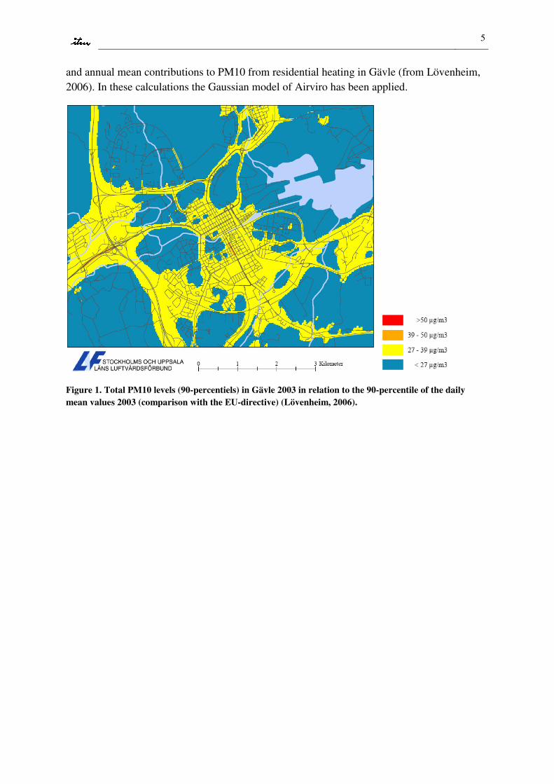
5

and annual mean contributions to PM10 from residential heating in Gävle (from Lövenheim, 2006). In these calculations the Gaussian model of Airviro has been applied.

Figure 1. Total PM10 levels (90-percentiels) in Gävle 2003 in relation to the 90-percentile of the daily

mean values 2003 (comparison with the EU-directive) (Lövenheim, 2006).

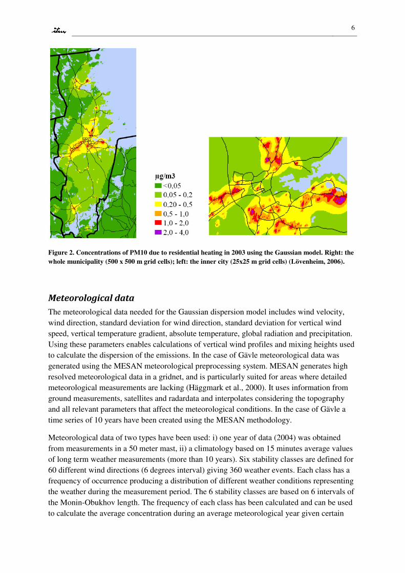
6

Figure 2. Concentrations of PM10 due to residential heating in 2003 using the Gaussian model. Right: the

whole municipality (500 x 500 m grid cells); left: the inner city (25x25 m grid cells) (Lövenheim, 2006).

Meteorological data

The meteorological data needed for the Gaussian dispersion model includes wind velocity, wind direction, standard deviation for wind direction, standard deviation for vertical wind speed, vertical temperature gradient, absolute temperature, global radiation and precipitation. Using these parameters enables calculations of vertical wind profiles and mixing heights used to calculate the dispersion of the emissions. In the case of Gävle meteorological data was generated using the MESAN meteorological preprocessing system. MESAN generates high resolved meteorological data in a gridnet, and is particularly suited for areas where detailed meteorological measurements are lacking (Häggmark et al., 2000). It uses information from ground measurements, satellites and radardata and interpolates considering the topography and all relevant parameters that affect the meteorological conditions. In the case of Gävle a time series of 10 years have been created using the MESAN methodology.

Meteorological data of two types have been used: i) one year of data (2004) was obtained from measurements in a 50 meter mast, ii) a climatology based on 15 minutes average values of long term weather measurements (more than 10 years). Six stability classes are defined for 60 different wind directions (6 degrees interval) giving 360 weather events. Each class has a frequency of occurrence producing a distribution of different weather conditions representing the weather during the measurement period. The 6 stability classes are based on 6 intervals of the Monin-Obukhov length. The frequency of each class has been calculated and can be used to calculate the average concentration during an average meteorological year given certain

7

emissions. This means that we have a statistical set of weather events representative for a long time period (15 years). The purpose with the climatology simulation is to assess long term impacts on air quality of emission scenarios, without having to run very long time periods every time.

The meteorological data is input to a wind model. Both the Gaussian model and the grid model use wind fields originating from the diagnostic wind model (built-in as part of the Airviro system). The wind field for the whole model domain is calculated based on the concept first described by Danard (1976). This concept assumes that small scale winds can be seen as a local adaptation of large scale winds (free winds) due to local fluxes of heat and momentum from the sea or earth surface. Any non-linear interaction between the scales is neglected. It is also assumed that the adaptation process is very fast and that horizontal processes can be described by non-linear equations while the vertical processes can be parameterised as linear functions. The large scale winds as well as vertical fluxes of momentum and temperature are estimated from profile measurements in one or several meteorological masts (called principal masts). For the model domain analysed in this study (35 km2) only one principal mast is used. This is located in the southern part of the city. Topography and land use data for the Danard model are given by 500 meter resolution. Since the topography of Gävle relatively smooth, without dominating ridges or valleys, the free wind can be assumed to be horizontally uniform in the whole domain. For a detailed description of the wind model equations (stability and turbulence parameterisations, meteorological pre-processing, the terrain-following co-ordinate system and the numerical methods) it is referred to the Airviro documentation (http://airviro.smhi.se).

Calculation domain and resolutions

The horizontal resolution has been varied: 250, 500, 1000 meters. In the vertical the gridmodel calculations is performed using a terrain-following system with 5 layers. This means that the depth of the layers may vary depending on topography and surface roughness. In central Gävle the levels are: 0-2, 2-11.9, 11.9-59.3, 59.3-253.6 and 253.6-800 meters.

8

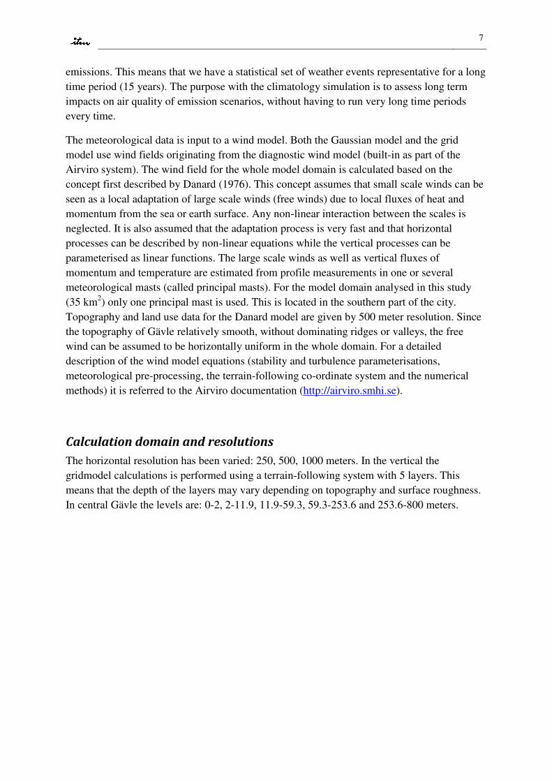
Figure 1. Point sources in calculation area. Figure 2. Point sources in Central Gävle.

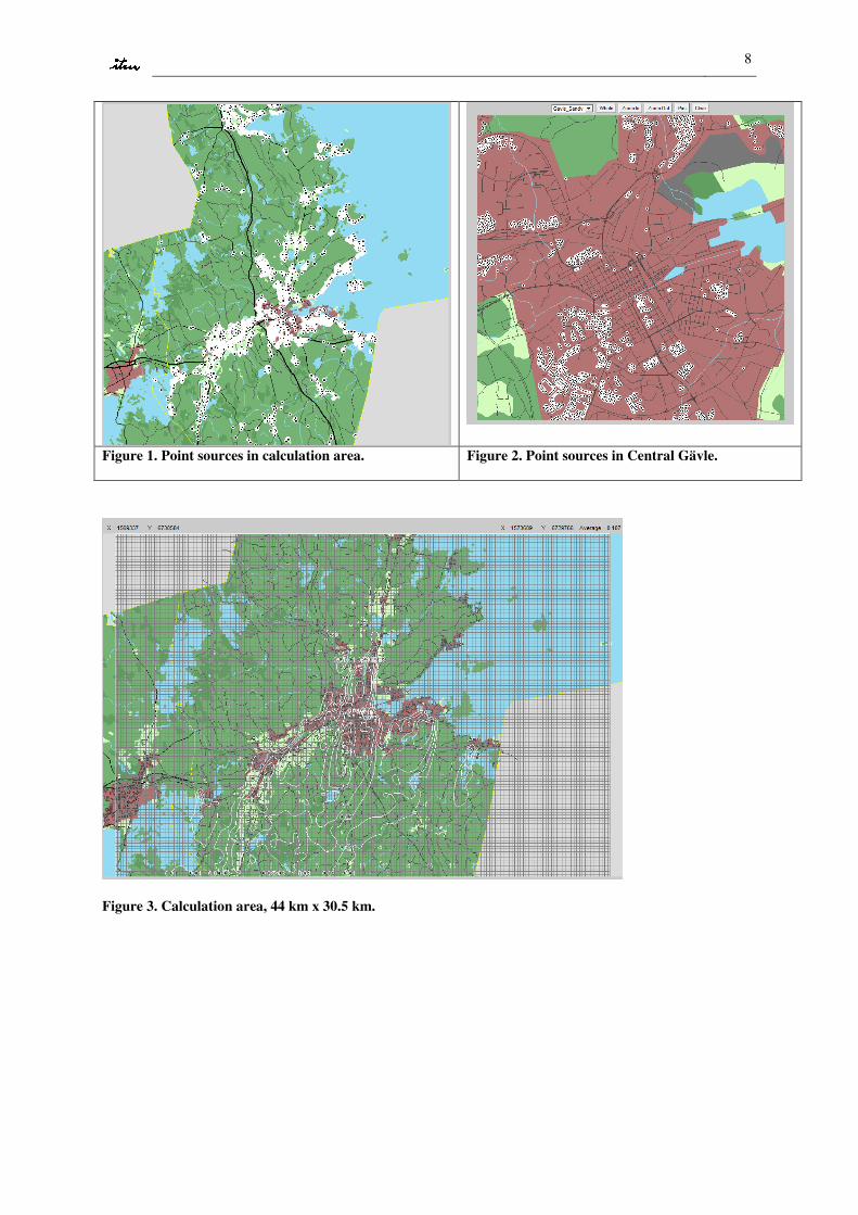
Figure 3. Calculation area, 44 km x 30.5 km.

9

Calculation grid (250 m x 250 m), with the receptorpoint at Drottninggatan indicated by a red dot.

Results

The assessment of the importance for calculated concentrations are based either on a time series of meteorological data (January 2004 or the whole year of 2004) or on the climatology, which consist of 360 weather conditions (see above). The reason for performing the assessment on different meteorological data sets is to ensure that the conclusions are not biased due to meteorology.

Assessment based on real time meteorology for one winter month

Calculated NOx concentrations for January 2004 from the two source types using the grid and Gaussian model are compared in Table 2. Identical calculation areas with 176x122 grid cells and a horizontal resolution of 250 meters have been used in these calculations.

The ratios of the concentrations as obtained from the two different models are presented in Table 3. This shows that the Grid model gives on average higher values by a factor 2.41 as

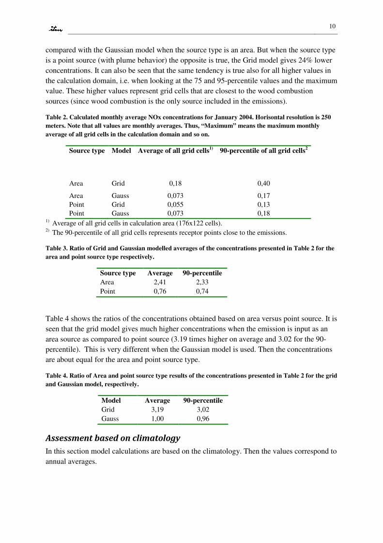
10

compared with the Gaussian model when the source type is an area. But when the source type is a point source (with plume behavior) the opposite is true, the Grid model gives 24% lower concentrations. It can also be seen that the same tendency is true also for all higher values in the calculation domain, i.e. when looking at the 75 and 95-percentile values and the maximum value. These higher values represent grid cells that are closest to the wood combustion sources (since wood combustion is the only source included in the emissions).

Table 2. Calculated monthly average NOx concentrations for January 2004. Horisontal resolution is 250

meters. Note that all values are monthly averages. Thus, “Maximum” means the maximum monthly

average of all grid cells in the calculation domain and so on.

Source type Model Average of all grid cells1) 90-percentile of all grid cells2

Area Grid 0,18 0,40

Area Gauss 0,073 0,17 Point Grid 0,055 0,13 Point Gauss 0,073 0,18

1) Average of all grid cells in calculation area (176x122 cells). 2) The 90-percentile of all grid cells represents receptor points close to the emissions.

Table 3. Ratio of Grid and Gaussian modelled averages of the concentrations presented in Table 2 for the

area and point source type respectively.

Source type Average 90-percentile

Area 2,41 2,33 Point 0,76 0,74

Table 4 shows the ratios of the concentrations obtained based on area versus point source. It is seen that the grid model gives much higher concentrations when the emission is input as an area source as compared to point source (3.19 times higher on average and 3.02 for the 90-percentile). This is very different when the Gaussian model is used. Then the concentrations are about equal for the area and point source type.

Table 4. Ratio of Area and point source type results of the concentrations presented in Table 2 for the grid

and Gaussian model, respectively.

Model Average 90-percentile

Grid 3,19 3,02 Gauss 1,00 0,96

Assessment based on climatology

In this section model calculations are based on the climatology. Then the values correspond to annual averages.

11

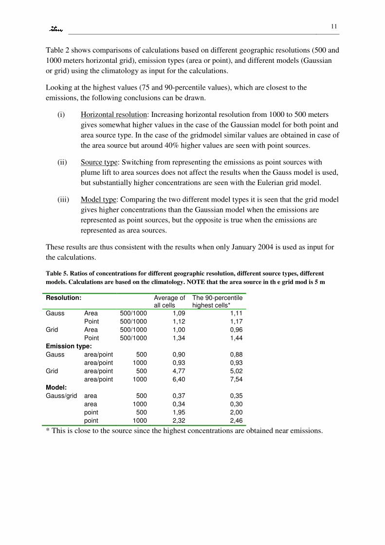
Table 2 shows comparisons of calculations based on different geographic resolutions (500 and 1000 meters horizontal grid), emission types (area or point), and different models (Gaussian or grid) using the climatology as input for the calculations.

Looking at the highest values (75 and 90-percentile values), which are closest to the emissions, the following conclusions can be drawn.

(i) Horizontal resolution: Increasing horizontal resolution from 1000 to 500 meters gives somewhat higher values in the case of the Gaussian model for both point and area source type. In the case of the gridmodel similar values are obtained in case of the area source but around 40% higher values are seen with point sources.

(ii) Source type: Switching from representing the emissions as point sources with plume lift to area sources does not affect the results when the Gauss model is used, but substantially higher concentrations are seen with the Eulerian grid model.

(iii) Model type: Comparing the two different model types it is seen that the grid model gives higher concentrations than the Gaussian model when the emissions are represented as point sources, but the opposite is true when the emissions are represented as area sources.

These results are thus consistent with the results when only January 2004 is used as input for the calculations.

Table 5. Ratios of concentrations for different geographic resolution, different source types, different

models. Calculations are based on the climatology. NOTE that the area source in th e grid mod is 5 m

Resolution: Average of all cells

The 90-percentile highest cells*

Gauss Area 500/1000 1,09 1,11

Point 500/1000 1,12 1,17

Grid Area 500/1000 1,00 0,96

Point 500/1000 1,34 1,44

Emission type:

Gauss area/point 500 0,90 0,88

area/point 1000 0,93 0,93

Grid area/point 500 4,77 5,02

area/point 1000 6,40 7,54

Model:

Gauss/grid area 500 0,37 0,35

area 1000 0,34 0,30

point 500 1,95 2,00

point 1000 2,32 2,46

* This is close to the source since the highest concentrations are obtained near emissions.

12

0

5

10

15

20

25

0 1 2 3 4 5 6

punkt

area

500 m

0

10

20

30

40

50

60

70

80

0 1 2 3 4 5 6

punkt

area

250 m

0

2

4

6

8

10

12

14

16

18

0 1 2 3 4 5 6

punkt

area

100 m

0-1 1-2 2-3 3-4 >4 m/s

0-1 1-2 2-3 3-4 >4 m/s

0-1 1-2 2-3 3-4 >4 m/s

Wind speed

The Gaussian model was run in small area with only one single source either as point or as area. This was done for three spatial resolutions; 100 m, 250 m and 500 m. The concentrations were calculated for one receptor point close to the source.

At moderate wind speeds up to 3 m/s the point source gives higher concentrations compared to the area source.

At higher wind speeds the area source gives higher values, especially when the spatial resolution is increased. This seems reasonable since then the plume is more efficiently diluted before reaching the ground, while the area source is releases at ground level and will thus have a larger impact on the ground level concentrations.

Discussion

Since a Gaussian model is well suited for chimney plumes, it should do the point source calculations quite reliably. In the Gauss model the centerline plume trajectory is followed to the receptor point. The model is solved analytically.

In the grid model point source plumes are initially treated as Gaussian puffs until their radius reaches 2 times the size of the grid, then the pollutant is released into the 3-D grid volumes that the plume covers. On a small scale less than 100 meter this treatment might not be as good a description of the plume behavior as using the Gaussian plume model (Häggkvist, SMHI, Norrköping, Sweden, pers comm., September 2007).

The Gaussian model assumes stationary conditions for the whole domain and as meteorological conditions may change the Gaussian plume calculation may become invalid at large distances from the source. The results of the grid model on the other hand are more sensitive to both the horizontal and vertical grid resolution. According to Table 5 the grid

Windspeed (m/s)

Concentration at receptor Ratio of point/area

500 m 250 m 100 m

0-1 1,12 1,03 0,44

1-2 1,51 1,54 1,22

2-3 1,58 1,80 1,45

3-4 1,58 0,42 0,33

>4 0,95 0,76 0,50

13

model gives about a factor of 2 higher concentrations as compared to the Gaussian model for point sources irrespective of horizontal resolution for 5 vertical layers at 2.0, 11.9, 59.3, 253.6 and 800 meters.

Both for the Gaussian model and for the grid model the resolution of the calculations determine the extent of the emission from the area sources. Thus, even though the area sources are only 25 meters by 25 meters the emission input in the calculation extend over the same as the size of the horizontal grid resolution. Despite this similarity in the source input the grid model gives a factor 3 or more higher concentration as compared to the Gaussian model.

Conclusions

From a heath assessment and exposure point of view it is important to be able to capture the large gradients in concentrations that might occur in residential areas that have a large number of point emissions of wood smoke. This study only focus on how to best describe the dispersion of pollutants in residential areas.

Considering the emissions as point sources with plume lift or simply as area sources introduces uncertainties depending on what type of model is used

With a Grid model there can be a factor of 3 or more difference

With a Gaussian model it is of less importance

The Airviro Grid model gives

much higher concentrations than the Gaussian model if area sources are used

similar concentrations if point sources with plume lift are used.

It seems that Gaussian models are better suited for describing concentrations and exposure due to wood smoke emissions in residential areas with many point sources (plumes) and were a high spatial resolution is required in order to capture the gradients in the concentrations. The importance of non-stationary conditions has not been assessed in this study, but may be very important in some cities during wintertime.

Acknowledgement

This study was financed by the Nordic Ministry Council under contract 07FOX2 (SRIMPART).

References

Bellander T, Berglind N, Gustavsson P, Jonson T, Nyberg F, Pershagen G, Järup L. Using geographic information systems to assess individual historical exposure to air pollution in Stockholm County. EHP 2001;109(6):633-639.

14

Danard, M., 1977. A Simple Model for Mesoscale Effects of Topography on Surface Winds. Monthly Weather Review.,99,831-839.

Eneroth, K. and Johansson, C., 2006. Exposure – Comparison between measurements and calculations based on dispersion modeling (EXPOSE). LVF 2006:12. SLB analys, Stockholm Environment and Health Protection Administration, Box 8136, 104 20 Stockholm. (http://slb.nu/slb/rapporter/pdf/lvf2006_12.pdf).

Ekman, M., 2007. Luftföroreningar i Stockholms och Uppsala än samt Gävle och Sandviken kommun – Utsläppsdata för år 2005. LVF 2007:9. SLB analys, Stockholm Environment and Health Protection Administration, Box 8136, 104 20 Stockholm. (http://slb.nu/slb/rapporter/pdf/lvf2007_9.pdf).

Gidhagen, L., C. Johansson, J. Langner and V. Foltescu, 2005. Urban scale modeling of particle number concentration in Stockholm. Atmospheric Environment, 39, 1711-1725.

Hanna, S.R., Briggs, G.A. and Hosker Jr, R.P., 1982. ’Handbook on Atmospheric diffusion’, Technical Information center, U.S. Department of Energy.

Häggmark, L., Ivarson, K.-I., Gollvik, S., Olofsson, P.-O., 2000. Mesan, an operational mesoscale analysis system. Tellus, Vol 52A, 1-20.

Johansson, C. and Eneroth, K., 2007. Traffic emissions Socioeconomic valuation and Socioeconomic measures (TESS). Part I. LVF 2007:2. SLB analys, Stockholm Environment and Health Protection Administration, Box 8136, 104 20 Stockholm. (http://slb.nu/slb/rapporter/pdf/lvf2007_2.pdf).

Johansson, C., Hadenius, A., Johansson, P.-Å., and Jonson, T., 1999. The Stockholm study on Health effects of Air Pollution and its Economic Consequences. Part I. NO2 and Particulate Matter in Stockholm. AQMA Report 6:98, Stockholm Environment and Health Protection Administration, Box 38 024, 100 64 Stockholm, Sweden.

Johansson, C., Norman, M., Gidhagen, L. Spatial & temporal variations of particle mass (PM10) and particle number in urban air – Implications for health impact assessment. 2007 Environ. Monit. Assess. vol:127 pages:477-487 DOI:10.1007/s10661-006-9296-4.

Lövenheim, B., 2006. Kartläggnig av kvävedioxid- och partikelhalter (PM10) i Gävle kommun. Jämförelser med miljökvalitetsnormer. LVF 2006:39. SLB analys, Stockholm Environment and Health Protection Administration, Box 8136, 104 20 Stockholm. (http://slb.nu/slb/rapporter/pdf/lvf2006_39.pdf).

Lövenheim, B., Johansson, C. Jonsson, T. and Bellander, T., exponering för partikelhalter (PM10) i Stockholms län. LVF 2007: 17. SLB analys, Stockholm Environment and Health Protection Administration, Box 8136, 104 20 Stockholm. (http://slb.nu/slb/rapporter/pdf/lvf2007_17.pdf).

15

Mukherjee, P. and Viswanathan, S., 2001. ‘Carbon monoxide modelling from transport sources’, Chemosphere 45, pp. 1071-1083.

Murkherjee, P., Viswanathan, S. and Choon, L.C, 2000. ‘Modeling mobile source emissions in presence of stationary sources’, Journal of Hazardous Materials 76, pp. 23-37.

Namdeo, A., Mitchell, G. and Dixon, R., 2002. ‘TEMMS: in integrated package for modelling and mapping urban traffic emissions and air quality’, Environmental Modelling and

Software 17, pp. 177-188.

Nyberg F, Gustavsson P, Järup L, Bellander T, Berglind N, Jakobsson R, Pershagen G. Urban Air Pollution and Lung Cancer in Stockholm. Epidemiology 2000;11(5):487-495.

Rosenlund M, Berglind N, Hallqvist J, Jonsson T, Pershagen G, Bellander T. Long-term Exposure to

Urban Air Pollution and Myocardial Infarction. Epidemiology 2006, 17, 383-390.

16

Appendix 1. Description of the domestic wood burning emission data

base for Gävle

Types of installations

Number of installations Efficiency, %

Environmental pellet stove 625 80

Environmental wood boiler 227 80

Wood boiler 1445 60

Oil boiler 2992 80

Combination boiler, oil or electricity (Oktav/ctc 1100)

62 80

Small wood stove (pleasure heating)

5721 70

Tile 2165 70

Stove for solid fuel 911 70

Sauna stove 103

Cooker, large 81

Cooker, normal 3558

Fireplace 4122

Sum 22 012

Energy supply of each appliance

Assume: 20000 kWh per year (excluding household electricity)

A stove or alike is estimated to give 2000 kWh per year. Based on the energy consultant for Gävle.

Energy supplied for different installations

kWh Ton Bränsle

Miljögodkänd pelletsvedpanna 25000 5,4

Miljögodkänd vedpanna 25000 6,5

Icke miljögodkänd vedpanna 33300 8,7

17

Värmepanna eldad med olja 25000 2,1

Oktav/ctc 1100 (kombipanna olja/el) 50% 25000 1,1

Lokaleldstäder 2857 0,74

Det finns installationer med identiska koordinater. För dessa har x-koordinaten förskjutits 1 meter. Vi räknar inte med att någon/några lokaleldstäder bidrar till uppvärmningen och därmed reducerar producerad energimängd från Villapannan.

Supporting information in Airviro

Namn

Miljögodkänd pelletsvedpanna Pellets

Miljögodkänd vedpanna V_MGA

Vedpanna utan acktank V_MGD

Värmepanna eldad med olja OE

Oktav/ctc 1100 (kombipanna olja/el) OEKpoe

Braskamin L_BK

Kakelugn L_KU

Kamin med fastbränsle L_K

Bastuugn

Spis större L_SS

Spis vanlig L_SV

Öppen spis L_OS

Namnsträngen i Airviro ska innehålla 2 data:

Första positionerna visar typ av installation t ex V_MGA fram till tecknet ”;”

Data 2 inleds med tecknet ”#”, därefter gatuadress.

Exempel: V_Epv;#Timmervägen 4

Då blir det möjligt att söka fram utsläpp utifrån typ av installation och gator.

Info 1: här läggs uppgifter in om installationen är miljögodkänd och har ackumulatortank.

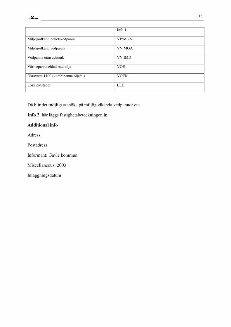
18

Info 1

Miljögodkänd pelletsvedpanna VP:MGA

Miljögodkänd vedpanna VV:MGA

Vedpanna utan acktank VV:IMD

Värmepanna eldad med olja VOE

Oktav/ctc 1100 (kombipanna olja/el) VOEK

Lokaleldstäder LLE

Då blir det möjligt att söka på miljögodkända vedpannor etc.

Info 2: här läggs fastighetsbeteckningen in

Additional info

Adress

Postadress

Informant: Gävle kommun

Miscellaneous: 2003

Inläggningsdatum

19

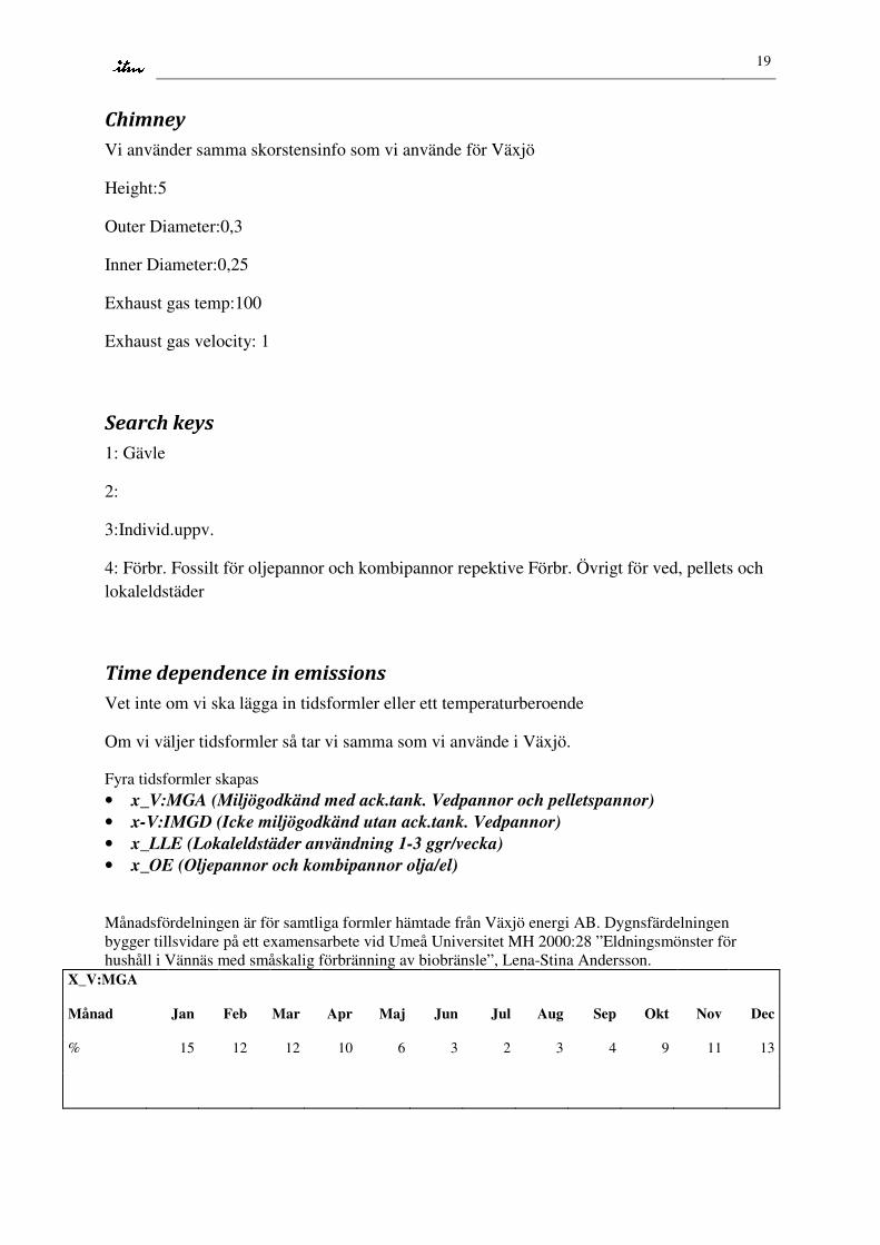
Chimney

Vi använder samma skorstensinfo som vi använde för Växjö

Height:5

Outer Diameter:0,3

Inner Diameter:0,25

Exhaust gas temp:100

Exhaust gas velocity: 1

Search keys

1: Gävle

2:

3:Individ.uppv.

4: Förbr. Fossilt för oljepannor och kombipannor repektive Förbr. Övrigt för ved, pellets och lokaleldstäder

Time dependence in emissions

Vet inte om vi ska lägga in tidsformler eller ett temperaturberoende

Om vi väljer tidsformler så tar vi samma som vi använde i Växjö.

Fyra tidsformler skapas • x_V:MGA (Miljögodkänd med ack.tank. Vedpannor och pelletspannor) • x-V:IMGD (Icke miljögodkänd utan ack.tank. Vedpannor) • x_LLE (Lokaleldstäder användning 1-3 ggr/vecka) • x_OE (Oljepannor och kombipannor olja/el)

Månadsfördelningen är för samtliga formler hämtade från Växjö energi AB. Dygnsfärdelningen bygger tillsvidare på ett examensarbete vid Umeå Universitet MH 2000:28 ”Eldningsmönster för hushåll i Vännäs med småskalig förbränning av biobränsle”, Lena-Stina Andersson.

X_V:MGA

Månad Jan Feb Mar Apr Maj Jun Jul Aug Sep Okt Nov Dec

% 15 12 12 10 6 3 2 3 4 9 11 13

20

Veckodag Mån Till Sönd

Tid 05-09 09-17 17-21

% 50 0 100

X_V:IMGD

Månad Jan Feb Mar Apr Maj Jun Jul Aug Sep Okt Nov Dec

% 15 12 12 10 6 3 2 3 4 9 11 13

Veckodag Mån Till Fred Lö Till Sö

Tid 05-09 9-12 12-17 17-21 05-09 9-12 12-14 14-17 17-21

% 100 28 41 86 100 38 50 38 88

X_LLE

Månad Jan Feb Mar Apr Maj Jun Jul Aug Sep Okt Nov Dec

% 15 12 12 10 6 3 2 3 4 9 11 13

Veckodag Mån Till sönd

Tid 05-14 14-17 17-21

% 0 3 20

X_OE

Månad Jan Feb Mar Apr Maj Jun Jul Aug Sep Okt Nov Dec

% 15 12 12 10 6 3 2 3 4 9 11 13

Veckodag Mån Till Sö

Tid 01-24

% 100

Substance groups

Använder samma emissionsfaktorer som i Vedair.

21

Vi behöver max använda oss av 6 grupper med tanke på befintlig kunskap om installationerna i Gävle. Vi läggar bara in dessa 6 grupper?

• x_LLE • x_V:MGA(miljögokänd med acktank) • x_V:IMGD(icke miljögodkänd utan acktank) • x_PEt • x_OE

Namn x_LLE Namn x_V:MGA

PM10 0,059 % PM10 0,035 %

Nox 0,11 % Nox 0,13 %

Bensen 7,4 % Bensen 3,8 %

CO 2,2 % CO 2,07 %

VOC 0 % VOC 0,06 %

Metan 0 % Metan 0,08 %

PAH 1656 % PAH 2346 %

Bezoapyrene 11 % Bezoapyrene 8 %

Namn x_IMGD Namn x_OE

PM10 1,79 % PM10 0,037 %

Nox 0,05 % Nox 0,16 %

Bensen 71,7 % Bensen 0,12 %

CO 16,5 % CO 0,023 %

VOC 2,76 % VOC 0,002 %

Metan 2,89 % Metan 0,002 %

PAH 165600 % PAH 378 %

Bezoapyrene 317 % Bezoapyrene 2 %

Namn x_PE

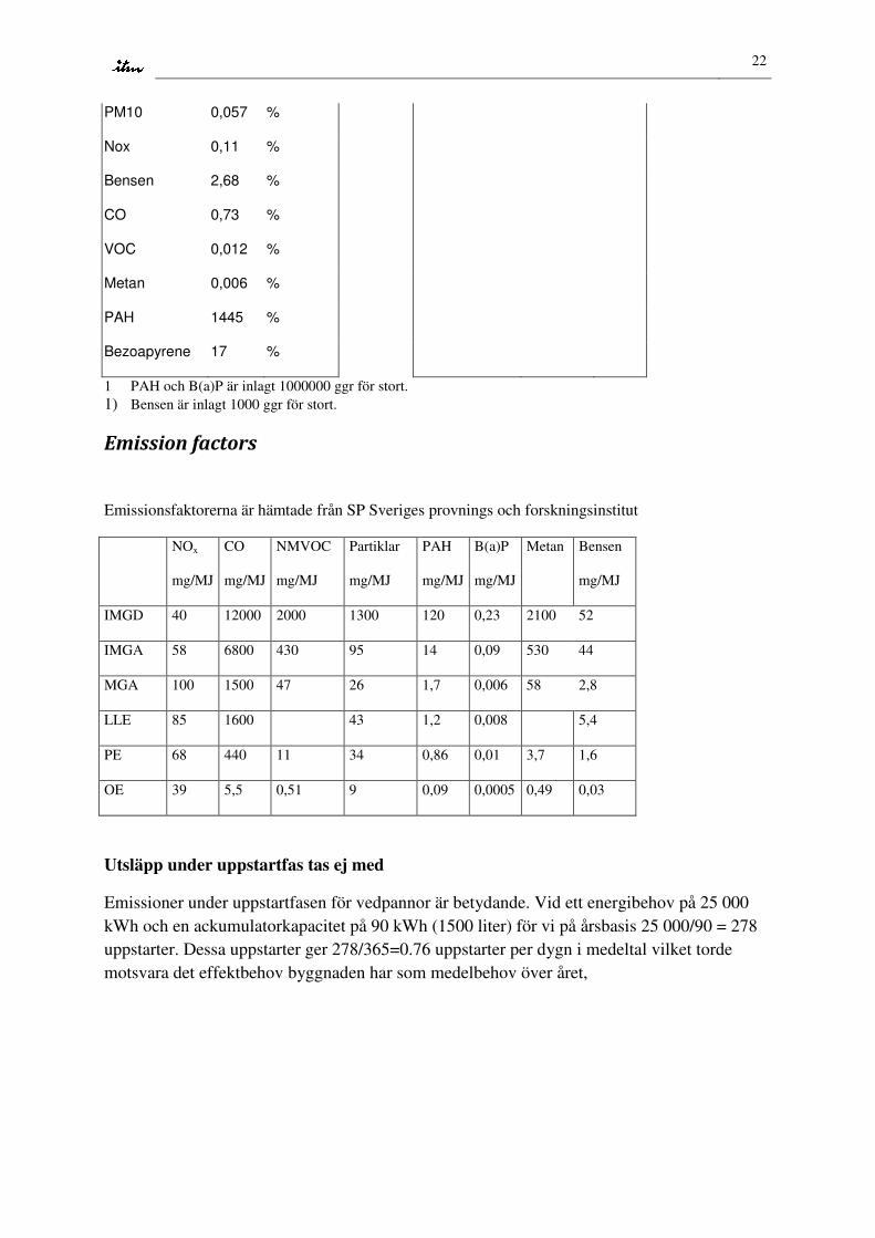
22

PM10 0,057 %

Nox 0,11 %

Bensen 2,68 %

CO 0,73 %

VOC 0,012 %

Metan 0,006 %

PAH 1445 %

Bezoapyrene 17 %

1 PAH och B(a)P är inlagt 1000000 ggr för stort. 1) Bensen är inlagt 1000 ggr för stort.

Emission factors

Emissionsfaktorerna är hämtade från SP Sveriges provnings och forskningsinstitut

NOx

mg/MJ

CO

mg/MJ

NMVOC

mg/MJ

Partiklar

mg/MJ

PAH

mg/MJ

B(a)P

mg/MJ

Metan Bensen

mg/MJ

IMGD 40 12000 2000 1300 120 0,23 2100 52

IMGA 58 6800 430 95 14 0,09 530 44

MGA 100 1500 47 26 1,7 0,006 58 2,8

LLE 85 1600 43 1,2 0,008 5,4

PE 68 440 11 34 0,86 0,01 3,7 1,6

OE 39 5,5 0,51 9 0,09 0,0005 0,49 0,03

Utsläpp under uppstartfas tas ej med

Emissioner under uppstartfasen för vedpannor är betydande. Vid ett energibehov på 25 000 kWh och en ackumulatorkapacitet på 90 kWh (1500 liter) för vi på årsbasis 25 000/90 = 278 uppstarter. Dessa uppstarter ger 278/365=0.76 uppstarter per dygn i medeltal vilket torde motsvara det effektbehov byggnaden har som medelbehov över året,

ISSN 1103-341X ISRN SU-ITM-R-185-SE

DEPARTMENT OF APPLIED ENVIRONMENTAL SCIENCE

STOCKHOLM UNIVERSITY

106 91 STOCKHOLM

Telefon 08-674 70 00 vx - Fax 08-674 72 39