Digital Creativity 2005, Vol. 16, No. 2, pp. 79–92

1462-6268/05/1602-0078$16.00

1 Introduction

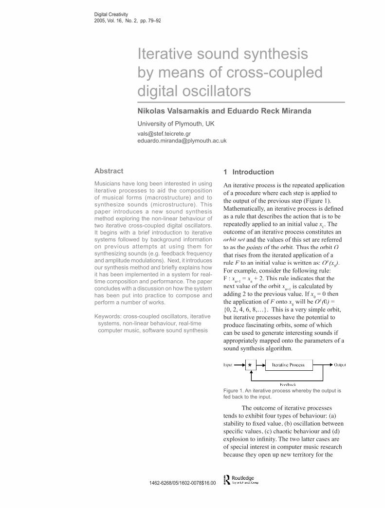
An iterative process is the repeated application of a procedure where each step is applied to the output of the previous step (Figure 1). Mathematically, an iterative process is defi ned as a rule that describes the action that is to be repeatedly applied to an initial value x

0. The

outcome of an iterative process constitutes an orbit set and the values of this set are referred orbit set and the values of this set are referred orbit setto as the points of the orbit. Thus the orbit Othat rises from the iterated application of a rule F to an initial value is written as: F to an initial value is written as: F OFOFO (x

0)

0)

0.

For example, consider the following rule: F : x

n+1 = x

n + 2. This rule indicates that the

next value of the orbit xn+1

is calculated by adding 2 to the previous value. If x

0 = 0 then

the application of F onto F onto F x0 will be OFOFO (0(0( ) = 0) = 0

{0, 2, 4, 6, 8,…}. This is a very simple orbit, but iterative processes have the potential to produce fascinating orbits, some of which can be used to generate interesting sounds if appropriately mapped onto the parameters of a sound synthesis algorithm.

Figure 1. An iterative process whereby the output is fed back to the input.

The outcome of iterative processes tends to exhibit four types of behaviour: (a) stability to fi xed value, (b) oscillation between specifi c values, (c) chaotic behaviour and (d) explosion to infi nity. The two latter cases are of special interest in computer music research because they open up new territory for the

Iterative sound synthesis by means of cross-coupled digital oscillatorsNikolas Valsamakis and Eduardo Reck Miranda

University of Plymouth, UK

vals@stef.teicrete.greduardo.miranda@plymouth.ac.uk

Abstract

Musicians have long been interested in using iterative processes to aid the composition of musical forms (macrostructure) and to synthesize sounds (microstructure). This paper introduces a new sound synthesis method exploring the non-linear behaviour of two iterative cross-coupled digital oscillators. It begins with a brief introduction to iterative systems followed by background information on previous attempts at using them for synthesizing sounds (e.g. feedback frequency and amplitude modulations). Next, it introduces our synthesis method and briefl y explains how it has been implemented in a system for real-time composition and performance. The paper concludes with a discussion on how the system has been put into practice to compose and perform a number of works.

Keywords: cross-coupled oscillators, iterative systems, non-linear behaviour, real-time computer music, software sound synthesis

Dig

ital C

reat

ivity

, Vol

. 16,

No.

2Valsamakis and Miranda

80

exploration of new composition methods and synthesis techniques. There have been a number of attempts at exploring the behaviour of iterative processes in music, notably those exhibiting chaotic behaviour (Pressing 1988; Bidlack 1992). A brief survey on the application of iterative processes in musical composition can be found in Miranda (2001). Less attention has been paid, however, to the potential of iterative processes for sound synthesis. The chaotic iterative processes that have been studied in sound synthesis include the sine map (F : F : F xn+1 = sin(r x xn), where r is r is ra scaling constant) and the logistic map (F: xn+1 = r x xn x (1 - xn), where r is a constant r is a constant rrepresenting the growth rate), both explored by Di Scipio (1996, 2002). There is also the Mandelbrot set (F : F : F xn+1 = xn

2 + c, where c is a complex constant), which has been explored by Dobson and Fitch (1995). In these cases, the orbits are either used to control the parameters of sound synthesis algorithms or are relayed directly as sound samples. This paper, however, presents a slightly different approach to exploring iterative processes in sound synthesis: the function F is replaced by F is replaced by Fa digital oscillator.

2 Feedback digital oscillators

The digital oscillator is a fundamental component in many sound synthesis systems (Miranda 2002). As implemented on a computer, a digital oscillator often works by repeating a template waveform, stored on a lookup table. The speed at which the lookup table is scanned defi nes the frequency of the sound. Although this waveform does not necessarily need to be a sinusoid, for the sake of clarity we have chosen to focus solely on sinusoidal oscillators in this paper.

An oscillator normally requires the specifi cation of three parameters: frequency, amplitude and phase. An iterative process is created if the output of an oscillator is fed

back to one of its own inputs. Two types of iterative processes like this have been explored in sound synthesis technology, depending on the input to which the output of the oscillator is fed back: Feedback Amplitude Modulation (FAM), if the oscillatorʼs output is fed back to its own amplitude [1] and Feedback Frequency Modulation (FFM), if the oscillatorʼs output is fed back to its own frequency [2]:

where fxfxf is the frequency of the sine wave x is the frequency of the sine wave xoscillator and I is the modulation index, or in I is the modulation index, or in Ithis case, the feedback factor. In equation [2] the product (I x fxfxf ) is the amount of frequency deviation from the carrier frequency. In equation [1] the feedback signal is converted from bipolar to unipolar. This is a case of classic amplitude modulation where the modulating signal takes only positive values in the range between 0 and 1. To accomplish this conversion, an offset +1 is added to the bipolar signal, which is then normalised by dividing by two.

Risset was probably the fi rst to employ a feedback oscillator in sound synthesis in the late 1960s at Bell Telephone Laboratories in the USA. In 1969 he published an algorithm where the output of the oscillator was fed back to its own amplitude input, resulting in FAM (Risset 1969). Various implementations of feedback oscillators have appeared since then, including an FFM scheme patented by Yamaha (Chowning et al. 1986).

3 Cross-coupled oscillators

We have extended the concepts of FAM and FFM by employing two cross-coupled oscillators instead of a single oscillator. In this

81

Digital C

reativity, Vol. 16, N

o. 2Iterative sound synthesis by means of cross-coupled digital oscillators

where S is the scaling factor: -1 ≤ S is the scaling factor: -1 ≤ S S < 1. If S < 1. If S S = S = S0.5 then the signals from both oscillators are heard with equal contribution to the resulting sound. Values equal to 0.0 or 1.0 output the signal of only one of the oscillators.

4 Auditioning nonlinear phenomena

Cross-coupled oscillators are interesting because they allow for the exploration of nonlinear phenomena to synthesise new sounds with interesting micro-temporal properties that are very diffi cult, if not impossible, to produce using other synthesis methods. In order to gain a better understanding of these phenomena with respect to sound synthesis, we have tested a number of settings on a trial-and-error basis, but in a systematic fashion. We looked primarily for initial values that produced unstable behaviour.

The system displayed the typical nonlinear phenomena that one would normally expect to observe in a dynamic system. Three out of the four types of outcomes for iterative processes mentioned earlier could be observed here: (a) stability to a fi xed value, (b) oscillation between specifi c values, and (c) chaotic behaviour.

From our own subjective assessment, the most interesting of the three confi gurations of cross-coupled oscillators proved to be CFFM. CFHM also produced interesting sounds, probably due to its asymmetrical structure. On the whole, CFAM produced less interesting sounds. From here on our discussion will focus on the CFFM confi guration.

The CFFM confi guration proved to have a strong dependency on the initial conditions, which is a typical characteristic of dynamic systems. There are four different

way, one oscillator functions as the modulator of the other and vice-versa. Two feedback factors, referred to as cross-modulation indices, control the amount of output signal that is fed from one oscillator to the input of the other. At the output stage a scaling factorcontrols the contribution of each oscillator to the synthesised sound.

There can be three possible confi gurations of cross-coupled oscillators: (a) Cross-Feedback Amplitude Modulation

(CFAM)(b) Cross-Feedback Frequency Modulation

(CFFM)(c) Cross-Feedback Hybrid Modulation

(CFHM)Whereas in CFAM the output of an oscillator is fed to the amplitude input of the other, and vice-versa [3], in CFFM the output of an oscillator is fed to the frequency input of the other, and vice-versa [4]. Finally, there is CFHM, where the output of the one oscillator is fed to the amplitude input of the other, while the output of the second oscillator is fed to the frequency input of the fi rst [5]:

where, fx

fx

f and fy

fy

f are the frequencies of the two sine-wave oscillators, and I

x and I

y are the

feedback factors, one for each oscillator.The output scaling factor controls

the amplitude of the signals relayed by each oscillator to the output as follows [6]:

Dig

ital C

reat

ivity

, Vol

. 16,

No.

2Valsamakis and Miranda

82

initial variables: the central frequencies, fx

fx

fand f

yfy

f , of the two oscillators and the feedback factors, I

x and I

y. The two frequencies played

a less signifi cant role in the exhibition of nonlinear phenomena. Most important in this algorithm are the feedback factors I

x and I

y,

where even subtle changes (e.g. ~0.001 %) are capable of producing completely different sounds.

Stability to a fi xed value produced monotonous buzz-like sounds commonly

found in standard AM and FM synthesis. The stabilisation of the system emerged from either the fi rst iteration or after some cycles. In the latter case, the number of iterations the system needed to stabilise was unpredictable. Stabilisation often occurred when experimenting with small values for the feedback factors, I

x and I

y, but also occurred

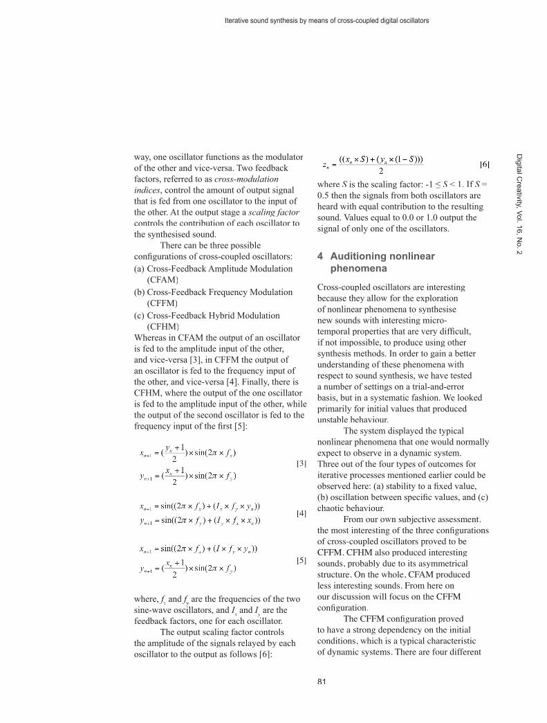
unexpectedly with larger values. This is, however, a general property of dynamic systems: regions of order can be found within chaos as well as chaos emerging within areas of order. The spectrogram of a sound from this class of behaviour is shown in Figure 2. This sound exhibits initial chaotic behaviour and after around 700 milliseconds it stabilises

unexpectedly to a fi xed spectrum. The values producing this sound were: fxfxf =60Hz, fy, fy, f = 60Hz, Ix= 10.58, I

y= 10.58, I

y= 10.58, I = 18, S = 0.5.

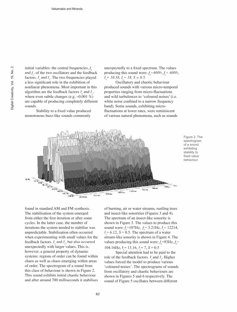
Oscillatory and chaotic behaviour produced sounds with various micro-temporal properties ranging from micro-fl uctuations and wild turbulences to ‘coloured noises’ (i.e. white noise confi ned to a narrow frequency band). Some sounds, exhibiting micro-fl uctuations at lower rates, were reminiscent of various natural phenomena, such as sounds

of burning, air or water streams, rustling trees and insect-like sonorities (Figures 3 and 4). The spectrum of an insect-like sonority is shown in Figure 3. The values to produce this sound were: fxfxf =107Hz, fy fy f = 3.21Hz, Ix= 12214, I

y= 6.12, S = 0.5. The spectrum of a water S = 0.5. The spectrum of a water S

stream-like sonority is shown in Figure 4. The values producing this sound were: fxfxf =93Hz, fyfyf =

104.16Hz, Ix= 13.16, Iy= 7, S = 0.5S = 0.5S

Special attention had to be paid to the role of the feedback factors, Ix and I

y. Higher

values forced the model to produce various ʻcoloured noisesʼ. The spectrograms of sounds from oscillatory and chaotic behaviours are shown in Figures 5 and 6 respectively. The sound of Figure 5 oscillates between different

Figure 2. The spectrogram of a sound exhibiting stability to fi xed value behaviour.

83

Digital C

reativity, Vol. 16, N

o. 2Iterative sound synthesis by means of cross-coupled digital oscillators

spectral confi gurations. The values producing this sound were: fxfxf =60Hz, fy, fy, f = 30Hz, I

x= 42,

Iy= 9.5, S = 0.5.

The sound of Figure 6 exhibits chaotic behaviour and has a coloured noise spectrum. Interestingly, there are short moments of order when the sound settles to a specifi c harmonic spectrum before returning to chaos. The values producing this sound were: fxfxf =420Hz, fy, fy, f = 420Hz, I

x= 1.7, I

y= 1.7, I

y= 1.7, I = 1.16, S = 0.5.

5 Making interactive music with iterative sound synthesis

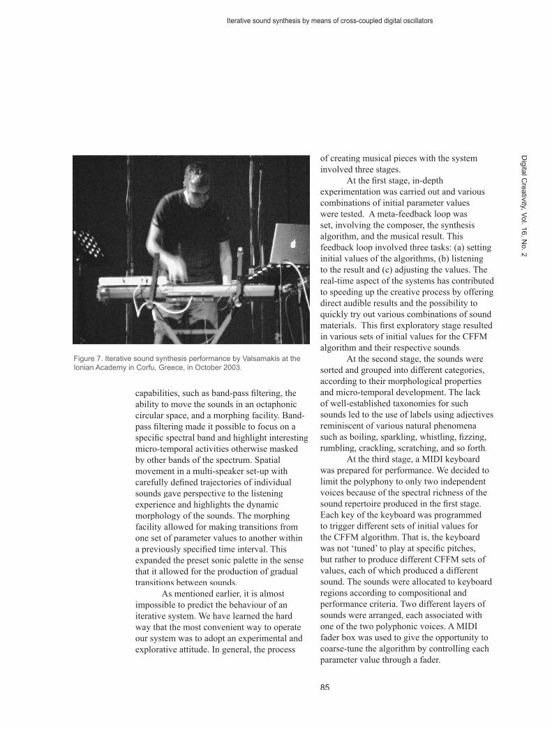
In the following paragraphs we introduce a case study where the coupled-feedback oscillators technique has been implemented in a system for real-time composition and performance. The system has been used extensively by Valsamakis to compose and perform at a number of international festivals and concerts (Figure 7).

Figure 4. The spectrogram of a water stream-like sound.

Figure 3. The spectrogram of an insect-like sound.

Dig

ital C

reat

ivity

, Vol

. 16,

No.

2Valsamakis and Miranda

84

Composition with iterative sound synthesis belongs to the territory of non-standard synthesis where the sound-generating process does not rely on the simulation of a pre-existing acoustical model, as is the case with Physical Modelling, Additive, FM, AM and other standard techniques, but on a network of relations between a set of machine instructions. It is a ‘bottom-up’ composition approach where the morphological properties emerge from an abstract model of sound construction. The compositional process is applied directly to the microstructure level of sound. Historically, non-standard synthesis has

been used by composers such as H. Brün, G. M. Koening and I. Xenakis, and more recently by P. Berg, A. Di Scipio, A. Chandra and M. Hamman.

Only CFFM was implemented in this system and the chosen platform was the Max/MSP programming environment running Max/MSP programming environment running Max/MSPon a Macintosh PowerBook, under Mac OS X. There is no specifi c technical reason for choosing this platform apart from personal preference. The core of the instrument is shown in Figure 8.

A few extra features were added to the core CFFM algorithm in order to add extra

Figure 6. The spectrogram of a sound exhibiting “chaotic” behaviour.

Figure 5. The spectrogram of a sound exhibiting “oscillatory” behaviour.

85

Digital C

reativity, Vol. 16, N

o. 2Iterative sound synthesis by means of cross-coupled digital oscillators

Figure 7. Iterative sound synthesis performance by Valsamakis at the Ionian Academy in Corfu, Greece, in October 2003.

capabilities, such as band-pass fi ltering, the ability to move the sounds in an octaphonic circular space, and a morphing facility. Band-pass fi ltering made it possible to focus on a specifi c spectral band and highlight interesting micro-temporal activities otherwise masked by other bands of the spectrum. Spatial movement in a multi-speaker set-up with carefully defi ned trajectories of individual sounds gave perspective to the listening experience and highlights the dynamic morphology of the sounds. The morphing facility allowed for making transitions from one set of parameter values to another within a previously specifi ed time interval. This expanded the preset sonic palette in the sense that it allowed for the production of gradual transitions between sounds.

As mentioned earlier, it is almost impossible to predict the behaviour of an iterative system. We have learned the hard way that the most convenient way to operate our system was to adopt an experimental and explorative attitude. In general, the process

of creating musical pieces with the system involved three stages.

At the fi rst stage, in-depth experimentation was carried out and various combinations of initial parameter values were tested. A meta-feedback loop was set, involving the composer, the synthesis algorithm, and the musical result. This feedback loop involved three tasks: (a) setting initial values of the algorithms, (b) listening to the result and (c) adjusting the values. The real-time aspect of the systems has contributed to speeding up the creative process by offering direct audible results and the possibility to quickly try out various combinations of sound materials. This fi rst exploratory stage resulted in various sets of initial values for the CFFM algorithm and their respective sounds.

At the second stage, the sounds were sorted and grouped into different categories, according to their morphological properties and micro-temporal development. The lack of well-established taxonomies for such sounds led to the use of labels using adjectives reminiscent of various natural phenomena such as boiling, sparkling, whistling, fi zzing, rumbling, crackling, scratching, and so forth.

At the third stage, a MIDI keyboard was prepared for performance. We decided to limit the polyphony to only two independent voices because of the spectral richness of the sound repertoire produced in the fi rst stage. Each key of the keyboard was programmed to trigger different sets of initial values for the CFFM algorithm. That is, the keyboard was not ‘tuned’ to play at specifi c pitches, but rather to produce different CFFM sets of values, each of which produced a different sound. The sounds were allocated to keyboard regions according to compositional and performance criteria. Two different layers of sounds were arranged, each associated with one of the two polyphonic voices. A MIDI fader box was used to give the opportunity to coarse-tune the algorithm by controlling each parameter value through a fader.

Dig

ital C

reat

ivity

, Vol

. 16,

No.

2Valsamakis and Miranda

86

6 Final remarks

Our iterative sound synthesis technique using cross-coupled digital oscillators has proved to be a fruitful tool for exploring the dynamics of non-linear systems in musical composition and performance. Our experiments yielded a large number of different sounds characterised by interesting micro-temporal structures. The morphological properties of these sounds are unique in the sense that they are not likely to be produced by other synthesis techniques.

The implementation discussed in this paper employed only two sinusoidal oscillators. A natural further step in this work would be to expand the iterative idea by adding more inter-modulating oscillators. However, the addition of extra oscillators will increase the number of possible feedback paths and therefore the complexity of the

system and the sounds as a whole. Such complexity would certainly require more sophisticated control methods, possibly using artifi cial intelligence technology supported by powerful numerical methods to analyse complexity.

References

Bidlack, R. (1992) Chaotic systems as simple (but complex) compositional algorithms. Computer Music Journal 16(3) 33–47.

Chowning, J. and Bristow, D. (1986) FM theory and applications for musicians. Yamaha Music Foundation, Tokyo.

Di Scipio, A. and Prignano, I. (1996) Synthesis by functional iterations. a revitalization of nonstandard synthesis. Journal of New Music Research 25(1) 31–46.

Figure 8. The core instrument as implemented in Max/MSP.

87

Digital C

reativity, Vol. 16, N

o. 2Iterative sound synthesis by means of cross-coupled digital oscillators

Di Scipio, A. (2002) The synthesis of environmental sound textures by iterated nonlinear functions, and its ecological relevance to perceptual modeling. Journal of New Music Research 31(2) 109–117.

Dobson, R. and Fitch, J. (1995) Experiments with chaotic oscillators. Proceedings of the 1995 International Computer Music Conference. International Computer Music Association (ICMA), San Francisco, CA, pp. 45–48.

Miranda, E. R. (2002) Computer sound design: synthesis techniques and programming. Elsevier, Oxford.

Miranda, E. R. (2001) Composing music with computers. Focal Press, Oxford.

Peitgen, H-O., Jurgens, H., and Saupe, D. (1992) Chaos and fractals, new frontiers of science. Springer-Verlag, New York.

Pressing, J. (1988) Nonlinear maps as generators of musical design. Computer Music Journal 12(2) 35–46.

Risset, J-C. (1969) An introductory catalogue of computer synthesized sounds. Bell Telephone Laboratories, Murray Hill, New Jersey. Reprinted in The historical CD of digital sound synthesis, Computer Music Currents 13, Wer 2033-2, Schott Wergo Music Media GmbH, Meinz, Germany.

Nikolas Valsamakis is a composer and Lecturer in the Music Technology and Acoustics Department of the Technological Educational Institute of Crete, Greece. He has an MSc in Music Information Technology from City University (London, UK) and is currently studying for a PhD in Computer Music at the University of Plymouth’s School of Computing Communications and Electronics (UK). His research interests are live electroacoustic music composition and performance, sound synthesis and complex systems.

Eduardo Reck Miranda is a composer and Reader in Artifi cial Intelligence and Music at the University of Plymouth (UK), where he is head of Computer Music Research. He has an MSc in Music Technology from the University of York (UK) and a PhD in Music from the University of Edinburgh (UK). His research interests are composition, sound synthesis, new musical interfaces, artifi cial intelligence and evolutionary computation. Dr Miranda is a member of the editorial boards of Leonardo Music Journal and Music Journal and Music Journal Contemporary Music Review, and is the regional editor for Latin America of Organised Sound.Organised Sound.Organised Sound