Embed Size (px)
Citation preview
NUMERICAL ANALYSIS PRO~EC$MANUSCIUPT~NA-91-05
NOVEMBER 1991
Iterative ‘Solution of Linear Systems
bY
Roland W. FkeundGene H. Golub
Noel M. Nachtigal
NUMERICAL ANALYSIS PROJECTCOMPUTER SCIENCE DEPARTMENT. STANFORD UNIVERSITYSTANFORD$ALIFORNIA 94305

Iterative Solution of Linear Systems
Roland W. Freund *RIACS, Mail Stop Ellis StreetNASA Ames Research Center
Moffett Field, CA 94035E-mail: na.fkeundQna-net.oml.gov
Gene H. Golub tComputer Science Department
St anford University _Stanford, CA 9@05
E-mail: [email protected]
N&l M. Nachtigal $RIACS, Mail Stop Ellis StreetNASA Ames Research Center
Moffett Field, CA 94035E-mail: [email protected]
Recent advances in the field of iterative methods for solving large linear sys-tems are reviewed. The main focus is on developments in the area of conjugategradient-type algorithms and Krylov subspace methods for non-Hermitian ma-trices.
CONTENTS1 Introduction2 Background3 Lanczos-based Krylov subspace methods4 Solving the normal equations is not always bad5 Estimating spectra for hybrid methods6 CG-type methods for complex linear systems7 Large dense linear systems8 Concludixig remarks
l References
l The work of this author was supported by DARPA via Cooperative Agreement NCC2-387 between NASA and the Universities Space Research Association (USRA).
+ The work of this author was supported in part by the National Science Foundationunder Grant NSF CCR-8821078.
t The work of this author was supported by Cooperative Agreement NCC 2-387 betweenNASA and the Universities Space Research Association (USRA).
2 R.W. FREUND, G.H. GOLUB AND N.M. NACHTIGAL
1. Introduction
One of the fundamental building blocks of numerical computing is the abilityto solve linear systems
Ax = b. (11).
These systems arise very frequently in scientific computing, for example,from finite difference or finite element approximations to partial differen-tial equations, as intermediate steps in computing the solution of nonlinearproblems, or as subproblems in linear and nonlinear programming.
For linear systems of small size, the standard approach is to use directmethods, such as Gaussian elimination. These algorithms obtain the solu-tion of (1.1) based on a factorization of the coefficient matrix A. However, inpractice linear systems arise that can be arbitrarily large; this is particularlytrue when solving partial differential equations. Fortunately, the resultingsystems usually have some special structure; sparsity, i.e., matrices withonly few nonzero entries, is the most common case. Often, direct methodscan be adapted to exploit the special structure of the matrix and then re-main useful even for large linear systems. However, in many cases, especiallyfor systems arising from three-dimensional partial differential equations, di-rect approaches are prohibitive both in terms of storage requirements andcomputing time, and then the only alternative is to use iterative algorithms.
Especially attractive are iterative methods that involve the coefficient ma-trix only in the form of matrix-vector products with A or AH. Such schemesnaturally exploit the special structure of large sparse linear systems. Theyare also well suited for the solution of certain dense large systems for whichmatrix-vector products can be obtained cheaply. The, most powerful iter-ative scheme of this type is the conjugate gradient method (CG) due toHestenes and Stiefel (1952), which is an algorithm for solving Hermitianpositive definite linear systems. Although CG was introduced as early as1952, its true potential was not appreciated until the work of Reid (1971)and Concus et al. (1976) in the seventies. Since then, a considerable part ofthe research in numerical linear. algebra has been devoted to generalizationsof CG to indefinite and non-Hermitian linear systems.
A straightforward extension to general non-Herr&an matrices is to applyCG to either one of the Hermitian positive definite linear systems
AHAx = AHb,
orAAHy = b, x = AHy. (13).
Solving (1.2) by CG was mentioned already by Hestenes and Stiefel (1952);we will refer to this approach as CGNR. Applying CG to (1.3) was pro-posed by Craig (1955); we will refer to this second approach as CGNE.
(12).
ITERATIVE SOLUTION OF LINEAR SYSTEMS 3
Although there are special situations where CGNR or CGNE are the opti-mal extensions of CG, both algorithms generally converge very slowly andhence they usually are not satisfactory generalizations of CG to arbitrarynon-Hermitian matrices.
Consequently, CG-type algorithms were sought that are applied to theoriginal system (l.l), rather than (1.2) or (1.3). A number of such methodshave been proposed since the mid-seventies, the most widely used of whichis the generalized minimum residual algorithm (GMRES) due to Saad andSchultz (1986). While GMRES’and related schemes generate at each itera-tion optimal approximate solutions of (l.l), their work and storage require-ments per iteration grow linearly. Therefore, it becomes prohibitive to runthe full version of these algorithms and restarts are necessary, which oftenleads to very slow convergence.
For this reason, since the late eighties, research in non-Hermitian matrixiterations has focused mainly on schemes that can be implemented with lowand roughly constant work and storage requirements per iteration. A num-ber of new algorithms with this feature have been proposed, all of whichare related to the nonsymmetric Lanczos process. It is these recent devel-opments in CG-type methods for non-Hermitian linear systems that we willemphasize in this survey.
The outline of this paper is as follows. In Section 2, we present somebackground material on general Krylov subspace methods, of which CG-type algorithms are a special case. We recall the outstanding propertiesof CG and discuss the issue of optimal extensions of CG to non-Hermitianmatrices. We also review GMRES and related methods, as welI as CG-likealgorithms for the special case of Hermitian indefinite linear systems. Fi-nally, we briefly discuss the basic idea of preconditioning. In Section 3, weturn to Lanczos-based iterative methods for general non-Hermitian linearsystems. First, we consider the nonsymmetric Lanczos process, with par-ticular emphasis on the possible breakdowns and potential instabilities inthe classical algorithm. Then we describe recent advances in understandingthese problems and overcoming them by using look-ahead techniques. More-over, we describe the quasi-minimal residual algorithm (QMR) proposed byFreund and Nachtigal(1990), which uses the look-ahead Lanczos process toobtain quasi-optimal approximate solutions. Next, a survey of transpose-free Lanczos-based methods is given. We conclude this section with com-ments on other related work and some historical remarks. In Section 4, weelaborate on CGNR and CGNE and we point out situations where theseapproaches are optimal. The general class of Krylov subspace methods alsocontains parameter-dependent algorithms that, unlike CG-type schemes, re-quire explicit information on the spectrum of the coefficient matrix. InSection 5, we discuss recent insights in obtaining appropriate spectral in-formation for parameter-dependent Krylov subspace methods. After that,
/ 4 R.W. FREUND, G.H. GOLUB AND N.M. NACHTIGAL
we turn to special classes of linear systems. First, in Section 6, we considerCG-type algorithms for complex symmetric and shifted Hermitian matrices.In Section 7, we review cases of dense large linear systems for which iterativealgorithms are a viable alternative to direct methods. Finally, in Section 8,we make some concluding remarks.
Today, the field of iterative methods is a rich and extremely active researcharea, and it has become impossible to cover in a survey paper all recentadvances. For example, we have not included any recent developments inpreconditioning of linear systems, nor any discussion of the efficient use ofiterative schemes on advanced architectures. Also, we would like to point thereader to the following earlier survey papers. Stoer (1983) reviews the stateof CG-like algorithms up to the early eighties. In the paper by Axelsson(1985), the focus is on preconditioning of iterative methods. More moderniterative schemes, such as GMR.ES, and issues related to the implementationof Krylov subspace methods on supercomputers are treated in the surveyby Saad (1989). An annotated bibliography on CG and CG-like methodscovering the period up to 1976 was compiled by Golub and O’Leary (1989).Finally, readers interested in direct methods for sparse linear systems arereferred to the book by Duff et al. (1986) and, for the efficient use of thesetechniques on parallel machines, to Heath et al. (1991).
Throughout the paper, ail vectors and matrices are in general assumed tobe complex. As usual, i = fl. For any matrix M = [ ?njk ], we use thefollowing notation:
M = 1-1 = the complex conjugate of M,MT = [m&j] = the transpose of M,
MH = M’ = the Hermitian of M,ReM = (M +x)/2 = the real part of M,ImM = (M - M)/(2i) = the imaginary part of JN,u ( M ) = the set of singular values of M,
%axw) = the largest singular value of M,
umdw = the smallest singular value of M,
Wll 2 = a,,(M) = the a-norm of M,
~2W) = ~max(M)l~~,(M)= the 2-condition number of M, if M has full rank.
For any vector c E C” and any matrix B E CmXm, we denote by
&(c,B) = span{c,Bc,. . .,P-lc}
the nth Krylov subspace of C”, generated by c and B. Furthermore, we
ITERATIVE SOLUTION OF LINEAR SYSTEMS
use the following notation:
II IIc2 = d& = Euclidean norm of c,
II IICB = A/Pz= B-norm of c, if B is Hermitian positive definite,
X(B) = the set of eigenvalues of B,
Lx(B) = the largest eigenvalue of B, if B is Hermitian,X&(B) = the smallest eigenvalue of B, if B is Hermitian.
Moreover, we denote by In the 71 x n identity matrix; if the dimension 7tis evident from the context, we will simply write I. The symbol 0 will beused both for the number 0 and for the zero matrix; in the latter case, thedimension will always be apparent. We denote by
Pn = {(b(X) = 0, + UJ + l -+u☺� la ,,a ,,...,a ,E C}the set of complex polynomials of degree at most n.
Throughout this paper, N denotes the dimension of the coefficient matrixA of (1.1) and A E CNxN is in general non-Hermit&r. In addition, unlessotherwise stated, A is always assumed to be nonsingular. Moreover, we usethe following notation:
x, = initial guess for the solution of (l.l),*n = nth iterate,rn = b-Ax, = nth residual vector.
If it is not apparent from the context which iterative method we are con-sidering, quantities from different algorithms will be distinguished by super-scripts, e.g., xEG or x,GMRES.
2. BackgroundIn this section, we present some background material on general Krylovsubspace methods.
2.1. Krylov subspace methodsMany iterative schemes for solving the linear system (1.1) belong to the classof Krylov subspace methods: they produce approximations x, to A-lb ofthe form
x, EX,+K,(~,,A), n= 1,2 ,... . (2 1).
Here, x, E CN is any initial guess for the solution of (l.l), r. = b - Ax, isthe corresponding residual vector, and Xn(rO, A) is the nth Krylov subspacegenerated by r. and A. In view of
L(ro*A) = {4(A)ro 14 E Pnwl}, (2 2).
6 R.W. FREUND, G.H. GOLUB AND N.M. NACHTIGAL
schemes with iterates (2.1) are also referred to as polynomial-based iterativemethods. In particular, the residual vector corresponding to the nth iteratex, can be expressed in terms of polynomials:
r, = b - Ax, = &,(A)r,, (2 3).
wheretin E pn9 with tin(O) = 1. (2 4).
Generally, any polynomial satisfying (2.4) is called an nth residual polyno-Illid.
As (2.3) shows, the goal in designing a Krylov subspace method is tochoose at each step the polynomial en such that r, k: 0 in some sense. Oneoption is to actually minimize some norm of the residual r,:
II II.r, =
xaco~(M) lb - Ml(2 5)
l
=
sEp ~o )=l M a 4
Here II l II is a vector norm on CN, which may even depend on the iterationnumber n (see Section 3.3). Another option is to require that the residualsatisfies a Gale&in-type condition:
sHrn = 0 forall SE&, (2 6).
where Sn c CN is a subspace of dimension n. Note that an iterate satisfying(2.6) need not exist for each n; in contrast, the existence of iterates with(2.5) is always guaranteed. The point is that iterates with (2.5) or (2.6) canbe obtained from a basis for &(r,,A) (and a basis for Sn in the case of(2.6)), without requiring any a priori choice of other iteration parameters.
In contrast to parameter-free schemes based on (2.5) or (2.6), parameter-dependent Krylov subspace methods require some advance information onthe spectral properties of A for the construction of &,. Usually, knowledgeof some compact set G with
A(A)EBcC,- O$M, (2 7).
is needed. For example, assume that A is diagonalizable, and let U be anymatrix of eigenvectors of A. For the case of the Euclidean norm, it thenfollows from (2.3) and (2.7) that
(2 8).
Ideally, one would like to choose the residual polynomial +,, such that the
ITERATIVE SOLUTION OF LINEAR SYSTEMS 7
right-hand side in (2.8) is minimal, i.e.,
Unfortunately, the exact solution of the approximation problem (2.9) isknown only for a few special cases. For example, if G is a real interval,then shifted and scaled Chebyshev polynomials are optimal in (2.9); theresulting algorithm is the well-known Chebyshev semi-iterative method forHermitian positive definite matrices (see Golub and Varga, 1961). Later,Manteuffel (1977) extended the Chebyshev iteration to the class of non-Hermitian matrices for which &Z in (2.7) can be chosen as an ellipse. Weremark that, in this case, Chebyshev polynomials are always nearly optimalfor (2.9), but-contrary to popular belief-in general they are not the exact
’solutions of (2.9), as was recently shown by Fischer and Freund (1990,199l).The solution of (2.9) is also known explicitly for complex line segments 6that are parallel to the imaginary axis and symmetric about the real line(see Freund and Ruscheweyh, 1986); this case corresponds to shifted skew-symmetric matrices A of the form (2.14) below. In the general case however,the exact solution of (2.9) is not available and is expensive to compute nu-merically. Instead, one chooses polynomials that are only asymptoticallyoptimal for (2.9). An elegant theory for semi-iterative methods of this typewas developed by Eiermann et ul. (1985).
In this survey, we will focus mainly on parameter-free algorithms with iter-ates characterized by (2.5) or (2.6). Parameter-dependent Krylov subspacemethods will be only briefly discussed in Section 5.
2.2. CG and optimal extensionsClassical CG is a Krylov subspace method for Hermitian positive definitematrices A with two outstanding features. First, its iterates x, satisfy aminimization property, namely (2.5) in the A-l-norm:
IIb - A*nIIA-1 = xExoetro Aj lib - A*IIA-~*n 9(2.10)
Secondly, x, can be computed efficiently,-based on simple three-term recur-rences.
An ideal extension of CG to non-Hermitian matrices A would have similarfeatures. However, since in general II l IlA-1 is no longer a norm, one usuallyreplaces (2.10) with either the minimization property
.lib - AXnll2 = xcQ*tro A) lib - Axll29n *
(2.11)
.
or the Gale&in condition
sH (b - Ax,) = 0 for all s f K,(r,, A). (2.12)
In the sequel, a Krylov subspace algorithm with iterates (2.1) defined by
8 R.W. FREUND, G.H. GOLUB AND N.M. NACHTIGAL
(2.11) or (2.12) will be called a minimal residual (MR) method or an or-thogonal residual (OR) method, respectively. We remark that (2.10) and(2.12) are equivalent for Hermitian positive definite A, and hence (2.12) isan immediate extension of (2.10). Unfortunately, for non-Hermitian A andeven for Hermitian indefinite A, an iterate x, with (2.12) need not exist ateach step n. In contrast, there is always a unique iterate x, E x, + K,( r,, A)satisfying (2.11). We note that the conjugate residual algorithm (CR) dueto Stiefel (1955) is a variant of CG that generates iterates characterized by(2.11) for the special case of Hermitian positive definite A.
An ideal CG-like scheme for solving non-Hermitian linear systems wouldthen have the following features:
(i) its iterates would be characterized by the-MR or OR property, and(ii) it could be implemented based on short vector recursions, so that work
and storage requirements per iteration would be low and roughly con-stant.
Unfortunately, it turns out that, for general matrices, the conditions (i)and (ii) can not be fulfilled simultaneously. This result is due to Faberand Manteuffel (1984, 1987) who proved the following theorem (see alsoVoevodin, 1983, and Joubert and Young, 1987).
Theorem 2.1 (Faber and Manteuffel, 1984 and 1987)Except for a few anomalies, ideal CG-like methods that satisfy both require-ments (i) and (ii) exist only for matrices of the special form
A=e’*(T+d), w h e r e T=TH, t&R, OEC. (2.13)
The class (2.13) consists of just the shifted and rotated Hermitian matri-ces. Note that the important subclass of real nonsymmetric matrices
A = I- S, where S = -ST is real, (2.14)
is contained in (2.13), with eie = i, 0 = -i, and T = is. Concus and Golub(1976) and Widlund (1978) were the first- to devise an implementation of aOR method for the family (2.14). The first MR algorithm for (2.14) wasproposed by .Rapoport (1978), and different implementations were given byEisenstat et ~2. (1983) and Freund (1983). For a brief discussion of actualCG-type algorithms for the general class of complex non-Hermitian matrices(2.14), we refer the reader to Section 6.2.
Finally, we remark that ideal CG-like methods also exist for the moregeneral family of shifted and rotated B-Hermit&n matrices
A=e”(T+aI), where TB = (TB)H, OE R, UE C. (2.15)
Here B is a fixed given Hermitian positive definite N x N matrix (see Ashby
ITERATIVE SOLUTION OF LINEAR SYSTEMS 9
et al., 1990). However, since for any matrix A of the form (2.15),A’ = B’/2AB-‘/2
is of the type (2.13), without loss of generality the case (2.15) can always bereduced to (2.13).
2.3. CG-type algorithms for Hermitian indefinite linear systemci
The family (2.13) also contains Hermitian indefinite matrices; next we reviewCG-type methods for this special case.
Luenberger (1969) was the first to propose a modification of standard CGfor Hermitian indefinite matrices; however, his algorithm encountered someunresolved computational difficulties. The first numerically stable schemesfor Hermitian indefinite linear systems were derived by Paige and Saunders(1975). Their SYMMLQ algorithm is an implementation of the OR ap-proach and hence the immediate generalization of classical CG. As pointedout earlier, an OR iterate x, satisfying (2.12) need not exist for each n, and,in fact, SYMMLQ generates x, only indirectly. Instead of the OR iterates,a second sequence of well-defined iterates xi is updated, from which exist-ing x, can then be obtained cheaply. Paige and Saunders also proposed theMINRES algorithm, which produces iterates defined by the MR property(2.11) and thus can be viewed as an extension of CR to Hermitian indefinitematrices. SYMMLQ and MINRES both use the Hermitian Lanczos recur-sion to generate an orthonormal basis for the Krylov subspaces K,(rO, A),and, like the latter, they can be implemented based on simple three-termrecurrences. We would like to stress that the work of Paige and Saunderswas truly pioneering, in that they were the fist to extend CG beyond theclass of Hermitian positive definite matrices in a numerically stable manner.
SYMMLQ is also closely connected with an earlier algorithm due to Frid-man (1963), which generates iterates xFE E x, + IC,(ArO, A) defined by theminimal error (ME) property
(2.16)
Unfortunately, Fridman’s original implementation of the ME approach is un-stable. Fridman’s algorithm was later rediscovered by Fletcher (1976) whoshowed that, in exact arithmetic, the ME iterate xFE coincides with theauxiliary quantity xk in SYMMLQ. Hence, as a by-product, SYMMLQ alsoprovides a stable implementation of the ME method. Another direct stabi-lization of Fridman’s algorithm was proposed by Stoer and Freund (1982).
Finally, we remark that Chandra (1978) proposed the SYMMBK algo-rithm, which is a slightly less expensive variant of SYMMLQ, and derivedanother stable implementation of the MR method, different from MINRES.
10 R.W. FREUND, G.H. GOLUB AND N.M. NACHTIGAL
2.4. GMRES and related algorithms
We now return to Krylov subspace methods for general non-Hermitian ma-trices. Numerous algorithms for computing the iterates characterized by theMR or OR property (2.11) or (2.12), respectively, have been proposed; seeVinsome (1976), Axelsson (1980,1987), Young and Jea (1980), Saad (1981,1982, 1984), EIman (1982), Saad and Schultz (1985, 1986). Interestingly, asimple implementation of the MR approach was already described in a paperby Khabaza (1963), which is not referenced at all in the recent literature.In view of Theorem 2.1, all these algorithms generally involve long vectorrecursions, and typically work and storage requirements per iteration growlinearly with the iteration index n. Consequently, in practice, one cannotafford to run the full algorithms, and it becomes necessary to use restartsor to truncate the vector recursions.
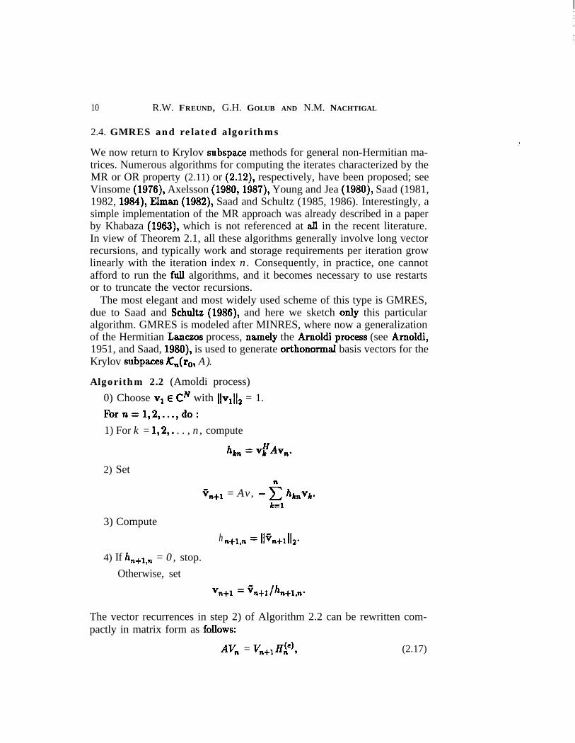
The most elegant and most widely used scheme of this type is GMRES,due to Saad and Schultz (1986), and here we sketch only this particularalgorithm. GMRES is modeled after MINRES, where now a generalizationof the Hermitian Lanczos process, namely the Arnoldiprocess (see Arnold.&1951, and Saad, 1980), is used to generate orthonormal basis vectors for theKrylov subpaces AC,&, A).
Algorithm 2.2 (Amoldi process)0) Choose v1 E CN with Ilvll12 = 1.Fern= 1,2,...,do:1) For k = 1,2,. . . , n, compute
2) Set
iin+l = Av, - 2 hk,,vk.k=l
3) Computehn+l,n = Ilsn+ll12*
4) If hn+l,n = 0, stop.Otherwise, set
vn+l = zin+l lhn+l,n-
The vector recurrences in step 2) of Algorithm 2.2 can be rewritten com-pactly in matrix form as fol.lows:
AV, = vn+l Ht)9 (2.17)
ITERATIVE SOLUTION OF LINEAR SYSTEMS
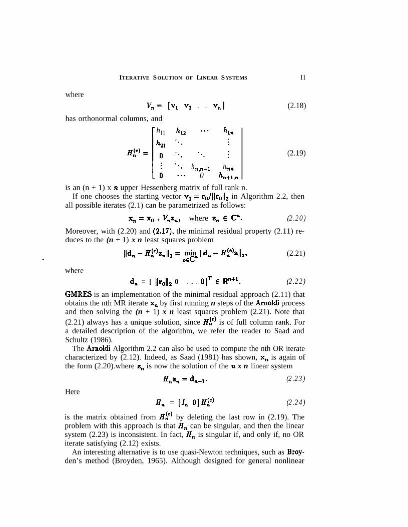
wherevn= [VI v2 l *- vn]
has orthonormal columns, and
r h h,, ..- h,,11
. . . . hn,n-1 hb -0. 0 h,&
11
(2.18)
(2.19)
is an (n + 1) x n upper Hessenberg matrix of full rank n.If one chooses the starting vector vr = ro/ljrol12 in Algorithm 2.2, then
all possible iterates (2.1) can be parametrized as follows:
xn = X, + vnzn9 where z, E Cn. (2.20)
Moreover, with (2.20) and (2.17), the minimal residual property (2.11) re-duces to the (n + 1) x n least squares problem
(2.21)
whered, = [ llrol12 0 l l l OIT E R’? (2.22)
GMRES is an implementation of the minimal residual approach (2.11) thatobtains the nth MR iterate x, by first running n steps of the Arnoldi processand then solving the (n + 1) x n least squares problem (2.21). Note that(2.21) always has a unique solution, since Ht) is of full column rank. Fora detailed description of the algorithm, we refer the reader to Saad andSchultz (1986).
The Arnoldi Algorithm 2.2 can also be used to compute the nth OR iteratecharacterized by (2.12). Indeed, as Saad (1981) has shown, x, is again ofthe form (2.20).where z,, is now the solution of the n x n linear system
H,zn = dn-1. (2.23)
HereH, = [In O]Ht’ (2.24)
is the matrix obtained from Ht’by deleting the last row in (2.19). Theproblem with this approach is that H, can be singular, and then the linearsystem (2.23) is inconsistent. In fact, Hn is singular if, and only if, no ORiterate satisfying (2.12) exists.
An interesting alternative is to use quasi-Newton techniques, such as Broy-den’s method (Broyden, 1965). Although designed for general nonlinear
12 R.W. FREUND, G.H. GOLUB AND N.M. NACHTIGAL
equations, these schemes can be applied to non-Hermitian linear systems asa special case. In addition to the iterates x,, these algorithms also produceapproximations to A-l, updated from step to step by a simple rank-l correc-tion. While these schemes look different at a first glance, they also belongto the class of Krylov subspace methods, as was first observed by Elman(1982). Furthermore, Deuflhard et al. (1990) have demonstrated that Broy-den’s rank-l update combined with a suitable line search strategy leads toan iterative algorithm that is competitive with GMRES. Eirola and Nevan-linna (1989) have proposed two methods based on a different rank-l updateand shown that one of the resulting schemes is mathematically equivalentto GMRES. These algorithms were studied further by Vuik (1990).
2.5. Preconditioned Krylov subspace methods
For the solution of realistic problems, it is crucial to combine Krylov sub-space methods with an efficient preconditioning technique. The basic ideahere is a8 follows. Let M be a given nonsingular N x IV matrix, whichapproximates in *some sense the coefficient matrix A.of the original linearsystem (1.1). Moreover, assume that M is decomposed in the form
M = MlM2. (2.25)
The Krylov subspace method is then used to solve the preconditioned linearsystem
A’x’ = b’, (2.26)
whereA’ = MC’AM,“, b’ = Mi’b, X’ = MAX.
Clearly, (2.26) is equivalent to (1.1). This process generates approximatesolutions of (2.26) of the form
(2.27)
Usually, one avoids the explicit calculation of primed quantities, and insteadone rewrites the resulting algorithm in terms of the corresponding quantitiesfor the original system. For example, iterates and residual vectors for (1.1)and (2.26) are connected by
x, = M,‘xk and r, = MI&. (2.28)
In particular, note that, by (2.27) and (2.28), the resulting approximationsto A-lb are of the form
x, E x, + K,, (M-‘r,, M-‘A) .
We remark that the special cases Ml = I or Ma = I in (2.25) are referred toas right or left preconditioning, respectively. For right preconditioning, by
ITERATIVE SOLUTION OF LINEAR SYSTEMS 13
(2.28), the preconditioned residual vectors coincide with their counterpartsfor the original system. For this reason, right preconditioning is usuallypreferred for MR-type Krylov subspace methods based on (2.11). Moreover,if A has some special structure, the decomposition (2.25) can often be chosensuch that the structure is preserved for A’. For example, for Hermitianpositive definite A this is the case if one sets M2 = My in (2.25).
Obviously, there are two (in general conflicting) requirements for thechoice of the preconditioning matrix M for a given Krylov subspace method.First, M-l should approximate A-l well enough so that the algorithm ap-plied to (2.26) will converge faster than for the original system (1.1). Onthe other hand, preconditioned Krylov subspace methods require at eachiteration the solution of one linear system of the type
M p = q . (2.29)
Moreover, for algorithms that involve matrix-vector products with AT (seeSection 3), one has to solve an additional linear system of the form
M=p = q. (2.30)
Therefore, the preconditioner M needs to be such that linear systems (2.29)respectively (2.30) can be solved cheaply. In this paper, the problem of howto actually construct such preconditioners is not addressed at all. Instead,we refer the reader to the papers by Axelsson (1985) and Saad (1989) foran overview of common preconditioning techniques.
Finally, one more note. In Section 3, explicit descriptions of some Krylovsubspace algorithms are given. For simplicity, we have stated these algo-rithms without preconditioning. It is straightforward to incorporate pre-conditioning by using the transition rules (2.28).
3. Lanczos-based Krylov subspace methodsIn this section, we discuss Krylov subspace met hods that are based on thenonsymmetric Lanczos process..
3.1. The classical Lanczos algorithm and BCG
The nonsymmetric Lanczos method was proposed by Lanczos (1950) as ameans to reduce an arbitrary matrix A E CNxN to tridiagonal form. Onestarts the process with two nonzero vectors vr E CN and w1 E CN and thengenerates basis vectors {vj} for EC,(v,,A) and {vvj} for Kn(wl, AT) suchthat the biorthogonality condition
WjTvk = 1 k= j,0 otherwise, (3 1).
holds. The point is that the two bases can be built with just three-term
14 R.W. FREUND, G.H. GOLUB AND N.M. NACHTIGAL
recurrences, thus requiring minimal amounts of work and storage per step.The complete algorithm is straightforward and can be stated as follows.
Algorithm 3.1 (Classical Lanczos method)0) Choose Or, %, E CN with Gr, G, # 0.
Set v. = w. = 0.For n = 1,2,..., do :1) Compute ijn = *zGn.
If 6n = 0, set L = n - 1 and stop.* 2) Otherwise, choose P,,r, E C with P,r, = Sn.
Set v, = C,,/T,, and w, = dir,,//&. -3) Compute
n = w,TAv,,Gp,, A v - anvn - Pnvn-19iCn+l : ATin - (Y,w, - ~,,w,,~.
If Gn+l = 0 or Gn+r = 0, set L = n and stop.
The particular choice of the coefficients a,, &, and 7, ensures that thebiorthogonality relation (3.1) is satisfied.
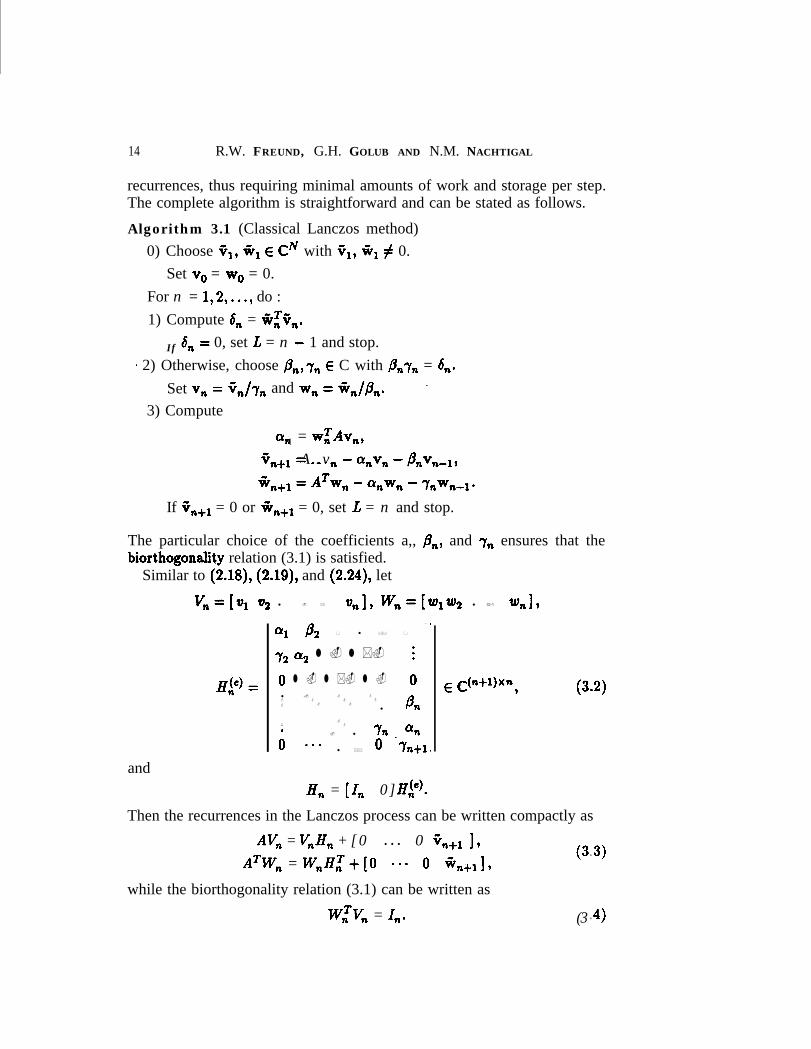
Similar to (2.18), (2.19), and (2.24), let
V,=[tQ tr2 l - * u,], Wn=☯tq
and
a1 & 0 l ** 0 .(
y2 a 2 l . l *. i
0 l . l *. l . 0l . . .. . . .. . .
l Pn
:.
.
;,. l Yn %
. . .l ** O -7n+l,
A, = [In 0] HP).
w, l a 8 wn19
E &+wo 9 (3 2).
Then the recurrences in the Lanczos process can be written compactly as
AV, = V,H, + [ 0 l l l 0 Gn+l 1,ATWn = W,H,T+[O .** 0 *n+l],
(3 3).
while the biorthogonality relation (3.1) can be written as
w,‘v, = In. (3 4).
ITERATIVE SOLUTION OF LINEAR SYSTEMS 15
We note that the Lanczos method is invariant under shifts of the form
A w A + al, where 0 E C,
in that the process generates the same vectors {vj} and {wj} and only thetridiagonal matrix (3.2) is shifted:
Hnw Hn+aIn.
In particular, for the Lanczos algorithm it is irrelevant whether the matrixA is singular or not.
Moreover, we would like to stress that the Lanczos process can also beformulated with AH instead of AT, by simply conjugating the three-termrecurrences for the vectors { wj}. We chose the- transpose because one canthen avoid complex conjugated recurrence coefficients. Finally, we remarkthat the Lanczos process reduces to only one recursion in two importantspecial cases, namely A = AH (with starting vectors +, = q) and complexsymmetric matrices A = AT (with starting vectors G, = 3,). In both cases,one must also choose & = 7,. In the first case, the resulting algorithm isthe well-known Hermitian Lanczos method, which has been studied exten-sively (see, e.g., Golub and Van Loan, 1989, and the references therein). Inthe second case, the resulting algorithm is the complex symmetric Lanczosprocess.
In exact arithmetic, the classical Lanczos method terminates after a finitenumber of steps. As indicated in Algorithm 3.1, there are two different sit-uations in which the process can stop. The first one, referred to as regulartermination, occurs when vL+r = 0 or wL+l = 0. In this case, the Lanc-zos algorithm has found an invariant subspace of CN: if vL+~ = 0, thenthe right Lanczos vectors vr, . . . , vL span an A-invariant subspace, while ifWL+1 -- 0, then the left Lanczos vectors wr , . . . , wL span an AT-invariantsubspace. The second case, referred to as a serious breakdown by Wilkin-son (1965), occurs when wzvL = 0 with neither vL = 0 nor wL = 0. Inthis case, the Lanczos vectors span neither an A-invariant subspace nor anAT-invariant subspace of CN. We will discuss in Section 3.2 techniques forhandling the serious breakdowns. We remark that, in the special case of theHermitian Lanczos process, breakdowns are excluded. In contrast, break-downs can occur in the complex symmetric Lanczos algorithm (see Cullumand Willoughby, 1985, and Freund, 1989b, 1992).
The Lanczos algorithm was originally introduced to compute eigenvalues,as-in view of (3.3)-the eigenvalues of H, can be used as approximationsfor eigenvalues of A. However, Lanczos (1952) also proposed a closely relatedmethod, the biconjugate gradient algorithm (BCG), for solving general non-singular non-Hermitian linear systems (1.1). By and large, BCG was ignoreduntil the mid-seventies, when Fletcher (1976) revived the method.
The BCG algorithm is a Krylov subspace approach that generates iterates
16 R.W. FREUND, G.H. GOLUB AND N.M. NACHTIGAL
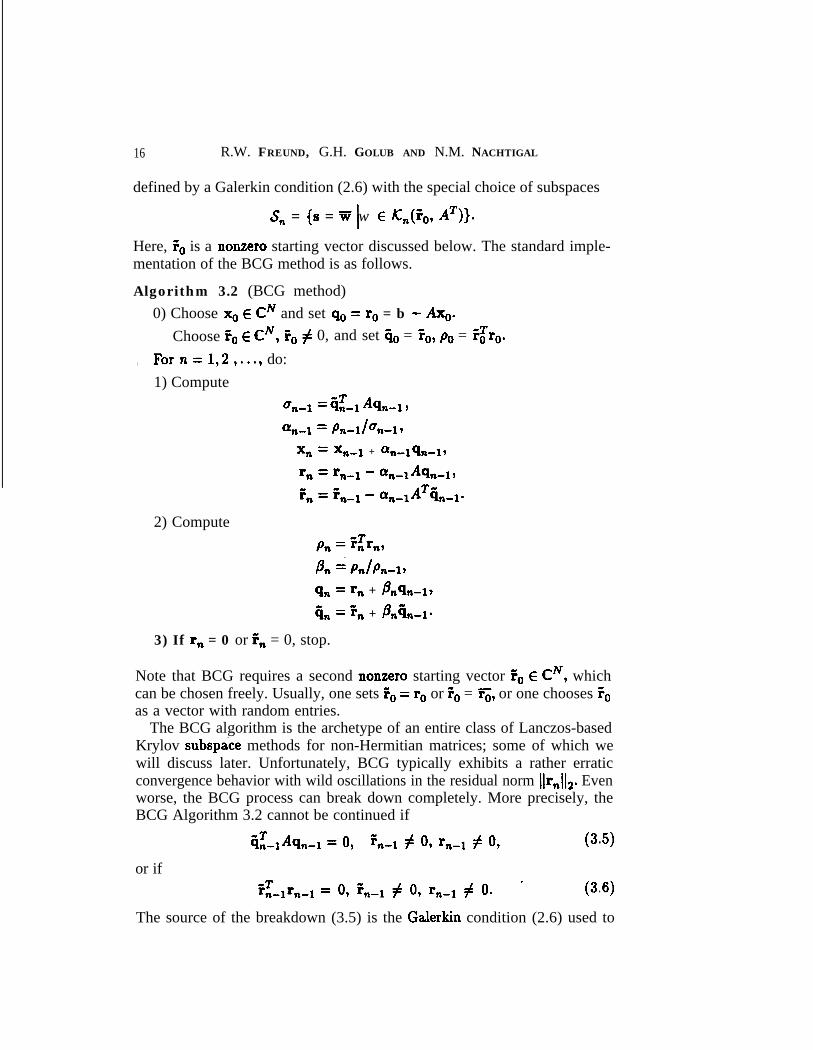
defined by a Galerkin condition (2.6) with the special choice of subspaces
sn = (8 = w w E K,(T,, A=)}.IHere, PO is a nonzero starting vector discussed below. The standard imple-mentation of the BCG method is as follows.
Algorithm 3.2 (BCG method)0) Choose x0 E CN and set q. = r. = b - A-.
Choose f. E CN, f. # 0, and set co = So, p. = ?$ro., Forn=1,2 ,..., do:
1) Compute
un-1 = Cz-1 Aqn-l 9
S-1 = Pn-Iton-
X* = xn-l + an-lQn-l9
r, = rnwl - an-1Aqn-1,
Fn = fn-1 - an-lAT&-l*
2) Compute
Qn = rn + Pnqn-19
iin = En + &k-l*
3) If r, = 0 or En = 0, stop.
Note that BCG requires a second nonzero starting vector f. E CN, whichcan be chosen freely. Usually, one sets To = r. or F. = 5, or one chooses E.as a vector with random entries.
The BCG algorithm is the archetype of an entire class of Lanczos-basedKrylov subspace methods for non-Hermitian matrices; some of which wewill discuss later. Unfortunately, BCG typically exhibits a rather erraticconvergence behavior with wild oscillations in the residual norm Ilrnl12. Evenworse, the BCG process can break down completely. More precisely, theBCG Algorithm 3.2 cannot be continued if
Z-,Aqn-1 = 0, Fn-1 # 0, r,,l # 0, (3 5).
or if-Trn-lrn-l -- 09 Pm-1 # 0, r,-l # 0. ’ (3 6).
The source of the breakdown (3.5) is the Gale&in condition (2.6) used to
ITERATIVE SOLUTION OF LINEAR SYSTEMS 17
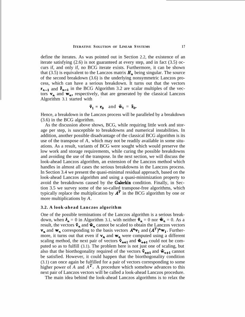
define the iterates. As was pointed out in Section 2.2, the existence of aniterate satisfying (2.6) is not guaranteed at every step, and in fact (3.5) oc-curs if, and only if, no BCG iterate exists. Furthermore, it can be shownthat (3.5) is equivalent to the Lanczos matrix H, being singular. The sourceof the second breakdown (3.6) is the underlying nonsymmetric Lanczos pro-cess, which can have a serious breakdown. It turns out that the vectorsr,-l and en-1 in the BCG Algorithm 3.2 are scalar multiples of the vec-tors v, and w,, respectively, that are generated by the classical LanczosAlgorithm 3.1 started with ’
8, = r. and %, = E,.
Hence, a breakdown in the Lanczos process will be paralleled by a breakdown(3.6) in the BCG algorithm.
As the discussion above shows, BCG, while requiring little work and stor-age per step, is susceptible to breakdowns and numerical instabilities. Inaddition, another possible disadvantage of the classical BCG algorithm is itsuse of the transpose of A, which may not be readily available in some situ-ations. As a result, variants of BCG were sought which would preserve thelow work and storage requirements, while curing the possible breakdownsand avoiding the use of the transpose. In the next section, we will discuss thelook-ahead Lanczos algorithm, an extension of the Lanczos method whichhandles in almost all cases the serious breakdowns in the Lanczos process.In Section 3.4 we present the quasi-minimal residual approach, based on thelook-ahead Lanczos algorithm and using a quasi-minimization property toavoid the breakdowns caused by the Gale&in condition. Finally, in Sec-tion 3.5 we survey some of the so-called transpose-free algorithms, whichtypically replace the multiplication by AT in the BCG algorithm by one ormore multiplications by A.
3.2. A look-ahead Lanczos algorithmOne of the possible terminations of the Lanczos algorithm is a serious break-down, when S, = 0 in Algorithm 3.1, with neither +,, = 0 nor +,, = 0. As aresult, the vectors qn and +, cannot be scaled to obtain the Lanczos vectorsv, and w, corresponding to the basis vectors Anvl and (AT)“wl. Further-more, it turns out that even if v, and w, were computed using a differentscaling method, the next pair of vectors Gn+r and Gn+r could not be com-puted so as to fulfill (3.1). The problem here is not just one of scaling, butalso that the biorthogonality required of the vectors Cin+r and Gn+r cannotbe satisfied. However, it could happen that the biorthogonality condition(3.1) can once again be fulfilled for a pair of vectors corresponding to somehigher power of A and A‘. A procedure which somehow advances to thisnext pair of Lanczos vectors will be called a look-ahead Lanczos procedure.
The main idea behind the look-ahead Lanczos algorithms is to relax the
18 R.W. FREUND, G.H. GOLUB AND N.M. NACHTIGAL
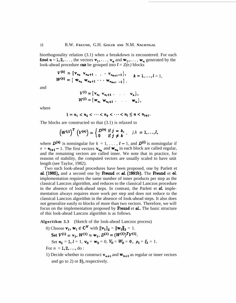
biorthogonality relation (3.1) when a breakdown is encountered. For eachfixed n = l,2,. . . , the vectors vl,. . . , v, and wl,. . . , w, generated by thelook-ahead procedure ca.n be grouped into 2 = Z(n) blocks
v(k) = ivnk vnk+l l l ’ VQ+~-~], k
=W(k) = 1 Wnk wn,+l ’ ’ ’ wnk+, -11 ,
1,...,z- 1,
andV(�)=☯v,, vnl+* l * - v,],
W(�)=☯wnl wr it+* l * * w,],
wherel=nl<n2<“‘<nk<“*<n1<n<n~+le
The blocks are constructed so that (3.1) is relaxed to
(W(j))= (If(‘)) = {f(*) E; z ig , j,k = l,...,Z,
where Dik) is nonsingular for k = 1, . . . , I - 1, and D(‘) is nonsingular ifn = nf+l - 1. The first vectors v,, and wnk in each block are called regular,and the remaining vectors are called inner. We note that in practice, forreasons of stability, the computed vectors are usually scaled to have unitlength (see Taylor, 1982).
Two such look-ahead procedures have been proposed, one by Parlett et~2. (1985), and a second one by Ereund et ul. (1991b). The Freund et al.implementation requires the same number of inner products per step as theclassical Lanczos algorithm, and reduces to the classical Lanczos procedurein the absence of look-ahead steps. In contrast, the Parlett et al. imple-mentation always requires more work per step and does not reduce to theclassical Lanczos algorithm in the absence of look-ahead steps. It also doesnot generalize easily to blocks of more than two vectors. Therefore, we willfocus on the implementation proposed by F’reund et al.. The basic structureof this look-ahead Lanczos algorithm is as follows.
Algorithm 3.3 (Sketch of the look-ahead Lanczos process)0) Choose vl, wl E CN with IlvIl12 = IlwIl12 = 1.
Set V(l) = vl, W(‘) = w*, D(‘) = (W(‘))=V(*).
Set nl = 1,z = 1, ve = we = 0, v, = we = 0, p1 = & = 1.For n = 1,2,..., do :1) Decide whether to construct v,+r and w,+r as regular or inner vectors
and go to 2) or 3), respectively.
ITERATIVE SOLUTION OF LINEAR SYSTEMS
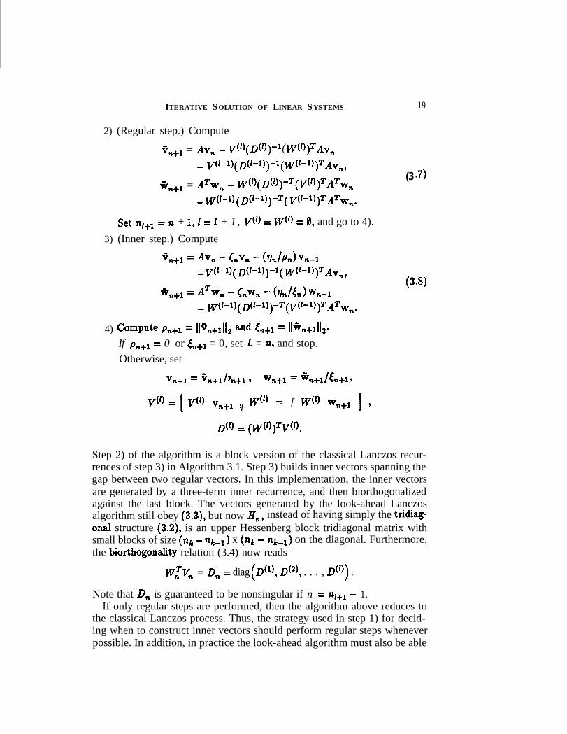
2) (Regular step.) Compute
iin+* = Av, - v(‘) (D(l))-’ ( ~(‘))=Av,- V(‘-‘)(D(‘-‘))-*(W(‘-‘))=Av,,
i%,,+* = A=w, - w(‘)( D(l))-=( V(‘))=A=w,_ w(‘-1) (D(‘-‘I)-=( V(‘-‘))=A=w,.
set nz+1 = n + 1, 2 = 2 + 1, V(‘) = W(‘) = 0, and go to 4).
3) (Inner step.) Compute
+n+l= Avn - CnVn - CSJPnIVn-1- v(‘-‘)( D(‘-*I)-‘( W+‘))=Av,,
*n+l= ATwn - Cnwn - (QJLIWn-1_ w(‘-‘)(D(‘-‘))-=(V(~-‘))=A=~,.
4) Compute Pn+l = llcn+ll12 ad tn+l = Il+n+lll2*
If pn+l = 0 or &+r = 0, set L = n, and stop.Otherwise, set
vn+l = +n+l Pn+l 9I wn+l = *n+l Itn+l9
19
(3 7).
(3 8).
VU) = 1 V(*) V,+* 9 W(‘) = [ W(‘) Wn+l ] )I
D(‘) = (w(‘))=vm.
Step 2) of the algorithm is a block version of the classical Lanczos recur-rences of step 3) in Algorithm 3.1. Step 3) builds inner vectors spanning thegap between two regular vectors. In this implementation, the inner vectorsare generated by a three-term inner recurrence, and then biorthogonalizedagainst the last block. The vectors generated by the look-ahead Lanczosalgorithm still obey (3.3), but now Hn, instead of having simply the tridiag-onal structure (3.2), is an upper Hessenberg block tridiagonal matrix withsmall blocks of size (nk - n&r) x (nk - n&r) on the diagonal. Furthermore,the biorthogonality relation (3.4) now reads
WTVn = D, = diag (D(l), Dt2), . . . , D(l)) .
Note that D, is guaranteed to be nonsingular if n = nz+l - 1.If only regular steps are performed, then the algorithm above reduces to
the classical Lanczos process. Thus, the strategy used in step 1) for decid-ing when to construct inner vectors should perform regular steps wheneverpossible. In addition, in practice the look-ahead algorithm must also be able
20 R.W. FREUND, G.H. GOLUB AND N.M. NACHTIGAL
to handle near-breakdowns, that is, situations when
ik;o, % 0 , cn $0, G, $ 0 .
Freund et al. (1991b) proposed a practical procedure for the decision instep 1) based on three different checks. For a regular step, it is necessarythat D(‘) be nonsingular. Therefore, one of the checks monitors the size of~min(D(‘)). The other two checks attempt to ensure the linear independenceof the Lanczos vectors. The algorithm monitors the size of the componentsalong the two previous blocks If(‘) and V(z-l), respectively W(l) and W(‘-‘1,in (3.7), and performs a regular step only if these terms do not dominatethe components Av, and ATwn in the new Krylov spaces. For details, seeFreund et al. (1991b).
The look-ahead algorithm outlined above wiil handle serious breakdownsand near-breakdowns in the classical Lanczos algorithm, except for the spe-cial event of an incurable breakdown (Taylor, 1982). These are situationswhere the look-ahead procedure would build an infinite block, without everfinding a nonsingular D(l). Taylor (1982) has shown in his Mismatch Theo-rem that in case of an incurable breakdown, one can still recover eigenvalueinformation, as the eigenvalues of the Hnl are also eigenvalues of A. For lin-ear systems, an incurable breakdown would require restarting the procedurewith a different choice of starting vectors. Fortunately, in practice round-offerrors will make an incurable breakdown highly unlikely.
Finally, we remark that, for the important class of p-cyclic matrices A,serious breakdowns in the Lanczos process occur in a regular pattern. Inthis case, look-ahead steps are absolutely necessary if one wants to exploitthe pcyclic structure. For details of a look-ahead Lanczos algorithm forpcyclic matrices, we refer the reader to Freund et al. (1991a).
3.3. The QMR algorithm
We now turn to the quasi-minimal residual approach. The procedure wasfirst proposed by Freund (1989b) for the case of complex symmetric linearsystems, and then extended by.Freund and Nachtigal(l991) for the case ofgeneral non-Hermitian matrices. -
Recall from (2.2) that the nth iterate of any Krylov subspace method isof the form
xn E X0 + xn(rO1 A)*If now we choose
Vl = ~o/ll~oll2 (3 9).
in Algorithm 3.3, then the right Lanczos vectors vl, . . . , v, span the Krylovspace KZn(ro, A), hence we can write
7
. .
ITERATIVE SOLUTION OF LINEAR SYSTEMS 21
for some 2, E Cn. Together with (3.9) and the first relation in (3.3), thisgives for the residual
r, = r. - AV,z, = K+l (dn - Ht)zn) 9 (3.10)
where d, is defined as in (2.22). As Vn+l is not unitary, it is not possibleto minimize the Euclidean norm of the residual without expending O(IVn’)work and O(Nn) storage. Instead, one minimizes just the Euclidean normof the coefficient vector in (3.10), that is, z, E Cn is chosen as the solutionof the least squares problem
(3.11)
As was pointed out by Manteuffel(1991), solving the minimization problem ’(3.11) is equivalent to minimizing the residual in a norm that changes withthe step number:
.x~~$:(r~,A)
IID,-:Iw,T,,(b - A34112, n = nk - 2.
Thus, the QMR does not contradict the Faber and Manteuffel Theorem 2.1,which excludes only methods that minimize in a fized norm.
To solve the least-squares problem (3.11), one uses a QR factorizationof HP). As Ht’ is upper Hessenberg, its QR factorization can be easilycomputed and updated using Givens rotations; the approach is a standardone (see, e.g., Golub and Van Loan, 1989). One computes a unitary matrixQ, E c(“+‘)x(“+‘) and an upper triangular matrix R,, E C”‘ such that
I&H:) = 2 ,[ I
and then obtains z, from
% = Rlltn, tn = [In O] Qndn,
(3.12)
(3.13)
which givesx, = x0 + V,R,‘t,. (3.14)
This gives the following QMR algorithm.
Algorithm 3.4 (QMR algorithm)0) Choose x, E CN and set r. = b - Axe, p. = Ilrol12, vl = ro/po.
Choose wl E CN with llwll12 = 1.For n = 1,2,..., do:1) Perform the nth iteration of the look-ahead Lanczos Algorithm 3.3.
22 R.W. FREUND, G.H. GOLUB AND N.M. NACHTIGAL
This yields matrices Vn, Vn+l, HF) which satisfy
AV, = Vn+l Ht’.
2) Update the QR factorization (3.12) of rr,‘:’ and the vector t, in(3.13).
3) Compute x, from (3.14).4) If x, has converged, stop.
We note that since 4, is a product of Givens rotations, the vector t, is easilyupdated in step 2). Also, as Hn is block tridiagonal, R, also has a blockstructure that is used in step 3) to update x, using only short recurrences.For complete details, see Freund and Nachtigal (1991).
The point of the quasi-minimal residual approach is that the least-squaresproblem (3.11) always has a unique solution. From step 4) of Algorithm 3.3,pk, the subdiagonal entries of Ht), are a,l.l nonzero, hence H(e) has fullcolumn rank, R, is nonsingular, and so (3.11) always defines a unique it-erate x,. This then avoids the Gale&in breakdown in the BCG algorithm.But more importantly, the quasi-minimization (3.11) is strong enough toenable us to prove a convergence theorem for QMR. This is in contrast toBCG and methods derived from BCG, for which no convergence results areknown. Indeed, one can prove two theorems for QMR, both relating theQMR convergence behavior to the convergence of GMRES.
Theorem 3.5 (Freund and Nachtigal, 1991)Suppose that the L x L matrix HL generated by the look-ahead Lanczosalgorithm is diagonalizable, and let X E CLxL be a matrix of eigenvectorsofHL. Thenforn= l , . . . , L - l ,
l'rry'2 5 llvn+*l12 IE2Cx) 589II II
By comparison, the convergence result for GMRES reads as follows.
Theorem 3.6 (Saad and Schultz, 1986)Suppose that A is diagonalizable, and let U be a matrix of eigenvectors ofA. Then,forn= 1,2 ,...,
II rGMRESn II 2II IIro 2
5 K2(“) c:n9
where cn is as above.
ITERATIVE SOLUTION OF LINEAR SYSTEMS 23
Thus, Theorem 3.5 shows that GMRES and QMR solve the same approxima-tion problem. The second convergence result gives a quantitative descriptionof the departure from optima&y due to the quasi-optimal approach.
Theorem 3.7 (Nachtigal, 1991)
IIrt?MRl12 5 K2Ka+l) llr~MmSI12*
For both Theorem 3.5 and Theorem 3.7, we note that the right Lanczosvectors {vi) obtained from Algorithm 3.4 are unit vectors, and hence thecondition number of Vn+l can be bounded by a slowly growing function,
llK+Ill2 5 ATi*,Next, we note that it is possible to recover BCG iterates, when they exist,
from the corresponding QMR iterates. We have
Theorem 3.8 (Freund and Nachtigal, 1991)Let n = nk - 1, k = 1,. . . . Then,
II
Here, pn is the nth column of VnRil and is computed anyway as part ofstep 3) of the QMR Algorithm 314, s, and c, are the sine and cosine of thenth Givens rotation involved in the QR decomposition of Ht), and r,, isthe (n + 1)st component of Q,d,. The point is that the BCG iterate andthe norm of the BCG residual are both by-products of the QMR algorithm,available at little extra cost, and the existence of the BCG iterate can bechecked by monitoring the size of the Givens rotation cosine c,. Thus, QMRcan also be viewed as a stable implementation of BCG.
Finally, we remark that for the special case of Hermitian matrices, theQMR Algorithm 3.4 (with wl = ~1) is mathematically equivalent to MIN-RES. Hence, QMR can also be-viewed as an extension of MINRES to non-Hermitian matrices.
3.4. Transpose-free met hods
In contrast to Krylov subspace methods based on the Arnoldi Algorithm 2.2,which only require matrix-vector multiplications with A, algorithms such asBCG and QMR, which are based directly on the Lanczos process, involvematrix-vector products with A and A=. This is a disadvantage for certainapplications, where AT is not readily available. It is possible to deviseLanczos-based Krylov subspace methods that do not involve the transposeof A. In this section, we give an overview of such transpose-free schemes.
First, we consider the QMR algorithm. As pointed out by Freund and
24 R.W. FREUND, G.H. GOLUB AND N.M. NACHTIGAL
Zha (1991), in principle it is always possible to eliminate AT altogether, bychoosing the starting vector wr suitably. This observation is based on thefact that any square matrix is similar to its transpose. In particular, therealways exists a nonsingular matrix P such that
A=P = PA. (3.15)
Now suppose that in the QMR Algorithm 3.4 we choose the special startingvector w1 = pvllllpvlll2~ Then, with (3.15), one readily verifies that thevectors generated by look-ahead Lanczos Algorithm 3.3 satisfy
Wra = PvJ~~Pv,~~~ for all 72. (3.16)
Hence, instead of updating the left Lanczos vectors {w,) by means of therecursions in (3.7) or (3.8), they can be computed directly from (3.16). Theresulting QMR algorithm no longer involves the transpose of A; in exchange,it requires one matrix-vector multiplication with P in each iteration step.Therefore, this approach is only viable for special classes of matrices A, forwhich one can find a matrix P satisfying (3.15) easily, and for which, at thesame time, matrix-vector products with P can be computed cheaply. Themost trivial case are complex symmetric matrices (see Section 6), whichful6l.l (3.15) with P = I. Another simple case are matrices A that are sym-metric with respect to the antidiagonal. These so-called centrosymmetricmatrices, by their very definition, satisfy (3.15) with P = J, where
1 0 l ** 0is the N x N antidiagonal identity matrix. Note that Toeplitz matrices(see Section 7) are a special case of centrosymmetric matrices. Finally, thecondition (3.15) is also fulfilled for matrices of the form
A = TM-‘, P = M-‘,
where T and M are real symmetric matrices and M is nonsingular. Ma-trices A of this type arise when real symmetric linear systems Tz = b arepreconditioned by M. The resulting QMR algorithm for the solution ofpreconditioned symmetric linear system has the same work and storage re-quirements as preconditioned SYMMLQ or MINRES. However, the QMRapproach is more general, in that it can be combined with any nonsingu-lar symmetric preconditioner M, while SYMMLQ and MINRES require Mto be positive definite M (see, e.g., Gill et al., 1990). For strongly indefi-nite matrices T, the use of indefinite preconditioners M typically leads toconsiderably faster convergence; see Freund and Zha (1991) for numericalexamples.
ITERATIVE SOLUTION OF LINEAR SYSTEMS 25
Next, we turn to transpose-free variants of the BCG method. Sonneveld(1989) with his conjugate gradients squared algorithm (CGS) was the firstto devise a transpose-free BCG-type scheme. Note that, in the BCG Al-gorithm 3.2, the matrix AT appears merely in the update formulas for thevectors i!,, and 6,. On the other hand, these vectors are then used onlyfor the computation of the vector products pn = FTr, and a, = GTAq,.Sonneveld observed that, by rewriting these products, the transpose can beeliminated from the formulas, while at the same time one obtains iterates
x2n E x, + &,(q,,A), 7~ = LL-, (3.17)
that are contained in a Krylov subspace of twice the dimension, as comparedto BCG. First, we consider p,,. From Algorithm 3.2 it is obvious that
r7a = &,(A)r, and :,, = $n(AT)&,, (3.18)
where $,, is the nth residual polynomials (recall (2.3) and (2.4)) of the BCGprocess. With (3.18), one obtains the identity
which shows that p,, can be computed without using AT. Similarly,
Qn = cp,(A)r, and 4, = (p,(A=)co,for some polynomial v,, E Pn, and hence
% = ?$A ((P,(A))~ r,.
(3.19)
(3.20)
By rewriting the vector recursions in Algorithm 3.2 in terms of $n and (Piand by squaring the resulting polynomial relations, Sonneveld showed thatthe vectors in (3.19) and (3.20) can be updated by means of short recursions.Furthermore, the actual iterates (3.17) generated by CGS are characterizedbY .
r;!' = b - Axzn = (ti:cG(4)2 roe (3.21)
Hence the CGS residual polynomials &!!! = $EcG( >2
are just the squaredBCG polynomials. As pointed out earlier, BCG typically exhibits a rathererratic convergence behavior. As is clear from (3.21), these effects are magni-fied in CGS, and CGS typically accelerates convergence as well as divergenceof BCG. Moreover, there are cases for which CGS diverges, while BCG stillconverges.
For this reason, more smoothly converging variants of CGS have beensought. Van der Vorst (1990) was the first to propose such a method. His Bi-CGSTAB again produces iterates of the form (3.17), but instead of squaringthe BCG polynomials as in (3.21), the residual vector is now of the form
r2n = +:CG(A)XTa(4~o*
26 R.W. FREUND, G.H. GOLUB AND N.M. NACHTIGAL
Here xn E P,,, with ~~(0) = 1, is a polynomial that is updated from step tostep by adding a new linear factor:
x,(4 = (1 - %J)Xn-*(U (3.22)
The free parameter qn in (3.22) is determined by a local steepest descentstep, i.e., q,, is the optimal solution of
g- IIU - tlA)x,-1(A)~~cG(A)~ol12~Due to the steepest descent steps, Bi-CGSTAB typically has much smootherconvergence behavior than BCG or CGS. However, the norms of the Bi-CGSTAB residuals may still oscillate considerably for difficult problems.Finally, Gutknecht (1991) has noted that, for real A, the polynomials xnwill always have real roots only, even if A has complex eigenvalues. Heproposed a variant of Bi-CGSTAB with polynomials (3.22) that are updatedby quadratic factors in each step and thus can have complex roots in general.
In the CGS algorithm, the iterates (3.17) are updated by means of aformula of the form
CGS = CGSX2* X2+1) + %a-dY2n-I + Yanb (3.23)
Here the vectors yl, y2, . . . , yzn satisfy
sP={Y,, Y29 l l l 9 y,} = K,(r,,A), m = 1,2 ,..., 2n.
In other words, in each iteration of the CGS algorithm two search directionsy2n-1 and y2,, are available, while the actual iterate is updated by the one-dimensional step (3.23) only. Based on this observation, Freund (1991b) hasproposed a variant of CGS that makes use of all available search directions.More precisely, instead of one iterate x$!zs per step it produces two iteratesxZnBl and x2,, of the form
%a =xo+[y1 Y2 l * - Yml%, %b ECr n*(3.24)
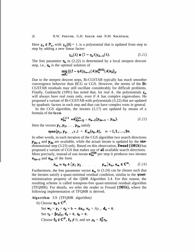
Furthermore, the free parameter vector z, in (3.24) can be chosen such thatthe iterates satisfy a quasi-minimal residual condition, similar to the quasi-minimization property of the QMR Algorithm 3.4. For this reason, theresulting scheme is called transpose-free quasi-minimal residual algorithm(TFQMR). For details, we refer the reader to Freund (1991b), where thefollowing implementation of TFQMR is derived.
Algorithm 3.9 (TFQMR algorithm)0) Choose x, E CN.
Set w1 = y1 = r. = b - Axe, v. = Ay,, do = 0.Set r. = Ilrol12, 6, = 0, q. = 0.Choose f. E CN, f. # 0, and set p. = F$ro.
27ITERATIVE SOLUTION OF LINEAR SYSTEMS
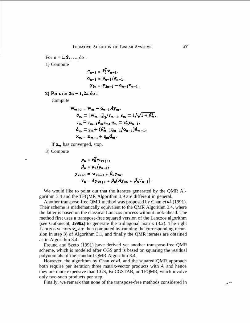
For n = 1,2,..., do :1) Compute
G-1 -T= =ov,-1,
an-1 = Pn-lbla-1,
Y2n = Y2n-1 - a ,-IV,-1 l
2)Form=2n-1,2ndo:Compute
&a+1 = Wrn - %-1 AYm10, = llw,+IllJ7m-1~ %a = 1/m,7, = +*$l&, t7m = cam,-*,d, = Ym + (~Llrlm-l/%-J&n-19x, = %n-1+ %dln*
If x, has converged, stop.3) Compute
Pn = 65v2*+1,
48 = PnlPn-19
Y2n+l = W2n+l + PnY2n9
vn = AYzn+1 + MAYan + Pnvn-l)*
We would like to point out that the iterates generated by the QMR Al-gorithm 3.4 and the TFQMR Algorithm 3.9 are different in general.
Another transpose-free QMR method was proposed by Chan et al. (1991).Their scheme is mathematically equivalent to the QMR Algorithm 3.4, wherethe latter is based on the classical Lanczos process without look-ahead. Themethod first uses a transpose-free squared version of the Lanczos algorithm(see Gutknecht, 1990a) to generate the tridiagonal matrix (3.2). The rightLanczos vectors v, are then computed by-running the corresponding recur-sion in step 3) of Algorithm 3.1, and finally the QMR iterates are obtainedas in Algorithm 3.4.
Freund and Szeto (1991) have derived yet another transpose-free QMRscheme, which is modeled after CGS and is based on squaring the residualpolynomials of the standard QMR Algorithm 3.4.
However, the algorithm by Chan et al. and the squared QMR approachboth require per iteration three matrix-vector products with A and hencethey are more expensive than CGS, Bi-CGSTAB, or TFQMR, which involveonly two such products per step.
Finally, we remark that none of the transpose-free methods considered in
28 R.W. FREUND, G.H. GOLUB AND N-M. NACHTIGAL
this section, except for Freund and Zha’s simplified QMR algorithm basedon (3.15), addresses the problem of breakdowns. Indeed, in exact arithmetic,all these schemes break down every time a breakdown (3.5) or (3.6) occursin the BCG Algorithm 3.2. Practical look-ahead techniques for avoidingexact and near-breakdowns in these transpose-free methods still have to bedeveloped.
3.5 Related work and historical remarks
The problem of breakdowns in the classical Lanczos algorithm has beenknown from the beginning. Although a rare event in practice, the possibil-ity of breakdowns certainly has brought the method into discredit and hasprevented many people from actually using the algorithm. On the otherhand, it was also demonstrated (see Cullum and Willoughby, 1986) that the .Lanczos process-even without look-ahead-is a powerful tool for sparsematrix computation.
The Lanczos method has intimate connections with many other areas ofMathematics, such as formally orthogonal polynomials (FOPS), Pad6 ap-proximation, Hankel matrices, and control theory. The problem of break-downs has a corresponding formulation in all of these areas, and remediesfor breakdowns in these different settings have been known for quite sometime. For example, the breakdown in the Lanczos process is equivalent to abreakdown of the generic three-term recurrence relation for FOPS, and it iswell known how to overcome such breakdowns by modifying the recursionsfor FOPS (see Gragg, 1974, Draux, 1983, Gutknecht, 1990b, and the refer-ences given there). Kung (1977) and Gragg and Lindquist (1983) presentedremedies for breakdowns in the context of the partial realization problem incontrol theory. The Lanczos process is also closely related to fast algorithmsfor the factorization of Hankel matrices, and again it is well known how toovercome possible breakdowns of these algorithms (see Heinig and Rost,1984). However, in all these cases, only the problem of exact breakdownshas been addressed. Taylor (1982) and Parlett et ul. (1985) were the first topropose a modification of the classical Lanczos process that remedies bothexact and nearibreakdowns.
In recent years, there has been a revival of the nonsymmetric Lanczosalgorithm, and since 1990, in addition to the papers we have already citedin this section, there are several others dealing with various aspects of theLanczos process. We refer the reader to the papers by Boley et al. (1991),Boley and Golub (1991), Brezinski et al. (1991), Gutknecht (199Oc), Joubert(1990), Parlett (1990), and the references given therein.
Note that Algorithm 3.2 is only one of several possible implementationsof the BCG approach; see Joubert (1990) and Gutknecht (1990a) for anoverview of the different BCG variants. As for the nonsymmetric Lanczosprocess, exact and near-breakdowns in the BCG methods can be avoided
ITERATIVE SOLUTION OF LINEAR SYSTEMS 29
by incorporating look-ahead procedures. Such look-ahead BCG algorithmshave been proposed by Joubert (1990) and Gutknecht (199Oc). Particu-larly attractive in this context is the algorithm called Lanczos/Orthodir inJoubert (1990). Instead of generating the search directions q,, and 6, bycoupled two-term recursions as in Algorithm 3.2, in Lanczos/Orthodir theyare computed by three-term recurrences. This eliminates the vectors r, andF,, and hence the second of the two possible breakdowns (3.5) and (3.6).We note that Brezinski et al. ( 1991) have proposed an implementation ofthe BCG approach that is mathematically equivalent to Lanczos/Orthodir.
Finally, recall that the algorithms QMR, Bi-CGSTAB, and TFQMR aredesigned to generate iterates that converge more smoothly than BCG andCGS. A different remedy for the erratic convergence behavior of BCG orCGS was proposed by Schiinauer (see Weiss, 1990). The approach used isto run plain BCG or CGS and then apply a smoothing procedure to thesequence of BCG or CGS iterates, resulting in iterates with monotonicallydecreasing residual norms. However, since the process is based directly onBCG or CGS, this approach inherits the numerical problems of BCG andCGS.
4. Solving the normal equations is not always badIn this section, we consider CGNR and CGNE in more detail. Recall fromSection 1 that CGNR and CGNE are the algorithms that result when (1.1)is solved by applying standard CG to either one of the normal equations( 1.2) or (1.3), respectively. Clearly, for nonsingular A, both systems ( 1.2)and (1.3) are equivalent to the original system (1.1). From the minimizationproperty (2.10) of CG, it follows that CGNR produces iterates
x,Ex,+K,(AHro,AHA), n=l,2,..., (4 1).
that are characterized by the minimal residual condition
Jib - AXnll2 = . minxExo+L(AHrdHA) lib - AxlIz*
Similarly, CGNE generates iterates (4.1) that satisfy the minimal error prop-erty
IIA-‘b - x,l12 = .x~xo+nm$%o ,AHA)
IIA-‘b - xl12.
Note that the letters “R” and “E” in CGNR and CGNE indicate the mini-mization of the residual or of the error, respectively. We also remark that theLSQR algorithm of Paige and Saunders (1982) is mathematically equivalentto CGNR, but has better numerical properties.
Since the convergence of CG depends on the spectrum of the coefficient
30 R.W. FREUND, G.H. GOLUB AND N.M. NACHTIGAL
matrix, the convergence behavior of CGNR and CGNE depends on
X(AHA) = (02 1 o E o(A)},
i.e., on the squares of the singular values of A. In particular, the worst-caseconvergence behavior of CGNR and CGNE is governed by
~~ AHA = (K~(A))~,( >which suggests that convergence can be very slow even for matrices A withmoderate condition numbers. This is indeed true in many cases, and gen-erally it is preferable to use CG-type methods that are applied directly to(1.1) rather than CGNR or CGNE.
Nevertheless there are special cases for which solving the normal equationsis optimal. A simple case are unitary matrices A for which CGNR andCGNE find the exact solution after only one step, while Krylov subspacemethods with iterates (2.1) tend to converge very slowly (see Nachtigal et al.,1990a). More interesting are cases for which CGNR and CGNE are optimal,in that they are mathematically equivalent to ideal CG-type methods basedon the MR or OR conditions (2.11) or (2.12). Typically, these situations arisewhen the spectrum of A has certain symmetries. Since these equivalencesare not widely known, we collect here a few of these results. In the following,xyR and eR denote iterates defined by (2.11) and (2.12), respectively.
First, we consider the case of real skew-symmetric matrices.
Theorem 4.1 (Freund, 1983)Let A = -AT be a real N x N matrix, and let b E RN and x, E RN. Then:
xE:l =MR
X2n = nXCGNR 9 n = O,l,...,
OR - =X2n xCGNEn 9 n = 1 2, ,... .
Moreover, no odd OR iterate xf:-r exists.
Next, we turn to shifted skew-symmetric-matrices of the form (2.13). Forthis class of matrices Eisenstat (1983a, 1983b) has obtained the followingresult (see also Szyld and Widlund, 1989).
Theorem 4.2 Let A = I - S where S = -ST is a real N x iV matrix, andlet b E RN and x0 E RN. Let xEGNE and xCGNE denote the iterates gener-ated by CGNE started with initial guess x,lnd 2, = b + Sxo, respectively.Then, for n = 0, 1, . . . , it holds:
ORX2n = eGNE,
x!iii+l = n%CGNE
l
ITERATIVE SOLUTION OF LINEAR SYSTEMS 31
We remark that for the MR and CGNR approaches a result correspondingto Theorem 4.2 does not hold (see Freund, 1983).
Finally, we consider linear systems (1.1) with Hermitian coefficient ma-trices A. Note that A has a complete set of orthonormal eigenvectors, andhence one can always expand the initial residual in the form:
mr. = c Pjzj (4 2).
j=l
In the following theorem, x,ME denotes the iterate defined by (2.16).
Theorem 4.3 (Freund, 1983)Assume that the expansion (4.2) is “symmetric”, i.e., m = 22 is even and
Aj = -X,+*-j, IPjl = IPm+*-jl9 i = 19%***9~=
Then, for n = 0, 1, . . . , it holds:
xi% = x!)fnR= nXCGNR , n= O,l,...,ME
X2n = xymt* = ORX2n = cGNE, n=1,2 ,....
Moreover, no odd OR iterate x& exists.
5. Estimating spectra for hybrid methodsWe now turn to parameter-dependent schemes. As mentioned in Section 2.1,methods in this class require a priori knowledge of some spectral propertiesof the matrix. Typically, it is assumed that some compact set c is known,which in a certain sense approximates the spectrum of A and in particularsatisfies (2.7). Given such a set 0, one then constructs residual polynomials+,, as some approximations to the optimal polynomials in (2.9). We wouldlike to stress that, in view of (2.4) and (2.9), it is crucial that Q excludesthe origin. Since in general one does not-know in advance a suitable set 0,parameter-dependent methods combine an approach for estimating the setG with an approach for solving the approximation problem (2.9), usuallycycling between the two parts in order to improve the estimate for 6. Forthis reason, the algorithms in this class are often called hybrid methods.In this section, we review some recent insights in the problem of how toestimate the set 6.
The standard approach for obtaining G is to run a few steps of the ArnoldiAlgorithm 2.2 to generate the upper Hessenberg matrix Hn (2.24) and thencompute its spectrum A@,). Saad (1980) showed that the eigenvalues ofH, are Ritz values for A and can be used to approximate the spectrum
32 R.W. FREUND, G.H. GOLUB AND N.M. NACHTIGAL
A(A), hence one takes the convex hull of A(&) as the set G. Once the setis obtained, a hybrid method turns to solving the complex approximationproblem (2.9), and the possibilities here are numerous.
However, there are problems with the approach outlined above, originat-ing from the use of the Arnoldi Ritz values. In general, there is no guaranteethat the convex hull of X(Hn) does not include the origin, or indeed, thatone of the Ritz values is not at or near the origin. For matrices with spec-trum in both the left and right half-planes, the convex hull of the Ritz valuesmight naturally enclose the origin. Nachtigal et al. (1990b) give an exam-ple of a matrix whose spectrum is symmetric with respect to the origin,SQ that the convex hull of A(&) will generally contain the origin, and onevery other step, one of the Ritz values will be close to the origin. A secondproblem is that the approach aims to estimate the spectrum of A, whichmay be highly sensitive to perturbations, especially for nonnormal matri-ces. In these cases, a more natural concept is the pseudospectrum X,(A),introduced by Trefethen (1991):
Definition 5.1 For c 2 0 and A E CNxN, the e-pseudospectrum &(A) isgiven by
X,(A) = {X E C 1 X E ;\(A + A), 11412 5 + (5 1).
As is apparent from (5. l), the pseudospectrum in general can be expectedto be insensitive to perturbations of A, even for highly nonnormal matrices.For practical purposes, the sets X,(A) of interest correspond to values ofthe parameter t: that are small relative to the norm of A but larger thanround-off.
It is easy to construct examples where a hybrid algorithm using the exactspectrum A(A) of A will in fact diverge, while the same hybrid algorithmusing the pseudospectrum X,(A) will converge (see Nachtigal et al., 1990b,and Trefethen, 1991). Unfortunately, in general the pseudospectrum X,(A)cannot be easily computed directly. Fortunately, it turns out that one cancompute approximations to the pseudospectrum; this is the approach takenin the hybrid introduced by Nachtigal et- al. (1990b). They observed thatthe level curves-or lemniscates-of the GMRES residual polynomial boundregions that approximate the pseudospectrum X,(A). Let
cm = v E c 1 I~nWl = f7h rl2 09
be any lemniscate of the residual polynomial &. Due to the normalization(2.4), the region bounded by C,(q) with q < 1 will automatically excludethe origin; in particular, 0 cannot be a root of a residual polynomial. Inaddition, since GMRES is solving the minimization problem (2.11), y& willnaturally be small on an appropriate set &7. Motivated by these considera-tions, Nachtigal et al. observed that the region bounded by the lemniscate
ITERATIVE SOLUTION OF LINEAR SYSTEMS 33
wl,) with
II II=n 2?h=iixr<l
usually yields a suitable set G.11=0112
The GMRES residual polynomials are kernel polynomials, and their rootsare a type of Ritz values called pseudo-Ritz values by Freund (1989a). Infact, one is not restricted to using the GMRES residual polynomial, butcould use the residual polynomials from other minimization methods, suchas QMR or its transpose-free versions. In these cases, the residual poly-nomials are no longer kernel polynomials, but rather, they are quasi-kernelpolynomials (Freund, 1991c). Nevertheless, their lemniscates still yield suit-able sets G, and their roots are also pseudo-Ritz values of A.
Freund has also proposed an algorithm to compute pseudo-Ritz values,using the upper Hessenberg matrix Ht) (2.19) appearing in the recurrence(2.17). One uses the fact that kernel and quasi-kernel polynomials can bedefined by
which makes it clear that the roots of +, can be obtained from the general-ized eigenvalue problem
(lrp)H(l?~,> z = xlil,Hz, 2 # 0 E c*.Finally, we should point out another set that has been proposed as a
candidate for g in (2.7), namely the field of values. Defined as
the field of values has the advantage that it is easier to compute (see, e.g.,Ruhe, 1987) than the pseudospectrum. However, the field of values is convexand always at least as large as the convex hull of A(A), and hence may onceagain enclose the origin. For more details on the field of values in iterativemethods, we refer the reader to Eiermann (1991).
The literature on hybrid methods for non-Hermitian linear systems startswith an algorithm proposed by Manteuffel (1978), which combines a modi-fied power method with the Chebyshev iteration. Since then, literally dozensof hybrid methods have been proposed, most of which use Arnoldi in the firstphase and differ in the way they compute the residual polynomial $, in (2.9).For an overview of some of these algorithms, see Nachtigal et al. (1990b).The hybrid by Nachtigal et al. was the first to avoid the explicit compu-tation of an estimate of X(A). Instead, it explicitly obtains the GMRES
34 R.W. FREUND, G.H. GOLUB AND N.M. NACHTIGAL
residual polynomial and applies it using Richardson’s method until conver-gence. Finally, hybrids recently introduced include an algorithm by Saylorand Smolarski (1991), which combines Arnoldi with Richardson’s method,and an algorithm proposed by Starke and Varga (1991), which combinesArnoldi with Faber polynomials.
6. CG-type methods for complex linear systemsWhile most linear systems arising in practice are real, there are importantapplications that lead to linear systems with complex* coefficient matricesA. Partial differential equations that model dissipative processes usually in-volve complex coefficient functions or complex boundary conditions, and dis-cretizing them yields complex linear systems. An important example for thiscategory is the complex Helmholtz equations. Other applications that leadto complex linear systems include the numerical solution of Schriidinger’sequation, underwater acoustics, frequency response computations in con-trol theory, semiconductor device simulation, and numerical computationsin quantum chromodynamics; for details and further references, see Baylissand Goldstein (1983), Barbour et al. (1987), Freund (1989b, 1991a), andLaux (1985). In all these applications, the resulting linear systems are usu-ally non-Hermitian. In this section, we review some recent advances inunderstanding the issues related to solving complex non-Hermitian systems.
Until recently, the prevailing approaches used when solving complex linearsystems have consisted of either solving the normal equations or rewritingthe complex system as a real system of dimension 2N. However, as indicatedalready in Section 4, the normal equations often lead to systems with verypoor convergence rates, and this has indeed been observed for many of thecomplex. systems of interest. The other option is to split the original matrixA into its real and imaginary parts and combine them into a real systemof dimension 2N. There are essentially only two different possibilities fordoing this, namely
(6 1).
and
Unfortunately, it turns out that this option is not viable either. As Freund(1989b, 1992) pointed out, both A, and A, have spectral properties thatmake them far more unsuitable for Krylov space iterations than the original
* In this section, “complex” wiIl imply the presence of imaginary components.
ITERATIVE SOLUTION OF LINEAR SYSTEMS 35
system was. The spectrum of A, in (6.1) is given by
A@*) = X(A) u W), (6 3).while the spectrum of A, in (6.2) is given by
X(A,) = {X E C 1 X2 E X@A)). (6 4).
In particular, note that the spectrum (6.3) is symmetric with respect to thereal axis, while the spectrum (6.4) is symmetric with respect to both the realand imaginary axes. The point is that in both cases, the spectrum of the realsystem is either very likely to or is guaranteed to contain the origin, thuspresenting a Krylov subspace iteration with the worst possible eigenvaluedistribution. As a result, both approaches have had very poor results in
’practice, and have often led to the conclusion that complex systems areill-suited for iterative methods.
Therefore, instead of solving the normal equations or either one of theequivalent real systems (6.1) or (6.2), it is generally preferable to solve theoriginal linear system by a CG-like Krylov subspace methods. In partic-ular, if A is a general non-Hermitian matrix, then we recommend to usethe Lanczos-based algorithms discussed in Section 3 or GMRES. However,in many applications, the resulting complex linear systems have additionalstructure that can be exploited. For example, often complex matrices of theform (2.13) arise. Recall from Theorem 2.1 that ideal CG-type algorithmsbased on the MR or OR property (2.11) or (2.12) exist for such shifted Her-mitian matrices. Freund (1990) has derived practical implementations of theMR and OR approaches for the class of matrices (2.13). These algorithmscan be viewed as extensions of Paige and Saunders’ MINRES and SYMMLQfor Hermitian matrices (see Section 2.3). As in the case of SYMMLQ, theOR implementation for shifted Hermitian matrices also generates auxiliaryiterates xFE E xc, + &(AHro, A) that are characterized by the minimalerror property
IIA-‘b - xf;““ll, = xExo+pfiHro Al IIA-lb - xl12*n 9
Hence the OR algorithm proposed by Freund also generalizes Fridman’smethod to shifted Hermitian matrices. Unfortunately, when matrices Aof the form (2.13) are preconditioned by standard techniques, the specialstructure of A is destroyed. In Freund (1989) it is shown that the shiftstructure can be preserved when polynomial preconditioning is used, andresults on the optimal choice of the polynomial preconditioner are given.
Another special case that arises frequently in applications are complexsymmetric matrices A = AT. For example, the complex Helmholtz equa-tions leads to complex symmetric systems. As pointed out in Section 3.4, theQMR Algorithm 3.4 can take advantage of this special structure, and work
36 R.W. FREUND, G.H. GOLUB AND N.M. NACHTIGAL
and storage is roughly halved. We remark that the complex symmetry struc-ture is preserved when preconditioning is used, if the preconditioner M isagain symmetric, as is the case for all standard techniques. For an overviewof other CG-type methods and further results for complex symmetric linearsystems, we refer the reader to Freund (1991a, 1992).
7. Large dense linear systems
As mentioned in Section 1, there are certain classes of large dense linearsystems for which it is possible to compute matrix-vector products cheaply;for these systems, iterative methods remain an attractive option. Typically,the matrix-vector product takes advantage of either some special structureof the matrix or of some special property of the underlying operator. Wewill briefly discuss one situation from each class.
The first case is the solution of integral equations involving a decayingpotential, such as a gravitational or Coulombic potential. Some typicalapplications are the solution of N-body problems, vortex methods, poten-tial theory, and others. In these problems, the effort required by a naivecomputation of a matrix-vector product is generally O(N2), as it involvescomputing the influence of each of N points on all the other N - 1 points.However, Carrier et al. (1988) noticed that it is possible to approximatethe result of the matrix-vector product Ax in only O(N) time, rather thanO( N2).
The main idea behind their algorithm is to group points in clusters andevaluate the influence of entire clusters on faraway points. The cumulativepotential generated by m charges in a cluster can be expressed as a powerseries. If the power series is truncated after p terms, then the work requiredto compute it turns out to be O(mp). Applying the cumulative influenceto n points in a cluster well-separated from the first requires an additionalO(np) work, for a total of O(mp + np) work, as compared to the O(mn)work required to compute the individual interactions. Finally, the point isthat the number p of terms in the series is determined by the preassignedprecision to which the series is computed, and once chosen, p becomes aconstant, giving an O(m + n) algorithm. For a complete description of thealgorithm, see Carrier et al. (1988).
While the Carrier et al. algorithm is the first in the class of fast multipolemethods, it falls in the bigger class of hierarchical algorithms. Several otheralgorithms have been proposed in this class; see for example Hackney andEastwood (1981), Appel (1985), Rokhlin (1985). More recently, Hanrahanet al. (1991) have proposed a hierarchical algorithm for radiosity problemsin computer graphics, and Greenbaum et al. (1991) have introduced analgorithm that uses the Carrier et a(. algorithm combined with GMRES to
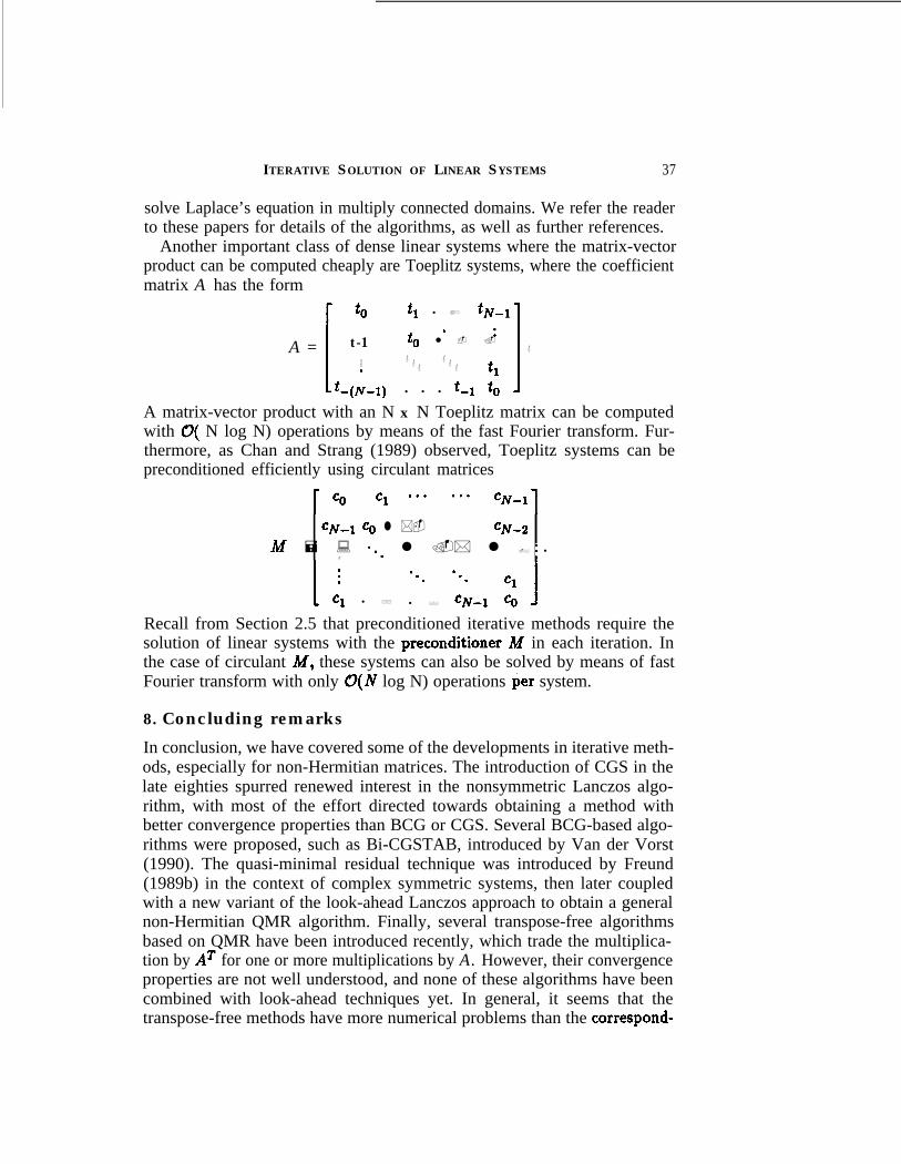
ITERATIVE SOLUTION OF LINEAR SYSTEMS 37
solve Laplace’s equation in multiply connected domains. We refer the readerto these papers for details of the algorithms, as well as further references.
Another important class of dense linear systems where the matrix-vectorproduct can be computed cheaply are Toeplitz systems, where the coefficientmatrix A has the form
r t0 tl l a *tN-l 1
I t-1. :
A = to l - ..
: . .. .
t-(N-q
. . t1l l l t-1 to I
A matrix-vector product with an N x N Toeplitz matrix can be computedwith 0( N log N) operations by means of the fast Fourier transform. Fur-thermore, as Chan and Strang (1989) observed, Toeplitz systems can bepreconditioned efficiently using circulant matrices
CN-1 c , l *- CN-2M = : 0.. l .* l .* i l
.: . .. .. . . ClCl l ** l ** CN-1 Q I
Recall from Section 2.5 that preconditioned iterative methods require thesolution of linear systems with the preconditioner M in each iteration. Inthe case of circulant M, these systems can also be solved by means of fastFourier transform with only U(N log N) operations per system.
8. Concluding remarksIn conclusion, we have covered some of the developments in iterative meth-ods, especially for non-Hermitian matrices. The introduction of CGS in thelate eighties spurred renewed interest in the nonsymmetric Lanczos algo-rithm, with most of the effort directed towards obtaining a method withbetter convergence properties than BCG or CGS. Several BCG-based algo-rithms were proposed, such as Bi-CGSTAB, introduced by Van der Vorst(1990). The quasi-minimal residual technique was introduced by Freund(1989b) in the context of complex symmetric systems, then later coupledwith a new variant of the look-ahead Lanczos approach to obtain a generalnon-Hermitian QMR algorithm. Finally, several transpose-free algorithmsbased on QMR have been introduced recently, which trade the multiplica-tion by AT for one or more multiplications by A. However, their convergenceproperties are not well understood, and none of these algorithms have beencombined with look-ahead techniques yet. In general, it seems that thetranspose-free methods have more numerical problems than the correspond-
38 R.W. FREUND, G.H. GOLUB AND N.M. NACHTIGAL
ing methods that use AT, and more research is needed into studying theirbehavior.
With the advent of Lanczos-based methods that require little work andstorage per step, the importance of preconditioners has decreased. WithGMRES or similar algorithms, the high cost of the method makes restartsnecessary in practice, which generally results in much slower convergence.As a result, preconditioned GMRES requires a very effective preconditioner,so that the preconditioned system requires few iterations to converge. Theproblem is that effective preconditioners are often too expensive, especiallyon parallel machines, where the inherently serial nature of many precondi-tioners makes their use unappealing. In contrast, restarts are not necessarywith Lanczos-based methods, and hence a wider array of preconditioners-inparticular, cheaper or more parallelizable preconditioners-becomes usable.
Finally, even though the field of iterative methods has made great progressin the last few years, it is still in its infancy, especially with regard tothe packaged software available. Whereas there are well-established robustgeneral-purpose solvers based on direct methods, the same cannot be saidabout solvers based on iterative methods. There are no established itera-tive packages of the same robustness and wide acceptance as, for example,the LINPACK library, and as a result many of the scientists who use itera-tive methods write their own specialized solvers. We feel that this situationneeds to change, and we would like to encourage researchers to provide codefor their methods.
AcknowledgmentsWe would like to thank Susanne fieund for her help with UT@ and MarlisHochbruck for her careful reading of this paper. The first and third authorsare grateful to the San Jose radio station KSJO for keeping them awake lateat night. The first author would like to thank the Printers Lnc Book Storein Mountain View for providing countless mega espressos.
REFERENCESA.W. Appel (1985), “An efficient program for many-body simulation”, SIAM J.
Sci. Statist. Compuf. 6, 85-103.W.E. Arnoldi (1951), “The principle of minimized iterations in the solution of the
matrix eigenvalue problem”, Quart. Appl. Math. 9, 17-29.S.F. Ashby, T.A. Manteuffel and P.E. Saylor (1990), “A taxonomy for conjugate
gradient methods”, SIAM J. Numcr. Anal. 27, 1542-1568.0. Axelsson (1980), ‘Conjugate gradient type methods for unsymmetric and incon-
sistent systems of linear equations”, Linear Algebra Appl. 29, 1-16.0. Axelsson (1985), “A survey of preconditioned iterative methods for linear sys-
tems of algebraic equations”, BIT 25, 166-187.0. Axelsson (1987), “A generalized conjugate gradient, least square method”, Nu-
mer. Math. 51, 209-227.
ITERATIVE SOLUTION OF LINEAR SYSTEMS 39
A. Bayliss and C.I. Goldstein (1983), “An iterative method for the Helmholtz equa-tion”, J. Comput. Phys. 49, 443-457.
I.M. Barbour, N.-E. Behilil, P.E. Gibbs, M. Rafiq, K.J.M. Moriarty and G. Schier-holz (1987), “Updating fermions with the Lanczos method”, J. Comput. Phys.68,227-236.
D.L. Boley, S. Elhay, G.H. Golub and M.H. Gutknecht (1991), “Nonsymmet-ric Lanczos and finding orthogonal polynomials associated with indefiniteweights”, Numer. Algorithms 1, 21-43.
D.L. Boley and G.H. Golub (1991), “The nonsymmetric Lanczos algorithm andcontrollability”, Systems Contrvl Lett. 16, 97-105
C. Brezinski, M. Redivo Zaglia and H. Sadok (1991), “A breakdown-free Lanczos* type algorithm for solving linear systems”, Technical Report ANO-239, Uni-
versite des Sciences et Techniques de Lille Flandres-Artois, Villeneuve d’Ascq.C.G. Broyden (1965), “A 1c ass of methods for solving nonlinear simultaneous equa-
tions”, Math. Comp. 19, 577-593.J. Carrier, L. Greengard and V. Rokhlin (1988), “A fast adaptive multipole algo-
rithm for particle simulations”, SIAM J. Sci. Stat. Comput. 9,669-686.R.H. Chan and G. Strang (1989), “Toeplitz equations by conjugate gradients with
circulant preconditioner”, SIAM J. Sci. Stat. Compui. 10, 104-119.T.F. Chan, L. de Pillis and H.A. Van der Vorst (1991), “A transpose-free squared
Lanczos algorithm and application to solving nonsymmetric linear systems”,Technical Report, University of California at Los Angeles.
R. Chandra (1978), “Conjugate gradient methods for partial differential equations”,Ph.D. Dissertation, Yale University, New Haven.
P. Concus and G.H. Golub (1976), “A generalized conjugate gradient method fornonsymmetric systems of linear equations”, in Computing Methods in AppliedSciences und Engineering (R. Glowinski and J.L. Lions, eds.), Lecture Notesin Economics and Mathematical Systems 134, Springer, Berlin, 56-65.
P. Concus, G.H. Golub and D.P. O’Leary (1976), “A generalized conjugate gradientmethod for the numerical solution of elliptic partial differential equations”, inSparse Mutriz Computations (J.R. Bunch and D.J. Rose, eds.), AcademicPress, New York, 309-332.
E.J. Craig (1955), “The N-step iteration procedures”, J. Moth. Phys. 34, 64-73.J. Cullum and R.A. Willoughby (1985) Lanczos algorithms for large symmetric
eigenvalue computations, Volume 1, Theory, Birkhiiuser, Basel.J. Cullum and R.A. Willoughby (1986) “A practical procedure for computing eigen-
values of large sparse nonsymmetric matrices”, in Large Scale EigenvalueProblems (J. Cullum and R.A. Willoughby, eds.), North-Holland, Amster-dam, 193-240.
P. Deuflhard, R.W. Freund and A. Walter (1990), “Fast secant methods for theiterative solution of large nonsymmetric linear systems”, IMPACT Comput.Sci. Eng. 2, 244-276.
A. Draux (1983), PolynGmes Orthogonauz Formels - Applications, Lecture Notesin Mathematics 974, Springer, Berlin.
I.S. Duff, A.M. Erisman and J.K. Reid (1986), Direct Methods for Sparse Matrices,Oxford University Press, Oxford.
40 R.W. FREUND, G.H. GOLUB AND N.M. NACHTIGAL
M. Eiermann (1991), “Fields of values and iterative methods”, Preprint, IBM Sci-entific Center, Heidelberg.
M. Eiermann, W. Niethammer and R.S. Varga (1985), “A study of semiiterativemethods for nonsymmetric systems of linear equations”, Numer. Math. 47,505-533.
T. Eirola and 0. Nevanlinna (1989), “Accelerating with rank-one updates”, LinearAlgebrvr Appl. 121, 511-520.
S.C. Eisenstat (1983a), “A note on the generalized conjugate gradient method”,SIAM J. Numer. Anal. 20,358-361.
S.C. Eisenstat (1983b), “Some observations on the generalized conjugate gradientmethod”, in Numerical methods, Proceedings, Curocas 1982 (V. Pereyra andA. Reinoza, eds.), Lecture Notes in Mathematics 1005, Springer, Berlin, 99-107.
S.C. Eisenstat, H.C. Elman and M.H. Schultz (1983), “Variational iterative methodsfor nonsymmetric systems of linear equations”, SIAM J. Numer. Anal. 20,345-357.
B.C. Elman (1982), “Iterative methods for large sparse nonsymmetric systems oflinear equations”, Ph.D. Dissertation, Yale University, New Haven.
V. Faber and T. Manteuffel (1984), “Necessary and sufficient conditions for theexistence of a conjugate gradient method”, SIAM J. Numer. Awl. 21, 352-362.
V. Faber and T. Manteuffel(1987), “Orthogonal error methods”, SIAM J. Numer.Anal. 24, 170-187.
B. Fischer and R.W. Freund (1990), “On the constrained Chebyshev approximationproblem on ellipses”, J. Appmz. Theory 62,297-315.
B. Fischer and R.W. Freund (1991), “Chebyshev polynomials are not always opti-mal”, J. Appvvz. Theory 65,261-272.
R. Fletcher (1976), “Conjugate gradient methods for indefinite systems”, in Numer-ical Analysis Dundee 1975 (G.A. Watson, ed.), Lecture Notes in Mathematics506, Springer, Berlin, 73-89.
R. W. Freund (1983), “fiber einige cg-iihnliche Verfahren zur Liigung linearer Gle-ichungssysteme”, Doctoral Dissertation, Universitiit Wiirzburg.
R.W. Freund (1989a), “PseudeRitz values for indefinite Hermitian matrices”, RI-ACS Technical Report 89.33; NASA Ames Research Center, Moffett Field.
R.W. Freund (1989b), “Conjugate gradient type methods for linear systems withcomplex symmetric coefficient matrices”, RIACS Technical Report 89.54,NASA Ames Research Center, Moffett Field.
R.W. Freund (1990), “0n conjugate gradient type methods and polynomial pre-conditioners for a class of complex non-Hermitian matrices”, Numer. Math.57,285-312.
R.W. Freund (1991a), “Krylov subspace methods for complex non-Hermitian linearsystems”, Habilitation Thesis, Universitiit Wiirzburg.
R.W. Freund (1991b), “A transpose-free quasi-minimal residual algorithm for non-Hermi tian linear systems”, RIACS Technical Report 91.18, NASA Ames Re-search Center, Moffett Field.
ITERATIVE SOLUTION OF LINEAR SYSTEMS 41
R.W. Freund (1991c), “Quasi-kernel polynomials and their use in non-Hermitianmatrix iteration# , RIACS Technical Report 91.20, NASA Ames ResearchCenter, Moffett Field.
R.W. Freund (1992), “Conjugate gradient-type methods for linear systems withcomplex symmetric coefficient matricesn , SIAM J. Sci. Stat. Comput. 13, toappear.
R.W. Freund, G.H. Golub and M. Hochbruck (1991a) “Krylov subspace methodsfor non-Hermitian p-cyclic matrices”, Technical Report, RIACS, NASA AmesResearch Center, Moffett Field.
R-W. Freund, M.H. Gutknecht and N.M. Nachtigal (1991b), “An Implementationof the Look-Ahead Lanczos Algorithm for non-Hermitian Matrices”, TechnicalReport 91.09, RIACS, NASA Ames Research Center, Moffett Field.
R.W. Freund and N.M. Nachtigal(1991), “QMR: aquasi-minimal residual methodfor non-Hermitian linear systems”, Numer. Math., to appear.
R.W. Freund and St. Ruscheweyh (1986), “On a class of Chebyshev approximationproblems which arise in connection with a conjugate gradient type method”,Numer. Math. 48, 525-542.
R.W. Freund and T. Szeto (1991)) “A quasi-minimal residual squared algorithmfor non-Hermitian linear systems”, Technical Report, RIACS, NASA AmesResearch Center, Moffett Field.
R.W. Freund and H. Zha (1991), “Simplifications of the nonsymmetric Lanczosprocess and a new algorithms for solving indefinite symmetric linear systems”,Technical Report, RIACS, NASA Ames Research Center, Moffett Field.
V.M. Fridman (1963), “The method of minimum iterations with minimum errorsfor a system of linear algebraic equations with a symmetrical matrix”, USSRComput. Math. and Math. Phys. 2, 362-363.
P.E. Gill, W. Murray, D.B. Poncelecjn and M.A. Saunders (1990), “Preconditionersfor indefinite systems arising in optimization”, Technical Report SOL 90-8,Stanford University.
G.H. Golub and D.P. O’Leary (1989), “Some history of the conjugate gradient andLanczos algorithms: 1948-1976”, SIAM Review 31, 50-102.
G.H. Golub and C.F. Van Loan (1989), Matrix Computations, Second Edition, TheJohns Hopkins University Press, Baltimore.
G.H. Golub and R.S. Varga (1961), “Chebyshev semi-iterative methods, succes-sive overrelaxation iterative methods, and second order Richardson iterativemethods”, Numer. Math. 3, 147-168.
W.B. Gragg (1974), uMatrix interpretations and applications of the continued frac-tion algorithm”, Rocky Mountain J. Math. 4, 213-225.
W.B. Gragg and A. Lindquist (1983), “On the partial realization problem”, LinearAlgebra Appl. 50, 277-319.
A. Greenbaum, L. Greengard and G.B. McFadden (1991), “Laplace’s equation andthe Dirichlet-Neumann map in multiply connected domains”, Technical Re-port, Courant Institute of Mathematical Sciences, New York University.
M.H. Gutknecht (1990a), “The unsymmetric Lanczos algorithms and their rela-tions to Padi approximation, continued fractions, and the QD algorithm”, inProceedings of the Copper Mountain Conference on Iterative Methods.
42 R.W. FREUND, G.H. GOLUB AND N.M. NACHTIGAL
M.H. Gutknecht (1990b), “A completed theory of the unsymmetric Lanczos processand related algorithms, Part I”, SIAM J. Matriz Anal. Appl., to appear.
M.H. Gutknecht (199Oc), “A completed theory of the unsymmetric Lanczos processand related algorithms, Part II”, IPS Research Report No. 90-16, ETH Zurich.
M-H. Gutknecht (1991), “Variants of BICGSTAB for matrices with complex spec-trum”, IPS Research Report No. 91-14, ETH Ziirich.
P. Hanrahan, D. Salzman and L. Aupperle (1991), “A rapid hierarchical radiosityalgorithm”, Computer Grvrphics (Ppoc. SIGGRAPH ‘91) 25, 197-206.
M.T. Heath, E. Ng and B.W. Peyton (1991), “Parallel algorithms for sparse linearsystems”, SIAM Review 33, 420-460.
G. Heinig and K. Rost (1984), “Algebraic methods for Toeplitz-like matrices and1 operators”, Birkhguser, Basel.
M.R. Hestenes and E. Stiefel (1952), “Methods of conjugate gradients for solvinglinear systems”, J. Res. Nat. Bur. Stand. 49, 409-436.
R. W. Hackney and J . W. Eastwood (1981)) “Computer Simulation Using Particles”,McGraw-Hill, New York.
W.D. Joubert (1990), “Generalized conjugate gradient and Lanczos methods for thesolution of nonsymmetric systems of linear equations”, Ph.D. Dissertation,The University of Texas at Austin.
W.D. Joubert and D.M. Young (1987), UNecessary and sufficient conditions for thesimplification of generalized conjugate-gradient algorithms”, Lineur AlgebraAppl. M/89,449-485.
I.M. Khabaza (1963), “An iterative least-square method suitable for solving largesparse matrices”, Compuf. J. 6, 202-206.
S. Kung (1977), “Multivariable and multidimensional systems: analysis and de-sign”, Ph.D. Dissertation, Stanford University.
C. Lanczos (1950), “An iteration method for the solution of the eigenvalue problemof linear differential and integral operators”, J. Res. Nutl. Barr. Stand. 45,255-282.
C. Lanczos (1952), “Solution of systems of linear equations by minimized itera-tions”, J. Res. Ntatl. Bur. Stand. 49, 33-53.
S.E. Laux (1985), “Techniques for small-signal analysis of semiconductor devices”,IEEE lkans. Electron Dev. ED-32,2028-2037.
D.G. Luenberger (1969), “Hyperbolic pairs in the method of conjugate gradients”,SIAM J. Appl. Math. 17, 1263-1267.
T.A. Manteuffel (1977), “The Tchebychev iteration for nonsymmetric linear sys-tems”, Numer. Math. 28, 307-327.
T.A. Manteuffel (1978), “Adaptive procedure for estimating parameters for thenonsymmetric Tchebychev iteration”, Numer. Math. 31, 183-208.
T.A. Manteuffel (1991), “Recent developments in iterative methods for large sparselinear systems”, Seminar presentation, Numerical Analysis/Scientific Com-puting Seminar, Stanford University.
N .M. Nachtigal (1991), “A look-ahead variant of the Lanczos algorithm and itsapplication to the quasi-minimal residual method for non-Hermitian linearsystems”, Ph.D. Dissertation, Massachusetts Institute of Technology, Cam-bridge.
ITERATIVE SOLUTION OF LINEAR SYSTEMS 43
N.M. Nachtigal, S.C. Reddy and L.N. Trefethen (1990a), “How fast are nonsym-metric matrix iterations?“, SIAM J. Matriz Anal. Appl., to appear.
N.M. Nachtigal, L. Reichel and L.N. Trefethen (1990b), “A hybrid GMRES al-gorithm for nonsymmetric linear systems”, SIAM J. Matrix Anal. Appl., toappear.
C.C. Paige and M.A. Saunders (1975), “Solution of sparse indefinite systems oflinear equations”, SIAM J. Numer. Anal. 12,617-629.
C.C. Paige and M.A. Saunders (1982), “LSQR: an algorithm for sparse linear equa-tions and sparse least squares”, ACM Tkans. Math. Sojtw. 8,43-71.
P.N. Parlett (1990), “Reduction to tridiagonal form and minimal realizations”,Preprint, University of California at Berkeley.
B.N. Parlett, D.R. Taylor and Z.A. Liu (1985), “A look-ahead Lanczos algorithmfor unsymmetric matrices”, iUath. Comp. 44, !05-124.
D. Rapoport (1978), “A nonlinear Lanczos algorithm and the stationary Navier-Stokes equation”, Ph.D. Dissertation, New York University.
J.K. Reid (1971), “On the method of conjugate gradients for the solution of largesparse systems of linear equations”, in Large Sparse Sets of Linear Equations(J.K. Reid, ed.), Academic Press, New York, 231-253.
V. Rokhlin (1985), “Rapid solution of integral equations of.classical potential the-ory”, J. Comp. Phys. 60, 187-207.
A. Ruhe (1987), “Closest normal matrix finally found!“, BIT 27,585-598.Y. Saad (1980), “Variations of Arnoldi’s method for computing eigenelements of
large unsymmetric matrices”, Linear Algebrta Appl. 34, 269-295.Y. Sad (1981), “Krylov subspace methods for solving large unsymmetric linear
systems”, Math. Comp. 37, 105-126.Y. Saad (1982), “The Lanczos biorthogonalization algorithm and other oblique
projection methods for solving large unsymmetric systems”, SIAM J. Numer.Anal. 19,48!%506.
Y. Saad (1984), “Practical use of some Krylov subspace methods for solving in-definite and nonsymmetric linear systems”, SIAM J. Sci. Std. Comput. 5,203-227.
Y. Saad (1989), “Krylov subspace methods on supercomputers”, SIAM J. Sci. Std.Comput. 10, 1200-1232.
Y. Saad and M.H. Schultz (1985), uConjugate gradient-like algorithms for solvingnonsymmetric linear systems”., Math. Comp. 44, 417-424.
Y. Saad and M.H. Schultz (1986), “GMRES: a generalized minimal residual algo-rithm for solving nonsymmetric linear systems”, SIAM J. Sci. Stat. Comput.7,856-869.
P.E. Saylor and D.C. Smolarski (1991), “Implementation of an adaptive algorithmfor Richardson’s method”, Linear Algebra Appl. 154-156,615-646.
P. Sonneveld (1989), “CGS, a fast Lanczos-type solver for nonsymmetric linearsystems”, SIAM J. Sci. Stat. Comput. 10, 36-52.
G. Starke and R.S. Varga (1991), “A hybrid Arnoldi-Faber iterative method fornonsymmetric systems of linear equations”, Technical Report ICM-9108- 11,Kent State University, Kent.
E. Stiefel (1955), “Relaxationsmethoden bester Strategie zur L&wng linearer Glei-chungssysteme” , Comm. Math. Helv. 29, 157-179.
44 R.W. FREUND, G.H. GOLUB AND N.M. NACHTIGAL
J. Stoer (1983), “Solution of large linear systems of equations by conjugate gra-dient type methods”, in Mathematical Programming - The State of the Art(A. Bachem, M. Griitschel and B. Korte, eds.), Springer, Berlin, 546-565.
J. Stoer and R.W. Freund (1982), “On the solution of large indefinite systems oflinear equations by conjugate gradient algorithms”, in Computing Methodsin Applied Sciences and Engineering V (R. Glowinski and J.L. Lions, eds.),North-Holland, Amsterdam, 35-53.
D-B. Szyld and O.B. Widlund (1989), “Variational analysis of some conjugate griGdient methods”, Technical Report CS-1989-28, Duke University, Durham.
D.R. Taylor (1982), “Analysis of the look ahead Lanczos algorithm”, Ph.D. Disser-tation, University of California at Berkeley.
L,N. Trefethen (1991), UPseudospectra of matrices”, in Proceedings of the 14thDundee Biennial Conference on Numerical Analysis (D.F. Griffiths andG.A. Watson, eds.), to appear.
H.A. Van der Vorst (1990), “Bi-CGSTAB: A fast and smoothly converging variant ofBi-CG for the solution of nonsymmetric linear systems”, Preprint, Universityof Utrecht.
P.K.W. Vinsome (1976), uOrthomin, an iterative method for solving sparse sets ofsimultaneous linear equations”, in Proceedings of the Fourth Symposium onReservoir Simulafion, Society of Petroleum Engineers of AIME, Los Angeles.
V.V. Voevodin (1983), “The problem of a non-selfadjoint generalization of the con-jugate gradient method has been closed”, USSR Comput. hiufh. and Moth.Phys. 23,143-144.
C. Vuik (1990), “A comparison of some GMRES-like methods”, Technical Report,Delft University of Technology, Delft.
R. Weiss (1990), “Convergence behavior of generalized conjugate gradient meth-ads”, Doctoral Dissertation, Universitiit Karlsruhe.
0. Widlund (1978), “A Lanczos method for a class of nonsymmetric systems oflinear equations”, SIAM J. Numer. Awl. 15,801-812.
J.H. Wilkinson (1965), The Algebruic Eigenvolue Pmblem, Oxford University Press,Oxford.
D.M. Young and K.C. Jea (1980), “Generalized conjugate gradient acceleration ofnonsymmetrizable iterative methods”, Linear Algebra Appl. 34, 159-194.