Kinematic response of single piles for different boundary

conditions: analytical solutions and normalization schemes

by

George AnoyatisDepartment of Civil Engineering, University of Patras, Rio, Greece

Raffaele Di LaoraDepartment of Civil Engineering, Second University of Naples, Aversa (CE), Italy

Alessandro MandoliniDepartment of Civil Engineering, Second University of Naples, Aversa (CE), Italy

George Mylonakis (Corresponding author)Department of Civil Engineering,

University of Patras, Rio, Greece, GR-26500

Phone: +30-2610-996542

Fax: +30-2610-996576

e-mail: mylo@upatras.gr

Abstract

Kinematic pile-soil interaction is investigated analytically through a Beam-on-

Dynamic-Winkler-Foundation model. A cylindrical vertical pile in a homogeneous

stratum, excited by vertically-propagating harmonic shear waves, is examined in the

realm of linear viscoelastic material behaviour. New closed-form solutions for

bending, as well as displacements and rotations atop the pile, are derived for different

boundary conditions at the head (free, fixed) and tip (free, hinged, fixed). Contrary to

classical elastodynamic theory where pile response is governed by six dimensionless

ratios, in the realm of Winkler analysis three dimensionless parameters suffice for

describing pile-soil interaction: (1) a mechanical slenderness accounting for geometry

and pile-soil stiffness contrast, (2) a dimensionless frequency (which is different from

the classical elastodynamic parameter ), (3) soil material damping. With

reference to kinematic pile bending, insight into the physics of the problem is gained

through a rigorous superposition scheme involving an infinitely-long pile excited

kinematically, and a pile of finite length excited by a concentrated force and a

moment at the tip. It is shown that for long piles kinematic response is governed by a

single dimensionless frequency parameter, leading to a single master curve pertaining

to all pile lengths and pile-soil stiffness ratios.

2

Notation

Latin symbols

cutoff frequency

dimensionless frequency

soil acceleration

pile cross-sectional area

, , , integration constants

Winkler dashpot coefficient

pile diameter

pile Young’s modulus

soil Young’s modulus, soil shear modulus

thickness of soil layer

pile cross-sectional moment of inertia

translational kinematic response factor

rotational kinematic response factors

complex-valued Winkler modulus

dynamic Winkler stiffness

pile length, soil thickness

bending moment

mass per unit pile length

shear force

soil wavenumber

pile-soil curvature ratio at depth z

pile head curvature over soil surface curvature (z=0)

3

pile tip curvature over soil surface curvature (z=L)

free-field displacement

free-field displacement amplitude

base displacement

base displacement amplitude

complex-valued soil shear wave propagation velocity

pile displacement

vertical coordinate

complementary curvature at depth z

pile curvature at depth z

pile curvature at head (level )

static pile curvature at head (level )

soil curvature at depth z

Greek symbols

Winkler damping coefficient

soil material damping coefficient

dimensionless response coefficient

Winkler stiffness coefficient ( )

Winkler wavenumber

static Winkler “wavenumber”

soil Poisson’s ratio

soil, pile mass density

soil shear stress

cyclic excitation frequency

4

Keywords: pile, kinematic interaction, subgrade reaction, Winkler model, closed-

form solution

1 Introduction

It is well known that the passage of seismic waves through soft soil causes

deformations in the soil mass that excite dynamically embedded bodies such as piles.

As a result, a pile foundation will, even in the absence of a superstructure, be

subjected to a spatially-variable displacement field imposed by the surrounding soil

which gives rise to a dynamic interplay known as “kinematic interaction” [1, 2, 3].

The ensuing deformations naturally coexist with motions transmitted onto the pile

through the pile cap due to structural dynamics, an effect commonly referred to as

“inertial interaction” [1, 2, 3]. Note that inertial interaction is affected by kinematic

interaction as the input motion to the former problem is the output motion of the

latter [4, 5, 6, 7].

Starting with the pioneering work by Blaney et al [8], a large number of analytical

studies have demonstrated the importance of kinematic effects on piles [9, 10, 11, 12,

13, 14]. In addition to the theoretical work, post-earthquake investigations [15, 16, 17]

have highlighted the vulnerability of pile foundations (even in non-liquefied soil) by

revealing damage at the pile head and/or depths where inertial forces are negligible.

Seismic regulations [18, 19] have acknowledged the accumulated evidence, enforcing

the evaluation of kinematic effects in design of deep foundations, even though only in

the presence of a layered profile. Note in this regard that a wealth of research results

have demonstrated that significant kinematic bending can develop at the pile head

even in perfectly homogeneous soil [12, 20, 21, 22, 23].

5

The simplest approach for computing kinematic bending along a pile is to neglect

pile-soil interaction and assume that pile and soil movement coincides at all times.

This procedure has been suggested by Margason [9] and yields the following

predictive equation for pile bending moment:

11\* MERGEFORMAT ()

where and are the Young’s modulus and the cross-sectional moment of inertia

of the pile, and are the pile and soil curvature, respectively,

or is the depth-varying horizontal ground acceleration and

is the shear wave propagation velocity in the soil. A drawback of this approach

lies clearly in the inability of Eq. 1 to handle layered soil (as soil curvature is infinite

at interfaces separating soil layers of different stiffness) and boundary conditions at

the pile head and tip. For instance, Eq. 1 would always predict maximum bending at

the pile head even in the absence of a restraining cap (free head conditions).

To account for pile-soil interaction and, thereby, stiffness mismatch between pile and

soil as well as different boundary conditions at the ends of the pile, various analytical

techniques have been developed over the past decades. A particularly attractive family

of methods are the Winkler models which consider the pile as a beam connected to a

bed of independent springs and dashpots distributed along its axis, to simulate the

restraining and dissipative action of the soil. On the basis of this approach, Flores-

Berrones & Whitman [10] derived (implicitly) the ratio of pile and soil curvature for a

fixed-head pile embedded in a homogeneous halfspace under harmonic excitation

consisting of vertically-propagating S waves. In this case, pile-to-soil curvature ratio

6

was found to be always smaller than unity and to decrease with frequency, thus

reflecting the inability of the pile to follow short wavelengths in the soil.

Further studies by Dobry and O’Rourke [11], Mylonakis [13], Nikolaou et al [16] and

de Sanctis et al [20], resulted in a number of analytical solutions and empirical

formulas for bending of piles embedded in homogeneous or two-layer soil, showing

that pile curvature may exceed soil curvature under certain conditions. Other

contributions [17, 24, 25, 26, 27, 28, 29, 30] have investigated the behaviour of piles

in two- and multi-layer soil deposits under both harmonic and transient excitation.

Despite these efforts, certain fundamental mechanisms governing the development of

bending along kinematically-loaded piles remain poorly understood, even for

idealized conditions such as homogeneous soil and low-frequency seismic excitation.

Of particular interest are counterintuitive cases where pile curvature is larger than soil

curvature and the role of boundary conditions at pile head and tip. The work at hand

aims at offering insight into these aspects by: (1) presenting a new set of analytical

solutions pertaining to different boundary conditions; (2) introducing new

dimensionless parameters governing static and dynamic pile response to vertically-

propagating SH waves.

2 Problem definition

The problem considered is depicted in Fig. 1: a single vertical cylindrical pile of

length , diameter , mass density and Young's modulus is embedded in a

homogeneous soil layer of thickness resting on a rigid base. Soil is modelled

as a linear elastic material of Poisson's ratio , mass density and frequency-

7

independent material damping , expressed through a complex-valued shear

modulus . The pile is loaded by vertically propagating shear waves

expressed in the form of a harmonic horizontal displacement

applied at rock level. Considering different boundary conditions at the pile head

(fixed, free to rotate) and pile tip (fixed, hinged, free to displace and rotate), provides

six distinct cases to be examined (Fig. 1). Positive notation for stresses and

displacements is provided in Fig. 2.

The problem at hand is governed by seven dimensional parameters ( , , , ,

, , ), in addition to the inherently dimensionless ratios and . Given that

three fundamental dimensions are involved (Mass, Time, Length), Buckingham’s

theorem [31] suggests that the interaction problem can be fully described by six

dimensionless ratios (e.g., , , , , and ).

As will be shown in the ensuing, the adopted Winkler model leads to a drastic

reduction in the number of governing independent variables. In particular, response in

the static regime is found to be controlled by a unique dimensionless variable,

whereas in the dynamic regime two parameters are generally sufficient for describing

the interaction problem. It will also be shown that in the realm of the Winkler model,

pile-soil interaction for long piles can be described through a single backbone curve,

depending solely on a novel frequency parameter.

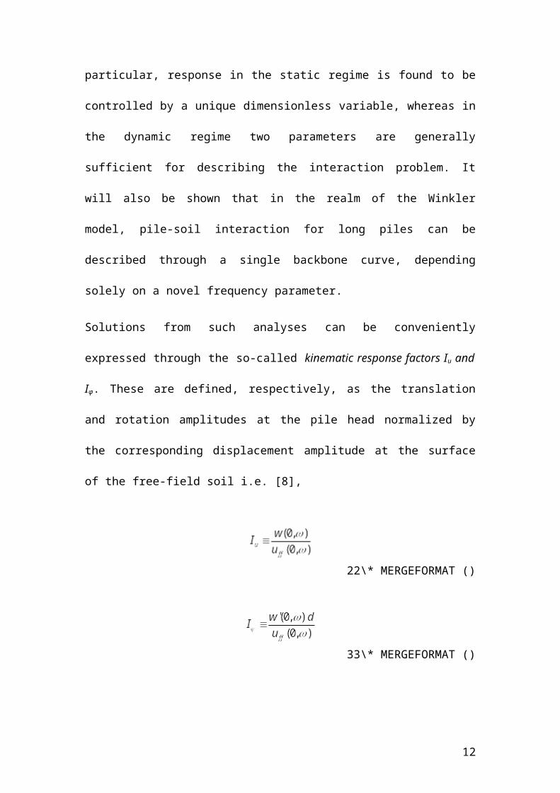
Solutions from such analyses can be conveniently expressed through the so-called

kinematic response factors Iu and Iφ. These are defined, respectively, as the translation

8

and rotation amplitudes at the pile head normalized by the corresponding

displacement amplitude at the surface of the free-field soil i.e. [8],

22\* MERGEFORMAT ()

33\* MERGEFORMAT ()

and is the frequency- and depth-dependent displacement of the

pile and the free-field soil, respectively, and pile diameter.

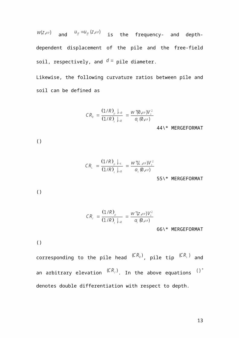
Likewise, the following curvature ratios between pile and soil can be defined as

44\* MERGEFORMAT

()

55\* MERGEFORMAT

()

66\* MERGEFORMAT

()

9

corresponding to the pile head , pile tip and an arbitrary elevation

. In the above equations denotes double differentiation with respect to depth.

3 Model development

Following earlier studies, the problem is treated in the context of two modular

problems, namely the analysis of free-field soil response and the response of the pile.

Each sub-problem is addressed separately below.

3.1 Free-field response

In one-dimensional analysis, the linear stress-strain law is according to the notation of

Fig. 2

77\* MERGEFORMAT ()

where is the complex soil shear modulus, is the shear stress and is

the time- and depth-dependent displacement in the free-field soil.

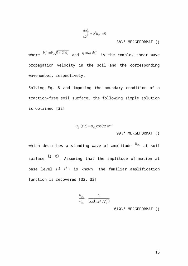
Considering forced harmonic oscillations of the type , the

equilibrium of forces in the horizontal direction acting upon an arbitrary soil element

yields the familiar second-order differential equation

88\* MERGEFORMAT ()

10

where and is the complex shear wave propagation

velocity in the soil and the corresponding wavenumber, respectively.

Solving Eq. 8 and imposing the boundary condition of a traction-free soil surface, the

following simple solution is obtained [32]

99\* MERGEFORMAT ()

which describes a standing wave of amplitude at soil surface . Assuming

that the amplitude of motion at base level ( ) is known, the familiar

amplification function is recovered [32, 33]

1010\* MERGEFORMAT ()

3.2 Pile response

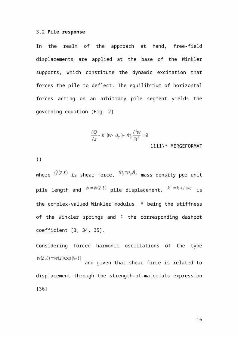
In the realm of the approach at hand, free-field displacements are applied at the base

of the Winkler supports, which constitute the dynamic excitation that forces the pile to

deflect. The equilibrium of horizontal forces acting on an arbitrary pile segment yields

the governing equation (Fig. 2)

1111\* MERGEFORMAT

()

11

where is shear force, mass density per unit pile length and

pile displacement. is the complex-valued Winkler modulus,

being the stiffness of the Winkler springs and the corresponding dashpot

coefficient [3, 34, 35].

Considering forced harmonic oscillations of the type and

given that shear force is related to displacement through the strength-of-materials

expression [36]

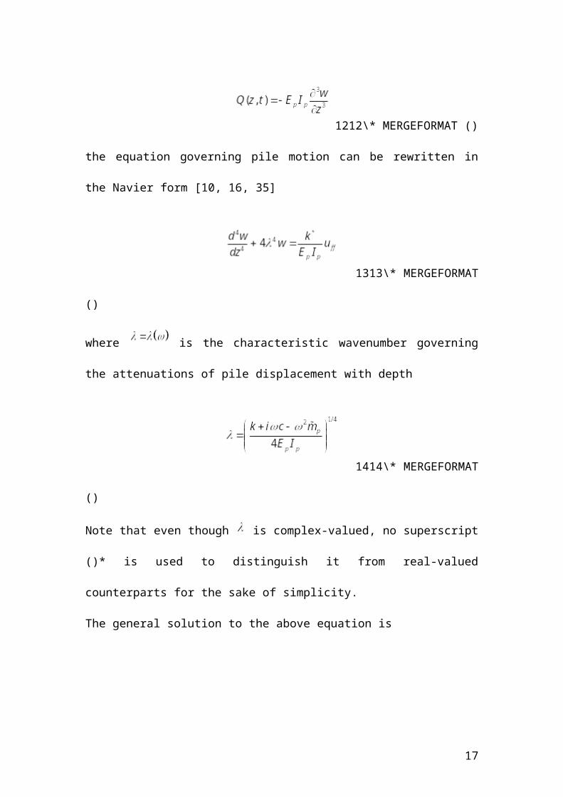
1212\* MERGEFORMAT ()

the equation governing pile motion can be rewritten in the Navier form [10, 16, 35]

1313\* MERGEFORMAT ()

where is the characteristic wavenumber governing the attenuations of pile

displacement with depth

1414\* MERGEFORMAT ()

Note that even though is complex-valued, no superscript ()* is used to distinguish

it from real-valued counterparts for the sake of simplicity.

The general solution to the above equation is

12

1515\*

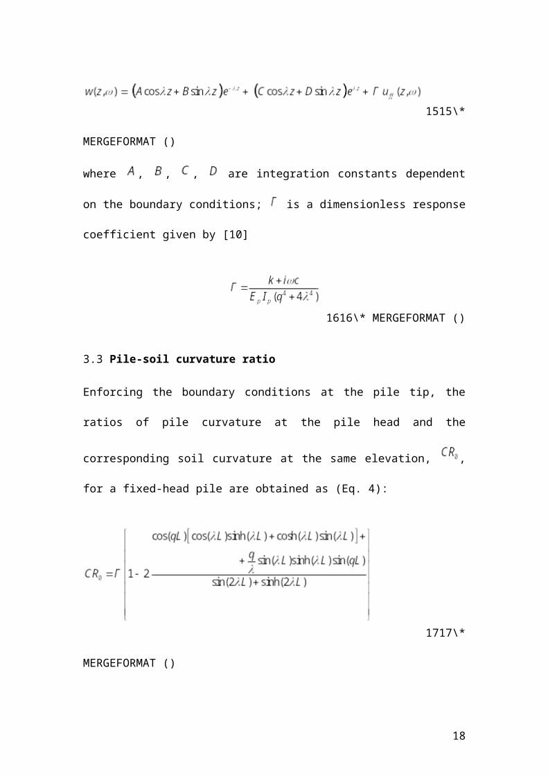
MERGEFORMAT ()

where , , , are integration constants dependent on the boundary conditions;

is a dimensionless response coefficient given by [10]

1616\* MERGEFORMAT ()

3.3 Pile-soil curvature ratio

Enforcing the boundary conditions at the pile tip, the ratios of pile curvature at the

pile head and the corresponding soil curvature at the same elevation, , for a fixed-

head pile are obtained as (Eq. 4):

1717\*

MERGEFORMAT ()

13

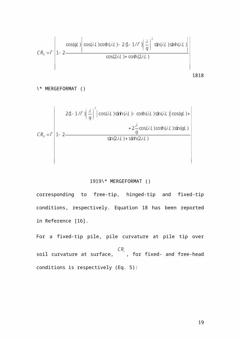
1818\

* MERGEFORMAT ()

1919\* MERGEFORMAT ()

corresponding to free-tip, hinged-tip and fixed-tip conditions, respectively. Equation

18 has been reported in Reference [16].

For a fixed-tip pile, pile curvature at pile tip over soil curvature at surface, , for

fixed- and free-head conditions is respectively (Eq. 5):

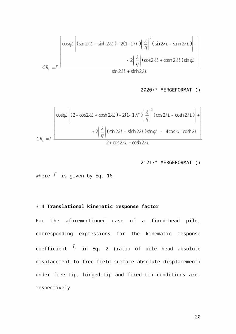
2020\* MERGEFORMAT ()

14

21\* MERGEFORMAT ()

where is given by Eq. 16.

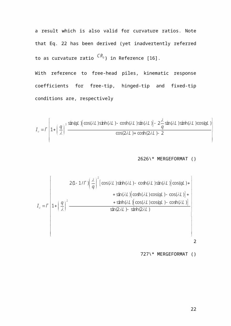
3.4 Translational kinematic response factor

For the aforementioned case of a fixed-head pile, corresponding expressions for the

kinematic response coefficient in Eq. 2 (ratio of pile head absolute displacement to

free-field surface absolute displacement) under free-tip, hinged-tip and fixed-tip

conditions are, respectively

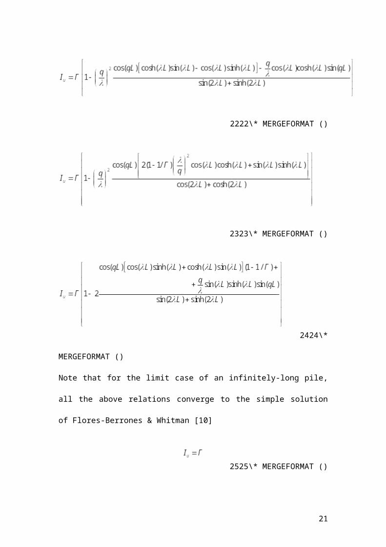
2222\* MERGEFORMAT ()

2323\* MERGEFORMAT ()

15

2424\*

MERGEFORMAT ()

Note that for the limit case of an infinitely-long pile, all the above relations converge

to the simple solution of Flores-Berrones & Whitman [10]

2525\* MERGEFORMAT ()

a result which is also valid for curvature ratios. Note that Eq. 22 has been derived (yet

inadvertently referred to as curvature ratio ) in Reference [16].

With reference to free-head piles, kinematic response coefficients for free-tip, hinged-

tip and fixed-tip conditions are, respectively

2626\* MERGEFORMAT ()

16

27\* MERGEFORMAT ()

28\* MERGEFORMAT ()

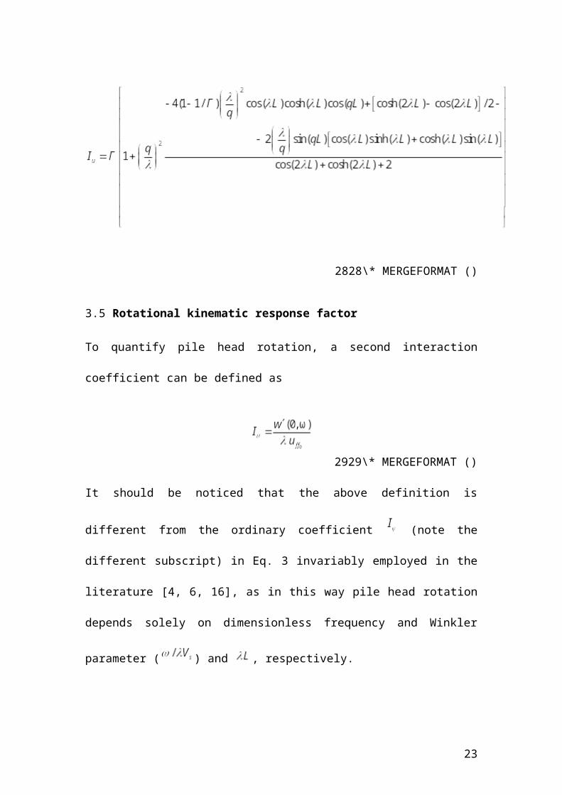
3.5 Rotational kinematic response factor

To quantify pile head rotation, a second interaction coefficient can be defined as

2929\* MERGEFORMAT ()

It should be noticed that the above definition is different from the ordinary coefficient

(note the different subscript) in Eq. 3 invariably employed in the literature [4, 6,

17

16], as in this way pile head rotation depends solely on dimensionless frequency and

Winkler parameter ( ) and , respectively.

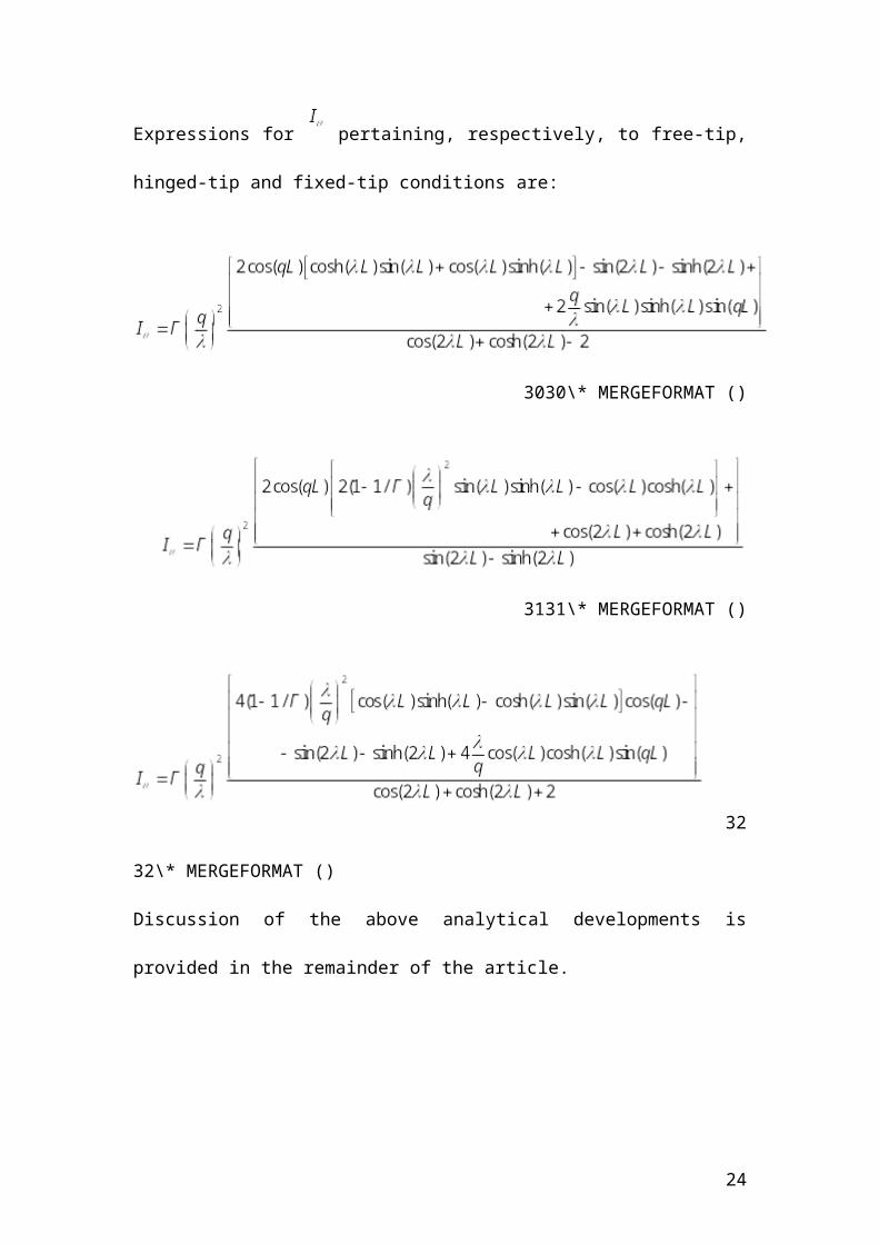
Expressions for pertaining, respectively, to free-tip, hinged-tip and fixed-tip

conditions are:

3030\* MERGEFORMAT ()

3131\* MERGEFORMAT ()

3232\

* MERGEFORMAT ()

Discussion of the above analytical developments is provided in the remainder of the

article.

18

4 Interpretation of results & comparison with other solutions

For comparison purposes, rigorous Finite Element (FE) analyses were performed by

means of the commercial computer platform ANSYS [37]. Given that the geometry is

axisymmetric and the load anti-symmetric, stresses and displacements were expanded

in Fourier series along the circumferential direction, following the technique

introduced by Wilson [38] and later employed by Blaney et al. [8] and Syngros [39].

For the problem at hand, only the first term of the series is relevant and, thereby,

solving a single FE configuration is sufficient. Owing to this procedure, the original

three-dimensional problem is conveniently reduced to a two dimensional. The domain

was discretised using 4-noded axisymmetric elements; following a sensitivity

analysis, the lateral dimension of the model was set equal to 200d, to ensure that soil

response close to the boundaries is not affected by outward-spreading waves emitted

from the pile-soil interface. Likewise, vertical displacements were restrained along the

lateral boundary of the mesh to simulate 1-dimensional conditions for S-waves at

large distances from the pile. In addition, nodes at the base of the model were fully

restrained to represent the rigid bedrock. Vertical size of the elements was kept

constant, equal to which was found to be sufficiently accurate and economical.

The analyses were carried out in the frequency domain [8, 21, 37], the load being

applied in the form of a harmonic horizontal body force in each element.

4.1 Static Response

It is well-known that in Winkler models pile-soil interaction is controlled by the key

dimensionless parameter [10, 35]

19

3333\*

MERGEFORMAT ()

being the product of (evaluated for ) in Eq. 14 and pile length . In such

models is a unique parameter controlling static response, which can be interpreted

as a “mechanical slenderness” (as opposed to the familiar geometrical slenderness

L/d) as it encompasses both geometry and pile-soil relative stiffness ( ).

In addition, is function of the Winkler stiffness coefficient , the value of

which lies in the core of the Winkler representation. The effect of on kinematic

response is examined in Figs. 3 and 4, where pile-soil curvature ratio is plotted against

pile slenderness for two values of pile-soil stiffness contrast. It is evident by

inspecting Figs. 3 and 4, that the predictions of Winkler models employing the

commonly used value pertaining to inertial interaction analyses [40, 41], are

not in good agreement with the FE results for certain cases examined. In Figs. 3a and

3b the value of that matches the FE results seems to decrease with increasing pile

slenderness and with decreasing pile-soil stiffness ratio. Moreover, different values

for “optimum” are obtained depending on boundary conditions at the tip as shown

in Figs. 3c and 3d. In addition, optimum clearly depends on the parameter to be

matched. For instance, it is evident from Figs. 4a and 4b that values of matching

(ratio of pile curvature at tip over soil curvature at soil surface) differ from those

in Fig. 3, referring to , and are independent of pile slenderness . In light of

20

this observation, results for static pile-soil curvature ratio presented in Figs. 5 to 14

are plotted in terms of .

In Fig. 5, static pile-soil curvature ratio at the pile head is plotted against for

different boundary conditions at the pile tip. Naturally, all curves start from zero since

for the pile degenerates into a rigid disk, thus experiencing zero moment

regardless of restraints at the tip. With increasing curvature ratio gradually

increases attaining unity at points A1,2 and A3, and reaching a maximum, above unity,

at points M1, M2, M3 depending on the conditions at the tip. A further increase in

causes pile curvature to drop and gradually converge to soil curvature (B1,2, B3, T), as

the pile becomes sufficiently flexible to follow soil deformation, regardless of tip

conditions.

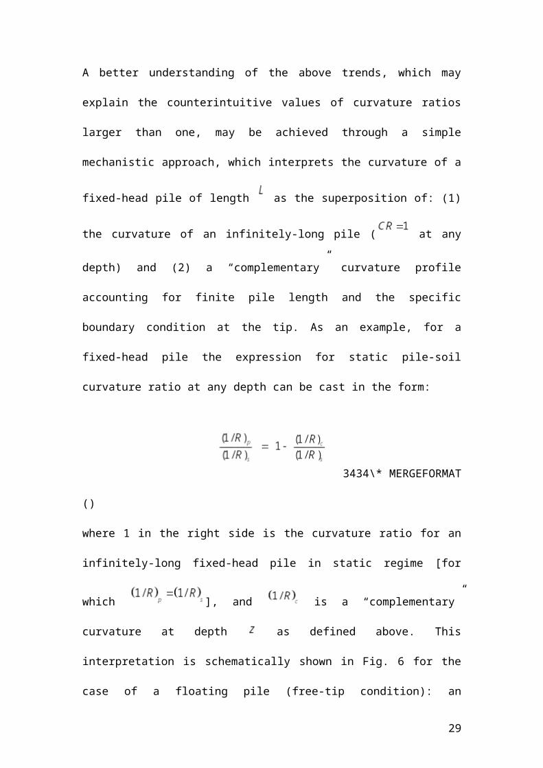
A better understanding of the above trends, which may explain the counterintuitive

values of curvature ratios larger than one, may be achieved through a simple

mechanistic approach, which interprets the curvature of a fixed-head pile of length

as the superposition of: (1) the curvature of an infinitely-long pile ( at any

depth) and (2) a “complementary” curvature profile accounting for finite pile length

and the specific boundary condition at the tip. As an example, for a fixed-head pile

the expression for static pile-soil curvature ratio at any depth can be cast in the form:

3434\* MERGEFORMAT ()

21

where 1 in the right side is the curvature ratio for an infinitely-long fixed-head pile in

static regime [for which ], and is a “complementary”

curvature at depth as defined above. This interpretation is schematically shown in

Fig. 6 for the case of a floating pile (free-tip condition): an infinitely-long pile

embedded in homogeneous soil is conceptually separated from the underlain material

at depth (Fig. 6a). The curvature pattern of the upper part of the pile in Fig. 6a

is tantamount to the superposition of the curvature along a free-tip pile of length

(Fig. 6b) and the complementary curvature of the same pile subjected at its tip to an

action (Fig. 6c), due to the “detached” lower part in Fig. 6a. For this

particular case, substituting the expression for (see [42]), Eq. 34 duly reduces

to Eq. 17 for .

The above procedure can be extended to account for the more general case of a

restrained pile tip. This can be achieved by introducing in Fig. 6b the pertinent

restraining actions at the tip. To ensure equilibrium, the opposite actions must be

applied at pile tip in Fig. 6c. For hinged-tip condition a horizontal force must be

applied at the tip, whereas for a fixed-tip both a force and a moment are required.

Note that because of the statically indeterminate nature of the problem in Fig. 6b, the

values of these restraining actions are not known a priori.

An alternative interpretation of the trends observed in Fig. 5 is possible by means of

the aforementioned superposition approach. Indeed, the complementary curvature at

the pile head may possess different signs depending on the value of . Specifically:

for a very short pile the complementary moment at the pile head will be equal to soil

curvature, thus leading to a zero overall moment at the top. On the other hand, for an

22

infinitely-long pile curvature at the head will be equal to soil curvature, as the external

moment in Fig. 6c will not be transmitted to the pile top. For short piles the moment

transmitted to the head has the same sign as the applied moment. This results in pile-

soil curvature ratios lower than unity. For longer piles, the complementary moment

becomes negative leading to a curvature ratio higher than unity.

The profile of pile curvature with depth over soil curvature at surface, , is

presented in Figs. 7 to 9 for various head and tip conditions and the values of

shown at the insert of Fig. 5. For fixed-head, free-tip conditions (Fig. 7a) the bending

moment along a short pile ( 5.49, Fig. 5) attains its maximum value at the top,

decreasing monotonically with depth. For long piles ( 5.49, Fig. 5) the maximum

curvature ratio develops at depth and attains the value of 1.04. The depth

corresponding to maximum curvature ratio may be related to by means of the

aforementioned superposition scheme through the easy-to-derive expressions valid for

free-tip conditions

3535\* MERGEFORMAT

()

For free-head, free-tip piles (Fig. 7b) all curves are symmetrical. Specifically, for

(short piles) pile bending attains its peak value at mid-depth. For

(long piles) a maximum is observed at two symmetric distances

from the head and tip.

23

Pile-soil curvature ratio for hinged-tip piles is presented in Fig. 8. The behaviour of

fixed-head piles depicted in Fig. 8a is similar to the one shown in Fig 7a: bending

moment attains its maximum at the top for short piles ( 4.71, Fig. 5), whereas for

long piles ( 4.71, Fig. 5) maximum curvature ratio develops at depth and attains

a constant value of . In the same fashion, depth corresponding to the

maximum curvature ratio is related to through the expression

3636\* MERGEFORMAT

()

The hinged-tip pile in Fig. 8b experiences a curvature pattern analogous to that in

Fig. 7b. The maximum value of curvature ratio is observed at for

(short piles), whereas for higher values of the maximum is

observed at the depth given by Eq. 36

For fixed-tip piles, the maximum curvature is always observed at the tip and has an

opposite sign compared to the one at the top (Fig. 9). It is noted in passing that a quick

estimate of the curvature ratio at the pile base can be obtained using the expression of

Dobry & O'Rourke [11] derived for an infinitely-long pile in two-layer soil,

considering an infinitely-stiff bottom layer. This leads to an overestimation of

curvature ratio at the pile tip equal to .

24

4.2 Dynamic Response

Employing the approximate relations for the distributed dashpot coefficient along the

pile derived using planar wave-propagation analysis

[34], the complex-valued wavenumber can be related to its static value through

3737\*

MERGEFORMAT ()

where and are obtained from Eqs. 14 and 33, respectively, and stands

for a characteristic frequency (termed “cutoff frequency”) below which no stress

waves can be emitted from the pile-soil interface to propagate horizontally in the soil

medium and, thereby, no radiation damping is generated. The cutoff frequency is,

therefore, associated with a sudden increase in damping and coincides with the

fundamental frequency of the soil layer in shearing and is expressed in dimensionless

form as

3838\* MERGEFORMAT ()

Note that for the range of frequencies relevant to earthquake engineering, the term

related to pile density in Eq. 37 may be neglected without significant error.

In the same spirit as in static analysis, dynamic pile response can be described by a

unique dimensionless parameter. This is achieved by using the static value of in

25

Eq. 33 in the dynamic regime. The validity of the approximation is explored in Fig.

10, in which pile-soil curvature ratio at the head is plotted against frequency

for selected pile-soil configurations. Predictions using the static value of

in Eq. 33 are compared to those obtained from the complete formulation in Eq. 37

and to FE results. Different values for are used for each case, based on an optimal

selection according to Fig. 3. A convergence of all curves below cutoff frequency is

observed. Beyond cutoff, however, the static assumption leads to a better agreement

with the more rigorous FE results. This is probably due to the approximate description

of radiation damping employed in Eq. 37 which was based on inertial interaction

considerations [34]. Nevertheless, even under a more realistic representation of

geometric energy dissipation, the benefit stemming from the simplified approach

cannot be overstated. It is also worth noting that optimum exhibits only a weak

dependence on frequency. Accordingly, optimum for static analysis (Fig. 3) can be

employed in the dynamic regime (Fig. 10).

Additional comparisons of the proposed model against FE results obtained as part of

this study [37] and from the literature [6] are presented in Figs. 11 and 12 in terms of

translational and rotational kinematic response factors and . It is evident that the

predictions of the model are in satisfactory agreement with the results of the more

rigorous solutions for all configurations examined.

In the remainder of the article, dynamic effects are discussed in terms of pile

curvature and kinematic response factors and . In light of the analytical

developments in Eqs. 22-32, it can be readily recognized that the adoption of

26

(which is independent of mechanical slenderness) as an independent frequency

variable would not allow ( ) to be the main parameter controlling the response. It is

observed that the excitation frequency appears in the solutions only in dimensionless

terms and , thereby, these frequency parameters can

be used for expressing results in the dynamic regime.

For an infinitely-long fixed-head pile, pile-soil curvature ratio at all depths, , and

kinematic response factor can be cast in the form

3939\* MERGEFORMAT

()

Which coincides with factor in Eq. 16 and clearly indicates that the response of

long piles depends solely on the unique frequency parameter and soil

material damping , not on dimensionless frequency .

In Fig. 13, the dynamic de-amplification of curvature ratio at the pile head is plotted

against for fixed-head piles under different boundary conditions at the tip.

Dynamic pile curvature decreases with frequency for all piles of finite length, as the

pile is unable to follow short wavelengths in the soil. For the trivial case

dynamic de-amplification is equal to one, as dynamic pile curvature is always zero.

With increasing all curves approach the one corresponding to the infinitely-long

27

pile regardless of tip conditions. The threshold value of beyond which a pile

behaves as an infinitely-long beam depends on end condition

and is strictly related to the static behaviour depicted in Fig. 5. Indeed,

if a pile behaves as an infinitely-long beam under static conditions

( 4.71, 5.49 - Fig. 5), it behaves the same way in the dynamic regime. Note that

with increasing the curves do not evolve in a monotonic manner. Interestingly,

the lower curve corresponds to the value of for which the curvature ratio is

maximum in static conditions ( corresponding to 2.57, 2.31, π - Fig. 5).

Similar observations can be made for the kinematic response factor (Fig. 14),

except for that the threshold values of mechanical slenderness are lower than in the

previous case. This pattern may reflect that strains are more sensitive to boundary

conditions than displacements.

For free-head piles kinematic response factors and are plotted in Figs. 15 and

16. A common trend is observed: both factors increase with increasing frequency up

to a certain value of . Beyond this value the trend is reversed with and

decreasing with frequency. This behaviour can be explained in light of

wavelengths developing in the soil at different frequencies. With increasing

frequency, wavelengths become shorter forcing the pile to experience stronger

rotations along its length. This also leads to higher displacements atop free-head piles.

Note that the maximum rotation at the pile head is equal to the ratio of free-field

displacement

28

at the soil surface, , and the characteristic wavelength of the

pile, .

5 CONCLUSIONS

A Beam-on-Dynamic-Winkler-Foundation model was employed to investigate the

behaviour of kinematically stressed piles of finite length embedded in a homogeneous

soil layer, for different boundary conditions at the head and tip. Analytical solutions

for pile response were provided in closed form.

The main conclusions of the study may be summarized as follows:

1) Owing to its simplicity, the adopted analytical model can shed light on certain

fundamental mechanisms controlling pile-soil interaction. Its performance,

however, is related to a proper selection of stiffness coefficient which depends

on a number of parameters such as pile slenderness, pile-soil stiffness ratio,

boundary conditions, as well as on the parameter to be matched (i.e., pile

curvature, pile displacement, etc). Nevertheless, it is observed (Fig. 3) that

attains higher values for small pile slenderness and large pile-soil stiffness ratios,

and appears to be independent of frequency (Figs. 3 and 10).

2) In Winkler models, pile-soil kinematic interaction is governed by a unique

dimensionless parameter, , (Eq. 33) which can be interpreted as a “mechanical

slenderness”, encompassing key problem parameters namely pile slenderness,

pile-soil stiffness ratio and Winkler coefficient . A unique parameter ( )

governs the response at static conditions. The same parameter controls the

29

behaviour in the dynamic regime if pile inertia and radiation damping are

neglected. This simplification allows for a better understanding of the interaction

phenomenon and leads to a better agreement of the closed-form solutions with

rigorous numerical results.

3) Pile curvature may be decomposed into the sum of soil curvature and a

complementary curvature that develops along the pile subjected to pertinent forces

and moments at the two ends. These forces depend on the specific boundary

conditions and are responsible for the counterintuitive phenomenon of pile

curvature higher than soil curvature for certain values of pile slenderness.

4) A new dimensionless frequency factor was introduced for normalizing

response in the dynamic regime. It was shown that this allows long piles to exhibit

the same response regardless of actual length and pile-soil stiffness ratio. This can

be understood, since the dimensionless frequency is expressed as ratio of

characteristic pile wavelength and soil wavelength at a given

frequency. As a follow up, a new kinematic response factor was introduced to

describe pile head rotation (Eq. 29). In this way, the interaction is function only of

the aforementioned frequency factor and mechanical slenderness.

Acknowledgements

The research reported in this paper was conducted under the auspices of the ReLUIS

project “Methods for risk evaluation and management of existing buildings”, funded

by the Italian National Emergency Management Agency and was partially supported

by the University of Patras through a Caratheodory Grant (No. C.580). The authors

30

are grateful for this support. The authors also would like to thank the anonymous

Reviewers whose comments improved the quality of the manuscript.

References

[1] Roesset JM, Whitman RV, Dobry R. Modal analysis for structures with

foundation interaction. Journal of the Structural Division 1973; 99 (3): 399-

416.

[2] Wolf JP. Dynamic Soil–Structure Interaction. Englewood Cliffs, NJ, Prentice-

Hall, 1985.

[3] Gazetas G, Mylonakis G. Seismic soil-structure interaction: new evidence and

emerging issues, in Geotechnical Earthquake Engineering and Soil

Dynamics III ASCE, eds. P. Dakoulas, Evl. K. Yegian, and R. D. Holtz,

1998

[4] Kaynia AM, Kausel E. Dynamic stiffness and seismic response of pile groups.

Research Report R82-03. Cambridge, MA: Massachusetts Institute of

Technology, 1982.

[5] Mamoon SM, Banerjee PK. Response of piles and pile groups to travelling SH

waves. Earthquake Engineering and Structural Dynamics 1990;

19:597-610.

[6] Fan K, Gazetas G, Kaynia A, Kausel E, Ahmad S. Kinematic seismic response

of single piles and piles groups. Journal of Geotechnical Engineering

Division ASCE 1991; 117(12):1860-1879.

[7] Rovithis E, Mylonakis G, Pitilakis K. Inertial and kinematic response of piles

in layered inhomogeneous soil: Winkler analysis. Second International

Conference on Performance-Based Design in Earthquake Geotechnical

Engineering, 28-30 May, Taormina, ID:11.21, 2012.

31

[8] Blaney GW, Kausel E, Roesset JM. Dynamic stiffness of piles, in Proceedings

in 2nd International Conference on Numerical Methods in Geomechanics

ASCE, Blackburg, Virginia, 1976.

[9] Margason E. Pile bending during earthquakes. Lecture ASCE/UC-Berkeley

seminar on design construction & performance of deep foundations, 1975.

[10] Flores-Berrones R, Whitman RV. Seismic response of end-bearing

piles.Journal of Geotechnical Engineering Division ASCE 1982;

108(4):554-569.

[11] Dobry R, O'Rourke MJ. Discussion on “Seismic response of end-bearing

piles” by Flores-Berrones R & Whitman RV,” Journal of the Geotechnical

Engineering Division 1983, p. 109.

[12] Kavvadas M, Gazetas G. Kinematic seismic response and bending of free-

head piles in layered soil. Géotechnique 1993; 43(2):207-222.

[13] Mylonakis G. Analytical solutions for seismic pile bending. Unpublished

research report, City University of New York, 1999.

[14] Mylonakis G. Simplified model for seismic pile bending at soil layer

interfaces. Soils and Foundations 2001; 41(4):47-58.

[15] Tazoh T, Shimizu K, Wakahara T. Seismic observations and analysis of

grouped piles. Dynamic response of pile foundations: experiment, analysis

and observation. Geotechnical Special Publication 1987; 11:1-20.

[16] Nikolaou AS, Mylonakis G, Gazetas G, Tazoh T. Kinematic pile bending

during earthquakes analysis and field measurements. Géotechnique 2011:

51(5):425-440.

32

[17] Di Laora R, Mandolini A, Mylonakis G. Insight on kinematic bending of

flexible piles in layered soil. Soil Dynamics and Earthquake Engineering

2012, 43:309-322.

[18] CEN/TC 250. Eurocode 8. Design of structures for earthquake resistance Part

5: Foundations, retaining structures and geotechnical aspects. European

Committee for Standardization Technical Committee 250, Standard EN

1998–5, Brussels, Belgium, 2003.

[19] National Earthquake Hazard Reduction Program. Recommended provisions

for the development of seismic regulations for new buildings. FEMA

publication 274, Building Seismic Safety Council, Washington, D.C., 1997.

[20] de Sanctis L, Maiorano RMS, Aversa S. A method for assessing kinematic

bending moments at the pile head. Earthquake Engineering and Structural

Dynamics 2010; 39:375–397.

[21] Di Laora R. Seismic soil-structure interaction for pile supported systems.

Ph.D. Thesis, University of Napoli “Federico II”, Napoli, 2009.

[22] Di Laora R, Mylonakis G, Mandolini A. Pile-head kinematic bending in

layered soil. Earthquake Engineering and Structural Dynamics 2012; DOI:

10.1002/eqe.2201.

[23] Di Laora R, Mandolini A, Mylonakis G. Selection criteria for pile diameter in

seismic areas. Second International conference on Performance-based

Design in Earthquake Geotechnical Engineering. 28-30 May, Taormina,

Italy. ID:10.15, 2012.

[24] Pender M. Seismic pile foundation design analysis. Bulletin of the New

Zealand National Society for Earthquake Engineering 1993; 26(1):49-160.

33

[25] Kaynia AM, Mahzooni S. Forces in pile foundations under seismic loading.

Journal of Engineering Mechanics ASCE 1996; 122(1):46-53.

[26] Castelli F, Maugeri M. Simplified approach for the seismic response of a pile

foundation. Journal of Geotechnical and Geoenvironmental Engineering

2009; 135(10):1440-1451.

[27] Maiorano RMS, de Sanctis L, Aversa S, Mandolini A. Kinematic response

analysis of piled foundations under seismic excitations. Canadian

Geotechnical Journal 2009; 46(5):571-584.

[28] Dezi F, Carbonari S, Leoni G. Kinematic bending moments in pile

foundations. Soil Dynamics and Earthquake Engineering 2009;

30(3):119-132.

[29] Sica S, Mylonakis G, Simonelli AL. Transient kinematic pile bending in two-

layer soil. Soil Dynamics and Earthquake Engineering 2011; 31(7): 891-905.

[30] Cairo R, Chidichimo A. Nonlinear analysis for pile kinematic response. Fifth

International Conference on Earthquake Geotechnical Engineering. Santiago

(Chile), 10-13 January, 2011.

[31] Buckingham E. On physically similar systems; illustrations of the use of

dimensional equations. Physical Review 1914; 4(4):345-376.

[32] Kramer SL. Geotechnical Earthquake Engineering. New York: Prentice-Hall,

1996.

[33] Roesset JM. Soil amplification of earthquakes, in Numerical Methods in

Geotechnical Engineering (Eds. Desai CS and Christian JT), New York,

McGraw-Hill, 1977.

[34] Gazetas G, Dobry R, Horizontal response of piles in layered soils. Journal of

Geotechnical Engineering ASCE 1984; 110(1): 20-40.

34

[35] Mylonakis G. Contributions to Static and Dynamic Analysis of Piles and Pile-

Supported Bridge Piers. Ph.D. Thesis, State University of New York at

Buffalo, 1995.

[36] Den Hartog JP. Advanced Strength of Materials. New York: McGraw-Hill,

1952.

[37] Inc., ANSYS. ANSYS Theory Reference 10.0. Canonsburg, Pennsylvania,

US, 2005.

[38] Wilson EL. Structural analysis of axisymmetric solids. American Institute of

Aeronautics and Astronautics Journal AIAA 1965; 3:2269-2274.

[39] Syngros C. Seismic response of piles and pile-supported bridge piers

evaluated through case histories. Ph.D. Thesis , City University of New

York, 2004.

[40] Novak M, Nogami T, Aboul-Ella F. Dynamic soil reactions for plane strain

case. Journal of the Engineering Mechanics Division ASCE 1978;

104(4):953-959.

[41] Roesset JM. The use of simple models in soil-structure interaction, in ASCE

specialty conference, Civil Engineering and Nuclear Power, Knoxville, TN,

1980.

[42] Hetenyi M. Beams on Elastic Foundations. Michigan: University of Michigan

Press, Ann Arbor, 1946.

35

FIGURES

Fig. 1. Problem considered and associated boundary conditions at pile head and tip.

Fig. 2. Positive notation for forces and stresses on pile and soil, respectively.

36

Fig. 3. Variation of pile-soil curvature ratio at pile head under static conditions (ω=0), as function of pile slenderness for selected values of Winkler stiffness parameter δ.

37

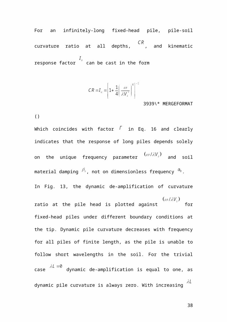
Fig. 4. Variation of pile-soil curvature ratio at pile tip under static conditions (ω=0), as function of pile slenderness for selected values of Winkler stiffness parameter δ.

38

Fig. 6. Kinematic bending along an infinitely-long pile as a superposition of a kinematic and an external load on two piles of finite length (Hatched areas denote

bending moment).

39

Fig. 7. Variation of static pile-soil curvature ratio with depth for free-tip piles, for different geometric and material configurations.

40

Fig. 8. Variation of static pile-soil curvature ratio with depth for hinged-tip piles, for different geometric and material configurations.

41

Fig. 9. Variation of static pile-soil curvature ratio with depth for fixed-tip piles, for different geometric and material configurations.

42

Fig. 10. Variation of dynamic pile-soil curvature ratio at pile head with frequency for fixed-head free-tip piles, for different geometric and material configurations:

comparisons of rigorous elastodynamic FE results with Winkler solutions obtained using the optimum static δ value in Fig. 3. βs=0.10

43

Fig. 11. Variation of kinematic response factor Iu for free-head free-tip piles: comparisons of rigorous elastodynamic FE results with Winkler solutions obtained

using the optimum static δ value in Fig. 3. βs=0.05

44

Fig. 12. Variation of kinematic response factor for free-head free-tip piles: comparisons of rigorous elastodynamic FE results with Winkler solutions obtained

using the optimum static δ value in Fig. 3. βs=0.05

45

Fig. 13. Variation of dynamic pile curvature ratio at pile head with frequency for fixed-head piles under different tip conditions.

46

Fig. 14. Variation of kinematic response factor Iu with frequency for fixed-head piles under different tip conditions.

47

Fig. 15. Variation of kinematic response factor Iu with frequency for free-head piles under different tip conditions.

48

Fig. 16. Variation of kinematic response factor Iθ with frequency for free-head piles under different tip conditions.

49