Italian Meteorological Service Italian Department of Civil ...hsaf.meteoam.it/documents/PUM/PUM-08.pdf · Product User Manual, 31 August 2010 - PUM-08 (Product SM-OBS-2) Page 1 Italian

Product User Manual, 31 August 2010 - PUM-08 (Product SM-OBS-2) Page 1

Italian Meteorological Service

Italian Department of Civil Defence

H-SAF Product User Manual (PUM)

SM-OBS-2 - Small-scale surface soil moisture by

radar scatterometer

Zentralanstalt für Meteorologie und

Geodynamik

Vienna University of Technology Institut für Photogrammetrie

und Fernerkundung Royal Meteorological Institute of Belgium

European Centre for Medium-Range Weather Forecasts

Finnish Meteorological Institute

Finnish Environment Institute

Helsinki University of Technology

Météo-France CNRS Laboratoire Atmosphères,

Milieux, Observations Spatiales CNRS Centre d'Etudes

Spatiales de la BIOsphere Bundesanstalt für Gewässerkunde

Hungarian Meteorological Service

CNR - Istituto Scienze dell’Atmosfera

e del Clima Università di Ferrara

Institute of Meteorology and Water Management

Romania National Meteorological Administration

Slovak Hydro-Meteorological Institute

Turkish State Meteorological Service

Middle East Technical University

Istanbul Technical University Anadolu University

31 August 2010


H-SAF Product User Manual PUM-08 Product SM-OBS-2

Small-scale surface soil moisture by radar scatterometer

INDEX

Page

Acronyms 04

1. Introduction to H-SAF 06 1.1 The EUMETSAT Satellite Application Facilities 06 1.2 H-SAF Objectives and products 06 1.3 Evolution of H-SAF products 08 1.4 User service 10 1.4.1 Product coverage 10 1.4.2 Data circulation and management 10 1.4.3 The H-SAF web site 11 1.4.4 The Help desk 11 1.5 The Products User Manual and its linkage with other documents 11 1.6 Relevant staff associated to the User Service and to product SM-OBS-2 12

2. Introduction to product SM-OBS-2 13 2.1 Principle of sensing 13 2.2 Status of satellites and instruments 13 2.3 Highlights of the algorithm 14 2.4 Architecture of the products generation chain 16 2.5 Product coverage and appearance 17

3. Product operational characteristics 18 3.1 Horizontal resolution and sampling 18 3.2 Vertical resolution if applicable 18 3.3 Observing cycle and time sampling 18 3.4 Timeliness 18

4. Product validation 19 4.1 Validation strategy 19 4.2 Summary of results 19

5. Product availability 21 5.1 Site 21 5.2 Formats and codes 21 5.3 Description of the files 21 5.4 Condition for use 22

Appendix: SM-OBS-2 Output description 23


List of Tables

Table 01 - List of H-SAF products 07Table 02 - User community addressed by H-SAF products 08Table 03 - Definition of the development status of a product according to EUMETSAT 09Table 04 - Relevant persons associated to the User service and to product SM-OBS-2 12Table 05 - Current status of MetOp and Envisat satellites (as of March 2010) 13Table 06 - Main features of ASCAT 14Table 07 - Main features of ASAR 14Table 08 - Statistical scores for SM-OBS-2 21Table 09 - Summary instructions for accessing SM-OBS-2 data 21

List of Figures

Fig. 01 - Conceptual scheme of the EUMETSAT application ground segment 06Fig. 02 - Current composition of the EUMETSAT SAF network (in order of establishment) 06Fig. 03 - Logic of the incremental development scheme 09Fig. 04 - Required H-SAF coverage: 25-75°N lat, 25°W - 45°E 10Fig. 05 - H-SAF central archive and distribution facilities 10Fig. 06 - Scanning geometry of ASCAT 13Fig. 07 - Principle of disaggregation by auxiliary data 13Fig. 08 - Flow chart of the processing chain for the disaggregated soil moisture product 15Fig. 09 - Conceptual architecture of the SM-OBS-2 production chain 16Fig. 10 - Example of small-scale surface soil moisture (SM-OBS-2) from ASCAT. Note the two

side swaths (550 km each) and the 670 km gap in between. MetOp-A, 30 September 2009, 20:12 UTC

17

Fig. 11 - Detailed view of SM-OBS-2 over central Europe (left panel). MetOp-A, 5 June 2007, 19:18 - 19:19 UTC. Area of ∼ 880 x 650 km2. For comparison, the SM-OBS-1 product is shown (right panel). No-data values are masked

17

Fig. 12 - Structure of the Soil moisture products validation team 19


Acronyms

ASAR Advanced Synthetic Aperture Radar (on Envisat) ASAR GM ASAR Global Mode ASCAT Advanced Scatterometer (on MetOp) ATDD Algorithms Theoretical Definition Document AU Anadolu University (in Turkey) BfG Bundesanstalt für Gewässerkunde (in Germany) BUFR Binary Universal Form for the Representation of meteorological data CAF Central Application Facility (of EUMETSAT) CC Correlation Coefficient CDA Command and Data Acquisition station CESBIO Centre d'Etudes Spatiales de la BIOsphere (of CNRS, in France) CM-SAF SAF on Climate Monitoring CNMCA Centro Nazionale di Meteorologia e Climatologia Aeronautica (in Italy) CNR Consiglio Nazionale delle Ricerche (of Italy) CNRS Centre Nationale de la Recherche Scientifique (of France) CORINE COoRdination of INformation on the Environment DPC Dipartimento Protezione Civile (of Italy) DWD Deutscher Wetterdienst EARS EUMETSAT Advanced Retransmission Service ECMWF European Centre for Medium-range Weather Forecasts Envisat Environmental Satellite ESA European Space Agency EUM Short for EUMETSAT EUMETCast EUMETSAT’s Broadcast System for Environmental Data EUMETSAT European Organisation for the Exploitation of Meteorological Satellites FMI Finnish Meteorological Institute FTP File Transfer Protocol GEO Geostationary Earth Orbit GMES Global Monitoring for Environment and Security GRAS-SAF SAF on GRAS Meteorology H-SAF SAF on Support to Operational Hydrology and Water Management IFOV Instantaneous Field Of View IMWM Institute of Meteorology and Water Management (in Poland) IPF Institut für Photogrammetrie und Fernerkundung (of TU-Wien, in Austria) IR Infra Red IRM Institut Royal Météorologique (of Belgium) (alternative of RMI) ISAC Istituto di Scienze dell’Atmosfera e del Clima (of CNR, Italy) ITU İstanbul Technical University (in Turkey) LATMOS Laboratoire Atmosphères, Milieux, Observations Spatiales (of CNRS, in France) LEO Low Earth Orbit LSA-SAF SAF on Land Surface Analysis LST Local Solar Time (of a sunsynchronous orbit) ME Mean Error Météo France National Meteorological Service of France MetOp Meteorological Operational satellite METU Middle East Technical University (in Turkey) MTF Modulation Transfer Function MW Micro Wave NMA National Meteorological Administration (of Romania) NOAA National Oceanic and Atmospheric Administration (Agency and satellite)


NWC Nowcasting NWC-SAF SAF in support to Nowcasting & Very Short Range Forecasting NWP Numerical Weather Prediction NWP-SAF SAF on Numerical Weather Prediction O3M-SAF SAF on Ozone and Atmospheric Chemistry Monitoring OMSZ Hungarian Meteorological Service ORR Operations Readiness Review OSI-SAF SAF on Ocean and Sea Ice Pixel Picture element PNG Portable Network Graphics PUM Product User Manual PVR Product Validation Report REP-3 H-SAF Products Valiadation Report RMI Royal Meteorological Institute (of Belgium) (alternative of IRM) RMSE Root Mean Square Error SAF Satellite Application Facility SAR Synthetic Aperture Radar SD Standard Deviation SHMÚ Slovak Hydro-Meteorological Institute SYKE Suomen ympäristökeskus (Finnish Environment Institute) TKK Teknillinen korkeakoulu (Helsinki University of Technology) TSMS Turkish State Meteorological Service TU-Wien Technische Universität Wien (in Austria) UniFe University of Ferrara (in Italy) URL Uniform Resource Locator UTC Universal Coordinated Time VIS Visible WARP-H WAter Retrieval Package for hydrologic applications ZAMG Zentralanstalt für Meteorologie und Geodynamik (of Austria)


1. Introduction to H-SAF

1.1 The EUMETSAT Satellite Application Facilities

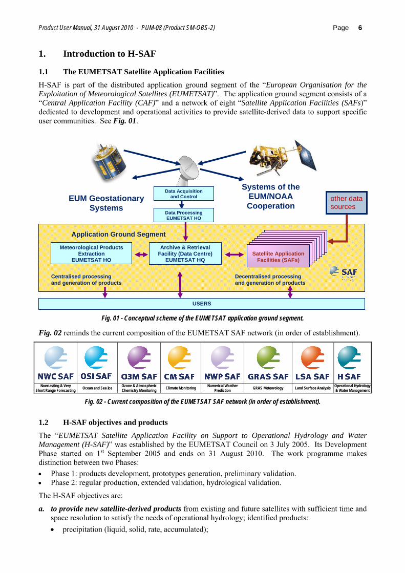
H-SAF is part of the distributed application ground segment of the “European Organisation for the Exploitation of Meteorological Satellites (EUMETSAT)”. The application ground segment consists of a “Central Application Facility (CAF)” and a network of eight “Satellite Application Facilities (SAFs)” dedicated to development and operational activities to provide satellite-derived data to support specific user communities. See Fig. 01.

Fig. 01 - Conceptual scheme of the EUMETSAT application ground segment.

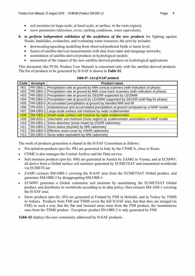
Fig. 02 reminds the current composition of the EUMETSAT SAF network (in order of establishment).

Nowcasting & Very

Short Range Forecasting Ocean and Sea Ice Ozone & Atmospheric Chemistry Monitoring Climate Monitoring Numerical Weather

Prediction GRAS Meteorology Land Surface Analysis Operational Hydrology & Water Management

Fig. 02 - Current composition of the EUMETSAT SAF network (in order of establishment).

1.2 H-SAF objectives and products

The “EUMETSAT Satellite Application Facility on Support to Operational Hydrology and Water Management (H-SAF)” was established by the EUMETSAT Council on 3 July 2005. Its Development Phase started on 1st September 2005 and ends on 31 August 2010. The work programme makes distinction between two Phases: • Phase 1: products development, prototypes generation, preliminary validation. • Phase 2: regular production, extended validation, hydrological validation.

The H-SAF objectives are:

a. to provide new satellite-derived products from existing and future satellites with sufficient time and space resolution to satisfy the needs of operational hydrology; identified products: • precipitation (liquid, solid, rate, accumulated);

Decentralised processing and generation of products

EUM Geostationary Systems

Systems of the EUM/NOAA Cooperation

Centralised processing and generation of products

Data Acquisition and Control

Data Processing EUMETSAT HQ

Meteorological Products Extraction

EUMETSAT HQ

Archive & Retrieval Facility (Data Centre)

EUMETSAT HQ

USERS

Application Ground Segment

other data sources

Satellite Application

Facilities (SAFs)


• soil moisture (at large-scale, at local-scale, at surface, in the roots region); • snow parameters (detection, cover, melting conditions, water equivalent);

b. to perform independent validation of the usefulness of the new products for fighting against floods, landslides, avalanches, and evaluating water resources; the activity includes: • downscaling/upscaling modelling from observed/predicted fields to basin level; • fusion of satellite-derived measurements with data from radar and raingauge networks; • assimilation of satellite-derived products in hydrological models; • assessment of the impact of the new satellite-derived products on hydrological applications.

This document (the PUM, Product User Manual) is concerned only with the satellite-derived products. The list of products to be generated by H-SAF is shown in Table 01.

Table 01 - List of H-SAF products Code Acronym Product name H01 PR-OBS-1 Precipitation rate at ground by MW conical scanners (with indication of phase) H02 PR-OBS-2 Precipitation rate at ground by MW cross-track scanners (with indication of phase) H03 PR-OBS-3 Precipitation rate at ground by GEO/IR supported by LEO/MW H04 PR-OBS-4 Precipitation rate at ground by LEO/MW supported by GEO/IR (with flag for phase) H05 PR-OBS-5 Accumulated precipitation at ground by blended MW and IR H06 PR-ASS-1 Instantaneous and accumulated precipitation at ground computed by a NWP model H07 SM-OBS-1 Large-scale surface soil moisture by radar scatterometer H08 SM-OBS-2 Small-scale surface soil moisture by radar scatterometer H09 SM-ASS-1 Volumetric soil moisture (roots region) by scatterometer assimilation in NWP model H10 SN-OBS-1 Snow detection (snow mask) by VIS/IR radiometry H11 SN-OBS-2 Snow status (dry/wet) by MW radiometry H12 SN-OBS-3 Effective snow cover by VIS/IR radiometry H13 SN-OBS-4 Snow water equivalent by MW radiometry

The work of products generation is shared in the H-SAF Consortium as follows: • Precipitation products (pre-fix: PR) are generated in Italy by the CNMCA, close to Rome. • CNMCA also manages the Central Archive and the Data service. • Soil moisture products (pre-fix: SM) are generated in Austria by ZAMG in Vienna, and at ECMWF;

all derive from a Global surface soil moisture generated by EUMETSAT and transmitted worldwide via EUMETCast.

• ZAMG extracts SM-OBS-1 covering the H-SAF area from the EUMETSAT Global product, and generates SM-OBS-2 by disaggregating SM-OBS-1.

• ECMWF generates a Global volumetric soil moisture by assimilating the EUMETSAT Global product, and distributes its worldwide according to its data policy; then extracts SM-ASS-1 covering the H-SAF area.

• Snow products (pre-fix: SN) are generated in Finland by FMI in Helsinki, and in Turkey by TSMS in Ankara. Products from FMI and TSMS cover the full H-SAF area, but then they are merged (in FMI) in such a way that the flat and forested areas stem from the FMI product, the mountainous ones from the TSMS product. Exception: product SN-OBS-2 is only generated by FMI.

Table 02 deploys the user community addressed by H-SAF products.


Table 02 - User community addressed by H-SAF products

Entity Application Precipitation Soil moisture Snow parameters Fluvial basins management

Early warning of potential floods.

Landslides and flash flood forecasting.

Evaluation of flood damping or enhancing factors.

Extreme events statistics and hydrological risk mapping. Territory

management Public works planning.

Soil characterisation and hydrological response units.

Dimes and exploitation of snow and glaciers for river regime regularisation.

Operational hydrological units

Water reservoirs evaluation

Inventory of potential stored water resources.

Monitoring of available water to sustain vegetation.

Dimes and exploitation of snow and glaciers for drinkable water and irrigation.

Assimilation to represent latent heat release inside the atmosphere.

Numerical Weather Prediction Evaluation of NWP model’s

skill.

Input of latent heat by evapotranspiration through the Planetary Boundary Layer.

Input of radiative heat from surface to atmosphere.

Public information on actual weather. Warning of avalanches.

Warning for fishery and coastal zone activities. Tourism information. Nowcasting

Warning for agricultural works and crop protection.

Warning on the status of the territory for transport in emergencies.

Assistance to aviation during take-off and landing. Monitoring glacier extension.

National meteorological services

Climate monitoring

Representation of the global water cycle in General Circulation Models.

Monitoring of desertification processes. Monitoring changes of

planetary albedo. Progressive level of attention function of rainfall monitoring.

Monitoring soil moisture growth. Monitoring snow accumulation.

Preparation for emergencies Preparation of facilities and

staff for a possible emergency. Planning of in-field activities for event mitigation.

Planning of in-field activities for event mitigation.

Emergency management Alert to population.

Operational conditions for transport and use of staff and mitigation facilities.

Operational conditions for transport and use of staff and mitigation facilities.

Withdrawing of staff and mitigation facilities.

Withdrawing of staff and mitigation facilities.

Civil defence

Post-emergency phase

De-ranking of alert level and monitoring of event ceasing. Assessment of vulnerability to

possible event iteration. Assessment of vulnerability to possible event iteration.

Improved knowledge of the precipitation process. Meteorology Assimilation of precipitation observation in NWP models.

Assessment of the role of observed soil moisture in NWP, either for verification or initialisation.

Assessment of the role of observed snow parameters in NWP, either for verification or initialisation.

Downscaling/upscaling of satellite precipitation observations.

Downscaling/upscaling of satellite soil moisture observations.

Downscaling/upscaling of satellite snow observations.

Fusion with ground-based observations.

GIS-based fusion with ground-based observations.

GIS-based fusion with ground-based observations.

Hydrology

Assimilation and impact studies.



Research & development activities

Civil defence Decisional models for the alert system.

Organisational models for operating over moist soil.

Organisational models for operating over snow.

1.3 Evolution of H-SAF products

One special requirement of the H-SAF work plan was that the Hydrological validation programme, that started downstream of products availability, lasts for a sufficient time There was therefore a need to make available as soon as possible at least part of the products, accepting that their status of consolidation was still incomplete, the quality was not yet the best, and the characterisation was still poor due to limited validation. According to EUMETSAT definitions, the status of development of a product is qualified as in Table 03.


Table 03 - Definition of the development status of a product according to EUMETSAT In development Products or software packages that are in development and not yet available to users

Demonstrational Products or software packages that are provided to users without any commitment on the quality or availability of the service and have been considered by the relevant Steering Group to be useful to be disseminated in order to enabling users to test the product and to provide feedback

Pre-operational Products or software packages with documented limitations that are able to satisfy the majority of applicable requirements and/or have been considered by the relevant Steering Group suitable for distribution to users

Operational Products or software packages with documented non-relevant limitations that largely satisfy the requirements applicable and/or have been considered by the relevant Steering Group mature enough for distribution to users

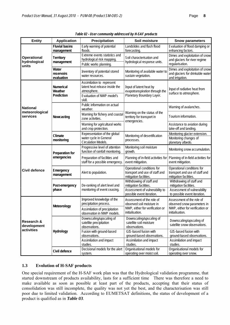
The need for early release of products to activate the Hydrological validation programme as soon as possible led to define a stepwise approach for H-SAF products development. This is shown in Fig. 03.

The time reference for this work plan is as follows: • after approximately two years from the start of the Project (i.e. starting from the nominal date of 1st

January 2008) a substantial fraction of the products listed in Table 01 are released first as “in development” and then after, as soon as some validation is performed, as “demonstrational”;

• in the remaining three years the Hydrological validation programme builds up and grows. Mid-time, i.e. in mid-2009, the products of the first release are supposed to become “pre-operational”, and the products missing the first release reach at least a demonstrational status. All products should become “operational” at the end of the Development Phase (31 August 2010).

Until the products are in the development status, their distribution is limited to the so-called beta users. Demonstrational, pre-operational and operational products have open distribution.

It is fair to record that not all products have been able to follow this schedule. Therefore, at the end of the Development Phase, the status of “in development”, “demonstrational”, “pre-operational” and “operational” will apply differently to the different products.

End-user feedback

Augmented databases

Advanced algorithms

New instruments

Initial databases

Baseline algorithms

Current instruments

Cal/val programme

1st release 2nd release Final release Prototyping

Representative End-users and Hydrological validation programme

Fig. 03 - Logic of the incremental development scheme.

Demonstrational products

Pre-operationalproducts

Operational products

Limited distribution (to beta users)

Progressively open distribution

Open distribution

Open distribution

Products in development Prototypes

Special distribution


1.4 User service

In this section a short overview of the User service is provided, in terms of product geographic coverage, data circulation and management, Web site and Help desk.

1.4.1 Product coverage

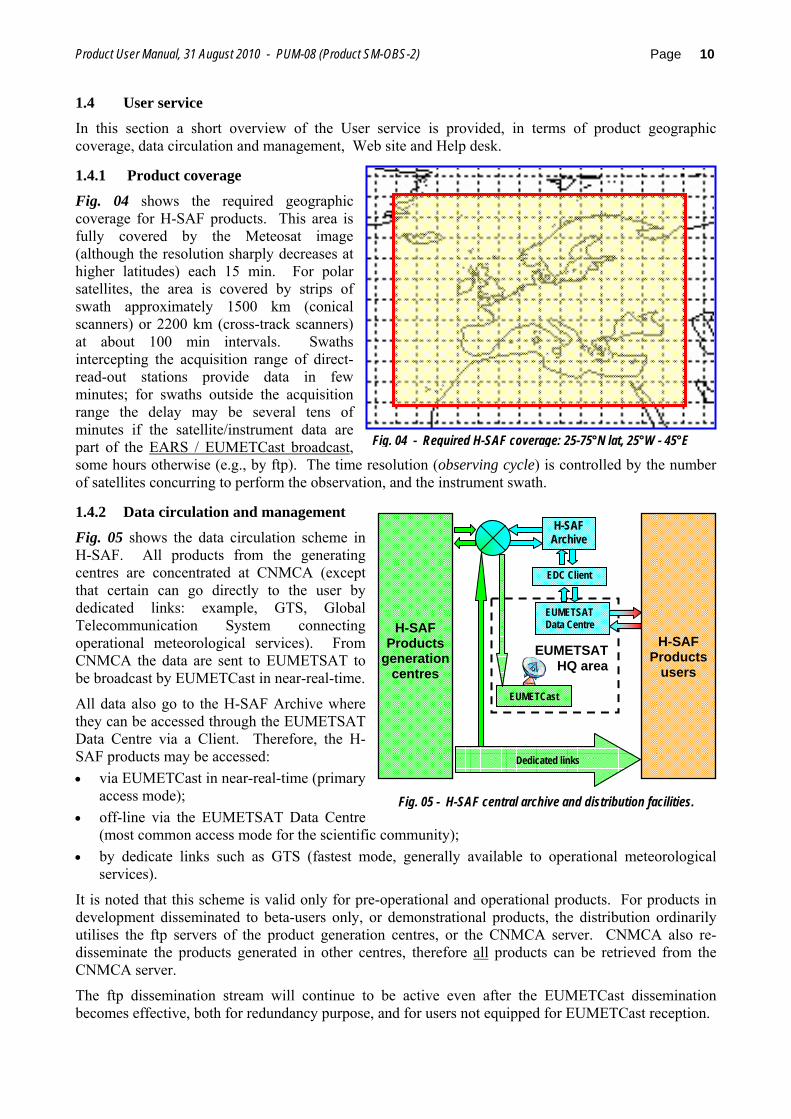
Fig. 04 shows the required geographic coverage for H-SAF products. This area is fully covered by the Meteosat image (although the resolution sharply decreases at higher latitudes) each 15 min. For polar satellites, the area is covered by strips of swath approximately 1500 km (conical scanners) or 2200 km (cross-track scanners) at about 100 min intervals. Swaths intercepting the acquisition range of direct-read-out stations provide data in few minutes; for swaths outside the acquisition range the delay may be several tens of minutes if the satellite/instrument data are part of the EARS / EUMETCast broadcast, some hours otherwise (e.g., by ftp). The time resolution (observing cycle) is controlled by the number of satellites concurring to perform the observation, and the instrument swath.

1.4.2 Data circulation and management

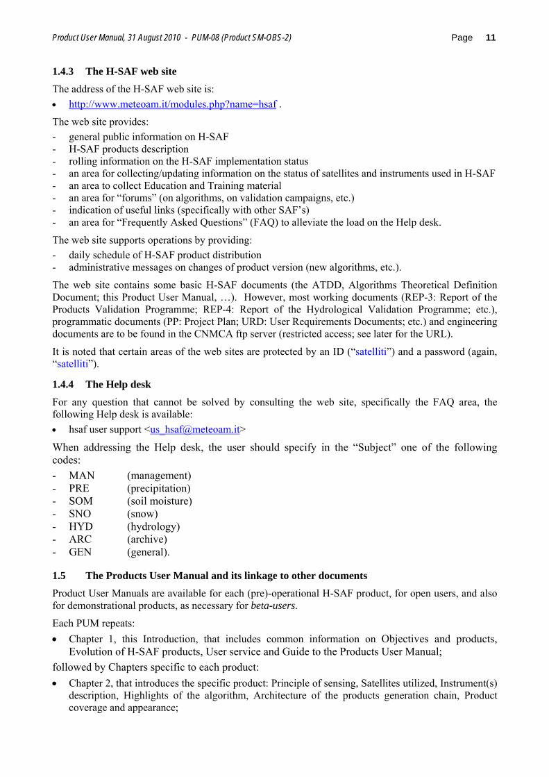
Fig. 05 shows the data circulation scheme in H-SAF. All products from the generating centres are concentrated at CNMCA (except that certain can go directly to the user by dedicated links: example, GTS, Global Telecommunication System connecting operational meteorological services). From CNMCA the data are sent to EUMETSAT to be broadcast by EUMETCast in near-real-time.

All data also go to the H-SAF Archive where they can be accessed through the EUMETSAT Data Centre via a Client. Therefore, the H-SAF products may be accessed: • via EUMETCast in near-real-time (primary

access mode); • off-line via the EUMETSAT Data Centre

(most common access mode for the scientific community); • by dedicate links such as GTS (fastest mode, generally available to operational meteorological

services).

It is noted that this scheme is valid only for pre-operational and operational products. For products in development disseminated to beta-users only, or demonstrational products, the distribution ordinarily utilises the ftp servers of the product generation centres, or the CNMCA server. CNMCA also re-disseminate the products generated in other centres, therefore all products can be retrieved from the CNMCA server.

The ftp dissemination stream will continue to be active even after the EUMETCast dissemination becomes effective, both for redundancy purpose, and for users not equipped for EUMETCast reception.

Fig. 04 - Required H-SAF coverage: 25-75°N lat, 25°W - 45°E

EUMETSAT HQ area

Dedicated links

H-SAF Archive

EUMETSAT Data Centre

Fig. 05 - H-SAF central archive and distribution facilities.

EDC Client

EUMETCast

H-SAF Products

generation centres

H-SAF Products

users


1.4.3 The H-SAF web site

The address of the H-SAF web site is: • http://www.meteoam.it/modules.php?name=hsaf .

The web site provides: - general public information on H-SAF - H-SAF products description - rolling information on the H-SAF implementation status - an area for collecting/updating information on the status of satellites and instruments used in H-SAF - an area to collect Education and Training material - an area for “forums” (on algorithms, on validation campaigns, etc.) - indication of useful links (specifically with other SAF’s) - an area for “Frequently Asked Questions” (FAQ) to alleviate the load on the Help desk.

The web site supports operations by providing: - daily schedule of H-SAF product distribution - administrative messages on changes of product version (new algorithms, etc.).

The web site contains some basic H-SAF documents (the ATDD, Algorithms Theoretical Definition Document; this Product User Manual, …). However, most working documents (REP-3: Report of the Products Validation Programme; REP-4: Report of the Hydrological Validation Programme; etc.), programmatic documents (PP: Project Plan; URD: User Requirements Documents; etc.) and engineering documents are to be found in the CNMCA ftp server (restricted access; see later for the URL).

It is noted that certain areas of the web sites are protected by an ID (“satelliti”) and a password (again, “satelliti”).

1.4.4 The Help desk

For any question that cannot be solved by consulting the web site, specifically the FAQ area, the following Help desk is available: • hsaf user support <[email protected]>

When addressing the Help desk, the user should specify in the “Subject” one of the following codes: - MAN (management) - PRE (precipitation) - SOM (soil moisture) - SNO (snow) - HYD (hydrology) - ARC (archive) - GEN (general).

1.5 The Products User Manual and its linkage to other documents

Product User Manuals are available for each (pre)-operational H-SAF product, for open users, and also for demonstrational products, as necessary for beta-users.

Each PUM repeats: • Chapter 1, this Introduction, that includes common information on Objectives and products,

Evolution of H-SAF products, User service and Guide to the Products User Manual; followed by Chapters specific to each product: • Chapter 2, that introduces the specific product: Principle of sensing, Satellites utilized, Instrument(s)

description, Highlights of the algorithm, Architecture of the products generation chain, Product coverage and appearance;


• Chapter 3, that describes the main product operational characteristics: Horizontal resolution and sampling, Vertical resolution if applicable (only for SM-ASS-1), Observing cycle and time sampling, Timeliness;

• Chapter 4, that provides an overview of the product validation activity: Validation strategy, Global statistics, Product characterisation

• Chapter 5, that provides basic information on product availability: Access modes, Description of the code, Description of the file structure

Although reasonably self-standing, the PUM’s rely on other documents for further details. Specifically: • ATDD (Algorithms Theoretical Definition Document), for extensive details on the algorithms, only

highlighted here; • PVR (Product Validation Report), for full recount of the validation activity, both the evolution and

the latest results.

These documents are structured as this PUM, i.e. one document for each product. They can be retrieved from the CNMCA site: • ftp://ftp.meteoam.it - username: hsaf - password: 00Hsaf - directory: hsaf - folder: Final-Report-

Development-Phase.

On the same site, it is interesting to consult, although not closely connected to this PUM, the full reporting on hydrological validation experiments (impact studies): • HVR (Hydrological Validation Report), spread in 10 Parts, first one on requirements, tools and

models, then 8, each one for one participating country, and a last Part with overall statements on the impact of H-SAF products in Hydrology.

1.6 Relevant staff associated to the User Service and to product SM-OBS-2

Table 04 records the names of the persons associated to the development and operation of the User service and of product SM-OBS-2.

Table 04 - Relevant persons associated to the User service and to product SM-OBS-2

User service development and operation Adriano Raspanti (Leader) [email protected] Leonardo Facciorusso [email protected] Francesco Coppola [email protected] Giuseppe Leonforte

Centro Nazionale di Meteorologia e Climatologia Aeronautica (CNMCA) Italy

[email protected] Product Development Team Wolfgang Wagner (Leader) [email protected] Stefan Hasenauer [email protected] Marcela Doubkova [email protected] Daniel Sabel

Technische Universität Wien (TU-Wien), Institut für Photogrammetrie und Fernerkundung (IPF) Austria

[email protected] Product Operations Team Barbara Zeiner (Leader) Zentralanstalt für Meteorologie und Geodynamik (ZAMG) Austria [email protected]


2. Introduction to product SM-OBS-2

2.1 Principle of sensing

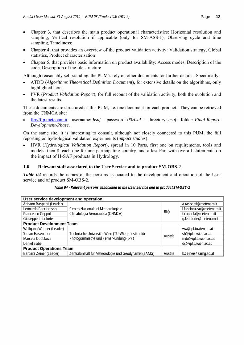
Product SM-OBS-2 (Small-scale surface soil moisture by radar scatterometer) results from post-processing of the SM-OBS-1 product extracted by ZAMG from the Global surface soil moisture product distributed by EUMETSAT. Product SM-OBS-1 is based on the radar scatterometer ASCAT embarked on MetOp satellites. The instrument scans the scene in a push-broom mode by six side-looking antennas, three left-hand, three right-hand (see Fig. 06). On each side, the three antennas, looking aside, + 45° and - 45° respectively, provide three views of each earth location under different viewing angles measuring three backscattering coefficients (σ0, sigma-nought) at slightly different time. Each antenna triplet provides a side swath of 550 km. The two swaths leave a gap (close to the sub-satellite track) of ~ 670 km. Global coverage over Europe is achieved in ~ 1.5 days.

The basic instrument sampling distance is 12.5 km. The primary ASCAT observation, sea-surface wind, is processed at 50 km resolution. For soil moisture, processing is performed at 50 km (operational) and 25 km (research) resolution.

For the purpose of SM-OBS-2, the 25-km resolution SM-OBS-1 product is disaggregated and re-sampled at 1-km intervals to better fit hydrological requirements.

The disaggregation process (see Fig. 07) makes use of a fine-mesh layer pre-computed and stored in a parameter database. The fine-mesh information includes backscatter and scaling characteristics derived from SAR imagery from Envisat ASAR operating in the ScanSAR Global monitoring mode.

2.2 Status of satellites and instruments

The current status of MetOp and Envisat satellites is shown in Table 05. Table 05 - Current status of MetOp and Envisat satellites (as of March 2010)

Satellite Launch End of service Height LST Status Instruments used in H-SAF MetOp-A 19 Oct 2006 expected ≥ 2011 817 km 09:30 d Operational ASCAT Envisat 1 Mar 2002 expected ≥ 2013 800 km 10:00 d Operational ASAR

Although ASCAT data are not directly used (the processed SM-OBS-1 product is used instead), its main characteristics, that are reflected in SM-OBS-2, are recorded in the Table 06. The main features of ASAR, that is used for building the database of disaggregation parameters, are recorded in Table 07. Envisat is managed by ESA, and ASAR data are available from the ESA archives. Since ASAR is operated in time sharing among several modes, building the database for SM-OBS-2 is a lengthy undertaking.

Fig. 06 - Scanning geometry of ASCAT.

Fig. 07 - Principle of disaggregation by auxiliary data.


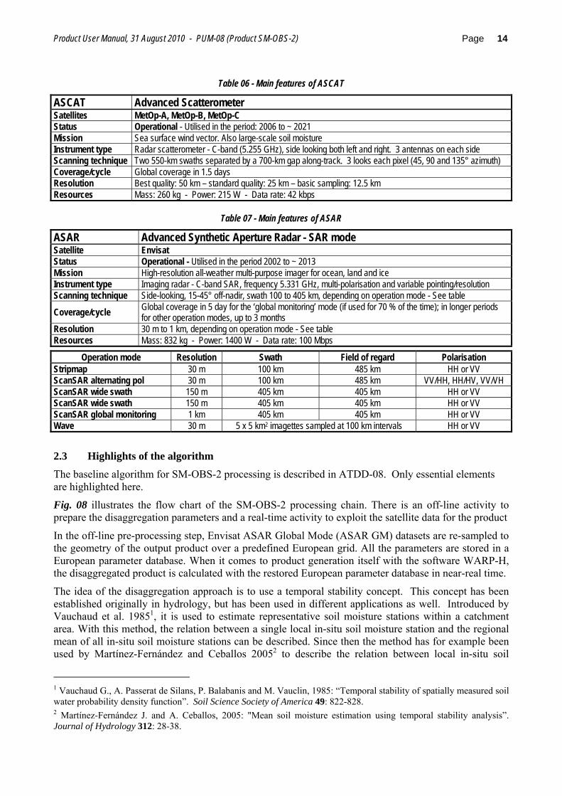
Table 06 - Main features of ASCAT

ASCAT Advanced Scatterometer Satellites MetOp-A, MetOp-B, MetOp-C Status Operational - Utilised in the period: 2006 to ~ 2021 Mission Sea surface wind vector. Also large-scale soil moisture Instrument type Radar scatterometer - C-band (5.255 GHz), side looking both left and right. 3 antennas on each side Scanning technique Two 550-km swaths separated by a 700-km gap along-track. 3 looks each pixel (45, 90 and 135° azimuth) Coverage/cycle Global coverage in 1.5 days Resolution Best quality: 50 km – standard quality: 25 km – basic sampling: 12.5 km Resources Mass: 260 kg - Power: 215 W - Data rate: 42 kbps

Table 07 - Main features of ASAR

ASAR Advanced Synthetic Aperture Radar - SAR mode Satellite Envisat Status Operational - Utilised in the period 2002 to ~ 2013 Mission High-resolution all-weather multi-purpose imager for ocean, land and ice Instrument type Imaging radar - C-band SAR, frequency 5.331 GHz, multi-polarisation and variable pointing/resolution Scanning technique Side-looking, 15-45° off-nadir, swath 100 to 405 km, depending on operation mode - See table

Coverage/cycle Global coverage in 5 day for the ‘global monitoring’ mode (if used for 70 % of the time); in longer periods for other operation modes, up to 3 months

Resolution 30 m to 1 km, depending on operation mode - See table Resources Mass: 832 kg - Power: 1400 W - Data rate: 100 Mbps

Operation mode Resolution Swath Field of regard Polarisation Stripmap 30 m 100 km 485 km HH or VV ScanSAR alternating pol 30 m 100 km 485 km VV/HH, HH/HV, VV/VH ScanSAR wide swath 150 m 405 km 405 km HH or VV ScanSAR wide swath 150 m 405 km 405 km HH or VV ScanSAR global monitoring 1 km 405 km 405 km HH or VV Wave 30 m 5 x 5 km2 imagettes sampled at 100 km intervals HH or VV

2.3 Highlights of the algorithm

The baseline algorithm for SM-OBS-2 processing is described in ATDD-08. Only essential elements are highlighted here.

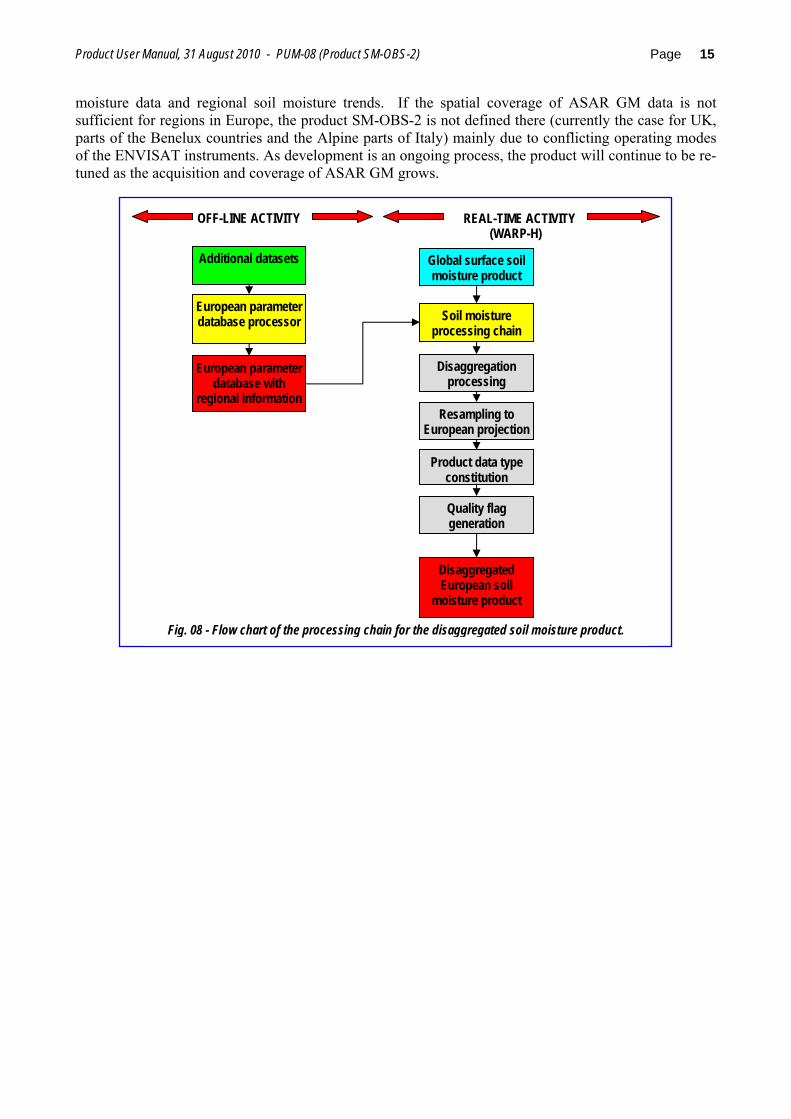
Fig. 08 illustrates the flow chart of the SM-OBS-2 processing chain. There is an off-line activity to prepare the disaggregation parameters and a real-time activity to exploit the satellite data for the product

In the off-line pre-processing step, Envisat ASAR Global Mode (ASAR GM) datasets are re-sampled to the geometry of the output product over a predefined European grid. All the parameters are stored in a European parameter database. When it comes to product generation itself with the software WARP-H, the disaggregated product is calculated with the restored European parameter database in near-real time.

The idea of the disaggregation approach is to use a temporal stability concept. This concept has been established originally in hydrology, but has been used in different applications as well. Introduced by Vauchaud et al. 19851, it is used to estimate representative soil moisture stations within a catchment area. With this method, the relation between a single local in-situ soil moisture station and the regional mean of all in-situ soil moisture stations can be described. Since then the method has for example been used by Martínez-Fernández and Ceballos 20052 to describe the relation between local in-situ soil

1 Vauchaud G., A. Passerat de Silans, P. Balabanis and M. Vauclin, 1985: “Temporal stability of spatially measured soil water probability density function”. Soil Science Society of America 49: 822-828. 2 Martínez-Fernández J. and A. Ceballos, 2005: "Mean soil moisture estimation using temporal stability analysis”. Journal of Hydrology 312: 28-38.


moisture data and regional soil moisture trends. If the spatial coverage of ASAR GM data is not sufficient for regions in Europe, the product SM-OBS-2 is not defined there (currently the case for UK, parts of the Benelux countries and the Alpine parts of Italy) mainly due to conflicting operating modes of the ENVISAT instruments. As development is an ongoing process, the product will continue to be re-tuned as the acquisition and coverage of ASAR GM grows.

European parameter database processor

OFF-LINE ACTIVITY REAL-TIME ACTIVITY(WARP-H)

Fig. 08 - Flow chart of the processing chain for the disaggregated soil moisture product.

Additional datasets

Disaggregated European soil

moisture product

European parameter database with

regional information

Disaggregation processing

Resampling to European projection

Product data type constitution

Quality flag generation

Soil moisture processing chain

Global surface soil moisture product


2.4 Architecture of the products generation chain

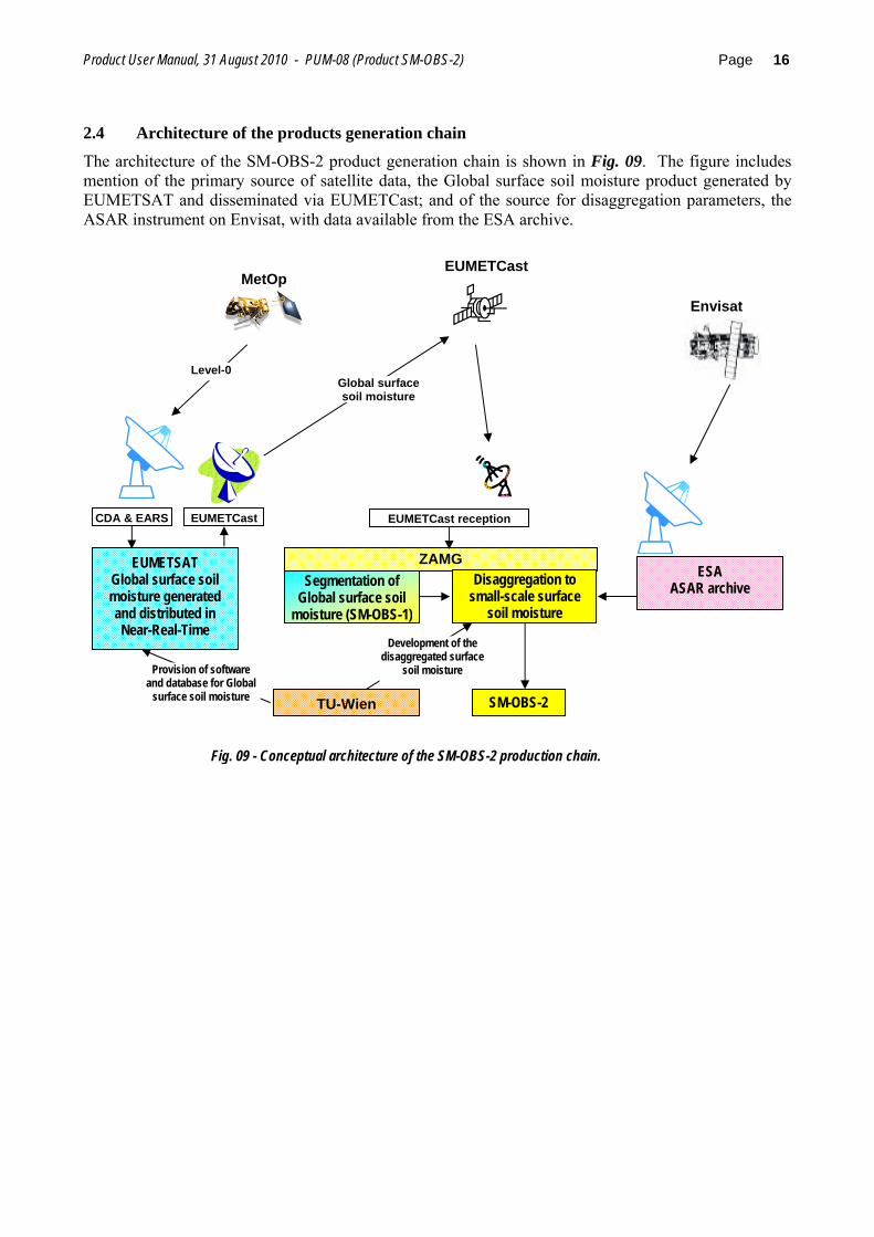
The architecture of the SM-OBS-2 product generation chain is shown in Fig. 09. The figure includes mention of the primary source of satellite data, the Global surface soil moisture product generated by EUMETSAT and disseminated via EUMETCast; and of the source for disaggregation parameters, the ASAR instrument on Envisat, with data available from the ESA archive.

EUMETCastMetOp

Global surface soil moisture

Level-0

CDA & EARS EUMETCast EUMETCast reception

EUMETSAT Global surface soil moisture generated and distributed in Near-Real-Time

ZAMG

TU-Wien

Provision of software and database for Global

surface soil moisture

Segmentation of Global surface soil

moisture (SM-OBS-1)

Disaggregation to small-scale surface

soil moisture

Development of the disaggregated surface

soil moisture

SM-OBS-2

Fig. 09 - Conceptual architecture of the SM-OBS-2 production chain.

ESA ASAR archive

Envisat


2.5 Product coverage and appearance

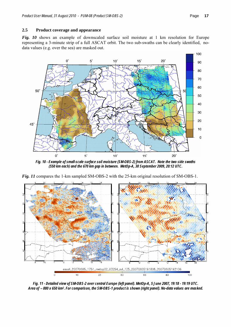
Fig. 10 shows an example of downscaled surface soil moisture at 1 km resolution for Europe representing a 3-minute strip of a full ASCAT orbit. The two sub-swaths can be clearly identified, no-data values (e.g. over the sea) are masked out.

Fig. 10 - Example of small-scale surface soil moisture (SM-OBS-2) from ASCAT. Note the two side swaths (550 km each) and the 670 km gap in between. MetOp-A, 30 September 2009, 20:12 UTC.

Fig. 11 compares the 1-km sampled SM-OBS-2 with the 25-km original resolution of SM-OBS-1.

Fig. 11 - Detailed view of SM-OBS-2 over central Europe (left panel). MetOp-A, 5 June 2007, 19:18 - 19:19 UTC. Area of ∼ 880 x 650 km2. For comparison, the SM-OBS-1 product is shown (right panel). No-data values are masked.


3. Product operational characteristics

3.1 Horizontal resolution and sampling

The horizontal resolution (∆x) is the convolution of several features (sampling distance, degree of independence of the information relative to nearby samples, …). To simplify matters, it is generally agreed to refer to the sampling distance between two successive product values, assuming that they carry forward reasonably independent information. The horizontal resolution descends from the instrument Instantaneous Field of View (IFOV), sampling distance (pixel), Modulation Transfer Function (MTF) and number of pixels to co-process for filtering out disturbing factors (e.g. clouds) or improving accuracy. It may be appropriate to specify both the resolution ∆x associated to independent information, and the sampling distance, useful to minimise aliasing problems when data have to undertake resampling (e.g., for co-registration with other data).

In the case of SM-OBS-2, the effective resolution is controlled by the originating product, SM-OBS-1, therefore the worst-case figure representative of the SM-OBS-2 resolution is: ∆x = 25 km. However, the disaggregation process performs re-sampling at 1 km intervals, that therefore would constitute the resolution in best conditions. The effectiveness of disaggregation depends on the availability and the effectiveness of the disaggregation parameters, that in certain areas may be of poor quality. The SM-OBS-2 resolution is therefore ∆x = 1 ÷ 25 km. The sampling distance is 1 km.

3.2 Vertical resolution if applicable

The vertical resolution (∆z) also is defined by referring to the vertical sampling distance between two successive product values, assuming that they carry forward reasonably independent information. The vertical resolution descends from the exploited remote sensing principle and the instrument number of channels, or spectral resolution. It is difficult to be estimated a-priori: it is generally evaluated a-posteriori by means of the validation activity.

The only product in H-SAF that provides profiles (below surface) is SM-ASS-1 (Volumetric soil moisture (roots region) by scatterometer assimilation in NWP model).

3.3 Observing cycle and time sampling

The observing cycle (∆t) is defined as the average time interval between two measurements over the same area. In general the area is, for GEO, the disk visible from the satellite, for LEO, the Globe. In the case of H-SAF we refer to the European area shown in Fig. 04. In the case of LEO, the observing cycle depends on the instrument swath and the number of satellites carrying the addressed instrument.

The ASCAT swath is 550 + 550 km on the two sides, with a 670 km gap in between. The gap left by ascending orbits is mostly filled by descending orbits. In average the observing cycle over Europe is ∆t ~ 36 h, improving with latitude. However, areas where disaggregation parameters are not available, are not processed, therefore the SM-OBS-2 maps leave several gaps of coverage. These gaps will progressively reduce along with progress of the ASAR coverage [and ultimately with the availability of the ESA/GMES Sentinel-1: launch scheduled in 2012]

3.4 Timeliness

The timeliness (δ) is defined as the time between observation taking and product available at the user site assuming a defined dissemination mean. The timeliness depends on the satellite transmission facilities, the availability of acquisition stations, the processing time required to generate the product and the reference dissemination means. In the case of H-SAF the future dissemination tool is EUMETCast, but currently we refer to the availability on the FTP site.

The product is generated shortly after reception of the Global product from EUMETSAT via EUMETCast, that has a timeliness of ~ 1.5 h. The processing time is less than 20 minutes. Adding 10 min for distribution we have: δ ~ 2 h.


4. Product validation

4.1 Validation strategy

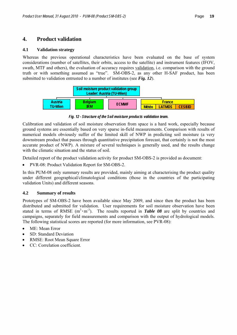
Whereas the previous operational characteristics have been evaluated on the base of system considerations (number of satellites, their orbits, access to the satellite) and instrument features (IFOV, swath, MTF and others), the evaluation of accuracy requires validation, i.e. comparison with the ground truth or with something assumed as “true”. SM-OBS-2, as any other H-SAF product, has been submitted to validation entrusted to a number of institutes (see Fig. 12).

Soil moisture product validation group Leader: Austria (TU-Wien)

France Austria TU-Wien Belgium

IRM ECMWF Météo LATMOS CESBIO

Fig. 12 - Structure of the Soil moisture products validation team.

Calibration and validation of soil moisture observation from space is a hard work, especially because ground systems are essentially based on very sparse in-field measurements. Comparison with results of numerical models obviously suffer of the limited skill of NWP in predicting soil moisture (a very downstream product that passes through quantitative precipitation forecast, that certainly is not the most accurate product of NWP). A mixture of several techniques is generally used, and the results change with the climatic situation and the status of soil.

Detailed report of the product validation activity for product SM-OBS-2 is provided as document: • PVR-08: Product Validation Report for SM-OBS-2.

In this PUM-08 only summary results are provided, mainly aiming at characterising the product quality under different geographical/climatological conditions (those in the countries of the participating validation Units) and different seasons.

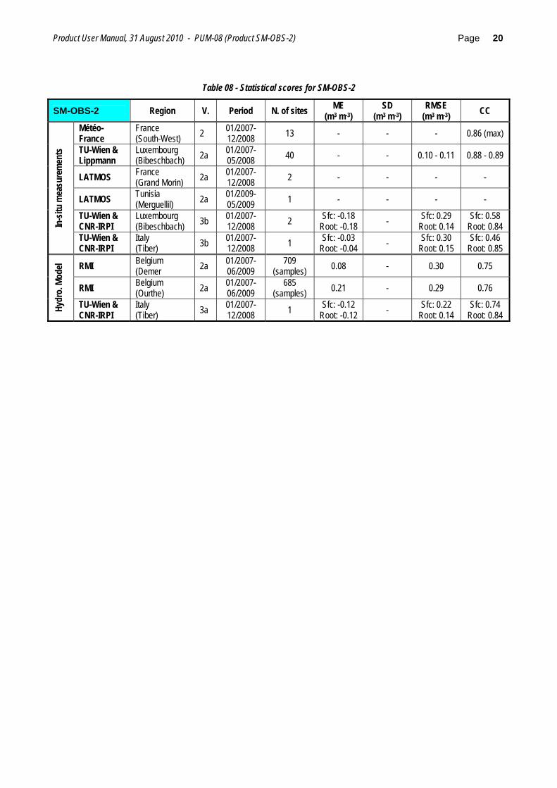
4.2 Summary of results

Prototypes of SM-OBS-2 have been available since May 2009, and since then the product has been distributed and submitted for validation. User requirements for soil moisture observation have been stated in terms of RMSE (m3٠m-3). The results reported in Table 08 are split by countries and campaigns, separately for field measurements and comparison with the output of hydrological models. The following statistical scores are reported (for more information, see PVR-08): • ME: Mean Error • SD: Standard Deviation • RMSE: Root Mean Square Error • CC: Correlation coefficient.


Table 08 - Statistical scores for SM-OBS-2

SM-OBS-2 Region V. Period N. of sites ME (m3�m-3)

SD (m3�m-3)

RMSE (m3�m-3) CC

Météo- France

France (South-West) 2 01/2007-

12/2008 13 - - - 0.86 (max)

TU-Wien & Lippmann

Luxembourg (Bibeschbach) 2a 01/2007-

05/2008 40 - - 0.10 - 0.11 0.88 - 0.89

LATMOS France (Grand Morin) 2a 01/2007-

12/2008 2 - - - -

LATMOS Tunisia (Merguellil) 2a 01/2009-

05/2009 1 - - - -

TU-Wien & CNR-IRPI

Luxembourg (Bibeschbach) 3b 01/2007-

12/2008 2 Sfc: -0.18 Root: -0.18 - Sfc: 0.29

Root: 0.14 Sfc: 0.58

Root: 0.84 In-s

itu m

easu

rem

ents

TU-Wien & CNR-IRPI

Italy (Tiber) 3b 01/2007-

12/2008 1 Sfc: -0.03 Root: -0.04 - Sfc: 0.30

Root: 0.15 Sfc: 0.46

Root: 0.85

RMI Belgium (Demer 2a 01/2007-

06/2009 709

(samples) 0.08 - 0.30 0.75

RMI Belgium (Ourthe) 2a 01/2007-

06/2009 685

(samples) 0.21 - 0.29 0.76

Hydr

o. M

odel

TU-Wien & CNR-IRPI

Italy (Tiber) 3a 01/2007-

12/2008 1 Sfc: -0.12 Root: -0.12 - Sfc: 0.22

Root: 0.14 Sfc: 0.74

Root: 0.84


5. Product availability

5.1 Site

SM-OBS-2 will be available via EUMETCast (when authorized) and via FTP (after log in).

The current access is via FTP at the following site: • URL: ftp://ftp.meteoam.it • username: hsaf • password: 00Hsaf .

The data are loaded in the directory: • products, for near-real-time dissemination and data holding for nominally 1-2 months, often more;

Older data are stored in the permanent H-SAF archive, and can be recovered on request.

Quick-looks of the latest 3 days of SM-OBS-2 maps, covering some H-SAF areas, can be viewed on the H-SAF web site: • http://www.meteoam.it/modules.php?name=hsaf • directory: products, sub-directory: soil moisture, ID: satelliti, password: satelliti.

5.2 Formats and codes

SM-OBS-2 is codes as: • the digital data: BUFR • the image-like maps: PNG

In the directory “utilities”, the folder Bufr_decode provides the instructions for reading the digital data. In addition, the output description of SM-OBS-2 is provided in Appendix.

5.3 Description of the files

The data are available under • Directory: products • Sub-directory: h08 • Two folders:

- h08_cur_mon_buf - h08_cur_mon_png

Table 09 summarises the situation and provides the information on the file structure. Table 09 - Summary instructions for accessing SM-OBS-2 data

URL: ftp://ftp.meteoam.it username: hsaf password: 00Hsaf directory: products h08_cur_mon_buf digital data of current months Product identifier: h08.

Folders under h08: h08_cur_mon_png Images of current months h08_yyyymmdd_hhmmss_satellite_nnnnn_ZAMG.buf.gz digital data Files description of

current month: h08_yyyymmdd_hhmmss_satellite_nnnnn_ZAMG.png image data yyyymmdd: year, month, day hhmmss: hour, minute, second of first scan line (ascending: southernmost; descending: northernmost) satellite: name of the satellite (currently: metopa) nnnnn: orbit number


5.4 Condition for use

All H-SAF products are owned by EUMETSAT, and the EUMETSAT SAF Data Policy applies. They are available for all users free of charge.

Users should recognise the respective roles of EUMETSAT, the H-SAF Leading Entity and the H-SAF Consortium when publishing results that are based on H-SAF products. EUMETSAT’s ownership of and intellectual property rights into the SAF data and products is best safeguarded by simply displaying the words “© EUMETSAT” under each of the SAF data and products shown in a publication or website.

See Appendix: SM-OBS-2 Output description


Appendix: SM-OBS-2 Output description

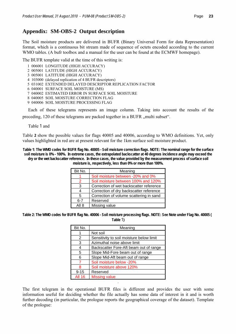
The Soil moisture products are delivered in BUFR (Binary Universal Form for data Representation) format, which is a continuous bit stream made of sequence of octets encoded according to the current WMO tables. (A bufr toolbox and a manual for the user can be found at the ECMWF homepage).

The BUFR template valid at the time of this writing is: 1 006001 LONGITUDE (HIGH ACCURACY) 2 005001 LATITUDE (HIGH ACCURACY) 3 005001 LATITUDE (HIGH ACCURACY) 4 103000 (delayed replication of 4 BUFR descriptors) 5 031002 EXTENDED DELAYED DESCRIPTOR REPLICATION FACTOR 6 040001 SURFACE SOIL MOISTURE (MS) 7 040002 ESTIMATED ERROR IN SURFACE SOIL MOISTURE 8 040005 SOIL MOISTURE CORRECTION FLAG 9 040006 SOIL MOISTURE PROCESSING FLAG

Each of these telegrams represents an image column. Taking into account the results of the preceding, 120 of these telegrams are packed together in a BUFR „multi subset“.

Table 1 and

Table 2 show the possible values for flags 40005 and 40006, according to WMO definitions. Yet, only values highlighted in red are at present relevant for the 1km surface soil moisture product.

Table 1: The WMO codes for BUFR flag No. 40005 - Soil moisture correction flags. NOTE: The nominal range for the surface soil moisture is 0% - 100%. In extreme cases, the extrapolated backscatter at 40 degrees incidence angle may exceed the

dry or the wet backscatter reference. In these cases, the value provided by the measurement process of surface soil moisture is, respectively, less than 0% or more than 100%.

Bit No. Meaning 1 Soil moisture between -20% and 0% 2 Soil moisture between 100% and 120% 3 Correction of wet backscatter reference 4 Correction of dry backscatter reference 5 Correction of volume scattering in sand

6-7 Reserved All 8 Missing value

Table 2: The WMO codes for BUFR flag No. 40006 - Soil moisture processing flags. NOTE: See Note under Flag No. 40005 (

Table 1)

Bit No. Meaning 1 Not soil 2 Sensitivity to soil moisture below limit 3 Azimuthal noise above limit 4 Backscatter Fore-Aft beam out of range 5 Slope Mid-Fore beam out of range 6 Slope Mid-Aft beam out of range 7 Soil moisture below -20% 8 Soil moisture above 120%

9-15 Reserved All 16 Missing value

.

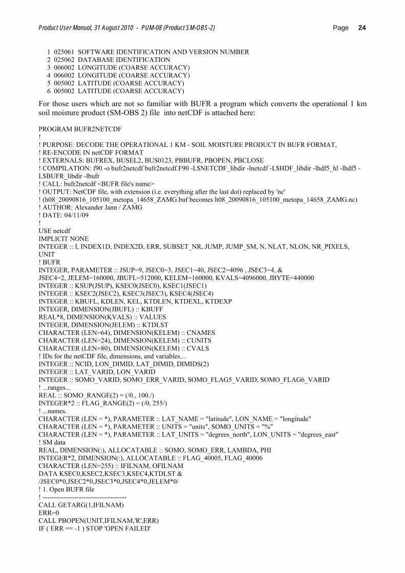
The first telegram in the operational BUFR files is different and provides the user with some information useful for deciding whether the file actually has some data of interest in it and is worth further decoding (in particular, the prologue reports the geographical coverage of the dataset). Template of the prologue:


1 025061 SOFTWARE IDENTIFICATION AND VERSION NUMBER 2 025062 DATABASE IDENTIFICATION 3 006002 LONGITUDE (COARSE ACCURACY) 4 006002 LONGITUDE (COARSE ACCURACY) 5 005002 LATITUDE (COARSE ACCURACY) 6 005002 LATITUDE (COARSE ACCURACY)

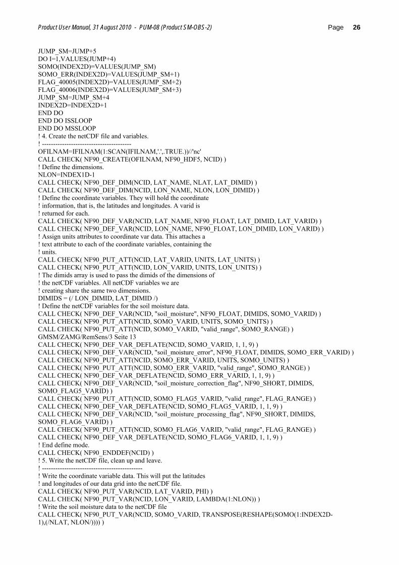
For those users which are not so familiar with BUFR a program which converts the operational 1 km soil moisture product (SM-OBS 2) file into netCDF is attached here: PROGRAM BUFR2NETCDF ! ! PURPOSE: DECODE THE OPERATIONAL 1 KM - SOIL MOISTURE PRODUCT IN BUFR FORMAT, ! RE-ENCODE IN netCDF FORMAT ! EXTERNALS: BUFREX, BUSEL2, BUS0123, PBBUFR, PBOPEN, PBCLOSE ! COMPILATION: f90 -o bufr2netcdf bufr2netcdf.F90 -L$NETCDF_libdir -lnetcdf -L$HDF_libdir -lhdf5_hl -lhdf5 - L$BUFR_libdir -lbufr ! CALL: bufr2netcdf <BUFR file's name> ! OUTPUT: NetCDF file, with extension (i.e. everything after the last dot) replaced by 'nc' ! (h08_20090816_105100_metopa_14658_ZAMG.buf becomes h08_20090816_105100_metopa_14658_ZAMG.nc) ! AUTHOR: Alexander Jann / ZAMG ! DATE: 04/11/09 ! USE netcdf IMPLICIT NONE INTEGER :: I, INDEX1D, INDEX2D, ERR, SUBSET_NR, JUMP, JUMP_SM, N, NLAT, NLON, NR_PIXELS, UNIT ! BUFR INTEGER, PARAMETER :: JSUP=9, JSEC0=3, JSEC1=40, JSEC2=4096 , JSEC3=4, & JSEC4=2, JELEM=160000, JBUFL=512000, KELEM=160000, KVALS=4096000, JBYTE=440000 INTEGER :: KSUP(JSUP), KSEC0(JSEC0), KSEC1(JSEC1) INTEGER :: KSEC2(JSEC2), KSEC3(JSEC3), KSEC4(JSEC4) INTEGER :: KBUFL, KDLEN, KEL, KTDLEN, KTDEXL, KTDEXP INTEGER, DIMENSION(JBUFL) :: KBUFF REAL*8, DIMENSION(KVALS) :: VALUES INTEGER, DIMENSION(JELEM) :: KTDLST CHARACTER (LEN=64), DIMENSION(KELEM) :: CNAMES CHARACTER (LEN=24), DIMENSION(KELEM) :: CUNITS CHARACTER (LEN=80), DIMENSION(KELEM) :: CVALS ! IDs for the netCDF file, dimensions, and variables... INTEGER :: NCID, LON_DIMID, LAT_DIMID, DIMIDS(2) INTEGER :: LAT_VARID, LON_VARID INTEGER :: SOMO_VARID, SOMO_ERR_VARID, SOMO_FLAG5_VARID, SOMO_FLAG6_VARID ! ...ranges... REAL :: SOMO_RANGE(2) = (/0., 100./) INTEGER*2 :: FLAG_RANGE(2) = (/0, 255/) ! ...names. CHARACTER (LEN = *), PARAMETER :: LAT_NAME = "latitude", LON_NAME = "longitude" CHARACTER (LEN = *), PARAMETER :: UNITS = "units", SOMO_UNITS = "%" CHARACTER (LEN = *), PARAMETER :: LAT_UNITS = "degrees_north", LON_UNITS = "degrees_east" ! SM data REAL, DIMENSION(:), ALLOCATABLE :: SOMO, SOMO_ERR, LAMBDA, PHI INTEGER*2, DIMENSION(:), ALLOCATABLE :: FLAG_40005, FLAG_40006 CHARACTER (LEN=255) :: IFILNAM, OFILNAM DATA KSEC0,KSEC2,KSEC3,KSEC4,KTDLST & /JSEC0*0,JSEC2*0,JSEC3*0,JSEC4*0,JELEM*0/ ! 1. Open BUFR file ! ------------------------------------- CALL GETARG(1,IFILNAM) ERR=0 CALL PBOPEN(UNIT,IFILNAM,'R',ERR) IF ( ERR == -1 ) STOP 'OPEN FAILED'


IF ( ERR == -2 ) STOP 'INVALID FILE NAME' IF ( ERR == -3 ) STOP 'INVALID OPEN MODE SPECIFIED' ! 2. Decode prologue ! ------------------------------------- ERR=0 CALL PBBUFR(UNIT,KBUFF,JBYTE*4,KBUFL,ERR) IF (ERR /= 0) STOP 'cannot even read the prologue :-(' KBUFL=KBUFL/4+1 CALL BUS0123(KBUFL, KBUFF, KSUP, KSEC0, KSEC1, KSEC2, KSEC3, ERR) KEL=KVALS/KSEC3(3) IF (KEL > KELEM) KEL=KELEM ! Expand BUFR message. CALL BUFREX(KBUFL, KBUFF, KSUP, KSEC0, KSEC1, KSEC2, KSEC3, KSEC4, & KEL, CNAMES, CUNITS, KVALS, VALUES, CVALS, ERR) NLON=NINT((VALUES(4)-VALUES(3))/0.00416667) ! maximum; # of columns may actually be less NLAT=NINT((VALUES(6)-VALUES(5))/0.00416667) NR_PIXELS=NLON*NLAT ALLOCATE(SOMO(1:NR_PIXELS)) ALLOCATE(SOMO_ERR(1:NR_PIXELS)) ALLOCATE(FLAG_40005(1:NR_PIXELS)) ALLOCATE(FLAG_40006(1:NR_PIXELS)) ALLOCATE(LAMBDA(1:NLON)) ALLOCATE(PHI(1:NLAT)) ! 3. Decode actual soil moisture data. ! ------------------------------------- INDEX1D=1 INDEX2D=1 MSSLOOP: DO KBUFL=0 CALL PBBUFR(UNIT,KBUFF,JBYTE*4,KBUFL,ERR) IF (ERR == -1) THEN CALL PBCLOSE(UNIT,ERR) EXIT MSSLOOP ENDIF IF (ERR == -2) STOP 'FILE HANDLING PROBLEM' IF (ERR == -3) STOP 'ARRAY TOO SMALL FOR PRODUCT' N=N+1 KBUFL=KBUFL/4+1 CALL BUS0123(KBUFL, KBUFF, KSUP, KSEC0, KSEC1, KSEC2, KSEC3, ERR) IF (ERR /= 0) THEN PRINT*,'ERROR IN BUS0123: ',ERR, 'FOR MESSAGE NUMBER ',N ERR=0 CYCLE MSSLOOP ENDIF KEL=KVALS/KSEC3(3) IF (KEL > KELEM) KEL=KELEM ! Expand BUFR message. CALL BUFREX(KBUFL, KBUFF, KSUP, KSEC0, KSEC1, KSEC2, KSEC3, KSEC4, & KEL, CNAMES, CUNITS, KVALS, VALUES, CVALS, ERR) IF (ERR /= 0) CALL EXIT(2) ISSLOOP: DO SUBSET_NR=0,KSUP(6)-1 JUMP=SUBSET_NR*KEL CALL BUSEL2(SUBSET_NR+1,KEL,KTDLEN,KTDLST,KTDEXL,KTDEXP,CNAMES, & CUNITS,ERR) LAMBDA(INDEX1D)=VALUES(JUMP+1) IF (INDEX1D == 1) THEN DO I=1,NLAT PHI(I)=VALUES(JUMP+2)+0.00416667*(I-1) END DO ENDIF INDEX1D=INDEX1D+1 ! Resolve replication


JUMP_SM=JUMP+5 DO I=1,VALUES(JUMP+4) SOMO(INDEX2D)=VALUES(JUMP_SM) SOMO_ERR(INDEX2D)=VALUES(JUMP_SM+1) FLAG_40005(INDEX2D)=VALUES(JUMP_SM+2) FLAG_40006(INDEX2D)=VALUES(JUMP_SM+3) JUMP_SM=JUMP_SM+4 INDEX2D=INDEX2D+1 END DO END DO ISSLOOP END DO MSSLOOP ! 4. Create the netCDF file and variables. ! ---------------------------------------- OFILNAM=IFILNAM(1:SCAN(IFILNAM,'.',.TRUE.))//'nc' CALL CHECK( NF90_CREATE(OFILNAM, NF90_HDF5, NCID) ) ! Define the dimensions. NLON=INDEX1D-1 CALL CHECK( NF90_DEF_DIM(NCID, LAT_NAME, NLAT, LAT_DIMID) ) CALL CHECK( NF90_DEF_DIM(NCID, LON_NAME, NLON, LON_DIMID) ) ! Define the coordinate variables. They will hold the coordinate ! information, that is, the latitudes and longitudes. A varid is ! returned for each. CALL CHECK( NF90_DEF_VAR(NCID, LAT_NAME, NF90_FLOAT, LAT_DIMID, LAT_VARID) ) CALL CHECK( NF90_DEF_VAR(NCID, LON_NAME, NF90_FLOAT, LON_DIMID, LON_VARID) ) ! Assign units attributes to coordinate var data. This attaches a ! text attribute to each of the coordinate variables, containing the ! units. CALL CHECK( NF90_PUT_ATT(NCID, LAT_VARID, UNITS, LAT_UNITS) ) CALL CHECK( NF90_PUT_ATT(NCID, LON_VARID, UNITS, LON_UNITS) ) ! The dimids array is used to pass the dimids of the dimensions of ! the netCDF variables. All netCDF variables we are ! creating share the same two dimensions. DIMIDS = (/ LON_DIMID, LAT_DIMID /) ! Define the netCDF variables for the soil moisture data. CALL CHECK( NF90_DEF_VAR(NCID, "soil_moisture", NF90_FLOAT, DIMIDS, SOMO_VARID) ) CALL CHECK( NF90_PUT_ATT(NCID, SOMO_VARID, UNITS, SOMO_UNITS) ) CALL CHECK( NF90_PUT_ATT(NCID, SOMO_VARID, "valid_range", SOMO_RANGE) ) GMSM/ZAMG/RemSens/3 Seite 13 CALL CHECK( NF90_DEF_VAR_DEFLATE(NCID, SOMO_VARID, 1, 1, 9) ) CALL CHECK( NF90_DEF_VAR(NCID, "soil_moisture_error", NF90_FLOAT, DIMIDS, SOMO_ERR_VARID) ) CALL CHECK( NF90_PUT_ATT(NCID, SOMO_ERR_VARID, UNITS, SOMO_UNITS) ) CALL CHECK( NF90_PUT_ATT(NCID, SOMO_ERR_VARID, "valid_range", SOMO_RANGE) ) CALL CHECK( NF90_DEF_VAR_DEFLATE(NCID, SOMO_ERR_VARID, 1, 1, 9) ) CALL CHECK( NF90_DEF_VAR(NCID, "soil_moisture_correction_flag", NF90_SHORT, DIMIDS, SOMO_FLAG5_VARID) ) CALL CHECK( NF90_PUT_ATT(NCID, SOMO_FLAG5_VARID, "valid_range", FLAG_RANGE) ) CALL CHECK( NF90_DEF_VAR_DEFLATE(NCID, SOMO_FLAG5_VARID, 1, 1, 9) ) CALL CHECK( NF90_DEF_VAR(NCID, "soil_moisture_processing_flag", NF90_SHORT, DIMIDS, SOMO_FLAG6_VARID) ) CALL CHECK( NF90_PUT_ATT(NCID, SOMO_FLAG6_VARID, "valid_range", FLAG_RANGE) ) CALL CHECK( NF90_DEF_VAR_DEFLATE(NCID, SOMO_FLAG6_VARID, 1, 1, 9) ) ! End define mode. CALL CHECK( NF90_ENDDEF(NCID) ) ! 5. Write the netCDF file, clean up and leave. ! --------------------------------------------- ! Write the coordinate variable data. This will put the latitudes ! and longitudes of our data grid into the netCDF file. CALL CHECK( NF90_PUT_VAR(NCID, LAT_VARID, PHI) ) CALL CHECK( NF90_PUT_VAR(NCID, LON_VARID, LAMBDA(1:NLON)) ) ! Write the soil moisture data to the netCDF file CALL CHECK( NF90_PUT_VAR(NCID, SOMO_VARID, TRANSPOSE(RESHAPE(SOMO(1:INDEX2D-1),(/NLAT, NLON/)))) )


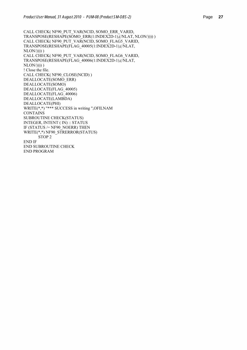
CALL CHECK( NF90_PUT_VAR(NCID, SOMO_ERR_VARID, TRANSPOSE(RESHAPE(SOMO_ERR(1:INDEX2D-1),(/NLAT, NLON/)))) ) CALL CHECK( NF90_PUT_VAR(NCID, SOMO_FLAG5_VARID, TRANSPOSE(RESHAPE(FLAG_40005(1:INDEX2D-1),(/NLAT, NLON/)))) ) CALL CHECK( NF90_PUT_VAR(NCID, SOMO_FLAG6_VARID, TRANSPOSE(RESHAPE(FLAG_40006(1:INDEX2D-1),(/NLAT, NLON/)))) ) ! Close the file. CALL CHECK( NF90_CLOSE(NCID) ) DEALLOCATE(SOMO_ERR) DEALLOCATE(SOMO) DEALLOCATE(FLAG_40005) DEALLOCATE(FLAG_40006) DEALLOCATE(LAMBDA) DEALLOCATE(PHI) WRITE(*,*) "*** SUCCESS in writing ",OFILNAM CONTAINS SUBROUTINE CHECK(STATUS) INTEGER, INTENT ( IN) :: STATUS IF (STATUS /= NF90_NOERR) THEN WRITE(*,*) NF90_STRERROR(STATUS) STOP 2 END IF END SUBROUTINE CHECK END PROGRAM