h 0 0 00 0 9 8

A.I In the user's manual, it was mentioned that the mass balance was notoutput* How was the maas balance checked for the Iron ton model?

The user's manual does not describe the mass balance output which is includedin che current version of GEOFLOW (the version used for the Ironton modeling).

The mass balance for the Ironton flow model was examined and for simulation

No. 1 is as follows:

o Flow In =* 57,420 cubic feet per day (ft3/day) fromrecharge

o Flow Out = 46,040 ft /day net boundary flows plus pump-ing well flows, plus 11,380 ft /day net leakage to IceCreek = 57,420 ft3/day.

Therefore, because .the volumetric flow into the model equals the flow out, theIronton model is functioning correctly.

A. 2 I cannot verify Figure 3-2 in the user's manual with the Theis equationfor nonsteady flow in confined aquifers:

3 = W(u)

Please explain your results.

The notation used to develop Figure 3-2 is

s = drawdown

Q a pumping rate

T a transmissivityt = time

r = radiusS - storage coefficient.

Also note that in the Theis equation

2r s4T7

and W(u) = Well function.

Dimensioniess time, t', is plotted on the horizontal axis of Figure 3-2.Dimensioniess time has been defined as:

' _ 1 4Tt"~7~*

Dimensioniess drawdown, s', is plotted on the vertical axis of Figure 3-2Dimensioniess drawdown has been defined as:

Using this notation the Theis equation is written as:

i t= s = W(u) =* W(-f)

Therefore, the analytical solution on Figure 3-2 is a plot of s' versus t'where:

' = w(4)

Calculation of a few of the points used to draw the analytical curve is shownin the following table:

3 = W ( u )

1,0001001051

t

lO-3

io-210"1

0.21

. 64

110

.3315

.0379

.3229

.2227

.2194

The well function W(u) was obtained from Table 8-2, pp. 320-321, of Hydraulicsof Groundwater by Jacob Bear (1979).

The daca points shown in Figure 3-2 and identified as the numerical solutionwere obtained from drawdowns calculated at Node Point 11 of the model shown inFigure 3-1. For this data point r = 1,500 Sec (45°) = 2121.32 ft. Also forthe GEOFLOW computer run:

T = 10,000 ft2/dayS = 0.01Q = 24,000 ft3/day

In the GEOFLOW model one quarter of the total flow was applied since a singlequadrant of che flow domain was modeled.

Hence the GEOFLOW model data points corresponding to Mode Point 11 are plottedat:

4(1 x IO4)rS (2121.32^(0.01)

4it( l x 104)s , ...3 = ~ = —— 2^000 —— - 5 . 2 3 6 s

The values of s versus t obtained from GEOFLOW and corresponding dimensionless

values, sf versus c1, are as follows!

DIMENSIONLESS £:MEN"IONLESSTIME, TIME, DRAWDOWN, ORA..DOWN,C r' 3 3*

2.0 1.73 0.114 0.603.0 2.67 0.166 0.374.0 3.56 0.207 1.085.0 4.44 0.242 1.276.0 5.33 0.271 1.427.0 6.22 0.296 1.558.0 7.11 0.318 1.679.0 8.00 0.338 1.7710,0 8.89 0.356 1.8611,0 9.78 0.373 1.9512.0 10.67 0.388 2.0313.0 11.56 0.402 2.1014.0 12.44 0.416 2.1815.0 13.33 0.428 2.2420.0 17.78 0.480 2.5125.0 22.22 0.520 2.7230.0 26.67 0.553 2.90

Therefore, it has been verified that the data plotted in Figure 3-2 of theGEOFLOW User's Manual correctly represents the Theis equation for nonsteadyflow in confined aquifers.

A.3 Figure 3-3 of the user's manual doesn't seem to make sense for the con-stant infiltration. Could you explain the shape of the potential surface.

Figure 3-3 shows che water level in an unconfined finite aquifer subject topumping and uniform infiltration. The effect of pumping alone and of infil-tration alone is shown in the attached Figure A-3(a> and A-3(b), respec-tively. The combined effect is shown in Figure A-3(c). The effects are notcombined by linear superposition in an unconfined aquifer; however, Figure A-3illustrates the qualitative shape of the GEOFLOW solution. In Figure A-3(a)che ground water shows a cone of depression at the well. In Figure A-3(b) aground water mound appears due to infiltration. The combined effect is aground water mound with a cone of depression at the pumping well. Therefore,che shape of the potential surface shown in Figure 3-3 of che GEOFLOW User'sManual is as should be expected.

A.4 The match in Figure 3-10 does not appear to be very good. Have youestimated the percent error? Were different sized elements used to attempt toreduce this error?

4

The analytical solution shown in the GEOFLOW User's Manual is an approximatesolution. To further assess the accuracy of GEOFLOW, a general analyticalsolution of the problem of two dimensional dispersion in a finite width striphas been derived using procedures by Batu (1983). This solution has been

evaluated and Figure A-4 shows the analytical solution in comparison Co theGEOFLOW solution. At distances greater than three centimeters from thesource, the GEOFLOW and analytical solution are in good agreement and error isless than 4 percent. Larger differences near the source are due to the coarsegrid in this region of high concentration gradient.

Therefore, the match between GEOFLOW and the analytical solution is very good.

A.5 Which subroutines of GEOFLOW were used? Have they all been verified? Ifnot, how can you be confident in the model results?

All subroutines within the GEOFLOW program were used with the exception ofthose dealing strictly with either time dependent retardation factors or acidfront neutralization. The remaining subroutines which were called containsome options which were not used; for example, decay was not included in thecontaminant migration, nor is it a phenomena which would be expected to occur.

The subroutine and appropriate options have been verified by the test problemscontained within the GEOFLOW user's manual. The program has received exten-sive usage whereby results have been checked. For example, in one recentproject, model results of a model similar in complexity to the Ironton model

were compared to the USGS model SUTRA. Such comparisons have given additionalconfidence to the program performance.

In revisions performed since preparation of the May 1983 GEOFLOW user's

manual, routines have been added to print element and nodal flows of bothwater and contaminant. These are used to provide a mass balance which giveadditional confidence that the governing equations are assembled and solvedcorrectly.

In addition, the program now prints the Peclet and Courant numbers for each

element of the domain. These ensure that grid size and time step are adequate

Co ensure an accurate solution. Printing o£ these numbers by GEOFLOW adds tothe confidence in our results.

Therefore, our overall confidence in the program GEOFLOW is based upon checombined use of verification problems together with a long history of use ofthe program along with checks internal to the program.

A.6 Please explain whether "acid neutralization" affects the chemistry of themigrating fluid at the Ironton site.

Acid neutralization has not been considered in the chemistry of the groundwater contaminant transport model. Acid neutralization is typically onlyconsidered when acidic leachate or ground water plumes are present (i.e., atailings pond leachate). This is not the case at the Ironton site; the groundwater is not acidic.

B.I What does steady-state dispersion indicate as opposed to transient dis-persion modeling? Why do you think it represents the worst case?

Steady-state simulations represent the maximum predicted spatial migration ofa chemical constituent plume from a source of continuous strength. In addi-tion, the computed concentration at any given Location will be at its maximumlevel under steady-state conditions.

Steady-state conditions represent a worst-case analysis because, for a given

source strength, computed concentrations will be maximums for the modeledconditions. Steady-state dispersion is also a realistic representation of theIronton site, because the plant facilities have been present for approximately70 years. It is, therefore, both conservative and realistic to model steady-state dispersion for the Ironton site.

3.2 What are the data which justify the no-flow boundaries of the model?Please expand on the explanation in the HI.

The no-flow boundary along the eastern edge of the grid was assigned on thebasis of the presence of highlands areas, i.e., uplands representing the

Limics of the alluvi'aL aquifer. The pocenciaL exists for some flow inco thealluvial aquifer from che uplands regions through fracture flow; however, thisflow 13 likely to be small relative to infiltration to the alluvial aquifer.Furthermore, neglecting this flow represents a conservative assumption becauseunderflow from the highlands across this boundary would flow toward the CoalGrove wells, reducing potential flows from the Allied sice area to che wells.

The no-flow boundaries at the northern and southern edges of the grid repre-sent areas where flow is likely Co discharge Co either Ice Creek or che OhioRiver, chereby, flowing approximately parallel to the boundary. Both areasare at distances from che modeled area of interest which are sufficient Coprevent interference with computations. The no-flow boundaries allow themodel more inherent variability than constant heads.

The constant head boundaries at the northern end of the grid were assigned byextrapolating contours of observed ground water levels.

We believe that che boundary conditions we have used are justified and chatthe model cakes a conservative approach and accurately simulates fieldconditions.

B.3 Were the nodes along both Ice Creek and the Ohio River held in themodel? If not, why not?

Modes in the Ice Creek area were not specified as constant heads, because to

do so would necessarily preclude the occurrence of ground water flow from the

site to Che Coal Grove area. A conservative approach was used setting IceCreek as a leakage zone of constant head overlying variably resistivesediments.

The Ohio River was specified as a constant head boundary due to its dominantinfluence on the adjacent aquifer.

B.4 The tern "model validation" is used improperly in the RI. The model hasbeen calibrated. The data are not available for model validation.

We have used the term "validated" in the Phase II report to indicate chat chemodel is accurately representing the actual conditions in the field. Subse-quent to our discussion, we realize that there is confusion about the termi-nology we chose to use. We will change the terminology in the report toeliminate the confusion. The wording of the text will be revised co say thatthe model has been calibrated to obtain a best-fit match to observed values in

the field.

B.5 Why was the analytical solution for vertical flow representative of aconfined aquifer?

Analytical analyses of vertical flow in the Phase I report (Appendix F) andthe Phase II report (page F-21) are representative of semi-confined conditionswhich occur when water completely fills the aquifer materials up to the semi-confining bed, with some leakage occurring through the semi-confining deposits(in this case, the Ice Creek bottom sediments).

3.6 A Latin Hypercube or Monte Carlo sensitivity analysis would provide a

better assessment of the sensitivity of the model to input parameters.

IT Corporation has applied the Monte Carlo method in the past to structuralengineering and geotechnical problems. Our experience is that the Monte Carlomethod is particularly suitable for problems where statistical variations ininput parameters to a model are well defined. An example of a problem having

well defined statistical distributions would be a structural design problemsuch as design of a concrete column. In this case a major source of variabil-ity could be readily associated with the random variation of concrete strengthfor which a realistic definition of a probability distribution could be easilyassigned.

For modeling geohydrological flow and contaminant transport problems it ismuch more difficult to define statistical input parameters. Assumptionsregarding the appropriate probability distributions and correlations must be

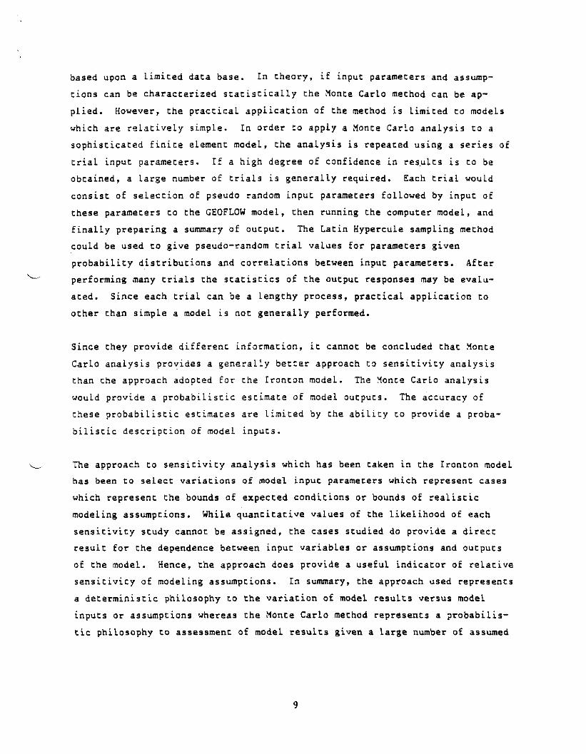
based upon a limited data base. In theory, if input parameters and assump-tions can be characterized statistically the Monte Carlo method can be ap-plied. However, the practical application of the method is limited to modelswhich are relatively simple. In order to apply a Monte Carlo analysis to asophisticated finite element model, the analysis is repeated using a series oftrial input parameters. If a high degree of confidence in results is to beobtained, a large number of trials is generally required. Each trial wouldconsist of selection of pseudo random input parameters followed by input ofthese parameters to the GEOFLOW model, then running the computer model, andfinally preparing a summary of output. The Latin Hypercule sampling methodcould be used to give pseudo-random trial values for parameters givenprobability distributions and correlations between input parameters. Afterperforming many trials the statistics of the output responses may be evalu-ated. Since each trial can be a lengthy process, practical application toother than simple a model is not generally performed.

Since they provide different information, it cannot be concluded that MonteCarlo analysis provides a generally better approach to sensitivity analysisthan the approach adopted for the Ironton model. The Monce Carlo analysiswould provide a probabilistic estimate of model outputs. The accuracy ofthese probabilistic estimates are limited by the ability to provide a proba-bilistic description of model inputs.

The approach to sensitivity analysis which has been taken in the Ironcon modelhas been to select variations of model input parameters which represent cases

which represent the bounds of expected conditions or bounds of realisticmodeling assumptions. While quantitative values of the likelihood of eachsensitivity study cannot be assigned, the cases studied do provide a directresult for the dependence between input variables or assumptions and outputsof the model. Hence, the approach does provide a useful indicator of relativesensitivity of modeling assumptions. In summary, the approach used representsa deterministic philosophy to the variation of model results versus modelinputs or assumptions whereas the Monte Carlo method represents a probabilis-tic philosophy to assessment of model results given a large number of assumed

probabilistic inputs and ocher assumptions. The approach adopted for sensi-tivity analysis for the Ironcon model can give the engineer a better determi-nation of the impact of his assumptions in modeling, in a deterministic sense,while Monte Carlo methods, if they can be applied practically, determineprobabilistic outputs of the model.

3.7 How was the clay beneath Ice Creek simulated la the model?

The clay beneath Ice Creek was incorporated as a leakage zone in a quasi-three-dimensional sense; vertical leakage is computed through the clay based

on the specified overlying simulated head and the head in the aquifer beneath

the creek.

B.S Were any cores taken of the Ohio River bank sediments Co verify theirlithology and hydraulic conductivity? Why do you think the conductivity ofthe Ohio River sediments are different further north? How was the width ofthe "low-permeability11 bank zone determined to be 100 feet?

Core samples from borings MW-1, MW-14, MW-13, and MW-5 were taken from the

river bank zone area to provide information on the zone's lithology.

The near-river borings confirmed the presence of low-permeability silty clay

deposits. The locations of the low permeability zones used in modeling were

determined by examination of observed ground water levels. Comparativelymoderate gradients in the north-of-Goldcamp and near-Ice Creek area of theriver bank indicate less influence of the low permeability deposits. Lack of

drawdown in Well MW-5 (near the Coal Grove wells) indicates that no additionalimpediment to flow from the Ohio River occurs in this region.

The 100-foot width of the low-permeability zone was based on the grid con-figuration. Variations in bank permeability during simulations implicitly

incorporate bank zone width variations, giving a representative bank zoneresistance.

Kernodle (1977) used a bank zone permeability of 1/25 aquifer permeability to

simulate water levels along the Ohio River, approximately 25 miles from the

10

Ironton sice. This racio was used as a rough guide for adjusting the hy-draulic conductivity of the Low-permeability zone.

Therefore, based on river bank zone borings, observed ground water Levels,modeling studies in the literature, and realistic computed results, the simu-lated river bank zone in the Ironton model is representative of siteconditions.

B.9 Does the horizontal dispersion modeling give values for flow under theclay finger? If so, how?

The model simulates the Ice Creek sediments as a resistive layer allowingvertical leakage to or from the underlying aquifer. The flow model, there-fore, computes heads in the aquifer beneath the Ice Creek clays. The headsreflect the influence of leakage from Ice Cceek.

The dispersion modeling allows computation of concentrations due to advectiveand dispersive flux. Because horizontal ground water flow occurs beneath thecreek bed clays, associaced concentrations are also computed in this area.The concentrations computed for this region are reflective of leakage from orto Ice Creek.

3.10 Why did you conclude that higher concentrations of contaminants are notpresent at shallow depths (page P-29)? It seems as though the contaminantswhich are not denser than water should have higher concentrations near the

source.

The report section referenced was not intended to imply that concentrationscould not be higher at locations vertically closer to sources; rather, theintent was to point out that due to relatively fast flow rates, fluctuationsdue to Ohio River stage changes, limited vertical thickness of the aquifer,and the likely long, continued presence of sources, concentrations are ex-pected to be well-mixed vertically within a short distance of the sources.This means that 2-D horizontal modeling results will be representative for thesite.

11

The paragraph in question wilL be reworded as follows:

"During Che Phase II field investigations, monitoring wells were installedwhich had screened intervals extending throughout the aquifer's saturatedthickness. Water quality samples from these wells were taken at differentvertical locations within the aquifer. The similarity of chemical constituentconcentrations for the upper, middle, and lower portions of the aquifer atthese wells indicates that the system is well-mixed vertically."

Analytical results supporting the assumption of vertical mixing for the major-ity of the site were obtained from Phase II sampling.

B.ll How were the dispersion coefficients selected? Were any sensitivityanalyses performed to evaluate the effect of changing these coefficients?

The value of longitudinal dispersivity, as well as the ratio of longitudinalto transverse dispersivity, was selected as typical for a sandy aquifer basedon published values for similar materials [Konikow (1977), Finder (1973), andAnderson (1984); see also Robson (1971), Gray and Hoffman (1983), Schwarts(1977), Naymik and Barcelona (1981), Valocchi, et al. (1981), and Sudicky, et

al. (1983)].

Past experience with dispersion sensitivity analyses provides a good under-standing of the effect of dispersivity variation. These effects are somewhatsignificant for steady-state analyses. Mo attempt was made to calibrate toobserved concentrations, therefore, no dispersion sensitivity runs were madefor the Ironton model relative to the RI modeling objectives. However, thedispersion sensitivity analysis would be useful for determining final remedialalternatives.

B.12 On pages F-38 through F-40 you state that the mass transport calcula-tions differ from observed values. What is the difference?

Specific comparisons between computed concentrations and observed values arepresented on pages F-38 through F-40. In general, differences occur becausethe dispersion modeling was not designed to directly simulate the current

12

distribution of various contaminants in the aquifer. Rather, the simulationswere primarily intended to indicate the areas which may be affected by a givensource and to assess relative mass loadings to receptors which may result from

each potential source.

No attempt was made to calibrate the dispersion simulations to observed con-centrations because the observed data show wide variability and do not indi-cate discernible plumes. This variability is due to:

o Multiple sourceso Multiple contaminantso Likely discontinuity of sourceso Past pumping scheduleso Raised pool elevation in Ohio Rivero Flood events

These varied influences indicate that it would be impossible to simulate allfactors which have contributed to the current concentration distribution;however, for the modeling purposes, the steady-state simulations providerepresentative results. Actual existing concentrations would be significantinput data for simulations of remedial alternatives.

8.13 la Figures F-10 and P-12 the concentration distribution does not seem tobe affected by the clay finger.

The figures show a relative concentration of less than 0.01 to the south ofIce Creek. These low values are the result of mass discharging to Ice Creekand dilution by leakage from Ice Creek. The concentrations are affected by

leakage from the creek, rather than being directly affected by the creeksediments themselves.

The computed plumes definitely show the influence of a flow component towardthe Coal Grove wells, with the spread diminished by communication with IceCreek.

13

B.14 On page P-40, Source 5, is Well T-13 suppose to be Well T-12? What isthe magnitude of the difference between calculated and observed values?

T-13 is shown in .Figure 2-12, Phase I reporc. It is Located very close co

Well MW-1S and was not sampled in Phase II.

Compuced relative concencrations in the vicinity of Wells T-13 and MW-18 areon the order of 0.15 (C/Co). Observed concentrations for Well MW-18 (Table4.3) indicate 0.06 mg/1 ammonia, 16 mg/l chloride, and ND for the ocher £ourindicator parameters. If Chese concentrations represent 15 percent of sourceconcentration, the source must be at a relatively low strength compared to

ocher site areas.

B.15 On page P-39, how can the mass loadings from Source 2 give about thesame results in both up and downgradient wells?

The simulation referred to modeled the lagoons as an areal source. Since bothup and downgradient wells mentioned are immediately adjacent to the arealsource, concencracions are similar. Qpgradient migracion is limited by cheground water flow direction, while downgradient migration is limited by chevery short distance to discharge into Ice Creek.

B.16 Why do you think that the model predicted potential surface and theOctober 3, 1984 potential surface vary by more than a foot in places (e.g.,Wells MW-7, MW-8, MW-15, and C-2)? This seems like quite a large variationfor a site which has only a three-foot gradient from one side to the other.

Differences at MW-15 and C-2 are Likely due to the Location of the outerlagoon dike zone in the model. The steeper gradients in this area are weLLsimuLated.

WelL MW-7 is Located within the Coal Grove wells' cone of depression, wherethe overall head difference is on the order of 15 feet. The difference ofless than 2 feet between simulated and measured heads is not, therefore,significant for the simulation purposes. Furthermore, intermittent use ofWell CC-4 may have affected observed water Levels.

14

Well MW-8 may be affected by transient changes in Ohio River stage. Sice

variations in ground water LeveLs over shore time periods may be on the orderof 1 foot, these variations should not affect the modeling of long-term repre-

sentative conditions.

8.17 How were the percentages of flow calculated for the flow in the CoalGrove wells?

GEOFtOW output includes the volumetric flow rates at nodes, as well as leakage

rates at elements. The appropriate nodal flows were summed across boundariesof the specified control volume (Figure F-5) and expressed as percentages of

the total well flow.

3.18 Do you have an explanation for the one half-foot vertical gradientbetween Wells T-5S and MW-1S?

The water Level elevation at Well T-5S for October 3, 1984 (Figure 4-6, Phase

II report) is in error. The water Level elevation should be 518.81 feet,instead of 519.36 feet. This results in a difference of only 0.03 foot be-

tween Wells T-5S and MW-14.

Figure 4-6 will be changed to show the corrected value at Well T-5S and simi-larly the saturated thickness isopach (Figure 4-8) will be changed accord-

ingly. The change will have no effect on our interpretation of the data forinput to the model. Saturated thicknesses would change slightly but input

values for the model were to the nearest foot for each element and would not

be affected.

Table F-2, which compares computed heads with actual heads, indicates the

correct value for Well T-5S.

3.19 The distribution of contaminants in the dispersion modeling does not

appear to match the concentrations for any of the contaminants that you men-tion (chloride, benzene, cyanide, ammonia, and phenol).

15

The modeling purpose was Co indicate areas which may be affected by a givensource and Co determine primary receptors for source areas. No actempt wasmade co match existing concentration distributions, due to the site's variablehistory (see also response, Question B.12).

8.20 Please explain, in more detail, the arguments concerning horizontalseepage and effective resistivity mentioned on page P-8.

Assigning a value for effective resistivity to the Ice Creek sediments allowsthe model to compute a vertical leakage equal to the actual volumetric leakagefrom Ice Creek, which occurs primarily through the channel sides.

Creek sediment resistivity values were adjusted to provide the best simulationof observed water levels (e.g., at Well C-13), implying that the modeledvolumetric leakage was representative of actual leakage rates.

C.I Better control could be gained on the seepage flux to Ice Creek by doinga seepage meter analysis. This would measure the flux into or out of thecreek, validating the assumptions that Ice Creek is gaining water adjacent tothe site and losing water near the Coal Grove well field.

Ground water Level measurements have consistently been higher than creeklevels on the south and lower on the north. Water table contours indicatethat there is some communication between the creek and the aquifer; therefore,low is expected to be occurring as presented.

Measurements of ground water and surface water elevations indicate seepagedirections associated with the observed hydraulic gradients and are likely toprovide more representative data than seepage meter studies; experience withseepage meter use in a study of ground water/surface water interactionindicates:

o Results may be influenced by Localized nonhomogenietiesin sediment composition

o Results vary quantitatively with initial water volumesused in the meters

16

o Seepage meters can give misleading resales in situa-cions where seepage occurs from che surface water bodyco che underlying aquifer.

Therefore, che consistent Crend of observed wacer Levels characterizes che

seepage which occurs in che Ice Creek area, and a seepage meter study may notprovide resulcs which are quantitatively or qualitatively representacive of

Che actual surface water/ground water interaction which occurs in Ice Creek.

C.2 Why do you consider the aquifer beneath Ice Creek to be confined, whenthe creek and aquifer are obviously interconnected?

The aquifer beneath Ice Creek is semi-confined. Water levels are above the

bottom of the clay deposits, but leakage can occur vertically through theclay.

C.3 Can you justify the use of 20 inches per year (in/yr) recharge in Zone

I? This amount seems excessive. It also seems as though the lagoon areashould have a higher recharge rate than the surrounding area.

A 20 in/yr recharge was used for one zone (Zone 4) in the Phase I report. The

Phase II report uses a recharge value of 3 in/yr over che entire area.

Lagoons may have increased reception of runoff, but higher aquifer rechargefrom the area was not modeled because:

o Lagoon waste hydraulic conductivity is two to threeorders of magnitude lower than aquifer hydraulicconductivity

o Mo water table mounding is seen upgradient of chelagoons

o Steeper gradients in the outer lagoon dike/Ice Creekare seen in areas away from the lagoons as well asadjacent Co them.

17

C.4 Please send me your reference on the use of creek bed resistivity.

This question was resolved at the October 22, 1985 meeting and no further

action is required.

C.5 When the natural sand pack was installed, how did you prevent contami-nated sediments above the well screen from forming the sand pack?

The monitoring wells were installed according to the following procedures:

L. Six and one fourth-inch I.D. hollow-stem augers were usedto bore the hole.

2. Augers were left in the hole and the well screen and casingwere set inside the augers.

3. The augers were slowly pulled allowing sand and gravel fromthe aquifer to collapse around the screen.

4. Augers were left at the top of the sand and gravel or atthe elevation of the top of the screen.

5. A calculated volume (volume needed for a five-foot plug) ofbentonite was piped down the augers.

6. Five feet of auger was pulled allowing the bentonite toflow ouc and form the five-foot plug.

7. A cremie pipe was placed down the auger to within two orthree feet of the bentonite plug.

3. The augers were filled with a bentonite/cement grout andthe tremie pipe was removed.

9. Augers were slowly pulled allowing grout to fill the hole.

10. As the level of grout dropped in the augers as they werepulled, more grout was poured in.

11. Wells were grouted to within one foot of the ground surfaceand the grout was allowed to set.

12. Wells were finished with concrete to the surface.

Appendix G of the Phase II RI report shows well installation details for the

Phase II monitoring wells. Installation of the bentonite seal, before pullingthe augers, would prevent contaminated surface soil from forming part of the

natural sand pack.

18

C.6 On page E-8 of the Phase II report, you mention drilling fluid returnswhile using a hollow—stem auger. Could you explain this?

The term "drilling fluid" was used incorrectly in this instance. The sentencein question states "An oily sheen was noted on the drilling fluid recurn. . "."

The hollow-seem auger was bringing up cuttings from below che water table.The oily sheen was seen on the ground water coming up with these cuttings.

We will change the sentence to eliminate the use of the term drilling fluid.

The changed sentence will read as follows:

o "An oily sheen was noted on the ground water returningwith the auger cuttings from a depth of 45 feet inboring MW-14."

C.7 Please send me your documentation on how the falling head tests wereconducted and how the hydraulic conductivity was calculated from the tests.

Falling head tests were performed on the monitoring wells by raising che water

level above che level of che ground water in the well and observing che fall06 che water level as a function of time.

The tested wells were filled from a hose supplying water at a rate of approx-

imately 30 gallons per minute. For the wells at the Ironton site, this meanschat filling to the cop of casing would take place in approximately 30 secondsor less. Based on observed rates of water level declines at che tested wells,the amount of water lost to the formation during chis filling period would beon che order of 0.1 to 0.7 gallons. The period of time and amount of wacerlost while filling the wells are not significant relative to the long-term

nature of che tests.

Hydraulic conductivity was calculated using one of the following equations:

H — Hi I g for cased hole, soil flushll(t. - c.) H- - H with bottom of casing

19

or

2(H-R2

L2)<

Ll - L2 Hl\t2 - EI> Ul R Al H2

- H- H

g

for cased holeuncased or perforated extension ofLength L - L

^'Equations after HvorsLev (1951).

We calculated a range of permeability at each well based on the early datafrom the test and data collected later in the test. The values reported inTable 4.2 in the Phase II report are the high values calculated for each well

C.S On page F-9 of the 81, you state that groundvater levels indicate perme-ability. Can you explain this?

This sentence will be reworded as follows:

"Measured ground water Levels (Figure 4-6) show discreteareas of steeper hydraulic gradients along the Ohio River,indicating that the riverbank is less permeable . . ."

C.9 Why weren't deep wells installed to monitor water quality?

Deep wells were not instalLed for the following reasons:

o Packer testing of the bedrock indicates a very Lowhydraulic conductivity. Future use of the bedrock inthis area for a water supply is not Likely because itis not capable of a sustained yield.

o The gradient of the regional ground water flow systemis toward the Ohio River. The gradient in the bedrockis most Likely upward to the alluvial aquifer.

o Potential receptors of site-derived contaminants arenot located in the bedrock. Wells which may be ad-versely affected are screened in the alluvial aquifer.

20

C.10 How were the deep aquifer teats conducted? How do you obtain a hy-

draulic conductivity of zero?

The bedrock at the Ironton site cannot be considered a deep aquifer. Thebedrock is not a viable source of water because of the Low hydraulic conduc-

tivity.

Packer pressure testing was conducted in four of the deep borings to determinethe hydraulic conductivity of the bedrock.

Borings B-lt B-3, and B-6 were pressure tested using a double pneumatic packerarrangement. This arrangement allowed sequential testing of select five-footintervals in each boring.

Boring B-2 was tested by setting a single packer near the top of bedrock and

testing a large interval in one single test. This was done for the followingreasons:

o "No take" low permeability conditions were expected

o Boring B-2 had an oily separate phase liquid in thebottom of the boring. Packer testing was done in onestep to expedite the test so the boring could begrouted shut.

Table A.2, which indicates hydraulic conductivities of zero, will be corrected

to indicate "no take" conditions.

C.ll Well MW-15 is screened in the bentonite seal and the top of the screenis nine feet below the ground surface. What do you think the effect of thisis on the chemistry results? Can surface water be leaching into the groundwater through this boring?

The well installation details for Well MW-15 shown in Appendix G indicate that

the well screen is 1.2 feet into the bentonite seal. This portion of thescreen is located in the unsaturated zone; the water level is approximately

eight feet below the bentonite seal; therefore, this portion of the screen isgrouted.

21

Review of the analytical data for Well MW-15 indicates trace amounts ofbenzo(a)anthracene and chrysene (<10 ppb) only. The absence of elevatedlevels of other constituents indicates that contaminants are not migratingdown the boring to the ground water.

C.12 How were Wells T-10 and T-ll backfilled in the bedrock? Are these wellconduits from the sand and gravel aquifer to the bedrock?

Wells T-10 and T-ll were installed in 1978 by Geraghty and Miller. Wellcompletion details for these wells are not available. We requested all avail-able information for the tar plant monitoring wells (T-series) and were ableto obtain boring logs only.

Although the well logs for Wells T-10 and T-ll indicate that the borings are12 feet into bedrock, there is no evidence that bedrock was ever reached.Borings were advanced using hollow-stem augers and split-spoon samples werecollected. The sample logs indicate that no samples were recovered from thelast 30 feet of the borings. There are no samples to verify that the boringsare in bedrock. There is also no indication that bedrock was cored.

When the data from the boring logs were used in the construction of geologiccross sections, it was evident that there was an error in the logs. Bedrockelevation in the boring logs for T-10 and T-ll would be approximately491 feet—ten feet higher than any surrounding wells. Our interpretation isshown in Figure 4-4 (cross section B-B1) of the Phase II report.

C.13 Please justify the use and configuration of the finger of clay beneathIce Creek?

The presence of the "finger of clay" is based on our interpretation of the IceCreek boring logs. A total of 19 borings were drilled at 12 locations as partof the Ice Creek investigation* Borings drilled in the reaches of Ice Creekdownstream of the coke plant lagoons encountered stream sediments comprisedprimarily of low-permeability silt and clay. The boring logs (Phase I,Appendix H) indicate that these fine-grained sediments are approximately 36feet thick near the mouth of the creek (Boring ICB-3) and become gradually

22

chinner upscream. The configuration of the cLay is the result of the follow-ing occurrences:

o Previous to the construction of the Greenup Lock andDam on the Ohio River, normal elevation of the OhioRiver was 490.5 feet and Ice Creek had cut its channelinto the alluvial aquifer.

o Construction of the Greenup Dam caused the normal ele-vation (pool) of the river to rise to 516 feet andcreate a back, water condition in Ice Creek.. The IceCreek channel has slowly filled with fine-grained sedi-ments to form the finger of clay.

C.14 Why do you think that the clay beneath Ice Creek has the same hydraulicconductivity as the surrounding older clay?

Ice Creek sediment hydraulic conductivities were tested during the Phase IIprogram. No relation to older clays is intended to be made in the report.

C.15 Why are the depths of the lagoons and the CoIdcamp dump different inFigures 1-2, 1-3, and 4-4?

The three-dimensional cross sections in Figures 1-2 and 1-3 are conceptualdrawings that are intended to provide a generalized overview of the site. Thevertical exaggeration and viewing angles for the different plates of the cross

sections makes it impossible to scale depth or thicknesses of features in thedrawings. The vertical scales which are different from one side of the draw-ing to the other were provided to indicate the relative thickness of thesections.

Furthermore, the three-dimensional cross sections (Figures 1-2 and 1-3) and

the generalized geologic cross sections (Figures 4-4 and 4-5) do not show thesame sections of the site. Comparison of different site features cannot bemade.

C.16 What is the nature of the fill in Figures 4-4 and 4-5?

Boring logs for the borings used in constructing the cross sections in Figures4-4 and 4-5 are shown in Appendix H. The composition of the fill is variable

23

from boring Co boring. Generally, che fill is composed of fine Co coarse

silcy sand, silcy clays, coal fines, cinders, and traces of car and gravel.Specifically, the composition of che fill at various locacions is as follows:

Cross Section A-A"Boring MW-5 - Coat fines, silcy fine sand, fine Cocoarse sand, Crace gravel size slag

Cross Section B-B"Boring 8-2 - Sitty sand, fine Co coarse sand, someslag, some gravelBoring MW-13 - Fine to coarse sand, some gravel,trace coal fines

Cross Seccion D-D1Boring MW-1 - Fine Co coarse sand and coal, silcysand, some slag, Crace gravelBoring B-6 - Fine to coarse sand, trace silt and coalBoring LB-4 - Fine to coarse cinders, Crace coal

(lagoon dike) Boring B-4 (MW-16) -clayey silt, silty clay, silcysand, some sand, gravel and slag

Cross Section E-E*Boring B-5 - Fine coal, fine Co coarse slag, somefine gravelBoring LB-3 - Fine Co coarse coal, coke and slag,some concrete fragments, some silt and sand, somelime sludgeBoring LB-2 - Fine Co coarse gravelly sand, somecinders and slag, traces of coal, car, organicmaterial

(lagoon dike) Boring C-l - Silty clay, fine to coarse cinders.

C.17 Why were hydraulic conductivities not calculated for wells with a flow

rate of less than 0.25 gallons per minute (gpm)? Is it certain that fractur-ing only occurs along the bedding planes of the bedrock?

As stated on page 4-7 of che Phase II report, the flow mecer used during

packer pressure teacing at che sice has a normal operating range of 0.25 to20 gpm. Calculations of permeability with flows below the normal operatingrange of che flow meter would not produce reliable results. In addicion, cheK for flows less than 0.25 gpm would be very small.

Packer testing of che bedrock has indicated very low or unmeasurable hydraulicconductivities. Our review of photographic records of rock cores, rock frac-ture logs and boring logs indicates that the presence of bedding plane

24

partings is most likely responsible for the measured permeability values in

Borings B-2, B-3, and B-6. The rock cores and fracture logs do not indicatethe presence of vertical fractures.

The absence of vertical fractures in the six deep borings does not necessarilymean there are no vertical fractures; however, the presence of such fractureswill not affect the results of the study.

C.18 What parameters were used to calculate the 0.3-foot/day ground watervelocity? How does this velocity compare with that of the model?

The velocities presented were obtained by averaging model-computed flow ratesat 25 nodes across the site area between potential sources and site boundaries(i.e., Ohio River and Ice Creek). The resulting velocities are consistentwith hand calculations using site-representative data.

25

REFERENCES CITED

Anderson, M. P., 1984, "Movement of Contaminants in Groundwacer: GroundwacerTransport - Advection and Dispersion,11 Groundwacer Contamination, NationalAcademy Press, Washington, D.C.

Gray, W. G. and J. L. Hoffman, 1983, "A Numerical Model Study o£ GroundwaterContamination from Price's Landfill, Mew Jersey - II, Sensitivity Analysis andContaminant Plume Simulations," Groundwater, Vol. 21(1), pp. 15-21.

HvorsLev, M. J., 1951, "Time Lag and Soil Permeability in Ground Water Obser-vations," Waterways Exp. Sta. Bulletin Mo. 36, U.S. Array Corps of Engineers,Vicksburg, Mississippi.

Kernodle, J., 1977, Theoretical Drawdown Due to Simulated Pumpage from theOhio River Alluvial Aquifer Near Siloam, Kentucky, U.S. Geological Survey,Louisville, Kentucky.

Konikow, L. F., 1977, "Modeling Chloride Movement in the Alluvial Aquifer atRocky Mountain Arsenal, Colorado," Water Supply Paper 2044, U.S. GeologicalSurvey.

Naymik, T. G. and M. J. Barcelona, 1981, "Characterization of a ContaminantPlume in Ground Water, Meredosia, Illinois," Groundwater, Vol. 19(5), pp. 517-526.

Pinder, G. F., 1973, "A Galerkin Finite Element Simulation of GroundwaterContamination on Long Island, New York," Water Resources Research, Vol. 9(6),pp. 1657-1669.

Robson, S. G., 1978, "Application of Digital Profile Modeling Techniques toGroundwater Solute Transport at Barstow, California," Water Supply Paper No.2050, U.S. Geological Survey.

Schwartz, F. W., 1977, "On Radioactive Waste Management: Model Analysis of aProposed Site," J. Hydrology, Vol. 32.

Sudicky, E. A., J. A. Cherry, and E. 0. Frind, 1983, "Migration of Contami-nants in Groundwater at a Landfill: A Case Study," J. Hydrology, Vol. 63, pp.81-108.

Valocchi, A. J., P. V. Roberts, G. A. Parks, and R. L. Street, 1981, "Simula-tion of the Transport of Ion-Exchange Solutes Using Laboratory-DeterminedChemical Parameter Values," Groundwater, Vol. 19(6), pp.600-607.

26

FIGURES

roCO

°rr?£3|<r 2c z

Srf

CD

Y

. . • _ • _ / • -*v , •. .

FIGURE A - 3 ( a )

v * N V _v_ _} f_ y v v v

*

•* •"*^*

/ / / " / / / / / / / ' / ' / ' x ' / / '

FIGURE A-3(b)

v v v v \ ' v y v v

N

/ ~y/ r /"/ / / / / / / ' /rx s s / s/s/s//// ss/sFIGURE A-3(c)

9 198* IT CORPORATIONALL COPYRIGHTS RESERVED

FIGURE A-3

DRAWDOWN IN ANAXISYMMETRIC UNCONFINED AQUIFER

WITH APUMPING WELL AND INFILTRATION

PREPARED FOR

ALLIED CORPORATIONMORRISTOWN, NEW JERSEY

f * - < - . * • * •. . . creating a saier TomorrowDo Not 3cai« This

CO

C\J

CD

< 5CC 2c z

ANALYTICAL, Y=-0.5

GEOFLOW. Y=-0.5

cr 0.3 o

ANALYTICAL AND GEOFLOW= 0.0

ANALYTICAL, Y = +0.5

GEOFLOW, Y=+0.5

5 6 7 8 9 10

DISTANCE ALONG X (CM)

t 1984 IT CORPORATIONALL COPYRIGHTS RESERVED

FIGURE A-4

COMPARISON OFGEOFLOW AND ANALYTICAL RESULTSGEOFLOW TEST PROBLEM NUMBER 5

TWO-DIMENSIONAL DISPERSION,UNIFORM FLOW

PREPARED FOR

ALLIED CORPORATIONMORRISTOWN, NEW JERSEY

.. Creating a Safer Tomorrow'Do Not Scale This Drawing

FORMS

FIELD PERMEABILITY TESTS

FALLING HEAD *

PROJECT __PROJECT NO..SORING NO. _

TESTED BYCALCULATED BYCHECKED BY _

DATEDATEDATE

RADIUS OF TEST SORING, R_________HEIGHT OF CASING {REF. LEVEL)

ABOVE GROUND SURFACE, Hc____DEPTH TO BOTTOM OF TEST POCKET, LDEPTH TO TOP OF TEST POCKET, l_2_DEPTH TO GROUNOWATER TABLE

FROM TOP OF CASING ,HG_

PERMEABILITY, K,

*CASED HOLE. UNCASED ORPERFORATED EXTENSION OFLENGTH, L|-L2 -

ELAPSEDTIME

tSEC.

DEPTH TO WATERIN CASING

HMeters

1.0

03

Q7

06*«»

* 05

"5

0.3Xl

o 02t-fC

aUJx

H2-HGNOTE: THE EQUATION ASSUMES THE HORIZONTAL AND

VERTICAL PERMEABILITIES ARE EQUAL.

TIME, tH, = DEPTH TO WATER N CASING FROM TOP

OF CASING AT TIME, t,H2= DEPTH TO WATER IN CASING FROM TOP

OF CASING AT TIME , t2

FIELD PERMEABILITY TESTS IN BOREHOLES

PRESSURE (PACKER) TESTS-FIELD DATA

PROJECT NAMEPROJECT NO. __

TESTED BY_ DATE CALCULATED BY.CHECKED BY__

PAGE____OFDATE_______DATE______

BORING NO. ____________.BORING RADIUS, R ________GROUND SURFACE ELEVATION __DEPTH TO GROUNDWATER TABLEGAGE HEIGHT, HG

(l* _______

CONTRACTORDRILLER __

ID. OF WATER PIPE (DRILL ROD)DEPTH OF CASING __________

TYPE a NO OF PUMP_______TYPE 8 NO. OF WATER METER _TYPE a NO. OF PRESSURE GAGETYPE a WIDTH OF PACKER___TYPE OF SWIVEL ___________

DATETEST TIME(2)

BEGIN

(HR.)

END

(HR.)

TEST TIMEINTERVAL

AT

(MIN.)

DEPTH TO TOPOF TEST ZONE

L2(FT.)

DEPTH TOBOTTOM OFTEST ZONE

Li

(FT)

DEPTH (3) TOGROUNDWATER

Hw

(FT.)

GAGEPRESSURE

Hp

(PSI)

PACKERINFLATIONPRESSURE

(PSI)

WATER METERREADING

BEGIN

(GAL.)

END

(GAL.)

VOLUME OFTEST FLOW

V

(GAL)

(1) VERTICAL DISTANCE FROM GROUND SURFACE TO GAGE

(2) USE 24 HOUR SYSTEM; i.e., 1457 HOURS NOT 2=57 PM

(3) VERTICAL DISTANCE FROM GROUND SURFACE TO WATER IN WATERPIPE (DRILL ROD); OR IF TEST ZONE IS ABOVE THE GROUNDWAULEVEL, THE VERTICAL DISTANCE FROM THE GROUND SURFACETO MIDPOINT OF TEST ZONE

FIELD PERMEABILITY TESTS IN BOREHOLESPRESSURE (PACKER) TESTS - DATA REDUCTION

PROJECT NAMEPROJECT NO. _

CALCULATED BYCHECKED BY__

PAGE.DATEDATE

OF.

BORING NO.BORING RADIUS. R ———TEST ZONE LENGTH, l_

(0

(2)

GAGE HEIGHT, HG

I D OF WATER PIPE (DRILL ROD)

DATETEST TIMEINTERVALAT

(MIN )

TEST DEPTHINTERVAL

L 2

(FT.)

Li(FT)

DEPTH TOGROUNOVWTER

H 13>nw

(FT)

- -

GAGEPRESSURE

Hp

(PSD (FT)(4)

FRICTION LOSS

PER100 FT

(FT)

TOTALHF<5)

(FT )

TOTALHEAD

H(6)

( F T )

VOLUME OFTEST FLOW

V

(GAL.)

MEASUREDFLOW RATE

Qm(GPM)

FACTOR

Cp«"

(I /FT)

PERMEABILITY

k

(FT/YR)(9> (CM/SEC) CO*

(t) VERTICAL DISTANCE FROM GROUND SURFACE TO GAGE

(2) L=L, -L 2

(3) VERTICAL DISTANCE FROM GROUND SURFACE TO WATERIN WATER PIPE (DRILL ROD); OR IF TEST ZONE IS ABOVETHE GROUNOWATER LEVEL, THE VERTICAL DISTANCE FROMTHE GROUND SURFACE TO MIDPOINT OF TEST ZONE

(4) Hp (FT) =2.31 Hp (PSD

.5)H -/LOSS PFfr \ /VERTICAL DISTAW* FROM GAGE \.F "V IOO FT J \ TO MIDPOINT OF TEST ZONE /

(6) H = HG + Hw + Hp (FT ) - HF

100

(8)

(9)

^

(7) K (cm/sec)=967»lO-