Embed Size (px)
Citation preview

It Ain’t What You Do It’s The Way That You Do I.T.:Investigating the US Productivity Miracle
using Multinationals
John Van Reenen, Department of Economics, LSE; Director of the Centre for Economic Performance, NBER & CEPR
Nick Bloom, Stanford, CEP & NBER
Raffaella Sadun, LSE & CEP
European productivity had been catching up with the US for 50 years…
10
20
30
40
50
Out
put p
er
ho
ur w
ork
ed, $
1000
's (
200
5 P
PP
)
1960 1970 1980 1990 2000 2010year
USA EU 15
Source: GGDC Dataset
Labor Productivity Levels

…but since 1995 US productivity accelerated away again from Europe.
25
30
35
40
45
50
Out
put p
er
ho
ur w
ork
ed, $
1000
's (
200
5 P
PP
)
1980 1985 1990 1995 2000 2005year
USA EU 15
Source: GGDC Dataset
Labor Productivity Levels

.01
.01
5.0
2.0
25
.03
Gro
wth
in L
abo
ur
pro
du
ctiv
ity p
er
ho
ur
wo
rked
, 5 y
ea
r m
ovi
ng a
vera
ge
1985 1990 1995 2000 2005year
EU 15 USA
Source: GGDC Dataset
Labor Productivity Growth
The US resurgence is known as the “productivity miracle”.

The “productivity miracle” started as quality adjusted computer price falls started to accelerate.
-.3
-.25
-.2
-.15
-.1
% F
all
in R
ea
l Co
mpu
ter
price
s, 5
yea
r m
ovi
ng a
vera
ge
1985 1990 1995 2000 2005Year
Source: Jorgenson (2001)
Fall in Real Computer Prices

Source: Oliner and Sichel (2000, 2005)See also Jorgenson (2001, AER) and Stiroh (2002, AER)
Interestingly, in the US the “miracle” appears linked in particular to the “IT using” sectors…

-
Change in annual growth in output per hour from 1990 –95 to 1995 –2001%
3.5
1.9
-0.5
ICT-using sectors
ICT-producing sectors
Non-ICT sectors
U.S.
-0.1
1.6
-1.1
EU
Increase in annual growth rate – from 1.2% in 1990 –95 to
4.7% from 1995 Static growth – at around 2% a year –during the early and
late 1990s
… but no acceleration of productivity growth in Europe in the same IT using sectors.
Source: O’Mahony and Van Ark (2003, Gronnigen Data and European Commission)

And Europe also did not have the same IT investment boom as the US
02
46
8IT
Ca
pita
l S
tock p
er
Hou
rs W
ork
ed
, 20
00 E
uro
s
1980 1985 1990 1995 2000 2005year
USA EU 15
Source: GGDC
IT Capital Stock per Hours Worked

Question
Why did the US achieve a productivity miracle and not Europe?
Two types of arguments proposed (not mutually exclusive):
1) Standard: US advantage lies in geographic/business environment (e.g. less planning regulation, faster demand growth, larger market size, better skills, younger labor force, etc.)
2) Alternative: US advantage lies in their firm organization/management practices (e.g. Martin Bailey)
Paper will present micro evidence from UK data that supports (2)-Key idea is to look within one country (holds environment constant) but look across US multinationals vs. non-US MNEs

Summary of Results
• New micro data - unbalanced panel of c.11,000 establishments located in UK 1995-2003– US multinationals (MNE) more productive than non-US
multinationals – US establishments have more IT capital, but higher US
productivity mainly due to higher returns to IT• Also true for US takeovers of UK establishments• Result driven by “IT using” sectors
• Rationalize the results with a simple model – Common production function (IT-org complementarity) – But lower adjustment costs of changing organization in
US relative to Europe

Macro facts and motivation
New micro results
Our intuition and a possible model
Conclusion

Why use UK micro data?
• The UK has a lot of multinational activity– In our sample, 40% plants are multinational (10% US, 30%
non-US)– Frequent M&A generates lots of ownership change
• No productivity acceleration in UK
• UK census data is excellent for this purpose– Data on IT and productivity for manufacturing and services
(where much of the “US miracle” occurred) – Combined 4 unused surveys of IT expenditure with ABI (like
US LRD)– About 23,000 observations from 1995 to 2003

Stiroh/Van Ark “IT Intensive / Non-Intensive” and Services / Manufacturing split
IT Intensive # obs IT non-intensive # obs
Wholesale trade 2620 Food, drink and tobacco 1116
Retail trade 1399 Hotels & catering 1012
Machinery and equipment
736 Construction 993
Printing and publishing
639 Supporting transport services (travel agencies)
740
Professional business services
489 Real estate 700
Industries (SIC-2) in blue are services and in black are manufacturing

-30
-20
-10
0
10
20
30
40
50
60
Employment Value addedper Employee
Non-IT Capitalper Employee
IT Capital perEmployee
US Multinationals
Non-US Multinationals
UK domestic
Preliminary figures already show US multinationals are particularly different in terms of IT use
Observations: 576 US; 2228 other MNE; 4770 Domestic UK
% difference from 4 digit industry mean in 2001

Estimate a standard production function (in logs) for establishment i at time t:
Where
q = ln(Gross Output)
a = ln(TFP)
m = ln(Materials)
l = ln(Labor)
k = ln(Non-IT capital)
c = ln(IT capital)
Also include age, multi-plant dummy, region controls (z)
itCitit
Kitit
Litit
Mititit cklmaq
Econometric Methodology (1)

• TFP can depend on ownership (UK domestic is omitted base)
• Coefficient on factor J depends on ownership (and sector, h)
Empirically, only IT coefficient varies significantly (table 2)
MNEit
MNEJh
USAit
USAJh
Jh
Jit DD ,,0,
ithMNEit
MNEh
USAit
USAhit zDDa ~'
US MNE Non-US MNE
US MNE Non-US MNE
Econometric Methodology (2)

• Include full set of four-digit industry dummies interacted with year dummies to control for industry level shocks (e.g. output price differences)
• Main specifications also include establishment fixed effects
• Standard errors clustered by establishment
• Try to address endogeneity using GMM-SYS (Blundell and Bond, 1998, 2000) and Olley Pakes (1996)
• Also consider takeover sample (discuss below)
Econometric Methodology (3): Other Issues

Dep Variable ln(GO) ln(GO) ln(GO) ln(GO) ln(GO) ln(GO)
Sectors All All IT Using Others IT Using Others
Fixed effects No No No No Yes Yes
Ln(C) 0.043*** 0.041*** 0.036*** 0.044*** 0.021*** 0.027***
US MNE *ln(C)
- 0.011** 0.019** 0.007 0.029*** 0.000
Non- US MNE*ln(C)
- 0.004 -0.000 0.007* 0.004 -0.002
Ln(Materials) 0.538*** 0.538*** 0.614*** 0.501*** 0.559*** 0.411***
Ln(Non-IT K) 0.118*** 0.118*** 0.102*** 0.134*** 0.139*** 0.211***
Ln(Labour) 0.287*** 0.286*** 0.233*** 0.303*** 0.253*** 0.339***
US MNE 0.074*** 0.015 -0.055 0.050 -0.166*** 0.014
Non-US MNE 0.041*** 0.023 0.031 0.008 -0.006 0.044* Obs 22,736 22,736 7,876 14,860 7,876 14,860
Table 1: IT Coefficient (C) by ownership status
Note: All regression SE are clustered by establishment

All inputs interacted
Another IT measure1
Translog Wages(Skills)
Value added
Fixed effects Yes No Yes Yes Yes
Dependent : ln(GO) ln(GO) ln(GO) ln(GO) ln(VA)
Ln(C) 0.0184*** 0.0385*** 0.0181*** -0.0028 0.0503***
USA*ln(C) 0.0441*** 0.0311* 0.0292*** 0.0163* 0.0681***
MNE*ln(C) 0.0059 0.0014 0.0002 0.0033 -0.0104
Ln(Wages)*Ln(C)
- - - 0.0048 -
Ln(Wages) - - - 0.2455*** -
Obs 7,876 2,859 7,876 7,872 7,876
Table 2: Robustness Checks (IT Intensive sectors)
1 log(No. of employees using a computer) from a matched computer use survey.Note: All columns estimated on IT intensive sample. All variables of Table 1 included (labour, non-IT, capital, materials,…). All regression SE clustered by establishment

Dep Variable ln(GO) ln(GO) ln(GO) ln(GO)
SectorsAll IT-
intensiveWholesale Retail
Rest of IT intensive
Fixed effects Yes Yes Yes Yes
Ln(C) 0.021*** 0.018*** 0.013*** 0.024***
US MNE *ln(C) 0.029*** 0.029 0.030** 0.025*
Non- US MNE*ln(C) 0.004 -0.001 -0.012 0.003
Ln(Materials) 0.559*** 0.679*** 0.638*** 0.445***
Ln(Non-IT K) 0.139*** 0.100*** 0.106*** 0.216***
Ln(Labour) 0.253*** 0.177*** 0.219*** 0.311***
US MNE -0.166*** -0.072 -0.297*** -0.163*
Non-US MNE -0.006 0.079* 0.091 -0.030 Obs 7,876 2,620 1,399 3,857
IT Intensive industries in more detail
Note: All regression SE are clustered by establishment

Other Issues
• US firms have to “cross the Ocean” so have to be more efficient? Divide into EU and non-EU MNEs – no different
• US firms select into high IT sectors – use % of US establishments in 4 digit industry (col 7 table 2)
• Revenue productivity? But in standard Klette-Griliches this implies different coefficients on all factor inputs if US mark-ups different (col 2 of table 2)
• Unobserved US HQ inputs (e.g. software)? – But why larger than non-US MNE inputs– Software results– No significant interaction of IT with global firm size in UK sample– US firms global size same at median compared to non-US MNE global size
• Endogeneity of IT: GMM-SYS and Olley-Pakes

Worried about unobserved heterogeneity?
• Maybe US firms “cherry pick” plants with high IT productivity?
• Or maybe some kind of other unobserved difference
• So test by looking at production functions before and after establishment is take-over by US firms (compared to other takeovers)
• No difference before takeover. After takeover results look very similar to table 1 (and interesting dynamics)

Table 3: US Takeovers and IT Coefficients
Note: All variables of Table 1 included, SE clustered by establishment
SampleBefore
takeoverBefore
takeoverAfter
takeoverAfter
takeoverAftertakeover
US MNE, all years 0.047 0.170 0.087*** -0.035
NON- US MNE, all years -0.012 0.001 0.048** -0.017
US MNE*ln(C), all years -0.022 0.023*
NON-US MNE*ln(C), all yrs -0.002 0.013
US*ln(C), 1 year after TO -0.005
US*ln(C), 2+ yrs after TO 0.038**
NON-US*ln(C),1 yr after TO 0.009
NON-US*ln(C), 2+ yrs after 0.014
US MNE, 1 year after TO 0.107
US MNE, 2+ yrs after TO -0.113
NON-US, 1 year after TO -0.044
NON-US, 2+ yrs after TO 0.004
Obs 2,365 2,365 3,353 3,353 3,353

Dep. Variable Ln(IIT) Ln(IIT) Ln(IIT)
Timing versus TO Before After After
US MNE,(all years)
0.040 0.424***
US MNE,(1 year after TO)
0.519***
US MNE,(2+ years after TO)
0.359**
Non-US MNE 0.066 0.222*** 0.223
Ln(Labour) 1.110*** 1.011*** 1.010*** Obs 2,365 3,353 3,353
Table 4: US Takeovers and IT Investment
US dummy significant higher than Non-US MNE dummy at 5% level
Note: All variables of Table 1 included, firm clustered SE

Macro facts and motivation
New micro results
Our intuition and a possible model
Conclusion

The US advantage is better organizational and managerial structures?
Macro and micro estimates consistent with the idea of an unobserved factor which is:
• Complementary with IT
• Abundant in US firms relative to others
We think the unobserved factor is the different organizational and managerial structure of US firms (see next slide)

European Firms 4.13
4.93US Firms
Domestic Firms in Europe
4.87
3.67
4.11
Non-US MNEs in Europe
US MNEsin Europe
Organizational devolvement
European Firms
US Firms
3.74
3.12
3.11
Management practices
3.32
3.14
Source: Bloom and Van Reenen (2006) survey of 732 firms in the US, UK, France and Germany. Differences between “US-multinational” and “Domestic” firms significant at 1% level in all panels except bottom left which is significant at the 10% level.
Domestic Firms in Europe
Non-US MNEs in Europe
US MNEsin Europe
Organizational devolvement(firms located in Europe)
Management practices(firms located in Europe)
US firms are organized and managed differently

Effective IT use appears associated with these different organizational (and managerial) practices
1. Econometric firm level evidence, i.e.• Complementarity of IT and organizational practices in
production functions (Bresnahan, Brynjolfsson & Hitt (QJE, 2002), Caroli and Van Reenen (QJE, 2002))
2. Case study evidence, i.e.• Introduction of ATMs & PCs in banking (Hunter, 2002)
– Teller positions reduced due to ATM’s– “Personal banker” role expanded using CRM software
and customer databases to cross-sell– Remaining staff have more responsibility, skills and
decision making– Not all banks did this smoothly or successfully (e.g.
much slower in EU)

0.40
0.42
0.52 0.75
0.65
0.42Domestic Firms
Non-US MNEs
US MNEs
Source: WIRS data (1984 and 1990) plots the proportion of establishments experiencing organizational change in previous 3 years (all establishments in the UK). US MNEs (N=190), Non-US MNEs (N=147), Domestic (N=2848). Senior manager is asked “whether there has been any change in work organization not involving new plant/equipment in the past three years” CIS data: we plot the proportion of establishments experiencing organizational or managerial change in previous 3 years. The firm is asked “Did your enterprize make major changes in the following areas of business structure and practices during the three year period 1998-2001?” with answers to either “Advanced Management techniques” or “Major changes in organizational structure” recorded as an organizational change.
Domestic Firms
Non-US MNEs
US MNEs
Organizational change in the UK during 1981-1990 (WIRS data)
US multinationals also change their organizational structures more frequently
Organizational change in the UK during 1998-2000 (CIS data)

One simple way to model the all this macro, micro and survey data is based on three simple elements
1. IT is complementary with newer organizational/managerial structures
2. IT prices are falling rapidly, especially since 1995, increasing IT inputs
3. US “re-organizes” more quickly because more flexible• Maybe because less labor market regulation and union
restrictions

organizational structure (O) as an optimal choice
(1) Firms optimally choose their organization between:–Old-style “Fordism”, complementary with physical capital–New style organizational structures complementary with
IT (“decentralized”)
Q = A Cα+σO Kβ-σO L1-α- β
π = PQ- G(ΔO)- pcIC – pKIK – pLL
Where:
Q=Output, A=TFP, π=profits C = IT capital (IC = investment in IT), K = non-IT capital (IK=investment), L=Labor
O=organizational structure (between 0 and 1)
σ=Complementarity between IT and organizational structure
G(ΔO)= Organizational adjustment costs

IT price and organizational adjustment
(2) IT prices fall fast so firms want to re-organize quickly
(3) But rapid re-organization is costly, with adjustment costs higher in EU than US,
G(ΔO) = ωk(Ot-Ot-1)2 + ηPQ| ΔO≠0|
Quadratic costwith
ω EU > ωUS
Fixed “Disruption”
cost

Other details
The model is:– “De-trended” so no baseline TFP growth– Deterministic so IT price path known– Allows for imperfect (monopolistic) competition– EU and US identical except organization adjustment costs
In the long run US and EU the same, but transition dynamics different
Solving the model– Almost everywhere unique continuous solution and policy
correspondences: O*(O-1,Pc),K*(O-1,Pc),C*(O-1,Pc), L*(O-1,Pc)
– But need numerical methods for precise parameterisation1
1 Full Matlab code on http://cep.lse.ac.uk/matlabcode/

US re-organizes first due to lower adjustment costs
US re-organizes, particularly as IT prices start falling rapidly
Initially “centralized” best
EU re-organizes later and more slowly

IT intensity (C/K) rises everywhere, but faster in US
US decentralization increases optimal IT investment
US
EU

Decentralized US obtains higher labor productivity
Note: Assumed baseline TFP equal in US and EU, with no TFP growth
Higher IT inputs lead to higher productivity (Q/L), particularly in more decentralized US
US
EU
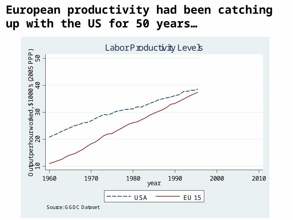
Extension: Multinationals
What happens when a firm expands abroad?
Assumption:
Costly for multinationals to have different management and organizational structures (easier to integrate managers, HR, training, software etc. if org is similar across borders)
Implication:
Then US multinationals and EU multinationals abroad will adjust to their parent’s organizational structure
Consistent with range of case-study evidence (e.g. Bartlett & Ghoshal, 1999, Muller-Camen et al. 2004) and true for well-known firms (P&G, Unilever, McKinsey, Starbucks etc..)

Plants rapidly reorganize after a US takeover
US firm EU firmUS firm takes-over an EU firm
Note: Assumes cost of non-alignment = sales x (OPARENT - OSUBSIDIARY)2

The model provides:
1. A rationale for differences in organizational structures between US and European firms
1. A simple way to interpret the macro stylized facts on productivity dynamics and IT investment in the US and Europe
1. A useful framework to link the micro findings on US multinationals active in the UK to the macro picture

Other extensions we consider to the model
1. Industry heterogeneity– If the degree of complementarity is higher in some sectors (e.g. “IT
intensive using” industries) and zero in others, then these patterns will be sector specific
– EU does just as well as US when no complementarity (σ = 0)
2. Adjustment costs for IT capital– Qualitative findings the same– TFP also will appear to grow faster in the transition
3. Permanent differences in management quality – Possible alternative story: US firms able to transfer management practices
across international boundaries
Q = A OζCα+σO Kβ - σO L1-α- β- ζ
- But implies a permanently higher US labor productivity even after controlling for IT level and higher coefficient
- Can test using new management data we are collecting

Macro facts and motivation
New micro results
A possible model
Conclusion

Conclusion
New micro evidence (cross section, panel and takeovers)– US establishments have higher TFP than non-US
multinationals– This is almost all due to higher coefficient on IT (“the way
that you do I.T.”)– Driven by same sectors responsible for US “productivity
miracle”
Micro, macro and survey findings consistent with a simple re-organization model– IT changes the optimal structure of the firm – So as IT prices fall firms want to restructure– Occurred in the US but much less in the EU (regulations)– When will the EU resume the catching up process?

Next Steps
• Bringing management and organizational data together with firm IT, organization and productivity data. New survey data following up Bloom and Van Reenen, 2006, forthcoming QJE. 12 countries (including China, Japan), 3,000+ firms
• Understanding determination of organizational decentralization (Acemoglu and Van Reenen et al, 2006)
• Structural estimation of the adjustment cost model (e.g. Simulated Method of Moments). See examples in Bloom, Bond and Van Reenen (forthcoming ReStud)
• More on IT endogeneity (e.g. broadband natural experiment)

Back Up

European Firms
US Firms
“Operations” management “Monitoring” management
Source: Bloom and Van Reenen (2006) survey of 732 firms in the US, UK, France and Germany. “Targets” and “incentives” management differences significant at the 1% level.
US firm also have different management “styles”
0.01
0.02
“Targets” management “Incentives” management
-0.01
0.04
European Firms
US Firms
European Firms
US Firms
-0.065
0.107
-0.122
0.172
European Firms
US Firms

Europe also did not have the same IT investment boom as the US
02
46
8IT
Ca
pita
l Sto
ck p
er
Hou
rs W
ork
ed, 2
00
0 E
uro
s
1980 1985 1990 1995 2000 2005year
USA EU 15
Source: GGDC
IT Capital Stock per Hours Worked

Non IT capital per hour worked
30
35
40
45
50
55
Non
IT S
tock
pe
r H
ours
Wo
rked
, 20
00 U
S$
1980 1985 1990 1995 2000 2005year
USA EU 15
Source: GGDC
Non IT Stock per Hours Worked

organization matters for the productivity of IT
Source: Bresnahan, Brynjolfsson & Hitt (2002) “Information Technology, Workplace Organization and the Demand for skilled labor” Quarterly Journal of Economics

IT Capital Stocks Estimates
• Methodology
Perpetual inventory method (PIM) to generate
establishment level estimates of IT stocks
• Robustness test assumptions on:– Initial Conditions
– Depreciation and deflation rates
1,,, 1 tititi KIK

Issue Choice Notes
Initial Conditions
We do not observe all firms in their first year of activity.
How do we approximate the existing capital stock?
Use industry data (SIC2) and impute:
Similar to Martin (2002)Industry IT capital stocks from NIESRRobust to alternative methods
Depreciation Rates
How to choose δ ? Follow Oliner et al (2004) and set δ = 0.36 (obsolescence)
Basu and Oulton suggest 0.31. Results not affected by alternative δ
Deflators
Need real investment to generate real capital
Use NIESR hedonic deflators (based on US estimates)
Re-evaluation effects included in deflators
Jjji
I
K
I
K
jt
jt
it
it
and
Methodological Choices

(1) (2) (3) Estimation Method OLS,
No FE OLS, FE
OLS, FE
Dependent variable: ln(GO) = ln(Gross Output)
Ln(Ct) 0.0440*** 0.0299*** 0.0265*** IT capital (0.0023) (0.0040) (0.0063)
Ln(Ct-1) - - - IT capital, lagged
Ln(Mt) 0.5384*** 0.4665*** 0.4702*** Materials (0.0080) (0.0193) (0.0283)
Ln(Mt-1) - - - Materials, lagged
Ln(Kt) 0.1193*** 0.1650*** 0.1953*** Non-IT Capital (0.0063) (0.0153) (0.0234)
Ln(Kt-1) - - Non-IT Capital, lagged
Ln(Lt) 0.2868*** 0.3177*** 0.2979*** Labour (0.0062) (0.0198) (0.0209)
Ln(Lt-1) - - Labour, lagged
Ln(Yt-1) - - - Gross Output, lagged
Rho, ρ - - -
Observations 22,736 22,736 6,763
Fixed effects NO YES YES
Basic Production functions (Table A4)
(at least 3 continuous time series observations)

Dep Variable ln(GO) ln(GO) ln(GO) ln(GO) ln(GO) ln(GO) ln(GO)
Sectors All All All IT Using Others IT Using Others
Fixed effects No No No No No Yes Yes
Ln (C) 0.043*** 0.041*** 0.036*** 0.044*** 0.021*** 0.027***
US MNE *ln(C)
- 0.011** 0.019** 0.007 0.029*** 0.000
Non- US MNE*ln(C)
- 0.004 -0.000 0.007* 0.004 -0.002
Ln(Materials) 0.547*** 0.538*** 0.538*** 0.614*** 0.501*** 0.559*** 0.411***
Ln(Non-IT K) 0.130*** 0.118*** 0.118*** 0.102*** 0.134*** 0.139*** 0.211***
Ln(Labour) 0.315*** 0.287*** 0.286*** 0.233*** 0.303*** 0.253*** 0.339***
US MNE 0.085*** 0.074*** 0.015 -0.055 0.050 -0.166*** 0.014
Non-US MNE 0.048*** 0.041*** 0.023 0.031 0.008 -0.006 0.044*
Obs 22,736 22,736 7,876 14,860 7,876 14,860
Table 1: IT Coefficient by ownership status
Note: All regression SE are clustered by establishment

BASIC PRODUCTION FUNCTION ESTIMATES, CONT. (TABLE A4)
(1) (2) (3) (4) (5) (6) (7)
Estimation Method OLS,No FE
OLS,FE
OLS,FE
GMM,Static
GMM,Dynamic
(Unrestricted)
GMM COMFAC
(Restricted)
Olley-Pakes
Dependent variable: ln(GO) = ln(Gross Output)
Ln(Ct) 0.0440*** 0.0299*** 0.0265*** 0.0391*** 0.0656* 0.0430** 0.0204***
IT capital (0.0023) (0.0040) (0.0063) (0.0171) (0.0373) (0.0211) (0.0030)
Ln(Ct-1) - - - - -0.0343 - -
IT capital, lagged (0.0242)
Ln(Mt) 0.5384*** 0.4665*** 0.4702*** 0.3998*** 0.3293*** 0.3595*** 0.5562***
Materials (0.0080) (0.0193) (0.0283) (0.0402) (0.0750) (0.0494) (0.0102)
Ln(Mt-1) - - - - -0.0715 - -
Materials, lagged (0.0534)
Ln(Kt) 0.1193*** 0.1650*** 0.1953*** 0.1584*** 0.3618*** 0.2937*** 0.1511***
Non-IT Capital (0.0063) (0.0153) (0.0234) (0.0410) (0.0869) (0.0526) (0.0115)
Ln(Kt-1) - - - -0.1815*** -
Non-IT Capital, lagged (0.0592)
Ln(Lt) 0.2868*** 0.3177*** 0.2979*** 0.4158*** 0.2981*** 0.3524*** 0.2611***
Labour (0.0062) (0.0198) (0.0209) (0.0479) (0.0829) (0.0560) (0.0080)
Ln(Lt-1) - - - 0.0091 -
Labour, lagged (0.0624)
Ln(Yt-1) - - - - 0.2330*** - -
Gross Output, lagged (0.0581)

Other Notes on Results
• Higher coefficient on IT than expected from share in gross output, but not as large as Brynjolfsson and Hitt (2003) on US firm-level data (example of TFP specification over)
• Methodological and data differences from BH (e.g. firms vs. establishments; BH pre 1995 we are post 1995; we use standard investment method BH use stock survey; we have more observations)
• But may be because we are looking at different countries

TFP BASED SPECIFICATIONS
(1) (2) (3) (4)
Dependent variable Δln(TFP) Δln(TFP) Δln(TFP) Δln(TFP)
Length of differencing first second third fourth
(e.g. first differencing vs. longer differencing)
Sectors All All All All
ΔLn(C) 0.0137*** 0.0150*** 0.0154*** 0.0155*
IT capital (0.0022) (0.0030) (0.0057) (0.0082)
Observations 10,122 4,079 920 404

What do we expect in TFP regressions?
PQ
XPS
PQ
CPS
XSCSQ
xx
cc
xc
;
;lnlnln
XOCOQA ln)1(ln)(lnln
cc SPQ
CPO
MTFP, measured TFP is
In our model “true” TFP is
So we measure TFP correctly even in presence of O

Using micro data
• In the data the higher O firms will have higher C so on average coefficient on C is positive in TFP regressions unless we use exact factor share of C by firm.
• On average, US firms will have no higher coefficient on C in TFP equation if we use the US revenue share
• Extensions– Allow adjustment costs on C. Implies that IT share “too low” when
calculating TFP, so measured TFP higher for high O firms

What do we expect in TFP regressions?
ithdiitdhitdhMNEitd
MNEh
USAitd
USAh
itMNEitd
MNEhit
USAitd
USAhitdhitd
uzDDD
cDbcDbcbTFP
,00
0
~'
)~()~(~

Precise parameterization
variable Mnemonic Value Reference
C coefficient (IT capital)
α 0.025 Share of IT in value added
K coefficient β 0.3 Share of capital costs in value added
Complementarity σ 0.017 α (1-e-1)
Mark-up (p-mc)/mc 1/(e-1) 0.5 Hall (1988)
Relative quadratic adjustment cost of O
ωEU/ωUS 4 Nicoletti and Scarpetta (2003)
Disruption cost of O (as a % of sales)
η 0.2% Bloom (2006), Cooper & Haltiwanger (2003)
IT prices pc -15% p.a. until 1995 then -30%
BLS

Table A1 BREAKDOWN OF INDUSTRIES (1 of 3)
IT Intensive (Using Sectors)
IT-using manufacturing18 Wearing apparel, dressing and dying of fur22 Printing and publishing29 Machinery and equipment31, excl. 313 Electrical machinery and apparatus, excluding insulated wire33, excl. 331 Precision and optical instruments, excluding IT instruments351 Building and repairing of ships and boats353 Aircraft and spacecraft352+359 Railroad equipment and transport equipment36-37 miscellaneous manufacturing and recycling
IT-using services51 Wholesale trades52 Retail trade71 Renting of machinery and equipment73 Research and development741-743 Professional business services

BREAKDOWN OF INDUSTRIES (2 of 3)
Non- IT Intensive (Using Sectors)
Non-IT intensive manufacturing15-16 Food drink and tobacco17 Textiles19 Leather and footwear20 wood21pulp and paper23 mineral oil refining, coke and nuclear24 chemicals25 rubber and plastics26 non-metallic mineral products27 basic metals28 fabricated metal products 34 motor vehicles
Non-IT Services50 sale, maintenance and repair of motor vehicles55 hotels and catering60 Inland transport61 Water transport62 Air transport
63 Supporting transport services, and travel agencies70 Real estate749 Other business activities n.e.c.90-93 Other community, social and personal services95 Private Household99 Extra-territorial organizations
Non-IT intensive other sectors01 Agriculture02 Forestry05 Fishing10-14 Mining and quarrying50-41 Utilities45 Construction

BREAKDOWN OF INDUSTRIES (3 of 3)
IT Producing Sectors
IT Producing manufacturing30 Office Machinery313 Insulated wire321 Electronic valves and tubes322 Telecom equipment323 radio and TV receivers331 scientific instruments
IT producing services64 Communications72 Computer services and related activity