Embed Size (px)
Citation preview
E-PFRP N. 12
2015
ISTITUTO DI ECONOMIA E FINANZA
PUBLIC FINANCE RESEARCH PAPERS
AN ANALYSIS ON OPTIMAL TAXATION AND ON POLICY CHANGES IN
AN ENDOGENOUS GROWTH MODEL WITH PUBLIC EXPENDITURE
THOMAS RENSTRÖM AND LUCA SPATARO
Pu
bli
c Fi
na
nce
Re
sea
rch
Pa
pe
rs (
ISS
N 2
28
4-2
52
7)
2
E-PFRP N. 12
Thomas Renström, University of Durham (UK).
Email: t.i.Renströ[email protected].
Luca Spataro, Dipartimento di Economia e Management, University of Pisa (Italy).
Email: [email protected].
Si prega di citare così: Thomas Renström and Luca Spataro (2014), “An analysis on
optimal taxation and on policy changes in an endogenous growth model with public
expenditure”, Public Finance Research Papers, Istituto di Economia e Finanza, DIGEF,
Sapienza University of Rome, n. 12 (http://www.digef.uniroma1.it/ricerca).
3
E-PFRP N. 12
Thomas Renström and Luca Spataro
An analysis on optimal taxation and on policy changes in an
endogenous growth model with public expenditure
Abstract
In this work we analyse the issue of optimal taxation and of policy changes in an
endogenous growth model driven by public expenditure, in the presence of endogenous
fertility and labour supply. While normative analysis confirms the Chamley-Judd result of
zero capital income tax, positive analysis reveals that the presence of endogenous fertility
produces different results as for the effects of taxes on total employment.
JEL Classification: D63, E21, H21, J13, O4.
Keywords: Taxation, endogenous fertility, critical level utilitarianism, population.
4
E-PFRP N. 12
1. Introduction
An extensive literature on optimal taxation of factor incomes in a general
equilibrium-dynamic framework has been flourishing in the last three decades. A
well-established finding of such works is that, in the long run, capital income
should not be taxed, thus shifting the burden from factor income taxation toward
labor (Judd, 1985, Chamley, 1986, Judd, 1999). Although the result is robust with
respect to several extensions, some exceptions may arise, such as in the case of
borrowing constraints (Aiyagari 1995 and Chamley 2001), market imperfections
(Judd 1997), incomplete set of taxes (Correia 1996, Cremer et al. 2003),
overlapping generations (Eros and Gervais 2002), social discounting and
disconnected economies (De Bonis and Spataro 2005, 2010), government time-
inconsistency and lack of commitment (Reis 2012), externalities from suboptimal
policy rules (Turnovsky 1996).
The case of externalities is particularly relevant for endogenous growth models:
Romer (1986) introduces externalities deriving from existing capital (spillovers as
“learning by doing”); Lucas (1988) shows that decreasing returns to capital could
be avoided by adopting a broad view of capital itself that entails human capital as
well (externalities from “human capital”); in Barro (1990), spillovers from
productive public expenditure avoid diminishing returns to capital and are the
engine of sustained long run growth; finally, in a subsequent work, Romer (1990)
himself applies the concept of nonrivalty to “ideas” or “discoveries” that can
enhance production efficiency and technological progress, and obtained increasing
returns in production and thus sustained per-capita income growth.1
In this work we extend the analysis of optimal taxation and public expenditure
policies to an endogenous growth setting with productive public expenditure by
allowing for endogenous labour supply and endogenous fertility. This has been
never done so far.
In fact, several works have analysed the impact of fiscal policies on economic
growth, such as Barro (1990), Jones and Manuelli (1990) and Rebelo (1991). As for
welfare analysis, Lucas (1990) and Turnovsky (1992) compare the effects of a tax
on capital versus a tax on labour and find the former to be inferior to the latter from
the viewpoint of economic welfare. Turnovsky (1996) analyses the issue of first-
best optimal taxation and expenditure policies in an endogenous growth model with
externalities stemming from public goods both in the utility and in the production
function and Turnovsky (2000) extends the analysis to the case of endogenous
labour supply2.
In this type of models, direct taxation brings about a natural trade-off: on the
one hand, it distorts incentives to save and work, hence reducing growth; on the
other, it increases the marginal productivity of private inputs, thus increasing
growth and possibly welfare. This is the key contribution of Barro (1990), which
was extended in several subsequent studies.
1 The literature on endogenous technological change through R&D activities, schumpeterian
competition and spillovers has been evolving over the last decade (for a review see Acemoglu 2009
chapters 13 and subsequent ones). 2 Discussions of the effects of taxation in models of endogenous labour supply are also provided by
Rebelo (1991).
5
E-PFRP N. 12
However, in all these works population growth is either absent or exogenous. In
fact, the observed large variations in fertility rates both across countries and across
times, has led an increasing number of scholars to work on the reformulation of
economic theory of endogenous fertility and on the provision of different social
criteria for allocation efficiency with variable population.3 Moreover, most of the
endogenous growth models mentioned above suffer from the “scale effect”,
meaning that the steady-state growth rate increases with the size (scale) of the
economy, as indexed, for example, by population. In order to overcome this
problem non-scale models have been provided by Jones (1995) and subsequent
works, although still hinging on exogenous population.
In order to breach this gap, in the present work we extend Barro (1990) model,
in which the engine of growth is productive public expenditure, by allowing for
both endogenous labour supply (as in Turnovsky 2000) and endogenous population
(as in Spataro and Renstrom 2012) and we use this model to analyse fiscal policy in
the form of distortionary taxes and government expenditure changes.
We retain Barro (1990) approach since there is consolidated evidence that
public expenditure in favour of productive services have a sizable impact on growth
(for major insights, see, among others, Turnovsky 1996, García Peñalosa and
Turnovsky, 2005). More precisely, we carry out our analysis under two different
types of public expenditure: a) optimal amount of public services (as in Barro
1990); b) fixed fraction of GDP (either fixed at the optimal level or not – as in
Turnovsky 1996).
We also note that our model allows to avoid two shortcoming of the
aforementioned nonscale growth models: first, the direct positive link between
economic and demographic growth entailed, which is not supported by post-war
data (see Agemoglu 2009, p. )4 and, second, the fact that the long-run equilibrium
growth rate is determined by technological parameters and is independent of macro
policy instruments.
The assumption of endogenous population, however, poses major issues related
to welfare analysis. In fact, given that under these circumstances welfare
evaluations typically imply the comparisons between states of the world in which
the size of population is different, the Pareto criterion cannot be used. To overcome
this issue, we adopt individual preferences that allow for social orderings that are
based on desirable welfarist axioms in presence of variable population.
We show that, while some well-established results on second-best taxation
extend also to our model, positive analysis produces results that are somehow in
contrast with the existing literature, due to the presence of endogenous fertility.
The work as organized as follows: in section 2, after laying out the expenditure
flow model, with both suboptimal and optimal government expenditure, we
characterize the optimal taxation rules and public debt; in section 3 we perform the
3 See, among others, Becker and Barro (1988), Barro and Becker (1989), Jaeger and Kuhle (2009),
Yew and Zhang (2009), de la Croix et al. (2012), Golosov et al. (2007), Renstrom and Spataro
(2011). 4 See Renstrom and Spataro (2014) for an endogenous growth model driven by human capital with
variable population, where the relationship between population growth and economic growth is not
necessarily positive.
6
E-PFRP N. 12
same in the public capital model. In section 4 we present a tax reforms analysis, in
order to verify the impact of the latter on economic growth. Section 5 concludes.
2. The model In this section we lay out the benchmark model. We denote individual
quantities by lower case letters, and aggregate quantities by corresponding upper
case letters, so that V = Nv, with N population size. As anticipated above, we find it
instructive to present both the case in which public expenditure is chosen optimally
(model 1) and or is fixed as a fraction of GDP (model 2). In the latter case, we will
first assume that the share of public expenditure is set arbitrarily while in the
second stage it is set optimally. This approach will enhance our understanding of
the optimal capital income tax rate which, as it will be shown, depends upon both
the socially optimal level of government expenditure and the deviation of actual
expenditure from its social optimum.
2.1. Households
We assume that the representative agent is endowed with a unit of time that
can be allocated either to leisure or the work or to child rearing. We also assume,
for the sake of simplicity, that each generation lives for one period, and life-time
utility is u(ct,lt), where ct is life-time consumption for that individual, lt is labour
supply. We assume that utility is increasing in ct, decreasing in lt and strictly
concave. We also follow the convention that u(0,.) = 0 represents neutrality at
individual level (i.e. if u < 0 the individual prefers not to have been born), and
denote the critical level utility as α.
An individual family chooses consumption, labour supply, savings and the
number of children (i.e. the change in the cohort size N).
We also assume that raising children is costly. We nest the existing
approaches in the literature by assuming the cost per family member in the number
of children, )(n , can either be linear (as in Becker and Barro, 1989, Cremer et al.
2006) or strictly convex (as in Tertilt 2005 and Growiec 2006). Convex cost implies
decreasing returns to scale in child rearing.
As for firms, we assume perfectly competitive markets and constant return
to scale technology. The consequence of the assumptions on the production side is
that we retain the “standard” second-best framework, in the sense that there are no
profits and the competitive equilibrium is Pareto efficient in absence of taxation.
Otherwise there would be corrective elements of taxation. Finally, we assume the
government finances an exogenous stream of per-capita expenditure x, that enters
as an input in private sector production function, by issuing debt and levying taxes.
To retain the second-best, we levy taxes on the choices made by the
families, i.e. savings, labour supply and children. Consequently we introduce the
capital-income tax and labour income tax, possibly conditional on the number of
children.
2.1.1 Preferences
We focus on a single dynasty (household) or a policymaker choosing
consumption and population growth over time, so as to maximize:
7
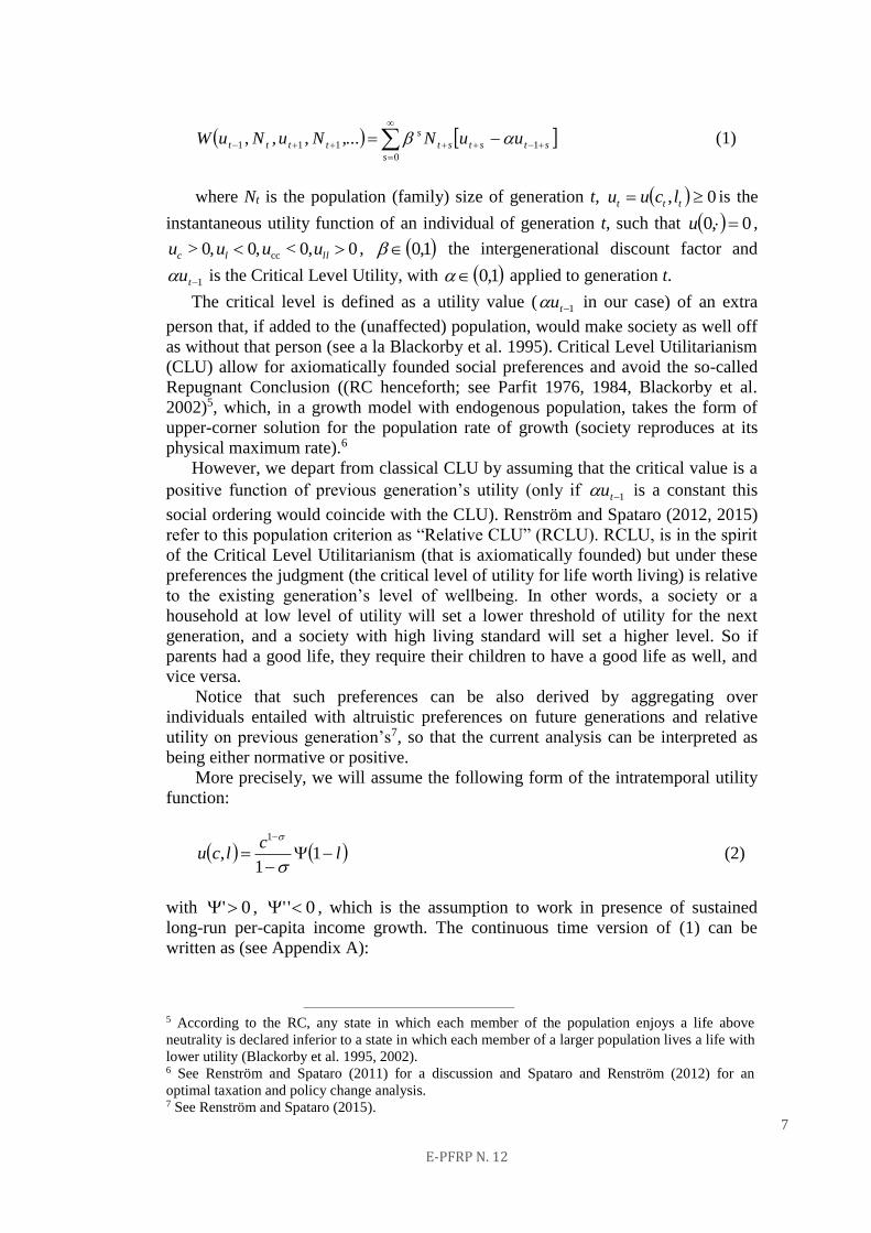
E-PFRP N. 12
0
1111 ,...,,,s
ststst
s
tttt uuNNuNuW (1)
where Nt is the population (family) size of generation t, 0, ttt lcuu is the
instantaneous utility function of an individual of generation t, such that 0,0 u ,
0,00,0, cc lllc u<uu>u , 1,0 the intergenerational discount factor and
1tu is the Critical Level Utility, with 1,0 applied to generation t.
The critical level is defined as a utility value ( 1tu in our case) of an extra
person that, if added to the (unaffected) population, would make society as well off
as without that person (see a la Blackorby et al. 1995). Critical Level Utilitarianism
(CLU) allow for axiomatically founded social preferences and avoid the so-called
Repugnant Conclusion ((RC henceforth; see Parfit 1976, 1984, Blackorby et al.
2002)5, which, in a growth model with endogenous population, takes the form of
upper-corner solution for the population rate of growth (society reproduces at its
physical maximum rate).6
However, we depart from classical CLU by assuming that the critical value is a
positive function of previous generation’s utility (only if 1tu is a constant this
social ordering would coincide with the CLU). Renström and Spataro (2012, 2015)
refer to this population criterion as “Relative CLU” (RCLU). RCLU, is in the spirit
of the Critical Level Utilitarianism (that is axiomatically founded) but under these
preferences the judgment (the critical level of utility for life worth living) is relative
to the existing generation’s level of wellbeing. In other words, a society or a
household at low level of utility will set a lower threshold of utility for the next
generation, and a society with high living standard will set a higher level. So if
parents had a good life, they require their children to have a good life as well, and
vice versa.
Notice that such preferences can be also derived by aggregating over
individuals entailed with altruistic preferences on future generations and relative
utility on previous generation’s7, so that the current analysis can be interpreted as
being either normative or positive.
More precisely, we will assume the following form of the intratemporal utility
function:
lc
lcu
11
,1
(2)
with 0' , 0'' , which is the assumption to work in presence of sustained
long-run per-capita income growth. The continuous time version of (1) can be
written as (see Appendix A):
5 According to the RC, any state in which each member of the population enjoys a life above
neutrality is declared inferior to a state in which each member of a larger population lives a life with
lower utility (Blackorby et al. 1995, 2002). 6 See Renström and Spataro (2011) for a discussion and Spataro and Renström (2012) for an
optimal taxation and policy change analysis. 7 See Renström and Spataro (2015).
8
E-PFRP N. 12
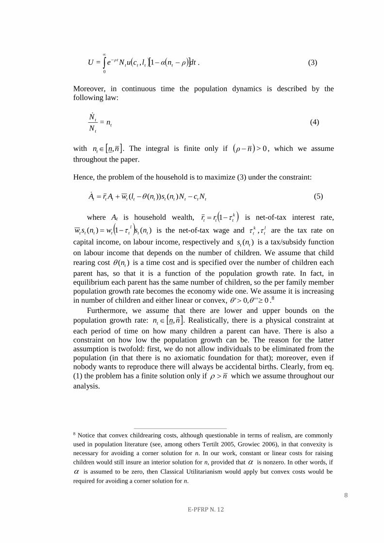
dtρnαlcuNe=U tttt
ρt
0
1, . (3)
Moreover, in continuous time the population dynamics is described by the
following law:
t
t
t n=N
N (4)
with nnnt , . The integral is finite only if 0>nρ , which we assume
throughout the paper.
Hence, the problem of the household is to maximize (3) under the constraint:
ttttttttttt NcNnsnlwArA )())(( (5)
where At is household wealth, k
ttt rr 1 is net-of-tax interest rate,
)(1)( tt
l
ttttt nswnsw is the net-of-tax wage and k
t , l
t are the tax rate on
capital income, on labour income, respectively and )( tt ns is a tax/subsidy function
on labour income that depends on the number of children. We assume that child
rearing cost )( tn is a time cost and is specified over the number of children each
parent has, so that it is a function of the population growth rate. In fact, in
equilibrium each parent has the same number of children, so the per family member
population growth rate becomes the economy wide one. We assume it is increasing
in number of children and either linear or convex, 0'',0' .8
Furthermore, we assume that there are lower and upper bounds on the
population growth rate: nnnt , . Realistically, there is a physical constraint at
each period of time on how many children a parent can have. There is also a
constraint on how low the population growth can be. The reason for the latter
assumption is twofold: first, we do not allow individuals to be eliminated from the
population (in that there is no axiomatic foundation for that); moreover, even if
nobody wants to reproduce there will always be accidental births. Clearly, from eq.
(1) the problem has a finite solution only if n which we assume throughout our
analysis.
8 Notice that convex childrearing costs, although questionable in terms of realism, are commonly
used in population literature (see, among others Tertilt 2005, Growiec 2006), in that convexity is
necessary for avoiding a corner solution for n. In our work, constant or linear costs for raising
children would still insure an interior solution for n, provided that is nonzero. In other words, if
is assumed to be zero, then Classical Utilitarianism would apply but convex costs would be
required for avoiding a corner solution for n.
9
E-PFRP N. 12
2.2. Firms
We assume constant-returns-to-scale production technology with labour-
augmenting productive public expenditure. More precisely, the production function
is:
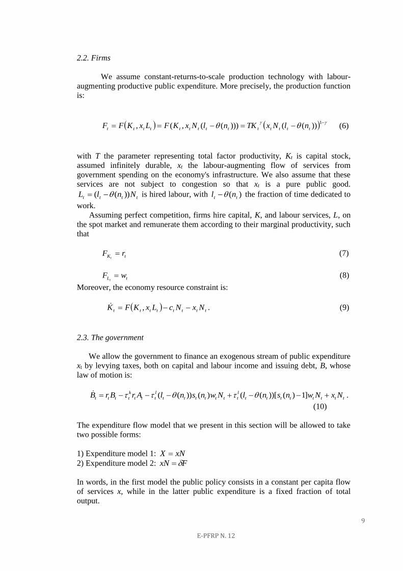
1))(()))((,(, tttttttttttttt nlNxTKnlNxKFLxKFF (6)
with T the parameter representing total factor productivity, Kt is capital stock,
assumed infinitely durable, xt the labour-augmenting flow of services from
government spending on the economy's infrastructure. We also assume that these
services are not subject to congestion so that xt is a pure public good.
tttt NnlL ))(( is hired labour, with )( tt nl the fraction of time dedicated to
work.
Assuming perfect competition, firms hire capital, K, and labour services, L, on
the spot market and remunerate them according to their marginal productivity, such
that
tK rFt (7)
tL wFt (8)
Moreover, the economy resource constraint is:
tttttttt NxNcLxKFK , . (9)
2.3. The government
We allow the government to finance an exogenous stream of public expenditure
xt by levying taxes, both on capital and labour income and issuing debt, B, whose
law of motion is:
tttttttt
l
ttttttt
l
ttt
k
tttt NxNwnsnlNwnsnlArBrB ]1)())[(()())(( .
(10)
The expenditure flow model that we present in this section will be allowed to take
two possible forms:
1) Expenditure model 1: xNX
2) Expenditure model 2: FxN
In words, in the first model the public policy consists in a constant per capita flow
of services x, while in the latter public expenditure is a fixed fraction of total
output.
10
E-PFRP N. 12
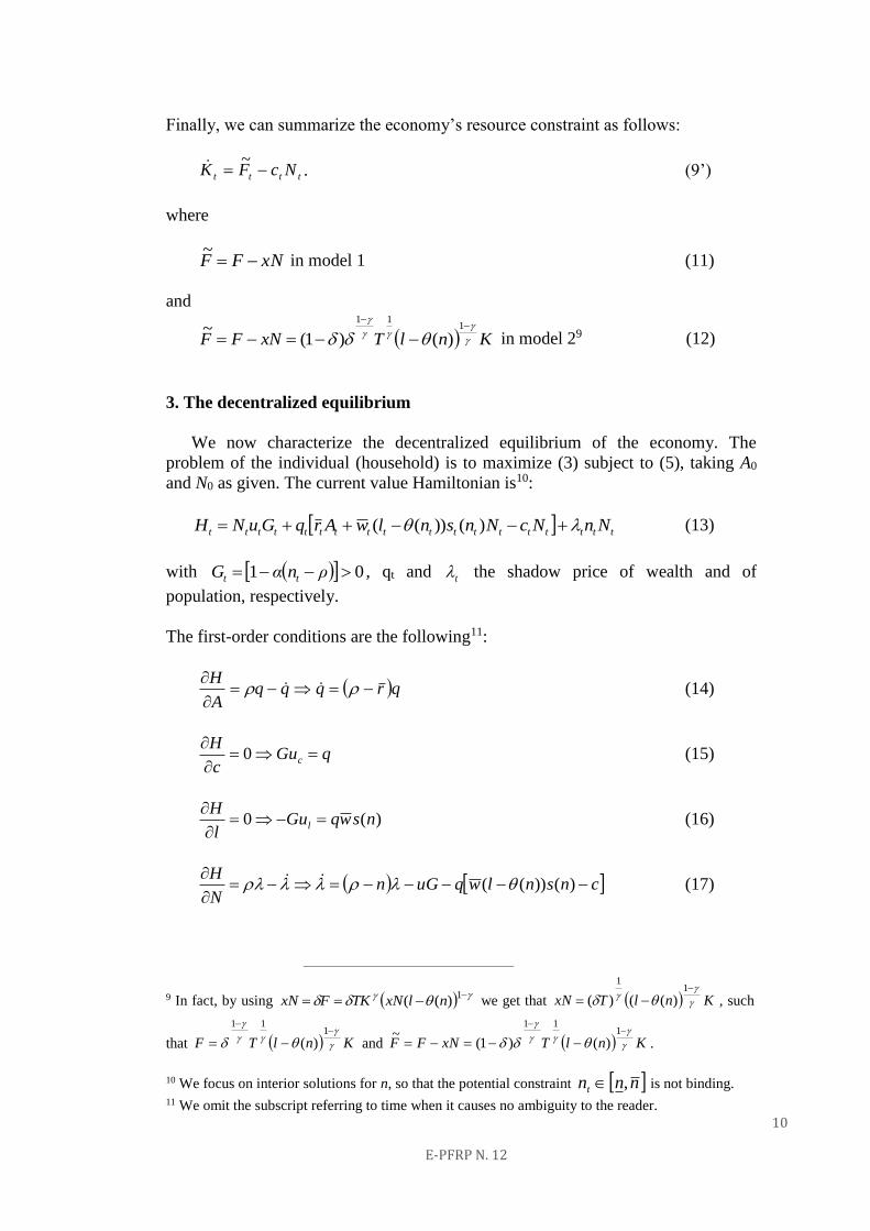
Finally, we can summarize the economy’s resource constraint as follows:
tttt NcFK ~ . (9’)
where
xNFF ~
in model 1 (11)
and
KnlTxNFF
1
11
)()1(~
in model 29 (12)
3. The decentralized equilibrium
We now characterize the decentralized equilibrium of the economy. The
problem of the individual (household) is to maximize (3) subject to (5), taking A0
and N0 as given. The current value Hamiltonian is10:
tttttttttttttttttt NnNcNnsnlwArqGuNH )())(( (13)
with 01 ρnαG tt , qt and t the shadow price of wealth and of
population, respectively.
The first-order conditions are the following11:
qrqqqA
H
(14)
qGuc
Hc
0 (15)
)(0 nswqGul
Hl
(16)
cnsnlwquGnN
H
)())(( (17)
9 In fact, by using
1
)(( nlxNTKFxN we get that KnlTxN
1
1
)(()( , such
that KnlTF
1
11
)( and KnlTxNFF
1
11
)()1(~
.
10 We focus on interior solutions for n, so that the potential constraint nnnt , is not binding.
11 We omit the subscript referring to time when it causes no ambiguity to the reader.
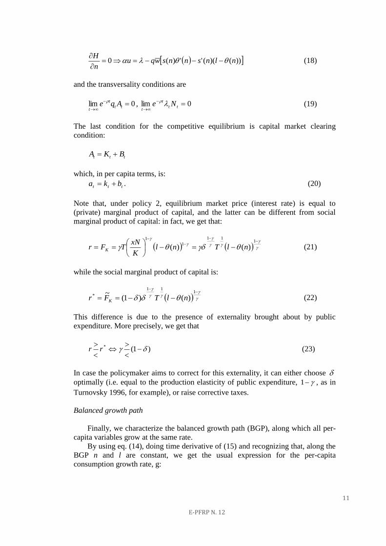
11
E-PFRP N. 12
))()(('')(0 nlnsnnswqun
H
(18)
and the transversality conditions are
0lim
tt
t
tAqe
, 0lim
tt
t
tNe
(19)
The last condition for the competitive equilibrium is capital market clearing
condition:
ttt BKA
which, in per capita terms, is:
ttt bka . (20)
Note that, under policy 2, equilibrium market price (interest rate) is equal to
(private) marginal product of capital, and the latter can be different from social
marginal product of capital: in fact, we get that:
111
1
1
)()( nlTnlK
xNTFr K
(21)
while the social marginal product of capital is:
1
11
* )()1(~
nlTFr K (22)
This difference is due to the presence of externality brought about by public
expenditure. More precisely, we get that
)1(*
rr (23)
In case the policymaker aims to correct for this externality, it can either choose
optimally (i.e. equal to the production elasticity of public expenditure, 1 , as in
Turnovsky 1996, for example), or raise corrective taxes.
Balanced growth path
Finally, we characterize the balanced growth path (BGP), along which all per-
capita variables grow at the same rate.
By using eq. (14), doing time derivative of (15) and recognizing that, along the
BGP n and l are constant, we get the usual expression for the per-capita
consumption growth rate, g:
12
E-PFRP N. 12
r
c
cg
(24)
We can notice that, as usual, the economy growth rate is proportional to the net-of-
tax interest rate. This, in turn, depends on the whole set of the endogenous
variables, namely, the population growth rate, labour supply, and capital intensity,
and on the deep parameters of the economy, comprising taxes. We will address the
effects of the latter on the economy growth rate in section 5, after characterizing the
optimal taxation rules.
4. The Ramsey problem
We now solve the optimal tax problem (Ramsey problem). In doing so, we
adopt the primal approach, consisting of the maximization of a direct social welfare
function through the choice of quantities (i.e. allocations; see Atkinson and Stiglitz
1972)12. For this purpose we must restrict the set of allocations among which the
government can choose to those that can be decentralized as a competitive
equilibrium. We now provide the constraints that must be imposed on the
government’s problem in order to comply with this requirement.
In our framework there is an implementability constraint associated with the
individual family’s intertemporal consumption choice. More precisely this
constraint is the individual budget constraint with prices substituted for by using the
consumption Euler equation, which yields (see Appendix A.2):
dtNnlucuGeuAG tttltct
t
c tt))((
0
00 0
(25)
Finally there three feasibility constraints, one which requires that private and public
consumption plus investment be equal to aggregate output (eq. 9); the other is given
by eq. (17) (again, where we make use of individuals’s FOCs (15) and (16)), the
last one is eq. (4).
Hence, supposing that the policy is introduced in period 0, the problem of the
policymaker is to maximize (1) subject to eq. (25), and, 0t , eqs. (9’), (17) and
(4). Hence, the current value Hamiltonian is:
tttttttttltctttt NnNcFnlucuuGNHtt
~
))]((([ (26)
which can be written as (omitting time subscripts):
nNcNFunlucuGNuNGH lc ~
]))(([1 (27)
where , and are the multipliers associated with the constraints.
12 On the contrary, the dual approach takes prices and tax rates as control variables. For a survey see
Renström (1999).
13
E-PFRP N. 12
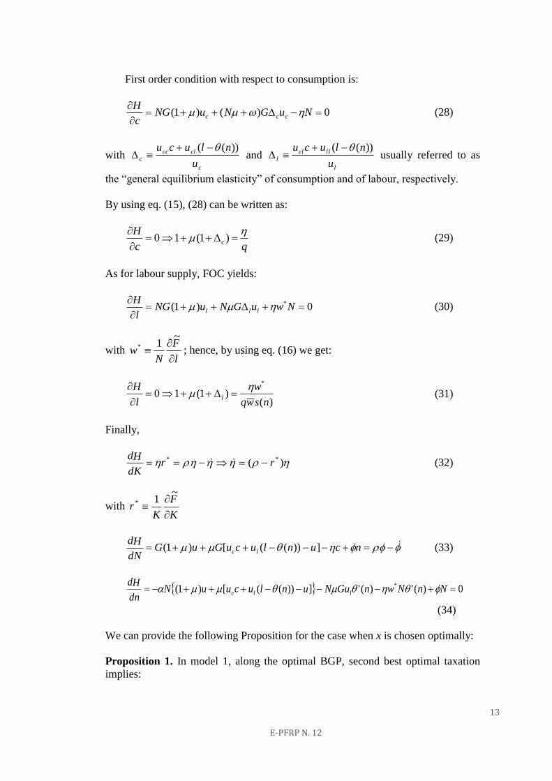
First order condition with respect to consumption is:
0)()1(
NuGNuNG
c
Hccc (28)
with c
clcc
cu
nlucu ))(( and
l
llcl
lu
nlucu ))(( usually referred to as
the “general equilibrium elasticity” of consumption and of labour, respectively.
By using eq. (15), (28) can be written as:
qc
Hc
)1(10 (29)
As for labour supply, FOC yields:
0)1( *
NwuGNuNG
l
Hlll (30)
with l
F
Nw
~1* ; hence, by using eq. (16) we get:
)()1(10
*
nswq
w
l
Hl
(31)
Finally,
)( ** rrdK
Hd (32)
with K
F
Kr
~1*
ncunlucuGuGdN
Hdlc ]))(([)1( (33)
0)(')(']))(([)1( * NnNwnGuNunlucuuNdn
Hdllc
(34)
We can provide the following Proposition for the case when x is chosen optimally:
Proposition 1. In model 1, along the optimal BGP, second best optimal taxation
implies:
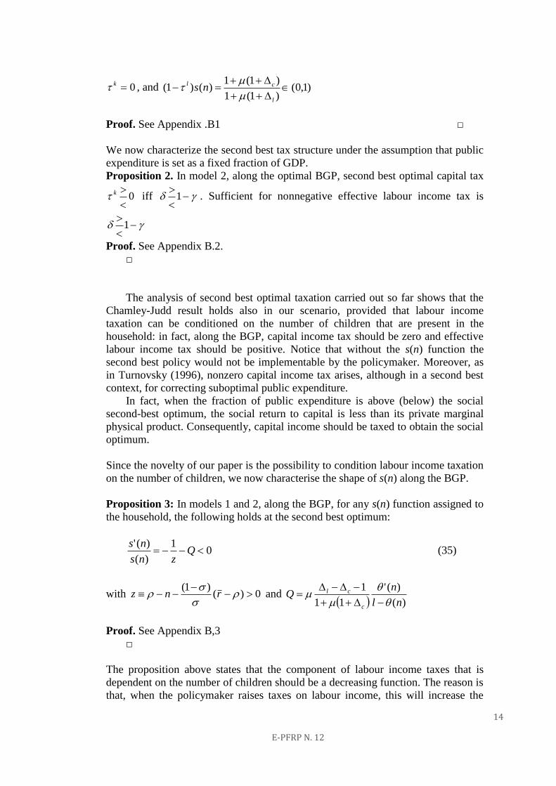
14
E-PFRP N. 12
0k , and )1,0()1(1
)1(1)()1(
l
cl ns
Proof. See Appendix .B1 □
We now characterize the second best tax structure under the assumption that public
expenditure is set as a fixed fraction of GDP.
Proposition 2. In model 2, along the optimal BGP, second best optimal capital tax
0
k iff
1 . Sufficient for nonnegative effective labour income tax is
1
Proof. See Appendix B.2.
□
The analysis of second best optimal taxation carried out so far shows that the
Chamley-Judd result holds also in our scenario, provided that labour income
taxation can be conditioned on the number of children that are present in the
household: in fact, along the BGP, capital income tax should be zero and effective
labour income tax should be positive. Notice that without the s(n) function the
second best policy would not be implementable by the policymaker. Moreover, as
in Turnovsky (1996), nonzero capital income tax arises, although in a second best
context, for correcting suboptimal public expenditure.
In fact, when the fraction of public expenditure is above (below) the social
second-best optimum, the social return to capital is less than its private marginal
physical product. Consequently, capital income should be taxed to obtain the social
optimum.
Since the novelty of our paper is the possibility to condition labour income taxation
on the number of children, we now characterise the shape of s(n) along the BGP.
Proposition 3: In models 1 and 2, along the BGP, for any s(n) function assigned to
the household, the following holds at the second best optimum:
01
)(
)(' Q
zns
ns (35)
with 0)()1(
rnz and
)(
)('
11
1
nl
nQ
c
cl
Proof. See Appendix B,3
□
The proposition above states that the component of labour income taxes that is
dependent on the number of children should be a decreasing function. The reason is
that, when the policymaker raises taxes on labour income, this will increase the
15
E-PFRP N. 12
number of children (see also Proposition 6). Hence, the s(n) function will be shaped
in such a way to counterbalance this increase.
Finally, it is possible to provide a shape of the s(n) function that is implementable
by the policymaker.
Proposition 4: An s(n) function implementing the second best is:
nns )()( . (36)
Where 0)( , n and 10 are policy instruments taken as given by the
household.
Proof: See Appendix B.4. □
While , and are taken as given by the household, in the second best
equilibrium they are functions of equilibrium quantities.
Finally, we can characterize the same function in the case of fixed costs for raising
children.
Corollary 1: If )(' n is equal to zero, the function s(n) implementing the second
best is nns )( , where )()1(
r and r are taken as given by the
household.
Proof: When 0)(' n Q is equal to zero and it is clear from (35) that s=z
implements the second best equilibrium. Eq. (B.8) when Q=0, substituted into (36)
gives zz )( , yielding )(1 z , which holds at 1 and 1)1( . □
Note that in this case there are fewer extra policy instruments needed, in that s(n) is
simply a function of n and , the latter being set directly by the policymaker at its
(second best) equilibrium value.
Finally, the Proposition that follows provides the result concerning the sign of the
optimal level of debt:
Proposition 5: Under model 1 and 2 optimal debt is negative.
Proof. See Appendix B.5. □
This result states that along the second-best optimal BGP public expenditure should
entirely be financed by labour income taxes and by the returns of public assets (in
model 1) or by also capital income taxes (in model 2, if )1( ).
5. Tax reforms
We now analyse the effects of policy changes on the equilibrium levels of the main
variables (i.e. labour supply )(nl , population growth rate n and the growth rate
16
E-PFRP N. 12
of the economy, g, which is proportional to r , in that /rddg ), along the BGP.
To simplify the analysis and without loss of generality, we assume s(n)=1 and that
childbearing costs are linear, so that 0)('' n 13. The analysis below encompasses
both models 1 and 2.
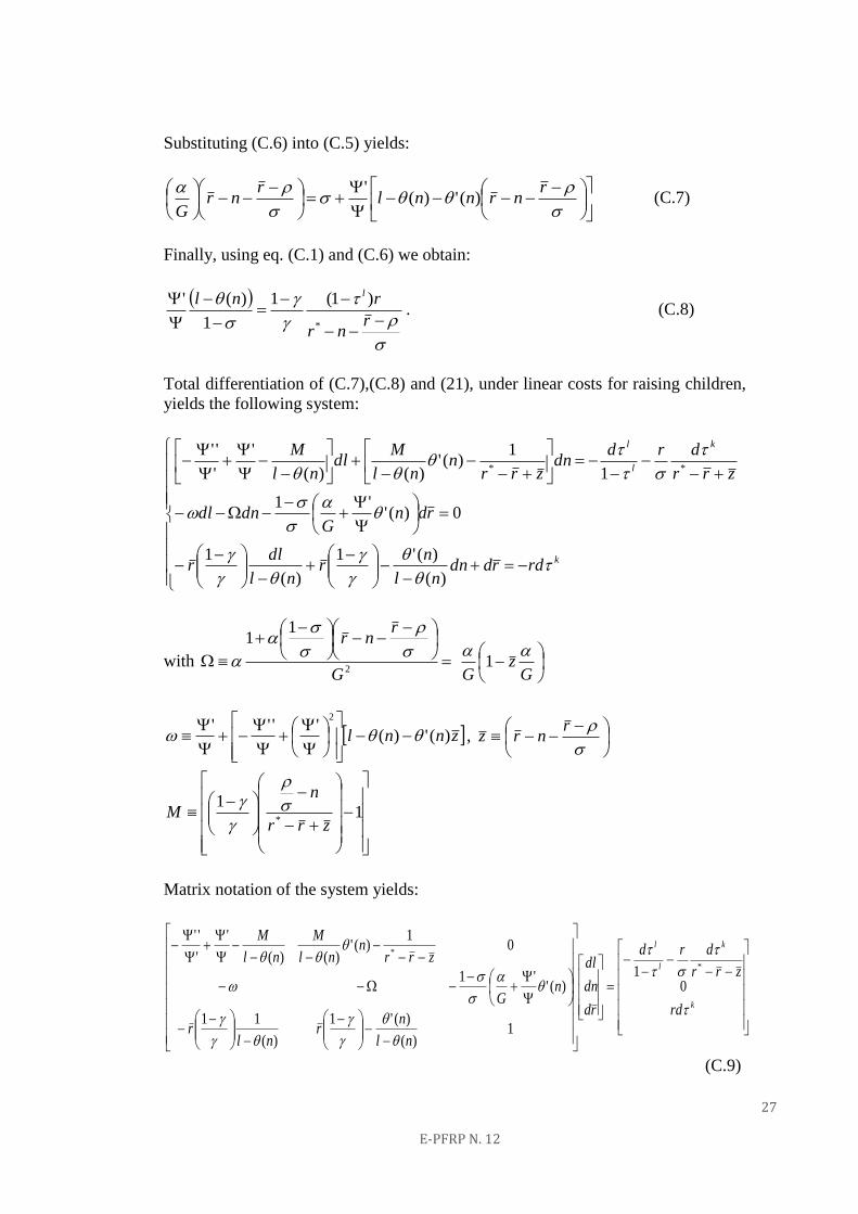
From decentralized equilibrium, we get (see Appendix C.1):
)(
)(
)(')(
1
1
1nl
c
w
nl
n
rnr
nlc
w
G
(37)
rnr
rnl l
*
)1(1
1
)('. (38)
and
1
11
)()1()1( nlTFr k
K
k (39)
With the economy always being on a balanced growth path, the effects of
government policy
on the equilibrium are obtained by taking the differentials of (37)-(132). Routine
calculations yield the qualitative responses with respect to k and l which we can
summarize in the following proposition:
Proposition 6. Along the BGP, the effects of policy changes are the following:
0,0))((
,0
lll
nnlg
0,0))((
,0
kkk
nnlg
Proof. See Appendix C.1. □
The results on economic growth are somehow intuitive: higher taxes produce
lower growth. However, differently from previous literature on endogenous growth
models and endogenous labour supply, the effects of taxes on employment may be
different. For example, in Turnovsky 2000 the signs of the effect of either taxes on
labour supply are quite the same and negative. The difference in our results are due
to the presence of endogenous fertility. In other words, it emerges that the
transmission channel of fiscal policies on economic growth are qualitatively
different: on the one hand, the labour income tax, while depressing wages, reduces
the incentive for net accumulation but reduces the opportunity cost of raising
children (i.e. net-wage; see eq. 16). This will increase the number of children per
household and reduce the household’s time dedicated to work.
13 See footnote 8.
17
E-PFRP N. 12
On the other hand, the capital income tax, while reducing the incentives towards
net accumulation (lower net interest rates) as well, increases the incentives of
devoting more time on the job (and relatively less to raising children); finally, by
hitting future consumption, a higher capital income tax exerts a reinforcing effect
towards the reduction of the number of descendents.
Finally, given that the effects of taxes on the BGP equilibrium variables are
qualitatively different, one might wonder what are the effects of policies that
redistribute the burden of taxation between production inputs.
For this purpose we focus on the case in which the government operates a
redistribution of taxes in such a way that total tax revenues (TR) remain fixed
proportion of GDP. Needless to say, we will only consider those cases in which the
economy is on the “upward-sloped trait” of the Laffer curve, meaning that any
change of either tax rate will imply a change of the opposite sign in the other tax,
i.e. 0
)/(
YTR
k
l
d
d
. Otherwise, there would be room for decreasing both taxes while
keeping the b/k ratio constant.
Given that we have shown that the changes in the capital income and labour
income taxes have opposite effect on labour supply and population growth,
respectively, the results of the constant-debt-redistributive policy on the latter
variables are clear. However, in principle the effects on the economy growth rate
are ambiguous: for example, an increase of capital income will tend to reduce g,
while the corresponding decrease of the labour income tax will exert a positive
effect on it. The final effect on the BGP rate of growth will depend on which force
dominates. The results of this exercise are summarized in the following
proposition:
Proposition 7. Along the BGP, a tax reform consisting in an increase (decrease) of
the capital income tax and a corresponding reduction (increase) of the tax on
labour income in such a way to leave the total-tax-revenues/GDP ratio unchanged,
implies that equilibrium labour supply increases (decreases) and the population
growth rate decreases (increases), while the change of the growth rate of per-capita
income is ambiguous. However, sufficient for the latter to be negative (positive) is
that the capital income tax is not lower than the labour income tax.
Proof. See Appendix C.2.
The content of Proposition 5 has clear-cut policy implications: since the effects
of the redistributive policy are dominated by those of capital income taxes, if a
policymaker aims at boosting per-capita growth, with constant tax revenues over
GDP, it should redistribute the burden of taxation towards labour income and
maintain the labour income tax lower than the capital income tax. This, in turn,
would also increase the rate of growth of population. The latter result can be
explained in terms of “quality-quantity” trade-off (higher taxes on labour income
reduce the opportunity cost of raising children) already unveiled by several works
on population economics.
18
E-PFRP N. 12
7. Conclusions
In the present work we have carried out an analysis of optimal taxation and
policy changes in an endogenous growth model in presence of endogenous fertility
and labour supply. As far as the normative analysis is concerned, we show that, at
the steady state the second-best policy entails zero capital income tax, positive
labour income tax and negative debt. Optimal nonzero tax on capital income
results as a corrective device only in the case of suboptimal public spending, as in
Turnovsky (1996), although in a second best analysis.
From a positive standpoint we show that a rise of taxes (either on labour
income or on capital income), depresses per-capita growth. However, while an
increase of fiscal pressure on labour input reduces labour supply and increases the
population growth rate, an increase of taxes on capital produces the opposite
results. This result is in contrast with existing literature (see for example
Turnovsky 2000), due to the presence of endogenous fertility.
Finally, we have also analysed the effects of a fiscal policy aiming at
redistributing the tax burden in such a way to maintain tax revenues a fixed
proportion of GDP. The analysis has shown that the effects are qualitatively the
same of the case of a capital tax change, although the sign of the change of the
BGP rate of growth is in general ambiguous. Sufficient for such a variation to be
unambiguous is that the capital income tax is greater than or equal to the labour
income tax.
Consequently, the latter result suggests that an economy that wishes to boost
economic growth without resorting to extra public debt, should reduce capital
income taxes and increase labour income taxes, while keeping both taxes roughly
of the same magnitude. This policy, in turn, would also increase the population
rate of growth.
In this paper we have treated public expenditure as a flow variable (services
from current expenditure). A natural extension of our study is to analyse the case
of public expenditure as financing a stock of public goods (infrastructure): this
case is left for future research.
References
Acemoglu D (2009) Introduction to Modern Economic Growth. Princeton
Economic Press. Princeton and Oxford;
Atkinson, A. B. and Stiglitz, J. E. (1972): "The Structure of Indirect Taxation and
Economic Efficiency." Journal of Public Economics, 1, 97-119;
Basu, P., Marsiliani, L., and Renström, T.I., (2004): "Optimal Dynamic Taxation
with Indivisible Labour", The Manchester School 72(s1), 34-54;
Basu, P. and Renström, T.I. (2007): “Optimal dynamic labour taxation”,
Macroeconomic dynamics, 11 (5), 567-588;
Barro R.J. and Becker G.S. (1988): “Fertility Choice in a Model of Economic
Growth”, Econometrica, 57, 481-501;
Barro, R.J., (1990): “Government spending in a simple model of endogenous
growth”, Journal of Political Economy 98, S103-S125.
Becker, G.S. and Barro, R.J., (1989): “A Reformulation of the Economic Theory of
Fertility”, Quarterly Journal of Economics, 103, 1-25;
19
E-PFRP N. 12
Blackorby, C., Bossert, W., and Donaldson, D., (1995): “Intertemporal population
ethics: critical-level utilitarian principles”, Econometrica 63, 1303-20;
Blackorby, C., Bossert, W., and Donaldson, D., (2002): “Critical –level population
principles and the repugnant conclusion”, Department of Economics,
University of British Columbia Discussion paper n.: 02-16;
Chamley, C. (1986): “Optimal taxation of capital income in general equilibrium
with infinite lives”, Econometrica 54(3), 607–622;
Chamley, C. (2001): “Capital Income Taxation, Wealth Distribution and
Borrowing Constraints", Journal of Public Economics 79, 55-69.
Cremer, H., Gahvari, F., and Pestieau, P. (2006): “Pensions with endogenous and
stochastic fertility”, Journal of Public Economics, 90: 2303–21.
De Bonis, V. and Spataro L. (2005): “Taxing capital income as Pigouvian
correction: the role of discounting future”, Macroeconomic dynamics, 9(4),
469-77;
De Bonis, V. and Spataro, L. (2010): “Social discounting, migration, and optimal
taxation of savings”, Oxford Economic Papers, 62(3), 603-23;
de la Croix, D., Pestieau, P., and Ponthiere, G. (2012): “How powerful is
demography? The Serendipity Theorem revisited”, Journal of Population
Economics, 25(3): 899-922;
Erosa, A. and Gervais, M, (2002): “Optimal Taxation in Life-Cycle Economies”,
Journal of Economic Theory, 105(2), 388-369;
García Peñalosa, C. and Turnovsky, S.J. (2005): “Second-best optimal taxation of
capital and labor in a developing economy”, Journal of Public Economics, 89,
1045-74.
Golosov, M., Jones, L.E., and Tertilt M., (2007): “Efficiency with Endogenous
Population Growth”, Econometrica, 75, 1039-71;
Growiec, J. (2006): “Fertility Choice and Semi-Endogenous Growth: Where
Becker Meets Jones”, Topics in Macroeconomics, The Berckeley Electronic
Press, 6(2), Art. 10;
Jaeger K. and Kuhle, W. (2009): “The optimum growth rate for population
reconsidered”, Journal of Population Economics, 22(1): 23-41;
Jones, C.I. (1995): “R&D-Based Models of Economic Growth”. Journal of
Political Economics 103: 759–784;
Jones, L., and Manuelli, R. (1990): "A Convex Model of Equilibrium Growth:
Theory and Policy Implications", Journal of Political Economy, 98, 5, 1990,
1008-1038;
Judd, K.L, (1985): “Redistributive taxation in a simple perfect foresight model”,
Journal of Public Economy 28(1), 59–83;
Judd, K.L. (1997): “The Optimal Tax Rate for Capital Income is Negative”, NBER
Working Paper 6004;
Parfit, D. (1976): “On Doing the Best for Our Children”, in Ethics and
Populations, ed. By M. Bayles. Cambridge: Schenkman;
Parfit, D. (1984): “Reasons and Persons”, Oxford/New York: Oxford University
Press;
Rebelo, S. (1991): “Long-run policy analysis and long-run growth”, Journal of
Political Economy 99, 500-521.
Renström T.I. (1999): “Optimal Dynamic Taxation” in Dahiya, S.B. (Ed.) (1999),
The Current State of Economic Science, vol. 4, Spellbound Publications, 1717-
1743;
20
E-PFRP N. 12
Renström T.I. and Spataro L. (2011): “The Optimum Growth Rate for Population
under Critical-Level Utilitarism”; Journal of Population Economics 24(3),
1181-201;
Renström T.I. and Spataro L. (2015): “Population Growth and Human Capital: a
Welfarist Approach”, The Manchester School, forthcoming.
Spataro L. and Renström, T.I. (2012): “Optimal taxation, critical-level
utilitarianism and economic growth”, Journal of Public Economics, 96: 727-
738;
Tertilt, M. (2005): “Polygyny, Fertility and Savings”, Journal of Political
Economy, 113 (6), 1341-371;
Turnovsky, S.J., (1992): “Alternative forms of government expenditure financing:
A comparative welfare analysis”, Economica 59, 235-252;
Turnovsky, S.J. (1996): "Optimal Tax, Debt, and Expenditure Policies in a
Growing Economy" Journal of Public Economics, 60, 21-44;
Turnovsky, S.J. (2000): “Fiscal policy, elastic labor supply, and endogenous
growth”, Journal of Monetary Economics 45, 185– 210;
Turnovsky, S.J. and Fisher, W.H. (1995): “The Composition of Government
Expenditure and Its Consequences for Macroeconomic Performance”, Journal
of Economic Dynamics and Control, 19, 747-786.
Yew, S.L. and Zhang, J. (2009): “Optimal social security in a dynastic model with
human capital externalities, fertility and endogenous growth”, Journal of
Public Economics, 93(3-4): 605-19;
Appendix
Appendix A.1: The form of eq. (2) (drawn from Renström and Spataro 2012)
By starting from eq. (1) and collecting utility terms of the same date, the welfare
function W can be written as:
10
0
11
cuNncuNWt
ttt
t (A.1)
By ignoring 1c as it is irrelevant for the planning horizon, and defining
1
1
we get:
0 1
11
1
1
t
t
tt
t
ncuN
. In continuous time, by approximating
t
t nn
1
1 the latter expression can be written as follows:
dtncuNeU ttt
t
0
1 □ (A.2)
21
E-PFRP N. 12
Appendix A.2. Implementability constraint
First, let us take the following time derivative:
tttttt AqAqAqdt
d
which, exploiting eqs. (5) and (14) can be written as
tttttttttttttttt NcNnsnlwArqAqrAqdt
d )())((
Using (15) and (16) it follows:
)(( ttlctttttt nlucuGNAqAqdt
d
Hence, pre-multiplying by te and integrating both sides, making use of
transversality conditions and of eq. (15), we obtain eq. (25) in the text:
dtNnlucuGeuAG tttltct
t
c tt))((
0
00 0
Appendix B.1. Proof of proposition 1
As for the capital income tax, from (32) we get:
)( *r
and given that q
must be constant along the BGP (by eq. 22), the rate of growth of
and q must be equal, so that *rr .
Given that, in model 1, *rr , then 0k .
As for the labour income tax, from (29) and (31)
)1(1
)1(1)(*
l
c
w
nsw
(B.1)
Given that in model 1 *ww , then
)1(1
)1(1)()1(
l
cl ns
22
E-PFRP N. 12
with
0)('
lc
0)('
''1
ll . □
Appendix B.2. Proof of Proposition 2
As for capital income tax, given that, it must be true that *rr and in model 2,
*
)1(rr
, it follows that 0
11
k iff
1 .
As for effective labour income tax, given that
2111
* )()1()1(
nlN
KTw and
1
*ww , eq. (B.1) implies:
)1(1
)1(11)()1(
l
cl ns
which can be greater or smaller than 1. Given l >0 and c <0, if )1( >0,
then effective labour income taxation is positive (i.e. )()1( nsl <1). □
Appendix B.3. Proof of Proposition 3
Preliminarily, note that, by eq. 2 and the definition of c :
clc
u
unlucu
))(( (B.2)
so that, eq. (34), when divided by u becomes:
)(')(
')('
']1[
*
nnsw
wG
qnG
uc
. (B.3)
where we have used
'
u
ul and )(
'
)(
)( ***
nsw
wG
qnsw
w
u
nswq
qw
u
.
Along the BGP,
' and ))((
'nlc
are constant and
)(
' *
nsw
wG
q
is constant as well, so that u
is constant. (33) gives
u
cG
un
uc
)1()(
; using the latter and eq. (24) we have
23
E-PFRP N. 12
0)1(
u
cG
uz
u
u
uuudt
dc
, which yields
u
cG
uz c
)1( . Exploiting the latter, eq. (B.3) gives:
)(']1['
)1( nGzu
c
z
Glc
(B.4)
Notice that )1(
z
G
qzqu
cGu
zqu
qc
zu
c c . Next, (29), (B.4) becomes
)(']1['
)1( nGz
Glc
(B.5)
Now, dividing eq. (18) by u gives
))()(('')( nlnsnnsu
wq
u
(B.6)
As noticed above, u
wq is constant along the BGP and so is
u
.
Hence:
0
cG
uz
u
u
uuudt
d (B.7)
where we used (17) and (B.2), so that cGu
z
. Combining the latter with (B.6)
we have:
))()(('')( nlnsnnsu
wq
z
Gc
Exploiting )('
lc , (16) and (2) we obtain
))((
)(
)(''
'))((
'nl
ns
nsnGnl
z
G
z
G
Finally, exploiting (B.5) we obtain (35) □
Appendix B.4. Proof of Proposition 4
Differentiating (36) with respect to n and combining with (35) we obtain:
24
E-PFRP N. 12
Q
zn
1 (B.8)
Any pair of and satisfying (B.8) potentially implements the second best
equilibrium. The only caveat is that first order condition of the household with
respect to n must characterize a maximum and not a minimum; therefore the
derivative of (28) with respect to n should be non-positive, i.e.
0)(''))(()(')('2)()('' nsnlnsnnsn
To incorporate the case of linear costs, where 0)('' n , sufficient for the equation
above to hold, for our s(n) function (36) is 0)1))((())(('2 nlnn .
Using (B.8) the latter inequality implies:
zQ
z
nl
n
1))((
)('2
1
(B.9)
It is clear that (B.9) can be satisfied as LHS when 0 , so that LHS can
be made arbitrarily large. For any satisfying (B.9), the corresponding is found
by eq. (B.8). □
Appendix B.5. Proof of Proposition 5
Let us start from inputs remuneration:
KnlTl
F
2111
)()1(1
~
. By exploiting the definition of
l
F
Nw
~1* then
N
Fnlw
~1
)(*
.
Next, K
FrnlT
K
F~
)()1(1
~*
111
So,
11~
~1)(
*
*
kF
K
N
F
kr
nlw
Next rewriting tttt NcFK ~ in per capita terms, we get:
nk
crn
k
c
k
F
k
k *
~, so that
k
knr
k
c * . Given that along the BGP
*r
c
c
k
k we get that:
25
E-PFRP N. 12
zr
nrk
c
**
Next, let us exploit the individuals’ budget constraint,
cnsnlwanra )())(()( . (B.10)
and given that
*r
c
c
a
a (B.11)
it follows:
)())(()(*
nsnla
wrnr
a
c
Moreover, exploiting
1)()()()()( *
*
*
*
*
*r
a
k
w
nswr
kr
nsnlw
a
k
w
w
a
nsnlw
we can rewrite eq. above as:
1)( *
*r
a
k
w
nswz
a
c.
Finally,
1)(1)( *
*
*
*r
w
nsw
k
az
z
k
a
ra
k
w
nswz
z
a
ck
c
k
a
and collecting terms we get:
01)(
1 *
*
r
w
nsw
k
az
and, by recalling that k
b
k
a
1 we get:
26
E-PFRP N. 12
0
1)(
**
*
*
rnr
rw
nsw
k
b.
Appendix C.1. Proof of Proposition 6
Equating eq. (24) and k
cnr
k
k *
it follows:
rnr
k
c * (C.1)
By eq. (18) and (2)
nc
w
qcGqc
u'
1
1
(C.2)
whereby it follows that along the BGP, qc
is constant, so that:
0c
c
q
q
(C.3)
and, using (14), (17) and (24), eq. (C.3) yields:
rnr
nlc
w
qc
)(1 (C.4)
(which implies that
rnr >0).
it follows that, along the BGP path,
Using (18) and (C.4) we get:
)(
)(
)(')(
1
1
1nl
c
w
nl
n
rnr
nlc
w
G
(C.5)
Next, by exploiting (15), (16) and (2) one gets:
)(
1
)('nl
c
wnl
(C.6)
27
E-PFRP N. 12
Substituting (C.6) into (C.5) yields:
rnrnnl
rnr
G)(')(
' (C.7)
Finally, using eq. (C.1) and (C.6) we obtain:
rnr
rnl l
*
)1(1
1
)('. (C.8)
Total differentiation of (C.7),(C.8) and (21), under linear costs for raising children,
yields the following system:
k
k
l
l
rdrddnnl
nr
nl
dlr
rdnG
dndl
zrr
drddn
zrrn
nl
Mdl
nl
M
)(
)('1
)(
1
0)(''1
1
1)('
)()(
'
'
''**
with
2
11
G
rnr
Gz
G
1
znnl )(')(''''
2
,
rnrz
1
1* zrr
n
M
Matrix notation of the system yields:
k
k
l
l
rd
zrr
drd
rd
dn
dl
nl
nr
nlr
nG
zrrn
nl
M
nl
M
01
1)(
)('1
)(
11
)(''1
01
)(')()(
'
'
''
*
*
(C.9)
28
E-PFRP N. 12
Notice that 0 . As for the sign of sufficient for 0 is that
znnl )(')( >0; preliminarily note that , given r , it follows:
nnnrz
11
11 .
Now, suppose that )()( nAn (when n=0 population is constant, which
means that each adult gives birth to one child, whose cost is A ) then )(' n .
So, it follows that
)()()(')( AlnnAlznnl . (C.10)
Assuming that the RHS of eq. (C.10) is positive, if follows that 0 . The latter
assumption states that, at the equilibrium, the parameters of the economy are such
that the time devoted to work after raising the maximum number of children (
)n is still positive. We will maintain such hypothesis in the remainder of the
proof.
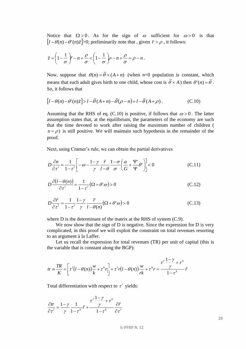
Next, using Cramer’s rule, we can obtain the partial derivatives
0''11
1
1
Gl
rnD
ll (C.11)
0'
1
1)(
ll
nlD (C.12)
0')(
1
1
1
nl
rrD
ll (C.13)
where D is the determinant of the matrix at the RHS of system (C.9).
We now show that the sign of D is negative. Since the expression for D is very
complicated, in this proof we will exploit the constraint on total revenues resorting
to an argument à la Laffer.
Let us recall the expression for total revenues (TR) per unit of capital (this is
the variable that is constant along the BGP):
rrrk
wnlrr
k
wnl
K
TRtr
k
kl
klkl
1
1
)()(
Total differentiation with respect to l yields:
lk
kl
kl
rr
tr
1
1
1
11
29
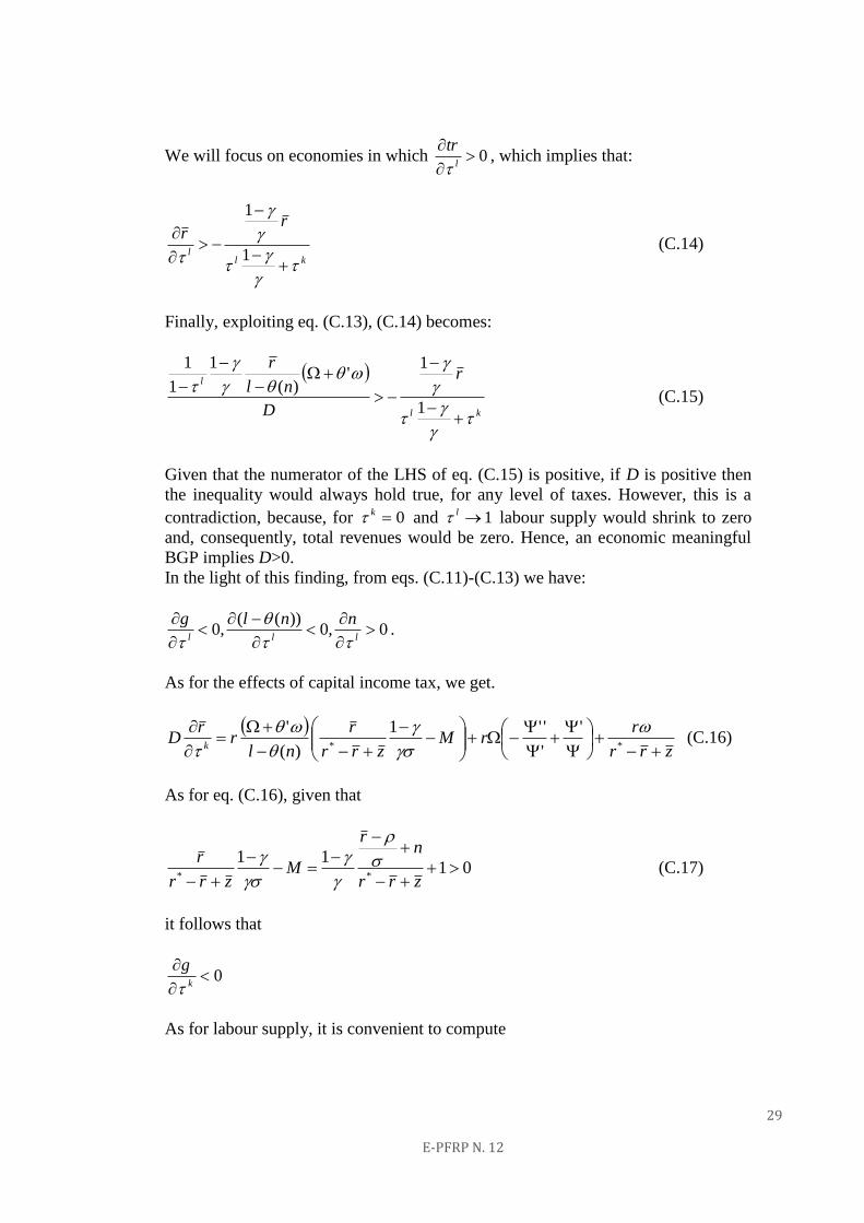
E-PFRP N. 12
We will focus on economies in which 0
l
tr
, which implies that:
kll
rr
1
1
(C.14)
Finally, exploiting eq. (C.13), (C.14) becomes:
kl
lr
D
nl
r
1
1'
)(
1
1
1
(C.15)
Given that the numerator of the LHS of eq. (C.15) is positive, if D is positive then
the inequality would always hold true, for any level of taxes. However, this is a
contradiction, because, for 0k and 1l labour supply would shrink to zero
and, consequently, total revenues would be zero. Hence, an economic meaningful
BGP implies D>0.
In the light of this finding, from eqs. (C.11)-(C.13) we have:
0,0))((
,0
lll
nnlg
.
As for the effects of capital income tax, we get.
zrr
rrM
zrr
r
nlr
rD
k
**
'
'
''1
)(
'
(C.16)
As for eq. (C.16), given that
0111
**
zrr
nr
Mzrr
r
(C.17)
it follows that
0
k
g
As for labour supply, it is convenient to compute
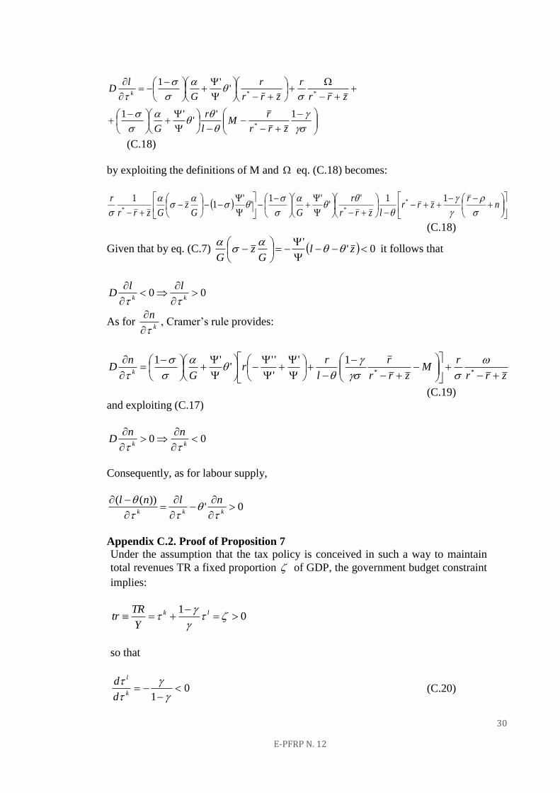
30
E-PFRP N. 12
1''
'1
''1
*
**
zrr
rM
l
r
G
zrr
r
zrr
r
G
lD
k
(C.18)
by exploiting the definitions of M and eq. (C.18) becomes:
n
rzrr
lzrr
r
GGz
Gzrr
r
11''
'1'
'1
1 *
**
(C.18)
Given that by eq. (C.7) 0''
zl
Gz
G
it follows that
00
kk
llD
As for k
n
, Cramer’s rule provides:
zrr
rM
zrr
r
l
rr
G
nD
k
**
1'
'
'''
'1
(C.19)
and exploiting (C.17)
00
kk
nnD
Consequently, as for labour supply,
0'))((
kkk
nlnl
Appendix C.2. Proof of Proposition 7
Under the assumption that the tax policy is conceived in such a way to maintain
total revenues TR a fixed proportion of GDP, the government budget constraint
implies:
01
lk
Y
TRtr
so that
01
k
l
d
d (C.20)
31
E-PFRP N. 12
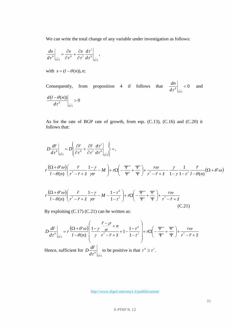
We can write the total change of any variable under investigation as follows:
)()( tr
k
l
lk
tr
k d
dxx
d
dx
,
with ;)),(( nnlx
Consequently, from proposition 4 if follows that 0)(
tr
kd
dn
and
0))((
)(
tr
kd
nld
As for the rate of BGP rate of growth, from eqs. (C.13), (C.16) and (C.20) it
follows that:
)()( tr
k
l
lk
tr
k d
drrD
d
rdD
,
'
)(1
1
1
'
'
''1
)(
'**
nl
r
zrr
rrM
zrr
r
nlr
l
zrr
rrM
zrr
r
nlr
l
k
**
'
'
''
1
11
)(
'
(C.21)
By exploiting (C.17) (C.21) can be written as:
zrr
rr
zrr
nr
nlr
d
rdD
l
k
tr
k
**
)(
'
'
''
1
11
1
)(
'
Hence, sufficient for )(tr
kd
rdD
to be positive is that lk .
http://www.digef.uniroma1.it/pubblicazioni