ISTANBUL TECHNICAL UNIVERSITY F GRADUATE SCHOOL OF SCIENCE

ENGINEERING AND TECHNOLOGY

GENERAL DERIVATION AND A DESIGN METHODOLOGYFOR INTERVAL TYPE-2 FUZZY LOGIC SYSTEMS

Ph.D. THESIS

Mortaza ALIASGHARY

Department of Control and Automation Engineering

Control and Automation Engineering Programme

Thesis Advisor: Prof. Dr. Ibrahim EKSIN

APRIL 2013

ISTANBUL TECHNICAL UNIVERSITY F GRADUATE SCHOOL OF SCIENCE

ENGINEERING AND TECHNOLOGY

GENERAL DERIVATION AND A DESIGN METHODOLOGYFOR INTERVAL TYPE-2 FUZZY LOGIC SYSTEMS

Ph.D. THESIS

Mortaza ALIASGHARY(504082108)

Department of Control and Automation Engineering

Control and Automation Engineering Programme

Thesis Advisor: Prof. Dr. Ibrahim EKSIN

APRIL 2013

ISTANBUL TEKNIK ÜNIVERSITESI F FEN BILIMLERI ENSTITÜSÜ

ARALIK DEGERLI TIP-2 BULANIK MANTIKSISTEMLER IÇIN GENEL ÇIKARIMLAR

VE BIR TASARIM YÖNTEMI

DOKTORA TEZI

Mortaza ALIASGHARY(504082108)

Kontrol ve Otomasyon Mühendisligi Anabilim Dalı

Kontrol ve Otomasyon Mühendisligi Programı

Tez Danısmanı: Prof. Dr. Ibrahim EKSIN

NISAN 2013

Mortaza ALIASGHARY, a Ph.D. student of ITU Graduate School of Science En-gineering and Technology , student ID 504082108 , successfully defended the thesisentitled “GENERAL DERIVATION AND A DESIGN METHODOLOGY FORINTERVAL TYPE-2 FUZZY LOGIC SYSTEMS ”, which he prepared after ful-filling the requirements specified in the associated legislations, before the jury whosesignatures are below.

Thesis Advisor : Prof. Dr. Ibrahim EKSIN ..............................Istanbul Technical University

Co-advisor : Prof. Dr. Müjde GÜZELKAYA ..............................Istanbul Technical University

Jury Members : Prof. Dr. Serhat SEKER ..............................Istanbul Technical University

Assistant Prof. Dr. Gülay Öke ..............................Istanbul Technical University

Assistant Prof. Dr. Taner ARSAN ..............................Kadir Has University

Assistant Prof. Dr. Osman Kaan EROL ..............................Istanbul Technical University

Assistant Prof. Dr. Ilker ÜSTOGLU ..............................Yildiz Technical University

Date of Submission : 15 FEBRUARY 2013Date of Defense : 02 APRIL 2013

v

vi

To the One who will give peace and justice to the world

vii

viii

FOREWORD

I would like to express my extreme gratitude and appreciation to my supervisors,Prof. Dr. Ibrahim Eksin and Prof. Dr. Müjde Güzelkaya, for their generous guidance,encouragement and support. Without their help, it would not be possible to finish mythesis quickly and successfully.

I would also like to thank the members of my thesis committee; Prof.Dr. SerhatSEKER, Assistant Prof. Dr. Taner ARSAN and Assistant Prof. Dr. Gülay ÖKE fortheir guidance and valuable advice.

I also wish to thank Dr. Tufan Kumbasar and Nasser Arghavani for their valuablefeedbacks and suggestions.

I would also like to thank my friends Ali Naderi and his wife Hajer, Hadi Gasemzadehand his wife Raziyeh who made me feel at home during my Ph.D. study. I never forgetgreat times which we spent together.

I should also thank all the members of Mechatronics Education and Research Centerespecially Prof. Dr. Ata Mugan and Prof. Dr. Metin Gökasan for their moral supportand helpful feedbacks.

Finally, there is no word to describe my sincere gratitude to my family. My great father,patient mother, lovely sisters and brothers-in-law have always been a great support andlove during my life.

APRIL 2013 Mortaza ALIASGHARY(Control Engineer, M.Sc.)

ix

x

RELATIONS IN INTERVAL TYPE-2 FUZZY LOGIC SYSTEMS......... 21

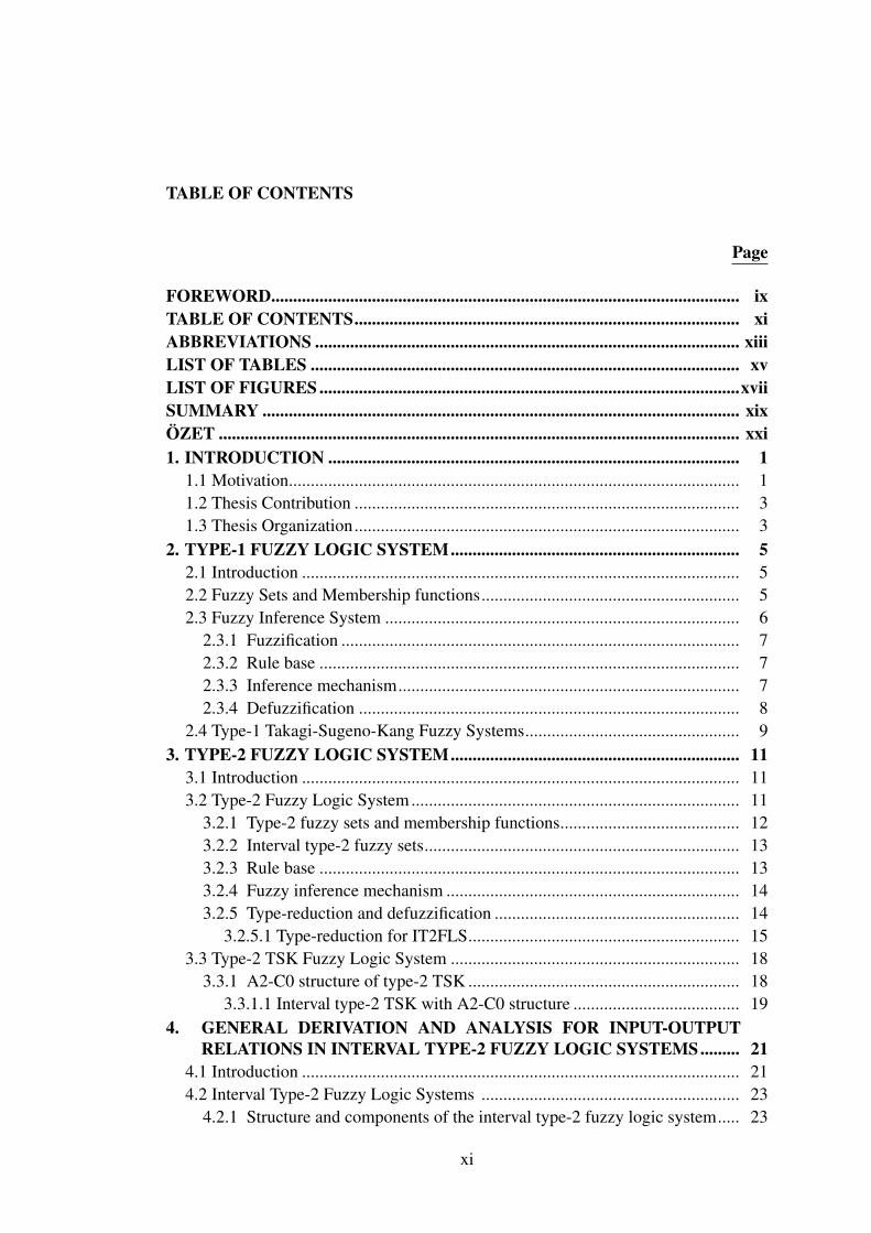
TABLE OF CONTENTS

Page

FOREWORD........................................................................................................... ixTABLE OF CONTENTS........................................................................................ xiABBREVIATIONS ................................................................................................. xiiiLIST OF TABLES .................................................................................................. xvLIST OF FIGURES ................................................................................................xviiSUMMARY ............................................................................................................. xixÖZET ....................................................................................................................... xxi1. INTRODUCTION .............................................................................................. 1

1.1 Motivation....................................................................................................... 11.2 Thesis Contribution ........................................................................................ 31.3 Thesis Organization........................................................................................ 3

2. TYPE-1 FUZZY LOGIC SYSTEM.................................................................. 52.1 Introduction .................................................................................................... 52.2 Fuzzy Sets and Membership functions........................................................... 52.3 Fuzzy Inference System ................................................................................. 6

2.3.1 Fuzzification ........................................................................................... 72.3.2 Rule base ................................................................................................ 72.3.3 Inference mechanism.............................................................................. 72.3.4 Defuzzification ....................................................................................... 8

2.4 Type-1 Takagi-Sugeno-Kang Fuzzy Systems................................................. 93. TYPE-2 FUZZY LOGIC SYSTEM.................................................................. 11

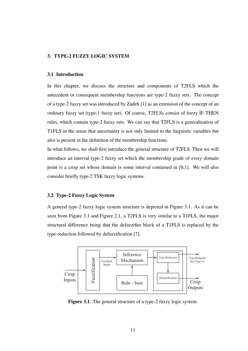
3.1 Introduction .................................................................................................... 113.2 Type-2 Fuzzy Logic System........................................................................... 11

3.2.1 Type-2 fuzzy sets and membership functions......................................... 123.2.2 Interval type-2 fuzzy sets........................................................................ 133.2.3 Rule base ................................................................................................ 133.2.4 Fuzzy inference mechanism ................................................................... 143.2.5 Type-reduction and defuzzification ........................................................ 14

3.2.5.1 Type-reduction for IT2FLS.............................................................. 153.3 Type-2 TSK Fuzzy Logic System .................................................................. 18

3.3.1 A2-C0 structure of type-2 TSK .............................................................. 183.3.1.1 Interval type-2 TSK with A2-C0 structure ...................................... 19

4. GENERAL DERIVATION AND ANALYSIS FOR INPUT-OUTPUT

4.1 Introduction .................................................................................................... 214.2 Interval Type-2 Fuzzy Logic Systems ........................................................... 23

4.2.1 Structure and components of the interval type-2 fuzzy logic system..... 23

xi

CURRICULUM VITAE......................................................................................... 89

METHOD ....................................................................................................... 71

TYPE-2 FUZZY PI/PD CONTROLLERS................................................... 41

4.2.2 The comparison of IT2FLS and T1FLS outputs ................................... 254.3 The Derivation of the Analytical Structure of IT2FLS .................................. 284.4 The Analytical Input-Output Relation of IT2FLS in Case of 3 × 3

Rule-Base ...................................................................................................... 314.5 Conclusion...................................................................................................... 39

5. A DESIGN METHODOLOGY AND ANALYSIS FOR INTERVAL

5.1 Introduction .................................................................................................... 415.2 The General Structure and the Components of the Proposed IT2-FLC ......... 445.3 The Methodology and Analytical Derivation for the Proposed IT2-FLC ...... 46

5.3.1 The analytical formulation for the output of IT2-FLC in case of 2×2rule base ................................................................................................. 50

5.3.2 The analytical formulation for the output of IT2-FLC in case of 2×3rule base ................................................................................................. 51

5.3.3 Illustrative example ................................................................................ 535.4 Simulation Studies.......................................................................................... 56

5.4.1 The performance comparison of the proposed IT2-FLC23 with thelinear controllers on benchmark processes ............................................ 57

5.4.2 Robustness of the proposed IT2-FLCs to process parameter variations 605.5 Experiment ..................................................................................................... 665.6 Conclusion...................................................................................................... 69

6. OPTIMIZATION OF IT2-FLCS WITH BIG BANG-BIG CRUNCH

6.1 Introduction .................................................................................................... 716.2 Ellipsoidal Type-2 Membership Function ...................................................... 736.3 Big Bang-Big Crunch Optimization Method ................................................. 746.4 Simulation Studies.......................................................................................... 756.5 Conclusion...................................................................................................... 80

7. CONCLUSIONS................................................................................................. 81REFERENCES........................................................................................................ 83

xii

ABBREVIATIONS

PID : Proportional-Integral-DerivativePI : Proportional-IntegralPD : Proportional-DerivativeFLS : Fuzzy Logic SystemFLC : Fuzzy Logic ControlFIS : Fuzzy Inference SystemT1FLS : Type-1 Fuzzy Logic SystemT1-FLC : Type-1 Fuzzy Logic ControllerMF : Membership FunctionTSK : Takagi-Sugeno-KangCOA : Center Of AreaMOM : Mean Of MaximumT2FLS : Type-2 Fuzzy Logic SystemT2FS : Type-2 Fuzzy SetUMF : Upper Membership FunctionLMF : Lower Membership FunctionFOU : Footprint Of UncertaintyIT2FS : Interval Type-2 Fuzzy SetIT2FLS : Interval Type-2 Fuzzy Logic SystemKM : Karnik-MendelIT2-FLC : Interval Type-2 Fuzzy Logic ControllerTR : Type-ReductionNT : Nie-TanFOPTD : First-Order Plus Time DelayITAE : Integral Time Absolute ErrorIAE : Integral Absolute ErrorBB-BC : Big Bang-Big CrunchBIBO : Bounded-Input/Bounded-OutputSNR : Signal to Noise Ratio

xiii

xiv

LIST OF TABLES

Page

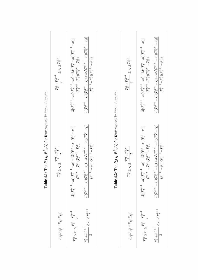
Table 4.1 : The P1(xi,Fjii ,∆) for four regions in input domain. ............................ 29

Table 4.2 : The P2(xi,Fjii ,∆) for four regions in input domain. ............................ 29

Table 4.3 : The Q(xi,Fjii ,∆) for four regions in input domain. ............................. 30

Table 4.4 : The 3×3 rule-base for IT2FLS. ......................................................... 32Table 4.5 : The input-output relation of IT2FLS in case of 3×3 rule base.......... 38Table 5.1 : IT2-FLC rule base for a system with given inputs. ............................. 47Table 5.2 : The expressions of G(xi,F

jii ,∆) for four regions in input domain. ..... 49

Table 5.3 : The expressions of U for four regions in input domain. ..................... 50Table 5.4 : The expressions of P(xi,F

jii ,K,∆) and Q(xi,F

jii ,∆) for eight

regions in the input domain................................................................. 52Table 5.5 : The values of the performance indices for the three cases.................. 60Table 5.6 : The performance values for the G5(s) with parameter variations....... 65Table 5.7 : Parameter of the ball and beam system. .............................................. 67Table 5.8 : Comparison of the performance of the two controllers....................... 68Table 6.1 : The values of the performance indices................................................ 76Table 6.2 : The values of the performance in the presence of noise. .................... 80

xv

xvi

61

LIST OF FIGURES

Page

Figure 2.1 : Some typical membership functions which are used in T1FLS. ....... 6Figure 2.2 : Basic structure of a type-1 fuzzy logic system. ................................. 7Figure 3.1 : The general structure of a type-2 fuzzy logic system........................ 11Figure 3.2 : The membership function of a general type-2 fuzzy set. .................. 12Figure 3.3 : The membership function of an interval type-2 fuzzy set. ................ 13Figure 4.1 : The diamond-shaped type-2 membership functions.......................... 24Figure 4.2 : IT2FLS output surface for 3×3 rule base......................................... 25Figure 4.3 : IT2FLS output surface for 5×5 rule base......................................... 25Figure 4.4 : The outputs difference of T1FLS and IT2FLS for 3×3 rule base.... 26Figure 4.5 : The outputs difference of T1FLS and IT2FLS for 5×5 rule base.... 26Figure 4.6 : The contour plot of the difference between outputs of T1FLS and

IT2FLS for 3×3 rule base.................................................................. 27Figure 4.7 : The contour plot of the difference between outputs of T1FLS and

IT2FLS for 5×5 rule base.................................................................. 27Figure 4.8 : The (a) antecedent membership functions (b) Singleton

consequents of IT2FLS. ...................................................................... 31Figure 5.1 : The structure of (a) the feedback control system (b) the IT2-FLC. .. 44Figure 5.2 : Illustration of the step responses the control signals for ∆ = 0.2. ..... 54Figure 5.3 : Illustration of the step responses the control signals for ∆ = 0.4. ..... 55Figure 5.4 : Illustration of the term γ(x1,x2,∆) for (a) ∆ = 0.2 (b) ∆ = 0.4...... 56Figure 5.5 : Illustration of α and β for different ∆ values. .................................. 56Figure 5.6 : Illustration of the system step responses. .......................................... 57Figure 5.7 : Illustration of the control signals. ...................................................... 58Figure 5.8 : Illustration of the system step responses. .......................................... 58Figure 5.9 : Illustration of the control signals. ...................................................... 59Figure 5.10:Figure 5.11:Figure 5.12: Illustration of the step responses for IT2-FLC22. ............................. 61Figure 5.13: Illustration of the step responses for IT2-FLC23. ............................. 61Figure 5.14: Illustration of the control signals for IT2-FLC22.............................. 62Figure 5.15: Illustration of the control signals for IT2-FLC23.............................. 62Figure 5.16: Illustration of the step responses on the plant by varying static

gain parameter to K = 1.5 for IT2-FLC22.......................................... 63Figure 5.17: Illustration of the step responses on the plant by varying static

gain parameter to K = 1.5 for IT2-FLC23.......................................... 63Figure 5.18: Illustration of the step responses on the plant by varying the

system time delay parameter to L = 4 for IT2-FLC22. ...................... 64

xvii

Illustration of the system step responses. .......................................... 59Illustration of the control signals. ......................................................

Figure 5.19: Illustration of the step responses on the plant by varying thesystem time delay parameter to L = 4 for IT2-FLC23. ...................... 64

Figure 5.20: Illustration of the ball and beam experimental system. ..................... 66Figure 5.21: Illustration of the cascade control system.......................................... 66Figure 5.22: Illustration of the ball position responses in case of simulation........ 67Figure 5.23: Illustration of the ball position responses in case of experiment....... 68Figure 5.24: The output results of T1-FLC and IT2-FLC for experimental test.... 69Figure 5.25: The motor input voltages of T1-FLC and IT2-FLC for

experimental test. ................................................................................ 69Figure 6.1 : The ellipsoidal type-2 membership functions. .................................. 73Figure 6.2 : Illustration of the step responses for optimal controllers. ................. 76Figure 6.3 : Illustration of the control signals for optimal controllers. ................. 76Figure 6.4 : Diamond-shaped membership functions after optimization using

BB-BC. ............................................................................................... 77Figure 6.5 : Ellipsoidal membership functions after optimization using BB-BC. 77Figure 6.6 : Illustration of the step responses in presence of noise (SNR=30

dB). ..................................................................................................... 78Figure 6.7 : Illustration of the control signals in presence of noise (SNR=30

dB). ..................................................................................................... 78Figure 6.8 : Illustration of the step responses in presence of noise (SNR=50

dB). ..................................................................................................... 79Figure 6.9 : Illustration of the control signals in presence of noise (SNR=50

dB). ..................................................................................................... 79

xviii

GENERAL DERIVATION AND A DESIGN METHODOLOGYFOR INTERVAL TYPE-2 FUZZY LOGIC SYSTEMS

SUMMARY

Fuzzy logic systems have been widely developed and utilized in many practicalapplications and engineering systems like signal processing, pattern recognition,system modeling and control system design. Since fuzzy logic systems are consideredas black-box systems, the main question about them is that why and how they work.Revealing the mathematical input-output relations of a fuzzy logic system clarifies theirunknown internal structure and gives ability to understand their behavior. Dependingon these mathematical expressions effective suggestions can be made on the designand parameter adjustment of fuzzy logic systems.

In this thesis, firstly, general analytical closed-form expressions are derived for theinput-output relation of an interval type-2 fuzzy logic system. In comparison withtype-1 fuzzy logic systems, there are few studies which analyze the mathematicalclosed-form structure of interval type-2 fuzzy logic systems in the literature. In thesestudies, the choice of classical type-2 membership functions and Zadeh AND operatorcause complexity in the mathematical expressions giving the relation between theinputs and the output of fuzzy logic system. Therefore, it becomes very difficult togeneralize these analyses to interval type-2 fuzzy logic system with more than twomembership functions for each input. In this thesis, it has been assumed that the relatedfuzzy system possesses diamond-shaped type-2 fuzzy sets for each input and singletonsfor output. Moreover, the product AND operator and the Nie-Tan inference engineis preferred. The simplicity in the derivation of the analytical structure of intervaltype-2 fuzzy logic system with product AND operator makes it possible to generalizethe derivation to inputs with n fuzzy sets. Since the Karnik-Mendel type-reductioncannot be formulated in closed-form, the Nie-Tan inference engine is used. Thediamond-shaped type-2 membership functions possessing “0” value at both ends ofthe support and “1” value at the modal point provide an easiness in the analyticalderivation of mathematical closed-form expressions. An important advantage of theproposed technique is that the analytical input-output relations are applicable for anynumber of input fuzzy sets. Analytical structure of special case of interval type-2 fuzzylogic system which uses three membership functions for each input is derived in detail.

The main difficulty in fuzzy logic controller design is to determine the parametersof the fuzzy logic controllers (e.g. membership functions, rules, scaling factors)for inputs and outputs of a fuzzy system. To ease the fuzzy logic controller designprocess, the researchers proposed a general methodology to systematically constructa type-1 fuzzy logic controller based on the existence of a linear controller. Thismethodology guarantees an identical performance for type-1 fuzzy logic controller asthe existing linear controller. Since the performance of controllers are identical, it hasbeen advised to use expert knowledge to improve the performance of fuzzy controllerby appropriately changing the rule base.

xix

In the thesis, secondly, a systematical methodology is introduced to constructthe rule base of an interval type-2 fuzzy logic controller based on an existinglinear proportional-integral or proportional-derivative controller. For this purposethe analytical closed-form expressions between input and output of an intervaltype-2 fuzzy logic controller which have been obtained in this thesis are used anddiamond-shaped type-2 fuzzy sets are utilized within the proposed controller. Whenthe footprint of uncertainties of the antecedent membership functions are taken to bezero, the interval type-2 fuzzy logic controller will be reduced to type-1 fuzzy logiccontroller; thus, an identical mapping will be accomplished between conventionallinear controller and the proposed controller. If footprint of uncertainty is not equalto zero, then an additional degree of freedom is acquired that provides an uncertaintycloud over the proposed controller. This provides the designer an additional toolto cope with the uncertainties and nonlinearities that may exist in the system tobe controlled. Another beneficial feature of this technique is the ease and rapidgeneration of the fuzzy rules of the interval type-2 fuzzy logic controller based on theexisting linear controller. Two special cases of the proposed controller with 2×2 and2× 3 rule bases are mathematically analyzed in detail to show the effect of variablegains that are introduced by proposed interval type-2 fuzzy logic controller. Thefootprint of uncertainty in type-2 membership function causes variable gains for theproposed controller. Simulations on various processes including those with time delay,integrating and non-minimum phase characteristics and a real time application on balland beam system demonstrate that the interval type-2 fuzzy logic controller is morerobust and capable to manage the uncertainties much better than conventional linearcontroller and type-1 fuzzy logic controllers.

Finally, an optimization method is used to train the free parameters of type-2membership function. The performance of an interval type-2 fuzzy logic controlleris highly dependent on the parameters of the type-2 membership function. Theseparameters are usually chosen due to theoretical and practical knowledge of an expertor simply by trial and error method. Various optimization methods are implemented toestimate the parameters of type-2 membership function. Because of high convergencespeed and the low computation time properties, Big Bang-Big Crunch optimizationmethod is used to train the parameters of the chosen type-2 membership functions.The performance of the optimal controller is also analyzed in presence of measurementnoise with different levels of signal to noise ratio. Results show that the optimalinterval type-2 fuzzy logic controller can reduce the noise effect in system performancemuch better than linear conventional and type-1 fuzzy logic controllers.

xx

ARALIK DEGERLI TIP-2 BULANIK MANTIKSISTEMLER IÇIN GENEL ÇIKARIMLAR

VE BIR TASARIM YÖNTEMI

ÖZET

Oransal-integral-türev (PID) ile kontrol, uyarlamalı kontrol, dayanıklı kontrol,dogrusal olmayan kontrol yöntemleri ve benzeri geleneksel yöntemler, pek çoksistemin kontrolüne basarıyla uygulanmalarına ragmen kontrol edilecek sisteminmatematiksel modeline gereksinim duyarlar. Ancak sistemin matematiksel modelihakkında bilgi olmaması, kısmen bilinmeyenlere sahip olması ya da yüksek derecededogrusal olamayan bir yapıya sahip olması durumunda bu geleneksel yöntemlerinbasarımı azalabilir ya da tasarımın karmasıklıgı artabilir. Bulanık mantık sistemleri,matematiksel modelleri dogrusal olmayan ya da kolay bir sekilde elde edilemeyensistemlerin kontrolü ve modellenmesi için son derece kullanıslıdır.

Bulanık mantık, isaret isleme, örüntü tanıma, sistem modelleme ve kontrol sistemtasarımı gibi pek çok alanda yaygın olarak kullanılmaktadır. Tip-1 bulanık sistemlerile gerçeklestirilen bulanık mantık kontrol çalısmaları literatürde önemli bir yer tutar.Tip-1 bulanık mantık sistemlerinin bir uzantısı olan ve ilk olarak Zadeh tarafındanönerilen Tip-2 bulanık mantık sistemleri de çesitli mühendislik problemlerineçözümüne basarıyla uygulanmaktadır.

Tip-2 bulanık mantık sistemleri, üyelik fonksiyonlarındaki belirsizlik alanınınsagladıgı ek bir serbestlik derecesi sayesinde, belirsizliklerin ifade edilmesinde tip-1bulanık mantık sistemlerinden daha iyi bir basarım saglarlar. Tip-2 bulanık mantıksistemlerinin ifade edilmesindeki karmasıklıgı azaltmak amacı ile “aralık degerli tip-2bulanık mantık sistemleri” önerilmistir. Bu tezde aralık degerli tip-2 bulanık mantıksistemleri üzerine çalısılmıstır.

Bulanık mantık sistemi bir kara kutu sistemi olarak kabul edildiginden, iliskinmatematiksel ifadelerin türetilmesi bu sistemlerin neden ve nasıl çalıstıklarınınanlasılabilmesi açısından önemlidir. Bir bulanık mantık sisteminin matematikselgiris-çıkıs iliskilerinin belirlenmesi ile bulanık mantık sistemlerinin iç yapısınınyorumlanması kolaylasır. Böylece, elde edilen matematiksel denklemler sayesinde,bulanık mantık sistemlerinin tasarımı ve parametrelerinin ayarlanması için çesitli etkinönerilerde bulunulabilir.

Bu tezde öncelikle, bir aralık degerli tip-2 bulanık mantık sisteminin matematikselgiris-çıkıs iliskisine ait kapalı yapıdaki analitik denklemler elde edilmistir. Literatürde,aralık degerli tip-2 bulanık mantık sistemlerinin giris-çıkıs iliskisini analiz edenyayın sayısı çok azdır. Bu çalısmalarda ise klasik tip-2 üyelik fonksiyonlarının ve“Zadeh VE” operatörünün kullanılmasından dolayı, giris-çıkıs iliskisinin matematikselifadesi oldukça karmasık hale gelmektedir. Bu nedenle, her bir giris için ikidenfazla üyelik fonksiyonuna sahip olan aralık degerli tip-2 bulanık mantık sistemininanalizinde zorluklarla karsılasılmaktadır. Bu tezde, aralık degerli tip-2 bulanık mantıksistemine ait her giris için baklava biçimli tip-2 üyelik fonksiyonları, çıkıs için

xxi

tekil üyelik fonksiyonları, “çarpımsal VE” operatörü ve “Nie-Tan karar vericisi”kullanılmaktadır. Sistemin giris-çıkıs iliskisini veren analitik ifadeleri elde etmek içinçarpımsal VE operatörünün kullanılması, Zadeh VE operatörünün kullanılmasındandaha kolaydır. Bu nedenle, elde edilecek denklemlerin n adet üyelik fonksiyonuiçin genellestirilmesi mümkün olmustur. Karnik-Mandel tip indirgemesi, kapalıbiçimde formüle edilemediginden Nie-Tan karar vericisi kullanılmıstır. Baklavabiçimli tip-2 üyelik fonksiyonu ise, köse noktalarında belirsizliginin daima sıfır olmasınedeniyle, matematiksel denklemlerin çıkarılmasında büyük kolaylık saglamıstır.Klasik yapıdaki tip-2 üyelik fonksiyonları sözü edilen özelligi saglamadıklarından, butür üyelik fonksiyonuna sahip bulanık sistemlere iliskin matematisel ifadeleri n adetüyelik fonksiyonu için genellestirmek çok daha zordur. Tezde ayrıca genel ifadelerdısında, farklı sayılarda üyelik fonksiyonu kullanan aralık degerli tip-2 bulanık mantıksistemlerine ait analitik iliskiler de detaylı bir sekilde elde edilmistir. Kapalı biçimdekianalitik ifadeler incelendiginde, aralık degerli tip-2 bulanık mantık sisteminin tip-1bulanık mantık sistemlerde görülmeyen bir giris-çıkıs yapısı oldugu görülmektedir.Elde edilen matematiksel iliskiler, aralık degerli tip-2 bulanık mantık sistemin içselyapısını anlamak ve degerlendirmek için fikir saglamaktadır.

Bulanık mantık kontrolör tasarımında en büyük zorluk kontrolör parametrelerinin(üyelik fonksiyonları, kurallar, ölçeklendirme katsayıları, vb.) belirlenmesidir. Bunukolaylastırmak için, literatürde tip-1 bulanık mantık kontrolör tasarımını sistematikbir sekle getirmek amacıyla dogrusal kontrolör tabanlı bir yöntem önerilmistir. Buyöntem, tasarımı yapılan tip-1 bulanık mantık kontrolör ile ele alınan dogrusalkontrolörün basarımlarının birebir aynı olmasını garanti eder. Daha sonra, tip-1bulanık mantık kontrolörün basarımı kural tabanı degistirilerek artırılabilir.

Tezde ikinci olarak, aralık degerli tip-2 bulanık mantık sistemin kural tabanınıolusturmak için oransal-integral veya oransal-türevsel kontrolör tabanlı sistematikbir yöntem gelistirilmistir. Bu yöntem, geleneksel yapıdaki dogrusal kontrolörleri(oransal-integral, oransal-türevsel vs.) dogrusal olmayan aralık degerli tip-2 bulanıkmantık kontrolörüne dönüstürmektedir. Yöntemin gelistirilmesinde aralık degerlitip-2 bulanık mantık sistemleri için tezde elde edilen giris-çıkıs iliskilerinin kapalıyapıdaki analitik ifadelerinden faydalanılmıstır. Elde edilen kontrolör, baklavabiçimli tip-2 üyelik fonksiyonlarına sahiptir. Eger baklava biçimli tip-2 üyelikfonksiyonunun belirsizlik alanı sıfır alınırsa, bu üyelik fonksiyonu, tip-1 üçgenüyelik fonksiyonu haline gelmektedir. Böylece önerilen kontrolör, gelenekselyapıdaki dogrusal kontrolörle aynı özellikleri tasıyan dogrusal tip-1 bulanık mantıkkontrolörüne dönüsmektedir. Eger bu belirsizlik alanı sıfırdan farklı olursa, dogrusaloransal-integral veya oransal-türevsel kontrolör, degisken kazançlı oransal-integralveya oransal-türevsel kontrolöre dönüsmüs olur. Bu sayede dogrusal kontrolörünvarlıgına dayalı olarak, dogrusal olmayan aralık degerli tip-2 bulanık mantıkkontrolörüne iliskin kural tabanını kolayca elde edilebilmektedir. Tip-2 yapınınbelirsizlik alanı ise tasarımcıya ek bir serbestlik derecesi sunmaktadır. Bu sayedetasarımcı, kontrolörün dogrusal olmayan yapısından ve tip-2 üyelik fonksiyonundakattıgı ekstra serbestlik derecesinden faydalanarak, basarımı daha da iyilestirebilir.Böylece, kontrol edilecek sistemlerin dogrusal olmayan davranısları ve sahipoldukları belirsizlikler karsısında tasarımcıya dayanıklı kontrolör tasarlamak içinimkân sunulmaktadır.

xxii

Önerilen yöntemin iki özel durumunu olusturan 2× 2 ve 2× 3’lük kural tablolarınaait matematiksel analizler, degisken kazançlı kontrolörün sisteme olan etkilerinigöstermek adına, detaylarıyla incelenmistir. Zaman gecikmesi, integral etkisi veminimum fazlı olmayan sistemler üzerindeki benzetimler ve top-çubuk sistemininüzerindeki gerçek zamanlı uygulama, önerilen aralık degerli tip-2 bulanık mantıkkontrolörünün daha dayanıklı ve sistemdeki belirsizlikler ile basa çıkmada gelenekseldogrusal kontrolör ve tip-1 bulanık mantık kontrolörlerinden daha yetenekli oldugunugöstermistir.

Tezde son olarak, tip-2 üyelik fonksiyonun parametrelerin egitilmesi gösterilmistir.Önerilen kontrolörün tip-2 üyelik fonksiyonlarının parametrelerinin degisimi sisteminbasarımını iyi veya kötü yönde etkileyebilir. Bu nedenle bu parametrelerin optimalsekilde seçilmesi gerekmektedir. Literatürde pek çok optimizasyon yöntemi mevcuttur.Ancak bu çalısmada, kolay kullanımı ve hızlı çalısması nedeniyle “Büyük Patlama –Büyük Çöküs” optimizasyon yöntemi kullanılmıstır. Bu kontrolörün gürültü azaltmaözelligini göstermek için, benzetim ortamında farklı düzeylerde isaret-gürültü oranınasahip ölçme gürültüsü uygulanmıstır. Sonuç olarak aralık degerli tip-2 bulanık mantıkkontrolörünün tip-1 bulanık mantık kontrolöre göre gürültü azaltma özelliginin dahaiyi oldugu gösterilmistir.

xxiii

xxiv

1. INTRODUCTION

1.1 Motivation

Conventional control methods like proportional-integral-derivative (PID), adaptive

control, robust control, nonlinear control methods and etc. have provided numerous

techniques for designing controllers for dynamic systems. These conventional methods

offer a variety of ways for engineer to design a controller based on mathematical

model of the system. Unfortunately, the performance of conventional approaches may

decrease or the complexity of the design increase if the model of the system is difficult

to obtain, highly nonlinear or partly unknown. Fuzzy logic systems (FLSs) are useful

for controlling or modeling of the systems whose mathematical models are nonlinear

or for which mathematical models are simply not available.

FLSs have been widely developed and utilized in many practical applications and

engineering systems like signal processing, pattern recognition, system modeling and

control system design. However, the most important applications and studies about

FLSs have been committed in the field of fuzzy logic control (FLC). The type-2 fuzzy

logic systems (T2FLSs) are the extension of the type-1 (ordinary) fuzzy logic systems

(T1FLSs) which were first introduced by Zadeh [1]. Experiments show that the T2FLS

may achieve better performance in comparison with T1FLS because of the additional

degree of freedom provided by the footprint of uncertainty (FOU) in their membership

functions [2–5]. In order to reduce the complexity in computation of T2FLSs, interval

type-2 fuzzy logic systems (IT2FLSs) were proposed in [6]. These fuzzy logic systems

have attracted much research interest in recent years due to their ability to cope with

uncertainty and robustness in comparison with ordinary T1FLSs [7,8]. Several control

and engineering applications such as liquid-level process control [9]; autonomous

mobile robots [10]; prediction of air pollutant [11]; pH control [12]; control and the

identification of a real-time servo system [13] and face recognition [14] illustrate the

advantages of interval type-2 fuzzy sets (IT2FS). Studies that have been reported in the

literature show that the interval type-2 fuzzy logic controllers (IT2-FLCs) are generally

1

more robust than type-1 fuzzy logic controllers (T1-FLCs) [8] [15]. In this thesis, the

research activities are focused on the IT2FLS and IT2-FLC.

Since FLS is considered as a black-box system, the main question that may strike the

mind here is that why and how a fuzzy logic system works. Revealing the mathematical

input-output relations of a FLS clarify the unknown internal structure of FLSs and give

ability to understand their behavior. The analytical structure and derivation between

the input and output of T1FLS have been studied in various papers in the literature

[16–20]. Another question is that how the mathematical input-output relations of

a FLS can be useful for better designing of these systems. This information can be

useful in reducing the trial-and-error effort in the design and tuning of the parameters

of FLSs. In [21], a design procedure for parameter tuning has been proposed based

on the explicit expressions obtained in [22]. Furthermore, mathematical input-output

relations enable one to analyze the stability of FLSs. In [23], authors analyzed the

bounded-input/bounded-output (BIBO) stability of the nonlinear control systems using

the input-output mathematical relations derived in [16]. Also these expressions give

a chance to compare T2FLSs with T1FLSs. In comparison with T1FLS, there are

few studies which analyze the mathematical closed-form structure of IT2FLS in the

literature.

In this thesis, the analytical closed-form expressions for the input-output relation

related to an interval type-2 fuzzy logic system are studied. An important advantage of

the proposed technique in comparison with previous works [24,25] is that the analytical

input-output relations are applicable for any number of input fuzzy sets. Also a

systematical methodology to construct an interval type-2 fuzzy logic controller based

on conventional proportional-integral (PI) or proportional-derivative (PD) controller

is studied. The footprint of uncertainty in IT2-FLC changes the PI/PD controller

to nonlinear PI/PD controller with variable gains. It is obvious that, by tuning

or optimizing the parameters of IT2FLS or IT2-FLC, the designer will be able to

improve the performance of the fuzzy system or controller. In this thesis, we will use

Big Bang-Big Crunch (BB-BC) optimization method to optimize the FOU of type-2

membership functions in IT2-FLC. Also the performance of the optimal controller in

presence of measurement noise with different levels of signal to noise ratio is analyzed.

2

1.2 Thesis Contribution

In this thesis we will develop an analytical closed-form expressions for input-output

relation related to an interval type-2 fuzzy logic system. Knowing these mathematical

relations will enable designer to insightfully understand how and why interval type-2

fuzzy logic system works and also give ability to understand their behavior. The

following list describes the major and the minor contributions of this thesis in more

detail.

• Proposing a general derivation for input-output relations in IT2FLS. These relations

clarify the unknown internal structure of IT2FLS and give ability to understand its

behavior in comparison with its T1 counterpart.

• Developing a design methodology for interval type-2 fuzzy PI/PD controllers based

on an existing linear PI/PD controllers.

• Analyzing the IT2FLSs or IT2-FLCs based on derived analytical input-output

closed-form expressions.

• Using the BB-BC optimization technique to optimize the interval type-2 fuzzy logic

controllers.

1.3 Thesis Organization

In Chapter 2, the background of T1FLSs with fuzzy If-Then rules and type-1

membership functions, are presented. Also we will introduce the typical structure

of a fuzzy inference system (FIS) with its four components. Finally, type-1

Takagi-Sugeno-Kang (TSK) fuzzy model is studied in chapter 2.

In Chapter 3, the basic concepts, notation, and theory of T2FLSs which are required

in the following chapters, are presented. We will introduce an interval type-2 fuzzy

set which is the special case of type-2 fuzzy sets. We will also consider briefly type-2

TSK fuzzy logic systems in this chapter.

In Chapter 4, analytical closed-form expressions are derived for the input-output

relation related to an interval type-2 fuzzy logic system. The derived mathematical

3

relationships provide a chance to examine the internal structure of IT2FLS. Analytical

structure of a special case of IT2FLS which uses three membership functions for each

input and three singletons for output are derived in detail.

In Chapter 5, a systematical methodology is introduced to construct the rule base of

an interval type-2 fuzzy logic controller based on an existing linear PI/PD controller.

The methodology depends on a nonlinear mapping from an existing PI/PD control

law. The closed-form relation between input and output of an IT2-FLC provides a way

of understanding why IT2-FLC is more robust and how it copes with uncertainties.

Two special cases of the proposed controller with 2× 2 and 2× 3 rule base are

mathematically analyzed in detail. Finally, simulation studies and a real time

application on ball and beam system are given to demonstrate the beneficial sides of

IT2-FLCs.

In Chapter 6, we will provide a brief information about the BB-BC optimization

technique. Also we will use this optimization method to optimize the FOU parameters

of type-2 membership functions in IT2-FLC.

Finally, in Chapter 7 we present the conclusions of this thesis.

4

2. TYPE-1 FUZZY LOGIC SYSTEM

2.1 Introduction

The fuzzy logic theory was introduced in 1965 by L. A. Zadeh [26] and it

is a mathematical tool for dealing with uncertainty. In the last 40 years,

fuzzy sets and fuzzy logic theory have found a great variety of applications in

control engineering, power systems, telecommunication, pattern recognition, machine

intelligence, qualitative modeling, motor industry, robotics, and so on. This chapter

introduces the basic concepts and components of the T1FLS that will be needed in the

following chapters. In what follows, we shall first introduce the basic concepts of fuzzy

sets, and membership functions (MFs). Then we will introduce the typical structure of

a fuzzy inference system with its four components. Finally, type-1 TSK fuzzy model

will be overviewed.

2.2 Fuzzy Sets and Membership functions

Fuzzy logic starts with the concept of a fuzzy set. A fuzzy set is a set that does not have

a crisp boundary. It can contain elements with only a partial degree of membership.

Consider a universe of discourse X , whose elements are denoted as x. A fuzzy set A in

X may be defined as follows:

A = {(x,µA(x)) | x ∈ X} (2.1)

where µA(x) is the MF of x in A, which represents the degree of the x belongs to A. The

MF (µA(x)) maps each element in X to a continuous unit interval [0,1]. If µA(x) = 0,

it means that x is definitely not an element of fuzzy set A and if 0 < µA(x) < 1, it

indicates that x falls in the fuzzy boundary of fuzzy set A. It is obvious that a fuzzy set

is an extension of a classical crisp set by generalizing the range of the characteristic

function from the crisp numbers 0, 1 to the unit interval [0, 1].

A MF is a curve that defines how each point in the input space is mapped to a

membership value (or degree of membership) between 0 and 1. The input space is

sometimes referred to as the universe of discourse. The only condition a MF must

5

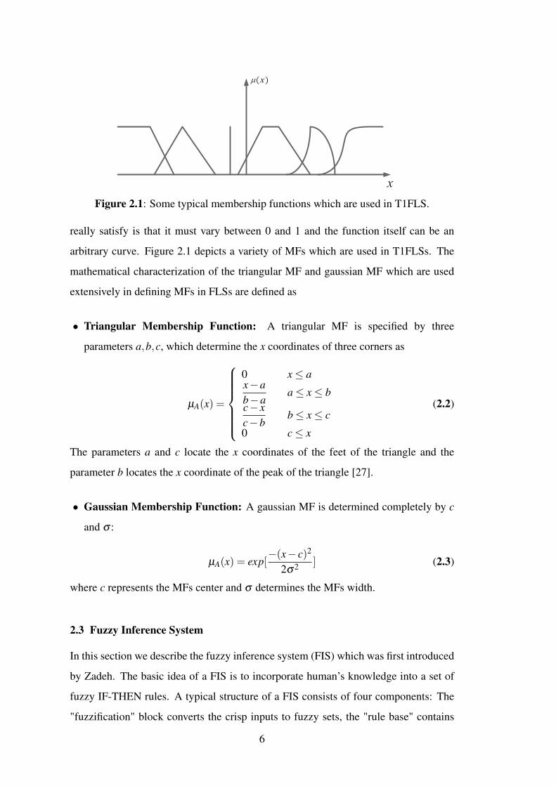
x

m

Figure 2.1: Some typical membership functions which are used in T1FLS.

really satisfy is that it must vary between 0 and 1 and the function itself can be an

arbitrary curve. Figure 2.1 depicts a variety of MFs which are used in T1FLSs. The

mathematical characterization of the triangular MF and gaussian MF which are used

extensively in defining MFs in FLSs are defined as

• Triangular Membership Function: A triangular MF is specified by three

parameters a,b,c, which determine the x coordinates of three corners as

µA(x) =

0 x≤ ax−ab−a

a≤ x≤ bc− xc−b

b≤ x≤ c

0 c≤ x

(2.2)

The parameters a and c locate the x coordinates of the feet of the triangle and the

parameter b locates the x coordinate of the peak of the triangle [27].

• Gaussian Membership Function: A gaussian MF is determined completely by c

and σ :

µA(x) = exp[−(x− c)2

2σ2 ] (2.3)

where c represents the MFs center and σ determines the MFs width.

2.3 Fuzzy Inference System

In this section we describe the fuzzy inference system (FIS) which was first introduced

by Zadeh. The basic idea of a FIS is to incorporate human’s knowledge into a set of

fuzzy IF-THEN rules. A typical structure of a FIS consists of four components: The

"fuzzification" block converts the crisp inputs to fuzzy sets, the "rule base" contains

6

a selection of fuzzy rules, the "inference mechanism" uses the fuzzy rules in the rule

base to produce fuzzy conclusions and the "defuzzification" block converts the fuzzy

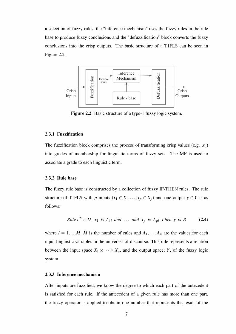
conclusions into the crisp outputs. The basic structure of a T1FLS can be seen in

Figure 2.2.

DefuzzificationInference

Mechanism

Rule - baseFuzzification

Fuzzified

inputs

Crisp

Inputs

Crisp

Outputs

Figure 2.2: Basic structure of a type-1 fuzzy logic system.

2.3.1 Fuzzification

The fuzzification block comprises the process of transforming crisp values (e.g. x0)

into grades of membership for linguistic terms of fuzzy sets. The MF is used to

associate a grade to each linguistic term.

2.3.2 Rule base

The fuzzy rule base is constructed by a collection of fuzzy IF-THEN rules. The rule

structure of T1FLS with p inputs (x1 ∈ X1, . . . ,xp ∈ Xp) and one output y ∈ Y is as

follows:

Rule lth : IF x1 is A1l and . . . and xp is Apl T hen y is B (2.4)

where l = 1, ...,M, M is the number of rules and A1, . . . ,Ap are the values for each

input linguistic variables in the universes of discourse. This rule represents a relation

between the input space X1× ·· · × Xp, and the output space, Y , of the fuzzy logic

system.

2.3.3 Inference mechanism

After inputs are fuzzified, we know the degree to which each part of the antecedent

is satisfied for each rule. If the antecedent of a given rule has more than one part,

the fuzzy operator is applied to obtain one number that represents the result of the

7

antecedent for that rule. The input for the implication process is a single number given

by the antecedent, and the output is a fuzzy set. Implication is implemented for each

rule. Since decisions are based on the testing of all of the rules in a FIS, the rules must

be combined in some manner in order to make a decision. Aggregation is the process

by which the fuzzy sets that represent the outputs of each rule are combined into a

single fuzzy set. Aggregation only occurs once for each output variable, just prior to

the final step, defuzzification.

2.3.4 Defuzzification

Defuzzifier refers to the way a crisp value is extracted from a fuzzy set as a

representative value, which is a necessary step as in often case a crisp number is

required for real application. In general, there are five methods for defuzzifying a fuzzy

set but the center of area (COA) and the mean of maximum (MOM) are the two most

commonly used methods in generating the crisp system output. A brief explanation of

these defuzzification methods are as following:

• Center of area:

This method produces the center of the fuzzy output area. The crisp system output for

discrete universe of discourse will be calculated as

y =∑

ni=1 xiµA(xi)

∑ni=1 µA(xi)

(2.5)

where n is the number of the discrete elements in the universe of discourse, xi is the

value of the discrete element and µA(xi) represents the corresponding MF value at the

xi [27]. For continuous universe of discourse, the crisp output can be calculated as

following:

y =∫

x∈X x.µA(x)dx∫x∈X µA(x)dx

(2.6)

• Mean of maximum:

Consider m as the number of the output points, whose MF values reach the maximum

value within the universe of discourse. The MOM dufuzzification calculates the mean

value of all the m output points. In the case of a discrete universe, the crisp output is

8

expressed as

y =∑

mi=1 xi

m(2.7)

where xi is the support value at these points, whose MF reaches the maximum value

µA(xi). The MOM method does not consider the shape of the fuzzy output, however

the defuzzification calculation is simplified [27].

2.4 Type-1 Takagi-Sugeno-Kang Fuzzy Systems

The fuzzy inference process discussed so far is Mamdani’s fuzzy inference method, the

most common methodology. This section discusses the so-called Takagi-Sugeno-Kang

(TSK), method of fuzzy inference. The TSK was proposed by Takagi, Sugeno and

Kang in an effort to develop a systematic approach to generating fuzzy rules from

a given input-output data set. The first two parts of the fuzzy inference process,

fuzzifying the inputs and applying the fuzzy operator, are exactly the same as Mamdani

method. The main difference that the TSK output membership functions are either

linear or constant. A typical rule in a TSK fuzzy model has the form as

Rule lth : IF x1 is A1l and . . . and xp is Apl T hen y = fl(x1, . . . ,xp) (2.8)

where l = 1, ...,M, M is the number of rules, A1, . . . ,Ap are the values for each input

linguistic variables in the universes of discourse and y = f (x1, . . . ,xp) is a predefined

function of the input variables for output. A simple expression is the linear and affine

functions as

Rule lth : IF x1 is A1l and . . . and xp is Apl T hen y= a1lx1+ · · ·+aplxp+a0l (2.9)

If a0l = 0, then the fl mapping is a linear mapping and if a0l 6= 0, then the mapping is

called affine. When fl is constant, then the mapping is called "zero-order TSK", which

can be viewed as a special case of the Mamdani inference system, in which each rule’s

consequent is specified by a fuzzy singleton.

9

10

3. TYPE-2 FUZZY LOGIC SYSTEM

3.1 Introduction

In this chapter, we discuss the structure and components of T2FLS which the

antecedent or consequent membership functions are type-2 fuzzy sets. The concept

of a type-2 fuzzy set was introduced by Zadeh [1] as an extension of the concept of an

ordinary fuzzy set (type-1 fuzzy set). Of course, T2FLSs consist of fuzzy IF-THEN

rules, which contain type-2 fuzzy sets. We can say that T2FLS is a generalization of

T1FLS in the sense that uncertainty is not only limited to the linguistic variables but

also is present in the definition of the membership functions.

In what follows, we shall first introduce the general structure of T2FLS. Then we will

introduce an interval type-2 fuzzy set which the membership grade of every domain

point is a crisp set whose domain is some interval contained in [0,1]. We will also

consider briefly type-2 TSK fuzzy logic systems.

3.2 Type-2 Fuzzy Logic System

A general type-2 fuzzy logic system structure is depicted in Figure 3.1. As it can be

seen from Figure 3.1 and Figure 2.1, a T2FLS is very similar to a T1FLS, the major

structural difference being that the defuzzifier block of a T1FLS is replaced by the

type-reduction followed by defuzzification [7].

Defuzzification

Inference

Mechanism

Rule - baseFuzzification

Fuzzified

inputs

Crisp

Inputs Crisp

Outputs

Type-Reduction Type-Reduced

Set (Type-1)

Figure 3.1: The general structure of a type-2 fuzzy logic system.

11

3.2.1 Type-2 fuzzy sets and membership functions

A type-2 fuzzy set (T2FS), denoted as A, is characterized by a type-2 MF µA(x,u),

where x ∈ X and u ∈ Jx ⊆ [0,1], i.e.

A = {(x,u),µA(x,u) | ∀x ∈ X ,∀u ∈ Jx ⊆ [0,1]} (3.1)

in which 0≤ µA(x,u)≤ 1. A can also be defined as

A =∫

x∈X

∫u∈Jx

µA(x,u)/(x,u) Jx ⊆ [0,1] (3.2)

where∫∫

denotes union over all admissible x and u.

Jx is the primary membership of x, where Jx ⊆ [0,1] for ∀x ∈ X . Additionally, there is

a secondary membership value corresponding to each primary membership value that

defines the possibility for fair uses.

Uncertainty in the primary memberships of a type-2 fuzzy set, A, consists of a bounded

region that we call the “footprint of uncertainty” (FOU). Mathematically, it is the union

of all primary MFs [7].

The MF of a general type-2 fuzzy set is three-dimensional which a cross-section of one

slice of the third dimension is shown in Figure 3.2. This cross-section, as well as all

others, sits in the FOU. Only the boundary of the cross-section is used to describe the

MF of a general type-2 fuzzy set.

primary variable

primary membership

FOU

m

Figure 3.2: The membership function of a general type-2 fuzzy set.

In the following subsection we will study a special case of type-2 fuzzy set which

called interval type-2 fuzzy set.

12

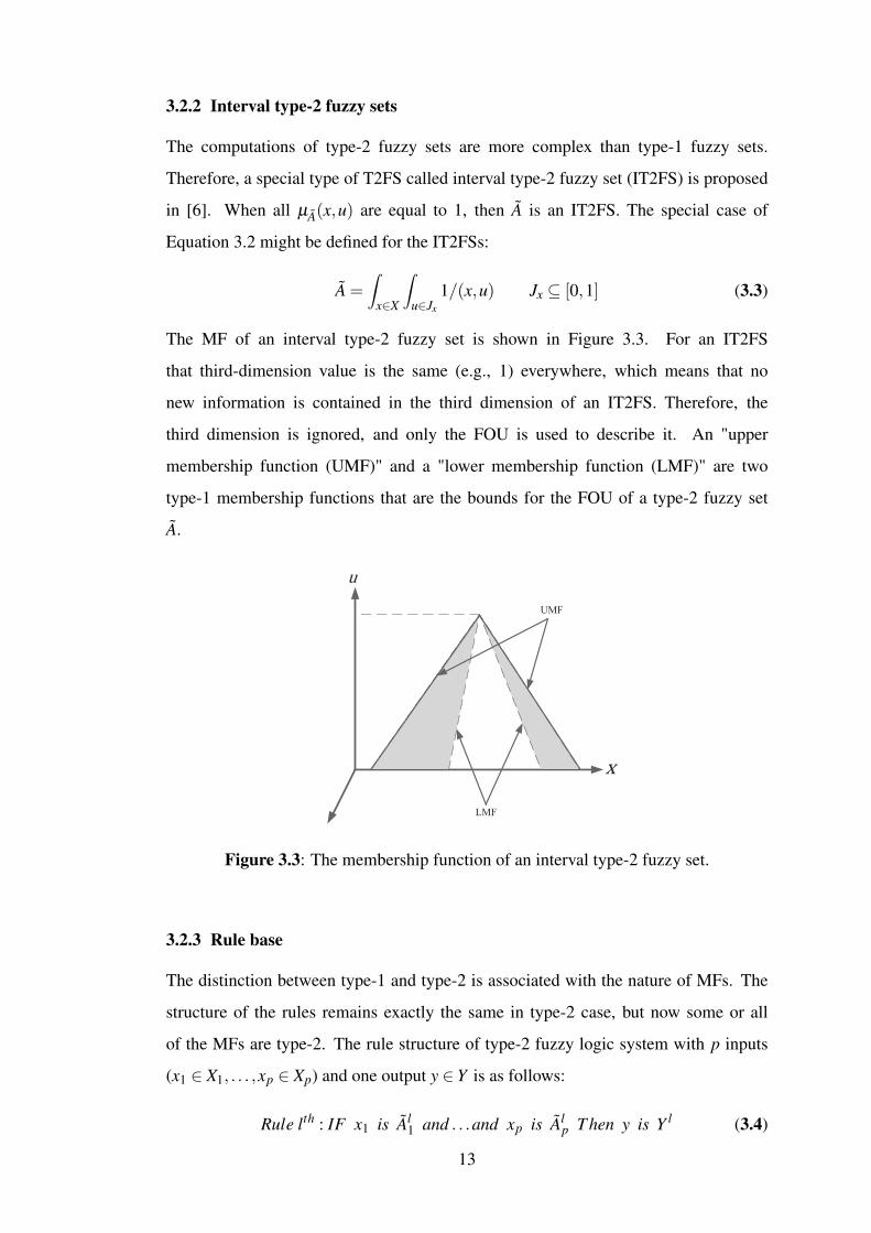
3.2.2 Interval type-2 fuzzy sets

The computations of type-2 fuzzy sets are more complex than type-1 fuzzy sets.

Therefore, a special type of T2FS called interval type-2 fuzzy set (IT2FS) is proposed

in [6]. When all µA(x,u) are equal to 1, then A is an IT2FS. The special case of

Equation 3.2 might be defined for the IT2FSs:

A =∫

x∈X

∫u∈Jx

1/(x,u) Jx ⊆ [0,1] (3.3)

The MF of an interval type-2 fuzzy set is shown in Figure 3.3. For an IT2FS

that third-dimension value is the same (e.g., 1) everywhere, which means that no

new information is contained in the third dimension of an IT2FS. Therefore, the

third dimension is ignored, and only the FOU is used to describe it. An "upper

membership function (UMF)" and a "lower membership function (LMF)" are two

type-1 membership functions that are the bounds for the FOU of a type-2 fuzzy set

A.

UMF

LMF

Figure 3.3: The membership function of an interval type-2 fuzzy set.

3.2.3 Rule base

The distinction between type-1 and type-2 is associated with the nature of MFs. The

structure of the rules remains exactly the same in type-2 case, but now some or all

of the MFs are type-2. The rule structure of type-2 fuzzy logic system with p inputs

(x1 ∈ X1, . . . ,xp ∈ Xp) and one output y ∈ Y is as follows:

Rule lth : IF x1 is Al1 and . . .and xp is Al

p T hen y is Y l (3.4)

13

where l = 1, ...,M and M is the number of rules . This rule represents a type-2 relation

between the input space X1× ·· · ×Xp, and the output space, Y , of the type-2 fuzzy

logic system. The Y l = [yl,yl] is an interval and in many applications we use yl = yl ,

i.e., each rule consequent is a crisp number [7].

3.2.4 Fuzzy inference mechanism

In the type-2 fuzzy logic system the inference process is very similar to type-1. The

inference engine combines rules and gives a mapping from input T2FSs to output

T2FSs. To do this one needs to compute unions and intersections of type-2 sets, as well

as compositions of type-2 relations. In type-2 fuzzy sets, join (t) and meet operators

(u) are used instead of union and intersection operators. These two new operators are

used in secondary membership functions, and they are defined and explained in detail

in [28].

3.2.5 Type-reduction and defuzzification

The type-2 output of the inference mechanism shown in Figure 3.1 must be

processed next by the output processor, the first operation of which is type-reduction.

Type-reduction (TR) methods include: centroid, center-of-sums, height, modified

height, and center-of-sets. Let’s assume that we perform centroid type-reduction. Then

each element of the type-reduced set is the centroid of some embedded type-1 set for

the output type-2 set of the fuzzy logic system. Each of these embedded sets can be

thought as an output set of an associated T1FLS, and, correspondingly, the T2FLS can

be viewed of as a collection of many different T1FLSs. Each T1FLS is embedded

in the T2FLS; hence, the type-reduced set is a collection of the outputs of all of the

embedded T1FLSs. The type-reduced set lets us represent the output of the T2FLS as

a fuzzy set rather than as a crisp number, which is something that cannot be done with

a T1FLS [29].

We defuzzify the type-reduced set to get a crisp output from the T2FLS. The most

natural way to do this seems to be finding the centroid of the type-reduced set.

Finding the centroid is equivalent to finding the weighted average of the outputs of

all the T1FLSs that are embedded in the T2FLS, where the weights correspond to the

memberships in the type-reduced set [7].

14

3.2.5.1 Type-reduction for IT2FLS

There have been many different approaches for for the TR of IT2FLSs. They can be

grouped into two categories [30]:

I. Enhancements to the Karnik-Mendel (KM) type-reduction algorithms, which

improve directly over the original KM type-reduction algorithms to speed them

up.

II. Alternative TR algorithms: Unlike the iterative KM algorithms, these alternative

TR algorithms have closed-form representations. They are usually fast

approximations of the KM algorithms.

For IT2FLS, there are two common methods for the TR: One is the KM iteration

algorithm [31] and the other is Wu-Mendel uncertainty bounds method [32] which are

based on the calculation of the centroid.

Assume that for the input vector (x), the firing interval of the lth rule in (3.4) is F l(x) =

[ f l, f l] and l = 1, ...,M. Regardless of which TR method we choose, the TR set is also

interval set, and has the following structure:

YT R = [yle f t ,yright ] (3.5)

Because YT R is an interval set, we defuzzify it using the average of yle f t and yright ;

hence, the defuzzified output of an IT2FLS is

y(x) =yle f t + yright

2(3.6)

yle f t and yright can be computed efficiently using the KM algorithms or Wu-Mendel

uncertainty bounds method as follows:

• Karnik-Mendel algorithm for TR:

KM Algorithm for Computing yle f t:

1. Sort yl , l = 1, ...,M in increasing order and call the sorted yl by the same name,

but now y1 ≤ y2 ≤ ·· · ≤ yl . Match the weights F l(x) with their respective yl and

renumber them so that their index corresponds to the renumbered yl .

15

2. Initialize f l by setting

f l =f l + f l

2(3.7)

and then compute

y =∑

Ml=1 yl f l

∑Ml=1 f l

(3.8)

3. Find switch point k (1≤ k ≤ l−1) such that

yk ≤ y≤ yk+1 (3.9)

4. Set

f l =

{f l n≤ kf l n > k

(3.10)

and compute

y′ =∑

Ml=1 yl f l

∑Ml=1 f l

(3.11)

5. Check if y′ = y. If yes, stop and set yle f t = y and L = k. If no, go to Step 6.

6. Set y = y′ and go to Step 3.

KM Algorithm for Computing yright:

1. Sort yl , l = 1, ...,M in increasing order and call the sorted yl by the same name,

but now y1 ≤ y2 ≤ ·· · ≤ yl . Match the weights F l(x) with their respective yl and

renumber them so that their index corresponds to the renumbered yl .

2. Initialize f l by setting

f l =f l + f l

2(3.12)

and then compute

y =∑

Ml=1 yl f l

∑Ml=1 f l

(3.13)

3. Find switch point k (1≤ k ≤ l−1) such that

yk ≤ y≤ yk+1 (3.14)

4. Set

f l =

{f l n≤ k

f l n > k(3.15)

and compute

y′ =∑

Ml=1 yl f l

∑Ml=1 f l

(3.16)

16

5. Check if y′ = y. If yes, stop and set yright = y and R = k. If no, go to Step 6.

6. Set y = y′ and go to Step 3.

The main idea of the KM algorithm is to find the switch points for yle f t and yright [33].

• Wu-Mendel uncertainty bounds method:

The uncertainty bound method, proposed by Wu and Mendel [32], computes the output

of the IT2FLS by (3.6), but

yle f t =yle f t + yle f t

2(3.17)

yright =yright + yright

2(3.18)

where

yle f t = min{y(0),y(l)}, yright = max{y(0),y(l)} (3.19)

yright = yright−∑

Ml=1( f l− f l)

∑Ml=1 f l

∑Ml=1 f l

×∑

Ml=1 f l(yl− y1)∑

Ml=1 f l

(yM− yl)

∑Ml=1 f l(yl− y1)+∑

Ml=1 f l

(yM− yl)(3.20)

yright = yright +∑

Ml=1( f l− f l)

∑Ml=1 f l

∑Ml=1 f l

×∑

Ml=1 f l

(yl− y1)∑Ml=1 f l(yM− yl)

∑Ml=1 f l

(yl− y1)+∑Ml=1 f l(yM− yl)

(3.21)

in which

y(0) =∑

Ml=1 yl f l

∑Ml=1 f l (3.22)

y(M) =∑

Ml=1 yl f l

∑Ml=1 f l (3.23)

y(M) =∑

Ml=1 yl f l

∑Ml=1 f l (3.24)

y(0) =∑

Ml=1 yl f l

∑Ml=1 f l (3.25)

Unlike the KM algorithms, the uncertainty bound method does not require yl and yl to

be sorted, though it still needs to identify the minimum and maximum of yl and yl [30].

17

3.3 Type-2 TSK Fuzzy Logic System

In this section, we will need to distinguish between the two kinds of T2FLS which

are Mamdani and TSK. Both are characterized by IF-THEN rules and have the

same antecedent structures. They differ in the structures of their consequents. The

consequent of a Mamdani rule is a fuzzy set, while the consequent of a TSK rule is a

function.

For type-2 TSK models, there are three possible structures [34]:

I. Antecedents are type-2 fuzzy sets, and consequents are type-1 fuzzy sets. This is

the most general case, and we call it A2-C1.

II. Antecedents are type-2 fuzzy sets, and consequents are crisp numbers. This is a

special case of A2-C1, and we call it A2-C0.

III. Antecedents are type-1 fuzzy sets, and consequents are type-1 fuzzy sets. This is

another special case of A2-C1, and we call it A1-C1. Some may argue that this

structure is a Mamdani T1FLS, but in a Mamdani T1FLS, the output is a crisp

number. In A1-C1, we take the weighted average of the inference output of each

rule as the output of the FLS, and this is a type-1 set, and not a crisp number.

Note that A and C represent the antecedent and the consequent of fuzzy rules, 0, 1 and

2 represent the crisp number, type-1 and type-2 fuzzy sets, respectively.

In this Ph.D. dissertation, A2-C0 TSK structure is used, therefore only A2-C0 TSK

structure will be explain in detail.

3.3.1 A2-C0 structure of type-2 TSK

In a type-2 TSK A2-C0 structure with a rule base of M rules, with each rule having p

antecedents, the lth rule is denoted as

Rule lth : IF x1 is Al1 and . . .and xp is Al

p T hen yl = a1lx1 + · · ·+aplxp +a0l (3.26)

where l = 1, ...,M, ail (i = 0,1, . . . , p) are the consequent parameters that are crisp

numbers; yl is an output and Ali are type-2 fuzzy sets. The final output of the model is

as follows [34]:

Y (F1, . . . ,FM) =∫

f1. . .∫

fMτ

Ml=1µFl

( fl)/∑

Ml=1 flyl

∑Ml=1 fl

(3.27)

18

where M is the number of rules fired, fl ∈ Fl , and τ indicates the t-norm.

3.3.1.1 Interval type-2 TSK with A2-C0 structure

In the interval type-2 TSK, the output of the A2-C0 structure in Equation 3.6 changes

as follows:

YA2−C0 =∫

f1∈[ f 1, f 1]. . .∫

fM∈[ f M , f M]1/

∑Ml=1 flyl

∑Ml=1 fl

(3.28)

where f l and f l are given by:

f l = µAl

1(x1)∗ · · · ∗µ

Alp(xp) (3.29)

f l= µ Al

1(x1)∗ · · · ∗µ Al

p(xp) (3.30)

in which ∗ represents the t-norm which is the product operator in this study.

19

20

4. GENERAL DERIVATION AND ANALYSIS FOR INPUT-OUTPUTRELATIONS IN INTERVAL TYPE-2 FUZZY LOGIC SYSTEMS

In this chapter, analytical closed-form expressions are derived for the input-output

relation related to an interval type-2 fuzzy logic system. It has been assumed that

the related fuzzy system possesses diamond-shaped type-2 fuzzy sets for each input

and singletons for output. Moreover, the Nie-Tan inference engine that provides

a closed-form is preferred. The footprint of uncertainty in diamond-shaped type-2

membership functions generates four times as many regions in analytical closed-form

expression as generated by standard triangular type-1 membership functions. The

derived mathematical relationships provide a chance to examine the internal structure

of an interval type-2 fuzzy logic system. These extra regions may enhance the

performance of an interval type-2 fuzzy logic system over the type-1 counterpart.

An important advantage of the proposed technique is that the analytical input-output

relations are applicable for any number of input fuzzy sets. Analytical structures

of a special case of interval type-2 fuzzy logic system which use three membership

functions for each input is derived in detail.

4.1 Introduction

IT2FLSs have attracted much research interest in recent years due to their ability

to cope with uncertainty and robustness in comparison with ordinary T1FLSs [7, 8].

Wu [15] summarizes some recent research results on understanding the fundamental

differences between interval type-2 and type-1 fuzzy logic controllers and proposes

several methods for visualizing and analysis of the effects of these differences.

Recently, two novel type-2 MFs have been proposed in the literature that have certain

values on both ends of the support and the kernel and some uncertain values for the

other values of the support; namely, diamond-shaped type-2 and ellipsoidal type-2

MFs [35, 36]. In [35], the authors have investigated the noise reduction property of

diamond-shaped type-2 MFs and showed the advantages of this kind of MFs.

21

The analytical structure and derivation between the input and output of T1FLS have

been studied in various papers in the literature [16–20]. In [16], the input space is

divided into several subregions and the relation between input and output is derived

for Mamdani fuzzy PI and PD controllers. The dynamic behavior of the product-sum

crisp type-1 fuzzy controller were analyzed in [18] by relating the fuzzy controller

to the PID controller. There, it has been proposed an adaptive method to tune the

parameters of the fuzzy controller in an on-line manner.

In comparison with T1FLS, there are few studies which analyze the mathematical

closed-form structure of IT2FLS in the literature. The mathematical structure of

Mamdani interval type-2 fuzzy PI which uses two triangular type-2 fuzzy sets for

each input and four singletons for output has been studied in [24]. The Zadeh AND

operator and two different type reducers; namely, the popular centroid and the average

defuzzifiers were used in their analysis. The analytical structure of a special class

of interval type-2 fuzzy PI and PD controllers that have symmetrical rule-base and

symmetrical consequent sets is presented in [25]. The Karnik-Mendel (KM) type

reduction [31] and Zadeh AND operator were used in analytical structure of this study.

In [25] , it has been shown that the IT2-FLCs partition the input domain into 31 extra

local regions in comparison with its type-1 counterpart and each region provides a

unique relationship between the inputs and output signals. In the mentioned study,

the IT2-FLC has been compared with the corresponding T1-FLC and the potential

advantages of using IT2-FLC over type-1 are examined. The classical type-2 MFs

and Zadeh AND operator in both of the above studies cause more complexity in

mathematical relationship between the inputs and the output of IT2FLS. Therefore,

it becomes very difficult to generalize these analyses to IT2FLS with more than two

MFs for each input. In practice, most of IT2FLS studies use product AND operator

because of a fine performance and simple algorithm that is easy to be implemented. A

systematical methodology to construct an IT2-FLC by using diamond-shaped type-2

MFs was proposed in [37]. There, the closed-form relation between input and output

of the proposed IT2-FLC was derived which provides a way of understanding why

IT2-FLC is more robust and how it copes with uncertainties.

In this chapter, analytical closed-form expressions are derived for the input - output

relation related to an IT2FLS. It has been assumed that the related fuzzy system

22

possesses diamond-shaped type-2 fuzzy sets for each input and singletons for output.

Moreover, the product AND operator and the Nie-Tan (NT) inference engine is

preferred. Although deriving the analytical structure of IT2FLS with product AND

operator is relatively simpler than Zadeh AND operator, its simplicity gives the chance

to generalize the derivation to inputs with n fuzzy sets. Since the KM type-reduction

cannot be formulated in closed-form, the NT inference engine given in [38] is used.

Besides the above mentioned advantages, the diamond-shaped type-2 MFs possessing

“0” value at both ends of the support and “1” value at the modal point provide an

easiness in the analytical derivation of mathematical closed-form expressions, while

other type-2 MFs do not possess this property. A special case of the derivation for

IT2FLS is mathematically derived in detail.

4.2 Interval Type-2 Fuzzy Logic Systems

4.2.1 Structure and components of the interval type-2 fuzzy logic system

In this subsection, the general structure and the components of an IT2FLS are given. In

the considered IT2FLS, the antecedent MFs are defined by interval type-2 fuzzy sets,

while the consequent part is defined by crisp singleton parameters. The rule structure

of IT2FLS is as follows:

Rule lth : IF x1 is F j11 and x2 is F j2

2 T hen ul (4.1)

where x1 and x2 are the inputs, ul is the consequent crisp set (l = 1, ...,M), M is the

number of rules and F jii denotes the type-2 MFs for jthi fuzzy set associated with the

ith input (i = 1,2 ji = 1, ...,n) and n is the number of MFs that cover the universe of

discourse of the inputs. The final output of the system can be written as

U =∫

f 1∈[ f 1, f 1]

. . .∫

f M∈[ f M , f M]

1/∑

Ml=1 f lul

∑Ml=1 f l

(4.2)

where f l and f l are given by

f l(x) = µF j1

1(x1)∗µ

F j22(x2) (4.3)

f l(x) = µ

F j11(x1)∗µ

F j22(x2) (4.4)

23

and µF ji

i, µ

F jii

are the upper and lower MFs for the lth rule, respectively. Here, the

operator ∗ represents the t-norm, which is the product operator. The output of the

IT2FLS is achieved in a closed-form via the NT inference engine given in [38] as

follows:

U =∑

Ml=1 f lul

∑Ml=1 f l +∑

Ml=1 f l +

∑Ml=1 f lul

∑Ml=1 f l +∑

Ml=1 f l (4.5)

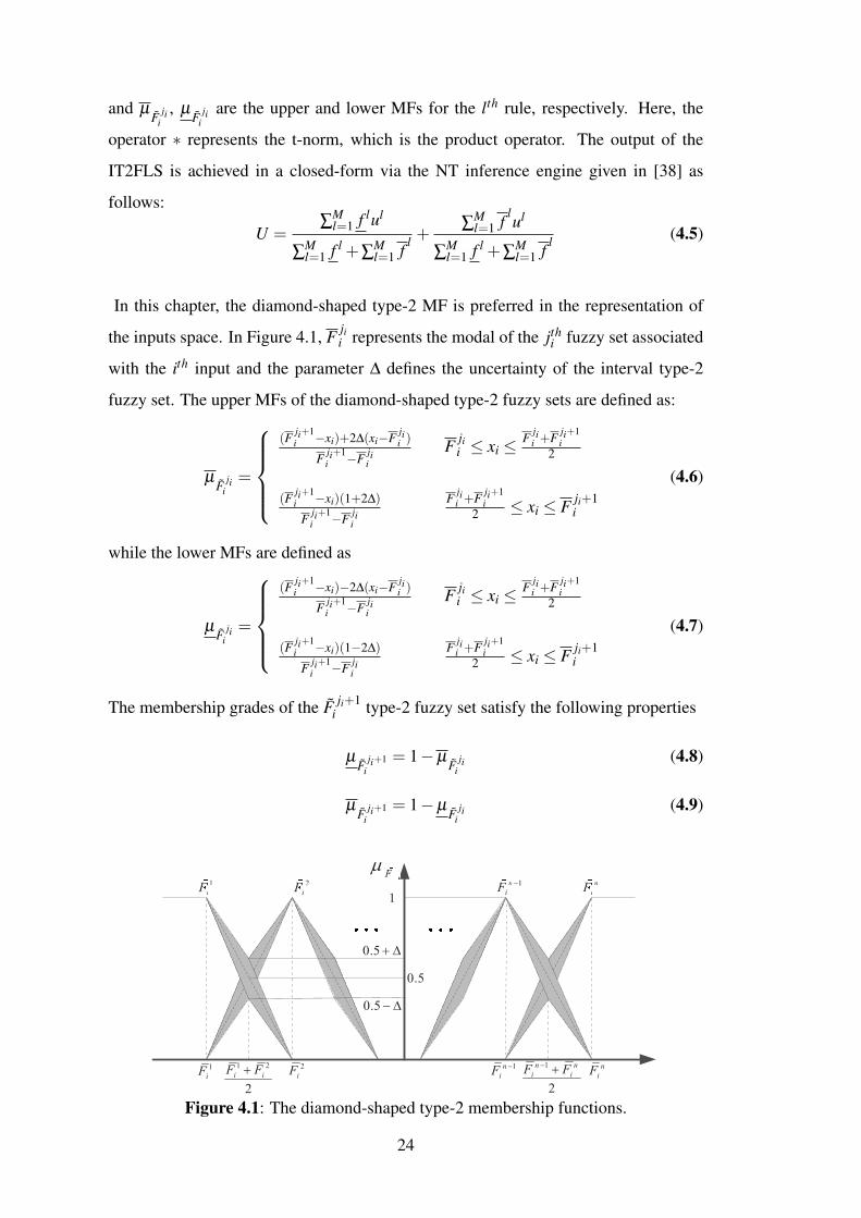
In this chapter, the diamond-shaped type-2 MF is preferred in the representation of

the inputs space. In Figure 4.1, F jii represents the modal of the jthi fuzzy set associated

with the ith input and the parameter ∆ defines the uncertainty of the interval type-2

fuzzy set. The upper MFs of the diamond-shaped type-2 fuzzy sets are defined as:

µF ji

i=

(F ji+1

i −xi)+2∆(xi−F jii )

F ji+1i −F ji

i

F jii ≤ xi ≤

F jii +F ji+1

i2

(F ji+1i −xi)(1+2∆)

F ji+1i −F ji

i

F jii +F ji+1

i2 ≤ xi ≤ F ji+1

i

(4.6)

while the lower MFs are defined as

µF ji

i=

(F ji+1

i −xi)−2∆(xi−F jii )

F ji+1i −F ji

i

F jii ≤ xi ≤

F jii +F ji+1

i2

(F ji+1i −xi)(1−2∆)

F ji+1i −F ji

i

F jii +F ji+1

i2 ≤ xi ≤ F ji+1

i

(4.7)

The membership grades of the F ji+1i type-2 fuzzy set satisfy the following properties

µF ji+1

i= 1−µ

F jii

(4.8)

µF ji+1

i= 1−µ

F jii

(4.9)

FmF

1

1

iF1

ii

2

iF2

ii

1n

iF

-1n

iFi

- n

iFn

ii

1n

iF

-2

iF

1

iF

n

iF

0.5 + D

0.5 - D

1 2

2

i iF F+

1

2

n n

i iF F

-+

0.5

Figure 4.1: The diamond-shaped type-2 membership functions.

24

The properties given in (4.8) and (4.9) of the diamond-shaped type-2 MF provide

easiness in the derivation of input-output relations, while other type-2 MFs do

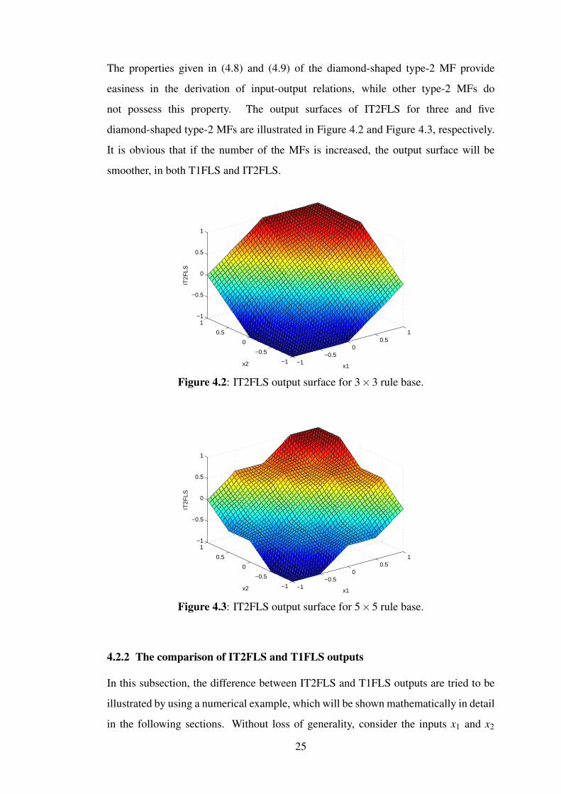
not possess this property. The output surfaces of IT2FLS for three and five

diamond-shaped type-2 MFs are illustrated in Figure 4.2 and Figure 4.3, respectively.

It is obvious that if the number of the MFs is increased, the output surface will be

smoother, in both T1FLS and IT2FLS.

−1−0.5

00.5

1

−1

−0.5

0

0.5

1−1

−0.5

0

0.5

1

x1x2

IT2F

LS

Figure 4.2: IT2FLS output surface for 3×3 rule base.

−1−0.5

00.5

1

−1

−0.5

0

0.5

1−1

−0.5

0

0.5

1

x1x2

IT2F

LS

Figure 4.3: IT2FLS output surface for 5×5 rule base.

4.2.2 The comparison of IT2FLS and T1FLS outputs

In this subsection, the difference between IT2FLS and T1FLS outputs are tried to be

illustrated by using a numerical example, which will be shown mathematically in detail

in the following sections. Without loss of generality, consider the inputs x1 and x2

25

which are normalized in [−1,1] with steps of 0.05 for x1 and x2, i.e. 41 points for each,

the fuzzy system has a total of N = 41×41 samples. Two IT2FLS with three and five

diamond-shaped type-2 MFs for each input are considered. Figure 4.4 and Figure 4.5

shows the output difference of T1FLS and IT2FLS whose configurations are exactly

the same except footprint of uncertainty (∆) which is equal to zero in T1FLS. As

−1−0.5

00.5

1

−1

−0.5

0

0.5

1−0.03

−0.02

−0.01

0

0.01

0.02

0.03

x1x2

IT2F

LS

Figure 4.4: The outputs difference of T1FLS and IT2FLS for 3×3 rule base.

−1

−0.5

0

0.5

1

−1

−0.5

0

0.5

1−0.05

0

0.05

x1x2

IT2F

LS

Figure 4.5: The outputs difference of T1FLS and IT2FLS for 5×5 rule base.

it can be seen from Figure 4.4 and Figure 4.5, the surfaces portioned into four and

sixteen regions, respectively, which the difference of T1FLS and IT2FLS is zero in

26

the areas between these regions. The reason is that there is no uncertainty, (∆ = 0),

in modal points of diamond-shaped MFs so the output of T1FLS and IT2FLS are the

same. Consequently, the difference between two fuzzy systems is equal to zero at the

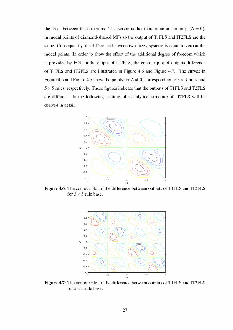
modal points. In order to show the effect of the additional degree of freedom which

is provided by FOU in the output of IT2FLS, the contour plot of outputs difference

of T1FLS and IT2FLS are illustrated in Figure 4.6 and Figure 4.7. The curves in

Figure 4.6 and Figure 4.7 show the points for ∆ 6= 0, corresponding to 3×3 rules and

5×5 rules, respectively. These figures indicate that the outputs of T1FLS and T2FLS

are different. In the following sections, the analytical structure of IT2FLS will be

derived in detail.

x2

x1−1 −0.5 0 0.5 1

−1

−0.8

−0.6

−0.4

−0.2

0

0.2

0.4

0.6

0.8

1

Figure 4.6: The contour plot of the difference between outputs of T1FLS and IT2FLSfor 3×3 rule base.

x2

x1−1 −0.5 0 0.5 1

−1

−0.8

−0.6

−0.4

−0.2

0

0.2

0.4

0.6

0.8

1

Figure 4.7: The contour plot of the difference between outputs of T1FLS and IT2FLSfor 5×5 rule base.

27

4.3 The Derivation of the Analytical Structure of IT2FLS

The input-output relations of IT2FLS give ability to understand and analyze the

behavior of this system. Therefore, the general analytical derivation for the IT2FLS is

performed in this section. It is clear from Figure 4.1 that at most two neighborhood

MFs have non-zero membership grades for any input set. Therefore, four rules are

always fired and considered in computation of the IT2FLS output for system with two

inputs (M = 4). The IT2FLS output for the input set (x1, x2) can be calculated using

(4.5) for active rules as follows

U =∑

4l=1 f lul +∑

4l=1 f lul

∑4l=1 f l +∑

4l=1 f l =

UN

UD (4.10)

In order to avoid the complexity in derivation, the output of IT2FLS is divided into

nominator and denominator parts. The nominator UN of (4.10) can be written as

UN =4

∑l=1

( f l + f l)ul (4.11)

Thus, UN can be subsequently derived as

UN = u1(µF j1

1µ

F j22+µ

F j11

µF j2

2)

+u2(µF j1

1µ

F j2+12

+µF j1

1µ

F j2+12

)

+u3(µF j1+1

1µ

F j22+µ

F j1+11

µF j2

2)

+u4(µF j1+1

1µ

F j2+12

+µF j1+1

1µ

F j2+12

)

(4.12)

Using the relations (4.8) and (4.9), (4.12) can be reformulated as

UN = (u1 +u4)(µF j1

1µ

F j22+µ

F j11

µF j2

2)

+(u2−u4)(µF j1

1+µ

F j11)

− (u2 +u3)(µF j1

1µ

F j22+µ

F j11

µF j2

2)

+(u3−u4)(µF j2

2+µ

F j22)+2u4

(4.13)

In order to simplify (4.13), the following equation is derived from the (4.6) and (4.7)

µF ji

i+µ

F jii=

2(F ji+1i − xi)

F ji+1i −F ji

i

(4.14)

and there are four different cases for P1(xi,Fjii ,∆) = µ

F j11

µF j2

2+ µ

F j11

µF j2

2and

P2(xi,Fjii ,∆) = µ

F j11

µF j2

2+ µ

F j11

µF j2

2in (13) according to the range that the inputs

are taking place. Thus, by substituting (4.6) and (4.7) in the equations, the simplified

functions are tabulated in Table 4.1 and Table 4.2.

28

Tabl

e4.

1:T

heP 1(x

i,F

j i i,∆

)fo

rfou

rreg

ions

inin

putd

omai

n.

µF

j 1 1µ

Fj 2 2+

µF

j 1 1µ

Fj 2 2

Fj 2 2≤

x 2≤

Fj 2 2+

Fj 2+

12

2F

j 2 2+

Fj 2+

12

2≤

x 2≤

Fj 2+

12

Fj 1 1≤

x 1≤

Fj 1 1+

Fj 1+

11

22[ (F

j 1+

11−

x 1)(

Fj 2+

12−

x 2)+

4∆2 (

Fj 1 1−

x 1)(

Fj 2 2−

x 2)]

(Fj 1+

11−

Fj 1 1)(

Fj 2+

12−

Fj 2 2)

2[ (Fj 1+

11−

x 1)(

Fj 2+

12−

x 2)−

4∆2 (

Fj 1 1−

x 1)(

Fj 2+

12−

x 2)]

(Fj 1+

11−

Fj 1 1)(

Fj 2+

12−

Fj 2 2)

Fj 1 1+

Fj 1+

11

2≤

x 1≤

Fj 1+

11

2[ ( Fj 1+

11−

x 1)(

Fj 2+

12−

x 2)−

4∆2 (

Fj 1+

11−

x 1)(

Fj 2 2−

x 2)]

(Fj 1+

11−

Fj 1 1)(

Fj 2+

12−

Fj 2 2)

2[ ( Fj 1+

11−

x 1)(

Fj 2+

12−

x 2)+

4∆2 (

Fj 1+

11−

x 1)(

Fj 2+

12−

x 2)]

(Fj 1+

11−

Fj 1 1)(

Fj 2+

12−

Fj 2 2)

Tabl

e4.

2:T

heP 2(x

i,F

j i i,∆

)fo

rfou

rreg

ions

inin

putd

omai

n.

µF

j 1 1µ

Fj 2 2+

µF

j 1 1µ

Fj 2 2

Fj 2 2≤

x 2≤

Fj 2 2+

Fj 2+

12

2F

j 2 2+

Fj 2+

12

2≤

x 2≤

Fj 2+

12

Fj 1 1≤

x 1≤

Fj 1 1+

Fj 1+

11

22[ (F

j 1+

11−

x 1)(

Fj 2+

12−

x 2)−

4∆2 (

Fj 1 1−

x 1)(

Fj 2 2−

x 2)]

(Fj 1+

11−

Fj 1 1)(

Fj 2+

12−

Fj 2 2)

2[ ( Fj 1+

11−

x 1)(

Fj 2+

12−

x 2)+

4∆2 (

Fj 1 1−

x 1)(

Fj 2+

12−

x 2)]

(Fj 1+

11−

Fj 1 1)(

Fj 2+

12−

Fj 2 2)

Fj 1 1+

Fj 1+

11

2≤

x 1≤

Fj 1+

11

2[ ( Fj 1+

11−

x 1)(

Fj 2+

12−

x 2)+

4∆2 (

Fj 1+

11−

x 1)(

Fj 2 2−

x 2)]

(Fj 1+

11−

Fj 1 1)(

Fj 2+

12−

Fj 2 2)

2[ (Fj 1+

11−

x 1)(

Fj 2+

12−

x 2)−

4∆2 (

Fj 1+

11−

x 1)(

Fj 2+

12−

x 2)]

(Fj 1+

11−

Fj 1 1)(

Fj 2+

12−

Fj 2 2)

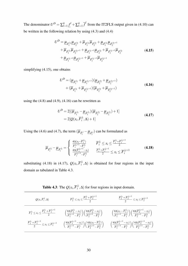
The denominator UD = ∑4l=1 f l +∑

4l=1 f l from the IT2FLS output given in (4.10) can

be written in the following relation by using (4.3) and (4.4)

UD = µF j1

1µ

F j22+µ

F j11

µF j2

2+µ

F j11

µF j2+1

2

+µF j1

1µ

F j2+12

+µF j1+1

1µ

F j22+µ

F j1+11

µF j2

2

+µF j1+1

1µ

F j2+12

+µF j1+1

1µ

F j2+12

(4.15)

simplifying (4.15), one obtains

UD = (µF j1

1+µ

F j1+11

)(µF j2

2+µ

F j2+12

)

+(µF j1

1+µ

F j1+11

)(µF j2

2+µ

F j2+12

)(4.16)

using the (4.8) and (4.9), (4.16) can be rewritten as

UD = 2[(µF j1

1−µ

F j11)(µ

F j22−µ

F j22)+1]

= 2[Q(xi,Fjii ,∆)+1]

(4.17)

Using the (4.6) and (4.7), the term (µ F ji−µ

F ji) can be formulated as

µF ji

i−µ

F jii=

4∆(xi−F ji

i )

F ji+1i −F ji

i

F jii ≤ xi ≤

F jii +F ji+1

i2

4∆(F ji+1i −xi)

F ji+1i −F ji

i

F jii +F ji+1

i2 ≤ xi ≤ F ji+1

i

(4.18)

substituting (4.18) in (4.17), Q(xi,Fjii ,∆) is obtained for four regions in the input

domain as tabulated in Table 4.3.

Table 4.3: The Q(xi,Fjii ,∆) for four regions in input domain.

Q(xi,Fjii ,∆) F j2

2 ≤ x2 ≤F j2

2 +F j2+12

2F j2

2 +F j2+12

2≤ x2 ≤ F j2+1

2

F j11 ≤ x1 ≤

F j11 +F j1+1

12

(4∆(F j1

1 − x1)

F j1+11 −F j1

1

)(4∆(F j2

2 − x2)

F j2+12 −F j2

2

) (4∆(x1−F j1

1 )

F j1+11 −F j1

1

)(4∆(F j2+1

2 − x2)

F j2+12 −F j2

2

)

F j11 +F j1+1

12

≤ x1 ≤ F j1+11

(4∆(F j1+1

1 − x1)

F j1+11 −F j1

1

)(4∆(x2−F j2

2 )

F j2+12 −F j2

2

) (4∆(F j1+1

1 − x1)

F j1+11 −F j1

1

)(4∆(F j2+1

2 − x2)

F j2+12 −F j2

2

)

30

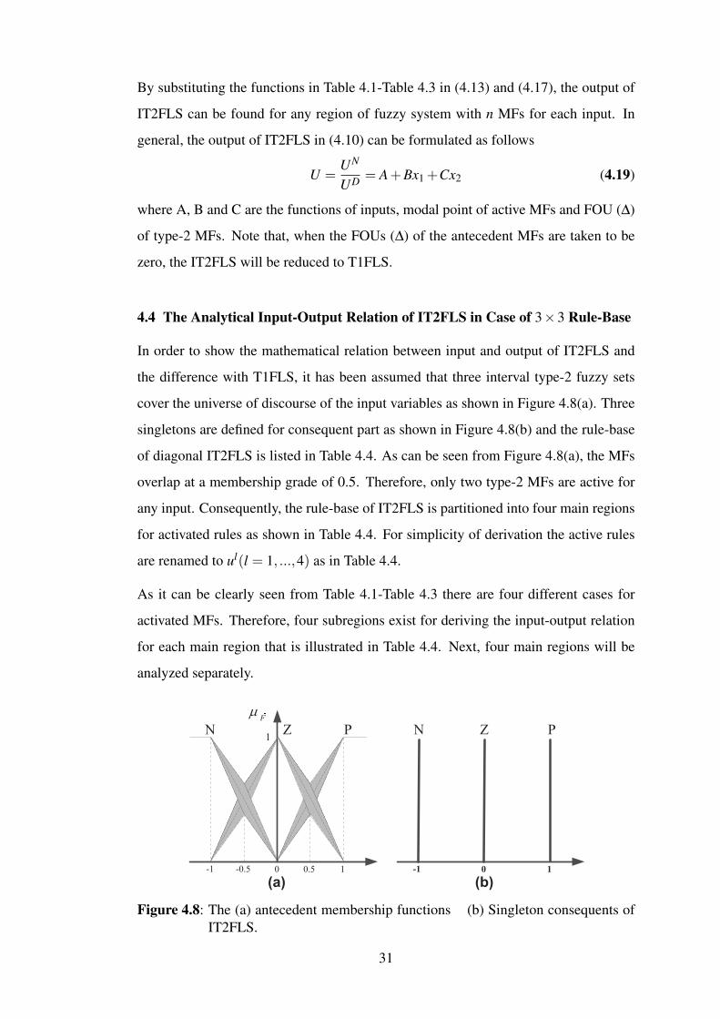
By substituting the functions in Table 4.1-Table 4.3 in (4.13) and (4.17), the output of

IT2FLS can be found for any region of fuzzy system with n MFs for each input. In

general, the output of IT2FLS in (4.10) can be formulated as follows

U =UN

UD = A+Bx1 +Cx2 (4.19)

where A, B and C are the functions of inputs, modal point of active MFs and FOU (∆)

of type-2 MFs. Note that, when the FOUs (∆) of the antecedent MFs are taken to be

zero, the IT2FLS will be reduced to T1FLS.

4.4 The Analytical Input-Output Relation of IT2FLS in Case of 3×3 Rule-Base

In order to show the mathematical relation between input and output of IT2FLS and

the difference with T1FLS, it has been assumed that three interval type-2 fuzzy sets

cover the universe of discourse of the input variables as shown in Figure 4.8(a). Three

singletons are defined for consequent part as shown in Figure 4.8(b) and the rule-base

of diagonal IT2FLS is listed in Table 4.4. As can be seen from Figure 4.8(a), the MFs

overlap at a membership grade of 0.5. Therefore, only two type-2 MFs are active for

any input. Consequently, the rule-base of IT2FLS is partitioned into four main regions

for activated rules as shown in Table 4.4. For simplicity of derivation the active rules

are renamed to ul(l = 1, ...,4) as in Table 4.4.

As it can be clearly seen from Table 4.1-Table 4.3 there are four different cases for

activated MFs. Therefore, four subregions exist for deriving the input-output relation

for each main region that is illustrated in Table 4.4. Next, four main regions will be

analyzed separately.

FmF

1N Z P

-1 -0.5 0 0.5 1

N Z P

-1 0 1

(a) (b)

Figure 4.8: The (a) antecedent membership functions (b) Singleton consequents ofIT2FLS.

31

Table 4.4: The 3×3 rule-base for IT2FLS.

N Z P

N

Z

P

N

N

N

Z

Z

Z

P P

P

1

2

3 4

X1

X2

Region 1: It is clear from Table 4.4 and Figure 4.8(b) that u1 = u2 = u3 = −1 and

u4 = 0 and from Figure 4.8(a) the modal points of active membership functions are as

following:

F j11 =−1 F j1+1

1 = 0 F j22 =−1 F j2+1

2 = 0

By substituting ul in (4.13), the nominator of IT2FLS for region 1 can be written as

UN =−(µF j1

1µ

F j22+µ

F j11

µF j2

2)− (µ

F j11+µ

F j11)

+2(µF j1

1µ

F j22+µ

F j11

µF j2

2)− (µ

F j22+µ

F j22)

(4.20)

The nominator and denominator of IT2FLS for four subregions can be simplified by

substituting the value of modal points in (4.20), (4.17) and Table 4.1-Table 4.3 as

follows:

• Subregion 1.1: In this subregion x1 and x2 fall in the interval of [−1,−0.5] and UN

is obtained as

UN =2[(F j1+1

1 − x1)(Fj2+12 − x2)−12∆2(F j1

1 − x1)(Fj22 − x2)

(F j1+11 −F j1

1 )(F j2+12 −F j1

2 )

−(F j1+1

1 − x1)(Fj2+12 −F j2

2 )+(F j2+12 − x2)(F

j1+11 −F j1

1 )]

(F j1+11 −F j1

1 )(F j2+12 −F j2

2 )

(4.21)

by substituting the related value of modal points, UN and UD can be written as

UN = 2[(1−12∆

2)x1x2 +(1−12∆2)x1 +(1−12∆

2)x2−12∆2] (4.22)

UD = 2[16∆

2(1+ x1)(1+ x2)+1]

(4.23)

32

• Subregion 1.2:In this subregion x1 falls in the interval of [−1,−0.5] and x2 falls in

the interval of [−0.5,0], therefore the nominator becomes

UN =2[(F j1+1

1 − x1)(Fj2+12 − x2)+12∆2(F j1

1 − x1)(Fj2+12 − x2)

(F j1+11 −F j1

1 )(F j2+12 −F j2

2 )

−(F j1+1

1 − x1)(Fj2+12 −F j2

2 )+(F j2+12 − x2)(F

j1+11 −F j1

1 )]

(F j1+11 −F j1

1 )(F j2+12 −F j2

2 )

(4.24)

by substituting F j11 =−1, F j1+1

1 = 0, F j22 =−1, F j2+1

2 = 0, UN and UD are simplified

as follows

UN = 2[(1+12∆

2)x1x2 + x1 +(1+12∆2)x2

](4.25)

UD = 2[−16∆

2(1+ x1)x2 +1]

(4.26)

• Subregion 1.3: In this subregion, the intervals of x1 and x2 are [−0.5,0] and

[−1,−0.5], respectively. Similarly, UN becomes

UN =2[(F j1+1

1 − x1)(Fj2+12 − x2)+12∆2(F j1+1

1 − x1)(Fj22 − x2)

(F j1+11 −F j1

1 )(F j2+12 −F j2

2 )

−(F j1+1

1 − x1)(Fj2+12 −F j2

2 )+(F j2+12 − x2)(F

j1+11 −F j1

1 )]

(F j1+11 −F j1

1 )(F j2+12 −F j2

2 )

(4.27)

by substituting the appropriate model points, UN and UD are obtained as

UN = 2[(1+12∆

2)x1x2 +(1+12∆2)x1 + x2

](4.28)

UD = 2[−16∆

2x1(1+ x2)+1]

(4.29)

• Subregion 1.4: In this subregion, the intervals of x1 and x2 are [−0.5,0], so the

nominator can be obtained as

UN =2[(F j1+1

1 − x1)(Fj2+12 − x2)−12∆2(F j1+1

1 − x1)(Fj2+12 − x2)

(F j1+11 −F j1

1 )(F j2+12 −F j2

2 )

−(F j1+1

1 − x1)(Fj2+12 −F j2

2 )+(F j2+12 − x2)(F

j1+11 −F j1

1 )]

(F j1+11 −F j1

1 )(F j2+12 −F j2

2 )

(4.30)

33

simplified nominator and denominator are as

UN = 2[(1−12∆

2)x1x2 + x1 + x2]

(4.31)

UD = 2[16∆

2x1x2 +1]

(4.32)

Region 2: The values of active consequent part of IT2FLS are u1 = −1,u2 = u3 = 0

and u4 = 1 in region 2 and modal points of active MFs can be written as the following

F j11 =−1 F j1+1

1 = 0 F j22 = 0 F j2+1

2 = 1

By substituting ul in (13), the nominator of IT2FLS in region 2 can be written as

UN =−(µF j1

1+µ

F j11)− (µ

F j22+µ

F j22)+2 (4.33)

by using (4.14), (4.33) can be rewritten as

UN =−[

2(F j1+11 − x1)

F j1+11 −F j1

1

+2(F j2+1

2 − x2)

F j2+12 −F j2

2

]+2 (4.34)

and finally by substituting the related value of modal points, (4.34) can be simplified

as

UN = 2(x1 + x2) (4.35)

Note that UN has the same value for all four subregions. Next, by substituting the

related value of modal points in Table 4.3 and using (4.17), UD can be written for four

subregions as

• Subregion 2.1: −1≤ x1≤−0.5 and 0≤ x2≤ 0.5

UD = 2[16∆

2(1+ x1)x2 +1]

(4.36)

• Subregion 2.2: −1≤ x1≤−0.5 and 0.5≤ x2≤ 1

UD = 2[16∆

2(1+ x1)(1− x2)+1]

(4.37)

• Subregion 2.3: −0.5≤ x1≤ 0 and 0≤ x2≤ 0.5

UD = 2[−16∆

2x1x2 +1]

(4.38)

34

• Subregion 2.4: −0.5≤ x1≤ 0 and 0.5≤ x2≤ 1

UD = 2[−16∆

2x1(1− x2)+1]

(4.39)

Region 3: It is obvious from Table 4.1-4.4 that the consequent part of region 2 and

region 3 are the same. Therefore, the nominator of IT2FLS of the region 3 is the same

as of region 2. The modal points of active MFs are as follows:

F j11 = 0 F j1+1

1 = 1 F j22 =−1 F j2+1

2 = 0

By substituting the related value of modal points in Table 4.3, the denominator of

IT2FLS for four subregions of region 3 can be written as follows

• Subregion 3.1: 0≤ x1≤ 0.5 and −1≤ x2≤−0.5

UD = 2[16∆

2x1(1+ x2)+1]

(4.40)

• Subregion 3.2: 0≤ x1≤ 0.5 and −0.5≤ x2≤ 0

UD = 2[−16∆

2x1x2 +1]

(4.41)

• Subregion 3.3: 0.5≤ x1≤ 1 and −1≤ x2≤−0.5

UD = 2[16∆

2(1− x1)(1+ x2)+1]

(4.42)

• Subregion 3.4: 0.5≤ x1≤ 1 and −0.5≤ x2≤ 0

UD = 2[−16∆

2(1− x1)x2 +1]

(4.43)

Region 4: The value of modal points for active MFs in region 4 are as following

F j11 = 0 F j1+1

1 = 1 F j22 = 0 F j2+1

2 = 1

and the consequent parts of active rules are u1 = 0 and u2 = u3 = u4 = 1. By

substituting ul in (4.13), UN for this region is obtained as

UN = (µF j1

1µ

F j22+µ

F j11

µF j2

2)−2(µ

F j11

µF j2

2+µ

F j11

µF j2

2)+2 (4.44)

The nominator and denominator of IT2FLS for four subregions are derived as

35

• Subregion 4.1: x1 and x2 lie in the interval of [0,0.5] in this subregion and UN

becomes

UN = 2[−(F j1+1

1 − x1)(Fj2+12 − x2)+12∆2(F j1

1 − x1)(Fj22 − x2)

(F j1+11 −F j1

1 )(F j2+12 −F j2

2 )

]+2 (4.45)

by substituting the related value of modal points, UN and UD can be written as

UN = 2[(12∆

2−1)x1x2 + x1 + x2]

(4.46)

UD = 2[16∆

2x1x2 +1]

(4.47)

• Subregion 4.2: The interval of x1 is [0,0.5] and the interval of x2 is [0.5,1], so the

nominator is calculated as

UN = 2[−(F j1+1

1 − x1)(Fj2+12 − x2)−12∆2(F j1

1 − x1)(Fj2+12 − x2)

(F j1+11 −F j1

1 )(F j2+12 −F j2

2 )

]+2 (4.48)

simplifying UN and UD by substituting the related value of modal points gives the

following

UN = 2[− (1+12∆

2)x1x2 +(1+12∆2)x1 + x2

](4.49)

UD = 2[16∆

2x1(1− x2)+1]

(4.50)

• Subregion 4.3: In this subregion x1 and x2 fall in the intervals [0.5,1] and [0,0.5],

respectively. UN becomes

UN = 2[−(F j1+1

1 − x1)(Fj2+12 − x2)−12∆2(F j1+1

1 − x1)(Fj22 − x2)

(F j1+11 −F j1

1 )(F j2+12 −F j2

2 )

]+2 (4.51)

similarly UN and UD are obtained as follows

UN = 2[− (1+12∆

2)x1x2 + x1 +(1+12∆2)x2

](4.52)

UD = 2[16∆

2(1− x1)x2 +1]

(4.53)

• Subregion 4.4: The interval for x1 and x2 is [0.5,1], therefore UN can be obtained

as

36

UN = 2[−(F j1+1

1 − x1)(Fj2+12 − x2)+12∆2(F j1+1

1 − x1)(Fj2+12 − x2)

(F j1+11 −F j1

1 )(F j2+12 −F j2

2 )

]+2 (4.54)

by substituting the related values of modal points nominator and denominator are

simplified as

UN = 2[(12∆

2−1)x1x2 +(1−12∆2)x1 +(1−12∆

2)x2 +12∆2] (4.55)

UD = 2[16∆

2(1− x1)(1− x2)+1]

(4.56)

Finally, by using (4.19), the input-output relation of IT2FLS in case of 3×3 rule-base

is summarized in Table 4.5.

When the mathematical input-output relations are clear, the designer can insightfully

study the benefits and weaknesses of IT2FLSs and therefore better make use of

them. It is clear from Table 4.5 that the IT2FLSs have a more complex input-output

relation in comparison with T1FLSs. These complexities are caused by the footprint

of uncertainty in IT2FLS membership functions which produces 16 regions in

input-output relation. When the FOUs of the antecedent MFs are taken to be zero, the

IT2FLS will be reduced to T1FLS. Thus the 16 regions will be reduced to 4 regions

in T1FLS. These extra regions may provide an asset to enhance the performance of

IT2FLC over T1FLS and better model and/or control the systems in the presence of

parameter uncertainty or measurement noise. Lesser number of type-2 MFs can cover

the input domain and consequently the system can be modeled and/or controlled by

smaller size rule-base when compared to T1FLS. As can be seen from Table 4.5 the

IT2FLS behaves like a PD controller if the inputs x1 and x2 are set equal to error and

derivative of error, respectively. Actually, this fuzzy system can be seen as a parameter

time-varying PD controller with additional degree of freedom, which is provided by

the FOU in their MFs. Comparing IT2FLS with its type-1 counterpart, FOU in type-2

MFs generate 12 extra regions that each has unique input-output relation. These extra

regions which cannot be achieved by a T1FLS indicate that IT2FLS may be able to

provide better performance.

37

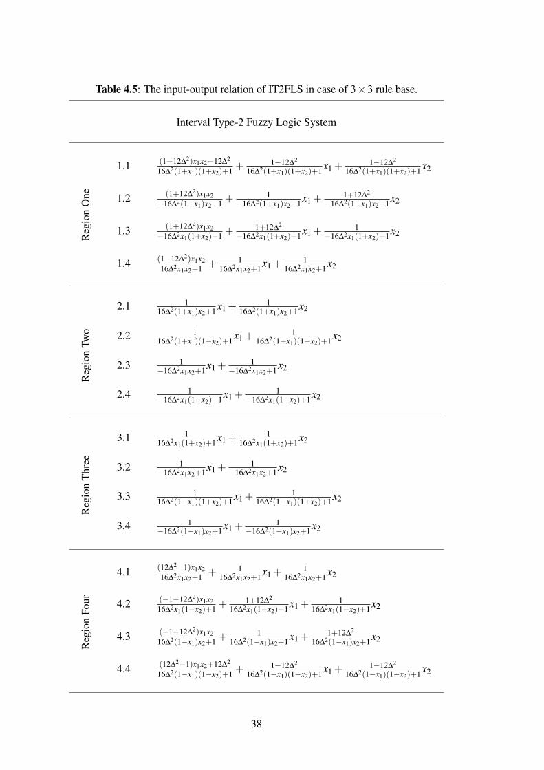
Table 4.5: The input-output relation of IT2FLS in case of 3×3 rule base.

Interval Type-2 Fuzzy Logic System

Reg

ion

One

1.1 (1−12∆2)x1x2−12∆2

16∆2(1+x1)(1+x2)+1 +1−12∆2

16∆2(1+x1)(1+x2)+1x1 +1−12∆2

16∆2(1+x1)(1+x2)+1x2

1.2 (1+12∆2)x1x2−16∆2(1+x1)x2+1 +

1−16∆2(1+x1)x2+1x1 +

1+12∆2

−16∆2(1+x1)x2+1x2

1.3 (1+12∆2)x1x2−16∆2x1(1+x2)+1 +

1+12∆2

−16∆2x1(1+x2)+1x1 +1

−16∆2x1(1+x2)+1x2

1.4 (1−12∆2)x1x216∆2x1x2+1 + 1

16∆2x1x2+1x1 +1

16∆2x1x2+1x2

Reg

ion

Two

2.1 116∆2(1+x1)x2+1x1 +

116∆2(1+x1)x2+1x2

2.2 116∆2(1+x1)(1−x2)+1x1 +

116∆2(1+x1)(1−x2)+1x2

2.3 1−16∆2x1x2+1x1 +

1−16∆2x1x2+1x2

2.4 1−16∆2x1(1−x2)+1x1 +

1−16∆2x1(1−x2)+1x2

Reg

ion

Thr

ee

3.1 116∆2x1(1+x2)+1x1 +

116∆2x1(1+x2)+1x2

3.2 1−16∆2x1x2+1x1 +

1−16∆2x1x2+1x2

3.3 116∆2(1−x1)(1+x2)+1x1 +

116∆2(1−x1)(1+x2)+1x2

3.4 1−16∆2(1−x1)x2+1x1 +

1−16∆2(1−x1)x2+1x2

Reg

ion

Four

4.1 (12∆2−1)x1x216∆2x1x2+1 + 1

16∆2x1x2+1x1 +1

16∆2x1x2+1x2

4.2 (−1−12∆2)x1x216∆2x1(1−x2)+1 +

1+12∆2

16∆2x1(1−x2)+1x1 +1

16∆2x1(1−x2)+1x2

4.3 (−1−12∆2)x1x216∆2(1−x1)x2+1 +

116∆2(1−x1)x2+1x1 +

1+12∆2

16∆2(1−x1)x2+1x2

4.4 (12∆2−1)x1x2+12∆2

16∆2(1−x1)(1−x2)+1 +1−12∆2

16∆2(1−x1)(1−x2)+1x1 +1−12∆2

16∆2(1−x1)(1−x2)+1x2

38

4.5 Conclusion

The mathematical expression between input and output of an interval type-2 fuzzy

logic systems is of great importance as it will deepen our understanding of how and

why these systems may be able to provide better performance over the type-1 fuzzy

logic systems. In this study, the general analytical structure of interval type-2 fuzzy

logic system with diamond-shaped type-2 fuzzy MFs is considered. The product fuzzy

AND operator, and the NT closed-form inference engine which are more practical in

real-time application are used. The FOU in type-2 MFs generate extra regions which

has a unique input-output relation and these regions may enhance robustness and noise

reduction properties of IT2FLS in comparison to its type-1 counterpart. A special

case of IT2FLS with three membership functions for each input and a diagonal 3× 3

rule-base are examined in detail.

39

40

5. A DESIGN METHODOLOGY AND ANALYSIS FOR INTERVAL TYPE-2FUZZY PI/PD CONTROLLERS

In this chapter, a systematical methodology is introduced to construct the rule base of

an interval type-2 fuzzy logic controller based on an existing linear PI/PD controller.

An easy and rapid generation of the fuzzy rules can be achieved through this technique.

A closed-form of the fuzzy controller output is achieved under the circumstances

that the input type-2 membership functions are diamond-shaped and a closed-form

inference engine is used. Consequently, a linear control law is transformed to a

nonlinear structure and certain elaborations can be done on the parameters of the

evolved closed output structure. Moreover, the designer can benefit from the nonlinear

structure of the proposed controller and the extra degree of freedom of type-2 fuzzy

sets. Simulation studies have been performed to demonstrate the superiority of the

proposed controller in comparison to linear controllers on benchmark processes. It can

be concluded from the results that the proposed controller can be more robust to the

parameter uncertainties and eliminate the oscillations much better than type-1 fuzzy

logic and linear conventional controllers.

5.1 Introduction

It is a known fact that PID controllers have continued to be the most widely used

controllers for industrial plants. A survey of more than 11,000 controllers in various

industries showed that 97 percent of controllers had the PID structure [39]. It is due

to the fact that they can assure satisfactory performance for a wide range of processes

despite their simplicity and ease of design. In literature, a wide variety of design

and tuning methods based on different performance criteria have been proposed for

PID controllers [40] [41]. Ziegler and Nichols [42] and Cohen and Coon [43] are

two well-known design methods. However, they have severe drawbacks since they

use insufficient process information and the closed loop system responses show poor

damping and poor robustness as a consequence of their design criteria [44]. These

drawbacks have been known for a long time and there have been many attempts to

41

overcome them [45] [46] [47]. Because of the simplicity, Ziegler Nichols method has,

however, remained very popular.

FLSs have been widely developed and utilized in the field of fuzzy logic control [48].

Various types of ordinary (type-1) fuzzy PID (including PI and PD) controllers have

been proposed in the literature [49] [50] [51] [52] [53]. A fuzzy controller based on the

decomposition of the multivariable rule base into simple rule bases has been studied

and compared to several PID-type FLCs and hybrid-type FLCs in [50]. In [49], a

fuzzy rule base shifting scheme is proposed for systems with time delay to improve

system performance. Analytical structure of the fuzzy PID controller and conditions

for bounded-input bounded-output stability of fuzzy PID control systems are obtained

in [51]. The performance of conventional PID controllers has been compared with

T1-FLC through different simulations in [17]. In [54], it has been shown that PID

controllers can be realized by fuzzy control and simplified fuzzy reasoning methods.

The main difficulty in T1-FLC design is to determine the parameters of the fuzzy logic

controllers (e.g. membership functions, rules, scaling factors) for inputs and outputs

of a fuzzy system. To ease the FLC design process, the researchers proposed a general

methodology to systematically construct a fuzzy logic controller based on the existence

of a linear controller in [55]. This methodology guarantees identical performance to

an existing linear controller. Since the performances of controllers are identical, it has

been advised to use expert knowledge to improve the performance of fuzzy controller

by appropriately changing the rule base.

IT2-FLCs have attracted much research interests in recent years due to their ability to

cope with uncertainty. A review on the design and optimization of IT2-FLCs has been

considered in [56]. Several control and engineering applications such as liquid-level

process control [9]; autonomous mobile robots [10]; prediction of air pollutant [11];

pH control [12]; control and the identification of a real-time servo system [13] and face

recognition [14] illustrate the advantages of interval type-2 fuzzy logic sets. Studies

have been reported in the literature that the IT2-FLCs are generally more robust than

T1-FLC [8] [15]. Wu [15] has discussed the fundamental differences between interval

type-2 and type-1 fuzzy logic controllers. There, it has also been shown that interval

type-2 PI controllers have smoother control surfaces than its type-1 counterpart in the

region around the zero. In [57], an interval type-2 fuzzy proportional controller with

42

a variable gain has been developed. A method to design interval type-2 TSK FLCs,

PD-type and PI-type fuzzy controllers to satisfy certain desired transient response, has

been proposed in [58]. Derivation and analysis of the two Mamdani interval type-2

fuzzy PI controllers that uses the center-of-sets type reducer and the average defuzzifier

are studied in [24]. The analytical structure of a special class of interval type-2 fuzzy

PI and PD controllers that have symmetrical rule base and symmetrical consequent sets

is presented in [25]. Authors show that the IT2-FLC partitions the input domain into

31 extra local regions in comparison with its T1 counterpart, which each provides a

unique relationship between the inputs and output signals. They compare the IT2-FLC

with the corresponding T1-FLC and the potential advantages of using IT2-FLC over

T1 fuzzy controller are examined.

In this chapter, a systematical methodology to construct an interval type-2 fuzzy logic

controller based on conventional controller is proposed. The methodology depends on

a nonlinear mapping from an existing conventional linear control law (e.g. PI, PD)

to IT2-FLC in which the beneficial sides of a linear controller in terms of simplicity

is captured. The proposed nonlinear mapping is done under certain circumstances

that input type-2 MFs are diamond-shaped and the closed-form inference engine

given in [38] is used. An important advantage of the proposed methodology is the

closed-form relation between input and output of an IT2-FLC. This provides a way of

understanding why IT2-FLC is more robust and how they cope with uncertainties. An

easy and rapid generation of the fuzzy rules based on the existence of linear control

law can be achieved through this technique. When the FOUs of the antecedent MFs are

taken to be zero, the IT2-FLC will be reduced to T1-FLC thus an identical mapping

is accomplished between conventional linear controller and the proposed controller.

If FOU is not equal to zero, then an additional degree of freedom is acquired that

provides an uncertainty cloud over the proposed controller. This provides the designer

an additional tool to cope with the uncertainties and nonlinearities, which may exist

in the system to be controlled. The FOU causes variable gains for the proposed

controller. Two special cases of the proposed controller with 2× 2 and 2× 3 rule

base are mathematically analyzed in detail to show the effect of variable gains that are

introduced by proposed IT2-FLC. Simulations on various processes including those

with time delay, integrating and non-minimum phase characteristics demonstrate that

43

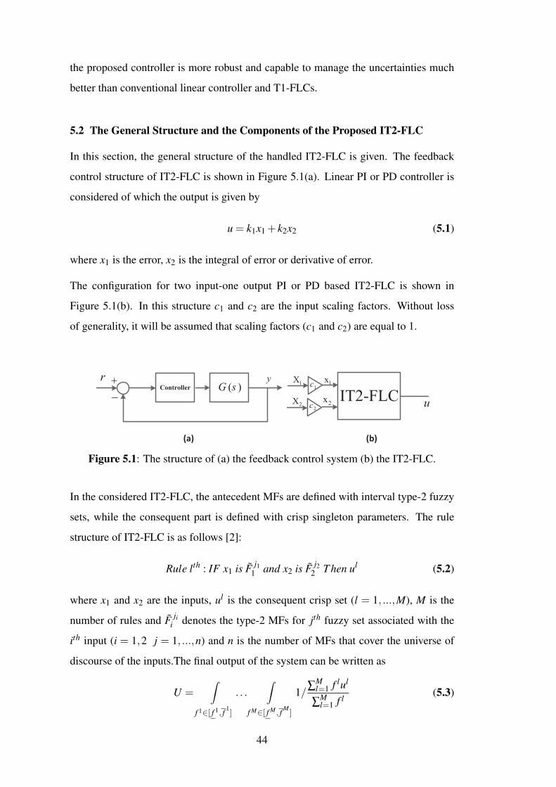
the proposed controller is more robust and capable to manage the uncertainties much

better than conventional linear controller and T1-FLCs.

5.2 The General Structure and the Components of the Proposed IT2-FLC

In this section, the general structure of the handled IT2-FLC is given. The feedback

control structure of IT2-FLC is shown in Figure 5.1(a). Linear PI or PD controller is

considered of which the output is given by

u = k1x1 + k2x2 (5.1)

where x1 is the error, x2 is the integral of error or derivative of error.

The configuration for two input-one output PI or PD based IT2-FLC is shown in

Figure 5.1(b). In this structure c1 and c2 are the input scaling factors. Without loss

of generality, it will be assumed that scaling factors (c1 and c2) are equal to 1.

(a) (b)

Controller ( )G s+

-

r y

IT2-FLCu

1c

2c

1X

2X

1x

2x

Figure 5.1: The structure of (a) the feedback control system (b) the IT2-FLC.

In the considered IT2-FLC, the antecedent MFs are defined with interval type-2 fuzzy

sets, while the consequent part is defined with crisp singleton parameters. The rule

structure of IT2-FLC is as follows [2]:

Rule lth : IF x1 is F j11 and x2 is F j2

2 T hen ul (5.2)

where x1 and x2 are the inputs, ul is the consequent crisp set (l = 1, ...,M), M is the

number of rules and F jii denotes the type-2 MFs for jth fuzzy set associated with the

ith input (i = 1,2 j = 1, ...,n) and n is the number of MFs that cover the universe of

discourse of the inputs.The final output of the system can be written as

U =∫

f 1∈[ f 1, f 1]

. . .∫

f M∈[ f M , f M]

1/∑

Ml=1 f lul

∑Ml=1 f l

(5.3)

44

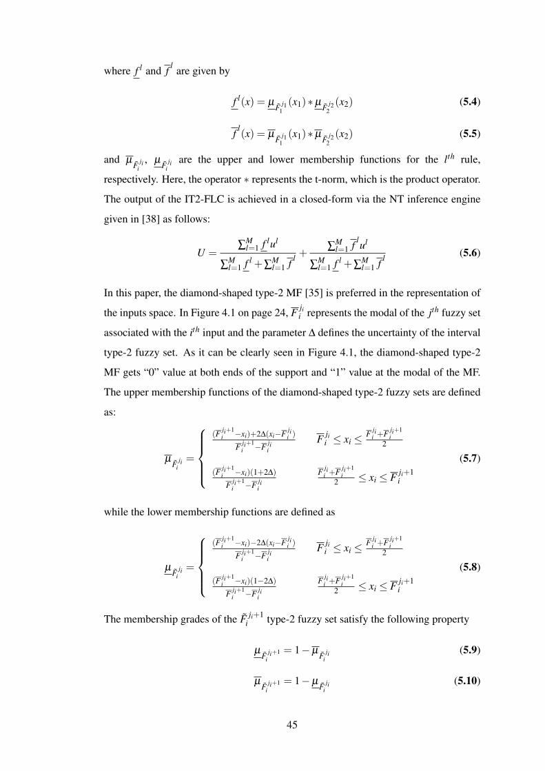
where f l and f l are given by

f l(x) = µF j1

1(x1)∗µ

F j22(x2) (5.4)

f l(x) = µ

F j11(x1)∗µ

F j22(x2) (5.5)

and µF ji

i, µ

F jii

are the upper and lower membership functions for the lth rule,

respectively. Here, the operator ∗ represents the t-norm, which is the product operator.

The output of the IT2-FLC is achieved in a closed-form via the NT inference engine

given in [38] as follows:

U =∑

Ml=1 f lul

∑Ml=1 f l +∑

Ml=1 f l +

∑Ml=1 f lul

∑Ml=1 f l +∑

Ml=1 f l (5.6)

In this paper, the diamond-shaped type-2 MF [35] is preferred in the representation of

the inputs space. In Figure 4.1 on page 24, F jii represents the modal of the jth fuzzy set

associated with the ith input and the parameter ∆ defines the uncertainty of the interval

type-2 fuzzy set. As it can be clearly seen in Figure 4.1, the diamond-shaped type-2

MF gets “0” value at both ends of the support and “1” value at the modal of the MF.

The upper membership functions of the diamond-shaped type-2 fuzzy sets are defined

as:

µF ji

i=

(F ji+1

i −xi)+2∆(xi−F jii )

F ji+1i −F ji

i

F jii ≤ xi ≤

F jii +F ji+1

i2

(F ji+1i −xi)(1+2∆)

F ji+1i −F ji

i

F jii +F ji+1

i2 ≤ xi ≤ F ji+1

i

(5.7)

while the lower membership functions are defined as

µF ji

i=

(F ji+1

i −xi)−2∆(xi−F jii )

F ji+1i −F ji

i

F jii ≤ xi ≤

F jii +F ji+1

i2

(F ji+1i −xi)(1−2∆)

F ji+1i −F ji

i

F jii +F ji+1

i2 ≤ xi ≤ F ji+1

i

(5.8)

The membership grades of the F ji+1i type-2 fuzzy set satisfy the following property

µF ji+1

i= 1−µ

F jii

(5.9)

µF ji+1

i= 1−µ

F jii

(5.10)

45

The location of the crisp numbers for the consequent part of IT2-FLC is the key feature

of this study. The structure of consequent part of the IT2-FLC is given as

ul = k1F j11 + k2F j2

2 ji ∈ {1, . . . ,n}, i = {1,2} and l ∈ {1, . . . ,M} (5.11)

where k1 is the proportional gain, k2 is the integral or derivative gain, F jii represents the

modal of the jthi fuzzy set associated with the ith input (i = 1,2 j = 1, ...,n) and n is the

number of MF that cover the universe of discourse of inputs [37]. As it is seen from

(5.11), the location of the crisp numbers for the consequent part of IT2-FLC directly

incorporates the linear conventional control law.

5.3 The Methodology and Analytical Derivation for the Proposed IT2-FLC

In this section, the analytical derivations for the proposed IT2-FLC based on

conventional PI or PD, shown in Figure 5.1(b), is examined. It is clear from Figure 4.1

that the MFs overlap at a membership grade of 0.5. Therefore, only two type-2 MFs

are active for any input set (n = 2). Consequently, four rules are always activated and

considered in computation of the IT2-FLC output (M = 4). The IT2-FLC output for

the input set (x1,x2) can be calculated using (5.6) as follows

U =∑

4l=1 f lul +∑

4l=1 f lul

∑4l=1 f l +∑

4l=1 f l =

UN

UD (5.12)

where the consequent part ul is given as:

u1 = k1F j11 + k2F j2

2

u2 = k1F j11 + k2F j2+1

2

u3 = k1F j1+11 + k2F j2

2

u4 = k1F j1+11 + k2F j2+1

2

(5.13)

where k1 = kp and k2 is kd or ki. Using the approach described by (5.11) and (5.13) the

consequent part of active rules for the given inputs are generated as in Table 5.1.

Theorem:

The output of IT2-FLC in (5.12) can be formulated as follows

U =UN

UD =P(xi,F

jii ,∆,K)+2(k1x1 + k2x2)

2[Q(xi,Fjii ,∆)+1]

(5.14)

if and only if

46

Table 5.1: IT2-FLC rule base for a system with given inputs.

I. The rule base contains all possible combinations of active input sets.

II. The input interval type-2 fuzzy sets are normal and satisfy (5.9) and (5.10) for

any given input set.

In (5.14), xi is the input, K = [k1 k2] is a vector of the conventional controller gains

and ∆ is the parameter that produces FOU for type-2 MF.

The proof of the theorem is given in two parts via two lemmas. The derivations of

the expressions for the denominator UD and the nominator UN and related proofs are

given in lemma 1 and 2, respectively.

Lemma 1:

For any input set, x1 and x2, the denominator UD =∑4l=1 f l+∑

4l=1 f l from the IT2-FLC

output given in (5.14) is equal to

UD = 2[Q(xi,Fjii ,∆)+1] (5.15)

Proof:

The denominator UD = ∑4l=1 f l +∑

4l=1 f l from the IT2FLS output given in (5.11) can

be written in the following relation by using (5.4) and (5.5)

UD = µF j1

1µ

F j22+µ

F j11

µF j2

2+µ

F j11

µF j2+1

2+µ

F j11

µF j2+1

2

+µF j1+1

1µ

F j22+µ

F j1+11

µF j2

2+µ

F j1+11

µF j2+1

2+µ

F j1+11

µF j2+1

2

(5.16)

Simplifying (5.16), one obtains

UD = (µF j1

1+µ

F j1+11

)(µF j2

2+µ

F j2+12

)

+(µF j1

1+µ

F j1+11

)(µF j2

2+µ

F j2+12

)(5.17)

47

Using the (5.9) and (5.10), (5.17) can be rewritten as

UD = 2[(µF j1

1−µ

F j11)(µ

F j22−µ

F j22)+1]

= 2[Q(xi,Fjii ,∆)+1]

(5.18)

Using the (5.7) and (5.8), the term (µF ji

i−µ

F jii) can be formulated as

µF ji

i−µ

F jii=

4∆(xi−F ji

i )

F ji+1i −F ji

i

F jii ≤ xi ≤

F jii +F ji+1

i2

4∆(F ji+1i −xi)

F ji+1i −F ji

i

F jii +F ji+1

i2 ≤ xi ≤ F ji+1

i

(5.19)

Substituting (5.19) in (5.18), Q(xi,Fjii ,∆) is obtained for four regions in the input

domain as tabulated in Table 4.3 on page 30.

Lemma 2:

For any input set, x1 and x2, the nominator UN = ∑4l=1( f l + f l

)ul from the IT2-FLC

output given in (5.12) is equal to

UN = P(xi,Fjii ,K,∆)+2(k1x1 + k2x2) (5.20)

Proof:

The nominator UN of (5.12) can be written as

UN = u1(µF j1

1µ

F j22+µ

F j11

µF j2

2)

+u2(µF j1

1µ

F j2+12

+µF j1

1µ

F j2+12

)

+u3(µF j1+1

1µ

F j22+µ

F j1+11

µF j2

2)

+u4(µF j1+1

1µ

F j2+12

+µF j1+1

1µ

F j2+12

)

(5.21)

Using the relations (5.9) and (5.10), (5.21) can be reformulated as

UN = (u1 +u4)(µF j1

1µ

F j22+µ

F j11

µF j2

2)

+(u2−u4)(µF j1

1+µ

F j11)

− (u2 +u3)(µF j1

1µ

F j22+µ

F j11

µF j2

2)

+(u3−u4)(µF j2

2+µ

F j22)+2u4

(5.22)

From (5.13) it is obvious that u1 +u4 = u2 +u3. Thus, (5.22) can be simplified as

UN = (u1 +u4)(µF j1

1µ

F j22+µ

F j11

µF j2

2−µ

F j11

µF j2

2−µ

F j11

µF j2

2)

+(u2−u4)(µF j1

1+µ

F j11)+(u3−u4)(µ

F j22+µ

F j22)+2u4

(5.23)

48

Table 5.2: The expressions of G(xi,Fjii ,∆) for four regions in input domain.

G(xi,Fjii ,∆) F j2

2 ≤ x2 ≤F j2

2 +F j2+12

2F j2

2 +F j2+12

2≤ x2 ≤ F j2+1

2

F j11 ≤ x1 ≤

F j11 +F j1+1

12

16∆2(F j11 − x1)(F

j22 − x2)

(F j1+11 −F j1

1 )(F j2+12 −F j2

2 )

−16∆2(F j11 − x1)(F

j2+12 − x2)

(F j1+11 −F j1

1 )(F j2+12 −F j2

2 )

F j11 +F j1+1

12

≤ x1 ≤ F j1+11

−16∆2(F j1+11 − x1)(F

j22 − x2)

(F j1+11 −F j1

1 )(F j2+12 −F j2

2 )

16∆2(F j1+11 − x1)(F

j2+12 − x2)

(F j1+11 −F j1

1 )(F j2+12 −F j2

2 )

In order to simplify (5.23), the following equation is derived from the (5.8) and (5.8)

µF ji

i+µ

F jii=

2(F ji+1i − xi)

F ji+1i −F ji

i

(5.24)

and G(xi,Fjii ,∆) is defined as:

G(xi,Fjii ,∆) = µ

F j11

µF j2

2+µ

F j11

µF j2

2−µ

F j11

µF j2

2−µ

F j11

µF j2

2(5.25)

There are four different cases for G(xi,Fjii ,∆) according to the range that the inputs

are taking place. Thus, by substituting (5.7) and (5.8) in (5.25) and simplifying,

G(xi,Fjii ,∆) is obtained as Table 5.2.

Substituting (5.24), (5.25) and (5.13) into (5.23), UN is obtained as

UN = P(xi,Fjii ,K,∆)+2(k1x1 + k2x2) (5.26)

where

P(xi,Fjii ,K,∆) =

((k1(F

j11 +F j1+1

1 )+ k2(Fj22 +F j2+1

2 ))×G(xi,F

jii ,∆) (5.27)

Note that if ∆ = 0, it is clear that Q(xi,Fjii ,∆) = 0 and P(xi,F

jii ,K,∆) = 0. Thus,

IT2-FLC reduces to a T1-FLC and has an identical output to the PI or PD control law

as followingU = k1x1 + k2x2 = kpe+ ki

∫ tt0 edt (PI)

orU = k1x1 + k2x2 = kpe+ kie (PD)

(5.28)

As it can be seen from (5.14), IT2-FLC produces a nonlinear controller, which has a

conventional linear controller part and nonlinear parts P(xi,Fjii ,K,∆) and Q(xi,F

jii ,∆)

that vary with its arguments. In the following two subsections, two special cases with

49

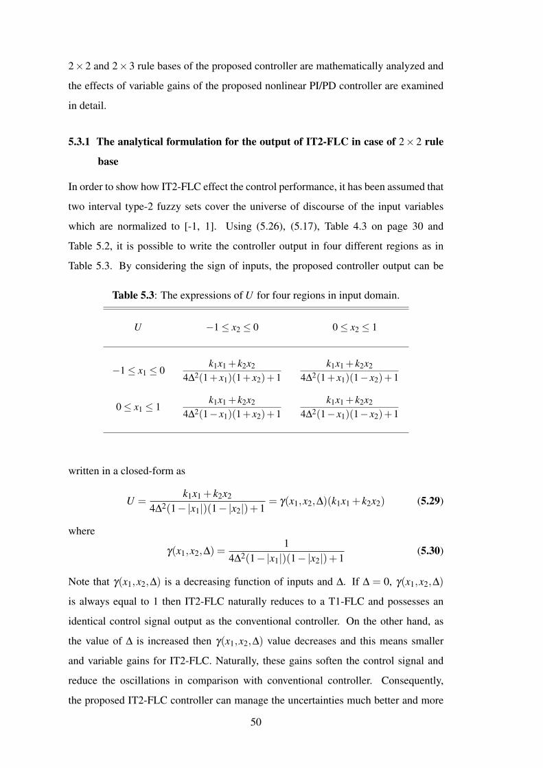
2×2 and 2×3 rule bases of the proposed controller are mathematically analyzed and

the effects of variable gains of the proposed nonlinear PI/PD controller are examined

in detail.

5.3.1 The analytical formulation for the output of IT2-FLC in case of 2× 2 rule

base

In order to show how IT2-FLC effect the control performance, it has been assumed that

two interval type-2 fuzzy sets cover the universe of discourse of the input variables

which are normalized to [-1, 1]. Using (5.26), (5.17), Table 4.3 on page 30 and

Table 5.2, it is possible to write the controller output in four different regions as in

Table 5.3. By considering the sign of inputs, the proposed controller output can be

Table 5.3: The expressions of U for four regions in input domain.

U −1≤ x2 ≤ 0 0≤ x2 ≤ 1

−1≤ x1 ≤ 0k1x1 + k2x2

4∆2(1+ x1)(1+ x2)+1k1x1 + k2x2

4∆2(1+ x1)(1− x2)+1

0≤ x1 ≤ 1k1x1 + k2x2

4∆2(1− x1)(1+ x2)+1k1x1 + k2x2

4∆2(1− x1)(1− x2)+1

written in a closed-form as

U =k1x1 + k2x2

4∆2(1−|x1|)(1−|x2|)+1= γ(x1,x2,∆)(k1x1 + k2x2) (5.29)

where

γ(x1,x2,∆) =1

4∆2(1−|x1|)(1−|x2|)+1(5.30)

Note that γ(x1,x2,∆) is a decreasing function of inputs and ∆. If ∆ = 0, γ(x1,x2,∆)

is always equal to 1 then IT2-FLC naturally reduces to a T1-FLC and possesses an

identical control signal output as the conventional controller. On the other hand, as

the value of ∆ is increased then γ(x1,x2,∆) value decreases and this means smaller

and variable gains for IT2-FLC. Naturally, these gains soften the control signal and

reduce the oscillations in comparison with conventional controller. Consequently,

the proposed IT2-FLC controller can manage the uncertainties much better and more

50

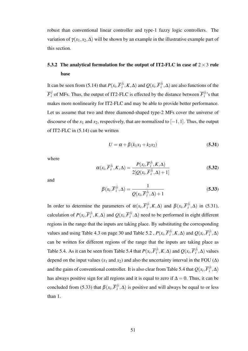
robust than conventional linear controller and type-1 fuzzy logic controllers. The

variation of γ(x1,x2,∆) will be shown by an example in the illustrative example part of

this section.

5.3.2 The analytical formulation for the output of IT2-FLC in case of 2× 3 rule

base

It can be seen from (5.14) that P(xi,Fjii ,K,∆) and Q(xi,F

jii ,∆) are also functions of the

F ji of MFs. Thus, the output of IT2-FLC is effected by the distance between F ji

i ’s that

makes more nonlinearity for IT2-FLC and may be able to provide better performance.

Let us assume that two and three diamond-shaped type-2 MFs cover the universe of

discourse of the x1 and x2, respectively, that are normalized to [−1,1]. Thus, the output

of IT2-FLC in (5.14) can be written

U = α +β (k1x1 + k2x2) (5.31)

where

α(xi,Fjii ,K,∆) =

P(xi,Fjii ,K,∆)

2[Q(xi,Fjii ,∆)+1]

(5.32)

and

β (xi,Fjii ,∆) =

1

Q(xi,Fjii ,∆)+1

(5.33)

In order to determine the parameters of α(xi,Fjii ,K,∆) and β (xi,F

jii ,∆) in (5.31),

calculation of P(xi,Fjii ,K,∆) and Q(xi,F

jii ,∆) need to be performed in eight different

regions in the range that the inputs are taking place. By substituting the corresponding

values and using Table 4.3 on page 30 and Table 5.2 , P(xi,Fjii ,K,∆) and Q(xi,F

jii ,∆)

can be written for different regions of the range that the inputs are taking place as

Table 5.4. As it can be seen from Table 5.4 that P(xi,Fjii ,K,∆) and Q(xi,F

jii ,∆) values

depend on the input values (x1 and x2) and also the uncertainty interval in the FOU (∆)

and the gains of conventional controller. It is also clear from Table 5.4 that Q(xi,Fjii ,∆)

has always positive sign for all regions and it is equal to zero if ∆ = 0. Thus, it can be

concluded from (5.33) that β (xi,Fjii ,∆) is positive and will always be equal to or less

than 1.

51

Tabl

e5.

4:T

heex

pres

sion

sof

P(x

i,F

j i i,K

,∆)

and

Q(x

i,F

j i i,∆

)fo

reig

htre

gion

sin

the

inpu

tdom

ain.

−1≤

x 2≤−

0.5

−0.

5≤

x 2≤

00≤

x 2≤

0.5

0.5≤

x 2≤

1

P(.)

−8∆

2 (1+

x 1)(

1+

x 2)k

2−

8∆2 (−

1−

x 1)(

x 2)k

28∆

2 (1+

x 1)(

x 2)k

2−

8∆2 (−

1−

x 1)(

1−

x 2)k

2−

1≤

x 1≤

0Q

(.)8∆

2 (−

1−

x 1)(−

1−

x 2)

−8∆

2 (1+

x 1)(

x 2)

−8∆

2 (−

1−

x 1)(

x 2)

8∆2 (

x 1+

1)(1−

x 2)

P(.)

8∆2 (

1−

x 1)(−

1−

x 2)k

28∆

2 (1−

x 1)(

x 2)k

28∆

2 (1−

x 1)(

x 2)k

28∆

2 (1−

x 1)(

1−

x 2)k

20≤

x 1≤

1Q

(.)8∆

2 (1−

x 1)(

1+

x 2)

−8∆

2 (1−

x 1)(

x 2)

8∆2 (

1−

x 1)(

x 2)

8∆2 (

1−

x 1)(

1−

x 2)

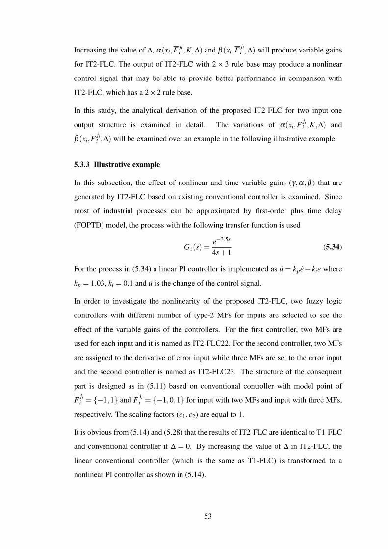
Increasing the value of ∆, α(xi,Fjii ,K,∆) and β (xi,F

jii ,∆) will produce variable gains

for IT2-FLC. The output of IT2-FLC with 2× 3 rule base may produce a nonlinear

control signal that may be able to provide better performance in comparison with

IT2-FLC, which has a 2×2 rule base.

In this study, the analytical derivation of the proposed IT2-FLC for two input-one

output structure is examined in detail. The variations of α(xi,Fjii ,K,∆) and

β (xi,Fjii ,∆) will be examined over an example in the following illustrative example.

5.3.3 Illustrative example

In this subsection, the effect of nonlinear and time variable gains (γ,α,β ) that are

generated by IT2-FLC based on existing conventional controller is examined. Since

most of industrial processes can be approximated by first-order plus time delay

(FOPTD) model, the process with the following transfer function is used

G1(s) =e−3.5s

4s+1(5.34)

For the process in (5.34) a linear PI controller is implemented as u = kpe+ kie where

kp = 1.03, ki = 0.1 and u is the change of the control signal.

In order to investigate the nonlinearity of the proposed IT2-FLC, two fuzzy logic

controllers with different number of type-2 MFs for inputs are selected to see the

effect of the variable gains of the controllers. For the first controller, two MFs are

used for each input and it is named as IT2-FLC22. For the second controller, two MFs

are assigned to the derivative of error input while three MFs are set to the error input

and the second controller is named as IT2-FLC23. The structure of the consequent

part is designed as in (5.11) based on conventional controller with model point of

F jii = {−1,1} and F ji

i = {−1,0,1} for input with two MFs and input with three MFs,

respectively. The scaling factors (c1,c2) are equal to 1.

It is obvious from (5.14) and (5.28) that the results of IT2-FLC are identical to T1-FLC

and conventional controller if ∆ = 0. By increasing the value of ∆ in IT2-FLC, the

linear conventional controller (which is the same as T1-FLC) is transformed to a

nonlinear PI controller as shown in (5.14).

53

0 50 100 1500

0.2

0.4

0.6

0.8

1

1.2

1.4

Time (s)

T1−FLC and PIIT2−FLC 22IT2−FLC 23

10 20 30 40 500.7

0.75

0.8

0.85

0.9

0.95

1

1.05

(a) the step responses

0 50 100 1500.5

0.6

0.7

0.8

0.9

1

1.1

1.2

1.3

1.4

1.5

Time (s)

Con

trol

Sig

nal

10 20 30 40 50

0.6

0.7

0.8

0.9

1

T1−FLC and PIIT2−FLC 22IT2−FLC 23

(b) the control signals

Figure 5.2: Illustration of the step responses the control signals for ∆ = 0.2.

Figure 5.2 shows the step responses and control signals of the process for the

conventional PI and IT2-FLC in the case ∆ is 0.2. By increasing the value of ∆ to 0.4,

the performance of IT2-FLC is improved compared to the conventional PI controller

as illustrated in Figure 5.3. As it has been proven in (5.29), IT2-FLC22 is a nonlinear

PI controller with a time varying parameter γ(x1,x2,∆). Figure 5.4 shows the variation

of γ(x1,x2,∆) for ∆ = 0.2 and ∆ = 0.4. It can be seen from Figure 5.4 that γ(x1,x2,∆)

is variable that acquires values smaller than 1.

By increasing the value of ∆ from 0.2 to 0.4, the value of the term γ(x1,x2,∆) will

decrease and produce variable gains for IT2-FLC. These gains will cause a smoother

54

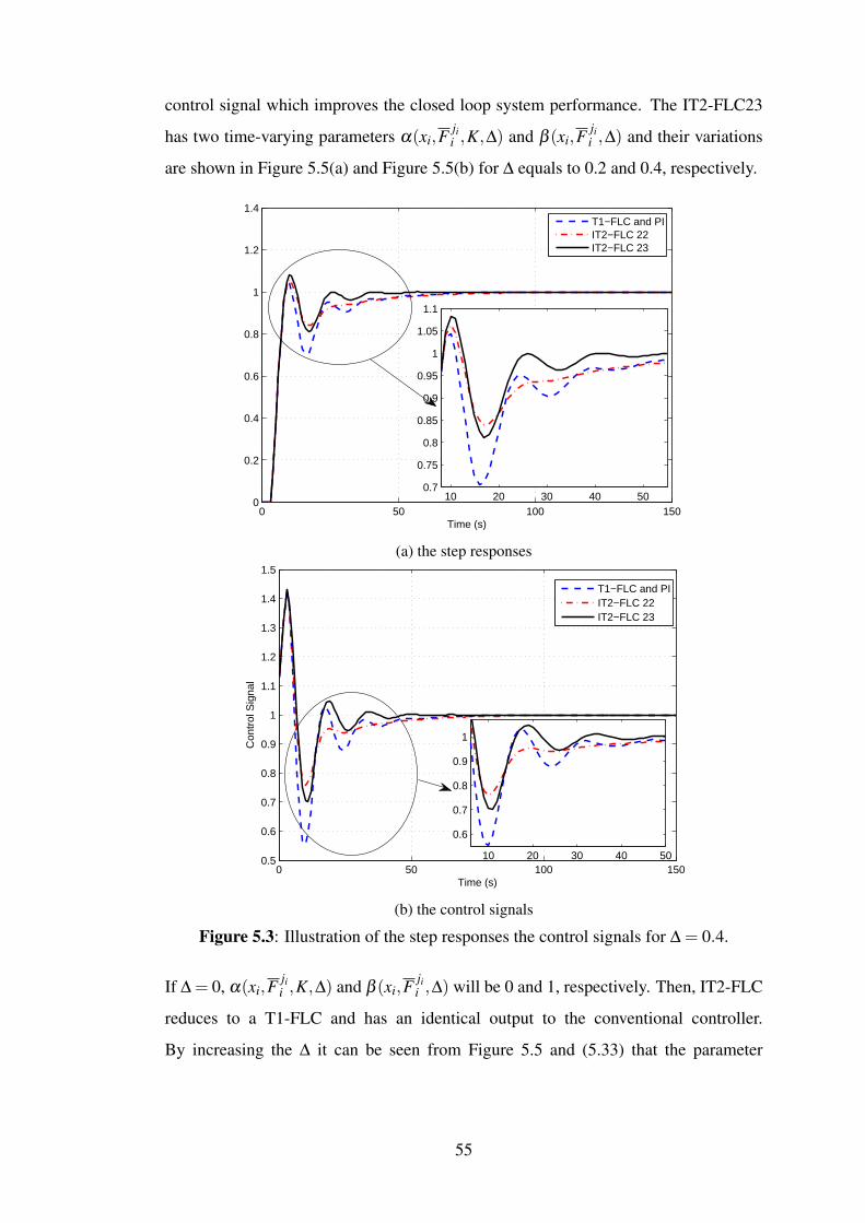
control signal which improves the closed loop system performance. The IT2-FLC23

has two time-varying parameters α(xi,Fjii ,K,∆) and β (xi,F

jii ,∆) and their variations

are shown in Figure 5.5(a) and Figure 5.5(b) for ∆ equals to 0.2 and 0.4, respectively.

0 50 100 1500

0.2

0.4

0.6

0.8

1

1.2

1.4

Time (s)

T1−FLC and PIIT2−FLC 22IT2−FLC 23

10 20 30 40 500.7

0.75

0.8

0.85

0.9

0.95

1

1.05

1.1

(a) the step responses

0 50 100 1500.5

0.6

0.7

0.8

0.9

1

1.1

1.2

1.3

1.4

1.5

Time (s)

Con

trol

Sig

nal

T1−FLC and PIIT2−FLC 22IT2−FLC 23

10 20 30 40 50

0.6

0.7

0.8

0.9

1

(b) the control signals

Figure 5.3: Illustration of the step responses the control signals for ∆ = 0.4.

If ∆ = 0, α(xi,Fjii ,K,∆) and β (xi,F

jii ,∆) will be 0 and 1, respectively. Then, IT2-FLC

reduces to a T1-FLC and has an identical output to the conventional controller.

By increasing the ∆ it can be seen from Figure 5.5 and (5.33) that the parameter

55

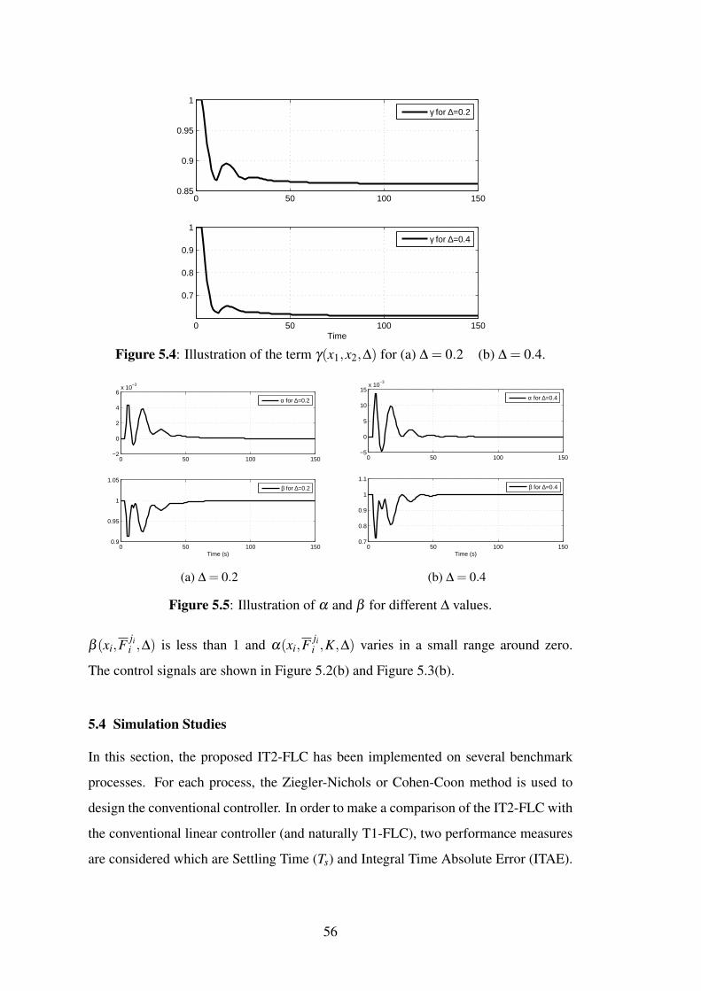
0 50 100 1500.85

0.9

0.95

1

γ for ∆=0.2

0 50 100 150

0.7

0.8

0.9

1

Time

γ for ∆=0.4

Figure 5.4: Illustration of the term γ(x1,x2,∆) for (a) ∆ = 0.2 (b) ∆ = 0.4.

0 50 100 150−2

0

2

4

6x 10

−3

α for ∆=0.2

0 50 100 1500.9

0.95

1

1.05

Time (s)

β for ∆=0.2

(a) ∆ = 0.2

0 50 100 150−5

0

5

10

15x 10

−3

α for ∆=0.4

0 50 100 1500.7

0.8

0.9

1

1.1

Time (s)

β for ∆=0.4

(b) ∆ = 0.4

Figure 5.5: Illustration of α and β for different ∆ values.

β (xi,Fjii ,∆) is less than 1 and α(xi,F

jii ,K,∆) varies in a small range around zero.

The control signals are shown in Figure 5.2(b) and Figure 5.3(b).

5.4 Simulation Studies

In this section, the proposed IT2-FLC has been implemented on several benchmark

processes. For each process, the Ziegler-Nichols or Cohen-Coon method is used to

design the conventional controller. In order to make a comparison of the IT2-FLC with

the conventional linear controller (and naturally T1-FLC), two performance measures

are considered which are Settling Time (Ts) and Integral Time Absolute Error (ITAE).

56

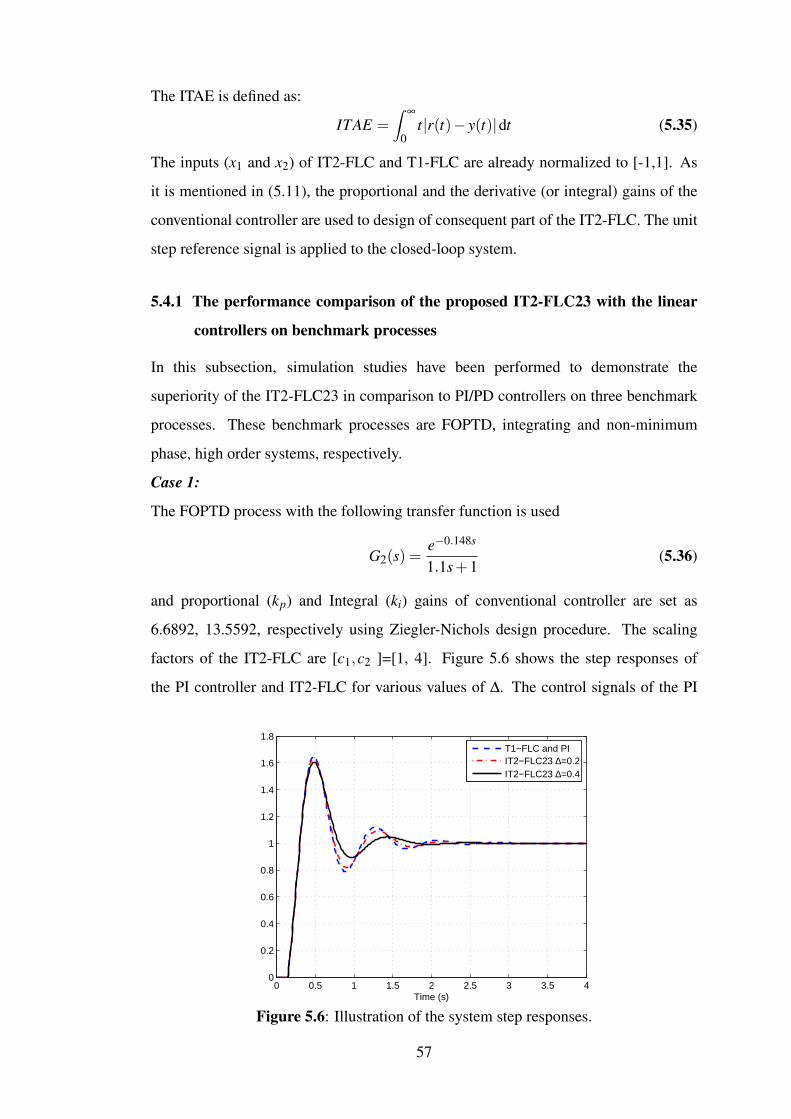
The ITAE is defined as:

ITAE =∫

∞

0t|r(t)− y(t)|dt (5.35)

The inputs (x1 and x2) of IT2-FLC and T1-FLC are already normalized to [-1,1]. As

it is mentioned in (5.11), the proportional and the derivative (or integral) gains of the

conventional controller are used to design of consequent part of the IT2-FLC. The unit

step reference signal is applied to the closed-loop system.

5.4.1 The performance comparison of the proposed IT2-FLC23 with the linear

controllers on benchmark processes

In this subsection, simulation studies have been performed to demonstrate the

superiority of the IT2-FLC23 in comparison to PI/PD controllers on three benchmark

processes. These benchmark processes are FOPTD, integrating and non-minimum

phase, high order systems, respectively.

Case 1:

The FOPTD process with the following transfer function is used

G2(s) =e−0.148s

1.1s+1(5.36)

and proportional (kp) and Integral (ki) gains of conventional controller are set as

6.6892, 13.5592, respectively using Ziegler-Nichols design procedure. The scaling

factors of the IT2-FLC are [c1,c2 ]=[1, 4]. Figure 5.6 shows the step responses of

the PI controller and IT2-FLC for various values of ∆. The control signals of the PI

0 0.5 1 1.5 2 2.5 3 3.5 40

0.2

0.4

0.6

0.8

1

1.2

1.4

1.6

1.8

Time (s)

T1−FLC and PIIT2−FLC23 ∆=0.2IT2−FLC23 ∆=0.4

Figure 5.6: Illustration of the system step responses.

57

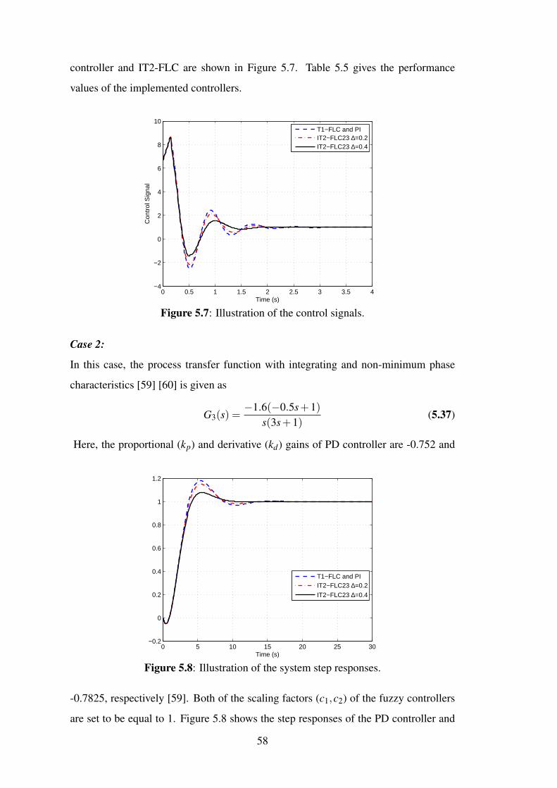
controller and IT2-FLC are shown in Figure 5.7. Table 5.5

values of the implemented controllers.

0 0.5 1 1.5 2 2.5 3 3.5 4−4

−2

0

2

4

6

8

10

Time (s)

Con

trol

Sig

nal

T1−FLC and PIIT2−FLC23 ∆=0.2IT2−FLC23 ∆=0.4

Figure 5.7: Illustration of the control signals.

Case 2:

In this case, the process transfer function with integrating and non-minimum phase

characteristics [59] [60] is given as

G3(s) =−1.6(−0.5s+1)

s(3s+1)(5.37)

Here, the proportional (kp) and derivative (kd) gains of PD controller are -0.752 and

0 5 10 15 20 25 30−0.2

0

0.2

0.4

0.6

0.8

1

1.2

Time (s)

T1−FLC and PIIT2−FLC23 ∆=0.2

IT2−FLC23 ∆=0.4

Figure 5.8: Illustration of the system step responses.

-0.7825, respectively [59]. Both of the scaling factors (c1,c2) of the fuzzy controllers

are set to be equal to 1. Figure 5.8 shows the step responses of the PD controller and

58

gives the performance

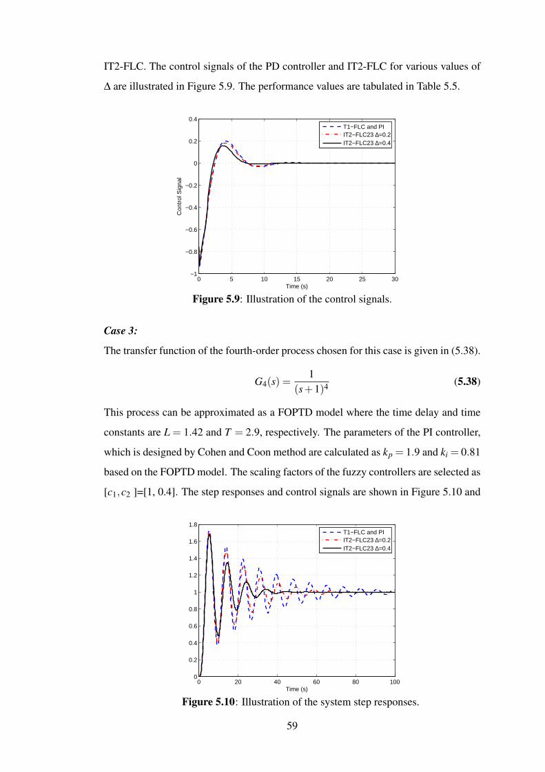
are illustrated in Figure 5.9. The performance values are tabulated in Table 5.5.

IT2-FLC. The control signals of the PD controller and IT2-FLC for various values of

∆

0 5 10 15 20 25 30−1

−0.8

−0.6

−0.4

−0.2

0

0.2

0.4

Time (s)

Con

trol

Sig

nal

T1−FLC and PIIT2−FLC23 ∆=0.2IT2−FLC23 ∆=0.4

Figure 5.9: Illustration of the control signals.

Case 3:

The transfer function of the fourth-order process chosen for this case is given in (5.38).

G4(s) =1

(s+1)4 (5.38)

This process can be approximated as a FOPTD model where the time delay and time

constants are L = 1.42 and T = 2.9, respectively. The parameters of the PI controller,

which is designed by Cohen and Coon method are calculated as kp = 1.9 and ki = 0.81

based on the FOPTD model. The scaling factors of the fuzzy controllers are selected as

[c1,c2 ]=[1, 0.4]. The step responses and control signals are shown in Figure 5.10 and

0 20 40 60 80 1000

0.2

0.4

0.6

0.8

1

1.2

1.4

1.6

1.8

Time (s)

T1−FLC and PIIT2−FLC23 ∆=0.2IT2−FLC23 ∆=0.4

Figure 5.10

59

: Illustration of the system step responses.

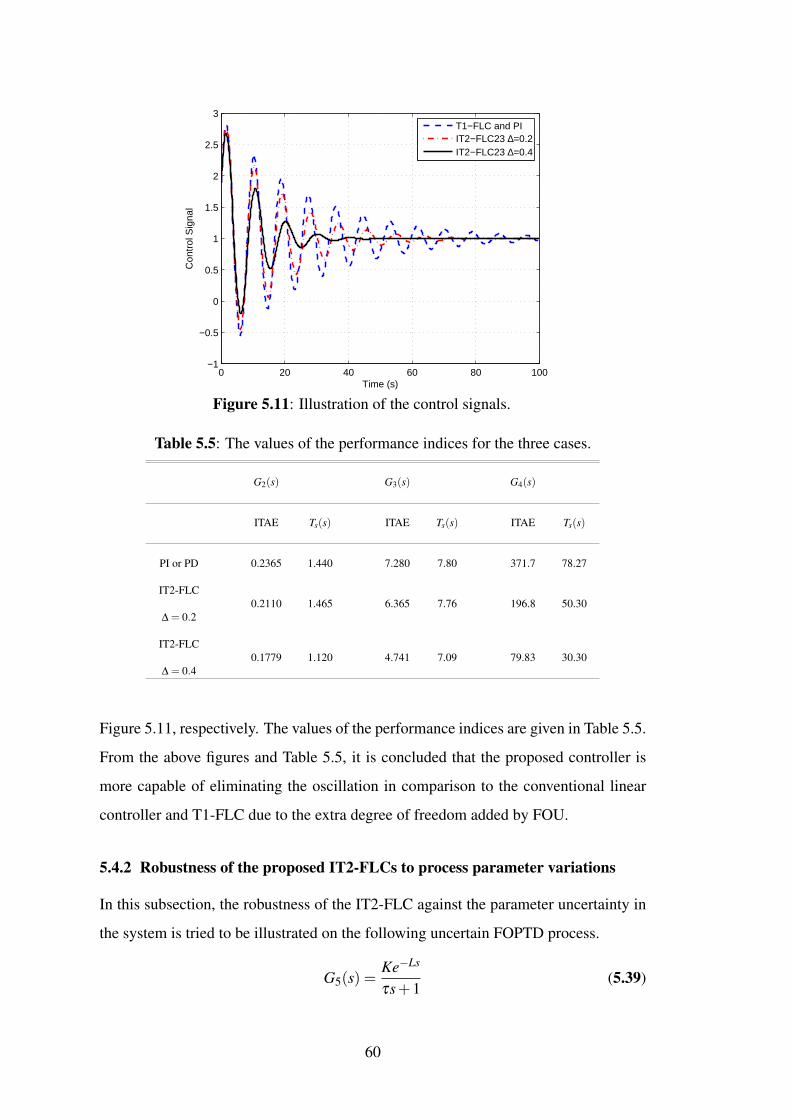
0 20 40 60 80 100−1

−0.5

0

0.5

1

1.5

2

2.5

3

Time (s)

Con

trol

Sig

nal

T1−FLC and PIIT2−FLC23 ∆=0.2IT2−FLC23 ∆=0.4

Figure 5.11

Table 5.5: The values of the performance indices for the three cases.

G2(s) G3(s) G4(s)

ITAE Ts(s) ITAE Ts(s) ITAE Ts(s)

PI or PD 0.2365 1.440 7.280 7.80 371.7 78.27

IT2-FLC0.2110 1.465 6.365 7.76 196.8 50.30

∆ = 0.2

IT2-FLC0.1779 1.120 4.741 7.09 79.83 30.30

∆ = 0.4

Figure 5.11, respectively. The values of the performance indices are given in Table 5.5.

From the above figures and Table 5.5, it is concluded that the proposed controller is

more capable of eliminating the oscillation in comparison to the conventional linear

controller and T1-FLC due to the extra degree of freedom added by FOU.

5.4.2 Robustness of the proposed IT2-FLCs to process parameter variations

In this subsection, the robustness of the IT2-FLC against the parameter uncertainty in

the system is tried to be illustrated on the following uncertain FOPTD process.

G5(s) =Ke−Ls

τs+1(5.39)

60

: Illustration of the control signals.

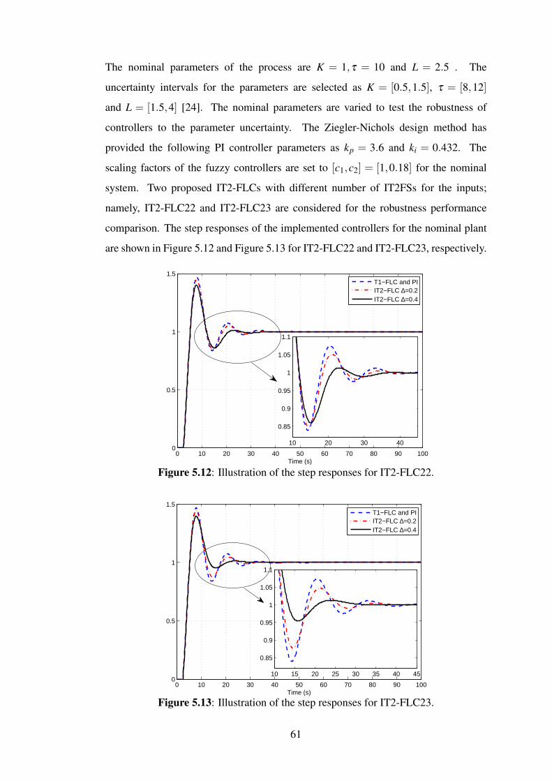
The nominal parameters of the process are K = 1,τ = 10 and L = 2.5 . The

uncertainty intervals for the parameters are selected as K = [0.5,1.5], τ = [8,12]

and L = [1.5,4] [24]. The nominal parameters are varied to test the robustness of

controllers to the parameter uncertainty. The Ziegler-Nichols design method has

provided the following PI controller parameters as kp = 3.6 and ki = 0.432. The

scaling factors of the fuzzy controllers are set to [c1,c2] = [1,0.18] for the nominal

system. Two proposed IT2-FLCs with different number of IT2FSs for the inputs;

namely, IT2-FLC22 and IT2-FLC23 are considered for the robustness performance

comparison. The step responses of the implemented controllers for the nominal plant

are shown in Figure 5.12 and Figure 5.13 for IT2-FLC22 and IT2-FLC23, respectively.

0 10 20 30 40 50 60 70 80 90 1000

0.5

1

1.5

Time (s)

10 20 30 40

0.85

0.9

0.95

1

1.05

1.1

T1−FLC and PIIT2−FLC ∆=0.2IT2−FLC ∆=0.4

Figure 5.12: Illustration of the step responses for IT2-FLC22.

0 10 20 30 40 50 60 70 80 90 1000

0.5

1

1.5

Time (s)

T1−FLC and PIIT2−FLC ∆=0.2IT2−FLC ∆=0.4

10 15 20 25 30 35 40 45

0.85

0.9

0.95

1

1.05

1.1

Figure 5.13: Illustration of the step responses for IT2-FLC23.

61

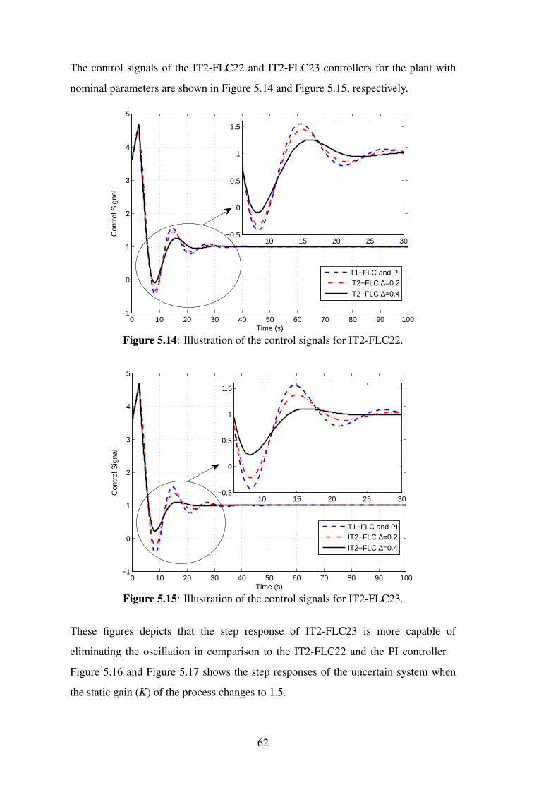
The control signals of the IT2-FLC22 and IT2-FLC23 controllers for the plant with

nominal parameters are shown in Figure 5.14 and Figure 5.15, respectively.

0 10 20 30 40 50 60 70 80 90 100−1

0

1

2

3

4

5

Time (s)

Con

trol

Sig

nal

T1−FLC and PIIT2−FLC ∆=0.2

IT2−FLC ∆=0.4

10 15 20 25 30−0.5

0

0.5

1

1.5

Figure 5.14: Illustration of the control signals for IT2-FLC22.

0 10 20 30 40 50 60 70 80 90 100−1

0

1

2

3

4

5

Time (s)

Con

trol

Sig

nal

T1−FLC and PIIT2−FLC ∆=0.2

IT2−FLC ∆=0.4

10 15 20 25 30−0.5

0

0.5

1

1.5

Figure 5.15: Illustration of the control signals for IT2-FLC23.

These figures depicts that the step response of IT2-FLC23 is more capable of

eliminating the oscillation in comparison to the IT2-FLC22 and the PI controller.

Figure 5.16 and Figure 5.17 shows the step responses of the uncertain system when

the static gain (K) of the process changes to 1.5.

62

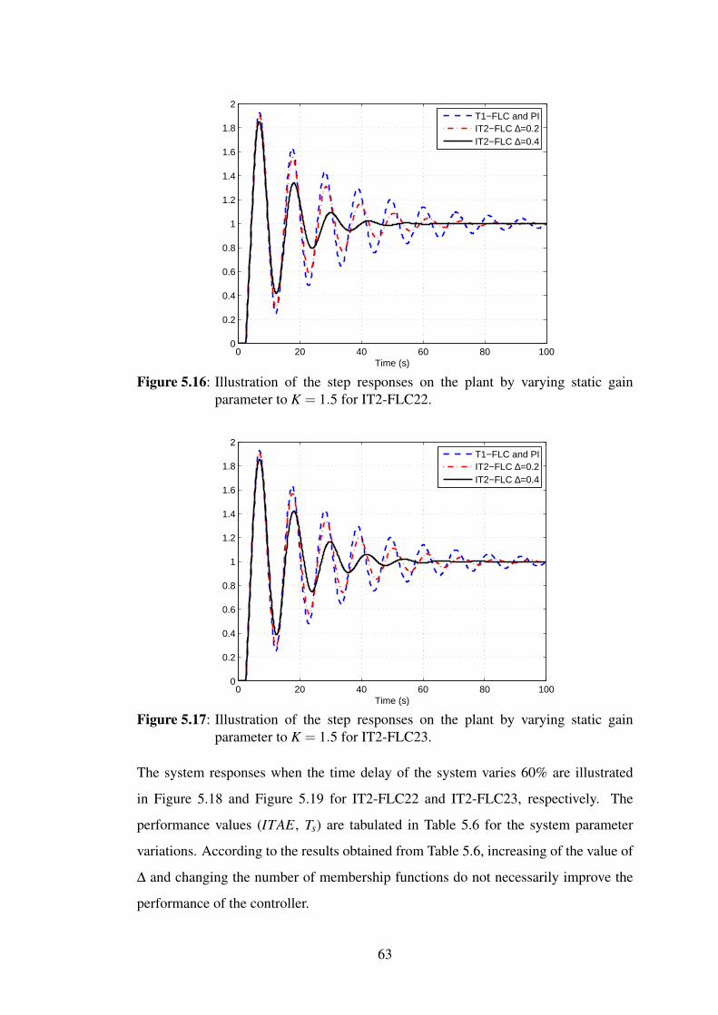
0 20 40 60 80 1000

0.2

0.4

0.6

0.8

1

1.2

1.4

1.6

1.8

2

Time (s)

T1−FLC and PIIT2−FLC ∆=0.2IT2−FLC ∆=0.4

Figure 5.16: Illustration of the step responses on the plant by varying static gainparameter to K = 1.5 for IT2-FLC22.

0 20 40 60 80 1000

0.2

0.4

0.6

0.8

1

1.2

1.4

1.6

1.8

2

Time (s)

T1−FLC and PIIT2−FLC ∆=0.2IT2−FLC ∆=0.4

Figure 5.17: Illustration of the step responses on the plant by varying static gainparameter to K = 1.5 for IT2-FLC23.

The system responses when the time delay of the system varies 60% are illustrated

in Figure 5.18 and Figure 5.19 for IT2-FLC22 and IT2-FLC23, respectively. The

performance values (ITAE, Ts) are tabulated in Table 5.6 for the system parameter

variations. According to the results obtained from Table 5.6, increasing of the value of

∆ and changing the number of membership functions do not necessarily improve the

performance of the controller.

63

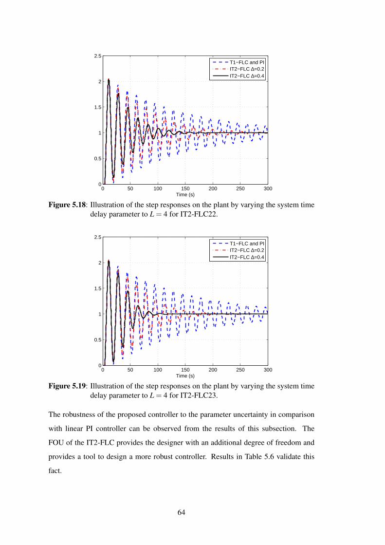
0 50 100 150 200 250 3000

0.5

1

1.5

2

2.5

Time (s)

T1−FLC and PIIT2−FLC ∆=0.2IT2−FLC ∆=0.4

Figure 5.18: Illustration of the step responses on the plant by varying the system timedelay parameter to L = 4 for IT2-FLC22.

0 50 100 150 200 250 3000

0.5

1

1.5

2

2.5

Time (s)

T1−FLC and PIIT2−FLC ∆=0.2IT2−FLC ∆=0.4

Figure 5.19: Illustration of the step responses on the plant by varying the system timedelay parameter to L = 4 for IT2-FLC23.

The robustness of the proposed controller to the parameter uncertainty in comparison

with linear PI controller can be observed from the results of this subsection. The

FOU of the IT2-FLC provides the designer with an additional degree of freedom and

provides a tool to design a more robust controller. Results in Table 5.6 validate this

fact.

64

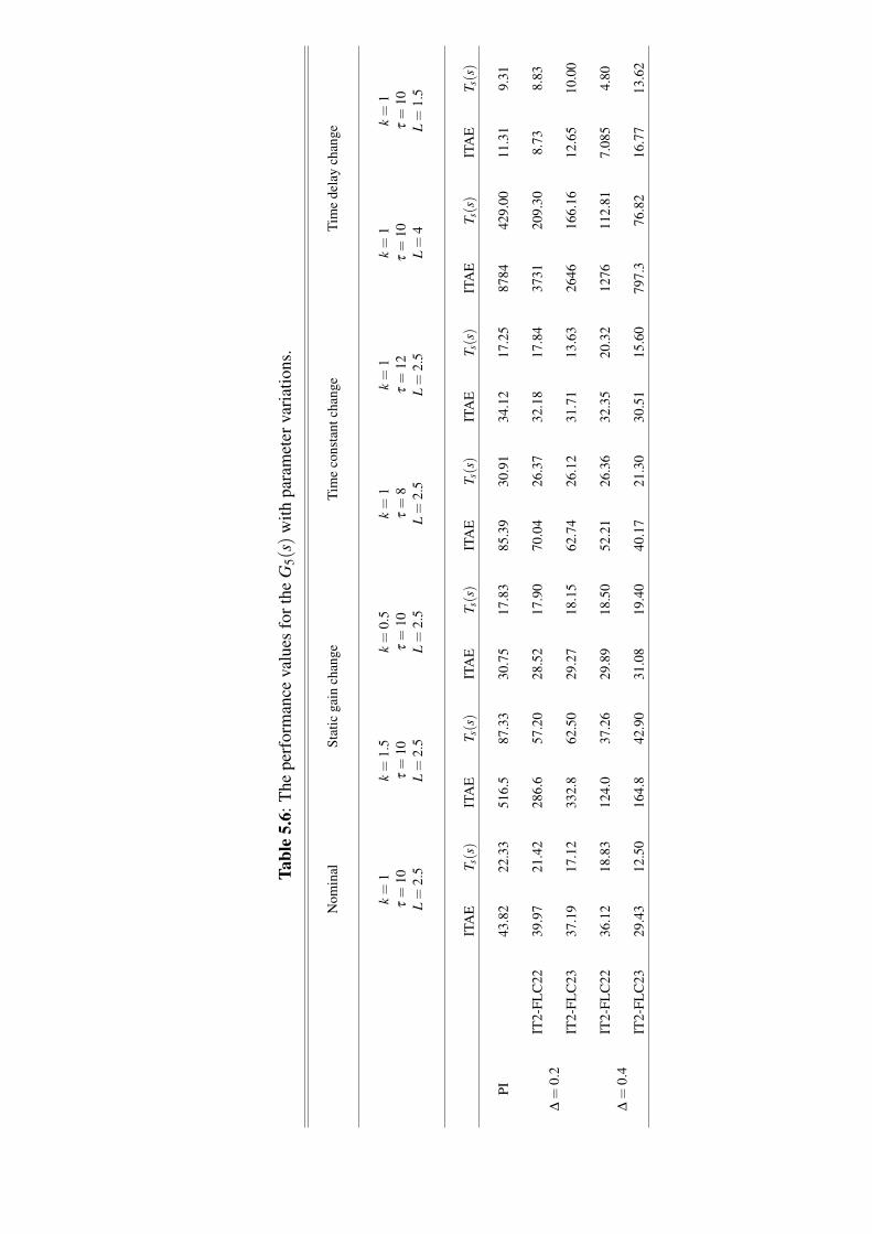
Tabl

e5.

6:T

hepe

rfor

man

ceva

lues

fort

heG

5(s)

with

para

met

erva

riat

ions

.

Nom

inal

Stat

icga

inch

ange

Tim

eco

nsta

ntch

ange

Tim

ede

lay

chan

ge

k=

1k=

1.5

k=

0.5

k=

1k=

1k=

1k=

1τ=

10τ=

10τ=

10τ=

8τ=

12τ=

10τ=

10L=

2.5

L=

2.5

L=

2.5

L=

2.5

L=

2.5

L=

4L=

1.5

ITA

ET s(s)

ITA

ET s(s)

ITA

ET s(s)

ITA

ET s(s)

ITA

ET s(s)

ITA

ET s(s)

ITA

ET s(s)

PI43

.82

22.3

351

6.5

87.3

330

.75

17.8

385

.39

30.9

134

.12

17.2

587

8442

9.00

11.3

19.

31

IT2-

FLC

2239

.97

21.4

228

6.6

57.2

028

.52

17.9

070

.04

26.3

732

.18

17.8

437

3120

9.30

8.73

8.83

∆=

0.2

IT2-

FLC

2337

.19

17.1

233

2.8

62.5

029

.27

18.1

562

.74

26.1

231

.71

13.6

326

4616

6.16

12.6

510

.00

IT2-

FLC

2236

.12

18.8

312

4.0

37.2

629

.89

18.5

052

.21

26.3

632

.35

20.3

212

7611

2.81

7.08

54.

80∆=

0.4

IT2-

FLC

2329

.43

12.5

016

4.8

42.9

031

.08

19.4

040

.17

21.3

030

.51

15.6

079

7.3

76.8

216

.77

13.6

2

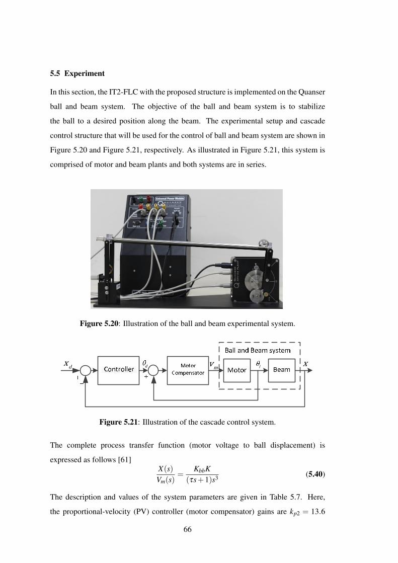
5.5 Experiment

In this section, the IT2-FLC with the proposed structure is implemented on the Quanser

ball and beam system. The objective of the ball and beam system is to stabilize

the ball to a desired position along the beam. The experimental setup and cascade

control structure that will be used for the control of ball and beam system are shown in

Figure 5.20 and Figure 5.21, respectively. As illustrated in Figure 5.21, this system is

comprised of motor and beam plants and both systems are in series.

Figure 5.20: Illustration of the ball and beam experimental system.

Figure 5.21: Illustration of the cascade control system.

The complete process transfer function (motor voltage to ball displacement) is

expressed as follows [61]X(s)Vm(s)

=KbbK

(τs+1)s3 (5.40)

The description and values of the system parameters are given in Table 5.7. Here,

the proportional-velocity (PV) controller (motor compensator) gains are kp2 = 13.6

66

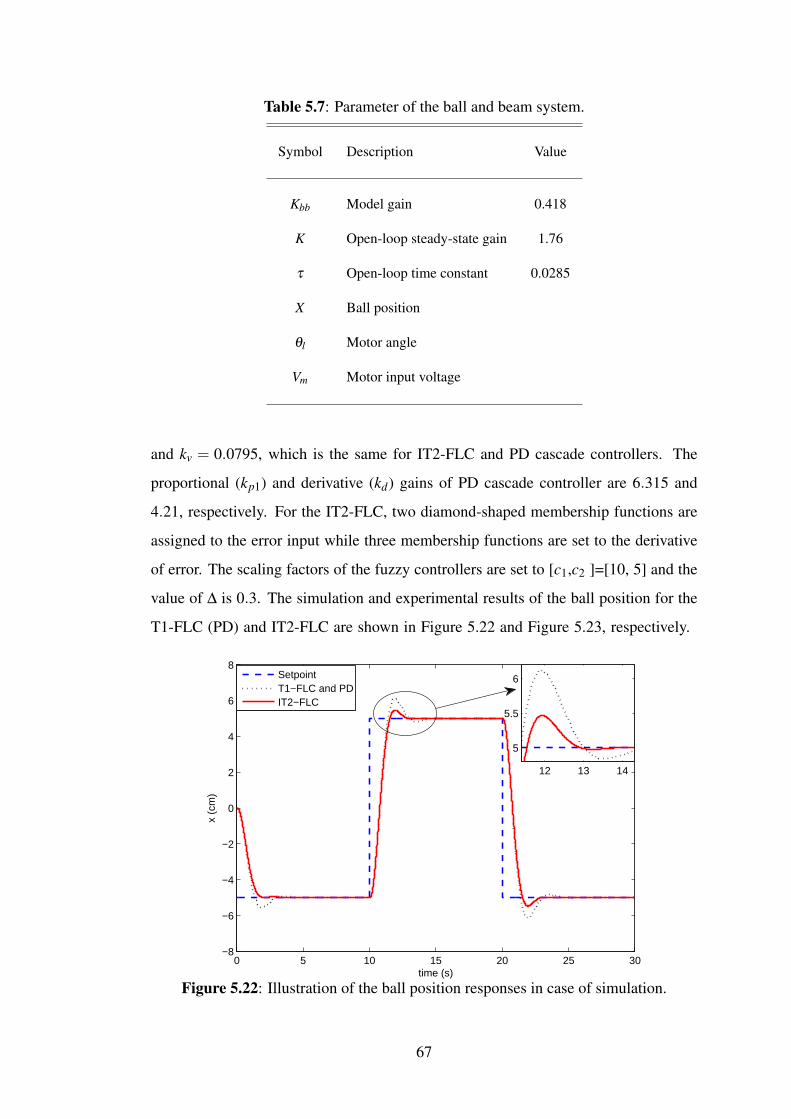
Table 5.7: Parameter of the ball and beam system.

Symbol Description Value

Kbb Model gain 0.418

K Open-loop steady-state gain 1.76

τ Open-loop time constant 0.0285

X Ball position

θl Motor angle

Vm Motor input voltage

and kv = 0.0795, which is the same for IT2-FLC and PD cascade controllers. The

proportional (kp1) and derivative (kd) gains of PD cascade controller are 6.315 and

4.21, respectively. For the IT2-FLC, two diamond-shaped membership functions are

assigned to the error input while three membership functions are set to the derivative

of error. The scaling factors of the fuzzy controllers are set to [c1,c2 ]=[10, 5] and the

value of ∆ is 0.3. The simulation and experimental results of the ball position for the

T1-FLC (PD) and IT2-FLC are shown in Figure 5.22 and Figure 5.23, respectively.

0 5 10 15 20 25 30−8

−6

−4

−2

0

2

4

6

8

x (c

m)

time (s)

SetpointT1−FLC and PDIT2−FLC

12 13 14

5

5.5

6

Figure 5.22: Illustration of the ball position responses in case of simulation.

67

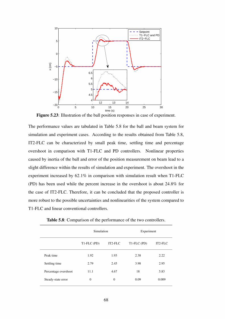
0 5 10 15 20 25 30−20

−15

−10

−5

0

5

10

x (c

m)

time (s)

SetpointT1−FLC and PDIT2−FLC

12 13 144

4.5

5

5.5

6

6.5

Figure 5.23: Illustration of the ball position responses in case of experiment.

The performance values are tabulated in Table 5.8 for the ball and beam system for

simulation and experiment cases. According to the results obtained from Table 5.8,

IT2-FLC can be characterized by small peak time, settling time and percentage

overshoot in comparison with T1-FLC and PD controllers. Nonlinear properties

caused by inertia of the ball and error of the position measurement on beam lead to a

slight difference within the results of simulation and experiment. The overshoot in the

experiment increased by 62.1% in comparison with simulation result when T1-FLC

(PD) has been used while the percent increase in the overshoot is about 24.8% for

the case of IT2-FLC. Therefore, it can be concluded that the proposed controller is

more robust to the possible uncertainties and nonlinearities of the system compared to

T1-FLC and linear conventional controllers.

Table 5.8: Comparison of the performance of the two controllers.

Simulation Experiment

T1-FLC (PD) IT2-FLC T1-FLC (PD) IT2-FLC

Peak time 1.92 1.93 2.38 2.22

Settling time 2.79 2.45 3.98 2.95

Percentage overshoot 11.1 4.67 18 5.83

Steady-state error 0 0 0.09 0.009

68

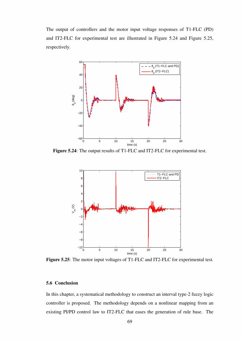
The output of controllers and the motor input voltage responses of T1-FLC (PD)

and IT2-FLC for experimental test are illustrated in Figure 5.24 and Figure 5.25,

respectively.

0 5 10 15 20 25 30−60

−40

−20

0

20

40

60

θ d (de

g)

time (s)

θ

d (T1−FLC and PD)

θd (IT2−FLC)

Figure 5.24: The output results of T1-FLC and IT2-FLC for experimental test.

0 5 10 15 20 25 30−10

−8

−6

−4

−2

0

2

4

6

8

10

Vm

(V

)

time (s)

T1−FLC and PDIT2−FLC

Figure 5.25: The motor input voltages of T1-FLC and IT2-FLC for experimental test.

5.6 Conclusion

In this chapter, a systematical methodology to construct an interval type-2 fuzzy logic

controller is proposed. The methodology depends on a nonlinear mapping from an

existing PI/PD control law to IT2-FLC that eases the generation of rule base. The

69

structure of the proposed controller is achieved under circumstances that input type-2

MFs are diamond-shaped and a certain closed-form inference engine is used. It has

been proven that these preferences provide a closed-form for the output of IT2-FLC.

Then, certain elaborations can be done on the parameters of the evolved closed output

form. If the FOU of the IT2-FLC is zero then the obtained control law is identical

to the conventional PI/PD controller. If FOU is not equal to zero, then an additional

degree of freedom is acquired and this provides the designer an additional tool to cope

with the uncertainties and nonlinearities.

Results show that the proposed controller is more robust to the parameter uncertainties

and eliminate the oscillations much better than type-1 fuzzy logic and linear

conventional controllers. However, it is not so fair and right to draw a general

conclusion that the system performance is necessarily guaranteed to be improved for

all systems and design methodologies. The analysis for the proposed IT2-FLC can be

generalized to different number and type of MFs for the inputs.

70

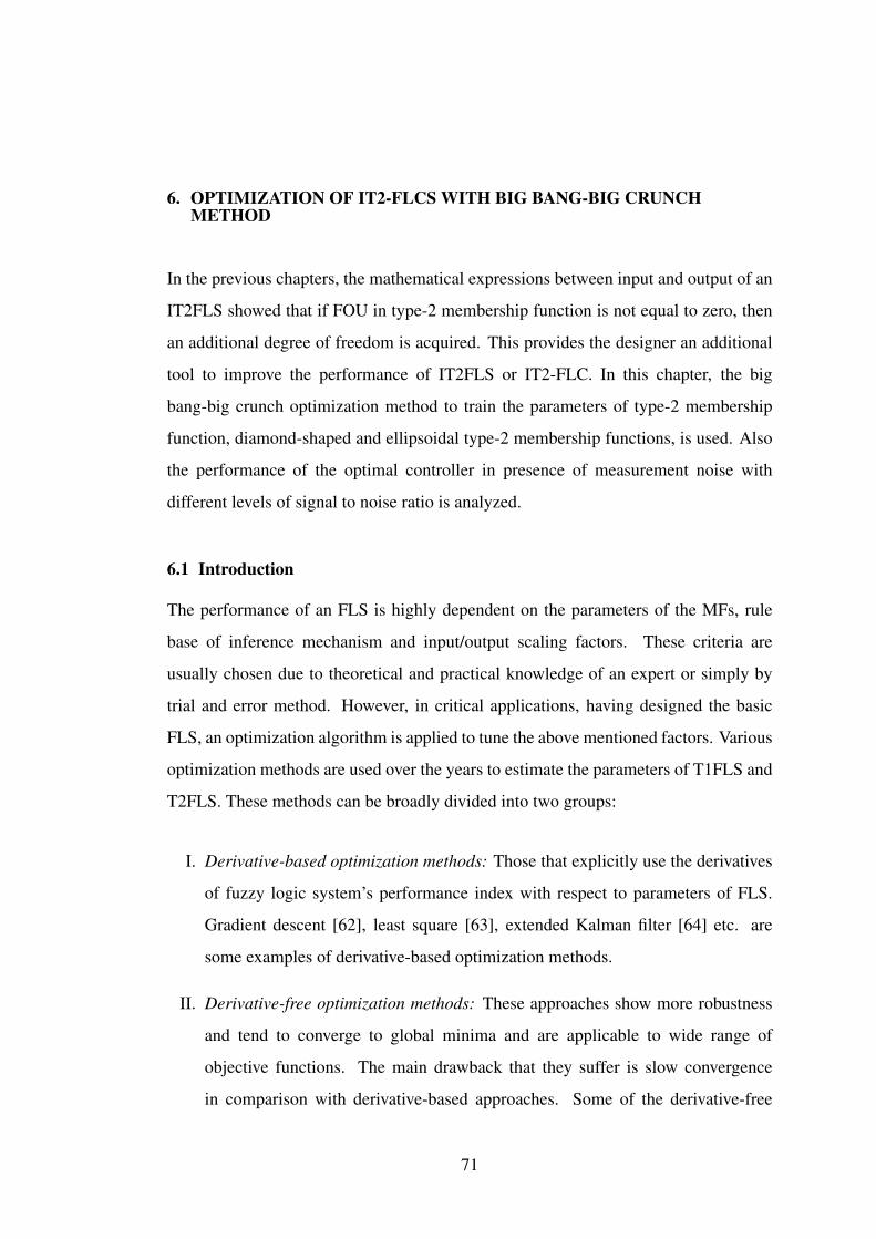
6. OPTIMIZATION OF IT2-FLCS WITH BIG BANG-BIG CRUNCHMETHOD

In the previous chapters, the mathematical expressions between input and output of an

IT2FLS showed that if FOU in type-2 membership function is not equal to zero, then

an additional degree of freedom is acquired. This provides the designer an additional

tool to improve the performance of IT2FLS or IT2-FLC. In this chapter, the big

bang-big crunch optimization method to train the parameters of type-2 membership

function, diamond-shaped and ellipsoidal type-2 membership functions, is used. Also

the performance of the optimal controller in presence of measurement noise with

different levels of signal to noise ratio is analyzed.

6.1 Introduction

The performance of an FLS is highly dependent on the parameters of the MFs, rule

base of inference mechanism and input/output scaling factors. These criteria are

usually chosen due to theoretical and practical knowledge of an expert or simply by

trial and error method. However, in critical applications, having designed the basic

FLS, an optimization algorithm is applied to tune the above mentioned factors. Various

optimization methods are used over the years to estimate the parameters of T1FLS and

T2FLS. These methods can be broadly divided into two groups:

I. Derivative-based optimization methods: Those that explicitly use the derivatives

of fuzzy logic system’s performance index with respect to parameters of FLS.

Gradient descent [62], least square [63], extended Kalman filter [64] etc. are

some examples of derivative-based optimization methods.

II. Derivative-free optimization methods: These approaches show more robustness

and tend to converge to global minima and are applicable to wide range of

objective functions. The main drawback that they suffer is slow convergence

in comparison with derivative-based approaches. Some of the derivative-free

71

methods are genetic algorithm [65], neural network [66], evolutionary

programming [67], big bang-big crunch (BB-BC) [68], etc.

IT2FLSs have been used successfully in a number of applications and various

optimization methods have been applied in the design of optimal IT2FLS. The methods

for designing an optimal IT2FLS can be classified into two categories. The first

category of methods assumes that an optimal (in some sense) T1FLS has already been

designed and afterwards a IT2FLS is constructed through some sound augmentation

of the existing model. The second class of design methods is concerned with the

construction of the IT2FLS directly from experimental data. In both cases, an

optimization method can help in obtaining the optimal IT2FLS for the particular

application [56].

Genetic algorithm was used by D. Wu and W. Tan [9] in optimization of IT2-FLC.

They apply genetic algorithm to design of IT2-FLC for the coupled-tank system.

Experimental results show that better control can be achieved using an IT2-FLC with

fewer fuzzy sets or rules. In [69], genetic algorithms and particle swarm optimization

methods were applied to design type-2 fuzzy controllers to minimize the steady

state error of linear plants. The optimal controllers obtained by two optimization

methods were compared using benchmark plants. The application of ant colony and

particle swarm optimization for the optimization of an interval type-2 fuzzy logic

controller for an autonomous wheeled mobile robot was presented in [70]. The

BB-BC optimization algorithm was used for type-2 fuzzy model inverse controller

design in [71]. The control performance of the proposed method was compared with

a type-1 fuzzy model inverse control structure. In [72] authors employed extended

Kalman filter for the optimization of the parameters of type-2 fuzzy logic systems.

The proposed type-2 fuzzy neuro structure was tested on different noisy input–output

data sets, and the results were compared with the particle swarm optimization and

gradient descent-based methods. A novel design methodology of interval type-2

Takagi Sugeno Kang fuzzy logic controllers for modular and reconfigurable robots

manipulators with uncertain dynamic parameters was presented in [73]. Authors

develop a mathematical framework for the design of IT2 TSK FLCs for tracking

purposes that can be effectively used in real-time applications.

72

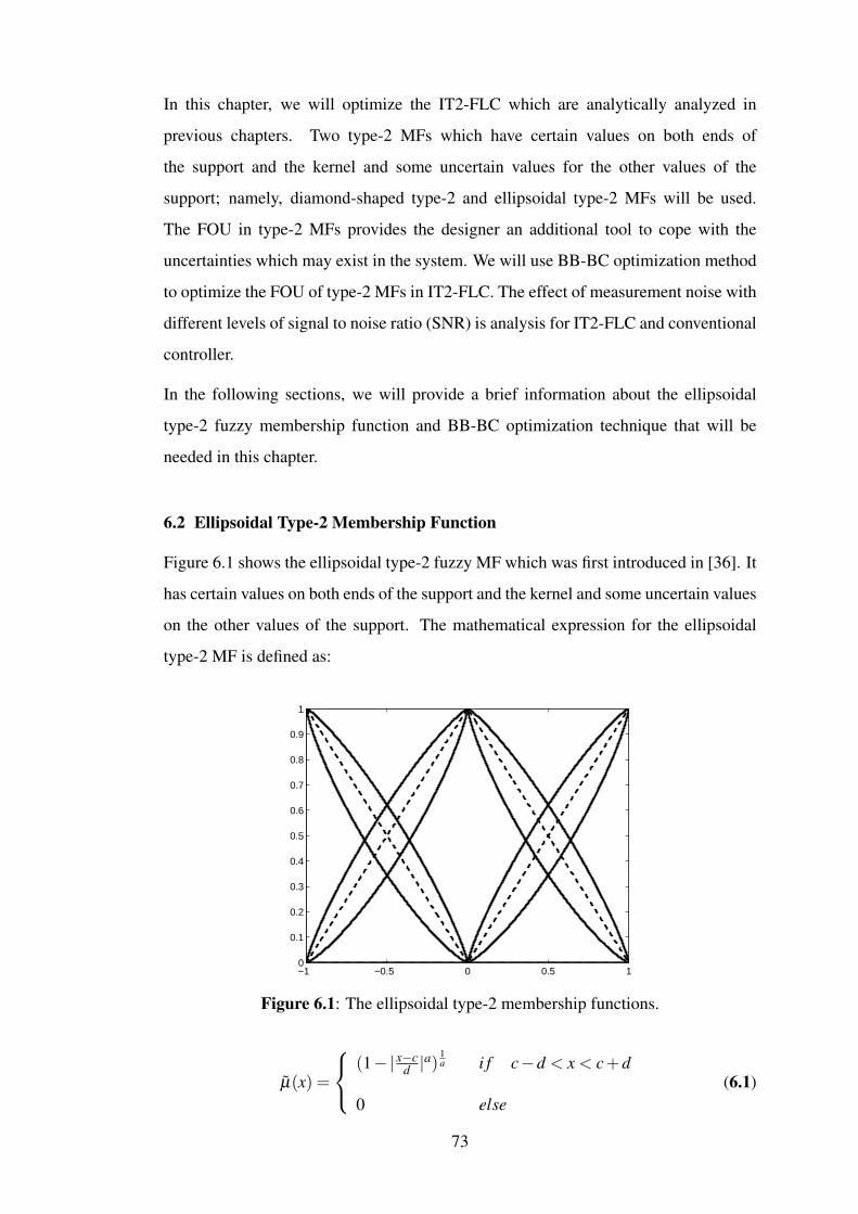
In this chapter, we will optimize the IT2-FLC which are analytically analyzed in

previous chapters. Two type-2 MFs which have certain values on both ends of

the support and the kernel and some uncertain values for the other values of the

support; namely, diamond-shaped type-2 and ellipsoidal type-2 MFs will be used.

The FOU in type-2 MFs provides the designer an additional tool to cope with the

uncertainties which may exist in the system. We will use BB-BC optimization method

to optimize the FOU of type-2 MFs in IT2-FLC. The effect of measurement noise with

different levels of signal to noise ratio (SNR) is analysis for IT2-FLC and conventional

controller.

In the following sections, we will provide a brief information about the ellipsoidal

type-2 fuzzy membership function and BB-BC optimization technique that will be

needed in this chapter.

6.2 Ellipsoidal Type-2 Membership Function

Figure 6.1 shows the ellipsoidal type-2 fuzzy MF which was first introduced in [36]. It

has certain values on both ends of the support and the kernel and some uncertain values

on the other values of the support. The mathematical expression for the ellipsoidal

type-2 MF is defined as:

−1 −0.5 0 0.5 10

0.1

0.2

0.3

0.4

0.5

0.6

0.7

0.8

0.9

1

Figure 6.1: The ellipsoidal type-2 membership functions.

µ(x) =

(1−|x−cd |

a)1a i f c−d < x < c+d

0 else(6.1)

73

where c and d are the center and the width of the MF, respectively and x is the input

vector. The parameters a1 and a2 (a2 < a < a1) determine the width of the uncertainty

of the proposed MF, and these parameters should be selected as the following form:

a1 > 1 (6.2)

0 < a2 < 1 (6.3)

The shape of the ellipsoidal type-2 MF is changed to that of a type-1 triangular MF

when its parameters are selected as a1 = a2 = 1. These parameters can be selected as

some constants, or they can be tuned adaptively [36].

6.3 Big Bang-Big Crunch Optimization Method

This section introduces the BB-BC optimization method. In [68] the authors propose a

new optimization method which is relied on the big bang and big crunch theory of the

evolution of the universe. The BB-BC optimization method has a low computational

time and high convergence speed. The performance of this method demonstrates

superiority and outperforms the classical genetic algorithm for many benchmark test

functions. The big bang and big crunch are two main steps of BB-BC optimization

method. In the former phase, candidate solutions are randomly distributed over the

search space and the latter phase works as a convergence operator where the center

of mass is generated. The initial big bang population is randomly generated over the

entire search space. All subsequent big bang phases are randomly distributed about

the center of mass or the best fit individual in a similar fashion. The procedure of the

BB-BC optimization can be summarized as the below [68]

Step 1: Big Bang Phase

An initial generation of N candidates is generated randomly in the search

space.

Step 2: The cost function values of all the candidate solutions are computed.

Step 3: Big Crunch Phase

The center of mass is calculated. Either the best fit individual or the center of

mass is chosen as the point of big bang Phase.

74

Step 4: The new candidates are calculated around the new point calculated in Step 3 by

adding or subtracting a random number whose value decreases as the iterations

elapse.

Step 5: Return to Step 2 until stopping criteria has been met.

In this chapter, the optimal FOU parameters of IT2-FLC is adjusted using the BB-BC

optimization method and the cost function J that is minimized is chosen as:

J = ITAE =∫

∞

0t|r(t)− y(t)|dt (6.4)

where r(t) and y(t) are the reference input and the output of plant, respectively.

6.4 Simulation Studies

In this section, the simulation results of the optimal IT2-FLC are presented. In previous

chapter, we have designed an IT2-FLC based on conventional PI or PD controller. As

it can be seen from this chapter, the parameters of type-2 MF which produce FOU

in MF changes the conventional controller (or T1-FLC) to nonlinear PI/PD controller

with variable gains. It is obvious that, by tuning these parameters, the designer will

be able to reduce or increase the value of control signal in order to achieve a better

performance.

The FOPTD process and IT2-FLC with the same structure introduced in

subsection 5.4.2 on page 60 are used. Two diamond-shaped and ellipsoidal type-2 MFs

are used for each input. With the purpose of study the effect of noise in the proposed

controller, the output of system is corrupted with white gaussian noise by different

levels of SNR. Three performance measures which are Integral Time Absolute Error

(ITAE), Integral Absolute Error (IAE) and settling time (Ts) are considered to make a

comparison of the optimal IT2-FLC with the PI and T1-FLC. The unit step reference

signal is applied to the closed-loop system. Figure 6.2 shows the step responses of

the FOPTD system in (5.39) when parameters of type-2 MF, (∆,a1,a2), are optimized

by BB-BC optimization method. The control signals of T1-FLC (PI) and optimal

IT2-FLC with two different MFs are illustrated in Figure 6.3. The performance

measures of conventional PI and optimal IT2-FLC with two different type-2 MFs are

given in Table 6.1.

75

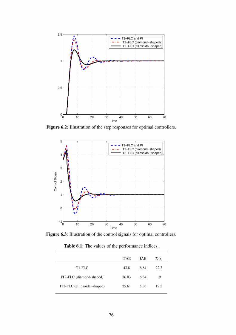
0 10 20 30 40 50 60 700

0.5

1

1.5

Time

T1−FLC and PIIT2−FLC (diamond−shaped)IT2−FLC (ellipsoidal−shaped)

Figure 6.2: Illustration of the step responses for optimal controllers.

0 10 20 30 40 50 60 70−1

0

1

2

3

4

5

Time

Con

trol

Sig

nal

T1−FLC and PIIT2−FLC (diamond−shaped)IT2−FLC (ellipsoidal−shaped)

Figure 6.3: Illustration of the control signals for optimal controllers.

Table 6.1: The values of the performance indices.

ITAE IAE Ts(s)

T1-FLC 43.8 6.84 22.3

IT2-FLC (diamond-shaped) 36.03 6.34 19

IT2-FLC (ellipsoidal-shaped) 25.61 5.36 19.5

76

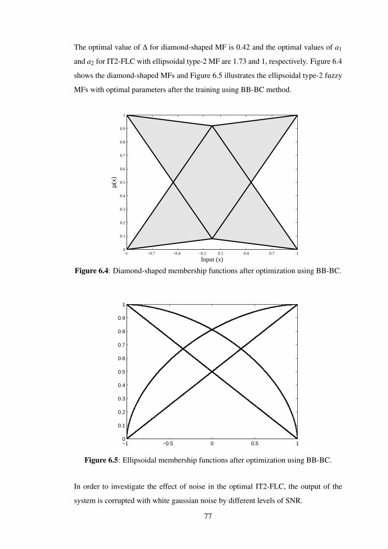
The optimal value of ∆ for diamond-shaped MF is 0.42 and the optimal values of a1

and a2 for IT2-FLC with ellipsoidal type-2 MF are 1.73 and 1, respectively. Figure 6.4

shows the diamond-shaped MFs and Figure 6.5 illustrates the ellipsoidal type-2 fuzzy

MFs with optimal parameters after the training using BB-BC method.

−1 −0.7 −0.4 −0.1 0.1 0.4 0.7 10

0.1

0.2

0.3

0.4

0.5

0.6

0.7

0.8

0.9

1

Input (x)

µ(x)

Figure 6.4: Diamond-shaped membership functions after optimization using BB-BC.

−1 −0.5 0 0.5 10

0.1

0.2

0.3

0.4

0.5

0.6

0.7

0.8

0.9

1

Figure 6.5: Ellipsoidal membership functions after optimization using BB-BC.

In order to investigate the effect of noise in the optimal IT2-FLC, the output of the

system is corrupted with white gaussian noise by different levels of SNR.

77

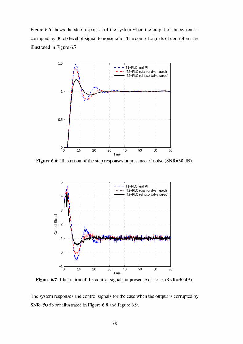
Figure 6.6 shows the step responses of the system when the output of the system is

corrupted by 30 db level of signal to noise ratio. The control signals of controllers are

illustrated in Figure 6.7.

0 10 20 30 40 50 60 700

0.5

1

1.5

Time

T1−FLC and PIIT2−FLC (diamond−shaped)IT2−FLC (ellipsoidal−shaped)

Figure 6.6: Illustration of the step responses in presence of noise (SNR=30 dB).

0 10 20 30 40 50 60 70−1

0

1

2

3

4

5

Time

Con

trol

Sig

nal

T1−FLC and PIIT2−FLC (diamond−shaped)IT2−FLC (ellipsoidal−shaped)

Figure 6.7: Illustration of the control signals in presence of noise (SNR=30 dB).

The system responses and control signals for the case when the output is corrupted by

SNR=50 db are illustrated in Figure 6.8 and Figure 6.9.

78

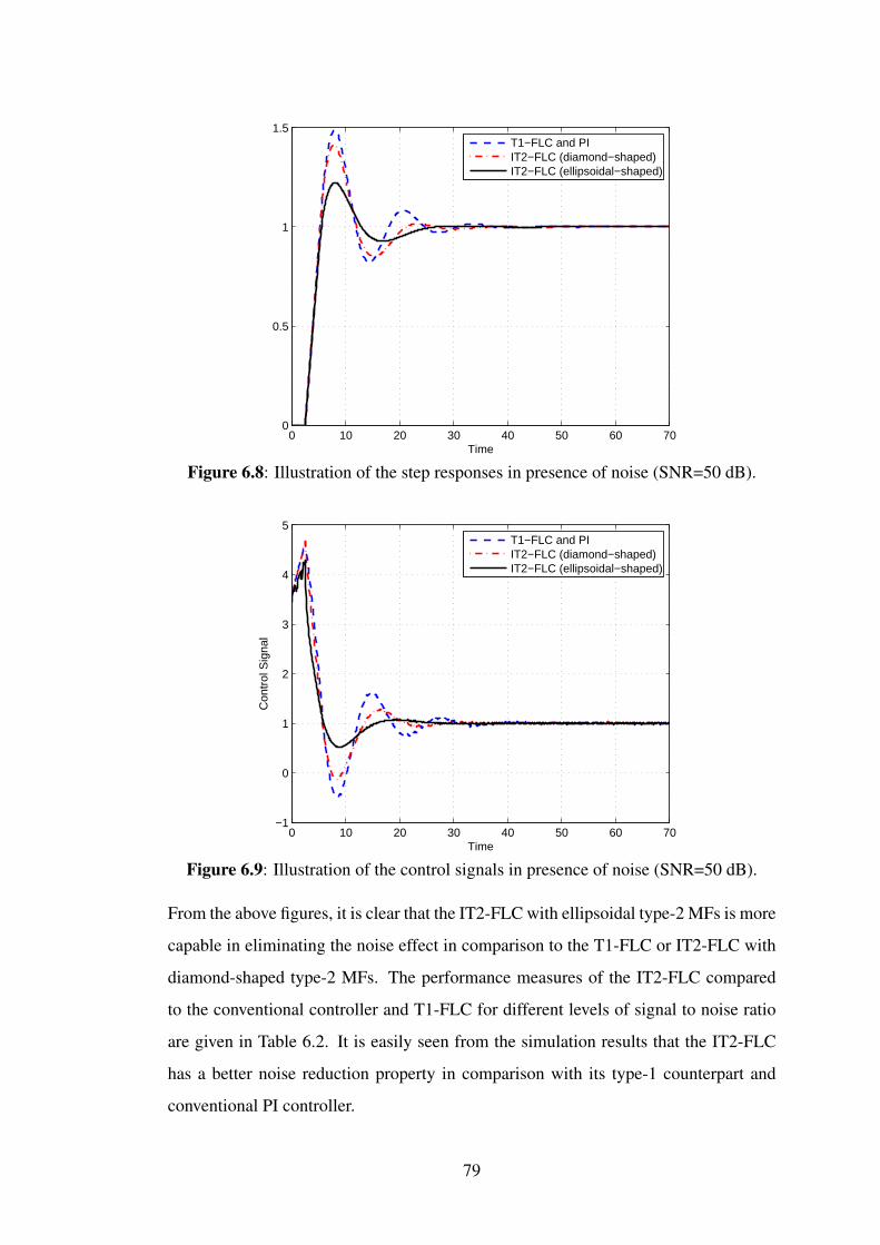
0 10 20 30 40 50 60 700

0.5

1

1.5

Time

T1−FLC and PIIT2−FLC (diamond−shaped)IT2−FLC (ellipsoidal−shaped)

Figure 6.8: Illustration of the step responses in presence of noise (SNR=50 dB).

0 10 20 30 40 50 60 70−1

0

1

2

3

4

5

Time

Con

trol

Sig

nal

T1−FLC and PIIT2−FLC (diamond−shaped)IT2−FLC (ellipsoidal−shaped)

Figure 6.9: Illustration of the control signals in presence of noise (SNR=50 dB).

From the above figures, it is clear that the IT2-FLC with ellipsoidal type-2 MFs is more

capable in eliminating the noise effect in comparison to the T1-FLC or IT2-FLC with

diamond-shaped type-2 MFs. The performance measures of the IT2-FLC compared

to the conventional controller and T1-FLC for different levels of signal to noise ratio

are given in Table 6.2. It is easily seen from the simulation results that the IT2-FLC

has a better noise reduction property in comparison with its type-1 counterpart and

conventional PI controller.

79

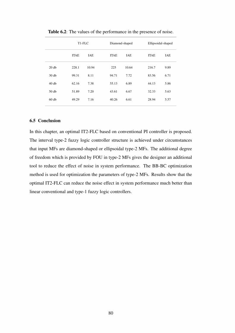
Table 6.2: The values of the performance in the presence of noise.

T1-FLC Diamond-shaped Ellipsoidal-shaped

ITAE IAE ITAE IAE ITAE IAE

20 db 228.1 10.94 225 10.64 216.7 9.89

30 db 99.31 8.11 94.71 7.72 83.56 6.71

40 db 62.16 7.38 55.13 6.89 44.13 5.86

50 db 51.89 7.20 43.61 6.67 32.33 5.63

60 db 49.29 7.16 40.26 6.61 28.94 5.57

6.5 Conclusion

In this chapter, an optimal IT2-FLC based on conventional PI controller is proposed.

The interval type-2 fuzzy logic controller structure is achieved under circumstances

that input MFs are diamond-shaped or ellipsoidal type-2 MFs. The additional degree

of freedom which is provided by FOU in type-2 MFs gives the designer an additional

tool to reduce the effect of noise in system performance. The BB-BC optimization

method is used for optimization the parameters of type-2 MFs. Results show that the

optimal IT2-FLC can reduce the noise effect in system performance much better than

linear conventional and type-1 fuzzy logic controllers.

80

7. CONCLUSIONS

The mathematical expression between input and output of an IT2FLSs is of great

importance as it will deepen our understanding of how and why these systems may

be able to provide better performance over the T1FLSs. In this thesis, the general

analytical structure of IT2FLS with diamond-shaped type-2 fuzzy MFs is considered.

The product fuzzy AND operator, and the NT closed-form inference engine which are

more practical in real-time application are used. The FOU in type-2 MFs generate

extra regions which has a unique input-output relation and these regions may enhance

robustness and noise reduction properties of IT2FLS in comparison to its type-1

counterpart. A special case of IT2FLS with three MFs for each input and a diagonal

3×3 rule-base are examined in detail.

In this thesis, a systematical methodology to construct an IT2-FLC is proposed. The

methodology depends on a nonlinear mapping from an existing PI or PD control law to

IT2-FLC that eases the generation of rule base. The structure of the proposed controller

is achieved under circumstances that input type-2 MFs are diamond-shaped and a

certain closed-form inference engine is used. It has been proven that these preferences

provide a closed-form for the output of IT2-FLC. Then, certain elaborations can

be done on the parameters of the evolved closed output form. If the FOU of the

IT2-FLC is zero then the obtained control law is identical to the conventional PI or

PD controller. If FOU is not equal to zero, then an additional degree of freedom is

acquired and this provides the designer an additional tool to cope with the uncertainties

and nonlinearities. Results show that the proposed controller is more robust to the

parameter uncertainties and eliminate the oscillations much better than type-1 fuzzy

logic and linear conventional controllers. However, it is not so fair and right to

draw a general conclusion that the system performance is necessarily guaranteed to

be improved for all systems and design methodologies.

An optimal IT2-FLC with diamond-shaped MF or ellipsoidal type-2 MF for inputs is

proposed. The BB-BC optimization method is used for optimization the parameters

81

of type-2 MFs. Also the effect of measurement noise with different levels of signal to

noise ratio is analyzed for optimal IT2-FLC. Results show that the optimal IT2-FLC

can reduce the noise effect in system performance much better than linear conventional

and type-1 fuzzy logic controllers.

82

fuzzy inverse controller design in nonlinear IMC structure.

mega-cities.

robot using genetic algorithms.

of interval type-2 fuzzy logic controllers.

autonomous mobile robots.

and New Directions.(vol.2):Prentice Hall.

design.

uncertainty using type-1 and type-2 fuzzy logic.

(2005). Handling Uncertainty in Controllers Using Type-2 Fuzzy Logic.

(2007). Type-2 FLCs: A New Generation of Fuzzy Controllers.

(2007). Type-2 fuzzy sets and systems: an overview.

approximate reasoning-I.

REFERENCES

[1] Zadeh, L. (1975). The concept of a linguistic variable and its application toInformation Sciences, 8(3), 199 – 249.

[2] Mendel, J. ComputationalIntelligence Magazine, IEEE, 2(1), 20 –29.

[3] Hagras, H.Computational Intelligence Magazine, IEEE, 2(1), 30 –43.

[4] Sepulveda, R., Castillo, O., Melin, P., Montiel, O. and Rodriguez-Diaz, A.

Journal of Intelligent Systems, 14(2-3), 237–262.

[5] Sepulveda, R., Castillo, O., Melin, P., Montiel, O., Rodriguez-Diaz, A. andMontiel, O. (2007). Experimental study of intelligent controllers under

Information Sciences,177(10), 2023 – 2048.

[6] Liang, Q. and Mendel, J. (2000). Interval type-2 fuzzy logic systems: theory andIEEE Transactions on Fuzzy Systems, 8(5), 535 –550.

[7] Mendel, J.M. (2001). Uncertain Rule-Based Fuzzy Logic Systems: Introduction

[8] Hagras, H. (2004). A hierarchical type-2 fuzzy logic control architecture forIEEE Transactions on Fuzzy Systems, 12(4),

524 – 539.

[9] Wu, D. and Wantan, W. (2006). Genetic learning and performance evaluationEngineering Applications of

Artificial Intelligence, 19(8), 829–841.

[10] Martínez, R., Castillo, O. and Aguilar, L.T. (2009). Optimization of intervaltype-2 fuzzy logic controllers for a perturbed autonomous wheeled mobile

Information Sciences, 179(13), 2158 –2174.

[11] Zarandi, M.F., Faraji, M. and Karbasian, M. (2012). Interval type-2 fuzzyexpert system for prediction of carbon monoxide concentration in

Applied Soft Computing, 12(1), 291 – 301.

[12] Kumbasar, T., Eksin, I., Guzelkaya, M. and Yesil, E. (2011). Interval type-2Engineering

Applications of Artificial Intelligence, 24(6), 996 – 1005.

83

, Automation and Control Engineering, Taylor & Francis.Control

.Information and Control

PD Controllers.

of the Interval Type-2 Fuzzy-PI and PD Controllers.

systems.

limiting structure theorems.

analysis for regulating processes with unknown mathematical models.

Operator.

gains.

adaptive method.

Applications

case.

Type-2 Fuzzy Logic Controllers.

modular neural networks for face recognition applications.

type-2 TSK fuzzy neural system.

[13] Kayacan, E., Oniz, Y., Aras, A.C., Kaynak, O. and Abiyev, R. (2011). A servosystem control with time-varying and nonlinear load conditions using

Applied Soft Computing, 11(8), 5735– 5744.

[14] Mendoza, O., Melín, P. and Castillo, O. (2009). Interval type-2 fuzzy logic andApplied Soft

Computing, 9(4), 1377 – 1387.

[15] Wu, D. (2012). On the Fundamental Differences Between Type-1 and IntervalIEEE Transactions on Fuzzy Systems,

[16] Ying, H., Siler, W. and Buckley, J.J. (1990). Fuzzy control theory: A nonlinearAutomatica, 26(3), 513 – 520.

[17] Ying, H. (2000). Fuzzy Control and Modeling: Analytical Foundations and

[18] Qiao, W.Z. and Mizumoto, M. (1996). PID type fuzzy controller and parametersFuzzy Sets and Systems, 78(1), 23 – 35.

[19] Haj-Ali, A. and Ying, H. (2004). Structural analysis of fuzzy controllers withnonlinear input fuzzy sets in relation to nonlinear PID control with variable

Automatica, 40(9), 1551 – 1559.

[20] Ying, H. (2006). Deriving Analytical Input-Output Relationship for FuzzyControllers Using Arbitrary Input Fuzzy Sets and Zadeh Fuzzy AND

IEEE Transactions on Fuzzy Systems, 14(5), 654 –662.

[21] Ying, H. (1994). Practical design of nonlinear fuzzy controllers with stability

Automatica, 30(7), 1185 – 1195.

[22] Ying, H. (1993). General analytical structure of typical fuzzy controllers and theirAutomatica, 29(4), 1139 – 1143.

[23] Chen, G. and Ying, H. (1997). BIBO stability of nonlinear fuzzy PI controlJournal of Intelligent and Fuzzy Systems, 5, 245 – 256.

[24] Du, X. and Ying, H. (2010). Derivation and Analysis of the Analytical StructuresIEEE Transactions

on Fuzzy Systems, 18(4), 802 –814.

[25] Nie, M. and Tan, W.W. (2012). Analytical Structure and Characteristics ofSymmetric Karnik-Mendel Type-Reduced Interval Type-2 Fuzzy PI and

IEEE Transactions on Fuzzy Systems, 20(3), 416 –430.

[26] Zadeh, L. (1965). Fuzzy sets, 8(3), 338 – 353.

[27] Xu, C. and Shin, Y. (2008). Intelligent Systems: Modeling, Optimization, and

84

. (1st ed.): Wiley-IEEE Press.

20(5), 832-848.

1999 IEEE International,

Relationships Based on Integral Performance Criteria.

controllers.

control performance monitoring-Honeywell’s experience.

1432.1425-Proc. Int. Conf. FUZZ,for interval type-2 fuzzy logic systems.

data.

627 – 632.Proc. Int. Conf. MED,Controller.

a Novel Type-2 Membership Function.

systems.

1–10.(2010). A Brief Tutorial on Interval Type-2 Fuzzy Sets and Systems.

interval type-2 fuzzy logic systems.

(1999). Type-2 fuzzy logic systems.

the computational cost of interval type-2 fuzzy logic controllers.

Studies in Fuzziness and Soft Computing: Springer.(vol.223).Type-2 Fuzzy Logic: Theory and Applications

(2001). Operations on type-2 fuzzy sets.[28] Karnik, N.N. and Mendel, J.M. FuzzySets and Systems, 122(2), 327 – 348.

[29] Castillo, O. and Melin, P. (2008).

[30] Wu, D. (2012). An overview of alternative type-reduction approaches for reducingFuzzy

Systems (FUZZ-IEEE), 2012 IEEE International Conference on, pp.1 –8.

[31] Karnik, N., Mendel, J. and Liang, Q. IEEETransactions on Fuzzy Systems, 7(6), 643 –658.

[32] Wu, H. and Mendel, J. (2002). Uncertainty bounds and their use in the design ofIEEE Transactions on Fuzzy Systems,

10(5), 622 – 639.

[33] Wu, D.

[34] Liang, Q. and Mendel, J. (1999). An introduction to type-2 TSK fuzzy logicFuzzy Systems Conference Proceedings, 1999. FUZZ-IEEE ’99.

[35] Khanesar, M., Teshnehlab, M., Kayacan, E. and Kaynak, O. (2010). A noveltype-2 fuzzy membership function: application to the prediction of noisy

Proc. Int. Conf. CIMSA

[36] Khanesar, M., Kayacan, E., Teshnehlab, M. and Kaynak, O. (2011). Analysisof the Noise Reduction Property of Type-2 Fuzzy Logic Systems Using

IEEE Trans on Systems, Man andCybernetics, Part B: Cybernetics, 41(5), 1395 –1406.

[37] Aliasghary, M., Eksin, I., Güzelkaya, M. and Kumbasar, T. (2012). Designof An Interval Type-2 Fuzzy Logic Controller based on Conventional PI

[38] Nie, M. and Tan, W.W. (2008). Towards an efficient type-reduction method

[39] Desborough, L. and R. Miller, I. (2001). Increasing customer value of industrialProc. 6th Int.

Conf. on Chemical Process Control (CPC VI), 172–192.

[40] Zhuang, M. and Atherton, D. (1993). Automatic tuning of optimum PIDControl Theory and Applications, IEE Proceedings D, 140(3),

216 – 224.

[41] Lopez, A.M., Murrill, P.W. and Smith, C.L. (1967). Controller TuningInstr. Technol,

14(11), 57.

85

3, 1534 –1539.

,128 –133.

interval type-2 fuzzy controllers.

controllers.

(1995). Realization of PID controls by fuzzy control methods.

extended Kalman filter.

control scheme for managing energy resources in buildings.

fuzzy PID controller.

trollers.

rule base modification scheme in fuzzy controllers for time-delay systems.

(2), 419 –435.(1990). Fuzzy logic in control systems: fuzzy logic controller. II.

response method for PID control.

rules for PI control.

Applications, IEE Proceedingscontrollers based on constrained optimisation.

(2001). The future of PID control.

Control.

Controllers.[42] Ziegler, J.G. and Nichols, N.B. (1993). Optimum Settings for Automatic

Journal of Dynamic Systems Measurement and Control,115(2B), 220.

[43] Cohen, G.H. and Coon, G.A. (1953). Theoretical Consideration of RetardedTransactions of ASME, 75, 827–834.

[44] Åström, K.J. and Hägglund, T. ControlEngineering Practice, 9(11), 1163–1175.

[45] Panagopoulos, H., Astrom, K. and Hagglund, T. (2002). Design of PIDControl Theory and

, 149(1), 32 –40.

[46] Hägglund, T. and Åström, K.J. (2002). Revisiting the Ziegler-Nichols tuningAsian Journal of Control, 4(4), 364–380.

[47] Åström, K. and Hägglund, T. (2004). Revisiting the Ziegler–Nichols stepJournal of Process Control, 14(6), 635

– 650.

[48] Lee, C. IEEETrans on Systems, Man and Cybernetics, 20

[49] Genc, H.M., Yesil, E., Eksin, I., Guzelkaya, M. and Tekin, O.A. (2009). A

Expert Systems with Applications, 36(4), 8476 – 8486.

[50] Golob, M. (2001). Decomposed fuzzy proportional–integral–derivative con-Applied Soft Computing, 1(3), 201 – 214.

[51] Mohan, B. and Sinha, A. (2008). Analytical structure and stability analysis of aApplied Soft Computing, 8(1), 749 – 758.

[52] Paris, B., Eynard, J., Grieu, S. and Polit, M. (2011). Hybrid PID-fuzzyApplied Soft

Computing, 11(8), 5068 – 5080.

[53] Ahn, K. and Truong, D. (2009). Online tuning fuzzy PID controller using robustJournal of Process Control, 19(6), 1011 – 1023.

[54] Mizumoto, M.Fuzzy Sets and Systems, 70(2–3), 171 – 182.

[55] Kubica, E., Madill, D. and Wang, D. (2005). Designing stable MIMO fuzzyIEEE Transactions on Systems, Man and Cybernetics, Part

B: Cybernetics, 35(2), 372 –380.

[56] Castillo, O. and Melin, P. (2012). A review on the design and optimization ofApplied Soft Computing, 12(4), 1267 –

1278.

86

Conference

International Conference, 724 –727.Particle Swarm Optimization.

Crunch.

with learning through the evolution of its knowledge base.

models of dynamical systems with applications to control.

controllers for nonlinear systems based on an improved genetic algorithm.

(2002). Training fuzzy systems with the extended Kalman filter.

algorithm approaches and stability analysis of training methods.

(2004). Computing derivatives in interval type-2 fuzzy logic systems.

Control:John Wiley & Sons, Inc.

Synthesis and Disturbance Rejection.

255 –261.

design of PD and PI like Interval Type-2 TSK fuzzy controllers.

, vol.3,1305 – 1310.controller.

[57] Tan, W.W. and Lai, J. (2004). Development of a type-2 fuzzy proportionalFuzzy Systems, 2004. Proceedings. 2004 IEEE International

[58] Biglarbegian, M., Melek, W. and Mendel, J. (2009). A practical approach forSystems,

Man and Cybernetics, 2009. SMC 2009. IEEE International Conference

[59] Chen, D. and Seborg, D.E. (2002). PI/PID Controller Design Based on DirectIndustrial & Engineering Chemistry

Research, 41(19), 4807–4822.

[60] Seborg, D.E., Edgar, T.F. and Mellichamp, D.A. (2004). Process Dynamics and

[61] Quanser. Ball and beam position control using QuaRC (manual),http://www.quanser.com.

[62] Mendel, J.IEEE Transactions on Fuzzy Systems, 12(1), 84 – 98.

[63] Shoorehdeli, M.A., Teshnehlab, M., Sedigh, A.K. and Khanesar, M.A.(2009). Identification using ANFIS with intelligent hybrid stable learning

AppliedSoft Computing, 9(2), 833 – 850.

[64] Simon, D. FuzzySets and Systems, 132(2), 189 – 199.

[65] Leung, F., Lam, H., Ling, S. and Tam, P. (2004). Optimal and stable fuzzy

IEEE Transactions on Industrial Electronics, 51(1), 172 – 182.

[66] Barada, S. and Singh, H. (1998). Generating optimal adaptive fuzzy-neuralIEEE

Transactions on Systems, Man, and Cybernetics, Part C: Applications andReviews, 28(3), 371 –391.

[67] Magdalena, L. and Monasterio-Huelin, F. (1997). A Fuzzy logic controllerInternational

Journal of Approximate Reasoning, 16(3-4), 335 – 358.

[68] Erol, O.K. and Eksin, I. (2006). A new optimization method: Big Bang-BigAdvances in Engineering Software, 37(2), 106 – 111.

[69] Martinez, R., Rodriguez, A., Castillo, O. and Aguilar, L. (2010). Type-2Fuzzy Logic Controllers Optimization Using Genetic Algoritms and

87

Granular Computing (GrC), IEEE

Theory and Experiments.

(11), 4443 –4455.Logic Systems and Its Experimental Evaluation.

The 18th IFAC World Congress, 5308 –5313.Model Inverse Controller Design Based on BB-BC Optimization Method.

of type-1 and type-2 fuzzy controllers for an autonomous mobile robot.

[70] Castillo, O., Martinez-Marroquin, R., Melin, P., Valdez, F. and Soria, J. (2012).Comparative study of bio-inspired algorithms applied to the optimization

Information Sciences, 192(0), 19 – 38.

[71] Kumbasar, T., Eksin, I., Guzelkaya, M. and Yesil, E. (2011). Type-2 Fuzzy

[72] Khanesar, M., Kayacan, E., Teshnehlab, M. and Kaynak, O. (2012).Extended Kalman Filter Based Learning Algorithm for Type-2 Fuzzy

IEEE Transactions onIndustrial Electronics, 59

[73] Biglarbegian, M., Melek, W. and Mendel, J. (2011). Design of Novel IntervalType-2 Fuzzy Controllers for Modular and Reconfigurable Robots:

,58(4), 1371 –1384.

88

IEEE Transactions on Industrial Electronics

CURRICULUM VITAE

Name Surname: Mortaza Aliasghary

Place and Date of Birth: Oroumieh - Iran - 23.12.1982

Adress: Mekatronik Egitim ve Arastırma Merkezi, Istanbul Teknik Üniversitesi,Maslak Kampüsü, 34469 Maslak - ISTANBUL

E-Mail: aliasghary@itu.edu.tr , m.aliasghari@gmail.com

B.Sc.: Oroumieh branch of Islamic Azad University, Oroumieh, Iran

M.Sc.: Science and Research branch of Islamic Azad University, Tehran, Iran

Professional Experience and Rewards:

• Mechatronics Education and Research Center of Istanbul Technical University,2009-2013.

• Iran Science & Research Ministry Scholarship, 2011.

• Erasmus IP grants for T.I.M.E. European Summer School, 2011.

• 3th place in “Multimedia software Programming Contests”, 2008.

• Intelligent System Lab, Department of Electrical Engineering, K.N. ToosiUniversity of Technology (During my M.S. Thesis, 2007-2008).

• 5th rank in the “Islamic Azad University Graduate School Entrance Exam" incontrol Engineering, 2005.

Remark: In 2005, about 1000 students participated in this exam, and only 40 wereadmitted to a university.

• 3th place in “Etrat, software Programming Contests”, 2003.

List of Publications and Patents:

PUBLICATIONS/PRESENTATIONS ON THE THESIS

Aliasghary M., Eksin I. and Güzelkaya M., Kumbasar T. (2013). A DesignMethodology And Analysis For Interval Type-2 Fuzzy PI/PD Controllers. accepted

89

for the publication in International Journal of Innovative Computing Information andControl.

Aliasghary M., Eksin I. and Güzelkaya M., Kumbasar T. (2013). General Derivationand Analysis for Input-Output Relations in Interval Type-2 Fuzzy Logic Systems.submitted to Soft Computing.

Aliasghary M., Eksin I. and Güzelkaya M., Kumbasar T. (2012). Design of anInterval Type-2 Fuzzy Logic Controller Based on Conventional PI Controller. 20th

Mediterranean Conference on Control and Automation, 3-6 July, Barcelona, Spain,627 – 632.

OTHER PUBLICATIONS

Aliasghary M.,Arghavani N. (2012). H∞ Estimation for Optimization ofRational-Powered Membership Functions. 13th IEEE International Symposium onComputational Intelligence and Informatics, 20-22 November, Budapest, Hungary,251 – 256.

Aliasghary M., Eksin I. and Güzelkaya M. (2011). Fuzzy-Sliding ModelReference Learning Control of Inverted Pendulum with Big Bang – Big CrunchOptimization Method. 11th International Conference on Intelligent Systems Designand Applications, 22-24 November, Córdoba, Spain, 380 – 384.

Naderi A. and Aliasghary M., Ghasemzadeh H. and Pourazar A. (2011). A19MFLIPS CMOS Fuzzy Controller to Control Continuously Variable TransmissionRatio. 7th Conference on PhD. Research in microelectronics & electronics, Trento,Italy, 45 – 48.

Aliasghary M., Ghasemzadeh H. and Naderi A. and Pourazar A. (2011). Designof Radial Basis Function Neural Networks Controller Based on Sliding Surface fora Coupled Tanks System. IEEE Joint International Information Technology andArtificial Intelligence Conference, Chongqing, China, 8 – 12.

Naderi A. and Ghasemzadeh H. and Pourazar A. and Aliasghary M. (2009)Design of a Fuzzy Controller Chip with New Structure Supporting Rational-PoweredMembership Functions. Amirkabir Journal, International Journal of Electrical andElectronics Engineering, 41(2), 65 – 71.

Naeimi M. and Teshnehlab and M. Shoorehdeli M.A and Aliasghary M.(2009). Stable Direct Adaptive Control as Nonlinear Hybrid Controller for FlexibleManipulator. Journal of Applied Sciences, 9(7), 1258 – 1266.

Aliasghary M. and Teshnehlab M. and Shoorehdeli M.A and Jalilvand A. and NekouiM. (2008). Hybrid Control of Magnetic Levitation System Based-on New IntelligentSliding Mode Control. Journal of Applied Sciences, 8(14), 2561 – 2568.

Aliasghary M. and Jalilvand A. and Teshnehlab M. and Shoorehdeli M.A. (2008).Sliding Mode Control of Magnetic Levitation System Using Radial Basis FunctionNeural Networks. IEEE Conference on Robotics, Automation and Mechatronics,China, 467 – 470.

Aliasghary M. and Shoorehdeli M.A and Teshnehlab M. and Jalilvand A. (2008)Magnetic Levitation Control Based-on Neural Network and Feedback Error Learning

90

Approach. IEEE International Conference on Power and Energy, Malaysia, 1426 –1430.

Sabahi K. and Sharifi A. and Shoorehdeli M.A and Teshnehlab M. and AliasgharyM. (2008). Load Frequency Control in Interconnected Power System UsingMulti-Objective PID Controller. Journal of Applied Sciences, 8(20), 3676 – 3682.

91

92