ISTANBUL TECHNICAL UNIVERSITY F INFORMATICS INSTITUTE

PyCASPESA: A NEW METHOD FOR CRYSTAL STRUCTURE PREDICTION

M.Sc. THESIS

Gözde Inis

Computational Science and Engineering Department

Computational Science and Engineering Master Programme

JUNE 2017

ISTANBUL TECHNICAL UNIVERSITY F INFORMATICS INSTITUTE

PyCASPESA: A NEW METHOD FOR CRYSTAL STRUCTURE PREDICTION

M.Sc. THESIS

Gözde Inis(702141011)

Computational Science and Engineering Department

Computational Science and Engineering Master Programme

Thesis Advisor: Assoc. Prof. Adem Tekin

JUNE 2017

ISTANBUL TEKNIK ÜNIVERSITESI F BILISIM ENSTITÜSÜ

PyCASPESA: KRISTAL YAPI TAHMINI IÇIN YENI BIR YÖNTEM

YÜKSEK LISANS TEZI

Gözde Inis(702141011)

Hesaplamalı Bilim ve Mühendislik Anabilim Dalı

Hesaplamalı Bilim ve Mühendislik Yüksek Lisans Programı

Tez Danısmanı: Assoc. Prof. Adem Tekin

HAZIRAN 2017

Gözde Inis, a M.Sc. student of ITU Informatics InstituteEngineering and Technology702141011 successfully defended the thesis entitled “PyCASPESA: A NEW METHODFOR CRYSTAL STRUCTURE PREDICTION”, which he/she prepared after fulfillingthe requirements specified in the associated legislations, before the jury whose signa-tures are below.

Thesis Advisor : Assoc. Prof. Adem Tekin ..............................Istanbul Technical University

Jury Members : Assoc. Prof. Adem Tekin ..............................Istanbul Technical University

Assoc. Prof. F. Aylin Sungur ..............................Istanbul Technical University

Assoc. Prof. Hikmet Hakan Gürel ..............................Kocaeli University

Date of Submission : 5 May 2017Date of Defense : 6 June 2017

v

vi

To my supportive family,

vii

viii

FOREWORD

There are many people i would like to thank particularly. First of all, I would liketo thank my advisor Assoc. Prof. Dr. Adem Tekin for giving me opportunity towork with him and for all his supports during the whole time. I would like to thankAssoc. Prof. Dr. F. Aylin Sungur for all her helps. I am also grateful for havingsuch wonderful friends. Especially I would like to thank Samet Demir and AhmetTuncer Durak for all their supports and their precious times that spend with me to helpme about my thesis. I would like to express my gratitude to Informatics Institute ofIstanbul Technical University for providing the computing resources. MARS and VISis used for all computations in this thesis. Finally, I want to thank my family, speciallyto my mother and father, they have given me courage and have been always supportivethroughout my life.

June 2017 Gözde Inis

ix

x

TABLE OF CONTENTS

Page

FOREWORD........................................................................................................... ixTABLE OF CONTENTS........................................................................................ xiABBREVIATIONS ................................................................................................. xiiiSYMBOLS............................................................................................................... xvLIST OF TABLES ..................................................................................................xviiLIST OF FIGURES ................................................................................................ xixSUMMARY ............................................................................................................. xxiÖZET .......................................................................................................................xxiii1. INTRODUCTION .............................................................................................. 1

1.1 Purpose of Thesis ........................................................................................... 22. CRYSTAL STRUCTURE PREDICTION........................................................ 5

2.1 Crystal Structure and Importance of Crystal Structure Prediction................. 52.2 CALYPSO ...................................................................................................... 62.3 XtalOpt ........................................................................................................... 72.4 USPEX ........................................................................................................... 72.5 GASP.............................................................................................................. 82.6 MUSE............................................................................................................. 82.7 CASPESA....................................................................................................... 8

3. METHODOLOGY ............................................................................................. 93.1 Computational Background............................................................................ 9

3.1.1 Simulated annealing ............................................................................... 93.1.1.1 Workflow of simulated annealing .................................................... 10

3.1.2 PyCASPESA .......................................................................................... 163.1.2.1 Implementation of DFT calculations ............................................... 173.1.2.2 Preparation of PyCASPESA input................................................... 20

3.2 Theoretical Background ................................................................................. 253.2.1 Schrödinger equation.............................................................................. 253.2.2 Density functional theory ....................................................................... 26

3.3 Application: Hydrogen Storage...................................................................... 273.3.1 Hydrogen storage methods ..................................................................... 28

4. RESULTS AND DISCUSSIONS ....................................................................... 294.1 Mg(BH4)2 Setup: SA part of PyCASPESA ................................................... 294.2 Mg(BH4)2 Setup: DFT part of PyCASPESA................................................. 304.3 Mg(BH4)2 Results .......................................................................................... 314.4 Conclusions .................................................................................................... 39

REFERENCES........................................................................................................ 41

xi

CURRICULUM VITAE......................................................................................... 45

xii

ABBREVIATIONS

ASE : Atomic Simulation EnvironmentBO : Born-OppenheimerCALYPSO : Crystal Structure AnaLYsis by Particle Swarm OptimizationCASPESA : CrystAl Structure PrEdiction via Simulated AnnealingCSP : Crystal Structure PredictionDFT : Density Functional Theoryfu : Formula UnitGASP : Genetic Algorithm for Structure PredictionKY : Kristal YapıKYT : Kristal Yapı TahminiMUSE : Multi-algorithm-collaborative Universal Structure-predictionPSO : Particle Swarm OptimizationQE : Quantum EspressoSA : Simulated AnnealingSP : Structure Predictionuc : Unit CellUSPEX : Universal Structure Predictor: Evolutionary XtallographyYFT : Yogunluk Fonksiyoneli Teorisi

xiii

xiv

SYMBOLS

ρ : Electron densityh : Planck constanth : Reduced Planck constant

xv

xvi

LIST OF TABLES

Page

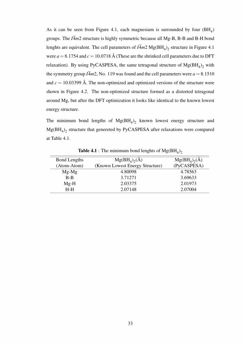
Table 4.1 : The minimum bond lenghts of Mg(BH4)2 ........................................ 33Table 4.2 : Crystallographic details of Mg(BH4)2 structures. ............................. 39

xvii

xviii

LIST OF FIGURES

Page

Figure 3.1 : Flowchart of the SA algorithm............................................................ 15Figure 3.2 : Flowchart of the PyCASPESA method............................................... 19Figure 3.3 : Geometry definitions part of the example input file of Mg(BH4)2 ..... 21Figure 3.4 : Translation and rotation part of the example input file of Mg(BH4)2 . 22Figure 3.5 : Objective function definitions part of the example input file of

Mg(BH4)2 ........................................................................................... 23Figure 3.6 : Threshold definitions part of the example input file of Mg(BH4)2 ..... 23Figure 3.7 : Unit cell definition part of the example input file of Mg(BH4)2 ......... 23Figure 3.8 : Nickname usage on another example input file of Mg(BH4)2 ............ 24Figure 4.1 : The known lowest energy tetragonal structure of Mg(BH4)2 with

the symmetry group I4m2, No. 119. Representations of colors:magnesium (Mg), brown; boron (B), green; hydrogen (H), lightgray. ................................................................................................... 31

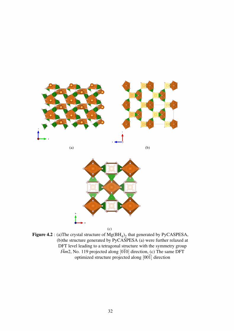
Figure 4.2 : (a)The crystal structure of Mg(BH4)2 that generated by Py-CASPESA, (b)the structure generated by PyCASPESA (a) werefurther relaxed at DFT level leading to a tetragonal structurewith the symmetry group I4m2, No. 119 projected along [010]direction, (c) The same DFT optimized structure projected along[001] direction ..................................................................................... 32

Figure 4.3 : Mg(BH4)2 structure with the symmetry group F222, No. 22 ........... 34Figure 4.4 : The crystal structures of Mg(BH4)2 that was generated by using

PyCASPESA with the symmetry group; (a) I4122, No. 98, (b)Ima2, No. 46, (c) Fdd2, No. 43, (d) Ama2, No. 40. .......................... 35

Figure 4.5 : The crystal structures of Mg(BH4)2 that was generated by usingPyCASPESA with the symmetry group; (a) I212121, No. 24, (b)Cc, No. 9, (c) P1m1, No. 6 (d) C2, No. 5, (e) C2, No. 5.................... 36

Figure 4.6 : The crystal structures of Mg(BH4)2 that was found for the firsttime by using PyCASPESA with the symmetry group; (a) P4n2,No. 118, (b) P42m, No. 111, (c) Cm, No. 8, (d) Cm, No. 8. .............. 37

xix

xx

PyCASPESA: A NEW METHOD FOR CRYSTAL STRUCTURE PREDICTION

SUMMARY

Predicting crystal structure of a material is one of the most important problemsin computational material sciences. There are several computational methods thatdeveloped for solving crystal structure prediction (CSP) problems. In all methods thatdeveloped for this purpose, firstly CSP problem is turned into a global optimizationproblem and than this problem is solved by using different methodologies. CrystAlStructure PrEdiction via Simulated Annealing (CASPESA) is one of these methodsand the method uses simulated annealing (SA) algorithm for solving the globaloptimization problem. Within the scope of this thesis, it is intended to improveCASPESA by merging simulated annealing algorithm and density functional theory(DFT) calculations. The new program which is named as PyCASPESA is written fromthe scratch and it is written in Python programming language. DFT calculations in thisnew program were performed by using GPAW under ASE and Quantum Espresso. Theprogram was improved in many aspects. The space search algorithm of the programwas refined, therefore it achieves higher success by making fewer trials in less time.PyCASPESA is more user-friendly in the matter of input file preparation. UnlikeCASPESA, the new implementation can work with the systems that has no unit cell.In addition to these, PyCASPESA is better at maximizing the shrinkage of the unit cellin volume. After these improvements, the program performs more robust CSP.

PyCASPESA is applied for determining the crystal structures of magnesiumborohydride (Mg(BH4)2) which is a promising hydrogen store material. Mg(BH4)2 isselected as the test case, because it has experimental data that gives us the opportunityto verify the program whether is working properly or not. The known tetragonalstructure of Mg(BH4)2 with the symmetry group I4m2, No. 119 is the true ground-statestructure. The program successfully yielded the structure with the symmetry groupI4m2. In this structure, each magnesium atom was surrounded by four BH4 groups.As a result of this study, crystal structures for Mg(BH4)2 with the symmetry groupF222 (No. 22), I4122 (No. 98), Ima2 (No. 46), Fdd2 (No. 43), Ama2 (No. 40),I212121 (No. 24), Cc (No. 9), P1m1 (No. 6) and C2 (No. 5) is found. In additionto these structures that reported in the literature before this study, the program is alsofound the new structures that did not reported in the literature with the symmetry groupP4n2 (No. 118), P42m (No. 111) and Cm (No. 8).

xxi

xxii

PyCASPESA: KRISTAL YAPI TAHMINI IÇIN YENI BIR YÖNTEM

ÖZET

Kristalin ne oldugu basit bir dil ile anlatılmak istenirse herhangi bir kristal yapıyı(KY) olusturan belirli atomların örüntülerinin üç boyutta defalarca tekrarlanmasıylaolusturulan katı objelerdir. Kristallerin atomik yapısı hakkında bilgi sahibi olmakçok büyük önem tasır, çünkü KY bir malzeme henüz sentezlenmemis dahi olsaözelliklerini öngörebilmemiz adına gerekli olan birçok bilgiyi bize sunar. Bu yüzdenkristal yapı tahmininin (KYT) malzeme bilimindeki yeri çok kritiktir. Her kimyasalbilesen için sonsuz sayıda muhtemel atomik düzenleme mevcuttur, fakat genel olarakelimizde kristallerin moleküler düzenlemesi hakkında yetersiz bilgi bulunmaktadır.KYT problemleri bu yüzden hesaplamalı malzeme bilimindeki en zorlu problemlerdenbiri olarak sayılırlar. Hesaplamalı malzeme tasarımındaki nihai amaç; bilinmeyenkristal yapıları tahmin etmek ve istenen özelliklere sahip yeni malzemeler tahminetmektir.

Bazı durumlarda kristal yapıyı deney yoluyla ortaya çıkarmak çok zor hattaimkansızdır. Bu amaçla hesaplamalı kristal yapı tahmini yöntemleri kullanmakmalzemelerin kristal yapılarının bilinmedigi durumlarda yapıyı belirlemek konusundakullanılacak nihai yoldur. KYT yöntemlerinin kullanım alanı oldukça genistir,fakat bu çalısma kapsamında gelistirilen yöntem sadece yeni hidrojen depolamamalzemelerinin kesfi amacıyla kullanılmıstır. Hidrojen hızla tükenmekte olan fosilyakıtlara alternatif olarak kullanılabilecek çevre dostu bir enerji kaynagıdır vebu nedenle hidrojenin güvenli, verimli ve geri dönüstürülebilir bir sekilde depoedilecegi uygun hidrojen depolama malzemeleri bulmak büyük önem arz etmektedir.Yüksek agırlıksal ve hacimsel yogunluga sahip hidrojen depolama malzemeleri mobiluygulamalarda ve özellikte arabalarda kullanılabilir olusları ile ön plandadırlar.

KYT için çesitli hesaplamalı yöntemler gelistirilmistir. Bu yöntemler benzetilmistavlama, makine ögrenmesi, evrimsel algoritma, basin-hopping gibi farklı algoritmalarbaz alınarak gelistirilmistir. Arastırma grubumuz tarafından gelistirilmis ve kristal yapıtahmini için kullandıgımız CASPESA yönteminde benzetilmis tavlama algoritması(BT) kullanılmaktadır. Bu kadar çok sayıda algoritma varken BT algoritmasınınbu yöntemde kullanılmak için seçilmis olmasının birçok nedeni vardır. BTfiziksel tavlama sürecinden ilham alınarak gelistirilmis bir en iyileme algoritmasıdır.Algoritmanın koordinat düzlemi boyunca adaptif hareketler ile iteratif rasgele aramayapan bir yaklasımı vardır. Algoritma herhangi deneysel veriye ihtiyaç duymaksızınsadece küresel minimumu bulmayı hedeflemez, yanı sıra katı haldeki bilesiginpotansiyel enerji yüzeyini kesfederek diger yerel minimumları da bulmaya çalısır.Eger tavlama süreci ideal sıcaklık düsüsleri ile gerçeklestirilirse, algoritmanın küreselminimumu bulma olasılıgı daha yüksek olacaktır. Algoritma dogru yerde ve dogrusekilde kullanılması halinde diger algoritmalara kıyasla oldukça güçlü olup, zor vekötü kosullu problemlerde bile daha düsük oranlarda basarısızla sonuçlanır. Daha önce

xxiii

CASPESA yöntemi kullanılarak birçok hidrojen depolama malzemesinin kristal yapısıbasarılı bir sekilde tahmin edilmistir.

CASPESA ile KYT islemi benzetilmis tavlama ve yogunluk fonksiyonel teori (YFT)hesaplamalarının birlestirilmesiyle yapılmaktadır. Bu tez kapsamında, CASPESA’nınFortran tabanlı ilk versiyonu Python’a geçirilmis ve yönteme çesitli yeniliklereklenmistir. Tüm program sıfırdan yazılıp, programa PyCASPESA ismi verilmistir.PyCASPESA’daki YFT hesaplamaları GPAW, izdüsürülmüs genisletilmis dalgaya(IGD) dayanan bir python YFT programı, ve Quantum Espresso kullanılarakyapılmıstır. GPAW ASE (Atomic Simulation Environment) altındaki hesaplayıcılardanbiridir ve bu hesaplayıcının kodu IGD yöntemi baz alınarak yazılmıstır. QuantumEspresso (QE) açık kaynak kodlu bir YFT yazılımıdır. PyCASPESAnın kullanımıoldukça kolaydır ve kristal yapı tahminine baslaması için birim hücre, atomlarınatomik pozisyonları ve önceden tanımlanmıs bag kısıtlarına ihtiyaç vardır. Tümparametre degerlerinin degisiklikleri tek bir girdi dosyası üzerinden yapılmaktadır.PyCASPESA birim hücresi bulunmayan sistemler için de kullanılabilmektedir. Uzayıarama algoritmasının gelistirilmesi ile PyCASPESAnın daha az deneme yaparakdaha basarılı sonuçlara daha kısa sürede erismesi saglanmıstır. Buna ek olarak,PyCASPESA birim hücredeki hacimsel küçülmeyi CASPESAya oranla daha iyimaksimize etmektedir. Bu gelismeler ısıgında, programın daha güçlü ve daha hızlı birsekilde KYT islemini gerçeklestirdigi gözlenmistir. Programın nasıl çalıstıgı birkaçadımda özetlenecek olursa; ilk olarak BT algoritması kullanılarak program kristalyapı tahminlerini yapar, ardından istenen özelliklere sahip, en iyi yapılar seçim betigikullanılarak enerjilerine ve yogunluklarına göre sıralandıktan sonra benzer yapılarelenerek ve belirli atomlar arasında yapılan bag sayıları da göz önünde bulundurularakseçim islemi yapılır. Seçilmis belirli sayıdaki yapı YFT hesapları yapılmak üzereGPAW’a veya QE’a yollanır. Son olarak YFT hesaplamalarıyla optimize edilmis tümyapılar arasından analiz betigi kullanılarak seçim yapılır. PyCASPESA’nın bahsedilenadımların çok büyük kısmını otomatik olarak yapması da diger bir gelisme olaraksayılabilir. Program hala gelistirilme süreci içerisinde olup daha verimli ve dahaotomatiklesmis bir hal alması için çalısmalar sürdürülmektedir.

PyCASPESA yönteminin gelistirilmesi ardından, programın istendigi sekilde çalısıpçalısmadıgını test etmek amacıyla yöntem deneysel yapısı hakkında bilgi sahibioldugumuz magnezyum borohidrit (Mg(BH4)2) bilesigine uygulanmıstır. Mg(BH4)2katı halde hidrojen depolama konusunda umut vaat eden bir malzemedir. Agırlıksalve hacimsel hidrojen yogunlugu yüksek olan magnezyum borohidrit teorik olarak16.8wt% miktarına kadar hidrojeni depo edebilir. Ilk olarak, yöntemin bulacagıyapıları karsılastırabilmek için bilinen en düsük enerjili Mg(BH4)2 yapısının YFThesaplamaları yapılmıs ve YFT enerjisi elde edilmistir. YFT ile optimize edilen buyapının simetrisi bozulmamıs olup, I4m2 (No.119) olarak korunmustur. PyCASPESAgirdi dosyası bir birim hücre içerisinde iki formül birim olacak sekilde hazırlanmıstır.Daha sonra PyCASPESA kullanılarak 1400’e yakın Mg(BH4)2 kristal yapısı tahminedilmistir ve elde edilen bu yapılar arasından umut vaad edici olanlar seçim betigiile seçilip, seçilenler YFT hesaplamaları ile optimize edilmis ve ardından simetrianalizleri yapılmıstır.

Mg(BH4)2 yapısı için elde edilen sonuçları kısaca degerlendirlendirecek olursak, I4m2(No. 119) simetrisine sahip tetragonal yapının birebir aynısı elde edilen yapılararasında bulunmustur. Bu yapı bazı çalısmalarda en düsük enerjili yapı olarak

xxiv

saptanmıstır. Yapıda her magnezyum dört BH4 grubu tarafından çevrelenmistir.Baska bir çalısma ise F222 (No. 22) simetrisine sahip yapıyı en düsük enerjiliyapı olarak belirlemistir. Bu F222 (No.22) simetrili biraz bozulmus ortorombik yapıda PyCASPESA’nın buldugu yapılar arasında bulunmaktadır. Bu iki yapı dısında,PyCASPESA ile daha önce literatürde bulundugu rapor edilmis ve edilmemis birçokyapı elde edilmistir. Daha önceki çalısmalarda rapor edilen yapılardan I4122 (No. 98),Ima2 (No. 46), Fdd2 (No. 43), Ama2 (No. 40), I212121 (No. 24), Cc (No. 9),P1m1 (No. 6), C2 (No. 5) simetrisine sahip yapılar bu çalısma kapsamında yenidenbulunmustur. Bu yapıların yanısıra P4n2 (No. 118), P42m (No. 111), Cm (No. 8)simetrisine sahip yeni kristal yapılarda bu çalısma çerçevesinde bulunmustur.

xxv

xxvi

1. INTRODUCTION

A crystal is a solid object that is simply a pattern of atoms which is repeated over and

over again in all three dimensions. Crystal structure occupies a critical role in material

science. Having the knowledge about atomic structure of a crystalline solid gives

access to significant amount of information to our understanding of their properties

(almost all of the properties of the material such as confirmation, connectivity and

precise bond length and angles). In some cases, determining the structures from the

experiments is very difficult or even impossible. From theoretical point of view,

using crystal structure prediction (CSP) methods to identify the structures of the

materials can be very efficient. An infinite number of possible atomic arrangements

are available for each chemical composition and generally we have poor information

about molecular arrangements of the crystals. That’s why CSP problem is one of

the most challenging problem in computational materials science. The main goal in

computational material design is finding unknown crystal structures and predicting

new materials that have desirable properties. If the crystal structure of a material is

unknown, computational methods can be used to predict the crystal structure. CSP is

an active research area and there are several computational methods developed for CSP

in last two decades. These methods are based on different algorithms such as simulated

annealing [1], evolutionary algorithms [2–4], particle swarm optimization [5], machine

learning, basin-hopping [6], minima hopping [2], random sampling etc.

Our research group developed an algorithm that named as CrystAl Structure PrEdiction

via Simulated Annealing (CASPESA) [1]. As can be understood from its name, it uses

simulated annealing (SA) algorithm for CSP. SA is a robust algorithm for finding a

good solution to an optimization problem. Aim of the method is finding not only the

global minimum, but also finding other local minimas by exploring the potential energy

surface of the solid compound without using any experimental data. The concept of

SA is based upon the process of physical annealing. If the annealing process can be

1

performed with the ideal temperature reduction, the probability of finding the global

minimum will be higher.

1.1 Purpose of Thesis

In this study, it is intended to improve CASPESA, written in Fortran, by merging

simulated annealing algorithm and density functional theory (DFT) calculations. The

whole program is written from scratch and it is named as PyCASPESA because it is

written in Python programming language. DFT calculations in PyCASPESA can be

performed by using GPAW under ASE (Atomic Simulation Environment) or Quantum

Espresso (QE). GPAW, a DFT code written in Python, is one of the calculators of ASE.

The code is based upon the projector-augmented wave (PAW) method. PyCASPESA

is easier to use and requires a unit cell selection, atomic positions of the atoms and

predefined bond constraints to start a crystal prediction. All these selections of the

parameters can be done by making changes on a single input file. Unlike CASPESA,

PyCASPESA can work with the systems that has no unit cell. Thanks to the refined

space search algorithm of PyCASPESA, the program achieves higher success by

making fewer trials. There are other improvements in PyCASPESA and they will

be explained detailedly in the third chapter. The answer to the question of how the

program works can be briefly summarized in a few steps. Firstly, the program makes

crystal structure predictions by using SA algorithm. Secondly, best resultant structures

are selected by using newly written SA analysis script. After that, a certain number of

selected structures are sent to GPAW or QE for further relaxation at DFT level. Plane

waves (PW) are used for describing the pseudo wave functions and RPBE (Resived

Perdew-Burke-Ernzerhof) is used as an exchange correlation functional in GPAW for

this study. PBE (Perdew-Burke-Ernzerhof) generalized gradient approximation is used

as the exchange correlation functional and norm-conserving pseudopotentials are used

in QE calculations in this study. Finally, new DFT analysis script can be run and the

structures that have desired properties can be selected among all resultant optimized

structures. PyCASPESA makes almost all of these steps automatically.

Within the scope of this thesis, magnesium borohydride which is a promising hydrogen

storage material (Mg(BH4)2) is chosen as our test case to predict its crystal structures

2

by using PyCASPESA, because it has experimental data that gives us the opportunity

to verify the program whether is working properly or not.

3

4

2. CRYSTAL STRUCTURE PREDICTION

In this chapter, the main definitions about crystal structure, importance of the crystal

structure prediction and methods that developed for CSP will be discussed.

2.1 Crystal Structure and Importance of Crystal Structure Prediction

Knowing the atomic structure of a crystalline solid is crucial, because the crystal

structure contains the main information of a material. Solving a crystal structure

means that detecting the accurate spatial arrangements of all the atoms in a crystalline

compound. When the structure of a crystal is wanted to be described, the main

knowledge that is necessary to know is the simplest "motif" and lengths and direction

of the three vectors.These describe the repetition in three dimensional space. This

motif can be a molecule or a building block of the structure. The three vectors in three

dimensions that define the translation of the motif are the basis vectors. By operating

these vectors one upon another, the lattice can be generated. Unit cell is the smallest

repeating volume of the lattice and it can be defined by three lattice constants (length

of the basis vectors and by three angles (angles between three basis vectors).When a

unit cell of an unknown structure is obtained computationally, its metric symmetry is

an important indicator about crystal system. There are seven lattice crystal systems

and these are cubic, hexagonal, monoclinic, orthorhombic, rhombohedral, tetragonal

and triclinic [7]. After giving the important definitions to improve our understanding

about crystal structures, we can back to the main topic. In some cases crystal structure

of a material is unknown and in these circumstances computational approaches play

a vital role for prediction of the CSs. Thanks to the increasing computational power

and improved techniques, CSP has become a fast growing research area. If we have

knowledge about the topology of the structure, lots of physical properties of the crystals

can be calculated by using quantum mechanical calculations. In material design, the

primary goal is finding unknown crystal structures and predicting new materials that

have desirable properties. In these days, the theoretical structure predictions can guide

5

the experimental synthesis and CSP methods are powerful tools for the theoretical

design of the materials.

As mentioned before in introduction, lots of methods developed for CSP. The main

goal of all these methods is to predict a crystal structure without any experimental data.

Experimental structures are only needed because they can be helpful for validating

the prediction approach. There are lots of codes that was developed for CSP such as

CALYPSO, XtalOpt, USPEX, GULP, GASP, EVO, MUSE etc. In next sections, state

of the art CSP codes will be introduced.

2.2 CALYPSO

CALYPSO (Crystal structure AnaLYsis by Particle Swarm Optimization) is a software

package that named its name from CALYPSO algorithm. Particle Swarm Optimization

(PSO) algorithm is a highly efficient, population based global optimization method.

The idea of using PSO algorithm for CSP was started to grow in 2006 and CALYPSO

was released as a beta version in 2009. CALYPSO has been continuing to develop

by CALYPSO team (Wang, Lv, Zhu and Ma) since that time [8]. CALYPSO method

is successful, because it uses several major techniques (to predict the energetically

stable/metastable CS of the materials and to design multi-functional materials)

for different purposes such as: PSO algorithm for structural evolution, symmetry

constrains for reduction of the search space during evolutionary generation process,

structural characterization techniques for elimination of similar structures, partial

random structures per generation for enhancing the structural diversity. CALYPSO

requires only the chemical compositions for the given compound to making predictions

at given external conditions. In this method, usage of the local or global PSO is

optional for the structural evolution. It can make prediction of the structures with

fixed cell parameters or fixed molecules or fixed space groups. It is interfaced with the

other codes such as Quantum Espresso, CASTEP, VASP, etc. It is free for academic

researchers and developers of the code are continuing regularly updating it. Its most

prominent limitation is about usage for the complex systems. [5]

6

2.3 XtalOpt

XtalOpt is an open source evolutionary algorithm that designed for CSP with C++

programming language [3]. XtalOpt is implemented as an extension to the Avogadro

molecular editor and makes use of OpenBabel C++ chemical tool kit. It is available

under GNU Public Licence and currently supports VASP, GULP, PWscf (Quantum

Espresso), CASTEP, and SIESTA codes for performing geometry optimizations. It

has an user friendly graphical interface. There are some issues about the code e.g.

Quantum espresso conversion in avogadro and openbabel does not work right all the

time or unspecified crashes may arise. But XtalOpt continues to be developed by its

creators and volunteer users for fixing the bugs and making the program more efficient.

2.4 USPEX

USPEX (Universal Structure Predictor: Evolutionary Xtallography) is a method that

developed by Oganov laboratory in 2004. USPEX code is based on an efficient

evolutionary algorithm developed by A.R. Oganov’s group (Artem R. Oganov, Colin

W. Glass, Andriy Lyakhov, Qiang Zhu) and it has options for using alternative methods

such as corrected PSO algorithms, random sampling, evolutionary metadynamics,

minima hopping-like algorithm etc. [2,4]. USPEX is interfaced with lots of codes such

as VASP, Quantum Espresso, GULP, CASTEP and so on. USPEX is able to predict

the stable and metastable structures by knowing only the chemical composition. For

elimination of unphysical and redundant regions of the search space, it uses efficient

constraint techniques. The method gives successful results and works efficiently for

systems with up to 100-200 atoms in the unit cell. It has limitations for larger systems

due to the increasing cost of ab initio calculations for increasing system sizes, and

also due to the rapidly increasing number of energy minima. When the system size

increases, the risk of being trapped in some local minimum goes up. USPEX is free for

academic use and the developers are continuing to work on for increasing the efficiency

of the code.

7

2.5 GASP

GASP (Genetic Algorithm for Structure Prediction) is a method that predicts the

structure and composition of stable and metastable phases of crystals, molecules,

atomic clusters. The initial version of this code was developed in the group of Gerbrand

Ceder at MIT in the summer of 2007. Since 2008, it has been developed by the

group of Richard Hennig at Cornell and the University of Florida. Developers and

contributors of the code are as follows Will Tipton, Ben Revard, Stewart Wenner, and

Anna Yesypenko. It is free and regularly updating.

2.6 MUSE

MUSE (Multi-algorithm-collaborative Universal Structure-prediction Environment)

was developed for easy use in structure prediction (SP) of materials under ambient or

extreme conditions. MUSE is written in python and it combined the evolutionary, SA

and basin hopping algorithms to collaboratively search the global energy minimum

of materials with the fixed stoichiometry. MUSE is relatively newer than the other

methods, but it is highly efficient for small systems [6].

2.7 CASPESA

CASPESA (CrystAl Structure PrEdiction via Simulated Annealing) was developed by

our research group in order to predict the crystal structures of the materials. CASPESA

and PyCASPESA that are mentioned before in introduction will be introduced in the

next chapter detailedly.

8

3. METHODOLOGY

3.1 Computational Background

In the scope of this section, SA algorithm is going to be explained methodologically.

After that, PyCASPESA method will be introduced in detail.

3.1.1 Simulated annealing

For finding a good solution to an optimization problem can be very difficult in

many cases. Because when the problem is large-scale, the algorithm has to search

through larger number of possible solutions to find the optimal solution. Simulated

annealing (SA) is an optimization algorithm that originally introduced to deal with

non-polynomial hard (NP-hard) global optimization problems for finding a good,

acceptable solution to a problem [9]. SA algorithm is basically an iterative random

search approach with adaptive moves along the coordinate directions. If there is a

maximization or minimization problem that needs to be solved, SA algorithm can be

a good choice in many cases. SA algorithm was inspired from the process of physical

annealing. When a metal is melted, the atoms are in disordered state. Then if the

temperature of the molten metal gradually decreases, the atoms can be crystallized

in an ordered manner. SA method can be considered as the most effective method for

finding the low energy conformers that are similar to the shape of the starting geometry.

The algorithm starts from a given geometry and if the global minimum is similar to

this geometry, algorithm has a better chance for finding the global minimum [10].

Algorithm does not guarantee to find the global minimum of the cost functions, but it

generally finds a good, near optimal local minimum. If the annealing process can be

performed slowly enough, the probability of finding the global minimum will be quite

high. Because, slow decrement of the temperature helps system to localize itself near

to a global minimum. For this reason, deciding the ideal cooling rate (temperature

reduction factor) is very important in SA algorithm. Temperature reduction factor (rT )

9

ranges from 0 to 1. If rT is close to 1, SA algorithm will be getting slower but the

chance of finding the global minimum will be higher. As opposed to this, if the rT is

close to 0, the algorithm will be getting faster but the probability of finding the global

minimum will be decreased. For this work, rT was set to 0.6. If rT needs to be changed,

it can easily adjustable from the input file.

There are many other methods that are successful in reaching to a global minimum,

but the percentage of time the low energy structures were found is substantially higher

in case of SA. SA algorithm is less likely to fail on difficult cost functions and gives

good results even if the problem is an ill-structured global optimization problem [11].

3.1.1.1 Workflow of simulated annealing

Workflow of the SA algorithm will be introduced step by step in below [12]. Flowchart

of the algorithm can be seen in Figure 3.1.

Let x = (x1,x2, ...,xn) be a vector in Rn. Let f (x) be a function to be minimized and

a1 < x1 < b1, ..., an < xn < bn be its variables. Each of these n variables is ranging in

a finite and continuous interval.

Step 0: (Initialization step)

Assign the initial parameters:

x0 (Starting point)

T0 (Starting temperature)

v0 (Starting step vector)

ε (Error tolerance for termination)

Nε (Number of successive temperature reductions for testing termination)

NS (Number of cycles)

c (Vector that controls the step length adjustment)

NT (Number of iterations before temperature reduction)

rT (The temperature reduction factor)

i (index that denotes successive points)

j (index that denotes successive cycles along all directions)

10

k (index that covers successive temperature reductions)

m (index that defines successive step adjustments)

h (index that denotes the direction along which trial point is generated, with starting

from the last accepted point.

Set the indices i, j, k, m to 0 and h to 1.

After setting the parameters,

Compute f0 = f (x0) and set the following parameters respectively:

xopt = x0 , fopt = f0

nu = 0 , when u = 1, ...,n

f ∗u = f0 , when u = 0,−1, ...,−Nε +1

Step 1:

To generate a random point x′ along the direction h by starting from the point xi,

following formulation is performed

x′ = xi + rvmheh

where r is a random number that generated between -1 and 1, eh is the vector of hth

direction and vmh is the component of the step length vector vm along the direction

h. Essentially, the next trial point x′ that is selected is between xi− vmi and xi + vmi .

Selection of vm is not that important, because SA adjusts vm to the correct value.

Step 2:

if x′h < ah or x′h > bh :

then return to Step 1.

If the new trial point that generated in Step 1 x′ falls outside of the definition domain

of f , algorithm returns to Step 1 and generates a new point until a point that belonging

to the definition domain is found. In addition to this, if too many function evaluations

occur, the algorithm is terminated.

if n f cnevl > maxevl :

Terminate the algorithm.

11

Where maxevl is the maximum number of function evaluations, nfncevl is the number

of the function evaluations.

Step 3:

Firstly, Compute f (x′) and assign to f ′

if f ′ ≤ fi :

Accept the new point:

Set xi+1 = x′ ,

Set fi+1 = f ′ ,

i = i+1 ,

nh = nh +1

if f ′ < fopt :

Set xopt = x′ ,

Set fopt = f ′

endif

else f ′ > fi :

Accept or reject the point by using acceptance probability p (Metropolis criteria):

p = exp(

fi− f ′

Tk

)if p′ < p :

The point is accepted.

(where p′ is a randomly generated number between 0 and 1)

Set xi+1 = x′ ,

Set fi+1 = f ′ ,

i = i+1 ,

nh = nh +1

else:

12

The point is rejected.

Step 4:

h = h+1

if h≤ n :

Go to Step 1

else:

Set h = 1

j = j+1

Step 5:

if j ≤ n :

Go to Step 1

else:

Adjust the step length vector vm

if nu > 0.6Ns :

v′u = vmu

(1+ cu

nu/NS−0.60.4

)else if nu < 0.4Ns :

v′u =vmu

1+ cu0.4−nu/NS

0.4

else:

v′u = vmu

When u is direction, v′u is the new step length vector component and cu is a parameter

that controls the step vector adjustments along each uth direction.

Set vm+1 = v′ ,

Set j = 0 ,

13

Set nu = 0 , when u = 1, ...,n

m = m+1

The aim of the adjustments in the step length vector is for maintaining the acceptance

of approximately half of all evaluations.

Step 6:

if m < NT :

Go to Step 1

else:

Reduce the temperature Tk

Set Tk+1 = rT .Tk ,

Set f ∗k = fi ,

k = k+1 ,

Set m = 0

Reduction of the temperature happens every NS.NT cycles of moves through each

direction and after NT step adjustments.

Step 6: (Termination step)

if | f ∗k − f ∗k−u| ≤ ε , when u = 1, ...,Nε .and. f ∗k − fopt ≤ ε :

Stop the search

else:

i = i+1 ,

Set xi = xopt ,

Set fi = fopt

Then go to Step 1.

In this thesis, SA algorithm will be used to find solutions for maximization problems

in PyCASPESA.

14

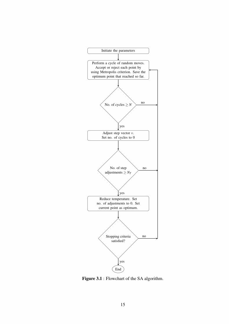
Initiate the parameters

Perform a cycle of random moves.Accept or reject each point by

using Metropolis criterion. Save theoptimum point that reached so far.

No. of cycles ≥ N

Adjust step vector v.Set no. of cycles to 0

No. of stepadjustments ≥ NT

Reduce temperature. Setno. of adjustments to 0. Set

current point as optimum.

Stopping criteriasatisfied?

End

yes

no

yes

no

yes

no

Figure 3.1 : Flowchart of the SA algorithm.

15

3.1.2 PyCASPESA

CASPESA is a method that has been successfully used to predict the crystal structures

of materials especially hydrogen storage materials such as metal borohydrides [1],

metal ammine borohydrides [13, 14] up to now. PyCASPESA has been developed for

the same purpose, but it is intended to improve the program especially by lowering

the required cpu time and making it more user friendly. For this purpose, firstly

the space search algorithm was refined in PyCASPESA. After this improvement, the

program achieves higher success by making fewer trials. PyCASPESA is better at

making arrangements by taking into consideration the interactions between unit cells.

Secondly, PyCASPESA tries to maximize the shrinkage of the unit cell in volume.

By this way, the program can predict more compact crystal structures. The program

requires a unit cell, atomic positions of the atoms and predefined bond distance

constraints to start the crystal prediction. Unlike CASPESA, with PyCASPESA we

can work with the systems that has no unit cell (by choosing the unit cell type as

none). In the metal borohydrides [1], the objective function in PyCASPESA are the

metal-hydrogen distances. After giving the objective function to the program properly,

the aim of the program is to make the arrangements (interactions that might lead to low

energy) as many number as possible which lower the total energy of the crystal. Since

there are no quantum mechanical calculations in CASPESA, in some cases the atoms

can be positioned too close to each other. For avoiding these nonphysical occurrences,

some bond distance thresholds are needed.

While preventing from unphysical situations and finding a solution that close enough

to the optimal solution in limited time, the constrains that mentioned above must be

introduced into models cautiously. In this new implementation, preparation of input

file is much easier than CASPESA’s. This procedure does not require any changes in

the source code. All the selections of the parameters can be done by making changes on

a single input file. The constrains generally obtained from the previous experimental

works. If there is no available data in the literature, these constrains can be determined

with the help of the DFT calculations. After performing the DFT calculations, CSP part

of the PyCASPESA will be started to run with these flawed constraints. If constraints

can be obtained from the experimental data, program will be started from the CSP

16

part of the PyCASPESA without making any DFT calculations. When the prediction

part is done, the best ones will be selected among the all predicted crystal structures

by using new SA analysis script. The SA analysis script makes selection according

to the following criteria. First of all, the script puts in an order all the structures in

terms of their densities and energies. Secondly, it eliminates the similar structures

among all the ordered structures. After that, it evaluates these structures according

to their bond numbers between the desired elements that we specified in the code,

e.g. a tetrahedral coordination (possibly will lower the total energy) around Mg in

Mg(BH4)2. After running the script, if the number of selected structures is greater

than Nmin, these resulting structures will be sent to GPAW or QE for further relaxation

at DFT level. If the number of selected structures is less than Nmin, the program returns

to the CSP step and starts from there to predict new structures. After the number of

structures reaches to Nmin, program will be started to make DFT calculations. If DFT

calculations are completed with success, the loop of the PyCASPESA will be done. In

this new implementation of the CASPESA, after the loop is completed, DFT analysis

script will be run. The DFT analysis script determines the space group symmetries of

the structures and writes all analysis results of the optimized structures to a file. This

script is written with the help of the FINDSYM program [15]. After running the DFT

analysis script, if there is a certain number of structure was found, stopping criteria

will be satisfied and the program will stop running. The flowchart of PyCASPESA can

be shown in Figure 3.2.

3.1.2.1 Implementation of DFT calculations

DFT calculations in PyCASPESA were performed generally by using GPAW, under

ASE. ASE is written in Python programming language. The code is actually a set of

tools and modules which developed with the aim of setting up, manipulating, running,

visualizing and analyzing atomistic simulations. It is freely available under GNU

licence. It is easy to use and it has a graphical user interface that named ase-gui. It is

possible with ASE to accomplish extremely complicated simulations without making

any code modifications. The code of ASE is structured as python modules that can

be used for different intentions. It is open to participation and modularity of the code

make it easy to contribute. There are many number of calculators available in ASE. A

calculator in ASE works as a black box that takes atomic numbers and positions from

17

an atoms object and calculates the energy and forces. GPAW is one of these calculators

and it is a DFT code that based on the projector-augmented wave (PAW) method. In

GPAW, the pseudo wave functions can be described in three ways: plane waves, atom

centered basis functions and finite difference (FD) approximation.

In PyCASPESA, DFT calculations can also be performed by using Quantum Espresso

[16]. QE is an open-source software and it is based on DFT, plane waves and

pseudopotentials. The scripts that make input file and DFT analysis were also written

for QE.

18

Initiate the parameters

Simulated AnnealingPart of PyCASPESA for

Crystal Structure Prediction

For Analyzing SAresults: Run the SAanalysis script andselect the best N

structures

Run the script thatmade GPAW or QE

input for the selectedN structures and thanRun these structures

at DFT level

Run the DFT Analysis Script andGet the symmetry analysis results

Stopping criteriasatisfied?

Stop

if N ≥ Nmin

if N < Nmin

if DFT runs completed succesfully

yes

no

Figure 3.2 : Flowchart of the PyCASPESA method.

19

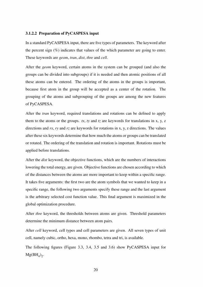
3.1.2.2 Preparation of PyCASPESA input

In a standard PyCASPESA input, there are five types of parameters. The keyword after

the percent sign (%) indicates that values of the which parameter are going to enter.

These keywords are geom, tran, dist, thre and cell.

After the geom keyword, certain atoms in the system can be grouped (and also the

groups can be divided into subgroups) if it is needed and then atomic positions of all

these atoms can be entered. The ordering of the atoms in the groups is important,

because first atom in the group will be accepted as a center of the rotation. The

grouping of the atoms and subgrouping of the groups are among the new features

of PyCASPESA.

After the tran keyword, required translations and rotations can be defined to apply

them to the atoms or the groups. tx, ty and tz are keywords for translations in x, y, z

directions and rx, ry and rz are keywords for rotations in x, y, z directions. The values

after these six keywords determine that how much the atoms or groups can be translated

or rotated. The ordering of the translation and rotation is important. Rotations must be

applied before translations.

After the dist keyword, the objective functions, which are the numbers of interactions

lowering the total energy, are given. Objective functions are chosen according to which

of the distances between the atoms are more important to keep within a specific range.

It takes five arguments: the first two are the atom symbols that we wanted to keep in a

specific range, the following two arguments specify these range and the last argument

is the arbitrary selected cost function value. This final argument is maximized in the

global optimization procedure.

After thre keyword, the thresholds between atoms are given. Threshold parameters

determine the minimum distance between atom pairs.

After cell keyword, cell types and cell parameters are given. All seven types of unit

cell, namely cubic, ortho, hexa, mono, rhombo, tetra and tri, is available.

The following figures (Figure 3.3, 3.4, 3.5 and 3.6) show PyCASPESA input for

Mg(BH4)2.

20

%geom@mg1Mg 0.000000 0.000000 0.000000@mg2Mg 0.000000 0.000000 0.000000@bh41B 4.08770 6.28222 6.05476H 3.05196 6.86603 6.32590H 5.12344 6.86603 6.32590H 4.08770 5.24607 6.70752H 4.08770 6.15812 4.84202@bh42B 4.08770 6.28222 6.05476H 3.05196 6.86603 6.32590H 5.12344 6.86603 6.32590H 4.08770 5.24607 6.70752H 4.08770 6.15812 4.84202@bh43B 4.08770 6.28222 6.05476H 3.05196 6.86603 6.32590H 5.12344 6.86603 6.32590H 4.08770 5.24607 6.70752H 4.08770 6.15812 4.84202@bh44B 4.08770 6.28222 6.05476H 3.05196 6.86603 6.32590H 5.12344 6.86603 6.32590H 4.08770 5.24607 6.70752H 4.08770 6.15812 4.84202

Figure 3.3 : Geometry definitions part of the example input file of Mg(BH4)2

In the geom part, free atoms and groups were declared and atomic positions are

assigned. As it can be seen in the example, atomic positions of the four BH4 groups

are given as the same. There is no problem about giving the atomic positions of the

atoms or groups as the same. In each BH4 group, B atoms defined firstly, because they

are selected as the center of the rotational motion.

21

%tran# Application of the rotations@bh41 rx 0. 6.28318530718@bh41 ry 0. 6.28318530718@bh41 rz 0. 6.28318530718@bh42 rx 0. 6.28318530718@bh42 ry 0. 6.28318530718@bh42 rz 0. 6.28318530718@bh43 rx 0. 6.28318530718@bh43 ry 0. 6.28318530718@bh43 rz 0. 6.28318530718@bh44 rx 0. 6.28318530718@bh44 ry 0. 6.28318530718@bh44 rz 0. 6.28318530718# Application of the translations@mg1 tx 0. 11.@mg1 ty 0. 11.@mg1 tz 0. 11.@mg2 tx 0. 11.@mg2 ty 0. 11.@mg2 tz 0. 11.@bh41 tx 0. 11.@bh41 ty 0. 11.@bh41 tz 0. 11.@bh42 tx 0. 11.@bh42 ty 0. 11.@bh42 tz 0. 11.@bh43 tx 0. 11.@bh43 ty 0. 11.@bh43 tz 0. 11.@bh44 tx 0. 11.@bh44 ty 0. 11.@bh44 tz 0. 11.

Figure 3.4 : Translation and rotation part of the example input file of Mg(BH4)2

In the part shown in Figure 3.4, rotations and translations are applied respectively.

Rotations are only applied to the groups. In this example, groups can be rotated with

any angle between 0 and 2π .

22

% distMg H 2.05 2.10 10Mg B 2.40 2.45 10

Figure 3.5 : Objective function definitions part of the example input file of Mg(BH4)2

% threMg B 2.40H H 1.85B B 3.20Mg Mg 4.20

Figure 3.6 : Threshold definitions part of the example input file of Mg(BH4)2

% cell# Assignments For the orthorhombic unit cell typeortho 0 18 0 18 0 18

#Assignment Examples For all different type of unit cells

#For tetragonal unit cell type#tetra 0 18 0 18

#For hexagonal unit cell type#hexa 0 18 0 18

#For cubic unit cell type#cubic 0 18

#For monoclinic unit cell type#mono 0 18 0 18

#For rhombohedral unit cell type#rhombo 0 18 0 18 0 18

#For triclinic unit cell type#tri 0 18 0 18 0 18 0 18 0 18 0 18 0 18 0 18 0 18

Figure 3.7 : Unit cell definition part of the example input file of Mg(BH4)2

23

%geom# grp1H refers that H atoms in only grp1@grp1B 4.08770 6.28222 6.05476 grp1BH 3.05196 6.86603 6.32590 grp1HH 5.12344 6.86603 6.32590 grp1HH 4.08770 5.24607 6.70752 grp1HH 4.08770 6.15812 4.84202 grp1H@grp2B 4.08770 6.28222 6.05476 grp2BH 3.05196 6.86603 6.32590 grp2HH 5.12344 6.86603 6.32590 grp2HH 4.08770 5.24607 6.70752 grp2HH 4.08770 6.15812 4.84202 grp2H

%thre# B.grp1B B.grp2B 3.20 means that distance threshold# between B atoms in grp1 and grp2 is 3.20B.grp1B B.grp2B 3.20H.grp1H H.grp2H 1.85

Figure 3.8 : Nickname usage on another example input file of Mg(BH4)2

As it can be seen from Figure 3.5, objective functions are selected as Mg−H and

Mg−B distances in this example. If any Mg−H distance in the system is between

2.05 and 2.10 Å, the objective function will be increased by 10. SA algorithm tries to

maximize the objective function until the program reaches to the termination criterion.

Figure 3.6 shows how the thresholds were assigned. As an example, when the threshold

between Mg and B is set to 2.40 Å, if Mg−B distance is lower than the threshold, the

program does not accept this formation and tries another new arrangement.

Figure 3.7 shows that how the unit cell type and the parameters are going to be assigned

for all seven types of unit cell. For the systems that has no need for unit cell, unit cell

type can be chosen as none. There is an optional fifth parameter in geom part of the

input file. If there is a need to give a nickname to an atom, this parameter can be used.

Usage of the parameter can be seen in Figure 3.8. In the example, grp1 has one B

atom with the nickname grp1B and grp2 has one B atom with the nickname grp2B.

Via giving the nicknames to the atoms, threshold value between the B atom in grp1

and the B atom in grp2 can be set to 3.20 Å.

24

3.2 Theoretical Background

3.2.1 Schrödinger equation

The famous Schrödinger equation were discovered in 1926 and solving this eigenvalue

problem has become one of the most important issue in quantum chemistry since that

time. For N-body systems the time-independent Schrödinger equation can be written

in this form

HΨ = EΨ (3.1)

where H is the Hamiltonian operator, Ψ is the N-body wave function of the quantum

system and E is the total energy of the system. Hamiltonian operator can be written in

the following form

H =−∑i

h2me

∇2i −∑

k

h2mk

∇2k−∑

i∑k

e2Zk

rik+∑

i< j

e2

ri j+∑

k<l

e2ZkZl

rkl(3.2)

where h is the reduced Planck constant and it equals to h/ 2π , me is the mass of

the electron, mk is the mass of the nucleus, e is the charge on the electron, Z is the

atomic number, rab is the distance between a and b, i and j indices denote to electrons

and k and l indices denote to nuclei. There are five contributions to the total energy

of the system. The first two terms in H represent the kinetic energy of the electrons

and the nuclei, respectively and the other three terms represent the attraction between

the electrons and nuclei, electron-electron (interelectronic) repulsion and nuclei-nuclei

(internuclear) repulsion, respectively.

Basically, If Schrödinger equation can be solved exactly in order to get the wave

function of the system, then the energy states of the system can be determined. But

unfortunately, Schrodinger equation can not be solved exactly for N-body systems.

The equation can be solved only by making approximations. In order to simplify the

problem, Born-Oppenheimer (BO) approximation can be used. BO approximation

assumes that the electronic motion and the nuclear motion in molecules are separable

and this idea is a cornerstone for the computational chemistry. Basically, BO

approximation neglects coupling between the nuclei and electronic motion. Because

25

the motion of the nuclei is much slower than the motion of the electrons in a molecular

system, nuclei can be considered as fixed. After the BO approximation, the electronic

Schrödinger equation can be written in the following form:

(Hel +VN)Ψel = EelΨel (3.3)

where VN is a constant for the nuclear-nuclear repulsion energy of the given system,

(Ψel) is the electronic wave function, Eel is the electronic energy and the electronic

Hamiltonian operator Hel is

Hel =−∑i

h2me

∇2i −∑

i∑k

e2Zk

rik+∑

i< j

e2

ri j(3.4)

As it can be seen from the equation (3.4), Hel operator includes only the first, third

and fourth terms of the typical Hamiltonian operator. Kinetic energy of the nuclei

(second term) is fixed as zero and potential energy that comes from the nuclear-nuclear

repulsion (fifth term) is fixed as a constant. The total energy of the system is the

summation of the electronic energy and and the constant nuclear-nuclear repulsion

energy [17]. After the simplification of the problem by using BO approximation,

solution of the Schrödinger equation becomes more viable. There are several

approaches to solving this problem and these approaches can be divided into three

main groups: ab-initio, semi-empirical and density functional theory (DFT) methods.

If solutions are generated from theoretical principles without using any experimental

data the methods usually named as ab-initio (means that "from the beginning" in latin),

in contrast to the ab-initio methods semi-empirical methods use experimental data. In

DFT methods, energy of the system is determined from the electron density instead of

the wave function. Computationally demanding ab-initio methods are more accurate

than the semi-empirical methods. Semi-empirical methods are faster than the ab-initio

methods, but on the other hand they require experimental parameters. DFT methods

are more recent than these methods and they are much faster than ab-initio methods

except Hartree-Fock approach.

3.2.2 Density functional theory

DFT is a widely used and successful approach for computing the electronic structure

of a matter. It is so popular because it is less computationally expensive than the

26

other methods with almost the same accuracy. DFT is being used for predicting some

molecular properties such as molecular structures, atomization energies, ionization

energies, vibrational frequencies, reaction paths, etc. In the beginning, DFT was

developed to obtain the electron density (ρ) and the total energy of the ground state

of electronic systems. In this work, DFT is the approach that we are using to find an

approximate solution for Schrödinger equation of many body systems.

3.3 Application: Hydrogen Storage

The primary energy source of the world is the fossil fuels such as coal, natural gas and

oil for a long time. But the fossil fuels are limited and they are running out rapidly as

a result of the highly increased world population and increased energy demand due to

technological developments. According to 2016 BP Statistics [18], if we continue to

consume energy resources at the current rate, in 2128 coal reserves, in 2069 natural gas

reserves and in 2067 crude oil reserves will be ran out. Actually we do not have that

much time, because The International Energy Agency expects that the energy demand

of the world will rise at least 50 percent until 2030. In addition to the fact that the

fossil fuel reserves dwindle, burning fossil fuels has an adverse effect on environment.

They are highly responsible for the air pollution on the Earth. When they burn, they

release huge amount of carbon dioxide to the atmosphere and CO2 is a greenhouse gas

that causes increment in the average temperature of the Earth. Release of CO2 to the

earth is also a threat for marine life. We must end the usage of fossil fuels for future

generations. In the view of these informations, the need for new, clean and renewable

energy source is much greater than ever. Hydrogen can be considered as a possible

solution for the energy problem of the world. It is the most abundant element in the

world and its energy density is the highest per mass. It is renewable and clean. It seems

perfect, but hydrogen is not an actual energy source, it is an energy carrier. It occurs in

the nature chemically bounded as H2O molecule in water or bounded to hydrocarbons.

There are major obstacles about production, storage and usage of the hydrogen as an

energy carrier.

If we can find practical solutions to overcome these obstacles, hydrogen can be used to

supply the energy demand of the world. If hydrogen is desired to be used as a source of

energy on mobile applications, storing it appropriately becomes the most challenging

27

part of the work. The storage method should be safe, durable and cost-efficient.

Hydrogen can be stored as gas, liquid and solid forms and there are various methods

for hydrogen storage is available.

3.3.1 Hydrogen storage methods

Any potential hydrogen storage material for mobile applications should have the

qualifications in terms of good revesibility, fast absorption and desorption of hydrogen

kinetics and high volumetric and gravimetric density. There are various methods for

hydrogen storage. According to Züttel, A. [19], there are six different method for

reversible hydrogen storage with a high volumetric and gravimetric density. These are

high pressure gas cylinders, storing hydrogen as liquid in cryogenic tanks, physically

adsorbed hydrogen, metal hydrides, complex hydrides, storing hydrogen via chemical

reactions between metals and complexes together with water. When these storage

methods are examined, the most long term solution for storing hydrogen for mobile

applications is the solid state storage. Discovery of the new hydrogen storage materials

can be done by using various crystal structure prediction methods. For this purpose,

CASPESA has used by our research group for a long time [1,13,14]. The starting point

of this thesis is the need for the improvement of CASPESA to perform much faster and

robust crystal structure predictions.

28

4. RESULTS AND DISCUSSIONS

In this thesis, magnesium borohydride (Mg(BH4)2) is chosen as our test case to test

newly implemented crystal structure prediction tool, PyCASPESA. In this chapter,

information about Mg(BH4)2 setups and the results of the study are going to be given

and discussed.

4.1 Mg(BH4)2 Setup: SA part of PyCASPESA

Magnesium borohydride (Mg(BH4)2) is a promising material for solid-state hydrogen

storage due to its gravimetric and volumetric hydrogen density. Mg(BH4)2 can

theoretically store hydrogen up to 16.8wt% and can achieve full reversibility [20, 21].

The first reported synthesis of Mg(BH4)2 is made by Wiberg and Bauer in 1950s [22].

After that, the interest for the material has continued to grow rapidly. For testing and

validating the new CASPESA implementation, we need to work with a material for

which its experimental crystal structure is known. For this purpose, Mg(BH4)2 is a

proper test case for us. According to previous studies about magnesium borohydride,

maximizing the numbers of Mg−H and Mg−B bonds within the (2x2x2) cut-through

lattice in Mg(BH4)2 is very important to stabilize the CS [1, 23]. In this model,

there are two formula units (fu) of Mg(BH4)2 in the unit cell. The distance ranges

(objective function) for Mg−H and Mg−B were set to (2.05,2.10) and (2.40,2.45) Å,

respectively. The bond distance thresholds for Mg−B, Mg−Mg, B−B and H−H were

set to 2.40,4.20,3.2,1.85, respectively. All these constrains were obtained from the

data that reported in the literature [1]. SA parameters that is mentioned before NS, NT

and rT were set to 80, 80 and 0.6 for this setup. There are 30 structural parameters in

the unit cell (uc) for Mg(BH4)2. Among these parameters, 12 of these are for rotational

movements of the BH4 groups and 18 of these are for translational movements of the

BH4 groups and Mg atoms. Besides these parameters, unit cell parameters must also be

given in input file. The number of the uc parameters depends on the unit cell type. For

example, if uc is chosen as cubic, there is only one parameter. But if we chose the uc

29

as orthorhombic, we should enter three parameters. The total numbers of parameters

that we used for this setup are 31 for cubic uc, 32 for hexagonal and tetragonal ucs and

33 for orthorhombic uc.

The results of the previous study [24] show that the tetragonal structure with the

symmetry group I4m2, No. 119 is the true ground-state structure. (No corresponds

to numbers of crystal symmetry that based on international tables of crystallography.)

In another study [25], the structure with the symmetry group F222, No. 22 is found as

the true ground-state structure. It has lower energy than all previously proposed phases

of Mg(BH4)2.

In this thesis, we tried to re-explore the crystal structure of Mg(BH4)2. By using

PyCASPESA, approximately 1400 CS was predicted for Mg(BH4)2 and after that

selected 170 structures were further relaxed at DFT level. As a result, the program

successfully yielded the structures with the symmetry group I4m2 and F222. Detailed

results are going to be given in the following pages of this chapter. Visualization of all

results is made by using VESTA program [26].

4.2 Mg(BH4)2 Setup: DFT part of PyCASPESA

Within the scope of this thesis, DFT calculations were performed by using GPAW

and QE. In the calculations that was made with GPAW for Mg(BH4)2, plane waves

(PW) were used for describing the pseudo wave functions and RPBE (Resived

Perdew-Burke-Ernzerhof) [27] was used as an exchange correlation functional. K

points were chosen as (2,2,2). Grid spacing parameter h was set to 0.2. Plane-wave

cutoff was set to its default value, 340. BFGS was used as the local optimization

algorithm.

In the calculations that was made with QE for Mg(BH4)2, PBE

(Perdew-Burke-Ernzerhof) [28] generalized gradient approximation is used as

the exchange correlation functional. Norm-conserving pseudopotentials are used in

the calculations. Kinetic energy cutoff determines the size of the plane wave basis set

that used to expand wave functions and it was set to 80 Ry. Density cutoff was set to

30

320 Ry. Energy and force thresholds was set to 10−5 and 10−4, respectively. K points

were chosen as (2,2,2).

4.3 Mg(BH4)2 Results

Cerný et al. [29] reported that Mg(BH4)2 crystallizes into a tetragonal lattice with the

symmetry of I4m2, it has a theoretical hydrogen storage capacity of 14.8 wt % and it

is also thermally quite stable compound.

Before the applications of PyCASPESA for Mg(BH4)2, the known lowest energy

structure was optimized at DFT level by using 4 formula units in the uc for being

able to make comparisons later. Optimized structure can be shown in Figure 4.1.

Figure 4.1 : The known lowest energy tetragonal structure of Mg(BH4)2 with thesymmetry group I4m2, No. 119. Representations of colors: magnesium

(Mg), brown; boron (B), green; hydrogen (H), light gray.

31

(a) (b)

(c)

Figure 4.2 : (a)The crystal structure of Mg(BH4)2 that generated by PyCASPESA,(b)the structure generated by PyCASPESA (a) were further relaxed atDFT level leading to a tetragonal structure with the symmetry groupI4m2, No. 119 projected along [010] direction, (c) The same DFT

optimized structure projected along [001] direction

32

As it can be seen from Figure 4.1, each magnesium is surrounded by four (BH4)

groups. The I4m2 structure is highly symmetric because all Mg-B, B-B and B-H bond

lenghts are equivalent. The cell parameters of I4m2 Mg(BH4)2 structure in Figure 4.1

were a= 8.1754 and c= 10.0718 Å (These are the shrinked cell parameters due to DFT

relaxation). By using PyCASPESA, the same tetragonal structure of Mg(BH4)2 with

the symmetry group I4m2, No. 119 was found and the cell parameters were a= 8.1510

and c = 10.03399 Å. The non-optimized and optimized versions of the structure were

shown in Figure 4.2. The non-optimized structure formed as a distorted tetragonal

around Mg, but after the DFT optimization it looks like identical to the known lowest

energy structure.

The minimum bond lengths of Mg(BH4)2 known lowest energy structure and

Mg(BH4)2 structure that genereted by PyCASPESA after relaxations were compared

at Table 4.1.

Table 4.1 : The minimum bond lenghts of Mg(BH4)2

Bond Lengths Mg(BH4)2(Å) Mg(BH4)2(Å)(Atom-Atom) (Known Lowest Energy Structure) (PyCASPESA)

Mg-Mg 4.80098 4.78563B-B 3.71271 3.69633

Mg-H 2.03375 2.01973H-H 2.07148 2.07004

33

The second Mg(BH4)2 structure that generated by PyCASPESA has a hexagonal

unit cell at the begining, but after all the relaxations it turns out a slighty distorted

orthorhombic structure with the symmetry group F222, No. 22. This structure is an

important CS. It was mentioned before in a computational study as a true ground-state

structure [25] and it can be shown in Figure 4.3.

Figure 4.3 : Mg(BH4)2 structure with the symmetry group F222, No. 22

In F222 structure, all Mg-B bond lenghts are equal, but the tetrahedral arrangement

around Mg is distorted because of the unequal B-B bond distances. As it can be seen

from Figure 4.3, magnesium is coordinated by four BH4 groups. A symmetry relation

analysis deduced that I4m2 and F222 structures are related with a symmetry relation:

F222 is a subgroup of I4m2 [1].

Except from these two structures that mentioned above, a lot of crystal structure of

Mg(BH4)2 was found in this study by using PyCASPESA. Some of these structures

were indicated in the literature previously, but some of them were never found until

this study. All the DFT relaxed structures shown in Figure 4.4 and 4.5 were already

reported structures in the literature.

34

(a) (b)

(c) (d)

Figure 4.4 : The crystal structures of Mg(BH4)2 that was generated by usingPyCASPESA with the symmetry group; (a) I4122, No. 98, (b) Ima2, No.

46, (c) Fdd2, No. 43, (d) Ama2, No. 40.

35

(a) (b)

(c) (d)

(e)

Figure 4.5 : The crystal structures of Mg(BH4)2 that was generated by usingPyCASPESA with the symmetry group; (a) I212121, No. 24, (b) Cc, No.

9, (c) P1m1, No. 6 (d) C2, No. 5, (e) C2, No. 5.

36

The following DFT optimized structures that reported in Figure 4.6 were found for the

first time.

(a) (b)

(c) (d)

Figure 4.6 : The crystal structures of Mg(BH4)2 that was found for the first time byusing PyCASPESA with the symmetry group; (a) P4n2, No. 118, (b)

P42m, No. 111, (c) Cm, No. 8, (d) Cm, No. 8.

37

The crystal structures of Mg(BH4)2 in Figure 4.4 (a,b,d), 4.5 (a) and 4.6 (a) were

found to be tetragonal with space groups I4122 (No. 98), Ima2 (No. 46), Ama2

(No. 40), I212121 (No. 24), P4n2 (No. 118) respectively after the DFT optimizations

by using a unit cell that contains two formula units. In these systems, each Mg was

surrounded by four distorted tetrahedrally coordinated BH4 groups. In crystal structure

with the symmetry group Fdd2 (No. 43) (Figure 4.4 (c)), each magnesium atom was

surrounded by distorted tetrahedrally coordinated four BH4 groups. The crystal lattice

system of the structure was found to be orthorhombic. In another crystal structure

with the symmetry group Cc (No. 9), BH4 groups showed highly distorted tetrahedral

coordination around magnesium atoms (Figure 4.5 (b)). At the starting point, the

unit cell of the structure was cubic, but after the DFT optimizations it is turned into

an monoclinic one. The structures in Figure 4.5(d) and 4.6(c) were found with the

space group C2 (No. 5) and Cm (No. 8), respectively. Unlike the others, some of

the magnesium atoms in these structures was surrounded by five BH4 groups and the

shape of this arrangement around Mg was looked like a distorted trigonal bipyramidal.

The crystal lattice systems of both structures was monoclinic. The structure in Figure

4.6(b) with the symmetry group 42m (No. 111) is a newly found pretty well-organized

tetragonal structure. It was similar to the known lowest energy structure and the

coordinations of BH4 groups around Mg atoms were tetrahedral. In the structure with

the symmetry group Cm (No. 8), each four BH4 groups is coordinated around Mg as a

distorted square. The crystal lattice system of the structure was found to be monoclinic

and it can be shown in Figure 4.6(d). Another newly found structure in Figure 4.6(e)

with the symmetry group P1m1 (No. 6) was found to be slightly distorted tetragonal

structure.

Table 4.2 shows crystallographic details of Mg(BH4)2 crystal structures that was

generated by PyCASPESA. Table 4.2 also shows the relative energies of the structures.

The structures in the table are named according to the figure numbers in which the

structure was shown. For example, Mg(BH4)2-4-4a is the structure in Figure 4.4 (a).

38

Table 4.2 : Crystallographic details of Mg(BH4)2 structures.

Structure a(Å) b(Å) c(Å) α(deg) β (deg) γ(deg) Symmetry Energy(eV)Mg(BH4)2-4-1 8.15100 8.15100 10.03399 90 90 90 I4m2(119) 0.000Mg(BH4)2-4-3 10.84101 10.33752 11.94221 90 90 90 F222(22) 0.017Mg(BH4)2-4-4a 7.41889 7.41889 12.12452 90 90 90 I4122(98) 0.021Mg(BH4)2-4-4b 8.57593 8.10830 8.43393 90 90 90 Ima2(46) 0.275Mg(BH4)2-4-4c 10.16081 9.06245 13.16463 90 90 90 Fdd2(43) 0.241Mg(BH4)2-4-4d 8.87591 6.62465 6.72052 90 90 90 Ama2(40) 0.791Mg(BH4)2-4-5a 6.63566 13.04401 7.16078 90 90 90 I212121(24) 0.287Mg(BH4)2-4-5b 10.97276 9.69908 8.25313 90 131.69 90 Cc(9) 0.149Mg(BH4)2-4-5c 9.10244 13.05448 6.60735 90 129.11 90 C2(5) 0.261Mg(BH4)2-4-5d 8.42218 14.62163 5.02396 90 92.33 90 C2(5) 0.656Mg(BH4)2-4-6a 5.65900 5.65900 5.85893 90 90 90 P4n2(118) 0.599Mg(BH4)2-4-6b 5.74426 5.74426 5.65929 90 90 90 P42m(111) 0.627Mg(BH4)2-4-6c 14.65681 8.43794 5.02254 90 92.90 90 Cm(8) 0.341Mg(BH4)2-4-6d 10.49244 8.74472 7.00519 90 124.79 90 Cm(8) 0.656Mg(BH4)2-4-6e 4.69658 8.95271 4.77625 90 90.47 90 P1m1(6) 0.745

4.4 Conclusions

CASPESA is a method that was developed by our research group for predicting the

crystal structures. In the scope of this thesis, a new CSP method PyCASPESA was

developed by improving CASPESA method. PyCASPESA uses simulated annealing

algorithm for prediction of the crystal structures and makes density functional theory

calculations for relation of the structures that generated in the first step of the program.

These DFT calculations are not applied all generated structures, they applied only the

selected structures. Between the SA part of the program and DFT part of the program,

a script runs and selects the best structures that have desired properties. After the

DFT calculations, the analysis script runs for analyzing the selected and optimized

structures. PyCASPESA was tested to discover the ground state crystal structures

of Mg(BH4)2, because there is an experimentally determined crystal structure for it.

The structure of Mg(BH4)2 with the symmetry group I4m2, No. 119 is a tetragonal

structure. By using PyCASPESA the structure with the symmetry group I4m2 was

successfully yielded. Besides this structure, the method also found lots of crystal

structure of Mg(BH4)2. Some of them were reported in the literature previously, but

some of them were never found until this study. The success obtained for Mg(BH4)2

39

encourages us to employ this new implementation for the other interesting solid state

materials e.g. used in storing hydrogen or battery applications.

40

REFERENCES

[1] Caputo, R., Tekin, A., Sikora, W. and Züttel, A. (2009). First-principlesdetermination of the ground-state structure of Mg (BH 4) 2, ChemicalPhysics Letters, 480(4), 203–209.

[2] Glass, C.W., Oganov, A.R. and Hansen, N. (2006). USPEX—evolutionarycrystal structure prediction, Computer Physics Communications, 175(11),713–720.

[3] Lonie, D.C. and Zurek, E. (2011). XtalOpt: An open-source evolutionary algo-rithm for crystal structure prediction, Computer Physics Communications,182(2), 372–387.

[4] Lyakhov, A.O., Oganov, A.R., Stokes, H.T. and Zhu, Q. (2013). Newdevelopments in evolutionary structure prediction algorithm USPEX,Computer Physics Communications, 184(4), 1172–1182.

[5] Wang, Y., Lv, J., Zhu, L. and Ma, Y. (2010). Crystal structure prediction viaparticle-swarm optimization, Physical Review B, 82(9), 094116.

[6] Liu, Z.L. (2014). MUSE: Multi-algorithm collaborative crystal structureprediction, Computer Physics Communications, 185(7), 1893–1900.

[7] Massa, W. (2013). Crystal structure determination, Springer Science & BusinessMedia.

[8] Wang, Y., Lv, J., Zhu, L. and Ma, Y. (2012). CALYPSO: A method forcrystal structure prediction, Computer Physics Communications, 183(10),2063–2070.

[9] Oganov, A.R. (2011). Modern methods of crystal structure prediction, John Wiley& Sons.

[10] Young, D. (2004). Computational chemistry: a practical guide for applyingtechniques to real world problems, John Wiley & Sons.

[11] Zabinsky, Z.B. (2009). Random search algorithms, Wiley Encyclopedia ofOperations Research and Management Science.

[12] Corona, A., Marchesi, M., Martini, C. and Ridella, S. (1987). Minimizingmultimodal functions of continuous variables with the simulated annealingalgorithm, ACM Transactions on Mathematical Software, 13(3), 262–280.

41

[13] Emdadi, A., Kıslak, Y., Demir, S. and Tekin, A. (2015). ComputationalScreening of Dual Cation Metal Ammine Borohydrides, 2nd Interna-tional Congress on Energy Efficiency and Energy Related Materials(ENEFM2014), Springer, p.581.

[14] Emdadi, A., Demir, S., Kıslak, Y. and Tekin, A. (2016). ComputationalScreening of Dual-Cation Metal Ammine Borohydrides by DensityFunctional Theory, The Journal of Physical Chemistry C, 120(25),13340–13350.

[15] Stokes, H.T. and Hatch, D.M. (2005). FINDSYM: program for identifying thespace-group symmetry of a crystal, Journal of Applied Crystallography,38(1), 237–238.

[16] Giannozzi, P., Baroni, S., Bonini, N., Calandra, M., Car, R., Cavazzoni, C.,Ceresoli, D., Chiarotti, G.L., Cococcioni, M., Dabo, I. et al. (2009).QUANTUM ESPRESSO: a modular and open-source software project forquantum simulations of materials, Journal of physics: Condensed matter,21(39), 395502.

[17] Lewars, E.G. (2016). Computational chemistry: introduction to the theory andapplications of molecular and quantum mechanics, Springer.

[18] (2016), BP Statistical Review of World Energy June 2016, http://www.bp.com/en/global/corporate/energy-economics/statistical-review-of-world-energy.html.

[19] Züttel, A. (2003). Materials for hydrogen storage, Materials today, 6(9), 24–33.

[20] Vajeeston, P., Ravindran, P., Kjekshus, A. and Fjellvåg, H. (2006). Highhydrogen content complex hydrides: a density-functional study, Appliedphysics letters, 89(7), 071906.

[21] Wu, H., Zhou, X., Rodriguez, E.E., Zhou, W., Udovic, T.J., Yildirim, T.and Rush, J.J. (2016). A new family of metal borohydride guanidinatecomplexes: Synthesis, structures and hydrogen-storage properties,Journal of Solid State Chemistry, 242, 186–192.

[22] Wiberg, E. and Bauer, R. (1950). Notizen: Zur Kenntnis einesMagnesium-bor-wasserstoffs Mg (AlH4) 2, Zeitschrift für NaturforschungB, 5(7), 397–398.

[23] Caputo, R., Kupczak, A., Sikora, W. and Tekin, A. (2013). Ab initio crystalstructure prediction by combining symmetry analysis representations andtotal energy calculations. An insight into the structure of Mg (BH 4) 2,Physical Chemistry Chemical Physics, 15(5), 1471–1480.

[24] Ozolins, V., Majzoub, E. and Wolverton, C. (2008). First-principles predictionof a ground state crystal structure of magnesium borohydride, Physicalreview letters, 100(13), 135501.

42

[25] Voss, J., Hummelshøj, J.S., Łodziana, Z. and Vegge, T. (2008). Structuralstability and decomposition of Mg (BH4) 2 isomorphs—an ab initio freeenergy study, Journal of Physics: Condensed Matter, 21(1), 012203.

[26] Momma, K. and Izumi, F. (2011). VESTA 3 for three-dimensional visualizationof crystal, volumetric and morphology data, Journal of AppliedCrystallography, 44(6), 1272–1276.

[27] Hammer, B., Hansen, L.B. and Nørskov, J.K. (1999). Improved ad-sorption energetics within density-functional theory using revisedPerdew-Burke-Ernzerhof functionals, Physical Review B, 59(11), 7413.

[28] Perdew, J.P., Burke, K. and Ernzerhof, M. (1996). Generalized gradientapproximation made simple, Physical review letters, 77(18), 3865.

[29] Cerny, R., Filinchuk, Y., Hagemann, H. and Yvon, K. (2007). Magnesiumborohydride: synthesis and crystal structure, Angewandte Chemie,119(30), 5867–5869.

43

44

CURRICULUM VITAE

Name Surname: Gözde Inis

Place and Date of Birth: Antalya, 1990

E-Mail: gozdeinis90@gmail.com

EDUCATION:

• B.Sc.: 2014, Istanbul Commerce University, Mathematics

• M.Sc.: 2017, Istanbul Technical University, Computational Science andEngineering

PROFESSIONAL EXPERIENCE AND REWARDS:PUBLICATIONS, PRESENTATIONS AND PATENTS ON THE THESIS:

45