Embed Size (px)
Citation preview
Issues in Political Economy, Vol 24, 2015, 85-100
85
Long-Term Guaranteed Contracts in the NBA: A Case for Moral Hazard Leonardo Pedicelli, American University ‘15
Incentives are integral to economics. At its heart, incentive theory generally focuses on tasks that
are too complicated or too costly to do oneself. As a result, a “principle” collects resources and
ultimately hires an “agent” with a special skill set to perform the task in question. In this
situation, the principle depends on the agent to produce a quality output within a productive time.
However, an essential problem arises when the input (effort) of the worker (agent) is not directly
and constantly observable due to its high functional costs (Nalebuff and Stiglitz, 1983). Under
such conditions, the worker will be inclined to expend a sub-optimal level of effort in performing
the task, which inherently invites shirking (Lazear and Rosen, 1981). This has led to an extensive
literature addressing the design of incentive-compatible labor contracts in attempt to induce
agents to operate in the principal’s interest (Prendergast, 1999). Some examples of incentive-
compatible labor contracts include profit-sharing arrangements, stock options for upper
management, incentive clauses in professional athletes’ contracts, and piece-rate pay for
production workers.
This paper is set to focus on the incentive-compatible labor contracts in regards to professional
sports. In particular, agency literature in sports economics has focused primarily on the shirking
problem associated with long-term labor contracts of professional athletes. Throughout previous
decades, the rise of guaranteed contracts in sports has caused uproar of debate questioning the
performance of players in relationship to guaranteed money1. The NBA (National Basketball
Association) is one league in which labor agreements are in the form of guaranteed contracts as
part of player relations. As a result, the NBA has been under constant scrutiny, since there is a
tendency among players to increase the amount of effort put forth in a contract year in order to
maximize their potential for a “juicy” multi-year contract the following season2. In the face of
such problems, contractual mechanisms typically evolve to combat such tendencies.
There are a number of reasons to be suspect about whether professional athletes can and do in
fact shirk. This skepticism is fueled by the growing literature’s mixed results. While some
authors have found evidence of shirking behavior (Lehn, 1982; Sen and Rice, 2011; Stiroh,
2007), other authors (Krautmann, 1990; Maxcy, et al., 2002) have not. Furthermore, adding to
the constant uncertainty, Berri and Krautmann (2006) find conflicting evidence of shirking
contingent upon on the methodology used to study the overarching phenomenon3. Nonetheless,
this paper will primarily focus on the dynamics of shirking by examining the behavior of NBA
athletes not only across an entire contract cycle, but also before and after entering a new
contract—an approach, which has been sparse in updated literature4.
I. CONCEPTUAL FRAMEWORK
The conceptual framework for this paper turns to the foundation that of Sen and Rice5 (2011) and
incorporates justifications based on related research. First, the framework itself will be
explained, followed by the underlying logic and economic intuition behind the construct. Finally,
the results of the framework will be analyzed in relation to agency-theory.

Issues in Political Economy, Volume 24, 2015
86
Theory suggests that NBA players perform better in the final year of their contract relative to
other years. In order to prove this notion, the interaction between player and team will be
modeled as a 3-period principle-agent game. This 3-period game relies on the two basic
assumptions of agency-theory: (1) both the principle and the agent are self-interested, utility-
maximizing actors and (2) the agent is risk-averse, while the principle is risk-neutral—or at least
less risk averse than the agent6.
In this 3-period game, the player chooses effort in each period though the salary for that period is
negotiated prior. The output (or outcome) is then realized at the end of every period and is
generally a function of the agent’s effort and of some other unobservable variables, which
influence the outcome in either a positive or a negative way. As a result, the agent’s output (or
principle’s revenue) is contingent upon the effort level of the player and a random component,
since the agent has no control over these exogenous effects. Since guaranteed contracts are
prevalent in the NBA, the agent will only demonstrate a high level of effort and incentive when
given the opportunity to affect future wages. Thus, the two most relevant contract structures to
compare in this 3-period game are those structures that cover either the first two periods of the
player’s life versus one, which covers a single period with a new contract to be negotiated in
period two7.
Every time the team and player negotiate a new contract there is some ex-ante belief about the
player’s underlying ability. The wages are then calculated. Since the output is partly affected by
the level of effort the player chooses to exert, the best solution for the principle—to induce the
optimal level of effort—is to base the salary directly on the agent’s expected effort level. In this
situation, the principle knows the amount of effort it takes to maximize his revenue, hence sets a
wage function accordingly. While doing so, the principle also inherently chooses the maximum
point at which the agent is willing to self-interestedly choose the optimal effort level. As a result,
the player will choose this level of effort rather than deviate to a lower level—this equilibrium
outcome is socially optimal.
The first noteworthy result that Sen and Rice (2011) derive from their simulation is that if a
player signs a guaranteed contract spanning two periods, effort levels increase over the span of
the contract. Thus, both effort and performance is greater in the second period relative to the
first. This is due to the fact that any effort exerted in the first period will only be beneficial in the
third period. Therefore, the player will tend to relax in the first period and work diligently in the
second period, only when the termination of the contract is imminent.
The second significant result rests on the idea that the overall effort level exerted in two one-
period contracts is less than the cumulative effort exerted in the two-period contract.
Subsequently, signing single period contracts over the duration of a player’s lifetime should be
optimal for the team (principle). This consequence raises the question of whether to adopt short-
term contract as an alternative to long-term contracts8. While this idea has its merits, the solution
of year-by-year contracts is not as ideal as depicted. This is because an agent’s risk aversion
comes into play. The player values security and is thus willing to make per-period discounts in
order to gain a longer guaranteed contract. Additionally, from the team’s perspective, signing a
player for long-term can provide positive returns in addition to a player’s on-court contributions.

Long-Term Guaranteed Contracts in the NBA, Pedicelli
87
For instance, players perform more effectively with specific teammates over time, a performance
consequence that results naturally when a core group of players stay with the same team for
multiple seasons. Put differently, long-term contracts reduce volatility by smoothing out risk
concerns over unpredictable circumstances (Stiroh, 2007).
From the abstract of the framework it is evident that players are restricted in term of bargaining
power, since they are economically bound by a monopsony situation. Shirking is most evident
upon competition in which rewards are based on individual performance in a group setting,
where all performances are relative. Without question, an environment such as this persists in the
NBA. Given the results of past research, the main hypothesis rest on the impression that NBA
players will have a positive coefficient on the independent variable representing the contract year
and a negative coefficient on the independent variable representing the first year of a new
contract.
II. DATA
A unique dataset of 100 players in the NBA was compiled from 2006 to 2014 (8-year panel).
Players were chosen based upon the average minutes played per game of fifteen minutes or
higher in the 2013-2014 season. Furthermore, in order to be considered for analysis, a player
must demonstrate at least one complete contract cycle throughout the eight years being studied.
Although some may agree that these particular prerequisites introduce a sampling bias, it is
important to remember that the sole interest of this paper is to measure the change in player
incentives within a long-term contract. As a result, it is necessary to choose those players who
not only receive lucrative long-term guaranteed contracts, but also have the potential to have an
immediate impact on their respective team.
The data for the regression analysis originates from a variety of sources, with the descriptive
statistics of the most notable variables listed in Table 1. Data obtained on player characteristics
and performance was collected from Basketball-Reference, which records information on all
NBA players. Player characteristics including position played, age, team, number of gamed
played per season, average minutes played per game, and team winning percentage was collected
into a single dataset. Player contract information from 2006 to 2014 primarily stems from the
Spotrac contract dataset, which contains information on contract duration, annual base salary,
and contract start and end dates for every player in the NBA9. In addition, Sportrac provides an
account of a player’s career in regards to overall draft rank, number of teams played under, and
number of years in the NBA.
The information gathered from Basketball-Reference and Spotrac was ultimately aggregated into
one complete dataset. Thus, all the contract information was assigned to each respective NBA
player for all possible years in the panel under investigation. Finally, the dependent variable
throughout the analysis is the NBA efficiency index (PER), which measures player efficiency in
per-minute units of productivity10
.

Issues in Political Economy, Volume 24, 2015
88
Table 1: Descriptive Statistics
Variable Obs. Mean Std. Dev. Minimum Maximum
PER 719 16.54 4.37 -8.4 31.7
AGE 719 26.56 3.71 19 37
EXP 720 5.48 3.63 0 17
SAL_BASE_MILL 713 7.23 5.56 0.079 30.45
WIN_PCT 713 0.522 0.147 0.106 0.817
NUM_YRS_TM 720 3.72 3.07 1 19
MINS_GAME 719 29.55 6.84 5 41.39
CONTRACT_LENGTH 720 4.001 1.28 1 7
DRAFT_RANK 701 16.65 13.71 1 57
GAMES_PLAYED 719 67.52 15.71 1 82
CYCLE 720 1.79 0.867 1 7
In all, there are a total of 800 player-year observations, which is derived from a panel of 100
NBA players over an eight-year span. The average player in the sample has PER of 16.5411
, is
approximately 27 years old, was the 17th
selection in the NBA draft, and has almost 6 full years
of professional experience. In addition, on average, each player is observed for 4 years
(maximum 7) throughout at least 2 contract cycles (maximum 7).
III. EMPIRICAL MODEL
In order to begin testing the principle hypothesis, it is imperative to construct a model that
manifests both economic and sports intuition. The first step is to establish a dependent variable
that measures performance. PER is used as a measurement for performance well within the NBA
and is a recurrent basketball statistic. Most importantly, it measures player performance on a per-
minute productivity basis and comprises of both positive and negative accomplishments12
. In
particular, the exact formula is given by:
PER = (PTS + TREB + STL +BLK + AST) – (TO + FGMS + FTMS). 13
(1)
The next step in developing a robust model is contingent upon the choice of which independent
variables to control in addition to contract year. Once doing so, it will be appropriate to isolate
the effect of long-term guaranteed contracts on PER. To begin with what can be considered as
the two most important variables, is the age and experience of a player. There is no doubt that
these variables will help capture the fluctuation in player performance. Surprisingly, in past
studies, both age and experience were never added into the same regression model. Although
without an explicit explanation, it is assumed that introducing both variables in the same
regression will threaten the model with multicollinearity—that one variable will highly capture
the effects of the other variable. However, in theory, age and experience should have a different
effect on productivity, since age is more physical while experience is more cognitive.
As humans grow older, the emphasized importance of physical activity to health shifts from the
prevention of disease to the conservation of physical performance in the activities of everyday
life. Overtime, there is a general loss of weight and muscle mass—muscle cachexia—that
introduces weakness and fatigability of the body. This phenomenon really hits home, once it is

Long-Term Guaranteed Contracts in the NBA, Pedicelli
89
understood that this process is even relevant for those who are healthy, maintain a proper diet,
and remain physically active (Young, 2007). Moreover, Young (2007) continues to explain the
age-associated differences seen in healthy men and women ultimately imply the deterioration of
static strength (1-2% per year), of explosive power (3-4% per year), and of aerobic power (1%
per year). Thus, it is evident that athletic ability is endangered as the athlete ages throughout his
career. Although each player reacts differently to this inevitable process, it still does happen and
attacks one of the most important abilities in basketball: explosiveness. As a result, it is
important to include a variable that will control for the decline in athleticism. Finally, it is
hypothesized that age will negatively impact player performance.
While age deals with athleticism, injury, and the general wear-and-tear of the body, experience
can be considered as the learning curve and the marginal improvement of a player. Thus, it
would appear that experience follows a non-linear pattern throughout a player’s career. This
holds true, since upon entering the NBA, a player is characterized to have an extraordinary
amount of potential for learning and quickly improving. However, as time progresses, there is
less and less to be gained from additional experience, as player potential comes to fruition. This
non-linear process is more forgiving of the body both in theory and in practice.
According to Fair (2007), the effect of age on cognition is less defined than the effect on physical
activity. Fair (2007) had subjects ranging from ages 35 to 94 perform various physical
activities—such as running, sprinting, and swimming—as well as perform a cognition activity in
the form of a chess game. He concludes that the age factor is generally larger for longer distances
in running and sprinting on overall performance for both males and females14
. However, when it
came to the performance of chess, Fair (2007) makes a striking discovery that all the participants
show much smaller rates of decline than for any of the physical activities15
. From this particular
study, it is evident that the physical human body is more reflective of its age, while experience is
more robust to its changes. As a result, it is expected that both age and experience will have their
respective differences on the impact of player performance.
Each player participates on a particular team, in which each team has its own culture and
management style. These norms are dictated by the request and actions of the general manager
who then influences the coach to behave and optimize that particular style of play. However, it
must be acknowledged that not all player abilities perfectly complement a team’s playing style.
For example, a true center with a great low post game will tend to play better on a slow-paced
team than one that heavily relies on fast-break points. Similarly, in any employments situation,
not all worker-specific skills are best utilized in particular professions. Misra and Srivastava
(2008) introduce the importance of certain managerial competencies on organizational
effectiveness. Further, the two authors examine the moderating effect of leadership style, goal
setting, and team building as relevant factors to identify what was done, what is being done, and
what needs to be done in terms of team success. In order to control for each team’s unique
business style, objective, and personality, an independent dummy variable taking the value of
each team will be included in the regression analysis. Possible management differences range
from selling tickets, focusing on winning, rebuilding, etc. Since this paper focuses on a sample of
an eight-year period, there is the lurking possibility that the model will not capture any drastic
changes in management style. As a result, it is logical to conclude that teams, which have
Issues in Political Economy, Volume 24, 2015
90
performed positively in past will have a positive relationship with performance, while those
teams that have performed negatively in past seasons will posit a negative relationship with
player performance.
The pay of each individual can serve as an integral part in dictating a player’s performance level
in the past and in the future. A player’s salary indirectly measures their value and commitment to
a team by the annual amount and duration of a current contract. Even if a player is a rookie, their
first contract (duration and annual base) serves as a vehicle to measure both their overall
potential and draft rank—since players that are drafted in early rounds are paid in larger amounts
of money. Furthermore, those players who are drafted in early ranking positions are more likely
to receive more playing minutes, thus even a player’s draft ranking serves as a secondary
measure for minutes played (Staw and Hoang, 1995). In order to capture the change in a player’s
salary (in the eight-year panel), the variable to be added must be measured in the annual base
salary, which changes year-to-year depending on the stipulations of the current contract16
.
For players to perform better, they need to be given the chance to demonstrate their set of skills.
This can only be done through the use of minutes in a game. In general, players who outperform
teammates are deemed more minutes. As a result, it is important to capture this process and
include a variable representing the total number of minutes a player receives per game.
Intuitively, this independent variable raises the question of causation: it is not clear of which way
the causation travels between minutes played and player performance. Does a player receive
more minutes in a game because he plays well, or does the player perform better because he
receives more minutes in a game? This uncertainty will be suppressed by also controlling for the
number of games played per season. Although it is acknowledged that the problem of causation
will exist in the background of the model, the hope is to provide more information about the
amount of time a player receives on the court both in terms of minutes played and games played.
Nonetheless, it is hypothesized that minutes played will have a positive effect on player
performance.
In order to capture the possible subsequent shirking behavior among players, it is crucial to
include a dummy variable outlining whether a player is in the final year of a current contract
cycle. In addition to the contract year dummy variable, another dummy variable will be included
in the regression model to capture the effects of being in the first year of a new contract. For the
purpose of this paper, it is pivotal to hypothesize a positive relationship between the contract
year and player performance and a negative relationship between the first year of a new contract
and player performance.
A player’s performance rating may also be dictated by a team’s winning percentage. An
individual playing on a winning team may find himself surrounded by better-skilled players; as a
result, his performance index may rise or even fall17
. For those players who have been traded
within a season, the winning percentage of the team the player spent the majority of that season
was extracted.
Table 2 illustrates each of the most relevant abbreviated independent variable names with a
column summary of the expected relationship to PER.

Long-Term Guaranteed Contracts in the NBA, Pedicelli
91
Table 2: Variable Definitions
Variable
Expected
Sign Definitions
PER
Player Efficiency Rating per player per season (per-
minute statistic)
FIRSTOFNEW -
Dummy year contract variable taking a value of 1 if
player is in first year of new contract cycle
CONTRACT_YEAR +
Dummy year contract variable taking a value of 1 if
player is in last year of current contract cycle
AGE -
Age of the player based from his birth date from the
first game of each season
EXP - Number of full years in the NBA
SALARY +
Base year salary for each season (in millions of
dollars)
WIN_PCT + Winning percentage of each player's team each season
NUM_YRS_TM + Number of years on a current team
ROOK_CONTRACT -
Rookie year contract variable, with value of 1 if player
is currently in his rookie contract cycle
MINS_GAME + Number of minutes played per game
NEW_TM -
New team variable, with value of 1 if player changes
teams in a season
YRS_REMAIN Ambiguous
Number of years remaining in a player's current
contract cycle
CON_LEN + Duration of a player's current contract cycle
GAMES_PLAYED + Number of games played per season
Given the explanations in Table 2, the base form of the regression, which will be used to
estimate the fixed effects model, is given by
PERi,t = β0 + β1tFIRSTOFNEW + β2t CONTRACT_YEAR + β3t AGE + β4t AGE2 + (2)
β5tEXP + β6t EXP2 + β7t LN (SALARY) + β8t WIN_PCT + β9tNUM_YRS_TM +
β10t MINS_GAME + β11t NEW_TM + β12t YRS_REMAIN + β13t CON_LEN+
αi + αt + αj + εi,t
Where α’s correspond to the fixed effects controlling for unobserved individual ability and
dummy variables for year (season) and team respectively. Overall, the fixed effects model was
chosen based upon the unobservable differences in ability specific to each player. Thus, the
model will capture these differences and squelch any possible shortcomings of the empirical
model such as the question as to whether to include a player’s weight, height, position, and draft
rank in the regression model.
Although the fixed effects regression model controls for individual-specific abilities, it does not
however address the possible shortcoming of the empirical model in regards to the measurement
of the dependent variable. While PER is used to measure player performance, it does not
measure the true definition of efficiency in economic terms18
. Berri and Krautmann (2006)
identify the deep weaknesses well within the NBA’s definition of PER. First, they conclude that

Issues in Political Economy, Volume 24, 2015
92
PER does not account for player position and all the terms in the equation are weighted equally.
The two authors argue that while using the marginal product method, players are punished for
the shots they attempt, which ultimately adds more value to their marginal measurement19
. The
significant difference between the marginal measure and PER is that the marginal productivity
punishes players for shooting inefficiently. By the NBA’s standards (PER), a player can easily
boost their PER by simply becoming a volume shooter. However, in Berri and Krautmann’s
(2006) measure, each shot attempt deducts the player’s productivity rating and forces the player
to make a higher percentage of his shots.
IV. RESULTS
The central hypotheses is that player effort as a consequence of performance will improve as the
expiry date of the current contract approaches and will shortly decline during the first year of a
new contract. A total of six models were constructed in attempt to capture both the linear and
non-linear effects of player performance. First, a simple OLS regression of performance on years
remaining was first constructed to serve as the baseline model. There are some obvious concerns
that arise with such a specification. The most significant is that observed player characteristics
cannot be fully captured and completely controlled for player ability. However, since a there are
multiple observations for each player in the sample collected, it is possible to run a fixed effects
model, which eliminates any concern of time-invariant unobserved individual heterogeneities
such as weight, height, draft rank, etc.
The main results are presented in table 3. Columns (1) and (2) represent the regression of a
strictly fixed effects linear specification while column (5) demonstrates a strictly non-linear fixed
effects specification. Finally, columns (3) and (4) illustrate the combination of the linear and
non-linear fixed effects specification and column (6) showcases the simple OLS baseline
regression. Of particular interest is the positive significant effect of winning percentage on PER
(significant at the 1% level) and the number of years a player spends on a team (significant at
least at the 5% level) across all fixed effects regression models. The positive significance of a
team’s winning percentage implies that when an athlete plays for a better team, production
increases. This behavior ultimately supports the theory laid out in the empirical section.
Similarly, the longer a player stays with a particular team, the more efficient he becomes. This
relationship makes sense, since the longer a player is on a team the more likely he is to be
acclimated with a team’s culture, playing style, and roster.

Long-Term Guaranteed Contracts in the NBA, Pedicelli
93
Table 3: Regression results of PER (efficiency) on player and contract characteristics
(1) (2) (3) (4) (5) (6)
FEM5 FEM4 FEM3 FEM2 FEM1 BaseReg2
VARIABLES PER PER PER PER PER PER
WIN_PCT 3.613*** 2.973*** 2.882*** 2.866*** 2.856*** 4.715***
(1.171) (1.004) (0.945) (1.006) (0.957) (0.929)
AGE 1.091*** 0.969*** 2.628*** 2.273*** -0.673
(0.227) (0.302) (0.641) (0.795) (0.795)
AGE2 -
0.0471***
-
0.0406**
0.0113
(0.0114) (0.0182) (0.0150)
YRS_REMAIN -0.0779 -0.0379 0.554 0.494 0.607 -0.284
(0.0747) (0.167) (0.446) (0.470) (0.466) (0.592)
YRS_REMAIN2 -0.0512 -0.0454 -0.0532 -0.00382
(0.0623) (0.0636) (0.0632) (0.0863)
SALARY -0.185 -0.308 -0.861*** -0.732*** -
0.913***
1.358***
(0.225) (0.221) (0.240) (0.266) (0.249) (0.307)
MINS_GAME 0.233*** 0.214*** 0.202*** 0.197*** 0.199*** 0.280***
(0.0382) (0.0433) (0.0399) (0.0411) (0.0400) (0.0372)
CON_LEN 0.00601 -0.0281 -0.0649 -0.0776 -0.0747 -
0.369***
(0.151) (0.123) (0.121) (0.120) (0.118) (0.132)
NUM_YRS_TM 0.205** 1.701*** 0.976** 1.082*** 0.887** 0.757
(0.0907) (0.351) (0.430) (0.399) (0.395) (0.496)
NEW_TM 0.165 0.531* 0.270 0.284 0.230 0.519
(0.273) (0.270) (0.283) (0.281) (0.284) (0.397)
NUM_YRS_TM_AGE -
0.0492***
-0.0244* -0.0287** -0.0215* -0.0148
(0.0114) (0.0141) (0.0130) (0.0129) (0.0157)
YRS_REMAIN_EXP -0.00511 -0.0515* -0.0482 -0.0579* 0.0142
(0.0241) (0.0269) (0.0307) (0.0300) (0.0385)
EXP -
1.276***
-0.988** -0.161 0.168 -0.386
(0.269) (0.379) (0.530) (0.511) (0.257)
EXP2 -
0.0407***
-0.0123 0.0158
(0.0128) (0.0191) (0.0145)
Constant -
14.45***
-12.36** -26.53***
9.216***
-21.90** 15.39
(3.987) (5.185) (9.001) (2.379) (9.162) (10.95)
Observations 712 712 712 712 712 712
R-squared 0.299 0.332 0.355 0.346 0.356 0.411 NOTE: The statistics derived from robust standard errors are reported in parentheses; All fixed effects regression models include
both team and year-specific dummies; *, **, and *** denote statistical significance at p < 0.1, p < 0.05, and p < 0.01
respectively.

Issues in Political Economy, Volume 24, 2015
94
Another interesting result lies on the consequence of the effect of both age and experience on
player efficiency. First, in regards to age, both its regular and square term has a positive impact
on PER in all model specifications at the 1% level, which implies a non-linear relationship on
PER. However, what is striking is the significance of the sign for both the first and second
degree of age. In the empirical model, it was hypothesized that age would have a negative effect
on player production. This theory was partially verified, as the results exhibit and positive
relationship on PER for the first degree and a negative relationship for the second degree. A
possible explanation of this small shortcoming is that the sample predominately consists of
younger players. As a result, such players mature into their prime years as basketball players,
hence increasing production as they continuously age throughout their careers. Furthermore, the
results of the model demonstrate the marginal decrease of the older players contained in the
sample.
In regards to experience, the second order is significant at the 1% level while its first order is not.
This result parallels to the theory previously stated in that when a player begins his career in the
NBA there is a lot of time and potential for learning. However, as time progresses, a player will
exhibit diminishing returns, since there is only so much a player can absorb.
Other notable results include the consistent significant negative impact of a player’s salary on
PER20
and the interaction between number of years remaining in a contract and experience. Both
of these results exhibit the opposite results of the hypothesized sign.
Finally, what can be considered as the most important results from table 3 is the significance of
the interaction between the number of years a player spends on a team and age. In fact, this
interaction term is significance—at least at the 10% level— across all fixed effects specifications
and is negative associated with PER21
. From the interaction term, the results imply that the
adverse effect of the number of years on a team is reduced for older players.
In table 4, are the fixed effects regression results of the performance effect conditioned upon a
player being in the first or last year of a current contract cycle as well as the last year of a
previous contract and the first year of a new contract. This is where the analysis of the central
hypotheses is presented. The reported coefficients are derived from the fixed effects regression
including the controlled variables from column (5) in table 3. The results are organized in two
panels, A and B, where Panel A represents the full sample of players (N = 712) and Panel B
represents a subsample of players (N = 305). The results in Panel A are derived from a version of
the estimated equation, substituting dummy variables denoting a player in the first or last year of
a current contract cycle. After isolating those players contingent on the first and last years of a
contract, no significance was found. Thus, no signs of shirking behavior among the sample of
NBA player are detected.
Panel B showcases the sub sample of players in the last year of a previous contract cycle, for
whom data on PER was collected for the first year of a subsequent contract. Using only these
two observations, a fixed effects model was constructed including two separate dummy
variables, in which capture the last year of a previous contract and the first year of a new
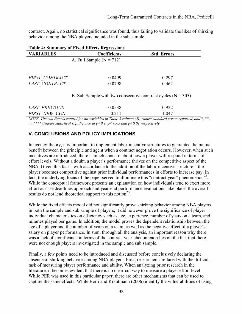
Long-Term Guaranteed Contracts in the NBA, Pedicelli
95
contract. Again, no statistical significance was found, thus failing to validate the likes of shirking
behavior among the NBA players included in the sub sample.
Table 4: Summary of Fixed Effects Regressions
VARIABLES Coefficients Std. Errors
A. Full Sample (N = 712)
FIRST_CONTRACT
0.0499
0.297
LAST_CONTRACT
0.0798
0.462
B. Sub Sample with two consecutive contract cycles (N = 305)
LAST_PREVIOUS
-0.0538
0.922
FIRST_NEW_CON
0.211
1.047
NOTE–The two Panels control for all variables in Table 3 column (5); robust standard errors reported, and *, **,
and *** denotes statistical significance at p<0.1, p< 0.05 and p<0.01 respectively
V. CONCLUSIONS AND POLICY IMPLICATIONS
In agency-theory, it is important to implement labor-incentive structures to guarantee the mutual
benefit between the principle and agent when a contract negotiation occurs. However, when such
incentives are introduced, there is much concern about how a player will respond in terms of
effort levels. Without a doubt, a player’s performance thrives on the competitive aspect of the
NBA. Given this fact—with accordance to the addition of the labor-incentive structure—the
player becomes competitive against prior individual performances in efforts to increase pay. In
fact, the underlying focus of the paper served to illuminate this “contract year” phenomenon22
.
While the conceptual framework presents an explanation on how individuals tend to exert more
effort as case deadlines approach and year-end performance evaluations take place, the overall
results do not lend theoretical support to this notion23
.
While the fixed effects model did not significantly prove shirking behavior among NBA players
in both the sample and sub sample of players, it did however prove the significance of player
individual characteristics on efficiency such as age, experience, number of years on a team, and
minutes played per game. In addition, the model proves the dependent relationship between the
age of a player and the number of years on a team, as well as the negative effect of a player’s
salary on player performance. In sum, through all the analysis, an important reason why there
was a lack of significance in terms of the contract year phenomenon lies on the fact that there
were not enough players investigated in the sample and sub sample.
Finally, a few points need to be introduced and discussed before conclusively declaring the
absence of shirking behavior among NBA players. First, researchers are faced with the difficult
task of measuring player performance and ability. When analyzing prior research in the
literature, it becomes evident that there is no clear-cut way to measure a player effort level.
While PER was used in this particular paper, there are other mechanisms that can be used to
capture the same effects. While Berri and Krautmann (2006) identify the vulnerabilities of using

Issues in Political Economy, Volume 24, 2015
96
PER as the dependent variable24
, they argue that it is necessary for the dependent variable to
measure the marginal contribution to a team’s winning percentage. This claim ultimately sheds
light on the fact that methodology is key in determining whether a model will significantly detect
shirking behavior among NBA players. As a result, it is recommended to measure the dependent
variable as the percent change or deviation from a player’s career average25
. By doing so, there
will be more relatively introduced in the model, which will inherently suppress any hidden
confounding effects.
Second, it is worth shedding light on alternative variables to analyze that have been overlooked
in previous research. The most important are those variables related to fantasy sports. Since
society has entered a new dimension of analysis, it is important to raise awareness of the
potential in researching the relationship between the decision making process of agents and the
use of fantasy markets. In fact, the behavior of such markets parallel to those of already well-
established markets in which are based upon economic intuition.
Nowadays, the Internet is inundated with information on which player to add, drop, or trade in
regards to an individual’s fantasy team. With this influx of information, it will be easy to parse
the process of decision-making when team owners try to optimize the output (wins) of their
respective teams. This is extremely important to consider since a large proportion of the
population participate in these fantasy activities26
. Finally, since the information on players is
readily available, fantasy sports can inherently be used as models to predict the expectation of
player production.
Thus, it is essential to transcend boundaries and begin analyzing fantasy sports to measure the
true value of professional athletes. For example, fantasy sports can be used as value indicators
through the average draft rank of a player or even through the amount of time a player spends on
the waiver wire before claimed by a team owner.
Finally, it is important to address the assumptions in which the principle-agency theory is based
upon. The main assumption is that the principle does not have the resources to continuously
observe the agent to ensure the interests of both parities are aligned. However, in terms of sports
economics, this assumption is quite threatened by the fact that a player’s performance is easily
observed and scrutinized. That is, coaches, managers, owners, fans, and even teammates
constantly observe the agent’s behaviors. Thus, although a general manager may not have the
time or resources to monitor any signs of shirking behavior, coaches and teammate on the other
hand do however. As a result, there is always a third observer present, which will ultimately
deter any athlete from performing below expectations (Fort (2003) and Berri and Krautmann
(2006)). As a result, it may be in best interest to allocate research towards establishing new
economic theories only applicable in the sports arena. The first step that must be taken in
expediting this process is to build a model, which analyzes the effect of media exposure on
player performance27
.
Altogether, the future of sports economics is quite imminent. Now that there are a number of
established researches on the behavior of professional athletes, it is time to surpass old economic
intuition and formulate a new era of theorems solely intended for the analysis of sports. As
society inches closer to an unprecedented era of new technologies, fantasy sports, and

Long-Term Guaranteed Contracts in the NBA, Pedicelli
97
convoluted statistical packages, much can be accomplished beyond the stretch of the
imagination.
VI. REFERENCES
Berri, David, and Anthony Krautmann. “Shirking On the Court: Testing for the Incentive Effects
of Guaranteed Pay.” Economic Inquiry 44.3 (2007): 536-546
Bougheas, Spiros, and Paul Downward. “The Economics of Professional Sports Leagues.
“Journal of Sports Economics 4.2 (2003): 87-107.
Fair, Ray. “Estimated Age Effects in Athletic Events and Chess.” Economic Inquiry 33.1 (2007):
37-57.
Harold Demsetz, Armen A. Alchain. “Production, Information Costs, and Economic
Organization.” The American Economic Review 62.5 (1972): 777-94.
Holmstrom, Bengt “Moral Hazard and Observability.” The Bell Journal of Economics 10.1
(1979): 74-91.
Holmstrom, Bengt “Moral Hazard in Teams.” Bell Journal of Economics 13.2 (1982): 324-40.
Jensen, Michael. “Theory of the Firm: Managerial Behavior, Agency Costs and Ownership
Structure.” Journal of Financial Economics 3.4 (1976): 305-360.
Lazear, Edward, and Sherwin Rosen. “Rank-Order Tournaments as Optimum Labor Contracts.
“The Journal of Political Economy 89.5 (1981): 841-864.
Lehn, Kenneth. “The Effectiveness of Incentive Mechanisms in Major League Baseball.”Journal
of Sports Economics 3.3 (2002): 246-255.
Maxcy, Joel, Rodney Fort, and Anthony Krautmann. “The Effectiveness of Incentive
Mechanisms in Major League Baseball.” Journal of Sports Economics 3.3 (2002): 246-255.
Mookherjee, Dilip. “Optimal Incentive Schemes with Many Agents.” Review of Economic
Studies 89.5 (1984): 433-446.
Nalebuff, Barry, and Joseph Stiglitz. “Prizes and Incentives: Towards a General Theory of
Compensation and Competition.” The Bell Journal of Economics 14.1 (1983): 21-43.
Prendergast, Canice. “The Provision of Incentives in Firms.” Journal of Economic
Literature 37.1 (1999): 7-63.
Rice, B. “Moral Hazard in Long-Term Guaranteed Contracts: Theory and Evidence From the
NBA.” MIT Sloan Sports Analytics Conference, 2011.
Issues in Political Economy, Volume 24, 2015
98
Sappington, David. “Incentives in Principal-Agent Relationships.” Journal of Economic
Perspectives 5.2 (1991): 45-66.
Staw, Barry, and Ha Hoang. “Sunk Costs in the Nba: Why Draft Order Affects Playing Time and
Survival in Professional Basketball.” Administrative Science Quarterly 40.3 (1995): 474-494.
Stiroh, Kevin. “Playing for Keeps: Pay and Performance in the NBA.” Economic Inquiry 45.1
(2007): 145-161.
Srivastava, Kailash, and Sunil Misra. “Impact of Goal Setting and Team Building Competencies
On Effectiveness.” Leadership and Organization Development Journal 24.6 (2008): 335-344.
Young, Archie. “Physical Activity for Patients: An Exercise Prescription.” Royal College of
Physicians (2001): 33-38
VII. ENDNOTES 1 This situation parallels with the literature of Alchian and Demsetz (1972) and Holmstrom
(1979), which suggests that unless monitoring or incentive mechanisms are employed, shirking
can generate inefficient pay and performance outcomes. 2 A contract year is defined as the last year in a player’s contract with a given team.
3 The methodology Berri and Krautmann (2006) used is further analyzed in the empirical
framework section of this paper. 4 Shirking is not solely confined to the first year of a new agreement. Shirking can occur during
any year of a contract; however, the literature expects players to shirk after signing a long-term
agreement, due to the little punishment for performing below expectations. In terms of the final
year, no one expects a player to shirk, since punishment is imminent as there is an impending
new contract the following year. 5 Since their article is the most updated with similar methodologies.
6 From economic theory, it is known that a utility-maximizing agent does not necessarily act
according to the principal’s interest. Normative agency-theory suggests how the agency problem
can be solved: to design a contract that provides the agent with incentives that make him act in
the best interest of the principal. See Jensen (1976). 7 Signing a three-period guaranteed contract does not make intuitive sense for the team because it
will ensure that any rational player will put forth zero effort over the span of the contract. This
occurs since there are no future contracts to be affected. While this may be true, it is important to
remember that even when a player displaces zero effort, a positive is still possible because of the
player’s inherent ability and the nature of the production function (output=unobserved ability+
effort+ random individual specific shock). See Sen and Rice (2011). 8 Stiroh (2007) poses the question: “If teams are worried that players might increase their effort
in contract years and then decrease it after signing a long-term contract, why not make every
season a contract year, and motivate players to play hard every year to earn a lucrative deal for
the next season?” See Stiroh (2007). 9 Player base salary is scaled in terms of millions of dollars
10 PER is a well-known robust basketball statistic created by John Hollinger.
Long-Term Guaranteed Contracts in the NBA, Pedicelli
99
11The average PER in the sample is slightly larger than the average league standardized PER
value, 15. This may be due to the fact that the sample chosen to analyze only includes those
players who receive more than fifteen minutes played per game. 12
When dealing with PER, there are two important things to understand: it is a per-minute and
pace-adjusted statistic. Thus, this statistic strips down the differences in minutes played and team
pace (number of possessions in a game) when comparing players. 13
The variables in this equation are defined as follows: PTS = points scored, TREB = total
rebounds, STL= steals, BLK = blocks, AST= assists, TO = turnovers, FGMS = field goals missed,
FTMS = free throws missed. 14
Performance is measured as the subject’s best time of completion of an event (100m, 200m,
and 400m runs, sprints, and laps) 15
The age factor for age 80 for chess was 1.11, which compares to the next smallest age-80 age
factor of 1.31 for a 50-meter swim 16
The logarithm of a player’s annual base salary will be included in the model for a more precise
interpretation—percent change, rather than a unit change. 17
A player’s PER may rise since he is surrounded by better skill-sets; however, the same player’s
PER may decline if his skills do not compare relative to his better teammates. As a result, his
services to the team may not be in such great demand. 18
The true measure of player’s efficiency should account for the marginal contribution to a
team’s winning percentage. In attempt to develop a more robust measure of player productivity,
Berri and Krautmann (2006) turned to an economic-inspired model that relies on marginal
contribution. This model hinges on the idea that team performance can be connected to player
statistics through marginal productivity. 19
The new efficiency rating Berri and Krautmann (2006) derive is given by: PRODMP = (PTS +
TREB + STL) – (TO + FGA + 0.44 FTA), where PRODMP = marginal productivity, PTS = points
scored, TREB = total rebounds, STL = steals, TO = turnovers, FGA = field goals attempted, and
FTA = free throws attempted. 20
To a degree this may even measure the possibility of shirking behavior among NBA players in
that a player deviates from their expected production after signing a lucrative contract. This
result sheds light on another possible study that can be solely dedicated to this result. 21
In past literature such a term has not been studied and analyzed. 22
In which players intentionally perform at a higher standard during the last year of a contract
cycle in order to justify their desires for a new money-spinning contract. 23
A large part of the reason why there was a lack of significance was due the small sample of
players analyzed in the analysis. When conducting research in sports, there is no excuse to fall
short of including all professional athletes of any particular league. This is true because sports
offer the rare occurrence where it is possible to obtain information on an entire population under
investigation. 24
These critics were discussed in the empirical section. 25
The dependent variable should not be limited to PER. In fact, it should include a plethora of
individual player statistics such as total points, rebounds, assists, steals, etc. The importance lies
on the fact that both offensive and defensive attributes are considered. 26
A large proportion of the population also participates in betting schemes, in terms of fantasy
sports, on Internet websites such as FanDuel and DraftKings. Thus, there is even potential
research in the economics of sports betting.

Issues in Political Economy, Volume 24, 2015
100
27It will be very interesting to see whether “hype” created by media affects player growth and
performance. This hypothesis rests on the idea that constant media attention causes un-wanted
stress and high expectations in which the player is forced to achieve.


![[XLS]navy-training-transformation2.wikispaces.com · Web view0. 15 15. 85 85. 100 100. 5. 85. 100. 0.3 1 0.35 0.35 1. 85 85 85 85. 85 85 85 85. 85 85 85 85. 85 85 85 85. 85 85 85](https://img.pdfslide.us/doc/110x75/5b3ecf5e7f8b9a5e2c8b55c9/xlsnavy-training-web-view0-15-15-85-85-100-100-5-85-100-03-1-035.jpg)
![Finale 2009 - [Untitled22] · ã bb bb bb bb # # # b bb 85 85 85 8 5 8 5 85 85 85 8 5 8 5 85 85 85 85 85 85 85 85 85 Piccolo Flüt Obua Fagot Eb Klarnet Bb Klarinet 1 Bb Klarinet](https://img.pdfslide.us/doc/110x75/5e7c68ed18b1387e7854a18b/finale-2009-untitled22-bb-bb-bb-bb-b-bb-85-85-85-8-5-8-5-85-85-85-8.jpg)