ISSN: ADAPTIVE NONLINEAR CONTROL OF … NONLINEAR CONTROL OF DOUBLY-FED INDUCTION MACHINE IN WIND POWER GENERATION 1MOHAMMED RACHIDI, 2BADR BOUOULID IDRISSI 1,2

Journal of Theoretical and Applied Information Technology 10

th May 2016. Vol.87. No.1

© 2005 - 2016 JATIT & LLS. All rights reserved.

ISSN: 1992-8645 www.jatit.org E-ISSN: 1817-3195

99

ADAPTIVE NONLINEAR CONTROL OF DOUBLY-FED

INDUCTION MACHINE IN WIND POWER GENERATION

1MOHAMMED RACHIDI,

2BADR BOUOULID IDRISSI

1,2Department of Electromechanical Engineering, Moulay Ismaïl University, Ecole Nationale Supérieure

d’Arts et Métiers, BP 4024, Marjane II, Beni Hamed, 50000, Meknès, Morocco

E-mail: [email protected],

[email protected]

ABSTRACT

This paper presents an adaptive nonlinear controller for Doubly-Fed Induction Generator (DFIG) in wind

power generation. The control objective is to extract the maximum power (Maximum Power Point

Tracking) and have a specified reactive power at the generator terminal despite the variable wind speed and

the unknown mechanical parameters and mechanical torque. To achieve such a decoupled control, the

nonlinear Backstepping approach was combined with the field orientation principle. The induction machine

is controlled in a synchronously reference frame oriented along the stator voltage vector position. The

mathematical development of the nonlinear Backstepping controller design is examined in detail. The

overall stability of the system is shown using Lyapunov approach. Application example on stabilizing a

DFIG-based Wind Energy Conversion System (WECS) subject to large mechanical parameters

uncertainties has been given to illustrate the design method and confirm the robustness and validity of the

proposed control.

Keywords: Wind Energy Conversion System, Doubly-Fed Induction Generator, Unknown Mechanical

Parameters and Torque, Adaptive Nonlinear control, Lyapunov Approach.

1. INTRODUCTION

Modern wind turbines generators can work at

variable wind speed and produce fixed frequency

electricity. These variable speed fixed frequency

generators use DFIG with a partial converter

interface or Permanent Magnet (PM) synchronous

generator with a full-converter interface. For high-

power wind generation, DFIG-based electric power

conversion systems are currently dominating the

market. A key DFIG benefit is that inverter rating is

typically 25% of total system power which gives a

substantial reduction in the power electronics cost

as compared with direct-in-line synchronous

generator systems. The power percentage fed

through the rotor converter is proportional to the

slip. At synchronous speed, the only power that

flows through the converter is what is needed for

ensuring the flow of DC excitation current through

rotor windings. Additionally, DFIG systems offer

the following advantages:

The speed range is ±30% around the

synchronous speed [1-2]. This allows to

continuously operating the wind turbine at its

optimum Tip Speed Ratio (TSR), which is

specific to the aerodynamic design of a given

turbine. This achieves maximum rotor

efficiency and hence maximum power

extraction.

Reduced cost of the inverter filters and EMI

filters, because filters are rated for 0.25 p.u.

total system power.

Power-factor control can be implemented at

lower cost. The four-quadrant converter in the

rotor circuit enables decoupled control of

active and reactive power of the generator.

However, DFIG-based WECS control is a complex

issue [3-8]. Indeed, this system is characterized by

multiple variables and operates in environments

with extreme variations in the operating conditions

(wind speed variation, electrical energy

consumption, etc.). On the other hand, DFIG-based

drive system is a nonlinear system which is subject

to parameter uncertainties and/or time-varying

dynamics. The control challenge is to keep the

generator at its maximum efficiency despite the

wind speed variations and system’s parameters

uncertainties. In this work, we propose an adaptive

nonlinear Backstepping controller design to extract

the maximum active power and have a specified

reactive power at the generator terminal even in the

presence of wind speed variations. The proposed

controller also stabilizes the DFIG-based WECS





100

even in the case of large changes in the damping

coefficient and moment of inertia, and mechanical

torque. In practice, the damping coefficient and

moment of inertia are approximately known and the

mechanical torque is a random process variable. To

still ensure the stability condition despite parameter

change, suitable update laws are derived.

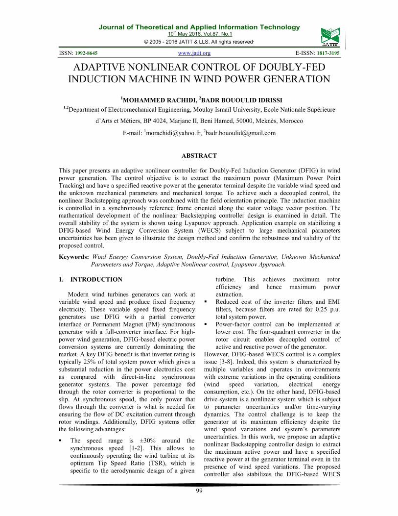
A basic view of the DFIG-based WECS is

illustrated in the figure 1. In this system, the power

captured by the wind turbine is converted into

electrical power by the generator and it is

transmitted to the grid by the stator and the rotor

windings. The rotor circuit is connected to the grid

through a back-to-back converter. The capacitor

connected on the DC side acts as the DC voltage

source. The electrical grid frequency and voltage

magnitude are assumed to be constant.

The control system generates the pitch angle

command and the voltage command signals for

converters. The grid-side converter (GSC) is

controlled to have unity power factor and a constant

voltage at the DC-link. The rotor-side converter

(RSC) is controlled to have optimal power

extraction from the wind and a specified reactive

power at the generator terminal.

The paper is structured as follows. The second

section presents a state-space modelling of the

DFIG-based wind power conversion system. The

induction machine is controlled in a rotating

reference frame oriented along the stator voltage

vector position. The third section describes the

proposed nonlinear controller design and gives

control and update laws for both RSC and GSC

converters. An application example on stabilizing a

DIFG-based wind power conversion system subject

to large mechanical parameters variations will be

given in the last section to show the merits of the

proposed controller. Simulation results and analysis

confirm the effectiveness of the proposed approach.

Figure. 1: DFIG-based wind power conversion system

2. SYSTEM MODEL

2.1. Modelling of the Wind Turbine

The aerodynamic turbine power Pt depends on

the power coefficient Cp as follows [9]:

3

p

2

tt v),(CR2

1P βλπρ=

(1a)

where:

ρ: Specific mass of the air (kg/m2);

v: Wind speed (m/s);

Rt: Radius of turbine (m);

Cp: Power coefficient;

β: Blade pitch angle (deg);

Ω: Generator speed (rad/s);

λ: Tip Speed Ratio (TSR) of the rotor

blade tip speed to wind speed.

The TSR is given by:

vG

R t Ω=λ (1b)

where G is mechanical speed multiplier. A generic

equation is used to model cp(λ,β), based on the

modeling turbine characteristics of [9]:

λ+λ

−−β−λ

=βλ 6

i

543

i

21p c)

cexp()cc

c(c),(C (1c)

Where 1

035.0

08.0

11

3 +−

+=

ββλλi

and the coefficients c1 to c6 are: c1 = 0.5176, c2 =

116, c3 = 0.4, c4 = 5, c5 = 21 and c6 = 0.0068.

Note that the maximum value of cp (cpmax= 0.48) is

achieved for β = 0° and λ = λopt =8.1.

In this work, we assume that the wind turbine

operates with β=0. To capture the maximum power,

a speed controller must control the mechanical

speed Ω so as to track a speed reference Ωc that

keeps the system at λopt (Maximum Power Point

Tracking strategy). According to (1b), the optimal

mechanical speed is:

optt

cR

vG

λ=Ω

(1d)

2.2. Induction Generator Model

The induction machine is controlled in a

synchronously rotating dq axis frame, with the d-

axis oriented along the stator-voltage vector

position (vsd=V, vsq=0). In this reference frame, the

electromechanical equations are [10]:

[ ] ]][[][

]][[ φωφ

++=dt

dIRV

(2a)

]][[][ IM=φ

(2b)





101

Ω−−=Ω

FTTdt

dJ emt

(2c)

)( rqsdrdsqmem iiiipLT −=

(2d)

where:

;

Rr000

0Rr00

00Rs0

000Rs

]R[

= ;

Lr0L0

0Lr0L

L0Ls0

0L0Ls

]M[

m

m

m

m

=

ω

ω−

ω

ω−

=ω

000

000

000

000

][

r

r

s

s

[V], [I] and [φ] are respectively voltage, current and

flux vectors.

The subscripts s, r, d and q stand respectively for

stator, rotor, direct and quadratic.

R, L, Lm, ω, J, F, p, Tt and Tem denote respectively

resistance, inductance, mutual inductance, electrical

speed, total inertia, damping coefficient, number of

pole pairs, mechanical torque and electromagnetic

torque.

By selecting currents and speed as the state

variables, the system (2) can be put into the

following state-space form:

111 u)x(gx β−=&

(3a)

222 u)x(gx β−=&

(3b)

133 u)x(gx α+=&

(3c)

244 u)x(gx α+=&

(3d)

))x(hTF(J

1

)TTF(J

1

t

emt

−+η−=

−+η−=η&

(3e)

Where

Ω=== η,),,,(),,,( 4321t

rqrdsqsdt iiiixxxxx

)()( 4132 xxxxaTxh em −==

rqrd vuvu == 21 ,

sr

m

r LL

L

L σβ

σα == ,

1

ηη

βηη

ηη

αηη

33134333234

43234333133

31114121112

41213121111

)(

)(

)(

)(

xmxnxaxbxcxg

xmxnxbxaxcxg

xnxmxcxaxbxg

xnxmxcxbxaxg

u

u

++−−=

−−−+−=

−−+−−=

+++++−=

rs

2

mu

r

m33

rs

sm33

r

r3

s

u

s

m11

rs

rm1s1

s

s1m

LL

L1;V

,L

Lpn,

pm,

LL

RLc,f2b

,L

Ra,V

L

1,

L

Lpn,

1pm

,LL

RLc,f2b,

L

Ra,pLa

−=σβ=β

σ=

σ=

σ=π=

σ=

σ=α

σ=

σσ−

=

σ=π=ω=

σ==

f and V are respectively the constant frequency and

magnitude of grid voltage.

Equations (3a) to (3.d) can be put into the following

compact form:

uAxgx += )(&

(3f)

where

tt uuuxgxgxgxgxg ),(,))(),(),(),(()( 214321 == ,

−

−=

αβαβ00

00A

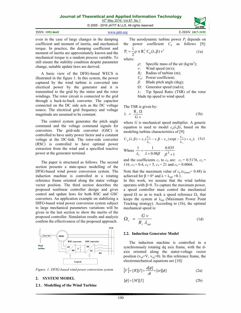
2.3. DC-link and Coupling Filter R-L Models

The GSC converter is connected to the grid

through an R-L filter (fig 2) [11].

Figure.2: DC-link and RL filter sign conventions

By using Kirchhoff’s laws and Park transformation,

we obtain the R-L filter dynamic equations in the

synchronous reference frame:

=+++=

=+−+=

000

0

0

000

0

qds

q

qsq

dqsd

dsd

vidt

diLRiv

Vvidt

diLRiv

ω

ω

(4a)





102

Neglecting losses, the DC-link dynamic equations

are:

=+

=+

−=

rdc

gdcqsqdsd

rgdc

iVxuxu

iViviv

iidt

dVC

4231

00

2

(4b)

Equations (4a) and (4b) can be put into the

following state-space form:

111211 )( vfvcb λζλµζζζ +=+−+−=& (4c)

222212 )( vfvbc λζλζζζ +=+−−=&

(4d)

13 ),( γζαζ += ux&

(4e)

where

;vv;vv;V;i;i oq2od1

2

dc3oq2od1 ===ζ=ζ=ζ

L

1,

L

V,

Lc,

L

Rb s −=λ−=µ

ω==

C

Vxuxu

Cux =+−= γα ),(

1),( 4231

3. CONTROL DESIGN

3.1. RSC Control

3.1.1. Backstepping control strategy

The RSC converter enables decoupled control

of stator reactive power and speed. Indeed, the

following expression of the stator reactive power

2)Im( xVivivIVQ sqsdsdsqsg −=−== ∗

(5a)

shows that the current variable x2 can be considered

as a virtual control of Qsg. According to equation

(3b), it is clear that the control variable u2 can be

designed so that the current variable x2 tracks its

reference. On the other hand, equation (3e) shows

that the electromagnetic torque Tem can be

considered as a virtual control for the speed η. The

following dynamic equation

231142

em

u)xx(au)xx(ag.h

T

β+α−β+α+∇=

υ=&

(5b)

shows that the control variable u1 can be designed

so that the electromagnetic torque Tem tracks its

reference.

3.1.2. Control and update laws

In the case of uncertain model where system

parameters are not known with enough accuracy,

suitable choice of control variables and update laws

must be done to still ensure the stability condition

[11-14]. In this study, it is assumed that the

mechanical parameters F, J and mechanical torque

Tt are unknown. F and J are constant parameters

whilst the torque Tt is assumed to vary slowly in

time. Estimates of F, J and Tt are denoted J,F and

tT , respectively. ηc, Temc and x2c are references of

the variables η, Tem and x2, respectively.

We define the following error variables:

t

t

t

t

t

t

ttt

emcem2

c1

c220

)T,J,F(ˆ

,)T~

,J~

,F~

(~

,)T,J,F(withˆ~TTT

~FFF

~JJJ

~TTz

z

xxz

=θ

=θ=θθ−θ=θ

−=

−=

−=

−=

η−η=

−=

Proposition 1: The following control and update

laws:

)))ˆ(zz)(zk(zk(J

))ˆ(zz(T

))ˆ(zzz(F

x)x(gzku

)xx(a

)xx(auz)kk(u

2111c

2

213

212t

21

2

21

c22002

42

1322121

θϕ−−η+γ−=

θϕ−γ=

θϕη+η−γ=

β

−+=

β+αα+β++−υ

=

&&

&

&

&

with

constants

design positivesareand,,k,k,k

FJk)ˆ(

)T,F,J,,(

F)z(T)zk(J

T)z,(

g.h)ˆ(zk.

321210

1

tcc

c1t11c

emc1

11

γγγ

−=θϕ

ηη=ξ

η+−+−η−=

=ξψ

∇−θϕ−ξψ∇=υ

&

&

&

achieve speed and current tracking objectives and

ensure asymptotic stability despite the changes in

mechanical parameters.





103

Proof:

a- Control law u2

Taking the derivative of z0 and using (3b) gives:

c2220 xu)x(gz && −β−=

(6)

Let2

00 z2

1V = be the Lyapunov candidate function;

the choice 000 zkz −=& , where k0 is a positive design

constant, makes negative the derivative 000 zzV && =

since 0zkV2

000 ≤−=& . With this choice, the control

law u2 can be obtained from equation (6):

β−+

= c20022

xzk)x(gu

&

(7)

b- Control u1 and update laws

Step 1: Virtual control emcT

Using equation (3e), the derivative of z1 is written

as:

cemt

J

TTFz η

η&& −

−+−=1

(8)

Since J, F and Tt are unknown; it will be replaced

with their estimates JF ˆ,ˆ and tT , respectively. Let

211

2

1zV = be the Lyapunov candidate function; the

choice 111 zkz −=& , where k1 is a positive design

constant, makes negative the derivative 111 zzV && =

since 02111 ≤−= zkV& .

Thus, equation (8) gives:

cemct

J

TTFzk η

η&−

−+−=−

ˆ

ˆˆ

11

(9)

which yields the following expression of the virtual

control Temc:

)z,(

)z(FT)zk(JT

1

c1t11Cemc

ξψ=

η+−+−η−= &

(10)

where η has been replaced by

cz η+1 and

)ˆ,ˆ,ˆ,,( tCc TFJηηξ &= .

Step 2: Control u1 and update laws

Equation (8) can be written as:

cemctt

J

TTF

J

zTFz η

ηη&& −

−+−+

−+−=

ˆˆ~~2

1

(11)

Subtracting (9) from (11) yields:

AJ

zzkz

~2111 +−−=&

(12)

where J

Jzk

J

F

J

TA C

t

~

)(

~~~

11 ηη &−+−= .

On the other hand, the derivative of z2 is:

emcTz && −=υ2

Using (10) and (12):

AzJ

zk

zz

Temc

~)ˆ(

)ˆ()ˆ(.

.

211

11

θϕθϕ

θϕξψ

ψξψ

+−−∇=

∂∂

+∇=

&

&&&

where FJkz

ˆˆ)ˆ( 11

−=∂∂

=ψ

θϕ .

Since:

J

Fk

J

JJJ

−+−=

+−=

1

)~

(

)()~

()ˆ(

θϕ

θϕθϕθϕ

The derivative 2z& becomes:

C~

zJ

FB

A~

)ˆ(zk

zJ

F

J

z)

~()ˆ(zk.z

2

21

2

2

112

+−=

θϕ−+

−θϕ−θϕ+ξψ∇−υ= &&

(13)

with

A~

)ˆ(J

z)

~(C

~

zk)ˆ(zk.B

2

2111

θϕ−θϕ−=

+θϕ+ξψ∇−υ= &

To design the control u1 and update laws, we

consider the following Lyapunov candidate

function:

J

J

J

T

J

FzzV t

2

3

2

2

2

1

22

211

~

2

1~

2

1~

2

1

2

1

2

1

γγγ++++=

Its derivative is given by:





104

JJ

JT

J

TF

J

FzzzzV t

t &&&&&& ˆ

~1ˆ

~1ˆ

~1

32122111 γγγ

−−−+=

Using (12) and (13), 1V& can be written as follows:

D~

BzzJ

F

J

zzzkV 2

2

2212

111 ++−−−=&

with

J

J~

J)zk))(ˆ(zz(zk

J

T~

T)ˆ(zz

J

F~

F))ˆ(zz(z

JJ

J~

1T

J

T~

1F

J

F~

1C~

zA~

zD~

3

C1121

2

21

t

2

t21

1

21

2

2

3

tt

21

21

γ−η−θϕ−+−+

γ−θϕ−+

γ−θϕ−η−=

γ−

γ−

γ−+=

&

&

&

&

&&&

The update laws are obtained by cancelling the

terms with J

F

J

J~

,

~

and J

Tt

~

:

))ˆ()(((ˆ

))ˆ((ˆ

))ˆ((ˆ

21112213

212

21221

θϕηγ

θϕγ

θϕηηγ

zzzkzkJ

zzT

zzzF

c

t

−−+−=

−=

+−=

&&

&

&

(14)

Subsequently, the derivative 1V& reduces to:

BzzJ

F

J

zzzkV 2

2

2212

111 +−−−=&

We choose 22 zkB −= , with k2 is a positive design

constant. Since 2

zzzz

2

2

2

121

+≤− for all z1, z2, we

have:

2

22

2

11

2

22

2

2212

111

z)J2

1

J

Fk(z)

J2

1k(

zkzJ

F

J

zzzkV

−+−−−≤

−−−−=&

By selecting k1 and k2 such that the inequalities

J2

1k1 > and

J2

1k 2 >

are verified, the derivative 1V&

becomes negative and so we ensure the stability

condition.

The control variable υ can then be obtained using

equation (13) and the choice 22 zkB −= :

22111 z)kk()ˆ(zk. +−θϕ−ξψ∇=υ &

Finally, equation (5b) gives the control law u1:

)xx(a

)xx(auz)kk(u

42

1322121 β+α

α+β++−υ=

(15)

Where

TF)z(J)zk(JF

TT

FF

JJ

.

c111ccc

t

t

c

C

c

c

&&&&&&&

&&&&&

&&&

+η+−−η−η−η−=

∂

ψ∂+

∂

ψ∂+

∂

ψ∂+η

η∂ψ∂

+ηη∂ψ∂

=ξψ∇

and

))x(gx)x(gx)x(gx)x(gx(ag.h 14412332 −−+=∇

Remark:

The term )( 42 xxa βα + is proportional to q-axis

flux sqφ :

sqrs

rqmsqsrs

rqrs

msq

r

LL

a

iLiLLL

a

iLL

Li

Laxxa

φσ

σ

σσβα

=

+=

+=+

)(

)1

()( 42

Since the effect of the stator resistance is negligible

especially in high power, and the stator voltage

vector is aligned along the d-axis of the reference

frame, the amplitude sqφ is proportional to voltage

V. Hence, the term )xx(a 42 β+α

becomes

different from zero as soon as the machine is

connected to the grid.

3.2. GSC Control

3.2.1. Backstepping control strategy

The GSC converter enables decoupled control

of rotor reactive power and DC-link voltage.

Indeed, the following expression of the rotor

reactive power

2)Im( ζVivivIVQ oqsdodsqrg −=−== ∗

(16)

shows that the current variable 2ζ can be

considered as a virtual control of Qrg. According to

equation (4d), it is clear that the control variable v2





105

can be designed so that the current variable 2ζ

tracks its reference. On the other hand, equation

(4e) shows that 1ζ can be considered as a virtual

control for DC-link voltage. Equation (4c) shows

that the control variable v1 can be designed so that

1ζ tracks its reference.

3.2.2. Control laws

We define the following error variables:

ce 111 ζζ −=

(16a)

ce 222 ζζ −=

(16b)

ce 333 ζζ −=

(16c)

where c1ζ , c2ζ and c3ζ are references of 1ζ , 2ζ

and 3ζ , respectively.

Proposition 2: The following control laws:

γλ

ζγ−α−γ+−γ−+ζ=

)(f)u,x(e)qq(e)q(v 11133

223c3

1

&&&

λ

ζ+ζ−−= c2222

2

)(feqv

&

With q1, q2 and q3 are positive design constants,

achieve the DC-link voltage and rotor reactive

power control objective and ensure the asymptotic

stability.

Proof:

a- Control law 2v

According to (4d), the dynamic equation of the

error 2e is:

cvfe 2222 )( ζλζ && −+=

(17)

To reduce the tracking error, we use the following

Lyapunov candidate function222

2

1eV = . The choice

222 eqe −=& , where q2 is a positive design constant,

makes negative the derivative 222 eeV && = since

02222 ≤−= eqV& . With this choice, the control law

v2 can be obtained from equation (17):

λζζ cfeq

v 22222

)( &+−−=

(18)

b- Control law 1v

Step 1: Virtual control c1ζ

According to (4e), the dynamic equation of the

error 3e is:

cuxe 313 ),( ζγζα && −+=

(19)

We consider the Lyapunov candidate function

2

33 e2

1V = . The choice 333 eqe −=& ,

where q3 is a

positive design constant, makes negative the

derivative 333 eeV && = and hence reduces the tracking

error e3. With this choice, the virtual control law ζ1c

can be obtained from equation (19):

γζα

ζ cc

equx 3331

),( &+−−=

(20)

Step 2: control law v1

According to (4c), the dynamic equation of the

error 1e is:

c1111 v)(fe ζ−λ+ζ= &&

(21)

The derivative of e3 can be re-written as:

331

c3c1c113

eqe

)()u,x(e

−γ=

ζ−γζ+ζ−ζγ+α= &&

(22)

From (20) and (22), we obtain the derivative c1ζ& :

γζγα

ζ cc

eqequx 333131

)(),( &&&&

+−−−=

(23)

We now consider the Lyapunov candidate function:

23

21

2

1

2

1eeVg +=

Its derivative is:

)ee(eeq

)eeq(eee

eeeeV

311

2

33

133311

3311g

γ++−=

γ+−+=

+=

&

&

&&&

With the choice 1131 eqee −=γ+& , we ensure the

negativity of gV& since 0233

211 ≤−−= eqeqVg

& .

Also, equation (21) yields:

113c111 eqev)(f −=γ+ζ−λ+ζ &

(24)

From (23) and (24), we obtain the control law v1:

γλ

ζγ−α−γ+−γ−+ζ=

)(f)u,x(e)qq(e)q(v 11133

22

3c31

&&&





106

4. SIMULATION RESULTS

To demonstrate the effectiveness of the

proposed controller, two SIMULINK models were

constructed which correspond respectively to the

conventional (without adaptation) and adaptive

(unknown mechanical parameters) Backstepping

controllers. The tracking capability was verified for

the adaptive controller in the case of time-varying

wind speed (Fig. 3). To show the robustness against

mechanical parameters and mechanical torque

change speed regulation performances were

compared at constant wind speed (Fig. 4). Constant

values for DC-link voltage, filter and stator

quadratic currents references were considered.

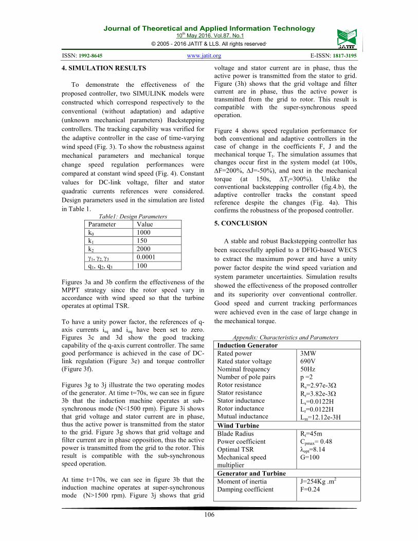
Design parameters used in the simulation are listed

in Table 1. Table1: Design Parameters

Parameter Value

k0 1000

k1 150

k2 2000

γ1, γ2, γ3 0.0001

q1, q2, q3 100

Figures 3a and 3b confirm the effectiveness of the

MPPT strategy since the rotor speed vary in

accordance with wind speed so that the turbine

operates at optimal TSR.

To have a unity power factor, the references of q-

axis currents isq and ioq have been set to zero.

Figures 3c and 3d show the good tracking

capability of the q-axis current controller. The same

good performance is achieved in the case of DC-

link regulation (Figure 3e) and torque controller

(Figure 3f).

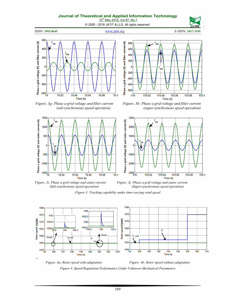
Figures 3g to 3j illustrate the two operating modes

of the generator. At time t=70s, we can see in figure

3b that the induction machine operates at sub-

synchronous mode (N<1500 rpm). Figure 3i shows

that grid voltage and stator current are in phase,

thus the active power is transmitted from the stator

to the grid. Figure 3g shows that grid voltage and

filter current are in phase opposition, thus the active

power is transmitted from the grid to the rotor. This

result is compatible with the sub-synchronous

speed operation.

At time t=170s, we can see in figure 3b that the

induction machine operates at super-synchronous

mode (N>1500 rpm). Figure 3j shows that grid

voltage and stator current are in phase, thus the

active power is transmitted from the stator to grid.

Figure (3h) shows that the grid voltage and filter

current are in phase, thus the active power is

transmitted from the grid to rotor. This result is

compatible with the super-synchronous speed

operation.

Figure 4 shows speed regulation performance for

both conventional and adaptive controllers in the

case of change in the coefficients F, J and the

mechanical torque Tt. The simulation assumes that

changes occur first in the system model (at 100s,

∆F=200%, ∆J=-50%), and next in the mechanical

torque (at 150s, ∆Tt=300%). Unlike the

conventional backstepping controller (fig.4.b), the

adaptive controller tracks the constant speed

reference despite the changes (Fig. 4a). This

confirms the robustness of the proposed controller.

5. CONCLUSION

A stable and robust Backstepping controller has

been successfully applied to a DFIG-based WECS

to extract the maximum power and have a unity

power factor despite the wind speed variation and

system parameter uncertainties. Simulation results

showed the effectiveness of the proposed controller

and its superiority over conventional controller.

Good speed and current tracking performances

were achieved even in the case of large change in

the mechanical torque.

Appendix: Characteristics and Parameters

Induction Generator

Rated power

Rated stator voltage

Nominal frequency

Number of pole pairs

Rotor resistance

Stator resistance

Stator inductance

Rotor inductance

Mutual inductance

3MW

690V

50Hz

p =2

Rs=2.97e-3Ω

Rr=3.82e-3Ω

Ls=0.0122H

Lr=0.0122H

Lm=12.12e-3H

Wind Turbine

Blade Radius

Power coefficient

Optimal TSR

Mechanical speed

multiplier

Rt=45m

Cpmax= 0.48

λopt=8.14

G=100

Generator and Turbine

Moment of inertia

Damping coefficient

J=254Kg .m2

F=0.24





107

Bus DC C = 38 mF,

vdc = 1200 V

Filter RL R = 0,075 Ω,

L = 0,75 mH

Electrical grid U = 690 V,

f = 50 Hz

REFERENCES:

[1] H. Li, Z. Chen, “Overview of different wind

generator systems and their comparisons” IET

Renewable Power Generation, 2008,

2(2):123-138.

[2] B. Multon ; X. Roboam ; B Dakyo ; C. Nichita ;

O Gergaud ; H. Ben Ahmed,

“Aérogénérateurs électriques”, techniques de

l’Ingénieur, Traités de génie électrique,

D3960, Novembre 2004.

[3] E. Koutroulis and K. Kalaitzakis, “Design of a

Maximum Power Tracking System for Wind-

Energy-Conversion Applications” IEEE

Transactions On Industrial Electronics, Vol.

53, No. 2, April 2006.

[4] L. L. Freris, “Wind Energy Conversion

Systems” Englewood Cliffs, NJ: Prentice-

Hall, 1990, pp. 182–184.

[5] Y.Hong, S. Lu, C. Chiou, “MPPT for PM wind

generator using gradient approximation”,

Energy Conversion and Management 50 (1),

pp. 82-89, 2009

[6] R. Pena, J. C. Clare, G. M. Asher, “Doubly fed

induction generator using back-to-back PWM

converters and its application to variable -

speed wind-energy generation,” IEE Proc.

Electr. Power Appl., vol. 143, no. 3, pp. 231-

241, May 996.

[7] Peresada, S., A. Tilli and A. Tonielli, “Robust

Active-reactive power control of a doubly-fed

induction generator”. In Proc. IEEE-

IECON’1998, Aachen, Germany, pp: 1621-

1625.

[8] Karthikeyan A., Kummara S.K, Nagamani C.

and Saravana Ilango G, “ Power control of

grid connected Doubly Fed Induction

Generator using Adaptive Back Stepping

approach“, in Proc 10th IEEE International

Conference on Environment and Electrical

Engineering EEEIC-2011, Rome, May 2011.

[9] Siegfried Heier, “Grid Integration of Wind

Energy Conversion Systems” John Wiley &

Sons Ltd, 1998, ISBN 0-471-97143-X

[10] J.P.Caron, J.P.Hautier, 1995 “Modélisation et

Commande de la Machine Asynchrone”

Edition Technip, Paris.

[11] A.El Magri, F.Giri, A. Elfadili, L. Dugard,

“Adaptive Nonlinear Control of Wind Energy

Conversion System with PMS Generator” 11th

IFAC International Workshop on Adaptation

and Learning in Control and Signal

Processing, Jul 2013, Caen, France. pp.n/c,

2013.

[12] M. Krstic, I. Kanellakopoulos, P. Kokotovic,“

Nonlinear and adaptive control design” John

Wilay & Sons, Inc, 1995.

[13] I. Kanellakopoulos, P.V. Kokotovic, and A.S.

Morse, “Systematic design of adaptive

controller for feedback linearizable systems”,

IEEE Trans. Auto. Control. 1991. Vol. 36,

(11), pp. 1241-1253.

[14] H. Tan, J. Chang, “Field orientation and

adaptive backstepping for induction motor

control” IEEE Proc. 1999.





108

Figure. 3a: Time-varying wind speed Figure. 3b: Rotor speed and its reference

Figure. 3c: Stator q-axis current and its reference Figure. 3d: Filter q-axis current and its reference

Figure. 3e: DC-link voltage and its reference Figure. 3f: Electromagnetic torque and its reference





109

Figure. 3g: Phase a grid voltage and filter current Figure. 3h: Phase a grid voltage and filter current

(sub-synchronous speed operation) (super-synchronous speed operation)

Figure. 3i: Phase a grid voltage and stator current Figure. 3j: Phase a grid voltage and stator current

(Sub-synchronous speed operation) (Super-synchronous speed operation)

Figure 3: Tracking capability under time-varying wind speed

-- Figure. 4a: Rotor speed with adaptation Figure. 4b: Rotor speed without adaptation

Figure 4: Speed Regulation Performance Under Unknown Mechanical Parameters

Documents

ISSN: ADAPTIVE NONLINEAR CONTROL OF … NONLINEAR CONTROL OF DOUBLY-FED INDUCTION MACHINE IN WIND POWER GENERATION 1MOHAMMED RACHIDI, 2BADR BOUOULID IDRISSI 1,2